Embed Size (px)
Citation preview
Type Theory & FunctionalProgramming
Simon Thompson
Computing Laboratory, University of Kent
March 1999
c© Simon Thompson, 1999
Not to be reproduced

i

ii
To my parents
Preface
Constructive Type theory has been a topic of research interest to computerscientists, mathematicians, logicians and philosophers for a number of years.For computer scientists it provides a framework which brings together logicand programming languages in a most elegant and fertile way: programdevelopment and verification can proceed within a single system. Viewedin a different way, type theory is a functional programming language withsome novel features, such as the totality of all its functions, its expressivetype system allowing functions whose result type depends upon the valueof its input, and sophisticated modules and abstract types whose interfacescan contain logical assertions as well as signature information. A thirdpoint of view emphasizes that programs (or functions) can be extractedfrom proofs in the logic.
Up until now most of the material on type theory has only appeared inproceedings of conferences and in research papers, so it seems appropriateto try to set down the current state of development in a form accessible tointerested final-year undergraduates, graduate students, research workersand teachers in computer science and related fields – hence this book.
The book can be thought of as giving both a first and a second course intype theory. We begin with introductory material on logic and functionalprogramming, and follow this by presenting the system of type theory itself,together with many examples. As well as this we go further, looking atthe system from a mathematical perspective, thus elucidating a numberof its important properties. Then we take a critical look at the profusionof suggestions in the literature about why and how type theory could beaugmented. In doing this we are aiming at a moving target; it must bethe case that further developments will have been made before the bookreaches the press. Nonetheless, such an survey can give the reader a muchmore developed sense of the potential of type theory, as well as giving thebackground of what is to come.
iii
iv PREFACE
Outline
It seems in order to give an overview of the book. Each chapter begins witha more detailed introduction, so we shall be brief here. We follow this witha guide on how the book might be approached.
The first three chapters survey the three fields upon which type theorydepends: logic, the λ-calculus and functional programming and construc-tive mathematics. The surveys are short, establishing terminology, notationand a general context for the discussion; pointers to the relevant literatureand in particular to more detailed introductions are provided. In the secondchapter we discuss some issues in the λ-calculus and functional program-ming which suggest analogous questions in type theory.
The fourth chapter forms the focus of the book. We give the formalsystem for type theory, developing examples of both programs and proofsas we go along. These tend to be short, illustrating the construct justintroduced – chapter 6 contains many more examples.
The system of type theory is complex, and in chapter which follows weexplore a number of different aspects of the theory. We prove certain resultsabout it (rather than using it) including the important facts that programsare terminating and that evaluation is deterministic. Other topics examinedinclude the variety of equality relations in the system, the addition of types(or ‘universes’) of types and some more technical points.
Much of our understanding of a complex formal system must derivefrom out using it. Chapter six covers a variety of examples and largercase studies. From the functional programming point of view, we choose tostress the differences between the system and more traditional languages.After a lengthy discussion of recursion, we look at the impact of the quan-tified types, especially in the light of the universes added above. We alsotake the opportunity to demonstrate how programs can be extracted fromconstructive proofs, and one way that imperative programs can be seen asarising. We conclude with a survey of examples in the relevant literature.
As an aside it is worth saying that for any formal system, we can reallyonly understand its precise details after attempting to implement it. Thecombination of symbolic and natural language used by mathematicians issurprisingly suggestive, yet ambiguous, and it is only the discipline of havingto implement a system which makes us look at some aspects of it. In thecase of TT , it was only through writing an implementation in the functionalprogramming language Miranda1 that the author came to understand thedistinctive role of assumptions in TT , for instance.
The system is expressive, as witnessed by the previous chapter, butare programs given in their most natural or efficient form? There is a
1Miranda is a trade mark of Research Software Limited
v
host of proposals of how to augment the system, and we look at these inchapter 7. Crucial to them is the incorporation of a class of subset types, inwhich the witnessing information contained in a type like (∃x :A) . B(x) issuppressed. As well as describing the subset type, we lay out the argumentsfor its addition to type theory, and conclude that it is not as necessary ashas been thought. Other proposals include quotient (or equivalence class)types, and ways in which general recursion can be added to the systemwithout its losing its properties like termination. A particularly elegantproposal for the addition of co-inductive types, such as infinite streams,without losing these properties, is examined.
Chapter eight examines the foundations of the system: how it compareswith other systems for constructive mathematics, how models of it areformed and used and how certain of the rules, the closure rules, may beseen as being generated from the introduction rules, which state what arethe canonical members of each type. We end the book with a survey ofrelated systems, implemented or not, and some concluding remarks.
Bibliographic information is collected at the end of the book, togetherwith a table of the rules of the various systems.
We have used standard terminology whenever were able, but when asubject is of current research interest this is not always possible.
Using the book
In the hope of making this a self-contained introduction, we have includedchapters one and two, which discuss natural deduction logic and the λ-calculus – these chapters survey the fields and provide an introduction tothe notation and terminology we shall use later. The core of the text ischapter four, which is the introduction to type theory.
Readers who are familiar with natural deduction logic and the λ-calculuscould begin with the brief introduction to constructive mathematics pro-vided by chapter three, and then turn to chapter four. This is the core ofthe book, where we lay out type theory as both a logic and an functionalprogramming system, giving small examples as we go. The chapters whichfollow are more or less loosely coupled.
Someone keen to see applications of type theory can turn to chaptersix, which contains examples and larger case studies; only occasionally willreaders need to need to refer back to topics in chapter five.
Another option on concluding chapter four is to move straight on tochapter five, where the system is examined from various mathematical per-spectives, and an number of important results on the consistency, express-ibility and determinacy are proved. Chapter eight should be seen as acontinuation of this, as it explores topics of a foundational nature.
vi PREFACE
Chapter seven is perhaps best read after the examples of chapter six,and digesting the deliberations of chapter five.
In each chapter exercises are included. These range from the routineto the challenging. Not many programming projects are included as itis expected that readers will to be able to think of suitable projects forthemselves – the world is full of potential applications, after all.
Acknowledgements
The genesis of this book was a set of notes prepared for a lecture series ontype theory given to the Theoretical Computer Science seminar at the Uni-versity of Kent, and subsequently at the Federal University of Pernambuco,Recife, Brazil. Thanks are due to colleagues from both institutions; I amespecially grateful to David Turner and Allan Grimley for both encourage-ment and stimulating discussions on the topic of type theory. I should alsothank colleagues at UFPE, and the Brazilian National Research Council,CNPq, for making my visit to Brazil possible.
In its various forms the text has received detailed commment and criti-cism from a number of people, including Martin Henson, John Hughes, NicMcPhee, Jerry Mead and various anonymous reviewers. Thanks to themthe manuscript has been much improved, though needless to say, I alonewill accept responsibility for any infelicities or errors which remain.
The text itself was prepared using the LaTeX document preparationsystem; in this respect Tim Hopkins and Ian Utting have put up with nu-merous queries of varying complexity with unfailing good humour – thanksto both of them. Duncan Langford and Richard Jones have given me muchappreciated advice on using the Macintosh.
The editorial and production staff at Addison-Wesley have been mosthelpful; in particular Simon Plumtree has given me exactly the right mix-ture of assistance and direction.
The most important acknowledgements are to Jane and Alice: Jane hassupported me through all stages of the book, giving me encouragementwhen it was needed and coping so well with having to share me with thisenterprise over the last year; without her I am sure the book would nothave been completed. Alice is a joy, and makes me realise how much morethere is to life than type theory.
Contents
Preface iii
Introduction 1
1 Introduction to Logic 71.1 Propositional Logic . . . . . . . . . . . . . . . . . . . . . . . 81.2 Predicate Logic . . . . . . . . . . . . . . . . . . . . . . . . . 16
1.2.1 Variables and substitution . . . . . . . . . . . . . . . 181.2.2 Quantifier rules . . . . . . . . . . . . . . . . . . . . . 211.2.3 Examples . . . . . . . . . . . . . . . . . . . . . . . . 24
2 Functional Programming and λ-Calculi 292.1 Functional Programming . . . . . . . . . . . . . . . . . . . . 302.2 The untyped λ-calculus . . . . . . . . . . . . . . . . . . . . 322.3 Evaluation . . . . . . . . . . . . . . . . . . . . . . . . . . . . 362.4 Convertibility . . . . . . . . . . . . . . . . . . . . . . . . . . 402.5 Expressiveness . . . . . . . . . . . . . . . . . . . . . . . . . 412.6 Typed λ-calculus . . . . . . . . . . . . . . . . . . . . . . . . 422.7 Strong normalisation . . . . . . . . . . . . . . . . . . . . . . 452.8 Further type constructors: the product . . . . . . . . . . . . 502.9 Base Types: Natural Numbers . . . . . . . . . . . . . . . . 532.10 General Recursion . . . . . . . . . . . . . . . . . . . . . . . 552.11 Evaluation revisited . . . . . . . . . . . . . . . . . . . . . . 56
3 Constructive Mathematics 59
4 Introduction to Type Theory 674.1 Propositional Logic: an Informal View . . . . . . . . . . . . 694.2 Judgements, Proofs and Derivations . . . . . . . . . . . . . 714.3 The Rules for Propositional Calculus . . . . . . . . . . . . . 73
vii
viii CONTENTS
4.4 The Curry Howard Isomorphism . . . . . . . . . . . . . . . 784.5 Some examples . . . . . . . . . . . . . . . . . . . . . . . . . 83
4.5.1 The identity function; A implies itself . . . . . . . . 834.5.2 The transitivity of implication; function composition 834.5.3 Different proofs. . . . . . . . . . . . . . . . . . . . . . 844.5.4 . . . and different derivations . . . . . . . . . . . . . . 854.5.5 Conjunction and disjunction . . . . . . . . . . . . . 86
4.6 Quantifiers . . . . . . . . . . . . . . . . . . . . . . . . . . . 884.6.1 Some example proofs . . . . . . . . . . . . . . . . . . 92
4.7 Base Types . . . . . . . . . . . . . . . . . . . . . . . . . . . 964.7.1 Booleans . . . . . . . . . . . . . . . . . . . . . . . . 964.7.2 Finite types . . . . . . . . . . . . . . . . . . . . . . . 984.7.3 > and ⊥ . . . . . . . . . . . . . . . . . . . . . . . . . 99
4.8 The natural numbers . . . . . . . . . . . . . . . . . . . . . . 1004.9 Well-founded types — trees . . . . . . . . . . . . . . . . . . 1054.10 Equality . . . . . . . . . . . . . . . . . . . . . . . . . . . . . 109
4.10.1 Equality over base types . . . . . . . . . . . . . . . . 1134.10.2 Inequalities . . . . . . . . . . . . . . . . . . . . . . . 1144.10.3 Dependent Types . . . . . . . . . . . . . . . . . . . . 1144.10.4 Equality over the I-types . . . . . . . . . . . . . . . 116
4.11 Convertibility . . . . . . . . . . . . . . . . . . . . . . . . . . 1174.11.1 Definitions; convertibility and equality . . . . . . . . 1174.11.2 An example – Adding one . . . . . . . . . . . . . . . 1194.11.3 An example – natural number equality . . . . . . . . 121
5 Exploring Type Theory 1255.1 Assumptions . . . . . . . . . . . . . . . . . . . . . . . . . . 1265.2 Naming and abbreviations . . . . . . . . . . . . . . . . . . . 130
5.2.1 Naming . . . . . . . . . . . . . . . . . . . . . . . . . 1315.2.2 Abbreviations . . . . . . . . . . . . . . . . . . . . . . 132
5.3 Revising the rules . . . . . . . . . . . . . . . . . . . . . . . . 1335.3.1 Variable binding operators and disjunction . . . . . 1335.3.2 Generalising ∨ . . . . . . . . . . . . . . . . . . . . . 1355.3.3 The Existential Quantifier . . . . . . . . . . . . . . . 136
5.4 Derivability . . . . . . . . . . . . . . . . . . . . . . . . . . . 1395.4.1 A is a type is derivable from a :A . . . . . . . . . . . 1405.4.2 Unique types . . . . . . . . . . . . . . . . . . . . . . 142
5.5 Computation . . . . . . . . . . . . . . . . . . . . . . . . . . 1445.5.1 Reduction . . . . . . . . . . . . . . . . . . . . . . . . 1445.5.2 The system TT ∗
0 . . . . . . . . . . . . . . . . . . . . 1465.5.3 Combinators and the system TT c
0 . . . . . . . . . . . 1485.6 TT c
0 : Normalisation and its corollaries . . . . . . . . . . . . 153
CONTENTS ix
5.6.1 Polymorphism and Monomorphism . . . . . . . . . . 1625.7 Equalities and Identities . . . . . . . . . . . . . . . . . . . . 163
5.7.1 Definitional equality . . . . . . . . . . . . . . . . . . 1635.7.2 Convertibility . . . . . . . . . . . . . . . . . . . . . . 1645.7.3 Identity; the I type . . . . . . . . . . . . . . . . . . . 1655.7.4 Equality functions . . . . . . . . . . . . . . . . . . . 1655.7.5 Characterising equality . . . . . . . . . . . . . . . . 167
5.8 Different Equalities . . . . . . . . . . . . . . . . . . . . . . . 1685.8.1 A functional programming perspective . . . . . . . . 1685.8.2 Extensional Equality . . . . . . . . . . . . . . . . . . 1695.8.3 Defining Extensional Equality in TT0 . . . . . . . . 171
5.9 Universes . . . . . . . . . . . . . . . . . . . . . . . . . . . . 1745.9.1 Type families . . . . . . . . . . . . . . . . . . . . . . 1765.9.2 Quantifying over universes . . . . . . . . . . . . . . . 1775.9.3 Closure axioms . . . . . . . . . . . . . . . . . . . . . 1785.9.4 Extensions . . . . . . . . . . . . . . . . . . . . . . . 179
5.10 Well-founded types . . . . . . . . . . . . . . . . . . . . . . . 1795.10.1 Lists . . . . . . . . . . . . . . . . . . . . . . . . . . . 1795.10.2 The general case - the W type. . . . . . . . . . . . . 1815.10.3 Algebraic types in Miranda . . . . . . . . . . . . . . 187
5.11 Expressibility . . . . . . . . . . . . . . . . . . . . . . . . . . 1895.12 The Curry Howard Isomorphism? . . . . . . . . . . . . . . . 191
5.12.1 Assumptions . . . . . . . . . . . . . . . . . . . . . . 1915.12.2 Normal Forms of Proofs . . . . . . . . . . . . . . . . 192
6 Applying Type Theory 1956.1 Recursion . . . . . . . . . . . . . . . . . . . . . . . . . . . . 196
6.1.1 Numerical functions . . . . . . . . . . . . . . . . . . 1976.1.2 Defining propositions and types by recursion . . . . 2006.1.3 Recursion over lists – 1 . . . . . . . . . . . . . . . . 2026.1.4 Recursion over lists – 2 . . . . . . . . . . . . . . . . 205
6.2 A Case Study – Quicksort . . . . . . . . . . . . . . . . . . . 2076.2.1 Defining the function . . . . . . . . . . . . . . . . . . 2076.2.2 Verifying the function . . . . . . . . . . . . . . . . . 209
6.3 Dependent types and quantifiers . . . . . . . . . . . . . . . 2146.3.1 Dependent Types . . . . . . . . . . . . . . . . . . . . 2146.3.2 The Existential Quantifier . . . . . . . . . . . . . . . 2166.3.3 The Universal Quantifier . . . . . . . . . . . . . . . 2176.3.4 Implementing a logic . . . . . . . . . . . . . . . . . . 2176.3.5 Quantification and Universes – ∀ . . . . . . . . . . . 2206.3.6 Quantification and Universes – ∃ . . . . . . . . . . . 223
6.4 A Case Study – Vectors . . . . . . . . . . . . . . . . . . . . 226
x CONTENTS
6.4.1 Finite Types Revisited . . . . . . . . . . . . . . . . . 2266.4.2 Vectors . . . . . . . . . . . . . . . . . . . . . . . . . 228
6.5 Proof Extraction; Top-Down Proof . . . . . . . . . . . . . . 2306.5.1 Propositional Logic . . . . . . . . . . . . . . . . . . . 2306.5.2 Predicate Logic . . . . . . . . . . . . . . . . . . . . . 2326.5.3 Natural Numbers . . . . . . . . . . . . . . . . . . . . 233
6.6 Program Development – Polish National Flag . . . . . . . . 2346.7 Program Transformation . . . . . . . . . . . . . . . . . . . . 238
6.7.1 map and fold . . . . . . . . . . . . . . . . . . . . . . 2396.7.2 The Algorithm . . . . . . . . . . . . . . . . . . . . . 2436.7.3 The Transformation . . . . . . . . . . . . . . . . . . 244
6.8 Imperative Programming . . . . . . . . . . . . . . . . . . . 2476.9 Examples in the literature . . . . . . . . . . . . . . . . . . . 249
6.9.1 Martin-Lof . . . . . . . . . . . . . . . . . . . . . . . 2506.9.2 Goteborg . . . . . . . . . . . . . . . . . . . . . . . . 2506.9.3 Backhouse et al. . . . . . . . . . . . . . . . . . . . . 2506.9.4 Nuprl . . . . . . . . . . . . . . . . . . . . . . . . . . 2516.9.5 Calculus of Constructions . . . . . . . . . . . . . . . 251
7 Augmenting Type Theory 2537.1 Background . . . . . . . . . . . . . . . . . . . . . . . . . . . 255
7.1.1 What is a specification? . . . . . . . . . . . . . . . . 2567.1.2 Computational Irrelevance; Lazy Evaluation . . . . . 258
7.2 The subset type . . . . . . . . . . . . . . . . . . . . . . . . . 2617.2.1 The extensional theory . . . . . . . . . . . . . . . . . 264
7.3 Propositions not types . . . . . . . . . . . . . . . . . . . . . 2657.3.1 ‘Squash’ types . . . . . . . . . . . . . . . . . . . . . 2657.3.2 The subset theory . . . . . . . . . . . . . . . . . . . 2667.3.3 Godel Interpretation . . . . . . . . . . . . . . . . . . 268
7.4 Are subsets necessary? . . . . . . . . . . . . . . . . . . . . . 2687.5 Quotient or Congruence Types . . . . . . . . . . . . . . . . 273
7.5.1 Congruence types . . . . . . . . . . . . . . . . . . . . 2767.6 Case Study – The Real Numbers . . . . . . . . . . . . . . . 2787.7 Strengthened rules; polymorphism . . . . . . . . . . . . . . 281
7.7.1 An Example . . . . . . . . . . . . . . . . . . . . . . 2817.7.2 Strong and Hypothetical Rules . . . . . . . . . . . . 2837.7.3 Polymorphic types . . . . . . . . . . . . . . . . . . . 2847.7.4 Non-termination . . . . . . . . . . . . . . . . . . . . 285
7.8 Well-founded recursion . . . . . . . . . . . . . . . . . . . . . 2867.9 Well-founded recursion in type theory . . . . . . . . . . . . 292
7.9.1 Constructing Recursion Operators . . . . . . . . . . 2927.9.2 The Accessible Elements . . . . . . . . . . . . . . . . 296
CONTENTS xi
7.9.3 Conclusions . . . . . . . . . . . . . . . . . . . . . . . 2987.10 Inductive types . . . . . . . . . . . . . . . . . . . . . . . . . 298
7.10.1 Inductive definitions . . . . . . . . . . . . . . . . . . 2987.10.2 Inductive definitions in type theory . . . . . . . . . . 301
7.11 Co-inductions . . . . . . . . . . . . . . . . . . . . . . . . . . 3037.11.1 Streams . . . . . . . . . . . . . . . . . . . . . . . . . 308
7.12 Partial Objects and Types . . . . . . . . . . . . . . . . . . . 3097.13 Modelling . . . . . . . . . . . . . . . . . . . . . . . . . . . . 310
8 Foundations 3158.1 Proof Theory . . . . . . . . . . . . . . . . . . . . . . . . . . 315
8.1.1 Intuitionistic Arithmetic . . . . . . . . . . . . . . . . 3168.1.2 Realizability . . . . . . . . . . . . . . . . . . . . . . 3198.1.3 Existential Elimination . . . . . . . . . . . . . . . . 321
8.2 Model Theory . . . . . . . . . . . . . . . . . . . . . . . . . . 3218.2.1 Term Models . . . . . . . . . . . . . . . . . . . . . . 3228.2.2 Type-free interpretations . . . . . . . . . . . . . . . 3228.2.3 An Inductive Definition . . . . . . . . . . . . . . . . 323
8.3 A General Framework for Logics . . . . . . . . . . . . . . . 3248.4 The Inversion Principle . . . . . . . . . . . . . . . . . . . . 326
9 Conclusions 3319.1 Related Work . . . . . . . . . . . . . . . . . . . . . . . . . . 331
9.1.1 The Nurpl System . . . . . . . . . . . . . . . . . . . 3319.1.2 TK: A theory of types and kinds . . . . . . . . . . . 3329.1.3 PX: A Computational Logic . . . . . . . . . . . . . . 3339.1.4 AUTOMATH . . . . . . . . . . . . . . . . . . . . . . 3349.1.5 Type Theories . . . . . . . . . . . . . . . . . . . . . 335
9.2 Concluding Remarks . . . . . . . . . . . . . . . . . . . . . . 337
Rule Tables 360

xii CONTENTS
Introduction
Types are types and propositions are propositions; types come from pro-gramming languages, and propositions from logic, and they seem to haveno relation to each other. We shall see that if we make certain assumptionsabout both logic and programming, then we can define a system which issimultaneously a logic and a programming language, and in which proposi-tions and types are identical. This is the system of constructive type theory,based primarily on the work of the Swedish logician and philosopher, PerMartin-Lof. In this introduction we examine the background in both logicand computing before going on to look at constructive type theory and itsapplications. We conclude with an overview of the book proper.
Correct Programming
The problem of correctness is ever-present in computing: a program iswritten with a particular specification in view and run on the assumptionthat it meets that specification. As is all too familiar, this assumptionis unjustified: in most cases the program does not perform as it should.How should the problem be tackled? Testing cannot ensure the absenceof errors; only a formal proof of correctness can guarantee that a programmeets its specification. If we take a naıve view of this process, we developthe program and then, post hoc, give a proof that it meets a specification. Ifwe do this the possibility exists that the program developed doesn’t performas it ought; we should instead try to develop the program in such a waythat it must behave according to specification.
A useful analogy here is with the types in a programming language. If weuse a typed language, we are prevented by the rules of syntax from formingan expression which will lead to a type error when the program is executed.We could prove that a similar program in an untyped language shares thisproperty, but we would have to do this for each program developed, whilstin the typed language it is guaranteed in every case.
1
2 INTRODUCTION
Our aim, then, is to design a language in which correctness is guaran-teed. We look in particular for a functional programming language withthis property, as semantically the properties of these languages are themost straightforward, with a program simply being a value of a particularexplicit type, rather than a state transformer.
How will the new language differ from the languages with which we arefamiliar?
• The type system will have to be more powerful. This is because wewill express a specification by means of a statement of the form
p :P
which is how we write ‘the value p has the type P ’. The language oftypes in current programming languages can express the domain andrange of a function, say, but cannot express the constraint that forevery input value (of numeric type), the result is the positive squareroot of the value.
• If the language allows general recursion, then every type containsat least one value, defined by the equation x = x. This mirrors theobservation that a non-terminating program meets every specificationif we are only concerned with partial correctness. If we require totalcorrectness we will need to design a language which only permits thedefinition of total functions and fully-defined objects. At the sametime we must make sure that the language is expressive enough to beusable practically.
To summarise, from the programming side, we are interested in develop-ing a language in which correctness is guaranteed just as type-correctness isguaranteed in most contemporary languages. In particular, we are lookingfor a system of types within which we can express logical specifications.
Constructive Logic
Classical logic is accepted as the standard foundation of mathematics. Atits basis is a truth-functional semantics which asserts that every propositionis true or false, so making valid assertions like A ∨ ¬A, ¬¬A⇒ A and
¬∀x.¬P (x)⇒ ∃x.P (x)
which can be given the gloss
If it is contradictory for no object x to have the property P (x),then there is an object x with the property P (x)
3
This is a principle of indirect proof, which has formed a cornerstone of mod-ern mathematics since it was first used by Hilbert in his proof of the BasisTheorem about one hundred years ago. The problem with the principle isthat it asserts the existence of an object without giving any indication ofwhat the object is. It is a non-constructive method of proof, in other words.We can give a different, constructive, rendering of mathematics, based onthe work of Brouwer, Heyting, Bishop and many others, in which everystatement has computational content; in the light of the discussion aboveit is necessary to reject classical logic and to look for modes of reasoningwhich permit only constructive derivations.
To explain exactly what can be derived constructively, we take a differ-ent foundational perspective. Instead of giving a classical, truth-functional,explanation of what is valid, we will explain what it means for a particularobject p to be a proof of the proposition P . Our logic is proof-functionalrather than truth-functional.
The crucial explanation is for the existential quantifier. An assertionthat ∃z.P (z) can only be deduced if we can produce an a with the propertyP (a). A proof of ∃z.P (z) will therefore be a pair, (a, p), consisting of anobject a and a proof that a does in fact have the property P . A universalstatement ∀z.Q(z) can be deduced only if there is a function taking anyobject a to a proof that Q(a). If we put these two explanations together, aconstructive proof of the statement
∀x.∃y.R(x, y)
can be seen to require that there is a function, f say, taking any a to avalue so that
R(a, f a)
Here we see that a constructive proof has computational content, in theshape of a function which gives an explicit witness value f a for each a.
The other proof conditions are as follows. A proof of the conjunctionA∧B can be seen as a pair of proofs, (p, q), with p a proof of A and q of B.A proof of the implication A ⇒ B can be seen as a proof transformation:given a proof of A, we can produce a proof of B from it. A proof of thedisjunction A ∨ B is either a proof of A or a proof of B, together withan indication of which (A or B). The negation ¬A is defined to be theimplication A ⇒ ⊥, where ⊥ is the absurd or false proposition, which hasno proof but from which we can infer anything. A proof of ¬A is thus afunction taking a proof of A to a proof of absurdity.
Given these explanations, it is easy to see that the law of the excludedmiddle will not be valid, as for a general A we cannot say that either A or¬A is provable. Similarly, the law of indirect proof will not be valid.
4 INTRODUCTION
Having given the background from both computing and logic, we turnto examining the link between the two.
The Curry Howard Isomorphism
The central theme of this book is that we can see propositions and typesas the same, the propositions-as-types notion, also known as the CurryHoward isomorphism, after two of the (many) logicians who observed thecorrespondence.
We have seen that for our constructive logic, validity is explained bydescribing the circumstances under which ‘p is a proof of the propositionP ’. To see P as a type, we think of it as the type of its proofs. It is thenapparent that familiar constructs in logic and programming correspond toeach other. We shall write
p :P
to mean, interchangeably, ‘p is of type P ’ and ‘p is a proof of propositionP ’.
The proofs of A ∧ B are pairs (a, b) with a from A and b from B —the conjunction forms the Cartesian product of the propositions as types.Proofs of A ⇒ B are functions from A to B, which is lucky as we use thesame notation for implication and the function space. The type A ∨ B isthe disjoint union or sum of the types A and B, the absurd proposition,⊥, which has no proofs, is the empty type, and so on.
The correspondence works in the other direction too, though it is slightlymore artificial. We can see the type of natural numbers N as expressingthe proposition ‘there are natural numbers’, which has the (constructive!)proofs 0, 1, 2, . . ..
One elegant aspect of the system is in the characterisation of inductivetypes like the natural numbers and lists. Functional programmers willbe familiar with the idea that functions defined by recursion have theirproperties proved by induction; in this system the principles of inductionand recursion are identical.
The dual view of the system as a logic and a programming languagecan enrich both aspects. As a logic, we can see that all the facilities ofa functional programming language are at our disposal in defining func-tions which witness certain properties and so forth. As a programminglanguage, we gain various novel features, and in particular the quantifiedtypes give us dependent function and sum types. The dependent functionspace (∀x : A) . B(x) generalises the standard function space, as the typeof the result B(a) depends on the value a : A. This kind of dependence isusually not available in type systems. One example of its use is in defining
5
array operations parametrised on the dimension of the array, rather thanon the type of the array elements. Dependent sum types (∃x : A) . B(x)can be used to represent modules and abstract data types amongst otherthings.
More radically, we have the possibility of combining verification andprogramming, as types can be used to represent propositions. As an ex-ample consider the existential type again. We can think of the elementsof (∃x : A) . B(x) as objects a of type A with the logical property B(a),witnessed by the proof b :B(a). We can give a third interpretation to p :P ,in the case that P is an existential proposition:
(a, b) : (∃x :A) . B(x)
can be read thus:
a of type A meets the specification B(x), as proved by b :B(a)
This fulfills the promise made in the introduction to logic that we wouldgive a system of types strong enough to express specifications. In our casethe logic is an extension of many-sorted, first-order predicate logic, which iscertainly sufficient to express all practical requirements. The system hereintegrates the process of program development and proof: to show that aprogram meets a specification we provide the program/proof pair.
As an aside, note that it is misleading to read p :P as saying ‘p meetsspecification P ’ when P is an arbitrary proposition, an interpretation whichseems to be suggested by much of the literature on type theory. This isbecause such statements include simple typings like
plus : N ⇒ N ⇒ N
in which case the right-hand side is a woeful under-specification of addition!The specification statement is an existential proposition, and objects of thattype include an explicit witness to the object having the required property:in other words we can only state that a program meets its specificationwhen we have a proof of correctness for it.
We mentioned that one motivation for re-interpreting mathematics ina constructive form was to extract algorithms from proofs. A proof of astatement like
∀x. ∃y. R(x, y)
contains a description of an algorithm taking any x into a y so that R(x, y).The logic we described makes explicit the proof terms. On the other handit is instead possible to suppress explicit mention of the proof objects,and extract algorithms from more succinct derivations of logical theorems,
6 INTRODUCTION
taking us from proofs to programs. This idea has been used with muchsuccess in the Nuprl system developed at Cornell University, and indeed inother projects.
Background
Our exposition of type theory and its applications will make continual refer-ence to the fields of functional programming and constructivism. Separateintroductions to these topics are provided by the introduction to chapter 2and by chapter 3 respectively. The interested reader may care to refer tothese now.
Section 9.2 contains some concluding remarks.
Chapter 1
Introduction to Logic
This chapter constitutes a short introduction to formal logic, which willestablish notation and terminology used throughout the book. We assumethat the reader is already familiar with the basics of logic, as discussed inthe texts [Lem65, Hod77] for example.
Logic is the science of argument. The purposes of formalization of logicalsystems are manifold.
• The formalization gives a clear characterisation of the valid proofsin the system, against which we can judge individual arguments, sosharpening our understanding of informal reasoning.
• If the arguments are themselves about formal systems, as is the casewhen we verify the correctness of computer programs, the argumentitself should be written in a form which can be checked for correctness.This can only be done if the argument is formalized, and correctnesscan be checked mechanically. Informal evidence for the latter require-ment is provided by Principia Mathematica [RW10] which containsnumerous formal proofs; unfortunately, many of the proofs are in-correct, a fact which all too easily escapes the human proof-reader’seye.
• As well as looking at the correctness or otherwise of individual proofsin a formal theory, we can study its properties as a whole. For ex-ample, we can investigate its expressive strength, relative to othertheories, or to some sort of meaning or semantics for it. This work,which is predominantly mathematical in nature, is called mathemat-ical logic, more details of which can be found in [Men87a] amongstothers.
7
8 CHAPTER 1. INTRODUCTION TO LOGIC
As we said earlier, our aim is to provide a formal system in which argumentsfor the validity of particular sentences can be expressed. There are a numberof different styles of logical system – here we look at natural deductionsystems for first propositional and then predicate logic.
1.1 Propositional Logic
Propositional logic formalises arguments which involve the connectives suchas ‘and’, ‘or’, ‘not’, ‘implies’ and so on. Using these connectives we buildcomplex propositions starting from the propositional variables or atomicpropositions.
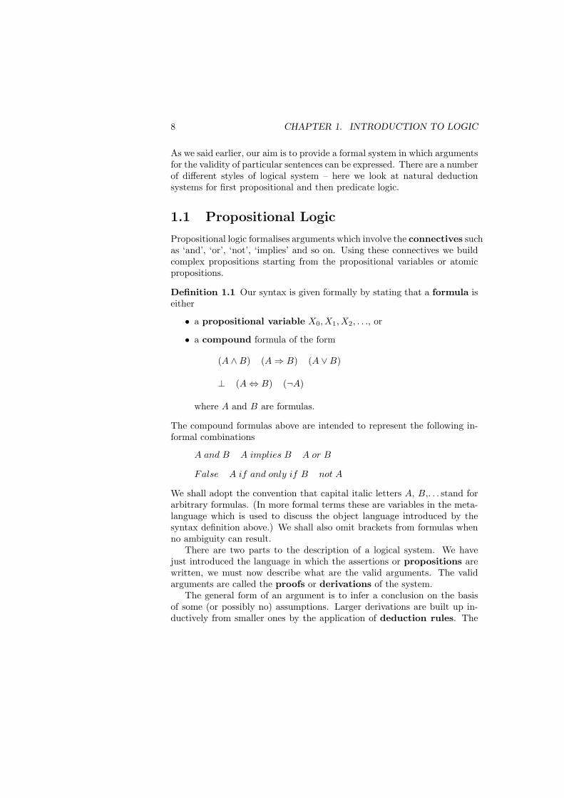
Definition 1.1 Our syntax is given formally by stating that a formula iseither
• a propositional variable X0, X1, X2, . . ., or
• a compound formula of the form
(A ∧B) (A⇒ B) (A ∨B)
⊥ (A⇔ B) (¬A)
where A and B are formulas.
The compound formulas above are intended to represent the following in-formal combinations
A and B A implies B A or B
False A if and only if B not A
We shall adopt the convention that capital italic letters A, B,. . . stand forarbitrary formulas. (In more formal terms these are variables in the meta-language which is used to discuss the object language introduced by thesyntax definition above.) We shall also omit brackets from formulas whenno ambiguity can result.
There are two parts to the description of a logical system. We havejust introduced the language in which the assertions or propositions arewritten, we must now describe what are the valid arguments. The validarguments are called the proofs or derivations of the system.
The general form of an argument is to infer a conclusion on the basisof some (or possibly no) assumptions. Larger derivations are built up in-ductively from smaller ones by the application of deduction rules. The
1.1. PROPOSITIONAL LOGIC 9
simplest derivations are introduced by the rule of assumptions, which statesthat any formula A can be derived from the assumption of A itself.
Assumption RuleThe proof
A
is a proof of the formula A from the assumption A.More complex derivations are built by combining simpler ones. The
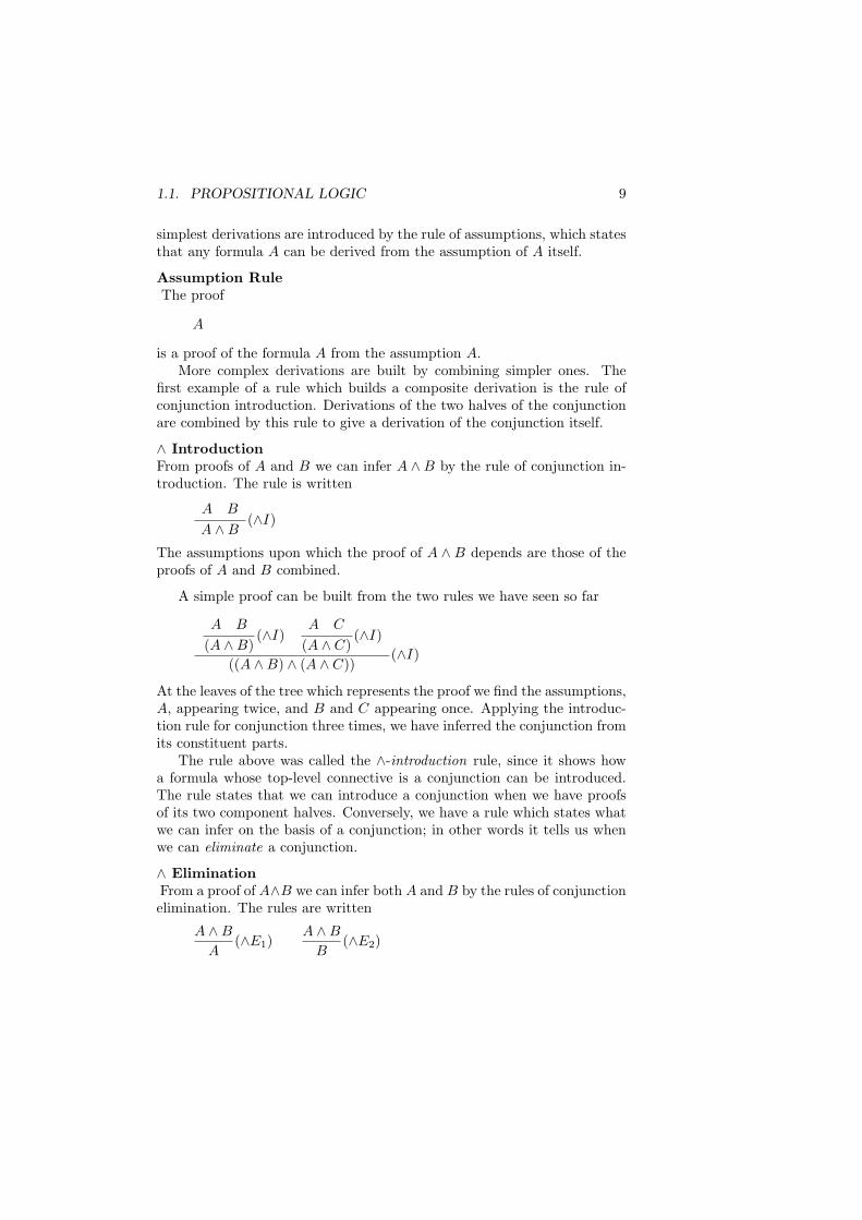
first example of a rule which builds a composite derivation is the rule ofconjunction introduction. Derivations of the two halves of the conjunctionare combined by this rule to give a derivation of the conjunction itself.
∧ IntroductionFrom proofs of A and B we can infer A ∧B by the rule of conjunction in-troduction. The rule is written
A B
A ∧B(∧I)
The assumptions upon which the proof of A ∧ B depends are those of theproofs of A and B combined.
A simple proof can be built from the two rules we have seen so far
A B
(A ∧B)(∧I)
A C
(A ∧ C)(∧I)
((A ∧B) ∧ (A ∧ C))(∧I)
At the leaves of the tree which represents the proof we find the assumptions,A, appearing twice, and B and C appearing once. Applying the introduc-tion rule for conjunction three times, we have inferred the conjunction fromits constituent parts.
The rule above was called the ∧-introduction rule, since it shows howa formula whose top-level connective is a conjunction can be introduced.The rule states that we can introduce a conjunction when we have proofsof its two component halves. Conversely, we have a rule which states whatwe can infer on the basis of a conjunction; in other words it tells us whenwe can eliminate a conjunction.
∧ EliminationFrom a proof of A∧B we can infer both A and B by the rules of conjunctionelimination. The rules are written
A ∧B
A(∧E1)
A ∧B
B(∧E2)
10 CHAPTER 1. INTRODUCTION TO LOGIC
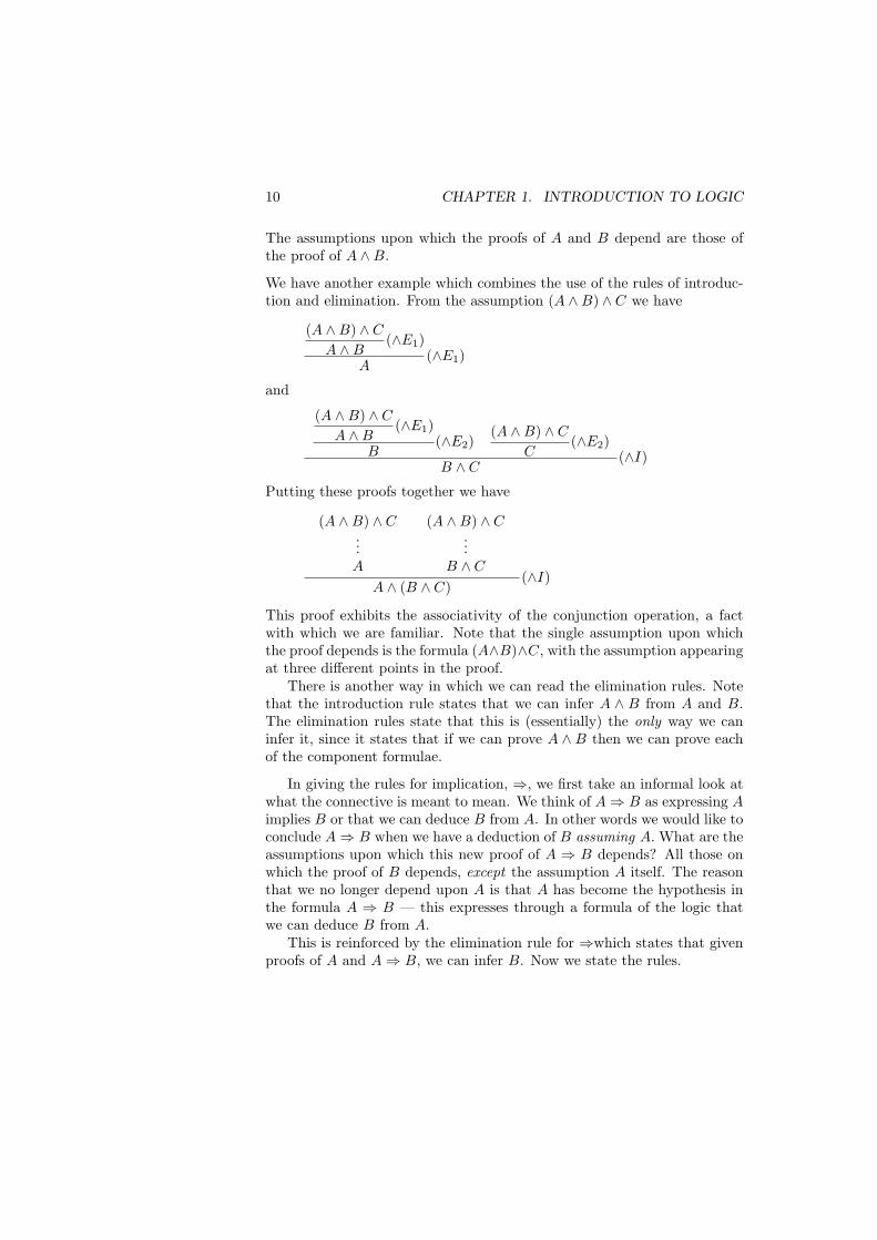
The assumptions upon which the proofs of A and B depend are those ofthe proof of A ∧B.
We have another example which combines the use of the rules of introduc-tion and elimination. From the assumption (A ∧B) ∧ C we have
(A ∧B) ∧ C
A ∧B(∧E1)
A(∧E1)
and
(A ∧B) ∧ C
A ∧B(∧E1)
B(∧E2)
(A ∧B) ∧ C
C(∧E2)
B ∧ C(∧I)
Putting these proofs together we have
(A ∧B) ∧ C...A
(A ∧B) ∧ C...
B ∧ C
A ∧ (B ∧ C)(∧I)
This proof exhibits the associativity of the conjunction operation, a factwith which we are familiar. Note that the single assumption upon whichthe proof depends is the formula (A∧B)∧C, with the assumption appearingat three different points in the proof.
There is another way in which we can read the elimination rules. Notethat the introduction rule states that we can infer A ∧ B from A and B.The elimination rules state that this is (essentially) the only way we caninfer it, since it states that if we can prove A ∧ B then we can prove eachof the component formulae.
In giving the rules for implication, ⇒, we first take an informal look atwhat the connective is meant to mean. We think of A⇒ B as expressing Aimplies B or that we can deduce B from A. In other words we would like toconclude A⇒ B when we have a deduction of B assuming A. What are theassumptions upon which this new proof of A ⇒ B depends? All those onwhich the proof of B depends, except the assumption A itself. The reasonthat we no longer depend upon A is that A has become the hypothesis inthe formula A ⇒ B — this expresses through a formula of the logic thatwe can deduce B from A.
This is reinforced by the elimination rule for ⇒which states that givenproofs of A and A⇒ B, we can infer B. Now we state the rules.
1.1. PROPOSITIONAL LOGIC 11
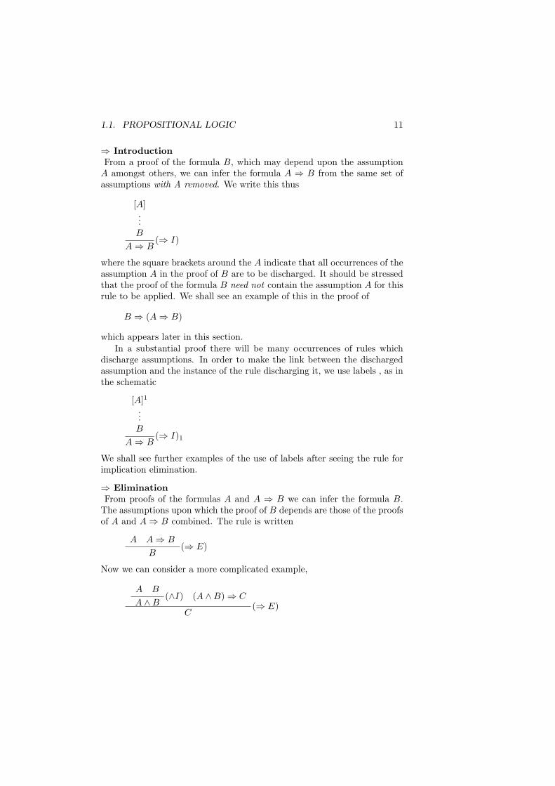
⇒ IntroductionFrom a proof of the formula B, which may depend upon the assumption
A amongst others, we can infer the formula A ⇒ B from the same set ofassumptions with A removed. We write this thus
[A]...B
A⇒ B(⇒ I)
where the square brackets around the A indicate that all occurrences of theassumption A in the proof of B are to be discharged. It should be stressedthat the proof of the formula B need not contain the assumption A for thisrule to be applied. We shall see an example of this in the proof of
B ⇒ (A⇒ B)
which appears later in this section.In a substantial proof there will be many occurrences of rules which
discharge assumptions. In order to make the link between the dischargedassumption and the instance of the rule discharging it, we use labels , as inthe schematic
[A]1...B
A⇒ B(⇒ I)1
We shall see further examples of the use of labels after seeing the rule forimplication elimination.
⇒ EliminationFrom proofs of the formulas A and A ⇒ B we can infer the formula B.
The assumptions upon which the proof of B depends are those of the proofsof A and A⇒ B combined. The rule is written
A A⇒ B
B(⇒ E)
Now we can consider a more complicated example,
A B
A ∧B(∧I) (A ∧B)⇒ C
C(⇒ E)
12 CHAPTER 1. INTRODUCTION TO LOGIC
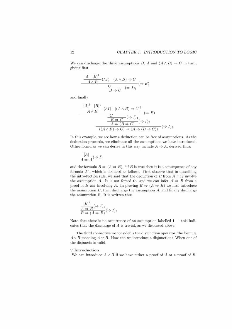
We can discharge the three assumptions B, A and (A ∧ B) ⇒ C in turn,giving first
A [B]1
A ∧B(∧I) (A ∧B)⇒ C
C(⇒ E)
B ⇒ C(⇒ I)1
and finally
[A]2 [B]1
A ∧B(∧I) [(A ∧B)⇒ C]3
C(⇒ E)
B ⇒ C(⇒ I)1
A⇒ (B ⇒ C)(⇒ I)2
((A ∧B)⇒ C)⇒ (A⇒ (B ⇒ C))(⇒ I)3
In this example, we see how a deduction can be free of assumptions. As thededuction proceeds, we eliminate all the assumptions we have introduced.Other formulas we can derive in this way include A⇒ A, derived thus:
[A]A⇒ A
(⇒ I)
and the formula B ⇒ (A⇒ B), “if B is true then it is a consequence of anyformula A”, which is deduced as follows. First observe that in describingthe introduction rule, we said that the deduction of B from A may involvethe assumption A. It is not forced to, and we can infer A ⇒ B from aproof of B not involving A. In proving B ⇒ (A ⇒ B) we first introducethe assumption B, then discharge the assumption A, and finally dischargethe assumption B. It is written thus
[B]2
A⇒ B(⇒ I)1
B ⇒ (A⇒ B)(⇒ I)2
Note that there is no occurrence of an assumption labelled 1 — this indi-cates that the discharge of A is trivial, as we discussed above.
The third connective we consider is the disjunction operator, the formulaA∨B meaning A or B. How can we introduce a disjunction? When one ofthe disjuncts is valid.
∨ IntroductionWe can introduce A ∨ B if we have either a proof of A or a proof of B.
1.1. PROPOSITIONAL LOGIC 13
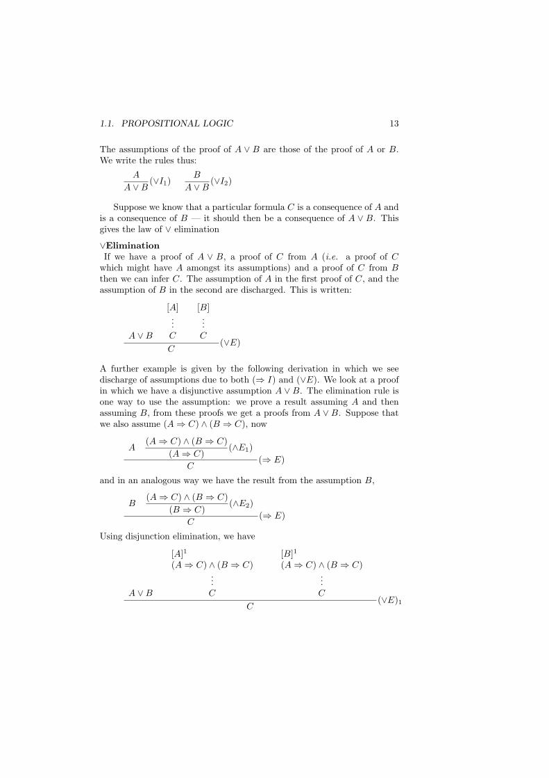
The assumptions of the proof of A ∨ B are those of the proof of A or B.We write the rules thus:
A
A ∨B(∨I1)
B
A ∨B(∨I2)
Suppose we know that a particular formula C is a consequence of A andis a consequence of B — it should then be a consequence of A ∨ B. Thisgives the law of ∨ elimination
∨EliminationIf we have a proof of A ∨ B, a proof of C from A (i.e. a proof of C
which might have A amongst its assumptions) and a proof of C from Bthen we can infer C. The assumption of A in the first proof of C, and theassumption of B in the second are discharged. This is written:
A ∨B
[A]...C
[B]...C
C(∨E)
A further example is given by the following derivation in which we seedischarge of assumptions due to both (⇒ I) and (∨E). We look at a proofin which we have a disjunctive assumption A ∨ B. The elimination rule isone way to use the assumption: we prove a result assuming A and thenassuming B, from these proofs we get a proofs from A ∨ B. Suppose thatwe also assume (A⇒ C) ∧ (B ⇒ C), now
A(A⇒ C) ∧ (B ⇒ C)
(A⇒ C)(∧E1)
C(⇒ E)
and in an analogous way we have the result from the assumption B,
B(A⇒ C) ∧ (B ⇒ C)
(B ⇒ C)(∧E2)
C(⇒ E)
Using disjunction elimination, we have
A ∨B
[A]1
(A⇒ C) ∧ (B ⇒ C)...C
[B]1
(A⇒ C) ∧ (B ⇒ C)...C
C(∨E)1
14 CHAPTER 1. INTRODUCTION TO LOGIC
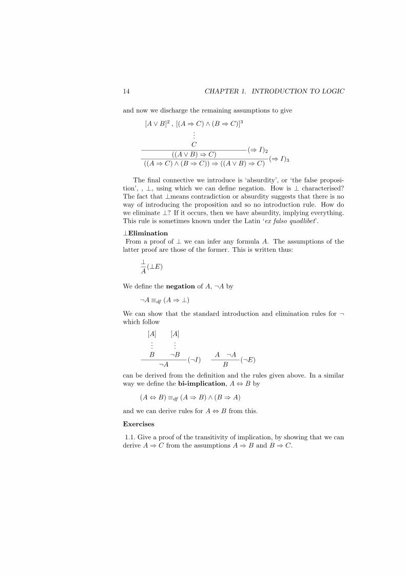
and now we discharge the remaining assumptions to give
[A ∨B]2 , [(A⇒ C) ∧ (B ⇒ C)]3...C
((A ∨B)⇒ C)(⇒ I)2
((A⇒ C) ∧ (B ⇒ C))⇒ ((A ∨B)⇒ C)(⇒ I)3
The final connective we introduce is ‘absurdity’, or ‘the false proposi-tion’, , ⊥, using which we can define negation. How is ⊥ characterised?The fact that ⊥means contradiction or absurdity suggests that there is noway of introducing the proposition and so no introduction rule. How dowe eliminate ⊥? If it occurs, then we have absurdity, implying everything.This rule is sometimes known under the Latin ‘ex falso quodlibet’.
⊥EliminationFrom a proof of ⊥ we can infer any formula A. The assumptions of the
latter proof are those of the former. This is written thus:
⊥A
(⊥E)
We define the negation of A, ¬A by
¬A≡df (A⇒ ⊥)
We can show that the standard introduction and elimination rules for ¬which follow
[A]...B
[A]...¬B
¬A(¬I)
A ¬A
B(¬E)
can be derived from the definition and the rules given above. In a similarway we define the bi-implication, A⇔ B by
(A⇔ B)≡df (A⇒ B) ∧ (B ⇒ A)
and we can derive rules for A⇔ B from this.
Exercises
1.1. Give a proof of the transitivity of implication, by showing that we canderive A⇒ C from the assumptions A⇒ B and B ⇒ C.
1.1. PROPOSITIONAL LOGIC 15
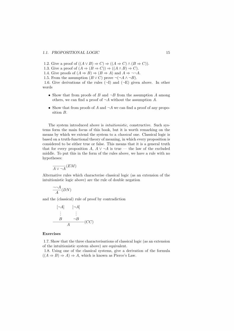
1.2. Give a proof of ((A ∨B)⇒ C)⇒ ((A⇒ C) ∧ (B ⇒ C)).1.3. Give a proof of (A⇒ (B ⇒ C))⇒ ((A ∧B)⇒ C).1.4. Give proofs of (A⇒ B)⇒ (B ⇒ A) and A⇒ ¬¬A.1.5. From the assumption (B ∨ C) prove ¬(¬A ∧ ¬B).1.6. Give derivations of the rules (¬I) and (¬E) given above. In other
words
• Show that from proofs of B and ¬B from the assumption A amongothers, we can find a proof of ¬A without the assumption A.
• Show that from proofs of A and ¬A we can find a proof of any propo-sition B.
The system introduced above is intuitionistic, constructive. Such sys-tems form the main focus of this book, but it is worth remarking on themeans by which we extend the system to a classical one. Classical logic isbased on a truth-functional theory of meaning, in which every proposition isconsidered to be either true or false. This means that it is a general truththat for every proposition A, A ∨ ¬A is true — the law of the excludedmiddle. To put this in the form of the rules above, we have a rule with nohypotheses:
A ∨ ¬A(EM)
Alternative rules which characterise classical logic (as an extension of theintuitionistic logic above) are the rule of double negation
¬¬A
A(DN)
and the (classical) rule of proof by contradiction
[¬A]...B
[¬A]...¬B
A(CC)
Exercises
1.7. Show that the three characterisations of classical logic (as an extensionof the intuitionistic system above) are equivalent.1.8. Using one of the classical systems, give a derivation of the formula
((A⇒ B)⇒ A)⇒ A, which is known as Pierce’s Law.
16 CHAPTER 1. INTRODUCTION TO LOGIC
1.2 Predicate Logic
In this section we look at predicate logic, that is the logic of properties orpredicates. In our exploration of propositional logic, the simplest proposi-tions were “atomic” or unanalysed. Here we build a system in which thepropositions are built up from statements to the effect that certain objectshave certain properties, or that certain objects are equal.
Syntactically, our language will have two categories, formulas and terms.
Definition 1.2 Terms are intended to denote objects, and have one ofthe forms below:
individual variables or simply variables, v0, v1, v2, . . .. We shall writex, y, z, u, v, . . . for arbitrary individual variables in the following ex-position.
individual constants c0, c1, c2, . . .. We shall use a, b, c, . . . for arbitraryconstants below.
composite terms These are formed by applying function symbols to otherterms .Each function symbol has an arity, 1,2,. . . ; an n-ary functionsymbol fn,m takes n argument terms t1, . . . , tn in forming the term
fn,m(t1, . . . , tn)
We will use f, g, h . . . to denote arbitrary function symbols in whatfollows.
We will use s, t, t1, . . . as a notation for arbitrary terms.Note that we can think of constants as 0-ary function symbols, if we so
wish, and also that the variables we have introduced here are intended tostand for objects, and not for propositions as did our propositional variablesabove. Our propositions are formed as follows.
Definition 1.3
Atomic formulas are of two forms. The first is
Pn,m(t1, . . . , tn)
where Pn,m is an n-ary predicate symbol and t1, . . . , tn are terms.This formula is intended to express the fact that the relation rep-resented by predicate symbol Pn,m holds of the sequence of values
1.2. PREDICATE LOGIC 17
denoted by t1, . . . , tn. We will use P,Q,R, . . . for arbitrary predicatesymbols.
Equality is taken to be a primitive of the system, so another class offormulas are the equalities
t1 = t2
where t1 and t2 are terms.
Propositional combinations of formulas under the propositional con-nectives ∨,∧,⇒,⇔,¬.
Quantified formulas
∀x.A ∃x.B
where as in the propositional case we use A,B, . . . for arbitrary for-mulas, as well as using x for an arbitrary variable.
The quantifiers ∀ — for all — and ∃ — there exists — are intended toexpress the assertions that a particular formula holds for all objects and forsome object, respectively. (Hence the name ‘quantifier’; quantified formulasexpress the quantity of objects with a particular property.)
To reinforce the intuitive interpretation of the quantifiers, we now lookat their use in expressing various properties. In each particular case, therewill be an intended domain of application of the quantifiers, so that “forall” will mean “for all fish”, “for all real numbers” and so on. We assumefor these examples that our domain of discourse is the natural numbers, sothat the quantifiers will range over 0, 1, 2, . . .. Moreover, we assume thatthe (infix) predicate symbol < is chosen so that x < y expresses
‘ y is greater than x ’
Suppose first that f is a function. We say that a value is in the rangeof f if it is the value of f at some argument. How can we state in logicalterms that m is the maximum value in the range? First we say that m isin the range
∃i.(f(i) = m)
and then that m is greater than or equal to every element in the range
∀j.(f(j) ≤ m)
18 CHAPTER 1. INTRODUCTION TO LOGIC
The complete property is expressed by the conjunction of the formulas:
∃i.(f(i) = m) ∧ ∀j.(f(j) ≤ m)
A second example shows that the order in which we write different quan-tifiers is significant. What does
∀x.∃y.(x < y)
express intuitively? For every x, there is a y greater than x. Clearly this istrue, as given a particular x we can choose y to be x + 1. The ys assertedto exist can, and in general will, be different for different xs — y can bethought of as a function of x, in fact. On the other hand
∃y.∀x.(x < y)
asserts that there is a single number y with the property that
∀x.(x < y)
That is, this y is greater than every number (including itself!), clearly afalsehood.
Exercises
1.9. With the same interpretation for the predicate x < y as above, ex-press the property that “between every distinct pair of numbers there is anumber”.1.10. How would you express the following properties of the function f
(from natural numbers to natural numbers, for example)f is a one-to-one functionf is an onto functionthe function f respects the relation <?
1.2.1 Variables and substitution
Before we supply the rules for the quantifiers, we have to consider the role ofvariables, and in particular those which are involved in quantified formulas.Remember that when we define a procedure in a programming language likePascal, the formal parameters have a special property: they are ‘dummies’in the sense that all the occurrences of a formal parameter can be replacedby any other variable, so long as that variable is not already ‘in use’ in theprogram. Quantified variables have a similar property. For instance, theformula
∀x.∀y.(P (x, y)⇒ P (y, x))
1.2. PREDICATE LOGIC 19
expresses exactly the same property as
∀w.∀q.(P (w, q)⇒ P (q, w))
Now we introduce some terminology.
Definition 1.4 An occurrence of a variable x within a sub-formula ∀x.Aor ∃x.A is bound; all other occurrences are free. We say that a variable xoccurs free in a formula A if some occurrence of x is free in A. A variablex is bound by the syntactically innermost enclosing quantifier ∀x or ∃x,if one exists, just as in any block-structured programming language.
The same variable may occur both bound and free in a single formula.For example, the second occurrence of x is bound in
∀y.(x > y ∧ ∀x.(P (x)⇒ P (y)) ∧Q(y, x))
whilst the first and third occurrences are free.In what follows we will need to substitute arbitrary terms, t say, for
variables x in formulas A. If the formula A is without quantifiers, we simplyreplace every occurrence of x by t, but in general, we only replace the freeoccurrences of x by t — the bound variable x is a dummy, used to expressa universal or existential property, not a property of the object named x.
There is a problem with the definition of substitution, which has notalways been defined correctly by even the most respected of logicians! Theterm t may contain variables, and these may become bound by the quan-tifiers in A. This is called variable capture. Consider the particularexample of
∃y.(y > x)
This asserts that for x we can find a value of y so that x < y holds. Supposethat we substitute the term y + 1 for x. We obtain the expression
∃y.(y > y + 1)
(‘+’ is an infix function symbol — an addition to the notation which weshall use for clarity). The y in the term y+1 which we have substituted hasbeen captured by the ∃y quantifier. The name of the quantified variable wasmeant to be a dummy; because of this we should ensure that we change itsname before performing the substitution to avoid the capture of variables.
In the example we would first substitute a new variable, z say, for thebound variable y, thus:
∃z.(z > x)
20 CHAPTER 1. INTRODUCTION TO LOGIC
and after that we would perform the substitution of y + 1 for x,
∃z.(z > y + 1)
We shall use the notation A[t/x] for the formula A with the term tsubstituted for x. The definition is by induction over the syntactic structureof the formula A. First we define substitution of t for x within a term s,for which we use the notation s[t/x]. In the definition we also use ‘≡’ for‘is identical with’.
Definition 1.5 The substitution s[t/x] is defined thus:
• x[t/x]≡df t and for a variable y 6≡ x, y[t/x]≡df y
• For composite terms
(fn,m(t1, . . . , tn))[t/x] ≡df fn,m(t1[t/x], . . . , tn[t/x])
Definition 1.6 The substitution A[t/x] is defined as follows
• For atomic formulas,
(Pn,m(t1, . . . , tn))[t/x] ≡df Pn,m(t1[t/x], . . . , tn[t/x])
(t1 = t2)[t/x] ≡df (t1[t/x] = t2[t/x])
• Substitution commutes with propositional combinations, so that
(A ∧B)[t/x] ≡df (A[t/x] ∧B[t/x])
and so on
• If A ≡ ∀x.B then A[t/x]≡df A.If y 6≡ x, and A ≡ ∀y.B then
– if y does not appear in t, A[t/x]≡df ∀y.(B[t/x]).
– if y does appear in t,
A[t/x]≡df ∀z.(B[z/y][t/x])
where z is a variable which does not appear in t nor B. (Notethat we have an infinite collection of variables, so that we canalways find such a z.)
• Substitution into A ≡ ∃x.B is defined in an analogous way to ∀x.B.
1.2. PREDICATE LOGIC 21
• In general, it is easy to see that if x is not free in A then A[t/x] is A
We shall use the notation above for substitution, but also on occasionsuse a more informal notation for substitution. If we use the notation A(t)we intend this to mean A[t/x] where the variable x should be understoodfrom the context. Note that in writing A(x), say, we neither mean that xoccurs in the formula A nor that it is the only variable occurring in A if itoccurs; it is simply used to indicate sufficient contextual information.
Throughout the book we shall identify formulas which are the sameafter change of bound variables.
Exercises
1.11. Identify the free and bound variables in the formula
∀x.(x < y ∧ ∀z.(y > z ⇒ ∃x.(x > z)))
and show to which quantifier each bound variable is bound.1.12. Suppose we want to rename as y the variable z in the formula
∀z.∃y.(z < y ∧ y < z)
explain how you would change names of bound variables to avoid variablecapture by one of the quantifiers.
1.2.2 Quantifier rules
The rules for the quantifiers will explain how we are to introduce and elim-inate quantified formulas. In order to find out how to do this we look atthe ways in which we use variables. There are two distinct modes of use,which we now explain.
First, we use variables in stating theorems. We intend free variables tobe arbitrary values, such as in the trigonometrical formula
sin2x + cos2x = 1
and indeed we could equally well make the formal statement
∀x.(sin2x + cos2x = 1)
This is a general phenomenon; if x is arbitrary then we should be able tomake the inference
A
∀x.A
This will be our rule for introducing ∀, once we have decided what we meanby ‘arbitrary’.
22 CHAPTER 1. INTRODUCTION TO LOGIC
On the other hand, in the process of proving a theorem we may usevariables in a different way. If we make an assumption with a free x, x > 0say, and then prove a result like
∀z.(z ≤ x ∨ z ≥ 0)
then this result is not true for all x. (Try x = −1!). This is preciselybecause the x is not arbitrary — we have assumed something about it:that it is greater than zero. In other words, we can say that x is arbitraryif and only if x does not appear free in any of the assumptions of the proofof the result.
We can now state formally our introduction rule for the universal quan-tifier:
∀ IntroductionFor any formula A, which may or may not involve the free variable x, we
can from a proof of A infer ∀x.A if x is arbitrary, that is if x does not occurfree in any of the assumptions of the proof of A(x). This is called the sidecondition of the rule.
A
∀x.A(∀I)
The assumptions of the proof derived are the same as those of the proof ofA. Note that the formula A may or may not involve the free variable x,and may involve free variables other than x.
The elimination rule for ∀ is easier to state. It says that a universallyquantified formula is true for an arbitrary object, and so is true of any term.We express this by substituting the term for the quantified variable.
∀ EliminationFrom a proof of ∀x.A(x) we can infer A(t) for any term t.
∀x.A(x)A(t)
(∀E)
With our notation for substitution as above, we would write
∀x.A
A[t/x](∀E)
Now we turn to the existential quantifier. There is a certain dualitybetween the two quantifiers and we find it reflected in the rules. Thesimpler of the rules to state is the existential introduction rule: it statesthat if we can prove a substitution instance of a formula, then we can inferthe existentially quantified statement.
1.2. PREDICATE LOGIC 23
∃ IntroductionIf for a particular term t we can prove A(t) then clearly we have demon-
strated that there is some object for which A is provable.
A(t)∃x.A(x)
(∃I)
Alternatively, we write
A[t/x]∃x.A
(∃I)
In order to frame the existential elimination rule we have to decide whatwe are able to deduce on the basis of ∃x.A. Let us return to the informaldiscussion we started on page 21. We looked there at an argument whichhad an assumption of the form
x > 0
What is the force of such an assumption? It is to assume the existence ofan object greater than zero, and to name it x. Now, suppose that on thebasis of this we can prove some B which does not mention x; if we alsoknow that indeed the existential assumption is valid, that is we know that
∃x.(x > 0)
then we can infer B outright, discharging the assumption.
∃Elimination
∃x.A
[A]...B
B(∃E)
where x is not free in B or any of the assumptions of the proof of B, exceptfor A itself, in which it may be free. (This stipulation is the side conditionfor the application of the rule.) The assumption A is discharged by theapplication of this rule, so that the assumptions of the resulting proof arethose of the proof of ∃x.A together with all those from the proof of B apartfrom A.
Thinking of the rule in programming terms, we can think of it as intro-ducing a temporary (or ‘local’) name x for the object asserted to exist bythe formula ∃x.A.
Returning to our informal discussion a second time, we can perhaps seemore clearly a duality between the two quantifiers and their treatment offormulas with free variables.
24 CHAPTER 1. INTRODUCTION TO LOGIC
• The formula A involving the free variable x has universal contentwhen x is arbitrary, that is when it occurs in the conclusion of anargument (and not in the assumptions.)
• The formula A has existential content when it occurs as an assump-tion, introducing a name for the object assumed to have the propertyA.
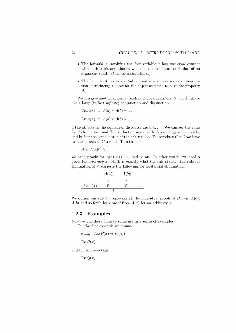
We can give another informal reading of the quantifiers. ∀ and ∃ behavelike a large (in fact infinite) conjunction and disjunction:
∀x.A(x) ≡ A(a) ∧A(b) ∧ . . .
∃x.A(x) ≡ A(a) ∨A(b) ∨ . . .
if the objects in the domain of discourse are a, b, . . .. We can see the rulesfor ∀ elimination and ∃ introduction agree with this analogy immediately,and in fact the same is true of the other rules. To introduce C ∧D we haveto have proofs of C and D. To introduce
A(a) ∧A(b) ∧ . . .
we need proofs for A(a), A(b), . . . and so on. In other words, we need aproof for arbitrary x, which is exactly what the rule states. The rule forelimination of ∨ suggests the following for existential elimination:
∃x.A(x)
[A(a)]...B
[A(b)]...B . . .
B
We obtain our rule by replacing all the individual proofs of B from A(a),A(b) and so forth by a proof from A(x) for an arbitrary x.
1.2.3 Examples
Now we put these rules to some use in a series of examples.For the first example we assume
θ ≡df ∀x.(P (x)⇒ Q(x))
∃x.P (x)
and try to prove that
∃x.Q(x)
1.2. PREDICATE LOGIC 25
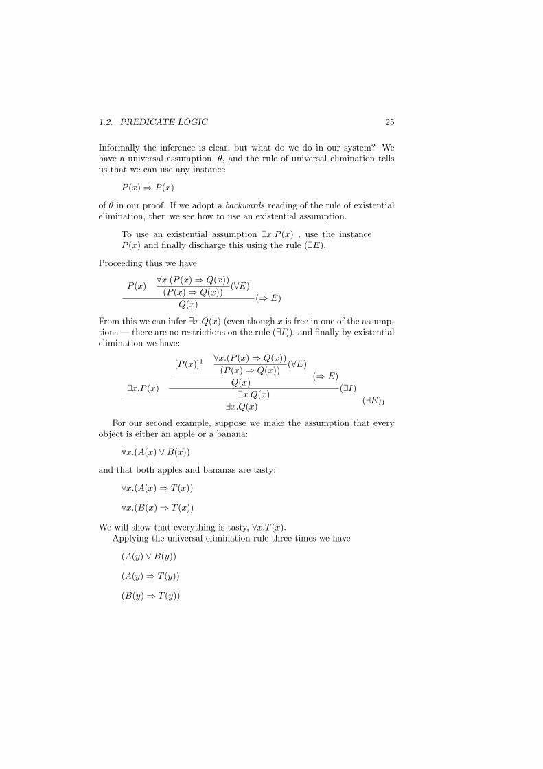
Informally the inference is clear, but what do we do in our system? Wehave a universal assumption, θ, and the rule of universal elimination tellsus that we can use any instance
P (x)⇒ P (x)
of θ in our proof. If we adopt a backwards reading of the rule of existentialelimination, then we see how to use an existential assumption.
To use an existential assumption ∃x.P (x) , use the instanceP (x) and finally discharge this using the rule (∃E).
Proceeding thus we have
P (x)∀x.(P (x)⇒ Q(x))
(P (x)⇒ Q(x))(∀E)
Q(x)(⇒ E)
From this we can infer ∃x.Q(x) (even though x is free in one of the assump-tions — there are no restrictions on the rule (∃I)), and finally by existentialelimination we have:
∃x.P (x)
[P (x)]1∀x.(P (x)⇒ Q(x))
(P (x)⇒ Q(x))(∀E)
Q(x)(⇒ E)
∃x.Q(x)(∃I)
∃x.Q(x)(∃E)1
For our second example, suppose we make the assumption that everyobject is either an apple or a banana:
∀x.(A(x) ∨B(x))
and that both apples and bananas are tasty:
∀x.(A(x)⇒ T (x))
∀x.(B(x)⇒ T (x))
We will show that everything is tasty, ∀x.T (x).Applying the universal elimination rule three times we have
(A(y) ∨B(y))
(A(y)⇒ T (y))
(B(y)⇒ T (y))
26 CHAPTER 1. INTRODUCTION TO LOGIC
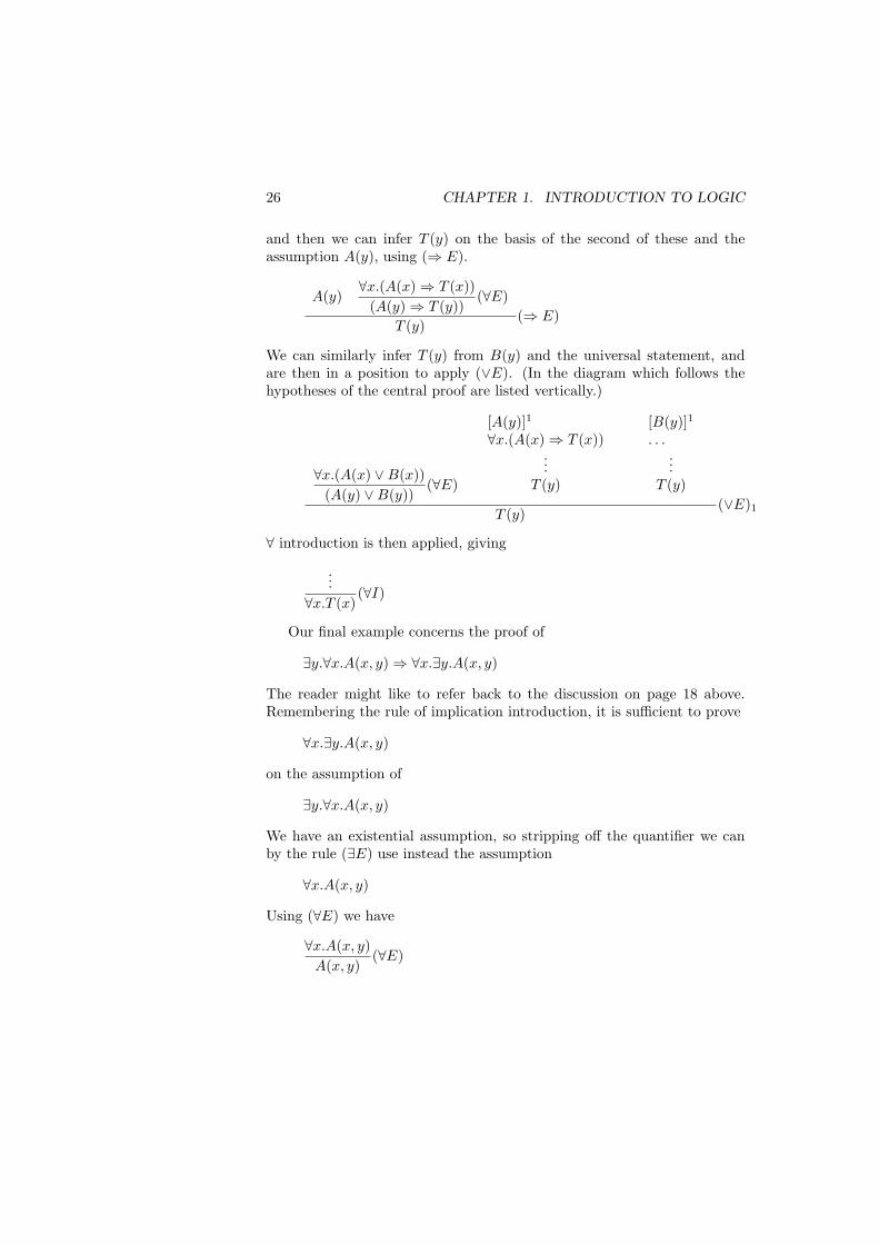
and then we can infer T (y) on the basis of the second of these and theassumption A(y), using (⇒ E).
A(y)∀x.(A(x)⇒ T (x))
(A(y)⇒ T (y))(∀E)
T (y)(⇒ E)
We can similarly infer T (y) from B(y) and the universal statement, andare then in a position to apply (∨E). (In the diagram which follows thehypotheses of the central proof are listed vertically.)
∀x.(A(x) ∨B(x))(A(y) ∨B(y))
(∀E)
[A(y)]1
∀x.(A(x)⇒ T (x))...
T (y)
[B(y)]1
. . ....
T (y)
T (y)(∨E)1
∀ introduction is then applied, giving
...∀x.T (x)
(∀I)
Our final example concerns the proof of
∃y.∀x.A(x, y)⇒ ∀x.∃y.A(x, y)
The reader might like to refer back to the discussion on page 18 above.Remembering the rule of implication introduction, it is sufficient to prove
∀x.∃y.A(x, y)
on the assumption of
∃y.∀x.A(x, y)
We have an existential assumption, so stripping off the quantifier we canby the rule (∃E) use instead the assumption
∀x.A(x, y)
Using (∀E) we have
∀x.A(x, y)A(x, y)
(∀E)
1.2. PREDICATE LOGIC 27
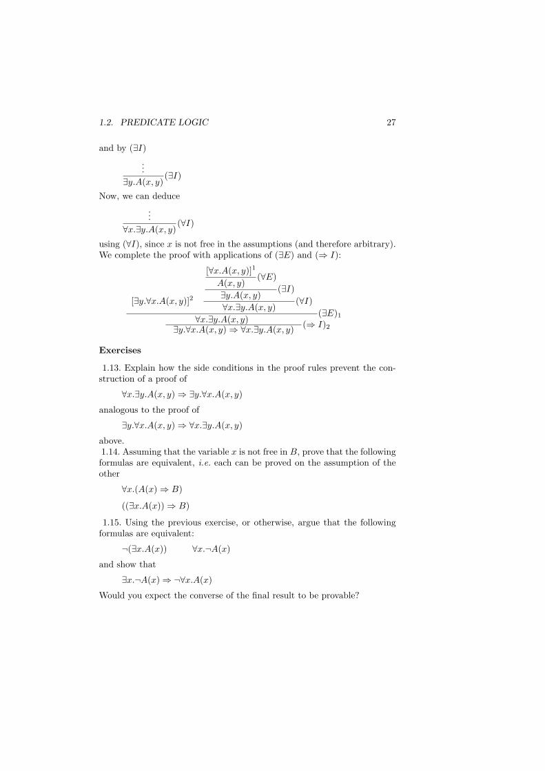
and by (∃I)
...∃y.A(x, y)
(∃I)
Now, we can deduce...
∀x.∃y.A(x, y)(∀I)
using (∀I), since x is not free in the assumptions (and therefore arbitrary).We complete the proof with applications of (∃E) and (⇒ I):
[∃y.∀x.A(x, y)]2
[∀x.A(x, y)]1
A(x, y)(∀E)
∃y.A(x, y)(∃I)
∀x.∃y.A(x, y)(∀I)
∀x.∃y.A(x, y)(∃E)1
∃y.∀x.A(x, y)⇒ ∀x.∃y.A(x, y) (⇒ I)2
Exercises
1.13. Explain how the side conditions in the proof rules prevent the con-struction of a proof of
∀x.∃y.A(x, y)⇒ ∃y.∀x.A(x, y)
analogous to the proof of
∃y.∀x.A(x, y)⇒ ∀x.∃y.A(x, y)
above.1.14. Assuming that the variable x is not free in B, prove that the followingformulas are equivalent, i.e. each can be proved on the assumption of theother
∀x.(A(x)⇒ B)
((∃x.A(x))⇒ B)
1.15. Using the previous exercise, or otherwise, argue that the followingformulas are equivalent:
¬(∃x.A(x)) ∀x.¬A(x)
and show that
∃x.¬A(x)⇒ ¬∀x.A(x)
Would you expect the converse of the final result to be provable?

28 CHAPTER 1. INTRODUCTION TO LOGIC
Chapter 2
Functional Programmingand λ-Calculi
Type theory has aspects of both a logic and a functional programming lan-guage. We have seen a brief introduction to logic in chapter 1; here wefirst survey current practice in functional programming and then look at anumber of λ-calculi, which are formal theories of functions. The λ-calculuswas invented in the nineteen thirties by Church as a notation for functions,with the aim of developing a foundation for mathematics. As with much ofthe work of that time, the original aim was not met, but the subject itselfhas become an object of study in its own right. Interest in the λ-calculushas grown again in the last two decades as it has found a role in the foun-dations of computing science, in particular through its model theory, whichunderpins much of denotational semantics. The theory usually studied isthe untyped λ-calculus, and we look at this first. We are lucky to havethe encyclopaedic [Bar84] to refer to for proofs, bibliographic and historicalinformation and so forth. Any important result in the untyped λ-calculusis to be found there, together with (at least!) one proof of it.
Running through our material, we first look at variable binding and sub-stitution, which are central to the λ-calculus. Variables are bound whena function is formed by abstraction, and when a function is applied, theformal parameters are replaced by their actual counterparts by substitu-tion. We then look at the relations of evaluation, or reduction, ‘→→’ andconvertibility ‘↔↔ ’, the latter of which represents a form of equality overthe λ-expressions. We discuss these from a general standpoint, which willform a foundation for similar discussions for type theory. In particularwe look at the determinacy of computation (the Church-Rosser property)
29
30 CHAPTER 2. FUNCTIONAL PROGRAMMING AND λ-CALCULI
and termination properties of evaluation, or as they are more commonlyknown, the normalisation properties of expressions. We draw a distinctionbetween different kinds of reduction rule — the computation and equiv-alence rules — which again we will carry through into the body of thebook. After a short look at the expressiveness of the untyped system, weturn to an examination of typed theories, which more closely reflect currentfunctional programming practice. We highlight the difference between thetyped and untyped by showing that the former is strongly normalising —all evaluation sequences are finite, meaning that, in particular, every pro-gram terminates. We give a proof of this theorem, which forms a modelfor other results of this sort in its proof by induction over types and itsformulation of a strong induction hypothesis, a method first introduced byWilliam Tait. Augmenting the type structure with product types and nat-ural numbers, we finish by returning to the discussion of computation andequivalence rules in the context of a typed language.
The survey [Hue90b] gives a useful overview of typed λ-calculi.
2.1 Functional Programming
The functional style of programming has been growing in popularity overthe last thirty years, from its beginnings in early dialects of LISP, to thepresent day and the availability of a number of production-quality lan-guages like Haskell, Hope, Miranda, and Standard ML (SML) amongstothers [HW90, BMS80, Tur85, Har86]. Although there are differences be-tween them, there is a wide degree of consensus about the form of thesystems, which provide
First-class functions: Functions may be passed as arguments to and re-turned as results of other functions; they may form components ofcomposite data structures and so on. An example is the map func-tion. It takes a function, f say, as argument, returning the functionwhich takes a list, x say, as argument and returns the list resultingfrom applying f to every item in x.
Strong type systems: The language contains distinctions between dif-ferent values, classing similar values into types. The typing of valuesrestricts the application of operators and data constructors, so thaterrors in which, for example, two boolean values are added, will notbe permitted. Moreover, and this is what is meant by the adjective‘strong’, no run-time errors can arise through type mismatches.
Polymorphic types: A potential objection to strong typing runs thus:in an untyped language we can re-use the same code for the identity
2.1. FUNCTIONAL PROGRAMMING 31
function over every type, after all it simply returns its argument. Sim-ilarly we can re-use the code to reverse a linked list over structurallysimilar lists (which only differ in the type of entries at each node)as the code is independent of the contents. We can accommodatethis kind of genericity and retain strong typing if we use the Hindley-Milner type system, [Mil78], or other sorts of polymorphic type. Thetype of the identity function becomes * -> *, where * is a type vari-able, indicating that the type of the function is a functional type, inwhich the domain and range type are the same. This means that itcan be used on booleans, returning a boolean, on numeric functionsreturning a numeric function, and so on.
Algebraic types: Lists, trees, and other types can be defined directlyby recursive definitions, rather than through pointer types. Themechanism of algebraic types generalises enumerated types, (variant)records, certain sorts of pointer type definitions, and also permits typedefinitions (like those of lists) to be parametrised over types (like thetype of their contents). Pattern matching is usually the means bywhich case analyses and selections of components are performed.
Modularity: The languages provide systems of modules of varying degreesof complexity by means of which large systems can be developed moreeasily.
One area in which there are differences is in the mechanism of evaluation.The SML system incorporates strict evaluation, under which scheme ar-guments of functions are evaluated before the instantiated function body,and components of data types are fully evaluated on object formation. Onthe other hand, Miranda and Haskell adopt lazy evaluation, under whichfunction arguments and data type components are only evaluated whenthis becomes necessary, if at all. This permits a distinctive style of pro-gramming based on infinite and partially-defined data structures. Thereare advantages of each system, and indeed there are hybrids like Hope+[Per89] which combine the two.
This is not the place to give a complete introduction to functional pro-gramming. There is a growing number of good introductory textbookson the subject [BW88, Rea89, Wik87], as well as books looking at thefoundations of the subject [Hue90a] and at current research directions[Pey87, Tur90]. We shall look at the topics described above as we de-velop our system of type theory; first, though, we investigate the lambdacalculus, which is both a precursor of current functional programming lan-guages, having been developed in the nineteen thirties, and an abstractversion of them.
32 CHAPTER 2. FUNCTIONAL PROGRAMMING AND λ-CALCULI
In what follows we use the phrase ‘languages like Miranda’ – it is meantto encompass all the languages discussed above rather than simply Miranda.
2.2 The untyped λ-calculus
The original version of the λ-calculus was developed by Church, and studiedby a number of his contemporaries including Turing, Curry and Kleene. Itprovides a skeletal functional programming language in which every objectis considered to be a function. (An alternative view of this, propoundedby [Sco80] amongst others, is of a typed theory containing a type which isisomorphic with its function space.) The syntax could not be simpler.
Definition 2.1There are three kinds of λ-expression (we use e, f, e1, e2, . . . for arbitraryλ-expressions). They are:
Individual variables or simply variables, v0, v1, v2, . . .. We shall writex, y, z, u, v, . . . for arbitrary individual variables in the following.
Applications (e1e2). This is intended to represent the application of ex-pression e1 to e2.
Abstractions (λx . e) This is intended to represent the function whichreturns the value e when given formal parameter x.
The notation above can become heavy with brackets, so we introduce thefollowing syntactic conventions.
Definition 2.2 The syntax of the system is made more readable by thefollowing syntactic conventions:
C1 Application binds more tightly than abstraction, so that λx . xy meansλx . (xy) and not (λx . x)y.
C2 Application associates to the left, implying that xyz denotes (xy)z andnot x(yz).
C3 λx1 . λx2 . . . . λxn . e means λx1 . (λx2 . . . . (λxn . e))
The crux of the calculus is the mechanism of λ-abstraction. The ex-pression
λx . e
is the general form that functions take in the system. To specify a functionwe say what is its formal parameter, here x, and what is its result, here e.
2.2. THE UNTYPED λ-CALCULUS 33
In a functional language like Miranda we give these definitions by equationswhich name the functions, such as
f x = e
and in mathematical texts we might well talk about the function f givenby
f(x) = e
In the λ-calculus we have an anonymous notation for the function whichintroduces the function without giving it a name (like f). The parameterx is a formal parameter and so we would expect that the function
λx . λy . xy
would be indistinguishable from
λu . λv . uv
for instance. Formally, as we saw in the chapter on logic, such variables xare called bound, the λ being the binding construct.
How do we associate actual parameters with the formals? We formapplications
(λx . e1) e2
To evaluate these applications, we pass the parameter: we substitute theactual parameter for the formal, which we denote
e1[e2/x]
As for the binding constructs of logic, the quantifiers, we have to be carefulabout how we define substitution, which we do, after saying formally whatit means to be bound and free.
Definition 2.3 An occurrence of a variable x within a sub-expression λx . eis bound; all other occurrences are free. The occurrence of x in λx. is thebinding occurrence which introduces the variable – other occurrences arecalled applied. We say that a variable x occurs free in an expression f ifsome occurrence of x is free in f . A variable x is bound by the syntacticallyinnermost enclosing λ, if one exists, just as in any block-structured pro-gramming language. An expression is closed if it contains no free variables,otherwise it is open .
34 CHAPTER 2. FUNCTIONAL PROGRAMMING AND λ-CALCULI
The same variable may occur both bound and free in an expression. Forexample, the first applied occurrence of x in
(λx . λy . yx)((λz . zx)x)
is bound, but the second and third applied occurrences are free.
Definition 2.4 The substitution of f for the free occurrences of x in e,written e[f/x], is defined thus:
• x[f/x]≡df f and for a variable y 6≡ x, y[f/x]≡df y
• For applications, we substitute into the two parts:
(e1 e2)[t/x] ≡df (e1[t/x] e2[t/x])
• If e ≡ λx . g then e[f/x]≡df e.If y is a variable distinct from x, and e ≡ λy . g then
– if y does not appear free in f , e[f/x]≡df λy . g[f/x].
– if y does appear free in f ,
e[f/x]≡df λz . (g[z/y][f/x])
where z is a variable which does not appear in f or g. (Notethat we have an infinite collection of variables, so that we canalways find such a z.)
• In general, it is easy to see that if x is not free in e then e[f/x] is e
Convention on Expression Equivalence: We shall not distinguish be-tween expressions which are equivalent up to change of bound variablenames in what follows. (As an aside, this convention which is easy to state,and indeed for us to follow, is surprisingly difficult to implement.)
As we said, we evaluate expressions by passing parameters in functionapplications. We formalise this by the following reduction or computationrules.
Definition 2.5 The rule of β-reduction states that for all x, e and f , wecan reduce the application
(λx . e)f →β e[f/x]
2.2. THE UNTYPED λ-CALCULUS 35
Definition 2.6 A sub-expression of a lambda expression of the form (λx . e)fis called a (β-)redex. We write g →β g′ if g′ results from applying β-reduction to a redex within g. Alternatively we can say that if e→β e′
then
(fe)→β (fe′)
(eg)→β (e′g)
λy . e→β λy . e′
Definition 2.7 We write e →→ f if there is a sequence of zero or morereductions so that
e ≡ e0→β · · · →β en ≡ f
representing a sequence of reduction steps. We call such an f a reduct ofe.
In the section which follows we look further at the reduction relation→→.One point is worthy of note before we do that. We have only introducedone argument functions into our theory; is this a restriction? It is not, aswe can represent a two argument function by a function which takes itsarguments one at a time. The addition function, for example, would berepresented by
λx . λy . (x + y)
where we assume (purely for illustrative purposes) that the language con-tains the + operator. This form of representation is known as the curriedform in honour of Haskell B. Curry, and has the property that it is sensibleto pass to it one of its arguments only. In this case, for instance,
(λx . λy . (x + y)) 4
is the function which adds four to its argument.
Exercises
2.1. Investigate the reduction behaviour of the following terms
(λx . x)((λy . (λz . z))(λx . x))
(λx . xxx)(λx . xxx)
36 CHAPTER 2. FUNCTIONAL PROGRAMMING AND λ-CALCULI
2.3 Evaluation
The reduction relation, →→, of the previous section embodies what it is forone expression to reduce to another by a number of elementary computationsteps. We can ask a number of fundamental questions about this relation.
It is somewhat artificial to examine evaluation in the context of theuntyped λ-calculus, since all we have in this context are functions, andwe do not usually consider functions to be objects which can be evaluatedthemselves, rather we work in typed systems and print only the results ofevaluating expressions of ground type, like numbers, pairs of booleans andso forth. Nonetheless we can both establish some terminology and begindiscussions here, even if we will have more to say later.
First, if the relation describes evaluation, what is it that expressionsevaluate to? There are a number of answers to this.
Definition 2.8
Normal Form: An expression is in normal form if it contains no redexes.
Head Normal Form: All expressions of the form
λx1 . . . . λxn . ye1 . . . em
where y is a variable, e1, . . . , em are arbitrary expressions and n andm are greater than or equal to zero, are in head normal form.
Weak Head Normal Form: All expressions which are either λ-abstractionsor of the form
ye1 . . . em
where y is a variable, e1, . . . , em are arbitrary expressions and m isgreater than or equal to zero, are in weak head normal form.
Definition 2.9 We say that e′ is a normal form (head normal form, etc.)of e if e→→ e′ and e′ is in normal form (head normal form, etc.).
The three definitions above are given in inclusion order: normal formsare head normal forms which are themselves weak head normal forms.Neither of the converses holds; λx . (x((λx . xx)(λx . xx))) is in head nor-mal form but not in normal form (and indeed has no normal form) whilst
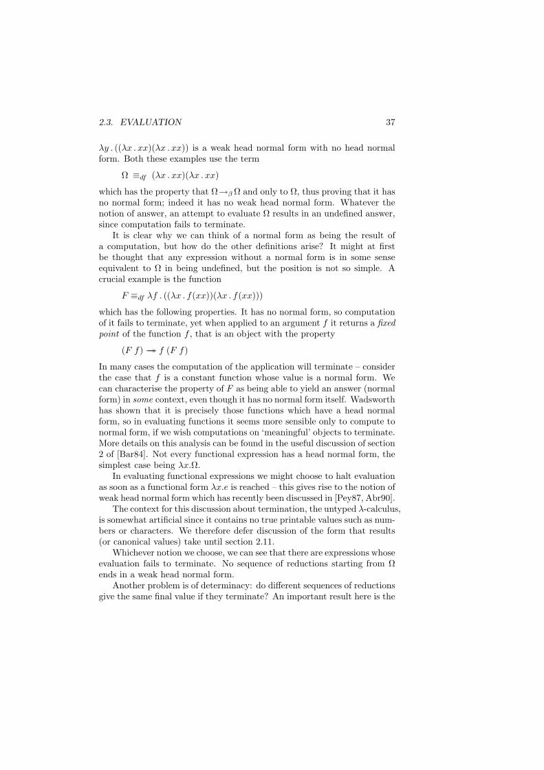
2.3. EVALUATION 37
λy . ((λx . xx)(λx . xx)) is a weak head normal form with no head normalform. Both these examples use the term
Ω ≡df (λx . xx)(λx . xx)
which has the property that Ω→β Ω and only to Ω, thus proving that it hasno normal form; indeed it has no weak head normal form. Whatever thenotion of answer, an attempt to evaluate Ω results in an undefined answer,since computation fails to terminate.
It is clear why we can think of a normal form as being the result ofa computation, but how do the other definitions arise? It might at firstbe thought that any expression without a normal form is in some senseequivalent to Ω in being undefined, but the position is not so simple. Acrucial example is the function
F ≡df λf . ((λx . f(xx))(λx . f(xx)))
which has the following properties. It has no normal form, so computationof it fails to terminate, yet when applied to an argument f it returns a fixedpoint of the function f , that is an object with the property
(F f)→→ f (F f)
In many cases the computation of the application will terminate – considerthe case that f is a constant function whose value is a normal form. Wecan characterise the property of F as being able to yield an answer (normalform) in some context, even though it has no normal form itself. Wadsworthhas shown that it is precisely those functions which have a head normalform, so in evaluating functions it seems more sensible only to compute tonormal form, if we wish computations on ‘meaningful’ objects to terminate.More details on this analysis can be found in the useful discussion of section2 of [Bar84]. Not every functional expression has a head normal form, thesimplest case being λx.Ω.
In evaluating functional expressions we might choose to halt evaluationas soon as a functional form λx.e is reached – this gives rise to the notion ofweak head normal form which has recently been discussed in [Pey87, Abr90].
The context for this discussion about termination, the untyped λ-calculus,is somewhat artificial since it contains no true printable values such as num-bers or characters. We therefore defer discussion of the form that results(or canonical values) take until section 2.11.
Whichever notion we choose, we can see that there are expressions whoseevaluation fails to terminate. No sequence of reductions starting from Ωends in a weak head normal form.
Another problem is of determinacy: do different sequences of reductionsgive the same final value if they terminate? An important result here is the
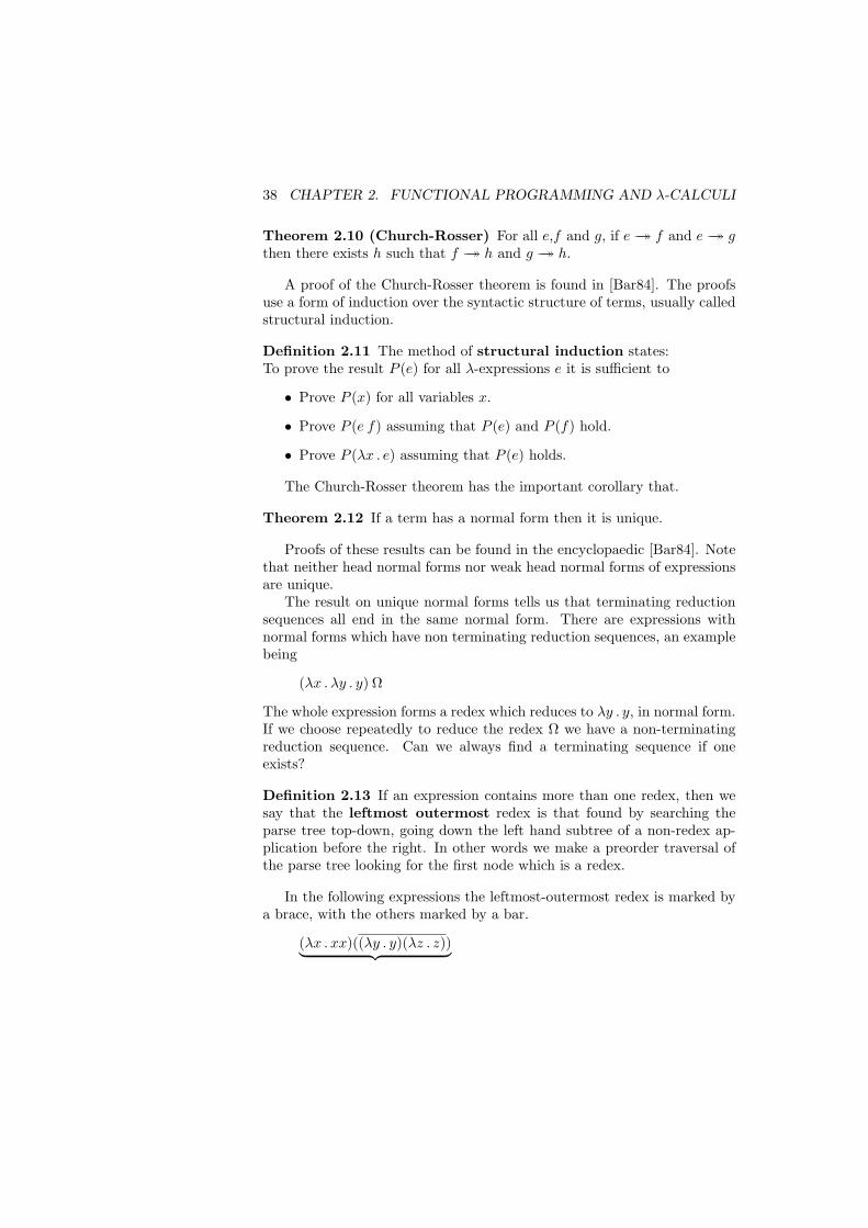
38 CHAPTER 2. FUNCTIONAL PROGRAMMING AND λ-CALCULI
Theorem 2.10 (Church-Rosser) For all e,f and g, if e→→ f and e→→ gthen there exists h such that f →→ h and g →→ h.
A proof of the Church-Rosser theorem is found in [Bar84]. The proofsuse a form of induction over the syntactic structure of terms, usually calledstructural induction.
Definition 2.11 The method of structural induction states:To prove the result P (e) for all λ-expressions e it is sufficient to
• Prove P (x) for all variables x.
• Prove P (e f) assuming that P (e) and P (f) hold.
• Prove P (λx . e) assuming that P (e) holds.
The Church-Rosser theorem has the important corollary that.
Theorem 2.12 If a term has a normal form then it is unique.
Proofs of these results can be found in the encyclopaedic [Bar84]. Notethat neither head normal forms nor weak head normal forms of expressionsare unique.
The result on unique normal forms tells us that terminating reductionsequences all end in the same normal form. There are expressions withnormal forms which have non terminating reduction sequences, an examplebeing
(λx . λy . y) Ω
The whole expression forms a redex which reduces to λy . y, in normal form.If we choose repeatedly to reduce the redex Ω we have a non-terminatingreduction sequence. Can we always find a terminating sequence if oneexists?
Definition 2.13 If an expression contains more than one redex, then wesay that the leftmost outermost redex is that found by searching theparse tree top-down, going down the left hand subtree of a non-redex ap-plication before the right. In other words we make a preorder traversal ofthe parse tree looking for the first node which is a redex.
In the following expressions the leftmost-outermost redex is marked bya brace, with the others marked by a bar.
(λx . xx)((λy . y)(λz . z))︸ ︷︷ ︸
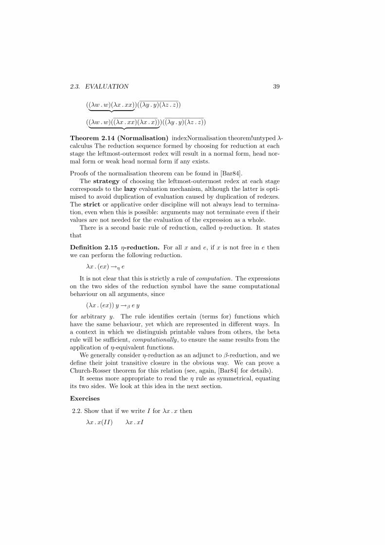
2.3. EVALUATION 39
((λw .w)(λx . xx)︸ ︷︷ ︸)((λy . y)(λz . z))
((λw .w)((λx . xx)(λx . x))︸ ︷︷ ︸)((λy . y)(λz . z))
Theorem 2.14 (Normalisation) indexNormalisation theorem!untyped λ-calculus The reduction sequence formed by choosing for reduction at eachstage the leftmost-outermost redex will result in a normal form, head nor-mal form or weak head normal form if any exists.
Proofs of the normalisation theorem can be found in [Bar84].The strategy of choosing the leftmost-outermost redex at each stage
corresponds to the lazy evaluation mechanism, although the latter is opti-mised to avoid duplication of evaluation caused by duplication of redexes.The strict or applicative order discipline will not always lead to termina-tion, even when this is possible: arguments may not terminate even if theirvalues are not needed for the evaluation of the expression as a whole.
There is a second basic rule of reduction, called η-reduction. It statesthat
Definition 2.15 η-reduction. For all x and e, if x is not free in e thenwe can perform the following reduction.
λx . (ex)→η e
It is not clear that this is strictly a rule of computation. The expressionson the two sides of the reduction symbol have the same computationalbehaviour on all arguments, since
(λx . (ex)) y→β e y
for arbitrary y. The rule identifies certain (terms for) functions whichhave the same behaviour, yet which are represented in different ways. Ina context in which we distinguish printable values from others, the betarule will be sufficient, computationally , to ensure the same results from theapplication of η-equivalent functions.
We generally consider η-reduction as an adjunct to β-reduction, and wedefine their joint transitive closure in the obvious way. We can prove aChurch-Rosser theorem for this relation (see, again, [Bar84] for details).
It seems more appropriate to read the η rule as symmetrical, equatingits two sides. We look at this idea in the next section.
Exercises
2.2. Show that if we write I for λx . x then
λx . x(II) λx . xI
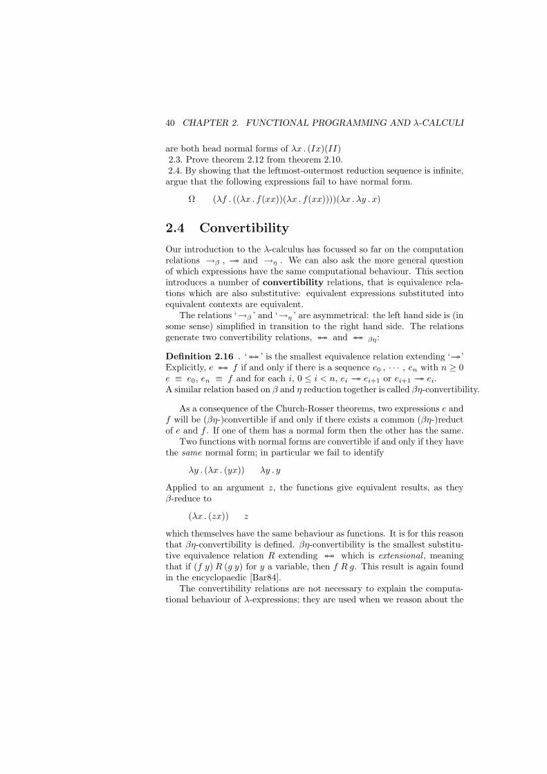
40 CHAPTER 2. FUNCTIONAL PROGRAMMING AND λ-CALCULI
are both head normal forms of λx . (Ix)(II)2.3. Prove theorem 2.12 from theorem 2.10.2.4. By showing that the leftmost-outermost reduction sequence is infinite,argue that the following expressions fail to have normal form.
Ω (λf . ((λx . f(xx))(λx . f(xx))))(λx . λy . x)
2.4 Convertibility
Our introduction to the λ-calculus has focussed so far on the computationrelations →β , →→ and →η . We can also ask the more general questionof which expressions have the same computational behaviour. This sectionintroduces a number of convertibility relations, that is equivalence rela-tions which are also substitutive: equivalent expressions substituted intoequivalent contexts are equivalent.
The relations ‘→β ’ and ‘→η ’ are asymmetrical: the left hand side is (insome sense) simplified in transition to the right hand side. The relationsgenerate two convertibility relations, ↔↔ and ↔↔ βη:
Definition 2.16 . ‘↔↔ ’ is the smallest equivalence relation extending ‘→→’Explicitly, e ↔↔ f if and only if there is a sequence e0 , · · · , en with n ≥ 0e ≡ e0, en ≡ f and for each i, 0 ≤ i < n, ei →→ ei+1 or ei+1 →→ ei.A similar relation based on β and η reduction together is called βη-convertibility.
As a consequence of the Church-Rosser theorems, two expressions e andf will be (βη-)convertible if and only if there exists a common (βη-)reductof e and f . If one of them has a normal form then the other has the same.
Two functions with normal forms are convertible if and only if they havethe same normal form; in particular we fail to identify
λy . (λx . (yx)) λy . y
Applied to an argument z, the functions give equivalent results, as theyβ-reduce to
(λx . (zx)) z
which themselves have the same behaviour as functions. It is for this reasonthat βη-convertibility is defined. βη-convertibility is the smallest substitu-tive equivalence relation R extending ↔↔ which is extensional , meaningthat if (f y) R (g y) for y a variable, then f R g. This result is again foundin the encyclopaedic [Bar84].
The convertibility relations are not necessary to explain the computa-tional behaviour of λ-expressions; they are used when we reason about the
2.5. EXPRESSIVENESS 41
behaviour of expressions, in particular they can tell us which functions havethe same behaviour, and which transformations (of one expression into an-other) are permissible. We shall return to this topic in section 2.11, afterdiscussing typed λ-calculi.
Exercises
2.5. Show that if e has the form λy . e′ where x is not free in e′ then
(λx . ex)→β e
2.5 Expressiveness
The untyped λ-calculus is a simple theory of (pure) functions, yet compu-tationally it is as strong as other fundamental theories of computation. Itis Turing-complete, exhibiting an equivalence with Turing computability.One half of this equivalence consists in showing that objects such as thenatural numbers, booleans and so forth can be represented as λ terms, andthat recursive functions can be defined over them. Yet again, Barendregtprovides a suitable reference for this material. One representation of thenatural numbers is as the iterators, n being represented by
λf . λx . f (f . . . f (f︸ ︷︷ ︸n
x) . . .)
which are in normal form. To derive recursive functions, with definitionslike
f x≡df . . . f . . .
which can be written
f ≡df λx. . . . f . . .
we need to be able to solve equations of the form
f ≡df R f
where R is a λ term. In fact we can define operations, F , called fixedpoint combinators which solve these equations thus:
F R→→ R (F R)
Two examples are the expressions:
θθ where θ ≡df λa . λb . (b(aab)))

42 CHAPTER 2. FUNCTIONAL PROGRAMMING AND λ-CALCULI
F ≡df λf . ((λx . f(xx))(λx . f(xx)))
Each of these expressions has a head normal form, but neither has a normalform. This is a general property of fixed point combinators, since
λx . (F x) →β λx . (x (F x))→β λx . (x (x (F x)))→β . . .
and F has a normal form if and only if λx . (F x) has. This is an interestingpoint: here we have meaningful functions which cannot be represented byexpressions in normal form, showing that the class of meaningful expres-sions extends beyond those with normal form.
2.6 Typed λ-calculus
The untyped λ-calculus is powerful, containing as it does the fixed pointcombinators, representatives of all the common base types and their combi-nations under standard type-forming operations. The disadvantage of thispower is the fact that our programs can continually break the stipulationsof our conceptual type system, which permits only numbers to be addedand so forth.
Another aspect of the system is the presence of non-termination: wehave seen that not every term has even a weak head normal form. Anyattempt to evaluate Ω results in a non-terminating computation. Ω doesnot have a legitimate type in any type system, except those which include areflexive type C isomorphic to its function space (C ⇒ C). Terms with thecomputational behaviour of Ω are introduced by a fixed point combinator:
F (λx . x) →β (λx . x) (F (λx . x))→β (F (λx . x))→β . . .
and the existence of such a combinator does not contradict the type disci-pline, despite the fact that the definitions of the previous section are nottypeable, containing as they do applications of objects to themselves.
We now examine a number of typed λ-calculi of differing expressivestrength which will culminate in the system of constructive type theoryitself.
In this chapter we are able to develop separately first the types andthen the terms of the theory. We begin by defining a system with functiontypes (and a number of base types), progressively adding further types andobjects.
2.6. TYPED λ-CALCULUS 43
Definition 2.17 Given a set B of base types, we form the set S of simpletypes closing under the rule of function type formation. This states thatif σ and τ are types then so is (σ ⇒ τ). We assume that ‘⇒’ is rightassociative, and omit brackets accordingly.
In typed lambda calculi each λ-expression (or term, we use these inter-changeably) has a type. We shall write
e :τ
for ‘e is a λ-expression of type τ ’. We specify the type of each definedλ-expression below.
Definition 2.18 The expressions of the typed λ-calculus have three forms.
Individual variables or simply variables, vτ,0, vτ,1,τ,2 , . . ., for each typeτ .
vτ,i :τ
We shall write xτ , yτ , zτ , . . ., with or without type subscripts for ar-bitrary individual variables in what follows.
Applications If e1 : (σ ⇒ τ) and e2 :σ then
(e1 e2) :τ
We can only form an application when the type of the argument isthe same as the type of the domain of the function.
Abstractions If x :σ and e :τ then
(λxσ . e) : (σ ⇒ τ)
The type of an abstraction is a function type, whose domain is thetype of the formal parameter and whose range is the type of thefunction body (or result).
Many notions defined in the untyped case carry over to here. Theseinclude the substitution mechanism, β- and η-reduction and convertibil-ity and the notions of canonical element: normal form, head normal formetcetera. It is easy to see that convertible expressions must be of the sametype.
Many results carry over too. The Church-Rosser theorems for β andβη-reduction have the same proofs. Given a variable xσ, we are unable toform the application xσxσ and thus unable to define Ω and the fixed pointcombinators we saw above. This is no accident, as we can prove
44 CHAPTER 2. FUNCTIONAL PROGRAMMING AND λ-CALCULI
Theorem 2.19 (Strong Normalisation) Every reduction sequence ter-minates.
This important result is proved in the next section, and also in [FLO83].Clearly the system is less expressive than the untyped calculus; precisedetails are also found in [FLO83].
We can present the calculus in a slightly different form, closer to thepractice in programming languages. Instead of there being an infinite classof variables for each type we can simply take one (infinite) class of variables.When we use a variable we assume it is associated with a type: we call this atype assumption but it might be more familiar as a declaration in a languagelike Pascal. We then assign types to expressions in the type context of anumber of type assumptions. We will write Γ, . . .for such contexts, usingΓ, x :τ for the context Γ with the type assumption x :τ added. We assumethroughout that all contexts Γ are consistent in containing at most oneoccurrence of each variable – we can give any expression a type using theappropriate inconsistent context. Writing
Γ ` e :τ
for ‘e has the type τ in the context Γ’, the syntax rules become
Definition 2.20
Individual variables For any context Γ,
Γ, x :τ ` x :τ
Applications If
Γ ` e1 : (σ ⇒ τ)
and
Γ ` e2 :σ
then
Γ ` (e1 e2) :τ
As before, we can only form an application when the type of theargument is the same as the type of the domain of the function.
2.7. STRONG NORMALISATION 45
Abstractions If
Γ, x :σ ` e :τ
then
Γ ` (λxσ . e) : (σ ⇒ τ)
The type of an abstraction is a function type, whose domain is thetype of the formal parameter and whose range is the type of thefunction body (or result).
The rule giving the type of an abstraction has one unusual aspect. Theassumption that x : σ is used in typing the body of the function, e, but isnot needed to give a type to the function itself. Why is this? In generalthe variable x will appear free in the expression e — we cannot type anexpression containing a free variable without knowing the type for the vari-able, and this is given by the assumption. On the other hand, in (λxσ . e)x is bound and associated with the type σ it is assumed to have in the ex-pression e, which is the scope of that particular declaration of the variablex.
Exercises
2.6. Show that
λx . λy . λz . (xz)(yz) : (σ ⇒ τ ⇒ ρ)⇒ (σ ⇒ τ)⇒ (σ ⇒ ρ)
2.7. Explain why λx . xx and the fixed point combinator F are not termsof the typed λ-calculus.
2.7 Strong normalisation
This section introduces a result which is important both in itself and be-cause of its method of proof. This method, introduced in [Tai67] and knownas the reducibility method, is a general means of proof for systems whichare typed. It involves an induction over the complexity of the types, ratherthan over syntactic complexity, which we saw was the major method ofproof for untyped systems.
Theorem 2.21 (Strong Normalisation) For all expressions e of the sim-ply typed λ-calculus, all reduction sequences beginning with e are finite.
46 CHAPTER 2. FUNCTIONAL PROGRAMMING AND λ-CALCULI
How should the proof proceed? One method we cannot use is a straight-forward structural induction, as a proof using this alone would carry overto the untyped case, where we know that not even the terms with normalform are strongly normalising. The method we use will involve an inductionover the structure of types:
Definition 2.22 The method of Induction over Types states that toprove the result P (τ) for all types τ it is sufficient to
• Prove P (σ) for all base types σ ∈ B. This is called the base case.
• Prove P (σ ⇒ τ) assuming that P (σ) and P (τ) hold. This is calledthe induction step.
As is common in proofs by induction, in order to prove a propertyR(e) of every expression e we in fact prove a strengthening R′ of R. This isbecause the obvious induction hypothesis will not be strong enough to workat the induction step. This is the case with the property of e is stronglynormalising which we abbreviate ‘e is SN’: two terms e and e′ may bestrongly normalising without it being clear that the application (e e′) is so.(It will of course be strongly normalising by the proof we construct, butthat begs the question of how we establish it.)
Definition 2.23 We say that an expression e of type τ is stable, writtene ∈ ‖τ‖ if
• If e is of base type and e is SN, or
• If e is of type σ ⇒ τ and for all e′ in ‖σ‖, (e e′) ∈ ‖τ‖
Stability is designed to be preserved by application, so that it is easierto see that it will be carried through that case of the induction. Note alsothat we use the type system in an essential way in this definition: we definestability for a function type in terms of stability for its domain and rangetypes.
Before we begin the proof of the theorem, we note the following prop-erties of the class of strongly normalising terms.
Lemma 2.24 If x is a variable then
(a) x ∈ SN
(b) If e1, . . . , ek ∈ SN then xe1 . . . ek ∈ SN .
(c) If ex ∈ SN then e ∈ SN .
2.7. STRONG NORMALISATION 47
(d) If e ∈ SN then (λx . e) ∈ SN
Proof: (a) This is obvious, as the variable contains no redex.
(b) Any reduction sequence from xe1 . . . ek will have the form
xe1 . . . ek→β . . . →β xf1 . . . fk→β xg1 . . . gk→β . . .
where at each stage for exactly one index j, fj →β gj and for the others,fi ≡ gi. This means that if there is an infinite reduction sequence fromxe1 . . . ek then there must be one from one of the eis, a contradiction totheir being SN.
(c) A reduction sequence from ex will either have the form
ex→β e1x→β e2x→β . . . →β enx→β . . .
or the form
ex→β e1x→β . . . →β (λy . f) x→β f [x/y]→β f1[x/y]→β f2[x/y]→β . . .
where
λy . f →β λy . f1→β λy . f2→β . . .
is a reduction sequence continuing e→β e1→β . . .. In either case an infinitesequence starting at ex gives rise one starting at e.
(d) A reduction sequence starting at λx . e will have the form
λy . e→β λy . e1→β λy . e2→β . . .
where
e→β e1→β e2→β . . .
and so an infinite sequence starting at λy . e gives rise to another startingat e. 2
The proof of the theorem itself is based on two further lemmas. Inthe first we show that stable objects are strongly normalising (at the sametime showing that variables are stable), and in the second we show that allobjects are stable.
Lemma 2.25 (a) If e ∈ ‖τ‖ then e ∈ SN
(b) If xe1 . . . en :τ and e1, . . . , en ∈ SN then xe1 . . . en ∈ ‖τ‖
(c) If x :τ then x ∈ ‖τ‖.
48 CHAPTER 2. FUNCTIONAL PROGRAMMING AND λ-CALCULI
Proof: We prove (a), (b) and (c) by a simultaneous induction over thetype τ .
Base case: τ is a base type. The property (a) is true by definition ofstability for a base type.For (b), if e1, . . . , en ∈ SN then by lemma 2.24, part (b), xe1 . . . ek will bestrongly normalising, and since τ is a base type, the expression is stable.Finally, to prove (c) observe that any variable is strongly normalising andtherefore stable if it is of base type.
Induction step: We assume that τ is the type (σ ⇒ ρ) and that theresults (a), (b) and (c) hold for the types σ, ρ.To prove (a) we assume that e ∈ ‖τ‖. We have to prove that e is SN. Takex of type σ. By (c) for σ, x is stable, and so by the definition of stabilityfor e, ex will be stable. ex is of type ρ and so by (a) for ρ, ex is SN. Usinglemma 2.24 part (c), e is therefore SN.Now we show (b). To prove that xe1 . . . en ∈ ‖τ‖ we need to show thatxe1 . . . enf is in ‖ρ‖, if f ∈ ‖σ‖. By hypothesis e1, . . . , en ∈ SN and by (a)for σ, f is also SN. The expression xe1 . . . enf is of type ρ and so by (b) forρ,
xe1 . . . enf ∈ ‖ρ‖
as required.Finally, we show (c). Suppose that f in ‖σ‖. By (a) for σ, f is SN, andsince the expression (xf) has type ρ, by (b) for ρ, (xf) is in ‖ρ‖, so x isstable. 2
Our task now is to show that all expressions are stable. We aim to do thisby structural induction over the expressions. We know that variables arestable by the previous result, and we prove easily that application preservesstability: indeed this was a motivation of the definition. The case of λ-abstraction is more tricky. We aim to prove that λx . f is stable, assumingf is, and so we have to prove that for all stable g of the appropriate type,
(λx . f) g
is stable. This expression reduces to f [g/x]. We need to deduce the sta-bility of the former from that of the latter. In fact we need to prove ageneralisation of this to get the induction to work, which readers can seefor themselves by trying a direct proof. The generalisation is clause (b) ofthe next lemma.
Before we state the lemma, we give another definition.
Definition 2.26 A s-instance e′ of an expression e is a substitution in-stance e′ ≡ e[g1/x1, . . . , gr/xr] where the gi are stable expressions.
2.7. STRONG NORMALISATION 49
Lemma 2.27 (a) If e and f are stable then so is (ef).
(b) For all k ≥ 0, if f [g/x]h1 . . . hk ∈ ‖τ‖ and g ∈ SN then
(λx . f)gh1 . . . hk ∈ ‖τ‖
(c) All s-instances e′ of expressions e are stable.
Proof: We prove the clauses one at a time.
(a): If e ∈ ‖σ ⇒ τ‖ and f ∈ ‖σ‖ then by definition of stability for thefunction space, (ef) ∈ ‖τ‖, in other words (ef) is stable.
(b): This we prove by induction over the type τ .Base case: Suppose first that τ is of base type. We need to prove that(λx . f)gh1 . . . hk is strongly normalising assuming that f [g/x]h1 . . . hk andg are.Consider the general form of a reduction sequence starting from
(λx . f)gh1 . . . hk
Redexes will either be contained in f , g and h1,. . .hk or consist of the headredex (λx . f)g. All sequences will take either the form
(λx . f)gh1 . . . hk →→ (λx . f ′)g′h′1 . . . h′k
→β f ′[g′/x]h′1 . . . h′k
→β . . .
or the form
(λx . f)gh1 . . . hk →→ (λx . f ′)g′h′1 . . . h′k
→β . . .
in which the top-level redex is not reduced in subsequent computation. Inthe first case, since
f [g/x]h1 . . . hk →→ f ′[g′/x]h′1 . . . h′k
the sequence must be finite, as f [g/x]h1 . . . hk is strongly normalising. Inthe second case, can we have an infinite reduction sequence without everreducing the top-level redex? A sequence of this form will consist of anumber of parallel sequences, for f , g and h1, . . . , hk. Such a sequence canbe factored into two separate sequences, one starting with g and the othercontaining no g reductions. The sequence of g reductions will be finite, asg is SN, and the other sequence will be finite as it can be transformed into
50 CHAPTER 2. FUNCTIONAL PROGRAMMING AND λ-CALCULI
a corresponding sequence of reductions of the term f [g/x]h1 . . . hk in whichno g reductions take place. Any such sequence must also be finite, so theexpression (λx . f)gh1 . . . hk is SN.Induction step: Suppose that τ is the functional type (σ ⇒ ρ). To showthat (λx . f)gh1 . . . hk ∈ ‖τ‖ we need to show that
(λx . f)gh1 . . . hkh ∈ ‖ρ‖
for every h in ‖σ‖. Now, since f [g/x]h1 . . . hk ∈ ‖τ‖,
f [g/x]h1 . . . hkh ∈ ‖ρ‖
and so by (b) for the type ρ, we have (λx . f)gh1 . . . hkh ∈ ‖ρ‖ as required.This completes the proof of (b).
(c): We prove (c) by structural induction over the expressions e. Thereare three cases.Case: Variables. For variables x, x′ will either be the stable expressiong, when the substitution has the form [. . . , g/x, . . .], or when x is not thetarget of a substitution, x′ is x which is stable by lemma 2.25, part (c).Case: Application. If e has the form (e1e2) then an s-instance of e willhave the form (e′1e
′2) where e′i is an s-instance of ei. By induction, each of
e′i is stable, and by lemma 2.27, part (a), the application (e′1e′2) is stable.
Case: Abstraction. Suppose that e has the form λx . f . We need to showthat every substitution instance of this is stable. These instances have theform λx . f ′ where f ′ is a substitution instance of f . Now, how do we provethe stability of λx . f ′? We have to show that
(λx . f ′) g
is stable for stable g. By lemma 2.25, part (a), g is SN, so applying lemma2.27, part (b) with k = 0 it is sufficient to show that f ′[g/x] is stable. Thisis also an s-instance of f and by induction it is stable. This completes theproof of this case, part (c) of the proof and therefore the proof itself. 2
Proof: (Theorem 2.21)By part (c) of lemma 2.27, every expression is stable (as it is the trivialsubstitution instance of itself), and by lemma 2.25(a), all stable expressionsare strongly normalising. 2
2.8 Further type constructors: the product
The simply typed λ-calculus could not be simpler: we have only someunspecified base types, carrying no operations, and a single form of type
2.8. FURTHER TYPE CONSTRUCTORS: THE PRODUCT 51
construction, the function space. We can extend the system in two differentways, adding both new base types and new constructors. First we look attype constructors.
Familiar type constructors include the product type and the disjointsum (or disjoint union). In Pascal these together are embodied in thevariant record type. The addition of these is standard; we review brieflythe addition of the product type to the simply typed λ-calculus now.
• To the definition of types we add the third clause that σ× τ is a typeif σ and τ are.
• We add two clauses to the definition of expressions:
Pairs If x :σ and y :τ then
(x, y) : σ × τ
The pair (x, y) is a member of the product type.Projections If p : σ × τ then fst p :σ and snd p :τ . The operations
fst and snd project a pair onto its components.
• To the rules of computation we add the rules
fst (p, q)→ p snd (p, q)→ q
which show that fst and snd do indeed behave as projection opera-tions, and we ask also that reduction is preserved by pairing, so thatif
p→ p′
then
(p, q)→ (p′, q) (q, p)→ (q, p′)
• To the rules we can also add
(fst p, snd p)→ p
for p of product type. This implies the extensionality rule that anelement of a product type is characterised by its components, since if
fst p ↔↔ fst q snd p ↔↔ snd q
then
p ↔↔ (fst p, snd p) ↔↔ (fst q, snd q) ↔↔ q
52 CHAPTER 2. FUNCTIONAL PROGRAMMING AND λ-CALCULI
We have added the operations fst and snd as primitives. Alternativelywe could think of them as constants, belonging to particular types. For thisto work here we need to add a collection of constants, one for each producttype, thus:
fstσ,τ : (σ × τ)⇒ σ
sndσ,τ : (σ × τ)⇒ τ
Our notation is made unwieldy by this addition; common practice in suchsituations is to omit the type subscripts from these constants — in anyexpression generated by the rules above we can deduce the type of eachinstance from the context.
A second alternative is to add two constants, but to allow each of themto have many types. fst would have the type (σ × τ) ⇒ σ for all thetypes σ and τ . This is the idea of polymorphism which we mentioned inour introduction to functional programming on page 30. To make thisintroduction in a disciplined way we need to strengthen the type systemto allow polymorphic types — a further extension of the calculus. Theliterature on polymorphism is extensive: [Mil78, Rey90].
A second distinction, touched upon in 2.4 was the distinction betweenβ and η reduction. We have a similar distinction between the two rules
fst (p, q)→ p snd (p, q)→ q
and the rule
(fst p, snd p)→ p
We shall call rules of the first sort computation rules and those of thelatter kind equivalence rules, as their main purpose is to develop a con-vertibility relation. A common distinction between the two pairs derivesfrom an examination of the types of the objects they relate: the computa-tion rules relate objects of arbitrary type:
(λx . e)f →→ e[f/x]
fst (p, q)→ p
where e and p are of arbitrary type. On the other hand, the equivalencerules relate elements of restricted type. In the case of η reduction
λx . (ex)→η e
2.9. BASE TYPES: NATURAL NUMBERS 53
for the left hand side to be a term of the typed calculus, e must be of afunction type. Similarly, in
(fst p, snd p)→ p
for fst p and snd p to be well-formed, p must be of product type. We willtake up this discussion further below, after adding a base type.
Exercises
2.8. Show that
λx . λy . λz . (x (y, z)) : ((σ × τ)⇒ ρ)⇒ (σ ⇒ τ ⇒ ρ)
and that
λx . λy . (x (fst y) (snd y)) : (σ ⇒ τ ⇒ ρ)⇒ ((σ × τ)⇒ ρ)
2.9 Base Types: Natural Numbers
Computations are usually performed over concrete types, such as numbers,booleans, characters and so forth. Here we look at how the natural numberscan be added to the typed λ-calculi above.
• We add the type N to our set of base types (we may have B = N).
• To the syntax of expressions we add two clauses
Numbers 0 is of type N , and if n :N then succ n :N .
Primitive Recursion For all types τ , if
e0 :τ f : (N ⇒ τ ⇒ τ)
then
Prec e0 f : N ⇒ τ
Prec is called the primitive recursor, and the term above isintended to be the primitive recursive function F defined by theequations
F 0 ≡df e0
F (n + 1) ≡df f n (F n)
To ensure the term does represent the function we add compu-tation rules for Prec, thus:
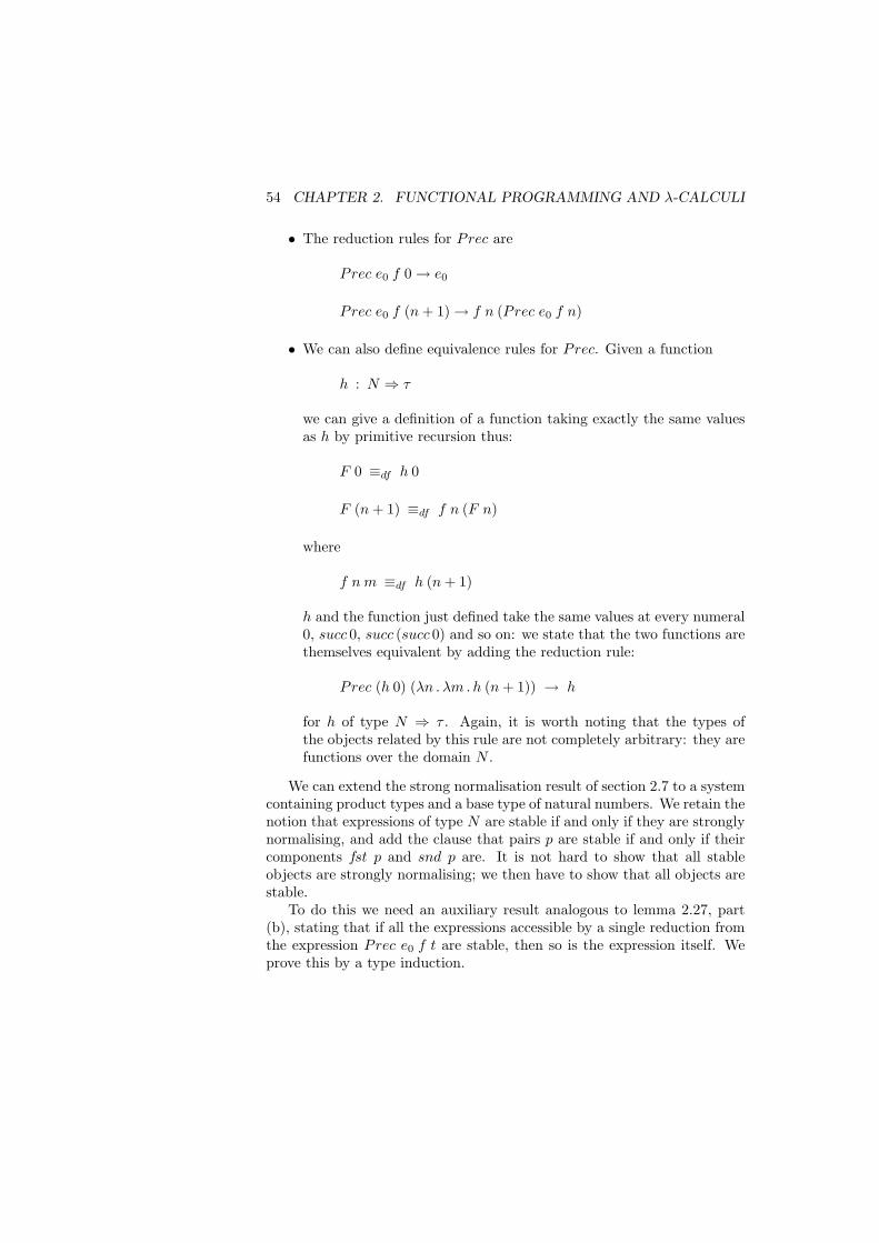
54 CHAPTER 2. FUNCTIONAL PROGRAMMING AND λ-CALCULI
• The reduction rules for Prec are
Prec e0 f 0→ e0
Prec e0 f (n + 1)→ f n (Prec e0 f n)
• We can also define equivalence rules for Prec. Given a function
h : N ⇒ τ
we can give a definition of a function taking exactly the same valuesas h by primitive recursion thus:
F 0 ≡df h 0
F (n + 1) ≡df f n (F n)
where
f n m ≡df h (n + 1)
h and the function just defined take the same values at every numeral0, succ 0, succ (succ 0) and so on: we state that the two functions arethemselves equivalent by adding the reduction rule:
Prec (h 0) (λn . λm . h (n + 1)) → h
for h of type N ⇒ τ . Again, it is worth noting that the types ofthe objects related by this rule are not completely arbitrary: they arefunctions over the domain N .
We can extend the strong normalisation result of section 2.7 to a systemcontaining product types and a base type of natural numbers. We retain thenotion that expressions of type N are stable if and only if they are stronglynormalising, and add the clause that pairs p are stable if and only if theircomponents fst p and snd p are. It is not hard to show that all stableobjects are strongly normalising; we then have to show that all objects arestable.
To do this we need an auxiliary result analogous to lemma 2.27, part(b), stating that if all the expressions accessible by a single reduction fromthe expression Prec e0 f t are stable, then so is the expression itself. Weprove this by a type induction.
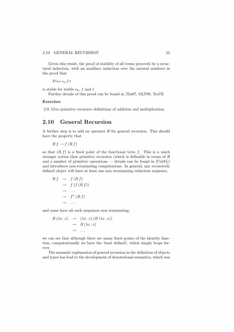
2.10. GENERAL RECURSION 55
Given this result, the proof of stability of all terms proceeds by a struc-tural induction, with an auxiliary induction over the natural numbers inthe proof that
Prec e0 f t
is stable for stable e0, f and t.Further details of this proof can be found in [Tai67, GLT89, Tro73]
Exercises
2.9. Give primitive recursive definitions of addition and multiplication.
2.10 General Recursion
A further step is to add an operator R for general recursion. This shouldhave the property that
R f → f (R f)
so that (R f) is a fixed point of the functional term f . This is a muchstronger notion than primitive recursion (which is definable in terms of Rand a number of primitive operations — details can be found in [Cut81])and introduces non-terminating computations. In general, any recursivelydefined object will have at least one non terminating reduction sequence,
R f → f (R f)→ f (f (R f))→ . . .
→ fn (R f)→ . . .
and some have all such sequences non terminating:
R (λx . x) → (λx . x) (R (λx . x))→ R (λx . x)→ . . .
we can see that although there are many fixed points of the identity func-tion, computationally we have the ‘least defined’, which simply loops for-ever.
The semantic explanation of general recursion in the definition of objectsand types has lead to the development of denotational semantics, which was
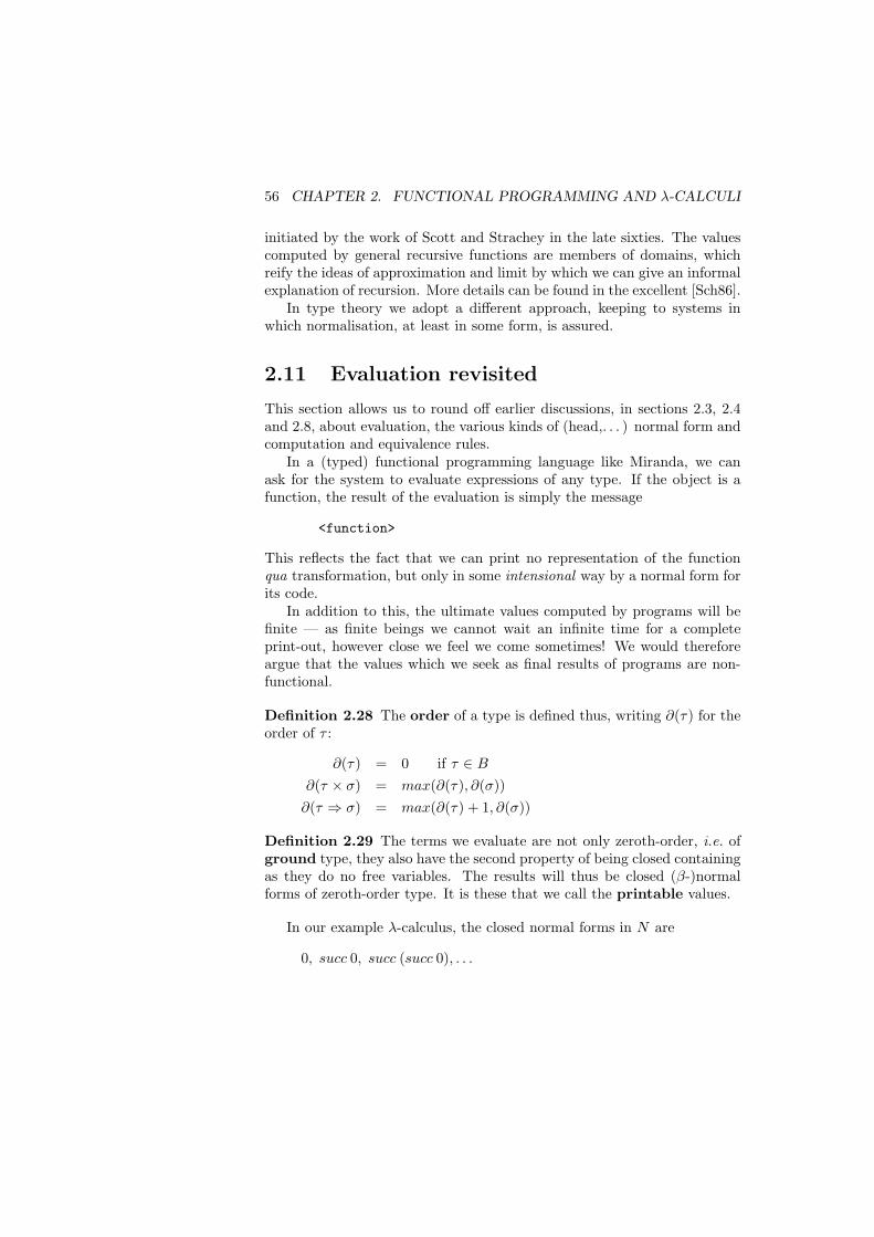
56 CHAPTER 2. FUNCTIONAL PROGRAMMING AND λ-CALCULI
initiated by the work of Scott and Strachey in the late sixties. The valuescomputed by general recursive functions are members of domains, whichreify the ideas of approximation and limit by which we can give an informalexplanation of recursion. More details can be found in the excellent [Sch86].
In type theory we adopt a different approach, keeping to systems inwhich normalisation, at least in some form, is assured.
2.11 Evaluation revisited
This section allows us to round off earlier discussions, in sections 2.3, 2.4and 2.8, about evaluation, the various kinds of (head,. . . ) normal form andcomputation and equivalence rules.
In a (typed) functional programming language like Miranda, we canask for the system to evaluate expressions of any type. If the object is afunction, the result of the evaluation is simply the message
<function>
This reflects the fact that we can print no representation of the functionqua transformation, but only in some intensional way by a normal form forits code.
In addition to this, the ultimate values computed by programs will befinite — as finite beings we cannot wait an infinite time for a completeprint-out, however close we feel we come sometimes! We would thereforeargue that the values which we seek as final results of programs are non-functional.
Definition 2.28 The order of a type is defined thus, writing ∂(τ) for theorder of τ :
∂(τ) = 0 if τ ∈ B
∂(τ × σ) = max(∂(τ), ∂(σ))∂(τ ⇒ σ) = max(∂(τ) + 1, ∂(σ))
Definition 2.29 The terms we evaluate are not only zeroth-order, i.e. ofground type, they also have the second property of being closed containingas they do no free variables. The results will thus be closed (β-)normalforms of zeroth-order type. It is these that we call the printable values.
In our example λ-calculus, the closed normal forms in N are
0, succ 0, succ (succ 0), . . .
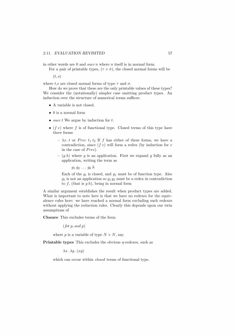
2.11. EVALUATION REVISITED 57
in other words are 0 and succ n where n itself is in normal form.For a pair of printable types, (τ × σ), the closed normal forms will be
(t, s)
where t,s are closed normal forms of type τ and σ.How do we prove that these are the only printable values of these types?
We consider the (notationally) simpler case omitting product types. Aninduction over the structure of numerical terms suffices:
• A variable is not closed.
• 0 is a normal form
• succ t We argue by induction for t.
• (f e) where f is of functional type. Closed terms of this type havethree forms
– λx . t or Prec t1 t2 If f has either of these forms, we have acontradiction, since (f e) will form a redex (by induction for ein the case of Prec).
– (g h) where g is an application. First we expand g fully as anapplication, writing the term as
g1 g2 . . . gk h
Each of the gi is closed, and g1 must be of function type. Alsog1 is not an application so g1 g2 must be a redex in contradictionto f , (that is g h), being in normal form
A similar argument establishes the result when product types are added.What is important to note here is that we have no redexes for the equiv-alence rules here: we have reached a normal form excluding such redexeswithout applying the reduction rules. Clearly this depends upon our twinassumptions of
Closure This excludes terms of the form
(fst p, snd p)
where p is a variable of type N ×N , say.
Printable types This excludes the obvious η-redexes, such as
λx . λy . (xy)
which can occur within closed terms of functional type.
58 CHAPTER 2. FUNCTIONAL PROGRAMMING AND λ-CALCULI
We therefore feel justified in making the distinction between the two kindsof rule which we called computation and equivalence rules above. Thecomputation rules suffice for the evaluation of particular terms, whilst theequivalence rules are used when reasoning about the general behaviour offunctions (applied to terms which may contain variables).
Chapter 3
Constructive Mathematics
The aim of this brief chapter is to introduce the major issues underlying theconflict between ‘constructive’ and ‘classical’ mathematics, but it cannothope to be anything other than an hors d’oeuvre to the substantial andlengthy dialogue between the two schools of thought which continues tothis day.
Luckily, there are other sources. Bishop gives a rousing call to theconstructive approach in the prologue to [BB85], which is followed by aclosely argued ‘Constructivist Manifesto’ in the first chapter. Indeed thewhole book is proof of the viability of the constructivism, developing as itdoes substantial portions of analysis from such a standpoint. It contains abibliography of further work in the field.
An invaluable historical account of the basis of the conflict as well assubsequent activity in the field can be found in the historical appendixof [Bee85]. The first part of [Bee85], entitled ‘Practice and Philosophy ofConstructive Mathematics’, also gives a most capable summary of both thescope and the foundations of constructive mathematics. [Dum77] is also agood introduction, looking in detail at the philosophy of intuitionism, andthe recent survey [TvD88] also serves its purpose well.
Bishop identifies constructivism with realism, contrasting it with theidealism of classical mathematics. He also says that it gives mathematicalstatements ‘empirical content’, as opposed to the purely ‘pragmatic’ natureof parts of classical mathematics, and sums up the programme of [BB85]thus ‘to give numerical [i.e. computational ] meaning to as much as possibleof classical abstract analysis’.
A constructive treatment of mathematics has a number of interlinkedaspects. We look at these in turn now.
59
60 CHAPTER 3. CONSTRUCTIVE MATHEMATICS
Existence and Logic
What constitutes a proof of existence of an object with certain properties?A mathematician will learn as a first-year undergraduate that to prove∃x.P (x) it is sufficient to prove that ∀x.¬P (x) is contradictory. The con-structivist would argue that all this proof establishes is the contradiction:the proof of existence must supply a t and show that P (t) is provable.Proofs of existential statements abound in mathematics: the fundamentaltheorem of algebra states that a polynomial of degree n has n complexroots; the intermediate value theorem asserts that continuous functionswhich change sign over a compact real interval have a zero in that interval,just to take two examples.
Sanction for proof by contradiction is given by the law of the excludedmiddle
A ∨ ¬A
which states in particular that
∃x.P (x) ∨ ¬∃x.P (x)
If ∀x.¬P (x), which is equivalent to ¬∃x.P (x), is contradictory, then wemust accept ∃x.P (x). Our view of existence thus leads us to reject oneof the classical logical laws, which are themselves justified by an idealisticview of truth: every statement is seen as true or false, independently of anyevidence either way. If we are to take the strong view of existence, we willhave to modify in a radical way our view of logic and particularly our viewof disjunction and existential quantification.
Bishop gives the interesting example that the classical theorem that ev-ery bounded non-empty set of reals has a least upper bound, upon whichresults like the intermediate value theorem depend, not only seems to de-pend for its proof upon non-constructive reasoning, it implies certain casesof the law of the excluded middle which are not constructively valid. Con-sider the set of reals rn | n ∈ N defined by
rn ≡df 1 if P (n)≡df 0 if not
The least upper bound of this set is 1 if and only if ∃x.P (x); we can certainlytell whether the upper bound is 1 or not, so
∃x.P (x) ∨ ¬∃x.P (x)
As a consequence of this, not only will a constructive mathematics dependupon a different logic, but also it will not consist of the same results. One
61
interesting effect of constructivising is that classically equivalent resultsoften split into a number of constructively inequivalent results, one or moreof which can be shown to be valid by constructive means.
The constructive view of logic concentrates on what it means to proveor to demonstrate convincingly the validity of a statement, rather than con-centrating on the abstract truth conditions which constitute the semanticfoundation of classical logic. We examine these proof conditions now.
To prove a conjunction A ∧B we should prove both A and B; to proveA ∨ B we should prove one of A,B, and know which of the two we haveproved. Under this interpretation, the law of the excluded middle is notvalid, as we have no means of going from an assertion to a proof of eitherit or its negation. On the other hand, with this strong interpretation, wecan extract computationally meaningful information from a proof of A∨B,as it allows us to decide which of A or B is proved, and to extract theinformation contained in the proof of whichever of the two statements wehave.
How might an implication A ⇒ B be given a constructive proof? Theproof should transform the information in a proof of A into similar infor-mation for B, in other words we give a function taking proofs of A intoproofs of B. A proof of a universally quantified formula ∀x.P (x) is also atransformation, taking an arbitrary a into a proof of the formula P (a). Weshall have more to say about the exact nature of functions in the sectionto come.
Rather than thinking of negation as a primitive operation, we can definethe negation of a formula ¬A to be an implication,
A⇒ ⊥
where ⊥ is the absurd proposition, which has no proof. A proof of a negatedformula has no computational content, and the classical tautology ¬¬A⇒A will not be valid — take the example where A is an existential statement.
Finally, to give a proof of an existential statement ∃x.P (x) we have togive two things. First we have to give a witness , a say, for which P (a) isprovable. The second thing we have to supply is, of course, the proof ofP (a). Now, given this explanation, we can see that a constructive proof of
∃x.P (x) ∨ ¬∃x.P (x)
constitutes a demonstration of the limited principle of omniscience. It givesa decision procedure for the predicates P (x) over the natural numbers, say,and can be used to decide the truth or otherwise of the Goldbach Conjec-ture, as well as giving a solution to the halting problem. It therefore seemsnot to be valid constructively, or at least no constructive demonstration ofits validity has so far been given!
62 CHAPTER 3. CONSTRUCTIVE MATHEMATICS
Given the explanation of the logic above, we can see that we have toabandon many classical principles, like ¬¬A⇒ A, ¬(¬A∧¬B)⇒ (A∨B),¬∀x.¬P (x)⇒ ∃x.P (x) and so on.
We shall see in the section to come that as well as modifying our logicwe have to modify our view of mathematical objects.
Mathematical objects
The nature of objects in classical mathematics is simple: everything is aset. The pair of objects a and b ‘is’ the set a, a, b and the number 4‘is’ the set consisting of
∅ , ∅ , ∅, ∅ , ∅, ∅, ∅, ∅
Functions are represented by sets of pairs constituting their graph, so thatthe successor function on the natural numbers is
(0, 1), (1, 2), (2, 3), . . .
which is itself shorthand for
∅, ∅, ∅ , ∅, ∅, ∅, ∅ . . .
Objects like this are infinite, and an arbitrary function graph will be in-finitary, that is it will have no finite description. Such objects fail to havecomputational content: given the finitary nature of computation, it is im-possible completely to specify such an object to an algorithm. This is anexample of a fundamental tenet of constructive mathematics:
Every object in constructive mathematics is either finite, likenatural or rational numbers, or has a finitary description, suchas the rule
λx . x + 1
which describes the successor function over the natural numbers
The real numbers provide an interesting example: we can supply a descrip-tion of such a number by a sequence of approximations, (an)n say. Thissequence is finitary if we can write down an algorithm or rule which allowsus to compute the transformation
n 7→ an
for all n. (We shall return to the example of the reals below.)
63
A second aspect of the set theoretic representation is the loss of distinc-tion between objects of different conceptual type. A pair is a set, a numberis a set, a function is a set, and so on. We are quite justified in forming aset like
(3, 4) ∪ 0 ∪ succ
although its significance is less than crystal clear! This does not reflectusual mathematical practice, in which the a priori distinctions betweennumbers, functions and so on are respected. In other words, the objects ofmathematics are quite naturally thought of as having types rather than allhaving the trivial type ‘set’. We summarise this by saying that
Constructive mathematics is naturally typed.
One obvious consequence of this is that quantification in a constructivesetting will always be typed.
If we accept that a typed system is appropriate, what exactly do wemean by saying that ‘object a has type A’? To understand what thismeans, we must explain type-by-type what are the objects of that type,and what it means for two objects of the type to be equal. For instance,for the type of functions, A ⇒ B, we might say that objects of the typeare (total) algorithms taking objects of A to objects of B, and that twoalgorithms are deemed equal if they give the same results on every input(the extensional equality on the function space).
Each object a should be given in such a way that we can decide whetherit is a member of the type A or not. Consider an example. Suppose thatwe say that the real numbers consist of the class of sequences (an)n whichare convergent, that is which satisfy
∀n.∃m.∀i ≥ m.∀j ≥ m . |ai − aj | < 1/n
When presenting such a sequence it is not sufficient to give the sequence,it must be presented with the witness that it has the property required.In this case the witnessing information will be a modulus of convergencefunction µ together with a proof that
∀n.∀i ≥ µ(n).∀j ≥ µ(n) . |ai − aj | < 1/n
This is an example of the general principle:
Principle of Complete Presentation. Objects in construc-tive mathematics are completely presented, in the sense that ifan object a is supposed to have type A then a should containsufficient witnessing information so that the assertion can beverified.
64 CHAPTER 3. CONSTRUCTIVE MATHEMATICS
This is a principle to which Bishop adheres in principle, but to smooth thepresentation of the results, he adopts a policy of systematic suppressionof the evidence, invoking it only when it is necessary. This schizophrenicattitude will also pervade the systems we shall introduce.
There is a relationship between this view and the classical. The con-structive model of objects like the reals can be seen as related to the classi-cal; witnessing evidence which can always be provided by a non-constructiveexistence proof in the classical setting is incorporated into the object itselfby the constructivist.
A final area of note is equality over infinite objects like the reals. Forthe natural numbers, we can judge whether two objects are equal or not,simply by examining their form. For the reals, we are not interested somuch in the syntactic form of two numbers as their respective limits. Tworeals (an)n, (bn)n (we suppress the evidence!) have the same limit, and soare deemed equal, if
∀n.∃m.∀i ≥ m.∀j ≥ m . |ai − bj | < 1/n
We cannot expect that for an arbitrary pair of reals that we can decidewhether a = b or a 6= b,as one consequence of this is the limited principleof omniscience. A final precept which is useful here is
Negative assertions should be replaced by positive assertionswhenever possible.
In this context we replace ‘6=’ by a notion of ‘apartness’. Two real numbers(an)n, (bn)n are separated, a#b, if
∃n.∃m.∀i ≥ m.∀j ≥ m . |ai − bj | > 1/n
This is a strong enough notion to replace the classically equivalent inequal-ity. We shall return to the topic of the real numbers in section 7.6.
Formalizing Constructive Mathematics
The reader should not conclude from the foregoing discussion that there is a‘Golden Road’ to the formalization of constructive mathematics. The typetheory which we explore below represents one important school of many,and we should say something about them now. [Bee85] provides a veryuseful survey addressing precisely this topic, and we refer the reader to thisfor more detailed primary references. The text covers theories like Intu-itionistic set theory (IZF), Feferman’s theories of operations and classes,[Fef79], as well as various formalized theories of rules, all of which havebeen proposed as foundations for a treatment of constructive mathematics.
65
One area which is overlooked in this study is the link between categorytheory and logic, the topic of [LS86]. This link has a number of threads,including the relationship between the λ-calculus and cartesian closed cat-egories, and the category-theoretic models of intuitionistic type theory pro-vided by toposes. The interested reader will want to follow up the primaryreferences in [LS86].
Conclusion
We have seen that constructive mathematics is based on principles quitedifferent from classical mathematics, with the idealistic aspects of the latterreplaced by a finitary system with computational content. Objects likefunctions are given by rules, and the validity of an assertion is guaranteedby a proof from which we can extract relevant computational information,rather than on idealist semantic principles. We lose some theorems, suchas
Theorem 3.1 (Intermediate Value Theorem - Classical)Suppose that f is continuous on [0, 1] with f(0) < 0 and f(1) > 0, thenthere is an r ∈ [0, 1] with f(r) = 0.
All is not lost, and we can prove the weaker
Theorem 3.2 (Intermediate Value Theorem - Constructive)Suppose that f is continuous on [0, 1] with f(0) < 0 and f(1) > 0, then
for all ε > 0 there is an r ∈ [0, 1] with |f(r)| < ε.
The constructive version states that we can get arbitrarily close to theroot, and of course, that is all we could expect to do, from a computationalpoint of view. In this respect, we have in the latter theorem a truer pictureof our ‘empirical’ capabilities.
For other examples, and more cogent pleading of the constructivist case,we would heartily recommend the opening passages of [BB85]. Indeed, thewhole book will repay detailed study. We now pass on to looking at ourformal system for type theory.
66 CHAPTER 3. CONSTRUCTIVE MATHEMATICS
Chapter 4
Introduction to TypeTheory
This chapter forms the focus of the book, drawing together the three themesof logic, functional programming and constructive mathematics into a singlesystem, which we investigate, develop and criticise in the chapters to come.The short discussion of constructive mathematics introduced the idea thatproofs should have computational content; we saw that to achieve this goal,the underlying logic of the system needed to be changed to one in whichwe only assert the validity of a proposition when we have a proof of theproposition. Because of this, the system we define is different from thoseof the first chapter, deriving as it does statements of the form
‘p is a proof of the proposition P ’,
which we write thus:
p : P
Central to type theory is the duality between propositions and types, proofsand elements: a proof of a proposition T can be seen as a member of thetype T , and conversely. Ideas which come from one side of the divide canbe re-interpreted on the other, enriching both fields. We first present typetheory as a logical system, and then re-interpret the derivation rules asrules for program construction in a typed functional language, with p : Pread as
‘p is a member of the type P ’
67
68 CHAPTER 4. INTRODUCTION TO TYPE THEORY
The chapter begins with an informal examination of what it means for some-thing to be a proof of a formula of propositional logic. Before introducingthe formal system itself, we look at the general form that the rules will take,and establish some important terminology which will distinguish betweenthe formal proof objects, like p above, and derivations of the statements,or judgements, like p :P .
With each connective or type forming operation we associate four kindsof rule. The familiar rules of introduction and elimination describe howcertain propositions can be proved. From the programming point of viewthey assert the existence of certain objects of certain types; in other words,they specify the syntax of a programming language. To describe a languagewe need to supply not only the syntax but also also to explain how toevaluate or run programs written in the language. The computation rulesexplain this, with
e1 → e2
denoting ‘e1 reduces to e2 in one step of computation’; their logical inter-pretation is a description of how proof objects may be simplified. We alsogive a formation rule which embodies the syntax of the connective: thispresentation of the syntax together with the rules of the system is one ofthe distinctive features of type theory, and it is necessary because of theinterdependence in the definitions of types and values.
The formal presentation of the logical rules for propositional calculus isfollowed by a number of examples, in which we see standard functions likecomposition serving as proofs of familiar statements like
(A⇒ B)⇒ (B ⇒ C)⇒ (A⇒ C)
After this we introduce the logical notions of universal and existential quan-tifiers, which when given a programming interpretation, define dependentfunction spaces and modules, amongst other things.
Programming is dependent on the presence of data types such as thebooleans, the finite types and the natural numbers, which are introducednext. The one and zero element types are also representatives of the logicalstatements Truth and Falsity, truth having the trivial proof, and falsityhaving none. Infinite data types are characterised by principles of definitionby recursion and proof by induction; as we cannot define every case of afunction or examine every case in a proof, we need these indirect methods.The two methods go hand-in-hand, as we define an object by recursionand then prove any property of the object by induction. One of the mostelegant aspects of the type theoretic approach is that the two are identical— a proof by induction is nothing other than a proof object defined usingrecursion.
4.1. PROPOSITIONAL LOGIC: AN INFORMAL VIEW 69
This recursive characterisation carries over to other types, and we lookat binary trees as an example of a general well-founded type construction.
The primitive propositions introduced thus far are the types bool, Nand so on. The assertion of the identity
a =A b
of two values a and b of type A forms a fundamental atomic proposition, ortype. Here we can see the interdependence between the definitions of typesand values in the language: a =A b is a type of the language if a and b arevalues of type A.
There is another relation linking items, generated by ‘ → ’: two ex-pressions are convertible if a sequence of forwards or backwards reductionsusing ‘→ ’ leads from the first to the second: as each step leads from equalsto equals, convertible expressions are deemed to be equal internally, so thatwe can use the relation ‘=’ to reason about the computational behaviourof programs. This means that our system gives an integrated treatment ofprogramming and verification: we can prove a program correct, or developit from a specification, in the same system in which the program is written.
4.1 Propositional Logic: an Informal View
Our first view of the material is an informal account of what it is to havea proof of a proposition built using the connectives ∧,⇒,∨ and ⊥. Recallthat we use the notation p : P for ‘p is a proof (or demonstration) of theproposition P ’.Looking at the connectives in turn, we have.
A ∧B A proof of A ∧ B will be a pair of proofs p and q, p : Aand q : B. The reasons for this should be obvious. In or-der to demonstrate that A ∧ B is valid we have to be ableto demonstrate the validity of both A and B separately, andfrom a proof of the conjunction we can extract proofs of thecomponent propositions. (It is interesting to observe that thisproperty will hold for classical systems as well as for construc-tive ones.)
A⇒ B A proof of A ⇒ B consists of a method or function whichtransforms any proof of A into a proof of B. Clearly, then,given proofs a of A and f of A ⇒ B we can derive a proof ofB by applying the proof transformer f to a.
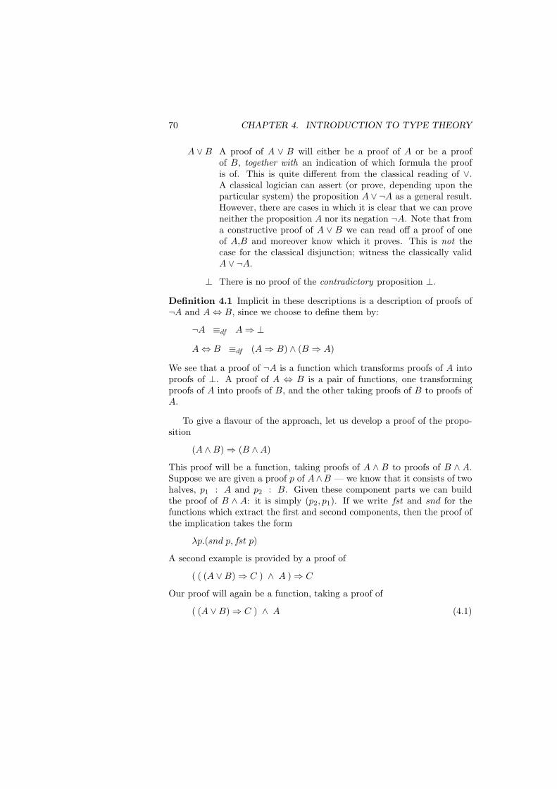
70 CHAPTER 4. INTRODUCTION TO TYPE THEORY
A ∨B A proof of A ∨ B will either be a proof of A or be a proofof B, together with an indication of which formula the proofis of. This is quite different from the classical reading of ∨.A classical logician can assert (or prove, depending upon theparticular system) the proposition A ∨ ¬A as a general result.However, there are cases in which it is clear that we can proveneither the proposition A nor its negation ¬A. Note that froma constructive proof of A ∨ B we can read off a proof of oneof A,B and moreover know which it proves. This is not thecase for the classical disjunction; witness the classically validA ∨ ¬A.
⊥ There is no proof of the contradictory proposition ⊥.
Definition 4.1 Implicit in these descriptions is a description of proofs of¬A and A⇔ B, since we choose to define them by:
¬A ≡df A⇒ ⊥
A⇔ B ≡df (A⇒ B) ∧ (B ⇒ A)
We see that a proof of ¬A is a function which transforms proofs of A intoproofs of ⊥. A proof of A ⇔ B is a pair of functions, one transformingproofs of A into proofs of B, and the other taking proofs of B to proofs ofA.
To give a flavour of the approach, let us develop a proof of the propo-sition
(A ∧B)⇒ (B ∧A)
This proof will be a function, taking proofs of A ∧ B to proofs of B ∧ A.Suppose we are given a proof p of A∧B — we know that it consists of twohalves, p1 : A and p2 : B. Given these component parts we can buildthe proof of B ∧ A: it is simply (p2, p1). If we write fst and snd for thefunctions which extract the first and second components, then the proof ofthe implication takes the form
λp.(snd p, fst p)
A second example is provided by a proof of
( ( (A ∨B)⇒ C ) ∧ A )⇒ C
Our proof will again be a function, taking a proof of
( (A ∨B)⇒ C ) ∧ A (4.1)
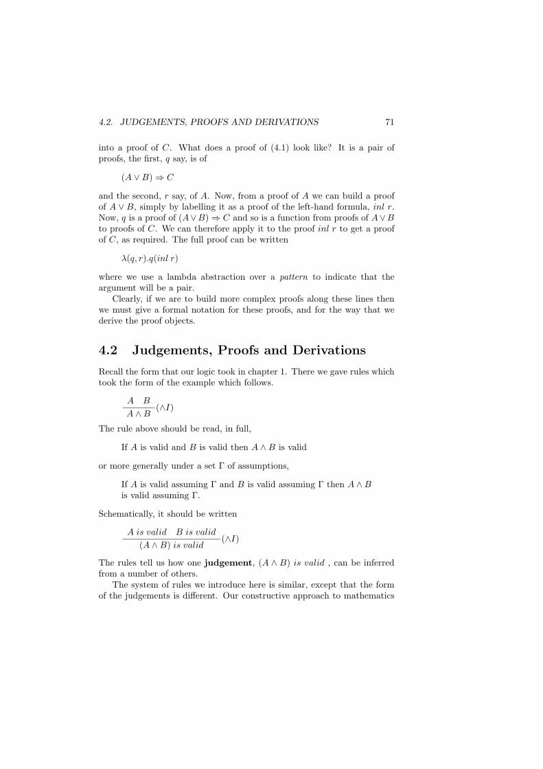
4.2. JUDGEMENTS, PROOFS AND DERIVATIONS 71
into a proof of C. What does a proof of (4.1) look like? It is a pair ofproofs, the first, q say, is of
(A ∨B)⇒ C
and the second, r say, of A. Now, from a proof of A we can build a proofof A ∨ B, simply by labelling it as a proof of the left-hand formula, inl r.Now, q is a proof of (A∨B)⇒ C and so is a function from proofs of A∨Bto proofs of C. We can therefore apply it to the proof inl r to get a proofof C, as required. The full proof can be written
λ(q, r).q(inl r)
where we use a lambda abstraction over a pattern to indicate that theargument will be a pair.
Clearly, if we are to build more complex proofs along these lines thenwe must give a formal notation for these proofs, and for the way that wederive the proof objects.
4.2 Judgements, Proofs and Derivations
Recall the form that our logic took in chapter 1. There we gave rules whichtook the form of the example which follows.
A B
A ∧B(∧I)
The rule above should be read, in full,
If A is valid and B is valid then A ∧B is valid
or more generally under a set Γ of assumptions,
If A is valid assuming Γ and B is valid assuming Γ then A ∧Bis valid assuming Γ.
Schematically, it should be written
A is valid B is valid
(A ∧B) is valid(∧I)
The rules tell us how one judgement, (A ∧ B) is valid , can be inferredfrom a number of others.
The system of rules we introduce here is similar, except that the formof the judgements is different. Our constructive approach to mathematics
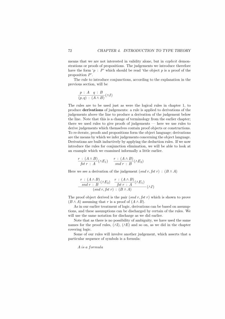
72 CHAPTER 4. INTRODUCTION TO TYPE THEORY
means that we are not interested in validity alone, but in explicit demon-strations or proofs of propositions. The judgements we introduce thereforehave the form ‘p : P ’ which should be read ‘the object p is a proof of theproposition P ’.
The rule to introduce conjunctions, according to the explanation in theprevious section, will be
p : A q : B
(p, q) : (A ∧B)(∧I)
The rules are to be used just as were the logical rules in chapter 1, toproduce derivations of judgements: a rule is applied to derivations of thejudgements above the line to produce a derivation of the judgement belowthe line. Note that this is a change of terminology from the earlier chapter;there we used rules to give proofs of judgements — here we use rules toderive judgements which themselves contain proof objects or constructions.To re-iterate, proofs and propositions form the object language; derivationsare the means by which we infer judgements concerning the object language.Derivations are built inductively by applying the deduction rules. If we nowintroduce the rules for conjunction elimination, we will be able to look atan example which we examined informally a little earlier.
r : (A ∧B)fst r : A
(∧E1)r : (A ∧B)snd r : B
(∧E2)
Here we see a derivation of the judgement (snd r, fst r) : (B ∧A)
r : (A ∧B)snd r : B
(∧E2)r : (A ∧B)fst r : A
(∧E1)
(snd r, fst r) : (B ∧A)(∧I)
The proof object derived is the pair (snd r, fst r) which is shown to prove(B ∧A) assuming that r is a proof of (A ∧B).
As in our earlier treatment of logic, derivations can be based on assump-tions, and these assumptions can be discharged by certain of the rules. Wewill use the same notation for discharge as we did earlier.
Note that as there is no possibility of ambiguity, we have used the samenames for the proof rules, (∧I), (∧E) and so on, as we did in the chaptercovering logic.
Some of our rules will involve another judgement, which asserts that aparticular sequence of symbols is a formula:
A is a formula
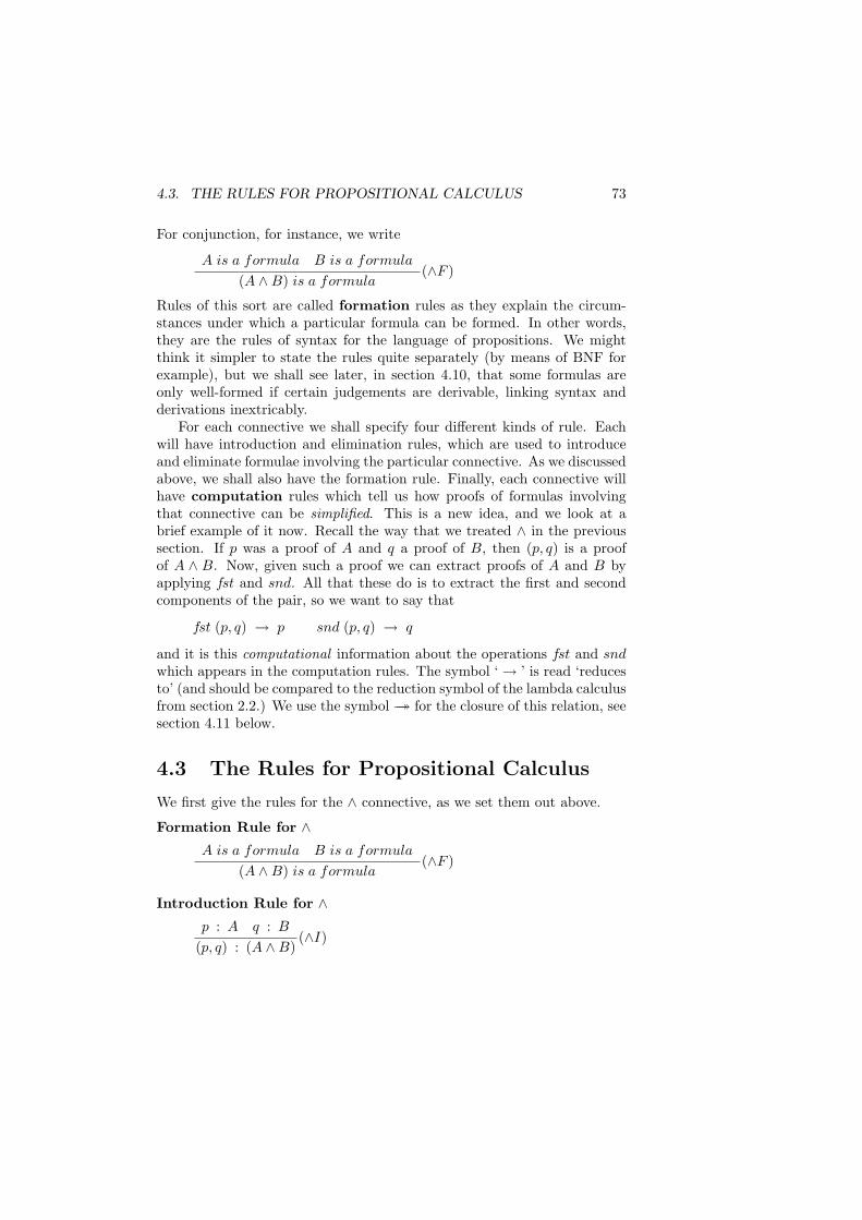
4.3. THE RULES FOR PROPOSITIONAL CALCULUS 73
For conjunction, for instance, we write
A is a formula B is a formula
(A ∧B) is a formula(∧F )
Rules of this sort are called formation rules as they explain the circum-stances under which a particular formula can be formed. In other words,they are the rules of syntax for the language of propositions. We mightthink it simpler to state the rules quite separately (by means of BNF forexample), but we shall see later, in section 4.10, that some formulas areonly well-formed if certain judgements are derivable, linking syntax andderivations inextricably.
For each connective we shall specify four different kinds of rule. Eachwill have introduction and elimination rules, which are used to introduceand eliminate formulae involving the particular connective. As we discussedabove, we shall also have the formation rule. Finally, each connective willhave computation rules which tell us how proofs of formulas involvingthat connective can be simplified. This is a new idea, and we look at abrief example of it now. Recall the way that we treated ∧ in the previoussection. If p was a proof of A and q a proof of B, then (p, q) is a proofof A ∧ B. Now, given such a proof we can extract proofs of A and B byapplying fst and snd. All that these do is to extract the first and secondcomponents of the pair, so we want to say that
fst (p, q) → p snd (p, q) → q
and it is this computational information about the operations fst and sndwhich appears in the computation rules. The symbol ‘→ ’ is read ‘reducesto’ (and should be compared to the reduction symbol of the lambda calculusfrom section 2.2.) We use the symbol→→ for the closure of this relation, seesection 4.11 below.
4.3 The Rules for Propositional Calculus
We first give the rules for the ∧ connective, as we set them out above.
Formation Rule for ∧A is a formula B is a formula
(A ∧B) is a formula(∧F )
Introduction Rule for ∧p : A q : B
(p, q) : (A ∧B)(∧I)
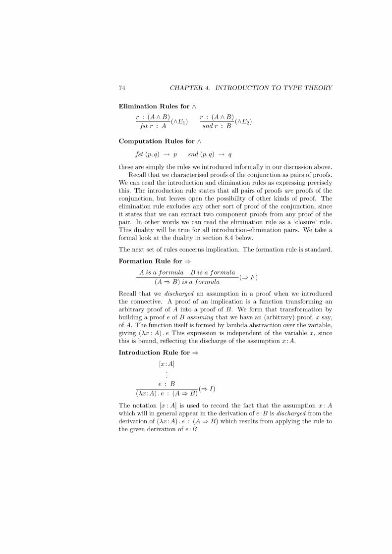
74 CHAPTER 4. INTRODUCTION TO TYPE THEORY
Elimination Rules for ∧r : (A ∧B)fst r : A
(∧E1)r : (A ∧B)snd r : B
(∧E2)
Computation Rules for ∧
fst (p, q) → p snd (p, q) → q
these are simply the rules we introduced informally in our discussion above.Recall that we characterised proofs of the conjunction as pairs of proofs.
We can read the introduction and elimination rules as expressing preciselythis. The introduction rule states that all pairs of proofs are proofs of theconjunction, but leaves open the possibility of other kinds of proof. Theelimination rule excludes any other sort of proof of the conjunction, sinceit states that we can extract two component proofs from any proof of thepair. In other words we can read the elimination rule as a ‘closure’ rule.This duality will be true for all introduction-elimination pairs. We take aformal look at the duality in section 8.4 below.
The next set of rules concerns implication. The formation rule is standard.
Formation Rule for ⇒A is a formula B is a formula
(A⇒ B) is a formula(⇒ F )
Recall that we discharged an assumption in a proof when we introducedthe connective. A proof of an implication is a function transforming anarbitrary proof of A into a proof of B. We form that transformation bybuilding a proof e of B assuming that we have an (arbitrary) proof, x say,of A. The function itself is formed by lambda abstraction over the variable,giving (λx : A) . e This expression is independent of the variable x, sincethis is bound, reflecting the discharge of the assumption x :A.
Introduction Rule for ⇒[x :A]
...e : B
(λx :A) . e : (A⇒ B)(⇒ I)
The notation [x : A] is used to record the fact that the assumption x : Awhich will in general appear in the derivation of e :B is discharged from thederivation of (λx :A) . e : (A⇒ B) which results from applying the rule tothe given derivation of e :B.
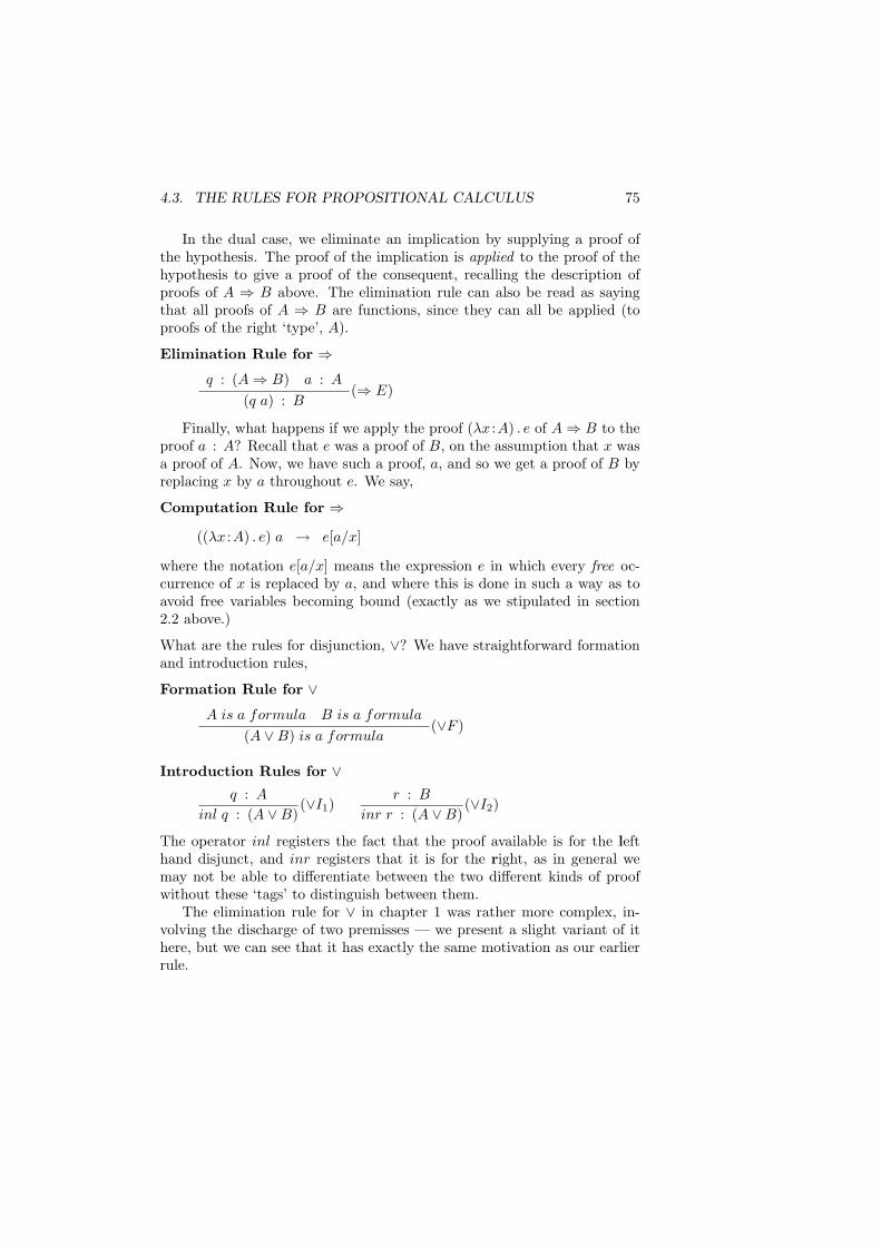
4.3. THE RULES FOR PROPOSITIONAL CALCULUS 75
In the dual case, we eliminate an implication by supplying a proof ofthe hypothesis. The proof of the implication is applied to the proof of thehypothesis to give a proof of the consequent, recalling the description ofproofs of A ⇒ B above. The elimination rule can also be read as sayingthat all proofs of A ⇒ B are functions, since they can all be applied (toproofs of the right ‘type’, A).
Elimination Rule for ⇒
q : (A⇒ B) a : A
(q a) : B(⇒ E)
Finally, what happens if we apply the proof (λx :A) . e of A⇒ B to theproof a : A? Recall that e was a proof of B, on the assumption that x wasa proof of A. Now, we have such a proof, a, and so we get a proof of B byreplacing x by a throughout e. We say,
Computation Rule for ⇒
((λx :A) . e) a → e[a/x]
where the notation e[a/x] means the expression e in which every free oc-currence of x is replaced by a, and where this is done in such a way as toavoid free variables becoming bound (exactly as we stipulated in section2.2 above.)
What are the rules for disjunction, ∨? We have straightforward formationand introduction rules,
Formation Rule for ∨
A is a formula B is a formula
(A ∨B) is a formula(∨F )
Introduction Rules for ∨q : A
inl q : (A ∨B)(∨I1)
r : B
inr r : (A ∨B)(∨I2)
The operator inl registers the fact that the proof available is for the lefthand disjunct, and inr registers that it is for the right, as in general wemay not be able to differentiate between the two different kinds of proofwithout these ‘tags’ to distinguish between them.
The elimination rule for ∨ in chapter 1 was rather more complex, in-volving the discharge of two premisses — we present a slight variant of ithere, but we can see that it has exactly the same motivation as our earlierrule.
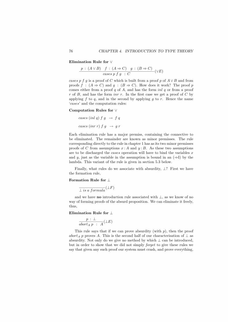
76 CHAPTER 4. INTRODUCTION TO TYPE THEORY
Elimination Rule for ∨
p : (A ∨B) f : (A⇒ C) g : (B ⇒ C)cases p f g : C
(∨E)
cases p f g is a proof of C which is built from a proof p of A∨B and fromproofs f : (A ⇒ C) and g : (B ⇒ C). How does it work? The proof pcomes either from a proof q of A, and has the form inl q or from a proofr of B, and has the form inr r. In the first case we get a proof of C byapplying f to q, and in the second by applying g to r. Hence the name‘cases’ and the computation rules:
Computation Rules for ∨
cases (inl q) f g → f q
cases (inr r) f g → g r
Each elimination rule has a major premiss, containing the connective tobe eliminated. The remainder are known as minor premisses. The rulecorresponding directly to the rule in chapter 1 has as its two minor premissesproofs of C from assumptions x : A and y : B. As these two assumptionsare to be discharged the cases operation will have to bind the variables xand y, just as the variable in the assumption is bound in an (⇒I) by thelambda. This variant of the rule is given in section 5.3 below.
Finally, what rules do we associate with absurdity, ⊥? First we havethe formation rule,
Formation Rule for ⊥
⊥ is a formula(⊥F )
and we have no introduction rule associated with ⊥, as we know of noway of forming proofs of the absurd proposition. We can eliminate it freely,thus,
Elimination Rule for ⊥p : ⊥
abortA p : A(⊥E)
This rule says that if we can prove absurdity (with p), then the proofabortA p proves A. This is the second half of our characterisation of ⊥ asabsurdity. Not only do we give no method by which ⊥ can be introduced,but in order to show that we did not simply forget to give these rules wesay that given any such proof our system must crash, and prove everything,
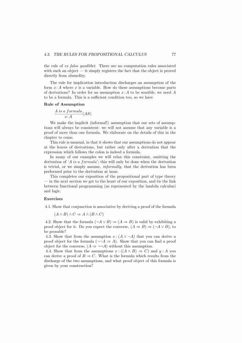
4.3. THE RULES FOR PROPOSITIONAL CALCULUS 77
the rule of ex falso quodlibet. There are no computation rules associatedwith such an object — it simply registers the fact that the object is proveddirectly from absurdity.
The rule for implication introduction discharges an assumption of theform x :A where x is a variable. How do these assumptions become partsof derivations? In order for an assumption x :A to be sensible, we need Ato be a formula. This is a sufficient condition too, so we have
Rule of Assumption
A is a formula
x :A(AS)
We make the implicit (informal!) assumption that our sets of assump-tions will always be consistent: we will not assume that any variable is aproof of more than one formula. We elaborate on the details of this in thechapter to come.
This rule is unusual, in that it shows that our assumptions do not appearat the leaves of derivations, but rather only after a derivation that theexpression which follows the colon is indeed a formula.
In many of our examples we will relax this constraint, omitting thederivation of ‘A is a formula’; this will only be done when the derivationis trivial, or we simply assume, informally, that the derivation has beenperformed prior to the derivation at issue.
This completes our exposition of the propositional part of type theory— in the next section we get to the heart of our exposition, and tie the linkbetween functional programming (as represented by the lambda calculus)and logic.
Exercises
4.1. Show that conjunction is associative by deriving a proof of the formula
(A ∧B) ∧ C ⇒ A ∧ (B ∧ C)
4.2. Show that the formula (¬A ∨ B)⇒ (A⇒ B) is valid by exhibiting aproof object for it. Do you expect the converse, (A⇒ B)⇒ (¬A ∨ B), tobe provable?4.3. Show that from the assumption x : (A ∨ ¬A) that you can derive a
proof object for the formula (¬¬A ⇒ A). Show that you can find a proofobject for the converse, (A⇒ ¬¬A) without this assumption.4.4. Show that from the assumptions x : ((A ∧ B) ⇒ C) and y : A you
can derive a proof of B ⇒ C. What is the formula which results from thedischarge of the two assumptions, and what proof object of this formula isgiven by your construction?
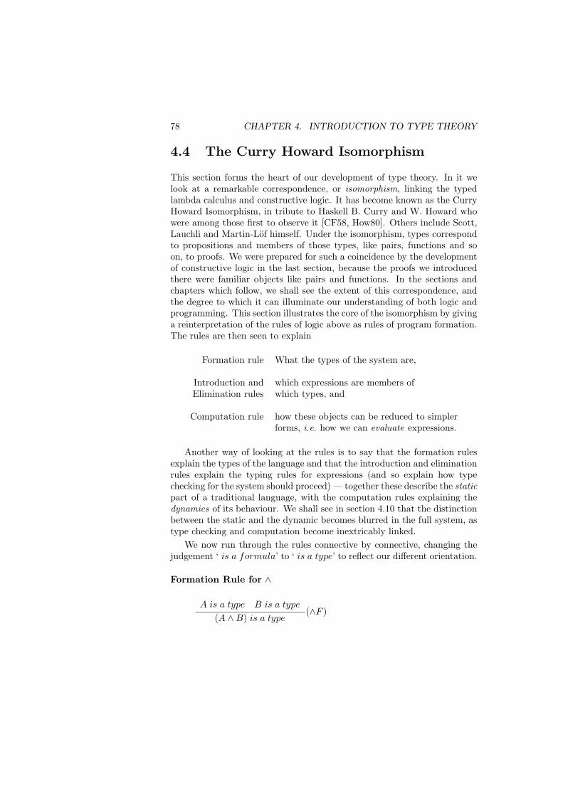
78 CHAPTER 4. INTRODUCTION TO TYPE THEORY
4.4 The Curry Howard Isomorphism
This section forms the heart of our development of type theory. In it welook at a remarkable correspondence, or isomorphism, linking the typedlambda calculus and constructive logic. It has become known as the CurryHoward Isomorphism, in tribute to Haskell B. Curry and W. Howard whowere among those first to observe it [CF58, How80]. Others include Scott,Lauchli and Martin-Lof himself. Under the isomorphism, types correspondto propositions and members of those types, like pairs, functions and soon, to proofs. We were prepared for such a coincidence by the developmentof constructive logic in the last section, because the proofs we introducedthere were familiar objects like pairs and functions. In the sections andchapters which follow, we shall see the extent of this correspondence, andthe degree to which it can illuminate our understanding of both logic andprogramming. This section illustrates the core of the isomorphism by givinga reinterpretation of the rules of logic above as rules of program formation.The rules are then seen to explain
Formation rule What the types of the system are,
Introduction and which expressions are members ofElimination rules which types, and
Computation rule how these objects can be reduced to simplerforms, i.e. how we can evaluate expressions.
Another way of looking at the rules is to say that the formation rulesexplain the types of the language and that the introduction and eliminationrules explain the typing rules for expressions (and so explain how typechecking for the system should proceed) — together these describe the staticpart of a traditional language, with the computation rules explaining thedynamics of its behaviour. We shall see in section 4.10 that the distinctionbetween the static and the dynamic becomes blurred in the full system, astype checking and computation become inextricably linked.
We now run through the rules connective by connective, changing thejudgement ‘ is a formula’ to ‘ is a type’ to reflect our different orientation.
Formation Rule for ∧
A is a type B is a type
(A ∧B) is a type(∧F )
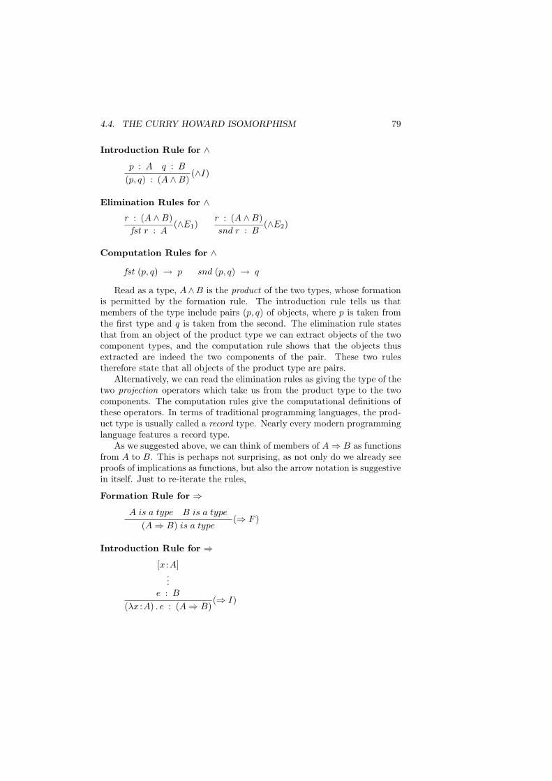
4.4. THE CURRY HOWARD ISOMORPHISM 79
Introduction Rule for ∧
p : A q : B
(p, q) : (A ∧B)(∧I)
Elimination Rules for ∧r : (A ∧B)fst r : A
(∧E1)r : (A ∧B)snd r : B
(∧E2)
Computation Rules for ∧
fst (p, q) → p snd (p, q) → q
Read as a type, A∧B is the product of the two types, whose formationis permitted by the formation rule. The introduction rule tells us thatmembers of the type include pairs (p, q) of objects, where p is taken fromthe first type and q is taken from the second. The elimination rule statesthat from an object of the product type we can extract objects of the twocomponent types, and the computation rule shows that the objects thusextracted are indeed the two components of the pair. These two rulestherefore state that all objects of the product type are pairs.
Alternatively, we can read the elimination rules as giving the type of thetwo projection operators which take us from the product type to the twocomponents. The computation rules give the computational definitions ofthese operators. In terms of traditional programming languages, the prod-uct type is usually called a record type. Nearly every modern programminglanguage features a record type.
As we suggested above, we can think of members of A⇒ B as functionsfrom A to B. This is perhaps not surprising, as not only do we already seeproofs of implications as functions, but also the arrow notation is suggestivein itself. Just to re-iterate the rules,
Formation Rule for ⇒
A is a type B is a type
(A⇒ B) is a type(⇒ F )
Introduction Rule for ⇒
[x :A]...
e : B
(λx :A) . e : (A⇒ B)(⇒ I)
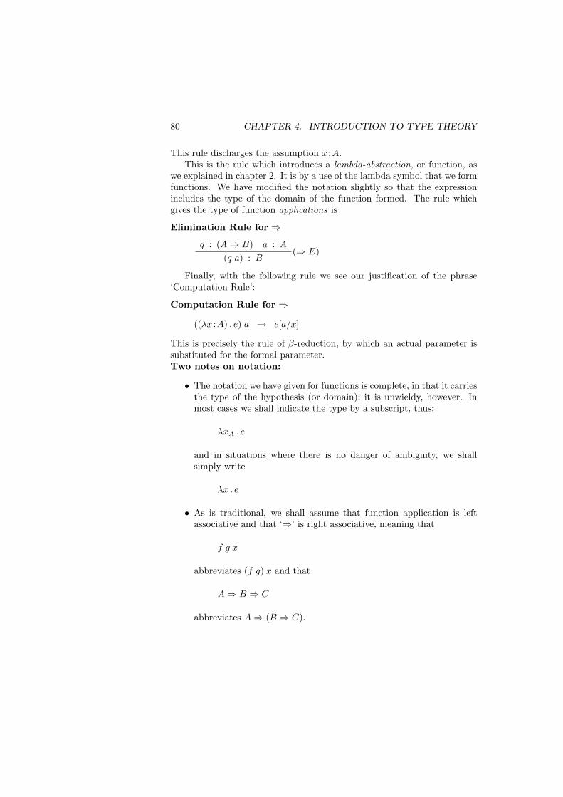
80 CHAPTER 4. INTRODUCTION TO TYPE THEORY
This rule discharges the assumption x :A.This is the rule which introduces a lambda-abstraction, or function, as
we explained in chapter 2. It is by a use of the lambda symbol that we formfunctions. We have modified the notation slightly so that the expressionincludes the type of the domain of the function formed. The rule whichgives the type of function applications is
Elimination Rule for ⇒
q : (A⇒ B) a : A
(q a) : B(⇒ E)
Finally, with the following rule we see our justification of the phrase‘Computation Rule’:
Computation Rule for ⇒
((λx :A) . e) a → e[a/x]
This is precisely the rule of β-reduction, by which an actual parameter issubstituted for the formal parameter.Two notes on notation:
• The notation we have given for functions is complete, in that it carriesthe type of the hypothesis (or domain); it is unwieldy, however. Inmost cases we shall indicate the type by a subscript, thus:
λxA . e
and in situations where there is no danger of ambiguity, we shallsimply write
λx . e
• As is traditional, we shall assume that function application is leftassociative and that ‘⇒’ is right associative, meaning that
f g x
abbreviates (f g) x and that
A⇒ B ⇒ C
abbreviates A⇒ (B ⇒ C).
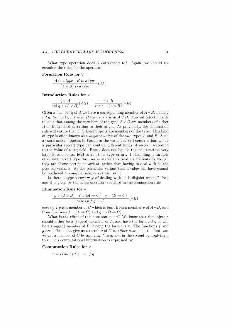
4.4. THE CURRY HOWARD ISOMORPHISM 81
What type operation does ∨ correspond to? Again, we should re-examine the rules for the operator:
Formation Rule for ∨A is a type B is a type
(A ∨B) is a type(∨F )
Introduction Rules for ∨q : A
inl q : (A ∨B)(∨I1)
r : B
inr r : (A ∨B)(∨I2)
Given a member q of A we have a corresponding member of A∨B, namelyinl q. Similarly, if r is in B then inr r is in A ∨ B. This introduction ruletells us that among the members of the type A ∨ B are members of eitherA or B, labelled according to their origin. As previously, the eliminationrule will ensure that only these objects are members of the type. This kindof type is often known as a disjoint union of the two types A and B. Sucha construction appears in Pascal in the variant record construction, wherea particular record type can contain different kinds of record, accordingto the value of a tag field. Pascal does not handle this construction veryhappily, and it can lead to run-time type errors. In handling a variableof variant record type the user is allowed to treat its contents as thoughthey are of one particular variant, rather than having to deal with all thepossible variants. As the particular variant that a value will have cannotbe predicted at compile time, errors can result.
Is there a type-secure way of dealing with such disjoint unions? Yes,and it is given by the cases operator, specified in the elimination rule
Elimination Rule for ∨p : (A ∨B) f : (A⇒ C) g : (B ⇒ C)
cases p f g : C(∨E)
cases p f g is a member of C which is built from a member p of A∨B, andfrom functions f : (A⇒ C) and g : (B ⇒ C).
What is the effect of this case statement? We know that the object pshould either be a (tagged) member of A, and have the form inl q or willbe a (tagged) member of B, having the form inr r. The functions f andg are sufficient to give us a member of C in either case — in the first casewe get a member of C by applying f to q, and in the second by applying gto r. This computational information is expressed by:
Computation Rules for ∨
cases (inl q) f g → f q
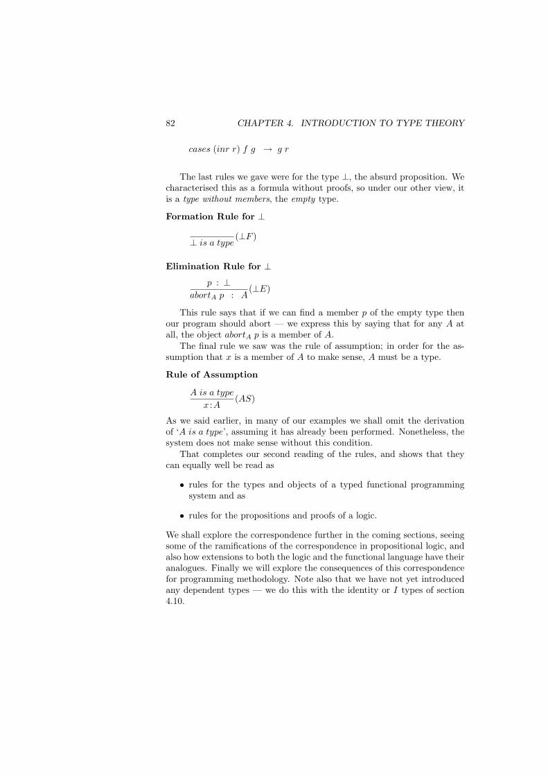
82 CHAPTER 4. INTRODUCTION TO TYPE THEORY
cases (inr r) f g → g r
The last rules we gave were for the type ⊥, the absurd proposition. Wecharacterised this as a formula without proofs, so under our other view, itis a type without members, the empty type.
Formation Rule for ⊥
⊥ is a type(⊥F )
Elimination Rule for ⊥
p : ⊥abortA p : A
(⊥E)
This rule says that if we can find a member p of the empty type thenour program should abort — we express this by saying that for any A atall, the object abortA p is a member of A.
The final rule we saw was the rule of assumption; in order for the as-sumption that x is a member of A to make sense, A must be a type.
Rule of Assumption
A is a type
x :A(AS)
As we said earlier, in many of our examples we shall omit the derivationof ‘A is a type’, assuming it has already been performed. Nonetheless, thesystem does not make sense without this condition.
That completes our second reading of the rules, and shows that theycan equally well be read as
• rules for the types and objects of a typed functional programmingsystem and as
• rules for the propositions and proofs of a logic.
We shall explore the correspondence further in the coming sections, seeingsome of the ramifications of the correspondence in propositional logic, andalso how extensions to both the logic and the functional language have theiranalogues. Finally we will explore the consequences of this correspondencefor programming methodology. Note also that we have not yet introducedany dependent types — we do this with the identity or I types of section4.10.
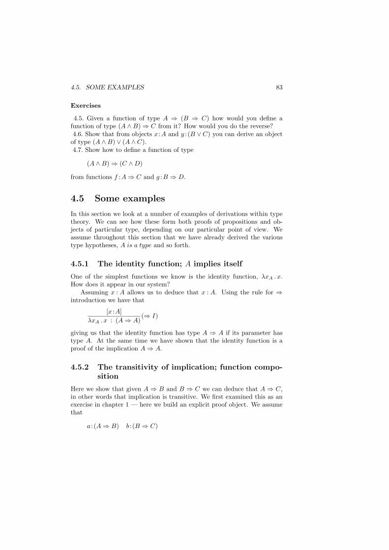
4.5. SOME EXAMPLES 83
Exercises
4.5. Given a function of type A ⇒ (B ⇒ C) how would you define afunction of type (A ∧B)⇒ C from it? How would you do the reverse?4.6. Show that from objects x :A and y : (B ∨ C) you can derive an object
of type (A ∧B) ∨ (A ∧ C).4.7. Show how to define a function of type
(A ∧B)⇒ (C ∧D)
from functions f :A⇒ C and g :B ⇒ D.
4.5 Some examples
In this section we look at a number of examples of derivations within typetheory. We can see how these form both proofs of propositions and ob-jects of particular type, depending on our particular point of view. Weassume throughout this section that we have already derived the varioustype hypotheses, A is a type and so forth.
4.5.1 The identity function; A implies itself
One of the simplest functions we know is the identity function, λxA . x.How does it appear in our system?
Assuming x : A allows us to deduce that x : A. Using the rule for ⇒introduction we have that
[x :A]λxA . x : (A⇒ A)
(⇒ I)
giving us that the identity function has type A ⇒ A if its parameter hastype A. At the same time we have shown that the identity function is aproof of the implication A⇒ A.
4.5.2 The transitivity of implication; function compo-sition
Here we show that given A ⇒ B and B ⇒ C we can deduce that A ⇒ C,in other words that implication is transitive. We first examined this as anexercise in chapter 1 — here we build an explicit proof object. We assumethat
a : (A⇒ B) b : (B ⇒ C)
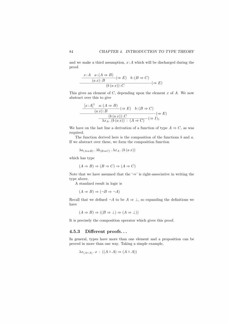
84 CHAPTER 4. INTRODUCTION TO TYPE THEORY
and we make a third assumption, x :A which will be discharged during theproof.
x :A a : (A⇒ B)(a x) :B
(⇒ E) b : (B ⇒ C)
(b (a x)) :C(⇒ E)
This gives an element of C, depending upon the element x of A. We nowabstract over this to give
[x :A]1 a : (A⇒ B)(a x) :B
(⇒ E) b : (B ⇒ C)
(b (a x)) :C(⇒ E)
λxA . (b (a x)) : (A⇒ C) (⇒ I)1
We have on the last line a derivation of a function of type A ⇒ C, as wasrequired.
The function derived here is the composition of the functions b and a.If we abstract over these, we form the composition function
λa(A⇒B) . λb(B⇒C) . λxA . (b (a x))
which has type
(A⇒ B)⇒ (B ⇒ C)⇒ (A⇒ C)
Note that we have assumed that the ‘⇒’ is right-associative in writing thetype above.
A standard result in logic is
(A⇒ B)⇒ (¬B ⇒ ¬A)
Recall that we defined ¬A to be A ⇒ ⊥, so expanding the definitions wehave
(A⇒ B)⇒ ((B ⇒ ⊥)⇒ (A⇒ ⊥))
It is precisely the composition operator which gives this proof.
4.5.3 Different proofs. . .
In general, types have more than one element and a proposition can beproved in more than one way. Taking a simple example,
λx(A∧A) . x : ((A ∧A)⇒ (A ∧A))
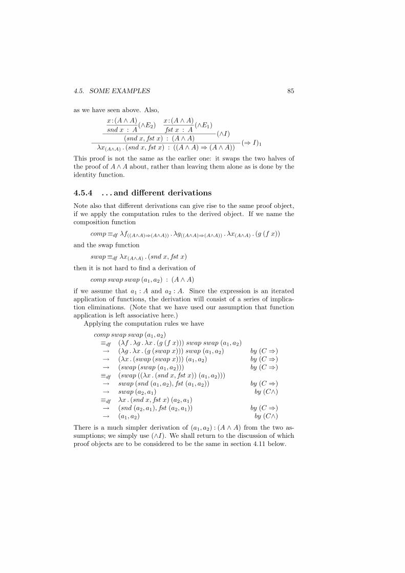
4.5. SOME EXAMPLES 85
as we have seen above. Also,
x : (A ∧A)snd x : A
(∧E2)x : (A ∧A)fst x : A
(∧E1)
(snd x, fst x) : (A ∧A)(∧I)
λx(A∧A) . (snd x, fst x) : ((A ∧A)⇒ (A ∧A))(⇒ I)1
This proof is not the same as the earlier one: it swaps the two halves ofthe proof of A∧A about, rather than leaving them alone as is done by theidentity function.
4.5.4 . . . and different derivations
Note also that different derivations can give rise to the same proof object,if we apply the computation rules to the derived object. If we name thecomposition function
comp≡df λf((A∧A)⇒(A∧A)) . λg((A∧A)⇒(A∧A)) . λx(A∧A) . (g (f x))
and the swap function
swap≡df λx(A∧A) . (snd x, fst x)
then it is not hard to find a derivation of
comp swap swap (a1, a2) : (A ∧A)
if we assume that a1 : A and a2 : A. Since the expression is an iteratedapplication of functions, the derivation will consist of a series of implica-tion eliminations. (Note that we have used our assumption that functionapplication is left associative here.)
Applying the computation rules we have
comp swap swap (a1, a2)≡df (λf . λg . λx . (g (f x))) swap swap (a1, a2)→ (λg . λx . (g (swap x))) swap (a1, a2) by (C ⇒)→ (λx . (swap (swap x))) (a1, a2) by (C ⇒)→ (swap (swap (a1, a2))) by (C ⇒)≡df (swap ((λx . (snd x, fst x)) (a1, a2)))→ swap (snd (a1, a2), fst (a1, a2)) by (C ⇒)→ swap (a2, a1) by (C∧)≡df λx . (snd x, fst x) (a2, a1)→ (snd (a2, a1), fst (a2, a1)) by (C ⇒)→ (a1, a2) by (C∧)
There is a much simpler derivation of (a1, a2) : (A ∧ A) from the two as-sumptions; we simply use (∧I). We shall return to the discussion of whichproof objects are to be considered to be the same in section 4.11 below.
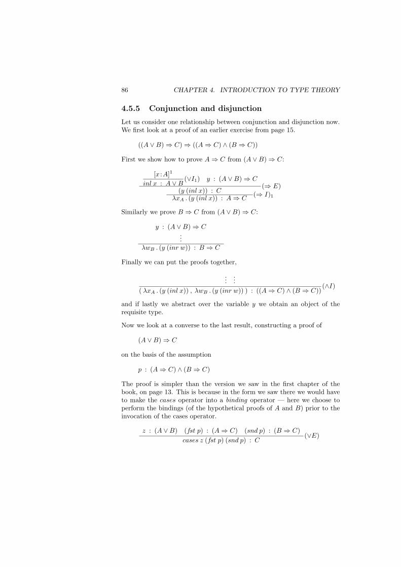
86 CHAPTER 4. INTRODUCTION TO TYPE THEORY
4.5.5 Conjunction and disjunction
Let us consider one relationship between conjunction and disjunction now.We first look at a proof of an earlier exercise from page 15.
((A ∨B)⇒ C)⇒ ((A⇒ C) ∧ (B ⇒ C))
First we show how to prove A⇒ C from (A ∨B)⇒ C:
[x :A]1
inl x : A ∨B(∨I1) y : (A ∨B)⇒ C
(y (inl x)) : C(⇒ E)
λxA . (y (inl x)) : A⇒ C(⇒ I)1
Similarly we prove B ⇒ C from (A ∨B)⇒ C:
y : (A ∨B)⇒ C...
λwB . (y (inr w)) : B ⇒ C
Finally we can put the proofs together,
......
( λxA . (y (inl x)) , λwB . (y (inr w)) ) : ((A⇒ C) ∧ (B ⇒ C))(∧I)
and if lastly we abstract over the variable y we obtain an object of therequisite type.
Now we look at a converse to the last result, constructing a proof of
(A ∨B)⇒ C
on the basis of the assumption
p : (A⇒ C) ∧ (B ⇒ C)
The proof is simpler than the version we saw in the first chapter of thebook, on page 13. This is because in the form we saw there we would haveto make the cases operator into a binding operator — here we choose toperform the bindings (of the hypothetical proofs of A and B) prior to theinvocation of the cases operator.
z : (A ∨B) (fst p) : (A⇒ C) (snd p) : (B ⇒ C)cases z (fst p) (snd p) : C
(∨E)
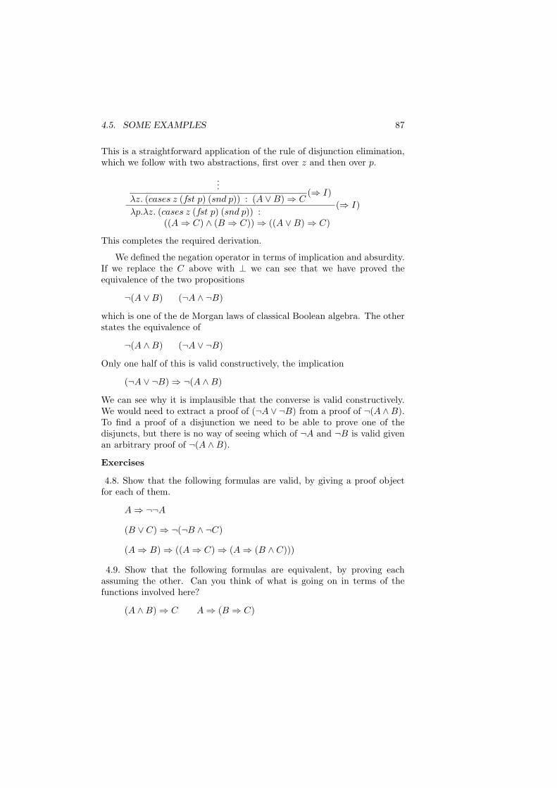
4.5. SOME EXAMPLES 87
This is a straightforward application of the rule of disjunction elimination,which we follow with two abstractions, first over z and then over p.
...λz. (cases z (fst p) (snd p)) : (A ∨B)⇒ C
(⇒ I)
λp.λz. (cases z (fst p) (snd p)) :((A⇒ C) ∧ (B ⇒ C))⇒ ((A ∨B)⇒ C)
(⇒ I)
This completes the required derivation.
We defined the negation operator in terms of implication and absurdity.If we replace the C above with ⊥ we can see that we have proved theequivalence of the two propositions
¬(A ∨B) (¬A ∧ ¬B)
which is one of the de Morgan laws of classical Boolean algebra. The otherstates the equivalence of
¬(A ∧B) (¬A ∨ ¬B)
Only one half of this is valid constructively, the implication
(¬A ∨ ¬B)⇒ ¬(A ∧B)
We can see why it is implausible that the converse is valid constructively.We would need to extract a proof of (¬A ∨ ¬B) from a proof of ¬(A ∧B).To find a proof of a disjunction we need to be able to prove one of thedisjuncts, but there is no way of seeing which of ¬A and ¬B is valid givenan arbitrary proof of ¬(A ∧B).
Exercises
4.8. Show that the following formulas are valid, by giving a proof objectfor each of them.
A⇒ ¬¬A
(B ∨ C)⇒ ¬(¬B ∧ ¬C)
(A⇒ B)⇒ ((A⇒ C)⇒ (A⇒ (B ∧ C)))
4.9. Show that the following formulas are equivalent, by proving eachassuming the other. Can you think of what is going on in terms of thefunctions involved here?
(A ∧B)⇒ C A⇒ (B ⇒ C)
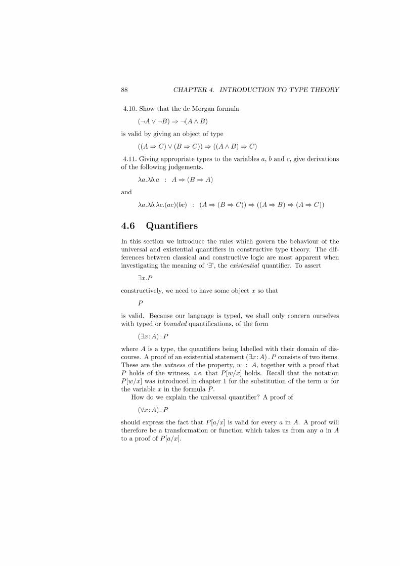
88 CHAPTER 4. INTRODUCTION TO TYPE THEORY
4.10. Show that the de Morgan formula
(¬A ∨ ¬B)⇒ ¬(A ∧B)
is valid by giving an object of type
((A⇒ C) ∨ (B ⇒ C))⇒ ((A ∧B)⇒ C)
4.11. Giving appropriate types to the variables a, b and c, give derivationsof the following judgements.
λa.λb.a : A⇒ (B ⇒ A)
and
λa.λb.λc.(ac)(bc) : (A⇒ (B ⇒ C))⇒ ((A⇒ B)⇒ (A⇒ C))
4.6 Quantifiers
In this section we introduce the rules which govern the behaviour of theuniversal and existential quantifiers in constructive type theory. The dif-ferences between classical and constructive logic are most apparent wheninvestigating the meaning of ‘∃’, the existential quantifier. To assert
∃x.P
constructively, we need to have some object x so that
P
is valid. Because our language is typed, we shall only concern ourselveswith typed or bounded quantifications, of the form
(∃x :A) . P
where A is a type, the quantifiers being labelled with their domain of dis-course. A proof of an existential statement (∃x :A) . P consists of two items.These are the witness of the property, w : A, together with a proof thatP holds of the witness, i.e. that P [w/x] holds. Recall that the notationP [w/x] was introduced in chapter 1 for the substitution of the term w forthe variable x in the formula P .
How do we explain the universal quantifier? A proof of
(∀x :A) . P
should express the fact that P [a/x] is valid for every a in A. A proof willtherefore be a transformation or function which takes us from any a in Ato a proof of P [a/x].
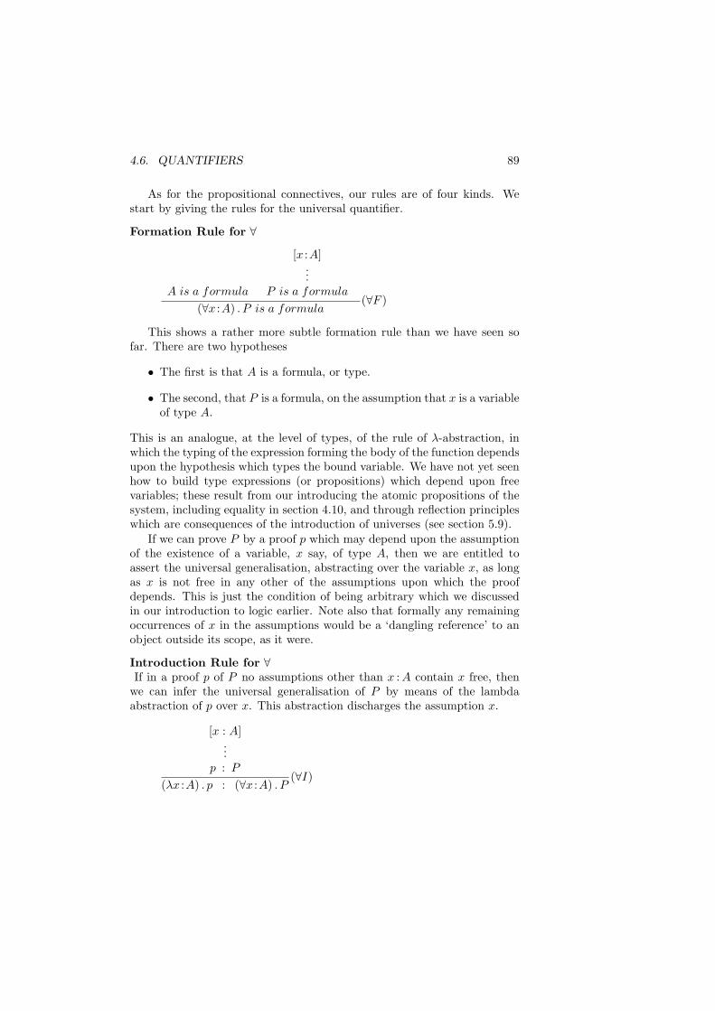
4.6. QUANTIFIERS 89
As for the propositional connectives, our rules are of four kinds. Westart by giving the rules for the universal quantifier.
Formation Rule for ∀
A is a formula
[x :A]...
P is a formula
(∀x :A) . P is a formula(∀F )
This shows a rather more subtle formation rule than we have seen sofar. There are two hypotheses
• The first is that A is a formula, or type.
• The second, that P is a formula, on the assumption that x is a variableof type A.
This is an analogue, at the level of types, of the rule of λ-abstraction, inwhich the typing of the expression forming the body of the function dependsupon the hypothesis which types the bound variable. We have not yet seenhow to build type expressions (or propositions) which depend upon freevariables; these result from our introducing the atomic propositions of thesystem, including equality in section 4.10, and through reflection principleswhich are consequences of the introduction of universes (see section 5.9).
If we can prove P by a proof p which may depend upon the assumptionof the existence of a variable, x say, of type A, then we are entitled toassert the universal generalisation, abstracting over the variable x, as longas x is not free in any other of the assumptions upon which the proofdepends. This is just the condition of being arbitrary which we discussedin our introduction to logic earlier. Note also that formally any remainingoccurrences of x in the assumptions would be a ‘dangling reference’ to anobject outside its scope, as it were.
Introduction Rule for ∀If in a proof p of P no assumptions other than x : A contain x free, then
we can infer the universal generalisation of P by means of the lambdaabstraction of p over x. This abstraction discharges the assumption x.
[x : A]...
p : P
(λx :A) . p : (∀x :A) . P(∀I)
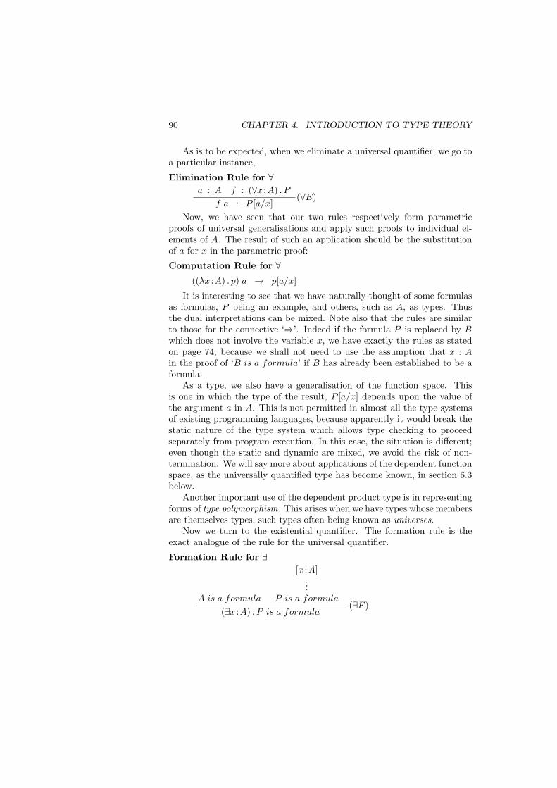
90 CHAPTER 4. INTRODUCTION TO TYPE THEORY
As is to be expected, when we eliminate a universal quantifier, we go toa particular instance,
Elimination Rule for ∀a : A f : (∀x :A) . P
f a : P [a/x](∀E)
Now, we have seen that our two rules respectively form parametricproofs of universal generalisations and apply such proofs to individual el-ements of A. The result of such an application should be the substitutionof a for x in the parametric proof:
Computation Rule for ∀((λx :A) . p) a → p[a/x]
It is interesting to see that we have naturally thought of some formulasas formulas, P being an example, and others, such as A, as types. Thusthe dual interpretations can be mixed. Note also that the rules are similarto those for the connective ‘⇒’. Indeed if the formula P is replaced by Bwhich does not involve the variable x, we have exactly the rules as statedon page 74, because we shall not need to use the assumption that x : Ain the proof of ‘B is a formula’ if B has already been established to be aformula.
As a type, we also have a generalisation of the function space. Thisis one in which the type of the result, P [a/x] depends upon the value ofthe argument a in A. This is not permitted in almost all the type systemsof existing programming languages, because apparently it would break thestatic nature of the type system which allows type checking to proceedseparately from program execution. In this case, the situation is different;even though the static and dynamic are mixed, we avoid the risk of non-termination. We will say more about applications of the dependent functionspace, as the universally quantified type has become known, in section 6.3below.
Another important use of the dependent product type is in representingforms of type polymorphism. This arises when we have types whose membersare themselves types, such types often being known as universes.
Now we turn to the existential quantifier. The formation rule is theexact analogue of the rule for the universal quantifier.
Formation Rule for ∃
A is a formula
[x :A]...
P is a formula
(∃x :A) . P is a formula(∃F )
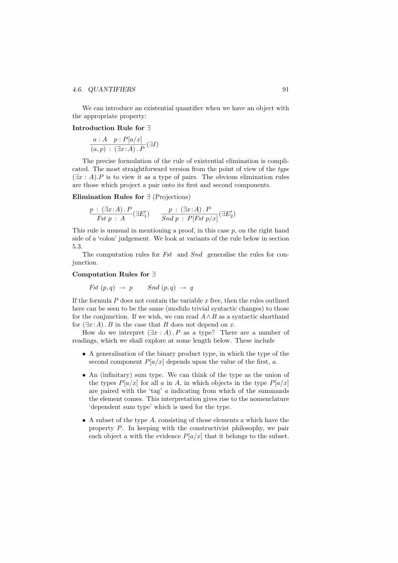
4.6. QUANTIFIERS 91
We can introduce an existential quantifier when we have an object withthe appropriate property:
Introduction Rule for ∃a : A p : P [a/x]
(a, p) : (∃x :A) . P(∃I)
The precise formulation of the rule of existential elimination is compli-cated. The most straightforward version from the point of view of the type(∃x : A).P is to view it as a type of pairs. The obvious elimination rulesare those which project a pair onto its first and second components.
Elimination Rules for ∃ (Projections)
p : (∃x :A) . P
Fst p : A(∃E′
1)p : (∃x :A) . P
Snd p : P [Fst p/x](∃E′
2)
This rule is unusual in mentioning a proof, in this case p, on the right handside of a ‘colon’ judgement. We look at variants of the rule below in section5.3.
The computation rules for Fst and Snd generalise the rules for con-junction.
Computation Rules for ∃
Fst (p, q) → p Snd (p, q) → q
If the formula P does not contain the variable x free, then the rules outlinedhere can be seen to be the same (modulo trivial syntactic changes) to thosefor the conjunction. If we wish, we can read A∧B as a syntactic shorthandfor (∃x :A) . B in the case that B does not depend on x.
How do we interpret (∃x : A) . P as a type? There are a number ofreadings, which we shall explore at some length below. These include
• A generalisation of the binary product type, in which the type of thesecond component P [a/x] depends upon the value of the first, a.
• An (infinitary) sum type. We can think of the type as the union ofthe types P [a/x] for all a in A, in which objects in the type P [a/x]are paired with the ‘tag’ a indicating from which of the summandsthe element comes. This interpretation gives rise to the nomenclature‘dependent sum type’ which is used for the type.
• A subset of the type A, consisting of those elements a which have theproperty P . In keeping with the constructivist philosophy, we paireach object a with the evidence P [a/x] that it belongs to the subset.
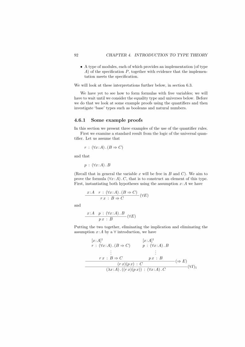
92 CHAPTER 4. INTRODUCTION TO TYPE THEORY
• A type of modules, each of which provides an implementation (of typeA) of the specification P , together with evidence that the implemen-tation meets the specification.
We will look at these interpretations further below, in section 6.3.
We have yet to see how to form formulas with free variables; we willhave to wait until we consider the equality type and universes below. Beforewe do that we look at some example proofs using the quantifiers and theninvestigate ‘base’ types such as booleans and natural numbers.
4.6.1 Some example proofs
In this section we present three examples of the use of the quantifier rules.First we examine a standard result from the logic of the universal quan-
tifier. Let us assume that
r : (∀x :A) . (B ⇒ C)
and that
p : (∀x :A) . B
(Recall that in general the variable x will be free in B and C). We aim toprove the formula (∀x :A) . C, that is to construct an element of this type.First, instantiating both hypotheses using the assumption x :A we have
x :A r : (∀x :A) . (B ⇒ C)r x : B ⇒ C
(∀E)
and
x :A p : (∀x :A) . B
p x : B(∀E)
Putting the two together, eliminating the implication and eliminating theassumption x :A by a ∀ introduction, we have
[x :A]1
r : (∀x :A) . (B ⇒ C)...
r x : B ⇒ C
[x :A]1
p : (∀x :A) . B...
p x : B
(r x)(p x) : C(⇒ E)
(λx :A) . ((r x)(p x)) : (∀x :A) . C(∀I)1
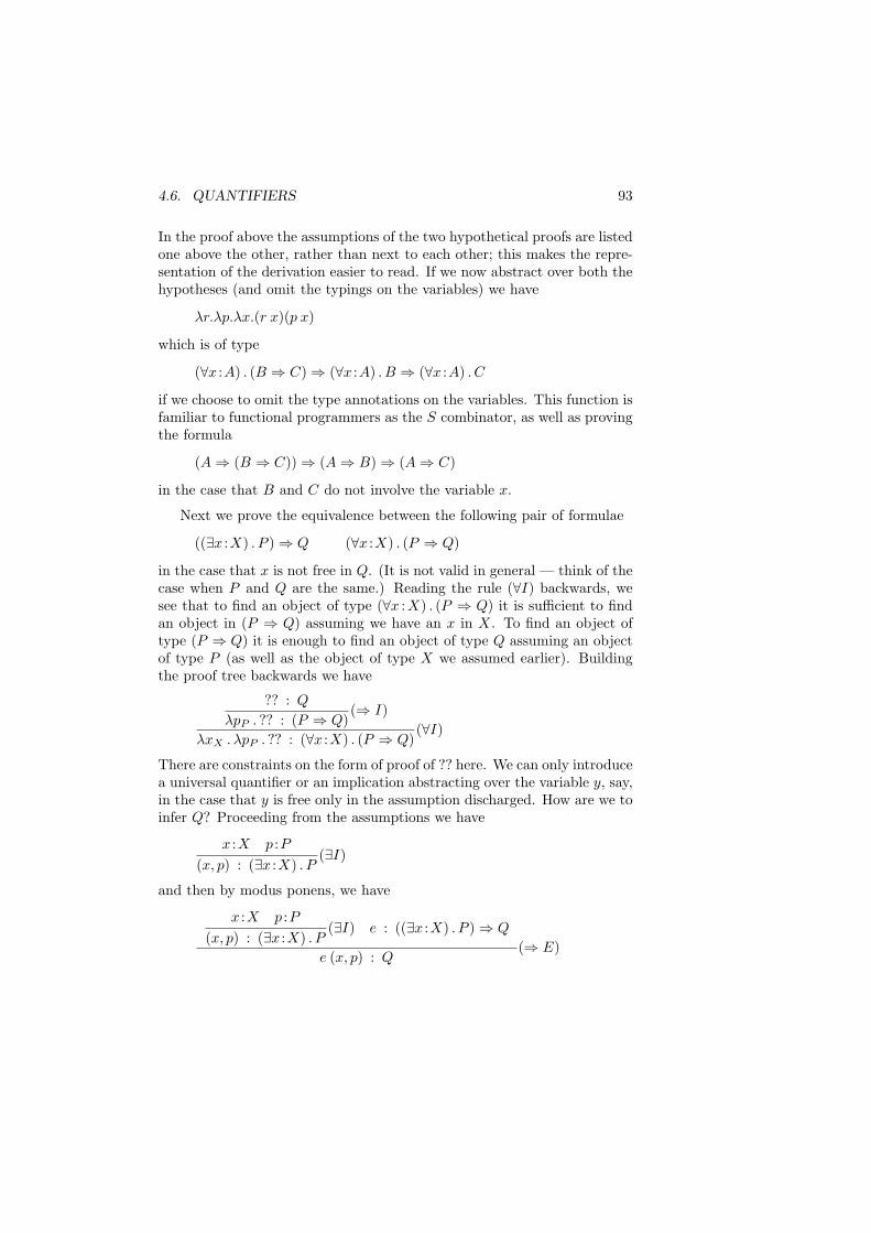
4.6. QUANTIFIERS 93
In the proof above the assumptions of the two hypothetical proofs are listedone above the other, rather than next to each other; this makes the repre-sentation of the derivation easier to read. If we now abstract over both thehypotheses (and omit the typings on the variables) we have
λr.λp.λx.(r x)(p x)
which is of type
(∀x :A) . (B ⇒ C)⇒ (∀x :A) . B ⇒ (∀x :A) . C
if we choose to omit the type annotations on the variables. This function isfamiliar to functional programmers as the S combinator, as well as provingthe formula
(A⇒ (B ⇒ C))⇒ (A⇒ B)⇒ (A⇒ C)
in the case that B and C do not involve the variable x.
Next we prove the equivalence between the following pair of formulae
((∃x :X) . P )⇒ Q (∀x :X) . (P ⇒ Q)
in the case that x is not free in Q. (It is not valid in general — think of thecase when P and Q are the same.) Reading the rule (∀I) backwards, wesee that to find an object of type (∀x :X) . (P ⇒ Q) it is sufficient to findan object in (P ⇒ Q) assuming we have an x in X. To find an object oftype (P ⇒ Q) it is enough to find an object of type Q assuming an objectof type P (as well as the object of type X we assumed earlier). Buildingthe proof tree backwards we have
?? : Q
λpP . ?? : (P ⇒ Q)(⇒ I)
λxX . λpP . ?? : (∀x :X) . (P ⇒ Q)(∀I)
There are constraints on the form of proof of ?? here. We can only introducea universal quantifier or an implication abstracting over the variable y, say,in the case that y is free only in the assumption discharged. How are we toinfer Q? Proceeding from the assumptions we have
x :X p :P(x, p) : (∃x :X) . P
(∃I)
and then by modus ponens, we have
x :X p :P(x, p) : (∃x :X) . P
(∃I) e : ((∃x :X) . P )⇒ Q
e (x, p) : Q(⇒ E)
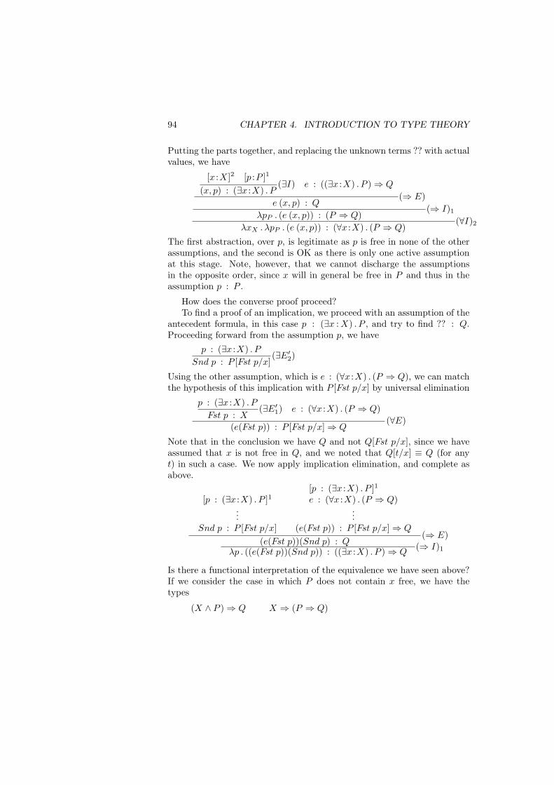
94 CHAPTER 4. INTRODUCTION TO TYPE THEORY
Putting the parts together, and replacing the unknown terms ?? with actualvalues, we have
[x :X]2 [p :P ]1
(x, p) : (∃x :X) . P(∃I) e : ((∃x :X) . P )⇒ Q
e (x, p) : Q(⇒ E)
λpP . (e (x, p)) : (P ⇒ Q)(⇒ I)1
λxX . λpP . (e (x, p)) : (∀x :X) . (P ⇒ Q)(∀I)2
The first abstraction, over p, is legitimate as p is free in none of the otherassumptions, and the second is OK as there is only one active assumptionat this stage. Note, however, that we cannot discharge the assumptionsin the opposite order, since x will in general be free in P and thus in theassumption p : P .
How does the converse proof proceed?To find a proof of an implication, we proceed with an assumption of the
antecedent formula, in this case p : (∃x : X) . P , and try to find ?? : Q.Proceeding forward from the assumption p, we have
p : (∃x :X) . P
Snd p : P [Fst p/x](∃E′
2)
Using the other assumption, which is e : (∀x :X) . (P ⇒ Q), we can matchthe hypothesis of this implication with P [Fst p/x] by universal elimination
p : (∃x :X) . P
Fst p : X(∃E′
1) e : (∀x :X) . (P ⇒ Q)
(e(Fst p)) : P [Fst p/x]⇒ Q(∀E)
Note that in the conclusion we have Q and not Q[Fst p/x], since we haveassumed that x is not free in Q, and we noted that Q[t/x] ≡ Q (for anyt) in such a case. We now apply implication elimination, and complete asabove.
[p : (∃x :X) . P ]1...
Snd p : P [Fst p/x]
[p : (∃x :X) . P ]1
e : (∀x :X) . (P ⇒ Q)...
(e(Fst p)) : P [Fst p/x]⇒ Q
(e(Fst p))(Snd p) : Q(⇒ E)
λp . ((e(Fst p))(Snd p)) : ((∃x :X) . P )⇒ Q(⇒ I)1
Is there a functional interpretation of the equivalence we have seen above?If we consider the case in which P does not contain x free, we have thetypes
(X ∧ P )⇒ Q X ⇒ (P ⇒ Q)
4.6. QUANTIFIERS 95
These two function spaces give two different representations of binary func-tions. In the first, the function takes a pair of arguments, of type (X ∧P ),to a result of type Q. The other representation, which is often called thecurried form in honour of Haskell B. Curry, the λ-calculus pioneer, makesthe function higher order. By this we mean that on being passed an argu-ment of type X, the function returns a function of type (P ⇒ Q) whichexpects an argument of type P , the second half of the pair. (We often callthe first representation the uncurried form, in contrast to the latter.)
The pair of functions we derived above can be seen to map from onefunction representation to another
λxX . λpP . (e (x, p))
takes separately the two arguments x and p, forms a pair from them and,applies the uncurried function e to the result. Conversely,
λp . ((e(Fst p))(Snd p))
takes a pair p as argument, and splits the pair into its components Fst pand Snd p, and applies the curried function e to the two halves one at atime.
The functions perform a similar function in the general case that Pdepends upon x, and we deal with dependent sum and product types.
Exercises
4.12. Give a derivation of a proof object of the formula
(∃x :X) .¬P ⇒ ¬(∀x :X) . P
Would you expect the reverse implication to be derivable?4.13. Show that the formulas (∀x :X) .¬P and ¬(∃x :X) . P are equivalentby deriving two functions mapping each into the other.4.14. Derive an object of type
(∀x :X) . (A⇒ B)⇒ ((∃x :X) . A⇒ (∃x :X) . B)
What is this formula in the case that A and B are independent of thevariable x?4.15. Derive an object of type
(∃y :Y ) . (∀x :X) . P ⇒ (∀x :X) . (∃y :Y ) . P
where in general P will contain x and y free. Under what circumstancescan you derive an object of the converse type?
(∀x :X) . (∃y :Y ) . P ⇒ (∃y :Y ) . (∀x :X) . P
Can you give a simpler reading of the formula in cases when P does notcontain both x and y free?
96 CHAPTER 4. INTRODUCTION TO TYPE THEORY
4.7 Base Types
The material in the chapter so far has had different emphases. The propo-sitional part of the system can be viewed as both a logic and a typedλ-calculus; the quantifiers are logical constructs, but have a natural pro-gramming interpretation. Now we introduce some base types, whose originslie in programming, but we shall see that they have a logical interpretationtoo.
In this and subsequent sections we introduce a number of familiar types:the booleans as an example of a finite type, finite types in general, with thespecial case of the one element type, the natural numbers, and finally treesas an example of an algebraic type.
4.7.1 Booleans
The system we are building here is one in which propositions, or formulas,are identified with types, and vice versa. Amongst these propositions arethe propositions ⊥, or “false”, >, or “true” (which we introduce below),and combinations of the propositions using logical connectives such as ∧and ∨. Each of these propositions is a type: the collection of proofs of thatproposition.
Consider the case in which we want to return one of two results condi-tional on some property. We need, informally, to be able to ask the questionand receive the answer Yes or the answer No, so we need a particular typewhich contains these two values. We call this the type bool of boolean val-ues and for the sake of tradition call the two values True and False. Thetype bool is simply a finite type containing two values. The role of the typeis computational: we can build the expression if . . . then . . . else . . .(where the condition is a boolean expression) in our language, allowing caseswitches in computations. The value of if b then e else f is e if b evaluatesto True, otherwise it is f .
To recap, True and False are values of the type bool, whilst ⊥ and >are the false and true propositions. Readers may be familiar with similardistinctions between boolean values and propositions from program verifi-cation. Languages such as Pascal contain a boolean type — if we reasonabout these programs we use an external logical language to construct state-ments about the language, we are not constructing expressions of type boolwhich are expressions of the language.
We should also note that these definitions form a template for the defi-nition of any type with a finite set of members.
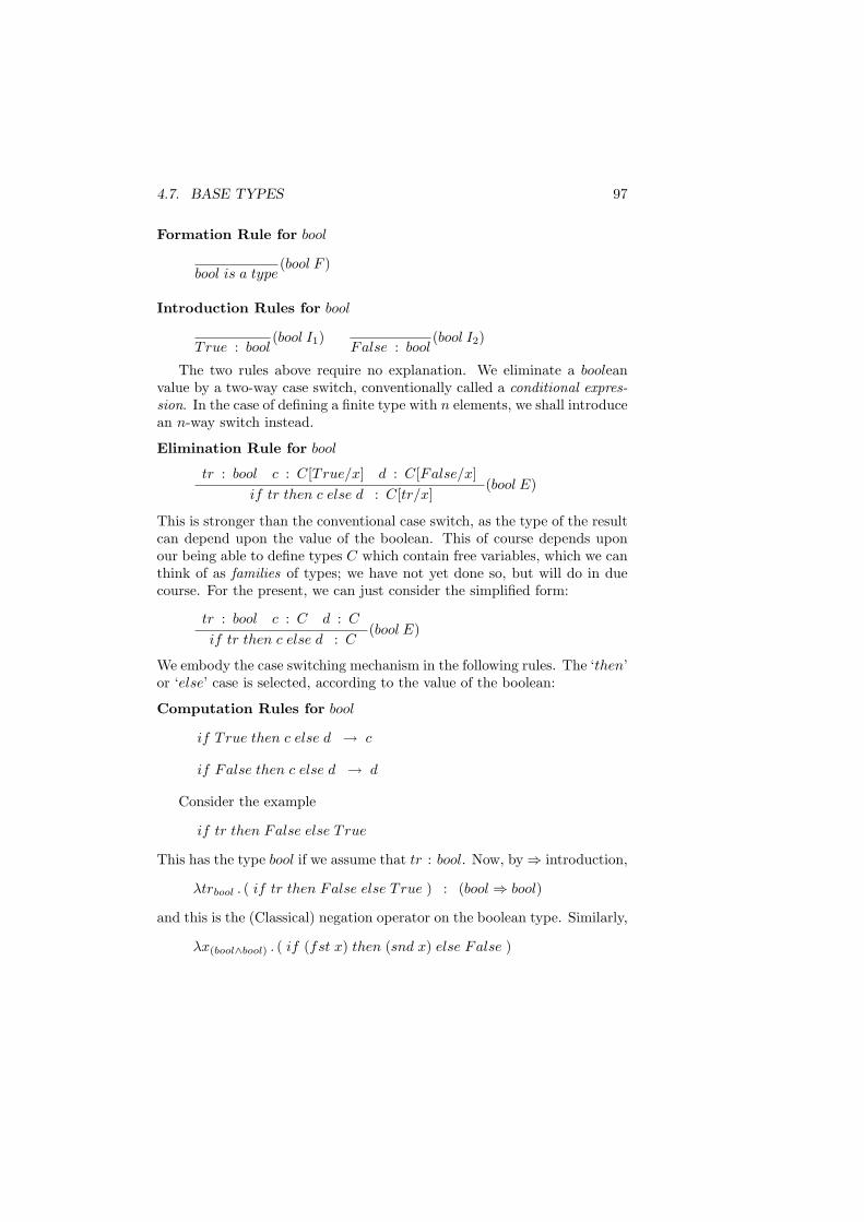
4.7. BASE TYPES 97
Formation Rule for bool
bool is a type(bool F )
Introduction Rules for bool
True : bool(bool I1)
False : bool(bool I2)
The two rules above require no explanation. We eliminate a booleanvalue by a two-way case switch, conventionally called a conditional expres-sion. In the case of defining a finite type with n elements, we shall introducean n-way switch instead.
Elimination Rule for bool
tr : bool c : C[True/x] d : C[False/x]if tr then c else d : C[tr/x]
(bool E)
This is stronger than the conventional case switch, as the type of the resultcan depend upon the value of the boolean. This of course depends uponour being able to define types C which contain free variables, which we canthink of as families of types; we have not yet done so, but will do in duecourse. For the present, we can just consider the simplified form:
tr : bool c : C d : C
if tr then c else d : C(bool E)
We embody the case switching mechanism in the following rules. The ‘then’or ‘else’ case is selected, according to the value of the boolean:
Computation Rules for bool
if True then c else d → c
if False then c else d → d
Consider the example
if tr then False else True
This has the type bool if we assume that tr : bool. Now, by⇒ introduction,
λtrbool . ( if tr then False else True ) : (bool⇒ bool)
and this is the (Classical) negation operator on the boolean type. Similarly,
λx(bool∧bool) . ( if (fst x) then (snd x) else False )
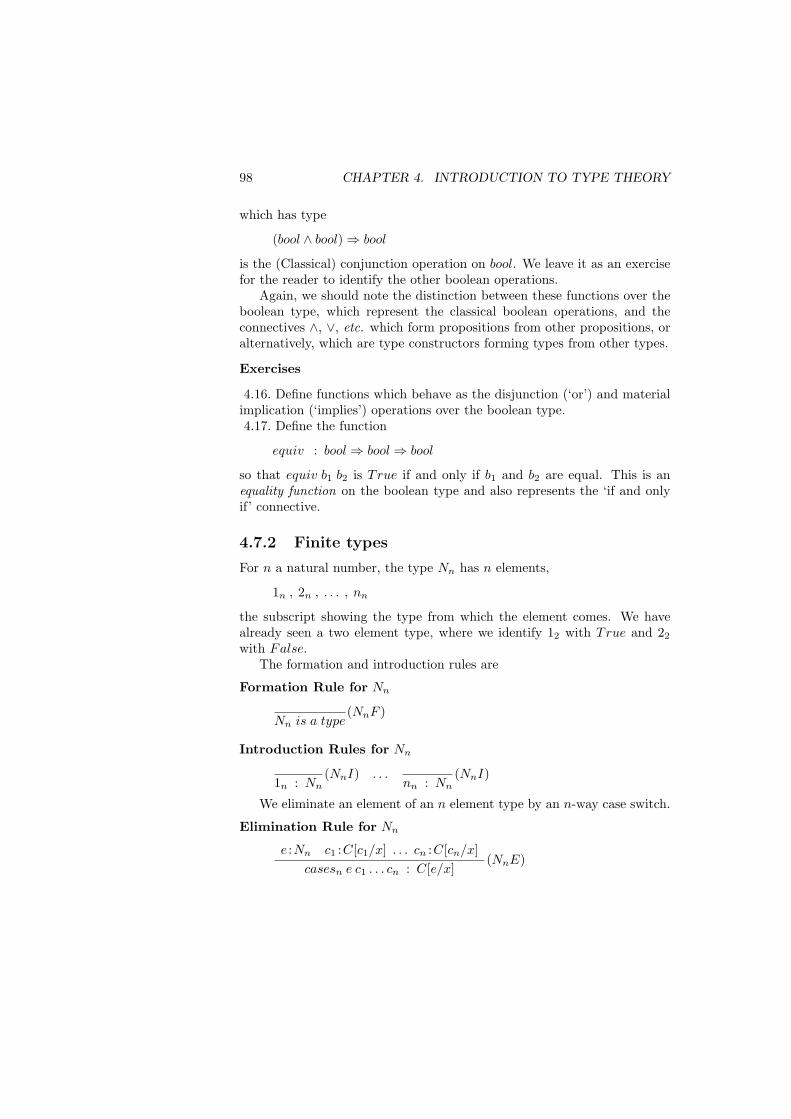
98 CHAPTER 4. INTRODUCTION TO TYPE THEORY
which has type
(bool ∧ bool)⇒ bool
is the (Classical) conjunction operation on bool. We leave it as an exercisefor the reader to identify the other boolean operations.
Again, we should note the distinction between these functions over theboolean type, which represent the classical boolean operations, and theconnectives ∧, ∨, etc. which form propositions from other propositions, oralternatively, which are type constructors forming types from other types.
Exercises
4.16. Define functions which behave as the disjunction (‘or’) and materialimplication (‘implies’) operations over the boolean type.4.17. Define the function
equiv : bool⇒ bool⇒ bool
so that equiv b1 b2 is True if and only if b1 and b2 are equal. This is anequality function on the boolean type and also represents the ‘if and onlyif’ connective.
4.7.2 Finite types
For n a natural number, the type Nn has n elements,
1n , 2n , . . . , nn
the subscript showing the type from which the element comes. We havealready seen a two element type, where we identify 12 with True and 22
with False.The formation and introduction rules are
Formation Rule for Nn
Nn is a type(NnF )
Introduction Rules for Nn
1n : Nn(NnI) . . .
nn : Nn(NnI)
We eliminate an element of an n element type by an n-way case switch.
Elimination Rule for Nn
e :Nn c1 :C[c1/x] . . . cn :C[cn/x]casesn e c1 . . . cn : C[e/x]
(NnE)
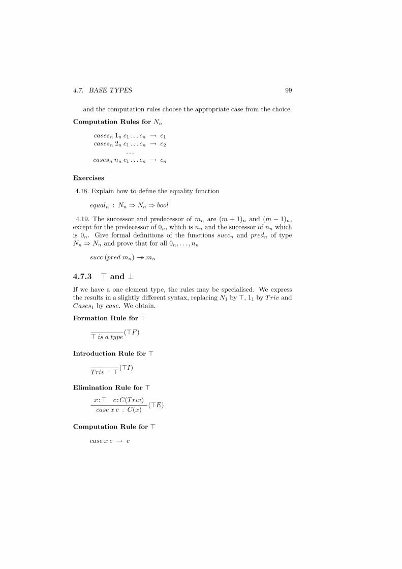
4.7. BASE TYPES 99
and the computation rules choose the appropriate case from the choice.
Computation Rules for Nn
casesn 1n c1 . . . cn → c1
casesn 2n c1 . . . cn → c2
. . .casesn nn c1 . . . cn → cn
Exercises
4.18. Explain how to define the equality function
equaln : Nn ⇒ Nn ⇒ bool
4.19. The successor and predecessor of mn are (m + 1)n and (m − 1)n,except for the predecessor of 0n, which is nn and the successor of nn whichis 0n. Give formal definitions of the functions succn and predn of typeNn ⇒ Nn and prove that for all 0n, . . . , nn
succ (pred mn)→→ mn
4.7.3 > and ⊥If we have a one element type, the rules may be specialised. We expressthe results in a slightly different syntax, replacing N1 by >, 11 by Triv andCases1 by case. We obtain.
Formation Rule for >
> is a type(>F )
Introduction Rule for >
Triv : >(>I)
Elimination Rule for >
x :> c :C(Triv)case x c : C(x)
(>E)
Computation Rule for >
case x c → c
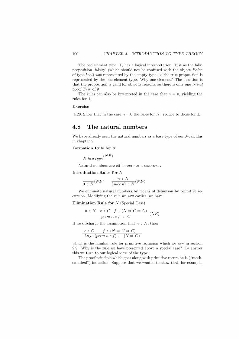
100 CHAPTER 4. INTRODUCTION TO TYPE THEORY
The one element type, >, has a logical interpretation. Just as the falseproposition ‘falsity’ (which should not be confused with the object Falseof type bool) was represented by the empty type, so the true proposition isrepresented by the one element type. Why one element? The intuition isthat the proposition is valid for obvious reasons, so there is only one trivialproof Triv of it.
The rules can also be interpreted in the case that n = 0, yielding therules for ⊥.
Exercise
4.20. Show that in the case n = 0 the rules for Nn reduce to those for ⊥.
4.8 The natural numbers
We have already seen the natural numbers as a base type of our λ-calculusin chapter 2.
Formation Rule for N
N is a type(NF )
Natural numbers are either zero or a successor.
Introduction Rules for N
0 : N(NI1)
n : N
(succ n) : N(NI2)
We eliminate natural numbers by means of definition by primitive re-cursion. Modifying the rule we saw earlier, we have
Elimination Rule for N (Special Case)
n : N c : C f : (N ⇒ C ⇒ C)prim n c f : C
(NE)
If we discharge the assumption that n : N , then
c : C f : (N ⇒ C ⇒ C)λnN . (prim n c f) : (N ⇒ C)
which is the familiar rule for primitive recursion which we saw in section2.9. Why is the rule we have presented above a special case? To answerthis we turn to our logical view of the type.
The proof principle which goes along with primitive recursion is (“math-ematical”) induction. Suppose that we wanted to show that, for example,
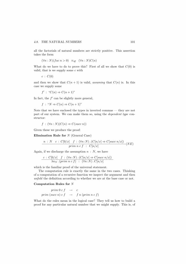
4.8. THE NATURAL NUMBERS 101
all the factorials of natural numbers are strictly positive. This assertiontakes the form
(∀n : N)(fac n > 0) ≡df (∀n : N)C(n)
What do we have to do to prove this? First of all we show that C(0) isvalid, that is we supply some c with
c : C(0)
and then we show that C(n + 1) is valid, assuming that C(n) is. In thiscase we supply some
f ′ : “C(n)⇒ C(n + 1)”
In fact, the f ′ can be slightly more general,
f : “N ⇒ C(n)⇒ C(n + 1)”
Note that we have enclosed the types in inverted commas — they are notpart of our system. We can make them so, using the dependent type con-structor:
f : (∀n : N)(C(n)⇒ C(succ n))
Given these we produce the proof:
Elimination Rule for N (General Case)
n : N c : C[0/x] f : (∀n :N) . (C[n/x]⇒ C[succ n/x])prim n c f : C[n/x]
(NE)
Again, if we discharge the assumption n : N , we have
c : C[0/x] f : (∀n :N) . (C[n/x]⇒ C[succ n/x])λnN . (prim n c f) : (∀n :N) . C[n/x]
which is the familiar proof of the universal statement.The computation rule is exactly the same in the two cases. Thinking
of a computation of a recursive function we inspect the argument and thenunfold the definition according to whether we are at the base case or not.
Computation Rules for N
prim 0 c f → c
prim (succ n) c f → f n (prim n c f)
What do the rules mean in the logical case? They tell us how to build aproof for any particular natural number that we might supply. This is, of
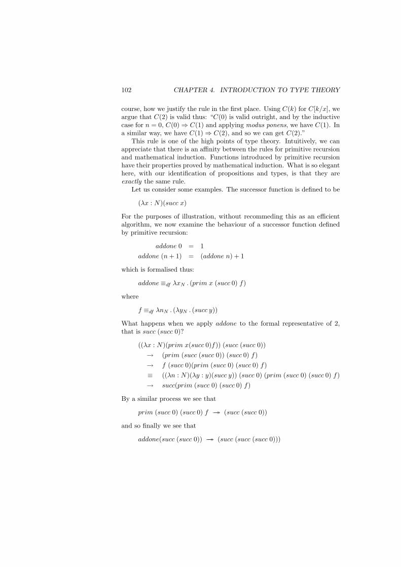
102 CHAPTER 4. INTRODUCTION TO TYPE THEORY
course, how we justify the rule in the first place. Using C(k) for C[k/x], weargue that C(2) is valid thus: “C(0) is valid outright, and by the inductivecase for n = 0, C(0)⇒ C(1) and applying modus ponens, we have C(1). Ina similar way, we have C(1)⇒ C(2), and so we can get C(2).”
This rule is one of the high points of type theory. Intuitively, we canappreciate that there is an affinity between the rules for primitive recursionand mathematical induction. Functions introduced by primitive recursionhave their properties proved by mathematical induction. What is so eleganthere, with our identification of propositions and types, is that they areexactly the same rule.
Let us consider some examples. The successor function is defined to be
(λx : N)(succ x)
For the purposes of illustration, without recommeding this as an efficientalgorithm, we now examine the behaviour of a successor function definedby primitive recursion:
addone 0 = 1addone (n + 1) = (addone n) + 1
which is formalised thus:
addone≡df λxN . (prim x (succ 0) f)
where
f ≡df λnN . (λyN . (succ y))
What happens when we apply addone to the formal representative of 2,that is succ (succ 0)?
((λx : N)(prim x(succ 0)f)) (succ (succ 0))→ (prim (succ (succ 0)) (succ 0) f)→ f (succ 0)(prim (succ 0) (succ 0) f)≡ ((λn : N)(λy : y)(succ y)) (succ 0) (prim (succ 0) (succ 0) f)→ succ(prim (succ 0) (succ 0) f)
By a similar process we see that
prim (succ 0) (succ 0) f →→ (succ (succ 0))
and so finally we see that
addone(succ (succ 0)) →→ (succ (succ (succ 0)))
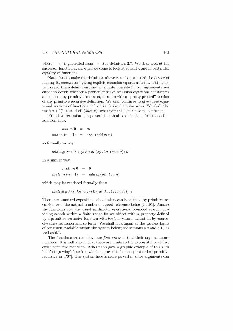
4.8. THE NATURAL NUMBERS 103
where ‘→→ ’ is generated from → a la definition 2.7. We shall look at thesuccessor function again when we come to look at equality, and in particularequality of functions.
Note that to make the definition above readable, we used the device ofnaming it, addone and giving explicit recursion equations for it. This helpsus to read these definitions, and it is quite possible for an implementationeither to decide whether a particular set of recursion equations constitutesa definition by primitive recursion, or to provide a “pretty printed” versionof any primitive recursive definition. We shall continue to give these equa-tional versions of functions defined in this and similar ways. We shall alsouse ‘(n + 1)’ instead of ‘(succ n)’ whenever this can cause no confusion.
Primitive recursion is a powerful method of definition. We can defineaddition thus:
add m 0 = m
add m (n + 1) = succ (add m n)
so formally we say
add≡df λm . λn . prim m (λp . λq . (succ q)) n
In a similar way
mult m 0 = 0mult m (n + 1) = add m (mult m n)
which may be rendered formally thus:
mult≡df λm . λn . prim 0 (λp . λq . (add m q)) n
There are standard expositions about what can be defined by primitive re-cursion over the natural numbers, a good reference being [Cut81]. Amongthe functions are: the usual arithmetic operations; bounded search, pro-viding search within a finite range for an object with a property definedby a primitive recursive function with boolean values; definition by course-of-values recursion and so forth. We shall look again at the various formsof recursion available within the system below; see sections 4.9 and 5.10 aswell as 6.1.
The functions we see above are first order in that their arguments arenumbers. It is well known that there are limits to the expressibility of firstorder primitive recursion. Ackermann gave a graphic example of this withhis ‘fast-growing’ function, which is proved to be non (first order) primitiverecursive in [P67]. The system here is more powerful, since arguments can
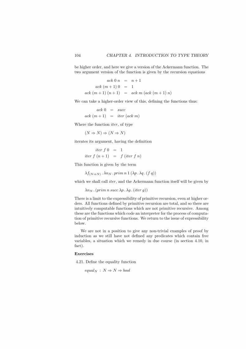
104 CHAPTER 4. INTRODUCTION TO TYPE THEORY
be higher order, and here we give a version of the Ackermann function. Thetwo argument version of the function is given by the recursion equations
ack 0 n = n + 1ack (m + 1) 0 = 1
ack (m + 1) (n + 1) = ack m (ack (m + 1) n)
We can take a higher-order view of this, defining the functions thus:
ack 0 = succ
ack (m + 1) = iter (ack m)
Where the function iter, of type
(N ⇒ N)⇒ (N ⇒ N)
iterates its argument, having the definition
iter f 0 = 1iter f (n + 1) = f (iter f n)
This function is given by the term
λf(N⇒N) . λnN . prim n 1 (λp . λq . (f q))
which we shall call iter, and the Ackermann function itself will be given by
λnN . (prim n succ λp . λg . (iter g))
There is a limit to the expressibility of primitive recursion, even at higher or-ders. All functions defined by primitive recursion are total, and so there areintuitively computable functions which are not primitive recursive. Amongthese are the functions which code an interpreter for the process of computa-tion of primitive recursive functions. We return to the issue of expressibilitybelow.
We are not in a position to give any non-trivial examples of proof byinduction as we still have not defined any predicates which contain freevariables, a situation which we remedy in due course (in section 4.10, infact).
Exercises
4.21. Define the equality function
equalN : N ⇒ N ⇒ bool

4.9. WELL-FOUNDED TYPES — TREES 105
4.22. Define the function geq of type
geq : N ⇒ N ⇒ bool
so that geq n m is True if and only if n is greater than or equal to m.[Hint: the best way to do this is to define the functions geq n by induction,that is to define geq0 outright (by induction) and to define geq (n+1) usinggeq n.]4.23. Using geq or otherwise show how to define the bounded search func-tion
search : (N ⇒ bool)⇒ N ⇒ N
so that search p n is the smallest l less than n so that (p l) is True, andwhich is n if no such l exists.4.24. Give a formal definition of the function sumf given by
sumf f n m≡df
m∑i=n
(f i)
What is its type? What type has the partial application
sumf id
where id x≡df x is the identity function?
4.9 Well-founded types — trees
In this section we look at an example of how to incorporate recursive datatypes like lists and trees into the system. The mechanism is similar tothe Miranda algebraic type mechanism. Martin-Lof has proposed a generalscheme to achieve this; we examine it in full generality in the followingchapter.
We call the types well-founded as they are types over which we candefine objects by recursion and prove properties by induction, as we did forthe natural numbers; informally, for this to be possible we need to be surethat when we make a recursive definition (or an inductive proof) we neverencounter an infinite sequence of simplifications, as in the simplificationfrom (n + 1) to n. If we have one of these infinite sequences, then thefunction will be defined on none of the values in that sequence, as eachvalue depends upon an earlier value; there is no foundation to the sequenceor the recursion, in other words.
We shall again see that the principles of induction and recursion areembodied by exactly the same rule.
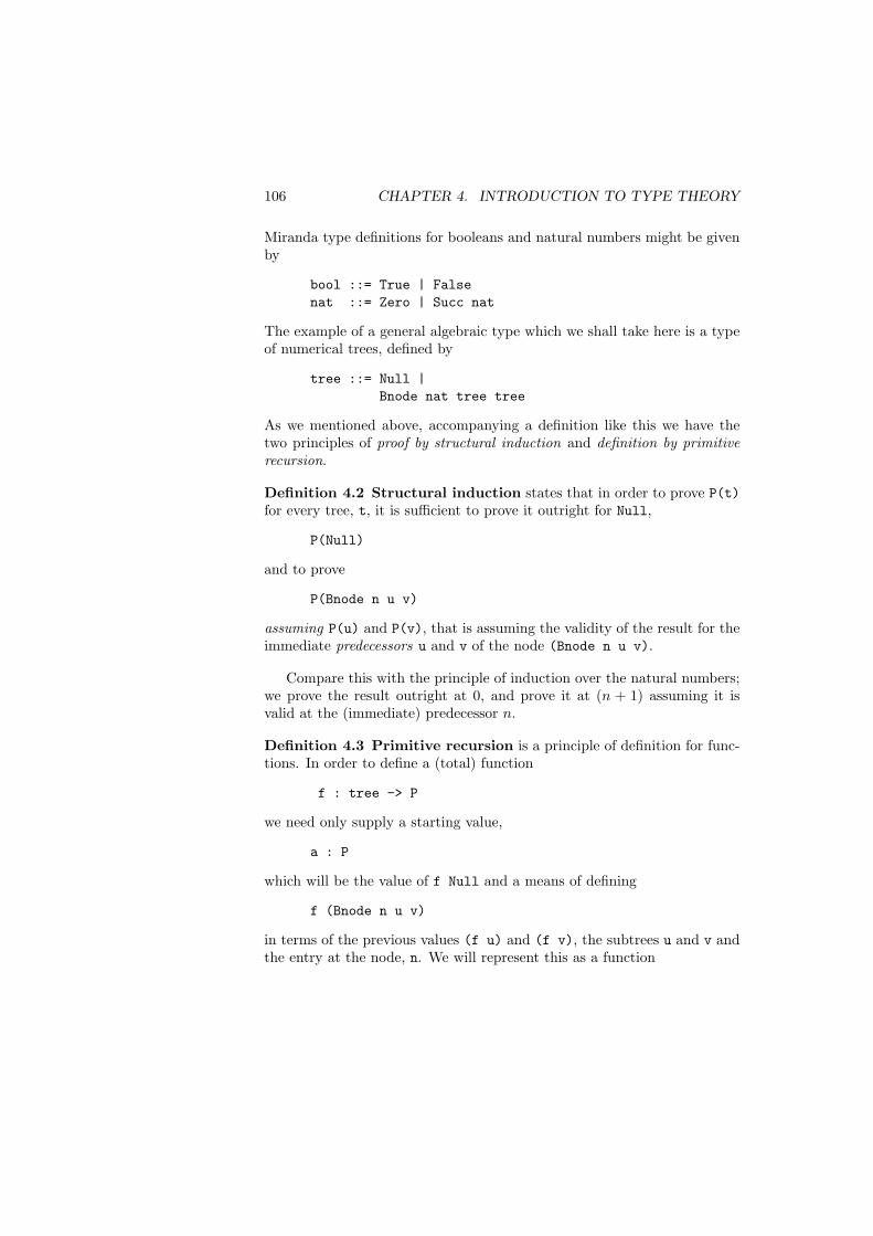
106 CHAPTER 4. INTRODUCTION TO TYPE THEORY
Miranda type definitions for booleans and natural numbers might be givenby
bool ::= True | Falsenat ::= Zero | Succ nat
The example of a general algebraic type which we shall take here is a typeof numerical trees, defined by
tree ::= Null |Bnode nat tree tree
As we mentioned above, accompanying a definition like this we have thetwo principles of proof by structural induction and definition by primitiverecursion.
Definition 4.2 Structural induction states that in order to prove P(t)for every tree, t, it is sufficient to prove it outright for Null,
P(Null)
and to prove
P(Bnode n u v)
assuming P(u) and P(v), that is assuming the validity of the result for theimmediate predecessors u and v of the node (Bnode n u v).
Compare this with the principle of induction over the natural numbers;we prove the result outright at 0, and prove it at (n + 1) assuming it isvalid at the (immediate) predecessor n.
Definition 4.3 Primitive recursion is a principle of definition for func-tions. In order to define a (total) function
f : tree -> P
we need only supply a starting value,
a : P
which will be the value of f Null and a means of defining
f (Bnode n u v)
in terms of the previous values (f u) and (f v), the subtrees u and v andthe entry at the node, n. We will represent this as a function
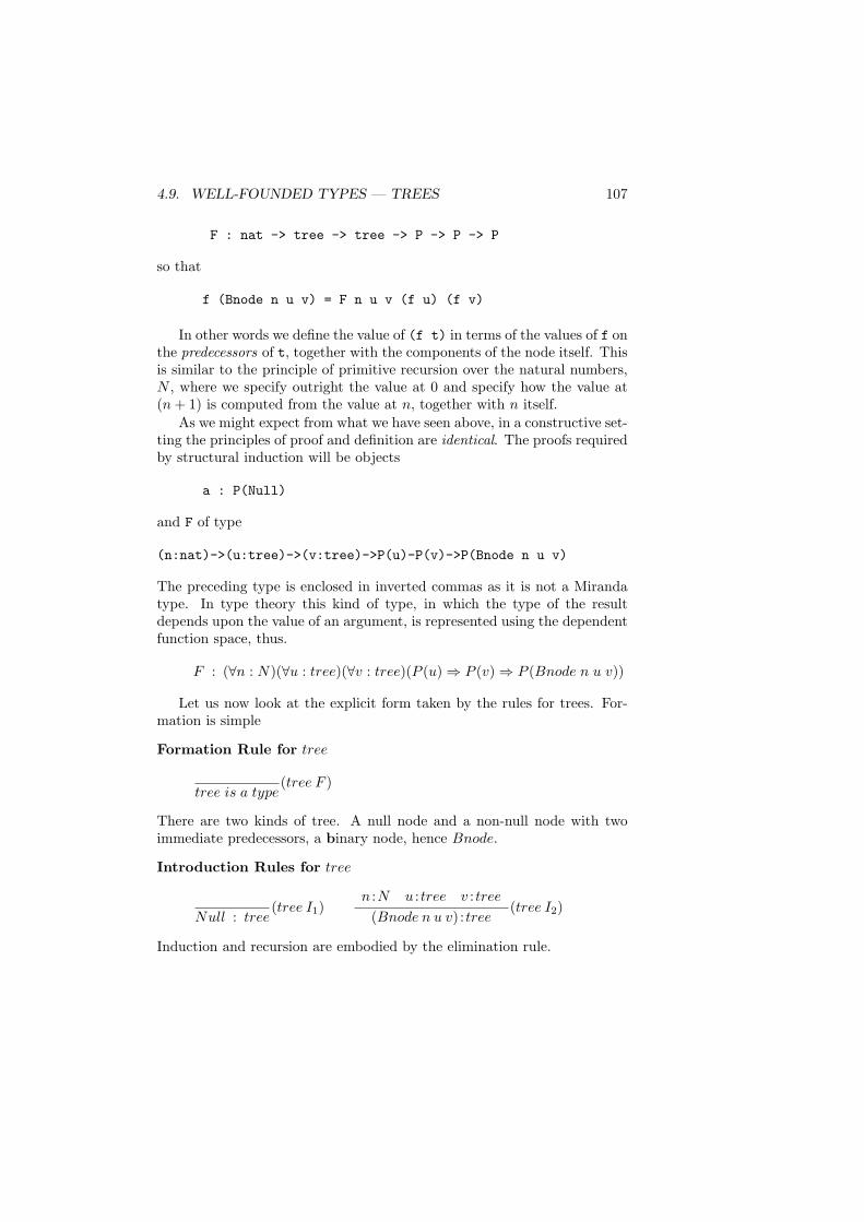
4.9. WELL-FOUNDED TYPES — TREES 107
F : nat -> tree -> tree -> P -> P -> P
so that
f (Bnode n u v) = F n u v (f u) (f v)
In other words we define the value of (f t) in terms of the values of f onthe predecessors of t, together with the components of the node itself. Thisis similar to the principle of primitive recursion over the natural numbers,N , where we specify outright the value at 0 and specify how the value at(n + 1) is computed from the value at n, together with n itself.
As we might expect from what we have seen above, in a constructive set-ting the principles of proof and definition are identical. The proofs requiredby structural induction will be objects
a : P(Null)
and F of type
(n:nat)->(u:tree)->(v:tree)->P(u)-P(v)->P(Bnode n u v)
The preceding type is enclosed in inverted commas as it is not a Mirandatype. In type theory this kind of type, in which the type of the resultdepends upon the value of an argument, is represented using the dependentfunction space, thus.
F : (∀n : N)(∀u : tree)(∀v : tree)(P (u)⇒ P (v)⇒ P (Bnode n u v))
Let us now look at the explicit form taken by the rules for trees. For-mation is simple
Formation Rule for tree
tree is a type(tree F )
There are two kinds of tree. A null node and a non-null node with twoimmediate predecessors, a binary node, hence Bnode.
Introduction Rules for tree
Null : tree(tree I1)
n :N u : tree v : tree(Bnode n u v) : tree
(tree I2)
Induction and recursion are embodied by the elimination rule.
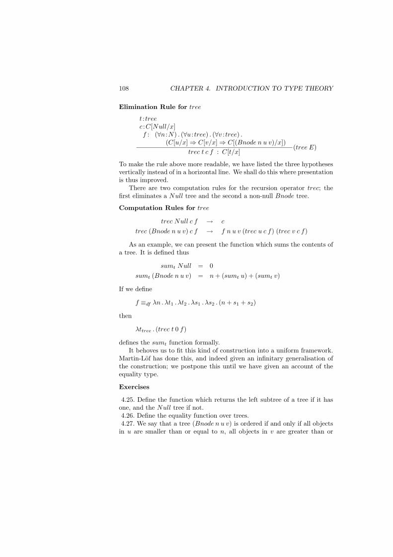
108 CHAPTER 4. INTRODUCTION TO TYPE THEORY
Elimination Rule for tree
t : treec :C[Null/x]f : (∀n :N) . (∀u : tree) . (∀v : tree) .
(C[u/x]⇒ C[v/x]⇒ C[(Bnode n u v)/x])trec t c f : C[t/x]
(tree E)
To make the rule above more readable, we have listed the three hypothesesvertically instead of in a horizontal line. We shall do this where presentationis thus improved.
There are two computation rules for the recursion operator trec; thefirst eliminates a Null tree and the second a non-null Bnode tree.
Computation Rules for tree
trec Null c f → c
trec (Bnode n u v) c f → f n u v (trec u c f) (trec v c f)
As an example, we can present the function which sums the contents ofa tree. It is defined thus
sumt Null = 0sumt (Bnode n u v) = n + (sumt u) + (sumt v)
If we define
f ≡df λn . λt1 . λt2 . λs1 . λs2 . (n + s1 + s2)
then
λttree . (trec t 0 f)
defines the sumt function formally.It behoves us to fit this kind of construction into a uniform framework.
Martin-Lof has done this, and indeed given an infinitary generalisation ofthe construction; we postpone this until we have given an account of theequality type.
Exercises
4.25. Define the function which returns the left subtree of a tree if it hasone, and the Null tree if not.4.26. Define the equality function over trees.4.27. We say that a tree (Bnode n u v) is ordered if and only if all objectsin u are smaller than or equal to n, all objects in v are greater than or
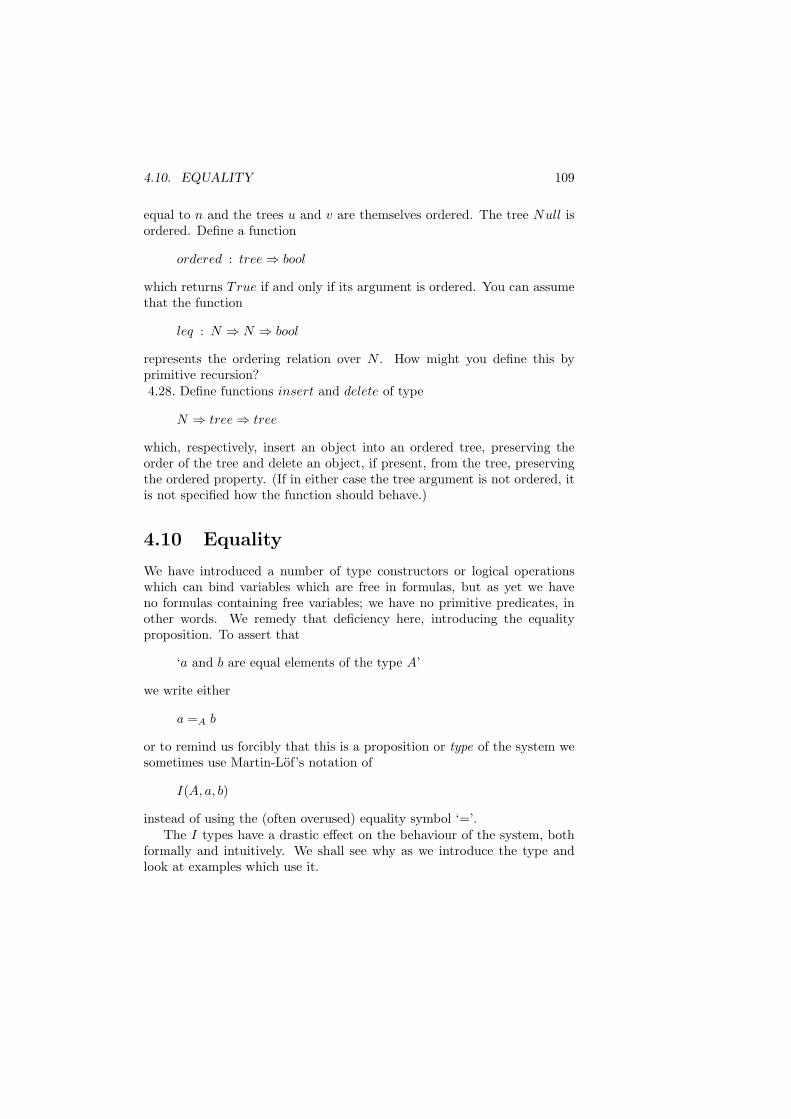
4.10. EQUALITY 109
equal to n and the trees u and v are themselves ordered. The tree Null isordered. Define a function
ordered : tree⇒ bool
which returns True if and only if its argument is ordered. You can assumethat the function
leq : N ⇒ N ⇒ bool
represents the ordering relation over N . How might you define this byprimitive recursion?4.28. Define functions insert and delete of type
N ⇒ tree⇒ tree
which, respectively, insert an object into an ordered tree, preserving theorder of the tree and delete an object, if present, from the tree, preservingthe ordered property. (If in either case the tree argument is not ordered, itis not specified how the function should behave.)
4.10 Equality
We have introduced a number of type constructors or logical operationswhich can bind variables which are free in formulas, but as yet we haveno formulas containing free variables; we have no primitive predicates, inother words. We remedy that deficiency here, introducing the equalityproposition. To assert that
‘a and b are equal elements of the type A’
we write either
a =A b
or to remind us forcibly that this is a proposition or type of the system wesometimes use Martin-Lof’s notation of
I(A, a, b)
instead of using the (often overused) equality symbol ‘=’.The I types have a drastic effect on the behaviour of the system, both
formally and intuitively. We shall see why as we introduce the type andlook at examples which use it.
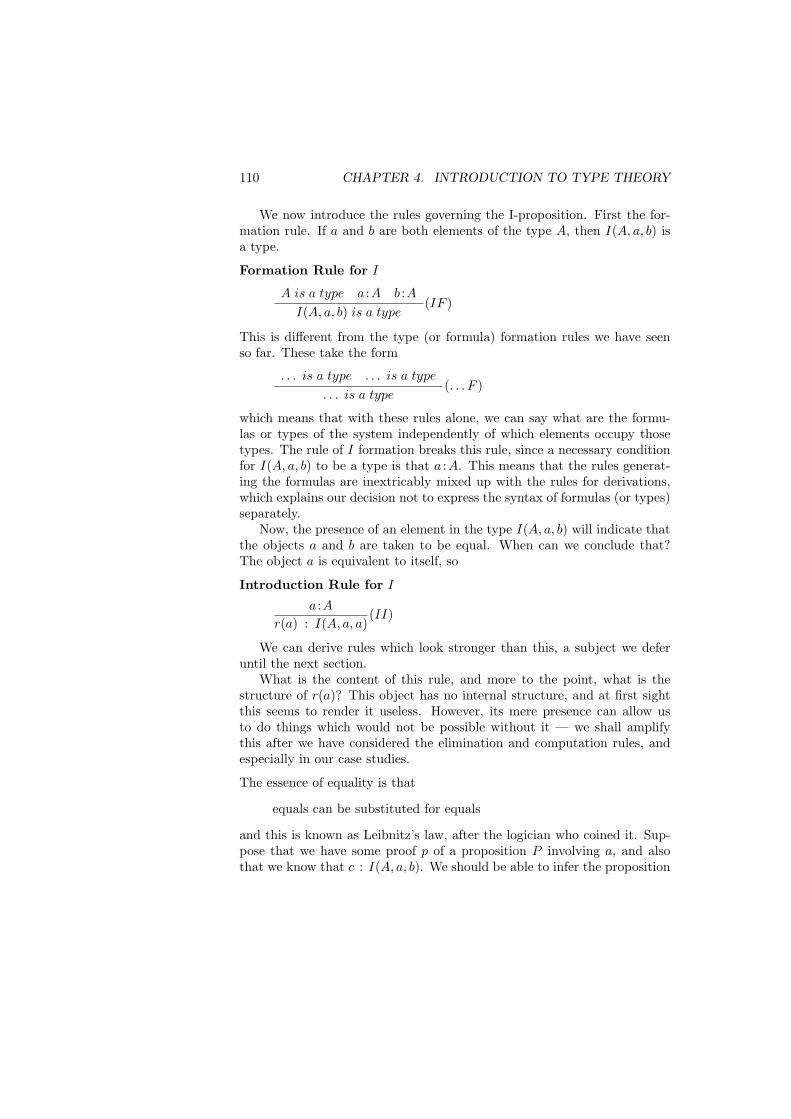
110 CHAPTER 4. INTRODUCTION TO TYPE THEORY
We now introduce the rules governing the I-proposition. First the for-mation rule. If a and b are both elements of the type A, then I(A, a, b) isa type.
Formation Rule for I
A is a type a :A b :AI(A, a, b) is a type
(IF )
This is different from the type (or formula) formation rules we have seenso far. These take the form
. . . is a type . . . is a type
. . . is a type(. . . F )
which means that with these rules alone, we can say what are the formu-las or types of the system independently of which elements occupy thosetypes. The rule of I formation breaks this rule, since a necessary conditionfor I(A, a, b) to be a type is that a :A. This means that the rules generat-ing the formulas are inextricably mixed up with the rules for derivations,which explains our decision not to express the syntax of formulas (or types)separately.
Now, the presence of an element in the type I(A, a, b) will indicate thatthe objects a and b are taken to be equal. When can we conclude that?The object a is equivalent to itself, so
Introduction Rule for I
a :Ar(a) : I(A, a, a)
(II)
We can derive rules which look stronger than this, a subject we deferuntil the next section.
What is the content of this rule, and more to the point, what is thestructure of r(a)? This object has no internal structure, and at first sightthis seems to render it useless. However, its mere presence can allow usto do things which would not be possible without it — we shall amplifythis after we have considered the elimination and computation rules, andespecially in our case studies.
The essence of equality is that
equals can be substituted for equals
and this is known as Leibnitz’s law, after the logician who coined it. Sup-pose that we have some proof p of a proposition P involving a, and alsothat we know that c : I(A, a, b). We should be able to infer the proposition
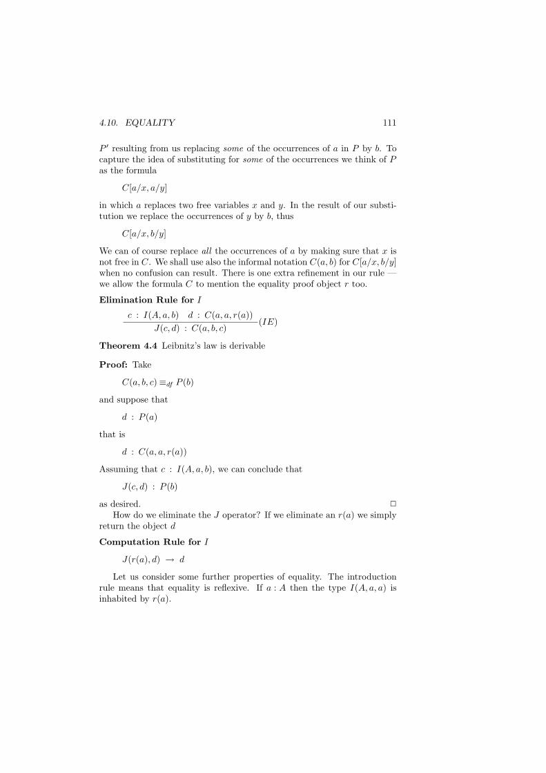
4.10. EQUALITY 111
P ′ resulting from us replacing some of the occurrences of a in P by b. Tocapture the idea of substituting for some of the occurrences we think of Pas the formula
C[a/x, a/y]
in which a replaces two free variables x and y. In the result of our substi-tution we replace the occurrences of y by b, thus
C[a/x, b/y]
We can of course replace all the occurrences of a by making sure that x isnot free in C. We shall use also the informal notation C(a, b) for C[a/x, b/y]when no confusion can result. There is one extra refinement in our rule —we allow the formula C to mention the equality proof object r too.
Elimination Rule for I
c : I(A, a, b) d : C(a, a, r(a))J(c, d) : C(a, b, c)
(IE)
Theorem 4.4 Leibnitz’s law is derivable
Proof: Take
C(a, b, c)≡df P (b)
and suppose that
d : P (a)
that is
d : C(a, a, r(a))
Assuming that c : I(A, a, b), we can conclude that
J(c, d) : P (b)
as desired. 2
How do we eliminate the J operator? If we eliminate an r(a) we simplyreturn the object d
Computation Rule for I
J(r(a), d) → d
Let us consider some further properties of equality. The introductionrule means that equality is reflexive. If a : A then the type I(A, a, a) isinhabited by r(a).
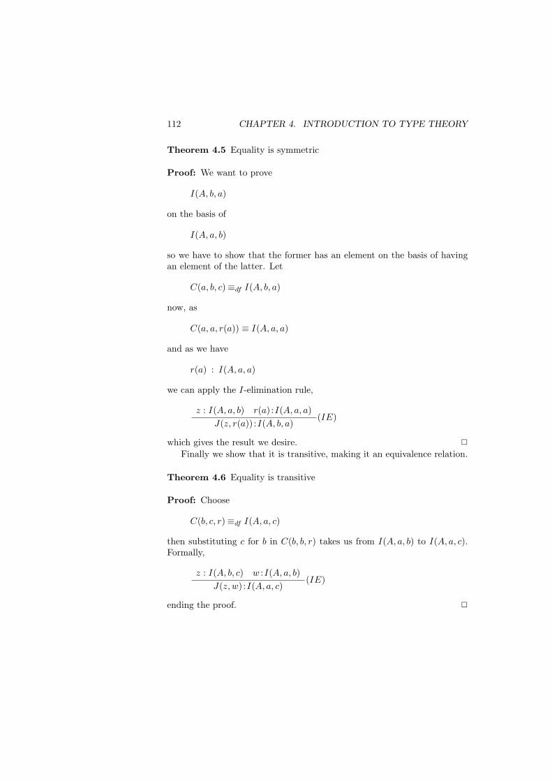
112 CHAPTER 4. INTRODUCTION TO TYPE THEORY
Theorem 4.5 Equality is symmetric
Proof: We want to prove
I(A, b, a)
on the basis of
I(A, a, b)
so we have to show that the former has an element on the basis of havingan element of the latter. Let
C(a, b, c)≡df I(A, b, a)
now, as
C(a, a, r(a)) ≡ I(A, a, a)
and as we have
r(a) : I(A, a, a)
we can apply the I-elimination rule,
z : I(A, a, b) r(a) :I(A, a, a)J(z, r(a)) :I(A, b, a)
(IE)
which gives the result we desire. 2
Finally we show that it is transitive, making it an equivalence relation.
Theorem 4.6 Equality is transitive
Proof: Choose
C(b, c, r)≡df I(A, a, c)
then substituting c for b in C(b, b, r) takes us from I(A, a, b) to I(A, a, c).Formally,
z : I(A, b, c) w :I(A, a, b)J(z, w) :I(A, a, c)
(IE)
ending the proof. 2
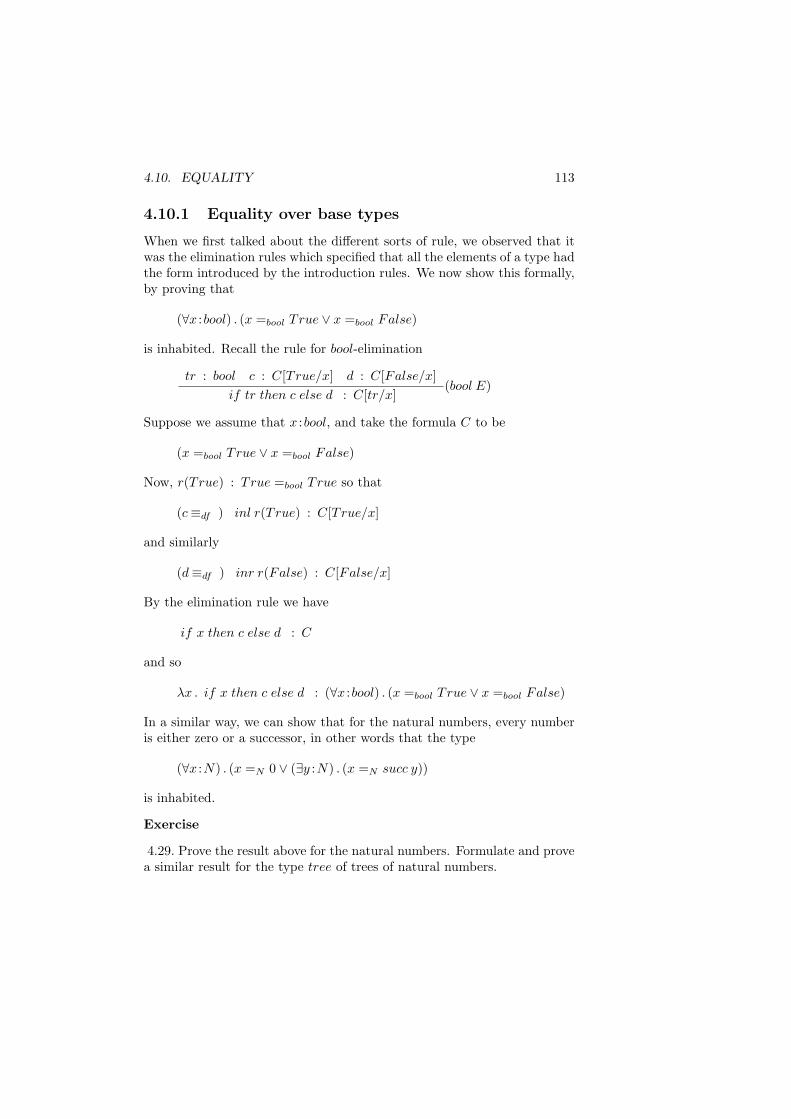
4.10. EQUALITY 113
4.10.1 Equality over base types
When we first talked about the different sorts of rule, we observed that itwas the elimination rules which specified that all the elements of a type hadthe form introduced by the introduction rules. We now show this formally,by proving that
(∀x :bool) . (x =bool True ∨ x =bool False)
is inhabited. Recall the rule for bool-elimination
tr : bool c : C[True/x] d : C[False/x]if tr then c else d : C[tr/x]
(bool E)
Suppose we assume that x :bool, and take the formula C to be
(x =bool True ∨ x =bool False)
Now, r(True) : True =bool True so that
(c≡df ) inl r(True) : C[True/x]
and similarly
(d≡df ) inr r(False) : C[False/x]
By the elimination rule we have
if x then c else d : C
and so
λx . if x then c else d : (∀x :bool) . (x =bool True ∨ x =bool False)
In a similar way, we can show that for the natural numbers, every numberis either zero or a successor, in other words that the type
(∀x :N) . (x =N 0 ∨ (∃y :N) . (x =N succ y))
is inhabited.
Exercise
4.29. Prove the result above for the natural numbers. Formulate and provea similar result for the type tree of trees of natural numbers.
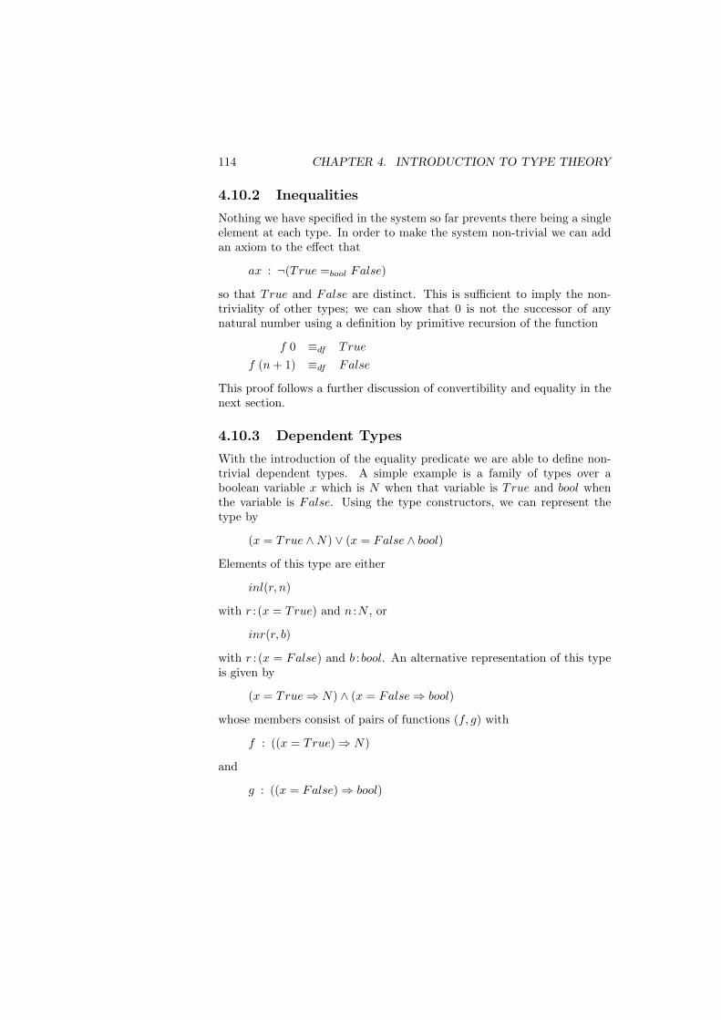
114 CHAPTER 4. INTRODUCTION TO TYPE THEORY
4.10.2 Inequalities
Nothing we have specified in the system so far prevents there being a singleelement at each type. In order to make the system non-trivial we can addan axiom to the effect that
ax : ¬(True =bool False)
so that True and False are distinct. This is sufficient to imply the non-triviality of other types; we can show that 0 is not the successor of anynatural number using a definition by primitive recursion of the function
f 0 ≡df True
f (n + 1) ≡df False
This proof follows a further discussion of convertibility and equality in thenext section.
4.10.3 Dependent Types
With the introduction of the equality predicate we are able to define non-trivial dependent types. A simple example is a family of types over aboolean variable x which is N when that variable is True and bool whenthe variable is False. Using the type constructors, we can represent thetype by
(x = True ∧N) ∨ (x = False ∧ bool)
Elements of this type are either
inl(r, n)
with r : (x = True) and n :N , or
inr(r, b)
with r : (x = False) and b :bool. An alternative representation of this typeis given by
(x = True⇒ N) ∧ (x = False⇒ bool)
whose members consist of pairs of functions (f, g) with
f : ((x = True)⇒ N)
and
g : ((x = False)⇒ bool)
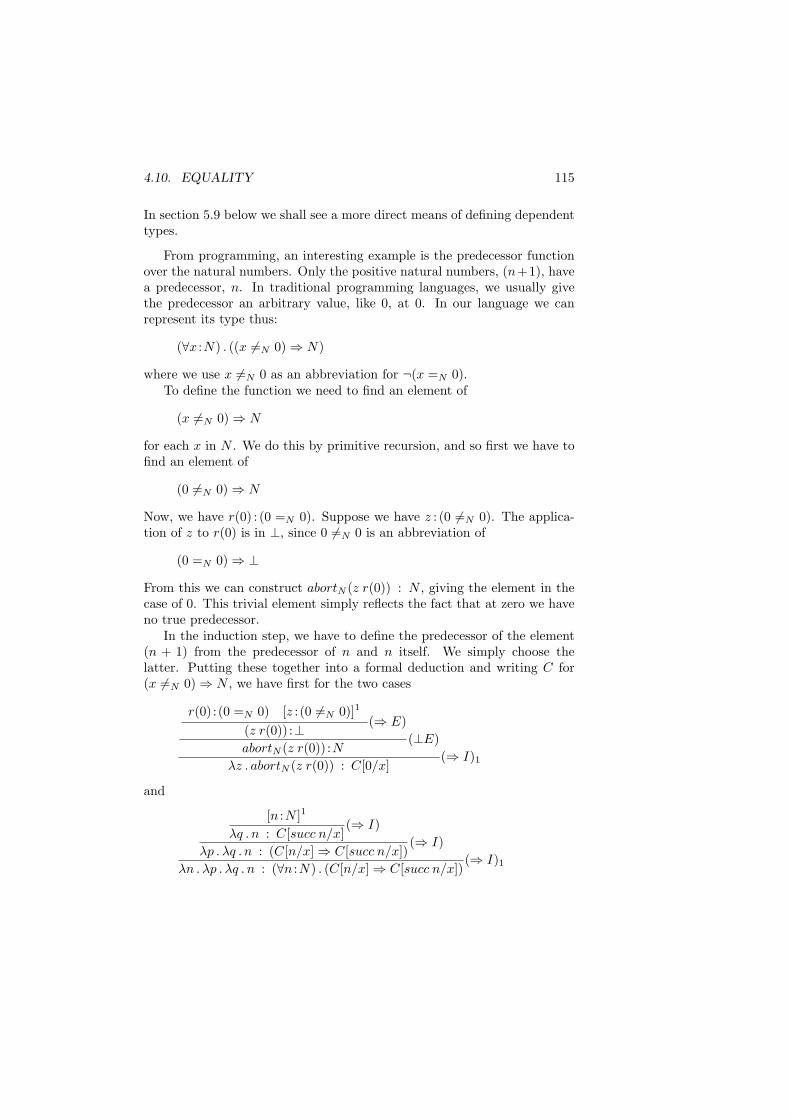
4.10. EQUALITY 115
In section 5.9 below we shall see a more direct means of defining dependenttypes.
From programming, an interesting example is the predecessor functionover the natural numbers. Only the positive natural numbers, (n+1), havea predecessor, n. In traditional programming languages, we usually givethe predecessor an arbitrary value, like 0, at 0. In our language we canrepresent its type thus:
(∀x :N) . ((x 6=N 0)⇒ N)
where we use x 6=N 0 as an abbreviation for ¬(x =N 0).To define the function we need to find an element of
(x 6=N 0)⇒ N
for each x in N . We do this by primitive recursion, and so first we have tofind an element of
(0 6=N 0)⇒ N
Now, we have r(0) : (0 =N 0). Suppose we have z : (0 6=N 0). The applica-tion of z to r(0) is in ⊥, since 0 6=N 0 is an abbreviation of
(0 =N 0)⇒ ⊥
From this we can construct abortN (z r(0)) : N , giving the element in thecase of 0. This trivial element simply reflects the fact that at zero we haveno true predecessor.
In the induction step, we have to define the predecessor of the element(n + 1) from the predecessor of n and n itself. We simply choose thelatter. Putting these together into a formal deduction and writing C for(x 6=N 0)⇒ N , we have first for the two cases
r(0) : (0 =N 0) [z : (0 6=N 0)]1
(z r(0)) :⊥(⇒ E)
abortN (z r(0)) :N(⊥E)
λz . abortN (z r(0)) : C[0/x](⇒ I)1
and
[n :N ]1
λq . n : C[succ n/x](⇒ I)
λp . λq . n : (C[n/x]⇒ C[succ n/x])(⇒ I)
λn . λp . λq . n : (∀n :N) . (C[n/x]⇒ C[succ n/x])(⇒ I)1
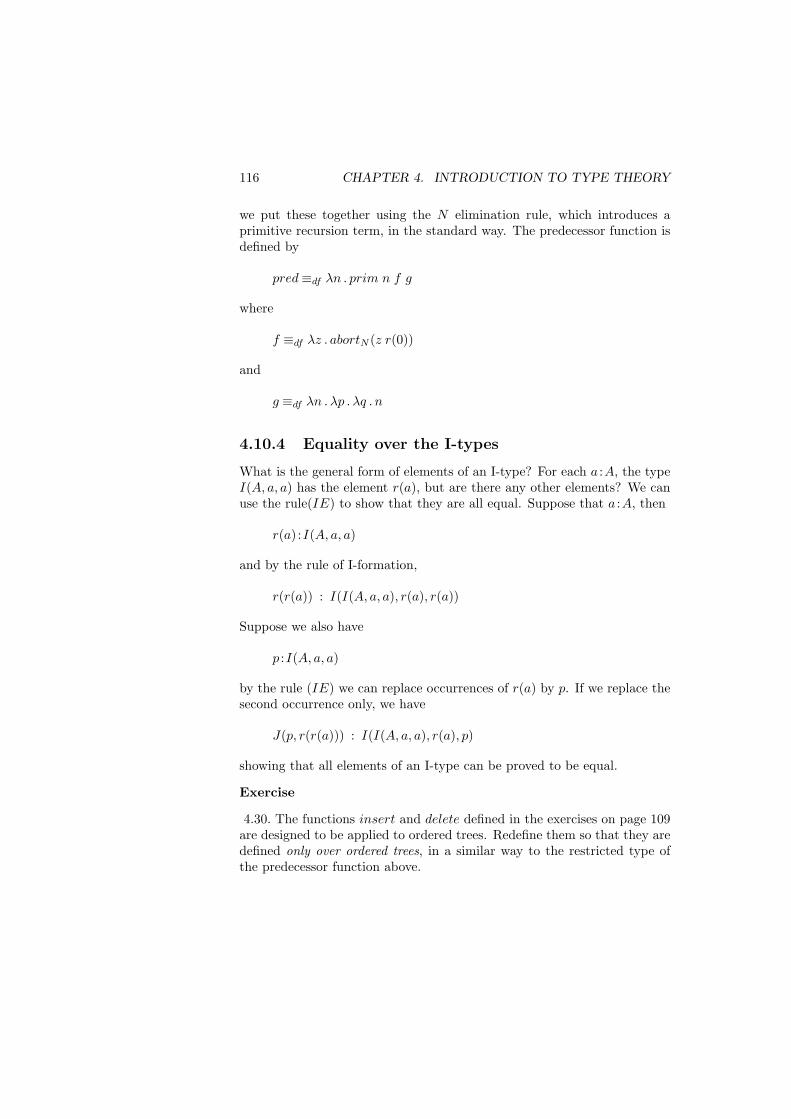
116 CHAPTER 4. INTRODUCTION TO TYPE THEORY
we put these together using the N elimination rule, which introduces aprimitive recursion term, in the standard way. The predecessor function isdefined by
pred≡df λn . prim n f g
where
f ≡df λz . abortN (z r(0))
and
g ≡df λn . λp . λq . n
4.10.4 Equality over the I-types
What is the general form of elements of an I-type? For each a :A, the typeI(A, a, a) has the element r(a), but are there any other elements? We canuse the rule(IE) to show that they are all equal. Suppose that a :A, then
r(a) :I(A, a, a)
and by the rule of I-formation,
r(r(a)) : I(I(A, a, a), r(a), r(a))
Suppose we also have
p :I(A, a, a)
by the rule (IE) we can replace occurrences of r(a) by p. If we replace thesecond occurrence only, we have
J(p, r(r(a))) : I(I(A, a, a), r(a), p)
showing that all elements of an I-type can be proved to be equal.
Exercise
4.30. The functions insert and delete defined in the exercises on page 109are designed to be applied to ordered trees. Redefine them so that they aredefined only over ordered trees, in a similar way to the restricted type ofthe predecessor function above.
4.11. CONVERTIBILITY 117
4.11 Convertibility
In this section we examine the rules of computation together with the re-lation of equivalence or convertibility generated by them.
The rules of our system have two quite distinct forms and purposes. Theformation, introduction and elimination rules describe how derivations ofjudgements are constructed. If we are simply interested in finding out fromthe logical point of view which propositions have proofs, or are inhabited ,then this category of rules would seem to suffice. This would be the case ifwe were to omit the equality rules, but in the full system the derivability ofequality propositions is closely linked with the computability rules throughthe convertibility relation and the rules of substitution.
On the other hand, if we read the rules as those of a programminglanguage, then the first three kinds of rule express only the syntax of thelanguage, specifying as they do which expressions have which type. Inprogramming the process of execution or evaluation is central, and it is thisthat the rules express. We might ask what it is in logic that corresponds toevaluation? It is the idea of simplification of proof objects. For example,suppose we choose the following (partial) proof for A. ‘Given proofs a : Aand b : B, build the proof (a, b) of A ∧ B, then construct a proof of A bytaking the first component’. This is the proof fst (a, b) and the proof objectwe have constructed can be reduced simply to the object a.
4.11.1 Definitions; convertibility and equality
First we give some definitions which generalise those of the simply typedλ-calculus.
Definition 4.7 We call a sub-expression f of an expression e a free subex-pression of the expression e if none of the free variables in f is bound withine.
A free sub-expression of an expression e is exactly the kind of sub-expression of an expression which could arise by substitution into e —sub-expressions which contain variables bound within e cannot arise thus.
Definition 4.8 The rules for computation → have been introducedconstruct-by-construct above. We call a sub-expression of an expressiona redex if it matches the left-hand sides of these rules. We extend therelation → so that we write e1 → e2 when a free sub-expression f1 of e1
is a redex, and e2 results from e1 by replacing f1 with the correspondingright-hand side, or reduct.
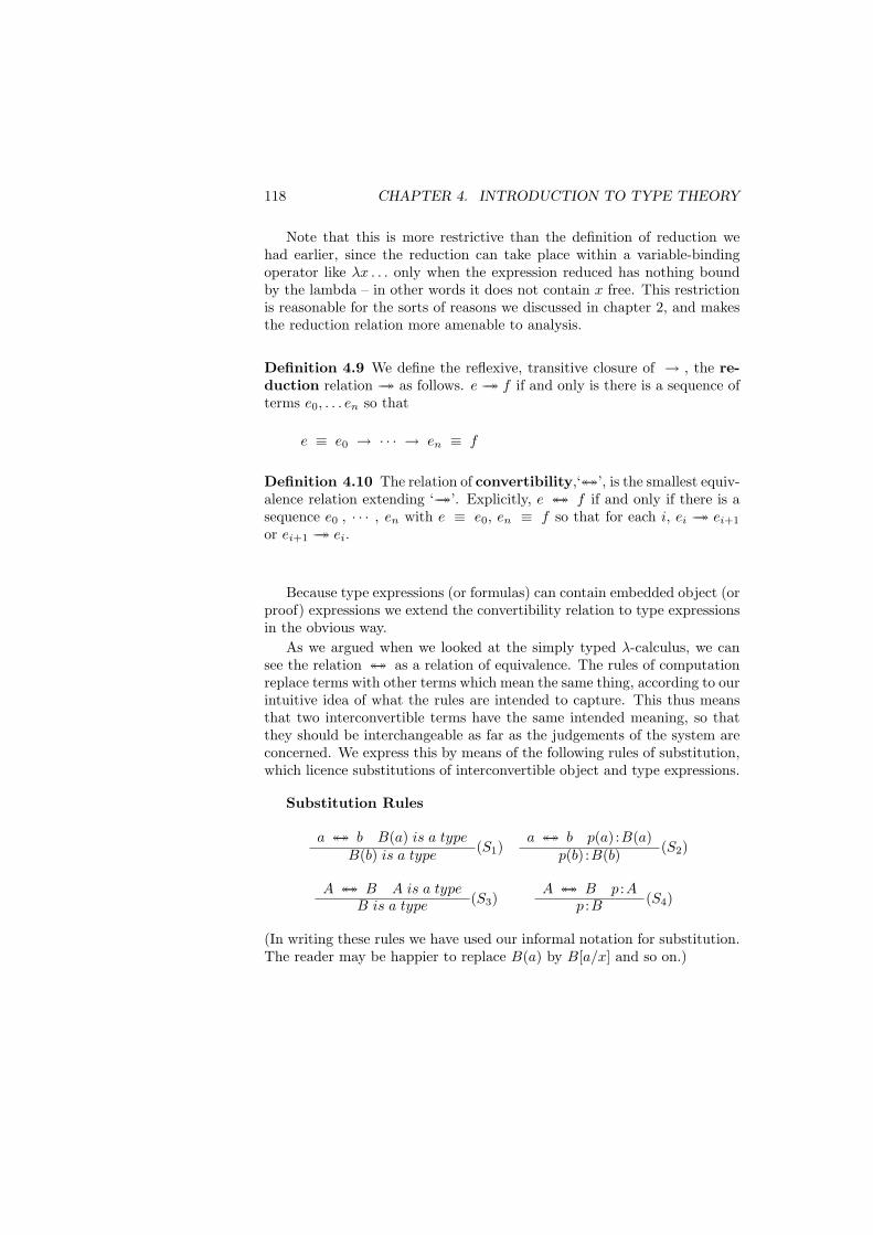
118 CHAPTER 4. INTRODUCTION TO TYPE THEORY
Note that this is more restrictive than the definition of reduction wehad earlier, since the reduction can take place within a variable-bindingoperator like λx . . . only when the expression reduced has nothing boundby the lambda – in other words it does not contain x free. This restrictionis reasonable for the sorts of reasons we discussed in chapter 2, and makesthe reduction relation more amenable to analysis.
Definition 4.9 We define the reflexive, transitive closure of → , the re-duction relation →→ as follows. e→→ f if and only is there is a sequence ofterms e0, . . . en so that
e ≡ e0 → · · · → en ≡ f
Definition 4.10 The relation of convertibility,‘↔↔’, is the smallest equiv-alence relation extending ‘→→’. Explicitly, e ↔↔ f if and only if there is asequence e0 , · · · , en with e ≡ e0, en ≡ f so that for each i, ei →→ ei+1
or ei+1 →→ ei.
Because type expressions (or formulas) can contain embedded object (orproof) expressions we extend the convertibility relation to type expressionsin the obvious way.
As we argued when we looked at the simply typed λ-calculus, we cansee the relation ↔↔ as a relation of equivalence. The rules of computationreplace terms with other terms which mean the same thing, according to ourintuitive idea of what the rules are intended to capture. This thus meansthat two interconvertible terms have the same intended meaning, so thatthey should be interchangeable as far as the judgements of the system areconcerned. We express this by means of the following rules of substitution,which licence substitutions of interconvertible object and type expressions.
Substitution Rules
a ↔↔ b B(a) is a typeB(b) is a type
(S1)a ↔↔ b p(a) :B(a)
p(b) :B(b) (S2)
A ↔↔ B A is a typeB is a type (S3)
A ↔↔ B p :Ap :B (S4)
(In writing these rules we have used our informal notation for substitution.The reader may be happier to replace B(a) by B[a/x] and so on.)
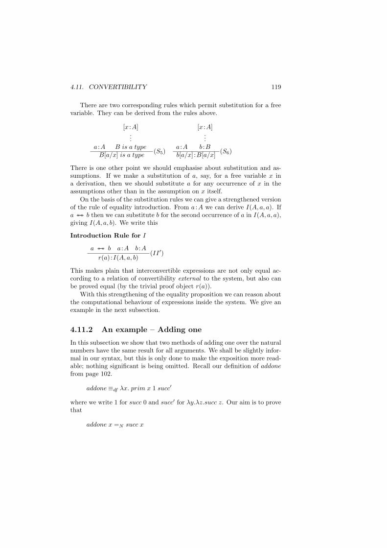
4.11. CONVERTIBILITY 119
There are two corresponding rules which permit substitution for a freevariable. They can be derived from the rules above.
a :A
[x :A]...
B is a typeB[a/x] is a type
(S5)a :A
[x :A]...
b :Bb[a/x] :B[a/x] (S6)
There is one other point we should emphasise about substitution and as-sumptions. If we make a substitution of a, say, for a free variable x ina derivation, then we should substitute a for any occurrence of x in theassumptions other than in the assumption on x itself.
On the basis of the substitution rules we can give a strengthened versionof the rule of equality introduction. From a :A we can derive I(A, a, a). Ifa ↔↔ b then we can substitute b for the second occurrence of a in I(A, a, a),giving I(A, a, b). We write this
Introduction Rule for I
a ↔↔ b a :A b :Ar(a) :I(A, a, b)
(II ′)
This makes plain that interconvertible expressions are not only equal ac-cording to a relation of convertibility external to the system, but also canbe proved equal (by the trivial proof object r(a)).
With this strengthening of the equality proposition we can reason aboutthe computational behaviour of expressions inside the system. We give anexample in the next subsection.
4.11.2 An example – Adding one
In this subsection we show that two methods of adding one over the naturalnumbers have the same result for all arguments. We shall be slightly infor-mal in our syntax, but this is only done to make the exposition more read-able; nothing significant is being omitted. Recall our definition of addonefrom page 102.
addone≡df λx. prim x 1 succ′
where we write 1 for succ 0 and succ′ for λy.λz.succ z. Our aim is to provethat
addone x =N succ x
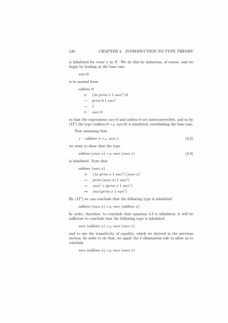
120 CHAPTER 4. INTRODUCTION TO TYPE THEORY
is inhabited for every x in N . We do this by induction, of course, and webegin by looking at the base case.
succ 0
is in normal form
addone 0≡ (λx.prim x 1 succ′) 0→ prim 0 1 succ′
→ 1≡ succ 0
so that the expressions succ 0 and addone 0 are interconvertible, and so by(II ′) the type (addone0 =N succ0) is inhabited, establishing the base case.
Now assuming that
z : addone x =N succ x (4.2)
we want to show that the type
addone (succ x) =N succ (succ x) (4.3)
is inhabited. Note that
addone (succ x)≡ (λx.prim x 1 succ′) (succ x)→ prim (succ x) 1 succ′)→ succ′ x (prim x 1 succ′)→→ succ(prim x 1 succ′)
By (II ′) we can conclude that the following type is inhabited
addone (succ x) =N succ (addone x)
In order, therefore, to conclude that equation 4.3 is inhabited, it will besufficient to conclude that the following type is inhabited
succ (addone x) =N succ (succ x)
and to use the transitivity of equality, which we derived in the previoussection. In order to do that, we apply the I elimination rule to allow us toconclude
succ (addone x) =N succ (succ x)
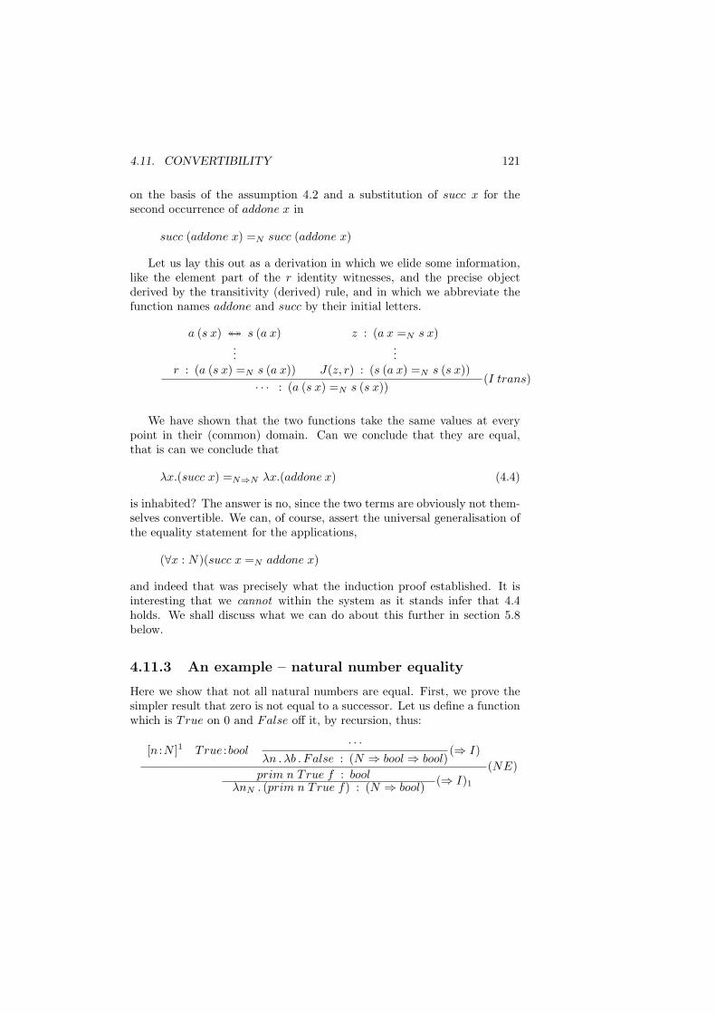
4.11. CONVERTIBILITY 121
on the basis of the assumption 4.2 and a substitution of succ x for thesecond occurrence of addone x in
succ (addone x) =N succ (addone x)
Let us lay this out as a derivation in which we elide some information,like the element part of the r identity witnesses, and the precise objectderived by the transitivity (derived) rule, and in which we abbreviate thefunction names addone and succ by their initial letters.
a (s x) ↔↔ s (a x)...
r : (a (s x) =N s (a x))
z : (a x =N s x)...
J(z, r) : (s (a x) =N s (s x))· · · : (a (s x) =N s (s x))
(I trans)
We have shown that the two functions take the same values at everypoint in their (common) domain. Can we conclude that they are equal,that is can we conclude that
λx.(succ x) =N⇒N λx.(addone x) (4.4)
is inhabited? The answer is no, since the two terms are obviously not them-selves convertible. We can, of course, assert the universal generalisation ofthe equality statement for the applications,
(∀x : N)(succ x =N addone x)
and indeed that was precisely what the induction proof established. It isinteresting that we cannot within the system as it stands infer that 4.4holds. We shall discuss what we can do about this further in section 5.8below.
4.11.3 An example – natural number equality
Here we show that not all natural numbers are equal. First, we prove thesimpler result that zero is not equal to a successor. Let us define a functionwhich is True on 0 and False off it, by recursion, thus:
[n :N ]1 True :bool· · ·
λn . λb . False : (N ⇒ bool⇒ bool)(⇒ I)
prim n True f : bool(NE)
λnN . (prim n True f) : (N ⇒ bool) (⇒ I)1
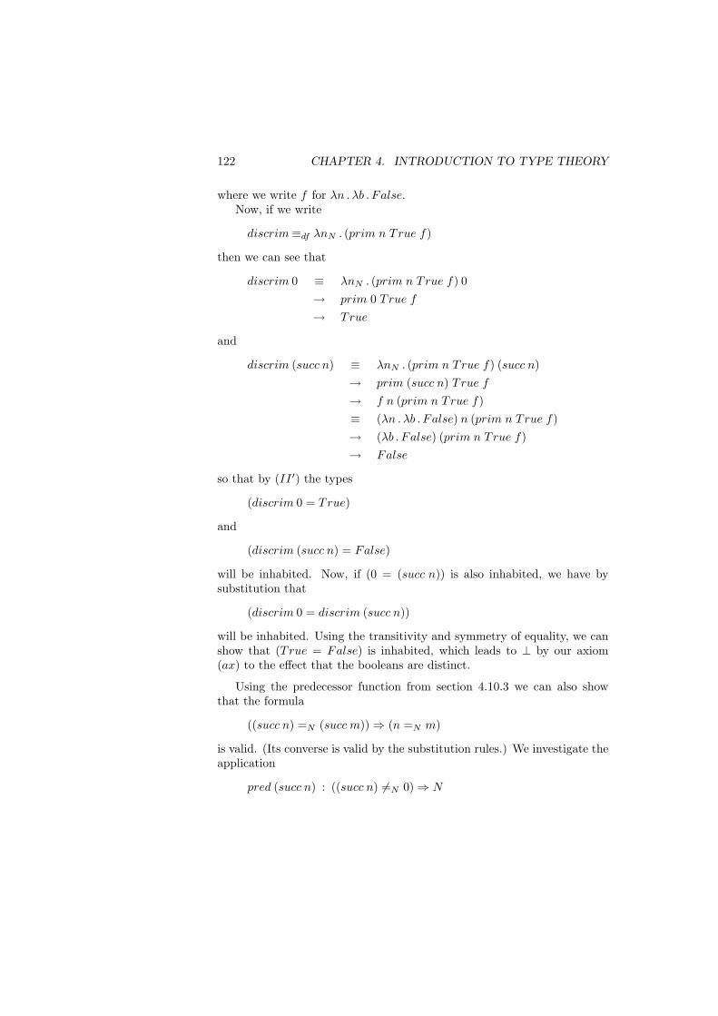
122 CHAPTER 4. INTRODUCTION TO TYPE THEORY
where we write f for λn . λb . False.Now, if we write
discrim≡df λnN . (prim n True f)
then we can see that
discrim 0 ≡ λnN . (prim n True f) 0→ prim 0 True f
→ True
and
discrim (succ n) ≡ λnN . (prim n True f) (succ n)→ prim (succ n) True f
→ f n (prim n True f)≡ (λn . λb . False) n (prim n True f)→ (λb . False) (prim n True f)→ False
so that by (II ′) the types
(discrim 0 = True)
and
(discrim (succ n) = False)
will be inhabited. Now, if (0 = (succ n)) is also inhabited, we have bysubstitution that
(discrim 0 = discrim (succ n))
will be inhabited. Using the transitivity and symmetry of equality, we canshow that (True = False) is inhabited, which leads to ⊥ by our axiom(ax) to the effect that the booleans are distinct.
Using the predecessor function from section 4.10.3 we can also showthat the formula
((succ n) =N (succ m))⇒ (n =N m)
is valid. (Its converse is valid by the substitution rules.) We investigate theapplication
pred (succ n) : ((succ n) 6=N 0)⇒ N
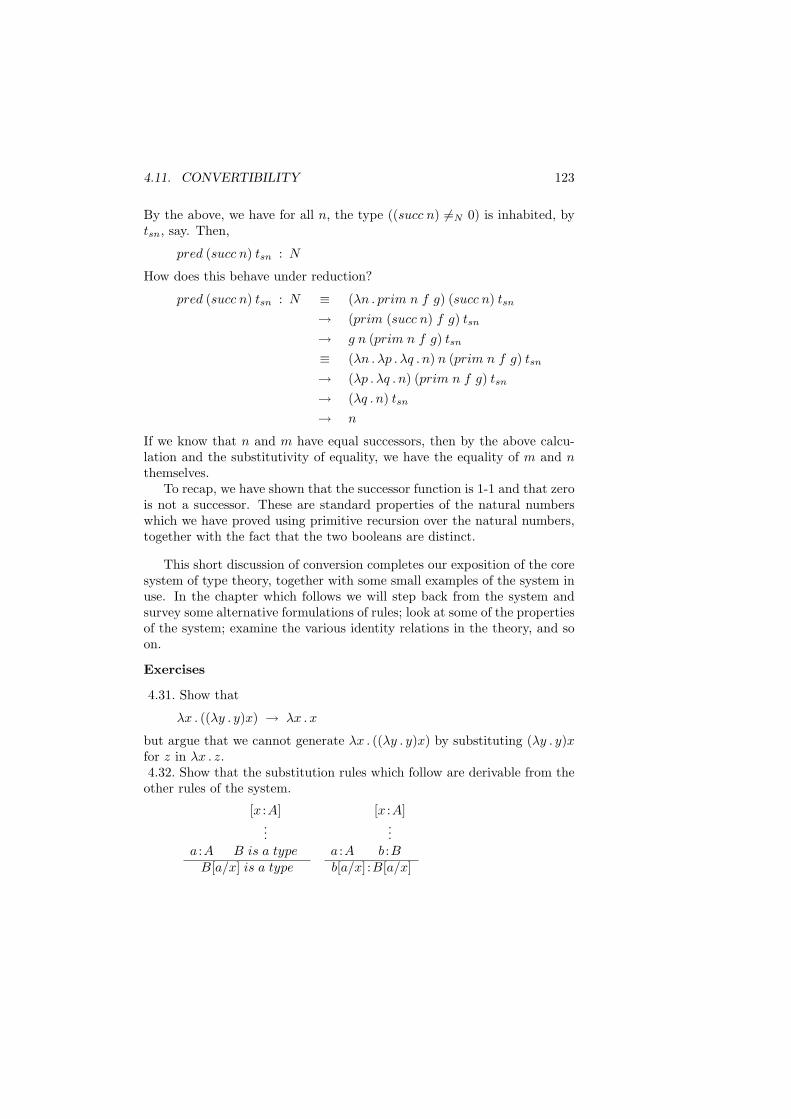
4.11. CONVERTIBILITY 123
By the above, we have for all n, the type ((succ n) 6=N 0) is inhabited, bytsn, say. Then,
pred (succ n) tsn : N
How does this behave under reduction?
pred (succ n) tsn : N ≡ (λn . prim n f g) (succ n) tsn
→ (prim (succ n) f g) tsn
→ g n (prim n f g) tsn
≡ (λn . λp . λq . n) n (prim n f g) tsn
→ (λp . λq . n) (prim n f g) tsn
→ (λq . n) tsn
→ n
If we know that n and m have equal successors, then by the above calcu-lation and the substitutivity of equality, we have the equality of m and nthemselves.
To recap, we have shown that the successor function is 1-1 and that zerois not a successor. These are standard properties of the natural numberswhich we have proved using primitive recursion over the natural numbers,together with the fact that the two booleans are distinct.
This short discussion of conversion completes our exposition of the coresystem of type theory, together with some small examples of the system inuse. In the chapter which follows we will step back from the system andsurvey some alternative formulations of rules; look at some of the propertiesof the system; examine the various identity relations in the theory, and soon.
Exercises
4.31. Show that
λx . ((λy . y)x) → λx . x
but argue that we cannot generate λx . ((λy . y)x) by substituting (λy . y)xfor z in λx . z.4.32. Show that the substitution rules which follow are derivable from theother rules of the system.
a :A
[x :A]...
B is a typeB[a/x] is a type
a :A
[x :A]...
b :Bb[a/x] :B[a/x]
124 CHAPTER 4. INTRODUCTION TO TYPE THEORY
We say that a rule is derivable if whenever we can derive the hypotheses ofa rule then we can derive the conclusions of the corresponding instance ofthe rule, with the appropriate hypotheses discharged.4.33. Formulate a characterisation of equality on tree similar to that on Nformulated above.4.34. Formulate and prove the results that the insert and delete functionsdefined on page 109 preserve the ordering of their tree arguments.4.35. Formulate and prove that result that the factorial of any natural
number is greater than zero.
This concludes our introduction to type theory. We shall call the systemintroduced here TT0, and in the next chapter we explore some of the prop-erties of the system, after clarifying some of the more technical points of thepresentation. In fact, the system TT0 is defined in full in section 5.3 below,where we give a generalisation of the elimination rules for disjunction (∨)and the existential quantifier (∃).
Chapter 5
Exploring Type Theory
The last chapter was taken up with the introduction of the system of typetheory TT0. It is a complicated system, with many of its aspects deservingof further study — this we do here.
As type theory is a formal system, it is amenable to study as an objectin its own right. In section 5.4 we show that from some derivations, likea :A we can deduce others, like A is a type. Following that, we show thatthe derivable types of objects are unique, and that the substitution rulescan be derived.
An important aspect of type theory is its computational behaviour, andwe study this for two systems related to TT0. We introduced the basicquestions in our earlier introduction to the λ-calculus — here we ask themof the system of type theory. First we give (in section 5.5) a strong nor-malisation result for the system TT ∗
0 , which unfortunately fails to have theChurch-Rosser property. We then present TT c
0 which was first introducedby Martin-Lof in [ML75b]. This differs from TT0 in the way in which ab-straction is performed. After explaining the abstraction mechanism andshowing that TT c
0 is an extension of TT0, we prove a normalisation theo-rem for it. From the proof we obtain a number of important corollaries,including the Church-Rosser property for TT c
0 and the decidability of ‘↔↔ ’and of judgements in general. It is interesting to note that the precise formof λ-abstraction in TT c
0 is very close to the way in which it is performed inmodern ‘compiled’ implementations of functional programming languages,[Pey87].
We begin the chapter by looking at some more technical aspects of thesystem which merit more attention than they received in the introduction.These include the precise role played by assumptions and ways in whichterms can be made more readable by naming and abbreviation. Naming
125
126 CHAPTER 5. EXPLORING TYPE THEORY
is a fundamental part of any programming language; we look at how ourprograms and proofs can be made more comprehensible by judicious abbre-viations. The version of disjunction elimination given in the last chapterwas simplified somewhat; here we give the general version. We also give avariant formulation of the existential elimination rule, as well as mentioninga weaker version, which is more akin to the traditional rule of the first-orderpredicate calculus.
Our introduction to the system involves the use of four different notionsof equality: definitional equality is as close as we get to literal identity: twoexpressions being definitionally equal if they are identical up to change ofbound variables after all definitions have been expanded out. Convertibilityis external to the system, with the I-type giving an internal representationof it as a proposition, so allowing it to be combined into complex proposi-tions. Lastly, there are equality functions, which return values in the typebool when given two elements of a particular type; these are used in com-putations, giving the conditional expressions familiar to programmers. Insections 5.7 and 5.8 we compare these different relations, and then exam-ine how a truly extensional equality can be added to the system withoutdestroying its admirable formal properties.
The system TT0 can be augmented in a number of ways; we look at twomeans of strengthening it in sections 5.9 and 5.10. The notion of a type oftypes is inconsistent, roughly because it allows the impredicative definitionof classes in terms of themselves, a la Russell’s paradox, but we show howa sequence of ‘universes’ of types can be added in a coherent way. Thenwe give the general mechanism by which well-founded types are defined,incidentally giving the rules for lists as well.
We conclude the chapter with a second look at the Curry Howard iso-morphism, particularly at the treatment of assumptions and the process ofproof normalisation, both cases where the isomorphism seem less than onehundred percent happy.
5.1 Assumptions
The derivations we construct using the rules of type theory depend in gen-eral upon collections of assumptions. In this section we look at the preciseform that these collections take, together with consistency criteria thatthey should obey, and re-examine the rules and tighten up their statementin some cases.
A useful exercise for anyone interested in a formal system is to make animplementation of it. Many of the issues discussed here became apparentto the author while writing an implementation of type theory in the func-
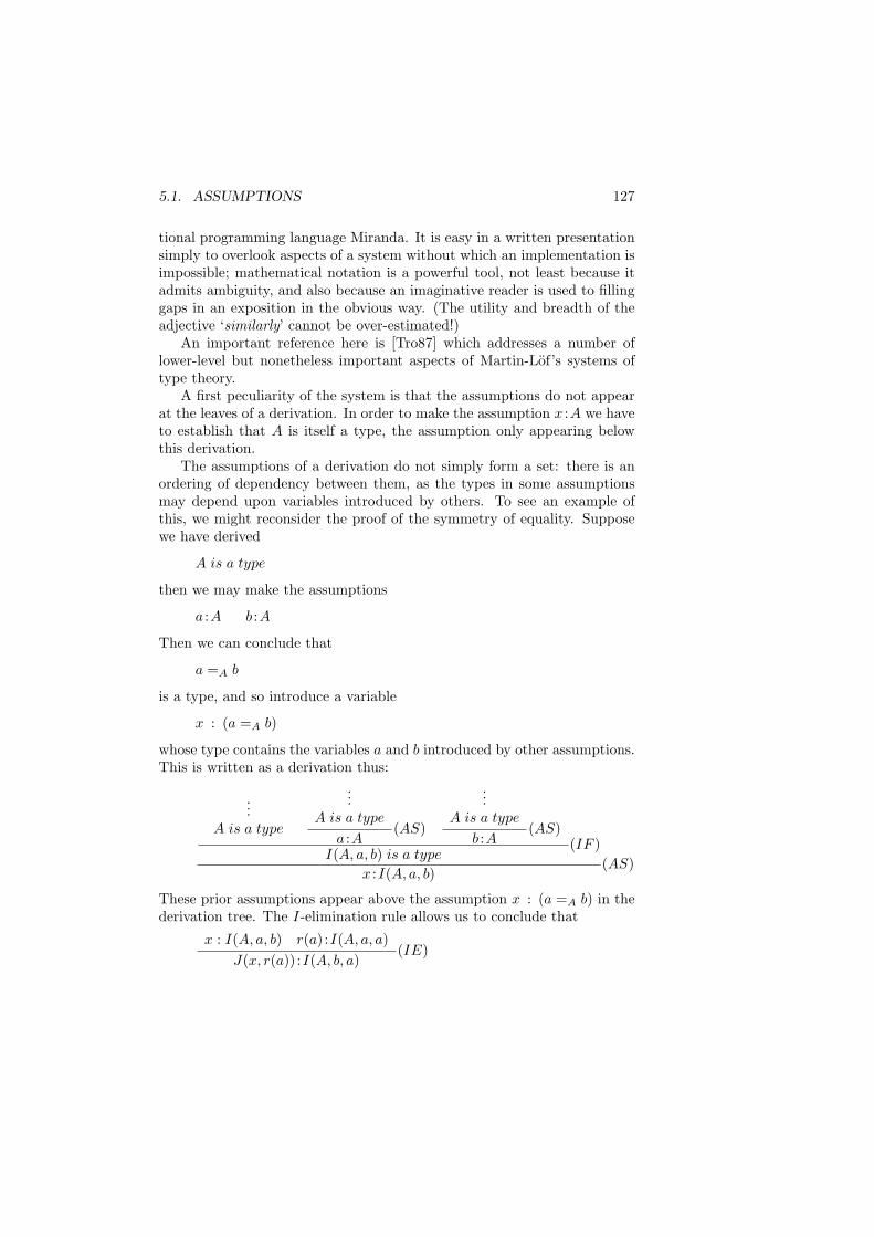
5.1. ASSUMPTIONS 127
tional programming language Miranda. It is easy in a written presentationsimply to overlook aspects of a system without which an implementation isimpossible; mathematical notation is a powerful tool, not least because itadmits ambiguity, and also because an imaginative reader is used to fillinggaps in an exposition in the obvious way. (The utility and breadth of theadjective ‘similarly’ cannot be over-estimated!)
An important reference here is [Tro87] which addresses a number oflower-level but nonetheless important aspects of Martin-Lof’s systems oftype theory.
A first peculiarity of the system is that the assumptions do not appearat the leaves of a derivation. In order to make the assumption x :A we haveto establish that A is itself a type, the assumption only appearing belowthis derivation.
The assumptions of a derivation do not simply form a set: there is anordering of dependency between them, as the types in some assumptionsmay depend upon variables introduced by others. To see an example ofthis, we might reconsider the proof of the symmetry of equality. Supposewe have derived
A is a type
then we may make the assumptions
a :A b :A
Then we can conclude that
a =A b
is a type, and so introduce a variable
x : (a =A b)
whose type contains the variables a and b introduced by other assumptions.This is written as a derivation thus:
...A is a type
...A is a type
a :A(AS)
...A is a type
b :A(AS)
I(A, a, b) is a type(IF )
x :I(A, a, b)(AS)
These prior assumptions appear above the assumption x : (a =A b) in thederivation tree. The I-elimination rule allows us to conclude that
x : I(A, a, b) r(a) :I(A, a, a)J(x, r(a)) :I(A, b, a)
(IE)
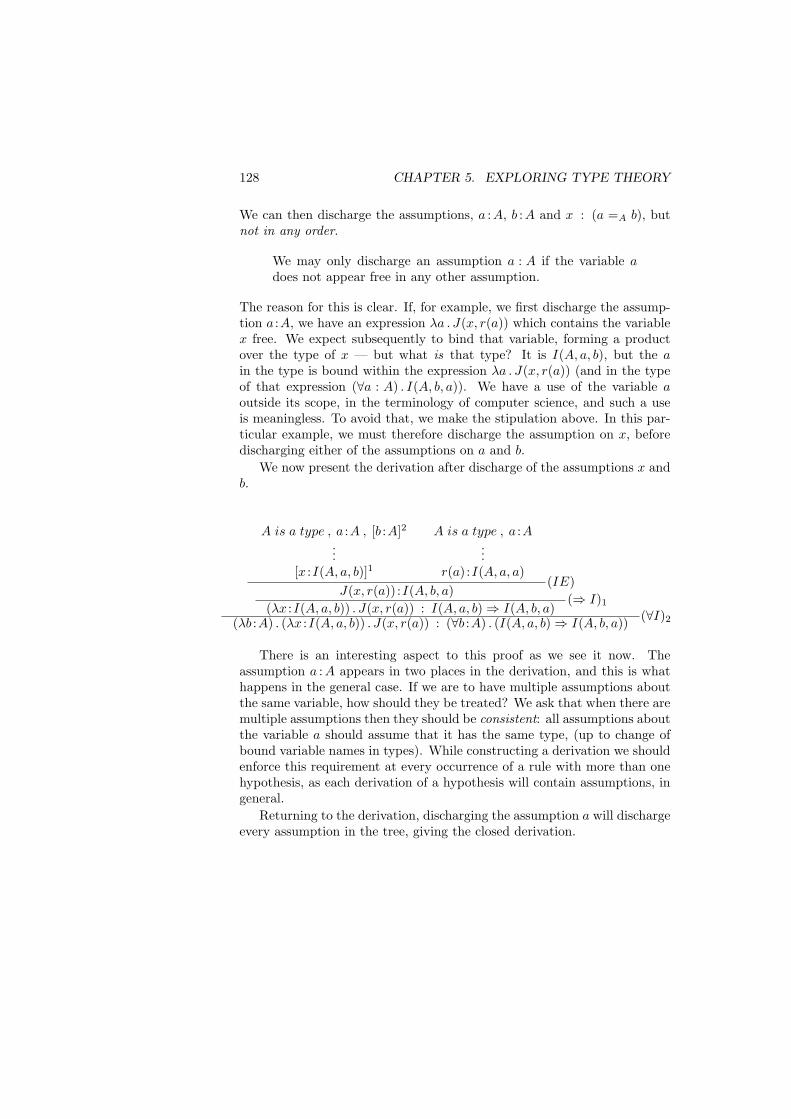
128 CHAPTER 5. EXPLORING TYPE THEORY
We can then discharge the assumptions, a :A, b :A and x : (a =A b), butnot in any order.
We may only discharge an assumption a : A if the variable adoes not appear free in any other assumption.
The reason for this is clear. If, for example, we first discharge the assump-tion a :A, we have an expression λa . J(x, r(a)) which contains the variablex free. We expect subsequently to bind that variable, forming a productover the type of x — but what is that type? It is I(A, a, b), but the ain the type is bound within the expression λa . J(x, r(a)) (and in the typeof that expression (∀a : A) . I(A, b, a)). We have a use of the variable aoutside its scope, in the terminology of computer science, and such a useis meaningless. To avoid that, we make the stipulation above. In this par-ticular example, we must therefore discharge the assumption on x, beforedischarging either of the assumptions on a and b.
We now present the derivation after discharge of the assumptions x andb.
A is a type , a :A , [b :A]2...
[x :I(A, a, b)]1
A is a type , a :A...
r(a) :I(A, a, a)J(x, r(a)) :I(A, b, a)
(IE)
(λx :I(A, a, b)) . J(x, r(a)) : I(A, a, b)⇒ I(A, b, a)(⇒ I)1
(λb :A) . (λx :I(A, a, b)) . J(x, r(a)) : (∀b :A) . (I(A, a, b)⇒ I(A, b, a)) (∀I)2
There is an interesting aspect to this proof as we see it now. Theassumption a :A appears in two places in the derivation, and this is whathappens in the general case. If we are to have multiple assumptions aboutthe same variable, how should they be treated? We ask that when there aremultiple assumptions then they should be consistent: all assumptions aboutthe variable a should assume that it has the same type, (up to change ofbound variable names in types). While constructing a derivation we shouldenforce this requirement at every occurrence of a rule with more than onehypothesis, as each derivation of a hypothesis will contain assumptions, ingeneral.
Returning to the derivation, discharging the assumption a will dischargeevery assumption in the tree, giving the closed derivation.
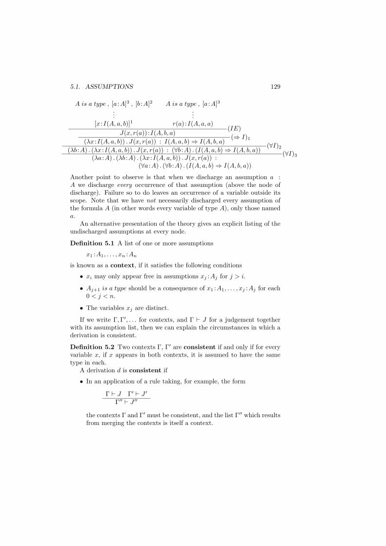
5.1. ASSUMPTIONS 129
A is a type , [a :A]3 , [b :A]2...
[x :I(A, a, b)]1
A is a type , [a :A]3...
r(a) :I(A, a, a)J(x, r(a)) :I(A, b, a)
(IE)
(λx :I(A, a, b)) . J(x, r(a)) : I(A, a, b)⇒ I(A, b, a)(⇒ I)1
(λb :A) . (λx :I(A, a, b)) . J(x, r(a)) : (∀b :A) . (I(A, a, b)⇒ I(A, b, a))(∀I)2
(λa :A) . (λb :A) . (λx :I(A, a, b)) . J(x, r(a)) :(∀a :A) . (∀b :A) . (I(A, a, b)⇒ I(A, b, a))
(∀I)3
Another point to observe is that when we discharge an assumption a :A we discharge every occurrence of that assumption (above the node ofdischarge). Failure so to do leaves an occurrence of a variable outside itsscope. Note that we have not necessarily discharged every assumption ofthe formula A (in other words every variable of type A), only those nameda.
An alternative presentation of the theory gives an explicit listing of theundischarged assumptions at every node.
Definition 5.1 A list of one or more assumptions
x1 :A1, . . . , xn :An
is known as a context, if it satisfies the following conditions
• xi may only appear free in assumptions xj :Aj for j > i.
• Aj+1 is a type should be a consequence of x1 :A1, . . . , xj :Aj for each0 < j < n.
• The variables xj are distinct.
If we write Γ,Γ′, . . . for contexts, and Γ ` J for a judgement togetherwith its assumption list, then we can explain the circumstances in which aderivation is consistent.
Definition 5.2 Two contexts Γ, Γ′ are consistent if and only if for everyvariable x, if x appears in both contexts, it is assumed to have the sametype in each.
A derivation d is consistent if
• In an application of a rule taking, for example, the form
Γ ` J Γ′ ` J ′
Γ′′ ` J ′′
the contexts Γ and Γ′ must be consistent, and the list Γ′′ which resultsfrom merging the contexts is itself a context.
130 CHAPTER 5. EXPLORING TYPE THEORY
• We may only discharge an assumption xj :Aj from a context Γ if xj
does not occur free in any assumption xk :Ak (k > j) of Γ.
The rules above may best be understood by realizing that the linearordering of the assumptions in a valid context is simply an (arbitrary) ex-tension of the partial ordering on the assumptions induced by their positionin a derivation tree constructed according to the restrictions we outlinedabove, and which we summarise now.
• We may only discharge an assumption x : A if the variable x appearsfree in the (types of) no other assumptions.
• In applying a rule with at least two hypotheses, the assumptionsshould be consistent: a variable x must be assumed to have the sametype, up to change of bound variable names, in all the derivations ofthe hypotheses.
We might ask whether we could relax the restriction on consistency ofassumptions to their types being convertible, rather than the same. In factby the rules of substitution this is no stronger; see the exercises below. Notehowever that to perform the test for convertibility as part of the process ofderivation construction would require that convertibility was decidable.
Exercises
5.1. Show that if we have derivations of p :P and q :Q from the assumptionsx : A and x : A′ respectively, then we can construct derivations of P ∨ Qfrom either x :A or x :A′.5.2. From a logical point of view, do we ever require two or more assump-tions x : A, y : A, . . . of the same formula A? From the programming side,why do we need them?5.3. Give a version of the derivation of the symmetry of equality above in
which the contexts are made explicit at each point.5.4. What is the effect on the system of relaxing the consistency condition?
5.2 Naming and abbreviations
In order to make the expressions and derivations of the system more read-able, we allow expressions to be named and allow certain forms of abbrevi-ation in derivations, judgements and expressions.
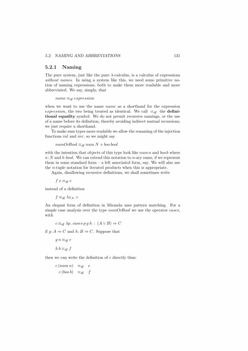
5.2. NAMING AND ABBREVIATIONS 131
5.2.1 Naming
The pure system, just like the pure λ-calculus, is a calculus of expressionswithout names. In using a system like this, we need some primitive no-tion of naming expressions, both to make them more readable and moreabbreviated. We say, simply, that
name≡df expression
when we want to use the name name as a shorthand for the expressionexpression, the two being treated as identical. We call ≡df the defini-tional equality symbol. We do not permit recursive namings, or the useof a name before its definition, thereby avoiding indirect mutual recursions;we just require a shorthand.
To make sum types more readable we allow the renaming of the injectionfunctions inl and inr, so we might say
numOrBool ≡df num N + boo bool
with the intention that objects of this type look like numn and boo b wheren :N and b :bool. We can extend this notation to n-ary sums, if we representthem in some standard form – a left associated form, say. We will also usethe n-tuple notation for iterated products when this is appropriate.
Again, disallowing recursive definitions, we shall sometimes write
f x≡df e
instead of a definition
f ≡df λxA . e
An elegant form of definition in Miranda uses pattern matching. For asimple case analysis over the type numOrBool we use the operator cases,with
c≡df λp . cases p g h : (A ∨B)⇒ C
if g :A⇒ C and h :B ⇒ C. Suppose that
g n≡df e
h b≡df f
then we can write the definition of c directly thus:
c (num n) ≡df e
c (boo b) ≡df f
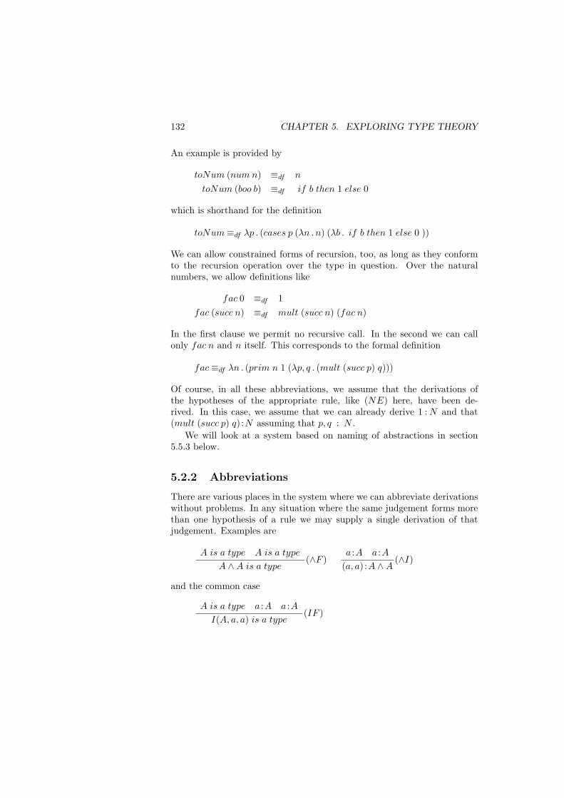
132 CHAPTER 5. EXPLORING TYPE THEORY
An example is provided by
toNum (num n) ≡df n
toNum (boo b) ≡df if b then 1 else 0
which is shorthand for the definition
toNum≡df λp . (cases p (λn . n) (λb . if b then 1 else 0 ))
We can allow constrained forms of recursion, too, as long as they conformto the recursion operation over the type in question. Over the naturalnumbers, we allow definitions like
fac 0 ≡df 1fac (succ n) ≡df mult (succ n) (fac n)
In the first clause we permit no recursive call. In the second we can callonly fac n and n itself. This corresponds to the formal definition
fac≡df λn . (prim n 1 (λp, q . (mult (succ p) q)))
Of course, in all these abbreviations, we assume that the derivations ofthe hypotheses of the appropriate rule, like (NE) here, have been de-rived. In this case, we assume that we can already derive 1 : N and that(mult (succ p) q) :N assuming that p, q : N .
We will look at a system based on naming of abstractions in section5.5.3 below.
5.2.2 Abbreviations
There are various places in the system where we can abbreviate derivationswithout problems. In any situation where the same judgement forms morethan one hypothesis of a rule we may supply a single derivation of thatjudgement. Examples are
A is a type A is a type
A ∧A is a type(∧F )
a :A a :A(a, a) :A ∧A
(∧I)
and the common case
A is a type a :A a :AI(A, a, a) is a type
(IF )
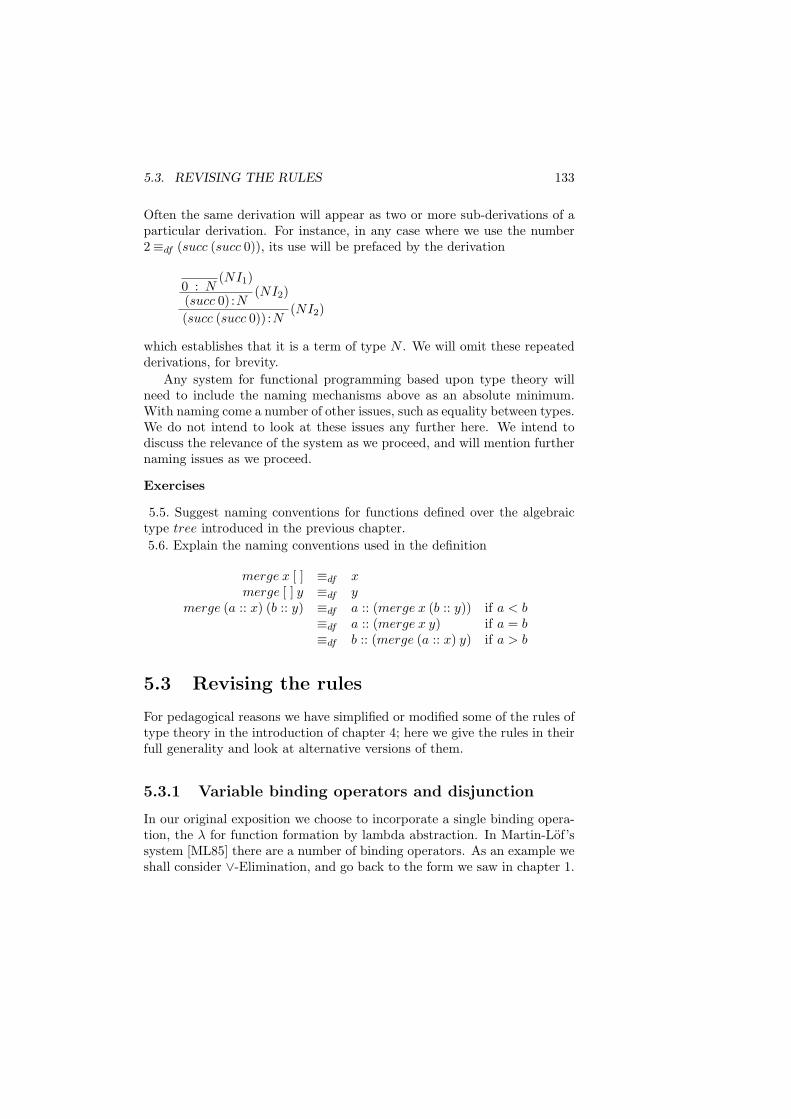
5.3. REVISING THE RULES 133
Often the same derivation will appear as two or more sub-derivations of aparticular derivation. For instance, in any case where we use the number2≡df (succ (succ 0)), its use will be prefaced by the derivation
0 : N(NI1)
(succ 0) :N(NI2)
(succ (succ 0)) :N(NI2)
which establishes that it is a term of type N . We will omit these repeatedderivations, for brevity.
Any system for functional programming based upon type theory willneed to include the naming mechanisms above as an absolute minimum.With naming come a number of other issues, such as equality between types.We do not intend to look at these issues any further here. We intend todiscuss the relevance of the system as we proceed, and will mention furthernaming issues as we proceed.
Exercises
5.5. Suggest naming conventions for functions defined over the algebraictype tree introduced in the previous chapter.5.6. Explain the naming conventions used in the definition
merge x [ ] ≡df xmerge [ ] y ≡df y
merge (a :: x) (b :: y) ≡df a :: (merge x (b :: y)) if a < b≡df a :: (merge x y) if a = b≡df b :: (merge (a :: x) y) if a > b
5.3 Revising the rules
For pedagogical reasons we have simplified or modified some of the rules oftype theory in the introduction of chapter 4; here we give the rules in theirfull generality and look at alternative versions of them.
5.3.1 Variable binding operators and disjunction
In our original exposition we choose to incorporate a single binding opera-tion, the λ for function formation by lambda abstraction. In Martin-Lof’ssystem [ML85] there are a number of binding operators. As an example weshall consider ∨-Elimination, and go back to the form we saw in chapter 1.
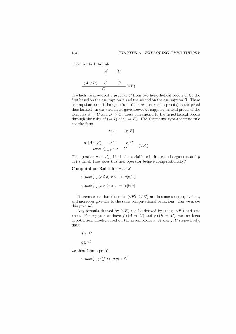
134 CHAPTER 5. EXPLORING TYPE THEORY
There we had the rule
(A ∨B)
[A]...C
[B]...C
C(∨E)
in which we produced a proof of C from two hypothetical proofs of C, thefirst based on the assumption A and the second on the assumption B. Theseassumptions are discharged (from their respective sub-proofs) in the proofthus formed. In the version we gave above, we supplied instead proofs of theformulas A⇒ C and B ⇒ C: these correspond to the hypothetical proofsthrough the rules of (⇒ I) and (⇒ E). The alternative type-theoretic rulehas the form
p : (A ∨B)
[x :A]...
u :C
[y :B]...
v :Cvcases′x,y p u v : C
(∨E′)
The operator vcases′x,y binds the variable x in its second argument and yin its third. How does this new operator behave computationally?
Computation Rules for vcases′
vcases′x,y (inl a) u v → u[a/x]
vcases′x,y (inr b) u v → v[b/y]
It seems clear that the rules (∨E), (∨E′) are in some sense equivalent,and moreover give rise to the same computational behaviour. Can we makethis precise?
Any formula derived by (∨E) can be derived by using (∨E′) and viceversa. For suppose we have f : (A ⇒ C) and g : (B ⇒ C), we can formhypothetical proofs, based on the assumptions x :A and y :B respectively,thus:
f x :C
g y :C
we then form a proof
vcases′x,y p (f x) (g y) : C
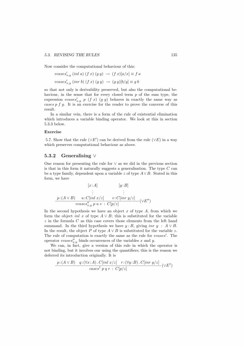
5.3. REVISING THE RULES 135
Now consider the computational behaviour of this:
vcases′x,y (inl a) (f x) (g y) → (f x)[a/x] ≡ f a
vcases′x,y (inr b) (f x) (g y) → (g y)[b/y] ≡ g b
so that not only is derivability preserved, but also the computational be-haviour, in the sense that for every closed term p of the sum type, theexpression vcases′x,y p (f x) (g y) behaves in exactly the same way ascases p f g. It is an exercise for the reader to prove the converse of thisresult.
In a similar vein, there is a form of the rule of existential eliminationwhich introduces a variable binding operator. We look at this in section5.3.3 below.
Exercise
5.7. Show that the rule (∨E′) can be derived from the rule (∨E) in a waywhich preserves computational behaviour as above.
5.3.2 Generalising ∨One reason for presenting the rule for ∨ as we did in the previous sectionis that in this form it naturally suggests a generalisation. The type C canbe a type family, dependent upon a variable z of type A∨B. Stated in thisform, we have
p : (A ∨B)
[x :A]...
u :C[inl x/z]
[y :B]...
v :C[inr y/z]vcases′′x,y p u v : C[p/z]
(∨E′′)
In the second hypothesis we have an object x of type A, from which weform the object inl x of type A ∨ B; this is substituted for the variablez in the formula C as this case covers those elements from the left handsummand. In the third hypothesis we have y : B, giving inr y : A ∨ B.In the result, the object P of type A ∨ B is substituted for the variable z.The rule of computation is exactly the same as the rule for vcases′. Theoperator vcases′′x,y binds occurrences of the variables x and y.
We can, in fact, give a version of this rule in which the operator isnot binding, but it involves our using the quantifiers; this is the reason wedeferred its introduction originally. It is
p : (A ∨B) q : (∀x :A) . C[inl x/z] r : (∀y :B) . C[inr y/z]
cases† p q r : C[p/z](∨E†)
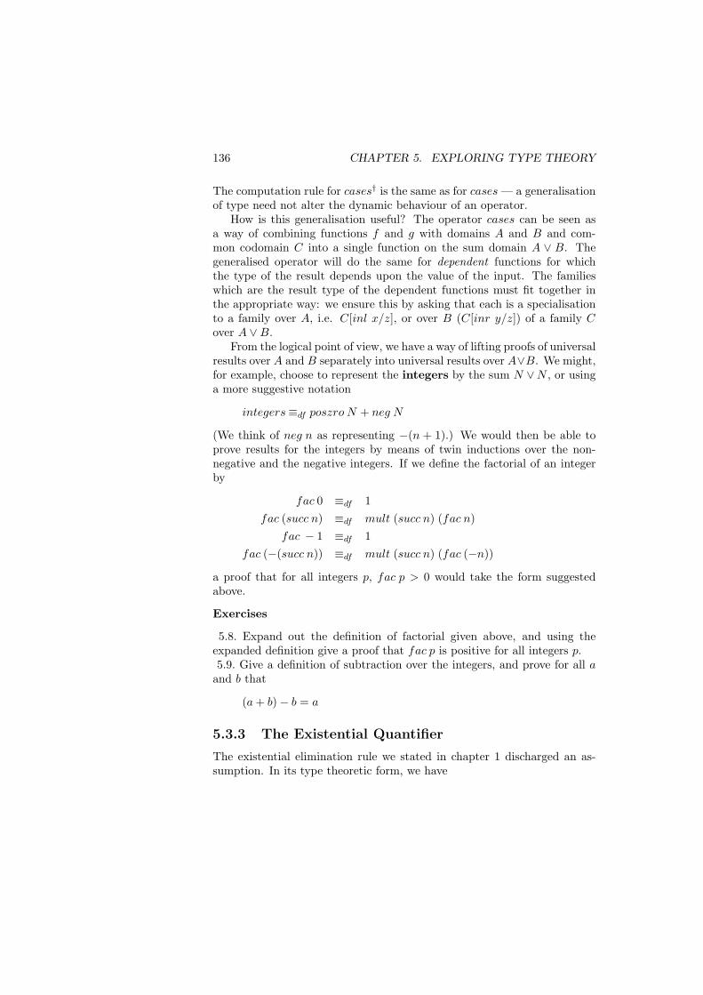
136 CHAPTER 5. EXPLORING TYPE THEORY
The computation rule for cases† is the same as for cases — a generalisationof type need not alter the dynamic behaviour of an operator.
How is this generalisation useful? The operator cases can be seen asa way of combining functions f and g with domains A and B and com-mon codomain C into a single function on the sum domain A ∨ B. Thegeneralised operator will do the same for dependent functions for whichthe type of the result depends upon the value of the input. The familieswhich are the result type of the dependent functions must fit together inthe appropriate way: we ensure this by asking that each is a specialisationto a family over A, i.e. C[inl x/z], or over B (C[inr y/z]) of a family Cover A ∨B.
From the logical point of view, we have a way of lifting proofs of universalresults over A and B separately into universal results over A∨B. We might,for example, choose to represent the integers by the sum N ∨N , or usinga more suggestive notation
integers≡df poszro N + neg N
(We think of neg n as representing −(n + 1).) We would then be able toprove results for the integers by means of twin inductions over the non-negative and the negative integers. If we define the factorial of an integerby
fac 0 ≡df 1fac (succ n) ≡df mult (succ n) (fac n)
fac − 1 ≡df 1fac (−(succ n)) ≡df mult (succ n) (fac (−n))
a proof that for all integers p, fac p > 0 would take the form suggestedabove.
Exercises
5.8. Expand out the definition of factorial given above, and using theexpanded definition give a proof that fac p is positive for all integers p.5.9. Give a definition of subtraction over the integers, and prove for all a
and b that
(a + b)− b = a
5.3.3 The Existential Quantifier
The existential elimination rule we stated in chapter 1 discharged an as-sumption. In its type theoretic form, we have
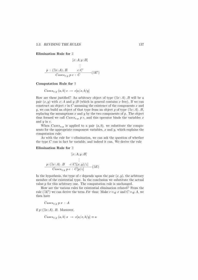
5.3. REVISING THE RULES 137
Elimination Rule for ∃
p : (∃x :A) . B
[x :A; y :B]...
c :CCasesx,y p c : C
(∃E′)
Computation Rule for ∃
Casesx,y (a, b) c → c[a/x, b/y]
How are these justified? An arbitrary object of type (∃x : A) . B will be apair (x, y) with x :A and y :B (which in general contains x free). If we canconstruct an object c in C assuming the existence of the components x andy, we can build an object of that type from an object p of type (∃x :A) . B,replacing the assumptions x and y by the two components of p. The objectthus formed we call Casesx,y p c, and this operator binds the variables xand y in c.
When Casesx,y is applied to a pair (a, b), we substitute the compo-nents for the appropriate component variables, x and y, which explains thecomputation rule.
As with the rule for ∨-elimination, we can ask the question of whetherthe type C can in fact be variable, and indeed it can. We derive the rule
Elimination Rule for ∃
p : (∃x :A) . B
[x :A; y :B]...
c :C[(x, y)/z]Casesx,y p c : C[p/z]
(∃E)
In the hypothesis, the type of c depends upon the pair (x, y), the arbitrarymember of the existential type. In the conclusion we substitute the actualvalue p for this arbitrary one. The computation rule is unchanged.
How are the various rules for existential elimination related? From therule (∃E′) we can derive the term Fst thus: Make c≡df x and C ≡df A, wethen have
Casesx,y p x : A
if p : (∃x :A) . B. Moreover,
Casesx,y (a, b) x → x[a/x, b/y] ≡ a
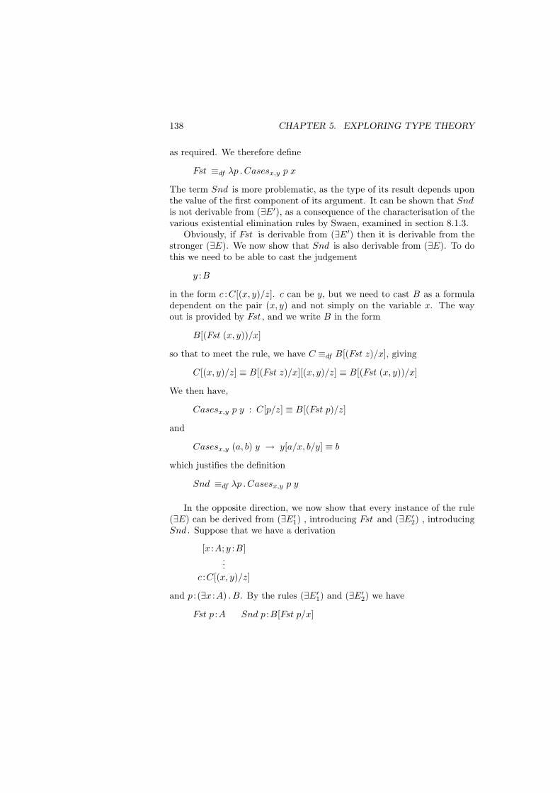
138 CHAPTER 5. EXPLORING TYPE THEORY
as required. We therefore define
Fst ≡df λp . Casesx,y p x
The term Snd is more problematic, as the type of its result depends uponthe value of the first component of its argument. It can be shown that Sndis not derivable from (∃E′), as a consequence of the characterisation of thevarious existential elimination rules by Swaen, examined in section 8.1.3.
Obviously, if Fst is derivable from (∃E′) then it is derivable from thestronger (∃E). We now show that Snd is also derivable from (∃E). To dothis we need to be able to cast the judgement
y :B
in the form c :C[(x, y)/z]. c can be y, but we need to cast B as a formuladependent on the pair (x, y) and not simply on the variable x. The wayout is provided by Fst , and we write B in the form
B[(Fst (x, y))/x]
so that to meet the rule, we have C ≡df B[(Fst z)/x], giving
C[(x, y)/z] ≡ B[(Fst z)/x][(x, y)/z] ≡ B[(Fst (x, y))/x]
We then have,
Casesx,y p y : C[p/z] ≡ B[(Fst p)/z]
and
Casesx,y (a, b) y → y[a/x, b/y] ≡ b
which justifies the definition
Snd ≡df λp . Casesx,y p y
In the opposite direction, we now show that every instance of the rule(∃E) can be derived from (∃E′
1) , introducing Fst and (∃E′2) , introducing
Snd . Suppose that we have a derivation
[x :A; y :B]...
c :C[(x, y)/z]
and p : (∃x :A) . B. By the rules (∃E′1) and (∃E′
2) we have
Fst p :A Snd p :B[Fst p/x]
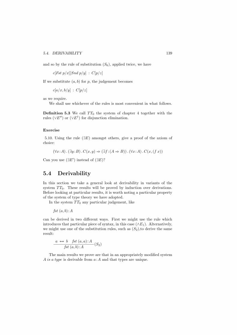
5.4. DERIVABILITY 139
and so by the rule of substitution (S6), applied twice, we have
c[Fst p/x][Snd p/y] : C[p/z]
If we substitute (a, b) for p, the judgement becomes
c[a/x, b/y] : C[p/z]
as we require.We shall use whichever of the rules is most convenient in what follows.
Definition 5.3 We call TT0 the system of chapter 4 together with therules (∨E′′) or (∨E†) for disjunction elimination.
Exercise
5.10. Using the rule (∃E) amongst others, give a proof of the axiom ofchoice:
(∀x :A) . (∃y :B) . C(x, y)⇒ (∃f : (A⇒ B)) . (∀x :A) . C(x, (f x))
Can you use (∃E′) instead of (∃E)?
5.4 Derivability
In this section we take a general look at derivability in variants of thesystem TT0. These results will be proved by induction over derivations.Before looking at particular results, it is worth noting a particular propertyof the system of type theory we have adopted.
In the system TT0 any particular judgement, like
fst (a, b) :A
can be derived in two different ways. First we might use the rule whichintroduces that particular piece of syntax, in this case (∧E1). Alternatively,we might use one of the substitution rules, such as (S2),to derive the sameresult:
a ↔↔ b fst (a, a) :Afst (a, b) :A
(S2)
The main results we prove are that in an appropriately modified systemA is a type is derivable from a :A and that types are unique.
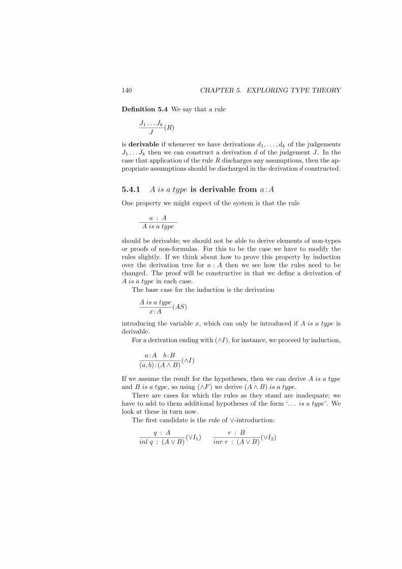
140 CHAPTER 5. EXPLORING TYPE THEORY
Definition 5.4 We say that a rule
J1 . . . Jk
J(R)
is derivable if whenever we have derivations d1, . . . , dk of the judgementsJ1 . . . Jk then we can construct a derivation d of the judgement J . In thecase that application of the rule R discharges any assumptions, then the ap-propriate assumptions should be discharged in the derivation d constructed.
5.4.1 A is a type is derivable from a :A
One property we might expect of the system is that the rule
a : AA is a type
should be derivable; we should not be able to derive elements of non-typesor proofs of non-formulas. For this to be the case we have to modify therules slightly. If we think about how to prove this property by inductionover the derivation tree for a : A then we see how the rules need to bechanged. The proof will be constructive in that we define a derivation ofA is a type in each case.
The base case for the induction is the derivation
A is a type
x :A(AS)
introducing the variable x, which can only be introduced if A is a type isderivable.
For a derivation ending with (∧I), for instance, we proceed by induction,
a :A b :B(a, b) : (A ∧B)
(∧I)
If we assume the result for the hypotheses, then we can derive A is a typeand B is a type, so using (∧F ) we derive (A ∧B) is a type.
There are cases for which the rules as they stand are inadequate; wehave to add to them additional hypotheses of the form ‘. . . is a type’. Welook at these in turn now.
The first candidate is the rule of ∨-introduction:
q : A
inl q : (A ∨B)(∨I1)
r : B
inr r : (A ∨B)(∨I2)
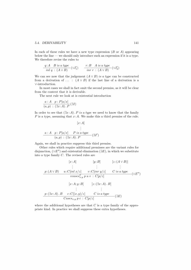
5.4. DERIVABILITY 141
In each of these rules we have a new type expression (B or A) appearingbelow the line — we should only introduce such an expression if it is a type.We therefore revise the rules to
q :A B is a type
inl q : (A ∨B)(∨I ′1)
r :B A is a type
inr r : (A ∨B)(∨I ′2)
We can see now that the judgement (A ∨ B) is a type can be constructedfrom a derivation of . . . : (A ∨ B) if the last line of a derivation is a∨-introduction.
In most cases we shall in fact omit the second premiss, as it will be clearfrom the context that it is derivable.
The next rule we look at is existential introduction
a : A p : P [a/x](a, p) : (∃x :A) . P
(∃I)
In order to see that (∃x :A) . P is a type we need to know that the familyP is a type, assuming that x :A. We make this a third premiss of the rule.
a : A p : P [a/x]
[x :A]...
P is a type
(a, p) : (∃x :A) . P(∃I ′)
Again, we shall in practice suppress this third premiss.Other rules which require additional premisses are the variant rules for
disjunction, (∨E′′) and existential elimination (∃E), in which we substituteinto a type family C. The revised rules are
p : (A ∨B)
[x :A]...
u :C[inl x/z]
[y :B]...
v :C[inr y/z]
[z : (A ∨B)]...
C is a type
vcases′′x,y p u v : C[p/z](∨E′′)
p : (∃x :A) . B
[x :A; y :B]...
c :C[(x, y)/z]
[z : (∃x :A) . B]...
C is a type
Casesx,y p c : C[p/z](∃E)
where the additional hypotheses are that C is a type family of the appro-priate kind. In practice we shall suppress these extra hypotheses.
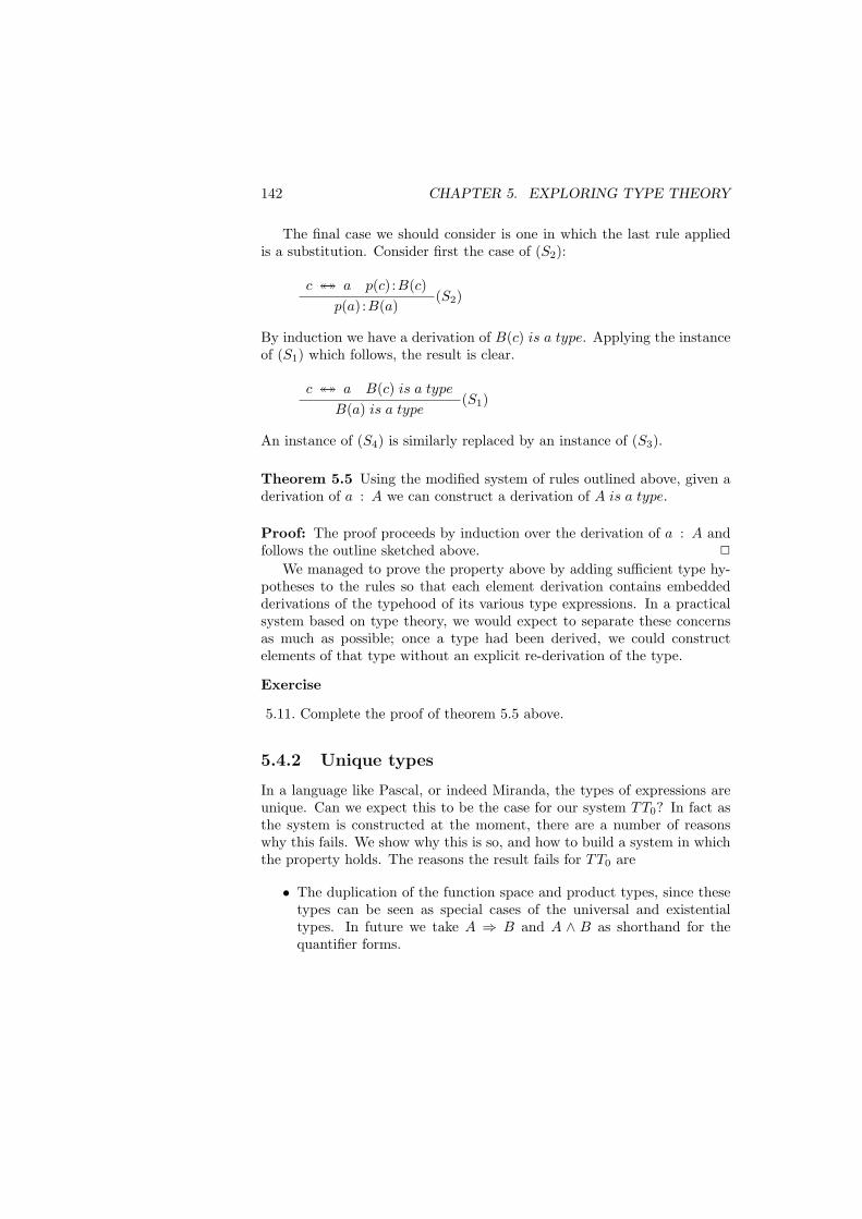
142 CHAPTER 5. EXPLORING TYPE THEORY
The final case we should consider is one in which the last rule appliedis a substitution. Consider first the case of (S2):
c ↔↔ a p(c) :B(c)p(a) :B(a)
(S2)
By induction we have a derivation of B(c) is a type. Applying the instanceof (S1) which follows, the result is clear.
c ↔↔ a B(c) is a type
B(a) is a type(S1)
An instance of (S4) is similarly replaced by an instance of (S3).
Theorem 5.5 Using the modified system of rules outlined above, given aderivation of a : A we can construct a derivation of A is a type.
Proof: The proof proceeds by induction over the derivation of a : A andfollows the outline sketched above. 2
We managed to prove the property above by adding sufficient type hy-potheses to the rules so that each element derivation contains embeddedderivations of the typehood of its various type expressions. In a practicalsystem based on type theory, we would expect to separate these concernsas much as possible; once a type had been derived, we could constructelements of that type without an explicit re-derivation of the type.
Exercise
5.11. Complete the proof of theorem 5.5 above.
5.4.2 Unique types
In a language like Pascal, or indeed Miranda, the types of expressions areunique. Can we expect this to be the case for our system TT0? In fact asthe system is constructed at the moment, there are a number of reasonswhy this fails. We show why this is so, and how to build a system in whichthe property holds. The reasons the result fails for TT0 are
• The duplication of the function space and product types, since thesetypes can be seen as special cases of the universal and existentialtypes. In future we take A ⇒ B and A ∧ B as shorthand for thequantifier forms.
5.4. DERIVABILITY 143
• The injection operators inl and inr do not have unique ranges. In-deed,
inl 0
is a member of (N ∨A) for any type A. We remedy this by labellingthe injection operators with their range type, so that
inl(N∨A) 0 : (N ∨A)
We can now see the unlabelled operators as shorthand for these op-erators.
Theorem 5.6 In the theory TT0, if from a consistent collection of assump-tions we can derive the judgements a :A and a :B then A ↔↔ B.
Proof: The proof is performed by induction over the derivation of a :A.Consider first the case of a variable x :A. Judgements of this sort will
be derived in one of two ways. First we may use the rule of assumptions,in which case there is only one choice of type A by the consistency of theassumption set. Alternatively, we can use the substitution rule (S4) or (S2).In the former case, we have a derivation ending in
C ↔↔ A x :Cx :A
(S4)
Appealing to induction, the type of x is unique up to convertibility, and thefinal step simply gives an equivalent typing to x. The case of (S2) is similar.For each syntactic form we have the possibility of using a substitution rule:it is handled in the same way each time.
At the induction step we perform a case analysis over the rule formingthe final deduction of the derivation. We take as an example the rules fordisjunction. If the expression has the form inl(A∨B) q then this has type(A ∨ B) if and only if q : A, and B is a type. If the expression has twotypes then the second type will be of the form (A′ ∨B), in contradiction tothe unique type of q, which we assume by induction. In a similar way, forthe elimination rule, the (cases p f g) expression can only have two typesif both f and g have two, a contradiction. 2
Exercises
5.12. Complete the proof of the previous result.5.13. Show that the rules (S3) and (S4) are derivable in the system whichresults from TT0 by deleting them. Can the rules (S1) and (S2) be derivedin a system entirely without substitution rules?
144 CHAPTER 5. EXPLORING TYPE THEORY
5.5 Computation
Up to now we have devoted the major part of our exposition to the staticproperties of the system, in looking at how the various judgements arederived. Whilst doing this we have introduced computation rules which areof fundamental importance from the point of view of programming, sinceit is these rules which define the dynamic behaviour of the system; how theprograms are executed, in other words. This section looks at the rules froma general perspective.
The reduction rules are also used to generate a relation of conversion,which is an equivalence relation; convertible objects are seen as being thesame, and this allows the substitution of one for the other in any context.
The issues of interest for reduction will be those we discussed first insections 2.3, 2.4 and 2.11. Does evaluation terminate (along all paths)? —is the system (strongly) normalising? Can any two evaluation sequences beextended to yield a common expression — the Church-Rosser Property?
This will be the case for the system TT0; in this section we presenttwo variants for which there are the results we require in the literature.The first, TT ∗
0 , is one in which reduction, ‘ → ’ is limited. This systempossesses normalisation properties, but has the drawback that it is notChurch-Rosser.
The second system, called TT c0 , is based on a quite different way of
introducing functions, and types, though it is equivalent to TT0. Insteadof introducing binding operators like λ, or type forming operators like ∀and so on, functions are introduced as constants, each constant having acorresponding reduction rule. Types are introduced in a similar way. Thisbears a striking resemblance not only to the top-level form of languageslike Miranda, but also in its details to the methods of λ-lifting [Joh85] andsupercombinators [Hug83] used in functional language implementations.
5.5.1 Reduction
When we evaluate an expression written in a functional programming lan-guage, we expect the final result to be presented in some printable form.We are familiar with Arabic notation for numbers, and lists, trees and so oncan be represented in syntactic form. How is a function from (for example)N to N to be printed? Two options present themselves.
• A function is described extensionally if we say what is its valueon every argument — an infinite amount of information needs to beprinted, which is infeasible.
5.5. COMPUTATION 145
• The alternative is to print some representation of a program for thefunction. Different results will not necessarily denote different func-tions, yet since (extensional) equality between functions can’t be im-plemented, we cannot give a standard representation to each function.The difficulty with implementing extensional equality is that in orderto conclude that two functions are equal, an infinite amount of datahas to be surveyed, and this operation is simply not computable.
In a sense, this is not a problem, because the results we will be inter-ested in will be finite. (This approach does not ignore the ‘infinitary’ listsof languages like Miranda — these are a sequence of finite results, pro-duced one-by-one, rather than a single infinite result.) We say that a typeis ground if it involves no (embedded) function or universally quantifiedtypes, and we identify the printable values to be those of ground type. Theevaluation of an object of functional type is declined politely, at least bythe Miranda system.
In the untyped λ-calculus, everything interesting has to be representedby a function, and the unrestricted rule of β-reduction is invaluable. Inthe untyped context we have to extract meaningful information preciselyfrom representations of functions. ([Abr90] gives a penetrating analysisof the untyped λ-calculus from the point of view of making it consistentwith evaluation in untyped functional languages). For this reason, the rulethat if e → f then λx . e → λx . f , even with x free in e and f , isof central importance. (We call a redex within an expression like λx . e aredex within a lambda.)
Evaluation of printable values in the typed situation is quite different.Functions are ultimately applied to their arguments, and so any reductionwithin the body of a λ-abstraction can be deferred until the argument hasreplaced the bound variable. In a simple case we can see this in action
(λx . (II)x) 2 → (λx . Ix) 2 → (λx . x) 2 → 2
can alternatively be reduced thus:
(λx . (II)x) 2 → (II)2 → I 2 → 2
Indeed, it is not hard to see that there will be no reductions within a lambdaon the leftmost-outermost reduction sequence (c.f. section 2.3). This isbecause if the leftmost-outermost redex ever lies within a lambda then thelambda will never be reduced, since altering the internal redex will changenothing outside the lambda. (This is illustrated by the example above,where the second sequence is the leftmost outermost.)
The argument we have given is to motivate the definition of reductionfor the system TT ∗
0 which we introduce next.
146 CHAPTER 5. EXPLORING TYPE THEORY
Exercise
5.14. In the untyped λ-calculus, the natural number n is represented bythe function “apply n times”, that is
λf . λx . f (f . . . f (f︸ ︷︷ ︸n
x) . . .)
and addition is represented by the function
add≡df λf . λg . λh . λx . f h(g h x)
Show that add 2 3 reduces to 5, but observe that the unrestricted β-reduction rule must be used to achieve the result.
5.5.2 The system TT ∗0
The system TT ∗0 contains the same rules of formation, introduction, elim-
ination and computation. We only change the definition of the relation‘→ ’, with the consequent effect on ‘→→’ and ‘↔↔ ’, as follows:
Definition 5.7 We say that one expression e reduces to another f in asingle step if the following conditions hold. First, e can be represented thus:e ≡ g[e′/z], with the additional property that this z occurs within none ofthe binding constructs of the language which appear in the expression. Wealso require that e′ reduces to f ′ according to one of the computation rules,and finally that f is the result of substituting this reduced form into g, thatis f ≡ g[f ′/z].
This weaker notion of reduction is related to the idea of weak headnormal form which we discussed earlier. We have reached a similar notionby changing the definition of reduction itself, rather than the definition ofnormal form, which we leave alone.
The important result about this system follows.
Theorem 5.8 (Troelstra) The system TT ∗0 is strongly normalising.
Proof: The proof, given in [Tro87], is by means of a translation intoanother system entirely, for which the strong normalisation theorem is asimple generalisation of our proof in section 2.7.
The system in question is that of intuitionistic finite-type arithmetic,which is known as N −HAω in the encyclopaedic [Tro73]. The systemcontains the type structure of products and function spaces built over thetype N . The normalisation result for the system without products is in
5.5. COMPUTATION 147
[Tro73], 2.2.30, and it is shown in [Tro86] how products may be eliminatedfrom the system.
The translations of the type A and the term a are written A∗ and a∗.The crucial property of the translation is that although some of the powerof TT ∗
0 is lost in the translation, reduction is preserved, so that if a → bin TT ∗
0 then a∗ → b∗ in N−HAω. A non-terminating sequence in theoriginal system will give rise to one in the target system, contradicting itsstrong normalisation property.
The translation goes as follows: (note that ‘0’ is used for the type N in[Tro73] — we shall use N),
N∗ ≡df N
which is the obvious translation. The identity types, which have one ele-ment, are represented thus also:
(I(A, a, b))∗ ≡df N
with its single element being represented by 0. In a similar way we can alsorepresent the booleans, and indeed all the finite types.
In choosing to represent the I-types by a constant type N we haveremoved any dependency of the types on values, so that we say
((∀x :A) . B)∗ ≡df A∗ ⇒ B∗ ((∃x :A) . B)∗ ≡df A∗ ×B∗
representing the quantified types by their non-variable special cases. Theelements of these types have images given by
(λx . e)∗ ≡df λx . (e∗)
(a, b)∗ ≡df (a∗, b∗)
The only slight trick is in coding the sum type, which is mapped into aproduct
(A ∨B)∗ ≡df N ×A∗ ×B∗
We represent (inl a) by (0, a, 0B∗) and (inr b) by (1, 0A∗ , b). The values0A∗ , 0B∗ are fixed ‘dummy’ values which are constant zero functions orproducts of same, depending on the form of the types A, B etc. Theoperation of primitive recursion over N is sufficient to implement the casesoperator over the disjoint sum.
To complete the proof we simply need to check that if a → b thena∗ → b∗, which we leave as an exercise for the reader. 2
We should remark that the system N −HAω is simpler than TT0 asit does not contain dependent types. As can be seen from the proof, the
148 CHAPTER 5. EXPLORING TYPE THEORY
reduction properties of the system are preserved by a translation whichloses these dependencies, reducing the universal and existential types tofunction space and product respectively.
There is a problem with the system TT ∗0 . The Church Rosser property
fails for it, as can be seen from the following, functional term.
(λx . (λy . x)) (II) → (λx . (λy . x)) I
→ λy . I
On the other hand if we reduce the outer redex first,
(λx . (λy . x)) (II) → λy . (II)
The final terms of these sequences are normal forms, since no reductionis permitted inside a λ, and distinct, so there is no term to complete thediamond between the two.
This failure is for a term with a functional type, so we might ask whetherwe can claim a limited result for ground types. It looks as though thereshould be such a result, but quite how it would be established is an openquestion. The failure at the functional type is, in fact, still distressing forreasons which will become clearer as we proceed. Without the Church-Rosser property we cannot establish the uniqueness of normal forms, whichhas in turn the consequence that the relation ‘↔↔ ’ is decidable: we reducetwo terms to their normal forms, and then see if the two are identical. Thesystem which follows will have these desirable properties.
Exercises
5.15. Show that in the proof of theorem 5.8 the translation respects reduc-tion, so that if a → b then a∗ → b∗.5.16. Argue that objects in normal form in the system TT ∗
0 are in weakhead normal form in a system with unrestricted β-reduction.
5.5.3 Combinators and the system TT c0
In the last section we modified the definition of ‘→ ’, disallowing reductionunder the λ; here we modify the system giving an entirely different accountof functional abstraction and type formation.
All the systems we have looked at so far have shared one aspect: eachhas used λ-abstraction as a means of forming terms of functional type.Given a term e generally involving the variable x amongst others, we canform the term λx . e with the property that
(λx . e) a → e[a/x]
5.5. COMPUTATION 149
Instances of this might be the term λx . (x + y), and the term λx . (II), inwhich the redex (II) is still visible.
An alternative is to make a function or combinator definition for theterm, saying
f x → e
but there is a problem with doing simply this, exemplified by the additionexample we saw above. Our definition would state
f x → (x + y)
which contains an unbound variable on the right-hand side. To make aproper definition of a function we need to include the variable y amongstthe arguments, and say
f y x → (x + y)
The term λx . (x + y) will now be replaced by the term (f y), as it is thisapplication which represents the abstraction over x. In general, a func-tion constant formed in this way needs to have as arguments not only theabstracted variable, but also all the other variables free in the expression.These variables can be called the parameters of the definition. In order toform the abstraction of interest, these parameters must then be passed tothe constant to form the required abstraction. In the case of the additionfunction above, the abstraction over x is given by the term (f y) and notthe ‘bare’ constant f .
For our second example above, λx . (II), the definition is simpler, wejust have to write
c x → (II)
and form the term c. Note that in the constant there is no redex. Thismethod of constant definitions hides from view the redexes within the bod-ies of functions, only making them visible when the function is applied tosufficiently many arguments.
Definition 5.9 Combinator abstraction. Suppose that the derivationof the judgement
e :B
depends upon the assumptions
x1 :A1 , . . . , xk :Ak , x :A
150 CHAPTER 5. EXPLORING TYPE THEORY
then we can form a new function constant f which will take arguments ofthe types A1, . . . , Ak (as ‘parameters’) and A, giving a result of type B. Inother words, we can introduce the term
fx1 . . . xk
of type (∀x :A) . B. The computation rule for the term f is given by
fx1 . . . xk x → e
We can give the type of the new constant f directly:
(∀x1 :A1) . . . . (∀xk :Ak) . (∀x :A) . B
which, when none of the dependencies are exhibited by B, reduces to
A1 ⇒ . . .⇒ Ak ⇒ A⇒ B
The introduction rule can be written in a familiar form, thus
[x :A]...
e :Bf x1 . . . xk : (∀x :A) . B
(∀Ic)
where the undischarged assumptions of the derivation of the hypothesis arex1 :A1, . . . , xk :Ak, and the new constant to be introduced is called f . Thecomputation rule is stated above and the formation and elimination rulesfor the type (∀x : A) . B (and therefore for the implication A ⇒ B) are asbefore.
Let us consider a simple example. Assuming we have derived that Aand B are types then on the basis of the assumptions
x :A , y :B
we can derive
x :A
Suppose we wish to form the (informal) expression λx . λy . x, we first haveto abstract over y. In doing this we produce a binary function constant, f ,which will take the free variable x as an argument as well as the variable ywhich is the variable bound by the definition
f x y → x
5.5. COMPUTATION 151
and we form the term
f x : (B ⇒ A)
which is based on the assumption of x : A. Now we can abstract over x,giving the constant g, with the property
g x → f x
and the type
g : A⇒ (B ⇒ A)
(In fact in this case f and g have the same properties, but in general thesecond and subsequent abstractions are non-trivial). We can consider theexample of the term, which gives a counter-example to the Church Rosserproperty for the system TT ∗
0 ,
(λx . (λy . x)) (II)
This is now represented by the term (g (II)), which reduces thus:
g (II) → f (II) → f I
The whole term f (II) does not itself form a redex since the function con-stant f has two formal arguments in its reduction rule, and in this situationit is presented with only one — the Church Rosser theorem is not violatedin this particular case. It is in fact never violated, as we shall see in thenext section.
It appears from what we have said so far that no reduction can takeplace inside an abstraction. In the example of λx . (II) we saw that it wasrendered by the constant c with the reduction rule
c x → (II)
so that no reduction of the functional term itself, given by c, is possible.The crucial observation to be made here is that the same λ-expression maybe represented in different ways by constant abstraction. The clue to thisis to see the expression II as an instance of a parameter, in which case wesee the whole expression as an instance of the expression
λx . y
with y of the appropriate type. Abstraction here leads to the constant
c′ y x → y
152 CHAPTER 5. EXPLORING TYPE THEORY
with the particular expression represented by
c′ (II)
In this representation of λx . (II) the redex (II) is visible, and so may bereduced, yielding c′ I, which represents λx . I.
Definition 5.10 A proper subexpression f of a lambda expression e is afree subexpression of e with respect to x if the variable x does not appearfree in f . Such an expression is a maximal free expression (or mfe) withrespect to x if it is free with respect to x and moreover is maximal such: itis not a proper sub-expression of an mfe with respect to x.
Definition 5.11 Supercombinator abstraction To form the supercom-binator abstraction of e over x we first identify the mfes f1, . . . , fl of e withrespect to x. We now introduce a new constant g with the reduction rule
g k1 . . . kl x → e[k1/f1, . . . , kl/fl]
The abstraction of e over x is given by
g f1 . . . fl
The formal parameters k1 . . . kl replace the maximal free expressions, towhich the function constant is then applied.
Now we look at a particular example, the supercombinator abstraction
λx . λy . ((II)x)
First we form the supercombinator abstraction
λy . ((II)x)
There is a single mfe in the body, ((II)x), so we form the constant c whosereduction rule is
c k1 y → k1
with the expression
c ((II)x)
forming the supercombinator abstraction over y. Now we abstract overx. There is a single mfe in the expression above, (II), and we form theconstant d with reduction rule
d k1 x → c (k1 x)
5.6. TTC0 : NORMALISATION AND ITS COROLLARIES 153
the final abstraction being
d (II)
It is important to observe that the redex (II) is visible in this supercombi-nator abstraction. This is the case in general.
Definition 5.12 The system TT c0 is defined from TT0 as follows. All the
type forming rules are modified so that types are introduced as constants.The parameters may be chosen to make certain redexes visible and othersinvisible. The rules of function and universal quantifier introduction aremodified as above, as is the rule (∨E′′) which uses the binding operatorvcases.,..
Lemma 5.13 If we use the supercombinator abstraction algorithm to givefunctional abstraction in TT c
0 , then all the redexes which could be reducedin the system TT0, that is all redexes which are free, can be reduced in TT c
0
There is therefore an embedding of the system TT0 within TT c0 which
preserves the reduction and computation properties of the former. We shallinvestigate these properties for TT c
0 in the following section, and claim theobvious corollaries for TT0 there too.
Note that for readability we shall retain the old notation of type formingoperations, but we should always recall that it is a shorthand for a notationwhich is more expressive in allowing a particular expression to be describedin different ways, making redexes visible or invisible.
Exercises
5.17. Give the combinator and supercombinator abstractions for the term
h≡df λa . λb . λc . (abc)
5.18. Follow the evaluation behaviour of the expression h (II) (II) 3 usingthe two versions of the code compiled in the previous exercise.5.19. Give a proof of lemma 5.13 above.
5.6 TT c0 : Normalisation and its corollaries
In this section we shall prove that every term of the type theory TT c0 has a
normal form, a result which can be strengthened to a strong normalisationresult. The proof is a Tait-style proof, as first seen in section 2.7, andit is based on Martin-Lof’s proof of normalisation for his 1975 system, in[ML75b]. Its exposition is simpler in omitting the proof information which
154 CHAPTER 5. EXPLORING TYPE THEORY
Martin-Lof’s proof carries — this was done originally to make the prooflocally formalizable in the [type] theory itself ([ML75a], section 2.1.4) —the approach here is not so formal. The result is proved in such a waythat it has a number of important corollaries for the system, includingthe facts that normal forms are unique, and the Church-Rosser propertyfor reduction holds. Martin-Lof observes that the Church-Rosser propertydoes not have a direct combinatorial proof to his knowledge, this routeproviding the only means of proof.
As we have seen a number of times up to now, the fact that in typetheory the types and the objects are defined by a simultaneous inductionmeans that we have to prove things in a different manner than in the typedλ-calculus. In section 2.7 we were able first to define stability by inductionover the types, and then to show all elements are stable. Here we work byinduction over the derivations of closed judgements
a : A A is a type
(a closed judgement is one which depends upon no assumptions, and so inparticular one for which a and A are closed). The induction defines
• A′, a closed normal form of A.
• a′, a closed normal form of a so that a→→ a′. a′ is also a member ofthe set ‖A‖.
• ‖A‖, the set of stable terms of type A, which are members of thetype A′. Our proof will show that each closed term is reducible to astable term, and these terms are clearly seen to be closed and normal.
Because assumptions in open derivations can be discharged, we need alsoto look at open judgements and derivations. For the open judgement a :A,made in the context
x1 :A1, . . . , xn :An
we also define functions a′ and A′, depending upon (meta-)variables
x′1, . . . , x′n
which range (respectively) over closed normal terms of type
A′1, . . . , A
′n(x′1, . . . x
′n−1)
It is important to note that these functions are not defined by terms ofthe system, in general: they are the operations which assign closed normalforms depending upon the closed normal forms which are their parameters.
5.6. TTC0 : NORMALISATION AND ITS COROLLARIES 155
To choose a concrete example, if a :N depends upon x :N , then a′ will be afunction from numerals to numerals, since numerals are the closed normalforms of natural number type.
We require two conditions of the functions a′ and A′
• First we require that for all closed normal forms
a′1 :A′1, . . . , a
′n :A′
n
we have the property
a[a′1/x′1 . . . , a′n/x′n]→→ a′[a′1/x′1 . . . , a′n/x′n]
(There is a similar definition for A′.)
• We also require that the definitions commute with substitution. Givenderivations of
a1 :A1 , . . . , an :An[a1/x1, . . . , an−1/xn−1]
we require that
(a(a1, . . . , an))′ ≡ a′(a′1, . . . , a′n)
with a similar definition for A′. (Recall that we use ≡ to mean ‘iden-tical up to change of bound variable’). In the proof we say that a′ isparametric if it has this pair of properties.
Theorem 5.14 (Normalisation for TT c0 ) Every closed term b of type
theory has a normal form b′, and moreover if b ↔↔ c then b′ ≡ c′.
Proof: As outlined above we use induction over the length of derivationsof judgements. We must go through the constructs of the theory in turn.We must also verify at each step that the normal forms assigned to the twosides of a computability rule like
fst (a, b) → a
are equal — this is used in proving that the normal forms given to convert-ible terms are identical. We shall not cover the cases of function spaces orconjunctions as they are simply special cases of universally and existentiallyquantified types.
156 CHAPTER 5. EXPLORING TYPE THEORY
Before we look at the cases in turn, it is worth examining the exactmechanism for type formation in TT c
0 . Suppose we want to form a typelike
(∀x :N) . I(N, f x, 0 + 0)
then there are a number of ways of so doing. In the first we simply forma new type constant on this basis, but we may also form a type operatorwhich is parametrised over y, yielding
(∀x :N) . I(N, f x, y)
In our particular case we apply this to the (free) expression 0 + 0, allowingthis to be reduced. If an expression is so parametrised, then in the nor-mal form parameters will themselves be reduced to normal form. In thefollowing we assume that types are not parametrised, but this is simply fornotational clarity.
Case x a variableWe define x′ to be the (informal) variable x′. Obviously this is parametric.
Case ∀The formation rule introduces a new constant, for which we use the short-hand ((∀x :A) . B). As we said above, we shall assume that the type is notparametrised, and so we define
((∀x :A) . B)′ ≡df (∀x :A) . B
We make similar definitions for the other type forming operations, apartfrom the I-types. The set of stable terms of this type, ‖((∀x :A) . B)‖, con-tains all those closed normal terms c′ of type (∀x :A) . B with the propertythat for all closed normal forms (cnfs) a′ in A′, (c′ a′) reduces to a closednormal form in B′[a′/x].∀ introduction gives a λ-abstraction, λx . e. If we use supercombinator
abstraction, we have a new constant f
f k1 . . . kl x → e[k1/f1, . . . , kl/fl]
where f1 . . . fl are the maximal free expressions of e with respect to x. Theabstraction itself is defined to be
f f1 . . . fl
Now, the normal form of f is
f ′ ≡df f
5.6. TTC0 : NORMALISATION AND ITS COROLLARIES 157
and the normal form for the expression (f f1 . . . fl) is given by the clausefor ∀ elimination below.
If we restrict ourselves to the simple case of no parameters ki, then f ′
is stable since for any cnf a′,
f ′ a′ → e[a′/x]→→ e′[a′/x] ≡ (e[a/x])′
the equivalence holding by the parametricity property for e, which we as-sume by induction. For the general case we argue in a similar way, alsoinvoking the case for ∀ elimination below.∀ elimination gives an application. We define (f a)′ to be the closed
normal form to which (f ′ a′) reduces, which exists by induction and thedefinition of convertibility for the universal type. The computation rule for∀ states that
f a → e[a/x]
now observe that
(f a)′ ≡ e′[a′/x] ≡ (e[a/x])′
The first equivalence holds by the definition of convertibility for the λ-abstraction and the second by parametricity for e′.
It is not hard to see that the definitions for ∀-introduction and elimina-tion are parametric.
Case ∃As for the universal type, we define
((∃x :A) . B)′ ≡df (∃x :A) . B
The stable terms of this type are pairs of stable terms, (a′, b′), with a :A′
and b′ :B′[a′/x]. The introduction rules introduce a pair, we say that
(a, b)′ ≡df (a′, b′)
The elimination rules (∃E′1) and (∃E′
2) introduce the projection operators.If we have terms
Fst p Snd p
then p′, the cnf of p, will be a pair (q′, r′). We therefore set
(Fst p)′ ≡df q′ (Snd p)′ ≡df r′
A pair of parametric terms will be parametric, as will be the components ofa parametric pair, so the two constructs preserve parametricity. This willapply similarly in all other cases of non-variable-binding constructs.

158 CHAPTER 5. EXPLORING TYPE THEORY
Finally we should check that the normal forms of the two sides of thecomputation rules are identical. The rules state that
Fst (q, r) → q Snd (q, r) → r
By the definitions above
(Fst (q, r))′ ≡ (Fst (q′, r′)) ≡ q′
as we require. A similar proof shows the result for Snd .
Case ∨We define
(A ∨B)′ ≡df (A′ ∨B′)
and take the set of stable elements, ‖(A ∨B)‖ to be (‖A‖ ∨ ‖B‖).In introducing an element of a disjunction we inject the object into
either the left-hand or right-hand side. We define
(inl a)′ ≡df inl a′ (inr b)′ ≡df inr b′
in eliminating an element by means of (∨E′) we use the vcases′ construct,vcases′x,y puv. p′ will take the form of (inl q′) or (inr r′). In the first case,let
(cases p u v)′ ≡df u′[q′/x]
and in the second
(cases p u v)′ ≡df v′[r′/x]
The forms defined are stable by the parametricity property, which is alsopreserved by the definition. It is also easy to check that the definitionsrespect the computation rules for vcases.
Case ⊥The cnf of ⊥, ⊥′ is ⊥ itself, and the set of stable terms is the emptyset. There are no introduction rules for terms of type ⊥, but there is theelimination rule. We write
(abortA p)′ ≡df abortA′ p′
This clearly satisfies parametricity. As there is no introduction rule, thereis no computation rule, and therefore no condition to check. In fact thiscase is a special case of the finite types, which follow.
5.6. TTC0 : NORMALISATION AND ITS COROLLARIES 159
Case Nn
The cnf of Nn is Nn, and the stable terms are
1n, . . . , nn
so that it is easy to see that for the introduction rules we have
1n′ ≡df 1n, . . . , nn
′ ≡df nn
For the elimination rule we have the n-way case statement
casesn e c1 . . . cn
The cnf of e will be mn for some 1 ≤ m ≤ n. We define
(casesn mn c1 . . . cn)′ ≡df cm′
Again, parametricity is plain. The computation rule selects the appropriatecase according to the value of the object of type Nn — this is respected bythe definition.
Note that this also covers the special cases of >, bool, and indeed ⊥.
Case NN ′ is defined to be N , and the collection of stable terms is defined by(meta-theoretical) induction thus:
• 0 is a stable term.
• (succ n) is a stable term if n is.
It should be clear how we define the cnfs for the introduction rules:
0′ ≡df 0 (succ n)′ ≡df (succ n′)
In the case of elimination, we have terms of the form
prim m c f
The cnf m′ will be either 0 or (succ n) for some n. By an induction overthe cnf we say that
(prim 0 c f)′ ≡df c′
(prim (succ n) c f)′ ≡df y
where y is the cnf of the term given by the application
f ′ n (prim n c f)′
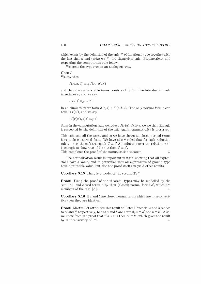
160 CHAPTER 5. EXPLORING TYPE THEORY
which exists by the definition of the cnfs f ′ of functional type together withthe fact that n and (prim n c f)′ are themselves cnfs. Parametricity andrespecting the computation rule follow.
We treat the type tree in an analogous way.
Case IWe say that
I(A, a, b)′ ≡df I(A′, a′, b′)
and that the set of stable terms consists of r(a′). The introduction ruleintroduces r, and we say
(r(a))′ ≡df r(a′)
In an elimination we form J(c, d) : C(a, b, c). The only normal form c canhave is r(a′), and we say
(J(r(a′), d))′ ≡df d′
Since in the computation rule, we reduce J(r(a), d) to d, we see that this ruleis respected by the definition of the cnf. Again, parametricity is preserved.
This exhausts all the cases, and so we have shown all closed normal termshave a closed normal form. We have also verified that for each reductionrule b → c, the cnfs are equal: b′ ≡ c′ An induction over the relation ‘↔↔ ’is enough to show that if b ↔↔ c then b′ ≡ c′.This completes the proof of the normalisation theorem. 2
The normalisation result is important in itself, showing that all expres-sions have a value, and in particular that all expressions of ground typehave a printable value, but also the proof itself can yield other results.
Corollary 5.15 There is a model of the system TT c0 .
Proof: Using the proof of the theorem, types may be modelled by thesets ‖A‖, and closed terms a by their (closed) normal forms a′, which aremembers of the sets ‖A‖. 2
Corollary 5.16 If a and b are closed normal terms which are interconvert-ible then they are identical.
Proof: Martin-Lof attributes this result to Peter Hancock. a and b reduceto a′ and b′ respectively, but as a and b are normal, a ≡ a′ and b ≡ b′. Also,we know from the proof that if a ↔↔ b then a′ ≡ b′, which gives the resultby the transitivity of ‘≡’. 2
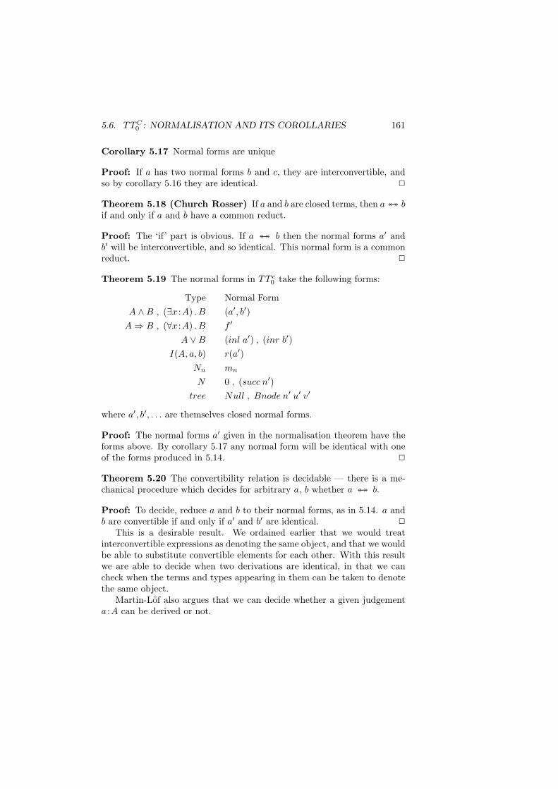
5.6. TTC0 : NORMALISATION AND ITS COROLLARIES 161
Corollary 5.17 Normal forms are unique
Proof: If a has two normal forms b and c, they are interconvertible, andso by corollary 5.16 they are identical. 2
Theorem 5.18 (Church Rosser) If a and b are closed terms, then a↔↔ bif and only if a and b have a common reduct.
Proof: The ‘if’ part is obvious. If a ↔↔ b then the normal forms a′ andb′ will be interconvertible, and so identical. This normal form is a commonreduct. 2
Theorem 5.19 The normal forms in TT c0 take the following forms:
Type Normal FormA ∧B , (∃x :A) . B (a′, b′)
A⇒ B , (∀x :A) . B f ′
A ∨B (inl a′) , (inr b′)I(A, a, b) r(a′)
Nn mn
N 0 , (succ n′)tree Null , Bnode n′ u′ v′
where a′, b′, . . . are themselves closed normal forms.
Proof: The normal forms a′ given in the normalisation theorem have theforms above. By corollary 5.17 any normal form will be identical with oneof the forms produced in 5.14. 2
Theorem 5.20 The convertibility relation is decidable — there is a me-chanical procedure which decides for arbitrary a, b whether a ↔↔ b.
Proof: To decide, reduce a and b to their normal forms, as in 5.14. a andb are convertible if and only if a′ and b′ are identical. 2
This is a desirable result. We ordained earlier that we would treatinterconvertible expressions as denoting the same object, and that we wouldbe able to substitute convertible elements for each other. With this resultwe are able to decide when two derivations are identical, in that we cancheck when the terms and types appearing in them can be taken to denotethe same object.
Martin-Lof also argues that we can decide whether a given judgementa :A can be derived or not.
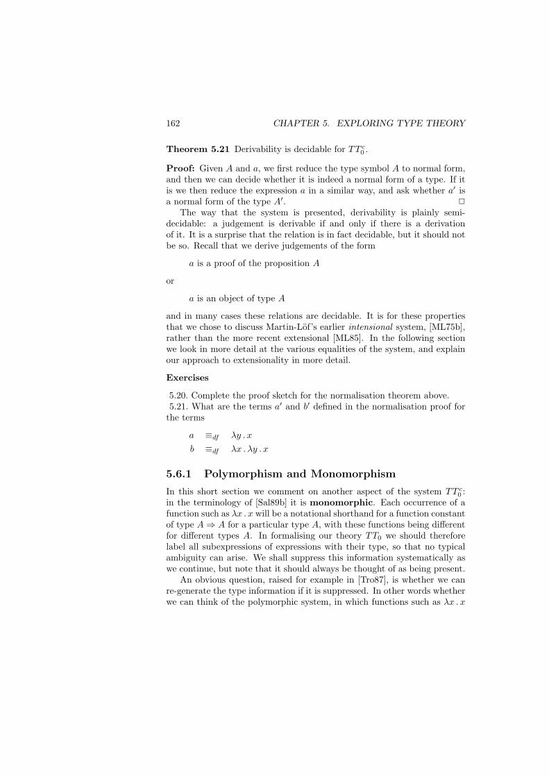
162 CHAPTER 5. EXPLORING TYPE THEORY
Theorem 5.21 Derivability is decidable for TT c0 .
Proof: Given A and a, we first reduce the type symbol A to normal form,and then we can decide whether it is indeed a normal form of a type. If itis we then reduce the expression a in a similar way, and ask whether a′ isa normal form of the type A′. 2
The way that the system is presented, derivability is plainly semi-decidable: a judgement is derivable if and only if there is a derivationof it. It is a surprise that the relation is in fact decidable, but it should notbe so. Recall that we derive judgements of the form
a is a proof of the proposition A
or
a is an object of type A
and in many cases these relations are decidable. It is for these propertiesthat we chose to discuss Martin-Lof’s earlier intensional system, [ML75b],rather than the more recent extensional [ML85]. In the following sectionwe look in more detail at the various equalities of the system, and explainour approach to extensionality in more detail.
Exercises
5.20. Complete the proof sketch for the normalisation theorem above.5.21. What are the terms a′ and b′ defined in the normalisation proof for
the terms
a ≡df λy . x
b ≡df λx . λy . x
5.6.1 Polymorphism and Monomorphism
In this short section we comment on another aspect of the system TT c0 :
in the terminology of [Sal89b] it is monomorphic. Each occurrence of afunction such as λx . x will be a notational shorthand for a function constantof type A⇒ A for a particular type A, with these functions being differentfor different types A. In formalising our theory TT0 we should thereforelabel all subexpressions of expressions with their type, so that no typicalambiguity can arise. We shall suppress this information systematically aswe continue, but note that it should always be thought of as being present.
An obvious question, raised for example in [Tro87], is whether we canre-generate the type information if it is suppressed. In other words whetherwe can think of the polymorphic system, in which functions such as λx . x
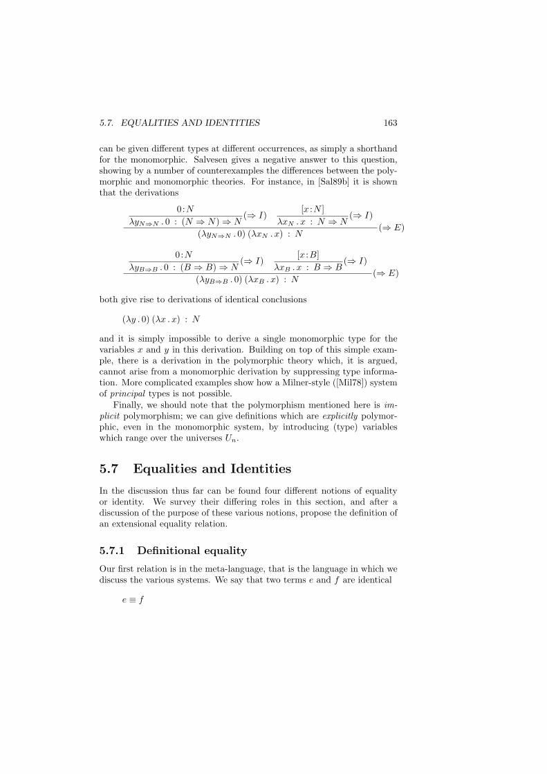
5.7. EQUALITIES AND IDENTITIES 163
can be given different types at different occurrences, as simply a shorthandfor the monomorphic. Salvesen gives a negative answer to this question,showing by a number of counterexamples the differences between the poly-morphic and monomorphic theories. For instance, in [Sal89b] it is shownthat the derivations
0:NλyN⇒N . 0 : (N ⇒ N)⇒ N
(⇒ I)[x :N ]
λxN . x : N ⇒ N(⇒ I)
(λyN⇒N . 0) (λxN . x) : N(⇒ E)
0 :NλyB⇒B . 0 : (B ⇒ B)⇒ N
(⇒ I)[x :B]
λxB . x : B ⇒ B(⇒ I)
(λyB⇒B . 0) (λxB . x) : N(⇒ E)
both give rise to derivations of identical conclusions
(λy . 0) (λx . x) : N
and it is simply impossible to derive a single monomorphic type for thevariables x and y in this derivation. Building on top of this simple exam-ple, there is a derivation in the polymorphic theory which, it is argued,cannot arise from a monomorphic derivation by suppressing type informa-tion. More complicated examples show how a Milner-style ([Mil78]) systemof principal types is not possible.
Finally, we should note that the polymorphism mentioned here is im-plicit polymorphism; we can give definitions which are explicitly polymor-phic, even in the monomorphic system, by introducing (type) variableswhich range over the universes Un.
5.7 Equalities and Identities
In the discussion thus far can be found four different notions of equalityor identity. We survey their differing roles in this section, and after adiscussion of the purpose of these various notions, propose the definition ofan extensional equality relation.
5.7.1 Definitional equality
Our first relation is in the meta-language, that is the language in which wediscuss the various systems. We say that two terms e and f are identical
e ≡ f
164 CHAPTER 5. EXPLORING TYPE THEORY
if they are identical up to change of bound variable after all the definedterms, introduced by means of the definitional equality ‘ ≡df ’, have beenexpanded out. We simply treat identical expressions as identical — thereare no contexts in which we wish to distinguish between two identical ex-pressions.
As an aside, it is worth noting that although it is obvious what thisrelation is, we have to do some work in a computer implementation toensure that we can decide exactly when two expressions are identical.
5.7.2 Convertibility
Two expressions are convertible if the computation steps embodied in thecomputation rules for the system are sufficient to bring them together.Formally we build the relation ‘ ↔↔ ’ by taking the reflexive, symmetrictransitive and substitutive closure of the relation ‘→ ’. In other words, weask that, for all expressions a, b, c, . . . and variables x,
Computation If a → b then a ↔↔ b.
Reflexivity a ↔↔ a.
Symmetry If a ↔↔ b then b ↔↔ a.
Transitivity If a ↔↔ b and b ↔↔ c then a ↔↔ c.
Substitutivity If a ↔↔ b and c ↔↔ d then a[c/x] ↔↔ b[d/x].
We saw in the last section that two terms were convertible if and only if theyhave the same normal form, this means that the relation of convertibilityis decidable.
The definition of convertibility is external to the system — a ↔↔ b isintended to embody the fact that the two expressions a and b denote thesame object. In the light of the characterisation above, we can identify thisobject as the normal form of the expression, if we wish.
In section 4.11 we introduced the rules of substitution which allow in-terconvertible expressions to be substituted for each other in derivations ofjudgements. This emphasizes the fact that judgements are intended to beabout the objects denoted by the expressions, rather than the expressionsthemselves. We shall come back to this important distinction below.
Because ‘a ↔↔ b’ is not a proposition of the system, we are unable tobuild more complex assertions on the basis of it. To do this we turn to ourthird relation, the identity predicate.
5.7. EQUALITIES AND IDENTITIES 165
5.7.3 Identity; the I type
As a primitive proposition (or type) forming operator we have the I oper-ation, forming a type thus:
A is a type a :A b :AI(A, a, b) is a type
(IF )
The type is also written a =A b or even a = b when no confusion can result.I(A, a, b) is provable, by the object r(a), when a ↔↔ b, so we can see thetype as an internalisation of convertibility. On top of the I type we canbuild more complex assertions, such as
(∀x, y :A) . ((x =A y)⇒ ((f x) =B (g y)))
where f and g are functions of type A⇒ B. Proof that I is the internali-sation of ‘↔↔ ’ is given by the result
Theorem 5.22 For closed a and b, the judgement I(A, a, b) is derivable ifand only if a ↔↔ b.
Proof: Clearly the ‘if’ part is valid. Suppose that p :I(A, a, b) is derivable;taking normal forms a la theorem 5.14 we have
p′ :I(A′, a′, b′)
but for this to be derivable, it must be the case that a′ ≡ b′, which meansthat a ↔↔ b 2
The expression x =A y denotes a proposition or type of the system. Inorder to test for identity in a computation we require a function or operationwhich returns not a type but rather a value True or False of boolean type.
5.7.4 Equality functions
An equality function is a boolean valued function which can be used in acomputation to test for the equality of two objects.
Definition 5.23 An equality function (or equality operation) overthe type A is a term equalA of type equalA : A⇒ A⇒ bool such that thefollowing propositions are valid
(∀a, b :A) . (a =A b ⇒ equalA a b =bool True)
(∀a, b :A) . (a 6=A b ⇒ equalA a b =bool False)
166 CHAPTER 5. EXPLORING TYPE THEORY
Note that one consequence of the definition is that for closed a,b if a ↔↔ bthen
equalA a b ↔↔ True
but on the other hand the non-derivability of a ↔↔ b does not imply that
equalA a b ↔↔ False
Over which types do we have an equality operation? We start our discussionwith two definitions.
Definition 5.24 A predicate P (x1, . . . , xk) is formally decidable if andonly if the following proposition is derivable
(∀x1 :A1) . . . . (∀xk :Ak) . (P (x1, . . . , xk) ∨ ¬P (x1, . . . , xk)) (5.1)
Definition 5.25 A predicate P (x1, . . . , xk) is representable if and onlyif for some term r the following propositions are derivable
(∀x1 :A1) . . . . (∀xk :Ak) .(r x1 . . . xk =bool True⇒ P (x1, . . . , xk)) (5.2)
(∀x1 :A1) . . . . (∀xk :Ak) .(r x1 . . . xk =bool False⇒ ¬P (x1, . . . , xk)) (5.3)
Theorem 5.26 A predicate is representable if and only if it is formallydecidable.
Proof: To prove that a representable predicate is decidable, note first thatusing the axiom of bool elimination we can derive
(∀b :bool) . (b =bool True ∨ b =bool False)
(a proof of this appears in section 4.10.1). By means of the propositions5.2, 5.3, we can derive the formula 5.1, as required.
To prove the converse, we need to take the derivation given by 5.1,
d : (∀x1 :A1) . (∀xk :Ak) . (P (x1, . . . , xk) ∨ ¬P (x1, . . . , xk))
The term d is a function, which we compose with the function defined overa disjunction which returns True over the first disjunct and False over thesecond. This function is given by the term
λx . (cases x (λx . True) (λx . False))
The resulting function will form a representation of the predicate. 2
5.7. EQUALITIES AND IDENTITIES 167
Corollary 5.27 A type A carries an equality function if and only if theequality over that type is formally decidable.
Proof: The equality function is a representation of equality over the type.The theorem therefore applies the result immediately. 2
Theorem 5.28 A ground type A carries an equality function.
Proof: By the previous corollary it is sufficient to show that equalityover the type is formally decidable. We can prove by induction over theconstruction of ground types that equality is decidable for them. Indeed,we have given direct definitions of equality functions in the exercises in theprevious chapter. 2
Will equality over any other types be decidable? It seems highly unlikelythat this is so. Two closed terms of type N ⇒ N can be proved equal ifand only if they have the same normal form, but there is no way, internallyto type theory to compare normal forms. An extensional equality, to whichwe turn in the following section, has other drawbacks. From an extensionaldecidability predicate over a functional type we are able to prove a resultlike
((∀x :N) . f x =N 0) ∨ ¬((∀x :N) . f x =N 0)
which is not in general acceptable to the constructivist, breaking as it doesthe constraint that properties be finitary.
5.7.5 Characterising equality
The elimination rules for the various type constructors allow us to derivecharacterisations of equality for types in terms of their component parts.In section 4.10.1 we saw that
(∀b :bool) . (b =bool True ∨ b =bool False)
and we argued that other similar results could also be proved. In particular,we gave as an exercise the proof of
(∀x :N) . (x =N 0 ∨ (∃y :N) . (x =N succ y))
We would also mention the other characterisations
(∀x :A ∧B) . (∃y :A) . (∃z :B) . (x = (y, z))
and
(∀x :A ∨B) . ((∃y :A) . (x = (inl y)) ∨ (∃z :B) . (x = (inr z)))
168 CHAPTER 5. EXPLORING TYPE THEORY
and for the finite types
(∀x :Nn) . (x = 1n ∨ . . . ∨ x = nn)
with the special case that
(∀x :>) . x = Triv
These results are all proved in similar ways, using the axiom of eliminationfor the type in question.
Exercises
5.22. Complete the proof of theorem 5.26 by exhibiting the term r explicitly.5.23. Give a definition of the equality function over the tree type.5.24. Prove the characterisations of equality for conjunction (product) anddisjunction (sum) types given above.
5.8 Different Equalities
As we saw in the last section, there are a number of differing notions ofequality for a system like type theory. Here we take a longer view andask both what is the exact purpose of an equality relation, and proposemodified definitions based on the results of these ruminations.
5.8.1 A functional programming perspective
When we first learn arithmetic at school, we write down calculations like
(2 + 3) + (4 + 5) = 5 + (4 + 5)= 5 + 9= 14
which can be thought of as proofs that particular equations are true. In asimilar way, when we reason about the behaviour of functional programs,we might write chains like
map id (a:x) = id a : map id x= a : map id x= a : x
where map is the function which applies its first argument, a function, toevery element of its second, a list, and id is the identity function.
5.8. DIFFERENT EQUALITIES 169
For the functional programmer (or the primary school child) the interestof such a proof is that two expressions which are not prima facie equivalentin fact have the same meaning.
These proofs have in common the fact that they would be consideredtrivial in the context of type theory; they simply involve showing that twoexpressions are convertible, and this is formalised outside the theory in theconvertibility relation.
In order to extend the theory to embrace this kind of equality reasoning,we have radically to modify the theory. The proof objects of the equality(I) types will no longer have the trivial form r(a), but will need to reflectthe chains of equalities as above. Also the proposition
(2 + 3) + (4 + 5) = 14
must be distinguished from the proposition
14 = 14
since the latter is trivial, whilst the former reflects three non-trivial com-putation steps; proof objects of the two types will be completely different.
The departure here is to consider proofs to be about linguistic expres-sions (such as (2 + 2)) rather than about mathematical objects (like thenumber 4). It would be interesting to see a complete development of atheory analogous to type theory along the lines proposed here.
5.8.2 Extensional Equality
As we said above, type theory addresses itself to objects and their relations,so that we identify expressions which are convertible, allowing their inter-substitution in any context. This is because we take convertible expressionsto have the same meaning, and this is surely correct. What is more, as acorollary of the normalisation theorem we saw that the relation of convert-ibility was decidable, so that separately from the system itself questions ofequivalence could be decided.
There remains the question whether convertibility captures fully whatit is for two expressions to mean the same thing. For objects of ground typethere is no question that this is so, but for functions the question is morecomplex. We saw in section 4.11.2 that two different ways of adding one toan arbitrary natural number gave the same value on every argument, andan extensional equality would deem them to be equal. Can we augmentthe system to make equality extensional? We shall review a number ofproposals now.
170 CHAPTER 5. EXPLORING TYPE THEORY
A first attempt might be made to augment the convertibility rules, witha rule like η conversion, which we saw first in section 2.3:
λx . (f x) → f
if the variable x is not free in the expression f . Given the definition ofconvertibility in chapter 2 which allows conversion under the λ, we can saythat if
f x ↔↔ g x (5.4)
then by two η conversions we have
f ↔↔ λx . (f x) ↔↔ λx . (g x) ↔↔ g
so it appears that we have an extensional convertibility.This is not the case, however, as the equivalence (5.4) is a weak one,
based as it is on convertibility between two expressions involving an arbi-trary value represented by the variable x. In our proof of the equivalenceof the two functions adding one, we inferred
(∀x :N) . f x = g x
by induction, a proof-theoretic technique based on a case analysis over thevariable x, rather than simply a rewriting a la (5.4). It appears then thatwe cannot capture a fully extensional equality as a conversion relation.Martin-Lof proposes a rule in his 1979 system, [ML85], which contains afully extensional conversion, by means of the rule
c :I(A, a, b)a ↔↔ b
(IEext)
This addition has unfortunate consequences for the general properties ofthe system: convertibility is undecidable, the system fails to be stronglynormalising and so on, and it is for these reasons that we have chosento adopt Martin-Lof’s earlier system as the basis of ours here. It is nosurprise that these are the consequences of the rule (IEext), since it makesthe relation of conversion have a proof-theoretic link which it fails to havein the earlier system. Before we leave the topic of convertibility, it is worthreferring back to our commments of section 2.11 on the superfluity of the(so-called) conversion rules like η-reduction. In particular the remark thatthese rules are not needed to reduce closed terms of ground type to normalform still applies in the context of TT0.
Is there an alternative to Martin-Lof’s method of including an exten-sional equality in the system?
5.8. DIFFERENT EQUALITIES 171
Turner has proposed in the unpublished [Tur89] that an extensional Itype can be defined. He argues that the type
I(N ⇒ N, f, g)
can be inhabited by terms other than r — a proof of the equality of all thevalues of the function, in other words an object p of type
(∀n :N) . (f n = g n)
can be injected into the type also, giving
ext p : I(N ⇒ N, f, g)
If we add new canonical elements to a type we require new rules of elim-ination and computation if the classes of canonical objects of other typesare not to be enlarged with spurious members. Some rules to accomplishthis are to be found in [Tur89], and it appears that a system in which nospurious canonical forms are introduced could be built on the basis of thesystem there. The complete presentation might involve a theory of struc-tured equality objects, so that proofs of equality of pairs would be pairsof equality proofs, equalities between functions would be functions provingthe equality of all results, etc.
A variant of this approach suggests itself, and that is to introduce anelement of the equality thus
p : (∀x :A) . (f x =B g x)r : I(A⇒ B, f, g)
(II ′)
but this means that the proof-theoretic information contained in the objectp is lost. This happens in the standard introduction rule, yet in that casethe information lost is convertibility information, which can be recovered bythe decision procedure for conversion. If we are to adhere to the principleof complete presentation, then we should reject this course; if not, thispresents a way to proceed.
5.8.3 Defining Extensional Equality in TT0
The option we explore here is to define explicitly the relation of extensionalequality within the theory TT0 whose equality is intensional. We retainthe decidability of ‘↔↔ ’, as well as adhering to the principle of completepresentation.
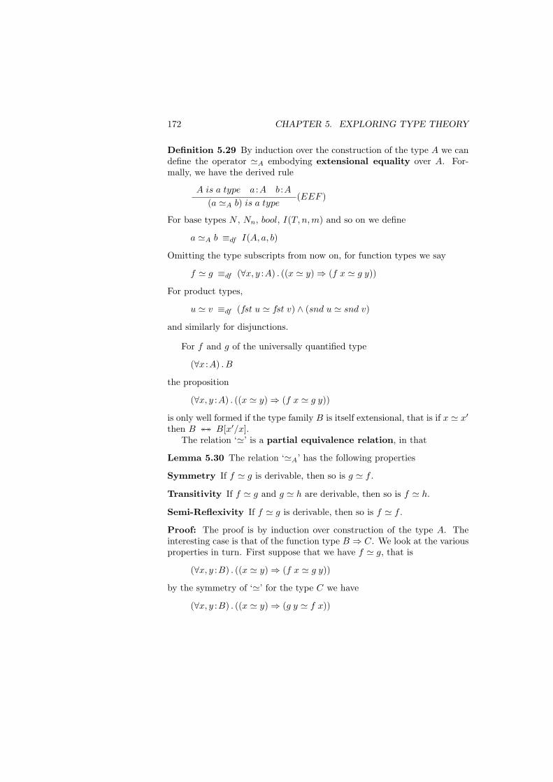
172 CHAPTER 5. EXPLORING TYPE THEORY
Definition 5.29 By induction over the construction of the type A we candefine the operator 'A embodying extensional equality over A. For-mally, we have the derived rule
A is a type a :A b :A(a 'A b) is a type
(EEF )
For base types N , Nn, bool, I(T, n, m) and so on we define
a 'A b ≡df I(A, a, b)
Omitting the type subscripts from now on, for function types we say
f ' g ≡df (∀x, y :A) . ((x ' y)⇒ (f x ' g y))
For product types,
u ' v ≡df (fst u ' fst v) ∧ (snd u ' snd v)
and similarly for disjunctions.
For f and g of the universally quantified type
(∀x :A) . B
the proposition
(∀x, y :A) . ((x ' y)⇒ (f x ' g y))
is only well formed if the type family B is itself extensional, that is if x ' x′
then B ↔↔ B[x′/x].The relation ‘'’ is a partial equivalence relation, in that
Lemma 5.30 The relation ‘'A’ has the following properties
Symmetry If f ' g is derivable, then so is g ' f .
Transitivity If f ' g and g ' h are derivable, then so is f ' h.
Semi-Reflexivity If f ' g is derivable, then so is f ' f .
Proof: The proof is by induction over construction of the type A. Theinteresting case is that of the function type B ⇒ C. We look at the variousproperties in turn. First suppose that we have f ' g, that is
(∀x, y :B) . ((x ' y)⇒ (f x ' g y))
by the symmetry of ‘'’ for the type C we have
(∀x, y :B) . ((x ' y)⇒ (g y ' f x))
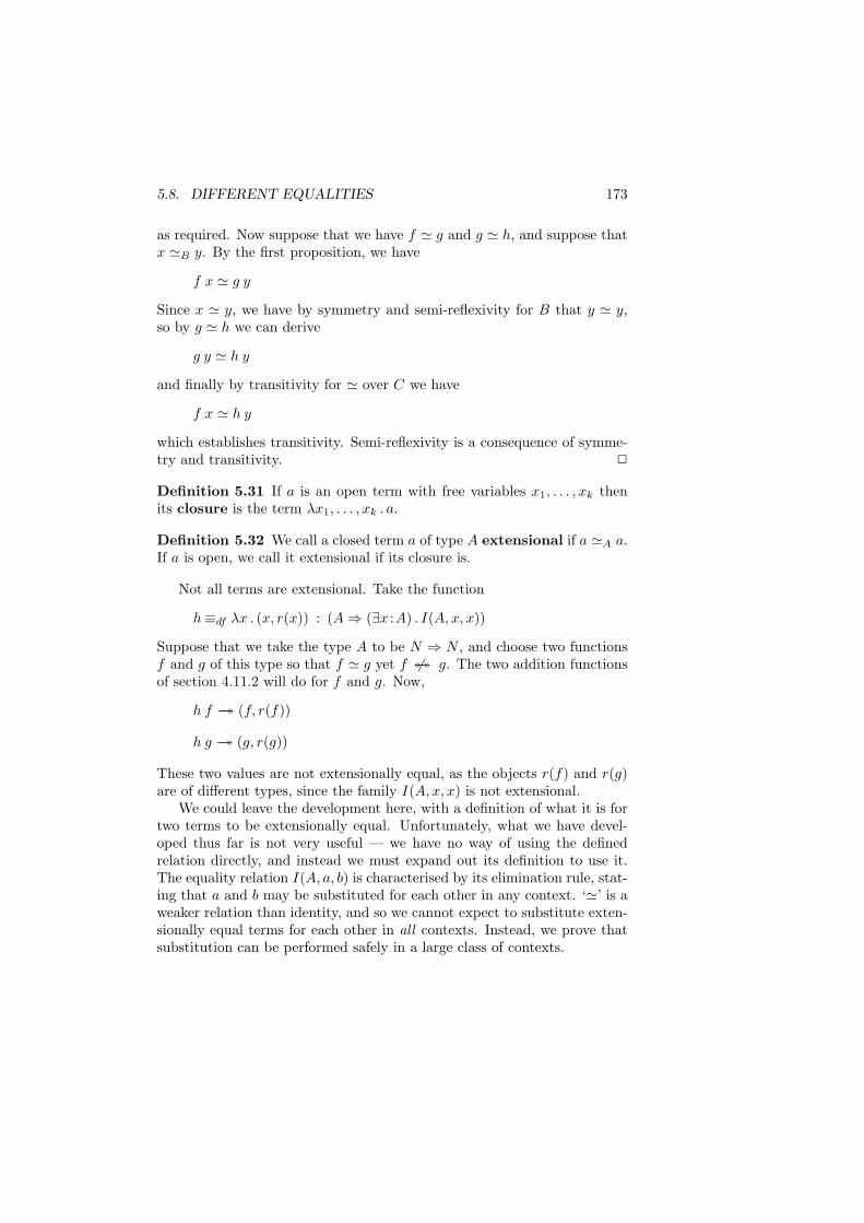
5.8. DIFFERENT EQUALITIES 173
as required. Now suppose that we have f ' g and g ' h, and suppose thatx 'B y. By the first proposition, we have
f x ' g y
Since x ' y, we have by symmetry and semi-reflexivity for B that y ' y,so by g ' h we can derive
g y ' h y
and finally by transitivity for ' over C we have
f x ' h y
which establishes transitivity. Semi-reflexivity is a consequence of symme-try and transitivity. 2
Definition 5.31 If a is an open term with free variables x1, . . . , xk thenits closure is the term λx1, . . . , xk . a.
Definition 5.32 We call a closed term a of type A extensional if a 'A a.If a is open, we call it extensional if its closure is.
Not all terms are extensional. Take the function
h≡df λx . (x, r(x)) : (A⇒ (∃x :A) . I(A, x, x))
Suppose that we take the type A to be N ⇒ N , and choose two functionsf and g of this type so that f ' g yet f 6↔↔ g. The two addition functionsof section 4.11.2 will do for f and g. Now,
h f →→ (f, r(f))
h g →→ (g, r(g))
These two values are not extensionally equal, as the objects r(f) and r(g)are of different types, since the family I(A, x, x) is not extensional.
We could leave the development here, with a definition of what it is fortwo terms to be extensionally equal. Unfortunately, what we have devel-oped thus far is not very useful — we have no way of using the definedrelation directly, and instead we must expand out its definition to use it.The equality relation I(A, a, b) is characterised by its elimination rule, stat-ing that a and b may be substituted for each other in any context. ‘'’ is aweaker relation than identity, and so we cannot expect to substitute exten-sionally equal terms for each other in all contexts. Instead, we prove thatsubstitution can be performed safely in a large class of contexts.
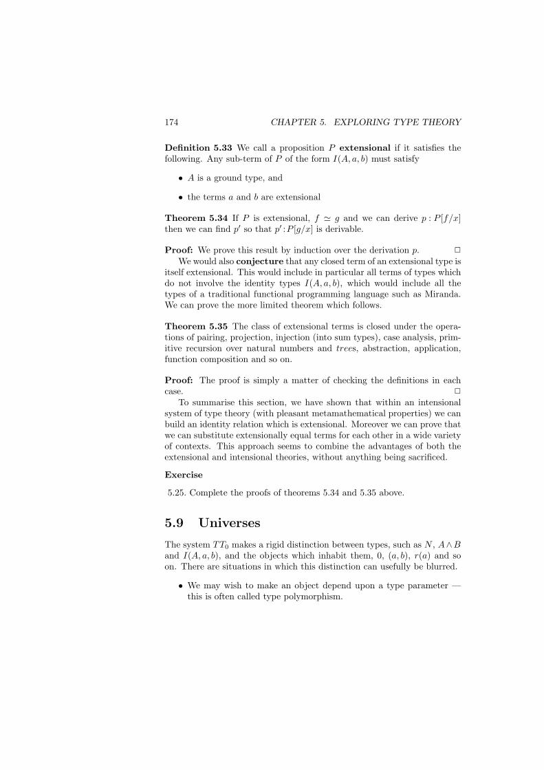
174 CHAPTER 5. EXPLORING TYPE THEORY
Definition 5.33 We call a proposition P extensional if it satisfies thefollowing. Any sub-term of P of the form I(A, a, b) must satisfy
• A is a ground type, and
• the terms a and b are extensional
Theorem 5.34 If P is extensional, f ' g and we can derive p : P [f/x]then we can find p′ so that p′ :P [g/x] is derivable.
Proof: We prove this result by induction over the derivation p. 2
We would also conjecture that any closed term of an extensional type isitself extensional. This would include in particular all terms of types whichdo not involve the identity types I(A, a, b), which would include all thetypes of a traditional functional programming language such as Miranda.We can prove the more limited theorem which follows.
Theorem 5.35 The class of extensional terms is closed under the opera-tions of pairing, projection, injection (into sum types), case analysis, prim-itive recursion over natural numbers and trees, abstraction, application,function composition and so on.
Proof: The proof is simply a matter of checking the definitions in eachcase. 2
To summarise this section, we have shown that within an intensionalsystem of type theory (with pleasant metamathematical properties) we canbuild an identity relation which is extensional. Moreover we can prove thatwe can substitute extensionally equal terms for each other in a wide varietyof contexts. This approach seems to combine the advantages of both theextensional and intensional theories, without anything being sacrificed.
Exercise
5.25. Complete the proofs of theorems 5.34 and 5.35 above.
5.9 Universes
The system TT0 makes a rigid distinction between types, such as N , A∧Band I(A, a, b), and the objects which inhabit them, 0, (a, b), r(a) and soon. There are situations in which this distinction can usefully be blurred.
• We may wish to make an object depend upon a type parameter —this is often called type polymorphism.
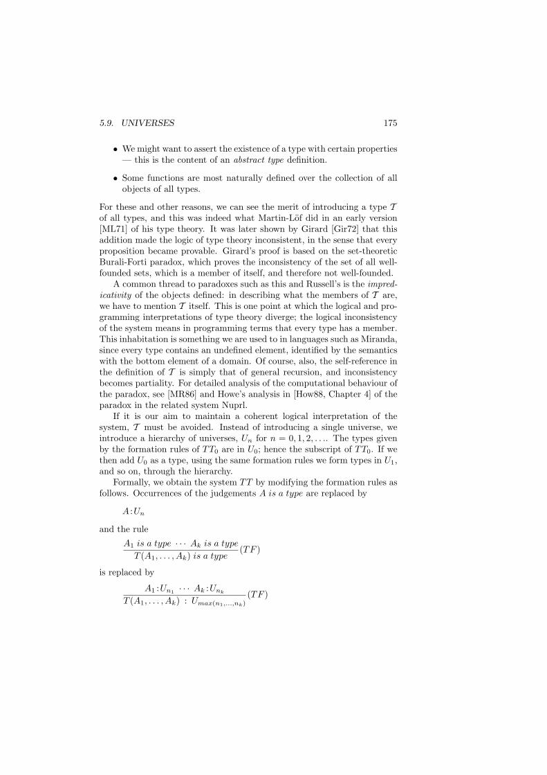
5.9. UNIVERSES 175
• We might want to assert the existence of a type with certain properties— this is the content of an abstract type definition.
• Some functions are most naturally defined over the collection of allobjects of all types.
For these and other reasons, we can see the merit of introducing a type Tof all types, and this was indeed what Martin-Lof did in an early version[ML71] of his type theory. It was later shown by Girard [Gir72] that thisaddition made the logic of type theory inconsistent, in the sense that everyproposition became provable. Girard’s proof is based on the set-theoreticBurali-Forti paradox, which proves the inconsistency of the set of all well-founded sets, which is a member of itself, and therefore not well-founded.
A common thread to paradoxes such as this and Russell’s is the impred-icativity of the objects defined: in describing what the members of T are,we have to mention T itself. This is one point at which the logical and pro-gramming interpretations of type theory diverge; the logical inconsistencyof the system means in programming terms that every type has a member.This inhabitation is something we are used to in languages such as Miranda,since every type contains an undefined element, identified by the semanticswith the bottom element of a domain. Of course, also, the self-reference inthe definition of T is simply that of general recursion, and inconsistencybecomes partiality. For detailed analysis of the computational behaviour ofthe paradox, see [MR86] and Howe’s analysis in [How88, Chapter 4] of theparadox in the related system Nuprl.
If it is our aim to maintain a coherent logical interpretation of thesystem, T must be avoided. Instead of introducing a single universe, weintroduce a hierarchy of universes, Un for n = 0, 1, 2, . . .. The types givenby the formation rules of TT0 are in U0; hence the subscript of TT0. If wethen add U0 as a type, using the same formation rules we form types in U1,and so on, through the hierarchy.
Formally, we obtain the system TT by modifying the formation rules asfollows. Occurrences of the judgements A is a type are replaced by
A :Un
and the rule
A1 is a type · · · Ak is a type
T (A1, . . . , Ak) is a type(TF )
is replaced by
A1 :Un1 · · · Ak :Unk
T (A1, . . . , Ak) : Umax(n1,...,nk)(TF )
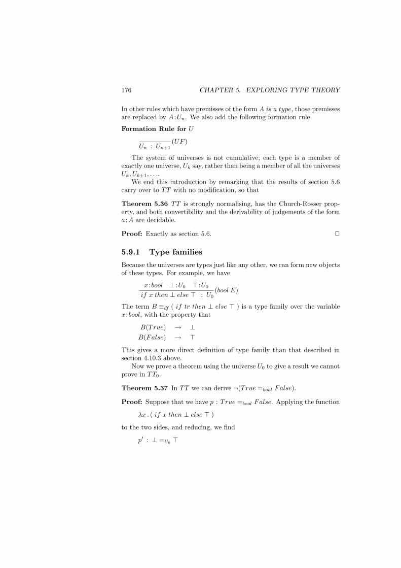
176 CHAPTER 5. EXPLORING TYPE THEORY
In other rules which have premisses of the form A is a type, those premissesare replaced by A :Un. We also add the following formation rule
Formation Rule for U
Un : Un+1(UF )
The system of universes is not cumulative; each type is a member ofexactly one universe, Uk say, rather than being a member of all the universesUk, Uk+1, . . ..
We end this introduction by remarking that the results of section 5.6carry over to TT with no modification, so that
Theorem 5.36 TT is strongly normalising, has the Church-Rosser prop-erty, and both convertibility and the derivability of judgements of the forma :A are decidable.
Proof: Exactly as section 5.6. 2
5.9.1 Type families
Because the universes are types just like any other, we can form new objectsof these types. For example, we have
x :bool ⊥ :U0 > :U0
if x then ⊥ else > : U0(bool E)
The term B ≡df ( if tr then ⊥ else > ) is a type family over the variablex :bool, with the property that
B(True) → ⊥B(False) → >
This gives a more direct definition of type family than that described insection 4.10.3 above.
Now we prove a theorem using the universe U0 to give a result we cannotprove in TT0.
Theorem 5.37 In TT we can derive ¬(True =bool False).
Proof: Suppose that we have p : True =bool False. Applying the function
λx . ( if x then ⊥ else > )
to the two sides, and reducing, we find
p′ : ⊥ =U0 >
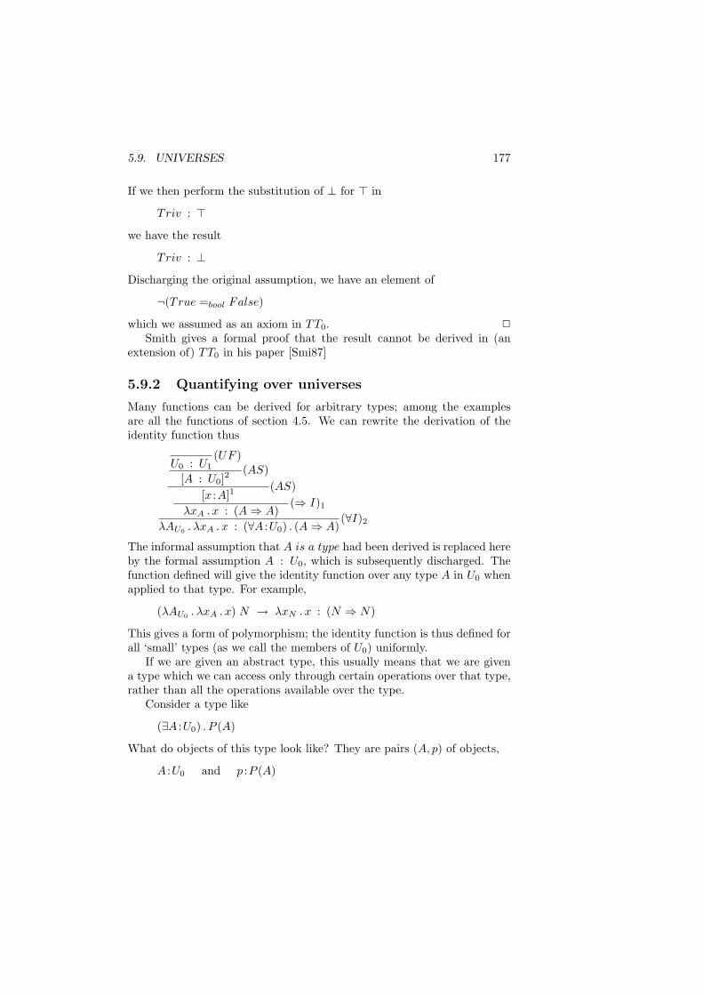
5.9. UNIVERSES 177
If we then perform the substitution of ⊥ for > in
Triv : >
we have the result
Triv : ⊥
Discharging the original assumption, we have an element of
¬(True =bool False)
which we assumed as an axiom in TT0. 2
Smith gives a formal proof that the result cannot be derived in (anextension of) TT0 in his paper [Smi87]
5.9.2 Quantifying over universes
Many functions can be derived for arbitrary types; among the examplesare all the functions of section 4.5. We can rewrite the derivation of theidentity function thus
U0 : U1(UF )
[A : U0]2(AS)
[x :A]1(AS)
λxA . x : (A⇒ A)(⇒ I)1
λAU0 . λxA . x : (∀A :U0) . (A⇒ A)(∀I)2
The informal assumption that A is a type had been derived is replaced hereby the formal assumption A : U0, which is subsequently discharged. Thefunction defined will give the identity function over any type A in U0 whenapplied to that type. For example,
(λAU0 . λxA . x) N → λxN . x : (N ⇒ N)
This gives a form of polymorphism; the identity function is thus defined forall ‘small’ types (as we call the members of U0) uniformly.
If we are given an abstract type, this usually means that we are givena type which we can access only through certain operations over that type,rather than all the operations available over the type.
Consider a type like
(∃A :U0) . P (A)
What do objects of this type look like? They are pairs (A, p) of objects,
A :U0 and p :P (A)
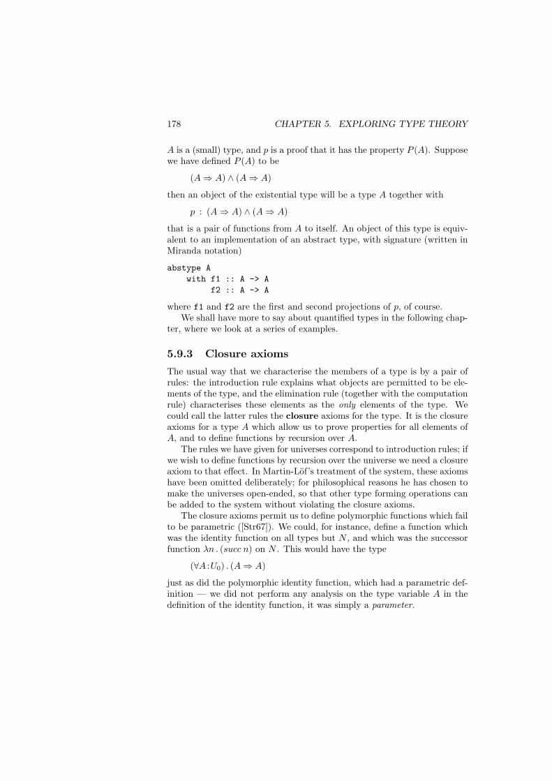
178 CHAPTER 5. EXPLORING TYPE THEORY
A is a (small) type, and p is a proof that it has the property P (A). Supposewe have defined P (A) to be
(A⇒ A) ∧ (A⇒ A)
then an object of the existential type will be a type A together with
p : (A⇒ A) ∧ (A⇒ A)
that is a pair of functions from A to itself. An object of this type is equiv-alent to an implementation of an abstract type, with signature (written inMiranda notation)
abstype Awith f1 :: A -> A
f2 :: A -> A
where f1 and f2 are the first and second projections of p, of course.We shall have more to say about quantified types in the following chap-
ter, where we look at a series of examples.
5.9.3 Closure axioms
The usual way that we characterise the members of a type is by a pair ofrules: the introduction rule explains what objects are permitted to be ele-ments of the type, and the elimination rule (together with the computationrule) characterises these elements as the only elements of the type. Wecould call the latter rules the closure axioms for the type. It is the closureaxioms for a type A which allow us to prove properties for all elements ofA, and to define functions by recursion over A.
The rules we have given for universes correspond to introduction rules; ifwe wish to define functions by recursion over the universe we need a closureaxiom to that effect. In Martin-Lof’s treatment of the system, these axiomshave been omitted deliberately; for philosophical reasons he has chosen tomake the universes open-ended, so that other type forming operations canbe added to the system without violating the closure axioms.
The closure axioms permit us to define polymorphic functions which failto be parametric ([Str67]). We could, for instance, define a function whichwas the identity function on all types but N , and which was the successorfunction λn . (succ n) on N . This would have the type
(∀A :U0) . (A⇒ A)
just as did the polymorphic identity function, which had a parametric def-inition — we did not perform any analysis on the type variable A in thedefinition of the identity function, it was simply a parameter.
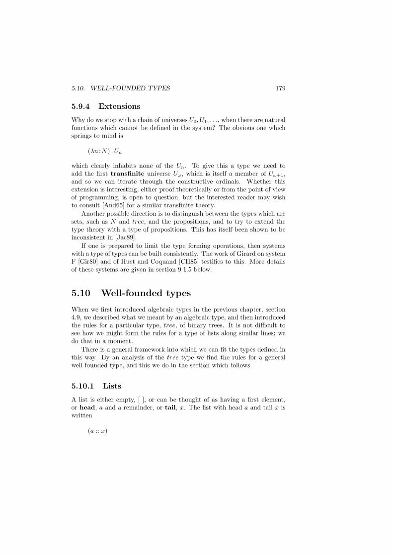
5.10. WELL-FOUNDED TYPES 179
5.9.4 Extensions
Why do we stop with a chain of universes U0, U1, . . ., when there are naturalfunctions which cannot be defined in the system? The obvious one whichsprings to mind is
(λn :N) . Un
which clearly inhabits none of the Un. To give this a type we need toadd the first transfinite universe Uω, which is itself a member of Uω+1,and so we can iterate through the constructive ordinals. Whether thisextension is interesting, either proof theoretically or from the point of viewof programming, is open to question, but the interested reader may wishto consult [And65] for a similar transfinite theory.
Another possible direction is to distinguish between the types which aresets, such as N and tree, and the propositions, and to try to extend thetype theory with a type of propositions. This has itself been shown to beinconsistent in [Jac89].
If one is prepared to limit the type forming operations, then systemswith a type of types can be built consistently. The work of Girard on systemF [Gir80] and of Huet and Coquand [CH85] testifies to this. More detailsof these systems are given in section 9.1.5 below.
5.10 Well-founded types
When we first introduced algebraic types in the previous chapter, section4.9, we described what we meant by an algebraic type, and then introducedthe rules for a particular type, tree, of binary trees. It is not difficult tosee how we might form the rules for a type of lists along similar lines; wedo that in a moment.
There is a general framework into which we can fit the types defined inthis way. By an analysis of the tree type we find the rules for a generalwell-founded type, and this we do in the section which follows.
5.10.1 Lists
A list is either empty, [ ], or can be thought of as having a first element,or head, a and a remainder, or tail, x. The list with head a and tail x iswritten
(a :: x)
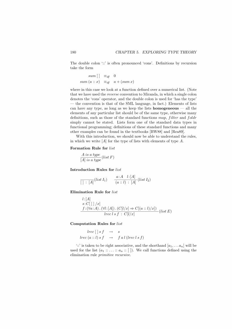
180 CHAPTER 5. EXPLORING TYPE THEORY
The double colon ‘::’ is often pronounced ‘cons’. Definitions by recursiontake the form
sum [ ] ≡df 0sum (a :: x) ≡df a + (sum x)
where in this case we look at a function defined over a numerical list. (Notethat we have used the reverse convention to Miranda, in which a single colondenotes the ‘cons’ operator, and the double colon is used for ‘has the type’— the convention is that of the SML language, in fact.) Elements of listscan have any type, as long as we keep the lists homogeneous — all theelements of any particular list should be of the same type, otherwise manydefinitions, such as those of the standard functions map, filter and foldrsimply cannot be stated. Lists form one of the standard data types infunctional programming; definitions of these standard functions and manyother examples can be found in the textbooks [BW88] and [Rea89].
With this introduction, we should now be able to understand the rules,in which we write [A] for the type of lists with elements of type A.
Formation Rule for list
A is a type
[A] is a type(list F )
Introduction Rules for list
[ ] : [A](list I1)
a :A l : [A](a :: l) : [A]
(list I2)
Elimination Rule for list
l : [A]s :C[ [ ] /x]f : (∀a :A) . (∀l : [A]) . (C[l/x]⇒ C[(a :: l)/x])
lrec l s f : C[l/x](list E)
Computation Rules for list
lrec [ ] s f → s
lrec (a :: l) s f → f a l (lrec l s f)
‘::’ is taken to be right associative, and the shorthand [a1, . . . an] will beused for the list (a1 :: . . . :: an :: [ ]). We call functions defined using theelimination rule primitive recursive.
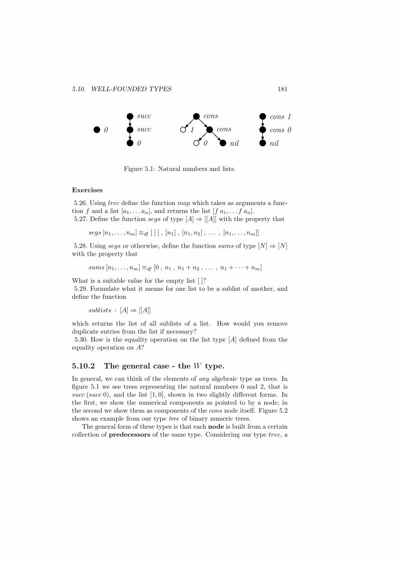
5.10. WELL-FOUNDED TYPES 181
y0
ysucc?ysucc?y0
ycons@
@R
g 1 ycons@
@R
ynilg 0
ycons 1?ycons 0?ynil
Figure 5.1: Natural numbers and lists.
Exercises
5.26. Using lrec define the function map which takes as arguments a func-tion f and a list [a1, . . . an], and returns the list [f a1, . . . f an].5.27. Define the function segs of type [A]⇒ [[A]] with the property that
segs [n1, . . . , nm]≡df [ [ ] , [n1] , [n1, n2] , . . . , [n1, . . . , nm]]
5.28. Using segs or otherwise, define the function sums of type [N ]⇒ [N ]with the property that
sums [n1, . . . , nm]≡df [0 , n1 , n1 + n2 , . . . , n1 + · · ·+ nm]
What is a suitable value for the empty list [ ]?5.29. Formulate what it means for one list to be a sublist of another, and
define the function
sublists : [A]⇒ [[A]]
which returns the list of all sublists of a list. How would you removeduplicate entries from the list if necessary?5.30. How is the equality operation on the list type [A] defined from the
equality operation on A?
5.10.2 The general case - the W type.
In general, we can think of the elements of any algebraic type as trees. Infigure 5.1 we see trees representing the natural numbers 0 and 2, that issucc (succ 0), and the list [1, 0], shown in two slightly different forms. Inthe first, we show the numerical components as pointed to by a node; inthe second we show them as components of the cons node itself. Figure 5.2shows an example from our type tree of binary numeric trees.
The general form of these types is that each node is built from a certaincollection of predecessors of the same type. Considering our type tree, a
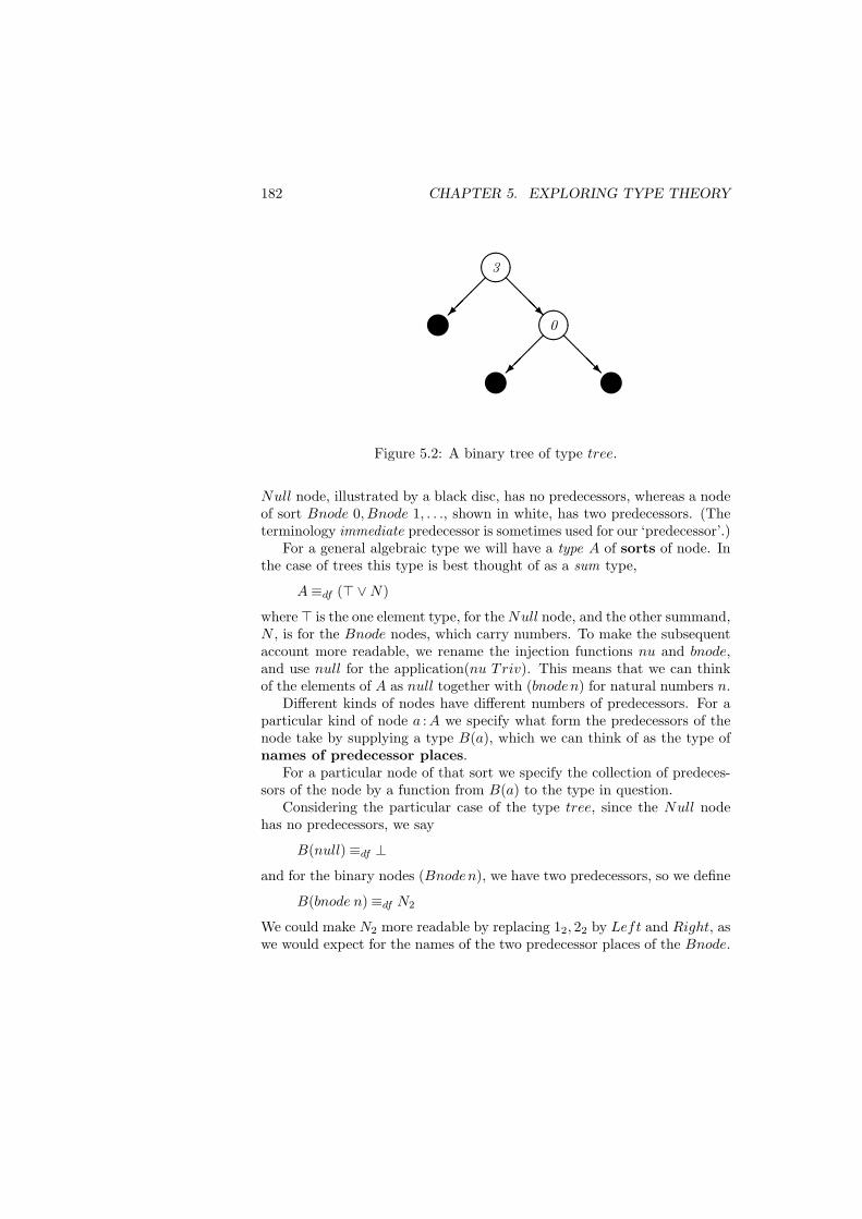
182 CHAPTER 5. EXPLORING TYPE THEORY
3
@@@R
~ 0
@@@R
~~
Figure 5.2: A binary tree of type tree.
Null node, illustrated by a black disc, has no predecessors, whereas a nodeof sort Bnode 0, Bnode 1, . . ., shown in white, has two predecessors. (Theterminology immediate predecessor is sometimes used for our ‘predecessor’.)
For a general algebraic type we will have a type A of sorts of node. Inthe case of trees this type is best thought of as a sum type,
A≡df (> ∨N)
where> is the one element type, for the Null node, and the other summand,N , is for the Bnode nodes, which carry numbers. To make the subsequentaccount more readable, we rename the injection functions nu and bnode,and use null for the application(nu Triv). This means that we can thinkof the elements of A as null together with (bnoden) for natural numbers n.
Different kinds of nodes have different numbers of predecessors. For aparticular kind of node a :A we specify what form the predecessors of thenode take by supplying a type B(a), which we can think of as the type ofnames of predecessor places.
For a particular node of that sort we specify the collection of predeces-sors of the node by a function from B(a) to the type in question.
Considering the particular case of the type tree, since the Null nodehas no predecessors, we say
B(null)≡df ⊥
and for the binary nodes (Bnoden), we have two predecessors, so we define
B(bnode n)≡df N2
We could make N2 more readable by replacing 12, 22 by Left and Right, aswe would expect for the names of the two predecessor places of the Bnode.
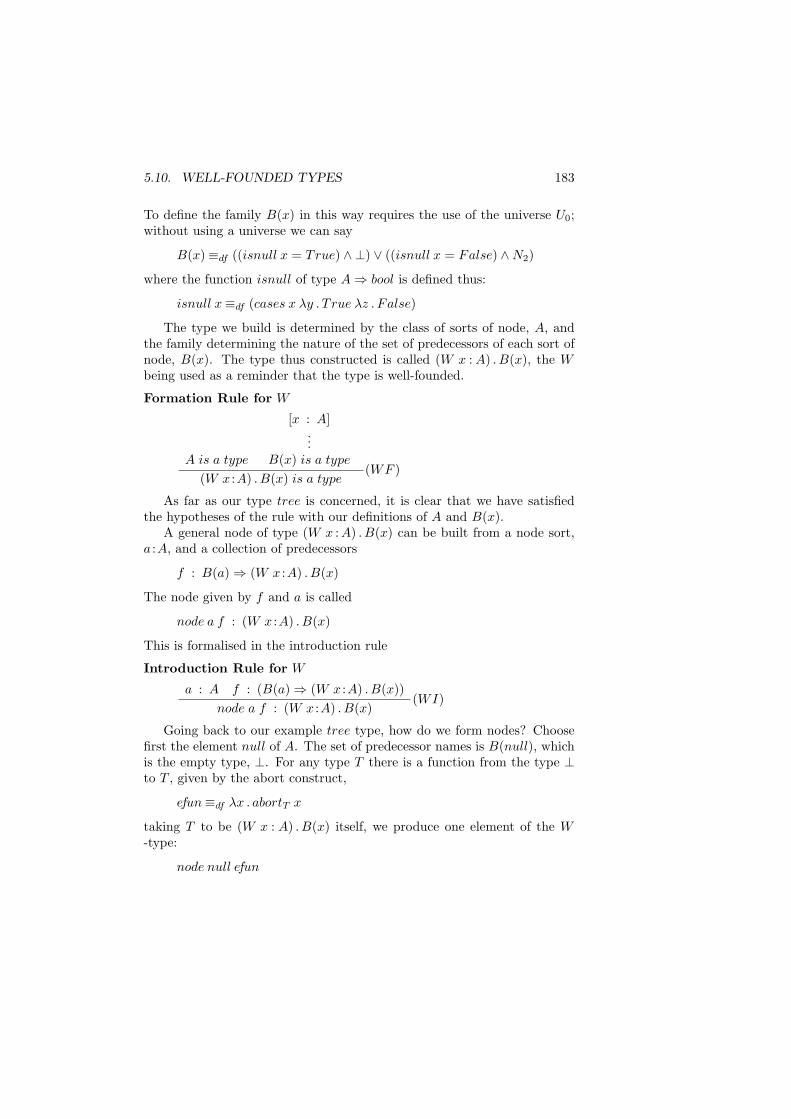
5.10. WELL-FOUNDED TYPES 183
To define the family B(x) in this way requires the use of the universe U0;without using a universe we can say
B(x)≡df ((isnull x = True) ∧ ⊥) ∨ ((isnull x = False) ∧N2)
where the function isnull of type A⇒ bool is defined thus:
isnull x≡df (cases x λy . True λz . False)
The type we build is determined by the class of sorts of node, A, andthe family determining the nature of the set of predecessors of each sort ofnode, B(x). The type thus constructed is called (W x : A) . B(x), the Wbeing used as a reminder that the type is well-founded.
Formation Rule for W
A is a type
[x : A]...
B(x) is a type
(W x :A) . B(x) is a type(WF )
As far as our type tree is concerned, it is clear that we have satisfiedthe hypotheses of the rule with our definitions of A and B(x).
A general node of type (W x :A) . B(x) can be built from a node sort,a :A, and a collection of predecessors
f : B(a)⇒ (W x :A) . B(x)
The node given by f and a is called
node a f : (W x :A) . B(x)
This is formalised in the introduction rule
Introduction Rule for W
a : A f : (B(a)⇒ (W x :A) . B(x))node a f : (W x :A) . B(x)
(WI)
Going back to our example tree type, how do we form nodes? Choosefirst the element null of A. The set of predecessor names is B(null), whichis the empty type, ⊥. For any type T there is a function from the type ⊥to T , given by the abort construct,
efun≡df λx . abortT x
taking T to be (W x : A) . B(x) itself, we produce one element of the W-type:
node null efun
184 CHAPTER 5. EXPLORING TYPE THEORY
This is the representative of the node Null, which has no predecessors, andthe argument above constitutes an informal derivation of the rule (treeI1).How can we derive the other tree introduction rule from (WI)? The hy-potheses of (treeI2) are that n :N , u : tree and v : tree. The term
fu,v ≡df λx . (cases2 x u v)
is of type (N2 ⇒ tree), and N2 ≡ B(bnode n), which means that this isa predecessor function for a (bnode n) node. Formally, (WI) allows theformation of
node (bnode n) fu,v
which represents the node (Bnode n u v). Using the notation Null for theterm (node null efun), the node
node (bnode 3) fNull,g
where g ≡ (node (bnode 0) fNull,Null), represents the tree
Bnode 3 Null (Bnode 0 Null Null)
as illustrated in figure 5.2.We eliminate a node by the operator which performs recursion or in-
duction, which we shall call Rec. The idea of an induction is to prove
C(node a f)
on the basis of proofs of
C(p)
for all the predecessors p of the node. Remember that the predecessorsare given by the values of the function f over the type B(a), so that thiscollection of proofs will have the form
pr : (∀y : B(a)).C(f y)
The object which performs the proof transformation, i.e. the induction stepof the proof, for a particular node (node a f) is therefore an object tra,f oftype
tra,f : (∀y : B(a)).(C(f y)⇒ C(node a f))
Finally, this should be parametrised over f and a, giving our general prooftransformer or induction step as an object of type
(∀a : A)(∀f : (B(a)⇒ (W x :A) . B(x)))((∀y : B(a))C(f y)⇒ C(node a f))
5.10. WELL-FOUNDED TYPES 185
which we shall abbreviate Ind(A,B,C). Now we can state our rule
Elimination Rule for W
w : (W x :A) . B(x) R :Ind(A,B,C)(Rec w R) : C(w)
(WE)
Note that on the basis of this, if we discharge the first assumption, we have
λw.(Rec w R) : (∀w : ((W x :A) . B(x))) . C(w)
showing that the rule (WE) defines a function over the well-founded type(W x : A) . B(x) by induction. What is the computation rule for theseobjects? The value at a node (nodeaf) is computed from the values at thepredecessors, and those predecessors themselves, using the R operator.
Computation Rule for W
Rec (node a f) R → R a f (λx .Rec (f x) R)
Observe that as x ranges over B(a), (f x) ranges over the predecessors ofnode a f , so that
λx . Rec (f x) R
ranges over the values of the recursive function on the predecessors of thenode node a f . Also the parameter f specifies the predecessors themselves.
Consider the type tree again. How do the elimination and computationrules for the W type generalise those for tree? In the case of tree, recallthat
A ≡df (> ∨N)B(null) ≡df ⊥
B(bnode n) ≡df N2
How can we define an operator R
R : (∀a : A)(∀f : (B(a)⇒ (W x :A) . B(x)))((∀y : B(a))C(f y)⇒ C(node a f))
for these types? We need to define R(a) for each a in A. Starting withnull, we have to define an object of type
(∀f : (⊥ ⇒ (W x :A) . B(x)))((∀y : ⊥)C(f y)⇒ C(node a f))
What are the functions f of type (⊥ ⇒ (W x :A) . B(x))? If we adopt anextensional approach there is but one, the function efun, since the domain
186 CHAPTER 5. EXPLORING TYPE THEORY
of the function is the empty type. In that case we have to define an objectof type
((∀y : ⊥)C(f y)⇒ C(Null))
(where we replace (node null efun) with Null). What is the domain typehere? Again it is easy to argue that there is a single function in the de-pendent type (∀y : ⊥)C(f y), so that the function type above collapsesto
C(Null)
In other words, our starting value for the induction is a single value c oftype C(Null), just as it is in the rule (treeE). A similar argument, withfewer simplifications, allows us to see that the case of the nodes
(Bnode n u v)
is also covered by R applied to the elements (bnode n) — we leave this asan exercise for the reader.
Finally, we look at the computation rule in the case of the Null node.We assume that R is determined for tree as outlined above, and note thatthe general rule is
Rec (node a f) R → R a f (λx .Rec (f x) R)
In the case of (node null efun), it becomes
Rec Null R → R null efun (λx . Rec (efun x) R)
but recalling the definition above, the right hand side is simply the valuec :C(null). A similar argument applies in the Bnode case.
It is worth observing that we needed to move to an extensional equalitybetween functions to prove the uniqueness of the function from an emptydomain. If it is wished to remain in an intensional system, the alterna-tive seems to be to introduce the rules explicitly, type-by-type. Anotheralternative is to introduce a type of finite functions, which can be treatedextensionally in an intensional system; this would only work for a limitedclass of W types, in which A is finite and B(a) is finite for each a :A.
Making the argument above more formal, we can say that we haveestablished that certain types are extensionally isomorphic, where this isdefined thus.
Definition 5.38 Two types A and B are extensionally isomorphic ifthere are two functions
f :A⇒ B g :B ⇒ A
5.10. WELL-FOUNDED TYPES 187
so that the following proposition is derivable.
(∀x :A) . (g(f x) 'A x) ∧ (∀y :B) . (f(g y) 'B y)
The two functions f, g form an isomorphism pair, up to extensional equality.
We can simplify some of the notation above when we are looking at therecursive definitions of functions of non-dependent type — in these cases Cwill not be parametrised. Note that in proofs, though, it is crucial that C isparametrised, as otherwise we are proving the same proposition repeatedly,which is safe but not very useful.
As we remarked earlier, these recursions and inductions are made muchmore readable by the introduction of names. This is clearly a feature whichhas to be added to the W -types as ‘syntactic sugar’ if they are to be usedin a real programming environment.
Definition 5.39 We call the system of TT with the full rules for W TT+,retaining the name TT for the system containing just tree or equivalentlyall W types for which all the predecessor types B(a) are finite.
Theorem 5.40 TT+ is strongly normalising, has the Church-Rosser prop-erty, and both convertibility and the derivability of judgements of the forma :A are decidable.
Proof: Exactly as section 5.6. 2
5.10.3 Algebraic types in Miranda
Our method here has been adopted for two reasons. It provides a simple wayof writing down objects like trees without our having to introduce namesfor constructors, which is what we do in (e.g.) Miranda. We also see thatit provides a non-trivial generalisation of finite ‘algebraic’ types. There wasno stipulation that the sets of predecessor places, B(a), need be finite, andso we can have infinitely branching trees as objects of our language. Thisallows us to define, for example, the countable ordinal numbers. In fact,we can do a similar thing in Miranda, thus:
ordinal ::= Zero |Succ ordinal |Limit (nat -> ordinal)
In fact, in Miranda we can define more general types still.
• We can define a number of types by definitions which are mutuallyrecursive. These, if they are well-founded, can be modelled in TT bya definition of a sum type, from which we project the types of interest.
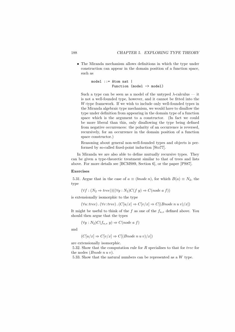
188 CHAPTER 5. EXPLORING TYPE THEORY
• The Miranda mechanism allows definitions in which the type underconstruction can appear in the domain position of a function space,such as
model ::= Atom nat |Function (model -> model)
Such a type can be seen as a model of the untyped λ-calculus — itis not a well-founded type, however, and it cannot be fitted into theW -type framework. If we wish to include only well-founded types inthe Miranda algebraic type mechanism, we would have to disallow thetype under definition from appearing in the domain type of a functionspace which is the argument to a constructor. (In fact we couldbe more liberal than this, only disallowing the type being definedfrom negative occurrences: the polarity of an occurrence is reversed,recursively, for an occurrence in the domain position of a functionspace constructor.)
Reasoning about general non-well-founded types and objects is per-formed by so-called fixed-point induction [Sto77].
In Miranda we are also able to define mutually recursive types. Theycan be given a type-theoretic treatment similar to that of trees and listsabove. For more details see [BCMS89, Section 6], or the paper [PS87].
Exercises
5.31. Argue that in the case of a ≡ (bnode n), for which B(a) ≡ N2, thetype
(∀f : (N2 ⇒ tree))((∀y : N2)C(f y)⇒ C(node a f))
is extensionally isomorphic to the type
(∀u : tree) . (∀v : tree) . (C[u/x]⇒ C[v/x]⇒ C[(Bnode n u v)/x])
It might be useful to think of the f as one of the fu,v defined above. Youshould then argue that the types
(∀y : N2)C(fu,v y)⇒ C(node a f)
and
(C[u/x]⇒ C[v/x]⇒ C[(Bnode n u v)/x])
are extensionally isomorphic.5.32. Show that the computation rule for R specialises to that for trec forthe nodes (Bnode n u v).5.33. Show that the natural numbers can be represented as a W type.
5.11. EXPRESSIBILITY 189
5.11 Expressibility
This section gives a characterisation of the functions which can be writtenin the system TT0.
Definition 5.41 A term e of TT0 (or TT , TT+) represents the functionf over the natural numbers if and only if for all natural numbers n1, . . . , nk,
e n1 . . . nk →→ f n1 . . . nk
where n is the representation of the natural number n, given by
succ (succ . . . (succ︸ ︷︷ ︸n
0))
How can we characterise the functions f which are representable? First weknow by the normalisation theorem that they are recursive, since for eachterm e, to find the value of
e n1 . . . nk
we simply have to reduce the expression to normal form, and the applicationof the rules is certainly a mechanical process. It is equally clear that wecannot represent all recursive functions in this way, since if we could adiagonalisation argument would lead to a contradiction. (For an expositionof the elementary details of computability theory see, for example, [Cut81,Rog67].)
We thus have that the class of functions is properly contained betweenthe classes of primitive recursive functions and total recursive functions. Aclue to the precise characterisation lies in the normalisation result, and theformalisation of its proof term by term.
Theorem 5.42 For each term e of TT0, the proof of normalisation of ecan be formalised in the theory of first-order intuitionistic arithmetic, HA,or its classical counterpart PA.
Proof: The proof uses a coding (or Godel numbering) of the system TT0
within the theory of arithmetic. It involves checking that the steps of theproof outlined in section 5.6 can be encoded thus. 2
Note that the result does not claim that the complete normalisationproof can be coded as a whole — the coding is uniform, but the individualresults cannot be combined into a single proof, as the logical complexityof the individual proofs grows unboundedly with the complexity of theexpression e.
Just as we explained what it was for a function f to be representable inone of our type theories, we can define how a function is representable inPA.
190 CHAPTER 5. EXPLORING TYPE THEORY
Definition 5.43 The term g of PA represents a k-ary function f if andonly if for all n1, . . . , nk,
PA ` g n1 . . . nk = f n1 . . . nk
where n is the representation of the natural number n in PA.
Definition 5.44 A representable k-ary function f is provably total inPA (HA) if and only if we can prove in PA (HA) that its representativeis total, i.e.
PA ` (∀ x1, . . . , xk)(∃ y)(g x1 . . . xk = y)
Theorem 5.42 can be seen now in a slightly different light, showing thatevery function representable in TT0 is provably total in PA. We can alsoprove a converse to this, which shows that all functions provable total inPA can be represented in TT0. The origins of this result lie with Godel’sDialectica interpretation of PA in a theory of functions which itself canbe viewed as a subtheory of TT0 [G58]. More details of this and manyother topics relating to the metamathematics of intuitionism can be foundin [Tro73].
Theorem 5.45 A function f over the natural numbers is representable inTT0 if and only if it is provably total in PA (or HA).
The author is unaware of precise characterisations of the functions repre-sentable in the stronger theories TT and TT+, although [Bee85] gives somepartial results, including one for a system with a single universe. Whateverthe case, the class of functions representable in the type theories is verylarge, and indeed it can be argued that this more than encompasses all thefunctions we might ever wish to program. In terms of sheer computationtime all the functions we program are primitive recursive, in the sense thatby suitable transformation any more complex calculations can be boundedby primitive recursive bounds. This is not the most natural way to pro-ceed; in the next chapter we look at the ways in which functions are mostnaturally implemented in the language.
Exercise
5.34. One function which cannot be written in TT is an interpreter for theexpressions of TT itself. Discuss how a bounded interpreter for the languagecan be written.
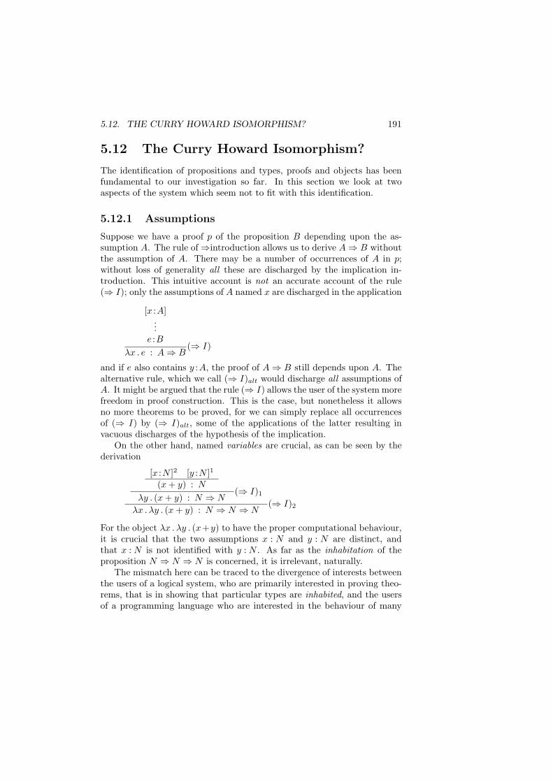
5.12. THE CURRY HOWARD ISOMORPHISM? 191
5.12 The Curry Howard Isomorphism?
The identification of propositions and types, proofs and objects has beenfundamental to our investigation so far. In this section we look at twoaspects of the system which seem not to fit with this identification.
5.12.1 Assumptions
Suppose we have a proof p of the proposition B depending upon the as-sumption A. The rule of⇒introduction allows us to derive A⇒ B withoutthe assumption of A. There may be a number of occurrences of A in p;without loss of generality all these are discharged by the implication in-troduction. This intuitive account is not an accurate account of the rule(⇒ I); only the assumptions of A named x are discharged in the application
[x :A]...
e :Bλx . e : A⇒ B
(⇒ I)
and if e also contains y :A, the proof of A⇒ B still depends upon A. Thealternative rule, which we call (⇒ I)alt would discharge all assumptions ofA. It might be argued that the rule (⇒ I) allows the user of the system morefreedom in proof construction. This is the case, but nonetheless it allowsno more theorems to be proved, for we can simply replace all occurrencesof (⇒ I) by (⇒ I)alt, some of the applications of the latter resulting invacuous discharges of the hypothesis of the implication.
On the other hand, named variables are crucial, as can be seen by thederivation
[x :N ]2 [y :N ]1
(x + y) : N
λy . (x + y) : N ⇒ N(⇒ I)1
λx . λy . (x + y) : N ⇒ N ⇒ N(⇒ I)2
For the object λx . λy . (x+y) to have the proper computational behaviour,it is crucial that the two assumptions x : N and y : N are distinct, andthat x : N is not identified with y : N . As far as the inhabitation of theproposition N ⇒ N ⇒ N is concerned, it is irrelevant, naturally.
The mismatch here can be traced to the divergence of interests betweenthe users of a logical system, who are primarily interested in proving theo-rems, that is in showing that particular types are inhabited, and the usersof a programming language who are interested in the behaviour of many
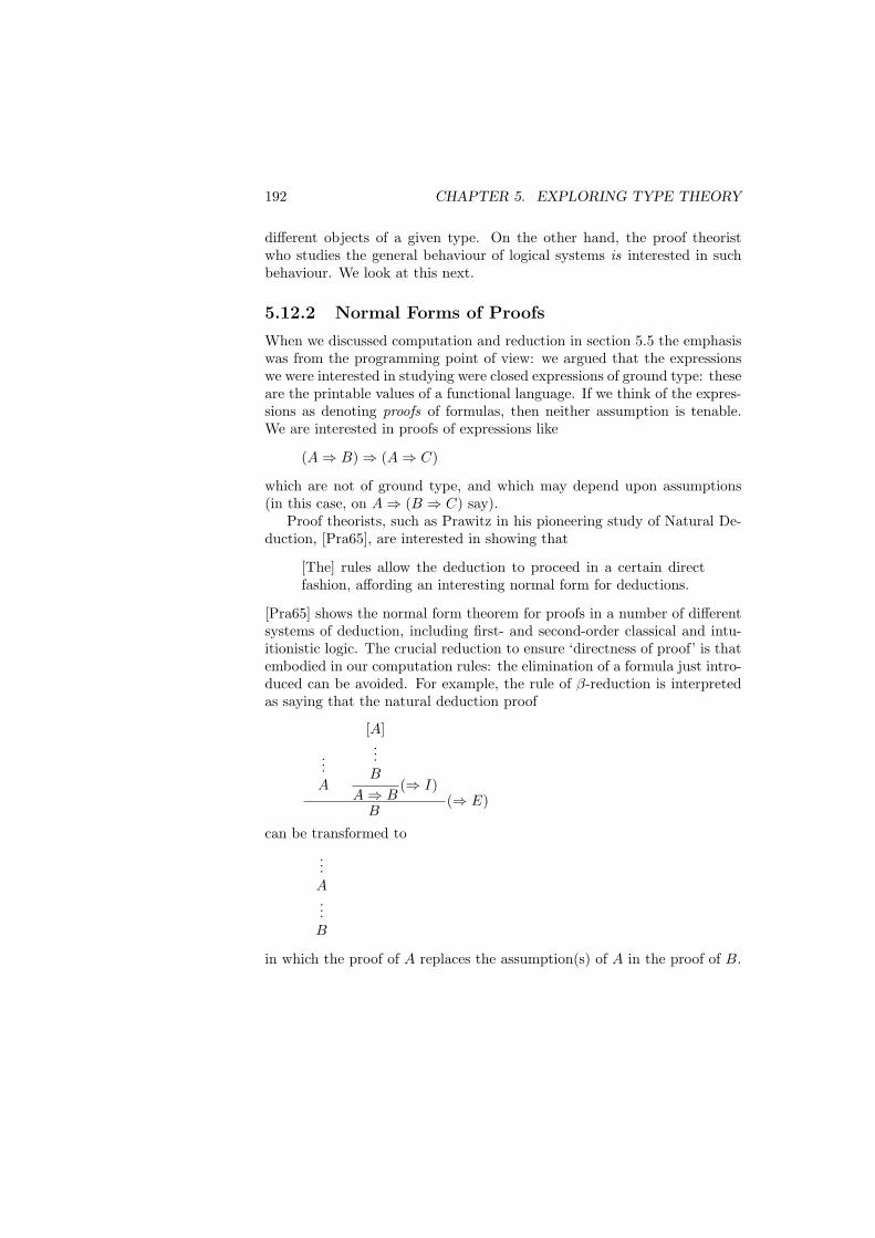
192 CHAPTER 5. EXPLORING TYPE THEORY
different objects of a given type. On the other hand, the proof theoristwho studies the general behaviour of logical systems is interested in suchbehaviour. We look at this next.
5.12.2 Normal Forms of Proofs
When we discussed computation and reduction in section 5.5 the emphasiswas from the programming point of view: we argued that the expressionswe were interested in studying were closed expressions of ground type: theseare the printable values of a functional language. If we think of the expres-sions as denoting proofs of formulas, then neither assumption is tenable.We are interested in proofs of expressions like
(A⇒ B)⇒ (A⇒ C)
which are not of ground type, and which may depend upon assumptions(in this case, on A⇒ (B ⇒ C) say).
Proof theorists, such as Prawitz in his pioneering study of Natural De-duction, [Pra65], are interested in showing that
[The] rules allow the deduction to proceed in a certain directfashion, affording an interesting normal form for deductions.
[Pra65] shows the normal form theorem for proofs in a number of differentsystems of deduction, including first- and second-order classical and intu-itionistic logic. The crucial reduction to ensure ‘directness of proof’ is thatembodied in our computation rules: the elimination of a formula just intro-duced can be avoided. For example, the rule of β-reduction is interpretedas saying that the natural deduction proof
...A
[A]...B
A⇒ B(⇒ I)
B(⇒ E)
can be transformed to
...A...B
in which the proof of A replaces the assumption(s) of A in the proof of B.
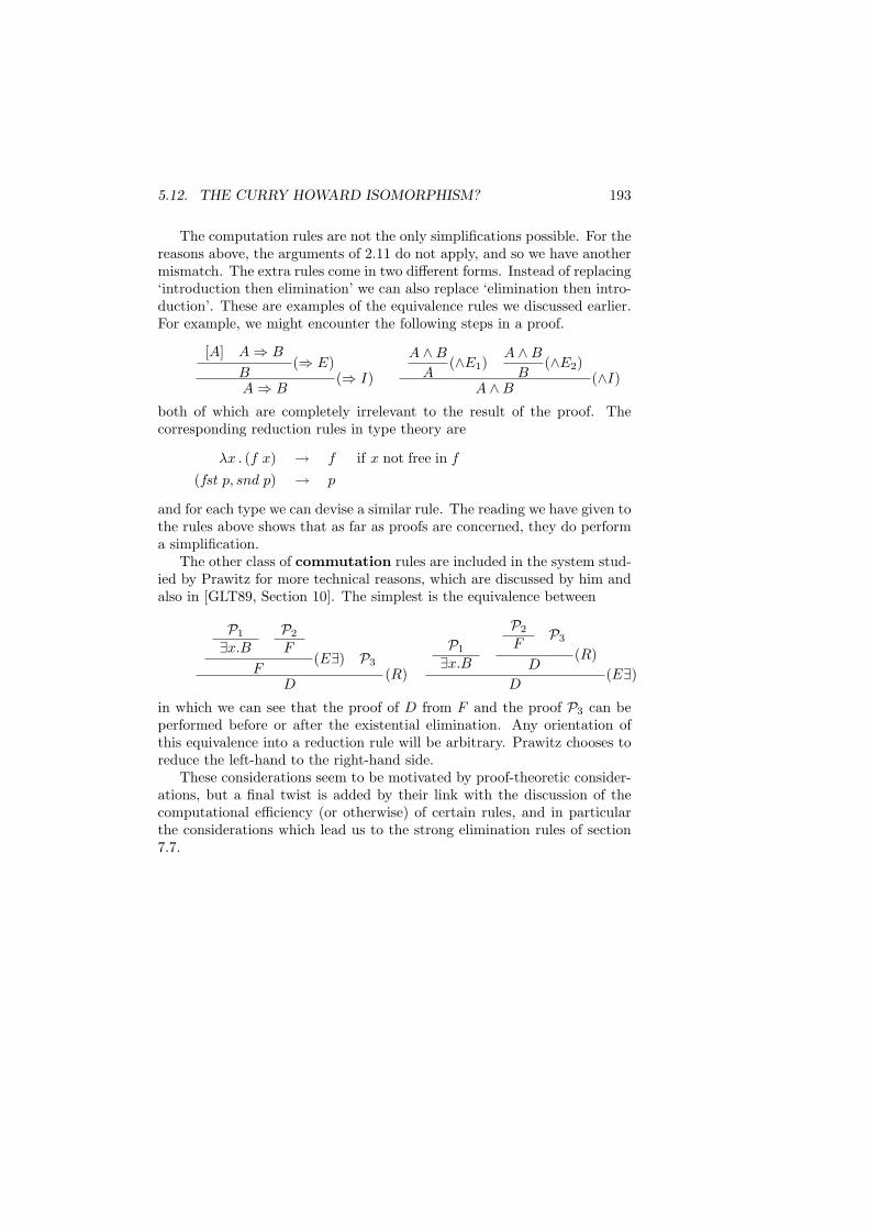
5.12. THE CURRY HOWARD ISOMORPHISM? 193
The computation rules are not the only simplifications possible. For thereasons above, the arguments of 2.11 do not apply, and so we have anothermismatch. The extra rules come in two different forms. Instead of replacing‘introduction then elimination’ we can also replace ‘elimination then intro-duction’. These are examples of the equivalence rules we discussed earlier.For example, we might encounter the following steps in a proof.
[A] A⇒ B
B(⇒ E)
A⇒ B(⇒ I)
A ∧B
A(∧E1)
A ∧B
B(∧E2)
A ∧B(∧I)
both of which are completely irrelevant to the result of the proof. Thecorresponding reduction rules in type theory are
λx . (f x) → f if x not free in f
(fst p, snd p) → p
and for each type we can devise a similar rule. The reading we have given tothe rules above shows that as far as proofs are concerned, they do performa simplification.
The other class of commutation rules are included in the system stud-ied by Prawitz for more technical reasons, which are discussed by him andalso in [GLT89, Section 10]. The simplest is the equivalence between
P1
∃x.BP2
F
F(E∃) P3
D(R)
P1
∃x.B
P2
FP3
D(R)
D(E∃)
in which we can see that the proof of D from F and the proof P3 can beperformed before or after the existential elimination. Any orientation ofthis equivalence into a reduction rule will be arbitrary. Prawitz chooses toreduce the left-hand to the right-hand side.
These considerations seem to be motivated by proof-theoretic consider-ations, but a final twist is added by their link with the discussion of thecomputational efficiency (or otherwise) of certain rules, and in particularthe considerations which lead us to the strong elimination rules of section7.7.

194 CHAPTER 5. EXPLORING TYPE THEORY
Chapter 6
Applying Type Theory
This chapter investigates the different ways in which the system of typetheory can be used.
• We are already familiar with type theory as a constructive logic, andhave seen a number of examples of proofs being built in, for example,sections 4.5 and 4.6.1.
• We have also seen that TT can be seen as a functional programminglanguage, with a number of novel features, such as:
– Every expression has a defined value; every program terminates.
– The system of types is more expressive than those in commonuse, allowing as it does dependent product and function spaces.
– The functional language is integrated with a logic in which toreason about the programs.
• Another view of program development is provided by the insight thatin TT we can think of programs as being extracted from construc-tive proofs. This combines the two interpretations in an elegant andpowerful way.
• Not only can we use the logical system to reason about the prop-erties of programs, we can also use to system to support programtransformation.
• Finally, we show how we can develop imperative programs within atype-theoretic framework.
195
196 CHAPTER 6. APPLYING TYPE THEORY
We begin our discussion by looking at TT as a functional language. Weassume that the reader is familiar with the elements of functional program-ming as covered in [BW88] and [Rea89], so that in choosing examples welook for distinctive features of programming in TT , rather than runningthrough the traditional repertoire of functional programming techniques.In section 6.1 we show how primitive recursion is used to define functionsand types (or propositions). Because the language is terminating, a numberof familiar functions, like the function taking the head of a list, need to bedefined in novel ways. Using the more expressive type system we are able togive the head function its ‘proper’ type, as a function acting over the type ofnon-empty lists. TT contains only primitive recursion over each primitivetype; we show how more complex forms of recursion, like course-of-valuesrecursion, can be programmed in TT .
In section 6.2 we investigate a larger example, that of the quicksortfunction over lists. Here we develop the program first and then prove thatit meets its specification, showing that we have a system in which program-ming and verification are integrated. We follow this with a more detailedsurvey of the uses of dependent types, especially in the presence of uni-verses. These give dependent function and sum types, which can be seento support polymorphic functions, abstract data types, type classes (a laHaskell, [HW90]) and modules. In section 6.4 we apply these ideas in de-veloping a type of vectors.
We look at how programs can be extracted from a number of simplederivations in section 6.5, before discussing a general strategy for programderivation in section 6.6. We also use this opportunity to give a novel viewof specifications in type theory, and examine the ideas in the context of thewell-known problem of the Dutch (or Polish) National Flag.
Our view of programming has been exclusively functional up to thispoint. In section 6.8 we argue that imperative programs can be seen asfunctional programs of a particularly restricted sort, the tail-recursive func-tions. We can thus view TT as extending an imperative programming lan-guage and we give a general result about the transformation of primitiverecursive programs into tail-recursive form, after looking at various concreteexamples.
We conclude the chapter with a survey of other examples discussed inthe literature of type theory.
6.1 Recursion
One of the properties of the systems of type theory TT0, TT and TT+ isstrong normalisation: every computation sequence terminates. This means
6.1. RECURSION 197
that the system does not permit full general recursion to be used, as in anunrestricted form this can lead to non-termination. A simple example isgiven by
f 0 ≡df 0f (n + 1) ≡df f (n + 2) + 1
and other, less obvious, examples can be constructed.As a counterbalance to the weaker recursion operation, we have a more
powerful type system than is common in programming languages. We areable thus to express more precisely the true types of functions, using forinstance the existential quantifier to build a subset type, over which thefunction is total.
In some cases, the definition of the function itself depends upon aninductive proof that it terminates; the effect of this is to give functionswhose definitions manipulate information witnessing certain facts, as well asthe computational data. This intermingling of verification and computationis characteristic of type theory.
We concentrate on examples over the natural numbers and lists in thissection, with some introduction of quantified types as we go along. We lookin more depth at these types in the next section.
Before examining particular examples of definitions, it is worth men-tioning that two general methods present themselves.
• Theorem 5.45 shows that anything provably total in PA can be pro-grammed in TT0, and indeed the proof will provide a term. Thisdoes beg the question of how the function is proved total; we wouldargue that the system TT0 provides exactly the right environment inwhich to give such proofs, as it allows a constructive derivation of thefunction which assures its totality.
• Proof theorists have characterised classes of provably total functionsby means of the well-orderings which can be used in defining thesefunctions by recursion [Sch77]. We could use this characterisation togive functions in TT0, but again would argue for the natural natureof the system itself. There have been a number of proposals for in-corporating principles of well-founded or general recursion; we lookat these in section 7.9.
6.1.1 Numerical functions
We look at some examples embodying common patterns of recursion, andshow how they are coded in TT0. First, consider the naıve addition algo-
198 CHAPTER 6. APPLYING TYPE THEORY
rithm,
add a 0 ≡df a
add a (n + 1) ≡df add (a + 1) n
This appears to be primitive recursive, except for the fact that the argumenta is increased on the recursive call. To make a properly primitive recursivedefinition, we observe that we can define the values add a n simultaneouslyfor all a, by induction on n. In other words, we define the functions
λa . (add a n)
by induction over n. That this is possible is due to the fact that in thedefinition of adda (n+1) we appeal to a value of add with second argumentn. Formally, if we let C ≡df (N ⇒ N), then at the base case we define
c≡df λa . a : C
To give the recursion step, we say
f n h a≡df h (a + 1)
where n, a :N and h :C. This gives
f : (N ⇒ C ⇒ C)
and so by a simplified form of (NE) in which C is constant,
n : N c : C f : (N ⇒ C ⇒ C)prim n c f : C
(NE)
with the reduction properties
prim 0 c f a → c a
≡ (λa . a) a
→ a
prim (n + 1) c f a → f n (prim n c f) a
→ (prim n c f) (a + 1)
We therefore have the definition
add≡df λa . λn . (prim n c f a)
There is an analogy between the generalisation we had to make here, fromdefining one function to defining a class of functions simultaneously, andthe generalisations of induction hypotheses we often have to make when
6.1. RECURSION 199
we prove a result by induction. If + is the usual addition operator and wewish to prove that
add a n = (a + n)
by induction, then the hypothesis we shall have to take is that
(∀a :N) . (add a n = (a + n))
rather than the ‘bare’ equation with a as a parameter.Primitive recursion defines a value at (n + 1) from the value at the
immediate predecessor n — sometimes it is natural to use a value at anumber m smaller than n. A case in point is the power function
power k 0 ≡df 1
power k n ≡df (power k (n div 2))2 ∗ k(n mod 2)
where the value at positive n is derived from that at (n div 2). (Note thatwe are not using the power function in the second multiplicand: this iseither 1 or k depending upon whether n is even or odd. Observe also thatin contrast to the first argument of add that here k is simply a parameterof the definition — its value is unchanged on the recursive call.)
This definition provides an example of a general phenomenon, calledcourse-of-values recursion. To give a sketch of the method, we replace adefinition of the form
f 0 ≡df a
f (n + 1) ≡df . . . f 0 . . . f 1 . . . f n . . .
by a definition of the function
g n≡df [f 0 , . . . , f n]
which has as its value at n the list of values of f on numbers up to n. Thedefinition of g (n + 1) is made by defining f (n + 1) from the list g n andappending the value to the list. We obtain the value f n by taking the lastvalue in the list g n. We shall show how to realise this form of definition intype theory after looking at lists.
Exercises
6.1. Show how to define the ‘natural subtraction’ operation over the naturalnumbers
natsub m n≡df max 0 (m− n)
where (m− n) is intended to denote integer subtraction.6.2. In section 5.3 we gave a definition of the type of integers: how would
you define the arithmetic operations of addition, subtraction and multipli-cation over the integers defined in that way?
200 CHAPTER 6. APPLYING TYPE THEORY
6.1.2 Defining propositions and types by recursion
Using the universes U0, U1, . . . we can make definitions of parametric typesor propositions by recursion. Consider the predicate ‘non-zero’ over thenatural numbers. One way to define it is to use the equality relation overN and say
nonzero n≡df ¬(n =N 0)
If n is zero then an element of this type will be a function
(0 =N 0)⇒ ⊥
which when applied to the equality witness will yield ⊥, so this type isinhabited if and only if every type is. On the other hand it can be shownthat for every other element of N , the type will be inhabited, a consequenceof the axiom which asserts that the two boolean values are distinct:
ax : ¬(True =bool False)
which was introduced in chapter 4.Rather than defining the predicate in terms of other predicates, we can
simply give a direct definition of it, as a function with result in U0. We saythat
nz 0 ≡df ⊥nz (n + 1) ≡df >
The proof objects in this case are either non-existent, in the case of 0 orTriv, the trivial proof, in the case of (n + 1). Recalling the type of listsintroduced earlier, we can give a similar definition of the predicate for non-empty lists:
nonempty : [A]⇒ U0
nonempty [ ] ≡df ⊥nonempty (a :: x) ≡df >
Given this predicate we can define the type of non-empty lists thus:
nelist A≡df (∃l : [A]) . (nonempty l)
elements of which will be pairs
(l, p)
with p : (nonempty l). In the case that l is empty, this p will be a proof of⊥ and in any other case it will be Triv.
6.1. RECURSION 201
In the cases above we have simply used the case analysis aspect ofprimitive recursion in making the definitions. Now we look at an examplewhich uses the full power of recursion in defining the ‘less than’ relationover the natural numbers.
Informally, nothing is smaller than zero, zero is smaller than n + 1,and m + 1 is smaller than n + 1 if and only if m is smaller than n. Twopossibilities suggest themselves for the representation of the relation. Wecan define the boolean function
lt1 : N ⇒ N ⇒ bool
lt1 m 0 ≡df False
lt1 0 (n + 1) ≡df True
lt1 (m + 1) (n + 1) ≡df lt1 m n
The proposition that m is smaller than n is given by the equality
I(bool, lt1 m n , True)
The alternative is direct.
lt2 : N ⇒ N ⇒ U0
lt2 m 0 ≡df ⊥lt2 0 (n + 1) ≡df >
lt2 (m + 1) (n + 1) ≡df lt2 m n
so that for m and n in N
lt2 m n
is itself a proposition. (Note that in both these cases, we have to make thedefinitions simultaneously on all the values of the first argument.) In whatfollows we shall use the second of these definitions, so that lt ≡df lt2 andwe shall write lt m n thus: m < n.
Exercises
6.3. Show that, given the axiom asserting that the boolean values aredistinct, the proposition
(∀x :N) . ((x =N 0) ∨ ¬(x =N 0))
is inhabited.6.4. Show that for all natural numbers n and m the propositions lt1 m n
and lt2 m n are equivalent.
202 CHAPTER 6. APPLYING TYPE THEORY
6.5. How would you formulate the relation ‘less than or equal to’ by analogywith the formulations above?6.6. Give a recursive definition of the iterated cartesian product operator,which maps a type A and a natural number n to the product
A ∧ (A ∧ . . . (A ∧A) . . .)︸ ︷︷ ︸n
where the product of zero copies of A is defined to be >. How would youdefine the projection operations on these types?
6.1.3 Recursion over lists – 1
Lists were introduced in section 5.10 as an example of a well-founded type,which carries a recursion/induction operator, lrec. In this section some ofthe more common list-manipulating functions are discussed. A number ofthese come from the standard environment of Miranda which is a library offunction definitions made available to the Miranda user. As we mentionedabove a non-empty list, (a :: x), has a head, a, and a tail, x. Can wedefine functions returning these values? There is a problem here — whatare we to do with the empty list, [ ], which has neither head nor tail? Thesolutions we present here can be applied to many examples of ostensiblypartial functions.
• We can supply an extra parameter to the function, which is to bereturned in the case that the list argument is the empty list. Forexample
head1 : A⇒ [A]⇒ A
head1 h [ ] ≡df h
head1 h (a :: x) ≡df a
In some situations, there is a ‘natural’ choice for this element, as thecase of the tail function:
tail1 : [A]⇒ [A]tail1 [ ] ≡df [ ]
tail1 (a :: x) ≡df x
• We can make the result type of the function a sum type. Recallingour naming conventions from section 5.2.1, we can write
error A≡df ok A + err >
6.1. RECURSION 203
where we abbreviate (err Triv) by error. Now we can define
head2 : [A]⇒ error A
head2 [ ] ≡df error
head2 (a :: x) ≡df ok a
and similarly,
tail2 : [A]⇒ error [A]tail2 [ ] ≡df error
tail2 (a :: x) ≡df ok x
• Instead of enlarging the range of the function, we can restrict thedomain, which is perhaps the most natural thing to do. We want toapply the functions to non-empty lists, so we define
nelist A≡df (∃l : [A]) . (nonempty l)
as we did in section 6.1.2. The head function can be given the type
head3 : nelist A ⇒ A
so we aim to derive the head of the list l on the basis of the pair (l, r).Working by cases, if l is (a :: x) then the head is a, and we are done.If, on the other hand, l is [ ], we have
nonempty l ≡df ⊥
so that r :⊥. We then have
abortA r : A
which gives us the element of A which was required. A similar deriva-tion gives us
tail3 : nelist A ⇒ [A]
• We can define functions head4 and tail4 of type
(∀l : [A]) . (ne l⇒ A) and (∀l : [A]) . (ne l⇒ [A])
with the appropriate properties since these types are extensionallyisomorphic with the types of head3 and tail3 respectively, a propertywe proved in section 4.6.1.
204 CHAPTER 6. APPLYING TYPE THEORY
Whichever choice of definition we make there will be a proof-theoretic obli-gation to show that the argument is non-empty, as if it is not then
• if we are using head1 we may get the default value as a result;
• if we are using head2 we may get the value error as the result ratherthan an ‘ok’ value; and finally,
• if we are using head3 we need a proof that the list is non-empty inorder to apply the function itself.
In what follows we shall use the third definition, so that hd≡df head3 andtl ≡df tail3. We leave the definition of the function which returns the lastelement of a non-empty list,
last :nelist A ⇒ A
as an exerciseTwo standard functions which we can define without difficulty are the
function returning the length of a list, usually written #, and the functionwhich joins two lists together, ++. Equationally they are given by
# [ ] ≡df 0# (a :: x) ≡df #x + 1
[ ] ++ y ≡df y
(a :: x) ++ y ≡df a :: (x ++ y)
the reader should have no problem putting them in lrec form.With the example of course-of-values recursion in mind, we need to
define a function which will extract one of the values from a list. Informally,
[a0, . . . , an−1] ! m≡df am
What do we do when m is out of the range 0, . . . , n− 1? One option is toreturn a default value, or the last value in the case of a non-empty list, butwe can define the function so that its type is sufficiently restricted not toallow indexing which is ‘out of range’. Given a list l the permissible indicesare those less than the length # l. The next subsection explores variousoptions for this.
Exercises
6.7. Give a definition of the function last mentioned in the section above.6.8. Give an explicit definition of the function
head4 : (∀l : [A]) . (ne l⇒ A)
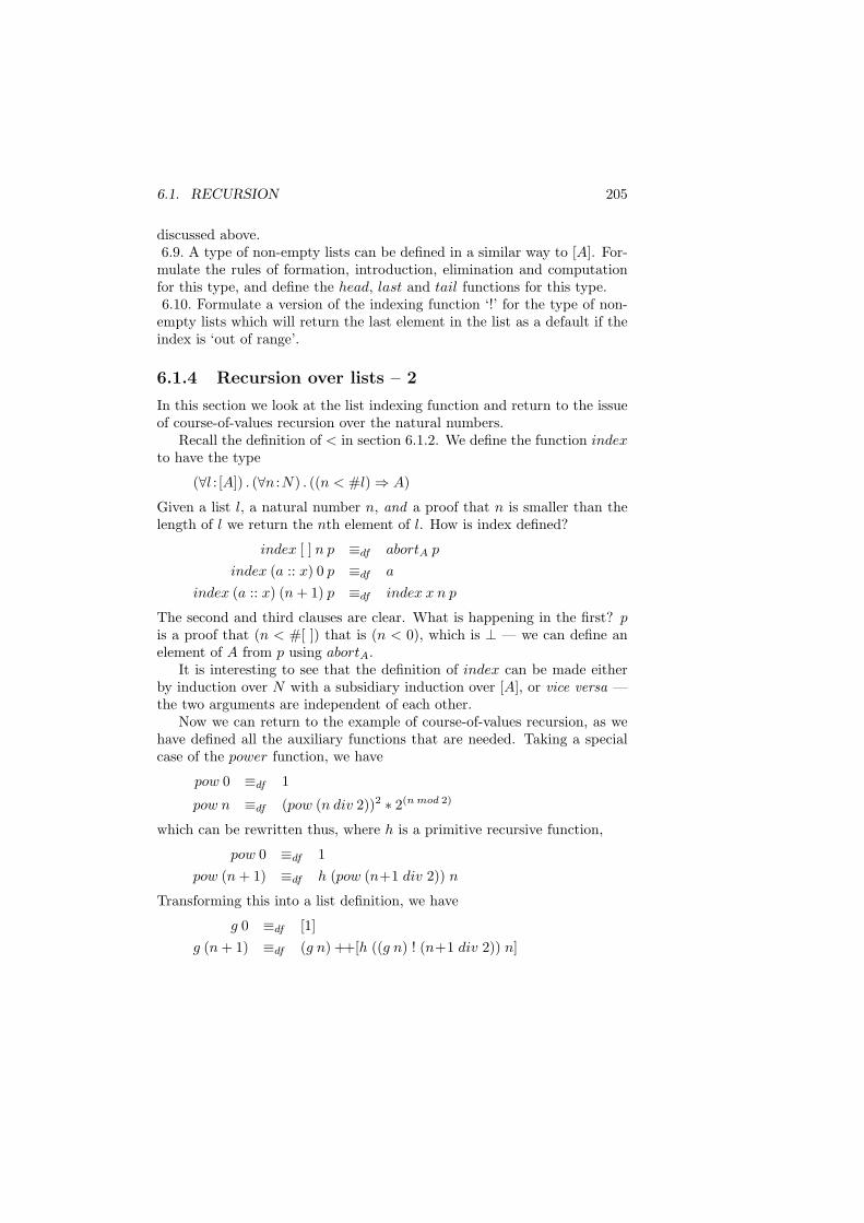
6.1. RECURSION 205
discussed above.6.9. A type of non-empty lists can be defined in a similar way to [A]. For-mulate the rules of formation, introduction, elimination and computationfor this type, and define the head, last and tail functions for this type.6.10. Formulate a version of the indexing function ‘!’ for the type of non-
empty lists which will return the last element in the list as a default if theindex is ‘out of range’.
6.1.4 Recursion over lists – 2
In this section we look at the list indexing function and return to the issueof course-of-values recursion over the natural numbers.
Recall the definition of < in section 6.1.2. We define the function indexto have the type
(∀l : [A]) . (∀n :N) . ((n < #l)⇒ A)
Given a list l, a natural number n, and a proof that n is smaller than thelength of l we return the nth element of l. How is index defined?
index [ ] n p ≡df abortA p
index (a :: x) 0 p ≡df a
index (a :: x) (n + 1) p ≡df index x n p
The second and third clauses are clear. What is happening in the first? pis a proof that (n < #[ ]) that is (n < 0), which is ⊥ — we can define anelement of A from p using abortA.
It is interesting to see that the definition of index can be made eitherby induction over N with a subsidiary induction over [A], or vice versa —the two arguments are independent of each other.
Now we can return to the example of course-of-values recursion, as wehave defined all the auxiliary functions that are needed. Taking a specialcase of the power function, we have
pow 0 ≡df 1
pow n ≡df (pow (n div 2))2 ∗ 2(n mod 2)
which can be rewritten thus, where h is a primitive recursive function,
pow 0 ≡df 1pow (n + 1) ≡df h (pow (n+1 div 2)) n
Transforming this into a list definition, we have
g 0 ≡df [1]g (n + 1) ≡df (g n) ++[h ((g n) ! (n+1 div 2)) n]
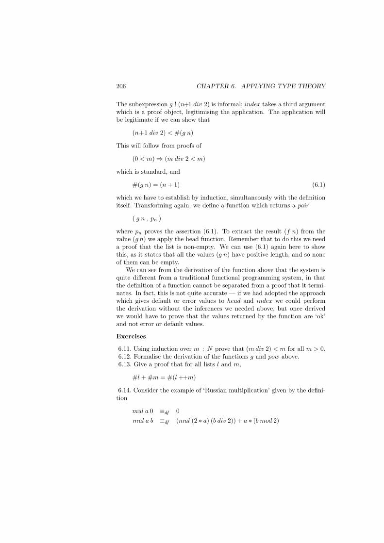
206 CHAPTER 6. APPLYING TYPE THEORY
The subexpression g ! (n+1 div 2) is informal; index takes a third argumentwhich is a proof object, legitimising the application. The application willbe legitimate if we can show that
(n+1 div 2) < #(g n)
This will follow from proofs of
(0 < m)⇒ (m div 2 < m)
which is standard, and
#(g n) = (n + 1) (6.1)
which we have to establish by induction, simultaneously with the definitionitself. Transforming again, we define a function which returns a pair
( g n , pn )
where pn proves the assertion (6.1). To extract the result (f n) from thevalue (g n) we apply the head function. Remember that to do this we needa proof that the list is non-empty. We can use (6.1) again here to showthis, as it states that all the values (g n) have positive length, and so noneof them can be empty.
We can see from the derivation of the function above that the system isquite different from a traditional functional programming system, in thatthe definition of a function cannot be separated from a proof that it termi-nates. In fact, this is not quite accurate — if we had adopted the approachwhich gives default or error values to head and index we could performthe derivation without the inferences we needed above, but once derivedwe would have to prove that the values returned by the function are ‘ok’and not error or default values.
Exercises
6.11. Using induction over m : N prove that (m div 2) < m for all m > 0.6.12. Formalise the derivation of the functions g and pow above.6.13. Give a proof that for all lists l and m,
#l + #m = #(l ++m)
6.14. Consider the example of ‘Russian multiplication’ given by the defini-tion
mul a 0 ≡df 0mul a b ≡df (mul (2 ∗ a) (b div 2)) + a ∗ (b mod 2)
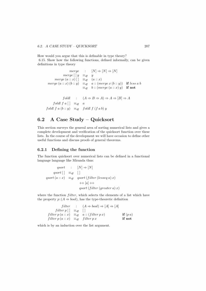
6.2. A CASE STUDY – QUICKSORT 207
How would you argue that this is definable in type theory?6.15. Show how the following functions, defined informally, can be given
definitions in type theory
merge : [N ]⇒ [N ]⇒ [N ]merge [ ] y ≡df y
merge (a :: x) [ ] ≡df (a :: x)merge (a :: x) (b :: y) ≡df a :: (merge x (b :: y)) if less a b
≡df b :: (merge (a :: x) y) if not
foldl : (A⇒ B ⇒ A)⇒ A⇒ [B]⇒ A
foldl f a [ ] ≡df a
foldl f a (b :: y) ≡df foldl f (f a b) y
6.2 A Case Study – Quicksort
This section surveys the general area of sorting numerical lists and gives acomplete development and verification of the quicksort function over theselists. In the course of the development we will have occasion to define otheruseful functions and discuss proofs of general theorems.
6.2.1 Defining the function
The function quicksort over numerical lists can be defined in a functionallanguage language like Miranda thus:
qsort : [N ]⇒ [N ]qsort [ ] ≡df [ ]
qsort (a :: x) ≡df qsort (filter (lesseq a) x)++ [a] ++qsort (filter (greater a) x)
where the function filter, which selects the elements of a list which havethe property p : (A⇒ bool), has the type-theoretic definition
filter : (A⇒ bool)⇒ [A]⇒ [A]filter p [ ] ≡df [ ]
filter p (a :: x) ≡df a :: (filter p x) if (p a)filter p (a :: x) ≡df filter p x if not
which is by an induction over the list argument.
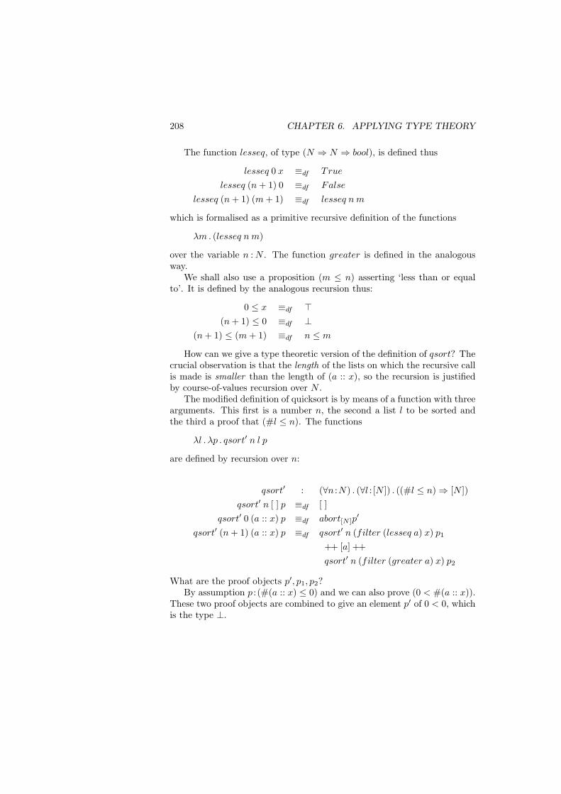
208 CHAPTER 6. APPLYING TYPE THEORY
The function lesseq, of type (N ⇒ N ⇒ bool), is defined thus
lesseq 0 x ≡df True
lesseq (n + 1) 0 ≡df False
lesseq (n + 1) (m + 1) ≡df lesseq n m
which is formalised as a primitive recursive definition of the functions
λm . (lesseq n m)
over the variable n : N . The function greater is defined in the analogousway.
We shall also use a proposition (m ≤ n) asserting ‘less than or equalto’. It is defined by the analogous recursion thus:
0 ≤ x ≡df >(n + 1) ≤ 0 ≡df ⊥
(n + 1) ≤ (m + 1) ≡df n ≤ m
How can we give a type theoretic version of the definition of qsort? Thecrucial observation is that the length of the lists on which the recursive callis made is smaller than the length of (a :: x), so the recursion is justifiedby course-of-values recursion over N .
The modified definition of quicksort is by means of a function with threearguments. This first is a number n, the second a list l to be sorted andthe third a proof that (#l ≤ n). The functions
λl . λp . qsort′ n l p
are defined by recursion over n:
qsort′ : (∀n :N) . (∀l : [N ]) . ((#l ≤ n)⇒ [N ])qsort′ n [ ] p ≡df [ ]
qsort′ 0 (a :: x) p ≡df abort[N ]p′
qsort′ (n + 1) (a :: x) p ≡df qsort′ n (filter (lesseq a) x) p1
++ [a] ++qsort′ n (filter (greater a) x) p2
What are the proof objects p′, p1, p2?By assumption p : (#(a :: x) ≤ 0) and we can also prove (0 < #(a :: x)).
These two proof objects are combined to give an element p′ of 0 < 0, whichis the type ⊥.
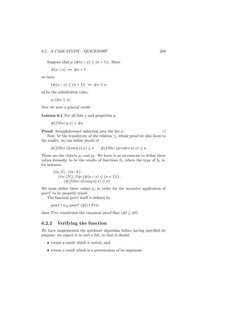
6.2. A CASE STUDY – QUICKSORT 209
Suppose that p : (#(a :: x) ≤ (n + 1)). Since
#(a :: x) ↔↔ #x + 1
we have
(#(a :: x) ≤ (n + 1)) ↔↔ #x ≤ n
so by the substitution rules,
p : (#x ≤ n)
Now we note a general result.
Lemma 6.1 For all lists x and properties p,
#(filter p x) ≤ #x
Proof: Straightforward induction over the list x. 2
Now, by the transitivity of the relation ≤, whose proof we also leave tothe reader, we can define proofs of
#(filter (lesseq a) x) ≤ n #(filter (greater a) x) ≤ n
These are the objects p1 and p2. We leave it as an exercise to define thesevalues formally, to be the results of functions hi, where the type of h1 is,for instance,
(∀a :N) . (∀n :N) .(∀x : [N ]) . (∀p : (#(a :: x) ≤ (n + 1))) .
(#(filter (lesseq a) x) ≤ n)
We must define these values pi in order for the recursive application ofqsort′ to be properly typed.
The function qsort itself is defined by
qsort l ≡df qsort′ (#l) l T riv
since Triv constitutes the canonical proof that (#l ≤ #l).
6.2.2 Verifying the function
We have implemented the quicksort algorithm before having specified itspurpose: we expect it to sort a list, so that it should
• return a result which is sorted, and,
• return a result which is a permutation of its argument
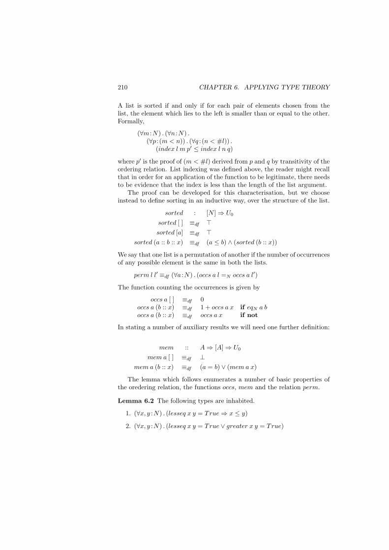
210 CHAPTER 6. APPLYING TYPE THEORY
A list is sorted if and only if for each pair of elements chosen from thelist, the element which lies to the left is smaller than or equal to the other.Formally,
(∀m :N) . (∀n :N) .(∀p : (m < n)) . (∀q : (n < #l)) .
(index l m p′ ≤ index l n q)
where p′ is the proof of (m < #l) derived from p and q by transitivity of theordering relation. List indexing was defined above, the reader might recallthat in order for an application of the function to be legitimate, there needsto be evidence that the index is less than the length of the list argument.
The proof can be developed for this characterisation, but we chooseinstead to define sorting in an inductive way, over the structure of the list.
sorted : [N ]⇒ U0
sorted [ ] ≡df >sorted [a] ≡df >
sorted (a :: b :: x) ≡df (a ≤ b) ∧ (sorted (b :: x))
We say that one list is a permutation of another if the number of occurrencesof any possible element is the same in both the lists.
perm l l′ ≡df (∀a :N) . (occs a l =N occs a l′)
The function counting the occurrences is given by
occs a [ ] ≡df 0occs a (b :: x) ≡df 1 + occs a x if eqN a boccs a (b :: x) ≡df occs a x if not
In stating a number of auxiliary results we will need one further definition:
mem :: A⇒ [A]⇒ U0
mem a [ ] ≡df ⊥mem a (b :: x) ≡df (a = b) ∨ (mem a x)
The lemma which follows enumerates a number of basic properties ofthe oredering relation, the functions occs, mem and the relation perm.
Lemma 6.2 The following types are inhabited.
1. (∀x, y :N) . (lesseq x y = True⇒ x ≤ y)
2. (∀x, y :N) . (lesseq x y = True ∨ greater x y = True)
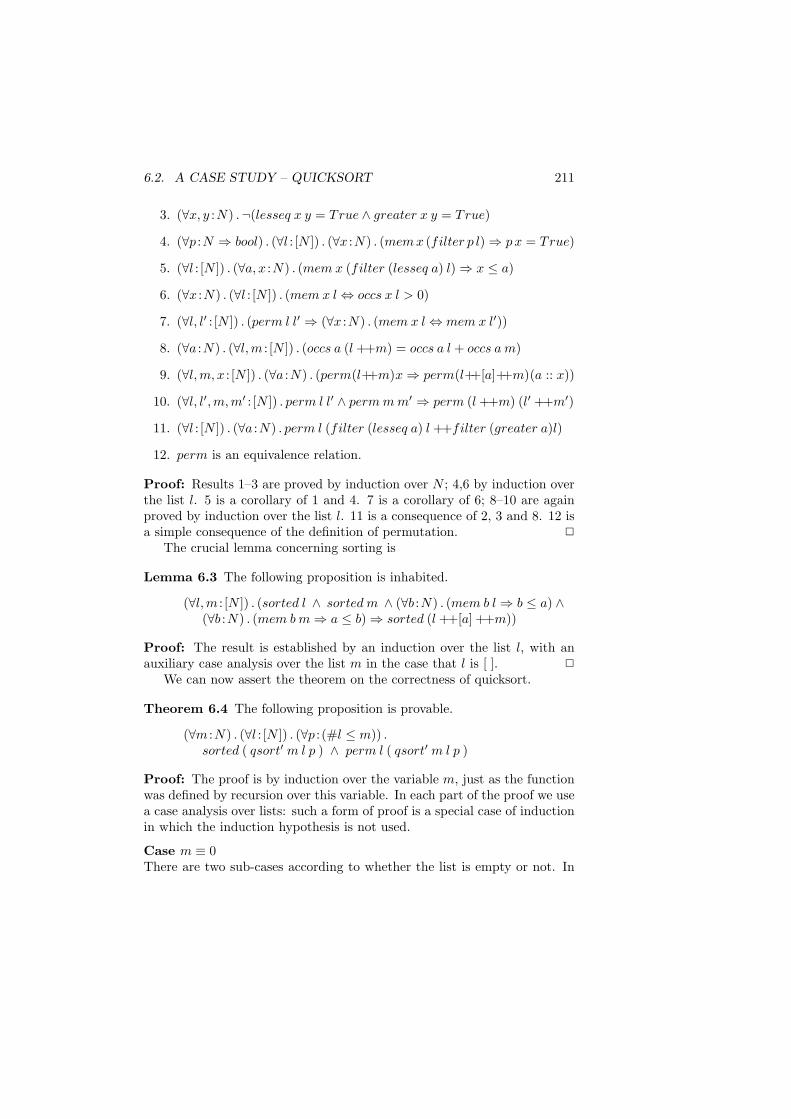
6.2. A CASE STUDY – QUICKSORT 211
3. (∀x, y :N) .¬(lesseq x y = True ∧ greater x y = True)
4. (∀p :N ⇒ bool) . (∀l : [N ]) . (∀x :N) . (memx (filter p l)⇒ px = True)
5. (∀l : [N ]) . (∀a, x :N) . (mem x (filter (lesseq a) l)⇒ x ≤ a)
6. (∀x :N) . (∀l : [N ]) . (mem x l⇔ occs x l > 0)
7. (∀l, l′ : [N ]) . (perm l l′ ⇒ (∀x :N) . (mem x l⇔ mem x l′))
8. (∀a :N) . (∀l,m : [N ]) . (occs a (l ++m) = occs a l + occs a m)
9. (∀l,m, x : [N ]) . (∀a :N) . (perm(l++m)x⇒ perm(l++[a]++m)(a :: x))
10. (∀l, l′,m, m′ : [N ]) . perm l l′ ∧ perm m m′ ⇒ perm (l ++m) (l′ ++m′)
11. (∀l : [N ]) . (∀a :N) . perm l (filter (lesseq a) l ++filter (greater a)l)
12. perm is an equivalence relation.
Proof: Results 1–3 are proved by induction over N ; 4,6 by induction overthe list l. 5 is a corollary of 1 and 4. 7 is a corollary of 6; 8–10 are againproved by induction over the list l. 11 is a consequence of 2, 3 and 8. 12 isa simple consequence of the definition of permutation. 2
The crucial lemma concerning sorting is
Lemma 6.3 The following proposition is inhabited.
(∀l,m : [N ]) . (sorted l ∧ sorted m ∧ (∀b :N) . (mem b l⇒ b ≤ a) ∧(∀b :N) . (mem b m⇒ a ≤ b)⇒ sorted (l ++[a] ++m))
Proof: The result is established by an induction over the list l, with anauxiliary case analysis over the list m in the case that l is [ ]. 2
We can now assert the theorem on the correctness of quicksort.
Theorem 6.4 The following proposition is provable.
(∀m :N) . (∀l : [N ]) . (∀p : (#l ≤ m)) .sorted ( qsort′ m l p ) ∧ perm l ( qsort′ m l p )
Proof: The proof is by induction over the variable m, just as the functionwas defined by recursion over this variable. In each part of the proof we usea case analysis over lists: such a form of proof is a special case of inductionin which the induction hypothesis is not used.
Case m ≡ 0There are two sub-cases according to whether the list is empty or not. In
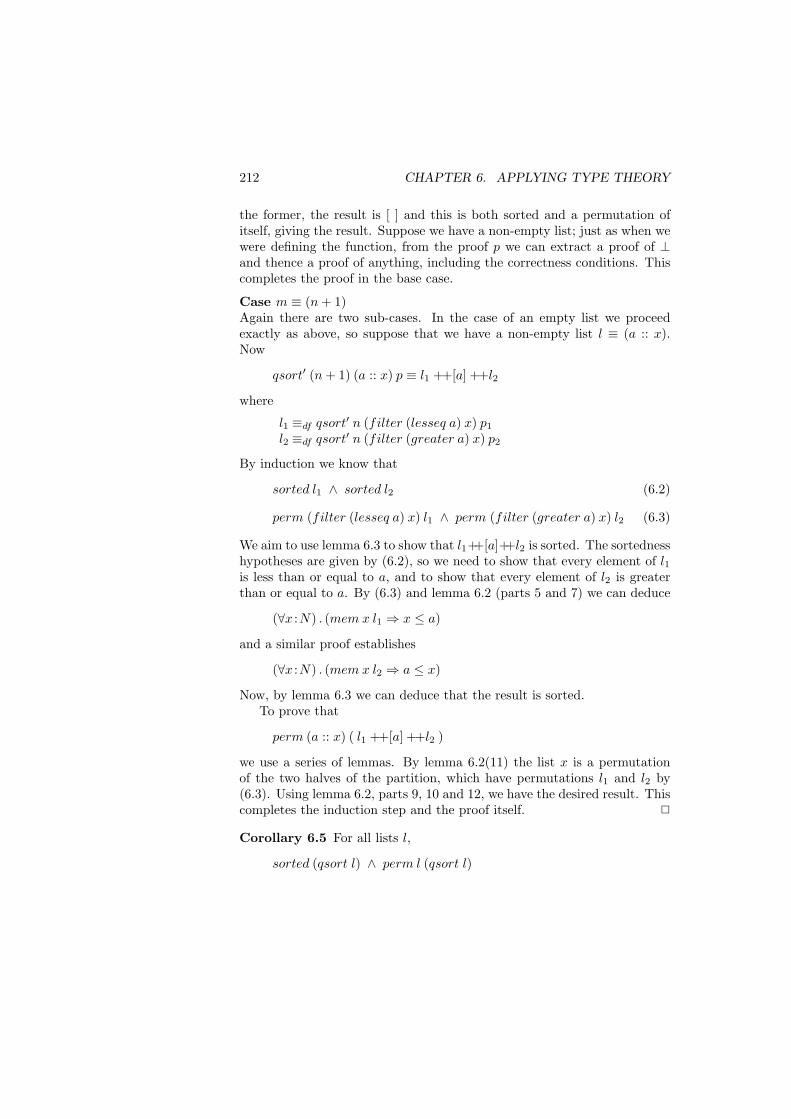
212 CHAPTER 6. APPLYING TYPE THEORY
the former, the result is [ ] and this is both sorted and a permutation ofitself, giving the result. Suppose we have a non-empty list; just as when wewere defining the function, from the proof p we can extract a proof of ⊥and thence a proof of anything, including the correctness conditions. Thiscompletes the proof in the base case.
Case m ≡ (n + 1)Again there are two sub-cases. In the case of an empty list we proceedexactly as above, so suppose that we have a non-empty list l ≡ (a :: x).Now
qsort′ (n + 1) (a :: x) p ≡ l1 ++[a] ++l2
where
l1 ≡df qsort′ n (filter (lesseq a) x) p1
l2 ≡df qsort′ n (filter (greater a) x) p2
By induction we know that
sorted l1 ∧ sorted l2 (6.2)
perm (filter (lesseq a) x) l1 ∧ perm (filter (greater a) x) l2 (6.3)
We aim to use lemma 6.3 to show that l1++[a]++l2 is sorted. The sortednesshypotheses are given by (6.2), so we need to show that every element of l1is less than or equal to a, and to show that every element of l2 is greaterthan or equal to a. By (6.3) and lemma 6.2 (parts 5 and 7) we can deduce
(∀x :N) . (mem x l1 ⇒ x ≤ a)
and a similar proof establishes
(∀x :N) . (mem x l2 ⇒ a ≤ x)
Now, by lemma 6.3 we can deduce that the result is sorted.To prove that
perm (a :: x) ( l1 ++[a] ++l2 )
we use a series of lemmas. By lemma 6.2(11) the list x is a permutationof the two halves of the partition, which have permutations l1 and l2 by(6.3). Using lemma 6.2, parts 9, 10 and 12, we have the desired result. Thiscompletes the induction step and the proof itself. 2
Corollary 6.5 For all lists l,
sorted (qsort l) ∧ perm l (qsort l)
6.2. A CASE STUDY – QUICKSORT 213
Proof: Simply take the appropriate case of the theorem. 2
A number of remarks are in order.
• In most cases of program verification, the induction used in verifyingthe result is of the same form as that used in the definition of thefunction; the proof we have given is no exception. qsort is definedto be a special case of qsort′, and we verified a generalisation of theresult using the same induction as we used to derive qsort′.
• The function qsort′ appears to be less efficient than the Mirandaalgorithm, as the former contains the proof-theoretic information,transmitted through the recursive calls. This is the case if we useapplicative order evaluation, which forces the evaluation of functionarguments prior to evaluation of the body. On the other hand, ifwe use lazy evaluation, it can be seen that the terms p1, p2 in therecursive calls will never be evaluated. We come back to this point inchapter 7.
• The presentation of sorting we have given here presents the algorithmfirst and the verification second. It is possible to reverse this, derivingthe result that
(∀l : [N ]) . (∃l′ : [N ]) . ( sorted l′ ∧ perm l l′ ) (6.4)
and extracting the quicksort function from the proof. This seemshighly artificial in this case where the function is well-known, but thereader may wish to reconstruct the result in this way.
The definition of quicksort is an example of a general phenomenon, in whicha general recursive definition of a function g over a type A
g x≡df . . . g (h x) . . .
is justified by appeal to induction over another type B, where there is afunction
f : A⇒ B
so that
f (h x)
is a predecessor of (f x) in . The recursion g is justified by the inverseimage of recursion over B using the function f . In the case of quicksort,we use the inverse image of induction over N under the length function. In
214 CHAPTER 6. APPLYING TYPE THEORY
related areas this function is often called a norm. This method justifiesmany important definitions, some of which are included in the exerciseswhich follow.
Exercises
6.16. There are many other sorting algorithms over lists, amongst which areinsertion sort and tree sort. Show first how these expressed in type theoryand then show how they meet the specification of a sorting algorithm.Alternatively prove the result (6.4) in such a way as to make the functionextracted from the proof the algorithm you wish to express.6.17. How would you show that the greatest common divisor function
defined by
gcd n m ≡df n if n = mgcd n m ≡df gcd m n if n < mgcd n m ≡df gcd (n−m) m if n > m > 0gcd n 0 ≡df 0 if not
can be defined in type theory?6.18. Show how the algorithm for the permutations of a list, which uses
the Miranda list comprehension notation, can be coded in type theory.
perms [ ] ≡df [ [ ] ]perms x ≡df [ (a :: p) | a← x ; p← perms (x−− a) ]
6.3 Dependent types and quantifiers
One of the features of TT which distinguishes it from traditional program-ming languages is its ability to express dependent types. These are types,or more correctly type expressions, which depend upon the value of oneor more variables which they contain. The operations ∀, ∃ and W formtypes from these families of types, namely the dependent product type,the dependent sum or subset type and a well-founded type. This sectionconcentrates on the two quantifiers, ∀ and ∃, after a discussion of howdependent types, or type families, can be defined.
6.3.1 Dependent Types
By a dependent type we mean any type (expression) which contains one ormore free variables. Under the logical interpretation such types are simplypredicates, of course. Dependency is introduced in two ways.
6.3. DEPENDENT TYPES AND QUANTIFIERS 215
The rule of I formation introduces values into the types. Recall the rule
A is a type a :A b :AI(A, a, b) is a type
(IF )
which forms the atomic equality proposition which is also written a =A b.Clearly the expressions a and b can contain free variables, and thus arevariables introduced into the types; depending on the complexity of a andb we build more or less complex propositions. Other dependent types arethen formed using the propositional connectives and quantifiers, but theseintroduce no additional dependency. We have already seen examples ofthis, in sections 4.10 and 6.1.2; another atomic example is the type
(#l =N n)
where l and n are variables of type [A] and N , and from this we can formthe dependent type
(∃l : [A]) . (#l =N n)
which contains the variable n free. For a fixed value of n, this is the typeof lists of that length, or more strictly, pairs
(l, r)
where r is a witness to (or proof of) the proposition (#l =N n).One general class of propositions we can define in this way are those
which are representable by a boolean-valued function, such as the ‘lessthan’ relation by
lt1 : (N ⇒ N ⇒ bool)
This is turned into a proposition by forming
I(bool , lt1 m n , True)
with n,m free. Propositions representable by boolean-valued functions aredecidable, and so this class of propositions is not closed under quantificationover infinite domains. Once we have turned such a representation into aproposition as above its universal and existential closure as a propositioncan be formed. This method of forming propositions is indirect: we definea boolean-valued function, by recursion say, and then make a propositionby equating its application to True or False.
Using the universes U0, . . . we can define dependent propositions di-rectly. The ‘small’ types are members of the type U0, and so we can usethe expression forming operators, such as cases and recursion, to form type
216 CHAPTER 6. APPLYING TYPE THEORY
expressions. This approach is not restricted to the members of U0; we canmake the same constructions at each level Un, and from an informal pointof view these constructions are often uniform in n. We have already seen anumber of examples of these definitions in section 6.1.2.
It has been proposed that a facility be added to TT0 which allows thedefinition of types (or propositions) inductively without using the universeU0 – we return to this topic in section 7.10 below.
6.3.2 The Existential Quantifier
The type (∃x : A) . B consists of pairs (a, b) with a : A and b : B[a/x]. IfB[a/x] is thought of as a type, then the construct looks like a sum of thetypes B(x) as x ranges over A. On the other hand if B is a predicate,then the construct can be seen as a subset of A, consisting of those a inA with the property B[a/x]. Consistent with the principle of completepresentation, the objects a are paired with the proofs b of the propertyB[a/x]. We saw an application of the subset type in the definition of thetype of non-empty lists earlier.
An interesting class of subsets of [A] is given by the family
[A]n ≡df (∃l : [A]) . (#l = n)
of lists of length n, where n :N . Taking the sum over N , we have
(∃n :N) . (∃l : [A]) . (#l = n)
which is isomorphic to [A], by the functions
f : [A]⇒ (∃n :N) . (∃l : [A]) . (#l = n)f l ≡df (#l, (l, r(#l)))
where r(#l) is the canonical member of (#l = #l), and
g : (∃n :N) . (∃l : [A]) . (#l = n)⇒ [A]g (n, (l, s)) ≡df l
This division of the type seems arbitrary, and indeed we could have dividedthe type according to any function
h : [A]⇒ . . .
but in this case it is interesting that many standard functions on lists can bemade to commute with this stratification, since they preserve the lengthsof the lists to which they are applied. One example is the map function,mentioned on page 181, and we have a family of functions
mapn : (A⇒ B)⇒ [A]n ⇒ [B]n
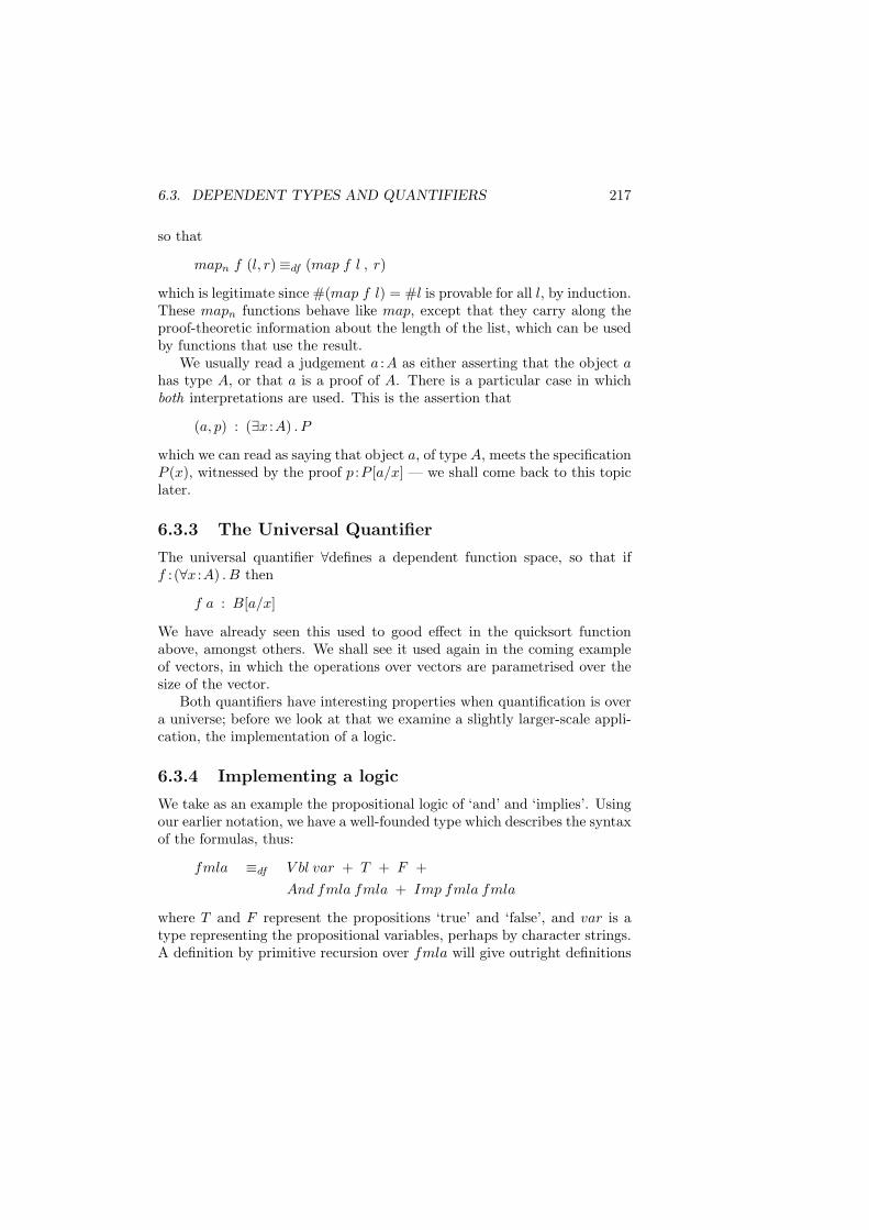
6.3. DEPENDENT TYPES AND QUANTIFIERS 217
so that
mapn f (l, r)≡df (map f l , r)
which is legitimate since #(map f l) = #l is provable for all l, by induction.These mapn functions behave like map, except that they carry along theproof-theoretic information about the length of the list, which can be usedby functions that use the result.
We usually read a judgement a :A as either asserting that the object ahas type A, or that a is a proof of A. There is a particular case in whichboth interpretations are used. This is the assertion that
(a, p) : (∃x :A) . P
which we can read as saying that object a, of type A, meets the specificationP (x), witnessed by the proof p :P [a/x] — we shall come back to this topiclater.
6.3.3 The Universal Quantifier
The universal quantifier ∀defines a dependent function space, so that iff : (∀x :A) . B then
f a : B[a/x]
We have already seen this used to good effect in the quicksort functionabove, amongst others. We shall see it used again in the coming exampleof vectors, in which the operations over vectors are parametrised over thesize of the vector.
Both quantifiers have interesting properties when quantification is overa universe; before we look at that we examine a slightly larger-scale appli-cation, the implementation of a logic.
6.3.4 Implementing a logic
We take as an example the propositional logic of ‘and’ and ‘implies’. Usingour earlier notation, we have a well-founded type which describes the syntaxof the formulas, thus:
fmla ≡df V bl var + T + F +And fmla fmla + Imp fmla fmla
where T and F represent the propositions ‘true’ and ‘false’, and var is atype representing the propositional variables, perhaps by character strings.A definition by primitive recursion over fmla will give outright definitions
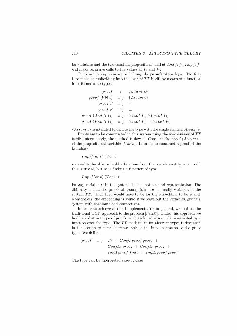
218 CHAPTER 6. APPLYING TYPE THEORY
for variables and the two constant propositions, and at Andf1 f2, Impf1 f2
will make recursive calls to the values at f1 and f2.There are two approaches to defining the proofs of the logic. The first
is to make an embedding into the logic of TT itself, by means of a functionfrom formulas to types.
proof : fmla⇒ U0
proof (V bl v) ≡df Assum vproof T ≡df >proof F ≡df ⊥
proof (And f1 f2) ≡df (proof f1) ∧ (proof f2)proof (Imp f1 f2) ≡df (proof f1)⇒ (proof f2)
Assum v is intended to denote the type with the single element Assum v.Proofs are to be constructed in this system using the mechanisms of TT
itself; unfortunately, the method is flawed. Consider the proof (Assum v)of the propositional variable (V ar v). In order to construct a proof of thetautology
Imp (V ar v) (V ar v)
we need to be able to build a function from the one element type to itself:this is trivial, but so is finding a function of type
Imp (V ar v) (V ar v′)
for any variable v′ in the system! This is not a sound representation. Thedifficulty is that the proofs of assumptions are not really variables of thesystem TT , which they would have to be for the embedding to be sound.Nonetheless, the embedding is sound if we leave out the variables, giving asystem with constants and connectives.
In order to achieve a sound implementation in general, we look at thetraditional ‘LCF’ approach to the problem [Pau87]. Under this approach webuild an abstract type of proofs, with each deduction rule represented by afunction over the type. The TT mechanism for abstract types is discussedin the section to come, here we look at the implementation of the prooftype. We define
proof ≡df Tr + ConjI proof proof +ConjE1 proof + ConjE2 proof +ImpI proof fmla + ImpE proof proof
The type can be interpreted case-by-case
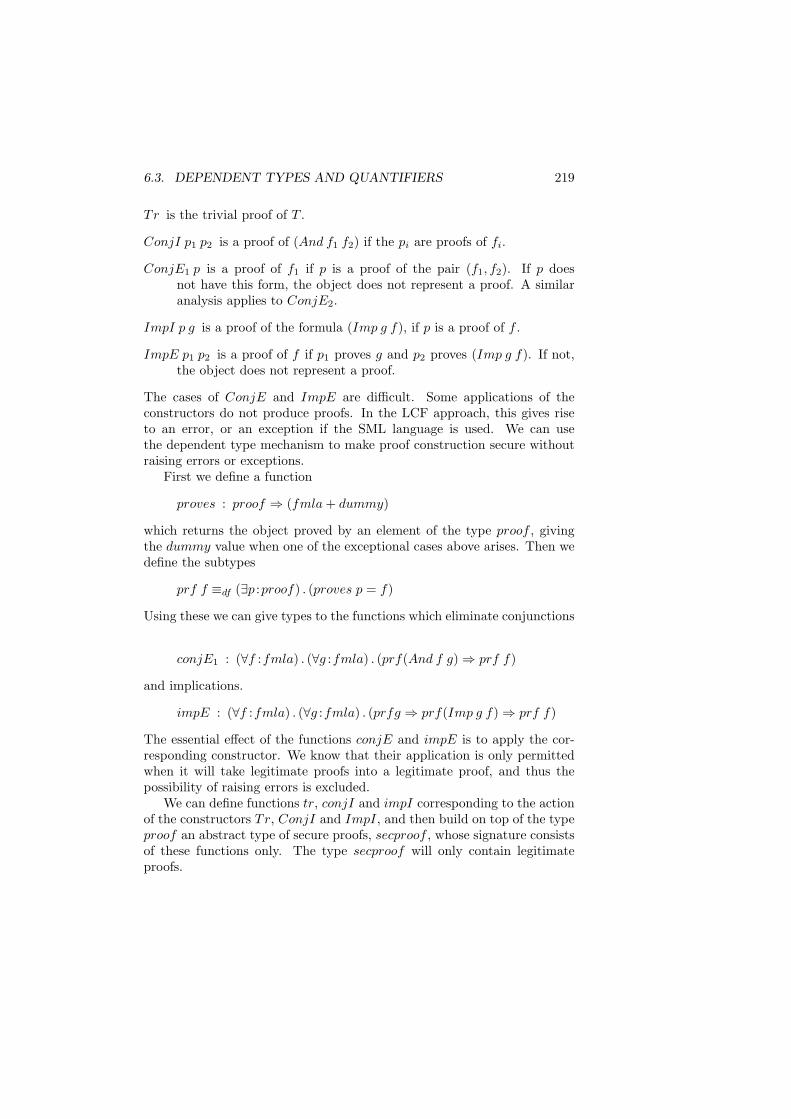
6.3. DEPENDENT TYPES AND QUANTIFIERS 219
Tr is the trivial proof of T .
ConjI p1 p2 is a proof of (And f1 f2) if the pi are proofs of fi.
ConjE1 p is a proof of f1 if p is a proof of the pair (f1, f2). If p doesnot have this form, the object does not represent a proof. A similaranalysis applies to ConjE2.
ImpI p g is a proof of the formula (Imp g f), if p is a proof of f .
ImpE p1 p2 is a proof of f if p1 proves g and p2 proves (Imp g f). If not,the object does not represent a proof.
The cases of ConjE and ImpE are difficult. Some applications of theconstructors do not produce proofs. In the LCF approach, this gives riseto an error, or an exception if the SML language is used. We can usethe dependent type mechanism to make proof construction secure withoutraising errors or exceptions.
First we define a function
proves : proof ⇒ (fmla + dummy)
which returns the object proved by an element of the type proof , givingthe dummy value when one of the exceptional cases above arises. Then wedefine the subtypes
prf f ≡df (∃p :proof) . (proves p = f)
Using these we can give types to the functions which eliminate conjunctions
conjE1 : (∀f :fmla) . (∀g :fmla) . (prf(And f g)⇒ prf f)
and implications.
impE : (∀f :fmla) . (∀g :fmla) . (prfg ⇒ prf(Imp g f)⇒ prf f)
The essential effect of the functions conjE and impE is to apply the cor-responding constructor. We know that their application is only permittedwhen it will take legitimate proofs into a legitimate proof, and thus thepossibility of raising errors is excluded.
We can define functions tr, conjI and impI corresponding to the actionof the constructors Tr, ConjI and ImpI, and then build on top of the typeproof an abstract type of secure proofs, secproof , whose signature consistsof these functions only. The type secproof will only contain legitimateproofs.
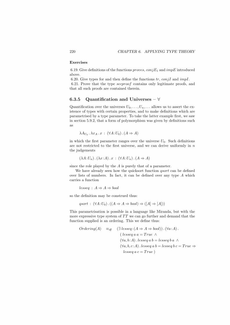
220 CHAPTER 6. APPLYING TYPE THEORY
Exercises
6.19. Give definitions of the functions proves, conjE1 and impE introducedabove.6.20. Give types for and then define the functions tr, conjI and impI.6.21. Prove that the type secproof contains only legitimate proofs, and
that all such proofs are contained therein.
6.3.5 Quantification and Universes – ∀Quantification over the universes U0, . . . , Un, . . . allows us to assert the ex-istence of types with certain properties, and to make definitions which areparametrised by a type parameter. To take the latter example first, we sawin section 5.9.2, that a form of polymorphism was given by definitions suchas
λAU0 . λxA . x : (∀A :U0) . (A⇒ A)
in which the first parameter ranges over the universe U0. Such definitionsare not restricted to the first universe, and we can derive uniformly in nthe judgements
(λA :Un) . (λx :A) . x : (∀A :Un) . (A⇒ A)
since the role played by the A is purely that of a parameter.We have already seen how the quicksort function qsort can be defined
over lists of numbers. In fact, it can be defined over any type A whichcarries a function
lesseq : A⇒ A⇒ bool
so the definition may be construed thus:
qsort : (∀A :U0) . ((A⇒ A⇒ bool)⇒ ([A]⇒ [A]))
This parametrisation is possible in a language like Miranda, but with themore expressive type system of TT we can go further and demand that thefunction supplied is an ordering. This we define thus:
Ordering(A) ≡df (∃ lesseq : (A⇒ A⇒ bool)) . (∀a :A) .
( lesseq a a = True ∧(∀a, b :A) . lesseq a b = lesseq b a ∧(∀a, b, c :A) . lesseq a b = lesseq b c = True⇒
lesseq a c = True )
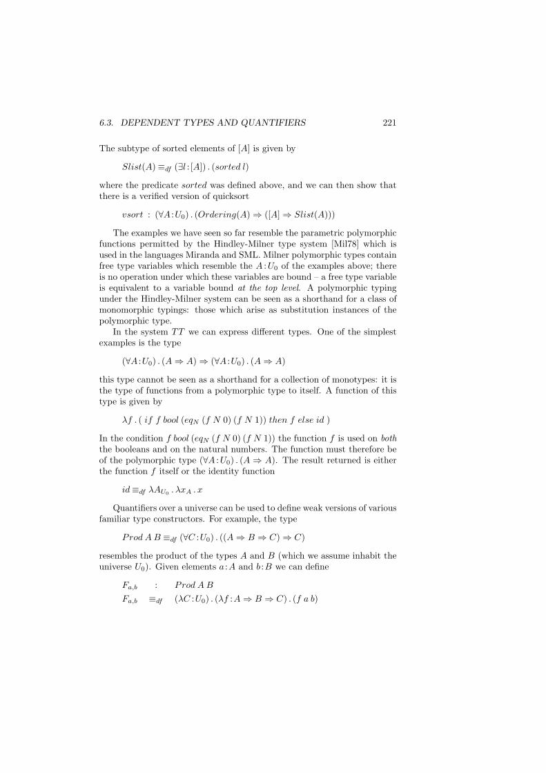
6.3. DEPENDENT TYPES AND QUANTIFIERS 221
The subtype of sorted elements of [A] is given by
Slist(A)≡df (∃l : [A]) . (sorted l)
where the predicate sorted was defined above, and we can then show thatthere is a verified version of quicksort
vsort : (∀A :U0) . (Ordering(A)⇒ ([A]⇒ Slist(A)))
The examples we have seen so far resemble the parametric polymorphicfunctions permitted by the Hindley-Milner type system [Mil78] which isused in the languages Miranda and SML. Milner polymorphic types containfree type variables which resemble the A :U0 of the examples above; thereis no operation under which these variables are bound – a free type variableis equivalent to a variable bound at the top level. A polymorphic typingunder the Hindley-Milner system can be seen as a shorthand for a class ofmonomorphic typings: those which arise as substitution instances of thepolymorphic type.
In the system TT we can express different types. One of the simplestexamples is the type
(∀A :U0) . (A⇒ A)⇒ (∀A :U0) . (A⇒ A)
this type cannot be seen as a shorthand for a collection of monotypes: it isthe type of functions from a polymorphic type to itself. A function of thistype is given by
λf . ( if f bool (eqN (f N 0) (f N 1)) then f else id )
In the condition f bool (eqN (f N 0) (f N 1)) the function f is used on boththe booleans and on the natural numbers. The function must therefore beof the polymorphic type (∀A :U0) . (A ⇒ A). The result returned is eitherthe function f itself or the identity function
id≡df λAU0 . λxA . x
Quantifiers over a universe can be used to define weak versions of variousfamiliar type constructors. For example, the type
Prod A B ≡df (∀C :U0) . ((A⇒ B ⇒ C)⇒ C)
resembles the product of the types A and B (which we assume inhabit theuniverse U0). Given elements a :A and b :B we can define
Fa,b : Prod A B
Fa,b ≡df (λC :U0) . (λf :A⇒ B ⇒ C) . (f a b)
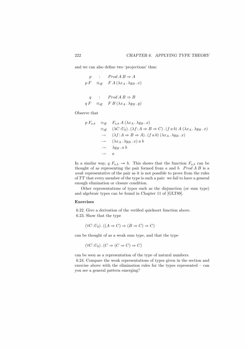
222 CHAPTER 6. APPLYING TYPE THEORY
and we can also define two ‘projections’ thus:
p : Prod A B ⇒ A
p F ≡df F A (λxA . λyB . x)
q : Prod A B ⇒ B
q F ≡df F B (λxA . λyB . y)
Observe that
p Fa,b ≡df Fa,b A (λxA . λyB . x)≡df (λC :U0) . (λf :A⇒ B ⇒ C) . (f a b) A (λxA . λyB . x)→ (λf :A⇒ B ⇒ A) . (f a b) (λxA . λyB . x)→ (λxA . λyB . x) a b
→ λyB . a b
→ a
In a similar way, q Fa,b →→ b. This shows that the function Fa,b can bethought of as representing the pair formed from a and b. Prod A B is aweak representative of the pair as it is not possible to prove from the rulesof TT that every member of the type is such a pair: we fail to have a generalenough elimination or closure condition.
Other representations of types such as the disjunction (or sum type)and algebraic types can be found in Chapter 11 of [GLT89].
Exercises
6.22. Give a derivation of the verified quicksort function above.6.23. Show that the type
(∀C :U0) . ((A⇒ C)⇒ (B ⇒ C)⇒ C)
can be thought of as a weak sum type, and that the type
(∀C :U0) . (C ⇒ (C ⇒ C)⇒ C)
can be seen as a representation of the type of natural numbers.6.24. Compare the weak representations of types given in the section and
exercise above with the elimination rules for the types represented – canyou see a general pattern emerging?
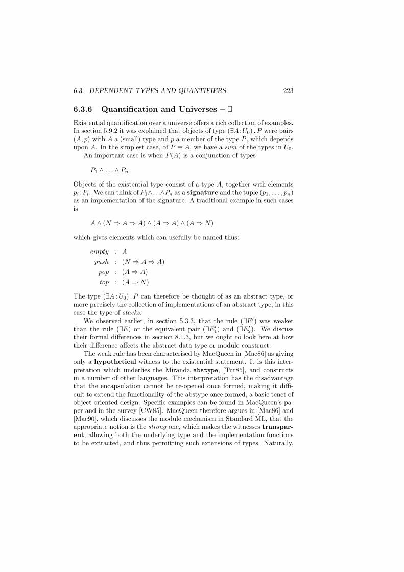
6.3. DEPENDENT TYPES AND QUANTIFIERS 223
6.3.6 Quantification and Universes – ∃Existential quantification over a universe offers a rich collection of examples.In section 5.9.2 it was explained that objects of type (∃A :U0) . P were pairs(A, p) with A a (small) type and p a member of the type P , which dependsupon A. In the simplest case, of P ≡ A, we have a sum of the types in U0.
An important case is when P (A) is a conjunction of types
P1 ∧ . . . ∧ Pn
Objects of the existential type consist of a type A, together with elementspi :Pi. We can think of P1∧. . .∧Pn as a signature and the tuple (p1, . . . , pn)as an implementation of the signature. A traditional example in such casesis
A ∧ (N ⇒ A⇒ A) ∧ (A⇒ A) ∧ (A⇒ N)
which gives elements which can usefully be named thus:
empty : A
push : (N ⇒ A⇒ A)pop : (A⇒ A)top : (A⇒ N)
The type (∃A : U0) . P can therefore be thought of as an abstract type, ormore precisely the collection of implementations of an abstract type, in thiscase the type of stacks.
We observed earlier, in section 5.3.3, that the rule (∃E′) was weakerthan the rule (∃E) or the equivalent pair (∃E′
1) and (∃E′2). We discuss
their formal differences in section 8.1.3, but we ought to look here at howtheir difference affects the abstract data type or module construct.
The weak rule has been characterised by MacQueen in [Mac86] as givingonly a hypothetical witness to the existential statement. It is this inter-pretation which underlies the Miranda abstype, [Tur85], and constructsin a number of other languages. This interpretation has the disadvantagethat the encapsulation cannot be re-opened once formed, making it diffi-cult to extend the functionality of the abstype once formed, a basic tenet ofobject-oriented design. Specific examples can be found in MacQueen’s pa-per and in the survey [CW85]. MacQueen therefore argues in [Mac86] and[Mac90], which discusses the module mechanism in Standard ML, that theappropriate notion is the strong one, which makes the witnesses transpar-ent, allowing both the underlying type and the implementation functionsto be extracted, and thus permitting such extensions of types. Naturally,
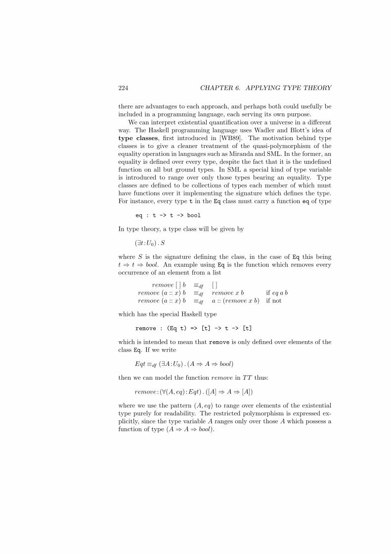
224 CHAPTER 6. APPLYING TYPE THEORY
there are advantages to each approach, and perhaps both could usefully beincluded in a programming language, each serving its own purpose.
We can interpret existential quantification over a universe in a differentway. The Haskell programming language uses Wadler and Blott’s idea oftype classes, first introduced in [WB89]. The motivation behind typeclasses is to give a cleaner treatment of the quasi-polymorphism of theequality operation in languages such as Miranda and SML. In the former, anequality is defined over every type, despite the fact that it is the undefinedfunction on all but ground types. In SML a special kind of type variableis introduced to range over only those types bearing an equality. Typeclasses are defined to be collections of types each member of which musthave functions over it implementing the signature which defines the type.For instance, every type t in the Eq class must carry a function eq of type
eq : t -> t -> bool
In type theory, a type class will be given by
(∃t :U0) . S
where S is the signature defining the class, in the case of Eq this beingt ⇒ t ⇒ bool. An example using Eq is the function which removes everyoccurrence of an element from a list
remove [ ] b ≡df [ ]remove (a :: x) b ≡df remove x b if eq a bremove (a :: x) b ≡df a :: (remove x b) if not
which has the special Haskell type
remove : (Eq t) => [t] -> t -> [t]
which is intended to mean that remove is only defined over elements of theclass Eq. If we write
Eqt≡df (∃A :U0) . (A⇒ A⇒ bool)
then we can model the function remove in TT thus:
remove : (∀(A, eq) :Eqt) . ([A]⇒ A⇒ [A])
where we use the pattern (A, eq) to range over elements of the existentialtype purely for readability. The restricted polymorphism is expressed ex-plicitly, since the type variable A ranges only over those A which possess afunction of type (A⇒ A⇒ bool).
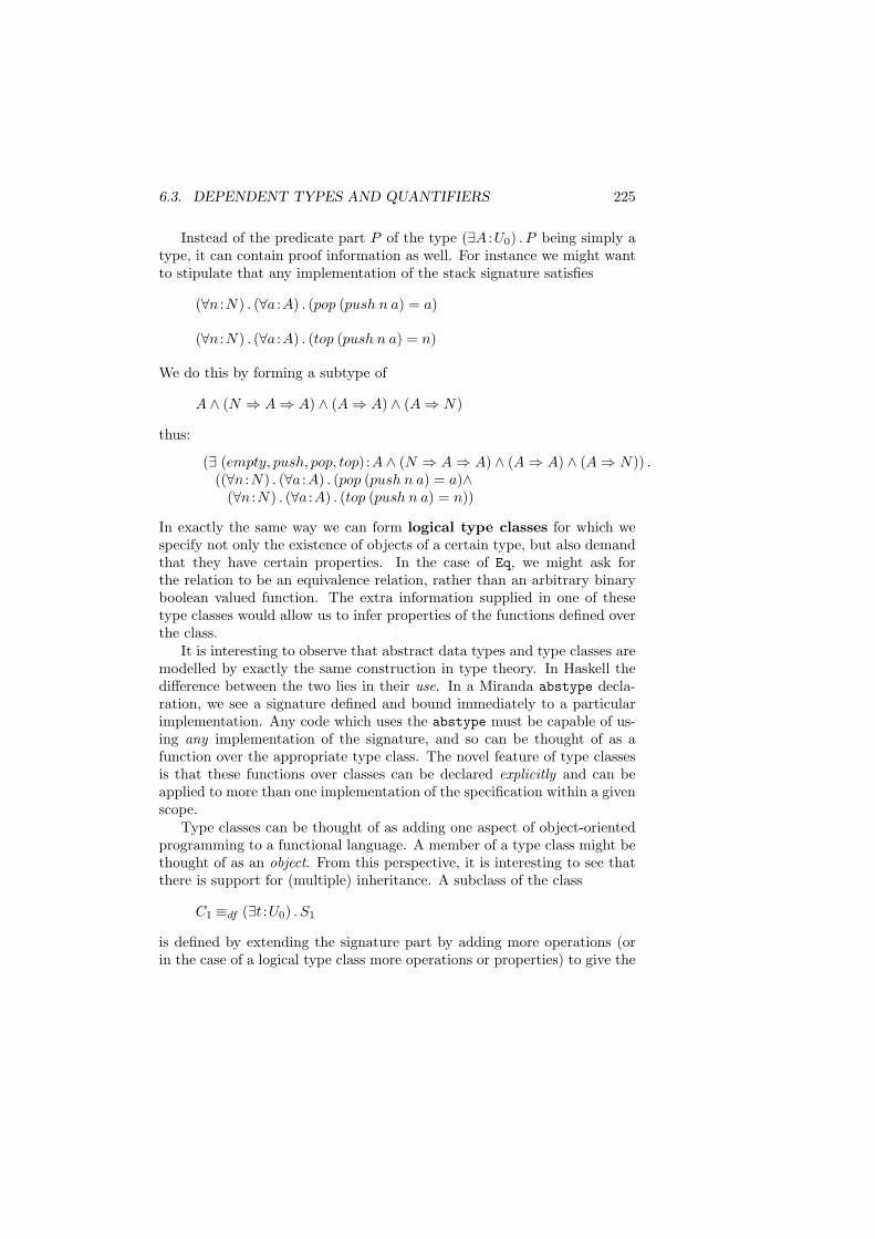
6.3. DEPENDENT TYPES AND QUANTIFIERS 225
Instead of the predicate part P of the type (∃A :U0) . P being simply atype, it can contain proof information as well. For instance we might wantto stipulate that any implementation of the stack signature satisfies
(∀n :N) . (∀a :A) . (pop (push n a) = a)
(∀n :N) . (∀a :A) . (top (push n a) = n)
We do this by forming a subtype of
A ∧ (N ⇒ A⇒ A) ∧ (A⇒ A) ∧ (A⇒ N)
thus:
(∃ (empty, push, pop, top) :A ∧ (N ⇒ A⇒ A) ∧ (A⇒ A) ∧ (A⇒ N)) .((∀n :N) . (∀a :A) . (pop (push n a) = a)∧
(∀n :N) . (∀a :A) . (top (push n a) = n))
In exactly the same way we can form logical type classes for which wespecify not only the existence of objects of a certain type, but also demandthat they have certain properties. In the case of Eq, we might ask forthe relation to be an equivalence relation, rather than an arbitrary binaryboolean valued function. The extra information supplied in one of thesetype classes would allow us to infer properties of the functions defined overthe class.
It is interesting to observe that abstract data types and type classes aremodelled by exactly the same construction in type theory. In Haskell thedifference between the two lies in their use. In a Miranda abstype decla-ration, we see a signature defined and bound immediately to a particularimplementation. Any code which uses the abstype must be capable of us-ing any implementation of the signature, and so can be thought of as afunction over the appropriate type class. The novel feature of type classesis that these functions over classes can be declared explicitly and can beapplied to more than one implementation of the specification within a givenscope.
Type classes can be thought of as adding one aspect of object-orientedprogramming to a functional language. A member of a type class might bethought of as an object. From this perspective, it is interesting to see thatthere is support for (multiple) inheritance. A subclass of the class
C1 ≡df (∃t :U0) . S1
is defined by extending the signature part by adding more operations (orin the case of a logical type class more operations or properties) to give the
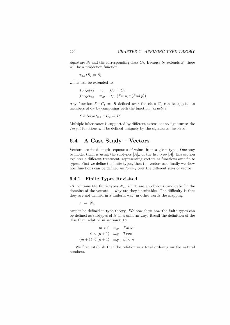
226 CHAPTER 6. APPLYING TYPE THEORY
signature S2 and the corresponding class C2. Because S2 extends S1 therewill be a projection function
π2,1 :S2 ⇒ S1
which can be extended to
forget2,1 : C2 ⇒ C1
forget2,1 ≡df λp . (Fst p, π (Snd p))
Any function F : C1 ⇒ R defined over the class C1 can be applied tomembers of C2 by composing with the function forget2,1
F forget2,1 : C2 ⇒ R
Multiple inheritance is supported by different extensions to signatures: theforget functions will be defined uniquely by the signatures involved.
6.4 A Case Study – Vectors
Vectors are fixed-length sequences of values from a given type. One wayto model them is using the subtypes [A]n of the list type [A]; this sectionexplores a different treatment, representing vectors as functions over finitetypes. First we define the finite types, then the vectors and finally we showhow functions can be defined uniformly over the different sizes of vector.
6.4.1 Finite Types Revisited
TT contains the finite types Nn, which are an obvious candidate for thedomains of the vectors — why are they unsuitable? The difficulty is thatthey are not defined in a uniform way; in other words the mapping
n 7→ Nn
cannot be defined in type theory. We now show how the finite types canbe defined as subtypes of N in a uniform way. Recall the definition of the‘less than’ relation in section 6.1.2
m < 0 ≡df False
0 < (n + 1) ≡df True
(m + 1) < (n + 1) ≡df m < n
We first establish that the relation is a total ordering on the naturalnumbers.
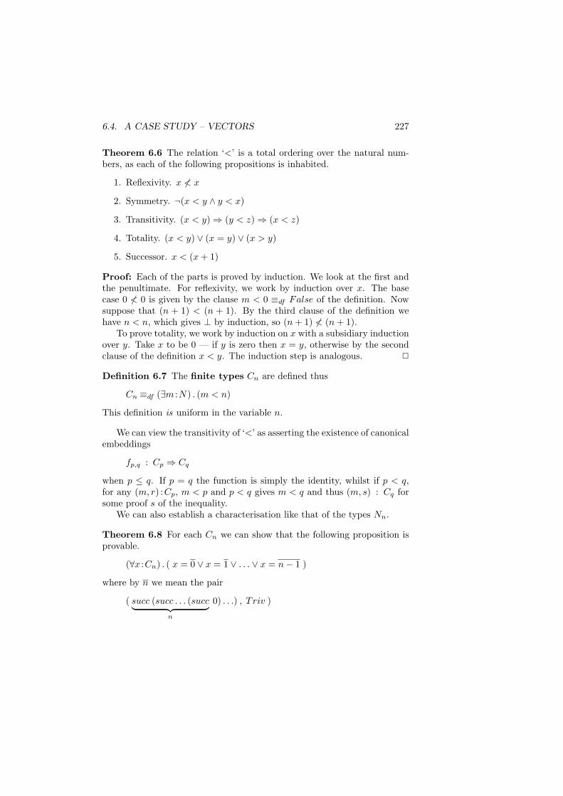
6.4. A CASE STUDY – VECTORS 227
Theorem 6.6 The relation ‘<’ is a total ordering over the natural num-bers, as each of the following propositions is inhabited.
1. Reflexivity. x 6< x
2. Symmetry. ¬(x < y ∧ y < x)
3. Transitivity. (x < y)⇒ (y < z)⇒ (x < z)
4. Totality. (x < y) ∨ (x = y) ∨ (x > y)
5. Successor. x < (x + 1)
Proof: Each of the parts is proved by induction. We look at the first andthe penultimate. For reflexivity, we work by induction over x. The basecase 0 6< 0 is given by the clause m < 0 ≡df False of the definition. Nowsuppose that (n + 1) < (n + 1). By the third clause of the definition wehave n < n, which gives ⊥ by induction, so (n + 1) 6< (n + 1).
To prove totality, we work by induction on x with a subsidiary inductionover y. Take x to be 0 — if y is zero then x = y, otherwise by the secondclause of the definition x < y. The induction step is analogous. 2
Definition 6.7 The finite types Cn are defined thus
Cn ≡df (∃m :N) . (m < n)
This definition is uniform in the variable n.
We can view the transitivity of ‘<’ as asserting the existence of canonicalembeddings
fp,q : Cp ⇒ Cq
when p ≤ q. If p = q the function is simply the identity, whilst if p < q,for any (m, r) :Cp, m < p and p < q gives m < q and thus (m, s) : Cq forsome proof s of the inequality.
We can also establish a characterisation like that of the types Nn.
Theorem 6.8 For each Cn we can show that the following proposition isprovable.
(∀x :Cn) . ( x = 0 ∨ x = 1 ∨ . . . ∨ x = n− 1 )
where by n we mean the pair
( succ (succ . . . (succ︸ ︷︷ ︸n
0) . . .) , T riv )
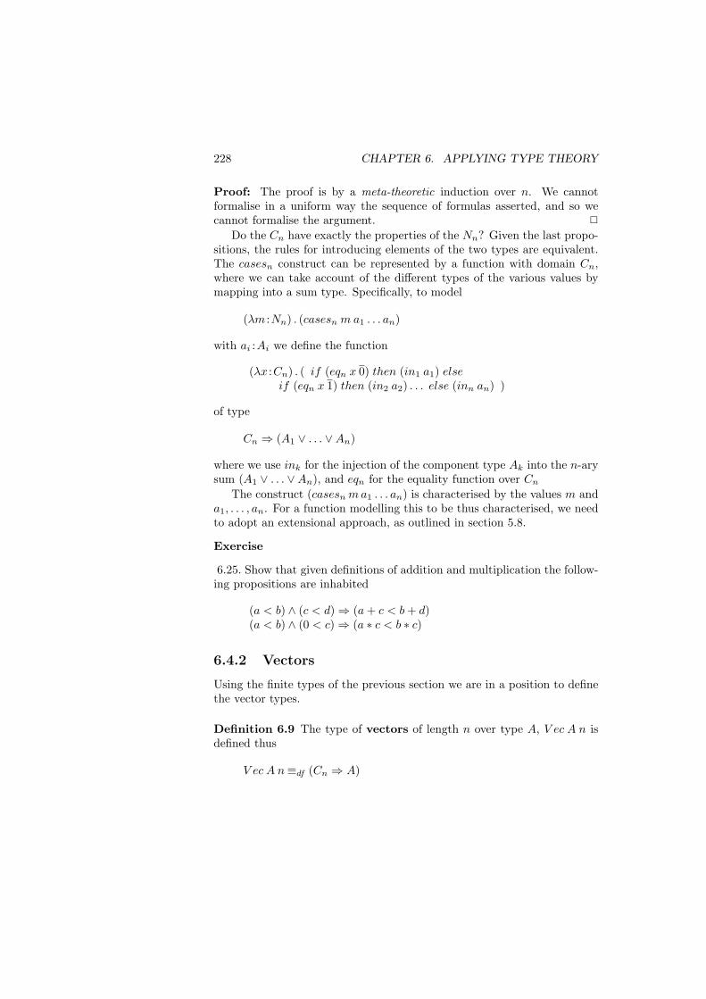
228 CHAPTER 6. APPLYING TYPE THEORY
Proof: The proof is by a meta-theoretic induction over n. We cannotformalise in a uniform way the sequence of formulas asserted, and so wecannot formalise the argument. 2
Do the Cn have exactly the properties of the Nn? Given the last propo-sitions, the rules for introducing elements of the two types are equivalent.The casesn construct can be represented by a function with domain Cn,where we can take account of the different types of the various values bymapping into a sum type. Specifically, to model
(λm :Nn) . (casesn m a1 . . . an)
with ai :Ai we define the function
(λx :Cn) . ( if (eqn x 0) then (in1 a1) elseif (eqn x 1) then (in2 a2) . . . else (inn an) )
of type
Cn ⇒ (A1 ∨ . . . ∨An)
where we use ink for the injection of the component type Ak into the n-arysum (A1 ∨ . . . ∨An), and eqn for the equality function over Cn
The construct (casesn m a1 . . . an) is characterised by the values m anda1, . . . , an. For a function modelling this to be thus characterised, we needto adopt an extensional approach, as outlined in section 5.8.
Exercise
6.25. Show that given definitions of addition and multiplication the follow-ing propositions are inhabited
(a < b) ∧ (c < d)⇒ (a + c < b + d)(a < b) ∧ (0 < c)⇒ (a ∗ c < b ∗ c)
6.4.2 Vectors
Using the finite types of the previous section we are in a position to definethe vector types.
Definition 6.9 The type of vectors of length n over type A, V ec A n isdefined thus
V ec A n≡df (Cn ⇒ A)
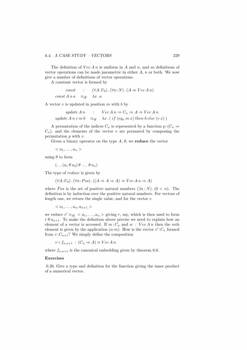
6.4. A CASE STUDY – VECTORS 229
The definition of V ec A n is uniform in A and n, and so definitions ofvector operations can be made parametric in either A, n or both. We nowgive a number of definitions of vector operations.
A constant vector is formed by
const : (∀A :U0) . (∀n :N) . (A⇒ V ec A n)const A n a ≡df λx . a
A vector v is updated in position m with b by
update A n : V ec A n⇒ Cn ⇒ A⇒ V ec A n
update A n v m b ≡df λx . ( if (eqn m x) then b else (v x) )
A permutation of the indices Cn is represented by a function p : (Cn ⇒Cn), and the elements of the vector v are permuted by composing thepermutation p with v.
Given a binary operator on the type A, θ, we reduce the vector
< a1, . . . , an >
using θ to form
(. . . (a1 θ a2) θ . . . θ an)
The type of reduce is given by
(∀A :U0) . (∀n :Pos) . ((A⇒ A⇒ A)⇒ V ec A n⇒ A)
where Pos is the set of positive natural numbers (∃n : N) . (0 < n). Thedefinition is by induction over the positive natural numbers. For vectors oflength one, we return the single value, and for the vector v
< a1, . . . , an, an+1 >
we reduce v′ ≡df < a1, . . . , an > giving r, say, which is then used to formr θ an+1. To make the definition above precise we need to explain how anelement of a vector is accessed. If m : Cn and w : V ec A n then the mthelement is given by the application (w m). How is the vector v′ :Cn formedfrom v :Cn+1? We simply define the composition
v fn,n+1 : (Cn ⇒ A) ≡ V ec A n
where fn,n+1 is the canonical embedding given by theorem 6.6.
Exercises
6.26. Give a type and definition for the function giving the inner productof a numerical vector.
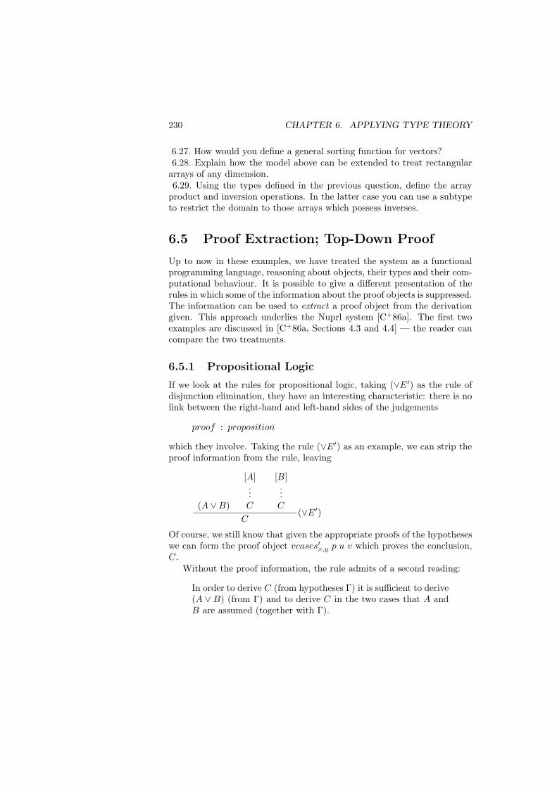
230 CHAPTER 6. APPLYING TYPE THEORY
6.27. How would you define a general sorting function for vectors?6.28. Explain how the model above can be extended to treat rectangular
arrays of any dimension.6.29. Using the types defined in the previous question, define the array
product and inversion operations. In the latter case you can use a subtypeto restrict the domain to those arrays which possess inverses.
6.5 Proof Extraction; Top-Down Proof
Up to now in these examples, we have treated the system as a functionalprogramming language, reasoning about objects, their types and their com-putational behaviour. It is possible to give a different presentation of therules in which some of the information about the proof objects is suppressed.The information can be used to extract a proof object from the derivationgiven. This approach underlies the Nuprl system [C+86a]. The first twoexamples are discussed in [C+86a, Sections 4.3 and 4.4] — the reader cancompare the two treatments.
6.5.1 Propositional Logic
If we look at the rules for propositional logic, taking (∨E′) as the rule ofdisjunction elimination, they have an interesting characteristic: there is nolink between the right-hand and left-hand sides of the judgements
proof : proposition
which they involve. Taking the rule (∨E′) as an example, we can strip theproof information from the rule, leaving
(A ∨B)
[A]...C
[B]...C
C(∨E′)
Of course, we still know that given the appropriate proofs of the hypotheseswe can form the proof object vcases′x,y p u v which proves the conclusion,C.
Without the proof information, the rule admits of a second reading:
In order to derive C (from hypotheses Γ) it is sufficient to derive(A ∨ B) (from Γ) and to derive C in the two cases that A andB are assumed (together with Γ).
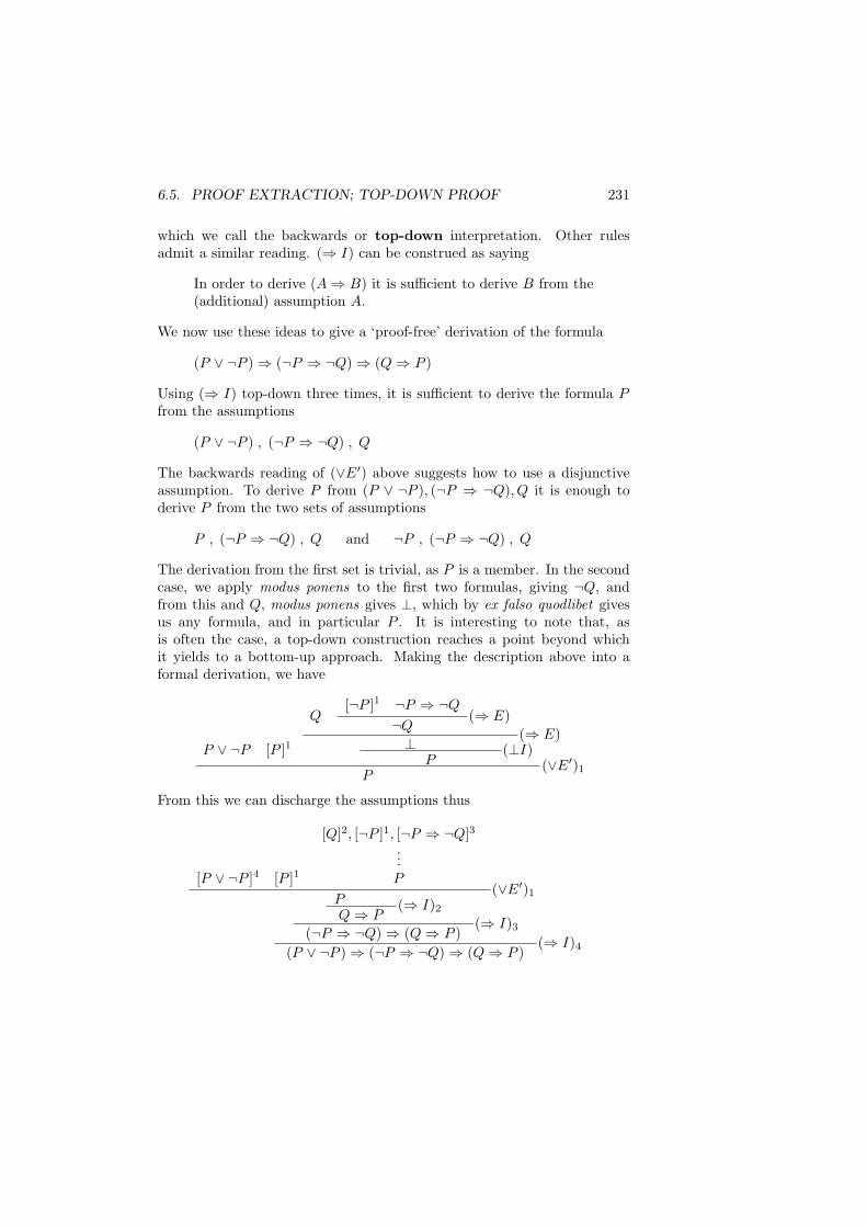
6.5. PROOF EXTRACTION; TOP-DOWN PROOF 231
which we call the backwards or top-down interpretation. Other rulesadmit a similar reading. (⇒ I) can be construed as saying
In order to derive (A⇒ B) it is sufficient to derive B from the(additional) assumption A.
We now use these ideas to give a ‘proof-free’ derivation of the formula
(P ∨ ¬P )⇒ (¬P ⇒ ¬Q)⇒ (Q⇒ P )
Using (⇒ I) top-down three times, it is sufficient to derive the formula Pfrom the assumptions
(P ∨ ¬P ) , (¬P ⇒ ¬Q) , Q
The backwards reading of (∨E′) above suggests how to use a disjunctiveassumption. To derive P from (P ∨ ¬P ), (¬P ⇒ ¬Q), Q it is enough toderive P from the two sets of assumptions
P , (¬P ⇒ ¬Q) , Q and ¬P , (¬P ⇒ ¬Q) , Q
The derivation from the first set is trivial, as P is a member. In the secondcase, we apply modus ponens to the first two formulas, giving ¬Q, andfrom this and Q, modus ponens gives ⊥, which by ex falso quodlibet givesus any formula, and in particular P . It is interesting to note that, asis often the case, a top-down construction reaches a point beyond whichit yields to a bottom-up approach. Making the description above into aformal derivation, we have
P ∨ ¬P [P ]1
Q[¬P ]1 ¬P ⇒ ¬Q
¬Q(⇒ E)
⊥(⇒ E)
P(⊥I)
P(∨E′)1
From this we can discharge the assumptions thus
[P ∨ ¬P ]4 [P ]1
[Q]2, [¬P ]1, [¬P ⇒ ¬Q]3...P
P(∨E′)1
Q⇒ P(⇒ I)2
(¬P ⇒ ¬Q)⇒ (Q⇒ P )(⇒ I)3
(P ∨ ¬P )⇒ (¬P ⇒ ¬Q)⇒ (Q⇒ P )(⇒ I)4
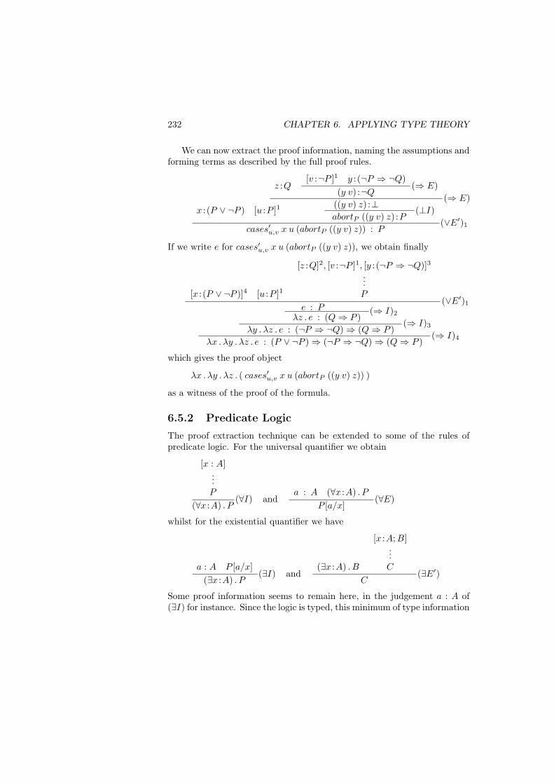
232 CHAPTER 6. APPLYING TYPE THEORY
We can now extract the proof information, naming the assumptions andforming terms as described by the full proof rules.
x : (P ∨ ¬P ) [u :P ]1
z :Q[v :¬P ]1 y : (¬P ⇒ ¬Q)
(y v) :¬Q(⇒ E)
((y v) z) :⊥(⇒ E)
abortP ((y v) z) :P(⊥I)
cases′u,v x u (abortP ((y v) z)) : P(∨E′)1
If we write e for cases′u,v x u (abortP ((y v) z)), we obtain finally
[x : (P ∨ ¬P )]4 [u :P ]1
[z :Q]2, [v :¬P ]1, [y : (¬P ⇒ ¬Q)]3...P
e : P(∨E′)1
λz . e : (Q⇒ P )(⇒ I)2
λy . λz . e : (¬P ⇒ ¬Q)⇒ (Q⇒ P )(⇒ I)3
λx . λy . λz . e : (P ∨ ¬P )⇒ (¬P ⇒ ¬Q)⇒ (Q⇒ P )(⇒ I)4
which gives the proof object
λx . λy . λz . ( cases′u,v x u (abortP ((y v) z)) )
as a witness of the proof of the formula.
6.5.2 Predicate Logic
The proof extraction technique can be extended to some of the rules ofpredicate logic. For the universal quantifier we obtain
[x : A]...P
(∀x :A) . P(∀I) and
a : A (∀x :A) . P
P [a/x](∀E)
whilst for the existential quantifier we have
a : A P [a/x](∃x :A) . P
(∃I) and(∃x :A) . B
[x :A;B]...C
C(∃E′)
Some proof information seems to remain here, in the judgement a : A of(∃I) for instance. Since the logic is typed, this minimum of type information
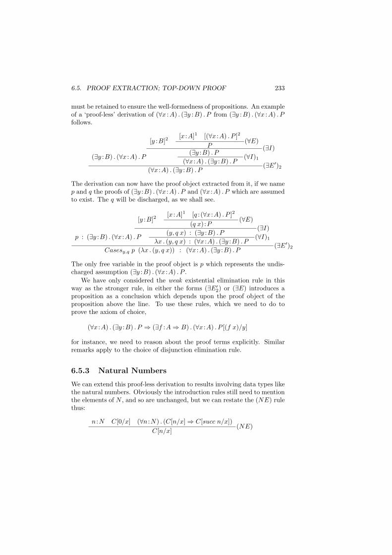
6.5. PROOF EXTRACTION; TOP-DOWN PROOF 233
must be retained to ensure the well-formedness of propositions. An exampleof a ‘proof-less’ derivation of (∀x :A) . (∃y :B) . P from (∃y :B) . (∀x :A) . Pfollows.
(∃y :B) . (∀x :A) . P
[y :B]2[x :A]1 [(∀x :A) . P ]2
P(∀E)
(∃y :B) . P(∃I)
(∀x :A) . (∃y :B) . P(∀I)1
(∀x :A) . (∃y :B) . P(∃E′)2
The derivation can now have the proof object extracted from it, if we namep and q the proofs of (∃y :B) . (∀x :A) . P and (∀x :A) . P which are assumedto exist. The q will be discharged, as we shall see.
p : (∃y :B) . (∀x :A) . P
[y :B]2[x :A]1 [q : (∀x :A) . P ]2
(q x) :P(∀E)
(y, q x) : (∃y :B) . P(∃I)
λx . (y, q x) : (∀x :A) . (∃y :B) . P(∀I)1
Casesy,q p (λx . (y, q x)) : (∀x :A) . (∃y :B) . P(∃E′)2
The only free variable in the proof object is p which represents the undis-charged assumption (∃y :B) . (∀x :A) . P .
We have only considered the weak existential elimination rule in thisway as the stronger rule, in either the forms (∃E′
2) or (∃E) introduces aproposition as a conclusion which depends upon the proof object of theproposition above the line. To use these rules, which we need to do toprove the axiom of choice,
(∀x :A) . (∃y :B) . P ⇒ (∃f :A⇒ B) . (∀x :A) . P [(f x)/y]
for instance, we need to reason about the proof terms explicitly. Similarremarks apply to the choice of disjunction elimination rule.
6.5.3 Natural Numbers
We can extend this proof-less derivation to results involving data types likethe natural numbers. Obviously the introduction rules still need to mentionthe elements of N , and so are unchanged, but we can restate the (NE) rulethus:
n :N C[0/x] (∀n :N) . (C[n/x]⇒ C[succ n/x])C[n/x]
(NE)
234 CHAPTER 6. APPLYING TYPE THEORY
An example we might prove thus is (∀n :N) . (0 < fac n) where the propo-sition (m < n) was first defined in section 6.1.2, and fac has the definition
fac 0 ≡df 1fac (n + 1) ≡df (n + 1) ∗ (fac n)
We first have to derive (0 < 1) which is a special case of (0 < n+1), whichis itself trivially derivable. In the second case we have to derive
(∀n :N) . ((0 < fac n)⇒ (0 < fac (n + 1)))
for which, using the rules (∀I) and (⇒ I) top-down, it is sufficient to derive(0 < fac (n + 1)) on the assumption that n : N and (0 < fac n). Sincefac (n + 1) is the product
(n + 1) ∗ (fac n)
and as it is a standard result (and exercise!) that a product of positivenumbers is positive, the result is derived.
Exercises
6.30. Give ‘proof-less’ derivations of the formulas (B ∨C)⇒ ¬(¬B ∧¬C),A⇒ ¬¬A and (¬A ∨ ¬B)⇒ ¬(A ∧B), and from your derivations extractthe corresponding proof objects.6.31. Find a ‘proof-less’ derivation of the formula
(∀x :X) . (A⇒ B)⇒ ((∃x :X) . A⇒ (∃x :X) . B)
and extract a proof object from the derivation.6.32. Formalise the ‘proof-less’ derivation of the fact that all values of
fac are positive, assuming the lemma on multiplication, and give the proofobject that it generates.6.33. Making a suitable definition of the multiplication operation ‘∗’ over
N , give a ‘proof-less’ derivation of the lemma that a product of positivenumbers is positive.
6.6 Program Development – Polish NationalFlag
This section addresses the problem of the Polish National Flag, which is aninessential simplification of the problem of the Dutch National Flag. Thiswas first addressed in [Dij76]. In the context of type theory it was firstinvestigated in [PS85] and later in section 22.2 of [NPS90]. The problem,
6.6. PROGRAM DEVELOPMENT – POLISH NATIONAL FLAG 235
baldly stated, is this: given a sequence of items which are either red orwhite, return a permuted sequence in which all the red items precede thewhite.
Our approach differs from that in [NPS90] in two ways. First, we ex-press the specification in a different way, so as to separate the computationalfrom the proof-theoretic; secondly, we eschew the use of the subset type.We shall discuss this type in some detail in chapter 7. We also use an ‘equa-tional’ notation which is closer to that in use in the majority of functionalprogramming languages.
Our development depends upon some of the functions and predicateswhich were introduced earlier; in particular we shall use ++, the list con-catenation operator, the predicate perm l m, which expresses the fact thatthe list l is a permutation of the list m, together with the auxiliary occs a l,which counts the number of occurrences of a in the list l. We assume thatthe colours are represented by the boolean type, bool (which we shall ab-breviate C, for colour), with the value True representing the colour red.We therefore say isReda≡df a = True and similarly for isWhite. Also, wedefine
allRed : [bool]⇒ U0
allRed [ ] ≡df >allRed (a :: x) ≡df isRed a ∧ allRed x
with the corresponding definition for allWhite. One way to express thespecification of the problem is then to say
(∀l : [C]) . (∃(l′, l′′) : [C] ∧ [C]) .(allRed l′ ∧ allWhite l′′ ∧ perm l (l′ ++l′′)) (6.5)
What we seek is, in fact, a function which returns the pair of lists (l′, l′′)corresponding to each l, so we modify the specification to read
(∃f : [C]⇒ [C] ∧ [C]) . (∀l : [C]) .allRed (fst (f l)) ∧ allWhite (snd (f l))∧perm l ((fst (f l)) ++(snd (f l)))
(6.6)
What will a proof of this formula consist of? It will be a pair (f, p) with
f : [C]⇒ [C] ∧ [C]
and p a proof that for all lists l
allRed (fst (f l)) ∧ allWhite (snd (f l))∧perm l ((fst (f l)) ++(snd (f l))) (6.7)
236 CHAPTER 6. APPLYING TYPE THEORY
This pair consists precisely of the function required together with a proofthat is has the property required of it. This is the general form that aspecification in type theory should take – we return to this topic in chapter7. Note that the transformation of the first specification into the secondis by no means ad hoc – we have applied the axiom of choice to the firstto obtain the second; indeed given this axiom the two specifications arelogically equivalent. The axiom of choice is the statement
(∀x :A) . (∃y :B) . P (x, y)⇒ (∃f :A⇒ B) . (∀x :A) . P (x, f x)
It is not hard to show that this type is inhabited; it is left as an exercisefor the reader, who will be able to find a proof in [ML85].
There are two distinct ways of proving a statement like 6.6.
• We can prove the statement by giving a term f and proving theformula 6.7. This method corresponds to traditional program devel-opment in a functional programming language: we first define thefunction we think has the desired property and separately we provethat it does have the property, an exercise in program verification.This was the method we used in developing quicksort in section 6.2.
• Alternatively, we can develop the proof from the top down, reducingthe existential statement 6.6 to 6.5. We then try to prove this formuladirectly and from the proof we extract a function by applying theaxiom of choice. This program extraction technique is the one whichwe follow here: note that both methods can lead to the same definitionof the required function.
Using the first method we would define the function
split : [C]⇒ [C] ∧ [C]split [ ] ≡df ([ ], [ ])
split (a :: m) ≡df (a :: l′, l′′) if a≡df (l′, a :: l′′) if not
where(l′, l′′) ≡ split m
and then attempt to verify, by induction, that split has the property (6.7).Alternatively we try to prove the result (6.5) directly; this we do now.
Theorem 6.10 For all lists l : [C],
(∃(l′, l′′) : [C] ∧ [C]) .(allRed l′ ∧ allWhite l′′ ∧ perm l (l′ ++l′′)) (6.8)
6.6. PROGRAM DEVELOPMENT – POLISH NATIONAL FLAG 237
Proof: We prove the result by induction over the list l. We shall call thestatement (6.8) P (l).
Case: l ≡ [ ]It is immediate that the types allRed [ ] and allWhite [ ] are inhabited.Also [ ] ++ [ ] ≡ [ ] and as perm is reflexive (see lemma 6.2, part 12) wehave
perm l (l′ ++l′′)
is inhabited. Putting the proof objects together we have some p0,
p0 : P ([ ])
as required in an inductive proof.
Case: l ≡ (a :: m)Suppose that pm : P (m). Now,
pm ≡ ((l′, l′′), q)
where q ≡ (q1, q2, q3) and
(q1, q2, q3) : (allRed l′ ∧ allWhite l′′ ∧ perm m (l′ ++l′′))
Now, since there are only two booleans, a will be either red or white. Theproof proceeds now by a case analysis. Suppose that
csw : isWhite a
It is not hard to see that
q′2 ≡df (csr, q2) : allWhite (a :: l′′)
and certainly
q1 : allred l′
Now, by an earlier result on the simple properties of perm, lemma 6.2, parts9 and 11, we can find
q′3 : perm (a :: m) (l′ ++(a :: l′′))
where q′3 depends upon the proof object q3. Pulling this together, we have
qw ≡df (q1, q′2, q
′3) :
(allRed l′ ∧ allWhite (a :: l′′) ∧ perm m (l′ ++(a :: l′′)))
and so
pw ≡df ( (l′, (a :: l′′)) , qw ) : P (a :: m)
238 CHAPTER 6. APPLYING TYPE THEORY
In a similar way if we assume
csr : isRed a
then we can find
pr ≡df ( ((a :: l′), l′′) , qr ) : P (a :: m)
Since every element a is either red or white, we have
p′ ≡df if a then pr else pw : P (a :: m)
This gives us an inductive construction of an element of P (a :: m) fromobjects a :C, m : [C] and a proof q :P (m), and so amounts to the proof ofthe induction step.
Formalising the derivation, we have
λl . (lrec l p0 λa . λm . λq . p′) : (∀l : [C]) . P (l)
which completes the derivation of an object of the type required. 2
We can see that the function extracted from the proof by the methodwhich was outlined above will be exactly the function split defined earlier.
6.7 Program Transformation
We have so far seen a number of approaches to program construction intype theory. In this section we consider the transformational approachto program development. We show how a program may be transformedwithin the system TT into another program which has the same behaviouryet which has other desirable properties like time or space efficiency orparallelisability.
How might the starting point of a sequence of transformations arise?Two ways suggest themselves:
• A program may be written directly to reflect the specification, anexecutable specification in the popular jargon.
• A program may be extracted from a proof: often a proof will use‘brute force’ rather than subtlety to achieve its result.
The example we look at in this section can be thought of arising in eitherway, in fact. Our example has been examined in a number of places in-cluding [Tho89a] and the excellent [Ben86], Column 7. It is the problem of
6.7. PROGRAM TRANSFORMATION 239
finding the maximum sum of a contiguous segment of a finite sequence ofintegers. For the sequence
−2 3 4 −3 5︸ ︷︷ ︸9
−2 1
the segment indicated has the maximum value.The essence of program transformation is to take a program into another
with the same applicative behaviour, yet improved in some aspect like timeefficiency or space usage. Two functions have the same behaviour whenthey return the same results for all arguments, when they are extensionallyequal, in other words. In TT program transformation will therefore involvethe replacement of an object by an extensionally equivalent one, through aseries of simple steps of the same kind.
In the discussion of the problem here, a list of integers is used to imple-ment the sequence. One implementation of the integers was given on page136.
We begin our discussion by introducing the operators map and fold,and examining some of their properties, including how they are modified tooperate over non-empty lists. Readers who are familiar with these functionsmay prefer to move straight on to the transformation, returning to the nextsubsection when and if necessary.
6.7.1 map and fold
Two of the most useful operations over lists are map and fold. map ap-plies a function to every element of a list, and has the primitive recursivedefinition
map : (A⇒ B)⇒ [A]⇒ [B]map f [ ] ≡df [ ]
map f (a :: x) ≡df (f a) :: (map f x)
which can be written formally
λf . λl . lrec l [ ] hf
where
hf a l p≡df (f a) :: p
By the rule of I introduction and the computation rules for lrec, we cansee that for all f , the types
map f [ ] = [ ] (6.9)map f (a :: x) = (f a) :: (map f x) (6.10)
240 CHAPTER 6. APPLYING TYPE THEORY
are inhabited. The composition operator , which is written in an infixform for readability, has the definition
(g f)≡df λx . (g (f x)) (6.11)
Recall also that the ++ operator joins two lists together.The transformations we give later are based on the application of a small
number of general ‘laws’ embodying properties of the standard functions.The first law relates map and the append operation
Theorem 6.11 mapf (l ++m) = (mapf l)++(mapf m) for all lists l andm.
Proof: The proof is by induction over l. 2
The second law relates map and composition
Theorem 6.12 map g map f ' map (g f) for all functions f and g.
Proof: We show that for all x
(map g map f) x = map (g f) x
which we do by induction over the list argument x. In the base case wehave to prove that
(map g map f) [ ] = map (g f) [ ]
By 6.11
(map g map f) [ ] = map g (map f [ ])
which by 6.9
= map g [ ]
which by 6.9 again is [ ]. A single application of the same equation showsthat the right hand side also equals [ ].
At the induction step, we aim to show
(map g map f) (a :: x) = map (g f) (a :: x) (6.12)
using
(map g map f) x = map (g f) x (6.13)
Expanding the left hand side of 6.12 first by 6.11 and then by 6.10 twice,we have
= map g (map f (a :: x))= map g ((f a) :: (map f x))= (g (f a)) :: (map g (map f x))
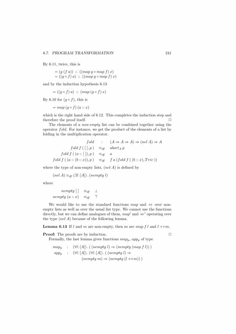
6.7. PROGRAM TRANSFORMATION 241
By 6.11, twice, this is
= (g (f a)) :: ((map g map f) x)= ((g f) a) :: ((map g map f) x)
and by the induction hypothesis 6.13
= ((g f) a) :: (map (g f) x)
By 6.10 for (g f), this is
= map (g f) (a :: x)
which is the right hand side of 6.12. This completes the induction step andtherefore the proof itself. 2
The elements of a non-empty list can be combined together using theoperator fold. For instance, we get the product of the elements of a list byfolding in the multiplication operator.
fold : (A⇒ A⇒ A)⇒ (nel A)⇒ A
fold f ( [ ], p ) ≡df abortA p
fold f ( (a :: [ ]), p ) ≡df a
fold f ( (a :: (b :: x)), p ) ≡df f a (fold f ( (b :: x), T riv ))
where the type of non-empty lists, (nel A) is defined by
(nel A)≡df (∃l : [A]) . (nempty l)
where
nempty [ ] ≡df ⊥nempty (a :: x) ≡df >
We would like to use the standard functions map and ++ over non-empty lists as well as over the usual list type. We cannot use the functionsdirectly, but we can define analogues of them, map′ and ++′ operating overthe type (nel A) because of the following lemma.
Lemma 6.13 If l and m are non-empty, then so are map f l and l ++m.
Proof: The proofs are by induction. 2
Formally, the last lemma gives functions mapp, appp of type
mapp : (∀l : [A]) . ( (nempty l)⇒ (nempty (map f l)) )appp : (∀l : [A]) . (∀l : [A]) . ( (nempty l)⇒
(nempty m)⇒ (nempty (l ++m)) )
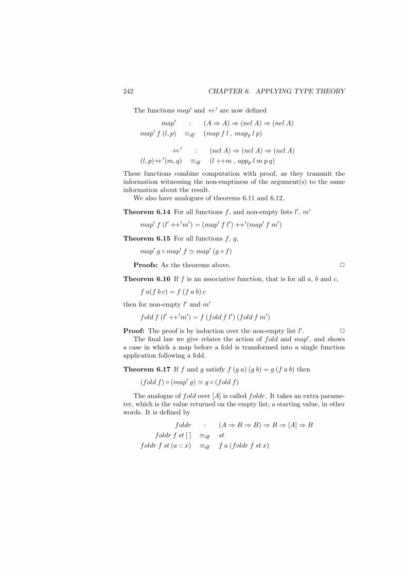
242 CHAPTER 6. APPLYING TYPE THEORY
The functions map′ and ++′ are now defined
map′ : (A⇒ A)⇒ (nel A)⇒ (nel A)map′ f (l, p) ≡df (map f l , mapp l p)
++′ : (nel A)⇒ (nel A)⇒ (nel A)(l, p)++′(m, q) ≡df (l ++m , appp l m p q)
These functions combine computation with proof, as they transmit theinformation witnessing the non-emptiness of the argument(s) to the sameinformation about the result.
We also have analogues of theorems 6.11 and 6.12,
Theorem 6.14 For all functions f , and non-empty lists l′, m′
map′ f (l′ ++′m′) = (map′ f l′) ++′(map′ f m′)
Theorem 6.15 For all functions f , g,
map′ g map′ f ' map′ (g f)
Proofs: As the theorems above. 2
Theorem 6.16 If f is an associative function, that is for all a, b and c,
f a(f b c) = f (f a b) c
then for non-empty l′ and m′
fold f (l′ ++′m′) = f (fold f l′) (fold f m′)
Proof: The proof is by induction over the non-empty list l′. 2
The final law we give relates the action of fold and map′, and showsa case in which a map before a fold is transformed into a single functionapplication following a fold.
Theorem 6.17 If f and g satisfy f (g a) (g b) = g (f a b) then
(fold f) (map′ g) ' g (fold f)
The analogue of fold over [A] is called foldr. It takes an extra parame-ter, which is the value returned on the empty list; a starting value, in otherwords. It is defined by
foldr : (A⇒ B ⇒ B)⇒ B ⇒ [A]⇒ B
foldr f st [ ] ≡df st
foldr f st (a :: x) ≡df f a (foldr f st x)
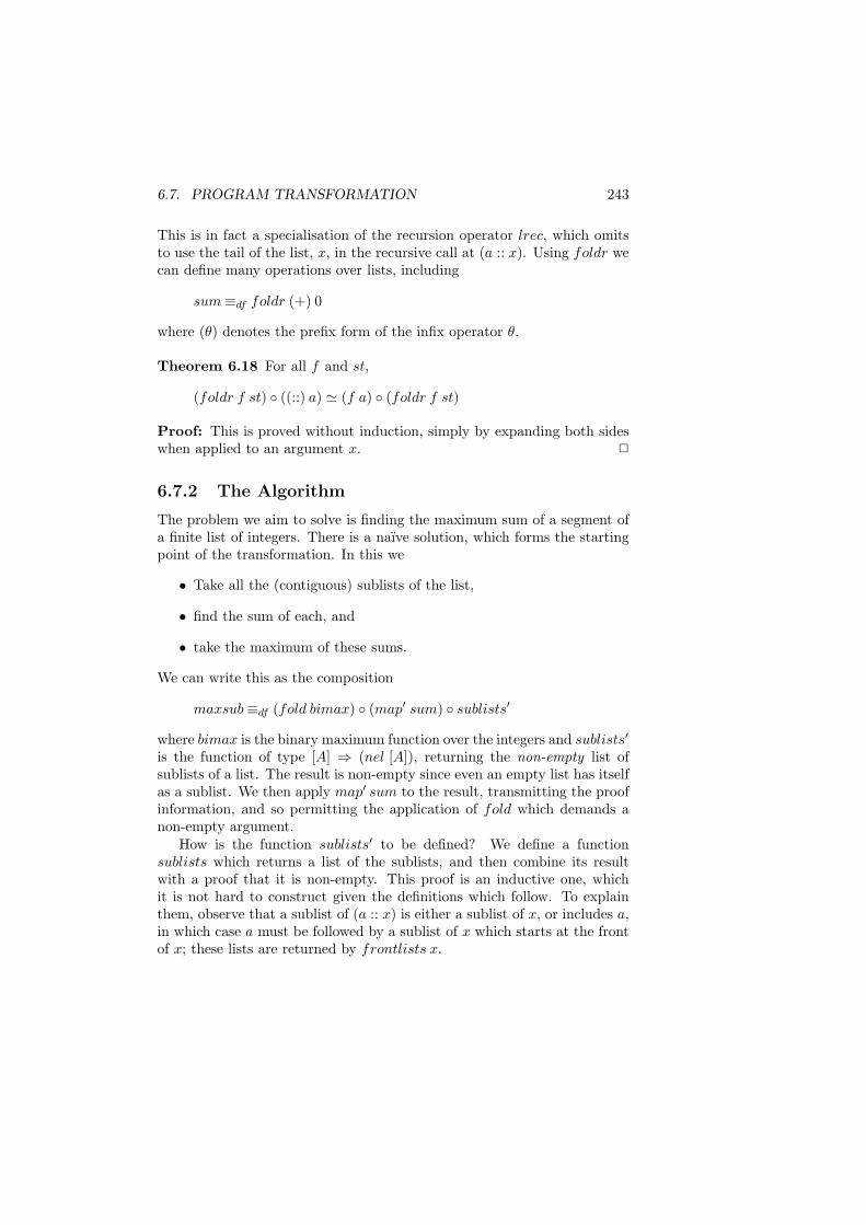
6.7. PROGRAM TRANSFORMATION 243
This is in fact a specialisation of the recursion operator lrec, which omitsto use the tail of the list, x, in the recursive call at (a :: x). Using foldr wecan define many operations over lists, including
sum≡df foldr (+) 0
where (θ) denotes the prefix form of the infix operator θ.
Theorem 6.18 For all f and st,
(foldr f st) ((::) a) ' (f a) (foldr f st)
Proof: This is proved without induction, simply by expanding both sideswhen applied to an argument x. 2
6.7.2 The Algorithm
The problem we aim to solve is finding the maximum sum of a segment ofa finite list of integers. There is a naıve solution, which forms the startingpoint of the transformation. In this we
• Take all the (contiguous) sublists of the list,
• find the sum of each, and
• take the maximum of these sums.
We can write this as the composition
maxsub≡df (fold bimax) (map′ sum) sublists′
where bimax is the binary maximum function over the integers and sublists′
is the function of type [A] ⇒ (nel [A]), returning the non-empty list ofsublists of a list. The result is non-empty since even an empty list has itselfas a sublist. We then apply map′ sum to the result, transmitting the proofinformation, and so permitting the application of fold which demands anon-empty argument.
How is the function sublists′ to be defined? We define a functionsublists which returns a list of the sublists, and then combine its resultwith a proof that it is non-empty. This proof is an inductive one, whichit is not hard to construct given the definitions which follow. To explainthem, observe that a sublist of (a :: x) is either a sublist of x, or includes a,in which case a must be followed by a sublist of x which starts at the frontof x; these lists are returned by frontlists x.
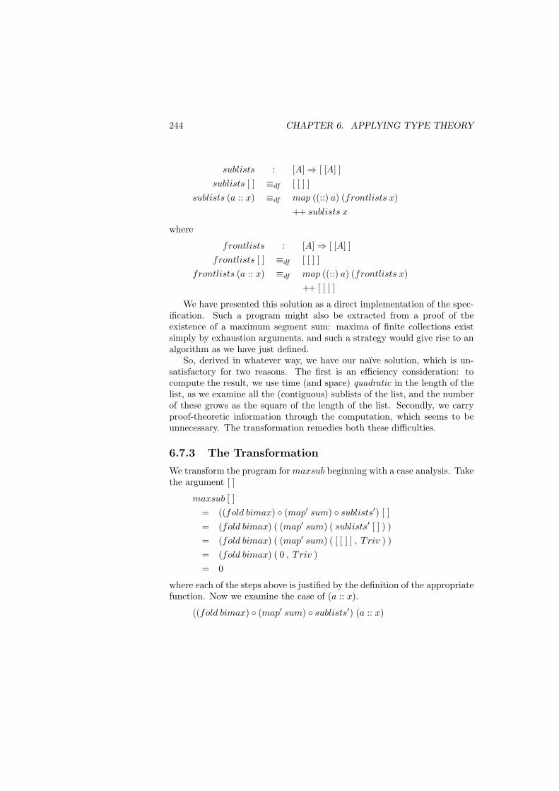
244 CHAPTER 6. APPLYING TYPE THEORY
sublists : [A]⇒ [ [A] ]sublists [ ] ≡df [ [ ] ]
sublists (a :: x) ≡df map ((::) a) (frontlists x)++ sublists x
where
frontlists : [A]⇒ [ [A] ]frontlists [ ] ≡df [ [ ] ]
frontlists (a :: x) ≡df map ((::) a) (frontlists x)++ [ [ ] ]
We have presented this solution as a direct implementation of the spec-ification. Such a program might also be extracted from a proof of theexistence of a maximum segment sum: maxima of finite collections existsimply by exhaustion arguments, and such a strategy would give rise to analgorithm as we have just defined.
So, derived in whatever way, we have our naıve solution, which is un-satisfactory for two reasons. The first is an efficiency consideration: tocompute the result, we use time (and space) quadratic in the length of thelist, as we examine all the (contiguous) sublists of the list, and the numberof these grows as the square of the length of the list. Secondly, we carryproof-theoretic information through the computation, which seems to beunnecessary. The transformation remedies both these difficulties.
6.7.3 The Transformation
We transform the program for maxsub beginning with a case analysis. Takethe argument [ ]
maxsub [ ]= ((fold bimax) (map′ sum) sublists′) [ ]= (fold bimax) ( (map′ sum) ( sublists′ [ ] ) )= (fold bimax) ( (map′ sum) ( [ [ ] ] , T riv ) )= (fold bimax) ( 0 , T riv )= 0
where each of the steps above is justified by the definition of the appropriatefunction. Now we examine the case of (a :: x).
((fold bimax) (map′ sum) sublists′) (a :: x)
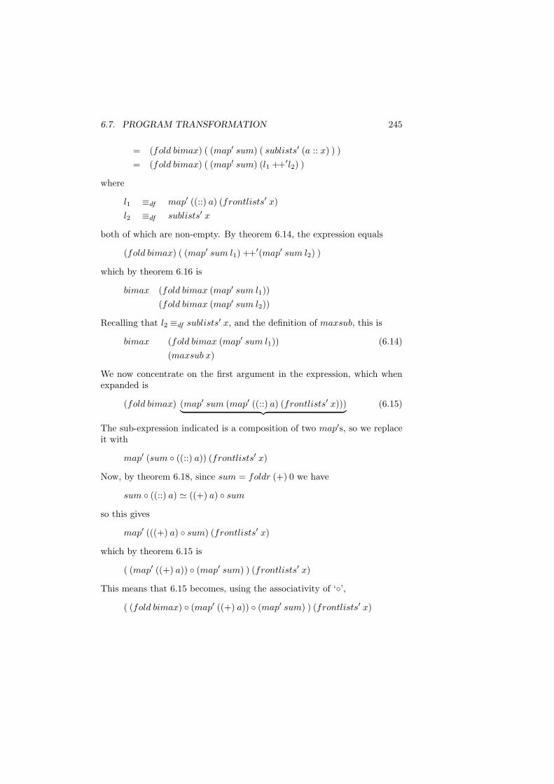
6.7. PROGRAM TRANSFORMATION 245
= (fold bimax) ( (map′ sum) ( sublists′ (a :: x) ) )= (fold bimax) ( (map′ sum) (l1 ++′l2) )
where
l1 ≡df map′ ((::) a) (frontlists′ x)l2 ≡df sublists′ x
both of which are non-empty. By theorem 6.14, the expression equals
(fold bimax) ( (map′ sum l1) ++′(map′ sum l2) )
which by theorem 6.16 is
bimax (fold bimax (map′ sum l1))(fold bimax (map′ sum l2))
Recalling that l2 ≡df sublists′ x, and the definition of maxsub, this is
bimax (fold bimax (map′ sum l1)) (6.14)(maxsub x)
We now concentrate on the first argument in the expression, which whenexpanded is
(fold bimax) (map′ sum (map′ ((::) a) (frontlists′ x)))︸ ︷︷ ︸ (6.15)
The sub-expression indicated is a composition of two map′s, so we replaceit with
map′ (sum ((::) a)) (frontlists′ x)
Now, by theorem 6.18, since sum = foldr (+) 0 we have
sum ((::) a) ' ((+) a) sum
so this gives
map′ (((+) a) sum) (frontlists′ x)
which by theorem 6.15 is
( (map′ ((+) a)) (map′ sum) ) (frontlists′ x)
This means that 6.15 becomes, using the associativity of ‘’,
( (fold bimax) (map′ ((+) a)) (map′ sum) ) (frontlists′ x)
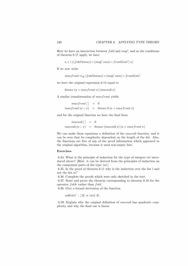
246 CHAPTER 6. APPLYING TYPE THEORY
Here we have an interaction between fold and map′, and as the conditionsof theorem 6.17 apply, we have
a + ( ((fold bimax) (map′ sum) frontlists′) x)
If we now write
maxfront≡df (fold bimax) (map′ sum) frontlists′
we have the original expression 6.14 equal to
bimax (a + maxfront x) (maxsub x)
A similar transformation of maxfront yields
maxfront [ ] = 0maxfront (a :: x) = bimax 0 (a + maxfront x)
and for the original function we have the final form
maxsub [ ] = 0maxsub (a :: x) = bimax (maxsub x) (a + maxfront x)
We can make these equations a definition of the maxsub function, and itcan be seen that its complexity dependent on the length of the list. Also,the functions are free of any of the proof information which appeared inthe original algorithm, because it used non-empty lists.
Exercises
6.34. What is the principle of induction for the type of integers int intro-duced above? [Hint: it can be derived from the principles of induction onthe component parts of the type int.]6.35. In the proof of theorem 6.11 why is the induction over the list l andnot the list m?6.36. Complete the proofs which were only sketched in the text.6.37. State and prove the theorem corresponding to theorem 6.16 for the
operator foldr rather than fold.6.38. Give a formal derivation of the function
sublists′ : [A]⇒ (nel A)
6.39. Explain why the original definition of maxsub has quadratic com-plexity and why the final one is linear.
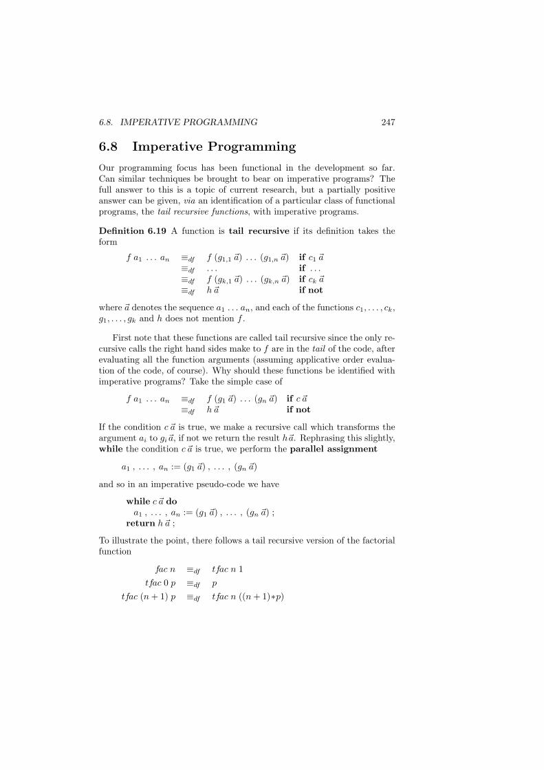
6.8. IMPERATIVE PROGRAMMING 247
6.8 Imperative Programming
Our programming focus has been functional in the development so far.Can similar techniques be brought to bear on imperative programs? Thefull answer to this is a topic of current research, but a partially positiveanswer can be given, via an identification of a particular class of functionalprograms, the tail recursive functions, with imperative programs.
Definition 6.19 A function is tail recursive if its definition takes theform
f a1 . . . an ≡df f (g1,1 ~a) . . . (g1,n ~a) if c1 ~a≡df . . . if . . .≡df f (gk,1 ~a) . . . (gk,n ~a) if ck ~a≡df h~a if not
where ~a denotes the sequence a1 . . . an, and each of the functions c1, . . . , ck,g1, . . . , gk and h does not mention f .
First note that these functions are called tail recursive since the only re-cursive calls the right hand sides make to f are in the tail of the code, afterevaluating all the function arguments (assuming applicative order evalua-tion of the code, of course). Why should these functions be identified withimperative programs? Take the simple case of
f a1 . . . an ≡df f (g1 ~a) . . . (gn ~a) if c ~a≡df h~a if not
If the condition c ~a is true, we make a recursive call which transforms theargument ai to gi~a, if not we return the result h~a. Rephrasing this slightly,while the condition c ~a is true, we perform the parallel assignment
a1 , . . . , an := (g1 ~a) , . . . , (gn ~a)
and so in an imperative pseudo-code we have
while c ~a doa1 , . . . , an := (g1 ~a) , . . . , (gn ~a) ;
return h~a ;
To illustrate the point, there follows a tail recursive version of the factorialfunction
fac n ≡df tfac n 1tfac 0 p ≡df p
tfac (n + 1) p ≡df tfac n ((n + 1)∗p)
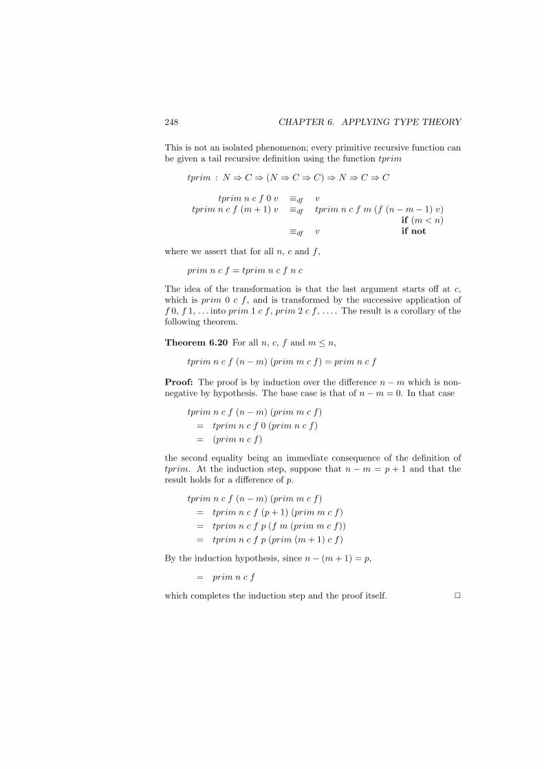
248 CHAPTER 6. APPLYING TYPE THEORY
This is not an isolated phenomenon; every primitive recursive function canbe given a tail recursive definition using the function tprim
tprim : N ⇒ C ⇒ (N ⇒ C ⇒ C)⇒ N ⇒ C ⇒ C
tprim n c f 0 v ≡df vtprim n c f (m + 1) v ≡df tprim n c f m (f (n−m− 1) v)
if (m < n)≡df v if not
where we assert that for all n, c and f ,
prim n c f = tprim n c f n c
The idea of the transformation is that the last argument starts off at c,which is prim 0 c f , and is transformed by the successive application off 0, f 1, . . . into prim 1 c f , prim 2 c f , . . . . The result is a corollary of thefollowing theorem.
Theorem 6.20 For all n, c, f and m ≤ n,
tprim n c f (n−m) (prim m c f) = prim n c f
Proof: The proof is by induction over the difference n−m which is non-negative by hypothesis. The base case is that of n−m = 0. In that case
tprim n c f (n−m) (prim m c f)= tprim n c f 0 (prim n c f)= (prim n c f)
the second equality being an immediate consequence of the definition oftprim. At the induction step, suppose that n − m = p + 1 and that theresult holds for a difference of p.
tprim n c f (n−m) (prim m c f)= tprim n c f (p + 1) (prim m c f)= tprim n c f p (f m (prim m c f))= tprim n c f p (prim (m + 1) c f)
By the induction hypothesis, since n− (m + 1) = p,
= prim n c f
which completes the induction step and the proof itself. 2
6.9. EXAMPLES IN THE LITERATURE 249
Corollary 6.21 For all n, c and f ,
tprim n c f n c = prim n c f
Proof: Take m = 0 in the theorem. 2
Note that in the action of tprim the first three arguments are not mod-ified in the recursive calls — they act as parameters or constants of theprogram, and no storage locations need to be allocated to them; the othertwo parameters do of course need to be allotted space.
The corollary justifies the transformation of any primitive recursivefunction into a tail recursive one, and thus into an imperative form. Wecan prove similar theorems for the other recursion operators in the system,so a functional program can form an intermediate step in the developmentof an imperative program, as long as the imperative target language cansupport all the higher order data types of TT . In the case that it cannot,other coding techniques can be found, but the correspondence is less direct.
If we take any imperative program there will be a functional form forit, in which the only recursion is tail recursion. However that tail recursionmay not be formalizable in TT , since it may lead to non-termination. Ifwe can supply a proof of termination for the imperative program, and theproof can be formalised in first-order arithmetic (see section 5.11), thenthere will be an equivalent of the program in TT .
Exercises
6.40. Give tail recursive forms of the recursion operators over lists andtrees.6.41. Comment on the space efficiency of the tail recursive form of the fac-torial function. Does your observation depend upon the form of evaluationchosen for terms of TT?
6.9 Examples in the literature
This section provides a survey of examples in the published literature ofproof and program development in theories similar to TT . Many of theexamples use the subset type; we shall discuss this and its relevance toprogram development in the chapter to come, which contains examples ofnew concepts as they are introduced.
250 CHAPTER 6. APPLYING TYPE THEORY
6.9.1 Martin-Lof
In Martin-Lof’s work there are few examples. The extensional version ofthe theory, [ML85], contains a proof of the axiom of choice,
(∀x :A) . (∃y :B) . C ⇒ (∃f : (∀x :A) . B) . (∀x :A) . C[(f x)/y]
which involves the strong existential elimination rule, (∃E), in an essentialway. As well as a proof of the axiom of choice, the Padova notes [ML84],contain small examples but nothing large-scale. Martin-Lof’s notes on con-structive mathematics, [ML70], contain examples of mathematical proofsdeveloped from a constructive standpoint, but it is fair to say that theybear little formal relation to proofs in TT .
6.9.2 Goteborg
A source of many examples is the Programming Methodology Group at theUniversity of Goteborg and Chalmers University of Technology, in Sweden.In [Dyb87] type theory is examined as one of a number of systems appliedto the example of the derivation of an algorithm to normalise the syntacticform of propositional expressions.
Generalising the idea of a multilevel array, as used in VDL and VDM,is the type of multilevel functions, which also encompasses the types ofvectors, natural numbers, lists and others. A formal presentation of thistype as an addition to TT is given in [Nor85]. The types could also bedeveloped using the W -types of TT+ but the authors argue that it is morenatural to add the new rules to embody the type directly.
In [NP85] there is a discussion of how the quantifiers and dependenttypes of TT can be used to provide specifications of modules.
6.9.3 Backhouse et al.
Roland Backhouse and his co-workers at the Universities of Groningen andEindhoven have written widely on the topic of type theory. We shall look attheir work later when we look at extensions of the theory, but there are anumber of sources we should mention now. The tutorial notes [Bac87a]contain a number of shorter examples, chosen to illustrate the systemconstruct-by-construct. The paper [BCMS89], which introduces a num-ber of additions, also contains useful examples, such as the Boyer-Mooremajority vote algorithm and a collection of game playing operations, similarto those in [Hug90].
6.9. EXAMPLES IN THE LITERATURE 251
A substantial derivation of a parsing algorithm is given in [Chi87]. Theparser is specified by the assertion
(∀w :Word) . Parse w ∨ ¬Parse w
where the proposition Parse w is an assertion of the fact that the string wis a sentence of the language. Proofs of this proposition consist of showingthat there is a valid parse tree for the word, as expressed by
w = spell pt
spell being the function to ‘spell out’ the word coded by a parse tree pt. Theimplementation is compared with the result of an earlier effort to derive aprogram using the LCF system, [CM82].
6.9.4 Nuprl
Constable’s group at Cornell University have concentrated in their Nuprlsystem, which we shall discuss in more detail in section 9.1.1 on ‘Imple-menting Mathematics’, which is indeed the title of their exposition of Nuprl,[C+86a]. The system is sufficiently close to type theory for the majorityof their examples to be comprehensible if not translatable. [C+86a] con-tains short expository examples, of course, but also develops a number oflibraries of mathematical objects in Chapter 11.
Howe’s thesis, [How88], gives a detailed analysis of Girard’s paradox inChapter 4. Sections 3.10 and 3.11 contain a number-theoretic example, anda saddleback search, and chapter 5 addresses the issue of reflection, whichis taken up by [KC86]. The addition of partial objects to type theory isdiscussed in [CS87]
A more concrete application to hardware specification and verificationis presented in [BdV89]. The specific component investigated is the frontend of a floating point adder/subtractor.
6.9.5 Calculus of Constructions
One other system which bears a rather less close relation to TT is Huet andCoquand’s Calculus of Constructions, [CH85]. An example of algorithm de-velopment is to be found in [PM87] and the extraction of programs fromproofs in the calculus is examined in [PM89]. An analysis of Girard’s para-dox is given in [Coq86].

252 CHAPTER 6. APPLYING TYPE THEORY
Chapter 7
Augmenting Type Theory
Using type theory as a program development system has lead a number ofpeople to propose that new constructs be added to the theory. Although wehave seen that in theory the system is highly expressive, there are questionsof whether it expresses what is required in either a natural or an efficientway. This chapter contains an account of the proposals concerning ways inwhich the system may be augmented.
An important point which should be made before we embark is thateach of the additions, whilst arguably adding to the power of the systemin some way, also makes it more complicated, either from a user’s point ofview, or for foundational reasons, such as the loss of strong normalisation.We shall discuss the pros and cons of each proposal section-by-section, andshall in the conclusion to the book have something more to say on the topic.
Central to the proposals is the notion of a subset type, distinct from theexistential type, whose members are simply those elements of the base typewith the required property, rather than such objects paired with a witnessto that property. To set the discussion in its proper context, we begin insection 7.1 by looking at the exact nature of specifications, a topic we firstexamined when we looked at the case study of the Polish National Flag.What precisely are specifications in type theory has been the subject ofsome confusion in the literature; we hope to have to clarified the issue here.
Another general topic connected with the introduction of the subset typeis that of computational relevance: some parts of expressions seem to have apurely logical role, rather than contributing to the result of a computationalprocess. We discuss two approaches to capturing this intuition, and alsolook at how it is linked with lazy evaluation. Naturally, any argumentabout computational relevance or efficiency can only be conducted relativeto some evaluation scheme, and we argue that many of the reasons advanced
253
254 CHAPTER 7. AUGMENTING TYPE THEORY
for a more complicated type system in view of computational efficiency areirrelevant in case the system is implemented using lazy evaluation.
After this background discussion, in section 7.2 we introduce the naıvedefinition of the subset type, and examine some of its theoretical draw-backs. As we said above, much of the motivation for subsets is to achievea separation between logical and computational aspects of type theory; insection 7.3 we look at how subsets can properly be expressed only in asystem in which propositions and types are no longer identified.
We give a review of the proposals in section 7.4 where we argue thatall the examples of subsets in the literature can be handled quite smoothlywithin TT , without recourse to the new type. This is achieved by a lazyimplementation together with a judicious choice of types in specifications:we choose to specify a function by asserting its existence rather than bya ∀∃-formula, for instance. We provide a number of general and concreteexamples by way of illustration.
The primitive type forming operation, W , constructs free data types,whilst there are examples in which an abstract object can best be repre-sented by a collection of concrete items: a set represented as a list is onecase. To reason and program most simply with such a type it is argued thata quotient type, consisting of equivalence classes, be formed. We examinetwo variants of this idea in section 7.5.
An important application area for constructive mathematics is real anal-ysis. Section 7.6 gives the beginnings of a treatment of the topic, and alsoserves as a case study in which to examine the utility of the subset andquotient type.
Various infelicities have been shown in the rules for elimination — thefollowing section examines proposals to overcome these by means of thestrong elimination rules. A generalisation of these, the polymorphic typesof Backhouse et. al. are also introduced. It is interesting to observe thatan addition of this sort can lead to a term which has no normal formand indeed no weak head normal form: a genuine non-termination is thuspresent in the augmented system. This will maybe underline the fact the‘reasonable’ additions to a system made in an ad hoc way can lead tounforeseen circumstances, and that we should make quite certain that anyaddition we make does not destroy something more important than it adds.
As we saw in the last chapter, recursions can be coded in type theoryonly in terms of the primitives provided. The most general form of termi-nating recursion is called well-founded recursion. We first look at what thisis in a set-theoretic context in section 7.8, and then in the following sectionwe look at two different ways that well-founded recursion can be addedto type theory. The general mechanism provided derives once-and-for-allthe principles of which particular cases, like quicksort, were derived in the
7.1. BACKGROUND 255
course of the proof developments of the last chapter.A different approach again is to provide new methods of defining types,
together with definition mechanisms. Equivalent to well-founded recursionwe can add types defined by a general principle of induction, which we do insection 7.10. We discuss the relation between these types and the W typesof TT , and argue that the latter can be used to provide a representation ofthe former.
A novel idea, at least from the programming point of view, is to de-fine the co-inductive types, which are the largest solutions of certain typeequations. If we solve the equation characterising lists, then the smallestsolution contains simply the finite elements, whilst the largest contains infi-nite elements also. The presence of infinite lists is not a surprise to the lazyfunctional programmer, but remarkable is the absence of partial lists. Weshow how a general scheme of co-induction is introduced, and then exam-ine in more detail the type of infinite lists or streams. In this context it isinteresting to note that if we use infinite lists as models for communicationsbetween communicating processes (a la Kahn and MacQueen) then in typetheory we can be sure that if a recursion is possible it give a completelydefined list, ruling out the possibility of deadlock.
Consistency of TT as a logical system will be lost if partial objects arepermitted to inhabit every type, since then the undefined element will bea member of each type, which from a logical point of view means thatevery theorem is provable. There are other ways for partial objects to beadded, however – a proposal for the incorporation of a representation ofsuch objects is given in section 7.12. This is done without sacrificing theCurry Howard isomorphism or the consistency of the logical system.
The proposals thus far are general, but another kind of extension ispossible. Martin-Lof has always stressed the open-endedness of the system,and in the final section we look at how a particular kind of object, the semi-group, can be modelled by adding a set of new rules governing its behaviour.We contrast this approach with that of forming an explicit model of the typewithin the theory. Naturally, this approach is not limited to semi-groupsbut can be used in any particular application area.
7.1 Background
This section explores some of the background to the introduction of thesubset type into TT , before we go on to discuss exactly how this might bedone, and indeed whether it is necessary.
256 CHAPTER 7. AUGMENTING TYPE THEORY
7.1.1 What is a specification?
We first examined this question in section 6.6 above in the particular con-text of the Polish National Flag problem. Here we reconsider it from amore general point of view.
The judgement a : A can be thought of as expressing ‘a proves theproposition A’ and ‘a is an object of type A’, but it has also been proposed,in [ML85, PS85] for example, that it be read as saying
a is a program which meets the specification A (†)
This interpretation does not apply in general to every judgement a : A.Take for instance the case of a function f which sorts lists; this has type[A]⇒ [A], and so,
f : [A]⇒ [A]
Should we therefore say that it meets the specification [A] ⇒ [A]? Itdoes, but then so do the identity and the reverse functions! The type ofa function is but one aspect of its specification, which should describe therelation between its input and output. This characterisation takes the form
The result (f l) is ordered and a permutation of the list l
for which we will write S(f). To assert that the specification can be metby some implementation, we write
(∃x : [A]⇒ [A]) . S(x)
What form do objects of this type take? They are pairs (f, p) with f :[A] ⇒ [A] and p a proof that f has the property S(f). The confusion in(†) is thus that the object a consists not only of the program meeting thespecification, but also of the proof that it meets that specification.
In the light of the discussion above, it seems sensible to suggest thatwe conceive of specifications as statements (∃o :T ) . P , and that the formalassertion
(o, p) : (∃o :T ) . P
be interpreted as saying
The object o, of type T is shown to meet the specification P bythe proof object p.
an interpretation which combines the logical and programming interpre-tations of the language in an elegant way. This would be obvious to a
7.1. BACKGROUND 257
constructivist, who would argue that we can only assert (†) if we have theappropriate evidence, namely the proof object.
In developing a proof of the formula (∃o :T ) . P we construct a pair con-sisting of an object of type T and a proof that the object has the propertyP . Such a pair keeps separate the computational and logical aspects of thedevelopment, so that we can extract directly the computational part simplyby choosing the first element of the pair.
There is a variation on this theme, mentioned in [NPS90] and examinedin section 6.6, which suggests that a specification of a function should beof the form
(∀x :A) . (∃y :B) . P (x, y) (7.1)
Elements of this type are functions F so that for all x :A,
F x : (∃y :B) . P (x, y)
and each of these values will be a pair (yx, px) with
yx :B and px :P (x, y)
The pair consists of value and proof information, showing that under thisapproach the program and its verification are inextricably mixed. It hasbeen argued that the only way to achieve this separation is to replacethe inner existential type with a subset type, which removes the proofinformation px. This can be done, but the intermingling can be avoidedwithout augmenting the system. We simply have to give the intendedfunction a name. That such a naming can be achieved in general is asimple consequence of the axiom of choice, which states that
(∀x :A) . (∃y :B) . P (x, y)⇒ (∃f :A⇒ B) . (∀x :A) . P (x, f x)
and applying modus ponens to this and (7.1) we deduce an ‘existential’specification as above. Note that the converse implication to that of theaxiom of choice is easily derivable, making the two forms of the specificationlogically equivalent.
The equivalent specifications can be thought of as suggesting differentprogram development methods: using the ∃∀ form, we develop the functionand its proof as separate entities, either separately or together, whilst inthe ∀∃ form we extract a function from a proof, post hoc.
This analysis of specifications makes it clear that when we seek a pro-gram to meet a specification, we look for the first component of a mem-ber of an existential type; the second proves that the program meets theconstraint part of the specification. As long as we realise this, it seemsirrelevant whether or not our system includes a type of first components,
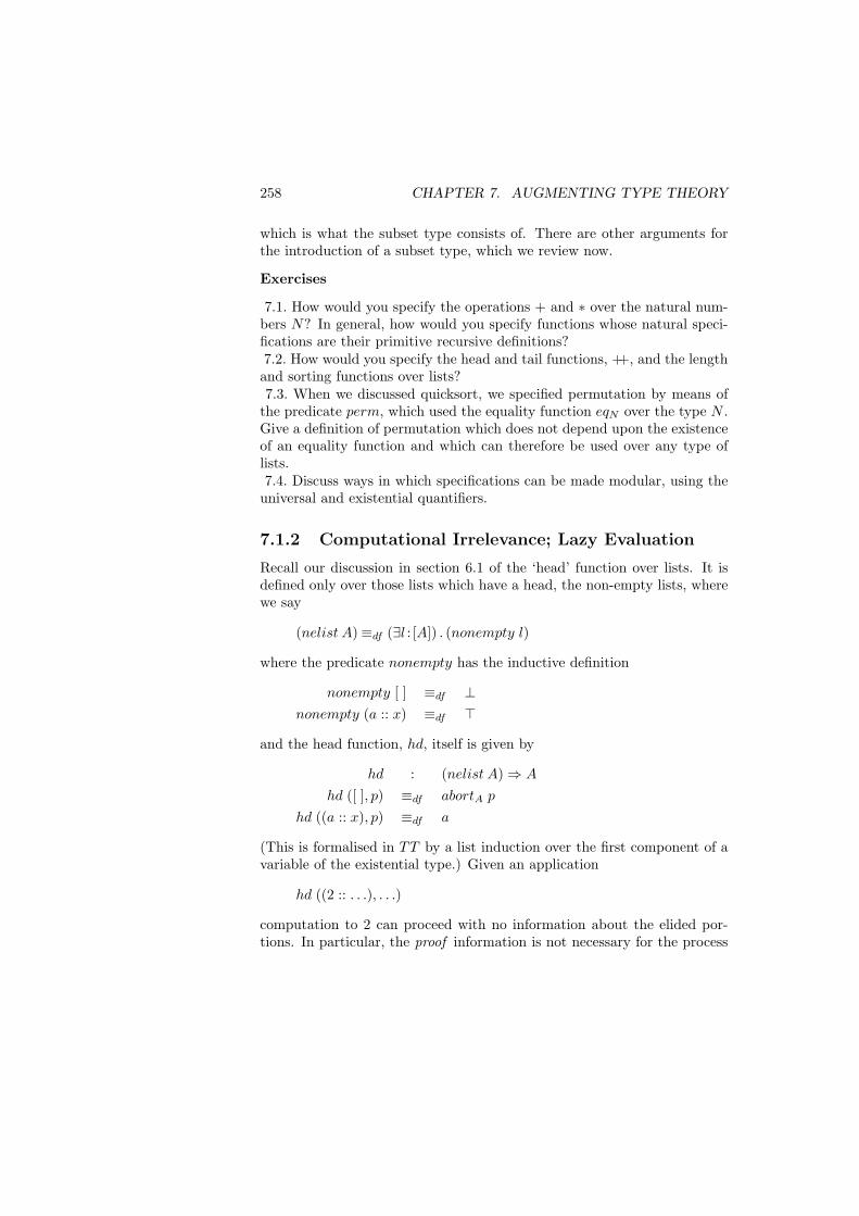
258 CHAPTER 7. AUGMENTING TYPE THEORY
which is what the subset type consists of. There are other arguments forthe introduction of a subset type, which we review now.
Exercises
7.1. How would you specify the operations + and ∗ over the natural num-bers N? In general, how would you specify functions whose natural speci-fications are their primitive recursive definitions?7.2. How would you specify the head and tail functions, ++, and the lengthand sorting functions over lists?7.3. When we discussed quicksort, we specified permutation by means of
the predicate perm, which used the equality function eqN over the type N .Give a definition of permutation which does not depend upon the existenceof an equality function and which can therefore be used over any type oflists.7.4. Discuss ways in which specifications can be made modular, using the
universal and existential quantifiers.
7.1.2 Computational Irrelevance; Lazy Evaluation
Recall our discussion in section 6.1 of the ‘head’ function over lists. It isdefined only over those lists which have a head, the non-empty lists, wherewe say
(nelist A)≡df (∃l : [A]) . (nonempty l)
where the predicate nonempty has the inductive definition
nonempty [ ] ≡df ⊥nonempty (a :: x) ≡df >
and the head function, hd, itself is given by
hd : (nelist A)⇒ A
hd ([ ], p) ≡df abortA p
hd ((a :: x), p) ≡df a
(This is formalised in TT by a list induction over the first component of avariable of the existential type.) Given an application
hd ((2 :: . . .), . . .)
computation to 2 can proceed with no information about the elided por-tions. In particular, the proof information is not necessary for the process
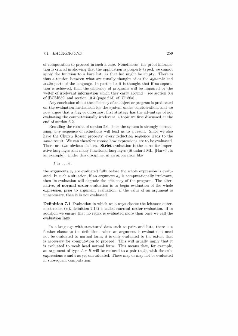
7.1. BACKGROUND 259
of computation to proceed in such a case. Nonetheless, the proof informa-tion is crucial in showing that the application is properly typed; we cannotapply the function to a bare list, as that list might be empty. There isthus a tension between what are usually thought of as the dynamic andstatic parts of the language. In particular it is thought that if no separa-tion is achieved, then the efficiency of programs will be impaired by thewelter of irrelevant information which they carry around – see section 3.4of [BCMS89] and section 10.3 (page 213) of [C+86a].
Any conclusion about the efficiency of an object or program is predicatedon the evaluation mechanism for the system under consideration, and wenow argue that a lazy or outermost first strategy has the advantage of notevaluating the computationally irrelevant, a topic we first discussed at theend of section 6.2.
Recalling the results of section 5.6, since the system is strongly normal-ising, any sequence of reductions will lead us to a result. Since we alsohave the Church Rosser property, every reduction sequence leads to thesame result. We can therefore choose how expressions are to be evaluated.There are two obvious choices. Strict evaluation is the norm for imper-ative languages and many functional languages (Standard ML, [Har86], isan example). Under this discipline, in an application like
f a1 . . . an
the arguments ai are evaluated fully before the whole expression is evalu-ated. In such a situation, if an argument ak is computationally irrelevant,then its evaluation will degrade the efficiency of the program. The alter-native, of normal order evaluation is to begin evaluation of the wholeexpression, prior to argument evaluation: if the value of an argument isunnecessary, then it is not evaluated.
Definition 7.1 Evaluation in which we always choose the leftmost outer-most redex (c.f. definition 2.13) is called normal order evaluation. If inaddition we ensure that no redex is evaluated more than once we call theevaluation lazy.
In a language with structured data such as pairs and lists, there is afurther clause to the definition: when an argument is evaluated it neednot be evaluated to normal form; it is only evaluated to the extent thatis necessary for computation to proceed. This will usually imply that itis evaluated to weak head normal form. This means that, for example,an argument of type A ∧ B will be reduced to a pair (a, b), with the sub-expressions a and b as yet unevaluated. These may or may not be evaluatedin subsequent computation.
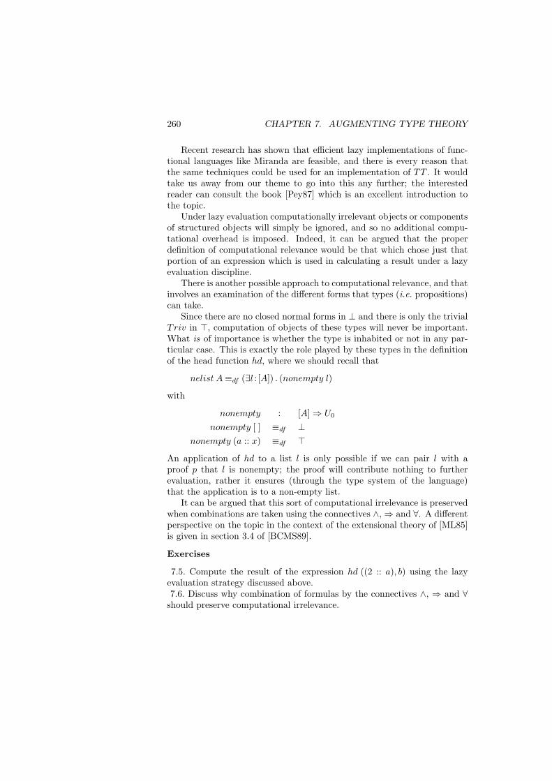
260 CHAPTER 7. AUGMENTING TYPE THEORY
Recent research has shown that efficient lazy implementations of func-tional languages like Miranda are feasible, and there is every reason thatthe same techniques could be used for an implementation of TT . It wouldtake us away from our theme to go into this any further; the interestedreader can consult the book [Pey87] which is an excellent introduction tothe topic.
Under lazy evaluation computationally irrelevant objects or componentsof structured objects will simply be ignored, and so no additional compu-tational overhead is imposed. Indeed, it can be argued that the properdefinition of computational relevance would be that which chose just thatportion of an expression which is used in calculating a result under a lazyevaluation discipline.
There is another possible approach to computational relevance, and thatinvolves an examination of the different forms that types (i.e. propositions)can take.
Since there are no closed normal forms in ⊥ and there is only the trivialTriv in >, computation of objects of these types will never be important.What is of importance is whether the type is inhabited or not in any par-ticular case. This is exactly the role played by these types in the definitionof the head function hd, where we should recall that
nelist A≡df (∃l : [A]) . (nonempty l)
with
nonempty : [A]⇒ U0
nonempty [ ] ≡df ⊥nonempty (a :: x) ≡df >
An application of hd to a list l is only possible if we can pair l with aproof p that l is nonempty; the proof will contribute nothing to furtherevaluation, rather it ensures (through the type system of the language)that the application is to a non-empty list.
It can be argued that this sort of computational irrelevance is preservedwhen combinations are taken using the connectives ∧,⇒ and ∀. A differentperspective on the topic in the context of the extensional theory of [ML85]is given in section 3.4 of [BCMS89].
Exercises
7.5. Compute the result of the expression hd ((2 :: a), b) using the lazyevaluation strategy discussed above.7.6. Discuss why combination of formulas by the connectives ∧, ⇒ and ∀
should preserve computational irrelevance.
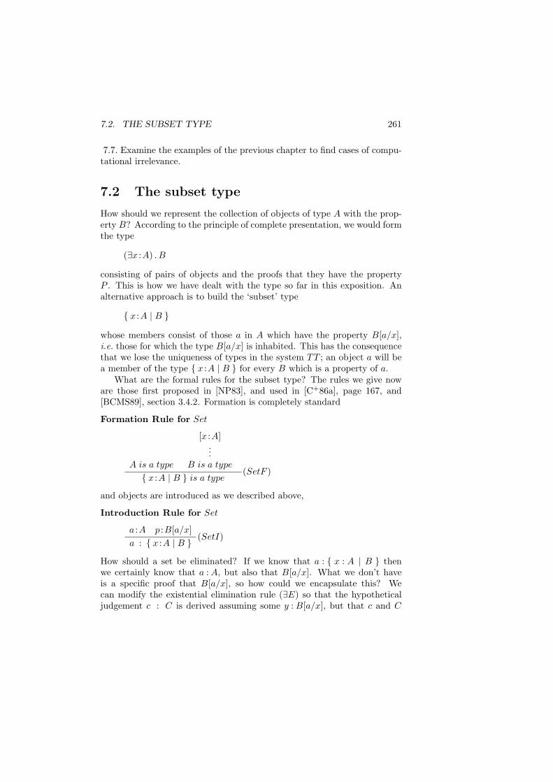
7.2. THE SUBSET TYPE 261
7.7. Examine the examples of the previous chapter to find cases of compu-tational irrelevance.
7.2 The subset type
How should we represent the collection of objects of type A with the prop-erty B? According to the principle of complete presentation, we would formthe type
(∃x :A) . B
consisting of pairs of objects and the proofs that they have the propertyP . This is how we have dealt with the type so far in this exposition. Analternative approach is to build the ‘subset’ type
x :A | B
whose members consist of those a in A which have the property B[a/x],i.e. those for which the type B[a/x] is inhabited. This has the consequencethat we lose the uniqueness of types in the system TT ; an object a will bea member of the type x :A | B for every B which is a property of a.
What are the formal rules for the subset type? The rules we give noware those first proposed in [NP83], and used in [C+86a], page 167, and[BCMS89], section 3.4.2. Formation is completely standard
Formation Rule for Set
A is a type
[x :A]...
B is a type
x :A | B is a type(SetF )
and objects are introduced as we described above,
Introduction Rule for Set
a :A p :B[a/x]a : x :A | B
(SetI)
How should a set be eliminated? If we know that a : x : A | B thenwe certainly know that a : A, but also that B[a/x]. What we don’t haveis a specific proof that B[a/x], so how could we encapsulate this? Wecan modify the existential elimination rule (∃E) so that the hypotheticaljudgement c : C is derived assuming some y : B[a/x], but that c and C
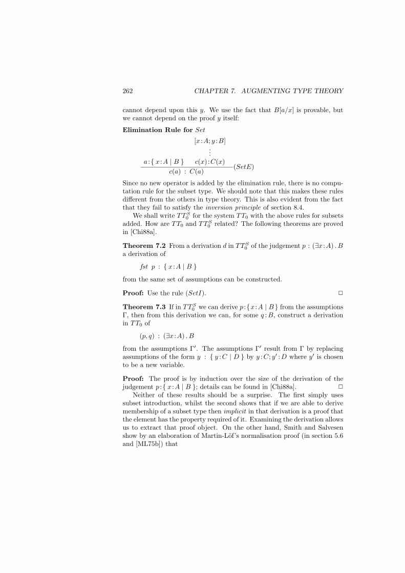
262 CHAPTER 7. AUGMENTING TYPE THEORY
cannot depend upon this y. We use the fact that B[a/x] is provable, butwe cannot depend on the proof y itself:
Elimination Rule for Set
a : x :A | B
[x :A; y :B]...
c(x) :C(x)c(a) : C(a)
(SetE)
Since no new operator is added by the elimination rule, there is no compu-tation rule for the subset type. We should note that this makes these rulesdifferent from the others in type theory. This is also evident from the factthat they fail to satisfy the inversion principle of section 8.4.
We shall write TTS0 for the system TT0 with the above rules for subsets
added. How are TT0 and TTS0 related? The following theorems are proved
in [Chi88a].
Theorem 7.2 From a derivation d in TTS0 of the judgement p : (∃x :A) . B
a derivation of
fst p : x :A | B
from the same set of assumptions can be constructed.
Proof: Use the rule (SetI). 2
Theorem 7.3 If in TTS0 we can derive p :x :A | B from the assumptions
Γ, then from this derivation we can, for some q :B, construct a derivationin TT0 of
(p, q) : (∃x :A) . B
from the assumptions Γ′. The assumptions Γ′ result from Γ by replacingassumptions of the form y : y :C | D by y :C; y′ :D where y′ is chosento be a new variable.
Proof: The proof is by induction over the size of the derivation of thejudgement p : x :A | B ; details can be found in [Chi88a]. 2
Neither of these results should be a surprise. The first simply usessubset introduction, whilst the second shows that if we are able to derivemembership of a subset type then implicit in that derivation is a proof thatthe element has the property required of it. Examining the derivation allowsus to extract that proof object. On the other hand, Smith and Salvesenshow by an elaboration of Martin-Lof’s normalisation proof (in section 5.6and [ML75b]) that
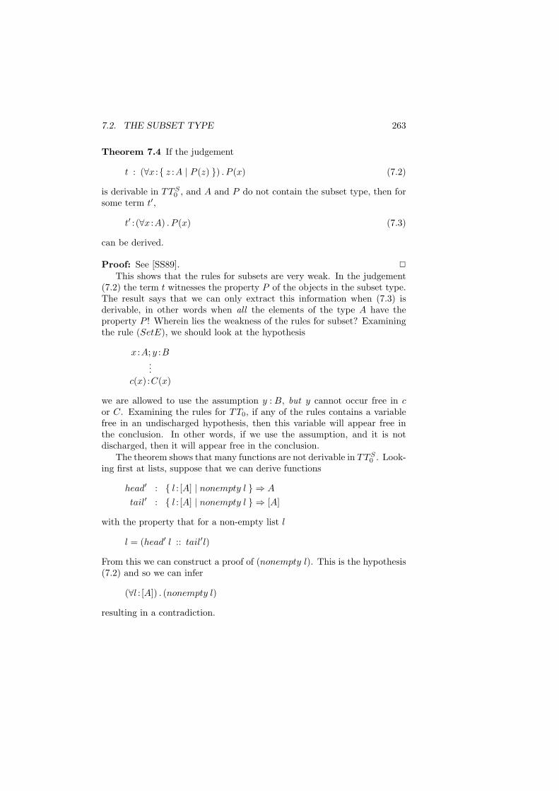
7.2. THE SUBSET TYPE 263
Theorem 7.4 If the judgement
t : (∀x : z :A | P (z) ) . P (x) (7.2)
is derivable in TTS0 , and A and P do not contain the subset type, then for
some term t′,
t′ : (∀x :A) . P (x) (7.3)
can be derived.
Proof: See [SS89]. 2
This shows that the rules for subsets are very weak. In the judgement(7.2) the term t witnesses the property P of the objects in the subset type.The result says that we can only extract this information when (7.3) isderivable, in other words when all the elements of the type A have theproperty P ! Wherein lies the weakness of the rules for subset? Examiningthe rule (SetE), we should look at the hypothesis
x :A; y :B...
c(x) :C(x)
we are allowed to use the assumption y : B, but y cannot occur free in cor C. Examining the rules for TT0, if any of the rules contains a variablefree in an undischarged hypothesis, then this variable will appear free inthe conclusion. In other words, if we use the assumption, and it is notdischarged, then it will appear free in the conclusion.
The theorem shows that many functions are not derivable in TTS0 . Look-
ing first at lists, suppose that we can derive functions
head′ : l : [A] | nonempty l ⇒ A
tail′ : l : [A] | nonempty l ⇒ [A]
with the property that for a non-empty list l
l = (head′ l :: tail′l)
From this we can construct a proof of (nonempty l). This is the hypothesis(7.2) and so we can infer
(∀l : [A]) . (nonempty l)
resulting in a contradiction.
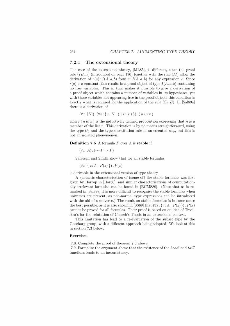
264 CHAPTER 7. AUGMENTING TYPE THEORY
7.2.1 The extensional theory
The case of the extensional theory, [ML85], is different, since the proofrule (IEext) (introduced on page 170) together with the rule (II) allow thederivation of r(a) : I(A, a, b) from e : I(A, a, b) for any expression e. Sincer(a) is a constant, this results in a proof object of type I(A, a, b) containingno free variables. This in turn makes it possible to give a derivation ofa proof object which contains a number of variables in its hypotheses, yetwith these variables not appearing free in the proof object: this condition isexactly what is required for the application of the rule (SetE). In [Sal89a]there is a derivation of
(∀x : [N ]) . (∀n : z :N | ( z in x ) ) . ( n in x )
where ( n in x ) is the inductively defined proposition expressing that n is amember of the list x. This derivation is by no means straightforward, usingthe type U0 and the type substitution rule in an essential way, but this isnot an isolated phenomenon.
Definition 7.5 A formula P over A is stable if
(∀x :A) . (¬¬P ⇒ P )
Salvesen and Smith show that for all stable formulas,
(∀x : z :A | P (z) ) . P (x)
is derivable in the extensional version of type theory.A syntactic characterisation of (some of) the stable formulas was first
given by Harrop in [Har60], and similar characterisations of computation-ally irrelevant formulas can be found in [BCMS89]. (Note that as is re-marked in [Sal89a] it is more difficult to recognise the stable formulas whenuniverses are present, as non-normal type expressions can be introducedwith the aid of a universe.) The result on stable formulas is in some sensethe best possible, as it is also shown in [SS89] that (∀x :z :A | P (z)) . P (x)cannot be proved for all formulas. Their proof is based on an idea of Troel-stra’s for the refutation of Church’s Thesis in an extensional context.
This limitation has lead to a re-evaluation of the subset type by theGoteborg group, with a different approach being adopted. We look at thisin section 7.3 below.
Exercises
7.8. Complete the proof of theorem 7.3 above.7.9. Formalise the argument above that the existence of the head′ and tail′
functions leads to an inconsistency.
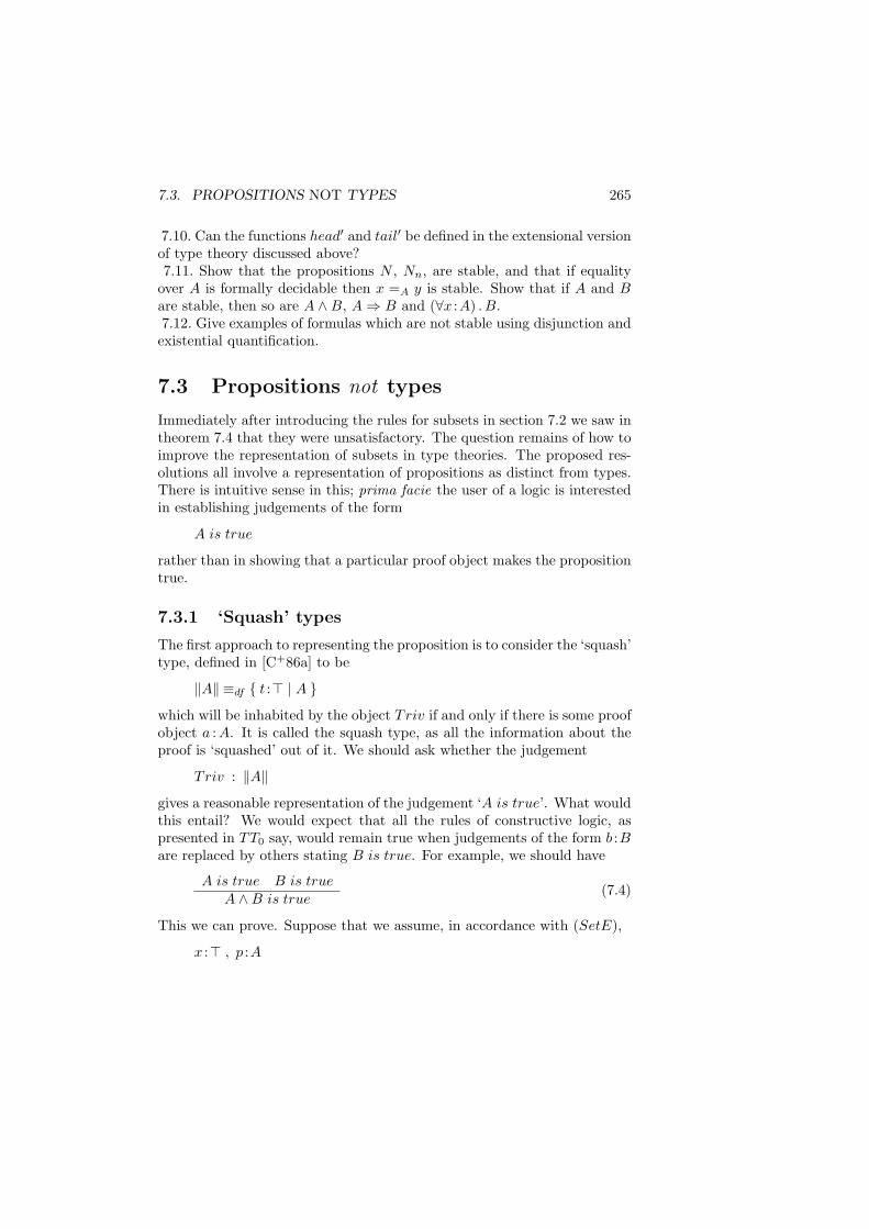
7.3. PROPOSITIONS NOT TYPES 265
7.10. Can the functions head′ and tail′ be defined in the extensional versionof type theory discussed above?7.11. Show that the propositions N , Nn, are stable, and that if equality
over A is formally decidable then x =A y is stable. Show that if A and Bare stable, then so are A ∧B, A⇒ B and (∀x :A) . B.7.12. Give examples of formulas which are not stable using disjunction andexistential quantification.
7.3 Propositions not types
Immediately after introducing the rules for subsets in section 7.2 we saw intheorem 7.4 that they were unsatisfactory. The question remains of how toimprove the representation of subsets in type theories. The proposed res-olutions all involve a representation of propositions as distinct from types.There is intuitive sense in this; prima facie the user of a logic is interestedin establishing judgements of the form
A is true
rather than in showing that a particular proof object makes the propositiontrue.
7.3.1 ‘Squash’ types
The first approach to representing the proposition is to consider the ‘squash’type, defined in [C+86a] to be
‖A‖ ≡df t :> | A
which will be inhabited by the object Triv if and only if there is some proofobject a :A. It is called the squash type, as all the information about theproof is ‘squashed’ out of it. We should ask whether the judgement
Triv : ‖A‖
gives a reasonable representation of the judgement ‘A is true’. What wouldthis entail? We would expect that all the rules of constructive logic, aspresented in TT0 say, would remain true when judgements of the form b :Bare replaced by others stating B is true. For example, we should have
A is true B is trueA ∧B is true
(7.4)
This we can prove. Suppose that we assume, in accordance with (SetE),
x :> , p :A
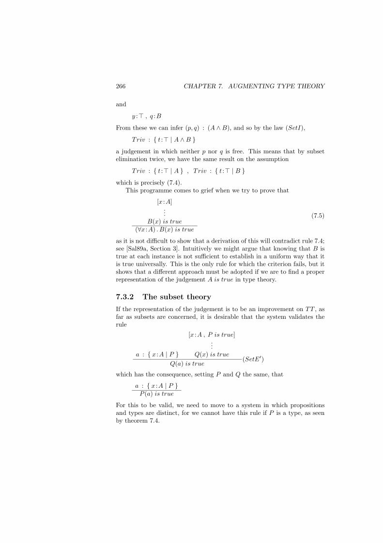
266 CHAPTER 7. AUGMENTING TYPE THEORY
and
y :> , q :B
From these we can infer (p, q) : (A ∧B), and so by the law (SetI),
Triv : t :> | A ∧B
a judgement in which neither p nor q is free. This means that by subsetelimination twice, we have the same result on the assumption
Triv : t :> | A , T riv : t :> | B
which is precisely (7.4).This programme comes to grief when we try to prove that
[x :A]...
B(x) is true(∀x :A) . B(x) is true
(7.5)
as it is not difficult to show that a derivation of this will contradict rule 7.4;see [Sal89a, Section 3]. Intuitively we might argue that knowing that B istrue at each instance is not sufficient to establish in a uniform way that itis true universally. This is the only rule for which the criterion fails, but itshows that a different approach must be adopted if we are to find a properrepresentation of the judgement A is true in type theory.
7.3.2 The subset theory
If the representation of the judgement is to be an improvement on TT , asfar as subsets are concerned, it is desirable that the system validates therule
a : x :A | P
[x :A , P is true]...
Q(x) is true
Q(a) is true(SetE′)
which has the consequence, setting P and Q the same, that
a : x :A | P P (a) is true
For this to be valid, we need to move to a system in which propositionsand types are distinct, for we cannot have this rule if P is a type, as seenby theorem 7.4.
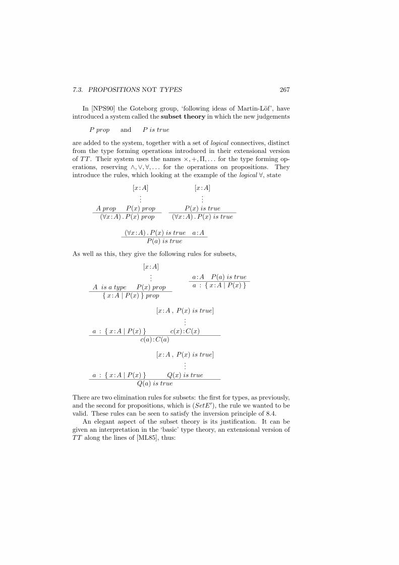
7.3. PROPOSITIONS NOT TYPES 267
In [NPS90] the Goteborg group, ‘following ideas of Martin-Lof’, haveintroduced a system called the subset theory in which the new judgements
P prop and P is true
are added to the system, together with a set of logical connectives, distinctfrom the type forming operations introduced in their extensional versionof TT . Their system uses the names ×,+,Π, . . . for the type forming op-erations, reserving ∧,∨,∀, . . . for the operations on propositions. Theyintroduce the rules, which looking at the example of the logical ∀, state
A prop
[x :A]...
P (x) prop(∀x :A) . P (x) prop
[x :A]...
P (x) is true(∀x :A) . P (x) is true
(∀x :A) . P (x) is true a :AP (a) is true
As well as this, they give the following rules for subsets,
A is a type
[x :A]...
P (x) prop x :A | P (x) prop
a :A P (a) is truea : x :A | P (x)
a : x :A | P (x)
[x :A , P (x) is true]...
c(x) :C(x)c(a) :C(a)
a : x :A | P (x)
[x :A , P (x) is true]...
Q(x) is trueQ(a) is true
There are two elimination rules for subsets: the first for types, as previously,and the second for propositions, which is (SetE′), the rule we wanted to bevalid. These rules can be seen to satisfy the inversion principle of 8.4.
An elegant aspect of the subset theory is its justification. It can begiven an interpretation in the ‘basic’ type theory, an extensional version ofTT along the lines of [ML85], thus:
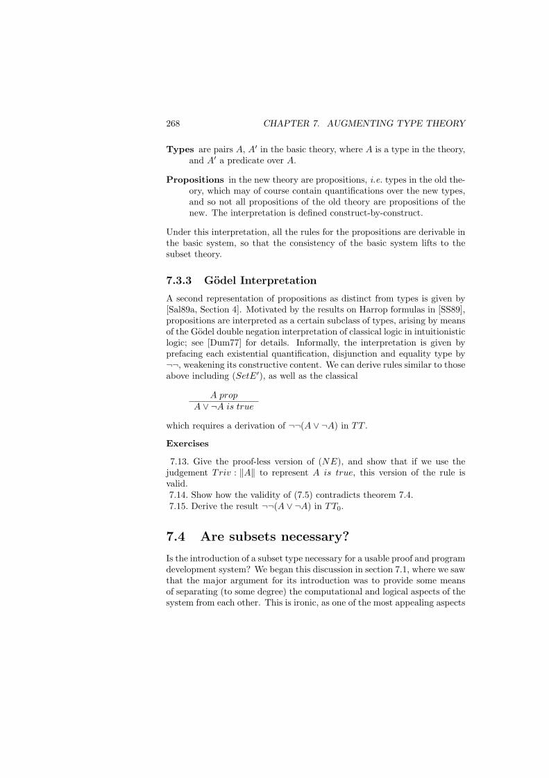
268 CHAPTER 7. AUGMENTING TYPE THEORY
Types are pairs A, A′ in the basic theory, where A is a type in the theory,and A′ a predicate over A.
Propositions in the new theory are propositions, i.e. types in the old the-ory, which may of course contain quantifications over the new types,and so not all propositions of the old theory are propositions of thenew. The interpretation is defined construct-by-construct.
Under this interpretation, all the rules for the propositions are derivable inthe basic system, so that the consistency of the basic system lifts to thesubset theory.
7.3.3 Godel Interpretation
A second representation of propositions as distinct from types is given by[Sal89a, Section 4]. Motivated by the results on Harrop formulas in [SS89],propositions are interpreted as a certain subclass of types, arising by meansof the Godel double negation interpretation of classical logic in intuitionisticlogic; see [Dum77] for details. Informally, the interpretation is given byprefacing each existential quantification, disjunction and equality type by¬¬, weakening its constructive content. We can derive rules similar to thoseabove including (SetE′), as well as the classical
A propA ∨ ¬A is true
which requires a derivation of ¬¬(A ∨ ¬A) in TT .
Exercises
7.13. Give the proof-less version of (NE), and show that if we use thejudgement Triv : ‖A‖ to represent A is true, this version of the rule isvalid.7.14. Show how the validity of (7.5) contradicts theorem 7.4.7.15. Derive the result ¬¬(A ∨ ¬A) in TT0.
7.4 Are subsets necessary?
Is the introduction of a subset type necessary for a usable proof and programdevelopment system? We began this discussion in section 7.1, where we sawthat the major argument for its introduction was to provide some meansof separating (to some degree) the computational and logical aspects of thesystem from each other. This is ironic, as one of the most appealing aspects
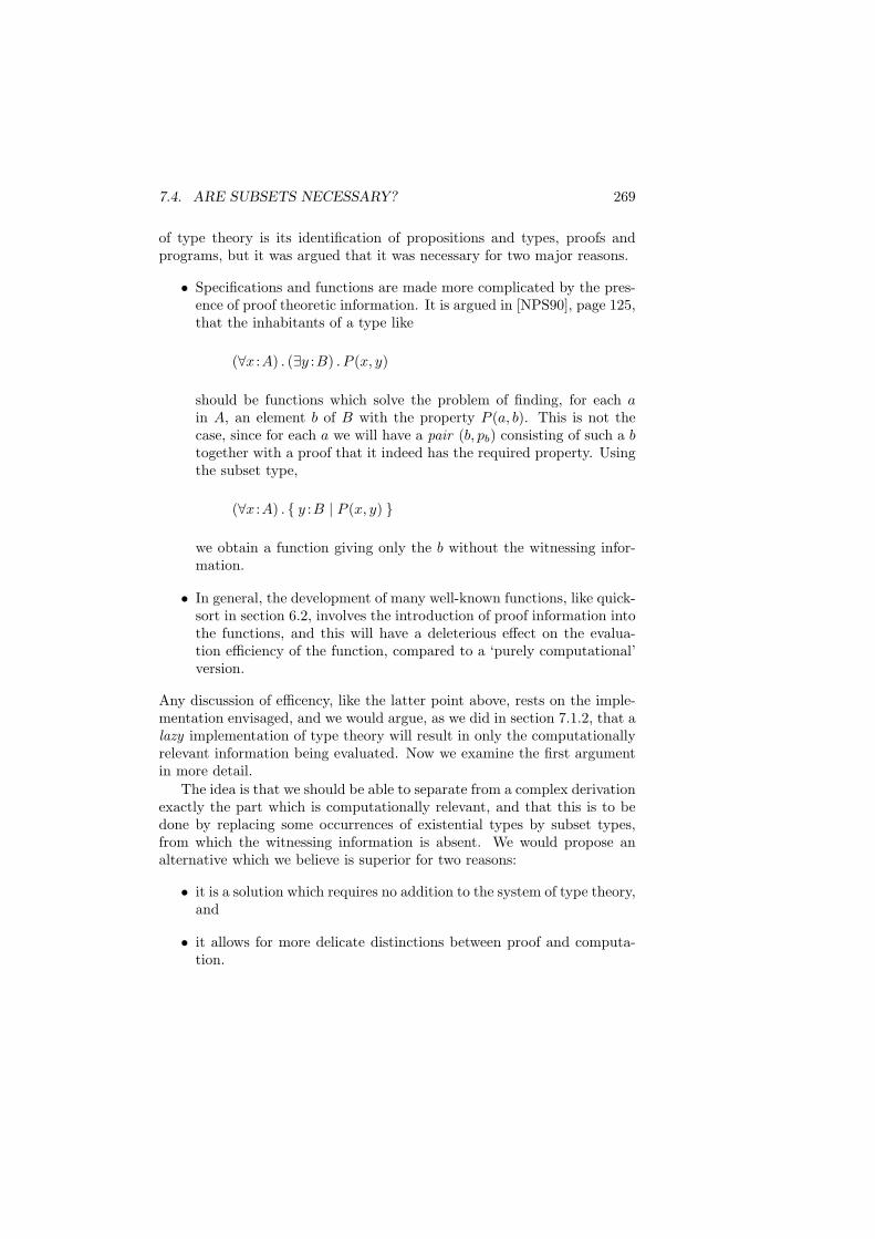
7.4. ARE SUBSETS NECESSARY? 269
of type theory is its identification of propositions and types, proofs andprograms, but it was argued that it was necessary for two major reasons.
• Specifications and functions are made more complicated by the pres-ence of proof theoretic information. It is argued in [NPS90], page 125,that the inhabitants of a type like
(∀x :A) . (∃y :B) . P (x, y)
should be functions which solve the problem of finding, for each ain A, an element b of B with the property P (a, b). This is not thecase, since for each a we will have a pair (b, pb) consisting of such a btogether with a proof that it indeed has the required property. Usingthe subset type,
(∀x :A) . y :B | P (x, y)
we obtain a function giving only the b without the witnessing infor-mation.
• In general, the development of many well-known functions, like quick-sort in section 6.2, involves the introduction of proof information intothe functions, and this will have a deleterious effect on the evalua-tion efficiency of the function, compared to a ‘purely computational’version.
Any discussion of efficency, like the latter point above, rests on the imple-mentation envisaged, and we would argue, as we did in section 7.1.2, that alazy implementation of type theory will result in only the computationallyrelevant information being evaluated. Now we examine the first argumentin more detail.
The idea is that we should be able to separate from a complex derivationexactly the part which is computationally relevant, and that this is to bedone by replacing some occurrences of existential types by subset types,from which the witnessing information is absent. We would propose analternative which we believe is superior for two reasons:
• it is a solution which requires no addition to the system of type theory,and
• it allows for more delicate distinctions between proof and computa-tion.
270 CHAPTER 7. AUGMENTING TYPE THEORY
The solution is simply to name the appropriate operations and objectssought, which in the case cited above involves us in invoking the axiom ofchioce to change the specification to
(∃f :A⇒ B) . (∀x :A) . P (x, (f x))
Now, inhabitants of this type are pairs, (f, p) which are the function soughttogether with a proof that it has the required property. Giving this functionan explicit name, which is known as Skolemizing the quantifiers in a logicalcontext, has resulted in a specification which expresses more naturally whatis required. This method applies to more complex specifications as well.
Take as an example a simplification of the specification of the Pol-ish/Dutch national flag problem as given in [NPS90]. We now show how itmay be written without the subset type. The original specification has theform
(∀x :A) . y : y′ :B | C(y′) | P (x, y)
with the intention that for each a we find b in the subset y′ :B | C(y′) ofB with the property P (a, b). If we replace the subsets by existential types,we have
(∀x :A) . (∃y : (∃y′ :B) . C(y′)) . P (x, y)
This is logically equivalent to
(∀x :A) . (∃y :B) . ( C(y) ∧ P (x, y) ) (7.6)
and by the axiom of choice to
(∃f :A⇒ B) . (∀x :A) . ( C(f x) ∧ P (x, (f x)) )
which is inhabited by functions together with proofs of their correctness.It can be argued that this expresses in a clear way what was rather moreimplicit in the specification based on sets – the formation of an existentialtype bundles together data and proof, the transformation to (7.6) makesexplicit the unbundling process.
As a final example, consider a problem in which we are asked to producefor each a in A with the property D(a) some b with the property P (a, b).There is an important question of whether the b depends just upon the a,or upon both the a and the proof that it has the property D(a). In thelatter case we could write the specification thus:
(∀x : (∃x′ :A) . D(x′)) . (∃y :B) . P (x, y)
and Skolemize to give
(∃f : (∃x′ :A) . D(x′)⇒ B) . (∀x : (∃x′ :A) . D(x′)) . P (x, (f x))
7.4. ARE SUBSETS NECESSARY? 271
If we use the Curry equivalence, first proved in section 4.6.1, page 93, whichreplaces existential quantifiers in the domain position of a function type,we have
(∃f : (∀z :A) . (D(z)⇒ B)) . (∀x′ :A) . (∀p :D(x′)) . P ((x′, p), (f x′ p))
which makes manifest the functional dependence required. Observe thatwe could indeed have written this formal specification directly on the basisof the informal version from which we started.
If we do not wish the object sought to depend upon the proof of theproperty D, we can write the following specification:
(∃f :A⇒ B) . (∀x′ :A) . (∀p :D(x′)) . P ((x′, p), (f x′)) (7.7)
in which it is plain that the object (f x′) in B is not dependent on the proofobject p :D(x′). Observe that there is still dependence of the property Pon the proof p; if we were to use a subset type to express the specification,thus, we would have something of the form
(∀x′ : x′ :A | D(x′) ) . (∃y :B) . P ′(x′, y)
where the property P ′(x, y) relates x′ : A and y : B. This is equivalent tothe specification
(∃f :A⇒ B) . (∀x′ :A) . (∀p :D(x′)) . P ′(x′, (f x′))
in which the property P ′ must not mention the proof object p, so that withour more explicit approach we have been able to express the specification7.7 which cannot be expressed under the naıve subset discipline.
It is instructive to examine examples from the literature in which thesubset type has been used. We have already discussed the Polish flag prob-lem, a second example is the parsing algorithm of [Chi87]. In fact we findthat in Chisholm’s derivation of the parsing algorithm, the subset type isnot used in an essential way: the solution is presented as a member of thetype
(∀w :Word) . (Parse w) ∨ ¬(Parse w)
where
Parse w ≡df pt :PT | w = spell pt
the function spell giving the word spelt out by the parse tree pt which is amember of the algebraic type PT of parse trees. The subset type is usednowhere else in the derivation, and it is used here only because the proof
272 CHAPTER 7. AUGMENTING TYPE THEORY
object for w = spell pt can be ignored ‘because it has no computationalcontent’. It makes no difference to the derivation to replace the set by
(∃pt :PT ) . (w = spell pt)
which carries the proof objects explicitly. Our remarks in section 7.1.2would apply as far as the efficiency of the final algorithm is concerned.
As a final example, consider the problem of finding a root of a func-tion. It is argued, in [C+86a] section 2.4 for example, that the naturalspecification for such a function is
(∀f : f :N ⇒ N | (∃n :N) . (f n) = 0 ) . ( (∃n :N) . (f n) = 0 )
which might be read ‘given a function for which a root exists, we can finda root’. It is a simple consequence of theorem 7.4 that the existence of anobject of this type leads to a contradiction.
In any case, this specification seems to miss the point about root finding.The sort of algorithms we find used in practice are those embodied bytheorems of the form
(∀f :N ⇒ N) . ( C(f)⇒ (∃n :N) . (f n) = 0 )
which we would read ‘if f satisfies the condition C(f) then we can finda root’. Many of the most important and difficult theorems of numbertheory and numerical analysis are precisely theorems of this kind, fromwhich algorithms are derived. In contrast, the specification above begs thequestion of where the proof of existence of the root comes from.
To summarise, there are two responses to the computationally irrele-vant. We can first ignore it, exploiting lazy evaluation. The second expedi-ent is to transform the specification so that the computation and verificationare separated. We did this above by a simple series of transformations; ingeneral, simply naming the function we aim to compute and writing thespecification and derivation in terms of that function can achieve the de-sired effect. This approach seems to achieve the separation between thelogical and the computational to the appropriate degree, without introduc-ing the subset type. We have found no example in the literature which isnot amenable to this kind of treatment.
Using the subset type to represent a subset brings problems; as we sawin the previous section, it is not possible in general to recover the witnessinginformation from a subset type, especially in an intensional system like TT ,and so in these cases, the existential type should be used, retaining thewitnessing information.
7.5. QUOTIENT OR CONGRUENCE TYPES 273
7.5 Quotient or Congruence Types
An important tool for the programmer and the mathematician is the capa-bility to define an equality relation over a class of objects. For instance inthis account we stipulated that we would consider as the same two expres-sions which differ only in their bound variables. In a program we mightchoose to represent finite sets by finite lists, by taking as equal those listswhich have the same elements, irrespective of their multiplicity or ordering.In both cases we can be seen to define a new type by taking the quotient ofa type by an equivalence relation (a relation which is reflexive, symmetricand transitive).
These types are a part of the Nuprl system, [C+86a], and a variantof them, congruence types, appear in the type theory of [BCMS89]. Westart with an exposition of the quotient type adapted to the context of TT ,and then compare it with the congruence type. Because of the number ofhypotheses in the following rule, we write them in a vertical list.
Formation Rule for A//Ex,y
A is a typex :A , y :A ` E is a typex :A ` r : E[x/x, x/y]x :A , y :A , r :E ` s :E[y/x, x/y]x :A , y :A , z :A ,
r :E , s :E[y/x, z/y] ` t :E[x/x, z/y]A//Ex,y is a type
(QF )
In this rule we have written hypothetical judgements such as
[x :A , y :A]...
E is a type
in the horizontal form
x :A , y :A ` E is a type
In each case the hypotheses to the left of the ‘`’ are discharged by theapplication of the rule.
In forming the type, we have to verify that the predicate is an equiva-lence relation — that is the purpose of the final three premisses of the rule.We use the subscript of x, y to indicate that it is these two variables, free inE, which are bound by the type construct. When no confusion can result,they will be omitted.
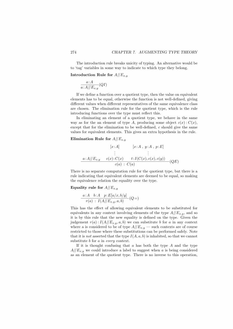
274 CHAPTER 7. AUGMENTING TYPE THEORY
The introduction rule breaks unicity of typing. An alternative would beto ‘tag’ variables in some way to indicate to which type they belong.
Introduction Rule for A//Ex,y
a :Aa :A//Ex,y
(QI)
If we define a function over a quotient type, then the value on equivalentelements has to be equal, otherwise the function is not well-defined, givingdifferent values when different representatives of the same equivalence classare chosen. The elimination rule for the quotient type, which is the ruleintroducing functions over the type must reflect this.
In eliminating an element of a quotient type, we behave in the sameway as for the an element of type A, producing some object c(x) : C(x),except that for the elimination to be well-defined, c should give the samevalues for equivalent elements. This gives an extra hypothesis in the rule.
Elimination Rule for A//Ex,y
a :A//Ex,y
[x :A]...
c(x) :C(x)
[x :A , y :A , p :E]...
t :I(C(x), c(x), c(y))c(a) : C(a)
(QE)
There is no separate computation rule for the quotient type, but there is arule indicating that equivalent elements are deemed to be equal, so makingthe equivalence relation the equality over the type.
Equality rule for A//Ex,y
a :A b :A p :E[a/x, b/y]r(a) : I(A//Ex,y, a, b)
(Q=)
This has the effect of allowing equivalent elements to be substituted forequivalents in any context involving elements of the type A//Ex,y, and soit is by this rule that the new equality is defined on the type. Given thejudgement r(a) : I(A//Ex,y, a, b) we can substitute b for a in any contextwhere a is considered to be of type A//Ex,y — such contexts are of courserestricted to those where these substitutions can be performed safely. Notethat it is not asserted that the type I(A, a, b) is inhabited, so that we cannotsubstitute b for a in every context.
If it is thought confusing that a has both the type A and the typeA//Ex,y we could introduce a label to suggest when a is being consideredas an element of the quotient type. There is no inverse to this operation,
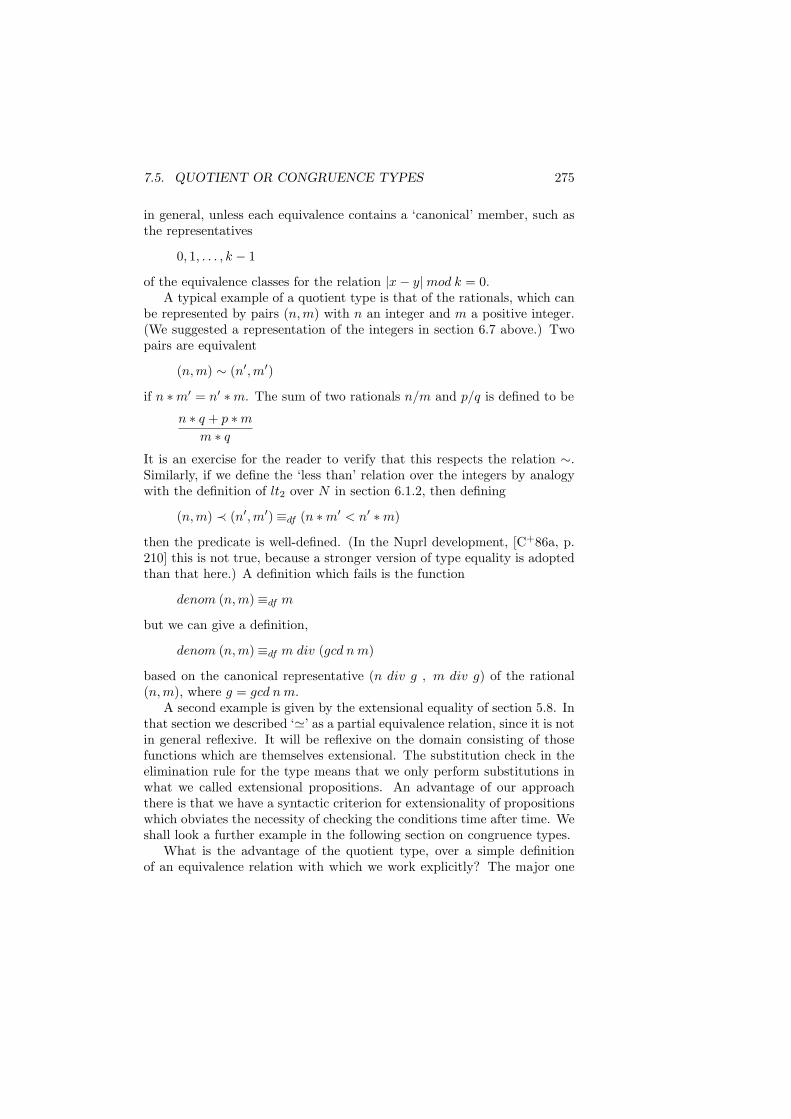
7.5. QUOTIENT OR CONGRUENCE TYPES 275
in general, unless each equivalence contains a ‘canonical’ member, such asthe representatives
0, 1, . . . , k − 1
of the equivalence classes for the relation |x− y|mod k = 0.A typical example of a quotient type is that of the rationals, which can
be represented by pairs (n, m) with n an integer and m a positive integer.(We suggested a representation of the integers in section 6.7 above.) Twopairs are equivalent
(n, m) ∼ (n′,m′)
if n ∗m′ = n′ ∗m. The sum of two rationals n/m and p/q is defined to be
n ∗ q + p ∗m
m ∗ q
It is an exercise for the reader to verify that this respects the relation ∼.Similarly, if we define the ‘less than’ relation over the integers by analogywith the definition of lt2 over N in section 6.1.2, then defining
(n, m) ≺ (n′,m′)≡df (n ∗m′ < n′ ∗m)
then the predicate is well-defined. (In the Nuprl development, [C+86a, p.210] this is not true, because a stronger version of type equality is adoptedthan that here.) A definition which fails is the function
denom (n, m)≡df m
but we can give a definition,
denom (n, m)≡df m div (gcd n m)
based on the canonical representative (n div g , m div g) of the rational(n, m), where g = gcd n m.
A second example is given by the extensional equality of section 5.8. Inthat section we described ‘'’ as a partial equivalence relation, since it is notin general reflexive. It will be reflexive on the domain consisting of thosefunctions which are themselves extensional. The substitution check in theelimination rule for the type means that we only perform substitutions inwhat we called extensional propositions. An advantage of our approachthere is that we have a syntactic criterion for extensionality of propositionswhich obviates the necessity of checking the conditions time after time. Weshall look a further example in the following section on congruence types.
What is the advantage of the quotient type, over a simple definitionof an equivalence relation with which we work explicitly? The major one
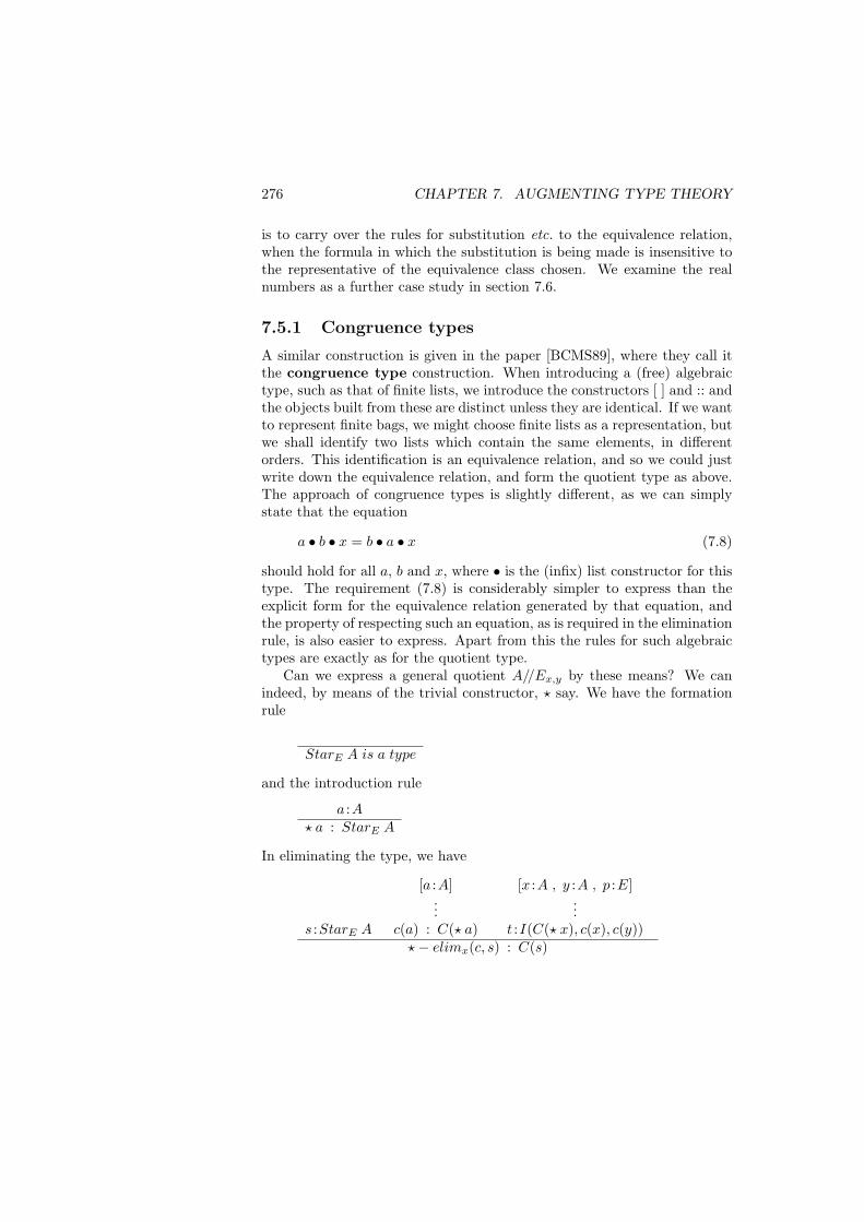
276 CHAPTER 7. AUGMENTING TYPE THEORY
is to carry over the rules for substitution etc. to the equivalence relation,when the formula in which the substitution is being made is insensitive tothe representative of the equivalence class chosen. We examine the realnumbers as a further case study in section 7.6.
7.5.1 Congruence types
A similar construction is given in the paper [BCMS89], where they call itthe congruence type construction. When introducing a (free) algebraictype, such as that of finite lists, we introduce the constructors [ ] and :: andthe objects built from these are distinct unless they are identical. If we wantto represent finite bags, we might choose finite lists as a representation, butwe shall identify two lists which contain the same elements, in differentorders. This identification is an equivalence relation, and so we could justwrite down the equivalence relation, and form the quotient type as above.The approach of congruence types is slightly different, as we can simplystate that the equation
a • b • x = b • a • x (7.8)
should hold for all a, b and x, where • is the (infix) list constructor for thistype. The requirement (7.8) is considerably simpler to express than theexplicit form for the equivalence relation generated by that equation, andthe property of respecting such an equation, as is required in the eliminationrule, is also easier to express. Apart from this the rules for such algebraictypes are exactly as for the quotient type.
Can we express a general quotient A//Ex,y by these means? We canindeed, by means of the trivial constructor, ? say. We have the formationrule
StarE A is a type
and the introduction rule
a :A? a : StarE A
In eliminating the type, we have
s :StarE A
[a :A]...
c(a) : C(? a)
[x :A , y :A , p :E]...
t :I(C(? x), c(x), c(y))?− elimx(c, s) : C(s)
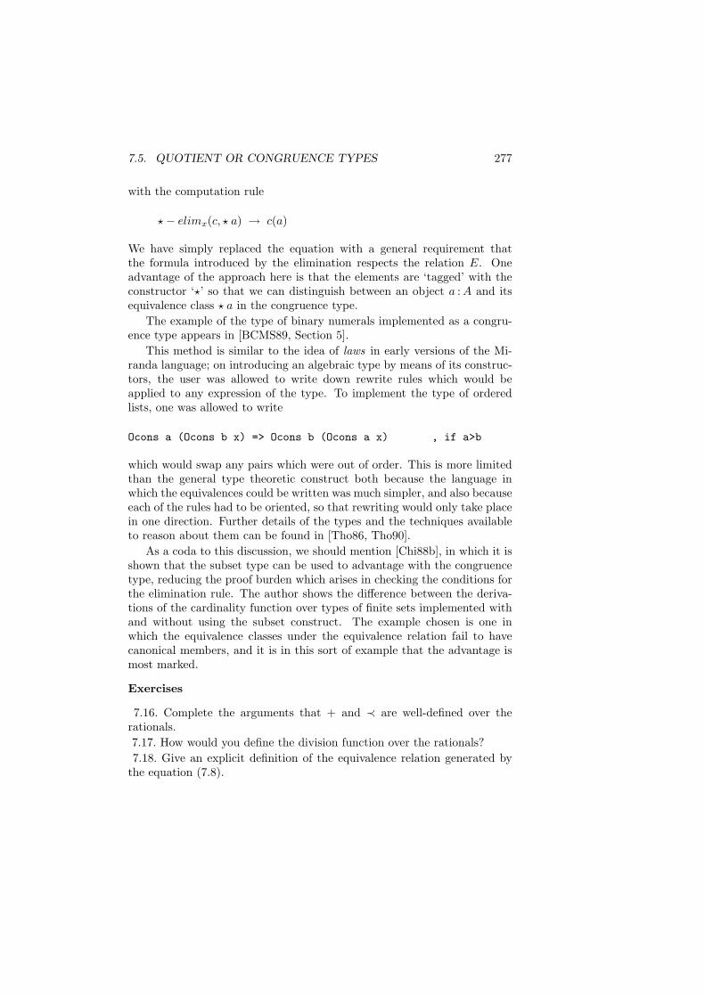
7.5. QUOTIENT OR CONGRUENCE TYPES 277
with the computation rule
?− elimx(c, ? a) → c(a)
We have simply replaced the equation with a general requirement thatthe formula introduced by the elimination respects the relation E. Oneadvantage of the approach here is that the elements are ‘tagged’ with theconstructor ‘?’ so that we can distinguish between an object a : A and itsequivalence class ? a in the congruence type.
The example of the type of binary numerals implemented as a congru-ence type appears in [BCMS89, Section 5].
This method is similar to the idea of laws in early versions of the Mi-randa language; on introducing an algebraic type by means of its construc-tors, the user was allowed to write down rewrite rules which would beapplied to any expression of the type. To implement the type of orderedlists, one was allowed to write
Ocons a (Ocons b x) => Ocons b (Ocons a x) , if a>b
which would swap any pairs which were out of order. This is more limitedthan the general type theoretic construct both because the language inwhich the equivalences could be written was much simpler, and also becauseeach of the rules had to be oriented, so that rewriting would only take placein one direction. Further details of the types and the techniques availableto reason about them can be found in [Tho86, Tho90].
As a coda to this discussion, we should mention [Chi88b], in which it isshown that the subset type can be used to advantage with the congruencetype, reducing the proof burden which arises in checking the conditions forthe elimination rule. The author shows the difference between the deriva-tions of the cardinality function over types of finite sets implemented withand without using the subset construct. The example chosen is one inwhich the equivalence classes under the equivalence relation fail to havecanonical members, and it is in this sort of example that the advantage ismost marked.
Exercises
7.16. Complete the arguments that + and ≺ are well-defined over therationals.7.17. How would you define the division function over the rationals?7.18. Give an explicit definition of the equivalence relation generated by
the equation (7.8).
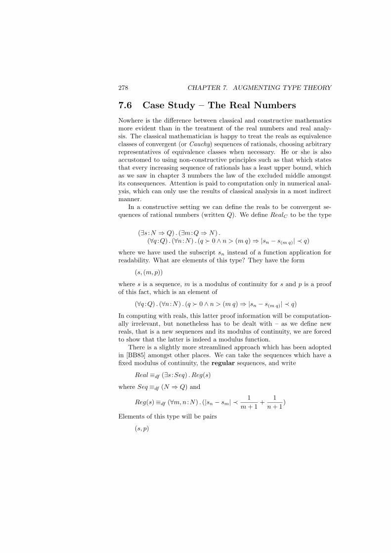
278 CHAPTER 7. AUGMENTING TYPE THEORY
7.6 Case Study – The Real Numbers
Nowhere is the difference between classical and constructive mathematicsmore evident than in the treatment of the real numbers and real analy-sis. The classical mathematician is happy to treat the reals as equivalenceclasses of convergent (or Cauchy) sequences of rationals, choosing arbitraryrepresentatives of equivalence classes when necessary. He or she is alsoaccustomed to using non-constructive principles such as that which statesthat every increasing sequence of rationals has a least upper bound, whichas we saw in chapter 3 numbers the law of the excluded middle amongstits consequences. Attention is paid to computation only in numerical anal-ysis, which can only use the results of classical analysis in a most indirectmanner.
In a constructive setting we can define the reals to be convergent se-quences of rational numbers (written Q). We define RealC to be the type
(∃s :N ⇒ Q) . (∃m :Q⇒ N) .(∀q :Q) . (∀n :N) . (q 0 ∧ n > (m q)⇒ |sn − s(m q)| ≺ q)
where we have used the subscript sn instead of a function application forreadability. What are elements of this type? They have the form
(s, (m, p))
where s is a sequence, m is a modulus of continuity for s and p is a proofof this fact, which is an element of
(∀q :Q) . (∀n :N) . (q 0 ∧ n > (m q)⇒ |sn − s(m q)| ≺ q)
In computing with reals, this latter proof information will be computation-ally irrelevant, but nonetheless has to be dealt with – as we define newreals, that is a new sequences and its modulus of continuity, we are forcedto show that the latter is indeed a modulus function.
There is a slightly more streamlined approach which has been adoptedin [BB85] amongst other places. We can take the sequences which have afixed modulus of continuity, the regular sequences, and write
Real ≡df (∃s :Seq) . Reg(s)
where Seq ≡df (N ⇒ Q) and
Reg(s)≡df (∀m,n :N) . (|sn − sm| ≺1
m + 1+
1n + 1
)
Elements of this type will be pairs
(s, p)
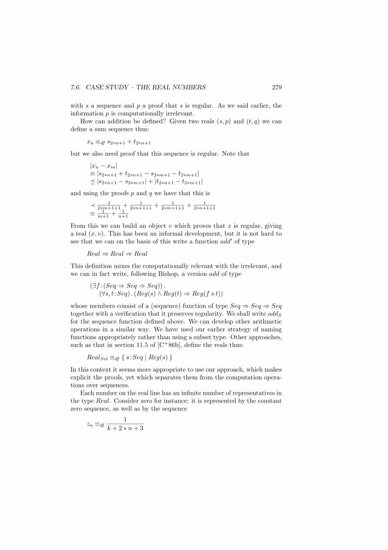
7.6. CASE STUDY – THE REAL NUMBERS 279
with s a sequence and p a proof that s is regular. As we said earlier, theinformation p is computationally irrelevant.
How can addition be defined? Given two reals (s, p) and (t, q) we candefine a sum sequence thus:
xn ≡df s2∗n+1 + t2∗n+1
but we also need proof that this sequence is regular. Note that
|xn − xm|≡ |s2∗n+1 + t2∗n+1 − s2∗m+1 − t2∗m+1| |s2∗n+1 − s2∗m+1|+ |t2∗n+1 − t2∗m+1|
and using the proofs p and q we have that this is
≺ 12∗m+1+1 + 1
2∗n+1+1 + 12∗m+1+1 + 1
2∗n+1+1
≡ 1m+1 + 1
n+1
From this we can build an object v which proves that x is regular, givinga real (x, v). This has been an informal development, but it is not hard tosee that we can on the basis of this write a function add′ of type
Real⇒ Real⇒ Real
This definition mixes the computationally relevant with the irrelevant, andwe can in fact write, following Bishop, a version add of type
(∃f : (Seq ⇒ Seq ⇒ Seq)) .(∀s, t :Seq) . (Reg(s) ∧Reg(t)⇒ Reg(f s t))
whose members consist of a (sequence) function of type Seq ⇒ Seq ⇒ Seqtogether with a verification that it preserves regularity. We shall write addS
for the sequence function defined above. We can develop other arithmeticoperations in a similar way. We have used our earlier strategy of namingfunctions appropriately rather than using a subset type. Other approaches,such as that in section 11.5 of [C+86b], define the reals thus:
RealSet ≡df s :Seq | Reg(s)
In this context it seems more appropriate to use our approach, which makesexplicit the proofs, yet which separates them from the computation opera-tions over sequences.
Each number on the real line has an infinite number of representatives inthe type Real. Consider zero for instance: it is represented by the constantzero sequence, as well as by the sequence
zn ≡df1
k + 2 ∗ n + 3
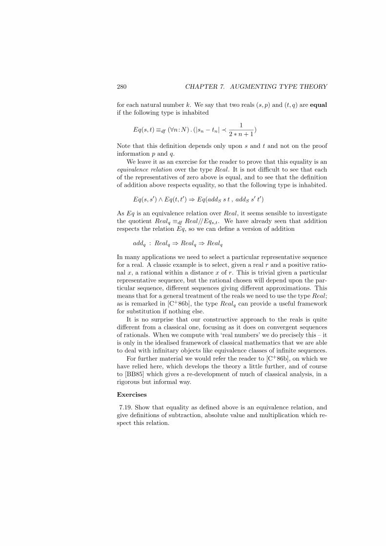
280 CHAPTER 7. AUGMENTING TYPE THEORY
for each natural number k. We say that two reals (s, p) and (t, q) are equalif the following type is inhabited
Eq(s, t)≡df (∀n :N) . (|sn − tn| ≺1
2 ∗ n + 1)
Note that this definition depends only upon s and t and not on the proofinformation p and q.
We leave it as an exercise for the reader to prove that this equality is anequivalence relation over the type Real. It is not difficult to see that eachof the representatives of zero above is equal, and to see that the definitionof addition above respects equality, so that the following type is inhabited.
Eq(s, s′) ∧ Eq(t, t′)⇒ Eq(addS s t , addS s′ t′)
As Eq is an equivalence relation over Real, it seems sensible to investigatethe quotient Realq ≡df Real//Eqs,t. We have already seen that additionrespects the relation Eq, so we can define a version of addition
addq : Realq ⇒ Realq ⇒ Realq
In many applications we need to select a particular representative sequencefor a real. A classic example is to select, given a real r and a positive ratio-nal x, a rational within a distance x of r. This is trivial given a particularrepresentative sequence, but the rational chosen will depend upon the par-ticular sequence, different sequences giving different approximations. Thismeans that for a general treatment of the reals we need to use the type Real;as is remarked in [C+86b], the type Realq can provide a useful frameworkfor substitution if nothing else.
It is no surprise that our constructive approach to the reals is quitedifferent from a classical one, focusing as it does on convergent sequencesof rationals. When we compute with ‘real numbers’ we do precisely this – itis only in the idealised framework of classical mathematics that we are ableto deal with infinitary objects like equivalence classes of infinite sequences.
For further material we would refer the reader to [C+86b], on which wehave relied here, which develops the theory a little further, and of courseto [BB85] which gives a re-development of much of classical analysis, in arigorous but informal way.
Exercises
7.19. Show that equality as defined above is an equivalence relation, andgive definitions of subtraction, absolute value and multiplication which re-spect this relation.
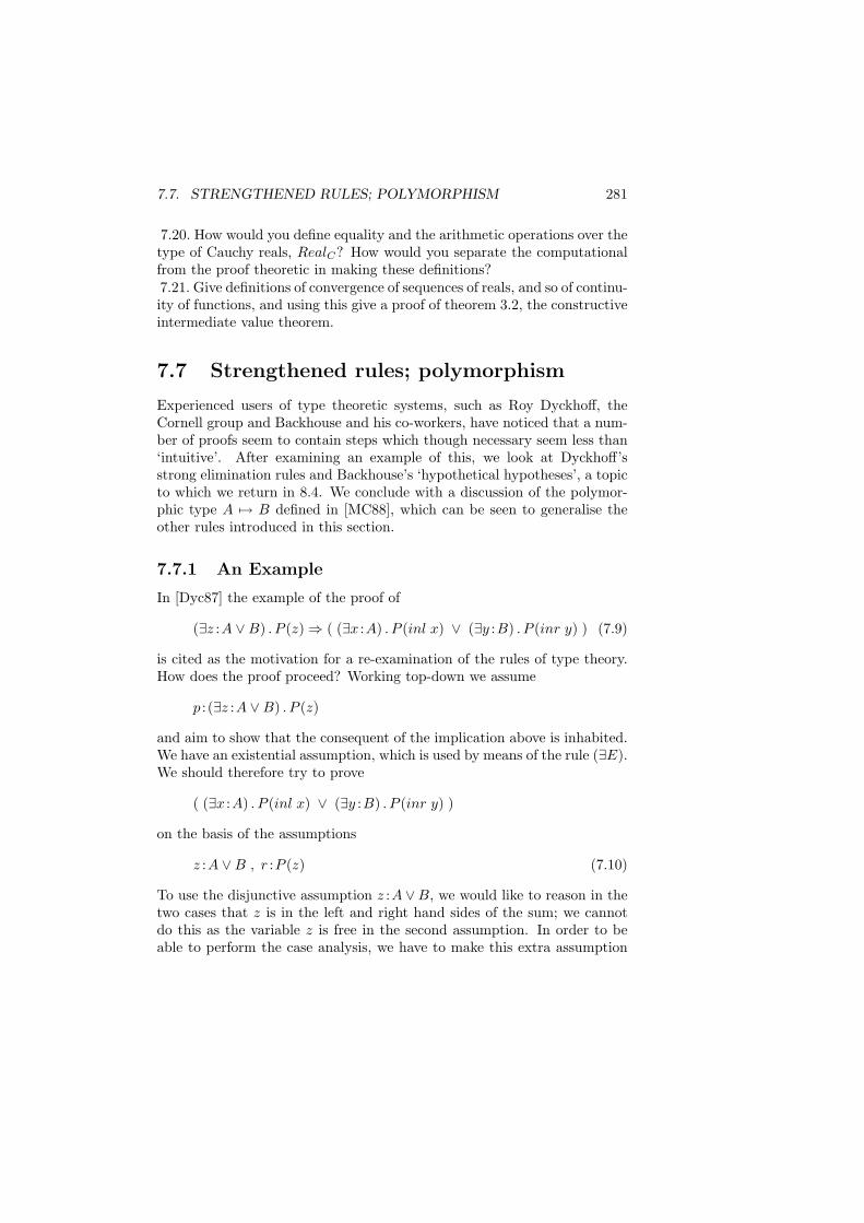
7.7. STRENGTHENED RULES; POLYMORPHISM 281
7.20. How would you define equality and the arithmetic operations over thetype of Cauchy reals, RealC? How would you separate the computationalfrom the proof theoretic in making these definitions?7.21. Give definitions of convergence of sequences of reals, and so of continu-ity of functions, and using this give a proof of theorem 3.2, the constructiveintermediate value theorem.
7.7 Strengthened rules; polymorphism
Experienced users of type theoretic systems, such as Roy Dyckhoff, theCornell group and Backhouse and his co-workers, have noticed that a num-ber of proofs seem to contain steps which though necessary seem less than‘intuitive’. After examining an example of this, we look at Dyckhoff’sstrong elimination rules and Backhouse’s ‘hypothetical hypotheses’, a topicto which we return in 8.4. We conclude with a discussion of the polymor-phic type A 7→ B defined in [MC88], which can be seen to generalise theother rules introduced in this section.
7.7.1 An Example
In [Dyc87] the example of the proof of
(∃z :A ∨B) . P (z)⇒ ( (∃x :A) . P (inl x) ∨ (∃y :B) . P (inr y) ) (7.9)
is cited as the motivation for a re-examination of the rules of type theory.How does the proof proceed? Working top-down we assume
p : (∃z :A ∨B) . P (z)
and aim to show that the consequent of the implication above is inhabited.We have an existential assumption, which is used by means of the rule (∃E).We should therefore try to prove
( (∃x :A) . P (inl x) ∨ (∃y :B) . P (inr y) )
on the basis of the assumptions
z :A ∨B , r :P (z) (7.10)
To use the disjunctive assumption z :A ∨B, we would like to reason in thetwo cases that z is in the left and right hand sides of the sum; we cannotdo this as the variable z is free in the second assumption. In order to beable to perform the case analysis, we have to make this extra assumption
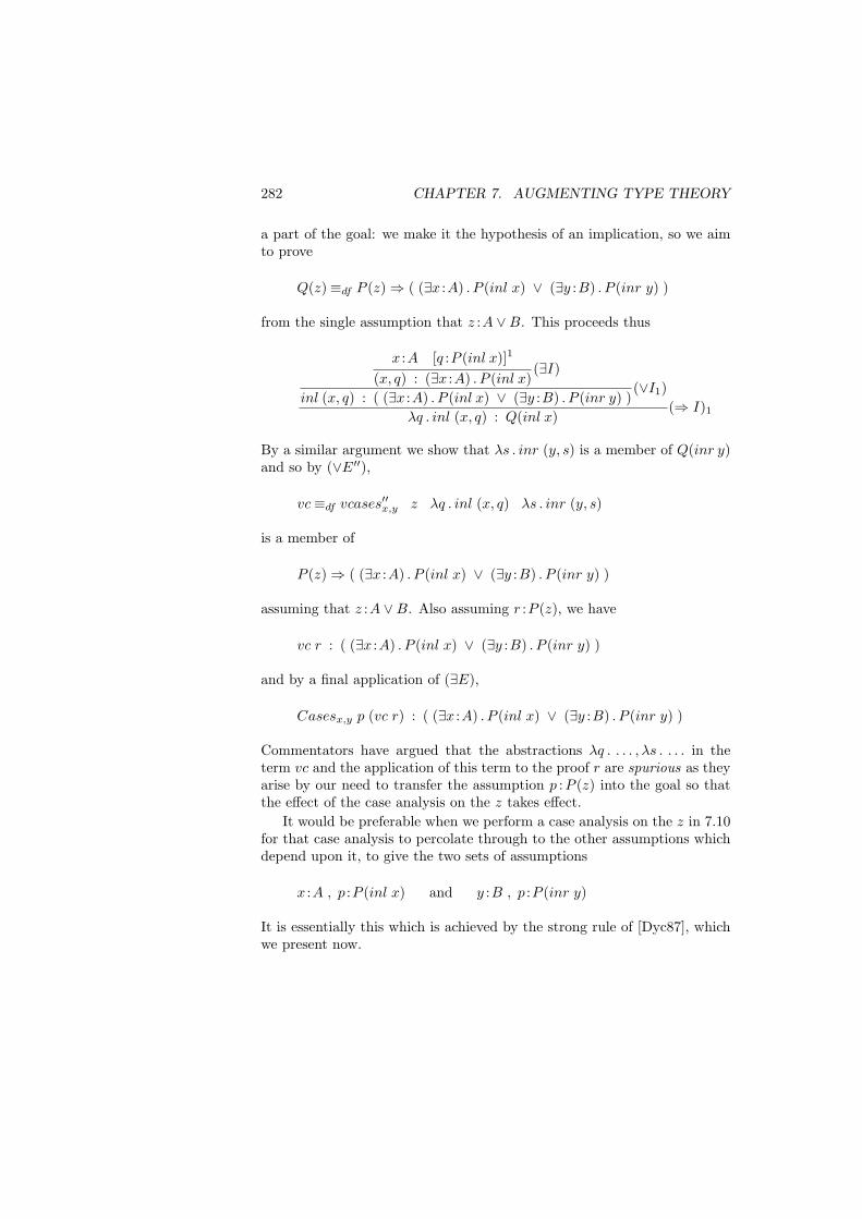
282 CHAPTER 7. AUGMENTING TYPE THEORY
a part of the goal: we make it the hypothesis of an implication, so we aimto prove
Q(z)≡df P (z)⇒ ( (∃x :A) . P (inl x) ∨ (∃y :B) . P (inr y) )
from the single assumption that z :A ∨B. This proceeds thus
x :A [q :P (inl x)]1
(x, q) : (∃x :A) . P (inl x)(∃I)
inl (x, q) : ( (∃x :A) . P (inl x) ∨ (∃y :B) . P (inr y) )(∨I1)
λq . inl (x, q) : Q(inl x)(⇒ I)1
By a similar argument we show that λs . inr (y, s) is a member of Q(inr y)and so by (∨E′′),
vc≡df vcases′′x,y z λq . inl (x, q) λs . inr (y, s)
is a member of
P (z)⇒ ( (∃x :A) . P (inl x) ∨ (∃y :B) . P (inr y) )
assuming that z :A ∨B. Also assuming r :P (z), we have
vc r : ( (∃x :A) . P (inl x) ∨ (∃y :B) . P (inr y) )
and by a final application of (∃E),
Casesx,y p (vc r) : ( (∃x :A) . P (inl x) ∨ (∃y :B) . P (inr y) )
Commentators have argued that the abstractions λq . . . . , λs . . . . in theterm vc and the application of this term to the proof r are spurious as theyarise by our need to transfer the assumption p :P (z) into the goal so thatthe effect of the case analysis on the z takes effect.
It would be preferable when we perform a case analysis on the z in 7.10for that case analysis to percolate through to the other assumptions whichdepend upon it, to give the two sets of assumptions
x :A , p :P (inl x) and y :B , p :P (inr y)
It is essentially this which is achieved by the strong rule of [Dyc87], whichwe present now.
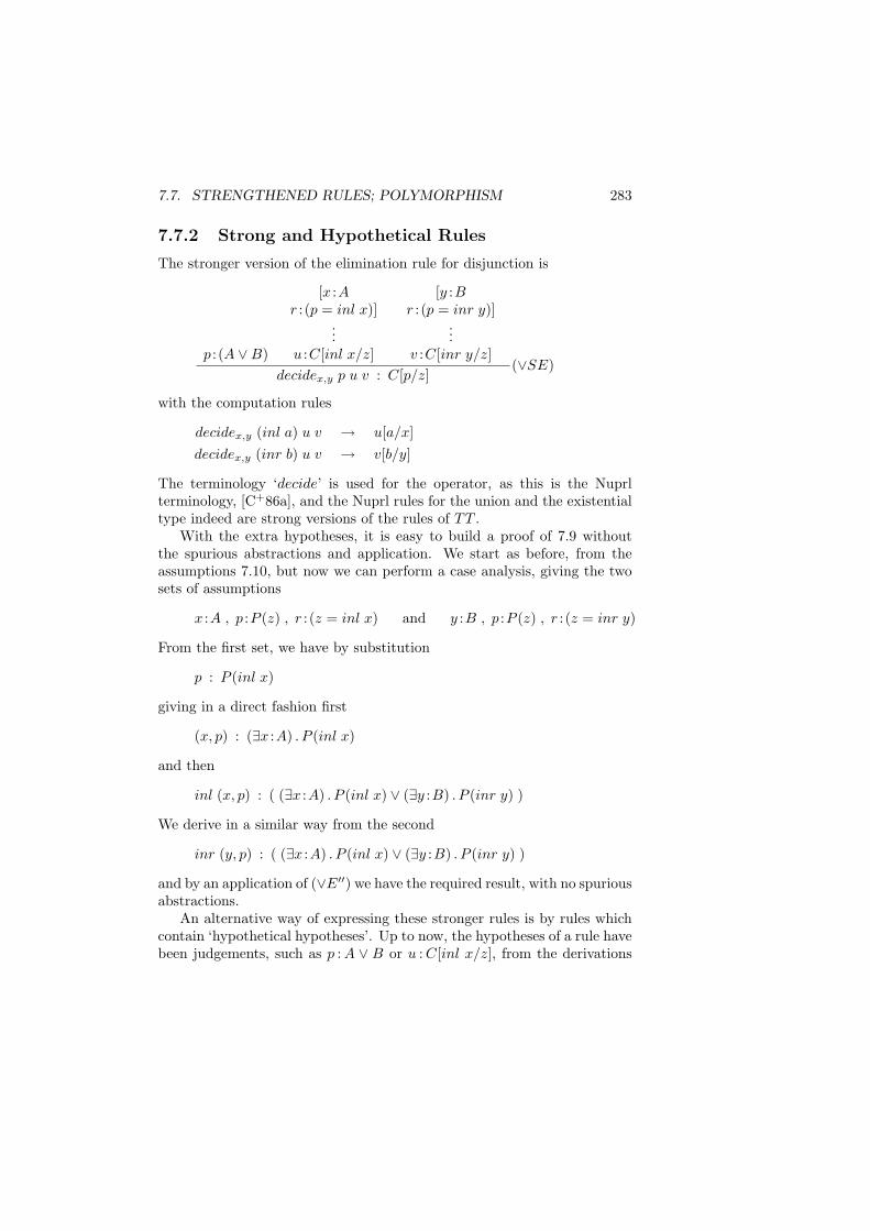
7.7. STRENGTHENED RULES; POLYMORPHISM 283
7.7.2 Strong and Hypothetical Rules
The stronger version of the elimination rule for disjunction is
p : (A ∨B)
[x :Ar : (p = inl x)]
...u :C[inl x/z]
[y :Br : (p = inr y)]
...v :C[inr y/z]
decidex,y p u v : C[p/z](∨SE)
with the computation rules
decidex,y (inl a) u v → u[a/x]decidex,y (inr b) u v → v[b/y]
The terminology ‘decide’ is used for the operator, as this is the Nuprlterminology, [C+86a], and the Nuprl rules for the union and the existentialtype indeed are strong versions of the rules of TT .
With the extra hypotheses, it is easy to build a proof of 7.9 withoutthe spurious abstractions and application. We start as before, from theassumptions 7.10, but now we can perform a case analysis, giving the twosets of assumptions
x :A , p :P (z) , r : (z = inl x) and y :B , p :P (z) , r : (z = inr y)
From the first set, we have by substitution
p : P (inl x)
giving in a direct fashion first
(x, p) : (∃x :A) . P (inl x)
and then
inl (x, p) : ( (∃x :A) . P (inl x) ∨ (∃y :B) . P (inr y) )
We derive in a similar way from the second
inr (y, p) : ( (∃x :A) . P (inl x) ∨ (∃y :B) . P (inr y) )
and by an application of (∨E′′) we have the required result, with no spuriousabstractions.
An alternative way of expressing these stronger rules is by rules whichcontain ‘hypothetical hypotheses’. Up to now, the hypotheses of a rule havebeen judgements, such as p : A ∨ B or u : C[inl x/z], from the derivations
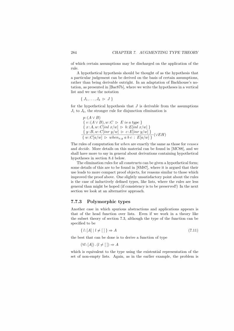
284 CHAPTER 7. AUGMENTING TYPE THEORY
of which certain assumptions may be discharged on the application of therule.
A hypothetical hypothesis should be thought of as the hypothesis thata particular judgement can be derived on the basis of certain assumptions,rather than being derivable outright. In an adaptation of Backhouse’s no-tation, as presented in [Bac87b], where we write the hypotheses in a verticallist and we use the notation
J1, . . . , Jk J
for the hypothetical hypothesis that J is derivable from the assumptionsJ1 to Jk, the stronger rule for disjunction elimination is
p : (A ∨B) v : (A ∨B), w :C E is a type x :A,w :C[inl x/w] b :E[inl x/w] y :B,w :C[inr y/w] c :E[inr y/w] w :C[a/w] whenx,y a b c : E[a/w]
(∨EH)
The rules of computation for when are exactly the same as those for vcasesand decide. More details on this material can be found in [MC88], and weshall have more to say in general about derivations containing hypotheticalhypotheses in section 8.4 below.
The elimination rules for all constructs can be given a hypothetical form;some details of this are to be found in [SM87], where it is argued that theiruse leads to more compact proof objects, for reasons similar to those whichimproved the proof above. One slightly unsatisfactory point about the rulesis the case of inductively defined types, like lists, where the rules are lessgeneral than might be hoped (if consistency is to be preserved!) In the nextsection we look at an alternative approach.
7.7.3 Polymorphic types
Another case in which spurious abstractions and applications appears isthat of the head function over lists. Even if we work in a theory likethe subset theory of section 7.3, although the type of the function can bespecified to be
l : [A] | l 6= [ ] ⇒ A (7.11)
the best that can be done is to derive a function of type
(∀l : [A]) . (l 6= [ ])⇒ A
which is equivalent to the type using the existential representation of theset of non-empty lists. Again, as in the earlier example, the problem is
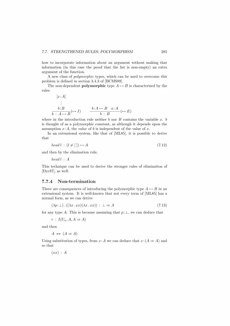
7.7. STRENGTHENED RULES; POLYMORPHISM 285
how to incorporate information about an argument without making thatinformation (in this case the proof that the list is non-empty) an extraargument of the function.
A new class of polymorphic types, which can be used to overcome thisproblem is defined in section 3.4.3 of [BCMS89].
The non-dependent polymorphic type A 7→ B is characterised by therules
[x :A]...
b :Bb : A 7→ B
(7→ I)b :A 7→ B a :A
b : B(7→ E)
where in the introduction rule neither b nor B contains the variable x. bis thought of as a polymorphic constant, as although it depends upon theassumption x :A, the value of b is independent of the value of x.
In an extensional system, like that of [ML85], it is possible to derivethat
head l : (l 6= [ ]) 7→ A (7.12)
and then by the elimination rule,
head l : A
This technique can be used to derive the stronger rules of elimination of[Dyc87], as well.
7.7.4 Non-termination
There are consequences of introducing the polymorphic type A 7→ B in anextensional system. It is well-known that not every term of [ML85] has anormal form, as we can derive
(λp :⊥) . ((λx . xx)(λx . xx)) : ⊥ ⇒ A (7.13)
for any type A. This is because assuming that p :⊥, we can deduce that
r : I(Un, A, A⇒ A)
and then
A ↔↔ (A⇒ A)
Using substitution of types, from x :A we can deduce that x : (A⇒ A) andso that
(xx) : A
286 CHAPTER 7. AUGMENTING TYPE THEORY
Further deductions give (7.13). On the other hand, we can show that everyclosed expression has a canonical value, or weak head normal form (c.f.section 2.3), so that with this weaker notion, the system is terminating. Ifwe include the polymorphic type, then there are terms without canonicalform, so the system is not terminating. Take the derivation that
((λx . xx)(λx . xx)) : A
depending upon the assumption p :⊥. By (7→ I), we have
((λx . xx)(λx . xx)) : ⊥ 7→ A
depending upon no assumptions. This term has no canonical form, since
((λx . xx)(λx . xx)) → e
if and only if e ≡ ((λx . xx)(λx . xx)).In an intensional theory like TT , there is no difficulty of this kind in
adding the polymorphic type, but note that the polymorphic types willcontain fewer objects since as was argued in [SS89] none of the rules of TTlose mention of objects mentioned in their hypotheses.
Exercises
7.22. Give a strengthened elimination rule for the existential quantifier,and an example in which its use simplifies a proof object.7.23. Show how the strong elimination rule for ∨ is a consequence of the
hypothetical rule (∨EH).7.24. Give ‘hypothetical’ versions of the strengthened rules for ∃and N
elimination.7.25. Give a derivation of the judgement (7.12) and use this to show that
head can be given the type (7.11).7.26. Complete the derivation of the judgement (7.13).
7.8 Well-founded recursion
Rather than giving completely explicit definitions of functions, or proofs ofuniversal propositions, we often have to use recursion, which allows func-tions to be defined in terms of their values at ‘simpler’ arguments, or prop-erties to be proved assuming that they already hold of ‘simpler’ objects.
The recursions in the system TT are structural, that is they are linkedto the inductive generation of a data type like N , lists, trees and the Wtypes. For these types we say that the component parts of an object, suchas the subtrees u and v of the tree
Bnode n u v
7.8. WELL-FOUNDED RECURSION 287
are simpler than the tree itself. The elimination rule for these types legit-imises definition by recursion and proof by induction over the types. Suchrecursions are limited, in that we limit our notion of what is simpler to astructural one: component parts are simpler than the whole. The ques-tion we address in this section is whether there is a more general notion of‘simpler than’ over which we can make recursive definitions and inductiveproofs. We shall see that indeed there is, and that some of the examples ofrecursion we have seen in chapter 6 can be cast in a more natural form inthis way.
We shall go on to look at other ways in which the recursive capabilitiesof the system may be increased. In particular we shall also examine howa wider class of ‘inductive’ type definitions can be added to the system,and also how a treatment of partial functions can be included, withoutbreaking the important property of strong normalisation. First, however,we examine well-founded types and recursion.
As this section is intended to be an introduction to the idea of well-founded recursion, we shall use ideas and notation of naıve set theory, asdiscussed in [End77] for instance, going on in the next section to examinehow these ideas can best be incorporated into type theory.
Definition 7.6 A binary relation ≺ is a partial order if for all x, y, z,
x 6≺ x
x ≺ y ∧ y ≺ z ⇒ x ≺ z
We can think of x ≺ y as expressing ‘x is simpler than y’, as we arecertain by the first clause that we have no loops x ≺ x, and in combinationwith the second that we have nothing of the form
xo ≺ x1 ≺ . . . ≺ xn ≺ x0
However, being a partial order is insufficient to guarantee that we canperform recursion over the ordering, and the classic example is the relation
n ≺ m≡df m < n
so that
. . . n + 1 ≺ n ≺ . . . ≺ 1 ≺ 0
How would a recursion over this type work? We would have to definethe value at 0 in terms of the value at 1, 2, . . .. In turn, the value at 1 isdetermined by values at 2, 3, . . .: never at any point do we make a start with
288 CHAPTER 7. AUGMENTING TYPE THEORY
the definition. Consider the concrete case of the definition f : (N ⇒ N) by‘recursion’ over ≺:
f n≡df f (n + 1)− 1 (7.14)
The problem with this is that it does not define a unique function, for thefunctions fk with
fk n≡df n + k
are all solutions of the recursion equation (7.14). Not only is this exampleclassic, but it characterises those orderings over which recursion fails.
Definition 7.7 A partial ordering ≺ over A is well-founded if and onlyif there are no sequences <xn>n in A so that
. . . xn+1 ≺ xn ≺ . . . ≺ x1 ≺ x0
Such a sequence is called an infinite descending chain.
In any ordering with an infinite descending chain, we can reproduce theexample above, showing that ‘recursive’ definitions do not lead to uniquesolutions. On the other hand, we can show that recursive definitions arewell-defined over well-founded orderings.
This characterisation of well-foundedness has classical equivalents whichare more suited to a constructive context, as they are more explicit. Theone we shall use is
Theorem 7.8 A partial ordering is well-founded if and only if it satisfies
∀x(∀y(y ≺ x⇒ y ∈ z)⇒ x ∈ z)⇒ ∀x(x ∈ z) (7.15)
for all sets z.
Proof: Standard set theory; see [End77] for example. 2
This characterisation legitimises proof by induction over the ordering.To prove that P (x) holds for all x, we take z ≡df y ∈ A|P (y) so that(7.15) reads, in rule form
∀x(∀y(y ≺ x⇒ P (y))⇒ P (x))∀xP (x)
Every partial ordering has a well-founded, or accessible, part.
Definition 7.9 The well-founded or accessible part Acc(A,≺) of the or-dering ≺ over A is defined to be
x ∈ A | ¬∃ <xn>n such that x x0 . . . xn xn+1 . . .
7.8. WELL-FOUNDED RECURSION 289
Theorem 7.10 The accessible part of a partial ordering ≺ over A is thesmallest subset z of A with the property that
(∀y(y ≺ x⇒ y ∈ z))⇒ x ∈ z
Proof: As for theorem 7.8. 2
Corollary 7.11 The principle of induction over ≺ given above holds forAcc(A,≺).
Theorem 7.10 shows that we can think of defining functions either byrecursion over a well-founded ordering, or by recursion over the well-foundedpart of an arbitrary partial ordering. In the latter case the definition willoften be linked with a characterisation of Acc(A,≺), so as to show thatparticular arguments of interest lie within the accessible part.
How are functions defined by recursion over a well-founded ordering?We define the value at an argument a using the values at simpler argumentsx≺a.
Definition 7.12 The function f is defined by well-founded recursionover the relation ≺ if it has the form
f a≡df . . . f a1 . . . f an . . . (7.16)
where each ai ≺ a
As an example, it is easy to see that the definition of pow from section6.1.4
pow 0 ≡df 1
pow n ≡df (pow (n div 2))2 ∗ 2(n mod 2)
is justified by induction over the well-founded ordering < on N .The formal treatment of well-founded recursion is slightly more general.
If we write f↓a for the function f restricted to the domain
y ∈ x|y ≺ a
then the recursion is defined by a function F , taking the values so far anda itself to the value at a
F (f↓a) a = fa (7.17)
This generalises course-of-values recursion — we define the value at a usingthe values at all the points preceding a in the ordering, just as we did insection 6.1.1 above for the natural numbers. We now argue that recursionis well-defined over well-founded orderings.
290 CHAPTER 7. AUGMENTING TYPE THEORY
Theorem 7.13 For every function F as above, there is a unique solutionto the equation (7.17).
Proof: The proof is by induction over the relation ≺. 2
Just to show how the formal treatment works, we look again at the powfunction. The function F defining the recursion is given by
F h 0 ≡df 1
F h n ≡df (h (n div 2))2 ∗ 2(n mod 2)
where the function h gives the values of the recursion on arguments smallerthan the second argument. h is only applied to smaller arguments here:in the first case it is not used, and in the second it is only applied to(n div 2) < n when n > 0. The F notation is slightly cumbersome, so weshall tend to present function definitions in the form of (7.16) above.
What examples of well-founded orderings are there? For each of thetypes A in TT with a recursion operator we can define a well-foundedordering ≺A which embodies that recursion. We can read off the relationfrom the introduction rules, the elements of the type which appear abovethe line being the immediate predecessors of those appearing below it.
For instance, for the type of trees there are two cases as there are twointroduction rules. The node Null has no predecessors, and for a Bnode,we have
u ≺1 (Bnode n u v) v ≺1 (Bnode n u v)
and for n + 1 > 1,
t ≺n+1 t′ ≡df ∃u(t ≺1 u ∧ u ≺n t′)
Finally, we say that
t ≺ t′ ≡df ∃n(t ≺n t′)
The definition of ≺ specifies the formation of the transitive closure ofthe immediate predecessor relation ≺1.
Using the original definition of well-foundedness, it is easy to see thatthere is a wealth of well-founded orderings. We summarise them now,leaving proofs to the reader.
• The orderings induced by the introduction rules for the types N , [A],tree and the W types in general are well-founded.
• If ≺′ is a well-founded ordering on B and f : (A ⇒ B) then theordering ≺ on A defined by
a ≺ a′ ≡df (fa) ≺′ (fa′)
7.8. WELL-FOUNDED RECURSION 291
is well-founded. We call the ordering ≺ the inverse image ≺′ underf . An example of this is the ordering on lists given by the lengthfunction, #,
l ≺ m≡df #l < #m
• A sub-ordering ≺≺ of a well-founded ordering will be well-founded.By a sub-ordering we mean that for all a, b,
a ≺≺ b⇒ a ≺ b
• Given orderings ≺ on A and ≺′ on B, we can define a number ofwell-founded orderings.
– The product ordering on A × B: (a, b) ≺≺ (a′, b′) if and only ifa ≺ a′ and b ≺′ b′.
– The lexicographic product ordering on A×B: (a, b) ≺≺ (a′, b′) ifand only if either a ≺ a′ or a = a′ and b ≺′ b′. This is called thelexicographic ordering, as it is the way that words are orderedin a dictionary, and indeed it can be extended to n-ary productsand lists in general.
– The sum ordering on A ∨B: for which we define
(inl a) ≺≺ (inl a′)≡df a ≺ a′
(inr b) ≺≺ (inr b′)≡df b ≺′ b′
with items from different sides of the sum incomparable.
Having introduced the general subject in a free-wheeling way, we mustnow show how we can introduce well-founded recursion into type theory ina suitable manner. There are a number of proposals to look at, and we dothis in the section to come.
Exercises
7.27. Show that the set Acc(A,≺) is downwards closed, i.e. that if y ≺ xand x ∈ Acc(A,≺) then y ∈ Acc(A,≺).7.28. Give explicit definitions of the well-founded orderings induced on listsand on a general W type by their structure.7.29. Argue that suborderings, and the product, lexicographic product andsum orderings are well-founded if their component orderings are.7.30. Try to discover the orderings over which definitions in chapter 6 are
most naturally expressed. Look in particular at the examples of quicksortand the Ackermann function.
292 CHAPTER 7. AUGMENTING TYPE THEORY
7.9 Well-founded recursion in type theory
Having introduced the idea of well-founded recursion, here we look at howbest to add it to our system TT . The most straightforward idea, firstinvestigated in [Pau86], is to take the characterisation of well-foundednessgiven by theorem 7.8, to translate it into type theory and then to askwhich orderings meet the definition. It transpires that all the well-foundedorderings mentioned in the last section can be shown to be well-foundedunder the type theoretic characterisation.
A second approach, introduced in [Nor88] and developed in [SM87], isto permit recursion along the accessible parts of any partial ordering ≺.The collection of elements Acc(A,≺) has then to be defined in some way,and this is done by giving type theoretic rules, just as for other types. Thecharacterisation is unusual, in that we have to reason about the membershiprelation
b : B
to characterise properly the class Acc(A,≺), and so some proposition rep-resenting this judgement has to be introduced, analogous to the internalrepresentation of equality by ‘=’.
7.9.1 Constructing Recursion Operators
In our earlier discussion, we characterised the well-foundedness of the or-dering ≺ by
∀x(∀y(y ≺ x⇒ y ∈ z)⇒ x ∈ z)⇒ ∀x(x ∈ z) (7.18)
for all sets z. How can we express the quantification ‘for all sets z’ in typetheory? We can think of it as expressing ‘for all properties P ’, where bya property we mean a predicate over A. A predicate P (z) over A gives aproposition P (a) for every a :A, so we can think of a predicate as a memberof
A⇒ U0
(In fact, of course, there are also predicates in the larger universes Un, butwe restrict ourselves to the ‘small’ predicates in U0.) As the ordering ≺ isa binary relation, we can think of it as a function in A ⇒ A ⇒ U0. Weshall continue to write it in infix form.
7.9. WELL-FOUNDED RECURSION IN TYPE THEORY 293
Definition 7.14 A partial ordering ≺ is well-founded in TT if and onlyif the type
(∀P :A⇒ U0) .( (∀x :A) . ((∀y :A) . (y ≺ x⇒ P y)⇒ P x)⇒ (∀x :A) . (P x) )
(7.19)
is inhabited by an object Ξ satisfying
Ξ P F x = F (λy . λr . (Ξ P F y)) (7.20)
It is worth examining the premiss of the implication (7.19).
(∀x :A) . ((∀y :A) . (y ≺ x⇒ P y)⇒ P x)
An object of this type is like the F of (7.20), taking the values on thepredecessors y of x to the value on x, in P x. Given such a function, wereturn a function of type (∀x : A) . (P x) that is defined on the whole ofA. Asking purely that we have an object of type (7.19) guarantees that wehave proof by induction over the type; we add the rider (7.20) to guaranteethat we can also define functions by recursion. The equation states that thevalue at x, Ξ P F x, is got by applying F to the values at the predecessors
λy . λr . (Ξ P F y)
Note that the second argument to the function is the proof that y ≺ x.Given the operator Ξ we can define functions using the syntactic form
f a≡df . . . f a1 . . . f an . . .
where each ai ≺ a and we shall do this in what follows.To show that the orderings over well-founded types such as lists, trees
and N are well-founded, we have to show that the course-of-values recursionoperator is defined, where the previous values are presented in the form ofa function of type
(∀y :A) . (y ≺ x⇒ P y)
rather than as a list as we did for the natural numbers in section 6.1.4.This is not difficult to achieve, and we leave it as an exercise for the reader.
As an example derivation, we show that
Theorem 7.15 If ≺′ is a well-founded ordering on B, and f :A⇒ B, thenthe ordering ≺ defined on A by
y ≺ x ≡df f y ≺′ f x (7.21)
is well-founded.
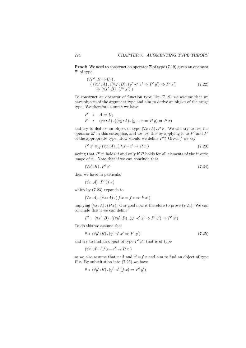
294 CHAPTER 7. AUGMENTING TYPE THEORY
Proof: We need to construct an operator Ξ of type (7.19) given an operatorΞ′ of type
(∀P ′ :B ⇒ U0) .( (∀x′ :A) . ((∀y′ :B) . (y′ ≺′ x′ ⇒ P ′ y′)⇒ P ′ x′)⇒ (∀x′ :B) . (P ′ x′) )
(7.22)
To construct an operator of function type like (7.19) we assume that wehave objects of the argument type and aim to derive an object of the rangetype. We therefore assume we have
P : A⇒ U0
F : (∀x :A) . ((∀y :A) . (y ≺ x⇒ P y)⇒ P x)
and try to deduce an object of type (∀x : A) . P x. We will try to use theoperator Ξ′ in this enterprise, and we use this by applying it to P ′ and F ′
of the appropriate type. How should we define P ′? Given f we say
P ′ x′ ≡df (∀x :A) . ( f x=x′ ⇒ P x ) (7.23)
saying that P ′ x′ holds if and only if P holds for all elements of the inverseimage of x′. Note that if we can conclude that
(∀x′ :B) . P ′ x′ (7.24)
then we have in particular
(∀x :A) . P ′ (f x)
which by (7.23) expands to
(∀x :A) . (∀z :A) . ( f x = f z ⇒ P x )
implying (∀x :A) . (P x). Our goal now is therefore to prove (7.24). We canconclude this if we can define
F ′ : (∀x′ :B) . ((∀y′ :B) . (y′ ≺′ x′ ⇒ P ′ y′)⇒ P ′ x′)
To do this we assume that
θ : (∀y′ :B) . (y′ ≺′ x′ ⇒ P ′ y′) (7.25)
and try to find an object of type P ′ x′, that is of type
(∀x :A) . ( f x=x′ ⇒ P x )
so we also assume that x :A and x′=f x and aim to find an object of typeP x. By substitution into (7.25) we have
θ : (∀y′ :B) . (y′ ≺′ (f x)⇒ P ′ y′)
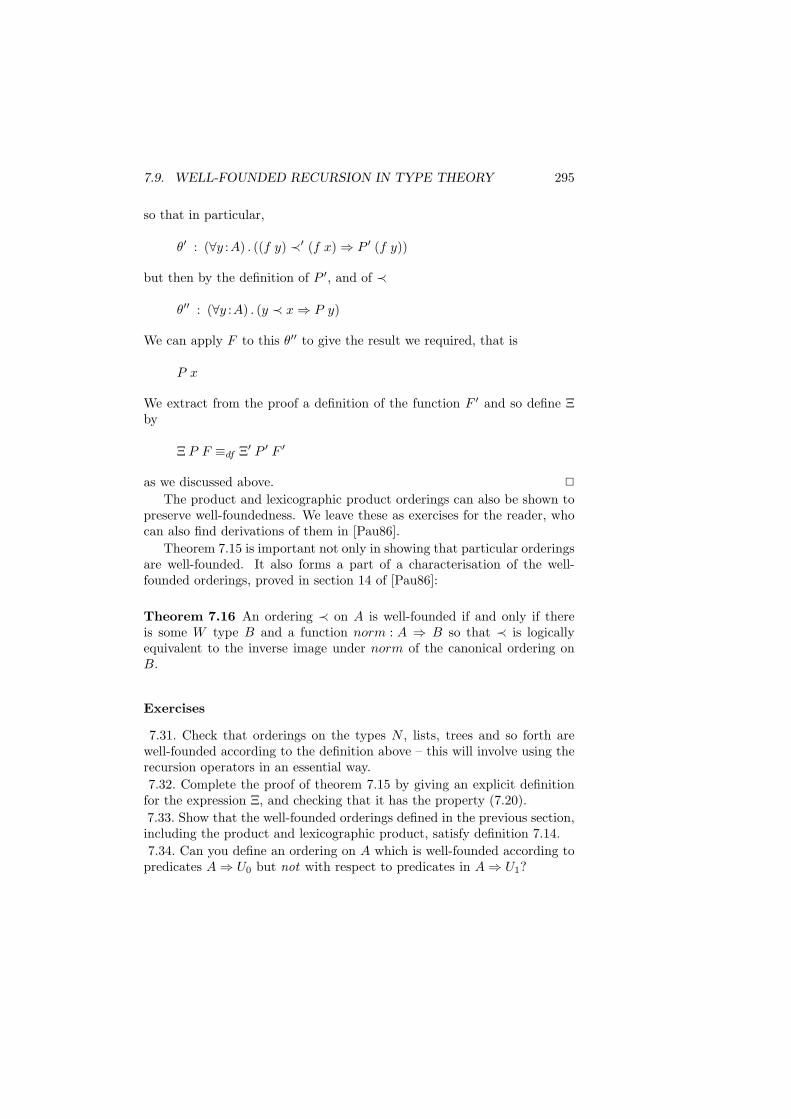
7.9. WELL-FOUNDED RECURSION IN TYPE THEORY 295
so that in particular,
θ′ : (∀y :A) . ((f y) ≺′ (f x)⇒ P ′ (f y))
but then by the definition of P ′, and of ≺
θ′′ : (∀y :A) . (y ≺ x⇒ P y)
We can apply F to this θ′′ to give the result we required, that is
P x
We extract from the proof a definition of the function F ′ and so define Ξby
Ξ P F ≡df Ξ′ P ′ F ′
as we discussed above. 2
The product and lexicographic product orderings can also be shown topreserve well-foundedness. We leave these as exercises for the reader, whocan also find derivations of them in [Pau86].
Theorem 7.15 is important not only in showing that particular orderingsare well-founded. It also forms a part of a characterisation of the well-founded orderings, proved in section 14 of [Pau86]:
Theorem 7.16 An ordering ≺ on A is well-founded if and only if thereis some W type B and a function norm : A ⇒ B so that ≺ is logicallyequivalent to the inverse image under norm of the canonical ordering onB.
Exercises
7.31. Check that orderings on the types N , lists, trees and so forth arewell-founded according to the definition above – this will involve using therecursion operators in an essential way.7.32. Complete the proof of theorem 7.15 by giving an explicit definition
for the expression Ξ, and checking that it has the property (7.20).7.33. Show that the well-founded orderings defined in the previous section,including the product and lexicographic product, satisfy definition 7.14.7.34. Can you define an ordering on A which is well-founded according to
predicates A⇒ U0 but not with respect to predicates in A⇒ U1?
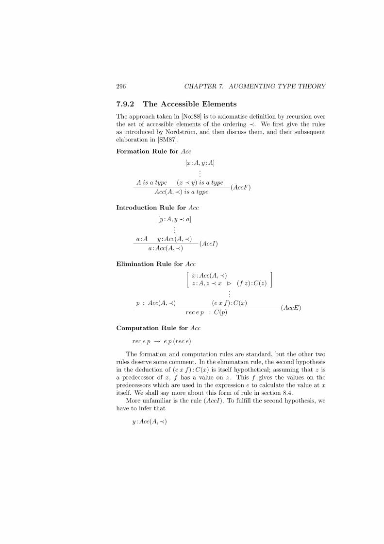
296 CHAPTER 7. AUGMENTING TYPE THEORY
7.9.2 The Accessible Elements
The approach taken in [Nor88] is to axiomatise definition by recursion overthe set of accessible elements of the ordering ≺. We first give the rulesas introduced by Nordstrom, and then discuss them, and their subsequentelaboration in [SM87].
Formation Rule for Acc
A is a type
[x :A, y :A]...
(x ≺ y) is a type
Acc(A,≺) is a type(AccF )
Introduction Rule for Acc
a :A
[y :A, y ≺ a]...
y :Acc(A,≺)a :Acc(A,≺)
(AccI)
Elimination Rule for Acc
p : Acc(A,≺)
[x :Acc(A,≺)z :A, z ≺ x (f z) :C(z)
]...
(e x f) :C(x)rec e p : C(p)
(AccE)
Computation Rule for Acc
rec e p → e p (rec e)
The formation and computation rules are standard, but the other tworules deserve some comment. In the elimination rule, the second hypothesisin the deduction of (e x f) : C(x) is itself hypothetical; assuming that z isa predecessor of x, f has a value on z. This f gives the values on thepredecessors which are used in the expression e to calculate the value at xitself. We shall say more about this form of rule in section 8.4.
More unfamiliar is the rule (AccI). To fulfill the second hypothesis, wehave to infer that
y :Acc(A,≺)
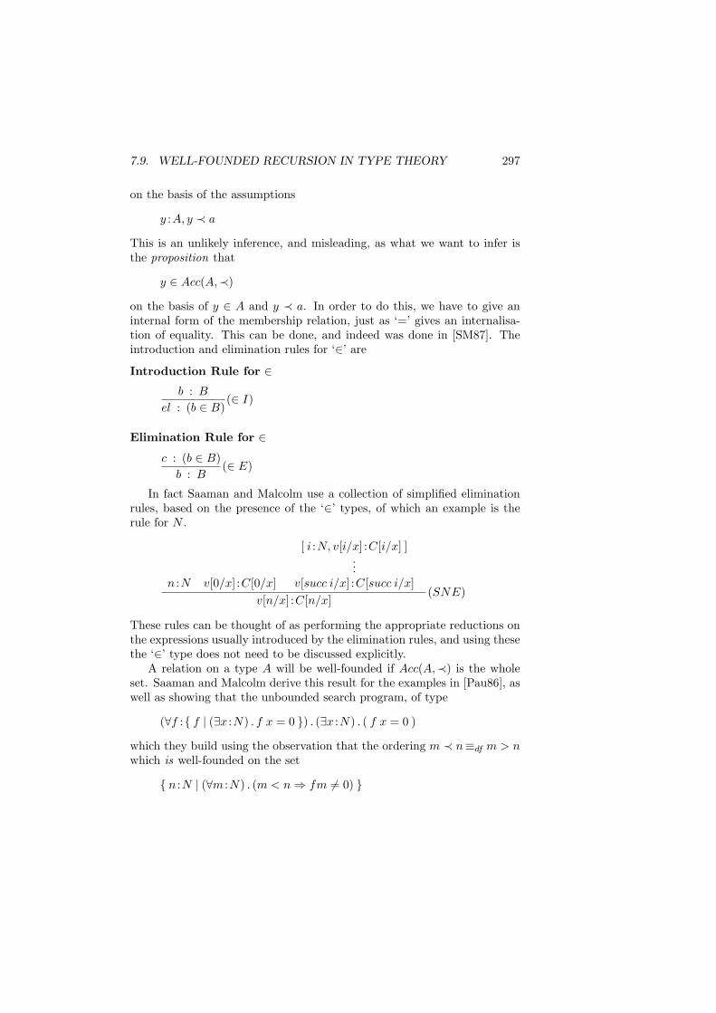
7.9. WELL-FOUNDED RECURSION IN TYPE THEORY 297
on the basis of the assumptions
y :A, y ≺ a
This is an unlikely inference, and misleading, as what we want to infer isthe proposition that
y ∈ Acc(A,≺)
on the basis of y ∈ A and y ≺ a. In order to do this, we have to give aninternal form of the membership relation, just as ‘=’ gives an internalisa-tion of equality. This can be done, and indeed was done in [SM87]. Theintroduction and elimination rules for ‘∈’ are
Introduction Rule for ∈b : B
el : (b ∈ B)(∈ I)
Elimination Rule for ∈
c : (b ∈ B)b : B
(∈ E)
In fact Saaman and Malcolm use a collection of simplified eliminationrules, based on the presence of the ‘∈’ types, of which an example is therule for N .
n :N v[0/x] :C[0/x]
[ i :N, v[i/x] :C[i/x] ]...
v[succ i/x] :C[succ i/x]v[n/x] :C[n/x]
(SNE)
These rules can be thought of as performing the appropriate reductions onthe expressions usually introduced by the elimination rules, and using thesethe ‘∈’ type does not need to be discussed explicitly.
A relation on a type A will be well-founded if Acc(A,≺) is the wholeset. Saaman and Malcolm derive this result for the examples in [Pau86], aswell as showing that the unbounded search program, of type
(∀f : f | (∃x :N) . f x = 0 ) . (∃x :N) . ( f x = 0 )
which they build using the observation that the ordering m ≺ n≡df m > nwhich is well-founded on the set
n :N | (∀m :N) . (m < n⇒ fm 6= 0)
298 CHAPTER 7. AUGMENTING TYPE THEORY
Exercises
7.35. Show that the class of elements accessible under the ordering ‘<’ onN is N itself.7.36. Given orderings ≺ and ≺′ on A and A′, how would you charac-
terise the elments accessible in the product, lexicographic product and sumorderings on A ∧B and A ∨B?
7.9.3 Conclusions
Two alternatives have been suggested to augment the ‘structural’ recur-sions over types such as N , lists, trees and so on. In the first, in [Pau86],the theory TT is shown to be sufficiently powerful to define many of the re-cursion operators over well-founded relations. This has the advantage thatno changes need to be made to the system, and also the advantage over thederivations given in chapter 6, in which implicitly at least, the derivationof well-foundedness has to be repeated for each function definition. In thisrespect Paulson’s approach adds a useful modularity to the system.
Saaman and Chisholm’s proposal is more far-reaching, involving theintroduction of a new predicate ‘∈’ of uncertain effect on, for example, thetermination properties of the system. On the other hand, they claim thatit simplifies considerably the proof objects given by Paulson’s approach, aswell as allowing the definition of the root-finding program.
7.10 Inductive types
The idea examined in this section is that types can be generated by induc-tion. We begin with an informal introduction, and then turn to a discussionof how the process can be formalised in type theory. [Mos74] gives an ele-gant treatment of inductive definitions from a set-theoretic standpoint, thetype theoretic-treatment appearing in [Men87b] and [Dyb88].
7.10.1 Inductive definitions
We look at the idea of inductive generation of types using the runningexample of finite lists of natural numbers. We have already seen that listscan be introduced by means of the W -type mechanism, but an informalspecification might say
[ ] is a list, and if n is a number, and x a list, then (n :: x) isalso a list . . .
7.10. INDUCTIVE TYPES 299
The type of lists L, has to contain [ ], and if it contains x it must contain(n :: x) also. Moreover, the intention of the definition is that L is thesmallest such set, as the informal specification has the implicit conclusion
. . . and lists can only arise in this way.
We can formalise by saying that L is the smallest solution of the equation
L≡df [ ] ∨ (N ∧ L)
if we represent the list (n :: x) by the pair (n, x). We shall in fact continueto use the familiar notation (n :: x) instead of the pair. Not every equation
T ≡ Θ T
has a solution or a least solution: a sufficient condition for a least solutionis that the operator Θ is monotonic, so that if S ⊆ T then
Θ S ⊆ Θ T
The least solution of the equation is called the least fixed point of theoperator Θ, and we write it FixΘ. To show that the equation has a solutionwe consider the sequence of sets
Θ0 ≡df ∅ ⊆ . . . ⊆ Θα+1 ≡df Θ Θα ⊆ . . .
Assuming that we are working in some universe set, this sequence musthave a fixed point, Θβ+1 = Θβ . In general, the superscript β may be aninfinite ordinal number, reflecting the complexity of the type thus defined.This fixed point is the least fixed point of Θ, but we can also deduce thata least fixed point exists from the fact that for a monotonic operator, theintersection of all the solutions is itself a solution, and that will be the leastsuch.
We shall use the notation L for the operator of which L is the least fixedpoint:
L T ≡df [ ] ∨ (N ∧ T )
The equation
L ≡ [ ] ∨ (N ∧ L)
characterises that L is a fixed point of L. How do we characterise that Lis the least solution?
We need to express that elements only go in by the action of the operatorL. We do this by giving an elimination rule which constructs a function byrecursion over L. To make such a definition it is necessary and sufficient
300 CHAPTER 7. AUGMENTING TYPE THEORY
to state a value at [ ] and a way of going from a value at x to a value at(n :: x). Looking at this in a slightly different way, we have give a way ofgoing from a value at an object of type T to a value at an object of typeL T , since a value of type
L T ≡ [ ] ∨ (N ∧ T )
will be either [ ] or (n :: x) with x :T .Abstracting from this, to define a function
fix g : Fix L ⇒ R
we give a function
g : (T ⇒ R)⇒ (L T ⇒ R)
Consider the example of the sum function, which returns the sum of anumerical list. This is characterised by the function g,
g f [ ] ≡df 0g f (n, x) ≡df n + (f x)
since if we define its fixed point, fix g, it will satisfy
fix g [ ] ≡ 0fix g (n, x) ≡ n + (fix g x)
In the general case this is encapsulated by the computation rule
(fix g) → g (fix g)
Before we give a type theoretic treatment of inductive definitions, we ob-serve that there is a link between inductively defined sets and well-foundedorderings. Every inductive set has an ordering given by comparing thestages at which the elements go into the set. We define
‖x‖ ≡df the α such that x ∈ Θα+1 −Θα
Now we say that x ≺ y if and only if ‖x‖ < ‖y‖; this ordering is well-founded as it is the inverse image of the ordering of the ordinal numbers.This characterisation also suggests that we can give a representation ofinductively defined sets by means of well-founded recursion, and ultimatelyby means of the W -types.
Exercises
7.37. Show that the type of finite and infinite lists of natural numbers is asolution of the equation
L≡df [ ] ∨ (N ∧ L)
7.10. INDUCTIVE TYPES 301
How would you argue that it does not meet the inductive characterisationof the least fixed point?7.38. Argue that the operator which sends T to 1 if 0 ∈ T , and to 0 ifnot has no fixed point.7.39. Show that the intersection of a non-empty set of fixed points of a
monotonic operator Θ is a fixed point of Θ, and therefore that a least fixedpoint exists.7.40. Give fixed point definitions of the types of natural numbers and trees.7.41. How would you define a type of lists whose elements are either naturalnumbers or lists themselves?7.42. Give a fixed point definition of a type of finite and countable ordinalnumbers.
7.10.2 Inductive definitions in type theory
Formation of inductive types is permitted when we have a monotonic op-eration
Θ : Type⇒ Type
There are two approaches to verifying the monotonicity of an operator.In the first, which is adopted in [Dyb88], a meta-theorem guarantees thatoperations of a restricted syntactic form are monotonic. If the symbol Tdoes not appear embedded in the domain part of any function or universaltype in T , then the operation
Θ:T 7→ T
is called positive, and can readily be shown to be monotonic. We canrefine this to sanction negative appearances of T in the domain part, wheresuch appearances have the dual definition to positive ones.
In [Men87b], an explicit check for monotonicity is added to the rule,forcing the verification of a statement like
T1 ⊆ T2 T [T1/T ] ⊆ T [T2/T ]
To facilitate this, various straightforward rules for the new judgement formT1 ⊆ T2 have to be added to the system. The two approaches are com-plementary, and there is no reason at all why they should not be usedtogether.
The rules for the inductive type take the form
Formation Rule for Ind
Θ monotonicFix Θ is a type
(IndF )
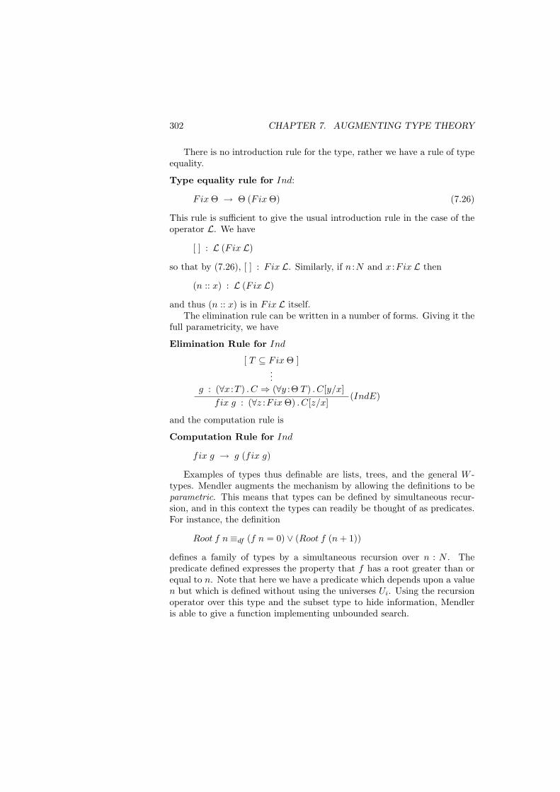
302 CHAPTER 7. AUGMENTING TYPE THEORY
There is no introduction rule for the type, rather we have a rule of typeequality.
Type equality rule for Ind:
Fix Θ → Θ (Fix Θ) (7.26)
This rule is sufficient to give the usual introduction rule in the case of theoperator L. We have
[ ] : L (Fix L)
so that by (7.26), [ ] : Fix L. Similarly, if n :N and x :Fix L then
(n :: x) : L (Fix L)
and thus (n :: x) is in Fix L itself.The elimination rule can be written in a number of forms. Giving it the
full parametricity, we have
Elimination Rule for Ind
[ T ⊆ Fix Θ ]...
g : (∀x :T ) . C ⇒ (∀y :Θ T ) . C[y/x]fix g : (∀z :Fix Θ) . C[z/x]
(IndE)
and the computation rule is
Computation Rule for Ind
fix g → g (fix g)
Examples of types thus definable are lists, trees, and the general W -types. Mendler augments the mechanism by allowing the definitions to beparametric. This means that types can be defined by simultaneous recur-sion, and in this context the types can readily be thought of as predicates.For instance, the definition
Root f n≡df (f n = 0) ∨ (Root f (n + 1))
defines a family of types by a simultaneous recursion over n : N . Thepredicate defined expresses the property that f has a root greater than orequal to n. Note that here we have a predicate which depends upon a valuen but which is defined without using the universes Ui. Using the recursionoperator over this type and the subset type to hide information, Mendleris able to give a function implementing unbounded search.
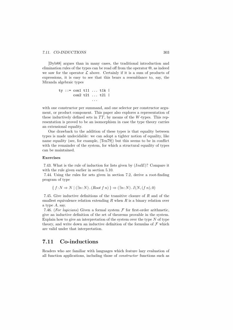
7.11. CO-INDUCTIONS 303
[Dyb88] argues than in many cases, the traditional introduction andelimination rules of the types can be read off from the operator Θ, as indeedwe saw for the operator L above. Certainly if it is a sum of products ofexpressions, it is easy to see that this bears a resemblance to, say, theMiranda algebraic types
ty ::= con1 t11 ... t1k |con2 t21 ... t2l |
...
with one constructor per summand, and one selector per constructor argu-ment, or product component. This paper also explores a representation ofthese inductively defined sets in TT , by means of the W -types. This rep-resentation is proved to be an isomorphism in case the type theory carriesan extensional equality.
One drawback to the addition of these types is that equality betweentypes is made undecidable: we can adopt a tighter notion of equality, likename equality (see, for example, [Ten79]) but this seems to be in conflictwith the remainder of the system, for which a structural equality of typescan be maintained.
Exercises
7.43. What is the rule of induction for lists given by (IndE)? Compare itwith the rule given earlier in section 5.10.7.44. Using the rules for sets given in section 7.2, derive a root-finding
program of type
f :N ⇒ N | (∃n :N) . (Root f n) ⇒ (∃n :N) . I(N, (f n), 0)
7.45. Give inductive definitions of the transitive closure of R and of thesmallest equivalence relation extending R when R is a binary relation overa type A, say.7.46. (For logicians) Given a formal system F for first-order arithmetic,
give an inductive definition of the set of theorems provable in the system.Explain how to give an interpretation of the system over the type N of typetheory, and write down an inductive definition of the formulas of F whichare valid under that interpretation.
7.11 Co-inductions
Readers who are familiar with languages which feature lazy evaluation ofall function applications, including those of constructor functions such as
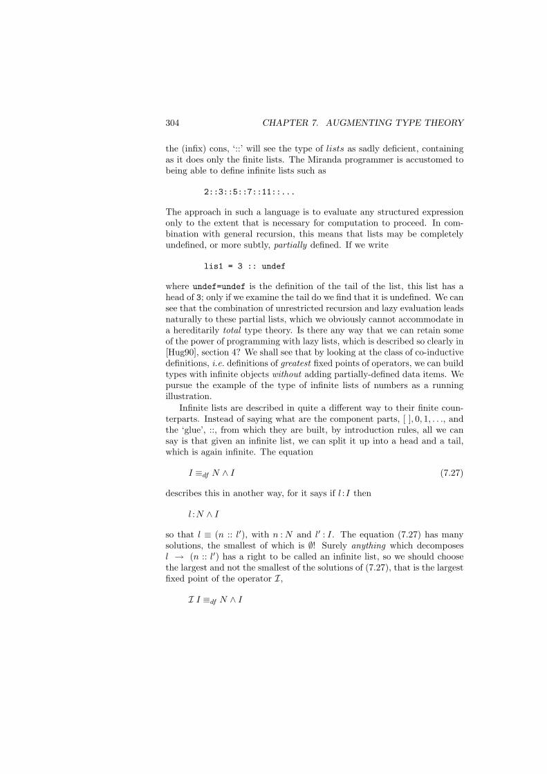
304 CHAPTER 7. AUGMENTING TYPE THEORY
the (infix) cons, ‘::’ will see the type of lists as sadly deficient, containingas it does only the finite lists. The Miranda programmer is accustomed tobeing able to define infinite lists such as
2::3::5::7::11::...
The approach in such a language is to evaluate any structured expressiononly to the extent that is necessary for computation to proceed. In com-bination with general recursion, this means that lists may be completelyundefined, or more subtly, partially defined. If we write
lis1 = 3 :: undef
where undef=undef is the definition of the tail of the list, this list has ahead of 3; only if we examine the tail do we find that it is undefined. We cansee that the combination of unrestricted recursion and lazy evaluation leadsnaturally to these partial lists, which we obviously cannot accommodate ina hereditarily total type theory. Is there any way that we can retain someof the power of programming with lazy lists, which is described so clearly in[Hug90], section 4? We shall see that by looking at the class of co-inductivedefinitions, i.e. definitions of greatest fixed points of operators, we can buildtypes with infinite objects without adding partially-defined data items. Wepursue the example of the type of infinite lists of numbers as a runningillustration.
Infinite lists are described in quite a different way to their finite coun-terparts. Instead of saying what are the component parts, [ ], 0, 1, . . ., andthe ‘glue’, ::, from which they are built, by introduction rules, all we cansay is that given an infinite list, we can split it up into a head and a tail,which is again infinite. The equation
I ≡df N ∧ I (7.27)
describes this in another way, for it says if l :I then
l :N ∧ I
so that l ≡ (n :: l′), with n : N and l′ : I. The equation (7.27) has manysolutions, the smallest of which is ∅! Surely anything which decomposesl → (n :: l′) has a right to be called an infinite list, so we should choosethe largest and not the smallest of the solutions of (7.27), that is the largestfixed point of the operator I,
I I ≡df N ∧ I
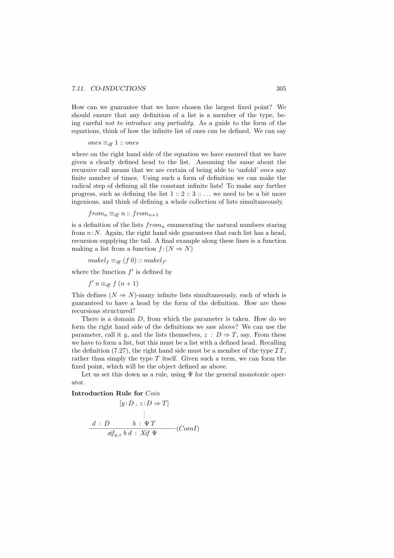
7.11. CO-INDUCTIONS 305
How can we guarantee that we have chosen the largest fixed point? Weshould ensure that any definition of a list is a member of the type, be-ing careful not to introduce any partiality. As a guide to the form of theequations, think of how the infinite list of ones can be defined. We can say
ones≡df 1 :: ones
where on the right hand side of the equation we have ensured that we havegiven a clearly defined head to the list. Assuming the same about therecursive call means that we are certain of being able to ‘unfold’ ones anyfinite number of times. Using such a form of definition we can make theradical step of defining all the constant infinite lists! To make any furtherprogress, such as defining the list 1 :: 2 :: 3 :: . . . we need to be a bit moreingenious, and think of defining a whole collection of lists simultaneously.
fromn ≡df n :: fromn+1
is a definition of the lists fromn enumerating the natural numbers staringfrom n :N . Again, the right hand side guarantees that each list has a head,recursion supplying the tail. A final example along these lines is a functionmaking a list from a function f : (N ⇒ N)
makelf ≡df (f 0) :: makelf ′
where the function f ′ is defined by
f ′ n≡df f (n + 1)
This defines (N ⇒ N)-many infinite lists simultaneously, each of which isguaranteed to have a head by the form of the definition. How are theserecursions structured?
There is a domain D, from which the parameter is taken. How do weform the right hand side of the definitions we saw above? We can use theparameter, call it y, and the lists themselves, z : D ⇒ T , say. From thesewe have to form a list, but this must be a list with a defined head. Recallingthe definition (7.27), the right hand side must be a member of the type I T ,rather than simply the type T itself. Given such a term, we can form thefixed point, which will be the object defined as above.
Let us set this down as a rule, using Ψ for the general monotonic oper-ator.
Introduction Rule for Coin
d : D
[y :D , z :D ⇒ T ]...
b : Ψ T
xify,z b d : Xif Ψ(CoinI)
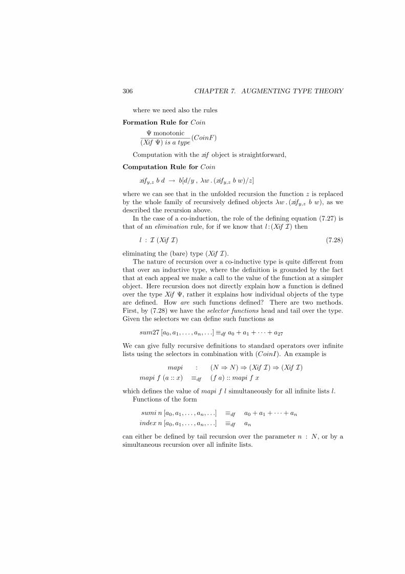
306 CHAPTER 7. AUGMENTING TYPE THEORY
where we need also the rules
Formation Rule for Coin
Ψ monotonic(Xif Ψ) is a type
(CoinF )
Computation with the xif object is straightforward,
Computation Rule for Coin
xify,z b d → b[d/y , λw . (xify,z b w)/z]
where we can see that in the unfolded recursion the function z is replacedby the whole family of recursively defined objects λw . (xify,z b w), as wedescribed the recursion above.
In the case of a co-induction, the role of the defining equation (7.27) isthat of an elimination rule, for if we know that l : (Xif I) then
l : I (Xif I) (7.28)
eliminating the (bare) type (Xif I).The nature of recursion over a co-inductive type is quite different from
that over an inductive type, where the definition is grounded by the factthat at each appeal we make a call to the value of the function at a simplerobject. Here recursion does not directly explain how a function is definedover the type Xif Ψ, rather it explains how individual objects of the typeare defined. How are such functions defined? There are two methods.First, by (7.28) we have the selector functions head and tail over the type.Given the selectors we can define such functions as
sum27 [a0, a1, . . . , an, . . .]≡df a0 + a1 + · · ·+ a27
We can give fully recursive definitions to standard operators over infinitelists using the selectors in combination with (CoinI). An example is
mapi : (N ⇒ N)⇒ (Xif I)⇒ (Xif I)mapi f (a :: x) ≡df (f a) :: mapi f x
which defines the value of mapi f l simultaneously for all infinite lists l.Functions of the form
sumi n [a0, a1, . . . , an, . . .] ≡df a0 + a1 + · · ·+ an
index n [a0, a1, . . . , an, . . .] ≡df an
can either be defined by tail recursion over the parameter n : N , or by asimultaneous recursion over all infinite lists.
7.11. CO-INDUCTIONS 307
Other types which can be defined in this way are the type of finite andinfinite lists, the largest fixed point of the operator L, infinite trees and thelike.
We can define sophisticated functions over the type of infinite lists ifwe are prepared to incorporate some proof-theoretic information into thedomain. One example might be a function which splits a stream of char-acters into a stream of words, splitting at each white space character. Wecannot define this function over all the infinite lists, but only those withwhite space occurring infinitely often. We can describe exactly this classas an existential or subset type, and therefore define the function.
Equality over these types is interesting also. If it is intensional, then wewill only identify (for example) two infinite lists if they are defined in thesame way. An alternative is to adopt an extensional approach, saying that
l ' l′ ⇔ (∀n :N) . ( index n l = index n l′ )
This approach is adopted in a logic for Miranda, [Tho89b], where it ax-iomatises equality of infinite lists. Using the denotational semantics forMiranda, we can of course prove that this is the case.
In conclusion, we would suggest that many of the advantages advancedfor lazy lists accrue here also. In particular, the examples of [Hug90, Section4] seem to carry over with no difficulty.
Exercises
7.47. Give formal definitions of the functions mapi, sumi and index definedabove.7.48. Define the functions
iterate f st≡df [ st , f st , f (f st) , . . .]
infold f st [a0, a1, . . . , an, . . .]≡df [ st , f st a0 , f (f st a0) a1 , . . .]
7.49. A natural number greater than one is called a Hamming number ifits only prime factors are 2, 3 and 5. Show how to define a function whichwill merge two infinite lists, removing duplicate occurrences which appearin both lists and preserving order in the case that the lists are ordered.Using this function and the iterate function above give a definition of thelist of Hamming numbers, enumerated in ascending order. (This problemis described in more detail in [Dij76].)7.50. Give a definition of the list of prime numbers.7.51. Write a definition of a general map function over the finite and infinitelists.
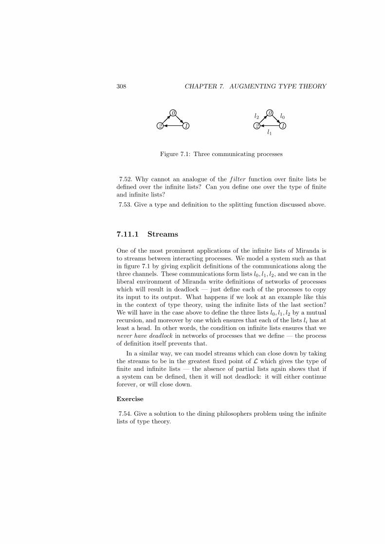
308 CHAPTER 7. AUGMENTING TYPE THEORY
i0@@Ri2 i1
i0@@Ri2 i1
l0l2
l1
Figure 7.1: Three communicating processes
7.52. Why cannot an analogue of the filter function over finite lists bedefined over the infinite lists? Can you define one over the type of finiteand infinite lists?
7.53. Give a type and definition to the splitting function discussed above.
7.11.1 Streams
One of the most prominent applications of the infinite lists of Miranda isto streams between interacting processes. We model a system such as thatin figure 7.1 by giving explicit definitions of the communications along thethree channels. These communications form lists l0, l1, l2, and we can in theliberal environment of Miranda write definitions of networks of processeswhich will result in deadlock — just define each of the processes to copyits input to its output. What happens if we look at an example like thisin the context of type theory, using the infinite lists of the last section?We will have in the case above to define the three lists l0, l1, l2 by a mutualrecursion, and moreover by one which ensures that each of the lists li has atleast a head. In other words, the condition on infinite lists ensures that wenever have deadlock in networks of processes that we define — the processof definition itself prevents that.
In a similar way, we can model streams which can close down by takingthe streams to be in the greatest fixed point of L which gives the type offinite and infinite lists — the absence of partial lists again shows that ifa system can be defined, then it will not deadlock: it will either continueforever, or will close down.
Exercise
7.54. Give a solution to the dining philosophers problem using the infinitelists of type theory.
7.12. PARTIAL OBJECTS AND TYPES 309
7.12 Partial Objects and Types
The literature contains a number of proposals for adding non-terminatingor ‘partial’ objects to type theory. The naıve proposal would be simplyto allow unrestricted recursion and thus non-terminating computations inthe systems TT0 etc. As a programming language this results in somethingmuch closer to current systems like Miranda and Haskell, but we also ap-pear to lose the logical interpretation of the system. Since the undefinedobject, ↑, or bottom (which is confusingly denoted ⊥ in the literature ondenotational semantics) is a member of every type, the logical interpreta-tion is inconsistent, as every formula is provable, by the proof ↑. Moreover,principles such as induction have to be modified to take account of the ad-ditional members of types like N . (Details of how this is done can be foundin [Pau87, Tho89b].)
Can a logical interpretation be given to such a system? It would seemthat there is at least a chance of so doing, if we can identify preciselythose objects which represent ‘total’ and not ‘partial’ proofs. The logic forMiranda alluded to earlier shows how the total objects can be identifiedat simple types, but there is a choice in what should be deemed the totalobjects at type
(N ⇒ N)⇒ (N ⇒ N)
say. It would be an interesting research project to see precisely how such alogical interpretation would work.
A quite different approach is suggested in [CS87], which supersedes theearlier version of partial types discussed in [C+86a], section 12.2. This pro-poses the addition of types T which consist of computations of elementsof T , the partial objects which may or may not result in values in the typeT itself. The advantage of this approach over the naıve one is the degreeof descriptive power that it affords. For instance, we can distinguish thefollowing types of numerical functions
N ⇒ N N ⇒ N N ⇒ N N ⇒ N N ⇒ N N ⇒ N
each of which is sensible and embodies a different notion of function from Nto N . It is a revealing exercise to discover the relations between the typesby finding which embeddings exist between them, and by showing which donot exist by finding the appropriate counterexamples. A basic relationshipbetween types is that members of T are members of T , and in the conversedirection, if an element of T is shown to have a canonical form then it isin T . So as to allow explicit reasoning about termination, we will have tointroduce the membership predicate, a ∈ A, as in section 7.9.2 above.
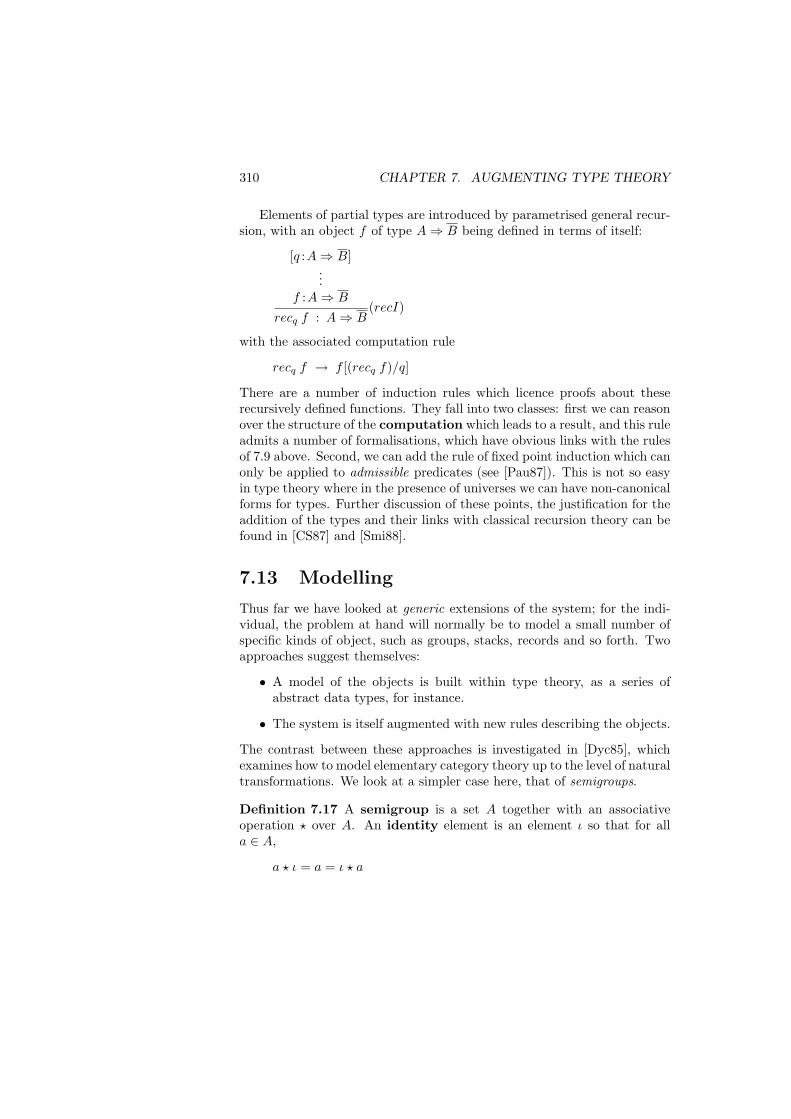
310 CHAPTER 7. AUGMENTING TYPE THEORY
Elements of partial types are introduced by parametrised general recur-sion, with an object f of type A⇒ B being defined in terms of itself:
[q :A⇒ B]...
f :A⇒ B
recq f : A⇒ B(recI)
with the associated computation rule
recq f → f [(recq f)/q]
There are a number of induction rules which licence proofs about theserecursively defined functions. They fall into two classes: first we can reasonover the structure of the computation which leads to a result, and this ruleadmits a number of formalisations, which have obvious links with the rulesof 7.9 above. Second, we can add the rule of fixed point induction which canonly be applied to admissible predicates (see [Pau87]). This is not so easyin type theory where in the presence of universes we can have non-canonicalforms for types. Further discussion of these points, the justification for theaddition of the types and their links with classical recursion theory can befound in [CS87] and [Smi88].
7.13 Modelling
Thus far we have looked at generic extensions of the system; for the indi-vidual, the problem at hand will normally be to model a small number ofspecific kinds of object, such as groups, stacks, records and so forth. Twoapproaches suggest themselves:
• A model of the objects is built within type theory, as a series ofabstract data types, for instance.
• The system is itself augmented with new rules describing the objects.
The contrast between these approaches is investigated in [Dyc85], whichexamines how to model elementary category theory up to the level of naturaltransformations. We look at a simpler case here, that of semigroups.
Definition 7.17 A semigroup is a set A together with an associativeoperation ? over A. An identity element is an element ι so that for alla ∈ A,
a ? ι = a = ι ? a
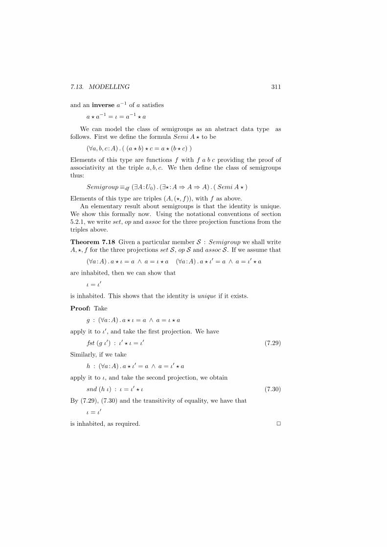
7.13. MODELLING 311
and an inverse a−1 of a satisfies
a ? a−1 = ι = a−1 ? a
We can model the class of semigroups as an abstract data type asfollows. First we define the formula Semi A ? to be
(∀a, b, c :A) . ( (a ? b) ? c = a ? (b ? c) )
Elements of this type are functions f with f a b c providing the proof ofassociativity at the triple a, b, c. We then define the class of semigroupsthus:
Semigroup≡df (∃A :U0) . (∃? :A⇒ A⇒ A) . ( Semi A ? )
Elements of this type are triples (A, (?, f)), with f as above.An elementary result about semigroups is that the identity is unique.
We show this formally now. Using the notational conventions of section5.2.1, we write set, op and assoc for the three projection functions from thetriples above.
Theorem 7.18 Given a particular member S : Semigroup we shall writeA, ?, f for the three projections set S, op S and assoc S. If we assume that
(∀a :A) . a ? ι = a ∧ a = ι ? a (∀a :A) . a ? ι′ = a ∧ a = ι′ ? a
are inhabited, then we can show that
ι = ι′
is inhabited. This shows that the identity is unique if it exists.
Proof: Take
g : (∀a :A) . a ? ι = a ∧ a = ι ? a
apply it to ι′, and take the first projection. We have
fst (g ι′) : ι′ ? ι = ι′ (7.29)
Similarly, if we take
h : (∀a :A) . a ? ι′ = a ∧ a = ι′ ? a
apply it to ι, and take the second projection, we obtain
snd (h ι) : ι = ι′ ? ι (7.30)
By (7.29), (7.30) and the transitivity of equality, we have that
ι = ι′
is inhabited, as required. 2
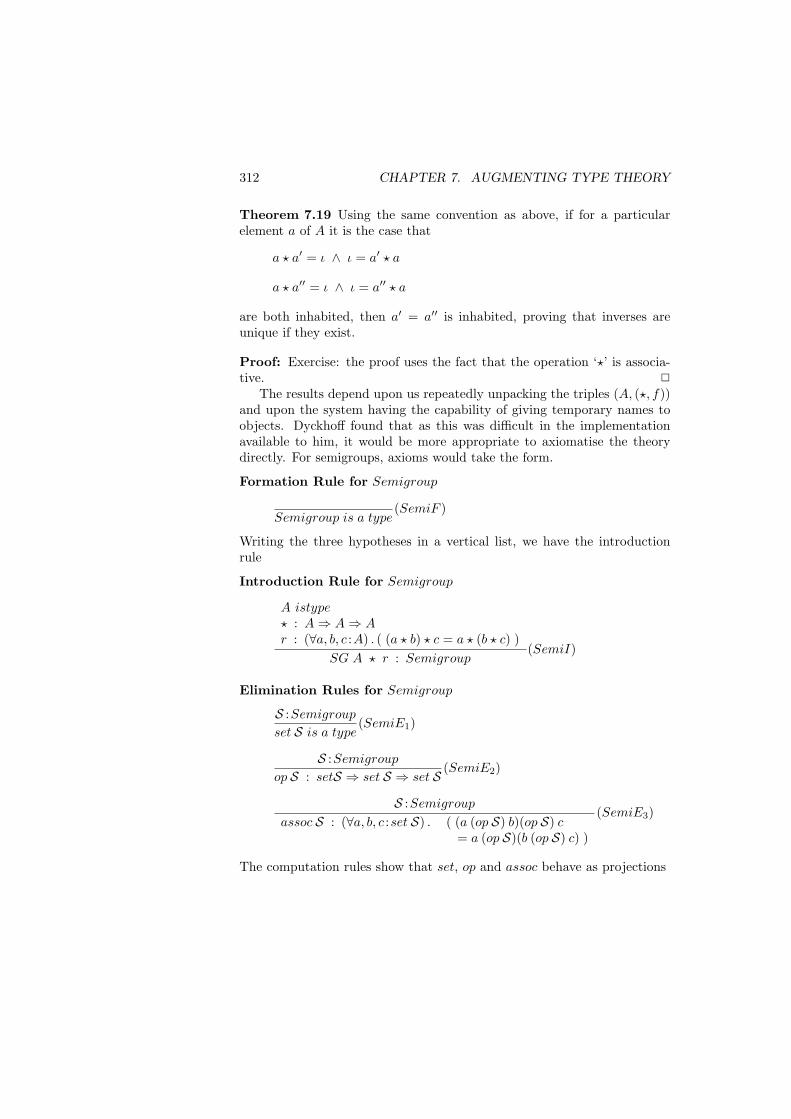
312 CHAPTER 7. AUGMENTING TYPE THEORY
Theorem 7.19 Using the same convention as above, if for a particularelement a of A it is the case that
a ? a′ = ι ∧ ι = a′ ? a
a ? a′′ = ι ∧ ι = a′′ ? a
are both inhabited, then a′ = a′′ is inhabited, proving that inverses areunique if they exist.
Proof: Exercise: the proof uses the fact that the operation ‘?’ is associa-tive. 2
The results depend upon us repeatedly unpacking the triples (A, (?, f))and upon the system having the capability of giving temporary names toobjects. Dyckhoff found that as this was difficult in the implementationavailable to him, it would be more appropriate to axiomatise the theorydirectly. For semigroups, axioms would take the form.
Formation Rule for Semigroup
Semigroup is a type(SemiF )
Writing the three hypotheses in a vertical list, we have the introductionrule
Introduction Rule for Semigroup
A istype? : A⇒ A⇒ Ar : (∀a, b, c :A) . ( (a ? b) ? c = a ? (b ? c) )
SG A ? r : Semigroup(SemiI)
Elimination Rules for Semigroup
S :Semigroup
set S is a type(SemiE1)
S :Semigroup
op S : setS ⇒ set S ⇒ set S(SemiE2)
S :Semigroup
assoc S : (∀a, b, c :set S) . ( (a (op S) b)(op S) c= a (op S)(b (op S) c) )
(SemiE3)
The computation rules show that set, op and assoc behave as projections
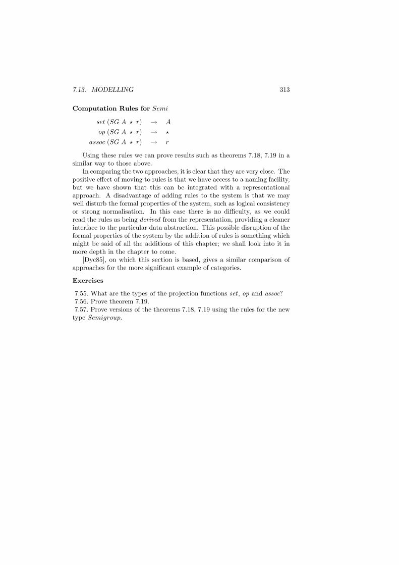
7.13. MODELLING 313
Computation Rules for Semi
set (SG A ? r) → A
op (SG A ? r) → ?
assoc (SG A ? r) → r
Using these rules we can prove results such as theorems 7.18, 7.19 in asimilar way to those above.
In comparing the two approaches, it is clear that they are very close. Thepositive effect of moving to rules is that we have access to a naming facility,but we have shown that this can be integrated with a representationalapproach. A disadvantage of adding rules to the system is that we maywell disturb the formal properties of the system, such as logical consistencyor strong normalisation. In this case there is no difficulty, as we couldread the rules as being derived from the representation, providing a cleanerinterface to the particular data abstraction. This possible disruption of theformal properties of the system by the addition of rules is something whichmight be said of all the additions of this chapter; we shall look into it inmore depth in the chapter to come.
[Dyc85], on which this section is based, gives a similar comparison ofapproaches for the more significant example of categories.
Exercises
7.55. What are the types of the projection functions set , op and assoc?7.56. Prove theorem 7.19.7.57. Prove versions of the theorems 7.18, 7.19 using the rules for the newtype Semigroup.

314 CHAPTER 7. AUGMENTING TYPE THEORY
Chapter 8
Foundations
This chapter marks a return to looking at the system as a whole, ratherthan at particular examples of terms and proofs derivable in it, or at pos-sible extensions. We investigate various questions about the mathematicalfoundations of the system. From the point of view of traditional proof the-ory, we can compare its strength with other formal systems for arithmetic— this we do in the first section. The technique used here is that of realiz-ability, which forms one sort of model of the formal system. We discuss themotivation for developing a model theory of TT in the subsequent section,giving other methods of model construction.
The topic of realizability is interesting not just from the proof-theoreticpoint of view: it provides a general mechanism for extracting the compu-tational content of a derivation, and as such may give a means of derivingmore efficient programs from type theoretic derivations.
We conclude the discussion with an overview of Schroeder-Heister andDybjer’s work on the inversion of proof rules. At an intuitive level, if weare given the introduction rules for a type then we seem to know all theforms that elements can take, and this really characterises the type. Theinversion principle gives a formal description of how an introduction rulecan be inverted to generate the elimination and computation rules. We alsolook at a primitive justification of the inversion principle itself.
8.1 Proof Theory
In this section we look at the relationship between the systems TT0, . . . andmore traditional presentations of constructive arithmetic. In particular weexamine the system HA of first-order intuitionistic arithmetic and its gen-
315
316 CHAPTER 8. FOUNDATIONS
eralisation to the simple types, HAω. The ‘H’ in these titles is in honour ofthe intuitionist Heyting, who was one of the first constructivists. We followthis with a discussion of the technique of realizability, which is used to giveinterpretations of intuitionistic systems, and which can form the basis of amore flexible algorithm extraction discipline than that of type theory. Weconclude with a discussion of the various rules for existential elimination,and what consequences the choice of rules has for our implementation ofmodules.
8.1.1 Intuitionistic Arithmetic
Definition 8.1 A full definition the system of First Order HeytingArithmetic, HA, is given in [Tro73], section I.3. The system consistsof a first order theory of the natural numbers, with a function constantfor each primitive recursive function. Axioms assert the basic properties ofequality; the standard Peano axioms stating that zero is not a successor,that the successor is 1-1 and the axiom scheme of induction
φ(0) ∧ ∀n.(φ(n)⇒ φ(n + 1))⇒ ∀n.φ(n)
for every formula ‘φ’; and finally the defining equations of each of theprimitive recursive functions.
The rules of deduction are the standard set for constructive predicatecalculus, which can be derived, by omitting the proof objects, from ourintroduction and elimination rules for ∧, ∨, ⇒, ⊥, ∀, ∃, choosing the weakrules for the elimination of disjunction and the existential quantifier, viz.(∨E) and (∃E′).
Definition 8.2 The system of Heyting Arithmetic at Finite Types,HAω, and called N −HAω in the definition [Tro73] section I.6, is similarto HA, except that objects can be of any of the finite types formed from Nby the function space constructor. An operator which embodies definitionby primitive recursion is included at each type. Quantifiers range overparticular types, rather than the whole domain.
These systems have been studied extensively, and their relation withTT0 can tell us something about the system itself. Obviously the systemHAω is an extension of HA in a sense to be made clearer by the nextdefinition. We write S ` φ for ‘φ is a theorem of the formal system S’.
Definition 8.3 Given two formal systems S1 and S2, a function f fromthe formulas of S1 to those of S2 is an embedding of the first system inthe second if for all formulas φ,
S1 ` φ implies S2 ` (f φ)
8.1. PROOF THEORY 317
If the relationship above is an equivalence, then S2 is called a conservativeextension of S1, and we can call the function f an interpretation of S1
in S2.
The system S2 is a conservative extension of S1 if the two theories provethe same theorems in the language of the smaller, S1; they give consistentpictures of their common domain.
Obviously there is an embedding of HA in HAω. We can also embedthe formulas of HAω as formulas of TT0, and prove the result that
Theorem 8.4 For any formula φ, if HAω ` φ then for some term t, wecan derive in TT0 the judgement t :φ.
Proof: The term t is a coding of the proof of φ in HAω. More details aregiven in [Bee85], theorem XI.17.1. 2
Moreover, if we add to HAω the axiom of choice over finite types, ACFT ,
∀x.∃y.A(x, y)⇒ ∃f.∀x.A(x, f x)
this is also validated by TT0. Showing that the Axiom of Choice is derivablein type theory is one of Martin-Lof’s few concessions to examples in hispapers. See [ML85, ML84], and observe that the derivation does not useextensionality. If we adopt the extensional theory of [ML85], then our typetheory extends the extensional version HAω + Ext + ACFT .
What results can we derive on the basis of this relationship?Our first result, due to Troelstra, is typical of the gain we can get by
looking at these inter-relationships: we are able to transfer a negative resultfrom HAω to type theory. First we give another definition.
Definition 8.5 A function F from N ⇒ N to N is called continuous iffor all f : (N ⇒ N) there is an n, so that if f i = g i for all i ≤ n, thenF f = F g. The value n is called a modulus of continuity of F at f .
Continuity is an assertion of the finitary nature of the functions overN ⇒ N : the value of such a function at f is determined by a finite amountof information about f . We would therefore expect that this would be trueof all the functions F definable in TT0. However, we can show that TT0
does not prove the formal statement of this,
(∀F : (N ⇒ N)⇒ N) . Cont(F )
This itself follows from the theorem
318 CHAPTER 8. FOUNDATIONS
Theorem 8.6 The theory
HAω + ACFT + Ext + (∀F : (N ⇒ N)⇒ N) . Cont(F )
is inconsistent (i.e. derives ⊥)
Proof: See [Bee85], theorem XI.19.1. Using the axiom of choice, we candefine a function µ returning the modulus of continuity of a function Fat the argument f . Extensionality means that this modulus is determinedby function values rather than representations, and this can be shown tolead to a finite procedure solving the limited principle of omniscience, acontradiction. 2
Corollary 8.7 The theory TT0 does not prove
(∀F : (N ⇒ N)⇒ N) . Cont(F )
Proof: If TT0 proves this, then the extensional version of type theoryproves it also and, as it also derives the axiom of choice, by the theorem isinconsistent. We have a proof of consistency, and so the original assumptionis untrue. 2
Can we characterise the arithmetical theorems provable in type theory?Again, the answer is yes,
Theorem 8.8 TT0 is a conservative extension of HA, where we say thatTT0 makes a proposition A valid when we can derive t :A for some expres-sion t.
Proof: This is due to a number of authors, including Beeson and Renardel,[Bee85, DT84]. The proof uses the technique of realizability, to which weturn in the next section. 2
It is worth noting what the theorem says. It asserts that the system ofTT0 — which extends first-order arithmetic by embedding it in a system oftypes, for which the axiom of choice is assumed to hold (and which mightbe made extensional as far as this result is concerned) — is no strongerthan first-order arithmetic as far as arithmetical statements are concerned.
We have said nothing about the theories TT , TT+ and TT+0 . Each of
these is stronger than TT0. We have already shown that TT is strongerthan TT0, other remarks about this can be found in [Bee85], section XIII.5.We know of no results for the theories with the full W -type.
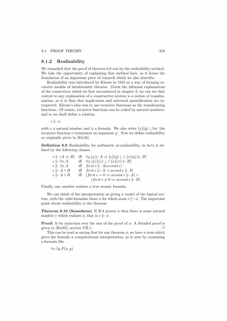
8.1. PROOF THEORY 319
8.1.2 Realizability
We remarked that the proof of theorem 8.8 was by the realizability method.We take the opportunity of explaining that method here, as it forms thefoundation of an important piece of research which we also describe.
Realizability was introduced by Kleene in 1945 as a way of forming re-cursive models of intuitionistic theories. Given the informal explanationsof the connectives which we first encountered in chapter 3, we can see thatcentral to any explanation of a constructive system is a notion of transfor-mation, as it is thus that implication and universal quantification are in-terpreted. Kleene’s idea was to use recursive functions as the transformingfunctions. Of course, recursive functions can be coded by natural numbers,and so we shall define a relation
e ‖− φ
with e a natural number and φ a formula. We also write e(q) ↓ for ‘therecursive function e terminates on argument q’. Now we define realizabilityas originally given in [Kle45]:
Definition 8.9 Realizability for arithmetic (r-realizability, in fact) is de-fined by the following clauses.
e ‖− (A⇒ B) iff ∀q.(q ‖−A⇒ e(q) ↓ ∧ e(q) ‖−B)e ‖− ∀x.A iff ∀x.(e(x) ↓ ∧ e(x) ‖−B)e ‖− ∃x.A iff first e ‖−A(second e)e ‖−A ∧B iff first e ‖−A ∧ second e ‖−Be ‖−A ∨B iff (first e = 0⇒ second e ‖−A) ∧
(first e 6= 0⇒ second e ‖−B)
Finally, any number realizes a true atomic formula.
We can think of the interpretation as giving a model of the logical sys-tem, with the valid formulas those φ for which some e‖−φ. The importantpoint about realizability is the theorem
Theorem 8.10 (Soundness) If HA proves φ then there is some naturalnumber e which realizes φ, that is e ‖− φ.
Proof: Is by induction over the size of the proof of φ. A detailed proof isgiven in [Bee85], section VII.1. 2
This can be read as saying that for any theorem φ, we have a term whichgives the formula a computational interpretation, as is seen by examininga formula like
∀x.∃y.P (x, y)
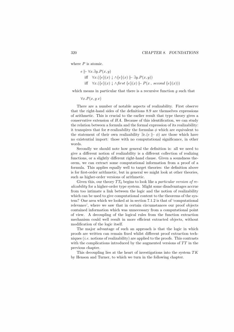
320 CHAPTER 8. FOUNDATIONS
where P is atomic.
e ‖− ∀x.∃y.P (x, y)iff ∀x.(e(x) ↓ ∧e(x) ‖− ∃y.P (x, y))iff ∀x.(e(x) ↓ ∧first e(x) ‖− P (x , second e(x)))
which means in particular that there is a recursive function g such that
∀x.P (x, g x)
There are a number of notable aspects of realizability. First observethat the right-hand sides of the definitions 8.9 are themselves expressionsof arithmetic. This is crucial to the earlier result that type theory gives aconservative extension of HA. Because of this identification, we can studythe relation between a formula and the formal expression of its realizability:it transpires that for r-realizability the formulas φ which are equivalent tothe statement of their own realizability ∃e.(e ‖− φ) are those which haveno existential import: those with no computational significance, in otherwords.
Secondly we should note how general the definition is: all we need togive a different notion of realizability is a different collection of realizingfunctions, or a slightly different right-hand clause. Given a soundness the-orem, we can extract some computational information from a proof of aformula. This applies equally well to target theories: the definition aboveis for first-order arithmetic, but in general we might look at other theories,such as higher-order versions of arithmetic.
Given this, our theory TT0 begins to look like a particular version of re-alizability for a higher-order type system. Might some disadvantages accruefrom too intimate a link between the logic and the notion of realizabilitywhich can be used to give computational content to the theorems of the sys-tem? One area which we looked at in section 7.1.2 is that of ‘computationalrelevance’, where we saw that in certain circumstances our proof objectscontained information which was unnecessary from a computational pointof view. A decoupling of the logical rules from the function extractionmechanism could well result in more efficient extracted objects, withoutmodification of the logic itself.
The major advantage of such an approach is that the logic in whichproofs are written can remain fixed whilst different proof extraction tech-niques (i.e. notions of realizability) are applied to the proofs. This contrastswith the complications introduced by the augmented versions of TT in theprevious chapter.
This decoupling lies at the heart of investigations into the system TKby Henson and Turner, to which we turn in the following chapter.
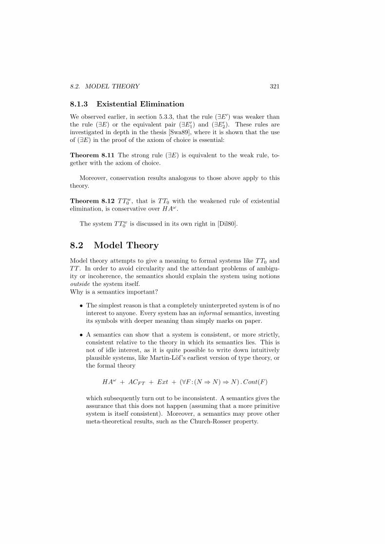
8.2. MODEL THEORY 321
8.1.3 Existential Elimination
We observed earlier, in section 5.3.3, that the rule (∃E′) was weaker thanthe rule (∃E) or the equivalent pair (∃E′
1) and (∃E′2). These rules are
investigated in depth in the thesis [Swa89], where it is shown that the useof (∃E) in the proof of the axiom of choice is essential:
Theorem 8.11 The strong rule (∃E) is equivalent to the weak rule, to-gether with the axiom of choice.
Moreover, conservation results analogous to those above apply to thistheory.
Theorem 8.12 TTw0 , that is TT0 with the weakened rule of existential
elimination, is conservative over HAω.
The system TTw0 is discussed in its own right in [Dil80].
8.2 Model Theory
Model theory attempts to give a meaning to formal systems like TT0 andTT . In order to avoid circularity and the attendant problems of ambigu-ity or incoherence, the semantics should explain the system using notionsoutside the system itself.Why is a semantics important?
• The simplest reason is that a completely uninterpreted system is of nointerest to anyone. Every system has an informal semantics, investingits symbols with deeper meaning than simply marks on paper.
• A semantics can show that a system is consistent, or more strictly,consistent relative to the theory in which its semantics lies. This isnot of idle interest, as it is quite possible to write down intuitivelyplausible systems, like Martin-Lof’s earliest version of type theory, orthe formal theory
HAω + ACFT + Ext + (∀F : (N ⇒ N)⇒ N) . Cont(F )
which subsequently turn out to be inconsistent. A semantics gives theassurance that this does not happen (assuming that a more primitivesystem is itself consistent). Moreover, a semantics may prove othermeta-theoretical results, such as the Church-Rosser property.
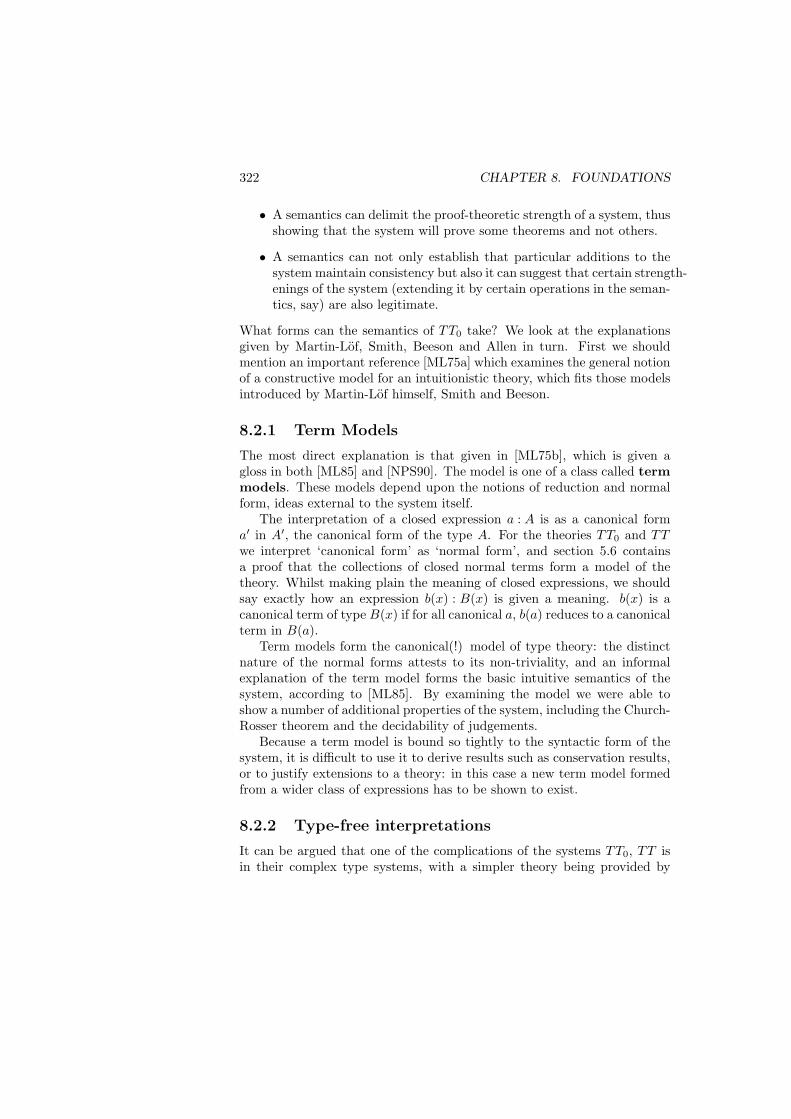
322 CHAPTER 8. FOUNDATIONS
• A semantics can delimit the proof-theoretic strength of a system, thusshowing that the system will prove some theorems and not others.
• A semantics can not only establish that particular additions to thesystem maintain consistency but also it can suggest that certain strength-enings of the system (extending it by certain operations in the seman-tics, say) are also legitimate.
What forms can the semantics of TT0 take? We look at the explanationsgiven by Martin-Lof, Smith, Beeson and Allen in turn. First we shouldmention an important reference [ML75a] which examines the general notionof a constructive model for an intuitionistic theory, which fits those modelsintroduced by Martin-Lof himself, Smith and Beeson.
8.2.1 Term Models
The most direct explanation is that given in [ML75b], which is given agloss in both [ML85] and [NPS90]. The model is one of a class called termmodels. These models depend upon the notions of reduction and normalform, ideas external to the system itself.
The interpretation of a closed expression a : A is as a canonical forma′ in A′, the canonical form of the type A. For the theories TT0 and TTwe interpret ‘canonical form’ as ‘normal form’, and section 5.6 containsa proof that the collections of closed normal terms form a model of thetheory. Whilst making plain the meaning of closed expressions, we shouldsay exactly how an expression b(x) : B(x) is given a meaning. b(x) is acanonical term of type B(x) if for all canonical a, b(a) reduces to a canonicalterm in B(a).
Term models form the canonical(!) model of type theory: the distinctnature of the normal forms attests to its non-triviality, and an informalexplanation of the term model forms the basic intuitive semantics of thesystem, according to [ML85]. By examining the model we were able toshow a number of additional properties of the system, including the Church-Rosser theorem and the decidability of judgements.
Because a term model is bound so tightly to the syntactic form of thesystem, it is difficult to use it to derive results such as conservation results,or to justify extensions to a theory: in this case a new term model formedfrom a wider class of expressions has to be shown to exist.
8.2.2 Type-free interpretations
It can be argued that one of the complications of the systems TT0, TT isin their complex type systems, with a simpler theory being provided by
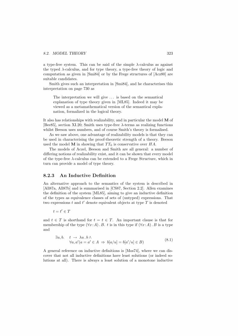
8.2. MODEL THEORY 323
a type-free system. This can be said of the simple λ-calculus as againstthe typed λ-calculus, and for type theory, a type-free theory of logic andcomputation as given in [Smi84] or by the Frege structures of [Acz80] aresuitable candidates.
Smith gives such an interpretation in [Smi84], and he characterises thisinterpretation on page 730 as
The interpretation we will give . . . is based on the semanticalexplanation of type theory given in [ML85]. Indeed it may beviewed as a metamathematical version of the semantical expla-nation, formalized in the logical theory.
It also has relationships with realizability, and in particular the model M of[Bee85], section XI.20; Smith uses type-free λ-terms as realizing functionswhilst Beeson uses numbers, and of course Smith’s theory is formalised.
As we saw above, one advantage of realizability models is that they canbe used in characterising the proof-theoretic strength of a theory. Beesonused the model M in showing that TT0 is conservative over HA.
The models of Aczel, Beeson and Smith are all general: a number ofdiffering notions of realizability exist, and it can be shown that every modelof the type-free λ-calculus can be extended to a Frege Structure, which inturn can provide a model of type theory.
8.2.3 An Inductive Definition
An alternative approach to the semantics of the system is described in[All87a, All87b] and is summarised in [CS87, Section 2.2]. Allen examinesthe definition of the system [ML85], aiming to give an inductive definitionof the types as equivalence classes of sets of (untyped) expressions. Thattwo expressions t and t′ denote equivalent objects at type T is denoted
t = t′ ∈ T
and t ∈ T is shorthand for t = t ∈ T . An important clause is that formembership of the type (∀x :A) . B. t is in this type if (∀x :A) . B is a typeand
∃u, b. t → λu . b ∧∀a, a′(a = a′ ∈ A ⇒ b[a/u] = b[a′/u] ∈ B) (8.1)
A general reference on inductive definitions is [Mos74], where we can dis-cover that not all inductive definitions have least solutions (or indeed so-lutions at all). There is always a least solution of a monotone inductive
324 CHAPTER 8. FOUNDATIONS
definition, and a sufficient condition for monotonicity is for the definingformula (8.1) to be positive in the relation
. . . = . . . ∈ . . .
This is not the case, as the relation appears in the hypothesis of an impli-cation. This failure means that the definition cannot be given simply as aninductive definition in this form.
Instead, Allen defines his system in a more complicated way, specifyinga definition of an operator M, which can be thought of as a monotoneoperator on type theories. In turn, a type theory is seen as a two placerelation T where
T A∼A
holds if and only if A is a type, carrying the equality relation ∼A in the typetheory T . Since the operatorM is monotone, a semantics is then given bythe least fixed point of the operator.
In both [All87a] and [All87b] it is argued that this approach is close tothat of Beeson, with Allen’s more faithful to the lazy evaluation in Martin-Lof’s informal semantics of the system.
An advantage of an inductive definition is that it can readily be extendedto augmented systems. In [CS87] it is shown how to extend the semantics tothe partial types of that paper. Allen himself argues that it can be used injustification of some of the ‘direct computation rules’ of Nuprl, which allowthe reduction of terms under fewer hypotheses than would be permitted inTT .
8.3 A General Framework for Logics
Our introduction to the theories TT0 and TT has been somewhat infor-mal as far as syntax is concerned, and in this section we review how thepresentation can be formalised.
The operations which form types and elements have a definite metathe-oretical type. For example, ⇒ is of meta-type
Type→ Type→ Type
where we write ‘→’ for the function space constructor at the meta-level, andType is the meta-type of types. Similarly, the injection inl can be giventhe meta-type
(Πt :Type).(Πs :Type).( El(s)→ El(s ∨ t) )
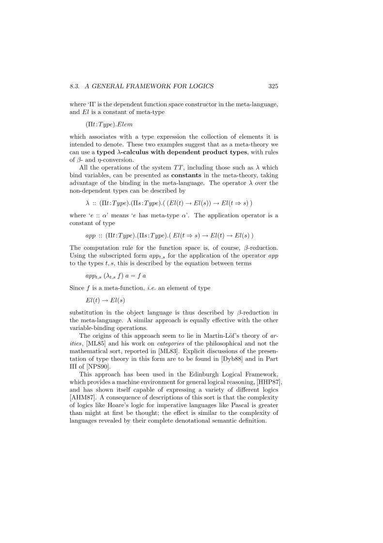
8.3. A GENERAL FRAMEWORK FOR LOGICS 325
where ‘Π’ is the dependent function space constructor in the meta-language,and El is a constant of meta-type
(Πt :Type).Elem
which associates with a type expression the collection of elements it isintended to denote. These two examples suggest that as a meta-theory wecan use a typed λ-calculus with dependent product types, with rulesof β- and η-conversion.
All the operations of the system TT , including those such as λ whichbind variables, can be presented as constants in the meta-theory, takingadvantage of the binding in the meta-language. The operator λ over thenon-dependent types can be described by
λ :: (Πt :Type).(Πs :Type).( (El(t)→ El(s))→ El(t⇒ s) )
where ‘e :: α’ means ‘e has meta-type α’. The application operator is aconstant of type
app :: (Πt :Type).(Πs :Type).( El(t⇒ s)→ El(t)→ El(s) )
The computation rule for the function space is, of course, β-reduction.Using the subscripted form appt,s for the application of the operator appto the types t, s, this is described by the equation between terms
appt,s (λt,s f) a = f a
Since f is a meta-function, i.e. an element of type
El(t)→ El(s)
substitution in the object language is thus described by β-reduction inthe meta-language. A similar approach is equally effective with the othervariable-binding operations.
The origins of this approach seem to lie in Martin-Lof’s theory of ar-ities, [ML85] and his work on categories of the philosophical and not themathematical sort, reported in [ML83]. Explicit discussions of the presen-tation of type theory in this form are to be found in [Dyb88] and in PartIII of [NPS90].
This approach has been used in the Edinburgh Logical Framework,which provides a machine environment for general logical reasoning, [HHP87],and has shown itself capable of expressing a variety of different logics[AHM87]. A consequence of descriptions of this sort is that the complexityof logics like Hoare’s logic for imperative languages like Pascal is greaterthan might at first be thought; the effect is similar to the complexity oflanguages revealed by their complete denotational semantic definition.
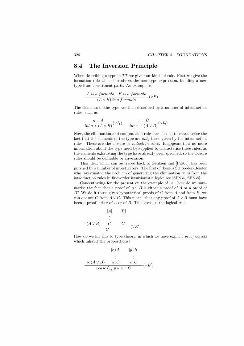
326 CHAPTER 8. FOUNDATIONS
8.4 The Inversion Principle
When describing a type in TT we give four kinds of rule. First we give theformation rule which introduces the new type expression, building a newtype from constituent parts. An example is
A is a formula B is a formula
(A ∨B) is a formula(∨F )
The elements of the type are then described by a number of introductionrules, such as
q : A
inl q : (A ∨B)(∨I1)
r : B
inr r : (A ∨B)(∨I2)
Now, the elimination and computation rules are needed to characterise thefact that the elements of the type are only those given by the introductionrules. These are the closure or induction rules. It appears that no moreinformation about the type need be supplied to characterise these rules, asthe elements exhausting the type have already been specified, so the closurerules should be definable by inversion.
This idea, which can be traced back to Gentzen and [Pra65], has beenpursued by a number of investigators. The first of these is Schroeder-Heisterwho investigated the problem of generating the elimination rules from theintroduction rules in first-order intuitionistic logic; see [SH83a, SH83b].
Concentrating for the present on the example of ‘∨’, how do we sum-marise the fact that a proof of A ∨ B is either a proof of A or a proof ofB? We do it thus: given hypothetical proofs of C from A and from B, wecan deduce C from A ∨B. This means that any proof of A ∨B must havebeen a proof either of A or of B. This gives us the logical rule
(A ∨B)
[A]...C
[B]...C
C(∨E′)
How do we lift this to type theory, in which we have explicit proof objectswhich inhabit the propositions?
p : (A ∨B)
[x :A]...
u :C
[y :B]...
v :Cvcases′x,y p u v : C
(∨E′)
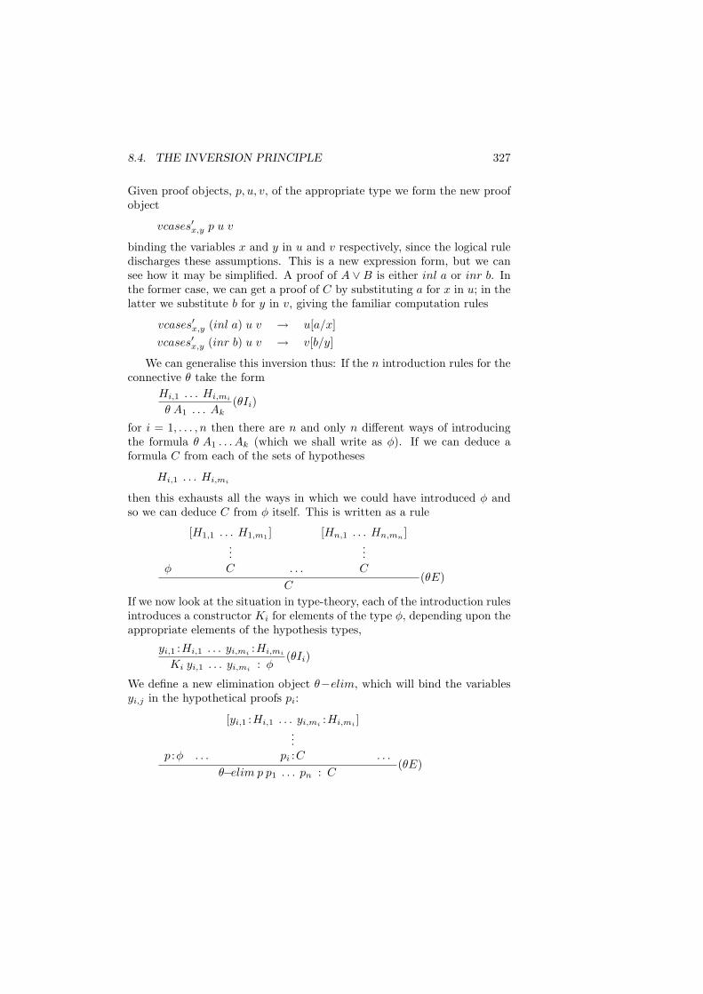
8.4. THE INVERSION PRINCIPLE 327
Given proof objects, p, u, v, of the appropriate type we form the new proofobject
vcases′x,y p u v
binding the variables x and y in u and v respectively, since the logical ruledischarges these assumptions. This is a new expression form, but we cansee how it may be simplified. A proof of A ∨ B is either inl a or inr b. Inthe former case, we can get a proof of C by substituting a for x in u; in thelatter we substitute b for y in v, giving the familiar computation rules
vcases′x,y (inl a) u v → u[a/x]vcases′x,y (inr b) u v → v[b/y]
We can generalise this inversion thus: If the n introduction rules for theconnective θ take the form
Hi,1 . . . Hi,mi
θ A1 . . . Ak(θIi)
for i = 1, . . . , n then there are n and only n different ways of introducingthe formula θ A1 . . . Ak (which we shall write as φ). If we can deduce aformula C from each of the sets of hypotheses
Hi,1 . . . Hi,mi
then this exhausts all the ways in which we could have introduced φ andso we can deduce C from φ itself. This is written as a rule
φ
[H1,1 . . . H1,m1 ]...C . . .
[Hn,1 . . . Hn,mn]
...C
C(θE)
If we now look at the situation in type-theory, each of the introduction rulesintroduces a constructor Ki for elements of the type φ, depending upon theappropriate elements of the hypothesis types,
yi,1 :Hi,1 . . . yi,mi:Hi,mi
Ki yi,1 . . . yi,mi : φ(θIi)
We define a new elimination object θ−elim, which will bind the variablesyi,j in the hypothetical proofs pi:
p :φ . . .
[yi,1 :Hi,1 . . . yi,mi:Hi,mi
]...
pi :C . . .
θ−elim p p1 . . . pn : C(θE)
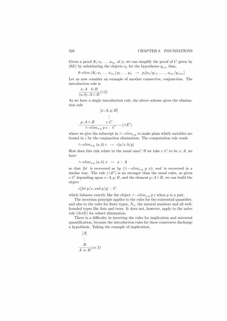
328 CHAPTER 8. FOUNDATIONS
Given a proof Ki a1 . . . amiof φ, we can simplify the proof of C given by
(θE) by substituting the objects aj for the hypotheses yi,j , thus,
θ−elim (Ki a1 . . . ami) p1 . . . pn → pi[a1/yi,1 , . . . , ami/yi,mi ]
Let us now consider an example of another connective, conjunction. Theintroduction rule is
a :A b :B(a, b) :A ∧B
(∧I)
As we have a single introduction rule, the above scheme gives the elimina-tion rule
p :A ∧B
[x :A, y :B]...
c :C∧−elimx,y p c : C
(∧E′)
where we give the subscript in ∧−elimx,y to make plain which variables arebound in c by the conjunction elimination. The computation rule reads
∧−elimx,y (a, b) c → c[a/x, b/y]
How does this rule relate to the usual ones? If we take c :C to be x :A, wehave
∧−elimx,y (a, b) x → a : A
so that fst is recovered as λp . (∧−elimx,y p x); snd is recovered in asimilar way. The rule (∧E′) is no stronger than the usual rules, as givenc :C depending upon x :A, y :B, and the element p :A∧B, we can build theobject
c[fst p/x, snd p/y] : C
which behaves exactly like the object ∧−elimx,y p c when p is a pair.The inversion principle applies to the rules for the existential quantifier,
and also to the rules for finite types, Nn, the natural numbers and all well-founded types like lists and trees. It does not, however, apply to the naıverule (SetE) for subset elimination.
There is a difficulty in inverting the rules for implication and universalquantification, because the introduction rules for these constructs dischargea hypothesis. Taking the example of implication,
[A]...B
A⇒ B(⇒ I)
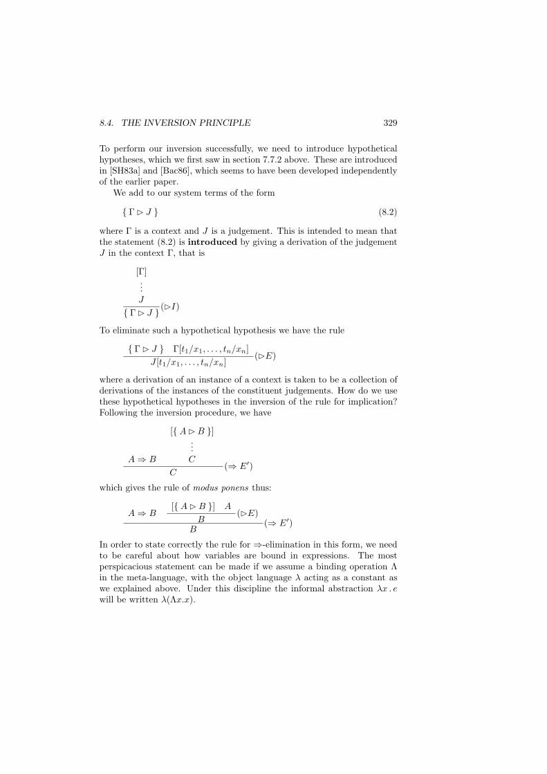
8.4. THE INVERSION PRINCIPLE 329
To perform our inversion successfully, we need to introduce hypotheticalhypotheses, which we first saw in section 7.7.2 above. These are introducedin [SH83a] and [Bac86], which seems to have been developed independentlyof the earlier paper.
We add to our system terms of the form
Γ J (8.2)
where Γ is a context and J is a judgement. This is intended to mean thatthe statement (8.2) is introduced by giving a derivation of the judgementJ in the context Γ, that is
[Γ]...J
Γ J (I)
To eliminate such a hypothetical hypothesis we have the rule
Γ J Γ[t1/x1, . . . , tn/xn]J [t1/x1, . . . , tn/xn]
(E)
where a derivation of an instance of a context is taken to be a collection ofderivations of the instances of the constituent judgements. How do we usethese hypothetical hypotheses in the inversion of the rule for implication?Following the inversion procedure, we have
A⇒ B
[A B ]...C
C(⇒ E′)
which gives the rule of modus ponens thus:
A⇒ B[A B ] A
B(E)
B(⇒ E′)
In order to state correctly the rule for ⇒-elimination in this form, we needto be careful about how variables are bound in expressions. The mostperspicacious statement can be made if we assume a binding operation Λin the meta-language, with the object language λ acting as a constant aswe explained above. Under this discipline the informal abstraction λx . ewill be written λ(Λx.x).
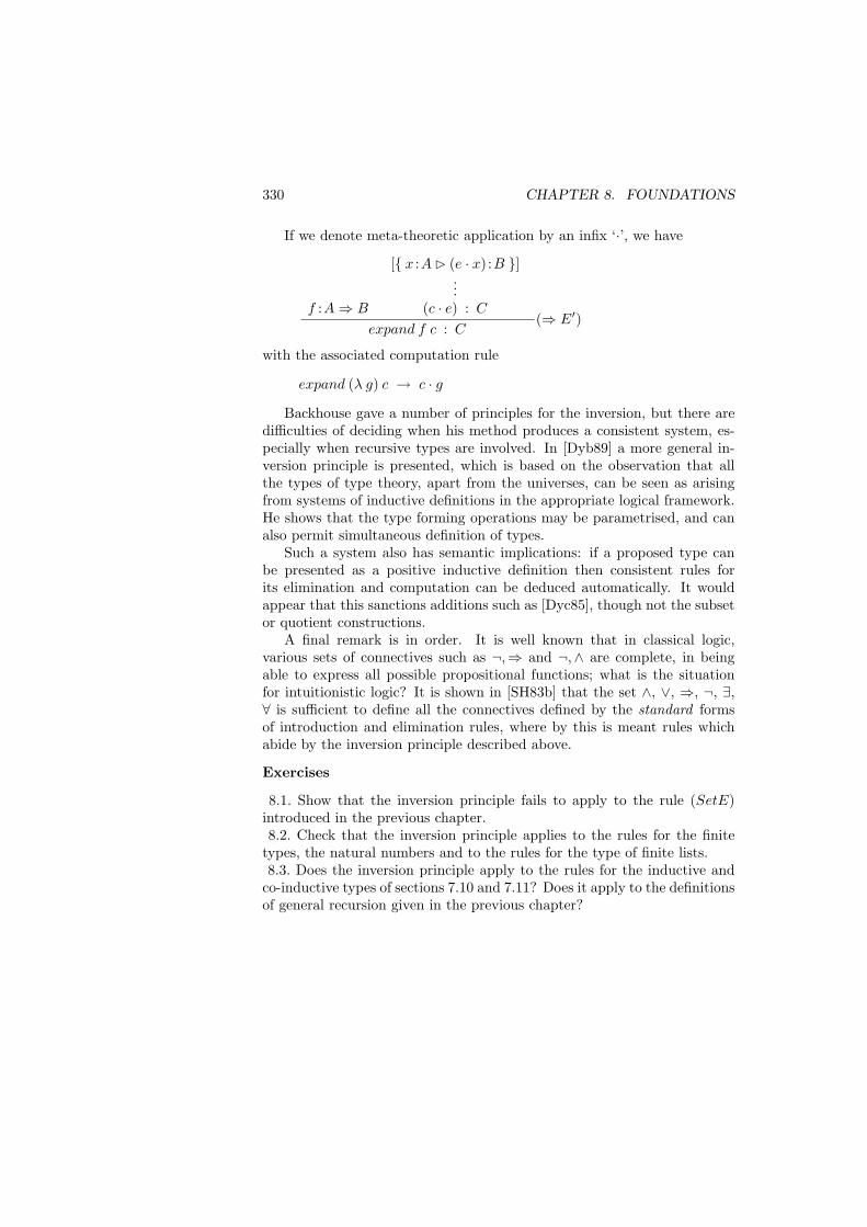
330 CHAPTER 8. FOUNDATIONS
If we denote meta-theoretic application by an infix ‘·’, we have
f :A⇒ B
[ x :A (e · x) :B ]...
(c · e) : C
expand f c : C(⇒ E′)
with the associated computation rule
expand (λ g) c → c · g
Backhouse gave a number of principles for the inversion, but there aredifficulties of deciding when his method produces a consistent system, es-pecially when recursive types are involved. In [Dyb89] a more general in-version principle is presented, which is based on the observation that allthe types of type theory, apart from the universes, can be seen as arisingfrom systems of inductive definitions in the appropriate logical framework.He shows that the type forming operations may be parametrised, and canalso permit simultaneous definition of types.
Such a system also has semantic implications: if a proposed type canbe presented as a positive inductive definition then consistent rules forits elimination and computation can be deduced automatically. It wouldappear that this sanctions additions such as [Dyc85], though not the subsetor quotient constructions.
A final remark is in order. It is well known that in classical logic,various sets of connectives such as ¬,⇒ and ¬,∧ are complete, in beingable to express all possible propositional functions; what is the situationfor intuitionistic logic? It is shown in [SH83b] that the set ∧, ∨, ⇒, ¬, ∃,∀ is sufficient to define all the connectives defined by the standard formsof introduction and elimination rules, where by this is meant rules whichabide by the inversion principle described above.
Exercises
8.1. Show that the inversion principle fails to apply to the rule (SetE)introduced in the previous chapter.8.2. Check that the inversion principle applies to the rules for the finite
types, the natural numbers and to the rules for the type of finite lists.8.3. Does the inversion principle apply to the rules for the inductive and
co-inductive types of sections 7.10 and 7.11? Does it apply to the definitionsof general recursion given in the previous chapter?
Chapter 9
Conclusions
This chapter gives a survey of a number of approaches related to some de-gree to constructive type theory; we have tried to stress the major points ofdifference between these systems and type theory itself, but to do completejustice to them would require another book of this size.
9.1 Related Work
This section examines various systems, implemented or theoretical, whichare related to Martin-Lof’s Type Theory. Rather than give exhaustivedescriptions, the chapter contains brief introductions to the systems, bib-liographic references and finally a discussion of points of similarity anddifference between the systems. Throughout our exposition we have con-centrated on the intensional version of type theory, [ML75b]; we have dis-cussed differences between this and the extensional version as we have gonealong.
9.1.1 The Nurpl System
For the past fifteen years there has been an active research group in theComputer Science Department of Cornell, lead by Constable and Bates, in-terested in the implementation of logics. In particular interest has focussedupon logics for the formalisation of mathematics and program development,and this research has culminated in the development of the Nuprl system,described in the book [C+86a]. Nuprl consists of an implementation of atype theory related to the extensional version of TT , [ML85], but modifiedand augmented in a number of ways, which we discuss presently. Con-
331
332 CHAPTER 9. CONCLUSIONS
stable’s book provides the comprehensive reference on the system, shorteraccounts of the underlying ideas can be found in [BC85, CKB84].
More importantly, the orientation of the system is different from ourtreatment of type theory in this book, which we have viewed principallyas a functional programming system. The emphasis of Nuprl is logical,in that it is designed to support the top-down construction of derivationsof propositions in a natural deduction system. The proof objects of typetheory are called ‘extract terms’, the idea being that these are extractedpost hoc from derivations in which they appear only implicitly.
Proofs are constructed in a top-down way, using the tactics and tacticalsmuch in the same way as the LCF system, [Pau87]. Indeed the logic isembedded in the ML metalanguage, exactly as LCF.
We mentioned earlier that the system differed somewhat from [ML85].In particular it features the strong elimination rules of section 7.7.2, aswell as the liberal notion of direct computation rules, [C+86a], AppendixC, which allow the rewriting of terms without demanding the usual atten-dant proofs of well-formedness, which are necessitated by the interlinkingof syntax and derivation in type theoretic systems.
It is also augmented in a number of ways, including as it does subsets(see section 7.2), quotient types (section 7.5), partial function types (section7.12) and so forth. It should be said that many of the additional constructsare introduced with the aim of eliminating computationally irrelevant in-formation from the objects extracted, as we discussed in section 7.1.2. Thisis in part due to the implicit nature of the proof objects in many of thederivations.
9.1.2 TK: A theory of types and kinds
The system TK is introduced in the paper [HT88] which contains a usefulcomparison between TT and TK; the topic of program development in TKis discussed in [Hen89]. TK is a theory of constructive sets ‘designed withprogram development as the major desideratum’.
The principle of complete presentation together with the identificationof types and propositions are central to type theory as we have introducedit here, and Henson and Turner argue that they leads to a number of itsshortcomings, including the unsatisfactory treatment of subsets and generalrecursion. They propose instead that the system TK should separate thetwo, with a simpler collection of types (or sets) and a separate collectionof logical assertions. The principal set formation operations are separationand induction. Separation allows definitions like
x|Φ(x)
9.1. RELATED WORK 333
which contains precisely those x which have the property Φ. Inductiveconstructions are performed along lines similar to section 7.10 above. Toincrease expressibility, a hierarchy of universes or kinds are also added tothe set theory – hence the name TK.
Another difference betweem TK and TT is that terms in the formertheory can be partial or undefined, whereas in TT they are, of course,total. The merits of the two approaches can be argued; note that since thelogic and the types are no longer identified the presence of partial objectsdoes not make the logic inconsistent.
Reasoning about the sets is performed in a rich logical language, andsince the logic is constructive, there are realisability models for it. Usingthe techniques outlined in section 8.1.2 programs can be extracted fromconstructive proofs, and it is this technique for program development whichthe authors stress, especially in [Hen89]. The realizability approach allowsa lot of flexibility in the choice of realizing operations: for example, aconditional assertion can be added to the language and its realizers can bemade quite distinct from those of its usual logical definition, for example.
Another advantage of the realizability approach is that computationallyirrelevant parts of functions need not appear, a topic we discussed earlierand which is examined in [Hen91].
On the other hand, we have seen that in TT both the options of programextraction and explicit functional programming are available and can becombined within a single development – whether they can be combined sowell in TK is not clear.
Work on the theoretical foundations of TK and on an implementationboth proceed, and it seems certain that our understanding of TT will beenriched by these. It remains to be seen which, if either, of the two systemsis the superior for practical program development purposes.
9.1.3 PX: A Computational Logic
It is not only from a type theory that proofs can be extracted; realizabilitymodels of intuitionistic formal systems allow the extraction of computationsfrom the system. A markedly different system, called PX, has been built atthe Research Institute of Mathematical Sciences at Kyoto University, andis introduced in [Hay90] and described in detail in the monograph [HN88].
PX is a logic for a type-free theory of computations, based on Fefer-man’s T0, [Fef79], from which LISP programs are extracted by a notion ofrealizability called px-realizability. Hayashi argues the requirement that atheory like TT be total is too restrictive for practical program development,in justification of his logic being based around a system of possibly non-terminating computations. Because of this possibility he incorporates two
334 CHAPTER 9. CONCLUSIONS
sorts of variable in the system, one kind ranging over terminating objects,the other over all objects, together with a definedness predicate, E, muchas in [Sco79].
Crucial to the logic is the principle of CIG (for Conditional InductiveGeneration). This is the means by which sub-classes of the domain aredefined, by which recursions proceed and by which inductive proofs, in-cluding proofs of termination over a domain, are given. In this respect itis analogous to the recursive definitions given by well-founded recursion insection 7.9, as well as the inductive types of section 7.10.
Hayashi defines a subset of the language consisting of the formulas whichcontain no ∨ or ∃ and which are said to be of Rank 0 . No realising termsare needed for rank zero formulas, as they have no computational content.An example of a formula of rank zero is the inclusion A ⊆ B; an instance ofsuch a formula might be an assertion of termination: the set A is containedin the domain of definition, B, of the function f . It is shown that suchformulas can be proved using classical logic without risking the consistencyor computational interpretation of the system, manifesting the flexibilitywe discussed in the previous section.
9.1.4 AUTOMATH
The AUTOMATH project was begun at Eindhoven University under thedirection of Nicolaas de Bruijn in 1966, with the aim
to develop a system of writing entire mathematical theories insuch a precise fashion that verification of the correctness can becarried out by formal operations on the text.
The quotation comes from [dB80] which gives a survey of the project; exam-ples of the style of presentation of mathematics in the system can be foundin [dB73]. A pinnacle in the achievements of the group is the completeformalization of Landau’s Grundlagen, a text on analysis.
The system itself uses a form of type theory, based on the notion ofpropositions as types, to represent logics of either classical or constructivemathematics. Amongst its technical innovations are a discussion of theirrelevance of proofs when working in a classical context, which is oneof the reasons advanced by de Bruijn for the separation between the no-tions of type and prop in the system, an idea anticipating by some yearsdiscussions in the computing science community, reported in section 7.1.2.
In the course of implementing the system, the problem of identifyingλ-expressions which agree up to a change of bound variable names (α-conversion) was found to be a considerable overhead. [dB72] introducesa most useful method of circumventing the problem. Variable names are
9.1. RELATED WORK 335
replaced by numerical indexes; an occurrence of a variable x is replaced bythe number of λ’s which lie between the occurrence and the λx binding it,so that for example the λ expression
λa . λb . λc . (ac)(bc)
is replaced by
λ.λ.λ.(20)(10)
This technique has found application in the implementation of functionalprogramming languages as well as logics, see [Hue90a], Part I.
9.1.5 Type Theories
The systems TT0 and TT can be seen as extensions of the simply typed λ-calculus, as explored in chapter 2. Other extensions exist, and we examinethe two most important here. The first is the second-order or polymorphicλ-calculus, invented independently by [Rey74] and [Gir72], the latter callingthe calculus System F. A short yet comprehensive introduction is providedby [Rey90].
The calculus extends the first-order lambda calculus by allowing typevariables α, β, . . . so that a function like
K ≡df λx . λy . x
can be given the type α ⇒ β ⇒ α, just as is possible in polymorphic lan-guages like SML and Miranda. The variables in the expression above can bethought of as being implicitly universally quantified, the function K havingthe type α⇒ β ⇒ α for all instances of α and β. This implicit quantifica-tion is made explicit in the second-order λ-calculus with the introductionof the type abstraction operator Λ and the type forming Π. Given
Kα,β ≡df λxα . λyβ . x : α⇒ β ⇒ α
we can form
K ≡df Λα. Λβ. λxα . λyβ . x : Πα. Πβ. (α⇒ β ⇒ α)
In general, if
e : t
then the expression Λα. e is parametrised over the type variable α, givingit the type Πα. t. Type abstractions are applied just as ordinary ones, and
(Λα. e) ξ : t[ξ/α]
336 CHAPTER 9. CONCLUSIONS
where ξ is an arbitrary type expression. The system is stronger than theMilner type system, as types can contain embedded universal quantifiers,such as
(Πα.(α⇒ α))⇒ (Πα.(α⇒ α))
but here lies a twist: this type is in the domain of the Πα . . . quantification,so that there is a circularity in the definition of the type. Contrast this withthe TT type
((∀α :U0) . (α⇒ α))⇒ ((∀α :U0) . (α⇒ α))
whose definition is not circular — the type lies in U1 and not U0 and so isoutside the range of the quantifier (∀α :U0) . . . ..
We are used to circularities in definitions of recursive functions andtypes, so we should not abandon hope about the system. Indeed, it canshown consistent and strongly normalizing, having the proof theoretic strengthof second-order arithmetic, thus making it more expressive than TT0. Theseresults can be found in [GLT89], and a number of papers on the semanticsof the second-order λ-calculus can be found in [Hue90a], Part II.
The Curry Howard isomorphism extends to this situation, with quan-tification over types having the equivalent of quantifying over all propo-sitions. This has the interesting corollary that we can define many of thepropositional connectives from Π. For instance, recalling the simple rulefor disjunction elimination, we have
(A ∨B) (A⇒ C) (B ⇒ C)C
(∨E)
From A∨B we can infer (A⇒ C)⇒ (B ⇒ C)⇒ C for all propositions C,so that in the terminology of the second-order λ-calculus, we have
ΠC. ( (A⇒ C)⇒ (B ⇒ C)⇒ C )
Given an element a :A we can form an object of this type,
ΛC. λf . λg . (f a)
and of course we can do the same with b : B. Are all elements of thetype of this form? This question revolves around quite subtle issues in thesemantics of the calculus, discussed in [Hue90a], Part II.
The second-order calculus provides no means of defining the type trans-formation
A,B 7→ ΠC. ( (A⇒ C)⇒ (B ⇒ C)⇒ C )
9.2. CONCLUDING REMARKS 337
as an operation of the calculus itself. This extension of the system is pro-vided by the Calculus of Constructions of Coquand and Huet, to whichwe turn now. The system was introduced in [CH85], and is discussed in thecontext of other type theories in [Hue90b], and it allows direct definitionof such operators. One means of so doing is the addition of a new typeProp of propositions, but we have seen earlier that this leads to logicalinconsistency, [Gir72]. Without allowing this, the theory of constructionsallows the definition of these type operators, and thus a large portion ofmathematics is developed in a very simple foundational theory. One pointto note is the apparent undefinability of a strong existential type in thelanguage, the definition which embodies the equivalence between
(∀x :A) . ( C(x)⇒ B ) and ( (∃x :A) . C(x) )⇒ B
(when x is not free in B) defines a weak equality. The difficulty is the wayin which the proof objects and types are mingled in the elimination rule forthe strong existential type.
A realizability semantics for the Calculus of Constructions is discussedin [Hue90a], Part III.
9.2 Concluding Remarks
It can be seen from the contents of the last two chapters that research intotype theory is still in flux; despite this, the core of the system has beenshown to be a sound and elegant combination of logic and functional pro-gramming, and I hope that the reader can share my enthusiasm for thesubject. One of the keenest intellectual pleasures is to see connections inthe hitherto unconnected, and I can still remember the thrill on discoveringthat the proof of the deduction theorem for a Hilbert-style logic, learnedas a beginning graduate student in logic, is exactly the same as the bracketabstraction algorithm in the λ-calculus, a result used in the implementa-tion of functional programming languages, and which I came upon in acomputing context, years later.
Reflecting on the material in chapter 7, one negative conclusion seemsinescapable: additions to the system are quite possible, but each of themseems to extract a price, either by increasing the complexity of the sys-tem or by changing some of its metamathematical properties. We shouldtherefore be quite certain that we need to add a feature before doing so.This conclusion is obvious to anyone familiar with the majority of program-ming languages, in which a jumble of features co-exist in a most precariousfashion; perhaps it is something we have to learn for ourselves.
338 CHAPTER 9. CONCLUSIONS
Nonetheless, the plight of imperative programming seems to get evermore hopeless. Although it is in theory quite possible to develop proofs forprograms written in Pascal and C, it simply doesn’t happen. Functionallanguages offer a much brighter prospect, as their clean semantics makesproofs shorter and higher level. The next step seems to be to move to asystem like type theory, which can provide a single foundation for activitiesof program development, transformation and verification, just as a LISPMachine supports integrated debugging, profiling and the like. There isstill much to be done in making type theory a usable and attractive systemwhich supports programming in the large, but I am certain that languagesbased on type theory will be as popular in a few years years time as con-temporary functional languages like Miranda and ML based on the simplytyped λ-calculus.
Bibliography
[Abr90] Samson Abramsky. The lazy lambda calculus. In David A.Turner, editor, Research Topics in Functional Programming.Addison Wesley, 1990.
[Acz80] Peter Aczel. Frege structures and the notions of proposition,truth and set. In The Kleene Symposium. North-Holland, 1980.
[AHM87] Arnon Avron, Furio A. Honsell, and Ian A. Mason. Using typedlambda calculus to implement formal systems on a machine.Technical Report ECS-LFCS-87-31, LFCS, Department of Com-puter Science, University of Edinburgh, 1987.
[All87a] Stuart Allen. A non-type-theoretic definition of Martin-Lof’stypes. In Proceedings of the Second Annual Symposium on Logicin Computer Science. IEEE, 1987.
[All87b] Stuart Allen. A Non-Type-Theoretic Semantics for Type-Theoretic Language. PhD thesis, Cornell University, 1987.Available as technical report TR 87-866 from the Departmentof Computer Science, Cornell University.
[And65] Peter Bruce Andrews. A transfinite type theory with type vari-ables. Studies in logic and the foundations of mathematics.North-Holland, 1965.
[Bac86] Roland Backhouse. On the meaning and construction of therules in Martin-Lof’s theory of types. Technical Report CS 8606,Department of Mathematics and Computing Science, Universityof Groningen, 1986.
[Bac87a] Roland Backhouse. Notes on Martin–Lof’s theory of types.FACS FACTS, 9(3), October 1987. Newsletter of the BCS For-mal Aspects of Computing Science Special Interest Group.
339
340 BIBLIOGRAPHY
[Bac87b] Roland Backhouse. Overcoming the mismatch between pro-grams and proofs. In Peter Dybjer et al., editors, Proceedingsof the Workshop on Programming Logic. Programming Method-ology Group, University of Goteborg and Chalmers Universityof Technology, 1987. Technical Report, number 37.
[Bar84] Henk P. Barendregt. The lambda calculus — its syntax andsemantics, volume 103 of Studies in Logic and Foundations ofMathematics. North-Holland, 1984.
[BB85] Errett Bishop and Douglas Bridges. Constructive Mathe-matics, volume 279 of Grundlehren der Mathematischen Wis-senschaften. Springer-Verlag, 1985.
[BC85] Joseph L. Bates and Robert L. Constable. Proofs as programs.ACM Transactions on Programming Languages and Systems, 7,1985.
[BCMS89] Roland Backhouse, Paul Chisholm, Grant Malcolm, and ErikSaaman. Do-it-yourself type theory. Formal Aspects of Com-puting, 1, 1989.
[BdV89] David A. Basin and Peter del Vecchio. Verification of computa-tional logic in Nuprl. Technical Report TR 89-1018, Departmentof Computer Science, Cornell University, 1989.
[Bee85] Michael J. Beeson. Foundations of Constructive Mathematics.Springer-Verlag, 1985.
[Ben86] Jon Bentley. Programming Pearls. Addison Wesley, 1986.
[BMS80] Rod M. Burstall, David B. MacQueen, and Donald T. Sanella.HOPE: An experimental applicative language. Technical re-port, Department of Computer Science, University of Edin-burgh, 1980.
[BW88] Richard Bird and Philip Wadler. An Introduction to FunctionalProgramming. Prentice-Hall, 1988.
[C+86a] Robert L. Constable et al. Implementing Mathematics with theNuprl Proof Development System. Prentice-Hall Inc., 1986.
[C+86b] Robert L. Constable et al. Implementing Mathematics with theNuprl proof development system. Prentice-Hall, 1986.
BIBLIOGRAPHY 341
[CF58] Haskell B. Curry and Robert Feys. Combinatory Logic, vol-ume I. North-Holland, 1958.
[CH85] Thierry Coquand and Gerard Huet. A theory of constructions.In Semantics of Data Types. Springer-Verlag, 1985.
[Chi87] Paul Chisholm. Derivation of a parsing algorithm in Martin–Lof’s theory of types. Science of Computer Programming, 8,1987.
[Chi88a] Paul Chisholm. On the relationship between the subset andsigma types in Martin- Lof’s 1979 type theory. Technical ReportCS 8802, Department of Mathematics and Computing Science,University of Groningen, 1988.
[Chi88b] Paul Chisholm. Reducing the proof burden when reasoning withcongruence types. Technical Report CS 8807, Department ofMathematics and Computing Science, University of Groningen,1988.
[CKB84] Robert L. Constable, Todd Knoblock, and Joseph L. Bates.Writing programs that construct proofs. Journal of AutomatedReasoning, 1, 1984.
[CM82] Avra Cohn and Robin Milner. On using Edinburgh LCF toprove the correctness of a parsing algorithm. Technical ReportCSR-113-82, Computer Science Department, Edinburgh Uni-versity, 1982.
[Coq86] Thierry Coquand. An analysis of Girard’s paradox. In Pro-ceedings of the First Annual Symposium on Logic in ComputerScience. IEEE, 1986.
[CS87] Robert L. Constable and Scott Fraser Smith. Partial objects inconstructive type theory. In Proceedings of the Second AnnualSymposium on Logic in Computer Science. IEEE, 1987.
[Cut81] Nigel J. Cutland. Computability. Cambridge University Press,1981.
[CW85] Luca Cardelli and Peter Wegner. On understanding types, dataabstraction and polymorphism. Computing Surveys, 17, 1985.
[dB72] Nicolaas G. de Bruijn. Lambda calculus notation with namelessdummies, a tool for automatic formula manipulation, with anapplication to the Church Rosser theorem. Indag. Math., 34,1972.
342 BIBLIOGRAPHY
[dB73] Nicolaas G. de Bruijn. AUTOMATH, a language for mathemat-ics. Technical report, Les Presses de l’Universite de Montreal,1973.
[dB80] Nicolaas G. de Bruijn. A survey of the project AUTOMATH.In Jonathan P. Seldin and J. Roger Hindley, editors, To H.B. Curry: Essays on combinatory logic, lambda calculus andformalism. Academic Press, 1980.
[Dij76] Edsger W. Dijkstra. A Discipline of Programming. PrenticeHall International, 1976.
[Dil80] Justus Diller. Modified realization and the formulae-as-typesnotion. In Jonathan P. Seldin and J. Roger Hindley, editors, ToH. B. Curry: Essays on combinatory logic, lambda calculus andformalism. Academic Press, 1980. A reprint of an unpublishedmanuscript from 1969.
[DT84] Justus Diller and Anne S. Troelstra. Realizability and intuition-istic logic. Synthese, 60, 1984.
[Dum77] Michael Dummett. Elements of Intuitionism. Oxford UniversityPress, 1977.
[Dyb87] Peter Dybjer. From type theory to LCF — a case study in pro-gram verification (draft). In Peter Dybjer et al., editors, Pro-ceedings of the Workshop on Programming Logic. ProgrammingMethodology Group, University of Goteborg and Chalmers Uni-versity of Technology, 1987. Technical Report, number 37.
[Dyb88] Peter Dybjer. Inductively defined sets in Martin-Lof’s type the-ory. In Proceedings of the Workshop on General Logic, Edin-burgh, February 1897, 1988. Report ECS-LFCS-88-52, Labora-tory for the Foundations of Computer Science, Edinburgh Uni-versity.
[Dyb89] Peter Dybjer. An inversion principle for Martin-Lof’s type the-ory. In Peter Dybjer et al., editors, Proceedings of the Work-shop on Programming Logic. Programming Methodology Group,University of Goteborg and Chalmers University of Technology,1989. Technical Report, number 54.
[Dyc85] Roy Dyckhoff. Category theory as an extension of Martin–Loftype theory. Technical Report CS/85/3, Department of Com-putational Science, University of St Andrews, 1985.
BIBLIOGRAPHY 343
[Dyc87] Roy Dyckhoff. Strong elimination rules in type theory. In PeterDybjer et al., editors, Proceedings of the Workshop on Program-ming Logic. Programming Methodology Group, University ofGoteborg and Chalmers University of Technology, 1987. Tech-nical Report, number 37.
[End77] Herbert B. Enderton. Elements of Set Theory. Academic Press,1977.
[Fef79] Solomon Feferman. Constructive theories of functions andclasses. In M. Boffa, D. van Dalen, and K. MacAloon, editors,Logic Colloquium ’78. North Holland, 1979.
[FLO83] Steven Fortune, Daniel Leviant, and Michael O’Donnell. Theexpressiveness of simple and second-order type structures. Jour-nal of the ACM, 30(1):151–185, 1983.
[G58] Kurt Godel. Uber eine bisher noch nicht benutze Erweiterungdes finiten Standpunktes. Dialectica, 12, 1958.
[Gir72] Jean-Yves Girard. Interpretation fonctionelle et elimination descoupures dans l’arithmetique d’ordre superieure. These d’Etat,Universite Paris VII, 1972.
[Gir80] Jean-Yves Girard. The system F of variable types, fifteen yearslater. Theoretical Computer Science, 45, 1980.
[GLT89] Jean-Yves Girard, Yves Lafont, and Paul Taylor. Proofs andTypes, volume 7 of Cambridge Tracts in Theoretical ComputerScience. Cambridge University Press, 1989.
[Har60] Ronald Harrop. Concerning formulas of the types A → B ∨C, A → (∃x)B(x) in intuitionistic formal systems. Journal ofSymbolic Logic, 25, 1960.
[Har86] Robert Harper. Introduction to Standard ML. Technical Re-port ECS-LFCS-86-14, Laboratory for Foundations of Com-puter Science, Department of Computer Science, University ofEdinburgh, November 1986.
[Hay90] Susumu Hayashi. An introduction to PX. In Gerard Huet, ed-itor, Logical Foundations of Functional Programming. AddisonWesley, 1990.
[Hen89] Martin C. Henson. Program development in the constructiveset theory TK. Formal Aspects of Computing, 1, 1989.
344 BIBLIOGRAPHY
[Hen91] Martin C. Henson. Information loss in the programming logicTK. In Proceedings of the IFIP TC2 Working Conference onProgramming Concepts and Methods. Elsevier, 1991.
[HHP87] Robert Harper, Furio Honsell, and Gordon Plotkin. A frame-work for defining logics. In Proceedings of the Symposium onLogic in Computer Science. IEEE, 1987.
[HN88] Susumu Hayashi and Hiroshi Nakano. PX: A ComputationalLogic. The MIT Press, 1988.
[Hod77] Wilfrid Hodges. Logic. Penguin Books, 1977.
[How80] William A. Howard. The formulae-as-types notion of construc-tion. In Jonathan P. Seldin and J. Roger Hindley, editors, ToH. B. Curry: Essays on combinatory logic, lambda calculus andformalism. Academic Press, 1980. A reprint of an unpublishedmanuscript from 1969.
[How88] Douglas J. Howe. Automating Reasoning in an Implementationof Constructive Type Theory. PhD thesis, Cornell University,1988. Available as technical report TR 88-925 from the Depart-ment of Computer Science, Cornell University.
[HT88] Martin C. Henson and Raymond Turner. A constructive settheory for program development. In Proceedings of the 8th Con-ference on FST and TCS, volume 338 of Lecture Notes in Com-puter Science. Springer Verlag, 1988.
[Hue90a] Gerard Huet, editor. Logical Foundations of Functional Pro-gramming. Addison Wesley, 1990.
[Hue90b] Gerard Huet. A uniform approach to type theory. In GerardHuet, editor, Logical Foundations of Functional Programming.Addison Wesley, 1990.
[Hug83] John Hughes. The Design and Implementation of ProgrammingLanguages. PhD thesis, University of Oxford, 1983.
[Hug90] John Hughes. Why Functional Programming Matters. InDavid A. Turner, editor, Research Topics in Functional Pro-gramming. Addison Wesley, 1990.
[HW90] Paul Hudak and Philip Wadler. Report on the functional pro-gramming language Haskell. Draft proposed standard for thefunctional programming language, designed by the authors andtwelve others., 1990.
BIBLIOGRAPHY 345
[Jac89] Bart Jacobs. The inconsistency of higher order extensions ofMartin–Lof’s type theory. Journal of Philosophical Logic, 18,1989.
[Joh85] Thomas Johnsson. Lambda lifting – transforming programs torecursive equations. In J. P. Jouannaud, editor, Functional Pro-gramming Languages and Computer Architecture, volume 201 ofLecture Notes in Computer Science. Springer-Verlag, 1985.
[KC86] Todd B. Knoblock and Robert L. Constable. Formalized metar-easoning in type theory. Technical Report TR 86-742, Depart-ment of Computer Science, Cornell University, 1986.
[Kle45] Stephen C. Kleene. On the interpretation of intuitionistic num-ber theory. Journal of Symbolic Logic, 10, 1945.
[Lem65] E. J. Lemmon. Beginning Logic. Thomas Nelson and SonsLimited, 1965.
[LS86] J. Lambek and P. J. Scott. Introduction to higher order cate-gorical logic. Cambridge University Press, 1986.
[Mac86] David MacQueen. Using dependent types to express modularstructure. In Proceedings of the 13th ACM Symposium on Prin-ciples of Programming Languages. ACM Press, 1986.
[Mac90] David MacQueen. A higher-order type system for functionalprogramming. In David A. Turner, editor, Research Topicsin Functional Programming. Addison Wesley, 1990. First Pub-lished in The Computer Journal, April 1989.
[MC88] Grant Malcolm and Paul Chisholm. Polymorphism and infor-mation loss in Martin- Lof’s type theory. Technical Report CS8814, Department of Mathematics and Computing Science, Uni-versity of Groningen, 1988.
[Men87a] Elliott Mendelson. Introduction to Mathematical Logic.Wadsworth, third edition, 1987.
[Men87b] Paul Francis Mendler. Inductive Definition in Type Theory.PhD thesis, Cornell University, 1987. Available as technicalreport TR 87-870 from the Department of Computer Science,Cornell University.
[Mil78] Robin Milner. A theory of type polymorphism in programming.Journal of Computer and System Sciences, 17, 1978.
346 BIBLIOGRAPHY
[ML70] Per Martin-Lof. Notes on Constructive Mathematics. Almqvist& Wiksell, Stockholm, 1970.
[ML71] Per Martin-Lof. A theory of types. Technical Report 71-3,Department of Mathematics, University of Stockholm, 1971.
[ML75a] Per Martin-Lof. About models for intuitionistic type theoriesand the notion of definitional equality. In Stig Kanger, edi-tor, Proceedings of the Third Scandinavian Logic Symposium,Studies in Logic and the Foundations of Mathematics. North-Holland, 1975.
[ML75b] Per Martin-Lof. An intuitionistic theory of types: Predicativepart. In H. Rose and J. C. Shepherdson, editors, Logic Collo-quium 1973. North-Holland, 1975.
[ML83] Per Martin-Lof. On the meanings of the logical constants andthe justifications of the logical laws. Notes taken by GiovanniSambin and Aldo Ursini of a short course given at the meet-ing Teoria della Dimostrazione e Filosofia della Logica, Siena,April., 1983.
[ML84] Per Martin-Lof. Intuitionistic Type Theory. Bibliopolis, Naples,1984. Based on a set of notes taken by Giovanni Sambin of aseries of lectures given in Padova, June 1980.
[ML85] Per Martin-Lof. Constructive mathematics and computer pro-gramming. In C. A. R. Hoare, editor, Mathematical Logic andProgramming Languages. Prentice-Hall, 1985.
[Mos74] Yiannis N. Moschovakis. Elementary Induction on AbstractStructures, volume 77 of Studies in Logic and Foundations ofMathematics. North-Holland, 1974.
[MR86] Albert R. Meyer and M. B. Reinhold. Type is not a type. InProceedings of the 13th ACM Symposium on Principles of Pro-gramming Languages. ACM Press, 1986.
[Nor85] Bengt Nordstrom. Multilevel functions in Martin–Lof’s typetheory. In Programs as Data Objects, volume 217 of LectureNotes in Computer Science. Springer-Verlag, 1985.
[Nor88] Bengt Nordstrom. Terminating general recursion. BIT, 28,1988.
BIBLIOGRAPHY 347
[NP83] Bengt Nordstrom and Kent Petersson. Types and specifications.In IFIP’83. Elsevier, 1983.
[NP85] Bengt Nordstrom and Kent Petersson. The semantics of modulespecifications in Martin–Lof’s type theory. Technical Report 36,Programming Methodology Group, University of Goteborg andChalmers University of Technology, 1985.
[NPS90] Bengt Nordstrom, Kent Petersson, and Jan M. Smith. Program-ming in Martin-Lof ’s Type Theory — An Introduction. OxfordUniversity Press, 1990.
[P67] Rosa Peter. Recursive Functions. Academic Press, 1967.
[Pau86] Lawrence C. Paulson. Constructing recursion operators in in-tuitionistic type theory. Journal of Symbolic Computation, 2,1986.
[Pau87] Laurence C. Paulson. Logic and Computation — Interactiveproof with Cambridge LCF. Cambridge University Press, 1987.
[Per89] Nigel Perry. Hope+. Technical report, Department of Comput-ing, Imperial College, London, 1989. Version 6.
[Pey87] Simon Peyton Jones. The Implementation of Functional Pro-gramming Languages. Prentice Hall, 1987.
[PM87] Christine Paulin-Mohring. An example of algorithm develop-ment in the calculus of constructions: Binary search for thecalculation of the lambo function. In Peter Dybjer et al.,editors, Proceedings of the Workshop on Programming Logic.Programming Methodology Group, University of Goteborg andChalmers University of Technology, 1987. Technical Report,number 37.
[PM89] Christine Paulin-Mohring. Extracting Fω’s programs fromproofs in the calculus of constructions. In Proceedings of the 16thACM Symposium on Principles of Programming Languages.ACM Press, 1989.
[Pra65] Dag Prawitz. Natural Deduction — A Proof-Theoretical Study.Almqvist & Wiksell, 1965.
[PS85] Kent Petersson and Jan Smith. Program derivation in type the-ory: The Polish flag problem. In Peter Dybjer et al., editors,Proceedings of the Workshop on Specification and Derivation
348 BIBLIOGRAPHY
of Programs. Programming Methodology Group, University ofGoteborg and Chalmers University of Technology, 1985. Tech-nical Report, number 18.
[PS87] Kent Petersson and Dan Synek. A set constructor for induc-tive sets in Martin–Lof’s type theory. Technical Report 48,Programming Methodology Group, University of Goteborg andChalmers University of Technology, 1987.
[Rea89] Chris Reade. Elements of Functional Programming. AddisonWesley, 1989.
[Rey74] John C. Reynolds. Towards a theory of type structure. InColloque sur la Programmation, volume 19 of Lecture Notes inComputer Science. Springer-Verlag, 1974.
[Rey90] John C. Reynolds. Polymorphic lambda calculus – introduc-tion to part II. In Gerard Huet, editor, Logical Foundations ofFunctional Programming. Addison Wesley, 1990.
[Rog67] Hartley Rogers. Theory of Recursive Functions and EffectiveOperations. McGraw Hill, 1967.
[RW10] Bertrand Russell and Alfred North Whitehead. Principia Math-ematica. Cambridge University Press, 1910.
[Sal89a] Anne Salvesen. On specifications, subset types and interpre-tation of propositions in type theory. In Peter Dybjer et al.,editors, Proceedings of the Workshop on Programming Logic.Programming Methodology Group, University of Goteborg andChalmers University of Technology, 1989. Technical Report,number 54.
[Sal89b] Anne Salvesen. Polymorphism and monomorphism in Martin-Lof’s type theory. Updated version of a Technical Report fromthe Norwegian Computing Centre, 1988, 1989.
[Sch77] Kurt Schutte. Proof Theory. Springer-Verlag, 1977.
[Sch86] David A. Schmidt. Denotational Semantics. Allyn and Bacon,1986.
[Sco79] Dana S. Scott. Identity and existence in intuitionistic logic. InM. P. Fourman, C. S. Mulvey, and D. S. Scott, editors, Appli-cations of Sheaves. Springer Verlag, 1979.
BIBLIOGRAPHY 349
[Sco80] Dana S. Scott. Relating theories of the lambda calculus. InJonathan P. Seldin and J. Roger Hindley, editors, To H. B.Curry: Essays on combinatory logic, lambda calculus and for-malism. Academic Press, 1980.
[SH83a] Peter Schroeder-Heister. The completeness of intuitionistic logicwith respect to a validity concept based on an inversion princi-ple. Journal of Philosophical Logic, 12, 1983.
[SH83b] Peter Schroeder-Heister. Generalized rules for quantifiers andthe completeness of the intuitionistic operators &,∨,⊃,⊥,∀,∃.In Computation and Proof Theory, Proceedings of Logic Collo-quium Aachen. Springer-Verlag, 1983.
[SM87] Erik Saaman and Grant Malcolm. Well-founded recursion intype theory. Technical Report CS 8710, Department of Mathe-matics and Computing Science, University of Groningen, 1987.
[Smi84] Jan M. Smith. An interpretation of Martin-Lof’s type theory ina type-free theory of propositions. Journal of Symbolic Logic,49, 1984.
[Smi87] Jan M. Smith. The independence of Peano’s fourth axiomfrom Martin–Lof’s type theory without universes. Technical Re-port 31, Programming Methodology Group, University of Gote-borg and Chalmers University of Technology, 1987.
[Smi88] Scott Fraser Smith. Partial Objects in Type Theory. PhD the-sis, Cornell University, 1988. Available as technical report TR88-938 from the Department of Computer Science, Cornell Uni-versity.
[SS89] Anne Salvesen and Jan Smith. The strength of the subset typein Martin-Lof’s type theory. In Proceedings of the Third AnnualSymposium on Logic in Computer Science. IEEE Computer So-ciety Press, 1989.
[Sto77] Joseph E. Stoy. Denotational Semantics: The Scott-Stracheyapproach to programming language theory. MIT Press, 1977.
[Str67] Christopher Strachey. Fundamental concepts in programminglanguages. In Proceedings of International Summer School inComputer Programming, 1967.
350 BIBLIOGRAPHY
[Swa89] Marco D. G. Swaen. Weak and Strong Sum-Elimination in In-tuitionistic Type Theory. PhD thesis, University of Amsterdam,1989.
[Tai67] William W. Tait. Intensional interpretation of functionals offinite type, I. Journal of Symbolic Logic, 32, 1967.
[Ten79] Robert D. Tennent. Principles of Programming Languages.Prentice Hall, 1979.
[Tho86] Simon Thompson. Laws in Miranda. In Proceedings of the ACMConference on LISP and Functional Programming. ACM Press,1986.
[Tho89a] Simon Thompson. Functional programming: Executable spec-ifications and program transformation. In Proceedings of FifthInternational Workshop on Software Specification and Design.IEEE Press, 1989.
[Tho89b] Simon Thompson. A Logic for Miranda. Formal Aspects ofComputing, 1, 1989.
[Tho90] Simon Thompson. Lawful functions and program verification inMiranda. Science of Computer Programming, 13, 1990.
[Tro73] Anne S. Troelstra, editor. Metamathematical Investigation ofIntuitionistic Arithmetic and Analysis, volume 344 of LectureNotes in Mathematics. Springer-Verlag, 1973.
[Tro86] Anne S. Troelstra. Strong normalization for typed terms withsurjective pairing. Notre Dame Journal of Formal Logic, 27,1986.
[Tro87] Anne S. Troelstra. On the syntax of Martin-Lof’s type theories.Theoretical Computer Science, 51, 1987.
[Tur85] David A. Turner. Miranda: a non-strict functional languagewith polymorphic types. In J. P. Jouannaud, editor, FunctionalProgramming Languages and Computer Architecture. Springer-Verlag, 1985.
[Tur89] David A. Turner. A new formulation of constructive type theory.In Peter Dybjer et al., editors, Proceedings of the Workshop onProgramming Logic. Programming Methodology Group, Univer-sity of Goteborg and Chalmers University of Technology, 1989.Technical Report, number 54.
BIBLIOGRAPHY 351
[Tur90] David A. Turner. Research Topics in Functional Programming.Addison Wesley, 1990.
[TvD88] Anne S. Troelstra and D. van Dalen. Constructivism in Mathe-matics, An Introduction, volume I and II. North-Holland, 1988.
[WB89] Philip Wadler and Stephen Blott. Making ad hoc polymorphismless ad hoc. In Proceedings of the 16th ACM Symposium onPrinciples of Programming Languages. ACM Press, 1989.
[Wik87] Ake Wikstrom. Functional Programming in Standard ML.Prentice-Hall, 1987.
Index
Fst , see existential quantifierSnd , see product typeXif , see co-inductive types∀, see universal quantifier∧, see conjunction⇔, see bi-implication⊥, see absurdity↔↔ , see convertibility≡df , see definitional equality↓, see well-founded recursion, realiz-
ability[ ], see list type∃, see existential quantifierfst , see product type⇒, see implicationinl , see sum typeinr , see product type¬, see negation∨, see disjunction++, see list type→ , see reduction‖−, see realizability≡, see definitional equality', see extensional equalitysnd , see product type→→, see reduction>, see true propositionxif , see co-inductive types
abstract type, 176, 221, 308and type classes, 223proof information in, 223versions of, 221
absurdity, 14elimination rule, 76
propositional, 14formation rule, 76
Ackermann function, 104algebraic type, 31, 186, 274arithmetic
intuitionistic, finite-type, 146, 314intuitionistic, first-order, 314
arity, 16assumptions, 9, 10, 126–130, 190
consistency between, 128contexts, 129
consistency between, 129dependencies between, 127discharge of, 11, 72, 74, 133
labelled, 11labelled, 11order of discharge, 128rule, 9, 77
Automath, 332axiom of choice, 139, 255
β-reduction, 34restricted form, 145
bi-implication, 14, 70bool, see boolean typeboolean type, 96
computation rules, 97conditional expression, 96elements unequal, 175elimination rule, 97equality, 113
352
INDEX 353
False, 96formation rule, 97introduction rules, 97True, 96
bracket abstraction, 335
Calculus of Constructions, 335examples, 249
canonical value, see printable valuecategory theory, 65Church Rosser theorem
TT c0 , 160
failure for TT ∗0 , 147
untyped λ-calculus, 37closure
of term, 172co-inductive types, 301–306
computation rule, 304elimination rule, 304formation rule, 303infinite lists, 301introduction rule, 303
combinator, 148combinator abstraction, 149
example, 150commutation rule, 192complete presentation, principle of,
63computation, 143–145computation rule, 52, 73computational irrelevance, 256–258,
262, 277, 318syntactic criteria, 258
conjunction, 9computation rules, 74elimination rules, 74
propositional, 9formation rule, 73introduction rule, 73
propositional, 9connective, propositional, 8conservative extension, 315
constructive mathematics, 59–65formalization, 64
continuity, 315convertibility, 40, 118, 163, 169correctness, problem of, 1course-of-values recursion, 197, 287Curry Howard isomorphism, 4, 78
and assumptions, 190difficulties with, 190
de Morgan laws, 87decidibility
convertibility for TT c0 , 161
derivability for TT c0 , 161
deduction rule, 8, 71hypothetical form, 282side condition, 22
deduction theorem, 335definitional equality, 131, 163definitions, 130–132
injection functions, 131pattern matching, 131recursion, 132
dependent function space, see uni-versal quantifier
dependent sum type, see existentialquantifier
dependent types, 114, 212–224examples, 217
derivability, 139of typehood, 140
extra premisses required, 140uniqueness of types, 142
derivation, 72a general property of, 139abbreviation of, 132
disjoint union type, see disjunctiondisjunction, 12
cases operator, 81computation rules, 76
alternative (vcases′), 134elimination rule, 76
354 INDEX
alternative (∨E′), 134equivalent versions, 134general (∨E′′), 135motivation for generalisation,
135propositional, 13
formation rule, 75introduction rule
propositional, 12introduction rules, 75
double negation, rule, 15
efficiency, 211, 242, 267and lazy evaluation, 258
elimination rule, 9, 10, 74major premiss, 76minor premiss, 76strong, 279–281
embedding, 314empty type, see absurdityequality, 270
characterisations, 166extensional, 63, 169, 237, 273
in TT0, 170in functional programming, 167purpose of, 167rule for extensional, 169
equality function, 165existence of, 166
equality operation, see equality func-tion
equality proposition, 109–116computation rule, 111elimination rule, 111elimination rule (extensional), 169equality over, 116formation rule, 110introduction rule, 110
general version, 119equivalence rule, 52, 192error values, 200η-reduction, 39
evaluation, 35, 55lazy, 31, 39, 257normal order, 257results of, see printable valuestrict, 31, 39, 257termination of, 36
ex falso quodlibet, see absurdity elim-ination
examplesbasic, 83–87, 92–95functions over N , 195implementing logic, 215in the literature, 247–249infinite lists, 301list functions, 200–204maximum segment sum, 241Polish National Flag, 232, 268quicksort, 205rationals, 272real numbers, 275streams, 306successor is one-one, 122vectors, 226
excluded middle, law of, 15existence
constructive view of, 60witness, 61, 63, 88
existential quantifierand universes, 221–224computation rule
Cases, 137projection version, 91
elimination rule, 23alternate form (∃E), 137projection version, 91relations between versions, 137,
318weaker version (∃E′), 136
examples, 214formation rule, 90interpretation as type, 91introduction rule, 23, 91
INDEX 355
expressibility, 188expression equivalence, convention,
34extensional equality in TT0, 171extensional relation, 40extensionality, 184, 226, 262
false proposition, see absurdityfinite types
Cn, subtypes of N , 224computation rules, 99elimination rule, 98formation rule, 98introduction rules, 98
fixed point, 37, 41formalization, reasons for, 7formation rule, 73
modification for universes, 174free subexpression, 117, 151function
curried, 35, 95provably total, 189representation of, 188, 189
function definitionparameters of, 149
function space, see implicationfunctional programming, 30–31
general recursion, 55, 307
head normal form, 36hypothesis, hypothetical, 282, 326
I type, see equality propositionidealism, 60identity, 164imperative programming, 245implementation, 126implication, 10
computation rule, 75elimination rule, 75
propositional, 11
formation rule, 74introduction rule, 74
propositional, 11transitivity of, 14
inconsistency, logical, 174, 307, 316indirect proof, principle of, 3induction over types, 45inductive definitions, in set theory,
296least fixed point, 297monotonic, 297
inductive types, 296–301and algebraic types, 300computation rule, 300elimination rule, 300formation rule, 299type equality rule, 300
integers, 136intensionality, 56, 161intermediate value theorem, 65interpretation, 315introduction rule, 9inversion principle, 260, 265, 323–
328and inductive types, 328
judgement, 71
λ-calculus, second-order, 333λ-abstraction
notation for, 80laws (in Miranda), 275Leibnitz’s law, 110list, see list typelist type
head, tail functions, 200map and fold functions, 237computation rules, 179elimination rule, 179formation rule, 179indexing, 203introduction rules, 179
356 INDEX
membership function, 208primitive recursion, 179
lists, nonempty, 198map and ++ over, 239
logicclassical, 15, 276framework for, 322intuitionistic, 15
mathematical objects, contrasting viewsof, 62
maximal free expression, 151membership relation, as proposition,
295model theory, 317, 319–322
importance of, 319inductive definition, 321term models, 320type-free interpretations, 320
modelling, 308–311monomorphism
of type theory, 162
Nn, see finite typesnaming of expressions, see definitionsnatural numbers, 100–104
addition, 103computation rules, 101elimination rule
general case, 101special case, 100
equality, 113, 121equality of functions, 119formation rule, 100introduction rules, 100iteration, 104mathematical induction, 100multiplication, 103ordering, 199primitive recursion, 100representation in λ-calculus, 41
negation, 14, 70
elimination rulepropositional, 14
introduction rulepropositional, 14
nodeof well-founded type, 180
normal form, 36normalisation theorem
TT c0 , 155corollaries, 159
formalised in PA, 188notational conventions, 80Nuprl, 271, 281, 307, 329
examples, 249
object-oriented programming, 223omniscience,limited principle of, 61one element type, see true proposi-
tion
partial equivalence relation, 171partial objects, type of, 306–308
in Nuprl, 307naıve proposal, 307
partial order, 285accessible part, 286
pattern matching, see definitionspolymorphic types (a la Backhouse),
282head function, 283disadvantage of, 283
polymorphism, 30, 218explicit vs. implicit, 162non parametric, 219of type theory, 162parametric, 177, 219universes and, 176
predecessorimmediate, 288in well-founded type, 180
predicateformally decidable, 165
INDEX 357
representable, 165predicate logic, 15–27
formulas, 16atomic, 16propositional combinations, 17quantified, 17
predicate symbol, 16terms, 16
composite, 16constants, 16variables, 16
printable value, 56, 145product type, see conjunction
pair, 79projections, 79
program development, 234, 255program extraction, 5, 228, 234program transformation, 236–244proof
normal form of, 191top-down, 229
proof by contradiction, rule, 15proof conditions, 61, 69proof extraction, 228–232proof theory, 313–319proposition
as distinct from type, 263definition by recursion, 198extensional, 173representable, 213
propositional logic, 8–15formula, 8
compound, 8proof, 8variable, 8
PX, a computational logic, 331
quantifier, 17, 88–95duality, 23
quicksort, see sortingquotient type, 270–273
congruence type, comparison, 274
elimination rule, 272equality rule, 272formation rule, 271introduction rule, 271
real numbers, 62–65, 275–279addition, 277Cauchy reals, 276equality, 64, 278quotient type, 278regular sequences, 276separated, 64
realizability, 316–318∀∃ formula, 318
recursioninverse image of, 211structural, 284
redex, 34, 117leftmost outermost, 38visibility, 149, 152within a lambda, 145
reducibility method, 45reduct, 35, 117reduction, 73, 118
restricted version (TT ∗0 ), 146
relation, transitive closure of, 288representation theorem for TT0, 189
semigroup, 308as abstract type, 308rules for, 310
separation of computation and proof,233, 266
Skolemizing, 268sorting, 205–212
polymorphic, 219quicksort, correctness of, 209
specification, 5, 234, 254–256, 267–270
and naming, 255, 268sorting, 208
squash types, 263
358 INDEX
strong normalisation theorem, 54TT ∗
0 , 146typed λ-calculus, 43
proof, 45–50strong type system, 30structural induction
over λ-expressions, 37over trees, 106
subset theory, 264–266subset type, 214, 259–270, 277
and extensional theory, 262elimination rule, 260formation rule, 259introduction rule, 259necessary?, 266–270stronger rules, see subset theoryweakness of rules, 261
substitutionextensional, 173in λ expressions, 34in formulas, 20in terms, 20notation, 21
substitution rules, 118sum type, see disjunctionsupercombinator abstraction, 151
tail recursion, 245and primitive recursion, 246
termextensional, 172parametric, 155stable, 154
TK, theory of types and kinds, 330tree, see tree typetree type, 105
computation rules, 108elimination rule, 108formation rule, 107introduction rules, 107primitive recursion, 106
true proposition
computation rule, 99elimination rule, 99formation rule, 99introduction rule, 99
TT , 174TT+, 186TTS
0 , 260relation with TT , 260
TT0, 139and intuitionistic arithmetic, 315–
316and realizability, 318
TT c0 , 152
TT c0 , TT0 relation between, 152
typeextensionally isomorphic, 185ground, 56order of, 56
type classes, 222type constructors, definitions, 219type context, 44
consistency, 44type family
definition of, 175, 198extensional, 171
type of all types, 174type theory, modes of application,
193typed λ-calculus, 42–57
alternative syntax, 44expressions
abstractions, 43applications, 43s-instance, 48stable, 46strongly normalising (SN), 46variables, 43
natural numbers, 53primitive recursor, 53
product type, 50simple types, 42with dependent products, 323
INDEX 359
uniqueness of types, see derivabilityuniversal quantifier
and universes, 218–220computation rule, 90elimination rule, 22, 90examples, 215formation rule, 89interpretation as type, 90introduction rule, 22, 89
combinator form (∀Ic), 150universes, 173–178
closure axioms, 177formation rule, 175quantification over, 176transfinite, 178
untyped λ-calculus, 32–41expressions
abstractions, 32applications, 32closed, 33open, 33variables, 32
syntactic conventions, 32
variableapplied occurrence, 33binding occurrence, 33bound, 19, 33free, 19, 33
variable binding operators, 133variable capture, 19variables, modes of use, 21
weak head normal form, 36well-founded ordering, 286
and W types, 293characterisation in TT , 290examples, 288examples in TT , 291inverse image, 289, 291
well-founded recursion, 284–296in set theory, 284–289
in type theory, 290–296Accessible elements, 293comparing approaches, 296
well-founded types, 178–187computation rule, 184elimination rule, 184formation rule, 182introduction rule, 182ordinals, 186
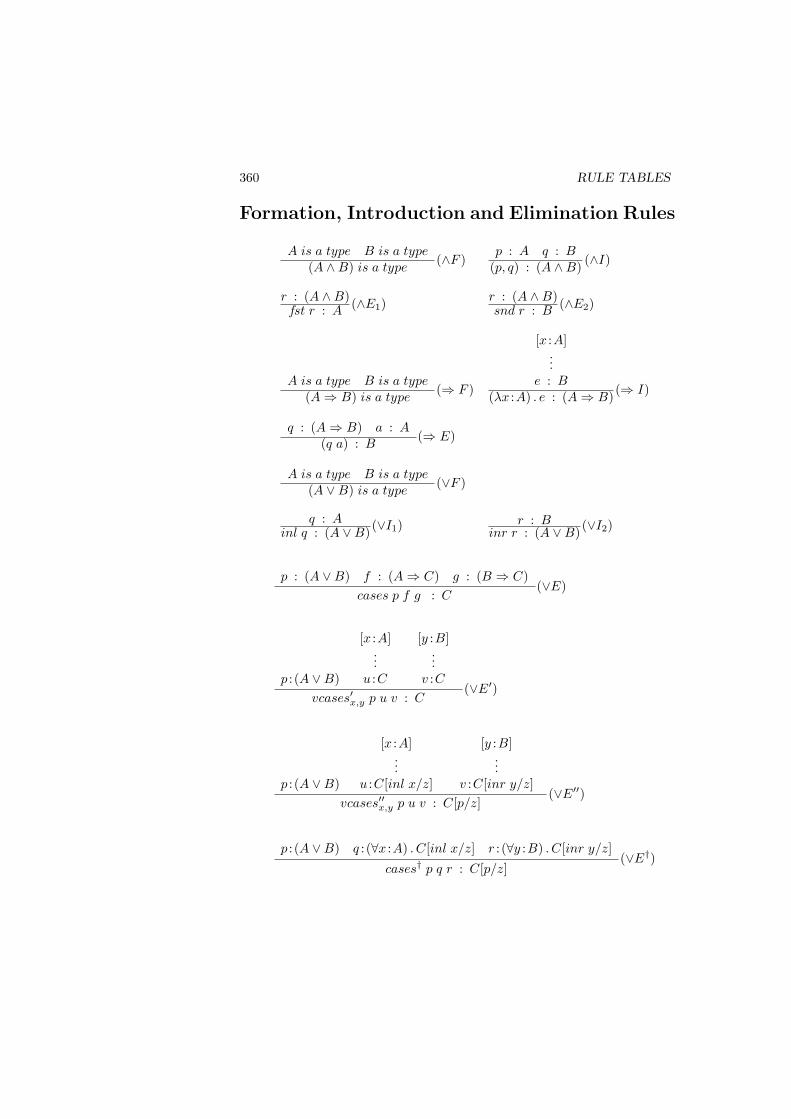
360 RULE TABLES
Formation, Introduction and Elimination Rules
A is a type B is a type(A ∧B) is a type
(∧F )p : A q : B
(p, q) : (A ∧B) (∧I)
r : (A ∧B)fst r : A
(∧E1)r : (A ∧B)snd r : B
(∧E2)
A is a type B is a type(A⇒ B) is a type
(⇒ F )
[x :A]...
e : B(λx :A) . e : (A⇒ B) (⇒ I)
q : (A⇒ B) a : A(q a) : B
(⇒ E)
A is a type B is a type(A ∨B) is a type
(∨F )
q : Ainl q : (A ∨B) (∨I1) r : B
inr r : (A ∨B) (∨I2)
p : (A ∨B) f : (A⇒ C) g : (B ⇒ C)cases p f g : C
(∨E)
p : (A ∨B)
[x :A]...
u :C
[y :B]...
v :Cvcases′x,y p u v : C
(∨E′)
p : (A ∨B)
[x :A]...
u :C[inl x/z]
[y :B]...
v :C[inr y/z]vcases′′x,y p u v : C[p/z]
(∨E′′)
p : (A ∨B) q : (∀x :A) . C[inl x/z] r : (∀y :B) . C[inr y/z]
cases† p q r : C[p/z](∨E†)
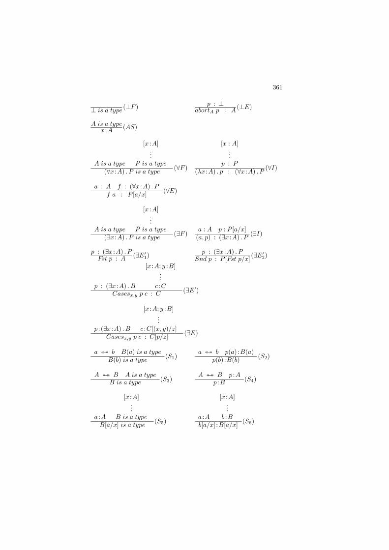
361
⊥ is a type(⊥F ) p : ⊥
abortA p : A(⊥E)
A is a typex :A (AS)
A is a type
[x :A]...
P is a type(∀x :A) . P is a type
(∀F )
[x : A]...
p : P(λx :A) . p : (∀x :A) . P
(∀I)
a : A f : (∀x :A) . Pf a : P [a/x] (∀E)
A is a type
[x :A]...
P is a type(∃x :A) . P is a type
(∃F )a : A p : P [a/x]
(a, p) : (∃x :A) . P(∃I)
p : (∃x :A) . PFst p : A (∃E′
1)p : (∃x :A) . P
Snd p : P [Fst p/x] (∃E′2)
p : (∃x :A) . B
[x :A; y :B]...
c :CCasesx,y p c : C (∃E′)
p : (∃x :A) . B
[x :A; y :B]...
c :C[(x, y)/z]Casesx,y p c : C[p/z] (∃E)
a ↔↔ b B(a) is a typeB(b) is a type
(S1)a ↔↔ b p(a) :B(a)
p(b) :B(b) (S2)
A ↔↔ B A is a typeB is a type (S3)
A ↔↔ B p :Ap :B (S4)
a :A
[x :A]...
B is a typeB[a/x] is a type
(S5)a :A
[x :A]...
b :Bb[a/x] :B[a/x] (S6)
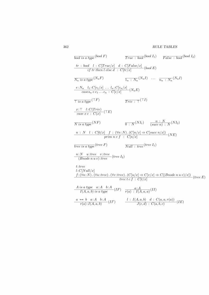
362 RULE TABLES
bool is a type(bool F )
True : bool(bool I1) False : bool
(bool I2)
tr : bool l : C[True/x] d : C[False/x]if tr then l else d : C[tr/x] (bool E)
Nn is a type (NnF ) 1n : Nn(NnI) . . . nn : Nn
(NnI)
e :Nn l1 :C[c1/x] . . . ln :C[cn/x]casesn e c1 . . . cn : C[e/x] (NnE)
> is a type(>F )
Triv : > (>I)
x :> l :C(Triv)case x c : C(x) (>E)
N is a type (NF ) 0 : N (NI1) n : N(succ n) : N
(NI2)
n : N l : C[0/x] f : (∀n :N) . (C[n/x]⇒ C[succ n/x])prim n c f : C[n/x] (NE)
tree is a type (tree F )Null : tree
(tree I1)
n :N u : tree v : tree(Bnode n u v) : tree (tree I2)
t : treel :C[Null/x]f : (∀n :N) . (∀u : tree) . (∀v : tree) . (C[u/x]⇒ C[v/x]⇒ C[(Bnode n u v)/x])
trec t c f : C[t/x] (tree E)
A is a type a :A b :AI(A, a, b) is a type
(IF ) a :Ar(a) : I(A, a, a) (II)
a ↔↔ b a :A b :Ar(a) :I(A, a, b) (II ′)
l : I(A, a, b) d : C(a, a, r(a))J(c, d) : C(a, b, c) (IE)
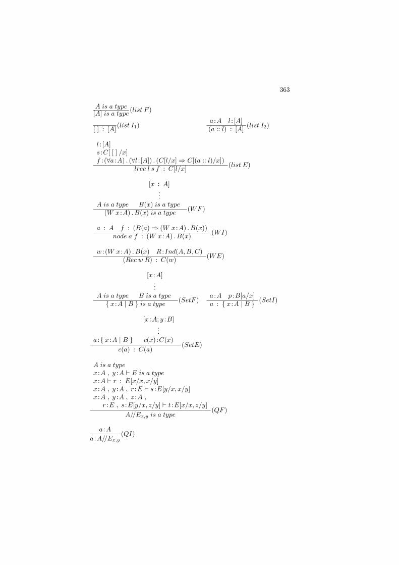
363
A is a type[A] is a type
(list F )
[ ] : [A] (list I1)a :A l : [A](a :: l) : [A] (list I2)
l : [A]s :C[ [ ] /x]f : (∀a :A) . (∀l : [A]) . (C[l/x]⇒ C[(a :: l)/x])
lrec l s f : C[l/x] (list E)
A is a type
[x : A]...
B(x) is a type(W x :A) . B(x) is a type
(WF )
a : A f : (B(a)⇒ (W x :A) . B(x))node a f : (W x :A) . B(x) (WI)
w : (W x :A) . B(x) R :Ind(A,B,C)(Rec w R) : C(w) (WE)
A is a type
[x :A]...
B is a type x :A | B is a type
(SetF )a :A p :B[a/x]a : x :A | B (SetI)
a : x :A | B
[x :A; y :B]...
c(x) :C(x)c(a) : C(a)
(SetE)
A is a typex :A , y :A ` E is a typex :A ` r : E[x/x, x/y]x :A , y :A , r :E ` s :E[y/x, x/y]x :A , y :A , z :A ,
r :E , s :E[y/x, z/y] ` t :E[x/x, z/y]A//Ex,y is a type
(QF )
a :Aa :A//Ex,y
(QI)
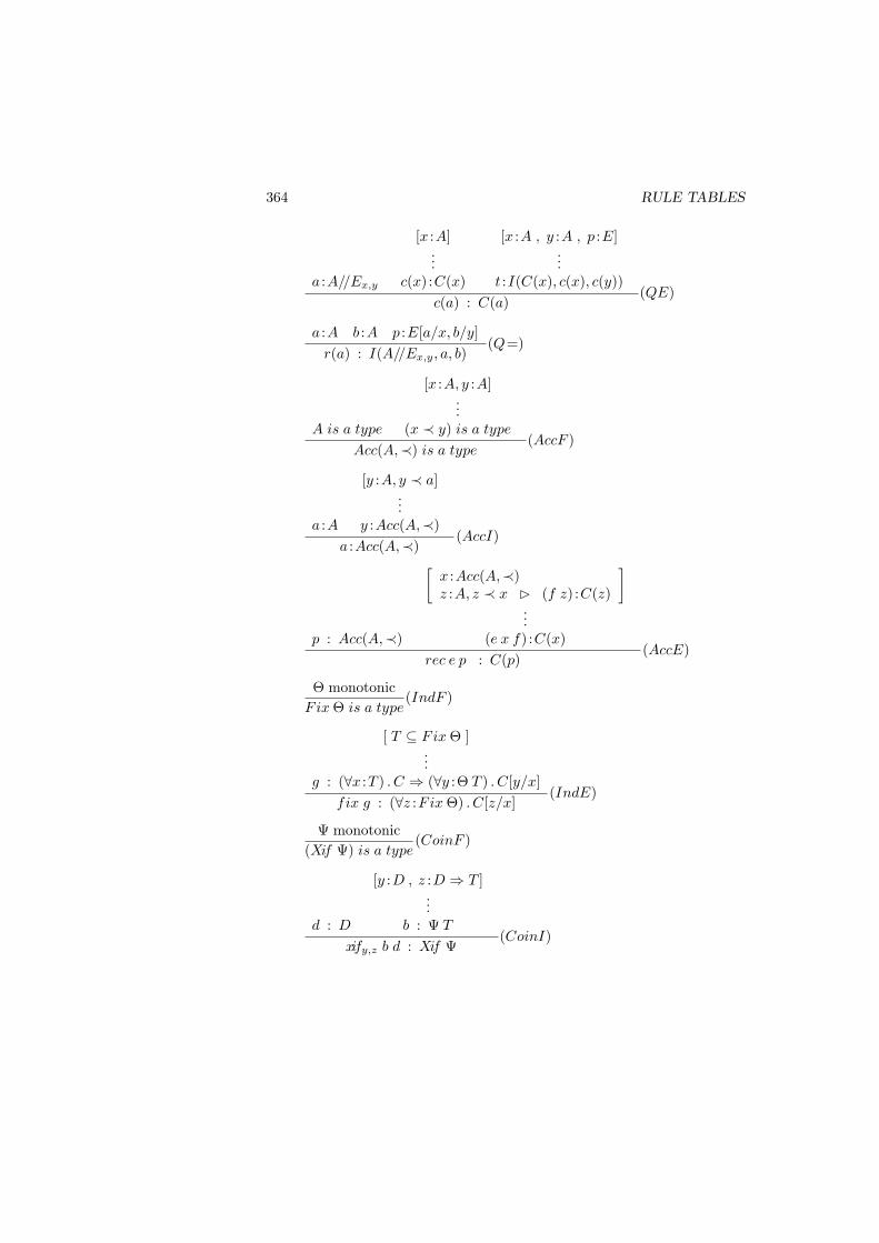
364 RULE TABLES
a :A//Ex,y
[x :A]...
c(x) :C(x)
[x :A , y :A , p :E]...
t :I(C(x), c(x), c(y))c(a) : C(a)
(QE)
a :A b :A p :E[a/x, b/y]r(a) : I(A//Ex,y, a, b)
(Q=)
A is a type
[x :A, y :A]...
(x ≺ y) is a type
Acc(A,≺) is a type(AccF )
a :A
[y :A, y ≺ a]...
y :Acc(A,≺)a :Acc(A,≺)
(AccI)
p : Acc(A,≺)
[x :Acc(A,≺)z :A, z ≺ x (f z) :C(z)
]...
(e x f) :C(x)rec e p : C(p)
(AccE)
Θ monotonicFix Θ is a type
(IndF )
[ T ⊆ Fix Θ ]...
g : (∀x :T ) . C ⇒ (∀y :Θ T ) . C[y/x]fix g : (∀z :Fix Θ) . C[z/x]
(IndE)
Ψ monotonic(Xif Ψ) is a type
(CoinF )
d : D
[y :D , z :D ⇒ T ]...
b : Ψ T
xify,z b d : Xif Ψ(CoinI)
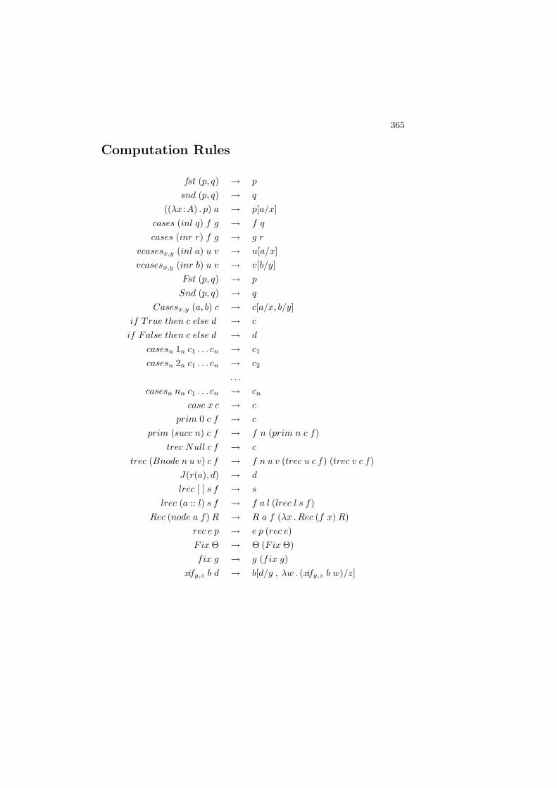
365
Computation Rules
fst (p, q) → p
snd (p, q) → q
((λx :A) . p) a → p[a/x]cases (inl q) f g → f q
cases (inr r) f g → g r
vcasesx,y (inl a) u v → u[a/x]vcasesx,y (inr b) u v → v[b/y]
Fst (p, q) → p
Snd (p, q) → q
Casesx,y (a, b) c → c[a/x, b/y]if True then c else d → c
if False then c else d → d
casesn 1n c1 . . . cn → c1
casesn 2n c1 . . . cn → c2
. . .
casesn nn c1 . . . cn → cn
case x c → c
prim 0 c f → c
prim (succ n) c f → f n (prim n c f)trec Null c f → c
trec (Bnode n u v) c f → f n u v (trec u c f) (trec v c f)J(r(a), d) → d
lrec [ ] s f → s
lrec (a :: l) s f → f a l (lrec l s f)Rec (node a f) R → R a f (λx .Rec (f x) R)
rec e p → e p (rec e)Fix Θ → Θ (Fix Θ)fix g → g (fix g)
xify,z b d → b[d/y , λw . (xify,z b w)/z]