UBICC Article 522 522

8/7/2019 UBICC Article 522 522

http://slidepdf.com/reader/full/ubicc-article-522-522 1/8

IMPROVING CLASSIFICATION WITH COST-SENSITIVE

APPROACH FOR DISTRIBUTED DATABASES

Maria Muntean, Honoriu Vă

lean, Ioan Ileană

, Corina Rotar1 Decembrie 1918 University of Alba Iulia, Romania

Technical University of Cluj Napoca, Romania

[email protected], [email protected]

ABSTRACT

A problem arises in data mining, when classifying unbalanced datasets using

Support Vector Machines. Because of the uneven distribution and the soft margin

of the classifier, the algorithm tries to improve the general accuracy of classifying

a dataset, and in this process it might misclassify a lot of weakly represented

classes, confusing their class instances as overshoot values that appear in the

dataset, and thus ignoring them. This paper introduces the Enhancer, a new

algorithm that improves the Cost-sensitive classification for Support VectorMachines, by multiplying in the training step the instances of the underrepresented

classes. We have discovered that by oversampling the instances of the class of

interest, we are helping the Support Vector Machine algorithm to overcome the

soft margin. As an effect, it classifies better future instances of this class of interest.Experimentally we have found out that our algorithm performs well on distributed

databases.

Keywords: classification; distributed databases; Cost-Sensitive Classifier; Support

Vector Machine.

1 INTRODUCTION

Most of the real-world data are imbalanced in

terms of proportion of samples available for each

class, which can cause problems such as over fit orlittle relevance. The Support Vector Machine (SVM),

a classification technique based on statistical

learning theory, was applied with great success in

many challenging non-linear classification problems

and was successfully applied to imbalanced

databases.

2 SUPPORT VECTOR MACHINES

The Support Vector Machine (SVM), proposedby Vapnik and his colleagues in 1990’s [1], is a new

machine learning method based on Statistical

Learning Theory and it is widely used in the area of

regressive, pattern recognition and probability

density estimation due to its simple structure and

excellent learning performance. Joachims validated

its outstanding performance in the area of text

categorization in 1998 [2]. SVM can also overcome

the over fitting and under fitting problems [3], [4],

and it has been used for imbalanced data

classification [5], [6].

The SVM technique is based on two class

classification. There are some methods used forclassification in more than two classes. Looking at

the two dimensional problem we actually want to

find a line that “best” separates points in the positive

class from the points in the negative class. Thehyperplane is characterized by the decision function f

(x) = sgn(w , Φ(x) + b), where “w” is the weight

vector, orthogonal to the hyperplane, “b” is a scalarthat represents the margin of the hyperplane, “x” is

the current sample tested, “Φ(x)” is a function that

transforms the input data into a higher dimensional

feature space and “,” representing the dot product.

Sgn is the signum function. If “w” has unit length,

then <w, Φ(x)> is the length of “Φ(x)” along thedirection of “w”.

To construct the SVM classifier one has to

minimize the norm of the weight vector “w” (where

||w|| represents the Euclidian norm) under theconstraint that the training patterns of each class

reside on opposite sides of the separating surface.

The training part of the algorithm needs to find the

normal vector “w” that leads to the largest “b” of the

hyperplane. Since the input vectors enter the dual

only in form of dot products the algorithm can be

generalized to non-linear classification by mapping

the input data into a higher-dimensional feature

space via an a priori chosen non-linear mapping

function “Φ” and construct a separating hyperplane

with the maximum margin.

In solving the quadratic optimization problem of

the linear SVM (i.e. when searching for a linearSVM in the new higher dimensional space), the

training tuples appear only in the form of dot



products, <Φ(xi) , Φ(xj)> , where “Φ(x)” is simply

the nonlinear mapping function applied to transformthe training tuples. Expensive calculation of dot

products <Φ(xi) , Φ(xj)> in a high-dimensional space

can be avoided by introducing a kernel function “K”:

)()(),( ji ji

x x x xK φ φ ⋅=

(1)

The kernel trick can be applied since all featurevectors only occur in dot products. The weight

vectors than become an expression in the feature

space, and therefore “Φ” will be the function throughwhich we represent the input vector in the new space.

Thus it is obtained the decision function having the

following form:

)),(sgn()( ∑ℜ∈

+=i

iii b x xk y x f α

(2)

where αi represent the Lagrange multipliers and the

samples xi for which αi > 0 are called Support

Vectors [7].

The idea of the kernel is to compute the norm of

the difference between two vectors in a higherdimensional space without representing those vectors

in the new space. Regarding the final SVM

formulation, the free parameters of SVMs to be

determined within model selection are given by the

regularization parameter c and the kernel, together

with additional parameters of the respective kernelfunction.

We chose to perform the experiments with

Polynomial Kernel function that is given by:e

ji ji n x xm x xK )(),( +⋅⋅= (3),

where e represents the exponent of the Polynomial

Kernel function, and m, n are the coefficients of thisexpression.

Training a SVM requires the solution of a very

large quadratic programming (QP) optimization

problem. So, the Sequential Minimal Optimization

(SMO) algorithm is proposed in the literature [7] for

training SVM breaks this large QP problem into a

series of smallest possible QP problems. These small

QP problems are solved analytically, which avoidsusing a time-consuming numerical QP optimization

as an inner loop. The amount of memory required for

SMO is linear in the training set size, which allows

SMO to handle very large training sets. Because

matrix computation is avoided, SMO scalessomewhere between linear and quadratic in thetraining set size for various test problems, while the

standard chunking SVM algorithm scales somewhere

between linear and cubic in the training set size. We

used the SMO method in our experiments in order to

train faster the SVM.

The SVMs have a great disadvantage inimbalanced classification the: because of the uneven

distribution and the soft margin of the SVM, the

algorithm tries to improve the general accuracy of

classifying a dataset, and in this process it might

misclassify a lot of weakly represented classes.

Various methods enrich the SVM algorithm to

obtain efficient techniques for solving classification

problems. An example of such method is the Cost-sensitive metaclassifier [9], [10], [11], that targets

the imbalanced learning problem by using different

cost matrices that describe the costs for

misclassifying any particular dataset.

3 COST-SENSITIVE APPROACH

Fundamental to the Cost-sensitive learning

methodology is the concept of the cost matrix. This

approach takes the classify cost into account, and it

aims to reduce the classify cost to the least. Instead

of creating balanced data distributions throughdifferent sampling strategies, Cost-sensitive learning

targets the imbalanced learning problem by using

different cost matrices that describe the costs for

misclassifying any particular dataset.

A very useful tool, the Confusion Matrix for two

classes is shown in Table 1.

Table 1: confusion matrix for a two class problem

Predicted Class

Class = 1 Class = 0

Actual Class Class = 1 TP FN

Class = 0 FP TN

The true positives (TP) and true negatives (TN)

are correct classifications. A false positive (FP)

occurs when the outcome is incorrectly predicted as

1 (or positive) when it is actually 0 (negative). A

false negative (FN) occurs when the outcome is

incorrectly predicted as negative when it is actuallypositive.

In addition, the accuracy measure may be

defined. It represents the ratio between correctly

classified instances and the sum of all instances

classified, both correct and incorrect ones. The above

measure was defined as:

FN FPTN TP

TN TPaccuracy

+++

+= (4)

More precisely, the classification gives equal

importance to all the misclassified data (false

negatives and false positives are equally significant).

The Cost-sensitive classifications strive to minimize

the total cost of the errors made by amisclassification, rather than the total amount of

misclassified data.

This paper introduces an algorithm named

Enhancer aimed for increasing the TP of

underrepresented classes of datasets, using Cost-sensitive classification and SVM.

4 DESCRIPTION OF THE ENHANCER

Experimentally we have found out that the

features that help in raising the TP of a class are thecost matrix and the amount of instances that the class

has. The last one can be modified by multiplying the



number of instances of that class that the dataset

initially has. The algorithm can be applied to notwell represented classes from imbalanced data sets.

Imbalanced data sets occur in two class domains

when one class contains a large number of examples,

while the other class contains only a few examples.

The Enhancer algorithm is detailed in thefollowing pseudo code:1. Read and validate input;

2. For all the classes that are not well represented:

BEGIN

Evaluate class with no attribute added

Evaluate class at Max multiplication rate

Evaluate the class at Half multiplicationREPEAT

Flag = False

Evaluate the intervals (beginning,

middle),

(middle, end)

If the end condition is metFlag = True

If the first interval has better results we

should use this, otherwise the other

Find the class evaluation after

multiplying class instances middle

times

UNTIL Flag = False

END

3. Multiply all the classes with the best factor

obtained;

4. Evaluate dataset.

While reading and validating the input we

collected from the command line the parameters thatwere used by this classifier, together with the

classifier parameters that were usually transmitted to

the program. The input parameters needed were the

number of the class that needs to have its TP

improved and the ε that is the maximum allowed

difference between the evaluation of the two

intervals (beginning, middle) and (middle, end).

Our classifier had also as input parameters the

multiplicands that the optimization algorithm hadused. There are available two kinds of evaluations

that also accept class multiplication:

• Evaluating a dataset with only the instances of

one class being multiplied, and keeping the other stillto their initial value. This kind of operation was

especially useful when we tried to find out what wasthe best multiplicand for a certain class.

• Evaluation of a dataset where the instances of

all classes could undergo a multiplication process.

The multiplication of the classes could be any real

number greater or equal to 1. If the multiplicand was

1, then the class remained with the initial number of

instance.

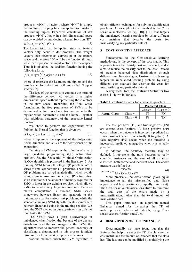
It is important to avoid performing the

evaluation on data that the algorithm used to train the

model on, because otherwise the algorithm is going

to over fit on this particular dataset, and when new

data is going to be introduced to be tested, the results

are going to be disastrous. This way of evaluation isthe 10 fold cross validation. Like this the dataset is

being randomized, and stratified using an integer

seed that takes values in the range 1-10. The

algorithm performs 10 times the evaluation of the

data set, and all the time has a different test set (Fig.1).

Figure 1: 10 fold Cross Validation

So, after performing the stratification, each time

the data set was split into the training and test set, the

Enhancer took the training set and applied

classMultiply() on it. Like this the instances thatwere going to be multiplied were not going to be

among that data that was going to test the result of

the SMO model.

The performance of the algorithm is only due to

the multiplied data, and there is no over fitting to this

specific data set. The data was trained in order to beevaluated as accurately as possible by a general test

set, and not only by the one for testing.

The instances were multiplied using theproperties of the Instances object in which they were

stored following this pseudo code:

1 aux← all instances of class x from dataset2 for i=0 to max do

3 add (instance from aux to dataset)

4 randomize dataset

By performing this series of operations the

number of instances of the desired class wasmultiplied by the desired amount and in the same

time we had a good distribution of instances inside

the dataset in order not to harm or benefit any of the

classes in the new dataset.

In order to see what the best improvement is, weneed to calculate an ending property of the logarithm.After some experiments the conclusion was that we

must optimize the TP and in the same time keep the

accuracy as high as possible. This can be translated

in the following equation:

max=∆+∆= CC i ATPϕ (5)

This means that we are trying all the time tomaximize the TP of classes and also the Accuracy.

The only flaw in this equation is the Accuracy is

medium (50%) and the TP of that certain class is

really close to 0. If realize to get the TP of the class

as high as 80-90%, the loss in the accuracy, that is

going to appear inevitably, is going to pass unnoticed



by this function. That is why we needed to introduce

the following constraint: θ >∆ CC A , where “θ” is the

minimum allowed drop in the accuracy.

The Enhancer algorithm described in the pseudo

code used a Divide et Impera technique, that

searched in the space (0 multiplication – max

multiplication) for the optimal multiplier for the class.The algorithm is going to stop its search under twocircumstances:

• The granulation is getting to thin, i.e., the

difference between the beginning and end of an

interval is very small (under a set epsilon). This

constraint is set, in order not to let the algorithm

wonder around searching for solutions that vary onefrom another by a very small number (<10-2).

• The modulus of the difference between the

CC i ATP ∆+∆from the first and the second interval

should be bigger that a known value. This value is

the considered to be the deviation of the Accuracyadded to the deviation of the TP of that class:

TP ACC σ σ µ += (6)

After finding the best multiplicand for the class

that we are trying to optimize, we constructed a

training set that contained each class instances

multiplied by the optimal multiplicand found at the

previous step. The experiments were performed on

the multiplicands of each of the other weakly

represented classes, in order to raise the accuracy and

the TP of the other classes while keeping the TP of

the interested class at least at the same value that the

algorithm retrieved.

5 EXPERIMENTAL RESULTS

5.1 Database description

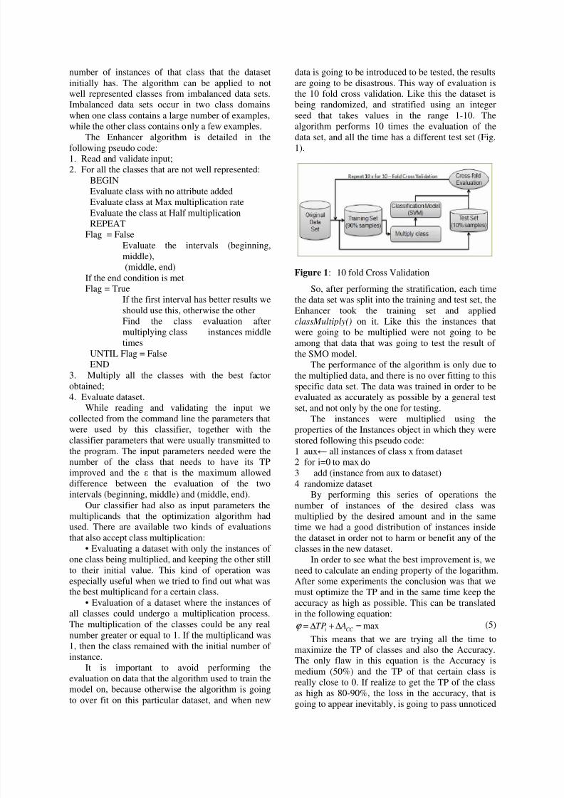
For the evaluation, we used the Dermatology

database, obtained from the online UCI Machine

Learning Repository [12]. A brief description of the

dataset is presented in Table 2 and Fig. 2.

This database has accuracy levels which are notvery high, so improvement is possible.

Table 2: the database used in the experiments

Database No of

attributes

No of

instances

Attributes

types

Dermatology 34+1 358 Num,Nom

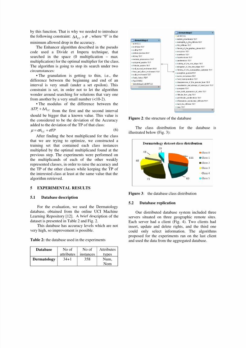
Figure 2: the structure of the database The class distribution for the database is

illustrated below (Fig. 3):

Figure 3: the database class distribution

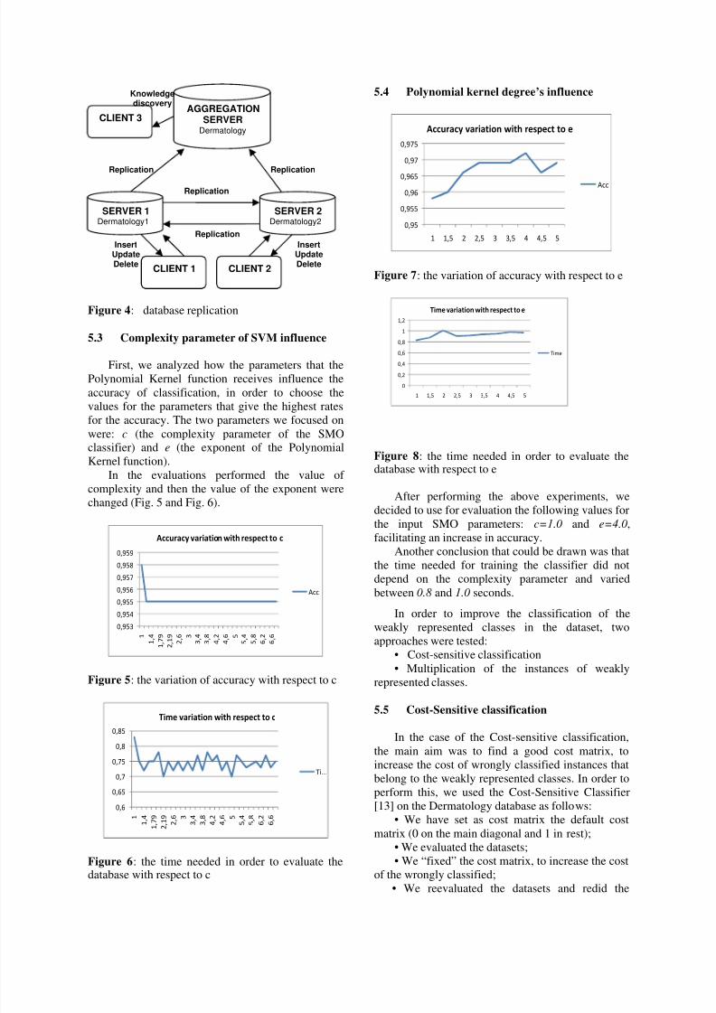
5.2 Database replication

Our distributed database system included three

servers situated on three geographic remote sites.

Each server had a client (Fig. 4). Two clients had

insert, update and delete rights, and the third one

could only select information. The algorithms

proposed for the experiments ran on the last client

and used the data from the aggregated database.



Figure 4: database replication

5.3 Complexity parameter of SVM influence

First, we analyzed how the parameters that the

Polynomial Kernel function receives influence the

accuracy of classification, in order to choose the

values for the parameters that give the highest rates

for the accuracy. The two parameters we focused on

were: c (the complexity parameter of the SMOclassifier) and e (the exponent of the Polynomial

Kernel function).

In the evaluations performed the value of

complexity and then the value of the exponent were

changed (Fig. 5 and Fig. 6).

0,953

0,954

0,955

0,956

0,957

0,958

0,959

1

1 ,

4

1 ,

7 9

2 ,

1 9

2 ,

6 3

3 ,

4

3 ,

8

4 ,

2

4 ,

6 5

5 ,

4

5 ,

8

6 ,

2

6 ,

6

Accuracy variation with respect to c

Acc

Figure 5: the variation of accuracy with respect to c

0,6

0,65

0,7

0,75

0,8

0,85

1

1 ,

4

1 ,

7 9

2 ,

1 9

2 ,

6 3

3 ,

4

3 ,

8

4 ,

2

4 ,

6 5

5 ,

4

5 ,

8

6 ,

2

6 ,

6

Time variation with respect to c

Ti…

Figure 6: the time needed in order to evaluate thedatabase with respect to c

5.4 Polynomial kernel degree’s influence

0,95

0,955

0,96

0,965

0,97

0,975

1 1,5 2 2,5 3 3,5 4 4,5 5

Accuracy variation with respect to e

Acc

Figure 7: the variation of accuracy with respect to e

0

0,2

0,4

0,6

0,8

1

1,2

1 1,5 2 2,5 3 3,5 4 4,5 5

Time variation with respect to e

Time

Figure 8: the time needed in order to evaluate thedatabase with respect to e

After performing the above experiments, we

decided to use for evaluation the following values for

the input SMO parameters: c=1.0 and e=4.0,

facilitating an increase in accuracy.

Another conclusion that could be drawn was that

the time needed for training the classifier did not

depend on the complexity parameter and varied

between 0.8 and 1.0 seconds.

In order to improve the classification of the

weakly represented classes in the dataset, two

approaches were tested:

• Cost-sensitive classification

• Multiplication of the instances of weakly

represented classes.

5.5 Cost-Sensitive classification

In the case of the Cost-sensitive classification,

the main aim was to find a good cost matrix, to

increase the cost of wrongly classified instances that

belong to the weakly represented classes. In order to

perform this, we used the Cost-Sensitive Classifier

[13] on the Dermatology database as follows:

• We have set as cost matrix the default cost

matrix (0 on the main diagonal and 1 in rest);

• We evaluated the datasets;

• We “fixed” the cost matrix, to increase the cost

of the wrongly classified;

• We reevaluated the datasets and redid the

AGGREGATIONSERVERDermatology

SERVER 1Dermatology1

CLIENT 1

SERVER 2Dermatology2

CLIENT 2

CLIENT 3

Replication Replication

Replication

Replication

InsertUpdateDelete

InsertUpdateDelete

Knowledgediscovery



previous step.

After performing the experiments we observedthat the accuracy and the TP of the classes 0, 2, 4 and

5 remained constant with respect to Cost Matrix

change (Fig. 9).

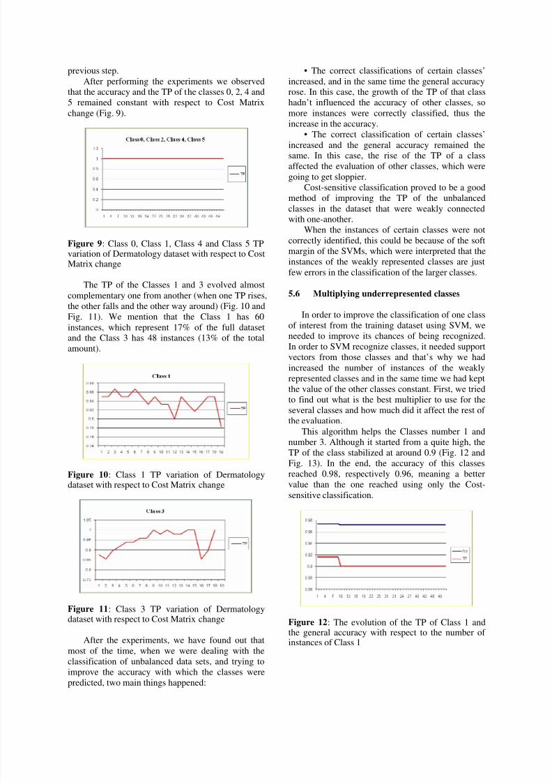
Figure 9: Class 0, Class 1, Class 4 and Class 5 TPvariation of Dermatology dataset with respect to CostMatrix change

The TP of the Classes 1 and 3 evolved almost

complementary one from another (when one TP rises,

the other falls and the other way around) (Fig. 10 and

Fig. 11). We mention that the Class 1 has 60

instances, which represent 17% of the full datasetand the Class 3 has 48 instances (13% of the total

amount).

Figure 10: Class 1 TP variation of Dermatologydataset with respect to Cost Matrix change

Figure 11: Class 3 TP variation of Dermatologydataset with respect to Cost Matrix change

After the experiments, we have found out that

most of the time, when we were dealing with the

classification of unbalanced data sets, and trying to

improve the accuracy with which the classes were

predicted, two main things happened:

• The correct classifications of certain classes’

increased, and in the same time the general accuracyrose. In this case, the growth of the TP of that class

hadn’t influenced the accuracy of other classes, so

more instances were correctly classified, thus the

increase in the accuracy.

• The correct classification of certain classes’increased and the general accuracy remained thesame. In this case, the rise of the TP of a class

affected the evaluation of other classes, which were

going to get sloppier.

Cost-sensitive classification proved to be a good

method of improving the TP of the unbalanced

classes in the dataset that were weakly connectedwith one-another.

When the instances of certain classes were not

correctly identified, this could be because of the soft

margin of the SVMs, which were interpreted that the

instances of the weakly represented classes are just

few errors in the classification of the larger classes.

5.6 Multiplying underrepresented classes

In order to improve the classification of one class

of interest from the training dataset using SVM, we

needed to improve its chances of being recognized.

In order to SVM recognize classes, it needed support

vectors from those classes and that’s why we had

increased the number of instances of the weakly

represented classes and in the same time we had kept

the value of the other classes constant. First, we tried

to find out what is the best multiplier to use for the

several classes and how much did it affect the rest of the evaluation.

This algorithm helps the Classes number 1 and

number 3. Although it started from a quite high, the

TP of the class stabilized at around 0.9 (Fig. 12 and

Fig. 13). In the end, the accuracy of this classes

reached 0.98, respectively 0.96, meaning a better

value than the one reached using only the Cost-

sensitive classification.

Figure 12: The evolution of the TP of Class 1 andthe general accuracy with respect to the number of instances of Class 1



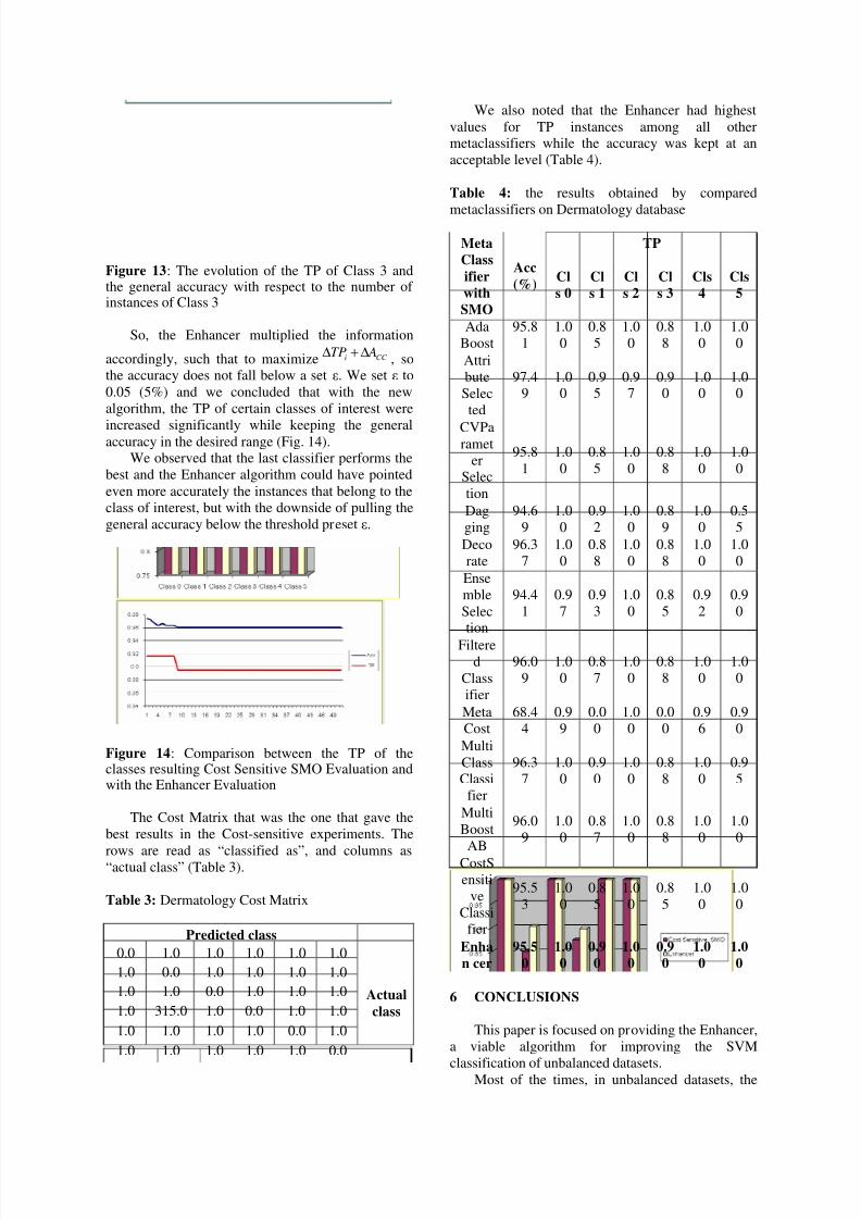
Figure 13: The evolution of the TP of Class 3 andthe general accuracy with respect to the number of instances of Class 3

So, the Enhancer multiplied the information

accordingly, such that to maximize CC i ATP ∆+∆, so

the accuracy does not fall below a set ε. We set ε to

0.05 (5%) and we concluded that with the new

algorithm, the TP of certain classes of interest were

increased significantly while keeping the generalaccuracy in the desired range (Fig. 14).

We observed that the last classifier performs the

best and the Enhancer algorithm could have pointed

even more accurately the instances that belong to the

class of interest, but with the downside of pulling the

general accuracy below the threshold preset ε.

Figure 14: Comparison between the TP of theclasses resulting Cost Sensitive SMO Evaluation andwith the Enhancer Evaluation

The Cost Matrix that was the one that gave the

best results in the Cost-sensitive experiments. The

rows are read as “classified as”, and columns as“actual class” (Table 3).

Table 3: Dermatology Cost Matrix

Predicted class

0.0 1.0 1.0 1.0 1.0 1.0

1.0 0.0 1.0 1.0 1.0 1.0

1.0 1.0 0.0 1.0 1.0 1.0

1.0 315.0 1.0 0.0 1.0 1.0

1.0 1.0 1.0 1.0 0.0 1.0

1.0 1.0 1.0 1.0 1.0 0.0

Actual

class

We also noted that the Enhancer had highest

values for TP instances among all othermetaclassifiers while the accuracy was kept at an

acceptable level (Table 4).

Table 4: the results obtained by compared

metaclassifiers on Dermatology database

TP Meta

Class

ifier

with

SMO

Acc

(%) Cl

s 0

Cl

s 1

Cl

s 2

Cl

s 3

Cls

4

Cls

5

Ada

Boost

95.8

1

1.0

0

0.8

5

1.0

0

0.8

8

1.0

0

1.0

0

Attri

bute

Selec

ted

97.49

1.00

0.95

0.97

0.90

1.00

1.00

CVParamet

erSelec

tion

95.8

1

1.0

0

0.8

5

1.0

0

0.8

8

1.0

0

1.0

0

Dag

ging

94.6

9

1.0

0

0.9

2

1.0

0

0.8

9

1.0

0

0.5

5

Deco

rate

96.3

7

1.0

0

0.8

8

1.0

0

0.8

8

1.0

0

1.0

0

Ense

mble

Selection

94.4

1

0.9

7

0.9

3

1.0

0

0.8

5

0.9

2

0.9

0

Filtered

Class

ifier

96.0

9

1.0

0

0.8

7

1.0

0

0.8

8

1.0

0

1.0

0

Meta

Cost

68.4

4

0.9

9

0.0

0

1.0

0

0.0

0

0.9

6

0.9

0

Multi

ClassClassi

fier

96.3

7

1.0

0

0.9

0

1.0

0

0.8

8

1.0

0

0.9

5

Multi

Boost

AB

96.0

9

1.0

0

0.8

7

1.0

0

0.8

8

1.0

0

1.0

0

CostS

ensiti

ve

Classi

fier

95.5

3

1.0

0

0.8

5

1.0

0

0.8

5

1.0

0

1.0

0

Enha

n cer

95.5

0

1.0

0

0.9

0

1.0

0

0.9

0

1.0

0

1.0

0

6 CONCLUSIONS

This paper is focused on providing the Enhancer,

a viable algorithm for improving the SVM

classification of unbalanced datasets.Most of the times, in unbalanced datasets, the



classifiers have a tendency of classifying in a very

accurate manner the instances belonging to the bestrepresented classes and do a sloppy job with the rest.

By doing this, most of the classification have an

above average classification rate simply because in

practice we are going to encounter more instances of

the well represented class. On the other side most of the times the damage done by not classifying one of the other classes correctly produces more damage

than the other way around.

This solution is especially important when it is

far more important to classify the instances of a class

correctly, and if in this process we might classify

some of the other instances as belonging to this classwe do not produce any harm. For instance it is better

to send people suspect of different diseases to further

investigations, than sending ill people at home and

telling them they don’t have anything to worry about.

In order to overcome this problem we have

developed the new classifying algorithm that canclassify the instances of a class of interest up to

better than the classification of the Cost Sensitive

and SVM algorithm. All of this is happening while

keeping the accuracy at an acceptable level. The

algorithm improves the classification of the weakly

represented class in the dataset and it can be used for

solving real medical diagnosis problems. We have

discovered that by over sampling the instances of the

class of interest, we are helping the SVM algorithm

to overcome the soft margin. As an effect, it

classifies better future instances of this class of

interest.

7 REFERENCES

[1] V N. Vapnik: The nature of statistical learning

theory, New York: Springer-Verlag (2000).

[2] I. Joachims: Text categorization with Support

Vector Machines: Learning with many relevant

features, Proceedings of the European

Conference on Machine Learning, Berlin:

Springer (1998).[3] M. Hong, G. Yanchun, W. Yujie, and L.

Xiaoying: Study on classification method based

on Support Vector Machine, 2009 First

International Workshop on EducationTechnology and Computer Science, Wuhan,

China, pp.369-373, March, 7-8 (2009).[4] X. Duan, G. Shan, and Q. Zhang: Design of a

two layers Support Vector Machine for

classification, 2009 Second International

Conference on Information and Computing

Science, Manchester, UK, pp. 247-250, May, 21-22 (2009).

[5] X. Duan, G. Shan, and Q. Zhang: Design of a

two layers Support Vector Machine for

classification, 2009 Second International

Conference on Information and ComputingScience, Manchester, UK, pp. 247-250, May, 21-22 (2009).

[6] Y. Li, X. Danrui, and D. Zhe: A new method of

Support Vector Machine for class imbalance

problem, 2009 International Joint Conference on

Computational Sciences and Optimization,

Hainan Island, China, pp. 904-907, April 24-26(2009).

[7] Z. Xinfeng, X. Xiaozhao, C. Yiheng, and L.

Yaowei: A weighted hyper-sphere SVM, 2009

Fifth International Conference on Natural

Computation, Tianjin, China, pp. 574-577, 14-

16, August (2009).[8] J., Platt: Fast Training of Support Vector

Machines using Sequential Minimal

Optimization, Advances in Kernel Methods –

Support Vector Learning, B. Scholkopf, C.

Burges, A. Smola, eds., MIT Press (1998).

[9] D. I. Morariu, L. N. Vintan: A Better

Correlation of the SVM Kernel’s Parameters, 5th

RoEduNet IEEE International Conference, Sibiu,

Romania (2006).

[10] H. He and E. A. Garcia, Learning from

imbalanced data, IEEE Transactions on

Knowledge and Data Engineering, VOL. 21, NO.

9, September: (2009).[11] Y. Dai, H. Chen, and T. Peng: Cost-sensitive

Support Vector Machine based on weighted

attribute, 2009 International Forum on

Information Technology and Applications,

Chengdu, China, pp. 690-692, 15-17, May

(2009).

[12] R. Santos-Rodriguez, D. Garcia-Garcia, and J.

Cid-Sueiro: Cost-sensitive classification based

on Bregman divergences for medical diagnosis,2009 International Conference on Machine

Learning and Applications, Florida, USA, pp.

551-556, 13-15, December (2009).

[13] University of California Irvine. UCI MachineLearning Repository,

http://archive.ics.uci.edu/ml/.[14] E. Frank, L. Trigg, G. Holmes, Ian H. Witten:

Technical Note: Naive Bayes for Regression,

Machine Learning, v.41 n.1, p.5-25 (2000).

Documents

UBICC Article 522 522