Ubiquitous Pattern Matching and Its Applications(Biology, Security, Multimedia)∗

W. Szpankowski†

Department of Computer SciencePurdue University

W. Lafayette, IN 47907

September 14, 2005

∗This research is supported by NSF and NIH.†Joint work with P. Flajolet, A. Grama, R. Gwadera, S. Lonardi, M. Regnier, B. Vallee, M. Ward.

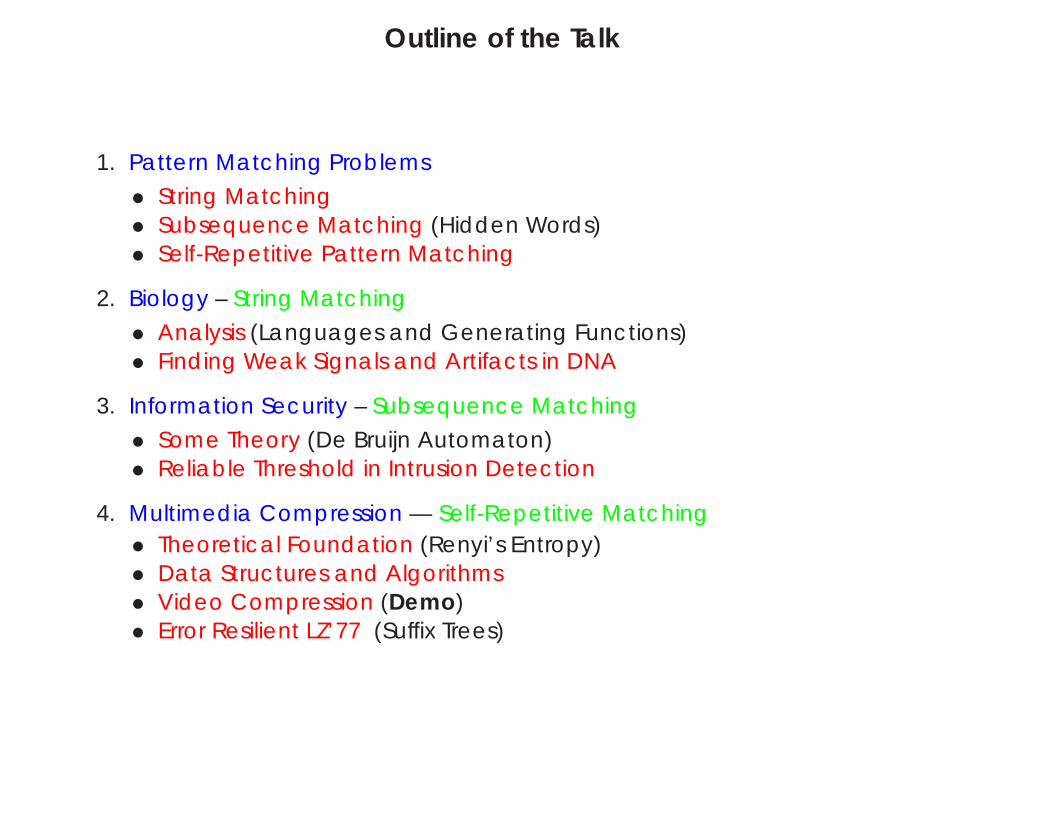
Outline of the Talk

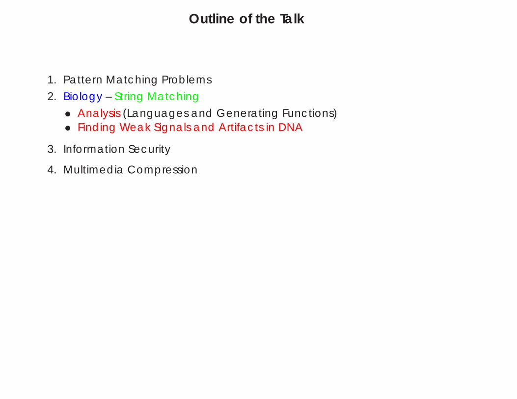
1. Pattern Matching Problems

• String Matching• Subsequence Matching (Hidden Words)• Self-Repetitive Pattern Matching

2. Biology – String Matching

• Analysis (Languages and Generating Functions)• Finding Weak Signals and Artifacts in DNA

3. Information Security – Subsequence Matching

• Some Theory (De Bruijn Automaton)• Reliable Threshold in Intrusion Detection

4. Multimedia Compression — Self-Repetitive Matching• Theoretical Foundation (Renyi’s Entropy)• Data Structures and Algorithms• Video Compression (Demo)• Error Resilient LZ’77 (Suffix Trees)

Pattern Matching

Let W and T be (set of) strings generated over a finite alphabet A.

We call W the pattern and T the text. The text T is of length n and isgenerated by a probabilistic source.

We shall writeT n

m = Tm . . . Tn.

The pattern W can be a single string

W = w1 . . . wm, wi ∈ A

or a set of stringsW = W1, . . . ,Wd

with Wi ∈ Ami being a set of strings of length mi.

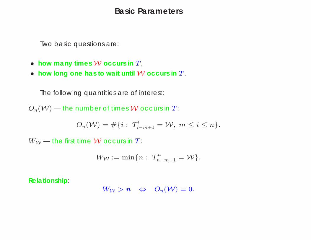
Basic Parameters

Two basic questions are:

• how many times W occurs in T ,

• how long one has to wait until W occurs in T .

The following quantities are of interest:

On(W) — the number of times W occurs in T :

On(W) = #i : T ii−m+1 = W, m ≤ i ≤ n.

WW — the first time W occurs in T :

WW := minn : T nn−m+1 = W.

Relationship:WW > n ⇔ On(W) = 0.

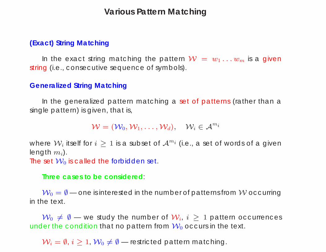
Various Pattern Matching

(Exact) String Matching

In the exact string matching the pattern W = w1 . . . wm is a givenstring (i.e., consecutive sequence of symbols).

Generalized String Matching

In the generalized pattern matching a set of patterns (rather than asingle pattern) is given, that is,

W = (W0,W1, . . . ,Wd), Wi ∈ Ami

where Wi itself for i ≥ 1 is a subset of Ami (i.e., a set of words of a givenlength mi).The set W0 is called the forbidden set.

Three cases to be considered:

W0 = ∅ — one is interested in the number of patterns from W occurringin the text.

W0 6= ∅ — we study the number of Wi, i ≥ 1 pattern occurrencesunder the condition that no pattern from W0 occurs in the text.

Wi = ∅, i ≥ 1, W0 6= ∅ — restricted pattern matching.

Pattern Matching Problems

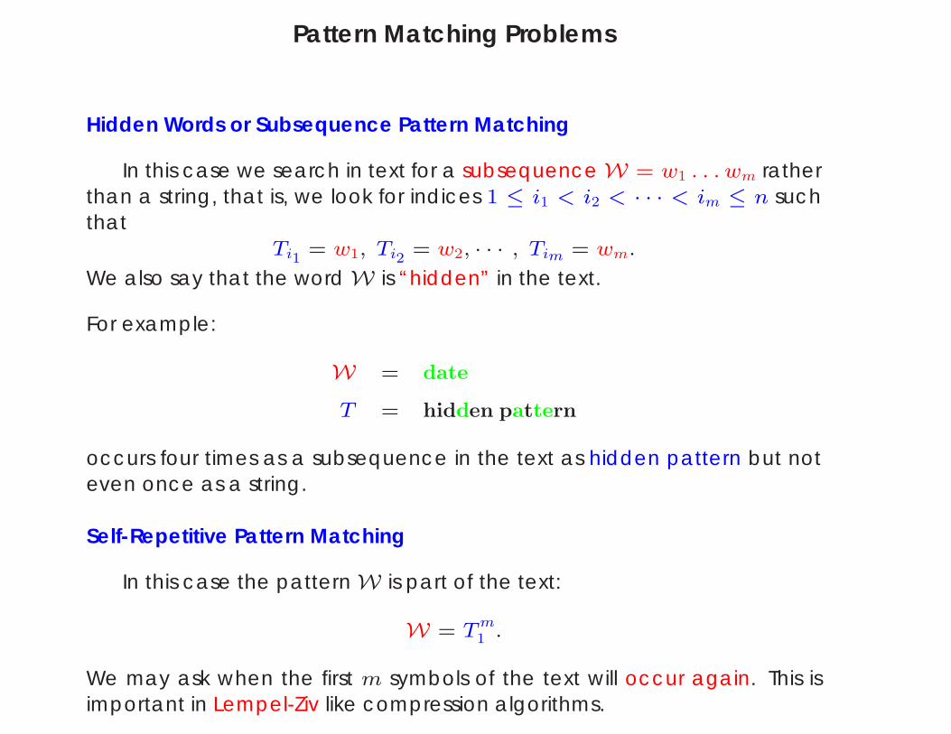
Hidden Words or Subsequence Pattern Matching

In this case we search in text for a subsequence W = w1 . . . wm ratherthan a string, that is, we look for indices 1 ≤ i1 < i2 < · · · < im ≤ n suchthat

Ti1= w1, Ti2

= w2, · · · , Tim = wm.

We also say that the word W is “hidden” in the text.

For example:

W = date

T = hidden pattern

occurs four times as a subsequence in the text as hidden pattern but noteven once as a string.

Self-Repetitive Pattern Matching

In this case the pattern W is part of the text:

W = Tm1 .

We may ask when the first m symbols of the text will occur again. This isimportant in Lempel-Ziv like compression algorithms.

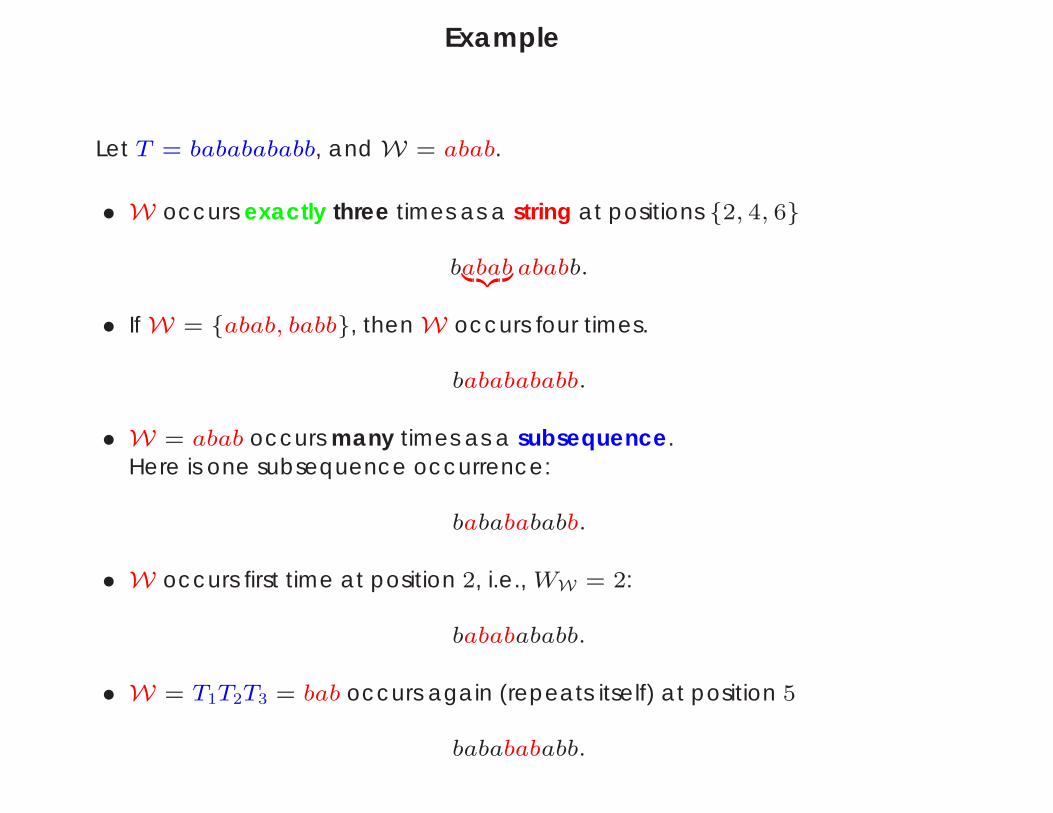
Example

Let T = bababababb, and W = abab.

• W occurs exactly three times as a string at positions 2, 4, 6

babab| z ababb.

• If W = abab, babb, then W occurs four times.

bababababb.

• W = abab occurs many times as a subsequence.Here is one subsequence occurrence:

bababababb.

• W occurs first time at position 2, i.e., WW = 2:

bababababb.

• W = T1T2T3 = bab occurs again (repeats itself) at position 5

bababababb.

Probabilistic Sources

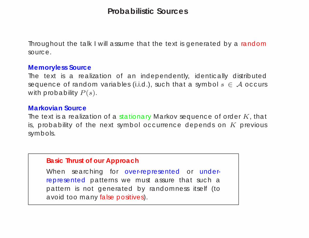
Throughout the talk I will assume that the text is generated by a randomsource.

Memoryless SourceThe text is a realization of an independently, identically distributedsequence of random variables (i.i.d.), such that a symbol s ∈ A occurswith probability P (s).

Markovian SourceThe text is a realization of a stationary Markov sequence of order K, thatis, probability of the next symbol occurrence depends on K previoussymbols.

Basic Thrust of our Approach

When searching for over-represented or under-represented patterns we must assure that such apattern is not generated by randomness itself (toavoid too many false positives).

Outline of the Talk

1. Pattern Matching Problems

2. Biology – String Matching

• Analysis (Languages and Generating Functions)• Finding Weak Signals and Artifacts in DNA

3. Information Security

4. Multimedia Compression

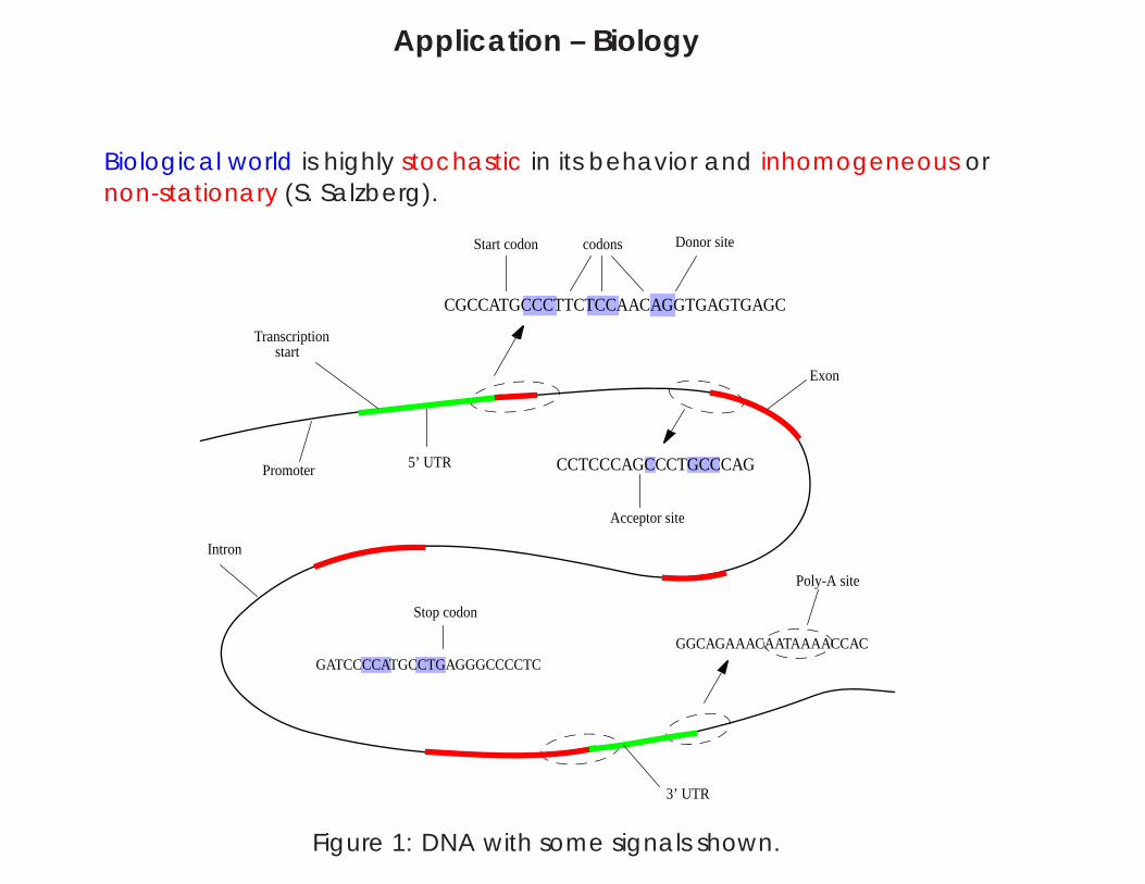
Application – Biology

Biological world is highly stochastic in its behavior and inhomogeneous ornon-stationary (S. Salzberg).

Start codon codons Donor site

CGCCATGCCCTTCTCCAACAGGTGAGTGAGC

Transcription start

Exon

Promoter 5’ UTR CCTCCCAGCCCTGCCCAG

Acceptor site

Intron

Stop codon

GATCCCCATGCCTGAGGGCCCCTCGGCAGAAACAATAAAACCAC

Poly-A site

3’ UTR

Figure 1: DNA with some signals shown.

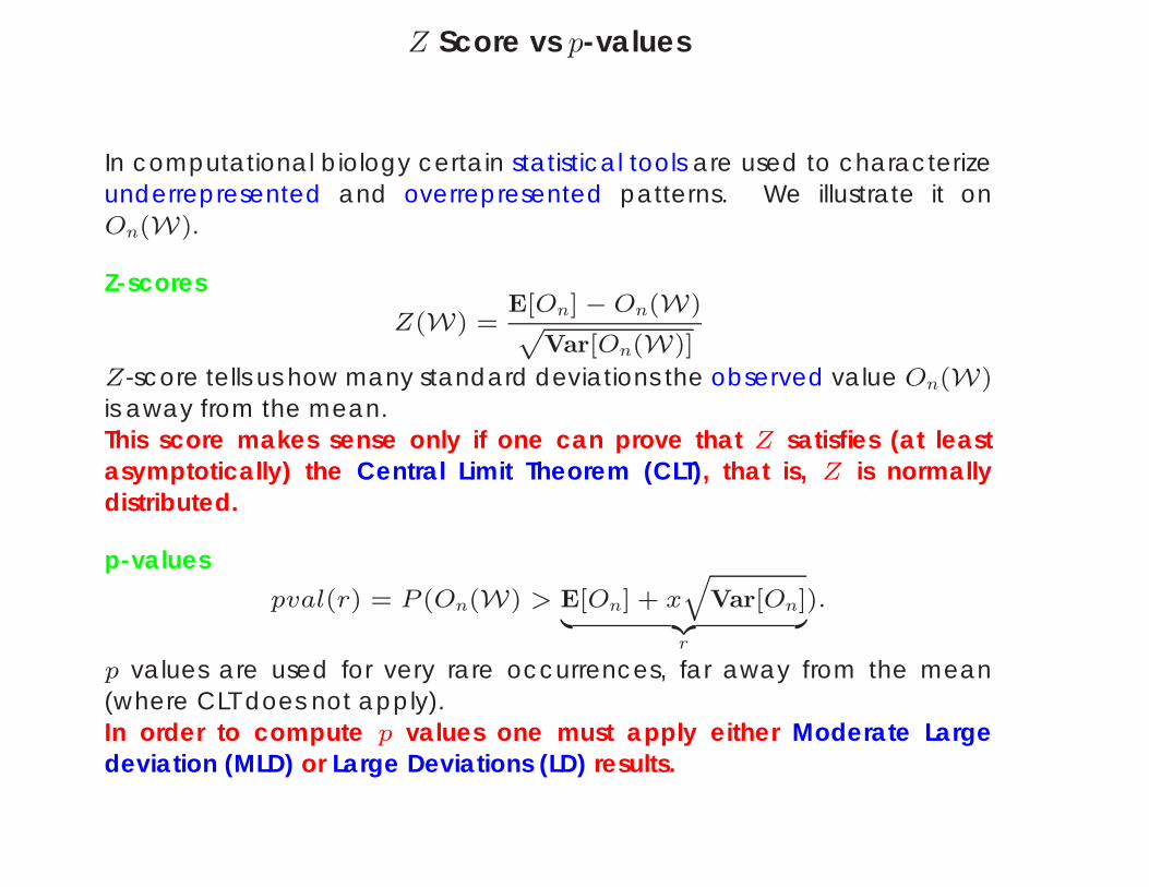
Z Score vs p-values

In computational biology certain statistical tools are used to characterizeunderrepresented and overrepresented patterns. We illustrate it onOn(W).

Z-scoresZ(W) =

E[On] − On(W)pVar[On(W)]

Z-score tells us how many standard deviations the observed value On(W)is away from the mean.This score makes sense only if one can prove that Z satisfies (at leastasymptotically) the Central Limit Theorem (CLT), that is, Z is normallydistributed.

p-valuespval(r) = P (On(W) > E[On] + x

qVar[On]| z

r

).

p values are used for very rare occurrences, far away from the mean(where CLT does not apply).In order to compute p values one must apply either Moderate Largedeviation (MLD) or Large Deviations (LD) results.

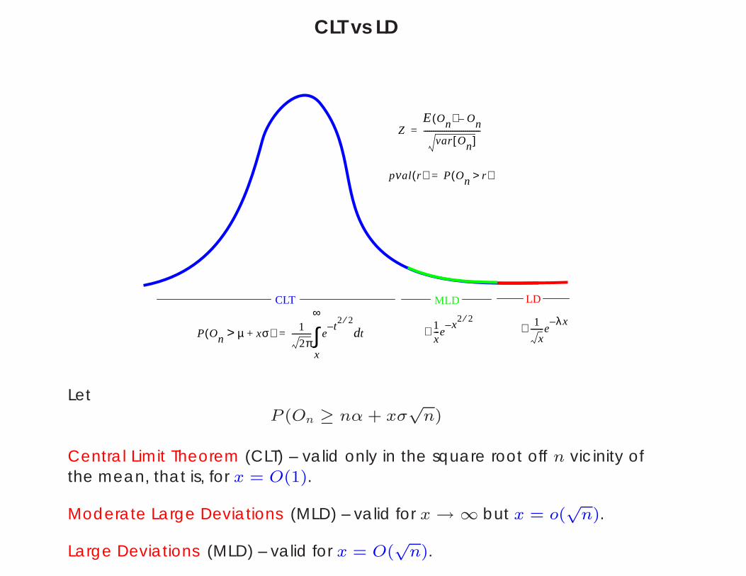
CLT vs LD

P On µ xσ+>( ) 1

2π---------- e

t2 2⁄

–td

x

∞

∫=1x---e

x2 2⁄

–∼1

x-------e

λx–∼

pval r( ) P On r>( )=

ZE On( ) On–

var On[ ]------------------------------=

CLT MLD LD

LetP (On ≥ nα + xσ

√n)

Central Limit Theorem (CLT) – valid only in the square root off n vicinity ofthe mean, that is, for x = O(1).

Moderate Large Deviations (MLD) – valid for x → ∞ but x = o(√

n).

Large Deviations (MLD) – valid for x = O(√

n).

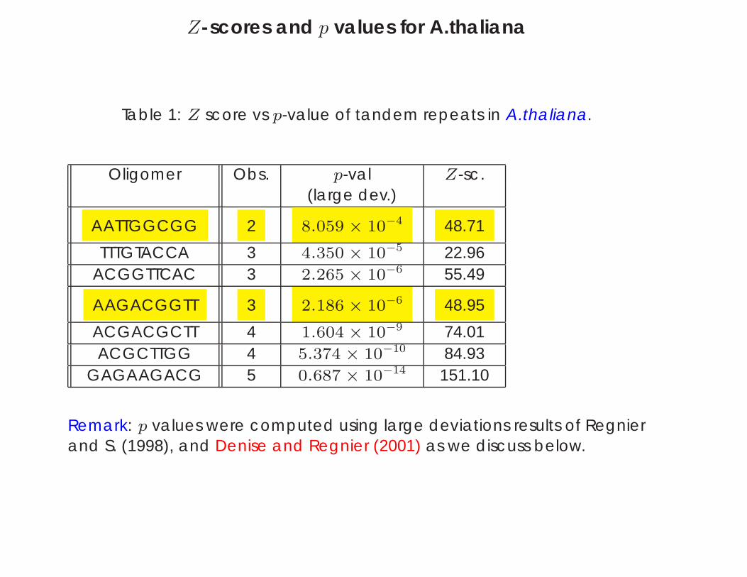
Z-scores and p values for A.thaliana

Table 1: Z score vs p-value of tandem repeats in A.thaliana.

Oligomer Obs. p-val Z-sc.(large dev.)

AATTGGCGG 2 8.059 × 10−4 48.71

TTTGTACCA 3 4.350 × 10−5 22.96ACGGTTCAC 3 2.265 × 10−6 55.49

AAGACGGTT 3 2.186 × 10−6 48.95

ACGACGCTT 4 1.604 × 10−9 74.01ACGCTTGG 4 5.374 × 10−10 84.93

GAGAAGACG 5 0.687 × 10−14 151.10

Remark: p values were computed using large deviations results of Regnierand S. (1998), and Denise and Regnier (2001) as we discuss below.

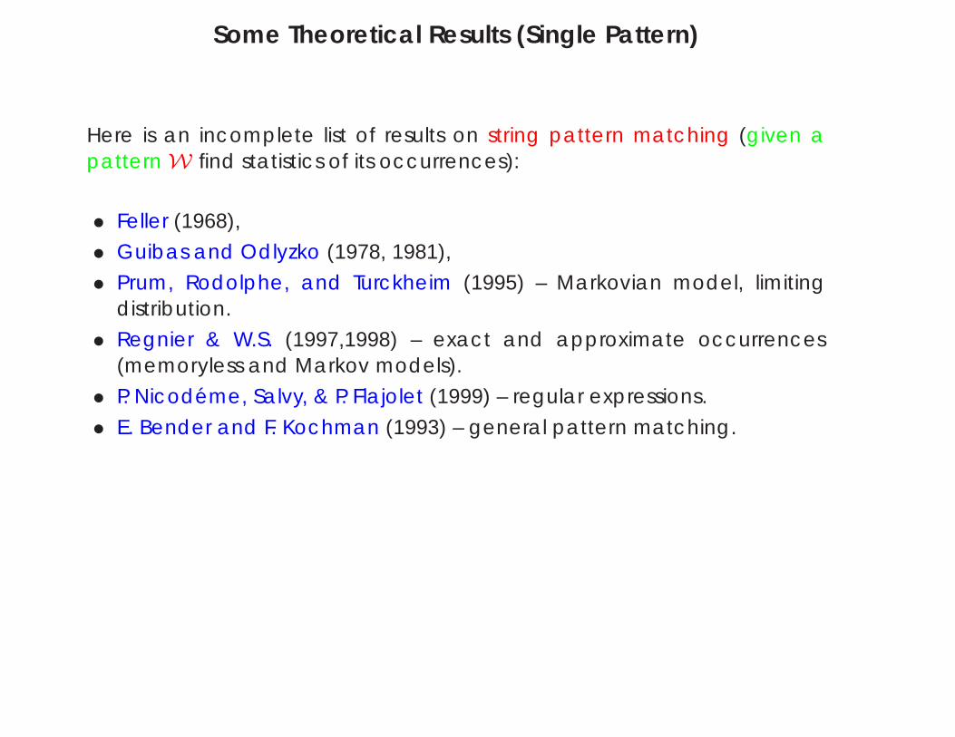
Some Theoretical Results (Single Pattern)

Here is an incomplete list of results on string pattern matching (given apattern W find statistics of its occurrences):

• Feller (1968),

• Guibas and Odlyzko (1978, 1981),

• Prum, Rodolphe, and Turckheim (1995) – Markovian model, limitingdistribution.

• Regnier & W.S. (1997,1998) – exact and approximate occurrences(memoryless and Markov models).

• P. Nicodeme, Salvy, & P. Flajolet (1999) – regular expressions.

• E. Bender and F. Kochman (1993) – general pattern matching.

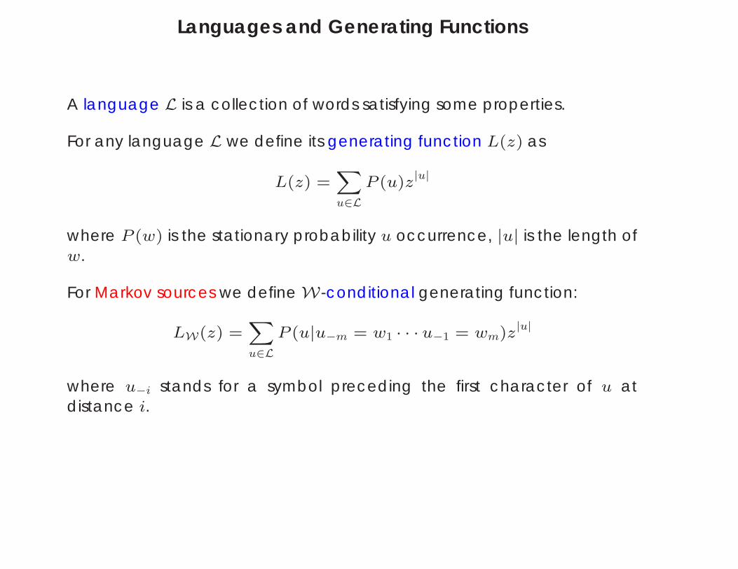
Languages and Generating Functions

A language L is a collection of words satisfying some properties.

For any language L we define its generating function L(z) as

L(z) =Xu∈L

P (u)z|u|

where P (w) is the stationary probability u occurrence, |u| is the length ofw.

For Markov sources we define W-conditional generating function:

LW(z) =Xu∈L

P (u|u−m = w1 · · ·u−1 = wm)z|u|

where u−i stands for a symbol preceding the first character of u atdistance i.

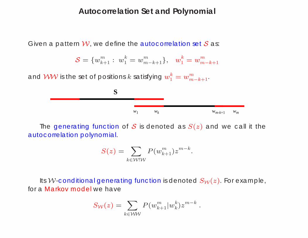
Autocorrelation Set and Polynomial

Given a pattern W , we define the autocorrelation set S as:

S = wmk+1 : wk

1 = wmm−k+1, wk

1 = wmm−k+1

and WW is the set of positions k satisfying wk1 = wm

m−k+1.

w1 wk wm-k+1 wm

S

The generating function of S is denoted as S(z) and we call it theautocorrelation polynomial.

S(z) =X

k∈W!WP (wm

k+1)zm−k.

Its W-conditional generating function is denoted SW(z). For example,for a Markov model we have

SW(z) =X

k∈WWP (wm

k+1|wkk)z

m−k .

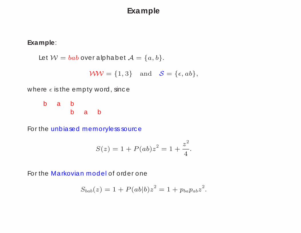
Example

Example:

Let W = bab over alphabet A = a, b.

WW = 1, 3 and S = ε, ab,

where ε is the empty word, since

b a bb a b

For the unbiased memoryless source

S(z) = 1 + P (ab)z2= 1 +

z2

4.

For the Markovian model of order one

Sbab(z) = 1 + P (ab|b)z2= 1 + pbapabz

2.

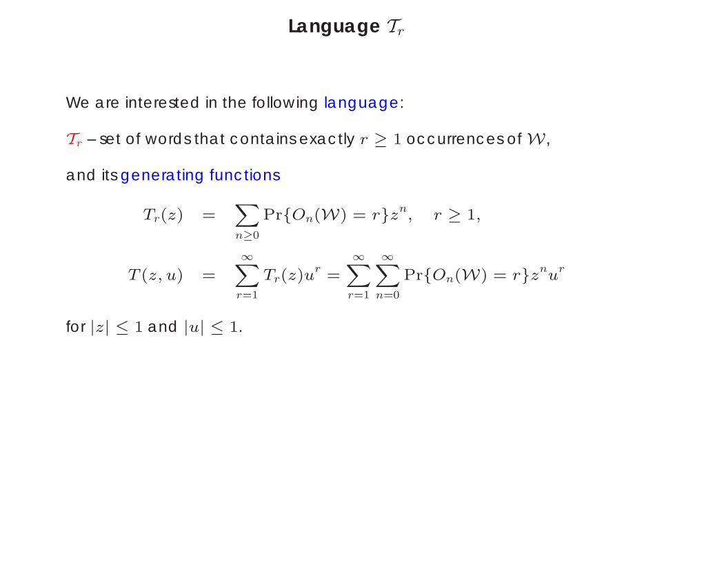
Language Tr

We are interested in the following language:

Tr – set of words that contains exactly r ≥ 1 occurrences of W ,

and its generating functions

Tr(z) =Xn≥0

PrOn(W) = rzn, r ≥ 1,

T (z, u) =∞X

r=1

Tr(z)ur =∞X

r=1

∞Xn=0

PrOn(W) = rznur

for |z| ≤ 1 and |u| ≤ 1.

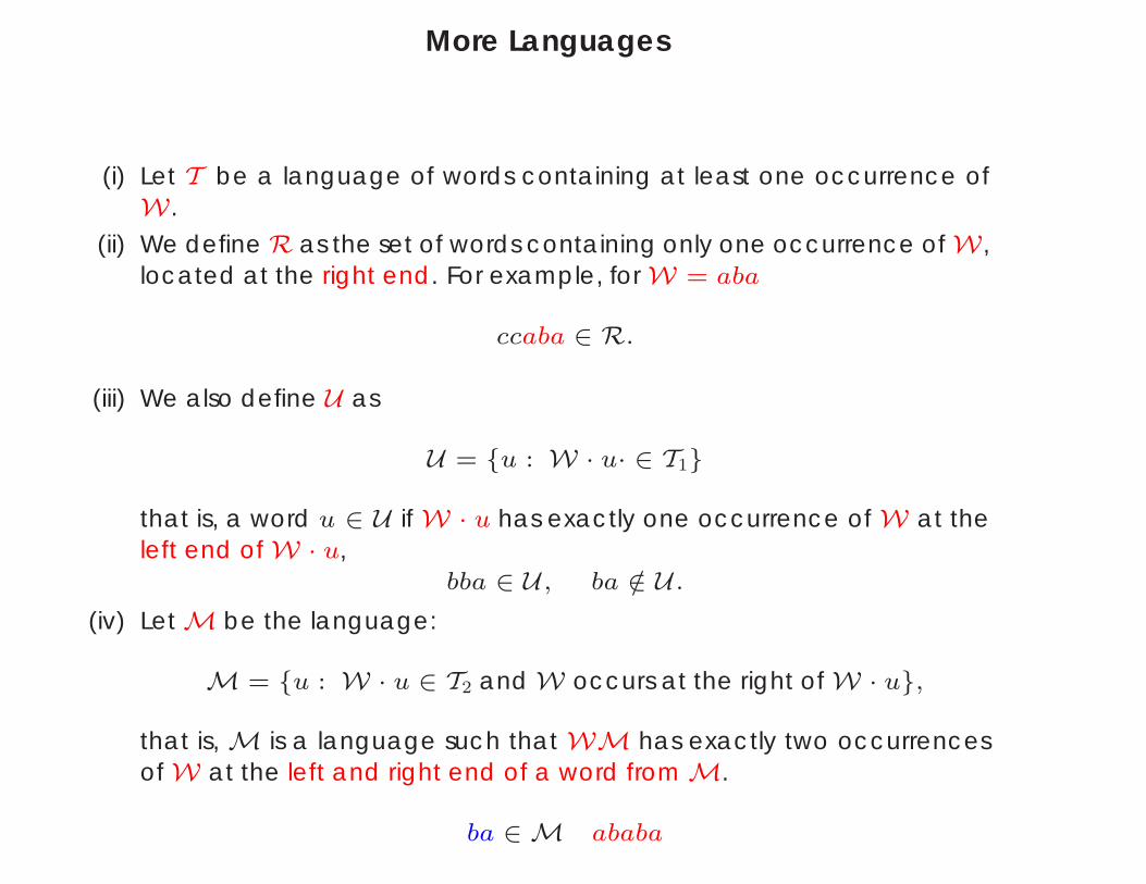
More Languages

(i) Let T be a language of words containing at least one occurrence ofW .

(ii) We define R as the set of words containing only one occurrence of W ,located at the right end. For example, for W = aba

ccaba ∈ R.

(iii) We also define U as

U = u : W · u· ∈ T1

that is, a word u ∈ U if W · u has exactly one occurrence of W at theleft end of W · u,

bba ∈ U , ba /∈ U .

(iv) Let M be the language:

M = u : W · u ∈ T2 and W occurs at the right of W · u,

that is, M is a language such that WM has exactly two occurrencesof W at the left and right end of a word from M.

ba ∈ M ababa

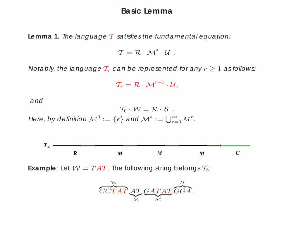
Basic Lemma

Lemma 1. The language T satisfies the fundamental equation:

T = R · M∗ · U .

Notably, the language Tr can be represented for any r ≥ 1 as follows:

Tr = R · Mr−1 · U ,

andT0 · W = R · S .

Here, by definition M0 := ε and M∗ :=S∞

r=0 Mr.

R M M M UT4

Example: Let W = TAT . The following string belongs T3:

Rz | CCTAT AT|z

MGATAT| z

M

Uz | GGA .

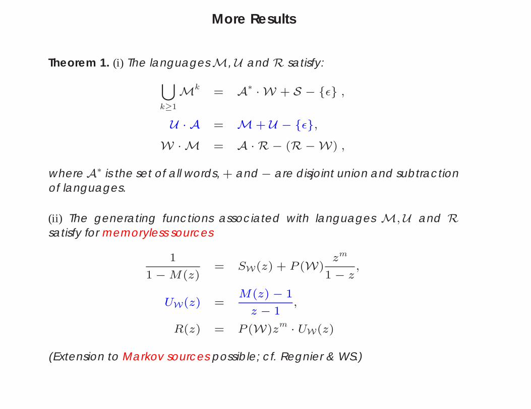
More Results

Theorem 1. (i) The languages M, U and R satisfy:[k≥1

Mk= A∗ · W + S − ε ,

U · A = M + U − ε,

W · M = A · R − (R − W) ,

where A∗ is the set of all words, + and − are disjoint union and subtractionof languages.

(ii) The generating functions associated with languages M,U and Rsatisfy for memoryless sources

1

1 − M(z)= SW(z) + P (W)

zm

1 − z,

UW(z) =M(z) − 1

z − 1,

R(z) = P (W)zm · UW(z)

(Extension to Markov sources possible; cf. Regnier & WS.)

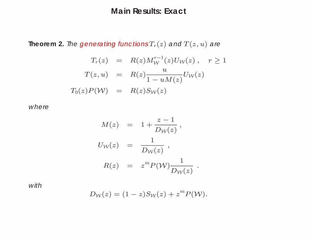
Main Results: Exact

Theorem 2. The generating functions Tr(z) and T (z, u) are

Tr(z) = R(z)Mr−1W (z)UW(z) , r ≥ 1

T (z, u) = R(z)u

1 − uM(z)UW(z)

T0(z)P (W) = R(z)SW(z)

where

M(z) = 1 +z − 1

DW(z),

UW(z) =1

DW(z),

R(z) = zmP (W)1

DW(z).

withDW(z) = (1 − z)SW(z) + z

mP (W).

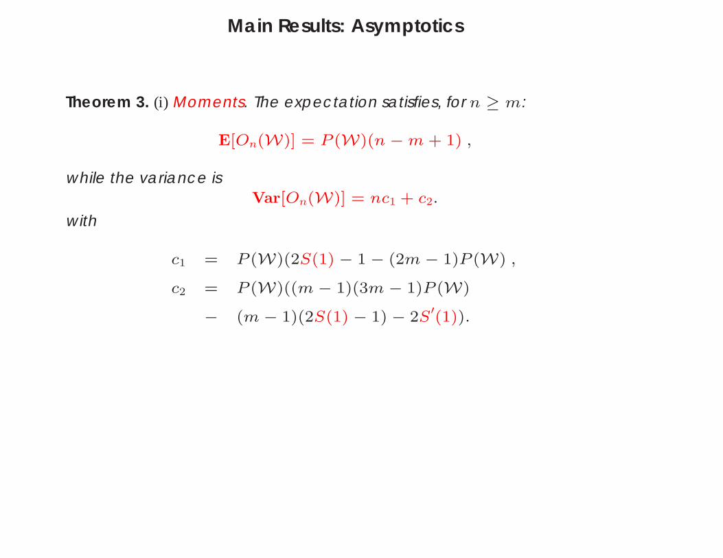
Main Results: Asymptotics

Theorem 3. (i) Moments. The expectation satisfies, for n ≥ m:

E[On(W)] = P (W)(n − m + 1) ,

while the variance isVar[On(W)] = nc1 + c2.

with

c1 = P (W)(2S(1) − 1 − (2m − 1)P (W) ,

c2 = P (W)((m − 1)(3m − 1)P (W)

− (m − 1)(2S(1) − 1) − 2S′(1)).

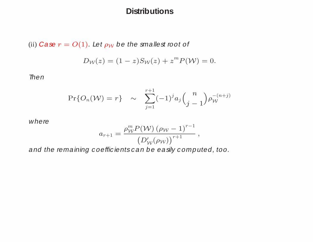
Distributions

(ii) Case r = O(1). Let ρW be the smallest root of

DW(z) = (1 − z)SW(z) + zm

P (W) = 0.

Then

PrOn(W) = r ∼r+1Xj=1

(−1)jaj

“ n

j − 1

”ρ−(n+j)W

where

ar+1 =ρmWP (W) (ρW − 1)r−1`

D′W(ρW)

´r+1,

and the remaining coefficients can be easily computed, too.

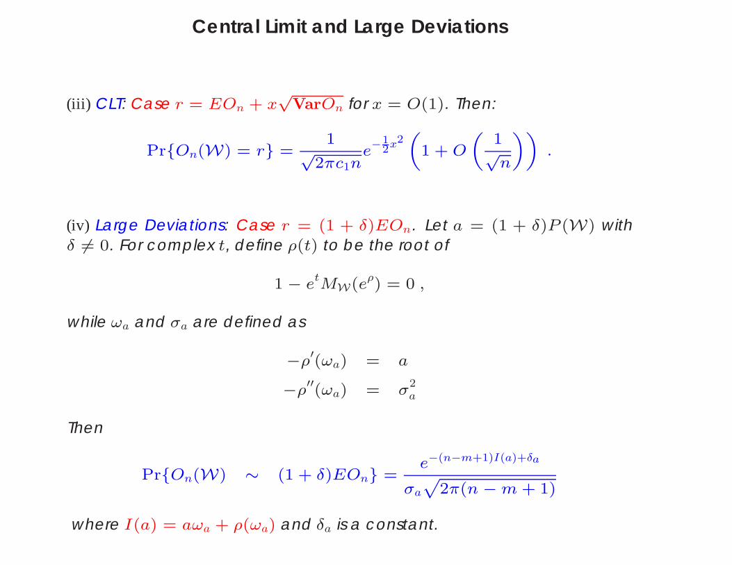
Central Limit and Large Deviations

(iii) CLT: Case r = EOn + x√

VarOn for x = O(1). Then:

PrOn(W) = r =1

√2πc1n

e−1

2x2„

1 + O

„1

√n

««.

(iv) Large Deviations: Case r = (1 + δ)EOn. Let a = (1 + δ)P (W) withδ 6= 0. For complex t, define ρ(t) to be the root of

1 − etMW(eρ) = 0 ,

while ωa and σa are defined as

−ρ′(ωa) = a

−ρ′′(ωa) = σ2a

Then

PrOn(W) ∼ (1 + δ)EOn =e−(n−m+1)I(a)+δa

σa

p2π(n − m + 1)

where I(a) = aωa + ρ(ωa) and δa is a constant.

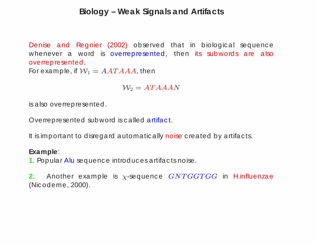
Biology – Weak Signals and Artifacts

Denise and Regnier (2002) observed that in biological sequencewhenever a word is overrepresented, then its subwords are alsooverrepresented.For example, if W1 = AATAAA, then

W2 = ATAAAN

is also overrepresented.

Overrepresented subword is called artifact.

It is important to disregard automatically noise created by artifacts.

Example:1. Popular Alu sequence introduces artifacts noise.

2. Another example is χ-sequence GNTGGTGG in H.influenzae(Nicodeme, 2000).

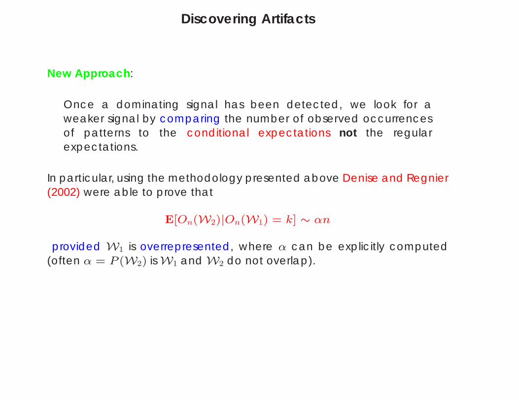
Discovering Artifacts

New Approach:

Once a dominating signal has been detected, we look for aweaker signal by comparing the number of observed occurrencesof patterns to the conditional expectations not the regularexpectations.

In particular, using the methodology presented above Denise and Regnier(2002) were able to prove that

E[On(W2)|On(W1) = k] ∼ αn

provided W1 is overrepresented, where α can be explicitly computed(often α = P (W2) is W1 and W2 do not overlap).

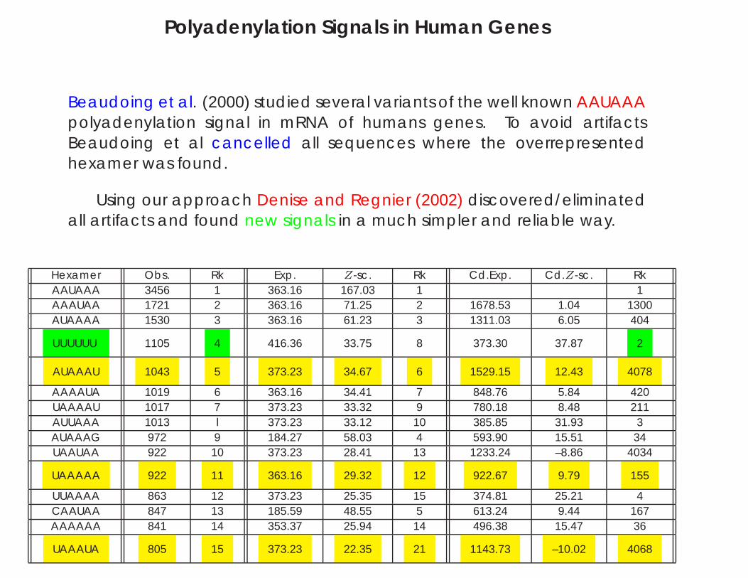
Polyadenylation Signals in Human Genes

Beaudoing et al. (2000) studied several variants of the well known AAUAAApolyadenylation signal in mRNA of humans genes. To avoid artifactsBeaudoing et al cancelled all sequences where the overrepresentedhexamer was found.

Using our approach Denise and Regnier (2002) discovered/eliminatedall artifacts and found new signals in a much simpler and reliable way.

Hexamer Obs. Rk Exp. Z-sc. Rk Cd.Exp. Cd.Z-sc. RkAAUAAA 3456 1 363.16 167.03 1 1AAAUAA 1721 2 363.16 71.25 2 1678.53 1.04 1300AUAAAA 1530 3 363.16 61.23 3 1311.03 6.05 404

UUUUUU 1105 4 416.36 33.75 8 373.30 37.87 2

AUAAAU 1043 5 373.23 34.67 6 1529.15 12.43 4078

AAAAUA 1019 6 363.16 34.41 7 848.76 5.84 420UAAAAU 1017 7 373.23 33.32 9 780.18 8.48 211AUUAAA 1013 l 373.23 33.12 10 385.85 31.93 3AUAAAG 972 9 184.27 58.03 4 593.90 15.51 34UAAUAA 922 10 373.23 28.41 13 1233.24 –8.86 4034

UAAAAA 922 11 363.16 29.32 12 922.67 9.79 155

UUAAAA 863 12 373.23 25.35 15 374.81 25.21 4CAAUAA 847 13 185.59 48.55 5 613.24 9.44 167AAAAAA 841 14 353.37 25.94 14 496.38 15.47 36

UAAAUA 805 15 373.23 22.35 21 1143.73 –10.02 4068

Outline of the Talk

1. Pattern Matching Problems

2. Biology

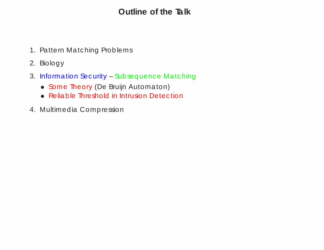
3. Information Security – Subsequence Matching

• Some Theory (De Bruijn Automaton)• Reliable Threshold in Intrusion Detection

4. Multimedia Compression

Application – Information Security

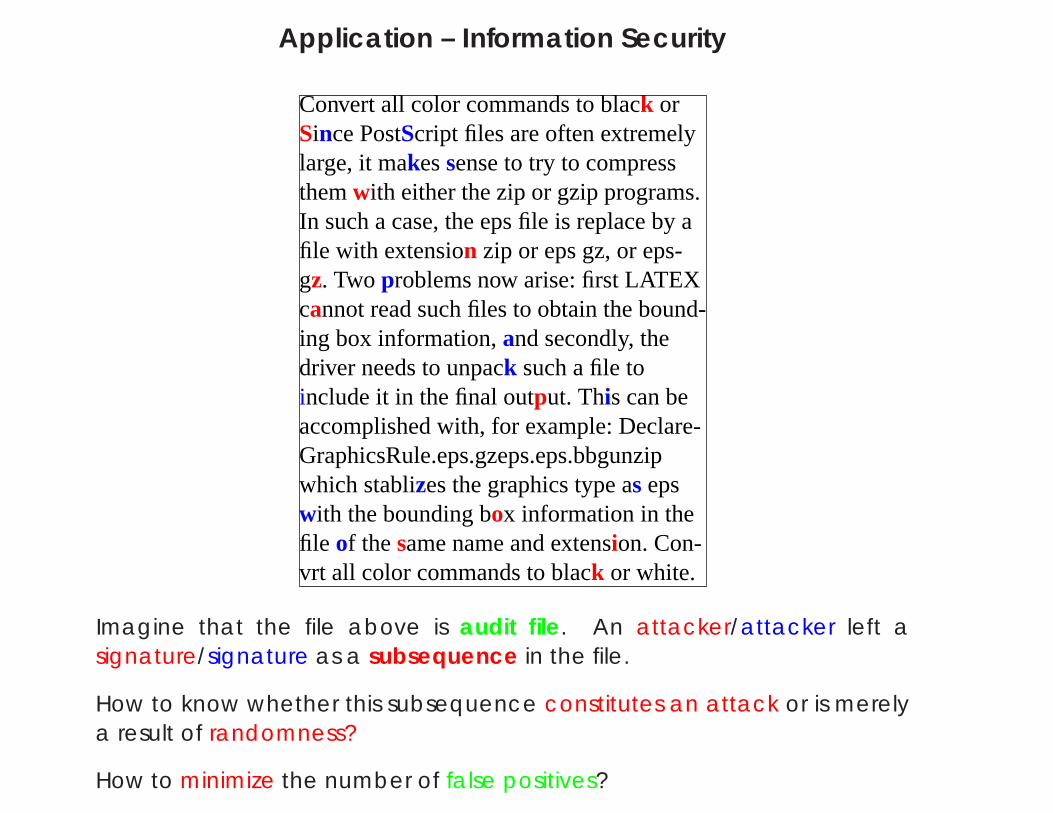
Convert all color commands to black orSince PostScript files are often extremelylarge, it makessense to try to compressthemwith either the zip or gzip programs.In such a case, the eps file is replace by afile with extension zip or eps gz, or eps-gz. Two problems now arise: first LATEXcannot read such files to obtain the bound-ing box information,and secondly, thedriver needs to unpack such a file toinclude it in the final output. This can beaccomplished with, for example: Declare-GraphicsRule.eps.gzeps.eps.bbgunzipwhich stablizes the graphics type as epswith the bounding box information in thefile of thesame name and extension. Con-vrt all color commands to black or white.

Imagine that the file above is audit file. An attacker/attacker left asignature/signature as a subsequence in the file.

How to know whether this subsequence constitutes an attack or is merelya result of randomness?

How to minimize the number of false positives?

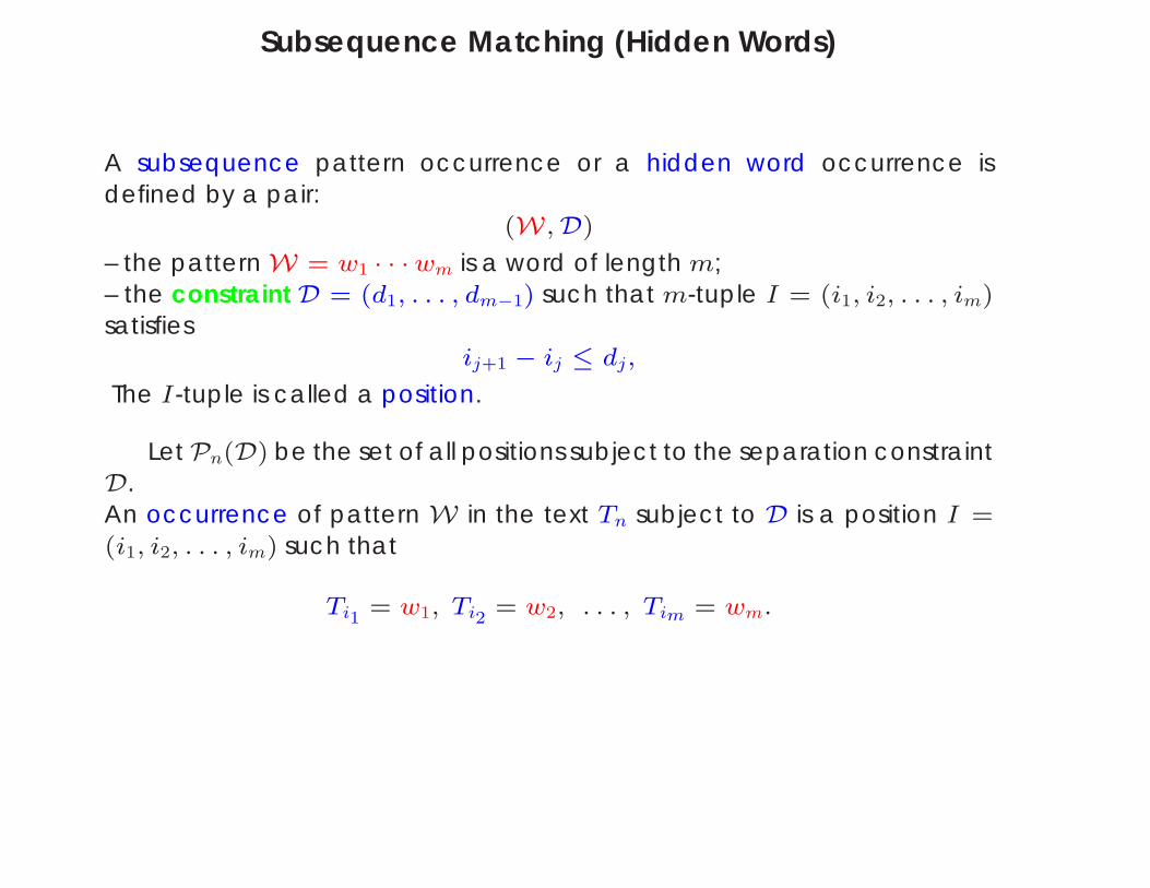
Subsequence Matching (Hidden Words)

A subsequence pattern occurrence or a hidden word occurrence isdefined by a pair:

(W,D)

– the pattern W = w1 · · ·wm is a word of length m;– the constraint D = (d1, . . . , dm−1) such that m-tuple I = (i1, i2, . . . , im)satisfies

ij+1 − ij ≤ dj,

The I-tuple is called a position.

Let Pn(D) be the set of all positions subject to the separation constraintD.An occurrence of pattern W in the text Tn subject to D is a position I =(i1, i2, . . . , im) such that

Ti1= w1, Ti2

= w2, . . . , Tim = wm.

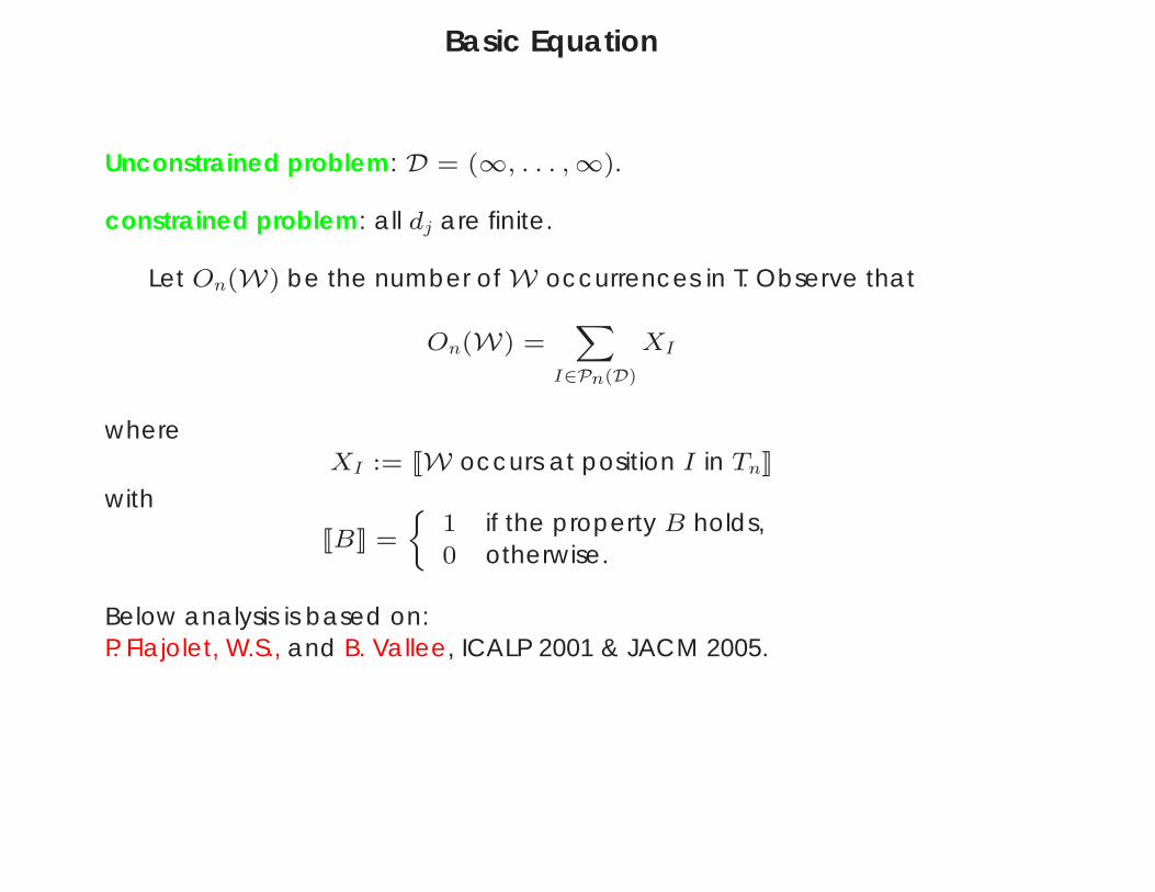
Basic Equation

Unconstrained problem: D = (∞, . . . ,∞).

constrained problem: all dj are finite.

Let On(W) be the number of W occurrences in T. Observe that

On(W) =X

I∈Pn(D)

XI

whereXI := [[W occurs at position I in Tn]]

with

[[B]] =

1 if the property B holds,0 otherwise.

Below analysis is based on:P. Flajolet, W.S., and B. Vallee, ICALP 2001 & JACM 2005.

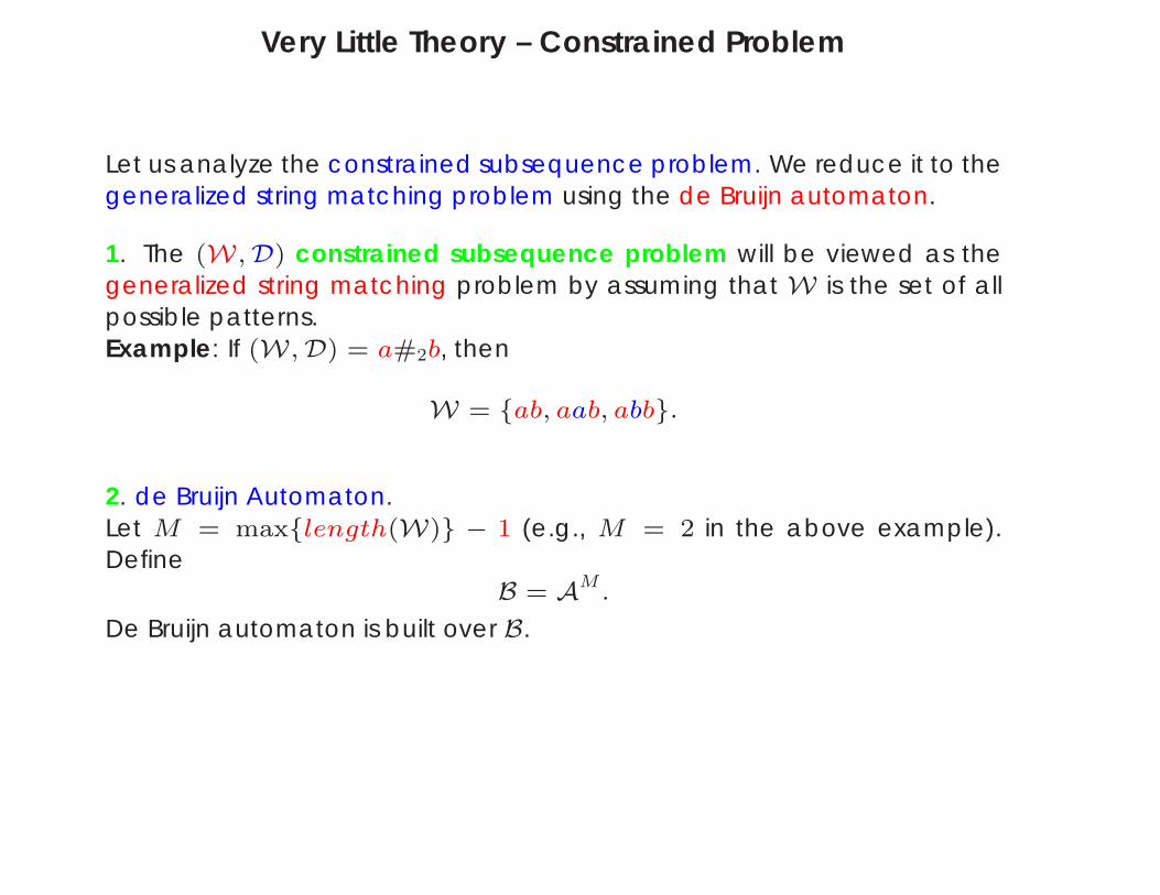
Very Little Theory – Constrained Problem

Let us analyze the constrained subsequence problem. We reduce it to thegeneralized string matching problem using the de Bruijn automaton.

1. The (W,D) constrained subsequence problem will be viewed as thegeneralized string matching problem by assuming that W is the set of allpossible patterns.Example: If (W,D) = a#2b, then

W = ab, aab, abb.

2. de Bruijn Automaton.Let M = maxlength(W) − 1 (e.g., M = 2 in the above example).Define

B = AM.

De Bruijn automaton is built over B.

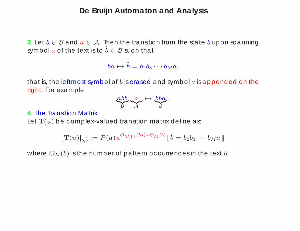
De Bruijn Automaton and Analysis

3. Let b ∈ B and a ∈ A. Then the transition from the state b upon scanningsymbol a of the text is to b ∈ B such that

ba 7→ b = b2b3 · · · bMa,

that is, the leftmost symbol of b is erased and symbol a is appended on theright. For example

abb|zB

a|zA

7→ bba|zB

.

4. The Transition MatrixLet T(u) be complex-valued transition matrix define as:

[T(u)]b,b := P (a)uOM+1(ba)−OM (b)

[[ b = b2b3 · · · bMa ]]

where OM(b) is the number of pattern occurrences in the text b.

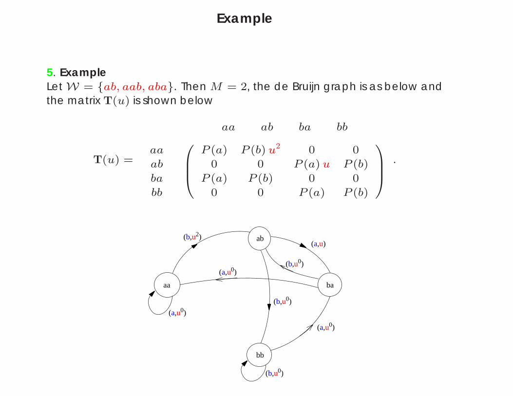
Example

5. ExampleLet W = ab, aab, aba. Then M = 2, the de Bruijn graph is as below andthe matrix T(u) is shown below

T(u) =

aa ab ba bb

aa

ab

ba

bb

0BB@

P (a) P (b) u2 0 0

0 0 P (a) u P (b)

P (a) P (b) 0 0

0 0 P (a) P (b)

1CCA .

ab

aa

bb

ba

(b,u2)

(b,u0)

(a,u)

(a,u0)

(b,u0)

(a,u0)

(b,u0)

(a,u0)

Generating Functions

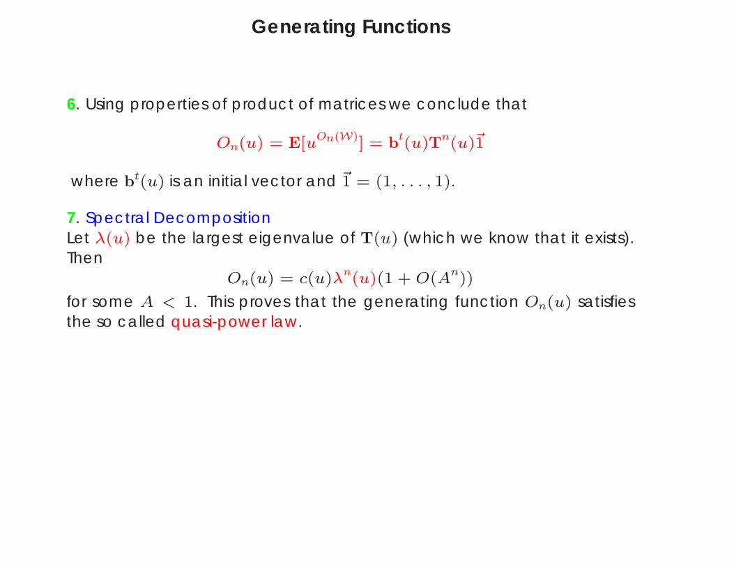
6. Using properties of product of matrices we conclude that

On(u) = E[uOn(W)] = bt(u)Tn(u)~1

where bt(u) is an initial vector and ~1 = (1, . . . , 1).

7. Spectral DecompositionLet λ(u) be the largest eigenvalue of T(u) (which we know that it exists).Then

On(u) = c(u)λn(u)(1 + O(A

n))

for some A < 1. This proves that the generating function On(u) satisfiesthe so called quasi-power law.

Final Results

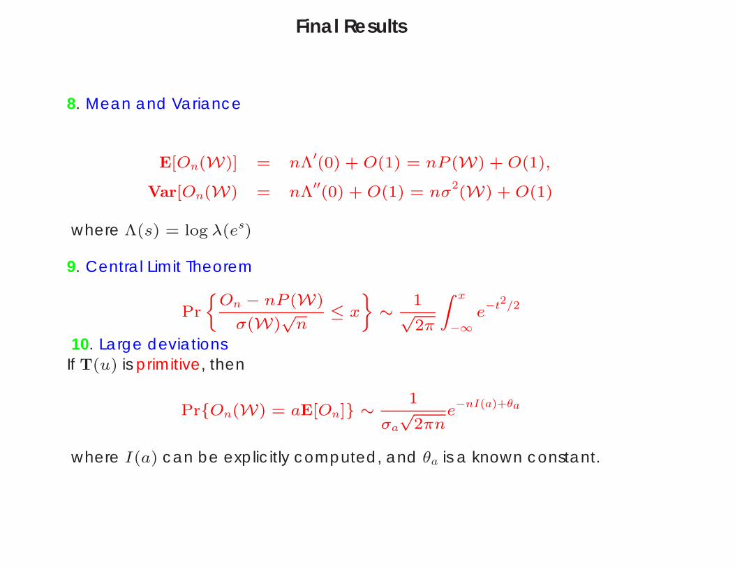
8. Mean and Variance

E[On(W)] = nΛ′(0) + O(1) = nP (W) + O(1),

Var[On(W) = nΛ′′(0) + O(1) = nσ

2(W) + O(1)

where Λ(s) = log λ(es)

9. Central Limit Theorem

Pr

On − nP (W)

σ(W)√

n≤ x

ff∼

1√

2π

Z x

−∞e−t2/2

10. Large deviationsIf T(u) is primitive, then

PrOn(W) = aE[On] ∼1

σa

√2πn

e−nI(a)+θa

where I(a) can be explicitly computed, and θa is a known constant.

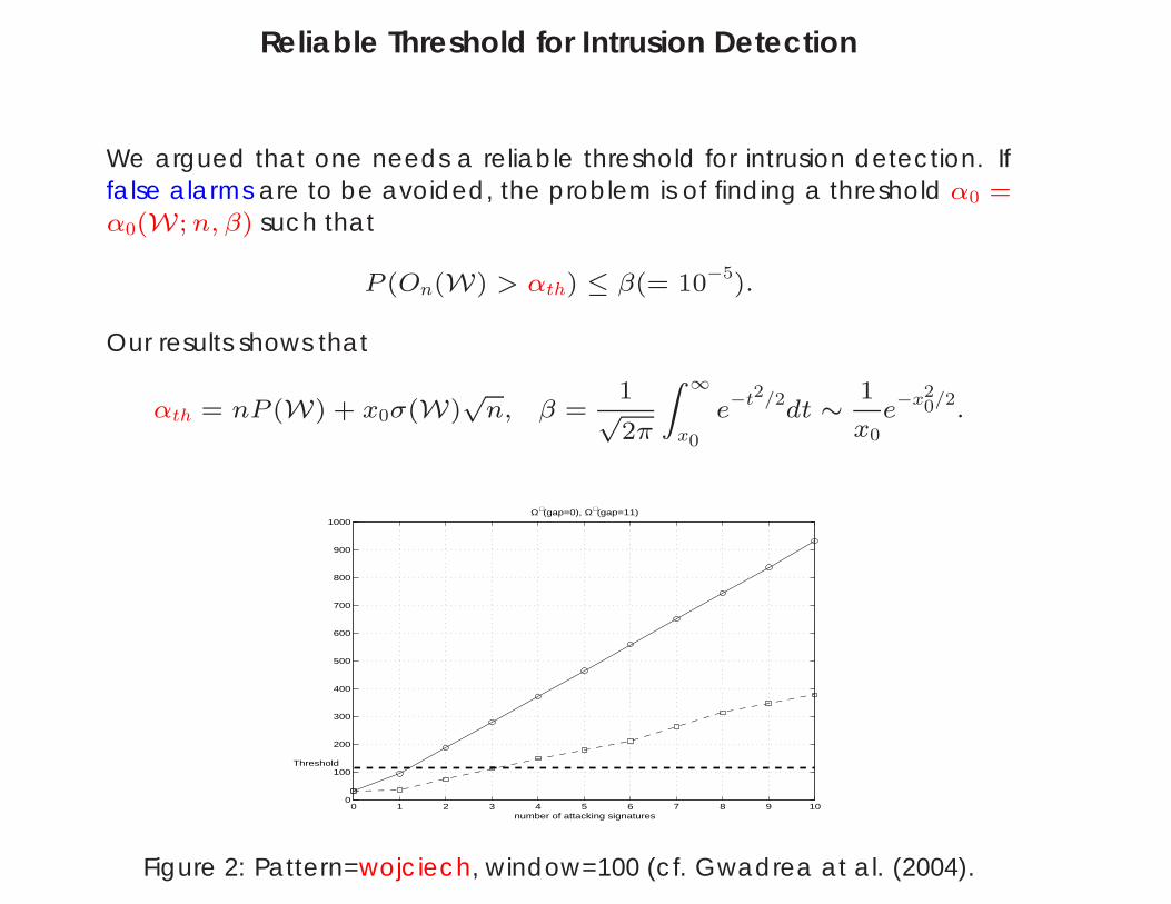
Reliable Threshold for Intrusion Detection

We argued that one needs a reliable threshold for intrusion detection. Iffalse alarms are to be avoided, the problem is of finding a threshold α0 =α0(W; n, β) such that

P (On(W) > αth) ≤ β(= 10−5).

Our results shows that

αth = nP (W) + x0σ(W)√

n, β =1

√2π

Z ∞

x0

e−t2/2

dt ∼1

x0

e−x2

0/2.

0 1 2 3 4 5 6 7 8 9 100

100

200

300

400

500

600

700

800

900

1000

number of attacking signatures

Ω∃(gap=0), Ω∃(gap=11)

Threshold

Figure 2: Pattern=wojciech, window=100 (cf. Gwadrea at al. (2004).

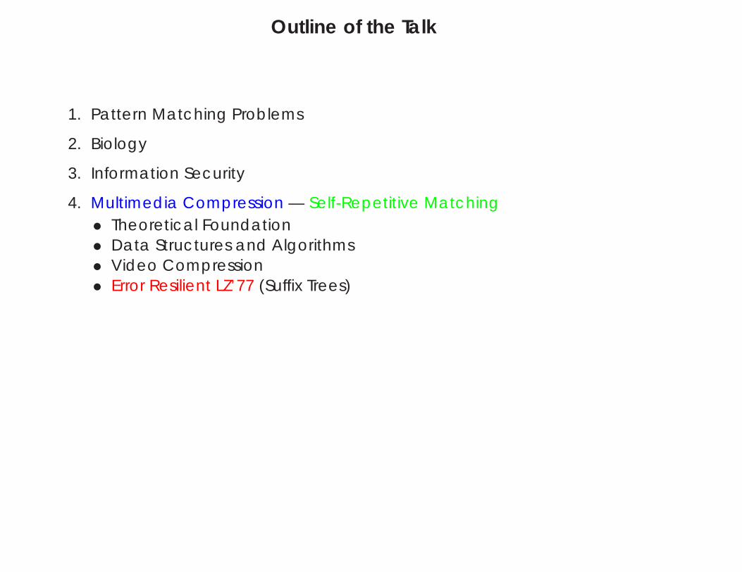
Outline of the Talk

1. Pattern Matching Problems

2. Biology

3. Information Security

4. Multimedia Compression — Self-Repetitive Matching• Theoretical Foundation (Renyi’s Entropy)• Data Structures and Algorithms• Video Compression (Demo)• Error Resilient LZ’77 (Suffix Trees)

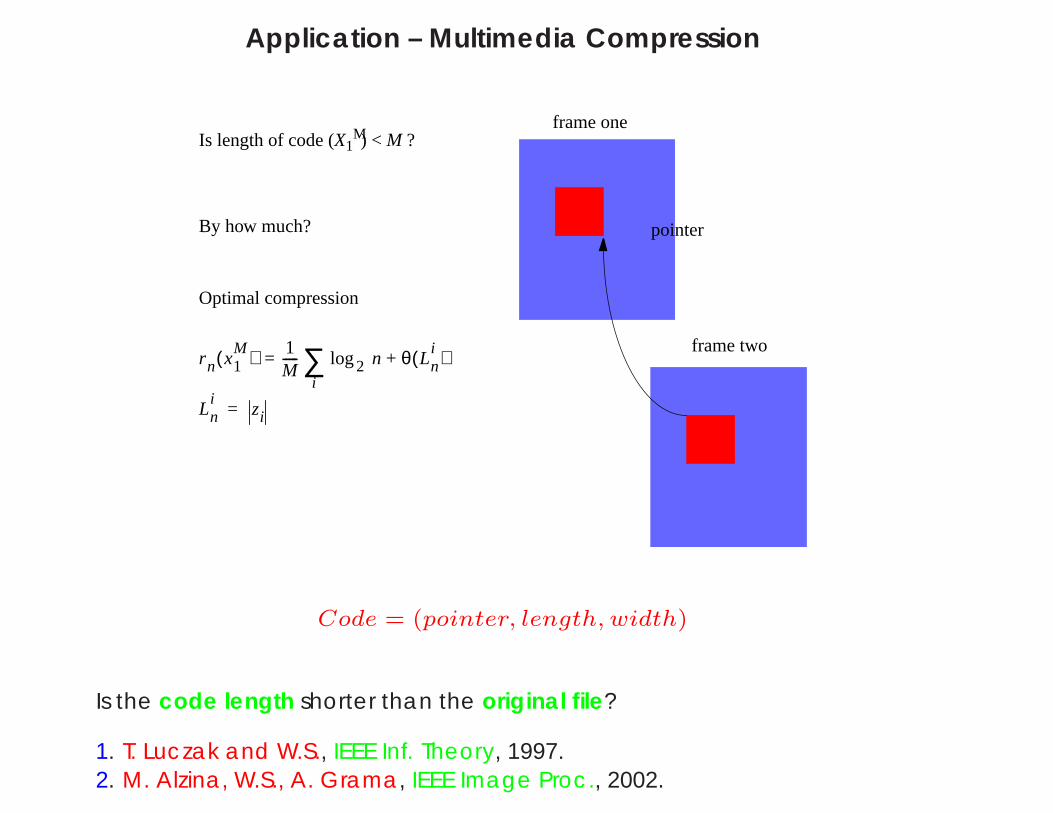
Application – Multimedia Compression

frame one

frame two

pointer

Is length of code (X1M) < M ?

By how much?

Optimal compression

rn x1M( ) 1

M----- log2 n θ Ln

i( )+i

∑=

Lni

zi=

Code = (pointer, length, width)

Is the code length shorter than the original file?

1. T. Luczak and W.S., IEEE Inf. Theory, 1997.2. M. Alzina, W.S., A. Grama, IEEE Image Proc., 2002.

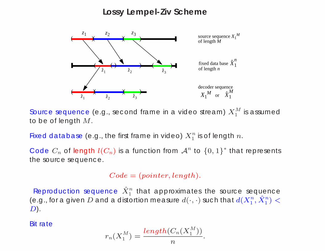
Lossy Lempel-Ziv Scheme

z1 z2 z3( ( (

)

) ) )

z3

z2z1 z3

z2z1

)(

( ))

(

(

source sequenceX1M

of length M

fixed data baseX1n

of lengthn

decoder sequence

X1M

X1M or

)(

(

)

Source sequence (e.g., second frame in a video stream) XM1 is assumed

to be of length M .

Fixed database (e.g., the first frame in video) Xn1 is of length n.

Code Cn of length l(Cn) is a function from An to 0, 1∗ that representsthe source sequence.

Code = (pointer, length).

Reproduction sequence Xn1 that approximates the source sequence

(e.g., for a given D and a distortion measure d(·, ·) such that d(Xn1 , Xn

1 ) <D).

Bit rate

rn(XM1 ) =

length(Cn(XM1 ))

n.

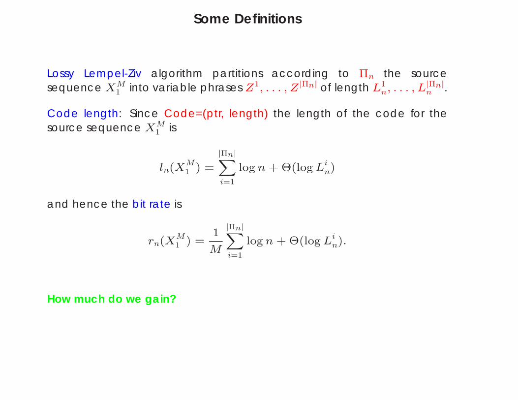
Some Definitions

Lossy Lempel-Ziv algorithm partitions according to Πn the sourcesequence XM

1 into variable phrases Z1, . . . , Z|Πn| of length L1n, . . . , L|Πn|

n .

Code length: Since Code=(ptr, length) the length of the code for thesource sequence XM

1 is

ln(XM1 ) =

|Πn|Xi=1

log n + Θ(log Lin)

and hence the bit rate is

rn(XM1 ) =

1

M

|Πn|Xi=1

log n + Θ(log Lin).

How much do we gain?

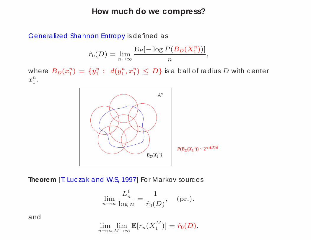
How much do we compress?

Generalized Shannon Entropy is defined as

r0(D) = limn→∞

EP [− log P (BD(Xn1 ))]

n,

where BD(xn1 ) = yn

1 : d(yn1 , xn

1 ) ≤ D is a ball of radius D with centerxn

1 .

An

BD(X1n)

P(BD(X1n)) ~ 2-r0(D)⋅n

Theorem [T. Luczak and W.S, 1997] For Markov sources

limn→∞

L1n

log n=

1

r0(D), (pr.).

andlim

n→∞lim

M→∞E[rn(X

M1 )] = r0(D).

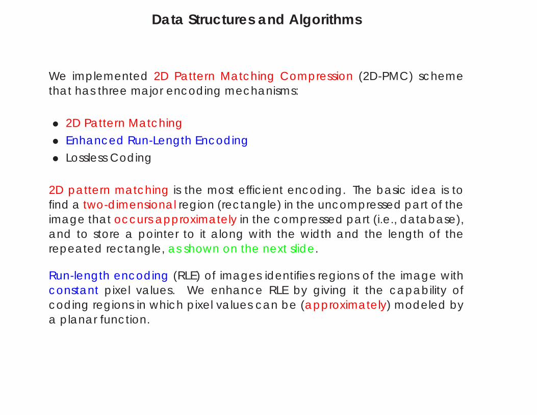
Data Structures and Algorithms

We implemented 2D Pattern Matching Compression (2D-PMC) schemethat has three major encoding mechanisms:

• 2D Pattern Matching

• Enhanced Run-Length Encoding

• Lossless Coding

2D pattern matching is the most efficient encoding. The basic idea is tofind a two-dimensional region (rectangle) in the uncompressed part of theimage that occurs approximately in the compressed part (i.e., database),and to store a pointer to it along with the width and the length of therepeated rectangle, as shown on the next slide.

Run-length encoding (RLE) of images identifies regions of the image withconstant pixel values. We enhance RLE by giving it the capability ofcoding regions in which pixel values can be (approximately) modeled bya planar function.

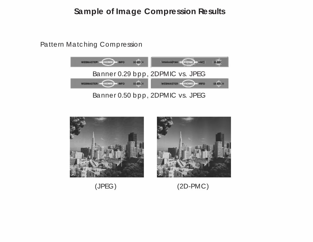
Sample of Image Compression Results

Pattern Matching Compression

Banner 0.29 bpp, 2DPMIC vs. JPEG

Banner 0.50 bpp, 2DPMIC vs. JPEG

(JPEG) (2D-PMC)

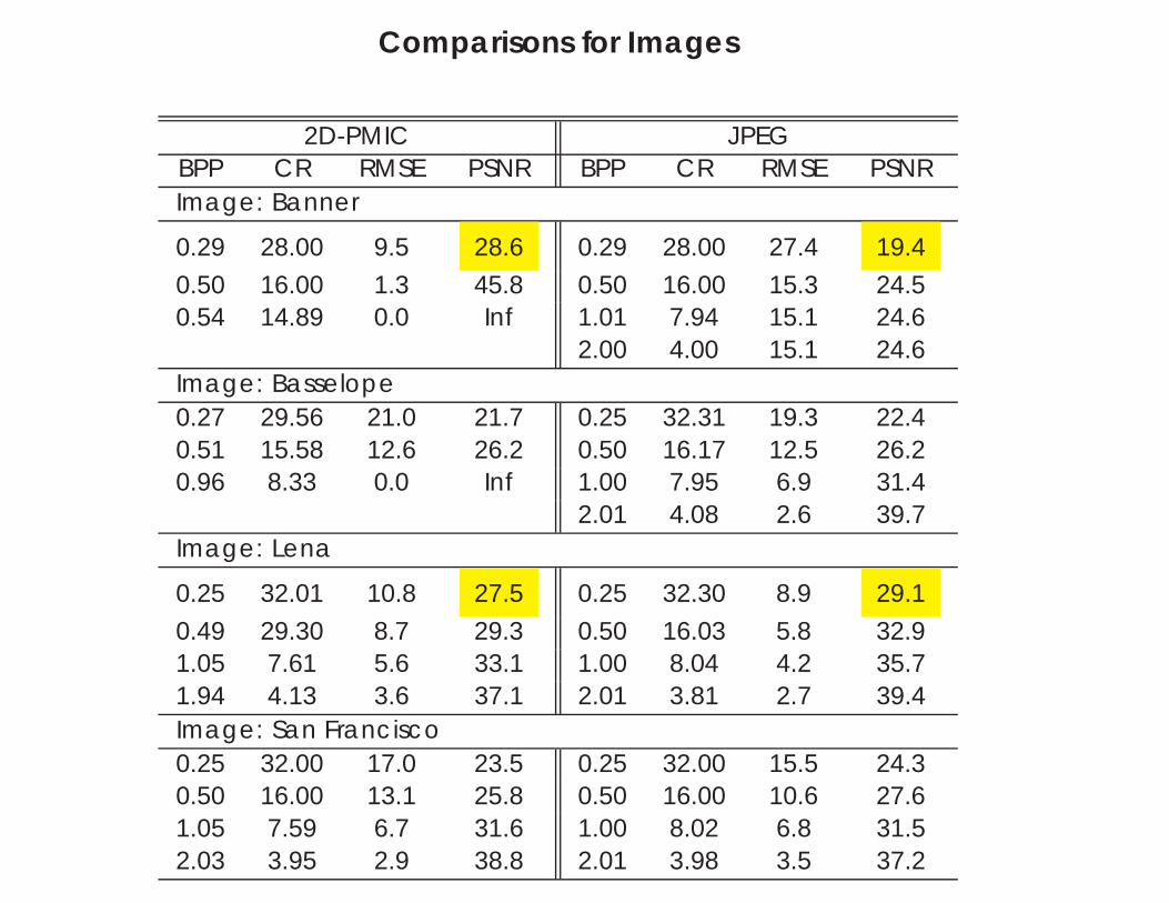
Comparisons for Images

2D-PMIC JPEGBPP CR RMSE PSNR BPP CR RMSE PSNRImage: Banner

0.29 28.00 9.5 28.6 0.29 28.00 27.4 19.4

0.50 16.00 1.3 45.8 0.50 16.00 15.3 24.50.54 14.89 0.0 Inf 1.01 7.94 15.1 24.6

2.00 4.00 15.1 24.6Image: Basselope0.27 29.56 21.0 21.7 0.25 32.31 19.3 22.40.51 15.58 12.6 26.2 0.50 16.17 12.5 26.20.96 8.33 0.0 Inf 1.00 7.95 6.9 31.4

2.01 4.08 2.6 39.7Image: Lena

0.25 32.01 10.8 27.5 0.25 32.30 8.9 29.1

0.49 29.30 8.7 29.3 0.50 16.03 5.8 32.91.05 7.61 5.6 33.1 1.00 8.04 4.2 35.71.94 4.13 3.6 37.1 2.01 3.81 2.7 39.4Image: San Francisco0.25 32.00 17.0 23.5 0.25 32.00 15.5 24.30.50 16.00 13.1 25.8 0.50 16.00 10.6 27.61.05 7.59 6.7 31.6 1.00 8.02 6.8 31.52.03 3.95 2.9 38.8 2.01 3.98 3.5 37.2

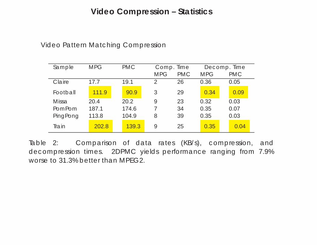
Video Compression – Statistics

Video Pattern Matching Compression

Sample MPG PMC Comp. Time Decomp. TimeMPG PMC MPG PMC

Claire 17.7 19.1 2 26 0.36 0.05

Football 111.9 90.9 3 29 0.34 0.09

Missa 20.4 20.2 9 23 0.32 0.03PomPom 187.1 174.6 7 34 0.35 0.07PingPong 113.8 104.9 8 39 0.35 0.03

Train 202.8 139.3 9 25 0.35 0.04

Table 2: Comparison of data rates (KB/s), compression, anddecompression times. 2DPMC yields performance ranging from 7.9%worse to 31.3% better than MPEG2.

Outline of the Talk

1. Pattern Matching Problems

2. Biology

3. Information Security

4. Multimedia Compression — Self-Repetitive Matching• Theoretical Foundation• Data Structures and Algorithms• Video Compression• Error Resilient LZ’77 (Suffix Trees)

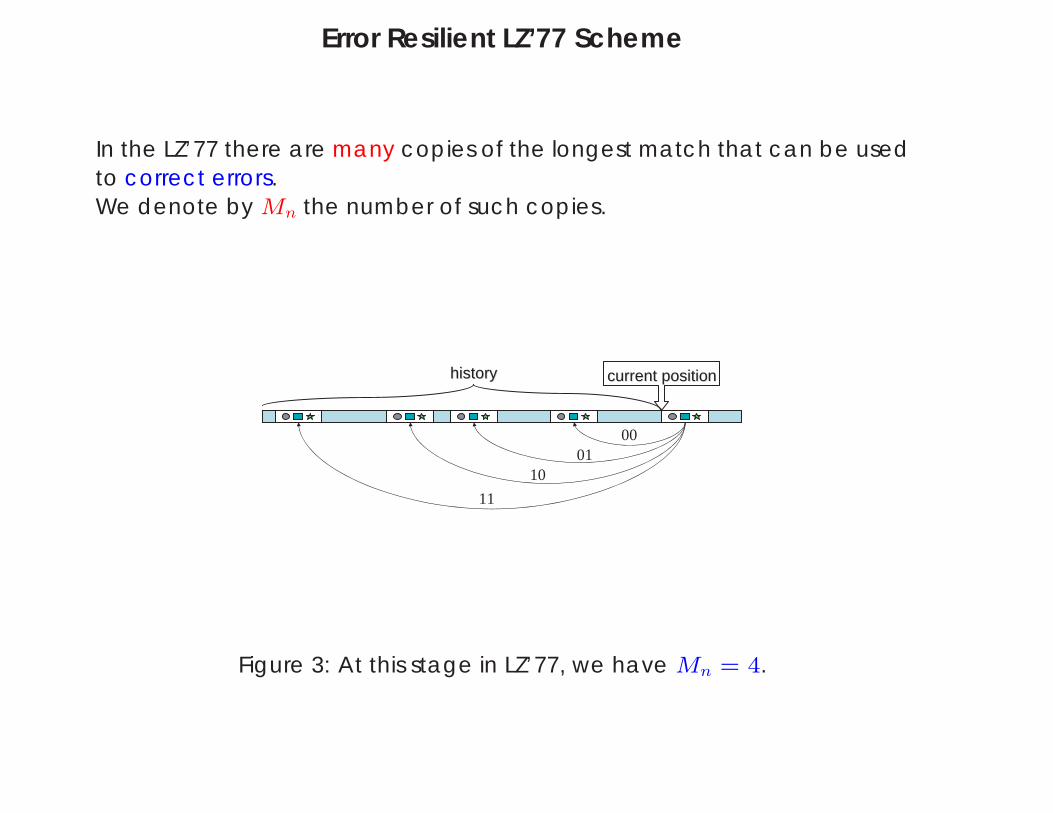
Error Resilient LZ’77 Scheme

In the LZ’77 there are many copies of the longest match that can be usedto correct errors.We denote by Mn the number of such copies.

historyhistory current positioncurrent position

0001

10

11

Figure 3: At this stage in LZ’77, we have Mn = 4.

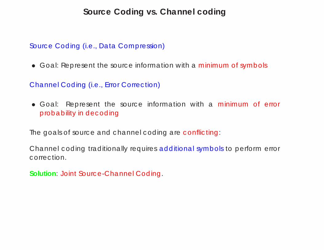
Source Coding vs. Channel coding

Source Coding (i.e., Data Compression)

• Goal: Represent the source information with a minimum of symbols

Channel Coding (i.e., Error Correction)

• Goal: Represent the source information with a minimum of errorprobability in decoding

The goals of source and channel coding are conflicting:

Channel coding traditionally requires additional symbols to perform errorcorrection.

Solution: Joint Source-Channel Coding.

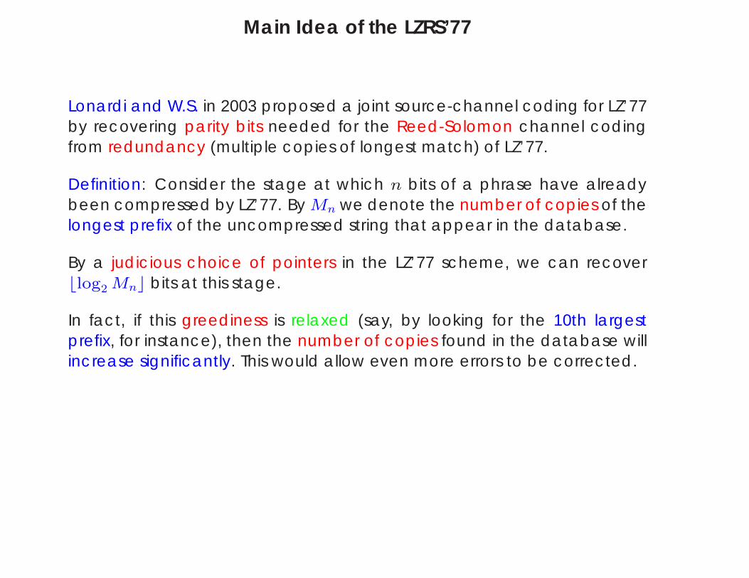
Main Idea of the LZRS’77

Lonardi and W.S. in 2003 proposed a joint source-channel coding for LZ’77by recovering parity bits needed for the Reed-Solomon channel codingfrom redundancy (multiple copies of longest match) of LZ’77.

Definition: Consider the stage at which n bits of a phrase have alreadybeen compressed by LZ’77. By Mn we denote the number of copies of thelongest prefix of the uncompressed string that appear in the database.

By a judicious choice of pointers in the LZ’77 scheme, we can recoverblog2 Mnc bits at this stage.

In fact, if this greediness is relaxed (say, by looking for the 10th largestprefix, for instance), then the number of copies found in the database willincrease significantly. This would allow even more errors to be corrected.

Encoder and Decoder of LZRS’77

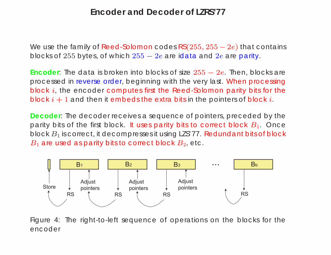
We use the family of Reed-Solomon codes RS(255, 255− 2e) that containsblocks of 255 bytes, of which 255 − 2e are idata and 2e are parity.

Encoder: The data is broken into blocks of size 255 − 2e. Then, blocks areprocessed in reverse order, beginning with the very last. When processingblock i, the encoder computes first the Reed-Solomon parity bits for theblock i + 1 and then it embeds the extra bits in the pointers of block i.

Decoder: The decoder receives a sequence of pointers, preceded by theparity bits of the first block. It uses parity bits to correct block B1. Onceblock B1 is correct, it decompresses it using LZS’77. Redundant bits of blockB1 are used as parity bits to correct block B2, etc.

RS

Adjust

pointers

RS

Adjust

pointers

B1 ...

RS

B2 B3 Bb

RS

Adjust

pointersStore

Figure 4: The right-to-left sequence of operations on the blocks for theencoder

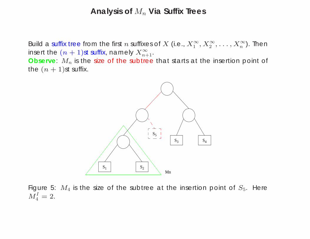
Analysis of Mn Via Suffix Trees

Build a suffix tree from the first n suffixes of X (i.e., X∞1 , X∞

2 , . . . , X∞n ). Then

insert the (n + 1)st suffix, namely X∞n+1.

Observe: Mn is the size of the subtree that starts at the insertion point ofthe (n + 1)st suffix.

S1 S2

S3 S4

S5

Mn

Figure 5: M4 is the size of the subtree at the insertion point of S5. HereMI

4 = 2.

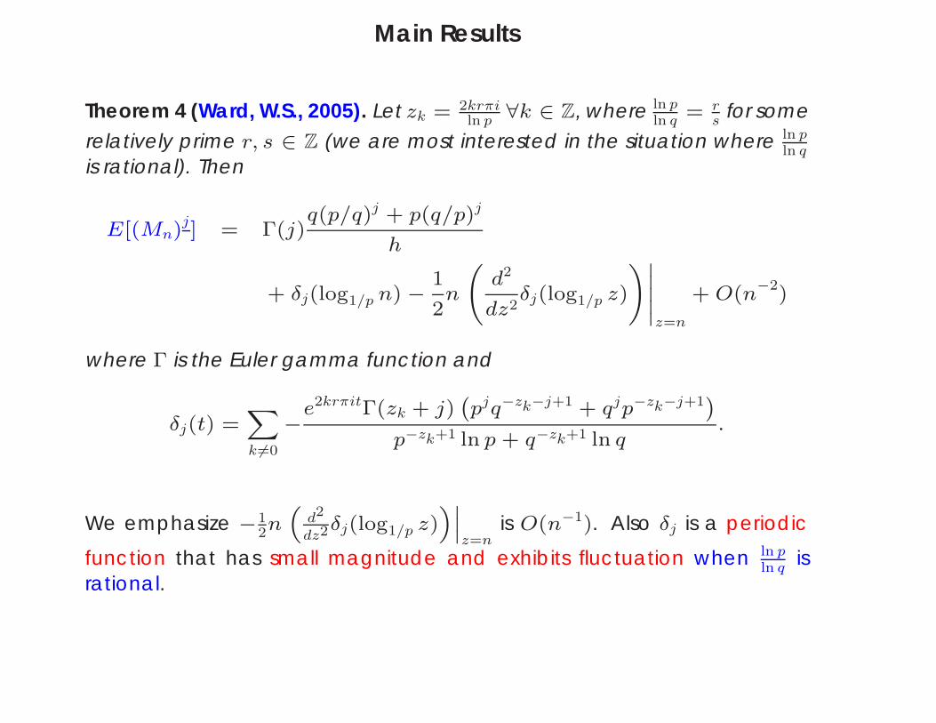
Main Results

Theorem 4 (Ward, W.S., 2005). Let zk = 2krπiln p ∀k ∈ Z, where ln p

ln q = rs for some

relatively prime r, s ∈ Z (we are most interested in the situation where ln pln q

is rational). Then

E[(Mn)j] = Γ(j)

q(p/q)j + p(q/p)j

h

+ δj(log1/p n) −1

2n

d2

dz2δj(log1/p z)

!˛˛z=n

+ O(n−2

)

where Γ is the Euler gamma function and

δj(t) =Xk 6=0

−e2krπitΓ(zk + j)

`pjq−zk−j+1 + qjp−zk−j+1

´p−zk+1 ln p + q−zk+1 ln q

.

We emphasize −12n“

d2

dz2δj(log1/p z)”˛

z=nis O(n−1). Also δj is a periodic

function that has small magnitude and exhibits fluctuation when ln pln q is

rational.

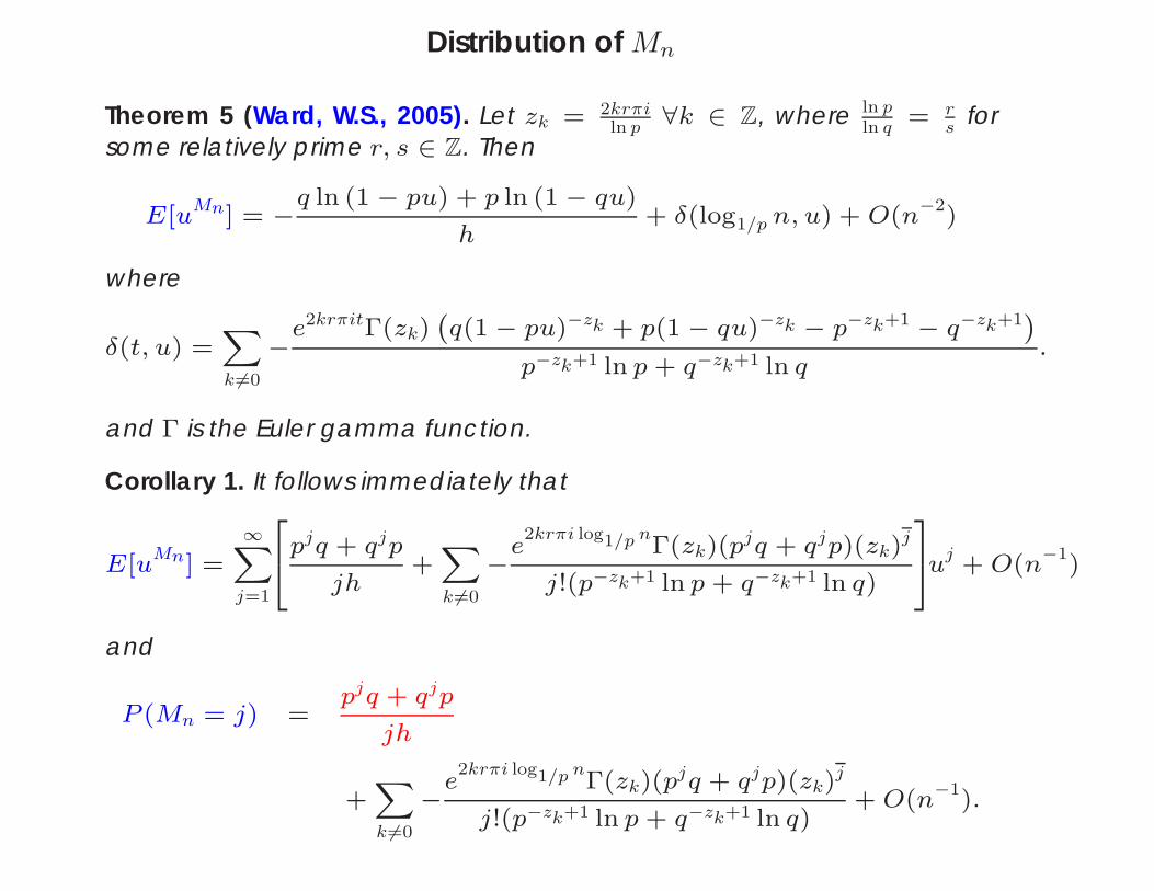
Distribution of Mn

Theorem 5 (Ward, W.S., 2005). Let zk = 2krπiln p ∀k ∈ Z, where ln p

ln q = rs for

some relatively prime r, s ∈ Z. Then

E[uMn] = −q ln (1 − pu) + p ln (1 − qu)

h+ δ(log1/p n, u) + O(n−2)

where

δ(t, u) =Xk 6=0

−e2krπitΓ(zk)

`q(1 − pu)−zk + p(1 − qu)−zk − p−zk+1 − q−zk+1

´p−zk+1 ln p + q−zk+1 ln q

.

and Γ is the Euler gamma function.

Corollary 1. It follows immediately that

E[uMn] =

∞Xj=1

24pjq + qjp

jh+Xk 6=0

−e

2krπi log1/p nΓ(zk)(p

jq + qjp)(zk)j

j!(p−zk+1 ln p + q−zk+1 ln q)

35uj

+ O(n−1

)

and

P (Mn = j) =pjq + qjp

jh

+Xk 6=0

−e

2krπi log1/p nΓ(zk)(p

jq + qjp)(zk)j

j!(p−zk+1 ln p + q−zk+1 ln q)+ O(n−1).