HAL Id: hal-00696408https://hal.inria.fr/hal-00696408

Submitted on 13 May 2012

HAL is a multi-disciplinary open accessarchive for the deposit and dissemination of sci-entific research documents, whether they are pub-lished or not. The documents may come fromteaching and research institutions in France orabroad, or from public or private research centers.

L’archive ouverte pluridisciplinaire HAL, estdestinée au dépôt et à la diffusion de documentsscientifiques de niveau recherche, publiés ou non,émanant des établissements d’enseignement et derecherche français ou étrangers, des laboratoirespublics ou privés.

Uncertainty control for reliable video understanding oncomplex environments

Marcos Zuniga, Francois Bremond, Monique Thonnat

To cite this version:Marcos Zuniga, Francois Bremond, Monique Thonnat. Uncertainty control for reliable video under-standing on complex environments. Weiyao Lin. Video Surveillance, InTech, 2011, 978-953-307-436-8.<10.5772/15606>. <hal-00696408>

1

Uncertainty control for reliable video undertandingon complex environments

Marcos Zúñigamarcos.zuniga@usm.cl

Electronics Department, Universidad Técnica Federico Santa María, Av. España 1680,Valparaíso, Chile

François Brémond and Monique ThonnatFrancois.Bremond@sophia.inria.fr,Monique.Thonnat@sophia.inria.fr

Project-Team PULSAR, INRIA, 2004 route des Lucioles,Sophia Antipolis, France

1. Introduction

Themost popular applications for video understanding are those related to video-surveillance(e.g. alarms, abnormal behaviours, expected events, access control). Video understanding hasseveral other applications of high impact to the society as medical supervision, traffic control,violent acts detection, crowd behaviour analysis, among many others. This interest can beclearly observed trough the significant number of research projects approved in this domain:GERHOME 1, CARETAKER 2, ETISEO 3, BEWARE 4, SAMURAI 5, among many others.We propose a new generic video understanding approach able to extract and learn valu-able information from noisy video scenes for real-time applications. This approach is ableto estimate the reliability of the information associated to the objects tracked in the scene, inorder to properly control the uncertainty of data due to noisy videos and many other diffi-culties present in video applications. This approach comprises motion segmentation, objectclassification, tracking and event learning phases.A fundamental objective of this new approach is to treat the video understanding problemin a generic way. This implies implementing a platform able to classify and track diverse ob-jects (e.g. persons, cars, air-planes, animals), and to dynamically adapt to different scene andvideo configurations. This generality will allow to adapt the approach to different applica-tions with minimal effort. Achieving a completely general video understanding approach isan extremely ambitious goal, due to the complexity of the problem and the infinite possibili-ties of situations occurring in real-time. That is why it must be considered as a long term goal,considering many building blocks in the process. This work is focused on building the first

1 GERHOME Project 2005, http://gerhome.cstb.fr2 CARETAKER Project 2006, http://cordis.europa.eu/ist/kct/caretaker_synopsis.htm3 ETISEO Project 2006, http://www-sop.inria.fr/orion/ETISEO/4 BEWARE Project 2008, http://www.eecs.qmul.ac.uk/~sgg/BEWARE/5 SAMURAI Project 2008, http://www.samurai-eu.org/

fundamental blocks allowing a proper management of uncertainty of data in every phaseof the video understanding process.To date, several video understanding platforms have been proposed in the literature (Hu et al.,2004; Lavee et al., 2009). These platforms are normally designed for specific contexts or fortreating specific issues. Normally, they are tested over well-known videos or in extremelycontrolled environments in order to be validated. Moreover, reality is not controlled and itis hardly well-known. The main novelty of this research is to treat the video understand-ing problem in a general way, by modelling different types of uncertainty introduced whenanalysing a video sequence. Modelling uncertainty allows to understand when somethingwill go wrong in the analysis and then to prepare the system to take the necessary actions forpreventing this situation.The main contributions of the proposed approach are: (i) a new algorithm for tracking multi-ple objects in noisy environments, (ii) the utilisation of reliability measures for modelling un-certainty in data and for proper selection of valuable information extracted from noisy data,(iii) the improved capability of tracking to manage multiple visual evidence-target associa-tions, (iv) the combination of 2D image data with 3D information in a dynamics model gov-erned by reliability measures for proper control of uncertainty in data, and (v) a new approachfor event recognition through incremental event learning, driven by reliability measures forselecting the most stable and relevant data.This chapter is organised as follows. First, Section 2 describes the state-of-the-art focused onjustifying the decisions taken for each phase of the approach. Next, Section 3 describes theproposed approach and the involved phases. Then, Section 4 presents results for differentbenchmark videos and applications.

2. Related work

As properly stated in (Hu et al., 2004), general structure in video understanding is comprisedby four main phases: motion segmentation, object classification, tracking, and behaviour anal-ysis (event recognition and learning). In general, two phases can be identified as critical forthe correct achievement of any further event analysis in video: image segmentation and objecttracking. Image segmentation (McIvor, 2000) consists in extracting motion from a currentlyanalysed image frame, based on information extracted from previously acquired information(e.g. background image or model). Multi-target tracking (MTT) problem (Yilmaz et al., 2006)consists in estimating the trajectory of multiple objects as they move in a video scene. In otherwords, tracking consists in assigning consistent labels to the tracked objects in different framesof a video.One of the first approaches focusing on MTT problem is the Multiple Hypothesis Tracking(MHT) algorithm (Reid, 1979), which maintains several correspondence hypotheses for eachobject at each frame. Over more than 30 years, MHT approaches have evolved mostly oncontrolling the exponential growth of hypotheses (Bar-Shalom et al., 2007; Blackman et al.,2001). For controlling this combinatorial explosion of hypotheses all the unlikely hypotheseshave to be eliminated at each frame (for details refer to (Pattipati et al., 2000)). MHT methodshave been extensively used in radar (Rakdham et al., 2007) and sonar tracking systems (Moranet al., 1997). In (Blackman, 2004) a good summary ofMHT applications is presented. However,most of these systems have been validated with simple situations (e.g. non-noisy data).The dynamics models for tracked object attributes and for hypothesis probability calculationutilised by the MHT approaches are sufficient for point representation, but are not suitablefor this work because of their simplicity. The common feature in the dynamics model of these

algorithms is the utilisation of Kalman filtering (Kalman, 1960) for estimation and predictionof object attributes.An alternative to MHT methods is the class of Monte Carlo methods. The most popularof these algorithms are CONDENSATION (CONditional DENSity PropagATION) (Isard &Blake, 1998) and particle filtering (Hue et al., 2002). They represent the state vector by a setof weighted hypotheses, or particles. Monte Carlo methods have the disadvantage that therequired number of samples grows exponentially with the size of the state space. In thesetechniques, uncertainty is modelled as a single probability measure, whereas uncertainty canarise frommany different sources (e.g. object model, geometry of scene, segmentation quality,temporal coherence, appearance, occlusion).When objects to track are represented as regions or multiple points other issues must be ad-dressed to properly perform tracking. Some approaches have been found pointing in thisdirection (e.g. in (Brémond & Thonnat, 1998), the authors propose a method for trackingmultiple non-rigid objects; in (Zhao & Nevatia, 2004), the authors use a set of ellipsoids toapproximate the 3D shape of a human).For a complete video understanding approach, the problem of obtaining reliable informationfrom video concerns the proper treatment of the information in every phase of the video un-derstanding process. For solving this problem, each phase has to measure the quality of theconcerning information, in order to be able of evaluating the overall reliability of a frame-work. Reliability measures have been used in the literature for focusing on the relevant in-formation, allowing more robust processing (e.g. (Heisele, 2000; Nordlund & Eklundh, 1999;Treetasanatavorn et al., July 2005)). Nevertheless, these measures have been only used forspecific tasks of the video understanding process.The object representation is a critical choice in tracking, as it determines the featureswhichwillbe available to determine the correspondences between objects and acquired visual evidence.Simple 2D shape models (e.g. rectangles (Cucchiara et al., 2005), ellipses (Comaniciu et al.,2003)) can be quickly calculated, but they lack in precision and their features are unreliable,as they are dependant on the object orientation and position relative to camera. In the otherextreme, specific object models (e.g. articulated models (Boulay et al., 2006)) are very precise,but expensive to be calculated and lack of flexibility to represent objects in general. In themiddle, 3D shape models (e.g. cylinders (Scotti et al., 2005), parallelepipeds (Yoneyama et al.,2005)) present a more balanced solution, as they can still be quickly calculated and they canrepresent various objects, with a reasonable feature precision and stability. As an alternative,appearance models utilise visual features as colour, texture template, or local descriptors tocharacterise an object (Quack et al., 2007). They can be very useful for separating objectsin presence of dynamic occlusion, but they are ineffective in presence of noisy videos, lowcontrast, or objects too far in the scene, as the utilised features become less discriminative.In the context of video event learning, most of these approaches are supervised using gen-eral techniques as Hidden Markov Models (HMM) and Dynamic Bayesian Network (DBN)(Ghahramani, 1998), requesting annotated videos representative of the events to be learnt.Few approaches can learn events in an unsupervised way using clustering techniques. Forexample, in (Xiang & Gong, 2008) the authors propose a method for unusual event detection,which first clusters a set of seven blob features using a Gaussian Mixture Model, and thenrepresents behaviours as an HMM, using the cluster set as the states of the HMM.Some other techniques can learn on-line the event model by taking advantage of specific eventdistributions. For example, in (Piciarelli et al., 2005), the authors propose a method for incre-mental trajectory clustering by mapping the trajectories into the ground plane decomposed in

a zone partition. Their approach performs learning only on spatial information, it cannot takeinto account time information, and do not handle noisy data.Briefing, among the main issues present in video analysis applications are their lack of gen-erality and adaptability to new scenarios. This lack of generality can be observed in severalaspects: (a) applications focused on few object attributes and not suited to process new ones,(b) processes not capable of interpreting uncertainty in input, processed data, and algorithms,(c) tracking approaches not properly prepared to treat several observations (visual evidences)associated to the same target (or object) (e.g. detected object parts), (d) learning approachesincorporating data that can be really noisy or even false, (e) applications focused in scenarioswith very restricted environmental (e.g. illumination), structural (e.g. cluttered scene) andgeometric conditions (e.g. camera view angle).Next section details a new video understanding approach, facing several of the main issuespreviously discussed.

3. Video Analysis Approach with Reliability Measures for Unc ertainty Control

All the issues involved with the different stages of the video understanding process introducedifferent types of uncertainty. For instance, different zones of an image frame can be affectedby different issues (e.g. illumination changes, reflections, shadows), or object attributes atdifferent distances with respect to the camera present different estimation errors, and so on.In order to properly control this uncertainty, reliability measures can be utilised. Differenttypes of uncertainty can be modelled by different reliability measures, and these measurescan be scaled and combined to represent the uncertainty of different processes (e.g. motionsegmentation, object tracking, event learning).This new video understanding approach is composed of four tasks, as depicted in Figure 1.

Scene ContextualInformation

ObjectTracking

MotionSegmentation

segmentedblobs

trackedmobileobjects

blobs to classify

Blob3D Classification

classified blobs+ 3D attributes+ reliability measures

LearningContexts

recognisedevents

EventLearning andRecognition

updated eventhierarchy

videoimage

Fig. 1. Proposed video understanding approach.

First, at each video frame, a segmentation task detects the moving regions, represented bybounding boxes enclosing them. We first apply an image segmentation method to obtain aset of moving regions enclosed by a bounding box (blobs from now on). More specifically,we apply a background subtraction method for segmentation, but any other segmentationmethod giving as output a set of blobs can be used. The proper selection of a segmentationalgorithm is crucial for obtaining quality overall system results. For the context of this work,we have considered a basic thresholding algorithm (McIvor, 2000) for segmentation in order

to validate the robustness of the tracking approach on noisy input data. Anyway, keeping thesegmentation phase simple allows the system to perform in real-time.Second, and using the output blobs from segmentation as input, a new tracking approachis performed to generate the hypotheses of tracked objects in the scene. The tracking phaseuses the blobs information of the current frame to create or update hypotheses of the mobilespresent in the scene. These hypotheses are validated or rejected according to estimates of thetemporal coherence of visual evidence. The hypotheses can also be merged or split accordingto the separability of observed blobs, allowing to divide the tracking problem into groups ofhypotheses, each group representing a tracking sub-problem. The tracking process uses a 2Dmerge task to combine neighbouring blobs, in order to generate hypotheses of new objects en-tering the scene, and to group visual evidence associated to a mobile being tracked. This blobmerge task simply combines 2D information. A new 3D classification approach is also utilisedin order to obtain 3D information about the tracked objects, which provides newmeans of val-idating or rejecting hypotheses according to a priori information about the expected objects inthe scene.This new 3D classifier associates an object class label (e.g. person, vehicle) to a moving re-gion. This class label represents the object model which better fits with the 2D informationextracted from the moving region. The objects are modelled as a 3D parallelepiped describedby its width, height, length, position, orientation, and visual reliability measures of these at-tributes. The proposed parallelepiped model representation allows to quickly determine thetype of object associated to a moving region and to obtain a good approximation of the real3D dimensions and position of an object in the scene. This representation tries to cope withthe majority of the limitations imposed by 2Dmodels, but being general enough to be capableof modelling a large variety of objects and still preserving high efficiency for real world ap-plications. Due to its 3D nature, this representation is independent from the camera view andobject orientation. Its simplicity allows users to easily define new expected mobile objects.For modelling uncertainty associated to visibility of parallelepiped 3D dimensions, reliabilitymeasures have been proposed, also accounting for occlusion situations.Finally, we propose a new general event learning approach called MILES (Method forIncremental Learning of Events and States). This method aggregates on-line the attributesand reliability information of tracked objects (e.g. people) to learn a hierarchy of conceptscorresponding to events. Reliability measures are used to focus the learning process on themost valuable information. Simultaneously, MILES recognises new occurrences of events pre-viously learnt. The only hypothesis of MILES is the availability of tracked object attributes,which are the needed input for the approach, which is fulfilled by the new proposed trackingapproach. MILES is an incremental approach, which allows on-line learning, as no extensivereprocessing is needed upon the arrival of new information. The incremental aspect is im-portant as the available examples of the training phase can be insufficient for describing allthe possible scenarios in a video scene. This approach proposes an automatic bridge betweenthe low-level image data and higher level conceptual information, where the learnt eventscan serve as building blocks for higher level behavioural analysis. The main novelties of theapproach are the capability of learning events in general and on-line, the utilisation of a ex-plicit quality measure for the built event hierarchy, and the consideration of measures to focuslearning in reliable data.The 3D classification method utilised in this work is discussed in the next section 3.1. Then, insection 3.2 the proposed tracking algorithm is described. Next, in section 3.3, MILES algorithmfor event learning is described.

3.1 Reliable Classification using 3D Generic ModelsThe proposed tracking approach interacts with a 3D classificationmethodwhich uses a genericparallelepiped 3D model of the expected objects in the scene. The parallelepiped model is de-scribed by its 3D dimensions (width w, length l, and height h), and orientation α with respectto the ground plane of the 3D referential of the scene, as depicted in Figure 2(a).The utilised representation tries to cope with several limitations imposed by 2D representa-tions, but keeping its capability of being a general model able to describe different objects, anda performance adequate for real world applications.

(a)

yz

l

w

x

h

X

Y

(b)

y

x

w l

Orientation

P 3

P 0

P 1

P 2

(c)

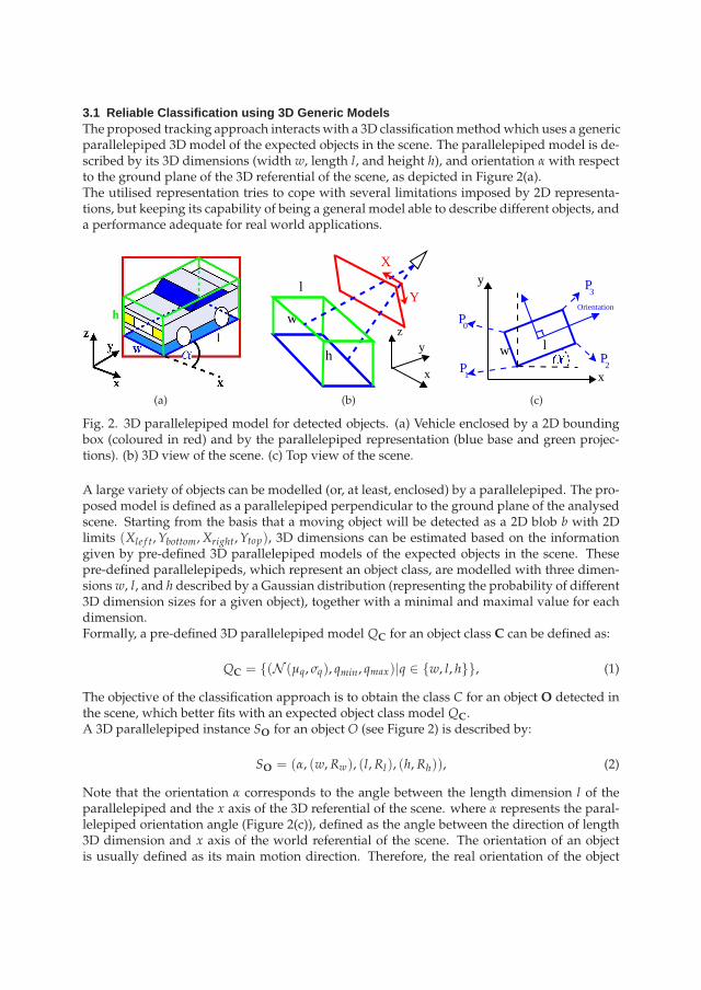
Fig. 2. 3D parallelepiped model for detected objects. (a) Vehicle enclosed by a 2D boundingbox (coloured in red) and by the parallelepiped representation (blue base and green projec-tions). (b) 3D view of the scene. (c) Top view of the scene.

A large variety of objects can be modelled (or, at least, enclosed) by a parallelepiped. The pro-posed model is defined as a parallelepiped perpendicular to the ground plane of the analysedscene. Starting from the basis that a moving object will be detected as a 2D blob b with 2Dlimits (Xle f t,Ybottom,Xright,Ytop), 3D dimensions can be estimated based on the informationgiven by pre-defined 3D parallelepiped models of the expected objects in the scene. Thesepre-defined parallelepipeds, which represent an object class, are modelled with three dimen-sions w, l, and h described by a Gaussian distribution (representing the probability of different3D dimension sizes for a given object), together with a minimal and maximal value for eachdimension.Formally, a pre-defined 3D parallelepiped model QC for an object class C can be defined as:

QC = (N (µq, σq), qmin, qmax)|q ∈ w, l, h, (1)

The objective of the classification approach is to obtain the class C for an object O detected inthe scene, which better fits with an expected object class model QC.A 3D parallelepiped instance SO for an object O (see Figure 2) is described by:

SO = (α, (w,Rw), (l,Rl), (h,Rh)), (2)

Note that the orientation α corresponds to the angle between the length dimension l of theparallelepiped and the x axis of the 3D referential of the scene. where α represents the paral-lelepiped orientation angle (Figure 2(c)), defined as the angle between the direction of length3D dimension and x axis of the world referential of the scene. The orientation of an objectis usually defined as its main motion direction. Therefore, the real orientation of the object

leftX

SegLeft

X

Y

rightX

topY

bottomY

SegRight

SegTop

SegBottom

l

hw

(a)

l

h w

P (x , y )3 3 3

(0)

P (x , y )1 1 1

(0)P (x , y )

1 1 1

(h)

P (x , y )0 0 0

(0)

P (x , y )0 0 0

(h)

P (x , y )3 3 3

(h)

P (x , y )2 2 2

(0)

P (x , y )2 2 2

(0)

T T

T L

T R

T B

(b)

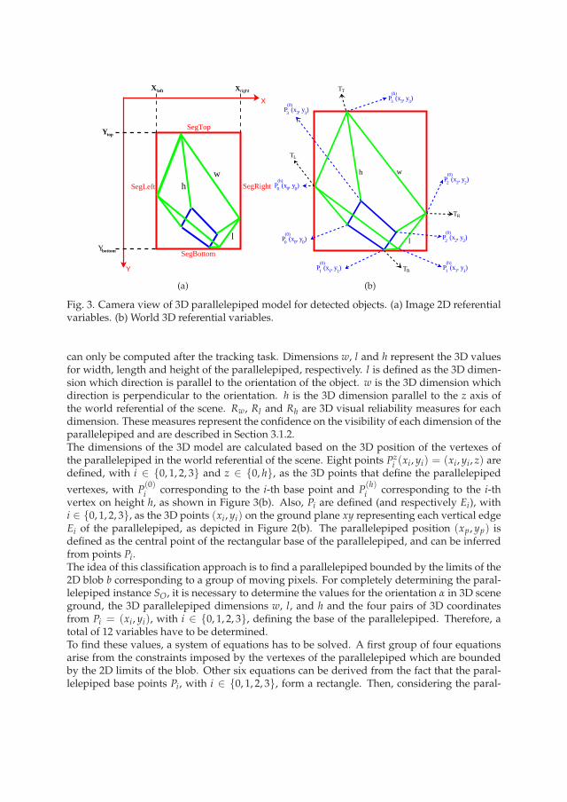
Fig. 3. Camera view of 3D parallelepiped model for detected objects. (a) Image 2D referentialvariables. (b) World 3D referential variables.

can only be computed after the tracking task. Dimensions w, l and h represent the 3D valuesfor width, length and height of the parallelepiped, respectively. l is defined as the 3D dimen-sion which direction is parallel to the orientation of the object. w is the 3D dimension whichdirection is perpendicular to the orientation. h is the 3D dimension parallel to the z axis ofthe world referential of the scene. Rw, Rl and Rh are 3D visual reliability measures for eachdimension. These measures represent the confidence on the visibility of each dimension of theparallelepiped and are described in Section 3.1.2.The dimensions of the 3D model are calculated based on the 3D position of the vertexes ofthe parallelepiped in the world referential of the scene. Eight points Pz

i (xi, yi) = (xi, yi, z) aredefined, with i ∈ 0, 1, 2, 3 and z ∈ 0, h, as the 3D points that define the parallelepiped

vertexes, with P(0)i corresponding to the i-th base point and P

(h)i corresponding to the i-th

vertex on height h, as shown in Figure 3(b). Also, Pi are defined (and respectively Ei), withi ∈ 0, 1, 2, 3, as the 3D points (xi, yi) on the ground plane xy representing each vertical edgeEi of the parallelepiped, as depicted in Figure 2(b). The parallelepiped position (xp, yp) isdefined as the central point of the rectangular base of the parallelepiped, and can be inferredfrom points Pi.The idea of this classification approach is to find a parallelepiped bounded by the limits of the2D blob b corresponding to a group of moving pixels. For completely determining the paral-lelepiped instance SO, it is necessary to determine the values for the orientation α in 3D sceneground, the 3D parallelepiped dimensions w, l, and h and the four pairs of 3D coordinatesfrom Pi = (xi, yi), with i ∈ 0, 1, 2, 3, defining the base of the parallelepiped. Therefore, atotal of 12 variables have to be determined.To find these values, a system of equations has to be solved. A first group of four equationsarise from the constraints imposed by the vertexes of the parallelepiped which are boundedby the 2D limits of the blob. Other six equations can be derived from the fact that the paral-lelepiped base points Pi, with i ∈ 0, 1, 2, 3, form a rectangle. Then, considering the paral-

lelepiped orientation α, these equations are written in terms of the parallelepiped base pointsPi = (xi, yi), as shown in Equation (3).

x2 − x1 = l × cos(α) ; y2 − y1 = l × sin(α) ;x3 − x2 = −w× sin(α) ; y3 − y2 = w× cos(α) ;x0 − x3 = −l × cos(α) ; y0 − y3 = −l × sin(α)

(3)

These six6 equations define the rectangular base of the parallelepiped, considering an orien-tation α and base dimensions w and l. As there are 12 variables and 10 equations (consideringthe first four from blob bounds), there are two degrees of freedom for this problem. In fact,posed this way, the problem defines a complex non-linear system, as sinusoidal functions areinvolved, and the indexes j ∈ L, B,R, T for the set of bounded vertexes T are determined bythe orientation α. Then, the wisest decision is to consider α as a known parameter. This way,the system becomes linear. But, there is still one degree of freedom. The best next choice mustbe a variable with known expected values, in order to be able to fix its value with a coherentquantity. Variables w, l and h comply with this requirement, as a pre-defined Gaussian modelfor each of these variables is available. The parallelepiped height h has been arbitrarily chosenfor this purpose.Therefore, the resolution of the system results in a set of linear relations in terms of h of theform presented in Equation (4). Just three expressions for w, l, and x3 were derived fromthe resolution of the system, as the other variables can be determined from the four relationsarising from the vertexes of the parallelepiped which are bounded by the 2D limits of the bloband the relations presented in Equation (3).

w = Mw(α;M, b)× h+ Nw(α;M, b)l = Ml(α;M, b)× h+ Nl(α;M, b)

x3 = Mx3 (α;M, b)× h+ Nx3 (α;M, b)(4)

Therefore, considering perspective matrix M and 2D blob b = (Xle f t,Ybottom,Xright,Ytop), aparallelepiped instance SO for a detected object O can be completely defined as a function f :

SO = f (α, h,M, b) (5)

Equation (5) states that a parallelepiped model O can be determined with a function depend-ing on parallelepiped height h, and orientation α, 2D blob b limits, and the calibration matrixM. The visual reliability measures remain to be determined and are described below.The obtained solution states that the parallelepiped orientation α and height hmust be knownin order to calculate the parallelepiped. Taking these factors into consideration h and α arefound for the optimal fit for each pre-defined parallelepiped class model, based on the proba-bility measure PM defined in Equation (6)).

PM(SO,C) = ∏q∈w,l,h

PrqC (qO|µqC , σqC ) (6)

After finding the optimal model for each class based on PM, the class of the model with thehighest PM value is considered as the class associated to the analysed 2D blob. This operationis performed for each blob on the current video frame.

6 In fact there are eight equations of this type. The two missing equations correspond to the relationsbetween the variable pairs (x0; x1) and (y0; y1), but these equations are not independent. Hence, theyhave been suppressed.

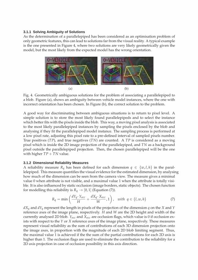
3.1.1 Solving Ambiguity of SolutionsAs the determination of a parallelepiped has been considered as an optimisation problem ofonly geometric features, this can lead to solutions far from the visual reality. A typical exampleis the one presented in Figure 4, where two solutions are very likely geometrically given themodel, but the most likely from the expected model has the wrong orientation.

(a) (b)

Fig. 4. Geometrically ambiguous solutions for the problem of associating a parallelepiped toa blob. Figure (a), shows an ambiguity between vehicle model instances, where the one withincorrect orientation has been chosen. In Figure (b), the correct solution to the problem.

A good way for discriminating between ambiguous situations is to return to pixel level. Asimple solution is to store the most likely found parallelepipeds and to select the instancewhich better fits with the pixels inside the blob. This way, a moving pixel analysis is associatedto the most likely parallelepiped instances by sampling the pixels enclosed by the blob andanalysing if they fit the parallelepiped model instance. The sampling process is performed ata low pixel rate, adjusting this pixel rate to a pre-defined interval of sampled pixels number.True positives (TP), and true negatives (TN) are counted. A TP is considered as a movingpixel which is inside the 2D image projection of the parallelepiped, and TN as a backgroundpixel outside the parallelepiped projection. Then, the chosen parallelepiped will be the onewith higher TP+ TN value.

3.1.2 Dimensional Reliability MeasuresA reliability measure Rq has been defined for each dimension q ∈ w, l, h in the paral-lelepiped. Thismeasure quantifies the visual evidence for the estimated dimension, by analysinghow much of the dimension can be seen from the camera view. The measure gives a minimalvalue 0 when attribute is not visible, and a maximal value 1 when the attribute is totally visi-ble. It is also influenced by static occlusion (image borders, static objects). The chosen functionfor modelling this reliability is Rq → [0, 1] (Equation (7)).

Rq = min(

dYq·YoccH

+dXq·Xocc

W, 1)

, with q ∈ l,w, h (7)

dXq and dYq represent the length in pixels of the projection of the dimension q on the X and Yreference axes of the image plane, respectively. H and W are the 2D height and width of thecurrently analysed 2D blob. Yocc and Xocc are occlusion flags, which value is 0 if occlusion ex-ists with respect to the Y or X reference axes of the image plane, respectively. These measuresrepresent visual reliability as the sum of contributions of each 3D dimension projection ontothe image axes, in proportion with the magnitude of each 2D blob limiting segment. Thus,the maximal value 1 is achieved if the the sum of the partial contributions for each 2D axis ishigher than 1. The occlusion flags are used to eliminate the contribution to the reliability for a2D axis projection in case of occlusion possibility in this axis direction.

3.2 Reliability Multi Hypothesis TrackingIn this section, the new tracking algorithm, Reliability Multi-Hypothesis Tracking (RMHT), isdescribed in detail. In general terms, this method presents similar ideas in the structure forcreating, generating, and eliminating mobile object hypotheses compared to the MHT meth-ods presented in Section 2. The main differences from these methods are induced by theobject representation utilised for tracking (section 3.1), and the dynamics model enriched byuncertainty control (section 3.2.1). The utilisation of region-based representations implies thatseveral visual evidences could be associated to a mobile object (object parts). This considera-tion implies adapting the methods for creation and updating of object hypotheses. For furtherdetails on these adaptations, refer to (Zuniga, 2008).

3.2.1 Dynamics ModelThe dynamics model is the process for computing and updating the attributes of the mobileobjects. Each mobile object in a hypothesis is represented as a set of statistics inferred from vi-sual evidences of their presence in the scene. These visual evidences are stored in a short-termhistory buffer of blobs representing these evidences, called blob buffer. The attributes consid-ered for the calculation of themobile statistics belong to the set A = X,Y,W,H, xp, yp,w, l, h, α.(X,Y) is the centroid position of the blob,W and H are the 2D blob width and height in imageplane coordinates, respectively. (xp, yp) is the centroid position of the calculated 3D paral-lelepiped base. w, l, and h correspond to the 3D width, length, and height of the calculatedparallelepiped in 3D scene coordinates. At the same time, an attribute Va for each attributea ∈ A is calculated, representing the instant speed based on values estimated from visualevidence at different frames.

3.2.1.1 Modelling Uncertainty with Reliability MeasuresUncertainty on data can arise from many different sources. For instance, these sources canbe the object model, the geometry of the scene, segmentation quality, temporal coherence,appearance, occlusion, among others. Following this idea, the proposed dynamics modelintegrates several reliability measures, representing different uncertainty sources.Let RVak be the visual reliability of the attribute a, extracted from the visual evidence ob-served at frame k. The visual reliability of an attribute RVak changes according to the attribute.In the case of 3D dimensional attributes w, l, and h, these measures are obtained with theEquation (7). For 3D attributes xp, yp, and α, their visual reliability is calculated as the meanbetween the visual reliability of w and l, because the calculation of these three attributes isrelated to the base of the parallelepiped 3D representation. For 2D attributes W, H, X and Ya visual reliability measure inversely proportional to the distance to the camera is calculated,accounting for the fact that the segmentation error increases when objects are farther from thecamera.To account for the coherence of values obtained for attribute a throughout time, the coherencereliabilitymeasure RCa(tc), updated to current time tc, is defined:

RCa(tc) = 1.0−min

(

1.0,σa(tc)

amax − amin

)

, (8)

where values amax and amin in (8) correspond to pre-defined minimal and maximal values fora, respectively. The standard deviation σa(tc) of the attribute a at time tc (incremental form) is

defined as:

σa(tc) =

√

RV(a)·(

σa(tp)2 +RVac · (ac − a(tp))2

RVacca(tc)

)

, (9)

where ac is the value of attribute a extracted from visual evidence at frame c, and a(tp) (aslater defined in Equation (14)) is the mean value of a, considering information until previousframe p.

RVacca(tc) = RVac + e−λ·(tc−tp)· RVacca(tp), (10)

is the accumulated visual reliability, adding current reliability RVac to previously accumu-lated values RVacca(tp) weighted by a cooling function, and

RV(a) =e−λ·(tc−tp)· RVacca(tp)

RVacca(tc)(11)

is defined as the ratio between current and previous accumulated visual reliability, weightedby a cooling function.The value e−λ·(tc−tp), present in Equations (9) and (10), and later in Equation (16), correspondsto the cooling function of the previously observed attribute values. It can be interpreted as aforgetting factor for reinforcing the information obtained from newer visual evidence. Theparameter λ ≥ 0 is used to control the strength of the forgetting factor. A value of λ = 0 rep-resents a perfect memory, as forgetting factor value is always 1, regardless the time differencebetween frames, and it is used for attributes w, l, and h when the mobile is classified with arigid model (i.e. a model of an object with only one posture (e.g. a car)).Then, the mean visual reliability measure RVa(tk) represents the mean of visual reliabilitymeasures RVa until frame k, and is defined using the accumulated visual reliability (Equation(10)) as

RVa(tc) =RVacca(tc)

sumCooling(tc), (12)

withsumCooling(tc) = sumCooling(tp) + e−λ·(tc−tp), (13)

where sumCooling(tc) is the accumulated sum of cooling function values.In the same way, reliability measures can be calculated for the speed Va of attribute a. LetVak correspond to current instant velocity, extracted from the values of attribute a observed atvideo frames k and j, where j corresponds to the nearest valid previous frame index in timeto k. Then, RVVak

corresponds to the visual reliability of the current instant velocity and iscalculated as the mean between the visual reliabilities RVak and RDaj .

3.2.1.2 Mathematical Formulation of DynamicsThe statistics associated to an attribute a ∈ A, similarly to the presented reliability measures,are calculated incrementally in order to have a better processing time performance, conform-ing a new dynamics model for tracked object attributes. This dynamics model proposes anew way of utilising reliability measures to weight the contribution of the new informationprovided by the visual evidence at the current image frame. The model also incorporates acooling function utilised as a forgetting factor for reinforcing the information obtained fromnewer visual evidence.

Considering tc as the time-stamp of the current frame c and tp the time-stamp of the previousframe p, the obtained statistics for each mobile are now described. The mean value a forattribute a is defined as:

a(tc) =aexp(tc)· Raexp (tc) + aest(tc)· Raest (tc)

Raexp (tc) + Raest (tc), (14)

where the expected value aexp corresponds to the expected value for attribute a at current timetc, based on previous information, and aest represents the value of a estimated from the ob-served visual evidence associated to the mobile until current time tc. These two values are in-tentionally related to respective prediction and filtering estimates of Kalman filters (Kalman,1960). Their computation radically differs from these estimates by incorporating reliabilitymeasures and cooling functions to control pertinence of attribute data. Raexp (tc) and Raest (tc)correspond to reliability measures weighting the contributions of each of these elements.The expected value aexp of a corresponds to the value of a predicatively obtained from thedynamics model. Given the mean value a(tp) for a at the previous frame time tp, and theestimated speed Va(tp) of a at previous frame p, it is defined as

aexp(tc) = a(tp) +Va(tp)· (tc − tp). (15)

Va(tc) corresponds to the estimated velocity of a (equation (17)) at current frame c.The reliability measure Raexp represents the reliability of the estimated value aest of attribute a.It is determined as the mean of the global reliabilities Ra and RVa

of a and Va, respectively, atthe previous time tp. This way, the uncertainty of elements used for the calculation of aexp asa(tp) andVa(tp), is utilised for modelling the uncertainty of aexp. A global reliabilitymeasureRx(tk) for an attribute x can be calculated as the mean between Raexp and Raest at tk.The estimated value aest represents the value of a extracted from the observed visual evidenceassociated to the mobile, and is defined in Equation (16). This way, aest(tc) value is updatedby adding the value of the attribute for the current visual evidence, weighted by the visualreliability value for this attribute value, while previously obtained estimation is weighted bythe forgetting factor.

aest(tc) =ac· RVac + e−λ·(tc−tp)· aest(tp)· RVacca(tp)

RVacca(tc), (16)

where ak is the value and RVak is the visual reliability of the attribute a, extracted from thevisual evidence observed at frame k. RVacca(tk) is the accumulated visual reliability untilframe k, as described in Equation 10). e−λ·(tc−tp) is the cooling function.The reliability measure Raest represents the reliability of the estimated value aest of attribute a.It is calculated as the mean between the visual reliability RVa(tc) (Equation (12) ) and coher-ence reliability RCa(tc) (Equation (8) ) values at current frame c, weighted by the reliabilitymeasure Rvalid. The Rvalid reliability measure corresponds to the number of valid blobs in theblob buffer of the mobile over the size of the buffer. For a 2D attribute, a valid blob correspondsto a blob not corresponding to a lost object (no visual evidence correspondence), while for a3D attribute, a valid blob corresponds to a blob which has been classified and has then valid3D information. Not classified blobs correspond to blobs where the 3D classification methodwas not able to find a coherent 3D solution with respect to the current mobile attributes 3Dinformation.

The statistics considered for velocity Va follow the same idea of the previously defined equa-tions for attribute a, with the difference that no expected value for the velocity of a is calcu-lated, obtaining the value of the statistics of Va directly from the visual evidence data. Thevelocity Va of a is then defined as

Va(tc) =Vac · RVVac

+ e−λ·(tc−tp)·Va(tp)· RVaccVa(tp)

RVaccVa(tc)

, (17)

where Vak corresponds to current instant velocity, extracted from the a attribute values ob-served at video frames k and j, where j corresponds to the nearest previous valid frame indexprevious to k. RVVak

corresponds to the visual reliability of the current instant velocity as de-fined in previous Section 3.2.1.1. Then, visual and coherence reliability measures for attributeVa can be calculated in the same way as for any other attribute, as described in Section 3.2.1.1.Finally, the likelihoodmeasure pm for a mobilem can be defined inmanyways by combiningthe present attribute statistics. The chosen likelihoodmeasure for pm is a weightedmean of theprobability measures for different group of attributes (group w, l, h as D3D, x, y as V3D,W, L as D2D, and X,Y as V2D), weighted by a joint reliability measure for each group,throughout the video sequence, as presented in Equation (18).

pm =

∑k∈K

RkCk

∑k∈K

Rk

(18)

with K = D3D ,V3D,D2D,V2D and

CD3D =

∑d∈w,l,h

(RCd + Pd)RVd

2 ∑d∈w,l,h

RDd

(19)

CV3D =MPV + PV + RCV

3.0, (20)

CD2D = Rvalid2D ·RCW + RCH

2, (21)

CV2D = Rvalid2D ·RCVX

+ RCVY

2.0, (22)

where Rvalid2D is the Rvalid measure for 2D information, corresponding to the number of notlost blobs in the blob buffer, over the current blob buffer size. From equation (18), RD2D is themean betweenmean visual reliabilities RVW(tc) and RVH(tc), multiplied by Rvalid2D measure.RV2D is the mean between RVX(tc) and RVY(tc), also multiplied by Rvalid2D measure. RD3D isthe mean between RVw(tc), RV l(tc), and RVh(tc) for 3D dimensions w, l, and h, respectively,and multiplied by Rvalid3D measure. Rvalid3D is the Rvalid measure for 3D information, corre-sponding to the number of not classified blobs in the blob buffer, over the current blob buffersize. RV3D is the mean between RVx(tc) and RVy(tc) for 3D coordinates x and y, also multi-plied by Rvalid3D measure. Measures CD2D , CD3D , CV2D , and CV3D are considered as measuresof temporal coherence (i.e. discrepancy between estimated and measured values) of the di-mensional attributes (D2D and D3D) and the position velocities (V2D and V3D). The measures

RD3D , RV3D , RD2D , and RV2D are the accumulation of visibility measures in time (with decreas-ing factor).Pw, Pl , and Ph in Equation (19) correspond to the mean probability of the dimensional at-tributes according to the a priori models of objects expected in the scene, considering thecooling function as in Equation (16). Note that parameter tc has been removed for simplicity.MPV , PV , and RCV values present in Equation (20) are inferred from attribute speeds Vx and

Vy. MPV represents the probability of the current velocity magnitude V =√

V2x +V2

y withrespect to a pre-defined velocity model for the classified object, added to the expected objectmodel, defined in the same way as described in Section 3.1. PV corresponds to the mean prob-ability for the position probabilities PVx

and PVy, calculated with the values of Pw and Pl , as

the 3D position is inferred from the base dimensions of the parallelepiped. RCV correspondsto the mean between RCVx

and RCVy.

This way, the value pm for a mobile object m will mostly consider the probability values forattribute groups with higher reliability, using the values that can be trusted the most. At thesame time, different aspects of uncertainty have been considered in order to better representand identify several issues present in video analysis.

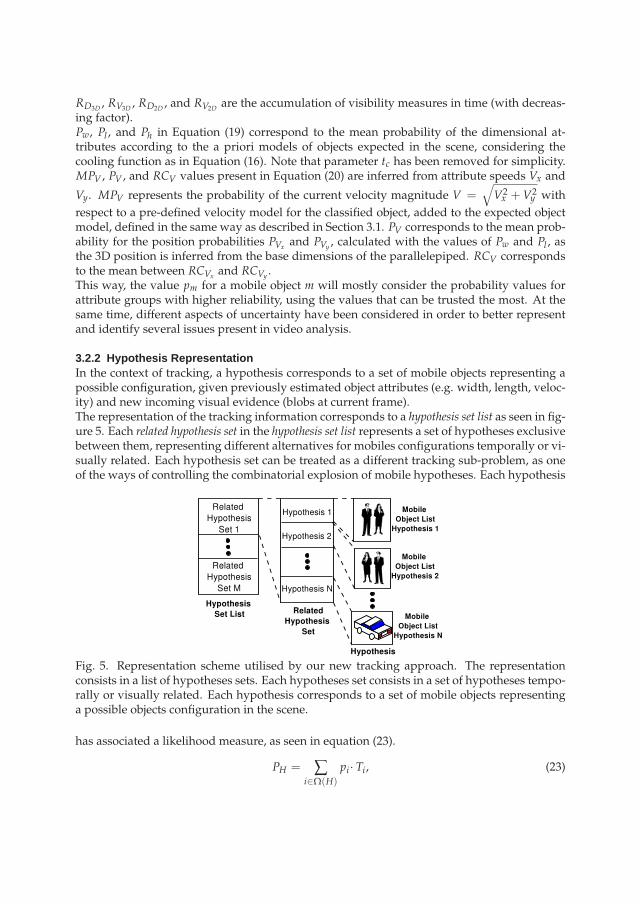
3.2.2 Hypothesis RepresentationIn the context of tracking, a hypothesis corresponds to a set of mobile objects representing apossible configuration, given previously estimated object attributes (e.g. width, length, veloc-ity) and new incoming visual evidence (blobs at current frame).The representation of the tracking information corresponds to a hypothesis set list as seen in fig-ure 5. Each related hypothesis set in the hypothesis set list represents a set of hypotheses exclusivebetween them, representing different alternatives for mobiles configurations temporally or vi-sually related. Each hypothesis set can be treated as a different tracking sub-problem, as oneof the ways of controlling the combinatorial explosion of mobile hypotheses. Each hypothesis

Fig. 5. Representation scheme utilised by our new tracking approach. The representationconsists in a list of hypotheses sets. Each hypotheses set consists in a set of hypotheses tempo-rally or visually related. Each hypothesis corresponds to a set of mobile objects representinga possible objects configuration in the scene.

has associated a likelihood measure, as seen in equation (23).

PH = ∑i∈Ω(H)

pi· Ti, (23)

where Ω(H) corresponds to the set ofmobiles represented in hypothesis H, pi to the likelihoodmeasure for a mobile i (as previously obtained from the dynamics model in Equation (18)),and Ti to a temporal reliability measure for a mobile i relative to hypothesis H, based on thelife-time of the object in the scene.Then, the likelihood measure PH for an hypothesis H corresponds to the summation of thelikelihood measures for each mobile object, weighted by a temporal reliability measure foreach mobile, accounting for the life-time of each mobile. This reliability measure allows togive higher likelihood to hypotheses containing objects validated for more time in the scene,and is defined in equation (24).

Ti =Fi

∑j∈Ω(H) Fj. (24)

This reliability measure intends to grant the survival of hypotheses containing objects ofproved existence.

3.3 MILES: A new approach for incremental event learning and recognitionMILES is based on incremental concept formation models (Gennari et al., 1990). Conceptual clus-tering consists in describing classes by first generating their conceptual descriptions and thenclassifying the entities according to these descriptions. Incremental concept formation models isa conceptual clustering approach which incrementally creates a new concept without exten-sive reprocessing of the previously encountered instances. The knowledge is represented bya hierarchy of concepts partially ordered by generality. A category utility function is used toevaluate the quality of the obtained concept hierarchies (McKusick & Thompson, 1990).MILES is an extension of incremental concept formation models for learning video events.The approach uses as input a set of attributes from the tracked objects in the scene. Hence, theonly hypothesis of MILES is the availability of tracked object attributes (e.g. position, posture,class, speed). MILES constructs a hierarchy of state and event concepts h, based on the stateand event instances extracted from the tracked object attributes.A state concept is the model of a spatio-temporal property valid at a given instant or stableon a time interval. A state concept S(c), in a hierarchy h, is modelled as a set of attributemodels ni, with i ∈ 1, .., T, where ni is modelled as a random variable Ni which followsa Gaussian distribution Ni ∼ N (µni ; σni ). T is the number of attributes of interest. The stateconcept S(c) is also described by its number of occurrences N(S(c)), its probability of occur-

renceP(S(c)) = N(S(c))/N(S(p)) (S(p) is the root state concept of h), and the number of event

occurrences NE(S(c)) (number of times that state S(c) passed to another state, generating an

event).A state instance is an instantiation of a state concept, associated to a tracked object o. The stateinstance S(o) is represented as the set attribute-value-measure triplets To = (vi;Vi;Ri), withi ∈ 1, . . . , T, where Ri is the reliability measure associated to the obtained value Vi for theattribute vi. The measure Ri ∈ [0, 1] is 1 if associated data is totally reliable, and 0 if totallyunreliable.An event concept E(c) is defined as the change from a starting state concept S(c)a to the arriving

state concept S(c)b in a hierarchy h. An event concept E(c) is described by its number of

occurrences N(E(c)), and its probability of occurrence P(E(c)) = N(E(c))/NE(S(c)a ) (with

S(c)a its starting state concept).

The state concepts are hierarchically organised by generality, with the children of each staterepresenting specifications of their parent. A unidirectional link between two state concepts

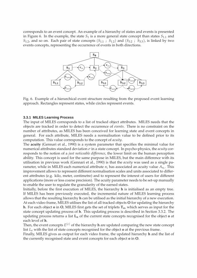
corresponds to an event concept. An example of a hierarchy of states and events is presentedin Figure 6. In the example, the state S1 is a more general state concept than states S1.1 andS1.2, and so on. Each pair of state concepts (S1.1 ; S1.2) and (S3.2 ; S3.3), is linked by twoevents concepts, representing the occurrence of events in both directions.

S0

S1 S2 S3

S1.1 S1.2 S3.1 S3.2 S3.3

e1.2-1.1

e1.1-1.2

e1-2

e1.2-2

e2-3

e2-3.2

e3.2-3.1 e3.2-3.3

e3.3-3.2

Fig. 6. Example of a hierarchical event structure resulting from the proposed event learningapproach. Rectangles represent states, while circles represent events.

3.3.1 MILES Learning ProcessThe input of MILES corresponds to a list of tracked object attributes. MILES needs that theobjects are tracked in order to detect the occurrence of events. There is no constraint on thenumber of attributes, as MILES has been conceived for learning state and event concepts ingeneral. For each attribute, MILES needs a normalisation value to be defined prior to itscomputation. This value corresponds to the concept of acuity.The acuity (Gennari et al., 1990) is a system parameter that specifies the minimal value fornumerical attributes standard deviation σ in a state concept. In psycho-physics, the acuity cor-responds to the notion of a just noticeable difference, the lower limit on the human perceptionability. This concept is used for the same purpose in MILES, but the main difference with itsutilisation in previous work (Gennari et al., 1990) is that the acuity was used as a single pa-rameter, while in MILES each numerical attribute ni has associated an acuity value Ani . Thisimprovement allows to represent different normalisation scales and units associated to differ-ent attributes (e.g. kilo, meter, centimetre) and to represent the interest of users for differentapplications (more or less coarse precision). The acuity parameter needs to be set-upmanuallyto enable the user to regulate the granularity of the earned states.Initially, before the first execution of MILES, the hierarchy h is initialised as an empty tree.If MILES has been previously executed, the incremental nature of MILES learning processallows that the resulting hierarchy h can be utilised as the initial hierarchy of a new execution.At each video frame, MILES utilises the list of all tracked objectsO for updating the hierarchyh. For each object o in O, MILES first gets the set of triplets To, which serves as input for thestate concept updating process of h. This updating process is described in Section 3.3.2. Theupdating process returns a list Lo of the current state concepts recognised for the object o ateach level of h.Then, the event concepts E(c) of the hierarchy h are updated comparing the new state conceptlist Lo with the list of state concepts recognised for the object o at the previous frame.Finally, MILES gives as output for each video frame, the updated hierarchy h and the list ofthe currently recognised state and event concepts for each object o in O.

3.3.2 States Updating AlgorithmThe hierarchy updating algorithm incorporates the new information at each level of the tree,starting from the root state.The algorithm starts by accessing the analysed state C from the current hierarchy h. If the treeis empty, the initialisation of the hierarchy is performed by creating a state with the tripletsTo, for the first processed object.Then, for the case that C corresponds to a terminal state (the state has no children), a cutofftest is performed. The cutoff is a criteria utilised for stopping the creation (i.e. specialisation)of children states. It can be defined as:

cutoff =

true if µni −Vni ≤ Ani

| ∀ i ∈ 1, .., T false else

, (25)

where Vni is the value of the i-th triplet of To. This equation means that the learning process

will stop at the concept state S(c)k if no meaningful difference exists between each attribute

value of To and the mean value µni of the attribute ni for the state concept S(c)k (based on the

attribute acuity Ani ).If the cutoff test is passed, two children are generated for C, one initialised with To and theother as a copy of C. Then, passing or not passing the cutoff test, To is incorporated to the stateC (state incorporation is described in Section 3.3.3). In this terminal state case, the updatingprocess then stops.If C has children, first To is immediately incorporated to C. Next, different new hierarchy con-figurations have to be evaluated among all the children of C. In order to determine in whichstate concept the triplets list To is next incorporated (i.e. the state concept is recognised),a quality measure for state concepts called category utility is utilised, which measures howwell the instances are represented by a given category (i.e. state concept).The category utility CU for a class partition of K state concepts (corresponding to a possibleconfiguration of the children for the currently analysed state C) is defined as:

CU =

K

∑k=1

P(S(c)k )

T

∑i=1

(

Ani

σ(k)ni

− Ani

σ(p)ni

)

2· T· √π

K, (26)

where σ(k)ni

(respectively for σ(p)ni

) is the standard deviation for the attribute ni of To, with

i ∈ 1, 2, .., T, in the state concept S(c)k (respectively for the root state S(c)p ).It is worthy to note that the category utility CU serves as the major criteria to decide how tobalance the states given the learning data. CU is an efficient criteria because it compares therelative frequency of the candidate states together with the relative Gaussian distribution oftheir attributes, weighted by their significant precision (predefined acuity).Then, the different alternatives for the incorporation of To are:(a) The incorporation of To to a existing state P gives the best CU score. In this case, thehierarchy updating algorithm is recursively called, considering P as root.(b) The generation of a new state conceptQ from instance To gives the best CU score x. In thiscase, the new state Q is inserted as child of C, and the updating process stops.

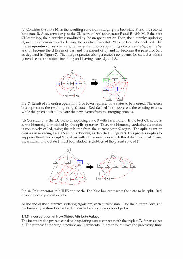
(c) Consider the state M as the resulting state from merging the best state P and the secondbest state R. Also, consider y as the CU score of replacing states P and R with M. If the bestCU score is y, the hierarchy is modified by the merge operator. Then, the hierarchy updatingalgorithm is recursively called, using the sub-tree from stateM as the tree to be analysed. Themerge operator consists in merging two state concepts Sp and Sq into one state SM, while Sp

and Sq become the children of SM, and the parent of Sp and Sq becomes the parent of SM,as depicted in Figure 7. The merge operator also generates new events for state SM whichgeneralise the transitions incoming and leaving states Sp and Sq.

0S

S4

S1

S2

3S

S3.1 S3.2

SM

0S

S4S1 S2 3S

S3.1 S3.2

Merge

Fig. 7. Result of a merging operation. Blue boxes represent the states to be merged. The greenbox represents the resulting merged state. Red dashed lines represent the existing events,while the green dashed lines are the new events from the merging process.

(d) Consider z as the CU score of replacing state P with its children. If the best CU score isz, the hierarchy is modified by the split operator. Then, the hierarchy updating algorithmis recursively called, using the sub-tree from the current state C again. The split operatorconsists in replacing a state Swith its children, as depicted in Figure 8. This process implies tosuppress the state concept S together with all the events in which the state is involved. Then,the children of the state S must be included as children of the parent state of S.

0S

S3.1 S3.2 S3.3S1.2S1.1

S2 3SS1

0S

S3.1 S3.2 S3.3

S1.2S1.1

S2S1Split

Fig. 8. Split operator in MILES approach. The blue box represents the state to be split. Reddashed lines represent events.

At the end of the hierarchy updating algorithm, each current state C for the different levels ofthe hierarchy is stored in the list L of current state concepts for object o.

3.3.3 Incorporation of New Object Attribute ValuesThe incorporation process consists in updating a state concept with the triplets To for an objecto. The proposed updating functions are incremental in order to improve the processing time

performance of the approach. The incremental updating function for the mean value µn of anattribute n is presented in Equation (27).

µn(t) =Vn· Rn + µn(t− 1)· Sumn(t− 1)

Sumn(t), (27)

withSumn(t) = Rn + Sumn(t− 1), (28)

where Vn is the attribute value and Rn is the reliability. Sumn is the accumulation of reliabilityvalues Rn.The incremental updating function for the standard deviation σn for attribute n is presentedin Equation (29).

σn(t) =

√

Sumn(t−1)Sumn(t)

·(

σn(t− 1)2 + Rn ·∆n

Sumn(t)

)

.

with

∆n = (Vn − µn(t− 1))2

(29)

For a new state concept, the initial values taken for Equations (27), (28), and (29) with t = 0correspond to µn(0) = Vn, Sumn(0) = Rn, and σn(0) = An, where An is the acuity for theattribute n.In case that, after updating the standard deviation Equation (29), the value of σn(i) is lowerthan the acuity An, σn(i) is reassigned to An. This way, the acuity value establishes a lowerbound for the standard deviation of an attribute.

4. Evaluation and Results

4.1 Evaluating TrackingFor evaluating the tracking approach, four benchmark videos publicly accessible have beenevaluated. These videos are part of the evaluation framework proposed in ETISEO project(Nghiem et al., 2007). The obtained results have been compared with other algorithms whichhave participated in the ETISEO project. These four chosen videos are:

• AP-11-C4: Airport video of an apron (AP) with one person and four vehicles moving inthe scene over 804 frames.

• AP-11-C7: Airport video of an apron (AP) with five vehicles moving in the scene over804 frames.

• RD-6-C7: Video of a road (RD) with approximately 10 persons and 15 vehicles movingin the scene over 1200 frames.

• BE-19-C1: Video of a building entrance (BE) with three persons and one vehicle over1025 frames.

The tests were performed with a computer with processor Intel Xeon CPU 3.00 GHz, with2 Giga Bytes of memory. For obtaining the 3D model information, two parallelepiped mod-els have been pre-defined for person and vehicle classes. The precision on 3D parallelepipedheight values to search the classification solutions has been fixed in 0.08[m], while the preci-sion on orientation angle has been fixed in π/40[rad].

0

0.1

0.2

0.3

0.4

0.5

0.6

0.7

0.8

0.9

1

G1 G3 G8 G9 G12 G13 G14 G15 G17 G19 G20 G23 G28 G29 G32 MZ

Tra

ckin

g T

ime

Met

ric

Research Group

AP-11-C4

AP-11-C7

RD-6-C7

BE-19-C1

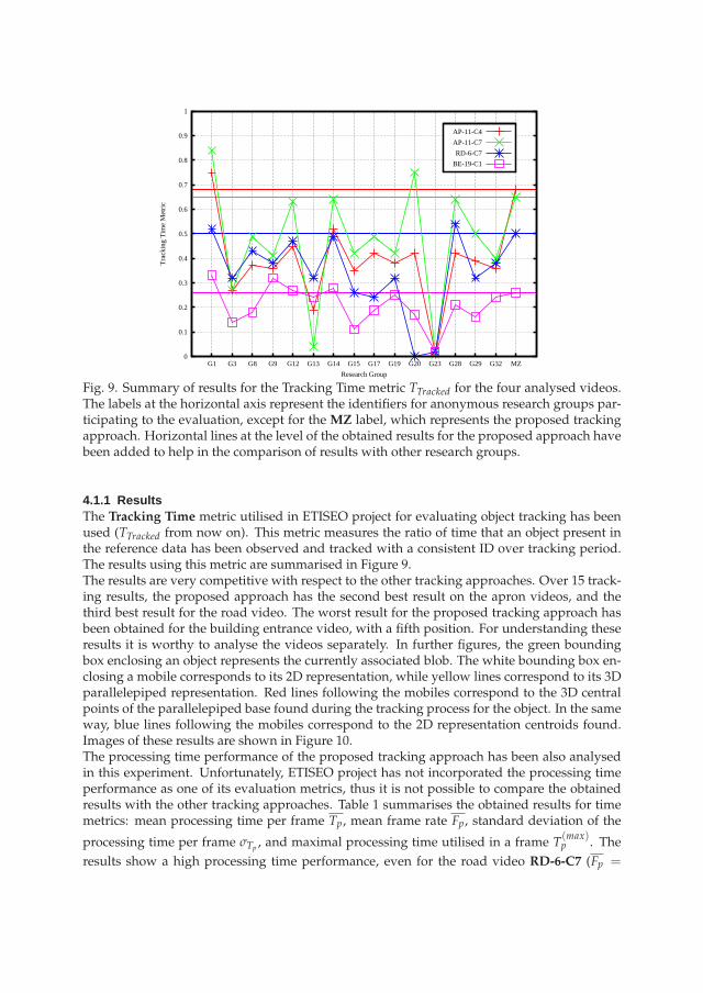
Fig. 9. Summary of results for the Tracking Time metric TTracked for the four analysed videos.The labels at the horizontal axis represent the identifiers for anonymous research groups par-ticipating to the evaluation, except for the MZ label, which represents the proposed trackingapproach. Horizontal lines at the level of the obtained results for the proposed approach havebeen added to help in the comparison of results with other research groups.

4.1.1 ResultsThe Tracking Time metric utilised in ETISEO project for evaluating object tracking has beenused (TTracked from now on). This metric measures the ratio of time that an object present inthe reference data has been observed and tracked with a consistent ID over tracking period.The results using this metric are summarised in Figure 9.The results are very competitive with respect to the other tracking approaches. Over 15 track-ing results, the proposed approach has the second best result on the apron videos, and thethird best result for the road video. The worst result for the proposed tracking approach hasbeen obtained for the building entrance video, with a fifth position. For understanding theseresults it is worthy to analyse the videos separately. In further figures, the green boundingbox enclosing an object represents the currently associated blob. The white bounding box en-closing a mobile corresponds to its 2D representation, while yellow lines correspond to its 3Dparallelepiped representation. Red lines following the mobiles correspond to the 3D centralpoints of the parallelepiped base found during the tracking process for the object. In the sameway, blue lines following the mobiles correspond to the 2D representation centroids found.Images of these results are shown in Figure 10.The processing time performance of the proposed tracking approach has been also analysedin this experiment. Unfortunately, ETISEO project has not incorporated the processing timeperformance as one of its evaluation metrics, thus it is not possible to compare the obtainedresults with the other tracking approaches. Table 1 summarises the obtained results for timemetrics: mean processing time per frame Tp, mean frame rate Fp, standard deviation of the

processing time per frame σTp, and maximal processing time utilised in a frame T

(max)p . The

results show a high processing time performance, even for the road video RD-6-C7 (Fp =

(a) AP-11-C7 (b) AP-11-C4

(c) RD-6-C7 (d) BE-19-C1

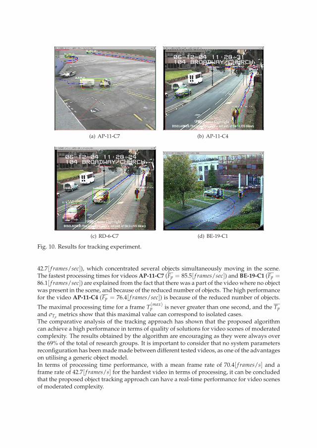
Fig. 10. Results for tracking experiment.

42.7[ f rames/sec]), which concentrated several objects simultaneously moving in the scene.The fastest processing times for videosAP-11-C7 (Fp = 85.5[ f rames/sec]) and BE-19-C1 (Fp =86.1[ f rames/sec]) are explained from the fact that there was a part of the video where no objectwas present in the scene, and because of the reduced number of objects. The high performancefor the video AP-11-C4 (Fp = 76.4[ f rames/sec]) is because of the reduced number of objects.

The maximal processing time for a frame T(max)p is never greater than one second, and the Tp

and σTpmetrics show that this maximal value can correspond to isolated cases.

The comparative analysis of the tracking approach has shown that the proposed algorithmcan achieve a high performance in terms of quality of solutions for video scenes of moderatedcomplexity. The results obtained by the algorithm are encouraging as they were always overthe 69% of the total of research groups. It is important to consider that no system parametersreconfiguration has beenmademade between different tested videos, as one of the advantageson utilising a generic object model.In terms of processing time performance, with a mean frame rate of 70.4[ f rames/s] and aframe rate of 42.7[ f rames/s] for the hardest video in terms of processing, it can be concludedthat the proposed object tracking approach can have a real-time performance for video scenesof moderated complexity.

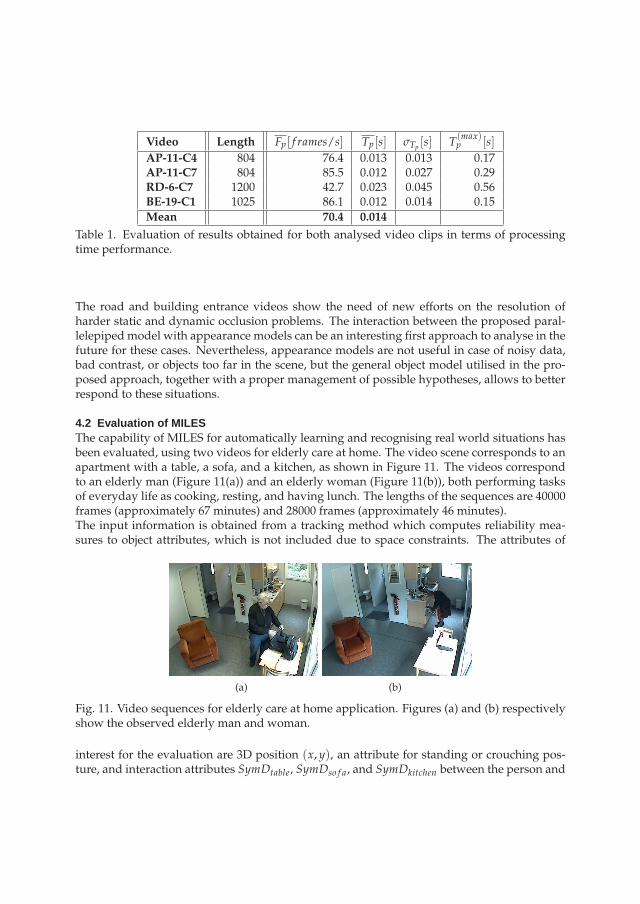
Video Length Fp[ f rames/s] Tp[s] σTp[s] T

(max)p [s]

AP-11-C4 804 76.4 0.013 0.013 0.17AP-11-C7 804 85.5 0.012 0.027 0.29RD-6-C7 1200 42.7 0.023 0.045 0.56BE-19-C1 1025 86.1 0.012 0.014 0.15Mean 70.4 0.014

Table 1. Evaluation of results obtained for both analysed video clips in terms of processingtime performance.

The road and building entrance videos show the need of new efforts on the resolution ofharder static and dynamic occlusion problems. The interaction between the proposed paral-lelepiped model with appearance models can be an interesting first approach to analyse in thefuture for these cases. Nevertheless, appearance models are not useful in case of noisy data,bad contrast, or objects too far in the scene, but the general object model utilised in the pro-posed approach, together with a proper management of possible hypotheses, allows to betterrespond to these situations.

4.2 Evaluation of MILESThe capability of MILES for automatically learning and recognising real world situations hasbeen evaluated, using two videos for elderly care at home. The video scene corresponds to anapartment with a table, a sofa, and a kitchen, as shown in Figure 11. The videos correspondto an elderly man (Figure 11(a)) and an elderly woman (Figure 11(b)), both performing tasksof everyday life as cooking, resting, and having lunch. The lengths of the sequences are 40000frames (approximately 67 minutes) and 28000 frames (approximately 46 minutes).The input information is obtained from a tracking method which computes reliability mea-sures to object attributes, which is not included due to space constraints. The attributes of

(a) (b)

Fig. 11. Video sequences for elderly care at home application. Figures (a) and (b) respectivelyshow the observed elderly man and woman.

interest for the evaluation are 3D position (x, y), an attribute for standing or crouching pos-ture, and interaction attributes SymDtable, SymDso f a, and SymDkitchen between the person and

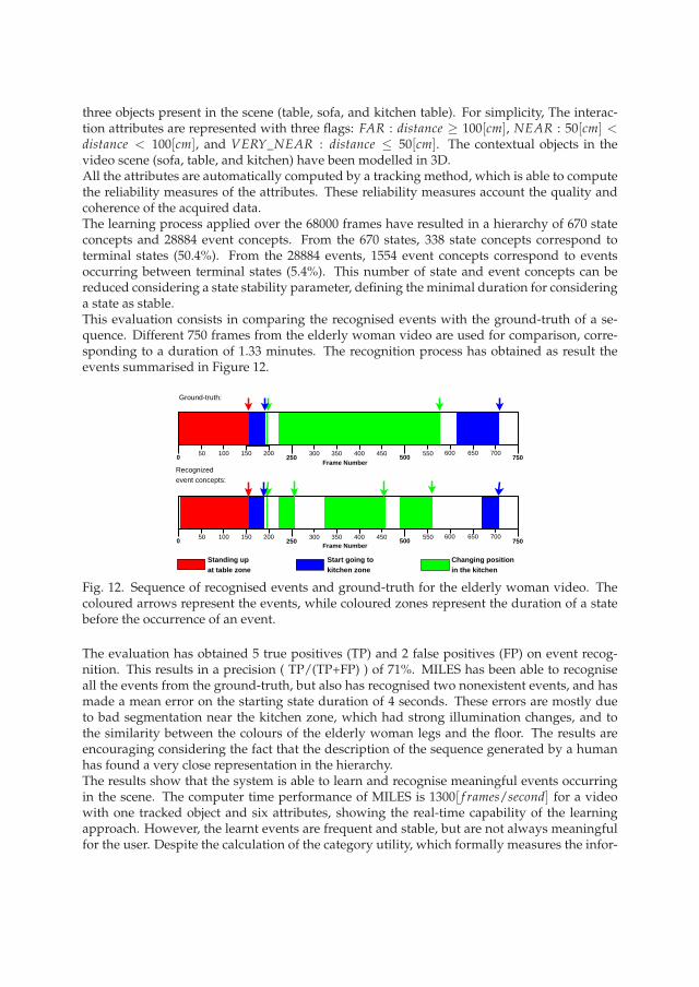
three objects present in the scene (table, sofa, and kitchen table). For simplicity, The interac-tion attributes are represented with three flags: FAR : distance ≥ 100[cm], NEAR : 50[cm] <distance < 100[cm], and VERY_NEAR : distance ≤ 50[cm]. The contextual objects in thevideo scene (sofa, table, and kitchen) have been modelled in 3D.All the attributes are automatically computed by a tracking method, which is able to computethe reliability measures of the attributes. These reliability measures account the quality andcoherence of the acquired data.The learning process applied over the 68000 frames have resulted in a hierarchy of 670 stateconcepts and 28884 event concepts. From the 670 states, 338 state concepts correspond toterminal states (50.4%). From the 28884 events, 1554 event concepts correspond to eventsoccurring between terminal states (5.4%). This number of state and event concepts can bereduced considering a state stability parameter, defining the minimal duration for consideringa state as stable.This evaluation consists in comparing the recognised events with the ground-truth of a se-quence. Different 750 frames from the elderly woman video are used for comparison, corre-sponding to a duration of 1.33 minutes. The recognition process has obtained as result theevents summarised in Figure 12.

300 350 400 450 550 600 650 7000 250 500 750

50 100 150 200

Frame NumberRecognized event concepts:

Ground-truth:

300 350 400 450 550 600 650 7000 250 500 750

50 100 150 200Frame Number

Standing up at table zone

Start going to kitchen zone

Changing position in the kitchen

Fig. 12. Sequence of recognised events and ground-truth for the elderly woman video. Thecoloured arrows represent the events, while coloured zones represent the duration of a statebefore the occurrence of an event.

The evaluation has obtained 5 true positives (TP) and 2 false positives (FP) on event recog-nition. This results in a precision ( TP/(TP+FP) ) of 71%. MILES has been able to recogniseall the events from the ground-truth, but also has recognised two nonexistent events, and hasmade a mean error on the starting state duration of 4 seconds. These errors are mostly dueto bad segmentation near the kitchen zone, which had strong illumination changes, and tothe similarity between the colours of the elderly woman legs and the floor. The results areencouraging considering the fact that the description of the sequence generated by a humanhas found a very close representation in the hierarchy.The results show that the system is able to learn and recognise meaningful events occurringin the scene. The computer time performance of MILES is 1300[ f rames/second] for a videowith one tracked object and six attributes, showing the real-time capability of the learningapproach. However, the learnt events are frequent and stable, but are not always meaningfulfor the user. Despite the calculation of the category utility, which formally measures the infor-

mation density, an automatic process for measuring the usefulness of the learnt events for theuser is still needed.

5. Conclusion

Addressing real world applications implies that a video analysis approach must be able toproperly handle the information extracted from noisy videos. This requirement has been con-sidered by proposing a generic mechanism to measure in a consistent way the reliability ofthe information in the whole video analysis process.The proposed tracking method presents similar ideas in the structure of MHT methods. Themain difference from these methods lies in the dynamics model, where features from differentmodels (2D and 3D) are combined according to their reliability. This new dynamics modelkeeps redundant tracking of 2D and 3D object information, in order to increase robustness.This dynamics model integrates a reliability measure for each tracked object feature, whichaccounts for quality and coherence of utilised information. The calculation of this featuresconsiders a forgetting function (or cooling function) to reinforce the latest acquired informa-tion.The reliability measures have been utilised to control the uncertainty in the obtained informa-tion, learning more robust object attributes and knowing which is the quality of the obtainedinformation. These reliability measures have been also utilised in the event learning task ofthe video understanding framework to determine the most valuable information to be learnt.The proposed tracking method has shown that is capable of achieving a high processing timeperformance for sequences of moderated complexity. But nothing can still be said for morecomplex situations. The results on object tracking have shown to be really competitive com-pared with other tracking approaches in benchmark videos, with a minimal reconfigurationeffort. However, there is still work to do in refining the capability of the approach on copingwith occlusion situations.MILES algorithm allows to learn a model of the states and events occurring in the scene, whenno a priori model is available. It has been conceived for learning state and event concepts ina general way. Depending on the availability of tracked object features, the possible combi-nations are large. MILES has shown its capability for recognising events, processing noisyimage-level data with a minimal configuration effort. The proposed method computes theprobability of transition between two states, similarly as HMM. The contribution MILES is tolearn the global structure of the states and the events and to structure them in a hierarchy.This work can be extended in several ways. Even if the proposed object representation servesfor describing a large variety of objects, the result from the classification algorithm is a coarsedescription of the object. More detailed and class-specific object models could be utilisedwhen needed, as articulated models, object contour, or appearance models. The proposedtracking approach is able to cope with dynamic occlusion situations where the occluding ob-jects keep the coherence in the observed behaviour previous to the occlusion situation. Futurework can point to the utilisation of appearance models utilised pertinently in these situationsin order to identify which part of the visual evidence belongs to each object. The tracking ap-proach could also be used in a feedback process with the motion segmentation phase in orderto focus on zones where movement can occur, based on reliable mobile objects. For the eventlearning approach, more evaluation is still needed for other type of scenes, for other attributesets, and for different number and type of tracked objects. The anomaly detection capability ofthe approach on a large application must also be evaluated. Future work will be also focusedin the incorporation of attributes related to interactions between tracked objects (e.g. meeting

someone). The automatic association between the learnt events and semantic concepts anduser defined events will be also studied.

6. References

Bar-Shalom, Y., Blackman, S. & Fitzgerald, R. J. (2007). The dimensionless score functionfor measurement to track association, IEEE Transactions on Aerospace and ElectronicSystems 41(1): 392–400.

Blackman, S. (2004). Multiple hypothesis tracking for multiple target tracking, IEEE Transac-tions on Aerospace and Electronic Systems 19(1): 5–18.

Blackman, S., Dempster., R. & Reed, R. (2001). Demonstration of multiple hypothesis tracking(mht) practical real-time implementation feasibility, in . E. Drummond (ed.), Signaland Data Processing of Small Targets, Vol. 4473, SPIE Proceedings, pp. 470–475.

Boulay, B., Bremond, F. & Thonnat, M. (2006). Applying 3d human model in a posture recog-nition system, Pattern Recognition Letter, Special Issue on vision for Crime Detection andPrevention 27(15): 1788–1796.

Brémond, F. & Thonnat, M. (1998). Tracking multiple non-rigid objects in video sequences,IEEE Transaction on Circuits and Systems for Video Technology Journal 8(5).

Comaniciu, D., Ramesh, V. & Andmeer, P. (2003). Kernel-based object tracking, IEEE Transac-tions on Pattern Analysis and Machine Intelligence 25: 564–575.

Cucchiara, R., Prati, A. & Vezzani, R. (2005). Posture classification in a multi-camera indoorenvironment, Proceedings of IEEE International Conference on Image Processing (ICIP),Vol. 1, Genova, Italy, pp. 725–728.

Gennari, J., Langley, P. & Fisher, D. (1990). Models of incremental concept formation, in J. Car-bonell (ed.), Machine Learning: Paradigms and Methods, MIT Press, Cambridge, MA,pp. 11 – 61.

Ghahramani, Z. (1998). Learning dynamic bayesian networks, Adaptive Processing of Sequencesand Data Structures, International Summer School on Neural Networks, Springer-Verlag,London, UK, pp. 168–197.

Heisele, B. (2000). Motion-based object detection and tracking in color image sequences, Pro-ceedings of the Fourth Asian Conference on Computer Vision (ACCV2000), Taipei, Taiwan,pp. 1028–1033.

Hu, W., Tan, T., Wang, L. & Maybank, S. (2004). A survey on visual surveillance of objectmotion and behaviors, IEEE Transactions on Systems, Man, and Cybernetics - Part C:Applications and Reviews 34(3): 334–352.

Hue, C., Cadre, J.-P. L. & Perez, P. (2002). Sequential monte carlo methods for multiple targettracking and data fusion, IEEE Transactions on Signal Processing 50(2): 309–325.

Isard, M. & Blake, A. (1998). Condensation - conditional density propagation for visual track-ing, International Journal of Computer Vision 29(1): 5–28.

Kalman, R. (1960). A new approach to linear filtering and prediction problems, Journal of BasicEngineering 82(1): 35–45.

Lavee, G., Rivlin, E. & Rudzsky, M. (2009). Understanding video events: A survey of methodsfor automatic interpretation of semantic occurrences in video, SMC-C 39(5): 489–504.

McIvor, A. (2000). Background subtraction techniques, Proceedings of the Conference on Imageand Vision Computing (IVCNZ 2000), Hamilton, New Zealand, pp. 147–153.

McKusick, K. & Thompson, K. (1990). Cobweb/3: A portable implementation, Technical re-port, Technical Report Number FIA-90-6-18-2, NASA Ames Research Center, MoffettField, CA.

Moran, B. A., Leonard, J. J. & Chryssostomidis, C. (1997). Curved shape reconstruction usingmultiple hypothesis tracking, IEEE Journal of Oceanic Engineering 22(4): 625–638.

Nghiem, A.-T., Brémond, F., Thonnat, M. & Valentin, V. (2007). Etiseo, performance evalu-ation for video surveillance systems, Proceedings of IEEE International Conference onAdvanced Video and Signal based Surveillance (AVSS 2007), London (United Kingdom),pp. 476–481.

Nordlund, P. & Eklundh, J.-O. (1999). Real-time maintenance of figure-ground segmentation,Proceedings of the First International Conference on Computer Vision Systems (ICVS’99),Vol. 1542 of Lecture Notes in Computer Science, Las Palmas, Gran Canaria, Spain,pp. 115–134.

Pattipati, K. R., Popp, R. L. & Kirubarajan, T. (2000). Survey of assignment techniques for mul-titarget tracking, in Y. Bar-Shalom & W. D. Blair (eds), Multitarget-Multisensor Track-ing: Advanced Applications, chapter 2, Vol. 3, Artech House, Norwood, MA, pp. 77–159.

Piciarelli, C., Foresti, G. & Snidaro, L. (2005). Trajectory clustering and its applications forvideo surveillance, Proceedings of the IEEE International Conference on Advanced Videoand Signal-Based Surveillance (AVSS 2005), IEEE Computer Society Press, Los Alami-tos, CA, pp. 40–45.

Quack, T., Ferrari, V., Leibe, B. & Van Gool, L. (2007). Efficient mining of frequent and distinc-tive feature configurations, International Conference on Computer Vision (ICCV 2007),Rio de Janeiro, Brasil, pp. 1–8.

Rakdham, B., Tummala, M., Pace, P. E., Michael, J. B. & Pace, Z. P. (2007). Boost phase ballisticmissile defense using multiple hypothesis tracking, Proceedings of the IEEE Interna-tional Conference on System of Systems Engineering (SoSE’07), San Antonio, TX, pp. 1–6.

Reid, D. B. (1979). An algorithm for tracking multiple targets, IEEE Transactions on AutomaticControl 24(6): 843–854.

Scotti, G., Cuocolo, A., Coelho, C. & Marchesotti, L. (2005). A novel pedestrian classificationalgorithm for a high definition dual camera 360 degrees surveillance system, Proceed-ings of the International Conference on Image Processing (ICIP 2005), Vol. 3, Genova, Italy,pp. 880–883.

Treetasanatavorn, S., Rauschenbach, U., Heuer, J. & Kaup, A. (July 2005). Model based seg-mentation of motion fields in compressed video sequences using partition projectionand relaxation, Proceedings of SPIE Visual Communications and Image Processing (VCIP),Vol. 5960, Beijing, China, pp. 111–120.

Xiang, T. & Gong, S. (2008). Video behavior profiling for anomaly detection, IEEE Transactionson Pattern Analysis and Machine Intelligence 30(5): 893–908.

Yilmaz, A., Javed, O. & Shah, M. (2006). Object tracking: A survey, ACM Computer Surveillance38(4). Article 13, 45 pages.

Yoneyama, A., Yeh, C. & Kuo, C.-C. (2005). Robust vehicle and traffic information extractionfor highway surveillance, EURASIP Journal on Applied Signal Processing 2005(1): 2305–2321.

Zhao, T. & Nevatia, R. (2004). Tracking multiple humans in crowded environment, Proceed-ings of the IEEE Computer Society Conference on Computer Vision and Pattern Recognition(CVPR04), Vol. 2, IEEE Computer Society, Washington, DC, USA, pp. 406–413.

Zuniga, M. (2008). Incremental Learning of Events in Video using Reliable Information, PhD thesis,Université de Nice Sophia Antipolis, École Doctorale STIC.