Embed Size (px)
Citation preview
Uncertainty Quantification and Reduction in Urban Water Systems (UWS) Modelling: Evaluation report

© 2010 PREPARED The European Commission is funding the Collaborative project ‘PREPARED Enabling Change’ (PREPARED, project number 244232) within the context of the Seventh Framework Programme 'Environment'.All rights reserved. No part of this book may be reproduced, stored in a database or retrieval system, or published, in any form or in any way, electronically, mechanically, by print, photoprint, microfilm or any other means without prior written permission from the publisher
COLOPHON Title Uncertainty Quantification and Reduction in Urban Water Systems (UWS) Modelling: Evaluation Report Report number D3.6.1 PREPARED 2011.005
Deliverable number D3.6.1 Author(s) Hutton, C.J., Vamvakeridou-Lyroudia, L.S., Kapelan, Z., and Savic, D.A. (UNEXE) Quality Assurance By Jean-Luc Bertrand-Krajewski (INSA)
Document history
Version Team member Status Date update Comments
1.0 Hutton, C.J. Draft 9/2/2011
1.1 L.S.V amvakeridou –Lyroudia
Z. Kapelan
Draft 28/2/2011 Review/additions
This report is: PU = Public
Quantifying Uncertainty in Urban Water Systems (UWS) Modelling. © PREPARED - 1 - February 2011
Summary
The evaluation report on methods for quantifying and reducing uncertainty in Urban Water Systems (UWS) modelling fulfils the requirements of Deliverable 3.6.1 within work package 3.6 of the PREPARED Enabling change project (EC Seventh Framework Programme Theme 6). This report has evaluated existing methods applied in a number of related fields for quantifying and reducing uncertainty in models that may be applied in Urban Water Systems. Numerical models may be applied to address one of the key aims of the PREPARED project, and aid in optimising the use of existing water supply and sanitation systems. However, such modelling approaches must consider inherent system uncertainty, which is reviewed in Section 2 of this report; uncertainty of both aleatory and epistemic nature affects UWS modelling in both Water Distribution Networks and Urban Waste Water Systems. A range of techniques for quantifying and reducing uncertainty have been developed in systems models applied in a range of disciplines; the most widely applied and developed approaches have focussed on methods for quantifying and reducing parameter uncertainty, including parameter optimisation procedures, formal and informal (e.g. Generalised Likelihood Uncertainty Estimation (GLUE)) probabilistic approaches, and within these frameworks, techniques for efficiently quantifying/reducing parameter uncertainty (e.g. Genetic Algorithms (GA), Markov Chain Monte Carlo (MCMC)). These methods may be best applied where data availability for model calibration and evaluation are good. Recent advances, including Total Error Analysis and implicit uncertainty methods, have helped to move beyond a focus on model parameter uncertainty within probabilistic approaches towards also accounting for input uncertainty, model structural uncertainty, and output (evaluation) data uncertainty. Such recent advances, however, require more data to constrain and understand the effect of different sources of uncertainty on model performance. Where data availability is poorer, restricted to expert opinion, and where there is uncertainty regarding the possibility of future events, Possibility theory and Evidence theory may form more appropriate frameworks for representing uncertainty and informing decision making. Evidence theory forms a more appropriate framework for combining different sources and types of information to reduce system uncertainty. Model development may, and should be considered as an iterative process alongside data collection. As such, sensitivity analysis methods outlined in

Quantifying Uncertainty in Urban Water Systems (UWS) Modelling. © PREPARED - 2 - February 2011
Section 3 of this report may be applied to reduce model uncertainty and monitoring costs by informing where network monitoring should take place. Therefore some of the methods outlines in Section 3 may be suitable to address the aims of PREPARED work package 3.5. A range of real-time approaches have been briefly introduced in Section 4, which are considered most applicable for addressing Task 3.6.3, and may also be applied successfully when coupled with the methods reviews in Section 3 for joint state and parameter estimation. The application of real-time approaches is constrained by the availability of real-time data for application, and the time available to make computations to provide useful system forecasts. These issues will be reviewed more fully in Deliverable 3.6.2. Although the methods presented here, as well as the techniques and methodologies that will be implemented in Task 3.6.2 can be considered as generic, the final selection of the methodologies to be applied depends also on the specific requirements of the PREPARED cities selected for demonstration, and data availability therein.
Quantifying Uncertainty in Urban Water Systems (UWS) Modelling. © PREPARED - 3 - February 2011
Contents
Summary 1
Contents 3
1 Introduction 5
1.1 Introduction to PREPARED 5
1.2 Report Structure 7
2 Uncertainty In Urban Water Systems (UWS) 9
2.1 Introduction 9
2.2 Defining Uncertainty 9
2.3 Types of Uncertainty 10
2.4 Sources of Uncertainty in Water Distribution Network modelling 12 2.4.1 Skeletonisation 13 2.4.2 Demand 15 2.4.3 Pipes and roughness 18 2.4.4 Pumps, valves and tanks 19 2.4.5 Water quality 20
2.5 Sources of Uncertainty in Urban Waste Water Systems (UWWS) Modelling 21 2.5.1 Rainfall uncertainty 22 2.5.2 Dry weather Flow 25 2.5.3 Sewer System Uncertainty 26 2.5.4 WWTP uncertainty 28 2.5.5 River Uncertainty 29
2.6 Conclusions 30
3 Calibration, uncertainty quantification and reduction in Urban Water Systems (UWS) 31
3.1 Introduction 31
3.2 Calibration and Uncertainty Quantification 32
3.3 Optimisation techniques 33
3.4 First-order second-moment (FOSM) 34
3.5 Formal Bayesian procedures 35 3.5.1 Multiple error sources and Bayesian Total Error Analysis (BATEA) 39 3.5.2 Multi-model approaches 41
3.6 Informal ‘Pseudo’ Bayesian approaches: Generalised Likelihood Uncertainty Estimation (GLUE) 42
3.7 Sensitivity Analysis 44
3.8 Limitations of Probabilistic approaches 45
3.9 Possibility theory and Fuzzy approaches 46
3.10 Evidence Theory 48
Quantifying Uncertainty in Urban Water Systems (UWS) Modelling. © PREPARED - 4 - February 2011
3.11 Monte Carlo Sampling (MCS) procedures 49 3.11.1 Latin Hypercube Sampling (LHS) 50 3.11.2 Markov Chain Monte Carlo (MCMC) Methods 51
3.12 Conclusions 52
4 Real-time uncertainty quantification and reduction 54
4.1 Introduction 54
4.2 Outline of Real-time methods 55
4.3 Conclusions 56
5 Conclusions 57
6 References 59
7 Appendix A: Tabular Classification of Uncertainty Methodologies 80
8 Appendix B: Glossary of Terms 82

Quantifying Uncertainty in Urban Water Systems (UWS) Modelling. © PREPARED - 5 - February 2011
1 Introduction
This report fulfils the requirements of Deliverable 3.6.1 within work package 3.6 of the PREPARED Enabling change project (EC Seventh Framework Programme Theme 6). The report evaluates existing methods applied to quantify and reduce uncertainty in models applied to UWS, and in other related fields. Further, the report reviews the potential application of novel, and yet untested methods for uncertainty quantification and reduction within in the context of UWS modelling.
1.1 Introduction to PREPARED
Projected climatic change over the 21st century is predicted to manifest itself regionally through changes in water availability; Northern Europe and Southern Europe are projected to experience, respectively, an increase and decrease in mean precipitation, as well as an increase in the magnitude and frequency of extreme events (e.g. extreme precipitation events for Northern Europe and drought conditions in Central and Southern Europe; Christensen et al. 2007). Through impacts on the availability and quality of water in the water cycle (Figure 1), such changes will have direct consequences for what the World Health Organisation (WHO) considers the foundation of public health and development: the provision of drinking water and sanitation (WHO 2009). In Urban Environments drinking water is provided by the Water Distribution Network (WDN) to consumers and industry, and sanitation chiefly provided for by the sewer network (Figure 1.). Adaptive strategies are required to reduce the vulnerability of UWS to climatic variability and change. The aim of PREPARED is to show that the water supply and sanitation systems of cities and their catchments can adapt and be resilient to the challenges of climate change. In order to respond to the risks posed by climatic change, the impacts of which are currently surrounded by uncertainty, adaptive strategies are required that move beyond the current approach of building larger infrastructure that cannot be relied upon to deliver acceptable risk. Strategies are required to better manage potential risk. Strategies that can be optimised as new information becomes available to avoid two potential scenarios: First, the potential for under-investment as climate change impacts are under-estimated; Second, the potential for over-investment, and an unnecessary use of resources.
Quantifying Uncertainty in Urban Water Systems (UWS) Modelling. © PREPARED - 6 - February 2011
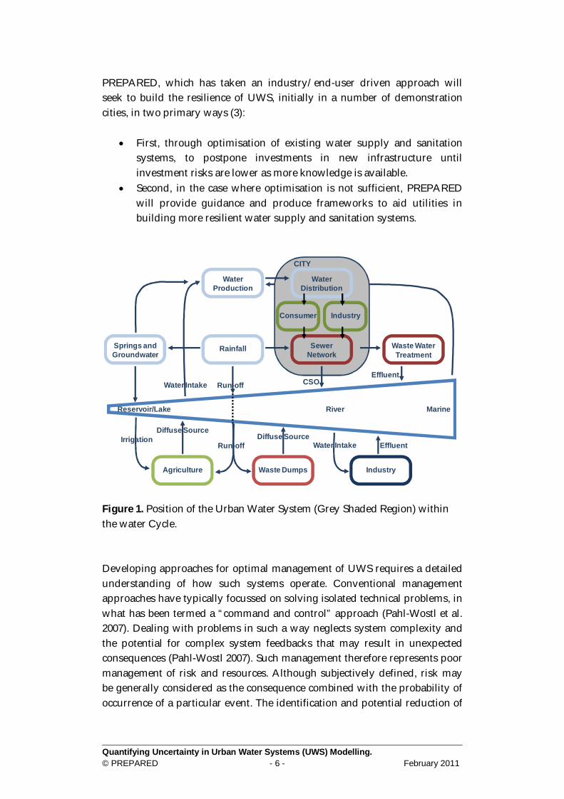
PREPARED, which has taken an industry/end-user driven approach will seek to build the resilience of UWS, initially in a number of demonstration cities, in two primary ways (3):
First, through optimisation of existing water supply and sanitation systems, to postpone investments in new infrastructure until investment risks are lower as more knowledge is available.
Second, in the case where optimisation is not sufficient, PREPARED will provide guidance and produce frameworks to aid utilities in building more resilient water supply and sanitation systems.
Figure 1. Position of the Urban Water System (Grey Shaded Region) within the water Cycle. Developing approaches for optimal management of UWS requires a detailed understanding of how such systems operate. Conventional management approaches have typically focussed on solving isolated technical problems, in what has been termed a “command and control” approach (Pahl-Wostl et al. 2007). Dealing with problems in such a way neglects system complexity and the potential for complex system feedbacks that may result in unexpected consequences (Pahl-Wostl 2007). Such management therefore represents poor management of risk and resources. Although subjectively defined, risk may be generally considered as the consequence combined with the probability of occurrence of a particular event. The identification and potential reduction of
Waste Water Treatment
Rainfall SewerNetwork
Springs and Groundwater
Water Distribution
Consumer
Agriculture Waste Dumps Industry
MarineRiverReservoir/Lake
Diffuse SourceIrrigation
Run-off CSOEffluent
Water Intake
Water Production
CITY
Water Intake EffluentDiffuse Source
Run-off
Industry
Quantifying Uncertainty in Urban Water Systems (UWS) Modelling. © PREPARED - 7 - February 2011
risk associated with Urban Water System management (PREPARED work package 2.3) requires a deeper, holistic understanding of inherent system complexity and uncertainty to better inform an understanding of the probability of event occurrence. An essential and innovative aspect of PREPARED is the development of a toolbox for real time monitoring and modelling (Work area 3.6). The toolbox is required to increase the technological capacity of existing water supply and sanitation systems to deal with changes in the quality and quantity of system input resulting from climatic change, alongside potential changes in demand. Such demands call for an integrated real time control strategy, supported by monitoring and modelling approaches (e.g. Lynggaard-Jensen and Lading 2006; Nielsen et al. 2002; Rauch et al. 2002; Rauch and Harremoes 1999), to provide decision support in the face of inherent system uncertainty. Towards this end, Work package 3.6 will investigate existing methodologies for uncertainty quantification in UWS modelling, and identify possible steps to reduce model uncertainty through real-time modelling, calibration and data assimilation. Studies will be conducted with partner cities/utilities to assess the effectiveness of classical uncertainty propagation methods, e.g., Monte Carlo approach, and some advanced methodologies, such as Markov Chain Monte Carlo methods (e.g., Metropolis-Hastings or the Shuffled Complex Evolution Metropolis algorithm) or the General Likelihood Uncertainty Estimation (GLUE) method. Some promising, but yet untested methods in the context of UWS, such as the Total Error Framework that accounts for and propagates all sources of uncertainties at the same time, will be considered for particular application in UWS. Very recently (2009), an international joint study has attempted to establish a consensus on evaluation of modelling uncertainties for urban sewer systems. Similar attempts have been made by a number of groups assessing other components of UWS (e.g. wastewater treatment plants). As some of the involved researchers are also partners of PREPARED (INSA, UNEXE, Monash, UNINNS, etc) PREPARED will benefit from these recent coordinated efforts and will be a significant contributor to the further development of this work and of its dissemination for the entire UWS.
1.2 Report Structure The report is structured as follows: Section 2 defines types of uncertainty that affect modelling from a systems perspective. In order to understand the potential application of different
Quantifying Uncertainty in Urban Water Systems (UWS) Modelling. © PREPARED - 8 - February 2011
methods for quantifying and reducing uncertainty in UWS, Section 2 first reviews the types of uncertainty affecting our understanding, and therefore ability to model UWS. Section 3 reviews different methods that have been applied within the context of UWS modelling, and in relate scientific fields, for model calibration (reduction of parameter uncertainty) and more recently developed methods for quantifying different types of uncertainty, including structural uncertainty and data uncertainty. Section 3 will also introduce methods applied for sensitivity analysis (3.7), different mathematical representations of uncertainty, including possibility theory (3.9) and evidence theory (3.10), and parameter sampling procedures (3.11). The methods considered in Section 3 are primarily developed to reduce uncertainty prior to model application. Section 4 briefly considers various methods developed and applied specifically to deal with quantifying and reducing uncertainty in (near) real-time. The methods considered in Section 4 are those considered most applicable for addressing Task 3.6.3 (A scientific report on data assimilation techniques for improving the accuracy of model predictions), and shall be reviewed more fully in Deliverable 3.6.2 due in month 18. Section 5 Provides a summary of the conclusions of the report. Section 6 References. Appendix A, provides a tabular classification of the uncertainty methodologies reviewed in Section 3. Appendix B, Provides a Glossary of relevant terms to aid in interpretation of the themes covered in this document.
Quantifying Uncertainty in Urban Water Systems (UWS) Modelling. © PREPARED - 9 - February 2011
2 Uncertainty In Urban Water Systems (UWS)
2.1 Introduction To facilitate the development of an understanding regarding the applicability of different methods for quantifying and reducing uncertainty in UWS, Section 2 will first define uncertainty, and review existing uncertainties affecting our ability to simulate both Water Distribution Networks (WDN; 2.4) and Urban Waste Water Systems (UWWS; 2.5).
2.2 Defining Uncertainty Uncertainty may be broadly defined as a state where we do not have exact knowledge to describe the components of a given system. Uncertainty is usually divided into two categories: aleatory uncertainty, and epistemic uncertainty (Hall 2003; Helton and Burmaster 1996):
Aleatory uncertainty, also referred to as ‘Variability’ (Anderson and Hattis 1999; Nauta 2000) or ‘inherent’ uncertainty (Hall 2003), refers to variability in known populations, where observations/measurements conform to a probability distribution. Such uncertainties include the spatial and temporal variability in rainfall. Hall (2003) prefers an operational definition of aleatory uncertainty that is a specific feature of measurements (phenomenal knowledge) to avoid insubstantial assertions about reality (Noumenal). It is widely held that such uncertainty is irreducible due to its inherent nature.
Epistemic uncertainty results from incomplete knowledge of the system in question, and an inability to understand and describe that system. Numerical models that seek to represent reality are a form of epistemic uncertainty; given the inherent simplification moving from the ‘real world’ to numeric representation, models can never be confirmed as ‘true’ (Popper 1969). However, unlike aleatory uncertainty, epistemic uncertainty can be reduced through greater understanding of the system.
An explicit incorporation of either type of uncertainty in many areas of scientific research (and modelling) is often lacking (Pappenberger et al. 2006). Whilst the lack of uncertainty treatment in scientific analysis at best represents bad practise, in the case of risk management, decisions made based on deterministic predictions may lead to misplaced confidence and severe consequences (Nauta 2000). Over the last decade, contemporaneous with
Quantifying Uncertainty in Urban Water Systems (UWS) Modelling. © PREPARED - 10 - February 2011
advances in data collection and computer power, the application of uncertainty analysis in the fields of hydroinformatics has grown (Hall 2003). In order to address uncertainty when modelling UWS, three areas need to be considered: understanding, quantification, and reduction of uncertainty (Liu and Gupta 2007). Prior to an evaluation of existing methods for quantifying and reducing uncertainty in UWS modelling (Section 3 and Section 4), it is first necessary to consider types of uncertainty in the context of systems modelling (Section 2.3), and the nature and sources of uncertainty in UWS (Section 2.4 and Section 2.5).
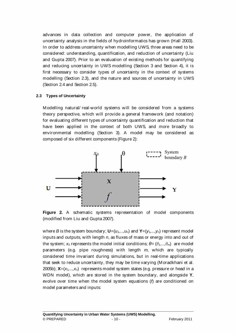
2.3 Types of Uncertainty Modelling natural/real-world systems will be considered from a systems theory perspective, which will provide a general framework (and notation) for evaluating different types of uncertainty quantification and reduction that have been applied in the context of both UWS, and more broadly to environmental modelling (Section 3). A model may be considered as composed of six different components (Figure 2):
Figure 2. A schematic systems representation of model components (modified from Liu and Gupta 2007). where B is the system boundary; U=(u1,...,un) and Y=(y1,...,yn) represent model inputs and outputs, with length n, as fluxes of mass or energy into and out of the system; x0 represents the model initial conditions; θ=(θ1,...,θm) are model parameters (e.g. pipe roughness) with length m, which are typically considered time invariant during simulations, but in real-time applications that seek to reduce uncertainty, they may be time varying (Moradkhani et al. 2005b); X=(x1,...,xn) represents model system states (e.g. pressure or head in a WDN model), which are stored in the system boundary, and alongside Y, evolve over time when the model system equations (f) are conditioned on model parameters and inputs:
Quantifying Uncertainty in Urban Water Systems (UWS) Modelling. © PREPARED - 11 - February 2011
Y, X = 푓(U,푥 ,휃,퐵) (2.1) The model equations (f) may be considered as a formalised mathematical representation of reality, which will contain epistemic uncertainty. As such these equations seek to make the correct mapping from system inputs to states and system outputs. In general, there are three different types of model uncertainty, which incorporate the model system components described above: Structural uncertainty, Parameter uncertainty and Data uncertainty. Structural uncertainty refers to errors in the mathematical representation of reality that result from system conceptualisation (abstraction), numerical representation, and discretisation of a model in space and time. The system boundary (B), and model equations (f) are both part of the model structure. Structural uncertainty is a form of epistemic uncertainty, which can be reduced as more information becomes available to constrain understanding of a system, and enhance model representation. However, as models can never be confirmed as ‘true’, structural uncertainty will never be eliminated. Structural uncertainty (error) is widely known as systems are often simplified for reasons other than epistemic uncertainty (e.g. computational and data constraints lead to simpler system representation). Such errors, whilst known to exist, are often not accounted for fully/explicitly as they are difficult to quantify (see Section 3 and Section 4). Parameter uncertainty reflects uncertainty in the value of variables used in equations to represent model system components (e.g. pipe roughness). Parameter uncertainty may be a form of both aleatory uncertainty and epistemic uncertainty. Nodal demands in WDN are a form of aleatory uncertainty as demand varies temporally throughout the day. Epistemic uncertainty in model parameter values often results from the discretisation of model equations in time and space, resulting in an inability to reconcile the scale of observations with model parameters. Many model parameters (e.g. roughness) are often ‘effective’ (Lane 2005), as they cannot be observed directly in nature, and are estimated indirectly via calibration (Kapelan et al. 2007). Parameter uncertainty can result in large errors in model predictions, and of all forms of uncertainty, has received widest attention in the research literature. Measurement/Data uncertainty refers to uncertainty in the quantities used to define initial conditions (x0), model inputs (U) and observations used to evaluate model predictions (either system states (X) or outputs (Y)). Such uncertainty can result from either instrumentation error that fails to accurately and precisely record the quantity of interest (Bargiela and
Quantifying Uncertainty in Urban Water Systems (UWS) Modelling. © PREPARED - 12 - February 2011
Hainsworth 1989), or result from the spatial and/or temporal miss-match between the scale/resolution of observation, and that required/predicted by the model. Measurement uncertainty can be both aleatory and epistemic in nature. In modelling UWS structural, parameter and measurement uncertainty results in unknowns that will lead to uncertain model predictions. To understand, and maximally reduce the final total uncertainty in model predictions, all of these aspects of uncertainty need to quantified, propagated through the system, and where possible, reduced. A first step towards quantification is to first understand sources of uncertainty in UWS, and uncertainties in the models typically used to represent them.
2.4 Sources of Uncertainty in Water Distribution Network modelling The primary objective of the Water Distribution Network is to provide drinking water at sufficient pressure and volume for end users (domestic and industrial). To meet this demand a WDN typically consists of a number of links (pipes, pumps and valves) that are joined at junction nodes, and control distribution of drinking water, via storage tanks, from a water production to the consumer and industry (Figure 1). Under normal design (steady state conditions), the network must be capable of supplying anticipated demands with adequate pressures. Networks are typically designed as looped structures (Figure 3) to overcome problems of water stagnation, customer isolation during cut-off, demand flexibility, and because looped systems are less sensitive to uncertainty associated with system design (Boulos et al. 2004). Network models that seek to represent the WDN consist of a collection of pipes, pumps and valves, which are connected together at a series of nodes, where consumer demand is specified. The detail with which the original WDN is represented in both time and space depends on the purpose to which the model is to be used. For a given demand (pattern) the system equations conserving mass at junction nodes and energy along pipes may be solved for steady state and extended period simulation (EPS; a series of steady state periods with additional equations for tank levels). Whilst such solutions may be adequate for master planning studies, the transition between hydraulic conditions may be important in surge analysis (Jung et al. 2007). In such situations the governing equations of mass and momentum need to be solved to simulate pressure wave propagation (Boulos et al. 2004). The choice of correct model structure will potentially introduce uncertainty into the
Quantifying Uncertainty in Urban Water Systems (UWS) Modelling. © PREPARED - 13 - February 2011
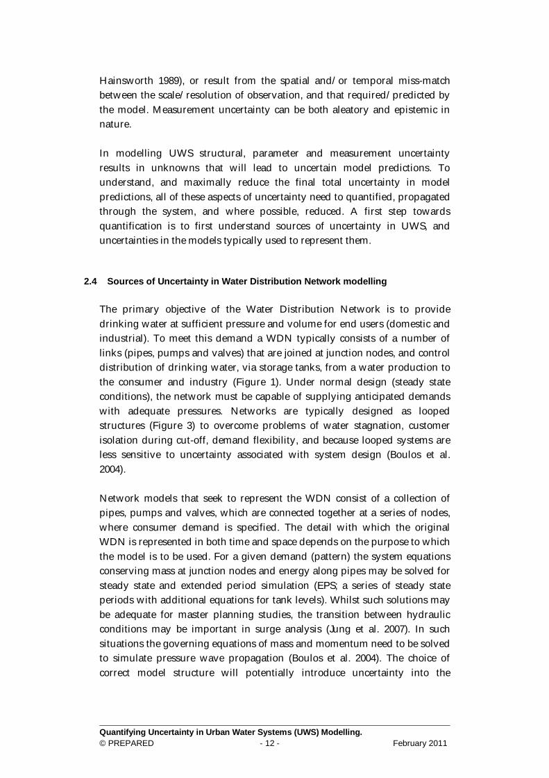
modelling process, alongside existing aleatory uncertainties associated with, for example, demand patterns.
Figure 3. The Anytown network layout as an example of a WDN layout, including a source of water to the system, via a pump and two storage tanks (Walski et al. 1987).
2.4.1 Skeletonisation In model construction the process of skeletonisation involves the removal of pipes that are not considered essential to the analysis conducted by the model, and thereby preserving the performance of the original system. Pipes in series with similar characteristics are often merged to reduce segmentation, and based on hydraulic equivalence theory parallel pipes are merged to a single equivalent pipe with the same hydraulic characteristics. Pipes running to dead ends and pipes less than a given diameter may also be trimmed (Figure 4). The example skeletonised pipe network shown in Figure 4 follows the guidelines set out by the US Environmental Protection Agency (USEPA 2006) whose guidelines for Skeletonisation include preserving at least 80% of the pipe volume in the system, all pipes greater than or equal to 12 inches, and pipes greater than 8 inches in demand areas connected to storage facilities, pumps and valves. A comparison of the original (Figure 4A) and skeletonised network (Figure 4B) for steady-state conditions show hydraulic equivalency, however following a pump trip at 5 seconds, the skeletonised
Quantifying Uncertainty in Urban Water Systems (UWS) Modelling. © PREPARED - 14 - February 2011
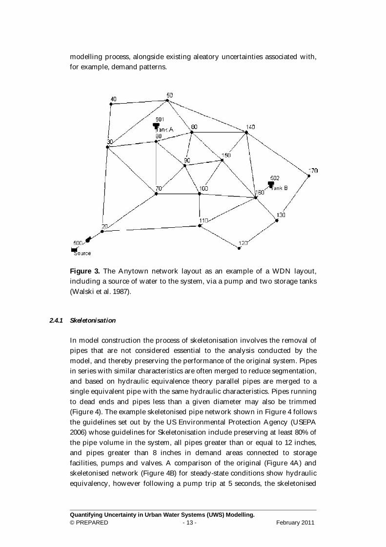
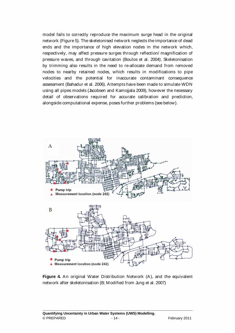
model fails to correctly reproduce the maximum surge head in the original network (Figure 5). The skeletonised network neglects the importance of dead ends and the importance of high elevation nodes in the network which, respectively, may affect pressure surges through reflection/magnification of pressure waves, and through cavitation (Boulos et al. 2004). Skeletonisation by trimming also results in the need to re-allocate demand from removed nodes to nearby retained nodes, which results in modifications to pipe velocities and the potential for inaccurate contaminant consequence assessment (Bahadur et al. 2006). Attempts have been made to simulate WDN using all pipes models (Jacobsen and Kamojjala 2009), however the necessary detail of observations required for accurate calibration and prediction, alongside computational expense, poses further problems (see below).
Figure 4. An original Water Distribution Network (A), and the equivalent network after skeletonisation (B; Modified from Jung et al. 2007)
Quantifying Uncertainty in Urban Water Systems (UWS) Modelling. © PREPARED - 15 - February 2011
Figure 5. Transient head recorded at node 242 (Figure 4) following Pump Trip (Jung et al. 2007).
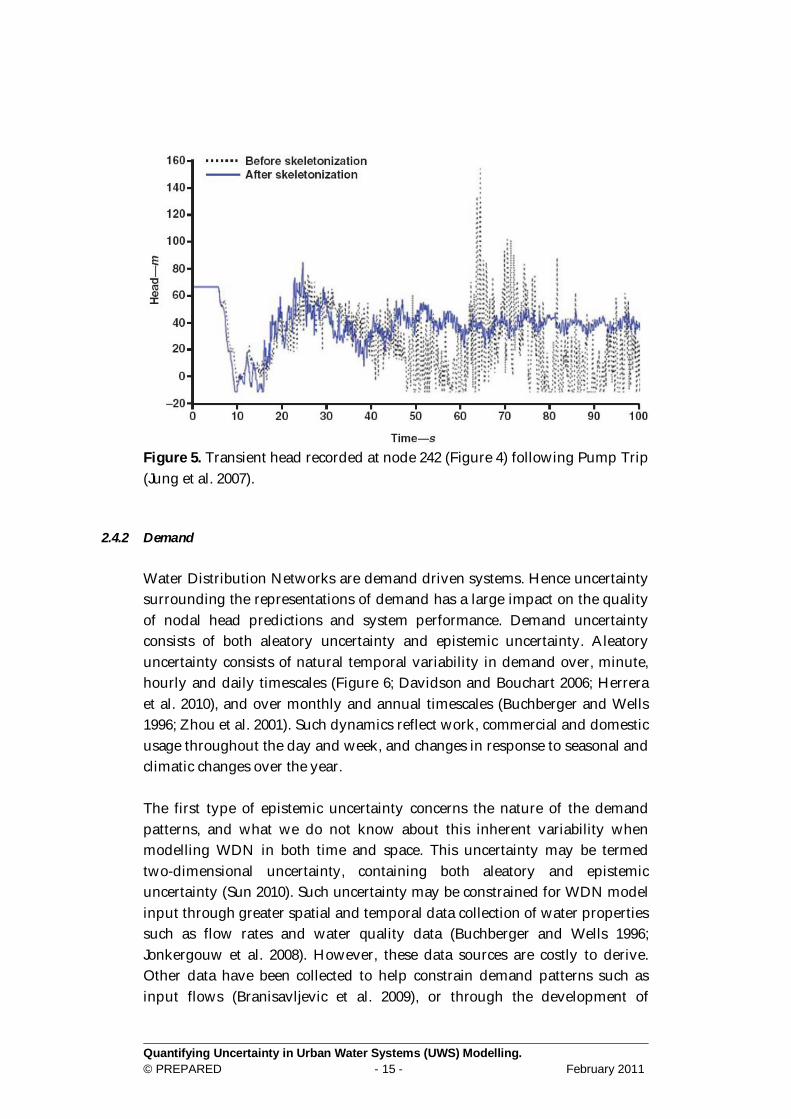
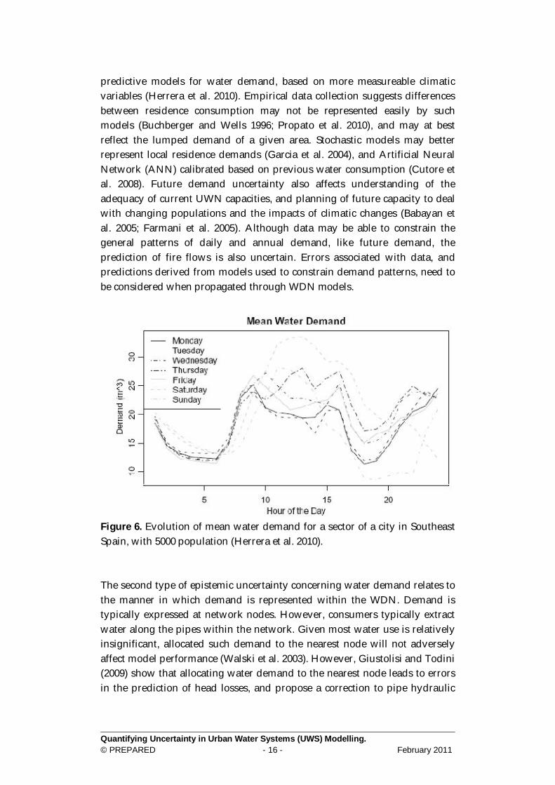
2.4.2 Demand Water Distribution Networks are demand driven systems. Hence uncertainty surrounding the representations of demand has a large impact on the quality of nodal head predictions and system performance. Demand uncertainty consists of both aleatory uncertainty and epistemic uncertainty. Aleatory uncertainty consists of natural temporal variability in demand over, minute, hourly and daily timescales (Figure 6; Davidson and Bouchart 2006; Herrera et al. 2010), and over monthly and annual timescales (Buchberger and Wells 1996; Zhou et al. 2001). Such dynamics reflect work, commercial and domestic usage throughout the day and week, and changes in response to seasonal and climatic changes over the year. The first type of epistemic uncertainty concerns the nature of the demand patterns, and what we do not know about this inherent variability when modelling WDN in both time and space. This uncertainty may be termed two-dimensional uncertainty, containing both aleatory and epistemic uncertainty (Sun 2010). Such uncertainty may be constrained for WDN model input through greater spatial and temporal data collection of water properties such as flow rates and water quality data (Buchberger and Wells 1996; Jonkergouw et al. 2008). However, these data sources are costly to derive. Other data have been collected to help constrain demand patterns such as input flows (Branisavljevic et al. 2009), or through the development of
Quantifying Uncertainty in Urban Water Systems (UWS) Modelling. © PREPARED - 16 - February 2011
predictive models for water demand, based on more measureable climatic variables (Herrera et al. 2010). Empirical data collection suggests differences between residence consumption may not be represented easily by such models (Buchberger and Wells 1996; Propato et al. 2010), and may at best reflect the lumped demand of a given area. Stochastic models may better represent local residence demands (Garcia et al. 2004), and Artificial Neural Network (ANN) calibrated based on previous water consumption (Cutore et al. 2008). Future demand uncertainty also affects understanding of the adequacy of current UWN capacities, and planning of future capacity to deal with changing populations and the impacts of climatic changes (Babayan et al. 2005; Farmani et al. 2005). Although data may be able to constrain the general patterns of daily and annual demand, like future demand, the prediction of fire flows is also uncertain. Errors associated with data, and predictions derived from models used to constrain demand patterns, need to be considered when propagated through WDN models.
Figure 6. Evolution of mean water demand for a sector of a city in Southeast Spain, with 5000 population (Herrera et al. 2010). The second type of epistemic uncertainty concerning water demand relates to the manner in which demand is represented within the WDN. Demand is typically expressed at network nodes. However, consumers typically extract water along the pipes within the network. Given most water use is relatively insignificant, allocated such demand to the nearest node will not adversely affect model performance (Walski et al. 2003). However, Giustolisi and Todini (2009) show that allocating water demand to the nearest node leads to errors in the prediction of head losses, and propose a correction to pipe hydraulic
Quantifying Uncertainty in Urban Water Systems (UWS) Modelling. © PREPARED - 17 - February 2011
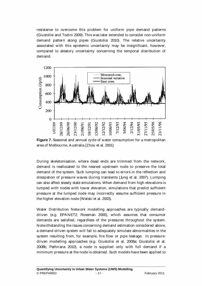
resistance to overcome this problem for uniform pipe demand patterns (Giustolisi and Todini 2009). This was later extended to consider non-uniform demand pattern along pipes (Giustolisi 2010). The relative uncertainty associated with this epistemic uncertainty may be insignificant, however, compared to aleatory uncertainty concerning the temporal distribution of demand.
Figure 7. Seasonal and annual cycle of water consumption for a metropolitan area of Melbourne, Australia (Zhou et al. 2001) During skeletonisation, where dead ends are trimmed from the network, demand is reallocated to the nearest upstream node to preserve the total demand of the system. Such lumping can lead to errors in the reflection and dissipation of pressure waves during transients (Jung et al. 2007). Lumping can also affect steady state simulations. When demand from high elevations is lumped with nodes with lower elevation, simulations that predict sufficient pressure at the lumped node may incorrectly assume sufficient pressure in the higher elevation node (Walski et al. 2003). Water Distribution Network modelling approaches are typically demand-driven (e.g. EPANET2; Rossman 2000), which assumes that consumer demands are satisfied, regardless of the pressures throughout the system. Notwithstanding the issues concerning demand estimation considered above, a demand-driven system will fail to adequately simulate abnormalities in the system resulting from, for example, fire flow or pipe leakage. In pressure-driven modelling approaches (e.g. Giustolisi et al. 2008a; Giustolisi et al. 2008b; Pathirana 2010), a node is supplied only with full demand if a minimum pressure at the node is obtained. Such models have been applied to
Quantifying Uncertainty in Urban Water Systems (UWS) Modelling. © PREPARED - 18 - February 2011
investigate the impact of valve shutdowns (Giustolisi et al. 2008a), and better represent pressure dependent leakage losses in system models (Giustolisi et al. 2008b), however, the approach may require extensive data to determine the relationship between pressure head and flow (Ozger and Mays 2004).
2.4.3 Pipes and roughness Pipes form an integral part of the WDN, distributing water between nodes from source to customer. During model setup the diameter and length of pipes in the system needs to be specified, along with pipe roughness to solve the conservation of energy equation for pipes. Roughness, alongside demand, represents one of the most significant sources of uncertainty in WDN modelling. As pipes age deposits build up due to calcium carbonate precipitation, and in the case of iron pipes due to the build up of oxidation products (Boulos et al. 2004). Such deposits will reduce the pipe diameter, increase roughness, and reduce flow efficiency. The extent of pipe deterioration will depend upon pipe material, water quality, and pipe flow over time, making pipe roughness increasingly difficult to predict with increasing age. This type of epistemic uncertainty is difficult to constrain directly due to the difficulty of measurement, and the effectiveness of roughness values that have little direct physical meaning. Roughness values are usually constrained (calibrated) with junction pressure measurements, and although technically different, also represent the effects of changes in pipe diameter on flow pressures. Such observations are difficult to obtain over the whole network due to cost. Methods have been employed to optimally locate limited measurement locations such that the pressures measured are most sensitive to changes in pipe roughness (de Schaetzen et al. 2000). Different optimisation methods used to locate sensors may result in different observational patterns, and lead to different parameter calibrations, contributing to model uncertainty. The difficulty of obtaining enough distributed measurements to constrain all pipe roughness results in the need to group pipes into roughness categories to reduce the dimensions of the calibration problem (Mallick et al. 2002). However, as the number of parameters reduces, so does model accuracy. Methods to group pipes include grouping of pipes in a similar geographical area (Bascia and Tucciarelli 2003) and the application of k-means clustering to group pipes based on age and diameter in a network (Kumar et al. 2010). Zonal grouping is advantageous in that pipes exposed to similar water quality conditions are grouped, however this will group close pipes irrespective of diameter or age. Calibration predictions derived from the k-
Quantifying Uncertainty in Urban Water Systems (UWS) Modelling. © PREPARED - 19 - February 2011
means clustering method will be sensitive to the number of groupings and the method by which the clusters are initiated, further contributing to model uncertainty. Other methods relate pipe roughness to age, however, the choice of function to relate these variables is uncertain, and likely to be system dependent (Koppel and Vassiljev 2009).
2.4.4 Pumps, valves and tanks Pumps, valves and tanks are key system components allowing managers to control the movement of water in the distribution network. Pumps are designed to raise the hydraulic head to overcome elevation differences and friction losses in the system. The performance of a pump in a network model is simulated using a pump curve that relates head to discharge. The relationship is typically supplied by the manufacturer of the pump, however, in practise pumps do not typically operate at this efficiency (Walski et al. 2003), and over time performance will deteriorate due to cavitation and wear (Hirschi et al. 1998). Further uncertainty may be introduced depending on how well the pump curve relationship is approximated, by either linear, polynomial or exponential relationships during model setup. Pumps represented as links between nodes in a WDN model may ignore important head losses along the pipes between the pump and nodes, which is also the case when representing pressure reducing valves (Walski et al. 2003). Valves control the flow of water through the WDN, and operate in different ways depending on their purpose. Common valve types include isolation valves, which shut off flow to part of the network, check valves which restrict water flow in one direction, pressure reducing valves (PRV’s), which prevent excess pressure, and flow control valves (FCV’s) which limit flow rates. The effect of some valves may be adequately represented by a minor loss coefficient, and potentially incorporated into a pipe roughness coefficient. Other valves such as PRV’s and FCV’s may be represented explicitly by their maximum pressure or flow setting and minor loss coefficient. Air release valves are often not included within WDN models, however, may be significant to represent in transient analysis (Walski et al. 2003). Tanks store water in the distribution network, and are characterised by a maximum and minimum capacity, and a rating curve between head and storage volume. In steady–state simulations the hydraulic head remains fixed, however in EPS, when inputs and outputs to the tank change over time, changes in tank water level need to be simulated.
Quantifying Uncertainty in Urban Water Systems (UWS) Modelling. © PREPARED - 20 - February 2011
2.4.5 Water quality Accurate predictions of water quality depend on the quality of the underlying hydraulic model, and the additional modelling assumptions required. Water quality in a network can be described by the advection-dispersion-reaction equation (Blokker et al. 2008). Given water quality is dominated by advective transport (Pasha and Lansey 2005), the dispersion terms are neglected in EPANET2 (Rossman 2000). Whilst this is a reasonable assumption for turbulent flows, dispersion is important in laminar flows (Blokker et al. 2008). When simulating the movement of both conservative and non-conservative substances, a key assumption applied in WDN (e.g. EPANET2; Rossman 2000) is that of complete and instantaneous mixing at network junctions. Computational Fluid Dynamics (CFD) modelling and experimental work has demonstrated that the perfect mixing assumption is inaccurate (Austin et al. 2008; Romero-Gomez et al. 2008), which leads to erroneous predictions of pollutant concentration within the network. A water quality model names AZRED has been developed to overcome the perfect mixing assumptions within EPANET2 (Choi et al. 2008). In addition to the issues of hydraulic model uncertainty discussed above, velocity prediction along pipes is essential for knowing the fate and transport of contaminants, and is important in controlling chlorine decay rates (Menaia et al. 2003). Velocity data may be obtained from conservative tracer studies (Savic et al. 2009). Skeletonisation affects the accuracy of water velocity predictions, but also, by lumping demand (consumption) at nodes, the population actually affected by a given contamination event may be incorrect (Bahadur et al. 2006). Relatively little attention has been given to joint calibration of WDN and water quality models, which is surprising given the dependencies of the latter on the former. Water quality models are typically calibrated assuming the underlying WDN model is correct. However, given that water companies are more likely to be concerned with delivering (and therefore calibrating for) correct water pressure (Savic et al. 2009), velocity predictions required for accurate water quality modelling are unlikely to be correct. When simulating non-conservative substances, such as chlorine and disinfectant by-products, additional equations and model parameters are required. Chlorine decay has been widely simulated using an exponential decay formula; the exponent in the formula is controlled by both decay within the bulk of water itself, and decay at or near the wall of the pipe (Jonkergouw et al. 2005). The rate of decay at the wall of the pipe is pipe dependent, and relates to pipe age and material, as well as water quality
Quantifying Uncertainty in Urban Water Systems (UWS) Modelling. © PREPARED - 21 - February 2011
passing through the pipe (Hallam et al. 2002). The difficulty of quantifying pipe characteristics for all pipes in the network again results in the need to group pipes for calibration purposes (Munavalli and Kumar 2005), which introduces uncertainties as outlined previously.
2.5 Sources of Uncertainty in Urban Waste Water Systems (UWWS) Modelling UWWS consist of three principal components: Sewer System, Wastewater treatment plant, and receiving water body (Figure 1). The combined system complements the delivery of potable water to consumers and industry by removing wastewater and rainwater through the sewer system, either directly to the receiving water body through Combined Sewer Overflow (CSO), or via the Wastewater Treatment Plant (WWTP). UWWS have been designed and implemented to meet two principal objectives (Korving et al. 2003): first, to mitigate flooding during storm events, and second to provide good sanitation for urban areas by reducing exposure to faecal contamination. Two types of system exist to meet these objectives: separate systems and combined systems. Separate systems have two pipe networks, one for transporting excess rainwater/runoff, and the other for transporting wastewater via the WWTP to the receiving water body. Most major cities around the world have combined sanitary and storm-water flows. Although a combined system has the advantage of fewer pipes, during rainfall events the WWTP has to deal with a larger volume of relatively dilute wastewater, increasing processing costs. In addition, when the sewer system reaches hydraulic capacity, excess untreated water enters directly to the water body (CSO), with potentially detrimental impacts on water quality (Casadio et al. 2008). Traditionally, each component of the UWWS was managed separately, often by a different company, with management aims of meeting legal emission limits without considering direct consequences for receiving water bodies (Devesa et al. 2009). This situation is reflected in the wide range of sector specific simulation tools (Butler and Schutze 2005). However, facilitated by advances in numerical modelling (Butler and Schutze 2005), GIS and data collection techniques (Horoshenkov et al. 2003; Mizaikoff 2003), integrated management approaches have developed to meet a number of requirements: First to meet concerns for the vulnerability of water quality (Beck 2005), as exemplified by the introduction of the Water Framework Directive (WFD; Bloch 1999); and second in public expectation and involvement in attaining higher levels of service (Pahl-Wostl 2005). In order to meet the requirements listed above, a number of approaches moving towards integrated modelling of UWWS have been developed both
Quantifying Uncertainty in Urban Water Systems (UWS) Modelling. © PREPARED - 22 - February 2011
in the research literature (Butler and Schutze 2005; Vanrolleghem et al. 2005), and commercially (e.g. WEST and SIMBA; Rauch et al. 2002). Such models are required to help optimise the performance of existing UWWS, by explicitly accounting for interactions between different components of the system (Butler and Schutze 2005). In doing so the models facilitate incremental adaptation (Butler and Parkinson 1997), and delay the need for constructing new and expensive infrastructure. However, the integrated UWWS is complex, involving a number of epistemic and aleatory uncertainties (Benedetti et al. 2008; Korving et al. 2003). Such uncertainties need to be understood, quantified and reduced to maximise the use of models in system management.
2.5.1 Rainfall uncertainty Rainfall represents the key input to UWWS during Wet Weather Flow (WWF), and enters into the river via surface runoff and groundwater flow, or via the sewer network (Figure 1). Excess rainwater during storm events may cause sewers to exceed their hydraulic capacity; in such cases urban flooding may occur (surcharge), and the WWTP may no longer be able to deal with wastewater, leading to CSO discharges. These discharges are a particular problem in sewer systems resulting in potential pollution of water courses (Beck 1996). Uncertainty surrounding rainfall may be considered as both aleatory and epistemic. Aleatory uncertainty relates to natural spatial and temporal variability in rainfall. Temporally, rainfall varies over annual timescales reflecting seasonal variations and climatic circulation patterns (Rodriguez-Puebla et al. 1998); over daily timescales due to convective processes in the atmosphere (Kutiel and Sharon 1980; Kutiel and Sharon 1981); and over storm event timescales relating to the movement of clouds/rain cells (Morin et al. 2006). Uncertainty surrounding the temporal sequence of rainfall events is important to understand, specifically as the magnitude and frequency of rainfall events exerts a significant control on the performance of the sewer system. For example in Helsinborg, Sweden, CSO events are associated with convective rainfall events which generally occur in late summer and autumn (Semadeni-Davies et al. 2008). The magnitude of the first flush phenomenon, where pollutants concentrations are higher during the initial stages of a storm event (hysteresis), have been found to depend on event magnitude (Gupta and Saul 1996), and on the length of the antecedent dry period for both separate sewer systems, relating to the build up of dry weather flow deposition and traffic related pollutants on the surface (Krein et al. 2007). In some environments the first flush phenomenon is considered too scarce to elaborate treatment
Quantifying Uncertainty in Urban Water Systems (UWS) Modelling. © PREPARED - 23 - February 2011
strategies (Saget et al. 1996), and not simply related to rainfall (Deletic 1998), reflecting a complexity of processes and factors affecting the phenomena (Bertrand-Krajewski et al. 1998). The seasonal phenomenon is particularly important in environments with Mediterranean type climates that experience long dry periods (Asaf et al. 2004; Lee et al. 2004). This situation may be exacerbated because of future predictions of extended drought periods (Christensen et al. 2007). The importance of temporal effects on pollution, however, depends on the site and the types of pollutant loads considered (Gupta and Saul 1996), and uncertainty relating to mobilisation of sediment (Kanso et al. 2005). Spatially, rainfall varies over large scales relating to climatic patterns (e.g. over the Iberian peninsula; Rodriguez-Puebla et al. 1998) and continental topography (Jang 2010); over sub-catchment scales in response to local topographic forcing (Chaubey et al. 1999) and wind shelter (Sevruk and Nevenic 1998); and over short distances (102m) at event timescales in response to the spatial structure of convective rainfall cells (Faures et al. 1995). Spatial patterns in rainfall may be induced by the presence of the urban area itself; studies have identified that by promoting convective heating, urban areas may increase local rainfall (Jauregui and Romales 1996; Thielen and Gadian 1997). However, the production of aerosols and other pollutants in cities may lead to rain suppression (Rosenfeld 2000). In order to quantify aleatory rainfall uncertainty as input to UWWS models, measurements are required, which are themselves uncertain. Epistemic uncertainties in rainfall measurements result from measurement errors and errors in the spatial and temporal resolution of the phenomena. Point rainfall measurements are typically obtained from rain gauges, such as tipping bucket and Hellmann gauges. Rain gauge measurements are subject to systematic errors relating to wind speed (Sevruk 1996; Sevruk et al. 1994; Sevruk and Nespor 1998), rainfall intensity (Ciach 2003), evapotranspiration, and calibration error (Rauch et al. 1998; Stransky et al. 2007), and random errors due to data transmission, mechanical problems and clogging (Rauch et al. 1998). For integrated urban modelling rainfall time series with a temporal resolution of the order of minutes are potentially required (Rauch et al. 1998). In tipping bucket rain gauges such a resolution may not be achieved depending on rainfall intensity, introducing uncertainty into the nature of temporal rainfall patterns. The temporal resolution of rainfall has been shown to affect urban drainage model performance and uncertainty (Aronica et al. 2005). Point rainfall measurements require spatial interpolation for input to sewer models. The assumption of uniform rainfall, which is often made due to a low
Quantifying Uncertainty in Urban Water Systems (UWS) Modelling. © PREPARED - 24 - February 2011
resolution of rain gauges, introduces significant error. As in hydrological applications (Yatheendradas et al. 2008), rainfall uncertainty may dominate over model and parameter uncertainty for the prediction of sewer flow emissions (Willems 1999). Other interpolation methods have used topography (Goovaerts 2000), stochastic methods for reproducing rain cells (Willems and Berlamont 1998), Artificial Neural Networks (Sivapragasam et al. 2010), and conventional interpolation procedures (Bargaoui and Chebbi 2009) to constrain uncertainty in the rainfall field. However, accuracy in interpolation is strongly dependent on the density and quality of point measurements. Over the latter decades of the twentieth century, rainfall radar has been increasingly used, alongside point rainfall measurements, to reproduce the rainfall field for urban sewer studies (Vieux and Vieux 2005). Although a series of radar stations may provide complete spatial coverage of the area of interest, the algorithm used to convert a radar signal to rainfall intensity often requires bias correction due to uncertain parameters (Vieux and Vieux 2005). Further, runoff predictions may be sensitive to the resolution of radar measurements (Ogden and Julien 1994). Point gauge measurements are typically used for bias correction (Campolongo et al. 2007), which as discussed above are themselves uncertain. Such uncertainty needs to be propagated through UWS models (Collier 2009). Many urban sewer systems are situated in wider hydrological catchments. In such circumstances, rainfall does not directly enter the sewer system, but enters via depression storage, infiltration, overland flow and through flow. There is considerable uncertainty surrounding the rainfall-runoff process (Wagener et al. 2003), and even more uncertainty concerning the transport of sediment and pollutants during runoff, both from agriculture (Beven et al. 2005) and urban environments (Deletic et al. 2000). This is a particular problem for understanding the potential impacts of CSOs during wet periods, as the state of the river will be independently altered by rainfall-runoff. A number of methods discussed in Section 3 for constraining uncertainty in UWS modelling have been initially developed for application to conceptual rainfall-runoff modelling (Kapelan et al. 2007; Vrugt et al. 2003). Where runoff entering the UWWS cannot be monitored, catchment models or urban surface runoff models may be applied in conjunction with an UWWS model (Djordjevic et al. 1999). However, liked models of water demand used as input to WDN models, such models also contain considerable uncertainty that needs to be propagated through the UWWS model.
Quantifying Uncertainty in Urban Water Systems (UWS) Modelling. © PREPARED - 25 - February 2011
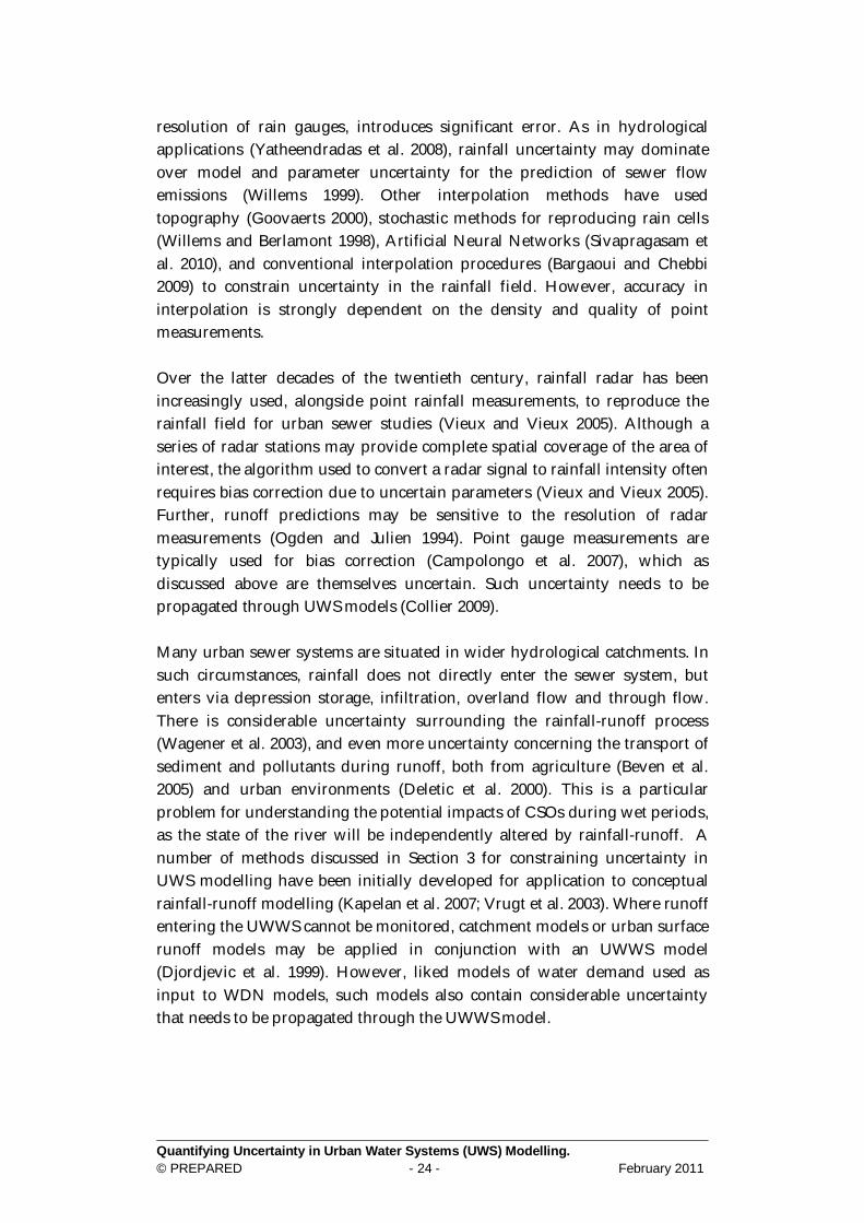
2.5.2 Dry weather Flow Dry Weather Flow (DWF) consists of flow outputs from domestic and industrial users into the UWWS (Figure 1). Similar to water consumption (demand) in the WDN, uncertainty in DWF is both aleatory, reflecting changing consumer inputs over different timescales, and epistemic because of the difficulty in quantifying the volume and quality of waste water from consumers and industry. Uncertainty in DWF from source is important to understand as it is the main source of pollution to the UWWS, and is important to constrain for isolating the action of within sewer processes. Domestic wastewater may be made up of contributions from a variety of different household appliances (e.g. WC, Shower, Dishwasher, Sink, Washing Machine), each with their own patterns of use that vary between weekday and weekend (Butler 1993; Friedler et al. 1996), and diurnally (Figure 8; Figure 9; Almeida et al. 1999). For example, Butler (1993) identified the WC as the most frequently used appliance throughout the day with a well defined morning peak in weekdays, and a smaller and lagged peak during weekends. The WC alongside the kitchen sink has been identified as the largest contributor to volume waste and for the majority of water quality determinands (Almeida et al. 1999). Uncertainty in the temporal sequence of pollution also results as different types of pollutants are produced by different appliances in different quantities (Figure 8), which each may have multiple functions, and therefore loads (Almeida et al. 1999; Friedler and Butler 1996). Further aleatory uncertainty results from different usage amongst different users, which has been found to dominate uncertainty introduced by different types of WC when considering risks of overloading a treatment plant (Wong and Mui 2007).
Figure 8. Diurnal pattern for the total COD load, proportions produced per appliance (Almeida et al. 1999).
Quantifying Uncertainty in Urban Water Systems (UWS) Modelling. © PREPARED - 26 - February 2011
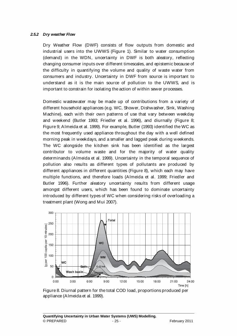
Figure 9. Diurnal pattern for load in wastewater for CODt, PO4, TSS, NH3 and NO3 (Almeida et al. 1999). There is significant epistemic uncertainty in the nature of DWF from domestic properties, owing to the difficulty of measuring actual discharge per household. Actual volume and pollutant loads have been determined by consumer survey (Almeida et al. 1999; Wong and Mui 2007), coupled with appliance measurement for average usage and literature figures for different pollutants (Siegrist et al. 1976) . Therefore, there is uncertainty regarding the reliability of multiplying up short period measurements with consumer survey information, as both may not be representative of reality.
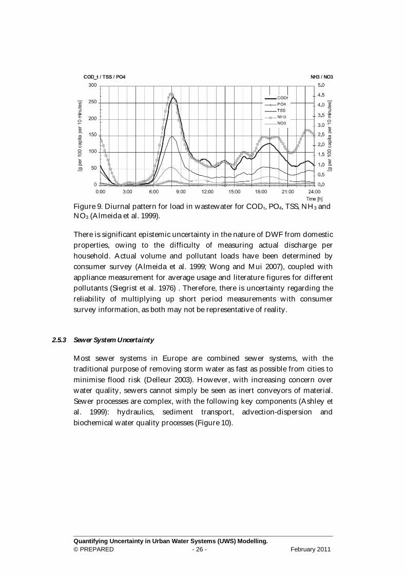
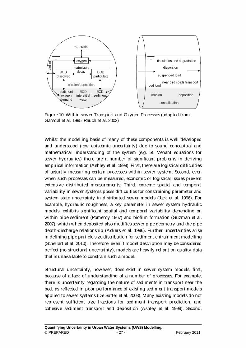
2.5.3 Sewer System Uncertainty Most sewer systems in Europe are combined sewer systems, with the traditional purpose of removing storm water as fast as possible from cities to minimise flood risk (Delleur 2003). However, with increasing concern over water quality, sewers cannot simply be seen as inert conveyors of material. Sewer processes are complex, with the following key components (Ashley et al. 1999): hydraulics, sediment transport, advection-dispersion and biochemical water quality processes (Figure 10).
Quantifying Uncertainty in Urban Water Systems (UWS) Modelling. © PREPARED - 27 - February 2011
Figure 10. Within sewer Transport and Oxygen Processes (adapted from Garsdal et al. 1995; Rauch et al. 2002) Whilst the modelling basis of many of these components is well developed and understood (low epistemic uncertainty) due to sound conceptual and mathematical understanding of the system (e.g. St. Venant equations for sewer hydraulics) there are a number of significant problems in deriving empirical information (Ashley et al. 1999): First, there are logistical difficulties of actually measuring certain processes within sewer system; Second, even when such processes can be measured, economic or logistical issues prevent extensive distributed measurements; Third, extreme spatial and temporal variability in sewer systems poses difficulties for constraining parameter and system state uncertainty in distributed sewer models (Jack et al. 1996). For example, hydraulic roughness, a key parameter in sewer system hydraulic models, exhibits significant spatial and temporal variability depending on within pipe sediment (Pomeroy 1967) and biofilm formation (Guzman et al. 2007), which when deposited also modifies sewer pipe geometry and the pipe depth-discharge relationship (Ackers et al. 1996). Further uncertainties arise in defining pipe particle size distribution for sediment entrainment modelling (Schellart et al. 2010). Therefore, even if model description may be considered perfect (no structural uncertainty), models are heavily reliant on quality data that is unavailable to constrain such a model. Structural uncertainty, however, does exist in sewer system models, first, because of a lack of understanding of a number of processes. For example, there is uncertainty regarding the nature of sediments in transport near the bed, as reflected in poor performance of existing sediment transport models applied to sewer systems (De Sutter et al. 2003). Many existing models do not represent sufficient size fractions for sediment transport prediction, and cohesive sediment transport and deposition (Ashley et al. 1999). Second,
Quantifying Uncertainty in Urban Water Systems (UWS) Modelling. © PREPARED - 28 - February 2011
model simplifications are necessary due to system complexity and computational resources (Fischer et al. 2009), leading to known structural uncertainty. For example, simplifications of the fully dynamic 1D St Venant equations to diffusive wave and kinematic wave have been applied to sewer systems, in addition to conceptual store models when computational times and data are not available/required to support a more detailed model representation (Vaes and Berlamont 1999). Structural conceptual model uncertainty may be constrained through calibration to more dynamic models that can, for example, account for backwater effects (Sartor 1999).
2.5.4 WWTP uncertainty A WWTP model typically consists of an ensemble of components that typically include a clarifier, an active sludge model, hydraulic model, oxygen transfer model, and sedimentation tank model. The WWTP is subject aleatory input uncertainties associated with dry weather flow and rainfall input, as well as potential modification of flow volume and quality in the sewer system due to sewer residence times and within sewer processes (Nielsen et al. 1992; Van Veldhuizen et al. 1999). Further, when influent contains a non negligible amount of industrial wastewater, model modifications and data for specific calibration may be required (Coen et al. 1998; Ky et al. 2001). Despite the development of complex models to represent the processes governing the different components of the WWTP (Gernaey et al. 2004), there are difficulties in applying such models, particularly when integrated with other system components, due to parameter demands that are often substantial and difficult to constrain (Sin et al. 2009). For example, parameters governing the active sludge process are often determined from laboratory studies (Van Veldhuizen et al. 1999), which may not be representative of field conditions. Coefficients to correct for temperature in ASM2 are only valid between 10oC and 25oC (Henze et al. 1995), which may not be representative of field conditions. Further parameter uncertainty may occur when models, which are often calibrated for dry flow conditions, are applied to wet flow conditions (Gernaey et al. 2004). Given the complexity of biological processes a certain amount of greyness may need to be introduced into process representation. Black-box models, calibrated based on input and output data may provide better system representations in cases when white-box models fail to correctly describe all system dynamics (Gernaey et al. 2004). A failure to adequately characterise reactor hydraulics has been identified as a limitation in extending sludge
Quantifying Uncertainty in Urban Water Systems (UWS) Modelling. © PREPARED - 29 - February 2011
models beyond the location of calibration (Cinar et al. 1998), exemplifying the potential for model over-fitting and uncertain process representation. Other simplifications are often applied in WWTP models leading to known structural uncertainty. For example, only in particular cases are hydraulic models applied explicitly to simulate flow through reactors (De Clercq et al. 1999), which are typically assumed instantaneous (Rauch et al. 2002). Further, Clarifiers are often applied in reduced dimensional form (e.g. 1D), and are therefore not fully representative of the 3D process (Takacs et al. 1991). Finally sludge models have been identified as deficient in the representation of settling properties (Harremoes and Rauch 1999), of which there is debate regarding the best settling functions applied to clarifiers (Rauch et al. 2002). Further details of structural uncertainties in the WWTP may be found else ware (e.g. Gernaey et al. 2004; Rauch et al. 1999)
2.5.5 River Uncertainty Rivers are the primary receiving water bodies for many UWWS, however, waste water systems also discharge effluent and CSOs into lakes and coastal waters. Rivers are vulnerable to oxygen depletion resulting from discharge of degradable organic matter, and eutrophication owing to sewer and WWTP effluent nutrient loads (Harremoes and Rauch 1999). Rivers have the same general input uncertainties as described for sewer systems, in addition to uncertain water volume (and quality) derived from non-urban sources (e.g. agricultural: Bilotta and Brazier 2008; Bilotta et al. 2008). The quality of receiving water bodies is one of the key policy drivers of integrated modelling approaches, and therefore data obtained from rivers on water quality (e.g. sediment, COD, O, N, P) are essential to evaluate performance of UWWS and their models. However, data relating to the relationship between water quality and river properties, such as ecology, is often lacking, because knowledge of such processes in uncertain (Bilotta and Brazier 2008; Borchardt and Statzner 1990). For example, different organisms respond differently to certain flow dynamics/exposures, and may have different recovery times. The determination of ecologically meaningful hydrological parameters and thresholds is difficult owing to nonlinear dynamics and multiple causes (Groffman et al. 2006), and limited to specific case studies (Borchardt and Statzner 1990). Furthermore, traditional measures of pollution impact (emission standards), such as the frequency or volume of CSO spill (Lau et al. 2002), may not be compatible with measures of stream water quality standard (Freni et al. 2010), nor reflect actual pollution (Lau et al. 2002). Therefore there are difficulties in imposing which properties emitted from the UWWS to focus on when monitoring for integrated modelling studies (Vanrolleghem et
Quantifying Uncertainty in Urban Water Systems (UWS) Modelling. © PREPARED - 30 - February 2011
al. 2001). Such data are essential to understand given system complexity and resources available for data collection/remediation, which are often limited when conducting uncertainty analysis of integrated models (Mannina et al. 2006; Willems and Berlamont 2002). Receiving water bodies may be simulated using standard hydraulic approaches as applied to sewer systems (St Venant and simplifications) and conceptual store models for water quantity, and mass-transport advection-dispersion equations for water quality (Butler and Schutze 2005). Issues surrounding epistemic uncertainties in these two fundamental model components are similar to those discussed in section 2.4.4 and 2.4.5 (see also: Reichert et al. 2001; Reichert and Vanrolleghem 2001); model complexity may be increased, if possible, to reduce structural uncertainty, however this comes at the expense of needing to constrain more parameters, which due to data limitations are themselves uncertain. If model structural complexity is reduced to a simpler conceptual approach it is often difficult to infer the physical meaning of model parameters, which require sufficient data for calibration.
2.6 Conclusions Both WDN networks and UWWS are subject to structural, parameter and data uncertainties. Data/Measurement uncertainties are primarily associated with natural variability in driving conditions; for WDN this uncertainty primarily resides in demand uncertainty, and for UWWS such uncertainty surrounds dry weather inputs from domestic and industrial sources, and rainfall inputs. Further models applied to both systems have known structural uncertainties given the complexity of the systems and the need for system simplification from both computational and data constraints. In addition, model parameters employed in models applied to both systems are difficult to constrain because of the difficulty of system measurement. Such uncertainties and constraints are well understood conceptually, as they are in a range of other modelled systems. However, to address the aims of the PREPARED project, and optimally use existing UWS infrastructure, formal methods are required to encode this uncertainty within models applied for system management. Section 3 and Section 4 will now consider methods for dealing with Parameter, Data and Structural uncertainties.
Quantifying Uncertainty in Urban Water Systems (UWS) Modelling. © PREPARED - 31 - February 2011
3 Calibration, uncertainty quantification and reduction in Urban Water Systems (UWS)
3.1 Introduction Section 2 introduced the key types of uncertainty that exist in general systems modelling, and details of uncertainties that exist specifically in the context of urban water systems modelling. Two key issues exist when faced with the problem of dealing with uncertainty in systems modelling. First, methods are required to move beyond epistemological understanding, and formally represent our uncertain knowledge of system variables, states, and parameters mathematically. Probability theory has been the dominant paradigm for representing uncertainty (Hall 2003), however, more recently other methods such as fuzzy methods (Vamvakeridou-Lyroudia et al. 2005) and evidence theory (Sadiq et al. 2006) are regarded as legitimate extensions of classical probability (Helton et al. 2004). As Hall (2003) argues, the choice between different methods for formally representing uncertainty in systems modelling is no longer one of mathematical coherence; rather the argument concerns the relative parsimony of different theories, and issues of elicitation (Hall 2003). Of particular relevance to the point of elicitation relates to the quality and quantity of data available to define our uncertainty about specific system parts, which may be lacking (Dubois 2010). Further issues that need to be addressed concern the practicalities of combining mathematical representations of uncertainty, and propagating them through systems models to define predictive and parameter uncertainty to inform the decision making process. Section 3 will review methods applied to quantify and reduce parameter, input data and structural uncertainty through the calibration process. Many methods applied to deal with uncertainty have been initially applied and developed more fully in related fields, such as hydrology (Vrugt et al. 2003) and climate modelling (Zhang and Pu 2010), and only recently applied in an UWS context (e.g. Kapelan et al. 2007). Where relevant, examples of the different methods applied within the context of UWS modelling will be expanded upon, alongside methods currently not applied within UWS modelling. Appendix A contains a tabular classification of some applications of the methods reviewed in Section 3.
Quantifying Uncertainty in Urban Water Systems (UWS) Modelling. © PREPARED - 32 - February 2011
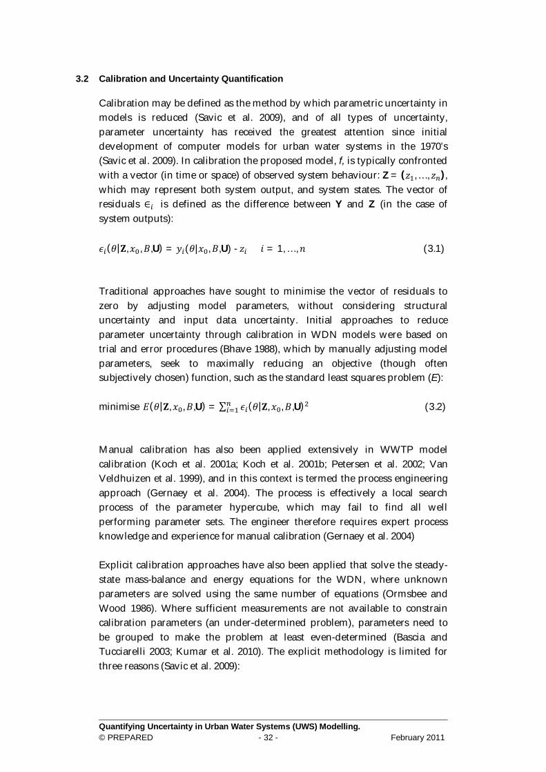
3.2 Calibration and Uncertainty Quantification Calibration may be defined as the method by which parametric uncertainty in models is reduced (Savic et al. 2009), and of all types of uncertainty, parameter uncertainty has received the greatest attention since initial development of computer models for urban water systems in the 1970’s (Savic et al. 2009). In calibration the proposed model, f, is typically confronted with a vector (in time or space) of observed system behaviour: Z = (푧 , … , 푧 ), which may represent both system output, and system states. The vector of residuals ∈ is defined as the difference between Y and Z (in the case of system outputs): 휖 (휃|퐙,푥 ,퐵,U) = 푦 (휃|푥 ,퐵,U) - 푧 푖 = 1, … ,푛 (3.1) Traditional approaches have sought to minimise the vector of residuals to zero by adjusting model parameters, without considering structural uncertainty and input data uncertainty. Initial approaches to reduce parameter uncertainty through calibration in WDN models were based on trial and error procedures (Bhave 1988), which by manually adjusting model parameters, seek to maximally reducing an objective (though often subjectively chosen) function, such as the standard least squares problem (E): minimise 퐸(휃|퐙, 푥 ,퐵,U) = ∑ 휖 (휃|퐙, 푥 ,퐵,U) (3.2) Manual calibration has also been applied extensively in WWTP model calibration (Koch et al. 2001a; Koch et al. 2001b; Petersen et al. 2002; Van Veldhuizen et al. 1999), and in this context is termed the process engineering approach (Gernaey et al. 2004). The process is effectively a local search process of the parameter hypercube, which may fail to find all well performing parameter sets. The engineer therefore requires expert process knowledge and experience for manual calibration (Gernaey et al. 2004) Explicit calibration approaches have also been applied that solve the steady-state mass-balance and energy equations for the WDN, where unknown parameters are solved using the same number of equations (Ormsbee and Wood 1986). Where sufficient measurements are not available to constrain calibration parameters (an under-determined problem), parameters need to be grouped to make the problem at least even-determined (Bascia and Tucciarelli 2003; Kumar et al. 2010). The explicit methodology is limited for three reasons (Savic et al. 2009):
Quantifying Uncertainty in Urban Water Systems (UWS) Modelling. © PREPARED - 33 - February 2011
The posed calibration problem must be at least even-determined. Measurements are assumed 100% accurate and data errors are not
considered. Uncertainty in estimated parameters cannot be quantified.
Both manual and explicit calibration approaches are considered to only have historical significance (Savic et al. 2009), and have largely been superseded by implicit optimisation techniques in model calibration that are more flexible in dealing with uncertainties.
3.3 Optimisation techniques Implicit optimisation techniques seek to minimise the value of an objective function (e.g. Equation 3.1) by applying an optimisation technique coupled with a hydraulic solver (e.g. EPANET2; Rossman 2000). Parameters are typically constrained, as in other techniques discussed later, by upper and lower search bounds (Savic et al. 2009). The optimisation technique operates within the search bounds of each parameter that in WDN typically include pipe roughness, node demands, and valve and pump settings, to minimise the objective function. A number of optimisation methods have been employed in this context for steady-state, EPN and transients simulation, including a Gauss-Newton sensitivity technique (Datta and Sridharan 1994), gradient-based optimisation (Lansey and Basnet 1991), Harmony Search algorithm (Kim et al. 2010), genetic algorithms (Shen and McBean 2010; Vitkovsky et al. 2000), and hybrid genetic algorithms (Kapelan 2002). Genetic Algorithms (GA’s) have also been applied in sewer system modelling (Rauch and Harremoes 1999; Tait et al. 2003), and WDN water quality modelling (Mulligan and Brown 1998). The majority of calibration approaches applied in WDN modelling have focussed on the most computationally efficient way of (maximally) reducing parameter uncertainty through calibration (i.e. finding the optimal parameter set), without explicitly quantifying the uncertainty in parameter values and model predictions. Calibration approaches have been developed, however, that consider multiple objectives; a single optimum simulation may not meet competing demands of, for example total operational/design cost versus water supply and quality (Farmani et al. 2006). In such cases Multi-objective algorithms, such as The Multi-objective Genetic Algorithm (Laucelli et al. 2010), The Preference Order Genetic Algorithm (Khu et al. 2008), The Artificial Neural Network Genetic Algorithm (Fu and Kapelan 2010), and The SCE-UA algorithm (Duan et al. 1992; Madsen 2000; Madsen 2003), can be applied to construct a Pareto Optimal Front between competing objectives.
Quantifying Uncertainty in Urban Water Systems (UWS) Modelling. © PREPARED - 34 - February 2011
Optimisation techniques have been criticised in that given uncertainties outlined relating to data uncertainty and incorrect model structure (as outlined for UWS in Section 2), a single optimal parameter set does not exist; within complex model (parameter) space a number of local optima may exist that produce as acceptable model fits as those found near the ‘Pareto’ optima (Beven 2006). In such cases it has been argued that the parameter probability density should be estimated (Beven 2006).
3.4 First-order second-moment (FOSM) Uncertainty estimation in WDN has typically been achieved using the FOSM method (Bush and Uber 1998; Lansey et al. 2001), which estimates parameter or output variance by approximating a function with a linear Taylor series expansion. The method has been applied first following Lansey et al. (2001), to estimate variances in model parameters (e.g. Roughness, X) due to imprecise measurement errors, in for example pressure head (H):
푐표푣(푋) =훿퐻훿푋
휎훿퐻훿푋
(3.3)
where 휎 is variance in pressure heads. The diagonal elements of the covariance matrix define the variance of model parameters. Using the resultant covariance matrix for model parameters the FOSM method can be applied a second time to estimate uncertainty in model outputs (Kang and Lansey 2009; Kapelan et al. 2005):
푐표푣(푍) =훿푍훿푋
푐표푣(푋)훿푍훿푋
(3.4)
where X is a vector of model parameters, Z is a vector of model outputs, and cov(X) is the matrix of model input parameters. The diagonal elements of cov(Z) define the variance of predictive outputs. The FOSM method, which has also been applied in the context of water quality modelling (Kang et al. 2009), has compared well in quantifying uncertainty in comparison to full Monte Carlo Simulations (MCS; explicit sampling across parameter space to define posterior and parameter uncertainty) for pressure head predictions and chlorine concentrations (Kang and Lansey 2009; Xu and Goulter 1998), notably under steady state conditions (Kang et al. 2009). However, the FOSM
Quantifying Uncertainty in Urban Water Systems (UWS) Modelling. © PREPARED - 35 - February 2011
method did not perform well in predicting chlorine concentrations under unsteady flow conditions (Kang et al. 2009). The FOSM method has several underlying assumptions and limitations that limit application of the method (Kang et al. 2009; Kapelan et al. 2007; Maskey and Guinot 2003):
The linear approximation of the method is only suitable at best for weakly nonlinear problems, or where parameter variance is low.
Assumes independence of calibration parameter values and measurement errors.
Assumes normality of calibration parameter values and measurement errors.
Requires calculation of derivatives of model variables with respect to parameters, which may be computationally demanding.
Output uncertainty is only described up to the second moment (variance), and so theoretical distributions are often assumed to describe the distribution of uncertainty.
The FOSM method may not be applied readily to complex nonlinear problems; in such cases other methods (e.g. MSC) may be required to evaluate performance.
3.5 Formal Bayesian procedures Probability theory has traditionally provided the basis for a mathematical description of uncertainty in engineering and a range of related scientific disciplines (Hall 2003; Helton et al. 2004). In practical modelling Bayesian Statistics has provided the basis to combine prior knowledge with a set of observations to make statistical inferences. The basis for this procedure is encapsulated in Bayes’ Theorem:
푃(퐵|퐴) =푃(퐴|퐵) ∙ 푃(퐵)
푃(퐴) (3.5)
where the conditional probability of B given A, P(B|A) depends on the marginal probabilities P(A) and P(B) and the conditional probability of A given B, P(B|A). Bayes’ theorem can be reformulated to incorporate all forms of uncertainty. In the (typical) case where only parameter uncertainty is considered, the posterior distribution Po(휃|퐙) is dependent on the product of the prior distribution of the vector of model parameters Pr(휃) and the likelihood of predicting the observations conditional on the parameters P(퐙|휃):
Quantifying Uncertainty in Urban Water Systems (UWS) Modelling. © PREPARED - 36 - February 2011
푃 (휃|퐙) =푃(퐙|휃) ∙ 푃 (휃)
푃(퐙) (3.6)
where 푃(퐙) is a constant that normalises the posterior probability mass to unity. Bayes’ equation allows for subjective decisions regarding the nature of prior information, and as such is seen as a method for representing a degree of belief (an epistemic representation as opposed to a frequentist representation), and may be used iteratively as more data are gathered (Freni and Mannina 2010). In such cases the posterior becomes the prior, model simulations are conducted, and model output is confronted with new data. To implement the Bayesian approach to address uncertainty, four issues need to be considered:
Nature of prior information (e.g. shape of the prior probability density function (PDF) for each model parameter).
Choice of an appropriate likelihood function. Choice of an appropriate error model. In special cases uncertainty may be propagated analytically, but in the
case of most models applied to urban water systems, approximate numerical methods typically based on a MCS are employed (Section 3.9).
Assuming first the least squares likelihood function (Equation 3.1 and Equation 3.2), and second that the residuals between measured and modelled output are mutually independent (non-correlated), homoscedastic, and Gaussian distributed with zero mean and variance (휎 ), the posterior distribution takes the following form (Vrugt et al. 2009b):
푃 (휃|퐙,푥 ,퐵,U)=c∙푃 (휃)1
2휋휎exp −
휖 (휃|퐙,푥 ,퐵,U)2휎
(3.7)
where c is a normalising constant. Uncertain prediction limits due to parameter uncertainty may be derived by running the model for all parameter sets over a given time series, and for each observation calculating 95% confidence limits (Engeland et al. 2005). Uncertainty bounds are typically presented alongside the observed time series and optimal model prediction (Figure 11; Freni and Mannina 2010).
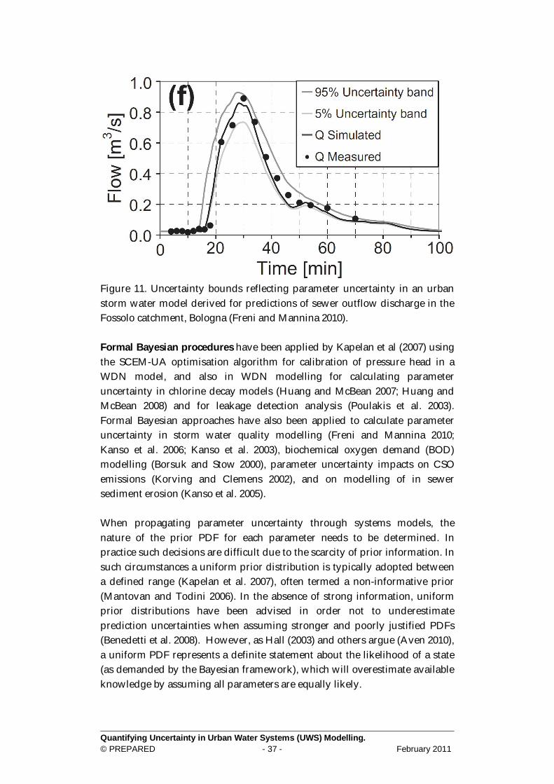
Quantifying Uncertainty in Urban Water Systems (UWS) Modelling. © PREPARED - 37 - February 2011
Figure 11. Uncertainty bounds reflecting parameter uncertainty in an urban storm water model derived for predictions of sewer outflow discharge in the Fossolo catchment, Bologna (Freni and Mannina 2010). Formal Bayesian procedures have been applied by Kapelan et al (2007) using the SCEM-UA optimisation algorithm for calibration of pressure head in a WDN model, and also in WDN modelling for calculating parameter uncertainty in chlorine decay models (Huang and McBean 2007; Huang and McBean 2008) and for leakage detection analysis (Poulakis et al. 2003). Formal Bayesian approaches have also been applied to calculate parameter uncertainty in storm water quality modelling (Freni and Mannina 2010; Kanso et al. 2006; Kanso et al. 2003), biochemical oxygen demand (BOD) modelling (Borsuk and Stow 2000), parameter uncertainty impacts on CSO emissions (Korving and Clemens 2002), and on modelling of in sewer sediment erosion (Kanso et al. 2005). When propagating parameter uncertainty through systems models, the nature of the prior PDF for each parameter needs to be determined. In practice such decisions are difficult due to the scarcity of prior information. In such circumstances a uniform prior distribution is typically adopted between a defined range (Kapelan et al. 2007), often termed a non-informative prior (Mantovan and Todini 2006). In the absence of strong information, uniform prior distributions have been advised in order not to underestimate prediction uncertainties when assuming stronger and poorly justified PDFs (Benedetti et al. 2008). However, as Hall (2003) and others argue (Aven 2010), a uniform PDF represents a definite statement about the likelihood of a state (as demanded by the Bayesian framework), which will overestimate available knowledge by assuming all parameters are equally likely.
Quantifying Uncertainty in Urban Water Systems (UWS) Modelling. © PREPARED - 38 - February 2011
Freni and Mannina (2010) investigated the impact of assuming different amounts of prior information on storm water quality model parameter uncertainty, and concluded that using weak information from other studies to inform prior PDFs can lead to wrong estimations of uncertainty. The study also noted that as the model is ran against more data, the importance of prior hypothetical PDF assumptions are gradually reduced; the length of influence of the prior depends on the difference between the prior PDF and ‘true’ posterior distribution (Freni and Mannina 2010). Further, model performance can be sensitive to the size and type of data used for calibration (Dembele et al. 2010). The use of conditioned posterior information for further application (e.g. validation) depends on the difference in driving conditions between calibration and validation stages, which alongside model sensitivity will determine the validity of the now prior information. Two key decisions governing the applicability of formal Bayesian approaches are the choice of an appropriate likelihood function and the choice of an error model, which will represent structural and input uncertainty. The basic assumptions made in formulating Equation 3.7 are only likely to hold in the simplest of cases; model residuals typically show complex structures involving non-stationarity, autocorrelation, heteroscedasticity, and non-Gaussianity (Beven et al. 2008; Vrugt et al. 2009b). The validity of residual error assumptions should be tested using posterior diagnostic checks, including plots of residual error against output (e.g. discharge) magnitude, quantile-quantile plots for normality, and plots of auto-correlation against time lag (Engeland et al. 2005; Thyer et al. 2009; Yang et al. 2007). Although various error sources have attempted to be accounted for in UWS modelling, alongside parameter uncertainty (e.g.Willems 2008), few attempts have been made to evaluate the assumptions of formal likelihood functions. A key problem with posterior diagnostic checks is that the error model structure is typically calculated with residuals based on a single parameter vector, such as that which produces the maximum or modal likelihood estimation (Engeland et al. 2005; Yang et al. 2007). As pointed out by Beven et al (2008) and Schaefli et al (2007), this residual error is unlikely to apply everywhere in model space. Further, the mode of the posterior distribution will depend on the choice of the error model and the subsequent likelihood function. Beven et al (2008) proposed an iterative approach to constructing an error model by first correcting for Heteroscedasticity and then for autocorrelation. However, the fitted error structure cannot necessarily account for non-linear processing of input error (Beven et al. 2008), and there is no guarantee that it will hold for predictive purposes as the true nature of input and structural error are not known.
Quantifying Uncertainty in Urban Water Systems (UWS) Modelling. © PREPARED - 39 - February 2011
The above problems arise because the decisions governing the choice of likelihood function and error model are typically borne from a focus on parameter uncertainty that implicitly make key assumptions regarding the nature of other sources of error:
Observed system forcing (e.g. in rainfall) is assumed to be equal to the true system forcing (i.e. equating phenomenal with noumenal (Hall, 2003) and ignoring aleatory and epistemic uncertainties in data).
The model is assumed to be a true representation of reality; i.e. there are no structural (epistemic) errors.
The observed system behaviour to evaluate model performance is also considered free from error.
These assumptions, and the associated choice of a simple error model may lead to what has been termed over-conditioning (Beven 2006); that the model fits the data well, and that the likelihood function will be very peaked, as it is assumed that the optimal model is correct. When the above assumptions are made with a non-linear model, there is doubt over the adequacy of the assumed likelihood function, which because of the over-conditioning results in peaked likelihood functions, and inadequate sampling of parameter space. As noted recently, multiple local maxima may exist in parameter space, resulting in difficulties in adequately estimating model parameters (Yang et al. 2007). The result of choosing an inappropriate likelihood function, such as SLS can result in an underestimation of parameter uncertainty (Schoups and Vrugt 2010; Thyer et al. 2009). The lack of general theory of the information content of data, particularly when model structural error is significant, means there is no unambiguous answer for representing and disaggregating the effects of different sources of uncertainty (Beven et al. 2008). Two general approaches, one that remains with a formal Bayesian approach, and one that employs ‘pseudo’ Bayesian approaches (Section 3.2.4), have been employed in an attempt to overcome the problems outlined above.
3.5.1 Multiple error sources and Bayesian Total Error Analysis (BATEA) Formal Bayesian approaches applied to better address all forms of uncertainty may be summed up by the philosophical standpoint of the Bayesian Total Error Analysis (BATEA), which was developed with the aim of explicitly representing each source of uncertainty affecting calibration and prediction (Kuczera et al. 2006). Although this is a difficult aim to achieve, a number of promising approaches have been utilised to overcome some of the
Quantifying Uncertainty in Urban Water Systems (UWS) Modelling. © PREPARED - 40 - February 2011
problems highlighted above, and represent all sources of error, either implicitly or explicitly. In the case where assumptions about the nature of errors are invalid, Heteroscedasticity and non-normality may be overcome using residual transformations, including logarithmic (Romanowicz et al. 1994) and Box-Cox transformation (Freni and Mannina 2010; Sakia 1992). However transformation methods do not account well for heavy tailed residuals (Yang et al. 2007), and as argued by Shaefli et al (2007), the modelling error may not have zero mean in the retransformed variable space, even though Gaussianity holds in the transformed output variable space. A mixture distribution approach has also been proposed, which with the addition of statistical parameters also inferred from the sampling procedure, uses a mixture of normal distributions to represent error structures at low-flow and high-flow periods (Schaefli et al. 2007). Autoregressive models may be employed in attempt to account for correlated errors (Beven and Freer 2001b; Romanowicz et al. 1994; Schoups and Vrugt 2010; Vrugt et al. 2009b; Yang et al. 2007). For example Yang et al 2007 applied a time-varying autoregressive model, which alongside seasonal parameters, improved on traditional error assumptions (e.g. zero mean and constant variance) when subjected to posterior diagnostic tests. Schoups and Vrugt (2010) also applied an autoregressive time-series model, and instead of employing a statistical transformation to achieve Gausssianity of residuals, employed an explicit statistical model. Heteroscedasticity was achieved by modelling standard deviation as a linear function of output flow magnitude, and non-normality accounted for with additional skeweness and kurtosis parameters, which allowed the relaxation of Gaussianity (Schoups and Vrugt 2010). The additional statistical parameters require determination alongside conventional model parameters during model calibration, however the added flexibility in employing Laplace distribution was more robust against outliers. Some of the above methods, although correcting for some of the error assumptions in parameter inference procedures, may be criticised for not attempting to explicitly account for different sources of error (rather, they aim to produce the correct statistical description of the data). As outlined in Section 2, rainfall errors are one of the key factors affecting model uncertainty in UWWS models. Rainfall errors have been accounted for using PDFs to account for event magnitude bias and aerial averaged rainfall (Willems 2001), and applied to individual storm events understand the effect of different sources of uncertainty of sewer water quality modelling (Willems 2008). Similar methods have been applied in the hydrological literature, including storm dependent rainfall multipliers (Kuczera et al. 2006; Thyer et al. 2009),
Quantifying Uncertainty in Urban Water Systems (UWS) Modelling. © PREPARED - 41 - February 2011
and daily multipliers, which have been found to yield more consistent parameter estimates, which are less likely to inadvertently account for structural errors compared to event multipliers, but come at increased computational cost (Thyer et al. 2009). In stormwater models systematic rainfall uncertainties have been shown to impact the model calibration process, and result in different optimal parameter sets depending on the rainfall error (Kleidorfer et al. 2009). Thyer et al (2009) also employed an error model to account for errors in the output stage-discharge relationship. Explicitly accounting for such errors has been found to increase parameter uncertainty (Thyer et al. 2009; Vrugt et al. 2005), emphasising the potential for over-conditioning if such sources of error are ignored. Similar approaches have also been applied to account for measurement error in sewer water quality modelling by removing the estimate measurement error from previous studies to obtain structural error (Willems 2008). Further, in WDN modelling measurement error in pressure measurements it typically accounted for with a standard deviation (Kapelan et al. 2003). Alongside input/output and measurement errors, structural errors have been dealt with explicitly by storm dependent perturbation of model parameters (Kuczera et al. 2006; Renard et al. 2010), in addition to some real time approaches (See section 3.3), and approaches that decompose the posterior uncertainty to reveal the remnant structural uncertainty (Willems 2008). However, when both input and structural errors are accounted for by latent variables, and only vague prior information on input errors is available, decomposition of input and structural errors becomes ill-posed, as respective latent variables will interact (Beven 2009; Renard et al. 2010; Thyer et al. 2009). The ultimate problem of many modelling applications rests in the inability to adequately define a structural error model. Where total uncertainty is of importance for the decision maker the implicit approach of Schoups and Vrugt (2010) that focuses on the correct statistical description of the data may be preferred.
3.5.2 Multi-model approaches Two approaches to deal with model structural uncertainty are Bayesian Model Averaging (BMA) and the Multimodel Ensemble Method (MME). In BMA the posterior distribution of the prediction is given based on a weighted sum of the posteriors distributions from a number of different models (Duan et al. 2007; Zhang et al. 2009). The MME approach, which has been widely applied for weather and climate forecasting (Fowler and Ekstrom 2009; Manning et al. 2009; Tebaldi and Knutti 2007), and used in the IPCC report for projected climate change (IPCC 2001), samples from the output
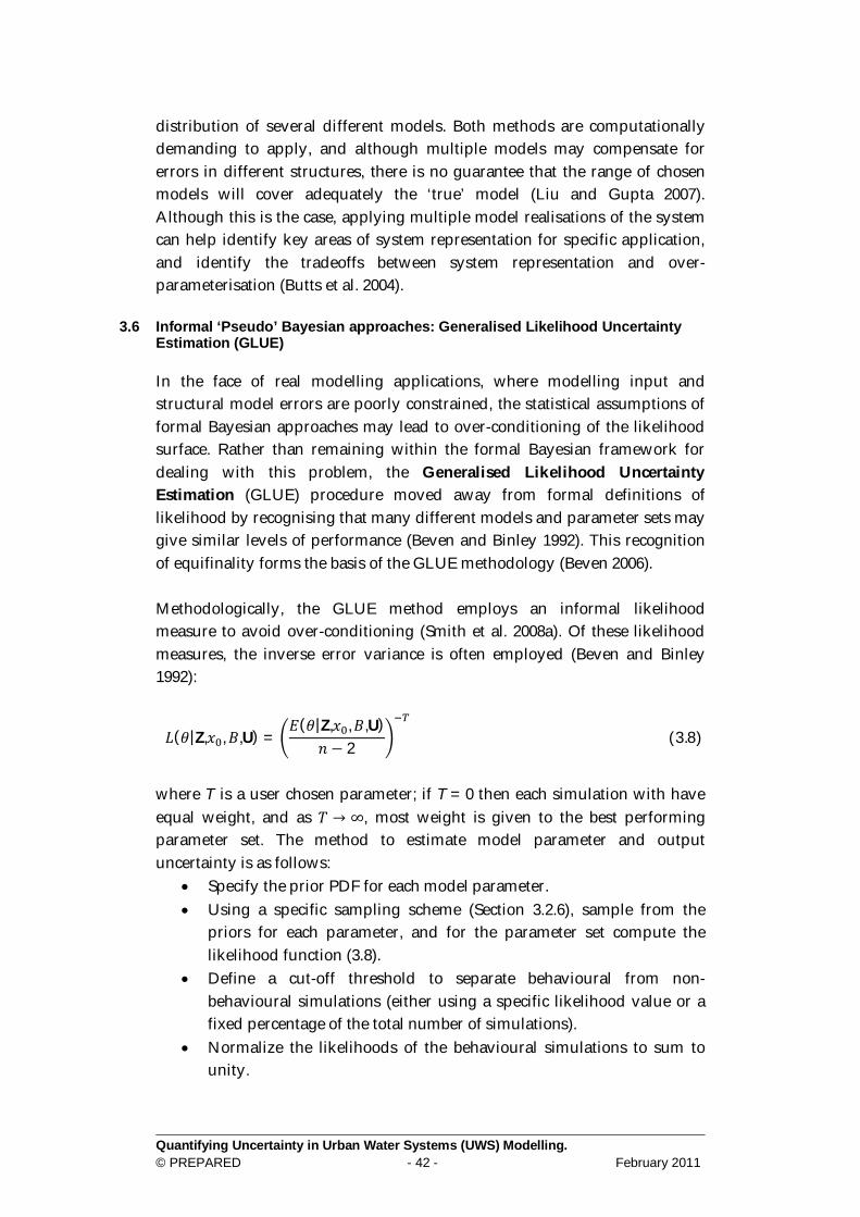
Quantifying Uncertainty in Urban Water Systems (UWS) Modelling. © PREPARED - 42 - February 2011
distribution of several different models. Both methods are computationally demanding to apply, and although multiple models may compensate for errors in different structures, there is no guarantee that the range of chosen models will cover adequately the ‘true’ model (Liu and Gupta 2007). Although this is the case, applying multiple model realisations of the system can help identify key areas of system representation for specific application, and identify the tradeoffs between system representation and over-parameterisation (Butts et al. 2004).
3.6 Informal ‘Pseudo’ Bayesian approaches: Generalised Likelihood Uncertainty Estimation (GLUE) In the face of real modelling applications, where modelling input and structural model errors are poorly constrained, the statistical assumptions of formal Bayesian approaches may lead to over-conditioning of the likelihood surface. Rather than remaining within the formal Bayesian framework for dealing with this problem, the Generalised Likelihood Uncertainty Estimation (GLUE) procedure moved away from formal definitions of likelihood by recognising that many different models and parameter sets may give similar levels of performance (Beven and Binley 1992). This recognition of equifinality forms the basis of the GLUE methodology (Beven 2006). Methodologically, the GLUE method employs an informal likelihood measure to avoid over-conditioning (Smith et al. 2008a). Of these likelihood measures, the inverse error variance is often employed (Beven and Binley 1992):
퐿(휃|Z,푥 ,퐵,U) =퐸(휃|Z,푥 ,퐵,U)
푛 − 2 (3.8)
where T is a user chosen parameter; if T = 0 then each simulation with have equal weight, and as 푇 → ∞, most weight is given to the best performing parameter set. The method to estimate model parameter and output uncertainty is as follows:
Specify the prior PDF for each model parameter. Using a specific sampling scheme (Section 3.2.6), sample from the
priors for each parameter, and for the parameter set compute the likelihood function (3.8).
Define a cut-off threshold to separate behavioural from non-behavioural simulations (either using a specific likelihood value or a fixed percentage of the total number of simulations).
Normalize the likelihoods of the behavioural simulations to sum to unity.
Quantifying Uncertainty in Urban Water Systems (UWS) Modelling. © PREPARED - 43 - February 2011
Sort the parameter sets (and associated probabilities) to create the PDF and CDF of model output prediction, and use these to generate uncertainty intervals.
The GLUE methodology has seen wide application and development in the field of hydrology (Beven and Freer 2001a; Freer et al. 1996; Pappenberger et al. 2005; Pappenberger et al. 2007), and also related fields such as soil erosion (Brazier et al. 2000) and water quality (Smith et al. 2005). More recently the method has been applied within UWWS models to quantify uncertainty in sewer water quality models (Freni et al. 2009b; Lindblom et al. 2007; Mannina et al. 2006), urban runoff models (Thorndahl et al. 2008), input rainfall now-casting (Thorndahl et al. 2010) and WWTP (Cosenza et al. 2010). Thorndahl et al. (2008) used the GLUE methodology to understand model uncertainty in the commercial MOUSE model when applied to the Frejlev urban catchment in Denmark; the methodology highlighted improved performance in MOUSE when applied with aerial weighted rainfall and also with a kinematic surface runoff model. Further, the relative insensitivity of model output to within sewer model parameters was also highlighted (Thorndahl et al. 2008). It should also be noted that the GLUE methodology has been applied with formal Bayesian error models (Beven and Freer 2001b; Romanowicz et al. 1994). Three key, subjective decisions affect the performance of the GLUE methodology; first, the choice of likelihood function; second, the choice of T; and third, the choice of behavioural threshold. A number of studies have investigated the sensitivity of uncertainty assessment to these subjective choices. Increasing the number of parameter sets classed as behavioural has the effect of increasing the uncertainty bounds, and therefore increasing the percentage of observations bracketed by the error bounds (Beven et al. 2008; Freni et al. 2008; Jin et al. 2010; Li et al. 2010). Increasing T has the effect of reducing the width of the uncertainty bounds (Blasone et al. 2008; Freni et al. 2009a; Stedinger et al. 2008). Freni et al (2009a), in application to sewer system models, found that using exponential likelihood functions increased the relative weight of the best simulations compared to the Nash- Sutcliffe performance measure, which similar to increasing the value of T may set a too restrictive condition for defining acceptable parameter sets. The relative sensitivity of model output and parameter error to these subjective choices will depend strongly on the specific model used in application. Accurate probabilistic forecasting requires that the uncertainty bounds have the appropriate statistical coverage (i.e. an appropriate number of observations fall inside the correct uncertainty bounds). A key limit of the informal GLUE methodology is that the uncertainty bounds will not
Quantifying Uncertainty in Urban Water Systems (UWS) Modelling. © PREPARED - 44 - February 2011
necessarily encompass a specific portion of the observations (Beven 2006). Although the correct statistical coverage can be achieved, this may often require calibration of the subjective choices highlighted above (Blasone et al. 2008). This will have the effect of giving magnitude dependent uncertainty estimates (Stedinger et al. 2008), and not correctly account for error variance, particularly in validation. Studies have identified that GLUE can produce similar uncertainty bounds to formal Bayesian approaches (Jin et al. 2010; Vrugt et al. 2009b), which themselves may not provide the correct statistical coverage (Li et al. 2010). As the treatment of residual error (structural and input) in GLUE is left implicit, then the characteristics of the residual error for a particular parameter are also weighted; consistency in under-prediction during calibration is also likely to hold in prediction, and the set of behavioural models may also bracket the observations (Smith et al. 2008a). A criticism of GLUE is that it does not attempt to separate out different forms of model uncertainty. In a similar way that some formal methods have sought to represent different forms of uncertainty (Section 3.2.3), the Limits of Acceptability approach has been developed as an extension of GLUE (Beven 2006). Models are treated as members of the behavioural model set if they lie within the limits of acceptability, which may be defined for each output observation accounting for calibration data measurement uncertainty (Liu et al. 2009). Accounting for errors on a measurement basis, and using information per observation to evaluate consistent over- or under-prediction of observed results, allows for better evaluation of non-stationary error that may facilitate diagnosing structural or input errors.
3.7 Sensitivity Analysis Sensitivity analysis (SA) can form a key model development stage for dealing with parameter uncertainty, particularly prior to real-time modelling approaches that often do not explicitly consider parameter uncertainty (Section 4). SA methods may be broadly split into local, one-factor-at-a-time (OAT) methods that vary one parameter at a time to evaluate output sensitivity (Arabi et al. 2007), and global approaches such as the elementary effects method (Campolongo et al. 2007), and MCS sampling approaches (Helton et al. 2006b). Global approaches, such as ANOVA based Sobol methods (Saltelli et al. 2004), although computationally more expensive, are better able to identify parameter interactions; OAT methods are considered unacceptable in that they do not allow for the co-operative effect of different uncertain parameters on model output (Saltelli et al. 2006).
Quantifying Uncertainty in Urban Water Systems (UWS) Modelling. © PREPARED - 45 - February 2011
Identifying insensitive (unimportant) parameters (e.g. Freni et al. 2011) may reduce the dimensions of the parameter hypercube, and therefore unnecessary MCS sampling during subsequent application (e.g. in real time). SA may be particularly powerful in identifying key, sensitive model parameters (e.g. McCarthy et al. 2010) and locations of sensitive system states (Kapelan et al. 2007) that may form the focus of data collection when resources are limited (e.g. Sensor location optimisation; PREPARED Work Package 3.5). Furthermore SA can reveal parameter interactions between different model components (e.g. between catchment and in the sewer processes; Freni et al. 2011) that can guide the location of further data collection (e.g. intermediate catchment locations such as WWTP effluent point).
3.8 Limitations of Probabilistic approaches An extensive discussion of the application of formal and informal Bayesian approaches to deal with different forms of model uncertainty is present in the research literature (Bargaoui and Chebbi 2009; Beven 2006; Beven et al. 2008; Blasone et al. 2008; Mantovan and Todini 2006; Mantovan et al. 2007; Renard et al. 2010). It is evident that what both informal and formal methods have in common is the presence of subjective assumptions regarding choices made during modelling inference, and what both methods require are techniques for better defining and representing input and structural uncertainty. Both formal and informal Bayesian approaches seek to represent information probabilistically. The probabilistic framework requires the selection of a uniform distribution in the face of ignorance about the probability of an event (or parameter), which is unlikely to be justified by evidence. Such a representation conflates indeterminancy with equiprobability, which when propagated through a model will result in a single posterior probability distribution, which may be bias compared to the original information provided (Dubois 2010; Ferson and Ginzburg 1996). Bayesian approaches may be defended in that although prior assumptions are initially uncertain, confronting models with new data results in sequential updating of prior information, until initial prior assumptions are no longer influential (Freni and Mannina 2010). However, such a distribution may remain a function of both aleatory and epistemic uncertainty unless the influence of structural and data errors on the residual model errors are correctly accounted. Posterior separation of sources of uncertainty remains an active area of research (Renard et al. 2010; Willems 2008).
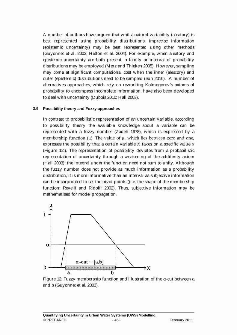
Quantifying Uncertainty in Urban Water Systems (UWS) Modelling. © PREPARED - 46 - February 2011
A number of authors have argued that whilst natural variability (aleatory) is best represented using probability distributions, imprecise information (epistemic uncertainty) may be best represented using other methods (Guyonnet et al. 2003; Helton et al. 2004). For example, when aleatory and epistemic uncertainty are both present, a family or interval of probability distributions may be employed (Merz and Thieken 2005). However, sampling may come at significant computational cost when the inner (aleatory) and outer (epistemic) distributions need to be sampled (Sun 2010). A number of alternatives approaches, which rely on reworking Kolmogorov’s axioms of probability to encompass incomplete information, have also been developed to deal with uncertainty (Dubois 2010; Hall 2003).
3.9 Possibility theory and Fuzzy approaches In contrast to probabilistic representation of an uncertain variable, according to possibility theory the available knowledge about a variable can be represented with a fuzzy number (Zadeh 1978), which is expressed by a membership function (µ). The value of µ, which lies between zero and one, expresses the possibility that a certain variable X takes on a specific value x (Figure 12.). The representation of possibility deviates from a probabilistic representation of uncertainty through a weakening of the additivity axiom (Hall 2003); the integral under the function need not sum to unity. Although the fuzzy number does not provide as much information as a probability distribution, it is more informative than an interval as subjective information can be incorporated to set the pivot points ((i.e. the shape of the membership function; Revelli and Ridolfi 2002). Thus, subjective information may be mathematised for model propagation.
Figure 12. Fuzzy membership function and illustration of the α-cut between a and b (Guyonnet et al. 2003).
Quantifying Uncertainty in Urban Water Systems (UWS) Modelling. © PREPARED - 47 - February 2011
The propagation of uncertainty, expressed by fuzzy numbers, is an extension of interval analysis (Guyonnet et al. 2003): first, a threshold α-cut is selected, which generates an interval [a,b]; this interval is then used in the mathematical function to obtain a posterior interval; other α-cuts are sampled and used to obtain posterior intervals, from which the posterior possibility distribution is recovered. This methodology only applies when the function is monotonic, which does not hold for many WDN models which display strong nonlinearity. In such cases an optimisation procedure will be required to sample the interval [a,b] to derive the minimum and maximum values of X for each α-cut (Branisavljevic et al. 2009). Revelli and Ridolfi (2002) used fuzzy membership functions to describe pipe roughness parameter uncertainty due to material ageing, and employed a Newton-type iterative procedure to solve a steady-state water distribution network problem. Small uncertainties in pipe age, represented by fuzzy membership functions translated into large uncertainties in discharge and head in the network, which increased when demand uncertainty was also represented (Revelli and Ridolfi 2002). The effect of demand uncertainty has also been investigated with Fuzzy representation using input flow as a global constraint, where GA’s are used to solve the optimisation problem (Branisavljevic et al. 2009). Fuzzy membership functions have also been applied to represent rainfall uncertainty in rainfall-runoff models (Maskey et al. 2004), uncertain emissions scenarios in low dimensional climate models (Hall et al. 2007), and used in real-time data anomaly (Branisavljevic et al. In Press). Given computational execution times for optimisation solvers, particularly when applying GA’s with global constraints (Branisavljevic et al. 2009), the fuzzy methods considered may not be applicable to understand uncertainty in complex networks involving many nodes. In such cases a linearization of the hydraulic solver may be required for Fuzzy application (Xu 2003), which comes at a cost of introducing structural uncertainty by not fully representing the non-linear system. Parameters represented by fuzzy membership functions may be combined with parameters represented by PDF’s, where information is available to constrain the latter. A hybrid approach has been developed in order to propagate both forms of uncertainty representation through models by nesting the α-cut sampling procedure described above within a Monte Carlo Sampling procedure of the parameters represented for PDFs (Guyonnet et al. 2003). The result is an ensemble of posterior fuzzy membership functions, each conditioned on a parameter set of the parameters represented probabilistically. Therefore initially probabilistic information becomes possibilistic, a distinction that should be clarified should the method be applied to inform the decision making process (Ross et al. 2002).
Quantifying Uncertainty in Urban Water Systems (UWS) Modelling. © PREPARED - 48 - February 2011
Fuzzy methods have also been applied for optimal looped WDN design with GA optimisation, by replacing strict (or ‘crisp’) criteria for GA penalties with fuzzy membership functions describing performance quality criteria (Vamvakeridou-Lyroudia et al. 2005). The method has been applied for both single- and multi-objective optimisation as a tool to facilitate in decision support (Vamvakeridou-Lyroudia et al. 2006; Vamvakeridou-Lyroudia et al. 2005; Xu and Goulter 1999).
3.10 Evidence Theory Evidence theory, also referred to as Dempster-Shafer theory (Hall et al. 2007), is the simplest method of combining probability and possibility theory into the same theoretical framework (Hall 2003). Evidence theory may be viewed as an extension of probability theory in that the basic probability assignment (BPA), m() (as opposed to p() in probability theory) is assigned to sets as opposed to mutually exclusive singletons. More formally let Θ represent a set of elements (n), each representing a discrete value of a parameter θ (Luo and Caselton 1997): Θ = (휃 , … ,휃 ) (3.9) Evidence theory allows the assignment of probability mass (BPA) to unions of subsets of Θ, such as (θ1, θ2) and also to individual elements of the subset (θ1). All subsets (A) are elements of the power set P(θ). Mass is assigned to a given subset (A), in the interval between 0 and 1, and the sum of BPA’s for all subsets of the power set is 1:
푚(퐴) = 1 (3.10)∈ ( )
Mass assigned to a subset does not say anything about the way in which mass is assigned to singletons or sets contained within A. When mass is only assigned to singletons of Θ evidence theory collapses to probability theory. Unlike probability theory where p() defines the probabilities which are fundamental measures of likelihood, in evidence theory two measures of likelihood for a subset, belief Bel(A) and plausibility Pl(A) are obtained from m(A) (Helton et al. 2004):
Quantifying Uncertainty in Urban Water Systems (UWS) Modelling. © PREPARED - 49 - February 2011
퐵푒푙(퐴) = 푚(퐵) (3.11)⊆
푃푙(퐴) = 푚(퐵) (3.12)∩
where φ is the null set, and B is a subset. Therefore belief is the sum of all the basic probability assignments of all proper subsets of A, when B ⊆ A. Plausibility is the sum of all the basic probability assignments of the subsets that intersect the set of interest (B ∩ A ≠ φ). The interval between belief and plausibility represents the range in which the true probability may lie; therefore when belief equals plausibility the probability is uniquely determined. Evidence theory has been applied to understand and quantify uncertainty associated with contaminant intrusion in water distribution networks (Sadiq et al. 2006), and to combine different sources of uncertain information for pipe deterioration assessment (Bai et al. 2008). Bicik et al (In Press) recently applied evidence theory to combine different sources of information. Combining information from a pipe burst detection model, a hydraulic model and a customer contacts model with evidence theory was able to account for uncertainty in the credibility of different evidence sources, and aid in locating pipe bursts (Bicik et al. In Press). Hall (2003) also demonstrated the use of evidence theory to propagate uncertain information through a simple coastal overtopping problem. Evidence theory has seen relatively little application for propagating uncertain information through UWS models, reflecting both the dominance of other probabilistic paradigms and the added computational expense (Helton et al. 2007), particularly when the number of elements of a set is high. Evidence theory has seen wider application for risk assessment (Helton et al. 2006a); a situation where subjective, limited and uncertain data regarding the possibility of future events is better represented with evidence theory.
3.11 Monte Carlo Sampling (MCS) procedures The procedures considered in Section 3.2 for representing uncertainty, notably Bayesian type probabilistic procedures, require methods to propagate the uncertainty in input and parameter values through the numerical model. In special cases where an analytical solution is present, this integration is relatively straightforward. However, this is rarely the case, and numerical sampling procedures are required to sample parameters sets in order to construct posterior parameter and output distributions.
Quantifying Uncertainty in Urban Water Systems (UWS) Modelling. © PREPARED - 50 - February 2011
The simplest method for parameter sampling is random sampling, also termed Monte Carlo Sampling (MCS) where parameters are randomly drawn from the prior distributions, and used to construct the posterior density function (Freni et al. 2009b). MCS procedures have been applied to evaluate the modelling performance and uncertainty quantification of system linearisation, and FOSM (Bargiela and Hainsworth 1989; Kang and Lansey 2009). A key criticism of MCS procedures is the computational time required to adequately sample parameter space, which for high dimensional problems will be considerable. Random sampling provides no guarantee that higher likelihood parameter space is adequately sampled, not least due to the difficult of identifying a priori the required number of samples. In methods applying MCS procedures to UWS models, where often less than 1000 simulations are conducted, little evidence is provided that these samples provide adequate sampling of parameter space (e.g. Freni et al. 2008; Willems 2008). Methods to test for convergence of the posterior distribution include Kolmogorov-Smirnov, Fluctuation, Geweke’s Zg test, Kuiper test and Gelman-Rubin (El Adlouni et al. 2006; Goldman et al. 2008; Pappenberger et al. 2005), and should be conducted to provide confidence in sensitivity analysis and uncertainty bounds produced.
3.11.1 Latin Hypercube Sampling (LHS) Latin hypercube sampling (LHS) provides a more efficient and stratified means of sampling parameter space; each parameter range is divided into n disjoint intervals of equal probability, and a random sample selected from each interval. This sample is joined with one interval sample from all other parameter ranges without replacement to generate a parameter set (Helton and Davis 2003). LHS methods have been applied to parameter sampling using evidence theory (Helton et al. 2006a), and in probabilistic methods (Blasone et al. 2008; Manache and Melching 2004). Whilst LHS methods improve over MCS procedures in that they guarantee more even sampling of parameter space, they also may not adequately sample the high probability density (HPD) region of parameter space (Blasone et al. 2008). A key limitation of the sampling methods outlined above is that they do not use information from the model sampling procedure at each run to better sample the HPD region of parameter space. More efficient methods are required in complex UWS models to sample the HPD region given potential model complexity, particularly with integrated UWWS models.
Quantifying Uncertainty in Urban Water Systems (UWS) Modelling. © PREPARED - 51 - February 2011
3.11.2 Markov Chain Monte Carlo (MCMC) Methods A family of sampling methods known as Markov Chain Monte Carlo methods (MC2 or MCMC) have been developed and applied to modelling problems to sample more efficiently model parameter space and identify well performing model parameter sets. The Metropolis-Hastings (MH) algorithm was one of the first and most general class of MCMC algorithms to be applied in a formal Bayesian framework (Kuczera and Parent 1998; Schaefli et al. 2007), and has recently been applied to storm water modelling (Dotto et al. 2009; Kleidorfer et al. 2009; McCarthy et al. 2010), and water demand estimation at the household level (Arandia-Perez et al. 2010). The method, which may be initiated with multiple chains, starts a chain at a given point in parameter space and randomly samples from a multivariate jump probability distribution. The ratio of the probability of the current parameter set (j1) to that derived from the previous jump (j0) is calculated, and compared to a random sample from a uniform distribution over the interval [0, 1] to evaluate whether the chain moves to the new location in hyper-parameter space or remains at (j0) to initiate the next jump (Kuczera and Parent 1998). The method is therefore more likely to move to samples of higher probability, but will also sample lower probability regions. Although the method was shown to improve over importance sampling in finding the HPD region (Kuczera and Parent 1998), a poor choice of proposal distribution can lead to slow convergence rates due to the lack of prior information on the location of the HPD region in parameter space (Vrugt et al. 2003). In response to the limitations of early MCMC approaches an active area of research has been in developing more efficient methods for adequately sample the (multiple) HPD regions of model parameter space. Advances over the MH algorithm include the SCHEM-UA algorithm, a development of the SCE-UA algorithm (Duan et al. 1992), which although recently applied to a WDN calibration problem (Alvisi and Franchini 2010) and also to a multi-objective optimisation problem (Madsen 2000), has a tendency to collapse to a single HPD region (Vrugt et al. 2003). The SCHEM-UA algorithm employs multiple parallel chains to enhance the search of multiple HPD regions of parameter space, and exchanges information between the ranked and grouped proposal sample points of each chain (based on decreasing order of posterior probability) to inform the proposal distribution of each candidate point in each group (Vrugt et al. 2003). The method was recently applied in a water distribution network model calibration problem (Kapelan et al. 2007), and also to a water consumption prediction model (Cutore et al. 2008). Further advances in the application include the DREAM (Vrugt et al. 2009b) and DREAM-ZS algorithm (Schoups and Vrugt 2010; Vrugt et al. 2009a), which samples from past states to avoid a large number of parallel chains.
Quantifying Uncertainty in Urban Water Systems (UWS) Modelling. © PREPARED - 52 - February 2011
The DREAM-ZS algorithm includes a snooker updater which generates jumps beyond parallel direction updates (ter Braak and Vrugt 2008). Although the advances in MCMC sampling procedures are primarily motivated by the need to efficiently sample parameter space, a lack or slowness of convergence may be used to identify and understand ill-posed problems. For example, a lack of MCMC convergence may be indicative of an ill-posed problem when there are insufficient data available to constrain model structural and data errors (Renard et al. 2010). A number of the advanced methods discussed above may be appropriate for further application in UWS modelling, and represent a key computational consideration governing the ability to adequately characterise posterior and parameter uncertainty.
3.12 Conclusions A range of methods for quantifying and reducing uncertainty in UWS are available, including a number of methods that have yet to be applied fully in this context, yet have made advances in moving beyond primarily dealing with parameter uncertainty to better accounting for a measurement and structural uncertainty. Methods based in probability theory may be best applied where data availability is good; within this framework a number of approaches for dealing with different forms of uncertainty have been developed. Where data availability is poorer and restricted to expert opinion, and where there is uncertainty regarding the possibility of future events, Possibility theory and Evidence theory may form more appropriate frameworks for representing uncertainty and informing decision making. Model development should be seen as iterative with data collection, and should not be seen as an end point for purely predictive purposes. As such, many of the methods outlined above may be used for model uncertainty reduction by allowing one to target where network monitoring can be applied to constrain structural uncertainty on limited resources, as is the aim of PREPARED work package 3.5. Further, many of the calibration and sensitivity analysis methods considered, although not directly amenable to real-time simulation due to computational constraints, may form a central role in application by constrain parameter uncertainty that has not traditionally been considered in real-time modelling. Of the methods in Section 3, it is difficult to specify a priori whether a particular method will be applicable within the context of UWS modelling; however, their success in other related scientific fields (most notably in

Quantifying Uncertainty in Urban Water Systems (UWS) Modelling. © PREPARED - 53 - February 2011
hydrology), supports the application of some of the methods for uncertainty quantification within Work Package 3.6. Although the methods presented here, as well as the techniques and methodologies that will be implemented in Task 3.6.2 can be considered as generic, the final selection of the methodologies to be applied depends also on the specific requirements of the PREPARED cities selected for demonstration.
Quantifying Uncertainty in Urban Water Systems (UWS) Modelling. © PREPARED - 54 - February 2011
4 Real-time uncertainty quantification and reduction
4.1 Introduction Real-time control (RTC) of UWS, both for Water Distribution and Sewerage Management, has received increased attention in recent years given the demands for improved system performance to meet consumer and regulatory needs, often at reduced cost (Jamieson et al. 2007). Such control is required in WDN to reduce pumping costs (e.g. by filling tanks in low tariff periods) whilst maintain adequate system pressure to meet fluctuating consumer demands (Davidson and Bouchart 2006). Higher system pressures than necessary are normally maintained due to current control limitations, which leads to higher leakage losses from the system (Jamieson et al. 2007). Further, pump-scheduling for system control typically takes the form of lapsed-time control in response to average demand curves over a 24 hour period (Rao et al. 2007) , which does not take full advantage of on-line monitoring data. In UWWS the volume and quality of CSO discharge needs to be minimised by optimally using regulatory devises (e.g. gates, weirs, pumps and treatment works) to manage the flux of sewerage within the wastewater system, through for example, inline storage (Darsono and Labadie 2007). There are three basic approaches for RTC (Vanrolleghem et al. 2005): volume-based, pollution-based and emission based. Although volume-based approaches do not necessarily minimise pollution impact (Lau et al. 2002; Rauch and Harremoes 1999), a relative dearth of data means volume-based approaches are often the most practical approach. It has been argued that in current systems much of this management is limited to reactive control (Pleau et al. 2005), without demonstrating the full potential of on-line monitoring data such as that provided by Supervisory Control And Data Acquisition (SCADA) systems (Kang and Lansey 2009). State estimation (SE) is defined by as the process of combining field measurements and numerical models to gain a global system view of state variables (e.g. pressure) that are not directly measured (Bargiela and Hainsworth 1989). Real-time modelling is required to optimise the real-time control of UWS by providing the ability to predict state variables that are not directly measured due to the difficulty and cost of monitoring extensively in UWS. Further, SE is required to overcome reactive management to existing and often sparse information on system state by making predictions to anticipate future requirements (Jamieson et al. 2007). Although advances in computational power and the development of integrated models facilitates
Quantifying Uncertainty in Urban Water Systems (UWS) Modelling. © PREPARED - 55 - February 2011
the potential take-up of SE approaches in RTC, methods are required to deal with uncertainties in both data and models, and to deal with the computational issues associated with predicting in real-time to optimise system control. Section 4 will briefly outline existing approaches for dealing with uncertainties in real-time modelling of UWS. The methods considered in Section 4 are those considered most applicable for addressing Task 3.6.3 (A scientific report on data assimilation techniques for improving the accuracy of model predictions), and shall be reviewed more fully in Deliverable 3.6.2 due in month 18.
4.2 Outline of Real-time methods Artificial Neural Networks (ANN) are part of a class of data driven modelling approaches that seek to make the correct mapping from input to output data (Jeong and Kim 2005). Such model structures, which implicitly account for model structural errors during calibration are applicable to real-time modelling due to their fast execution times (Rao and Salomons 2007), and have been applied in ensemble to reproduce prediction intervals (Shrestha et al. 2009), consumption prediction with uncertainty derived from SCEM-UA (Cutore et al. 2008), and also for real-time detection of pipe burst events (Romano et al. 2010) The Kalman filter (KF) is a sequential filter method that updates model system state sequentially based on the relative magnitude of state error and measurement error. The method is best applied to linear estimation problems (Todini 1999) and performs poorly in non-linear problems (Kang and Lansey 2009). The Extended Kalman Filter (EKF) was developed to work better in cases of system non-linearity, and has been applied to real time demand estimation in WDN (Shang et al. 2006). Further advances include The Ensemble Kalman Filter (EnKF), introduced by Evensen (1994), was developed to overcome some of the linearity problems associated with the EKF, by propagating an ensemble (n) of model states derived from Monte Carlo perturbations of input state. Though computationally intensive, the method has been most widely applied in related scientific fields, including hydrology (Clark et al. 2008; Moradkhani et al. 2005b; Neal et al. 2007; Xie and Zhang 2010). Sequential Monte Carlo Sampling (Particle Filtering) is a similar estimation approach to Kalman filtering, which propagates multiple realisations (particles) representing a system model forward in time, and uses system observations to update weights associated with the probability of each particle. The particles are used to construct a posterior density function of
Quantifying Uncertainty in Urban Water Systems (UWS) Modelling. © PREPARED - 56 - February 2011
model predictions (Arulampalam et al. 2002; van Leeuwen 2009). The Particle filtering method has been applied in climatology, meteorology and hydrological modelling (Moradkhani et al. 2005a; Pham 2001; Salamon and Feyen 2009; Smith et al. 2008b; van Leeuwen 2009; Vossepoel and van Leeuwen 2007), and has been shown to outperform EnKF, but at increased computational cost (Pham 2001). Variational Data Assimilation (VDA) is a method unlike the family of KF and PF real-time methods in that VDA operates over a time-series of observation points, and is a method widely applied in weather forecasting (Li and Navon 2001). The method is applied by minimising of a cost function (J) that measures the weighted sum of squares between the background state and the observations over a given time interval (Ide et al. 1997) Whilst VDA methods are more suitable to complex problems as they are less demanding computationally, they do not provide an estimate of the predictive uncertainty. A combined approach where 4DVAR is coupled with EnKF was performed which was shown to outperform both methods separately, but at a large computational cost (Hansen and Smith 2001). Joint State and Parameter Estimation, unlike the majority of real time approaches, attempts to consider parameter uncertainty alongside state uncertainty during model application (Brdys and Chen 1995) . These methods may be broadly divided into approaches that apply DA over a time-series used for calibration (static parameters), such as Vrugt et al. (2005) who coupled the SCEM-UA algorithm for parameter estimation with the EnKF, and Dual estimation where both parameters and model states are considered time-varying (Brdys and Chen 1994; Brdys and Chen 1995; Moradkhani et al. 2005a; Moradkhani et al. 2005b; Salamon and Feyen 2009).
4.3 Conclusions A number of real-time modelling approaches for quantifying and reducing uncertainty have been outlined in Section 4. Extensive application in related scientific disciplines, including meteorology, climatology and hydrology, suggests there is strong potential for applying such methods in the context of Urban Water Systems modelling. As with some of the calibration approaches discussed in Section 3, the methods will also require information to define input data (e.g. rainfall) and output data (e.g. pertaining to system states or sewer CSO) uncertainty, which may be difficult to define. Improved rainfall monitoring and sensor placement/performance are other areas to be addressed in PREPARED work package 3 that will facilitate the application of the aforementioned methods for dealing with uncertainty.
Quantifying Uncertainty in Urban Water Systems (UWS) Modelling. © PREPARED - 57 - February 2011
5 Conclusions
This report fulfils the requirements of Deliverable 3.6.1 within work package 3.6 of the PREPARED Enabling change project (EC Seventh Framework Programme Theme 6), and has evaluated existing methods applied in a number of related fields for quantifying and reducing uncertainty in models, that may be applied in Urban Water Systems. Numerical models may be applied to address one of the key aims of the PREPARED project, and optimise the use of existing water supply and sanitation systems. However, such modelling approaches must consider inherent system uncertainty, which as reviewed in Section 2, is both aleatory and epistemic in nature, and affects a range of model components in both Water Distribution Networks and Urban Waste Water Systems. A range of techniques for quantifying and reducing uncertainty have been developed; the most widely applied and developed approaches have focussed on parameter uncertainty, including parameter optimisation procedures, and formal and informal (GLUE) probabilistic approaches. These methods may be best applied where data availability for model calibration and evaluation are good. Recent advances, including the Total Error Analysis and implicit uncertainty methods, have helped to move beyond a focus on model parameter uncertainty within probabilistic approaches towards also accounting for input uncertainty, model structural uncertainty, and output (evaluation) data uncertainty. Such recent advances also require data to constrain and understand the effect of different sources of uncertainty on model performance. Where data availability is poorer, restricted to expert opinion, and where there is uncertainty regarding the possibility of future events, Possibility theory and Evidence theory may form more appropriate frameworks for representing uncertainty and informing decision making. Evidence theory forms a more appropriate framework for combining different sources and types of information to reduce system uncertainty. Model development may, and should be considered as an iterative process alongside data collection. As such, many of the methods outlined in Section 3, notably sensitivity analysis methods, may be applied to reduce model uncertainty by informing where network monitoring should take place to constrain model parameter, and structural uncertainty. Application of such methods is particularly important when resources to provide sufficient distributed system monitoring are limited. Therefore some of the methods
Quantifying Uncertainty in Urban Water Systems (UWS) Modelling. © PREPARED - 58 - February 2011
outlines in Section 3 may be suitable to address the aims of PREPARED work package 3.5. A range of real-time approaches have been briefly introduced in Section 4, which given their extensive application in related scientific disciplines, including meteorology, climatology and hydrology, suggests there is strong potential for applying such methods in the context of Urban Water Systems modelling. Such methods may also be applied successfully when coupled with the calibration methods considered in Section 3 for joint state and parameter estimation. The application of real-time approaches is constrained by the availability of real-time data for application, and the time available to make computations to provide useful system forecasts. These issues will be reviewed more fully in Deliverable 3.6.2, in the context of the methods outlined in Section 4, which are considered most applicable for addressing Task 3.6.3. Although the methods presented here, as well as the techniques and methodologies that will be implemented in Task 3.6.2 can be considered as generic, the final selection of the methodologies to be applied depends also on the specific requirements of the PREPARED cities selected for demonstration.
Quantifying Uncertainty in Urban Water Systems (UWS) Modelling. © PREPARED - 59 - February 2011
6 References
Ackers, J. C., Butler, D., and May, R. W. P. (1996). "Design of sewers to control sediment problems." Report Number CIRIA 141, Construction Industry research and Information Association, London.
Almeida, M. C., Bulter, D., and Frielder, E. (1999). "At-source domestic wastewater quality." Urban Water, 1, 49-55.
Alvisi, S., and Franchini, M. (2010). "Calibration and Sensitivity Analysis of the C-town pipe network model." Water Distribution Systems Analysis 2010, WDSA2010, Tucson, AZ, USA.
Anderson, E. L., and Hattis, D. (1999). "Foundations: A. Uncertainty and Variability." Risk Analysis, 19(1), 47-49.
Arabi, M., Govindaraju, R. S., and Hantush, M. M. (2007). "A probabilistic approach for analysis of uncertainty in the evaluation of watershed management practices." Journal of Hydrology, 333(2-4), 459-471.
Arandia-Perez, Uber, J. G., Boccelli, D. L., Janke, R., Hartman, D., and Lee, Y. D. (2010). "Bayesian temporal modeling of water demands at household level." Water Distribution System Analysis 2010 - WDSA2010, Tucson, Arizona, USA.
Aronica, G., Freni, G., and Oliveri, E. (2005). "Uncertainty analysis of the influence of rainfall time resolution in the modelling of urban drainage systems." Hydrological Processes, 19(5), 1055-1071.
Arulampalam, M. S., Maskell, S., Gordon, N., and Clapp, T. (2002). "A tutorial on particle filters for online nonlinear/non-Gaussian Bayesian tracking." Ieee Transactions on Signal Processing, 50(2), 174-188.
Asaf, L., Nativ, R., Shain, D., Hassan, M., and Geyer, S. (2004). "Controls on the chemical and isotopic compositions of urban stormwater in a semiarid zone." Journal of Hydrology, 294(4), 270-293.
Ashley, R. M., Hvitved-Jacobsen, T., and Bertrand-Krajewski, J. L. (1999). "Quo vadis sewer process modelling?" Water Science and Technology, 39(9), 9-22.
Austin, R. G., Waanders, B. V., McKenna, S., and Choi, C. Y. (2008). "Mixing at cross junctions in water distribution systems. II: Experimental study." Journal of Water Resources Planning and Management-Asce, 134(3), 295-302.
Aven, T. (2010). "On the Need for Restricting the Probabilistic Analysis in Risk Assessments to Variability." Risk Analysis, 30(3), 354-360.
Babayan, A., Kapelan, Z., Savic, D., and Walters, G. (2005). "Least-cost design of water distribution networks under demand uncertainty." Journal of Water Resources Planning and Management-Asce, 131(5), 375-382.
Bahadur, R., Johnson, J., Janke, R., and Samuels, W. B. (2006). "Impact of Model Skeletonization on Water Distribution Model Parameters as Related to Water Quality and Contaminant Consequence Assessment." 8th Annual Water Distribution Systems Analysis Symposium, CIncinati, Ohio, USA.
Bai, H., Sadiq, R., Najjaran, H., and Rajani, B. (2008). "Condition assessment of buried pipes using hierarchical evidential reasoning model." Journal of Computing in Civil Engineering, 22(2), 114-122.
Quantifying Uncertainty in Urban Water Systems (UWS) Modelling. © PREPARED - 60 - February 2011
Bargaoui, Z. K., and Chebbi, A. (2009). "Comparison of two kriging interpolation methods applied to spatiotemporal rainfall." Journal of Hydrology, 365(1-2), 56-73.
Bargiela, A., and Hainsworth, G. D. (1989). "Pressure and Flow Uncertainty in Water-Systems." Journal of Water Resources Planning and Management-Asce, 115(2), 212-229.
Bascia, A., and Tucciarelli, T. (2003). "Simultaneous zonation and calibration of pipe network parameters." Journal of Hydraulic Engineering-Asce, 129(5), 394-403.
Beck, M. B. (1996). "Transient pollution events: Acute risks to the aquatic environment." Water Science and Technology, 33(2), 1-15.
Beck, M. B. (2005). "Vulnerability of water quality in intensively developing urban watersheds." Environmental Modelling & Software, 20(4), 379-380.
Benedetti, L., Bixio, D., Claeys, F., and Vanrolleghem, P. A. (2008). "Tools to support a model-based methodology for emission/immission and benefit/cost/risk analysis of wastewater systems that considers uncertainty." Environmental Modelling & Software, 23(8), 1082-1091.
Bertrand-Krajewski, J. L., Chebbo, G., and Saget, A. (1998). "Distribution of pollutant mass vs volume in stormwater discharges and the first flush phenomenon." Water Research, 32(8), 2341-2356.
Beven, K. (2006). "A manifesto for the equifinality thesis." Journal of Hydrology, 320(1-2), 18-36.
Beven, K., and Binley, A. (1992). "The Future of Distributed Models - Model Calibration and Uncertainty Prediction." Hydrological Processes, 6(3), 279-298.
Beven, K., and Freer, J. (2001a). "A dynamic TOPMODEL." Hydrological Processes, 15(10), 1993-2011.
Beven, K., and Freer, J. (2001b). "Equifinality, data assimilation, and uncertainty estimation in mechanistic modelling of complex environmental systems using the GLUE methodology." Journal of Hydrology, 249(1-4), 11-29.
Beven, K., Heathwaite, L., Haygarth, P., Walling, D., Brazier, R. E., and Withers, P. (2005). "On the concept of delivery of sediment and nutrients to stream channels." Hydrological Processes, 19, 551-556.
Beven, K. J. (2009). "Comment on "Equifinality of formal (DREAM) and informal (GLUE) Bayesian approaches in hydrologic modeling?" by Jasper A. Vrugt, Cajo J. F. ter Braak, Hoshin V. Gupta and Bruce A. Robinson." Stochastic Environmental Research and Risk Assessment, 23(7), 1059-1060.
Beven, K. J., Smith, P. J., and Freer, J. E. (2008). "So just why would a modeller choose to be incoherent?" Journal of Hydrology, 354(1-4), 15-32.
Bhave, P. R. (1988). "Calibrating Water Distribution Network Models." Journal of Environmental Engineering-Asce, 114(1), 120-136.
Bicik, J., Kapelan, Z., Makropoulos, C., and Savic, D. (In Press). "Pipe burst diagnostics using evidence theory." Journal of Hydroinformatics, doi:10.2166/hydro.2010.201.
Bilotta, G. S., and Brazier, R. E. (2008). "Understanding the influence of suspended solids on water quality and aquatic biota." Water Research, 42(12), 2849-2861.
Quantifying Uncertainty in Urban Water Systems (UWS) Modelling. © PREPARED - 61 - February 2011
Bilotta, G. S., Brazier, R. E., Haygarth, P. M., Macleod, C. J. A., Butler, R., Granger, S., Krueger, T., Freer, J., and Quinton, J. (2008). "Rethinking the contribution of drained and undrained grasslands to sediment-related water quality problems." Journal of Environmental Quality, 37(3), 906-914.
Blasone, R. S., Vrugt, J. A., Madsen, H., Rosbjerg, D., Robinson, B. A., and Zyvoloski, G. A. (2008). "Generalized likelihood uncertainty estimation (GLUE) using adaptive Markov chain Monte Carlo sampling." Advances in Water Resources, 31(4), 630-648.
Bloch, H. (1999). "The European Union Water Framework Directive, taking European water policy into the next millennium." Water Science and Technology, 40(10), 67-71.
Blokker, E. J. M., Vreeburg, J. H. G., Buchberger, S. G., and van Dijk, J. C. (2008). "Importance of demand modelling in network water quality models: a review." Drinking Water Engineering and Science, 1, 27-38.
Borchardt, D., and Statzner, B. (1990). "Ecological Impact of Urban Stormwater Runoff Studied in Experimental Flumes - Population Loss by Drift and Availability of Refugial Space." Aquatic Sciences, 52(4), 299-314.
Borsuk, M. E., and Stow, C. A. (2000). "Bayesian parameter estimation in a mixed-order model of BOD decay." Water Research, 34(6), 1830-1836.
Boulos, P. F., Lansey, K. E., and Karney, B. W. (2004). Comprehensive Water Distribution Systems Analysis Handbook For Engineers and Planners, MWH Soft, Inc., Pasadena, California.
Branisavljevic, N., Kapelan, B., and Prodanovic, D. (In Press). "Improved real-time data anomaly detection using context classification." Journal of Hydroinformatics, doi:10.2166/hydro.2011.042.
Branisavljevic, N., Prodanovic, D., and Ivetic, M. (2009). "Uncertainty reduction in water distribution network modelling using system inflow data." Urban Water Journal, 6(1), 69-79.
Brazier, R. E., Beven, K. J., Freer, J., and Rowan, J. S. (2000). "Equifinality and uncertainty in physically based soil erosion models: Application of the glue methodology to WEPP-the water erosion prediction project-for sites in the UK and USA." Earth Surface Processes and Landforms, 25(8), 825-845.
Brdys, M. A., and Chen, K. (1994). "Joint State and Parameter Estimation of Dynmaic Water Supply System Under bounded Uncertainty Using Geometric Programming." 10th IFAC Symposium of System Identification, Copenhagen, Denmark, 331-336.
Brdys, M. A., and Chen, K. (1995). "Set membership estimation of state and parameters in quantity models of water supply and distribution systems." Automatisierungstechnik, 43(2), 77-84.
Buchberger, S. G., and Wells, G. J. (1996). "Intensity, duration, and frequency of residential water demands." Journal of Water Resources Planning and Management-Asce, 122(1), 11-19.
Bush, C. A., and Uber, J. G. (1998). "Sampling design methods for water distribution model calibration." Journal of Water Resources Planning and Management-Asce, 124(6), 334-344.
Quantifying Uncertainty in Urban Water Systems (UWS) Modelling. © PREPARED - 62 - February 2011
Butler, D. (1993). "The influence of dwelling occupancy and day of the week on domestic appliance wastewater discharges " Building and Environment, 28, 73-79.
Butler, D., and Parkinson, J. (1997). "Towards sustainable urban drainage." Water Science and Technology, 35(9), 53-63.
Butler, D., and Schutze, M. (2005). "Integrating simulation models with a view to optimal control of urban wastewater systems." Environmental Modelling & Software, 20(4), 415-426.
Butts, M. B., Payne, J. T., Kristensen, M., and Madsen, H. (2004). "An evaluation of the impact of model structure on hydrological modelling uncertainty for streamflow simulation." Journal of Hydrology, 298(1-4), 242-266.
Campolongo, F., Cariboni, J., and Saltelli, A. (2007). "An effective screening design for sensitivity analysis of large models." Environmental Modelling & Software, 22(10), 1509-1518.
Casadio, A., Maglionico, M., Bolognesi, A., Artina, S., Salmoiraghi, G., and Locascio, A. (2008). "Toxicity and pollutant impact analysis into urban river due to CSO overflows." 11th International Conference on Urban Drainage, Edinburgh, Scotland.
Chaubey, I., Haan, C. T., Grunwald, S., and Salisbury, J. M. (1999). "Uncertainty in the model parameters due to spatial variability of rainfall." Journal of Hydrology, 220(1-2), 48-61.
Choi, C. Y., Shen, J. Y., and Austin, R. G. (2008). "Development of a Comprehensive Solute Mixing Model (AZRED) for Double-Tee, Cross, and Wye Junctions." 10th Annual Water Distribution Systems Analysis Symposium, South Africa.
Christensen, J. H., Hewitson, B., Busuioc, A., Chen, A., Gao, X., Held, I., Jones, R., Kolli, R. K., Kwon, W.-T., Laprise, R., Magaña Rueda, V., Mearns, L., Menéndez, C. G., Räisänen, J., Rinke, A., Sarr, A., and Whetton, P. (2007). "Regional Climate Projections." Climate Change 2007: The Physical Science Basis. Contribution of Working Group I to the Fourth Assessment Report of the Intergovernmental Panel on Climate Change S. Solomon, D. Qin, M. Manning, Z. Chen, M. Marquis, K. B. Averyt, M. Tignor, and H. L. Miller, eds., Cambridge University Press, Cambridge, United Kingdom.
Ciach, G. J. (2003). "Local random errors in tipping-bucket rain gauge measurements." Journal of Atmospheric and Oceanic Technology, 20(5), 752-759.
Cinar, O., Daigger, G. T., and Graef, S. P. (1998). "Evaluation of IAWQ Activated Sludge Model No. 2 using steady-state data from four full-scale wastewater treatment plants." Water Environment Research, 70(6), 1216-1224.
Clark, M. P., Rupp, D. E., Woods, R. A., Zheng, X., Ibbitt, R. P., Slater, A. G., Schmidt, J., and Uddstrom, M. J. (2008). "Hydrological data assimilation with the ensemble Kalman filter: Use of streamflow observations to update states in a distributed hydrological model." Advances in Water Resources, 31(10), 1309-1324.
Coen, F., Petersen, B., Vanrolleghem, P. A., Vanderhaegen, B., and Henze, M. (1998). "Model-based characterisation of hydraulic, kinetic and
Quantifying Uncertainty in Urban Water Systems (UWS) Modelling. © PREPARED - 63 - February 2011
influent properties of an industrial WWTP." Water Science and Technology, 37(12), 317-326.
Collier, C. G. (2009). "On the propagation of uncertainty in weather radar estimates of rainfall through hydrological models." Meteorological Applications, 16(1), 35-40.
Cosenza, A., Mannina, G., and Viviani, G. (2010). "Uncertainty of a biological nitrogen and phosphorus removal model." International Environmental Modelling and Software Society 2010 International Congree on Environmental Modelling and Software Modelling for Environment's Sake. Fifth Biennial Meeting, Ottawa, Canada.
Cutore, P., Campisano, A., Kapelan, Z., Modica, C., and Savic, D. (2008). "Probabilistic prediction of urban water consumption using the SCEM-UA algorithm." Urban Water Journal, 5(2), 125-132.
Darsono, S., and Labadie, J. W. (2007). "Neural-optimal control algorithm for real-time regulation of in-line storage in combined sewer systems." Environmental Modelling & Software, 22(9), 1349-1361.
Datta, R. S. N., and Sridharan, K. (1994). "Parameter-Estimation in Water-Distribution Systems by Least-Squares." Journal of Water Resources Planning and Management-Asce, 120(4), 405-422.
Davidson, J. W., and Bouchart, F. J. C. (2006). "Adjusting nodal demands in SCADA constrained real-time water distribution network models." Journal of Hydraulic Engineering-Asce, 132(1), 102-110.
De Clercq, B., Coen, F., Vanderhaegen, B., and Vanrolleghem, P. A. (1999). "Calibrating simple models for mixing and flow propagation in waste water treatment plants." Water Science and Technology, 39(4), 61-69.
de Schaetzen, W. B. F., Walters, G. A., and Savic, D. A. (2000). "Optimal sampling design for model calibration using shortest path, genetic and etropy algorithms." Urban Water, 2, 141-152.
De Sutter, R., Rushforth, P., Tait, S., Huygens, M., Verhoeven, R., and Saul, A. (2003). "Validation of existing bed load transport formulas using in-sewer sediment." Journal of Hydraulic Engineering-Asce, 129(4), 325-333.
Deletic, A. (1998). "The first flush load of urban surface runoff." Water Research, 32(8), 2462-2470.
Deletic, A., Ashley, R., and Rest, D. (2000). "Modelling input of fine granular sediment into drainage systems via gully-pots." Water Research, 34(15), 3836-3844.
Delleur, J. W. (2003). "The evolution of urban hydrology: Past, present, and future." Journal of Hydraulic Engineering-Asce, 129(8), 563-573.
Dembele, A., Bertrand-Krajewski, J. L., and Barillon, B. (2010). "Calibration of stormwater quality regression models: a random process?" Water Science and Technology, 62(4), 875-882.
Devesa, F., Comas, J., Turon, C., Freixo, A., Carrasco, F., and Poch, M. (2009). "Scenario analysis for the role of sanitation infrastructures in integrated urban wastewater management." Environmental Modelling & Software, 24(3), 371-380.
Djordjevic, S., Prodanovic, D., and Maksimovic, C. (1999). "An approach to stimulation of dual drainage." Water Science and Technology, 39(9), 95-103.
Quantifying Uncertainty in Urban Water Systems (UWS) Modelling. © PREPARED - 64 - February 2011
Dotto, C. B. S., Deletic, A., and Fletcher, T. D. (2009). "Analysis of parameter uncertainty of a flow and quality stormwater model." Water Science and Technology, 60(3), 717-725.
Duan, Q. Y., Ajami, N. K., Gao, X. G., and Sorooshian, S. (2007). "Multi-model ensemble hydrologic prediction using Bayesian model averaging." Advances in Water Resources, 30(5), 1371-1386.
Duan, Q. Y., Sorooshian, S., and Gupta, V. (1992). "Effective and Efficient Global Optimization for Conceptual Rainfall-Runoff Models." Water Resources Research, 28(4), 1015-1031.
Dubois, D. (2010). "Representation, Propagation, and Decision Issues in Risk Analysis Under Incomplete Probabilistic Information." Risk Analysis, 30(3), 361-368.
El Adlouni, S., Favre, A. C., and Bobee, B. (2006). "Comparison of methodologies to assess the convergence of Markov chain Monte Carlo methods." Computational Statistics & Data Analysis, 50(10), 2685-2701.
Engeland, K., Xu, C. Y., and Gottschalk, L. (2005). "Assessing uncertainties in a conceptual water balance model using Bayesian methodology." Hydrological Sciences Journal-Journal Des Sciences Hydrologiques, 50(1), 45-63.
Farmani, R., Walters, G., and Savic, D. (2006). "Evolutionary multi-objective optimization of the design and operation of water distribution network: total cost vs. reliability vs. water quality." Journal of Hydroinformatics, 8(3), 165-179.
Farmani, R., Walters, G. A., and Savic, D. A. (2005). "Trade-off between total cost and reliability for Anytown water distribution network." Journal of Water Resources Planning and Management-Asce, 131(3), 161-171.
Faures, J. M., Goodrich, D. C., Woolhiser, D. A., and Sorooshian, S. (1995). "Impact of Small-Scale Spatial Rainfall Variability on Runoff Modeling." Journal of Hydrology, 173(1-4), 309-326.
Ferson, S., and Ginzburg, L. R. (1996). "Different methods are needed to propagate ignorance and variability." Reliability Engineering & System Safety, 54(2-3), 133-144.
Fischer, A., Rouault, P., Kroll, S., Van Assel, J., and Pawlowsky-Reusing, E. (2009). "Possibilities of sewer model simplifications." Urban Water Journal, 6(6), 457-470.
Fowler, H. J., and Ekstrom, M. (2009). "Multi-model ensemble estimates of climate change impacts on UK seasonal precipitation extremes." International Journal of Climatology, 29(3), 385-416.
Freer, J., Beven, K., and Ambroise, B. (1996). "Bayesian estimation of uncertainty in runoff prediction and the value of data: An application of the GLUE approach." Water Resources Research, 32(7), 2161-2173.
Freni, G., and Mannina, G. (2010). "Bayesian approach for uncertainty quantification in water quality modelling: The influence of prior distribution." Journal of Hydrology, 392(1-2), 31-39.
Freni, G., Mannina, G., and Viviani, G. (2008). "Uncertainty in urban stormwater quality modelling: The effect of acceptability threshold in the GLUE methodology." Water Research, 42(8-9), 2061-2072.
Quantifying Uncertainty in Urban Water Systems (UWS) Modelling. © PREPARED - 65 - February 2011
Freni, G., Mannina, G., and Viviani, G. (2009a). "Uncertainty in urban stormwater quality modelling: The influence of likelihood measure formulation in the GLUE methodology." Science of the Total Environment, 408(1), 138-145.
Freni, G., Mannina, G., and Viviani, G. (2009b). "Urban runoff modelling uncertainty: Comparison among Bayesian and pseudo-Bayesian methods." Environmental Modelling & Software, 24(9), 1100-1111.
Freni, G., Mannina, G., and Viviani, G. (2010). "Emission standards versus immission standards for assessing the impact of urban drainage on ephemeral receiving water bodies." Water Science and Technology, 61(6), 1617-1629.
Freni, G., Mannina, G., and Viviani, G. (2011). "Assessment of the integrated urban water quality model complexity through identifiability analysis." Water Research, 45, 37-50.
Friedler, E., Brown, D. M., and Butler, D. (1996). "A study of WC derived sewer solids." Water Science and Technology, 33(9), 17-24.
Friedler, E., and Butler, D. (1996). "Quantifying the inherent uncertainty in the quantity and quality of domestic wastewater." Water Science and Technology, 33(2), 65-78.
Fu, G., and Kapelan, Z. (2010). "Embedding Neural Networks in Multiojective Genetic Algorithms for water distribution system design." Water Distribution Systems Analysis 2010 - WDSA2010, Tucson, Arizona, USA.
Garcia, V. J., Garcia-Bartual, R., Cabrera, E., Arregui, F., and Garcia-Serra, J. (2004). "Stochastic model to evaluate residential water demands." Journal of Water Resources Planning and Management-Asce, 130(5), 386-394.
Garsdal, H., Mark, O., Dorge, J., and Jepsen, S. E. (1995). "Mousetrap - Modeling of Water-Quality Processes and the Interaction of Sediments and Pollutants in Sewers." Water Science and Technology, 31(7), 33-41.
Gernaey, K. V., van Loosdrecht, M. C. M., Henze, M., Lind, M., and Jorgensen, S. B. (2004). "Activated sludge wastewater treatment plant modelling and simulation: state of the art." Environmental Modelling & Software, 19(9), 763-783.
Giustolisi, O. (2010). "Considering Actual Pipe Connections in Water Distribution Network Analysis." Journal of Hydraulic Engineering-Asce, 136(11), 889-900.
Giustolisi, O., Kapelan, Z., and Savic, D. (2008a). "Extended Period Simulation Analysis Considering Valve Shutdowns." Journal of Water Resources Planning and Management-Asce, 134(6), 527-537.
Giustolisi, O., Savic, D., and Kapelan, Z. (2008b). "Pressure-driven demand and leakage simulation for water distribution networks." Journal of Hydraulic Engineering-Asce, 134(5), 626-635.
Giustolisi, O., and Todini, E. (2009). "Pipe hydraulic resistance correction in WDN analysis." Urban Water Journal, 6(1), 39-52.
Goldman, E., Valiyeva, E., and Tsurumi, H. (2008). "Kolmogorov-Smirnov, fluctuation, and Z(g) tests for convergence of Markov Chain Monte Carlo draws." Communications in Statistics-Simulation and Computation, 37(2), 368-379.
Quantifying Uncertainty in Urban Water Systems (UWS) Modelling. © PREPARED - 66 - February 2011
Goovaerts, P. (2000). "Geostatistical approaches for incorporating elevation into the spatial interpolation of rainfall." Journal of Hydrology, 228(1-2), 113-129.
Goulsby, B., and Samuels, P. (2005). "Language of Risk: Project Definitions." Report: T32-04-01, www.floodsite.net.
Groffman, P., Baron, J., Blett, T., Gold, A., Goodman, I., Gunderson, L., Levinson, B., Palmer, M., Paerl, H., Peterson, G., Poff, N., Rejeski, D., Reynolds, J., Turner, M., Weathers, K., and Wiens, J. (2006). "Ecological thresholds: The key to successful environmental management or an important concept with no practical application?" Ecosystems, 9(1), 1-13.
Gupta, K., and Saul, A. J. (1996). "Specific relationships for the first flush load in combined sewer flows." Water Research, 30(5), 1244-1252.
Guyonnet, D., Bourgine, B., Dubois, D., Fargier, H., Come, B., and Chiles, J. P. (2003). "Hybrid approach for addressing uncertainty in risk assessments." Journal of Environmental Engineering-Asce, 129(1), 68-78.
Guzman, K., La Motta, E. J., McCorquodale, J. A., Rojas, S., and Ermogenous, M. (2007). "Effect of biofilm formation on roughness coefficient and solids deposition in small-diameter PVC sewer pipes." Journal of Environmental Engineering-Asce, 133(4), 364-371.
Hall, J., Fu, G. T., and Lawry, J. (2007). "Imprecise probabilities of climate change: aggregation of fuzzy scenarios and model uncertainties." Climatic Change, 81(3), 265-281.
Hall, J. W. (2003). "Handling uncertainty in the hydroinformatic process." Journal of Hydroinformatics, 5, 215-232.
Hallam, N. B., West, J. R., Forster, C. F., Powell, J. C., and Spencer, I. (2002). "The decay of chlorine associated with the pipe wall in water distribution systems." Water Research, 36(14), 3479-3488.
Hansen, J. A., and Smith, L. A. (2001). "Probabilistic noise reduction." Tellus Series a-Dynamic Meteorology and Oceanography, 53(5), 585-598.
Harremoes, P., and Rauch, W. (1999). "Optimal design and real time control of the integrated urban run-off system." Hydrobiologia, 410, 177-184.
Helton, J. C., and Burmaster, D. E. (1996). "Guest editorial: Treatment of aleatory and epistemic uncertainty in performance assessments for complex systems." Reliability Engineering & System Safety, 54(2-3), 91-94.
Helton, J. C., and Davis, F. J. (2003). "Latin hypercube sampling and the propagation of uncertainty in analyses of complex systems." Reliability Engineering & System Safety, 81(1), 23-69.
Helton, J. C., Johnson, J. D., and Oberkampf, W. L. (2004). "An exploration of alternative approaches to the representation of uncertainty in model predictions." Reliability Engineering & System Safety, 85(1-3), 39-71.
Helton, J. C., Johnson, J. D., Oberkampf, W. L., and Sallaberry, C. J. (2006a). "Sensitivity analysis in conjunction of with evidence theory representations epistemic uncertainty." Reliability Engineering & System Safety, 91(10-11), 1414-1434.
Helton, J. C., Johnson, J. D., Oberkampf, W. L., and Storlie, C. B. (2007). "A sampling-based computational of epistemic uncertainty in model strategy for the representation predictions with evidence theory."
Quantifying Uncertainty in Urban Water Systems (UWS) Modelling. © PREPARED - 67 - February 2011
Computer Methods in Applied Mechanics and Engineering, 196(37-40), 3980-3998.
Helton, J. C., Johnson, J. D., Sallaberry, C. J., and Storlie, C. B. (2006b). "Survey of sampling-based methods for uncertainty and sensitivity analysis." Reliability Engineering & System Safety, 91(10-11), 1175-1209.
Henze, M., Gujer, W., Mino, T., Matsuo, T., Wnetzel, M. C. M., and Marais, G. v. (1995). "Active Sludge Model No.2. IWA Scientific and Technical Report Number 3. ." London, UK.
Herrera, M., Torgo, L., Izquierdo, J., and Perez-Garcia, R. (2010). "Predictive models for forecasting hourly urban water demand." Journal of Hydrology, 387(1-2), 141-150.
Hirschi, R., Dupont, P., Avellan, F., Favre, J. N., Guelich, J. F., and Parkinson, E. (1998). "Centrifugal pump performance drop due to leading edge cavitation: Numerical predictions compared with model tests." Journal of Fluids Engineering-Transactions of the Asme, 120(4), 705-711.
Horoshenkov, K. V., Ashley, R. M., and Blanksby, J. (2003). "Determination of sewer roughness and sediment properties using acoustic techniques." Water Science and Technology, 47(2), 87-93.
Huang, J. J., and McBean, E. A. (2007). "Using Bayesian statistics to estimate the coefficients of a two-component second-order chlorine bulk decay model for a water distribution system." Water Research, 41(2), 287-294.
Huang, J. J., and McBean, E. A. (2008). "Using Bayesian statistics to estimate chlorine wall decay coefficients for water supply system." Journal of Water Resources Planning and Management-Asce, 134(2), 129-137.
Ide, K., Courtier, P., Ghil, M., and Lorenc, A. C. (1997). "Unified notation for data assimilation: Operational, sequential and variational." Journal of the Meteorological Society of Japan, 75(1B), 181-189.
IPCC. (2001). Climate change 2001: the scientific basis. Contribution of working group I to the third assessment report of the Intergorvernmental Panel on Climate Change, Cambridge University Press, Cambridge UK, .
Jack, A. G., Petrie, M. M., and Ashley, R. M. (1996). "The diversity of sewer sediments and the consequences for sewer flow quality modelling." Water Science and Technology, 33(9), 207-214.
Jacobsen, L. B., and Kamojjala. (2009). "Tools and processes for calibrating large all-pipes models." Urban Water Journal, 6(1), 29-38.
Jamieson, D. G., Shamir, U., Martinez, F., and Franchini, M. (2007). "Conceptual design of a generic, real-time, near-optimal control system for water-distribution networks." Journal of Hydroinformatics, 9(1), 3-14.
Jang, Y. (2010). "Topographic Factors in Precipitation Dynamics Affecting Water Resource Engineering in the Contiguous U.S.: Notes from Hydroclimatic Studies." World Environmental and Water Resources Congress 2010: Challenges of Change: Proceeding of the World Environmental and Water Resources Congress. ASCE Conference Proceedings,. 371, 19.
Jauregui, E., and Romales, E. (1996). "Urban effects on convective precipitation in Mexico city." Atmospheric Environment, 30(20), 3383-3389.
Quantifying Uncertainty in Urban Water Systems (UWS) Modelling. © PREPARED - 68 - February 2011
Jeong, D. I., and Kim, Y. O. (2005). "Rainfall-runoff models using artificial neural networks for ensemble streamflow prediction." Hydrological Processes, 19(19), 3819-3835.
Jin, X. L., Xu, C. Y., Zhang, Q., and Singh, V. P. (2010). "Parameter and modeling uncertainty simulated by GLUE and a formal Bayesian method for a conceptual hydrological model." Journal of Hydrology, 383(3-4), 147-155.
Jonkergouw, P., Keedwell, E., and Khu, S. T. (2005). "Modelling chlorine decay in water networks with genetic programming." Adaptive and Natural Computing Algorithms, 206-209.
Jonkergouw, P. M. R., Khu, S. T., Kapelan, Z. S., and Savic, D. A. (2008). "Water quality model calibration under unknown demands." Journal of Water Resources Planning and Management-Asce, 134(4), 326-336.
Jung, B. S., Boulos, P. F., and Wood, D. J. (2007). "Pitfalls of water distribution model skeletonization for surge analysis." Journal American Water Works Association, 99(12), 87-98.
Kang, D., and Lansey, K. (2009). "Real-Time Demand Estimation and Confidence Limit Analysis for Water Distribution Systems." Journal of Hydraulic Engineering-Asce, 135(10), 825-837.
Kang, D. S., Pasha, M. F. K., and Lansey, K. (2009). "Approximate methods for uncertainty analysis of water distribution systems." Urban Water Journal, 6(3), 233-249.
Kanso, A., Chebbo, G., and Tassin, B. (2005). "Bayesian analysis for erosion modelling of sediments in combined sewer systems." Water Science and Technology, 52(5), 135-142.
Kanso, A., Chebbo, G., and Tassin, B. (2006). "Application of MCMC-GSA model calibration method to urban runoff quality modeling." Reliability Engineering & System Safety, 91(10-11), 1398-1405.
Kanso, A., Gromaire, M. C., Gaume, E., Tassin, B., and Chebbo, G. (2003). "Bayesian approach for the calibration of models: application to an urban stormwater pollution model." Water Science and Technology, 47(4), 77-84.
Kapelan, Z. (2002). "Calibration of water distribution system hydraulic models," University of Exeter, Exeter, UK.
Kapelan, Z. S., Savic, D. A., and Walters, G. A. (2003). "Multiobjective sampling design for water distribution model calibration." Journal of Water Resources Planning and Management-Asce, 129(6), 466-479.
Kapelan, Z. S., Savic, D. A., and Walters, G. A. (2005). "Optimal sampling design methodologies for water distribution model calibration." Journal of Hydraulic Engineering-Asce, 131(3), 190-200.
Kapelan, Z. S., Savic, D. A., and Walters, G. A. (2007). "Calibration of water distribution hydraulic models using a Bayesian-Type procedure." Journal of Hydraulic Engineering-Asce, 133(8), 927-936.
Khu, S. T., Madsen, H., and di Pierro, F. (2008). "Incorporating multiple observations for distributed hydrologic model calibration: An approach using a multi-objective evolutionary algorithm and clustering." Advances in Water Resources, 31(10), 1387-1398.
Quantifying Uncertainty in Urban Water Systems (UWS) Modelling. © PREPARED - 69 - February 2011
Kim, J. H., Chung, G., and Yoo, D. G. (2010). "Calibration of C-Town Network using Harmony Search Algorithm." Water Distribution Systems Analysis 2010, WDSA2010, Tucson, AZ, USA.
Kleidorfer, M., Deletic, A., Fletcher, T. D., and Rauch, W. (2009). "Impact of input data uncertainties on urban stormwater model parameters." Water Science and Technology, 60(6), 1545-1554.
Koch, G., Kuhni, M., Rieger, L., and Siegrist, H. (2001a). "Calibration and validation of an ASM3-based steady-state model for activated sludge systems - Part II: Prediction of phosphorus removal." Water Research, 35(9), 2246-2255.
Koch, G., Kuhni, M., and Siegrist, H. (2001b). "Calibration and validation of an ASM3-based steady-state model for activated sludge systems - Part I: Prediction of nitrogen removal. and sludge production." Water Research, 35(9), 2235-2245.
Koppel, T., and Vassiljev, A. (2009). "Calibration of a model of an operational water distribution system containing pipes of different age." Advances in Engineering Software, 40(8), 659-664.
Korving, H., and Clemens, F. (2002). "Bayesian decision analysis as a tool for defining monitoring needs in the field of effects of CSOs on receiving waters." Water Science and Technology, 45(3), 175-184.
Korving, H., van Noortwijk, J. M., van Gelder, P. H. A. J. M., and Parkhi, R. S. (2003). "Coping with uncertainty in sewer system rehabilitation." Safety and Reliability, Vols 1 and 2, 959-967.
Krein, A., Salvia-Castellvi, M., Iffly, J. F., Pfister, L., and Hoffmann, L. (2007). "The importance of precedent hydro-climatological conditions for the mass transfer of pollutants in separated sewer systems and corresponding tributaries during storm events." Water Air and Soil Pollution, 182(1-4), 357-368.
Kuczera, G., Kavetski, D., Franks, S., and Thyer, M. (2006). "Towards a Bayesian total error analysis of conceptual rainfall-runoff models: Characterising model error using storm-dependent parameters." Journal of Hydrology, 331(1-2), 161-177.
Kuczera, G., and Parent, E. (1998). "Monte Carlo assessment of parameter uncertainty in conceptual catchment models: the Metropolis algorithm." Journal of Hydrology, 211(1-4), 69-85.
Kumar, S. M., Narasimhan, S., and Bhallamudi, S. M. (2010). "Parameter Estimation in Water Distribution Networks." Water Resources Management, 24(6), 1251-1272.
Kutiel, H., and Sharon, D. (1980). "Diurnal-Variation of Rainfall in Israel." Archiv Fur Meteorologie Geophysik Und Bioklimatologie Serie a-Meteorologie Und Geophysik, 29(4), 387-395.
Kutiel, H., and Sharon, D. (1981). "Diurnal-Variation in the Spatial Structure of Rainfall in the Northern Negev Desert Israel." Archives for Meteorology Geophysics and Bioclimatology Series B-Theoretical and Applied Climatology, 29(3), 239-243.
Ky, R. C., Comeau, Y., Perrier, M., and Takacs, I. (2001). "Modelling biological phosphorus removal from a cheese factory effluent by an SBR." Water Science and Technology, 43(3), 257-264.
Quantifying Uncertainty in Urban Water Systems (UWS) Modelling. © PREPARED - 70 - February 2011
Lane, S. N. (2005). "Roughness - time for a re-evaluation?" Earth Surface Processes and Landforms, 30(2), 251-253.
Lansey, K. E., and Basnet, C. (1991). "Parameter-Estimation for Water Distribution Networks." Journal of Water Resources Planning and Management-Asce, 117(1), 126-144.
Lansey, K. E., El-Shorbagy, W., Ahmed, I., Araujo, J., and Haan, C. T. (2001). "Calibration assessment and data collection for water distribution networks." Journal of Hydraulic Engineering-Asce, 127(4), 270-279.
Lau, J., Butler, D., and Schutze, M. (2002). "Is combined sewer overflow spill frequency/volume a good indicator of recieving water quality impact." Urban Water, 4(2), 181-189.
Laucelli, D., Vamakeridou-Lyroudia, L. S., Kapelan, Z., Savic, D., Berardi, L., Barbaro, G., and Giustolisi, O. (2010). "Calibration of Water Distribution System Using Topological Analysis." Water Distribution System Analysis 2010, WDSA2010, Tucson, AZ, USA.
Lee, H., Lau, S. L., Kayhanian, M., and Stenstrom, M. K. (2004). "Seasonal first flush phenomenon of urban stormwater discharges." Water Research, 38(19), 4153-4163.
Li, L., Xia, J., Xu, C. Y., and Singh, V. P. (2010). "Evaluation of the subjective factors of the GLUE method and comparison with the formal Bayesian method in uncertainty assessment of hydrological models." Journal of Hydrology, 390(3-4), 210-221.
Li, Z. J., and Navon, I. M. (2001). "Optimality of variational data assimilation and its relationship with the Kalman filter and smoother." Quarterly Journal of the Royal Meteorological Society, 127(572), 661-683.
Lindblom, E., Madsen, H., and Mikkelsen, P. S. (2007). "Comparative uncertainty analysis of copper loads in stormwater systems using GLUE and grey-box modeling." Water Science and Technology, 56(6), 11-18.
Liu, Y. L., Freer, J., Beven, K., and Matgen, P. (2009). "Towards a limits of acceptability approach to the calibration of hydrological models: Extending observation error." Journal of Hydrology, 367(1-2), 93-103.
Liu, Y. Q., and Gupta, H. V. (2007). "Uncertainty in hydrologic modeling: Toward an integrated data assimilation framework." Water Resources Research, 43(7), -.
Luo, W. B., and Caselton, B. (1997). "Using Dempster-Shafer theory to represent climate change uncertainties." Journal of Environmental Management, 49(1), 73-93.
Lynggaard-Jensen, A., and Lading, L. (2006). "On-line determination of sludge settling velocity for flux-based real-time control of secondary clarifiers." Water Science and Technology, 54(11-12), 249-256.
Madsen, H. (2000). "Automatic calibration of a conceptual rainfall-runoff model using multiple objectives." Journal of Hydrology, 235(3-4), 276-288.
Madsen, H. (2003). "Parameter estimation in distributed hydrological catchment modelling using automatic calibration with multiple objectives." Advances in Water Resources, 26(2), 205-216.
Quantifying Uncertainty in Urban Water Systems (UWS) Modelling. © PREPARED - 71 - February 2011
Mallick, K. N., Ahmed, I., Tickle, K. S., and Lansey, K. E. (2002). "Determining pipe groupings for water distribution networks." Journal of Water Resources Planning and Management-Asce, 128(2), 130-139.
Manache, G., and Melching, C. S. (2004). "Sensitivity analysis of a water-quality model using Latin hypercube sampling." Journal of Water Resources Planning and Management-Asce, 130(3), 232-242.
Mannina, G., Freni, G., Viviani, G., Saegrov, S., and Hafskjold, L. S. (2006). "Integrated urban water modelling with uncertainty analysis." Water Science and Technology, 54(6-7), 379-386.
Manning, L. J., Hall, J. W., Fowler, H. J., Kilsby, C. G., and Tebaldi, C. (2009). "Using probabilistic climate change information from a multimodel ensemble for water resources assessment." Water Resources Research, 45, doi:10.1029/2007WR006674.
Mantovan, P., and Todini, E. (2006). "Hydrological forecasting uncertainty assessment: Incoherence of the GLUE methodology." Journal of Hydrology, 330(1-2), 368-381.
Mantovan, P., Todini, E., and Martina, M. L. V. (2007). "Reply to comment by Keith Beven, Paul Smith and Jim Freer on "Hydrological forecasting uncertainty assessment: Incoherence of the GLUE methodology"." Journal of Hydrology, 338(3-4), 319-324.
Maskey, S., and Guinot, V. (2003). "Improved first-order second moment method for uncertainty estimation in flood forecasting." Hydrological Sciences Journal-Journal Des Sciences Hydrologiques, 48(2), 183-196.
Maskey, S., Guinot, V., and Price, R. K. (2004). "Treatment of precipitation uncertainty in rainfall-runoff modelling: a fuzzy set approach." Advances in Water Resources, 27(9), 889-898.
McCarthy, D. T., Deletic, A., Mitchell, V. G., and Diaper, C. (2010). "Sensitivity analysis of an urban stormwater microorganism model." Water Science and Technology, 62(6), 1393-1400.
Menaia, J., Coelho, S. T., Lopes, A., Fonte, E., and Palma, J. (2003). "Dependency of bulk chlorine decay rates on flow.velocity in water distribution networks." 3rd World Water Congress: Water Services Management, Operations and Monitoring, 3(1-2), 209-214.
Merz, B., and Thieken, A. H. (2005). "Separating natural and epistemic uncertainty in flood frequency analysis." Journal of Hydrology, 309(1-4), 114-132.
Mizaikoff, B. (2003). "Infrared optical sensors for water quality monitoring." Water Science and Technology, 47(2), 35-42.
Moradkhani, H., Hsu, K. L., Gupta, H., and Sorooshian, S. (2005a). "Uncertainty assessment of hydrologic model states and parameters: Sequential data assimilation using the particle filter." Water Resources Research, 41(5), -.
Moradkhani, H., Sorooshian, S., Gupta, H. V., and Houser, P. R. (2005b). "Dual state-parameter estimation of hydrological models using ensemble Kalman filter." Advances in Water Resources, 28(2), 135-147.
Morin, E., Goodrich, D. C., Maddox, R. A., Gao, X. G., Gupta, H. V., and Sorooshian, S. (2006). "Spatial patterns in thunderstorm rainfall events and their coupling with watershed hydrological response." Advances in Water Resources, 29(6), 843-860.
Quantifying Uncertainty in Urban Water Systems (UWS) Modelling. © PREPARED - 72 - February 2011
Mulligan, A. E., and Brown, L. C. (1998). "Genetic algorithms for calibrating water quality models." Journal of Environmental Engineering-Asce, 124(3), 202-211.
Munavalli, G. R., and Kumar, M. S. M. (2005). "Water quality parameter estimation in a distribution system under dynamic state." Water Research, 39(18), 4287-4298.
Nauta, M. J. (2000). "Separation of uncertainty and variability in quantitative microbial risk assessment models." International Journal of Food Microbiology, 57(1-2), 9-18.
Neal, J. C., Atkinson, P. M., and Hutton, C. W. (2007). "Flood inundation model updating using an ensemble Kalman filter and spatially distributed measurements." Journal of Hydrology, 336(3-4), 401-415.
Nielsen, M., Revsbech, N. P., Larsen, L. H., and Lynggaard-Jensen, A. (2002). "On-line determination of nitrite in wastewater treatment by use of a biosensor." Water Science and Technology, 45(4-5), 69-76.
Nielsen, P. H., Raunkjaer, K., Norsker, N. H., Jensen, N. A., and Hvitvedjacobsen, T. (1992). "Transformation of Waste-Water in Sewer Systems - a Review." Water Science and Technology, 25(6), 17-31.
Ogden, F. L., and Julien, P. Y. (1994). "Runoff Model Sensitivity to Radar Rainfall Resolution." Journal of Hydrology, 158(1-2), 1-18.
Ormsbee, L. E., and Wood, D. J. (1986). "Explicit Pipe Network Calibration." Journal of Water Resources Planning and Management-Asce, 112(2), 166-182.
Ozger, S., and Mays, L. W. (2004). "Optimal Location of Isolation Valves: A Reliability Approach." Water Supply Systems Security, L. W. Mays, ed., McGraw-Hill, New York.
Pahl-Wostl, C. (2005). "Information, public empowerment, and the management of urban watersheds." Environmental Modelling & Software, 20(4), 457-467.
Pahl-Wostl, C. (2007). "The implications of complexity for integrated resources management." Environmental Modelling & Software, 22(5), 561-569.
Pahl-Wostl, C., Sendzimir, J., Jeffrey, P., Aerts, J., Berkamp, G., and Cross, K. (2007). "Managing change toward adaptive water management through social learning." Ecology and Society, 12(2), -.
Pappenberger, F., Beven, K., Horritt, M., and Blazkova, S. (2005). "Uncertainty in the calibration of effective roughness parameters in HEC-RAS using inundation and downstream level observations." Journal of Hydrology, 302(1-4), 46-69.
Pappenberger, F., Frodsham, K., Beven, K., Romanowicz, R., and Matgen, P. (2007). "Fuzzy set approach to calibrating distributed flood inundation models using remote sensing observations." Hydrology and Earth System Sciences, 11(2), 739-752.
Pappenberger, F., Harvey, H., Beven, K., Hall, J., Romanowicz, R., and Smith, P. (2006). "FRMRC Research report UR2: Implementation Plan For Library of Tools For Uncertainty Evaluation ".
Pasha, M. F. K., and Lansey, K. E. (2005). "Analysis of uncertainty on water distribution hydraulics and water quality." Proceedings of the ASCE
Quantifying Uncertainty in Urban Water Systems (UWS) Modelling. © PREPARED - 73 - February 2011
world Water and Environmental Resources Congress, May 15-19 2005, Anchorage, Alaska, USA.
Pathirana, A. (2010). "EPANET2 desktop application for pressure driven demand modeling." Water Distribution System Analysis 2010 - WDSA2010, Tucson, AZ, USA.
Petersen, B., Gernaey, K., Henze, M., and Vanrooleghem, P. A. (2002). "Evaluation of an ASM1 model calibration procedure on a municipal-industrial wastewater treatment plant." Journal of Hydroinformatics, 4, 15-38.
Pham, D. T. (2001). "Stochastic methods for sequential data assimilation in strongly nonlinear systems." Monthly Weather Review, 129(5), 1194-1207.
Pleau, M., Colas, H., Lavallee, P., Pelletier, G., and Bonin, R. (2005). "Global optimal real-time control of the Quebec urban drainage system." Environmental Modelling & Software, 20(4), 401-413.
Pomeroy, R. D. (1967). "Flow Velocities in Small Sewers." Journal Water Pollution Control Federation, 39(9), 1525-&.
Popper, K. R. (1969). Conjectures and Refutations: the growth of scientific knowledge, Routledge and Kegan Paul, London
Poulakis, Z., Valougeorgis, D., and Papadimitriou, C. (2003). "Leakage detection in water pipe networks using a Bayesian probabilistic framework." Probabilistic Engineering Mechanics, 18(4), 315-327.
Propato, M., Le Gat, Y., and Renaud, E. (2010). "Analysis and estimation models of residential water demands from hourly monitored data." Water Distribution System Analysis 2010 - WDSA2010, Tucson, Arizona, USA.
Rao, Z. F., and Salomons, E. (2007). "Development of a real-time, near-optimal control process for water-distribution networks." Journal of Hydroinformatics, 9(1), 25-37.
Rao, Z. F., Wicks, J., and West, S. (2007). "Optimising water supply and distribution operations." Proceedings of the Institution of Civil Engineers-Water Management, 160(2), 95-101.
Rauch, W., Aalderink, H., Krebs, P., Schilling, W., and Vanrolleghem, P. (1998). "Requirements for integrated wastewater models - Driven by receiving water objectives." Water Science and Technology, 38(11), 97-104.
Rauch, W., Bertrand-Krajewski, J. L., Krebs, P., Mark, O., Schilling, W., Schutze, M., and Vanrolleghem, P. A. (2002). "Deterministic modelling of integrated urban drainage systems." Water Science and Technology, 45(3), 81-94.
Rauch, W., and Harremoes, P. (1999). "Genetic algorithms in real time control applied to minimize transient pollution from urban wastewater systems." Water Research, 33(5), 1265-1277.
Rauch, W., Vanhooren, H., and Vanrolleghem, P. A. (1999). "A simplified mixed-culture biofilm model." Water Research, 33(9), 2148-2162.
Reichert, P., Borchardt, D., Henze, M., Rauch, W., Shanahan, P., Somlyody, L., and Vanrolleghem, P. (2001). "River water quality model no. 1 (RWQM1): II. Biochemical process equations." Water Science and Technology, 43(5), 11-30.
Quantifying Uncertainty in Urban Water Systems (UWS) Modelling. © PREPARED - 74 - February 2011
Reichert, P., and Vanrolleghem, P. (2001). "Identifiability and uncertainty analysis of the River Water Quality Model No. 1 (RWQM1)." Water Science and Technology, 43(7), 329-338.
Renard, B., Kavetski, D., Kuczera, G., Thyer, M., and Franks, S. W. (2010). "Understanding predictive uncertainty in hydrologic modeling: The challenge of identifying input and structural errors." Water Resources Research, 46, -.
Revelli, R., and Ridolfi, L. (2002). "Fuzzy approach for analysis of pipe networks." Journal of Hydraulic Engineering-Asce, 128(1), 93-101.
Rodriguez-Puebla, C., Encinas, A. H., Nieto, S., and Garmendia, J. (1998). "Spatial and temporal patterns of annual precipitation variability over the Iberian Peninsula." International Journal of Climatology, 18(3), 299-316.
Romano, M., Kapelan, Z., and Savic, D. (2010). "Real-time leak detection in water distribution systems." Water Distribution Systems Analysis 2010 - WDSA2010, Tucson, AZ, USA.
Romanowicz, R., Beven, K. J., and Tawn, J. (1994). "Evaluation of predictive uncertainty in non-linear hydrological models using a Bayesian approach." Statistics for the Environment II: Water Related Issues, V. Barnett and K. F. Turkman, eds., John Wiley and Sons, Chichester, England, 297-317.
Romero-Gomez, P., Ho, C. K., and Choi, C. Y. (2008). "Mixing at cross junctions in water distribution systems. I: Numerical study." Journal of Water Resources Planning and Management-Asce, 134(3), 285-294.
Rosenfeld, D. (2000). "Suppression of rain and snow by urban and industrial air pollution." Science, 287(5459), 1793-1796.
Ross T.J., Booker J.M., and Parkinson W.J. (2002). Fuzzy logic and probability applications: bridging the gap, ASA-SIAM Series on Statistics and Applied Probability, SIAM, Philadelphia, ASA, Alexandria, VA
Rossman, L. A. (2000). EPANET2 Users Manual National Risk Management Research Laboratory, U.S. Environmental Protection Agency, http://www.image.unipd.it/salandin/IngAmbientale/Progetto_2/EPANET/EN2manual.pdf, Cincinnati, OH 45268, USA.
Sadiq, R., Kleiner, Y., and Rajani, B. (2006). "Estimating risk of contaminant intrusion in water distribution networks using Dempster-Shafer theory of evidence." Civil Engineering and Environmental Systems, 23(3), 129-141.
Saget, A., Chebbo, G., and Bertrand-Krajewski, J. L. (1996). "The first flush in sewer systems." Water Science and Technology, 33(9), 101-108.
Sakia, R. M. (1992). "The Box-Cox Transformation Technique - a Review." Statistician, 41(2), 169-178.
Salamon, P., and Feyen, L. (2009). "Assessing parameter, precipitation, and predictive uncertainty in a distributed hydrological model using sequential data assimilation with the particle filter." Journal of Hydrology, 376(3-4), 428-442.
Saltelli, A., Ratto, M., Tarantola, S., Campolongo, F., Commission, E., and Ispra, J. R. C. (2006). "Sensitivity analysis practices: Strategies for model-based inference." Reliability Engineering & System Safety, 91(10-11), 1109-1125.
Quantifying Uncertainty in Urban Water Systems (UWS) Modelling. © PREPARED - 75 - February 2011
Saltelli, A., Tarantola, S., Campolongo, F., and Ratto, M. (2004). Sensitivity Analysis in Practice, John Wiley and Sons, Chichester, England.
Sartor, I. (1999). "Simulating the influence of backwater effects in sewer systems using hydrological model components." Water Science and Technology, 39(9), 145-152.
Savic, D. A., Kapelan, Z. S., and Jonkergouw, P. M. R. (2009). "Quo vadis water distribution model calibration?" Urban Water Journal, 6(1), 3-22.
Schaefli, B., Talamba, D. B., and Musy, A. (2007). "Quantifying hydrological modeling errors through a mixture of normal distributions." Journal of Hydrology, 332(3-4), 303-315.
Schellart, A. N. A., Tait, S. J., and Ashley, R. M. (2010). "Estimation of Uncertainty in Long-Term Sewer Sediment Predictions Using a Response Database." Journal of Hydraulic Engineering-Asce, 136(7), 403-411.
Schoups, G., and Vrugt, J. A. (2010). "A formal likelihood function for parameter and predictive inference of hydrologic models with correlated, heteroscedastic, and non-Gaussian errors." Water Resources Research, 46, -.
Semadeni-Davies, A., Hernebring, C., Svensson, G., and Gustafsson, L. G. (2008). "The impacts of climate change and urbanisation on drainage in Helsingborg, Sweden: Combined sewer system." Journal of Hydrology, 350(1-2), 100-113.
Sevruk, B. (1996). "Adjustment of tipping-bucket precipitation gauge measurements." Atmospheric Research, 42(1-4), 237-246.
Sevruk, B., Hertig, J. A., and Tettamanti, R. (1994). "The Effect of Orifice Rim Thickness on the Wind-Speed above Precipitation Gauges." Atmospheric Environment, 28(11), 1939-1944.
Sevruk, B., and Nespor, V. (1998). "Empirical and theoretical assessment of the wind induced error of rain measurement." Water Science and Technology, 37(11), 171-178.
Sevruk, B., and Nevenic, M. (1998). "The geography and topography effects on the areal pattern of precipitation in a small prealpine basin." Water Science and Technology, 37(11), 163-170.
Shang, F., Uber, J. G., van Bloemen Waanders, B. G., Boccelli, D., and Janke, R. (2006). "Real Time Water Demand Estimation in Water Distribution System." 8th Annial water Distribution Systems Analysis Symposium, Cincinnati, Ohio, USA.
Shen, H., and McBean, E. (2010). "Hydraulic Calibration for a small water distribution network." Water Distribution System Analysis 2010, WDSA2010, Tucson, AZ, USA.
Shrestha, D. L., Kayastha, N., and Solomatine, D. P. (2009). "A novel approach to parameter uncertainty analysis of hydrological models using neural networks." Hydrology and Earth System Sciences, 13(7), 1235-1248.
Siegrist, R., Witt, M., and Boyle, W. C. (1976). "Characteristics of Rural Household Wastewater." Journal of the Environmental Engineering Division-Asce, 102(3), 533-548.
Sin, G., Gernaey, K. V., Neumann, M. B., van Loosdrecht, M. C. M., and Gujer, W. (2009). "Uncertainty analysis in WWTP model applications: A
Quantifying Uncertainty in Urban Water Systems (UWS) Modelling. © PREPARED - 76 - February 2011
critical discussion using an example from design." Water Research, 43(11), 2894-2906.
Sivapragasam, C., Arun, V. M., and Giridhar, D. (2010). "A simple approach for improving spatial interpolation of rainfall using ANN." Meteorology and Atmospheric Physics, 109(1-2), 1-7.
Smith, P., Beven, K. J., and Tawn, J. A. (2008a). "Informal likelihood measures in model assessment: Theoretic development and investigation." Advances in Water Resources, 31(8), 1087-1100.
Smith, P. J., Beven, K. J., and Tawn, J. A. (2008b). "Detection of structural inadequacy in process-based hydrological models: A particle-filtering approach." Water Resources Research, 44(1), -.
Smith, R. M. S., Evans, D. J., and Wheater, H. S. (2005). "Evaluation of two hybrid metric-conceptual models, for simulating phosphorus transfer from agricultural land in the river enborne, a lowland UK catchment." Journal of Hydrology, 304(1-4), 366-380.
Stedinger, J. R., Vogel, R. M., Lee, S. U., and Batchelder, R. (2008). "Appraisal of the generalized likelihood uncertainty estimation (GLUE) method." Water Resources Research, 44, -.
Stransky, D., Bares, V., and Fatka, P. (2007). "The effect of rainfall measurement uncertainties on rainfall-runoff processes modelling." Water Science and Technology, 55(4), 103-111.
Sun, S. (2010). "Decision-Making under Uncertainty: Optimal Storm Sewer Network Design Considering Flood Risk," Unpublished PhD, University of Exeter.
Tait, S. J., Chebbo, G., Skipworth, P. J., Ahyerre, M., and Saul, A. J. (2003). "Modeling in-sewer deposit erosion to predict sewer flow quality." Journal of Hydraulic Engineering-Asce, 129(4), 316-324.
Takacs, I., Patry, G. G., and Nolasco, D. (1991). "A Dynamic-Model of the Clarification Thickening Process." Water Research, 25(10), 1263-1271.
Tebaldi, C., and Knutti, R. (2007). "The use of the multi-model ensemble in probabilistic climate projections." Philosophical Transactions of the Royal Society a-Mathematical Physical and Engineering Sciences, 365(1857), 2053-2075.
ter Braak, C. J. F., and Vrugt, J. A. (2008). "Differential Evolution Markov Chain with snooker updater and fewer chains." Statistics and Computing, 18(4), 435-446.
Thielen, J., and Gadian, A. (1997). "Influence of topography and urban heat island effects on the outbreak of convective storms under unstable meteorological conditions: a numerical study." Meteorological Applications, 4, 139-149.
Thorndahl, S., Beven, K. J., Jensen, J. B., and Schaarup-Jensen, K. (2008). "Event based uncertainty assessment in urban drainage modelling, applying the GLUE methodology." Journal of Hydrology, 357(3-4), 421-437.
Thorndahl, S., Rasmussen, M. R., Nielsen, J. E., and Larsen, J. B. (2010). "Uncertainty in nowcasting rainfall - a case study of the GLUE methodology." ERAD 2010 - The Sixth european Conference on Radar in Meteorology and Hydrology, Sibiu, Romania.
Quantifying Uncertainty in Urban Water Systems (UWS) Modelling. © PREPARED - 77 - February 2011
Thyer, M., Renard, B., Kavetski, D., Kuczera, G., Franks, S. W., and Srikanthan, S. (2009). "Critical evaluation of parameter consistency and predictive uncertainty in hydrological modeling: A case study using Bayesian total error analysis." Water Resources Research, 45, -.
Todini, E. (1999). "Using a kalman filter approach for looped water distribution network calibration." Water industry systems: modelling and optimization applications, Volume 1., D. A. Savic and G. A. Walters, eds., Research Studies Press, Baldock, Hertforshire, England, 327-336.
USEPA. (2006). "Stage 2. Disinfectants and Disinfection Byproducts Initial Distribution System Evaluation Guidance Manual. ." USEPA, Washington.
Vaes, G., and Berlamont, J. (1999). "Emission predictions with a multi-linear reservoir model." Water Science and Technology, 39(2), 9-16.
Vamvakeridou-Lyroudia, L. S., Savic, D. A., and Walters, G. A. (2006). "Fuzzy hierarchical decision support system for water distribution network optimization." Civil Engineering and Environmental Systems, 23(3), 237-261.
Vamvakeridou-Lyroudia, L. S., Walters, G. A., and Savic, D. A. (2005). "Fuzzy multiobjective optimization of water distribution networks." Journal of Water Resources Planning and Management-Asce, 131(6), 467-476.
van Leeuwen, P. J. (2009). "Particle Filtering in Geophysical Systems." Monthly Weather Review, 137(12), 4089-4114.
Van Veldhuizen, H. M., Van Loosdrecht, M. C. M., and Heijnen, J. J. (1999). "Modelling biological phosphorus and nitrogen removal in a full scale activated sludge process." Water Research, 33(16), 3459-3468.
Vanrolleghem, P., Borchardt, D., Henze, M., Rauch, W., Reichert, P., Shanahan, P., and Somlyody, L. (2001). "River water quality model no. 1 (RWQM1): III. Biochemical submodel selection." Water Science and Technology, 43(5), 31-40.
Vanrolleghem, P. A., Benedetti, L., and Meirlaen, J. (2005). "Modelling and real-time control of the integrated urban wastewater system." Environmental Modelling & Software, 20(4), 427-442.
Vieux, B. E., and Vieux, J. E. (2005). "Statistical evaluation of a radar rainfall system for sewer system management." Atmospheric Research, 77(1-4), 322-336.
Vitkovsky, J. P., Simpson, A. R., and Lambert, M. F. (2000). "Leak detection and calibration using transients and genetic algorithms." Journal of Water Resources Planning and Management-Asce, 126(4), 262-265.
Vossepoel, F. C., and van Leeuwen, P. J. (2007). "Parameter estimation using a particle method: Inferring mixing coefficients from sea level observations." Monthly Weather Review, 135(3), 1006-1020.
Vrugt, J. A., Diks, C. G. H., Gupta, H. V., Bouten, W., and Verstraten, J. M. (2005). "Improved treatment of uncertainty in hydrologic modeling: Combining the strengths of global optimization and data assimilation." Water Resources Research, 41(1), -.
Vrugt, J. A., Gupta, H. V., Bouten, W., and Sorooshian, S. (2003). "A Shuffled Complex Evolution Metropolis algorithm for optimization and
Quantifying Uncertainty in Urban Water Systems (UWS) Modelling. © PREPARED - 78 - February 2011
uncertainty assessment of hydrologic model parameters." Water Resources Research, 39(8), -.
Vrugt, J. A., ter Braak, C. J. F., Diks, C. G. H., Robinson, B. A., Hyman, J. M., and Higdon, D. (2009a). "Accelerating Markov Chain Monte Carlo Simulation by Differential Evolution with Self-Adaptive Randomized Subspace Sampling." International Journal of Nonlinear Sciences and Numerical Simulation, 10(3), 273-290.
Vrugt, J. A., ter Braak, C. J. F., Gupta, H. V., and Robinson, B. A. (2009b). "Equifinality of formal (DREAM) and informal (GLUE) Bayesian approaches in hydrologic modeling?" Stochastic Environmental Research and Risk Assessment, 23(7), 1011-1026.
Wagener, T., McIntyre, N., Lees, M. J., Wheater, H. S., and Gupta, H. V. (2003). "Towards reduced uncertainty in conceptual rainfall-runoff modelling: Dynamic identifiability analysis." Hydrological Processes, 17(2), 455-476.
Walski, T., Chase, D. V., Savic, D. A., Grayman, W. M., Beckwith, S., and Koelle, E. (2003). Advanced Water Distribution Modeling and Management, Haestead Methods Press, Waterbury, Connecticut.
Walski, T. M., Brill, E. D., Gessler, J., Goulter, I. C., Jeppson, R. M., Lansey, K., Lee, H. L., Liebman, J. C., Mays, L., Morgan, D. R., and Ormsbee, L. (1987). "Battle of the Network Models - Epilogue." Journal of Water Resources Planning and Management-Asce, 113(2), 191-203.
WHO. (2009). "Summary and policy implications Vision 2030: the resiliance of water supply and sanitation in the face of climate change." WHO press, Geneva, Switzerland.
Willems, P. (1999). "Stochastic generation of spatial rainfall for urban drainage areas." Water Science and Technology, 39(9), 23-30.
Willems, P. (2001). "Stochastic description of the rainfall input errors in lumped hydrological models." Stochastic Environmental Research and Risk Assessment, 15(2), 132-152.
Willems, P. (2008). "Quantification and relative comparison of different types of uncertainties in sewer water quality modeling." Water Research, 42(13), 3539-3551.
Willems, P., and Berlamont, J. (1998). "Stochastic modelling of spatial rain cells." Hydrology in a Changing Environment, H. Wheather and C. Kirby, eds., John Wiley and sons, Chichester, England, 307-318.
Willems, P., and Berlamont, J. (2002). "Probabilistic emission and immission modelling: case-study of the combined sewer - WWTP - receiving water system at Dessel (Belgium)." Water Science and Technology, 45(3), 117-124.
Wong, L. T., and Mui, K. W. (2007). "Modeling water consumption and flow rates for flushing water systems in high-rise residential buildings in Hong Kong." Building and Environment, 42(5), 2024-2034.
Xie, X. H., and Zhang, D. X. (2010). "Data assimilation for distributed hydrological catchment modeling via ensemble Kalman filter." Advances in Water Resources, 33(6), 678-690.
Xu, C. (2003). "Discussion of "Fuzzy approach for Analysis of Pipe Networks" by Robero Revelli and Luca Ridolfi." American Society of Civil Engineers (ASCE), 129(7), 549-550.
Quantifying Uncertainty in Urban Water Systems (UWS) Modelling. © PREPARED - 79 - February 2011
Xu, C. C., and Goulter, I. C. (1998). "Probabilistic model for water distribution reliability." Journal of Water Resources Planning and Management-Asce, 124(4), 218-228.
Xu, C. C., and Goulter, I. C. (1999). "Optimal design of water distribution networks using fuzzy optimization." Civil Engineering and Environmental Systems, 16(4), 243-266.
Yang, J., Reichert, P., Abbaspour, K. C., and Yang, H. (2007). "Hydrological modelling of the chaohe basin in china: Statistical model formulation and Bayesian inference." Journal of Hydrology, 340(3-4), 167-182.
Yatheendradas, S., Wagener, T., Gupta, H., Unkrich, C., Goodrich, D., Schaffner, M., and Stewart, A. (2008). "Understanding uncertainty in distributed flash flood forecasting for semiarid regions." Water Resources Research, 44(5), -.
Zadeh, L. A. (1978). "Fuzzy sets as a basis for a theory of possibility." Fuzzy Sets and Systems, 1(1), 3-28.
Zhang, H., and Pu, Z. (2010). "Beating the uncertainties: Ensemble forecasting and ensemble based data assimilation (review article)." Advances in Meteorology, 2010, Article ID 432160 10pp.
Zhang, X. S., Srinivasan, R., and Bosch, D. (2009). "Calibration and uncertainty analysis of the SWAT model using Genetic Algorithms and Bayesian Model Averaging." Journal of Hydrology, 374(3-4), 307-317.
Zhou, S. L., McMahon, T. A., and Wang, Q. J. (2001). "Frequency analysis of water consumption for metropolitan area of Melbourne." Journal of Hydrology, 247(1-2), 72-84.
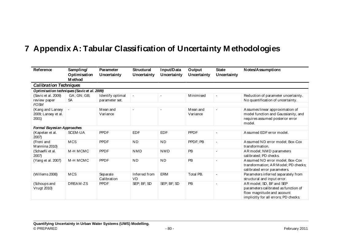
Quantifying Uncertainty in Urban Water Systems (UWS) Modelling. © PREPARED - 80 - February 2011
7 Appendix A: Tabular Classification of Uncertainty Methodologies
Reference Sampling/ Optimisation Method
Parameter Uncertainty
Structural Uncertainty
Input/Data Uncertainty
Output Uncertainty
State Uncertainty
Notes/Assumptions
Calibration Techniques Optimisation techniques (Savic et al. 2009) (Savic et al. 2009) review paper
GA; GN; GB; SA
Identify optimal parameter set.
- - Minimised - Reduction of parameter uncertainty. No quantification of uncertainty.
FOSM (Kang and Lansey 2009; Lansey et al. 2001)
- Mean and Variance
- - Mean and Variance
- Assumes linear approximation of model function and Gaussianity, and requires assumed posterior error model.
Formal Bayesian Approaches (Kapelan et al. 2007)
SCEM-UA PPDF EDF EDF PPDF - Assumed EDF error model.
(Freni and Mannina 2010)
MCS PPDF ND ND PPDF; PB - Assumed ND error model; Box-Cox transformation.
(Schaefli et al. 2007)
M-H MCMC PPDF NMD NMD PB - AR model; NMD parameters calibrated; PD checks.
(Yang et al. 2007) M-H MCMC PPDF ND ND PB - Assumed ND error model; Box-Cox transformation; AR Model; PD checks; calibrated error parameters.
(Willems 2008) MCS Separate Calibration
Inferred from VD
ERM Total PB. - Parameters inferred separately from structural and input error.
(Schoups and Vrugt 2010)
DREAM-ZS PPDF SEP; BF; SD SEP; BF; SD PB - AR model; SD, BF and SEP parameters calibrated as function of flow magnitude and account implicitly for all errors; PD checks.
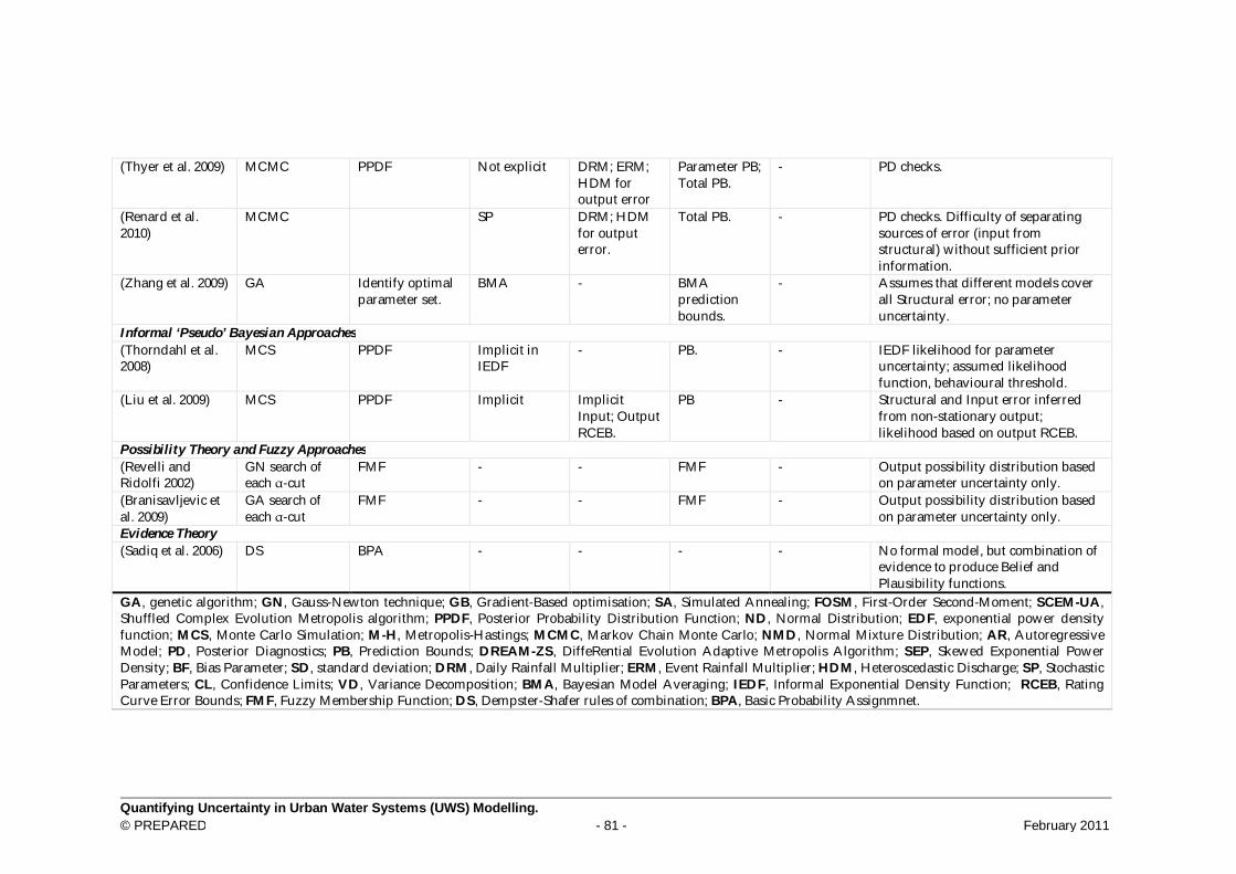
Quantifying Uncertainty in Urban Water Systems (UWS) Modelling. © PREPARED - 81 - February 2011
(Thyer et al. 2009) MCMC PPDF Not explicit DRM; ERM; HDM for output error
Parameter PB; Total PB.
- PD checks.
(Renard et al. 2010)
MCMC SP DRM; HDM for output error.
Total PB. - PD checks. Difficulty of separating sources of error (input from structural) without sufficient prior information.
(Zhang et al. 2009) GA Identify optimal parameter set.
BMA - BMA prediction bounds.
- Assumes that different models cover all Structural error; no parameter uncertainty.
Informal ‘Pseudo’ Bayesian Approaches (Thorndahl et al. 2008)
MCS PPDF Implicit in IEDF
- PB. - IEDF likelihood for parameter uncertainty; assumed likelihood function, behavioural threshold.
(Liu et al. 2009) MCS PPDF Implicit Implicit Input; Output RCEB.
PB - Structural and Input error inferred from non-stationary output; likelihood based on output RCEB.
Possibility Theory and Fuzzy Approaches (Revelli and Ridolfi 2002)
GN search of each α-cut
FMF - - FMF - Output possibility distribution based on parameter uncertainty only.
(Branisavljevic et al. 2009)
GA search of each α-cut
FMF - - FMF - Output possibility distribution based on parameter uncertainty only.
Evidence Theory (Sadiq et al. 2006) DS BPA - - - - No formal model, but combination of
evidence to produce Belief and Plausibility functions.
GA, genetic algorithm; GN, Gauss-Newton technique; GB, Gradient-Based optimisation; SA, Simulated Annealing; FOSM, First-Order Second-Moment; SCEM-UA, Shuffled Complex Evolution Metropolis algorithm; PPDF, Posterior Probability Distribution Function; ND, Normal Distribution; EDF, exponential power density function; MCS, Monte Carlo Simulation; M-H, Metropolis-Hastings; MCMC, Markov Chain Monte Carlo; NMD, Normal Mixture Distribution; AR, Autoregressive Model; PD, Posterior Diagnostics; PB, Prediction Bounds; DREAM-ZS, DiffeRential Evolution Adaptive Metropolis Algorithm; SEP, Skewed Exponential Power Density; BF, Bias Parameter; SD, standard deviation; DRM, Daily Rainfall Multiplier; ERM, Event Rainfall Multiplier; HDM, Heteroscedastic Discharge; SP, Stochastic Parameters; CL, Confidence Limits; VD, Variance Decomposition; BMA, Bayesian Model Averaging; IEDF, Informal Exponential Density Function; RCEB, Rating Curve Error Bounds; FMF, Fuzzy Membership Function; DS, Dempster-Shafer rules of combination; BPA, Basic Probability Assignmnet.

Quantifying Uncertainty in Urban Water Systems (UWS) Modelling. © PREPARED - 82 - February 2011
8 Appendix B: Glossary of Terms
A glossary of terms has been included to facilitate understanding of the relevant report sections (The Glossary has been modified from Goulsby and Samuels 2005). Accuracy - closeness to reality. Adaptive capacity - Is the ability to plan, prepare for, facilitate, and implement adaptation options. Factors that determine cities’ adaptive capacity include economic wealth, technology and infrastructure, knowledge and skills, the nature of its institutions, its commitment to equity, and its social capital. Adaptive Strategy – Method for optimising/expanding existing systems to reduce risk and vulnerability to change (e.g. climate change). Aims - The objectives of groups/individuals/organisations involved with a project. The aims are taken to include ethical and aesthetic considerations. Aleatory uncertainty – see Natural Variability. Basin (river) (see catchment area) - the area from which water runs off to a given river. Calibration – see Calibration parameters. Catchment area - the area from which water runs off to a river. Bias - The disposition to distort the significance of the various pieces of information that have to be used. Characterisation - The process of expressing the observed/predicted behaviour of a system and its components for optimal use in decision making. Climate Change – changes in weather over > 30 year time-periods, notably in response to modern anthropogenic influence. Combined Sewer Overflow (CSO) – Overflow discharge from combined sewer systems that bypasses the Wastewater Treatment Plant and enters directly into the receiving water body. CSO discharge typically occurs during rainfall events. Conditional probability - The likelihood of occurrence of an event given the prior occurrence of another event. Confidence interval - A measure of the degree of (un)certainty of an estimate, usually presented as a percentage. For example, a confidence level of 95% applied to an upper and lower bound of an estimate indicates there is a 95% chance the estimate lies between the specified bounds. Confidence limits can be calculated for some forms of uncertainty (see knowledge uncertainty), or estimated by an expert (see judgement). Consequence - An impact such as economic, social or environmental damage/improvement that may result from a flood or UWS failure. May be expressed quantitatively (e.g. monetary value), by category (e.g. High, Medium, Low) or descriptively. Coping capacity - The means by which people or organisations use available resources and abilities to face adverse consequences that could lead to a disaster.
Quantifying Uncertainty in Urban Water Systems (UWS) Modelling. © PREPARED - 83 - February 2011
Correlation - Between two random variables, the correlation is a measure of the extent to which a change in one tends to correspond to a change in the other. One measure of linear dependence is the correlation coefficient p. If variables are independent random variables then p = 0. Values of +1 and -1 correspond to full positive and negative dependence respectively. Note: the existence of some correlation need not imply that the link is one of cause and effect. Decision uncertainty - The rational inability to choose between alternative options. Design objective - The objective (put forward by a stakeholder), describing the desired performance of an intervention, once implemented. Dependence - The extent to which one variable depends on another variable. Dependence affects the likelihood of two or more thresholds being exceeded simultaneously. When it is not known whether dependence exists between two variables or parameters, guidance on the importance of any assumption can be provided by assessing the fully dependent and independent cases (see also correlation). Demand – Amount of water consumed/extracted by domestic and industrial users from the WDN (typically expressed in volumetric terms per unit time period). Deterministic process / method - A method or process that adopts precise, single-values for all variables and input values, giving a single value output. Discharge (stream, river, sewer pipe) - as measured by volume per unit of time. Dry Weather Flow – Flow in the sewer system during dry weather that originates from domestic and industrial users. Element - A component part of a system. Epistemology - A theory of what we can know and why or how we can know it. Error - Mistaken calculations (e.g. from a model) or measurements with quantifiable and predictable differences. Expectation – the expected value of a variable refers to the mean value the variable takes. For example, in a 100 year period, a 1 in 100 year event is expected to be equalled or exceeded once. This can be defined mathematically. Extrapolation - The inference of unknown data from known data, for instance future data from past data, by analysing trends and making assumptions. Applying a derived relationship from one time-period to conditions different from that in which the relationship was derived. Failure - Inability to achieve a defined performance threshold (response given loading). "Catastrophic" failure describes the situation where the consequences are immediate and severe, whereas "prognostic" failure describes the situation where the consequences only grow to a significant level when additional loading has been applied and/or time has elapsed. Failure mode - Description of one of any number of ways in which a system may fail to meet a particular performance indicator. Functional design - The design of an intervention with a clear understanding of the performance required of the intervention. Governance - The processes of decision making and implementation
Quantifying Uncertainty in Urban Water Systems (UWS) Modelling. © PREPARED - 84 - February 2011
Harm - Disadvantageous consequences; economic, social or environmental (See Consequence). Hazard - A physical event, phenomenon or human activity with the potential to result in harm. A hazard does not necessarily lead to harm. Hazard mapping - The process of establishing the spatial extents of hazardous phenomena. Hierarchy - A process where information cascades from a greater spatial or temporal scale to lesser scale and vice versa. Human reliability - Probability that a person correctly performs a specified task. Ignorance - Lack of knowledge. Institutional uncertainty - inadequate collaboration and/or trust among institutions, potentially due to poor communication, lack of understanding, overall bureaucratic culture, conflicting sub-cultures, traditions and missions. Integrated risk management- An approach to risk management that embraces all sources, pathways and receptors of risk and considers combinations of structural and non-structural solutions. Integrated Water Resource Management - IWRM is a process which promotes the co-ordinated management and development of water, land and related resources, in order to maximise the resultant economic and social welfare in an equitable manner without compromising the sustainability of vital ecosystems. Intervention - A planned activity designed to effect an improvement in an existing natural or engineered system (including social, organisation/defence systems). Joint probability - The probability of specific values of one or more variables occurring simultaneously. For example, extreme water levels in estuaries may occur at times of high river flow, times of high sea level or times when both river flow and sea level are above average levels. When assessing the likelihood of occurrence of high estuarine water levels it is therefore necessary to consider the joint probability of high river flows and high sea levels. Judgement - Decisions taken arising from the critical assessment of the relevant knowledge. Knowledge - Spectrum of known relevant information. Knowledge uncertainty - Uncertainty due to lack of knowledge of all the causes and effects in a physical or social system (also termed epistemic uncertainty). For example, a numerical model of the sewer system may not include an accurate mathematical description of all the relevant physical processes. The model is thus subject to a form of knowledge uncertainty. Various forms of knowledge uncertainty exist, including: Process model uncertainty - All models are an abstraction of reality and can never be considered true. They are thus subject to process model uncertainty. Measured data versus modelled data comparisons give an insight into the extent of model uncertainty but do not produce a complete picture. Statistical inference uncertainty - Formal quantification of the uncertainty of estimating the population from a sample. The uncertainty is related to the extent of data and variability of the data that make up the sample.
Quantifying Uncertainty in Urban Water Systems (UWS) Modelling. © PREPARED - 85 - February 2011
Statistical model uncertainty - Uncertainty associated with the fitting of a statistical model. The statistical model is usually assumed to be correct. However, if two different models fit a set of data equally well but have different extrapolations/interpolations then this assumption is not valid and there is statistical model uncertainty. Likelihood - A general concept relating to the chance of an event occurring. Likelihood is generally expressed as a probability or a frequency (as a value between 0 = impossible; 1 = certain). Marginal Probability – see Probability. Mitigation – to moderate the force or impacts of an event. Natural variability - Uncertainties that stem from the assumed inherent randomness and basic unpredictability in the natural world and are characterised by the variability in known or observable populations (also known as Aleatory uncertainty). Objectives – A goal, typically defined as the maximisation or minimisation of a given function. For example, minimise cost whilst maintain system performance. Optimisation – Intervention that achieves the best performance of a system in reference to one or more (competing) objectives. In modelling, adjustment of system parameters to achieve objectives pertaining to the modelled system. Parameters - The parameters in a model are the constants chosen to represent the chosen context and scenario. In general the following types of parameters can be recognised: Exact parameters - which are universal constants, such as the mathematical constant: Pi (3.14259...). Fixed parameters - which are well determined by experiment and may be considered exact, such as the acceleration of gravity, g (approximately 9.81 m/s). A-priori chosen parameters - which are parameters that may be difficult to identify by calibration and so are assigned certain values. However, the values of such parameters are associated with uncertainty that must be estimated on the basis of a-priori experience, for example detailed experimental or field measurements Calibration parameters - which must be established to represent particular circumstances. They must be determined by calibration of model results for historical data on both input and outcome. The parameters are generally chosen to minimise the difference between model outcomes and measured data on the same outcomes. It is unlikely that the set of parameters required to achieve a "satisfactory" calibration is unique, reflecting a state of equifinality. Parameter Hypercube - Multi-dimensional mode space where each dimension consists of a range of potential values for a particular model parameter. Performance - The degree to which a process or activity succeeds when evaluated against some stated aim or objective. Performance indicator - The well-articulated and measurable objectives of a particular project or policy. These may be detailed engineering performance indicators, such as acceptable CSO volumes, minimum pressure in WDN, rock stability, or more generic indicators such as public satisfaction.
Quantifying Uncertainty in Urban Water Systems (UWS) Modelling. © PREPARED - 86 - February 2011
Possibility – The likelihood of a state or event occurring in the future. Possibility differs from probability. Possibility theory was developed in the face of uncertain and often subjective understanding of the propensity for future states with little information from the past to inform on future likelihood. Precautionary Principle - Where there are threats of serious or irreversible damage, lack of full scientific certainty shall not be used as a reason for postponing cost-effective measures to prevent environmental degradation. Precision - degree of exactness regardless of accuracy. Preparedness - The ability to ensure effective response to the impact of hazards, including the issuance of timely and effective early warnings and the temporary evacuation of people and property from threatened locations. Probability - A measure of our strength of belief that an event will occur. For events that occur repeatedly the probability of an event is estimated from the relative frequency of occurrence of that event, out of all possible events. In all cases the event in question has to be precisely defined, so, for example, for events that occur through time reference has to be made to the time period, for example, annual exceedance probability. Probability can be expressed as a fraction, % or decimal. For example the probability of obtaining a six with a shake of four dice is 1/6, 16.7% or 0.167. Probabilistic method - Method in which the variability of input values and the sensitivity of the results are taken into account to give results in the form of a range of probabilities for different outcomes. Probability density function (distribution) - Function which describes the probability of different values across the whole range of a variable (for example across a parameter value in a particular model). Probabilistic reliability methods - These methods attempt to define the proximity of a structure to fail through assessment of a response function. They are categorised as Level III, II or I, based on the degree of complexity and the simplifying assumptions made (Level III being the most complex). Process model uncertainty - See Knowledge uncertainty. Project Appraisal - The comparison of the identified courses of action in terms of their performance against some desired ends. Progressive failure - Failure where, once a threshold is exceeded, significant (residual) resistance remains enabling the defence to maintain restricted performance. The immediate consequences of failure are not necessarily dramatic but further, progressive, failures may result eventually leading to a complete loss of function. Random events - Events which have no discernible pattern. Receiving water body – A water body, typically a river, lake or sea that receives effluent from the Sewer system or WWTP. Recovery time - The time taken for an element or system to return to its prior state after a perturbation or applied stress. Reliability index - A probabilistic measure of the structural reliability with regard to any limit state. Resilience - The ability of a system/community/society/defence to react to and recover from the damaging effect of realised hazards. Resistance . The ability of a system to remain unchanged by external events.

Quantifying Uncertainty in Urban Water Systems (UWS) Modelling. © PREPARED - 87 - February 2011
Return period - The expected (mean) time (usually in years) between the exceedence of a particular extreme threshold. Return period is traditionally used to express the frequency of occurrence of an event, although it is often misunderstood as being a probability of occurrence. Risk - Risk is a function of probability, exposure and vulnerability. Often, in practice, exposure is incorporated in the assessment of consequences, therefore risk can be considered as having two components: the probability that an event will occur and the impact (or consequence) associated with that event. See Section 4.3 above. Risk = Probability multiplied by consequence Risk analysis - A methodology to objectively determine risk by analysing and combining probabilities and consequences. Risk assessment - Comprises understanding, evaluating and interpreting the perceptions of risk and societal tolerances of risk to inform decisions and actions in the flood risk management process. Risk communication (in context) - Any intentional exchange of information on environmental and/or health risks between interested parties. Risk management - The complete process of risk analysis, risk assessment, options appraisal and implementation of risk management measures Risk management measure - An action that is taken to reduce either the probability of flooding or the consequences of flooding or some combination of the two Risk mapping - The process of establishing the spatial extent of risk (combining information on probability and consequences). Risk mapping requires combining maps of hazards and vulnerabilities. The results of these analyses are usually presented in the form of maps that show the magnitude and nature of the risk. Risk mitigation - See Risk reduction. Risk perception - Risk perception is the view of risk held by a person or group and reflects cultural and personal values, as well as experience. Risk reduction - The reduction of the likelihood of harm, by either reduction in the probability of a flood occurring or a reduction in the exposure or vulnerability of the receptors. Risk profile - The change in performance, and significance of the resulting consequences, under a range of loading conditions. In particular the sensitivity to extreme loads and degree of uncertainty about future performance. Risk register - An auditable record of the project risks, their consequences and significance, and proposed mitigation and management measures. Risk significance (in context) - The separate consideration of the magnitude of consequences and the frequency of occurrence. Robustness - Capability to cope with external stress. A decision is robust if the choice between the alternatives is unaffected by a wide range of possible future states of nature. Robust statistics are those whose validity does not depend on close approximation to a particular distribution function and/or the level of measurement achieved. SCADA – Supervisory Control And Data Acquisition. Computer systems that monitor the state of a system, and allow control of devises within the system. Scale - Difference in spatial extent or over time or in magnitude; critical determinant of vulnerability, resilience etc.
Quantifying Uncertainty in Urban Water Systems (UWS) Modelling. © PREPARED - 88 - February 2011
Scenario - A plausible description of a situation, based on a coherent and internally consistent set of assumptions. Scenarios are neither predictions nor forecasts. The results of scenarios (unlike forecasts) depend on the boundary conditions of the scenario. Sensitivity - Refers to either: the resilience of a particular receptor to a given hazard. For example, frequent sea water flooding may have considerably greater impact on a fresh water habitat, than a brackish lagoon; or: the change in a result or conclusion arising from a specific perturbation in input values or assumptions. Sensitivity Analysis - The identification of those parameters which critically affect the output of a model or process. Conducted to better understand system operation, and allocate resources to constrain model output. Sewer System – Infrastructure of pipes and control structures that conveys sewerage and rainfall-runoff in urban areas from buildings and the roads to the wastewater treatment plant and receiving water body. Skeletonisation – Removal of pipes not considered essential to the operation of a WDN model. Source - The origin of a hazard (for example, heavy rainfall, strong winds, surge etc). Stakeholders - Parties/persons with a direct interest (stake) in an issue. Stakeholder Engagement - Process through which the stakeholders have power to influence the outcome of the decision. Critically, the extent and nature of the power given to the stakeholders varies between different forms of stakeholder engagement. Statistic - A measurement of a variable of interest which is subject to random variation. Strategy - A strategy is a combination of long-term goals, aims, specific targets, technical measures, policy instruments, and process which are continuously aligned with the societal context. Strategic spatial planning - Process for developing plans explicitly containing strategic intentions referring to spatial development. Strategic plans typically exist at different spatial levels (local, regional etc). Statistical inference uncertainty - See Knowledge uncertainty Statistical model uncertainty - See Knowledge uncertainty Sustainable Development - is development that meets the needs of the present without compromising the ability of future generations to meet their own needs Susceptibility - The propensity of a particular receptor to experience harm. System - An assembly of elements, and the interconnections between them, constituting a whole and generally characterised by its behaviour. System state - The condition of a system at a point in time. Tolerability - Refers to willingness to live with a risk to secure certain benefits and in the confidence that it is being properly controlled. To tolerate a risk means that we do not regard it as negligible, or something we might ignore, but rather as something we need to keep under review, and reduce still further if and as we can. Tolerability does not mean acceptability. For example, tolerance of CSO or sewer surcharge.
Quantifying Uncertainty in Urban Water Systems (UWS) Modelling. © PREPARED - 89 - February 2011
Uncertainty - A general concept that reflects our lack of sureness about someone or something, ranging from just short of complete sureness to an almost complete lack of conviction about an outcome. Urban Wastewater System – triplet of components: Sewer System, Wastewater treatment plant and receiving water body designed to mitigate against flooding and provide sanitation. Validation - is the process of comparing model output with observations of the ’real world’. Variability - The change over time of the value or state of some parameter or system or element where this change may be systemic, cyclical or exhibit no apparent pattern. Variable - A quantity which can be measured, predicted or forecast which is relevant to describing the state of the flooding system e.g. water level, discharge, velocity, wave height, distance, or time. A prediction or forecast of a variable will often rely on a simulation model which incorporates a set of parameters. Vulnerability - Characteristic of a system that describes its potential to be harmed. This can be considered as a combination of susceptibility and value. Wastewater Treatment Plant (WWTP) – Treatment plant for the removal of contaminants and nutrients from sewerage for entry as effluent into the receiving water body. Water Distribution Network (WDN) – Network of pipes, pumps, nodes, tanks and valves that distributes drinking water to meet consumer demands.