Embed Size (px)
Citation preview
UNCERTAINTY
QUANTIFICATION IN ORBITAL
MECHANICSMassimiliano Vasile, Aerospace Centre of Excellence, Department of Mechanical & Aerospace Engineering, University of Strathclyde

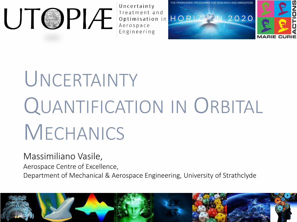
UTOPIAE is a €3.9M research and training
network supported by the European Commission to
focus on uncertainty treatment and optimisation
UTOPIAE will last 4 years starting 01 January 2017
15 partners over Europe
11 full partners + 4 associate
partners
7 universities
3 companies
5 national research centres
1 university research centre
Coordinated by
Strathclyde University
15 researchers will be recruited within UTOPIAE
8 major training & outreach events organised within UTOPIAE
Who’s who in the network?
Where are they?

utopiae_network http://utopiae.eu
OPEN POSITIONS
University of Durham (Department of Mathematics andStatistics): Marie Curie fellowship position on the ImpreciseProbabilities applied to large scale dynamic decisionprocesses. Closing date: end of September.
University of Strathclyde (Department of Mechanical &Aerospace Engineering): PhD position in Artificial Intelligencefor Space Mission Design. Closing date: end of September.
University of Strathclyde: Global Talent and Chancellor’sfellowship schemes.
Faculty positions at different levels from Lecturer to Professor. Closingdate: 24th of September.
utopiae_network http://utopiae.eu
What is
UQ?
Some UQ
Methods
Types of
UncertaintyModel
Uncertainty

utopiae_network http://utopiae.eu
What is UQ?
utopiae_network http://utopiae.eu
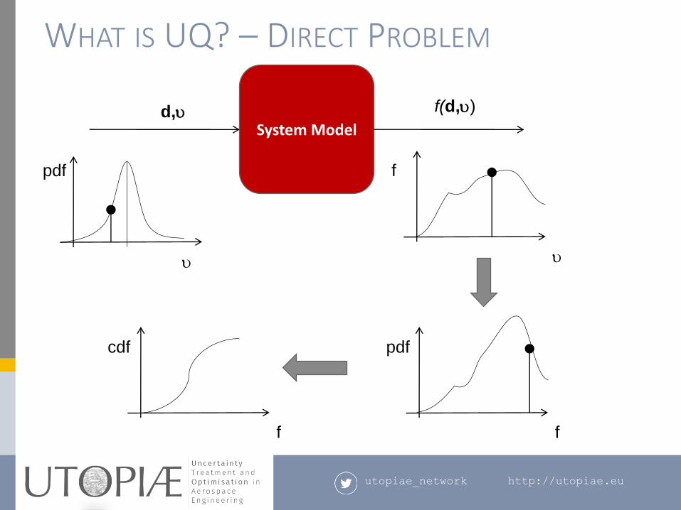
WHAT IS UQ? – DIRECT PROBLEM
System Modeld,u f(d,u)
u
fpdf
u
f
cdf
f
utopiae_network http://utopiae.eu
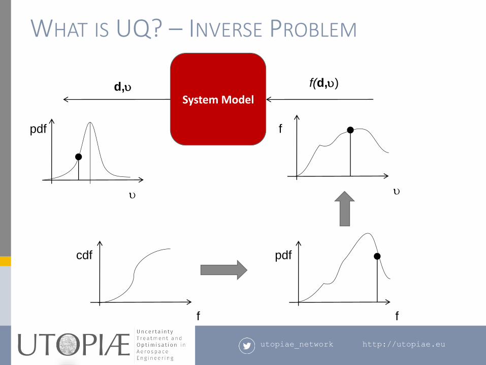
WHAT IS UQ? – INVERSE PROBLEM
System Modeld,u f(d,u)
u
fpdf
u
f
cdf
f
utopiae_network http://utopiae.eu
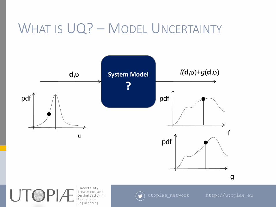
WHAT IS UQ? – MODEL UNCERTAINTY
System Model
?d,u f(d,u)+g(d,u)
u
pdfpdf
f
g
utopiae_network http://utopiae.eu
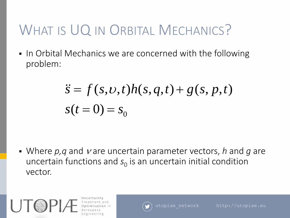
WHAT IS UQ IN ORBITAL MECHANICS?
In Orbital Mechanics we are concerned with the following problem:
Where p,q and n are uncertain parameter vectors, h and g are uncertain functions and s0 is an uncertain initial condition vector.
0
( , , ) ( , , ) ( , , )
( 0)
s f s t h s q t g s p t
s t s
u
utopiae_network http://utopiae.eu
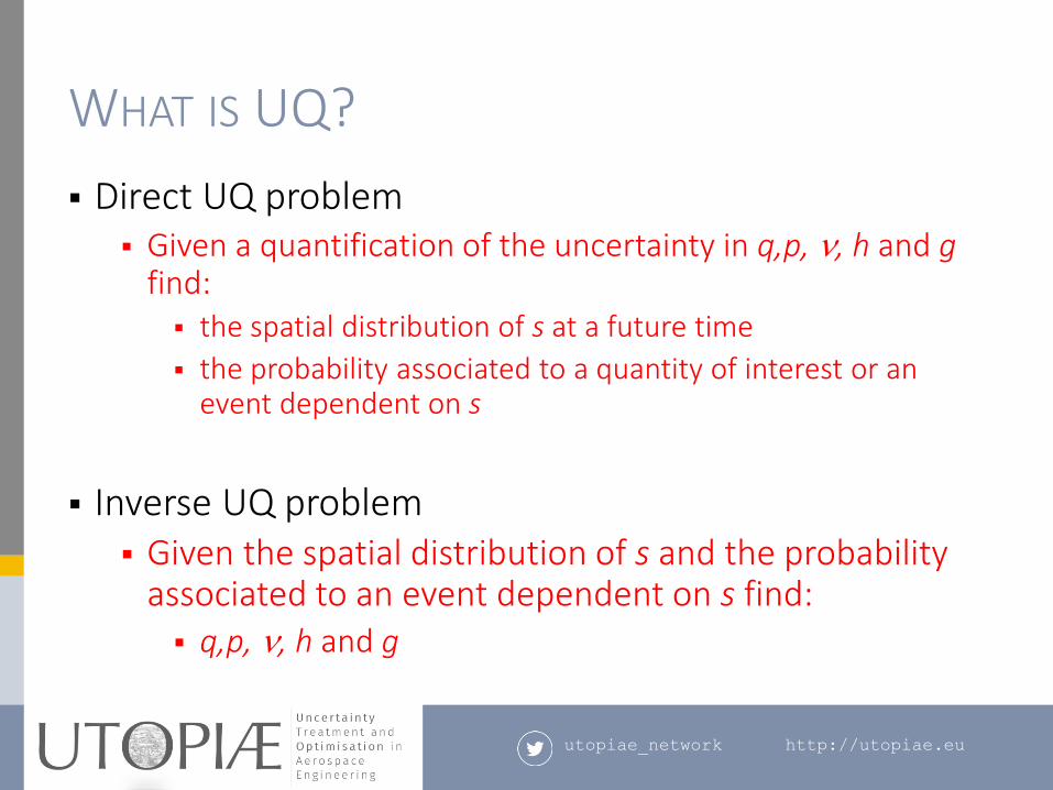
WHAT IS UQ?
Direct UQ problem Given a quantification of the uncertainty in q,p, n, h and g
find: the spatial distribution of s at a future time
the probability associated to a quantity of interest or an event dependent on s
Inverse UQ problem Given the spatial distribution of s and the probability
associated to an event dependent on s find: q,p, n, h and g
utopiae_network http://utopiae.eu
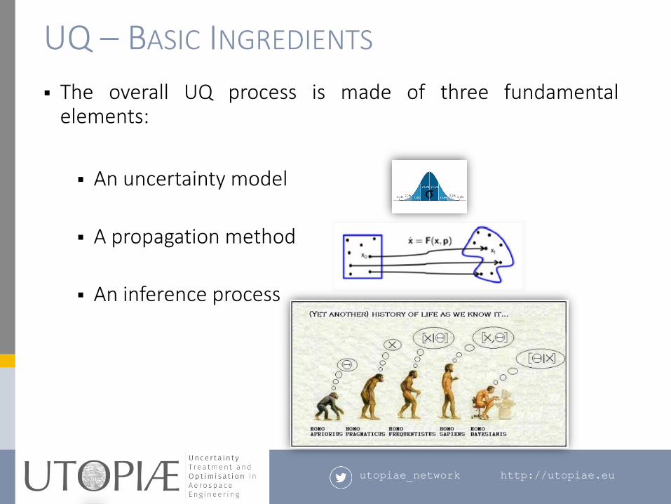
UQ – BASIC INGREDIENTS
The overall UQ process is made of three fundamentalelements:
An uncertainty model
A propagation method
An inference process
utopiae_network http://utopiae.eu
Types of Uncertainty
utopiae_network http://utopiae.eu
EPISTEMIC VS. ALEATORY: WHAT IS THE
DIFFERENCE?
Aleatory uncertainties are non-reducible uncertainties thatdepend on the very nature of the phenomenon underinvestigation. They can generally be captured by well definedprobability distributions as one can apply a frequentistapproach. E.g. measurement errors.
Epistemic uncertainties are reducible uncertainties and aredue to a lack of knowledge. Generally they cannot bequantified with a well defined probability distribution and amore subjectivist approach is required. Two classes:
a lack of knowledge on the distribution of the stochastic variablesor…
a lack of knowledge of the model used to represent the phenomenonunder investigation.
utopiae_network http://utopiae.eu
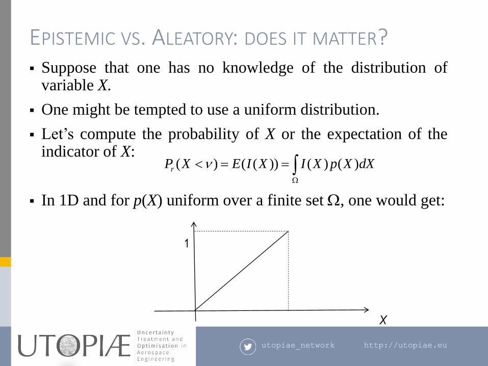
EPISTEMIC VS. ALEATORY: DOES IT MATTER? Suppose that one has no knowledge of the distribution of
variable X.
One might be tempted to use a uniform distribution.
Let’s compute the probability of X or the expectation of theindicator of X:
In 1D and for p(X) uniform over a finite set W, one would get:
( ) ( ( )) ( ) ( )rP X E I X I X p X dXnW
1
X
utopiae_network http://utopiae.eu
EPISTEMIC VS. ALEATORY: DOES IT MATTER?
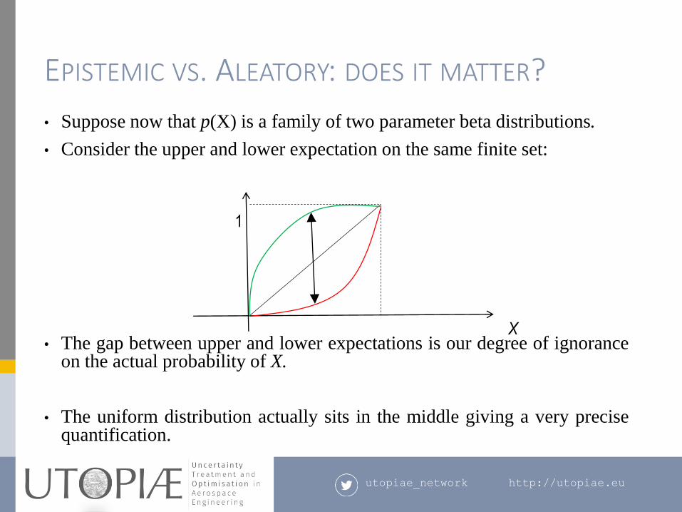
• Suppose now that p(X) is a family of two parameter beta distributions.
• Consider the upper and lower expectation on the same finite set:
• The gap between upper and lower expectations is our degree of ignoranceon the actual probability of X.
• The uniform distribution actually sits in the middle giving a very precisequantification.
1
X
utopiae_network http://utopiae.eu
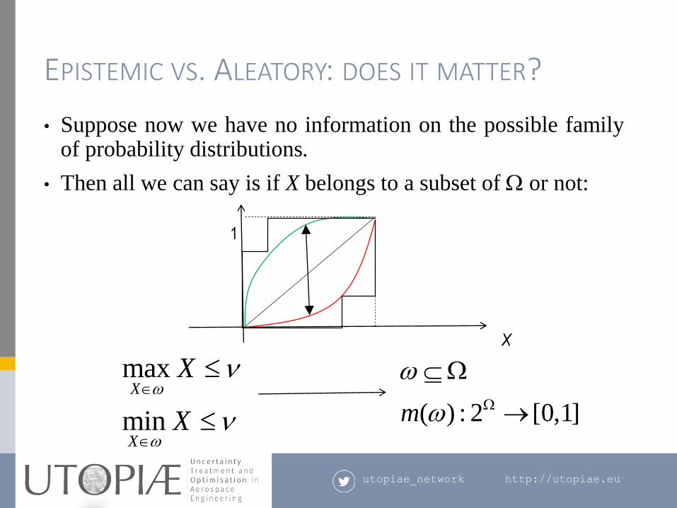
EPISTEMIC VS. ALEATORY: DOES IT MATTER?
• Suppose now we have no information on the possible familyof probability distributions.
• Then all we can say is if X belongs to a subset of W or not:
1
X
max
min
X
X
X
X
n
n
( ) : 2 [0,1]m
W
W
utopiae_network http://utopiae.eu
GENERAL CLASSIFICATION
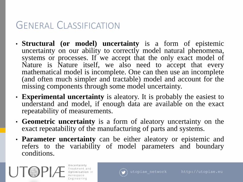
• Structural (or model) uncertainty is a form of epistemicuncertainty on our ability to correctly model natural phenomena,systems or processes. If we accept that the only exact model ofNature is Nature itself, we also need to accept that everymathematical model is incomplete. One can then use an incomplete(and often much simpler and tractable) model and account for themissing components through some model uncertainty.
• Experimental uncertainty is aleatory. It is probably the easiest tounderstand and model, if enough data are available on the exactrepeatability of measurements.
• Geometric uncertainty is a form of aleatory uncertainty on theexact repeatability of the manufacturing of parts and systems.
• Parameter uncertainty can be either aleatory or epistemic andrefers to the variability of model parameters and boundaryconditions.
utopiae_network http://utopiae.eu
GENERAL CLASSIFICATION
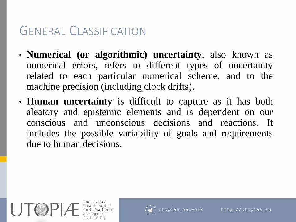
• Numerical (or algorithmic) uncertainty, also known asnumerical errors, refers to different types of uncertaintyrelated to each particular numerical scheme, and to themachine precision (including clock drifts).
• Human uncertainty is difficult to capture as it has bothaleatory and epistemic elements and is dependent on ourconscious and unconscious decisions and reactions. Itincludes the possible variability of goals and requirementsdue to human decisions.
utopiae_network http://utopiae.eu
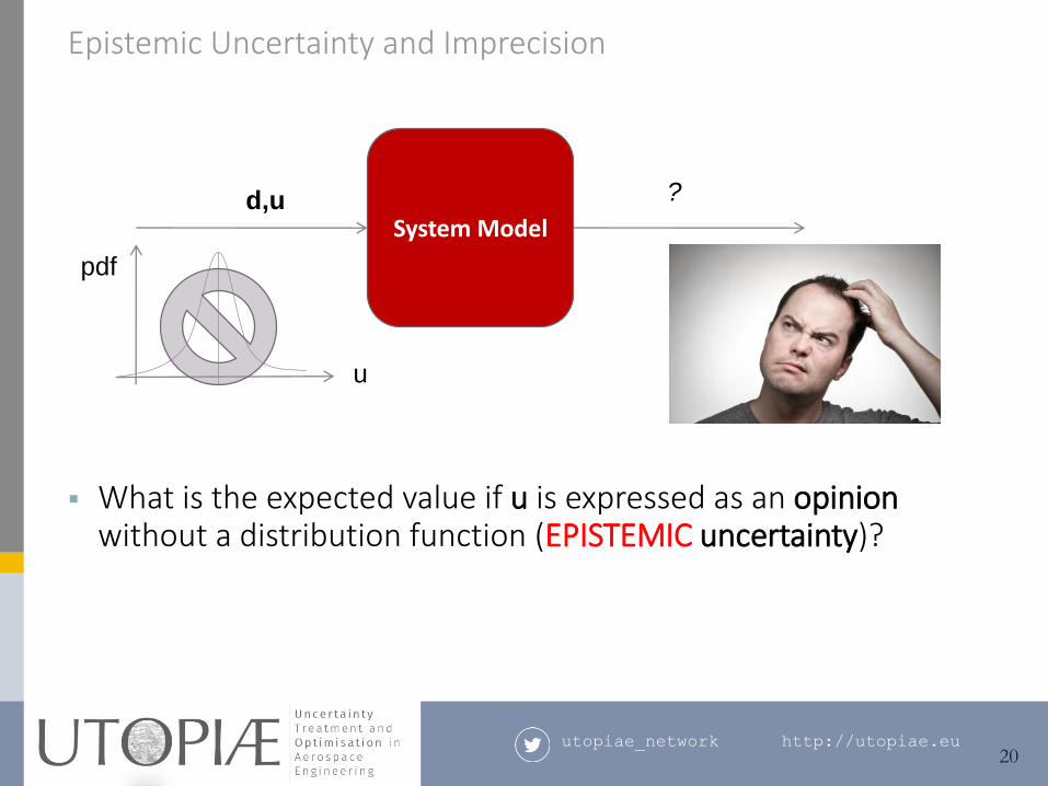
What is the expected value if u is expressed as an opinionwithout a distribution function (EPISTEMIC uncertainty)?
Epistemic Uncertainty and Imprecision
20
System Modeld,u ?
u
utopiae_network http://utopiae.eu
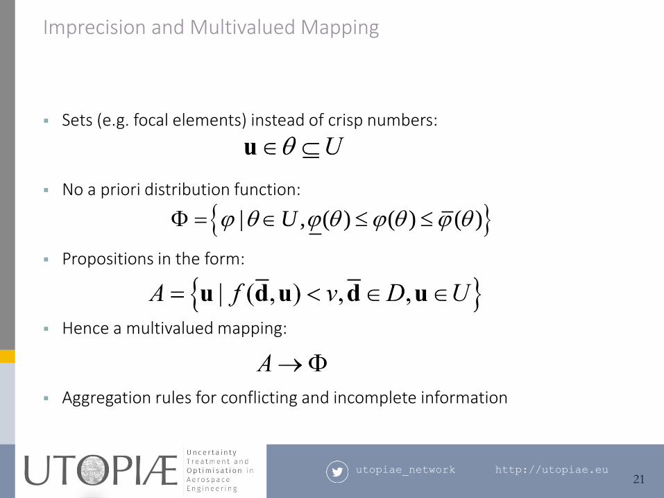
Sets (e.g. focal elements) instead of crisp numbers:
No a priori distribution function:
Propositions in the form:
Hence a multivalued mapping:
Aggregation rules for conflicting and incomplete information
Imprecision and Multivalued Mapping
21
| , ( ) ( ) ( )U
utopiae_network http://utopiae.eu
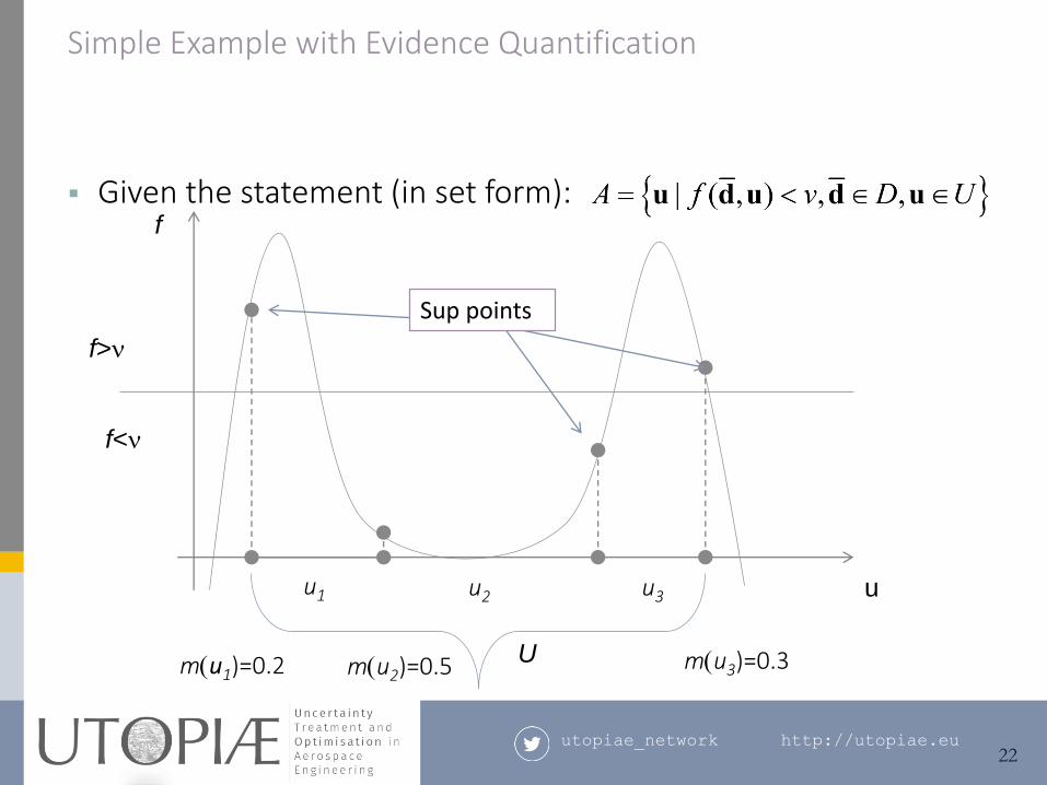
Given the statement (in set form):
Simple Example with Evidence Quantification
22
f
u
f>n
f<n
U
u1 u2 u3
m(u1)=0.2 m(u2)=0.5 m(u3)=0.3
Sup points
utopiae_network http://utopiae.eu
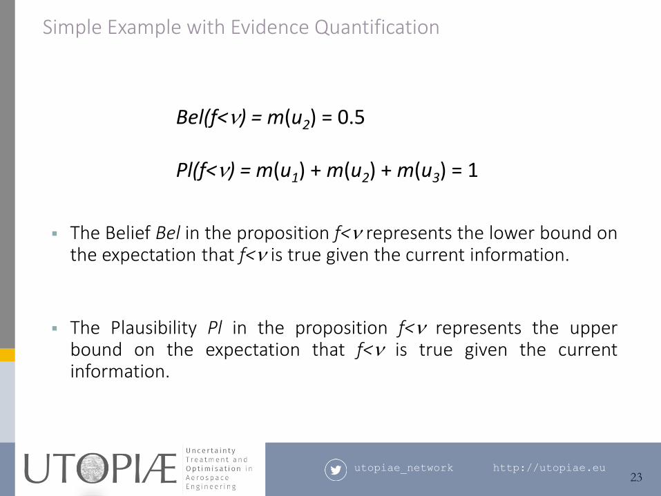
The Belief Bel in the proposition f<n represents the lower bound onthe expectation that f<n is true given the current information.
The Plausibility Pl in the proposition f<n represents the upperbound on the expectation that f<n is true given the currentinformation.
Simple Example with Evidence Quantification
23
Bel(f<n) = m(u2) = 0.5
Pl(f<n) = m(u1) + m(u2) + m(u3) = 1
utopiae_network http://utopiae.eu
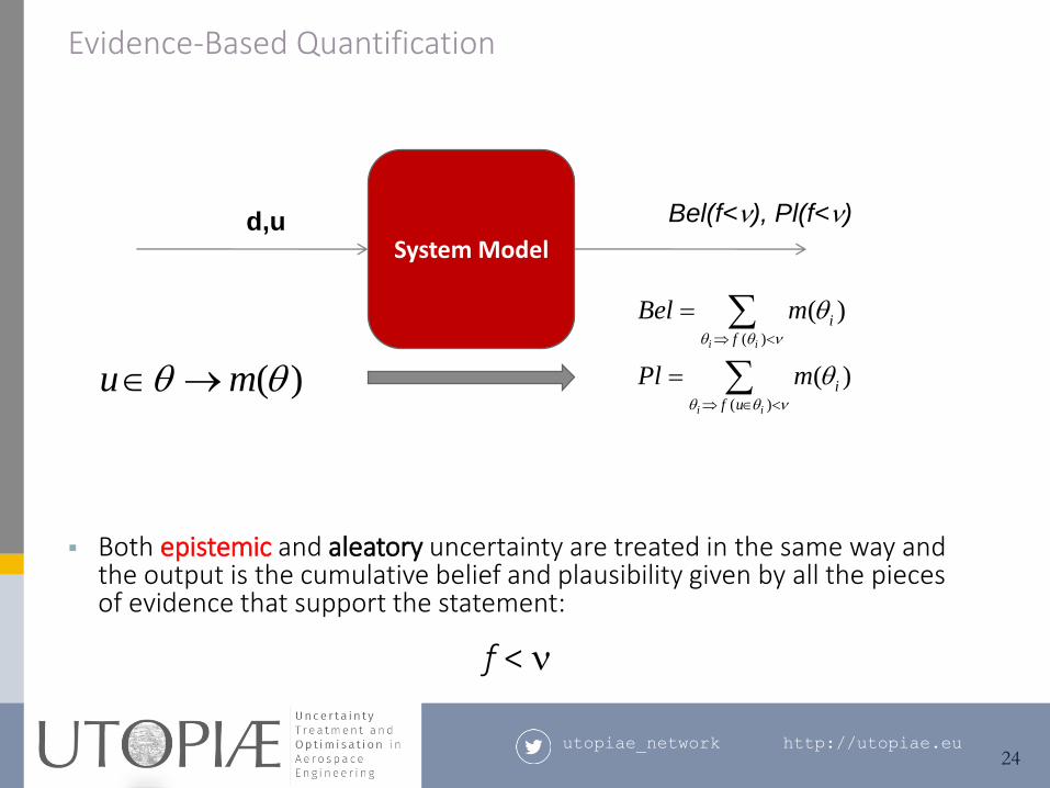
Both epistemic and aleatory uncertainty are treated in the same way and the output is the cumulative belief and plausibility given by all the pieces of evidence that support the statement:
f < n
Evidence-Based Quantification
24
System Modeld,u Bel(f<n), Pl(f<n)
( )u m
( )
( )
( )
( )
i i
i i
i
f
i
f u
Bel m
Pl m
n
n
utopiae_network http://utopiae.eu• 25
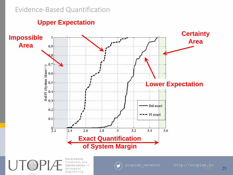
Certainty
AreaImpossible
Area
Exact Quantification
of System Margin
Evidence-Based Quantification
25
Upper Expectation
Lower Expectation
utopiae_network http://utopiae.eu
Some UQ Methods
utopiae_network http://utopiae.eu
INTRUSIVE VS. NON-INTRUSIVE – WHAT DOES IT MEAN?
Common terminology in the UQ community thatfundamentally indicates two classes of algorithms/methods.
Intrusive methods – the system/process model is not a blackbox and can be accessed to, for example, modify the algebraor compute derivatives, etc.
Non-intrusive methods – the system/process model is a blackbox that cannot be accessed and can be interrogate onlythrough sampling (oracle model).
utopiae_network http://utopiae.eu
NON-EXHAUSTIVE LIST TO NON-INTRUSIVE METHODS
• Monte Carlo Sampling - The most common and widely known.
• Unscented Transformation – A non-intrusive method in disguise related toorthogonal sampling methods.
• Polynomial Chaos Expansions and Stochastic Collocation– Popular alternativesto MCS, based on the Karhunen–Loève theorem.
• Gaussian Mixture Representation – Related to Kernel based approaches itrepresents complex distributions with a sum of basic Kernels
• High Dimensional Model Representation – Decomposition approach to reducethe dimensionality of the problem
• Chebyshev Interpolation – Example of interpolation approach
utopiae_network http://utopiae.eu
NON-EXHAUSTIVE LIST OF INTRUSIVE METHODS
• Taylor expansion of the quantity of interest – simple expansion of the quantity ofinterest through automatic differentiation or analytical derivatives.
• State Transition Matrix – first order method related to Taylor expansions of thequantity of interest to the first order.
• State Transition Tensor– higher order method related to Taylor expansions of thequantity of interest to the higher orders.
• Intrusive PCEs – embedding of the Polynomial Chaos Expansion in the system modeland propagation through operations among polynomials.
• Taylor Algebra – similar to intrusive PCEs with real algebra replaced by operationsamong Taylor polynomials.
• Generalised Algebra - similar to intrusive PCEs with real algebra replaced byoperations among general polynomials.
utopiae_network http://utopiae.eu
LINEAR VS. NON-LINEAR – WHAT DOES IT MEAN?
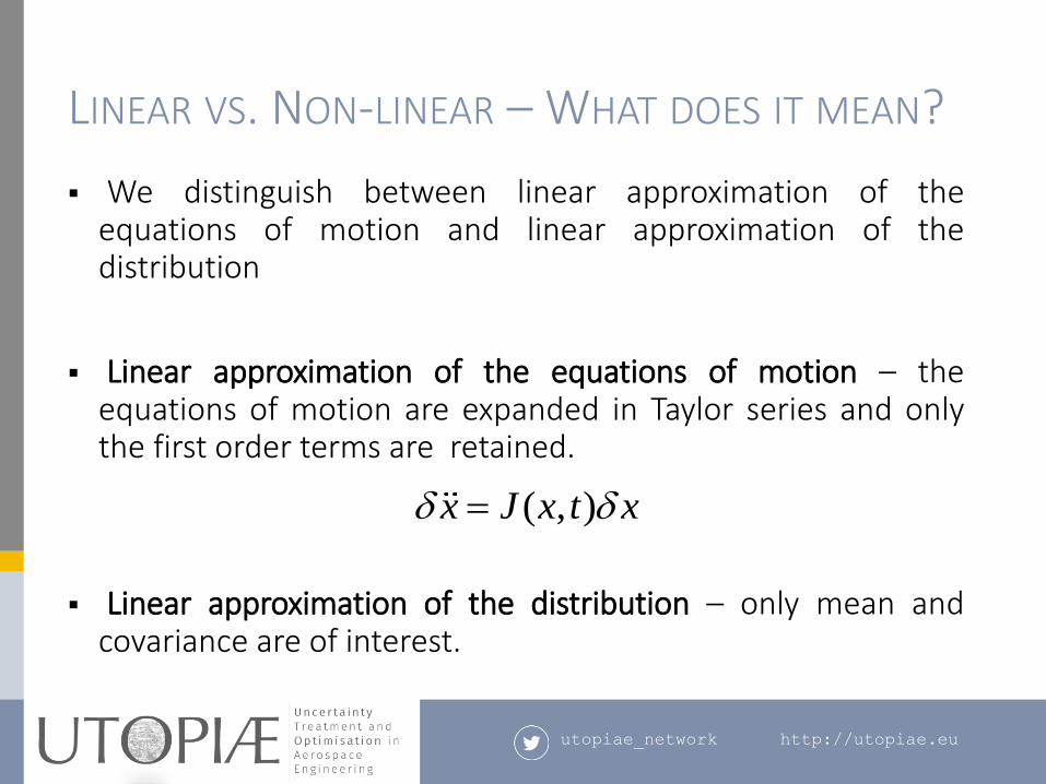
We distinguish between linear approximation of theequations of motion and linear approximation of thedistribution
Linear approximation of the equations of motion – theequations of motion are expanded in Taylor series and onlythe first order terms are retained.
Linear approximation of the distribution – only mean andcovariance are of interest.
( , )x J x t x
utopiae_network http://utopiae.eu
LINEAR VS. NON-LINEAR – WHAT DOES IT MEAN?
It was demonstrated, in the second half of the ’90 and morerecently, that a change of formulation from Cartesian toorbital elements can recover the quasi-linearity of themotion.
Junkins, J. L., Akella, M. R., and Alfriend, K. T. “Non-Gaussian Error Propagation in Orbital Mechanics.” Journal of
Astronautical Sciences, Vol. 44, No. 4, pp. 541–563, OctoberDecember 1996
J. M. Aristoff, J. T. Horwood, N. Singh, and A. B. Poore, “Nonlinear uncertainty propagation in orbital elements andtransformation to Cartesian space without loss of realism,” in Proceedings of the 2014 AAS/AIAA Astrodynamics SpecialistConference, San Diego, CA, August 2014 (Paper AIAA-2014-4167)
These methods require a reparameterisation of theequations of motion, typically in the form of orbital elements,and then uses a linear distribution model.
utopiae_network http://utopiae.eu
PROBABILITY DISTRIBUTION OR SPATIAL DISTRIBUTION?
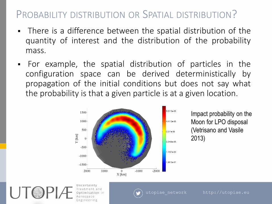
There is a difference between the spatial distribution of thequantity of interest and the distribution of the probabilitymass.
For example, the spatial distribution of particles in theconfiguration space can be derived deterministically bypropagation of the initial conditions but does not say whatthe probability is that a given particle is at a given location.
Impact probability on the
Moon for LPO disposal
(Vetrisano and Vasile
2013)
utopiae_network http://utopiae.eu
METHODS BASED ON GLOBAL QUANTITIES
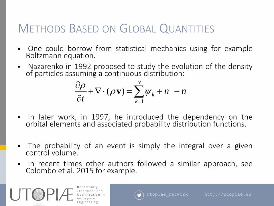
One could borrow from statistical mechanics using for exampleBoltzmann equation.
Nazarenko in 1992 proposed to study the evolution of the densityof particles assuming a continuous distribution:
In later work, in 1997, he introduced the dependency on theorbital elements and associated probability distribution functions.
The probability of an event is simply the integral over a givencontrol volume.
In recent times other authors followed a similar approach, seeColombo et al. 2015 for example.
1
( )N
k
k
n nt
v
utopiae_network http://utopiae.eu
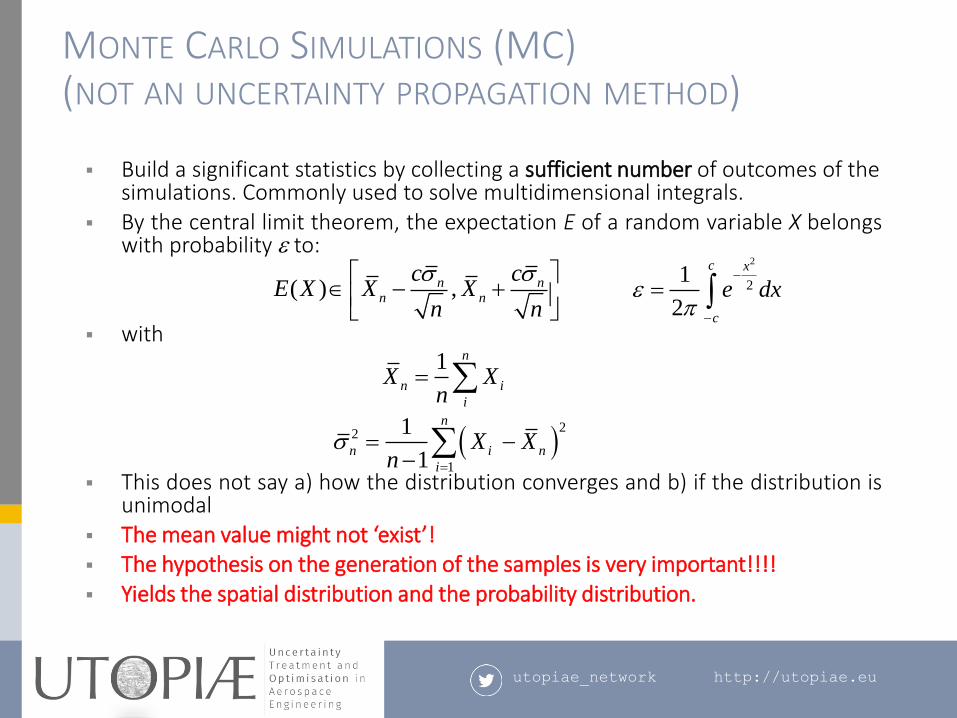
MONTE CARLO SIMULATIONS (MC)(NOT AN UNCERTAINTY PROPAGATION METHOD)
Build a significant statistics by collecting a sufficient number of outcomes of the simulations. Commonly used to solve multidimensional integrals.
By the central limit theorem, the expectation E of a random variable X belongswith probability e to:
with
This does not say a) how the distribution converges and b) if the distribution isunimodal
The mean value might not ‘exist’! The hypothesis on the generation of the samples is very important!!!! Yields the spatial distribution and the probability distribution.
( ) ,n nn n
c cE X X X
n n
1 n
n i
i
X Xn
( 2
2
1
1
1
n
n i n
i
X Xn
2
21
2
c x
c
e dxe
utopiae_network http://utopiae.eu
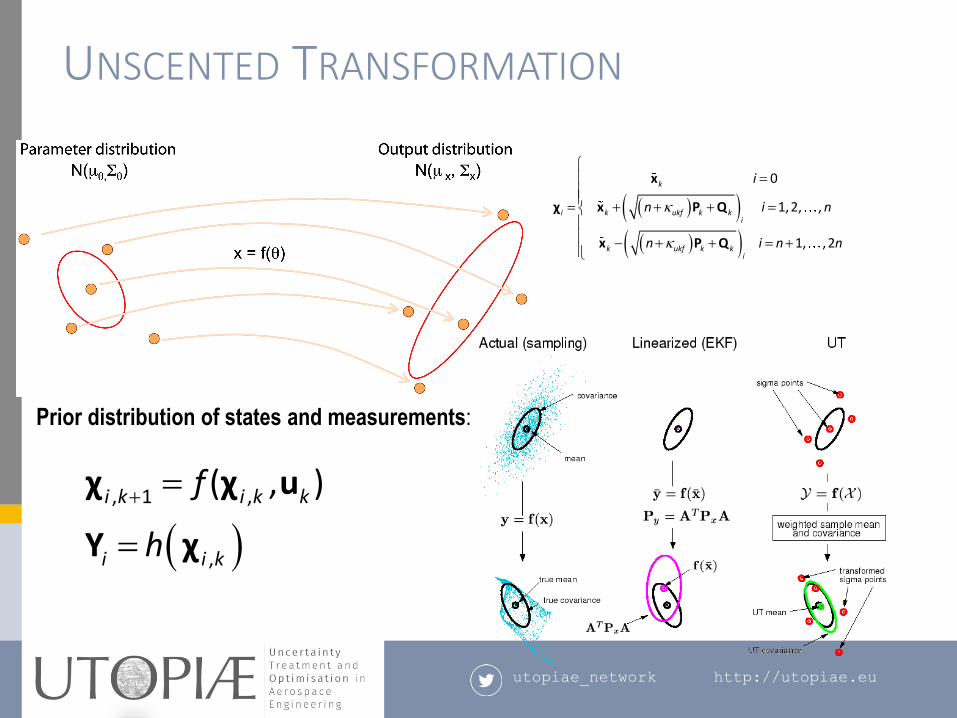
UNSCENTED TRANSFORMATION
Data fusion and state estimation.( ( ( (
0
1,2, ,
1, ,2
k
i k ukf k ki
k ukf k ki
i
n i n
n i n n
x
χ x P Q
x P Q
( , 1 ,
,
( , )i k i k k
i i k
f
h
χ χ u
Y χ
Prior distribution of states and measurements:
utopiae_network http://utopiae.eu
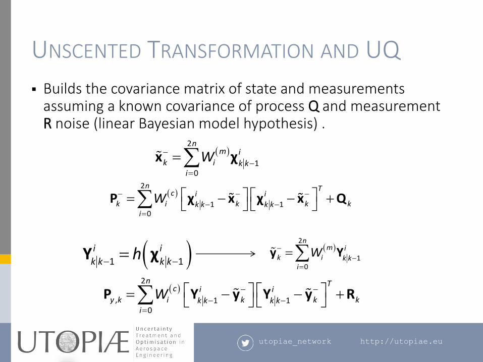
UNSCENTED TRANSFORMATION AND UQ
Builds the covariance matrix of state and measurements assuming a known covariance of process Q and measurement R noise (linear Bayesian model hypothesis) .
( 2
10
nm i
k i k ki
W
x χ
( 2
1 10
n Tc i i
k i k k kk k k ki
W
P χ x χ x Q
( 1 1
i i
k k k kh
Y χ (
2
10
nm i
k i k ki
W
y Y
( 2
, 1 10
n Tc i i
y k i k k kk k k ki
W
P Y y Y y R
utopiae_network http://utopiae.eu
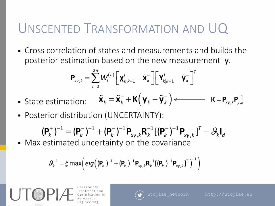
UNSCENTED TRANSFORMATION AND UQ
Cross correlation of states and measurements and builds the posterior estimation based on the new measurement y.
State estimation:
Posterior distribution (UNCERTAINTY):
Max estimated uncertainty on the covariance
( 2
, 1 10
n Tc i i
xy k i k kk k k ki
W
P χ x Y y
( k k k k x x K y y
,1 1 1
,1 1( ) ( ) ( ) [( ) ]k k
Tk k k dxy k k xy kP P P P PP R I
1, ,xy k y k
K P P
( (
11 1 1 1
,1
,max ( ) ( ) [( ) ]k k xy k k xy kT
k keig P P P P PR
utopiae_network http://utopiae.eu
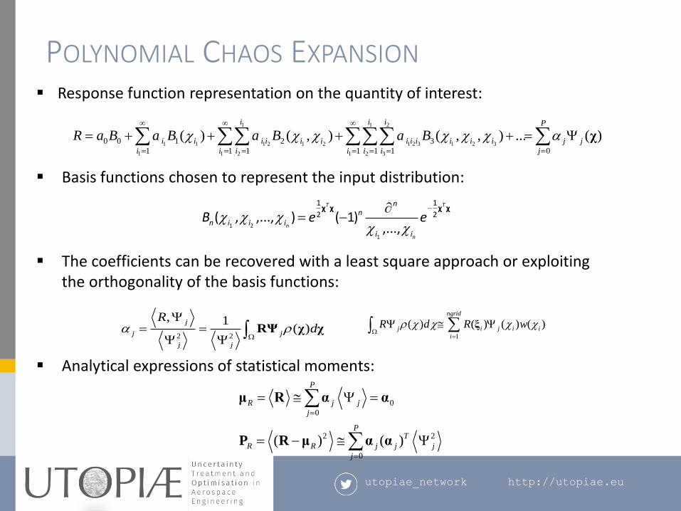
Response function representation on the quantity of interest:
Basis functions chosen to represent the input distribution:
The coefficients can be recovered with a least square approach or exploiting the orthogonality of the basis functions:
Analytical expressions of statistical moments:
POLYNOMIAL CHAOS EXPANSION
1
( ) ( ) ( ) ( )ngrid
j i j i i
i
R d R w W
ξ
0
0
2 2
0
( ) ( )
P
R j j
j
PT
R R j j j
j
μ R α α
P R μ α α
1 1 2
1 1 1 2 1 2 1 2 3 1 2 3
1 1 2 1 2 3
0 0 1 2 3
1 1 1 1 1 1 0
( ) ( , ) ( , , ) ... ( )i i i P
i i i i i i i i i i i i j j
i i i i i i j
R a B a B a B a B
χ
2 2
, 1( )
j
j j
j j
Rd
W
RΨ χ χ
1 2
1
1 1
2 2( , ,..., ) ( 1),...,
T T
n
n
nn
n i i i
i i
B e e
χ χ χ χ
utopiae_network http://utopiae.eu
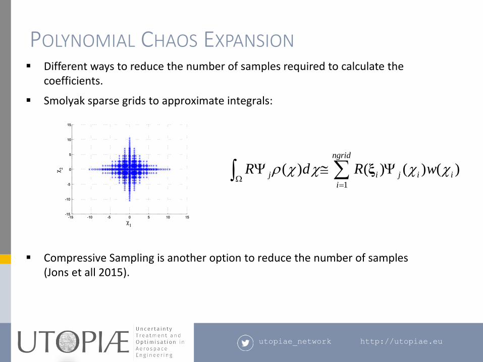
Different ways to reduce the number of samples required to calculate the coefficients.
Smolyak sparse grids to approximate integrals:
Compressive Sampling is another option to reduce the number of samples (Jons et all 2015).
POLYNOMIAL CHAOS EXPANSION
1
( ) ( ) ( ) ( )ngrid
j i j i i
i
R d R w W
ξ
utopiae_network http://utopiae.eu
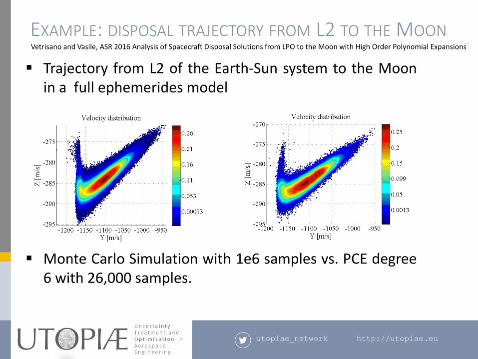
Trajectory from L2 of the Earth-Sun system to the Moonin a full ephemerides model
Monte Carlo Simulation with 1e6 samples vs. PCE degree6 with 26,000 samples.
EXAMPLE: DISPOSAL TRAJECTORY FROM L2 TO THE MOONVetrisano and Vasile, ASR 2016 Analysis of Spacecraft Disposal Solutions from LPO to the Moon with High Order Polynomial Expansions
utopiae_network http://utopiae.eu
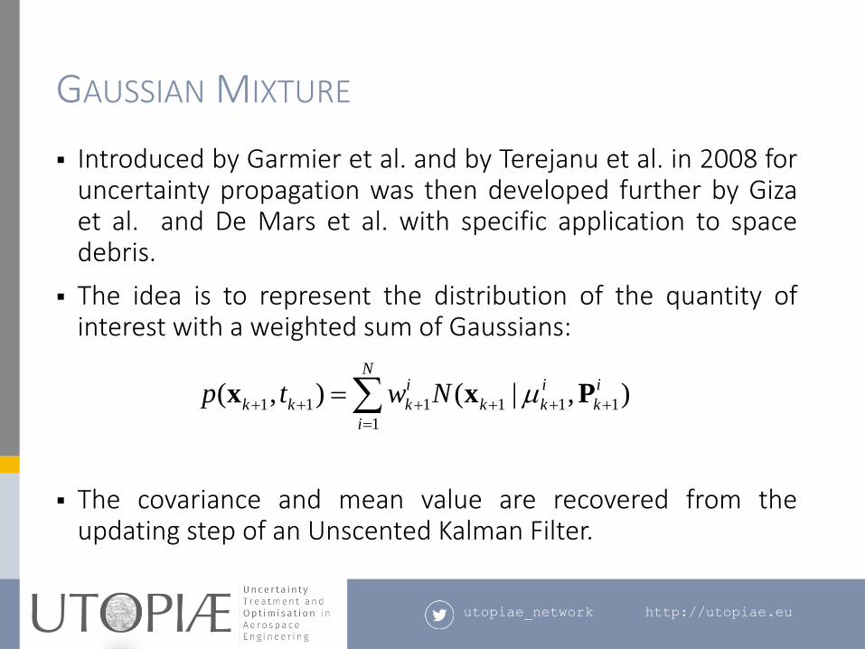
GAUSSIAN MIXTURE
Introduced by Garmier et al. and by Terejanu et al. in 2008 foruncertainty propagation was then developed further by Gizaet al. and De Mars et al. with specific application to spacedebris.
The idea is to represent the distribution of the quantity ofinterest with a weighted sum of Gaussians:
The covariance and mean value are recovered from theupdating step of an Unscented Kalman Filter.
1 1 1 1 1 1
1
( , ) ( | , )N
i i i
k k k k k k
i
p t w N
x x P
utopiae_network http://utopiae.eu
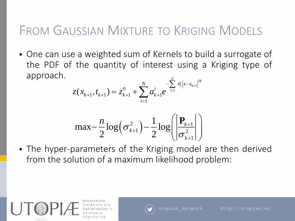
FROM GAUSSIAN MIXTURE TO KRIGING MODELS
One can use a weighted sum of Kernels to build a surrogate ofthe PDF of the quantity of interest using a Kriging type ofapproach.
The hyper-parameters of the Kriging model are then derivedfrom the solution of a maximum likelihood problem:
1
10
1 1 1 1
1
( , )
dpl
l k
l
N x xi
k k k k
i
z x t z a e
( 2 11 2
1
1max log log
2 2
kk
k
n
P
utopiae_network http://utopiae.eu
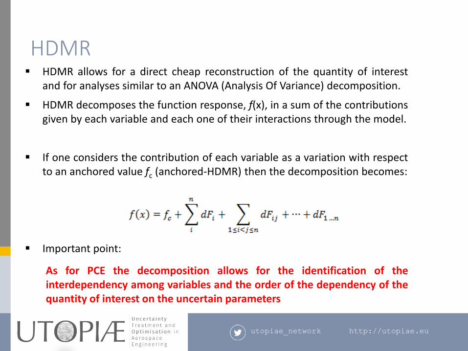
HDMR allows for a direct cheap reconstruction of the quantity of interestand for analyses similar to an ANOVA (Analysis Of Variance) decomposition.
HDMR decomposes the function response, f(x), in a sum of the contributionsgiven by each variable and each one of their interactions through the model.
If one considers the contribution of each variable as a variation with respectto an anchored value fc (anchored-HDMR) then the decomposition becomes:
Important point:
As for PCE the decomposition allows for the identification of theinterdependency among variables and the order of the dependency of thequantity of interest on the uncertain parameters
HDMR
utopiae_network http://utopiae.eu
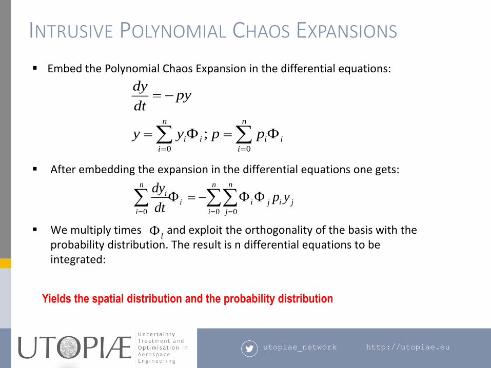
Embed the Polynomial Chaos Expansion in the differential equations:
After embedding the expansion in the differential equations one gets:
We multiply times and exploit the orthogonality of the basis with the probability distribution. The result is n differential equations to be integrated:
INTRUSIVE POLYNOMIAL CHAOS EXPANSIONS
Yields the spatial distribution and the probability distribution
0 0
;n n
i i i i
i i
dypy
dt
y y p p
0 0 0
n n ni
i i j i j
i i j
dyp y
dt
l
utopiae_network http://utopiae.eu
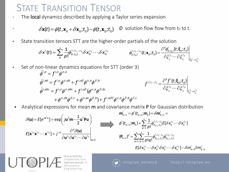
STATE TRANSITION TENSOR• The local dynamics described by applying a Taylor series expansion
• Φ solution flow flow from t0 to t.
• State transition tensors STT are the higher-order partials of the solution
• Set of non-linear dynamics equations for STT (order 3)
Analytical expressions for mean m and covariance matrix P for Gaussian distribution
0 0 0 0 0( ) ( , ; ) ( , ; )t t t t t x x x x
1
1
0 00 0
, ... 0 0
ξ x
( ; ; )p
p
j j
p ii f t t
f
ξ
, , ,
, , , , , ,
, , , , , ,
, , , , , , , ,
(
)
i a i a
i ab i ab i a b
i abc i abc i a bc
ab c ac b i a b c
f
f f
f f
f
1 1
0
, ...
( , ) 0 0
1( )
!p p
siit t
p
x t x xp
1 0
0 1
0 00 0
, ... ( , ) 0 0
( , ) 0 0
ξ x
( ; ; )( ; ; )p
p
j j
p ii t t
t t
t tt t
ξx
1 2
1 2
0
1( ) [ ] exp
2
( )[ ]
T
p
p
j T T
pp
E e j
E j
u x
u
u u m u Pu
ux x x
u u u
1 1
1
1 1
1 1
1 1
1 1 1
.
1 ( , )1
. .
1 ( , ) ( , )1 1
1 1
( ; )
1( ; ) [ ]
!
1( )
! !
[ ]
p p
k k
p q
k k k k
p q
i i ik k k k
sii
k k t t k kp
s si iij
k t t t tp q
i jk k k k k k
t
t E x xp
p q
E x x x x m m
m m m
m
P
utopiae_network http://utopiae.eu
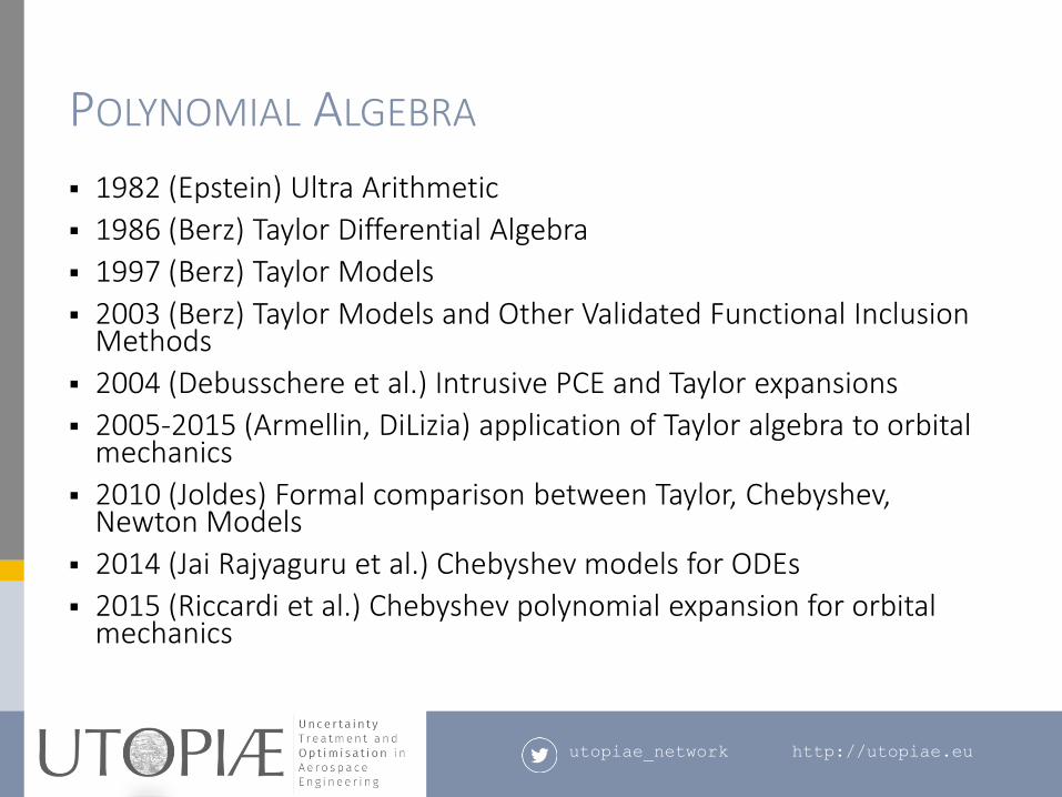
POLYNOMIAL ALGEBRA
1982 (Epstein) Ultra Arithmetic
1986 (Berz) Taylor Differential Algebra
1997 (Berz) Taylor Models
2003 (Berz) Taylor Models and Other Validated Functional Inclusion Methods
2004 (Debusschere et al.) Intrusive PCE and Taylor expansions
2005-2015 (Armellin, DiLizia) application of Taylor algebra to orbital mechanics
2010 (Joldes) Formal comparison between Taylor, Chebyshev, Newton Models
2014 (Jai Rajyaguru et al.) Chebyshev models for ODEs
2015 (Riccardi et al.) Chebyshev polynomial expansion for orbital mechanics
utopiae_network http://utopiae.eu
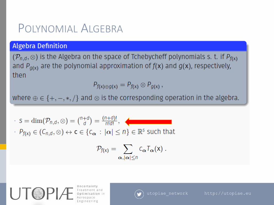
POLYNOMIAL ALGEBRA
utopiae_network http://utopiae.eu
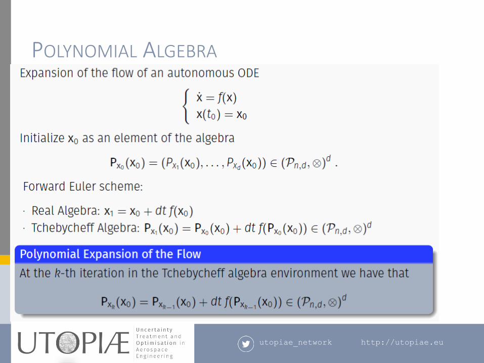
POLYNOMIAL ALGEBRA
utopiae_network http://utopiae.eu
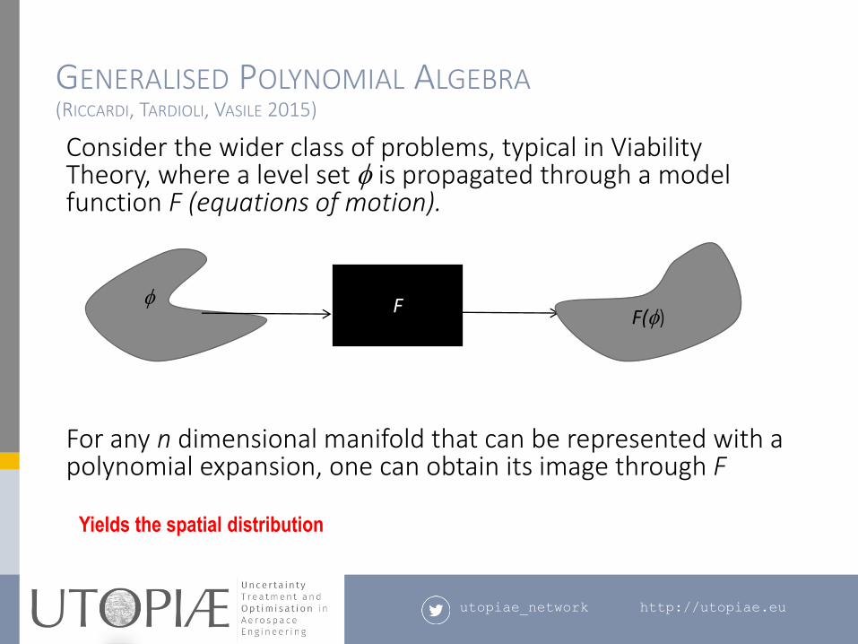
GENERALISED POLYNOMIAL ALGEBRA(RICCARDI, TARDIOLI, VASILE 2015)
Consider the wider class of problems, typical in Viability Theory, where a level set is propagated through a model function F (equations of motion).
For any n dimensional manifold that can be represented with a polynomial expansion, one can obtain its image through F
FF()
Yields the spatial distribution
utopiae_network http://utopiae.eu
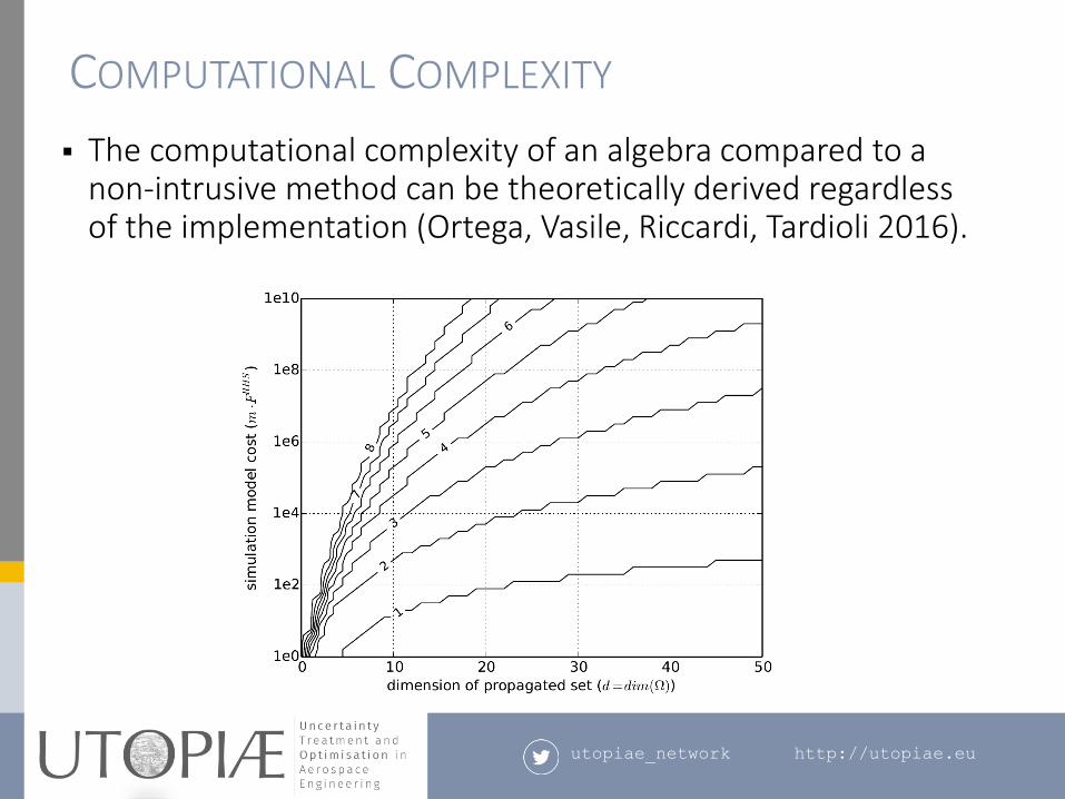
COMPUTATIONAL COMPLEXITY
The computational complexity of an algebra compared to a non-intrusive method can be theoretically derived regardless of the implementation (Ortega, Vasile, Riccardi, Tardioli 2016).
utopiae_network http://utopiae.eu
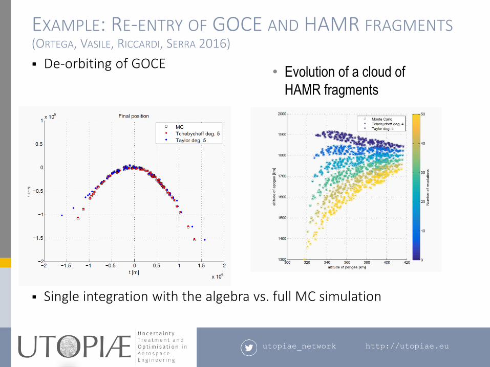
EXAMPLE: RE-ENTRY OF GOCE AND HAMR FRAGMENTS(ORTEGA, VASILE, RICCARDI, SERRA 2016)
De-orbiting of GOCE
Single integration with the algebra vs. full MC simulation
• Evolution of a cloud of
HAMR fragments
utopiae_network http://utopiae.eu
Model Uncertainty
utopiae_network http://utopiae.eu
BACKGROUND AND MOTIVATION
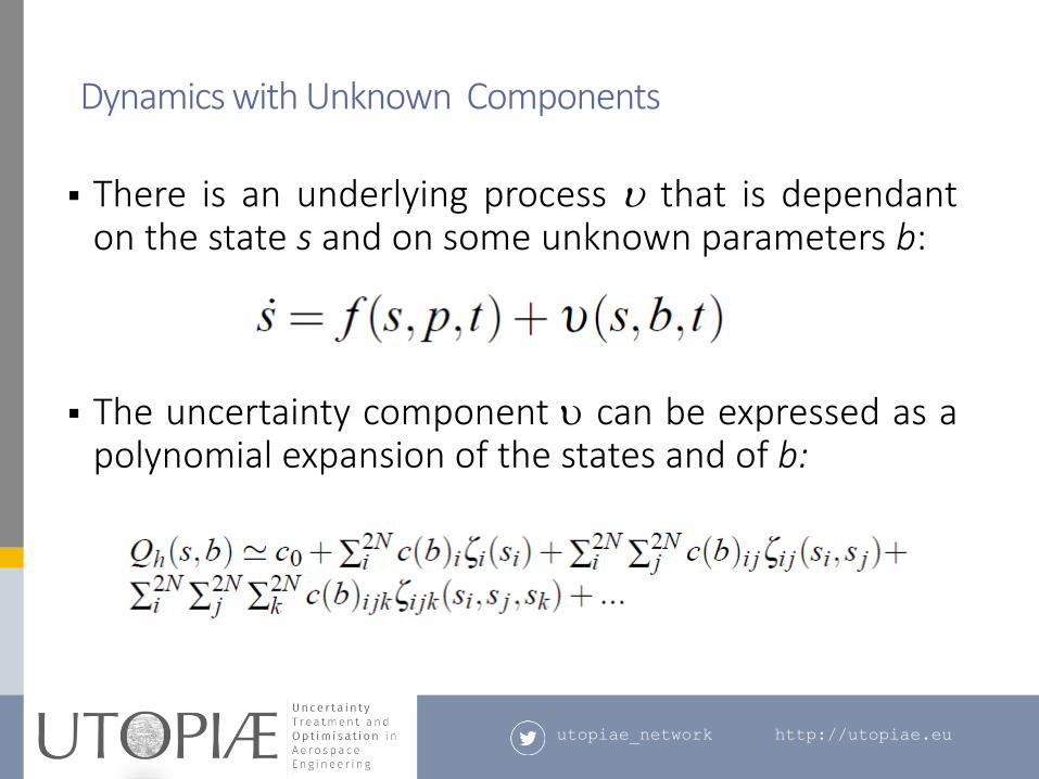
There is an underlying process u that is dependanton the state s and on some unknown parameters b:
The uncertainty component u can be expressed as apolynomial expansion of the states and of b:
Dynamics with Unknown Components
utopiae_network http://utopiae.eu
UNCERTAINTY FUNCTION AND DISTANCE
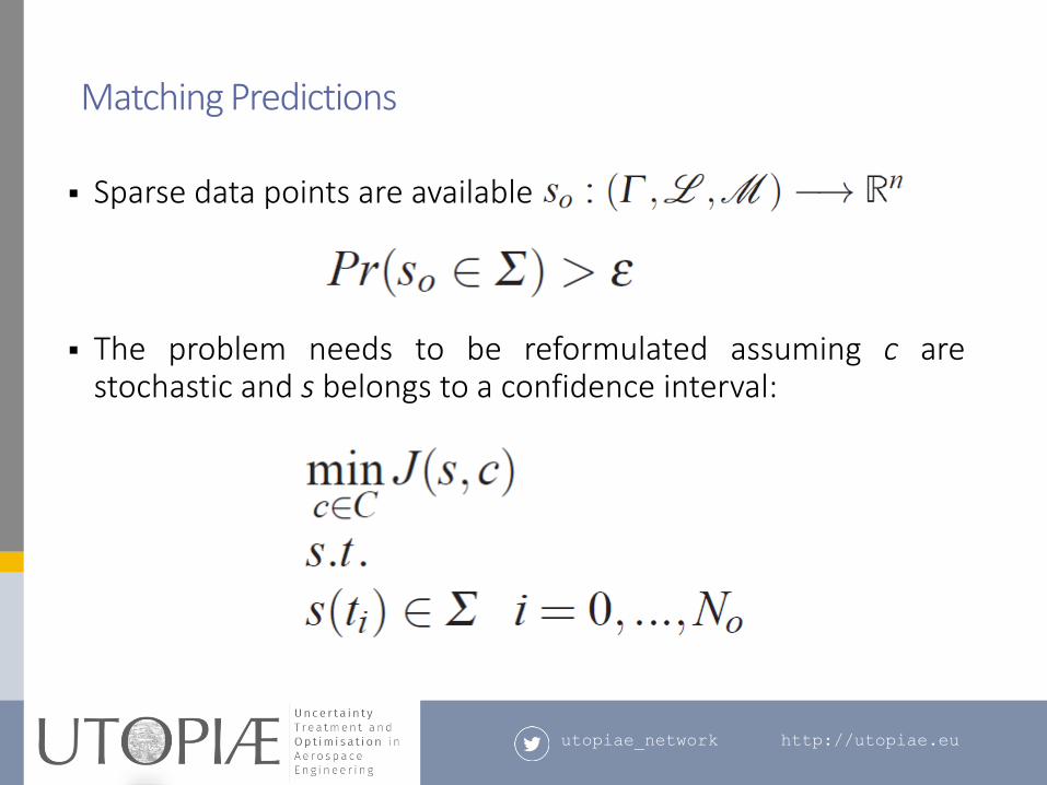
Sparse data points are available
The problem needs to be reformulated assuming c arestochastic and s belongs to a confidence interval:
Matching Predictions
utopiae_network http://utopiae.eu
SOME EXAMPLES
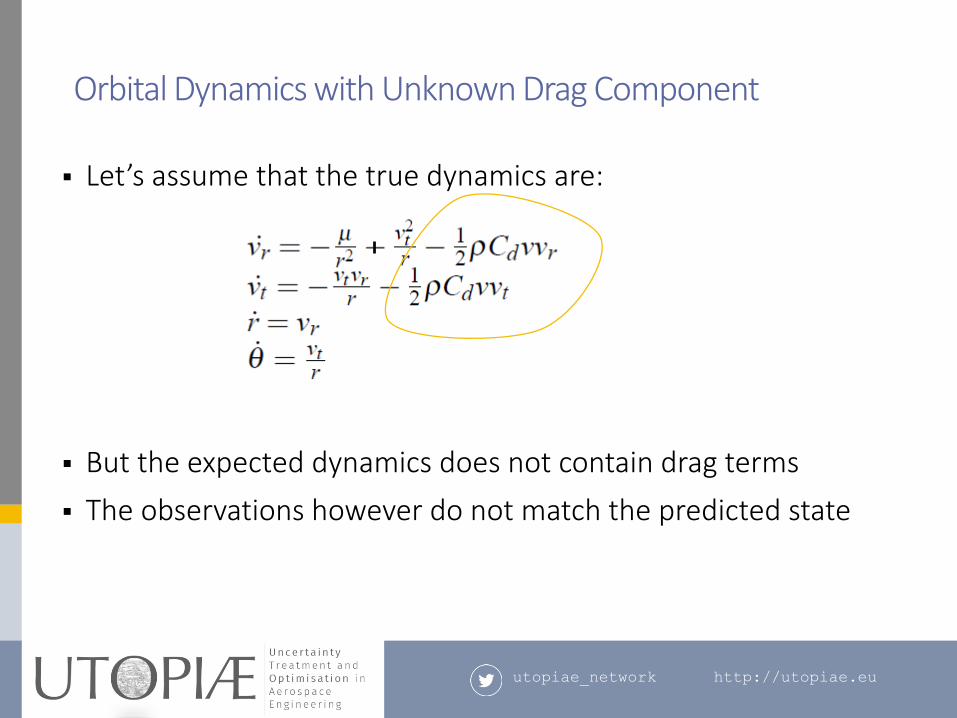
Let’s assume that the true dynamics are:
But the expected dynamics does not contain drag terms
The observations however do not match the predicted state
Orbital Dynamics with Unknown Drag Component
utopiae_network http://utopiae.eu
SOME EXAMPLES
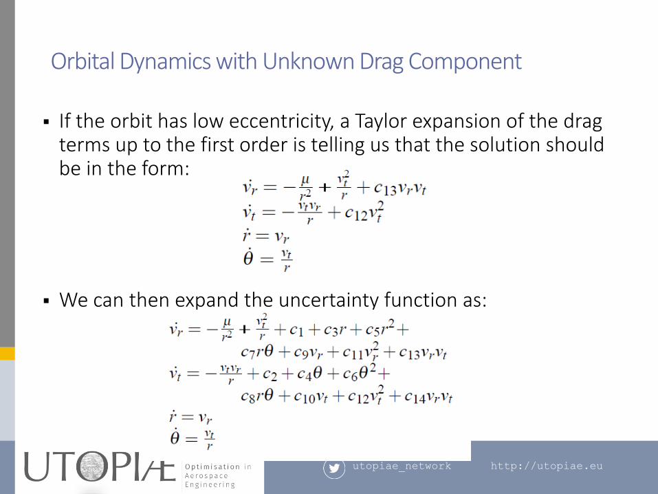
If the orbit has low eccentricity, a Taylor expansion of the drag terms up to the first order is telling us that the solution should be in the form:
We can then expand the uncertainty function as:
Orbital Dynamics with Unknown Drag Component
utopiae_network http://utopiae.eu
SOME EXAMPLES
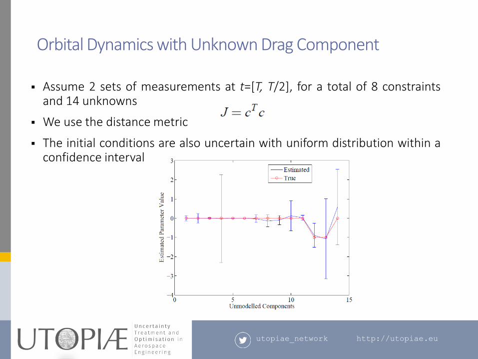
Assume 2 sets of measurements at t=[T, T/2], for a total of 8 constraintsand 14 unknowns
We use the distance metric
The initial conditions are also uncertain with uniform distribution within aconfidence interval
Orbital Dynamics with Unknown Drag Component
utopiae_network http://utopiae.eu
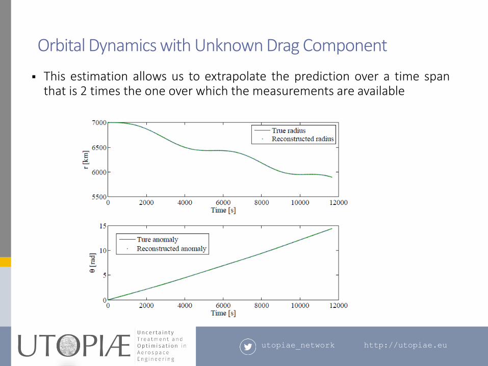
This estimation allows us to extrapolate the prediction over a time spanthat is 2 times the one over which the measurements are available
Orbital Dynamics with Unknown Drag Component

utopiae_network http://utopiae.eu
SOME EXAMPLES
This estimation allows us to extrapolate the prediction over a time spanthat is 2 times the one over which the measurements are available
Orbital Dynamics with Unknown Drag Component

Handling the unknown at the edge
of tomorrow
http://utopiae.eu
twitter.com/utopiae_network