Embed Size (px)
Citation preview
Excel 2010 Guide
To Accompany
UNDERSTANDING BASIC STATISTICS
SIXTH EDITION
Brase/Brase
Melissa M. Sovak, Ph.D.
California University of Pennsylvania

Contents
PREFACE ............................................................................................................................................... iv
UNDERSTANDING THE DIFFERENCES BETWEEN UNDERSTANDING BASIC STATISTICS
6/E AND UNDERSTANDABLE STATISTICS 10/E ............................................................................ v
Excel 2010 Guide
CHAPTER 1: GETTING STARTED
Getting started with Excel ................................................................................................................ 3
Entering Data .................................................................................................................................. 7
Using Formulas ............................................................................................................................. 10
Saving Workbooks .......................................................................................................................... 11
Lab Activities for Getting Started .................................................................................................. 13
Random Samples ............................................................................................................................ 14
Lab Activities for Random Samples ............................................................................................... 19
CHAPTER 2: ORGANIZING DATA
Frequency Distributions and Histograms ...................................................................................... 21
Lab Activities for Frequency Distributions and Histograms ......................................................... 23
Bar Graphs, Circle Graphs, and Time-Series Graphs ................................................................... 25
Lab Activities for Bar Graphs, Circle Graphs, and Time-Series Graphs ...................................... 29
CHAPTER 3: AVERAGES AND VARIATION
Central Tendency and Variation of Ungrouped Data ................................................................... 30
Lab Activities for Central Tendency and Variation of Ungrouped Data ....................................... 34
Box-and-Whisker Plots .................................................................................................................. 35
CHAPTER 4: REGRESSION AND CORRELATION
Linear Regression – Two Variables ............................................................................................... 37
Lab Activities for Two-Variable Linear Regression ...................................................................... 44
CHAPTER 5: ELEMENTARY PROBABILITY THEORY
Simulations ..................................................................................................................................... 47
Lab Activities for Simulations ........................................................................................................ 49
CHAPTER 6: THE BINOMIAL PROBABILITY DISTRIBUTION AND RELATED TOPICS
The Binomial Probability Distribution .......................................................................................... 50
Lab Activities for Binomial Probability Distributions ................................................................... 53
CHAPTER 7: NORMAL CURVES AND SAMPLING DISTRIBUTIONS
Graphs of Normal Probability Distributions ................................................................................. 55
Standard Scores and Normal Probabilities ................................................................................... 60
Lab Activities for Normal Distribution .......................................................................................... 63
Introduction to Sampling Distributions ......................................................................................... 64
CHAPTER 8: ESTIMATION
Confidence Intervals for the Mean – When σ is Known................................................................. 65
Confidence Intervals for the Mean – When σ is Unknown ............................................................. 66
Lab Activities for Confidence Intervals for the Mean .................................................................... 69
CHAPTER 9: HYPOTHESIS TESTING
Testing a Single Population Mean – When σ is Known ................................................................. 70
Lab Activities for Testing a Single Population Mean .................................................................... 73
CHAPTER 10: INFERENCES ABOUT DIFFERENCES
Tests Involving Paired Differences – Dependent Samples ............................................................ 74
Lab Activities for Tests Involving Paired Differences ................................................................... 76
Testing of Differences of Means .................................................................................................... 76
Lab Activities for Testing Differences of Means ............................................................................ 79
CHAPTER 11: ADDITIONAL TOPICS USING INFERENCE
Chi-Square Test of Independence .................................................................................................. 81
Lab Activities for Chi-Square Test of Independence ..................................................................... 84
Inference for Regression ................................................................................................................ 85
Lab Activities for Two-Variable Linear Regression ...................................................................... 89
TABLE OF EXCEL FUNCTIONS ...................................................................................................... 91
APPENDIX A
PREFACE ............................................................................................................................................ A-3
SUGGESTIONS FOR USING THE DATA SETS ............................................................................. A-3
DESCRIPTIONS OF DATA SETS ..................................................................................................... A-4

v
Preface
The use of computing technology can greatly enhance a student’s learning experience in statistics.
Understanding Basic Statistics is accompanied by four Technology Guides, which provide basic
instructions, examples, and lab activities for four different tools:
TI-83 Plus, TI-84 Plus and TI-Nspire
Microsoft Excel ®2010 with Analysis ToolPak for Windows ®
MINITAB Version 15
SPSS Version 18
The TI-83 Plus, TI-84 Plus and TI-Nspire are versatile, widely available graphing calculators made by
Texas Instruments. The calculator guide shows how to use their statistical functions, including plotting
capabilities.
Excel is an all-purpose spreadsheet software package. The Excel guide shows how to use Excel’s built-in
statistical functions and how to produce some useful graphs. Excel is not designed to be a complete
statistical software package. In many cases, macros can be created to produce special graphs, such as
box-and-whisker plots. However, this guide only shows how to use the existing, built-in features. In
most cases, the operations omitted from Excel are easily carried out on an ordinary calculator. The
Analysis ToolPak is part of Excel and can be installed from the same source as the basic Excel program
(normally, a CD-ROM) as an option on the installer program’s list of Add-Ins. Details for getting started
with the Analysis ToolPak are in Chapter 1 of the Excel guide. No additional software is required to use
the Excel functions described.
MINITAB is a statistics software package suitable for solving problems. It can be packaged with the text.
Contact Cengage Learning for details regarding price and platform options.
SPSS is a powerful tool that can perform many statistical procedures. The SPSS guide shows how to
manage data and perform various statistical procedures using this software.
The lab activities that follow accompany the text Understanding Basic Statistics, 6th edition by Brase and
Brase. On the following page is a table to coordinate this guide with Understanding Statistics, 10th
edition by Brase and Brase. Both texts are published by Cengage Learning.
In addition, over one hundred data files from referenced sources are described in the Appendix. These
data files are available via download from the Cengage Learning Web site:
http://www.cengage.com/statistics/brase
vi
Understanding the Differences Between Understanding Basic Statistics
6/e and Understandable Statistics 10/e
Understandable Basic Statistics is the brief, one-semester version of the larger book. It is currently in its
Sixth Edition.
Understandable Statistics is the full, two-semester introductory statistics textbook, which is now in its
Tenth Edition.
Unlike other brief texts, Understanding Basic Statistics is not just the first six or seven chapters of the full
text. Rather, topic coverage has been shortened in many cases and rearranged, so that the essential
statistics concepts can be taught in one semester.
The major difference between the two tables of contents is that Regression and Correlation are covered
much earlier in the brief textbook. In the full text, these topics are covered in Chapter 9. In the brief text,
they are covered in Chapter 4.
Analysis of Variance (ANOVA) is not covered in the brief text.
Understanding Statistics has 11 chapters and Understanding Basic Statistics has 11. The full text is a
hard cover book, while the brief is softcover.
The same pedagogical elements are used throughout both texts.
The same supplements package is shared by both texts.
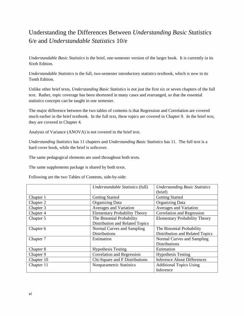
Following are the two Tables of Contents, side-by-side:
Understandable Statistics (full) Understanding Basic Statistics
(brief)
Chapter 1 Getting Started Getting Started
Chapter 2 Organizing Data Organizing Data
Chapter 3 Averages and Variation Averages and Variation
Chapter 4 Elementary Probability Theory Correlation and Regression
Chapter 5 The Binomial Probability
Distribution and Related Topics
Elementary Probability Theory
Chapter 6 Normal Curves and Sampling
Distributions
The Binomial Probability
Distribution and Related Topics
Chapter 7 Estimation Normal Curves and Sampling
Distributions
Chapter 8 Hypothesis Testing Estimation
Chapter 9 Correlation and Regression Hypothesis Testing
Chapter 10 Chi-Square and F Distributions Inference About Differences
Chapter 11
Nonparametric Statistics Additional Topics Using
Inference

vii

Excel 2010 Guide


3
CHAPTER 1: GETTING STARTED
GETTING STARTED WITH EXCEL
Microsoft Excel® is an all-purpose spreadsheet application with many functions. We will be using Excel 2010.
This guide is not a general Excel manual, but it will show you how to use many of Excel’s built-in statistical
functions. You may need to install the Analysis ToolPak from the original Excel software if your computer does not
have it. To determine if your installation of Excel includes the Analysis ToolPak, open Excel, click on File in the
main menu, and then click on Options. Next, click on Add-Ins and see if the ToolPak is listed in the Active
Application Add-Ins. If it is, the ToolPak is installed. If you do not see a listing for Analysis ToolPak in Active
Application Add-Ins, then you will need to install it from the original Excel installation source. To do this, click Go.
Then check the box next to Analysis ToolPak and click OK.
If you are familiar with Windows-based programs, you will find that many of the editing, formatting, and file-
handling procedures of Excel are similar to those you have used before. You use the mouse to select, drag, click, and
double-click as you would in any other Windows program.
If you have any questions about Excel not answered in this guide, consult the Excel manual or select Help on the
menu bar.
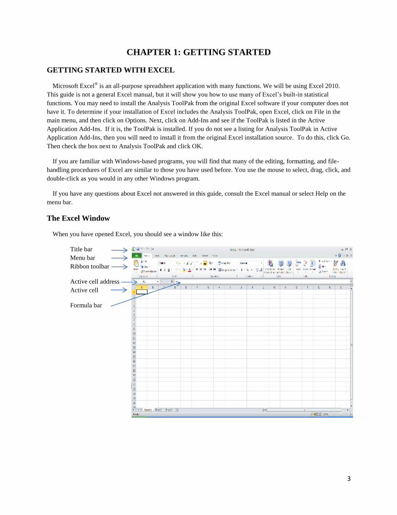
The Excel Window
When you have opened Excel, you should see a window like this:
Title bar
Menu bar
Ribbon toolbar
Active cell address
Active cell
Formula bar
4
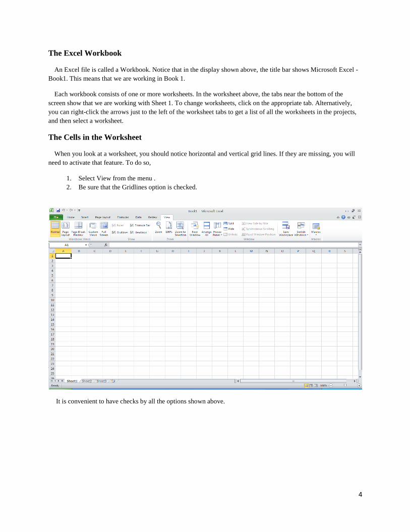
The Excel Workbook
An Excel file is called a Workbook. Notice that in the display shown above, the title bar shows Microsoft Excel -
Book1. This means that we are working in Book 1.
Each workbook consists of one or more worksheets. In the worksheet above, the tabs near the bottom of the
screen show that we are working with Sheet 1. To change worksheets, click on the appropriate tab. Alternatively,
you can right-click the arrows just to the left of the worksheet tabs to get a list of all the worksheets in the projects,
and then select a worksheet.
The Cells in the Worksheet
When you look at a worksheet, you should notice horizontal and vertical grid lines. If they are missing, you will
need to activate that feature. To do so,
1. Select View from the menu .
2. Be sure that the Gridlines option is checked.
It is convenient to have checks by all the options shown above.
5
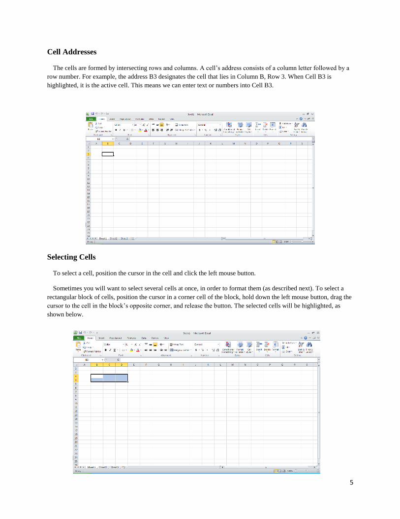
Cell Addresses
The cells are formed by intersecting rows and columns. A cell’s address consists of a column letter followed by a
row number. For example, the address B3 designates the cell that lies in Column B, Row 3. When Cell B3 is
highlighted, it is the active cell. This means we can enter text or numbers into Cell B3.
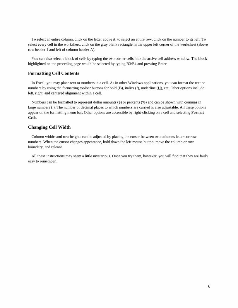
Selecting Cells
To select a cell, position the cursor in the cell and click the left mouse button.
Sometimes you will want to select several cells at once, in order to format them (as described next). To select a
rectangular block of cells, position the cursor in a corner cell of the block, hold down the left mouse button, drag the
cursor to the cell in the block’s opposite corner, and release the button. The selected cells will be highlighted, as
shown below.
6
To select an entire column, click on the letter above it; to select an entire row, click on the number to its left. To
select every cell in the worksheet, click on the gray blank rectangle in the upper left corner of the worksheet (above
row header 1 and left of column header A).
You can also select a block of cells by typing the two corner cells into the active cell address window. The block
highlighted on the preceding page would be selected by typing B3:E4 and pressing Enter.
Formatting Cell Contents
In Excel, you may place text or numbers in a cell. As in other Windows applications, you can format the text or
numbers by using the formatting toolbar buttons for bold (B), italics (I), underline (U), etc. Other options include
left, right, and centered alignment within a cell.
Numbers can be formatted to represent dollar amounts ($) or percents (%) and can be shown with commas in
large numbers (,). The number of decimal places to which numbers are carried is also adjustable. All these options
appear on the formatting menu bar. Other options are accessible by right-clicking on a cell and selecting Format
Cells.
Changing Cell Width
Column widths and row heights can be adjusted by placing the cursor between two columns letters or row
numbers. When the cursor changes appearance, hold down the left mouse button, move the column or row
boundary, and release.
All these instructions may seem a little mysterious. Once you try them, however, you will find that they are fairly
easy to remember.
7
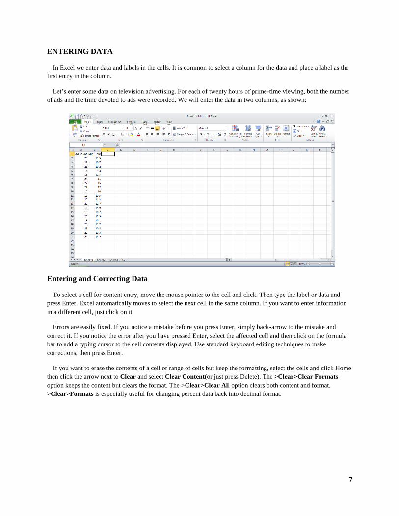
ENTERING DATA
In Excel we enter data and labels in the cells. It is common to select a column for the data and place a label as the
first entry in the column.
Let’s enter some data on television advertising. For each of twenty hours of prime-time viewing, both the number
of ads and the time devoted to ads were recorded. We will enter the data in two columns, as shown:
Entering and Correcting Data
To select a cell for content entry, move the mouse pointer to the cell and click. Then type the label or data and
press Enter. Excel automatically moves to select the next cell in the same column. If you want to enter information
in a different cell, just click on it.
Errors are easily fixed. If you notice a mistake before you press Enter, simply back-arrow to the mistake and
correct it. If you notice the error after you have pressed Enter, select the affected cell and then click on the formula
bar to add a typing cursor to the cell contents displayed. Use standard keyboard editing techniques to make
corrections, then press Enter.
If you want to erase the contents of a cell or range of cells but keep the formatting, select the cells and click Home
then click the arrow next to Clear and select Clear Content(or just press Delete). The >Clear>Clear Formats
option keeps the content but clears the format. The >Clear>Clear All option clears both content and format.
>Clear>Formats is especially useful for changing percent data back into decimal format.
8
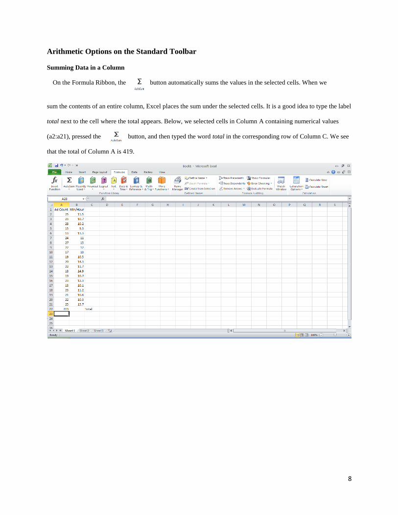
Arithmetic Options on the Standard Toolbar
Summing Data in a Column
On the Formula Ribbon, the button automatically sums the values in the selected cells. When we
sum the contents of an entire column, Excel places the sum under the selected cells. It is a good idea to type the label
total next to the cell where the total appears. Below, we selected cells in Column A containing numerical values
(a2:a21), pressed the button, and then typed the word total in the corresponding row of Column C. We see
that the total of Column A is 419.
9
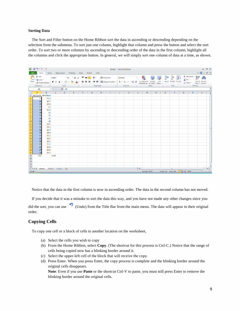
Sorting Data
The Sort and Filter button on the Home Ribbon sort the data in ascending or descending depending on the
selection from the submenu. To sort just one column, highlight that column and press the button and select the sort
order. To sort two or more columns by ascending or descending order of the data in the first column, highlight all
the columns and click the appropriate button. In general, we will simply sort one column of data at a time, as shown.
Notice that the data in the first column is now in ascending order. The data in the second column has not moved.
If you decide that it was a mistake to sort the data this way, and you have not made any other changes since you
did the sort, you can use (Undo) from the Title Bar from the main menu. The data will appear in their original
order.
Copying Cells
To copy one cell or a block of cells to another location on the worksheet,
(a) Select the cells you wish to copy
(b) From the Home Ribbon, select Copy. (The shortcut for this process is Ctrl-C.) Notice that the range of
cells being copied now has a blinking border around it.
(c) Select the upper-left cell of the block that will receive the copy.
(d) Press Enter. When you press Enter, the copy process is complete and the blinking border around the
original cells disappears.
Note: Even if you use Paste or the shortcut Ctrl-V to paste, you must still press Enter to remove the
blinking border around the original cells.
10
To copy one cell or a range of cells to another worksheet or workbook, follow steps (a) and (b) above. For step
(c), be sure you are in the destination worksheet or workbook and that the worksheet or workbook is activated. Then
proceed to step (d).
USING FORMULAS
A formula is an expression that generates a numerical value in a cell, usually based on values in other cells.
Formulas usually involve standard arithmetic operations. Excel uses + for addition, - (hyphen) for subtraction, * for
multiplication, / for division, and ^ (carat) for exponentiation (raising to a power).
For instance, if we want to divide the contents of Cell A2 by the contents of Cell B2 and place the results in Cell
C2, we do the following:
(a) Make Cell C2 the active cell.
(b) Click in the formula bar and type =A2/B2.
(c) Press Enter
The value in Cell C2 will be the quotient of the values in Cells A2 and B2.
If, for a whole series of rows, we wanted to divide the entry in Column A by the entry in Column B and put the
results in Column C, we could repeat the above process over and over. However, the typing would be tedious. We
can accomplish the same thing more easily by copying and pasting:
(a) Enter =A2/B2 in Cell C2 as described above
(b) Move the cursor to the lower right corner of Cell C2. The cursor should change shape to small black
cross (+). Now hold down the left mouse button and drag the + down until all the cells in Column C in
which you want the calculation done are highlighted.
(c) Release the mouse button and press Enter. The cell entries in Column C should equal the quotients of
the same-row entries in Columns A and B.
11
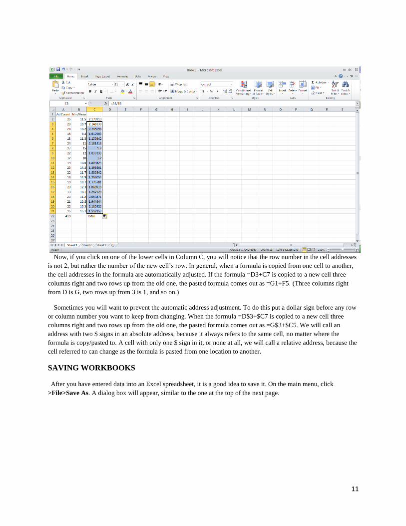
Now, if you click on one of the lower cells in Column C, you will notice that the row number in the cell addresses
is not 2, but rather the number of the new cell’s row. In general, when a formula is copied from one cell to another,
the cell addresses in the formula are automatically adjusted. If the formula =D3+C7 is copied to a new cell three
columns right and two rows up from the old one, the pasted formula comes out as =G1+F5. (Three columns right
from D is G, two rows up from 3 is 1, and so on.)
Sometimes you will want to prevent the automatic address adjustment. To do this put a dollar sign before any row
or column number you want to keep from changing. When the formula =D$3+$C7 is copied to a new cell three
columns right and two rows up from the old one, the pasted formula comes out as =G$3+$C5. We will call an
address with two $ signs in an absolute address, because it always refers to the same cell, no matter where the
formula is copy/pasted to. A cell with only one $ sign in it, or none at all, we will call a relative address, because the
cell referred to can change as the formula is pasted from one location to another.
SAVING WORKBOOKS
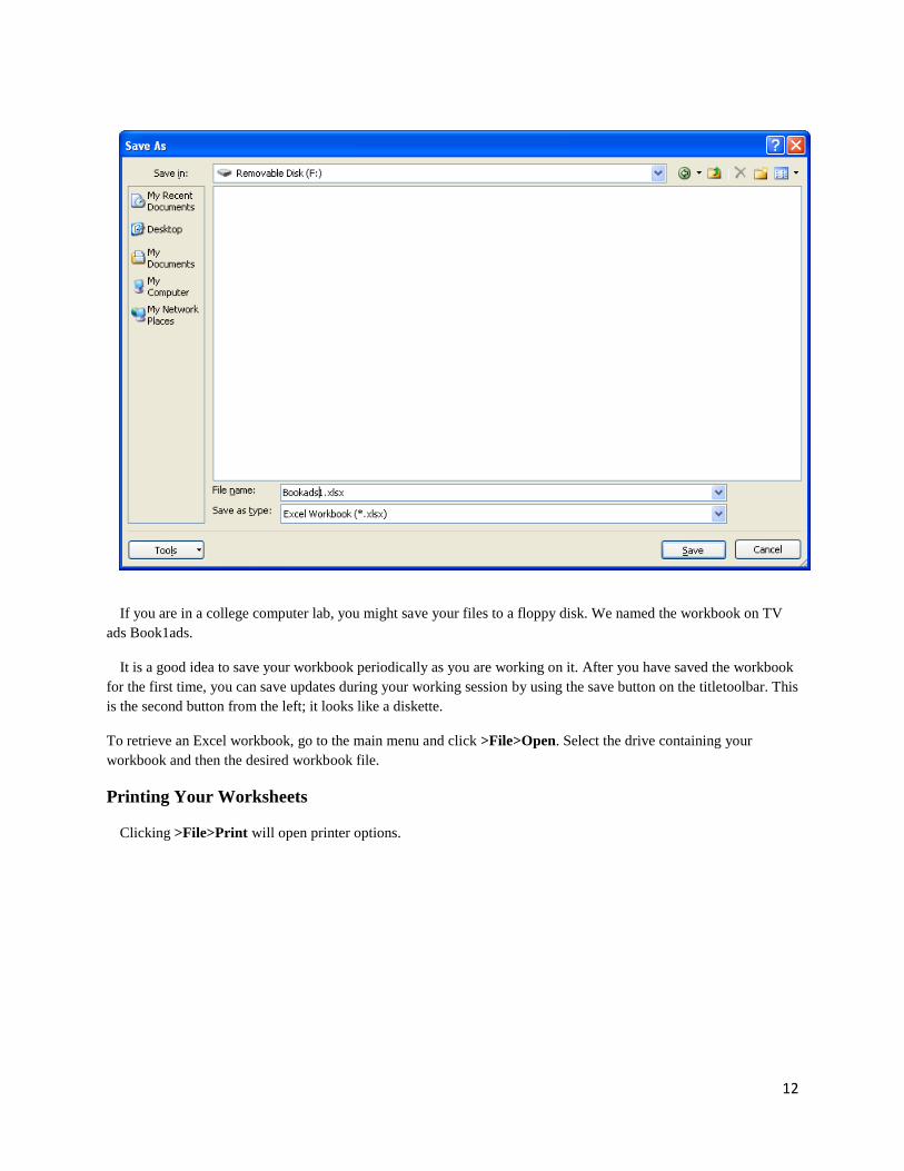
After you have entered data into an Excel spreadsheet, it is a good idea to save it. On the main menu, click
>File>Save As. A dialog box will appear, similar to the one at the top of the next page.
12
If you are in a college computer lab, you might save your files to a floppy disk. We named the workbook on TV
ads Book1ads.
It is a good idea to save your workbook periodically as you are working on it. After you have saved the workbook
for the first time, you can save updates during your working session by using the save button on the titletoolbar. This
is the second button from the left; it looks like a diskette.
To retrieve an Excel workbook, go to the main menu and click >File>Open. Select the drive containing your
workbook and then the desired workbook file.
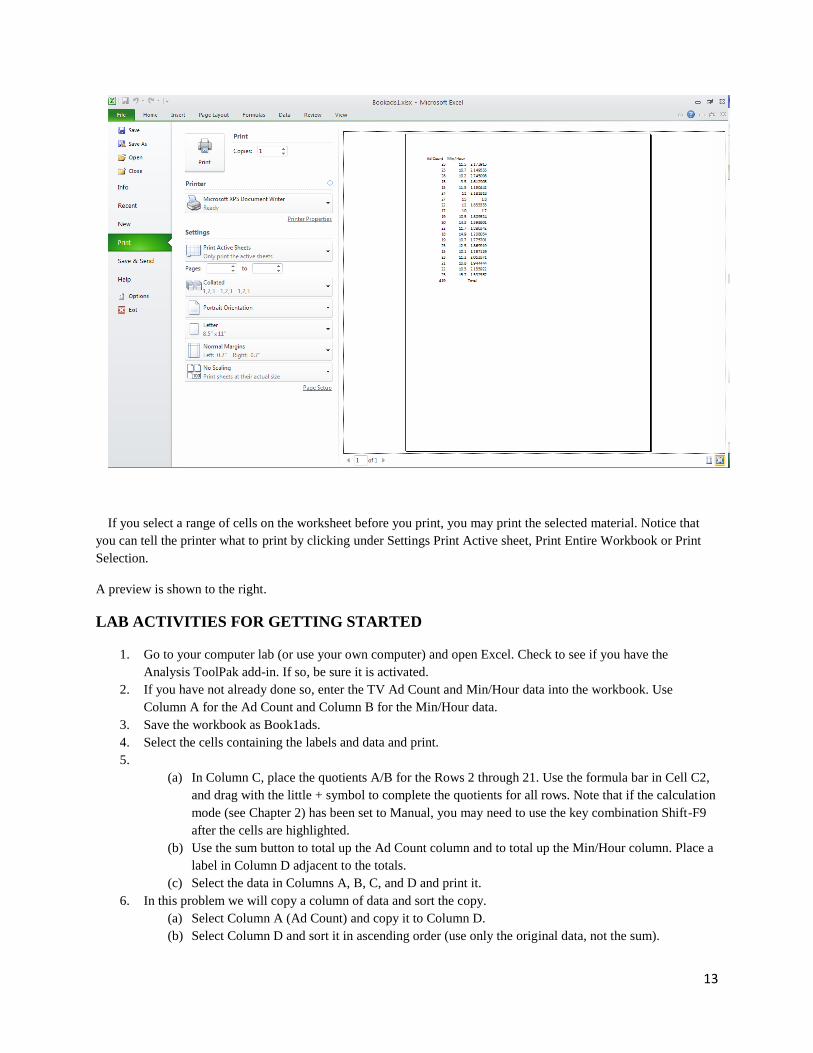
Printing Your Worksheets
Clicking >File>Print will open printer options.
13
If you select a range of cells on the worksheet before you print, you may print the selected material. Notice that
you can tell the printer what to print by clicking under Settings Print Active sheet, Print Entire Workbook or Print
Selection.
A preview is shown to the right.
LAB ACTIVITIES FOR GETTING STARTED
1. Go to your computer lab (or use your own computer) and open Excel. Check to see if you have the
Analysis ToolPak add-in. If so, be sure it is activated.
2. If you have not already done so, enter the TV Ad Count and Min/Hour data into the workbook. Use
Column A for the Ad Count and Column B for the Min/Hour data.
3. Save the workbook as Book1ads.
4. Select the cells containing the labels and data and print.
5.
(a) In Column C, place the quotients A/B for the Rows 2 through 21. Use the formula bar in Cell C2,
and drag with the little + symbol to complete the quotients for all rows. Note that if the calculation
mode (see Chapter 2) has been set to Manual, you may need to use the key combination Shift-F9
after the cells are highlighted.
(b) Use the sum button to total up the Ad Count column and to total up the Min/Hour column. Place a
label in Column D adjacent to the totals.
(c) Select the data in Columns A, B, C, and D and print it.
6. In this problem we will copy a column of data and sort the copy.
(a) Select Column A (Ad Count) and copy it to Column D.
(b) Select Column D and sort it in ascending order (use only the original data, not the sum).
14
(c) Select both Column A (Ad Count) and Column B (Min/Hour). Sort these columns by Column A in
descending order. Are the data entries of 13 in Column A still next to the data entries 11.3 and
10.1 in Column B? Are the data in Column B sorted?
RANDOM SAMPLES (SECTION 1.2 OF UNDERSTANDING BASIC STATISTICS)
Excel has several random number generators. The one we will find most convenient is the function
RANDBETWEEN(bottom,top). This function generates a random integer between (inclusively) whatever integer
is put in for “bottom” and whatever integer is put in for “top.”
To use RANDBETWEEN, select a cell in the active worksheet. Click in the formula bar, type an equals sign, and
on the standard toolbar click the Insert Function button:
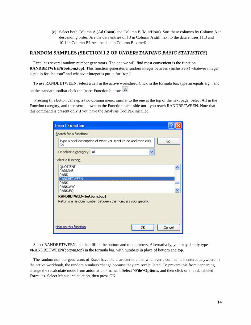
Pressing this button calls up a two-column menu, similar to the one at the top of the next page. Select All in the
Function category, and then scroll down on the Function name side until you reach RANDBETWEEN. Note that
this command is present only if you have the Analysis ToolPak installed.
Select RANDBETWEEN and then fill in the bottom and top numbers. Alternatively, you may simply type
=RANDBETWEEN(bottom,top) in the formula bar, with numbers in place of bottom and top.
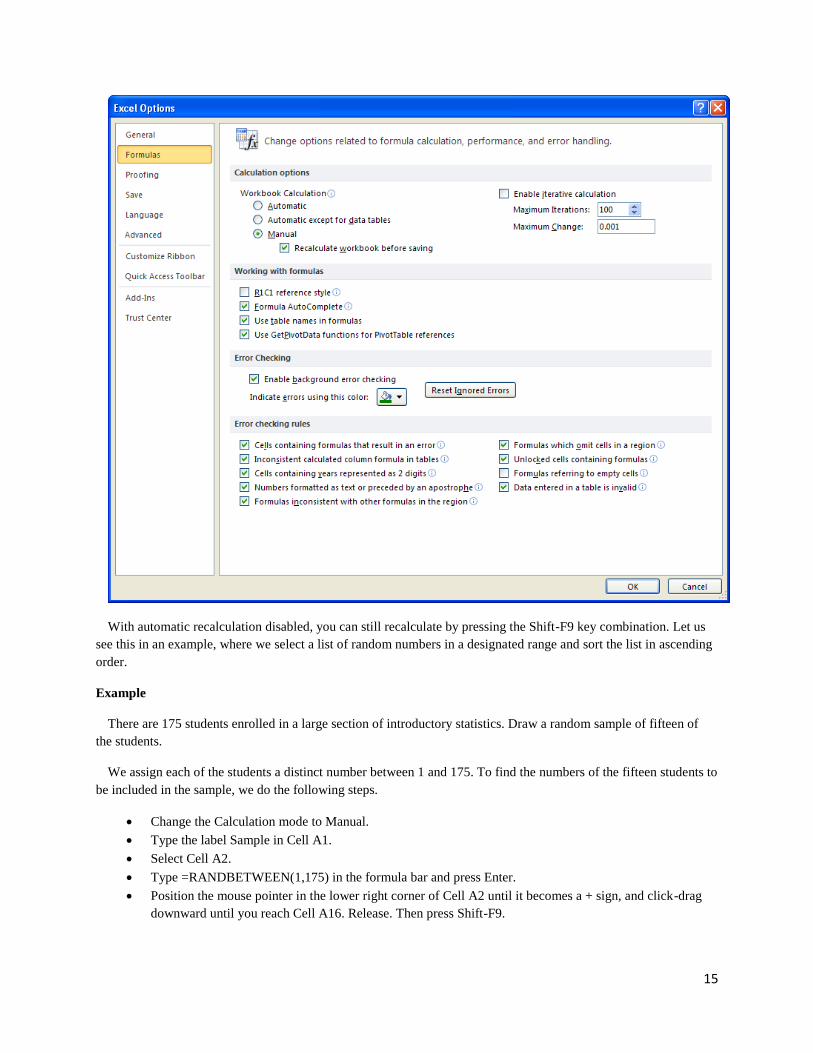
The random number generators of Excel have the characteristic that whenever a command is entered anywhere in
the active workbook, the random numbers change because they are recalculated. To prevent this from happening,
change the recalculate mode from automatic to manual. Select >File>Options, and then click on the tab labeled
Formulas. Select Manual calculation, then press OK.
15
With automatic recalculation disabled, you can still recalculate by pressing the Shift-F9 key combination. Let us
see this in an example, where we select a list of random numbers in a designated range and sort the list in ascending
order.
Example
There are 175 students enrolled in a large section of introductory statistics. Draw a random sample of fifteen of
the students.
We assign each of the students a distinct number between 1 and 175. To find the numbers of the fifteen students to
be included in the sample, we do the following steps.
Change the Calculation mode to Manual.
Type the label Sample in Cell A1.
Select Cell A2.
Type =RANDBETWEEN(1,175) in the formula bar and press Enter.
Position the mouse pointer in the lower right corner of Cell A2 until it becomes a + sign, and click-drag
downward until you reach Cell A16. Release. Then press Shift-F9.
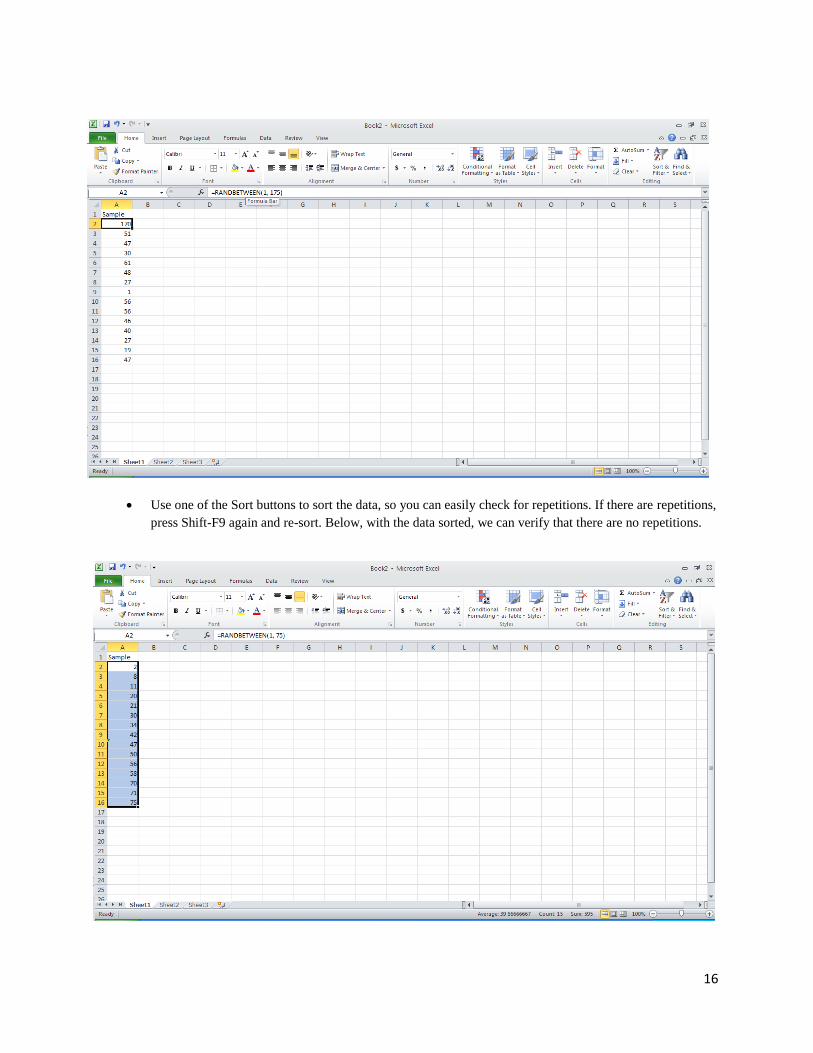
16
Use one of the Sort buttons to sort the data, so you can easily check for repetitions. If there are repetitions,
press Shift-F9 again and re-sort. Below, with the data sorted, we can verify that there are no repetitions.
17
Sometimes we will want to sample from data already in our worksheet. In such case, we can use the Sampling
dialog box. To reach the Sampling dialog box, use the man menu toolbar and select Sampling under >Datas>Data
Analysis.
Example
Enter the even numbers from 0 through 200 in Column A. Then take a sample of size ten, without replacement,
from the population of even numbers 0 through 200, and place the results in Column B.
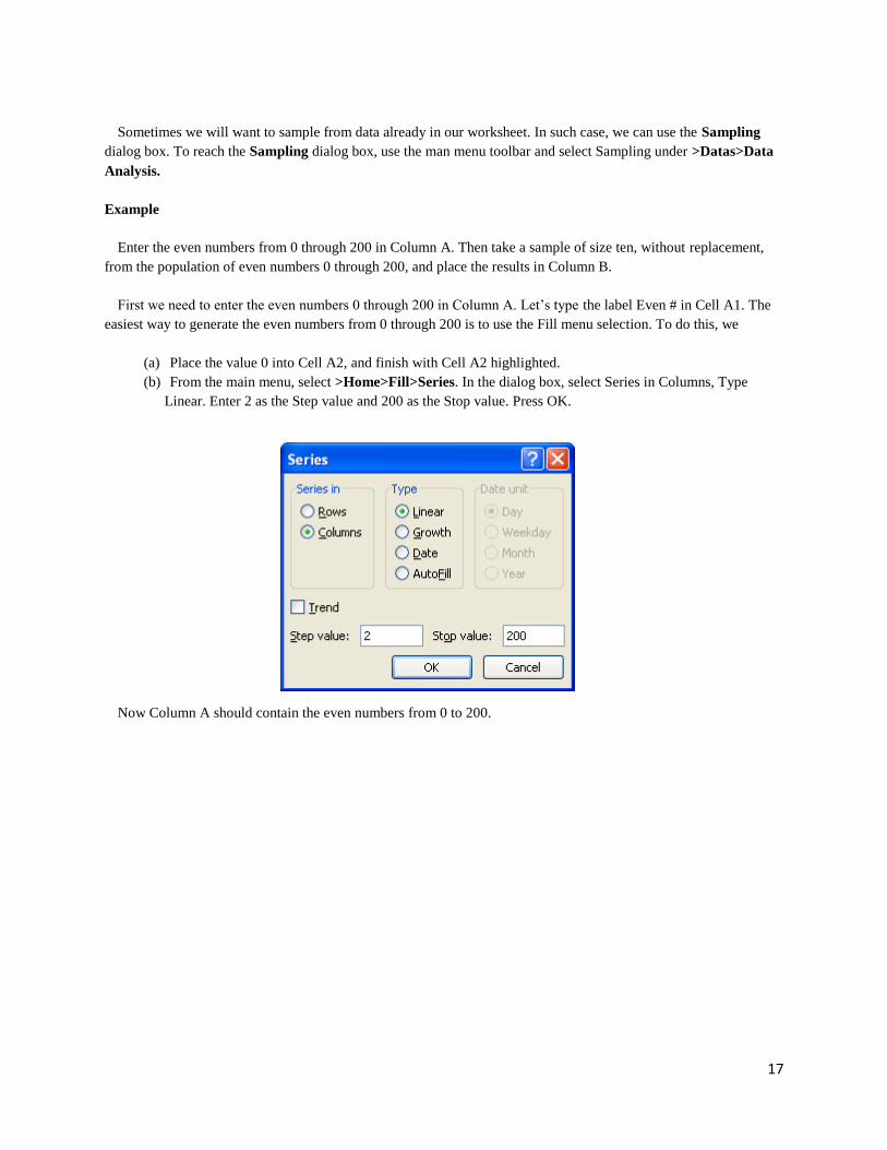
First we need to enter the even numbers 0 through 200 in Column A. Let’s type the label Even # in Cell A1. The
easiest way to generate the even numbers from 0 through 200 is to use the Fill menu selection. To do this, we
(a) Place the value 0 into Cell A2, and finish with Cell A2 highlighted.
(b) From the main menu, select >Home>Fill>Series. In the dialog box, select Series in Columns, Type
Linear. Enter 2 as the Step value and 200 as the Stop value. Press OK.
Now Column A should contain the even numbers from 0 to 200.
18
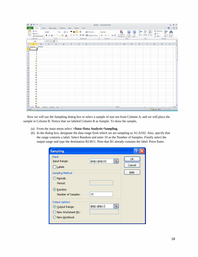
Now we will use the Sampling dialog box to select a sample of size ten from Column A, and we will place the
sample in Column B. Notice that we labeled Column B as Sample. To draw the sample,
(a) From the main menu select >Data>Data Analysis>Sampling.
(b) In the dialog box, designate the data range from which we are sampling as A1:A102. Also, specify that
the range contains a label. Select Random and enter 10 as the Number of Samples. Finally select the
output range and type the destination B2:B11. Note that B1 already contains the label. Press Enter.
19
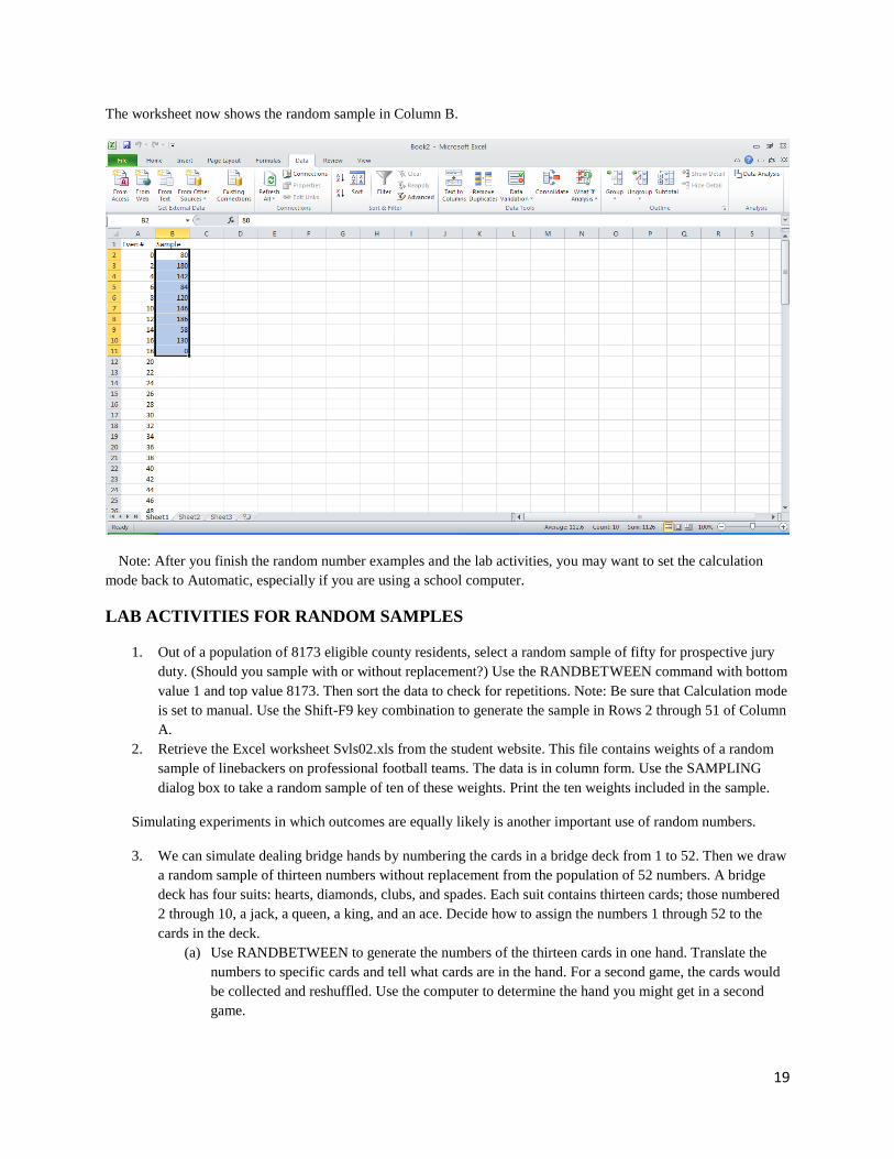
The worksheet now shows the random sample in Column B.
Note: After you finish the random number examples and the lab activities, you may want to set the calculation
mode back to Automatic, especially if you are using a school computer.
LAB ACTIVITIES FOR RANDOM SAMPLES
1. Out of a population of 8173 eligible county residents, select a random sample of fifty for prospective jury
duty. (Should you sample with or without replacement?) Use the RANDBETWEEN command with bottom
value 1 and top value 8173. Then sort the data to check for repetitions. Note: Be sure that Calculation mode
is set to manual. Use the Shift-F9 key combination to generate the sample in Rows 2 through 51 of Column
A. 2. Retrieve the Excel worksheet Svls02.xls from the student website. This file contains weights of a random
sample of linebackers on professional football teams. The data is in column form. Use the SAMPLING
dialog box to take a random sample of ten of these weights. Print the ten weights included in the sample.
Simulating experiments in which outcomes are equally likely is another important use of random numbers.
3. We can simulate dealing bridge hands by numbering the cards in a bridge deck from 1 to 52. Then we draw
a random sample of thirteen numbers without replacement from the population of 52 numbers. A bridge
deck has four suits: hearts, diamonds, clubs, and spades. Each suit contains thirteen cards; those numbered
2 through 10, a jack, a queen, a king, and an ace. Decide how to assign the numbers 1 through 52 to the
cards in the deck.
(a) Use RANDBETWEEN to generate the numbers of the thirteen cards in one hand. Translate the
numbers to specific cards and tell what cards are in the hand. For a second game, the cards would
be collected and reshuffled. Use the computer to determine the hand you might get in a second
game.

20
(b) Generate the numbers 1-52 in Column A, and then use the SAMPLING dialog box to sample
thirteen cards. Put the results in Column B, Label Column B as “My hand” and print the results.
Repeat this process to determine the hand you might get in a second game.
(c) Compare the four hands you have generated. Are they different? Would you expect this result?
4. We can also simulate the experiment of tossing a fair coin. The possible outcomes resulting from tossing a
coin are heads or tails. Assign the outcome heads the number 2 and the outcome tails the number 1. Use
RANDBETWEEN(1,2) to simulate the act of tossing a coin ten times. Simulate the experiment another
time. Do you get the same sequence of outcomes? Do you expect to? Why or why not?
21
CHAPTER 2: ORGANIZING DATA
FREQUENCY DISTRIBUTIONS AND HISTOGRAMS (SECTION 2.1 OF
UNDERSTANDING BASIC STATISTICS)
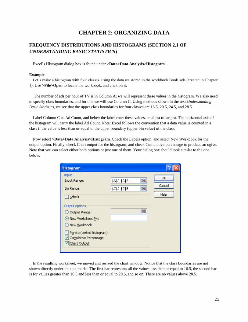
Excel’s Histogram dialog box is found under >Data>Data Analysis>Histogram.
Example
Let’s make a histogram with four classes, using the data we stored in the workbook Book1ads (created in Chapter
1). Use >File>Open to locate the workbook, and click on it.
The number of ads per hour of TV is in Column A; we will represent these values in the histogram. We also need
to specify class boundaries, and for this we will use Column C. Using methods shown in the text Understanding
Basic Statistics, we see that the upper class boundaries for four classes are 16.5, 20.5, 24.5, and 28.5.
Label Column C as Ad Count, and below the label enter these values, smallest to largest. The horizontal axis of
the histogram will carry the label Ad Count. Note: Excel follows the convention that a data value is counted in a
class if the value is less than or equal to the upper boundary (upper bin value) of the class.
Now select >Data>Data Analysis>Histogram. Check the Labels option, and select New Workbook for the
output option. Finally, check Chart output for the histogram, and check Cumulative percentage to produce an ogive.
Note that you can select either both options or just one of them. Your dialog box should look similar to the one
below.
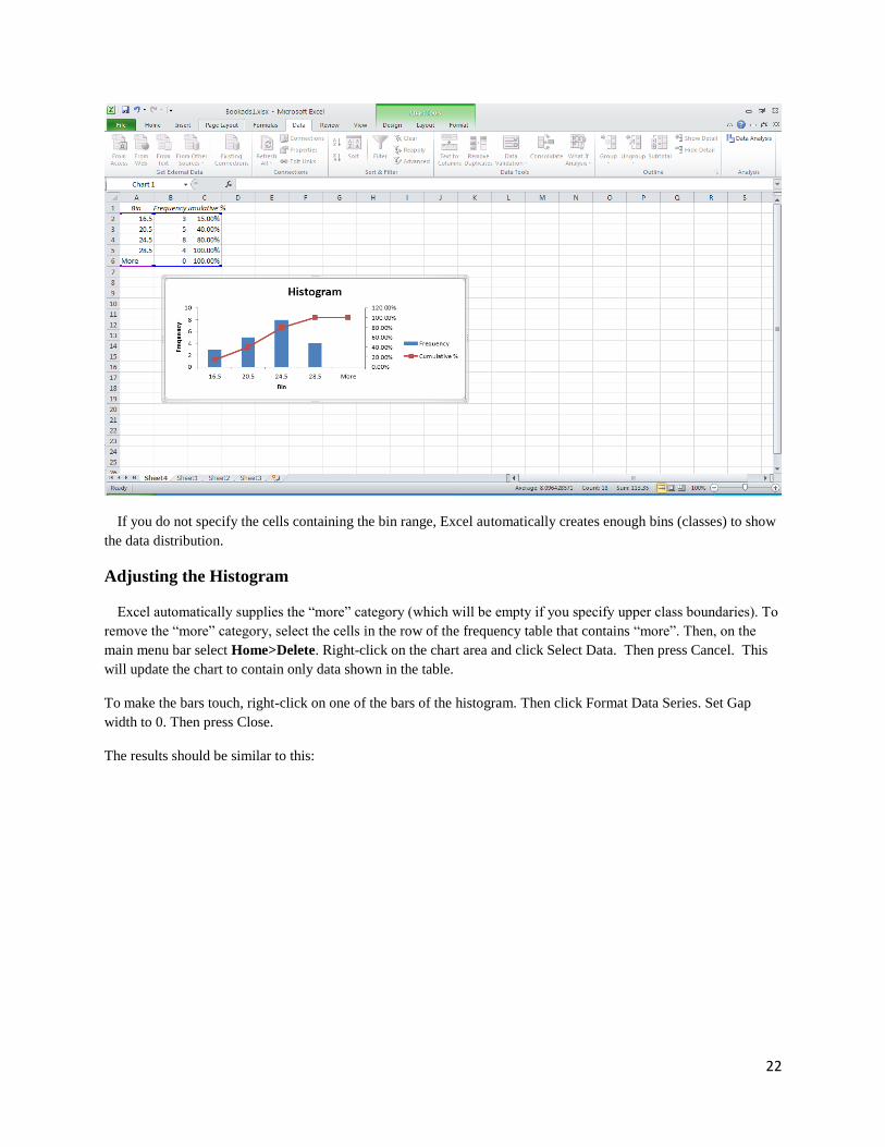
In the resulting worksheet, we moved and resized the chart window. Notice that the class boundaries are not
shown directly under the tick marks. The first bar represents all the values less than or equal to 16.5, the second bar
is for values greater than 16.5 and less than or equal to 20.5, and so on. There are no values above 28.5.
22
If you do not specify the cells containing the bin range, Excel automatically creates enough bins (classes) to show
the data distribution.
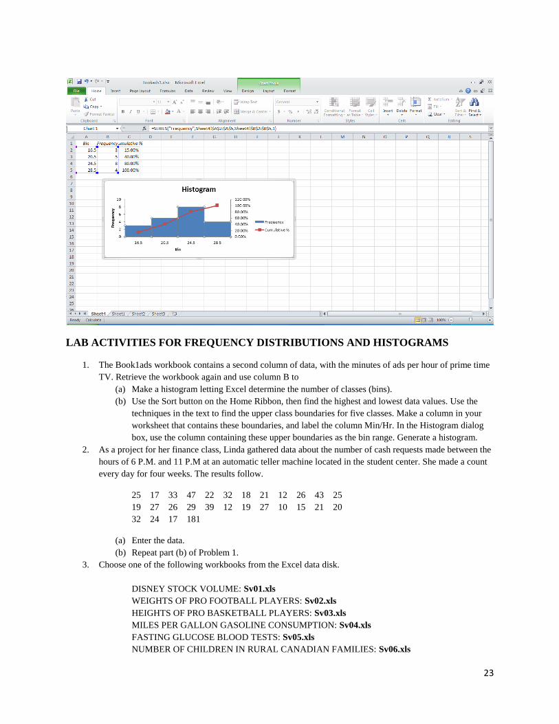
Adjusting the Histogram
Excel automatically supplies the “more” category (which will be empty if you specify upper class boundaries). To
remove the “more” category, select the cells in the row of the frequency table that contains “more”. Then, on the
main menu bar select Home>Delete. Right-click on the chart area and click Select Data. Then press Cancel. This
will update the chart to contain only data shown in the table.
To make the bars touch, right-click on one of the bars of the histogram. Then click Format Data Series. Set Gap
width to 0. Then press Close.
The results should be similar to this:
23
LAB ACTIVITIES FOR FREQUENCY DISTRIBUTIONS AND HISTOGRAMS
1. The Book1ads workbook contains a second column of data, with the minutes of ads per hour of prime time
TV. Retrieve the workbook again and use column B to
(a) Make a histogram letting Excel determine the number of classes (bins).
(b) Use the Sort button on the Home Ribbon, then find the highest and lowest data values. Use the
techniques in the text to find the upper class boundaries for five classes. Make a column in your
worksheet that contains these boundaries, and label the column Min/Hr. In the Histogram dialog
box, use the column containing these upper boundaries as the bin range. Generate a histogram.
2. As a project for her finance class, Linda gathered data about the number of cash requests made between the
hours of 6 P.M. and 11 P.M at an automatic teller machine located in the student center. She made a count
every day for four weeks. The results follow.
25 17 33 47 22 32 18 21 12 26 43 25
19 27 26 29 39 12 19 27 10 15 21 20
32 24 17 181
(a) Enter the data.
(b) Repeat part (b) of Problem 1.
3. Choose one of the following workbooks from the Excel data disk.
DISNEY STOCK VOLUME: Sv01.xls
WEIGHTS OF PRO FOOTBALL PLAYERS: Sv02.xls
HEIGHTS OF PRO BASKETBALL PLAYERS: Sv03.xls
MILES PER GALLON GASOLINE CONSUMPTION: Sv04.xls
FASTING GLUCOSE BLOOD TESTS: Sv05.xls
NUMBER OF CHILDREN IN RURAL CANADIAN FAMILIES: Sv06.xls
24
(a) Make a histogram letting Excel scale it.
(b) Make a histogram using five classes. Use the method of part (b) of Problem 1.
4. Histograms are not effective displays for some data. Consider the following data:
1 2 3 6 7 9 8 4 12 10
1 9 1 12 12 11 13 4 6 206
Enter the data and make a histogram letting Excel do the scaling. Now drop the high value, 206, from the
data set. Do you get more refined information from the histogram by eliminating the high and unusual data
value?
25
BAR GRAPHS, CIRCLE GRAPHS, AND TIME-SERIES GRAPHS (SECTION 2.2 OF
UNDERSTANDING BASIC STATISTICS)
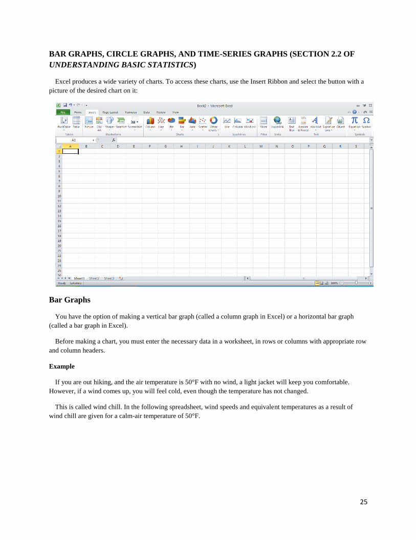
Excel produces a wide variety of charts. To access these charts, use the Insert Ribbon and select the button with a
picture of the desired chart on it:
Bar Graphs
You have the option of making a vertical bar graph (called a column graph in Excel) or a horizontal bar graph
(called a bar graph in Excel).
Before making a chart, you must enter the necessary data in a worksheet, in rows or columns with appropriate row
and column headers.
Example
If you are out hiking, and the air temperature is 50°F with no wind, a light jacket will keep you comfortable.
However, if a wind comes up, you will feel cold, even though the temperature has not changed.
This is called wind chill. In the following spreadsheet, wind speeds and equivalent temperatures as a result of
wind chill are given for a calm-air temperature of 50°F.
26
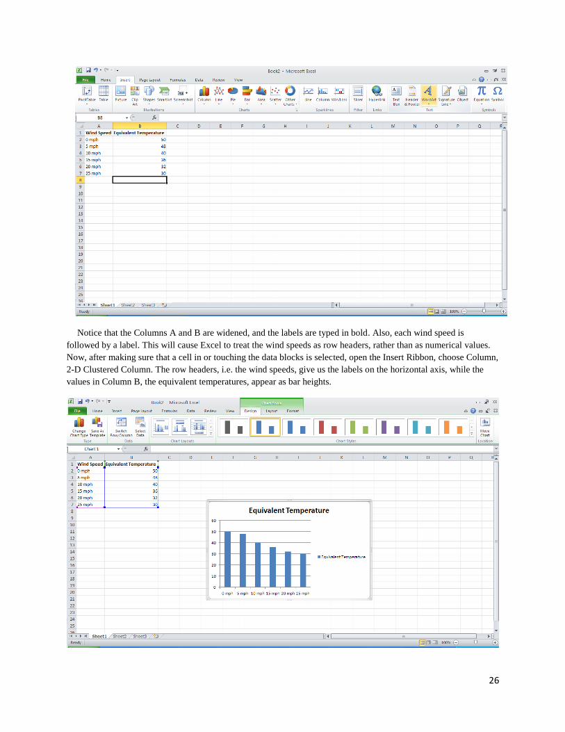
Notice that the Columns A and B are widened, and the labels are typed in bold. Also, each wind speed is
followed by a label. This will cause Excel to treat the wind speeds as row headers, rather than as numerical values.
Now, after making sure that a cell in or touching the data blocks is selected, open the Insert Ribbon, choose Column,
2-D Clustered Column. The row headers, i.e. the wind speeds, give us the labels on the horizontal axis, while the
values in Column B, the equivalent temperatures, appear as bar heights.
27
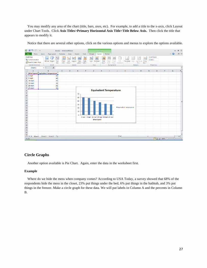
You may modify any area of the chart (title, bars, axes, etc). For example, to add a title to the x-axis, click Layout
under Chart Tools. Click Axis Titles>Primary Horizontal Axis Title>Title Below Axis. Then click the title that
appears to modify it.
Notice that there are several other options, click on the various options and menus to explore the options available.
Circle Graphs
Another option available is Pie Chart. Again, enter the data in the worksheet first.
Example
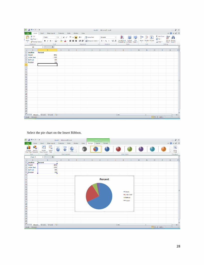
Where do we hide the mess when company comes? According to USA Today, a survey showed that 68% of the
respondents hide the mess in the closet, 23% put things under the bed, 6% put things in the bathtub, and 3% put
things in the freezer. Make a circle graph for these data. We will put labels in Column A and the percents in Column
B.
28
Select the pie chart on the Insert Ribbon.
29
Time-Series Graphs
You can make time charts by selecting Line Charts.
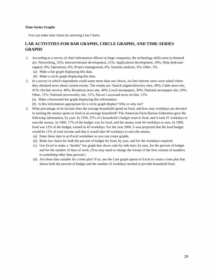
LAB ACTIVITIES FOR BAR GRAPHS, CIRCLE GRAPHS, AND TIME-SERIES
GRAPHS
1. According to a survey of chief information officers at large companies, the technology skills most in demand
are: Networking, 33%; Internet/intranet development, 21%; Applications development, 18%; Help desk/user
support, 8%; Operations, 6%; Project management, 6%, Systems analysis, 5%; Other, 3%.
(a) Make a bar graph displaying this data.
(b) Make a circle graph displaying this data.
2. In a survey in which respondents could name more than one choice, on-line Internet users were asked where
they obtained news about current events. The results are: Search engine/directory sites, 49%; Cable news site,
41%; On-line service; 40%; Broadcast news site, 40%; Local newspapers, 30%; National newspaper site; 24%;
Other, 13%; National newsweekly site, 12%; Haven’t accessed news on-line, 11%.
(a) Make a horizontal bar graph displaying this information.
(b) Is this information appropriate for a circle graph display? Why or why not?
3. What percentage of its income does the average household spend on food, and how may workdays are devoted
to earning the money spent on food in an average household? The American Farm Bureau Federation gave the
following information, by year: In 1930, 25% of a household’s budget went to food, and it took 91 workdays to
earn the money. In 1960, 17% of the budget was for food, and the money took 64 workdays to earn. In 1990,
food was 12% of the budget, earned in 43 workdays. For the year 2000, it was projected that the food budget
would be 11% of total income and that it would take 40 workdays to earn the money.
(a) Enter these data in an Excel worksheet so you can create graphs.
(b) Make bar charts for both the percent of budget for food, by year, and for the workdays required.
(c) Use Excel to make a “double” bar graph that shows side-by-side bars, by year, for the percent of budget
and for the number of days of work. (You may need to change the format of the first column of numbers
to something other than percent.)
(d) Are these data suitable for a time plot? If so, use the Line graph option in Excel to create a time plot that
shows both the percent of budget and the number of workdays needed to provide household food.
30
CHAPTER 3: AVERAGES AND VARIATION
CENTRAL TENDENCY AND VARIATION OF UNGROUPED DATA (SECTIONS 3.1 AND 3.2 OF
UNDERSTANDING BASIC STATISTICS)
Sections 3.1 and 3.2 of Understanding Basic Statistics describe some of the measures used to summarize the
character of a data set. Excel supports these descriptive measures.
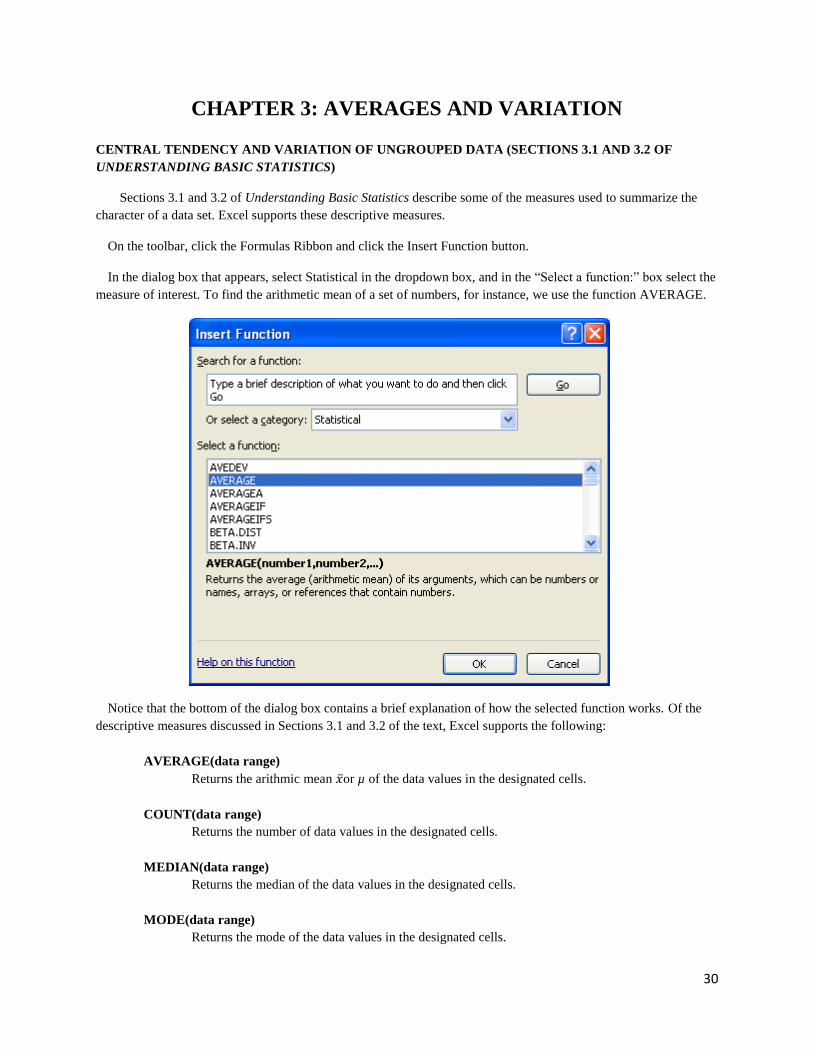
On the toolbar, click the Formulas Ribbon and click the Insert Function button.
In the dialog box that appears, select Statistical in the dropdown box, and in the “Select a function:” box select the
measure of interest. To find the arithmetic mean of a set of numbers, for instance, we use the function AVERAGE.
Notice that the bottom of the dialog box contains a brief explanation of how the selected function works. Of the
descriptive measures discussed in Sections 3.1 and 3.2 of the text, Excel supports the following:
AVERAGE(data range)
Returns the arithmic mean or µ of the data values in the designated cells.
COUNT(data range)
Returns the number of data values in the designated cells.
MEDIAN(data range)
Returns the median of the data values in the designated cells.
MODE(data range)
Returns the mode of the data values in the designated cells.
31
STDEV(data range)
Returns the sample standard deviation of the data values in the designated cells.
STDEVP(data range)
Returns the population standard deviation of the data values in the designated cells.
TRIMMEAN(data range, percent as a decimal)
Returns a trimmed mean based on the total percentage of data removed from both the bottom and
top of the ordered data values. If you want a 5% trimmed mean, implying that 5% of the bottom
data and 5% of the top data will be removed, then enter 0.10 for the percent in Excel.
Formatting the Worksheet to Display the Summary Statistics
It is a good idea to create a column in which you type the name of each descriptive measure you use, next to the
column where the corresponding computations are performed.
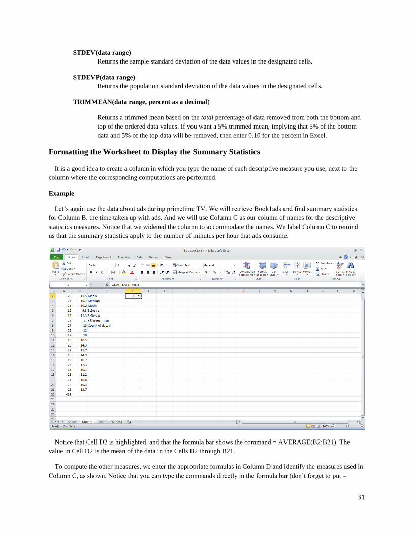
Example
Let’s again use the data about ads during primetime TV. We will retrieve Book1ads and find summary statistics
for Column B, the time taken up with ads. And we will use Column C as our column of names for the descriptive
statistics measures. Notice that we widened the column to accommodate the names. We label Column C to remind
us that the summary statistics apply to the number of minutes per hour that ads consume.
Notice that Cell D2 is highlighted, and that the formula bar shows the command = AVERAGE(B2:B21). The
value in Cell D2 is the mean of the data in the Cells B2 through B21.
To compute the other measures, we enter the appropriate formulas in Column D and identify the measures used in
Column C, as shown. Notice that you can type the commands directly in the formula bar (don’t forget to put =
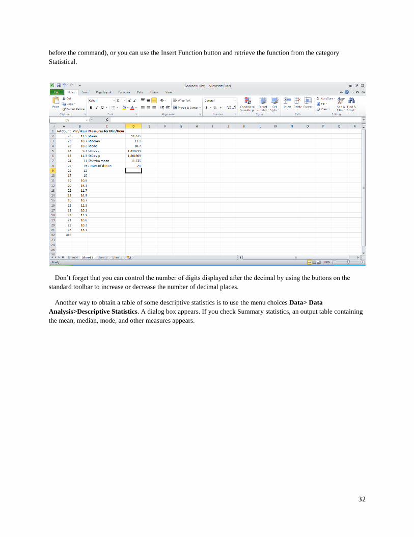
32
before the command), or you can use the Insert Function button and retrieve the function from the category
Statistical.
Don’t forget that you can control the number of digits displayed after the decimal by using the buttons on the
standard toolbar to increase or decrease the number of decimal places.
Another way to obtain a table of some descriptive statistics is to use the menu choices Data> Data
Analysis>Descriptive Statistics. A dialog box appears. If you check Summary statistics, an output table containing
the mean, median, mode, and other measures appears.
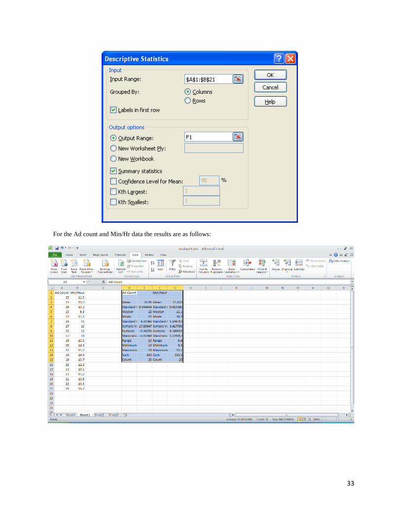
33
For the Ad count and Min/Hr data the results are as follows:
34
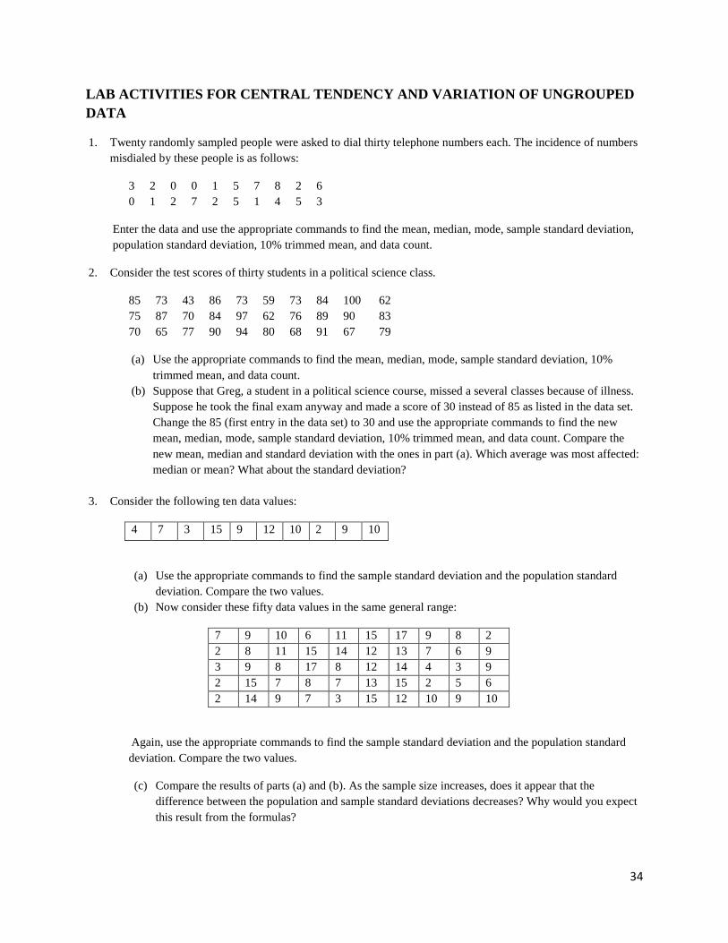
LAB ACTIVITIES FOR CENTRAL TENDENCY AND VARIATION OF UNGROUPED
DATA
1. Twenty randomly sampled people were asked to dial thirty telephone numbers each. The incidence of numbers
misdialed by these people is as follows:
3 2 0 0 1 5 7 8 2 6
0 1 2 7 2 5 1 4 5 3
Enter the data and use the appropriate commands to find the mean, median, mode, sample standard deviation,
population standard deviation, 10% trimmed mean, and data count.
2. Consider the test scores of thirty students in a political science class.
85 73 43 86 73 59 73 84 100 62
75 87 70 84 97 62 76 89 90 83
70 65 77 90 94 80 68 91 67 79
(a) Use the appropriate commands to find the mean, median, mode, sample standard deviation, 10%
trimmed mean, and data count.
(b) Suppose that Greg, a student in a political science course, missed a several classes because of illness.
Suppose he took the final exam anyway and made a score of 30 instead of 85 as listed in the data set.
Change the 85 (first entry in the data set) to 30 and use the appropriate commands to find the new
mean, median, mode, sample standard deviation, 10% trimmed mean, and data count. Compare the
new mean, median and standard deviation with the ones in part (a). Which average was most affected:
median or mean? What about the standard deviation?
3. Consider the following ten data values:
4 7 3 15 9 12 10 2 9 10
(a) Use the appropriate commands to find the sample standard deviation and the population standard
deviation. Compare the two values.
(b) Now consider these fifty data values in the same general range:
7 9 10 6 11 15 17 9 8 2
2 8 11 15 14 12 13 7 6 9
3 9 8 17 8 12 14 4 3 9
2 15 7 8 7 13 15 2 5 6
2 14 9 7 3 15 12 10 9 10
Again, use the appropriate commands to find the sample standard deviation and the population standard
deviation. Compare the two values.
(c) Compare the results of parts (a) and (b). As the sample size increases, does it appear that the
difference between the population and sample standard deviations decreases? Why would you expect
this result from the formulas?
35
4. In this problem we will explode the effects of changing data values by multiplying each data value by a constant,
or by adding the same constant to each data value.
(a) Clear your workbook or begin a new one. Then enter the following data into Column A, with the
column label “Original” in Cell A1.
1 8 3 5 7 2 10 9 4 6 3
(b) Now label Column B as A * 10. Select Cell B2. In the formula bar, type =A2*10 and press Enter.
Select Cell B2 again and move the cursor to the lower right corner of Cell B2. A small black + should
appear. Click-drag the + down the column so that Column B contains all the data of Column A, but
with each value in Column A multiplied by 10.
(c) Now suppose we add 30 to each data value in Column A and put the new data in Column C. First
label Column E as A + 30. Then select Cell C2. In the formula bar type =A2+30 and press Enter.
Then select Cell C2 again and position the cursor in the lower right corner. The cursor should change
shape to a small black +. Click-drag down Column C to generate all the entries of Column A
increased by 30.
(d) Predict how you think the mean and the standard deviation of Columns B and C will be similar to or
different from those values for column A. Use the >Data>Data Analysis>Descriptive Statistics
dialog box to find the mean and standard deviation for all three columns. Note: use all three columns
as input columns in the dialogue box. Compare the actual results to your predictions. What do you
predict will happen to these descriptive statistics values if you multiply each data value of Column A
by 50? If you add 50 to each data value in Column A?
BOX-AND-WHISKER PLOTS (SECTION 3.3 OF UNDERSTANDING BASIC
STATISTICS)
Excel does not have any commands or dialog boxes that produce box-and-whisker plots directly. Macros can be
written to accomplish the task. However, Excel does have commands to produce the five-number summary, and you
can then draw a box-and-whisker plot by hand.
The commands for the five-number summary can be found in the dialogue box obtained by pressing the Insert
Function (or function wizard) key on the tool bar.
MIN(data range) returns the minimum data value from the designated cells.
QUARTILE(data range, 1) returns the first quartile for the data in the designated cells.
MEDIAN(data range) returns the median of the data in the designated cells.
QUARTILE(data range, 3) returns the third quartile for the data in the designated cells.
MAX(data range) returns the maximum data value from the designated cells.
Example
Generate the five-number summary for the number of minutes of ads per hour on commercial TV, using the data
in Book1ads.
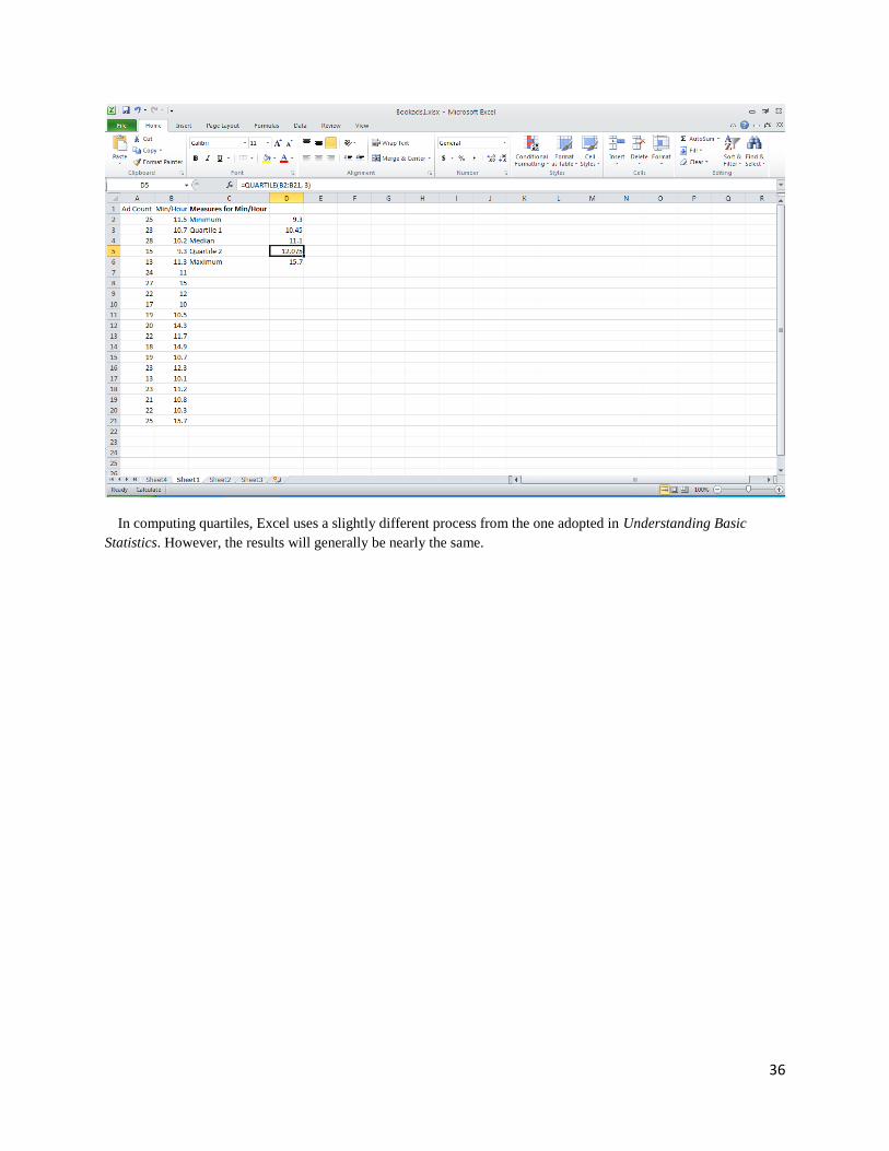
36
In computing quartiles, Excel uses a slightly different process from the one adopted in Understanding Basic
Statistics. However, the results will generally be nearly the same.
37
CHAPTER 4: REGRESSION AND CORRELATION
LINEAR REGRESSION - TWO VARIABLES (SECTIONS 4.1 and 4.2 OF
UNDERSTANDING BASIC STATISTICS)
Chapter 4 of Understanding Basic Statistics introduces linear regression. The formula for the correlation
coefficient r is given in Section 4.1. Formulas to find the equation of the least squares line, y = a + bx, are given in
Section 4.2. This section also contains the formula for the coefficient of determination, r2.
Excel supports several functions related to linear regression. To use these, first enter the paired data values in two
columns. Put the explanatory variable in a column labeled with x, or an appropriate descriptive name, and put the
response variable in a column labeled with y, or an appropriate descriptive name.
The functions and corresponding syntax are
LINEST(y range, x range)
which returns the slope b and y-intercept a of the least-squares line, in that order. Although this command can be
found under the Insert Function button menu, it is best to type it in because it is an array formula. (The full LINEST
function involves two more, optional parameters, but we will ignore these.) To use LINEST,
1. Activate two cells, the first to hold the slope b, the second for the intercept a.
2. In the formula bar, type =LINEST(y range,x range) with the appropriate cell ranges in place of x range and
y range.
3. Instead of pressing Enter, press Ctrl+Shift+Enter. This key combination activates the array formula
features so that you get the outputs for both b and a. Otherwise, you will get only the slope b of the least
squares line.
The other functions are employed in the usual way, by activating a cell and then either typing the command
directly in the formula bar, followed by Enter, or by using the Insert Function dialog box.
SLOPE(y range, x range) returns the slope b of the least-squares line.
INTERCEPT(y range, x range) returns the intercept a of the least-squares line.
CORREL(y range, x range) returns the correlation coefficient r.
FORECAST(x value, y range, x range) returns the predicted y value for the specified x value, using
extrapolation from the given pairs of x and y values. Note that you need to use a new FORECAST command
for each different x value.
We will now use Excel to generate a scatter diagram and then add the results of the least squares regression.
Example
In retailing, merchandise loss due to shoplifting, damage, and other causes is called shrinkage. The managers at
H.R. Merchandise think that there is a relationship between shrinkage and the number of clerks on duty. To explore
this relationship, a random sample of seven weeks was selected. During each week, the staffing level of sales clerks
was held constant and the dollar value (in hundreds of dollars) of the shrinkage was recorded.
X 10 12 11 15 9 13 8 Staffing level
Y 19 15 20 9 25 12 31 (in hundreds)
38
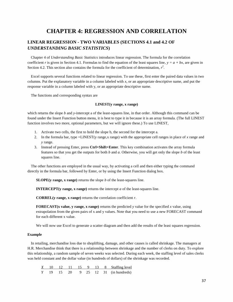
Open a worksheet. Place the X values in Column A with a corresponding label and the Y values in Column B.
Create a Scatter Diagram
Click on the Insert Ribbon and select Scatter. Select the data. Choose the first subtype, which shows only points.
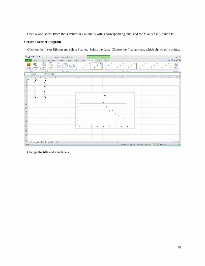
Change the title and axis labels.
39
Add least-squares results to the plot
The least-squares line can be added to the plot, along with its equation and the value of r2. Right-click on one of
the data points shown in the scatter diagram. A drop-down menu will appear. Select Add Trendline to call up a
dialog box.
40
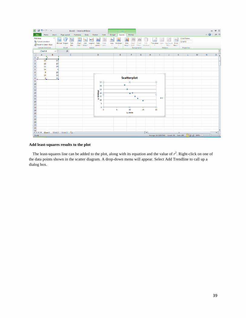
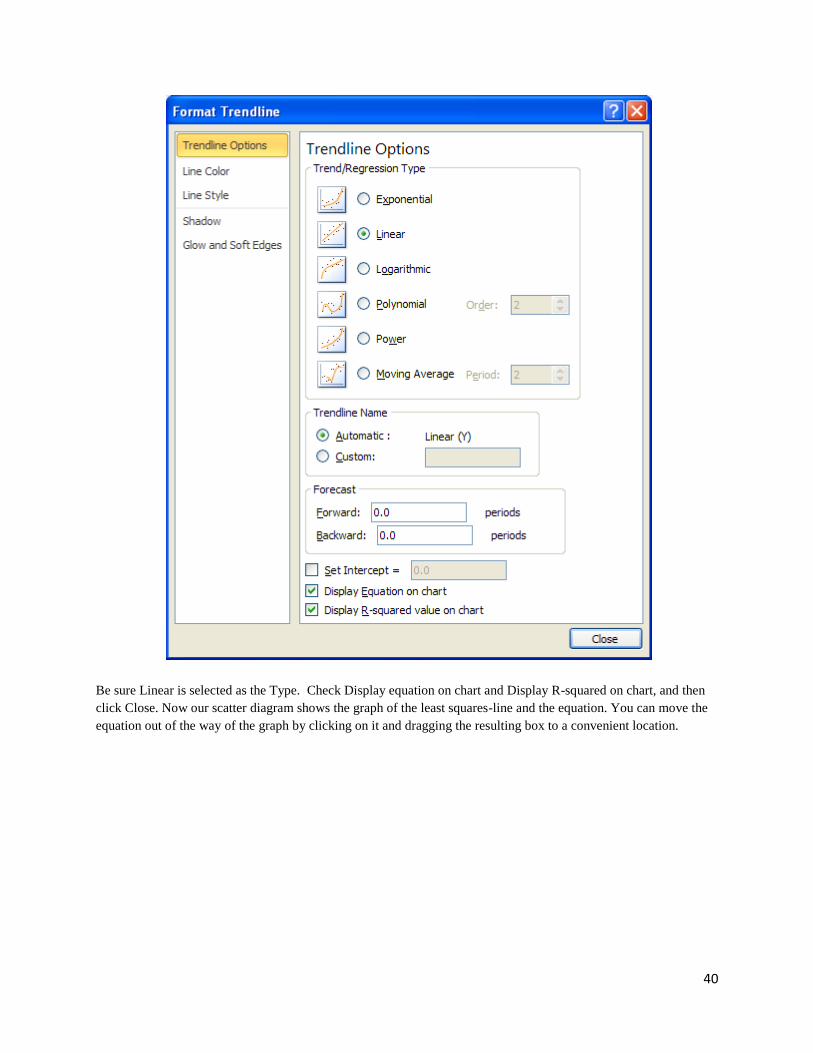
Be sure Linear is selected as the Type. Check Display equation on chart and Display R-squared on chart, and then
click Close. Now our scatter diagram shows the graph of the least squares-line and the equation. You can move the
equation out of the way of the graph by clicking on it and dragging the resulting box to a convenient location.
41
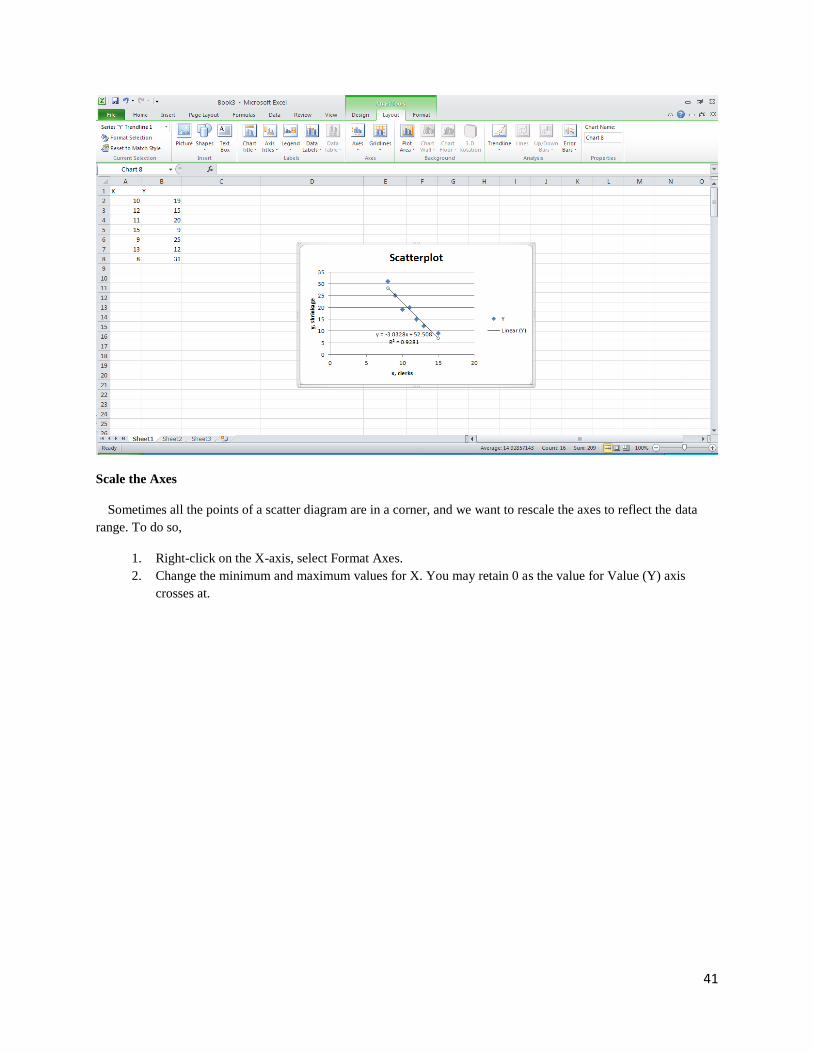
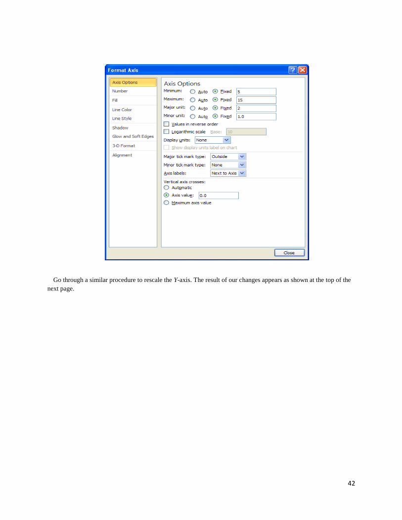
Scale the Axes
Sometimes all the points of a scatter diagram are in a corner, and we want to rescale the axes to reflect the data
range. To do so,
1. Right-click on the X-axis, select Format Axes.
2. Change the minimum and maximum values for X. You may retain 0 as the value for Value (Y) axis
crosses at.
42
Go through a similar procedure to rescale the Y-axis. The result of our changes appears as shown at the top of the
next page.
43
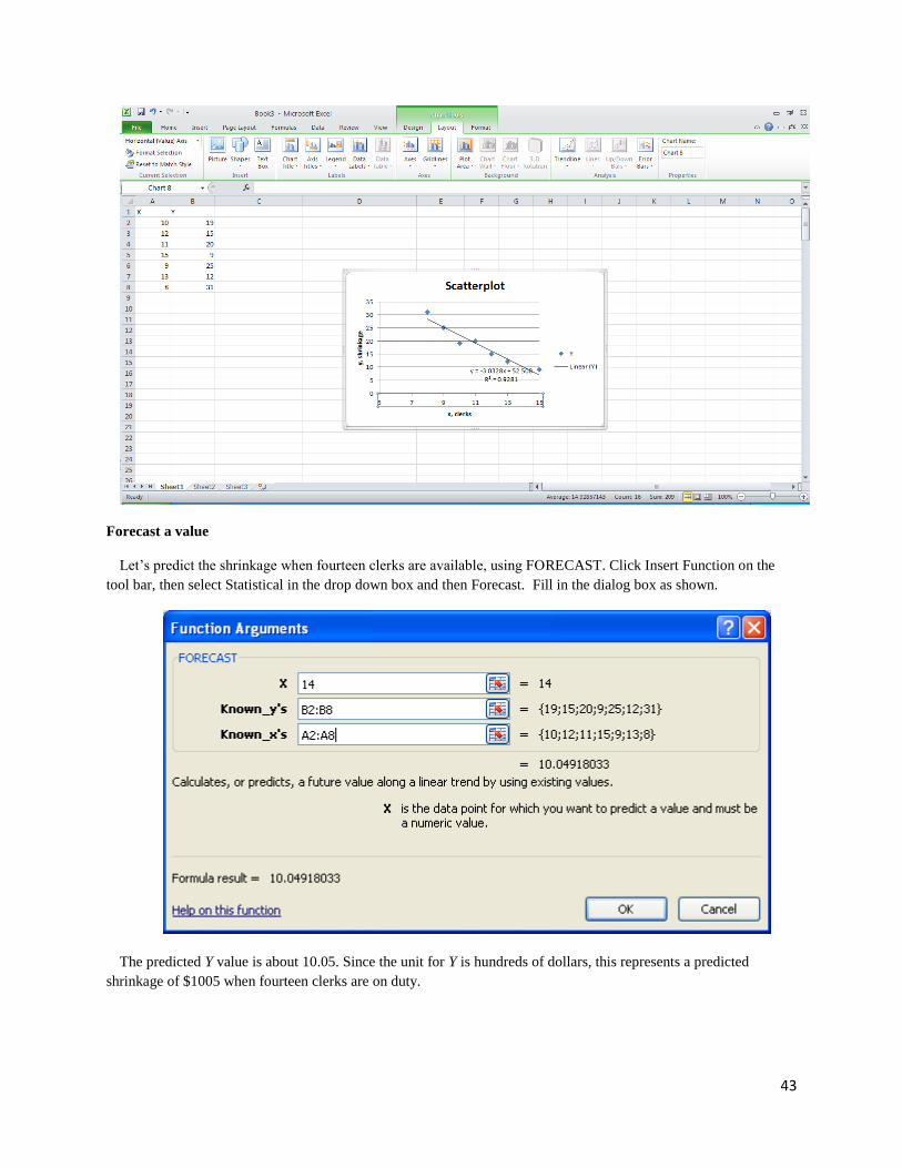
Forecast a value
Let’s predict the shrinkage when fourteen clerks are available, using FORECAST. Click Insert Function on the
tool bar, then select Statistical in the drop down box and then Forecast. Fill in the dialog box as shown.
The predicted Y value is about 10.05. Since the unit for Y is hundreds of dollars, this represents a predicted
shrinkage of $1005 when fourteen clerks are on duty.
44
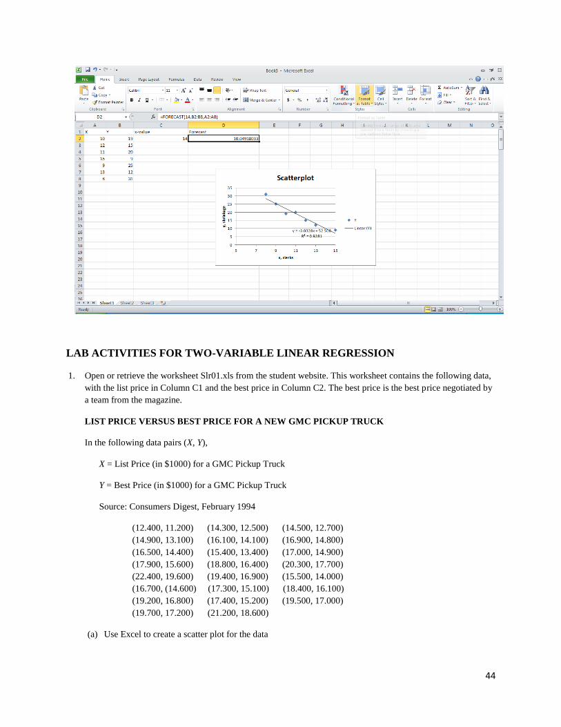
LAB ACTIVITIES FOR TWO-VARIABLE LINEAR REGRESSION
1. Open or retrieve the worksheet Slr01.xls from the student website. This worksheet contains the following data,
with the list price in Column C1 and the best price in Column C2. The best price is the best price negotiated by
a team from the magazine.
LIST PRICE VERSUS BEST PRICE FOR A NEW GMC PICKUP TRUCK
In the following data pairs (X, Y),
X = List Price (in $1000) for a GMC Pickup Truck
Y = Best Price (in $1000) for a GMC Pickup Truck
Source: Consumers Digest, February 1994
(12.400, 11.200) (14.300, 12.500) (14.500, 12.700)
(14.900, 13.100) (16.100, 14.100) (16.900, 14.800)
(16.500, 14.400) (15.400, 13.400) (17.000, 14.900)
(17.900, 15.600) (18.800, 16.400) (20.300, 17.700)
(22.400, 19.600) (19.400, 16.900) (15.500, 14.000)
(16.700, (14.600) (17.300, 15.100) (18.400, 16.100)
(19.200, 16.800) (17.400, 15.200) (19.500, 17.000)
(19.700, 17.200) (21.200, 18.600)
(a) Use Excel to create a scatter plot for the data
45
(b) Right-click on a data point and use the Add Trendline option to show the least-squares line on the scatter
diagram, along with its equation and the value of r2.
(c) Use the least-squares model to predict the best price for a truck with a list price of $20,000. Note: Enter
this value as 20, since X is assumed to be in thousands of dollars. (Use FORECAST.)
2. Other Excel worksheets appropriate to use for simple linear regression are:
Cricket Chirps Versus Temperature: Slr02.xls
Source: The Song of Insects by Dr. G.W. Pierce, Harvard Press
The chirps per second for the striped grouped cricket are stored in C1; the corresponding temperature in
degrees Fahrenheit is stored in C2.
Diameter of Sand Granules Versus Slope on a Natural Occurring Ocean Beach: Slr03.xls
Source Physical Geography by A.M. King, Oxford press
The median diameter (MM) of granules of sand is stored in C1; the corresponding gradient of
beach slope in degrees is stored in C2.
National Unemployment Rate Male Versus Female: Slr04.xls
Source: Statistical Abstract of the United States
The national unemployment rate for adult males is stored in C1; the corresponding unemployment rate for
adult females for the same period of time is stored in C2.
Select these worksheets and repeat Parts (a)-(c) of Problem 1, using Column A as the explanatory variable and
Column B as the response variable.
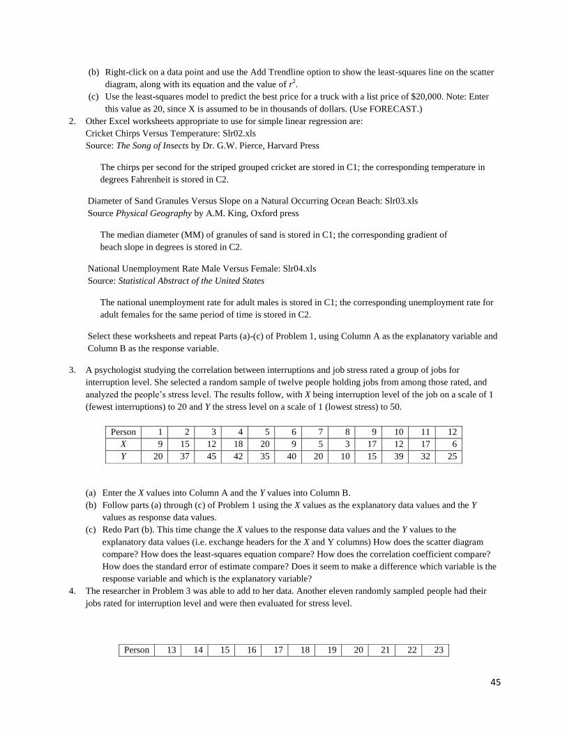
3. A psychologist studying the correlation between interruptions and job stress rated a group of jobs for
interruption level. She selected a random sample of twelve people holding jobs from among those rated, and
analyzed the people’s stress level. The results follow, with X being interruption level of the job on a scale of 1
(fewest interruptions) to 20 and Y the stress level on a scale of 1 (lowest stress) to 50.
(a) Enter the X values into Column A and the Y values into Column B.
(b) Follow parts (a) through (c) of Problem 1 using the X values as the explanatory data values and the Y
values as response data values.
(c) Redo Part (b). This time change the X values to the response data values and the Y values to the
explanatory data values (i.e. exchange headers for the X and Y columns) How does the scatter diagram
compare? How does the least-squares equation compare? How does the correlation coefficient compare?
How does the standard error of estimate compare? Does it seem to make a difference which variable is the
response variable and which is the explanatory variable?
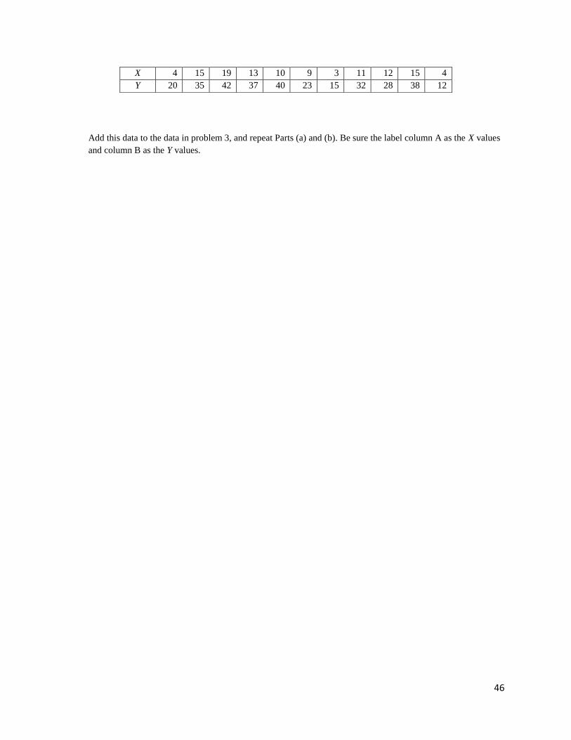
4. The researcher in Problem 3 was able to add to her data. Another eleven randomly sampled people had their
jobs rated for interruption level and were then evaluated for stress level.
Person 1 2 3 4 5 6 7 8 9 10 11 12
X 9 15 12 18 20 9 5 3 17 12 17 6
Y 20 37 45 42 35 40 20 10 15 39 32 25
Person 13 14 15 16 17 18 19 20 21 22 23
46
Add this data to the data in problem 3, and repeat Parts (a) and (b). Be sure the label column A as the X values
and column B as the Y values.
X 4 15 19 13 10 9 3 11 12 15 4
Y 20 35 42 37 40 23 15 32 28 38 12
47
CHAPTER 5: ELEMENTARY PROBABILITY THEORY
SIMULATIONS
Excel has several random number generators. Recall from Chapter 1 that RANDBETWEEN(Bottom,Top) puts
out a random integer between (and including) the bottom and top numbers. Again, the Analysis ToolPak needs to be
included as an Add-In to make RANDBETWEEN available. To find the RANDBETWEEN function, click the
Insert Function or Function Wizard button on the tool bar. Then select All in the category drop down box and scroll
down in until you find RANDBETWEEN. You can also type the command directly in the formula bar, but again,
remember to type = first.
We can use the random number generator to simulate experiments such as tossing coins or rolling dice.
Example
Simulate the experiment of tossing a fair coin 200 times. Look at the percent of heads and the percent of tails.
How do these compare with the expected 50% for each?
Assign the outcome heads to digit 1 and tails to digit 2. We will draw a random sample of size 200 from the
distributions of integers from a minimum of 1 to a maximum of 2. When using a random number generator, you are
best off setting recalculation to manual. To do this, go to File>Options and then click on the tab labeled Formulas.
Select Manual calculation, then press OK.
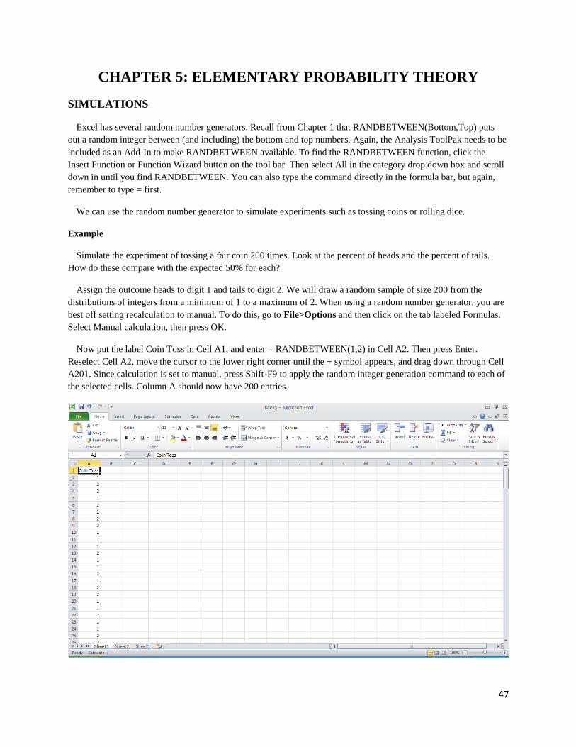
Now put the label Coin Toss in Cell A1, and enter = RANDBETWEEN(1,2) in Cell A2. Then press Enter.
Reselect Cell A2, move the cursor to the lower right corner until the + symbol appears, and drag down through Cell
A201. Since calculation is set to manual, press Shift-F9 to apply the random integer generation command to each of
the selected cells. Column A should now have 200 entries.
48
Count the number of heads and the number of tails
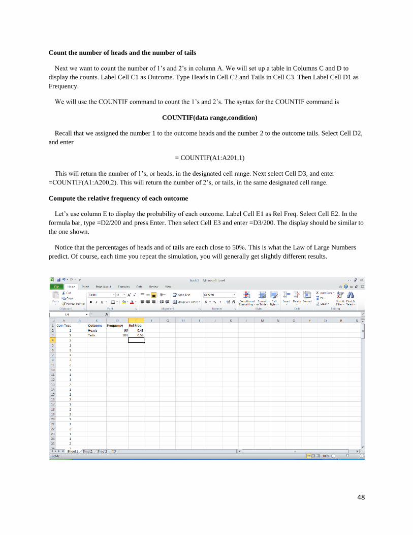
Next we want to count the number of 1’s and 2’s in column A. We will set up a table in Columns C and D to
display the counts. Label Cell C1 as Outcome. Type Heads in Cell C2 and Tails in Cell C3. Then Label Cell D1 as
Frequency.
We will use the COUNTIF command to count the 1’s and 2’s. The syntax for the COUNTIF command is
COUNTIF(data range,condition)
Recall that we assigned the number 1 to the outcome heads and the number 2 to the outcome tails. Select Cell D2,
and enter
= COUNTIF(A1:A201,1)
This will return the number of 1’s, or heads, in the designated cell range. Next select Cell D3, and enter
=COUNTIF(A1:A200,2). This will return the number of 2’s, or tails, in the same designated cell range.
Compute the relative frequency of each outcome
Let’s use column E to display the probability of each outcome. Label Cell E1 as Rel Freq. Select Cell E2. In the
formula bar, type =D2/200 and press Enter. Then select Cell E3 and enter =D3/200. The display should be similar to
the one shown.
Notice that the percentages of heads and of tails are each close to 50%. This is what the Law of Large Numbers
predict. Of course, each time you repeat the simulation, you will generally get slightly different results.
49
LAB ACTIVITIES FOR SIMULATIONS
1. Use the RANDBETWEEN command to simulate 50 tosses of a fair coin. Make a table showing the frequency
of the outcomes and the relative frequency. Compare the results with the theoretical expected percents (50%
heads, 50% tails). Repeat the process for 500 trials. Are these outcomes closer to the results predicted by
theory?
2. Use RANDBETWEEN to simulate 50 rolls of a fair die. Use the number 1 for the bottom value and 6 for the
top. Make a table showing the frequency of each outcome and the relative frequency. Compare the results
with the theoretical expected percents (16.7% for each outcome). Repeat the process for 500 tosses.Are these
outcomes closer to the results predicted by theory?
50
CHAPTER 6: THE BINOMIAL PROBABILITY
DISTRIBUTIONAND RELATED TOPICS
THE BINOMIAL PROBABILITY DISTRIBUTION (SECTIONS 6.2 AND 6.3 OF
UNDERSTANDING BASIC STATISTICS)
The binomial probability distribution is discussed in Chapter 6 of Understanding Basic Statistics. It is a discrete
probability distribution controlled by the number of trials, n, and the probability of success on a single trial, p.
The Excel function that generates binomial probabilities is
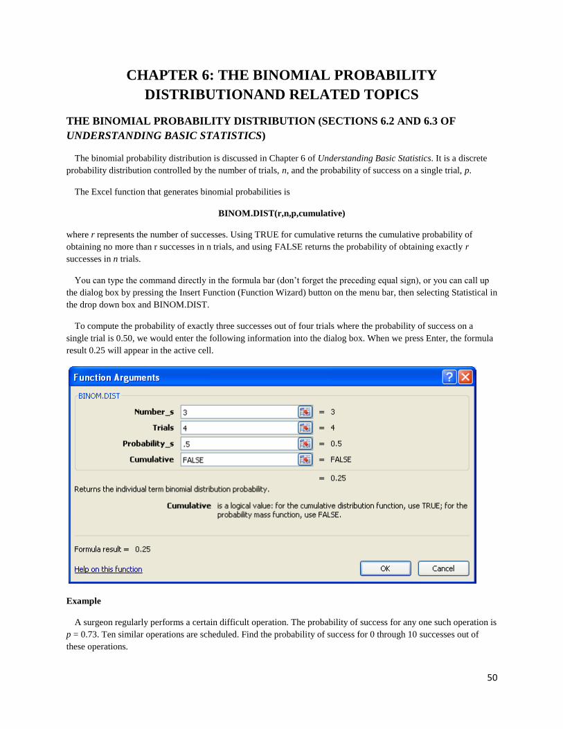
BINOM.DIST(r,n,p,cumulative)
where r represents the number of successes. Using TRUE for cumulative returns the cumulative probability of
obtaining no more than r successes in n trials, and using FALSE returns the probability of obtaining exactly r
successes in n trials.
You can type the command directly in the formula bar (don’t forget the preceding equal sign), or you can call up
the dialog box by pressing the Insert Function (Function Wizard) button on the menu bar, then selecting Statistical in
the drop down box and BINOM.DIST.
To compute the probability of exactly three successes out of four trials where the probability of success on a
single trial is 0.50, we would enter the following information into the dialog box. When we press Enter, the formula
result 0.25 will appear in the active cell.
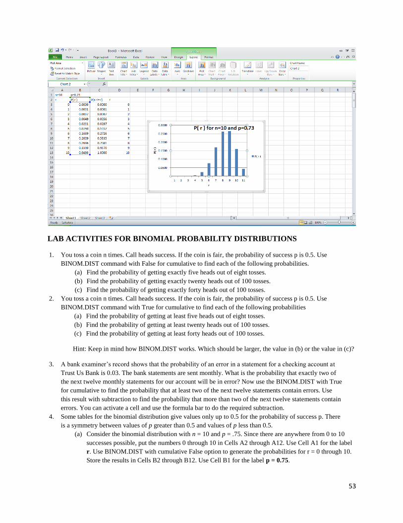
Example
A surgeon regularly performs a certain difficult operation. The probability of success for any one such operation is
p = 0.73. Ten similar operations are scheduled. Find the probability of success for 0 through 10 successes out of
these operations.
51
First let’s put information regarding the number of trials and probability of success on a single trial into the
worksheet. We type n = 10 in Cell A1 and p = 0.73 in Cell B1.
Next, we will put the possible values for the number of successes, r, in Cells A3 through A13 with the label r in
Cell A2. We can also duplicate A2 through A13 in D2 through D13 for easier reading of the finished table. Now
place the label P(r) in Cell B2 and the label P(X ≤ r) in Cell C2. We will have Excel generate theprobabilities of the
individual number of successes r in Cells B3 through B13 and the corresponding cumulative probabilities in Cells
C3 through C13.
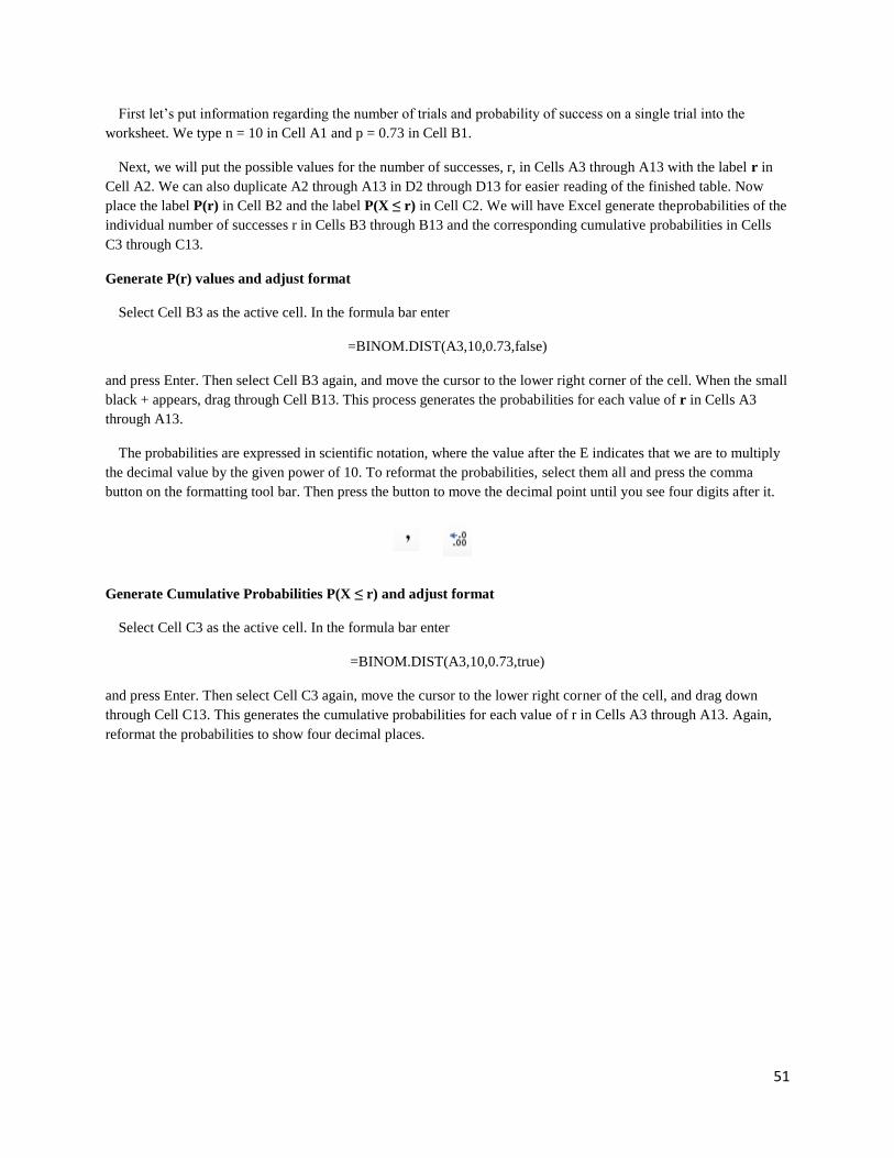
Generate P(r) values and adjust format
Select Cell B3 as the active cell. In the formula bar enter
=BINOM.DIST(A3,10,0.73,false)
and press Enter. Then select Cell B3 again, and move the cursor to the lower right corner of the cell. When the small
black + appears, drag through Cell B13. This process generates the probabilities for each value of r in Cells A3
through A13.
The probabilities are expressed in scientific notation, where the value after the E indicates that we are to multiply
the decimal value by the given power of 10. To reformat the probabilities, select them all and press the comma
button on the formatting tool bar. Then press the button to move the decimal point until you see four digits after it.
Generate Cumulative Probabilities P(X ≤ r) and adjust format
Select Cell C3 as the active cell. In the formula bar enter
=BINOM.DIST(A3,10,0.73,true)
and press Enter. Then select Cell C3 again, move the cursor to the lower right corner of the cell, and drag down
through Cell C13. This generates the cumulative probabilities for each value of r in Cells A3 through A13. Again,
reformat the probabilities to show four decimal places.
52
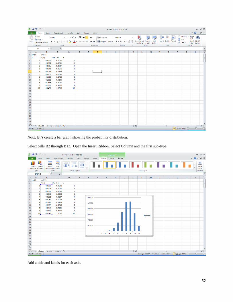
Next, let’s create a bar graph showing the probability distribution.
Select cells B2 through B13. Open the Insert Ribbon. Select Column and the first sub-type.
Add a title and labels for each axis.
53
LAB ACTIVITIES FOR BINOMIAL PROBABILITY DISTRIBUTIONS
1. You toss a coin n times. Call heads success. If the coin is fair, the probability of success p is 0.5. Use
BINOM.DIST command with False for cumulative to find each of the following probabilities.
(a) Find the probability of getting exactly five heads out of eight tosses.
(b) Find the probability of getting exactly twenty heads out of 100 tosses.
(c) Find the probability of getting exactly forty heads out of 100 tosses.
2. You toss a coin n times. Call heads success. If the coin is fair, the probability of success p is 0.5. Use
BINOM.DIST command with True for cumulative to find each of the following probabilities
(a) Find the probability of getting at least five heads out of eight tosses.
(b) Find the probability of getting at least twenty heads out of 100 tosses.
(c) Find the probability of getting at least forty heads out of 100 tosses.
Hint: Keep in mind how BINOM.DIST works. Which should be larger, the value in (b) or the value in (c)?
3. A bank examiner’s record shows that the probability of an error in a statement for a checking account at
Trust Us Bank is 0.03. The bank statements are sent monthly. What is the probability that exactly two of
the next twelve monthly statements for our account will be in error? Now use the BINOM.DIST with True
for cumulative to find the probability that at least two of the next twelve statements contain errors. Use
this result with subtraction to find the probability that more than two of the next twelve statements contain
errors. You can activate a cell and use the formula bar to do the required subtraction.
4. Some tables for the binomial distribution give values only up to 0.5 for the probability of success p. There
is a symmetry between values of p greater than 0.5 and values of p less than 0.5.
(a) Consider the binomial distribution with n = 10 and p = .75. Since there are anywhere from 0 to 10
successes possible, put the numbers 0 through 10 in Cells A2 through A12. Use Cell A1 for the label
r. Use BINOM.DIST with cumulative False option to generate the probabilities for r = 0 through 10.
Store the results in Cells B2 through B12. Use Cell B1 for the label p = 0.75.
54
(b) Now consider the binomial distribution with n = 10 and p = .25. Use BINOM.DIST with cumulative
False option to generate the probabilities for r = 0 through 10. Store the results in Cells C2 through
C12. Use Cell C1 for the label p = 0.25.
(c) Now compare the entries in Columns B and C. How does P(r = 4 successes with p = .75) compare to
P(r = 6 successes with p = .25)?
5.
(a) Consider a binomial distribution with fifteen trials and probability of success on a single trial p =
0.25. Create a worksheet showing values of r and corresponding binomial probabilities. Generate a
bar graph of the distribution.
(b) Consider a binomial distribution with fifteen trials and probability of success on a single trial p =
0.75. Create a worksheet showing values of r and the corresponding binomial probabilities. Generate
a bar graph.
(c) Compare the graphs of parts (a) and (b). How are they skewed? Is one symmetric with the other?
55
CHAPTER 7: NORMAL CURVES AND SAMPLING
DISTRIBUTIONS
GRAPHS OF NORMAL PROBABILITY DISTRIBUTIONS (SECTION 7.1 OF
UNDERSTANDING BASIC STATISTICS)
A normal distribution is a continuous probability distribution governed by the parameters µ (the mean) and σ (the
standard deviation), as discussed in Section 7.1 of Understanding Basic Statistics. The Excel command that
generates values for a normal distribution is
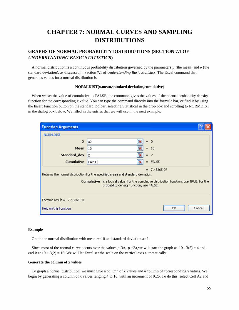
NORM.DIST(x,mean,standard deviation,cumulative)
When we set the value of cumulative to FALSE, the command gives the values of the normal probability density
function for the corresponding x value. You can type the command directly into the formula bar, or find it by using
the Insert Function button on the standard toolbar, selecting Statistical in the drop box and scrolling to NORMDIST
in the dialog box below. We filled in the entries that we will use in the next example.
Example
Graph the normal distribution with mean µ=10 and standard deviation σ=2.
Since most of the normal curve occurs over the values µ-3σ, µ +3σ,we will start the graph at 10 - 3(2) = 4 and
end it at 10 + 3(2) = 16. We will let Excel set the scale on the vertical axis automatically.
Generate the column of x values
To graph a normal distribution, we must have a column of x values and a column of corresponding y values. We
begin by generating a column of x values ranging 4 to 16, with an increment of 0.25. To do this, select Cell A2 and
56
enter the number 4. Select Cell A2 again and use the >Home>Fill>Series to open the dialog box shown next. Set
the options in the dialog box as shown and then press OK.
You will see that Column A now contains the numbers 4, 4.25, 4.50, … all the way up to 16.
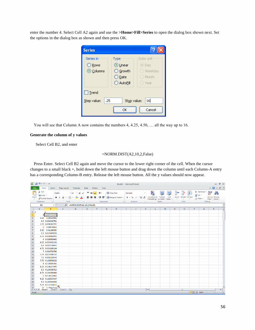
Generate the column of y values
Select Cell B2, and enter
=NORM.DIST(A2,10,2,False)
Press Enter. Select Cell B2 again and move the cursor to the lower right corner of the cell. When the cursor
changes to a small black +, hold down the left mouse button and drag down the column until each Column-A entry
has a corresponding Column-B entry. Release the left mouse button. All the y values should now appear.
57
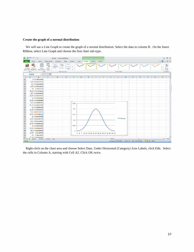
Create the graph of a normal distribution
We will use a Line Graph to create the graph of a normal distribution. Select the data in column B. On the Insert
Ribbon, select Line Graph and choose the first chart sub-type.
Right-click on the chart area and choose Select Data. Under Horizontal (Category) Axis Labels, click Edit. Select
the cells in Column A, starting with Cell A2. Click OK twice.
58
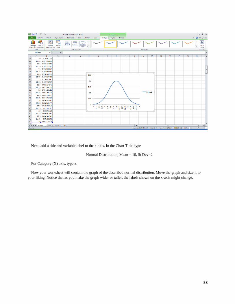
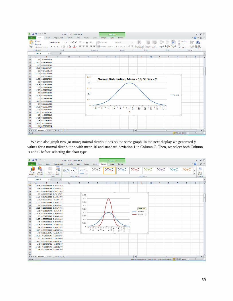
Next, add a title and variable label to the x-axis. In the Chart Title, type
Normal Distribution, Mean = 10, St Dev=2
For Category (X) axis, type x.
Now your worksheet will contain the graph of the described normal distribution. Move the graph and size it to
your liking. Notice that as you make the graph wider or taller, the labels shown on the x-axis might change.
59
We can also graph two (or more) normal distributions on the same graph. In the next display we generated y
values for a normal distribution with mean 10 and standard deviation 1 in Column C. Then, we select both Column
B and C before selecting the chart type.
60
STANDARD SCORES AND NORMAL PROBABILITIES
Excel has several built-in functions relating to normal distributions.
STANDARDIZE(x,mean,standard deviation) returns the z score for the given x value from a distribution with
the specified mean and standard deviation.
NORM.DIST(x1,mean,standard deviation,cumulative); when cumulative is TRUE, this returns probability that
a random value x selected from this distribution is ≤ x1, i.e. it returns P(x ≤ x1). This is the same as the area to the left
of the specified x1 value under the described normal distribution. When cumulative is FALSE, it returns the height
of the normal probability density function evaluated atx1. We used this function to graph a normal distribution.
NORM.INV(probability,mean,standard deviation) returns the inverse of the normal cumulative distribution. In
other words, when a probability is entered, the command returns the value from the normal distribution with
specified mean and standard deviation so that the area to the left of that value is equal to the designated probability.
NORM.S.DIST(z1) returns the probability that a randomly selected z score is less or equal the specified value of
z1, i.e. it returns P(z ≤ z1). This is the same as the area to the left of the specified z1 value under the standard normal
distribution. This command is equivalent to NORM.DIST(x1,0,1,true).
NORM.S.INV(probability) returns the value such that the area to its left under the standard normal distribution
is equal to the specified probability. This command is equivalent to NORM.INV(probability,0,1).
Each of these commands can be typed directly into the formula bar for an active cell or accessed by using the
Insert Function button.
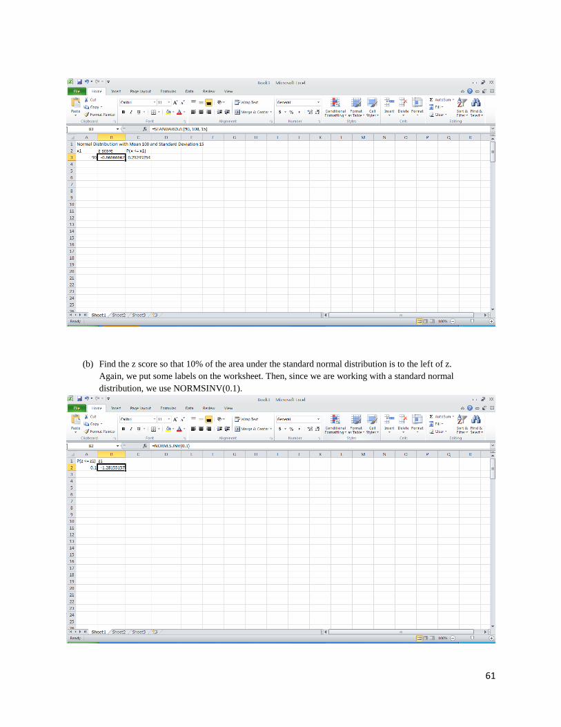
Examples
(a) Consider a normal distribution with mean 100 and standard deviation 15. Find the z score corresponding to
x = 90 and find the area to the left of 90 under the distribution.
First we place some headers and labels on the worksheet. Then,
1. in Cell B3, enter =STANDARDIZE(90,100,15)
2. in Cell C3, enter =NORMDIST(90,100,15,true)
61
(b) Find the z score so that 10% of the area under the standard normal distribution is to the left of z.
Again, we put some labels on the worksheet. Then, since we are working with a standard normal
distribution, we use NORMSINV(0.1).
62
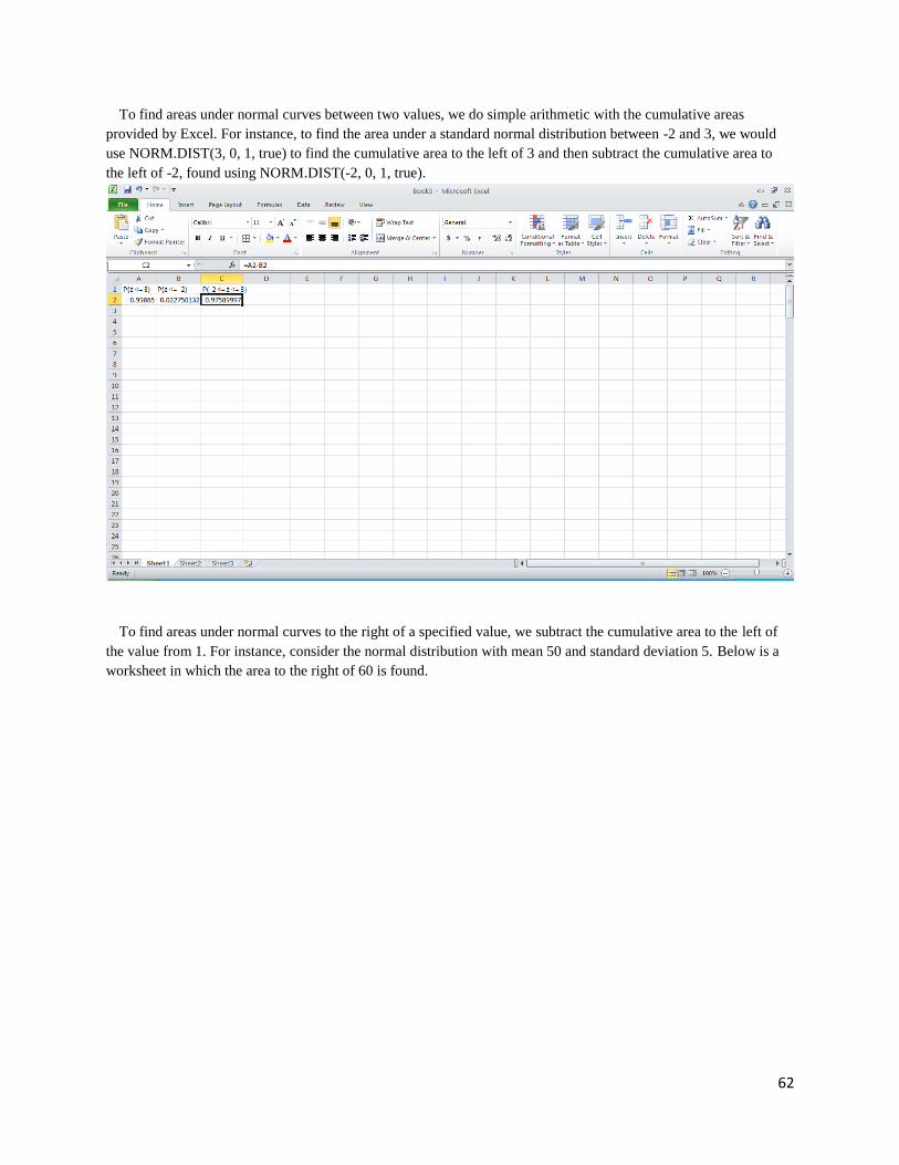
To find areas under normal curves between two values, we do simple arithmetic with the cumulative areas
provided by Excel. For instance, to find the area under a standard normal distribution between -2 and 3, we would
use NORM.DIST(3, 0, 1, true) to find the cumulative area to the left of 3 and then subtract the cumulative area to
the left of -2, found using NORM.DIST(-2, 0, 1, true).
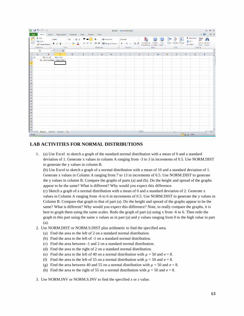
To find areas under normal curves to the right of a specified value, we subtract the cumulative area to the left of
the value from 1. For instance, consider the normal distribution with mean 50 and standard deviation 5. Below is a
worksheet in which the area to the right of 60 is found.
63
LAB ACTIVITIES FOR NORMAL DISTRIBUTIONS
1. (a) Use Excel to sketch a graph of the standard normal distribution with a mean of 0 and a standard
deviation of 1. Generate x values in column A ranging from -3 to 3 in increments of 0.5. Use NORM.DIST
to generate the y values in column B.
(b) Use Excel to sketch a graph of a normal distribution with a mean of 10 and a standard deviation of 1.
Generate x values in Column A ranging from 7 to 13 in increments of 0.5. Use NORM.DIST to generate
the y values in column B. Compare the graphs of parts (a) and (b). Do the height and spread of the graphs
appear to be the same? What is different? Why would you expect this difference.
(c) Sketch a graph of a normal distribution with a mean of 0 and a standard deviation of 2. Generate x
values in Column A ranging from -6 to 6 in increments of 0.5. Use NORM.DIST to generate the y values in
Column B. Compare that graph to that of part (a). Do the height and spread of the graphs appear to be the
same? What is different? Why would you expect this difference? Note, to really compare the graphs, it is
best to graph them using the same scales. Redo the graph of part (a) using x from -6 to 6. Then redo the
graph in this part using the same x values as in part (a) and y values ranging from 0 to the high value in part
(a).
2. Use NORM.DIST or NORM.S.DIST plus arithmetic to find the specified area.
(a) Find the area to the left of 2 on a standard normal distribution.
(b) Find the area to the left of -1 on a standard normal distribution.
(c) Find the area between -1 and 2 on a standard normal distribution.
(d) Find the area to the right of 2 on a standard normal distribution.
(e) Find the area to the left of 40 on a normal distribution with µ = 50 and σ = 8.
(f) Find the area to the left of 55 on a normal distribution with µ = 50 and σ = 8.
(g) Find the area between 40 and 55 on a normal distribution with µ = 50 and σ = 8.
(h) Find the area to the right of 55 on a normal distribution with µ = 50 and σ = 8.
3. Use NORM.INV or NORM.S.INV to find the specified x or z value.
64
(a) Find the z value so that 5% of the area under the standard normal curve falls to the left of z.
(b) Find the z value so that 15% of the area under the standard normal curve falls to the left of z.
(c) Consider a normal distribution with mean 10 and standard deviation 2. Find the x value so that 5% of
the area under the normal curve falls to the left of x.
(d) Consider a normal distribution with mean 10 and standard deviation 2. Find the x value so that 15% of
the area under the normal curve falls to the left of x.
INTRODUCTION TO SAMPLING DISTRIBUTIONS (SECTION 7.4 OF
UNDERSTANDING BASIC STATISTICS)
Excel has no commands that directly support the demonstration of sampling distributions.
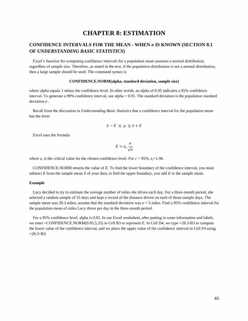
65
CHAPTER 8: ESTIMATION
CONFIDENCE INTERVALS FOR THE MEAN - WHEN σ IS KNOWN (SECTION 8.1
OF UNDERSTANDING BASIC STATISTICS)
Excel’s function for computing confidence intervals for a population mean assumes a normal distribution,
regardless of sample size. Therefore, as stated in the text, if the population distribution is not a normal distribution,
then a large sample should be used. The command syntax is
CONFIDENCE.NORM(alpha, standard deviation, sample size)
where alpha equals 1 minus the confidence level. In other words, an alpha of 0.05 indicates a 95% confidence
interval. To generate a 99% confidence interval, use alpha = 0.01. The standard deviation is the population standard
deviation σ .
Recall from the discussion in Understanding Basic Statistics that a confidence interval for the population mean
has the form
Excel uses the formula
√
where zc is the critical value for the chosen confidence level. For c = 95%, zc=1.96.
CONFIDENCE.NORM returns the value of E. To find the lower boundary of the confidence interval, you must
subtract E from the sample mean of your data; to find the upper boundary, you add E to the sample mean.
Example
Lucy decided to try to estimate the average number of miles she drives each day. For a three-month period, she
selected a random sample of 35 days and kept a record of the distance driven on each of those sample days. The
sample mean was 28.3 miles; assume that the standard deviation was σ = 5 miles. Find a 95% confidence interval for
the population mean of miles Lucy drove per day in the three-month period.
For a 95% confidence level, alpha is 0.05. In our Excel worksheet, after putting in some information and labels,
we enter =CONFIDENCE.NORM(0.05,5,35) in Cell B3 to represent E. In Cell D4, we type =28.3-B3 to compute
the lower value of the confidence interval, and we place the upper value of the confidence interval in Cell F4 using
=28.3+B3.
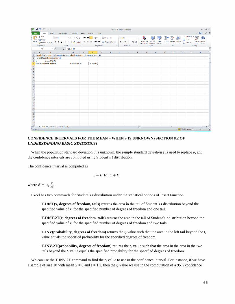
66
CONFIDENCE INTERVALS FOR THE MEAN – WHEN σ IS UNKNOWN (SECTION 8.2 OF
UNDERSTANDING BASIC STATISTICS)
When the population standard deviation σ is unknown, the sample standard deviation s is used to replace σ, and
the confidence intervals are computed using Student’s t distribution.
The confidence interval is computed as
where
√ .
Excel has two commands for Student’s t distribution under the statistical options of Insert Function.
T.DIST(x, degrees of freedom, tails) returns the area in the tail of Student’s t distribution beyond the
specified value of x, for the specified number of degrees of freedom and one tail.
T.DIST.2T(x, degrees of freedom, tails) returns the area in the tail of Student’s t distribution beyond the
specified value of x, for the specified number of degrees of freedom and two tails.
T.INV(probability, degrees of freedom) returns the tc value such that the area in the left tail beyond the tc
value equals the specified probability for the specified degrees of freedom.
T.INV.2T(probability, degrees of freedom) returns the tc value such that the area in the area in the two
tails beyond the tc value equals the specified probability for the specified degrees of freedom.
We can use the T.INV.2T command to find the tc value to use in the confidence interval. For instance, if we have
a sample of size 10 with mean = 6 and s = 1.2, then the tc value we use in the computation of a 95% confidence
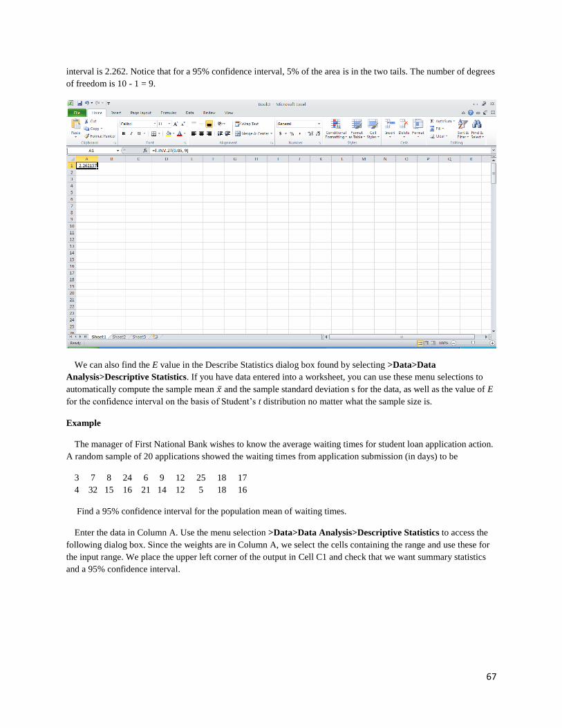
67
interval is 2.262. Notice that for a 95% confidence interval, 5% of the area is in the two tails. The number of degrees
of freedom is 10 - 1 = 9.
We can also find the E value in the Describe Statistics dialog box found by selecting >Data>Data
Analysis>Descriptive Statistics. If you have data entered into a worksheet, you can use these menu selections to
automatically compute the sample mean and the sample standard deviation s for the data, as well as the value of E
for the confidence interval on the basis of Student’s t distribution no matter what the sample size is.
Example
The manager of First National Bank wishes to know the average waiting times for student loan application action.
A random sample of 20 applications showed the waiting times from application submission (in days) to be
3 7 8 24 6 9 12 25 18 17
4 32 15 16 21 14 12 5 18 16
Find a 95% confidence interval for the population mean of waiting times.
Enter the data in Column A. Use the menu selection >Data>Data Analysis>Descriptive Statistics to access the
following dialog box. Since the weights are in Column A, we select the cells containing the range and use these for
the input range. We place the upper left corner of the output in Cell C1 and check that we want summary statistics
and a 95% confidence interval.
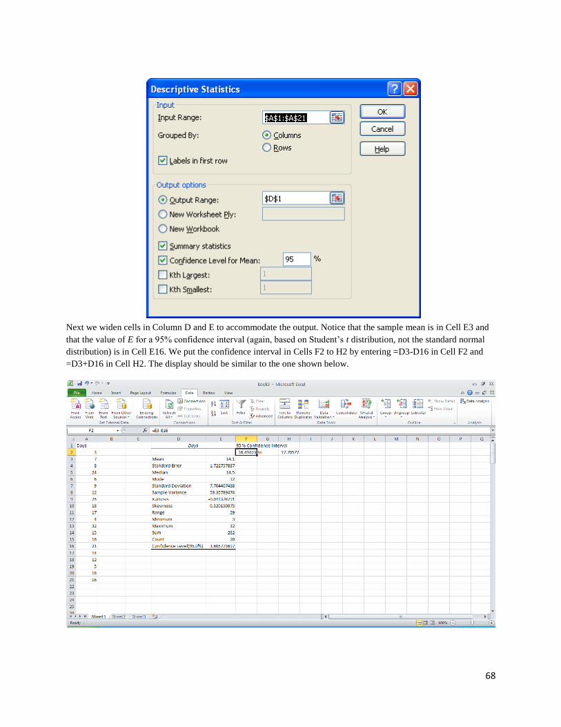
68
Next we widen cells in Column D and E to accommodate the output. Notice that the sample mean is in Cell E3 and
that the value of E for a 95% confidence interval (again, based on Student’s t distribution, not the standard normal
distribution) is in Cell E16. We put the confidence interval in Cells F2 to H2 by entering =D3-D16 in Cell F2 and
=D3+D16 in Cell H2. The display should be similar to the one shown below.
69
LAB ACTIVITIES FOR CONFIDENCE INTERVALS FOR THE MEAN
1. Retrieve the worksheet Sv03.xls. This contains the heights (in feet) of 65 randomly selected pro basketball
players. Use the Descriptive Statistics dialog box to get summary statistics for the data and to create a 90%
confidence interval.
2. Retrieve the worksheet Sv01.xls from the Excel data disk. This worksheet contains the number of shares of
Disney Stock (in hundreds of shares) sold for a random sample of sixty trading days in 1993 and 1994. Use
the Descriptive Statistics dialog box to get summary statistics for the data and to create the following
confidence intervals.
(a) Find a 99% confidence interval for the population mean volume.
(b) Find a 95% confidence interval for the population mean volume.
(c) Find a 90% confidence interval for the population mean volume.
(d) Find an 85% confidence interval for the population mean volume.
(e) What do you notice about the lengths of the intervals as the confidence level decreases?
3. There are many types of errors that will cause a computer program to terminate or give incorrect results.
One type of error is punctuation. For instance, if a comma is inserted in the wrong place, the program might
not run. A study of programs written by students in a beginning programming course showed that 75 out of
300 errors selected at random were punctuation errors. Find a 99% confidence interval for the proportion of
errors made by beginning programming students that are punctuation errors. Next find a 90% confidence
interval. Use the CONFIDENCE command to find the interval. Is this interval longer or shorter?
70
CHAPTER 9: HYPOTHESIS TESTING
TESTING A SINGLE POPULATION MEAN - WHEN σ IS KNOWN (SECTION 9.2
OF UNDERSTANDING BASIC STATISTICS)
Chapter 9 of Understanding Basic Statistics introduces tests of hypotheses. Testing involving a single mean is
found in Section 9.2. Hypothesis tests in this section test the value of the population mean, µ, against some specified
value, denoted by k.
When population standard deviation σ is known, one-sample z-tests are appropriate for testing the null hypothesis
H0: µ = k against one of the three alternative hypotheses H1: µ > k, H1: µ < k, or H1: µ ≠ k when (1) the data in the
sample are known to be from a normal distribution (in which case any sample size will do) or when (2) the data
distribution is unknown or the data are believed to be from a non-normal distribution, but the sample size, n, is large
(n ≥ 30).
In Excel, the Z.TEST function finds the P value for an upper- or right-tailed test, used to decide between
the hypotheses H0: µ = k and H1: µ > k. The null hypothesis says that value of the population mean µ is k. A
right-tailed test is used when the sample mean is greater than k, suggesting that µ may in fact be greater than
k, as the alternative hypothesis states.
The syntax is
Z.TEST(array, x, sigma)
The array is the list of sample values; what Excel calls x is k, and sigma is the known value of σ, the population
standard deviation. If the syntax used is Z.TEST(array, x), i.e. if there is no sigma value given, then Excel calculates
the sample standard deviation, s, from the sample data in array and uses that in place of σ.
The P value returned by Z.TEST is the probability, given that the null hypothesis is true, of getting results at least
as extreme as those observed in the sample. More precisely, Z.TEST gives the probability of obtaining a sample
mean greater than or equal to the observed sample mean, . When this probability is small, it means that the data in
the observed sample would be surprising if H0 were true. This is a reason to reject H0.
Z.TEST can also be used to apply a left-tailed test (H0: µ = k versus H1: µ < k) or a two-tailed test (H0: µ = k
versus H1: µ ≠ k). To apply a left-tailed test, for the case where the sample mean is less than k, simply apply a
right-tailed test and then subtract the result from 1. (When < k, the area found by Z.TEST in the upper “tail”
will be greater than 0.5, and 1 minus that area will be the area in the lower tail.) To apply a two-tailed test,
either double the P value from a right-tailed test (when > k) or double the P value from a left-tailed test
(when < k).
To call up the Z.TEST dialog box, click the Insert Function button on the tool bar, select Statistical
in the drop box, and scroll to Z.TEST. The dialog box should be similar to the one shown
on the top of the next page.
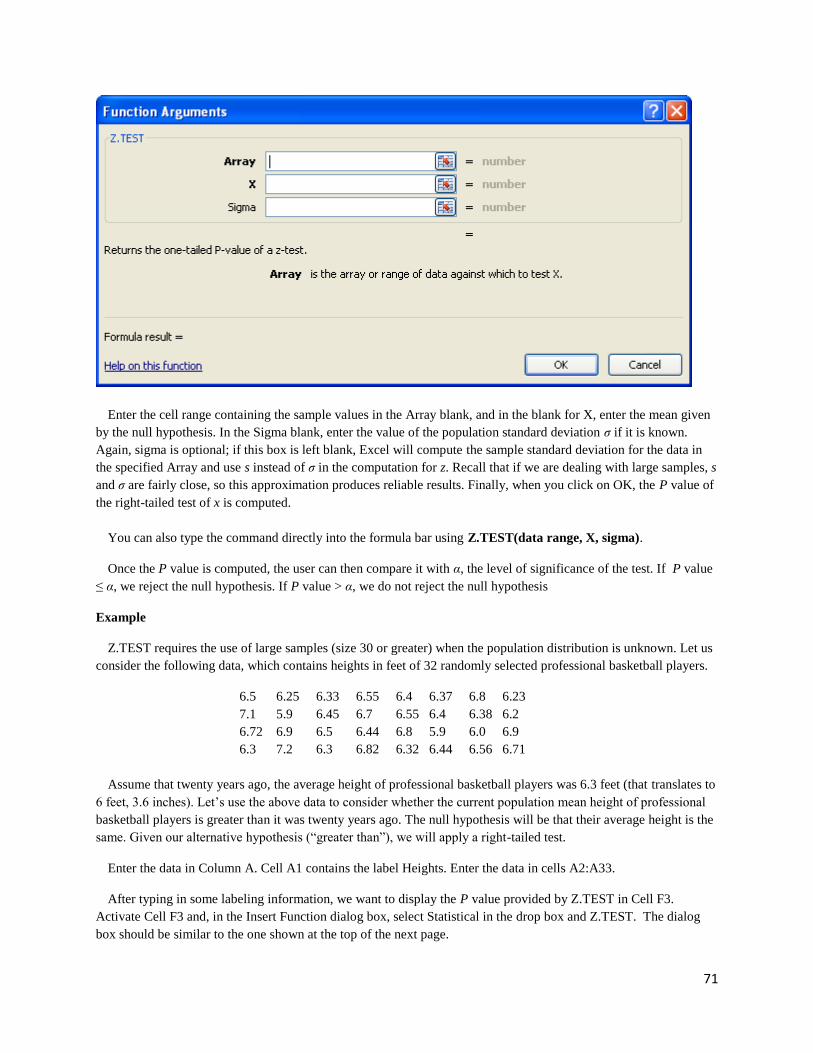
71
Enter the cell range containing the sample values in the Array blank, and in the blank for X, enter the mean given
by the null hypothesis. In the Sigma blank, enter the value of the population standard deviation σ if it is known.
Again, sigma is optional; if this box is left blank, Excel will compute the sample standard deviation for the data in
the specified Array and use s instead of σ in the computation for z. Recall that if we are dealing with large samples, s
and σ are fairly close, so this approximation produces reliable results. Finally, when you click on OK, the P value of
the right-tailed test of x is computed.
You can also type the command directly into the formula bar using Z.TEST(data range, X, sigma).
Once the P value is computed, the user can then compare it with α, the level of significance of the test. If P value
≤ α, we reject the null hypothesis. If P value > α, we do not reject the null hypothesis
Example
Z.TEST requires the use of large samples (size 30 or greater) when the population distribution is unknown. Let us
consider the following data, which contains heights in feet of 32 randomly selected professional basketball players.
6.5 6.25 6.33 6.55 6.4 6.37 6.8 6.23
7.1 5.9 6.45 6.7 6.55 6.4 6.38 6.2
6.72 6.9 6.5 6.44 6.8 5.9 6.0 6.9
6.3 7.2 6.3 6.82 6.32 6.44 6.56 6.71
Assume that twenty years ago, the average height of professional basketball players was 6.3 feet (that translates to
6 feet, 3.6 inches). Let’s use the above data to consider whether the current population mean height of professional
basketball players is greater than it was twenty years ago. The null hypothesis will be that their average height is the
same. Given our alternative hypothesis (“greater than”), we will apply a right-tailed test.
Enter the data in Column A. Cell A1 contains the label Heights. Enter the data in cells A2:A33.
After typing in some labeling information, we want to display the P value provided by Z.TEST in Cell F3.
Activate Cell F3 and, in the Insert Function dialog box, select Statistical in the drop box and Z.TEST. The dialog
box should be similar to the one shown at the top of the next page.
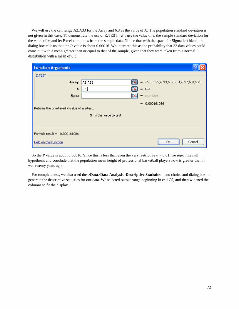
72
We will use the cell range A2:A33 for the Array and 6.3 as the value of X. The population standard deviation is
not given in this case. To demonstrate the use of Z.TEST, let’s use the value of s, the sample standard deviation for
the value of σ, and let Excel compute s from the sample data. Notice that with the space for Sigma left blank, the
dialog box tells us that the P value is about 0.00016. We interpret this as the probability that 32 data values could
come out with a mean greater than or equal to that of the sample, given that they were taken from a normal
distribution with a mean of 6.3.
So the P value is about 0.00016. Since this is less than even the very restrictive α = 0.01, we reject the null
hypothesis and conclude that the population mean height of professional basketball players now is greater than it
was twenty years ago.
For completeness, we also used the >Data>Data Analysis>Descriptive Statistics menu choice and dialog box to
generate the descriptive statistics for our data. We selected output range beginning in cell C5, and then widened the
columns to fit the display.
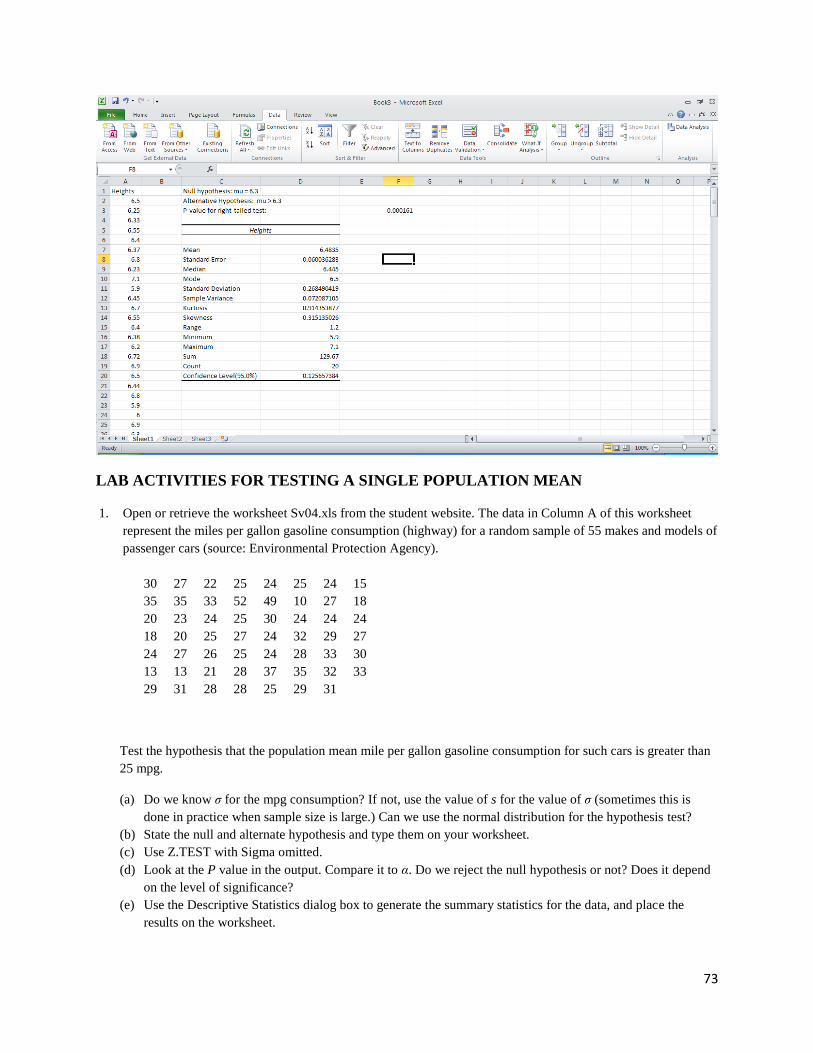
73
LAB ACTIVITIES FOR TESTING A SINGLE POPULATION MEAN
1. Open or retrieve the worksheet Sv04.xls from the student website. The data in Column A of this worksheet
represent the miles per gallon gasoline consumption (highway) for a random sample of 55 makes and models of
passenger cars (source: Environmental Protection Agency).
30 27 22 25 24 25 24 15
35 35 33 52 49 10 27 18
20 23 24 25 30 24 24 24
18 20 25 27 24 32 29 27
24 27 26 25 24 28 33 30
13 13 21 28 37 35 32 33
29 31 28 28 25 29 31
Test the hypothesis that the population mean mile per gallon gasoline consumption for such cars is greater than
25 mpg.
(a) Do we know σ for the mpg consumption? If not, use the value of s for the value of σ (sometimes this is
done in practice when sample size is large.) Can we use the normal distribution for the hypothesis test?
(b) State the null and alternate hypothesis and type them on your worksheet.
(c) Use Z.TEST with Sigma omitted.
(d) Look at the P value in the output. Compare it to α. Do we reject the null hypothesis or not? Does it depend
on the level of significance?
(e) Use the Descriptive Statistics dialog box to generate the summary statistics for the data, and place the
results on the worksheet.
74
CHAPTER 10: INFERENCES ABOUT DIFFERENCES
TESTS INVOLVING PAIRED DIFFERENCES - DEPENDENT SAMPLES (SECTION
10.1 OF UNDERSTANDING BASIC STATISTICS)
The test for difference of means of dependent samples is presented in Section 10.1 of Understanding Basic
Statistics. Dependent samples arise from before-and-after studies, some studies of data taken from the same subjects,
and some studies on identical twins.
In Excel there are two functions that produce the P value for a one- or two-tailed test of paired differences. The
first command is T.TEST, found using Insert Function with Statistical in the drop down box and T.TEST. You can
also activate a cell and type the command in the formula bar. This command returns only the P value for the test.
The syntax is
T.TEST(data range of sample 1, data range of sample 2, tails, type)
If tails = 1, then T.TEST returns the P value for a one-tailed test, and if tails = 2, then T.TEST returns the two-tailed
value. For the parameter called type, there are three choices:
Type Test performed using Student’s t distribution
1 Paired difference test
2 Difference of means test for two samples with equal variances
3 Difference of means test for two samples with unequal variances
The other Excel command, >Data>Data Analysis>t-Test: Paired Two Sample for Means, gives much more
information than T.TEST. We will use this command in the next example.
Example
Promoters of a state lottery decided to advertise the lottery heavily on television for one week during the middle
of one of the lottery games. To see if the advertising improved ticket sales, they surveyed a random sample of 8
ticket outlets and recorded weekly sales for one week before the television campaign and for one week after the
campaign. The results follow (in ticket sales) where row A gives sales prior to the campaign and row B gives sales
afterward.
A 3201 4529 1425 1272 1784 1733 2563 3129
B 3762 4851 1202 1131 2172 1802 2492 3151
Test the claim that the television campaign increased lottery ticket sales at the 0.05 level of significance.
We enter the data in Columns A and B, with appropriate headers. Next, open the dialog box below, using
>Data>Data Analysis> t-Test: Paired Two Sample for Means.
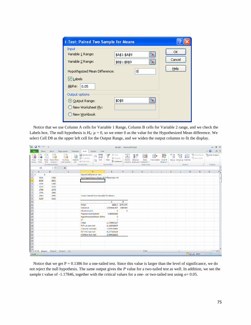
75
Notice that we use Column A cells for Variable 1 Range, Column B cells for Variable 2 range, and we check the
Labels box. The null hypothesis is H0: µ = 0, so we enter 0 as the value for the Hypothesized Mean difference. We
select Cell D8 as the upper left cell for the Output Range, and we widen the output columns to fit the display.
Notice that we get P = 0.1386 for a one-tailed test. Since this value is larger than the level of significance, we do
not reject the null hypothesis. The same output gives the P value for a two-tailed test as well. In addition, we see the
sample t value of -1.17846, together with the critical values for a one- or two-tailed test using α= 0.05.
76
LAB ACTIVITIES FOR TESTS INVOLVING PAIRED DIFFERENCES
1. Open or retrieve the worksheet Tvcds01.xls from the student website. The data are pairs of values where the
entries in Column A represents average salary ($1000/yr) for male faculty members at an institution and those
in Column B represent the average salary for female faculty members ($1000/yr) at the same institution. A
random sample of 22 U.S. colleges and universities was used (source: Academe, Bulletin of the American
Association of University Professors).
(34.5, 33.9) (30.5, 31.2) (35.1, 35.0) (35.7, 34.2) (31.5, 32.4)
(34.4, 34.1) (32.1, 32.7) (30.7, 29.9) (33.7, 31.2) (35.3, 35.5)
(30.7, 30.2) (34.2, 34.8) (39.6, 38.7) (30.5, 30.0) (33.8, 33.8)
(31.7, 32.4) (32.8, 31.7) (38.5, 38.9) (40.5, 41.5) (25.3, 25.5)
(28.6, 28.0) (35.8, 35.1)
(a) The data are in Columns A and B.
(b) Use the >Data>Data Analysis>t-Test Paired Two Sample for Means dialog box to test the hypothesis
that there is a difference in salary. What is the P value of the sample test statistic? Do we reject or fail to
reject the null hypothesis at the 5% level of significance? What about at the 1% level of significance?
(c) Use the >Data>Data Analysis>t-Test Paired Two Sample for Means dialog box to test the hypothesis
that female faculty members have a lower average salary than male faculty members. What is the test
conclusion at the 5% level of significance? At the 1% level of significance?
2. An audiologist is conducting a study on noise and stress. Twelve subjects selected at random were given a
stress test in a room that was quiet. Then the same subjects were given another stress test, this time in a room
with high-pitched background noise. The results of the stress tests were scores 1 through 20 with 20 indicating
the greatest stress. The results follow, where A represents the score of the test administered in the quiet room
and B represents the scores of the test administered in the room with the high-pitched background noise.
Subject 1 2 3 4 5 6 7 8 9 10 11 12
A 13 12 16 19 7 13 9 15 17 6 14 15
B 18 15 14 18 10 12 11 14 17 8 16 16
Test the hypothesis that the stress level was greater during exposure to high-pitched background noise. Look at
the P value. Should you reject the null hypothesis at the 1% level of significance? At the 5% level?
TESTING OF DIFFERENCES OF MEANS (SECTION 10.2 OF UNDERSTANDING
BASIC STATISTICS)
Tests of difference of means for independent samples are presented in Section 10.2 of Understanding Basic
Statistics. We consider the distribution. The null hypothesis is that there is no difference between means, so
H0:µ1 = µ2 or H0: µ1 - µ2 = 0.
When σ1 and σ2 are known
When we are testing the difference of means with known σ1 and σ2, the z-test based on normal distribution is used
if either the population has a normal distribution or the sample size is large. The values of population variance,
which is the square of population standard deviation, are actually needed in the Excel testing procedure dialog box.
Some examples used in this section do not provide the values of population standard deviations. In order to
demonstrate the use of the testing procedure, we use the sample variance values for the population variance values.
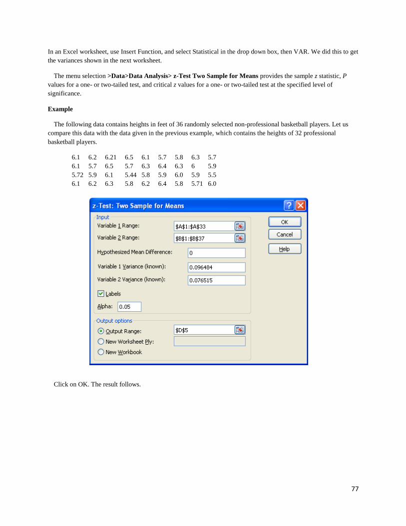
77
In an Excel worksheet, use Insert Function, and select Statistical in the drop down box, then VAR. We did this to get
the variances shown in the next worksheet.
The menu selection >Data>Data Analysis> z-Test Two Sample for Means provides the sample z statistic, P
values for a one- or two-tailed test, and critical z values for a one- or two-tailed test at the specified level of
significance.
Example
The following data contains heights in feet of 36 randomly selected non-professional basketball players. Let us
compare this data with the data given in the previous example, which contains the heights of 32 professional
basketball players.
6.1 6.2 6.21 6.5 6.1 5.7 5.8 6.3 5.7
6.1 5.7 6.5 5.7 6.3 6.4 6.3 6 5.9
5.72 5.9 6.1 5.44 5.8 5.9 6.0 5.9 5.5
6.1 6.2 6.3 5.8 6.2 6.4 5.8 5.71 6.0
Click on OK. The result follows.
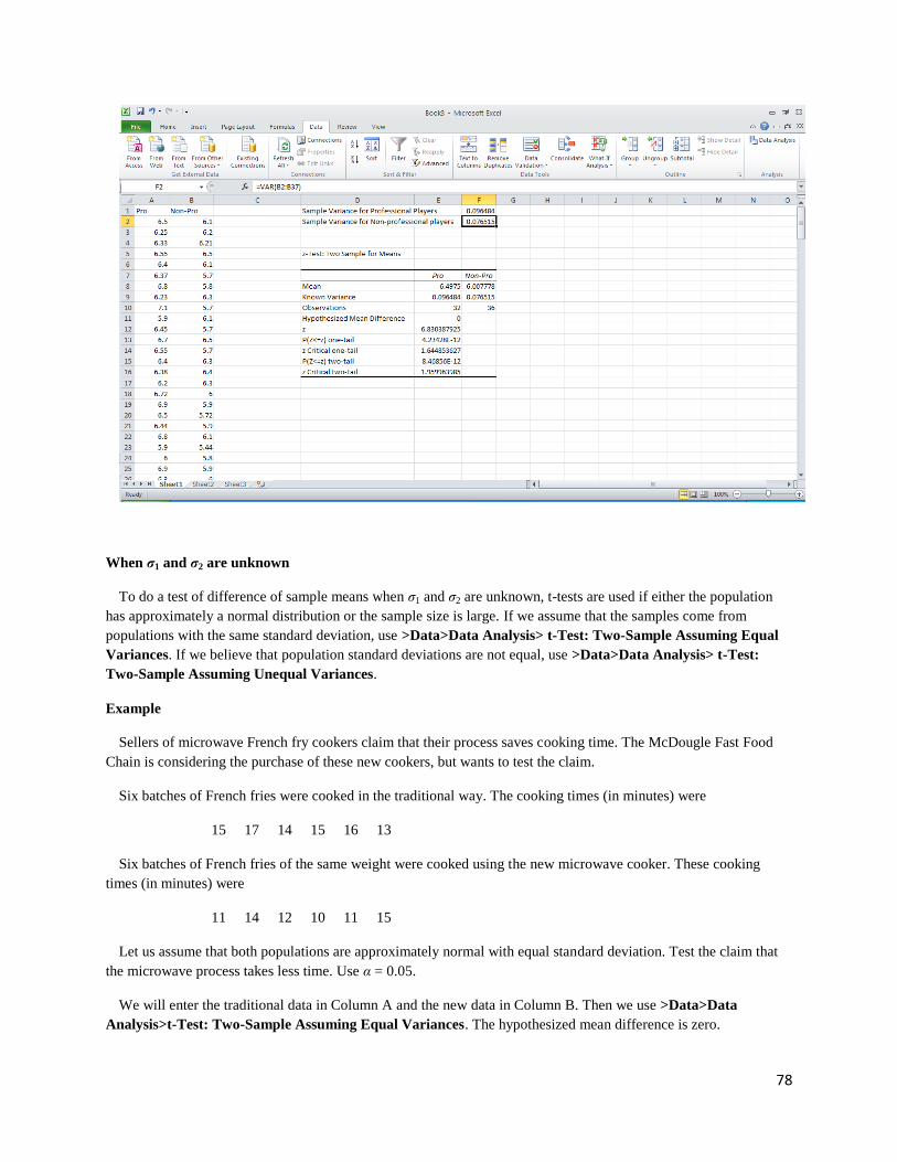
78
When σ1 and σ2 are unknown
To do a test of difference of sample means when σ1 and σ2 are unknown, t-tests are used if either the population
has approximately a normal distribution or the sample size is large. If we assume that the samples come from
populations with the same standard deviation, use >Data>Data Analysis> t-Test: Two-Sample Assuming Equal
Variances. If we believe that population standard deviations are not equal, use >Data>Data Analysis> t-Test:
Two-Sample Assuming Unequal Variances.
Example
Sellers of microwave French fry cookers claim that their process saves cooking time. The McDougle Fast Food
Chain is considering the purchase of these new cookers, but wants to test the claim.
Six batches of French fries were cooked in the traditional way. The cooking times (in minutes) were
15 17 14 15 16 13
Six batches of French fries of the same weight were cooked using the new microwave cooker. These cooking
times (in minutes) were
11 14 12 10 11 15
Let us assume that both populations are approximately normal with equal standard deviation. Test the claim that
the microwave process takes less time. Use α = 0.05.
We will enter the traditional data in Column A and the new data in Column B. Then we use >Data>Data
Analysis>t-Test: Two-Sample Assuming Equal Variances. The hypothesized mean difference is zero.
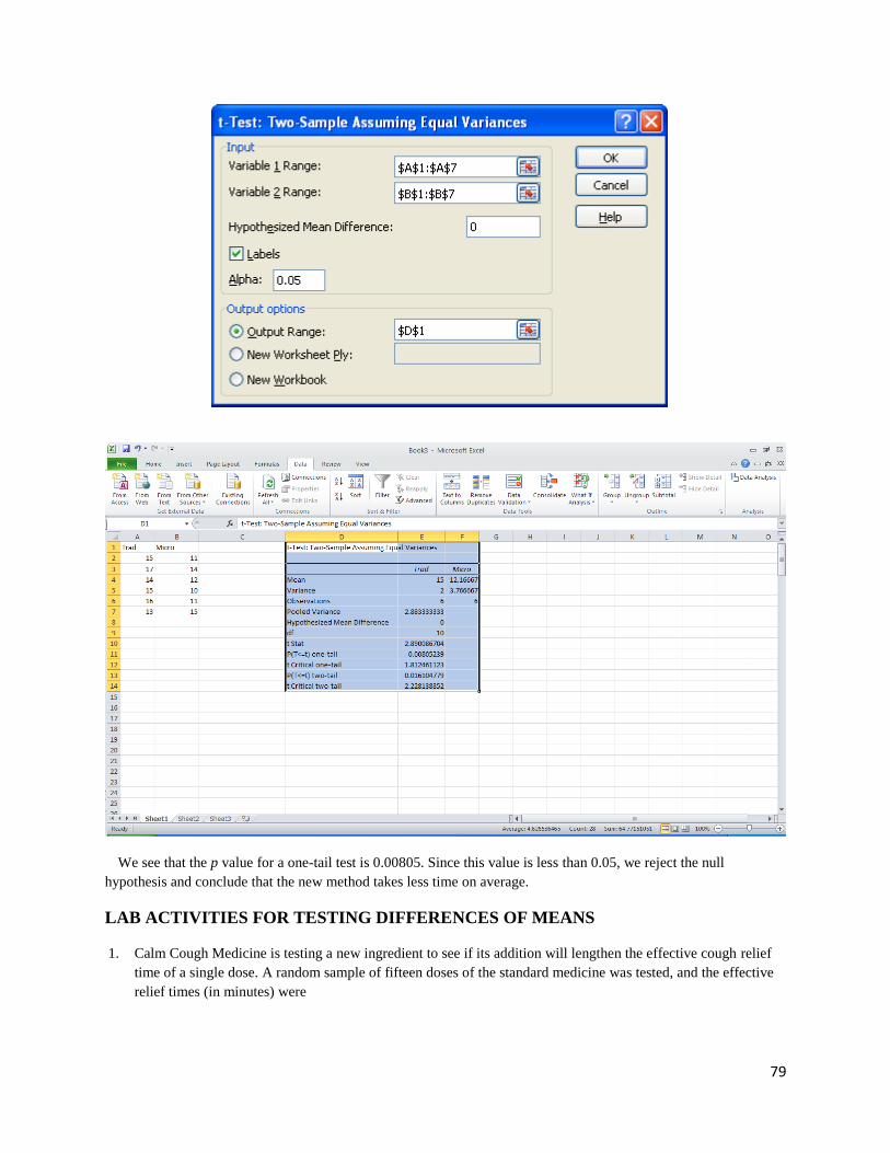
79
We see that the p value for a one-tail test is 0.00805. Since this value is less than 0.05, we reject the null
hypothesis and conclude that the new method takes less time on average.
LAB ACTIVITIES FOR TESTING DIFFERENCES OF MEANS
1. Calm Cough Medicine is testing a new ingredient to see if its addition will lengthen the effective cough relief
time of a single dose. A random sample of fifteen doses of the standard medicine was tested, and the effective
relief times (in minutes) were
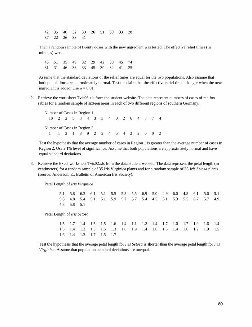
80
42 35 40 32 30 26 51 39 33 28
37 22 36 33 41
Then a random sample of twenty doses with the new ingredient was tested. The effective relief times (in
minutes) were
43 51 35 49 32 29 42 38 45 74
31 31 46 36 33 45 30 32 41 25
Assume that the standard deviations of the relief times are equal for the two populations. Also assume that
both populations are approximately normal. Test the claim that the effective relief time is longer when the new
ingredient is added. Use α = 0.01.
2. Retrieve the worksheet Tvis06.xls from the student website. The data represent numbers of cases of red fox
rabies for a random sample of sixteen areas in each of two different regions of southern Germany.
Number of Cases in Region 1
10 2 2 5 3 4 3 3 4 0 2 6 4 8 7 4
Number of Cases in Region 2
1 1 2 1 3 9 2 2 4 5 4 2 2 0 0 2
Test the hypothesis that the average number of cases in Region 1 is greater than the average number of cases in
Region 2. Use a 1% level of significance. Assume that both populations are approximately normal and have
equal standard deviations.
3. Retrieve the Excel worksheet Tvis02.xls from the data student website. The data represent the petal length (in
centimeters) for a random sample of 35 Iris Virginica plants and for a random sample of 38 Iris Setosa plants
(source: Anderson, E., Bulletin of American Iris Society).
Petal Length of Iris Virginica
5.1 5.8 6.3 6.1 5.1 5.5 5.3 5.5 6.9 5.0 4.9 6.0 4.8 6.1 5.6 5.1
5.6 4.8 5.4 5.1 5.1 5.9 5.2 5.7 5.4 4.5 6.1 5.3 5.5 6.7 5.7 4.9
4.8 5.8 5.1
Petal Length of Iris Setosa
1.5 1.7 1.4 1.5 1.5 1.6 1.4 1.1 1.2 1.4 1.7 1.0 1.7 1.9 1.6 1.4
1.5 1.4 1.2 1.3 1.5 1.3 1.6 1.9 1.4 1.6 1.5 1.4 1.6 1.2 1.9 1.5
1.6 1.4 1.3 1.7 1.5 1.7
Test the hypothesis that the average petal length for Iris Setosa is shorter than the average petal length for Iris
Virginica. Assume that population standard deviations are unequal.
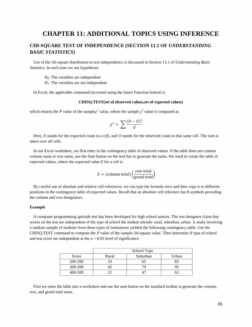
81
CHAPTER 11: ADDITIONAL TOPICS USING INFERENCE
CHI-SQUARE TEST OF INDEPENDENCE (SECTION 11.1 OF UNDERSTANDING
BASIC STATISTICS)
Use of the chi-square distribution to test independence is discussed in Section 11.1 of Understanding Basic
Statistics. In such tests we use hypotheses
H0: The variables are independent
H1: The variables are not independent
In Excel, the applicable command (accessed using the Insert Function button) is
CHISQ.TEST(set of observed values,set of expected values)
which returns the P value of the sampleχ2 value, where the sample χ
2 value is computed as
∑( )
Here, E stands for the expected count in a cell, and O stands for the observed count in that same cell. The sum is
taken over all cells.
In our Excel worksheet, we first enter in the contingency table of observed values. If the table does not contain
column sums or row sums, use the Sum button on the tool bar to generate the sums. We need to create the table of
expected values, where the expected value E for a cell is
( ) (
)
By careful use of absolute and relative cell references, we can type the formula once and then copy it to different
positions in the contingency table of expected values. Recall that an absolute cell reference has $ symbols preceding
the column and row designators.
Example
A computer programming aptitude test has been developed for high school seniors. The test designers claim that
scores on the test are independent of the type of school the student attends: rural, suburban, urban. A study involving
a random sample of students from these types of institutions yielded the following contingency table. Use the
CHISQ.TEST command to compute the P value of the sample chi-square value. Then determine if type of school
and test score are independent at the α = 0.05 level of significance.
First we enter the table into a worksheet and use the sum button on the standard toolbar to generate the column,
row, and grand total sums.
School Type
Score Rural Suburban Urban
200-299 33 65 83
300-399 45 79 95
400-500 21 47 63
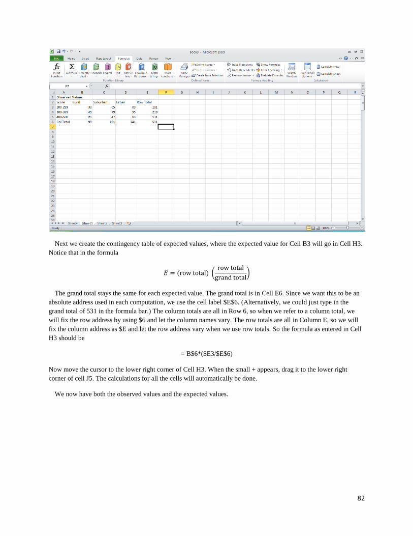
82
Next we create the contingency table of expected values, where the expected value for Cell B3 will go in Cell H3.
Notice that in the formula
( ) (
)
The grand total stays the same for each expected value. The grand total is in Cell E6. Since we want this to be an
absolute address used in each computation, we use the cell label $E$6. (Alternatively, we could just type in the
grand total of 531 in the formula bar.) The column totals are all in Row 6, so when we refer to a column total, we
will fix the row address by using $6 and let the column names vary. The row totals are all in Column E, so we will
fix the column address as $E and let the row address vary when we use row totals. So the formula as entered in Cell
H3 should be
= B$6*($E3/$E$6)
Now move the cursor to the lower right corner of Cell H3. When the small + appears, drag it to the lower right
corner of cell J5. The calculations for all the cells will automatically be done.
We now have both the observed values and the expected values.
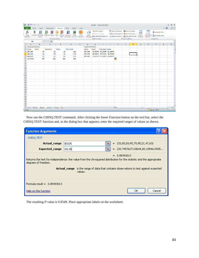
83
Now use the CHISQ.TEST command. After clicking the Insert Function button on the tool bar, select the
CHISQ.TEST function and, in the dialog box that appears, enter the required ranges of values as shown.
The resulting P value is 0.8549. Place appropriate labels on the worksheet.
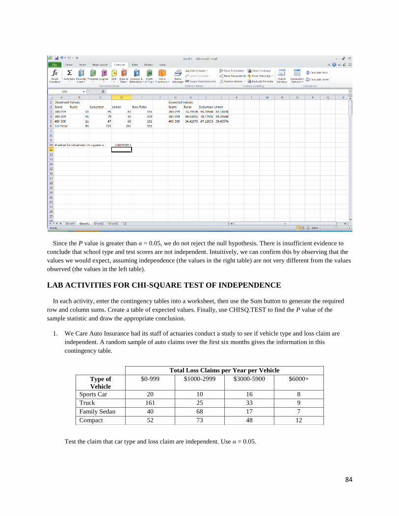
84
Since the P value is greater than α = 0.05, we do not reject the null hypothesis. There is insufficient evidence to
conclude that school type and test scores are not independent. Intuitively, we can confirm this by observing that the
values we would expect, assuming independence (the values in the right table) are not very different from the values
observed (the values in the left table).
LAB ACTIVITIES FOR CHI-SQUARE TEST OF INDEPENDENCE
In each activity, enter the contingency tables into a worksheet, then use the Sum button to generate the required
row and column sums. Create a table of expected values. Finally, use CHISQ.TEST to find the P value of the
sample statistic and draw the appropriate conclusion.
1. We Care Auto Insurance had its staff of actuaries conduct a study to see if vehicle type and loss claim are
independent. A random sample of auto claims over the first six months gives the information in this
contingency table.
Test the claim that car type and loss claim are independent. Use α = 0.05.
Total Loss Claims per Year per Vehicle
Type of
Vehicle
$0-999 $1000-2999 $3000-5900 $6000+
Sports Car 20 10 16 8
Truck 161 25 33 9
Family Sedan 40 68 17 7
Compact 52 73 48 12
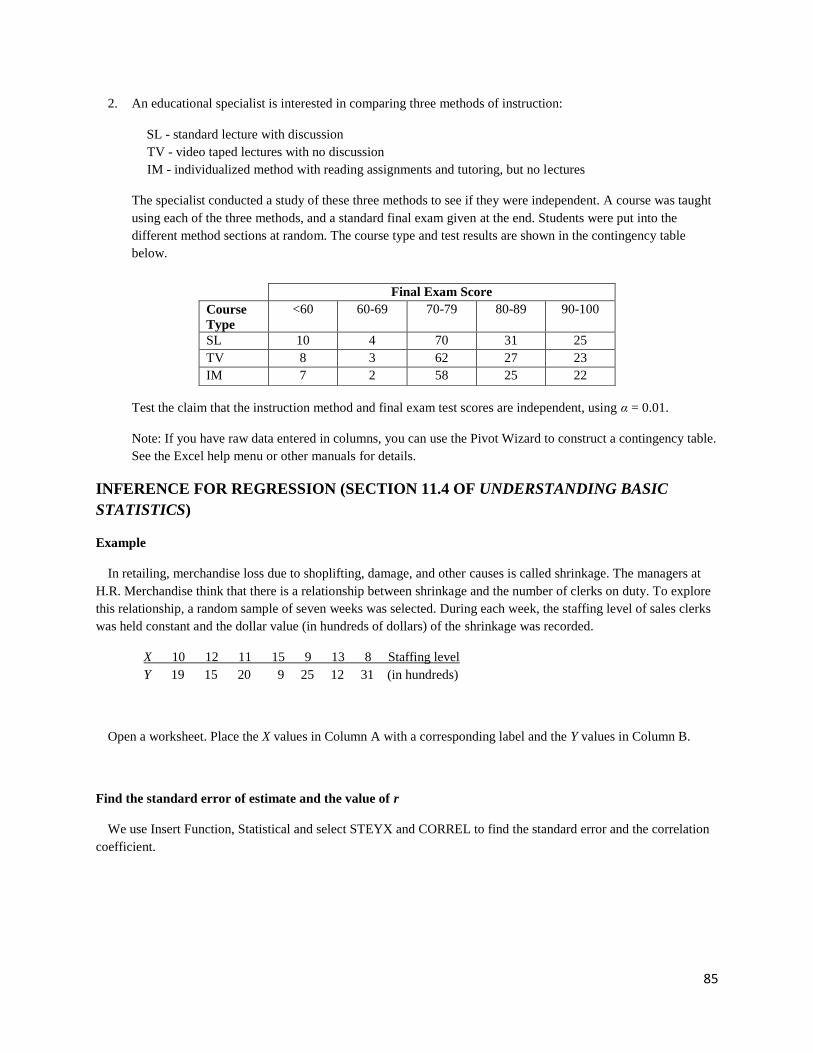
85
2. An educational specialist is interested in comparing three methods of instruction:
SL - standard lecture with discussion
TV - video taped lectures with no discussion
IM - individualized method with reading assignments and tutoring, but no lectures
The specialist conducted a study of these three methods to see if they were independent. A course was taught
using each of the three methods, and a standard final exam given at the end. Students were put into the
different method sections at random. The course type and test results are shown in the contingency table
below.
Test the claim that the instruction method and final exam test scores are independent, using α = 0.01.
Note: If you have raw data entered in columns, you can use the Pivot Wizard to construct a contingency table.
See the Excel help menu or other manuals for details.
INFERENCE FOR REGRESSION (SECTION 11.4 OF UNDERSTANDING BASIC
STATISTICS)
Example
In retailing, merchandise loss due to shoplifting, damage, and other causes is called shrinkage. The managers at
H.R. Merchandise think that there is a relationship between shrinkage and the number of clerks on duty. To explore
this relationship, a random sample of seven weeks was selected. During each week, the staffing level of sales clerks
was held constant and the dollar value (in hundreds of dollars) of the shrinkage was recorded.
X 10 12 11 15 9 13 8 Staffing level
Y 19 15 20 9 25 12 31 (in hundreds)
Open a worksheet. Place the X values in Column A with a corresponding label and the Y values in Column B.
Find the standard error of estimate and the value of r
We use Insert Function, Statistical and select STEYX and CORREL to find the standard error and the correlation
coefficient.
Final Exam Score
Course
Type
<60 60-69 70-79 80-89 90-100
SL 10 4 70 31 25
TV 8 3 62 27 23
IM 7 2 58 25 22

86
This worksheet shows the results.
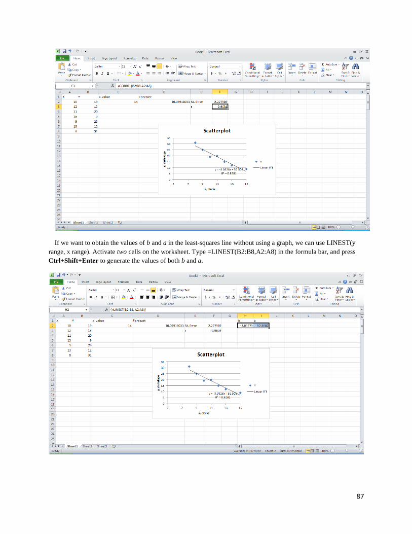
87
If we want to obtain the values of b and a in the least-squares line without using a graph, we can use LINEST(y
range, x range). Activate two cells on the worksheet. Type =LINEST(B2:B8,A2:A8) in the formula bar, and press
Ctrl+Shift+Enter to generate the values of both b and a.
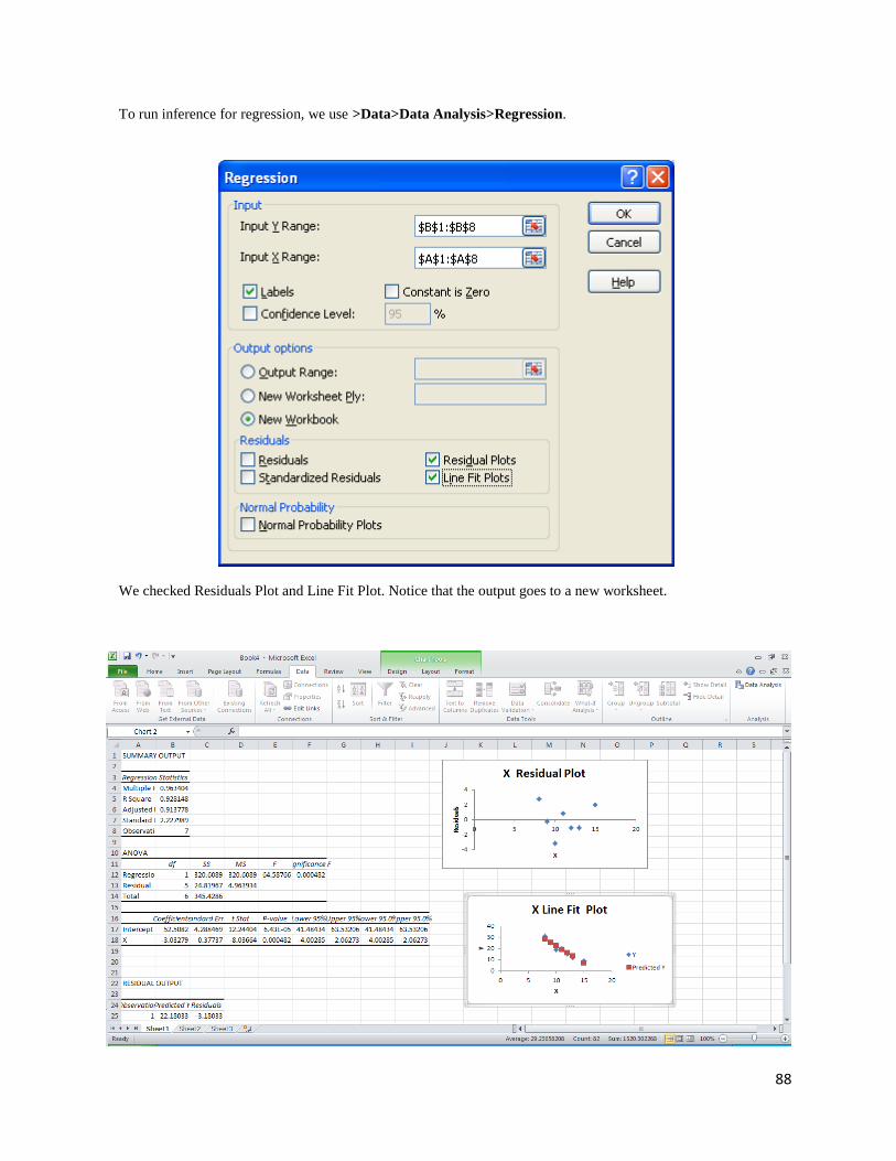
88
To run inference for regression, we use >Data>Data Analysis>Regression.
We checked Residuals Plot and Line Fit Plot. Notice that the output goes to a new worksheet.
89
The output shows the value of the t-statistic for the inference test for the slope along with its p-value. Scrolling
down would show the rest of the residual output.
LAB ACTIVITIES FOR TWO-VARIABLE LINEAR REGRESSION
5. Open or retrieve the worksheet Slr01.xls from the student website. This worksheet contains the following data,
with the list price in Column C1 and the best price in Column C2. The best price is the best price negotiated by
a team from the magazine.
LIST PRICE VERSUS BEST PRICE FOR A NEW GMC PICKUP TRUCK
In the following data pairs (X, Y),
X = List Price (in $1000) for a GMC Pickup Truck
Y = Best Price (in $1000) for a GMC Pickup Truck
Source: Consumers Digest, February 1994
(12.400, 11.200) (14.300, 12.500) (14.500, 12.700)
(14.900, 13.100) (16.100, 14.100) (16.900, 14.800)
(16.500, 14.400) (15.400, 13.400) (17.000, 14.900)
(17.900, 15.600) (18.800, 16.400) (20.300, 17.700)
(22.400, 19.600) (19.400, 16.900) (15.500, 14.000)
(16.700, (14.600) (17.300, 15.100) (18.400, 16.100)
(19.200, 16.800) (17.400, 15.200) (19.500, 17.000)
(19.700, 17.200) (21.200, 18.600)
(d) Use Excel to create a scatter plot for the data
(e) Right-click on a data point and use the Add Trendline option to show the least-squares line on the scatter
diagram, along with its equation and the value of r2.
(f) What is the value of the standard error of estimate? (Use STEYX.)
(g) What is the value of the correlation coefficient r? (Use CORREL.)
(h) Use the least-squares model to predict the best price for a truck with a list price of $20,000. Note: Enter
this value as 20, since X is assumed to be in thousands of dollars. (Use FORECAST.)
6. Other Excel worksheets appropriate to use for simple linear regression are:
Cricket Chirps Versus Temperature: Slr02.xls
Source: The Song of Insects by Dr. G.W. Pierce, Harvard Press
The chirps per second for the striped grouped cricket are stored in C1; the corresponding temperature in
degrees Fahrenheit is stored in C2.
Diameter of Sand Granules Versus Slope on a Natural Occurring Ocean Beach: Slr03.xls
Source Physical Geography by A.M. King, Oxford press
The median diameter (MM) of granules of sand is stored in C1; the corresponding gradient of
beach slope in degrees is stored in C2.
National Unemployment Rate Male Versus Female: Slr04.xls
Source: Statistical Abstract of the United States
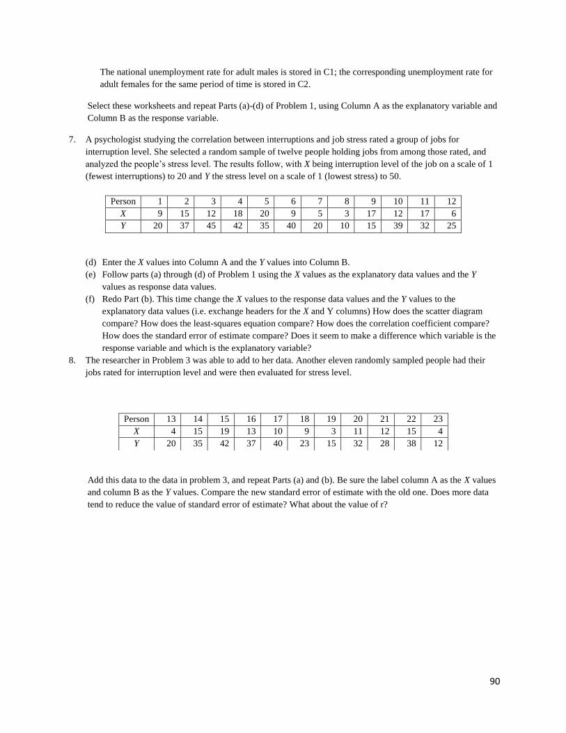
90
The national unemployment rate for adult males is stored in C1; the corresponding unemployment rate for
adult females for the same period of time is stored in C2.
Select these worksheets and repeat Parts (a)-(d) of Problem 1, using Column A as the explanatory variable and
Column B as the response variable.
7. A psychologist studying the correlation between interruptions and job stress rated a group of jobs for
interruption level. She selected a random sample of twelve people holding jobs from among those rated, and
analyzed the people’s stress level. The results follow, with X being interruption level of the job on a scale of 1
(fewest interruptions) to 20 and Y the stress level on a scale of 1 (lowest stress) to 50.
(d) Enter the X values into Column A and the Y values into Column B.
(e) Follow parts (a) through (d) of Problem 1 using the X values as the explanatory data values and the Y
values as response data values.
(f) Redo Part (b). This time change the X values to the response data values and the Y values to the
explanatory data values (i.e. exchange headers for the X and Y columns) How does the scatter diagram
compare? How does the least-squares equation compare? How does the correlation coefficient compare?
How does the standard error of estimate compare? Does it seem to make a difference which variable is the
response variable and which is the explanatory variable?
8. The researcher in Problem 3 was able to add to her data. Another eleven randomly sampled people had their
jobs rated for interruption level and were then evaluated for stress level.
Add this data to the data in problem 3, and repeat Parts (a) and (b). Be sure the label column A as the X values
and column B as the Y values. Compare the new standard error of estimate with the old one. Does more data
tend to reduce the value of standard error of estimate? What about the value of r?
Person 1 2 3 4 5 6 7 8 9 10 11 12
X 9 15 12 18 20 9 5 3 17 12 17 6
Y 20 37 45 42 35 40 20 10 15 39 32 25
Person 13 14 15 16 17 18 19 20 21 22 23
X 4 15 19 13 10 9 3 11 12 15 4
Y 20 35 42 37 40 23 15 32 28 38 12
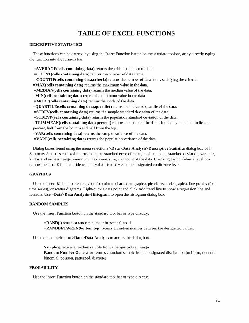
91
TABLE OF EXCEL FUNCTIONS
DESCRIPTIVE STATISTICS
These functions can be entered by using the Insert Function button on the standard toolbar, or by directly typing
the function into the formula bar.
=AVERAGE(cells containing data) returns the arithmetic mean of data.
=COUNT(cells containing data) returns the number of data items.
=COUNTIF(cells containing data,criteria) returns the number of data items satisfying the criteria.
=MAX(cells containing data) returns the maximum value in the data.
=MEDIAN(cells containing data) returns the median value of the data.
=MIN(cells containing data) returns the minimum value in the data.
=MODE(cells containing data) returns the mode of the data.
=QUARTILE(cells containing data,quartile) returns the indicated quartile of the data.
=STDEV(cells containing data) returns the sample standard deviation of the data.
=STDEVP(cells containing data) returns the population standard deviation of the data.
=TRIMMEAN(cells containing data,percent) returns the mean of the data trimmed by the total indicated
percent, half from the bottom and half from the top.
=VAR(cells containing data) returns the sample variance of the data.
=VARP(cells containing data) returns the population variance of the data.
Dialog boxes found using the menu selections >Data>Data Analysis>Descriptive Statistics dialog box with
Summary Statistics checked returns the mean standard error of mean, median, mode, standard deviation, variance,
kurtosis, skewness, range, minimum, maximum, sum, and count of the data. Checking the confidence level box
returns the error E for a confidence interval - E to + E at the designated confidence level.
GRAPHICS
Use the Insert Ribbon to create graphs for column charts (bar graphs), pie charts circle graphs), line graphs (for
time series), or scatter diagrams. Right-click a data point and click Add trend line to show a regression line and
formula. Use >Data>Data Analysis>Histogram to open the histogram dialog box.
RANDOM SAMPLES
Use the Insert Function button on the standard tool bar or type directly.
=RAND( ) returns a random number between 0 and 1.
=RANDBETWEEN(bottom,top) returns a random number between the designated values.
Use the menu selection >Data>Data Analysis to access the dialog box.
Sampling returns a random sample from a designated cell range.
Random Number Generator returns a random sample from a designated distribution (uniform, normal,
binomial, poisson, patterned, discrete).
PROBABILITY
Use the Insert Function button on the standard tool bar or type directly.
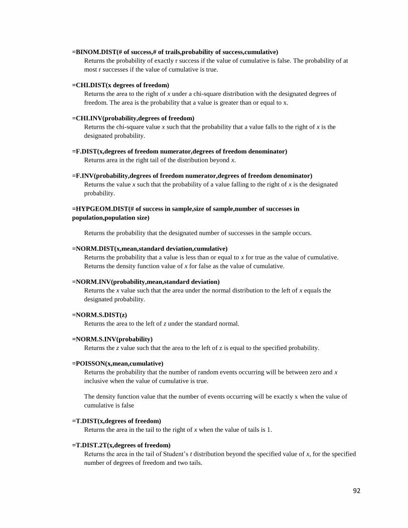
92
=BINOM.DIST(# of success,# of trails,probability of success,cumulative)
Returns the probability of exactly r success if the value of cumulative is false. The probability of at
most r successes if the value of cumulative is true.
=CHI.DIST(x degrees of freedom)
Returns the area to the right of x under a chi-square distribution with the designated degrees of
freedom. The area is the probability that a value is greater than or equal to x.
=CHI.INV(probability,degrees of freedom)
Returns the chi-square value x such that the probability that a value falls to the right of x is the
designated probability.
=F.DIST(x,degrees of freedom numerator,degrees of freedom denominator)
Returns area in the right tail of the distribution beyond x.
=F.INV(probability,degrees of freedom numerator,degrees of freedom denominator)
Returns the value x such that the probability of a value falling to the right of x is the designated
probability.
=HYPGEOM.DIST(# of success in sample,size of sample,number of successes in
population,population size)
Returns the probability that the designated number of successes in the sample occurs.
=NORM.DIST(x,mean,standard deviation,cumulative)
Returns the probability that a value is less than or equal to x for true as the value of cumulative.
Returns the density function value of x for false as the value of cumulative.
=NORM.INV(probability,mean,standard deviation)
Returns the x value such that the area under the normal distribution to the left of x equals the
designated probability.
=NORM.S.DIST(z)
Returns the area to the left of z under the standard normal.
=NORM.S.INV(probability)
Returns the z value such that the area to the left of z is equal to the specified probability.
=POISSON(x,mean,cumulative)
Returns the probability that the number of random events occurring will be between zero and x
inclusive when the value of cumulative is true.
The density function value that the number of events occurring will be exactly x when the value of
cumulative is false
=T.DIST(x,degrees of freedom)
Returns the area in the tail to the right of x when the value of tails is 1.
=T.DIST.2T(x,degrees of freedom)
Returns the area in the tail of Student’s t distribution beyond the specified value of x, for the specified
number of degrees of freedom and two tails.
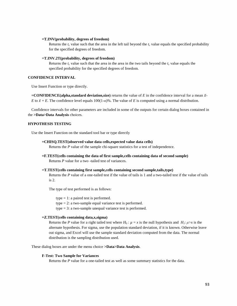
93
=T.INV(probability, degrees of freedom)
Returns the tc value such that the area in the left tail beyond the tc value equals the specified probability
for the specified degrees of freedom.
=T.INV.2T(probability, degrees of freedom)
Returns the tc value such that the area in the area in the two tails beyond the tc value equals the
specified probability for the specified degrees of freedom.
CONFIDENCE INTERVAL
Use Insert Function or type directly.
=CONFIDENCE(alpha,standard deviation,size) returns the value of E in the confidence interval for a mean -
E to + E. The confidence level equals 100(1-α)%. The value of E is computed using a normal distribution.
Confidence intervals for other parameters are included in some of the outputs for certain dialog boxes contained in
the >Data>Data Analysis choices.
HYPOTHESIS TESTING
Use the Insert Function on the standard tool bar or type directly
=CHISQ.TEST(observed value data cells,expected value data cells)
Returns the P value of the sample chi-square statistics for a test of independence.
=F.TEST(cells containing the data of first sample,cells containing data of second sample)
Returns P value for a two -tailed test of variances.
=T.TEST(cells containing first sample,cells containing second sample,tails,type)
Returns the P value of a one-tailed test if the value of tails is 1 and a two-tailed test if the value of tails
is 2.
The type of test performed is as follows:
type = 1: a paired test is performed.
type = 2: a two-sample equal variance test is performed.
type = 3: a two-sample unequal variance test is performed.
=Z.TEST(cells containing data,x,sigma)
Returns the P value for a right tailed test where H0 : µ = x is the null hypothesis and H1: μ>x is the
alternate hypothesis. For sigma, use the population standard deviation, if it is known. Otherwise leave
out sigma, and Excel will use the sample standard deviation computed from the data. The normal
distribution is the sampling distribution used.
These dialog boxes are under the menu choice >Data>Data Analysis.
F-Test: Two Sample for Variances
Returns the P value for a one-tailed test as well as some summary statistics for the data.
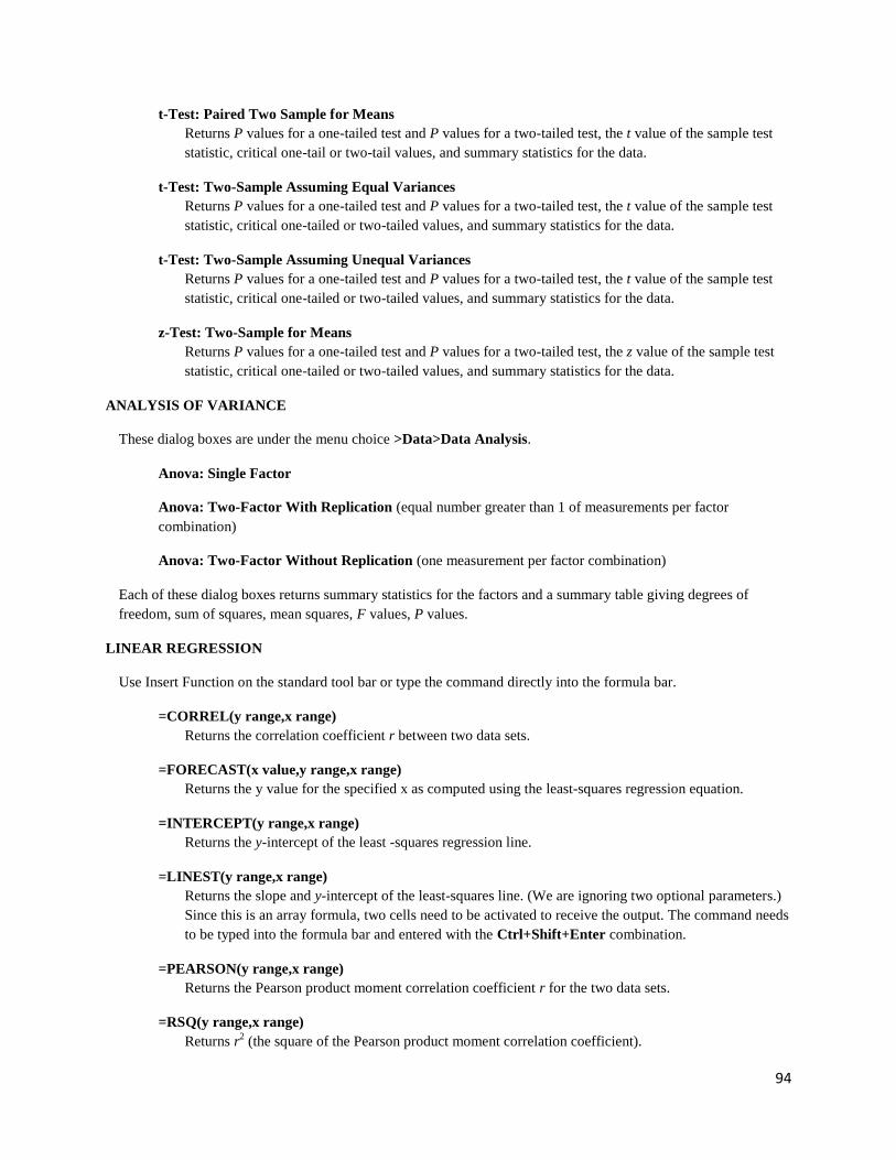
94
t-Test: Paired Two Sample for Means
Returns P values for a one-tailed test and P values for a two-tailed test, the t value of the sample test
statistic, critical one-tail or two-tail values, and summary statistics for the data.
t-Test: Two-Sample Assuming Equal Variances
Returns P values for a one-tailed test and P values for a two-tailed test, the t value of the sample test
statistic, critical one-tailed or two-tailed values, and summary statistics for the data.
t-Test: Two-Sample Assuming Unequal Variances
Returns P values for a one-tailed test and P values for a two-tailed test, the t value of the sample test
statistic, critical one-tailed or two-tailed values, and summary statistics for the data.
z-Test: Two-Sample for Means
Returns P values for a one-tailed test and P values for a two-tailed test, the z value of the sample test
statistic, critical one-tailed or two-tailed values, and summary statistics for the data.
ANALYSIS OF VARIANCE
These dialog boxes are under the menu choice >Data>Data Analysis.
Anova: Single Factor
Anova: Two-Factor With Replication (equal number greater than 1 of measurements per factor
combination)
Anova: Two-Factor Without Replication (one measurement per factor combination)
Each of these dialog boxes returns summary statistics for the factors and a summary table giving degrees of
freedom, sum of squares, mean squares, F values, P values.
LINEAR REGRESSION
Use Insert Function on the standard tool bar or type the command directly into the formula bar.
=CORREL(y range,x range)
Returns the correlation coefficient r between two data sets.
=FORECAST(x value,y range,x range)
Returns the y value for the specified x as computed using the least-squares regression equation.
=INTERCEPT(y range,x range)
Returns the y-intercept of the least -squares regression line.
=LINEST(y range,x range)
Returns the slope and y-intercept of the least-squares line. (We are ignoring two optional parameters.)
Since this is an array formula, two cells need to be activated to receive the output. The command needs
to be typed into the formula bar and entered with the Ctrl+Shift+Enter combination.
=PEARSON(y range,x range)
Returns the Pearson product moment correlation coefficient r for the two data sets.
=RSQ(y range,x range)
Returns r2 (the square of the Pearson product moment correlation coefficient).
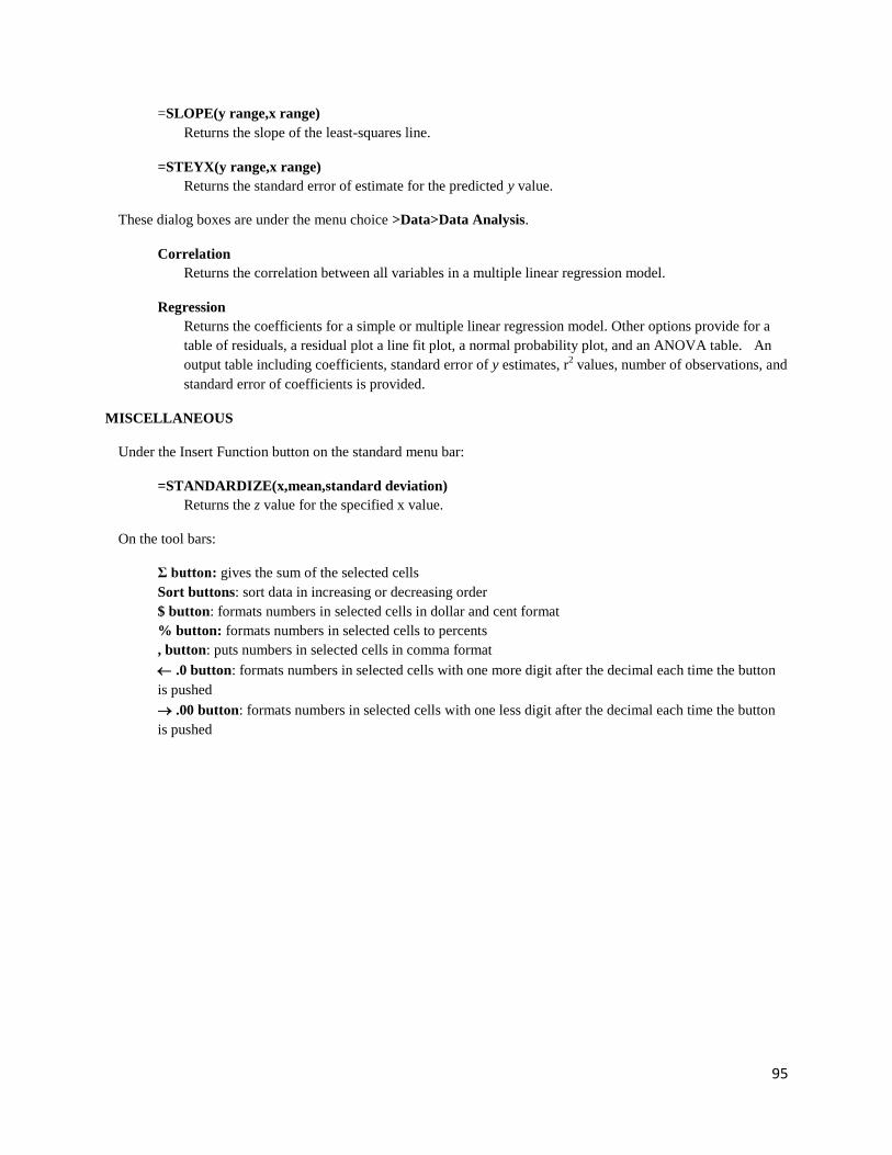
95
=SLOPE(y range,x range)
Returns the slope of the least-squares line.
=STEYX(y range,x range)
Returns the standard error of estimate for the predicted y value.
These dialog boxes are under the menu choice >Data>Data Analysis.
Correlation
Returns the correlation between all variables in a multiple linear regression model.
Regression
Returns the coefficients for a simple or multiple linear regression model. Other options provide for a
table of residuals, a residual plot a line fit plot, a normal probability plot, and an ANOVA table. An
output table including coefficients, standard error of y estimates, r2 values, number of observations, and
standard error of coefficients is provided.
MISCELLANEOUS
Under the Insert Function button on the standard menu bar:
=STANDARDIZE(x,mean,standard deviation)
Returns the z value for the specified x value.
On the tool bars:
Σ button: gives the sum of the selected cells
Sort buttons: sort data in increasing or decreasing order
$ button: formats numbers in selected cells in dollar and cent format
% button: formats numbers in selected cells to percents
, button: puts numbers in selected cells in comma format
.0 button: formats numbers in selected cells with one more digit after the decimal each time the button
is pushed
.00 button: formats numbers in selected cells with one less digit after the decimal each time the button
is pushed


Appendix: Descriptions of Data Sets on the
Student Website

3
Preface
There are over 70 data sets saved in Excel, Minitab Portable, SPSS, TI-83 Plus, TI-84 Plus, TI-Nspire/ASCII
formats to accompany Understanding Statistics, 6th
edition. These files can be found on the Brase/Brase statistics
site at http://www.cengage.com/statistics/brase. The data sets are organized by category.
A. The following are provided for each data set:
1. The category
2. A brief description of the data and variables with a reference when appropriate
3. File names for Excel, Minitab, SPSS, and TI-83 Plus, TI-84 Plus, TI-Nspire/ASCII formats
B. The categories are
1. Single variable large and small sample
File name prefix Sv followed by the data set number
42 data sets…………… …………………………………….page A-4
2. Two variable independent samples (large and small sample)
File name prefix Tvis followed by the data set number
10 data sets…………………………………………………...page A-21
3. Two variable dependent samples appropriate for t-tests
File name prefix Tvcds followed by the data set number
10 data sets……………………………………………………page A-26
4. Simple linear regression
File name prefix Slr followed by the data set number
12 data sets……………………………………………………page A-30
C. The formats are
1. Excel files in subdirectory Excel_10e. These files have suffix .xls
2. Minitab portable files in subdirectory Minitab_10e. These files have suffix .zip
3. TI-83 Plus and TI-84 Plus/ASCII files in subdirectory TI8384_10e. These files have suffix .zip
4. SPSS files in subdirectory SPSS_10e. These files have suffix .zip
Suggestions for Using the Data Sets
1. Single variable large and small sample (file name prefix Sv)
These data sets are appropriate for:
Graphs: Histograms, box plots
Descriptive statistics: Mean, median, mode, variance, standard deviation, coefficient of variation, 5 number
summary
Inferential statistics: Confidence intervals for the population mean, hypothesis tests of a single mean
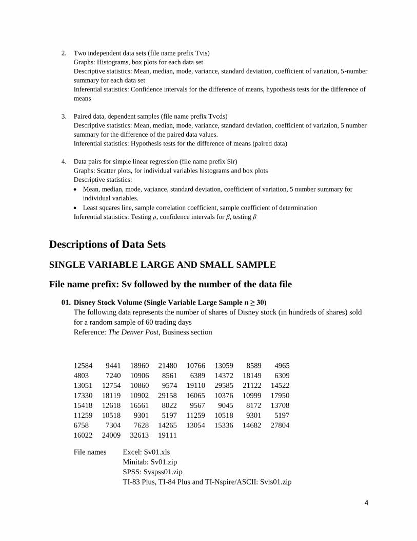
4
2. Two independent data sets (file name prefix Tvis)
Graphs: Histograms, box plots for each data set
Descriptive statistics: Mean, median, mode, variance, standard deviation, coefficient of variation, 5-number
summary for each data set
Inferential statistics: Confidence intervals for the difference of means, hypothesis tests for the difference of
means
3. Paired data, dependent samples (file name prefix Tvcds)
Descriptive statistics: Mean, median, mode, variance, standard deviation, coefficient of variation, 5 number
summary for the difference of the paired data values.
Inferential statistics: Hypothesis tests for the difference of means (paired data)
4. Data pairs for simple linear regression (file name prefix Slr)
Graphs: Scatter plots, for individual variables histograms and box plots
Descriptive statistics:
Mean, median, mode, variance, standard deviation, coefficient of variation, 5 number summary for
individual variables.
Least squares line, sample correlation coefficient, sample coefficient of determination
Inferential statistics: Testing ρ, confidence intervals for β, testing β
Descriptions of Data Sets
SINGLE VARIABLE LARGE AND SMALL SAMPLE
File name prefix: Sv followed by the number of the data file
01. Disney Stock Volume (Single Variable Large Sample n ≥ 30)
The following data represents the number of shares of Disney stock (in hundreds of shares) sold
for a random sample of 60 trading days
Reference: The Denver Post, Business section
12584 9441 18960 21480 10766 13059 8589 4965
4803 7240 10906 8561 6389 14372 18149 6309
13051 12754 10860 9574 19110 29585 21122 14522
17330 18119 10902 29158 16065 10376 10999 17950
15418 12618 16561 8022 9567 9045 8172 13708
11259 10518 9301 5197 11259 10518 9301 5197
6758 7304 7628 14265 13054 15336 14682 27804
16022 24009 32613 19111
File names Excel: Sv01.xls
Minitab: Sv01.zip
SPSS: Svspss01.zip
TI-83 Plus, TI-84 Plus and TI-Nspire/ASCII: Svls01.zip
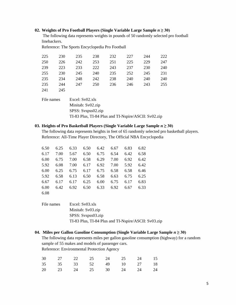
5
02. Weights of Pro Football Players (Single Variable Large Sample n ≥ 30)
The following data represents weights in pounds of 50 randomly selected pro football
linebackers.
Reference: The Sports Encyclopedia Pro Football
225 230 235 238 232 227 244 222
250 226 242 253 251 225 229 247
239 223 233 222 243 237 230 240
255 230 245 240 235 252 245 231
235 234 248 242 238 240 240 240
235 244 247 250 236 246 243 255
241 245
File names Excel: Sv02.xls
Minitab: Sv02.zip
SPSS: Svspss02.zip
TI-83 Plus, TI-84 Plus and TI-Nspire/ASCII: Sv02.zip
03. Heights of Pro Basketball Players (Single Variable Large Sample n ≥ 30)
The following data represents heights in feet of 65 randomly selected pro basketball players.
Reference: All-Time Player Directory, The Official NBA Encyclopedia
6.50 6.25 6.33 6.50 6.42 6.67 6.83 6.82
6.17 7.00 5.67 6.50 6.75 6.54 6.42 6.58
6.00 6.75 7.00 6.58 6.29 7.00 6.92 6.42
5.92 6.08 7.00 6.17 6.92 7.00 5.92 6.42
6.00 6.25 6.75 6.17 6.75 6.58 6.58 6.46
5.92 6.58 6.13 6.50 6.58 6.63 6.75 6.25
6.67 6.17 6.17 6.25 6.00 6.75 6.17 6.83
6.00 6.42 6.92 6.50 6.33 6.92 6.67 6.33
6.08
File names Excel: Sv03.xls
Minitab: Sv03.zip
SPSS: Svspss03.zip
TI-83 Plus, TI-84 Plus and TI-Nspire/ASCII: Sv03.zip
04. Miles per Gallon Gasoline Consumption (Single Variable Large Sample n ≥ 30)
The following data represents miles per gallon gasoline consumption (highway) for a random
sample of 55 makes and models of passenger cars.
Reference: Environmental Protection Agency
30 27 22 25 24 25 24 15
35 35 33 52 49 10 27 18
20 23 24 25 30 24 24 24
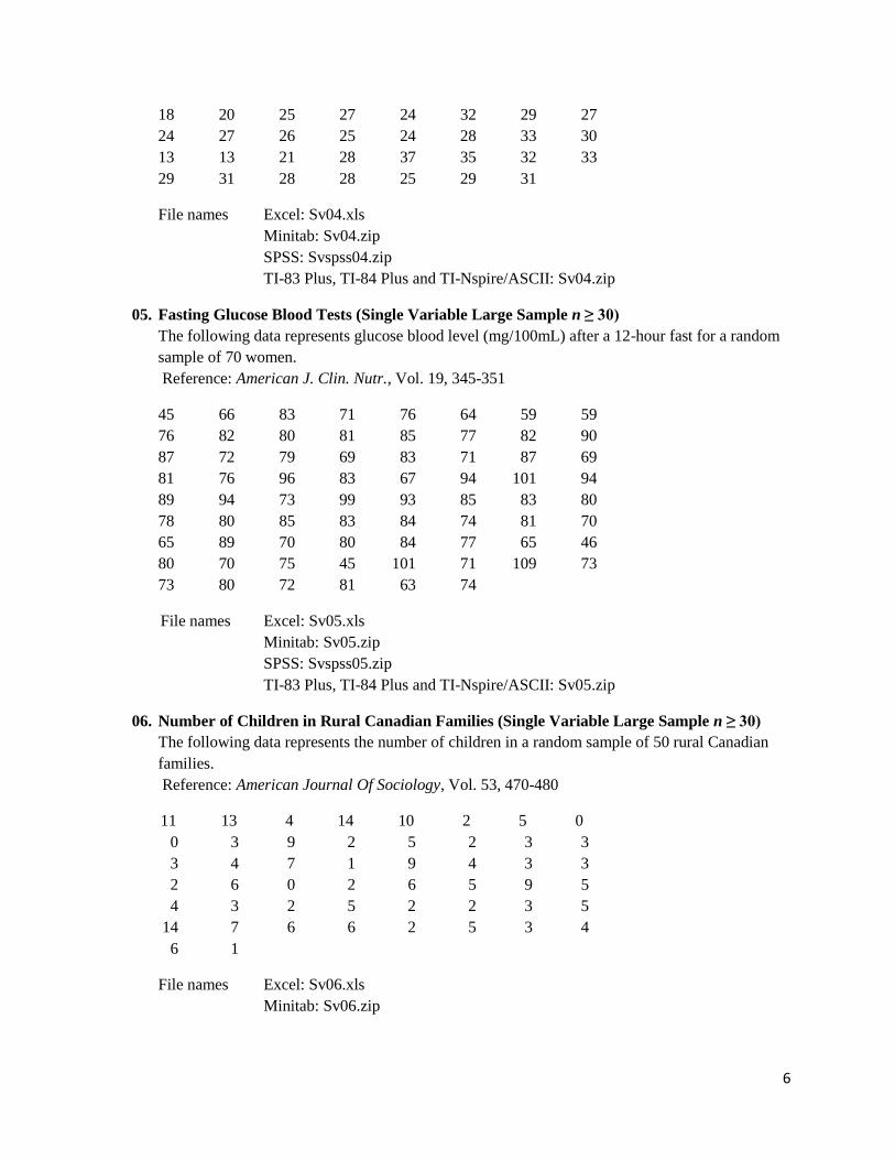
6
18 20 25 27 24 32 29 27
24 27 26 25 24 28 33 30
13 13 21 28 37 35 32 33
29 31 28 28 25 29 31
File names Excel: Sv04.xls
Minitab: Sv04.zip
SPSS: Svspss04.zip
TI-83 Plus, TI-84 Plus and TI-Nspire/ASCII: Sv04.zip
05. Fasting Glucose Blood Tests (Single Variable Large Sample n ≥ 30)
The following data represents glucose blood level (mg/100mL) after a 12-hour fast for a random
sample of 70 women.
Reference: American J. Clin. Nutr., Vol. 19, 345-351
45 66 83 71 76 64 59 59
76 82 80 81 85 77 82 90
87 72 79 69 83 71 87 69
81 76 96 83 67 94 101 94
89 94 73 99 93 85 83 80
78 80 85 83 84 74 81 70
65 89 70 80 84 77 65 46
80 70 75 45 101 71 109 73
73 80 72 81 63 74
File names Excel: Sv05.xls
Minitab: Sv05.zip
SPSS: Svspss05.zip
TI-83 Plus, TI-84 Plus and TI-Nspire/ASCII: Sv05.zip
06. Number of Children in Rural Canadian Families (Single Variable Large Sample n ≥ 30)
The following data represents the number of children in a random sample of 50 rural Canadian
families.
Reference: American Journal Of Sociology, Vol. 53, 470-480
11 13 4 14 10 2 5 0
0 3 9 2 5 2 3 3
3 4 7 1 9 4 3 3
2 6 0 2 6 5 9 5
4 3 2 5 2 2 3 5
14 7 6 6 2 5 3 4
6 1
File names Excel: Sv06.xls
Minitab: Sv06.zip
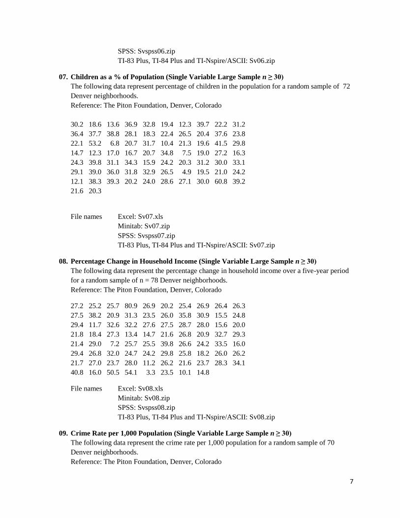
7
SPSS: Svspss06.zip
TI-83 Plus, TI-84 Plus and TI-Nspire/ASCII: Sv06.zip
07. Children as a % of Population (Single Variable Large Sample n ≥ 30)
The following data represent percentage of children in the population for a random sample of 72
Denver neighborhoods.
Reference: The Piton Foundation, Denver, Colorado
30.2 18.6 13.6 36.9 32.8 19.4 12.3 39.7 22.2 31.2
36.4 37.7 38.8 28.1 18.3 22.4 26.5 20.4 37.6 23.8
22.1 53.2 6.8 20.7 31.7 10.4 21.3 19.6 41.5 29.8
14.7 12.3 17.0 16.7 20.7 34.8 7.5 19.0 27.2 16.3
24.3 39.8 31.1 34.3 15.9 24.2 20.3 31.2 30.0 33.1
29.1 39.0 36.0 31.8 32.9 26.5 4.9 19.5 21.0 24.2
12.1 38.3 39.3 20.2 24.0 28.6 27.1 30.0 60.8 39.2
21.6 20.3
File names Excel: Sv07.xls
Minitab: Sv07.zip
SPSS: Svspss07.zip
TI-83 Plus, TI-84 Plus and TI-Nspire/ASCII: Sv07.zip
08. Percentage Change in Household Income (Single Variable Large Sample n ≥ 30)
The following data represent the percentage change in household income over a five-year period
for a random sample of n = 78 Denver neighborhoods.
Reference: The Piton Foundation, Denver, Colorado
27.2 25.2 25.7 80.9 26.9 20.2 25.4 26.9 26.4 26.3
27.5 38.2 20.9 31.3 23.5 26.0 35.8 30.9 15.5 24.8
29.4 11.7 32.6 32.2 27.6 27.5 28.7 28.0 15.6 20.0
21.8 18.4 27.3 13.4 14.7 21.6 26.8 20.9 32.7 29.3
21.4 29.0 7.2 25.7 25.5 39.8 26.6 24.2 33.5 16.0
29.4 26.8 32.0 24.7 24.2 29.8 25.8 18.2 26.0 26.2
21.7 27.0 23.7 28.0 11.2 26.2 21.6 23.7 28.3 34.1
40.8 16.0 50.5 54.1 3.3 23.5 10.1 14.8
File names Excel: Sv08.xls
Minitab: Sv08.zip
SPSS: Svspss08.zip
TI-83 Plus, TI-84 Plus and TI-Nspire/ASCII: Sv08.zip
09. Crime Rate per 1,000 Population (Single Variable Large Sample n ≥ 30)
The following data represent the crime rate per 1,000 population for a random sample of 70
Denver neighborhoods.
Reference: The Piton Foundation, Denver, Colorado
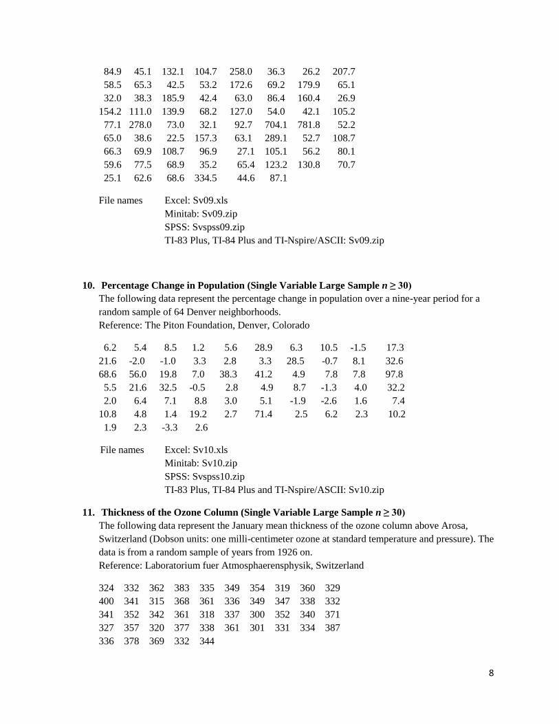
8
84.9 45.1 132.1 104.7 258.0 36.3 26.2 207.7
58.5 65.3 42.5 53.2 172.6 69.2 179.9 65.1
32.0 38.3 185.9 42.4 63.0 86.4 160.4 26.9
154.2 111.0 139.9 68.2 127.0 54.0 42.1 105.2
77.1 278.0 73.0 32.1 92.7 704.1 781.8 52.2
65.0 38.6 22.5 157.3 63.1 289.1 52.7 108.7
66.3 69.9 108.7 96.9 27.1 105.1 56.2 80.1
59.6 77.5 68.9 35.2 65.4 123.2 130.8 70.7
25.1 62.6 68.6 334.5 44.6 87.1
File names Excel: Sv09.xls
Minitab: Sv09.zip
SPSS: Svspss09.zip
TI-83 Plus, TI-84 Plus and TI-Nspire/ASCII: Sv09.zip
10. Percentage Change in Population (Single Variable Large Sample n ≥ 30)
The following data represent the percentage change in population over a nine-year period for a
random sample of 64 Denver neighborhoods.
Reference: The Piton Foundation, Denver, Colorado
6.2 5.4 8.5 1.2 5.6 28.9 6.3 10.5 -1.5 17.3
21.6 -2.0 -1.0 3.3 2.8 3.3 28.5 -0.7 8.1 32.6
68.6 56.0 19.8 7.0 38.3 41.2 4.9 7.8 7.8 97.8
5.5 21.6 32.5 -0.5 2.8 4.9 8.7 -1.3 4.0 32.2
2.0 6.4 7.1 8.8 3.0 5.1 -1.9 -2.6 1.6 7.4
10.8 4.8 1.4 19.2 2.7 71.4 2.5 6.2 2.3 10.2
1.9 2.3 -3.3 2.6
File names Excel: Sv10.xls
Minitab: Sv10.zip
SPSS: Svspss10.zip
TI-83 Plus, TI-84 Plus and TI-Nspire/ASCII: Sv10.zip
11. Thickness of the Ozone Column (Single Variable Large Sample n ≥ 30)
The following data represent the January mean thickness of the ozone column above Arosa,
Switzerland (Dobson units: one milli-centimeter ozone at standard temperature and pressure). The
data is from a random sample of years from 1926 on.
Reference: Laboratorium fuer Atmosphaerensphysik, Switzerland
324 332 362 383 335 349 354 319 360 329
400 341 315 368 361 336 349 347 338 332
341 352 342 361 318 337 300 352 340 371
327 357 320 377 338 361 301 331 334 387
336 378 369 332 344
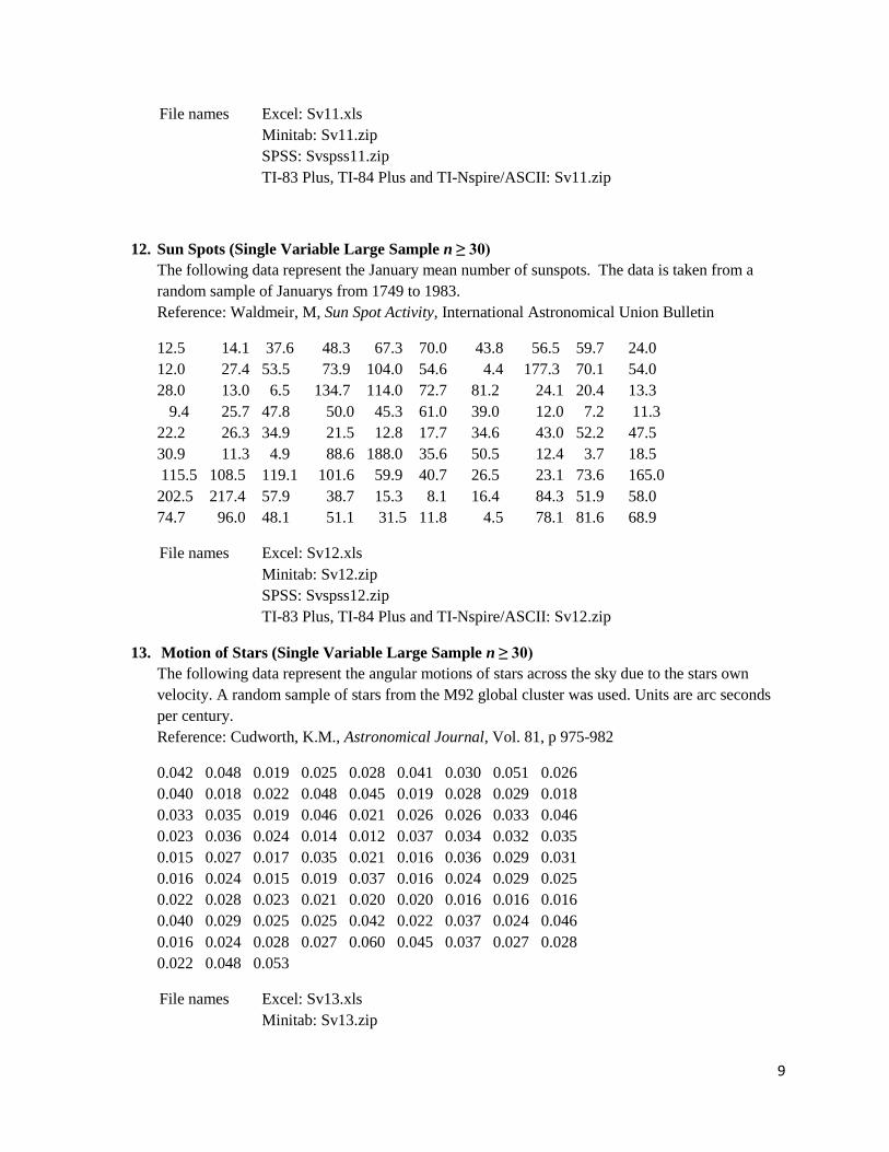
9
File names Excel: Sv11.xls
Minitab: Sv11.zip
SPSS: Svspss11.zip
TI-83 Plus, TI-84 Plus and TI-Nspire/ASCII: Sv11.zip
12. Sun Spots (Single Variable Large Sample n ≥ 30)
The following data represent the January mean number of sunspots. The data is taken from a
random sample of Januarys from 1749 to 1983.
Reference: Waldmeir, M, Sun Spot Activity, International Astronomical Union Bulletin
12.5 14.1 37.6 48.3 67.3 70.0 43.8 56.5 59.7 24.0
12.0 27.4 53.5 73.9 104.0 54.6 4.4 177.3 70.1 54.0
28.0 13.0 6.5 134.7 114.0 72.7 81.2 24.1 20.4 13.3
9.4 25.7 47.8 50.0 45.3 61.0 39.0 12.0 7.2 11.3
22.2 26.3 34.9 21.5 12.8 17.7 34.6 43.0 52.2 47.5
30.9 11.3 4.9 88.6 188.0 35.6 50.5 12.4 3.7 18.5
115.5 108.5 119.1 101.6 59.9 40.7 26.5 23.1 73.6 165.0
202.5 217.4 57.9 38.7 15.3 8.1 16.4 84.3 51.9 58.0
74.7 96.0 48.1 51.1 31.5 11.8 4.5 78.1 81.6 68.9
File names Excel: Sv12.xls
Minitab: Sv12.zip
SPSS: Svspss12.zip
TI-83 Plus, TI-84 Plus and TI-Nspire/ASCII: Sv12.zip
13. Motion of Stars (Single Variable Large Sample n ≥ 30)
The following data represent the angular motions of stars across the sky due to the stars own
velocity. A random sample of stars from the M92 global cluster was used. Units are arc seconds
per century.
Reference: Cudworth, K.M., Astronomical Journal, Vol. 81, p 975-982
0.042 0.048 0.019 0.025 0.028 0.041 0.030 0.051 0.026
0.040 0.018 0.022 0.048 0.045 0.019 0.028 0.029 0.018
0.033 0.035 0.019 0.046 0.021 0.026 0.026 0.033 0.046
0.023 0.036 0.024 0.014 0.012 0.037 0.034 0.032 0.035
0.015 0.027 0.017 0.035 0.021 0.016 0.036 0.029 0.031
0.016 0.024 0.015 0.019 0.037 0.016 0.024 0.029 0.025
0.022 0.028 0.023 0.021 0.020 0.020 0.016 0.016 0.016
0.040 0.029 0.025 0.025 0.042 0.022 0.037 0.024 0.046
0.016 0.024 0.028 0.027 0.060 0.045 0.037 0.027 0.028
0.022 0.048 0.053
File names Excel: Sv13.xls
Minitab: Sv13.zip
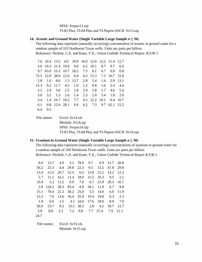
10
SPSS: Svspss13.zip
TI-83 Plus, TI-84 Plus and TI-Nspire/ASCII: Sv13.zip
14. Arsenic and Ground Water (Single Variable Large Sample n ≥ 30)
The following data represent (naturally occurring) concentration of arsenic in ground water for a
random sample of 102 Northwest Texas wells. Units are parts per billion.
Reference: Nichols, C.E. and Kane, V.E., Union Carbide Technical Report K/UR-1
7.6 10.4 13.5 4.0 19.9 16.0 12.0 12.2 11.4 12.7
3.0 10.3 21.4 19.4 9.0 6.5 10.1 8.7 9.7 6.4
9.7 63.0 15.5 10.7 18.2 7.5 6.1 6.7 6.9 0.8
73.5 12.0 28.0 12.6 9.4 6.2 15.3 7.3 10.7 15.9
5.8 1.0 8.6 1.3 13.7 2.8 2.4 1.4 2.9 13.1
15.3 9.2 11.7 4.5 1.0 1.2 0.8 1.0 2.4 4.4
2.2 2.9 3.6 2.5 1.8 5.9 2.8 1.7 4.6 5.4
3.0 3.1 1.3 2.6 1.4 2.3 1.0 5.4 1.8 2.6
3.4 1.4 10.7 18.2 7.7 6.5 12.2 10.1 6.4 10.7
6.1 0.8 12.0 28.1 9.4 6.2 7.3 9.7 62.1 15.5
6.4 9.5
File names Excel: Sv14.xls
Minitab: Sv14.zip
SPSS: Svspss14.zip
TI-83 Plus, TI-84 Plus and TI-Nspire/ASCII: Sv14.zip
15. Uranium in Ground Water (Single Variable Large Sample n ≥ 30)
The following data represent (naturally occurring) concentrations of uranium in ground water for
a random sample of 100 Northwest Texas wells. Units are parts per billion.
Reference: Nichols, C.E. and Kane, V.E., Union Carbide Technical Report K/UR-1
8.0 13.7 4.9 3.1 78.0 9.7 6.9 21.7 26.8
56.2 25.3 4.4 29.8 22.3 9.5 13.5 47.8 29.8
13.4 21.0 26.7 52.5 6.5 15.8 21.2 13.2 12.3
5.7 11.1 16.1 11.4 18.0 15.5 35.3 9.5 2.1
10.4 5.3 11.2 0.9 7.8 6.7 21.9 20.3 16.7
2.9 124.2 58.3 83.4 8.9 18.1 11.9 6.7 9.8
15.1 70.4 21.3 58.2 25.0 5.5 14.0 6.0 11.9
15.3 7.0 13.6 16.4 35.9 19.4 19.8 6.3 2.3
1.9 6.0 1.5 4.1 34.0 17.6 18.6 8.0 7.9
56.9 53.7 8.3 33.5 38.2 2.8 4.2 18.7 12.7
3.8 8.8 2.3 7.2 9.8 7.7 27.4 7.9 11.1
24.7
File names Excel: Sv15.xls
Minitab: Sv15.zip
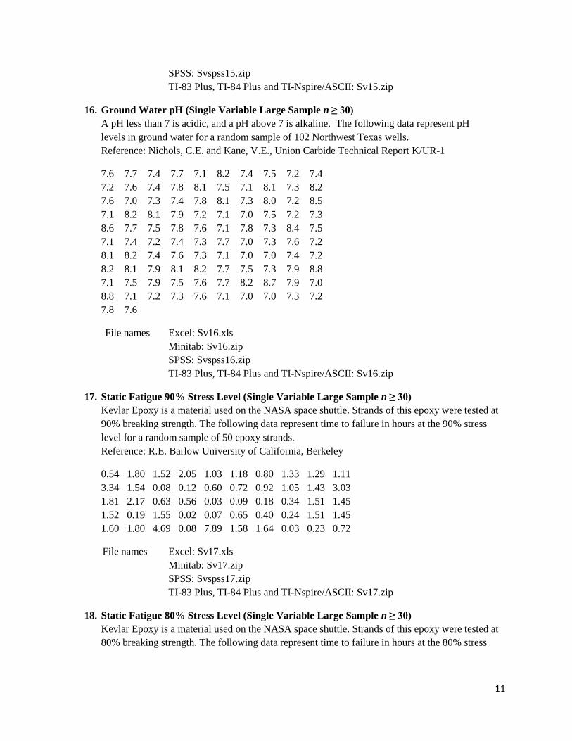
11
SPSS: Svspss15.zip
TI-83 Plus, TI-84 Plus and TI-Nspire/ASCII: Sv15.zip
16. Ground Water pH (Single Variable Large Sample n ≥ 30)
A pH less than 7 is acidic, and a pH above 7 is alkaline. The following data represent pH
levels in ground water for a random sample of 102 Northwest Texas wells.
Reference: Nichols, C.E. and Kane, V.E., Union Carbide Technical Report K/UR-1
7.6 7.7 7.4 7.7 7.1 8.2 7.4 7.5 7.2 7.4
7.2 7.6 7.4 7.8 8.1 7.5 7.1 8.1 7.3 8.2
7.6 7.0 7.3 7.4 7.8 8.1 7.3 8.0 7.2 8.5
7.1 8.2 8.1 7.9 7.2 7.1 7.0 7.5 7.2 7.3
8.6 7.7 7.5 7.8 7.6 7.1 7.8 7.3 8.4 7.5
7.1 7.4 7.2 7.4 7.3 7.7 7.0 7.3 7.6 7.2
8.1 8.2 7.4 7.6 7.3 7.1 7.0 7.0 7.4 7.2
8.2 8.1 7.9 8.1 8.2 7.7 7.5 7.3 7.9 8.8
7.1 7.5 7.9 7.5 7.6 7.7 8.2 8.7 7.9 7.0
8.8 7.1 7.2 7.3 7.6 7.1 7.0 7.0 7.3 7.2
7.8 7.6
File names Excel: Sv16.xls
Minitab: Sv16.zip
SPSS: Svspss16.zip
TI-83 Plus, TI-84 Plus and TI-Nspire/ASCII: Sv16.zip
17. Static Fatigue 90% Stress Level (Single Variable Large Sample n ≥ 30)
Kevlar Epoxy is a material used on the NASA space shuttle. Strands of this epoxy were tested at
90% breaking strength. The following data represent time to failure in hours at the 90% stress
level for a random sample of 50 epoxy strands.
Reference: R.E. Barlow University of California, Berkeley
0.54 1.80 1.52 2.05 1.03 1.18 0.80 1.33 1.29 1.11
3.34 1.54 0.08 0.12 0.60 0.72 0.92 1.05 1.43 3.03
1.81 2.17 0.63 0.56 0.03 0.09 0.18 0.34 1.51 1.45
1.52 0.19 1.55 0.02 0.07 0.65 0.40 0.24 1.51 1.45
1.60 1.80 4.69 0.08 7.89 1.58 1.64 0.03 0.23 0.72
File names Excel: Sv17.xls
Minitab: Sv17.zip
SPSS: Svspss17.zip
TI-83 Plus, TI-84 Plus and TI-Nspire/ASCII: Sv17.zip
18. Static Fatigue 80% Stress Level (Single Variable Large Sample n ≥ 30)
Kevlar Epoxy is a material used on the NASA space shuttle. Strands of this epoxy were tested at
80% breaking strength. The following data represent time to failure in hours at the 80% stress
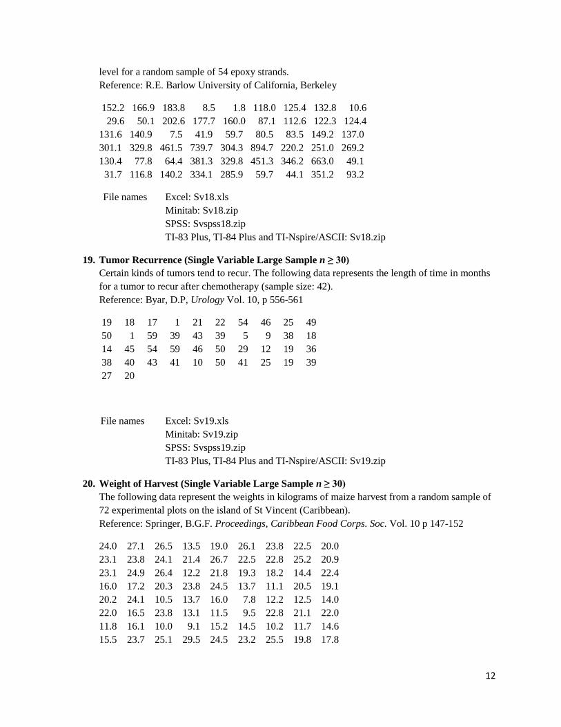
12
level for a random sample of 54 epoxy strands.
Reference: R.E. Barlow University of California, Berkeley
152.2 166.9 183.8 8.5 1.8 118.0 125.4 132.8 10.6
29.6 50.1 202.6 177.7 160.0 87.1 112.6 122.3 124.4
131.6 140.9 7.5 41.9 59.7 80.5 83.5 149.2 137.0
301.1 329.8 461.5 739.7 304.3 894.7 220.2 251.0 269.2
130.4 77.8 64.4 381.3 329.8 451.3 346.2 663.0 49.1
31.7 116.8 140.2 334.1 285.9 59.7 44.1 351.2 93.2
File names Excel: Sv18.xls
Minitab: Sv18.zip
SPSS: Svspss18.zip
TI-83 Plus, TI-84 Plus and TI-Nspire/ASCII: Sv18.zip
19. Tumor Recurrence (Single Variable Large Sample n ≥ 30)
Certain kinds of tumors tend to recur. The following data represents the length of time in months
for a tumor to recur after chemotherapy (sample size: 42).
Reference: Byar, D.P, Urology Vol. 10, p 556-561
19 18 17 1 21 22 54 46 25 49
50 1 59 39 43 39 5 9 38 18
14 45 54 59 46 50 29 12 19 36
38 40 43 41 10 50 41 25 19 39
27 20
File names Excel: Sv19.xls
Minitab: Sv19.zip
SPSS: Svspss19.zip
TI-83 Plus, TI-84 Plus and TI-Nspire/ASCII: Sv19.zip
20. Weight of Harvest (Single Variable Large Sample n ≥ 30)
The following data represent the weights in kilograms of maize harvest from a random sample of
72 experimental plots on the island of St Vincent (Caribbean).
Reference: Springer, B.G.F. Proceedings, Caribbean Food Corps. Soc. Vol. 10 p 147-152
24.0 27.1 26.5 13.5 19.0 26.1 23.8 22.5 20.0
23.1 23.8 24.1 21.4 26.7 22.5 22.8 25.2 20.9
23.1 24.9 26.4 12.2 21.8 19.3 18.2 14.4 22.4
16.0 17.2 20.3 23.8 24.5 13.7 11.1 20.5 19.1
20.2 24.1 10.5 13.7 16.0 7.8 12.2 12.5 14.0
22.0 16.5 23.8 13.1 11.5 9.5 22.8 21.1 22.0
11.8 16.1 10.0 9.1 15.2 14.5 10.2 11.7 14.6
15.5 23.7 25.1 29.5 24.5 23.2 25.5 19.8 17.8
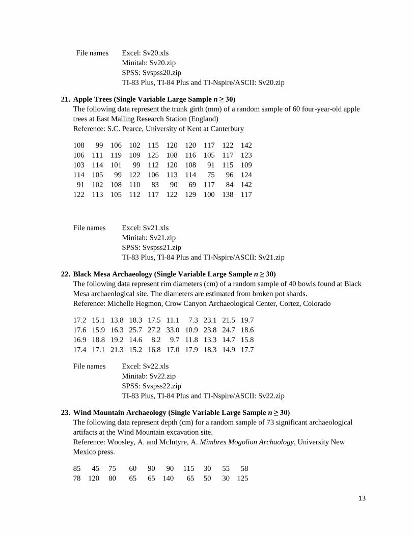
13
File names Excel: Sv20.xls
Minitab: Sv20.zip
SPSS: Svspss20.zip
TI-83 Plus, TI-84 Plus and TI-Nspire/ASCII: Sv20.zip
21. Apple Trees (Single Variable Large Sample n ≥ 30)
The following data represent the trunk girth (mm) of a random sample of 60 four-year-old apple
trees at East Malling Research Station (England)
Reference: S.C. Pearce, University of Kent at Canterbury
108 99 106 102 115 120 120 117 122 142
106 111 119 109 125 108 116 105 117 123
103 114 101 99 112 120 108 91 115 109
114 105 99 122 106 113 114 75 96 124
91 102 108 110 83 90 69 117 84 142
122 113 105 112 117 122 129 100 138 117
File names Excel: Sv21.xls
Minitab: Sv21.zip
SPSS: Svspss21.zip
TI-83 Plus, TI-84 Plus and TI-Nspire/ASCII: Sv21.zip
22. Black Mesa Archaeology (Single Variable Large Sample n ≥ 30)
The following data represent rim diameters (cm) of a random sample of 40 bowls found at Black
Mesa archaeological site. The diameters are estimated from broken pot shards.
Reference: Michelle Hegmon, Crow Canyon Archaeological Center, Cortez, Colorado
17.2 15.1 13.8 18.3 17.5 11.1 7.3 23.1 21.5 19.7
17.6 15.9 16.3 25.7 27.2 33.0 10.9 23.8 24.7 18.6
16.9 18.8 19.2 14.6 8.2 9.7 11.8 13.3 14.7 15.8
17.4 17.1 21.3 15.2 16.8 17.0 17.9 18.3 14.9 17.7
File names Excel: Sv22.xls
Minitab: Sv22.zip
SPSS: Svspss22.zip
TI-83 Plus, TI-84 Plus and TI-Nspire/ASCII: Sv22.zip
23. Wind Mountain Archaeology (Single Variable Large Sample n ≥ 30)
The following data represent depth (cm) for a random sample of 73 significant archaeological
artifacts at the Wind Mountain excavation site.
Reference: Woosley, A. and McIntyre, A. Mimbres Mogolion Archaology, University New
Mexico press.
85 45 75 60 90 90 115 30 55 58
78 120 80 65 65 140 65 50 30 125
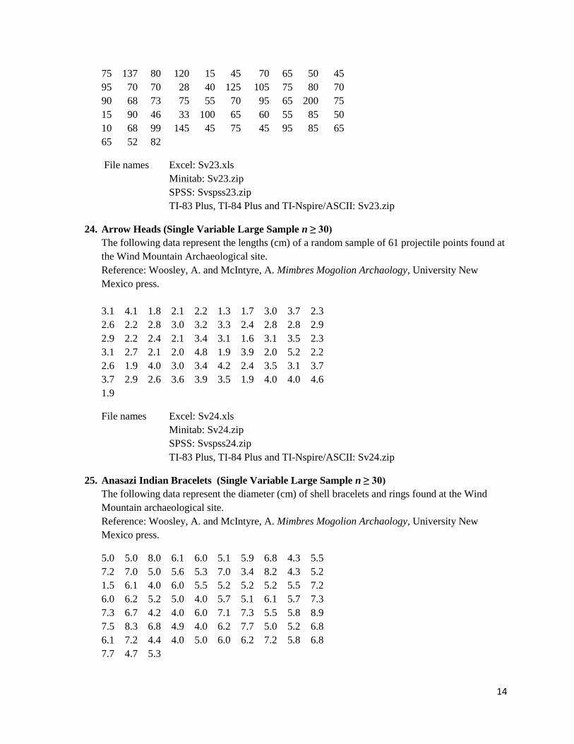
14
75 137 80 120 15 45 70 65 50 45
95 70 70 28 40 125 105 75 80 70
90 68 73 75 55 70 95 65 200 75
15 90 46 33 100 65 60 55 85 50
10 68 99 145 45 75 45 95 85 65
65 52 82
File names Excel: Sv23.xls
Minitab: Sv23.zip
SPSS: Svspss23.zip
TI-83 Plus, TI-84 Plus and TI-Nspire/ASCII: Sv23.zip
24. Arrow Heads (Single Variable Large Sample n ≥ 30)
The following data represent the lengths (cm) of a random sample of 61 projectile points found at
the Wind Mountain Archaeological site.
Reference: Woosley, A. and McIntyre, A. Mimbres Mogolion Archaology, University New
Mexico press.
3.1 4.1 1.8 2.1 2.2 1.3 1.7 3.0 3.7 2.3
2.6 2.2 2.8 3.0 3.2 3.3 2.4 2.8 2.8 2.9
2.9 2.2 2.4 2.1 3.4 3.1 1.6 3.1 3.5 2.3
3.1 2.7 2.1 2.0 4.8 1.9 3.9 2.0 5.2 2.2
2.6 1.9 4.0 3.0 3.4 4.2 2.4 3.5 3.1 3.7
3.7 2.9 2.6 3.6 3.9 3.5 1.9 4.0 4.0 4.6
1.9
File names Excel: Sv24.xls
Minitab: Sv24.zip
SPSS: Svspss24.zip
TI-83 Plus, TI-84 Plus and TI-Nspire/ASCII: Sv24.zip
25. Anasazi Indian Bracelets (Single Variable Large Sample n ≥ 30)
The following data represent the diameter (cm) of shell bracelets and rings found at the Wind
Mountain archaeological site.
Reference: Woosley, A. and McIntyre, A. Mimbres Mogolion Archaology, University New
Mexico press.
5.0 5.0 8.0 6.1 6.0 5.1 5.9 6.8 4.3 5.5
7.2 7.0 5.0 5.6 5.3 7.0 3.4 8.2 4.3 5.2
1.5 6.1 4.0 6.0 5.5 5.2 5.2 5.2 5.5 7.2
6.0 6.2 5.2 5.0 4.0 5.7 5.1 6.1 5.7 7.3
7.3 6.7 4.2 4.0 6.0 7.1 7.3 5.5 5.8 8.9
7.5 8.3 6.8 4.9 4.0 6.2 7.7 5.0 5.2 6.8
6.1 7.2 4.4 4.0 5.0 6.0 6.2 7.2 5.8 6.8
7.7 4.7 5.3
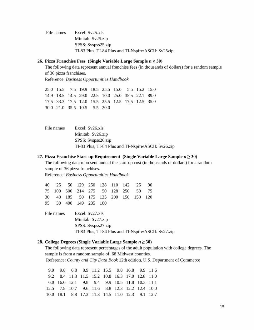
15
File names Excel: Sv25.xls
Minitab: Sv25.zip
SPSS: Svspss25.zip
TI-83 Plus, TI-84 Plus and TI-Nspire/ASCII: Sv25zip
26. Pizza Franchise Fees (Single Variable Large Sample n ≥ 30)
The following data represent annual franchise fees (in thousands of dollars) for a random sample
of 36 pizza franchises.
Reference: Business Opportunities Handbook
25.0 15.5 7.5 19.9 18.5 25.5 15.0 5.5 15.2 15.0
14.9 18.5 14.5 29.0 22.5 10.0 25.0 35.5 22.1 89.0
17.5 33.3 17.5 12.0 15.5 25.5 12.5 17.5 12.5 35.0
30.0 21.0 35.5 10.5 5.5 20.0
File names Excel: Sv26.xls
Minitab: Sv26.zip
SPSS: Svspss26.zip
TI-83 Plus, TI-84 Plus and TI-Nspire/ASCII: Sv26.zip
27. Pizza Franchise Start-up Requirement (Single Variable Large Sample n ≥ 30)
The following data represent annual the start-up cost (in thousands of dollars) for a random
sample of 36 pizza franchises.
Reference: Business Opportunities Handbook
40 25 50 129 250 128 110 142 25 90
75 100 500 214 275 50 128 250 50 75
30 40 185 50 175 125 200 150 150 120
95 30 400 149 235 100
File names Excel: Sv27.xls
Minitab: Sv27.zip
SPSS: Svspss27.zip
TI-83 Plus, TI-84 Plus and TI-Nspire/ASCII: Sv27.zip
28. College Degrees (Single Variable Large Sample n ≥ 30)
The following data represent percentages of the adult population with college degrees. The
sample is from a random sample of 68 Midwest counties.
Reference: County and City Data Book 12th edition, U.S. Department of Commerce
9.9 9.8 6.8 8.9 11.2 15.5 9.8 16.8 9.9 11.6
9.2 8.4 11.3 11.5 15.2 10.8 16.3 17.0 12.8 11.0
6.0 16.0 12.1 9.8 9.4 9.9 10.5 11.8 10.3 11.1
12.5 7.8 10.7 9.6 11.6 8.8 12.3 12.2 12.4 10.0
10.0 18.1 8.8 17.3 11.3 14.5 11.0 12.3 9.1 12.7
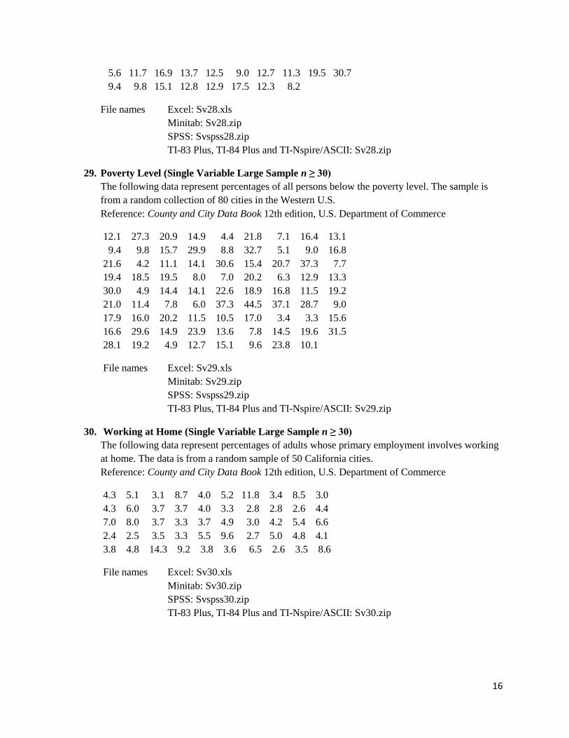
16
5.6 11.7 16.9 13.7 12.5 9.0 12.7 11.3 19.5 30.7
9.4 9.8 15.1 12.8 12.9 17.5 12.3 8.2
File names Excel: Sv28.xls
Minitab: Sv28.zip
SPSS: Svspss28.zip
TI-83 Plus, TI-84 Plus and TI-Nspire/ASCII: Sv28.zip
29. Poverty Level (Single Variable Large Sample n ≥ 30)
The following data represent percentages of all persons below the poverty level. The sample is
from a random collection of 80 cities in the Western U.S.
Reference: County and City Data Book 12th edition, U.S. Department of Commerce
12.1 27.3 20.9 14.9 4.4 21.8 7.1 16.4 13.1
9.4 9.8 15.7 29.9 8.8 32.7 5.1 9.0 16.8
21.6 4.2 11.1 14.1 30.6 15.4 20.7 37.3 7.7
19.4 18.5 19.5 8.0 7.0 20.2 6.3 12.9 13.3
30.0 4.9 14.4 14.1 22.6 18.9 16.8 11.5 19.2
21.0 11.4 7.8 6.0 37.3 44.5 37.1 28.7 9.0
17.9 16.0 20.2 11.5 10.5 17.0 3.4 3.3 15.6
16.6 29.6 14.9 23.9 13.6 7.8 14.5 19.6 31.5
28.1 19.2 4.9 12.7 15.1 9.6 23.8 10.1
File names Excel: Sv29.xls
Minitab: Sv29.zip
SPSS: Svspss29.zip
TI-83 Plus, TI-84 Plus and TI-Nspire/ASCII: Sv29.zip
30. Working at Home (Single Variable Large Sample n ≥ 30)
The following data represent percentages of adults whose primary employment involves working
at home. The data is from a random sample of 50 California cities.
Reference: County and City Data Book 12th edition, U.S. Department of Commerce
4.3 5.1 3.1 8.7 4.0 5.2 11.8 3.4 8.5 3.0
4.3 6.0 3.7 3.7 4.0 3.3 2.8 2.8 2.6 4.4
7.0 8.0 3.7 3.3 3.7 4.9 3.0 4.2 5.4 6.6
2.4 2.5 3.5 3.3 5.5 9.6 2.7 5.0 4.8 4.1
3.8 4.8 14.3 9.2 3.8 3.6 6.5 2.6 3.5 8.6
File names Excel: Sv30.xls
Minitab: Sv30.zip
SPSS: Svspss30.zip
TI-83 Plus, TI-84 Plus and TI-Nspire/ASCII: Sv30.zip
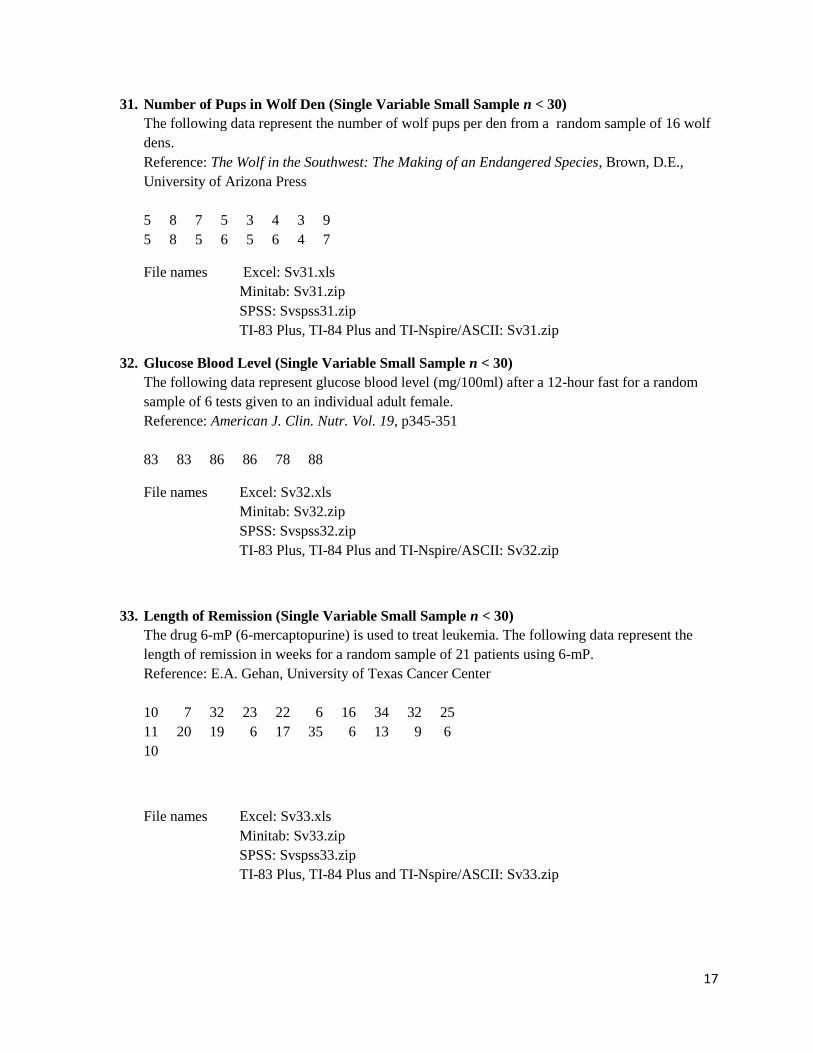
17
31. Number of Pups in Wolf Den (Single Variable Small Sample n < 30)
The following data represent the number of wolf pups per den from a random sample of 16 wolf
dens.
Reference: The Wolf in the Southwest: The Making of an Endangered Species, Brown, D.E.,
University of Arizona Press
5 8 7 5 3 4 3 9
5 8 5 6 5 6 4 7
File names Excel: Sv31.xls
Minitab: Sv31.zip
SPSS: Svspss31.zip
TI-83 Plus, TI-84 Plus and TI-Nspire/ASCII: Sv31.zip
32. Glucose Blood Level (Single Variable Small Sample n < 30)
The following data represent glucose blood level (mg/100ml) after a 12-hour fast for a random
sample of 6 tests given to an individual adult female.
Reference: American J. Clin. Nutr. Vol. 19, p345-351
83 83 86 86 78 88
File names Excel: Sv32.xls
Minitab: Sv32.zip
SPSS: Svspss32.zip
TI-83 Plus, TI-84 Plus and TI-Nspire/ASCII: Sv32.zip
33. Length of Remission (Single Variable Small Sample n < 30)
The drug 6-mP (6-mercaptopurine) is used to treat leukemia. The following data represent the
length of remission in weeks for a random sample of 21 patients using 6-mP.
Reference: E.A. Gehan, University of Texas Cancer Center
10 7 32 23 22 6 16 34 32 25
11 20 19 6 17 35 6 13 9 6
10
File names Excel: Sv33.xls
Minitab: Sv33.zip
SPSS: Svspss33.zip
TI-83 Plus, TI-84 Plus and TI-Nspire/ASCII: Sv33.zip
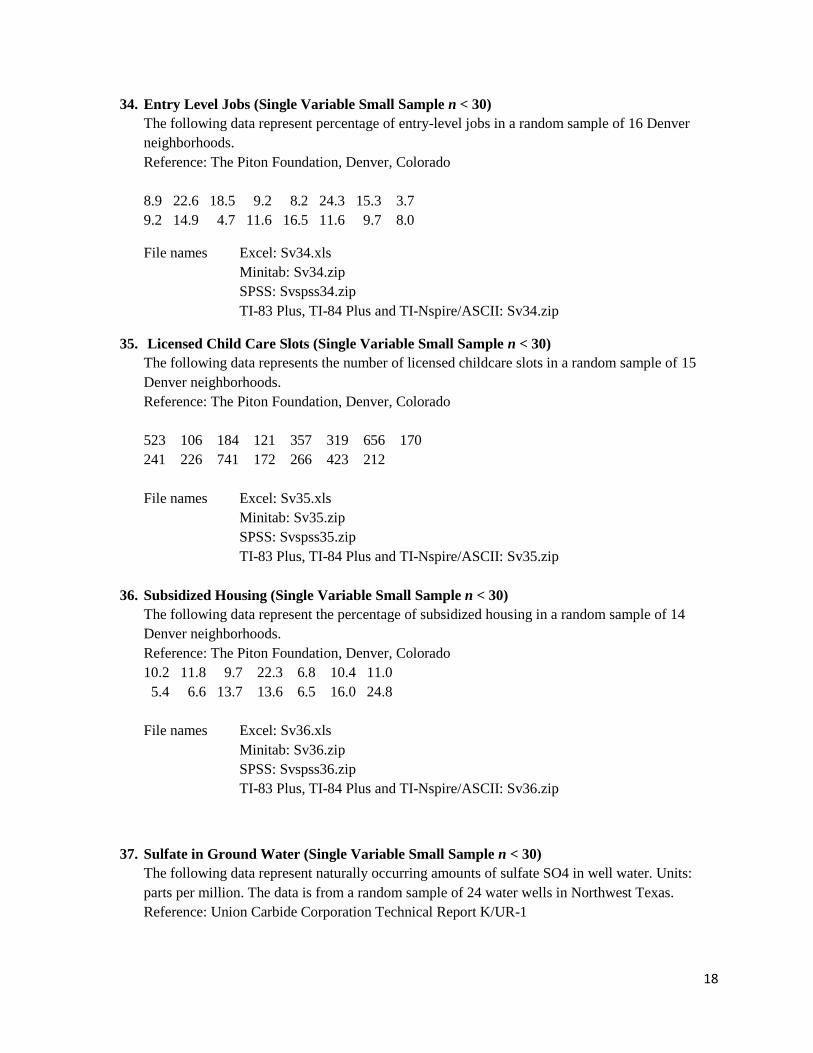
18
34. Entry Level Jobs (Single Variable Small Sample n < 30)
The following data represent percentage of entry-level jobs in a random sample of 16 Denver
neighborhoods.
Reference: The Piton Foundation, Denver, Colorado
8.9 22.6 18.5 9.2 8.2 24.3 15.3 3.7
9.2 14.9 4.7 11.6 16.5 11.6 9.7 8.0
File names Excel: Sv34.xls
Minitab: Sv34.zip
SPSS: Svspss34.zip
TI-83 Plus, TI-84 Plus and TI-Nspire/ASCII: Sv34.zip
35. Licensed Child Care Slots (Single Variable Small Sample n < 30)
The following data represents the number of licensed childcare slots in a random sample of 15
Denver neighborhoods.
Reference: The Piton Foundation, Denver, Colorado
523 106 184 121 357 319 656 170
241 226 741 172 266 423 212
File names Excel: Sv35.xls
Minitab: Sv35.zip
SPSS: Svspss35.zip
TI-83 Plus, TI-84 Plus and TI-Nspire/ASCII: Sv35.zip
36. Subsidized Housing (Single Variable Small Sample n < 30)
The following data represent the percentage of subsidized housing in a random sample of 14
Denver neighborhoods.
Reference: The Piton Foundation, Denver, Colorado
10.2 11.8 9.7 22.3 6.8 10.4 11.0
5.4 6.6 13.7 13.6 6.5 16.0 24.8
File names Excel: Sv36.xls
Minitab: Sv36.zip
SPSS: Svspss36.zip
TI-83 Plus, TI-84 Plus and TI-Nspire/ASCII: Sv36.zip
37. Sulfate in Ground Water (Single Variable Small Sample n < 30)
The following data represent naturally occurring amounts of sulfate SO4 in well water. Units:
parts per million. The data is from a random sample of 24 water wells in Northwest Texas.
Reference: Union Carbide Corporation Technical Report K/UR-1
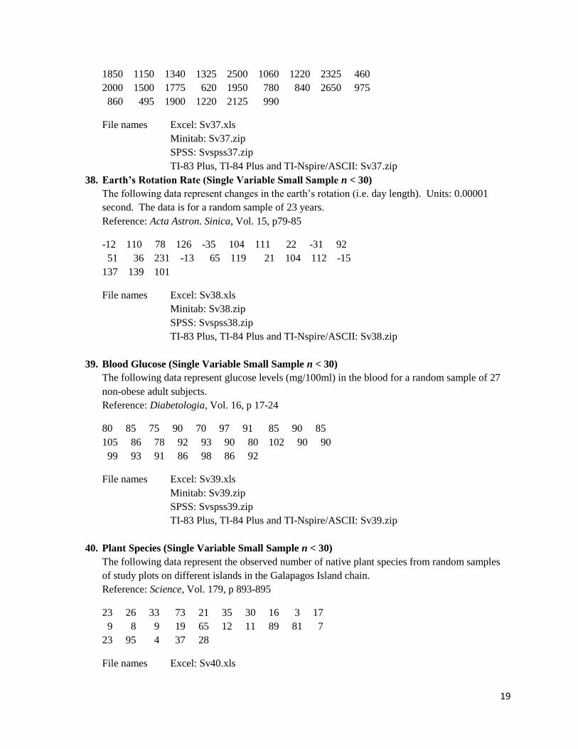
19
1850 1150 1340 1325 2500 1060 1220 2325 460
2000 1500 1775 620 1950 780 840 2650 975
860 495 1900 1220 2125 990
File names Excel: Sv37.xls
Minitab: Sv37.zip
SPSS: Svspss37.zip
TI-83 Plus, TI-84 Plus and TI-Nspire/ASCII: Sv37.zip
38. Earth’s Rotation Rate (Single Variable Small Sample n < 30)
The following data represent changes in the earth’s rotation (i.e. day length). Units: 0.00001
second. The data is for a random sample of 23 years.
Reference: Acta Astron. Sinica, Vol. 15, p79-85
-12 110 78 126 -35 104 111 22 -31 92
51 36 231 -13 65 119 21 104 112 -15
137 139 101
File names Excel: Sv38.xls
Minitab: Sv38.zip
SPSS: Svspss38.zip
TI-83 Plus, TI-84 Plus and TI-Nspire/ASCII: Sv38.zip
39. Blood Glucose (Single Variable Small Sample n < 30)
The following data represent glucose levels (mg/100ml) in the blood for a random sample of 27
non-obese adult subjects.
Reference: Diabetologia, Vol. 16, p 17-24
80 85 75 90 70 97 91 85 90 85
105 86 78 92 93 90 80 102 90 90
99 93 91 86 98 86 92
File names Excel: Sv39.xls
Minitab: Sv39.zip
SPSS: Svspss39.zip
TI-83 Plus, TI-84 Plus and TI-Nspire/ASCII: Sv39.zip
40. Plant Species (Single Variable Small Sample n < 30)
The following data represent the observed number of native plant species from random samples
of study plots on different islands in the Galapagos Island chain.
Reference: Science, Vol. 179, p 893-895
23 26 33 73 21 35 30 16 3 17
9 8 9 19 65 12 11 89 81 7
23 95 4 37 28
File names Excel: Sv40.xls
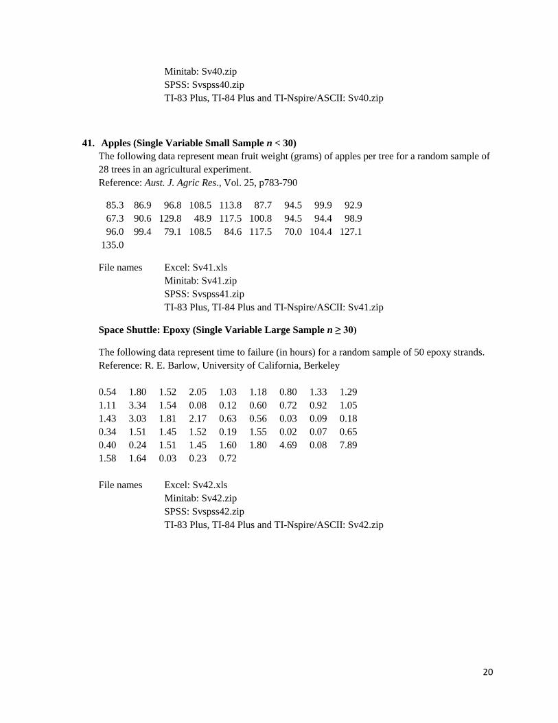
20
Minitab: Sv40.zip
SPSS: Svspss40.zip
TI-83 Plus, TI-84 Plus and TI-Nspire/ASCII: Sv40.zip
41. Apples (Single Variable Small Sample n < 30)
The following data represent mean fruit weight (grams) of apples per tree for a random sample of
28 trees in an agricultural experiment.
Reference: Aust. J. Agric Res., Vol. 25, p783-790
85.3 86.9 96.8 108.5 113.8 87.7 94.5 99.9 92.9
67.3 90.6 129.8 48.9 117.5 100.8 94.5 94.4 98.9
96.0 99.4 79.1 108.5 84.6 117.5 70.0 104.4 127.1
135.0
File names Excel: Sv41.xls
Minitab: Sv41.zip
SPSS: Svspss41.zip
TI-83 Plus, TI-84 Plus and TI-Nspire/ASCII: Sv41.zip
Space Shuttle: Epoxy (Single Variable Large Sample n ≥ 30)
The following data represent time to failure (in hours) for a random sample of 50 epoxy strands.
Reference: R. E. Barlow, University of California, Berkeley
0.54 1.80 1.52 2.05 1.03 1.18 0.80 1.33 1.29
1.11 3.34 1.54 0.08 0.12 0.60 0.72 0.92 1.05
1.43 3.03 1.81 2.17 0.63 0.56 0.03 0.09 0.18
0.34 1.51 1.45 1.52 0.19 1.55 0.02 0.07 0.65
0.40 0.24 1.51 1.45 1.60 1.80 4.69 0.08 7.89
1.58 1.64 0.03 0.23 0.72
File names Excel: Sv42.xls
Minitab: Sv42.zip
SPSS: Svspss42.zip
TI-83 Plus, TI-84 Plus and TI-Nspire/ASCII: Sv42.zip
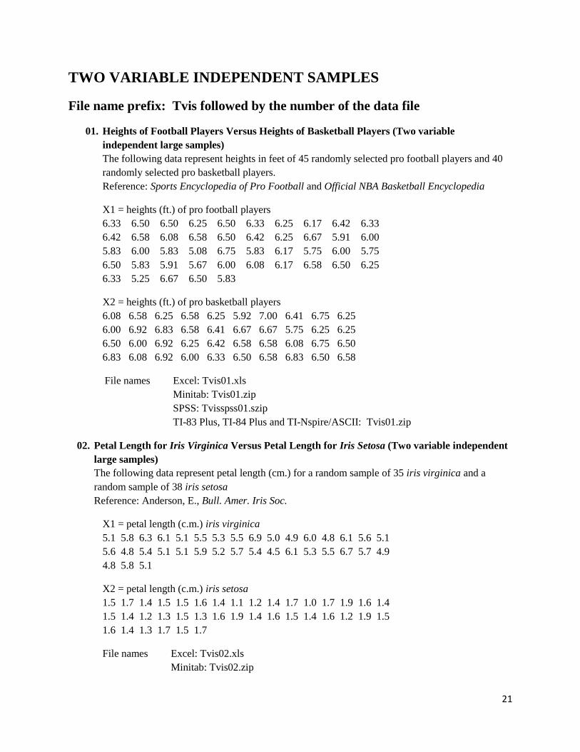
21
TWO VARIABLE INDEPENDENT SAMPLES
File name prefix: Tvis followed by the number of the data file
01. Heights of Football Players Versus Heights of Basketball Players (Two variable
independent large samples)
The following data represent heights in feet of 45 randomly selected pro football players and 40
randomly selected pro basketball players.
Reference: Sports Encyclopedia of Pro Football and Official NBA Basketball Encyclopedia
X1 = heights (ft.) of pro football players
6.33 6.50 6.50 6.25 6.50 6.33 6.25 6.17 6.42 6.33
6.42 6.58 6.08 6.58 6.50 6.42 6.25 6.67 5.91 6.00
5.83 6.00 5.83 5.08 6.75 5.83 6.17 5.75 6.00 5.75
6.50 5.83 5.91 5.67 6.00 6.08 6.17 6.58 6.50 6.25
6.33 5.25 6.67 6.50 5.83
X2 = heights (ft.) of pro basketball players
6.08 6.58 6.25 6.58 6.25 5.92 7.00 6.41 6.75 6.25
6.00 6.92 6.83 6.58 6.41 6.67 6.67 5.75 6.25 6.25
6.50 6.00 6.92 6.25 6.42 6.58 6.58 6.08 6.75 6.50
6.83 6.08 6.92 6.00 6.33 6.50 6.58 6.83 6.50 6.58
File names Excel: Tvis01.xls
Minitab: Tvis01.zip
SPSS: Tvisspss01.szip
TI-83 Plus, TI-84 Plus and TI-Nspire/ASCII: Tvis01.zip
02. Petal Length for Iris Virginica Versus Petal Length for Iris Setosa (Two variable independent
large samples)
The following data represent petal length (cm.) for a random sample of 35 iris virginica and a
random sample of 38 iris setosa
Reference: Anderson, E., Bull. Amer. Iris Soc.
X1 = petal length (c.m.) iris virginica
5.1 5.8 6.3 6.1 5.1 5.5 5.3 5.5 6.9 5.0 4.9 6.0 4.8 6.1 5.6 5.1
5.6 4.8 5.4 5.1 5.1 5.9 5.2 5.7 5.4 4.5 6.1 5.3 5.5 6.7 5.7 4.9
4.8 5.8 5.1
X2 = petal length (c.m.) iris setosa
1.5 1.7 1.4 1.5 1.5 1.6 1.4 1.1 1.2 1.4 1.7 1.0 1.7 1.9 1.6 1.4
1.5 1.4 1.2 1.3 1.5 1.3 1.6 1.9 1.4 1.6 1.5 1.4 1.6 1.2 1.9 1.5
1.6 1.4 1.3 1.7 1.5 1.7
File names Excel: Tvis02.xls
Minitab: Tvis02.zip
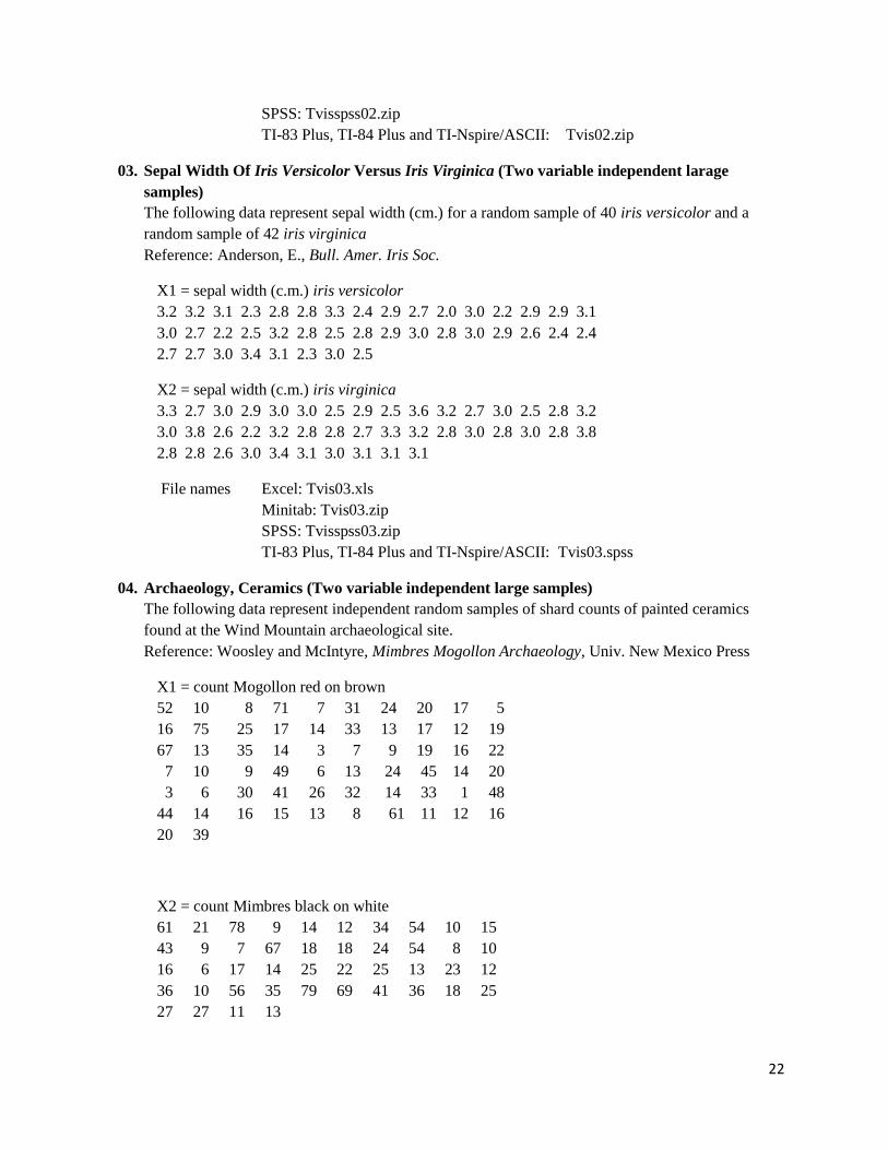
22
SPSS: Tvisspss02.zip
TI-83 Plus, TI-84 Plus and TI-Nspire/ASCII: Tvis02.zip
03. Sepal Width Of Iris Versicolor Versus Iris Virginica (Two variable independent larage
samples)
The following data represent sepal width (cm.) for a random sample of 40 iris versicolor and a
random sample of 42 iris virginica
Reference: Anderson, E., Bull. Amer. Iris Soc.
X1 = sepal width (c.m.) iris versicolor
3.2 3.2 3.1 2.3 2.8 2.8 3.3 2.4 2.9 2.7 2.0 3.0 2.2 2.9 2.9 3.1
3.0 2.7 2.2 2.5 3.2 2.8 2.5 2.8 2.9 3.0 2.8 3.0 2.9 2.6 2.4 2.4
2.7 2.7 3.0 3.4 3.1 2.3 3.0 2.5
X2 = sepal width (c.m.) iris virginica
3.3 2.7 3.0 2.9 3.0 3.0 2.5 2.9 2.5 3.6 3.2 2.7 3.0 2.5 2.8 3.2
3.0 3.8 2.6 2.2 3.2 2.8 2.8 2.7 3.3 3.2 2.8 3.0 2.8 3.0 2.8 3.8
2.8 2.8 2.6 3.0 3.4 3.1 3.0 3.1 3.1 3.1
File names Excel: Tvis03.xls
Minitab: Tvis03.zip
SPSS: Tvisspss03.zip
TI-83 Plus, TI-84 Plus and TI-Nspire/ASCII: Tvis03.spss
04. Archaeology, Ceramics (Two variable independent large samples)
The following data represent independent random samples of shard counts of painted ceramics
found at the Wind Mountain archaeological site.
Reference: Woosley and McIntyre, Mimbres Mogollon Archaeology, Univ. New Mexico Press
X1 = count Mogollon red on brown
52 10 8 71 7 31 24 20 17 5
16 75 25 17 14 33 13 17 12 19
67 13 35 14 3 7 9 19 16 22
7 10 9 49 6 13 24 45 14 20
3 6 30 41 26 32 14 33 1 48
44 14 16 15 13 8 61 11 12 16
20 39
X2 = count Mimbres black on white
61 21 78 9 14 12 34 54 10 15
43 9 7 67 18 18 24 54 8 10
16 6 17 14 25 22 25 13 23 12
36 10 56 35 79 69 41 36 18 25
27 27 11 13
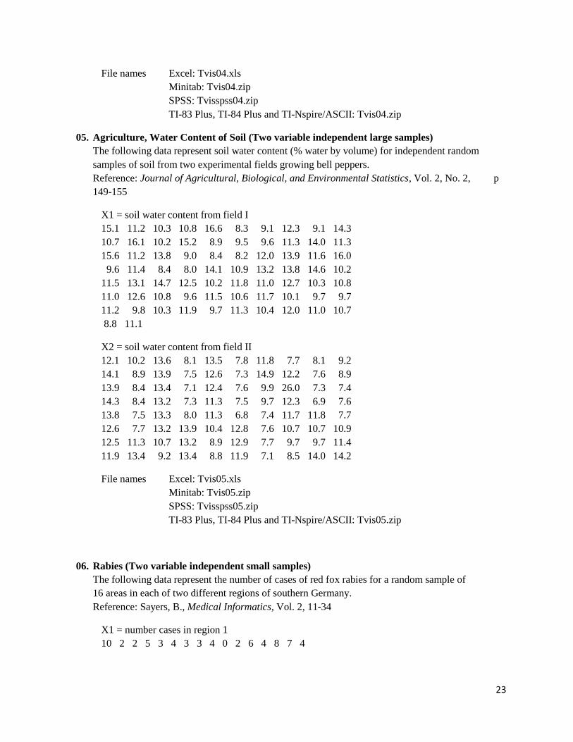
23
File names Excel: Tvis04.xls
Minitab: Tvis04.zip
SPSS: Tvisspss04.zip
TI-83 Plus, TI-84 Plus and TI-Nspire/ASCII: Tvis04.zip
05. Agriculture, Water Content of Soil (Two variable independent large samples)
The following data represent soil water content (% water by volume) for independent random
samples of soil from two experimental fields growing bell peppers.
Reference: Journal of Agricultural, Biological, and Environmental Statistics, Vol. 2, No. 2, p
149-155
X1 = soil water content from field I
15.1 11.2 10.3 10.8 16.6 8.3 9.1 12.3 9.1 14.3
10.7 16.1 10.2 15.2 8.9 9.5 9.6 11.3 14.0 11.3
15.6 11.2 13.8 9.0 8.4 8.2 12.0 13.9 11.6 16.0
9.6 11.4 8.4 8.0 14.1 10.9 13.2 13.8 14.6 10.2
11.5 13.1 14.7 12.5 10.2 11.8 11.0 12.7 10.3 10.8
11.0 12.6 10.8 9.6 11.5 10.6 11.7 10.1 9.7 9.7
11.2 9.8 10.3 11.9 9.7 11.3 10.4 12.0 11.0 10.7
8.8 11.1
X2 = soil water content from field II
12.1 10.2 13.6 8.1 13.5 7.8 11.8 7.7 8.1 9.2
14.1 8.9 13.9 7.5 12.6 7.3 14.9 12.2 7.6 8.9
13.9 8.4 13.4 7.1 12.4 7.6 9.9 26.0 7.3 7.4
14.3 8.4 13.2 7.3 11.3 7.5 9.7 12.3 6.9 7.6
13.8 7.5 13.3 8.0 11.3 6.8 7.4 11.7 11.8 7.7
12.6 7.7 13.2 13.9 10.4 12.8 7.6 10.7 10.7 10.9
12.5 11.3 10.7 13.2 8.9 12.9 7.7 9.7 9.7 11.4
11.9 13.4 9.2 13.4 8.8 11.9 7.1 8.5 14.0 14.2
File names Excel: Tvis05.xls
Minitab: Tvis05.zip
SPSS: Tvisspss05.zip
TI-83 Plus, TI-84 Plus and TI-Nspire/ASCII: Tvis05.zip
06. Rabies (Two variable independent small samples)
The following data represent the number of cases of red fox rabies for a random sample of
16 areas in each of two different regions of southern Germany.
Reference: Sayers, B., Medical Informatics, Vol. 2, 11-34
X1 = number cases in region 1
10 2 2 5 3 4 3 3 4 0 2 6 4 8 7 4
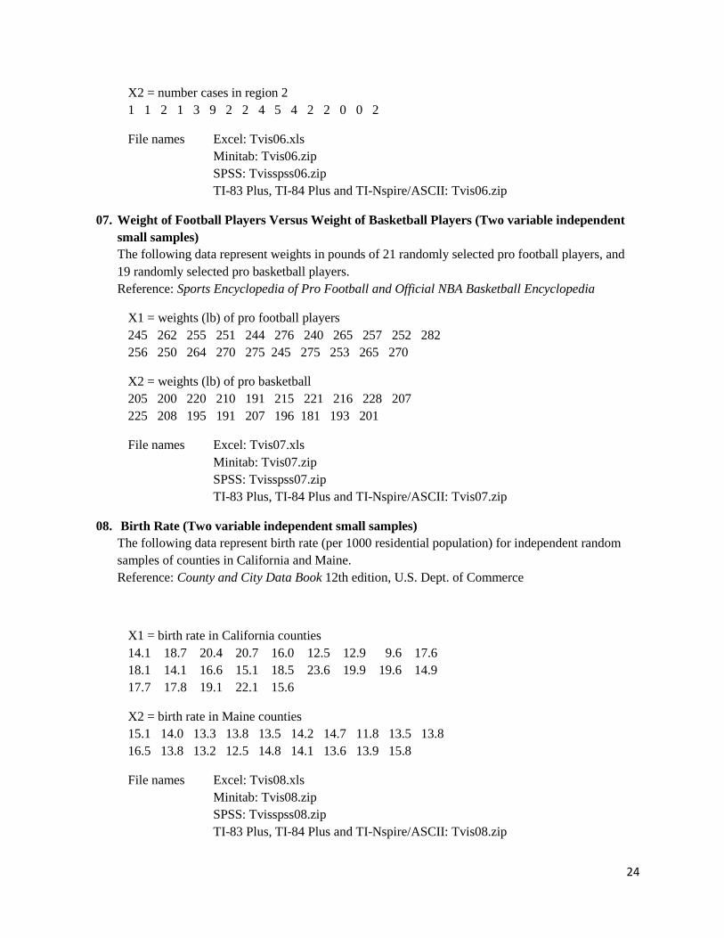
24
X2 = number cases in region 2
1 1 2 1 3 9 2 2 4 5 4 2 2 0 0 2
File names Excel: Tvis06.xls
Minitab: Tvis06.zip
SPSS: Tvisspss06.zip
TI-83 Plus, TI-84 Plus and TI-Nspire/ASCII: Tvis06.zip
07. Weight of Football Players Versus Weight of Basketball Players (Two variable independent
small samples)
The following data represent weights in pounds of 21 randomly selected pro football players, and
19 randomly selected pro basketball players.
Reference: Sports Encyclopedia of Pro Football and Official NBA Basketball Encyclopedia
X1 = weights (lb) of pro football players
245 262 255 251 244 276 240 265 257 252 282
256 250 264 270 275 245 275 253 265 270
X2 = weights (lb) of pro basketball
205 200 220 210 191 215 221 216 228 207
225 208 195 191 207 196 181 193 201
File names Excel: Tvis07.xls
Minitab: Tvis07.zip
SPSS: Tvisspss07.zip
TI-83 Plus, TI-84 Plus and TI-Nspire/ASCII: Tvis07.zip
08. Birth Rate (Two variable independent small samples)
The following data represent birth rate (per 1000 residential population) for independent random
samples of counties in California and Maine.
Reference: County and City Data Book 12th edition, U.S. Dept. of Commerce
X1 = birth rate in California counties
14.1 18.7 20.4 20.7 16.0 12.5 12.9 9.6 17.6
18.1 14.1 16.6 15.1 18.5 23.6 19.9 19.6 14.9
17.7 17.8 19.1 22.1 15.6
X2 = birth rate in Maine counties
15.1 14.0 13.3 13.8 13.5 14.2 14.7 11.8 13.5 13.8
16.5 13.8 13.2 12.5 14.8 14.1 13.6 13.9 15.8
File names Excel: Tvis08.xls
Minitab: Tvis08.zip
SPSS: Tvisspss08.zip
TI-83 Plus, TI-84 Plus and TI-Nspire/ASCII: Tvis08.zip
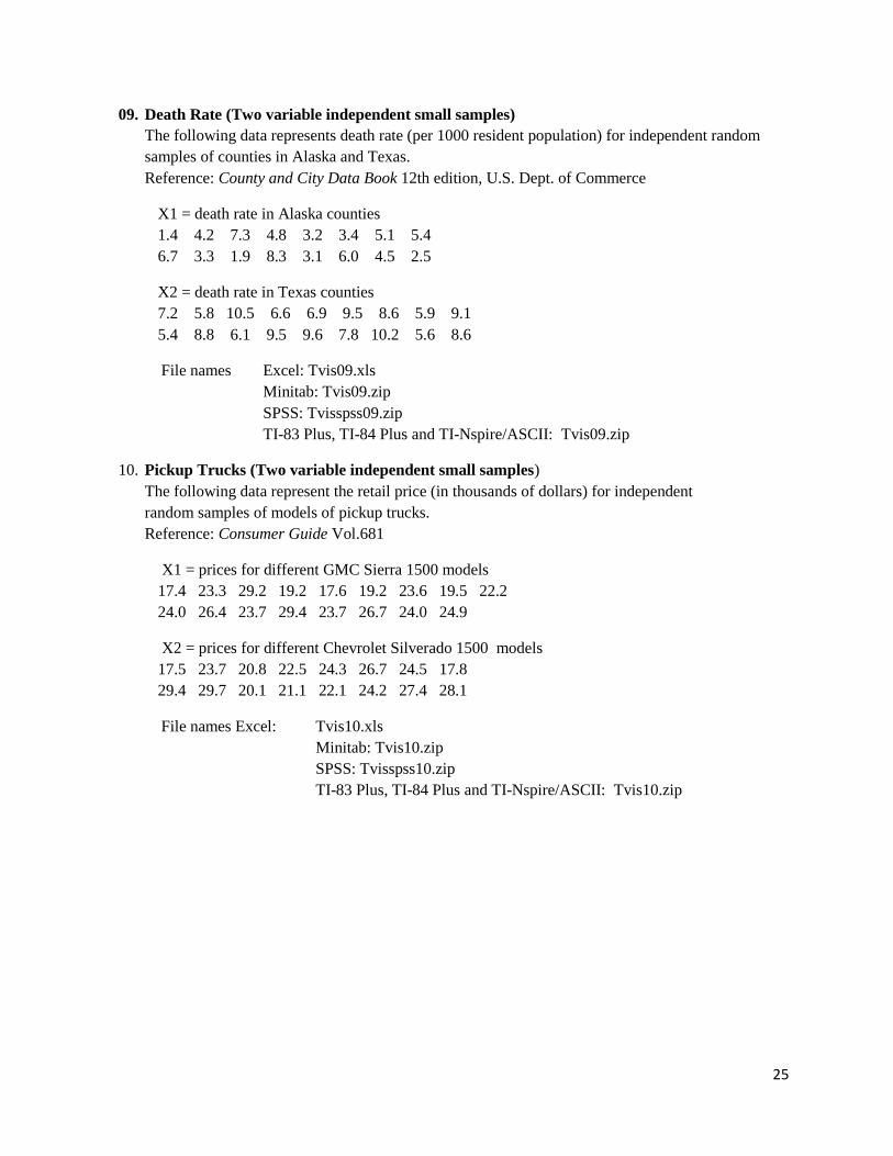
25
09. Death Rate (Two variable independent small samples)
The following data represents death rate (per 1000 resident population) for independent random
samples of counties in Alaska and Texas.
Reference: County and City Data Book 12th edition, U.S. Dept. of Commerce
X1 = death rate in Alaska counties
1.4 4.2 7.3 4.8 3.2 3.4 5.1 5.4
6.7 3.3 1.9 8.3 3.1 6.0 4.5 2.5
X2 = death rate in Texas counties
7.2 5.8 10.5 6.6 6.9 9.5 8.6 5.9 9.1
5.4 8.8 6.1 9.5 9.6 7.8 10.2 5.6 8.6
File names Excel: Tvis09.xls
Minitab: Tvis09.zip
SPSS: Tvisspss09.zip
TI-83 Plus, TI-84 Plus and TI-Nspire/ASCII: Tvis09.zip
10. Pickup Trucks (Two variable independent small samples)
The following data represent the retail price (in thousands of dollars) for independent
random samples of models of pickup trucks.
Reference: Consumer Guide Vol.681
X1 = prices for different GMC Sierra 1500 models
17.4 23.3 29.2 19.2 17.6 19.2 23.6 19.5 22.2
24.0 26.4 23.7 29.4 23.7 26.7 24.0 24.9
X2 = prices for different Chevrolet Silverado 1500 models
17.5 23.7 20.8 22.5 24.3 26.7 24.5 17.8
29.4 29.7 20.1 21.1 22.1 24.2 27.4 28.1
File names Excel: Tvis10.xls
Minitab: Tvis10.zip
SPSS: Tvisspss10.zip
TI-83 Plus, TI-84 Plus and TI-Nspire/ASCII: Tvis10.zip
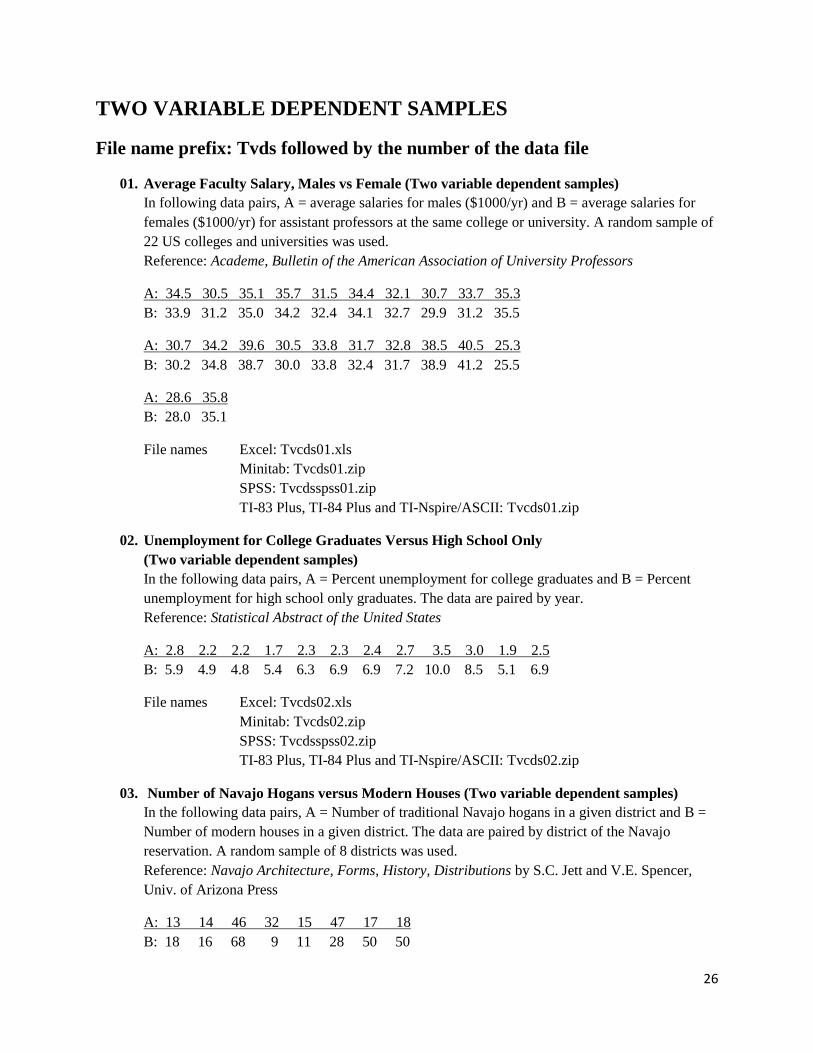
26
TWO VARIABLE DEPENDENT SAMPLES
File name prefix: Tvds followed by the number of the data file
01. Average Faculty Salary, Males vs Female (Two variable dependent samples)
In following data pairs, A = average salaries for males ($1000/yr) and B = average salaries for
females ($1000/yr) for assistant professors at the same college or university. A random sample of
22 US colleges and universities was used.
Reference: Academe, Bulletin of the American Association of University Professors
A: 34.5 30.5 35.1 35.7 31.5 34.4 32.1 30.7 33.7 35.3
B: 33.9 31.2 35.0 34.2 32.4 34.1 32.7 29.9 31.2 35.5
A: 30.7 34.2 39.6 30.5 33.8 31.7 32.8 38.5 40.5 25.3
B: 30.2 34.8 38.7 30.0 33.8 32.4 31.7 38.9 41.2 25.5
A: 28.6 35.8
B: 28.0 35.1
File names Excel: Tvcds01.xls
Minitab: Tvcds01.zip
SPSS: Tvcdsspss01.zip
TI-83 Plus, TI-84 Plus and TI-Nspire/ASCII: Tvcds01.zip
02. Unemployment for College Graduates Versus High School Only
(Two variable dependent samples)
In the following data pairs, A = Percent unemployment for college graduates and B = Percent
unemployment for high school only graduates. The data are paired by year.
Reference: Statistical Abstract of the United States
A: 2.8 2.2 2.2 1.7 2.3 2.3 2.4 2.7 3.5 3.0 1.9 2.5
B: 5.9 4.9 4.8 5.4 6.3 6.9 6.9 7.2 10.0 8.5 5.1 6.9
File names Excel: Tvcds02.xls
Minitab: Tvcds02.zip
SPSS: Tvcdsspss02.zip
TI-83 Plus, TI-84 Plus and TI-Nspire/ASCII: Tvcds02.zip
03. Number of Navajo Hogans versus Modern Houses (Two variable dependent samples)
In the following data pairs, A = Number of traditional Navajo hogans in a given district and B =
Number of modern houses in a given district. The data are paired by district of the Navajo
reservation. A random sample of 8 districts was used.
Reference: Navajo Architecture, Forms, History, Distributions by S.C. Jett and V.E. Spencer,
Univ. of Arizona Press
A: 13 14 46 32 15 47 17 18
B: 18 16 68 9 11 28 50 50
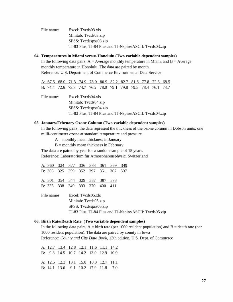
27
File names Excel: Tvcds03.xls
Minitab: Tvcds03.zip
SPSS: Tvcdsspss03.zip
TI-83 Plus, TI-84 Plus and TI-Nspire/ASCII: Tvcds03.zip
04. Temperatures in Miami versus Honolulu (Two variable dependent samples)
In the following data pairs, A = Average monthly temperature in Miami and B = Average
monthly temperature in Honolulu. The data are paired by month.
Reference: U.S. Department of Commerce Environmental Data Service
A: 67.5 68.0 71.3 74.9 78.0 80.9 82.2 82.7 81.6 77.8 72.3 68.5
B: 74.4 72.6 73.3 74.7 76.2 78.0 79.1 79.8 79.5 78.4 76.1 73.7
File names Excel: Tvcds04.xls
Minitab: Tvcds04.zip
SPSS: Tvcdsspss04.zip
TI-83 Plus, TI-84 Plus and TI-Nspire/ASCII: Tvcds04.zip
05. January/February Ozone Column (Two variable dependent samples)
In the following pairs, the data represent the thickness of the ozone column in Dobson units: one
milli-centimeter ozone at standard temperature and pressure.
A = monthly mean thickness in January
B = monthly mean thickness in February
The data are paired by year for a random sample of 15 years.
Reference: Laboratorium für Atmospharensphysic, Switzerland
A: 360 324 377 336 383 361 369 349
B: 365 325 359 352 397 351 367 397
A: 301 354 344 329 337 387 378
B: 335 338 349 393 370 400 411
File names Excel: Tvcds05.xls
Minitab: Tvcds05.zip
SPSS: Tvcdsspss05.zip
TI-83 Plus, TI-84 Plus and TI-Nspire/ASCII: Tvcds05.zip
06. Birth Rate/Death Rate (Two variable dependent samples)
In the following data pairs, A = birth rate (per 1000 resident population) and B = death rate (per
1000 resident population). The data are paired by county in Iowa
Reference: County and City Data Book, 12th edition, U.S. Dept. of Commerce
A: 12.7 13.4 12.8 12.1 11.6 11.1 14.2
B: 9.8 14.5 10.7 14.2 13.0 12.9 10.9
A: 12.5 12.3 13.1 15.8 10.3 12.7 11.1
B: 14.1 13.6 9.1 10.2 17.9 11.8 7.0
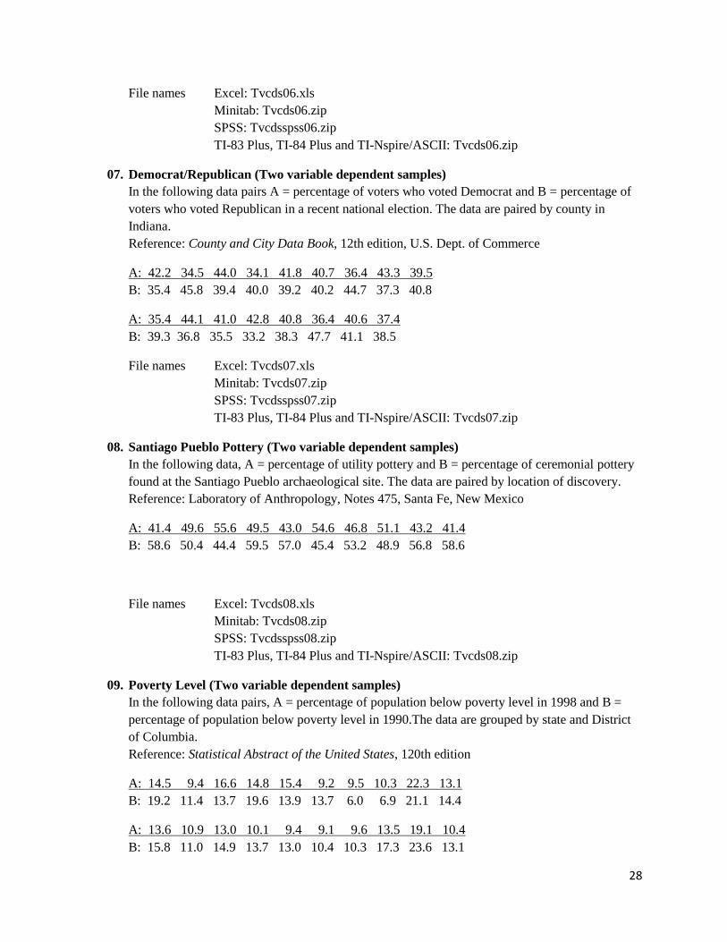
28
File names Excel: Tvcds06.xls
Minitab: Tvcds06.zip
SPSS: Tvcdsspss06.zip
TI-83 Plus, TI-84 Plus and TI-Nspire/ASCII: Tvcds06.zip
07. Democrat/Republican (Two variable dependent samples)
In the following data pairs A = percentage of voters who voted Democrat and B = percentage of
voters who voted Republican in a recent national election. The data are paired by county in
Indiana.
Reference: County and City Data Book, 12th edition, U.S. Dept. of Commerce
A: 42.2 34.5 44.0 34.1 41.8 40.7 36.4 43.3 39.5
B: 35.4 45.8 39.4 40.0 39.2 40.2 44.7 37.3 40.8
A: 35.4 44.1 41.0 42.8 40.8 36.4 40.6 37.4
B: 39.3 36.8 35.5 33.2 38.3 47.7 41.1 38.5
File names Excel: Tvcds07.xls
Minitab: Tvcds07.zip
SPSS: Tvcdsspss07.zip
TI-83 Plus, TI-84 Plus and TI-Nspire/ASCII: Tvcds07.zip
08. Santiago Pueblo Pottery (Two variable dependent samples)
In the following data, A = percentage of utility pottery and B = percentage of ceremonial pottery
found at the Santiago Pueblo archaeological site. The data are paired by location of discovery.
Reference: Laboratory of Anthropology, Notes 475, Santa Fe, New Mexico
A: 41.4 49.6 55.6 49.5 43.0 54.6 46.8 51.1 43.2 41.4
B: 58.6 50.4 44.4 59.5 57.0 45.4 53.2 48.9 56.8 58.6
File names Excel: Tvcds08.xls
Minitab: Tvcds08.zip
SPSS: Tvcdsspss08.zip
TI-83 Plus, TI-84 Plus and TI-Nspire/ASCII: Tvcds08.zip
09. Poverty Level (Two variable dependent samples)
In the following data pairs, A = percentage of population below poverty level in 1998 and B =
percentage of population below poverty level in 1990.The data are grouped by state and District
of Columbia.
Reference: Statistical Abstract of the United States, 120th edition
A: 14.5 9.4 16.6 14.8 15.4 9.2 9.5 10.3 22.3 13.1
B: 19.2 11.4 13.7 19.6 13.9 13.7 6.0 6.9 21.1 14.4
A: 13.6 10.9 13.0 10.1 9.4 9.1 9.6 13.5 19.1 10.4
B: 15.8 11.0 14.9 13.7 13.0 10.4 10.3 17.3 23.6 13.1
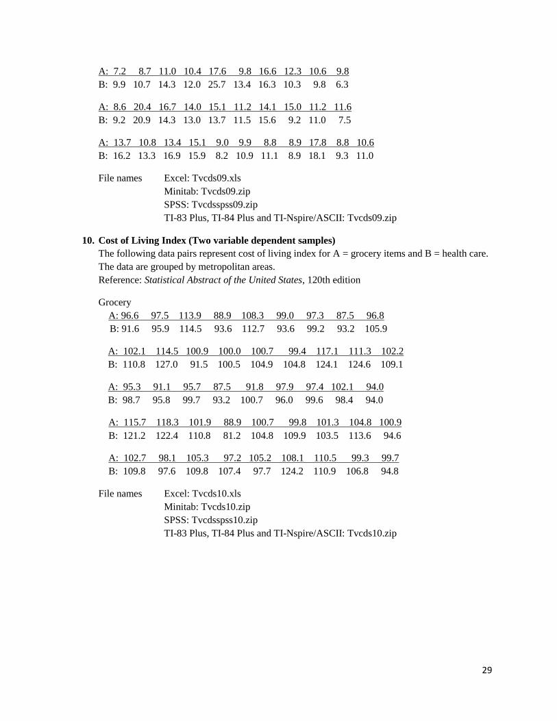
29
A: 7.2 8.7 11.0 10.4 17.6 9.8 16.6 12.3 10.6 9.8
B: 9.9 10.7 14.3 12.0 25.7 13.4 16.3 10.3 9.8 6.3
A: 8.6 20.4 16.7 14.0 15.1 11.2 14.1 15.0 11.2 11.6
B: 9.2 20.9 14.3 13.0 13.7 11.5 15.6 9.2 11.0 7.5
A: 13.7 10.8 13.4 15.1 9.0 9.9 8.8 8.9 17.8 8.8 10.6
B: 16.2 13.3 16.9 15.9 8.2 10.9 11.1 8.9 18.1 9.3 11.0
File names Excel: Tvcds09.xls
Minitab: Tvcds09.zip
SPSS: Tvcdsspss09.zip
TI-83 Plus, TI-84 Plus and TI-Nspire/ASCII: Tvcds09.zip
10. Cost of Living Index (Two variable dependent samples)
The following data pairs represent cost of living index for A = grocery items and B = health care.
The data are grouped by metropolitan areas.
Reference: Statistical Abstract of the United States, 120th edition
Grocery
A: 96.6 97.5 113.9 88.9 108.3 99.0 97.3 87.5 96.8
B: 91.6 95.9 114.5 93.6 112.7 93.6 99.2 93.2 105.9
A: 102.1 114.5 100.9 100.0 100.7 99.4 117.1 111.3 102.2
B: 110.8 127.0 91.5 100.5 104.9 104.8 124.1 124.6 109.1
A: 95.3 91.1 95.7 87.5 91.8 97.9 97.4 102.1 94.0
B: 98.7 95.8 99.7 93.2 100.7 96.0 99.6 98.4 94.0
A: 115.7 118.3 101.9 88.9 100.7 99.8 101.3 104.8 100.9
B: 121.2 122.4 110.8 81.2 104.8 109.9 103.5 113.6 94.6
A: 102.7 98.1 105.3 97.2 105.2 108.1 110.5 99.3 99.7
B: 109.8 97.6 109.8 107.4 97.7 124.2 110.9 106.8 94.8
File names Excel: Tvcds10.xls
Minitab: Tvcds10.zip
SPSS: Tvcdsspss10.zip
TI-83 Plus, TI-84 Plus and TI-Nspire/ASCII: Tvcds10.zip
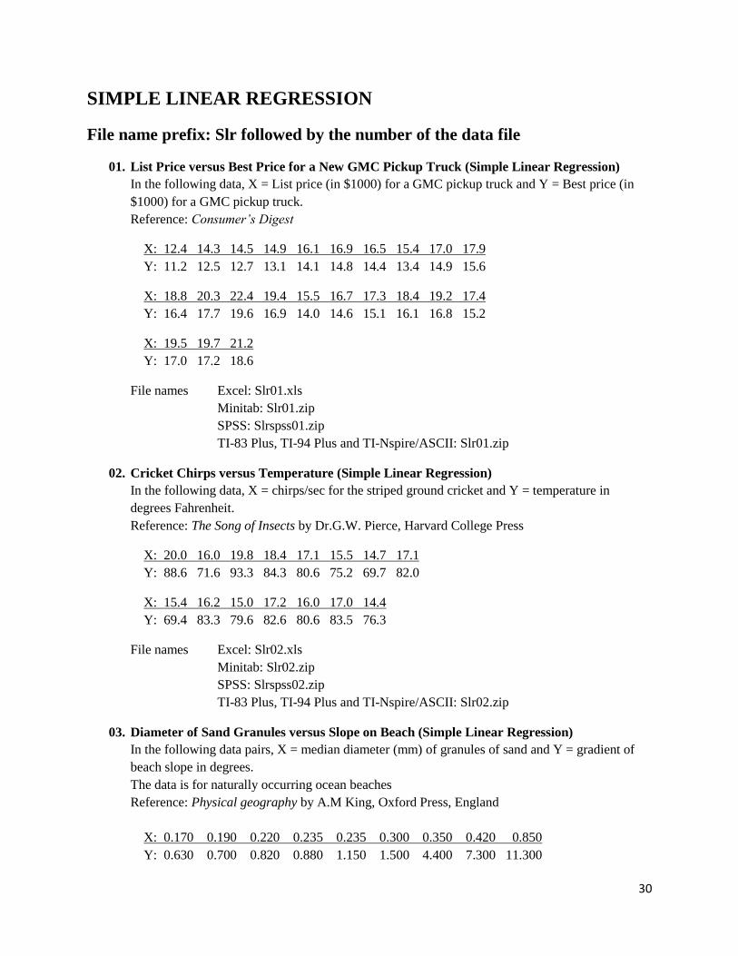
30
SIMPLE LINEAR REGRESSION
File name prefix: Slr followed by the number of the data file
01. List Price versus Best Price for a New GMC Pickup Truck (Simple Linear Regression)
In the following data, X = List price (in $1000) for a GMC pickup truck and Y = Best price (in
$1000) for a GMC pickup truck.
Reference: Consumer’s Digest
X: 12.4 14.3 14.5 14.9 16.1 16.9 16.5 15.4 17.0 17.9
Y: 11.2 12.5 12.7 13.1 14.1 14.8 14.4 13.4 14.9 15.6
X: 18.8 20.3 22.4 19.4 15.5 16.7 17.3 18.4 19.2 17.4
Y: 16.4 17.7 19.6 16.9 14.0 14.6 15.1 16.1 16.8 15.2
X: 19.5 19.7 21.2
Y: 17.0 17.2 18.6
File names Excel: Slr01.xls
Minitab: Slr01.zip
SPSS: Slrspss01.zip
TI-83 Plus, TI-94 Plus and TI-Nspire/ASCII: Slr01.zip
02. Cricket Chirps versus Temperature (Simple Linear Regression)
In the following data, X = chirps/sec for the striped ground cricket and Y = temperature in
degrees Fahrenheit.
Reference: The Song of Insects by Dr.G.W. Pierce, Harvard College Press
X: 20.0 16.0 19.8 18.4 17.1 15.5 14.7 17.1
Y: 88.6 71.6 93.3 84.3 80.6 75.2 69.7 82.0
X: 15.4 16.2 15.0 17.2 16.0 17.0 14.4
Y: 69.4 83.3 79.6 82.6 80.6 83.5 76.3
File names Excel: Slr02.xls
Minitab: Slr02.zip
SPSS: Slrspss02.zip
TI-83 Plus, TI-94 Plus and TI-Nspire/ASCII: Slr02.zip
03. Diameter of Sand Granules versus Slope on Beach (Simple Linear Regression)
In the following data pairs, X = median diameter (mm) of granules of sand and Y = gradient of
beach slope in degrees.
The data is for naturally occurring ocean beaches
Reference: Physical geography by A.M King, Oxford Press, England
X: 0.170 0.190 0.220 0.235 0.235 0.300 0.350 0.420 0.850
Y: 0.630 0.700 0.820 0.880 1.150 1.500 4.400 7.300 11.300
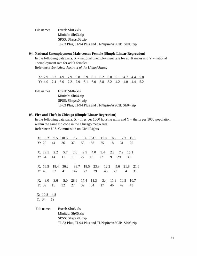
31
File names Excel: Slr03.xls
Minitab: Slr03.zip
SPSS: Slrspss03.zip
TI-83 Plus, TI-94 Plus and TI-Nspire/ASCII: Slr03.zip
04. National Unemployment Male versus Female (Simple Linear Regression)
In the following data pairs, X = national unemployment rate for adult males and Y = national
unemployment rate for adult females.
Reference: Statistical Abstract of the United States
X: 2.9 6.7 4.9 7.9 9.8 6.9 6.1 6.2 6.0 5.1 4.7 4.4 5.8
Y: 4.0 7.4 5.0 7.2 7.9 6.1 6.0 5.8 5.2 4.2 4.0 4.4 5.2
File names Excel: Slr04.xls
Minitab: Slr04.zip
SPSS: Slrspss04.zip
TI-83 Plus, TI-94 Plus and TI-Nspire/ASCII: Slr04.zip
05. Fire and Theft in Chicago (Simple Linear Regression)
In the following data pairs, X = fires per 1000 housing units and Y = thefts per 1000 population
within the same zip code in the Chicago metro area.
Reference: U.S. Commission on Civil Rights
X: 6.2 9.5 10.5 7.7 8.6 34.1 11.0 6.9 7.3 15.1
Y: 29 44 36 37 53 68 75 18 31 25
X: 29.1 2.2 5.7 2.0 2.5 4.0 5.4 2.2 7.2 15.1
Y: 34 14 11 11 22 16 27 9 29 30
X: 16.5 18.4 36.2 39.7 18.5 23.3 12.2 5.6 21.8 21.6
Y: 40 32 41 147 22 29 46 23 4 31
X: 9.0 3.6 5.0 28.6 17.4 11.3 3.4 11.9 10.5 10.7
Y: 39 15 32 27 32 34 17 46 42 43
X: 10.8 4.8
Y: 34 19
File names Excel: Slr05.xls
Minitab: Slr05.zip
SPSS: Slrspss05.zip
TI-83 Plus, TI-94 Plus and TI-Nspire/ASCII: Slr05.zip

32
06. Auto Insurance in Sweden (Simple Linear Regression)
In the following data, X = number of claims and Y = total payment for all the claims in thousands
of Swedish Kronor for geographical zones in Sweden
Reference: Swedish Committee on Analysis of Risk Premium in Motor Insurance
X: 108 19 13 124 40 57 23 14 45 10
Y: 392.5 46.2 15.7 422.2 119.4 170.9 56.9 77.5 214.0 65.3
X: 5 48 11 23 7 2 24 6 3 23
Y: 20.9 248.1 23.5 39.6 48.8 6.6 134.9 50.9 4.4 113.0
X: 6 9 9 3 29 7 4 20 7 4
Y: 14.8 48.7 52.1 13.2 103.9 77.5 11.8 98.1 27.9 38.1
X: 0 25 6 5 22 11 61 12 4 16
Y: 0.0 69.2 14.6 40.3 161.5 57.2 217.6 58.1 12.6 59.6
X: 13 60 41 37 55 41 11 27 8 3
Y: 89.9 202.4 181.3 152.8 162.8 73.4 21.3 92.6 76.1 39.9
X: 17 13 13 15 8 29 30 24 9 31
Y: 142.1 93.0 31.9 32.1 55.6 133.3 194.5 137.9 87.4 209.8
X: 14 53 26
Y: 95.5 244.6 187.5
File names Excel: Slr06.xls
Minitab: Slr06.zip
SPSS: Slrspss06.zip
TI-83 Plus, TI-94 Plus and TI-Nspire/ASCII: Slr06.zip
07. Gray Kangaroos (Simple Linear Regression)
In the following data pairs, X = nasal length (mm ×10) and Y = nasal width (mm × 10) for a male
gray kangaroo from a random sample of such animals.
Reference: Australian Journal of Zoology, Vol. 28, p607-613
X: 609 629 620 564 645 493 606 660 630 672
Y: 241 222 233 207 247 189 226 240 215 231
X: 778 616 727 810 778 823 755 710 701 803
Y: 263 220 271 284 279 272 268 278 238 255
X: 855 838 830 864 635 565 562 580 596 597
Y: 308 281 288 306 236 204 216 225 220 219
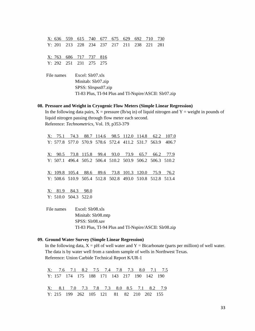
33
X: 636 559 615 740 677 675 629 692 710 730
Y: 201 213 228 234 237 217 211 238 221 281
X: 763 686 717 737 816
Y: 292 251 231 275 275
File names Excel: Slr07.xls
Minitab: Slr07.zip
SPSS: Slrspss07.zip
TI-83 Plus, TI-94 Plus and TI-Nspire/ASCII: Slr07.zip
08. Pressure and Weight in Cryogenic Flow Meters (Simple Linear Regression)
In the following data pairs, X = pressure (lb/sq in) of liquid nitrogen and Y = weight in pounds of
liquid nitrogen passing through flow meter each second.
Reference: Technometrics, Vol. 19, p353-379
X: 75.1 74.3 88.7 114.6 98.5 112.0 114.8 62.2 107.0
Y: 577.8 577.0 570.9 578.6 572.4 411.2 531.7 563.9 406.7
X: 90.5 73.8 115.8 99.4 93.0 73.9 65.7 66.2 77.9
Y: 507.1 496.4 505.2 506.4 510.2 503.9 506.2 506.3 510.2
X: 109.8 105.4 88.6 89.6 73.8 101.3 120.0 75.9 76.2
Y: 508.6 510.9 505.4 512.8 502.8 493.0 510.8 512.8 513.4
X: 81.9 84.3 98.0
Y: 510.0 504.3 522.0
File names Excel: Slr08.xls
Minitab: Slr08.mtp
SPSS: Slr08.sav
TI-83 Plus, TI-94 Plus and TI-Nspire/ASCII: Slr08.zip
09. Ground Water Survey (Simple Linear Regression)
In the following data, X = pH of well water and Y = Bicarbonate (parts per million) of well water.
The data is by water well from a random sample of wells in Northwest Texas.
Reference: Union Carbide Technical Report K/UR-1
X: 7.6 7.1 8.2 7.5 7.4 7.8 7.3 8.0 7.1 7.5
Y: 157 174 175 188 171 143 217 190 142 190
X: 8.1 7.0 7.3 7.8 7.3 8.0 8.5 7.1 8.2 7.9
Y: 215 199 262 105 121 81 82 210 202 155
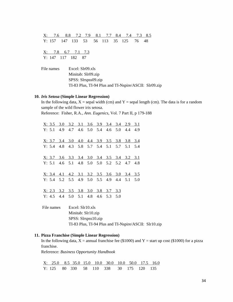
34
X: 7.6 8.8 7.2 7.9 8.1 7.7 8.4 7.4 7.3 8.5
Y: 157 147 133 53 56 113 35 125 76 48
X: 7.8 6.7 7.1 7.3
Y: 147 117 182 87
File names Excel: Slr09.xls
Minitab: Slr09.zip
SPSS: Slrspss09.zip
TI-83 Plus, TI-94 Plus and TI-Nspire/ASCII: Slr09.zip
10. Iris Setosa (Simple Linear Regression)
In the following data, X = sepal width (cm) and Y = sepal length (cm). The data is for a random
sample of the wild flower iris setosa.
Reference: Fisher, R.A., Ann. Eugenics, Vol. 7 Part II, p 179-188
X: 3.5 3.0 3.2 3.1 3.6 3.9 3.4 3.4 2.9 3.1
Y: 5.1 4.9 4.7 4.6 5.0 5.4 4.6 5.0 4.4 4.9
X: 3.7 3.4 3.0 4.0 4.4 3.9 3.5 3.8 3.8 3.4
Y: 5.4 4.8 4.3 5.8 5.7 5.4 5.1 5.7 5.1 5.4
X: 3.7 3.6 3.3 3.4 3.0 3.4 3.5 3.4 3.2 3.1
Y: 5.1 4.6 5.1 4.8 5.0 5.0 5.2 5.2 4.7 4.8
X: 3.4 4.1 4.2 3.1 3.2 3.5 3.6 3.0 3.4 3.5
Y: 5.4 5.2 5.5 4.9 5.0 5.5 4.9 4.4 5.1 5.0
X: 2.3 3.2 3.5 3.8 3.0 3.8 3.7 3.3
Y: 4.5 4.4 5.0 5.1 4.8 4.6 5.3 5.0
File names Excel: Slr10.xls
Minitab: Slr10.zip
SPSS: Slrspss10.zip
TI-83 Plus, TI-94 Plus and TI-Nspire/ASCII: Slr10.zip
11. Pizza Franchise (Simple Linear Regression)
In the following data, X = annual franchise fee ($1000) and Y = start up cost ($1000) for a pizza
franchise.
Reference: Business Opportunity Handbook
X: 25.0 8.5 35.0 15.0 10.0 30.0 10.0 50.0 17.5 16.0
Y: 125 80 330 58 110 338 30 175 120 135
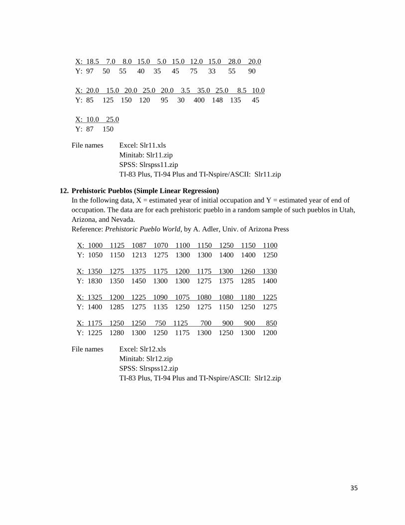
35
X: 18.5 7.0 8.0 15.0 5.0 15.0 12.0 15.0 28.0 20.0
Y: 97 50 55 40 35 45 75 33 55 90
X: 20.0 15.0 20.0 25.0 20.0 3.5 35.0 25.0 8.5 10.0
Y: 85 125 150 120 95 30 400 148 135 45
X: 10.0 25.0
Y: 87 150
File names Excel: Slr11.xls
Minitab: Slr11.zip
SPSS: Slrspss11.zip
TI-83 Plus, TI-94 Plus and TI-Nspire/ASCII: Slr11.zip
12. Prehistoric Pueblos (Simple Linear Regression)
In the following data, X = estimated year of initial occupation and Y = estimated year of end of
occupation. The data are for each prehistoric pueblo in a random sample of such pueblos in Utah,
Arizona, and Nevada.
Reference: Prehistoric Pueblo World, by A. Adler, Univ. of Arizona Press
X: 1000 1125 1087 1070 1100 1150 1250 1150 1100
Y: 1050 1150 1213 1275 1300 1300 1400 1400 1250
X: 1350 1275 1375 1175 1200 1175 1300 1260 1330
Y: 1830 1350 1450 1300 1300 1275 1375 1285 1400
X: 1325 1200 1225 1090 1075 1080 1080 1180 1225
Y: 1400 1285 1275 1135 1250 1275 1150 1250 1275
X: 1175 1250 1250 750 1125 700 900 900 850
Y: 1225 1280 1300 1250 1175 1300 1250 1300 1200
File names Excel: Slr12.xls
Minitab: Slr12.zip
SPSS: Slrspss12.zip
TI-83 Plus, TI-94 Plus and TI-Nspire/ASCII: Slr12.zip

36