UNDERSTANDING EFFECTS OF TAPERING CANTILEVERED

UNDERSTANDING EFFECTS OF TAPERING CANTILEVERED PIEZOELECTRIC

BIMORPHS FOR ENERGY HARVESTING FROM VIBRATIONS

by

Naved Ahmed Siddiqui

A dissertation submitted to the Graduate Faculty of

Auburn University

in partial fulfillment of the

requirements for the Degree of

Doctor of Philosophy

Auburn, AL

December 13, 2014

Keywords: Piezoelectric Energy Harvesting, Tapering, Resonance, Electromechanical Coupling

Coefficient, Impedance Spectroscopy, Damping,

Approved by:

Barton C. Prorok, Chair, Professor of Materials Engineering

Jeffrey W. Fergus, Professor of Materials Engineering

Dong-Joo Kim, Professor of Materials Engineering

Robert L. Jackson, Associate Professor of Mechanical Engineering

Ruel A. Overfelt, Professor of Materials Engineering

ii

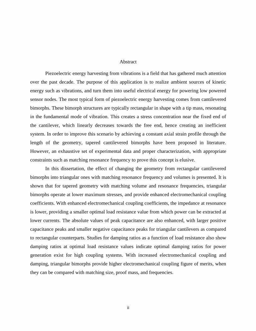
Abstract

Piezoelectric energy harvesting from vibrations is a field that has gathered much attention

over the past decade. The purpose of this application is to realize ambient sources of kinetic

energy such as vibrations, and turn them into useful electrical energy for powering low powered

sensor nodes. The most typical form of piezoelectric energy harvesting comes from cantilevered

bimorphs. These bimorph structures are typically rectangular in shape with a tip mass, resonating

in the fundamental mode of vibration. This creates a stress concentration near the fixed end of

the cantilever, which linearly decreases towards the free end, hence creating an inefficient

system. In order to improve this scenario by achieving a constant axial strain profile through the

length of the geometry, tapered cantilevered bimorphs have been proposed in literature.

However, an exhaustive set of experimental data and proper characterization, with appropriate

constraints such as matching resonance frequency to prove this concept is elusive.

In this dissertation, the effect of changing the geometry from rectangular cantilevered

bimorphs into triangular ones with matching resonance frequency and volumes is presented. It is

shown that for tapered geometry with matching volume and resonance frequencies, triangular

bimorphs operate at lower maximum stresses, and provide enhanced electromechanical coupling

coefficients. With enhanced electromechanical coupling coefficients, the impedance at resonance

is lower, providing a smaller optimal load resistance value from which power can be extracted at

lower currents. The absolute values of peak capacitance are also enhanced, with larger positive

capacitance peaks and smaller negative capacitance peaks for triangular cantilevers as compared

to rectangular counterparts. Studies for damping ratios as a function of load resistance also show

damping ratios at optimal load resistance values indicate optimal damping ratios for power

generation exist for high coupling systems. With increased electromechanical coupling and

damping, triangular bimorphs provide higher electromechanical coupling figure of merits, when

they can be compared with matching size, proof mass, and frequencies.

iii

Acknowledgements

As I arrive towards the culmination of this document, several thoughts race through my

head. I am thankful to a number of people who have helped me through the course of my Ph.D.

However, the first people that I have to acknowledge are my parents, Mohammed Fareed and

Fahmida Siddiqui. Without their prayers, and unconditional love and support from a distance,

this Ph.D would simply not have been possible. Words are not enough to describe the gratitude I

have for them. I would also like to acknowledge my siblings Sabah, Sarah, and Ahmed as well

for the same.

From a professional front, I would first like to thank Dr. Prorok, and Dr. Overfelt, both

for their support, during the course of my Ph.D. The training I received developed my aptitude in

critical thinking, which will be a lifelong tool that will allow me to take on scientific research

and engineering problems in a much more thoughtful manner. This will be invaluable for the rest

of my life.

I would like to thank Dr. Dong-Joo Kim, for his support with the project, serving on the

committee, and especially for allowing me to use his laboratory equipment, without which this

project would simply not be possible.

I would like to thank Dr. Fergus, who has become a role model for me; and someone who

mentored me, and allowed me in his office at any time, without any hesitation. I am also truly

thankful for the impromptu tutoring multiple times during the time I was preparing for my

qualifying exams. I am truly thankful to him, and honored to have him on my committee.

I would also like to thank Dr. Jackson for serving on my committee, and for his helpful

suggestions with this dissertation. The multi-physics modeling course I took under him turned

out to be invaluable for my career.

I would like to thank Dr. Ahmed for serving as my external reader for this dissertation,

and also for the mentorship and support, which greatly helped me through this Ph.D.

Finally, I would like to acknowledge several friendships I made during my time here at

Auburn. Patrick Bass and MariAnne Sullivan, who have become close friends, deserve a very

iv

special mention. A special mention also goes out to Sachin Jambovane, Nitilaksh Hiremath, and

Victor Agubra. I would also like to acknowledge my current and former lab-mates: Yan Chen,

Brandon Frye, Kevin Schweiker, Daniel Slater, Shakib Morshed, Zhan Xu. I would also like to

thank other group members: Ricky Lance Haney, Stanley Chou, Mobbassar Hassan Sk, Amy

Buck, Amanda Neer, John Andress, and Bethany Brooks. Matthew Roberts deserves a very

special mention for his help with developing the MATLAB code that I used for my damping

ratio calculations in this dissertation.

I would also like to mention all the other fellow graduate students that I went through this

program with (in no particular order): Yating Chai, Shin Horikawa, Kanchana Weerakoon,

Sadhwi Ravichandran, Zhizhi Sheng, Honglong Wang, Tong Yang, Wei Wang, Yu Zhao, Hyejin

Park, Yoonsung Chung, Seon-Bae Kim. I will have fond memories with each of them. I hope I

am not making the inevitable mistake of inadvertently forgetting anyone here.

Special thanks are also due to Steve Moore, who also became a very special friend.

Michael Crumpler, Steve Best, Clyde Wikle, Dr. Martin Baltazar-Lopez and L.C. Mathison

(deceased). I will cherish all the light hearted moments with each of you.

I also want to acknowledge my best friend Andrew Roszak, who has been a big part of

my life. I also want to thank Mr. Rakesh Ahuja and Dr. Philip Oldiges at IBM; thank you for the

incredible opportunity with the summer internship.

Once again, thank you everyone. I do not have enough words to express the gratitude that

I have for each of you.

Finally, above all, I have to thank the Almighty for his blessings

v

Table of Contents

Abstract ........................................................................................................................................... ii

Acknowledgements ........................................................................................................................ iii

List of Figures ............................................................................................................................... vii

List of Tables ................................................................................................................................ xv

CHAPTER 1: INTRODUCTION ................................................................................................... 1

CHAPTER 2: LITERATURE REVIEW ........................................................................................ 6

2.1 Brief introduction to piezoelectricity and piezoelectric bimorphs ........................ 6

2.2 Literature Review on Piezoelectric Generators ................................................... 12

2.2.1 Impact Coupled Devices .......................................................................... 12

2.3 Human Powered Piezoelectric Generation .................................................. 12

2.4 Energy Harvesting from constant base excitations ............................................. 14

2.4 Energy Harvesting from Vibrations using piezoelectric cantilever devices ....... 17

2.5 Distributed Parameters Models ........................................................................... 21

2.6 Shape Optimization of single cantilever beams .................................................. 23

2.7 Optimization of cantilever beams with zigzag structures ................................... 36

2.8 Optimized shape with variable thickness ............................................................ 38

2.9 Torsional system for d15 and d36 modes .............................................................. 39

2.10: Studies on parameter identification and optimization ...................................... 41

CHAPTER 3: METHODOLOGY ................................................................................................ 44

3.1 Numerical Modeling ............................................................................................ 44

3.2 Experimental Procedure ...................................................................................... 49

3.2.1 Sample Preparation ................................................................................... 49

3.2.2 Experimental Setup for Energy Harvesting .............................................. 50

3.2.4 Impedance Analyzer Measurements ........................................................ 53

CHAPTER 4: PRELIMENARY NUMERICAL ANALYSIS ..................................................... 55

4.1 Quasi-static numerical analysis for various shaped cantilevers .......................... 55

vi

4.2Effect of shape change on resonance frequency .................................................. 60

4.2.2 Constant resonance frequency and volumes .............................................. 62

4.2.3 Triangles with L=30.5mm and changing base widths ................................ 64

CHAPTER 5: EXPERIMENTAL RESULTS .............................................................................. 65

5.1 Introduction to a single experimental run ............................................................ 65

5.2: Experimental Results with no proof mass .......................................................... 75

5.2.1: 70 mm3 samples ........................................................................................ 75

5.2.2 104 mm3 samples ........................................................................................ 87

5.2.3 140 mm3 samples ........................................................................................ 94

5.2.4 Summary for no proof-mass samples ....................................................... 101

5.3 Studies with 2 gram Proof Mass Samples ......................................................... 106

5.3.1 RT70-1M .................................................................................................. 106

5.3.2 RT104-1M ................................................................................................ 118

5.3.3 RT140-1M ................................................................................................ 126

5.3.4 Summary for devices with 2 grams proof mass ............................................. 134

5.4 Increased Proof Masses ..................................................................................... 141

5.4.1: 70 mm3 devices with 4 grams proof mass ............................................ 141

5.4.2: Summary on 70 mm3 devices as a function of proof mass ..................... 149

5.5: Comparison with Triangles with L=21.5 mm .................................................. 154

5.5.1: R70-1M vs. T35-1M ............................................................................... 154

5.5.2: R140-1M vs. T70-1M ............................................................................. 164

5.5.3 Summary on constrained length devices .................................................. 173

5.6 Damping Ratio as a function of load resistance ................................................ 174

CHAPTER 6: CONCLUSIONS & FUTURE WORK ............................................................... 177

BIBLIOGRAPHY ....................................................................................................................... 179

APPENDIX A: Coupled-Field Numerical Simulations .............................................................. 183

vii

List of Figures

Figure 1: Comparison of three electromechanical transduction mechanisms [9] ........................... 3

Figure 2: Power Density estimates versus operation voltages for various sources of energy [7] .. 3

Figure 3: Perovskite Structure in PZT [19]..................................................................................... 6

Figure 4: Cartesian Coordinate System for Piezoelectric Materials [22] ....................................... 8

Figure 5: Series and Parallel poling in piezoelectric bimorphs [26] ............................................. 11

Figure 6: Electrical representation of (a) Series, (b) Parallel poled piezoelectric bimorphs [26] 11

Figure 7: Impact on a piezoelectric bulk generator [27] ............................................................... 12

Figure 8: Shoe insert power generator [10] .................................................................................. 13

Figure 9: An interial generator representing an energy scavenging system from vibrations [13] 14

Figure 10: Equivalent Circuit Model for Piezoelectric Bimorph with a Resistive Load [5] ........ 17

Figure 11: Vibrating Piezoelectric generator with attached proof mass [1] ................................. 19

Figure 12: Measured output power versus resistive load [1] ........................................................ 19

Figure 13: Design optimization for piezoelectric bender [6] ........................................................ 20

Figure 14: Quick Pack actuator for vibration energy harvesting [28] .......................................... 20

Figure 15: Effect of shape change on the transversal stress along the length of a cantilever [18] 23

Figure 16: Development of MEMS scale PZT harvester with a tapered piezoelectric patch [34] 24

Figure 17: Cross-sections of a) Homogeneous, b) symmetric heterogeneous and c) asymmetric

heterogeneous cantilevers [36] ..................................................................................................... 25

Figure 18: Mean curvature for rectangular, trapezoidal and triangular beam for various tip mass-

to beam mass ratio [37] ................................................................................................................. 29

Figure 19: Mode shapes for triangular beam with no tip mass [37] ............................................. 29

Figure 20: Normalized power for various shapes based on truncation ratio’s for different tip

masses [37].................................................................................................................................... 29

Figure 21: Maximum achievable excitation amplitude based for different shapes [37] ............... 29

Figure 22: Three geometries showing Rectangular, Tapered and Reverse-Tapered bimorphs .... 30

Figure 23: a) Mode shapes for the three geometries b) 2nd

spatial derivative of mode shape ...... 30

viii

Figure 24: a) Strain distribution along the length over the surface of the beam, and b) weighted

strain distribution due to tapering through the length of the beam ............................................... 31

Figure 25: Geometries showing a) optimal linear, and b) optimal curved profile ........................ 32

Figure 26: Non-linear optimized geometry................................................................................... 32

Figure 27: Effect of geometry on a) strain distribution, and b) weighted strain, when the

structures are under maximum allowable excitation amplitudes. ................................................. 33

Figure 28: Trapezoidal and Reverse Trapezoidal geometries [39] ............................................... 34

Figure 29: Reverse Trapezoidal geometry with a proof mass [14] ............................................... 34

Figure 30: FEM results from scavenger shapes of equal maximum transversal widths ............... 34

Figure 31: Optimal shapes: Maximum average power [15] ......................................................... 35

Figure 32: Single and Meandered cantilever device [16] ............................................................. 36

Figure 33: Zigzag cantilever device for piezoelectric energy harvesting [17] ............................. 37

Figure 34: Tapered cantilevered piezoelectric bimorph [18] ........................................................ 38

Figure 35: Operating principle of a shear mode piezoceramic. E1 is the electric field developed,

and P is the poling direction [19] .................................................................................................. 39

Figure 36: Poling and harvesting directions for the d15 shear mode harvester [19] ..................... 40

Figure 37: Poling and harvesting direction for the d36 mode energy harvester [19] ..................... 40

Figure 38: SOLID186 and SOLID226 element shapes ................................................................ 45

Figure 39: CIRCU98 Elements in ANSYS ................................................................................... 45

Figure 40: Example of a developed FEM model in ANSYS for a piezoelectric unimorph [51] .. 48

Figure 41: Abrasive Slurry Saw – Model 850, South Bay Technology ....................................... 50

Figure 42: Schematic of energy harvesting experimental setup [22] ........................................... 51

Figure 43: Energy Harvesting Experimental Setup in Laboratory [55] ........................................ 52

Figure 44: Piezoelectric voltage response to an impulse wave [5] ............................................... 53

Figure 45: Geometric considerations for cantilevered devices ..................................................... 56

Figure 46: Deflection Contours of cantilevered devices ............................................................... 57

Figure 47: Deflection along mid-span of cantilevered devices .................................................... 57

Figure 48: Axial Stress Contours on cantilevered devices ........................................................... 59

Figure 49: Axial Stresses along the length over the mid-span of the cantilevered devices .......... 59

Figure 50: Resonance Frequency of Rectangular cantilevered bimorph structures with

L=21.5mm, t=0.51mm and varying widths .................................................................................. 61

ix

Figure 51: Resonance Frequency of Triangular Cantilevers with L=21.5mm, t=0.51mm and

varying widths ............................................................................................................................... 62

Figure 52: Effect of length on resonance frequency for triangles 70 mm3 in volume .................. 63

Figure 53: Effect of base angle on triangles 70 mm3 in volume ................................................... 63

Figure 54: Resonance Frequency for triangular cantilevers with varying clamping widths ........ 64

Figure 55: Resonance frequency as a function of load resistance for the 70 mm3 rectangular

bimorph ......................................................................................................................................... 66

Figure 56: Normalized Resonance Frequency illustrating the electromechanical coupling in the

system ........................................................................................................................................... 67

Figure 57: RMS voltage generated from the piezoelectric bimorph into various load resistors at

resonance....................................................................................................................................... 68

Figure 58: Power generated by the piezoelectric bimorph as a function of load resistance, each at

their corresponding resonance frequency ..................................................................................... 69

Figure 59: Power Density of 70 mm3 device without a proof mass ............................................. 70

Figure 60: Impedance analyzer measurement for the 70 mm3 rectangular bimorph with 100 mV

oscillations as a function of frequency.......................................................................................... 71

Figure 61: Capacitance and Dissipation factor for 70 mm3 rectangular bimorph with 100 mV

oscillations as a function of frequency.......................................................................................... 72

Figure 62: Damped voltage response to an impulse wave from the cantilevered bimorph .......... 73

Figure 63: Calculation of damping ratio for 70 mm3 Rectangle under Open Circuit Conditions 74

Figure 64: Schematics for 70 mm3 devices without a proof mass ................................................ 75

Figure 65: Resonance frequency as a function of load resistance for 70 mm3 samples without a

proof mass ..................................................................................................................................... 76

Figure 66: Normalized resonance frequency for 70 mm3 samples without a proof mass ............ 77

Figure 67: Power Generated from 70 mm3 geometries without a proof mass .............................. 78

Figure 68: Deflection for 70 mm3 Rectangular Cantilevered bimorph structure (non-

piezoelectric) at resonance ............................................................................................................ 80

Figure 69: Deflection for 70 mm3 Triangular Cantilevered bimorph structure (non-piezoelectric)

at resonance ................................................................................................................................... 80

Figure 70: Axial Stress for 70 mm3 Rectangular Cantilevered bimorph structure (non-


x



Figure 72: Deflection of the 70 mm3 cantilevers along the beam mid-span ................................. 82

Figure 73: Axial stress per unit width along the beam midspan for 70 mm3 cantilevers ............. 82

Figure 74: Impedance and Phase angle for R70-0M .................................................................... 84

Figure 75: Impedance and Phase angle for T70-0M ..................................................................... 84

Figure 76: Capacitance and Dissipation factor for R70-0M ......................................................... 86

Figure 77: Capacitance and Dissipation factor for T70-0M ......................................................... 86

Figure 78: Schematic for 104 mm3 devices with no proof mass .................................................. 87

Figure 79: Resonance Frequency for 104 mm3 devices ................................................................ 88

Figure 80: Normalized resonance frequency for the 104 mm3 samples ....................................... 88

Figure 81: Power generated from 104 mm3 samples without a proof mass ................................. 89

Figure 82: Deflection of 104 mm3 cantilevers without a proof mass ........................................... 90

Figure 83: Axial Stress for 104 mm3 samples .............................................................................. 90

Figure 84: Impedance-Phase Angle for R104-0M ........................................................................ 92

Figure 85: Impedance-Phase Angle for T104-0M ........................................................................ 92

Figure 86: Capacitance-Dissipation factor for R104-0M ............................................................. 93

Figure 87: Capacitance-Dissipation Factor for T104-0M ............................................................. 93

Figure 88: Schematics for 140 mm3 devices without a proof mass .............................................. 94

Figure 89: Resonance frequency for 140 mm3 cantilevered bimorphs without proof mass ......... 95

Figure 90: Normalized Resonance frequency for 140 mm3 cantilevers without proof mass ....... 95

Figure 91: Power generated from 140 mm3 cantilevered bimorphs without proof mass ............. 96

Figure 92: Deflection along the mid-span for the 140 mm3 cantilevered bimorphs without proof

mass............................................................................................................................................... 97

Figure 93: Axial Stress for 140 mm3 cantilevered bimorphs without proof mass ........................ 97

Figure 94: Impedance-Phase Angle for R140-0M ........................................................................ 99

Figure 95: Impedance-Phase Angle for T140-0M ........................................................................ 99

Figure 96: Equivalent Parallel Capacitance-Dissipation Factor for R140-0M ........................... 100

Figure 97: Equivalent Parallel Capacitance-Dissipation Factor for T140-0M ........................... 100

Figure 98: Power density for rectangular cantilevered bimorphs without proof mass ............... 102

Figure 99: Power density for triangular cantilevered bimorphs without proof mass ................. 102

xi

Figure 100: Effect of changing geometry on the electromechanical coupling coefficient for

cantilevered piezoelectric bimorphs without a proof mass. ........................................................ 103

Figure 101: Damping Ratio in open circuit conditions for cantilevered piezoelectric bimorphs

without a proof mass ................................................................................................................... 103

Figure 102: Electromechanical Coupling figure of merit for cantilevered bimorphs without proof

mass............................................................................................................................................. 104

Figure 103: Maximum and Minimum Impedance values for cantilevered piezoelectric bimorphs

with no proof mass ...................................................................................................................... 105

Figure 104: Maximum and Minimum Equivalent Parallel Capacitance for piezoelectric bimorphs

with no proof mass ...................................................................................................................... 105

Figure 105: Schematic for R70-1M and T70-1M ....................................................................... 107

Figure 106: Resonance frequency as a function of load resistance for R70-1M and T70-1M ... 108

Figure 107: Normalized resonance frequencies as a function of load resistance for R70-1M and

T70-1M ....................................................................................................................................... 109

Figure 108: Power generated by R70-1M and T70-1M into various load resistors ................... 110

Figure 109: Deflection for 70 mm3 bimorphs with a 2 gram proof mass ................................... 112

Figure 110: Axial Stress along the length over the surface for 70mm3 bimorphs with a 2 gram

proof mass ................................................................................................................................... 112

Figure 111: Impedance-Phase Angle for R70-1M ...................................................................... 114

Figure 112: Impedance-Phase Angle for T70-1M ...................................................................... 114

Figure 113: Impedance-Phase Angle for T70-1M-P .................................................................. 115

Figure 114: Capacitance-Dissipation Factor for R70-1M .......................................................... 116

Figure 115: Capacitance-Dissipation factor for T70-0M ............................................................ 116

Figure 116: Capacitance-Dissipation Factor for T70-1M-P ....................................................... 117

Figure 117: 104 mm3 devices with a 2 gram proof mass ............................................................ 118

Figure 118: Resonance frequency of the 104 mm3 devices with a 2 gram proof mass as a function

of load resistance......................................................................................................................... 119

Figure 119: Short circuit normalized resonance frequency for 104 mm3 devices as a function of

load resistance ............................................................................................................................. 119

Figure 120: Power generated by the 104 mm3 devices with a 2 gram proof mass into various load

resistors ....................................................................................................................................... 121

xii

Figure 121: Deflection for 104 mm3 devices with a 2 gram proof mass .................................... 122

Figure 122: Axial stress along the mid-span length over the surface for the 104 mm3 devices with

a 2 gram proof mass .................................................................................................................... 122

Figure 123: Impedance - Phase Angle for R104-1M .................................................................. 124

Figure 124: Impedance – Phase Angle for T104-1M ................................................................. 124

Figure 125: Capacitance – Dissipation Factor for R104-1M ...................................................... 125

Figure 126: Capacitance – Dissipation Factor for T104-1M ...................................................... 125

Figure 127: 140 mm3 devices with a 2 gram proof mass ............................................................ 126

Figure 128: Resonance frequency for 140 mm3 devices with a 2 gram proof mass with varying

load resistance ............................................................................................................................. 127

Figure 129: Short circuit normalized resonance frequency for 140 mm3 devices with a 2 gram

proof mass ................................................................................................................................... 127

Figure 130: Power generated by 140 mm3 devices with a 2 gram proof mass into various load

resistors ....................................................................................................................................... 129

Figure 131: Deflection for the 140 mm3 devices with a 2 gram proof mass at resonance ......... 130


a 2 gram proof mass .................................................................................................................... 130

Figure 133: Impedance – Phase Angle for R140-1M ................................................................. 132

Figure 134: Impedance – Phase Angle for T140-1M ................................................................. 132

Figure 135: Capacitance – Dissipation Factor for R140-1M ...................................................... 133

Figure 136: Capacitance – Dissipation Factor for T140-1M ...................................................... 133

Figure 137: Power Density for 2 gram proof mass rectangular bimorphs as a function of load

resistance ..................................................................................................................................... 136

Figure 138: Power Density for 2 gram proof mass triangular bimorphs as a function of load

resistance ..................................................................................................................................... 136

Figure 139: Maximum tip deflection for 2 gram proof mass bimorphs ..................................... 137

Figure 140: Electromechanical Coupling Coefficient for devices with 2 gram proof mass ....... 137

Figure 141: Damping Ratio for 2 gram proof mass devices ....................................................... 138

Figure 142: Coupling Figure of Merit for 2 gram proof mass devices ....................................... 138

Figure 143: Minimum Impedance for 2 gram proof mass devices ............................................. 139

Figure 144: Maximum Impedance for devices with 2 gram proof mass .................................... 139

xiii

Figure 145: Capacitance peaks for 2 gram proof mass devices .................................................. 140

Figure 146: Schematic for R70-2M and T70-2M ....................................................................... 141

Figure 147: Resonance frequencies as a function of load resistance for 70 mm3 devices with 4

grams proof mass ........................................................................................................................ 142

Figure 148: Short circuit resonance frequency normalized resonance frequencies as a function of

load resistance for 70 mm3 devices with 4 grams proof mass .................................................... 142

Figure 149: Power generated by 70 mm3 samples with 4 grams proof mass as a function of load

resistance ..................................................................................................................................... 144

Figure 150: Deflection at resonance for R70-2M and T70-2M .................................................. 145

Figure 151: Axial stress along the mid-span length for R70-2M and T70-2M .......................... 145

Figure 152: Impedance – Phase Angle for R70-2M ................................................................... 147

Figure 153: Impedance – Phase Angle for T70-2M ................................................................... 147

Figure 154: Capacitance – Dissipation Factor for T70-2M ........................................................ 148

Figure 155: Capacitance – Dissipation factor for T70-2M ......................................................... 148

Figure 156: Electromechanical coupling coefficient for 70 mm3 devices as a function of proof

mass............................................................................................................................................. 150

Figure 157: Open Circuit Damping Ratio for 70 mm3 devices as a function of proof mass ...... 150

Figure 158: Electromechanical coupling figure of merit for 70 mm3 devices as a function of

proof mass ................................................................................................................................... 151

Figure 159: Minimum Impedance peaks for 70 mm3 devices as a function of proof mass ........ 152

Figure 160: Maximum Impedance peaks for 70 mm3 devices as a function of proof mass ....... 152

Figure 161: Capacitance measurements for 70 mm3 devices as a function of proof mass ......... 153

Figure 162: R70-1M and T35-1M .............................................................................................. 155

Figure 163: Resonance frequency for R70-1M and T35-1M as a function of load resistance ... 156

Figure 164: Short Circuit normalized Resonance frequency for R70-1M and T35-1M as a

function of load resistance .......................................................................................................... 156

Figure 165: Power generated by R70-1M and T35-1M-L into various load resistors................ 158

Figure 166: Power density for R70-1M and T35-1M into various load resistors ....................... 158

Figure 167: Longitudinal deflection along the mid-span for R70-1M and T35-1M-L .............. 160

Figure 168: Axial Stress over the midspan for R70-1M and T35-1M ........................................ 160

Figure 169: Impedance – Phase Angle for R70-1M (same as Figure 111) ................................ 162

xiv

Figure 170: Impedance – Phase Angle for T35-1M-L................................................................ 162

Figure 171: Capacitance – Dissipation Factor for R70-1M (same as Figure 114) .................... 163

Figure 172: Capacitance – Dissipation factor for T35-1M-L ..................................................... 163

Figure 173: Schematic for T140-1M and T70-1M-L ................................................................. 164

Figure 174: Resonance frequency vs. load resistance for R140-1M and T70-1M-L ................. 165

Figure 175: Short circuit normalized Resonance frequency vs. load resistance for R140-1M and

T70-1M-L ................................................................................................................................... 165

Figure 176: Power generated by R140-1M and T70-1M-L as a function of load resistance ..... 167

Figure 177: Power density for R140-1M and T70-1M-L as a function of load resistance ......... 167

Figure 178: Longitudinal Deflection for R140-1M and T70-1M-L at resonance ...................... 169

Figure 179: Axial Stress along the mid-span for R140-1M and T70-1M-L ............................... 169

Figure 180: Impedance – Phase angle for R140-1M .................................................................. 171

Figure 181: Impedance – Phase Angle for T70-1M-L................................................................ 171

Figure 182: Capacitance – Dissipation for R140-1M ................................................................. 172

Figure 183: Capacitance – Dissipation Factor for T70-1M-L .................................................... 172

Figure 184: Damping ratio as a function of load resistance for 104 mm3 devices with 2 grams

proof mass ................................................................................................................................... 176


proof mass ................................................................................................................................... 176

Figure 186: Real part of tip displacement for R70-0M at various load resistances .................... 184

Figure 187: Imaginary part of tip displacement for R70-0M at various load resistances ........... 184

Figure 188: Real part of electric potential for R70-0M at various load resistances ................... 185

Figure 189: Imaginary part of electric potential for R70-0M at various load resistances .......... 185

xv

List of Tables

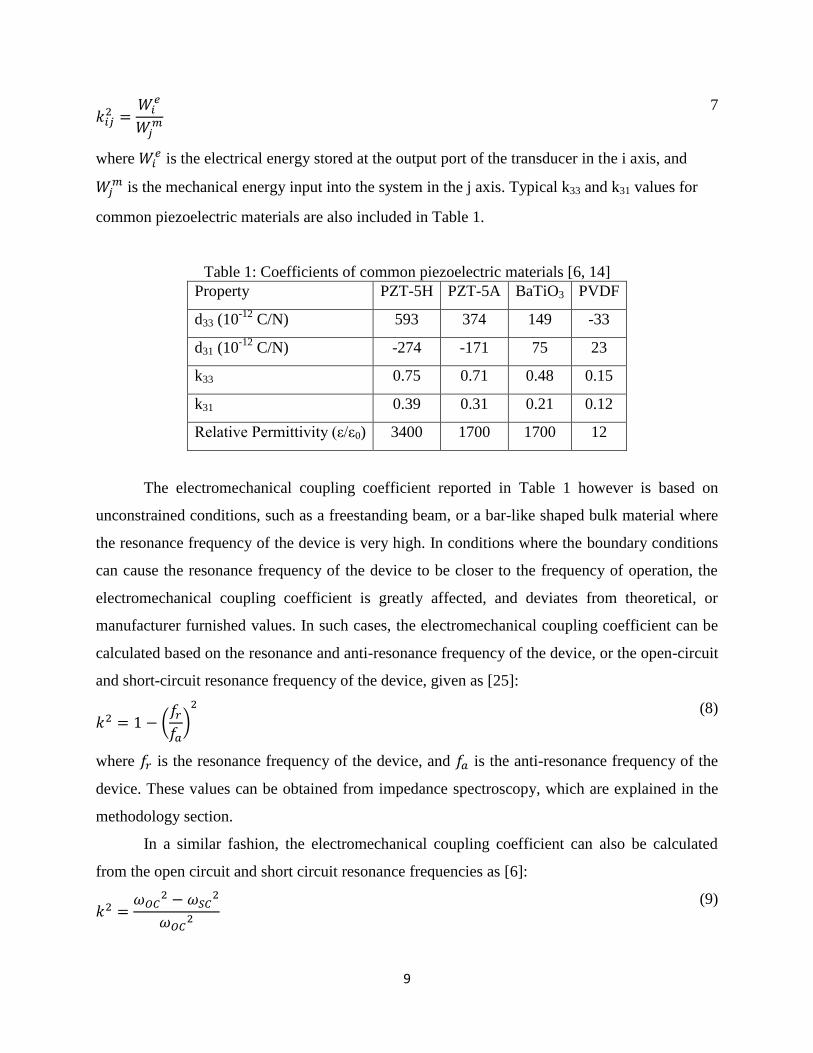
Table 1: Coefficients of common piezoelectric materials [6, 14] ................................................... 9

Table 2: Piezoelectric Bimorphs dimensions as available from Piezo Systems, Inc .................... 49

Table 3: Power output at optimal load resistance values for 70 mm3 samples without proof mass

....................................................................................................................................................... 78

Table 4: Impedance characteristics for 70 mm3 devices with no proof mass .............................. 83

Table 5: Capacitance characteristics for 70 mm3 devices with no proof mass ............................. 85


....................................................................................................................................................... 89

Table 7: Impedance measurements for 104 mm3 devices with no proof mass ............................. 91

Table 8: Capacitance measurements for 104 mm3 devices with no proof mass ........................... 91

Table 9: Power output at optimal load resistance’s for 140 mm3 devices without proof mass .... 96

Table 10: Impedance measurements for 140 mm3 samples with no proof mass .......................... 98

Table 11: Capacitance measurements for 140 mm3 samples with no proof mass ........................ 98

Table 12: Summary of Power generated from 70mm3 bimorphs with a 2 gram proof mass ..... 110

Table 13: Summary of impedance analysis for 70 mm3 devices with a 2 gram proof mass ...... 113

Table 14: Capacitance measurements for 70 mm3 devices with 2 gram proof mass .................. 115

Table 15: Power generated at optimal load resistance values for the 104 mm3 devices with a 2

gram proof mass .......................................................................................................................... 120

Table 16: Impedance characteristics for 104 mm3 devices with a 2 gram proof mass ............... 123

Table 17: Equivalent Parallel Capacitance for 104 mm3 devices with a 2 gram proof mass ..... 123


gram proof mass .......................................................................................................................... 128

Table 19: Impedance – Phase Angle for 140 mm3 devices with a 2 gram proof mass ............... 131

Table 20: Capacitance – Dissipation Factor for 140 mm3 devices with a 2 gram proof mass ... 131

Table 21: Power generated at optimal load resistance values for 70 mm3 devices with 4 grams

proof mass ................................................................................................................................... 143

xvi

Table 22: Impedance – Phase Angle for 70 mm3

devices with 4 grams proof mass .................. 146

Table 23: Capacitance – Dissipation Factor for 70 mm3 devices with 4 grams proof mass ....... 146

Table 24: Power generated by R70-1M and T35-1M at optimal load resistances ...................... 159

Table 25: Impedance measurements for T70-1M and T35-1M .................................................. 161

Table 26: Capacitance peaks for R70-1M and T35-1M-L .......................................................... 161

Table 27: Power at optimal load resistance for R140-1M and T70-1M ..................................... 166

Table 28: Impedance Analysis for R140-1M and T70-1M-L ..................................................... 170

Table 29: Capacitance peaks for R140-1M and T70-1M-L ........................................................ 170

CHAPTER 1: INTRODUCTION

With the developments and incredible advancements in silicon technology, and

developments of devices such as MEMS or NEMS (micro or nano- electro mechanical systems),

electronic devices are seeing very high levels of integration. [1, 2]. Examples of these very

highly integrated devices include multigate transistors such as FinFETs. With such high levels of

integration and complexity, electronic devices are comprised of a vast number of individual

sensor nodes [1] that are connected to larger wireless networks. These sensor nodes individually

require low levels of power for operation, which fall in the micro- to milli-watt range. In order to

power these nodes, traditional solutions have utilized electrochemical batteries, which can be

tedious and expensive to replace, and in some cases impractical, especially when sensors are

placed in remote locations [3]. A scenario such as this could be presented when sensors for

detection of harmful gases such as CO, CO2, ozone, tri-cresyl-phosphate (TCP) are placed on

board an airliner in the passenger cabin, or in the bleed air system of the aircraft, which would be

a highly inaccessible location [4]. In such cases, it would be very desirable to power up sensors,

or other such devices requiring low levels of power using a method alternative to batteries.

Some alternative solutions to batteries that have been presented, as reviewed by Roundy

et al [5, 6] and Cook-Chennault [7] include micro-batteries, micro-fuel cells, micro-turbine

generators, micro-heat engines; but these may require a source for fuel. In certain cases, they

might not have the desired efficiency, or may be expensive and cumbersome to integrate into low

powered sensor nodes. Truly renewable sources of energy that are completely regenerative

would utilize sources that are present within the sensors vicinity such as light, thermal or kinetic

energy in the environment. Photovoltaics for solar panels, and thermoelectric motors could

provide solutions, but the sources of energy required for their operation are insufficient in indoor

applications. Other sources of energy to consider could be kinetic energy in the environment;

such as ambient vibrations. [6, 7].

Vibrations are ubiquitous in the environment in the form of noise from various machines

such as microwave ovens, HVAC ducts, or on mobile structures such as automobile engines or

2

airplanes. Such ambient noise sources typically vibrate from 60 Hz for HVAC ducts to 240 Hz

for a refrigerator, with peak acceleration amplitudes ranging from 0.1 ms-2

for a refrigerator to 10

ms-2

for the base of a 5 horsepower 3-axis machine tool [6]. A publication depicting a study for

identification of vibration from various objects and instruments is provided in [8], and also

mentioned in [1, 6], which have been characterized in [9]. Such vibrations can also be harnessed

from human motion such as walking [10], or even heartbeats as well [11], which are

characterized by low frequency, high amplitude displacements. Therefore, there is a great

opportunity to harness these vibrations, which are forms of ambient kinetic energy in the

mechanical form, and convert them into usable electric energy for powering a sensor node.

The conversion of mechanical to electrical energy requires an electro-mechanical

transduction mechanism. Vibration energy is suitable in cases where an inertial frame is attached

to a vibrating host or generator, which acts as a fixed reference. This vibrating fixed reference

can transmit vibrations to a suspended inertial mass producing a relative displacement between

them. Such a system would possess a characteristic resonance frequency, which when matched

would amplify the relative displacement of the system [12]. Williams and Yates [13] identified

the use of three different transduction mechanisms in the form of these inertial generators, which

include electromagnetic, electrostatic, and piezoelectric devices. These transduction mechanisms

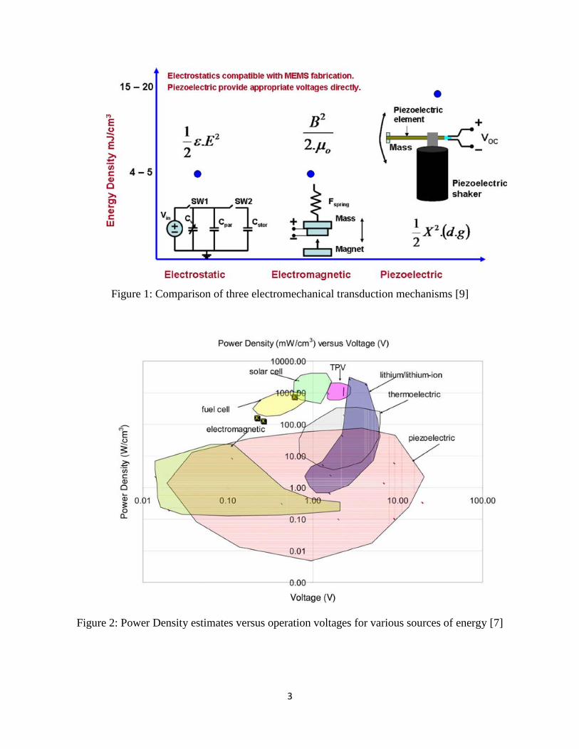
are described individually in [6], and have been compared by Priya [9] in Figure 1. Even though

electrostatic devices offer easy integration into microelectronics such as CMOS devices, they

suffer from high impedance, and require mechanical stops. Figure 2 [7], which illustrates

voltages versus power density for various devices, does not feature electrostatic devices due to

their high voltages. Electromagnetic devices tend to be somewhat bulky, and require multistage

post-processing to reach desired levels of voltages [14]. Piezoelectric devices however are less

bulky, and theoretically provide the largest energy density per volume when compared to other

inertial generators. They also have a direct voltage output, inherent to the material. Figure 2 [7]

depicts them as the most versatile in terms of output voltages, and fairly high power densities

compared to other sources of energy.

3

Figure 1: Comparison of three electromechanical transduction mechanisms [9]

Figure 2: Power Density estimates versus operation voltages for various sources of energy [7]

4

Therefore, piezoelectric materials are prime candidates for vibration energy harvesting,

and the publication of a number of review articles [2, 9, 12, 15-17] within the last 10 years bears

testament to this exploding area of research. Piezoelectric energy harvesting is usually carried

out using cantilevered bimorphs, which are heterogeneous structures consisting of two

piezoceramic layers sandwiching a metallic layer. These devices are attached on a vibrating host

generating a dynamic strain in the beam, resulting in an alternating voltage across their

electrodes. This is an inherent property of piezoelectric devices, which is described in the

following section.

Cantilevered piezoelectric bimorphs have been widely explored and studied in the past

decade for energy harvesting from vibrations. In this field, the d31 mode of operation is exploited,

where the cantilevered bimorph is attached on a vibrating host structure causing longitudinal

deflections in the bimorph, when resonating in the fundamental mode. This vibration causes

axial stresses over the surfaces of the bimorphs, while generating charge in the longitudinal

direction. Most commonly, these axial stresses are concentrated near the fixed end of the beam,

and linearly decrease towards the free end of the beam. This results in inefficiencies in the

cantilevered piezoelectric bimorphs wherein only a small portion of the device is engaged in

generating power. In order to circumvent this inefficiency, the geometry of the cantilevered

bimorph can be altered. Changing the geometry from a rectangular to triangular bimorph, where

the wide end of the isosceles triangle is clamped, can result in a linear stress profile [18].

This concept of tapering geometry and even shape optimization to obtain greater amounts

of power from a cantilevered device has been presented in a few studies, which are reviewed in

the following section. However, changing the geometry usually affects the resonance frequency

of the device, yielding results that are difficult to compare with rectangular counterparts.

Moreover, the effect of changing geometry on various important parameters such as

electromechanical coupling coefficients, impedance, capacitance, and damping ratios are elusive

in literature. Therefore, in this dissertation, various sets of rectangular and triangular cantilevered

piezoelectric bimorphs with matching volumes and resonance frequencies are found and

experimentally characterized for these parameters. The tests are conducted with piezoelectric

bimorphs with varying degrees of proof masses into varying load resistances. It is shown that

triangular devices with the given constraints of matching volume and resonance frequency

operate with lower values of maximum stress, resulting in larger electromechanical coupling

5

coefficients (k31), and larger electromechanical coupling figure of merits (k2Qm). It is also shown

that with these larger coupling coefficients, the triangular devices are more electrically

compliant, since they provide lower impedance values at resonance, and larger impedance values

at anti-resonance. The capacitance characteristics in the frequency domain are also measured,

indicating larger absolute values of positive and negative capacitance peaks in the case of

triangular bimorphs, compared to their rectangular counterparts. Therefore, the dissertation

reports an exhaustive electronic characterization of these materials, which so far have only been

partly reported in literature, mostly by means of numerical studies, showcasing the effects of

electronic parameters such as k31 and Qm from a hypothetical point of view.

6

CHAPTER 2: LITERATURE REVIEW

2.1 Brief introduction to piezoelectricity and piezoelectric bimorphs

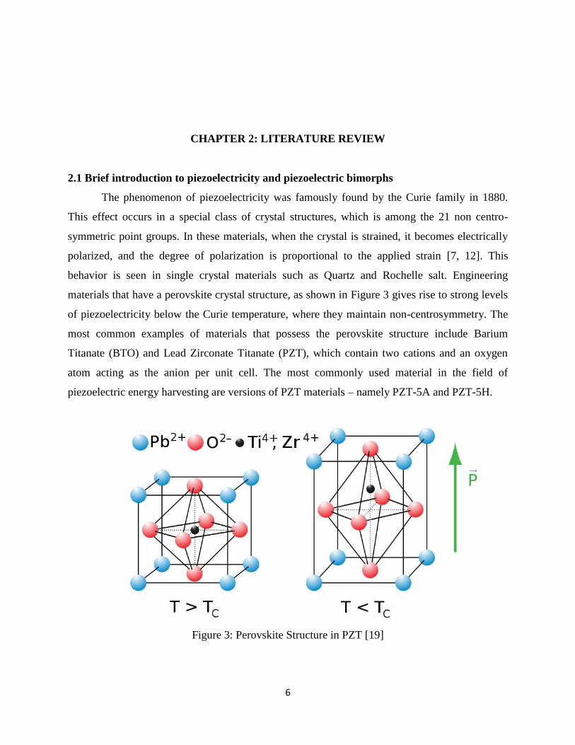
The phenomenon of piezoelectricity was famously found by the Curie family in 1880.

This effect occurs in a special class of crystal structures, which is among the 21 non centro-

symmetric point groups. In these materials, when the crystal is strained, it becomes electrically

polarized, and the degree of polarization is proportional to the applied strain [7, 12]. This

behavior is seen in single crystal materials such as Quartz and Rochelle salt. Engineering

materials that have a perovskite crystal structure, as shown in Figure 3 gives rise to strong levels

of piezoelectricity below the Curie temperature, where they maintain non-centrosymmetry. The

most common examples of materials that possess the perovskite structure include Barium

Titanate (BTO) and Lead Zirconate Titanate (PZT), which contain two cations and an oxygen

atom acting as the anion per unit cell. The most commonly used material in the field of

piezoelectric energy harvesting are versions of PZT materials – namely PZT-5A and PZT-5H.

Figure 3: Perovskite Structure in PZT [19]

7

Due to the mentioned non-centrosymmetry, piezoelectric materials exhibit anisotropic

characteristics in terms of stress, strain, compliance, stiffness, permittivity and piezoelectric

coefficients. These are related to the orientation of the ceramic material and the direction of

measurements and applied stresses/forces. Therefore, these properties are reported in tensor

forms. The constitutive equations [20, 21] that describe the piezoelectric effect are as follows:

𝑆𝑖𝑗 = 𝑠𝑖𝑗𝑘𝑙𝐸 𝑇𝑘𝑙 + 𝑑𝑘𝑖𝑗𝐸𝑘 (1)

𝐷𝑖 = 𝑑𝑖𝑘𝑙𝑇𝑘𝑙 + 휀𝑖𝑘𝑇 𝐸𝑘 (2)

where,

𝑆𝑖𝑗 is strain,

𝑠𝑖𝑗𝑘𝑙𝐸 is elastic compliance at constant electric field,

𝑇𝑘𝑙 is stress,

𝐸𝑘 is the electric field,

𝐷𝑖 is dielectric displacement component,

and 휀𝑖𝑘𝑇 is the permittivity of the material at constant stress.

The subscripts indicate the tensor notation.

𝑑𝑘𝑖𝑗, the piezoelectric coefficient is one of the most important properties, which is a third rank

tensor. This property is a representation of the charge developed based on the applied stress, or

the strain developed based on the applied electric field. Hence, it can be represented as [12]:

𝑑 =𝑠ℎ𝑜𝑟𝑡 𝑐𝑖𝑟𝑐𝑢𝑖𝑡 𝑐ℎ𝑎𝑟𝑔𝑒 𝑑𝑒𝑛𝑠𝑖𝑡𝑦

𝑎𝑝𝑝𝑙𝑖𝑒𝑑 𝑠𝑡𝑟𝑒𝑠𝑠𝐶/𝑁 (3)

𝑑 =𝑠𝑡𝑟𝑎𝑖𝑛 𝑑𝑒𝑣𝑒𝑙𝑜𝑝𝑒𝑑

𝑎𝑝𝑝𝑙𝑖𝑒𝑑 𝑓𝑖𝑒𝑙𝑑𝑚/𝑉 (4)

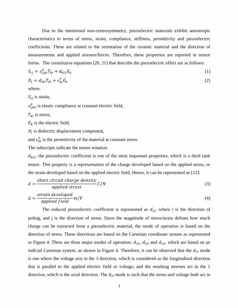
The reduced piezoelectric coefficient is represented as 𝑑𝑖𝑗, where i is the direction of

poling, and j is the direction of stress. Since the magnitude of stress/strain defines how much

charge can be extracted from a piezoelectric material, the mode of operation is based on the

direction of stress. These directions are based on the Cartesian coordinate system as represented

in Figure 4. There are three major modes of operation: 𝑑31, 𝑑33 and 𝑑15, which are based on an

indicial Cartesian system, as shown in Figure 4. Therefore, it can be observed that the d31 mode

is one where the voltage acts in the 3 direction, which is considered as the longitudinal direction

that is parallel to the applied electric field or voltage; and the resulting stresses act in the 1

direction, which is the axial direction. The d33 mode is such that the stress and voltage both act in

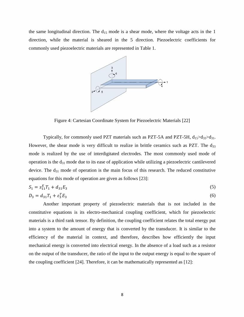
8

the same longitudinal direction. The d15 mode is a shear mode, where the voltage acts in the 1

direction, while the material is sheared in the 5 direction. Piezoelectric coefficients for

commonly used piezoelectric materials are represented in Table 1.

Figure 4: Cartesian Coordinate System for Piezoelectric Materials [22]

Typically, for commonly used PZT materials such as PZT-5A and PZT-5H, d15>d33>d31.

However, the shear mode is very difficult to realize in brittle ceramics such as PZT. The d33

mode is realized by the use of interdigitated electrodes. The most commonly used mode of

operation is the d31 mode due to its ease of application while utilizing a piezoelectric cantilevered

device. The d31 mode of operation is the main focus of this research. The reduced constitutive

equations for this mode of operation are given as follows [23]:

𝑆1 = 𝑠11𝐸 𝑇1 + 𝑑31𝐸3 (5)

𝐷3 = 𝑑31𝑇1 + 휀3𝑇𝐸3 (6)

Another important property of piezoelectric materials that is not included in the

constitutive equations is its electro-mechanical coupling coefficient, which for piezoelectric

materials is a third rank tensor. By definition, the coupling coefficient relates the total energy put

into a system to the amount of energy that is converted by the transducer. It is similar to the

efficiency of the material in context, and therefore, describes how efficiently the input

mechanical energy is converted into electrical energy. In the absence of a load such as a resistor

on the output of the transducer, the ratio of the input to the output energy is equal to the square of

the coupling coefficient [24]. Therefore, it can be mathematically represented as [12]:

9

𝑘𝑖𝑗2 =

𝑊𝑖𝑒

𝑊𝑗𝑚

7

where 𝑊𝑖𝑒 is the electrical energy stored at the output port of the transducer in the i axis, and

𝑊𝑗𝑚 is the mechanical energy input into the system in the j axis. Typical k33 and k31 values for

common piezoelectric materials are also included in Table 1.

Table 1: Coefficients of common piezoelectric materials [6, 14]

Property PZT-5H PZT-5A BaTiO3 PVDF

d33 (10-12

C/N) 593 374 149 -33

d31 (10-12

C/N) -274 -171 75 23

k33 0.75 0.71 0.48 0.15

k31 0.39 0.31 0.21 0.12

Relative Permittivity (ε/ε0) 3400 1700 1700 12

The electromechanical coupling coefficient reported in Table 1 however is based on

unconstrained conditions, such as a freestanding beam, or a bar-like shaped bulk material where

the resonance frequency of the device is very high. In conditions where the boundary conditions

can cause the resonance frequency of the device to be closer to the frequency of operation, the

electromechanical coupling coefficient is greatly affected, and deviates from theoretical, or

manufacturer furnished values. In such cases, the electromechanical coupling coefficient can be

calculated based on the resonance and anti-resonance frequency of the device, or the open-circuit

and short-circuit resonance frequency of the device, given as [25]:

𝑘2 = 1 − (𝑓𝑟

𝑓𝑎)

2

(8)

where 𝑓𝑟 is the resonance frequency of the device, and 𝑓𝑎 is the anti-resonance frequency of the

device. These values can be obtained from impedance spectroscopy, which are explained in the

methodology section.

In a similar fashion, the electromechanical coupling coefficient can also be calculated

from the open circuit and short circuit resonance frequencies as [6]:

𝑘2 =𝜔𝑂𝐶

2 − 𝜔𝑆𝐶2

𝜔𝑂𝐶2

(9)

10

where, 𝜔𝑂𝐶 is the resonance frequency of the device in open-circuit conditions, and 𝜔𝑆𝐶 is the

resonance frequency of the device under short circuit conditions.

Therefore, as mentioned earlier, the piezoelectric coefficients in the d33 mode are higher

than in d31 mode, and the higher coupling coefficients also illustrate that the longitudinal mode is

theoretically more efficient. However, this mode is more difficult to realize since piezoelectric

materials such as PZT are brittle, and under compression they can crack when mechanically

strained beyond certain limits. The d31 mode is realized in the form of cantilevered devices,

where the material is displaced in the direction of poling, and the charge is generated as a

function of strain in the material, and the cantilevered boundary condition allows for the

maximum possible strain on a beam or a plate like structure.

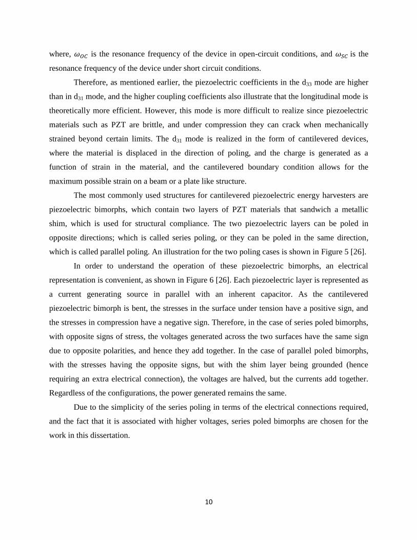
The most commonly used structures for cantilevered piezoelectric energy harvesters are

piezoelectric bimorphs, which contain two layers of PZT materials that sandwich a metallic

shim, which is used for structural compliance. The two piezoelectric layers can be poled in

opposite directions; which is called series poling, or they can be poled in the same direction,

which is called parallel poling. An illustration for the two poling cases is shown in Figure 5 [26].

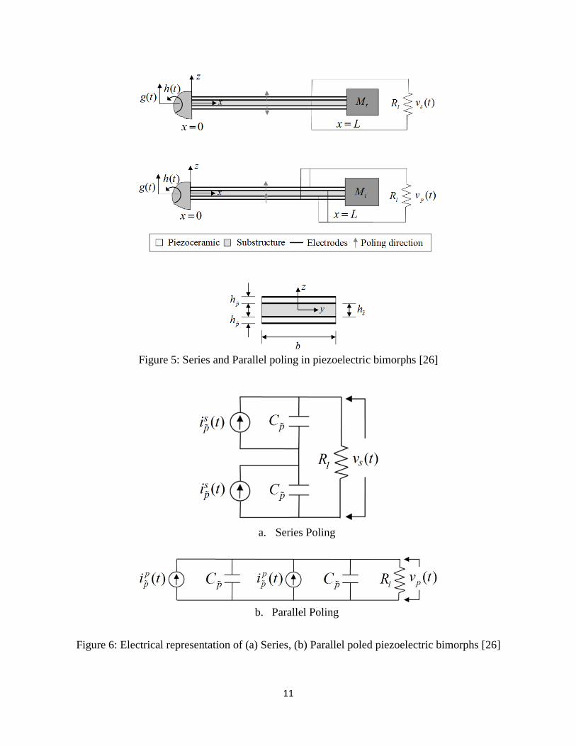
In order to understand the operation of these piezoelectric bimorphs, an electrical

representation is convenient, as shown in Figure 6 [26]. Each piezoelectric layer is represented as

a current generating source in parallel with an inherent capacitor. As the cantilevered

piezoelectric bimorph is bent, the stresses in the surface under tension have a positive sign, and

the stresses in compression have a negative sign. Therefore, in the case of series poled bimorphs,

with opposite signs of stress, the voltages generated across the two surfaces have the same sign

due to opposite polarities, and hence they add together. In the case of parallel poled bimorphs,

with the stresses having the opposite signs, but with the shim layer being grounded (hence

requiring an extra electrical connection), the voltages are halved, but the currents add together.

Regardless of the configurations, the power generated remains the same.

Due to the simplicity of the series poling in terms of the electrical connections required,

and the fact that it is associated with higher voltages, series poled bimorphs are chosen for the

work in this dissertation.

11

Figure 5: Series and Parallel poling in piezoelectric bimorphs [26]

a. Series Poling

b. Parallel Poling

Figure 6: Electrical representation of (a) Series, (b) Parallel poled piezoelectric bimorphs [26]

12

2.2 Literature Review on Piezoelectric Generators

Various types of piezoelectric transduction generators have surfaced in the past few

years. Some of the early studies were performed on impact coupled devices, followed by human

powered piezoelectric energy harvesting. This was done in order to test the feasibility of

piezoelectric devices for power generation, and have been mentioned very briefly.

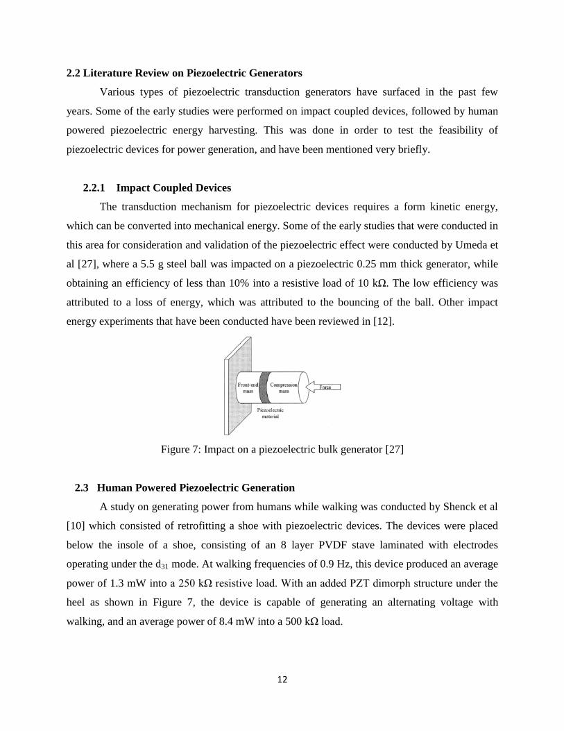
2.2.1 Impact Coupled Devices

The transduction mechanism for piezoelectric devices requires a form kinetic energy,

which can be converted into mechanical energy. Some of the early studies that were conducted in

this area for consideration and validation of the piezoelectric effect were conducted by Umeda et

al [27], where a 5.5 g steel ball was impacted on a piezoelectric 0.25 mm thick generator, while

obtaining an efficiency of less than 10% into a resistive load of 10 kΩ. The low efficiency was

attributed to a loss of energy, which was attributed to the bouncing of the ball. Other impact

energy experiments that have been conducted have been reviewed in [12].

Figure 7: Impact on a piezoelectric bulk generator [27]

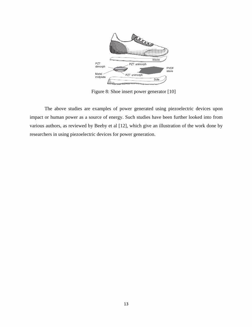
2.3 Human Powered Piezoelectric Generation

A study on generating power from humans while walking was conducted by Shenck et al

[10] which consisted of retrofitting a shoe with piezoelectric devices. The devices were placed

below the insole of a shoe, consisting of an 8 layer PVDF stave laminated with electrodes

operating under the d31 mode. At walking frequencies of 0.9 Hz, this device produced an average

power of 1.3 mW into a 250 kΩ resistive load. With an added PZT dimorph structure under the

heel as shown in Figure 7, the device is capable of generating an alternating voltage with

walking, and an average power of 8.4 mW into a 500 kΩ load.

13

Figure 8: Shoe insert power generator [10]

The above studies are examples of power generated using piezoelectric devices upon

impact or human power as a source of energy. Such studies have been further looked into from

various authors, as reviewed by Beeby et al [12], which give an illustration of the work done by

researchers in using piezoelectric devices for power generation.

14

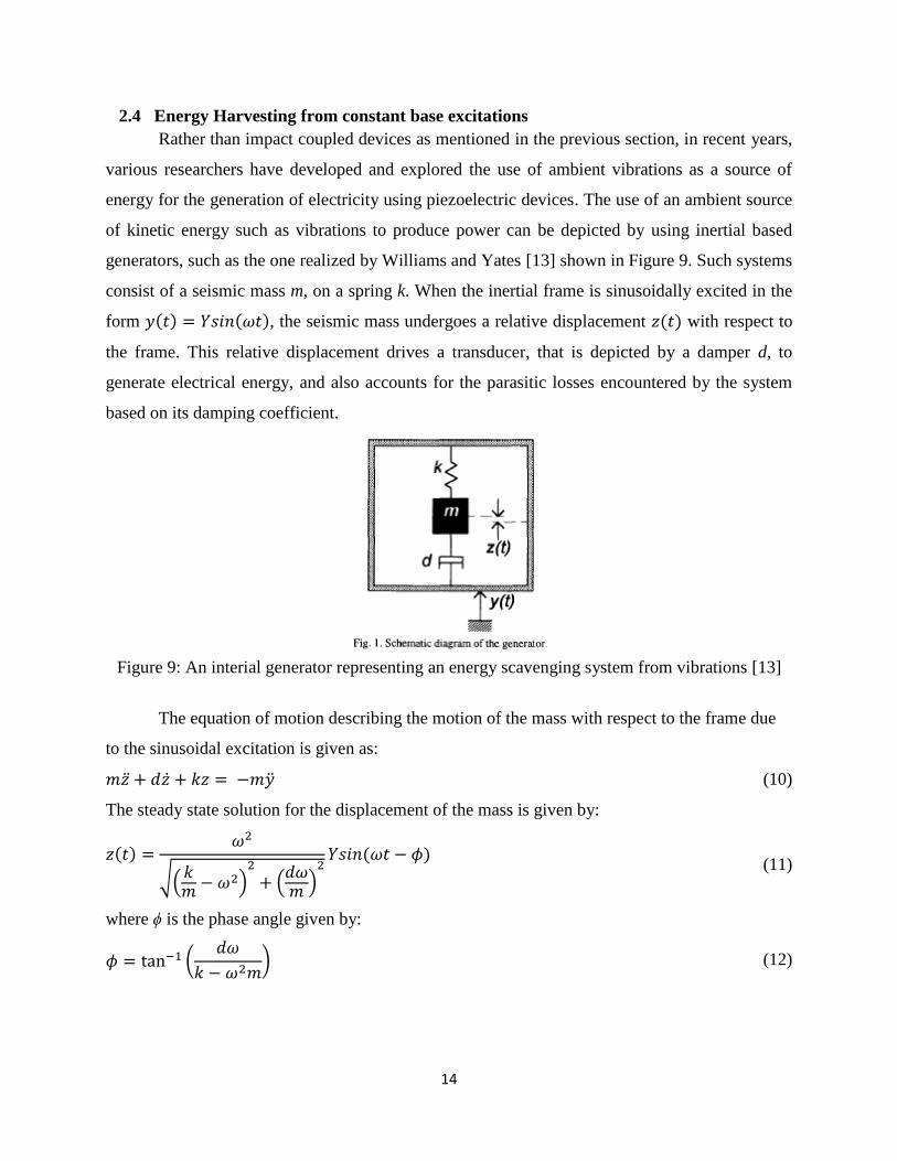
2.4 Energy Harvesting from constant base excitations

Rather than impact coupled devices as mentioned in the previous section, in recent years,

various researchers have developed and explored the use of ambient vibrations as a source of

energy for the generation of electricity using piezoelectric devices. The use of an ambient source

of kinetic energy such as vibrations to produce power can be depicted by using inertial based

generators, such as the one realized by Williams and Yates [13] shown in Figure 9. Such systems

consist of a seismic mass m, on a spring k. When the inertial frame is sinusoidally excited in the

form 𝑦(𝑡) = 𝑌𝑠𝑖𝑛(𝜔𝑡), the seismic mass undergoes a relative displacement 𝑧(𝑡) with respect to

the frame. This relative displacement drives a transducer, that is depicted by a damper d, to

generate electrical energy, and also accounts for the parasitic losses encountered by the system

based on its damping coefficient.

Figure 9: An interial generator representing an energy scavenging system from vibrations [13]

The equation of motion describing the motion of the mass with respect to the frame due

to the sinusoidal excitation is given as:

𝑚�̈� + 𝑑�̇� + 𝑘𝑧 = −𝑚�̈� (10)

The steady state solution for the displacement of the mass is given by:

𝑧(𝑡) =𝜔2

√(𝑘𝑚 − 𝜔2)

2

+ (𝑑𝜔𝑚 )

2𝑌𝑠𝑖𝑛(𝜔𝑡 − 𝜙)

(11)

where ϕ is the phase angle given by:

𝜙 = tan−1 (𝑑𝜔

𝑘 − 𝜔2𝑚) (12)

15

The instantaneous power can be calculated as the product of the force acting on the mass

and its velocity, which can be represented as:

𝑝(𝑡) = −𝑚�̈�[�̇�(𝑡) + �̇�(𝑡)] (13)

Taking Laplace transform for P, we arrive at:

𝑃 =𝑚휁𝑇𝜔3 (

𝜔𝜔𝑛

)3

𝑌2

(1 − (𝜔

𝜔𝑛)

2

)2

+ (2휁𝑇𝜔𝜔𝑛

)2 (14)

where

휁𝑇 =𝑑

2𝑚𝜔𝑛 (15)

and 𝜔𝑛 is the natural frequency of the system

If 𝜔 = 𝜔𝑛 then

𝑃 =𝑚𝑌2𝜔𝑛

3

4휁𝑇 (16)

Or,

𝑃 =𝑚𝐴2

4𝜔𝑛휁𝑇 (17)

However, since these are steady state solutions, the maximum power does not tend to

infinity as damping tends to zero. In fact, the power available from the vibrating structure is

limited by the undesirable parasitic damping 휁𝑝 such as air damping. Therefore 휁𝑇 is a

summation of parasitic damping 휁𝑝 and electrical damping 휁𝑒 . The expression for power obtained

can therefore be attained as

𝑃 =𝑚𝑌2𝜔𝑛

3휁𝑒

4(휁𝑒 + 휁𝑝)2 (18)

or in terms of excitation amplitude as

𝑃 =𝑚𝐴2휁𝑒

4𝜔𝑛(휁𝑒 + 휁𝑝)2 (19)

16

The above model has certain restrictions, wherein certain assumptions are to be made in

order to apply it to a piezoelectric transducer. One of the major assumptions is that the seismic

mass is much larger as compared to the system, and acts as the main driving force for the

generator. In addition, the transducer that is represented by the dashpot is assumed to be a linear

transducer. These assumptions are a bit crude for a cantilever beam with a small tip mass, but

important conclusions can be made based on the model that depicts important behavior for the

piezoelectric generator. These conclusions are provided in the following bullets [6, 13]:

- Maximum power is generated at the resonance frequency of the system where the

displacement is maximized. Therefore, a system could be designed where z(t) is maximized

within allowable limits.

- Power generated is finite, and reduction in the damping factor results in increased mass

displacement.

- However, low damping ratio results in a high peak power concentrated at a particular natural

frequency. Therefore, an increased bandwidth for power generation can be obtained with

higher damping factors.

- Since power generation is inversely proportional to the resonant frequency at a given

acceleration, the system should be designed to operate at the lowest available fundamental

frequency.

- The power generated is proportional to the square of the input acceleration amplitude

17

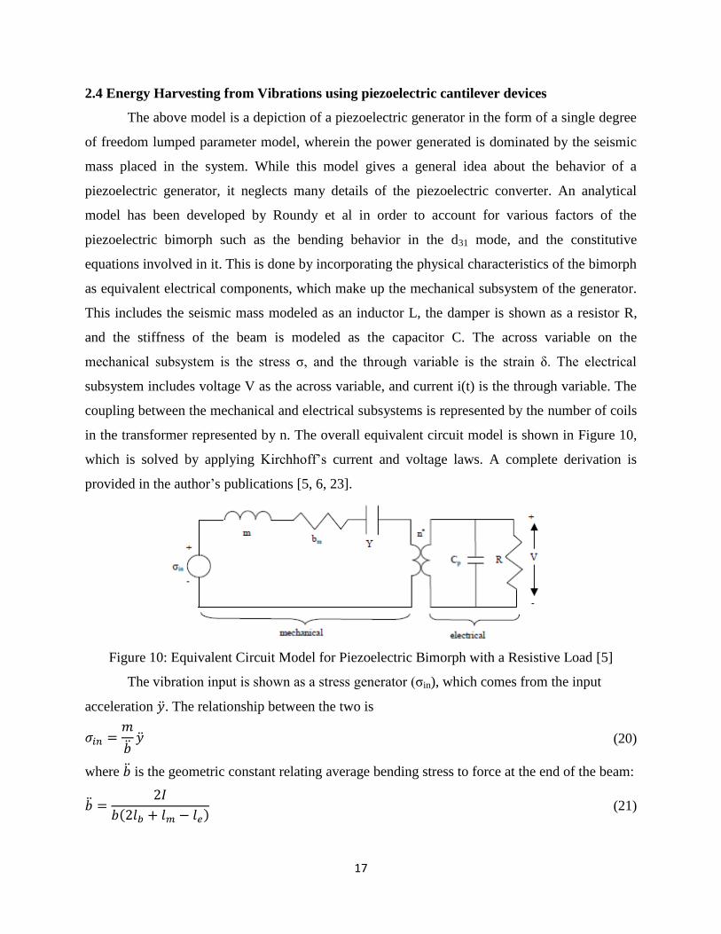
2.4 Energy Harvesting from Vibrations using piezoelectric cantilever devices

The above model is a depiction of a piezoelectric generator in the form of a single degree

of freedom lumped parameter model, wherein the power generated is dominated by the seismic

mass placed in the system. While this model gives a general idea about the behavior of a

piezoelectric generator, it neglects many details of the piezoelectric converter. An analytical

model has been developed by Roundy et al in order to account for various factors of the

piezoelectric bimorph such as the bending behavior in the d31 mode, and the constitutive

equations involved in it. This is done by incorporating the physical characteristics of the bimorph

as equivalent electrical components, which make up the mechanical subsystem of the generator.

This includes the seismic mass modeled as an inductor L, the damper is shown as a resistor R,

and the stiffness of the beam is modeled as the capacitor C. The across variable on the

mechanical subsystem is the stress σ, and the through variable is the strain δ. The electrical

subsystem includes voltage V as the across variable, and current i(t) is the through variable. The

coupling between the mechanical and electrical subsystems is represented by the number of coils

in the transformer represented by n. The overall equivalent circuit model is shown in Figure 10,

which is solved by applying Kirchhoff’s current and voltage laws. A complete derivation is

provided in the author’s publications [5, 6, 23].

Figure 10: Equivalent Circuit Model for Piezoelectric Bimorph with a Resistive Load [5]

The vibration input is shown as a stress generator (σin), which comes from the input

acceleration �̈�. The relationship between the two is

𝜎𝑖𝑛 =𝑚

�̈��̈� (20)

where �̈� is the geometric constant relating average bending stress to force at the end of the beam:

�̈� =2𝐼

𝑏(2𝑙𝑏 + 𝑙𝑚 − 𝑙𝑒) (21)

18

The constitutive equations for piezoelectricity are reduced to

𝜎 = −𝑑𝑌𝐸 (22)

𝐷 = −𝑑𝑌𝛿 (23)

Using the above equations, the resulting model is shown as:

�̈� =−𝑘𝑠𝑝

𝑚𝛿 −

𝑏𝑚𝑏∗∗

𝑚�̇� +

𝑘𝑠𝑝𝑑

𝑚𝑡𝑐𝑉 + 𝑏∗�̈� (24)

�̇� =−𝑌𝑑𝑡𝑐

휀�̇� (25)

Assuming 𝜔 = 𝜔𝑛, the analytical expression for power transferred to the load is shown as:

𝑃 = 1

𝜔𝑛2

𝑅𝐶𝑝2 (

𝑌𝑐𝑑31𝑡𝑐𝑏∗

휀 )2

(4휁2 + 𝑘314)(𝑅𝐶𝑝𝜔)

2+ 4휁𝑘31

2(𝑅𝐶𝑝𝜔) + 2휁2𝐴𝑖𝑛

2 (26)

where,

𝑏∗ =3𝑏

𝑙𝑏2

2𝑙𝑏 + 𝑙𝑚 − 𝑙𝑐

2𝑙𝑏 + 1.5𝑙𝑚 (27)

b = distance from center of piezo to center of shim

lb = length of the beam (not covered with mass)

le = length of electrode (in most cases assumed to be < or = to lb)

lm = length of the mass

This analytical model that was developed provides further insights into the piezoelectric

energy harvesting system from a cantilevered bimorph, that were absent in the Williams and

Yates model. The input parameters, driving frequency and acceleration amplitude have profound

effects on power generation. In addition, the equation describes the importance of the coupling

coefficient, the piezoelectric coefficient, damping ratio, and the geometric constants that are

dependent on the beam’s and proof mass geometry.

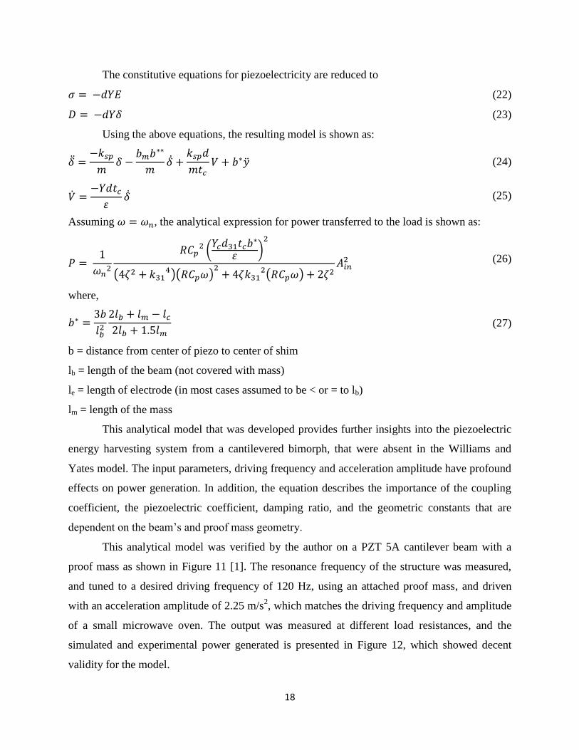
This analytical model was verified by the author on a PZT 5A cantilever beam with a

proof mass as shown in Figure 11 [1]. The resonance frequency of the structure was measured,

and tuned to a desired driving frequency of 120 Hz, using an attached proof mass, and driven

with an acceleration amplitude of 2.25 m/s2, which matches the driving frequency and amplitude

of a small microwave oven. The output was measured at different load resistances, and the

simulated and experimental power generated is presented in Figure 12, which showed decent

validity for the model.

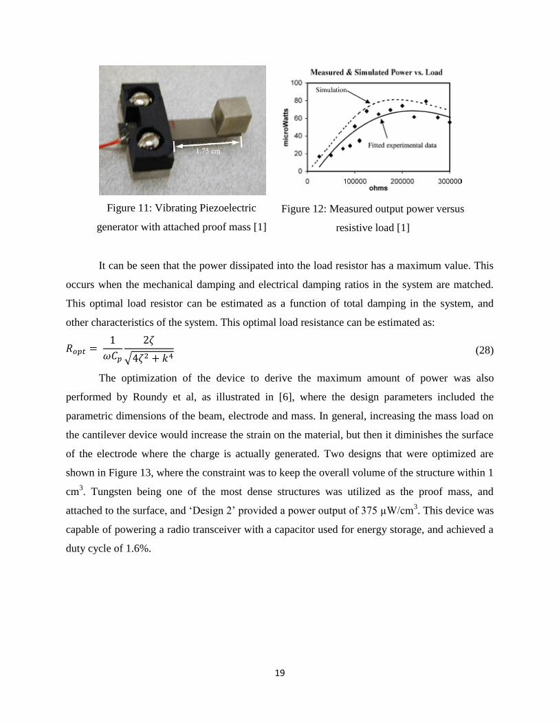
19

Figure 11: Vibrating Piezoelectric

generator with attached proof mass [1]

Figure 12: Measured output power versus

resistive load [1]

It can be seen that the power dissipated into the load resistor has a maximum value. This

occurs when the mechanical damping and electrical damping ratios in the system are matched.

This optimal load resistor can be estimated as a function of total damping in the system, and

other characteristics of the system. This optimal load resistance can be estimated as:

𝑅𝑜𝑝𝑡 = 1

𝜔𝐶𝑝

2휁

√4휁2 + 𝑘4 (28)

The optimization of the device to derive the maximum amount of power was also

performed by Roundy et al, as illustrated in [6], where the design parameters included the

parametric dimensions of the beam, electrode and mass. In general, increasing the mass load on

the cantilever device would increase the strain on the material, but then it diminishes the surface

of the electrode where the charge is actually generated. Two designs that were optimized are

shown in Figure 13, where the constraint was to keep the overall volume of the structure within 1

cm3. Tungsten being one of the most dense structures was utilized as the proof mass, and

attached to the surface, and ‘Design 2’ provided a power output of 375 µW/cm3. This device was

capable of powering a radio transceiver with a capacitor used for energy storage, and achieved a

duty cycle of 1.6%.

20

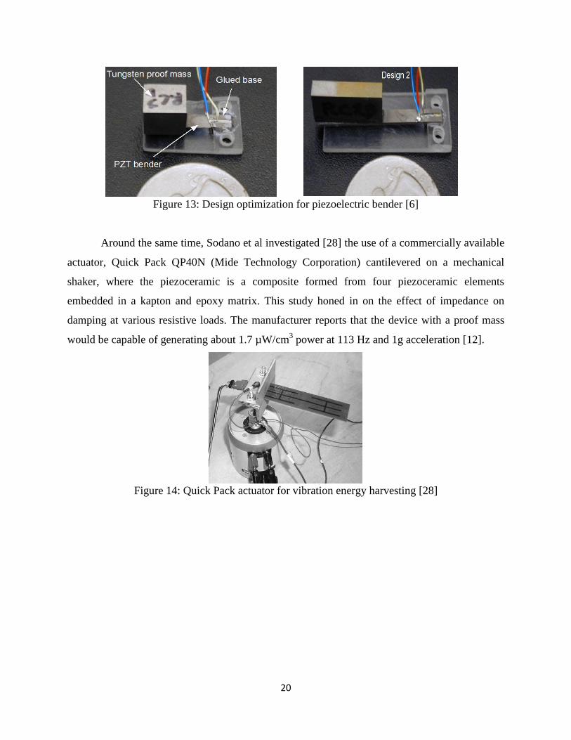
Figure 13: Design optimization for piezoelectric bender [6]

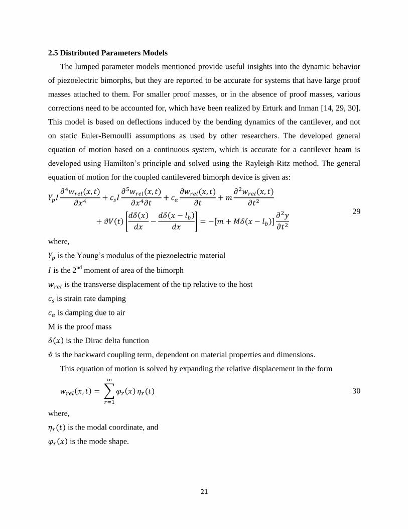
Around the same time, Sodano et al investigated [28] the use of a commercially available

actuator, Quick Pack QP40N (Mide Technology Corporation) cantilevered on a mechanical

shaker, where the piezoceramic is a composite formed from four piezoceramic elements

embedded in a kapton and epoxy matrix. This study honed in on the effect of impedance on

damping at various resistive loads. The manufacturer reports that the device with a proof mass

would be capable of generating about 1.7 µW/cm3 power at 113 Hz and 1g acceleration [12].

Figure 14: Quick Pack actuator for vibration energy harvesting [28]

21

2.5 Distributed Parameters Models

The lumped parameter models mentioned provide useful insights into the dynamic behavior

of piezoelectric bimorphs, but they are reported to be accurate for systems that have large proof

masses attached to them. For smaller proof masses, or in the absence of proof masses, various

corrections need to be accounted for, which have been realized by Erturk and Inman [14, 29, 30].

This model is based on deflections induced by the bending dynamics of the cantilever, and not

on static Euler-Bernoulli assumptions as used by other researchers. The developed general

equation of motion based on a continuous system, which is accurate for a cantilever beam is

developed using Hamilton’s principle and solved using the Rayleigh-Ritz method. The general

equation of motion for the coupled cantilevered bimorph device is given as:

𝑌𝑝𝐼𝜕4𝑤𝑟𝑒𝑙(𝑥, 𝑡)

𝜕𝑥4+ 𝑐𝑠𝐼

𝜕5𝑤𝑟𝑒𝑙(𝑥, 𝑡)

𝜕𝑥4𝜕𝑡+ 𝑐𝑎

𝜕𝑤𝑟𝑒𝑙(𝑥, 𝑡)

𝜕𝑡+ 𝑚

𝜕2𝑤𝑟𝑒𝑙(𝑥, 𝑡)

𝜕𝑡2

+ 𝜗𝑉(𝑡) [𝑑𝛿(𝑥)

𝑑𝑥−

𝑑𝛿(𝑥 − 𝑙𝑏)

𝑑𝑥] = −[𝑚 + 𝑀𝛿(𝑥 − 𝑙𝑏)]

𝜕2𝑦

𝜕𝑡2

29

where,

𝑌𝑝 is the Young’s modulus of the piezoelectric material

𝐼 is the 2nd

moment of area of the bimorph

𝑤𝑟𝑒𝑙 is the transverse displacement of the tip relative to the host

𝑐𝑠 is strain rate damping

𝑐𝑎 is damping due to air

M is the proof mass

𝛿(𝑥) is the Dirac delta function

𝜗 is the backward coupling term, dependent on material properties and dimensions.

This equation of motion is solved by expanding the relative displacement in the form

𝑤𝑟𝑒𝑙(𝑥, 𝑡) = ∑ 𝜑𝑟(𝑥)

∞

𝑟=1

휂𝑟(𝑡) 30

where,

휂𝑟(𝑡) is the modal coordinate, and

𝜑𝑟(𝑥) is the mode shape.

22

Therefore, the dynamics of the mode-shape can be described by the set of coupled equations:

휂̈𝑟(𝑡) + 2휁𝑟𝜔𝑟휂̇𝑟(𝑡) + 𝜔𝑟2휂𝑟(𝑡) + 𝜒𝑟𝑉(𝑡) = 𝑓𝑟(𝑡) 31

𝐶𝑝

2�̇�(𝑡) +

𝑉(𝑡)

𝑅𝐿= 𝑖(𝑡) 32

where, 𝜒𝑟 is the modal coupling term correlated to the mode shape 𝜑𝑟, 𝜔𝑟 is the resonant

frequency, 𝑓𝑟(𝑡) is the mechanical forcing function and 𝐶𝑝 is the inherent equivalent capacitance

of the piezoelectric layer.

Under a pure sinusoidal excitation of the fixed end of the cantilever with a frequency 𝜔𝑟, the

electric voltage across the piezoelectric layers in series becomes

𝑉 =𝑗2𝜔𝑅𝐿𝜘𝑟𝐹𝑟

(2 + 𝑗2𝜔𝑅𝐿𝐶𝑝)(𝜔𝑟2 − 𝜔2 + 𝑗2휁𝑟𝜔𝑟𝜔) + 𝑗2𝜔𝑅𝐿𝜘𝑟𝜒𝑟

33

where 𝐹𝑟 is the amplitude of the modal mechanical forcing function, and 𝜘𝑟 is the forward

coupling term

Based on a similar approach, with coupled equations of motion, similar to equations 31

and 32, a distributed parameters model for a piezoelectric bimorph with a varying cross-sectional

area was presented by Dietl and Garcia [31]. More recently, a similar analysis with expressions

for voltage generated by the piezoelectric cantilever have been presented by Rosa and De

Marquis Jr. [32]. The expression for voltage generated is given as:

𝑉(𝑡)

𝑎(𝑡)=

𝑉(𝑡)

−𝜔2𝑌0𝑒−𝑗𝜔𝑡

= 𝑗𝜔 (1

𝑅+ 𝑗𝜔𝐶𝑝)

−1

𝛩𝑇 × [−𝜔2𝐌 + j𝜔𝐂 + 𝐊 + 𝑗𝜔 (1

𝑅+ 𝑗𝜔𝐶𝑝)

−1

𝛩𝛩𝑇] 𝑝∗ (34)

where, 𝛩 is the electromechanical coupling matrix, and the superscript T is for constant stress.

𝑝∗ is the input matrix, defined in [32].

It can be noted that due to the changing cross-sectional area, equation (34), and similar

equations in [31, 32] for tip displacement or tip velocity are not provided in closed-form.

Detailed derivations for these expressions are available in the references mentioned. Hence the

terms M, C, K, are the mass, damping and stiffness matrices respectively, which are calculated

as a function of axial length of the device, where the width varies.

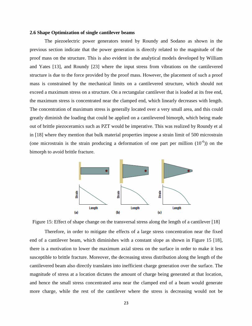
23

2.6 Shape Optimization of single cantilever beams

The piezoelectric power generators tested by Roundy and Sodano as shown in the

previous section indicate that the power generation is directly related to the magnitude of the

proof mass on the structure. This is also evident in the analytical models developed by William

and Yates [13], and Roundy [23] where the input stress from vibrations on the cantilevered

structure is due to the force provided by the proof mass. However, the placement of such a proof

mass is constrained by the mechanical limits on a cantilevered structure, which should not

exceed a maximum stress on a structure. On a rectangular cantilever that is loaded at its free end,

the maximum stress is concentrated near the clamped end, which linearly decreases with length.

The concentration of maximum stress is generally located over a very small area, and this could

greatly diminish the loading that could be applied on a cantilevered bimorph, which being made

out of brittle piezoceramics such as PZT would be imperative. This was realized by Roundy et al

in [18] where they mention that bulk material properties impose a strain limit of 500 microstrain

(one microstrain is the strain producing a deformation of one part per million (10-6

)) on the

bimorph to avoid brittle fracture.

Figure 15: Effect of shape change on the transversal stress along the length of a cantilever [18]

Therefore, in order to mitigate the effects of a large stress concentration near the fixed

end of a cantilever beam, which diminishes with a constant slope as shown in Figure 15 [18],

there is a motivation to lower the maximum axial stress on the surface in order to make it less

susceptible to brittle fracture. Moreover, the decreasing stress distribution along the length of the

cantilevered beam also directly translates into inefficient charge generation over the surface. The

magnitude of stress at a location dictates the amount of charge being generated at that location,

and hence the small stress concentrated area near the clamped end of a beam would generate

more charge, while the rest of the cantilever where the stress is decreasing would not be

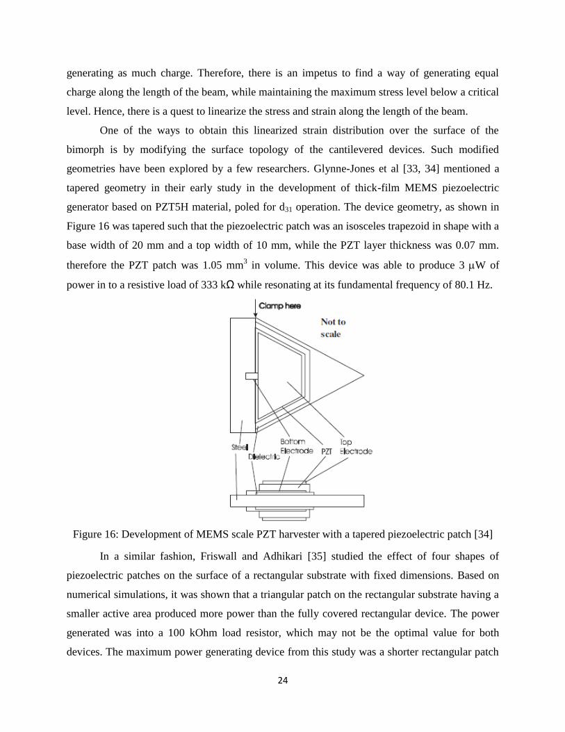
24

generating as much charge. Therefore, there is an impetus to find a way of generating equal

charge along the length of the beam, while maintaining the maximum stress level below a critical

level. Hence, there is a quest to linearize the stress and strain along the length of the beam.

One of the ways to obtain this linearized strain distribution over the surface of the

bimorph is by modifying the surface topology of the cantilevered devices. Such modified

geometries have been explored by a few researchers. Glynne-Jones et al [33, 34] mentioned a

tapered geometry in their early study in the development of thick-film MEMS piezoelectric

generator based on PZT5H material, poled for d31 operation. The device geometry, as shown in

Figure 16 was tapered such that the piezoelectric patch was an isosceles trapezoid in shape with a

base width of 20 mm and a top width of 10 mm, while the PZT layer thickness was 0.07 mm.

therefore the PZT patch was 1.05 mm3 in volume. This device was able to produce 3 W of

power in to a resistive load of 333 kΩ while resonating at its fundamental frequency of 80.1 Hz.

Figure 16: Development of MEMS scale PZT harvester with a tapered piezoelectric patch [34]

In a similar fashion, Friswall and Adhikari [35] studied the effect of four shapes of

piezoelectric patches on the surface of a rectangular substrate with fixed dimensions. Based on

numerical simulations, it was shown that a triangular patch on the rectangular substrate having a

smaller active area produced more power than the fully covered rectangular device. The power

generated was into a 100 kOhm load resistor, which may not be the optimal value for both

devices. The maximum power generating device from this study was a shorter rectangular patch

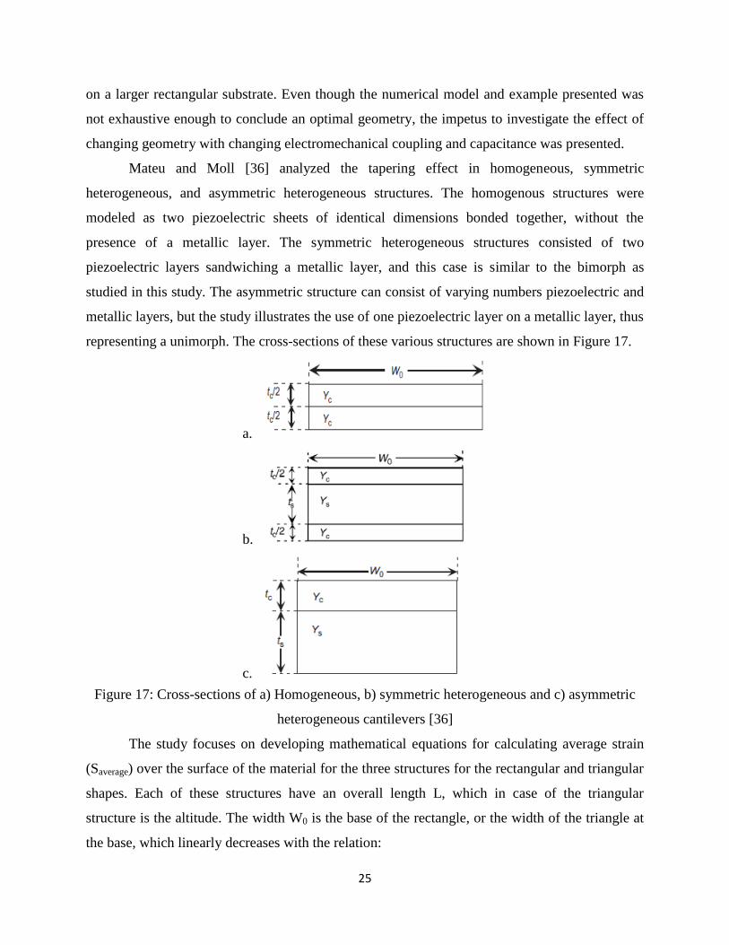
25

on a larger rectangular substrate. Even though the numerical model and example presented was

not exhaustive enough to conclude an optimal geometry, the impetus to investigate the effect of

changing geometry with changing electromechanical coupling and capacitance was presented.

Mateu and Moll [36] analyzed the tapering effect in homogeneous, symmetric

heterogeneous, and asymmetric heterogeneous structures. The homogenous structures were

modeled as two piezoelectric sheets of identical dimensions bonded together, without the

presence of a metallic layer. The symmetric heterogeneous structures consisted of two

piezoelectric layers sandwiching a metallic layer, and this case is similar to the bimorph as

studied in this study. The asymmetric structure can consist of varying numbers piezoelectric and

metallic layers, but the study illustrates the use of one piezoelectric layer on a metallic layer, thus

representing a unimorph. The cross-sections of these various structures are shown in Figure 17.

a.

b.

c.

Figure 17: Cross-sections of a) Homogeneous, b) symmetric heterogeneous and c) asymmetric

heterogeneous cantilevers [36]

The study focuses on developing mathematical equations for calculating average strain

(Saverage) over the surface of the material for the three structures for the rectangular and triangular

shapes. Each of these structures have an overall length L, which in case of the triangular

structure is the altitude. The width W0 is the base of the rectangle, or the width of the triangle at

the base, which linearly decreases with the relation:

26

𝑊(𝑥) = 𝑊0 (1 −𝑥

𝐿) (35)

where x is any position along the length of the beam.

The average strain for a homogenous structure can be defined as a product of the net

strain along the length (x) and thickness (z) directions as:

𝑆𝑎𝑣𝑒𝑟𝑎𝑔𝑒 =1

𝑡𝑐 2⁄

1

𝐿∫

𝑡𝑐 2⁄

0

∫𝑧

𝜌(𝑥)𝑑𝑧 𝑑𝑥

𝐿

0

(36)

where tc is the thickness of the piezoelectric layer, L is the length of the beam, z is the distance

from the neutral axis, which for the homogeneous case is tc/2, and ρ(x) is the radius of curvature

of the beam under a concentrated load at the free end of the cantilever.

This results in the following expressions for average strain and maximum deflection for a

rectangular homogeneous cantilever:

𝑆𝑥 =3𝐹𝐿

2𝑌𝑐𝑊0𝑡𝑐2

=3

8

𝑦𝑚𝑎𝑥𝑡𝑐

𝐿2 (37)

𝑦𝑚𝑎𝑥 =4𝐹𝐿3

𝑌𝑐𝑊0𝑡𝑐3 (38)

And for a triangular homogenous cantilever:

𝑆𝑥 =3𝐹𝐿

𝑌𝑐𝑊0𝑡𝑐2

=𝑦𝑚𝑎𝑥𝑡𝑐

2𝐿2 (39)



The above expressions provide very useful insights into behavior of cantilever beams

under a point load. For a triangular cantilever, the radius of curvature ρ(x) is a constant value,

and therefore, the strain becomes a constant value through its length. Therefore, for an identical

load, the average strain in a rectangular cantilever is 75% of the triangular cantilever as a

function of its maximum deflection. In fact in such a case, the maximum deflection of the

rectangular cantilever is also seen to be 67% of the triangular cantilever.

The authors in this study also develop similar expressions for the symmetric

heterogeneous (bimorph) case. However, here the maximum deflection is restricted by a cavity

depth (D), and therefore values for absolute maximum defection and average strain for these

cases are not available. However, it may be possible to replace D with y-max in these

27

expressions to obtain absolute deflections. The resulting expressions for triangular homogenous

cantilevers are:

𝑆𝑥 =𝐷𝑡𝑐

2𝐿2 (41)



𝑧𝑠 =𝑡𝑐

2 (43)

And for symmetric heterogeneous triangles, the expressions are given as:

𝑆𝑥 =𝐷𝑡𝑐

2𝐿2(1 + 2

𝑡𝑠

𝑡𝑐) (44)


𝑌𝑐𝑊0𝑡𝑐3

1

1 + 3(𝑡𝑠 𝑡𝑐⁄ ) + 3(𝑡𝑠 𝑡𝑐⁄ )2 + (𝑌𝑠 𝑌𝑐⁄ )(𝑡𝑠 𝑡𝑐⁄ )3 (45)

𝑧𝑠 =𝑡𝑐+𝑡𝑠

2 (46)

Therefore, these expressions can be quite useful in understanding the strain behavior in

different types of cantilevers. In the case of homogeneous and symmetric heterogeneous

triangular cantilevers, the average strain and maximum deflection are independent of the

Young’s modulus (which is not the case for asymmetric heterogeneous triangular cantilevers).

Also, the average strain in the triangular cantilevers can be increased with increasing thickness

ratio of shim thickness to piezoelectric layer thickness. Increasing strain also results in increased

charge, which is evident from the constitutive equations, and also equations for harvested power.

These equations are elaborated in the reference [36].

In a later study, Goldshmidtboeing and Woias [37] also characterized the differences

between rectangular and triangular cantilevers, and also included a truncated rectangle, which

was effectively a trapezoidal cantilever. They developed and verified an analytical model, based

on which the inferences are made in the study. Unlike the previous study where the cantilevers

were characterized for bending behavior using an average stress, this study employed the use of a

relative mean curvature κ’ in order to characterize the stress homogeneity:

𝜅′ =|𝜅𝑚𝑒𝑎𝑛|

|𝜅𝑚𝑎𝑥|

(47)

where 𝜅𝑚𝑒𝑎𝑛refers to the mean curvature of the piezoelectric layer at its surface, and 𝜅𝑚𝑎𝑥 is the

maximum absolute value at the surface. Based on the above equation, perfect homogeneity

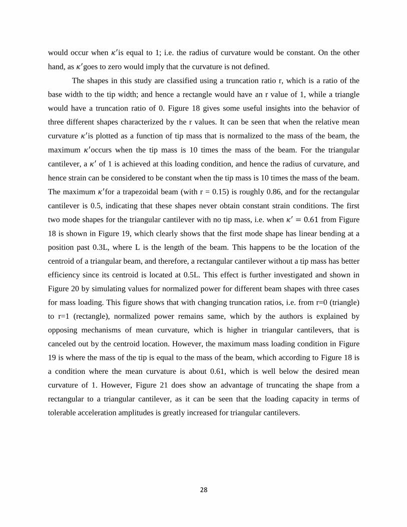
28

would occur when 𝜅′is equal to 1; i.e. the radius of curvature would be constant. On the other

hand, as 𝜅′goes to zero would imply that the curvature is not defined.

The shapes in this study are classified using a truncation ratio r, which is a ratio of the

base width to the tip width; and hence a rectangle would have an r value of 1, while a triangle

would have a truncation ratio of 0. Figure 18 gives some useful insights into the behavior of

three different shapes characterized by the r values. It can be seen that when the relative mean

curvature 𝜅′is plotted as a function of tip mass that is normalized to the mass of the beam, the

maximum 𝜅′occurs when the tip mass is 10 times the mass of the beam. For the triangular

cantilever, a 𝜅′ of 1 is achieved at this loading condition, and hence the radius of curvature, and

hence strain can be considered to be constant when the tip mass is 10 times the mass of the beam.

The maximum 𝜅′for a trapezoidal beam (with r = 0.15) is roughly 0.86, and for the rectangular

cantilever is 0.5, indicating that these shapes never obtain constant strain conditions. The first

two mode shapes for the triangular cantilever with no tip mass, i.e. when 𝜅′ = 0.61 from Figure

18 is shown in Figure 19, which clearly shows that the first mode shape has linear bending at a

position past 0.3L, where L is the length of the beam. This happens to be the location of the

centroid of a triangular beam, and therefore, a rectangular cantilever without a tip mass has better

efficiency since its centroid is located at 0.5L. This effect is further investigated and shown in

Figure 20 by simulating values for normalized power for different beam shapes with three cases

for mass loading. This figure shows that with changing truncation ratios, i.e. from r=0 (triangle)

to r=1 (rectangle), normalized power remains same, which by the authors is explained by

opposing mechanisms of mean curvature, which is higher in triangular cantilevers, that is

canceled out by the centroid location. However, the maximum mass loading condition in Figure

19 is where the mass of the tip is equal to the mass of the beam, which according to Figure 18 is

a condition where the mean curvature is about 0.61, which is well below the desired mean

curvature of 1. However, Figure 21 does show an advantage of truncating the shape from a

rectangular to a triangular cantilever, as it can be seen that the loading capacity in terms of

tolerable acceleration amplitudes is greatly increased for triangular cantilevers.

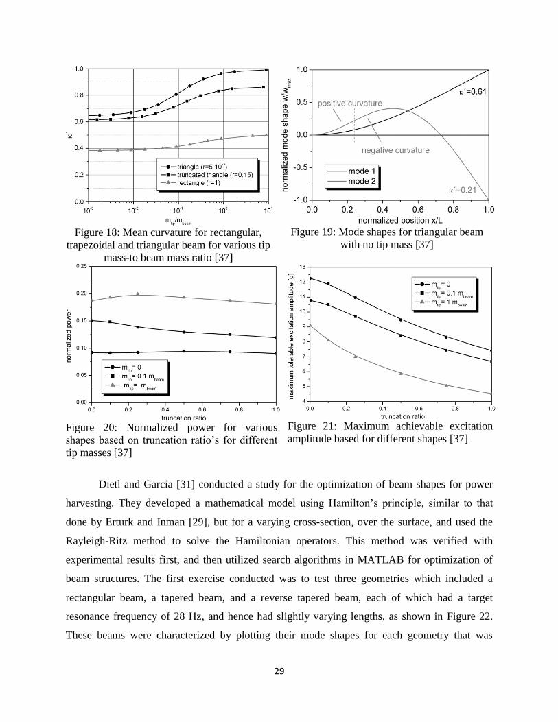
29

Figure 18: Mean curvature for rectangular,

trapezoidal and triangular beam for various tip

mass-to beam mass ratio [37]

Figure 19: Mode shapes for triangular beam

with no tip mass [37]

Figure 20: Normalized power for various

shapes based on truncation ratio’s for different

tip masses [37]

Figure 21: Maximum achievable excitation

amplitude based for different shapes [37]

Dietl and Garcia [31] conducted a study for the optimization of beam shapes for power

harvesting. They developed a mathematical model using Hamilton’s principle, similar to that

done by Erturk and Inman [29], but for a varying cross-section, over the surface, and used the

Rayleigh-Ritz method to solve the Hamiltonian operators. This method was verified with

experimental results first, and then utilized search algorithms in MATLAB for optimization of

beam structures. The first exercise conducted was to test three geometries which included a

rectangular beam, a tapered beam, and a reverse tapered beam, each of which had a target

resonance frequency of 28 Hz, and hence had slightly varying lengths, as shown in Figure 22.

These beams were characterized by plotting their mode shapes for each geometry that was

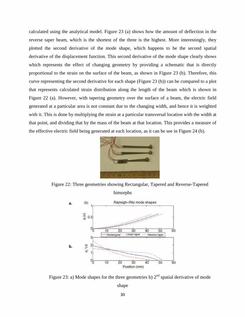
30

calculated using the analytical model. Figure 23 (a) shows how the amount of deflection in the

reverse taper beam, which is the shortest of the three is the highest. More interestingly, they

plotted the second derivative of the mode shape, which happens to be the second spatial

derivative of the displacement function. This second derivative of the mode shape clearly shows

which represents the effect of changing geometry by providing a schematic that is directly

proportional to the strain on the surface of the beam, as shown in Figure 23 (b). Therefore, this

curve representing the second derivative for each shape (Figure 23 (b)) can be compared to a plot

that represents calculated strain distribution along the length of the beam which is shown in

Figure 22 (a). However, with tapering geometry over the surface of a beam, the electric field

generated at a particular area is not constant due to the changing width, and hence it is weighted

with it. This is done by multiplying the strain at a particular transversal location with the width at

that point, and dividing that by the mass of the beam at that location. This provides a measure of

the effective electric field being generated at each location, as it can be see in Figure 24 (b).

Figure 22: Three geometries showing Rectangular, Tapered and Reverse-Tapered

bimorphs

Figure 23: a) Mode shapes for the three geometries b) 2nd

spatial derivative of mode

shape

a.

b.

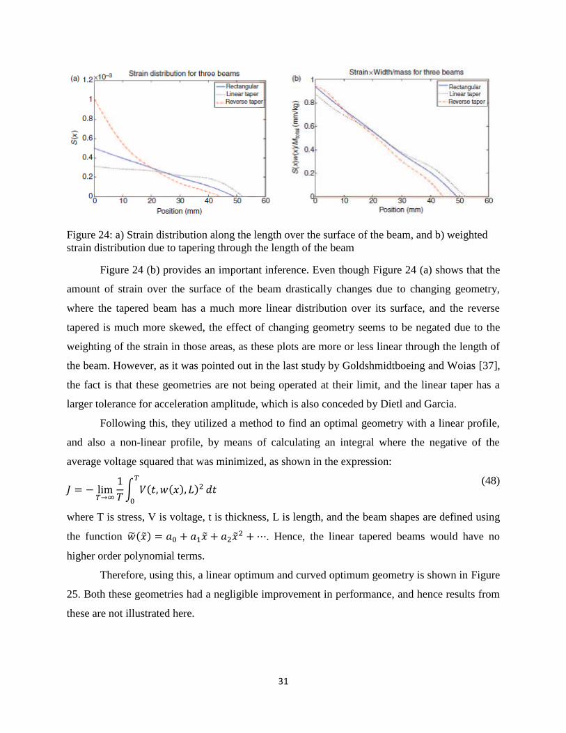
31

Figure 24: a) Strain distribution along the length over the surface of the beam, and b) weighted

strain distribution due to tapering through the length of the beam

Figure 24 (b) provides an important inference. Even though Figure 24 (a) shows that the

amount of strain over the surface of the beam drastically changes due to changing geometry,

where the tapered beam has a much more linear distribution over its surface, and the reverse

tapered is much more skewed, the effect of changing geometry seems to be negated due to the

weighting of the strain in those areas, as these plots are more or less linear through the length of

the beam. However, as it was pointed out in the last study by Goldshmidtboeing and Woias [37],

the fact is that these geometries are not being operated at their limit, and the linear taper has a

larger tolerance for acceleration amplitude, which is also conceded by Dietl and Garcia.

Following this, they utilized a method to find an optimal geometry with a linear profile,

and also a non-linear profile, by means of calculating an integral where the negative of the

average voltage squared that was minimized, as shown in the expression:

𝐽 = − lim𝑇→∞

1

𝑇∫ 𝑉(𝑡, 𝑤(𝑥), 𝐿)2 𝑑𝑡

𝑇

0

(48)

where T is stress, V is voltage, t is thickness, L is length, and the beam shapes are defined using

the function �̃�(�̃�) = 𝑎0 + 𝑎1�̃� + 𝑎2�̃�2 + ⋯. Hence, the linear tapered beams would have no

higher order polynomial terms.

Therefore, using this, a linear optimum and curved optimum geometry is shown in Figure

25. Both these geometries had a negligible improvement in performance, and hence results from

these are not illustrated here.

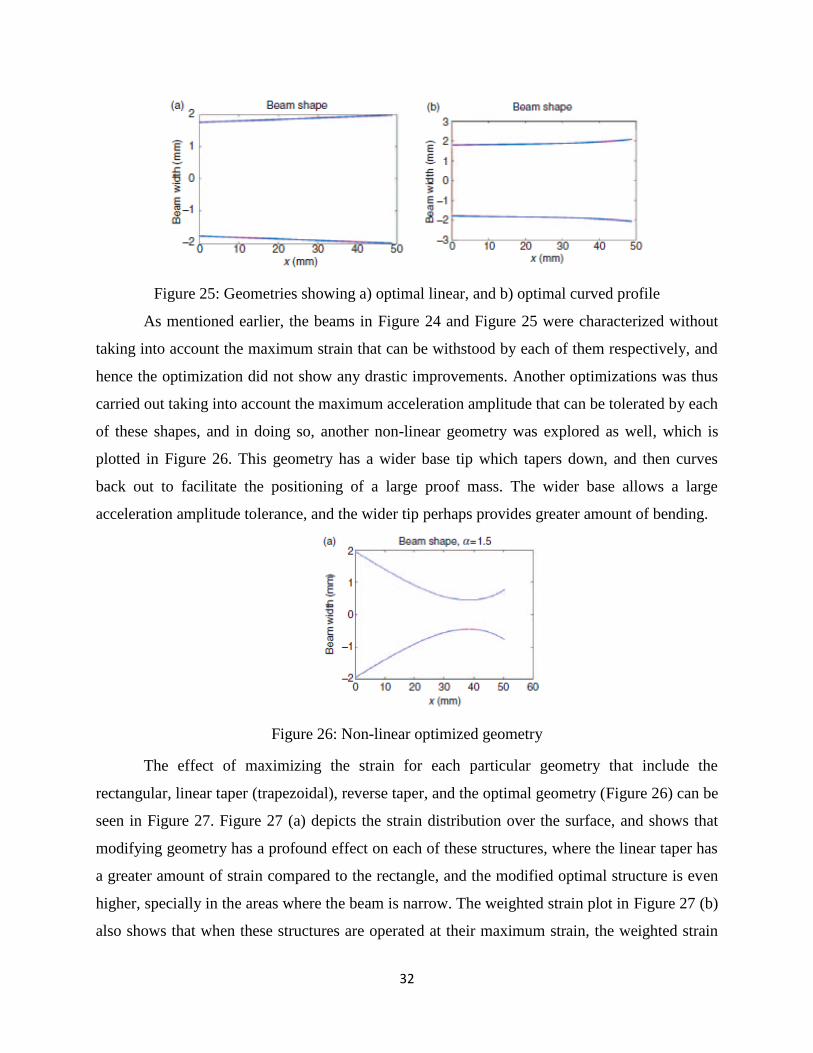
32

Figure 25: Geometries showing a) optimal linear, and b) optimal curved profile

As mentioned earlier, the beams in Figure 24 and Figure 25 were characterized without

taking into account the maximum strain that can be withstood by each of them respectively, and

hence the optimization did not show any drastic improvements. Another optimizations was thus

carried out taking into account the maximum acceleration amplitude that can be tolerated by each

of these shapes, and in doing so, another non-linear geometry was explored as well, which is

plotted in Figure 26. This geometry has a wider base tip which tapers down, and then curves

back out to facilitate the positioning of a large proof mass. The wider base allows a large

acceleration amplitude tolerance, and the wider tip perhaps provides greater amount of bending.

Figure 26: Non-linear optimized geometry

The effect of maximizing the strain for each particular geometry that include the

rectangular, linear taper (trapezoidal), reverse taper, and the optimal geometry (Figure 26) can be

seen in Figure 27. Figure 27 (a) depicts the strain distribution over the surface, and shows that

modifying geometry has a profound effect on each of these structures, where the linear taper has

a greater amount of strain compared to the rectangle, and the modified optimal structure is even

higher, specially in the areas where the beam is narrow. The weighted strain plot in Figure 27 (b)

also shows that when these structures are operated at their maximum strain, the weighted strain

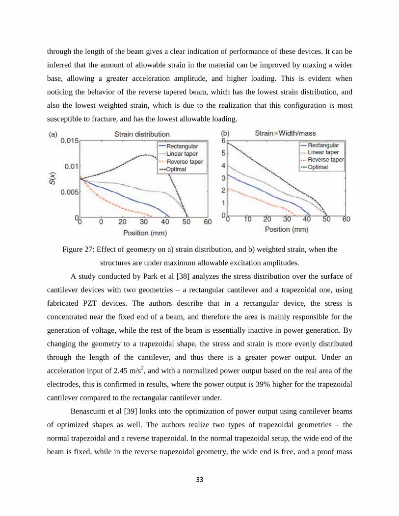
33

through the length of the beam gives a clear indication of performance of these devices. It can be

inferred that the amount of allowable strain in the material can be improved by maxing a wider

base, allowing a greater acceleration amplitude, and higher loading. This is evident when

noticing the behavior of the reverse tapered beam, which has the lowest strain distribution, and

also the lowest weighted strain, which is due to the realization that this configuration is most

susceptible to fracture, and has the lowest allowable loading.

Figure 27: Effect of geometry on a) strain distribution, and b) weighted strain, when the

structures are under maximum allowable excitation amplitudes.

A study conducted by Park et al [38] analyzes the stress distribution over the surface of

cantilever devices with two geometries – a rectangular cantilever and a trapezoidal one, using

fabricated PZT devices. The authors describe that in a rectangular device, the stress is

concentrated near the fixed end of a beam, and therefore the area is mainly responsible for the

generation of voltage, while the rest of the beam is essentially inactive in power generation. By

changing the geometry to a trapezoidal shape, the stress and strain is more evenly distributed

through the length of the cantilever, and thus there is a greater power output. Under an

acceleration input of 2.45 m/s2, and with a normalized power output based on the real area of the

electrodes, this is confirmed in results, where the power output is 39% higher for the trapezoidal

cantilever compared to the rectangular cantilever under.

Benascuitti et al [39] looks into the optimization of power output using cantilever beams

of optimized shapes as well. The authors realize two types of trapezoidal geometries – the

normal trapezoidal and a reverse trapezoidal. In the normal trapezoidal setup, the wide end of the

beam is fixed, while in the reverse trapezoidal geometry, the wide end is free, and a proof mass

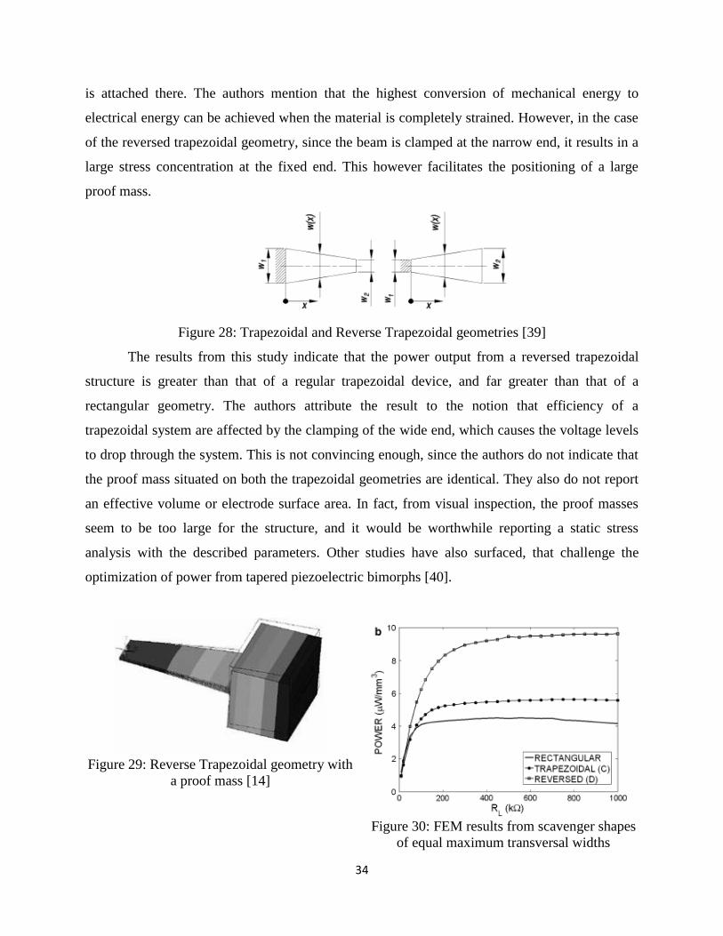
34

is attached there. The authors mention that the highest conversion of mechanical energy to

electrical energy can be achieved when the material is completely strained. However, in the case

of the reversed trapezoidal geometry, since the beam is clamped at the narrow end, it results in a

large stress concentration at the fixed end. This however facilitates the positioning of a large

proof mass.

Figure 28: Trapezoidal and Reverse Trapezoidal geometries [39]

The results from this study indicate that the power output from a reversed trapezoidal

structure is greater than that of a regular trapezoidal device, and far greater than that of a

rectangular geometry. The authors attribute the result to the notion that efficiency of a

trapezoidal system are affected by the clamping of the wide end, which causes the voltage levels

to drop through the system. This is not convincing enough, since the authors do not indicate that

the proof mass situated on both the trapezoidal geometries are identical. They also do not report

an effective volume or electrode surface area. In fact, from visual inspection, the proof masses

seem to be too large for the structure, and it would be worthwhile reporting a static stress

analysis with the described parameters. Other studies have also surfaced, that challenge the

optimization of power from tapered piezoelectric bimorphs [40].

Figure 29: Reverse Trapezoidal geometry with

a proof mass [14]

Figure 30: FEM results from scavenger shapes

of equal maximum transversal widths

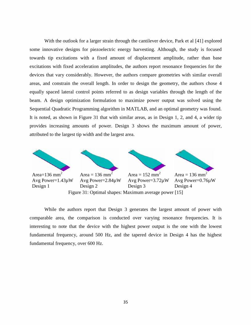
35

With the outlook for a larger strain through the cantilever device, Park et al [41] explored

some innovative designs for piezoelectric energy harvesting. Although, the study is focused

towards tip excitations with a fixed amount of displacement amplitude, rather than base

excitations with fixed acceleration amplitudes, the authors report resonance frequencies for the

devices that vary considerably. However, the authors compare geometries with similar overall

areas, and constrain the overall length. In order to design the geometry, the authors chose 4

equally spaced lateral control points referred to as design variables through the length of the

beam. A design optimization formulation to maximize power output was solved using the

Sequential Quadratic Programming algorithm in MATLAB, and an optimal geometry was found.

It is noted, as shown in Figure 31 that with similar areas, as in Design 1, 2, and 4, a wider tip

provides increasing amounts of power. Design 3 shows the maximum amount of power,

attributed to the largest tip width and the largest area.

Area=136 mm

2

Avg Power=1.43µW

Design 1

Area = 136 mm

2

Avg Power=2.84µW

Design 2

Area = 152 mm

2

Avg Power=3.72µW

Design 3

Area = 136 mm2

Avg Power=0.76µW

Design 4

Figure 31: Optimal shapes: Maximum average power [15]

While the authors report that Design 3 generates the largest amount of power with

comparable area, the comparison is conducted over varying resonance frequencies. It is

interesting to note that the device with the highest power output is the one with the lowest

fundamental frequency, around 500 Hz, and the tapered device in Design 4 has the highest

fundamental frequency, over 600 Hz.

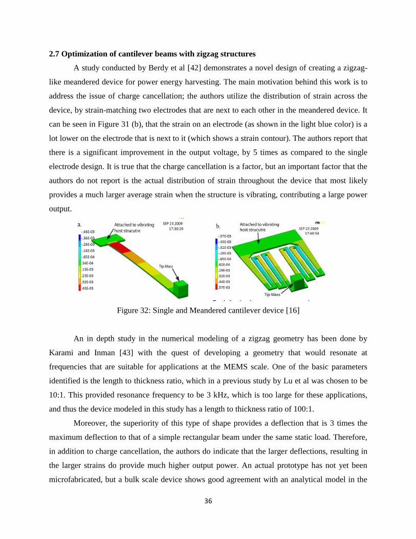
36

2.7 Optimization of cantilever beams with zigzag structures

A study conducted by Berdy et al [42] demonstrates a novel design of creating a zigzag-

like meandered device for power energy harvesting. The main motivation behind this work is to

address the issue of charge cancellation; the authors utilize the distribution of strain across the

device, by strain-matching two electrodes that are next to each other in the meandered device. It

can be seen in Figure 31 (b), that the strain on an electrode (as shown in the light blue color) is a

lot lower on the electrode that is next to it (which shows a strain contour). The authors report that

there is a significant improvement in the output voltage, by 5 times as compared to the single

electrode design. It is true that the charge cancellation is a factor, but an important factor that the

authors do not report is the actual distribution of strain throughout the device that most likely

provides a much larger average strain when the structure is vibrating, contributing a large power

output.

Figure 32: Single and Meandered cantilever device [16]

An in depth study in the numerical modeling of a zigzag geometry has been done by

Karami and Inman [43] with the quest of developing a geometry that would resonate at

frequencies that are suitable for applications at the MEMS scale. One of the basic parameters

identified is the length to thickness ratio, which in a previous study by Lu et al was chosen to be

10:1. This provided resonance frequency to be 3 kHz, which is too large for these applications,

and thus the device modeled in this study has a length to thickness ratio of 100:1.

Moreover, the superiority of this type of shape provides a deflection that is 3 times the

maximum deflection to that of a simple rectangular beam under the same static load. Therefore,

in addition to charge cancellation, the authors do indicate that the larger deflections, resulting in

the larger strains do provide much higher output power. An actual prototype has not yet been

microfabricated, but a bulk scale device shows good agreement with an analytical model in the

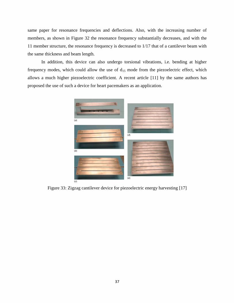
37

same paper for resonance frequencies and deflections. Also, with the increasing number of

members, as shown in Figure 32 the resonance frequency substantially decreases, and with the

11 member structure, the resonance frequency is decreased to 1/17 that of a cantilever beam with

the same thickness and beam length.

In addition, this device can also undergo torsional vibrations, i.e. bending at higher

frequency modes, which could allow the use of d15 mode from the piezoelectric effect, which

allows a much higher piezoelectric coefficient. A recent article [11] by the same authors has

proposed the use of such a device for heart pacemakers as an application.

Figure 33: Zigzag cantilever device for piezoelectric energy harvesting [17]

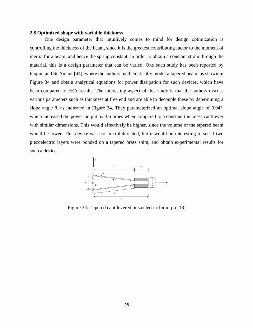
38

2.8 Optimized shape with variable thickness

One design parameter that intuitively comes to mind for design optimization is

controlling the thickness of the beam, since it is the greatest contributing factor to the moment of

inertia for a beam, and hence the spring constant. In order to obtain a constant strain through the

material, this is a design parameter that can be varied. One such study has been reported by

Paquin and St-Amant [44], where the authors mathematically model a tapered beam, as shown in

Figure 34 and obtain analytical equations for power dissipation for such devices, which have

been compared to FEA results. The interesting aspect of this study is that the authors discuss

various parameters such as thickness at free end and are able to decouple these by determining a

slope angle θ, as indicated in Figure 34. They parameterized an optimal slope angle of 0.94°,

which increased the power output by 3.6 times when compared to a constant thickness cantilever

with similar dimensions. This would effectively be higher, since the volume of the tapered beam

would be lower. This device was not microfabricated, but it would be interesting to see if two

piezoelectric layers were bonded on a tapered brass shim, and obtain experimental results for

such a device.

Figure 34: Tapered cantilevered piezoelectric bimorph [18]

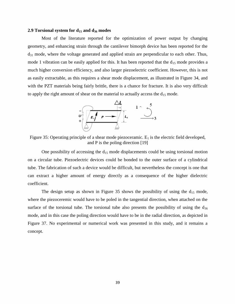
39

2.9 Torsional system for d15 and d36 modes

Most of the literature reported for the optimization of power output by changing

geometry, and enhancing strain through the cantilever bimorph device has been reported for the

d31 mode, where the voltage generated and applied strain are perpendicular to each other. Thus,

mode 1 vibration can be easily applied for this. It has been reported that the d15 mode provides a

much higher conversion efficiency, and also larger piezoelectric coefficient. However, this is not

as easily extractable, as this requires a shear mode displacement, as illustrated in Figure 34, and

with the PZT materials being fairly brittle, there is a chance for fracture. It is also very difficult

to apply the right amount of shear on the material to actually access the d15 mode.

Figure 35: Operating principle of a shear mode piezoceramic. E1 is the electric field developed,

and P is the poling direction [19]

One possibility of accessing the d15 mode displacements could be using torsional motion

on a circular tube. Piezoelectric devices could be bonded to the outer surface of a cylindrical

tube. The fabrication of such a device would be difficult, but nevertheless the concept is one that

can extract a higher amount of energy directly as a consequence of the higher dielectric

coefficient.

The design setup as shown in Figure 35 shows the possibility of using the d15 mode,

where the piezoceremic would have to be poled in the tangential direction, when attached on the

surface of the torsional tube. The torsional tube also presents the possibility of using the d36

mode, and in this case the poling direction would have to be in the radial direction, as depicted in

Figure 37. No experimental or numerical work was presented in this study, and it remains a

concept.

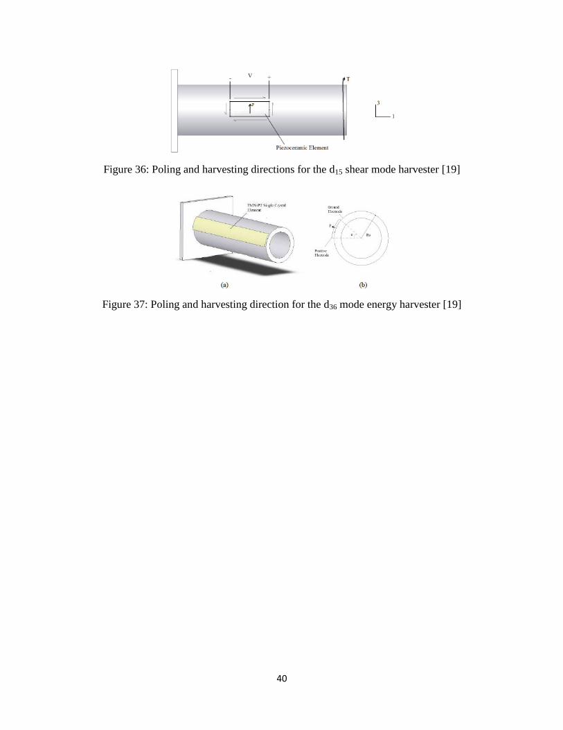
40

Figure 36: Poling and harvesting directions for the d15 shear mode harvester [19]

Figure 37: Poling and harvesting direction for the d36 mode energy harvester [19]

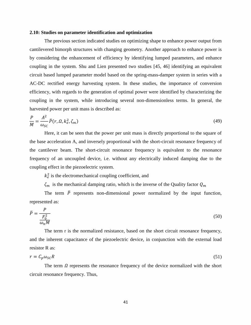
41

2.10: Studies on parameter identification and optimization

The previous section indicated studies on optimizing shape to enhance power output from

cantilevered bimorph structures with changing geometry. Another approach to enhance power is

by considering the enhancement of efficiency by identifying lumped parameters, and enhance

coupling in the system. Shu and Lien presented two studies [45, 46] identifying an equivalent

circuit based lumped parameter model based on the spring-mass-damper system in series with a

AC-DC rectified energy harvesting system. In these studies, the importance of conversion

efficiency, with regards to the generation of optimal power were identified by characterizing the

coupling in the system, while introducing several non-dimensionless terms. In general, the

harvested power per unit mass is described as:

𝑃

𝑀=

𝐴2

𝜔𝑆𝐶�̅�(𝑟, 𝛺, 𝑘𝑒

2, 휁𝑚) (49)

Here, it can be seen that the power per unit mass is directly proportional to the square of

the base acceleration A, and inversely proportional with the short-circuit resonance frequency of

the cantilever beam. The short-circuit resonance frequency is equivalent to the resonance

frequency of an uncoupled device, i.e. without any electrically induced damping due to the

coupling effect in the piezoelectric system.

𝑘𝑒2 is the electromechanical coupling coefficient, and

휁𝑚 is the mechanical damping ratio, which is the inverse of the Quality factor 𝑄𝑚

The term �̅� represents non-dimensional power normalized by the input function,

represented as:

�̅� =𝑃

𝐹02

𝜔𝑛𝑀

(50)

The term r is the normalized resistance, based on the short circuit resonance frequency,

and the inherent capacitance of the piezoelectric device, in conjunction with the external load

resistor R as:

𝑟 = 𝐶𝑝𝜔𝑆𝐶𝑅 (51)

The term 𝛺 represents the resonance frequency of the device normalized with the short

circuit resonance frequency. Thus,

42

𝛺 =𝜔

𝜔𝑆𝐶 (52)

Therefore, the short circuit and open-circuit resonance frequencies are:

𝛺𝑆𝐶 = 1 (53)

𝛺𝑂𝐶 = √1 + 𝑘𝑒2 (54)

It can be quickly realized that with large electromechanical coupling coefficients, the

shift from the short circuit resonance frequency to the open circuit resonance frequency would be

large.

The magnitude of the electromechanical coupling coefficient and the mechanical

damping ratio in fact has a much wider implication. It has been reported that small values of the

figure of merit, i.e. where 𝑘2𝑄𝑚 ≪ 1, there exits one value for the optimal load resistance, where

maximum power is generated. These are regarded as low coupling systems. In such cases, it is

reported that the maximum power generated can never match the power available in the

mechanical system. For higher coupling systems where 𝑘2𝑄𝑚 ≫ 1, there exist two values where

power can be maximized.

This discussion was further refined in Goldschmidtboeing et. al (2011) [47], where a

threshold value of 2 for the coupling figure of merit is presented, which is attributed due to the

presence of resonance and anti-resonance. This publication highlights the use of a unimorph with

a thick passive layer for a low coupling harvester, and the use of a bimorph with as the high

coupling harvester, where a 𝑘2𝑄𝑚 value of 8.2 was reached.

Lei et. al [48] provide an excellent explanation of the threshold value of 2 for the

electromechanical coupling figure of merit. Based on their SDOF equivalent circuit model, and

expressing impedance in terms of coupling and a transformation factor, it is found that the peak

phase angle becomes zero when 𝑘2𝑄𝑚 = 2. At this point, maximum power can be drawn from a

single optimal load resistance, by performing a complex conjugate impedance match [49]. As the

peak phase angle is greater than zero, two optimal load resistance values can be found,

contributing to two optimal load resistance values. In the instance where the peak phase angle is

less than zero, i.e. when it is negative, complex conjugate impedance matching is not possible.

Xiong and Oyadiji present an exhaustive numerical study [50] on parameterizing the

electromechanical coupling coefficient, quality factor, and the mass ratio. The mass ratio is

defined as the effective-mass-of-the-beam to the total mass of the beam. All three parameters

43

affect the electromechanical coupling figure of merit, and the study illustrates the transitioning of

the low coupling harvesters with a single optimal load resistor, to an intermediate region that

does not display optimal load resistance values as peaks, to high coupling systems where two

distinct optimal load resistance values are found. They also present a numerical study on tapered

piezoelectric beams, and report that the electromechanical coupling coefficient is enhanced with

tapering beams.

This very short compendium of a set of exhaustive and important publications highlights

a few key points. They describe the importance of electrical measurements for being able to

characterize piezoelectric energy harvesters, by measuring capacitance, impedance, and

determining the resonance and anti-resonance frequencies. The electromechanical coupling

figure of merit is an important aspect that describes the behavior of piezoelectric energy

harvesters, and the numerical studies so far indicate that they have a large impact on the power

generated. Therefore, this forms a basis for characterization of these materials, an aspect that is

taken into consideration for the entirety of this work.

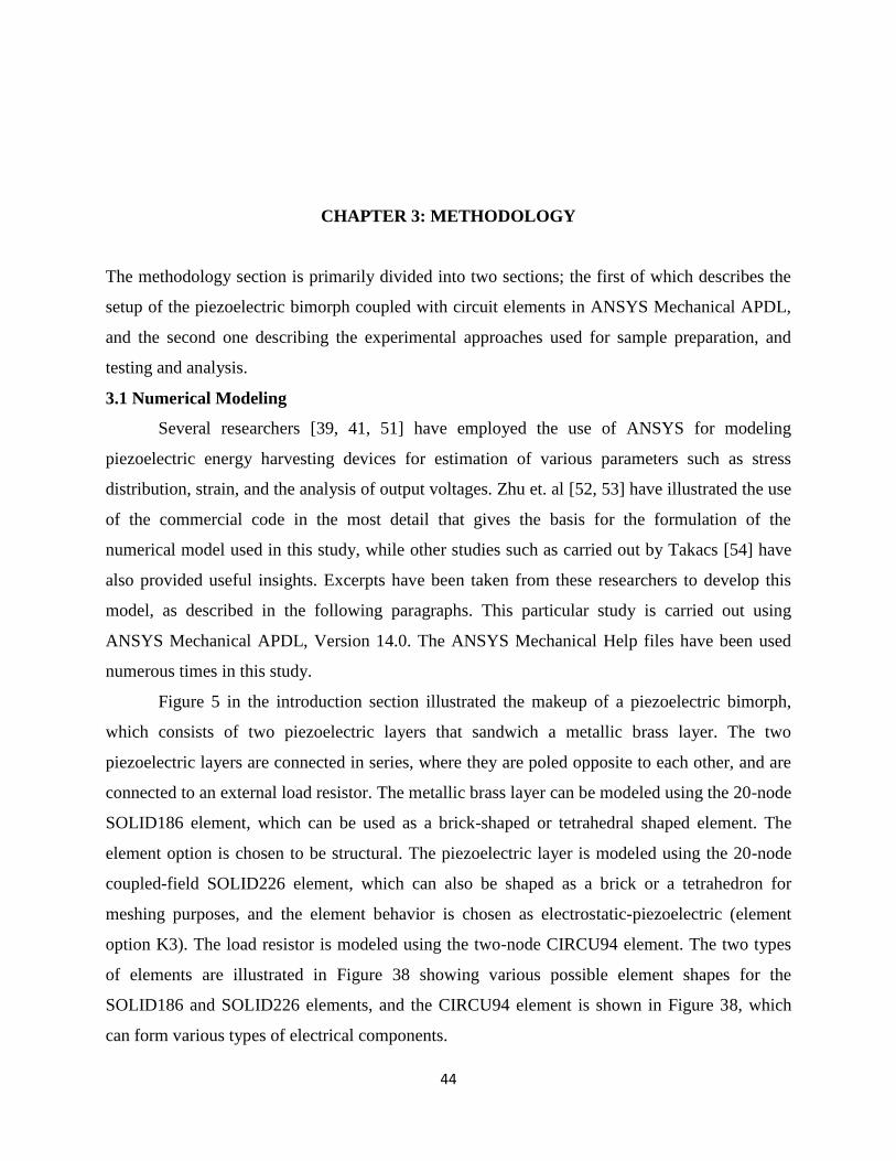
44

CHAPTER 3: METHODOLOGY

The methodology section is primarily divided into two sections; the first of which describes the

setup of the piezoelectric bimorph coupled with circuit elements in ANSYS Mechanical APDL,

and the second one describing the experimental approaches used for sample preparation, and

testing and analysis.

3.1 Numerical Modeling

Several researchers [39, 41, 51] have employed the use of ANSYS for modeling

piezoelectric energy harvesting devices for estimation of various parameters such as stress

distribution, strain, and the analysis of output voltages. Zhu et. al [52, 53] have illustrated the use

of the commercial code in the most detail that gives the basis for the formulation of the

numerical model used in this study, while other studies such as carried out by Takacs [54] have

also provided useful insights. Excerpts have been taken from these researchers to develop this

model, as described in the following paragraphs. This particular study is carried out using

ANSYS Mechanical APDL, Version 14.0. The ANSYS Mechanical Help files have been used

numerous times in this study.

Figure 5 in the introduction section illustrated the makeup of a piezoelectric bimorph,

which consists of two piezoelectric layers that sandwich a metallic brass layer. The two

piezoelectric layers are connected in series, where they are poled opposite to each other, and are

connected to an external load resistor. The metallic brass layer can be modeled using the 20-node

SOLID186 element, which can be used as a brick-shaped or tetrahedral shaped element. The

element option is chosen to be structural. The piezoelectric layer is modeled using the 20-node

coupled-field SOLID226 element, which can also be shaped as a brick or a tetrahedron for

meshing purposes, and the element behavior is chosen as electrostatic-piezoelectric (element

option K3). The load resistor is modeled using the two-node CIRCU94 element. The two types

of elements are illustrated in Figure 38 showing various possible element shapes for the

SOLID186 and SOLID226 elements, and the CIRCU94 element is shown in Figure 38, which

can form various types of electrical components.

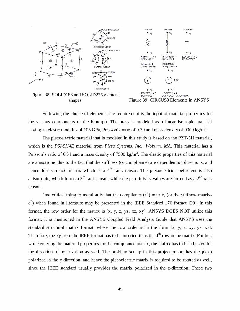
45

Figure 38: SOLID186 and SOLID226 element

shapes

Figure 39: CIRCU98 Elements in ANSYS

Following the choice of elements, the requirement is the input of material properties for

the various components of the bimorph. The brass is modeled as a linear isotropic material

having an elastic modulus of 105 GPa, Poisson’s ratio of 0.30 and mass density of 9000 kg/m3.

The piezoelectric material that is modeled in this study is based on the PZT-5H material,

which is the PSI-5H4E material from Piezo Systems, Inc., Woburn, MA. This material has a

Poisson’s ratio of 0.31 and a mass density of 7500 kg/m3. The elastic properties of this material

are anisotropic due to the fact that the stiffness (or compliance) are dependent on directions, and

hence forms a 6x6 matrix which is a 4th

rank tensor. The piezoelectric coefficient is also

anisotropic, which forms a 3rd

rank tensor, while the permittivity values are formed as a 2nd

rank

tensor.

One critical thing to mention is that the compliance (sE) matrix, (or the stiffness matrix-

cE) when found in literature may be presented in the IEEE Standard 176 format [20]. In this

format, the row order for the matrix is [x, y, z, yz, xz, xy]. ANSYS DOES NOT utilize this

format. It is mentioned in the ANSYS Coupled Field Analysis Guide that ANSYS uses the

standard structural matrix format, where the row order is in the form [x, y, z, xy, yz, xz].

Therefore, the xy from the IEEE format has to be inserted in as the 4th

row in the matrix. Further,

while entering the material properties for the compliance matrix, the matrix has to be adjusted for

the direction of polarization as well. The problem set up in this project report has the piezo

polarized in the y-direction, and hence the piezoelectric matrix is required to be rotated as well,

since the IEEE standard usually provides the matrix polarized in the z-direction. These two

46

adjustments – the insertion of row xy, in the 4th

row, and the rotation of the matrix to polarize the

material in the z-direction are critical to performing a proper piezoelectric analysis.

The adjusted and rotated piezoelectric compliance matrix in ANSYS format for the PZT-

5A material is given as [6, 7, 8]:

X Y Z XY YZ ZX

0.16400E-10 -0.72200E-11 -0.57400E-11 0.0000 0.0000 0.0000

-0.72200E-11 0.18800E-10 -0.72200E-11 0.0000 0.0000 0.0000

-0.57400E-11 -0.72200E-11 0.16400E-10 0.0000 0.0000 0.0000 (m/N2)

0.0000 0.0000 0.0000 0.47500E-10 0.0000 0.0000

0.0000 0.0000 0.0000 0.0000 0.0000 0.0000

The next property that is defined for the modeling of piezoelectric materials is the

piezoelectric strain matrix [d]. Once again, the format prescribed in the IEEE 176 Standard is

different than the one that ANSYS uses. The typical strain matrix is a 3x6 where the order of the

6 columns are [x, y, z, yz, xz, xy]. ANSYS requires the definition in terms of a 6x3 matrix.

Therefore the matrix in the IEEE format is first transposed to the 6x3 form, and then the xy row

is inserted in as the 4th

row. The PZT-5A piezoelectric strain matrix (d), poled in the +Y

direction is given as [6, 7, 8]:

X Y Z

X 0.0000 -0.17100E-09 0.0000

Y 0.0000 0.37400E-09 0.0000

Z 0.0000 -0.17100E-09 0.0000

XY 0.58400E-09 0.0000 0.0000 (C/N)

YZ 0.0000 0.0000 0.0000

XZ 0.0000 0.0000 0.0000

Also, when the bimorph is used in series operation, one of the piezoelectric layers is

poled in the –Y direction. This piezoelectric strain matrix has coefficients that are opposite in

sign to the +Y coefficients [52]

The third required material property for modeling of piezoelectric devices is the dielectric

permittivity matrix, which is an inherent material property. This is a 3x3 symmetric matrix for

PZT-5A at constant stress, and the values for the material are [6, 7, 8]:

1700 0 0

0 1730 0 (F/m)

0 0 1700

The next step is to create the geometry of the piezoelectric bimorphs. Since Solid

elements are being utilized in this work, the modeling is performed in 3-D. The piezoelectric

bimorphs that are described here are described for a simple rectangular geometry. A rectangular

layer with desired dimensions is modeled as an area, and then extruded to specific dimensions.

The chosen bimorphs from Piezo Systems, Inc. are of the T220 series, where the thickness of

47

each piezoelectric layer is 0.19 mm and the thickness of the brass layer is 0.13 mm. the three

extruded volumes are then glued together.

Following the generation of the structure, the volumes are meshed, but in order to do so,

each layer must be assigned the proper element attributes; i.e. the top and bottom layers are

modeled as SOLID226 layers, while the middle layer is assigned the SOLID186 element. The

top and bottom layers are assigned material properties relevant to the piezoelectric materials,

respective to poling directions, while the middle layer is assigned the material properties for the

elastic isotropic brass material. Once element attributes are assigned, the mesh is setup such that

the elements have an aspect ratio of 1:1 on the transverse plane (i.e. the xz plane as modeled).

For example, for a rectangular bimorph that has a clamped length of 21.5 mm and width of 12.7

mm has its length divided into 50 parts, and width divided into 15 parts. A mapped mesh is then

created resulting in brick shaped elements, giving an even distribution of nodes across the

different layers.

The nodes on the top and bottom layers of the piezoelectric material are then coupled for

voltages. This essentially creates a common node for each surface that can be used to create an

electrode connection, and an external load resistor can be added in between these coupled nodes.

The resistor is added by creating a single two-node CIRCU94 element between these coupled

nodes, and the value of the resistance is defined as a real constant.

The next step is to enter the solution phase of the modeling, where appropriate loads and

boundary conditions can be applied. The setup of the piezoelectric bimorphs is primarily as a

cantilevered device, hence the areas (there are three areas due to three layers) on one of the ends

of the beam are fixed in all three directions (i.e. Ux = Uy = Uz = 0). In addition to this, one of the

coupled nodes should be grounded by setting the voltage to nil, in order to provide a reference

for the voltage generated by the bimorph.

At this point, a modal analysis for the structure may be performed in order to obtain its

natural frequency. Therefore, the same is chosen from the “Analysis Type” menu, and the Block

Lanczos algorithm is chosen. Since we are only interested in the fundamental frequency of the

system, only one mode is expanded. The analysis is performed, and the fundamental frequency is

recorded.

In order to simulate the piezoelectric bimorph under excitation, a harmonic analysis is

performed, where the external excitation is applied by using the ACEL command. This

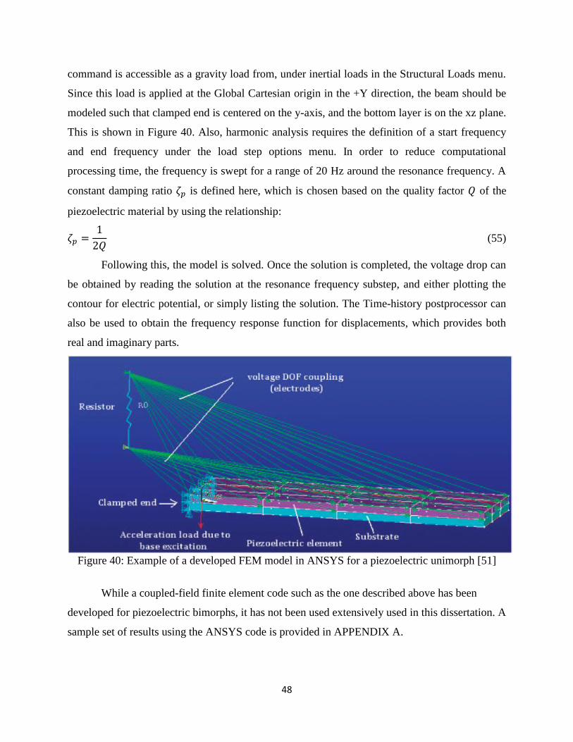
48

command is accessible as a gravity load from, under inertial loads in the Structural Loads menu.

Since this load is applied at the Global Cartesian origin in the +Y direction, the beam should be

modeled such that clamped end is centered on the y-axis, and the bottom layer is on the xz plane.

This is shown in Figure 40. Also, harmonic analysis requires the definition of a start frequency

and end frequency under the load step options menu. In order to reduce computational

processing time, the frequency is swept for a range of 20 Hz around the resonance frequency. A

constant damping ratio 휁𝑝 is defined here, which is chosen based on the quality factor 𝑄 of the

piezoelectric material by using the relationship:

휁𝑝 =1

2𝑄 (55)

Following this, the model is solved. Once the solution is completed, the voltage drop can

be obtained by reading the solution at the resonance frequency substep, and either plotting the

contour for electric potential, or simply listing the solution. The Time-history postprocessor can

also be used to obtain the frequency response function for displacements, which provides both

real and imaginary parts.

Figure 40: Example of a developed FEM model in ANSYS for a piezoelectric unimorph [51]

While a coupled-field finite element code such as the one described above has been

developed for piezoelectric bimorphs, it has not been used extensively used in this dissertation. A

sample set of results using the ANSYS code is provided in APPENDIX A.

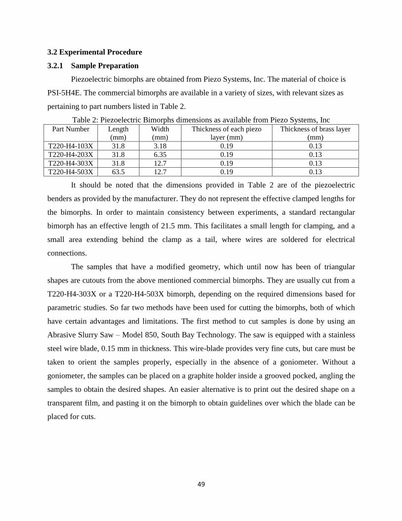
49

3.2 Experimental Procedure

3.2.1 Sample Preparation

Piezoelectric bimorphs are obtained from Piezo Systems, Inc. The material of choice is

PSI-5H4E. The commercial bimorphs are available in a variety of sizes, with relevant sizes as

pertaining to part numbers listed in Table 2.

Table 2: Piezoelectric Bimorphs dimensions as available from Piezo Systems, Inc Part Number Length

(mm)

Width

(mm)

Thickness of each piezo

layer (mm)

Thickness of brass layer

(mm)

T220-H4-103X 31.8 3.18 0.19 0.13

T220-H4-203X 31.8 6.35 0.19 0.13

T220-H4-303X 31.8 12.7 0.19 0.13

T220-H4-503X 63.5 12.7 0.19 0.13

It should be noted that the dimensions provided in Table 2 are of the piezoelectric

benders as provided by the manufacturer. They do not represent the effective clamped lengths for

the bimorphs. In order to maintain consistency between experiments, a standard rectangular

bimorph has an effective length of 21.5 mm. This facilitates a small length for clamping, and a

small area extending behind the clamp as a tail, where wires are soldered for electrical

connections.

The samples that have a modified geometry, which until now has been of triangular

shapes are cutouts from the above mentioned commercial bimorphs. They are usually cut from a

T220-H4-303X or a T220-H4-503X bimorph, depending on the required dimensions based for

parametric studies. So far two methods have been used for cutting the bimorphs, both of which

have certain advantages and limitations. The first method to cut samples is done by using an

Abrasive Slurry Saw – Model 850, South Bay Technology. The saw is equipped with a stainless

steel wire blade, 0.15 mm in thickness. This wire-blade provides very fine cuts, but care must be

taken to orient the samples properly, especially in the absence of a goniometer. Without a

goniometer, the samples can be placed on a graphite holder inside a grooved pocked, angling the

samples to obtain the desired shapes. An easier alternative is to print out the desired shape on a

transparent film, and pasting it on the bimorph to obtain guidelines over which the blade can be

placed for cuts.

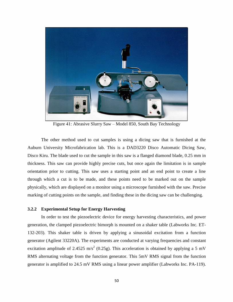
50

Figure 41: Abrasive Slurry Saw – Model 850, South Bay Technology

The other method used to cut samples is using a dicing saw that is furnished at the

Auburn University Microfabrication lab. This is a DAD3220 Disco Automatic Dicing Saw,

Disco Kiru. The blade used to cut the sample in this saw is a flanged diamond blade, 0.25 mm in

thickness. This saw can provide highly precise cuts, but once again the limitation is in sample

orientation prior to cutting. This saw uses a starting point and an end point to create a line

through which a cut is to be made, and these points need to be marked out on the sample

physically, which are displayed on a monitor using a microscope furnished with the saw. Precise

marking of cutting points on the sample, and finding these in the dicing saw can be challenging.

3.2.2 Experimental Setup for Energy Harvesting

In order to test the piezoelectric device for energy harvesting characteristics, and power

generation, the clamped piezoelectric bimorph is mounted on a shaker table (Labworks Inc. ET-

132-203). This shaker table is driven by applying a sinusoidal excitation from a function

generator (Agilent 33220A). The experiments are conducted at varying frequencies and constant

excitation amplitude of 2.4525 m/s2 (0.25g). This acceleration is obtained by applying a 5 mV

RMS alternating voltage from the function generator. This 5mV RMS signal from the function

generator is amplified to 24.5 mV RMS using a linear power amplifier (Labworks Inc. PA-119).

51

This 24.5 mV RMS signal is obtained using an output signal from an accelerometer (PCB

Piezotronics Inc. 480C02), that is connected to a channel on a digital oscilloscope (Tetronix TDS

3014B). The acceleration amplitude needs to be adjusted to 25 mV RMS each time the frequency

is changed using the function generator. This adjustment is needed due to the fact that a constant

voltage is supplied from the power amplifier. In order to keep acceleration constant with

changing frequency, a constant current source could help, and would get the base acceleration

relatively constant. A fool-proof method would be to employ the use a servo-feedback controller,

adjusting the input power each time the frequency is changed to obtain the desired acceleration.

The two wires that are soldered on the outer surfaces of the series-poled piezoelectric

device are connected to two probes that feed into a second channel on the digital oscilloscope. in

addition, a load resistor is connected in parallel with the piezoelectric device and the digital

oscilloscope. The value of this load resistor can be adjusted. In the absence of the load resistor,

or very high resistance values (>1 MΩ), the conditions are close to having an open circuit for

with the piezoelectric bimorph. Under open circuit conditions, the dielectric displacement is

zero, as there is no current flowing out of the device. Very low values of the load resistor provide

short circuit conditions, and here the electric potential is zero as the top and bottom layers of the

piezoelectric device are shunt. The digital oscilloscope reading from this channel provides the

voltage generated from the piezoelectric device, which is recorded manually. Figure 42 provides

a schematic for the experimental setup, which is also shown in a picture in Figure 43.

Figure 42: Schematic of energy harvesting experimental setup [22]

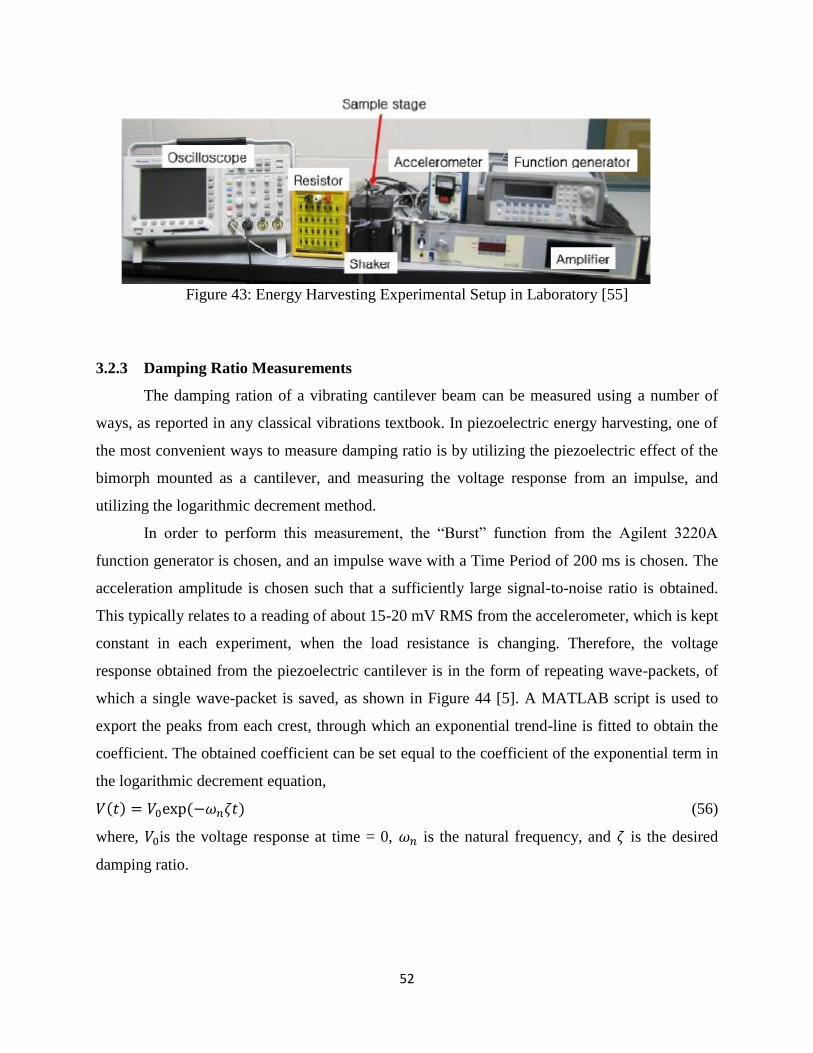
52

Figure 43: Energy Harvesting Experimental Setup in Laboratory [55]

3.2.3 Damping Ratio Measurements

The damping ration of a vibrating cantilever beam can be measured using a number of

ways, as reported in any classical vibrations textbook. In piezoelectric energy harvesting, one of

the most convenient ways to measure damping ratio is by utilizing the piezoelectric effect of the

bimorph mounted as a cantilever, and measuring the voltage response from an impulse, and

utilizing the logarithmic decrement method.

In order to perform this measurement, the “Burst” function from the Agilent 3220A

function generator is chosen, and an impulse wave with a Time Period of 200 ms is chosen. The

acceleration amplitude is chosen such that a sufficiently large signal-to-noise ratio is obtained.

This typically relates to a reading of about 15-20 mV RMS from the accelerometer, which is kept

constant in each experiment, when the load resistance is changing. Therefore, the voltage

response obtained from the piezoelectric cantilever is in the form of repeating wave-packets, of

which a single wave-packet is saved, as shown in Figure 44 [5]. A MATLAB script is used to

export the peaks from each crest, through which an exponential trend-line is fitted to obtain the

coefficient. The obtained coefficient can be set equal to the coefficient of the exponential term in

the logarithmic decrement equation,

𝑉(𝑡) = 𝑉0exp (−𝜔𝑛휁𝑡) (56)

where, 𝑉0is the voltage response at time = 0, 𝜔𝑛 is the natural frequency, and 휁 is the desired

damping ratio.

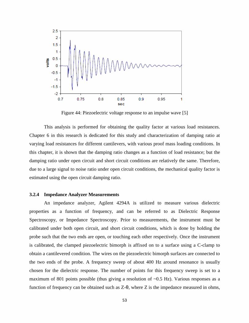
53

Figure 44: Piezoelectric voltage response to an impulse wave [5]

This analysis is performed for obtaining the quality factor at various load resistances.

Chapter 6 in this research is dedicated for this study and characterization of damping ratio at

varying load resistances for different cantilevers, with various proof mass loading conditions. In

this chapter, it is shown that the damping ratio changes as a function of load resistance; but the

damping ratio under open circuit and short circuit conditions are relatively the same. Therefore,

due to a large signal to noise ratio under open circuit conditions, the mechanical quality factor is

estimated using the open circuit damping ratio.

3.2.4 Impedance Analyzer Measurements

An impedance analyzer, Agilent 4294A is utilized to measure various dielectric

properties as a function of frequency, and can be referred to as Dielectric Response

Spectroscopy, or Impedance Spectroscopy. Prior to measurements, the instrument must be

calibrated under both open circuit, and short circuit conditions, which is done by holding the

probe such that the two ends are open, or touching each other respectively. Once the instrument

is calibrated, the clamped piezoelectric bimorph is affixed on to a surface using a C-clamp to

obtain a cantilevered condition. The wires on the piezoelectric bimorph surfaces are connected to

the two ends of the probe. A frequency sweep of about 400 Hz around resonance is usually

chosen for the dielectric response. The number of points for this frequency sweep is set to a

maximum of 801 points possible (thus giving a resolution of ~0.5 Hz). Various responses as a

function of frequency can be obtained such as Z-θ, where Z is the impedance measured in ohms,

54

and θ is the phase angle. Another response that is measured is Cp-D, where Cp is the parallel

capacitance of the piezoelectric device, and D is the dissipation factor, which is an inverse of the

loss tangent. All these values provide peaks at specific frequencies, which primarily relate to the

resonance and anti-resonance frequency of the device.

The peaks on the impedance curve provide some very important information. The

impedance value is maximized at the resonance frequency of the structure, and minimum at the

anti-resonance frequency of the structure. Moreover, the maximum impedance value at the

resonance frequency is a very important factor to measure, since this value gives an indication of

the internal resistance of the device. This value should be matched with an external load resistor

for maximum power dissipation through it. The phase angle θ, describes the phase difference

between the current and voltage in an AC field. Therefore, impedance when expressed as a

complex number has a real part, which is resistance, and the imaginary part is reactance.

The other quantity that is measured is equivalent parallel capacitance, which is an

important quantity that needs to be measured since it is a function of area of the overhanging

clamped piezoelectric beam. The effect of shape change on equivalent parallel capacitance

would also be an important parameter to identify. The dissipation factor, D is an inverse of the

quality factor of the piezoelectric device, and this can provide important information regarding

the damping ratio of the material.

55

CHAPTER 4: PRELIMENARY NUMERICAL ANALYSIS

This chapter primarily deals with numerical simulations and calculations that form the

basis of the experimental work of this dissertation. The first set of numerical simulations are

static calculations, that provide the impetus for the effect of geometry in terms of stress

distribution. Following static simulations, the simulations are of a dynamic nature by means of

modal analyses on the structures, to determine resonance frequencies, and design the devices to

obtain target resonance frequencies.

4.1 Quasi-static numerical analysis for various shaped cantilevers

As mentioned in the literature review and depicted in the piezoelectric constitutive

equations, one of the major factors that influences the generation of power in a device is the

amount of strain produced in the device when it is loaded. Therefore, a cantilevered piezoelectric

device under sinusoidal base excitation undergoing mode 1 vibration produces charge as a

function of the strain produced in the material. This mode shape can be mimicked in a quasi-

static state by applying a point load at the free end of a beam, and the bending characteristics of a

cantilevered device can be studied. The magnitude and distribution of strain, which is directly

related to stress by Hooke’s law over the surface of a device can be influenced by changing the

geometry of the device, and hence the effects of changing shapes is studied in this section in a

quasi-static manner.

The cantilever beams that are generated in the software have dimensions adopted from

commercially available piezoelectric bimorphs from Piezo Systems Inc. The adopted rectangular

beam is 31.8 mm in length, 12.7 mm in width and overall thickness is 0.51 mm. These

rectangular beams have been tapered into triangular shapes. The triangular beams that have been

generated maintain the same length and thickness as the rectangular cantilevers, while the width

at the base is altered to study the beams. The material properties applied utilize the d31

directional properties of PZT-5A from Piezo Inc. The Young’s modulus is 62 GPa, Poisson’s

ratio of 0.31, and mass density of 7750 kg m-3

.

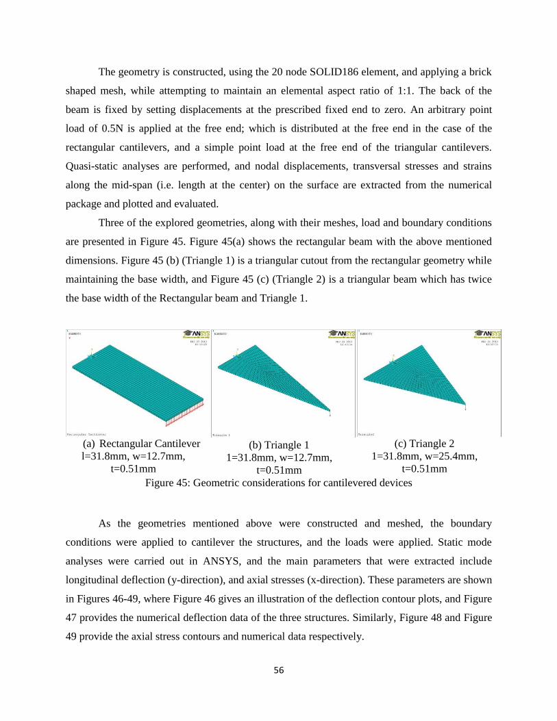
56

The geometry is constructed, using the 20 node SOLID186 element, and applying a brick

shaped mesh, while attempting to maintain an elemental aspect ratio of 1:1. The back of the

beam is fixed by setting displacements at the prescribed fixed end to zero. An arbitrary point

load of 0.5N is applied at the free end; which is distributed at the free end in the case of the

rectangular cantilevers, and a simple point load at the free end of the triangular cantilevers.

Quasi-static analyses are performed, and nodal displacements, transversal stresses and strains

along the mid-span (i.e. length at the center) on the surface are extracted from the numerical

package and plotted and evaluated.

Three of the explored geometries, along with their meshes, load and boundary conditions

are presented in Figure 45. Figure 45(a) shows the rectangular beam with the above mentioned

dimensions. Figure 45 (b) (Triangle 1) is a triangular cutout from the rectangular geometry while

maintaining the base width, and Figure 45 (c) (Triangle 2) is a triangular beam which has twice

the base width of the Rectangular beam and Triangle 1.

(a) Rectangular Cantilever

l=31.8mm, w=12.7mm,

t=0.51mm

(b) Triangle 1

1=31.8mm, w=12.7mm,

t=0.51mm

(c) Triangle 2

1=31.8mm, w=25.4mm,

t=0.51mm

Figure 45: Geometric considerations for cantilevered devices

As the geometries mentioned above were constructed and meshed, the boundary

conditions were applied to cantilever the structures, and the loads were applied. Static mode

analyses were carried out in ANSYS, and the main parameters that were extracted include

longitudinal deflection (y-direction), and axial stresses (x-direction). These parameters are shown

in Figures 46-49, where Figure 46 gives an illustration of the deflection contour plots, and Figure

47 provides the numerical deflection data of the three structures. Similarly, Figure 48 and Figure

49 provide the axial stress contours and numerical data respectively.

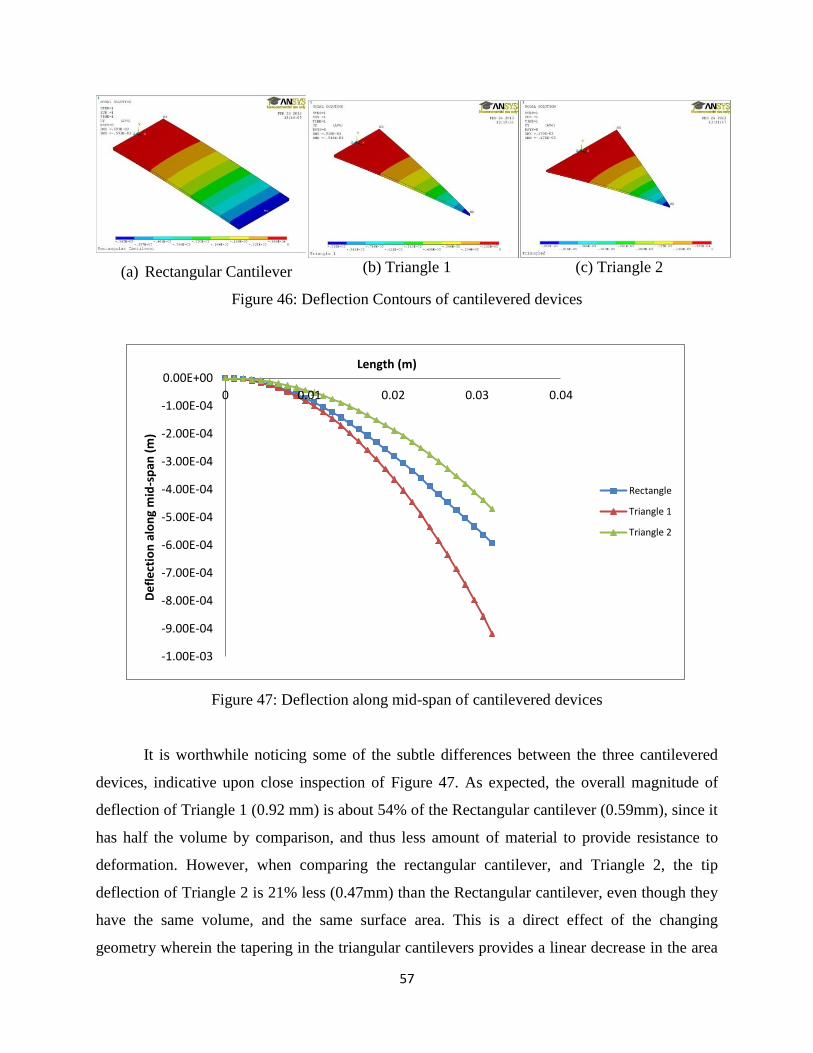
57

(a) Rectangular Cantilever (b) Triangle 1 (c) Triangle 2

Figure 46: Deflection Contours of cantilevered devices

Figure 47: Deflection along mid-span of cantilevered devices

It is worthwhile noticing some of the subtle differences between the three cantilevered

devices, indicative upon close inspection of Figure 47. As expected, the overall magnitude of

deflection of Triangle 1 (0.92 mm) is about 54% of the Rectangular cantilever (0.59mm), since it

has half the volume by comparison, and thus less amount of material to provide resistance to

deformation. However, when comparing the rectangular cantilever, and Triangle 2, the tip

deflection of Triangle 2 is 21% less (0.47mm) than the Rectangular cantilever, even though they

have the same volume, and the same surface area. This is a direct effect of the changing

geometry wherein the tapering in the triangular cantilevers provides a linear decrease in the area

-1.00E-03

-9.00E-04

-8.00E-04

-7.00E-04

-6.00E-04

-5.00E-04

-4.00E-04

-3.00E-04

-2.00E-04

-1.00E-04

0.00E+00

0 0.01 0.02 0.03 0.04

De

fle

ctio

n a

lon

g m

id-s

pan

(m

)

Length (m)

Rectangle

Triangle 1

Triangle 2

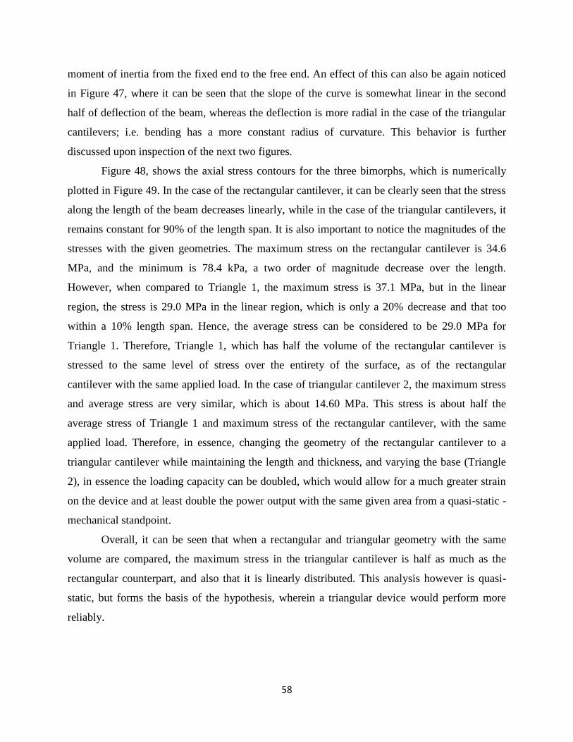
58

moment of inertia from the fixed end to the free end. An effect of this can also be again noticed

in Figure 47, where it can be seen that the slope of the curve is somewhat linear in the second

half of deflection of the beam, whereas the deflection is more radial in the case of the triangular

cantilevers; i.e. bending has a more constant radius of curvature. This behavior is further

discussed upon inspection of the next two figures.

Figure 48, shows the axial stress contours for the three bimorphs, which is numerically

plotted in Figure 49. In the case of the rectangular cantilever, it can be clearly seen that the stress

along the length of the beam decreases linearly, while in the case of the triangular cantilevers, it

remains constant for 90% of the length span. It is also important to notice the magnitudes of the

stresses with the given geometries. The maximum stress on the rectangular cantilever is 34.6

MPa, and the minimum is 78.4 kPa, a two order of magnitude decrease over the length.

However, when compared to Triangle 1, the maximum stress is 37.1 MPa, but in the linear

region, the stress is 29.0 MPa in the linear region, which is only a 20% decrease and that too

within a 10% length span. Hence, the average stress can be considered to be 29.0 MPa for

Triangle 1. Therefore, Triangle 1, which has half the volume of the rectangular cantilever is

stressed to the same level of stress over the entirety of the surface, as of the rectangular

cantilever with the same applied load. In the case of triangular cantilever 2, the maximum stress

and average stress are very similar, which is about 14.60 MPa. This stress is about half the

average stress of Triangle 1 and maximum stress of the rectangular cantilever, with the same

applied load. Therefore, in essence, changing the geometry of the rectangular cantilever to a

triangular cantilever while maintaining the length and thickness, and varying the base (Triangle

2), in essence the loading capacity can be doubled, which would allow for a much greater strain

on the device and at least double the power output with the same given area from a quasi-static -

mechanical standpoint.

Overall, it can be seen that when a rectangular and triangular geometry with the same

volume are compared, the maximum stress in the triangular cantilever is half as much as the

rectangular counterpart, and also that it is linearly distributed. This analysis however is quasi-

static, but forms the basis of the hypothesis, wherein a triangular device would perform more

reliably.

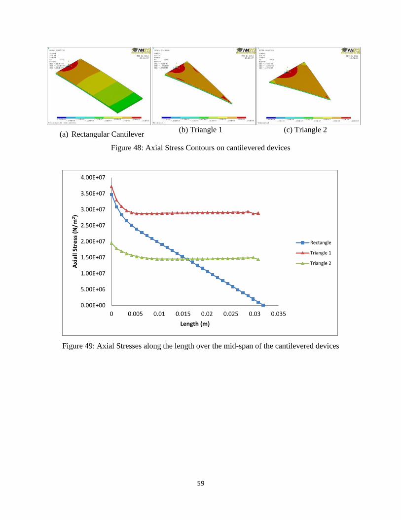
59

(a) Rectangular Cantilever (b) Triangle 1 (c) Triangle 2

Figure 48: Axial Stress Contours on cantilevered devices

Figure 49: Axial Stresses along the length over the mid-span of the cantilevered devices

0.00E+00

5.00E+06

1.00E+07

1.50E+07

2.00E+07

2.50E+07

3.00E+07

3.50E+07

4.00E+07

0 0.005 0.01 0.015 0.02 0.025 0.03 0.035

Axi

all S

tre

ss (

N/m

2)

Length (m)

Rectangle

Triangle 1

Triangle 2

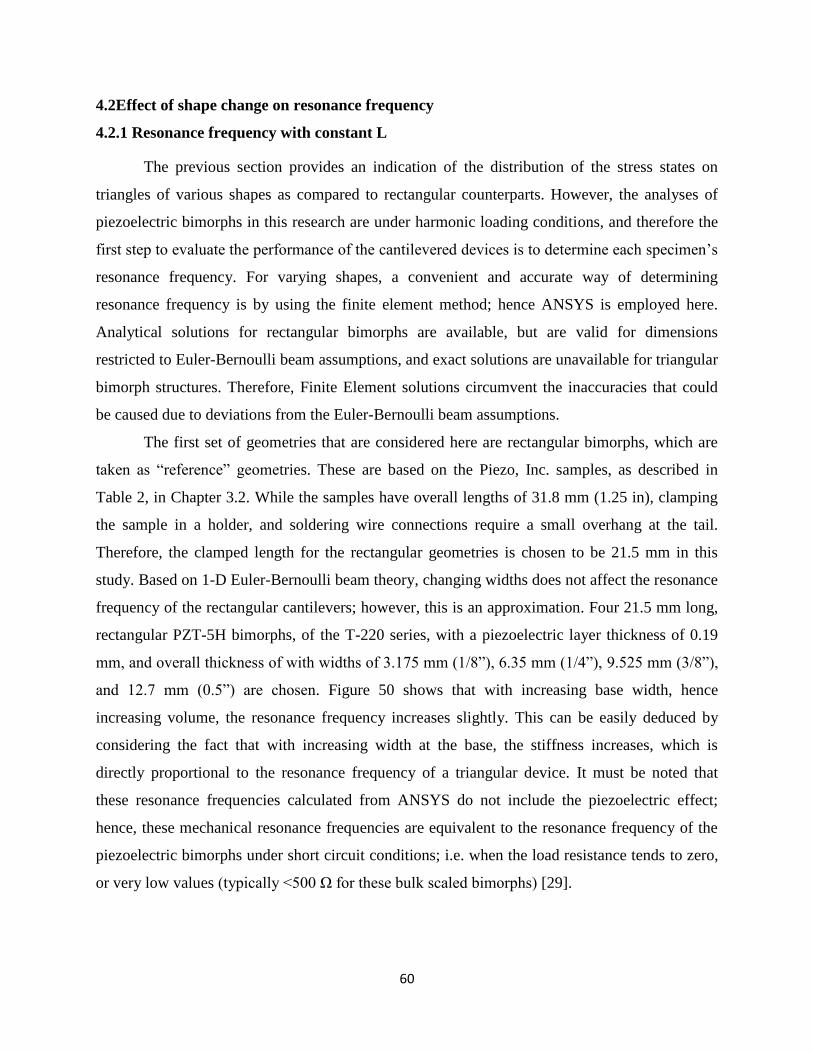
60

4.2Effect of shape change on resonance frequency

4.2.1 Resonance frequency with constant L

The previous section provides an indication of the distribution of the stress states on

triangles of various shapes as compared to rectangular counterparts. However, the analyses of

piezoelectric bimorphs in this research are under harmonic loading conditions, and therefore the

first step to evaluate the performance of the cantilevered devices is to determine each specimen’s

resonance frequency. For varying shapes, a convenient and accurate way of determining

resonance frequency is by using the finite element method; hence ANSYS is employed here.

Analytical solutions for rectangular bimorphs are available, but are valid for dimensions

restricted to Euler-Bernoulli beam assumptions, and exact solutions are unavailable for triangular

bimorph structures. Therefore, Finite Element solutions circumvent the inaccuracies that could

be caused due to deviations from the Euler-Bernoulli beam assumptions.

The first set of geometries that are considered here are rectangular bimorphs, which are

taken as “reference” geometries. These are based on the Piezo, Inc. samples, as described in

Table 2, in Chapter 3.2. While the samples have overall lengths of 31.8 mm (1.25 in), clamping

the sample in a holder, and soldering wire connections require a small overhang at the tail.

Therefore, the clamped length for the rectangular geometries is chosen to be 21.5 mm in this

study. Based on 1-D Euler-Bernoulli beam theory, changing widths does not affect the resonance

frequency of the rectangular cantilevers; however, this is an approximation. Four 21.5 mm long,

rectangular PZT-5H bimorphs, of the T-220 series, with a piezoelectric layer thickness of 0.19

mm, and overall thickness of with widths of 3.175 mm (1/8”), 6.35 mm (1/4”), 9.525 mm (3/8”),

and 12.7 mm (0.5”) are chosen. Figure 50 shows that with increasing base width, hence

increasing volume, the resonance frequency increases slightly. This can be easily deduced by

considering the fact that with increasing width at the base, the stiffness increases, which is

directly proportional to the resonance frequency of a triangular device. It must be noted that

these resonance frequencies calculated from ANSYS do not include the piezoelectric effect;

hence, these mechanical resonance frequencies are equivalent to the resonance frequency of the

piezoelectric bimorphs under short circuit conditions; i.e. when the load resistance tends to zero,

or very low values (typically <500 Ω for these bulk scaled bimorphs) [29].

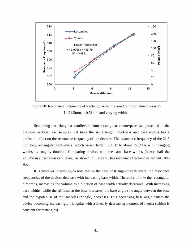
61

Figure 50: Resonance Frequency of Rectangular cantilevered bimorph structures with

L=21.5mm, t=0.51mm and varying widths

Sectioning out triangular cantilevers from rectangular counterparts (as presented in the

previous section), i.e. samples that have the same length, thickness and base widths has a

profound effect on the resonance frequency of the devices. The resonance frequency of the 21.5

mm long rectangular cantilevers, which varied from ~502 Hz to about ~512 Hz with changing

widths, is roughly doubled. Comparing devices with the same base widths (hence, half the

volume in a triangular cantilever), as shown in Figure 51 has resonance frequencies around 1000

Hz.

It is however interesting to note that in the case of triangular cantilevers, the resonance

frequencies of the devices decrease with increasing base width. Therefore, unlike the rectangular

bimorphs, increasing the volume as a function of base width actually decreases. With increasing

base widths, while the stiffness at the base increases, the base angle (the angle between the base

and the hypotenuse of the isosceles triangle) decreases. This decreasing base angle causes the

device becoming increasingly triangular with a linearly decreasing moment of inertia (which is

constant for rectangles).

y = 1.0769x + 498.79 R² = 0.9851

0

20

40

60

80

100

120

140

160

500

502

504

506

508

510

512

514

0 3 6 9 12 15

Vo

lum

e (

mm

3)

Re

son

ance

Fre

qu

en

cy (

Hz)

Base width (mm)

Rectangles

Volume

Linear (Rectangles)

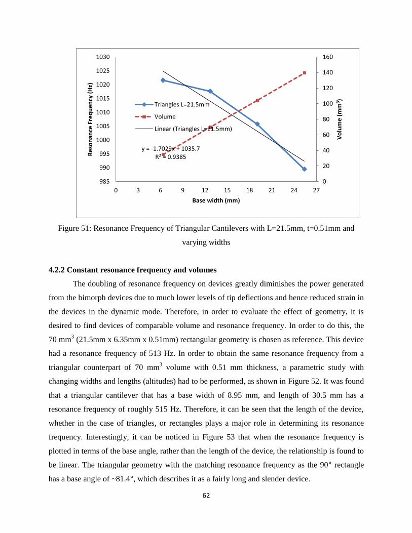
62

Figure 51: Resonance Frequency of Triangular Cantilevers with L=21.5mm, t=0.51mm and

varying widths

4.2.2 Constant resonance frequency and volumes

The doubling of resonance frequency on devices greatly diminishes the power generated

from the bimorph devices due to much lower levels of tip deflections and hence reduced strain in

the devices in the dynamic mode. Therefore, in order to evaluate the effect of geometry, it is

desired to find devices of comparable volume and resonance frequency. In order to do this, the

70 mm3 (21.5mm x 6.35mm x 0.51mm) rectangular geometry is chosen as reference. This device

had a resonance frequency of 513 Hz. In order to obtain the same resonance frequency from a

triangular counterpart of 70 mm3 volume with 0.51 mm thickness, a parametric study with

changing widths and lengths (altitudes) had to be performed, as shown in Figure 52. It was found

that a triangular cantilever that has a base width of 8.95 mm, and length of 30.5 mm has a

resonance frequency of roughly 515 Hz. Therefore, it can be seen that the length of the device,

whether in the case of triangles, or rectangles plays a major role in determining its resonance

frequency. Interestingly, it can be noticed in Figure 53 that when the resonance frequency is

plotted in terms of the base angle, rather than the length of the device, the relationship is found to

be linear. The triangular geometry with the matching resonance frequency as the 90° rectangle

has a base angle of ~81.4°, which describes it as a fairly long and slender device.

y = -1.7029x + 1035.7 R² = 0.9385

0

20

40

60

80

100

120

140

160

985

990

995

1000

1005

1010

1015

1020

1025

1030

0 3 6 9 12 15 18 21 24 27

Vo

lum

e (

mm

3)

Re

son

ance

Fre

qu

en

cy (

Hz)

Base width (mm)

Triangles L=21.5mm

Volume

Linear (Triangles L=21.5mm)

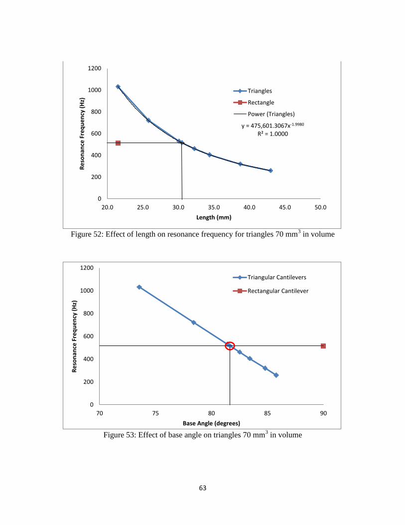
63

Figure 52: Effect of length on resonance frequency for triangles 70 mm

3 in volume

Figure 53: Effect of base angle on triangles 70 mm

3 in volume

y = 475,601.3067x-1.9980 R² = 1.0000

0

200

400

600

800

1000

1200

20.0 25.0 30.0 35.0 40.0 45.0 50.0

Re

son

ance

Fre

qu

en

cy (

Hz)

Length (mm)

Triangles

Rectangle

Power (Triangles)

0

200

400

600

800

1000

1200

70 75 80 85 90

Re

son

ance

Fre

qu

en

cy (

Hz)

Base Angle (degrees)

Triangular Cantilevers

Rectangular Cantilever

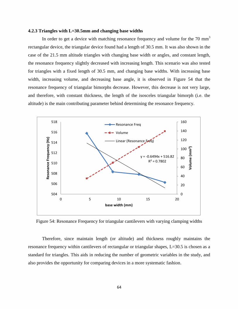
64

4.2.3 Triangles with L=30.5mm and changing base widths

In order to get a device with matching resonance frequency and volume for the 70 mm3

rectangular device, the triangular device found had a length of 30.5 mm. It was also shown in the

case of the 21.5 mm altitude triangles with changing base width or angles, and constant length,

the resonance frequency slightly decreased with increasing length. This scenario was also tested

for triangles with a fixed length of 30.5 mm, and changing base widths. With increasing base

width, increasing volume, and decreasing base angle, it is observed in Figure 54 that the

resonance frequency of triangular bimorphs decrease. However, this decrease is not very large,

and therefore, with constant thickness, the length of the isosceles triangular bimorph (i.e. the

altitude) is the main contributing parameter behind determining the resonance frequency.

Figure 54: Resonance Frequency for triangular cantilevers with varying clamping widths

Therefore, since maintain length (or altitude) and thickness roughly maintains the

resonance frequency within cantilevers of rectangular or triangular shapes, L=30.5 is chosen as a

standard for triangles. This aids in reducing the number of geometric variables in the study, and

also provides the opportunity for comparing devices in a more systematic fashion.

y = -0.6494x + 516.82 R² = 0.7802

0

20

40

60

80

100

120

140

160

504

506

508

510

512

514

516

518

0 5 10 15 20

Vo

lum

e (

mm

3)

Re

son

ance

Fre

qu

en

cy (

Hz)

base width (mm)

Resonance Freq

Volume

Linear (Resonance Freq)

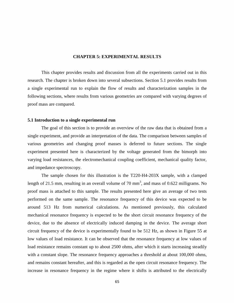
65

CHAPTER 5: EXPERIMENTAL RESULTS

This chapter provides results and discussion from all the experiments carried out in this

research. The chapter is broken down into several subsections. Section 5.1 provides results from

a single experimental run to explain the flow of results and characterization samples in the

following sections, where results from various geometries are compared with varying degrees of

proof mass are compared.

5.1 Introduction to a single experimental run

The goal of this section is to provide an overview of the raw data that is obtained from a

single experiment, and provide an interpretation of the data. The comparison between samples of

various geometries and changing proof masses is deferred to future sections. The single

experiment presented here is characterized by the voltage generated from the bimorph into

varying load resistances, the electromechanical coupling coefficient, mechanical quality factor,

and impedance spectroscopy.

The sample chosen for this illustration is the T220-H4-203X sample, with a clamped

length of 21.5 mm, resulting in an overall volume of 70 mm3, and mass of 0.622 milligrams. No

proof mass is attached to this sample. The results presented here give an average of two tests

performed on the same sample. The resonance frequency of this device was expected to be

around 513 Hz from numerical calculations. As mentioned previously, this calculated

mechanical resonance frequency is expected to be the short circuit resonance frequency of the

device, due to the absence of electrically induced damping in the device. The average short

circuit frequency of the device is experimentally found to be 512 Hz, as shown in Figure 55 at

low values of load resistance. It can be observed that the resonance frequency at low values of

load resistance remains constant up to about 2500 ohms, after which it starts increasing steadily

with a constant slope. The resonance frequency approaches a threshold at about 100,000 ohms,

and remains constant hereafter, and this is regarded as the open circuit resonance frequency. The

increase in resonance frequency in the regime where it shifts is attributed to the electrically

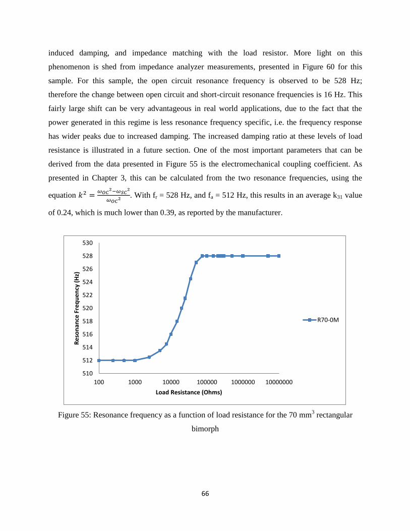
66

induced damping, and impedance matching with the load resistor. More light on this

phenomenon is shed from impedance analyzer measurements, presented in Figure 60 for this

sample. For this sample, the open circuit resonance frequency is observed to be 528 Hz;

therefore the change between open circuit and short-circuit resonance frequencies is 16 Hz. This

fairly large shift can be very advantageous in real world applications, due to the fact that the

power generated in this regime is less resonance frequency specific, i.e. the frequency response

has wider peaks due to increased damping. The increased damping ratio at these levels of load

resistance is illustrated in a future section. One of the most important parameters that can be

derived from the data presented in Figure 55 is the electromechanical coupling coefficient. As

presented in Chapter 3, this can be calculated from the two resonance frequencies, using the

equation 𝑘2 =𝜔𝑂𝐶

2−𝜔𝑆𝐶2

𝜔𝑂𝐶2 . With fr = 528 Hz, and fa = 512 Hz, this results in an average k31 value

of 0.24, which is much lower than 0.39, as reported by the manufacturer.

Figure 55: Resonance frequency as a function of load resistance for the 70 mm3 rectangular

bimorph

510

512

514

516

518

520

522

524

526

528

530

100 1000 10000 100000 1000000 10000000

Re

son

ance

Fre

qu

en

cy (

Hz)

Load Resistance (Ohms)

R70-0M

67

In order to illustrate the change in resonance frequency due to the change in stiffness in

the system due to the external load resistor, one can normalize the resonance frequency to the

short circuit resonance frequency in the system, where the open circuit resonance frequency is

dependent on stiffness due to the electromechanical coupling. This can be represented as.

Therefore, this would result in the short circuit resonance frequency normalized to unity, i.e.

𝑓𝑆𝐶 = 1 and 𝑓𝑂𝐶 = √1 + 𝑘2 [45]. Therefore, Figure 55 can be normalized, and represented in

Figure 56, illustrating the electromechanical coupling effect.

Figure 56: Normalized Resonance Frequency illustrating the electromechanical coupling in the

system

The data collected in order to estimate the power generated from a piezoelectric bimorph

is the RMS voltage into the load resistance at resonance. The voltage generated is also dependent

on the load resistance, and is a little more intuitive, based on Ohm’s law. At low values of load

resistance, the voltage generated is very low with high currents, and vice versa. It is however

interesting to notice in Figure 57 that the inflection points are noticeable in voltage generation as

well, as they were in Figure 55 and Figure 56 for resonance frequencies. The voltages have the

highest slope in the region where the maximum power is generated.

0.995

1

1.005

1.01

1.015

1.02

1.025

1.03

1.035

10 100 1000 10000 100000 1000000 10000000

f/f s

c


R70-0M

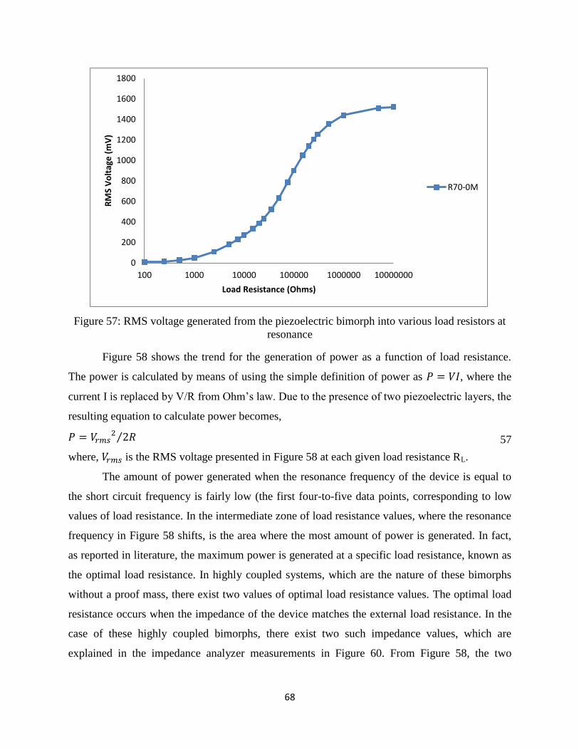
68

Figure 57: RMS voltage generated from the piezoelectric bimorph into various load resistors at

resonance

Figure 58 shows the trend for the generation of power as a function of load resistance.

The power is calculated by means of using the simple definition of power as 𝑃 = 𝑉𝐼, where the

current I is replaced by V/R from Ohm’s law. Due to the presence of two piezoelectric layers, the

resulting equation to calculate power becomes,

𝑃 = 𝑉𝑟𝑚𝑠2 2𝑅⁄ 57

where, 𝑉𝑟𝑚𝑠 is the RMS voltage presented in Figure 58 at each given load resistance RL.

The amount of power generated when the resonance frequency of the device is equal to

the short circuit frequency is fairly low (the first four-to-five data points, corresponding to low

values of load resistance. In the intermediate zone of load resistance values, where the resonance

frequency in Figure 58 shifts, is the area where the most amount of power is generated. In fact,

as reported in literature, the maximum power is generated at a specific load resistance, known as

the optimal load resistance. In highly coupled systems, which are the nature of these bimorphs

without a proof mass, there exist two values of optimal load resistance values. The optimal load

resistance occurs when the impedance of the device matches the external load resistance. In the

case of these highly coupled bimorphs, there exist two such impedance values, which are

explained in the impedance analyzer measurements in Figure 60. From Figure 58, the two

0

200

400

600

800

1000

1200

1400

1600

1800

100 1000 10000 100000 1000000 10000000

RM

S V

olt

age

(m

V)


R70-0M

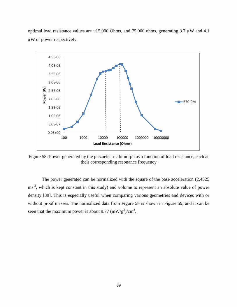
69

optimal load resistance values are ~15,000 Ohms, and 75,000 ohms, generating 3.7 W and 4.1

W of power respectively.

Figure 58: Power generated by the piezoelectric bimorph as a function of load resistance, each at

their corresponding resonance frequency

The power generated can be normalized with the square of the base acceleration (2.4525

ms-2

, which is kept constant in this study) and volume to represent an absolute value of power

density [30]. This is especially useful when comparing various geometries and devices with or

without proof masses. The normalized data from Figure 58 is shown in Figure 59, and it can be

seen that the maximum power is about 9.77 (mW/g2)/cm

3.

0.0E+00

5.0E-07

1.0E-06

1.5E-06

2.0E-06

2.5E-06

3.0E-06

3.5E-06

4.0E-06

4.5E-06

100 1000 10000 100000 1000000 10000000

Po

we

r (W

)


R70-0M

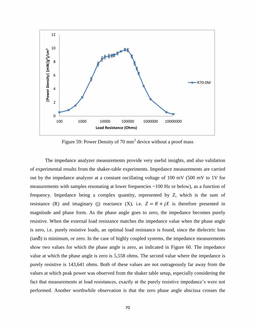
70

Figure 59: Power Density of 70 mm3 device without a proof mass

The impedance analyzer measurements provide very useful insights, and also validation

of experimental results from the shaker-table experiments. Impedance measurements are carried

out by the impedance analyzer at a constant oscillating voltage of 100 mV (500 mV to 1V for

measurements with samples resonating at lower frequencies ~100 Hz or below), as a function of

frequency. Impedance being a complex quantity, represented by Z, which is the sum of

resistance (R) and imaginary (j) reactance (X), i.e. 𝑍 = 𝑅 + 𝑗𝑋 is therefore presented in

magnitude and phase form. As the phase angle goes to zero, the impedance becomes purely

resistive. When the external load resistance matches the impedance value when the phase angle

is zero, i.e. purely resistive loads, an optimal load resistance is found, since the dielectric loss

(tanδ) is minimum, or zero. In the case of highly coupled systems, the impedance measurements

show two values for which the phase angle is zero, as indicated in Figure 60. The impedance

value at which the phase angle is zero is 5,558 ohms. The second value where the impedance is

purely resistive is 143,641 ohms. Both of these values are not outrageously far away from the

values at which peak power was observed from the shaker table setup, especially considering the

fact that measurements at load resistances, exactly at the purely resistive impedance’s were not

performed. Another worthwhile observation is that the zero phase angle abscissa crosses the

0

2

4

6

8

10

12

100 1000 10000 100000 1000000 10000000

|Po

we

r D

en

sity

| (m

W/g

2 )/c

m3


R70-0M

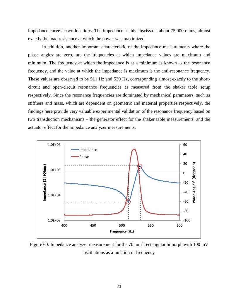
71

impedance curve at two locations. The impedance at this abscissa is about 75,000 ohms, almost

exactly the load resistance at which the power was maximized.

In addition, another important characteristic of the impedance measurements where the

phase angles are zero, are the frequencies at which impedance values are maximum and

minimum. The frequency at which the impedance is at a minimum is known as the resonance

frequency, and the value at which the impedance is maximum is the anti-resonance frequency.

These values are observed to be 511 Hz and 530 Hz, corresponding almost exactly to the short-

circuit and open-circuit resonance frequencies as measured from the shaker table setup

respectively. Since the resonance frequencies are dominated by mechanical parameters, such as

stiffness and mass, which are dependent on geometric and material properties respectively, the

findings here provide very valuable experimental validation of the resonance frequency based on

two transduction mechanisms – the generator effect for the shaker table measurements, and the

actuator effect for the impedance analyzer measurements.

Figure 60: Impedance analyzer measurement for the 70 mm3 rectangular bimorph with 100 mV

oscillations as a function of frequency

-100

-80

-60

-40

-20

0

20

40

60

1.0E+03

1.0E+04

1.0E+05

1.0E+06

400 450 500 550 600

Ph

ase

An

gle

θ (

deg

rees)

Imp

ed

ance

|Z|

(O

hm

s)

Frequency (Hz)

Impedance

Phase

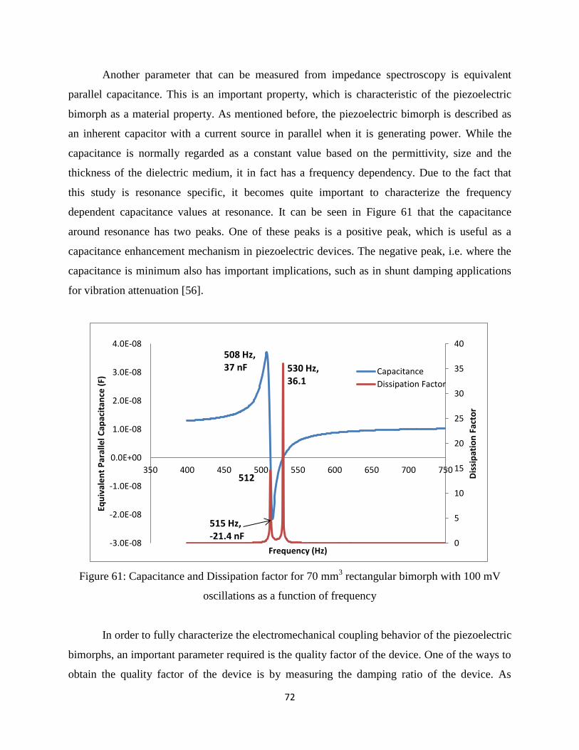
72

Another parameter that can be measured from impedance spectroscopy is equivalent

parallel capacitance. This is an important property, which is characteristic of the piezoelectric

bimorph as a material property. As mentioned before, the piezoelectric bimorph is described as

an inherent capacitor with a current source in parallel when it is generating power. While the

capacitance is normally regarded as a constant value based on the permittivity, size and the

thickness of the dielectric medium, it in fact has a frequency dependency. Due to the fact that

this study is resonance specific, it becomes quite important to characterize the frequency

dependent capacitance values at resonance. It can be seen in Figure 61 that the capacitance

around resonance has two peaks. One of these peaks is a positive peak, which is useful as a

capacitance enhancement mechanism in piezoelectric devices. The negative peak, i.e. where the

capacitance is minimum also has important implications, such as in shunt damping applications

for vibration attenuation [56].

Figure 61: Capacitance and Dissipation factor for 70 mm3 rectangular bimorph with 100 mV

oscillations as a function of frequency

In order to fully characterize the electromechanical coupling behavior of the piezoelectric

bimorphs, an important parameter required is the quality factor of the device. One of the ways to

obtain the quality factor of the device is by measuring the damping ratio of the device. As

0

5

10

15

20

25

30

35

40

-3.0E-08

-2.0E-08

-1.0E-08

0.0E+00

1.0E-08

2.0E-08

3.0E-08

4.0E-08

350 400 450 500 550 600 650 700 750D

issi

pat

ion

Fac

tor

Equ

ival

en

t P

aral

lel C

apac

itan

ce (

F)

Frequency (Hz)

Capacitance

Dissipation Factor

508 Hz, 37 nF

515 Hz, -21.4 nF

512

530 Hz, 36.1

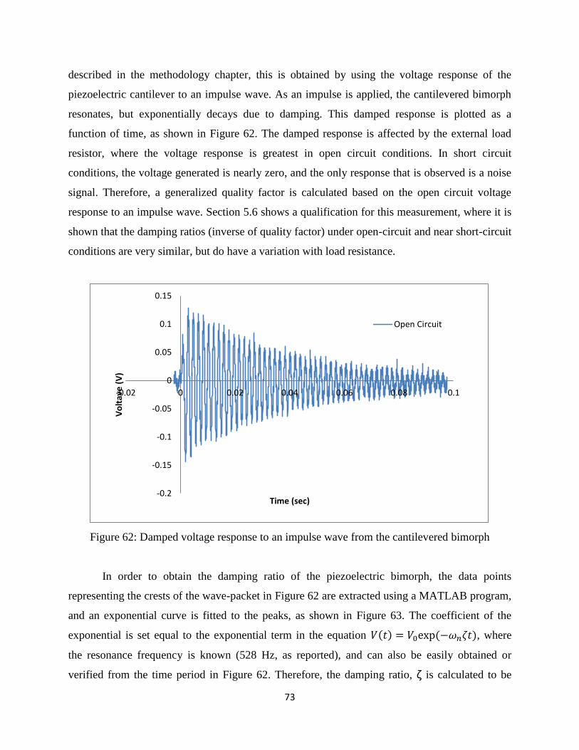
73

described in the methodology chapter, this is obtained by using the voltage response of the

piezoelectric cantilever to an impulse wave. As an impulse is applied, the cantilevered bimorph

resonates, but exponentially decays due to damping. This damped response is plotted as a

function of time, as shown in Figure 62. The damped response is affected by the external load

resistor, where the voltage response is greatest in open circuit conditions. In short circuit

conditions, the voltage generated is nearly zero, and the only response that is observed is a noise

signal. Therefore, a generalized quality factor is calculated based on the open circuit voltage

response to an impulse wave. Section 5.6 shows a qualification for this measurement, where it is

shown that the damping ratios (inverse of quality factor) under open-circuit and near short-circuit

conditions are very similar, but do have a variation with load resistance.

Figure 62: Damped voltage response to an impulse wave from the cantilevered bimorph

In order to obtain the damping ratio of the piezoelectric bimorph, the data points

representing the crests of the wave-packet in Figure 62 are extracted using a MATLAB program,

and an exponential curve is fitted to the peaks, as shown in Figure 63. The coefficient of the

exponential is set equal to the exponential term in the equation 𝑉(𝑡) = 𝑉0exp (−𝜔𝑛휁𝑡), where

the resonance frequency is known (528 Hz, as reported), and can also be easily obtained or

verified from the time period in Figure 62. Therefore, the damping ratio, ζ is calculated to be

-0.2

-0.15

-0.1

-0.05

0

0.05

0.1

0.15

-0.02 0 0.02 0.04 0.06 0.08 0.1

Vo

ltav

e (

V)

Time (sec)

Open Circuit

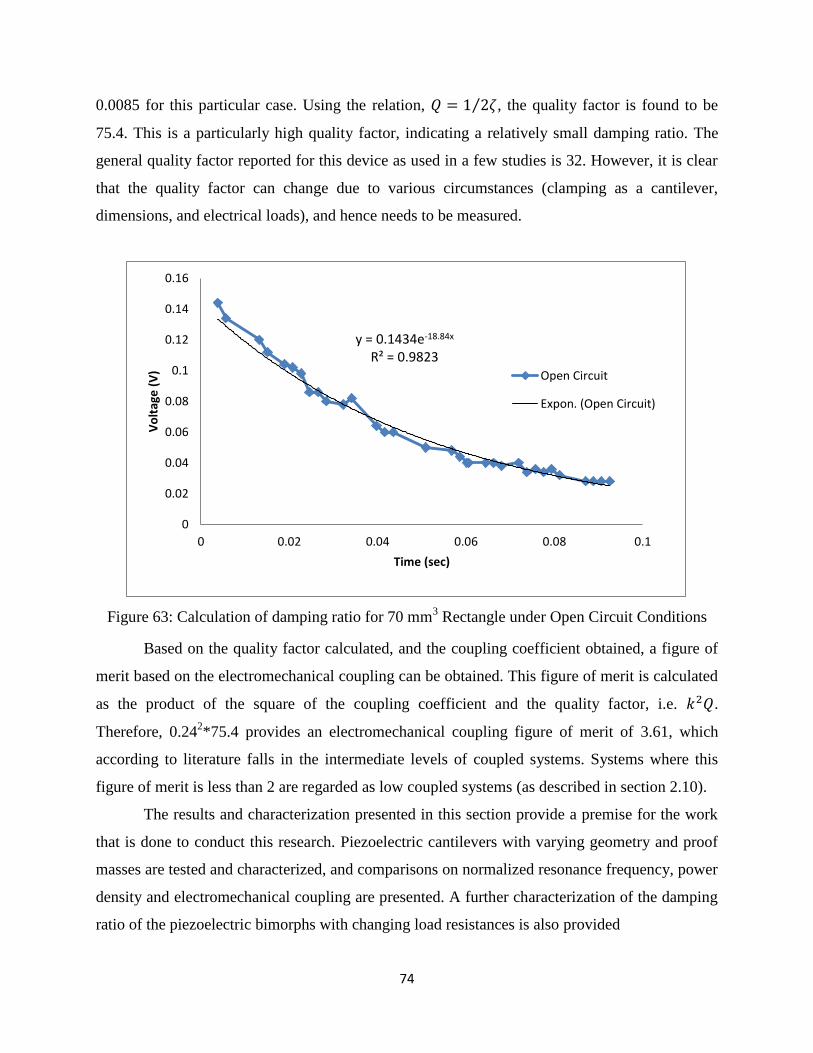
74

0.0085 for this particular case. Using the relation, 𝑄 = 1 2휁⁄ , the quality factor is found to be

75.4. This is a particularly high quality factor, indicating a relatively small damping ratio. The

general quality factor reported for this device as used in a few studies is 32. However, it is clear

that the quality factor can change due to various circumstances (clamping as a cantilever,

dimensions, and electrical loads), and hence needs to be measured.

Figure 63: Calculation of damping ratio for 70 mm3 Rectangle under Open Circuit Conditions

Based on the quality factor calculated, and the coupling coefficient obtained, a figure of

merit based on the electromechanical coupling can be obtained. This figure of merit is calculated

as the product of the square of the coupling coefficient and the quality factor, i.e. 𝑘2𝑄.

Therefore, 0.242*75.4 provides an electromechanical coupling figure of merit of 3.61, which

according to literature falls in the intermediate levels of coupled systems. Systems where this

figure of merit is less than 2 are regarded as low coupled systems (as described in section 2.10).

The results and characterization presented in this section provide a premise for the work

that is done to conduct this research. Piezoelectric cantilevers with varying geometry and proof

masses are tested and characterized, and comparisons on normalized resonance frequency, power

density and electromechanical coupling are presented. A further characterization of the damping

ratio of the piezoelectric bimorphs with changing load resistances is also provided

y = 0.1434e-18.84x R² = 0.9823

0

0.02

0.04

0.06

0.08

0.1

0.12

0.14

0.16

0 0.02 0.04 0.06 0.08 0.1

Vo

ltag

e (

V)

Time (sec)

Open Circuit

Expon. (Open Circuit)

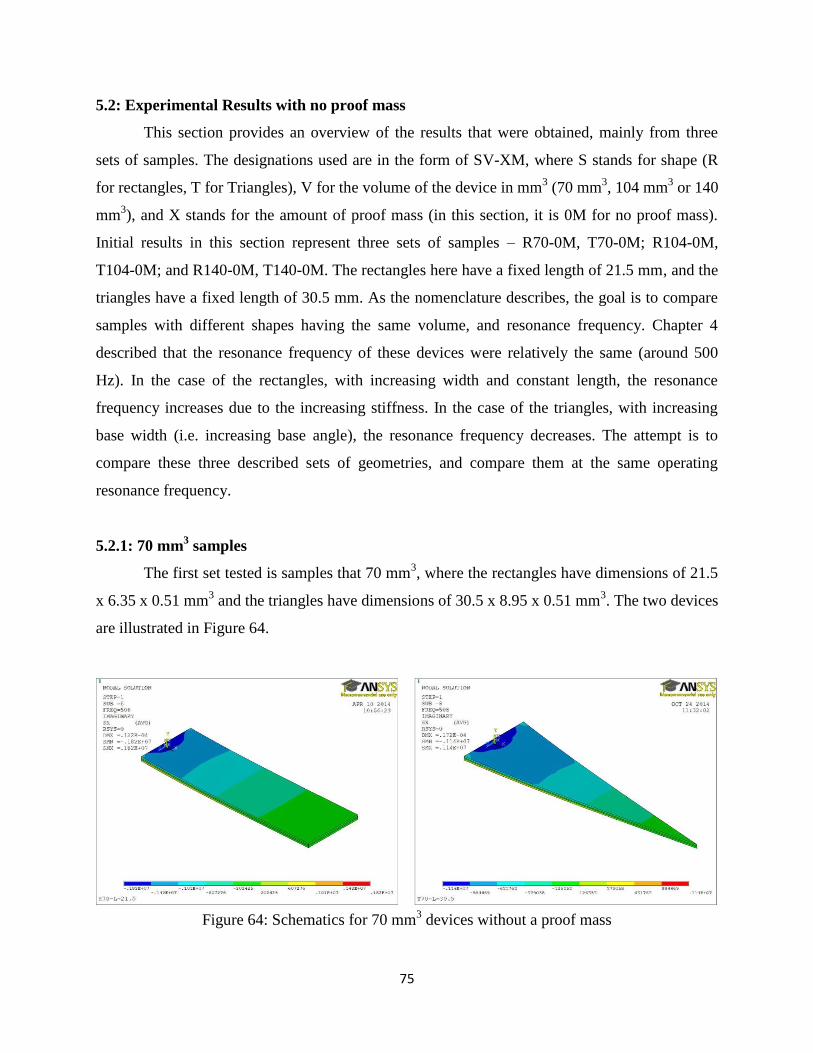
75

5.2: Experimental Results with no proof mass

This section provides an overview of the results that were obtained, mainly from three

sets of samples. The designations used are in the form of SV-XM, where S stands for shape (R

for rectangles, T for Triangles), V for the volume of the device in mm3 (70 mm

3, 104 mm

3 or 140

mm3), and X stands for the amount of proof mass (in this section, it is 0M for no proof mass).

Initial results in this section represent three sets of samples – R70-0M, T70-0M; R104-0M,

T104-0M; and R140-0M, T140-0M. The rectangles here have a fixed length of 21.5 mm, and the

triangles have a fixed length of 30.5 mm. As the nomenclature describes, the goal is to compare

samples with different shapes having the same volume, and resonance frequency. Chapter 4

described that the resonance frequency of these devices were relatively the same (around 500

Hz). In the case of the rectangles, with increasing width and constant length, the resonance

frequency increases due to the increasing stiffness. In the case of the triangles, with increasing

base width (i.e. increasing base angle), the resonance frequency decreases. The attempt is to

compare these three described sets of geometries, and compare them at the same operating

resonance frequency.

5.2.1: 70 mm3 samples

The first set tested is samples that 70 mm3, where the rectangles have dimensions of 21.5

x 6.35 x 0.51 mm3 and the triangles have dimensions of 30.5 x 8.95 x 0.51 mm

3. The two devices

are illustrated in Figure 64.

Figure 64: Schematics for 70 mm

3 devices without a proof mass

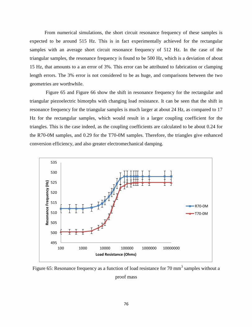
76

From numerical simulations, the short circuit resonance frequency of these samples is

expected to be around 515 Hz. This is in fact experimentally achieved for the rectangular

samples with an average short circuit resonance frequency of 512 Hz. In the case of the

triangular samples, the resonance frequency is found to be 500 Hz, which is a deviation of about

15 Hz, that amounts to a an error of 3%. This error can be attributed to fabrication or clamping

length errors. The 3% error is not considered to be as huge, and comparisons between the two

geometries are worthwhile.

Figure 65 and Figure 66 show the shift in resonance frequency for the rectangular and

triangular piezoelectric bimorphs with changing load resistance. It can be seen that the shift in

resonance frequency for the triangular samples is much larger at about 24 Hz, as compared to 17

Hz for the rectangular samples, which would result in a larger coupling coefficient for the

triangles. This is the case indeed, as the coupling coefficients are calculated to be about 0.24 for

the R70-0M samples, and 0.29 for the T70-0M samples. Therefore, the triangles give enhanced

conversion efficiency, and also greater electromechanical damping.

Figure 65: Resonance frequency as a function of load resistance for 70 mm3 samples without a

proof mass

495

500

505

510

515

520

525

530

535

100 1000 10000 100000 1000000 10000000

Re

son

ance

Fre

qu

en

cy (

Hz)


R70-0M

T70-0M

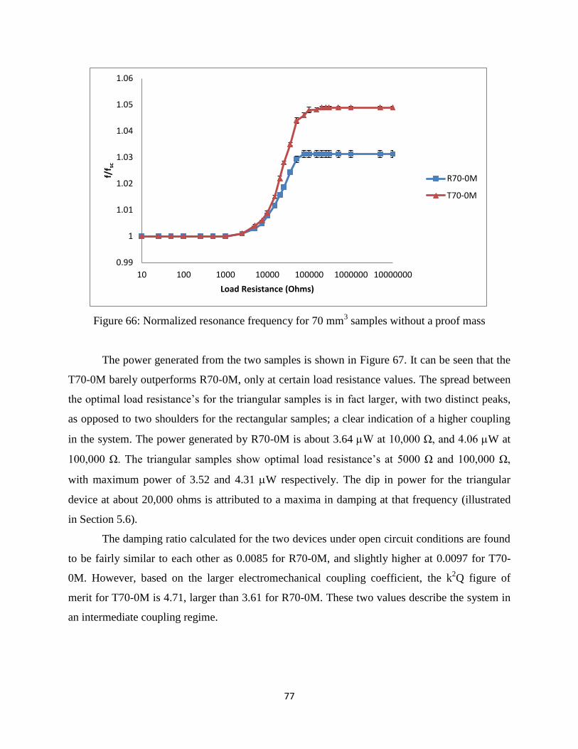
77

Figure 66: Normalized resonance frequency for 70 mm3 samples without a proof mass

The power generated from the two samples is shown in Figure 67. It can be seen that the

T70-0M barely outperforms R70-0M, only at certain load resistance values. The spread between

the optimal load resistance’s for the triangular samples is in fact larger, with two distinct peaks,

as opposed to two shoulders for the rectangular samples; a clear indication of a higher coupling

in the system. The power generated by R70-0M is about 3.64 W at 10,000 Ω, and 4.06 W at

100,000 Ω. The triangular samples show optimal load resistance’s at 5000 Ω and 100,000 Ω,

with maximum power of 3.52 and 4.31 W respectively. The dip in power for the triangular

device at about 20,000 ohms is attributed to a maxima in damping at that frequency (illustrated

in Section 5.6).

The damping ratio calculated for the two devices under open circuit conditions are found

to be fairly similar to each other as 0.0085 for R70-0M, and slightly higher at 0.0097 for T70-

0M. However, based on the larger electromechanical coupling coefficient, the k2Q figure of

merit for T70-0M is 4.71, larger than 3.61 for R70-0M. These two values describe the system in

an intermediate coupling regime.

0.99

1

1.01

1.02

1.03

1.04

1.05

1.06

10 100 1000 10000 100000 1000000 10000000

f/f s

c


R70-0M

T70-0M

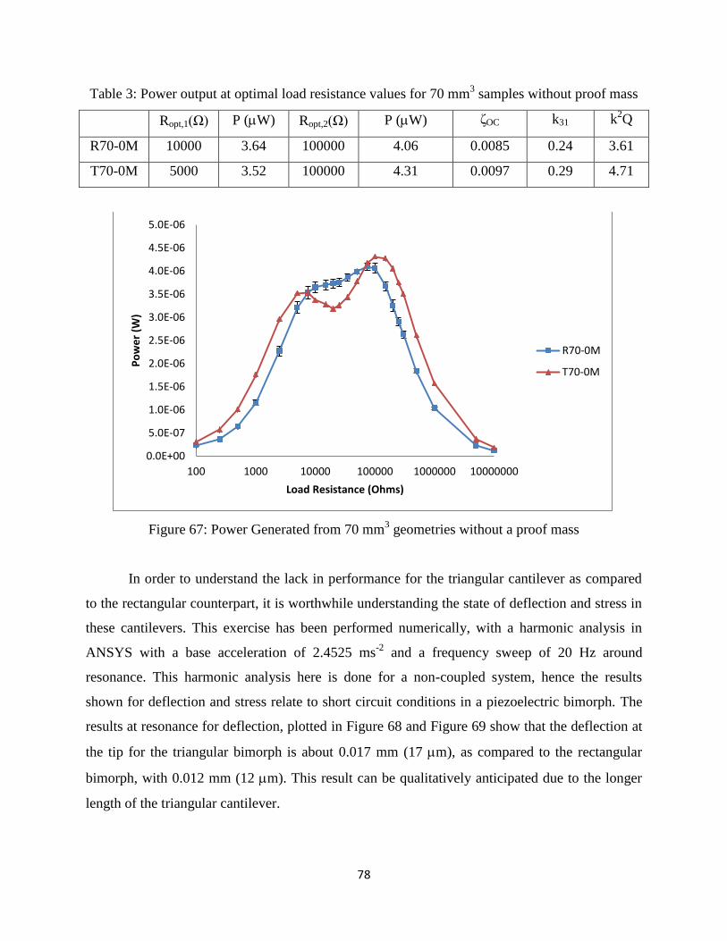
78


Ropt,1(Ω) P (W) Ropt,2(Ω) P (W) ζOC k31 k2Q

R70-0M 10000 3.64 100000 4.06 0.0085 0.24 3.61

T70-0M 5000 3.52 100000 4.31 0.0097 0.29 4.71

Figure 67: Power Generated from 70 mm3 geometries without a proof mass

In order to understand the lack in performance for the triangular cantilever as compared

to the rectangular counterpart, it is worthwhile understanding the state of deflection and stress in

these cantilevers. This exercise has been performed numerically, with a harmonic analysis in

ANSYS with a base acceleration of 2.4525 ms-2

and a frequency sweep of 20 Hz around

resonance. This harmonic analysis here is done for a non-coupled system, hence the results

shown for deflection and stress relate to short circuit conditions in a piezoelectric bimorph. The

results at resonance for deflection, plotted in Figure 68 and Figure 69 show that the deflection at

the tip for the triangular bimorph is about 0.017 mm (17 m), as compared to the rectangular

bimorph, with 0.012 mm (12 m). This result can be qualitatively anticipated due to the longer

length of the triangular cantilever.

0.0E+00

5.0E-07

1.0E-06

1.5E-06

2.0E-06

2.5E-06

3.0E-06

3.5E-06

4.0E-06

4.5E-06

5.0E-06

100 1000 10000 100000 1000000 10000000

Po

we

r (W

)


R70-0M

T70-0M

79

However, the results in Figure 70 and Figure 71, indicate the state of axial stresses are

more important for correlating the amount of power generated from the piezoelectric bimorphs.

It can be seen that the maximum stress, which is highly concentrated towards the fixed end of the

beam in the rectangular cantilever is higher in magnitude as compared to the triangular

cantilever. The maximum stress in the rectangular cantilever is 1.8 MPa, while in the case of the

triangular bimorph, even with greater deflection at the tip is lower at 1.1 MPa. This indicates that

the triangular structure, with the same volume, and roughly the same resonance frequency (not

much error between the two structures in ANSYS), is capable of handling a greater load at the

base due to its ability to distribute the stress in the structure more evenly.

This phenomenon is more apparent in Figure 72 and Figure 73, where the deflection and

stresses along the length of the beam, on the top surface are plotted. Even though the resonance

frequencies of the two devices are very similar, the deflection is greater in the case of the

rectangular bimorph everywhere it exists, while the triangular bimorph has a greater deflection

only where it is longer than the rectangular cantilever. The most likely explanation for this

difference in deflection between the two devices is due to the fact that with the tapering of the

beam, there is very little effective mass at the top of the beam in the case of the triangular device.

Therefore, unlike the rectangular device R70-0M, the triangular device T70-0M suffers from a

lack of inertial loading.

This lack of inertial loading at the tip shows a very apparent effect at the maximum

stress, at the base of the cantilevered triangular bimorph. It can be observed in Figure 73 that the

maximum stress in the case of the rectangular bimorph is 1.8 MPa, and in the case of the

triangular bimorph is 1.14 MPa. Moreover, with the absence of the tip loading, the desired

constant axial stress through the length of the device is not achieved. Overall, this indicates that

the triangular device, with the same given inertial loading due to base excitation is operating at

much lower levels of stress due to a stiffer base due to increased clamping width, and also

slightly more even distribution of stress (not up to the desired level though) with a smaller

declining slope over the axial stress profile.

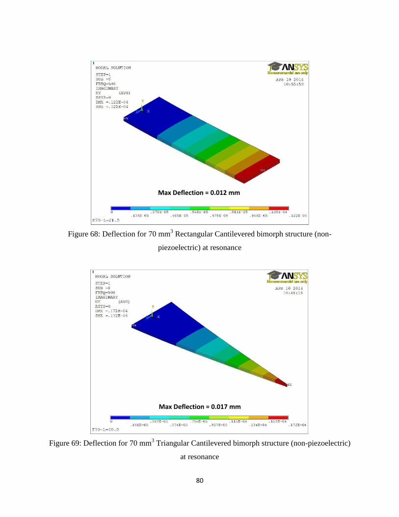
80

Figure 68: Deflection for 70 mm3 Rectangular Cantilevered bimorph structure (non-

piezoelectric) at resonance

Figure 69: Deflection for 70 mm3 Triangular Cantilevered bimorph structure (non-piezoelectric)

at resonance

Max Deflection = 0.012 mm

Max Deflection = 0.017 mm

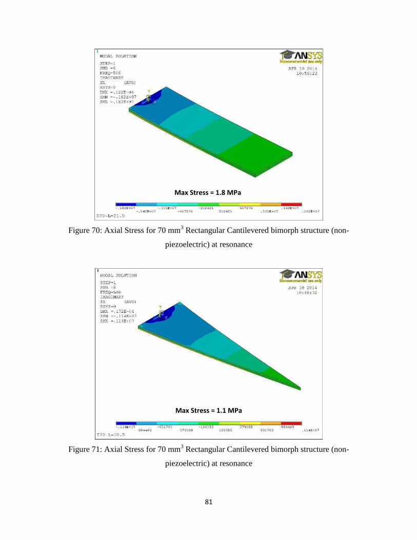
81





Max Stress = 1.8 MPa

Max Stress = 1.1 MPa

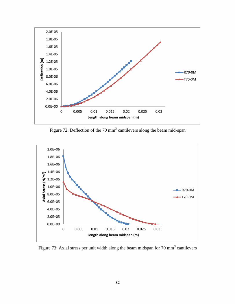
82

Figure 72: Deflection of the 70 mm3 cantilevers along the beam mid-span

Figure 73: Axial stress per unit width along the beam midspan for 70 mm3 cantilevers

0.0E+00

2.0E-06

4.0E-06

6.0E-06

8.0E-06

1.0E-05

1.2E-05

1.4E-05

1.6E-05

1.8E-05

2.0E-05

0 0.005 0.01 0.015 0.02 0.025 0.03

De

fle

ctio

n (

m)

Length along beam midspan (m)

R70-0M

T70-0M

0.0E+00

2.0E+05

4.0E+05

6.0E+05

8.0E+05

1.0E+06

1.2E+06

1.4E+06

1.6E+06

1.8E+06

2.0E+06

0 0.005 0.01 0.015 0.02 0.025 0.03

Axi

al S

tre

ss (

N/m

2 )


R70-0M

T70-0M

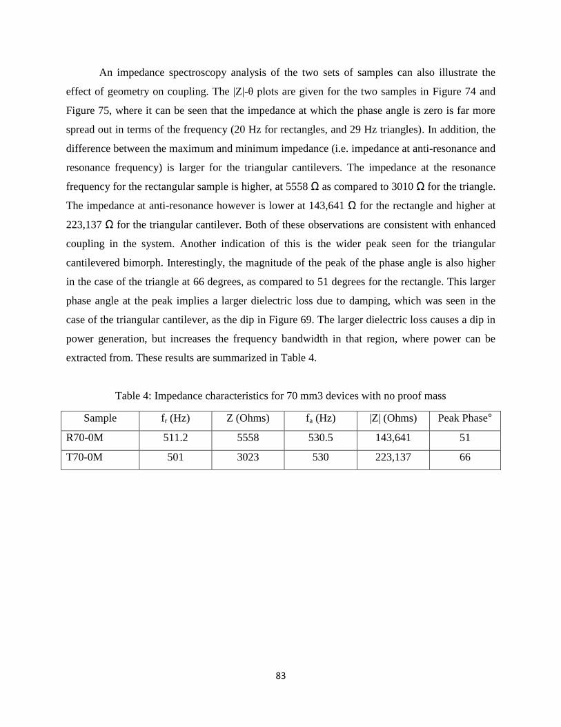
83

An impedance spectroscopy analysis of the two sets of samples can also illustrate the

effect of geometry on coupling. The |Z|-θ plots are given for the two samples in Figure 74 and

Figure 75, where it can be seen that the impedance at which the phase angle is zero is far more

spread out in terms of the frequency (20 Hz for rectangles, and 29 Hz triangles). In addition, the

difference between the maximum and minimum impedance (i.e. impedance at anti-resonance and

resonance frequency) is larger for the triangular cantilevers. The impedance at the resonance

frequency for the rectangular sample is higher, at 5558 Ω as compared to 3010 Ω for the triangle.

The impedance at anti-resonance however is lower at 143,641 Ω for the rectangle and higher at

223,137 Ω for the triangular cantilever. Both of these observations are consistent with enhanced

coupling in the system. Another indication of this is the wider peak seen for the triangular

cantilevered bimorph. Interestingly, the magnitude of the peak of the phase angle is also higher

in the case of the triangle at 66 degrees, as compared to 51 degrees for the rectangle. This larger

phase angle at the peak implies a larger dielectric loss due to damping, which was seen in the

case of the triangular cantilever, as the dip in Figure 69. The larger dielectric loss causes a dip in

power generation, but increases the frequency bandwidth in that region, where power can be

extracted from. These results are summarized in Table 4.

Table 4: Impedance characteristics for 70 mm3 devices with no proof mass

Sample fr (Hz) Z (Ohms) fa (Hz) |Z| (Ohms) Peak Phase°

R70-0M 511.2 5558 530.5 143,641 51

T70-0M 501 3023 530 223,137 66

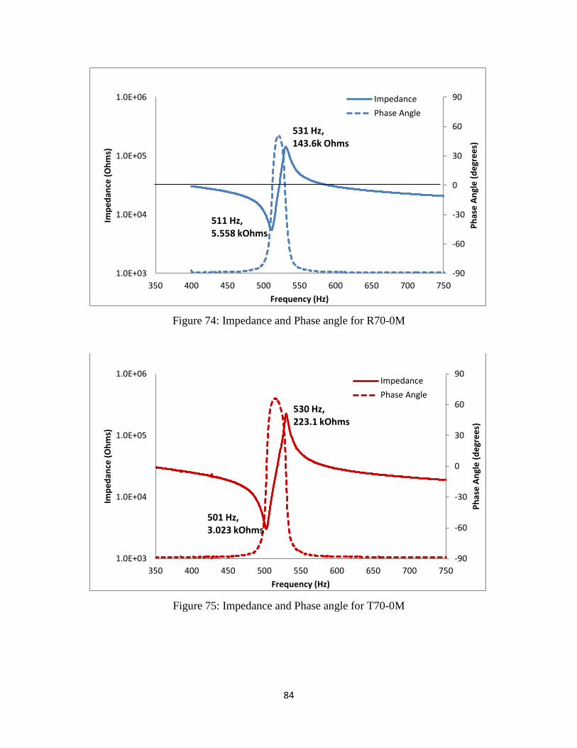
84

Figure 74: Impedance and Phase angle for R70-0M

Figure 75: Impedance and Phase angle for T70-0M

-90

-60

-30

0

30

60

90

1.0E+03

1.0E+04

1.0E+05

1.0E+06

350 400 450 500 550 600 650 700 750

Ph

ase

An

gle

(d

egr

ee

s)

Imp

ed

ance

(O

hm

s)

Frequency (Hz)

Impedance

Phase Angle

511 Hz, 5.558 kOhms

531 Hz, 143.6k Ohms

-90

-60

-30

0

30

60

90

1.0E+03

1.0E+04

1.0E+05

1.0E+06

350 400 450 500 550 600 650 700 750

Ph

ase

An

gle

(d

egr

ee

s)

Imp

ed

ance

(O

hm

s)

Frequency (Hz)

Impedance

Phase Angle

501 Hz, 3.023 kOhms

530 Hz, 223.1 kOhms

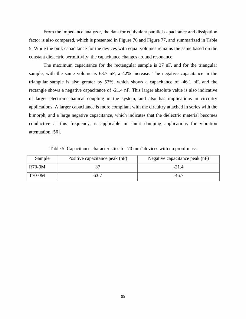
85

From the impedance analyzer, the data for equivalent parallel capacitance and dissipation

factor is also compared, which is presented in Figure 76 and Figure 77, and summarized in Table

5. While the bulk capacitance for the devices with equal volumes remains the same based on the

constant dielectric permittivity; the capacitance changes around resonance.

The maximum capacitance for the rectangular sample is 37 nF, and for the triangular

sample, with the same volume is 63.7 nF, a 42% increase. The negative capacitance in the

triangular sample is also greater by 53%, which shows a capacitance of -46.1 nF, and the

rectangle shows a negative capacitance of -21.4 nF. This larger absolute value is also indicative

of larger electromechanical coupling in the system, and also has implications in circuitry

applications. A larger capacitance is more compliant with the circuitry attached in series with the

bimorph, and a large negative capacitance, which indicates that the dielectric material becomes

conductive at this frequency, is applicable in shunt damping applications for vibration

attenuation [56].

Table 5: Capacitance characteristics for 70 mm3 devices with no proof mass

Sample Positive capacitance peak (nF) Negative capacitance peak (nF)

R70-0M 37 -21.4

T70-0M 63.7 -46.7

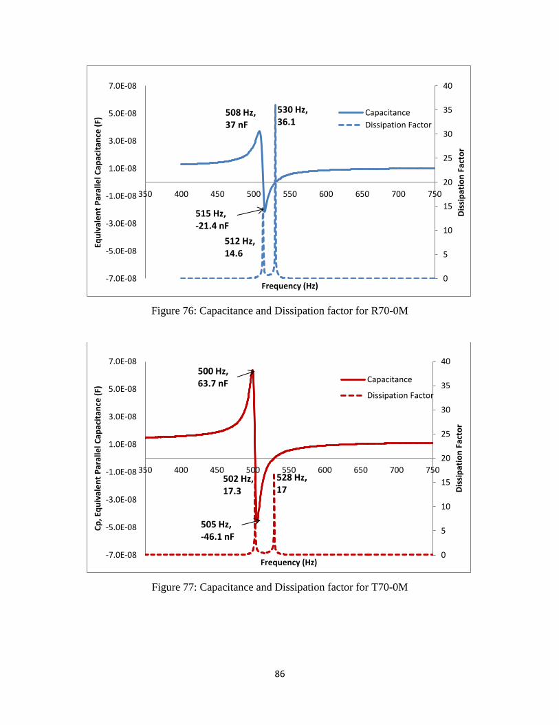
86

Figure 76: Capacitance and Dissipation factor for R70-0M

Figure 77: Capacitance and Dissipation factor for T70-0M

0

5

10

15

20

25

30

35

40

-7.0E-08

-5.0E-08

-3.0E-08

-1.0E-08

1.0E-08

3.0E-08

5.0E-08

7.0E-08

350 400 450 500 550 600 650 700 750

Dis

sip

atio

n F

acto

r

Equ

ival

en

t P

aral

lel C

apac

itan

ce (

F)

Frequency (Hz)

Capacitance

Dissipation Factor

508 Hz, 37 nF

515 Hz, -21.4 nF

512 Hz, 14.6

530 Hz, 36.1

0

5

10

15

20

25

30

35

40

-7.0E-08

-5.0E-08

-3.0E-08

-1.0E-08

1.0E-08

3.0E-08

5.0E-08

7.0E-08

350 400 450 500 550 600 650 700 750D

issi

pat

ion

Fac

tor

Cp

, Eq

uiv

ale

nt

Par

alle

l Cap

acit

ance

(F)

Frequency (Hz)

Capacitance

Dissipation Factor

500 Hz, 63.7 nF

505 Hz, -46.1 nF

502 Hz, 17.3

528 Hz, 17

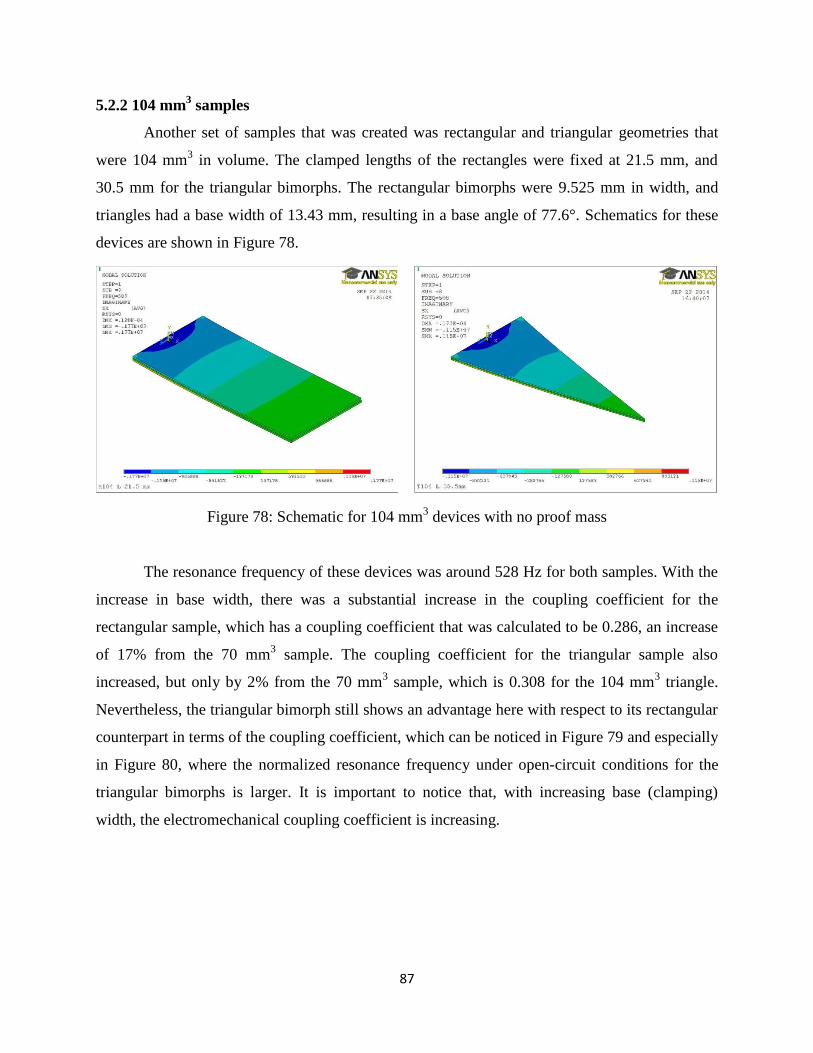
87

5.2.2 104 mm3 samples

Another set of samples that was created was rectangular and triangular geometries that

were 104 mm3 in volume. The clamped lengths of the rectangles were fixed at 21.5 mm, and

30.5 mm for the triangular bimorphs. The rectangular bimorphs were 9.525 mm in width, and

triangles had a base width of 13.43 mm, resulting in a base angle of 77.6°. Schematics for these

devices are shown in Figure 78.

Figure 78: Schematic for 104 mm3 devices with no proof mass

The resonance frequency of these devices was around 528 Hz for both samples. With the

increase in base width, there was a substantial increase in the coupling coefficient for the

rectangular sample, which has a coupling coefficient that was calculated to be 0.286, an increase

of 17% from the 70 mm3 sample. The coupling coefficient for the triangular sample also

increased, but only by 2% from the 70 mm3 sample, which is 0.308 for the 104 mm

3 triangle.

Nevertheless, the triangular bimorph still shows an advantage here with respect to its rectangular

counterpart in terms of the coupling coefficient, which can be noticed in Figure 79 and especially

in Figure 80, where the normalized resonance frequency under open-circuit conditions for the

triangular bimorphs is larger. It is important to notice that, with increasing base (clamping)

width, the electromechanical coupling coefficient is increasing.

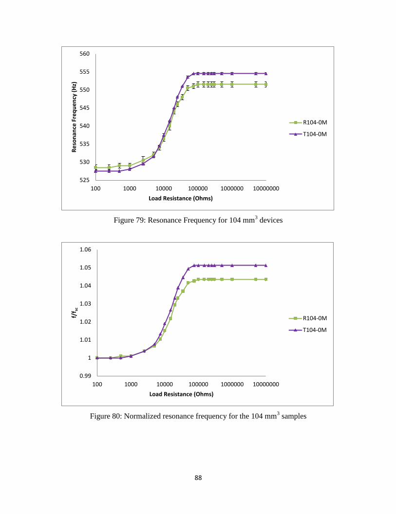
88

Figure 79: Resonance Frequency for 104 mm3 devices

Figure 80: Normalized resonance frequency for the 104 mm3 samples

525

530

535

540

545

550

555

560

100 1000 10000 100000 1000000 10000000

Re

son

ance

Fre

qu

en

cy (

Hz)


R104-0M

T104-0M

0.99

1

1.01

1.02

1.03

1.04

1.05

1.06

100 1000 10000 100000 1000000 10000000

f/f s

c


R104-0M

T104-0M

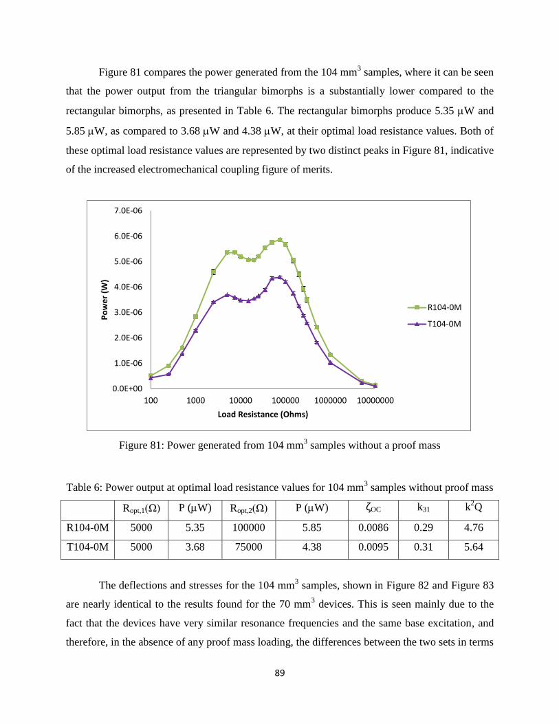
89

Figure 81 compares the power generated from the 104 mm3 samples, where it can be seen

that the power output from the triangular bimorphs is a substantially lower compared to the

rectangular bimorphs, as presented in Table 6. The rectangular bimorphs produce 5.35 W and

5.85 W, as compared to 3.68 W and 4.38 W, at their optimal load resistance values. Both of

these optimal load resistance values are represented by two distinct peaks in Figure 81, indicative

of the increased electromechanical coupling figure of merits.

Figure 81: Power generated from 104 mm3 samples without a proof mass


Ropt,1(Ω) P (W) Ropt,2(Ω) P (W) ζOC k31 k2Q

R104-0M 5000 5.35 100000 5.85 0.0086 0.29 4.76

T104-0M 5000 3.68 75000 4.38 0.0095 0.31 5.64

The deflections and stresses for the 104 mm3 samples, shown in Figure 82 and Figure 83

are nearly identical to the results found for the 70 mm3 devices. This is seen mainly due to the

fact that the devices have very similar resonance frequencies and the same base excitation, and

therefore, in the absence of any proof mass loading, the differences between the two sets in terms

0.0E+00

1.0E-06

2.0E-06

3.0E-06

4.0E-06

5.0E-06

6.0E-06

7.0E-06

100 1000 10000 100000 1000000 10000000

Po

we

r (W

)


R104-0M

T104-0M

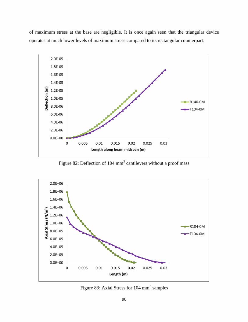
90

of maximum stress at the base are negligible. It is once again seen that the triangular device

operates at much lower levels of maximum stress compared to its rectangular counterpart.

Figure 82: Deflection of 104 mm3 cantilevers without a proof mass

Figure 83: Axial Stress for 104 mm3 samples

0.0E+00

2.0E-06

4.0E-06

6.0E-06

8.0E-06

1.0E-05

1.2E-05

1.4E-05

1.6E-05

1.8E-05

2.0E-05

0 0.005 0.01 0.015 0.02 0.025 0.03

De

fle

ctio

n (

m)


R140-0M

T104-0M

0.0E+00

2.0E+05

4.0E+05

6.0E+05

8.0E+05

1.0E+06

1.2E+06

1.4E+06

1.6E+06

1.8E+06

2.0E+06

0 0.005 0.01 0.015 0.02 0.025 0.03

Axi

al S

tre

ss (

N/m

2)

Length (m)

R104-0M

T104-0M

91

The results from the impedance spectroscopy here reinforce the results based on

electromechanical coupling from resonance frequency measurements and the occurrence of

double peaks at optimal load resistance values for the power generated between the two devices.

It can be clearly seen in Figure 84 and Figure 85 that the difference between the minimum and

maximum impedance for the triangular sample, as summarized in Table 7. It can be seen that the

triangular device has a lower impedance value (1979 Ω) at resonance and higher impedance at

anti-resonance (156,866 Ω) compared to the rectangular bimorph (3279 Ω and 107,373 Ω

respectively). Therefore, with the triangular device, peak power can be generated at lower load

resistance values with high voltages, which can be beneficial for external circuitry to extract

power with lower currents. Moreover, the wider spread between the optimal load resistance

values with the triangular devices would allow a greater number of load resistance values at

which appreciable power can be generated.

Table 7: Impedance measurements for 104 mm3 devices with no proof mass


R104-0M 523 3,297 547.5 107,373 55.15

T104-0M 521.5 1979 550.6 156,866 67.09

The capacitance measurements for the two devices with the same device volume are

presented in Figure 86 and Figure 87. The capacitance peaks for the two devices are appreciably

increased for the triangular device, with a 35% increase in the case of the positive peak, and a

50% increase in the case of the negative capacitance peak. This is again in relation with the

enhanced electromechanical coupling in the triangular device, at very similar resonance

frequencies, providing enhanced capacitance properties, for energy harvesting, or vibration

attenuation.

Table 8: Capacitance measurements for 104 mm3 devices with no proof mass


R104-0M 60.96 -34.70

T104-0M 93.45 -70.59

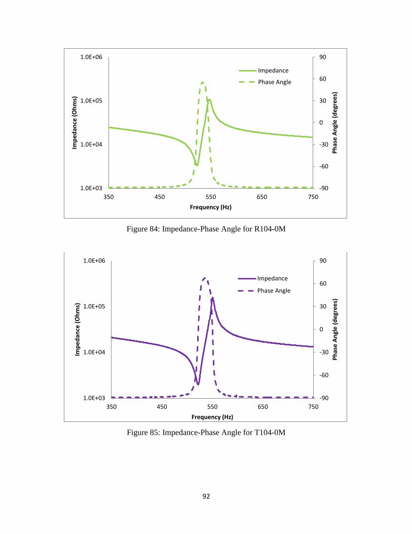
92

Figure 84: Impedance-Phase Angle for R104-0M

Figure 85: Impedance-Phase Angle for T104-0M

-90

-60

-30

0

30

60

90

1.0E+03

1.0E+04

1.0E+05

1.0E+06

350 450 550 650 750

Ph

ase

An

gle

(d

egr

ee

s)

Imp

ed

ance

(O

hm

s)

Frequency (Hz)

Impedance

Phase Angle

-90

-60

-30

0

30

60

90

1.0E+03

1.0E+04

1.0E+05

1.0E+06

350 450 550 650 750

Ph

ase

An

gle

(d

egr

ee

s)

Imp

ed

ance

(O

hm

s)

Frequency (Hz)

Impedance

Phase Angle

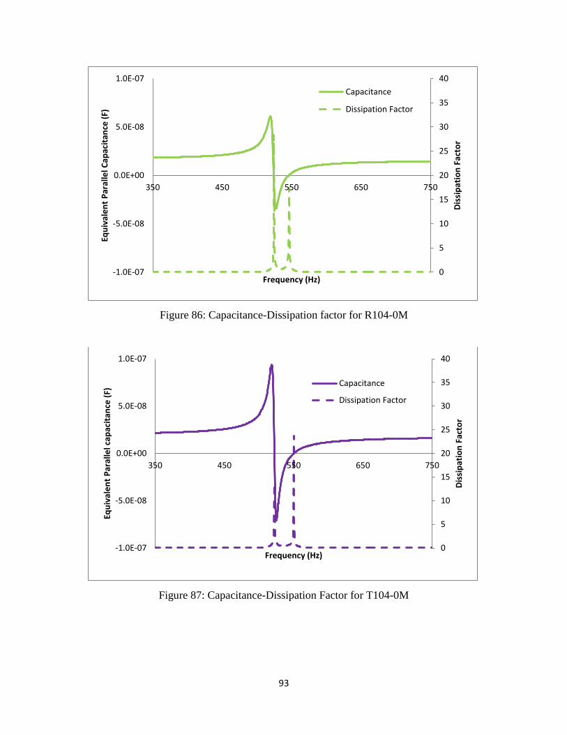
93

Figure 86: Capacitance-Dissipation factor for R104-0M

Figure 87: Capacitance-Dissipation Factor for T104-0M

0

5

10

15

20

25

30

35

40

-1.0E-07

-5.0E-08

0.0E+00

5.0E-08

1.0E-07

350 450 550 650 750

Dis

sip

atio

n F

acto

r

Equ

ival

en

t P

aral

lel C

apac

itan

ce (

F)

Frequency (Hz)

Capacitance

Dissipation Factor

0

5

10

15

20

25

30

35

40

-1.0E-07

-5.0E-08

0.0E+00

5.0E-08

1.0E-07

350 450 550 650 750D

issi

pat

ion

Fac

tor

Equ

ival

en

t P

aral

lel c

apac

itan

ce (

F)

Frequency (Hz)

Capacitance

Dissipation Factor

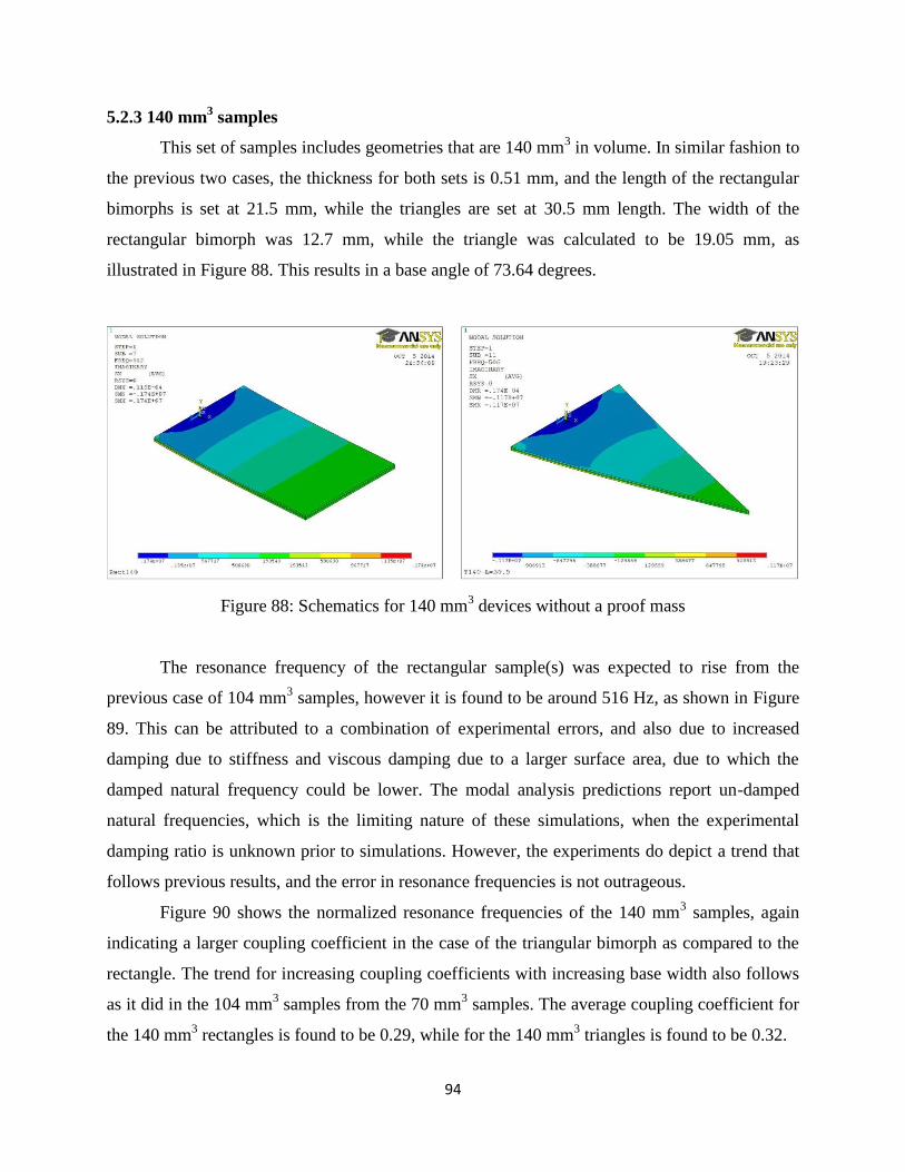
94

5.2.3 140 mm3 samples

This set of samples includes geometries that are 140 mm3 in volume. In similar fashion to

the previous two cases, the thickness for both sets is 0.51 mm, and the length of the rectangular

bimorphs is set at 21.5 mm, while the triangles are set at 30.5 mm length. The width of the

rectangular bimorph was 12.7 mm, while the triangle was calculated to be 19.05 mm, as

illustrated in Figure 88. This results in a base angle of 73.64 degrees.

Figure 88: Schematics for 140 mm3 devices without a proof mass

The resonance frequency of the rectangular sample(s) was expected to rise from the

previous case of 104 mm3 samples, however it is found to be around 516 Hz, as shown in Figure

89. This can be attributed to a combination of experimental errors, and also due to increased

damping due to stiffness and viscous damping due to a larger surface area, due to which the

damped natural frequency could be lower. The modal analysis predictions report un-damped

natural frequencies, which is the limiting nature of these simulations, when the experimental

damping ratio is unknown prior to simulations. However, the experiments do depict a trend that

follows previous results, and the error in resonance frequencies is not outrageous.

Figure 90 shows the normalized resonance frequencies of the 140 mm3 samples, again

indicating a larger coupling coefficient in the case of the triangular bimorph as compared to the

rectangle. The trend for increasing coupling coefficients with increasing base width also follows

as it did in the 104 mm3 samples from the 70 mm

3 samples. The average coupling coefficient for

the 140 mm3 rectangles is found to be 0.29, while for the 140 mm

3 triangles is found to be 0.32.

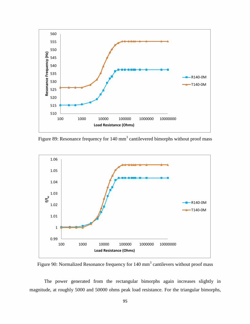
95

Figure 89: Resonance frequency for 140 mm3 cantilevered bimorphs without proof mass

Figure 90: Normalized Resonance frequency for 140 mm3 cantilevers without proof mass

The power generated from the rectangular bimorphs again increases slightly in

magnitude, at roughly 5000 and 50000 ohms peak load resistance. For the triangular bimorphs,

510

515

520

525

530

535

540

545

550

555

560

100 1000 10000 100000 1000000 10000000

Re

son

ance

Fre

qu

en

cy (

Hz)


R140-0M

T140-0M

0.99

1

1.01

1.02

1.03

1.04

1.05

1.06

100 1000 10000 100000 1000000 10000000

f/f s

c


R140-0M

T140-0M

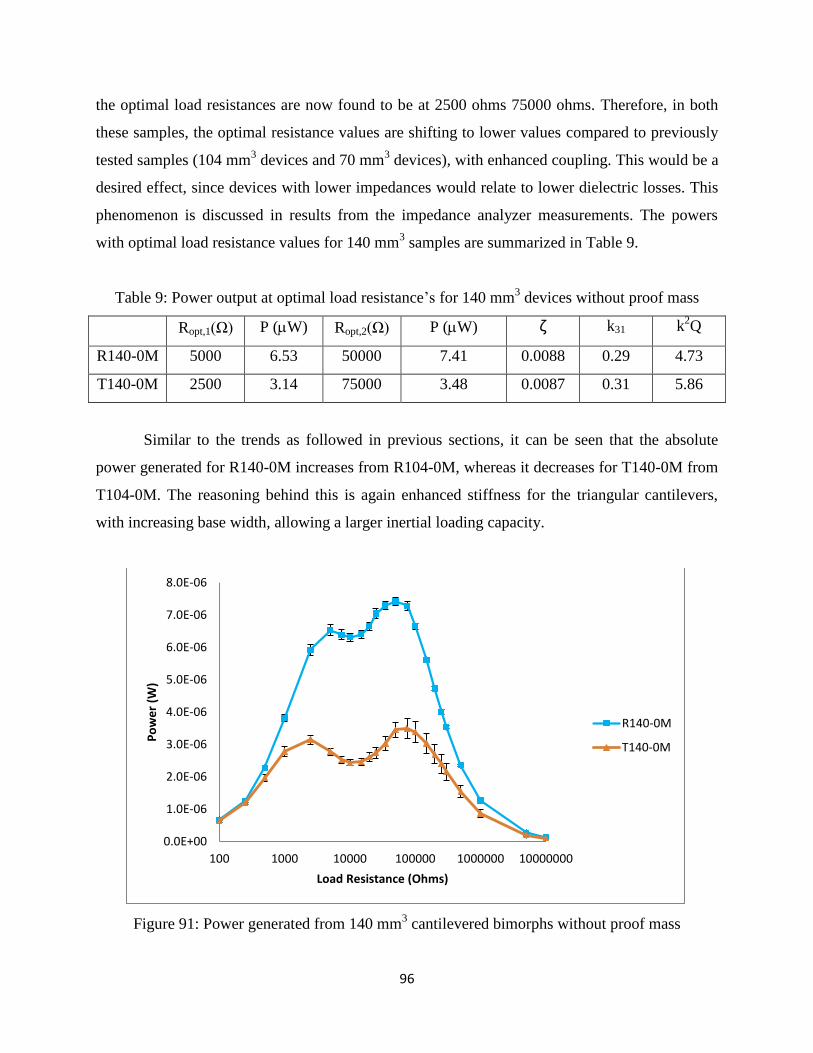
96

the optimal load resistances are now found to be at 2500 ohms 75000 ohms. Therefore, in both

these samples, the optimal resistance values are shifting to lower values compared to previously

tested samples (104 mm3 devices and 70 mm

3 devices), with enhanced coupling. This would be a

desired effect, since devices with lower impedances would relate to lower dielectric losses. This

phenomenon is discussed in results from the impedance analyzer measurements. The powers

with optimal load resistance values for 140 mm3 samples are summarized in Table 9.

Table 9: Power output at optimal load resistance’s for 140 mm3 devices without proof mass

Ropt,1(Ω) P (W) Ropt,2(Ω) P (W) ζ k31 k2Q

R140-0M 5000 6.53 50000 7.41 0.0088 0.29 4.73

T140-0M 2500 3.14 75000 3.48 0.0087 0.31 5.86

Similar to the trends as followed in previous sections, it can be seen that the absolute

power generated for R140-0M increases from R104-0M, whereas it decreases for T140-0M from

T104-0M. The reasoning behind this is again enhanced stiffness for the triangular cantilevers,

with increasing base width, allowing a larger inertial loading capacity.

Figure 91: Power generated from 140 mm3 cantilevered bimorphs without proof mass

0.0E+00

1.0E-06

2.0E-06

3.0E-06

4.0E-06

5.0E-06

6.0E-06

7.0E-06

8.0E-06

100 1000 10000 100000 1000000 10000000

Po

we

r (W

)


R140-0M

T140-0M

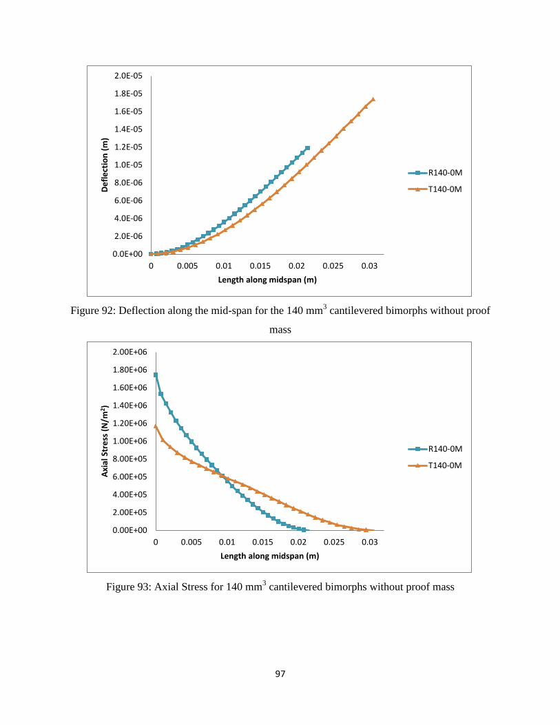
97

Figure 92: Deflection along the mid-span for the 140 mm3 cantilevered bimorphs without proof

mass

Figure 93: Axial Stress for 140 mm3 cantilevered bimorphs without proof mass

0.0E+00

2.0E-06

4.0E-06

6.0E-06

8.0E-06

1.0E-05

1.2E-05

1.4E-05

1.6E-05

1.8E-05

2.0E-05

0 0.005 0.01 0.015 0.02 0.025 0.03

De

fle

ctio

n (

m)

Length along midspan (m)

R140-0M

T140-0M

0.00E+00

2.00E+05

4.00E+05

6.00E+05

8.00E+05

1.00E+06

1.20E+06

1.40E+06

1.60E+06

1.80E+06

2.00E+06

0 0.005 0.01 0.015 0.02 0.025 0.03

Axi

al S

tre

ss (

N/m

2 )

Length along midspan (m)

R140-0M

T140-0M

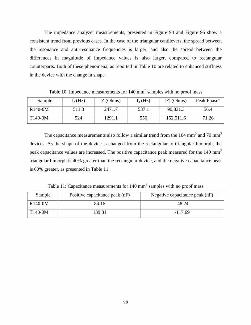
98

The impedance analyzer measurements, presented in Figure 94 and Figure 95 show a

consistent trend from previous cases. In the case of the triangular cantilevers, the spread between

the resonance and anti-resonance frequencies is larger, and also the spread between the

differences in magnitude of impedance values is also larger, compared to rectangular

counterparts. Both of these phenomena, as reported in Table 10 are related to enhanced stiffness

in the device with the change in shape.

Table 10: Impedance measurements for 140 mm3 samples with no proof mass


R140-0M 511.3 2471.7 537.1 90,831.3 56.4

T140-0M 524 1291.1 556 152,511.6 71.26

The capacitance measurements also follow a similar trend from the 104 mm3 and 70 mm

3

devices. As the shape of the device is changed from the rectangular to triangular bimorph, the

peak capacitance values are increased. The positive capacitance peak measured for the 140 mm3

triangular bimorph is 40% greater than the rectangular device, and the negative capacitance peak

is 60% greater, as presented in Table 11.

Table 11: Capacitance measurements for 140 mm3 samples with no proof mass


R140-0M 84.16 -48.24

T140-0M 139.81 -117.69

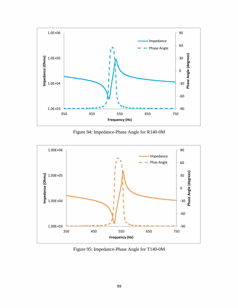
99



-90

-60

-30

0

30

60

90

1.0E+03

1.0E+04

1.0E+05

1.0E+06

350 450 550 650 750

Ph

ase

An

gle

(d

egr

ee

s)

Imp

ed

ance

(O

hm

s)

Frequency (Hz)

Impedance

Phase Angle

-90

-60

-30

0

30

60

90

1.00E+03

1.00E+04

1.00E+05

1.00E+06

350 450 550 650 750

Ph

ase

An

gle

(d

egr

ee

s)

Imp

ed

ance

(O

hm

s)

Frequency (Hz)

Impedance

Phas Angle

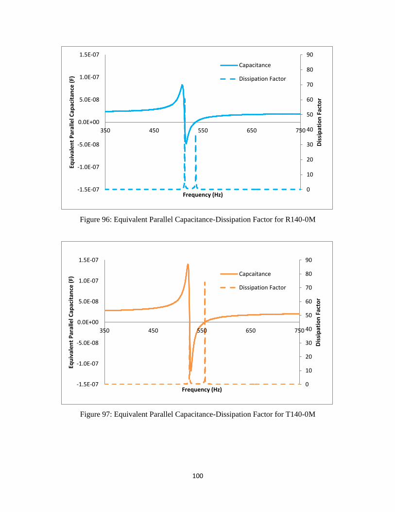
100

Figure 96: Equivalent Parallel Capacitance-Dissipation Factor for R140-0M

Figure 97: Equivalent Parallel Capacitance-Dissipation Factor for T140-0M

0

10

20

30

40

50

60

70

80

90

-1.5E-07

-1.0E-07

-5.0E-08

0.0E+00

5.0E-08

1.0E-07

1.5E-07

350 450 550 650 750

Dis

sip

atio

n F

acto

r

Equ

ival

en

t P

aral

lel C

apac

itan

ce (

F)

Frequency (Hz)

Capacitance

Dissipation Factor

0

10

20

30

40

50

60

70

80

90

-1.5E-07

-1.0E-07

-5.0E-08

0.0E+00

5.0E-08

1.0E-07

1.5E-07

350 450 550 650 750

Dis

sip

atio

n F

acto

r

Equ

ival

en

t P

aral

lel C

apac

itan

ce (

F)

Frequency (Hz)

Capcaitance

Dissipation Factor

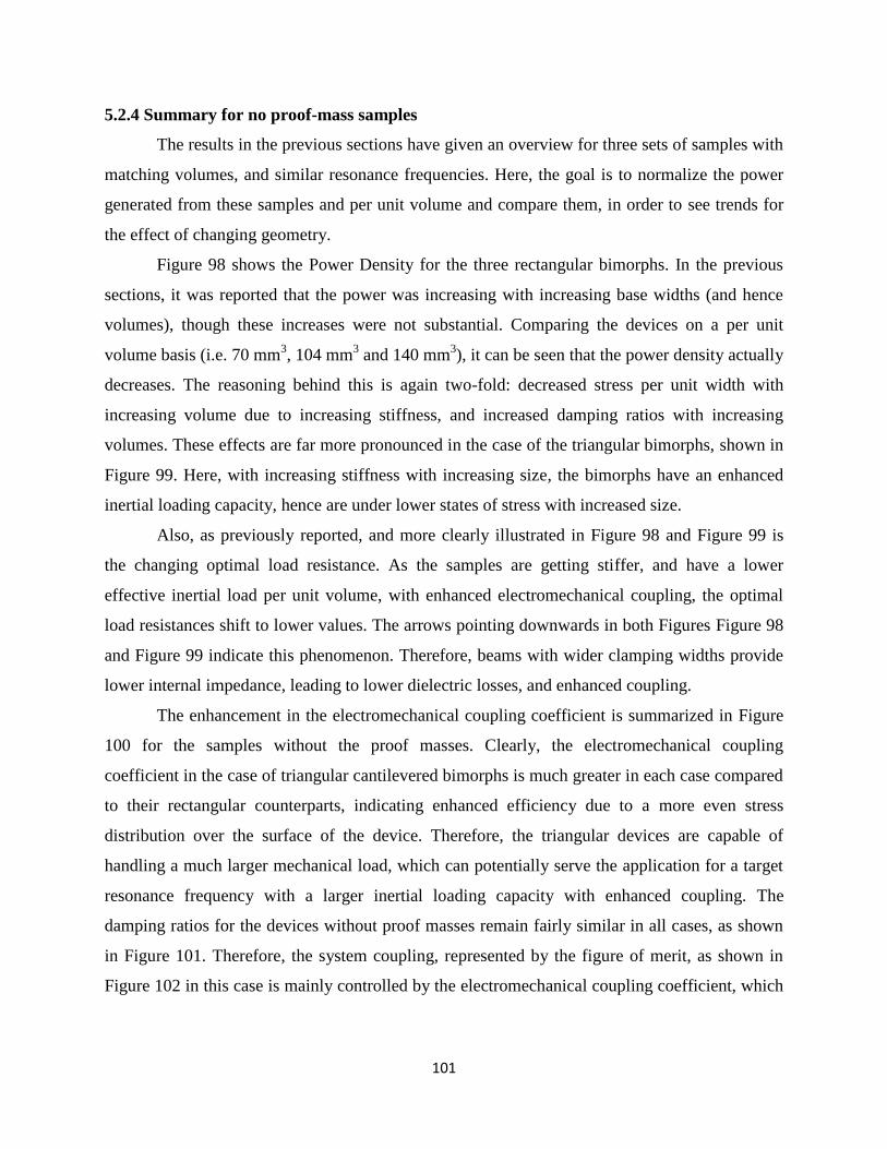
101

5.2.4 Summary for no proof-mass samples

The results in the previous sections have given an overview for three sets of samples with

matching volumes, and similar resonance frequencies. Here, the goal is to normalize the power

generated from these samples and per unit volume and compare them, in order to see trends for

the effect of changing geometry.

Figure 98 shows the Power Density for the three rectangular bimorphs. In the previous

sections, it was reported that the power was increasing with increasing base widths (and hence

volumes), though these increases were not substantial. Comparing the devices on a per unit

volume basis (i.e. 70 mm3, 104 mm

3 and 140 mm

3), it can be seen that the power density actually

decreases. The reasoning behind this is again two-fold: decreased stress per unit width with

increasing volume due to increasing stiffness, and increased damping ratios with increasing

volumes. These effects are far more pronounced in the case of the triangular bimorphs, shown in

Figure 99. Here, with increasing stiffness with increasing size, the bimorphs have an enhanced

inertial loading capacity, hence are under lower states of stress with increased size.

Also, as previously reported, and more clearly illustrated in Figure 98 and Figure 99 is

the changing optimal load resistance. As the samples are getting stiffer, and have a lower

effective inertial load per unit volume, with enhanced electromechanical coupling, the optimal

load resistances shift to lower values. The arrows pointing downwards in both Figures Figure 98

and Figure 99 indicate this phenomenon. Therefore, beams with wider clamping widths provide

lower internal impedance, leading to lower dielectric losses, and enhanced coupling.

The enhancement in the electromechanical coupling coefficient is summarized in Figure

100 for the samples without the proof masses. Clearly, the electromechanical coupling

coefficient in the case of triangular cantilevered bimorphs is much greater in each case compared

to their rectangular counterparts, indicating enhanced efficiency due to a more even stress

distribution over the surface of the device. Therefore, the triangular devices are capable of

handling a much larger mechanical load, which can potentially serve the application for a target

resonance frequency with a larger inertial loading capacity with enhanced coupling. The

damping ratios for the devices without proof masses remain fairly similar in all cases, as shown

in Figure 101. Therefore, the system coupling, represented by the figure of merit, as shown in

Figure 102 in this case is mainly controlled by the electromechanical coupling coefficient, which

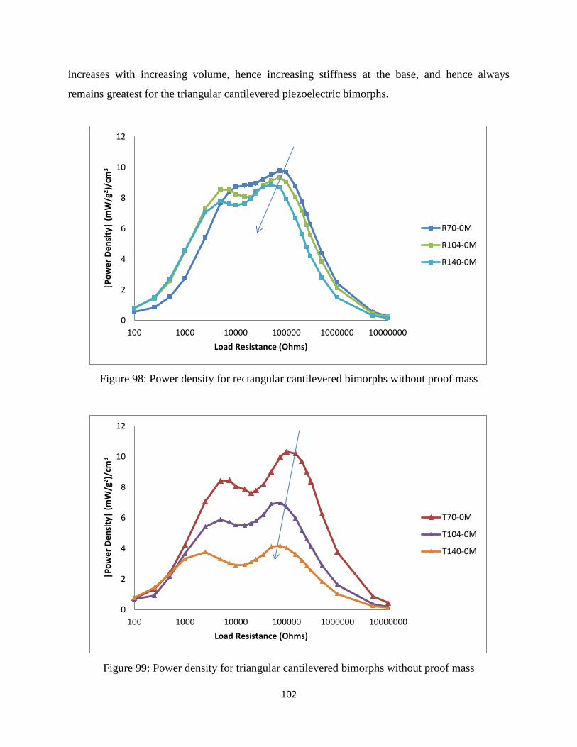
102

increases with increasing volume, hence increasing stiffness at the base, and hence always

remains greatest for the triangular cantilevered piezoelectric bimorphs.

Figure 98: Power density for rectangular cantilevered bimorphs without proof mass

Figure 99: Power density for triangular cantilevered bimorphs without proof mass

0

2

4

6

8

10

12

100 1000 10000 100000 1000000 10000000

|Po

we

r D

en

sity

| (m

W/g

2 )/c

m3


R70-0M

R104-0M

R140-0M

0

2

4

6

8

10

12

100 1000 10000 100000 1000000 10000000

|Po

we

r D

en

sity

| (m

W/g

2 )/c

m3


T70-0M

T104-0M

T140-0M

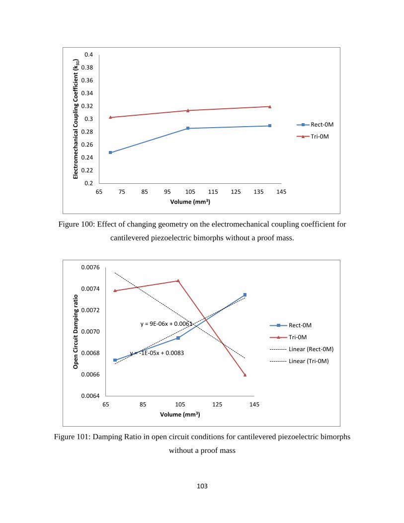
103

Figure 100: Effect of changing geometry on the electromechanical coupling coefficient for

cantilevered piezoelectric bimorphs without a proof mass.

Figure 101: Damping Ratio in open circuit conditions for cantilevered piezoelectric bimorphs

without a proof mass

0.2

0.22

0.24

0.26

0.28

0.3

0.32

0.34

0.36

0.38

0.4

65 75 85 95 105 115 125 135 145

Ele

ctro

me

chan

ical

Co

up

ling

Co

eff

icie

nt

(k3

1)

Volume (mm3)

Rect-0M

Tri-0M

y = 9E-06x + 0.0061

y = -1E-05x + 0.0083

0.0064

0.0066

0.0068

0.0070

0.0072

0.0074

0.0076

65 85 105 125 145

Op

en

Cir

cuit

Dam

pin

g ra

tio

Volume (mm3)

Rect-0M

Tri-0M

Linear (Rect-0M)

Linear (Tri-0M)

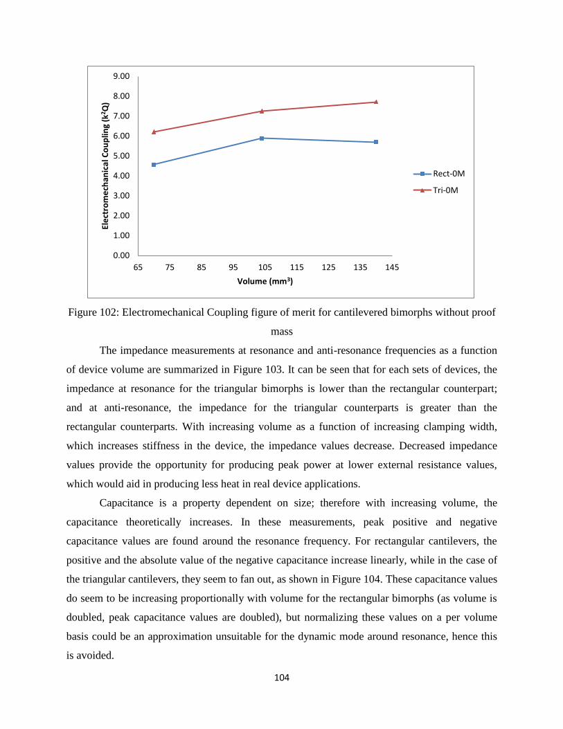
104

Figure 102: Electromechanical Coupling figure of merit for cantilevered bimorphs without proof

mass

The impedance measurements at resonance and anti-resonance frequencies as a function

of device volume are summarized in Figure 103. It can be seen that for each sets of devices, the

impedance at resonance for the triangular bimorphs is lower than the rectangular counterpart;

and at anti-resonance, the impedance for the triangular counterparts is greater than the

rectangular counterparts. With increasing volume as a function of increasing clamping width,

which increases stiffness in the device, the impedance values decrease. Decreased impedance

values provide the opportunity for producing peak power at lower external resistance values,

which would aid in producing less heat in real device applications.

Capacitance is a property dependent on size; therefore with increasing volume, the

capacitance theoretically increases. In these measurements, peak positive and negative

capacitance values are found around the resonance frequency. For rectangular cantilevers, the

positive and the absolute value of the negative capacitance increase linearly, while in the case of

the triangular cantilevers, they seem to fan out, as shown in Figure 104. These capacitance values

do seem to be increasing proportionally with volume for the rectangular bimorphs (as volume is

doubled, peak capacitance values are doubled), but normalizing these values on a per volume

basis could be an approximation unsuitable for the dynamic mode around resonance, hence this

is avoided.

0.00

1.00

2.00

3.00

4.00

5.00

6.00

7.00

8.00

9.00

65 75 85 95 105 115 125 135 145

Ele

ctro

me

chan

ical

Co

up

ling

(k2 Q

)

Volume (mm3)

Rect-0M

Tri-0M

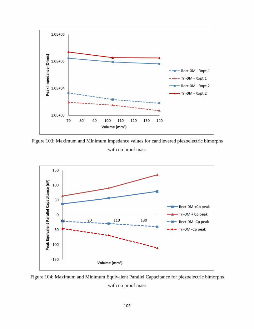
105

Figure 103: Maximum and Minimum Impedance values for cantilevered piezoelectric bimorphs

with no proof mass

Figure 104: Maximum and Minimum Equivalent Parallel Capacitance for piezoelectric bimorphs

with no proof mass

1.0E+03

1.0E+04

1.0E+05

1.0E+06

70 80 90 100 110 120 130 140

Pe

ak Im

pe

dan

ce (

Oh

ms)

Volume (mm3)

Rect-0M - Ropt,1

Tri-0M - Ropt,1

Rect-0M - Ropt,2

Tri-0M - Ropt,2

-150

-100

-50

0

50

100

150

70 90 110 130

Pe

ak E

qu

ival

en

t P

aral

lel C

apac

itan

ce (

nF)

Volume (mm3)

Rect-0M +Cp peak

Tri-0M + Cp peak

Rect-0M -Cp peak

Tri-0M -Cp peak

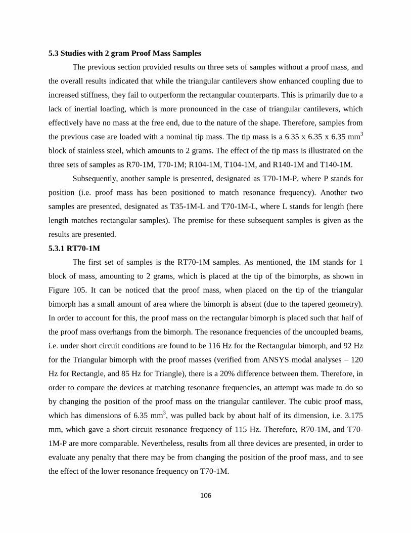
106

5.3 Studies with 2 gram Proof Mass Samples

The previous section provided results on three sets of samples without a proof mass, and

the overall results indicated that while the triangular cantilevers show enhanced coupling due to

increased stiffness, they fail to outperform the rectangular counterparts. This is primarily due to a

lack of inertial loading, which is more pronounced in the case of triangular cantilevers, which

effectively have no mass at the free end, due to the nature of the shape. Therefore, samples from

the previous case are loaded with a nominal tip mass. The tip mass is a 6.35 x 6.35 x 6.35 mm3

block of stainless steel, which amounts to 2 grams. The effect of the tip mass is illustrated on the

three sets of samples as R70-1M, T70-1M; R104-1M, T104-1M, and R140-1M and T140-1M.

Subsequently, another sample is presented, designated as T70-1M-P, where P stands for

position (i.e. proof mass has been positioned to match resonance frequency). Another two

samples are presented, designated as T35-1M-L and T70-1M-L, where L stands for length (here

length matches rectangular samples). The premise for these subsequent samples is given as the

results are presented.

5.3.1 RT70-1M

The first set of samples is the RT70-1M samples. As mentioned, the 1M stands for 1

block of mass, amounting to 2 grams, which is placed at the tip of the bimorphs, as shown in

Figure 105. It can be noticed that the proof mass, when placed on the tip of the triangular

bimorph has a small amount of area where the bimorph is absent (due to the tapered geometry).

In order to account for this, the proof mass on the rectangular bimorph is placed such that half of

the proof mass overhangs from the bimorph. The resonance frequencies of the uncoupled beams,

i.e. under short circuit conditions are found to be 116 Hz for the Rectangular bimorph, and 92 Hz

for the Triangular bimorph with the proof masses (verified from ANSYS modal analyses – 120

Hz for Rectangle, and 85 Hz for Triangle), there is a 20% difference between them. Therefore, in

order to compare the devices at matching resonance frequencies, an attempt was made to do so

by changing the position of the proof mass on the triangular cantilever. The cubic proof mass,

which has dimensions of 6.35 mm3, was pulled back by about half of its dimension, i.e. 3.175

mm, which gave a short-circuit resonance frequency of 115 Hz. Therefore, R70-1M, and T70-

1M-P are more comparable. Nevertheless, results from all three devices are presented, in order to

evaluate any penalty that there may be from changing the position of the proof mass, and to see

the effect of the lower resonance frequency on T70-1M.

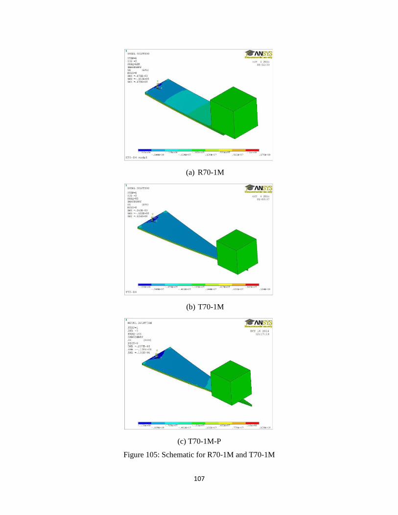
107

(a) R70-1M

(b) T70-1M

(c) T70-1M-P

Figure 105: Schematic for R70-1M and T70-1M

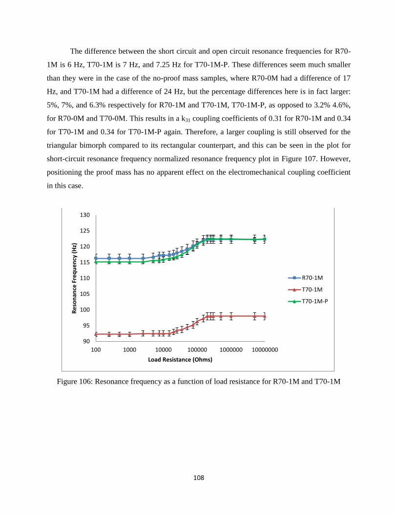
108

The difference between the short circuit and open circuit resonance frequencies for R70-

1M is 6 Hz, T70-1M is 7 Hz, and 7.25 Hz for T70-1M-P. These differences seem much smaller

than they were in the case of the no-proof mass samples, where R70-0M had a difference of 17

Hz, and T70-1M had a difference of 24 Hz, but the percentage differences here is in fact larger:

5%, 7%, and 6.3% respectively for R70-1M and T70-1M, T70-1M-P, as opposed to 3.2% 4.6%,

for R70-0M and T70-0M. This results in a k31 coupling coefficients of 0.31 for R70-1M and 0.34

for T70-1M and 0.34 for T70-1M-P again. Therefore, a larger coupling is still observed for the

triangular bimorph compared to its rectangular counterpart, and this can be seen in the plot for

short-circuit resonance frequency normalized resonance frequency plot in Figure 107. However,

positioning the proof mass has no apparent effect on the electromechanical coupling coefficient

in this case.

Figure 106: Resonance frequency as a function of load resistance for R70-1M and T70-1M

90

95

100

105

110

115

120

125

130

100 1000 10000 100000 1000000 10000000

Re

son

ance

Fre

qu

en

cy (

Hz)


R70-1M

T70-1M

T70-1M-P

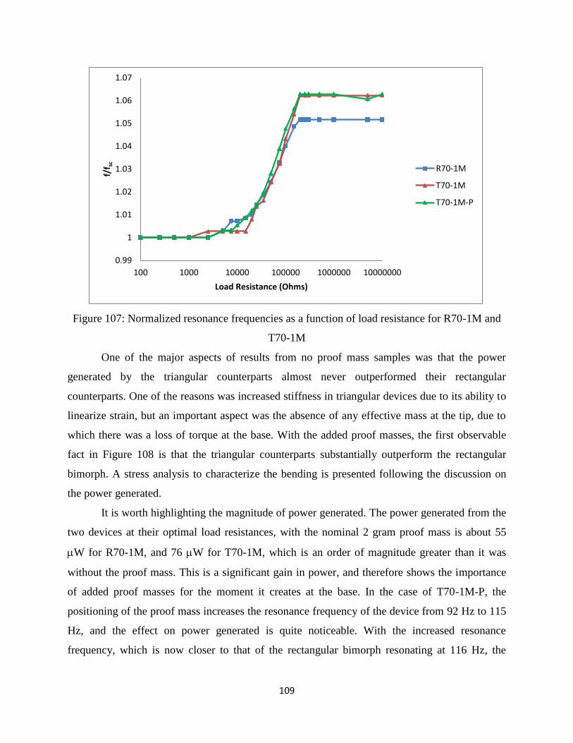
109

Figure 107: Normalized resonance frequencies as a function of load resistance for R70-1M and

T70-1M

One of the major aspects of results from no proof mass samples was that the power

generated by the triangular counterparts almost never outperformed their rectangular

counterparts. One of the reasons was increased stiffness in triangular devices due to its ability to

linearize strain, but an important aspect was the absence of any effective mass at the tip, due to

which there was a loss of torque at the base. With the added proof masses, the first observable

fact in Figure 108 is that the triangular counterparts substantially outperform the rectangular

bimorph. A stress analysis to characterize the bending is presented following the discussion on

the power generated.

It is worth highlighting the magnitude of power generated. The power generated from the

two devices at their optimal load resistances, with the nominal 2 gram proof mass is about 55

W for R70-1M, and 76 W for T70-1M, which is an order of magnitude greater than it was

without the proof mass. This is a significant gain in power, and therefore shows the importance

of added proof masses for the moment it creates at the base. In the case of T70-1M-P, the

positioning of the proof mass increases the resonance frequency of the device from 92 Hz to 115

Hz, and the effect on power generated is quite noticeable. With the increased resonance

frequency, which is now closer to that of the rectangular bimorph resonating at 116 Hz, the

0.99

1

1.01

1.02

1.03

1.04

1.05

1.06

1.07

100 1000 10000 100000 1000000 10000000

f/f s

c


R70-1M

T70-1M

T70-1M-P

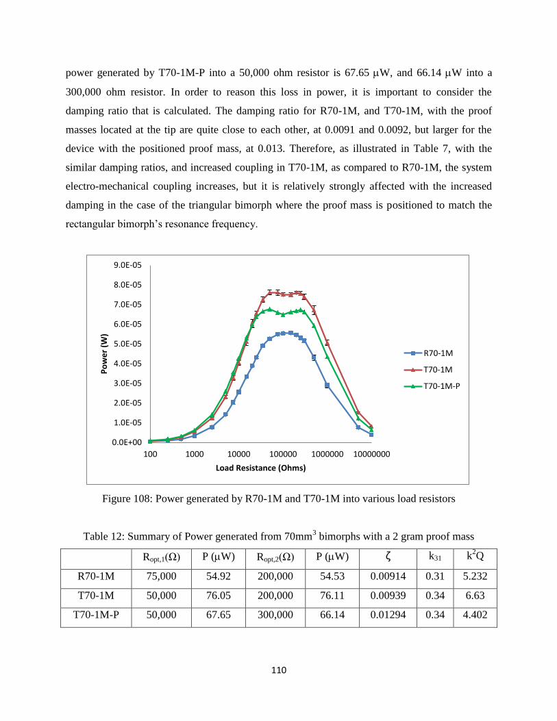
110

power generated by T70-1M-P into a 50,000 ohm resistor is 67.65 W, and 66.14 W into a

300,000 ohm resistor. In order to reason this loss in power, it is important to consider the

damping ratio that is calculated. The damping ratio for R70-1M, and T70-1M, with the proof

masses located at the tip are quite close to each other, at 0.0091 and 0.0092, but larger for the

device with the positioned proof mass, at 0.013. Therefore, as illustrated in Table 7, with the

similar damping ratios, and increased coupling in T70-1M, as compared to R70-1M, the system

electro-mechanical coupling increases, but it is relatively strongly affected with the increased

damping in the case of the triangular bimorph where the proof mass is positioned to match the

rectangular bimorph’s resonance frequency.

Figure 108: Power generated by R70-1M and T70-1M into various load resistors

Table 12: Summary of Power generated from 70mm3 bimorphs with a 2 gram proof mass


R70-1M 75,000 54.92 200,000 54.53 0.00914 0.31 5.232

T70-1M 50,000 76.05 200,000 76.11 0.00939 0.34 6.63

T70-1M-P 50,000 67.65 300,000 66.14 0.01294 0.34 4.402

0.0E+00

1.0E-05

2.0E-05

3.0E-05

4.0E-05

5.0E-05

6.0E-05

7.0E-05

8.0E-05

9.0E-05

100 1000 10000 100000 1000000 10000000

Po

we

r (W

)


R70-1M

T70-1M

T70-1M-P

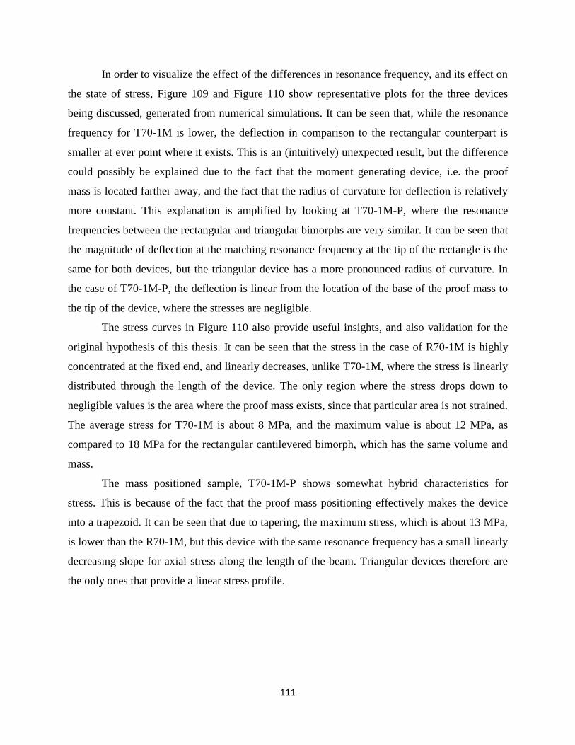
111

In order to visualize the effect of the differences in resonance frequency, and its effect on

the state of stress, Figure 109 and Figure 110 show representative plots for the three devices

being discussed, generated from numerical simulations. It can be seen that, while the resonance

frequency for T70-1M is lower, the deflection in comparison to the rectangular counterpart is

smaller at ever point where it exists. This is an (intuitively) unexpected result, but the difference

could possibly be explained due to the fact that the moment generating device, i.e. the proof

mass is located farther away, and the fact that the radius of curvature for deflection is relatively

more constant. This explanation is amplified by looking at T70-1M-P, where the resonance

frequencies between the rectangular and triangular bimorphs are very similar. It can be seen that

the magnitude of deflection at the matching resonance frequency at the tip of the rectangle is the

same for both devices, but the triangular device has a more pronounced radius of curvature. In

the case of T70-1M-P, the deflection is linear from the location of the base of the proof mass to

the tip of the device, where the stresses are negligible.

The stress curves in Figure 110 also provide useful insights, and also validation for the

original hypothesis of this thesis. It can be seen that the stress in the case of R70-1M is highly

concentrated at the fixed end, and linearly decreases, unlike T70-1M, where the stress is linearly

distributed through the length of the device. The only region where the stress drops down to

negligible values is the area where the proof mass exists, since that particular area is not strained.

The average stress for T70-1M is about 8 MPa, and the maximum value is about 12 MPa, as

compared to 18 MPa for the rectangular cantilevered bimorph, which has the same volume and

mass.

The mass positioned sample, T70-1M-P shows somewhat hybrid characteristics for

stress. This is because of the fact that the proof mass positioning effectively makes the device

into a trapezoid. It can be seen that due to tapering, the maximum stress, which is about 13 MPa,

is lower than the R70-1M, but this device with the same resonance frequency has a small linearly

decreasing slope for axial stress along the length of the beam. Triangular devices therefore are

the only ones that provide a linear stress profile.

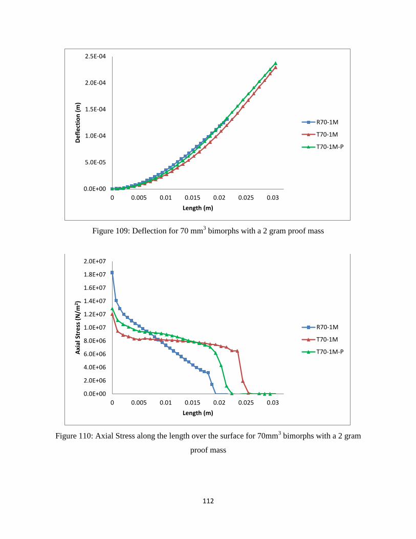
112

Figure 109: Deflection for 70 mm3 bimorphs with a 2 gram proof mass

Figure 110: Axial Stress along the length over the surface for 70mm3 bimorphs with a 2 gram

proof mass

0.0E+00

5.0E-05

1.0E-04

1.5E-04

2.0E-04

2.5E-04

0 0.005 0.01 0.015 0.02 0.025 0.03

De

fle

ctio

n (

m)

Length (m)

R70-1M

T70-1M

T70-1M-P

0.0E+00

2.0E+06

4.0E+06

6.0E+06

8.0E+06

1.0E+07

1.2E+07

1.4E+07

1.6E+07

1.8E+07

2.0E+07

0 0.005 0.01 0.015 0.02 0.025 0.03

Axi

al S

tre

ss (

N/m

2 )

Length (m)

R70-1M

T70-1M

T70-1M-P

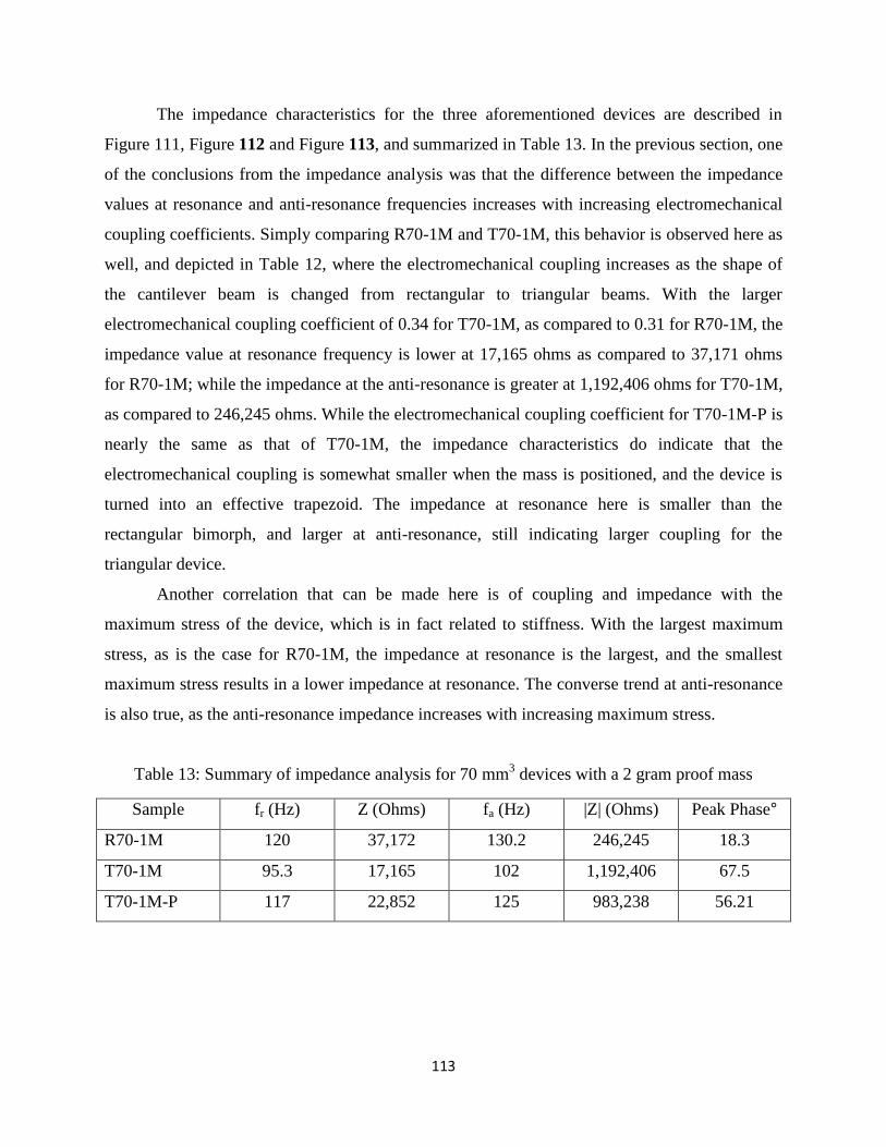
113

The impedance characteristics for the three aforementioned devices are described in

Figure 111, Figure 112 and Figure 113, and summarized in Table 13. In the previous section, one

of the conclusions from the impedance analysis was that the difference between the impedance

values at resonance and anti-resonance frequencies increases with increasing electromechanical

coupling coefficients. Simply comparing R70-1M and T70-1M, this behavior is observed here as

well, and depicted in Table 12, where the electromechanical coupling increases as the shape of

the cantilever beam is changed from rectangular to triangular beams. With the larger

electromechanical coupling coefficient of 0.34 for T70-1M, as compared to 0.31 for R70-1M, the

impedance value at resonance frequency is lower at 17,165 ohms as compared to 37,171 ohms

for R70-1M; while the impedance at the anti-resonance is greater at 1,192,406 ohms for T70-1M,

as compared to 246,245 ohms. While the electromechanical coupling coefficient for T70-1M-P is

nearly the same as that of T70-1M, the impedance characteristics do indicate that the

electromechanical coupling is somewhat smaller when the mass is positioned, and the device is

turned into an effective trapezoid. The impedance at resonance here is smaller than the

rectangular bimorph, and larger at anti-resonance, still indicating larger coupling for the

triangular device.

Another correlation that can be made here is of coupling and impedance with the

maximum stress of the device, which is in fact related to stiffness. With the largest maximum

stress, as is the case for R70-1M, the impedance at resonance is the largest, and the smallest

maximum stress results in a lower impedance at resonance. The converse trend at anti-resonance

is also true, as the anti-resonance impedance increases with increasing maximum stress.

Table 13: Summary of impedance analysis for 70 mm3 devices with a 2 gram proof mass


R70-1M 120 37,172 130.2 246,245 18.3

T70-1M 95.3 17,165 102 1,192,406 67.5

T70-1M-P 117 22,852 125 983,238 56.21

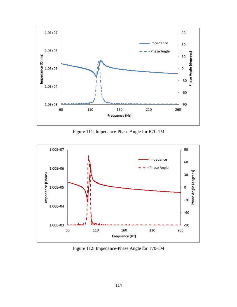
114



-90

-60

-30

0

30

60

90

1.0E+03

1.0E+04

1.0E+05

1.0E+06

1.0E+07

60 110 160 210 260

Ph

ase

An

gle

(d

egr

ee

s)

Imp

ed

ance

(O

hm

s)

Frequency (Hz)

Impedance

Phase Angle

-90

-60

-30

0

30

60

90

1.00E+03

1.00E+04

1.00E+05

1.00E+06

1.00E+07

60 110 160 210 260

Ph

ase

An

gle

(d

egr

ee

s)

Imp

ed

ance

(O

hm

s)

Frequency (Hz)

Impedance

Phase Angle

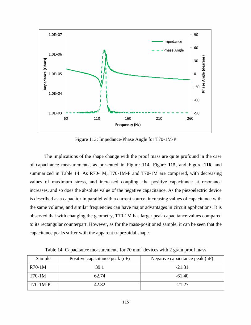
115

Figure 113: Impedance-Phase Angle for T70-1M-P

The implications of the shape change with the proof mass are quite profound in the case

of capacitance measurements, as presented in Figure 114, Figure 115, and Figure 116, and

summarized in Table 14. As R70-1M, T70-1M-P and T70-1M are compared, with decreasing

values of maximum stress, and increased coupling, the positive capacitance at resonance

increases, and so does the absolute value of the negative capacitance. As the piezoelectric device

is described as a capacitor in parallel with a current source, increasing values of capacitance with

the same volume, and similar frequencies can have major advantages in circuit applications. It is

observed that with changing the geometry, T70-1M has larger peak capacitance values compared

to its rectangular counterpart. However, as for the mass-positioned sample, it can be seen that the

capacitance peaks suffer with the apparent trapezoidal shape.

Table 14: Capacitance measurements for 70 mm3 devices with 2 gram proof mass


R70-1M 39.1 -21.31

T70-1M 62.74 -61.40

T70-1M-P 42.82 -21.27

-90

-60

-30

0

30

60

90

1.0E+03

1.0E+04

1.0E+05

1.0E+06

1.0E+07

60 110 160 210 260

Ph

ase

An

gle

(d

egr

ee

s)

Imp

ed

ance

(O

hm

s)

Frequency (Hz)

Impedance

Phase Angle

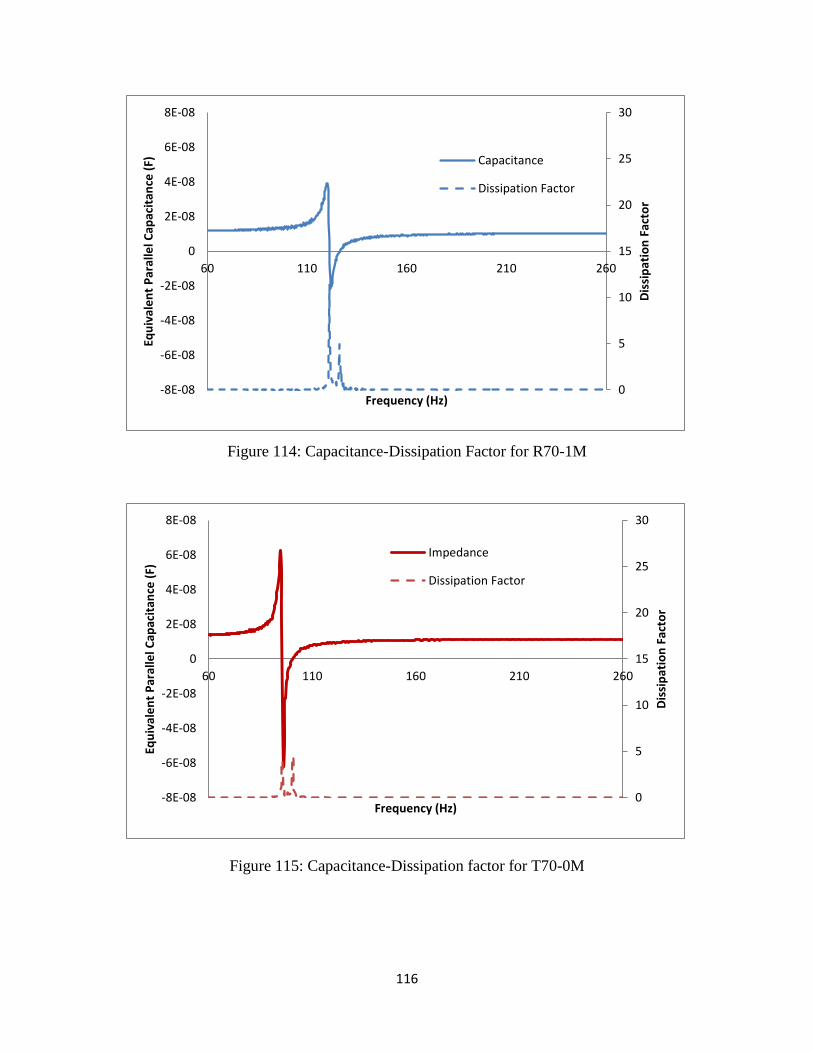
116

Figure 114: Capacitance-Dissipation Factor for R70-1M

Figure 115: Capacitance-Dissipation factor for T70-0M

0

5

10

15

20

25

30

-8E-08

-6E-08

-4E-08

-2E-08

0

2E-08

4E-08

6E-08

8E-08

60 110 160 210 260

Dis

sip

atio

n F

acto

r

Equ

ival

en

t P

aral

lel C

apac

itan

ce (

F)

Frequency (Hz)

Capacitance

Dissipation Factor

0

5

10

15

20

25

30

-8E-08

-6E-08

-4E-08

-2E-08

0

2E-08

4E-08

6E-08

8E-08

60 110 160 210 260D

issi

pat

ion

Fac

tor

Equ

ival

en

t P

aral

lel C

apac

itan

ce (

F)

Frequency (Hz)

Impedance

Dissipation Factor

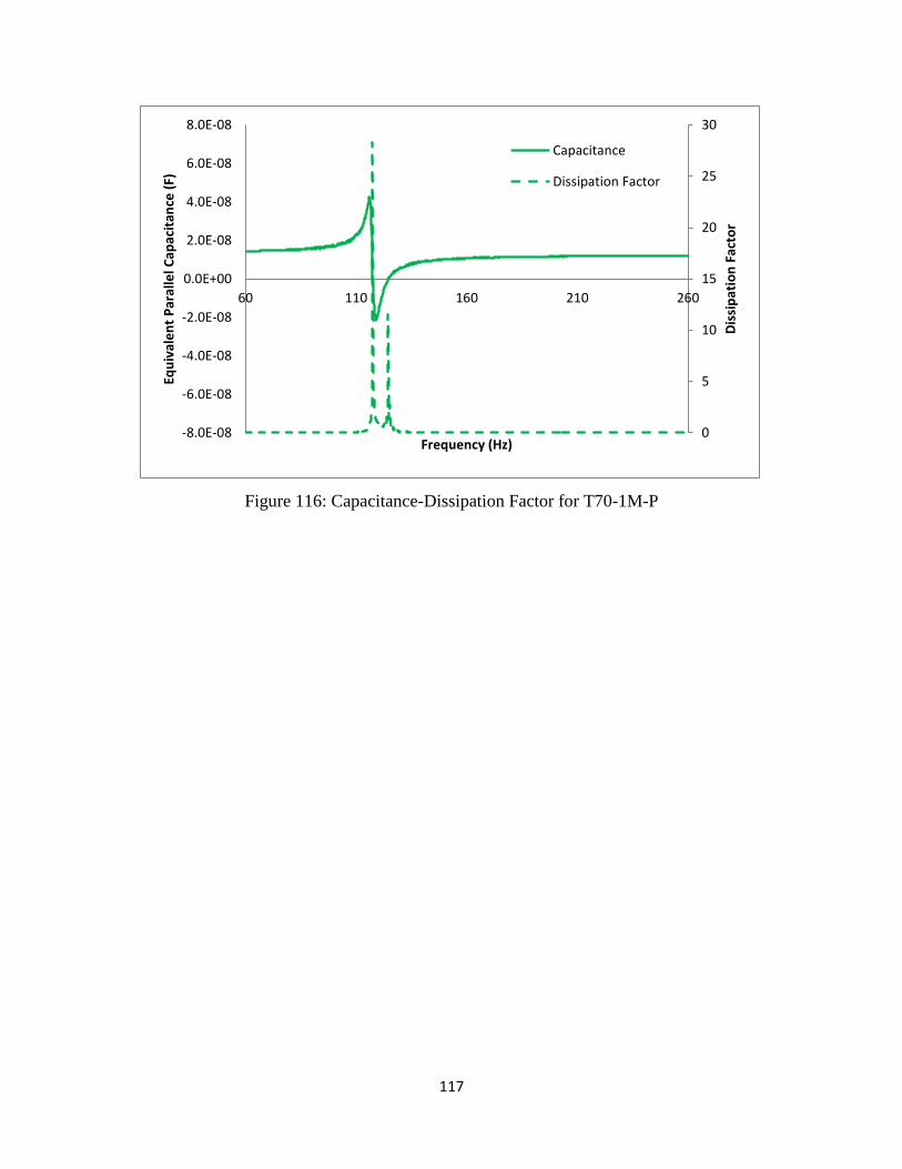
117

Figure 116: Capacitance-Dissipation Factor for T70-1M-P

0

5

10

15

20

25

30

-8.0E-08

-6.0E-08

-4.0E-08

-2.0E-08

0.0E+00

2.0E-08

4.0E-08

6.0E-08

8.0E-08

60 110 160 210 260

Dis

sip

atio

n F

acto

r

Equ

ival

en

t P

aral

lel C

apac

itan

ce (

F)

Frequency (Hz)

Capacitance

Dissipation Factor

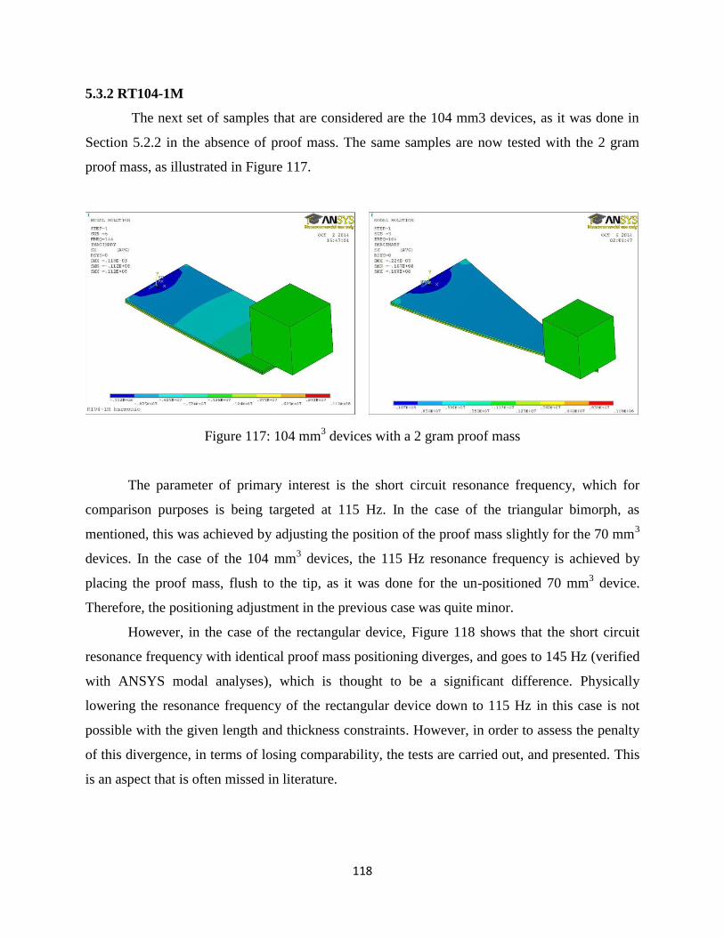
118

5.3.2 RT104-1M

The next set of samples that are considered are the 104 mm3 devices, as it was done in

Section 5.2.2 in the absence of proof mass. The same samples are now tested with the 2 gram

proof mass, as illustrated in Figure 117.

Figure 117: 104 mm3 devices with a 2 gram proof mass

The parameter of primary interest is the short circuit resonance frequency, which for

comparison purposes is being targeted at 115 Hz. In the case of the triangular bimorph, as

mentioned, this was achieved by adjusting the position of the proof mass slightly for the 70 mm3

devices. In the case of the 104 mm3 devices, the 115 Hz resonance frequency is achieved by

placing the proof mass, flush to the tip, as it was done for the un-positioned 70 mm3 device.

Therefore, the positioning adjustment in the previous case was quite minor.

However, in the case of the rectangular device, Figure 118 shows that the short circuit

resonance frequency with identical proof mass positioning diverges, and goes to 145 Hz (verified

with ANSYS modal analyses), which is thought to be a significant difference. Physically

lowering the resonance frequency of the rectangular device down to 115 Hz in this case is not

possible with the given length and thickness constraints. However, in order to assess the penalty

of this divergence, in terms of losing comparability, the tests are carried out, and presented. This

is an aspect that is often missed in literature.

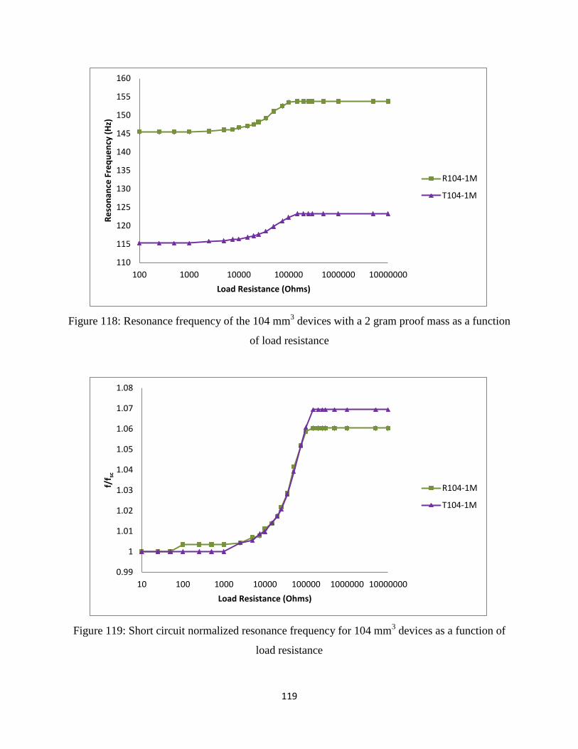
119

Figure 118: Resonance frequency of the 104 mm3 devices with a 2 gram proof mass as a function

of load resistance

Figure 119: Short circuit normalized resonance frequency for 104 mm3 devices as a function of

load resistance

110

115

120

125

130

135

140

145

150

155

160

100 1000 10000 100000 1000000 10000000

Re

son

ance

Fre

qu

en

cy (

Hz)


R104-1M

T104-1M

0.99

1

1.01

1.02

1.03

1.04

1.05

1.06

1.07

1.08

10 100 1000 10000 100000 1000000 10000000

f/f s

c


R104-1M

T104-1M

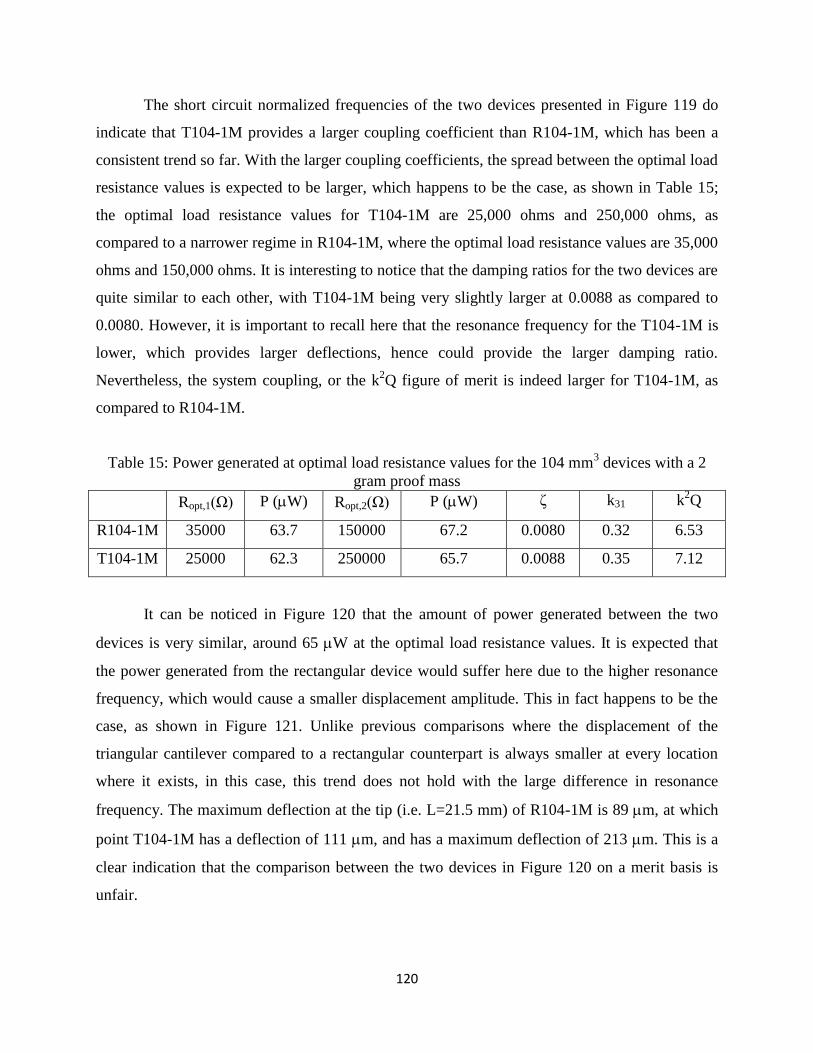
120

The short circuit normalized frequencies of the two devices presented in Figure 119 do

indicate that T104-1M provides a larger coupling coefficient than R104-1M, which has been a

consistent trend so far. With the larger coupling coefficients, the spread between the optimal load

resistance values is expected to be larger, which happens to be the case, as shown in Table 15;

the optimal load resistance values for T104-1M are 25,000 ohms and 250,000 ohms, as

compared to a narrower regime in R104-1M, where the optimal load resistance values are 35,000

ohms and 150,000 ohms. It is interesting to notice that the damping ratios for the two devices are

quite similar to each other, with T104-1M being very slightly larger at 0.0088 as compared to

0.0080. However, it is important to recall here that the resonance frequency for the T104-1M is

lower, which provides larger deflections, hence could provide the larger damping ratio.

Nevertheless, the system coupling, or the k2Q figure of merit is indeed larger for T104-1M, as

compared to R104-1M.


gram proof mass


R104-1M 35000 63.7 150000 67.2 0.0080 0.32 6.53

T104-1M 25000 62.3 250000 65.7 0.0088 0.35 7.12

It can be noticed in Figure 120 that the amount of power generated between the two

devices is very similar, around 65 W at the optimal load resistance values. It is expected that

the power generated from the rectangular device would suffer here due to the higher resonance

frequency, which would cause a smaller displacement amplitude. This in fact happens to be the

case, as shown in Figure 121. Unlike previous comparisons where the displacement of the

triangular cantilever compared to a rectangular counterpart is always smaller at every location

where it exists, in this case, this trend does not hold with the large difference in resonance

frequency. The maximum deflection at the tip (i.e. L=21.5 mm) of R104-1M is 89 m, at which

point T104-1M has a deflection of 111 m, and has a maximum deflection of 213 m. This is a

clear indication that the comparison between the two devices in Figure 120 on a merit basis is

unfair.

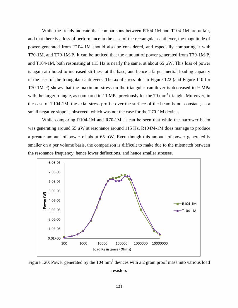
121

While the trends indicate that comparisons between R104-1M and T104-1M are unfair,

and that there is a loss of performance in the case of the rectangular cantilever, the magnitude of

power generated from T104-1M should also be considered, and especially comparing it with

T70-1M, and T70-1M-P. It can be noticed that the amount of power generated from T70-1M-P,

and T104-1M, both resonating at 115 Hz is nearly the same, at about 65 W. This loss of power

is again attributed to increased stiffness at the base, and hence a larger inertial loading capacity

in the case of the triangular cantilevers. The axial stress plot in Figure 122 (and Figure 110 for

T70-1M-P) shows that the maximum stress on the triangular cantilever is decreased to 9 MPa

with the larger triangle, as compared to 11 MPa previously for the 70 mm3 triangle. Moreover, in

the case of T104-1M, the axial stress profile over the surface of the beam is not constant, as a

small negative slope is observed, which was not the case for the T70-1M devices.

While comparing R104-1M and R70-1M, it can be seen that while the narrower beam

was generating around 55 W at resonance around 115 Hz, R104M-1M does manage to produce

a greater amount of power of about 65 W. Even though this amount of power generated is

smaller on a per volume basis, the comparison is difficult to make due to the mismatch between

the resonance frequency, hence lower deflections, and hence smaller stresses.

Figure 120: Power generated by the 104 mm3 devices with a 2 gram proof mass into various load

resistors

0.0E+00

1.0E-05

2.0E-05

3.0E-05

4.0E-05

5.0E-05

6.0E-05

7.0E-05

8.0E-05

100 1000 10000 100000 1000000 10000000

Po

we

r (W

)


R104-1M

T104-1M

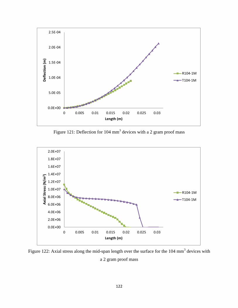
122

Figure 121: Deflection for 104 mm3 devices with a 2 gram proof mass


a 2 gram proof mass

0.0E+00

5.0E-05

1.0E-04

1.5E-04

2.0E-04

2.5E-04

0 0.005 0.01 0.015 0.02 0.025 0.03

De

fle

ctio

n (

m)

Length (m)

R104-1M

T104-1M

0.0E+00

2.0E+06

4.0E+06

6.0E+06

8.0E+06

1.0E+07

1.2E+07

1.4E+07

1.6E+07

1.8E+07

2.0E+07

0 0.005 0.01 0.015 0.02 0.025 0.03

Axi

al S

tre

ss (

N/m

2 )

Length (m)

R104-1M

T104-1M

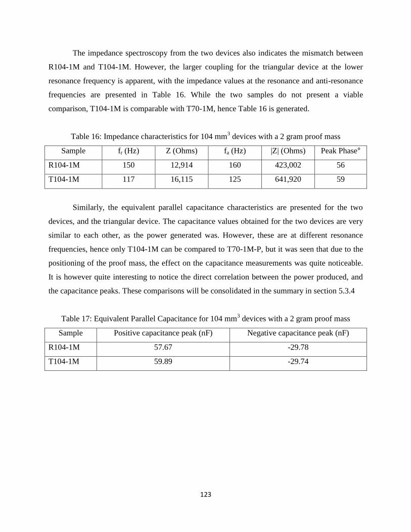
123

The impedance spectroscopy from the two devices also indicates the mismatch between

R104-1M and T104-1M. However, the larger coupling for the triangular device at the lower

resonance frequency is apparent, with the impedance values at the resonance and anti-resonance

frequencies are presented in Table 16. While the two samples do not present a viable

comparison, T104-1M is comparable with T70-1M, hence Table 16 is generated.

Table 16: Impedance characteristics for 104 mm3 devices with a 2 gram proof mass


R104-1M 150 12,914 160 423,002 56

T104-1M 117 16,115 125 641,920 59

Similarly, the equivalent parallel capacitance characteristics are presented for the two

devices, and the triangular device. The capacitance values obtained for the two devices are very

similar to each other, as the power generated was. However, these are at different resonance

frequencies, hence only T104-1M can be compared to T70-1M-P, but it was seen that due to the

positioning of the proof mass, the effect on the capacitance measurements was quite noticeable.

It is however quite interesting to notice the direct correlation between the power produced, and

the capacitance peaks. These comparisons will be consolidated in the summary in section 5.3.4

Table 17: Equivalent Parallel Capacitance for 104 mm3 devices with a 2 gram proof mass


R104-1M 57.67 -29.78

T104-1M 59.89 -29.74

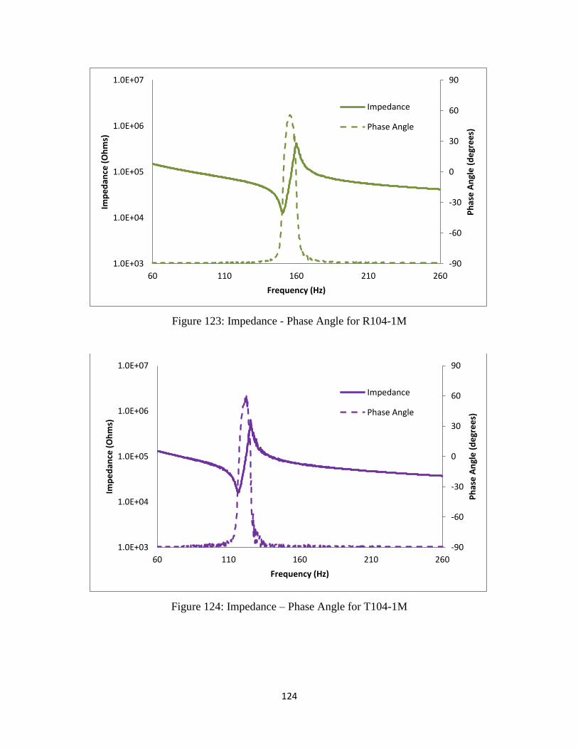
124

Figure 123: Impedance - Phase Angle for R104-1M

Figure 124: Impedance – Phase Angle for T104-1M

-90

-60

-30

0

30

60

90

1.0E+03

1.0E+04

1.0E+05

1.0E+06

1.0E+07

60 110 160 210 260

Ph

ase

An

gle

(d

egr

ee

s)

Imp

ed

ance

(O

hm

s)

Frequency (Hz)

Impedance

Phase Angle

-90

-60

-30

0

30

60

90

1.0E+03

1.0E+04

1.0E+05

1.0E+06

1.0E+07

60 110 160 210 260

Ph

ase

An

gle

(d

egr

ee

s)

Imp

ed

ance

(O

hm

s)

Frequency (Hz)

Impedance

Phase Angle

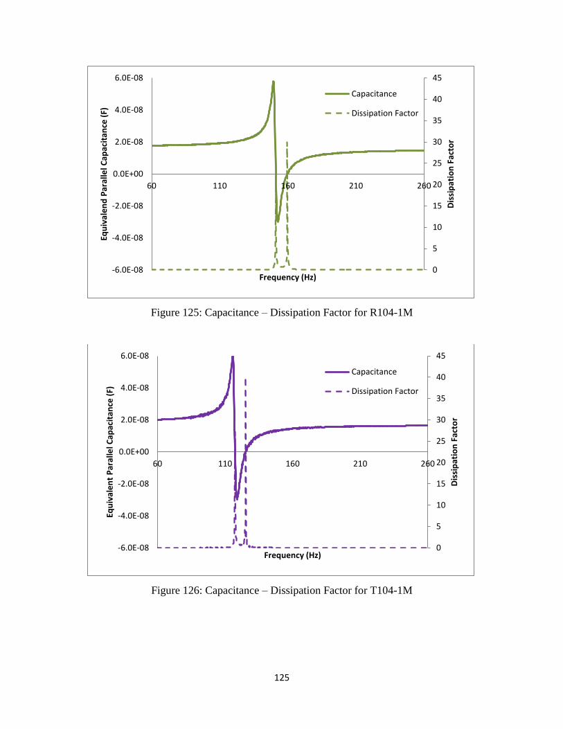
125

Figure 125: Capacitance – Dissipation Factor for R104-1M

Figure 126: Capacitance – Dissipation Factor for T104-1M

0

5

10

15

20

25

30

35

40

45

-6.0E-08

-4.0E-08

-2.0E-08

0.0E+00

2.0E-08

4.0E-08

6.0E-08

60 110 160 210 260

Dis

sip

atio

n F

acto

r

Equ

ival

en

d P

aral

lel C

apac

itan

ce (

F)

Frequency (Hz)

Capacitance

Dissipation Factor

0

5

10

15

20

25

30

35

40

45

-6.0E-08

-4.0E-08

-2.0E-08

0.0E+00

2.0E-08

4.0E-08

6.0E-08

60 110 160 210 260D

issi

pat

ion

Fac

tor

Equ

ival

en

t P

aral

lel C

apac

itan

ce (

F)

Frequency (Hz)

Capacitance

Dissipation Factor

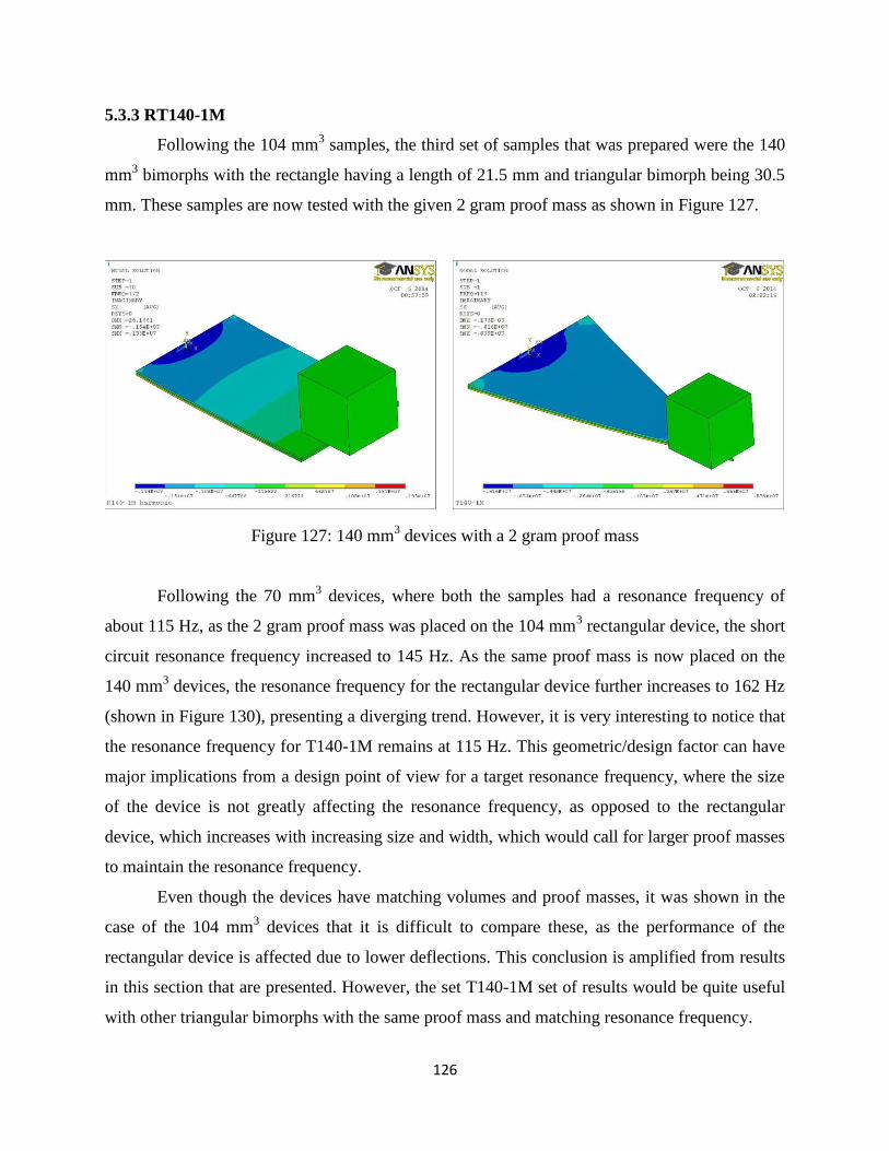
126

5.3.3 RT140-1M

Following the 104 mm3 samples, the third set of samples that was prepared were the 140

mm3 bimorphs with the rectangle having a length of 21.5 mm and triangular bimorph being 30.5

mm. These samples are now tested with the given 2 gram proof mass as shown in Figure 127.

Figure 127: 140 mm3 devices with a 2 gram proof mass

Following the 70 mm3 devices, where both the samples had a resonance frequency of

about 115 Hz, as the 2 gram proof mass was placed on the 104 mm3 rectangular device, the short

circuit resonance frequency increased to 145 Hz. As the same proof mass is now placed on the

140 mm3 devices, the resonance frequency for the rectangular device further increases to 162 Hz

(shown in Figure 130), presenting a diverging trend. However, it is very interesting to notice that

the resonance frequency for T140-1M remains at 115 Hz. This geometric/design factor can have

major implications from a design point of view for a target resonance frequency, where the size

of the device is not greatly affecting the resonance frequency, as opposed to the rectangular

device, which increases with increasing size and width, which would call for larger proof masses

to maintain the resonance frequency.

Even though the devices have matching volumes and proof masses, it was shown in the

case of the 104 mm3 devices that it is difficult to compare these, as the performance of the

rectangular device is affected due to lower deflections. This conclusion is amplified from results

in this section that are presented. However, the set T140-1M set of results would be quite useful

with other triangular bimorphs with the same proof mass and matching resonance frequency.

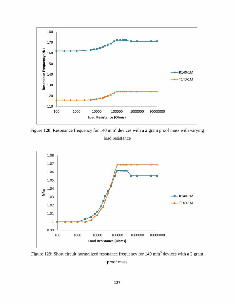
127

Figure 128: Resonance frequency for 140 mm3 devices with a 2 gram proof mass with varying

load resistance

Figure 129: Short circuit normalized resonance frequency for 140 mm3 devices with a 2 gram

proof mass

110

120

130

140

150

160

170

180

100 1000 10000 100000 1000000 10000000

Re

son

ance

Fre

qu

en

cy (

Hz)


R140-1M

T140-1M

0.99

1

1.01

1.02

1.03

1.04

1.05

1.06

1.07

1.08

100 1000 10000 100000 1000000 10000000

f/fs

c


R140-1M

T140-1M

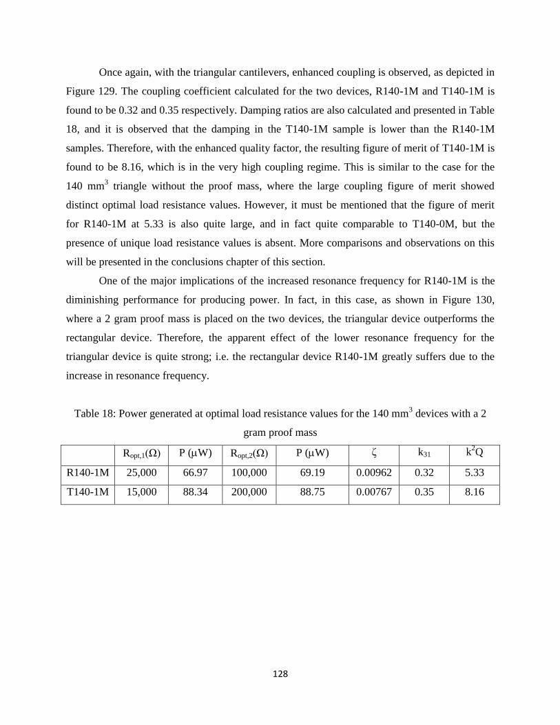
128

Once again, with the triangular cantilevers, enhanced coupling is observed, as depicted in

Figure 129. The coupling coefficient calculated for the two devices, R140-1M and T140-1M is

found to be 0.32 and 0.35 respectively. Damping ratios are also calculated and presented in Table

18, and it is observed that the damping in the T140-1M sample is lower than the R140-1M

samples. Therefore, with the enhanced quality factor, the resulting figure of merit of T140-1M is

found to be 8.16, which is in the very high coupling regime. This is similar to the case for the

140 mm3 triangle without the proof mass, where the large coupling figure of merit showed

distinct optimal load resistance values. However, it must be mentioned that the figure of merit

for R140-1M at 5.33 is also quite large, and in fact quite comparable to T140-0M, but the

presence of unique load resistance values is absent. More comparisons and observations on this

will be presented in the conclusions chapter of this section.

One of the major implications of the increased resonance frequency for R140-1M is the

diminishing performance for producing power. In fact, in this case, as shown in Figure 130,

where a 2 gram proof mass is placed on the two devices, the triangular device outperforms the

rectangular device. Therefore, the apparent effect of the lower resonance frequency for the

triangular device is quite strong; i.e. the rectangular device R140-1M greatly suffers due to the

increase in resonance frequency.


gram proof mass


R140-1M 25,000 66.97 100,000 69.19 0.00962 0.32 5.33

T140-1M 15,000 88.34 200,000 88.75 0.00767 0.35 8.16

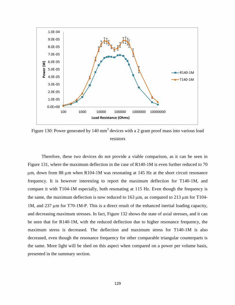
129

Figure 130: Power generated by 140 mm3 devices with a 2 gram proof mass into various load

resistors

Therefore, these two devices do not provide a viable comparison, as it can be seen in

Figure 131, where the maximum deflection in the case of R140-1M is even further reduced to 70

m, down from 88 m when R104-1M was resonating at 145 Hz at the short circuit resonance

frequency. It is however interesting to report the maximum deflection for T140-1M, and

compare it with T104-1M especially, both resonating at 115 Hz. Even though the frequency is

the same, the maximum deflection is now reduced to 163 m, as compared to 213 m for T104-

1M, and 237 m for T70-1M-P. This is a direct result of the enhanced inertial loading capacity,

and decreasing maximum stresses. In fact, Figure 132 shows the state of axial stresses, and it can

be seen that for R140-1M, with the reduced deflection due to higher resonance frequency, the

maximum stress is decreased. The deflection and maximum stress for T140-1M is also

decreased, even though the resonance frequency for other comparable triangular counterparts is

the same. More light will be shed on this aspect when compared on a power per volume basis,

presented in the summary section.

0.0E+00

1.0E-05

2.0E-05

3.0E-05

4.0E-05

5.0E-05

6.0E-05

7.0E-05

8.0E-05

9.0E-05

1.0E-04

100 1000 10000 100000 1000000 10000000

Po

we

r (W

)


R140-1M

T140-1M

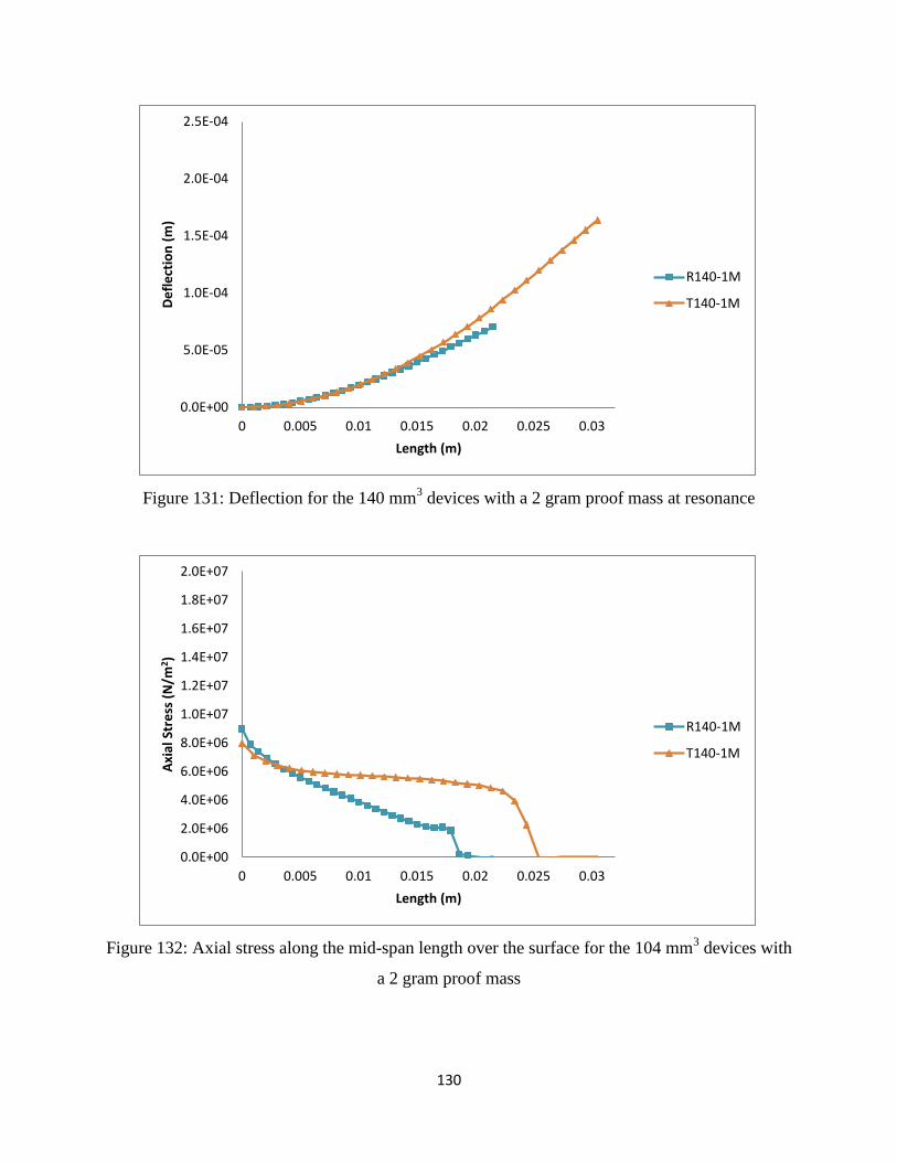
130

Figure 131: Deflection for the 140 mm3 devices with a 2 gram proof mass at resonance


a 2 gram proof mass

0.0E+00

5.0E-05

1.0E-04

1.5E-04

2.0E-04

2.5E-04

0 0.005 0.01 0.015 0.02 0.025 0.03

De

fle

ctio

n (

m)

Length (m)

R140-1M

T140-1M

0.0E+00

2.0E+06

4.0E+06

6.0E+06

8.0E+06

1.0E+07

1.2E+07

1.4E+07

1.6E+07

1.8E+07

2.0E+07

0 0.005 0.01 0.015 0.02 0.025 0.03

Axi

al S

tre

ss (

N/m

2 )

Length (m)

R140-1M

T140-1M

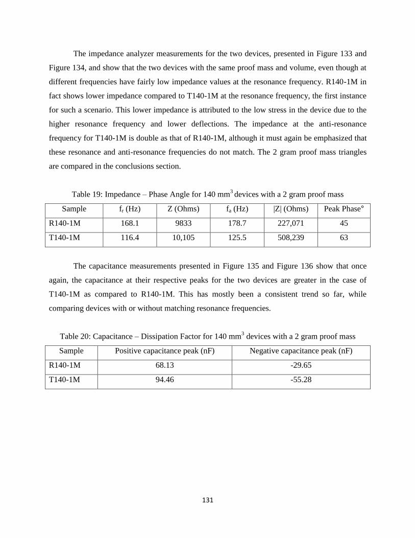
131

The impedance analyzer measurements for the two devices, presented in Figure 133 and

Figure 134, and show that the two devices with the same proof mass and volume, even though at

different frequencies have fairly low impedance values at the resonance frequency. R140-1M in

fact shows lower impedance compared to T140-1M at the resonance frequency, the first instance

for such a scenario. This lower impedance is attributed to the low stress in the device due to the

higher resonance frequency and lower deflections. The impedance at the anti-resonance

frequency for T140-1M is double as that of R140-1M, although it must again be emphasized that

these resonance and anti-resonance frequencies do not match. The 2 gram proof mass triangles

are compared in the conclusions section.

Table 19: Impedance – Phase Angle for 140 mm3 devices with a 2 gram proof mass


R140-1M 168.1 9833 178.7 227,071 45

T140-1M 116.4 10,105 125.5 508,239 63

The capacitance measurements presented in Figure 135 and Figure 136 show that once

again, the capacitance at their respective peaks for the two devices are greater in the case of

T140-1M as compared to R140-1M. This has mostly been a consistent trend so far, while

comparing devices with or without matching resonance frequencies.

Table 20: Capacitance – Dissipation Factor for 140 mm3 devices with a 2 gram proof mass


R140-1M 68.13 -29.65

T140-1M 94.46 -55.28

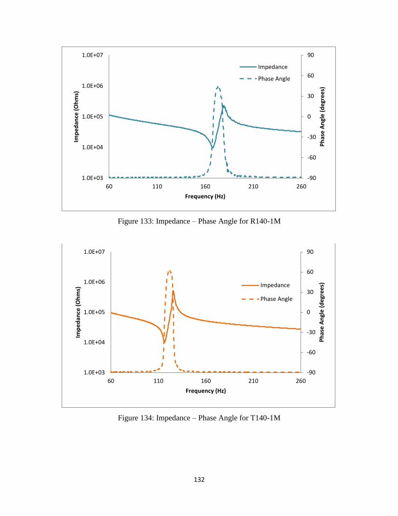
132

Figure 133: Impedance – Phase Angle for R140-1M


-90

-60

-30

0

30

60

90

1.0E+03

1.0E+04

1.0E+05

1.0E+06

1.0E+07

60 110 160 210 260

Ph

ase

An

gle

(d

egr

ee

s)

Imp

ed

ance

(O

hm

s)

Frequency (Hz)

Impedance

Phase Angle

-90

-60

-30

0

30

60

90

1.0E+03

1.0E+04

1.0E+05

1.0E+06

1.0E+07

60 110 160 210 260

Ph

ase

An

gle

(d

egr

ee

s)

Imp

ed

ance

(O

hm

s)

Frequency (Hz)

Impedance

Phase Angle

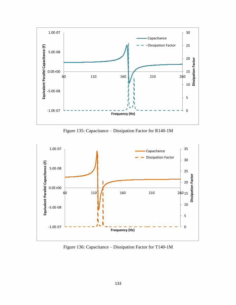
133

Figure 135: Capacitance – Dissipation Factor for R140-1M


0

5

10

15

20

25

30

-1.0E-07

-5.0E-08

0.0E+00

5.0E-08

1.0E-07

60 110 160 210 260

Dis

sip

atio

n F

acto

r

Equ

ival

en

t P

aral

lel C

apac

itan

ce (

F)

Frequency (Hz)

Capacitance

Dissipation Factor

0

5

10

15

20

25

30

35

-1.0E-07

-5.0E-08

0.0E+00

5.0E-08

1.0E-07

60 110 160 210 260D

issi

pat

ion

Fac

tor

Equ

ival

en

t P

aral

lel C

apac

itan

ce (

F)

Frequency (Hz)

Capacitance

Dissipation Factor

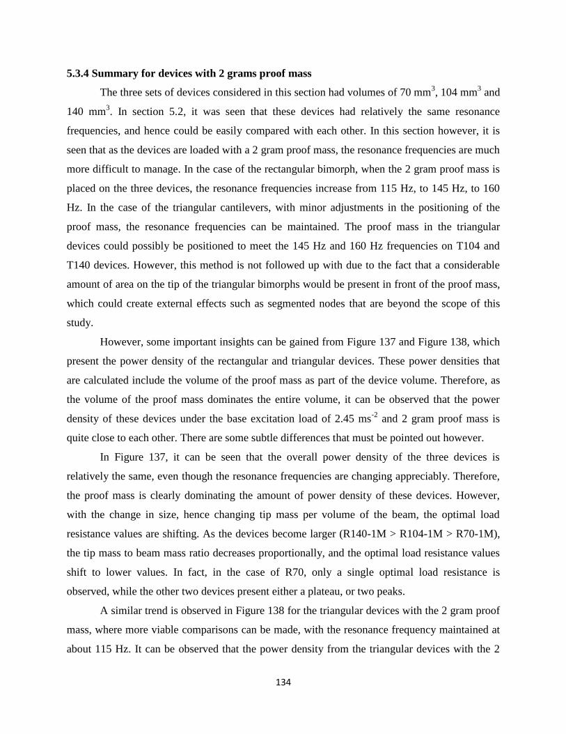
134

5.3.4 Summary for devices with 2 grams proof mass

The three sets of devices considered in this section had volumes of 70 mm3, 104 mm

3 and

140 mm3. In section 5.2, it was seen that these devices had relatively the same resonance

frequencies, and hence could be easily compared with each other. In this section however, it is

seen that as the devices are loaded with a 2 gram proof mass, the resonance frequencies are much

more difficult to manage. In the case of the rectangular bimorph, when the 2 gram proof mass is

placed on the three devices, the resonance frequencies increase from 115 Hz, to 145 Hz, to 160

Hz. In the case of the triangular cantilevers, with minor adjustments in the positioning of the

proof mass, the resonance frequencies can be maintained. The proof mass in the triangular

devices could possibly be positioned to meet the 145 Hz and 160 Hz frequencies on T104 and

T140 devices. However, this method is not followed up with due to the fact that a considerable

amount of area on the tip of the triangular bimorphs would be present in front of the proof mass,

which could create external effects such as segmented nodes that are beyond the scope of this

study.

However, some important insights can be gained from Figure 137 and Figure 138, which

present the power density of the rectangular and triangular devices. These power densities that

are calculated include the volume of the proof mass as part of the device volume. Therefore, as

the volume of the proof mass dominates the entire volume, it can be observed that the power

density of these devices under the base excitation load of 2.45 ms-2

and 2 gram proof mass is

quite close to each other. There are some subtle differences that must be pointed out however.

In Figure 137, it can be seen that the overall power density of the three devices is

relatively the same, even though the resonance frequencies are changing appreciably. Therefore,

the proof mass is clearly dominating the amount of power density of these devices. However,

with the change in size, hence changing tip mass per volume of the beam, the optimal load

resistance values are shifting. As the devices become larger (R140-1M > R104-1M > R70-1M),

the tip mass to beam mass ratio decreases proportionally, and the optimal load resistance values

shift to lower values. In fact, in the case of R70, only a single optimal load resistance is

observed, while the other two devices present either a plateau, or two peaks.

A similar trend is observed in Figure 138 for the triangular devices with the 2 gram proof

mass, where more viable comparisons can be made, with the resonance frequency maintained at

about 115 Hz. It can be observed that the power density from the triangular devices with the 2

135

gram proof mass is somewhat higher than the rectangular counterparts, even though the

maximum stresses reported each time are lower. This is a great advantage provided by the

triangular devices, as they would be operating much more reliably compared to the rectangular

counterparts. Moreover, the effect of enhanced strain distribution and lower stresses with the

same tip mass to beam ratios as rectangular counterparts also show an advantage. While the R70-

1M device shows only one optimal load resistance, the triangular device T70-1M-P (at 115 Hz)

shows the presence of two peaks.

In both cases, the position of the optimal load resistance shifts to lower values, and with

increasing size and lowering of stresses, the presence of two peaks becomes more apparent. This

is especially distinctive in the case of the T140-1M device, with the lowest value for the first

optimal load resistance, and presence of two distinct peaks.

The resulting electromechanical coupling coefficient, damping ratios, and figure of

merits are presented in Figures Figure 140Figure 141 and Figure 142. In these figures, the data

points for the rectangular devices are not connected due to the mismatch in resonance frequency.

It can be clearly seen that the k31 coupling coefficients for triangular devices with the 2 gram

proof mass are always higher compared to the rectangular counterparts. The figure of merit also

keeps increasing in the triangular devices with the decreasing tip mass to beam mass ratios;

however, this is affected in the case of the rectangular devices due to the increasing resonance

frequency.

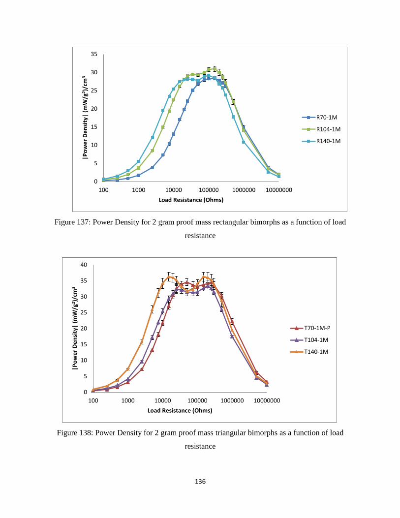
136

Figure 137: Power Density for 2 gram proof mass rectangular bimorphs as a function of load

resistance

Figure 138: Power Density for 2 gram proof mass triangular bimorphs as a function of load

resistance

0

5

10

15

20

25

30

35

100 1000 10000 100000 1000000 10000000

|Po

we

r D

en

sity

| (m

W/g

2 )/c

m3


R70-1M

R104-1M

R140-1M

0

5

10

15

20

25

30

35

40

100 1000 10000 100000 1000000 10000000

|Po

we

r D

en

sity

| (m

W/g

2)/

cm3


T70-1M-P

T104-1M

T140-1M

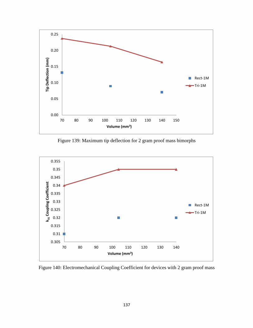
137

Figure 139: Maximum tip deflection for 2 gram proof mass bimorphs

Figure 140: Electromechanical Coupling Coefficient for devices with 2 gram proof mass

0.00

0.05

0.10

0.15

0.20

0.25

70 80 90 100 110 120 130 140 150

Tip

De

fle

ctio

n (

mm

)

Volume (mm3)

Rect-1M

Tri-1M

0.305

0.31

0.315

0.32

0.325

0.33

0.335

0.34

0.345

0.35

0.355

70 80 90 100 110 120 130 140

k 31

Co

up

ling

Co

eff

icie

nt

Volume (mm3)

Rect-1M

Tri-1M

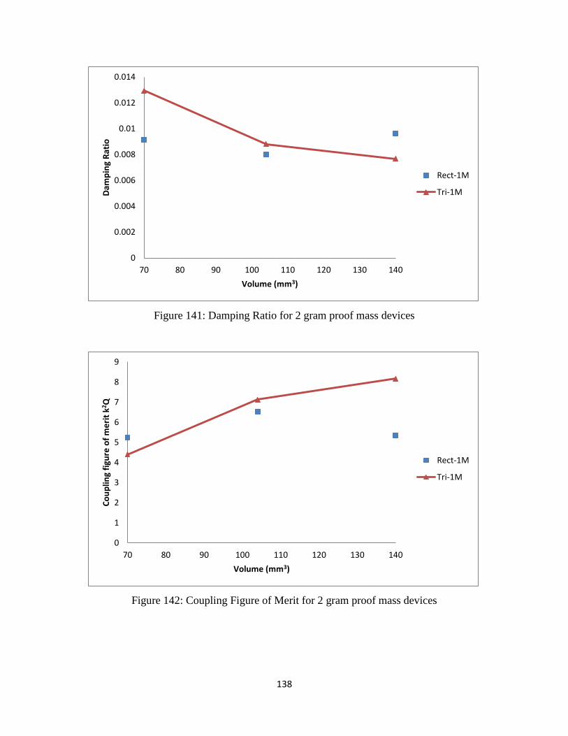
138

Figure 141: Damping Ratio for 2 gram proof mass devices

Figure 142: Coupling Figure of Merit for 2 gram proof mass devices

0

0.002

0.004

0.006

0.008

0.01

0.012

0.014

70 80 90 100 110 120 130 140

Dam

pin

g R

atio

Volume (mm3)

Rect-1M

Tri-1M

0

1

2

3

4

5

6

7

8

9

70 80 90 100 110 120 130 140

Co

up

ling

figu

re o

f m

eri

t k2 Q

Volume (mm3)

Rect-1M

Tri-1M

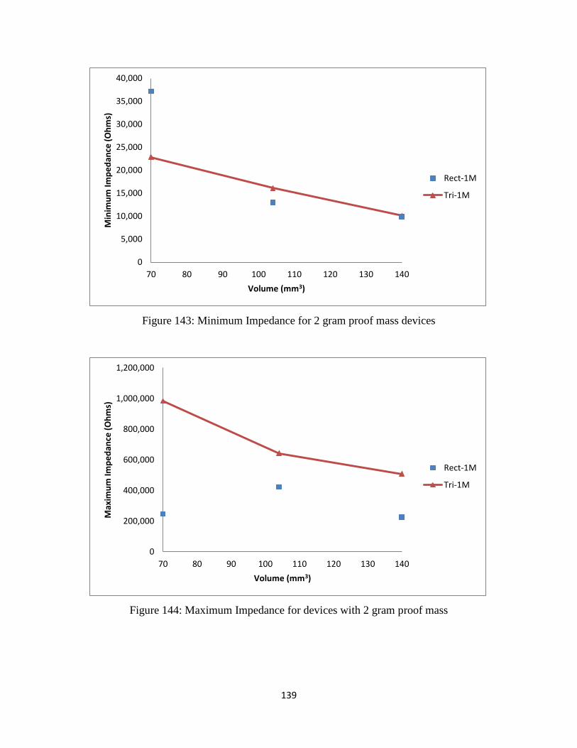
139

Figure 143: Minimum Impedance for 2 gram proof mass devices

Figure 144: Maximum Impedance for devices with 2 gram proof mass

0

5,000

10,000

15,000

20,000

25,000

30,000

35,000

40,000

70 80 90 100 110 120 130 140

Min

imu

m Im

pe

dan

ce (

Oh

ms)

Volume (mm3)

Rect-1M

Tri-1M

0

200,000

400,000

600,000

800,000

1,000,000

1,200,000

70 80 90 100 110 120 130 140

Max

imu

m Im

pe

dan

ce (

Oh

ms)

Volume (mm3)

Rect-1M

Tri-1M

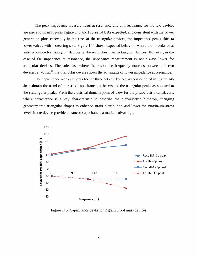
140

The peak impedance measurements at resonance and anti-resonance for the two devices

are also shown in Figures Figure 143 and Figure 144. As expected, and consistent with the power

generation plots especially in the case of the triangular devices, the impedance peaks shift to

lower values with increasing size. Figure 144 shows expected behavior, where the impedance at

anti-resonance for triangular devices is always higher than rectangular devices. However, in the

case of the impedance at resonance, the impedance measurement is not always lower for

triangular devices. The sole case where the resonance frequency matches between the two

devices, at 70 mm3, the triangular device shows the advantage of lower impedance at resonance.

The capacitance measurements for the three sets of devices, as consolidated in Figure 145

do maintain the trend of increased capacitance in the case of the triangular peaks as opposed to

the rectangular peaks. From the electrical domain point of view for the piezoelectric cantilevers,

where capacitance is a key characteristic to describe the piezoelectric bimorph, changing

geometry into triangular shapes to enhance strain distribution and lower the maximum stress

levels in the device provide enhanced capacitance, a marked advantage.

Figure 145: Capacitance peaks for 2 gram proof mass devices

-80

-60

-40

-20

0

20

40

60

80

100

120

70 90 110 130

Equ

ival

en

t P

aral

lel C

apac

itan

ce (

nF)

Frequency (Hz)

Rect-1M -Cp peak

Tri-1M -Cp peak

Rect-1M +Cp peak

Tri-1M +Cp peak

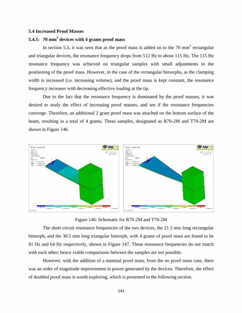
141

5.4 Increased Proof Masses

5.4.1: 70 mm3 devices with 4 grams proof mass

In section 5.3, it was seen that as the proof mass is added on to the 70 mm3 rectangular

and triangular devices, the resonance frequency drops from 512 Hz to about 115 Hz. The 115 Hz

resonance frequency was achieved on triangular samples with small adjustments in the

positioning of the proof mass. However, in the case of the rectangular bimorphs, as the clamping

width is increased (i.e. increasing volume), and the proof mass is kept constant, the resonance

frequency increases with decreasing effective loading at the tip.

Due to the fact that the resonance frequency is dominated by the proof masses, it was

desired to study the effect of increasing proof masses, and see if the resonance frequencies

converge. Therefore, an additional 2 gram proof mass was attached on the bottom surface of the

beam, resulting in a total of 4 grams. These samples, designated as R70-2M and T70-2M are

shown in Figure 146.

Figure 146: Schematic for R70-2M and T70-2M

The short circuit resonance frequencies of the two devices, the 21.5 mm long rectangular

bimorph, and the 30.5 mm long triangular bimorph, with 4 grams of proof mass are found to be

81 Hz and 64 Hz respectively, shown in Figure 147. These resonance frequencies do not match

with each other; hence viable comparisons between the samples are not possible.

However, with the addition of a nominal proof mass, from the no proof mass case, there

was an order of magnitude improvement in power generated by the devices. Therefore, the effect

of doubled proof mass is worth exploring, which is presented in the following section.

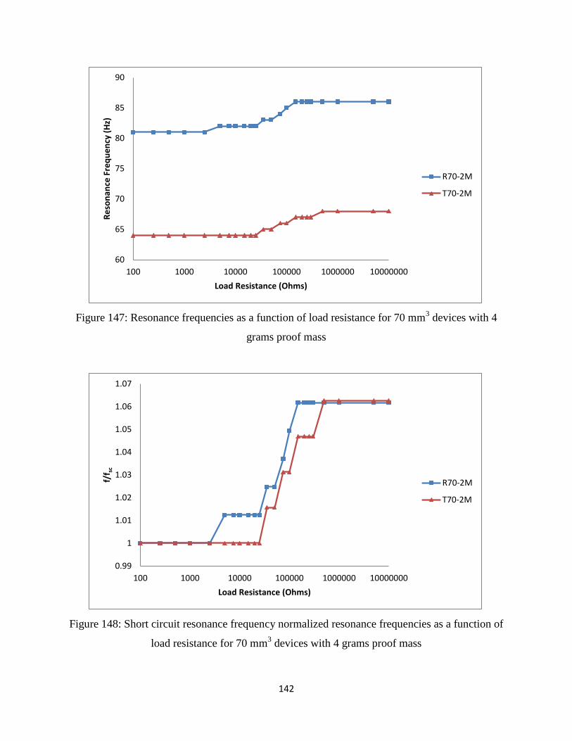
142

Figure 147: Resonance frequencies as a function of load resistance for 70 mm3 devices with 4

grams proof mass

Figure 148: Short circuit resonance frequency normalized resonance frequencies as a function of

load resistance for 70 mm3 devices with 4 grams proof mass

60

65

70

75

80

85

90

100 1000 10000 100000 1000000 10000000

Re

son

ance

Fre

qu

en

cy (

Hz)


R70-2M

T70-2M

0.99

1

1.01

1.02

1.03

1.04

1.05

1.06

1.07

100 1000 10000 100000 1000000 10000000

f/f s

c


R70-2M

T70-2M

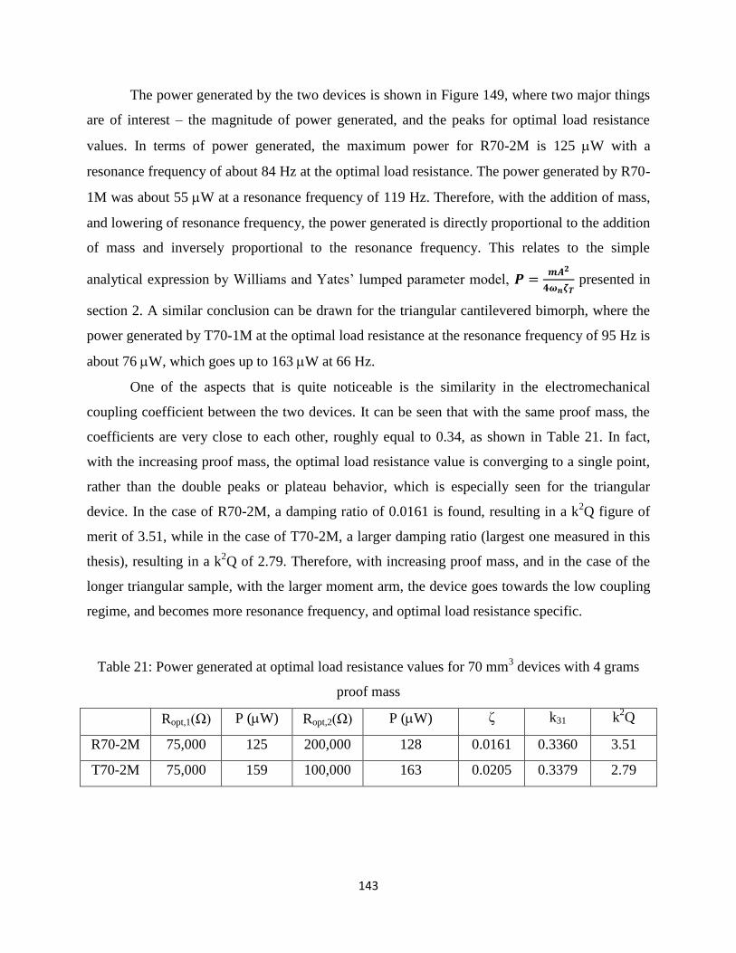
143

The power generated by the two devices is shown in Figure 149, where two major things

are of interest – the magnitude of power generated, and the peaks for optimal load resistance

values. In terms of power generated, the maximum power for R70-2M is 125 W with a

resonance frequency of about 84 Hz at the optimal load resistance. The power generated by R70-

1M was about 55 W at a resonance frequency of 119 Hz. Therefore, with the addition of mass,

and lowering of resonance frequency, the power generated is directly proportional to the addition

of mass and inversely proportional to the resonance frequency. This relates to the simple

analytical expression by Williams and Yates’ lumped parameter model, 𝑷 =𝒎𝑨𝟐

𝟒𝝎𝒏𝜻𝑻 presented in

section 2. A similar conclusion can be drawn for the triangular cantilevered bimorph, where the

power generated by T70-1M at the optimal load resistance at the resonance frequency of 95 Hz is

about 76 W, which goes up to 163 W at 66 Hz.

One of the aspects that is quite noticeable is the similarity in the electromechanical

coupling coefficient between the two devices. It can be seen that with the same proof mass, the

coefficients are very close to each other, roughly equal to 0.34, as shown in Table 21. In fact,

with the increasing proof mass, the optimal load resistance value is converging to a single point,

rather than the double peaks or plateau behavior, which is especially seen for the triangular

device. In the case of R70-2M, a damping ratio of 0.0161 is found, resulting in a k2Q figure of

merit of 3.51, while in the case of T70-2M, a larger damping ratio (largest one measured in this

thesis), resulting in a k2Q of 2.79. Therefore, with increasing proof mass, and in the case of the

longer triangular sample, with the larger moment arm, the device goes towards the low coupling

regime, and becomes more resonance frequency, and optimal load resistance specific.

Table 21: Power generated at optimal load resistance values for 70 mm3 devices with 4 grams

proof mass


R70-2M 75,000 125 200,000 128 0.0161 0.3360 3.51

T70-2M 75,000 159 100,000 163 0.0205 0.3379 2.79

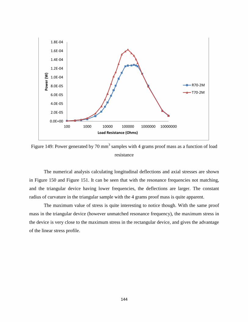
144

Figure 149: Power generated by 70 mm3 samples with 4 grams proof mass as a function of load

resistance

The numerical analysis calculating longitudinal deflections and axial stresses are shown

in Figure 150 and Figure 151. It can be seen that with the resonance frequencies not matching,

and the triangular device having lower frequencies, the deflections are larger. The constant

radius of curvature in the triangular sample with the 4 grams proof mass is quite apparent.

The maximum value of stress is quite interesting to notice though. With the same proof

mass in the triangular device (however unmatched resonance frequency), the maximum stress in

the device is very close to the maximum stress in the rectangular device, and gives the advantage

of the linear stress profile.

0.0E+00

2.0E-05

4.0E-05

6.0E-05

8.0E-05

1.0E-04

1.2E-04

1.4E-04

1.6E-04

1.8E-04

100 1000 10000 100000 1000000 10000000

Po

we

r (W

)


R70-2M

T70-2M

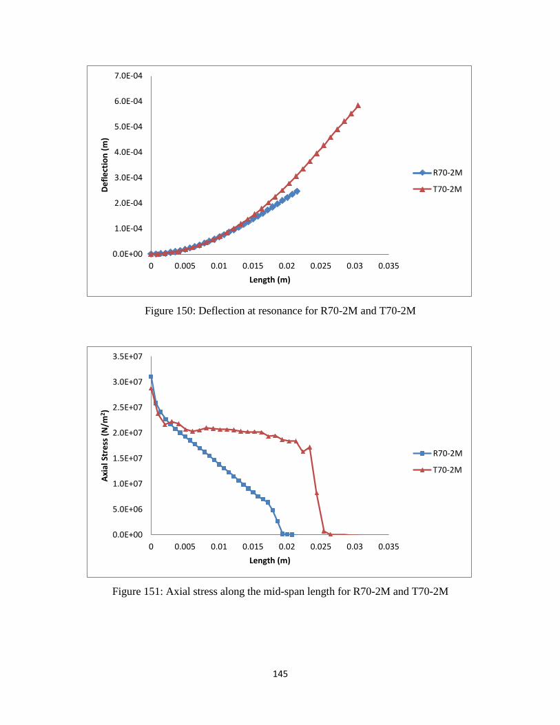
145

Figure 150: Deflection at resonance for R70-2M and T70-2M

Figure 151: Axial stress along the mid-span length for R70-2M and T70-2M

0.0E+00

1.0E-04

2.0E-04

3.0E-04

4.0E-04

5.0E-04

6.0E-04

7.0E-04

0 0.005 0.01 0.015 0.02 0.025 0.03 0.035

De

fle

ctio

n (

m)

Length (m)

R70-2M

T70-2M

0.0E+00

5.0E+06

1.0E+07

1.5E+07

2.0E+07

2.5E+07

3.0E+07

3.5E+07

0 0.005 0.01 0.015 0.02 0.025 0.03 0.035

Axi

al S

tre

ss (

N/m

2 )

Length (m)

R70-2M

T70-2M

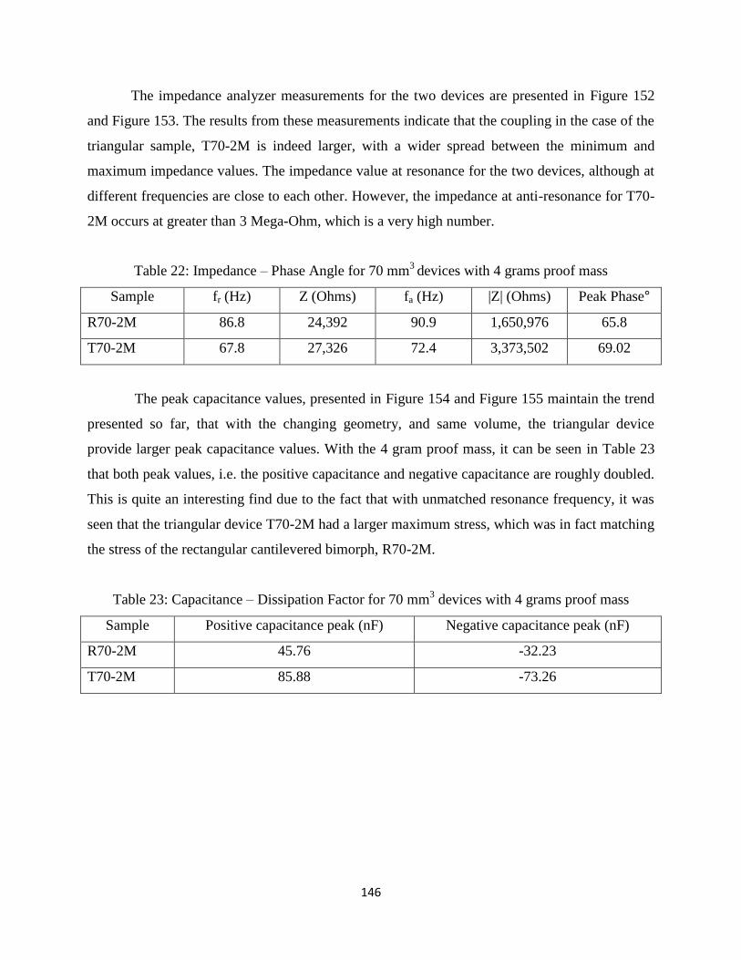
146

The impedance analyzer measurements for the two devices are presented in Figure 152

and Figure 153. The results from these measurements indicate that the coupling in the case of the

triangular sample, T70-2M is indeed larger, with a wider spread between the minimum and

maximum impedance values. The impedance value at resonance for the two devices, although at

different frequencies are close to each other. However, the impedance at anti-resonance for T70-

2M occurs at greater than 3 Mega-Ohm, which is a very high number.

Table 22: Impedance – Phase Angle for 70 mm3

devices with 4 grams proof mass


R70-2M 86.8 24,392 90.9 1,650,976 65.8

T70-2M 67.8 27,326 72.4 3,373,502 69.02

The peak capacitance values, presented in Figure 154 and Figure 155 maintain the trend

presented so far, that with the changing geometry, and same volume, the triangular device

provide larger peak capacitance values. With the 4 gram proof mass, it can be seen in Table 23

that both peak values, i.e. the positive capacitance and negative capacitance are roughly doubled.

This is quite an interesting find due to the fact that with unmatched resonance frequency, it was

seen that the triangular device T70-2M had a larger maximum stress, which was in fact matching

the stress of the rectangular cantilevered bimorph, R70-2M.

Table 23: Capacitance – Dissipation Factor for 70 mm3 devices with 4 grams proof mass


R70-2M 45.76 -32.23

T70-2M 85.88 -73.26

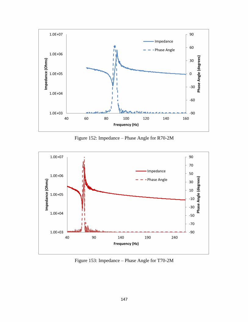
147

Figure 152: Impedance – Phase Angle for R70-2M


-90

-60

-30

0

30

60

90

1.0E+03

1.0E+04

1.0E+05

1.0E+06

1.0E+07

40 60 80 100 120 140 160

Ph

ase

An

gle

(d

egr

ee

s)

Imp

ed

ance

(O

hm

s)

Frequency (Hz)

Impedance

Phase Angle

-90

-70

-50

-30

-10

10

30

50

70

90

1.0E+03

1.0E+04

1.0E+05

1.0E+06

1.0E+07

40 90 140 190 240

Ph

ase

An

gle

(d

egr

ee

s)

Imp

ed

ance

(O

hm

s)

Frequency (Hz)

Impedance

Phase Angle

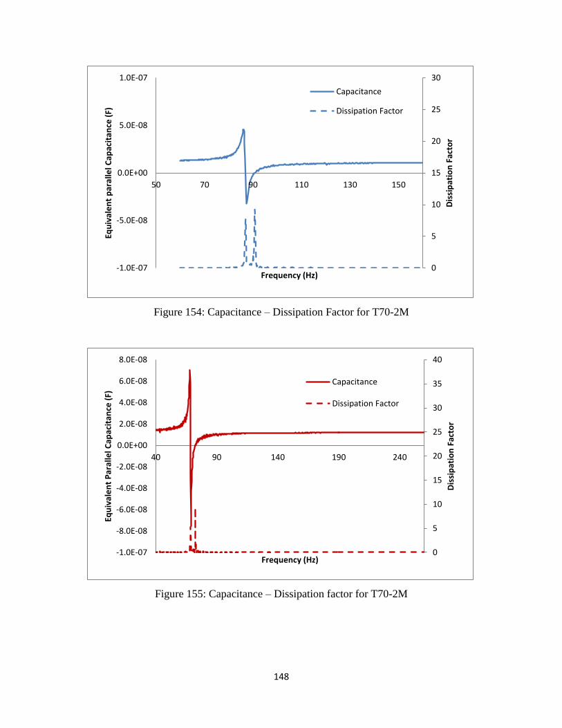
148


Figure 155: Capacitance – Dissipation factor for T70-2M

0

5

10

15

20

25

30

-1.0E-07

-5.0E-08

0.0E+00

5.0E-08

1.0E-07

50 70 90 110 130 150

Dis

sip

atio

n F

acto

r

Equ

ival

en

t p

aral

lel C

apac

itan

ce (

F)

Frequency (Hz)

Capacitance

Dissipation Factor

0

5

10

15

20

25

30

35

40

-1.0E-07

-8.0E-08

-6.0E-08

-4.0E-08

-2.0E-08

0.0E+00

2.0E-08

4.0E-08

6.0E-08

8.0E-08

40 90 140 190 240D

issi

pat

ion

Fac

tor

Equ

ival

en

t P

aral

lel C

apac

itan

ce (

F)

Frequency (Hz)

Capacitance

Dissipation Factor

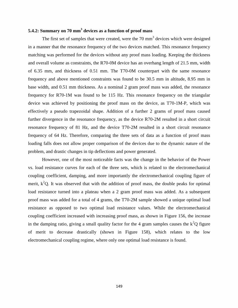
149

5.4.2: Summary on 70 mm3 devices as a function of proof mass

The first set of samples that were created, were the 70 mm3 devices which were designed

in a manner that the resonance frequency of the two devices matched. This resonance frequency

matching was performed for the devices without any proof mass loading. Keeping the thickness

and overall volume as constraints, the R70-0M device has an overhang length of 21.5 mm, width

of 6.35 mm, and thickness of 0.51 mm. The T70-0M counterpart with the same resonance

frequency and above mentioned constraints was found to be 30.5 mm in altitude, 8.95 mm in

base width, and 0.51 mm thickness. As a nominal 2 gram proof mass was added, the resonance

frequency for R70-1M was found to be 115 Hz. This resonance frequency on the triangular

device was achieved by positioning the proof mass on the device, as T70-1M-P, which was

effectively a pseudo trapezoidal shape. Addition of a further 2 grams of proof mass caused

further divergence in the resonance frequency, as the device R70-2M resulted in a short circuit

resonance frequency of 81 Hz, and the device T70-2M resulted in a short circuit resonance

frequency of 64 Hz. Therefore, comparing the three sets of data as a function of proof mass

loading falls does not allow proper comparison of the devices due to the dynamic nature of the

problem, and drastic changes in tip deflections and power generated.

However, one of the most noticeable facts was the change in the behavior of the Power

vs. load resistance curves for each of the three sets, which is related to the electromechanical

coupling coefficient, damping, and more importantly the electromechanical coupling figure of

merit, k2Q. It was observed that with the addition of proof mass, the double peaks for optimal

load resistance turned into a plateau when a 2 gram proof mass was added. As a subsequent

proof mass was added for a total of 4 grams, the T70-2M sample showed a unique optimal load

resistance as opposed to two optimal load resistance values. While the electromechanical

coupling coefficient increased with increasing proof mass, as shown in Figure 156, the increase

in the damping ratio, giving a small quality factor for the 4 gram samples causes the k2Q figure

of merit to decrease drastically (shown in Figure 158), which relates to the low

electromechanical coupling regime, where only one optimal load resistance is found.

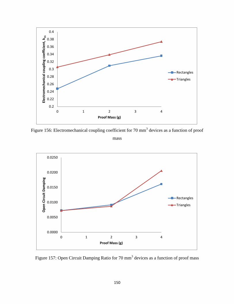
150

Figure 156: Electromechanical coupling coefficient for 70 mm3 devices as a function of proof

mass

Figure 157: Open Circuit Damping Ratio for 70 mm3 devices as a function of proof mass

0.2

0.22

0.24

0.26

0.28

0.3

0.32

0.34

0.36

0.38

0.4

0 1 2 3 4

Ele

ctro

me

chan

ical

co

up

ling

coe

ffic

ien

t, k

31

Proof Mass (g)

Rectangles

Triangles

0.0000

0.0050

0.0100

0.0150

0.0200

0.0250

0 1 2 3 4

Op

en

Cir

cuit

Dam

pin

g

Proof Mass (g)

Rectangles

Triangles

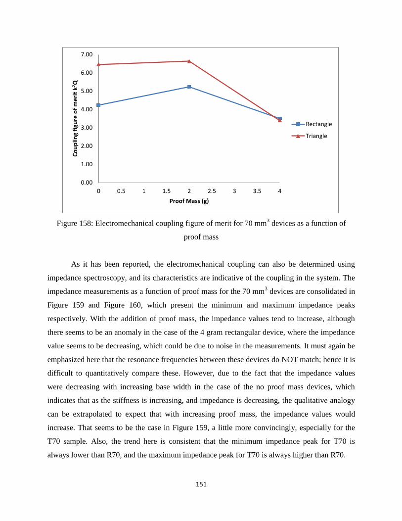
151

Figure 158: Electromechanical coupling figure of merit for 70 mm3 devices as a function of

proof mass

As it has been reported, the electromechanical coupling can also be determined using

impedance spectroscopy, and its characteristics are indicative of the coupling in the system. The

impedance measurements as a function of proof mass for the 70 mm3 devices are consolidated in

Figure 159 and Figure 160, which present the minimum and maximum impedance peaks

respectively. With the addition of proof mass, the impedance values tend to increase, although

there seems to be an anomaly in the case of the 4 gram rectangular device, where the impedance

value seems to be decreasing, which could be due to noise in the measurements. It must again be

emphasized here that the resonance frequencies between these devices do NOT match; hence it is

difficult to quantitatively compare these. However, due to the fact that the impedance values

were decreasing with increasing base width in the case of the no proof mass devices, which

indicates that as the stiffness is increasing, and impedance is decreasing, the qualitative analogy

can be extrapolated to expect that with increasing proof mass, the impedance values would

increase. That seems to be the case in Figure 159, a little more convincingly, especially for the

T70 sample. Also, the trend here is consistent that the minimum impedance peak for T70 is

always lower than R70, and the maximum impedance peak for T70 is always higher than R70.

0.00

1.00

2.00

3.00

4.00

5.00

6.00

7.00

0 0.5 1 1.5 2 2.5 3 3.5 4

Co

up

ling

figu

re o

f m

eri

t k2 Q

Proof Mass (g)

Rectangle

Triangle

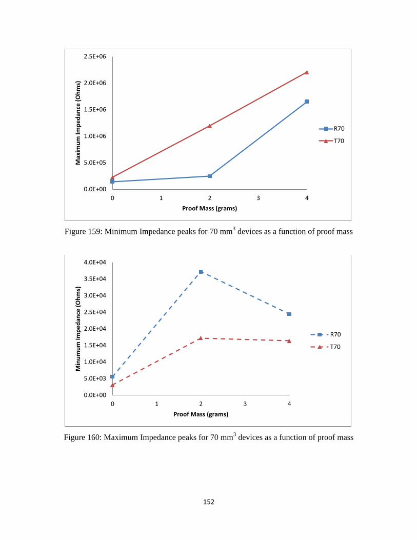
152

Figure 159: Minimum Impedance peaks for 70 mm3 devices as a function of proof mass

Figure 160: Maximum Impedance peaks for 70 mm3 devices as a function of proof mass

0.0E+00

5.0E+05

1.0E+06

1.5E+06

2.0E+06

2.5E+06

0 1 2 3 4

Max

imu

m Im

pe

dan

ce (

Oh

ms)

Proof Mass (grams)

R70

T70

0.0E+00

5.0E+03

1.0E+04

1.5E+04

2.0E+04

2.5E+04

3.0E+04

3.5E+04

4.0E+04

0 1 2 3 4

Min

um

um

Imp

ed

ance

(O

hm

s)

Proof Mass (grams)

R70

T70

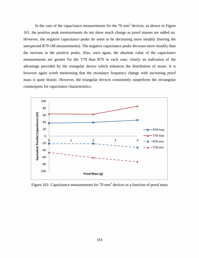
153

In the case of the capacitance measurements for the 70 mm3 devices, as shown in Figure

161, the positive peak measurements do not show much change as proof masses are added on.

However, the negative capacitance peaks do seem to be decreasing more steadily (barring the

unexpected R70-1M measurements). The negative capacitance peaks decrease more steadily than

the increase in the positive peaks. Also, once again, the absolute value of the capacitance

measurements are greater for the T70 than R70 in each case; clearly an indication of the

advantage provided by the triangular device which enhances the distribution of strain. It is

however again worth mentioning that the resonance frequency change with increasing proof

mass is quite drastic. However, the triangular devices consistently outperform the rectangular

counterparts for capacitance characteristics.

Figure 161: Capacitance measurements for 70 mm3 devices as a function of proof mass

-100

-80

-60

-40

-20

0

20

40

60

80

100

0 1 2 3 4

Equ

ival

en

t P

aral

lel C

apac

itan

ce (

nF)

Proof Mass (g)

R70-max

T70-max

R70-min

T70-min

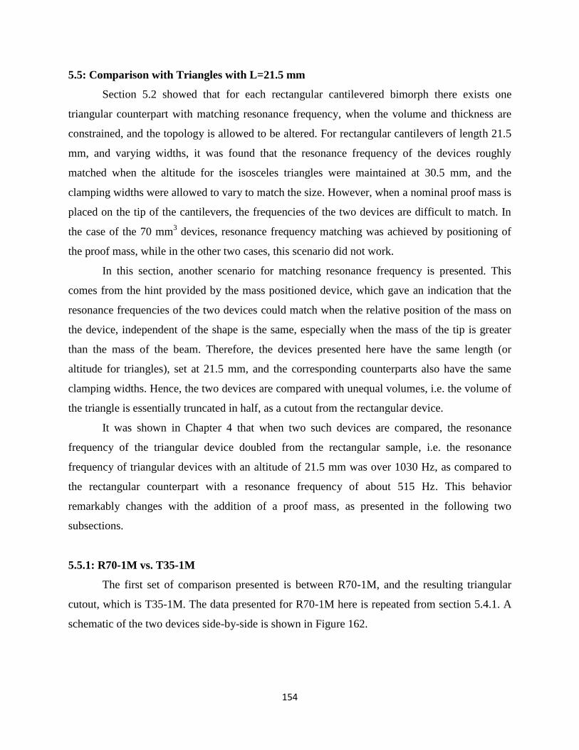
154

5.5: Comparison with Triangles with L=21.5 mm

Section 5.2 showed that for each rectangular cantilevered bimorph there exists one

triangular counterpart with matching resonance frequency, when the volume and thickness are

constrained, and the topology is allowed to be altered. For rectangular cantilevers of length 21.5

mm, and varying widths, it was found that the resonance frequency of the devices roughly

matched when the altitude for the isosceles triangles were maintained at 30.5 mm, and the

clamping widths were allowed to vary to match the size. However, when a nominal proof mass is

placed on the tip of the cantilevers, the frequencies of the two devices are difficult to match. In

the case of the 70 mm3 devices, resonance frequency matching was achieved by positioning of

the proof mass, while in the other two cases, this scenario did not work.

In this section, another scenario for matching resonance frequency is presented. This

comes from the hint provided by the mass positioned device, which gave an indication that the

resonance frequencies of the two devices could match when the relative position of the mass on

the device, independent of the shape is the same, especially when the mass of the tip is greater

than the mass of the beam. Therefore, the devices presented here have the same length (or

altitude for triangles), set at 21.5 mm, and the corresponding counterparts also have the same

clamping widths. Hence, the two devices are compared with unequal volumes, i.e. the volume of

the triangle is essentially truncated in half, as a cutout from the rectangular device.

It was shown in Chapter 4 that when two such devices are compared, the resonance

frequency of the triangular device doubled from the rectangular sample, i.e. the resonance

frequency of triangular devices with an altitude of 21.5 mm was over 1030 Hz, as compared to

the rectangular counterpart with a resonance frequency of about 515 Hz. This behavior

remarkably changes with the addition of a proof mass, as presented in the following two

subsections.

5.5.1: R70-1M vs. T35-1M

The first set of comparison presented is between R70-1M, and the resulting triangular

cutout, which is T35-1M. The data presented for R70-1M here is repeated from section 5.4.1. A

schematic of the two devices side-by-side is shown in Figure 162.

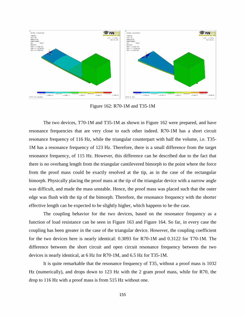
155

Figure 162: R70-1M and T35-1M

The two devices, T70-1M and T35-1M as shown in Figure 162 were prepared, and have

resonance frequencies that are very close to each other indeed. R70-1M has a short circuit

resonance frequency of 116 Hz, while the triangular counterpart with half the volume, i.e. T35-

1M has a resonance frequency of 123 Hz. Therefore, there is a small difference from the target

resonance frequency, of 115 Hz. However, this difference can be described due to the fact that

there is no overhang length from the triangular cantilevered bimorph to the point where the force

from the proof mass could be exactly resolved at the tip, as in the case of the rectangular

bimorph. Physically placing the proof mass at the tip of the triangular device with a narrow angle

was difficult, and made the mass unstable. Hence, the proof mass was placed such that the outer

edge was flush with the tip of the bimorph. Therefore, the resonance frequency with the shorter

effective length can be expected to be slightly higher, which happens to be the case.

The coupling behavior for the two devices, based on the resonance frequency as a

function of load resistance can be seen in Figure 163 and Figure 164. So far, in every case the

coupling has been greater in the case of the triangular device. However, the coupling coefficient

for the two devices here is nearly identical: 0.3093 for R70-1M and 0.3122 for T70-1M. The

difference between the short circuit and open circuit resonance frequency between the two

devices is nearly identical, at 6 Hz for R70-1M, and 6.5 Hz for T35-1M.

It is quite remarkable that the resonance frequency of T35, without a proof mass is 1032

Hz (numerically), and drops down to 123 Hz with the 2 gram proof mass, while for R70, the

drop to 116 Hz with a proof mass is from 515 Hz without one.

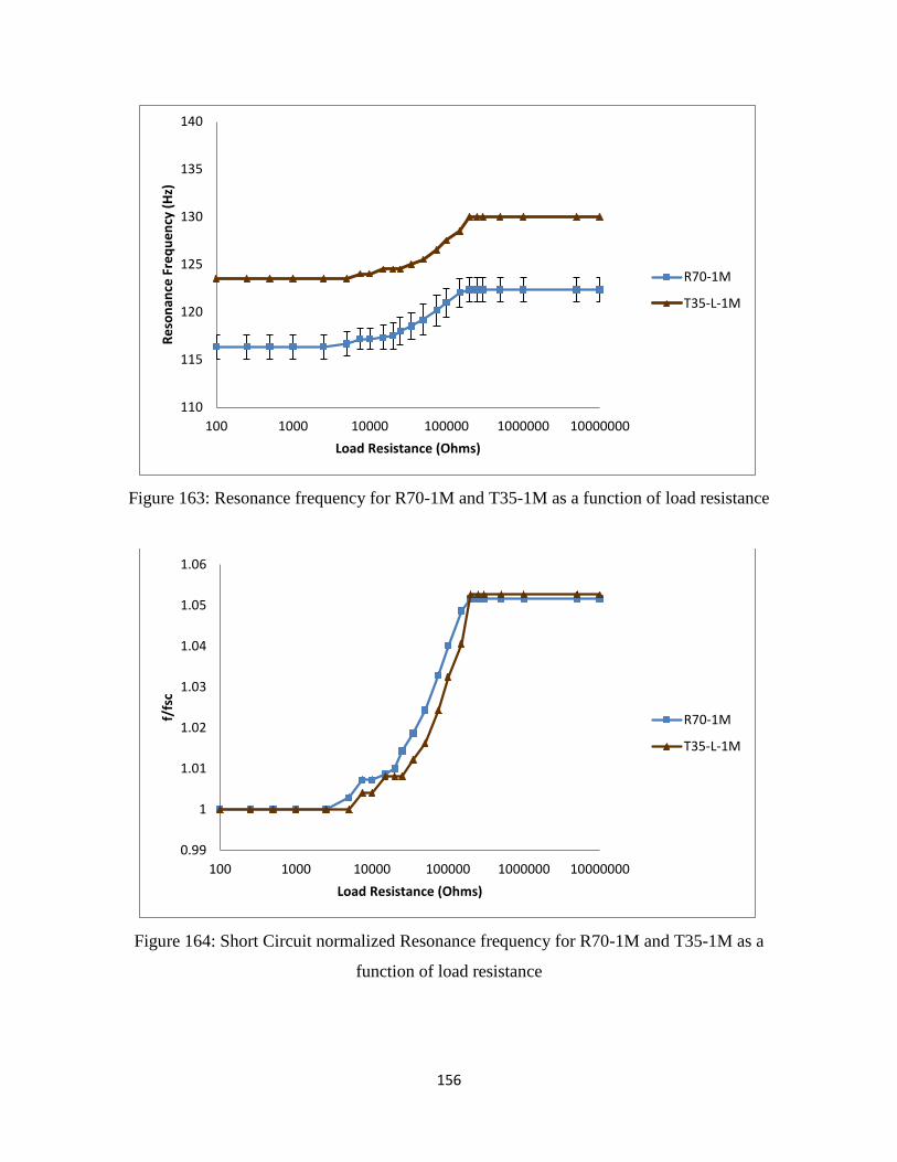
156

Figure 163: Resonance frequency for R70-1M and T35-1M as a function of load resistance

Figure 164: Short Circuit normalized Resonance frequency for R70-1M and T35-1M as a

function of load resistance

110

115

120

125

130

135

140

100 1000 10000 100000 1000000 10000000

Re

son

ance

Fre

qu

en

cy (

Hz)


R70-1M

T35-L-1M

0.99

1

1.01

1.02

1.03

1.04

1.05

1.06

100 1000 10000 100000 1000000 10000000

f/fs

c


R70-1M

T35-L-1M

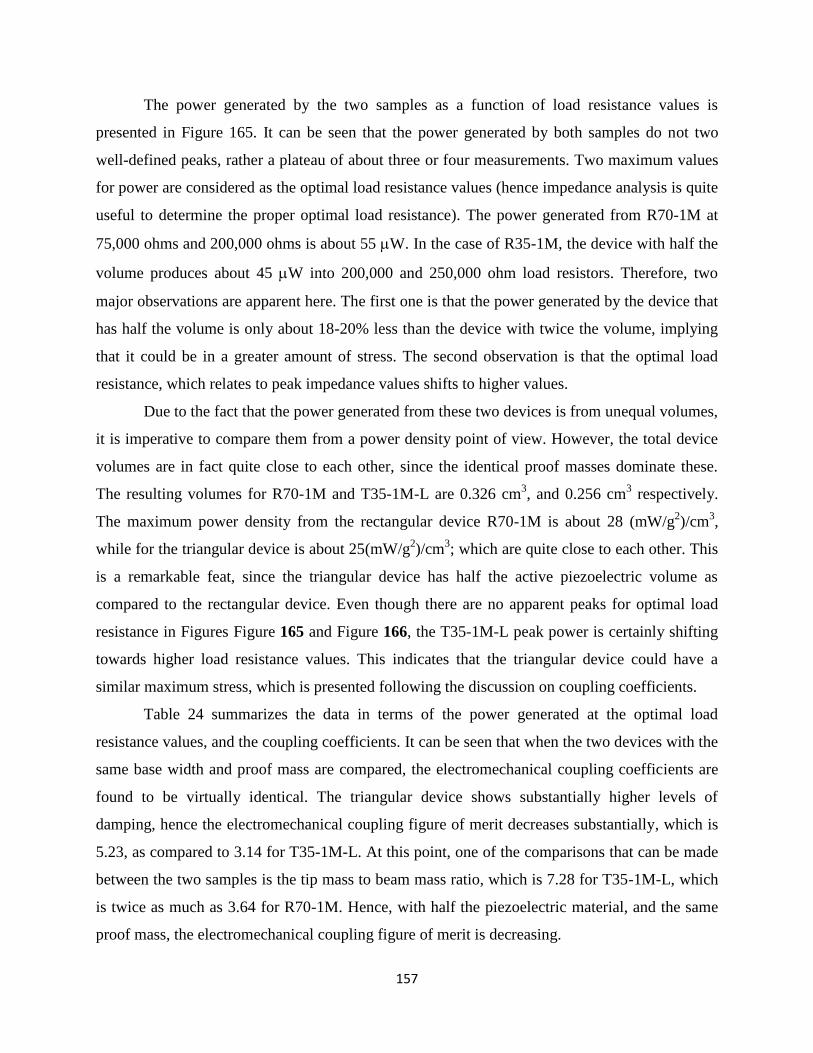
157

The power generated by the two samples as a function of load resistance values is

presented in Figure 165. It can be seen that the power generated by both samples do not two

well-defined peaks, rather a plateau of about three or four measurements. Two maximum values

for power are considered as the optimal load resistance values (hence impedance analysis is quite

useful to determine the proper optimal load resistance). The power generated from R70-1M at

75,000 ohms and 200,000 ohms is about 55 W. In the case of R35-1M, the device with half the

volume produces about 45 W into 200,000 and 250,000 ohm load resistors. Therefore, two

major observations are apparent here. The first one is that the power generated by the device that

has half the volume is only about 18-20% less than the device with twice the volume, implying

that it could be in a greater amount of stress. The second observation is that the optimal load

resistance, which relates to peak impedance values shifts to higher values.

Due to the fact that the power generated from these two devices is from unequal volumes,

it is imperative to compare them from a power density point of view. However, the total device

volumes are in fact quite close to each other, since the identical proof masses dominate these.

The resulting volumes for R70-1M and T35-1M-L are 0.326 cm3, and 0.256 cm

3 respectively.

The maximum power density from the rectangular device R70-1M is about 28 (mW/g2)/cm

3,

while for the triangular device is about 25(mW/g2)/cm

3; which are quite close to each other. This

is a remarkable feat, since the triangular device has half the active piezoelectric volume as

compared to the rectangular device. Even though there are no apparent peaks for optimal load

resistance in Figures Figure 165 and Figure 166, the T35-1M-L peak power is certainly shifting

towards higher load resistance values. This indicates that the triangular device could have a

similar maximum stress, which is presented following the discussion on coupling coefficients.

Table 24 summarizes the data in terms of the power generated at the optimal load

resistance values, and the coupling coefficients. It can be seen that when the two devices with the

same base width and proof mass are compared, the electromechanical coupling coefficients are

found to be virtually identical. The triangular device shows substantially higher levels of

damping, hence the electromechanical coupling figure of merit decreases substantially, which is

5.23, as compared to 3.14 for T35-1M-L. At this point, one of the comparisons that can be made

between the two samples is the tip mass to beam mass ratio, which is 7.28 for T35-1M-L, which

is twice as much as 3.64 for R70-1M. Hence, with half the piezoelectric material, and the same

proof mass, the electromechanical coupling figure of merit is decreasing.

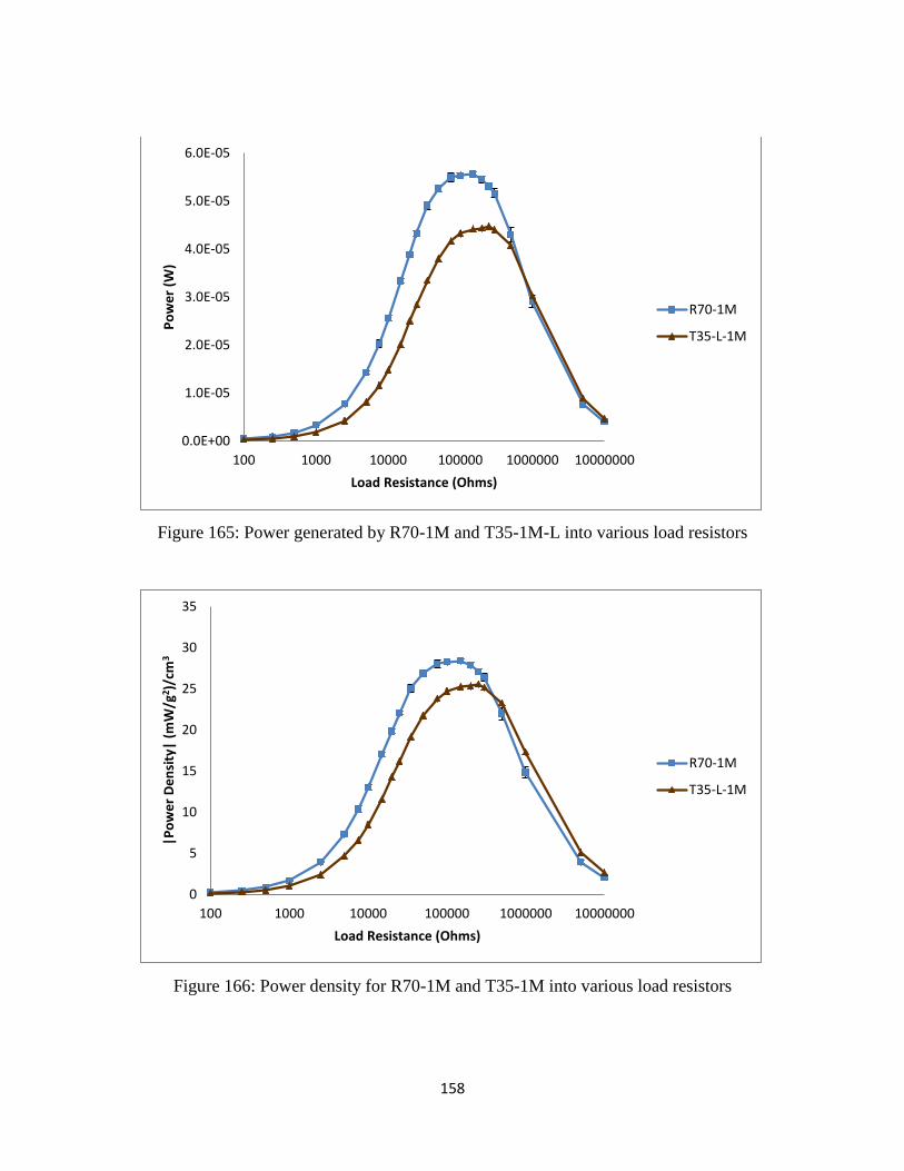
158

Figure 165: Power generated by R70-1M and T35-1M-L into various load resistors

Figure 166: Power density for R70-1M and T35-1M into various load resistors

0.0E+00

1.0E-05

2.0E-05

3.0E-05

4.0E-05

5.0E-05

6.0E-05

100 1000 10000 100000 1000000 10000000

Po

we

r (W

)


R70-1M

T35-L-1M

0

5

10

15

20

25

30

35

100 1000 10000 100000 1000000 10000000

|Po

we

r D

en

sity

| (m

W/g

2 )/c

m3


R70-1M

T35-L-1M

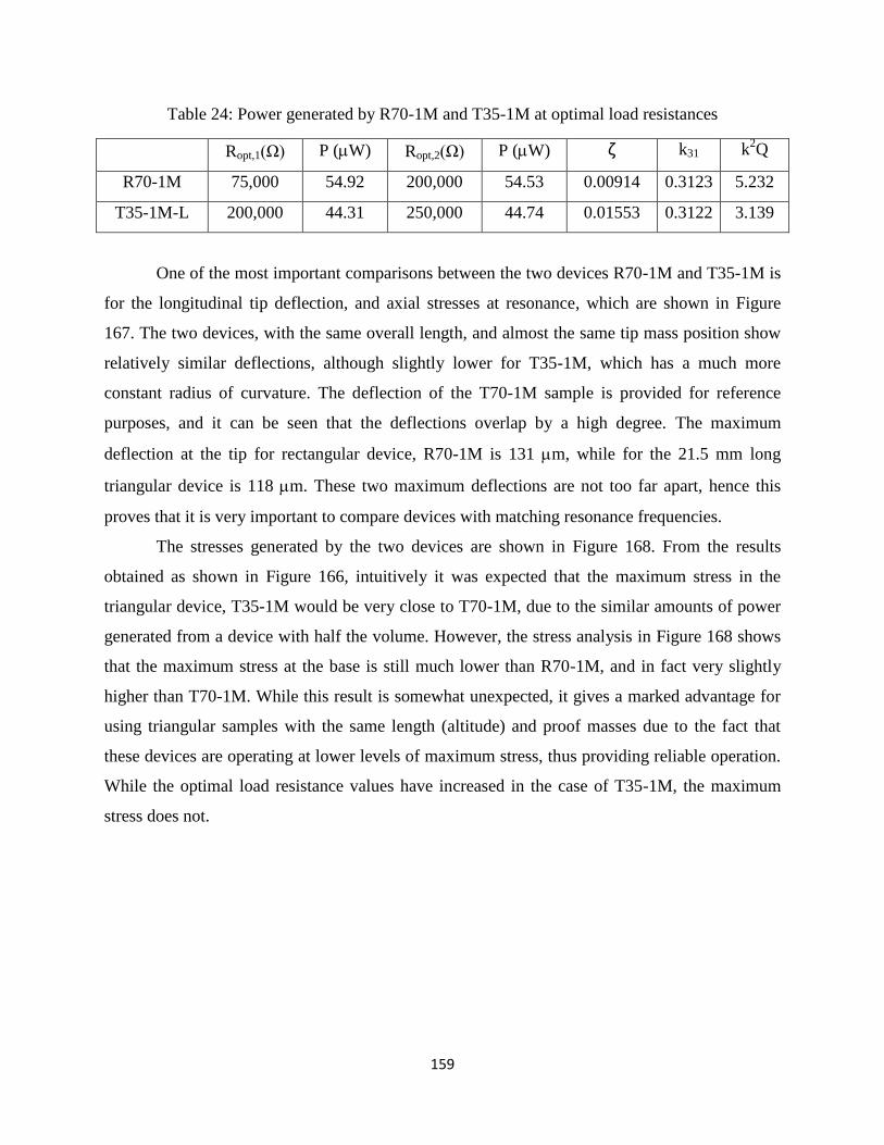
159

Table 24: Power generated by R70-1M and T35-1M at optimal load resistances


R70-1M 75,000 54.92 200,000 54.53 0.00914 0.3123 5.232

T35-1M-L 200,000 44.31 250,000 44.74 0.01553 0.3122 3.139

One of the most important comparisons between the two devices R70-1M and T35-1M is

for the longitudinal tip deflection, and axial stresses at resonance, which are shown in Figure

167. The two devices, with the same overall length, and almost the same tip mass position show

relatively similar deflections, although slightly lower for T35-1M, which has a much more

constant radius of curvature. The deflection of the T70-1M sample is provided for reference

purposes, and it can be seen that the deflections overlap by a high degree. The maximum

deflection at the tip for rectangular device, R70-1M is 131 m, while for the 21.5 mm long

triangular device is 118 m. These two maximum deflections are not too far apart, hence this

proves that it is very important to compare devices with matching resonance frequencies.

The stresses generated by the two devices are shown in Figure 168. From the results

obtained as shown in Figure 166, intuitively it was expected that the maximum stress in the

triangular device, T35-1M would be very close to T70-1M, due to the similar amounts of power

generated from a device with half the volume. However, the stress analysis in Figure 168 shows

that the maximum stress at the base is still much lower than R70-1M, and in fact very slightly

higher than T70-1M. While this result is somewhat unexpected, it gives a marked advantage for

using triangular samples with the same length (altitude) and proof masses due to the fact that

these devices are operating at lower levels of maximum stress, thus providing reliable operation.

While the optimal load resistance values have increased in the case of T35-1M, the maximum

stress does not.

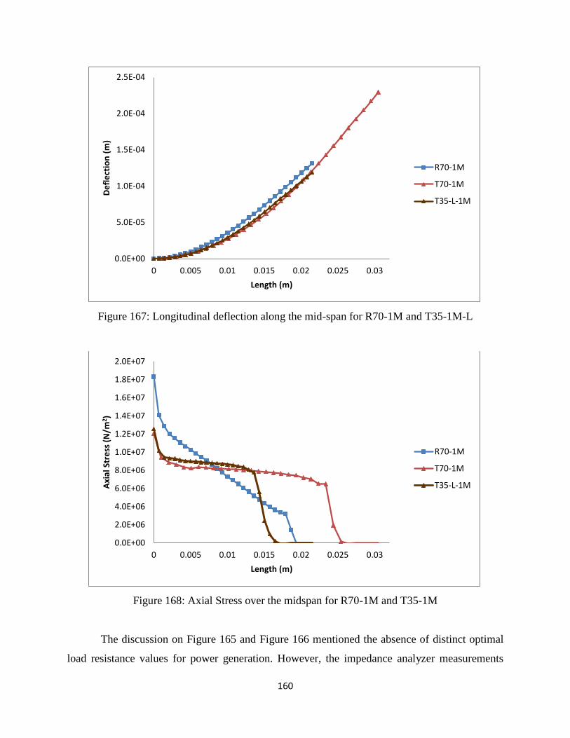
160

Figure 167: Longitudinal deflection along the mid-span for R70-1M and T35-1M-L

Figure 168: Axial Stress over the midspan for R70-1M and T35-1M

The discussion on Figure 165 and Figure 166 mentioned the absence of distinct optimal

load resistance values for power generation. However, the impedance analyzer measurements

0.0E+00

5.0E-05

1.0E-04

1.5E-04

2.0E-04

2.5E-04

0 0.005 0.01 0.015 0.02 0.025 0.03

De

fle

ctio

n (

m)

Length (m)

R70-1M

T70-1M

T35-L-1M

0.0E+00

2.0E+06

4.0E+06

6.0E+06

8.0E+06

1.0E+07

1.2E+07

1.4E+07

1.6E+07

1.8E+07

2.0E+07

0 0.005 0.01 0.015 0.02 0.025 0.03

Axi

al S

tre

ss (

N/m

2 )

Length (m)

R70-1M

T70-1M

T35-L-1M

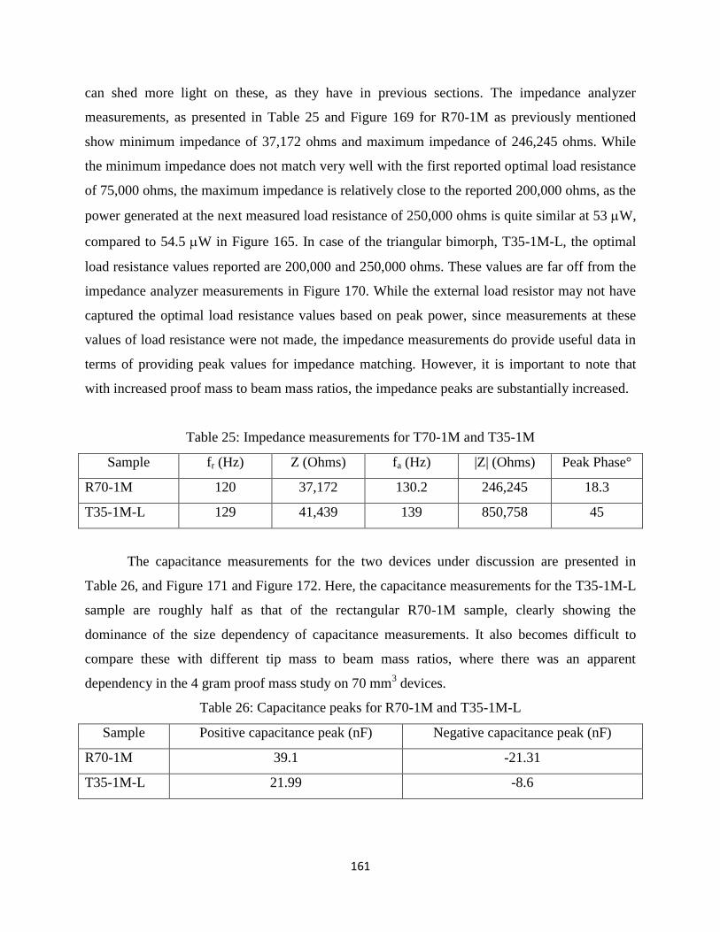
161

can shed more light on these, as they have in previous sections. The impedance analyzer

measurements, as presented in Table 25 and Figure 169 for R70-1M as previously mentioned

show minimum impedance of 37,172 ohms and maximum impedance of 246,245 ohms. While

the minimum impedance does not match very well with the first reported optimal load resistance

of 75,000 ohms, the maximum impedance is relatively close to the reported 200,000 ohms, as the

power generated at the next measured load resistance of 250,000 ohms is quite similar at 53 W,

compared to 54.5 W in Figure 165. In case of the triangular bimorph, T35-1M-L, the optimal

load resistance values reported are 200,000 and 250,000 ohms. These values are far off from the

impedance analyzer measurements in Figure 170. While the external load resistor may not have

captured the optimal load resistance values based on peak power, since measurements at these

values of load resistance were not made, the impedance measurements do provide useful data in

terms of providing peak values for impedance matching. However, it is important to note that

with increased proof mass to beam mass ratios, the impedance peaks are substantially increased.

Table 25: Impedance measurements for T70-1M and T35-1M


R70-1M 120 37,172 130.2 246,245 18.3

T35-1M-L 129 41,439 139 850,758 45

The capacitance measurements for the two devices under discussion are presented in

Table 26, and Figure 171 and Figure 172. Here, the capacitance measurements for the T35-1M-L

sample are roughly half as that of the rectangular R70-1M sample, clearly showing the

dominance of the size dependency of capacitance measurements. It also becomes difficult to

compare these with different tip mass to beam mass ratios, where there was an apparent

dependency in the 4 gram proof mass study on 70 mm3 devices.

Table 26: Capacitance peaks for R70-1M and T35-1M-L


R70-1M 39.1 -21.31

T35-1M-L 21.99 -8.6

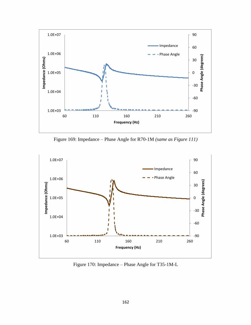
162

Figure 169: Impedance – Phase Angle for R70-1M (same as Figure 111)

Figure 170: Impedance – Phase Angle for T35-1M-L

-90

-60

-30

0

30

60

90

1.0E+03

1.0E+04

1.0E+05

1.0E+06

1.0E+07

60 110 160 210 260

Ph

ase

An

gle

(d

egr

ee

s)

Imp

ed

ance

(O

hm

s)

Frequency (Hz)

Impedance

Phase Angle

-90

-60

-30

0

30

60

90

1.0E+03

1.0E+04

1.0E+05

1.0E+06

1.0E+07

60 110 160 210 260

Ph

ase

An

gle

(d

egr

ee

s)

Imp

ed

ance

(O

hm

s)

Frequency (Hz)

Impedance

Phase Angle

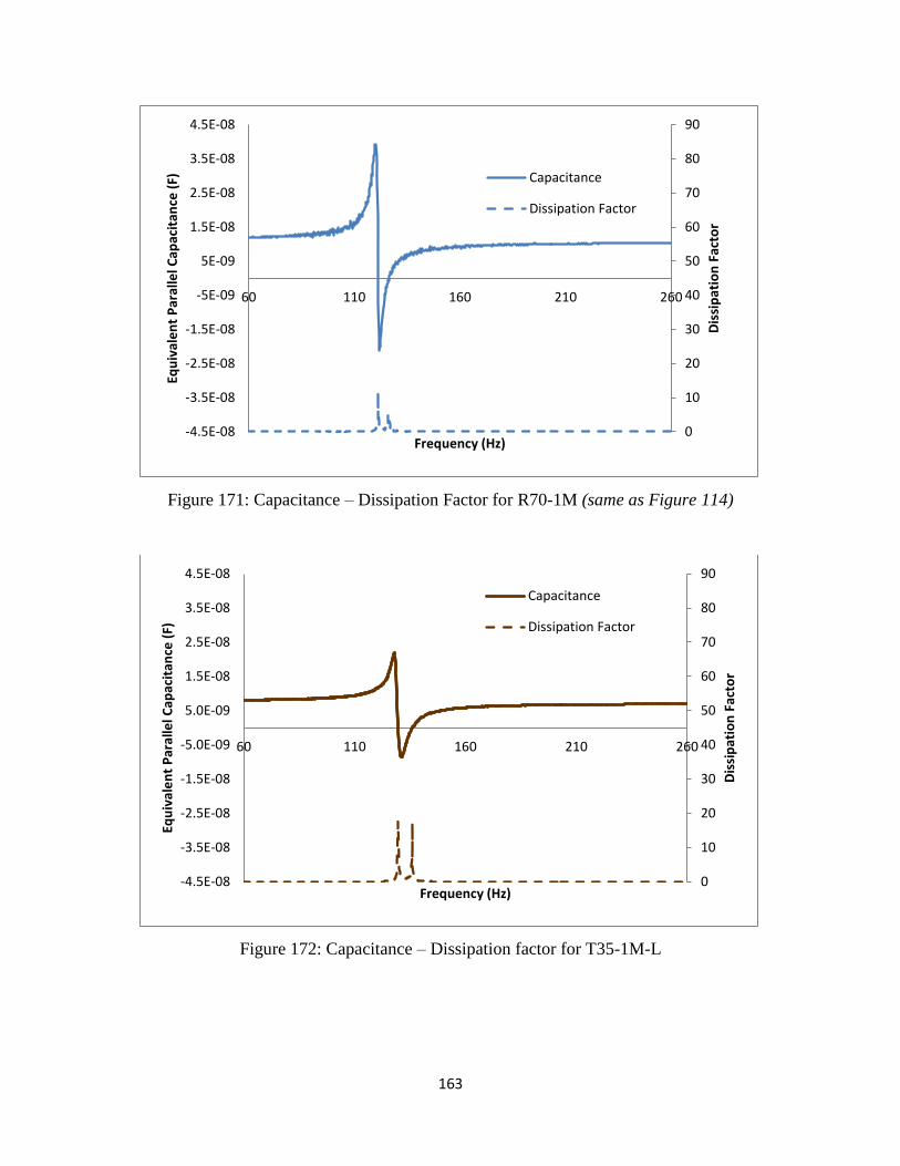
163

Figure 171: Capacitance – Dissipation Factor for R70-1M (same as Figure 114)

Figure 172: Capacitance – Dissipation factor for T35-1M-L

0

10

20

30

40

50

60

70

80

90

-4.5E-08

-3.5E-08

-2.5E-08

-1.5E-08

-5E-09

5E-09

1.5E-08

2.5E-08

3.5E-08

4.5E-08

60 110 160 210 260

Dis

sip

atio

n F

acto

r

Equ

ival

en

t P

aral

lel C

apac

itan

ce (

F)

Frequency (Hz)

Capacitance

Dissipation Factor

0

10

20

30

40

50

60

70

80

90

-4.5E-08

-3.5E-08

-2.5E-08

-1.5E-08

-5.0E-09

5.0E-09

1.5E-08

2.5E-08

3.5E-08

4.5E-08

60 110 160 210 260D

issi

pat

ion

Fac

tor

Equ

ival

en

t P

aral

lel C

apac

itan

ce (

F)

Frequency (Hz)

Capacitance

Dissipation Factor

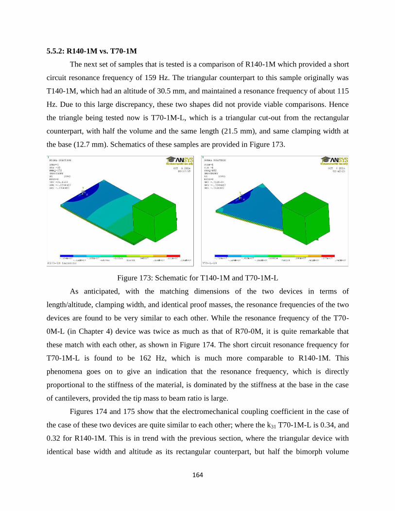
164

5.5.2: R140-1M vs. T70-1M

The next set of samples that is tested is a comparison of R140-1M which provided a short

circuit resonance frequency of 159 Hz. The triangular counterpart to this sample originally was

T140-1M, which had an altitude of 30.5 mm, and maintained a resonance frequency of about 115

Hz. Due to this large discrepancy, these two shapes did not provide viable comparisons. Hence

the triangle being tested now is T70-1M-L, which is a triangular cut-out from the rectangular

counterpart, with half the volume and the same length (21.5 mm), and same clamping width at

the base (12.7 mm). Schematics of these samples are provided in Figure 173.

Figure 173: Schematic for T140-1M and T70-1M-L

As anticipated, with the matching dimensions of the two devices in terms of

length/altitude, clamping width, and identical proof masses, the resonance frequencies of the two

devices are found to be very similar to each other. While the resonance frequency of the T70-

0M-L (in Chapter 4) device was twice as much as that of R70-0M, it is quite remarkable that

these match with each other, as shown in Figure 174. The short circuit resonance frequency for

T70-1M-L is found to be 162 Hz, which is much more comparable to R140-1M. This

phenomena goes on to give an indication that the resonance frequency, which is directly

proportional to the stiffness of the material, is dominated by the stiffness at the base in the case

of cantilevers, provided the tip mass to beam ratio is large.

Figures 174 and 175 show that the electromechanical coupling coefficient in the case of

the case of these two devices are quite similar to each other; where the k31 T70-1M-L is 0.34, and

0.32 for R140-1M. This is in trend with the previous section, where the triangular device with

identical base width and altitude as its rectangular counterpart, but half the bimorph volume

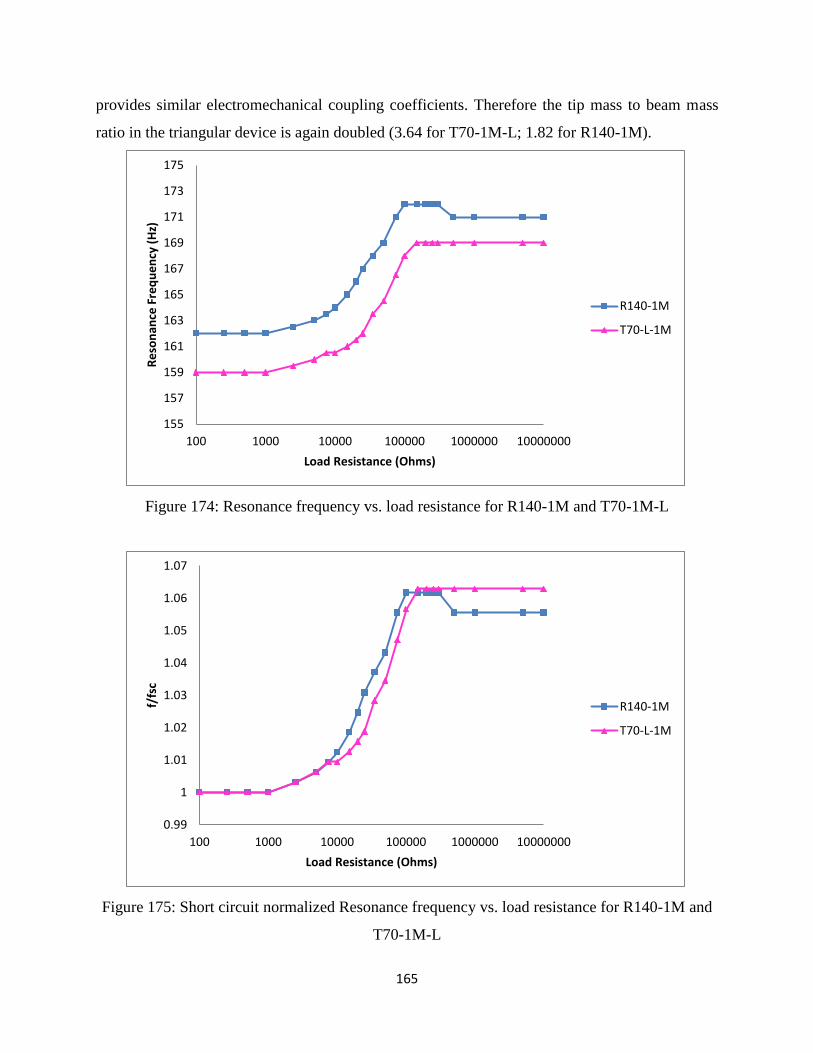
165

provides similar electromechanical coupling coefficients. Therefore the tip mass to beam mass

ratio in the triangular device is again doubled (3.64 for T70-1M-L; 1.82 for R140-1M).

Figure 174: Resonance frequency vs. load resistance for R140-1M and T70-1M-L

Figure 175: Short circuit normalized Resonance frequency vs. load resistance for R140-1M and

T70-1M-L

155

157

159

161

163

165

167

169

171

173

175

100 1000 10000 100000 1000000 10000000

Re

son

ance

Fre

qu

en

cy (

Hz)


R140-1M

T70-L-1M

0.99

1

1.01

1.02

1.03

1.04

1.05

1.06

1.07

100 1000 10000 100000 1000000 10000000

f/fs

c


R140-1M

T70-L-1M

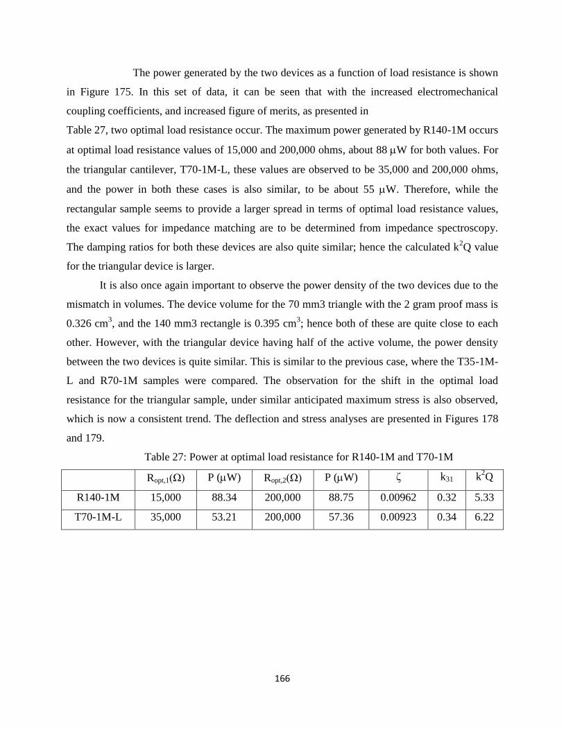
166

The power generated by the two devices as a function of load resistance is shown

in Figure 175. In this set of data, it can be seen that with the increased electromechanical

coupling coefficients, and increased figure of merits, as presented in

Table 27, two optimal load resistance occur. The maximum power generated by R140-1M occurs

at optimal load resistance values of 15,000 and 200,000 ohms, about 88 W for both values. For

the triangular cantilever, T70-1M-L, these values are observed to be 35,000 and 200,000 ohms,

and the power in both these cases is also similar, to be about 55 W. Therefore, while the

rectangular sample seems to provide a larger spread in terms of optimal load resistance values,

the exact values for impedance matching are to be determined from impedance spectroscopy.

The damping ratios for both these devices are also quite similar; hence the calculated k2Q value

for the triangular device is larger.

It is also once again important to observe the power density of the two devices due to the

mismatch in volumes. The device volume for the 70 mm3 triangle with the 2 gram proof mass is

0.326 cm3, and the 140 mm3 rectangle is 0.395 cm

3; hence both of these are quite close to each

other. However, with the triangular device having half of the active volume, the power density

between the two devices is quite similar. This is similar to the previous case, where the T35-1M-

L and R70-1M samples were compared. The observation for the shift in the optimal load

resistance for the triangular sample, under similar anticipated maximum stress is also observed,

which is now a consistent trend. The deflection and stress analyses are presented in Figures 178

and 179.

Table 27: Power at optimal load resistance for R140-1M and T70-1M


R140-1M 15,000 88.34 200,000 88.75 0.00962 0.32 5.33

T70-1M-L 35,000 53.21 200,000 57.36 0.00923 0.34 6.22

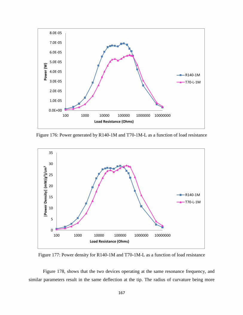
167

Figure 176: Power generated by R140-1M and T70-1M-L as a function of load resistance

Figure 177: Power density for R140-1M and T70-1M-L as a function of load resistance

Figure 178, shows that the two devices operating at the same resonance frequency, and

similar parameters result in the same deflection at the tip. The radius of curvature being more

0.0E+00

1.0E-05

2.0E-05

3.0E-05

4.0E-05

5.0E-05

6.0E-05

7.0E-05

8.0E-05

100 1000 10000 100000 1000000 10000000

Po

we

r (W

)


R140-1M

T70-L-1M

0

5

10

15

20

25

30

35

100 1000 10000 100000 1000000 10000000

|Po

we

r D

en

sity

| (m

W/g

2)/

cm3


R140-1M

T70-L-1M

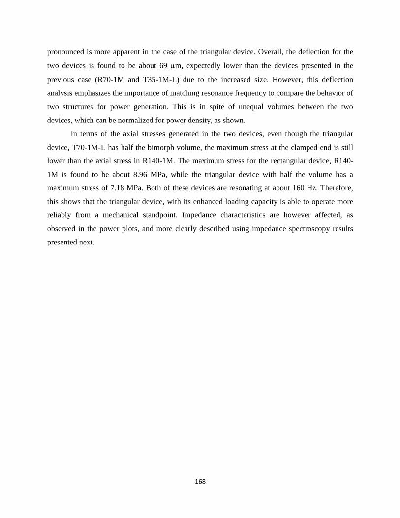
168

pronounced is more apparent in the case of the triangular device. Overall, the deflection for the

two devices is found to be about 69 m, expectedly lower than the devices presented in the

previous case (R70-1M and T35-1M-L) due to the increased size. However, this deflection

analysis emphasizes the importance of matching resonance frequency to compare the behavior of

two structures for power generation. This is in spite of unequal volumes between the two

devices, which can be normalized for power density, as shown.

In terms of the axial stresses generated in the two devices, even though the triangular

device, T70-1M-L has half the bimorph volume, the maximum stress at the clamped end is still

lower than the axial stress in R140-1M. The maximum stress for the rectangular device, R140-

1M is found to be about 8.96 MPa, while the triangular device with half the volume has a

maximum stress of 7.18 MPa. Both of these devices are resonating at about 160 Hz. Therefore,

this shows that the triangular device, with its enhanced loading capacity is able to operate more

reliably from a mechanical standpoint. Impedance characteristics are however affected, as

observed in the power plots, and more clearly described using impedance spectroscopy results

presented next.

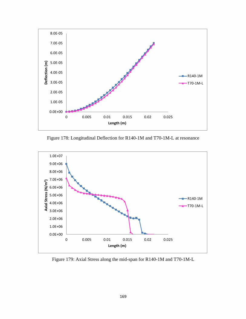
169

Figure 178: Longitudinal Deflection for R140-1M and T70-1M-L at resonance

Figure 179: Axial Stress along the mid-span for R140-1M and T70-1M-L

0.0E+00

1.0E-05

2.0E-05

3.0E-05

4.0E-05

5.0E-05

6.0E-05

7.0E-05

8.0E-05

0 0.005 0.01 0.015 0.02 0.025

De

fle

ctio

n (

m)

Length (m)

R140-1M

T70-1M-L

0.0E+00

1.0E+06

2.0E+06

3.0E+06

4.0E+06

5.0E+06

6.0E+06

7.0E+06

8.0E+06

9.0E+06

1.0E+07

0 0.005 0.01 0.015 0.02 0.025

Axi

al S

tre

ss (

N/m

2 )

Length (m)

R140-1M

T70-1M-L

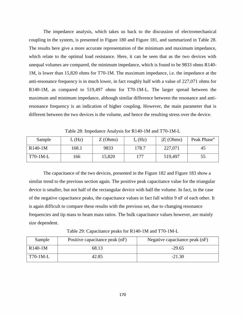
170

The impedance analysis, which takes us back to the discussion of electromechanical

coupling in the system, is presented in Figure 180 and Figure 181, and summarized in Table 28.

The results here give a more accurate representation of the minimum and maximum impedance,

which relate to the optimal load resistance. Here, it can be seen that as the two devices with

unequal volumes are compared, the minimum impedance, which is found to be 9833 ohms R140-

1M, is lower than 15,820 ohms for T70-1M. The maximum impedance, i.e. the impedance at the

anti-resonance frequency is in much lower, in fact roughly half with a value of 227,071 ohms for

R140-1M, as compared to 519,497 ohms for T70-1M-L. The larger spread between the

maximum and minimum impedance, although similar difference between the resonance and anti-

resonance frequency is an indication of higher coupling. However, the main parameter that is

different between the two devices is the volume, and hence the resulting stress over the device.

Table 28: Impedance Analysis for R140-1M and T70-1M-L


R140-1M 168.1 9833 178.7 227,071 45

T70-1M-L 166 15,820 177 519,497 55

The capacitance of the two devices, presented in the Figure 182 and Figure 183 show a

similar trend to the previous section again. The positive peak capacitance value for the triangular

device is smaller, but not half of the rectangular device with half the volume. In fact, in the case

of the negative capacitance peaks, the capacitance values in fact fall within 9 nF of each other. It

is again difficult to compare these results with the previous set, due to changing resonance

frequencies and tip mass to beam mass ratios. The bulk capacitance values however, are mainly

size dependent.

Table 29: Capacitance peaks for R140-1M and T70-1M-L


R140-1M 68.13 -29.65

T70-1M-L 42.85 -21.30

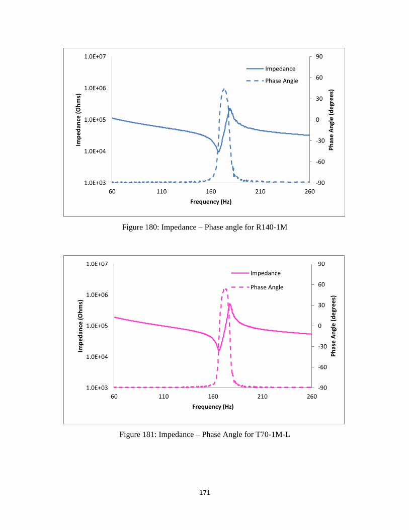
171

Figure 180: Impedance – Phase angle for R140-1M

Figure 181: Impedance – Phase Angle for T70-1M-L

-90

-60

-30

0

30

60

90

1.0E+03

1.0E+04

1.0E+05

1.0E+06

1.0E+07

60 110 160 210 260

Ph

ase

An

gle

(d

egr

ee

s)

Imp

ed

ance

(O

hm

s)

Frequency (Hz)

Impedance

Phase Angle

-90

-60

-30

0

30

60

90

1.0E+03

1.0E+04

1.0E+05

1.0E+06

1.0E+07

60 110 160 210 260

Ph

ase

An

gle

(d

egr

ee

s)

Imp

ed

ance

(O

hm

s)

Frequency (Hz)

Impedance

Phase Angle

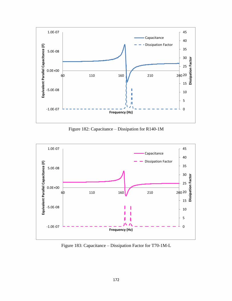
172

Figure 182: Capacitance – Dissipation for R140-1M

Figure 183: Capacitance – Dissipation Factor for T70-1M-L

0

5

10

15

20

25

30

35

40

45

-1.0E-07

-5.0E-08

0.0E+00

5.0E-08

1.0E-07

60 110 160 210 260

Dis

sip

atio

n F

acto

r

Equ

ival

en

t P

aral

lel C

apac

itan

ce (

F)

Frequency (Hz)

Capacitance

Dissipation Factor

0

5

10

15

20

25

30

35

40

45

-1.0E-07

-5.0E-08

0.0E+00

5.0E-08

1.0E-07

60 110 160 210 260D

issi

pat

ion

Fac

tor

Equ

ival

en

t P

aral

lel C

apac

itan

ce (

F)

Frequency (Hz)

Capacitance

Dissipation Factor

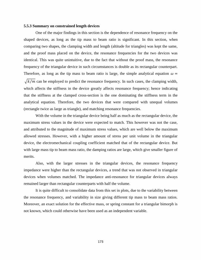
173

5.5.3 Summary on constrained length devices

One of the major findings in this section is the dependence of resonance frequency on the

shaped devices, as long as the tip mass to beam ratio is significant. In this section, when

comparing two shapes, the clamping width and length (altitude for triangles) was kept the same,

and the proof mass placed on the device, the resonance frequencies for the two devices was

identical. This was quite unintuitive, due to the fact that without the proof mass, the resonance

frequency of the triangular device in such circumstances is double as its rectangular counterpart.

Therefore, as long as the tip mass to beam ratio is large, the simple analytical equation 𝜔 =

√𝑘 𝑚⁄ can be employed to predict the resonance frequency. In such cases, the clamping width,

which affects the stiffness in the device greatly affects resonance frequency; hence indicating

that the stiffness at the clamped cross-section is the one dominating the stiffness term in the

analytical equation. Therefore, the two devices that were compared with unequal volumes

(rectangle twice as large as triangle), and matching resonance frequencies.

With the volume in the triangular device being half as much as the rectangular device, the

maximum stress values in the device were expected to match. This however was not the case,

and attributed to the magnitude of maximum stress values, which are well below the maximum

allowed stresses. However, with a higher amount of stress per unit volume in the triangular

device, the electromechanical coupling coefficient matched that of the rectangular device. But

with large mass tip to beam mass ratio, the damping ratios are large, which give smaller figure of

merits.

Also, with the larger stresses in the triangular devices, the resonance frequency

impedance were higher than the rectangular devices, a trend that was not observed in triangular

devices when volumes matched. The impedance anti-resonance for triangular devices always

remained larger than rectangular counterparts with half the volume.

It is quite difficult to consolidate data from this set in plots, due to the variability between

the resonance frequency, and variability in size giving different tip mass to beam mass ratios.

Moreover, an exact solution for the effective mass, or spring constant for a triangular bimorph is

not known, which could otherwise have been used as an independent variable.

174

5.6 Damping Ratio as a function of load resistance

One of the biggest contributing factors towards the electromechanical coupling figure of

merit 𝑘2𝑄𝑚 is the quality factor. This quality factor in common vibration literature is regarded as

the inverse of the damping ratio. In the figure of merits that have been reported in this study, the

quality factor used is the one calculated under open circuit conditions for each device. This is

done because of the fact that the voltage signal under open circuit conditions is the largest; and

as the load resistance tends to short circuit conditions, the voltage signal is very noisy and quite

difficult to read. The results in this section justify the use of the open circuit damping ratio as a

safe assumption for the mechanical quality factor.

While the literature uses the mechanical quality factor to describe the figure of merit,

very few studies [28, 57] have focused on the effect of the load resistance on damping ratio. This

section presents two sets of data on the effect of changing damping ratio with load resistance.

The first set presented is for R104-1M and T104-1M, where the two devices were found to have

pretty strong coupling with 𝑘2𝑄𝑚 > 5. The second set is from R70-2M and T70-2M, where the

𝑘2𝑄𝑚 figure of merit was approaching 2, the low coupling regime.

In both sets of data presented in Figure 184 and Figure 185, it is quite conclusive that the

damping ratio does not remain constant with load resistance. The behavior presented shows as

increase in the damping ratio with increase in load resistance up to a certain value, after which it

diminishes. This phenomenon begs a comparison with the power generated from the device.

In the case of the 104 mm3 devices with a 2 gram proof mass, it can be seen that the

damping ratio increases up to 25,000 ohms, after which a small dip is found at 35,000 ohms,

following which a small plateau exists. The damping ratio starts diminishing from 150,000 ohms.

Comparing this with the data in Table 15, the two load resistance values mentioned are the ones

where the optimal load resistance values were found for R70-1M. The plateau region is where

the power generated remained flat. In the case of the triangular sample T104-1M, a small peak at

15,000 ohms is more evident, showing a damping ratio of about 0.02 (𝑄 ≈ 33). This load

resistance is precisely the same value for the first optimal load resistance in Figure 120. The

second optimal load resistance was found at 250,000 ohms; interestingly where the damping

ratio is again 0.02. The damping ratio shows a peak values at 75,000 and 100,000 ohms, which in

the case of T104-1M triangles goes to about 0.032 (𝑄 ≈ 15). Interestingly, these are the same

load resistances where the dip in power is observed in Figure 120.

175

In the case of the 4 gram proof mass samples, as shown in Figure 185, it can be seen that

the small peak followed by a large peak at intermediate load resistance values are still evident.

The first peak for the R70-2M is observed at 15,000 ohms, and for the triangular device is

observed at 10,000 ohms. Following these peaks, a small dip is observed, at 20,000 ohms for

R70-2M, and 15,000 ohms for T70-2M. While two distinct optimal load resistance values for

power were not discernable in Figure 149, it is worth comparing this region against the

impedance minima for the two devices. The impedance at resonance frequency, although without

an external load resistor in series with the bimorph showed peak values of 24,392 ohms and

16,325 ohms for R70-2M and T70-2M respectively from Table 22, which are in good correlation

with the first peaks for the damping ratio. Therefore, the first peak damping ratio is related to the

first optimal load resistance value.

The damping ratio at the first peak of 15,000 ohms for R70-2M is 0.025; and this

particular damping ratio is found at 200,000 ohms. These are both locations where power is

maximized in Figure 149.

However, for the relatively low coupling harvester, T70-2M, which had a 𝑘2𝑄𝑚 value of

2.7, the power was maximum at 100,000 ohms; precisely the location where the maximum

damping ratio is found. Moreover, it can be seen that the damping ratio at this point is the

largest, with a value of 0.043; corresponding to a low Q-factor of about 11.6.

Therefore, damping ratio has a noticeable dependency with load resistance. The damping

ratio for triangular devices is found to be larger than rectangular counterparts. In the case of high

coupling harvesters, the damping ratio at which power is maximized is not the largest, but higher

than open or short circuit conditions. The highest damping ratio relates to the dip in the power

curve in high coupling harvesters, whereas in low coupling harvesters, it is where the power is

expected to be maximized.

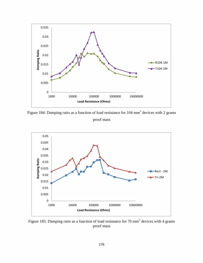
176


proof mass


proof mass

0

0.005

0.01

0.015

0.02

0.025

0.03

0.035

1000 10000 100000 1000000 10000000

Dam

pin

g R

atio


R104-1M

T104-1M

0

0.005

0.01

0.015

0.02

0.025

0.03

0.035

0.04

0.045

0.05

1000 10000 100000 1000000 10000000

Dam

pin

g R

atio


Rect - 2M

Tri-2M

177

CHAPTER 6: CONCLUSIONS & FUTURE WORK

In this study, the effect of changing geometry on cantilevered bimorphs has been

explored. Cantilevered bimorphs of traditional rectangular geometry have a limitation, which is

that the axial stress in the device under harmonic excitations is concentrated near the fixed end of

the beam. The idea of linearizing strain by altering the geometry of the device, and producing

more power has been presented in literature before. However, it was realized that in the dynamic

mode, it is very important to compare devices at matching resonance frequencies to evaluate

device characteristics. It was seen that managing the resonance frequency of two different

shapes, with and without proof mass can be a difficult task to manage. This self-imposed

constraint was attempted to be maintained throughout this study, with some success.

One of the aspects of changing geometry to enhance power output, with given constraints

that is missing in literature is an exhaustive characterization of the material, especially with

geometrical considerations. This was thoroughly performed by comparing power generated, the

calculation of electromechanical coupling, impedance spectroscopy, and comparison of damping

ratios. Several conclusions can be drawn from these studies, which are listed below:

- Changing the shape of the device from rectangular to triangular enhances the loading

capacity of the device, hence making it stiffer (consistent with literature review).

- When rectangular and triangular counterparts with no proof mass are considered, the

triangular bimorphs operate at very low axial stresses, providing more reliable operation.

They however produce less power in such a scenario.

- When rectangular and triangular counterparts with proof masses are considered, triangles

slightly produce greater power than rectangular bimorphs, provided the tip mass to beam

ratio is significant. In this study, the smallest tip mass to beam mass ratio where the triangles

outperformed rectangular counterparts was 3.6 (for example T70-1M).

- As rectangular and triangular devices with or without proof mass are compared, with each set

having matching resonance frequency and volumes, the triangular devices show enhanced

electromechanical coupling coefficients, which is quite significant for electrical parameters.

178

- With enhanced electromechanical coupling, the impedance at resonance is smaller, and

impedance at anti-resonance is larger. Therefore, power can be more easily extracted at lower

load resistance values from triangular devices, where the impedance minima are found.

- The triangular devices with larger electromechanical coupling also show larger capacitance

peaks around resonance compared to rectangular counterparts, a phenomena that was

observed very consistently. Therefore, triangular bimorphs are more efficient capacitors with

larger positive capacitance peaks, and better conductors with larger (absolute value) negative

capacitance peaks.

- The damping ratio for the triangular devices is usually larger than rectangular counterparts,

especially when resonance frequencies match. With higher damping ratios at optimal load

resistances, and smaller quality factors, a greater amount of power can be generated, and

larger electromechanical coupling figure of merits are obtained.

- Also, with smaller quality factors, the frequency bandwidth at which appreciable power can

be extracted is wider, making the devices more compliant, making them easier to tune for

resonance frequency.

- Overall, triangular bimorphs, when compared to rectangular bimorphs with matching

resonance frequency always operate with lower axial stresses, providing more reliable

operation.

Therefore, triangular devices provide several advantages over rectangular counterparts. The

only disadvantage is that with the added processes involved in cutting and producing requires

more design work or finite element modeling to target devices for certain applications. However,

with changing geometry as a function or size, it is quite difficult to manage the resonance

frequency to compare devices. Due to the fact that most parameters in this study are frequency

dependent, maintaining this becomes paramount.

From a future work perspective, an excellent study would be to study the effects of thickness

of cantilevered bimorphs, and also the thickness ratio of the piezoelectric layers to the shim

layer. However, due to the mismatch in elastic modulus and density between the shim and the

piezoelectric layers, it would be difficult to compare devices with similar resonance frequencies.

This would actually be quite difficult to constraint due to the fact that the resonance frequency in

the generic formula is directly proportional to the stiffness, and the stiffness has a cubic

proportionality with thickness. This would be a challenging but worthwhile study.

179

BIBLIOGRAPHY

[1] S. Roundy, P. K. Wright, and J. Rabaey, "A study of low level vibrations as a power

source for wireless sensor nodes," Computer Communications, vol. 26, pp. 1131-1144,

2003.

[2] H. A. Sodano, D. J. Inman, and G. Park, "A Review of Power Harvesting from Vibration

Using Piezoelectric Materials," The Shock and Vibration Digest, vol. 36, pp. 197-205,

2004.

[3] H. A. Sodano, D. J. Inman, and G. Park, "Comparison of Piezoelectric Energy Harvesting

Devices for Recharging Batteries," Journal of Intelligent Material Systems and

Structures, vol. 16, pp. 799-807, 2005.

[4] R. Overfelt, B. Jones, S. Loo, R. Haney, A. Neer, J. Andress, X. Yang, A. Zitova, B.

Prorok, and J. Fergus, "Sensors and Prognostics to Mitigate Bleed Air Contamination

Events," 2012.

[5] S. J. Roundy, "Energy Scavenging for Wireless Sensor Nodes with a Focus on Vibration

to Electricity Conversion," Mechanical Engineering, University of California, Berkeley,

Berkeley, CA, 2003.

[6] S. Roundy, P. K. Wright, and J. M. Rabaey, Energy scavenging for wireless sensor

networks: with special focus on vibrations: Kluwer Academic Publishers, 2004.

[7] K. A. Cook-Chennault, N. Thambi, and A. M. Sastry, "Powering MEMS portable

devices—a review of non-regenerative and regenerative power supply systems with

special emphasis on piezoelectric energy harvesting systems," Smart Materials and

Structures, vol. 17, p. 043001, 2008.

[8] E. K. Reilly, L. M. Miller, R. Fain, and P. Wright, "A study of ambient vibrations for

piezoelectric energy conversion," in Proc. PowerMEMS 2009, 2009, pp. 312-315.

[9] S. Priya, "Advances in energy harvesting using low profile piezoelectric transducers,"

Journal of Electroceramics, vol. 19, pp. 167-184, 2007.

[10] N. S. Shenck and J. A. Paradiso, "Energy scavenging with shoe-mounted piezoelectrics,"

Micro, IEEE, vol. 21, pp. 30-42, 2001.

[11] A. M. Karami and D. J. Inman, "Powering pacemakers from heartbeat vibrations using

linear and nonlinear energy harvesters," Applied Physics Letters, vol. 100, pp. 042901-

042901-4, 2012.

[12] S. P. Beeby, M. J. Tudor, and N. M. White, "Energy harvesting vibration sources for

microsystems applications," Measurement Science and Technology, vol. 17, pp. R175-

R195, 2006.

[13] C. B. Williams and R. B. Yates, "Analysis of a micro-electric generator for

microsystems," Sensors and Actuators A: Physical, vol. 52, pp. 8-11, 1996.

[14] A. Erturk and D. J. Inman, Piezoelectric energy harvesting: John Wiley & Sons, 2011.

[15] S. R. Anton and H. A. Sodano, "A review of power harvesting using piezoelectric

materials (2003–2006)," Smart Materials and Structures, vol. 16, p. R1, 2007.

[16] A. Khaligh, P. Zeng, and C. Zheng, "Kinetic energy harvesting using piezoelectric and

electromagnetic technologies—state of the art," Industrial Electronics, IEEE

Transactions on, vol. 57, pp. 850-860, 2010.

[17] H. Li, C. Tian, and Z. D. Deng, "Energy harvesting from low frequency applications

using piezoelectric materials," Applied Physics Reviews, vol. 1, pp. -, 2014.

180

[18] S. Roundy, E. S. Leland, J. Baker, E. Carleton, E. Reilly, E. Lai, B. Otis, J. M. Rabaey, P.

K. Wright, and V. Sundararajan, "Improving power output for vibration-based energy

scavengers," Pervasive Computing, IEEE, vol. 4, pp. 28-36, 2005.

[19] Wikimedia. Available: http://commons.wikimedia.org/wiki/File:Perovskite.svg#file

[20] F. Standards Committee of the IEEE Ultrasonics, and Frequency Control Society, "IEEE

Standard on Piezoelectricity," in ANSI/IEEE Std 176-1987, ed. New York: IEEE, 1987.

[21] T. O. Ikeda, Fundamentals of piezoelectricity. Oxford University Press, 1990.

[22] D. Shen, "Piezoelectric Energy Harvesting for Low Frequency Vibration Applications,"

Ph.D, Materials Engineering, Auburn University, Auburn, AL, 2009.

[23] S. Roundy and P. K. Wright, "A piezoelectric vibration based generator for wireless

electronics," Smart Materials and Structures, vol. 13, pp. 1131-1142, 2004.

[24] S. Roundy, "On the Effectiveness of Vibration-based Energy Harvesting," Journal of

Intelligent Material Systems and Structures, vol. 16, pp. 809-823, 2005.

[25] D. Isarakorn, D. Briand, P. Janphuang, A. Sambri, S. Gariglio, J. Triscone, F. Guy, J.

Reiner, C. Ahn, and N. De Rooij, "The realization and performance of vibration energy

harvesting MEMS devices based on an epitaxial piezoelectric thin film," Smart Materials

and Structures, vol. 20, p. 025015, 2011.

[26] A. Erturk, "Electromechanical Modeling of Piezoelectric Energy Harvesters," Doctor of

Philosophy, Engineering Mechanics, Virginia Polytechnic Institute and State University,

Blacksburg, VA, 2009.

[27] M. Umeda, K. Nakamura, and S. Ueha, "Analysis of the transformation of mechanical

impact energy to electric energy using piezoelectric vibrator," Japanese Journal of

Applied Physics, vol. 35, pp. 3267-3273, 1996.

[28] H. A. Sodano, G. Park, and D. J. Inman, "Estimation of Electric Charge Output for

Piezoelectric energy harvesting," Strain, vol. 40, pp. 49-58, 2004.

[29] A. Erturk and D. J. Inman, "A Distributed Parameter Electromechanical Model for

Cantilevered Piezoelectric Energy Harvesters," Journal of Vibration and Acoustics, vol.

130, p. 041002, 2008.

[30] A. Erturk and D. J. Inman, "An experimentally validated bimorph cantilever model for

piezoelectric energy harvesting from base excitations," Smart Materials and Structures,

vol. 18, p. 025009, 2009.

[31] J. M. Dietl and E. Garcia, "Beam shape optimization for power harvesting," Journal of

Intelligent Material Systems and Structures, vol. 21, pp. 633-646, 2010.

[32] M. Rosa and C. D. M. Junior, "Modeling and Analysis of a Piezoelectric Energy

Harvester with Varying Cross-Sectional Area," Shock and Vibration, vol. 2014, 2014.

[33] P. Glynne-Jones, S. Beeby, and N. White, "Towards a piezoelectric vibration-powered

microgenerator," in IEE Proceedings - Science, Measurement and Technology, 2001, pp.

68-72.

[34] N. M. White, P. Glynne-Jones, and S. P. Beeby, "A novel thick-film piezoelectric micro-

generator," Smart Materials and Structures, vol. 20, pp. 850-852, 2001.

[35] M. I. Friswell and S. Adhikari, "Sensor shape design for piezoelectric cantilever beams to

harvest vibration energy," Journal of Applied Physics, vol. 108, p. 014901, 2010.

[36] L. Mateu and F. Moll, "Optimum Piezoelectric Bending Beam Structures for Energy

Harvesting using Shoe Inserts," Journal of Intelligent Material Systems and Structures,

vol. 16, pp. 835-845, 2005.

http://commons.wikimedia.org/wiki/File:Perovskite.svg#file

181

[37] F. Goldschmidtboeing and P. Woias, "Characterization of different beam shapes for

piezoelectric energy harvesting," Journal of Micromechanics and Microengineering, vol.

18, p. 104013, 2008.

[38] J. H. Park, J. Kang, H. Ahn, S. B. Kim, D. Liu, and D. J. Kim, "Analysis of Stress

distribution in piezoelectric MEMS energy harvester using shaped cantilever structure,"

Ferroelectrics, vol. 409, pp. 55-61, 2010.

[39] D. Benasciutti, L. Moro, S. Zelenika, and E. Brusa, "Vibration energy scavenging via

piezoelectric bimorphs of optimized shapes," Microsystem Technologies, vol. 16, pp.

657-668, 2009.

[40] S. P. Matova, M. Renaud, M. Jambunathan, M. Goedbloed, and R. V. Schaijk, "Effect of

length/width ratio of tapered beams on the performance of piezoelectric energy

harvesters," Smart Materials and Structures, vol. 22, p. 075015, 2013.

[41] J. Park, S. Lee, and B. M. Kwak, "Design optimization of piezoelectric energy harvester

subject to tip excitation," Journal of Mechanical Science and Technology, vol. 26, pp.

137-143, 2012.

[42] D. F. Berdy, P. Srisungsitthisunti, X. Xu, J. Rhoades, B. Jung, and D. Peroulis, "Compact

low frequency meandered piezoelectric energy harvester," in PowerMEMS, Washington,

DC, 2009, pp. 71-74.

[43] M. A. Karami and D. J. Inman, "Analytical Modeling and Experimental Verification of

the Vibrations of the Zigzag Microstructure for Energy Harvesting," Journal of Vibration

and Acoustics, vol. 133, p. 011002, 2011.

[44] S. Paquin and Y. St-Amant, "Improving the performance of a piezoelectric energy

harvester using a variable thickness beam," Smart Materials and Structures, vol. 19, p.

105020, 2010.

[45] Y. Shu and I. Lien, "Efficiency of energy conversion for a piezoelectric power harvesting

system," Journal of Micromechanics and Microengineering, vol. 16, p. 2429, 2006.

[46] Y. C. Shu and I. C. Lien, "Analysis of power output for piezoelectric energy harvesting

systems," Smart Materials and Structures, vol. 15, pp. 1499-1512, 2006.

[47] G. Frank, W. Martin, E. Christoph, and W. Peter, "Parameter identification for resonant

piezoelectric energy harvesters in the low- and high-coupling regimes," Journal of

Micromechanics and Microengineering, vol. 21, p. 045006, 2011.

[48] A. Lei, R. Xu, L. M. Borregaard, M. Guizzetti, O. Hansen, and E. V. Thomsen,

"Impedance Based Characterization of a High-Coupled Screen Printed PZT Thick Film

Unimorph Energy Harvester," Journal of Microelectromechanical Systems, vol. 23, pp.

842-854, 2014.

[49] N. Kong, D. S. Ha, A. Erturk, and D. J. Inman, "Resistive impedance matching circuit for

piezoelectric energy harvesting," Journal of Intelligent Material Systems and Structures,

2010.

[50] X. Xiong and S. O. Oyadiji, "Modal electromechanical optimization of cantilevered

piezoelectric vibration energy harvesters by geometric variation," Journal of Intelligent

Material Systems and Structures, p. 1045389X13502872, 2013.

[51] Y. Yang and L. Tang, "Equivalent circuit modeling of piezoelectric energy harvesters,"

Journal of Intelligent Material Systems and Structures, vol. 20, pp. 2223-2235, 2009.

[52] Z. Meiling, E. Worthington, and J. Njuguna, "Analyses of power output of piezoelectric

energy-harvesting devices directly connected to a load resistor using a coupled

182

piezoelectric-circuit finite element method," Ultrasonics, Ferroelectrics and Frequency

Control, IEEE Transactions on, vol. 56, pp. 1309-1317, 2009.

[53] Z. Meiling, E. Worthington, and A. Tiwari, "Design study of piezoelectric energy-

harvesting devices for generation of higher electrical power using a coupled

piezoelectric-circuit finite element method," Ultrasonics, Ferroelectrics and Frequency

Control, IEEE Transactions on, vol. 57, pp. 427-437, 2010.

[54] G. Takács and B. Roha-Ilkiv, Model Predictive Vibration Control - Efficient Constrained

MPC Vibration Control for Lightly Damped Mechanical Structures: Springer, 2012.

[55] S.-B. Kim, "Piezoelectric Cantilever for Mechanical Energy Harvesting," Ph.D,

Mechanical Engineering, Auburn University, Auburn, AL, 2012.

[56] B. S. Beck, "Negative capacitance shunting of piezoelectric patches for vibration control

of continuous systems," 2012.

[57] H. Huang, C. Zheng, X. Ruan, J. Zeng, L. Zheng, W. Chen, and G. Li, "Elastic and

Electric Damping Effects on Piezoelectric Cantilever Energy Harvesting," Ferroelectrics,

vol. 459, pp. 1-13, 2014.

183

APPENDIX A: Coupled-Field Numerical Simulations

Numerical simulations using ANSYS have been performed in order to match

experimental results, and use these simulations as a tool to evaluate power generation

characteristics from devices of more complex geometry. In order to do so, a harmonic analysis is

performed on a modeled rectangular bimorph in a multi-physics environment, as described in the

methodology section. The rectangular bimorph has the same dimensions as mentioned for R70-

0M, where length is 21.5 mm, width is 6.35 mm, and the overall thickness is 0.51 mm, but here

three layers are modeled, where the piezoelectric layers are 0.19 mm and the brass layer is 0.13

mm in thickness respectively. The ANSYS model is able to calculate the transverse

displacements at the free end as shown in Figures 186 and 187, and also the electric potential

generated through the bimorph layers as shown in Figures 188 and 189.

It can be seen in Figures 188 and 189 that the value of the load resistance greatly

influences the voltage generated in the device. It is observed that, increasing values of load

resistances increase the amount of deflection in the device. This can be explained due to

increased damping in the device with increasing values of load resistances. As the amount of

electrical damping induced in the system increases, the device resonates at a lower frequency

with a greater amplitude.

Moreover, as it was seen in the previous sections that there was an optimal load

resistance for power generation. This effect may also be related to the large resonance frequency

shift that is seen in Figures 68-71 where it is seen that at load resistance values of 25k ohms and

below, the displacement and voltage plots show much lower resonance frequencies. The power

generated here would be different, since these values may be close to the optimal load resistance

of the device.

Figure 190 shows voltage generated by the device as a function of load resistances as

calculated by ANSYS and compared with experimental data. The ANSYS plot mimics the

behavior of the experimental data, but the values are quite far off from each other. This is once

again attributed to the improper damping ratio that is prescribed in the ANSYS model, which

utilized the equation ζp =1

2Q, where Q is the quality factor of the device, which was given as 32

for PZT-5H by the manufacturer. The results from the impedance analyzer measurements

suggest that this value changes when the devices are clamped as cantilevers. Therefore, the

numerical model needs to be fine-tuned with proper damping ratios.

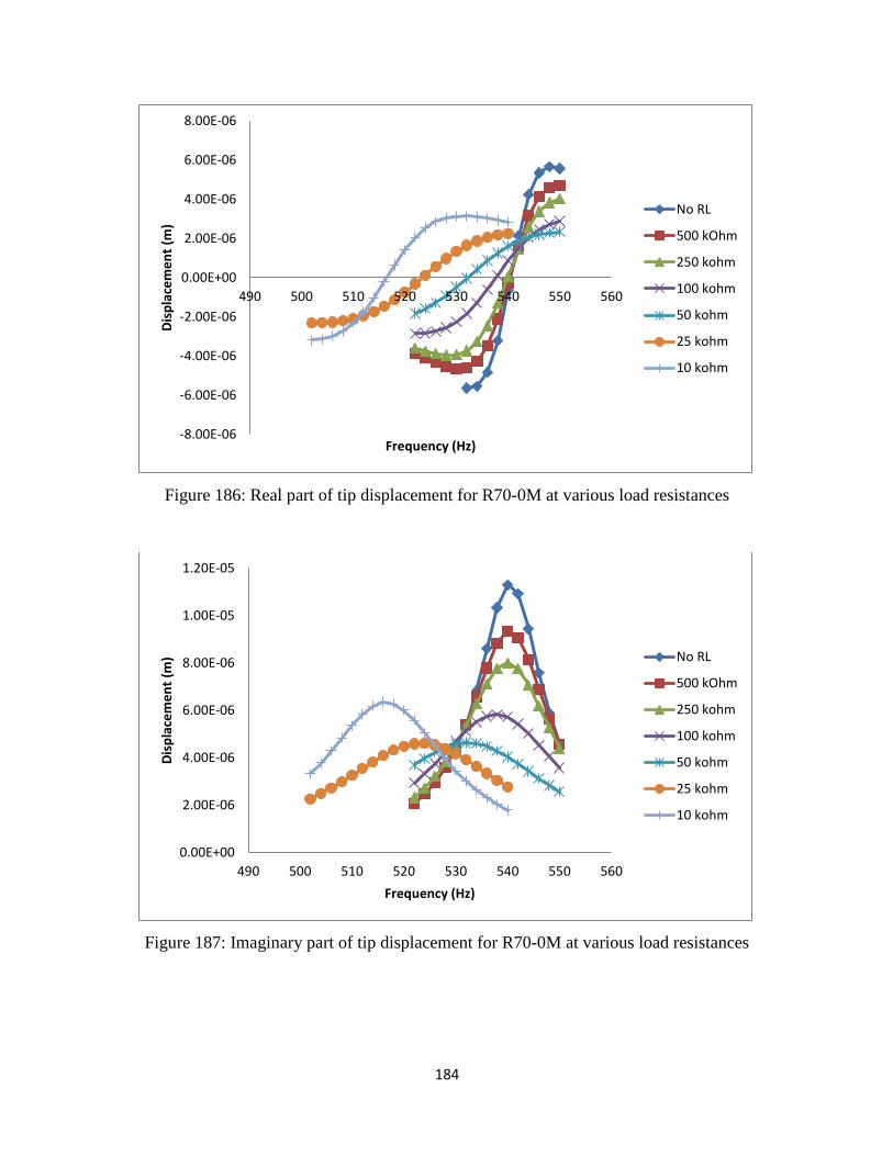
184

Figure 186: Real part of tip displacement for R70-0M at various load resistances

Figure 187: Imaginary part of tip displacement for R70-0M at various load resistances

-8.00E-06

-6.00E-06

-4.00E-06

-2.00E-06

0.00E+00

2.00E-06

4.00E-06

6.00E-06

8.00E-06

490 500 510 520 530 540 550 560

Dis

pla

cem

en

t (m

)

Frequency (Hz)

No RL

500 kOhm

250 kohm

100 kohm

50 kohm

25 kohm

10 kohm

0.00E+00

2.00E-06

4.00E-06

6.00E-06

8.00E-06

1.00E-05

1.20E-05

490 500 510 520 530 540 550 560

Dis

pla

cem

en

t (m

)

Frequency (Hz)

No RL

500 kOhm

250 kohm

100 kohm

50 kohm

25 kohm

10 kohm

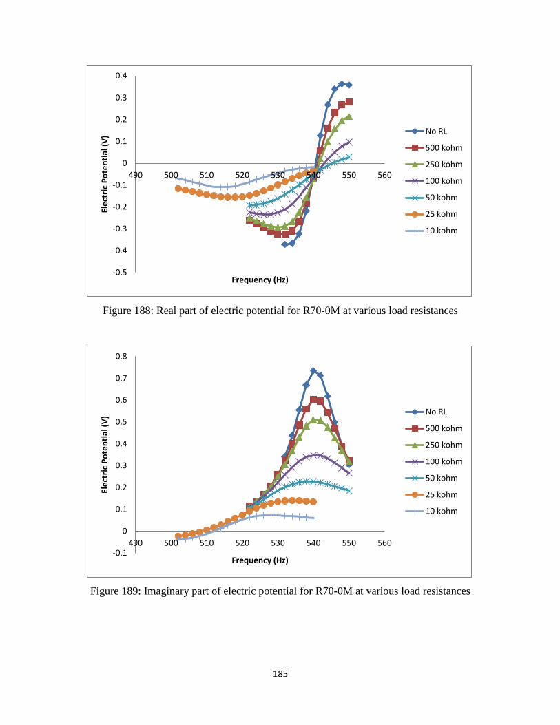
185

Figure 188: Real part of electric potential for R70-0M at various load resistances

Figure 189: Imaginary part of electric potential for R70-0M at various load resistances

-0.5

-0.4

-0.3

-0.2

-0.1

0

0.1

0.2

0.3

0.4

490 500 510 520 530 540 550 560

Ele

ctri

c P

ote

nti

al (

V)

Frequency (Hz)

No RL

500 kohm

250 kohm

100 kohm

50 kohm

25 kohm

10 kohm

-0.1

0

0.1

0.2

0.3

0.4

0.5

0.6

0.7

0.8

490 500 510 520 530 540 550 560

Ele

ctri

c P

ote

nti

al (

V)

Frequency (Hz)

No RL

500 kohm

250 kohm

100 kohm

50 kohm

25 kohm

10 kohm

186

Documents

UNDERSTANDING EFFECTS OF TAPERING CANTILEVERED