!

Understanding the Impact of Immigration on Crime*

Jörg L. Spenkuch

Northwestern University

July 2013

!!!!!!!!!!!!!!!!!!!!!!!!!!!!!!!!!!!!!!!!!!!!!!!!!!!!!!!!* I would like to thank the editor, Max Schanzenbach, an anonymous referee, as well as Gary Becker, Dana Chandler, Tony Cookson, Roland Fryer, David Toniatti, and especially Steven Levitt for helpful suggestions. I have also benefitted from comments by seminar participants at the University of Chicago and the University of Wisconsin–Whitewater. Financial support from the German National Academic Foundation is gratefully acknowledged. All views expressed in this paper as well as any remaining errors are solely my responsibility. Correspondence can be addressed to the author at Kellogg School of Management, Northwestern University, 2001 Sheridan Rd, Evanston, IL 60208, or by e-mail: j-spenkuch@kellogg.northwestern.edu.

! ! ! ! !

! 1

Abstract

Since the 1960s both crime rates and the share of immigrants among the American population have

more than doubled; and almost three quarters of Americans believe that immigration increases crime.

Yet, existing academic research has shown no such effect. Using panel data on US counties, this

paper presents empirical evidence on a systematic impact of immigration on crime. Consistent with

the economic model of crime this effect is strongest for crimes motivated by financial gain, such as

motor vehicle theft and robbery. Moreover, the effect is only present for those immigrants most

likely to have poor labor market outcomes. Failure to account for the cost of increased crime would

overstate the “immigration surplus” substantially, but it would not reverse its sign.

! ! ! ! !

! 2

I. Introduction

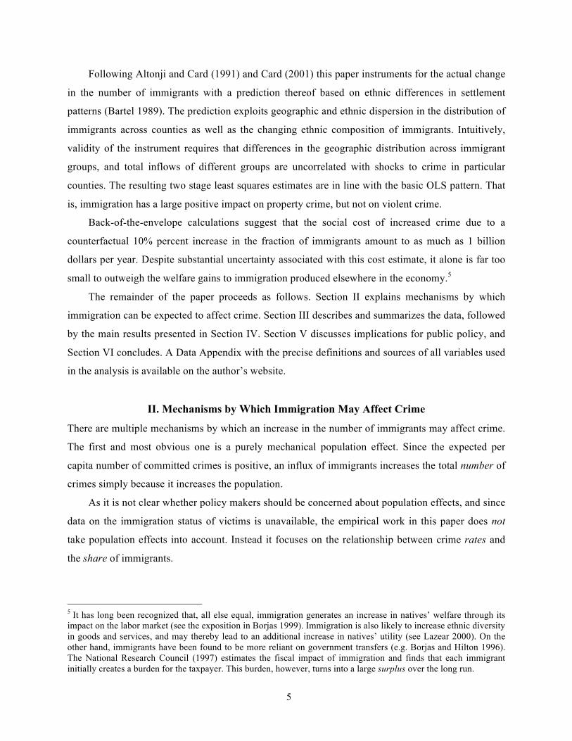
Since the end of World War II the flow of legal immigrants into the US has steadily increased.

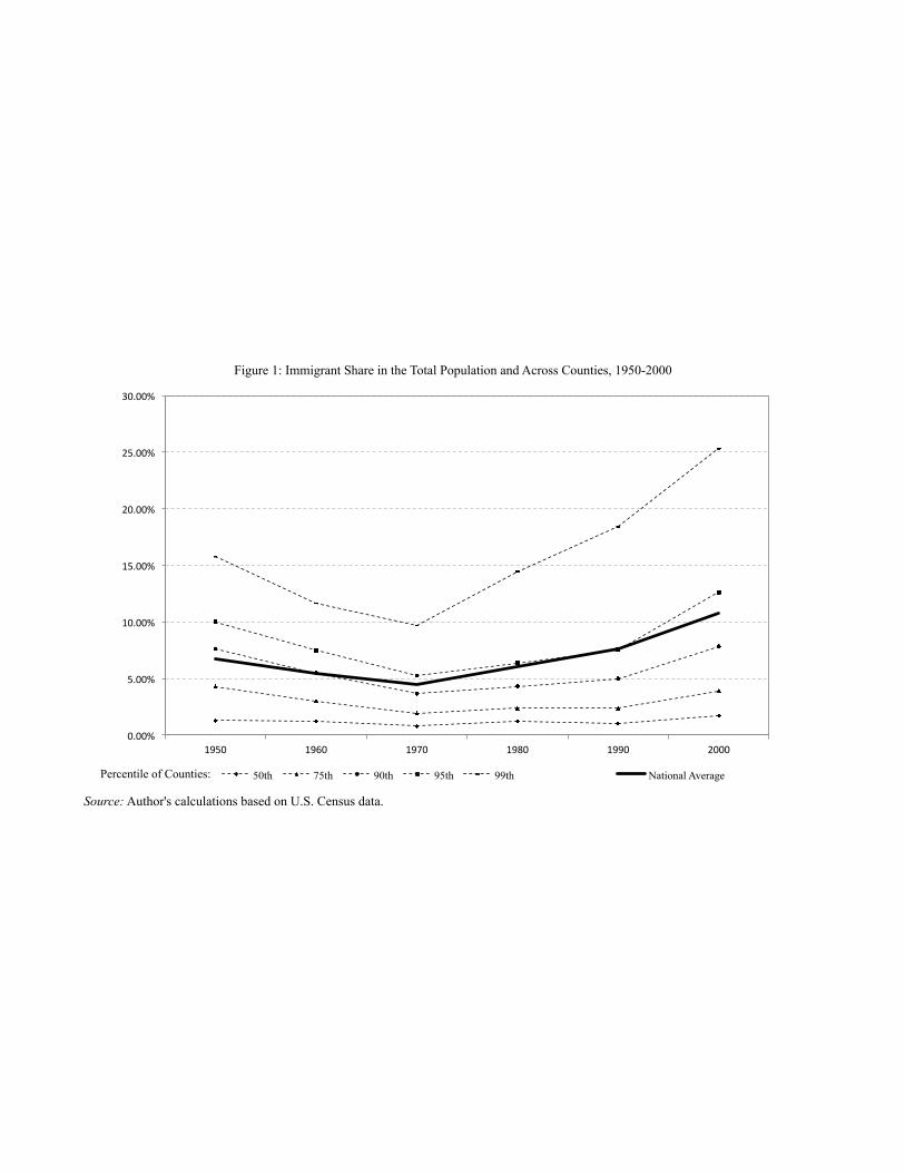
Consequently, the share of immigrants in the whole population more than doubled between 1960 and

2000 (cf. Figure 1).1 As this time period also coincided with a four-fold increase in violent crimes

and a doubling of property crime rates, it may not be surprising that Americans hold strong opinions

about the impact of immigration on crime. When asked what they think will happen as a consequence

of more immigrants coming to the US, 73.4% of respondents to the General Social Survey in 2000

thought it was “very likely” or “somewhat likely” that crime rates would increase.

Although casual empiricism hints at a link between immigration and criminal activity, the

empirical evidence is by no means unambiguous. As shown in Table 1, there exists a positive

correlation between changes property crime and changes in immigration, but there appears to be no

clear pattern for violent crime.

On theoretical grounds there are a priori reasons to believe that immigration may affect crime

rates. But the economic theory of crime offers little guidance as to the size, or even the sign of the

effect.

On one hand, theory predicts that, all else equal, individuals with lower outside options commit

more crime. Low levels of education, low wages, higher levels of unemployment, and difficulties

assimilating have all been documented for immigrants and can reasonably be associated with poorer

outside options—at least if one regards legal labor market employment as the relevant margin.

Furthermore, immigrants are disproportionately male and between the ages of 15 and 35. Existing

research has shown these groups to be especially likely to be involved in criminal activity (Freeman

1999).

On the other hand, the expected costs of committing a crime are likely higher for immigrants.

Not only do they face the same set of punishments as natives, but they are also subject to deportation,

which may be an important deterrent. Moreover, immigrants might be positively selected on various

unobservable dimensions, i.e. with respect to non-cognitive skills or industriousness, and may thus

have an inherently lower propensity to commit crime than natives.

Another channel through which immigration may affect crime are spillover effects. Even if

immigrants themselves commit fewer crimes than observationally similar natives, immigration could

cause an increase in crime if it reduces natives’ labor market opportunities inducing them to

!!!!!!!!!!!!!!!!!!!!!!!!!!!!!!!!!!!!!!!!!!!!!!!!!!!!!!!!1 Substantial uncertainty surrounds estimates of the number of illegal immigrants. A common estimate is 12.5 million for 2007.

! ! ! ! !

! 3

substitute toward criminal activity.2 At the same time immigration may be associated with positive

spillover effects. For instance, immigrants might move into and improve transitional neighborhoods

by bringing social capital that is otherwise lacking.

Although there exist extensive literatures on the economics of immigration (reviewed in Borjas

1999) and on the economics of crime (see Freeman 1999 for a survey), relatively little is known

about the impact of immigration on crime. The existing evidence relies in large part on incarceration

rates as proxy for involvement in criminal activity, and is not always consistent.3

Moehling and Piehl (2009) study incarceration rates of immigrants and natives during the first

half of the 20th century, uncovering only very small differences between the two groups. Similarly,

Butcher and Piehl (1998a, 2007) find that since the 1980s immigrants are less likely to be

incarcerated than natives, and attribute this finding to positive selection among immigrants. On the

other hand, immigrants represent a disproportionate share of inmates with drug related offenses

(Butcher and Piehl 2000). Grogger (1998) finds little evidence for spillover effects; but Borjas,

Grogger and Hanson (2010) argue that immigration caused unemployment and a decline in wages

among black men, thereby leading to an increase in incarceration rates for this group. The paper most

closely related to the present one is Butcher and Piehl (1998b). In a panel of forty-three metropolitan

areas during the 1980s, they find no effect of immigration on overall rates of crime as well as on

violent crime rates.

There exists also a recent literature on the link between immigration and crime in European

countries. Bianchi et al. (2012) study Italy, and Bell et al. (2011) look at the UK. Both papers show

that immigration had no impact on violent crime in the respective receiving countries, but may have

led to an increase in property crimes. Using decadal panel data on US counties and UCR crime data, this paper contributes to the

existing literature by presenting empirical evidence on the link between immigration and crime. The !!!!!!!!!!!!!!!!!!!!!!!!!!!!!!!!!!!!!!!!!!!!!!!!!!!!!!!!2 Although most studies have found only small effects of immigration on native’s wages and employment, it should be noted that this question has not yet been fully resolved in the literature (see Card 2001 and Borjas 2003 for opposing results). 3 In the US Census information on the institutionalized population is highly unreliable, as it is often based on administrative data or imputed. In a review of the 2000 Census the National Research Council (2004) found that for 53.0% of the prison population information on country of birth had to be imputed. Jonas (2003) shows that only 19.7% of individuals in correctional institutions filled out the Census form themselves or were interviewed by a Census enumerator, while 56.3% of answers are based on administrative data, and 24.0% result in non-response. While the foreign-born are underrepresented among the institutionalized population in the Census, recent reports by different government agencies seem to contradict this fact. The Federal Bureau of Prisons (2009), for instance, reports that 73.5% of inmates in federal prisons are native born. This means that 26.5% must have come to the US as immigrants. One possible explanation is that immigrants are overrepresented in federal prison because they are disproportionately likely to commit drug related offenses. For an overview of existing data on the immigration status of prisoners and its limitations see Camarota and Jensenius (2009).

! ! ! ! !

! 4

results presented below are broadly consistent with earlier work, but offer some new and interesting

insights with respect to the last two decades and in terms of heterogeneity among immigrant groups.

Least squares estimates suggest a large positive and statistically significant effect of

immigration on property crime. A 10% increase in the share of immigrants, i.e. slightly more than

one percentage point based on current numbers, is estimated to lead to an increase in the property

crime rate of 1.2%. To put this into perspective, an elasticity of .12 implies that the average

immigrant commits roughly 2.5 times as many property crimes as the average native.

Point estimates of the elasticity of the violent crime rate with respect to the share of immigrants

are only half as big in magnitude and sometimes negative, but statistically undistinguishable from

zero. These estimates control for county and year fixed effects as well as for changes in a host of

county characteristics over time, are robust to including county fixed effects in growth rates, and hold

in various subsamples of the data.

The most important reason for why the results reported here are at odds with those of Butcher

and Piehl (1998b) is that their sample covers only the 1980s, while this paper also considers the

1990s. As demonstrated below, the impact of immigration on crime is overwhelmingly concentrated

in the latter period.4

Decomposing property crimes and violent crimes into their respective components—i.e.

burglary, larceny, and motor vehicle theft for the former; murder, rape, aggravated assault and

robbery for the latter—shows that immigration increases each type of property crime as well as

robberies, but has almost no effect on rates of rape and aggravated assault. The point estimate with

respect to murder is large and positive, but depends heavily on the weighting scheme.

Consistent with the economic model of crime, it appears that immigration primarily increases

crimes motivated by financial gain. Moreover, splitting up immigrants into those from Mexico and

“all others” reveals that the effect is only present for the former group. As immigrants from Mexico

are particularly likely to experience poor labor market outcomes, this finding is consistent with the

economic model of crime as well.

Despite the robustness of this pattern and its concordance with the predictions of economic

theory, thorny issues of causality remain. Measurement error in the number of immigrants, omitted

variables, and endogeneity in immigrants’ settlement patterns could all bias the least squares

estimates.

!!!!!!!!!!!!!!!!!!!!!!!!!!!!!!!!!!!!!!!!!!!!!!!!!!!!!!!!4 Moreover, Butcher and Piehl’s estimates control for cities’ racial composition, in particular the fraction of Hispanics. As Table 7 shows, immigrants groups other than Mexicans have, indeed, no measurable impact on crime.

! ! ! ! !

! 5

Following Altonji and Card (1991) and Card (2001) this paper instruments for the actual change

in the number of immigrants with a prediction thereof based on ethnic differences in settlement

patterns (Bartel 1989). The prediction exploits geographic and ethnic dispersion in the distribution of

immigrants across counties as well as the changing ethnic composition of immigrants. Intuitively,

validity of the instrument requires that differences in the geographic distribution across immigrant

groups, and total inflows of different groups are uncorrelated with shocks to crime in particular

counties. The resulting two stage least squares estimates are in line with the basic OLS pattern. That

is, immigration has a large positive impact on property crime, but not on violent crime.

Back-of-the-envelope calculations suggest that the social cost of increased crime due to a

counterfactual 10% percent increase in the fraction of immigrants amount to as much as 1 billion

dollars per year. Despite substantial uncertainty associated with this cost estimate, it alone is far too

small to outweigh the welfare gains to immigration produced elsewhere in the economy.5

The remainder of the paper proceeds as follows. Section II explains mechanisms by which

immigration can be expected to affect crime. Section III describes and summarizes the data, followed

by the main results presented in Section IV. Section V discusses implications for public policy, and

Section VI concludes. A Data Appendix with the precise definitions and sources of all variables used

in the analysis is available on the author’s website.

II. Mechanisms by Which Immigration May Affect Crime

There are multiple mechanisms by which an increase in the number of immigrants may affect crime.

The first and most obvious one is a purely mechanical population effect. Since the expected per

capita number of committed crimes is positive, an influx of immigrants increases the total number of

crimes simply because it increases the population.

As it is not clear whether policy makers should be concerned about population effects, and since

data on the immigration status of victims is unavailable, the empirical work in this paper does not

take population effects into account. Instead it focuses on the relationship between crime rates and

the share of immigrants.

!!!!!!!!!!!!!!!!!!!!!!!!!!!!!!!!!!!!!!!!!!!!!!!!!!!!!!!!5 It has long been recognized that, all else equal, immigration generates an increase in natives’ welfare through its impact on the labor market (see the exposition in Borjas 1999). Immigration is also likely to increase ethnic diversity in goods and services, and may thereby lead to an additional increase in natives’ utility (see Lazear 2000). On the other hand, immigrants have been found to be more reliant on government transfers (e.g. Borjas and Hilton 1996). The National Research Council (1997) estimates the fiscal impact of immigration and finds that each immigrant initially creates a burden for the taxpayer. This burden, however, turns into a large surplus over the long run.

! ! ! ! !

! 6

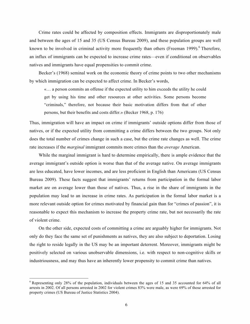
Crime rates could be affected by composition effects. Immigrants are disproportionately male

and between the ages of 15 and 35 (US Census Bureau 2009), and these population groups are well

known to be involved in criminal activity more frequently than others (Freeman 1999).6 Therefore,

an influx of immigrants can be expected to increase crime rates—even if conditional on observables

natives and immigrants have equal propensities to commit crime.

Becker’s (1968) seminal work on the economic theory of crime points to two other mechanisms

by which immigration can be expected to affect crime. In Becker’s words, «… a person commits an offense if the expected utility to him exceeds the utility he could

get by using his time and other resources at other activities. Some persons become

“criminals,” therefore, not because their basic motivation differs from that of other

persons, but their benefits and costs differ.» (Becker 1968, p. 176)

Thus, immigration will have an impact on crime if immigrants’ outside options differ from those of

natives, or if the expected utility from committing a crime differs between the two groups. Not only

does the total number of crimes change in such a case, but the crime rate changes as well. The crime

rate increases if the marginal immigrant commits more crimes than the average American.

While the marginal immigrant is hard to determine empirically, there is ample evidence that the

average immigrant’s outside option is worse than that of the average native. On average immigrants

are less educated, have lower incomes, and are less proficient in English than Americans (US Census

Bureau 2009). These facts suggest that immigrants’ returns from participation in the formal labor

market are on average lower than those of natives. Thus, a rise in the share of immigrants in the

population may lead to an increase in crime rates. As participation in the formal labor market is a

more relevant outside option for crimes motivated by financial gain than for “crimes of passion”, it is

reasonable to expect this mechanism to increase the property crime rate, but not necessarily the rate

of violent crime.

On the other side, expected costs of committing a crime are arguably higher for immigrants. Not

only do they face the same set of punishments as natives, they are also subject to deportation. Losing

the right to reside legally in the US may be an important deterrent. Moreover, immigrants might be

positively selected on various unobservable dimensions, i.e. with respect to non-cognitive skills or

industriousness, and may thus have an inherently lower propensity to commit crime than natives.

!!!!!!!!!!!!!!!!!!!!!!!!!!!!!!!!!!!!!!!!!!!!!!!!!!!!!!!!6 Representing only 28% of the population, individuals between the ages of 15 and 35 accounted for 64% of all arrests in 2002. Of all persons arrested in 2002 for violent crimes 83% were male, as were 69% of those arrested for property crimes (US Bureau of Justice Statistics 2004).

! ! ! ! !

! 7

Another channel through which immigration may affect crime are spillover effects. Borjas,

Grogger and Hanson (2010) argue that immigration caused a decline in wages and employment

among black men and thereby led to an increase in incarceration rates for this group. Thus,

immigration could cause an increase in crime rates, even if immigrants commit fewer crimes than

observationally similar natives. However, immigration may also be associated with positive spillover

effects. For instance, immigrants might move into transitional areas and improve their neighborhoods

by bringing social capital that is otherwise lacking (Putnam 2000).

In sum, there are a priori reasons to believe that immigration does affect crime rates. The

direction of the effect, however, is theoretically indeterminate.

III. Data Sources and Summary Statistics

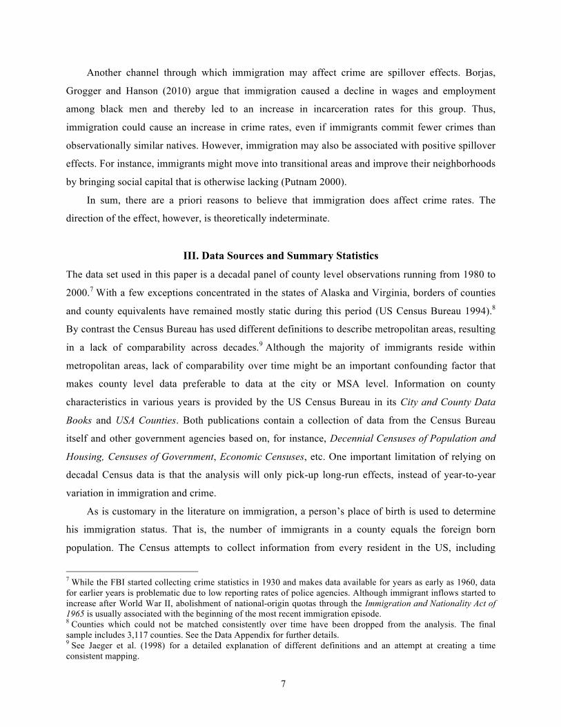
The data set used in this paper is a decadal panel of county level observations running from 1980 to

2000.7 With a few exceptions concentrated in the states of Alaska and Virginia, borders of counties

and county equivalents have remained mostly static during this period (US Census Bureau 1994).8

By contrast the Census Bureau has used different definitions to describe metropolitan areas, resulting

in a lack of comparability across decades.9 Although the majority of immigrants reside within

metropolitan areas, lack of comparability over time might be an important confounding factor that

makes county level data preferable to data at the city or MSA level. Information on county

characteristics in various years is provided by the US Census Bureau in its City and County Data

Books and USA Counties. Both publications contain a collection of data from the Census Bureau

itself and other government agencies based on, for instance, Decennial Censuses of Population and

Housing, Censuses of Government, Economic Censuses, etc. One important limitation of relying on

decadal Census data is that the analysis will only pick-up long-run effects, instead of year-to-year

variation in immigration and crime.

As is customary in the literature on immigration, a person’s place of birth is used to determine

his immigration status. That is, the number of immigrants in a county equals the foreign born

population. The Census attempts to collect information from every resident in the US, including

!!!!!!!!!!!!!!!!!!!!!!!!!!!!!!!!!!!!!!!!!!!!!!!!!!!!!!!!7 While the FBI started collecting crime statistics in 1930 and makes data available for years as early as 1960, data for earlier years is problematic due to low reporting rates of police agencies. Although immigrant inflows started to increase after World War II, abolishment of national-origin quotas through the Immigration and Nationality Act of 1965 is usually associated with the beginning of the most recent immigration episode. 8 Counties which could not be matched consistently over time have been dropped from the analysis. The final sample includes 3,117 counties. See the Data Appendix for further details. 9 See Jaeger et al. (1998) for a detailed explanation of different definitions and an attempt at creating a time consistent mapping.

! ! ! ! !

! 8

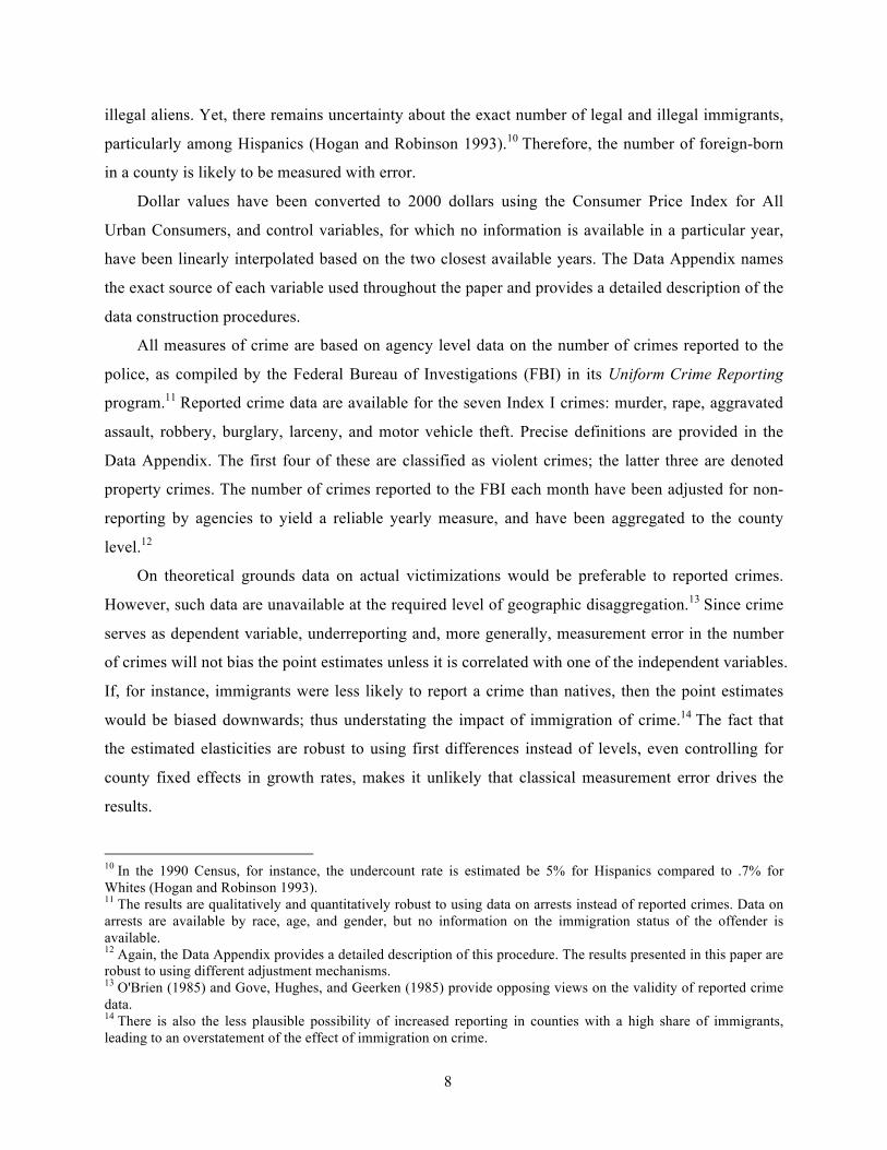
illegal aliens. Yet, there remains uncertainty about the exact number of legal and illegal immigrants,

particularly among Hispanics (Hogan and Robinson 1993).10 Therefore, the number of foreign-born

in a county is likely to be measured with error.

Dollar values have been converted to 2000 dollars using the Consumer Price Index for All

Urban Consumers, and control variables, for which no information is available in a particular year,

have been linearly interpolated based on the two closest available years. The Data Appendix names

the exact source of each variable used throughout the paper and provides a detailed description of the

data construction procedures.

All measures of crime are based on agency level data on the number of crimes reported to the

police, as compiled by the Federal Bureau of Investigations (FBI) in its Uniform Crime Reporting

program.11 Reported crime data are available for the seven Index I crimes: murder, rape, aggravated

assault, robbery, burglary, larceny, and motor vehicle theft. Precise definitions are provided in the

Data Appendix. The first four of these are classified as violent crimes; the latter three are denoted

property crimes. The number of crimes reported to the FBI each month have been adjusted for non-

reporting by agencies to yield a reliable yearly measure, and have been aggregated to the county

level.12

On theoretical grounds data on actual victimizations would be preferable to reported crimes.

However, such data are unavailable at the required level of geographic disaggregation.13 Since crime

serves as dependent variable, underreporting and, more generally, measurement error in the number

of crimes will not bias the point estimates unless it is correlated with one of the independent variables.

If, for instance, immigrants were less likely to report a crime than natives, then the point estimates

would be biased downwards; thus understating the impact of immigration of crime.14 The fact that

the estimated elasticities are robust to using first differences instead of levels, even controlling for

county fixed effects in growth rates, makes it unlikely that classical measurement error drives the

results.

!!!!!!!!!!!!!!!!!!!!!!!!!!!!!!!!!!!!!!!!!!!!!!!!!!!!!!!!10 In the 1990 Census, for instance, the undercount rate is estimated be 5% for Hispanics compared to .7% for Whites (Hogan and Robinson 1993). 11 The results are qualitatively and quantitatively robust to using data on arrests instead of reported crimes. Data on arrests are available by race, age, and gender, but no information on the immigration status of the offender is available. 12 Again, the Data Appendix provides a detailed description of this procedure. The results presented in this paper are robust to using different adjustment mechanisms. 13 O'Brien (1985) and Gove, Hughes, and Geerken (1985) provide opposing views on the validity of reported crime data. 14 There is also the less plausible possibility of increased reporting in counties with a high share of immigrants, leading to an overstatement of the effect of immigration on crime.

! ! ! ! !

! 9

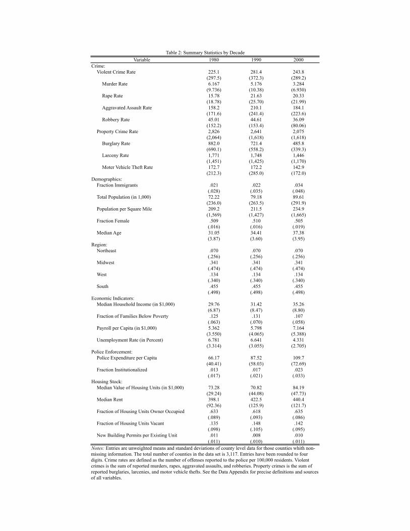
Summary statistics based on the raw, unweighted data for all variables used throughout the

analysis are presented in Table 2. There exists large variation in crime rates across counties and over

time. Most violent crimes are aggravated assaults, while the majority of property crimes are larcenies.

Crime rates increase until the late 1980s, or early 1990s and decline thereafter.15 In most cases their

variance follows a similar pattern.

The fraction of immigrants exhibits substantial variation across counties, too. As many new

immigrants settle in major cities, the share of immigrants increases much faster in the right tail of the

distribution; causing it to spread out (see also Figure 1). Over most of the sample period 90% of all

counties’ immigrant share is lower than the national average. This explains the relatively small mean

and its modest increase in Table 2.

Table 2 also shows that most counties are not very populous, and the majority of them lie in the

South and Midwest. The imbalance in population and the number of immigrants across counties

necessitates the use of appropriate weights in the analysis to follow.16

IV. Estimating the Impact of Immigration on Crime

A. Econometric Approach

The preceding discussion suggests a relationship between immigration and crime rates. In what

follows this relationship is explored more systematically by using panel data regressions to relate the

share of immigrants to county-level crime rates. The parameter of interest is the elasticity of the rate

of crime with respect to the population share of immigrants, which is identified by in the following

linear model:

(1) ,

where denotes the total number of incidences of a particular crime in county during year

, and are the total number of immigrants and residents, respectively;

!!!!!!!!!!!!!!!!!!!!!!!!!!!!!!!!!!!!!!!!!!!!!!!!!!!!!!!!15 As the data in Table 2 is not weighted, crime rates displayed therein do not match those published by the FBI in Crime in the United States. 16 Tables 8A and 8B demonstrate that the results are qualitatively robust to different weighting schemes.

!

"

!

ln(crimec,t ) ="ln(immigrantsc,t ) + #ln(populationc,t ) + $ X c,t% + µc +& t +' c,t

!

crimec,t

!

c

!

t

!

immigrantsc,t

!

populationc,t

! ! ! ! !

! 10

is a vector of additional county level covariates, denotes a county fixed effect, and a year

fixed effect. The error term is given by .17

Equation (1) is estimated by weighted least squares using county population as weights.

Standard errors are clustered at the state level to allow for arbitrary patterns of correlation in error

terms over time and across counties within a state.

The full set of additional county level covariates consists of controls for changes in

demographics, police enforcement, economic conditions, as well as quality and availability of

housing. County fixed effects absorb characteristics that are constant over time.

Covariates controlling for changes in demographic composition are the fraction of residents that

are female and the median age of the population. The natural logarithm of police expenditure per

capita and the log of the rate of institutionalization proxy for police enforcement; while the fraction

of families below the poverty line, logged median household income, payroll per capita, and the

unemployment rate proxy for economic conditions. The number of new building permits per existing

unit, the fraction of housing units that are vacant, the fraction of owner occupied units, as well as the

median rent and value of housing units control for factors affecting the quality and availability of

housing.

In choosing covariates one must be cautious not to control for endogenous factors. For instance,

immigrants and natives do differ on observables such as age, race, ethnicity, and income. By fully

controlling for these characteristics would not reflect the true effect of immigration on crime any

more. On the other hand, characteristics of a county’s population may change over time for reasons

unrelated to immigration. To the extent that these characteristics are correlated with crime one needs

to control for them in order to obtain unbiased estimates. The particular set of covariates chosen tries

to strike a balance between these two conflicting objectives. The results, however, are not sensitive to

specific controls.

At this point it is useful to point out how

!

" is identified. By including county and year fixed

effects in the econometric model only within county variation from national patterns over time

identifies the coefficients. This means that unobserved county characteristics that are constant over

time, or year effects common to all counties cannot bias the point estimate of

!

". Only unobservables

that do vary over time and across counties are a potential source of bias. For instance, new

!!!!!!!!!!!!!!!!!!!!!!!!!!!!!!!!!!!!!!!!!!!!!!!!!!!!!!!!17 To see that is the elasticity of the rate of crime with respect to the population share of immigrants rearrange (1)

to yield: .

Regarding the parameter of interest the two specifications are equivalent.

!

Xc,t

!

µc

!

" t

!

" c,t

!

"

!

"

!

lncrimec,t

populationc,t 100,000

"

# $

%

& ' =(ln

immigrantsc,tpopulationc,t

"

# $

%

& ' + )+( *1( ) ln populationc,t( ) + Xc,t

' + + µc + ln 100,000( ) +, t +- c,t

! ! ! ! !

! 11

immigrants might, ceteris paribus, be less likely to settle in a county experiencing a crime shock.

Section IV.C addresses these issues.

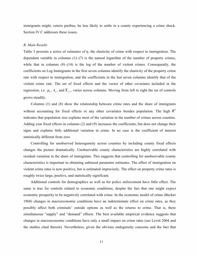
B. Main Results

Table 3 presents a series of estimates of !, the elasticity of crime with respect to immigration. The

dependent variable in columns (1)–(7) is the natural logarithm of the number of property crimes,

while that in columns (8)–(14) is the log of the number of violent crimes. Consequently, the

coefficients on Log Immigrants in the first seven columns identify the elasticity of the property crime

rate with respect to immigration, and the coefficients in the last seven columns identify that of the

violent crime rate. The set of fixed effects and the vector of other covariates included in the

regression, i.e. , , and , varies across columns. Moving from left to right the set of controls

grows steadily.

Columns (1) and (8) show the relationship between crime rates and the share of immigrants

without accounting for fixed effects or any other covariates besides population. The high

indicates that population size explains most of the variation in the number of crimes across counties.

Adding year fixed effects in columns (2) and (9) increases the coefficients, but does not change their

signs and explains little additional variation in crime. In no case is the coefficient of interest

statistically different from zero.

Controlling for unobserved heterogeneity across counties by including county fixed effects

changes the picture dramatically. Unobservable county characteristics are highly correlated with

residual variation in the share of immigrants. This suggests that controlling for unobservable county

characteristics is important in obtaining unbiased parameter estimates. The effect of immigration on

violent crime rates is now positive, but is estimated imprecisely. The effect on property crime rates is

roughly twice large, positive, and statistically significant.

Additional controls for demographics as well as for police enforcement have little effect. The

same is true for controls related to economic conditions, despite the fact that one might expect

economic prosperity to be negatively correlated with crime. In the economic model of crime (Becker

1968) changes in macroeconomic conditions have an indeterminate effect on crime rates, as they

possibly affect both criminals’ outside options as well as the returns to crime. That is, there

simultaneous “supply” and “demand” effects. The best available empirical evidence suggests that

changes in macroeconomic conditions have only a small impact on crime rates (see Levitt 2004 and

the studies cited therein). Nevertheless, given the obvious endogeneity concerns and the fact that

!

µc

!

" t

!

Xc,t

!

R2

! ! ! ! !

! 12

many of the controls are highly correlated, one should be very cautious in giving the elements of ! a

causal interpretation.

One might also argue that immigrants are more dependent on affordable housing than natives,

and that high crime rates depress housing prices. Failing to control for this effect would bias the

estimated elasticities upwards. Therefore, columns (7) and (14), which display the results of the

preferred specification, also include proxies for quality and availability of housing.

The point estimate of for violent crimes is .065 and statistically indistinguishable from zero.

The elasticity of property crime rates with respect to the share of immigrants, however, is estimated

to be .123 and is statistically significant. This constitutes an economically large effect. Taken at face

value, a 10% increase in the share of immigrants would lead to an increase in the property crime rate

of circa 1.23%.

To put this number into perspective, Levitt (1997) finds that a 10% increase in the number of

sworn police officers reduces property crime rates by 2–4%; and Levitt (1996) estimates the

elasticity of property crime rates with respect to the prison population to be -.321, i.e. a 10% increase

in the number of prisoners decreases property crime rates by circa 3.2%. To gauge the size of the

estimates it is also useful to convert them into relative crime rates.18 By this measure an elasticity

of .123 implies that immigrants commit circa 2.5 times as many crimes as the average native.19

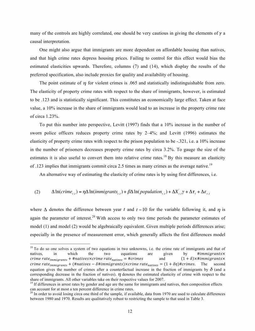
An alternative way of estimating the elasticity of crime rates is by using first differences, i.e.

(2)

where denotes the difference between year and for the variable following it, and is

again the parameter of interest.20 With access to only two time periods the parameter estimates of

model (1) and model (2) would be algebraically equivalent. Given multiple periods differences arise;

especially in the presence of measurement error, which generally affects the first differences model

!!!!!!!!!!!!!!!!!!!!!!!!!!!!!!!!!!!!!!!!!!!!!!!!!!!!!!!!18 To do so one solves a system of two equations in two unknowns, i.e. the crime rate of immigrants and that of natives, in which the two equations are given by #!""!#$%&'(×!!!"#$!!"#$!""!#$%&'! + #!"#$%&'×!"#$%!!"#$!"#$%&' = #!"#$%& and 1 + ! ×#!""!#$%&'(×!!"#$%!!"#$!""!#$%&'( + (#!"#$%&' − !#!""!#$%&'()×!"#$%!!"#$!"#$%&' = (1 + !")#!"#$%&. The second equation gives the number of crimes after a counterfactual increase in the fraction of immigrants by

!

" (and a corresponding decrease in the fraction of natives).

!

" denotes the estimated elasticity of crime with respect to the share of immigrants. All other variables take on their respective values for 2007. 19 If differences in arrest rates by gender and age are the same for immigrants and natives, then composition effects can account for at most a ten percent difference in crime rates. 20 In order to avoid losing circa one third of the sample, if available, data from 1970 are used to calculate differences between 1980 and 1970. Results are qualitatively robust to restricting the sample to that used in Table 3.

!

"

!

" ln(crimec,t ) =#" ln(immigrantsc,t ) + $" ln(populationc,t ) + "Xc,t' % + "& t + "' c,t

!

"

!

t

!

t "10

!

"

! ! ! ! !

! 13

more severely. The fact that the estimated elasticities in columns (1) and (3) of Table 4 are close to

those in Table 3, or even larger, suggests that measurement error is not a substantial problem.21 Some

of the other coefficients change sign and vary in size, but are often estimated imprecisely.

Columns (2) and (4) in Table 4 add county fixed effects to the model in equation (2). This has

the interpretation of controlling for county specific growth rates. Individual counties could be on very

different trajectories, which might influence settlement of patterns of forward-looking immigrants,

and thus be a source of bias. Controlling for county specific growth rates does not alter the estimated

effect of immigration on violent crimes. It remains close to zero. The estimated elasticity for property

crimes decreases slightly, but is very similar to that shown in Table 3 and statistically significant. It

appears that controlling for existing trends does not change the results in a meaningful way.

To facility comparison with previous work Table A.1 in the appendix displays point estimates

for models that include the share of immigrants instead of its of logged value. Since the data reject a

linear relationship between immigration and crime rates, these models use a quadratic specification.22

The sign pattern of the estimates suggests no, or even small negative effects for counties

experiencing only small changes in immigration, but large positive effects for those counties

receiving the most immigrants (relative to their respective population). Although the estimates are

less precise than their log-log counterparts, not controlling for county specific trends it is still

possible to reject the null hypothesis of no effect on the 1%-confidence level for property crime. For

results from more more flexible, semi-parametric specifications see Figure 2 in Section IV.E.

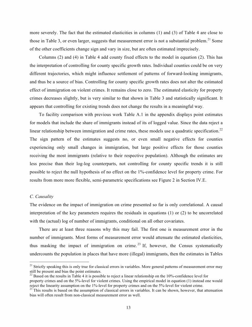
C. Causality

The evidence on the impact of immigration on crime presented so far is only correlational. A causal

interpretation of the key parameters requires the residuals in equations (1) or (2) to be uncorrelated

with the (actual) log of number of immigrants, conditional on all other covariates.

There are at least three reasons why this may fail. The first one is measurement error in the

number of immigrants. Most forms of measurement error would attenuate the estimated elasticities,

thus masking the impact of immigration on crime. 23 If, however, the Census systematically

undercounts the population in places that have more (illegal) immigrants, then the estimates in Tables !!!!!!!!!!!!!!!!!!!!!!!!!!!!!!!!!!!!!!!!!!!!!!!!!!!!!!!!21 Strictly speaking this is only true for classical errors in variables. More general patterns of measurement error may still be present and bias the point estimates. 22 Based on the results in Table 4 it is possible to reject a linear relationship on the 10%-confidence level for property crimes and on the 5%-level for violent crimes. Using the empirical model in equation (1) instead one would reject the linearity assumption on the 1%-level for property crimes and on the 5%-level for violent crime. 23 This results is based on the assumption of classical errors in variables. It can be shown, however, that attenuation bias will often result from non-classical measurement error as well.

! ! ! ! !

! 14

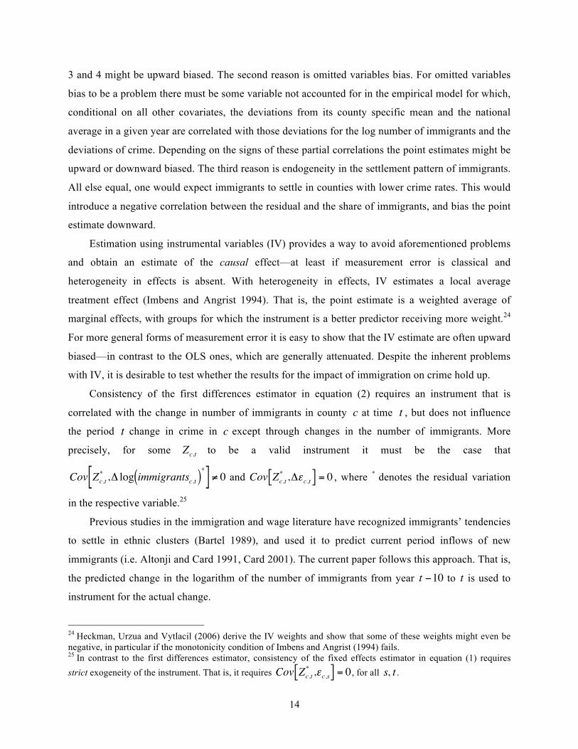
3 and 4 might be upward biased.!The second reason is omitted variables bias. For omitted variables

bias to be a problem there must be some variable not accounted for in the empirical model for which,

conditional on all other covariates, the deviations from its county specific mean and the national

average in a given year are correlated with those deviations for the log number of immigrants and the

deviations of crime. Depending on the signs of these partial correlations the point estimates might be

upward or downward biased. The third reason is endogeneity in the settlement pattern of immigrants.

All else equal, one would expect immigrants to settle in counties with lower crime rates. This would

introduce a negative correlation between the residual and the share of immigrants, and bias the point

estimate downward.

Estimation using instrumental variables (IV) provides a way to avoid aforementioned problems

and obtain an estimate of the causal effect—at least if measurement error is classical and

heterogeneity in effects is absent. With heterogeneity in effects, IV estimates a local average

treatment effect (Imbens and Angrist 1994). That is, the point estimate is a weighted average of

marginal effects, with groups for which the instrument is a better predictor receiving more weight.24

For more general forms of measurement error it is easy to show that the IV estimate are often upward

biased—in contrast to the OLS ones, which are generally attenuated. Despite the inherent problems

with IV, it is desirable to test whether the results for the impact of immigration on crime hold up.

Consistency of the first differences estimator in equation (2) requires an instrument that is

correlated with the change in number of immigrants in county at time , but does not influence

the period change in crime in except through changes in the number of immigrants. More

precisely, for some

!

Zc,t to be a valid instrument it must be the case that

!

Cov Zc,t* ," log immigrantsc,t( )*[ ] # 0 and

!

Cov Zc,t* ,"#c,t[ ] = 0 , where

!

* denotes the residual variation

in the respective variable.25

Previous studies in the immigration and wage literature have recognized immigrants’ tendencies

to settle in ethnic clusters (Bartel 1989), and used it to predict current period inflows of new

immigrants (i.e. Altonji and Card 1991, Card 2001). The current paper follows this approach. That is,

the predicted change in the logarithm of the number of immigrants from year

!

t "10 to

!

t is used to

instrument for the actual change.

!!!!!!!!!!!!!!!!!!!!!!!!!!!!!!!!!!!!!!!!!!!!!!!!!!!!!!!!24 Heckman, Urzua and Vytlacil (2006) derive the IV weights and show that some of these weights might even be negative, in particular if the monotonicity condition of Imbens and Angrist (1994) fails. 25 In contrast to the first differences estimator, consistency of the fixed effects estimator in equation (1) requires strict exogeneity of the instrument. That is, it requires

!

Cov Zc,t* ,"c,s[ ] = 0, for all

!

s, t .

!

c

!

t

!

t

!

c

! ! ! ! !

! 15

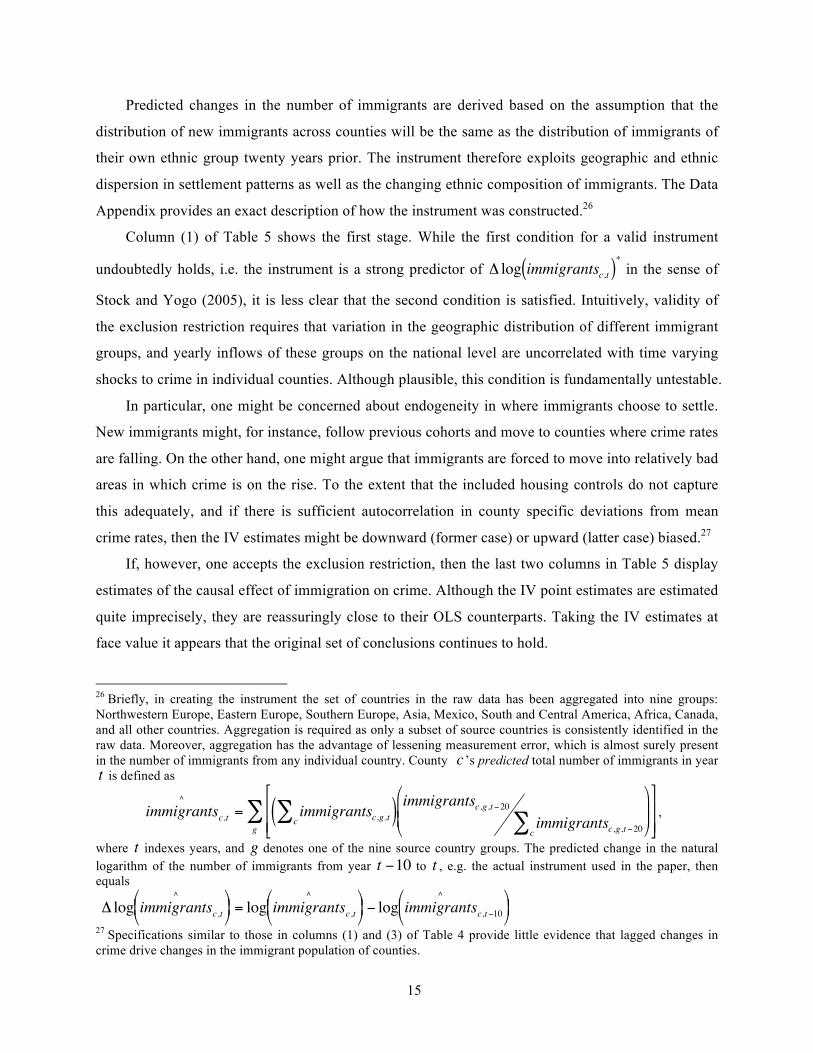
Predicted changes in the number of immigrants are derived based on the assumption that the

distribution of new immigrants across counties will be the same as the distribution of immigrants of

their own ethnic group twenty years prior. The instrument therefore exploits geographic and ethnic

dispersion in settlement patterns as well as the changing ethnic composition of immigrants. The Data

Appendix provides an exact description of how the instrument was constructed.26

Column (1) of Table 5 shows the first stage. While the first condition for a valid instrument

undoubtedly holds, i.e. the instrument is a strong predictor of

!

" log immigrantsc,t( )* in the sense of

Stock and Yogo (2005), it is less clear that the second condition is satisfied. Intuitively, validity of

the exclusion restriction requires that variation in the geographic distribution of different immigrant

groups, and yearly inflows of these groups on the national level are uncorrelated with time varying

shocks to crime in individual counties. Although plausible, this condition is fundamentally untestable.

In particular, one might be concerned about endogeneity in where immigrants choose to settle.

New immigrants might, for instance, follow previous cohorts and move to counties where crime rates

are falling. On the other hand, one might argue that immigrants are forced to move into relatively bad

areas in which crime is on the rise. To the extent that the included housing controls do not capture

this adequately, and if there is sufficient autocorrelation in county specific deviations from mean

crime rates, then the IV estimates might be downward (former case) or upward (latter case) biased.27

If, however, one accepts the exclusion restriction, then the last two columns in Table 5 display

estimates of the causal effect of immigration on crime. Although the IV point estimates are estimated

quite imprecisely, they are reassuringly close to their OLS counterparts. Taking the IV estimates at

face value it appears that the original set of conclusions continues to hold.

!!!!!!!!!!!!!!!!!!!!!!!!!!!!!!!!!!!!!!!!!!!!!!!!!!!!!!!!26 Briefly, in creating the instrument the set of countries in the raw data has been aggregated into nine groups: Northwestern Europe, Eastern Europe, Southern Europe, Asia, Mexico, South and Central America, Africa, Canada, and all other countries. Aggregation is required as only a subset of source countries is consistently identified in the raw data. Moreover, aggregation has the advantage of lessening measurement error, which is almost surely present in the number of immigrants from any individual country. County

!

c ’s predicted total number of immigrants in year

!

t is defined as

!

immigrants^

c,t = immigrantsc,g,tc"( ) immigrantsc,g,t#20 immigrantsc,g,t#20c

"$

% & &

'

( ) )

*

+ , ,

-

. / / g

" ,

where

!

t indexes years, and

!

g denotes one of the nine source country groups. The predicted change in the natural logarithm of the number of immigrants from year

!

t "10 to

!

t , e.g. the actual instrument used in the paper, then equals

!

" log immigrants^

c,t# $ %

& ' ( = log immigrants

^

c,t# $ %

& ' ( ) log immigrants

^

c,t)10# $ %

& ' (

27 Specifications similar to those in columns (1) and (3) of Table 4 provide little evidence that lagged changes in crime drive changes in the immigrant population of counties.

! ! ! ! !

! 16

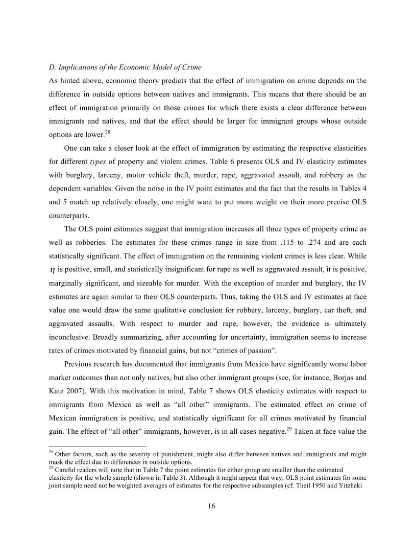
D. Implications of the Economic Model of Crime

As hinted above, economic theory predicts that the effect of immigration on crime depends on the

difference in outside options between natives and immigrants. This means that there should be an

effect of immigration primarily on those crimes for which there exists a clear difference between

immigrants and natives, and that the effect should be larger for immigrant groups whose outside

options are lower.28

One can take a closer look at the effect of immigration by estimating the respective elasticities

for different types of property and violent crimes. Table 6 presents OLS and IV elasticity estimates

with burglary, larceny, motor vehicle theft, murder, rape, aggravated assault, and robbery as the

dependent variables. Given the noise in the IV point estimates and the fact that the results in Tables 4

and 5 match up relatively closely, one might want to put more weight on their more precise OLS

counterparts.

The OLS point estimates suggest that immigration increases all three types of property crime as

well as robberies. The estimates for these crimes range in size from .115 to .274 and are each

statistically significant. The effect of immigration on the remaining violent crimes is less clear. While

is positive, small, and statistically insignificant for rape as well as aggravated assault, it is positive,

marginally significant, and sizeable for murder. With the exception of murder and burglary, the IV

estimates are again similar to their OLS counterparts. Thus, taking the OLS and IV estimates at face

value one would draw the same qualitative conclusion for robbery, larceny, burglary, car theft, and

aggravated assaults. With respect to murder and rape, however, the evidence is ultimately

inconclusive. Broadly summarizing, after accounting for uncertainty, immigration seems to increase

rates of crimes motivated by financial gains, but not “crimes of passion”.

Previous research has documented that immigrants from Mexico have significantly worse labor

market outcomes than not only natives, but also other immigrant groups (see, for instance, Borjas and

Katz 2007). With this motivation in mind, Table 7 shows OLS elasticity estimates with respect to

immigrants from Mexico as well as “all other” immigrants. The estimated effect on crime of

Mexican immigration is positive, and statistically significant for all crimes motivated by financial

gain. The effect of “all other” immigrants, however, is in all cases negative.29 Taken at face value the

!!!!!!!!!!!!!!!!!!!!!!!!!!!!!!!!!!!!!!!!!!!!!!!!!!!!!!!!28 Other factors, such as the severity of punishment, might also differ between natives and immigrants and might mask the effect due to differences in outside options. 29 Careful readers will note that in Table 7 the point estimates for either group are smaller than the estimated elasticity for the whole sample (shown in Table 3). Although it might appear that way, OLS point estimates for some joint sample need not be weighted averages of estimates for the respective subsamples (cf. Theil 1950 and Yitzhaki

!

"

! ! ! ! !

! 17

estimates for “Mexicans” suggest that an additional 1.2 million immigrants from Mexico (i.e. 10% of

the stock based on 2010 numbers) would increase property crime by almost .7% or by about 21

incidents per 100,000 inhabitants. Note, as “Mexicans” are markedly overrepresented among recent

legal and illegal immigrants, the estimates in Table 7 line up reasonably well with their counterparts

in Table 2, which suggested that a 10% increase in overall immigration would lead to an increase in

property crime of about 1.2%. Converted into crime rates, the estimates in Table 7 imply that

immigrants from Mexico commit between 3.5 and 5 times as many crimes as the average native,

while “all other” immigrants commit less than half as many crimes as natives.30

E. Sensitivity and Robustness

Tables 8A and 8B explore the sensitivity of the estimated elasticities across different specifications

and a wide variety of subsamples of the data. Only coefficients on Log Immigrants and associated

standard errors are reported. The first row in each table displays the baseline results, i.e. those from

the preferred specification.

The following two rows show that weighting has little influence on the point estimates, although

it does decrease them. In particular, results corrected for missing observations by inverse probability

weighting (IPW) are almost identical to the baseline results.31 Weighting seems to matter only for the

elasticity of murder with respect the share of immigrants.

In general, the estimates for murder vary widely across specifications and samples. However,

those for other types of crime are much more robust, especially those for crimes motivated by

financial gain.

Splitting the sample up by year and analyzing each cross-section separately shows that the effect

of immigration on property crimes is concentrated in the period from 1990 to 2000. This is consistent

with existing evidence on lower labor market returns for this later cohort of immigrants (e.g. Borjas

1990).

!!!!!!!!!!!!!!!!!!!!!!!!!!!!!!!!!!!!!!!!!!!!!!!!!!!!!!!!!!!!!!!!!!!!!!!!!!!!!!!!!!!!!!!!!!!!!!!!!!!!!!!!!!!!!!!!!!!!!!!!!!!!!!!!!!!!!!!!!!!!!!!!!!!!!!!!!!!!!!!!!!!!!!!!!!!!!!!!!!!1989). One reason for this surprising difference is that the estimated fixed effects as well as the trends terms differ across samples. This means that depending on the specification and on the sample the residual variation in crime rates and the share immigrants that identifies the coefficient of interest will be different. 30 A potential concern with these estimates is that Mexicans might not be as able as other immigrant groups to move away from areas that are on the decline. One way to address this issue is to directly control for changes in a counties population. If natives or other immigrant groups were indeed more able to move out of areas that experience higher rates of crime, then one would expect this to be reflected in changes in population. Yet, controlling for changes in population has practically no effect on the coefficients of interest. 31 IPW weights each observation by the inverse of the predicted probability of having a non-missing value. This is a valid non-parametric correction procedure if the probability of an observation containing missing information does not depend on unobservables.

! ! ! ! !

! 18

Of the 124 estimated elasticities for burglary, larceny, motor vehicle theft, and robbery, only 9

do not carry the expected sign, e.g. are negative. If all coefficients were independently distributed—

which is an obvious oversimplification—the probability that 9 or fewer of them would be negative is

effectively zero if immigration had no effect on crimes related to monetary gain. Thus, one would

reject the null that the elasticity of these crimes with respect to the share of immigrants is non-

positive.32 Of the 93 estimated elasticities for murder, rape, and aggravated assault, however, 29 are

negative. While this is less than the expected value under the null with independently distributed

coefficients (and would still lead to rejection of the null), once one takes into account that the

estimates are probably positively correlated the null appears less implausible.

There is some evidence that the effect of immigration on crime in the Northeast differs from that

in the rest of the country. With the exception of robbery, all elasticity estimates are negative for this

region. One admittedly unsatisfactory explanation is that the Northeast receives proportionately

fewer immigrants with poor labor market prospects. For instance, the fraction of immigrants from

Mexico is lower in the Northeast, than in the South and the West. However, Tables 8A and 8B also

show that the estimated effects are not solely driven by the “classical” immigration states California,

Texas, and Florida. In line with the results from Table A.1, the estimates in Tables 8A and 8B

demonstrates that the effects are driven by those counties receiving the largest influx of immigrants,

i.e. by counties falling into the second and third tercile of immigrants received between 1960 and

2000.

Lastly, Figure 2 provides additional robustness checks of the main results with respect to the

log-log specification in equations (1) and (2). The log-log functional form posits that the effect of a

percentage point increase in the share of immigrants has a different effect depending on the base

share. On theoretical grounds there is, of course, no clear reason to prefer this specification to one in

levels, i.e. one that posits a constant effect.

Elementary specification tests, however, strongly reject the assumption of a constant effect. That

is, the data suggest a relationship that is non-linear. To impose as little structure as possible Figure 2

displays semi-parametric estimates of functional relationship between immigration and crime. More

specifically, the left panels estimate

!!!!!!!!!!!!!!!!!!!!!!!!!!!!!!!!!!!!!!!!!!!!!!!!!!!!!!!!32 To see this, note that if the effect of immigration on these crimes is zero, then the probability of one coefficient being negative is one half, and the probability of any number of them being negative is binomially distributed. The probability that 17 or fewer of them are negative is given by Pr # ≤ 9 = !(!, .5)!

!!! ,where !(!, .5) denotes the binomial probability mass function for successes given the respective number of tries and a success probability of .5.

!

j

! ! ! ! !

! 19

(3a) ! ln !"#$!_!"#$!,! = ! ! ln !ℎ!"!_!""!#$%&'(!,! ! +!" ln !"!#$%&'"!!,! + !!!,!! ! + !!! + !!!,!, whereas those on the right correspond to

(3a) !"#$%!_!"#$!,! = ! !"ℎ!"!_!""!#$%&'(!,!

+!" ln !"!#$%&'"!!,! + !!!,!! ! + !!! + !!!,!. In both specifications the only restriction placed on !(∙) is that it is a continuous function of its one

argument. Thus, !(∙) will capture any possible nonlinearities in the relationship between changes in

immigration and changes crime. For details on the estimation procedure see Yatchew (1998).

As was the case in the previous (parametric) analysis, there is no clear evidence for an effect of

immigration on violent crime, independent of whether immigration and crime are measured in logs or

levels. In both cases, there are regions in which the slope of !(∙) is positive and ones in which it is

negative. Overall, in either of the lower two panels one cannot reject the null hypothesis of a zero

slope at all points.

This not the case when it comes to property crimes, as evidenced by the upper two panels. For

about 90% of counties the slope of !(∙), and hence the impact of immigration on property crime, is

positive. Moreover, the confidence bands are narrow enough to rule out no effect at all.

Interestingly, and somewhat at odds with the previous conclusions based on the log-log

specification when both crime rates and immigrant shares are measured in levels there seems to be a

negative relationship between immigration and crime for the 10% of counties that experienced that

largest immigration shock. Unfortunately, due to the relatively small number of counties in that

region and the large standard errors, it is difficult to explore this difference between the log-log and

level-level models more systematically. For instance, while it is possible to reject the null hypothesis

of equal changes in property crime rates at the 90th and 95th percentile in the distribution of counties,

it is not possible to do so for any two counties that experienced in increase in the share of immigrants

greater than 3 percentage points. Moreover, one might be concerned that counties which experienced

the largest influx of immigrants are exactly those that are also hit by some other kind of shock, say a

booming economy, which might, all else equal, depress crime.

Yet, even ignoring these important endogeneity concerns and taking the estimates in the panel

on the top right at face value, the average slope across counties is 783, indicating a positive impact of

immigration on rates of property crime. However, as is apparent from Figure 2, the average slope

will understate the effect for the vast majority of counties. The mean slope in the panel on the top left

is .063 and statistically indistinguishable from the parametric estimates in Tables 3 and 4.

! ! ! ! !

! 20

V. Policy Implications

To facilitate interpretation of the magnitude of the estimated effects and to aid in drawing

conclusions for public policy, estimates of the social cost of an immigration-induced increase in

crime are required. This section performs back of the envelope calculations for a counterfactual

increase in the stock of immigrants by 10%, which corresponds to about 3.7 million individuals in

2007. While the welfare estimates in this section refer to the US at the whole, it is important to note

that they are unlikely to be evenly distributed over localities.

Following Levitt (1996), estimates by Cohen (1988) and Miller, Cohen, and Rossman (1993) of

monetary and quality of life losses due to crime are used to derive the social cost of an immigration-

induced increase in crime. These papers attempt to capture both monetary costs, such as property loss,

medical bills, decreases in productivity, etc., as well as reductions in the quality of life due to

victimization. Estimates of reductions in the quality of life are based on jury awards in civil suits

(excluding punitive damages), which are mapped into distributions for a variety of injuries associated

with different types of crime. As these cost estimates correspond to the average crime and the

average crime might be more serious than the marginal one, they may overstate the cost of the

marginal crime. The cost estimates, however, do not include expenses related to victim precaution,

legal fees, or losses to employers.

Another important caveat in interpreting the following cost estimates is that they rely on the

assumption that the cost of reported and unreported crimes are equal. According to the National

Crime Victimization Survey in 2007 less than 40% of all crimes were reported to the police (US

Department of Justice 2010). Even serious crimes, such as aggravated assault and robbery, have

reporting rates of less than two thirds. Moreover, it is assumed that the elasticity of each type of

crime with respect to the share of immigrants is the same for reported and unreported crimes. This

assumption is potentially problematic, as crimes committed by and especially against immigrants

might be less likely to be reported.

Table 9 presents estimated yearly cost from a counterfactual increase in the share of immigrants

by 10%. As the analysis above finds no clear effect of immigration on “crimes of passion,” the table

takes only crimes related to monetary gain into account. Including murder, rape, and aggravated

assault would increase the social cost estimate in the upper panel and decrease the estimate in the

lower one. The basic conclusion, however, would remain unchanged (detailed results are available

from the author upon request). The values in Table 9 are in 2007 dollars and based on the number of

! ! ! ! !

! 21

crimes in 2007. The upper panel uses the OLS elasticity estimates from Table 6, while the lower one

relies on the respective IV estimates. Given the inherent uncertainty surrounding these back of the

envelope calculations the numbers reported in Table 9 should be taken with a grain of salt. At the

same time, when it comes to public policy it is paramount to think about social costs and benefits.

Columns (1) and (2) show the estimated change in the number of reported and unreported

crimes for each type of offense, respectively. The bulk of the increase in the number of crimes is due

to the least costly property crimes. Columns (3) and (4) are the Cohen (1988) and Miller, Cohen, and

Rossman (1993) cost estimates inflated to 2007 dollars.34 Column (5) combines the information in

the preceding columns and displays the estimated yearly social cost due to changes in crime

following a counterfactual increase in the share of immigrants.

The estimated costs for crimes related to monetary gain sum to slightly more than 760 million

dollars per year in the upper panel, and to about 940 million dollars in the lower one. Considering the

nature of the underlying assumptions and the variability in the elasticity estimates, in particular the

ones with respect to aggravated assault, these welfare calculations should be interpreted cautiously—

although both IV and OLS estimates lead to qualitatively very similar conclusions.

Despite the uncertainty surrounding the numbers in Table 9, it is useful to put them into

perspective. For instance, in 2007 the Department of Homeland Security spent circa 12 billion dollars

on border protection and immigration enforcement (US Department of Homeland Security 2007).

Another way to frame the cost estimates is to contrast them with estimates of the benefits of

immigration (accruing to natives). Borjas, Freeman, and Katz (1997) have estimated an annual gain

to the US economy due to the post-1979 inflow of immigrants into the labor market between .05

and .13 percent of GDP.35 In 2007 this amounts to approximately 7-18 billion dollars.

Under the assumption that the elasticity of crime with respect to the share of immigrants is

constant, the cost estimates in Table 9 can be extrapolated. Between 1980 and 1995, the last year

considered by Borjas, Freeman, and Katz (1997), the share of immigrants increased by almost 50%.

This yields a yearly cost estimate of approximately 3.8-4.7 billion dollars. Even if we were to

multiply this estimate by a factor of two, the social cost associated with an immigration induced

!!!!!!!!!!!!!!!!!!!!!!!!!!!!!!!!!!!!!!!!!!!!!!!!!!!!!!!!34 The estimates in Miller, Cohen, and Rossman (1993) update and extent those of Cohen (1988), but are only available for violent crimes. 35 The last year taken into account by Borjas, Freeman, and Katz (1997) is 1995. Since immigration continued to increase, their estimate understates the current welfare gain to immigration. Somewhat ironically the “immigration surplus” rises with its (negative) impact on wages (see Borjas 1999 for an exposition), which means that the welfare gain to immigration increases with the price elasticity of labor demand. Studies simulating the economic impact of immigration for a variety of elasticity values have found an immigration surplus between .01 and .3 percent of GDP (see Borjas 1999 and the studies cited therein).

! ! ! ! !

! 22

increase in property crime would still fall on the vey low end of the interval estimated by Borjas,

Freeman, and Katz (1997). Based on these back-of-the-envelope calculations it seems highly unlikely

that the costs due to an increase in crime outweigh the welfare gains produced elsewhere in the

economy.

VI. Conclusion

The economic theory of crime predicts that, all else equal, individuals with lower outside options

commit more crimes than others. While immigrants are known to have lower levels of education,

lower wages, and higher unemployment rates than natives, previous studies have not found a

relationship between immigration and crime, or proxies thereof.

Using decadal panel data on US counties from 1980 to 2000 this paper presents empirical

evidence of a systematic and economically meaningful impact of immigration on crime. A 10%

increase in the share of immigrants is estimated to lead to an increase in the property crime rate of

circa 1.2%, while the rate of violent crimes remains essentially unaffected.

Consistent with economic theory the effect of immigration on crime is stronger for crimes

motivated by financial gain, for instance robbery or motor vehicle theft, but not for “crimes of

passion”, such as rape, and aggravated assault. Moreover, the effect of immigration is only present

for immigrants from Mexico, who are more likely than others to have poor labor market outcomes.

The social costs of an immigration-induced increase in crime are substantial. Failure to account

for the cost of increased crime would overstate the social gain to a counterfactual 10% percent

increase in the fraction of immigrants by about 750–940 million dollars per year. Despite the

uncertainty associated with this cost estimate, it is far too small to outweigh the welfare gains to

immigration produced elsewhere in the economy.

References

Altonji, Joseph G., and David Card (1991). “The Effects of Immigration on the Labor Market Outcomes of Less-Skilled Natives,” (pp. 201-234) in John M. Abowd and Richard B. Freeman, eds., Immigration, Trade, and the Labor Market. Chicago: University of Chicago Press.

Bartel, Ann (1989). “Where Do the New U.S. Immigrants Live?” Journal of Labor Economics, 7, 371-391.

Becker, Gary S. (1968). “Crime and Punishment: An Economic Approach,” Journal of Political Economy, 76, 169-217.

Bell, Brian, Stephen Machin, and Francesco Fasani (2011). “Crime and Immigration: Evidence from Large Immigrant Waves,” Review of Economics and Statistics, forthcoming.

! ! ! ! !

! 23

Bianchi, Milo, Paolo Buonanno, and Paolo Pinotti (2012). “Do Immigrants Cause Crime?” Journal of the European Economic Association, forthcoming.

Borjas, George J. (1990). Friends or Strangers: The Impact of Immigrants on the U.S. Economy. New York: Basic Books.

Borjas, George J. (1999). “The Economic Analysis of Immigration,” (pp. 1697-1760) in Orley C. Ashenfelter and David Card, eds., Handbook of Labor Economics, Vol 3. Amsterdam: Elsevier.

Borjas, George J. (2003) “The Labor Demand Curve Is Downward Sloping: Reexamining the Impact of Immigration on the Labor Market,” Quarterly Journal of Economics, 118, 1335-1374.

Borjas, George J., Richard B. Freeman, and Lawrence F. Katz (1997). “How Much Do Immigration and Trade Affect Labor Market Outcomes?” Brookings Papers on Economic Activity, 1, 1-90.

Borjas, George J., Jeffrey Grogger, and Gordon H. Hanson (2010). “Immigration and the Economic Status of African-American Men,” Economica, 77, 255-282.

Borjas, George J., and Lynette Hilton (1996) “Immigration and the Welfare State: Immigrant Participation in Means-Tested Entitlement Programs,” Quarterly Journal of Economics, 111, 575-605.

Borjas, George J., and Lawrence F. Katz (2007). “The Evolution of the Mexican-Born Workforce in the United States,” (pp. 13-56) in George J. Borjas and Lawrence F. Katz, eds., Mexican Immigration to the United States. Chicago: University of Chicago Press.

Butcher, Kristin F. and Anne Morrison Piehl (1998a). “Recent Immigrants: Unexpected Implications for Crime and Incarceration,” Industrial and Labor Relations Review, 51, 654-679.

Butcher, Kristin F. and Anne Morrison Piehl (1998b). “Cross-City Evidence on the Relationship between Immigration and Crime,” Journal of Policy Analysis and Management, 17, 457-493.

Butcher, Kristin F. and Anne Morrison Piehl (2000). “The Role of Deportation in the Incarceration of Immigrants,” (pp. 351-385) in George J. Borjas, ed., Issues in the Economics of Immigration. Chicago: University of Chicago Press.

Butcher, Kristin F. and Anne Morrison Piehl (2007). “Why are Immigrants’ Incarceration Rates so Low? Evidence on Selective Immigration, Deterrence, and Deportation.” NBER Working Paper No. 13229.

Camarota, Steven A. and Karen Jensenius (2009). “Immigration and Crime: Assessing a Conflicted Issue.” Center for Immigration Studies.

Card, David (2001). “Immigrant Inflows, Native Outflows, and the Local Market Impacts of Higher Immigration,” Journal of Labor Economics, 19, 22-64.

Cohen, Mark (1988). “Pain, Suffering and Jury Awards: A Study of the Cost of Crime to Victims,” Law and Society Review, 22, 537-555.

Federal Bureau of Prisons (2009). The State of the Bureau 2008. Washington, D.C.: US Department of Justice.

Freeman, Richard B. (1999). “The Economics of Crime,” (pp. 3529-3571) in Orley C. Ashenfelter and David Card, eds., Handbook of Labor Economics, Vol 3. Amsterdam: Elsevier.

Gove, Walter, Michael Hughes, and Michael Geerken (1985). “Are Uniform Crime Reports a Valid Indicator of the Index Crimes? An Affirmative Answer with Minor Qualifications,” Criminology, 23, 451-501.

! ! ! ! !

! 24

Grogger, Jeffrey (1998) “Immigration and Crime among Young Black Men: Evidence from the NLSY,” (pp. 322-341) in Daniel S. Hamermesh and Frank D. Bean, eds., Help or Hindrance? The Economic Implications of Immigration for African Americans. New York: Russell Sage Foundation.

Heckman, James J., Sergio Urzua and Edward Vytlacil (2006) “Understanding Instrumental Variables in Models with Essential Heterogeneity,” Review of Economics and Statistics, 88, 389-432.

Hogan, Howard and Gregory Robinson (1993). “The Proceedings of the 1993 Research Conference on Undercounted Ethnic Population.” US Census Bureau Technical Papers.

Imbens, Guido W. and Joshua D. Angrist (1994) “Identification and Estimation of Local Average Treatment Effects,” Econometrica 62, 467-75.

Jaeger, David A., Susanna Loeb, Sarah E. Turner and John Bound (1998). “Coding Geographic Areas Across Census Years: Creating Consisting Definitions of Metropolitan Statistical Areas.” NBER Working Paper No. 6772.

Jonas, Kimball (2003). Group Quarters Enumeration. Census 2000 Evaluation E.5, US Census Bureau.

Lazear, Edward P. (2000). “Diversity and Immigration,” (pp. 117 - 142) in George J. Borjas, ed., Issues in the Economics of Immigration. Chicago: University of Chicago Press.

Levitt, Steven D. (1996). “The Effect of Prison Population Size on Crime Rates: Evidence from Prison Overcrowding Litigation,” Quarterly Journal of Economics, 111, 319-351.

Levitt, Steven D. (1997). “Using Electoral Cycles in Police Hiring to Estimate the Effect of Police on Crime,” American Economic Review, 87, 270-290.

Levitt, Steven D. (2004). “Understanding Why Crime Fell in the 1990s: Four Factors That Explain the Decline and Six That Do Not,” Journal of Economic Perspectives, 18, 163-190.

Miller, Ted R., Mark A. Cohen and Shelli B. Rossman (1993) “Victim Costs of Violent Crime and Resulting Injuries,” Health Affairs, 12, 186-97.

Moehling, Carolyn and Anne Morrison Piehl (2009). “Immigration, Crime, and Incarceration in Early 20th Century America,” Demography, 46, 739-763.

National Research Council (1997). The New Americans: Economic, Demographic, and Fiscal Effects of Immigration, Panel on the Demographic and Economic Impacts of Immigration, James P. Smith, and Barry Edmonston, eds., Washington, DC: The National Academy Press.

National Research Council (2004). The 2000 Census: Counting Under Adversity, Panel to Review the 2000 Census, Constance F. Citro, Daniel L. Cork, and Janet L. Norwood, eds., Committee on National Statistics, Division of Behavioral and Social Sciences. Washington, DC: The National Academy Press.

O’Brien, Robert (1995). Crime and Victimization Data. Beverly Hills, CA: Sage.

Putnam, Robert D. (2000). Bowling Alone: The Collapse and Revival of American Community. New York: Simon & Schuster.

Staiger, Douglas, and James H. Stock (1997). “Instrumental Variables Regression with Weak Instruments,” Econometrica, 65, 557-586.

! ! ! ! !

! 25

Stock, James H., and Motohiro Yogo (2005). “Testing for Weak Instruments in Linear IV Regression,” (pp. 80-108) in James H. Stock and Donald W. K. Andrews, eds., Identification and Inference for Econometric Models: Essays in Honor of Thomas J. Rothenberg, Cambridge: Cambridge University Press.

Theil, Henri (1950), “A rank-invariant method of linear and polynomial regression analysis. I, II, III,” Proceedings of the Royal Netherlands Academy of Sciences, 53, 386–392, 521–525, 1397–1412.

U.S. Bureau of Justice Statistics (2004). Sourcebook of Criminal Justice Statistics 2003. Washington, D.C.

U.S. Census Bureau (2009). Statistical Abstract of the United States: 2010. Washington, D.C.

U.S. Department of Homeland Security (2007). Annual Financial Report: Fiscal Year 2007. Washington, D.C.

Yatchew, Adonis (1998). “Nonparametric Regression Techniques in Economics,” Journal of Economic Literature, 36, 669-721.

Yitzhaki, Shlomo (1989), “On Using Linear Regression in Welfare Economics,” Department of Economics, Hebrew University, Working Paper No. 217.

Source: Author's calculations based on US Census data.

Source: Author's calculations based on U.S. Census data.

Figure 1: Immigrant Share in the Total Population and Across Counties, 1950-2000

0.00%$

5.00%$

10.00%$

15.00%$

20.00%$

25.00%$

30.00%$

1950$ 1960$ 1970$ 1980$ 1990$ 2000$

50th 75th 90th 95th 99th National Average Percentile of Counties:

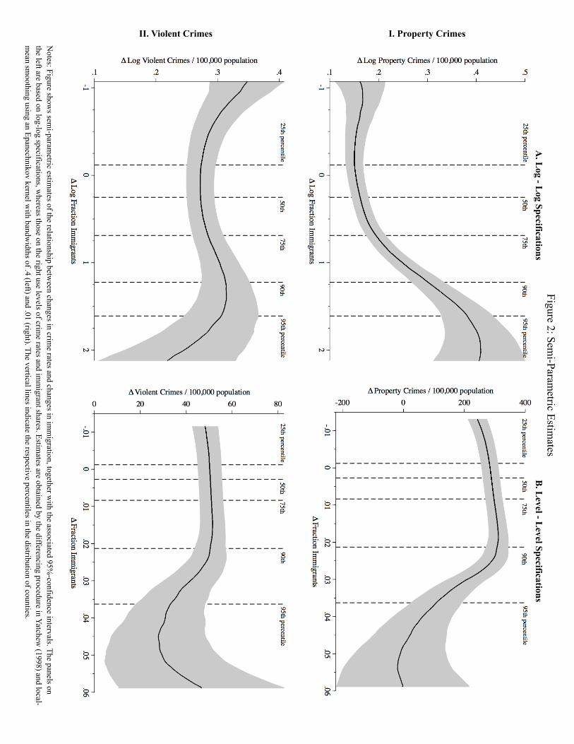
Notes: Figure show

s semi-param

etric estimates of the relationship betw

een changes in crime rates and changes in im

migration, together w

ith the associated 95%-confidence intervals. The panels on

the left are based on log-log specifications, whereas those on the right use levels of crim

e rates and imm

igrant shares. Estimates are obtained by the differencing procedure in Yatchew

(1998) and local-m

ean smoothing using an Epanechnikov kernel w

ith bandwidths of .4 (left) and .01 (right). The vertical lines indicate the respective percentiles in the distribution of counties.

Figure 2: Semi-Param

etric Estimates

A. L

og - Log Specifications

B. L

evel - Level Specifications

I. Property CrimesII. Violent Crimes

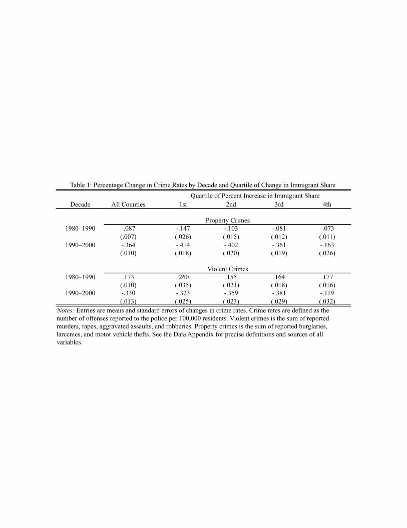
Decade All Counties 1st 2nd 3rd 4th

1980–1990 -.087 -.147 -.103 -.081 -.073(.007) (.026) (.015) (.012) (.011)

1990–2000 -.364 -.414 -.402 -.361 -.163(.010) (.018) (.020) (.019) (.026)

1980–1990 .173 .260 .155 .164 .177(.010) (.035) (.021) (.018) (.016)

1990–2000 -.330 -.323 -.359 -.381 -.119(.013) (.025) (.023) (.029) (.032)

Violent Crimes

Quartile of Percent Increase in Immigrant Share

Notes: Entries are means and standard errors of changes in crime rates. Crime rates are defined as the number of offenses reported to the police per 100,000 residents. Violent crimes is the sum of reported murders, rapes, aggravated assaults, and robberies. Property crimes is the sum of reported burglaries, larcenies, and motor vehicle thefts. See the Data Appendix for precise definitions and sources of all variables.

Table 1: Percentage Change in Crime Rates by Decade and Quartile of Change in Immigrant Share

Property Crimes

Variable 1980 1990 2000Crime:

Violent Crime Rate 225.1 281.4 243.8(297.5) (372.3) (289.2)

Murder Rate 6.167 5.176 3.284(9.736) (10.38) (6.930)

Rape Rate 15.78 21.63 20.33(18.78) (25.70) (21.99)

Aggravated Assault Rate 158.2 210.1 184.1(171.6) (241.4) (223.6)

Robbery Rate 45.01 44.61 36.09(152.2) (153.4) (80.06)

Property Crime Rate 2,826 2,641 2,075(2,064) (1,618) (1,618)

Burglary Rate 882.0 721.4 485.8(690.1) (558.2) (339.3)

Larceny Rate 1,771 1,748 1,446(1,451) (1,425) (1,170)

Moter Vehicle Theft Rate 172.7 172.2 142.9(212.3) (285.0) (172.0)

Demographics:Fraction Immigrants .021 .022 .034

(.028) (.035) (.048)Total Population (in 1,000) 72.22 79.18 89.61

(236.0) (263.5) (291.9)Population per Square Mile 209.2 211.5 234.9

(1,569) (1,427) (1,665)Fraction Female .509 .510 .505

(.016) (.016) (.019)Median Age 31.05 34.41 37.38

(3.87) (3.60) (3.95)Region:

Northeast .070 .070 .070(.256) (.256) (.256)

Midwest .341 .341 .341(.474) (.474) (.474)

West .134 .134 .134(.340) (.340) (.340)

South .455 .455 .455(.498) (.498) (.498)

Economic Indicators:Median Household Income (in $1,000) 29.76 31.42 35.26

(6.87) (8.47) (8.80)Fraction of Families Below Poverty .125 .131 .107

(.063) (.070) (.058)Payroll per Capita (in $1,000) 5.362 5.798 7.164

(3.550) (4.065) (5.388)Unemployment Rate (in Percent) 6.781 6.641 4.331

(3.314) (3.055) (2.705)Police Enforcement:

Police Expenditure per Capita 66.17 87.52 109.7(40.41) (58.03) (72.69)

Fraction Institutionalized .013 .017 .023(.017) (.021) (.033)

Housing Stock:Median Value of Housing Units (in $1,000) 73.28 70.82 84.19

(29.24) (44.08) (47.73)Median Rent 398.1 422.5 440.4

(92.36) (125.9) (121.7)Fraction of Housing Units Owner Occupied .633 .618 .635

(.089) (.093) (.086)Fraction of Housing Units Vacant .135 .148 .142

(.098) (.105) (.095)New Building Permits per Existing Unit .011 .008 .010

(.011) (.010) (.011)

Table 2: Summary Statistics by Decade

Notes: Entries are unweighted means and standard deviations of county level data for those counties whith non-missing information. The total number of counties in the data set is 3,117. Entries have been rounded to four digits. Crime rates are defined as the number of offenses reported to the police per 100,000 residents. Violent crimes is the sum of reported murders, rapes, aggravated assaults, and robberies. Property crimes is the sum of reported burglaries, larcenies, and motor vehicle thefts. See the Data Appendix for precise definitions and sources of all variables.

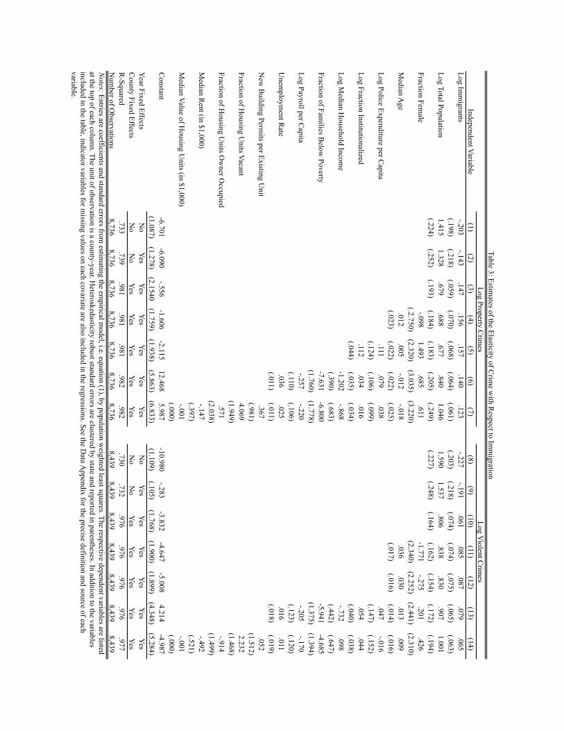
Independent Variable(1)

(2)(3)

(4)(5)

(6)(7)

(8)(9)

(10)(11)

(12)(13)

(14)Log Im

migrants

-.203-.143

.147.156

.157.140

.123-.227

-.191.061

.085.087

.079.065

(.198)(.218)

(.059)(.070)

(.068)(.064)

(.061)(.203)

(.218)(.074)

(.074)(.075)

(.065)(.063)

Log Total Population1.415

1.328.679

.688.677

.8401.046

1.5901.537

.806.838

.830.907

1.001(.224)

(.252)(.193)

(.184)(.183)

(.205)(.249)

(.227)(.248)

(.164)(.162)

(.154)(.172)

(.194)Fraction Fem

ale-.098

1.493.685

.611-1.771

-.275.201

.426(.2.750)

(2.320)(3.035)

(3.220)(2.340)

(2.252)(2.441)

(2.310)M

edian Age

.012.005

-.012-.018

.036.030

.013.009

(.023)(.022)

(.022)(.025)

(.017)(.016)

(.014)(.016)

Log Police Expenditure per Capita

.111.079

.038.047

-.016(.124)

(.106)(.099)

(.147)(.152)

Log Fraction Institutionalized.112

.034.016

.054.044

(.044)(.035)

(.034)(.040)

(.038)Log M

edian Household Incom

e-1.202

-.868-.732

.098(.390)

(.683)(.442)

(.647)Fraction of Fam

ilies Below

Poverty-7.631

-6.800-5.941

-4.685(1.760)

(1.778)(1.375)

(1.394)Log Payroll per C

apita-.257

-.220-.205

-.170(.110)

(.106)(.123)

(.120)U

nemploym

ent Rate

.036.025

.016.011

(.011)(.011)

(.018)(.019)

New

Building Perm

its per Existing Unit

.367.052

(.981)(1.512)

Fraction of Housing U

nits Vacant4.069

2.232(1.949)

(1.468)Fraction of H

ousing Units O

wner O

ccupied.571

-.914(2.038)

(1.499)M

edian Rent (in $1,000)

-.147-.492

(.397)(.521)

Median Value of H

ousing Units (in $1,000)

-.001-.001

(.000)(.000)

Constant

-6.701-6.090

-.556-1.606

-2.11512.468

5.987-10.980

-.283-3.832

-4.647-5.008

4.214-4.987

(1.087)(1.278)

(2.1540(1.759)

(1.938)(5.863)

(6.833)(1.109)

(.105)(1.768)

(1.900)(1.899)

(4.348)(5.284)

Year Fixed EffectsN

oYes

YesYes

YesYes

YesN

oYes

YesYes

YesYes

YesC

ounty Fixed EffectsN

oN

oYes

YesYes

YesYes

No

No

YesYes

YesYes

YesR

-Squared.733

.739.981

.981.981

.982.982

.730.732

.976.976

.976.976

.977N

umber of O

bservations8,736

8,7368,736

8,7368,736

8,7368,736

8,4398,439

8,4398,439

8,4398,439

8,439

Table 3: Estimates of the Elasticity of C

rime w

ith Respect to Im

migration

Log Property Crim

esLog V

iolent Crim

es

Notes: Entries are coefficients and standard errors from

estimating the em

pirical model, i.e. equation (1), by population w

eighted least squares. The respective dependent variables are listed at the top of each colum

n. The unit of observation is a county-year. Heteroskedasticity robust standard errors are clustered by state and reported in parentheses. In addition to the variables

included in the table, indicator variables for missing values on each covariate are also included in the regressions. See the D

ata Appendix for the precise definition and source of each

variable.

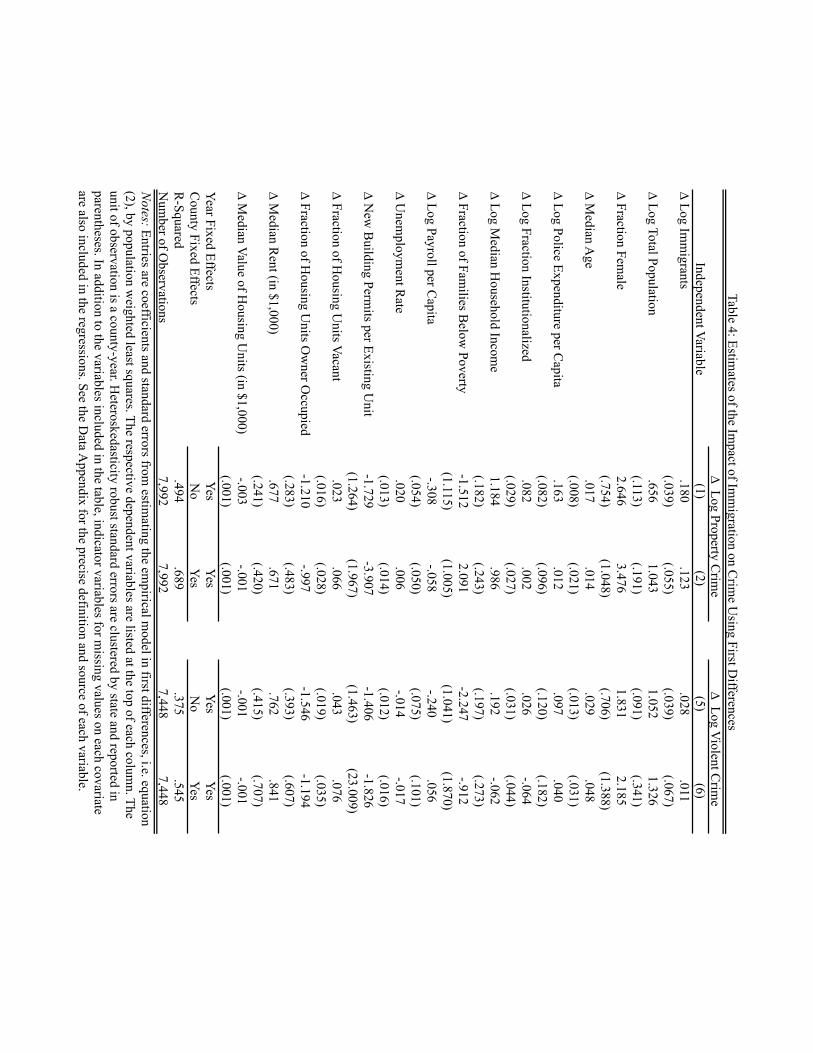
Independent Variable(1)

(2)(5)

(6)∆ Log Im

migrants

.180.123

.028.011

(.039)(.055)

(.039)(.067)

∆ Log Total Population.656

1.0431.052

1.326(.113)

(.191)(.091)

(.341)∆ Fraction Fem

ale2.646

3.4761.831

2.185(.754)

(1.048)(.706)

(1.388)∆ M

edian Age

.017.014

.029.048

(.008)(.021)

(.013)(.031)

∆ Log Police Expenditure per Capita

.163.012

.097.040

(.082)(.096)

(.120)(.182)

∆ Log Fraction Institutionalized.082

.002.026

-.064(.029)

(.027)(.031)

(.044)∆ Log M

edian Household Incom

e1.184

.986.192

-.062(.182)

(.243)(.197)

(.273)∆ Fraction of Fam

ilies Below

Poverty-1.512

2.091-2.247

-.912(1.115)

(1.005)(1.041)

(1.870)∆ Log Payroll per C

apita-.308

-.058-.240

.056(.054)

(.050)(.075)

(.101)∆ U

nemploym

ent Rate

.020.006

-.014-.017

(.013)(.014)

(.012)(.016)

∆ New

Building Perm

its per Existing Unit

-1.729-3.907

-1.406-1.826

(1.264)(1.967)

(1.463)(23.009)

∆ Fraction of Housing U

nits Vacant.023

.066.043

.076(.016)

(.028)(.019)

(.035)∆ Fraction of H

ousing Units O

wner O

ccupied-1.210

-.997-1.546

-1.194(.283)

(.483)(.393)

(.607)∆ M

edian Rent (in $1,000)

.677.671

.762.841

(.241)(.420)

(.415)(.707)

∆ Median Value of H

ousing Units (in $1,000)

-.003-.001

-.001-.001

(.001)(.001)

(.001)(.001)

Year Fixed EffectsYes

YesYes

YesC

ounty Fixed EffectsN

oYes

No

YesR

-Squared.494

.689.375

.545N

umber of O

bservations7,992

7,9927,448

7,448

Table 4: Estimates of the Im

pact of Imm

igration on Crim

e Using First D

ifferences ∆ Log V

iolent Crim

e ∆ Log Property C

rime

Notes: Entries are coefficients and standard errors from

estimating the em

pirical model in first differences, i.e. equation

(2), by population weighted least squares. The respective dependent variables are listed at the top of each colum

n. The unit of observation is a county-year. H

eteroskedasticity robust standard errors are clustered by state and reported in parentheses. In addition to the variables included in the table, indicator variables for m

issing values on each covariate are also included in the regressions. See the D

ata Appendix for the precise definition and source of each variable.

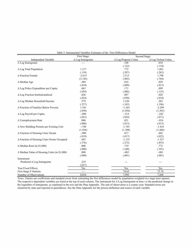
First Stage:Independent Variable ∆ Log Immigrants ∆ Log Property Crime ∆ Log Violent Crime

∆ Log Immigrants --- .108 .010(.122) (.154)

∆ Log Total Population 1.317 .772 1.081(.110) (.207) (.262)

∆ Fraction Female -2.615 2.513 1.798(3.182) (.803) (.764)

∆ Median Age -.001 .016 .029(.010) (.009) (.013)

∆ Log Police Expenditure per Capita .063 .171 .099(.054) (.086) (.125)

∆ Log Fraction Institutionalized .026 .087 .028(.024) (.030) (.034)

∆ Log Median Household Income .579 1.226 .203(.257) (.162) (.196)

∆ Fraction of Families Below Poverty 1.541 -1.365 -2.209(.850) (1.056) (1.203)

∆ Log Payroll per Capita -.090 -.314 -.242(.053) (.054) (.071)

∆ Unemployment Rate .006 .021 -.014(.008) (.013) (.012)

∆ New Building Permits per Existing Unit -.748 -1.765 -1.416(1.926) (1.308) (1.468)

∆ Fraction of Housing Units Vacant -.080 .017 .042(.019) (.017) (.022)

∆ Fraction of Housing Units Owner Occupied .695 -1.135 -1.527(.376) (.272) (.453)

∆ Median Rent (in $1,000) .000 .719 .772(.000) (.248) (.391)

∆ Median Value of Housing Units (in $1,000) .000 -.003 -.001(.000) (.001) (.001)

Instrument:Predicted ∆ Log Immigrants .235 --- ---

(.027)Year Fixed Effects Yes Yes YesFirst Stage F-Statistic --- 74.65 72.76Number of Observations 8,016 7,992 7,448Notes: Entries are coefficients and standard errors from estimating the first differences model by population weighted two stage least squares. The respective dependent variables are listed at the top of each column. The instrument for ∆ Log Immigrants at time t is the predicted change in the logarithm of immigrants, as explained in the text and the Dtaa Appendix. The unit of observation is a county-year. Standard errors are clustered by state and reported in parentheses. See the Data Appendix for the precise definition and source of each variable.

Table 5: Instrumental Variables Estimates of the First Differences ModelSecond Stage:

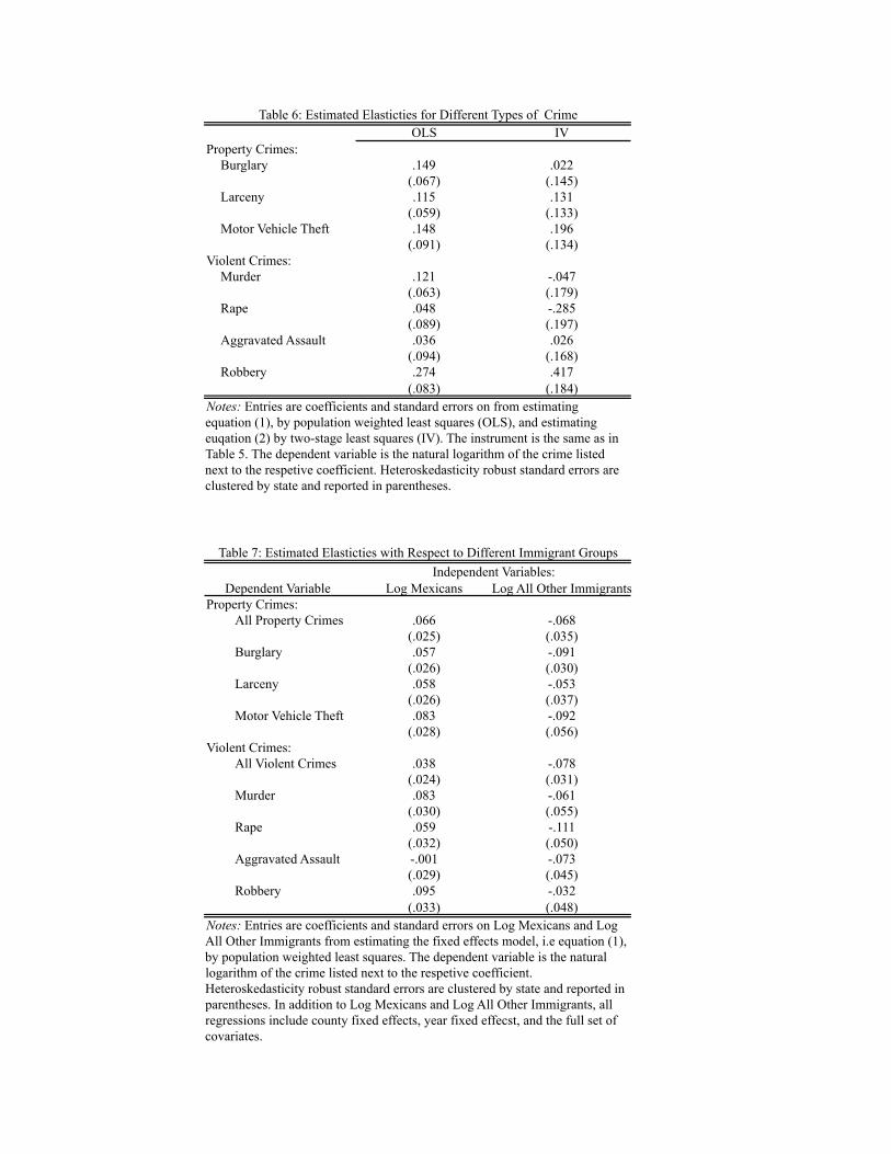
OLS IVProperty Crimes:

Burglary .149 .022(.067) (.145)

Larceny .115 .131(.059) (.133)

Motor Vehicle Theft .148 .196(.091) (.134)

Violent Crimes:Murder .121 -.047

(.063) (.179)Rape .048 -.285

(.089) (.197)Aggravated Assault .036 .026

(.094) (.168)Robbery .274 .417

(.083) (.184)

Dependent Variable Log Mexicans Log All Other ImmigrantsProperty Crimes:

All Property Crimes .066 -.068(.025) (.035)

Burglary .057 -.091(.026) (.030)

Larceny .058 -.053(.026) (.037)

Motor Vehicle Theft .083 -.092(.028) (.056)

Violent Crimes:All Violent Crimes .038 -.078

(.024) (.031)Murder .083 -.061

(.030) (.055)Rape .059 -.111

(.032) (.050)Aggravated Assault -.001 -.073

(.029) (.045)Robbery .095 -.032

(.033) (.048)Notes: Entries are coefficients and standard errors on Log Mexicans and Log All Other Immigrants from estimating the fixed effects model, i.e equation (1), by population weighted least squares. The dependent variable is the natural logarithm of the crime listed next to the respetive coefficient. Heteroskedasticity robust standard errors are clustered by state and reported in parentheses. In addition to Log Mexicans and Log All Other Immigrants, all regressions include county fixed effects, year fixed effecst, and the full set of covariates.

Table 6: Estimated Elasticties for Different Types of Crime

Notes: Entries are coefficients and standard errors on from estimating equation (1), by population weighted least squares (OLS), and estimating euqation (2) by two-stage least squares (IV). The instrument is the same as in Table 5. The dependent variable is the natural logarithm of the crime listed next to the respetive coefficient. Heteroskedasticity robust standard errors are clustered by state and reported in parentheses.

Independent Variables:Table 7: Estimated Elasticties with Respect to Different Immigrant Groups

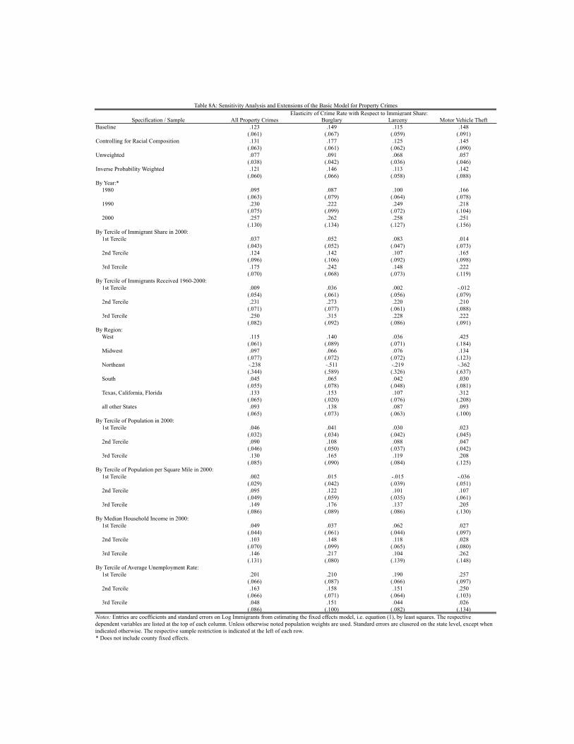
Specification / Sample All Property Crimes Burglary Larceny Motor Vehicle TheftBaseline .123 .149 .115 .148

(.061) (.067) (.059) (.091)Controlling for Racial Composition .131 .177 .125 .145

(.063) (.061) (.062) (.090)Unweighted .077 .091 .068 .057

(.038) (.042) (.036) (.046)Inverse Probability Weighted .121 .146 .113 .142

(.060) (.066) (.058) (.088)By Year:*

1980 .095 .087 .100 .166(.063) (.079) (.064) (.078)

1990 .230 .222 .249 .218(.075) (.099) (.072) (.104)

2000 .257 .262 .258 .251(.130) (.134) (.127) (.156)

By Tercile of Immigrant Share in 2000:1st Tercile .037 .052 .083 .014

(.043) (.052) (.047) (.073)2nd Tercile .124 .142 .107 .165

(.096) (.106) (.092) (.098)3rd Tercile .175 .242 .148 .222

(.070) (.068) (.073) (.119)By Tercile of Immigrants Received 1960-2000:

1st Tercile .009 .036 .002 -.012(.054) (.061) (.056) (.079)

2nd Tercile .231 .273 .220 .210(.071) (.077) (.061) (.088)

3rd Tercile .250 .315 .228 .222(.082) (.092) (.086) (.091)

By Region:West .115 .140 .036 .425

(.061) (.089) (.071) (.184)Midwest .097 .066 .076 .134

(.077) (.072) (.072) (.123)Northeast -.238 -.511 -.219 -.362

(.344) (.589) (.326) (.637)South .045 .065 .042 .030

(.055) (.078) (.048) (.081)Texas, California, Florida .133 .153 .107 .312

(.065) (.020) (.076) (.208)all other States .093 .138 .087 .093

(.065) (.073) (.063) (.100)By Tercile of Population in 2000:

1st Tercile .046 .041 .030 .023(.032) (.034) (.042) (.045)

2nd Tercile .090 .108 .088 .047(.046) (.050) (.037) (.042)

3rd Tercile .130 .165 .119 .208(.085) (.090) (.084) (.125)

By Tercile of Population per Square Mile in 2000:1st Tercile .002 .015 -.015 -.036

(.029) (.042) (.039) (.051)2nd Tercile .095 .122 .101 .107

(.049) (.059) (.035) (.061)3rd Tercile .149 .176 .137 .205

(.086) (.089) (.086) (.130)By Median Household Income in 2000:

1st Tercile .049 .037 .062 .027(.044) (.061) (.044) (.097)

2nd Tercile .103 .148 .118 .028(.070) (.099) (.065) (.080)

3rd Tercile .146 .217 .104 .262(.131) (.080) (.139) (.148)

By Tercile of Average Unemployment Rate:1st Tercile .201 .210 .190 .257

(.066) (.087) (.066) (.097)2nd Tercile .163 .158 .151 .250

(.066) (.071) (.064) (.103)3rd Tercile .048 .151 .044 .026

(.086) (.100) (.082) (.134)

* Does not include county fixed effects.

Elasticity of Crime Rate with Respect to Immigrant Share:Table 8A: Sensitivity Analysis and Extensions of the Basic Model for Property Crimes

Notes: Entries are coefficients and standard errors on Log Immigrants from estimating the fixed effects model, i.e. equation (1), by least squares. The respective dependent variables are listed at the top of each column. Unless otherwise noted population weights are used. Standard errors are clusered on the state level, except when indicated otherwise. The respective sample restriction is indicated at the left of each row.

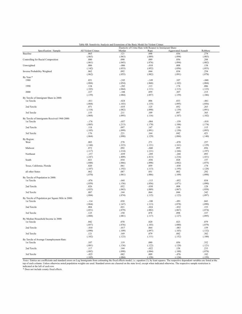
Specification / Sample All Violent Crimes Murder Rape Aggravated Assault RobberyBaseline .065 .121 .048 .036 .274

(.063) (.063) (.089) (.094) (.083)Controlling for Racial Composition .080 .090 .089 .056 .288

(.061) (.045) (.076) (.094) (.082)Unweighted .006 -.006 -.010 .008 .138

(.142) (.033) (.052) (.056) (.053)Inverse Probability Weighted .062 .092 .044 .034 .254

(.062) (.055) (.082) (.091) (.078)By Year:*

1980 .031 -.243 -.149 .107 -.048(.084) (.054) (.068) (.102) (.084)

1990 .124 -.282 .113 .174 .086(.103) (.064) (.111) (.113) (.123)

2000 .227 -.108 .059 .307 .215(.159) (.084) (.057) (.159) (.186)

By Tercile of Immigrant Share in 2000:1st Tercile -.011 -.024 .006 .033 -.061

(.068) (.103) (.135) (.095) (.056)2nd Tercile .071 -.035 .125 .052 .263

(.118) (.082) (.090) (.139) (.091)3rd Tercile .155 .211 .109 .097 .365

(.068) (.095) (.116) (.107) (.102)By Tercile of Immigrants Received 1960-2000:

1st Tercile -.176 -.057 -.084 -.159 -.018(.085) (.213) (.170) (.106) (.174)

2nd Tercile .118 .097 .147 .130 .115(.105) (.099) (.091) (.150) (.093)

3rd Tercile .176 .221 .164 .042 .421(.064) (.090) (.129) (.084) (.140)

By Region:West .003 .278 .271 -.070 .257

(.144) (.223) (.121) (.161) (.129)Midwest .072 .092 -.040 .095 .056

(.117) (.214) (.121) (.166) (.197)Northeast -.157 -.039 -.289 -.268 .093

(.247) (.409) (.413) (.216) (.431)South .021 .034 -.036 .028 .157

(.048) (.066) (.098) (.082) (.075)Texas, California, Florida .020 .061 .059 -.030 .174

(.107) (.192) (.113) (.195) (.128)all other States .062 .087 .051 .002 .292

(.070) (.061) (.086) (.109) (.098)By Tercile of Population in 2000:

1st Tercile -.076 -.041 -.115 -.052 .034(.059) (.156) (.056) (.071) (.090)

2nd Tercile .026 .052 -.030 .008 .128(.055) (.065) (.089) (.067) (.058)

3rd Tercile .087 .144 .064 .044 .342(.084) (.074) (.115) (.123) (.097)

By Tercile of Population per Square Mile in 2000:1st Tercile -.114 .038 -.100 -.091 .043

(.064) (.147) (.113) (.078) (.090)2nd Tercile .004 .021 -.024 -.032 .153

(.051) (.079) (.082) (.067) (.074)3rd Tercile .125 .150 .078 .098 .337

(.088) (.081) (.117) (.127) (.095)By Median Household Income in 2000:

1st Tercile .042 .070 .020 .023 .079(.057) (.076) (.103) (.080) (.079)

2nd Tercile -.010 -.017 .064 -.083 .159(.090) (.109) (.097) (.103) (.132)

3rd Tercile .121 .169 .079 .082 .382(.102) (.123) (.111) (.152) (.100)

By Tercile of Average Unemployment Rate:1st Tercile .107 .119 .080 .056 .352

(.081) (.136) (.122) (.120) (.121)2nd Tercile .117 .144 -.022 .158 .233

(.082) (.090) (.084) (.100) (.078)3rd Tercile -.025 .082 .009 -.076 .182

(.105) (.084) (.128) (.124) (.159)

* Does not include county fixed effects.

Table 8B: Sensitivity Analysis and Extensions of the Basic Model for Violent CrimesElasticity of Crime Rate with Respect to Immigrant Share:

Notes: Entries are coefficients and standard errors on Log Immigrants from estimating the fixed effects model, i.e. equation (1), by least squares. The respective dependent variables are listed at the top of each column. Unless otherwise noted population weights are used. Standard errors are clusered on the state level, except when indicated otherwise. The respective sample restriction is indicated at the left of each row.

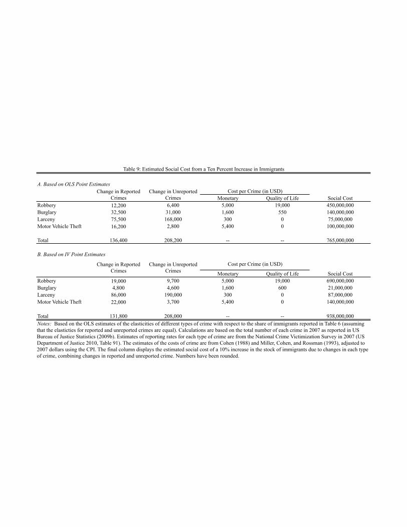
A. Based on OLS Point Estimates

Monetary Quality of Life Social CostRobbery 12,200 6,400 5,000 19,000 450,000,000Burglary 32,500 31,000 1,600 550 140,000,000Larceny 75,500 168,000 300 0 75,000,000Motor Vehicle Theft 16,200 2,800 5,400 0 100,000,000

Total 136,400 208,200 -- -- 765,000,000

B. Based on IV Point Estimates

Monetary Quality of Life Social CostRobbery 19,000 9,700 5,000 19,000 690,000,000Burglary 4,800 4,600 1,600 600 21,000,000Larceny 86,000 190,000 300 0 87,000,000Motor Vehicle Theft 22,000 3,700 5,400 0 140,000,000

Total 131,800 208,000 -- -- 938,000,000Notes: Based on the OLS estimates of the elasticities of different types of crime with respect to the share of immigrants reported in Table 6 (assuming that the elasticties for reported and unreported crimes are equal). Calculations are based on the total number of each crime in 2007 as reported in US Bureau of Justice Statistics (2009b). Estimates of reporting rates for each type of crime are from the National Crime Victimization Survey in 2007 (US Department of Justice 2010, Table 91). The estimates of the costs of crime are from Cohen (1988) and Miller, Cohen, and Rossman (1993), adjusted to 2007 dollars using the CPI. The final column displays the estimated social cost of a 10% increase in the stock of immigrants due to changes in each type of crime, combining changes in reported and unreported crime. Numbers have been rounded.

Table 9: Estimated Social Cost from a Ten Percent Increase in Immigrants

Change in Reported Crimes

Change in Unreported Crimes

Cost per Crime (in USD)

Change in Reported Crimes

Change in Unreported Crimes

Cost per Crime (in USD)