Embed Size (px)
Citation preview
Washington University in St. LouisWashington University Open Scholarship
All Theses and Dissertations (ETDs)
5-24-2012
Underwater Direction-of-Arrival Finding:Maximum Likelihood Estimation andPerformance AnalysisTao LiWashington University in St. Louis
Follow this and additional works at: https://openscholarship.wustl.edu/etd
This Dissertation is brought to you for free and open access by Washington University Open Scholarship. It has been accepted for inclusion in AllTheses and Dissertations (ETDs) by an authorized administrator of Washington University Open Scholarship. For more information, please [email protected].
Recommended CitationLi, Tao, "Underwater Direction-of-Arrival Finding: Maximum Likelihood Estimation and Performance Analysis" (2012). All Thesesand Dissertations (ETDs). 712.https://openscholarship.wustl.edu/etd/712
WASHINGTON UNIVERSITY IN ST. LOUIS
School of Engineering and Applied Science
Department of Electrical & Systems Engineering
Dissertation Examination Committee:Dr. Arye Nehorai, Chair
Dr. Nan LinDr. Hiro Mukai
Dr. Joseph O’SullivanDr. William ShannonDr. Jung-Tsung Shen
Underwater Direction-of-Arrival Finding:
Maximum Likelihood Estimation and Performance Analysis
by
Tao Li
A dissertation presented to the Graduate School of Arts and Sciencesof Washington University in partial fulfillment of the
requirements for the degree of
DOCTOR OF PHILOSOPHY
May 2012Saint Louis, Missouri

copyright by
Tao Li
2012
ABSTRACT OF THE DISSERTATION
Underwater Direction-of-Arrival Finding:
Maximum Likelihood Estimation and Performance Analysis
by
Tao Li
Doctor of Philosophy in Electrical Engineering
Washington University in St. Louis, May 2012
Research Advisor: Dr. Arye Nehorai
In this dissertation, we consider the problems of direction-of-arrival (DOA) finding
using acoustic sensor arrays in underwater scenarios, and develop novel signal models,
maximum likelihood (ML) estimation methods, and performance analysis results.
We first examine the underwater scenarios where the noise on sensor arrays are spa-
tially correlated, for which we consider using sparse sensor arrays consisting of widely
separated sub-arrays and develop ML DOA estimators based on the Expectation-
Maximization scheme. We examine both zero-mean and non-zero-mean Gaussian
incident signals and provide detailed estimation performance analysis. Our results
show that non-zero means in signals improve the accuracy of DOA estimation.
Then we consider the problem of DOA estimation of marine vessel sources such as
ships, submarines, or torpedoes, which emit acoustic signals containing both sinu-
soidal and random components. We propose a mixed signal model and develop an
ML estimator for narrow-band DOA finding of such signals and then generalize the
ii
results to the wide-band case. We provide thorough performance analysis for the pro-
posed signal model and estimators. We show that our mixed signal model and ML
estimators improve the DOA estimation performance in comparison with the typical
stochastic ones assuming zero-mean Gaussian signals.
At last, we derive a Barankin-type bound (BTB) on the mean-square error of DOA
estimation using acoustic sensor arrays. The typical DOA estimation performance
evaluation are usually based on the Cramer-Rao Bound (CRB), which cannot pre-
dict the threshold region of signal-to-noise ratio (SNR), below which the accuracy of
the ML estimation degrades rapidly. Identification of the threshold region has im-
portant applications for DOA estimation in practice. Our derived BTB provides an
approximation to the SNR threshold region.
iii
Acknowledgments
I am grateful to my PhD advisor, Dr. Arye Nehorai, for his valuable guidance through-
out my doctoral research.
I would also like to thank my dissertation committee members, Dr. Nan Lin, Dr. Hiro
Mukai, Dr. Joseph O’Sullivan, Dr. William Shannon, and Dr. Jung-Tsung Shen, for
carefully revising and providing constructive suggestions to this dissertation.
I express my sincere gratitude to my instructors at Washington University in. St.
Louis, including Dr. Tzyh-Jong Tarn, Dr. Daniel Fuhrmann, Dr. Joseph O’Sullivan,
Dr. Kenneth Kelton, Dr. Henric Krawczynski, and the late Dr. Christopher Byrnes,
for helping me construct a solid knowledge background for my research work.
I offer my thanks and regards to all my labmates. Their friendships and aids made
our lab a great place for work and research.
I convey my deepest gratitude to my parents and family in China for their endless
love and emotional encouragement.
Tao Li
Washington University in Saint Louis
May 2012
iv

To my parents.
v
Contents
Abstract . . . . . . . . . . . . . . . . . . . . . . . . . . . . . . . . . . . . . . ii
Acknowledgments . . . . . . . . . . . . . . . . . . . . . . . . . . . . . . . . iv
List of Figures . . . . . . . . . . . . . . . . . . . . . . . . . . . . . . . . . . ix
1 Introduction . . . . . . . . . . . . . . . . . . . . . . . . . . . . . . . . . . 11.1 Formulation . . . . . . . . . . . . . . . . . . . . . . . . . . . . . . . . 11.2 Maximum Likelihood Estimation . . . . . . . . . . . . . . . . . . . . 31.3 Our Contributions . . . . . . . . . . . . . . . . . . . . . . . . . . . . 51.4 Outline of the Dissertation . . . . . . . . . . . . . . . . . . . . . . . . 7
2 Maximum Likelihood Direction-of-Arrival Estimation in SpatiallyColored Noise Using Sparse Arrays . . . . . . . . . . . . . . . . . . . 92.1 Introduction . . . . . . . . . . . . . . . . . . . . . . . . . . . . . . . . 102.2 Measurement Models . . . . . . . . . . . . . . . . . . . . . . . . . . . 122.3 Maximum Likelihood Estimation . . . . . . . . . . . . . . . . . . . . 15
2.3.1 Deterministic ML Estimator . . . . . . . . . . . . . . . . . . . 152.3.2 Stochastic ML Estimator . . . . . . . . . . . . . . . . . . . . . 192.3.3 Mixed ML Estimator . . . . . . . . . . . . . . . . . . . . . . . 24
2.4 Analytical Performance Analysis . . . . . . . . . . . . . . . . . . . . . 272.4.1 Cramer-Rao Bounds and Asymptotic Errors . . . . . . . . . . 282.4.2 Analytical Performance Comparisons . . . . . . . . . . . . . . 32
2.5 Numerical Examples . . . . . . . . . . . . . . . . . . . . . . . . . . . 342.6 Summary . . . . . . . . . . . . . . . . . . . . . . . . . . . . . . . . . 41
3 Narrow-Band Direction-of-Arrival Estimation of Hydroacoustic Sig-nals From Marine Vessels . . . . . . . . . . . . . . . . . . . . . . . . . 423.1 Introduction . . . . . . . . . . . . . . . . . . . . . . . . . . . . . . . . 433.2 Measurement Model . . . . . . . . . . . . . . . . . . . . . . . . . . . 453.3 Maximum Likelihood Estimation . . . . . . . . . . . . . . . . . . . . 463.4 Analytical Performance Analysis . . . . . . . . . . . . . . . . . . . . . 513.5 Numerical Examples . . . . . . . . . . . . . . . . . . . . . . . . . . . 553.6 Summary . . . . . . . . . . . . . . . . . . . . . . . . . . . . . . . . . 59
4 Direction-of-Arrival Finding of Wide-Band Hydroacoustic SignalsFrom Marine Vessels: An Extension from the Narrow-Band Case 60
vi
4.1 Introduction . . . . . . . . . . . . . . . . . . . . . . . . . . . . . . . . 614.2 Measurement Model And Maximum Likelihood Estimation . . . . . . 62
4.2.1 Measurement Model . . . . . . . . . . . . . . . . . . . . . . . 624.2.2 Maximum Likelihood Estimation . . . . . . . . . . . . . . . . 64
4.3 Analytical Performance Analysis . . . . . . . . . . . . . . . . . . . . . 664.4 Numerical Example . . . . . . . . . . . . . . . . . . . . . . . . . . . . 684.5 Summary . . . . . . . . . . . . . . . . . . . . . . . . . . . . . . . . . 70
5 Direction-of-Arrival Estimation of Hydroacoustic Signals From Ma-rine Vessels: An Approach From Fourier Transform . . . . . . . . . 715.1 Measurement Models And DOA Estimation . . . . . . . . . . . . . . 72
5.1.1 Measurement Model . . . . . . . . . . . . . . . . . . . . . . . 725.1.2 DOA Estimation From A Modified Model . . . . . . . . . . . 74
5.2 Analytical Performance Analysis . . . . . . . . . . . . . . . . . . . . . 785.3 Numerical Example . . . . . . . . . . . . . . . . . . . . . . . . . . . . 805.4 Summary . . . . . . . . . . . . . . . . . . . . . . . . . . . . . . . . . 82
6 A Barankin-Type Bound on Direction-of-Arrival Estimation . . . 836.1 Introduction . . . . . . . . . . . . . . . . . . . . . . . . . . . . . . . . 846.2 Measurement Model . . . . . . . . . . . . . . . . . . . . . . . . . . . 856.3 Barankin-Type Bound . . . . . . . . . . . . . . . . . . . . . . . . . . 876.4 Numerical Examples . . . . . . . . . . . . . . . . . . . . . . . . . . . 93
6.4.1 Examples for Scalar-Sensor Array . . . . . . . . . . . . . . . . 936.4.2 Examples for Vector-Sensor Array . . . . . . . . . . . . . . . 95
6.5 Summary . . . . . . . . . . . . . . . . . . . . . . . . . . . . . . . . . 97
7 Conclusions . . . . . . . . . . . . . . . . . . . . . . . . . . . . . . . . . . 997.1 Key Contributions . . . . . . . . . . . . . . . . . . . . . . . . . . . . 997.2 Future Work . . . . . . . . . . . . . . . . . . . . . . . . . . . . . . . . 101
Appendix A Proof of Theorem 1 . . . . . . . . . . . . . . . . . . . . . 102
Appendix B Proof of Theorem 2 . . . . . . . . . . . . . . . . . . . . . 106
Appendix C Proof of Lemma 2 . . . . . . . . . . . . . . . . . . . . . . 112
Appendix D Proof of Proposition 5 . . . . . . . . . . . . . . . . . . . . 113
Appendix E Proof of Proposition 6 . . . . . . . . . . . . . . . . . . . . 115
Appendix F Proof of Lemma 3 . . . . . . . . . . . . . . . . . . . . . . 117
Appendix G Proof of Equation (3.8) . . . . . . . . . . . . . . . . . . . 119
Appendix H Proof of Proposition 8 . . . . . . . . . . . . . . . . . . . . 121
vii
Appendix I Proof of Proposition 9 . . . . . . . . . . . . . . . . . . . . 124
Appendix J Proof of Proposition 10 . . . . . . . . . . . . . . . . . . . 132
Appendix K Proof of Proposition 11 . . . . . . . . . . . . . . . . . . . 139
Appendix L Proof of Proposition 12 . . . . . . . . . . . . . . . . . . . 144
Appendix M Proof of Proposition 13 . . . . . . . . . . . . . . . . . . . 147
Appendix N Proof of Proposition 14 . . . . . . . . . . . . . . . . . . . 151
Appendix O Proof of Proposition 16 . . . . . . . . . . . . . . . . . . . 156
Appendix P Derivation of Equation (6.16) . . . . . . . . . . . . . . . 160
References . . . . . . . . . . . . . . . . . . . . . . . . . . . . . . . . . . . . . 162
Vita . . . . . . . . . . . . . . . . . . . . . . . . . . . . . . . . . . . . . . . . . 171
viii
List of Figures
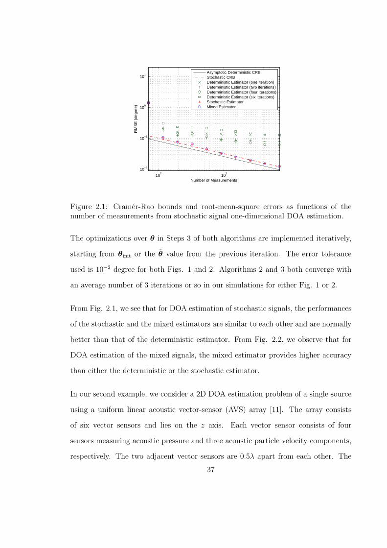
2.1 Cramer-Rao bounds and root-mean-square errors as functions of thenumber of measurements from stochastic signal one-dimensional DOAestimation. . . . . . . . . . . . . . . . . . . . . . . . . . . . . . . . . . 37
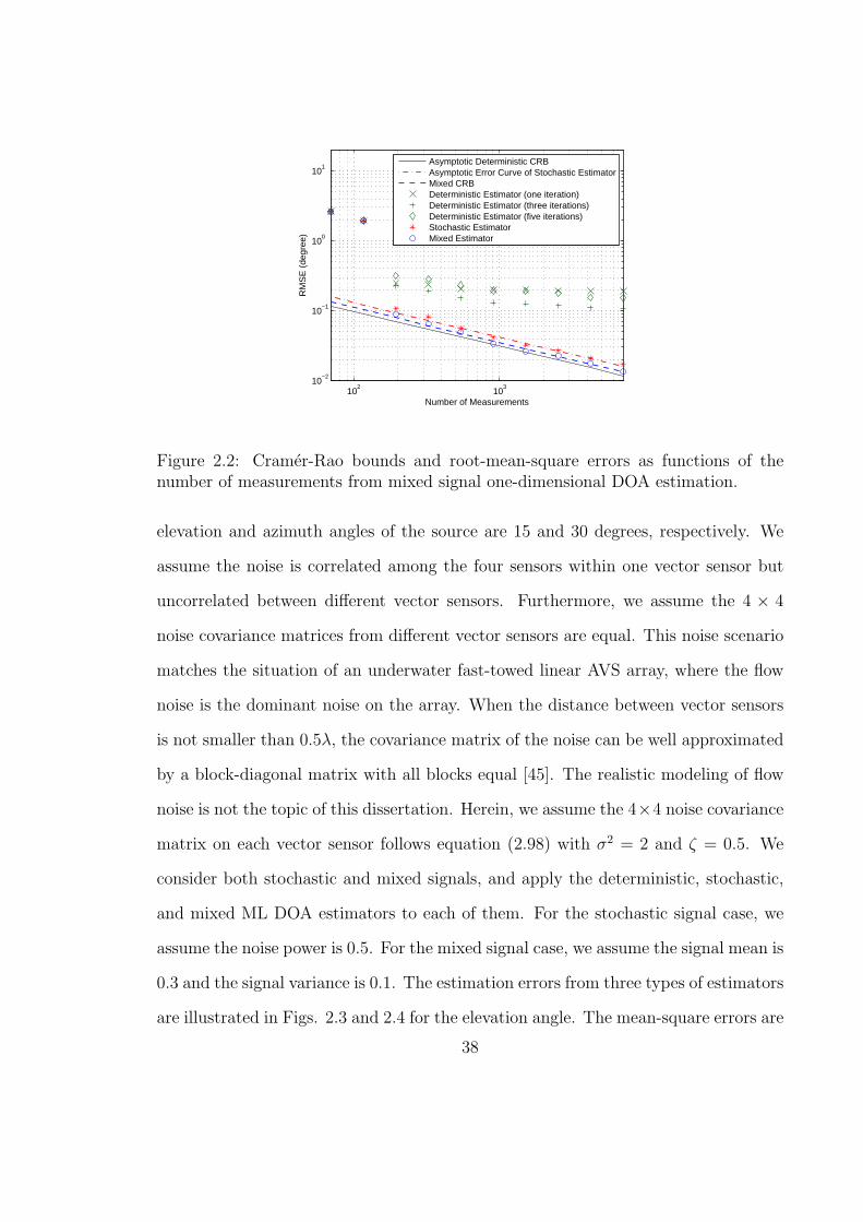
2.2 Cramer-Rao bounds and root-mean-square errors as functions of thenumber of measurements from mixed signal one-dimensional DOA es-timation. . . . . . . . . . . . . . . . . . . . . . . . . . . . . . . . . . . 38
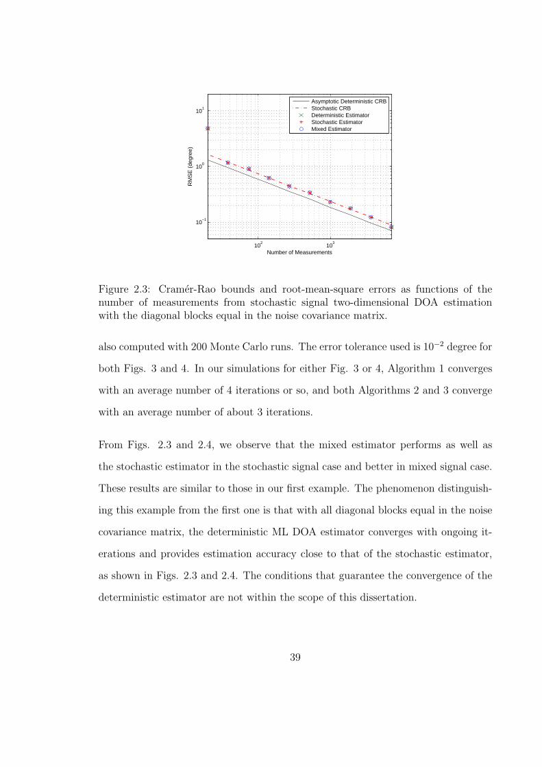
2.3 Cramer-Rao bounds and root-mean-square errors as functions of thenumber of measurements from stochastic signal two-dimensional DOAestimation with the diagonal blocks equal in the noise covariance matrix. 39
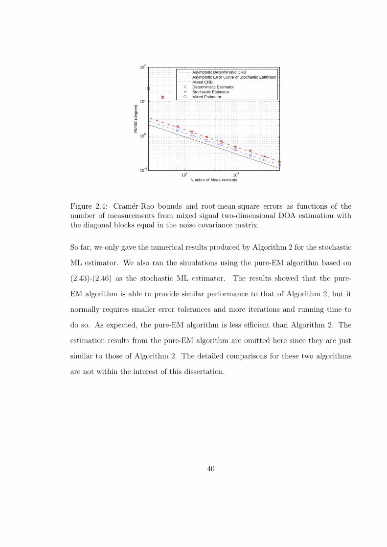
2.4 Cramer-Rao bounds and root-mean-square errors as functions of thenumber of measurements from mixed signal two-dimensional DOA es-timation with the diagonal blocks equal in the noise covariance matrix. 40
3.1 Cramer-Rao bound and root-mean-square errors as functions of thenumber of measurements from mixed signal DOA estimation underspatially white noise using uniform linear array. . . . . . . . . . . . . 56
3.2 Cramer-Rao bound and root-mean-square errors as functions of thenumber of measurements from mixed signal DOA estimation underspatially colored noise using linear array consisting of separated sub-arrays. . . . . . . . . . . . . . . . . . . . . . . . . . . . . . . . . . . . 58
4.1 Cramer-Rao bound and root-mean-square errors as functions of thenumber of measurements from wide-band mixed signal DOA estimationunder spatially white noise. . . . . . . . . . . . . . . . . . . . . . . . 69
5.1 Cramer-Rao bound and root-mean-square errors as functions of thenumber of subintervals Nd for mixed signal DOA estimation. . . . . . 81
6.1 Square roots of the derived Barankin-type bound and maximum like-lihood estimation mean-square error versus signal-to-noise ratio fornarrow-band direction of arrival estimation using uniform linear scalar-sensor array. . . . . . . . . . . . . . . . . . . . . . . . . . . . . . . . . 94
6.2 Same as in Fig.1, but for the wide-band direction of arrival estimation. 94
ix

6.3 Square roots of the derived Barankin-type bound, Cramer-Rao bound,and maximum likelihood estimation mean-square error versus signal-to-noise ratio for narrow-band direction of arrival estimation using uni-form linear acoustic vector-sensor arrays with d = λ, 2λ, and 3λ, re-spectively. . . . . . . . . . . . . . . . . . . . . . . . . . . . . . . . . . 96
6.4 Variation of maximum likelihood ambiguity functions with respect tothe inter-sensor distance d. . . . . . . . . . . . . . . . . . . . . . . . 97
x
Chapter 1
Introduction
Direction-of-arrival (DOA) estimation aims at finding the direction from which the
signals impinge on the sensor array, which consists of a group of sensors arranged in
a specific geometry that are able to measure the values of the impinging signals. In
the underwater environment, the impinging signals are often acoustic signals, which
are commonly called hydroacoustic signals whose DOAs can be estimated by acoustic
sensor arrays. Underwater DOA estimation has important applications in the detect-
ing, localizing, and tracking of marine vessels like ships, submarines, and torpedoes.
In this dissertation, we propose new signal models, maximum likelihood (ML) esti-
mation methods, and performance analysis results for underwater DOA estimation
problems.
1.1 Formulation
According to their bandwidths, the incident signals can be classified into narrow-band
and wide-band signals. The bandwidth of a narrow-band signal is small such that it
1
can be considered as sinusoidal. Usually a signal can be considered as narrow-band if
D/c≪ 1/B, (1.1)
where D, c, and B are the array length, signal propagation speed, and signal band-
width, respectively [1]-[3]. Suppose there are L signals incident on an array of M
sensors from the far field, which means the incident signal waves are plane waves. If
the signals are narrow-band, the array measurement model can be neatly formulated
as [1]
y(t) = A(θ)x(t) + ϵ(t), t = 1, . . . , N, (1.2)
where y(t) is a M × 1 vector containing the array output at the t-th snapshot,
A(θ) = [a(θ1), · · · ,a(θL)] (1.3)
is the array steering matrix, a(θl) is the L × 1 steering vector corresponding to the
l-th source, θ = [θ1, . . . , θL]T with θl the DOA of the l-th source, ·T denotes the
matrix transpose, x(t) is the L × 1 vector of signal values at the t-th snapshot, ϵ(t)
is an M × 1 vector of noise values on the array sensors, and N is the total number
of temporal measurements. The steering matrix A(θ) is determined by the array
geometry, signal carrier frequencies, and DOA (see [1] for the formulation of steering
matrix). But since both the array geometry and carrier frequencies are known, the
steering matrix becomes only a function of DOA. The aim of narrow-band DOA
finding is to estimate θ from the noise corrupted array output y(t), t = 1, . . . , N .
If the narrow-band condition in (1.1) is not satisfied, the signals are considered as
wide-band, and the measurement model in (1.2) cannot be applied. In this case, we
usually first decompose the wide frequency band into a set of narrow sub-bands [1], in
2
each of which the narrow-band condition is satisfied such that the model in (1.2) can
be applied. For instance, if we decompose the wide frequency band into K sub-bands,
in each of which (1.2) holds. Then the wide-band measurement model can be written
as
yk(t) = Ak(θ)xk(t) + ϵk(t), t = 1, . . . , N, k = 1, . . . , K, (1.4)
where yk(t) is the M × 1 measurement vector at the t-th snapshot from the k-th
sub-band,
Ak(θ) = [ak(θ1), · · · ,ak(θL)] (1.5)
is the array steering matrix for the k-th sub-band, xk(t) is the L × 1 signal value
vector from the k-th sub-band, ϵk(t) is theM×1 noise vector from the k-th sub-band.
Note that the DOA vector θ is identical for all sub-bands but the carrier frequencies
differ for different sub-bands. So the steering matrices from different sub-bands are
different.
1.2 Maximum Likelihood Estimation
Typical DOA estimation methods include beamforming techniques [4], subspace-
based methods such as MUSIC [6] and ESPRIT [2], and maximum likelihood (ML)
methods (see [7] for examples). Among varieties of DOA estimation methods, the ML
methods are often able to provide better performance than the others not only due to
their asymptotic performance usually achieving the Cramer-Rao bound (CRB), which
is a lower bound on estimation errors, but also because they can take advantage of
better signal or noise models to provide better DOA estimation performance (see [8]
for an example).
3
The ML methods aim at finding the DOA estimates by maximizing the log-likelihood
(LL) functions over the unknown parameters including DOAs and unknown signal and
noise parameters. Different signal or noise models may result in different LL functions
and therefore different ML estimators. For example, the deterministic (conditional)
signal model in [8] considers the signal values at all snapshots as deterministic un-
known parameters and assumes the noise to be spatially and temporally white. Under
this assumption, the unknown parameters in (1.2) include the DOA vector θ, the sig-
nal values x(t), t = 1, . . . , N , and the noise power σ2. By omitting constant terms,
the LL function can be written as
L(θ,X,Q) = −N log |Q| − traceQ−1C(θ,X)
, (1.6)
where
X = [x(1), · · · ,x(N)], (1.7)
C(θ,X) = [Y −A(θ)X][Y −A(θ)X]H , (1.8)
Y = [y(1), · · · ,y(N)], (1.9)
Q = σ2IM , IM is an M × M identity matrix, and | · | and trace· denote the
determinant and the trace of a matrix, respectively.
Also in [8], the stochastic (unconditional) signal model considers the noise as spatially
and temporally white as well but assumes the signal values are temporally indepen-
dent and follow a zero-mean Gaussian distribution with unknown correlation matrix
P at each snapshot. According to this model and after omitting constant terms, the
4
LL function can be formulated as
L(θ,P ,Q) = − log |A(θ)PAH(θ) +Q| − trace[A(θ)PAH(θ) +Q
]−1Ryy
, (1.10)
where
Ryy =1
NY Y H . (1.11)
The unknown parameters in (1.10) are θ, P , and σ2.
We can see that the LL functions in (1.6) and (1.10) have different formulations and
unknown parameters. Maximizing (1.6) and (1.10) with respect to their unknown
parameters,respectively, will definitely results in different ML DOA estimators. It
has been shown in [8] that the ML estimator based on the stochastic signal model
provides better performance than the ML estimator based on the deterministic signal
model for DOA estimation of zero-mean Gaussian signals. Therefore, to improve the
performance of ML DOA estimation, we ought to design signal and noise models to
be as accurate as possible.
1.3 Our Contributions
In this research, we develop new signal models, ML estimators, and performance
analysis results for some underwater DOA estimation problems. We summarize our
contributions as follows.
5
ML DOA Estimation in Spatially Colored Noise Using Sparse
Arrays
Sparse sensor arrays have been explored as an effective solution to DOA estimation
in spatially colored noise, which is quite common in underwater scenarios. We con-
sider the narrow-band DOA estimation in spatially colored noise using sparse sensor
arrays and develop new ML DOA estimators under the assumptions of zero-mean
and non-zero-mean Gaussian signals based on an Expectation-Maximization (EM)
framework. For the DOA finding of non-zero-mean Gaussian signals, we compute
the CRB as well as the asymptotic error covariance matrix of the ML estimator that
improperly assumes zero-mean Gaussian signals. We provide both analytical and nu-
merical comparisons for the existing deterministic and the proposed ML estimators.
The results show that the proposed estimators provide better accuracy than the ex-
isting deterministic estimator, and that the non-zero means in the signals improve
the accuracy of DOA estimation.
DOA Finding for Hydroacoustic Signals From Marine Vessels
The hydroacoustic signals from marine vessels are known to consist of two parts: the
noise-like part with continuous spectra and the sinusoidal part with discrete frequen-
cies, which can be exploited to improve the DOA estimation accuracy. We consider
the DOA estimation of hydroacoustic signals from marine vessel sources by modeling
such signals as the mixture of deterministic sinusoidal signals and stochastic Gaussian
signals, and derive the ML DOA estimator. We compute the asymptotic error covari-
ance matrix of the proposed ML estimator, as well as that of the typical ML estimator
6
assuming zero-mean Gaussian signals, for DOA estimation of such signals. Our an-
alytical comparisons and numerical examples show that compared with the typical
ML estimator, the proposed ML estimator enhances the DOA estimation accuracy
for the hydroacoustic signals from marine vessels.
A Barankin-Type Bound
Identification of the signal-to-noise ratio (SNR) threshold region, below which the
accuracy of the ML estimation degrades rapidly, has important applications in the
DOA estimation practice. The Barankin bound is a useful tool in estimation problems
for predicting this threshold region of SNR. We derive a Barankin-type bound on the
mean-square error (MSE) in estimating the DOAs of far-field sources using acoustic
sensor arrays. We consider both narrow-band and wide-band deterministic signals,
and scalar or vector sensors. Our results provide an approximation to the threshold of
the SNR below which the ML estimation performance degrades rapidly. For narrow-
band DOA estimation using uniform linear acoustic vector-sensor arrays, we show that
this threshold increases with the inter-sensor distance. As a result, for medium SNR
values, the performance does not necessarily improve with the inter-sensor distance.
1.4 Outline of the Dissertation
The rest of the dissertation is organized as follows. In Chapter 2, we present the results
for the ML DOA estimation in spatially colored noise using sparse arrays. In Chapter
3, we develop the narrow-band DOA estimation models and results for hydroacoustic
signals from marine vessels. Chapters 4 and 5 generalize the narrow-band results in
7

Chapter 3 to the wide-band case. In Chapter 6, we derive a Barankin-type bound on
DOA estimation. At last, in Chapter 7, we summarize our contributions and discuss
possible topics for future work.
8
Chapter 2
Maximum Likelihood
Direction-of-Arrival Estimation in
Spatially Colored Noise Using
Sparse Arrays1
Spatially colored noise is quite common on sensor arrays in underwater direction-
of-arrival (DOA) estimation scenarios. In this chapter, we consider the problem
of maximum likelihood (ML) DOA estimation of narrow-band signals in spatially
colored noise using sparse sensor arrays, which consist of widely separated sub-arrays
such that the unknown spatially colored noise field is uncorrelated between different
sub-arrays. We develop ML DOA estimators under the assumptions of zero-mean
and non-zero-mean Gaussian signals based on an Expectation-Maximization (EM)
framework. For DOA estimation of non-zero-mean Gaussian signals, we derive the
Cramer-Rao bound (CRB) as well as the asymptotic error covariance matrix of the
1Based on T. Li and A. Nehorai, “Maximum Likelihood Direction Finding in Spatially ColoredNoise Fields Using Sparse Sensor Arrays,” IEEE Trans. Signal Process., vol. 59, pp. 1048-1062, Mar.2011. c⃝[2011] IEEE.
9
ML estimator that improperly assumes zero-mean Gaussian signals. We provide
analytical and numerical performance comparisons for the existing deterministic and
the proposed ML estimators. The results show that the proposed estimators normally
provide better accuracy than the existing deterministic estimator, and that the non-
zero means in the signals improve the accuracy of DOA estimation.
2.1 Introduction
Array processing for DOA estimation has been a topic of intensive research interest
during the past two decades. Many proposed estimators assume spatially white noise
(see [7]-[11] for examples) such that the array noise covariance matrix is proportional
to an identity matrix. However, this assumption is not realistic in many practical
applications [12]-[18] where the noise fields are spatially colored. The spatial correla-
tion or nonuniformity in the colored noise may significantly degrade the performance
of the estimators assuming spatially white noise [19], [20]. In these applications, it is
beneficial to take the spatial color of the noise into account to improve the resolution
of DOA estimation.
Unfortunately, the problem of DOA estimation under spatially colored noise is not
solvable unless special constraints are imposed on signals or noise. For instance,
in [14], the noise field is assumed to satisfy a spatially autoregressive model. In [16],
the signals are required to be partially known as a linear combination of a set of basis
functions. The estimator proposed in [17] requires the temporal correlation length of
the signals to be larger than that of the noise. However, these assumptions do not
always hold in practice, and the performances of these estimators may deteriorate
when the required constraints are not satisfied.
10
To avoid the constraints on signals and noise, sparse arrays consisting of separated
sub-arrays were exploited for DOA estimation in spatially colored noise [21]-[24]. This
technique sets the sub-arrays to be well separated such that noise is uncorrelated
between different sub-arrays. As a result, the array noise covariance matrix presents
a block-diagonal structure, which guarantees the identifiability of DOA information
[24]. The early works on this topic [21]-[23] explored estimation methods using two
separated sub-arrays. Recently, a deterministic ML estimator was proposed for the
case of multiple sub-arrays [24].
In this chapter, under the assumption of Gaussian signals, we develop ML estimators
based on an Expectation-Maximization (EM) framework for narrow-band DOA esti-
mation in spatially colored noise using sparse arrays consisting of multiple sub-arrays.
To the best of our knowledge, no similar estimator has been proposed so far. Many
existing ML estimators assume the means of the Gaussian signals are zero (see [8]-
[11] for examples). In this chapter, we consider both zero-mean and non-zero-mean
Gaussian signals. The ML DOA estimation of non-zero mean signals under spatially
colored noise was addressed in [14], [25]. The estimator in [14] is developed based
on an autoregressive noise model, and is not a rigorous ML DOA estimator. The
work in [25] shows that the non-zero mean component can be used to extract DOA
information under spatially colored noise without any constraint needed on the sensor
arrays, signals or the noise field. Some applications with non-zero mean signals were
also given in [25], such as short-term MEG and EEG [26], [27], communication us-
ing amplitude-modulated or frequency-shift keying (with large frequency deviation)
signals [28], [29], and underground source localization using gradiometer arrays [30].
Non-zero mean signals can also be used to describe acoustic waves from ships and sub-
marines, which normally consist of sinusoidal components and noise with continuous
11
spectrums [31]. Since the frequency of a sinusoidal component can often be estimated
accurately (see [32]-[36] for examples), we can obtain a non-zero-mean complex am-
plitude from a narrow-band acoustic wave by focusing the carrier frequency on the
frequency of its sinusoidal component.
The ML estimator in [25] uses only the non-zero mean component in signals for
DOA estimation. Our proposed ML estimator takes advantage of the block-diagonal
structure of the noise covariance matrix and makes use of the total signal power for
DOA estimation. We present relevant performance analysis results and give both
analytical and numerical comparisons for estimators based on different signal models.
We show that with the same correlation matrices of signals and noise, the non-zero-
mean signals improve the accuracy of DOA estimation compared with the zero-mean
ones.
The remainder of this chapter is organized as follows. We present the measurement
models in Section 2.2, and derive our EM-based ML estimators in Section 2.3. Section
2.4 gives the results of analytical performance analysis. Numerical examples appear
in Section 2.5. We give our conclusions in Section 2.6.
2.2 Measurement Models
In this section, we give the narrow-band measurement models for DOA estimation
using sparse arrays under spatially colored noise.
Consider narrow-band signals from L distant sources impinging on a sparse array
composed of K separated sub-arrays, the k-th of which consists of Mk sensors. Let
M =∑K
k=1Mk be the total number of sensors in the array. For one-dimensional (1D)
12
DOA estimation, the array output can be written as
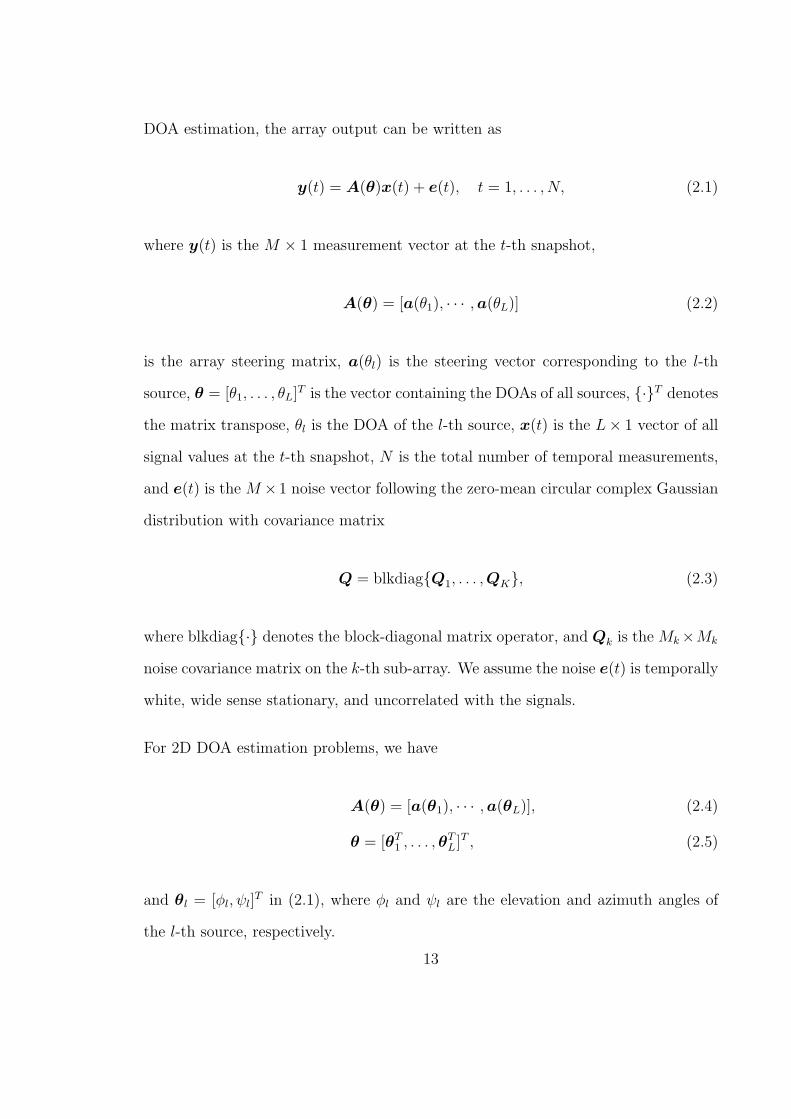
y(t) = A(θ)x(t) + e(t), t = 1, . . . , N, (2.1)
where y(t) is the M × 1 measurement vector at the t-th snapshot,
A(θ) = [a(θ1), · · · ,a(θL)] (2.2)
is the array steering matrix, a(θl) is the steering vector corresponding to the l-th
source, θ = [θ1, . . . , θL]T is the vector containing the DOAs of all sources, ·T denotes
the matrix transpose, θl is the DOA of the l-th source, x(t) is the L× 1 vector of all
signal values at the t-th snapshot, N is the total number of temporal measurements,
and e(t) is the M ×1 noise vector following the zero-mean circular complex Gaussian
distribution with covariance matrix
Q = blkdiagQ1, . . . ,QK, (2.3)
where blkdiag· denotes the block-diagonal matrix operator, and Qk is theMk×Mk
noise covariance matrix on the k-th sub-array. We assume the noise e(t) is temporally
white, wide sense stationary, and uncorrelated with the signals.
For 2D DOA estimation problems, we have
A(θ) = [a(θ1), · · · ,a(θL)], (2.4)
θ = [θT1 , . . . ,θTL]
T , (2.5)
and θl = [ϕl, ψl]T in (2.1), where ϕl and ψl are the elevation and azimuth angles of
the l-th source, respectively.
13
We now present the three types of signal models that will be considered in this chapter.
The deterministic signal model [8], [24] considers the signal values at all snapshots as
deterministic unknown parameters. Under the assumption of deterministic signals,
the unknown parameters in (2.1) consist of the DOA vector θ, the signal parameters
x(t), t = 1, . . . , T , and the noise covariance matrix Q.
In contrast, stochastic signal models consider x(t) to be a random process generated
from a specific probability density function (pdf), which is normally assumed to be
Gaussian. In this chapter, we consider both zero-mean and non-zero-mean circular
complex Gaussian signals.
For zero-mean complex Gaussian signals, we assume
Ex(t)x(s)H
= P δt,s, (2.6)
where E · denotes the expectation operator, ·H denotes the conjugate transpose,
P is the signal covariance matrix, and δt,s is the Kronecker delta function. Under the
assumption of zero-mean Gaussian signals, the unknown parameters in (2.1) consist
of the DOA vector θ, the signal covariance matrix P , and the noise covariance matrix
Q.
For non-zero-mean complex Gaussian signals, we assume
Ex(t) = b, (2.7)
E[x(t)− b][x(s)− b]H = P δt,s, (2.8)
14
where b is the signal mean. Under the assumption of non-zero-mean Gaussian signals,
the unknown parameters consist of the DOA vector θ, the signal mean b, the signal
covariance matrix P , and the noise covariance matrix Q.
Stochastic signals have been modeled with zero-mean Gaussian distributions in most
existing work (see [8], [10], [20] for examples). Non-zero-mean Gaussian signals can
be considered as mixtures of zero-mean Gaussian signals with deterministic unknown
constants. In the remainder of this chapter, for simplicity of notation and presenta-
tion, we use “stochastic signals” to represent zero-mean Gaussian signals and use
“mixed signals” to represent non-zero-mean Gaussian signals. Similarly, we use
“stochastic” and “mixed” estimators to represent the estimators developed under
the assumptions of zero-mean and non-zero-mean Gaussian signals, respectively.
2.3 Maximum Likelihood Estimation
In this section, we present our stochastic and mixed ML estimators for DOA finding
under spatially colored noise using sparse sensor arrays. For convenience of compari-
son and further analysis, we first summarize the results in [24] for the deterministic
ML DOA estimator.
2.3.1 Deterministic ML Estimator
After neglecting constant terms, the log-likelihood function based on the deterministic
signal model can be written as
L(θ,X,Q) = −N log |Q| − traceQ−1C(θ,X)
, (2.9)
15
where
X = [x(1), · · · ,x(N)], (2.10)
C(θ,X) = [Y −A(θ)X][Y −A(θ)X]H , (2.11)
Y = [y(1), · · · ,y(N)], (2.12)
and | · | and trace· denote the determinant and the trace of a matrix, respectively.
By fixing θ and X, the ML estimate of Q can be obtained as
Q(θ,X) =1
NC(θ,X)⊙E, (2.13)
where ⊙ denotes the Hadamard product,
E = blkdiagE1, . . . ,EK, (2.14)
and Ek is an Mk ×Mk matrix with all entries equal to one. By inserting (2.13) into
(2.9), the log-likelihood function can be simplified into
L(θ,X) = − log
∣∣∣∣ 1NC(θ,X)⊙E∣∣∣∣ . (2.15)
Similarly, by fixing θ and Q, the ML estimate of X can be expressed as
X(θ,Q) =[A
H(θ)A(θ)
]−1
AH(θ)Y , (2.16)
where A(θ) = Q− 12A(θ) and Y = Q− 1
2Y . By substituting (2.16) into (2.15), the
log-likelihood function can be rewritten as
16
L(θ,Q) = − log∣∣∣[Q 1
2Π⊥A(θ) ˆRyyΠ
⊥A(θ)Q
12
]⊙E
∣∣∣ , (2.17)
where
Π⊥A(θ) = I − A(θ)
[A
H(θ)A(θ)
]−1
AH(θ), (2.18)
I is the identity matrix, and
ˆRyy =1
NQ− 1
2Y Y HQ− 12 . (2.19)
The deterministic ML DOA estimator proposed in [24] is implemented in an iterative
manner as follows.
Algorithm 1: Deterministic ML DOA Estimator
Step 1: Initialize Q at Q = I, an identity matrix.
Step 2: Find the DOA estimate as
θ = argminθ
log
∣∣∣∣[Q 12Π⊥
A(θ) ˆRyyΠ
⊥A(θ)Q
12
]⊙E
∣∣∣∣ . (2.20)
Step 3: Compute X using equation (2.16) with the θ value obtained in step 2.
Refine Q using equation (2.13) and the obtained values of θ and X.
Iterate Steps 2 and 3 several times to obtain the final ML DOA estimate.
We now modify this estimator for the special case when all blocks in Q are equal.
Suppose Q1 = Q2 = · · · = QK = Q0. Then we have the log-likelihood function
L(θ,X,Q0) = −NK log |Q0| − traceQ−1
0 C0(θ,X),, (2.21)
17
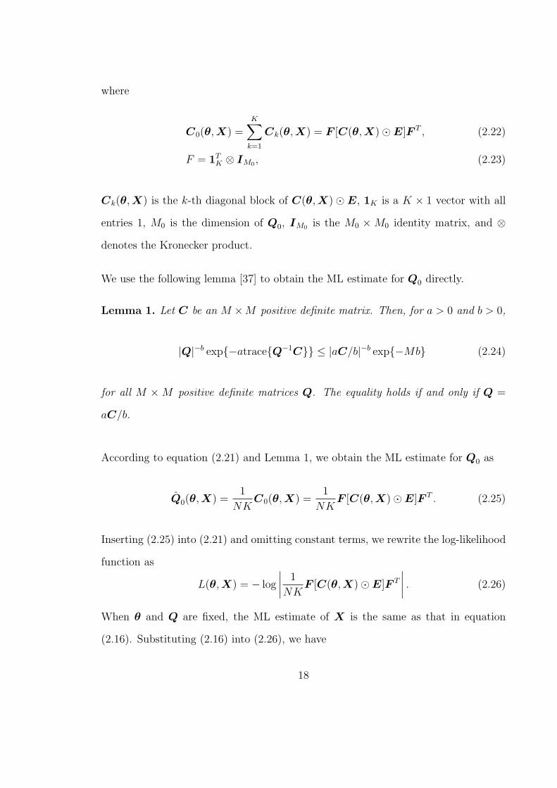
where
C0(θ,X) =K∑k=1
Ck(θ,X) = F [C(θ,X)⊙E]F T , (2.22)
F = 1TK ⊗ IM0 , (2.23)
Ck(θ,X) is the k-th diagonal block of C(θ,X) ⊙E, 1K is a K × 1 vector with all
entries 1, M0 is the dimension of Q0, IM0 is the M0 ×M0 identity matrix, and ⊗
denotes the Kronecker product.
We use the following lemma [37] to obtain the ML estimate for Q0 directly.
Lemma 1. Let C be an M ×M positive definite matrix. Then, for a > 0 and b > 0,
|Q|−b exp−atraceQ−1C ≤ |aC/b|−b exp−Mb (2.24)
for all M ×M positive definite matrices Q. The equality holds if and only if Q =
aC/b.
According to equation (2.21) and Lemma 1, we obtain the ML estimate for Q0 as
Q0(θ,X) =1
NKC0(θ,X) =
1
NKF [C(θ,X)⊙E]F T . (2.25)
Inserting (2.25) into (2.21) and omitting constant terms, we rewrite the log-likelihood
function as
L(θ,X) = − log
∣∣∣∣ 1
NKF [C(θ,X)⊙E]F T
∣∣∣∣ . (2.26)
When θ and Q are fixed, the ML estimate of X is the same as that in equation
(2.16). Substituting (2.16) into (2.26), we have
18
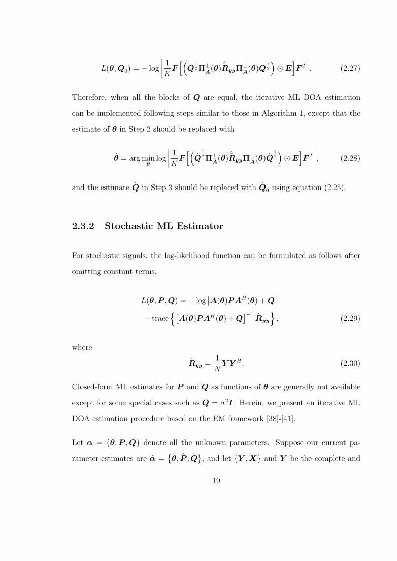
L(θ,Q0) = − log
∣∣∣∣ 1KF [(Q 12Π⊥
A(θ) ˆRyyΠ
⊥A(θ)Q
12
)⊙E
]F T
∣∣∣∣. (2.27)
Therefore, when all the blocks of Q are equal, the iterative ML DOA estimation
can be implemented following steps similar to those in Algorithm 1, except that the
estimate of θ in Step 2 should be replaced with
θ = argminθ
log
∣∣∣∣ 1KF [(Q 12Π⊥
A(θ) ˆRyyΠ
⊥A(θ)Q
12
)⊙E
]F T
∣∣∣∣, (2.28)
and the estimate Q in Step 3 should be replaced with Q0 using equation (2.25).
2.3.2 Stochastic ML Estimator
For stochastic signals, the log-likelihood function can be formulated as follows after
omitting constant terms.
L(θ,P ,Q) = − log∣∣A(θ)PAH(θ) +Q
∣∣−trace
[A(θ)PAH(θ) +Q
]−1Ryy
, (2.29)
where
Ryy =1
NY Y H . (2.30)
Closed-form ML estimates for P and Q as functions of θ are generally not available
except for some special cases such as Q = σ2I. Herein, we present an iterative ML
DOA estimation procedure based on the EM framework [38]-[41].
Let α = θ,P ,Q denote all the unknown parameters. Suppose our current pa-
rameter estimates are α =θ, P , Q
, and let Y ,X and Y be the complete and
19
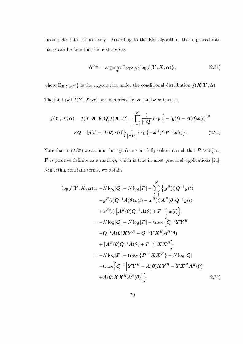
incomplete data, respectively. According to the EM algorithm, the improved esti-
mates can be found in the next step as
αnew = argmaxα
EX|Y ,α log f(Y ,X;α) , (2.31)
where EX|Y ,α· is the expectation under the conditional distribution f(X|Y , α).
The joint pdf f(Y ,X;α) parameterized by α can be written as
f(Y ,X;α) = f(Y |X,θ,Q)f(X;P ) =N∏t=1
1
|πQ|exp
− [y(t)−A(θ)x(t)]H
×Q−1 [y(t)−A(θ)x(t)] 1
|πP |exp
−xH(t)P−1x(t)
. (2.32)
Note that in (2.32) we assume the signals are not fully coherent such that P > 0 (i.e.,
P is positive definite as a matrix), which is true in most practical applications [21].
Neglecting constant terms, we obtain
log f(Y ,X;α)∝ −N log |Q| −N log |P | −N∑t=1
yH(t)Q−1y(t)
−yH(t)Q−1A(θ)x(t)− xH(t)AH(θ)Q−1y(t)
+xH(t)[AH(θ)Q−1A(θ) + P−1
]x(t)
= −N log |Q| −N log |P | − trace
Q−1Y Y H
−Q−1A(θ)XY H −Q−1Y XHAH(θ)
+[AH(θ)Q−1A(θ) + P−1
]XXH
= −N log |P | − trace
P−1XXH
−N log |Q|
−traceQ−1
[Y Y H −A(θ)XY H − Y XHAH(θ)
+A(θ)XXHAH(θ)]. (2.33)
20
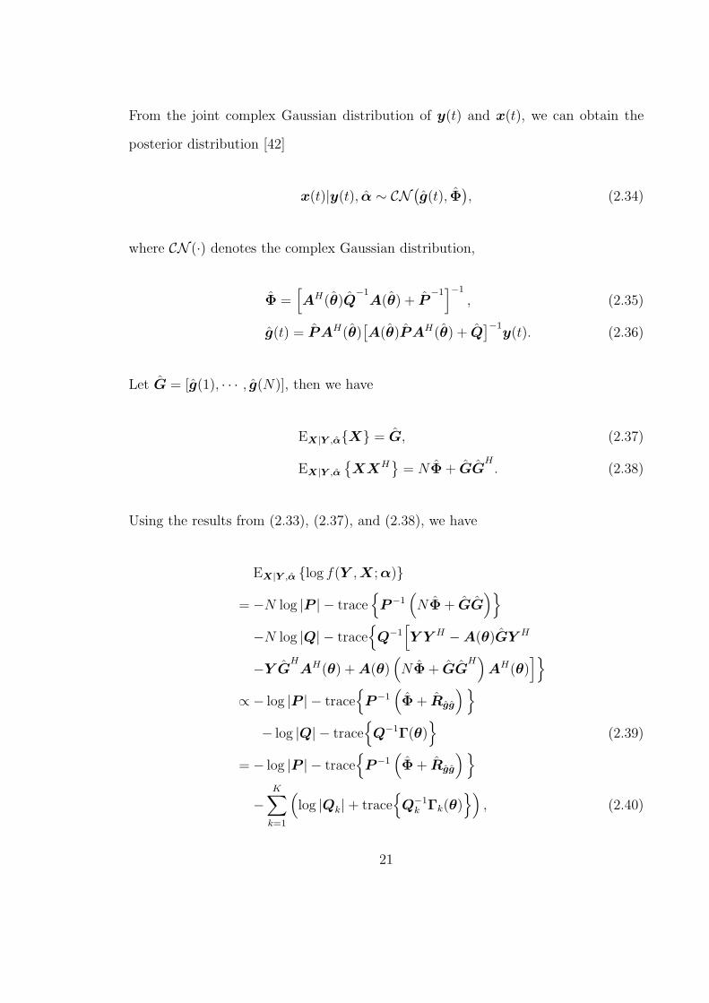
From the joint complex Gaussian distribution of y(t) and x(t), we can obtain the
posterior distribution [42]
x(t)|y(t), α ∼ CN(g(t), Φ
), (2.34)
where CN (·) denotes the complex Gaussian distribution,
Φ =[AH(θ)Q
−1A(θ) + P
−1]−1
, (2.35)
g(t) = PAH(θ)[A(θ)PAH(θ) + Q
]−1y(t). (2.36)
Let G = [g(1), · · · , g(N)], then we have
EX|Y ,αX = G, (2.37)
EX|Y ,α
XXH
= NΦ+ GG
H. (2.38)
Using the results from (2.33), (2.37), and (2.38), we have
EX|Y ,α log f(Y ,X;α)
= −N log |P | − traceP−1
(NΦ+ GG
)−N log |Q| − trace
Q−1
[Y Y H −A(θ)GY H
−Y GHAH(θ) +A(θ)
(NΦ+ GG
H)AH(θ)
]∝ − log |P | − trace
P−1
(Φ+ Rgg
)− log |Q| − trace
Q−1Γ(θ)
(2.39)
= − log |P | − traceP−1
(Φ+ Rgg
)−
K∑k=1
(log |Qk|+ trace
Q−1
k Γk(θ))
, (2.40)
21
where
Rgg =1
NGG =
1
N
N∑t=1
g(t)gH(t), (2.41)
Γ(θ) =1
N
[Y Y H −A(θ)GY H − Y G
HAH(θ)
+A(θ)(NΦ+ GG
)AH(θ)
]= A(θ)ΦAH(θ) +
1
N
(Y −A(θ)G
)(Y −A(θ)G
)H, (2.42)
and Γk(θ) is the k-th diagonal block of Γ(θ)⊙E.
According to Lemma 1, we have
Pnew
= Φ+ Rgg, (2.43)
Qnew
k = Γk(θ)∣∣θ=θ
new , (2.44)
Qnew
= Γ(θ)⊙E∣∣θ=θ
new . (2.45)
Inserting (2.43) and (2.45) into (2.39), we can obtain θnew
as
θnew
= argminθ
log |Γ(θ)⊙E| . (2.46)
Though we may implement the DOA estimation completely using the EM results in
(2.43)-(2.46), we note that when Q is fixed, the ML estimate for θ is [10]
θ = argminθ
log∣∣∣A(θ)P (θ)A
H(θ) + I
∣∣∣+trace
[A(θ)P (θ)A
H(θ) + I
]−1 ˆRyy
, (2.47)
22
where
P (θ) =[A
H(θ)A(θ)
]−1
AH(θ) ˆRyyA(θ)
×[A
H(θ)A(θ)
]−1
−[A
H(θ)A(θ)
]−1
. (2.48)
The ML estimate for P can be obtained as P (θ). Equations (2.47) and (2.48) provide
the optimal results for θ and P when Q is fixed. They also demonstrate that the
EM updates θnew
and Pnew
are not the best match for Q = Qnew
.
When θ and P are fixed, a closed-form ML estimate for Q is normally not available
[20]. However, we can update the estimate for Q using the EM result. Assuming the
existing parameter estimates are θ, P , and Q, according to the EM result in (2.45),
an improved estimate for Q can be found as
Qnew
= Γ(θ)⊙E. (2.49)
We now consider the special case when Q1 = Q2 = · · · = QK = Q0. For this special
case, the results in (2.47) and (2.48) still hold when Q is fixed. To obtain the EM
update equation for Q0, we rewrite (2.40) as
EX|Y ,α log f(Y ,X;α)
∝ − log |P | − traceP−1
(Φ+ Rgg
)−K
(log |Q0|+ trace
Q−1
0 Γ0(θ))
, (2.50)
where
Γ0(θ) =1
K
K∑k=1
Γk(θ) =1
KF [Γ(θ)⊙E]F T . (2.51)
23
So if the existing parameter estimates are θ, P , and Q, an improved estimate for Q0
is
Qnew
0 =1
KF [Γ(θ)⊙E]F T . (2.52)
Based on the results in (2.47)-(2.49) and (2.52), we propose our EM-based stochastic
DOA estimator as follows.
Algorithm 2: EM-Based Stochastic ML DOA Estimator
Step 1: Initialize the parameter estimates at θ = θinit, P = P init, and Q = Qinit.
Step 2: Update Q using equation (2.49).
Step 3: Fixing Q at the Q value obtained in Step 2, update θ and P using
(2.47) and (2.48).
Iterate Steps 2 and 3 until convergence to obtain the final ML DOA estimate.
Replace (2.49) in Step 2 with (2.52) for the special caseQ1 = Q2 = · · · = QK =
Q0.
2.3.3 Mixed ML Estimator
Omitting constant terms, we have the log-likelihood function for mixed signals as
L(θ, b,P ,Q) = − log∣∣A(θ)PAH(θ) +Q
∣∣−trace
[A(θ)PAH(θ) +Q
]−1Cyy(θ, b)
, (2.53)
24
where
Cyy(θ, b) =1
N
N∑t=1
[y(t)−A(θ)b][y(t)−A(θ)b]H . (2.54)
When Q is fixed, we can obtain the closed-form ML estimate for b as a function of θ
as
b(θ) =[A
H(θ)A(θ)
]−1
AH(θ)y, (2.55)
where y = 1N
∑Nt=1 y(t). Substituting (2.55) into (2.53), we can see that the result-
ing log-likelihood function L(θ, b(θ),P ,Q) is similar to the stochastic log-likelihood
function in (2.29). The only difference is that the matrix Ryy in (2.29) is replaced by
Cyy(θ) = Cyy(θ, b(θ)) in L(θ, b(θ),P ,Q). Consequently, the results for stochastic
signals in (2.47) and (2.48) still hold for mixed signals by replacing Ryy in them with
Cyy(θ) [10], or equivalently, by replacing y(t) in them with y(t)−A(θ)b(θ). There-
fore, for mixed signals, by fixing Q and using equations (2.47), (2.48) and (2.55), we
can obtain the ML estimate for θ as
θ = argminθ
log∣∣∣A(θ)P (θ)A
H(θ) + I
∣∣∣+trace
[A(θ)P (θ)A
H(θ) + I
]−1 ˆCyy(θ)
, (2.56)
where ˆCyy(θ) = Q− 1
2 Cyy(θ)Q− 1
2 and
P (θ) =[A
H(θ)A(θ)
]−1
AH(θ) ˆCyy(θ)A(θ)
×[A
H(θ)A(θ)
]−1
−[A
H(θ)A(θ)
]−1
. (2.57)
The ML estimates for b and P are b(θ) and P (θ), respectively. Similarly, if the
existing estimates are θ, b, P , and Q, then the update equations for Q in (2.49) and
25
(2.52) can still be used for mixed signals by replacing y(t) with y(t) −A(θ)b. We
thus propose the following algorithm for mixed ML DOA estimation.
Algorithm 3: EM-Based Mixed ML DOA Estimator
Step 1: Initialize the parameter estimates at θ = θinit, b = binit, P = P init, and
Q = Qinit.
Step 2: Update Q using equation (2.49), with y(t) replaced by y(t) −A(θ)b,
t = 1, . . . , N .
Step 3: Fixing Q at the Q value obtained in Step 2, update θ, b, and P using
(2.56), (2.55) and (2.57), respectively.
Iterate Steps 2 and 3 until convergence to obtain the final ML DOA estimate.
Replace (2.49) in Step 2 with (2.52) for the special caseQ1 = Q2 = · · · = QK =
Q0.
We now consider the mixed ML estimator for the special case of spatially white noise
with Q = σ2I. When Q = σ2I, the ML estimate of b becomes
b(θ) =[AH(θ)A(θ)
]−1AH(θ)y. (2.58)
Using (2.58) and the well-known results of DOA estimation for stochastic signals [8],
[10] under spatially white noise, we obtain the ML estimate of θ as
θ = argminθ
log∣∣∣A(θ)P (θ)AH(θ) + σ2(θ)I
∣∣∣ , (2.59)
26
where
σ2(θ) =1
M − Ltrace
[I −A(θ)
(AH(θ)A(θ)
)−1AH(θ)
]−1
Cyy(θ)
, (2.60)
P (θ) =[AH(θ)A(θ)
]−1AH(θ)Cyy(θ)A(θ)
×[AH(θ)A(θ)
]−1 − σ2(θ)[AH(θ)A(θ)
]−1. (2.61)
2.4 Analytical Performance Analysis
In this section, we present analytical results on the performances of the deterministic,
stochastic, and mixed ML DOA estimators. We also extend some well-known CRB
and asymptotic error results for 1D DOA estimation to the 2D case. Our theorems
and proportions derived in this section hold for both 1D and 2D DOA estimation
under arbitrary proper noise covariance matrices unless the DOA dimension or noise
covariance matrix structure is clearly specified for the theorem or proposition. For
convenience of formulation, we define the following notations.
R = A(θ)PAH(θ) +Q, (2.62)
D =
[da(θ1)
dθ1,da(θ2)
dθ2, · · · , da(θL)
dθL
], (2.63)
D = Q− 12D, (2.64)
D = R− 12D, (2.65)
D2 =
[∂a(θ1)
∂θT1,∂a(θ2)
∂θT2, · · · , ∂a(θL)
∂θTL
], (2.66)
D2 = Q− 1
2D2, (2.67)
D2 = R− 1
2D2, (2.68)
27
A(θ) = R− 12A(θ), (2.69)
∆ =
1 1
1 1
, (2.70)
Rxx =1
N
N∑t=1
x(t)xH(t), (2.71)
Rxx = Ex(t)x(t)H
, (2.72)
R = Q− 12RQ− 1
2 , (2.73)
Q′k =
dQ
dσk, k = 1, . . . , p, (2.74)
Q′k = Q
− 12Q′
kQ− 1
2 , (2.75)
P 2 = P ⊗ [1, 1], (2.76)
Λ =[vecQ
′1
, · · · , vec
Q
′p
], (2.77)
Ξ =[vece1e
T1
, · · · , vec
e2Le
T2L
], (2.78)
where σ1, σ2, . . . , σp are the real unknown parameters from Q, p is the number of real
unknown parameters in Q, vec· denotes the vectorization operator stacking all the
columns of a matrix, one below another, into a vector, and ek is a 2L× 1 vector with
the k-th element 1 and all the other elements 0. For simplicity, in the remainder of
this chapter, we omit θ and useA to representA(θ). Also we let σ = [σ1, σ2, . . . , σp]T
be the real vector containing all the real unknown parameters from Q.
2.4.1 Cramer-Rao Bounds and Asymptotic Errors
We first present the CRB on DOA estimation of mixed signals in the following theo-
rem.
28
Theorem 1. For DOA estimation of mixed signals, the mixed CRB matrix CRBM θ
can be written as
CRBM θ =[CRB−1
d θ +CRB−1S θ
]−1, (2.79)
where CRBd θ and CRBS θ are the deterministic and stochastic CRB matrices on
DOA estimation with measurements from CN(Ab,Q
)and CN
(0,R
), respectively,
in which the unknown parameters are θ, b, P , and σ.
Proof: See Appendix A.
The CRBs on 1D DOA estimation of deterministic and stochastic signals have been
well addressed in [19] and [43]. Herein, we extend these results to 2D DOA estimation.
Proposition 1. The CRB matrix on 2D DOA estimation of deterministic signals is
CRBD θ =1
2NRe(D
H
2 Π⊥AD2
)⊙(R
T
xx ⊗∆)−1
, (2.80)
and the resulting asymptotic CRB matrix is
ACRBD θ =1
2NRe(D
H
2 Π⊥AD2
)⊙(RT
xx ⊗∆)−1
. (2.81)
Proposition 2. The CRB matrix on 2D DOA estimation of stochastic signals is
CRBS θ =1
N
(Ω−MT−1MT
)−1, (2.82)
where
29
Ω= 2Re
(D
H
2 Π⊥AD2
)⊙[(PA
HR
−1AP
)T⊗∆
], (2.83)
M kl = 2RedH
2 kΠ⊥AQ
′lR
−1Ap2 k
, (2.84)
T kl = 2Retrace
Q
′kΠ
⊥AQ
′lR
−1
− traceQ
′kΠ
⊥AQ
′lΠ
⊥A
, (2.85)
M = 2ReΞT[(D
H
2 Π⊥A
)⊗(P T
2 ATR
−T)]
Λ∗, (2.86)
T = 2ReΛH
(R
−T ⊗Π⊥A
)Λ−ΛH
((Π⊥
A
)T ⊗Π⊥A
)Λ, (2.87)
where ·∗ denotes the complex conjugate, M kl and T kl are the (k, l)-th elements
of M and T respectively, and d2 k and p2 k are the k-th columns of D2 and P 2
respectively.
Note that if Q = σ2I, we have M = 0, and (2.82) simplifies to
CRBS θ =1
NΩ−1. (2.88)
When Q = σ2I, the asymptotic error covariance matrix for deterministic ML 1D
DOA estimation is given in [9] as
ACD θ =σ2
2N
[Re(DHΠ⊥
AD)⊙RT
xx
]−1Re(DHΠ⊥
AD)
⊙[Rxx + σ2
(AHA
)−1]T [
Re(DHΠ⊥
AD)⊙RT
xx
]−1. (2.89)
For 2D DOA estimation, we modify this result as follows.
Proposition 3. For 2D DOA estimation under spatially white noise Q = σ2I, the
asymptotic error covariance matrix of the deterministic ML DOA esimator is
30
ACD θ =σ2
2N
[Re(DH
2 Π⊥AD2
)⊙(RT
xx ⊗∆)]−1
×Re(DH
2 Π⊥AD2
)⊙[(Rxx + σ2
(AHA
)−1)T
⊗∆]
×[Re(DH
2 Π⊥AD2
)⊙(RT
xx ⊗∆)]−1
. (2.90)
Propositions 1 to 3 can be proved following the same procedures as in [19], [43],
and [9]. Details of the proofs are omitted here.
Now consider the asymptotic error covariance matrix of applying a stochastic ML
estimator on DOA estimation of mixed signals.
Theorem 2. If a stochastic ML estimator is applied on DOA estimation of mixed
signals with correlation matrix Rxx, then the asymptotic error covariance matrix
ACS θ is equal to the stochastic CRB matrix on DOA estimation with measurements
from CN (0, R), where
R = ARxxAH +Q (2.91)
and the unknown parameters are θ, Rxx, and σ.
Proof: See Appendix B, in which the following lemma is used in deriving the result.
Lemma 2. Suppose x ∼ CN (µ,C), B and D are two square matrices with the same
size as C. Then we have
ExHBxxHDx
= trace
B(C + µµH
)trace
D(C + µµH
)+trace
B(C + µµH)D
(C + µµH
)− µHBµµHDµ. (2.92)
Proof: See Appendix C.
31
2.4.2 Analytical Performance Comparisons
In this section, we present some analytical comparison results on the performances
of the three types of estimators. We first examine the performance of the mixed ML
estimator on DOA estimation of stochastic signals.
Proposition 4. For DOA estimation of stochastic signals,
CRBM θ = CRBS θ. (2.93)
Proof: According to the results in (A.7), (A.8), (A.11), and (A.15) in Appendix A,
we can see that CRB−1M θ = CRB−1
S θ if b = 0, from which we obtain (2.93).
Proposition 4 shows that for DOA estimation of stochastic signals, the asymptotic
accuracy of the mixed ML estimator is equal to that of the stochastic one.
For DOA estimation of stochastic signals, it was shown [43] that the asymptotic
deterministic CRB is not larger than the stochastic CRB. We compare the asymptotic
deterministic CRB with the mixed CRB and obtain the similar result as follows.
Proposition 5. For DOA estimation of mixed signals,
CRBM θ ≥ ACRBD θ. (2.94)
Proof: See Appendix D.
For DOA estimation of mixed signals, it seems difficult to make analytical comparisons
forACD θ, ACS θ, andCRBM θ under arbitrary properQ, since a closed-formACD θ
32
is still not available and an analytical comparison between ACS θ and CRBM θ seems
difficult. However, we have the following proposition holds under the special case
Q = σ2I.
Proposition 6. For ML DOA estimation of mixed signals under spatially white noise
Q = σ2I, we have
ACD θ ≥ ACS θ ≥ CRBM θ. (2.95)
Proof: See Appendix E. The following lemma is used in deriving ACD θ ≥ ACS θ
for 2D DOA estimation.
Lemma 3. Let A and C be two nonnegative definite matrices of the same size as B,
a Hermitian matrix, and let C† be the Moore-Penrose pseudoinverse of C. Suppose
NC ⊆ NB, where N· denotes the null space of a matrix. Then,
ReA⊙B−1ReA⊙C ReA⊙B−1 ≥ReA⊙
(BC†B
)−1(2.96)
if ReA⊙C−1 and all the matrix inverses in (2.96) exist.
Proof: See Appendix F.
When the noise is spatially white, the second inequality in (2.95) shows that with the
same signal correlation matrix and noise power, the mixed signals improve the DOA
estimation accuracy compared with the stochastic ones, and the mixed ML estimator
provides better performance than the stochastic ML estimator.
We have not shown (2.95) analytically for arbitrary proper noise covariance matrices.
However, since CRBM θ is the CRB on mixed signal DOA estimation, we should
33
always have ACD θ ≥ CRBM θ and ACS θ ≥ CRBM θ, where the equalities do not
always hold due to the result in Proposition 6.
For the more special case of 1D DOA estimation of a single source under spatially
white noise, we have the following proposition.
Proposition 7. For 1D DOA estimation of a single stochastic or mixed signal under
Q = σ2I, the asymptotic mean-square error of the deterministic ML estimator is
equal to that of the stochastic estimator, i.e, ACD θ = ACS θ.
Proof: For 1D DOA estimation of a single source, DHΠ⊥AD, Rxx, and
(AHA
)−1
are all real scalars. According to the result in (2.89), we have
ACD θ =σ2
2N
[(DHΠ⊥
AD)−1
R−Txx
] (DHΠ⊥
AD)
×[Rxx + σ2
(AHA
)−1]T [(
DHΠ⊥AD
)−1R−T
xx
]=
σ2
2N
(DHΠ⊥
AD) [R−1
xx + σ2R−1xx
(AHA
)−1R−1
xx
]−T−1
= ACS θ. (2.97)
The last equality holds from the result in [8].
2.5 Numerical Examples
In this section, we compare the performances of the deterministic, stochastic, and
mixed ML DOA estimators through two numerical examples.
In the first example, we consider a 1D DOA estimation problem of two sources using
a linear scalar-sensor array consisting of four separated linear sub-arrays, which are
composed of 3, 4, 3, and 4 scalar sensors, respectively. The distance between any
34
two adjacent sub-arrays is 3λ, where λ is the wavelength of the narrow-band signal.
Within each sub-array, the spacing between scalar sensors is 0.5λ. The linear sensor
array lies on the z axis. The elevation angles of the two sources are 15 and 30 degrees.
The elements of the noise covariance matrix are generated with the following widely
used noise model (see [24] and the references therein):
[Qi]kl = σ2i exp
− (k − l)2ζi
, (2.98)
where σ21 = 2, σ2
2 = 3, σ23 = 4, σ2
4 = 5, ζ1 = 0.6, ζ2 = 0.7, ζ3 = 0.8, and ζ4 = 0.9. We
consider both stochastic and mixed signals and apply the deterministic, stochastic,
and mixed ML DOA estimators to each of them. For the stochastic signal case, we
assume the signal covariance matrix
P =
1 0.3
0.3 1
. (2.99)
For the mixed signal case, we assume the signal mean b = [0.7, 0]T and the signal
covariance matrix
P =
0.2 0
0 0.8
. (2.100)
We consider the estimation algorithm achieves convergence at the n-th iteration if the
Euclidean norm of θn−θn−1 is smaller than an error tolerance. The root-mean-square
errors (RMSEs) from three types of estimators are illustrated in Figs. 2.1 and 2.2
for the source with θ = 15 degrees. The mean square errors are calculated with 200
Monte Carlo runs.
35
We first examine the performances of the deterministic ML DOA estimator (Algo-
rithm 1). From Figs. 2.1 and 2.2, we observe that the accuracy of the deterministic
estimator does not always increase with iterations going forward. Furthermore, in
the running of our MATLAB program, the deterministic estimator in Algorithm 1
diverged the value of the deterministic log-likelihood function to infinity and intro-
duced errors in MATLAB usually within 10 iterations. Examining the deterministic
log-likelihood function in (2.15), we can see that the deterministic ML DOA estimator
finds the DOA estimate by maximizing − log |C(θ,X) ⊙ E| over θ and X, where
C(θ,X) = [Y −A(θ)X][Y −A(θ)X]H . Due to the large number of nuisance pa-
rameters in X, no matter what value θ takes, there always exist X values that make
C(θ,X) ⊙E singular and the value of the log-likelihood function in (2.15) infinite.
This introduces severe instability in DOA estimation and explains the phenomena
we observed in the figures and program running. However, the first few iterations of
Algorithm 1 are still able to provide close DOA estimates, as shown in Figs. 2.1 and
2.2, as well as in [24].
We now examine the performances of the stochastic estimator (Algorithm 2) and the
mixed estimator (Algorithm 3). Both algorithms are initialized using the results from
one iteration of Algorithm 1. Specifically, suppose θ, Q, and X are the estimates
from one iteration of Algorithm 1. Then θ and Q are initialized as θinit = θ and
Qinit = Q for both estimators. For the stochastic estimator, P is initialized as
P init = XXH/N . For the mixed estimator, b and Q are initialized as
binit = ¯x =1
N
N∑t=1
x(t), (2.101)
P init =1
N
N∑t=1
[x(t)− ¯x
] [x(t)− ¯x
]H. (2.102)
36
102
103
10−2
10−1
100
101
Number of Measurements
RM
SE
(de
gree
)
Asymptotic Deterministic CRBStochastic CRBDeterministic Estimator (one iteration)Deterministic Estimator (two iterations)Deterministic Estimator (four iterations)Deterministic Estimator (six iterations)Stochastic EstimatorMixed Estimator
Figure 2.1: Cramer-Rao bounds and root-mean-square errors as functions of thenumber of measurements from stochastic signal one-dimensional DOA estimation.
The optimizations over θ in Steps 3 of both algorithms are implemented iteratively,
starting from θinit or the θ value from the previous iteration. The error tolerance
used is 10−2 degree for both Figs. 1 and 2. Algorithms 2 and 3 both converge with
an average number of 3 iterations or so in our simulations for either Fig. 1 or 2.
From Fig. 2.1, we see that for DOA estimation of stochastic signals, the performances
of the stochastic and the mixed estimators are similar to each other and are normally
better than that of the deterministic estimator. From Fig. 2.2, we observe that for
DOA estimation of the mixed signals, the mixed estimator provides higher accuracy
than either the deterministic or the stochastic estimator.
In our second example, we consider a 2D DOA estimation problem of a single source
using a uniform linear acoustic vector-sensor (AVS) array [11]. The array consists
of six vector sensors and lies on the z axis. Each vector sensor consists of four
sensors measuring acoustic pressure and three acoustic particle velocity components,
respectively. The two adjacent vector sensors are 0.5λ apart from each other. The
37
102
103
10−2
10−1
100
101
Number of Measurements
RM
SE
(de
gree
)
Asymptotic Deterministic CRBAsymptotic Error Curve of Stochastic EstimatorMixed CRBDeterministic Estimator (one iteration)Deterministic Estimator (three iterations)Deterministic Estimator (five iterations)Stochastic EstimatorMixed Estimator
Figure 2.2: Cramer-Rao bounds and root-mean-square errors as functions of thenumber of measurements from mixed signal one-dimensional DOA estimation.
elevation and azimuth angles of the source are 15 and 30 degrees, respectively. We
assume the noise is correlated among the four sensors within one vector sensor but
uncorrelated between different vector sensors. Furthermore, we assume the 4 × 4
noise covariance matrices from different vector sensors are equal. This noise scenario
matches the situation of an underwater fast-towed linear AVS array, where the flow
noise is the dominant noise on the array. When the distance between vector sensors
is not smaller than 0.5λ, the covariance matrix of the noise can be well approximated
by a block-diagonal matrix with all blocks equal [45]. The realistic modeling of flow
noise is not the topic of this dissertation. Herein, we assume the 4×4 noise covariance
matrix on each vector sensor follows equation (2.98) with σ2 = 2 and ζ = 0.5. We
consider both stochastic and mixed signals, and apply the deterministic, stochastic,
and mixed ML DOA estimators to each of them. For the stochastic signal case, we
assume the noise power is 0.5. For the mixed signal case, we assume the signal mean is
0.3 and the signal variance is 0.1. The estimation errors from three types of estimators
are illustrated in Figs. 2.3 and 2.4 for the elevation angle. The mean-square errors are
38
102
103
10−1
100
101
Number of Measurements
RM
SE
(de
gree
)
Asymptotic Deterministic CRBStochastic CRBDeterministic EstimatorStochastic EstimatorMixed Estimator
Figure 2.3: Cramer-Rao bounds and root-mean-square errors as functions of thenumber of measurements from stochastic signal two-dimensional DOA estimationwith the diagonal blocks equal in the noise covariance matrix.
also computed with 200 Monte Carlo runs. The error tolerance used is 10−2 degree for
both Figs. 3 and 4. In our simulations for either Fig. 3 or 4, Algorithm 1 converges
with an average number of 4 iterations or so, and both Algorithms 2 and 3 converge
with an average number of about 3 iterations.
From Figs. 2.3 and 2.4, we observe that the mixed estimator performs as well as
the stochastic estimator in the stochastic signal case and better in mixed signal case.
These results are similar to those in our first example. The phenomenon distinguish-
ing this example from the first one is that with all diagonal blocks equal in the noise
covariance matrix, the deterministic ML DOA estimator converges with ongoing it-
erations and provides estimation accuracy close to that of the stochastic estimator,
as shown in Figs. 2.3 and 2.4. The conditions that guarantee the convergence of the
deterministic estimator are not within the scope of this dissertation.
39
102
103
10−1
100
101
102
Number of Measurements
RM
SE
(de
gree
)
Asymptotic Deterministic CRBAsymptotic Error Curve of Stochastic EstimatorMixed CRBDeterministic EstimatorStochastic EstimatorMixed Estimator
Figure 2.4: Cramer-Rao bounds and root-mean-square errors as functions of thenumber of measurements from mixed signal two-dimensional DOA estimation withthe diagonal blocks equal in the noise covariance matrix.
So far, we only gave the numerical results produced by Algorithm 2 for the stochastic
ML estimator. We also ran the simulations using the pure-EM algorithm based on
(2.43)-(2.46) as the stochastic ML estimator. The results showed that the pure-
EM algorithm is able to provide similar performance to that of Algorithm 2, but it
normally requires smaller error tolerances and more iterations and running time to
do so. As expected, the pure-EM algorithm is less efficient than Algorithm 2. The
estimation results from the pure-EM algorithm are omitted here since they are just
similar to those of Algorithm 2. The detailed comparisons for these two algorithms
are not within the interest of this dissertation.
40
2.6 Summary
We considered the problem of narrow-band DOA estimation under spatially colored
noise using sparse sensor arrays and proposed new methods for ML DOA estimation
of stochastic and mixed signals based on an EM framework. We gave the CRB on
DOA estimation of mixed signals. We also derived the asymptotic error covariance
matrix of applying the stochastic DOA estimator on mixed signal DOA estimation.
We presented both analytical and numerical comparisons for the performances of
the deterministic, stochastic, and mixed estimators. Our results showed that: (i)
the performance of the deterministic estimator is normally inferior to those of the
stochastic and mixed estimators; (ii) for DOA estimation of stochastic signals, the
mixed estimator provides similar performance to that of the stochastic estimator; (iii)
for DOA estimation of mixed signals, the mixed estimator yields better performance
than the stochastic estimator.
41
Chapter 3
Narrow-Band Direction-of-Arrival
Estimation of Hydroacoustic
Signals From Marine Vessels 2
As a topic in Chapter 2, we considered the direction-of-arrival (DOA) estimation
of mixed signals, which are mixtures of non-zero means with the typical zero-mean
Gaussian signals assumed by the many existing DOA estimators. In this chapter,
we consider the DOA estimation problem of another type of mixed signals – the
underwater acoustic signals (hydroacoustic signals) from marine vessels like ships,
submarines, or torpedoes, which contain both sinusoidal and random components.
We model this type of signals as the sum of deterministic sinusoidal signals and zero-
mean Gaussian signals, and derive the maximum likelihood (ML) DOA estimator
for them under spatially white noise. We compute the asymptotic error covariance
matrix of the proposed ML estimator, as well as that of the typical ML estimator
assuming zero-mean Gaussian signals, for DOA estimation of this type of signals. Our
2Based on T. Li and A. Nehorai, “Maximum Likelihood Direction-of-Arrival Estimation of Un-derwater Acoustic Signals Containing Sinusoidal Components,” IEEE Trans. Signal Process., vol.59, pp. 5302-5314, Nov. 2011. c⃝[2011] IEEE.
42
analytical comparison and numerical examples show that the proposed ML estimator
improves the DOA estimation accuracy for the hydroacoustic signals from marine
vessels compared with the typical ML estimator assuming zero-mean Gaussian signals.
3.1 Introduction
Direction-of-arrival (DOA) estimation plays an important role in underwater sonar
applications such as the localization and tracking of ships and submarines. Among
diverse parameter estimation techniques, maximum likelihood (ML) estimation is
distinguished by its excellent asymptotic estimation performance often able to achieve
the Cramer-Rao bound (CRB) [42], which is highly desirable in many underwater
DOA estimation scenarios where the signal-to-noise ratios (SNRs) are usually low
whereas high DOA estimation accuracy is required.
ML methods estimate the DOA by maximizing the likelihood functions, which vary
with the models describing the signals. Among existing signal models, the determin-
istic and the stochastic models are the most widely exploited in ML DOA estimation
(see [7], [8], [10], [19], [20], and [24] for examples). The deterministic signal model
(see [7], [8], [19], and [24]) considers the signal values at all snapshots as deterministic
unknown parameters. As a result, the number of unknown parameters in the likeli-
hood function increases with the number of measurements, such that the ML DOA
estimator based on this model turns out not to be able to achieve the deterministic
CRB [8]. In contrast, the stochastic signal model (see [8], [10], and [20]) considers the
signals to be random processes following specific probability density functions (pdfs).
As a consequence, the unknown signal parameters in the likelihood function are fixed
in size with respect to the change in the number of measurements. The ML DOA
43
estimator based on the stochastic signal model achieves the stochastic CRB and is
shown to be able to provide better performance than the ML estimator based on the
deterministic signal model [8].
In most existing ML DOA estimation works using stochastic signal models, the signals
are assumed to follow Gaussian distributions with zero means (see [8], [10], and [20]
for examples). Though the zero-mean Gaussian distribution is able to well describe
a wide range of signals in practice, there exist applications where the signals cannot
be accurately characterized in this way (see [14] and [25]), and better estimation
accuracy may be achieved by using more precise signal models. In this chapter, we
consider the DOA estimation problem of hydroacoustic signals containing sinusoidal
components, which cannot be well described by the zero-mean Gaussian distribution.
The hydroacoustic signals from ships, submarines, or torpedoes are known to consist
of two parts ( [31], [48], [49]): the noise-like part with continuous spectra, and the
sinusoidal part with discrete frequencies. In this chapter, we call this type of sig-
nals “mixed signals”, and model them as the mixture of a zero-mean Gaussian part
with unknown covariance matrix and a sinusoidal part with unknown coefficients and
frequencies, which correspond to the noise-like part with continuous spectra and the
sinusoidal part with discrete frequencies, respectively. For simplicity of notation and
presentation, in the rest of this chapter, we use “stochastic signals” to represent zero-
mean Gaussian signals. We use “stochastic” and “mixed” estimators or CRBs to
represent the ML estimators or CRBs derived under the assumptions of “stochastic”
and “mixed” signals, respectively.
In this chapter, we derive the ML estimator and its asymptotic error covariance matrix
for DOA estimation of mixed signals. In addition, we compute the asymptotic error
44
covariance matrix of applying the stochastic estimator to DOA estimation of mixed
signals. We provide both analytical and numerical comparisons for the stochastic
and the proposed mixed estimators. The results show that the proposed mixed signal
model and estimator improve the DOA estimation accuracy for mixed signals.
The remainder of this chapter is organized as follows. We first give our measurement
model in Section 3.2, and derive the ML estimator in Section 3.3. Section 3.4 provides
the results of analytical performance analysis. Numerical examples and conclusions
appear in Sections 3.5 and 3.6, respectively.
3.2 Measurement Model
In this chapter, we limit our problem to narrow-band DOA estimation of mixed sig-
nals. Recall that the signal can be considered as narrow-band if D/c ≪ 1/B, where
D, c, and B are the array length, the signal propagation speed, and the signal band-
width, respectively. Consider the mixed signals from L far-field sources impinging on
an array of M sensors. We write the narrow-band array output as
y(t) = A(θ) [Cφ(ω, t) + x(t)] + ϵ(t), t = 1, . . . , N, (3.1)
where y(t) is the M × 1 measurement vector at the t-th snapshot,
A(θ) = [a(θ1), · · · ,a(θL)] (3.2)
is the array steering matrix, a(θl) is the steering vector corresponding to the l-th
source, θ = [θ1, . . . , θL]T is the DOA vector with θl the DOA of the l-th source,
45
·T denotes the matrix transpose, ω = [ω1, . . . , ωJ ]T with J the total number of
sinusoidal components with different frequencies in the received signals and ωm the
radian frequency of the m-th sinusoidal component, φ(ω, t) = [ejω1t, ..., ejωJ t]T with
j2 = −1, C is the L× J matrix containing the coefficients of φ(ω, t) for all sources,
x(t) is the L× 1 Gaussian signal vector, ϵ(t) is the M × 1 Gaussian noise vector, and
N is the total number of measurements.
In equation (3.1), the mixed signals are represented by the sum of Cφ(ω, t) and
x(t), which correspond to the parts with discrete frequencies and continuous spectra,
respectively. We assume x(t) and ϵ(t) follow zero-mean circularly complex Gaussian
distributions with unknown covariance matrices P and Q, respectively. We further
assume x(t) and ϵ(t) are both temporally white and uncorrelated with each other.
Additionally, we assume L is known, which is a quite common assumption in existing
DOA estimation research (see [7], [8], [10], [19], [20], and [24] for examples). Also,
we assume J is known, which is a quite common assumption as well in existing
sinusoidal frequency estimation research (see [33], [34], [36], [50], [51] for examples).
The unknown parameters in (3.1) are those from θ, C, ω, P , and Q.
3.3 Maximum Likelihood Estimation
In this section, we present the ML estimator for DOA finding of mixed signals, which
is called the mixed estimator in this chapter. For simplicity, we omit θ and ω in
notations, and use A and φ(t) to represent A(θ) and φ(ω, t), respectively.
Combining measurements from all snapshots, we rewrite the narrow-band measure-
ment model in (3.1) as
46
Y = ACϕ+AX +E, (3.3)
where Y = [y(1), · · · ,y(N)], ϕ = [φ(1), · · · ,φ(N)], X = [x(1), · · · ,x(N)], and
E = [ϵ(1), · · · , ϵ(N)]. Vectorizing both sides of (3.3), we obtain
y =[ϕT ⊗A
]vecC+ vec AX +E , (3.4)
where y = vecY = [yT (1), · · · ,yT (N)]T , ⊗ denotes the Kronecker product, and
vec· denotes the vectorization operator stacking all the columns of a matrix, one
below another, into a vector. Note that in the derivation of (3.4), we use the property
that
vecABC = [CT ⊗A]vecB (3.5)
for any matrices A, B, and C that can make ABC [44].
From (3.4), we have
y ∼ CN([ϕT ⊗A
]vecC, IN ⊗
(APAH +Q
)), (3.6)
where CN (·) denotes the complex Gaussian distribution, IN is the N × N identity
matrix, and ·H denotes the conjugate transpose. From (3.6), we obtain the ML
estimate for vecC as
vecC =[ϕT ⊗A
]H[IN ⊗
(APAH +Q
)−1]
×[ϕT ⊗A
]−1[ϕT ⊗A
]H[IN ⊗
(APAH +Q
)−1]y
=[(
ϕ∗ϕT)−1ϕ∗]⊗ [AH
(APAH +Q
)−1A]−1
×AH(APAH +Q
)−1y, (3.7)
47
where ·∗ denotes the complex conjugate.
In Appendix G, we show that
[AH(APAH +Q
)−1A]−1
AH(APAH +Q
)−1=(AHQ−1A
)−1AHQ−1. (3.8)
As a result, equation (3.7) becomes
vecC=[(ϕ∗ϕT
)−1ϕ∗]⊗[(AHQ−1A
)−1AHQ−1
]y, (3.9)
from which we obtain the ML estimate for C as
C =(AHQ−1A
)−1AHQ−1Y ϕH
(ϕϕH
)−1
=(A
HA)−1A
HY ϕH
(ϕϕH
)−1, (3.10)
where A = Q− 12A and Y = Q− 1
2Y . We can see that the ML estimate of C is a
function of θ, ω, and Q but independent of the signal covariance matrix P . This
result is important for the further reduction of P from the likelihood function.
By omitting constant terms, the log-likelihood (LL) function can be written as
L(θ,C,ω,P ,Q) = − log∣∣APAH +Q
∣∣− trace[APAH +Q
]−1Ryy
, (3.11)
where | · | denotes the matrix determinant, and
Ryy =1
N(Y −ACϕ) (Y −ACϕ)H . (3.12)
Substituting (3.10) into (3.11), we rewrite the LL function as
48
L(θ,ω,P ,Q) = − log∣∣APAH +Q
∣∣− trace [APAH +Q
]−1Ryy
(3.13)
= − log |Q| − log∣∣AP AH
+ IM∣∣− trace
[AP A
H+ IM
]−1
Ryy
, (3.14)
where
Ryy =1
N
(Y −ACϕ
)(Y −ACϕ
)H, (3.15)
and
Ryy =Q− 12 RyyQ
− 12
=1
N
(Y −ΠAYΠϕH
)(Y −ΠAYΠϕH
)H, (3.16)
in which ΠA = A(A
HA)−1
AH.
In (3.14), the last two terms on the right-hand side of the equality constitute a
function similar to the Gaussian LL function for stochastic signals under spatially
white noise [10]. Following procedures similar to those in [10], we have the ML
estimate for P as
P =[A
HA]−1
AHRyyA
[A
HA]−1
−[A
HA]−1
, (3.17)
which is a function of θ, ω, and Q.
Replacing P in (3.14) with the estimate in (3.17), we can obtain a reduced LL function
L(θ,ω,Q), which depends on θ, ω, and Q only. L(θ,ω,Q) can hardly be further
reduced, except in some special cases (see [20] and [52], and [53] for examples from
DOA estimation of stochastic signals). One such special case is DOA estimation
under spatially white noise, which has been widely addressed for deterministic and
stochastic signals (see [7], [8], [10], [52], and [54] for examples). In the following, we
49
give the expression of the further reduced LL function under spatially white noise
Q = σ2I for DOA estimation of mixed signals.
The LL function in (3.13) has a form similar to the Gaussian LL function for stochastic
signals. Thus, following procedures and results similar to those for stochastic signal
DOA estimation under spatially white noise [8], [52], we can obtain the ML estimates
of σ2 and P , along with the further reduced LL function under spatially white noise
as
σ2 =1
M − Ltrace
Π⊥
ARyy
, (3.18)
P = (AHA)−1AHRyyA(AHA)−1 − σ2(AHA)−1, (3.19)
L(θ,ω) = − log∣∣APAH + σ2IM
∣∣, (3.20)
where Π⊥A = IM −ΠA. Note that when Q = σ2I, we have
Ryy =1
N
(Y −ΠAYΠϕH
) (Y −ΠAYΠϕH
)H. (3.21)
We thus are able to simplify (3.18) as
σ2 =1
M − Ltrace
Π⊥
A
Y Y H
N
. (3.22)
Substituting (3.19), (3.21), and (3.22) into (3.20), we have
L(θ,ω) = − log∣∣APAH + σ2IM
∣∣= − log
∣∣ΠARyyΠA + σ2Π⊥A
∣∣= − log
∣∣∣∣ΠAYΠ⊥ϕHY
HΠA
N+ σ2Π⊥
A
∣∣∣∣. (3.23)
50
As a result, the mixed DOA estimator under spatially white noise can be implemented
by maximizing (3.23) with respect to θ and ω. When the noise is not spatially white
and Q cannot be reduced, the implementation of the mixed estimator requires the
maximization of L(θ,ω,Q) over Q as well as θ and ω (see [20] and [67] for examples
of the maximization over Q for stochastic signal DOA estimation).
3.4 Analytical Performance Analysis
In this section, we present analytical results on the performances of the stochastic
and the mixed estimators. For convenience of formulation, we define the following
notations:
D =
[da(θ1)
dθ1,da(θ2)
dθ2, · · · , da(θL)
dθL
], (3.24)
P = CCH + P , (3.25)
Q′i =
dQ
dσi, i = 1, . . . , lσ, (3.26)
Q′i = Q
− 12Q′
iQ− 1
2 , i = 1, . . . , lσ, (3.27)
Λ =[vecQ
′1
, · · · , vec
Q
′lσ
], (3.28)
Ξ =[vece1e
T1
, · · · , vec
eLe
TL
], (3.29)
where σ = [σ1, σ2, . . . , σlσ ]T is the vector of length lσ containing all the real unknown
parameters from Q, and ei is a L × 1 vector with the i-th element 1 and all the
other elements 0. We also let c, p, and p be the real column vectors containing the
unknown parameters from C, P , and P , respectively. Note that p consists of the
diagonal elements of P , and the real and imaginary parts of all the upper-triangular
51
elements above the diagonal in P . The vector p is composed similarly of those from
P .
In the following Proposition 1, we give the CRB on DOA estimation of mixed signals.
Proposition 8. For DOA estimation of mixed signals, the mixed CRB matrix CRBM θ
on DOA can be written as
CRBM θ =[CRB−1
D θ +CRB−1S θ
]−1, (3.30)
where CRBD θ is the deterministic CRB matrix on DOA estimation with the mea-
surement at snapshot t, t = 1, . . . , N , following CN(ACφ(t),Q
), in which θ, ω,
c, and σ are the unknown parameters, and CRBS θ is the stochastic CRB matrix
on DOA estimation with each of the N measurements following CN(0,R
), in which
R = APAH +Q and the unknown parameters are θ, p, and σ.
Proof: See Appendix H.
The equations for CRBD θ and CRBS θ have been addressed in [56], [57], and [43].
Though we now have the CRB for DOA estimation of mixed signals, it is not appropri-
ate to simply assume that the mixed ML estimator achieves the CRB asymptotically.
Since the measurements are not temporally stationary due to the sinusoidal compo-
nents, the conclusion that the error covariance matrix of the ML estimator asymp-
totically achieves the CRB (see [42]), which is typically based on the assumption of
independent and identically distributed measurements, can not be directly applied
here. Note that a similar concern has been addressed in [50] for ML estimation of si-
nusoidal frequencies, in which the measurements are not temporally stationary either
52
and a proof was given to show that the ML frequency estimator achieves the CRB
asymptotically.
In the following Proposition 9 and its proof in Appendix I, we confirm the asymptotic
efficiency of the mixed estimator.
Proposition 9. For DOA estimation of mixed signals, the error covariance matrix
of the mixed estimator on α = [θT ,pT ,σT , cT ,ωT ]T achieves the mixed CRB matrix
asymptotically.
The following Theorem 1 (Lindeberg-Feller central limit theorem) [58] is used in our
proof of Proposition 2. Note that the setup of our problem and thus the proof of
Proposition 2 are absolutely different from those in [50].
Theorem 3. Let γ1, · · · ,γN be independent random vectors, each of which are de-
pendent on N , such that as N → ∞,
N∑n=1
∫∥γn∥>ϵ
∥ γn ∥2 fγn(γn)dγn → 0 (3.31)
for arbitrary ϵ > 0 and∑N
n=1 covγn → Q, where ∥ · ∥ denotes the Euclidean
norm of a vector, fγn(γn) is the pdf of γn, and cov· denotes the covariance matrix
of a random vector. Then∑N
n=1 (γn − Eγn), where Eγn is the expectation of
γn, converges in distribution to a random vector following the normal distribution
N (0,Q) as N → ∞.
Now we examine the performance of applying the stochastic estimator to DOA es-
timation of mixed signals. In Appendix J, we show that the stochastic estimator
provides consistent estimate for ξ = [θT ,σT , pT ]T if it is used for mixed signal DOA
53
estimation, and we give the expression for the asymptotic error covariance matrix of
the stochastic estimator on ξ. We also show the following proposition in Appendix J.
Proposition 10. If the stochastic estimator is applied to DOA estimation of mixed
signals, the asymptotic error covariance matrix on ρ = [θT ,σT ]T equals CRBS ρ,
which is the stochastic CRB matrix on the estimation of ρ with each of the N mea-
surements following CN (0, R), where R = APAH +Q and the unknown parameters
are θ, p, and σ. As a result, the asymptotic error covariance matrix on θ equals
CRBS θ.
We can see from Proposition 3 that the stochastic and the mixed signals provide
similar asymptotic accuracy for the estimation of ρ using the stochastic estimator.
We now compare the performances of the stochastic and the mixed estimators. Let
CasM ρ be the asymptotic error covariance matrix on ρ of the mixed estimator. We
show the following proposition in Appendix K.
Proposition 11. For DOA estimation of mixed signals, CasM ρ ≤ CRBS ρ. As a
result, CasM θ ≤ CRBS θ.
Note that ρ consists of all the common unknown parameters that appear in both
the mixed and the stochastic LL functions, and can be estimated by both the mixed
and the stochastic estimators. We cannot make comparisons of the two estimators
for the parameters not included in ρ. Compared with the stochastic estimator, the
mixed estimator has two extra sets of parameters to estimate: the coefficients and
the frequencies of the sinusoidal components. However, from Proposition 11, we see
that with the same correlation matrices of signals and noise, the mixed signals and
estimator provide higher accuracy than the stochastic ones for common parameter
estimation as well as DOA estimation.
54
3.5 Numerical Examples
In this section, we compare the performances of the stochastic and the mixed estima-
tors through two numerical examples.
In the first example, we consider a DOA estimation problem of two sources under
spatially white noise using a uniform linear array of 10 sensors with the inter-sensor
distance equal to 0.5λ, where λ is the wavelength of the narrow-band signals. The
linear sensor array lies on the z axis, and the elevation angles of the two sources are
15 and 20 degrees, respectively. We assume there are two sinusoidal waves incident
on the array, one from each source, with radian frequencies −0.4π and 0.3π and
coefficients 0.8 and 0.7, respectively. For the random signal part, we assume the
covariance matrix is
P =
0.4 0.2
0.2 0.5
. (3.32)
We assume the noise power is σ2 = 10, and apply both the stochastic and the mixed
estimators to DOA estimation. The optimization for the proposed mixed estimator
is implemented iteratively, starting from selected initial values of θ and ω. The DOA
vector θ is initialized using the result from the stochastic estimator. The radian
frequency vector ω can be initialized using many well-developed techniques for fre-
quency estimation of sinusoidal signals (see [33]- [51] for examples). For instance, we
can obtain the initial value for ω by maximizing the likelihood function based on the
following measurement model:
y(t) = Gφ(t) + ϵ(t), (3.33)
55
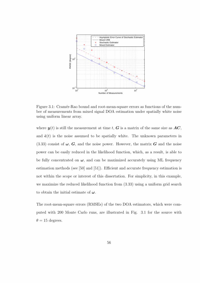
102
103
104
10−1
100
Number of Measurements
RM
SE
(de
gree
)
Asymptotic Error Curve of Stochastic EstimatorMixed CRBStochastic EstimatorMixed Estimator
Figure 3.1: Cramer-Rao bound and root-mean-square errors as functions of the num-ber of measurements from mixed signal DOA estimation under spatially white noiseusing uniform linear array.
where y(t) is still the measurement at time t, G is a matrix of the same size as AC,
and ϵ(t) is the noise assumed to be spatially white. The unknown parameters in
(3.33) consist of ω, G, and the noise power. However, the matrix G and the noise
power can be easily reduced in the likelihood function, which, as a result, is able to
be fully concentrated on ω, and can be maximized accurately using ML frequency
estimation methods (see [50] and [51]). Efficient and accurate frequency estimation is
not within the scope or interest of this dissertation. For simplicity, in this example,
we maximize the reduced likelihood function from (3.33) using a uniform grid search
to obtain the initial estimate of ω.
The root-mean-square errors (RMSEs) of the two DOA estimators, which were com-
puted with 200 Monte Carlo runs, are illustrated in Fig. 3.1 for the source with
θ = 15 degrees.
56
In our second example, we consider a DOA estimation problem under spatially colored
noise using a linear array consisting of separated sub-arrays. In this type of DOA esti-
mation problems (see [21], [24], [67], and [59] for examples), the noise is considered as
uncorrelated between the widely separated sub-arrays such that the noise covariance
matrix Q of the whole array has a block-diagonal structure, in which each diagonal
block is assumed to be arbitrarily positive definite and unknown. In this example, we
examine a DOA estimation problem of two sources using a linear array consisting of
four separated sub-arrays, which are composed of 3, 2, 3, and 2 sensors, respectively.
The distance between any two adjacent sub-arrays is 3λ. Within each sub-array, the
spacing between adjacent sensors is 0.5λ. The linear sensor array lies on the z axis.
The elevation angles of the two sources are 15 and 30 degrees. The (k, l)-th element
of Qi, which is the noise covariance matrix of the i-th sub-array, is generated by [24]
[Qi]kl = σ2i exp
− (k − l)2ζi
, (3.34)
with σ21 = 7, σ2
2 = 6, σ23 = 5, σ2
4 = 8, ζ1 = 0.6, ζ2 = 0.7, ζ3 = 0.7, and ζ4 = 0.6. We
assume there are two sinusoidal waves incident on the array, one from each source,
with radian frequencies −0.3π and 0.4π and coefficients 0.5 and 0.6, respectively. For
the random signal part, we assume the covariance matrix is
P =
0.2 0.0
0.0 0.5
. (3.35)
Unlike the case of spatially white noise, the block-diagonal array noise covariance
matrix Q in this example cannot be reduced from L(θ,ω,Q). To obtain the DOA
estimate, the iterative optimization needs to be implemented over Q as well as θ and
57
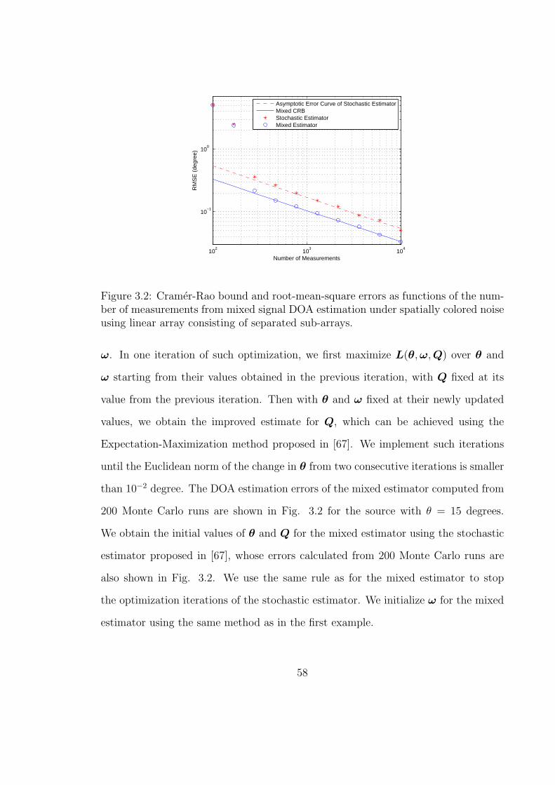
102
103
104
10−1
100
Number of Measurements
RM
SE
(de
gree
)
Asymptotic Error Curve of Stochastic EstimatorMixed CRBStochastic EstimatorMixed Estimator
Figure 3.2: Cramer-Rao bound and root-mean-square errors as functions of the num-ber of measurements from mixed signal DOA estimation under spatially colored noiseusing linear array consisting of separated sub-arrays.
ω. In one iteration of such optimization, we first maximize L(θ,ω,Q) over θ and
ω starting from their values obtained in the previous iteration, with Q fixed at its
value from the previous iteration. Then with θ and ω fixed at their newly updated
values, we obtain the improved estimate for Q, which can be achieved using the
Expectation-Maximization method proposed in [67]. We implement such iterations
until the Euclidean norm of the change in θ from two consecutive iterations is smaller
than 10−2 degree. The DOA estimation errors of the mixed estimator computed from
200 Monte Carlo runs are shown in Fig. 3.2 for the source with θ = 15 degrees.
We obtain the initial values of θ and Q for the mixed estimator using the stochastic
estimator proposed in [67], whose errors calculated from 200 Monte Carlo runs are
also shown in Fig. 3.2. We use the same rule as for the mixed estimator to stop
the optimization iterations of the stochastic estimator. We initialize ω for the mixed
estimator using the same method as in the first example.
58
From the results in Figs. 3.1 and 3.2, we can see that since the mixed model describes
the signals more accurately, the mixed estimator evidently provides better DOA esti-
mation performance than the stochastic estimator. This matches the result from our
analytical performance analysis.
3.6 Summary
We considered the narrow-band DOA estimation problem of hydroacoustic signals
from marine vessels containing both sinusoidal and random components, for which
we presented a mixed signal model and gave ML estimation results. We derived the
asymptotic error covariance matrix on ML DOA estimation of the mixed signals,
as well as that of applying the typical stochastic estimator on DOA estimation of
the mixed signals. We presented both analytical and numerical comparisons for the
performances of the typical stochastic and the proposed mixed estimators for mixed
signal DOA estimation. The results showed that the proposed mixed signal model
and estimator improve the mixed signal DOA estimation accuracy compared with the
typical stochastic ones. In practice, the hydroacoustic signals from marine vessels are
usually wide-band. We will address the wide-band DOA estimation of such signals in
the following two chapters.
59
Chapter 4
Direction-of-Arrival Finding of
Wide-band Hydroacoustic Signals
From Marine Vessels: An
Extension of the Narrow-Band
Case
In this chapter, we consider the problem of wide-band maximum likelihood (ML)
direction-of-arrival (DOA) finding of underwater sources like ships, submarines, or
torpedoes, which emit hydroacoustic signals containing sinusoidal waves. These sig-
nals, which we call mixed signals, are modeled as the mixture of sinusoidal waves and
stochastic Gaussian signals in Chapter 3 for narrow-band DOA estimation. In this
chapter, we generalize the narrow-band results in Chapter 3 to the wide-band case,
and give the wide-band ML DOA estimator for the mixed signals under spatially
white noise. We derive the asymptotic error covariance matrix of the ML estimator,
60
as well as that of the typical stochastic estimator assuming zero-mean Gaussian sig-
nals, for DOA estimation of wide-band mixed signals. Our results demonstrate that
compared with the typical stochastic estimator, the proposed ML estimator provides
better DOA estimation accuracy for wide-band mixed signals.
4.1 Introduction
Direction-of-arrival (DOA) estimation has important applications in the localization
and tracking of underwater acoustic sources like ships and submarines. This chapter
develops a wide-band ML method for DOA estimation of hydroacoustic signals from
ships, submarines, or torpedoes, which are found to consist of two parts (see [31], [48],
and [49]): the noise-like part with continuous spectra, and the tonal or sinusoidal part
with discrete frequencies.
In Chapter 3, these signals are called “mixed signals”, and are modeled as the mixture
of a zero-mean Gaussian part with unknown covariance matrix and a sinusoidal part
with unknown coefficients and frequencies. The work in Chapter 3 only considered the
narrow-band DOA estimation of the mixed signals, which, however, are usually wide-
band in practice. Therefore, the results developed in Chapter 3 cannot be directly
applied to mixed signal DOA estimation in practice. In this chapter, we extend the
narrow-band results in Chapter 3 to the wide-band case. We give the wide-band ML
DOA estimator for mixed signals and derive its asymptotic error covariance matrix.
Additionally, we derive the asymptotic error covariance matrix of applying the typical
stochastic estimator, which assumes zero-mean Gaussian signals, to wide-band mixed
signal DOA estimation. Our analytical comparison and numerical example show that
the proposed ML estimator improves the DOA estimation accuracy for mixed signals.
61
The remainder of this chapter is organized as follows. We give the wide-band mea-
surement model and ML estimator in Section 4.2. Section 4.3 presents the results of
analytical performance analysis. The numerical example and conclusions appear at
last in Sections 4.4 and 4.5, respectively. For simplicity of presentation, in the rest
of this chapter, we use “stochastic signals” to represent zero-mean Gaussian signals.
We use “stochastic” and “mixed” estimators or CRBs (Cramer-Rao bounds) to rep-
resent the ML estimators or CRBs derived under the assumptions of “stochastic” and
“mixed” signals, respectively.
4.2 Measurement Model AndMaximum Likelihood
Estimation
In this section, we give the wide-band measurement model and ML estimator for
DOA finding of mixed signals.
4.2.1 Measurement Model
Consider the wide-band mixed signals from L far-field sources impinging on an array
of M sensors. We decompose the frequency band into a set of non-overlapping (or
roughly non-overlapping) sub-bands, each of which is a narrow band. We make mea-
surements from each sub-band following the narrow-band measurement model (see
(1) in [67]), and formulate the wide-band measurement model as
yk(t) = Ak(θ) [Ckφk(ωk, t) + xk(t)] + ϵk(t), t = 1, . . . , Nk, k = 1, . . . , K, (4.1)
62
where yk(t) is the M × 1 measurement vector at the t-th snapshot from the k-th
sub-band, θ = [θ1, . . . , θL]T is the DOA vector with θl the DOA of the l-th source
and ·T denoting the matrix transpose, Ak(θ) = [ak(θ1), · · · ,ak(θL)] is the array
steering matrix with steering vector ak(θl) focused on the carrier frequency of the k-th
sub-band, ωk = [ωk,1, . . . , ωk,Jk ]T with Jk the total number of sinusoidal components
and ωk,m the radian frequency of them-th sinusoidal component in the k-th sub-band,
φk(ωk, t) = [ejωk,1t, ..., ejωk,Jkt]T with j2 = −1, Ck is the L× Jk coefficient matrix of
φk(ωk, t), xk(t) is the L × 1 Gaussian signal vector from the k-th sub-band, ϵk(t)
is the M × 1 Gaussian noise vector from the k-th sub-band, Nk is the number of
measurements from the k-th sub-band, and K is the total number of sub-bands. We
assume xk(t) and ϵk(t) are temporally white and uncorrelated with each other, and
that they follow circular complex Gaussian distributions CN (0,P k) and CN (0,Qk),
respectively, with unknown covariance matrices P k and Qk.
In (4.1), the mixed signals are represented in the k-th sub-band by the sum of
Ckφk(ωk, t) and xk(t), which correspond to the parts with discrete frequencies and
continuous spectra, respectively. We assume the number of sources is known. Also
we assume the number of sinusoidal components in each sub-band has been estimated
and known, which is a common assumption in existing sinusoidal frequency estima-
tion research (see [33], [50], [51], and [68]). We further assume the signals or noise
from different sub-bands are uncorrelated since different sub-bands do not overlap
in frequency. The value of Nk may vary for different sub-bands. This is often true
when sub-bands with different band widths are sampled at Nyquist rates. However,
the ratio Nk/Nm should roughly remain constant at τm/τk as N1, . . . , NK increase,
where τk is the sampling period of the k-th sub-band. The unknown parameters in
the wide-band model (4.1) are those from θ, Ck, ωk, P k, and Qk, k = 1, . . . , K.
63
4.2.2 Maximum Likelihood Estimation
In this sub-section, we present the mixed DOA estimator for wide-band mixed signals.
For simplicity, we omit θ and ωk in notations, and use Ak and φk(t) to represent
Ak(θ) and φk(ωk, t), respectively.
Recall that in our wide-band model, the measurements are captured separately from
each sub-band following the narrow-band measurement model, and recall that the
measurements from different sub-bands are uncorrelated. As a consequence, the wide-
band log-likelihood (LL) function is the sum of the narrow-band LL functions from
all sub-bands, which, by omitting constant factors, can be written as
L(α) =K∑k=1
Nk
−log
∣∣AkP kAHk +Qk
∣∣−trace [AkP kA
Hk +Qk
]−1Rykyk
, (4.2)
where α is the real vector containing all the unknown parameters in the wide-band
model, | · | denotes the matrix determinant, and
Rykyk=
1
Nk
Nk∑t=1
[yk(t)−AkCkφk(t)][yk(t)−AkCkφk(t)]H . (4.3)
Applying the same narrow-band analysis as from equations (2) to (22) in [67] to each
sub-band, we can obtain the wide-band ML estimation results as in the following
paragraph.
For arbitrary proper noise covariance matrices Qk, k = 1, . . . , K, the ML estimates
for Ck and P k as functions of θ, ωk, and Qk can be found as
Ck =(A
H
k Ak
)−1
AH
k Y kϕHk
(ϕkϕ
Hk
)−1, (4.4)
P k =[A
H
k Ak
]−1
AH
k RykykAk
[A
H
k Ak
]−1
−[A
H
k Ak
]−1
, (4.5)
64
where Ak = Q− 1
2k Ak, Y k = Q
− 12
k Y k with
Y k = [yk(1), · · · ,yk(Nk)], (4.6)
ϕk = [φk(1), · · · ,φk(Nk)], (4.7)
and
Rykyk=
1
Nk
(Y k −ΠAk
Y kΠϕHk
)(Y k −ΠAk
Y kΠϕHk
)H(4.8)
with ΠAk= Ak
(A
H
k Ak
)−1A
H
k . Substituting (4.4) and (4.5) into (4.2), we can obtain
the reduced LL function dependent on θ, ωk, and Qk, k = 1, . . . , K. For the special
case of spatially white noise Qk = σ2kIM , where IM is the M ×M identity matrix,
the noise parameters can be further reduced and the LL function becomes
L(θ, ω) = −K∑k=1
Nk log
∣∣∣∣ΠAk
Y kΠ⊥ϕH
kY H
k
Nk
ΠAk+ σ2
kΠ⊥Ak
∣∣∣∣ (4.9)
with ω = [ωT1 , . . . ,ω
TK ]
T , Π⊥Ak
= IM −ΠAk, and
σ2k =
1
M − Ltrace
Π⊥
Ak
Y kYHk
Nk
. (4.10)
The wide-band mixed DOA estimator under spatially white noise can be achieved by
maximizing (4.9) with respect to θ and ω. If noise parameters cannot be reduced
from the LL function, the wide-band mixed estimator requires maximizing the LL
function over Qk, k = 1, . . . , K, as well as θ and ω.
65
4.3 Analytical Performance Analysis
In this section, we present analytical results on the performances of the stochastic
and the mixed estimators. For convenience of formulation, we let
Dk =
[dak(θ1)
dθ1,dak(θ2)
dθ2, · · · , dak(θL)
dθL
], (4.11)
P k = CkCHk + P k, (4.12)
and ck, pk, pk, and σk be the real column vectors containing the unknown parameters
fromCk, P k, P k, andQk, respectively. Note that pk consists of the diagonal elements
of P k, and the real and imaginary parts of all the upper-triangular elements above
the diagonal in P k. The vector pk is composed similarly of those from P k.
In the following Proposition 1, we give the CRB on DOA estimation of mixed signals.
Proposition 12. For DOA estimation of wide-band mixed signals, the mixed CRB
matrix CRBM θ on DOA can be written as
CRBM θ =
[K∑k=1
(CRB−1
Dk θ +CRB−1Sk θ
)]−1
, (4.13)
where CRBDk θ is the deterministic CRB matrix on DOA estimation with the mea-
surement at snapshot t, t = 1, . . . , Nk, following CN(AkCkφk(t),Qk
), in which θ,
ck, ωk, and σk are the unknown parameters, and CRBSk θ is the stochastic CRB
matrix on DOA estimation with each of the Nk measurements from the sensor array
following CN(0,Rk
), in which Rk = AkP kA
Hk +Qk and the unknown parameters
are θ, pk, and σk.
Proof: See Appendix L.
66
The expressions of CRBDk θ and CRBSk θ can be formulated using the results in
[56], [57], and [43]. As stated in [67], it is not appropriate to simply assume the
mixed ML estimator achieves the CRB asymptotically, since the measurements are not
temporally stationary due to the sinusoidal components. In the following Proposition
13 and its proof in Appendix M, we verify the asymptotic efficiency of the wide-band
mixed estimator.
Proposition 13. For DOA estimation of wide-band mixed signals, the error covari-
ance matrix of the mixed estimator on α achieves the mixed CRB matrix asymptoti-
cally.
We also examine the performance of applying the stochastic estimator to DOA esti-
mation of wide-band mixed signals.
Proposition 14. If the stochastic estimator is applied to DOA estimation of wide-
band mixed signals, the asymptotic error covariance matrix on ρ = [θT ,σT1 , . . . ,σ
TK ]
T
equals CRBS ρ, which is the stochastic CRB matrix on the estimation of ρ with each
of the Nk measurements from the k-th sub-band, k = 1, ..., K, following CN (0, Rk),
where Rk = AkP kAHk +Qk and the unknown parameters are θ, pk, and σk. As a
result, the asymptotic error covariance matrix on θ equals CRBS θ.
We now compare the performances of the mixed and the stochastic estimators. Let
CasM θ be the asymptotic error covariance matrix on θ of the mixed estimator. We
have the following proposition proved.
Proposition 15. For DOA estimation of wide-band mixed signals, CasM θ ≤ CRBS θ.
Proof: According to Propositions 1 and 2, and the results in their proofs, we have
CasM θ =
(∑Kk=1C
as−1Mk θ
)−1, where Cas−1
Mk θ = CRBas−1Dk θ + CRB−1
Sk θ and CRBasDk θ is
67
the asymptotic value of CRBDk θ that can be obtained by replacing Rϕkϕkin (L.11)
with its asymptotic value, which is an identity matrix. From Proposition 4 in [67],
we have CasMk θ ≤ CRBSk θ, k = 1, . . . , K. We thus have the proposition holds.
From Proposition 15, we see that with the same correlation matrices of signals and
noise, the mixed signals and estimator provide better DOA estimation than the
stochastic ones.
4.4 Numerical Example
In this numerical example, we consider a wide-band DOA estimation problem of
two sources under spatially white noise using a uniform linear array consisting of
10 sensors. The linear sensor array lies on the z axis, and the elevation angles of
the two sources are 15 and 20 degrees, respectively. The wide frequency band of
the signals is composed of three narrow sub-bands, and the inter-sensor distance
d = 0.5λ1 = 0.4λ2 = 0.3λ3, where λ1, λ2, and λ3 are the wavelengths of the narrow-
band signals from three sub-bands. In each sub-band, there are two sinusoidal waves
incident on the array, one from each source, with radian frequencies −0.4π and 0.3π
and coefficients 0.8 and 0.7, respectively. For the random signal part and noise, we
assume
P 1 = P 2 = P 3 =
0.4 0.2
0.2 0.5
(4.14)
and σ21 = σ2
2 = σ23 = 10. In addition, we sample the same number of measurements
from each sub-band.
68
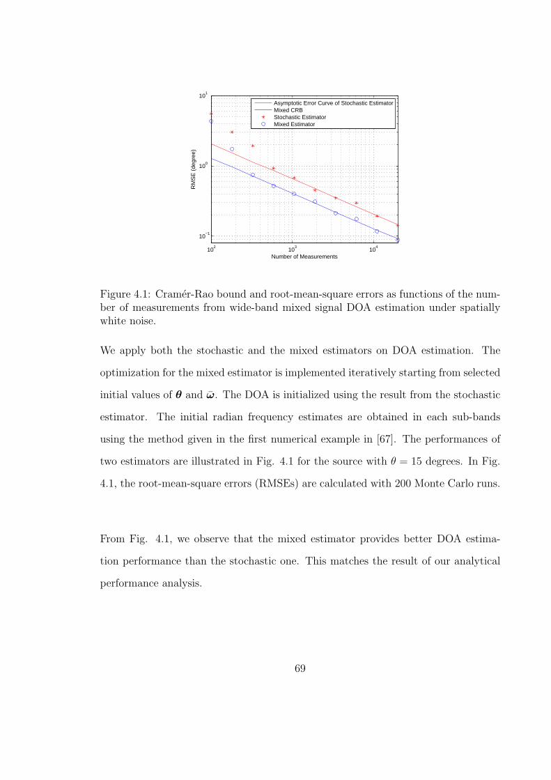
102
103
104
10−1
100
101
Number of Measurements
RM
SE
(de
gree
)
Asymptotic Error Curve of Stochastic EstimatorMixed CRBStochastic EstimatorMixed Estimator
Figure 4.1: Cramer-Rao bound and root-mean-square errors as functions of the num-ber of measurements from wide-band mixed signal DOA estimation under spatiallywhite noise.
We apply both the stochastic and the mixed estimators on DOA estimation. The
optimization for the mixed estimator is implemented iteratively starting from selected
initial values of θ and ω. The DOA is initialized using the result from the stochastic
estimator. The initial radian frequency estimates are obtained in each sub-bands
using the method given in the first numerical example in [67]. The performances of
two estimators are illustrated in Fig. 4.1 for the source with θ = 15 degrees. In Fig.
4.1, the root-mean-square errors (RMSEs) are calculated with 200 Monte Carlo runs.
From Fig. 4.1, we observe that the mixed estimator provides better DOA estima-
tion performance than the stochastic one. This matches the result of our analytical
performance analysis.
69
4.5 Summary
We considered the wide-band DOA estimation problem of the hydroacoustic signals
from marine vessel sources. We gave the ML DOA estimator. We computed the
asymptotic error covariance matrices of the proposed ML and the typical stochastic
estimators for DOA finding of such signals. Our analytical and numerical comparisons
showed that the proposed ML estimator improves the DOA estimation accuracy of
such signals compared with the typical stochastic estimator.
70
Chapter 5
Direction-of-Arrival Estimation of
Hydroacoustic Signals From
Marine Vessels: An Approach
From Fourier Transform
In Chapter 4, we considered the wide-band direction-of-arrival (DOA) estimation
problem for the hydroacoustic signals from marine vessels. In this chapter, we
reconsider this problem following a Fourier-transform-based approach, which is a
quite useful and common technique widely adopted in wide-band DOA estimation
(see [54], [69], and [70] for examples). We set up new wide-band measurement models
from the Fourier transform (FT) of the hydroacoustic signals from marine vessels,
based on which we give the maximum likelihood (ML) DOA estimator. We compute
and compare the asymptotic error covariance matrices of the proposed estimator, and
that of the typical stochastic estimator assuming zero-mean Gaussian signals. The
results show that the proposed estimator provides better DOA estimation than the
typical stochastic estimator.
71
The remainder of this chapter is presented as follows. The wide-band measurement
models and estimator are presented in Section 5.1. Section 5.2 gives analytical perfor-
mance analysis. The numerical example and conclusions appear in Sections 5.3 and
5.4, respectively. For simplicity, we use “mixed signals” to represent the wide-band
hydroacoustic signals containing both random and sinusoidal components.
5.1 Measurement Models And DOA Estimation
In this section, we present the measurement models and DOA estimator based on the
Fourier decomposition of the mixed signals.
5.1.1 Measurement Model
Assume L mixed signals from the far field incident on an array of M sensors. We
write the L incident signals at the t-th snapshot as
s(t) = Cφ(ν, t) + x(t), t = 1, . . . , N, (5.1)
where s(t) = [s1(t), ..., sL(t)]T with sl(t) the signal value of the l-th source and ·T
denoting the matrix transpose, φ(ν, t) = [ejν1t, ..., ejνKt]T contains the K sinusoids
from all sources with j2 = −1 and ν = [ν1, . . . , νK ]T , νk is the frequency of the k-th
sinusoid, C is an L × K matrix containing the coefficients of φ(ν, t), and x(t) =
[x1(t), ..., xL(t)]T is the random part of the signals, which is assumed to zero-mean
complex Gaussian. Here the mixed signals are represented in (5.1) as the sum of the
sinusoidal part Cφ(ν, t) and the random part x(t).
72
To apply Fourier decomposition to the mixed signals, we divide the total N snapshots
of signals into Td subintervals, each of which consists of Nd snapshots, i.e., N = NdTd.
For each subinterval, we implement a discrete Fourier transform (DFT) and obtain
sn(i) = Cϕn(ν, i) + xn(i), i = 1, . . . , Td, n = 1, . . . , Nd, (5.2)
where sn(i) and xn(i) are L × 1 vectors containing the DFT coefficients of s(t) and
x(t), respectively, from the i-th subinterval and n-th Fourier basis function, and
ϕn(ν, i) = [ϕn(ν1, i), . . . , ϕn(νK , i)]T with
ϕn(νk, i) =1√Nd
Nd∑t=1
ejνk[(i−1)Nd+t]e−jζn(t−1) = hk,nejNdνki, (5.3)
where
hk,n =ej(ζn−Ndνk) − ej(1−Nd)ζn
√Nd(e−j(νk−ζn) − 1)
, (5.4)
and ζn is the frequency of the n-th Fourier basis function. Therefore, we can write
the DFT-based measurement model as
yn(i) = An(θ) [Cϕn(ν, i) + xn(i)] + ϵn(i), i = 1, . . . , Td, n = 1, . . . , Nd, (5.5)
where yn(i) and ϵn(i) are M × 1 vectors, which respectively contain the array out-
put and array noise DFT coefficients from the i-th subinterval and n-th Fourier
basis function, θ = [θ1, . . . , θL]T with θl the DOA of the l-th source, An(θ) =
[an(θ1), · · · ,an(θL)] is the array steering matrix with theM×1 steering vector an(θl)
focused on frequency ζn, l = 1, . . . , L. We assume the number of sources is known.
Also we assume the number of sinusoidal components in each sub-band is known
(see [33] and [68] for similar assumptions). We assume xn(i) and ϵn(i) are temporally
73
white and uncorrelated with each other, and follow circular complex Gaussian distri-
butions CN (0,P n) and CN (0, σ2nIM), respectively, where IM is an M ×M identity
matrix. We further assume the DFT coefficients from different Fourier basis functions
are independent [54]. The unknown parameters in (5.5) are θ, C, ν, P n, and σn,
n = 1, . . . , Nd. For simplicity, we omit θ and ν is the following notations.
5.1.2 DOA Estimation From A Modified Model
We first consider the ML estimation based on the model in (5.5), for which we rewrite
(5.5) as
Y n = AnCϕn +AnXn +En, n = 1, . . . , Nd, (5.6)
where Y n = [yn(1), · · · ,yn(Td)], ϕn = [ϕn(1), · · · ,ϕn(Td)],Xn = [xn(1), · · · ,xn(Td)],
and En = [ϵn(1), · · · , ϵn(Td)]. Noting that vecABC = [CT ⊗A]vecB for any
matrices A, B, and C that can produce ABC, we have
yn =[ϕT
n ⊗An
]vecC+ vec AnXn +En , n = 1, . . . , Nd, (5.7)
where yn = vecY n = [yTn (1), · · · ,yT
n (Td)]T , ⊗ denotes the Kronecker product,
and vec· is the vectorization operator stacking all the columns of a matrix, one
below another, into a vector. Stacking the coefficients from all Fourier basis functions
together, we have
y = Aϕc+ n, (5.8)
where y = [yT1 , · · · ,yT
Nd]T , Aϕ = [(ϕT
1 ⊗ A1)T , · · · , (ϕT
Nd⊗ ANd
)T ]T , c = vecC,
and n = [vecA1X1 +E1T , · · · , vecANdXNd
+ENdT ]T .
74
Therefore, we have y ∼ CN(Aϕc,Σ
), where Σ = blkdiagITd
⊗(AnP nA
Hn +
Qn
)Nd
, which is a block-diagonal matrix with the n-th diagonal block equal to
ITd⊗(AnP nA
Hn +Qn
), n = 1, . . . , Nd. Thus, the ML estimate of c as a function of
θ, ν, σn, and P n, n = 1, . . . , Nd is
c =(AH
ϕΣ−1Aϕ
)−1AH
ϕΣ−1y
=
Nd∑n=1
(ϕ∗nϕ
Tn )⊗
[AH
n (AnP nAHn +Qn)
−1An
]−1
×Nd∑n=1
ϕ∗
n ⊗[AH
n (AnP nAHn +Qn)
−1]yn, (5.9)
where ·∗ denotes the complex conjugate.
In addition, we have the log-likelihood (LL) function from (5.6) as
L(α) =Nd∑n=1
Td
− log
∣∣AnP nAHn +Qn
∣∣− trace[AnP nA
Hn +Qn
]−1Rynyn
,(5.10)
where α is the real vector containing all the unknown parameters in (5.5), | · | denotes
the matrix determinant, trace· denotes the matrix trace, and
Rynyn=1
Td
Td∑t=1
[yn(t)−AnCϕn(t)][yn(t)−AnCϕn(t)]H . (5.11)
Substituting (5.9) back into From (5.10), we obtain a reduce LL function dependent
on θ, ν, as well as σn and P n , n = 1, . . . , Nd. To the best of our knowledge, the
nuisance parameters P n , n = 1, . . . , Nd, cannot be further reduced from the LL
function. Alternatively, we can first find the ML estimates of P n as a function of
θ, ν, C, and σn, n = 1, . . . , Nd, following the narrow-band estimation result in [67].
Substituting these estimates back into the LL function, we obtain another reduced
75
LL function dependent on θ, ν, C, and σn, n = 1, . . . , Nd. Again, the nuisance
parameters in C cannot be further reduced from the LL function.
To seek further reduction of nuisance parameters, we proposed the modified model
based on that in (5.5) as follows.
yn(i) = An(θ) [Cnφ(ω, i) + xn(i)] + ϵn(i), i = 1, . . . , Td, n = 1, . . . , Nd, (5.12)
where Cn = CHn, Hn = diagh1,n, . . . , hK,n, which is a diagonal matrix with di-
agonal elements h1,n, . . . , hK,n, and φ(ω, i) = [φ(ω1, i), . . . , φ(ωK , i)]T with φ(ωk, i) =
ejωki and ωk being the remainder of Ndνk/(2π). The unknown parameters in (5.12)
consist of θ, ω, Cn, P n, and σn, n = 1, . . . , Nd. Note that C1, · · · ,CNdare are
considered as arbitrarily unknown here. So the modified model in (5.12) has more
unknowns than the original model in (5.5). For simplicity of formulation, we omit θ
and ω in the following notations.
Note that the LL function from (5.12), which can be readily obtained using (5.10),
is the sum of Nd narrow-band LL functions, each of which is of the same form as
the narrow-band LL function in [67]. Thus, the ML estimates of Cn, P n, and σn for
(5.12) can be found as functions of θ and ω following the similar procedures in [67]
as
Cn =(AH
nAn
)−1AH
n Y nφH(φφH
)−1, (5.13)
P n =(AH
nAn
)−1AH
n RynynAn
(AH
nAn
)−1− σ2n
(AH
nAn
)−1, (5.14)
σ2n =
1
M − Ltrace
Π⊥
An
Y nYHn
Td
, (5.15)
76
where
Rynyn=
1
Td
(Y n −ΠAnY nΠφH
)(Y n −ΠAnY nΠφH
)H(5.16)
withΠ⊥An
= IM−ΠAn andΠAn = An
(AH
nAn
)−1AH
n . Substituting the ML estimates
in (5.13)-(5.15) into the LL function from (5.12) and omitting constant terms, we
obtain the reduced LL function dependent on θ and ω = [ωT1 , . . . , ω
TK ]
T as
L(θ,ω) = −Nd∑n=1
Td log
∣∣∣∣ΠAn
Y nΠ⊥φHY
Hn
TdΠAn + σ2
nΠ⊥An
∣∣∣∣. (5.17)
Remark: The maximization of the LL functions are usually implemented through an
iterative optimization method. Compared with the LL function in (5.17), the reduced
LL functions from the original model in (5.5) always have nuisance signal parameters
irreducible. This definitely introduces more optimization burden and less estimation
efficiency. Moreover, to guarantee a correct convergence, the iterative optimization
ought to start from initial parameter estimates close to the true parameter values.
However, we have not found an efficient method at present to initialize the frequencies
ν and the nuisance signal parameter C or P n. Due to the multiplication factor Nd in
the exponent in (5.3), the initialization errors in ν can be significantly enlarged in the
LL function. This introduces additional challenge in initializing the nuisance signal
parameters C or P n. In contrast, the LL function in (5.17) from the modified model
does not contain or require optimization over the nuisance signal parameters, and it
only needs the initialization of θ and the remainder of Ndνk/(2π) for iterative opti-
mization, which can be readily obtained from existing techniques. So the ML DOA
estimator based on the modified model is definitely more computationally efficient.
77
Though the ML estimator based on the original model in (5.5) may be able to give
better performance than that based on the modified model in (5.12), its efficient
implementation remains an unsolved problem to us mainly due to the initialization
problem of the frequencies and nuisance signal parameters. Moreover, the derivations
of the Cramer-Rao bound (CRB) and the asymptotic error covariance matrix of the
ML estimator based on the original model seem quite challenging, and we have not
been able to make the analytical performance analysis for the ML estimator based
on the original model. So the ML estimator based on the original model will be left
open as a topic of our future work, and will not be examined in this correspondence.
Instead, we will concentrate on the performance analysis of the ML estimator from
the modified model in (5.12) in the following sections. We will show that the ML DOA
estimator from the modified model still provides much better estimation performance
than the typical ML estimator assuming zero-mean Gaussian signals.
5.2 Analytical Performance Analysis
In this section, we present analytical results on the performances of different esti-
mators. For simplicity, we use “stochastic” estimator and CRB to represent the ML
estimator and CRB derived under the assumption of zero-mean Gaussian signals, re-
spectively (see [8] for examples). We use “mixed” estimator and CRB to represent the
ML estimator and CRB derived from the modified model in (5.12). Also, we define
P n = CnCHn +P n, and cn, pn, and pn to be the real column vectors containing the
unknown parameters from Cn, P n, and P n respectively. Note that pn consists of the
diagonal elements of P n, and the real and imaginary parts of all the upper-triangular
78
elements above the diagonal in P n. The vector pn is composed similarly of those
from P n. In Appendix O, we prove the following proposition.
Proposition 16. For DOA estimation based on the model in (5.12), the mixed CRB
matrix CRBM θ on DOA can be expressed as
CRBM θ =
[Nd∑n=1
(CRB−1
Dn θ +CRB−1Sn θ
)]−1
, (5.18)
where CRBDn θ is the CRB matrix on DOA estimation with the measurement at
snapshot t, t = 1, . . . , Td, following CN(AnCnφ(t),Qn
), in which θ, cn, ω, and σn
are the unknown parameters, and CRBSn θ is the stochastic CRB matrix on DOA
estimation with each of the Td measurements following CN(0,Rn
), in which Rn =
AnP nAHn +Qn and the unknown parameters are θ, pn, and σn.
The expressions for CRBSn θ and CRBDn θ can be found in [8]-[57]. As explained
in [67], since the measurements are not temporally stationary, we cannot take it for
granted that the mixed estimator achieves the mixed CRB asymptotically. However,
it is shown in [67] for the narrow-band case that the mixed estimator asymptotically
achieves the CRB. Since our LL function from the modified model in (5.12) is simply
the sum of a set of narrow-band LL functions, each of which is in the same form as the
narrow-band LL function in [67], we can easily show following the narrow-band results
in [67] that the error covariance matrix of the mixed estimator achieves the mixed
CRB matrix asymptotically for the wide-band case in (5.12). Similarly, following the
narrow-band results in [67] (see Propositions 3 and 4 in [67] and their proofs), we can
show the following two corollaries.
79
Corollary 1. If the stochastic estimator is applied to mixed signal DOA estimation,
the asymptotic error covariance matrix on θ is equal to CRBS θ, which is the stochas-
tic CRB matrix on DOA estimation with each of the Td measurements from the n-th
sub-band, n = 1, ..., Nd, following CN (0, Rn), where Rn = AnP nAHn +Qn and the
unknown parameters are θ, pn, and σn.
Corollary 2. For DOA estimation of the mixed signals, CasM θ ≤ CRBS θ, where
CasM θ denotes the asymptotic error covariance matrix on θ of the mixed estimator.
Corollary 1 examines the performance of the stochastic estimator when it is used
for DOA estimation of the mixed signals. Corollary 2 shows that the mixed esti-
mator provides higher accuracy than the stochastic estimator for mixed signal DOA
estimation.
5.3 Numerical Example
In this numerical example, we consider a DOA estimation problem under spatially
white noise using a uniform linear array of 10 sensors. The array lies on the z axis,
and the elevation angles of the two sources are 15 and 20 degrees, respectively. The
wide-band measurement model is constructed with 8 Fourier basis functions (Nd = 8).
The inter-sensor distance d = 0.5λ1 = 0.45λ2 = 0.4λ3 = 0.35λ4 = 0.3λ5 = 0.25λ6 =
0.2λ7 = 0.15λ8, where λ1, . . . , λ8 are the wavelengths of eight Fourier basis functions.
There are two sinusoidal waves incident on the array, one from each source, with
frequencies 0.6π and 1.2π and coefficients 0.6 and 0.7, respectively. For the random
80
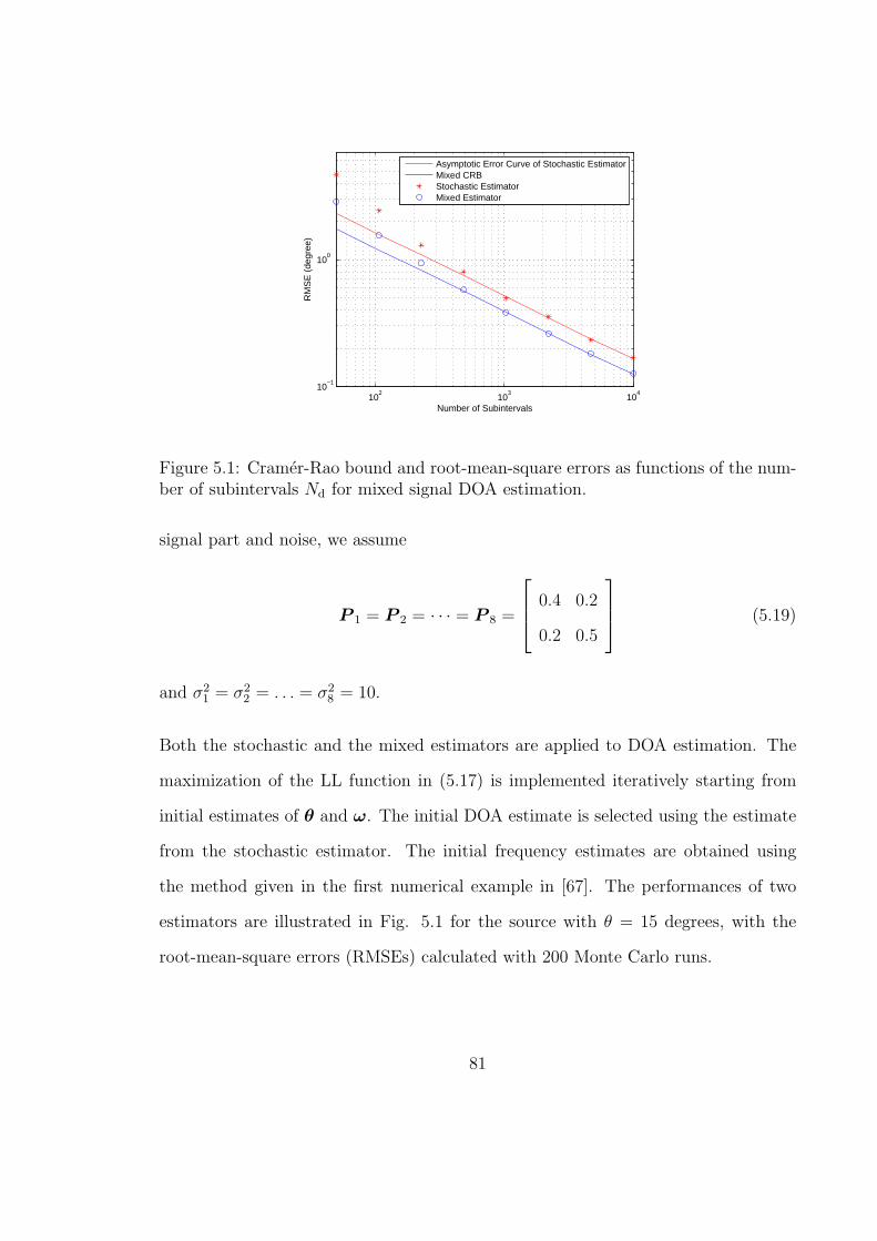
102
103
104
10−1
100
Number of Subintervals
RM
SE
(de
gree
)
Asymptotic Error Curve of Stochastic EstimatorMixed CRBStochastic EstimatorMixed Estimator
Figure 5.1: Cramer-Rao bound and root-mean-square errors as functions of the num-ber of subintervals Nd for mixed signal DOA estimation.
signal part and noise, we assume
P 1 = P 2 = · · · = P 8 =
0.4 0.2
0.2 0.5
(5.19)
and σ21 = σ2
2 = . . . = σ28 = 10.
Both the stochastic and the mixed estimators are applied to DOA estimation. The
maximization of the LL function in (5.17) is implemented iteratively starting from
initial estimates of θ and ω. The initial DOA estimate is selected using the estimate
from the stochastic estimator. The initial frequency estimates are obtained using
the method given in the first numerical example in [67]. The performances of two
estimators are illustrated in Fig. 5.1 for the source with θ = 15 degrees, with the
root-mean-square errors (RMSEs) calculated with 200 Monte Carlo runs.
81
We can see in Fig. 5.1 that the mixed estimator provides higher estimation accuracy
than the stochastic estimator. This matches our analytical performance analysis in
Section III.
5.4 Summary
We considered the DOA estimation problem of the hydroacoustic signals from marine
vessels. We derived the wide-band measurement model based on Fourier decompo-
sition, from which we further proposed a modified measurement model and its ML
DOA estimator that greatly simplify the estimation procedure. Both our analytical
and numerical results demonstrated that in comparison with the typical stochastic
estimator, the proposed estimator improves the DOA estimation accuracy for the
hydroacoustic signals considered.
82
Chapter 6
A Barankin-Type Bound on
Direction-of-Arrival Estimation 3
From the numerical examples and figures in the previous chapters, we can see that the
the Cramer-Rao bound (CRB) is able to predict the performance of the maximum
likelihood (ML) estimator only when the number of measurements is large. The
similar phenomenon occurs to the performance of the ML estimator with respect
to the signal-to-noise ratio (SNR). The CRB can predict the performance of the
ML estimator only at high SNR values. When the SNR is low, the mean-square
errors of the ML estimator deviate from the CRB. The SNR region below which
the performance of the ML estimator deviates rapidly from the CRB is called the
SNR threshold region. The CRB is not able to provide any information about this
threshold region.
In this chapter, we derive a Barankin-type bound (BTB) on the mean-square er-
ror (MSE) in estimating the directions of arrivals (DOAs) of far-field sources using
acoustic sensor arrays. We consider narrow-band and wide-band deterministic source
3Based on T. Li, J. Tabrikian, and A. Nehorai, “A Barankin-Type Bound on Direction Estima-tion Using Acoustic Sensor Arrays,” IEEE Trans. Signal Process., vol. 59, pp. 431-435, Jan. 2011.c⃝[2011] IEEE.
83
signals, and scalar or vector sensors. Our results provide an approximation to the
threshold of the SNR below which the performance of the maximum likelihood es-
timation (MLE) degrades rapidly. For narrow-band DOA estimation using uniform
linear vector-sensor arrays, we show that this threshold increases with the distance
between the sensors. As a result, for medium SNR values the performance does not
necessarily improve with this distance.
6.1 Introduction
The Barankin bound is the tightest lower bound on the mean square errors of any
unbiased estimator [71]–[75], and it is a useful tool in estimation problems for pre-
dicting the threshold region of SNR [76]–[79], below which the accuracy of the MLE
degrades rapidly. Identification of the threshold region enables to determine the oper-
ation conditions, such as observation time and transmission power, to obtain a desired
performance.
In the recent years many works have been carried out for identification of the threshold
region of the MLE. One approach is based on the method of interval estimation (MIE)
[80] in which the performance of the MLE in the threshold region is approximated.
However, it does not provide a performance lower bound. Another well investigated
approach is the use of the non-Bayesian bounds which can predict the threshold region
and provide a performance lower bound. In this chapter, we derive a Barankin-type
bound (BTB) on the DOA estimation of acoustic signals based on measurement
models with deterministic unknown parameters. The derived bound provides an
approximation for the threshold SNR even in the case of a high-dimensional unknown
parameter vector, for which computing the Barankin bound is usually formidable. We
84
examine the performance of the derived bound for both wide-band and narrow-band
DOA estimation problems.
In addition, we examine the effect of the distance between the acoustic vector sensors
(AVSs) in a uniform linear array on the narrow-band DOA estimation error. Unlike
scalar sensors, AVSs measure not only the sound pressure but also the components
of particle velocity [11]. One of the advantages of the AVS arrays over the scalar
ones is that the distance between adjacent AVSs can be larger than half of the signal
wavelength without introducing spatial ambiguities in narrow-band DOA estimation.
Thus, we may design the distance between the AVSs to achieve better estimation
results. Our examination of the derived BTB and actual MLE error shows that the
threshold SNR increases with the distance between the AVSs, and that enlarging this
distance does not always improve the estimation accuracy. Compared with the CRB,
which consistently decreases with the increase of inter-AVS distance, the derived
BTB provides more accurate reference for the optimal distance determination, as it
incorporates the effect of large estimation errors.
The remainder of this chapter is organized as follows. In Section 6.2, we formulate the
model for data collected by acoustic sensor arrays. In Section 6.3, we derive the BTB
for source localization. Section 6.4 presents the numerical examples. The conclusion
of this paper appears in Section 6.5.
6.2 Measurement Model
In this section, we present the measurement models for both wide-band and narrow-
band sources for uniform linear AVS arrays. The measurement models for other types
85
of sensor arrays can be formulated in the same way using the corresponding steering
vectors.
We first present the measurement model for wide-band sources. Consider signal waves
from K distant wide-band acoustic sources impinging on a uniform linear array of
M AVSs, each of which consists of m components. In similar to [69], [70], using the
wide-band harmonic signal model, we approximate the incident signal from the k-th
source as
xk(t) =J∑
j=1
ckjψj(t), (6.1)
where ψ1(t), . . . , ψJ(t) are the monochromatic waves representing Fourier series ker-
nels and ck1, . . . , ckJ are their coefficients. Assuming the frequency of ψj(t) is fj, we
write the measurement model as
y(t) =J∑
j=1
K∑k=1
aj(θk)ckjψj(t) + e(t)
=J∑
j=1
Aj(θ)cjψj(t) + e(t), t = 1, . . . , N, (6.2)
where y(t) is the Mm × 1 measurement vector, θk is the one- or two-dimensional
DOA of the k-th source, e(t) is the Mm × 1 noise vector, θ = [θT1 , . . . ,θTK ]
T , cj =
[c1j, . . . , cKj]T , “T” denotes the transpose operation, N is the number of temporal
measurements, Aj(θ) = [aj(θ1) · · ·aj(θK)], and aj(θk) is the steering vector for the
k-th source given by
aj(θk) = hj(θk)⊗
1
u(θk)
, (6.3)
where “⊗” donotes the Kronecker product, hj(θk) =[1, ei2πfjτ(θk), . . . , ei2πfj(M−1)τ(θk)
]Twith τ(θk) the differential time delay of the k-th source signal between two adjacent
86
AVSs, and u(θk) is the (m− 1)× 1 unit-norm direction vector from the array to the
k-th source. We assume the noise is zero-mean circular Gaussian with known spatial
covariance matrix Σ and is temporally white.
For narrow-band sources, the steering vectors can be assumed to be constant over the
signal bandwidth with frequency fixed on the carrier frequency of the narrow-band
sources, i.e., aj(θ) = a(θ), and the measurement model (6.2) then becomes
y(t) =K∑k=1
a(θk)
(J∑
j=1
ckjψj(t)
)+ e(t)
= A(θ)Cψ(t) + e(t), t = 1, . . . , N, (6.4)
where C is a K × J matrix whose (k, j)th entry is ckj, ψ(t) = [ψ1(t), . . . , ψJ(t)]T ,
A(θ) = [a(θ1) · · ·a(θK)], and
a(θk) = h(θk)⊗
1
u(θk)
, (6.5)
where h(θk) =[1, ei2πfτ(θk), . . . , ei2πf(M−1)τ(θk)
]Tand f is the carrier frequency of the
narrow-band signals. Note that in (6.4),∑J
j=1 ckjψj(t) is the complex amplitude of
the k-th incident signal approximated by Fourier series expansion.
6.3 Barankin-Type Bound
In this section, we derive a BTB on the DOA vector θ based on the measurement
models in Section II.
87
An analytical form of the Barankin bound is generally not available. We use the
Barankin-type lower bound developed in [72]–[74] to approximate the actual Barankin
Bound. For an unbiased estimator ϕ of an unknown deterministic parameter vector
ϕ, this lower bound can be formulated as
covϕ ≥ T (B − 11T )−1T T , (6.6)
where T = [ϕ1 − ϕ · · · ϕL − ϕ], ϕ1, . . . , ϕL are the test points selected from the
parameter space of ϕ, 1 is a column vector of dimension L with all entries equal to
1, and B is the L× L Barankin matrix whose (l, n)th entry is
Bln = Er(y, ϕl,ϕ)r(y, ϕn,ϕ), (6.7)
where E· denotes the expectation operation, r(y, ϕl,ϕ) = f(y; ϕl)/f(y;ϕ), and
f(y;ϕ) is the probability density function (pdf) of y with parameters ϕ. The supre-
mum of the BTB given in (6.6) approaches the actual Barankin bound when the
number of test points tends to infinity [81].
In the following, we first derive the BTB on θ based on the wide-band measurement
model (6.2).
Stacking all measurements together, we rewrite (6.2) as
Y =J∑
j=1
Aj(θ)cjψTj +E, (6.8)
where Y = [y(1) · · ·y(N)], E = [e(1) · · · e(N)], and ψj = [ψj(1), . . . , ψj(N)]T . Vec-
torizing both sides of (6.8), we obtain
88
y =J∑
j=1
(ψj ⊗Aj(θ)
)cj + e = R(θ)c+ e, (6.9)
where y = [yT (1), . . . ,yT (N)]T , e = [eT (1), . . . , eT (N)]T , c = [cT1 , . . . , cTJ ]
T , and
R(θ) = [ψ1 ⊗A1(θ) · · ·ψJ ⊗AJ(θ)].
The unknown parameter vector in (6.9) is ϕ =[θT ,Re
cT, Im
cT ]T
, in which
RecTand Im
cTare the real and imaginary parts of cT respectively. The prob-
ability density function of y with parameters ϕ is
f(y;ϕ) =1
det(πIN ⊗Σ)exp
−(y −R(θ)c)H
(IN ⊗Σ−1
)(y −R(θ)c)
(6.10)
where det(·) denotes the determinant of a matrix and IN is the unit matrix of size
N .
Substituting (6.10) into (6.7), we obtain
Bln =1
det(πIN ⊗Σ)
∫exp
(y −R(θ)c)H
(IN ⊗Σ−1
)(y −R(θ)c)−(
y −R(θl)cl)H (
IN ⊗Σ−1) (y −R(θl)cl
)−(
y −R(θn)cn)H (
IN ⊗Σ−1) (y −R(θn)cn
)dy
= A exp2Re
(R(θ)c−R(θl)cl
)H (IN ⊗Σ−1
) (R(θ)c−R(θn)cn
), (6.11)
where[θTl ,Re
cTl, Im
cTl ]T
is the lth selected test point for ϕ and
A =1
det(πIN ⊗Σ)
∫exp
(y −R(θl)cl −R(θn)cn +R(θ)c
)H (IN ⊗Σ−1
)×(y −R(θl)cl −R(θn)cn +R(θ)c
)dy = 1. (6.12)
Thus, we have
89
Bln = exp2Re
(R(θ)c−R(θl)cl
)H (IN ⊗Σ−1
) (R(θ)c−R(θn)cn
). (6.13)
To obtain a tight bound, we ought to choose the test points that maximize the right
side of (6.6). Observe that in many cases ϕ is a high-dimensional vector, which
generally requires a huge amount of test points to produce a tight bound. This would
inevitably augment the burden in computing the inverse of B − 11T .
We employ the approximation method proposed in [78] to reduce the required number
of test points. This method is adapted as follows for DOA estimation:
• Select L candidate test points θ1, . . . , θL for the DOA parameter θ.
• For each selected θl, l = 1, . . . , L, select test point cjl for cj, j = 1, . . . , J such
thatBll is minimized at ϕl =[θTl ,Re
cTl, Im
cTl ]T
=[θTl ,Re
[cT1l, . . . , c
TJl],
Im[cT1l, . . . , c
TJl] ]T
.
• From ϕ1, . . . , ϕL, choose the L test points producing the L smallest values in
B11, . . . , BLL as the test points to compute the bound [78]. Alternatively, choose
the test points at the L highest lobe peaks of B−111 , . . . , B
−1LL
provided that the
values of B−111 , . . . , B
−1LL
exhibit evident sidelobes.
To obtain the BTB according to the above method, we first find the test point cl that
minimizes Bll for a given θl. Taking the derivative of Bll with respect to cl, we have
the test point cl minimizing Bll is
cl = G−1(θl, θl)G(θl,θ)c, (6.14)
where G(θl,θ) = RH(θl)(IN ⊗Σ−1)R(θ).
90
The general result provided by (6.14) can be further simplified if we have
ψHk ψj = δkj (6.15)
with δkj the Kronecker delta function, which is a general property of the problem at
hand since ψ1(t), . . . , ψJ(t) can be chosen using the kernels of the Fourier series or
by Karhunen-Loeve transform. Using (6.14) and (6.15), we can further obtain (see
Appendix P) the test point cjl that minimizes Bll
cjl = P−1j (θl, θl)P j(θl,θ)cj, j = 1, . . . , J, (6.16)
where P j(θl,θ) = AHj (θl)Σ
−1Aj(θ).
Substituting (6.16) into (6.13), we obtain the following expression for the (l, n)th
entry of B:
Bln = exp2trReQH(θl,θ)Σ
−1Q(θn,θ)
, (6.17)
where tr· denotes the trace of a matrix, Q(θl,θ) =[q1(θl,θ) · · · qJ(θl,θ)
], and
qj(θl,θ) =(Aj(θ)−Aj(θl)P
−1j (θl, θl)P j(θl,θ)
)cj.
Assuming the noise covariance matrix Σ = σ2I and there is only one source, we are
able to simplify the formula in (6.17) as
Bln = exp
2
σ2
J∑j=1
Re(Aj(θ)cj)
H Λj(θl, θn) (Aj(θ)cj)
, (6.18)
where
Λj(θl, θn) =(I −Aj(θl)A
Hj (θl)/α
) (I −Aj(θn)A
Hj (θn)/α
). (6.19)
91
In (6.19), α is the square of the Euclidean norm of the steering vector. For scalar-
sensor arrays, we have α =M . For vector-sensor arrays, we have α = 2M (note that
the Euclidean norm of u(θ) is 1). The diagonal entries of B can be further simplified
as
Bll = exp
2
σ2
J∑j=1
cHj cj(α− |AH
j (θ)Aj(θl)|2/α)
, (6.20)
where | · | denotes the amplitude of a complex number.
Using the derived expressions of B, we are able to compute the BTB on an unbiased
estimator θ of θ, which is given by
covθ ≥ T θ(B − 11T )−1T Tθ , (6.21)
where T θ = [θ1 − θ · · · θL − θ].
The bound based on the narrow-band model (6.4) can be derived similarly and herein
we only present the results. For the narrow-band model in (6.4), the test point C l
minimizing Bll is
C l = P−1(θl, θl)P (θl,θ)C. (6.22)
where P (θl,θ) = AH(θl)Σ
−1A(θ). Under the condition in (6.15), the formula of B
for the narrow-band model can be written as
Bln = exp2trReQH(θl,θ)Σ
−1Q(θn,θ)
, (6.23)
where Q(θl,θ) =(A(θ)−A(θl)P
−1(θl, θl)P (θl,θ))C.
Note that though our test-point selection method is based on the idea in [78], our
models and derived results are more general than their deterministic counterparts
92
in [78] and thus have broader applications. Our derived bounds can be used as well
for some other array-processing problems such as DOA estimation for signals of known
waveforms [15], [16], in which ψ1, . . . ,ψJ denote the known signal waveforms.
6.4 Numerical Examples
To demonstrate the performance of the derived bound, we present numerical examples
of DOA estimation for both scalar- and vector-sensor arrays. For simplicity, we
assume the noise covariance matrix Σ = σ2I in all examples.
6.4.1 Examples for Scalar-Sensor Array
We present results of two examples for scalar-sensor array, one for narrow-band and
the other for wide-band signal. For the narrow-band example, we consider a sinusoidal
signal with elevation angle of 0 degree arriving at a uniform linear scalar-sensor array
of 40 sensors. The distance d between the sensors equals half of the signal’s wavelength
λ. We took 10 samples of measurement and uniformly selected 30 test points from
[−π/2, π/2] to compute the bound. Note that uniformly selecting test points is a
special case of the proposed test point selection method with L = L. Also for a
uniform linear scalar-sensor array, the distance between adjacent sensors should not
be larger than half of the signal wavelength to avoid ambiguity in the DOA estimation
of a narrow-band signal.
For the wide-band example, we assume the distance between the sensors is 1 meter
and the signal consists of 10 harmonic components, with elevation angle of 0 degree.
93
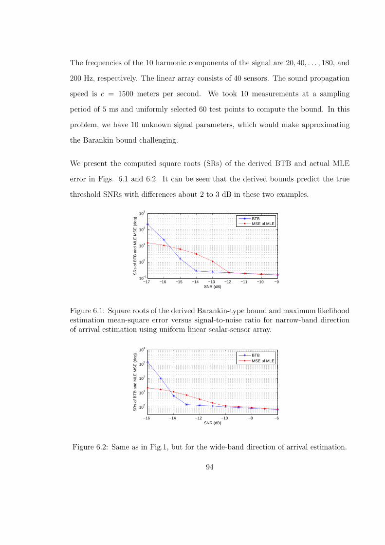
The frequencies of the 10 harmonic components of the signal are 20, 40, . . . , 180, and
200 Hz, respectively. The linear array consists of 40 sensors. The sound propagation
speed is c = 1500 meters per second. We took 10 measurements at a sampling
period of 5 ms and uniformly selected 60 test points to compute the bound. In this
problem, we have 10 unknown signal parameters, which would make approximating
the Barankin bound challenging.
We present the computed square roots (SRs) of the derived BTB and actual MLE
error in Figs. 6.1 and 6.2. It can be seen that the derived bounds predict the true
threshold SNRs with differences about 2 to 3 dB in these two examples.
−17 −16 −15 −14 −13 −12 −11 −10 −910
−1
100
101
102
103
SNR (dB)
SR
s of
BT
B a
nd M
LE M
SE
(de
g)
BTBMSE of MLE
Figure 6.1: Square roots of the derived Barankin-type bound and maximum likelihoodestimation mean-square error versus signal-to-noise ratio for narrow-band directionof arrival estimation using uniform linear scalar-sensor array.
−16 −14 −12 −10 −8 −6
100
101
102
103
104
SNR (dB)
SR
s of
BT
B a
nd M
LE M
SE
(de
g)
BTBMSE of MLE
Figure 6.2: Same as in Fig.1, but for the wide-band direction of arrival estimation.
94
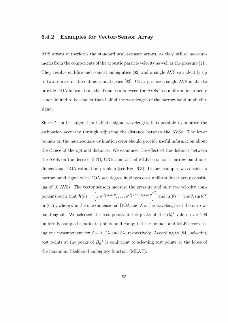
6.4.2 Examples for Vector-Sensor Array
AVS arrays outperform the standard scalar-sensor arrays, as they utilize measure-
ments from the components of the acoustic particle velocity as well as the pressure [11].
They resolve end-fire and conical ambiguities [82] and a single AVS can identify up
to two sources in three-dimensional space [83]. Clearly, since a single AVS is able to
provide DOA information, the distance d between the AVSs in a uniform linear array
is not limited to be smaller than half of the wavelength of the narrow-band impinging
signal.
Since d can be larger than half the signal wavelength, it is possible to improve the
estimation accuracy through adjusting the distance between the AVSs. The lower
bounds on the mean-square estimation error should provide useful information about
the choice of the optimal distance. We examined the effect of the distance between
the AVSs on the derived BTB, CRB, and actual MLE error for a narrow-band one-
dimensional DOA estimation problem (see Fig. 6.3). In our example, we consider a
narrow-band signal with DOA = 0 degree impinges on a uniform linear array consist-
ing of 10 AVSs. The vector sensors measure the pressure and only two velocity com-
ponents such that h(θ) =[1, ei
2πλd sin θ, . . . , ei
2πλ(M−1)d sin θ
]Tand u(θ) = [cos θ, sin θ]T
in (6.5), where θ is the one-dimensional DOA and λ is the wavelength of the narrow-
band signal. We selected the test points at the peaks of the B−1ll values over 200
uniformly sampled candidate points, and computed the bounds and MLE errors us-
ing one measurement for d = λ, 2λ and 3λ, respectively. According to [84], selecting
test points at the peaks of B−1ll is equivalent to selecting test points at the lobes of
the maximum likelihood ambiguity function (MLAF).
95
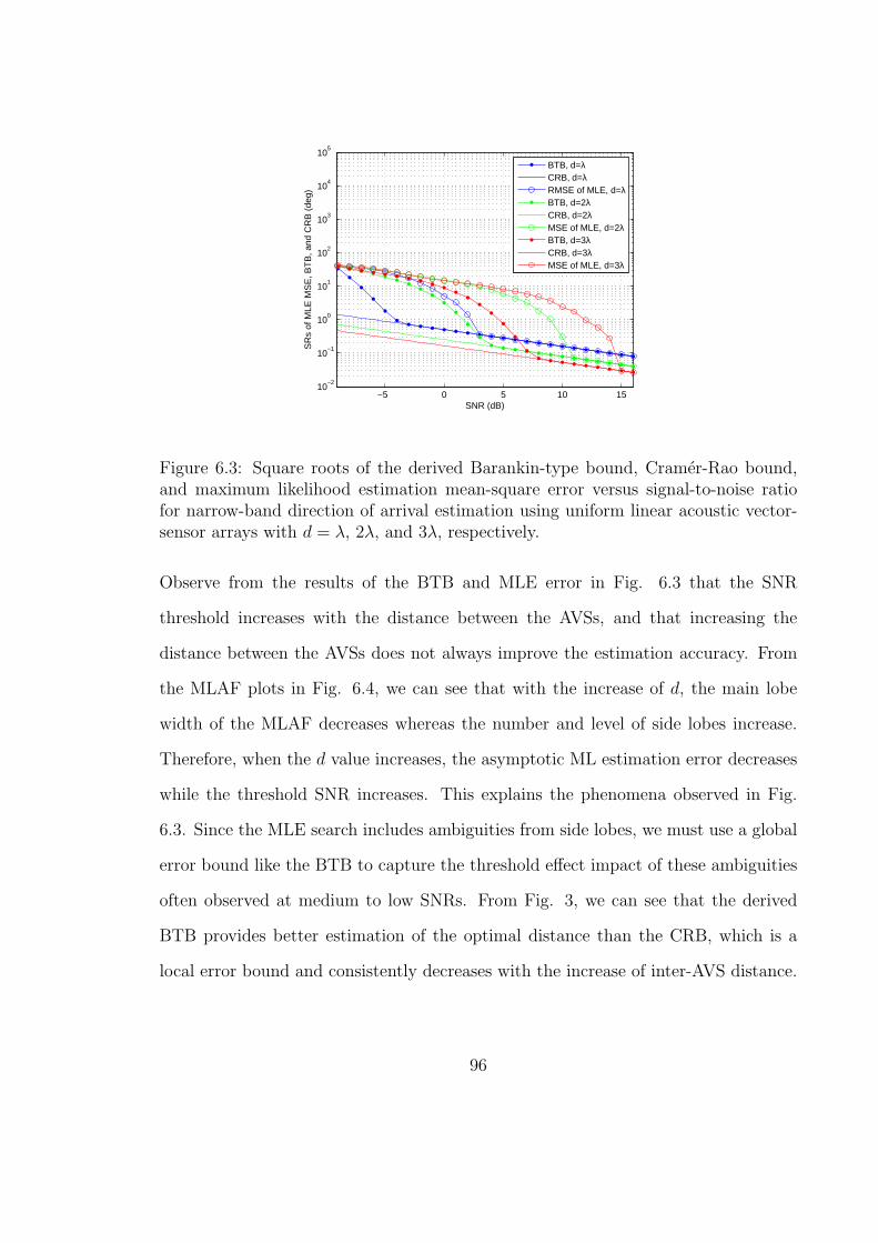
−5 0 5 10 1510
−2
10−1
100
101
102
103
104
105
SNR (dB)
SR
s of
MLE
MS
E, B
TB
, and
CR
B (
deg)
BTB, d=λCRB, d=λRMSE of MLE, d=λBTB, d=2λCRB, d=2λMSE of MLE, d=2λBTB, d=3λCRB, d=3λMSE of MLE, d=3λ
Figure 6.3: Square roots of the derived Barankin-type bound, Cramer-Rao bound,and maximum likelihood estimation mean-square error versus signal-to-noise ratiofor narrow-band direction of arrival estimation using uniform linear acoustic vector-sensor arrays with d = λ, 2λ, and 3λ, respectively.
Observe from the results of the BTB and MLE error in Fig. 6.3 that the SNR
threshold increases with the distance between the AVSs, and that increasing the
distance between the AVSs does not always improve the estimation accuracy. From
the MLAF plots in Fig. 6.4, we can see that with the increase of d, the main lobe
width of the MLAF decreases whereas the number and level of side lobes increase.
Therefore, when the d value increases, the asymptotic ML estimation error decreases
while the threshold SNR increases. This explains the phenomena observed in Fig.
6.3. Since the MLE search includes ambiguities from side lobes, we must use a global
error bound like the BTB to capture the threshold effect impact of these ambiguities
often observed at medium to low SNRs. From Fig. 3, we can see that the derived
BTB provides better estimation of the optimal distance than the CRB, which is a
local error bound and consistently decreases with the increase of inter-AVS distance.
96
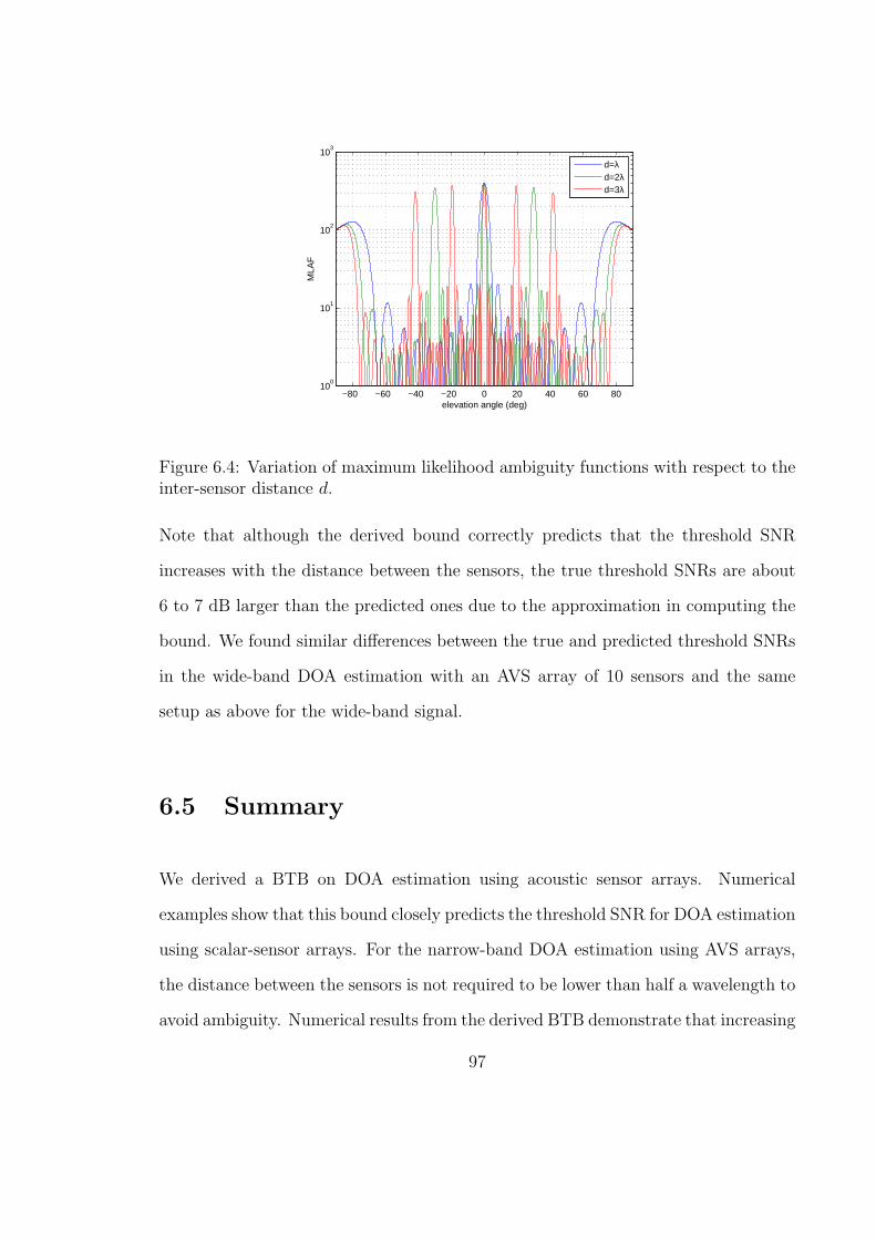
−80 −60 −40 −20 0 20 40 60 8010
0
101
102
103
elevation angle (deg)
MLA
F
d=λd=2λd=3λ
Figure 6.4: Variation of maximum likelihood ambiguity functions with respect to theinter-sensor distance d.
Note that although the derived bound correctly predicts that the threshold SNR
increases with the distance between the sensors, the true threshold SNRs are about
6 to 7 dB larger than the predicted ones due to the approximation in computing the
bound. We found similar differences between the true and predicted threshold SNRs
in the wide-band DOA estimation with an AVS array of 10 sensors and the same
setup as above for the wide-band signal.
6.5 Summary
We derived a BTB on DOA estimation using acoustic sensor arrays. Numerical
examples show that this bound closely predicts the threshold SNR for DOA estimation
using scalar-sensor arrays. For the narrow-band DOA estimation using AVS arrays,
the distance between the sensors is not required to be lower than half a wavelength to
avoid ambiguity. Numerical results from the derived BTB demonstrate that increasing
97

the distance between the AVSs improves the DOA estimation accuracy consistently
only at high SNRs, and it increases the threshold SNR as well. As a result, at medium
SNR values the estimation accuracy does not necessarily improve with this distance.
This predicts the behavior of the actual MLE error. The derived BTB exhibits evident
advantage over the CRB in determining the optimal distance between the AVSs.
98
Chapter 7
Conclusions
In this dissertation, we proposed new signal models, maximum likelihood (ML) es-
timators, and performance analysis results for some selected topics in underwater
direction-of-arrival (DOA) estimation. In the following, we first summarize the key
contributions of this dissertation, and then discuss possible topics for future research.
7.1 Key Contributions
We first considered the DOA estimation problem in spatially colored noise using
sparse sensor arrays, for which we developed new ML DOA estimators for both zero-
mean and non-zero-mean Gaussian signals based on an Expectation-Maximization
framework. We derived the CRB on DOA estimation of non-zero-mean Gaussian
signals, and the asymptotic error covariance matrix of using the typical stochastic
estimator, which assumes zero-mean Gaussian signals, for DOA estimation of non-
zero-mean Gaussian signals. Our analytical comparison and numerical examples show
that the non-zero means in the signals improves the accuracy of DOA estimation.
99
Next, we considered the narrow-band DOA estimation of hydroacoustic signals from
marine vessels containing both sinusoidal and random components, for which we
presented a new signal model and derived the ML estimator for DOA finding of such
hydroacoustic signals. We computed the asymptotic error covariance matrices of
the proposed ML estimator and the typical stochastic estimator assuming zero-mean
Gaussian signals on DOA finding of such hydroacoustic signals, which, together with
our analytical and numerical comparisons, showed that the proposed signal model
and estimator improve the DOA estimation accuracy for the hydroacoustic signals
from marine vessels in comparison with the typical stochastic ones.
We then generalized the narrow-band DOA estimation results to the wide-band case
for hydroacoustic signals from marine vessels through narrow-band decomposition
and Fourier series expansion. We proposed the wide-band measurement models and
ML estimators. We showed that compared with the typical stochastic estimators, the
proposed ML estimators provide better performance for wide-band DOA finding of
the hydroacoustic signals from marine vessels.
At last, to identify the SNR threshold region, we derived a Barankin-type bound on
DOA estimation using acoustic sensor arrays. Numerical examples show that this
bound closely predicts the threshold SNR for DOA estimation using scalar-sensor
arrays. The derived Barankin-type bound also demonstrated that increasing the dis-
tance between the acoustic vector sensors improves the DOA estimation accuracy
only at high SNRs, and it increases the SNR threshold as well, and the estimation
accuracy does not necessarily improve with this distance at medium SNR values.
This predicts the actual behavior of the ML estimation error. In addition, the de-
rived Barankin-type bound exhibits evident advantage over the Cramer-Rao bound
in determining the optimal distance between the acoustic vector sensors.
100
7.2 Future Work
In our future work, we will develop new schemes to improve the efficiency of DOA
estimation in spatially colored noise using sparse sensor arrays. Sparse modeling
techniques [85]-[89] have been shown to be quite efficient and accurate in DOA es-
timation under spatially white noise. However, concrete sparse modeling methods
for DOA estimation using sparse sensor arrays under spatially colored noise have not
been addressed yet to the best of our knowledge. We will develop novel and efficient
sparse-modeling-based estimators for DOA finding under spatially colored noise using
sparse sensor arrays.
Also in our future work, we will develop new methods to improve the accuracy and
efficiency for DOA estimation of hydroacoustic signals from marine vessels. We will
develop new DOA estimation methods based on the sparse modeling on both DOA
and sinusoidal frequencies to improve the estimation efficiency. For the wide-band
estimation based on Fourier transform, we will develop efficient estimation schemes
based on the measurement model proposed in (5.5) to improve the estimation per-
formance. This model is more accurate than the one in (5.12), based on which the
current estimator in Chapter 5 is developed. We expect it to introduce a better
estimator than the current one proposed in Chapter 5.
For the Barankin-type bound, we will develop more accurate computation of the
Barankin bound for high-dimensional unknown parameter vectors as well as better
signal models such as those assuming Gaussian signals. We will aim to improve the
approximation of the Barankin bound on DOA estimation by developing new test
point selection methods and considering alternative approximation approaches of the
Barankin bound such as the one in [81].
101
Appendix A
Proof of Theorem 1
Let β =[θT , δT , b
T ]Tbe the real column vector containing all the unknown param-
eters, where δ is the real column vector containing the unknown parameters from P
and Q, and b is the real column vector containing those from b. According to the
Fisher information matrix equation [42], we have
[FIMM]kl = 2NRe
∂[A(θ)b]H
∂βkR−1∂[A(θ)b]
∂βl
+Ntrace
R−1 ∂R
∂βkR−1∂R
∂βl
, (A.1)
where FIMM is the mixed Fisher information matrix, [FIMM]kl is the (k, l)-th element
of FIMM, Re· denotes the real part of a complex number, and βk is the k-th element
of β.
Let F d be the matrix whose entries are from the first term on the right side of (A.1).
If βk is a parameter from δ, we have
∂[A(θ)b]
∂βk
= 0. (A.2)
As a result, we obtain
102
F d =
F d θθ F d θδ F d θb
F d δθ F d δδ F d δb
F d bθ F d bδ F d bb
=
F d θθ 0 F d θb
0 0 0
F d bθ 0 F d bb
, (A.3)
where F d θθ,F d θδ, . . . ,F d bb are the sub-matrices of F d containing the elements
related to the parameters specified in their subscripts.
Similarly, let F S be the matrix whose entries are from the second term on the right
side of (A.1). Since
∂R
∂βk= 0 (A.4)
if βk is a parameter from b, we have
F S =
F S θθ F S θδ F S θb
F S δθ F S δδ F S δb
F S bθ F S bδ F S bb
=
F S θθ F S θδ 0
F S δθ F S δδ 0
0 0 0
. (A.5)
Combining the results from (A.3) and (A.5), we obtain
FIMM=F d + F S =
F d θθ + F S θθ F S θδ F d θb
F S δθ F S δδ 0
F d bθ 0 F d bb
. (A.6)
Therefore, we have
CRB−1M θ = F d θθ + F S θθ − [F S θδ F d θb]
F S δδ 0
0 F d bb
−1 F S δθ
F d bθ
= F d θθ − F d θbF
−1d bbFH
d θb + F S θθ − F S θδF−1S δδF
HS θδ, (A.7)
103
where
F S θθ − F S θδF−1S δδF
HS θδ = CRB−1
S θ. (A.8)
For 1D DOA estimation, we have
∂[A(θ)b]
∂θl= bl
da(θl)
dθl, (A.9)
where bl is the l-th element of b. As a result,
∂[A(θ)b]
∂θT=DH , (A.10)
where H = diagb is a diagonal matrix with diagonal elements from vector b.
According to the results in [19], we have
F d θθ − F d θbF−1d bbFH
d θb = 2NReHHD
HΠ⊥
ADH
= 2NRe(D
HΠ⊥
AD)⊙(bbH
)T= 2NRe
(D
HΠ⊥
AD)⊙(bbH
)T=CRB−1
d θ. (A.11)
The second last equality in (A.11) is obtained from the following result given in [43]:
R− 12Π⊥
AR− 1
2 = Q− 12Π⊥
AQ− 1
2 . (A.12)
For 2D DOA estimation, we have
∂[A(θ)b]
∂θTl=∂a(θl)
∂θTl
[bl 0
0 bl
]=
[da(θl)
dϕl
,da(θl)
dψl
] [bl 0
0 bl
], (A.13)
104
and thus
∂[A(θ)b]
∂θT=D2H2, (A.14)
where H2 =H ⊗ I2, and I2 is the 2× 2 identity matrix.
Therefore, for 2D DOA estimation,
F d θθ − F d θbF−1d bbFH
d θb = 2NReHH
2 DH2 Π
⊥AD2H2
= 2NRe
(D
H2 Π
⊥AD2
)⊙[(bbH
)⊗∆
]T= 2NRe
(D
H
2 Π⊥AD2
)⊙[(bbH
)⊗∆
]T=CRB−1
d θ. (A.15)
We thus prove Theorem 1.
105
Appendix B
Proof of Theorem 2
If the stochastic ML estimator is used for DOA estimation of mixed signals, as the
number of measurements N increases, the stochastic log-likelihood function tends to
the asymptotic stochastic log-likelihood function with signal covariance matrix equal
to Rxx = P + bbH , and we are still able to obtain consistent estimators for θ, Rxx,
and Q.
Let f(Y ;α) be the pdf based on the stochastic measurement model with α the real
column vector containing all the unknown parameters from θ,Rxx, andQ. Assuming
α is the ML estimator of α, we apply a Taylor expansion as follows around the true
value of α, which is denoted by α0.
∂ ln f(Y ;α)
∂α
∣∣∣∣α=α
=∂ ln f(Y ;α)
∂α
∣∣∣∣α=α0
+∂2 ln f(Y ;α)
∂α2
∣∣∣∣α=α
(α−α0) = 0, (B.1)
where α is a vector value between α0 and α. Thus we have
α−α0 = −[1
N
∂2 ln f(Y ;α)
∂α∂αT
]−1 ∣∣∣∣α=α
[1
N
∂ ln f(Y ;α)
∂α
] ∣∣∣∣α=α0
. (B.2)
106
Using equations (15.47) and (15.48) in [42], we can show that
E
∂ ln f(y(t);α)
∂α
∣∣∣∣α=α0
= 0, (B.3)
E
∂2 ln f(y(t);α)
∂αk∂αl
∣∣∣∣α=α0
=trace
R
−1∂R
∂αk
R−1∂R
∂αl
. (B.4)
Note that the expectations in (B.3) and (B.4) are computed under the pdf of the
mixed measurement model. This also holds for the all the following expectations in
this proof.
According to the central limit theorem, the second term on the right side of (B.2)
follows a Gaussian distribution with mean
E
1
N
∂ ln f(Y ;α)
∂α
∣∣∣∣α=α0
= 0 (B.5)
and covariance matrix
E
1
N2
∂ ln f(Y ;α)
∂α
∂ ln f(Y ;α)
∂αT
∣∣∣∣α=α0
=1
N2E
[N∑t=1
∂ ln f(y(t);α)
∂α
][N∑s=1
∂ ln f(y(s);α)
∂αT
]∣∣∣∣∣α=α0
=1
N2
N∑t=1
E
∂ ln f(y(t);α)
∂α
∂ ln f(y(t);α)
∂αT
∣∣∣∣∣α=α0
=1
NE
∂ ln f(y(t);α)
∂α
∂ ln f(y(t);α)
∂αT
∣∣∣∣∣α=α0
. (B.6)
Using equations (15.47) and (15.48) in [42], and after some algebraic manipulations,
we obtain
107
E
∂ ln f(y(t);α)
∂αk
∂ ln f(y(t);α)
∂αl
∣∣∣∣α=α0
= E
yH(t)R
−1 ∂R
∂αk
R−1y(t)yH(t)R
−1∂R
∂αl
R−1y(t)
−trace
R
−1 ∂R
∂αk
trace
R
−1∂R
∂αl
. (B.7)
Applying Lemma 2 to the first term on the right side of (B.7), we obtain
E
∂ ln f(y(t);α)
∂αk
∂ ln f(y(t);α)
∂αl
∣∣∣∣α=α0
= trace
R
−1 ∂R
∂αk
R−1∂R
∂αl
− trace
R
−1 ∂R
∂αk
R−1
×AbbHAHR−1∂R
∂αl
R−1AbbHAH
. (B.8)
Thus, we have
E
∂ ln f(y(t);α)
∂α
∂ ln f(y(t);α)
∂αT
∣∣∣∣α=α0
= F SS − F b, (B.9)
where [F SS]kl and [F b]kl are equal to the first and second terms on the right side of
(B.8), respectively. Note that F SS is the Fisher information matrix for α under the
single measurement pdf f(y(t);α).
For the first term on the right side of (B.2), according to the law of large numbers
and the consistency of α, we have the following result as N → ∞:
1
N
∂2 ln f(Y ;α)
∂αk∂αl
∣∣∣∣α=α
→ 1
N
∂2 ln f(Y ;α)
∂αk∂αl
∣∣∣∣α=α0
→ E
∂2 ln f(y(t);α)
∂αk∂αl
∣∣∣∣α=α0
. (B.10)
108
From the result in (B.4), as N → ∞, we obtain
1
N
∂2 ln f(Y ;α)
∂α∂αT
∣∣∣∣α=α
→ F SS. (B.11)
According to Slutsky’s Theorem, as N → ∞, α − α0 asymptotically follows the
Gaussian distribution N (0,CA), where the covariance matrix
CA =1
NF−1
SS (F SS − F b)F−1SS =
1
N(F−1
SS − F−1SSF bF
−1SS ). (B.12)
Now let us consider the asymptotic error covariance matrix ACS θ for DOA estima-
tion, which is a sub-matrix of CA. According to (B.12), we have
ACS θ = CS θ −Cb θ, (B.13)
where CS θ and Cb θ are the sub-matrices related to θ in F−1SS /N and F−1
SSF bF−1SS /N ,
respectively. Note that CS θ is the stochastic CRB on DOA estimation with mea-
surements from CN (0, R). Thus, to prove this theorem, we need to show Cb θ = 0.
We first reformulate F b as follows.
[F b]kl = trace
∂R
∂αk
R−1AbbHAHR
−1∂R
∂αl
R−1AbbHAHR
−1
=
(∂r
∂αk
)H [(R
−1AbbHAHR
−1)T
⊗(R
−1AbbHAHR
−1)]( ∂r
∂αl
), (B.14)
where r = vecR. The following equation [44] is used in the derivation of (B.14):
traceABCD =(vecAT)T (
DT ⊗B)vecC, (B.15)
109
which holds for any matrices A, B, C, and D that can make the product ABCD.
Thus, from (B.14) we can formulate F b as
F b =
(∂r
∂αT
)H [(R
−1AbbHAHR
−1)T
⊗(R
−1AbbHAHR
−1)] ∂r
∂αT
= ΦH
(AbbHA
H)T
⊗(AbbHA
H)]
Φ
= ΦH
[(Ab)∗ ⊗ (Ab)
] [(Ab)T ⊗ (Ab)H
]Φ, (B.16)
where
A = R− 1
2A, (B.17)
Φ =(R
−T2 ⊗ R− 1
2
) ∂r
∂αT. (B.18)
Let α = [θT ,ρT , qT ]T , where ρ and q are real column vectors containing the unknown
parameters from Rxx and Q, respectively. We partition Φ into [43]
Φ = [U |Ψ] =(R
−T2 ⊗ R− 1
2
)[ ∂r∂θT
∣∣∣∣ ∂r∂ρT,∂r
∂qT
], (B.19)
where Ψ can be further partitioned into
Ψ = [V |W ] =(R
−T2 ⊗ R− 1
2
)[ ∂r∂ρT
∣∣∣∣ ∂r∂qT]. (B.20)
Similarly, we partition F SS into [43]
F SS =
UH
ΨH
[U ,Ψ] =
UHU UHΨ
ΨHU ΨHΨ
. (B.21)
110
According to the results from (B.16)-(B.21) and after some matrix manipulations, we
can express Cb θ as
Cb θ = ΥΥH , (B.22)
where
Υ =(UHΠ⊥
ΨU)−1UHΠ⊥
Ψ
[(Ab)∗ ⊗ (Ab)
]. (B.23)
From the result in [43], we have
Π⊥Ψ = Π⊥
V −Π⊥VW
[WHΠ⊥
VW]−1WHΠ⊥
V , (B.24)
where Π⊥V can be expressed as
Π⊥V = Π⊥
A∗⊗A
= I ⊗Π⊥A +Π⊥
A∗ ⊗ I −Π⊥
A∗ ⊗Π⊥
A. (B.25)
Then we obtain
Π⊥V
[(Ab)∗ ⊗ (Ab)
]=[I ⊗Π⊥
A +Π⊥A
∗ ⊗ I −Π⊥A
∗ ⊗Π⊥A
] [(Ab)∗ ⊗ (Ab)
]=(Ab)∗ ⊗ (Π⊥
AAb)+(Π⊥
A∗A
∗b∗)⊗ (Ab)
−(Π⊥
A∗A
∗b∗)⊗(Π⊥
AAb)= 0. (B.26)
Therefore we have Υ = 0 and Cb θ = 0. The theorem is proved.
111
Appendix C
Proof of Lemma 2
From Theorem 1 in [46], we have
ExHBxxHDx
= E
xHBx
ExHDx
+E
xH ⊗ xH
E(Dx
)⊗(Bx)
+ExHE
BxxH
Dx − 2E
xHEBxE
xHEDx. (C.1)
Note that
ExHBx
= trace
B(C + µµH
), (C.2)
ExH ⊗ xH
E(Bx)⊗(Dx
)=(µH ⊗ µH
)×[(Bµ)⊗ (Dµ)] = µHBµµHDµ, (C.3)
ExHE
BxxH
Dx = E
xHB
(C + µµH
)Dx
= traceB(C + µµH
)EDxxH
= trace
B(C + µµH
)D(C + µµH
). (C.4)
Substituting (C.2), (C.3), and (C.4) into (C.1), we obtain (2.92).
112
Appendix D
Proof of Proposition 5
For 1D DOA estimation of mixed signals, according to the result in [19], we have
ACRB−1D θ = 2NRe
(D
H
2 Π⊥AD2
)⊙RT
xx
= 2NRe
(D
H
2 Π⊥AD2
)⊙ (bbH)T
+2NRe
(D
H
2 Π⊥AD2
)⊙ P T
=CRB−1
d θ + 2NRe(D
H
2 Π⊥AD2
)⊙ P T
. (D.1)
Note that 2NRe(D
H
2 Π⊥AD2
)⊙ P T
is the inverse of the asymptotic deterministic
CRB on DOA estimation with signal and noise correlation matrices equal to P and
Q. In [43], it was shown that
CRB−1S θ ≤ 2NRe
(D
H
2 Π⊥AD2
)⊙ P T
. (D.2)
According to (2.79) and (D.2), we obtain (2.94) for 1D DOA estimation.
For 2D DOA estimation, we have
ACRB−1D θ = CRB−1
d θ + 2NRe(D
H
2 Π⊥AD2
)⊙(P T ⊗∆
)(D.3)
113
According to Proposition 2, we have
CRBS θ ≥ 1
NΩ−1, (D.4)
where
1
NΩ−1 =
1
2NRe
(D
H
2 Π⊥AD2
)⊙[ (PA
HR
−1AP
)T⊗∆
]−1
≥ 1
2NRe(D
H
2 Π⊥AD2
)⊙(P T ⊗∆
)−1
, (D.5)
since P ≥ PAHR
−1AP [8]. Thus we get (2.94) for 2D DOA estimation.
114
Appendix E
Proof of Proposition 6
The first inequality in (2.95) was proved for 1D DOA estimation in [8]. For the 2D
case, since both Rxx and Rxx + σ2(AHA
)−1are nonsingular, we have
NRT
xx ⊗ ∆= N
(Rxx + σ2
(AHA
)−1)T
⊗∆
. (E.1)
Note that
[(Rxx + σ2
(AHA
)−1)T
⊗∆
]†=(Rxx + σ2
(AHA
)−1)−T
⊗∆†. (E.2)
According to Proposition 3 and Lemma 3, we have
ACD θ ≥σ2
2N
Re
(DH
2 Π⊥AD2
)⊙[(R−1
xx
+σ2R−1xx
(AHA
)−1R−1
xx
)−T
⊗∆]−1
= ACS θ. (E.3)
The last equality in (E.3) holds from (2.88) and the results in [8].
We now prove the second inequality in (2.95) for 1D DOA estimation. The 2D case
can be proved in a similar way. WhenQ = σ2I, we have the asymptotic deterministic
115
CRB as [7]
ACRBD θ =σ2
2NRe(DH
2 Π⊥AD2
)⊙RT
xx
−1. (E.4)
According to the results in Theorems 1 and 2, we obtain
ACRB−1D θ −CRB−1
M θ =2N
σ2Re(DHΠ⊥
AD)
⊙[P − PAH
(APAH + σ2I
)−1
AP]T
= 2NRe(DHΠ⊥
AD)⊙(σ2P−1 +AHA
)−T, (E.5)
ACRB−1D θ −AC−1
S θ =2N
σ2Re(DHΠ⊥
AD)⊙[Rxx
−RxxAH(ARxxA
H + σ2I)−1
ARxx
]T= 2NRe
(DHΠ⊥
AD)⊙(σ2R−1
xx +AHA)−T
. (E.6)
The second equalities in (E.5) and (E.6) hold from the results in [8].
For mixed signals, we have
Rxx = P + bbH ≥ P . (E.7)
Thus, we have
ACRB−1D θ −CRB−1
M θ ≤ ACRB−1D θ −AC−1
S θ, (E.8)
from which we obtain the second inequality in (2.95).
116
Appendix F
Proof of Lemma 3
We first present the following lemma [47] before proceeding to the proof.
Lemma 4. Suppose a Hermitian matrix
W =
T S
SH D
(F.1)
is partitioned symmetrically such that T and D are also Hermitian matrices. Then
W ≥ 0 if and only if T ≥ 0, D − SHT †S ≥ 0, and NT ⊆ NSH.
Using Lemma 4, we can easily show that the matrix
C B
B BC†B
≥ 0. (F.2)
As a result,
Re
A⊙C A⊙B
A⊙B A⊙ (BC†B)
= Re
A A
A A
⊙
C B
B BC†B
≥ 0. (F.3)
117

Thus, it holds that
ReA⊙
(BC†B
)− ReA⊙B ReA⊙C−1ReA⊙B ≥ 0, (F.4)
from which we obtain (2.96).
118
Appendix G
Proof of Equation (3.8)
Using the Woodbury matrix identity [60], we have
(APAH +Q
)−1= Q−1 −Q−1A
(P−1 +AHQ−1A
)−1AHQ−1, (G.1)
from which we have
AH(APAH +Q
)−1= AHQ−1 −AHQ−1A
×(P−1 +AHQ−1A
)−1AHQ−1
= AHQ−1 −[P +
(AHQ−1A
)−1]−1
PAHQ−1, (G.2)
and
AH(APAH +Q
)−1A = AHQ−1A−AHQ−1A
×(P−1 +AHQ−1A
)−1AHQ−1A
=AHQ−1A(P−1 +AHQ−1A
)−1P−1
=[P +
(AHQ−1A
)−1]−1
. (G.3)
119

We thus have
[AH(APAH +Q
)−1A]−1
AH(APAH +Q
)−1
=[P +
(AHQ−1A
)−1]IL −
[P +
(AHQ−1A
)−1]−1
PAHQ−1
=(AHQ−1A
)−1AHQ−1. (G.4)
120
Appendix H
Proof of Proposition 8
Let α =[θT , δT , bT
]T, where δ = [pT ,σT ]T , and b = [cT ,ωT ]T . According to the
Fisher information matrix equation [42], we have
[FIMM]mn = 2Re
N∑t=1
∂µH(t)
∂αm
R−1∂µ(t)
∂αn
+Ntrace
R−1 ∂R
∂αm
R−1 ∂R
∂αn
, (H.1)
where FIMM is the Fisher information matrix for α, [FIMM]mn is the (m,n)-th
element of FIMM, Re· denotes the real part of a complex number, µ(t) = ACφ(t),
and αm is the m-th element of α.
Let FD be the matrix of the same size as FIMM, with [FD]mn equal to the first term
on the right side of (H.1). If αm is a parameter from δ, we have ∂µ(t)∂αm
= 0. Therefore,
FD=
FD θθ FD θδ FD θb
FD δθ FD δδ FD δb
FD bθ FD bδ FD bb
=FD θθ 0 FD θb
0 0 0
FD bθ 0 FD bb
, (H.2)
where FD θθ,FD θδ, . . . ,FD bb are the sub-matrices of FD containing the elements
related to the parameters specified in their subscripts.
121
Similarly, let F S be the matrix of the same size as FIMM, with [F S]mn equal to the
second term on the right side of (H.1). Since
∂R
∂αm
= 0 (H.3)
if αm is a parameter from b, we have
F S=
F S θθ F S θδ F S θb
F S δθ F S δδ F S δb
F S bθ F S bδ F S bb
=F S θθ F S θδ 0
F S δθ F S δδ 0
0 0 0
. (H.4)
From the results in (H.2) and (H.4), we obtain
FIMM=FD+F S=
FD θθ + F S θθ F S θδ FD θb
F S δθ F S δδ 0
FD bθ 0 FD bb
, (H.5)
from which we have
CRB−1M θ = FD θθ + F S θθ − [F S θδ FD θb]
×
F S δδ 0
0 FD bb
−1 F S δθ
FD bθ
= FD θθ − FD θbF
−1D bbFD bθ
+F S θθ − F S θδF−1S δδF S δθ, (H.6)
where
F S θθ − F S θδF−1S δδF S δθ = CRB−1
S θ. (H.7)
122
Using the result in [57], we have
FD θθ − FD θbF−1D bbFD bθ
= 2NRe
(D
HΠ⊥
AD)⊙(CRϕϕC
H)T
= 2NRe
(D
HΠ⊥
AD)⊙(CRϕϕC
H)T
=CRB−1D θ, (H.8)
where D = R− 12D, A = R− 1
2A, D = Q− 12D, and Rϕϕ = 1
N
∑Nt=1φ(t)φ
H(t), and ⊙
denotes the Hadamard product. The second equality in (H.8) holds from the following
result given in [43]:
R− 12Π⊥
AR− 1
2 = Q− 12Π⊥
AQ− 1
2 . (H.9)
Substituting (H.7) and (H.8) into (H.6), we obtain (3.30).
123
Appendix I
Proof of Proposition 9
We first give a proof that the ML estimation is consistent, which we believe is neces-
sary since the typical conclusion (see [42]) that the ML estimation is consistent does
not straightforwardly hold here due to the temporally non-stationary measurements.
Let α0 = [θT0 , δT0 , c
T0 ,ω
T0 ]
T be the vector of true parameter values. Also we let
A0 = A(θ0) and ϕ0 = ϕ|ω=ω0 . According to (3.11), we have the LL function as
L(α) = − log |R| − traceR−1Ryy
, (I.1)
where
Ryy =1
N[Y −ACϕ][Y −ACϕ]H
=1
N[Y −A0C0ϕ0 +A0C0ϕ0 −ACϕ]
×[Y −A0C0ϕ0 +A0C0ϕ0 −ACϕ]H
=Ryy,0 +Ryy,1 +Ryy,2 +RHyy,2, (I.2)
in which
124
Ryy,0 =1
N[Y −A0C0ϕ0][Y −A0C0ϕ0]
H ,
Ryy,1 =1
N[A0C0ϕ0 −ACϕ][A0C0ϕ0 −ACϕ]H ,
Ryy,2 =1
N[Y −A0C0ϕ0][A0C0ϕ0 −ACϕ]H . (I.3)
Let rm be the m-th column of the matrix 1N[Y −A0C0ϕ0][A0C0ϕ0]
H , which can be
expressed as
rm =1
N
N∑t=1
[y(t)−A0C0φ0(t)]νTmφ
∗0(t), (I.4)
where νm is the m-th column of (A0C0)H . Note that the auto-covariance matrix of
y(t)−A0C0φ0(t) is R0, the true value of R. Therefore, we have
covrm = R0νTm
∑Nt=1φ
∗0(t)φ
T0 (t)
N2ν∗m. (I.5)
Since∑N
t=1 φ∗0(t)φ
T0 (t)
N2 → 0 as N → ∞, we have
1
N[Y −A0C0ϕ0][A0C0ϕ0]
H → 0 (I.6)
in probability when N → ∞. Similarly, we can show
1
N[Y −A0C0ϕ0][ACϕ]
H → 0 (I.7)
in probability as N → ∞. Therefore, we have
Ryy,2 → 0 (I.8)
in probability as N → ∞.
125
Since the limits of 1Nϕ0ϕ
H0 ,
1NϕϕH , and 1
NϕϕH
0 exist when N → ∞, the asymptotic
value of Ryy,1 also exists as N → ∞. For instance, 1Nϕ0ϕ
H0 converges to IJ as
N → ∞. We hence have the asymptotic value of Ryy,1 when ω = ω0 as
Rasyy,1 = [A0C0 −AC][A0C0 −AC]H . (I.9)
As a result of (I.8), (I.9), and the fact that Ryy,0 → R0 in probability as N → ∞,
we have
Ryy → R0 +Rasyy,1 (I.10)
in probability as N → ∞. We thus obtain L(α) converges in probability to its
asymptotic value Las(α) from the continuous mapping theorem [58]. Using the Levy’s
Theorem [61], we have L(α) also converges with probability 1 to Las(α).
Note that
Las(α) = − log |R| − traceR−1(R0 +R
asyy,1)
≤ − log |R0 +R
asyy,1| −M, (I.11)
where the inequality holds from the following Lemma 1 [37].
Lemma 5. Let Σ be an M ×M positive definite matrix. Then, for a > 0 and b > 0,
|R|−b exp−atraceR−1Σ ≤ |aΣ/b|−b exp−Mb (I.12)
for all M ×M positive definite matrices R. The equality holds if and only if R =
aΣ/b.
126
When α = α0, we have R = R0, Rasyy,1 = 0, and thus
Las(α0) = − log |R0| −M ≥ Las(α), (I.13)
from which we can see that the asymptotic LL function achieves its maximum at
α = α0. Assuming a unique maximum point for the LL function, we obtain the ML
estimation is consistent since the LL function is differentiable [62].
We now derive the asymptotic error covariance matrix of the mixed ML estimator.
Let a = a1 + a2 be the length of α, and a1 and a2 be the lengths of [θT , δT , cT ]T and
ω, respectively. We first define a new matrix ΓN , which is a a × a diagonal matrix
with the first a1 diagonal elements equal to√N and the last a2 diagonal elements
equal to N√N .
Assuming fY (Y ;α) is the pdf from the narrow-band measurement model and α is
the ML estimate of α, we apply a Taylor expansion on fY (Y ;α) around α0 such
that
∂ ln fY (Y ;α)
∂α
∣∣∣∣α=α
=∂ ln fY (Y ;α)
∂α
∣∣∣∣α=α0
+∂2 ln fY (Y ;α)
∂α∂αT
∣∣∣∣α=α
(α−α0) = 0, (I.14)
where α is a vector value between α0 and α. Thus we have
ΓN(α−α0) = −[Γ−1
N
∂2 ln fY (Y ;α)
∂α∂αTΓ−1
N
]−1 ∣∣∣∣α=α
[Γ−1
N
∂ ln fY (Y ;α)
∂α
] ∣∣∣∣α=α0
. (I.15)
Let
γt = Γ−1N
∂ ln fy(t)(y(t);α)
∂α
∣∣∣α=α0
. (I.16)
127
Using the results in [42], we have E γt = 0 and
[covΓNγt]mn= 2Re
∂µH(t)
∂αm
R−1∂µ(t)
∂αn
∣∣∣∣α=α0
+trace
R−1 ∂R
∂αm
R−1 ∂R
∂αn
∣∣∣∣α=α0
, (I.17)
We let F d(t) and F s be matrices with [F d(t)]mn and [F s]mn equal to the first and
the second terms on the right side of (I.17), respectively. For simplicity, we omit the
subscript α = α0 in the following equations.
The formula of F s, which is not dependent on ω, c, and t, has been well addressed
in [43]. We now consider the expression of F d(t). Since
µ(t)
∂ωm
= Acm∂ejωmt
∂ωm
= Acm · jtejωmt, (I.18)
where cm is the m-th column of C, we have
∂µ(t)
∂ωT=(φT
d (t)⊗A)C, (I.19)
where φd(t) = [jtejω1t, . . . , jtejωJ t]T , and C = blkdiagc1, . . . , cJ is a block diagonal
matrix with the J diagonal blocks equal to c1, . . . , cJ . From the results in [57], we
have
∂µ(t)
∂θT=[(φT (t)CT
)⊗ IM
]DA, (I.20)
∂µ(t)
∂cT= [1, j]⊗φT (t)⊗A, (I.21)
where DA = ∂vecA/∂θT . Therefore,
128
F d ωθ(t) = 2ReC
H[φ∗
d(t)⊗AH]R−1
[(φT (t)CT
)⊗ IM
]DA
= 2Re
C
H[(Cφ(t)φH
d (t))T ⊗
(AHR−1
)]DA
, (I.22)
F d ωc(t) = 2ReC
H[φ∗
d(t)⊗AH]R−1
([1, j]⊗φT (t)⊗A
)= 2Re
C
H[[1, j]⊗
(φ(t)φH
d (t))T ⊗
(AHR−1A
)], (I.23)
F d ωω(t) = 2ReC
H[φ∗
d(t)⊗AH]R−1
[φT
d (t)⊗A]C
= 2ReC
H[(φd(t)φ
Hd (t)
)T ⊗(AHR−1A
)]C. (I.24)
The expressions for F d θθ(t), F d θc(t), and F d cc(t) are given in [57] as
F d θθ(t)=2ReDH
A
[(Cφ(t)φH(t)CH
)T⊗R−1]DA
, (I.25)
F d θc(t) = 2Re[1, j]⊗
[DH
A
((φ(t)φH(t)CH
)T ⊗R−1A)]
, (I.26)
F d cc(t)= 2Re
1 j
−j 1
⊗[(φ(t)φH(t))T⊗ (AHR−1A
)]. (I.27)
From the results in (I.22)–(I.27), we have the covariance matrix of the second term
on the right side of (I.15) as
N∑t=1
covγt = F d + F s, (I.28)
where
F d=N∑t=1
Γ−1N F d(t)Γ
−1N =
F d θθ 0 F d θc F d θω
0 0 0 0
F d cθ 0 F d cc F d cω
F d ωθ 0 F d ωc F d ωω
, (I.29)
129
F d θθ = 1N
∑Nt=1 F d θθ(t), F d θc =
1N
∑Nt=1 F d θc(t), F d cc =
1N
∑Nt=1 F d cc(t), F d ωθ =
1N2
∑Nt=1 F d ωθ(t), F d ωc = 1
N2
∑Nt=1 F d ωc(t), and F d ωω = 1
N3
∑Nt=1 F d ωω(t). We
can see that the expressions for F d θθ,F d θc, . . . ,F d ωω can be obtained by replacing
φ(t)φH(t), φ(t)φHd (t), andφd(t)φ
Hd (t) in (I.22)–(I.27) with Rϕϕ = 1
N
∑Nt=1φ(t)φ
H(t),
Rϕϕd= 1
N2
∑Nt=1φ(t)φ
Hd (t), and Rϕdϕd
= 1N3
∑Nt=1φd(t)φ
Hd (t), respectively.
As N → ∞, we can easily show that Rϕϕ, Rϕϕd, and Rϕdϕd
all converge to finite
matrices. Therefore, as N increases, F d converges to a finite matrix F asd and
N∑t=1
covγt → F asd + F s. (I.30)
Let γt =√Nγt. Examining the results in (I.22)–(I.27), we can see that covγ1, . . . ,
covγN remain finite as N increases. Therefore, for arbitrary ϵ > 0, we have as
N → ∞,
N∑t=1
∫∥γt∥>ϵ
∥γt∥2fγt(γt;α)dγt =
1
N
N∑t=1
∫∥γt∥>
√Nϵ
∥γt∥2fγt(γt;α)dγt → 0. (I.31)
From (I.30) and (I.31), we can see that the sequence γ1, · · · ,γN satisfies the condi-
tions in Theorem 3. As a consequence, we have∑N
t=1 γt, which is the second term on
the right side of (I.15), asymptotically follows N (0,F asd + F s).
We now consider the first term on the right side of (I.15). Using the result in [42], we
have
∂ ln fy(t)(y(t);α)
∂αm
= −trace
R−1 ∂R
∂αm
+ [y(t)− µ(t)]H
×R−1 ∂R
∂αm
R−1[y(t)− µ(t)] + [y(t)− µ(t)]H
×R−1∂µ(t)
∂αm
+∂µH(t)
∂αm
R−1[y(t)− µ(t)]. (I.32)
130
Taking the second order partial derivative for (I.32), which resorts to equation (15.48)
in [42], we can obtain after some algebraic operations that (detailed derivation, which
is lengthy but simple, is omitted here)
Γ−1N
∂2 ln fY (Y ;α)
∂α∂αTΓ−1
N
∣∣∣∣α=α
→ −(F asd + F s) (I.33)
as N → ∞. Note that α→ α0 as N → ∞ due to the consistency of α.
According to Slutsky’s theorem, the result in (I.33), and the fact that∑N
t=1 γt asymp-
totically follows N (0,F asd + F s), we conclude that α − α0 asymptotically follows
N(0,Γ−1
N (F asd +F s)
−1Γ−1N
). From (I.17) and (I.28), we can see that ΓN(F d+F s)ΓN
is the Fisher information matrix for α. Using the fact that F d converges to F asd as
N increases, we obtain that the asymptotic CRB also equals Γ−1N (F as
d + F s)−1Γ−1
N .
We thus prove the proposition. The asymptotic CRB on θ can be obtained by using
(3.30) and replacing Rϕϕ in (H.8) with an identity matrix of the same size.
131
Appendix J
Proof of Proposition 10
If the stochastic estimator is used for DOA estimation of mixed signals, the objective
function to be maximized is the stochastic LL function
L(θ,P ,Q) = − log∣∣APAH +Q
∣∣− trace
[APAH +Q
]−1 Y Y H
N
. (J.1)
As N increases, Y Y H/N converges to the true value of APAH + Q. Thus, the
stochastic estimator provides consistent estimates for θ, P , and Q.
Let fY (Y ; ξ) be the pdf based on the stochastic measurement model. Assuming ξ is
the stochastic estimate of ξ, we apply a Taylor expansion as follows around the true
value of ξ, which is denoted by ξ0.
∂ ln fY (Y ; ξ)
∂ξ
∣∣∣∣ξ=ξ
=∂ ln fY (Y ; ξ)
∂ξ
∣∣∣∣ξ=ξ0
+∂2 ln fY (Y ; ξ)
∂ξ∂ξT
∣∣∣∣ξ=ξ
(ξ − ξ0) = 0, (J.2)
where ξ is a vector value between ξ0 and ξ. Thus we have
√N(ξ − ξ0) = −
[1
N
∂2 ln fY (Y ; ξ)
∂ξ∂ξT
]−1 ∣∣∣∣ξ=ξ
[1√N
∂ ln fY (Y ; ξ)
∂ξ
] ∣∣∣∣ξ=ξ0
. (J.3)
132
For simplicity, we omit the subscript ξ = ξ0 in the following equations. Using equa-
tions (15.47) and (15.48) in [42], we can show that
∂ ln fy(t)(y(t); ξ)
∂ξm= −trace
R
−1 ∂R
∂ξm
+ trace
R
−1 ∂R
∂ξmR
−1y(t)yH(t)
, (J.4)
∂2 ln fy(t)(y(t); ξ)
∂ξm∂ξn= trace
R
−1 ∂R
∂ξmR
−1∂R
∂ξn
− trace
R
−1 ∂R
∂ξm∂ξn
−trace
R
−1∂R
∂ξnR
−1 ∂R
∂ξmR
−1y(t)yH(t)
+trace
R
−1 ∂R
∂ξm∂ξnR
−1y(t)yH(t)
−trace
R
−1 ∂R
∂ξmR
−1∂R
∂ξnR
−1y(t)yH(t)
. (J.5)
Thus we have
E
∂ ln fy(t)(y(t); ξ)
∂ξm
= trace
KmR(t)
− trace
R
−1 ∂R
∂ξm
, (J.6)
where Km = R−1 ∂R
∂ξmR
−1and R(t) = R + µ(t)µH(t). Note that the expecta-
tion in (J.6) is computed under the pdf of the mixed measurement model. This
also holds for the all the following expectations in this proof. Using the fact that
1N
∑Nt=1 y(t)y
H(t) → R as N → ∞ and the consistency of ξ, we have
1
N
∂2 ln fY (Y ; ξ)
∂ξm∂ξn
∣∣∣∣ξ=ξ
→ −trace
R
−1 ∂R
∂ξmR
−1∂R
∂ξn
, (J.7)
as N → ∞.
Let
γt =1√Nγt =
1√N
ln fy(t)(y(t); ξ)
∂ξ, (J.8)
and [γt]m be the m-th element of γt. Using the results in (J.4) and (J.6), we have
133
[γt]m − E[γt]m
= trace
Km
[y(t)yH(t)− R(t)
]= trace
Km
[y(t)yH(t) + y(t)µH(t) + µ(t)yH(t)−R
], (J.9)
where y(t) = y(t) − µ(t). Using (J.9) and algebraic manipulations, we have the
covariance of [γt]m and [γt]n as
cov[γt]m, [γt]n
=
7∑i=1
Gi(t), (J.10)
where
G1(t) = EtraceKmy(t)y
H(t)traceKn y(t)yH(t)
= traceKmRtraceKnR+ traceKmRKnR, (J.11)
G2(t) = −EtraceKmRtraceKny(t)y
H(t)
= −traceKmRtraceKnR, (J.12)
G3(t) = EtraceKm[y(t)µ
H(t) + µ(t)yH(t)]
×traceKn[y(t)µH(t) + µ(t)yH(t)]
= traceKmRKnµ(t)µ
H(t)+ traceKmµ(t)µH(t)KnR, (J.13)
G4(t) = −EtraceKmy(t)y
H(t)traceKnR
= −traceKmRtraceKnR, (J.14)
G5(t) = traceKmRtraceKnR, (J.15)
G6(t) = EtraceKm[y(t)µ
H(t) + µ(t)yH(t)]traceKny(t)yH(t)
, (J.16)
G7(t) = EtraceKmy(t)y
H(t)traceKn[y(t)µH(t) + µ(t)yH(t)]
. (J.17)
Note that we obtain (J.13) by the fact that Ey(t)yT (t) = 0, and equation (J.11)
comes from Appendix 15C in [42]. Substituting the results in (J.11)-(J.17) into (J.10),
134
we have
cov[γt]m, [γt]n
= G6(t) +G7(t) + trace
KmRKnR
+trace
KmRKnµ(t)µ
H(t)+ trace
Kmµ(t)µ
H(t)KnR, (J.18)
Since 1N
∑Nt=1µ(t) → 0 and 1
N
∑Nt=1φ(t)φ
H(t) → IJ as N → ∞, we have
1
N
N∑t=1
G6(t) → 0, (J.19)
1
N
N∑t=1
G7(t) → 0, (J.20)
and
1
N
N∑t=1
µ(t)µH(t) → ACCHAH (J.21)
as N → ∞. From (J.18)-(J.21), we obtain
N∑t=1
covγt → F S − F µ (J.22)
as N → ∞, where
[F S]mn = trace
R
−1 ∂R
∂ξmR
−1∂R
∂ξn
, (J.23)
[F µ]mn = traceKmACC
HAHKnACCHAH
. (J.24)
In addition, we can see that γt is a random vector with finite correlation matrix.
Therefore, as N → ∞,
N∑t=1
∫∥γt∥>ϵ
∥γt∥2fγt(γt;α)dγt =
1
N
N∑t=1
∫∥γt∥>
√Nϵ
∥γt∥2fγt(γt;α)dγt → 0. (J.25)
135
From Theorem 1, we have∑N
t=1
[γt −Eγt
]asymptotically follows N (0,F S −F µ).
According to (J.6), we have
E[γt]m
= trace
KmR(t)
− trace
KmR
= trace
KmAC[φ(t)φH(t)− IJ ]CHAH
, (J.26)
from which we have∑N
t=1 Eγt → 0 asN → ∞ since 1√N
∑Nt=1
[φ(t)φH(t)−IJ
]→ 0
as N → ∞. As a result, we can see that∑N
t=1 γt, which is the second term on the
right side of (J.3), asymptotically follows N (0,F S − F µ). From this result and the
result in (J.7), we have ξ − ξ0 asymptotically follows N(0,
F−1
S−F−1
SF µF
−1
S
N
).
Using the property that
traceABCD =(vecAT)T (
DT ⊗B)vecC (J.27)
for arbitrary matrices A, B, C, and D that can produce ABCD [63], we rewrite
[F µ]mn = trace
∂R
∂ξmR
−1ACCHAHR
−1∂R
∂ξnR
−1ACCHAHR
−1
=
(∂r
∂ξm
)H [(R
−1ACCHAHR
−1)T
⊗(R
−1ACCHAHR
−1)]( ∂r
∂ξn
), (J.28)
where r = vecR. Thus we can formulate F µ as
F µ =
(∂r
∂ξT
)H [(R
−1ACCHAHR
−1)T
⊗(R
−1ACCHAHR
−1)] ∂r
∂ξT
=ΦH[(ACCHA
H)T
⊗(ACCHA
H) ]
Φ, (J.29)
136
where A = R− 1
2A, and
Φ =(R
−T2 ⊗ R− 1
2
) ∂r
∂ξT. (J.30)
Thus, we have
F−1SF µF
−1S
=WWH , (J.31)
where W = F−1SΦH[(A
∗C∗)⊗ (AC)
].
We partition Φ into
Φ = [U |V ] =(R
−T2 ⊗ R− 1
2
)[ ∂r∂θT
,∂r
∂σT
∣∣∣∣ ∂r∂pT], (J.32)
and partition F S (note that F S = ΦHΦ from (J.27)) into
F S =
UH
V H
[U ,V ] =
UHU UHV
V HU V HV
. (J.33)
Applying the block-wise matrix inversion (see equation (2.8.17) in [63]) to F S and
employing some algebraic matrix operations, we obtain
W 1:lρ =(UHΠ⊥
VU)−1UHΠ⊥
V
[(A
∗C∗)⊗ (AC)
], (J.34)
whereW 1:lρ is the matrix consisting of the first lρ rows ofW , and lρ is the length of
ρ.
According to the result in [43] that
Π⊥V = Π⊥
A∗⊗A
= I ⊗Π⊥A +Π⊥
A∗ ⊗ I −Π⊥
A∗ ⊗Π⊥
A, (J.35)
137
we have Π⊥V
[(A
∗C∗) ⊗ (AC)
]= 0 and W 1:lρ = 0. However, checking the value of
W (lρ+1):lξ , we find that it is not 0 in general. Therefore, F−1SF µF
−1S
is a matrix with
the bottom-right lp × lp sub-matrix non-negative definite, while all other elements
equal to 0. Note that lp and lξ are the lengths of p and ξ, respectively. Thus,
the asymptotic error covariance matrix on ρ equals the upper-left lρ × lρ sub-matrix
related to ρ inF−1
S
N, which is CRBS ρ, and the asymptotic error covariance matrix
on θ equals CRBS θ. The asymptotic error covariance matrix on p should generally
not be larger than CRBS p.
138
Appendix K
Proof of Proposition 11
Applying block-wise matrix inversion (see (2.8.17) in [63]) to (H.5) and using the
results in (H.8) and [43], we have
1
NCRB−1
M ρ =
1NCRB−1
D θ + F M
MT T
. (K.1)
where
F =1
N
(F S θθ − F S θpF
−1S ppF S pθ
)= 2Re
(D
HΠ⊥
AD)⊙(PA
HR
−1AP
)T, (K.2)
M =1
N
(F S θσ − F S θpF
−1S ppF S pσ
)= 2Re
ΞT[(D
HΠ⊥
A
)⊗(P T A
TR
−T)]
Λ∗, (K.3)
T =1
N
(F S σσ − F S σpF
−1S ppF S pσ
)= 2Re
ΛH(R
−T⊗Π⊥A
)Λ+ΛH
(Π⊥ T
A⊗Π⊥
A
)Λ, (K.4)
and R = Q− 12RQ− 1
2 . From (K.1) and the results in Proposition 2, we have
139
1
NCas−1
M ρ =
1NCRBas−1
D θ + F M
MT T
, (K.5)
where
CRBas−1D θ = 2NRe
(D
HΠ⊥
AD)⊙(CCH
)T. (K.6)
Also from the results in [43], we have
1
NCRB−1
S ρ=
F M
MT
T
, (K.7)
where the expressions of F , M , and T can be obtained by replacing P and R in
(K.2)-(K.4) with P and R, respectively.
In the following we first show that
1
N
(Cas−1
M ρ −CRB−1S ρ
)= [S,O]HΠ⊥
H [S,O] ≥ 0, (K.8)
where H = A∗⊗ A with A = R− 1
2A, O is an M2× lσ matrix with the m-th column
om = −vecR− 1
2 (Q′mQ
−1ABHAH +ABAHQ−1Q′m)R
− 12
, (K.9)
and S is an M2 × L matrix with the m-th column sm = vecZm + ZHm, in which
Zm = AbmdHmR
− 12 , dm is the m-th column of D, and bm is the m-th column of an
L× L matrix B satisfying BHAHR−1AB = ∆ with
∆ =(P
−1+ A
HA)−1 −
(P−1 + A
HA)−1 ≥ 0. (K.10)
140
We show the equality in (K.8) holds by showing that the matrices on the two sides of
the equality are blockwise equal. Using the fact that PAHR
−1AP = P −
(P−1 +
AHA)−1
[8], we can obtain
1
NCRBas−1
D θ + F − F = 2Re(D
HΠ⊥
AD)⊙∆T
, (K.11)
Following similar derivations in (27) and (30)-(32) in [43], we can obtain that
SHΠ⊥HS = 2Re
(D
HΠ⊥
AD)⊙(BA
HR
−1AB
)T, (K.12)
which equals the result in (K.11).
From the result in [8] that R−1A = A
(PA
HA + IL
)−1, we can obtain R
−1AP =
A(A
HA+ P−1
)−1and
M − M = −2ReΞT[(D
HΠ⊥
A
)⊗(A∆
)T]Λ∗. (K.13)
Following the derivation of (27) in [43], we can similarly obtain
Π⊥Hsm = vecΠ⊥
AZHm +ZmΠ
⊥A. (K.14)
Using (K.14) and the property that
traceXY = vecXHHvecY (K.15)
for any matrices X and Y that can make XY [64], we obtain
141
sHmΠ⊥Hon = −vecΠ⊥
AZHm +ZmΠ
⊥A
H
×vecR− 12 (Q′
nQ−1ABHAH +ABAHQ−1Q′
n)R− 1
2
= −2RetraceQ′nQ
−1ABHAHR−1AbmdHmQ
− 12Π⊥
AQ− 1
2
= −2RetraceQ′nA∆eme
TmD
HΠ⊥
A
= −2RevecQ′nHvecA∆eme
TmD
HΠ⊥
A
= −2RevecQ′nH [(D
HΠ⊥
A)T ⊗ (A∆)]vecemeTm
= −2RevecemeTmT [(DHΠ⊥
A)⊗ (A∆)T ]vecQ′
n∗. (K.16)
Note that in the derivation of the second equality in (K.16), we resort to the result in
(H.9) and the fact that Π⊥AZm = 0. From (K.16), we can see that SHΠ⊥
HO equals
the result in (K.13).
Using the Woodbury matrix identity, we have R−1
= IM − A(P−1 + A
HA)−1A
H.
As a result,
T − T = 2ReΛH[(A∆A
H)T ⊗Π⊥A
]Λ. (K.17)
Using the property in (3.5), the facts that Π⊥AA = 0 and Π⊥
A∗ = (Π⊥
A)T , and the
result in [43] that
Π⊥A
∗⊗A = IM ⊗Π⊥A +Π⊥
A∗ ⊗ IM −Π⊥
A∗ ⊗Π⊥
A, (K.18)
we can obtain after some algebraic manipulations
Π⊥Hon = −vecΠ⊥
AR− 1
2Q′nQ
−1ABHAHR− 12
+R− 12ABAHQ−1Q′
nR− 1
2Π⊥A, (K.19)
142
from which we can further obtain using (K.9) and (K.15) that
oHmΠ⊥Hon = 2RetraceR− 1
2ABAHQ−1Q′mR
− 12Π⊥
A
×R− 12Q′
nQ−1ABHAHR− 1
2
= 2RetraceQ′mΠ
⊥AQ
′nAB
HAHR−1ABAH
= 2RetraceQ′mΠ
⊥AQ
′nA∆A
H
= 2RevecQ′mHvecΠ⊥
AQ
′nA∆A
H
= 2RevecQ′
mH[(A∆A
H)T ⊗Π⊥
A
]vecQ′
n, (K.20)
from which we can see that OHΠ⊥HO is equal to the result in (K.17). We thus prove
that the equality in (K.8) holds, and show CasM ρ ≤ CRBS ρ and Cas
M θ ≤ CRBS θ.
If the noise is spatially white, we have M = 0 and M = 0 [43]. The proof of
CasM θ ≤ CRBS θ simplifies into
1
N
(Cas−1
M θ −CRB−1S θ
)=
1
NCRBas−1
D θ + F − F
= 2Re(D
HΠ⊥
AD)⊙∆T
≥ 0. (K.21)
143
Appendix L
Proof of Proposition 12
Let α =[θT , δ
T, b
T ]T, where δ = [δT1 , · · · , δTK ]T with δk = [pTk ,σ
Tk ]
T , and b =
[bT1 , · · · , bTK ]T with bk = [cTk ,ωTk ]
T . According to the Fisher information matrix equa-
tion [42], we have
[FIMM]mn =K∑k=1
2Re
Nk∑t=1
∂µHk (t)
∂αm
R−1k
∂µk(t)
∂αn
+K∑k=1
Nktrace
R−1
k
∂Rk
∂αm
R−1k
∂Rk
∂αn
, (L.1)
where FIMM is the Fisher information matrix for α based on the wide-band model,
[FIMM]mn is the (m,n)-th element of FIMM, Re· denotes the real part of a complex
value, µk(t) = AkCkφk(t), and αm is the m-th element of α.
Let FD be a matrix of the same size as FIMM with [FD]mn equal to the first term on
the right side of (L.1). If αm is a parameter from δ, we have ∂µk(t)∂αm
= 0. Therefore,
FD=
FD θθ FD θδ FD θb
FD δθ FD δδ FD δb
FD bθ FD bδ FD bb
=FD θθ 0 FD θb
0 0 0
FD bθ 0 FD bb
, (L.2)
144
where FD θθ,FD θδ, . . . ,FD bb are the sub-matrices of FD containing the elements
related to the parameters specified in their subscripts. Similarly, let F S be a matrix
of the same size as FIMM with [F S]mn equal to the second term on the right side of
(L.1). Since ∂Rk
∂αm= 0 if αm is a parameter from b,
F S=
F S θθ F S θδ F S θb
F S δθ F S δδ F S δb
F S bθ F S bδ F S bb
=F S θθ F S θδ 0
F S δθ F S δδ 0
0 0 0
. (L.3)
From the results in (L.2) and (L.3), we obtain
FIMM=FD+F S=
FD θθ + F S θθ F S θδ FD θb
F S δθ F S δδ 0
FD bθ 0 FD bb
, (L.4)
from which we have
CRB−1M θ = FD θθ + F S θθ − [F S θδ FD θb]
F S δδ 0
0 FD bb
−1 F S δθ
FD bθ
= FD θθ − FD θbF
−1D bb
FHD θb + F S θθ − F S θδF
−1S δδFH
S θδ. (L.5)
Note that FD θθ =∑K
k=1 FDk θθ, F S θθ =∑K
k=1 F Sk θθ, FD θb = [FD1 θb1 , · · · ,FDK θbK ],
F S θδ = [F S1 θδ1 , · · · ,F SK θδK ], where
[FDk]mn = 2Re
Nk∑t=1
∂µHk (t)
∂αk,m
R−1k
∂µk(t)
∂αk,n
, (L.6)
[F Sk ]mn = Nktrace
R−1
k
∂Rk
∂αk,m
R−1k
∂Rk
∂αk,n
, (L.7)
145
with αk,n the n-th element of αk = [θT , δTk , bTk ]
T .
Also we have
FD bb = blkdiagFD1 b1b1 , · · · ,FDK bKbK, (L.8)
F S δδ = blkdiagF S1 δ1δ1 , · · · ,F SK δKδK, (L.9)
which are two block-diagonal matrices with the k-th diagonal blocks equal to FDk bkbk
and F Sk δkδk , respectively. We therefore have
CRB−1M θ =
K∑k=1
(FDk θθ − FDk θbkF
−1Dk bkbk
FHDk θbk
+F Sk θθ − F Sk θδkF−1Sk δkδk
FHSk θδk
), (L.10)
where F Sk θθ −F Sk θδkF−1Sk δkδk
FHSk θδk
= CRB−1Sk θ. Using the result in [57], we have
FDk θθ − FDk θbkF−1Dk bkbk
FHDk θbk
= 2NkRe
(D
Hk Π
⊥AkDk
)⊙(CkRϕkϕk
CHk
)T= 2NkRe
(D
H
k Π⊥AkDk
)⊙(CkRϕkϕk
CHk
)T=CRB−1
Dk θ, (L.11)
where Dk = R− 1
2k Dk, Ak = R
− 12
k Ak, Dk = Q− 1
2k Dk, Rϕkϕk
= 1Nk
∑Nk
t=1φk(t)φHk (t),
and ⊙ denotes the Hadamard product. The second equality in (L.11) holds from the
result R− 1
2k Π⊥
AkR
− 12
k = Q− 1
2k Π⊥
AkQ
− 12
k given in [43]. We thus show (4.13).
146
Appendix M
Proof of Proposition 13
We first prove the ML estimation is consistent, since this conventional conclusion does
not straightforwardly holds here due to the temporally non-stationary measurements.
Let Lk(αk) = − log |Rk|−traceR−1
k Rykyk
, and αk0 and α0 be the true values of αk
and α, respectively. From the narrow-band result (see Appendix C in [67]), we have
Lk(αk) converges with probability 1 as Nk → ∞ to an asymptotic value Lask (αk)
satisfying Lask (αk) ≤ Las
k (αk0). Let N =∑K
k=1Nk, we rewrite the LL function as
L(α) =∑K
k=1Nk
NLk(αk). Since Nk
N→ hk = τ−1
k /∑K
k=1 τ−1k as N → ∞, we have
L(α) converges to Las(α) =∑K
k=1 hkLask (αk) with probability 1 as N → ∞ and
Las(α) ≤ Las(α0). Assuming a unique maximum point for the LL function, we have
the ML estimation of α is consistent since the LL function is differentiable [62].
We now examine the asymptotic error covariance matrix of the mixed estimator. Let
fY k(Y k;αk) be the probability density function (pdf) of Y k. Applying a Taylor
expansion around α0 to L(α), we have
147
Γ(α−α0
)=−
[Γ−1
(K∑k=1
∂2 ln fY k(Y k;αk)
∂α∂αT
)Γ−1
]−1∣∣∣∣∣α=α
×
[Γ−1
K∑k=1
∂ ln fY k(Y k;αk)
∂α
] ∣∣∣∣α=α0
, (M.1)
where α is the ML estimate of α, α is a vector between α0 and α, and Γ is a diagonal
matrix with the number of rows (columns) equal to the length of α and the m-th
diagonal element equal to: (i)√N if αm is one of θ; (ii)
√Nk if αm is one of δk or
ck; (iii) Nk
√Nk if αm is one of ωk. For simplicity, we omit the subscript α = α0 in
the following equations.
Let lk = lk1+lk2 be the length ofαk with lk1 and lk2 the lengths of [θT , δTk , c
Tk ]
T and ωk,
respectively. Let γk,t = Γ−1k ∂ ln fyk(t)(yk(t);αk)/∂αk, where Γk is an lk × lk diagonal
matrix with the first lk1 diagonal elements equal to√Nk and the last lk2 diagonal
elements equal to Nk
√Nk. According to the narrow-band results in [67], we have∑Nk
t=1 covγk,t → F asdk
+ F sk as Nk increases and∑Nk
t=1 γk,t asymptotically follows
N (0,F asdk
+ F sk), where expressions of F asdk
and F sk can be obtained by replacing
all the metrics in the equations of F asd and F s in [67] with their counterparts from
the k-th sub-band. Since F asdk αkδk
= 0, F sk αkbk = 0 (see [67]), and Nk/N → hk as
N → ∞, we obtain the second term on the right side of (M.1) asymptotically follows
a zero-mean Gaussian distribution with covariance matrix
F asM=
∑K
k=1 hk(Fasdk θθ + F sk θθ) F s θδ F
asd θb
F s δθ F s δδ 0
F asd bθ 0 F as
d bb
, (M.2)
where
148
F asd θb = [
√h1F
asd1 θb1
, · · · ,√hKF
asdK θbK
], (M.3)
F s θδ = [√h1F s1 θδ1 , · · · ,
√hKF sK θδK ], (M.4)
F asd bb = blkdiagF as
d1 b1b1, · · · ,F as
dK bKbK, (M.5)
F s δδ = blkdiagF s1 δ1δ1 , · · · ,F sK δKδK. (M.6)
Since α is consistent, by the narrow-band result in [67], we have
Γ−1k
∂2 ln fY k(Y k;αk)
∂αk∂αTk
Γ−1k
∣∣∣∣α=α
→ −(F asdk
+ F sk) (M.7)
as Nk → ∞. As a consequence,
[Γ−1
(K∑k=1
∂2 ln fY k(Y k;αk)
∂α∂αT
)Γ−1
]→ −F as
M (M.8)
whenN increases. We therefore have α−α0 followsN(0,(ΓF as
MΓ)−1)
asymptotically,
where
ΓF asMΓ=
∑K
k=1Nk(Fasdk θθ + F sk θθ) F S θδ F
asD θb
F S δθ F S δδ 0
F asD bθ 0 F as
D bb
(M.9)
with
F asD θb = [N1F
asd1 θc1
, N21F
asd1 θω1
, · · · , NKFasdK θcK
, N2KF
asdK θωK
], (M.10)
F asD bb = blkdiagN1F
asd1 c1c1
, N31F
asd1 ω1ω1
, · · · , NKFasdK cKcK
, N3KF
asdK ωKωK
,(M.11)
F S θδ = [N1F s1 θδ1 , · · · , NKF sK θδK ], (M.12)
F S δδ = blkdiagN1F s1 δ1δ1 , · · · , NKF sK δKδK. (M.13)
149
Note that in the derivation of (M.9), we assume Nk/N = hk without affecting the
asymptotic property.
Using the results in [42], we can check that the covariance matrix of∑K
k=1
∂ ln fY k(Y k;αk)
∂α,
which asymptotically equals ΓF asMΓ, is the Fisher information matrix on α. Hence,(
ΓF asMΓ)−1
is the asymptotic CRB on α and we prove the proposition. Note that the
asymptotic CRB on θ can be obtained by using (4.13) and replacing Rϕkϕkin (L.11)
with an identity matrix of the same size.
150
Appendix N
Proof of Proposition 14
For DOA estimation of wide-band mixed signals using the stochastic estimator, the
objective function to be maximized is the stochastic LL function
L(ξ) =K∑k=1
Nk
N
− log
∣∣AkP kAHk +Qk
∣∣−trace
[AkP kA
Hk +Qk
]−1 Y kYHk
Nk
, (N.1)
where ξ = [θT ,σT , pT ]T with p = [pT1 , . . . , pTK ]
T and σ = [σT1 , . . . ,σ
TK ]
T . As Nk
increases, Y kYHk /Nk converges with probability 1 to the true value ofAkP kA
Hk +Qk.
As a result, the asymptotic function of L(ξ) achieves its maximum at the true value
of ξ and the stochastic estimator is consistent for ξ.
Let fY k(Y k; ξk) be the pdf of Y k based on the stochastic measurement model, where
ξk = [θT ,σTk , p
Tk ]
T . Assuming ξ is the stochastic estimate of ξ and applying a Taylor
expansion to L(ξ) around ξ0, the true value of ξ, we have
151
√N(ξ − ξ0
)=−[1
N
( K∑k=1
∂2 ln fY k(Y k; ξk)
∂ξ∂ξT
)]−1∣∣∣∣ξ=ξ
×[
1√N
K∑k=1
∂ ln fY k(Y k; ξk)
∂ξ
]∣∣∣∣ξ=ξ0
, (N.2)
where ξ is a vector value between ξ0 and ξ. For simplicity, we omit the subscript
ξ = ξ0 in all the following equations. From the narrow-band result in [67] and the
consistency of ξ, we have as Nk → ∞,
− 1
Nk
∂2 ln fY k(Y k; ξk)
∂ξk,m∂ξk,n
∣∣∣∣ξ=ξ
→ trace
R
−1
k
∂Rk
∂ξk,mR
−1
k
∂Rk
∂ξk,n
. (N.3)
As a result, we have as N → ∞,
− 1
N
( K∑k=1
∂2 ln fY k(Y k; ξk)
∂ξ∂ξT
)→ F as
S =
∑K
k=1 hkF Sk θθ FasS θσ F as
S θp
F asS σθ F as
S σσ FasS σp
F asS pθ F as
S pσ F asS pp
, (N.4)
in which
F asS θσ = [h1F S1 θσ1
, · · · , hKF SK θσK], (N.5)
F asS σσ = blkdiagh1F S1 σ1σ1
, · · · , hKF SK σKσK, (N.6)
F asS θp = [h1F S1 θp1
, · · · , hKF SK θpK], (N.7)
F asS σp = blkdiagh1F S1 σ1p1
, · · · , hKF SK σK pK, (N.8)
F asS pp = blkdiagh1F S1 p1p1
, · · · , hKF SK pK pK, (N.9)
and [F Sk]mn equals the expression on the right side of (N.3).
152
Let γk,t =1√Nk
ln fyk(t)(yk(t);ξk)
∂ξk. According to the narrow-band result in [67], we have∑Nk
t=1 γk,t asymptotically follows N (0,F Sk− F µk
), where
[F µk]mn = trace
Kk,mAkCkC
Hk A
Hk Kk,nAkCkC
Hk A
Hk
(N.10)
with Kk,m = R−1
k∂Rk
∂ξk,mR
−1
k . We thus have the second term on the right side of (N.2)
asymptotically follows N (0,F asS − F as
µ ), where
F asµ =
∑K
k=1 hkF µk θθ Fasµ θσ F as
µ θp
F asµ σθ F as
µ σσ Fasµ σp
F asµ pθ F as
µ pσ F asµ pp
, (N.11)
in which
F asµ θσ = [h1F µ1 θσ1 , · · · , hKF µK θσK
], (N.12)
F asµ σσ = blkdiagh1F µ1 σ1σ1 , · · · , hKF µK σKσK
, (N.13)
F asµ θp = [h1F µ1 θp1
, · · · , hKF µK θpK], (N.14)
F asµ σp = blkdiagh1F µ1 σ1p1
, · · · , hKF µK σK pK, (N.15)
F asµ pp = blkdiagh1F µ1 p1p1
, · · · , hKF µK pK pK. (N.16)
Therefore, we have ξ− ξ0 asymptotically follows N (0,F−1S
−F−1SF µF
−1S), where the
expressions of F S and F µ can be obtained by replacing hk with Nk in (N.4) and
(N.11), respectively.
Using the results from (108)-(114) in [67], we can similarly formulate F µk= ΦH
k W kΦk
and F Sk= ΦH
k Φk, where
153
Φk = [Gk|U k|V k] =(R
−T2
k ⊗ R− 12
k
)[ ∂rk∂θT
∣∣∣∣ ∂rk∂σTk
∣∣∣∣ ∂rk∂pTk
], (N.17)
W k =(AkCkC
Hk A
H
k
)T⊗ (AkCkCHk A
H
k
), (N.18)
with rk = vecRk, Ak = R− 1
2k Ak, and vec· the vectorization operator stacking
all the columns of a matrix, one below another, into a vector. Substituting the
expressions of F µkand F Sk
back into F µ and F S and applying the block-wise matrix
inversion (see (2.8.17) in [63]) to F S, we obtain after algebraic matrix operations that
[F−1SF µF
−1S]ρρ = [F−1
S]ρρ
F θθ F θσ
FHθσ F σσ
[F−1S]ρρ, (N.19)
where [F−1SF µF
−1S]ρρ is the sub-matrix related to ρ in F−1
SF µF
−1S,
F θθ =K∑k=1
NkGHk Π
⊥V kW kΠ
⊥V kGk, (N.20)
F θσ = [N1GH1 Π
⊥V 1W 1Π
⊥V 1U 1, · · · , NKG
HKΠ
⊥V KWKΠ
⊥V KUK ], (N.21)
F σσ = blkdiagN1UH1 Π
⊥V 1W 1Π
⊥V 1U 1, · · · , NKU
HKΠ
⊥V KWKΠ
⊥V KUK. (N.22)
From the result in [67], we have Π⊥V kW kΠ
⊥V k
= 0, k = 1, . . . , K. Consequently,
[F−1SF µF
−1S]ρρ = 0, and the asymptotic error covariance matrix on ρ equals the
sub-matrix related to ρ in F−1S. We can readily check that F−1
Sis equal to CRBS α.
We thus prove the proposition. Applying the block-wise matrix inversion to F S, we
obtain
CRBS θ=
[ K∑k=1
Nk
(F Sk θθ − F Sk θqk
F Sk qkqkFH
Sk θqk
)]−1
=
( K∑k=1
CRB−1Sk θ
)−1
, (N.23)
154

where qk = [σTk , p
Tk ]
T and CRBSk θ is the stochastic CRB matrix on DOA estimation
based on Nk measurements, each of which follows CN (0, Rk) with θ, pk, and σk the
unknown parameters.
155

Appendix O
Proof of Proposition 16
Let β =[λT , δT , cT
]T, where λ = [θT ,ωT ]T , δ = [δT1 , · · · , δTNd
]T with δn = [pTn , σn]T ,
and c = [cT1 , · · · , cTNd]T . From the Fisher information matrix equation [42], we get
[FIMM]lm =
Nd∑n=1
2Re
Td∑t=1
∂µHn (t)
∂βlR−1
n
∂µn(t)
∂βm
(O.1)
+
Nd∑n=1
Tdtrace
R−1
n
∂Rn
∂βlR−1
n
∂Rn
∂βm
, (O.2)
in which FIMM is the Fisher information matrix for β based on the model in (5.12),
[FIMM]lm is the (l,m)-th element of FIMM, Re· denotes the real part of a complex
metric, µn(t) = AnCnφ(t), and βl is the l-th element of β.
Let FD be a matrix of the same size as FIMM with [FD]lm equal to the first term on
the right side of (O.2). If βl is in δ,∂µn(t)∂βl
= 0. Thus, we have
FD=
FD λλ FD λδ FD λc
FD δλ FD δδ FD δc
FD cλ FD cδ FD cc
=FD λλ 0 FD λc
0 0 0
FD cλ 0 FD cc
, (O.3)
156
where FD λλ,FD λδ, . . . ,FD cc are the sub-matrices of FD containing the elements
related to the parameters specified in their subscripts. Similarly, let F S be a matrix
of the same size as FIMM with [F S]lm equal to the second term on the right side of
(O.2). Because ∂Rn
∂βl= 0 if βl is in c, we have
F S=
F S λλ F S λδ F S λc
F S δλ F S δδ F S δc
F S cλ F S cδ F S cc
=F S λλ F S λδ 0
F S δλ F S δδ 0
0 0 0
. (O.4)
Using (O.3) and (O.4), we obtain
FIMM=FD+F S=
FD λλ + F S λλ F S λδ FD λc
F S δλ F S δδ 0
FD cλ 0 FD cc
(O.5)
and
CRB−1M λ = FD λλ + F S λλ − [F S λδ FD λc]
F S δδ 0
0 FD cc
−1 F S δλ
FD cλ
= FD λλ − FD λcF
−1D ccF
HD λc + F S λλ − F S λδF
−1S δδF
HS λδ. (O.6)
Let βn = [λT , δTn , cTn ]
T , βn,l be the l-th element of βn, and
[F Sn ]lm = Tdtrace
R−1
n
∂Rn
∂βn,lR−1
n
∂Rn
∂βn,m
. (O.7)
Since
157
F S λλ =
F S θθ 0
0 0
=
∑Nd
n=1 F Sn θθ 0
0 0
, (O.8)
F S λδ =
F S1 θδ1 · · · F SNdθδNd
F S1 ωδ1 · · · F SNdωδNd
=
F S1 θδ1 · · · F SNdθδNd
0 · · · 0
, (O.9)
and F S δδ = diagF Sn δ1δ1 , · · · ,F Sn δNdδNd
, we have
F S λλ − F S λδF−1S δδF
HS λδ =
∑Nd
n=1 F Sn 11 0
0 0
, (O.10)
where
F Sn 11 = F Sn θθ − F Sn θδnF−1Sn δnδn
FHSn θδn . (O.11)
Also, let
[FDn ]lm = 2Re
Td∑t=1
∂µHn (t)
∂βn,lR−1
n
∂µn(t)
∂βn,m
. (O.12)
Since FD cc = blkdiagFD1 c1c1 , · · · ,FDNdcNd
cNd, FD λc = [FD1 λc1 , · · · ,FDNd
λcNd],
and FD λλ =∑Nd
n=1 FDn λλ, we obtain
FD λλ − FD λcF−1D ccF
HD λc (O.13)
=
Nd∑n=1
(FDn λλ − FDn λcnF
−1Dn cncn
FHDn λcn
)(O.14)
=
Nd∑n=1
( FDn θθ FDn θω
FDn ωθ FDn ωω
−
FDn θcn
FDn ωcn
F−1Dn cncn
[FDn cnθ FDn cnω]
)(O.15)
=
Nd∑n=1
FDn 11 FDn 12
FDn 21 FDn 22
, (O.16)
158
where
FDn 11 = FDn θθ − FDn θcnF−1Dn cncn
FHDn θcn , (O.17)
FDn 12 = FHDn 21 = FDn θω − FDn θcnF
−1Dn cncn
FHDn ωcn , (O.18)
FDn 22 = FDn ωω − FDn ωcnF−1Dn cncn
FHDn ωcn . (O.19)
The expressions for FDn θω, FDn θcn , and FDn cncn are given in [67]. Substituting
them into (O.18), we can show that FDn 12 = 0. Therefore, from (O.6), (O.10), and
(O.16), we have
CRB−1M θ =
Nd∑n=1
(FDn 11 + F Sn 11
), (O.20)
where we can check that F Sn 11 = CRB−1Sn θ and FDn 11 = CRB−1
Dn θ (see [67]).
159
Appendix P
Derivation of Equation (6.16)
Note that
G(θl,θ) = R(θl)H(IN ⊗Σ−1
)R(θ)
=[ψj ⊗Aj(θl)
]H1×J
(IN ⊗Σ−1
) [ψj ⊗Aj(θ)
]1×J
=[ψj ⊗Aj(θl)
]H1×J
[ψj ⊗
(Σ−1Aj(θ)
)]1×J
=[(ψH
k ψj
)⊗(Ak(θl)
HΣ−1Aj(θ))]
J×J(P.1)
where[ψj ⊗Aj(θl)
]1×J
is a matrix with 1×J blocks whose jth block is ψj ⊗Aj(θl)
and[(ψH
k ψj
)⊗(Ak(θl)
HΣ−1Aj(θ))]
J×Jis a matrix with J×J blocks whose (k, j)th
block is(ψH
k ψj
)⊗(Ak(θl)
HΣ−1Aj(θ)).
Since ψHk ψj = δkj, we have
G(θl,θ
)= diag
[Aj(θl)
HΣ−1Aj(θ)]J, (P.2)
which is a block-diagonal matrix of J blocks with the jth block equal toAj(θl)HΣ−1Aj(θ).
160

Using (6.14), we obtain
cl = G(θl, θl)−1G(θl,θ)c
= diag[(Aj(θl)
HΣ−1Aj(θl))−1 (
Aj(θl)HΣ−1Aj(θ)
)]Jc
= diag[P j(θl, θl)
−1P j(θl,θ)]Jc, (P.3)
from which we derive (6.16).
161
References
[1] H. Krim and M. Viberg, “Two decades of array signal processing research - the
parametric approach,” IEEE Signal Processing Magazine, vol. 13, pp. 67-94, Jul.
1996.
[2] R. Roy and T. Kailath, “ESPRIT - estimation of signal parameters via rotational
invariance techniques,” IEEE Trans. Acoust., Speech, Signal Process., vol. 37, no.
7, pp. 984-995, Jul. 1989.
[3] R. T. Compton, Adaptive Antennas: Concepts and Performance, Prentice Hall,
1988.
[4] B. D. Van Veen and K. M. Buckley, “Beamforming: a versatile approach to spatial
filtering,” IEEE ASSP Magazine, vol. 5, pp. 4-24, Apr. 1988.
[5] C. Muravchik, and A. Nehorai, “Localization and identifying underground objects
using gravitational measurements,” 28th Asilomar Conference on Signals, Systems
and Computers, Pacific Grove, CA, Oct. 1994.
[6] G. Bienvenu and L. Kopp, “Adaptivity to background noise spatial coherence for
high resolution passive methods.” IEEE International Conference on Acoustics,
Speech, and Signal Processing, pp. 307-310, 1980.
[7] P. Stoica and A. Nehorai, “MUSIC, maximum likelihood and Cramer-Rao bound,”
IEEE Trans. Acoust., Speech, Signal Process., vol. 37, pp. 720-741, May 1989.
[8] P. Stoica and A. Nehorai, “Performance study of conditional and unconditional
direction-of-arrival estimation,” IEEE Trans. Acoust., Speech, Signal Process., vol.
38, pp. 1783-1795, Oct. 1990.
[9] P. Stoica and A. Nehorai, “MUSIC, maximum likelihood and Cramer-Rao bound:
further results and comparisons,” IEEE Trans. Acoust., Speech, Signal Process.,
vol. 38, pp. 2140-2150, Dec. 1990.
162
[10] A. G. Jaffer, “Maximum likelihood direction finding of stochastic sources: a
seperable solution,” Proc. IEEE Int. Conf. Acoust., Speech, Signal Process., Apr.
1988, pp. 2893-2896.
[11] A. Nehorai and E. Paldi, “Acoustic vector-sensor array processing,” IEEE Trans.
Signal Process., vol. 42, pp. 2481-2491, Sept. 1994.
[12] J. LeCadre, “Parametric methods for spatial signal processing in the presence of
unknown colored noise field,” IEEE Trans. Acoust., Speech, Signal Process., vol.
37, pp. 965-983, Jul. 1989.
[13] H. Ye and R. D. DeGroat, “Maximum likelihood DOA estimation and asymp-
totic Cramr-Rao bounds for additive unknown colored noise,” IEEE Trans. Signal
Process., vol. 43, pp. 938-949, Apr. 1995.
[14] V. Nagesha and S. Kay, “Maximum likelihood estimation for array processing in
colored noise,” IEEE Trans. Signal Process., vol. 44, pp. 169-180, Feb. 1996.
[15] J. Li, B. Halder, P. Stoica, and M. Viberg, “Computationally efficient angle
estimation for signals with known waveforms,” IEEE Trans. Signal Process., vol.
43, pp. 2154-2163, Sept. 1995.
[16] M. Viberg, P. Stoica, and B. Ottersten, “Maximum likelihood array processing in
spatially correlated noise fields using parameterized signals,” IEEE Trans. Signal
Process., vol. 45, pp. 996-1004, Apr. 1997.
[17] P. Stoica, M. Viberg, and B. Ottersten, “Instrumental variable approach to array
processing in spatially correlated noise fields,” IEEE Trans. Signal Process., vol.
42, pp 121-133, Jan. 1994.
[18] M. Viberg, P. Stoica, and B. Ottersten, “Array processing in correlated noise
fields based on instrumental variables and subspace fitting,” IEEE Trans. Signal
Process., vol. 43, pp. 1187-1199, May 1995.
[19] M. Pesavento and A. B. Gershman, “Maximum-likelihood direction of arrival
estimation in the presence of unknown nonuniform noise,” IEEE Trans. Signal
Process., vol. 49, pp. 1310-1324, Jul. 2001.
163
[20] C. E. Chen, F. Lorenzelli, R. E. Hudson, and K. Yao, “Stochastic maximum-
likelihood DOA estimation in the presence of unknown nonuniform noise,” IEEE
Trans. Signal Process., vol. 56, pp. 3038-3044, Jul. 2008.
[21] Q. Wu, K. M. Wong, and J. P. Reilly, “Maximum-likelihood direction-finding in
unknown noise environments,” IEEE Trans. Signal Process., vol. 42, pp. 980-983,
Apr. 1994.
[22] Q. Wu and K. M.Wong, “UN-MUSIC and UN-CLE: an application of generalized
correlation analysis to the estimation of the directions of arrival of signals in
unknown correlated noise,” IEEE Trans. Signal Process., vol. 42, pp. 2331-2343,
Sept. 1994.
[23] P. Stoica, M. Viberg, K. M. Wong, and Q. Wu, “Maximum-likelihood bearing
estimation with partly calibrated arrays in spatially correlated noise field,” IEEE
Trans. Signal Process., vol. 44, pp. 888-899, Apr. 1996.
[24] S. A. Vorobyov, A. B. Gershman, and K. M. Wong, “Maximum likelihood
direction-of-arrival estimation in unknown noise fields using sparse sensor arrays,”
IEEE Trans. Signal Process., vol. 53, pp. 34-43, Jan. 2005.
[25] P. Stoica, M. Agrawal, and P. Ahgren, “Array processing for signals with non-
zero means in colored noise fields,” Digital Signal Processing, vol. 14, pp. 296-311,
Jul. 2004.
[26] M. S. Hamalainen, R. Hari, R. Ilmoniemi, J. Knuutila, and O.V. Lounasmaa,
“Magnetoencephalography–theory, instrumentation, and applications to noninva-
sive studies of signal processing of the human brain,” Rev. Modern Phys., vol. 65,
pp. 413-497, 1993.
[27] M. Scherg and D. von Cramon, “Two bilateral sources of the late AEP as identi-
fied by a spatio-temporal dipole model,” Electroenceph. Clin. Neurophysiol., vol.
62, pp. 32-44, Jan. 1985.
[28] A. B. Carlsson, Communications Engineering, third ed., McGraw-Hill, 1986.
[29] J. Proakis, Digital Communications, fourth ed., McGraw-Hill, 2000.
164
[30] C. Muravchik, and A. Nehorai, “Localization and identifying underground ob-
jects using gravitational measurements,” 28th Asilomar Conference on Signals,
Systems and Computers, Pacific Grove, CA, Oct. 1994.
[31] R. J. Urick, Principles of Underwater Sound, third ed., McGraw-Hill, 1983.
[32] A. Tkacenko and P. P. Vaidyanathan, “Sinusoidal frequency estimation using fil-
ter banks,” Proc. IEEE Int. Conf. Acoust., Speech, Signal Process., vol. 5, pp.3089-
3092, May. 2001.
[33] K. W. Chan and H. C. So, “Accurate frequency estimation for real harmonic
sinusoids,” IEEE Signal Process. Lett., vol. 11, pp. 609-612, Jul. 2004.
[34] B. Halder and T. Kailath, “Efficient estimation of closely spaced sinusoidal fre-
quencies using subspace-based methods,” IEEE Signal Process. Lett., vol. 4, pp.
49-51, Feb. 1997.
[35] I. Djurovic, “Estimation of the sinusoidal signal frequency based on the marginal
median DFT,” IEEE Trans. Signal Process., vol. 55, pp. 2043-2051, May 2007.
[36] M. Kristensson, M. Jansson, and B. Ottersten, “Further results and insights on
subspace based sinusoidal frequency estimation,” IEEE Trans. Signal Process.,
vol. 49, pp. 2962-2974, Dec. 2001.
[37] A. Dogandzic and A. Nehorai, “Generalized multivariate analysis of variance: a
unified framework for signal processing in correlated noise,” IEEE Signal Process-
ing Magazine, vol. 20, pp. 39-54, Sept. 2003.
[38] A. P. Dempster, N. M. Laird, and D. B. Rubin, “Maximum likelihood from
incomplete data via the EM algorithm,” J. R. Statist. Soc. B, vol. 39, pp. 1-38,
1977.
[39] X. Meng and D. V. Dyk, “The EM algorithm–an old folk-song sung to a fast
new tune,” J. R. Statist. Soc. B, vol. 59, pp. 511-567, 1997.
[40] X. Meng and D. B. Rubin, “Maximum likelihood estimation via the ECM algo-
rithm: a general framework,” Biometrika, vol. 80, pp. 267-278, 1993.
165
[41] N. Laird, N. Lange, and D. Stram, “Maximum likelihood computations with
repeated measures: application of the EM algorithm,” Journal of the American
Statistical Association, vol. 82, pp. 97-105, Mar. 1987.
[42] S. M. Kay, Fundamentals of Statistical Singal Processing: Estimation Theory,
Upper Saddle River, NJ: Prentice-Hall, 1993.
[43] A. B. Gershman, P. Stoica, M. Pesavento, and E. G. Larsson, “Stochastic
Cramer-Rao bound for direction estimation in unknown noise fields,” IEE Proc.
Radar Sonar Navig., vol. 149, pp. 2-8, Feb. 2002.
[44] N. H. Timm, Applied Multivariate Analysis, Springer-Verlag, 2002.
[45] X. Yang, G. Sun, M. Li, and Q. Li, “Investigation of the spatial correlations of
flow noise in vector hydrophone towed linear array,” Chinese Journal of Acoustics,
vol. 27, No. 3, 2008.
[46] P. H. M. Janssen and P. Stoica, “On the expectation of the product of four
matrix-valued Gaussian random variables,” IEEE Trans. Automat. Contr., vol.
13, pp. 867-870, Sept. 1998.
[47] D. Carlson, E. Haynsworth, and T. Markham, “A generalization of the Schur
complement by means of the Moore-Penrose inverse”, SIAM J. Appl. Math., vol.
26, No. 1, pp. 169-175, Jan. 1974.
[48] L. E. Kinsler and A. R. Frey, Fundamentals of Acoustics, second ed., John Wiley
and Sons, 1962.
[49] M. J. Crocker, Handbook of Acoustics, John Wiley and Sons, 1998.
[50] P. Stoica, R. L. Moses, B. Friedlander, and T. Soderstrom, “Maximum likelihood
estimation of the parameters of multiple sinusoids from noisy measurements,”
IEEE Trans. Signal Process., vol. 37, pp. 378-391, Mar. 1989.
[51] S. Kay, “Mean likelihood frequency estimation,” IEEE Trans. Signal Process.,
vol. 48, pp. 1937-1946, Jul. 2000.
[52] U. Sandkuhler and J. F. Bohme, “Accuracy of maximum likelihood estimates for
array processing,” Proc. IEEE Int. Conf. Acoust., Speech, Signal Process., Dallas,
TX, Apr. 1987, pp. 2015-2018.
166
[53] B. Friedlander and A. J. Weiss, “Direction finding using noise covariance mod-
eling,” IEEE Trans. Signal Process., vol. 43, pp. 1557-1567, Jul. 1995.
[54] M. A. Doron, A. J. Weiss, and H. Messer, “Maximum-likelihood direction finding
of wide-band sources,” IEEE Trans. Signal Process., vol. 41, pp. 411-414, Jan.
1993.
[55] T. Li and A. Nehorai, “Maximum Likelihood Direction Finding in Spatially
Colored Noise Fields Using Sparse Sensor Arrays,” IEEE Trans. Signal Process.,
vol. 59, pp. 1048-1062, Mar. 2011.
[56] A. Dogandzic and A. Nehorai, “Space-time fading channel estimation and symbol
detection in unknown spatially correlated noise,” IEEE Trans. Signal Process.,
Vol. 50, pp. 457-474, Mar. 2002.
[57] A. Dogandzic and A. Nehorai, “Space-time fading channel estimation and symbol
detection in unknown spatially correlated noise,” Dept. Elect. Eng. Comput. Sci.,
Univ. Illinois, Chicago, Rep. UIC-EECS-00-9, Aug. 2000.
[58] A. W. Van Der Vaart, Asymptotic Statistics, Cambridge University Press, 1998.
[59] P. Stoica, M. Viberg, K. M. Wong, and Q. Wu, “Maximum-likelihood bearing
estimation with partly calibrated arrays in spatially correlated noise field,” IEEE
Trans. Signal Process., vol. 44, pp. 888-899, Apr. 1996.
[60] N. Higham, Accuracy and stability of numerical algorithms, second ed., SIAM,
2002.
[61] Y. S. Chow and H. Teicher, Probability Theory: Independence, Interchangeability,
Martingales, third ed., Springer, 1997.
[62] C. R. Rao, Linear Statistical Inference and Its Applications, second ed., J. Wiley,
1973.
[63] D. S. Bernstein, Matrix Mathematics, Princeton University Press, 2005.
[64] A. Graham, Kronecker products and matrix calculus with applications, Ellis Hor-
wood, London, 1981.
167
[65] M. A. Doron and E. Doron, “Wavefield modeling and array processing, part III
- resolution capacity,” IEEE Trans. Signal Process., vol. 42, pp. 2571-2580, Oct.
1994.
[66] C. E. Chen , F. Lorenzelli, R. E. Hudson, and K. Yao, “Maximum likelihood
DOA estimation of multiple wideband sources in the presence of nonuniform sensor
noise,” EURASIP Journal on Advances in Signal Processing, vol. 2008, article ID
835079.
[67] T. Li and A. Nehorai, “Maximum Likelihood Direction-of-Arrival Estimation of
Underwater Acoustic Signals Containing Sinusoidal Components,” IEEE Trans.
Signal Process., vol. 59, pp. 5302-5314, Nov. 2011.
[68] P. Stoica and T. Soderstrom, “Statistical Analysis of MUSIC and Subspace Ro-
tation Estimates of Sinusoidal Frequencies,” IEEE Trans. Signal Process., vol. 39,
pp. 1836-1847, Aug. 1991.
[69] S. M. Kay, V. Nagesh, and J. Slisbury, “Broadband detection based on two-
dimensional mixed autoregressive model,” IEEE Trans. Signal Process., vol. 41,
pp. 2413-2428, Jul. 1993.
[70] M. Agrawal and S. Prasad, “DOA Estimation of Wideband Sources Using a
Harmonic Source Model and Uniform Linear Array”, IEEE Trans. Signal Process.,
vol. 47, pp. 619-629, Mar. 1999.
[71] E. W. Barankin, “Locally best unbiased estimates,” Ann. Math. Statist., vol. 20,
pp. 477-501, 1949.
[72] J. M. Hammersley, “On Estimating Restricted Parameters,” Journal of the Royal
Statistical Society, Series B, Vol. 12, No. 2, pp. 192-240, 1950.
[73] D. G. Chapman and H. Robbins, “Minimum Variance Estimation Without Reg-
ularity Assumptions,” The Annals of Mathematical Statistics, Vol. 22, No. 4, pp.
581-586, Dec. 1951.
[74] R. J. McAulay and L. P. Seidman, “A useful form of the Barankin lower bound
and its application to PPM threshold analysis,” IEEE Trans. Inf. Theory, vol. 15,
no. 2, pp. 273-279, Mar. 1969.
168
[75] R. J. McAulay and E. M. Hofstetter, “Barankin bounds on parameter estima-
tion,” IEEE Trans. Inf. Theory, vol. 17, pp. 669676, Nov. 1971
[76] A. Zeira and P. M. Schultheiss, “Realizable lower bounds for time delay estima-
tion,” IEEE Trans. Signal Process., vol. 41, pp. 3102-3113, Nov. 1993.
[77] A. Zeira and P. M. Schultheiss, “Realizable lower bounds for time delay estima-
tion: Part 2 - threshold phenomena,” IEEE Trans. Signal Process., vol. 42, pp.
1001-1007, May 1994.
[78] J. Tabrikian and J. L. Krolik, “Barankin bounds for source localization in an
uncertain ocean environment” IEEE Trans. Signal Process., vol. 47, pp. 2917-
2927, Nov. 1999.
[79] A. Pinkus and J. Tabrikian, “Barankin bound for range and Doppler estima-
tion using orthogonal signal transmission,” Proc. of IEEE International Radar
Conference, Apr. 2006, pp. 94-99.
[80] F. Athley, “Threshold region performance of maximum likelihood direction of
arrival estimators,” IEEE Trans. Signal Process., Vol. 53, No. 4, pp. 1359-1373,
Apr. 2005.
[81] E. Chaumette, J. Galy, A. Quinlan, and P. Larzabal, “A new Barankin bound
approximation for the prediction of the threshold region performance of maximum
likelihood estimators,” IEEE Trans. Signal Process., vol. 56, pp. 5319-5333, Nov.
2008.
[82] M. Hawkes and A. Nehorai, “Acoustic vector-sensor beamforming and Capon
direction estimation,” IEEE Trans. Signal Process., vol. 46, pp. 2291-2304, Sept.
1998.
[83] B. Hochwald and A. Nehorai, “Identifiability in array processing models with
vector-sensor applications,” IEEE Trans. Signal Process., vol. 44, pp. 83-95, Jan.
1996.
[84] W. Xu, “Performances bounds on matched-field methods for source localization
and estimation of ocean environmental parameters,” PhD thesis, Massachusetts
Institute of Technology, Cambridge, MA, June 2001.
169
[85] D. Malioutov, M. Cetin, and A. Willsky, “A sparse signal reconstruction per-
spective for source localization with sensor arrays,” IEEE Trans. Signal Process.,
vol. 53, no. 8, pp. 3010-3022, Aug. 2005.
[86] Z. Tang, G. Blacquiere, and G. Leus, “Aliasing-Free Wideband Beamforming
Using Sparse Signal Representation,” IEEE Trans. Signal Process., vol. 59, no. 7,
pp. 3464-3469, Jul. 2011.
[87] M. M. Hyder and K. Mahata, “Direction-of-Arrival Estimation Using a Mixed l2,0
Norm Approximation,” IEEE Trans. Signal Process., vol. 58, no. 9, pp. 4646-4655,
Sept. 2010.
[88] Z. Liu, Z. Huang, and Y. Zhou, “Direction-of-Arrival Estimation of Wideband
Signals via Covariance Matrix Sparse Representation,” IEEE Trans. Signal Pro-
cess., vol. 59, no. 9, pp. 4256-4270, Sept. 2011.
[89] J. Yin and T. Chen, “Direction-of-Arrival Estimation Using a Sparse Represen-
tation of Array Covariance Vectors,” IEEE Trans. Signal Process., vol. 59, no. 9,
pp. 4489-4493, Sept. 2011.
170
Vita
Tao Li
Date of Birth October 5, 1977
Place of Birth Rizhao, China
Degrees Ph.D., Electrical Engineering,
Washington University in St. Louis, USA, May 2012
M.S., Systems Science and Mathematics,
Washington University in St. Louis, USA, May 2009
M.E., Electronic Engineering,
Tsinghua University, China, July 2002
B.E., Information & Communication Engineering,
Xi’an Jiaotong University, China, July 1999
Publications T. Li and A. Nehorai, “Maximum Likelihood Direction Find-
ing in Spatially Colored Noise Fields Using Sparse Sensor Ar-
rays,” IEEE Trans. Signal Process., vol. 59, pp. 1048-1062,
Mar. 2011.
T. Li and A. Nehorai, “Maximum Likelihood Direction-of-
Arrival Estimation of Underwater Acoustic Signals Contain-
ing Sinusoidal Components,” IEEE Trans. Signal Process.,
vol. 59, pp. 5302-5314, Nov. 2011.
T. Li and A. Nehorai, “A Barankin-Type Bound on Direc-
tion Estimation Using Acoustic Sensor Arrays,” IEEE Trans.
Signal Process., vol. 59, pp. 431-435, Jan. 2011.
May 2012
171

Direction-of-Arrival Estimation, Li, Ph.D. 2012