Unemployment and Inflation Prof Mike Kennedy. Unemployment and Inflation What happens to unemployment and inflation has important policy and economic

Unemployment and Inflation

Unemployment and Inflation

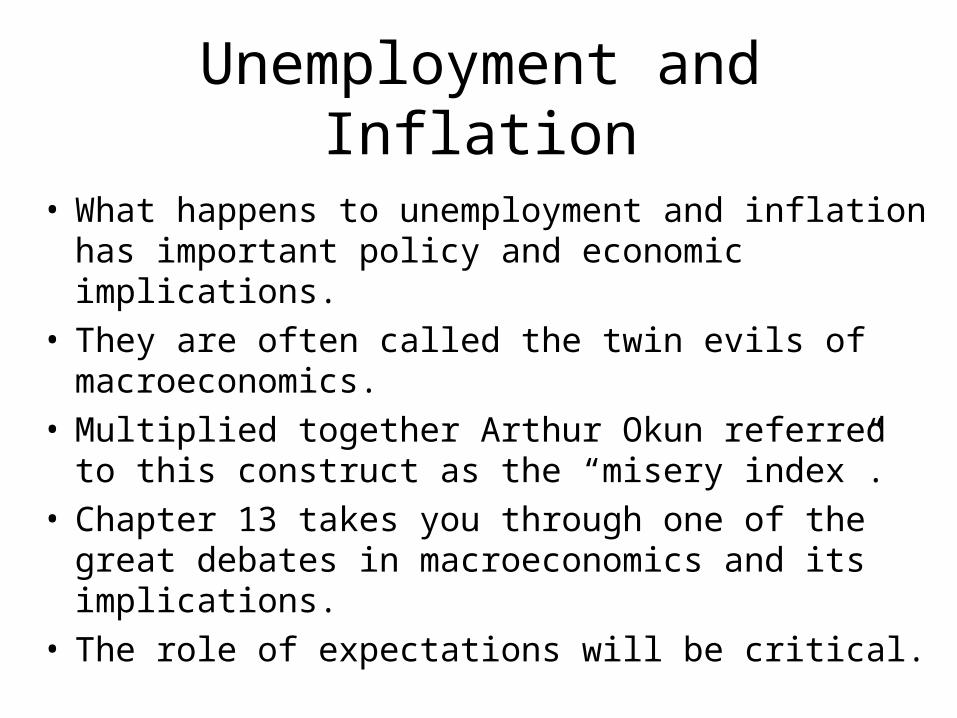
• What happens to unemployment and inflation has important policy and economic implications.

• They are often called the twin evils of macroeconomics.• Multiplied together Arthur Okun referred to this

construct as the “misery index”.• Chapter 13 takes you through one of the great debates

in macroeconomics and its implications.• The role of expectations will be critical.

Inflation and Unemployment in Canada

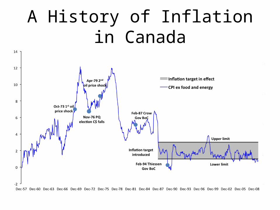
A History of Inflation in Canada

Unemployment and Inflation: Is There a Trade-Off?

• The Phillips curve is a negative empirical relationship between unemployment and wages, which appeared to be stable (Phillips looked at 97 years of UK data).

• The focus shifted to looking at unemployment and inflation.

• In Canada and elsewhere, up until the late 1960s, the Phillips curve seemed to show a stable relationship between inflation and unemployment suggesting a trade-off that could be exploited.

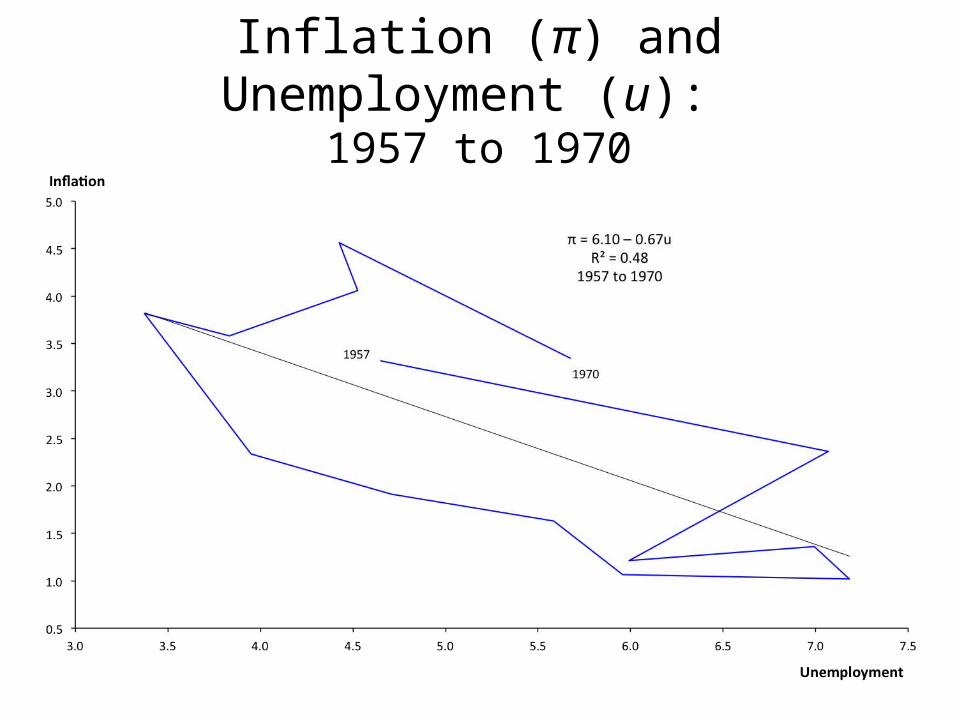
Inflation (π) and Unemployment (u): 1957 to 1970

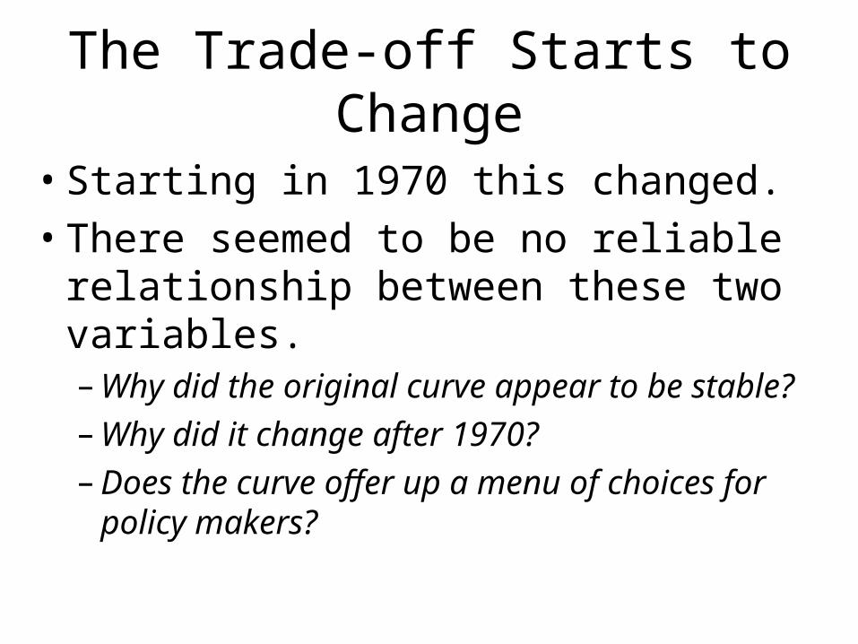
The Trade-off Starts to Change

• Starting in 1970 this changed. • There seemed to be no reliable

relationship between these two variables.–Why did the original curve appear to be stable?–Why did it change after 1970?– Does the curve offer up a menu of choices for

policy makers?

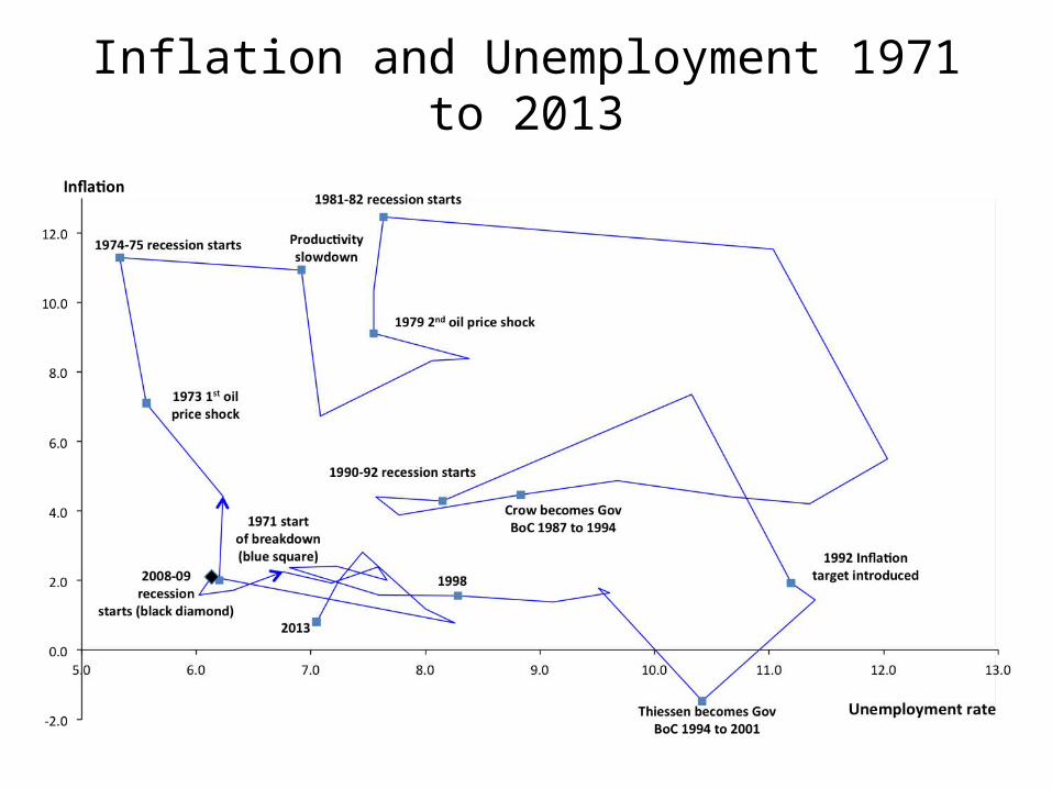
Inflation and Unemployment 1971 to 2013

The Expectations Augmented Phillips Curve

• The work done on explaining these puzzles, by Friedman (‘68) and Phelps (’70) – both of whom would get Nobel prizes, in part for this work – was actually completed prior to the shift in the relationship .

• In their view, a negative relationship should exist only between unanticipated inflation and cyclical unemployment, not between inflation and unemployment.

The Phillips Curve (continued)

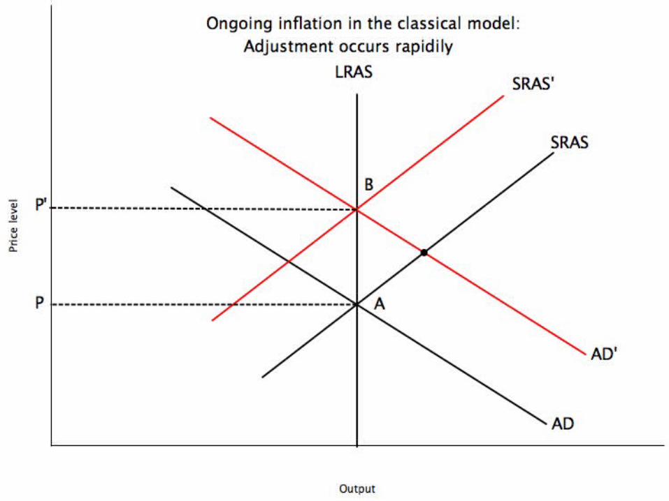
• To see how it works start with an economy in long-run equilibrium.

• If increases in M are anticipated, and if there are no misperceptions, the economy remains at u , unemployment remains at potential output , and cyclical unemployment (the difference between actual unemployment and ū is zero).

• But we do get shifts up in the AD (because of the increase in M) and SRAS curves (Figure next slide).

• An implication is that the long-run relationship between inflation and unemployment is a vertical line.


• Now suppose that the central bank increases the money supply by more than expected – this part is crucial for the analysis.

• The economy moves along its SRAS curve (output increases) and inflation rises but by less than the actual, unanticipated increase in M.

• Output rises because real M increases (it shifts the LM curve down or what is the same thing, it increases the AD curve).

• As well, firms now believe that the relative prices of the goods they produce have risen so they increase output and hire more workers to meet the increased demand.


• If the increase in M is unanticipated, unanticipated inflation is created, Y is above potential, and u is below ū.

π – πe = – h(u – ū)

• h measures the strength of the relationship between unanticipated inflation and cyclical unemployment.

• This is the relationship that should exist between inflation and unemployment.

An increase in money supply


• Rearranging terms slightly we can get a new relationship.

• The expectation-augmented Phillips curve states that if π exceeds πe then u is less than ū.

π – πe = –h(u – ū)

• h is also related to the slope of the SRAS curve as can be seen from the Figure in slide 14.

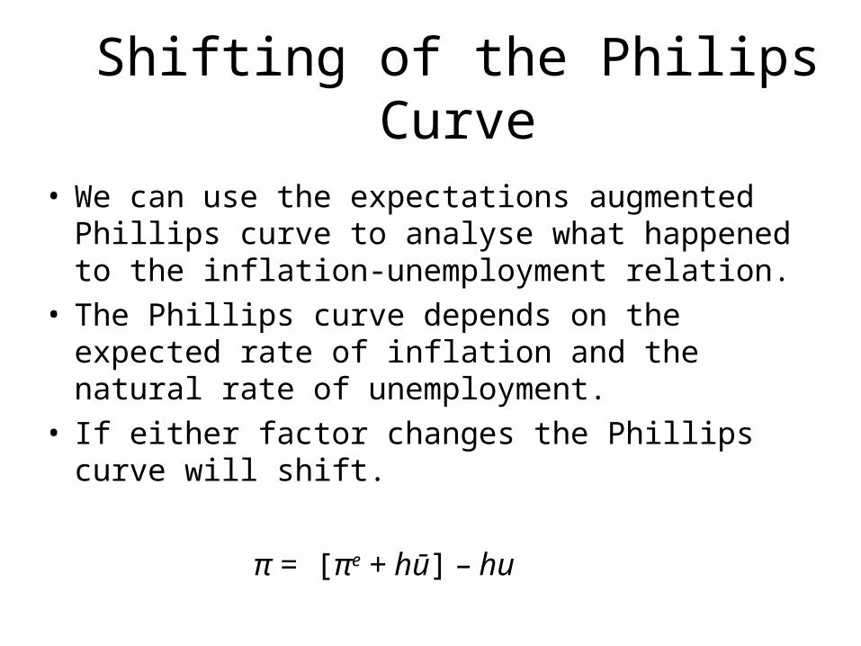
Shifting of the Philips Curve

• We can use the expectations augmented Phillips curve to analyse what happened to the inflation-unemployment relation.

• The Phillips curve depends on the expected rate of inflation and the natural rate of unemployment.

• If either factor changes the Phillips curve will shift.

π = [πe + hū] – hu

13-

Changes in the Expected Rate of Inflation

• If households anticipate a change in the price level their expectations of the price level (the rate of inflation) rise one-for-one.

• The Phillips curve shifts up by the amount of the increase in the expected rate of inflation.

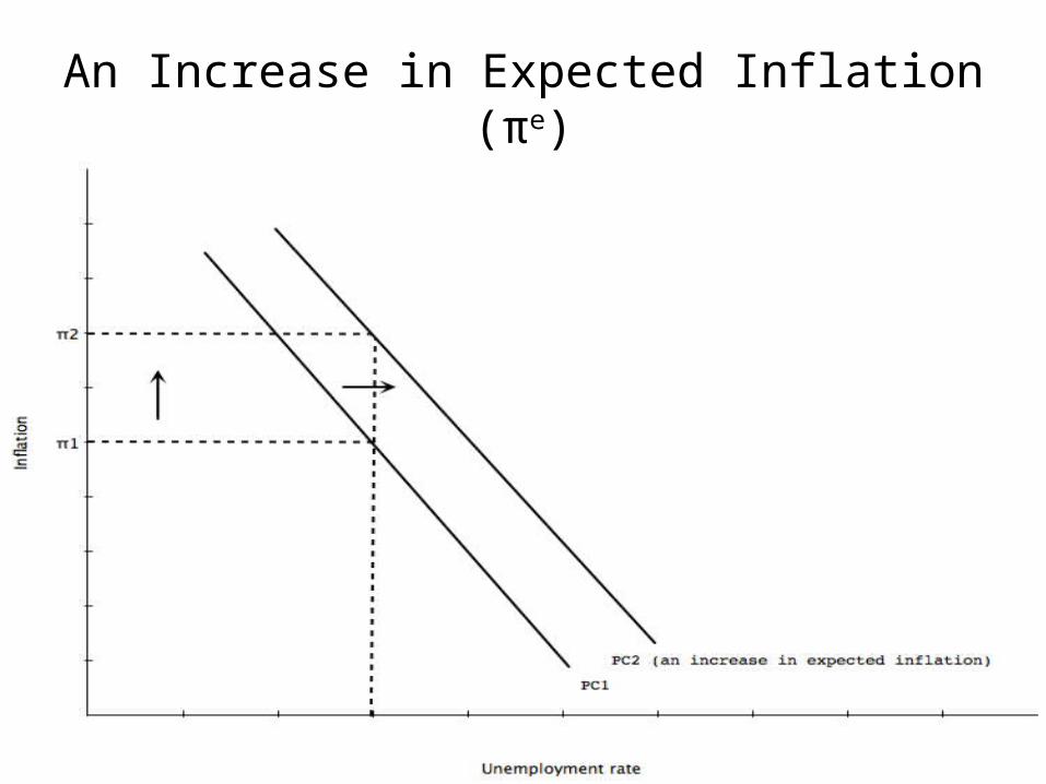
An Increase in Expected Inflation (πe)

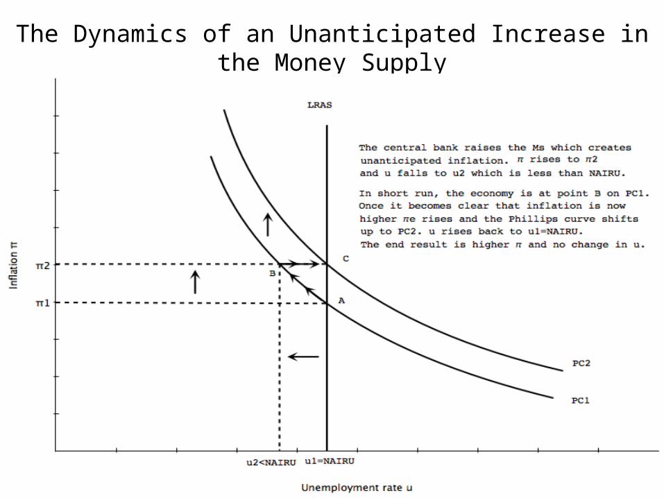
The Dynamics of an Unanticipated Increase in the Money Supply

Changes in the Natural Rate of Unemployment

• An increase in the natural unemployment rate causes the Phillips curve to shift up and to the right.

• The natural rate could shift for a variety of reasons, discussed later.

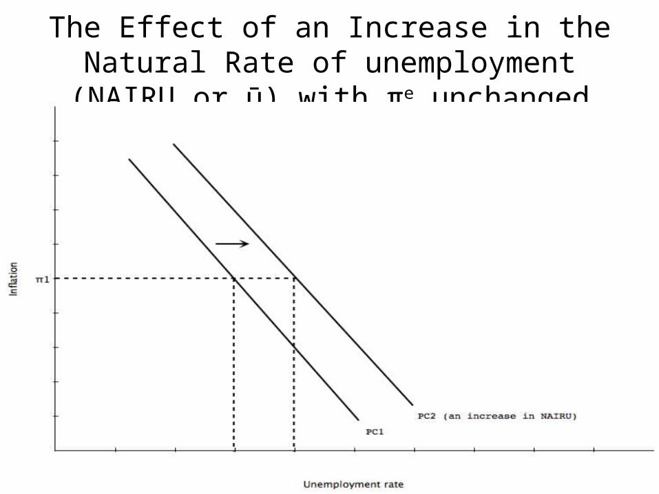
The Effect of an Increase in the Natural Rate of unemployment (NAIRU or ū) with πe unchanged

Supply Shocks and the Phillips Curve

• How well does the model fits the facts?• An adverse supply shock causes a burst of inflation, which may

lead people to expect higher inflation. • It also raises the natural rate of unemployment:

– by increasing the degree of mismatch between workers and jobs (classical economists);

– by reducing MPN and labour demanded at full employment, coupled with rigid wages (Keynesian economists);

– if the shock were thought to be permanent, it could increase labour supply and result in even more unemployment.

Supply Shocks and the Phillips Curve (con’t)

• An adverse supply shock should shift the Phillips curve up and to the right.

• The Phillips curve should be particularly unstable during periods of supply shocks, which we saw in the mid-1970s.

The Shifting Phillips Curve in Practice

• The Friedman-Phelps analysis shows that a negative relationship between the levels of inflation and unemployment holds as long as expected inflation and the natural unemployment rate are approximately constant.

• This was the case during the 1960s (and certainly true in the 1950s) and it was the relationship we saw in the Figure in slide 6 above.

The Shifting Phillips Curve in Practice (continued)

• During 1970-2006 there were a number of productivity shocks:– oil prices moved around dramatically;– these shocks tended to increase both the natural rate as well as

expected inflation.

• There were as well as changes in government and macroeconomic policies:– overly expansionary and then very restrictive monetary and fiscal

policies;– structural changes to employment insurance (EI).

• All these caused the relationship to change.

The Shifting Phillips Curve in Practice (continued)

• Nevertheless there is not a systematic relationship between inflation and unemployment.

• Rather the relationship is between unanticipated inflation and cyclical unemployment, and this does appear in the data.

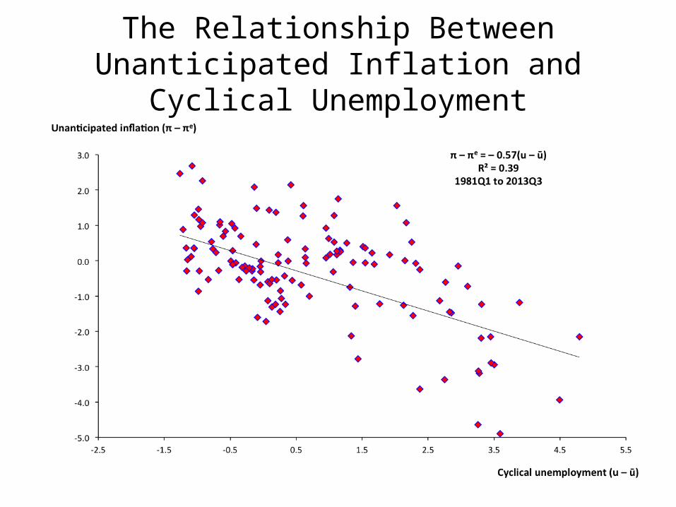
The Relationship Between Unanticipated Inflation and Cyclical Unemployment

Macroeconomic Policy and the Phillips Curve

• We have addressed two questions:– why the curve seemed to be stable in the

1960s;– and why it seemed to shift after that period.

• Now we want to see if we can exploit the relationship.

Macroeconomic Policy and the Phillips Curve (continued)

• In a recession, an expansionary AD policy can increase inflation back to the anticipated levels that were used as a basis for nominal wage contracts and pricing (Keynesian view).

• However, monetary policy cannot be used to lower u below ū.

• Indeed any attempt to do so would only result in ever increasing inflation and inflation expectations.

• The rate of unemployment that just keeps inflation constant is called the “non-accelerating inflation rate of unemployment” or NAIRU.

The Lucas Critique

• But are the responses of the economy predictable?• Policies are often based on models of the economy, which

in turn reflect historical experience.• New policies change the economic “rules” and often those

historical relationships.• Because of this, they affect economic behaviour, no one

can safely assume that historical relationships between variables will hold when policies change, in large part because these policy changes will influence how the economy responds.

• In part for such reasons, central banks tend to move cautiously – at least until recently.

The Long-Run Phillips Curve

• Economists agree that in the long run economy will adjust to the general equilibrium where π = πe and u = ū.

• The long-run Phillips curve is vertical line at u = ū.• It is from this relationship that we derive our notion of the

NAIRU. • It is related to the long-run neutrality of money.• Money is also “super neutral” – the growth in the money

supply cannot affect a real variable like u but rather only inflation.

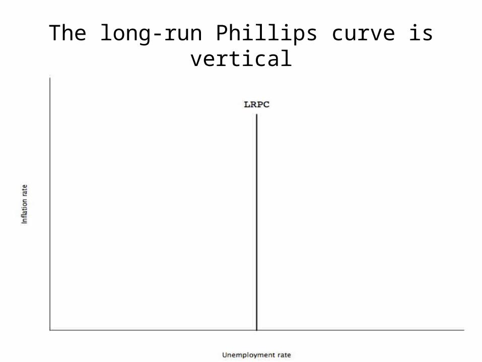
The long-run Phillips curve is vertical

The Cost of Unemployment

• Output is lost because fewer people are productively employed.

• Unemployed workers and their families face psychological cost.

• The offsetting factors are workers acquiring new skills and (perhaps!!) more leisure time.

The Long-Term Behaviour of the Unemployment Rate

• We can’t directly observe the natural rate, so it must be estimated.

• Base on work by Andrew Burns (Economic Council) and others:– in mid-1960s, the rate was roughly stable at 4½%;– it then rose to about 8½% by mid-80s;– it has since fallen back.

• The questions is why?

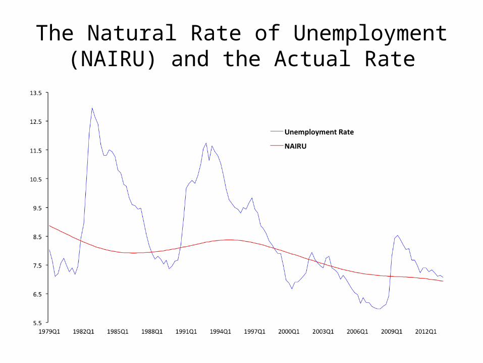
The Natural Rate of Unemployment (NAIRU) and the Actual Rate

The Long-Term Behaviour of the Unemployment Rate (continued)

• The long-term unemployment rate may be influenced by:– changes in the composition of the labour force by

age and sex;– structural changes in the economy; and– changes in the design of the employment insurance

program.

• All of these have had effects.


• Demographic changes:– younger workers and, until mid-90s, females have

higher unemployment rates so increases in their participation can raise the natural rate (a composition effect);

– since then, a fall in the number of younger workers and a change in the work patterns of females has lowered the natural rate.


• Technological change:– this would tend to create mismatches;– as well there were declines in the importance of

manufacturing and a rise in the share of services; and

– this explanation doesn’t explain recent declines when there has been even more technological change, so perhaps this is not the whole story.


• The role of employment insurance (EI):– persistent differences in unemployment rates between

provinces suggest a non-cyclical explanation;– key aspects of EI – replacement ratios, benefit duration

and eligibility requirements – vary by province and are related to local conditions;

– their generosity can create disincentives to look for work;– one study found that the disincentive effect was lowest in

Alberta and highest in Nova Scotia, with Ontario lying in between.


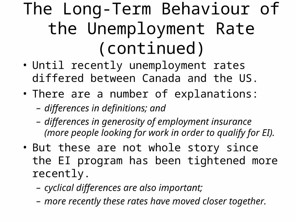
• Until recently unemployment rates differed between Canada and the US.

• There are a number of explanations:– differences in definitions; and– differences in generosity of employment insurance (more

people looking for work in order to qualify for EI).

• But these are not whole story since the EI program has been tightened more recently. – cyclical differences are also important; – more recently these rates have moved closer together.

Hysteresis in Unemployment

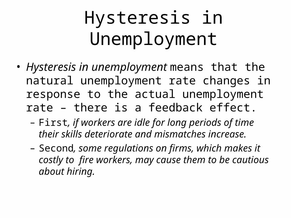
• Hysteresis in unemployment means that the natural unemployment rate changes in response to the actual unemployment rate – there is a feedback effect.– First, if workers are idle for long periods of time their skills

deteriorate and mismatches increase.– Second, some regulations on firms, which makes it costly to

fire workers, may cause them to be cautious about hiring.

Hysteresis in Unemployment (continued)

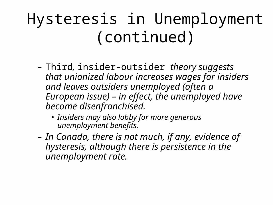
– Third, insider-outsider theory suggests that unionized labour increases wages for insiders and leaves outsiders unemployed (often a European issue) – in effect, the unemployed have become disenfranchised.• Insiders may also lobby for more generous unemployment

benefits.– In Canada, there is not much, if any, evidence of

hysteresis, although there is persistence in the unemployment rate.

Basing Policy on Estimates of the Natural Unemployment Rate

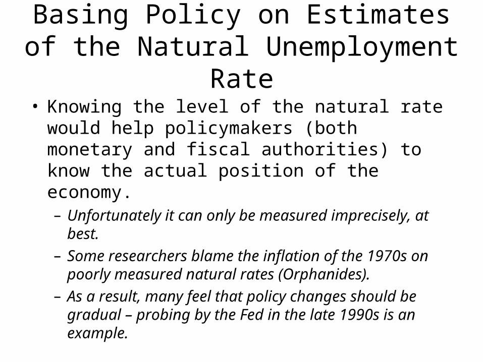
• Knowing the level of the natural rate would help policymakers (both monetary and fiscal authorities) to know the actual position of the economy.– Unfortunately it can only be measured imprecisely, at

best.– Some researchers blame the inflation of the 1970s on

poorly measured natural rates (Orphanides).– As a result, many feel that policy changes should be

gradual – probing by the Fed in the late 1990s is an example.

How to Reduce the Natural Rate of Unemployment

• With no exploitable trade-off, policymakers focus on fundamental causes of unemployment.

• Policies could include:– Increase government support for job training and

reallocation.– Increase labour-market flexibility.– Reform Employment Insurance programs.

• All economists (I would hope) agree that macro policies cannot be used to affect the natural rate.

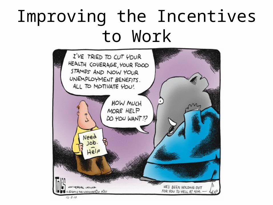
Improving the Incentives to Work

Perfectly Anticipated Inflation

• The costs of inflation depend whether or not it can be predicted.

• Because nominal wages are rising together with prices, the purchasing power is not hurt by the perfectly anticipated inflation.

• Perfectly anticipated inflation would also not hurt the value of savings accounts for similar reasons.

The Cost of Perfectly Anticipated Inflation

• But even perfectly anticipated inflation can have costs.– Shoe leather costs of inflation is time and effort incurred by people and

firms who are trying to minimize their holdings of cash. – Such costs have been estimated at about 0.3% of GDP in Canada.– Menu costs of inflation, the cost incurred in changing prices more

frequently, tend to be small.– Welfare costs of inflation-induced tax distortions.

• These costs are all small although perhaps non-trivial.

The Cost of Unanticipated Inflation

• The costs of unanticipated inflation are larger.• Creditors and those with incomes set in nominal terms are

hurt, whereas debtors and those who make fixed nominal payments are helped by unanticipated inflation – there is an arbitrary redistribution of income and wealth.

• While a redistribution nets out for the economy as a whole, people are made worse off by increasing risk of gaining or losing wealth.

• People must spend time and effort learning about different prices – price changes are no longer serving as a signal.

The Cost of Hyperinflation

• Hyperinflation occurs when the inflation rate is extremely high for a sustained period of time.– The shoe leather costs are enormous.– The government’s ability to collect taxes is undermined –

people delay paying.– The market efficiency is disrupted if not destroyed.

• A particularly high inflation rate occurred in Hungary after WWII – 19 800% per month!

• If this rate were annualized, it would be 3 followed by 52 digits – an enormous number.

Fighting Inflation: The Role of Inflationary Expectations

• Inflation occurs when the aggregate demand for goods exceed supply.

• The only factor that can create sustained rises in aggregate demand and ongoing inflation is a high rate of money growth.

• While monetary policy can be used to stimulate demand during a recession, the stimulus has to be withdrawn once full employment is achieved – in the past, failure to do so has led to inflation.

Fighting Inflation (continued)

• The process of disinflation – the reduction of money growth – can, and often does, lead to a recession.

• If inflation falls below the expected rate, unemployment will rise above the natural rate.

• The expectations augmented Phillips curve suggests a recession can be avoided (or at least lessened) if the expected inflation rate can be made to fall.

• How to lower expectations is the trick.

Rapid versus Gradual Disinflation

• A cold turkey strategy is a rapid and decisive reduction in the growth rate of the money supply.

• Some have argued that such an approach would quickly lower expectations.

• However, if prices and wages are slow to adjust, it will lead to rising unemployment.

• This seemed to be the case in Canada during the late 1980s, at least for a while.

Rapid versus Gradual Disinflation (continued)

• A policy of gradualism is a policy of reducing the rate of money growth gradually over a period of time.

• This policy will raise unemployment by less than the cold-turkey strategy, but the period of higher unemployment will be longer.

• As well, inflation expectations will be slow to adjust.

Rapid versus Gradual Disinflation (continued)

• The cost, in terms of lost output or rising unemployment, is called the sacrifice ratio.

• In the 1980s, inflation fell from 11.6% to 3.8%, a drop of 7.8 percentage points over 16 quarter period, while the cumulative output loss was 18.6% of potential GDP.

• The sacrifice ratio in that period was 2.4%, or for every one percentage point fall in inflation the cost was 2.4% of GDP.

• Part of the problem was that inflation expectations remained stubbornly high, at least for a while.

• The average sacrifice ratio in Canada is 1.5%.• Given these costs, is there an easier way to do this?

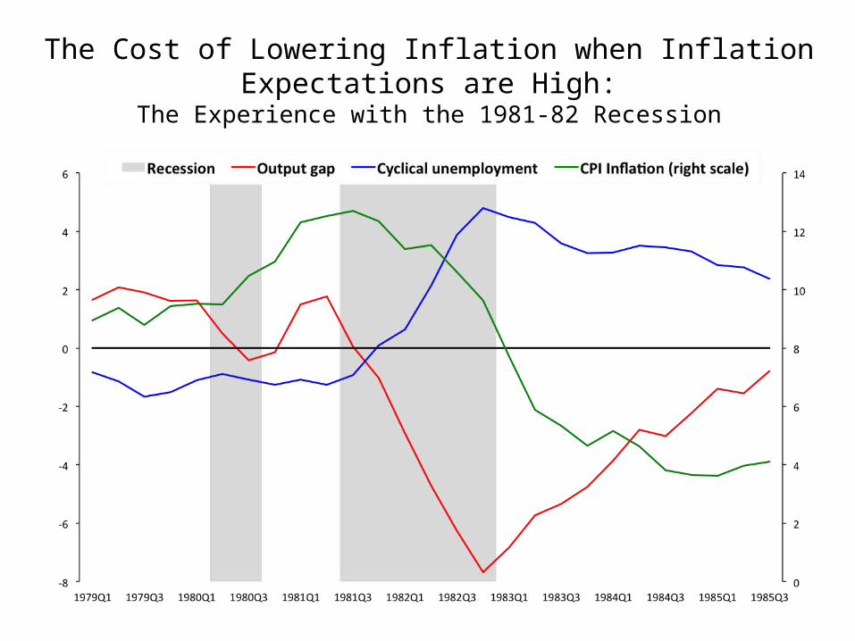
The Cost of Lowering Inflation when Inflation Expectations are High:The Experience with the 1981-82 Recession

Another Way: Wage and Price Controls

• Frustration with inflation has sometimes led governments to implement wage and price controls (income policies), which are legal limits on the ability of firms to raise wages or prices.

• Versions of this policy were tried in both Canada and the US in the 1970s, with mixed results. – Price controls are likely to create shortages and are hard to enforce in certain

markets – commodities for instance.– Other demand policies must go in the same direction, actions which would help

lower inflation expectations – this was not the case in the US but was so in Canada.

– Wage-price controls are intended to affect the public’s expectations of inflation but the public may in turn expect a catch-up after the controls are lifted – and this tended to happen.

– There was some success with the “6 and 5” program in the early 1980s on expectations but these were not comprehensive controls.

Credibility and Reputation • All economists agree that achieving low-cost disinflation

requires reducing πe. – The major message from Friedman and Phelps has sunk in.

• One way is to have clear and unambiguous announcement of policy – Canada has done this.

• Also need to develop a reputation. – This may take time – but there are benefits.

• As well you need an independent central bank – in 1997, the new Labour government made the Bank of England independent and long-term interest rates fell immediately.

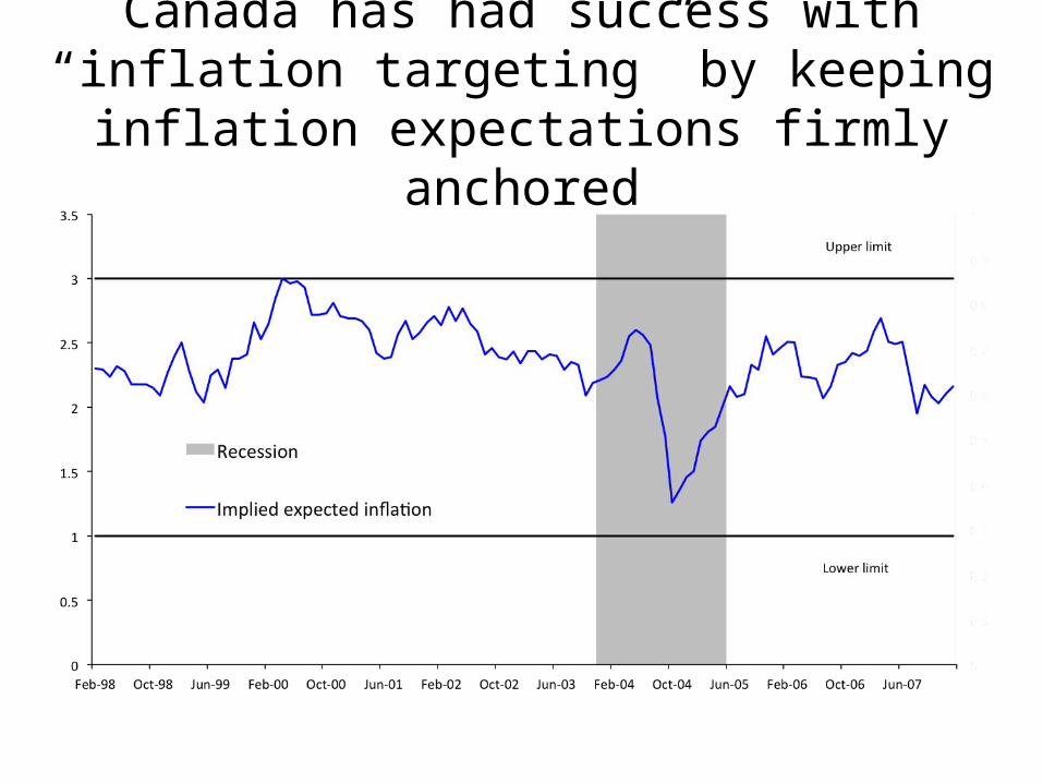
Canada has had success with “inflation targeting” by keeping inflation expectations firmly anchored

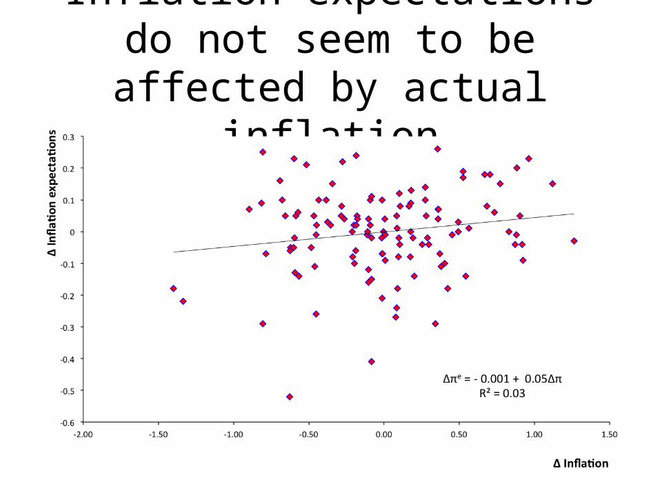
Inflation expectations do not seem to be affected by actual inflation

Using a Model to Calculate the Cost of Disinflation

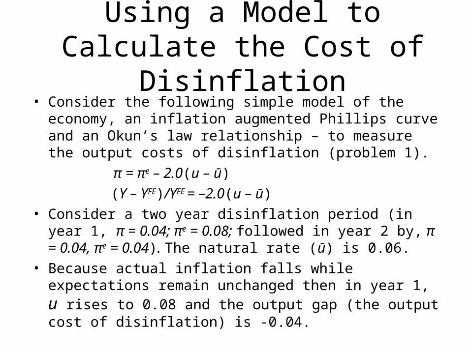
• Consider the following simple model of the economy, an inflation augmented Phillips curve and an Okun’s law relationship – to measure the output costs of disinflation (problem 1).

π = πe – 2.0(u – ū)

(Y – YFE)/YFE = –2.0(u – ū)

• Consider a two year disinflation period (in year 1, π = 0.04; πe = 0.08; followed in year 2 by, π = 0.04, πe = 0.04). The natural rate (ū) is 0.06.

• Because actual inflation falls while expectations remain unchanged then in year 1, u rises to 0.08 and the output gap (the output cost of disinflation) is -0.04.

Using a Model to Calculate the Cost of Disinflation (continued)

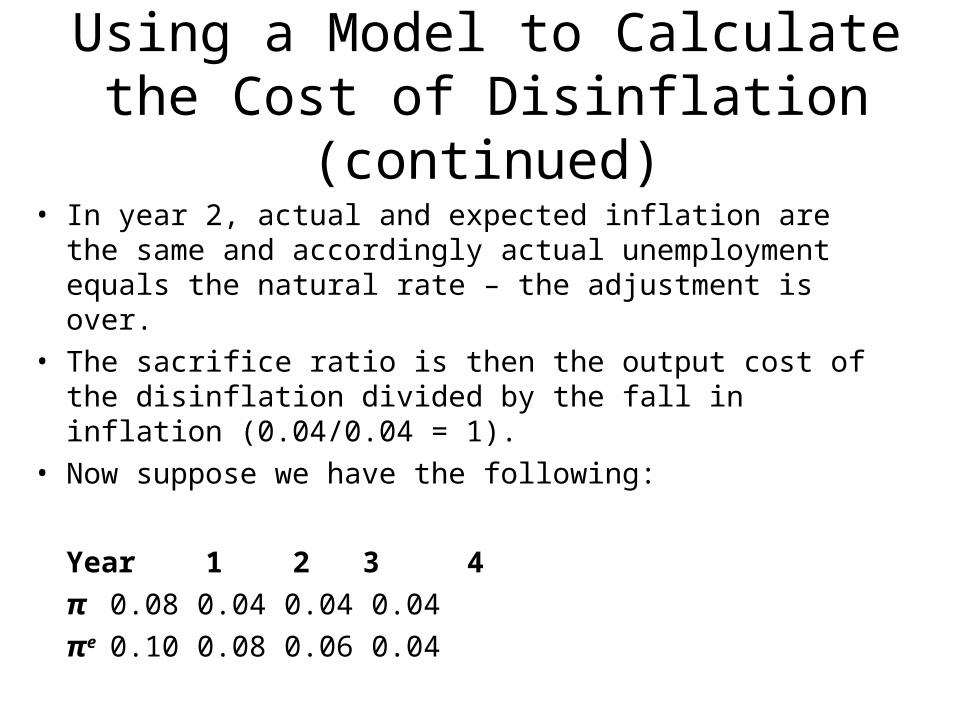
• In year 2, actual and expected inflation are the same and accordingly actual unemployment equals the natural rate – the adjustment is over.

• The sacrifice ratio is then the output cost of the disinflation divided by the fall in inflation (0.04/0.04 = 1).

• Now suppose we have the following:

Year 1 2 3 4π 0.08 0.04 0.04 0.04πe 0.10 0.08 0.06 0.04

Using a Model to Calculate the Cost of Disinflation (continued)

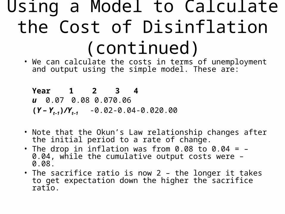
• We can calculate the costs in terms of unemployment and output using the simple model. These are:

Year 1 2 3 4u 0.07 0.08 0.07 0.06(Y – Yt–1)/Yt–1

-0.02 -0.04 -0.02 0.00

• Note that the Okun’s Law relationship changes after the initial period to a rate of change.

• The drop in inflation was from 0.08 to 0.04 = – 0.04, while the cumulative output costs were – 0.08.

• The sacrifice ratio is now 2 – the longer it takes to get expectation down the higher the sacrifice ratio.

The Importance of Getting the Fundamentals Correct

Documents

Unemployment and Inflation Prof Mike Kennedy. Unemployment and Inflation What happens to unemployment and inflation has important policy and economic