Chapter 2 Units, Dimensional Analysis, Problem Solving, and

Estimation

2.1 The Speed of light ................................................................................................... 1 2.2 International System of Units ................................................................................ 1

2.2.1 Standard Mass .................................................................................................... 2 Example 2.1 The International Prototype Kilogram ................................................... 3 Example 2.2 Mass of a Silicon Crystal ....................................................................... 4 2.2.2 The Atomic Clock and the Definition of the Second ......................................... 5 2.2.3 The Meter ........................................................................................................... 6 Example 2.3 Light-Year .............................................................................................. 6 2.2.4 Radians and Steradians ...................................................................................... 7 2.2.5 Radiant Intensity ................................................................................................ 9

2.3 Dimensions of Commonly Encountered Quantities ............................................. 9 2.3.1 Dimensional Analysis ...................................................................................... 11 Example 2.4 Period of a Pendulum ........................................................................... 11

2.4 Significant Digits, Scientific Notation, and Rounding ....................................... 12 2.4.1 Significant Digits ............................................................................................. 12 2.4.2 Scientific Notation ........................................................................................... 13 2.4.3 Rounding .......................................................................................................... 13

2.5 Problem Solving .................................................................................................... 13 2.5.1 General Approach to Problem Solving ............................................................ 14

2.6 Order of Magnitude Estimates - Fermi Problems ............................................. 16 2.6.1 Methodology for Estimation Problems ............................................................ 17 Example 2.5 Lining Up Pennies ............................................................................... 17 Example 2.6 Estimation of Mass of Water on Earth ................................................ 18

2-1

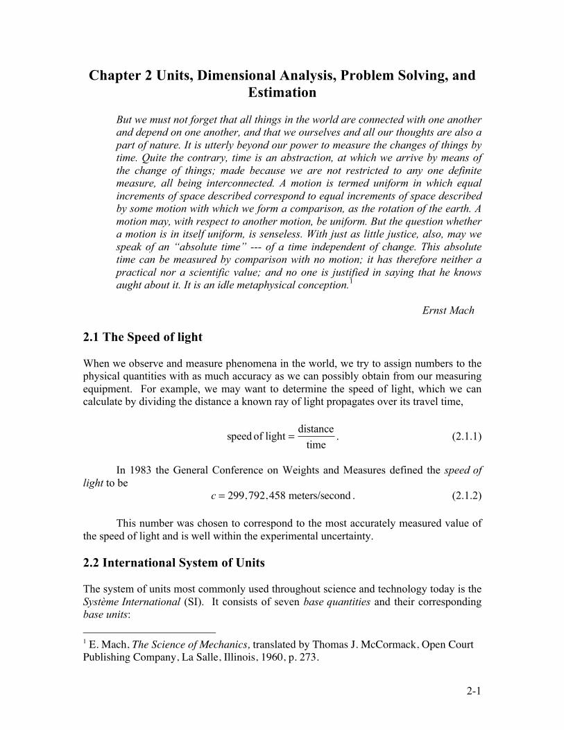
Chapter 2 Units, Dimensional Analysis, Problem Solving, and Estimation

But we must not forget that all things in the world are connected with one another and depend on one another, and that we ourselves and all our thoughts are also a part of nature. It is utterly beyond our power to measure the changes of things by time. Quite the contrary, time is an abstraction, at which we arrive by means of the change of things; made because we are not restricted to any one definite measure, all being interconnected. A motion is termed uniform in which equal increments of space described correspond to equal increments of space described by some motion with which we form a comparison, as the rotation of the earth. A motion may, with respect to another motion, be uniform. But the question whether a motion is in itself uniform, is senseless. With just as little justice, also, may we speak of an “absolute time” --- of a time independent of change. This absolute time can be measured by comparison with no motion; it has therefore neither a practical nor a scientific value; and no one is justified in saying that he knows aught about it. It is an idle metaphysical conception.1

Ernst Mach 2.1 The Speed of light When we observe and measure phenomena in the world, we try to assign numbers to the physical quantities with as much accuracy as we can possibly obtain from our measuring equipment. For example, we may want to determine the speed of light, which we can calculate by dividing the distance a known ray of light propagates over its travel time,

speed of light =

distancetime

. (2.1.1)

In 1983 the General Conference on Weights and Measures defined the speed of light to be c = 299,792,458 meters/second . (2.1.2)

This number was chosen to correspond to the most accurately measured value of the speed of light and is well within the experimental uncertainty. 2.2 International System of Units The system of units most commonly used throughout science and technology today is the Système International (SI). It consists of seven base quantities and their corresponding base units: 1 E. Mach, The Science of Mechanics, translated by Thomas J. McCormack, Open Court Publishing Company, La Salle, Illinois, 1960, p. 273.

2-2

Base Quantity Base Unit Length meter (m) Mass kilogram (kg) Time second (s) Electric Current ampere (A) Temperature kelvin (K) Amount of Substance mole (mol) Luminous Intensity candela (cd)

We shall refer to the dimension of the base quantity by the quantity itself, for example dim length ≡ length ≡ L, dim mass ≡ mass ≡M, dim time ≡ time ≡ T. (2.2.1) Mechanics is based on just the first three of these quantities, the MKS or meter-kilogram-second system. An alternative metric system to this, still widely used, is the so-called CGS system (centimeter-gram-second). 2.2.1 Standard Mass

The unit of mass, the kilogram (kg), remains the only base unit in the International System of Units (SI) that is still defined in terms of a physical artifact, known as the “International Prototype of the Standard Kilogram.” George Matthey (of Johnson Matthey) made the prototype in 1879 in the form of a cylinder, 39 mm high and 39 mm in diameter, consisting of an alloy of 90 % platinum and 10 % iridium. The international prototype is kept at the Bureau International des Poids et Mesures (BIPM) at Sevres, France under conditions specified by the 1st Conférence Générale des Poids et Mèsures (CGPM) in 1889 when it sanctioned the prototype and declared “This prototype shall henceforth be considered to be the unit of mass.” It is stored at atmospheric pressure in a specially designed triple bell-jar. The prototype is kept in a vault with six official copies. The 3rd Conférence Générale des Poids et Mesures CGPM (1901), in a declaration intended to end the ambiguity in popular usage concerning the word “weight” confirmed that:

The kilogram is the unit of mass; it is equal to the mass of the international prototype of the kilogram.

There is a stainless steel one-kilogram standard that can travel for comparisons with standard masses in other laboratories. In practice it is more common to quote a conventional mass value (or weight-in-air, as measured with the effect of buoyancy), than the standard mass. Standard mass is normally only used in specialized measurements wherever suitable copies of the prototype are stored.

2-3

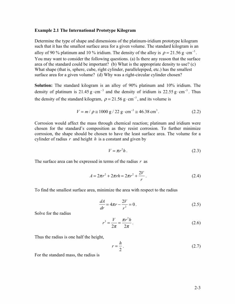
Example 2.1 The International Prototype Kilogram Determine the type of shape and dimensions of the platinum-iridium prototype kilogram such that it has the smallest surface area for a given volume. The standard kilogram is an alloy of 90 % platinum and 10 % iridium. The density of the alloy is ρ = 21.56 g ⋅cm−3 . You may want to consider the following questions. (a) Is there any reason that the surface area of the standard could be important? (b) What is the appropriate density to use? (c) What shape (that is, sphere, cube, right cylinder, parallelepiped, etc.) has the smallest surface area for a given volume? (d) Why was a right-circular cylinder chosen? Solution: The standard kilogram is an alloy of 90% platinum and 10% iridium. The density of platinum is 21.45 g ⋅cm−3 and the density of iridium is 22.55 g ⋅cm−3 . Thus the density of the standard kilogram, ρ = 21.56 g ⋅cm−3 , and its volume is V = m / ρ ≅ 1000 g / 22 g ⋅cm−3 ≅ 46.38 cm3 . (2.2) Corrosion would affect the mass through chemical reaction; platinum and iridium were chosen for the standard’s composition as they resist corrosion. To further minimize corrosion, the shape should be chosen to have the least surface area. The volume for a cylinder of radius r and height h is a constant and given by V = πr 2h . (2.3) The surface area can be expressed in terms of the radius r as

A = 2πr 2 + 2πrh = 2πr 2 +

2Vr

. (2.4)

To find the smallest surface area, minimize the area with respect to the radius

dAdr

= 4πr − 2Vr 2 = 0 . (2.5)

Solve for the radius

r3 =

V2π

=πr 2h2π

. (2.6)

Thus the radius is one half the height,

r = h

2. (2.7)

For the standard mass, the radius is

2-4

r = V

2π⎛⎝⎜

⎞⎠⎟

1 3

=46.38 cm3

2π⎛

⎝⎜⎞

⎠⎟

1 3

≅ 1.95 cm . (2.8)

Twice this radius is the diameter of the standard kilogram. Because the prototype kilogram is an artifact, there are some intrinsic problems associated with its use as a standard. It may be damaged, or destroyed. The prototype gains atoms due to environment wear and cleaning, at a rate of change of mass corresponding to approximately 1µg / year , ( 1µg ≡ 1microgram ≡ 1×10-6 g ).

Several new approaches to defining the SI unit of mass (kg) are currently being explored. One possibility is to define the kilogram as a fixed number of atoms of a particular substance, thus relating the kilogram to an atomic mass. Silicon is a good candidate for this approach because it can be grown as a large single crystal, in a very pure form. Example 2.2 Mass of a Silicon Crystal A given standard unit cell of silicon has a volume V0 and contains N0 atoms. The number of molecules in a given mole of substance is given by Avogadro’s constant

N A = 6.02214129(27)×1023 mol-1 . The molar mass of silicon is given by Mmol . Find the mass m of a volume V in terms of V0 , N0 , V , Mmol , and N A . Solution: The mass m0 of the unit cell is the density ρ of silicon cell multiplied by the volume of the cell V0 , m0 = ρV0 . (2.9) The number of moles in the unit cell is the total mass, m0 , of the cell, divided by the molar mass Mmol , n0 = m0 / Mmol = ρV0 / Mmol . (2.10) The number of atoms in the unit cell is the number of moles n0 times the Avogadro constant, N A ,

N0 = n0N A =

ρV0N A

Mmol

. (2.11)

The density of the crystal is related to the mass m of the crystal divided by the volume V of the crystal, ρ = m / V . (2.12)

2-5

The number of atoms in the unit cell can be expressed as

N0 =

mV0N A

VMmol

. (2.13)

The mass of the crystal is

m =

Mmol

N A

VV0

N0 (2.14)

The molar mass, unit cell volume and volume of the crystal can all be measured directly. Notice that Mmol / N A is the mass of a single atom, and (V / V0 )N0 is the number of atoms in the volume. This approach is therefore reduced to the problem of measuring the Avogadro constant, N A , with a relative uncertainty of 1 part in 108, which is equivalent to the uncertainty in the present definition of the kilogram. 2.2.2 The Atomic Clock and the Definition of the Second Isaac Newton, in the Philosophiae Naturalis Principia Mathematica (“Mathematical Principles of Natural Philosophy”), distinguished between time as duration and an absolute concept of time,

“Absolute true and mathematical time, of itself and from its own nature, flows equably without relation to anything external, and by another name is called duration: relative, apparent, and common time, is some sensible and external (whether accurate or unequable) measure of duration by means of motion, which is commonly used instead of true time; such as an hour, a day, a month, a year. ”2.

The development of clocks based on atomic oscillations allowed measures of

timing with accuracy on the order of 1 part in 1014 , corresponding to errors of less than one microsecond (one millionth of a second) per year. Given the incredible accuracy of this measurement, and clear evidence that the best available timekeepers were atomic in nature, the second (s) was redefined in 1967 by the International Committee on Weights and Measures as a certain number of cycles of electromagnetic radiation emitted by cesium atoms as they make transitions between two designated quantum states:

2 Isaac Newton. Mathematical Principles of Natural Philosophy. Translated by Andrew Motte (1729). Revised by Florian Cajori. Berkeley: University of California Press, 1934. p. 6.

2-6

The second is the duration of 9,192,631,770 periods of the radiation corresponding to the transition between the two hyperfine levels of the ground state of the cesium 133 atom.

2.2.3 The Meter The meter was originally defined as 1/10,000,000 of the arc from the Equator to the North Pole along the meridian passing through Paris. To aid in calibration and ease of comparison, the meter was redefined in terms of a length scale etched into a platinum bar preserved near Paris. Once laser light was engineered, the meter was redefined by the 17th Conférence Générale des Poids et Mèsures (CGPM) in 1983 to be a certain number of wavelengths of a particular monochromatic laser beam.

The meter is the length of the path traveled by light in vacuum during a time interval of 1/299 792 458 of a second.

Example 2.3 Light-Year Astronomical distances are sometimes described in terms of light-years (ly). A light-year is the distance that light will travel in one year (yr). How far in meters does light travel in one year?

Solution: Using the relationship distance = (speed of light) ⋅ (time) , one light year corresponds to a distance. Because the speed of light is given in terms of meters per second, we need to know how many seconds are in a year. We can accomplish this by converting units. We know that 1 year = 365.25 days, 1 day = 24 hours, 1 hour = 60 minutes, 1 minute = 60 seconds Putting this together we find that the number of seconds in a year is

1 year = 365.25 day( ) 24 hours

1day⎛⎝⎜

⎞⎠⎟

60 min1 hour

⎛⎝⎜

⎞⎠⎟

60 s1 min

⎛⎝⎜

⎞⎠⎟

=31,557,600 s . (2.2.15)

The distance that light travels in a one year is

1 ly =

299,792,458 m1s

⎛⎝⎜

⎞⎠⎟

31,557,600 s1 yr

⎛⎝⎜

⎞⎠⎟

1 yr( ) = 9.461×1015 m . (2.2.16)

The distance to the nearest star, a faint red dwarf star, Proxima Centauri, is 4.24

light years. A standard astronomical unit is the parsec. One parsec is the distance at which there is one arcsecond = 1/3600 degree angular separation between two objects that are separated by the distance of one astronomical unit, 111AU 1.50 10 m= × , which is the mean distance between the earth and sun. One astronomical unit is roughly equivalent

2-7

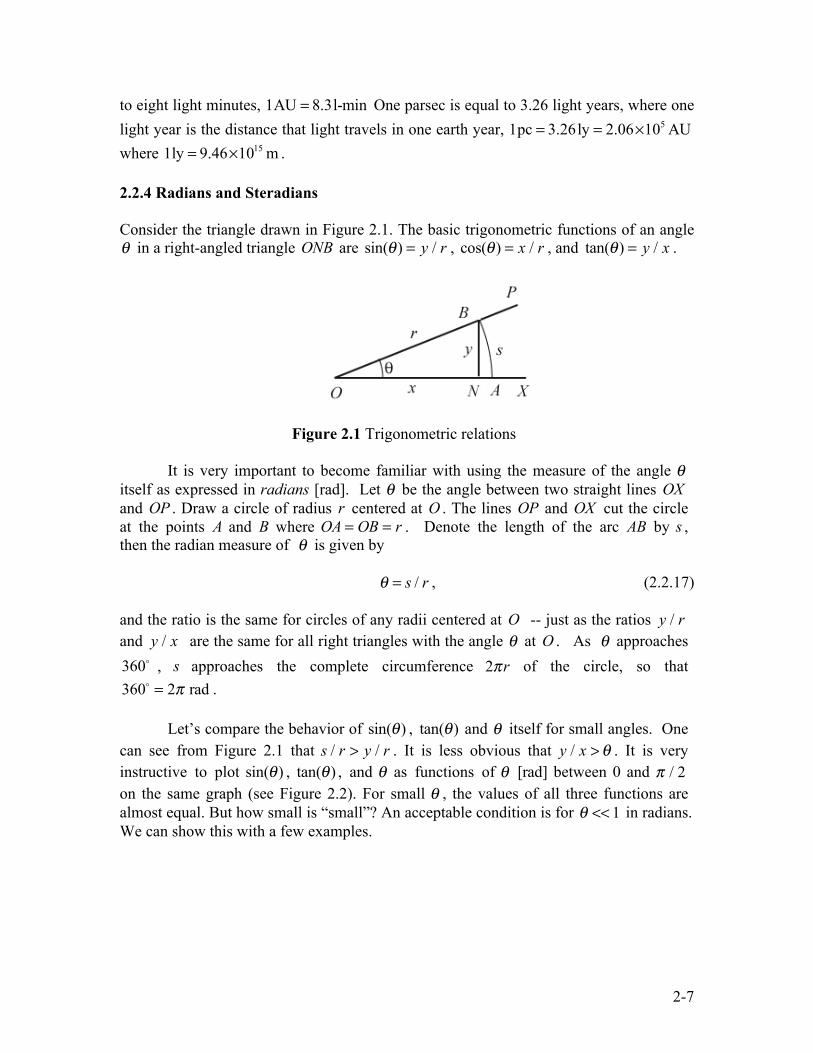
to eight light minutes, 1AU 8.3l-min= One parsec is equal to 3.26 light years, where one light year is the distance that light travels in one earth year, 51pc 3.26ly 2.06 10 AU= = × where 151ly 9.46 10 m= × . 2.2.4 Radians and Steradians Consider the triangle drawn in Figure 2.1. The basic trigonometric functions of an angle θ in a right-angled triangle ONB are sin(θ) = y / r , cos(θ) = x / r , and tan(θ) = y / x .

Figure 2.1 Trigonometric relations

It is very important to become familiar with using the measure of the angle θ itself as expressed in radians [rad]. Let θ be the angle between two straight lines OX and OP . Draw a circle of radius r centered at O . The lines OP and OX cut the circle at the points A and B where OA = OB = r . Denote the length of the arc AB by s , then the radian measure of θ is given by

θ = s / r , (2.2.17) and the ratio is the same for circles of any radii centered at O -- just as the ratios y / r and y / x are the same for all right triangles with the angle θ at O . As θ approaches

360 , s approaches the complete circumference 2πr of the circle, so that

360 = 2π rad .

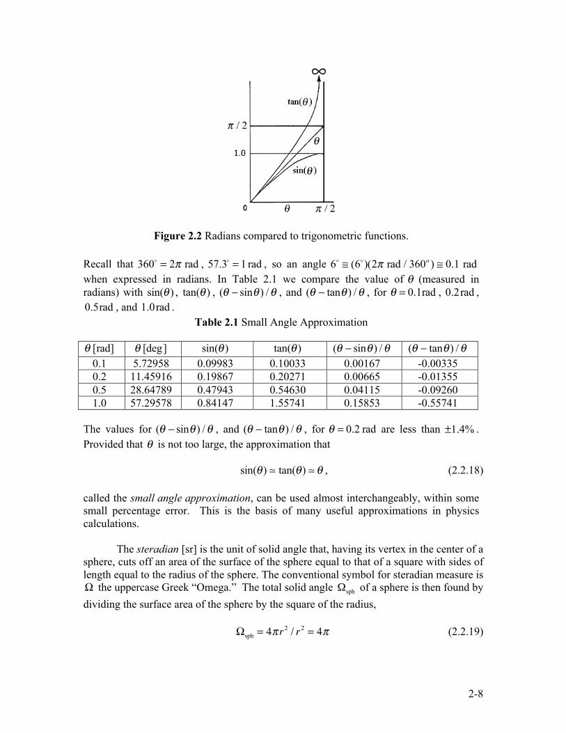
Let’s compare the behavior of sin(θ) , tan(θ) and θ itself for small angles. One can see from Figure 2.1 that s / r > y / r . It is less obvious that y / x > θ . It is very instructive to plot sin(θ) , tan(θ) , and θ as functions of θ [rad] between 0 and π / 2 on the same graph (see Figure 2.2). For small θ , the values of all three functions are almost equal. But how small is “small”? An acceptable condition is for θ << 1 in radians. We can show this with a few examples.

2-8

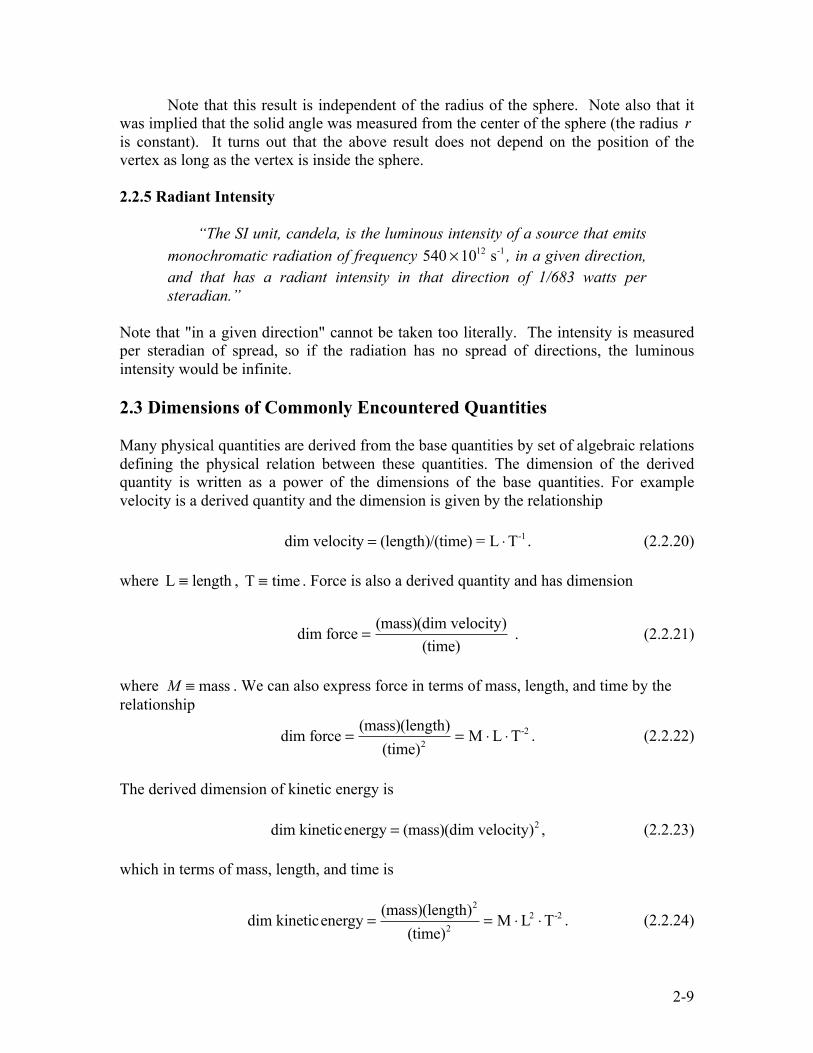
Figure 2.2 Radians compared to trigonometric functions. Recall that 360 = 2π rad , 57.3 = 1 rad , so an angle 6

≅ (6 )(2π rad / 360o ) ≅ 0.1 rad when expressed in radians. In Table 2.1 we compare the value of θ (measured in radians) with sin(θ ) , tan(θ ) , (θ − sinθ ) /θ , and (θ − tanθ ) /θ , for θ = 0.1rad , 0.2rad ,

0.5rad , and 1.0rad . Table 2.1 Small Angle Approximation

θ [rad] θ [deg] sin(θ ) tan(θ ) (θ − sinθ ) /θ (θ − tanθ ) /θ

0.1 5.72958 0.09983 0.10033 0.00167 -0.00335 0.2 11.45916 0.19867 0.20271 0.00665 -0.01355 0.5 28.64789 0.47943 0.54630 0.04115 -0.09260 1.0 57.29578 0.84147 1.55741 0.15853 -0.55741

The values for (θ − sinθ ) /θ , and (θ − tanθ ) /θ , for θ = 0.2 rad are less than ±1.4% . Provided that θ is not too large, the approximation that sin(θ) tan(θ) θ , (2.2.18) called the small angle approximation, can be used almost interchangeably, within some small percentage error. This is the basis of many useful approximations in physics calculations. The steradian [sr] is the unit of solid angle that, having its vertex in the center of a sphere, cuts off an area of the surface of the sphere equal to that of a square with sides of length equal to the radius of the sphere. The conventional symbol for steradian measure is Ω the uppercase Greek “Omega.” The total solid angle Ωsph of a sphere is then found by dividing the surface area of the sphere by the square of the radius, Ωsph = 4πr

2 / r2 = 4π (2.2.19)

2-9

Note that this result is independent of the radius of the sphere. Note also that it was implied that the solid angle was measured from the center of the sphere (the radius r is constant). It turns out that the above result does not depend on the position of the vertex as long as the vertex is inside the sphere. 2.2.5 Radiant Intensity

“The SI unit, candela, is the luminous intensity of a source that emits monochromatic radiation of frequency 540 ×1012 s-1 , in a given direction, and that has a radiant intensity in that direction of 1/683 watts per steradian.”

Note that "in a given direction" cannot be taken too literally. The intensity is measured per steradian of spread, so if the radiation has no spread of directions, the luminous intensity would be infinite. 2.3 Dimensions of Commonly Encountered Quantities Many physical quantities are derived from the base quantities by set of algebraic relations defining the physical relation between these quantities. The dimension of the derived quantity is written as a power of the dimensions of the base quantities. For example velocity is a derived quantity and the dimension is given by the relationship dim velocity = (length)/(time) = L ⋅T-1 . (2.2.20) where L ≡ length , T ≡ time . Force is also a derived quantity and has dimension

dim force =

(mass)(dim velocity)(time)

. (2.2.21)

where M ≡ mass . We can also express force in terms of mass, length, and time by the relationship

dim force =

(mass)(length)(time)2

= M ⋅L ⋅T-2 . (2.2.22)

The derived dimension of kinetic energy is dim kineticenergy = (mass)(dim velocity)2 , (2.2.23) which in terms of mass, length, and time is

dim kineticenergy =

(mass)(length)2

(time)2 = M ⋅L2 ⋅T-2 . (2.2.24)

2-10

The derived dimension of work is dim work = (dim force)(length) , (2.2.25) which in terms of our fundamental dimensions is

dim work =

(mass)(length)2

(time)2= M ⋅L2 ⋅T-2 . (2.2.26)

So work and kinetic energy have the same dimensions. Power is defined to be the rate of change in time of work so the dimensions are

dim power =

dim worktime

=(dim force)(length)

time=

(mass)(length)2

(time)3= M ⋅L2 ⋅T-3 .(2.2.27)

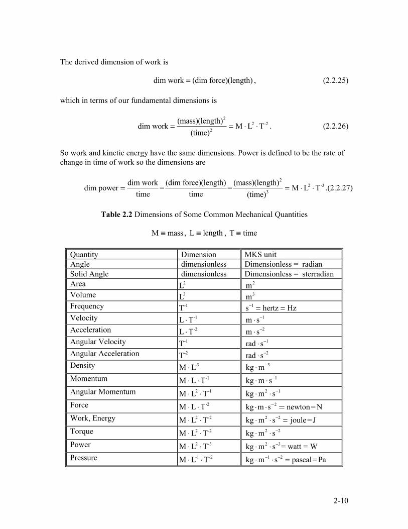
Table 2.2 Dimensions of Some Common Mechanical Quantities

M ≡ mass , L ≡ length , T ≡ time

Quantity Dimension MKS unit Angle dimensionless Dimensionless = radian Solid Angle dimensionless Dimensionless = sterradian

Area L2 m2 Volume L3 m3 Frequency T-1

s−1 = hertz = Hz

Velocity L ⋅T-1 m ⋅ s−1

Acceleration L ⋅T-2 m ⋅ s−2

Angular Velocity T-1 rad ⋅ s−1

Angular Acceleration T-2 rad ⋅ s−2

Density M ⋅L-3 kg ⋅m−3

Momentum M ⋅L ⋅T-1 kg ⋅m ⋅ s−1

Angular Momentum M ⋅L2 ⋅T-1 kg ⋅m2 ⋅ s−1

Force M ⋅L ⋅T-2 kg ⋅m ⋅s−2 = newton= N

Work, Energy M ⋅L2 ⋅T-2 kg ⋅m2 ⋅ s−2 = joule=J

Torque M ⋅L2 ⋅T-2 kg ⋅m2 ⋅ s−2

Power M ⋅L2 ⋅T-3 kg ⋅m2 ⋅ s−3= watt = W

Pressure M ⋅L-1 ⋅T-2 kg ⋅m−1 ⋅ s−2 = pascal= Pa

2-11

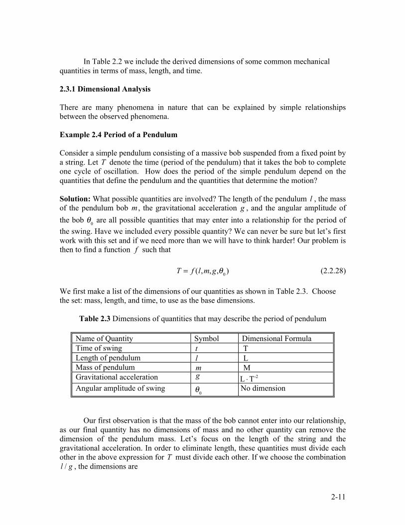
In Table 2.2 we include the derived dimensions of some common mechanical quantities in terms of mass, length, and time. 2.3.1 Dimensional Analysis There are many phenomena in nature that can be explained by simple relationships between the observed phenomena. Example 2.4 Period of a Pendulum Consider a simple pendulum consisting of a massive bob suspended from a fixed point by a string. Let T denote the time (period of the pendulum) that it takes the bob to complete one cycle of oscillation. How does the period of the simple pendulum depend on the quantities that define the pendulum and the quantities that determine the motion? Solution: What possible quantities are involved? The length of the pendulum l , the mass of the pendulum bob m , the gravitational acceleration g , and the angular amplitude of the bob θ0 are all possible quantities that may enter into a relationship for the period of the swing. Have we included every possible quantity? We can never be sure but let’s first work with this set and if we need more than we will have to think harder! Our problem is then to find a function f such that T = f (l,m,g,θ0 ) (2.2.28) We first make a list of the dimensions of our quantities as shown in Table 2.3. Choose the set: mass, length, and time, to use as the base dimensions.

Table 2.3 Dimensions of quantities that may describe the period of pendulum

Name of Quantity Symbol Dimensional Formula Time of swing t T Length of pendulum l L Mass of pendulum m M Gravitational acceleration g L ⋅T-2 Angular amplitude of swing

θ0 No dimension

Our first observation is that the mass of the bob cannot enter into our relationship, as our final quantity has no dimensions of mass and no other quantity can remove the dimension of the pendulum mass. Let’s focus on the length of the string and the gravitational acceleration. In order to eliminate length, these quantities must divide each other in the above expression for T

must divide each other. If we choose the combination l / g , the dimensions are

2-12

dim[l / g] =

lengthlength/(time)2 = (time)2 (2.2.29)

It appears that the time of swing is proportional to the square root of this ratio. We have an argument that works for our choice of constants, which depend on the units we choose for our fundamental quantities. Thus we have a candidate formula

T l

g⎛⎝⎜

⎞⎠⎟

1/2

. (2.2.30)

(in the above expression, the symbol “ ” represents a proportionality, not an approximation). Because the angular amplitude θ0 is dimensionless, it may or may not appear. We can account for this by introducing some function y(θ0 ) into our relationship, which is beyond the limits of this type of analysis. Then the time of swing is

T = y(θ0 ) l

g⎛⎝⎜

⎞⎠⎟

1/2

. (2.2.31)

We shall discover later on that y(θ0 ) is nearly independent of the angular amplitude θ0 for very small amplitudes and is equal to y(θ0 ) = 2π ,

T = 2π l

g⎛⎝⎜

⎞⎠⎟

1/2

(2.2.32)

2.4 Significant Digits, Scientific Notation, and Rounding 2.4.1 Significant Digits We shall define significant digits by the following rules.3

1. The leftmost nonzero digit is the most significant digit. 2. If there is no decimal point, the rightmost nonzero digit is the least significant

digit. 3. If there is a decimal point then the rightmost digit is the least significant digit

even if it is a zero.

3 Philip R Bevington and D. Keith Robinson, Data Reduction and Error Analysis for the Physical Sciences, 2nd Edition, McGraw-Hill, Inc., New York, 1992.

2-13

4. All digits between the least and most significant digits are counted as significant digits.

When reporting the results of an experiment, the number of significant digits used

in reporting the result is the number of digits needed to state the result of that measurement (or a calculation based on that measurement) without any loss of precision.

There are exceptions to these rules, so you may want to carry around one extra significant digit until you report your result. For example if you multiply 2 × 0.56 = 1.12 , not 1.1 . There is some ambiguity about the number of significant figure when the rightmost digit is 0, for example 1050, with no terminal decimal point. This has only three significant digits. If all the digits are significant the number should be written as 1050., with a terminal decimal point. To avoid this ambiguity it is wiser to use scientific notation. 2.4.2 Scientific Notation Careless use of significant digits can be easily avoided by the use of decimal notation times the appropriate power of ten for the number. Then all the significant digits are manifestly evident in the decimal number. Therefore the number 1050 = 1.05×103 while the number 1050. = 1.050 ×103 . 2.4.3 Rounding To round off a number by eliminating insignificant digits we have three rules. For practical purposes, rounding will be done automatically by a calculator or computer, and all we need do is set the desired number of significant figures for whichever tool is used.

1. If the fraction is greater than 1/2, increment the new least significant digit. 2. If the fraction is less than 1/2, do not increment. 3. If the fraction equals 1/2, increment the least significant digit only if it is odd.

The reason for Rule 3 is that a fractional value of 1/2 may result from a previous rounding up of a fraction that was slightly less than 1/2 or a rounding down of a fraction that was slightly greater than 1/2. For example, 1.249 and 1.251 both round to three significant digits 1.25. If we were to round again to two significant digits, both would yield the same value, either 1.2 or 1.3 depending on our convention in Rule 3. Choosing to round up if the resulting last digit is odd and to round down if the resulting last digit is even reduces the systematic errors that would otherwise be introduced into the average of a group of such numbers. 2.5 Problem Solving Solving problems is the most common task used to measure understanding in technical and scientific courses, and in many aspects of life as well. In general, problem solving

2-14

requires factual and procedural knowledge in the area of the problem, plus knowledge of numerous schema, plus skill in overall problem solving. Schema is loosely defined as a “specific type of problem” such as principal, rate, and interest problems, one-dimensional kinematic problems with constant acceleration, etc. In most introductory university courses, improving problem solving relies on three things:

1. increasing domain knowledge, particularly definitions and procedures 2. learning schema for various types of problems and how to recognize that a

particular problem belongs to a known schema 3. becoming more conscious of and insightful about the process of problem solving.

To improve your problem solving ability in a course, the most essential change of

attitude is to focus more on the process of solution rather than on obtaining the answer. For homework problems there is frequently a simple way to obtain the answer, often involving some specific insight. This will quickly get you the answer, but you will not build schema that will help solve related problems further down the road. Moreover, if you rely on insight, when you get stuck on a problem, you’re stuck with no plan or fallback position. 2.5.1 General Approach to Problem Solving A great many physics textbook authors recommend overall problem solving strategies. These are typically four-step procedures that descend from George Polya’s influential book, How to Solve It, on problem solving4. Here are his four steps:

1. Understand – get a conceptual grasp of the problem

What is the problem asking? What are the given conditions and assumptions? What domain of knowledge is involved? What is to be found and how is this determined or constrained by the given conditions? What knowledge is relevant? E.g. in physics, does this problem involve kinematics, forces, energy, momentum, angular momentum, equilibrium? If the problem involves two different areas of knowledge, try to separate the problem into parts. Is there motion or is it static? If the problem involves vector quantities such as velocity or momentum, think of these geometrically (as arrows that add vectorially). Get conceptual understanding: is some physical quantity (energy, momentum, angular momentum, etc.) constant? Have you done problems that involve the same concepts in roughly the same way? Model: Real life contains great complexity, so in physics (chemistry, economics…) you actually solve a model problem that contains the essential elements of the real problem. The bike and rider become a point mass (unless

4 G. Polya, How to Solve It, 2nd ed., Princeton University Press, 1957.

2-15

angular momentum is involved), the ladder’s mass is regarded as being uniformly distributed along its length, the car is assumed to have constant acceleration or constant power (obviously not true when it shifts gears), etc. Become sensitive to information that is implicitly assumed (Presence of gravity? No friction? That the collision is of short duration relative to the timescale of the subsequent motion? …). Advice: Write your own representation of the problem’s stated data; redraw the picture with your labeling and comments. Get the problem into your brain! Go systematically down the list of topics in the course or for that week if you are stuck.

2. Devise a Plan - set up a procedure to obtain the desired solution

General - Have you seen a problem like this – i.e., does the problem fit in a schema you already know? Is a part of this problem a known schema? Could you simplify this problem so that it is? Can you find any useful results for the given problem and data even if it is not the solution (e.g. in the special case of motion on an incline when the plane is at θ= 0 )? Can you imagine a route to the solution if only you knew some apparently not given information? If your solution plan involves equations, count the unknowns and check that you have that many independent equations. In Physics, exploit the freedoms you have: use a particular type of coordinate system (e.g. polar) to simplify the problem, pick the orientation of a coordinate system to get the unknowns in one equation only (e.g. only the x -direction), pick the position of the origin to eliminate torques from forces you don’t know, pick a system so that an unknown force acts entirely within it and hence does not change the system’s momentum… Given that the problem involves some particular thing (constant acceleration, momentum) think over all the equations that involve this concept.

3. Carry our your plan – solve the problem!

This generally involves mathematical manipulations. Try to keep them as simple as possible by not substituting in lengthy algebraic expressions until the end is in sight, make your work as neat as you can to ease checking and reduce careless mistakes. Keep a clear idea of where you are going and have been (label the equations and what you have now found), if possible, check each step as you proceed. Always check dimensions if analytic, and units if numerical.

4. Look Back – check your solution and method of solution

Can you see that the answer is correct now that you have it – often simply by retrospective inspection? Can you solve it a different way? Is the problem equivalent to one you’ve solved before if the variables have some specific values?

2-16

Check special cases (for instance, for a problem involving two massive objects moving on an inclined plane, if m1 = m2 or θ = 0 does the solution reduce to a simple expression that you can easily derive by inspection or a simple argument?) Is the scaling what you’d expect (an energy should vary as the velocity squared, or linearly with the height). Does it depend sensibly on the various quantities (e.g. is the acceleration less if the masses are larger, more if the spring has a larger k )? Is the answer physically reasonable (especially if numbers are given or reasonable ones substituted). Review the schema of your solution: Review and try to remember the outline of the solution – what is the model, the physical approximations, the concepts needed, and any tricky math manipulation.

2.6 Order of Magnitude Estimates - Fermi Problems Counting is the first mathematical skill we learn. We came to use this skill by distinguishing elements into groups of similar objects, but we run into problems when our desired objects are not easily identified, or there are too many to count. Rather than spending a huge amount of effort to attempt an exact count, we can try to estimate the number of objects in a collection. For example, we can try to estimate the total number of grains of sand contained in a bucket of sand. Because we can see individual grains of sand, we expect the number to be very large but finite. Sometimes we can try to estimate a number, which we are fairly sure but not certain is finite, such as the number of particles in the universe. We can also assign numbers to quantities that carry dimensions, such as mass, length, time, or charge, which may be difficult to measure exactly. We may be interested in estimating the mass of the air inside a room, or the length of telephone wire in the United States, or the amount of time that we have slept in our lives. We choose some set of units, such as kilograms, miles, hours, and coulombs, and then we can attempt to estimate the number with respect to our standard quantity. Often we are interested in estimating quantities such as speed, force, energy, or power. We may want to estimate our natural walking speed, or the force of wind acting against a bicycle rider, or the total energy consumption of a country, or the electrical power necessary to operate a university. All of these quantities have no exact, well-defined value; they instead lie within some range of values. When we make these types of estimates, we should be satisfied if our estimate is reasonably close to the middle of the range of possible values. But what does “reasonably close” mean? Once again, this depends on what quantities we are estimating. If we are describing a quantity that has a very large number associated with it, then an estimate within an order of magnitude should be satisfactory. The number of molecules in a breath of air is close to 1022 ; an estimate anywhere between 1021 and 1023 molecules is close enough. If we are trying to win a contest by estimating the number of marbles in a glass

2-17

container, we cannot be so imprecise; we must hope that our estimate is within 1% of the real quantity. These types of estimations are called Fermi Problems. The technique is named after the physicist Enrico Fermi, who was famous for making these sorts of “back of the envelope” calculations. 2.6.1 Methodology for Estimation Problems Estimating is a skill that improves with practice. Here are two guiding principles that may help you get started.

(1) You must identify a set of quantities that can be estimated or calculated. (2) You must establish an approximate or exact relationship between these quantities

and the quantity to be estimated in the problem. Estimations may be characterized by a precise relationship between an estimated quantity and the quantity of interest in the problem. When we estimate, we are drawing upon what we know. But different people are more familiar with certain things than others. If you are basing your estimate on a fact that you already know, the accuracy of your estimate will depend on the accuracy of your previous knowledge. When there is no precise relationship between estimated quantities and the quantity to be estimated in the problem, then the accuracy of the result will depend on the type of relationships you decide upon. There are often many approaches to an estimation problem leading to a reasonably accurate estimate. So use your creativity and imagination! Example 2.5 Lining Up Pennies Suppose you want to line pennies up, diameter to diameter, until the total length is 1 kilometer . How many pennies will you need? How accurate is this estimation? Solution: The first step is to consider what type of quantity is being estimated. In this example we are estimating a dimensionless scalar quantity, the number of pennies. We can now give a precise relationship for the number of pennies needed to mark off 1 kilometer

# of pennies = totaldistancediameter of penny

. (2.2.33)

We can estimate a penny to be approximately 2 centimeters wide. Therefore the number of pennies is

# of pennies=

totaldistancelengthof a penny

= (1km)(2 cm)(1km / 105 cm)

= 5×104 pennies . (2.2.34)

2-18

When applying numbers to relationships we must be careful to convert units whenever necessary. How accurate is this estimation? If you measure the size of a penny, you will find out that the width is 1.9 cm , so our estimate was accurate to within 5%. This accuracy was fortuitous. Suppose we estimated the length of a penny to be 1 cm. Then our estimate for the total number of pennies would be within a factor of 2, a margin of error we can live with for this type of problem. Example 2.6 Estimation of Mass of Water on Earth Estimate the mass of the water on the Earth? Solution: In this example we are estimating mass, a quantity that is a fundamental in SI units, and is measured in kg. We start by approximating that the amount of water on Earth is approximately equal to the amount of water in all the oceans. Initially we will try to estimate two quantities: the density of water and the volume of water contained in the oceans. Then the relationship we want is (mass)ocean =(density)water (volume)ocean . (2.2.35) One of the hardest aspects of estimation problems is to decide which relationship applies. One way to check your work is to check dimensions. Density has dimensions of mass/volume, so our relationship is

(mass)ocean =

massvolume

⎛⎝⎜

⎞⎠⎟

(volume)ocean . (2.2.36)

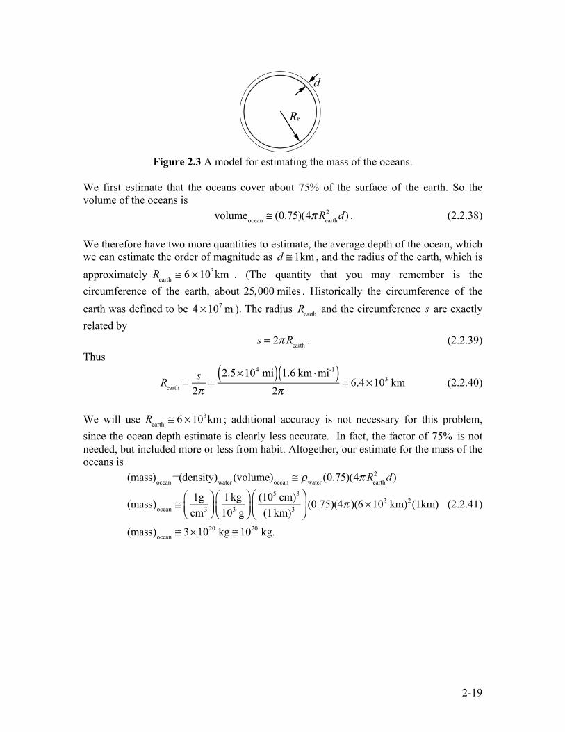
The density of fresh water is ρwater = 1.0 g ⋅cm−3 ; the density of seawater is slightly higher, but the difference won’t matter for this estimate. You could estimate this density by estimating how much mass is contained in a one-liter bottle of water. (The density of water is a point of reference for all density problems. Suppose we need to estimate the density of iron. If we compare iron to water, we estimate that iron is 5 to 10 times denser than water. The actual density of iron is ρiron = 7.8 g ⋅cm-3 ). Because there is no precise relationship, estimating the volume of water in the oceans is much harder. Let’s model the volume occupied by the oceans as if they completely cover the earth, forming a spherical shell (Figure 2.3, which is decidedly not to scale). The volume of a spherical shell of radius Rearth and thickness d is (volume)shell ≅ 4πRearth

2 d , (2.2.37) where Rearth is the radius of the earth and d is the average depth of the ocean.

2-19

Figure 2.3 A model for estimating the mass of the oceans.

We first estimate that the oceans cover about 75% of the surface of the earth. So the volume of the oceans is volumeocean ≅ (0.75)(4πRearth

2 d) . (2.2.38) We therefore have two more quantities to estimate, the average depth of the ocean, which we can estimate the order of magnitude as d ≅ 1km , and the radius of the earth, which is approximately Rearth ≅ 6 ×103km . (The quantity that you may remember is the circumference of the earth, about 25,000 miles . Historically the circumference of the earth was defined to be 4 ×107 m ). The radius Rearth and the circumference s are exactly related by s = 2πRearth . (2.2.39) Thus

Rearth =

s2π

=2.5×104 mi( ) 1.6 km ⋅mi-1( )

2π= 6.4×103 km (2.2.40)

We will use Rearth ≅ 6 ×103km ; additional accuracy is not necessary for this problem, since the ocean depth estimate is clearly less accurate. In fact, the factor of 75% is not needed, but included more or less from habit. Altogether, our estimate for the mass of the oceans is

(mass)ocean =(density)water (volume)ocean ≅ ρwater (0.75)(4πRearth2 d)

(mass)ocean ≅1g

cm3

⎛⎝⎜

⎞⎠⎟

1kg103 g

⎛⎝⎜

⎞⎠⎟

(105 cm)3

(1km)3

⎛⎝⎜

⎞⎠⎟

(0.75)(4π )(6×103 km)2(1km)

(mass)ocean ≅ 3×1020 kg ≅ 1020 kg.

(2.2.41)