Embed Size (px)
Citation preview
Advances in Applied Mathematics 61 (2014) 102–124
Contents lists available at ScienceDirect
Advances in Applied Mathematics
www.elsevier.com/locate/yaama
Unseparated pairs and fixed points in random
permutations ✩
Persi Diaconis a, Steven N. Evans b, Ron Graham c
a Department of Mathematics, Stanford University, Building 380, Sloan Hall, Stanford, CA 94305, USAb Department of Statistics #3860, University of California at Berkeley, 367 Evans Hall, Berkeley, CA 94720-3860, USAc Department of Computer Science, University of California at San Diego, 9500 Gilman Drive #0404, La Jolla, CA 92093-0404, USA
a r t i c l e i n f o a b s t r a c t
Article history:Received 25 August 2013Accepted 1 May 2014Available online xxxx
MSC:60C0560B1560F05
Keywords:ShuffleDerangementMarkov chainChinese restaurant processPoisson distributionStein’s methodCommutatorSmoosh
In a uniform random permutation Π of [n] := {1, 2, . . . , n}, the set of elements k ∈ [n − 1] such that Π(k+ 1) = Π(k) + 1has the same distribution as the set of fixed points of Πthat lie in [n − 1]. We give three different proofs of this fact using, respectively, an enumeration relying on the inclusion–exclusion principle, the introduction of two different Markov chains to generate uniform random permutations, and the construction of a combinatorial bijection. We also obtain the distribution of the analogous set for circular permutations that consists of those k ∈ [n] such that Π(k + 1 mod n) =Π(k) + 1 mod n. This latter random set is just the set of fixed points of the commutator [ρ, Π], where ρ is the n-cycle (1, 2, . . . , n). We show for a general permutation η that, under weak conditions on the number of fixed points and 2-cycles of η, the total variation distance between the distribution of
✩ P.D. was supported in part by NSF grant DMS-08-04324, S.N.E. was supported in part by NSF grant DMS-09-07630, R.G. was supported in part by NSF grant DUE-10-20548.
E-mail addresses: [email protected] (P. Diaconis), [email protected] (S.N. Evans), [email protected] (R. Graham).
URLs: http://www-stat.stanford.edu/~cgates/PERSI/ (P. Diaconis), http://www.stat.berkeley.edu/users/evans/ (S.N. Evans), http://cseweb.ucsd.edu/~rgraham/(R. Graham).
http://dx.doi.org/10.1016/j.aam.2014.05.0060196-8858/© 2014 Elsevier Inc. All rights reserved.
P. Diaconis et al. / Advances in Applied Mathematics 61 (2014) 102–124 103
Wash the number of fixed points of [η, Π] and a Poisson distribution with expected value 1 is small when n is large.
© 2014 Elsevier Inc. All rights reserved.
1. Introduction
The goal of any procedure for shuffling a deck of n cards labeled with, say, [n] :={1, 2, . . . , n} is to take the cards in some specified original order, which we may take to be (1, 2, . . . , n), and re-arrange them randomly in such a way that all n! possible orders are close to being equally likely. A natural approach to checking empirically whether the outcomes of a given shuffling procedure deviate from uniformity is to apply some fixed numerical function to each of the permutations produced by several independent instances of the shuffle and determine whether the resulting empirical distribution is close to the distribution of the random variable that would arise from applying the chosen function to a uniformly distributed permutation.
Smoosh shuffling (also known as wash, corgi, chemmy or Irish shuffling) is a simple physical mechanism for randomizing a deck of cards – see [18] for an article that has a brief discussion of smoosh shuffling and a link to a video of the first author carrying it out, and [7,17] for other short descriptions. In their forthcoming analysis of this shuffle, [1] use the approach described above with the function that takes a permutation π ∈ Sn, the set of permutations of [n] := {1, 2, . . . , n}, and returns the cardinality of the set of labels k ∈ [n −1] such that π(k+1) = π(k) +1. That is, they count the number of pairs of cards that were adjacent in the original deck and aren’t separated or in a different relative order at the completion of the shuffle. For example, the permutation π of [6] given by
π =(
1 2 3 4 5 6 75 6 7 4 1 2 3
)has {k ∈ [6] : π(k + 1) = π(k) + 1} = {1, 2, 5, 6}.
If we write Πn for a random permutation that is uniformly distributed on Sn and Sn ⊆ [n −1] for the set of labels k ∈ [n −1] such that Πn(k+1) = Πn(k) +1, then, in order to support the contention that the smoosh shuffle is producing a random permutation with a distribution close to uniform, it is necessary to know, at least approximately, the distribution of the integer-valued random variable #Sn. Banklader et al. [1] use Stein’s method (see, for example, [5] for a survey), to show that the distribution of #Sn is close to a Poisson distribution with expected value 1 when n is large.
The problem of computing P{#Sn = 0} (or, more correctly, the integer n!P{#Sn= 0}) appears in various editions of the 19th century textbook on combinatorics and probabil-ity, Choice and Chance by William Allen Whitworth. For example, Proposition XXXII in Chapter IV of [16] gives
P{#Sn = 0} =n∑ (−1)k
k! + 1n
n−1∑ (−1)k
k! . (1.1)
k=0 k=0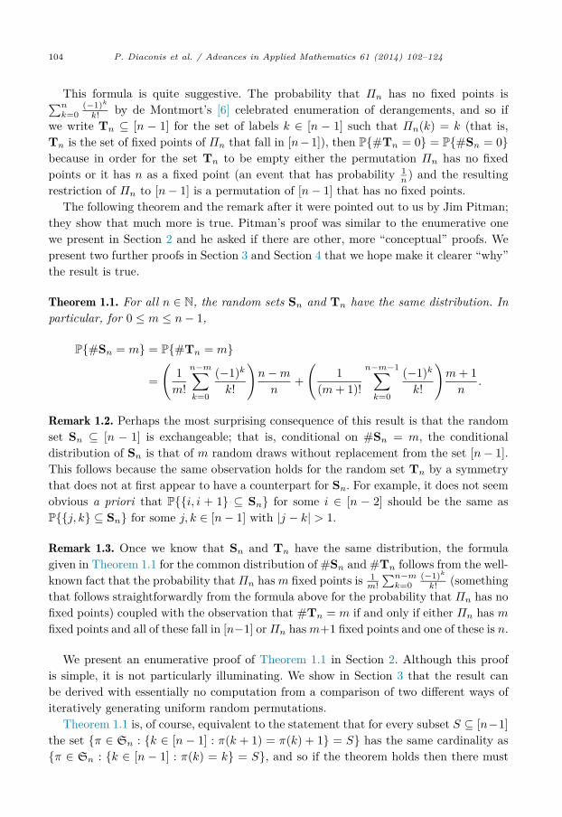
104 P. Diaconis et al. / Advances in Applied Mathematics 61 (2014) 102–124
This formula is quite suggestive. The probability that Πn has no fixed points is ∑nk=0
(−1)kk! by de Montmort’s [6] celebrated enumeration of derangements, and so if
we write Tn ⊆ [n − 1] for the set of labels k ∈ [n − 1] such that Πn(k) = k (that is, Tn is the set of fixed points of Πn that fall in [n −1]), then P{#Tn = 0} = P{#Sn = 0}because in order for the set Tn to be empty either the permutation Πn has no fixed points or it has n as a fixed point (an event that has probability 1
n ) and the resulting restriction of Πn to [n − 1] is a permutation of [n − 1] that has no fixed points.
The following theorem and the remark after it were pointed out to us by Jim Pitman; they show that much more is true. Pitman’s proof was similar to the enumerative one we present in Section 2 and he asked if there are other, more “conceptual” proofs. We present two further proofs in Section 3 and Section 4 that we hope make it clearer “why” the result is true.
Theorem 1.1. For all n ∈ N, the random sets Sn and Tn have the same distribution. In particular, for 0 ≤ m ≤ n − 1,
P{#Sn = m} = P{#Tn = m}
=(
1m!
n−m∑k=0
(−1)k
k!
)n−m
n+
(1
(m + 1)!
n−m−1∑k=0
(−1)k
k!
)m + 1n
.
Remark 1.2. Perhaps the most surprising consequence of this result is that the random set Sn ⊆ [n − 1] is exchangeable; that is, conditional on #Sn = m, the conditional distribution of Sn is that of m random draws without replacement from the set [n − 1]. This follows because the same observation holds for the random set Tn by a symmetry that does not at first appear to have a counterpart for Sn. For example, it does not seem obvious a priori that P{{i, i + 1} ⊆ Sn} for some i ∈ [n − 2] should be the same as P{{j, k} ⊆ Sn} for some j, k ∈ [n − 1] with |j − k| > 1.
Remark 1.3. Once we know that Sn and Tn have the same distribution, the formula given in Theorem 1.1 for the common distribution of #Sn and #Tn follows from the well-known fact that the probability that Πn has m fixed points is 1
m!∑n−m
k=0(−1)k
k! (something that follows straightforwardly from the formula above for the probability that Πn has no fixed points) coupled with the observation that #Tn = m if and only if either Πn has mfixed points and all of these fall in [n −1] or Πn has m +1 fixed points and one of these is n.
We present an enumerative proof of Theorem 1.1 in Section 2. Although this proof is simple, it is not particularly illuminating. We show in Section 3 that the result can be derived with essentially no computation from a comparison of two different ways of iteratively generating uniform random permutations.
Theorem 1.1 is, of course, equivalent to the statement that for every subset S ⊆ [n −1]the set {π ∈ Sn : {k ∈ [n − 1] : π(k + 1) = π(k) + 1} = S} has the same cardinality as {π ∈ Sn : {k ∈ [n − 1] : π(k) = k} = S}, and so if the theorem holds then there must
P. Diaconis et al. / Advances in Applied Mathematics 61 (2014) 102–124 105
exist a bijection H : Sn → Sn such that {k ∈ [n − 1] : π(k + 1) = π(k) + 1} = {k ∈[n − 1] : Hπ(k) = k}. Conversely, exhibiting such a bijection proves the theorem, and we present a natural construction of one in Section 4.
The analogue of Sn for circular permutations is the random set consisting of those k ∈ [n] such that Π(k+ 1 mod n) = Π(k) + 1 mod n. We obtain the distribution of this random set via an enumeration in Section 5 and then present some bijective proofs of facts suggested by the enumerative results.
Note that the latter random set is just the set of fixed points of the commutator [ρ, Π], where ρ is the n-cycle (1, 2, . . . , n). In Section 6 we show for a general permutation ηthat, under weak conditions on the number of fixed points and 2-cycles of η, the total variation distance between the distribution of the number of fixed points of [η, Π] and a Poisson distribution with expected value 1 is small when n is large.
Remark 1.4. It is clear from Theorem 1.1 that the common distribution of #Sn and #Tn
is approximately Poisson with expected value 1 when n is large. Write Fn := {k ∈ [n] :Πn(k) = k} for the set of fixed points of the uniform random permutation Πn and Q for the Poisson probability distribution with expected value 1. It is well-known that the total variation distance between the distribution of #Fn and Q is amazingly small:
dTV(P{#Fn ∈ ·},Q
)≤ 2n
n! ,
and so it is natural to ask whether the common distribution of #Sn and #Tn is similarly close to Q. Because P{#Tn �= #Fn} = 1
n , we might suspect that the total variation distance between the distributions of #Tn and #Fn is on the order of 1
n , and so the total variation distance between the distribution of #Sn and Q is also of that order. Indeed, it follows from (1.1) that
P{#Sn = 0} = P{#Fn = 0} + 1n
n−1∑k=0
(−1)k
k!
≥ Q{0} − 2n
n! + 1n
n−1∑k=0
(−1)k
k! ,
and so
dTV(P{#Sn ∈ ·},Q
)≥ e−1
n+ o
(1n
).
2. An enumerative proof
Our first approach to proving Theorem 1.1 is to compute #{π ∈ Sn : π(ki + 1) =π(ki) + 1, 1 ≤ i ≤ m} for a subset {k1, . . . , km} ⊆ [n − 1] and show that this number is (n −m)! = #{π ∈ Sn : π(ki) = ki, 1 ≤ i ≤ m}. This establishes that
106 P. Diaconis et al. / Advances in Applied Mathematics 61 (2014) 102–124
P{{k1, . . . , km} ⊆ Sn
}= P
{{k1, . . . , km} ⊆ Tn
},
and an inclusion–exclusion argument completes the proof.We begin by noting that we can build up a permutation of [n] by first taking the
elements of [n] in any order and then imagining that we lay elements down successively so that the hth element goes in one of the h “slots” defined by the h − 1 elements that have already been laid down, that is, the slot before the first element, the slot after the last element, or one of the h − 2 slots between elements.
Consider first the set {π ∈ Sn : π(k + 1) = π(k) + 1} for some fixed k ∈ [n − 1]. We can count this set by imagining that we first put down k and k+1 next to each other in that order and then successively lay down the remaining elements [n] \ {k, k+1} in such a way that no element is ever laid down in the slot between k and k + 1. It follows that
#{π ∈ Sn : π(k + 1) = π(k) + 1
}= 2 × 3 × · · · × (n− 1) = (n− 1)!,
as required.Now consider the set {π ∈ Sn : π(k + 1) = π(k) + 1 and π(k + 2) = π(k + 1) + 1}
for some fixed k ∈ [n − 2]. We can count this set by imagining that we first put down k, k + 1 and k + 2 next to each other in that order and then successively lay down the remaining elements [n] \ {k, k+1, k+2} in such a way that no element is ever laid down in the slot between k and k+ 1 or the slot between k+ 1 and k+ 2. The number of such permutations is thus 2 ×3 ×· · ·×(n −2) = (n −2)!, again as required. On the other hand, suppose we fix k, � ∈ [n − 1] with |j − k| > 1 and consider the set {π ∈ Sn : π(k + 1) =π(k) + 1 and π(� + 1) = π(�) + 1}. We imagine that we first put down k and k + 1 next to each other in that order and then � and � + 1 next to each other in that order either before or after the pair k and k+1. There are two ways to do this. Then we successively lay down the remaining elements [n] \ {k, k+1, �, � +1} in such a way that no element is ever laid down in the slot between k and k+1 or the slot between � and � +1. There are 3 ×4 ×· · ·×(n −2) ways to do this second part of the construction, and so the number of permutations we are considering is 2 ×3 ×4 ×· · ·×(n −2) = (n −2)!, once again as required.
It is clear how this argument generalizes. Suppose we have a subset {k1, . . . , km} ⊆[n − 1] and we wish to compute #{π ∈ Sn : π(ki + 1) = π(ki), 1 ≤ i ≤ m}. We can break {k1, . . . , km} up into r “blocks” of consecutive labels for some r. There are r! ways to lay down the blocks and then (r + 1) × (r + 2) × · · · × (n − m) ways of laying down the remaining labels [n] \ {k1, . . . , km} so that no label is inserted into a slot within one of the blocks. Thus, the cardinality we wish to compute is indeed r! × (r + 1) × (r + 2) × · · · × (n −m) = (n −m)!.
3. A Markov chain proof
The following proof proceeds by first showing that the random set Sn is exchangeable and then establishing that the distribution of #Sn is the same as the distribution of #Tn without explicitly calculating either distribution.
P. Diaconis et al. / Advances in Applied Mathematics 61 (2014) 102–124 107
Suppose that we build the uniform random permutations Π1, Π2, . . . sequentially in the following manner: Πn+1 is obtained from Πn by inserting n +1 uniformly at random into one of the n + 1 “slots” defined by the ordered list Πn (i.e. as in Section 2, we have slots before and after the first and last elements of the list and n − 1 slots between successive elements). The choice of slot is independent of Fn, where Fn is the σ-field generated by Π1, . . . , Πn.
It is clear that the set-valued stochastic process (Sn)n∈N is Markovian with respect to the filtration (Fn)n∈N. In fact, if we write Sn = {Xn
1 , . . . , XnMn
}, then
P{Sn+1 =
{Xn
1 , . . . , XnMn
}\{Xn
i
} ∣∣ Fn
}= 1
n + 1 , 1 ≤ i ≤ Mn,
corresponding to n + 1 being inserted in the slot between the successive elements Xni
and Xni + 1 in the list,
P{Sn+1 =
{Xn
1 , . . . , XnMn
}∪ {n}
∣∣ Fn
}= 1
n + 1 ,
corresponding to n + 1 being inserted in the slot to the right of n, and
P{Sn+1 =
{Xn
1 , . . . , XnMn
} ∣∣ Fn
}= (n + 1) −Mn − 1
n + 1 .
Moreover, it is obvious from the symmetry inherent in these transition probabilities and induction that Sn is an exchangeable random subset of [n − 1] for all n. Furthermore, the nonnegative integer valued process (Mn)n∈N = (#Sn)n∈N is also Markovian with respect to the filtration (Fn)n∈N with the following transition probabilities:
P{Mn+1 = Mn − 1 | Fn} = Mn
n + 1 ,
P{Mn+1 = Mn | Fn} = (n + 1) −Mn − 1n + 1 ,
and
P{Mn+1 = Mn + 1 | Fn} = 1n + 1 .
Because the conditional distribution of Sn given #Sn = m is, by exchangeability, the same as that of Tn given #Tn = m for 0 ≤ m ≤ n − 1, it will suffice to show that the distribution of #Sn is the same as that of #Tn. Moreover, because #Tn has the same distribution as #{2 ≤ k ≤ n : Πn(k) = k} for all n ∈ N and #S1 = #T1 = 0, it will certainly be enough to build another sequence (Σn)n∈N such that
• Σn is a uniform random permutation of [n] for all n ∈ N,• (Σn)n∈N is Markovian with respect to some filtration (Gn)n∈N,
108 P. Diaconis et al. / Advances in Applied Mathematics 61 (2014) 102–124
• (Nn)n∈N := (#{2 ≤ k ≤ n : Σn(k) = k})n∈N is also Markovian with respect to the filtration (Gn)n∈N with the following transition probabilities
P{Nn+1 = Nn − 1 | Gn} = Nn
n + 1 ,
P{Nn+1 = Nn | Gn} = (n + 1) −Nn − 1n + 1 ,
and
P{Nn+1 = Nn + 1 | Gn} = 1n + 1 .
We recall the simplest instance of the Chinese restaurant process that iteratively generates uniform random permutations (see, for example, [13]). Individuals labeled 1, 2, . . . successively enter a restaurant equipped with an infinite number of round tables. Individual 1 sits at some table. Suppose that after the first n − 1 individuals have entered the restaurant we have a configuration of individuals sitting around some number of tables. When individual n enters the restaurant he is equally likely to sit to the immediate left of one of the individuals already present or to sit at an unoccupied table. The permutation Σn is defined in terms of the resulting seating configuration by setting Σn(i) = j, i �= j, if individual j is sitting immediately to the left of individual iand Σn(i) = i if individual i is sitting by himself at some table. Each occupied table corresponds to a cycle of Σn and, in particular, tables with a single occupant correspond to fixed points of Σn.
It is clear that if we let Gn be the σ-field generated by Σ1, . . . , Σn, then all of the requirements listed above for (Σn)n∈N and (Nn)n∈N are met.
4. A bijective proof
As we remarked in the introduction, in order to prove Theorem 1.1 it suffices to find a bijection H : Sn → Sn such that {k ∈ [n − 1] : π(k + 1) = π(k) + 1} = {k ∈ [n − 1] :Hπ(k) = k} for all π ∈ Sn.
Not only will we find such a bijection, but we will prove an even more general result that requires we first set up some notation. Fix 1 ≤ h < n. Let ρ ∈ Sn be the permutation that maps i ∈ [n] to i +h mod n ∈ [n]. Next define the following bijection of Sn to itself that is essentially the transformation fondamentale of [8, Section 1.3] (such bijections seem to have been first introduced implicitly in [14, Chapter 8]). Take a permutation πand write it in cycle form (a1, a2, . . . , ar)(b1, b2, . . . , bs) · · · (c1, c2, . . . , ct), where in each cycle the leading element is the least element of the cycle and these leading elements form a decreasing sequence. That is, a1 > b1 > · · · > c1. Next, remove the parentheses to form an ordered listing (a1, a2, . . . , ar, b1, b2, . . . , bs, c1, c2, . . . , ct) of [n] and define π̂ ∈ Sn by taking (π̂(1), ̂π(2), . . . , ̂π(n)) to be this ordered listing.
The following result for h = 1 provides a bijection that establishes Theorem 1.1.
P. Diaconis et al. / Advances in Applied Mathematics 61 (2014) 102–124 109
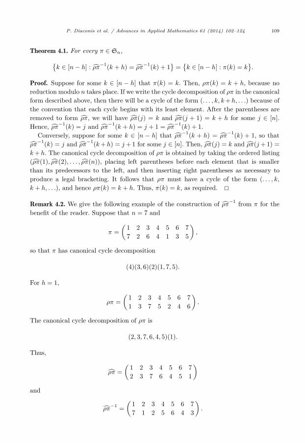
Theorem 4.1. For every π ∈ Sn,{k ∈ [n− h] : ρ̂π−1(k + h) = ρ̂π
−1(k) + 1}
={k ∈ [n− h] : π(k) = k
}.
Proof. Suppose for some k ∈ [n − h] that π(k) = k. Then, ρπ(k) = k + h, because no reduction modulo n takes place. If we write the cycle decomposition of ρπ in the canonical form described above, then there will be a cycle of the form (. . . , k, k+h, . . .) because of the convention that each cycle begins with its least element. After the parentheses are removed to form ρ̂π, we will have ρ̂π(j) = k and ρ̂π(j + 1) = k + h for some j ∈ [n]. Hence, ρ̂π−1(k) = j and ρ̂π−1(k + h) = j + 1 = ρ̂π
−1(k) + 1.Conversely, suppose for some k ∈ [n − h] that ρ̂π−1(k + h) = ρ̂π
−1(k) + 1, so that ρ̂π
−1(k) = j and ρ̂π−1(k+h) = j +1 for some j ∈ [n]. Then, ρ̂π(j) = k and ρ̂π(j +1) =k+ h. The canonical cycle decomposition of ρπ is obtained by taking the ordered listing (ρ̂π(1), ̂ρπ(2), . . . , ̂ρπ(n)), placing left parentheses before each element that is smaller than its predecessors to the left, and then inserting right parentheses as necessary to produce a legal bracketing. It follows that ρπ must have a cycle of the form (. . . , k,k + h, . . .), and hence ρπ(k) = k + h. Thus, π(k) = k, as required. �Remark 4.2. We give the following example of the construction of ρ̂π−1 from π for the benefit of the reader. Suppose that n = 7 and
π =(
1 2 3 4 5 6 77 2 6 4 1 3 5
),
so that π has canonical cycle decomposition
(4)(3, 6)(2)(1, 7, 5).
For h = 1,
ρπ =(
1 2 3 4 5 6 71 3 7 5 2 4 6
).
The canonical cycle decomposition of ρπ is
(2, 3, 7, 6, 4, 5)(1).
Thus,
ρ̂π =(
1 2 3 4 5 6 72 3 7 6 4 5 1
)and
ρ̂π−1 =
(1 2 3 4 5 6 7
).
7 1 2 5 6 4 3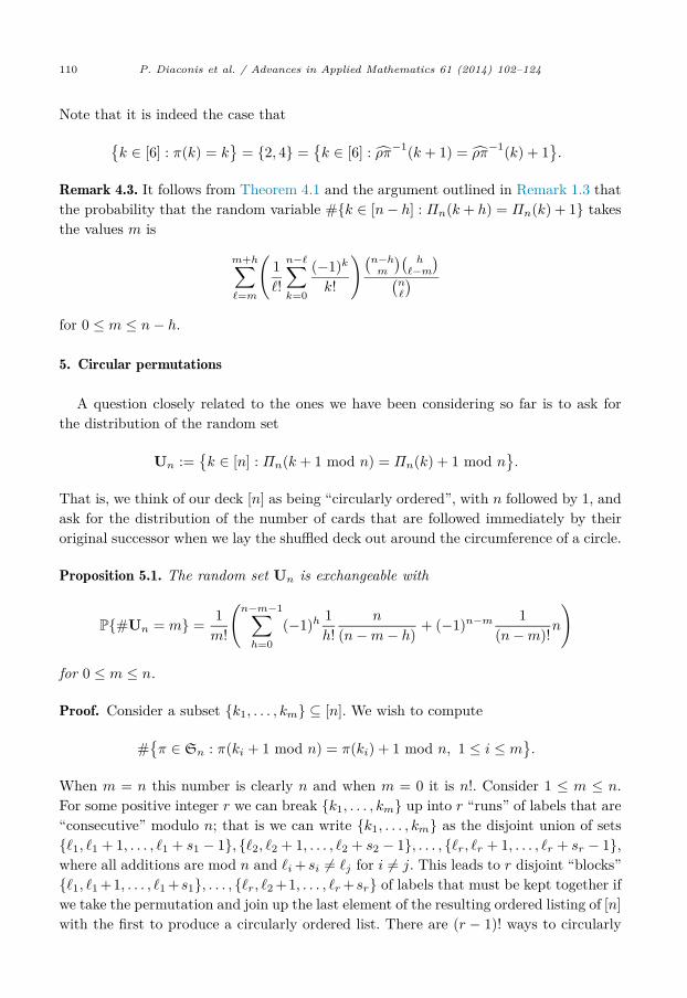
110 P. Diaconis et al. / Advances in Applied Mathematics 61 (2014) 102–124
Note that it is indeed the case that{k ∈ [6] : π(k) = k
}= {2, 4} =
{k ∈ [6] : ρ̂π−1(k + 1) = ρ̂π
−1(k) + 1}.
Remark 4.3. It follows from Theorem 4.1 and the argument outlined in Remark 1.3 that the probability that the random variable #{k ∈ [n − h] : Πn(k + h) = Πn(k) + 1} takes the values m is
m+h∑�=m
(1�!
n−�∑k=0
(−1)k
k!
)(n−hm
)(h
�−m
)(n�
)for 0 ≤ m ≤ n − h.
5. Circular permutations
A question closely related to the ones we have been considering so far is to ask for the distribution of the random set
Un :={k ∈ [n] : Πn(k + 1 mod n) = Πn(k) + 1 mod n
}.
That is, we think of our deck [n] as being “circularly ordered”, with n followed by 1, and ask for the distribution of the number of cards that are followed immediately by their original successor when we lay the shuffled deck out around the circumference of a circle.
Proposition 5.1. The random set Un is exchangeable with
P{#Un = m} = 1m!
(n−m−1∑h=0
(−1)h 1h!
n
(n−m− h) + (−1)n−m 1(n−m)!n
)
for 0 ≤ m ≤ n.
Proof. Consider a subset {k1, . . . , km} ⊆ [n]. We wish to compute
#{π ∈ Sn : π(ki + 1 mod n) = π(ki) + 1 mod n, 1 ≤ i ≤ m
}.
When m = n this number is clearly n and when m = 0 it is n!. Consider 1 ≤ m ≤ n. For some positive integer r we can break {k1, . . . , km} up into r “runs” of labels that are “consecutive” modulo n; that is we can write {k1, . . . , km} as the disjoint union of sets {�1, �1 + 1, . . . , �1 + s1 − 1}, {�2, �2 + 1, . . . , �2 + s2 − 1}, . . . , {�r, �r + 1, . . . , �r + sr − 1}, where all additions are mod n and �i + si �= �j for i �= j. This leads to r disjoint “blocks” {�1, �1 +1, . . . , �1 +s1}, . . . , {�r, �2 +1, . . . , �r +sr} of labels that must be kept together if we take the permutation and join up the last element of the resulting ordered listing of [n]with the first to produce a circularly ordered list. There are (r − 1)! ways to circularly
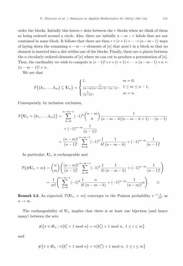
P. Diaconis et al. / Advances in Applied Mathematics 61 (2014) 102–124 111
order the blocks. Initially this leaves r slots between the r blocks when we think of them as being ordered around a circle. Also, there are initially n −m − r labels that are not contained in some block. It follows that there are then r× (r+1) ×· · ·× (n −m −1) ways of laying down the remaining n −m − r elements of [n] that aren’t in a block so that no element is inserted into a slot within one of the blocks. Finally, there are n places between the n circularly ordered elements of [n] where we can cut to produce a permutation of [n]. Thus, the cardinality we wish to compute is (r−1)! ×r× (r+1) ×· · ·× (n −m −1) ×n =(n −m − 1)! × n.
We see that
P{{k1, . . . , km} ⊆ Un
}=
⎧⎪⎨⎪⎩1, m = 0,
1(n−m)(n−m+1)···(n−1) , 1 ≤ m ≤ n− 1,
1(n−1)! , m = n.
Consequently, by inclusion–exclusion,
P{Un = {k1, . . . , km}
}=
n−m−1∑h=0
(−1)h(n−m
h
)1
(n−m− h)(n−m− h + 1) · · · (n− 1)
+ (−1)n−m 1(n− 1)!
= (n−m)!(n− 1)!
n−m−1∑h=0
(−1)h 1h!
1(n−m− h) + (−1)n−m 1
(n− 1)!
In particular, Un is exchangeable and
P{#Un = m} =(n
m
)((n−m)!(n− 1)!
n−m−1∑h=0
(−1)h 1h!
1(n−m− h) + (−1)n−m 1
(n− 1)!
)
= 1m!
(n−m−1∑h=0
(−1)h 1h!
n
(n−m− h) + (−1)n−m 1(n−m)!n
). �
Remark 5.2. As expected, P{Un = m} converges to the Poisson probability e−1 1m! as
n → ∞.
The exchangeability of Un implies that there is at least one bijection (and hence many) between the sets
#{π ∈ Sn : π
(k′i + 1 mod n
)= π
(k′i)
+ 1 mod n, 1 ≤ i ≤ m}
and
#{π ∈ Sn : π
(k′′i + 1 mod n
)= π
(k′′i
)+ 1 mod n, 1 ≤ i ≤ m
}
112 P. Diaconis et al. / Advances in Applied Mathematics 61 (2014) 102–124
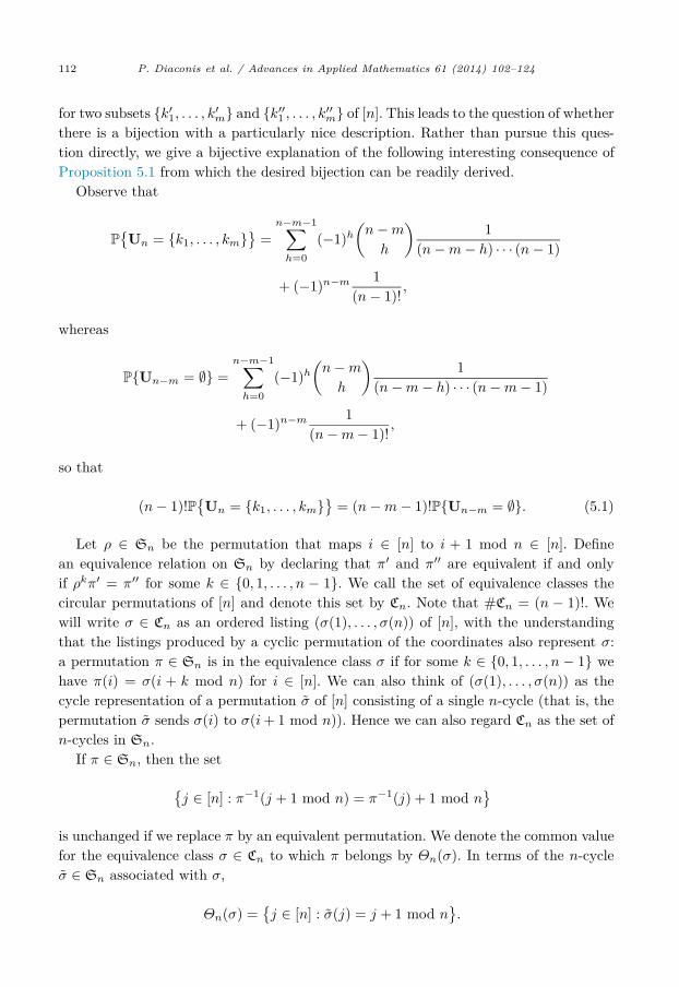
for two subsets {k′1, . . . , k′m} and {k′′1 , . . . , k′′m} of [n]. This leads to the question of whether there is a bijection with a particularly nice description. Rather than pursue this ques-tion directly, we give a bijective explanation of the following interesting consequence of Proposition 5.1 from which the desired bijection can be readily derived.
Observe that
P{Un = {k1, . . . , km}
}=
n−m−1∑h=0
(−1)h(n−m
h
)1
(n−m− h) · · · (n− 1)
+ (−1)n−m 1(n− 1)! ,
whereas
P{Un−m = ∅} =n−m−1∑h=0
(−1)h(n−m
h
)1
(n−m− h) · · · (n−m− 1)
+ (−1)n−m 1(n−m− 1)! ,
so that
(n− 1)!P{Un = {k1, . . . , km}
}= (n−m− 1)!P{Un−m = ∅}. (5.1)
Let ρ ∈ Sn be the permutation that maps i ∈ [n] to i + 1 mod n ∈ [n]. Define an equivalence relation on Sn by declaring that π′ and π′′ are equivalent if and only if ρkπ′ = π′′ for some k ∈ {0, 1, . . . , n − 1}. We call the set of equivalence classes the circular permutations of [n] and denote this set by Cn. Note that #Cn = (n − 1)!. We will write σ ∈ Cn as an ordered listing (σ(1), . . . , σ(n)) of [n], with the understanding that the listings produced by a cyclic permutation of the coordinates also represent σ: a permutation π ∈ Sn is in the equivalence class σ if for some k ∈ {0, 1, . . . , n − 1} we have π(i) = σ(i + k mod n) for i ∈ [n]. We can also think of (σ(1), . . . , σ(n)) as the cycle representation of a permutation σ̃ of [n] consisting of a single n-cycle (that is, the permutation σ̃ sends σ(i) to σ(i + 1 mod n)). Hence we can also regard Cn as the set of n-cycles in Sn.
If π ∈ Sn, then the set
{j ∈ [n] : π−1(j + 1 mod n) = π−1(j) + 1 mod n
}is unchanged if we replace π by an equivalent permutation. We denote the common value for the equivalence class σ ∈ Cn to which π belongs by Θn(σ). In terms of the n-cycle σ̃ ∈ Sn associated with σ,
Θn(σ) ={j ∈ [n] : σ̃(j) = j + 1 mod n
}.
P. Diaconis et al. / Advances in Applied Mathematics 61 (2014) 102–124 113
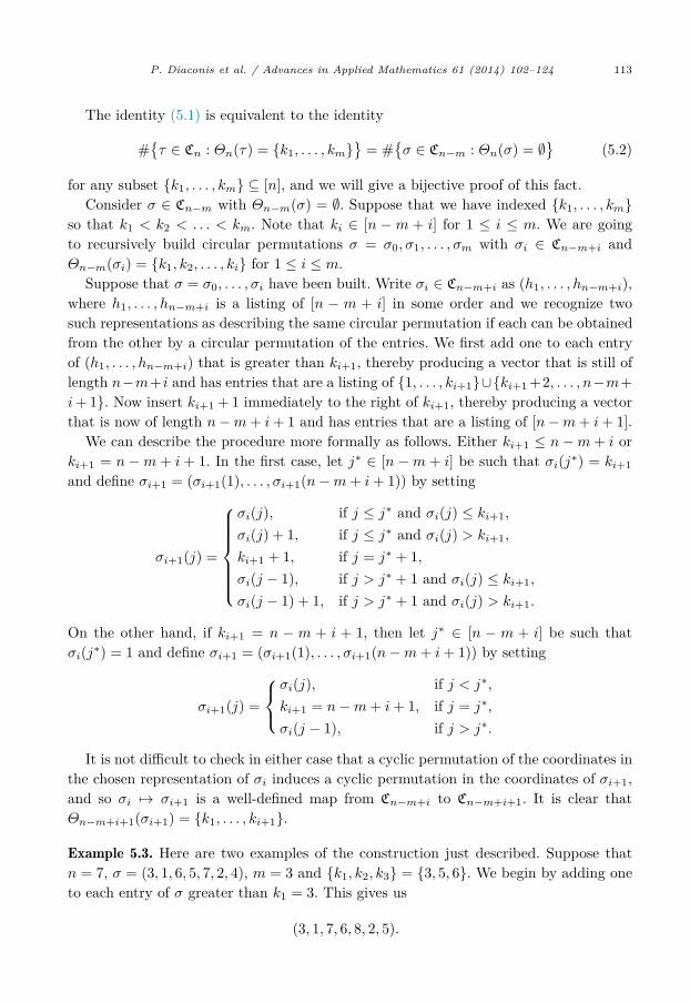
The identity (5.1) is equivalent to the identity
#{τ ∈ Cn : Θn(τ) = {k1, . . . , km}
}= #
{σ ∈ Cn−m : Θn(σ) = ∅
}(5.2)
for any subset {k1, . . . , km} ⊆ [n], and we will give a bijective proof of this fact.Consider σ ∈ Cn−m with Θn−m(σ) = ∅. Suppose that we have indexed {k1, . . . , km}
so that k1 < k2 < . . . < km. Note that ki ∈ [n − m + i] for 1 ≤ i ≤ m. We are going to recursively build circular permutations σ = σ0, σ1, . . . , σm with σi ∈ Cn−m+i and Θn−m(σi) = {k1, k2, . . . , ki} for 1 ≤ i ≤ m.
Suppose that σ = σ0, . . . , σi have been built. Write σi ∈ Cn−m+i as (h1, . . . , hn−m+i), where h1, . . . , hn−m+i is a listing of [n − m + i] in some order and we recognize two such representations as describing the same circular permutation if each can be obtained from the other by a circular permutation of the entries. We first add one to each entry of (h1, . . . , hn−m+i) that is greater than ki+1, thereby producing a vector that is still of length n −m + i and has entries that are a listing of {1, . . . , ki+1} ∪{ki+1 +2, . . . , n −m +i + 1}. Now insert ki+1 + 1 immediately to the right of ki+1, thereby producing a vector that is now of length n −m + i + 1 and has entries that are a listing of [n −m + i + 1].
We can describe the procedure more formally as follows. Either ki+1 ≤ n −m + i or ki+1 = n −m + i + 1. In the first case, let j∗ ∈ [n −m + i] be such that σi(j∗) = ki+1and define σi+1 = (σi+1(1), . . . , σi+1(n −m + i + 1)) by setting
σi+1(j) =
⎧⎪⎪⎪⎪⎪⎨⎪⎪⎪⎪⎪⎩
σi(j), if j ≤ j∗ and σi(j) ≤ ki+1,
σi(j) + 1, if j ≤ j∗ and σi(j) > ki+1,
ki+1 + 1, if j = j∗ + 1,σi(j − 1), if j > j∗ + 1 and σi(j) ≤ ki+1,
σi(j − 1) + 1, if j > j∗ + 1 and σi(j) > ki+1.
On the other hand, if ki+1 = n − m + i + 1, then let j∗ ∈ [n − m + i] be such that σi(j∗) = 1 and define σi+1 = (σi+1(1), . . . , σi+1(n −m + i + 1)) by setting
σi+1(j) =
⎧⎨⎩σi(j), if j < j∗,
ki+1 = n−m + i + 1, if j = j∗,
σi(j − 1), if j > j∗.
It is not difficult to check in either case that a cyclic permutation of the coordinates in the chosen representation of σi induces a cyclic permutation in the coordinates of σi+1, and so σi �→ σi+1 is a well-defined map from Cn−m+i to Cn−m+i+1. It is clear that Θn−m+i+1(σi+1) = {k1, . . . , ki+1}.
Example 5.3. Here are two examples of the construction just described. Suppose that n = 7, σ = (3, 1, 6, 5, 7, 2, 4), m = 3 and {k1, k2, k3} = {3, 5, 6}. We begin by adding one to each entry of σ greater than k1 = 3. This gives us
(3, 1, 7, 6, 8, 2, 5).
114 P. Diaconis et al. / Advances in Applied Mathematics 61 (2014) 102–124
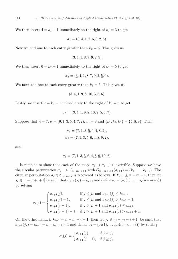
We then insert 4 = k1 + 1 immediately to the right of k1 = 3 to get
σ1 = (3, 4, 1, 7, 6, 8, 2, 5).
Now we add one to each entry greater than k2 = 5. This gives us
(3, 4, 1, 8, 7, 9, 2, 5).
We then insert 6 = k2 + 1 immediately to the right of k2 = 5 to get
σ2 = (3, 4, 1, 8, 7, 9, 2, 5, 6).
We next add one to each entry greater than k3 = 6. This gives us
(3, 4, 1, 9, 8, 10, 3, 5, 6).
Lastly, we insert 7 = k3 + 1 immediately to the right of k3 = 6 to get
σ3 = (3, 4, 1, 9, 8, 10, 2, 5, 6, 7).
Suppose that n = 7, σ = (6, 1, 3, 5, 4, 7, 2), m = 3 and {k1, k2, k3} = {5, 8, 9}. Then,
σ1 = (7, 1, 3, 5, 6, 4, 8, 2),
σ2 = (7, 1, 3, 5, 6, 4, 8, 9, 2),
and
σ3 = (7, 1, 3, 5, 6, 4, 8, 9, 10, 2).
It remains to show that each of the maps σi �→ σi+1 is invertible. Suppose we have the circular permutation σi+1 ∈ Cn−m+i+1 with Θn−m+i+1(σi+1) = {k1, . . . , ki+1}. The circular permutation σi ∈ Cn−m+i is recovered as follows. If ki+1 ≤ n −m + i, then let j∗ ∈ [n −m +i +1] be such that σi+1(j∗) = ki+1 and define σi = (σi(1), . . . , σi(n −m +i))by setting
σi(j) =
⎧⎪⎪⎪⎨⎪⎪⎪⎩σi+1(j), if j ≤ j∗ and σi+1(j) ≤ ki+1,
σi+1(j) − 1, if j ≤ j∗ and σi+1(j) > ki+1 + 1,σi+1(j + 1), if j > j∗ + 1 and σi+1(j) ≤ ki+1,
σi+1(j + 1) − 1, if j > j∗ + 1 and σi+1(j) > ki+1 + 1.
On the other hand, if ki+1 = n −m + i + 1, then let j∗ ∈ [n −m + i + 1] be such that σi+1(j∗) = ki+1 = n −m + i + 1 and define σi = (σi(1), . . . , σi(n −m + i)) by setting
σi(j) ={σi+1(j), if j < j∗,
σi+1(j + 1), if j ≥ j∗.
P. Diaconis et al. / Advances in Applied Mathematics 61 (2014) 102–124 115
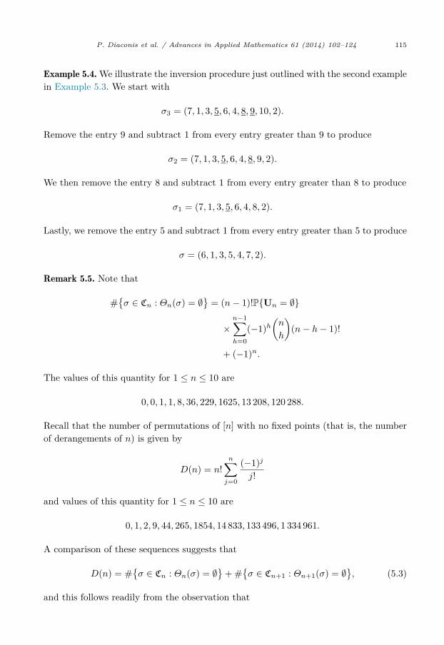
Example 5.4. We illustrate the inversion procedure just outlined with the second example in Example 5.3. We start with
σ3 = (7, 1, 3, 5, 6, 4, 8, 9, 10, 2).
Remove the entry 9 and subtract 1 from every entry greater than 9 to produce
σ2 = (7, 1, 3, 5, 6, 4, 8, 9, 2).
We then remove the entry 8 and subtract 1 from every entry greater than 8 to produce
σ1 = (7, 1, 3, 5, 6, 4, 8, 2).
Lastly, we remove the entry 5 and subtract 1 from every entry greater than 5 to produce
σ = (6, 1, 3, 5, 4, 7, 2).
Remark 5.5. Note that
#{σ ∈ Cn : Θn(σ) = ∅
}= (n− 1)!P{Un = ∅}
×n−1∑h=0
(−1)h(n
h
)(n− h− 1)!
+ (−1)n.
The values of this quantity for 1 ≤ n ≤ 10 are
0, 0, 1, 1, 8, 36, 229, 1625, 13 208, 120 288.
Recall that the number of permutations of [n] with no fixed points (that is, the number of derangements of n) is given by
D(n) = n!n∑
j=0
(−1)j
j!
and values of this quantity for 1 ≤ n ≤ 10 are
0, 1, 2, 9, 44, 265, 1854, 14 833, 133 496, 1 334 961.
A comparison of these sequences suggests that
D(n) = #{σ ∈ Cn : Θn(σ) = ∅
}+ #
{σ ∈ Cn+1 : Θn+1(σ) = ∅
}, (5.3)
and this follows readily from the observation that
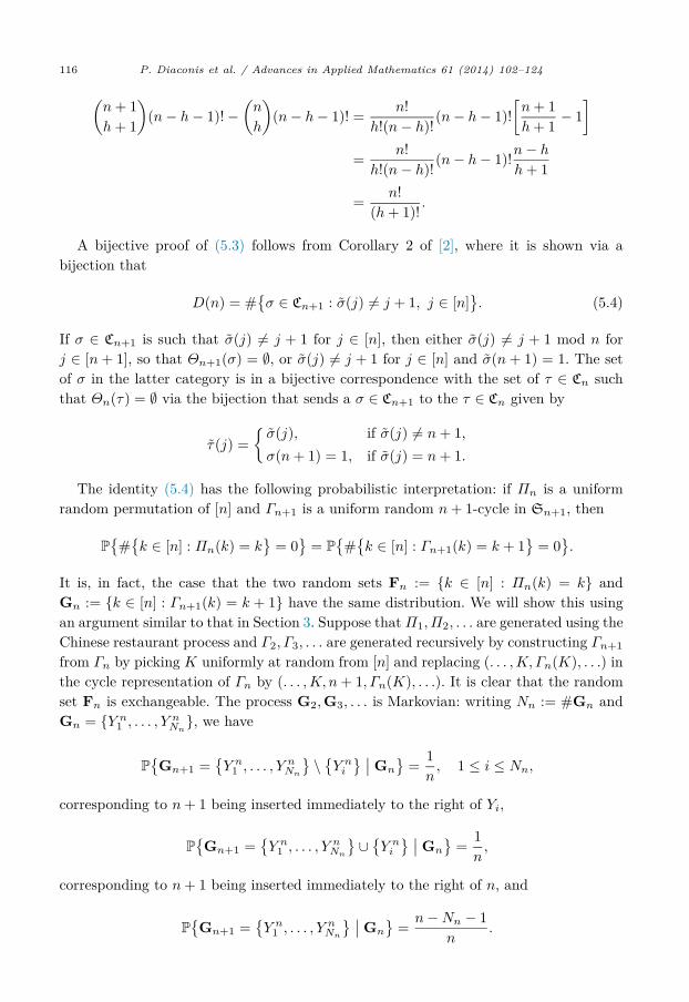
116 P. Diaconis et al. / Advances in Applied Mathematics 61 (2014) 102–124
(n + 1h + 1)(n− h− 1)! −
(n
h
)(n− h− 1)! = n!
h!(n− h)!(n− h− 1)!
[n + 1h + 1
− 1]
= n!h!(n− h)! (n− h− 1)!n− h
h + 1
= n!(h + 1)! .
A bijective proof of (5.3) follows from Corollary 2 of [2], where it is shown via a bijection that
D(n) = #{σ ∈ Cn+1 : σ̃(j) �= j + 1, j ∈ [n]
}. (5.4)
If σ ∈ Cn+1 is such that σ̃(j) �= j + 1 for j ∈ [n], then either σ̃(j) �= j + 1 mod n for j ∈ [n + 1], so that Θn+1(σ) = ∅, or σ̃(j) �= j + 1 for j ∈ [n] and σ̃(n + 1) = 1. The set of σ in the latter category is in a bijective correspondence with the set of τ ∈ Cn such that Θn(τ) = ∅ via the bijection that sends a σ ∈ Cn+1 to the τ ∈ Cn given by
τ̃(j) ={σ̃(j), if σ̃(j) �= n + 1,σ(n + 1) = 1, if σ̃(j) = n + 1.
The identity (5.4) has the following probabilistic interpretation: if Πn is a uniform random permutation of [n] and Γn+1 is a uniform random n + 1-cycle in Sn+1, then
P{#{k ∈ [n] : Πn(k) = k
}= 0
}= P
{#{k ∈ [n] : Γn+1(k) = k + 1
}= 0
}.
It is, in fact, the case that the two random sets Fn := {k ∈ [n] : Πn(k) = k} and Gn := {k ∈ [n] : Γn+1(k) = k + 1} have the same distribution. We will show this using an argument similar to that in Section 3. Suppose that Π1, Π2, . . . are generated using the Chinese restaurant process and Γ2, Γ3, . . . are generated recursively by constructing Γn+1from Γn by picking K uniformly at random from [n] and replacing (. . . , K,Γn(K), . . .) in the cycle representation of Γn by (. . . , K, n + 1, Γn(K), . . .). It is clear that the random set Fn is exchangeable. The process G2, G3, . . . is Markovian: writing Nn := #Gn and Gn = {Y n
1 , . . . , Y nNn
}, we have
P{Gn+1 =
{Y n
1 , . . . , Y nNn
}\{Y ni
} ∣∣ Gn
}= 1
n, 1 ≤ i ≤ Nn,
corresponding to n + 1 being inserted immediately to the right of Yi,
P{Gn+1 =
{Y n
1 , . . . , Y nNn
}∪{Y ni
} ∣∣ Gn
}= 1
n,
corresponding to n + 1 being inserted immediately to the right of n, and
P{Gn+1 =
{Y n
1 , . . . , Y nN
} ∣∣ Gn
}= n−Nn − 1
.
n n
P. Diaconis et al. / Advances in Applied Mathematics 61 (2014) 102–124 117
It is obvious from the symmetry inherent in these transition probabilities and induction that Gn is an exchangeable random subset of [n] for all n. It therefore suffices to show that Nn+1 has the same distribution as Mn := #Fn. Observe that M1 = N2 = 1. It is clear that N2, N3, . . . is a Markov chain with the following transition probabilities
P{Nn+1 = Nn − 1 | Nn} = Nn
n,
P{Nn+1 = Nn | Nn} = n−Nn − 1n
,
and
P{Nn+1 = Nn + 1 | Nn} = 1n.
It follows from the Chinese restaurant construction that
P{Mn+1 = Mn − 1 | Mn} = Mn
n + 1 ,
P{Mn+1 = Mn | Mn} = (n + 1) −Mn − 1n + 1 ,
and
P{Mn+1 = Mn + 1 | Mn} = 1n + 1 ,
and so Mn and Nn+1 do indeed have the same distribution for all n.
6. Random commutators
If we write ρ for the permutation of [n] given by ρ(i) = i +1 mod n, then the random set Un of Section 5 is nothing other than{
i ∈ [n] : ρΠn(i) = Πnρ(i)}
or, equivalently, the set {i ∈ [n] : ρ−1Π−1
n ρΠn(i) = i}.
This is just the set of fixed points of the commutator [ρ, Πn] = ρ−1Π−1n ρΠn. In this
section we investigate the asymptotic behavior of the distribution of the set of fixed points of the commutators [ηn, Πn] for a sequence of permutations (ηn)n∈N, where ηn ∈ Sn.
Write χn : Sn → {0, 1, . . . , n} for the function that gives the number of fixed points (i.e. χn is the character of the defining representation of Sn). It follows from [12, Corol-lary 1.2] (see also of [11, Theorem 25]) that if Π ′
n and Π ′′n are independent uniformly
118 P. Diaconis et al. / Advances in Applied Mathematics 61 (2014) 102–124
distributed permutations of [n], then the distribution of χn([Π ′n, Π
′′n ]) is approximately
Poisson with expected value 1 when n is large.The results of [12,11] suggest that if n is large and ηn is a “generic” element of Sn,
then the distribution of χn([ηn, Πn]) should be close to Poisson with expected value 1. Of course, such a result will not hold for arbitrary sequences (ηn)n∈N. For example, if ηn is the identity permutation, then χn([ηn, Πn]) = n. The behavior of χn([ηn, Πn]) for a de-terministic sequence (ηn)n∈N does not appear to have been investigated in the literature. However, we note that if Π̃n is an independent uniform permutation of [n], then
χn
([ηn, Πn]
)= χn
(η−1n Π−1
n ηnΠn
)= χn
(Π̃−1
n η−1n Π−1
n ηnΠnΠ̃n
)= χn
(Π̃−1
n η−1n Π̃nΠ̃
−1n Π−1
n ηnΠnΠ̃n
)= #
{i ∈ [n] : Un(i) = Vn(i)
},
where
Un := Π̃−1n ηnΠ̃n
and
Vn := Π̃−1n Π−1
n ηnΠnΠ̃n
are independent random permutations of [n] that are uniformly distributed on the con-jugacy class of ηn. Since Un has the same distribution as U−1
n , we see that χn([ηn, Πn])is distributed as the number of fixed points of the random permutation UnVn and we could, in principle, determine the distribution of χn([ηn, Πn]) if we knew the distribution of the conjugacy class to which UnVn belongs. Given a partition λ � n, write Cλ for the conjugacy class of Sn consisting of permutations with cycle lengths given by λ and let Kλ be the element
∑π∈Cλ
π of the group algebra of Sn. If Cν is another conjugacy class with cycle lengths μ � n, then, writing ∗ for the multiplication in the group algebra, Kλ ∗Kμ =
∑ν�n c
νλμKν for nonnegative integer coefficients cνλμ. Denote by γn � n the
partition of n given by the cycle lengths of ηn. If we knew cνγnγnfor all ν � n, then we
would know the distribution of the conjugacy class to which UnVn belongs and hence, in principle the distribution of χn([ηn, Πn]). Unfortunately, the determination of the coef-ficients cνλμ appears to be a rather difficult problem. The special case when λ = μ = n
(that is, the conjugacy class of n-cycles is being multiplied by itself) is treated in [4,15,9]and fairly explicit formulae for some other simple cases are given in [3,10], but in general there do not seem to be usable expressions.
In order to get a better feeling for what sort of conditions we will need to impose on (ηn)n∈N to get the hoped for Poisson limit, we make a couple of simple observations.
Firstly, it follows that if we write fn := χn(ηn) for the number of fixed points of ηn, then
P. Diaconis et al. / Advances in Applied Mathematics 61 (2014) 102–124 119
E[χn
([ηn, Πn]
)]= nP
{Un(i) = Vn(i)
}= n
[(n− fn
n
)2 1n− 1 +
(fnn
)2],
and so it appears that we will at least require some control on the sequence (fn)n∈N.A second, and somewhat more subtle, potential difficulty becomes apparent if we
consider the permutation ηn that is made up entirely of 2-cycles (so that n is necessarily even). In this case, Un(i) = Vn(i) if and only if Un(Un(i)) = i = Vn(Vn(i)), and so χn([ηn, Πn]) is even. Going a little further, we may write m = n/2, take ηn to have the cycle decomposition (1, m + 1)(2, m + 2) · · · (m, 2m), and note that χn([ηn, Πn]) =#{i ∈ [n] : Un(i) = Vn(i)} has the same distribution as #{i ∈ [n] : Un(i) = ηn(i)} =2#{i ∈ [m] : Un(i) = ηn(i)} = 2Mn, where Mn :=
∑mi=1 Ini, with Ini the indicator of
the event {Un(i) = ηn(i)}. It is not difficult to show that
E[Mn(Mn − 1) · · · (Mn − k + 1)
]= m(m− 1) · · · (m− k + 1)
(2m− 1)(2m− 3) · · · (2m− 2k + 1)
→ 12k as m → ∞,
and so the distribution of χn([ηn, Πn])/2 converges to a Poisson distribution with ex-pected value 1
2 .Returning to the case of a general permutation ηn and writing tn for the number of
2-cycles in the cycle decomposition of ηn, it seems that in order for the distribution of the random variable χn([ηn, Πn]) to be close to that of a Poisson random variable with expected value 1 when n is large we will need to at least impose suitable conditions on fn and tn. It will, in fact, suffice to suppose that fn and tn are bounded as n varies, as the following result shows.
Theorem 6.1. Suppose that a, b > 0. There exists a constant K that depends on a and b
but not on n ∈ N such that if Π is uniformly distributed on Sn and η ∈ Sn has at most a fixed points and at most b 2-cycles, then the total variation distance between the distribution of the number of fixed points of the commutator [η, Π] and a Poisson distribution with expected value 1 is at most Kn .
Proof. As we have observed above, the number of fixed points of [η, Π] has the same distribution as #{i ∈ [n] : U(i) = V (i)}, where U and V are independent random permutations that are uniformly distributed on the conjugacy class of η. We will write χ
for χn to simplify notation. Similarly, we write f for the number of fixed points of ηand t for the number of 2-cycles. We assume that f ≤ a and t ≤ b.
Let FU and TU be the random subsets of [n] that are, respectively, the fixed points of U and the elements that belong to the 2-cycles of U . Define FV and TV similarly. Set
N := #{i ∈ [n] : U(i) = V (i), i /∈ FU ∪ TU ∪ FV ∪ TV
}.
120 P. Diaconis et al. / Advances in Applied Mathematics 61 (2014) 102–124
Observe that
P{U(i) = V (i), i /∈ FU ∪ TU ∪ FV ∪ TV
}=
(n− f − 2t
n
)2 1n− 1 ,
so
P{χ([η,Π]
)�= N
}≤ E
[χ([η,Π]
)]− E[N ]
= n
[(n− f
n
)2 1n− 1 +
(f
n
)2
−(n− f − 2t
n
)2 1n− 1
].
In particular, nP{χ([η, Π]) �= N} is bounded in n.Let I, J be chosen elements uniformly without replacement from [n] and independent
of the permutations U and V . Set
A :={(I, J) ∩ (FU ∪ TU ∪ FV ∪ TV ) = ∅
}and
W := N1A.
Note that
P{W �= N} ≤ P(Ac
)= 1 −
(n− f − 2t
n
n− f − 2t− 1n− 1
)2
,
so that nP{W �= N}, and hence nP{W �= χ([η, Π])}, is bounded in n.It will therefore suffice to show that the total variation distance between the distribu-
tion of W and a Poisson distribution with expected value 1 is at most a constant multipleof 1
n . We will do this using Stein’s method. More precisely, we will use the version in [5, Section 1] that depends on the construction of an exchangeable pair ; that is, another random variable W ′ such that (W, W ′) has the same distribution as (W ′, W ).
Build another random permutation V ′ by interchanging I and J in the cycle repre-sentation of V . If, using a similar notation to that above, we set
N ′ := #{i ∈ [n] : U(i) = V ′(i), i /∈ FU ∪ TU ∪ FV ′ ∪ TV ′
}and
W ′ := N ′1A,
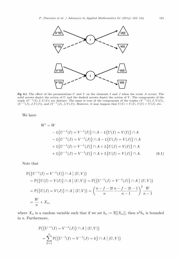
then (W, W ′) is clearly an exchangeable pair. We can represent the permutations Uand V when the event A occurs as in Fig. 6.1.
P. Diaconis et al. / Advances in Applied Mathematics 61 (2014) 102–124 121
Fig. 6.1. The effect of the permutations U and V on the elements I and J when the event A occurs. The solid arrows depict the action of U and the dashed arrows depict the action of V . The components of the triple (U−1(I), I, U(I)) are distinct. The same is true of the components of the triples (V −1(I), I, V (I)), (U−1(J), J, U(J)), and (V −1(J), J, V (J)). However, it may happen that U(I) = V (I), U(I) = V (J), etc.
We have
W ′ = W
− 1{U−1(I) = V −1(I)
}∩A− 1
{U(I) = V (I)
}∩A
− 1{U−1(J) = V −1(J)
}∩A− 1
{U(J) = V (J)
}∩A
+ 1{U−1(I) = V −1(J)
}∩A + 1
{U(J) = V (I)
}∩A
+ 1{U−1(J) = V −1(I)
}∩A + 1
{U(I) = V (J)
}∩A. (6.1)
Note that
P({
U−1(I) = V −1(I)}∩A
∣∣ (U, V ))
= P({
U(I) = V (I)}∩A
∣∣ (U, V ))
= P({
U−1(J) = V −1(J)}∩A
∣∣ (U, V ))
= P({
U(J) = V (J)}∩A
∣∣ (U, V ))
=(n− f − 2t
n
n− f − 2t− 1n− 1
)2W
n− 1
= W
n+ Xn,
where Xn is a random variable such that if we set bn := E[|Xn|], then n2bn is bounded in n. Furthermore,
P({
U−1(I) = V −1(J)}∩A
∣∣ (U, V ))
=n∑
P({
U−1(I) = V −1(J) = k}∩A
∣∣ (U, V ))
k=1
122 P. Diaconis et al. / Advances in Applied Mathematics 61 (2014) 102–124
=n∑
k=1
P({
I = U(k), J = V (k)}∩A
∣∣ (U, V ))
= n
(n− f − 2t
n
n− f − 2t− 1n− 1
)2(n− 1n
1n− f − 2t− 1
)2
= 1n
+ cn,
where cn is a constant such that n2cn is bounded in n, and similar arguments show that
P({
U(J) = V (I)}∩A
∣∣ (U, V ))
= P({
U−1(J) = V −1(I)}∩A
∣∣ (U, V ))
= P({
U(I) = V (J)}∩A
∣∣ (U, V ))
= n
(n− f − 2t
n
n− f − 2t− 1n− 1
)2(n− 1n
1n− f − 2t− 1
)2
= 1n
+ cn.
Suppose we can show that the probability of the intersection of any two of the events whose indicators appear on the right-hand side of (6.1) is at most a constant dn, where n2dn is bounded in n, then
E
[∣∣∣∣W − n
4P{W ′ = W − 1
∣∣ (U, V )}∣∣∣∣] ≤ nbn + 7ndn
E
[∣∣∣∣1 − n
4P{W ′ = W + 1
∣∣ (U, V )}∣∣∣∣] ≤ n|cn| + 7ndn.
It will follow from the main result of [5, Section 1] that the total variation distance between the distribution of W and a Poisson distribution with expected value 1 is at most Cn for a suitable constant C, and hence, as we have already remarked, the same is true (with a larger constant) for the distribution of χ([η, Π]).
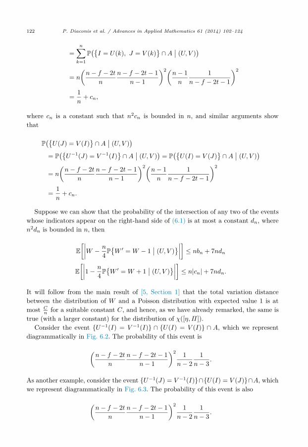
Consider the event {U−1(I) = V −1(I)} ∩ {U(I) = V (I)} ∩ A, which we represent diagrammatically in Fig. 6.2. The probability of this event is
(n− f − 2t
n
n− f − 2t− 1n− 1
)2 1n− 2
1n− 3 .
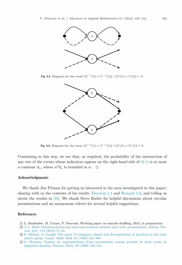
As another example, consider the event {U−1(J) = V −1(I)} ∩{U(I) = V (J)} ∩A, which we represent diagrammatically in Fig. 6.3. The probability of this event is also
(n− f − 2t n− f − 2t− 1
)2 1 1.
n n− 1 n− 2 n− 3
P. Diaconis et al. / Advances in Applied Mathematics 61 (2014) 102–124 123
Fig. 6.2. Diagram for the event {U−1(I) = V −1(I)} ∩ {U(I) = V (I)} ∩ A.
Fig. 6.3. Diagram for the event {U−1(J) = V −1(I)} ∩ {U(I) = V (J)} ∩ A.
Continuing in this way, we see that, as required, the probability of the intersection of any two of the events whose indicators appear on the right-hand side of (6.1) is at most a constant dn, where n2dn is bounded in n. �Acknowledgments
We thank Jim Pitman for getting us interested in the area investigated in this paper, sharing with us the contents of his results Theorem 1.1 and Remark 1.2, and telling us about the results in [16]. We thank Steve Butler for helpful discussions about circular permutations and an anonymous referee for several helpful suggestions.
References
[1] L. Banklader, M. Coram, P. Diaconis, Working paper on smoosh shuffling, 2013, in preparation.[2] J.-L. Baril, Statistics-preserving bijections between classical and cyclic permutations, Inform. Pro-
cess. Lett. 113 (2013) 17–22.[3] F. Bédard, A. Goupil, The poset of conjugacy classes and decomposition of products in the sym-
metric group, Canad. Math. Bull. 35 (1992) 152–160.[4] G. Boccara, Nombre de représentations d’une permutation comme produit de deux cycles de
longueurs données, Discrete Math. 29 (1980) 105–134.
124 P. Diaconis et al. / Advances in Applied Mathematics 61 (2014) 102–124
[5] S. Chatterjee, P. Diaconis, E. Meckes, Exchangeable pairs and Poisson approximation, Probab. Surv. 2 (2005) 64–106.
[6] P. Raymond de Montmort, Essay d’analyse sur les jeux de hazard, seconde edition, Jacque Quillau, Paris, 1713.
[7] P. Diaconis, Some things we’ve learned (about Markov chain Monte Carlo), Bernoulli 19 (2013) 1294–1305.
[8] D. Foata, M.-P. Schützenberger, Théorie géométrique des polynômes eulériens, Lecture Notes in Math., vol. 138, Springer-Verlag, Berlin, 1970.
[9] A. Goupil, On products of conjugacy classes of the symmetric group, Discrete Math. 79 (1989/1990) 49–57.
[10] A. Goupil, Decomposition of certain products of conjugacy classes of Sn, J. Combin. Theory Ser. A 66 (1994) 102–117.
[11] N. Linial, D. Puder, Word maps and spectra of random graph lifts, Random Structures Algorithms 37 (2010) 100–135.
[12] A. Nica, On the number of cycles of given length of a free word in several random permutations, Random Structures Algorithms 5 (1994) 703–730.
[13] J. Pitman, Combinatorial Stochastic Processes, Lecture Notes in Math., vol. 1875, Springer-Verlag, Berlin, 2006, lectures from the 32nd Summer School on Probability Theory held in Saint-Flour, July 7–24, 2002.
[14] J. Riordan, An Introduction to Combinatorial Analysis, Wiley Pub. Math. Statist., John Wiley & Sons Inc., New York, 1958.
[15] R.P. Stanley, Factorization of permutations into n-cycles, Discrete Math. 37 (1981) 255–262.[16] W.A. Whitworth, Choice and Chance with One Thousand Exercises, Hafner Publishing Company,
New York, London, 1965, reprint of the fifth edition much enlarged, issued in 1901.[17] Wikipedia, Shuffling, http://en.wikipedia.org/wiki/Shuffling, 2013.[18] J.R. Young, The magical mind of Persi Diaconis, The Chronicle of Higher Education, http://
chronicle.com/article/The-Magical-Mind-of-Persi/129404/, October 16, 2011.