Technology Assessment

Technology

Assessment Program Prepared for: Agency for Healthcare Research and Quality 540 Gaither Road Rockville, Maryland 20850

Use of Bayesian Techniques in Randomized Clinical Trials: A CMS Case Study

September 18, 2009

Use of Bayesian Techniques in Randomized Clinical

Trials: A CMS Case Study

Technology Assessment Report

Project ID: STAB0508

September 18, 2009

Duke Evidence-based Practice Center

Gillian D. Sanders, PhD; Lurdes Inoue, PhD; Gregory Samsa, PhD; Shalini Kulasingam, PhD, MPH; David Matchar, MD

This report is based on research conducted by the Duke Evidence-based Practice Center under contract to the Agency for Healthcare Research and Quality (AHRQ), Rockville, MD (Contract No. HHSA 290-2007-10066 I). The findings and conclusions in this document are those of the author(s) who are responsible for its contents; the findings and conclusions do not necessarily represent the views of AHRQ. No statement in this article should be construed as an official position of the Agency for Healthcare Research and Quality or of the U.S. Department of Health and Human Services. The information in this report is intended to help health care decisionmakers; patients and clinicians, health system leaders, and policymakers, make well-informed decisions and thereby improve the quality of health care services. This report is not intended to be a substitute for the application of clinical judgment. Decisions concerning the provision of clinical care should consider this report in the same way as any medical reference and in conjunction with all other pertinent information, i.e., in the context of available resources and circumstances presented by individual patients.

This report may be used, in whole or in part, as the basis for development of clinical practice guidelines and other quality enhancement tools, or as a basis for reimbursement and coverage policies. AHRQ or U.S. Department of Health and Human Services endorsement of such derivative products may not be stated or implied.

None of the investigators has any affiliations or financial involvement related to the material presented in this report.

Contents

Executive Summary ................................................................................................ 1 Chapter 1. Introduction, Tutorial, and Overview of Project ...................................... 5 Introduction ........................................................................................................ 5 Overview of the Report ...................................................................................... 6 Bayesian Tutorial ............................................................................................... 7 Chapter 2. Framing the Problem: CMS Contexts (or “Situations”) .......................... 17 Chapter 3. Literature Review................................................................................... 19 Methods ............................................................................................................. 19 Findings ............................................................................................................. 19 Chapter 4. Clinical Domain: The Implantable Cardioverter Defibrillator for the Prevention of Sudden Cardiac Death...................................................................... 34 Introduction ........................................................................................................ 34 Sudden Cardiac Death....................................................................................... 35 The Implantable Cardioverter Defibrillator ......................................................... 35 Current ICD Clinical Trials and Evidence of Efficacy ......................................... 35 Current Clinical Practice Guidelines for ICD Implantation.................................. 36 Current CMS Coverage of ICD Implantation...................................................... 37 ACC-NCDR® ICD Registry................................................................................. 38 Current Clinical and Policy Questions Regarding ICD Implantation................... 38 CMS Contexts.................................................................................................... 39 Chapter 5. ICD Case Study (Executive Summary).................................................. 42 Introduction ........................................................................................................ 42 Methods and Assumptions................................................................................. 42 Findings ............................................................................................................. 44 Methodological and Clinical Implications of Findings ......................................... 49 Chapter 6. Interpretation of Findings in the CMS Context ....................................... 50 Statement of Findings ........................................................................................ 50 Summary ........................................................................................................... 52 References.............................................................................................................. 53 Glossary of Terms................................................................................................... 60 Acronyms and Abbreviations................................................................................... 64 Figures .................................................................................................................... 65 Tables ..................................................................................................................... 81 Appendix: ICD Case Study

Executive Summary

Research Questions

What are the advantages and disadvantages of Bayesian statistical techniques in clinical trial design and analysis, and what is the potential impact of these approaches on policy-level decisionmaking by the Centers for Medicare & Medicaid Services (CMS)?

Methods

We provide a basic tutorial on Bayesian statistics and the possible uses of such

statistics in clinical trial design and analysis. We conducted a synthesis of existing published research focusing on how Bayesian techniques can modify inferences that affect policy-level decisionmaking. Noting that subgroup analysis is a particularly fruitful application of Bayesian methodology, and an area of particular interest to CMS, we focused our efforts there rather on the design of such trials. We used simulation studies and a case study of patient-level data from eight trials to explore Bayesian techniques in the CMS decisional context in the clinical domain of the prevention of sudden cardiac death and the use of the implantable cardioverter defibrillator (ICD). We combined knowledge gained through the literature review, simulation studies, and the case study to provide findings concerning the use of Bayesian approaches specific to the CMS context.

Results

Our literature review summarized articles categorized into four themes: (1) the

advantages and disadvantages of Bayesian techniques in clinical trial design and analysis; (2) the use of Bayesian techniques in subgroup analyses; (3) the use of Bayesian techniques in meta-analysis; and (4) the effect of using Bayesian techniques on policymaking/decisionmaking. Our simulation studies demonstrated that while single trials may be adequately powered to detect main treatment effects, they often have low power to detect treatment-covariate interactions. Furthermore, these studies demonstrated that combining data from trials improves the power to detect such treatment-covariate interactions. Our ICD case study explored the findings from our simulation studies and sought to provide evidence concerning the advantages and disadvantages of Bayesian techniques in clinical trial design and analysis. This case study led us to the following key findings:

• The analysis of the individual ICD trials found that, out of eight trials, five showed

evidence of treatment effect, but there was also a lot of variation in the estimates of ICD effect across trials. Within any trial, the results were fairly robust to

1

different model formulations. Generally there was no evidence of significant treatment-covariate interactions in the prognostic subgroups.

• Combining data from trials improves our inferences by increasing the precision of our estimates, as well as the power to detect main effects and interactions. A variety of modeling approaches allow us to combine data from different trials, but they do not necessarily lead to the same inference.

• Understanding the underlying model assumptions and limitations is important when interpreting the results from the combined analysis. For example, we observed that some models showed evidence for an interaction between treatment and age in the combined analysis. But this evidence arises from models that assume that this interaction is the same across all trials. If this assumption is regarded as unreasonable, and we consider instead a model that accounts for the variation of the interaction across trials, then the interaction between treatment and age is no longer significant.

• When considering Bayesian estimation, the role of priors should also be examined through a sensitivity analysis.

• Our analyses demonstrate that we can utilize Bayesian hierarchical models to predict survival from patients in subgroups. We found, however, that survival predictions from the analysis based on randomized trials may not be comparable to the empirical survival observed in the registry. One reason may be that patients in the registry may have different prognoses from those seen in clinical trials.

• We examined the use of patient-level data versus aggregate data as information accrues over time. Our analysis showed that the resulting inferences are not necessarily the same. The analysis of aggregate data may be more sensitive to priors.

• We note that an analysis which assesses the interactions between treatment and covariates defining the subgroups of interest may not be feasible with aggregate data.

Conclusions

Based on our review of the literature, simulation studies, and our case study, we

conclude the following concerning the use of Bayesian statistical approaches in CMS policy- and decisionmaking.

1. CMS should consider claims about differential subgroup effects only if

they are accompanied by a formal statistical test for interaction. a. Claims about differential subgroup effects based on stratified

analysis should only be considered as exploratory. These analyses are compromised by the small sample sizes and post hoc decisions regarding the number of tested subgroups.

b. Subgroup effects observed in a specific trial should be placed into context by using a statistical model that combines

2

information across trials and across subgroups. The random-effects/hierarchical models do both.

2. To increase the statistical power to detect those interactions that in fact exist, consider using all sources of data in order to stipulate within the statistical model which types of interaction are likely. For example, observational data and expert opinion might suggest that if an interaction is present it will take the form of decreasing ICD efficacy with increasing burden of disease

3. Base study design and decisionmaking only on those subgroup effects that are likely to be strong. The power to detect interactions is not universally high, and focusing attention on the most likely candidates will limit the number of subgroups that are analyzed, and thus limit the pernicious effects of random variation.

4. If the trial-based data are sufficient, do not directly combine trial-based data with information from other sources such as observational data and expert opinion. In this case the objective data are sufficient, and there is no need to utilize subjective information. Instead, use these other sources as informal sources of validation, and also to help design the statistical model for the trials (see below).

5. When little or no trial-based information about a subgroup is available, consider the use of other data (e.g., trial-based information from other subgroups, observational data, expert opinion) in order to specify a prior distribution. Unless special circumstances such as small patient pools are present, do not use this information to make final decisions about efficacy within the subgroups in question, but instead use this information to plan further studies. This suggests that the more controversial applications of Bayesian methodology should be reserved for those situations in which the decisionmaker has no other choice, and should, in any case, not be considered definitive.

6. Claims based on Bayesian methods should provide sensitivity analysis to the assumed priors. While for large trials the results are not sensitive to prior choices, this is not the case for small size trials. It is therefore important to demonstrate through sensitivity analyses how the choice of the prior impacts (or does not impact) the findings.

Summary

The use of Bayesian statistical approaches has gained broader acceptance within

the clinical trial community. The impact of these methods on CMS decisional contexts and policy-level decisionmaking however was uncertain. Our analyses explore the main proclaimed advantages of Bayesian statistics (namely, the use of prior information, sample size determination, borrowing strength from different trials, and sequential monitoring of trials) and provide examples of decisionmaking situations where the findings reached using these approaches both agree with and differ from findings reached using frequentist statistical techniques.

3

Our findings confirm that, like classical techniques, Bayesian approaches are affected by the problems of model specification (i.e., the relationship between various factors – patient, provider, intervention, and other contextual features – and the outcome of interest). In addition, Bayesian approaches can be substantially affected by the “Bayesian prior” – the representation of beliefs about the quantity of interest (e.g., relative risk of events when a new device is used vs. a conventional device). Thus, when considering using or interpreting Bayesian analyses, the focus of attention and thoughtful ex ante agreement are the specification of the model and specification of the Bayesian prior. The case study of the use of ICD therapy in the prevention of sudden cardiac death demonstrates the application of these techniques and highlights some of the practical challenges.

The use of Bayesian statistical approaches, and incorporation of our findings concerning their strengths and limitations into the CMS decisionmaking process will enable policymakers to harness the power of the available sources of clinical evidence, explore subgroup effects within a trial and across trials in a methodologically rigorous manner, assess the uncertainty in clinical trial findings, and – ideally – improve health outcomes for Medicare beneficiaries.

4

Chapter 1. Introduction, Tutorial, and Overview of Project

Introduction

The phrase “Bayesian statistics”a refers to an approach and method of analysis which combines prior knowledge and accumulated experience with current information in order to make inferences about a quantity of interest. Using Bayes’ theorem, Bayesian approaches are able to provide a formal method of learning from evidence as it accumulates. In the past, Bayesian approaches to clinical trial design and analysis have been difficult, given their computational intensity and their sometimes controversial method of using prior information. As a result of recent breakthroughs in computational algorithms, the computational limitations of Bayesian approaches have mostly been mitigated. The potential benefits of Bayesian approaches – especially when good prior information is available – have allowed the use of these techniques to become more popular within the clinical trial community.

As evidence of the rise of Bayesian statistical approaches in the clinical trial and regulatory communities, in 2006 the U.S. Food and Drug Administration (FDA) Center for Devices and Radiological Health (CDRH) issued draft guidance for industry and FDA staff entitled “Guidance for the Use of Bayesian Statistics in Medical Device Clinical Trials.”1 Although this guidance from the FDA provides a useful overview of Bayesian statistics and the recommended methods for employing such approaches in clinical trial design and analysis, it focuses on the use of Bayesian techniques at the FDA approval stage rather than at the stage at which the Centers for Medicare & Medicaid Services (CMS) determines whether evidence is sufficient to support their needed coverage decisions. In addition, it has been suggested that the FDA CDRH guidance in its current form puts substantial emphasis on calibrating Bayesian findings to classical (frequentist) calculations and therefore does not take full advantage of the Bayesian approach.

As Bayesian statistical techniques have gained broader acceptance within the clinical trial community, CMS seeks to assess the potential impact of such techniques on their policy-level decisionmaking. The Coverage and Analysis Group at the CMS requested this report from The Technology Assessment Program (TAP) at the Agency for Healthcare Research and Quality (AHRQ). AHRQ assigned this report to the following Evidence-based Practice Center (EPC): Duke EPC (Contract Number: HHSA 290 2007 10066 I).

The overall goal of this project is to provide CMS with a general approach for assessing the use of Bayesian techniques in its evidence-based policy processes. To reach this goal we had three specific aims:

1) To provide a synthesis of existing research regarding the advantages and

disadvantages of Bayesian techniques in clinical trial design and analysis,

a A glossary of terms is provided at the end of this report. Terms defined in the glossary appear in bold and italicized where they first appear in the main text of the report.

5

focusing on how such techniques can modify inferences that affect policy-level decisionmaking.

2) To explore Bayesian techniques in the CMS context through the specific clinical domain of the prevention of sudden cardiac death (SCD) trials to determine the effective use of the implantable cardioverter defibrillator (ICD).

3) To use the findings from the above two investigations to determine lessons learned specific to the CMS context, and to provide CMS with findings on: (a) the inclusion of studies that apply Bayesian techniques; (b) the circumstances in which such techniques may or may not be particularly appropriate; and (c) how such techniques can be used in conjunction with other data sources available to CMS, such as registries.

To help orient the reader we first provide an overview of the structure of the report,

and then provide a basic tutorial on Bayesian statistical approaches and their use in clinical trial design and analysis.

Overview of the Report

There are numerous areas within clinical trial design and analysis where the use of

Bayesian analyses can be and has been explored. These include applications to planning a clinical trial, performing and analyzing the trial, planning subsequent trials, combining data from multiple trials (and other sources), and incorporating registry data into the evidence base. These different potential applications of Bayesian approaches and the relative advantages and disadvantages of Bayesian approaches compared with more classical techniques are summarized in the literature review in Chapter 3.

Our main focus in this report, however, is on one of the potential applications of Bayesian analysis – subgroup analysis – within individual trials and across multiple trials. We chose this focus because it is a natural application of Bayesian methods from the CMS perspective, since (a) CMS is often presented with subgroup analyses that might suggest that a drug or device might work better or worse for particular categories of patient; (b) CMS is usually more interested in patients aged 65 years and above; and (c) results for particular subgroups are often based on small sample sizes, and/or are otherwise inconsistent, and thus require the introduction of additional information in order to draw sound conclusions. In Chapter 2 we define four decisional contexts or situations where CMS may consider the use of Bayesian approaches, and throughout our analysis we continually refer back to how our findings may apply to these contexts.

After defining these contexts, we provide a review of the literature, describing current knowledge of subgroup analyses from both the Bayesian and frequentist perspectives. We sought to determine whether there are circumstances under which Bayesian or frequentist statistical techniques provide design or analysis advantages for Phase III efficacy trials. In particular, we summarize the published literature exploring how Bayesian techniques of clinical trial design and analysis could modify inferences and potentially affect CMS policy-level decisionmaking.

6

We then illustrate the application of these findings to a clinical domain of interest to CMS – specifically, clinical trials evaluating the use of implantable cardioverter defibrillator (ICD) therapy in the prevention of sudden cardiac death (SCD). We used both simulation studies and a case study evaluating patient-level data from eight ICD clinical trials to highlight the advantages and disadvantages of Bayesian techniques as compared to frequentist approaches. These simulations are intended to illustrate and supplement the literature review.

We use the data from the ICD trials to illustrate how the analyses of these data might proceed using the Bayesian and frequentist perspectives. The primary goal of this case study is to help the reader visualize how a Bayesian analysis would proceed and be reported. In order to illustrate the two types of data that an analyst might encounter in practice, the case study includes both analyses of raw data and of summary data. We also explore the use of Bayesian statistical techniques in a clinical domain where registry data are available – such as those clinical domains where CMS issues a national coverage decision requiring, as a condition of coverage, the collection of additional patient data to supplement standard claims data (i.e., Coverage with Evidence Development). Although the simulation studies and case study focus on clinical trials of ICD use in primary and secondary prevention of SCD, we highlight throughout this report how our findings are generalizable to other clinical domains.

The report ends with a series of conclusions based on our review of the literature, the simulation studies, and the case study.

Bayesian Tutorial

Background and Scope

The two main schools of statistical thought are Bayesian and frequentist. Although some statisticians strongly prefer one approach over the other, most are willing to consider both, and, indeed, with the increased feasibility of Bayesian computation, practice appears to be moving toward a blending of these perspectives. This tutorial takes no position on the ongoing debate about the foundations of statistics. Instead, its purpose is to provide non-technical background for non-statisticians.

For this purpose, it is critical to recognize that the current environment is based almost entirely on frequentist ideas. Some of this emphasis is historical based on when Bayesian techniques were more difficult to implement than is presently the case. The other reason for the emphasis on frequentist ideas is that this approach can be implemented in a highly rule-based fashion. This allows agreement on the ground rules for what will be deemed statistically significant before data analysis begins, and confidence that such ground rules will be consistent from application to application. While Bayesian analyses can be pre-specified and rule-based, they are generally flexible - advocates of the Bayesian approach cite this as an advantage.

This section does not focus on circumstances where the Bayesian approach yields similar results but frames the analysis differently, or on those situations where the Bayesian approach might provide marginal improvements over a frequentist approach.

7

Recognizing the inherent limitations of non-technical tutorials, this section tries to provide answers to the following two questions:

(1) For the purposes of policy makers, what are Bayesian statistics? (2) For the purposes of policy makers, what are the situations where the

Bayesian approach is likely to be so much better than the frequentist approach that it should be strongly considered?

For a more comprehensive tutorial, we recommend the references cited in Chapter

3. Diagnostic Testing Example

Figure 1 illustrates the basic Bayesian paradigm, namely that “prior information and beliefs” plus “new data” yield “revised beliefs.” This paradigm can be illustrated by diagnostic testing.

Suppose that the physician suspects that a patient might have meningitis, and is considering whether to subject that patient to the risk and expense of a diagnostic test that can shed additional light on the matter. After taking a history and performing a physical examination, the physician believes that the patient has a 20 percent probability of meningitis. This “20 percent” is the “prior information.”

Prior information can be entirely objective, entirely subjective, or a combination of the two. An example of entirely objective information is the use of a risk score – for example, if the patient has a fever in excess of 103 degrees Fahrenheit a risk score would increase. An example of entirely subjective information is the physician’s intuition based on years of experience but impossible to quantify using precise rules. Combining the two begins with the quantitative risk score, with clinical intuition being used to modify the score. Note that in this example the “subjective” assessment is in fact based on a lot of information (i.e., it is a holistic application of extensive medical knowledge); however, it is “subjective” in the sense that it cannot be reduced to a reproducible quantitative algorithm.

As a general principle, applications of Bayesian inference are relatively uncontroversial when the prior information is objective and reproducible. Applications of Bayesian inference where prior beliefs are subjective and not reproducible are more controversial. These applications become increasingly controversial when the role of the prior beliefs increases relative to the role of the data, and the more that prior probability is guided by intuition or is otherwise idiosyncratic.

Suppose that the physician decides to perform the diagnostic test, and that the test has 90 percent sensitivity and 80 percent specificity. Recall that sensitivity is the probability that a patient with meningitis will have a positive test corresponding to “meningitis,” and that specificity is the probability that a patient without meningitis will have a negative test corresponding to “not meningitis” (see Figure 2). We posit a population of 1000 patients, of whom 200 have meningitis because the prior probability of disease is 20 percent. Of these, 180 will have a positive test because the sensitivity is 90 percent. The remaining entries of the table are filled in similarly. The positive predictive value is the probability that a patient with a positive test will actually have

8

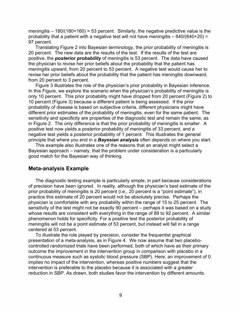
meningitis – 180/(180+160) = 53 percent. Similarly, the negative predictive value is the probability that a patient with a negative test will not have meningitis – 640/(640+20) = 97 percent.

Translating Figure 2 into Bayesian terminology, the prior probability of meningitis is 20 percent. The new data are the results of the test. If the results of the test are positive, the posterior probability of meningitis is 53 percent. The data have caused the physician to revise her prior beliefs about the probability that the patient has meningitis upward, from 20 percent to 53 percent. A negative test would cause her to revise her prior beliefs about the probability that the patient has meningitis downward, from 20 percent to 3 percent.

Figure 3 illustrates the role of the physician’s prior probability in Bayesian inference. In this Figure, we explore the scenario when the physician’s probability of meningitis is only 10 percent. This prior probability might have dropped from 20 percent (Figure 2) to 10 percent (Figure 3) because a different patient is being assessed. If the prior probability of disease is based on subjective criteria, different physicians might have different prior estimates of the probability of meningitis, even for the same patient. The sensitivity and specificity are properties of the diagnostic test and remain the same, as in Figure 2. The only difference is that the prior probability of meningitis is smaller. A positive test now yields a posterior probability of meningitis of 33 percent, and a negative test yields a posterior probability of 1 percent. This illustrates the general principle that where you end in a Bayesian analysis often depends on where you start.

This example also illustrates one of the reasons that an analyst might select a Bayesian approach – namely, that the problem under consideration is a particularly good match for the Bayesian way of thinking. Meta-analysis Example

The diagnostic testing example is particularly simple, in part because considerations of precision have been ignored. In reality, although the physician’s best estimate of the prior probability of meningitis is 20 percent (i.e., 20 percent is a “point estimate”), in practice this estimate of 20 percent would not be absolutely precise. Perhaps the physician is comfortable with any probability within the range of 15 to 25 percent. The sensitivity of the test might not be exactly 90 percent – perhaps it was based on a study whose results are consistent with everything in the range of 88 to 92 percent. A similar phenomenon holds for specificity. For a positive test the posterior probability of meningitis will not be a point estimate of 53 percent, but instead will fall in a range centered at 53 percent.

To illustrate the role played by precision, consider the frequentist graphical presentation of a meta-analysis, as in Figure 4. We now assume that two placebo-controlled randomized trials have been performed, both of which have as their primary outcome the improvement in the intervention group in comparison with placebo in a continuous measure such as systolic blood pressure (SBP). Here, an improvement of 0 implies no impact of the intervention, whereas positive numbers suggest that the intervention is preferable to the placebo because it is associated with a greater reduction in SBP. As drawn, both studies favor the intervention by different amounts.

9

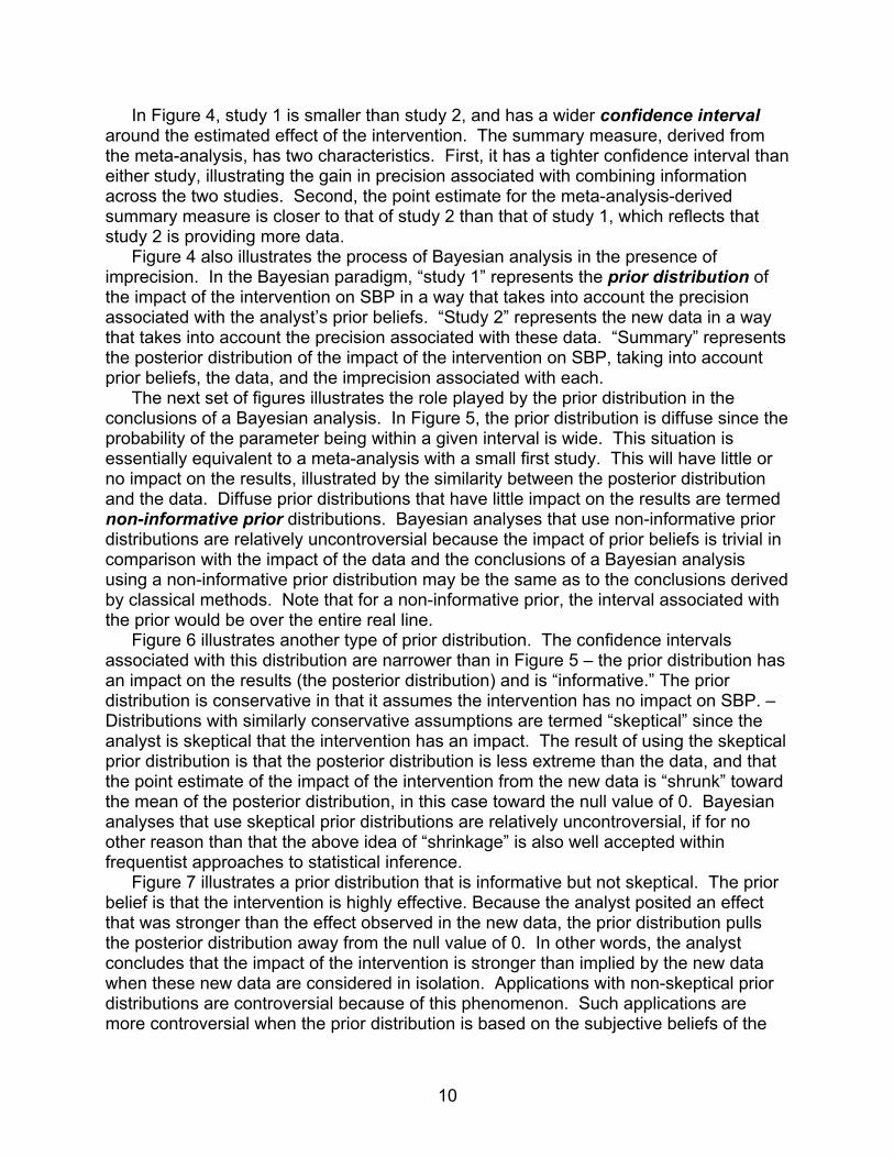
In Figure 4, study 1 is smaller than study 2, and has a wider confidence interval around the estimated effect of the intervention. The summary measure, derived from the meta-analysis, has two characteristics. First, it has a tighter confidence interval than either study, illustrating the gain in precision associated with combining information across the two studies. Second, the point estimate for the meta-analysis-derived summary measure is closer to that of study 2 than that of study 1, which reflects that study 2 is providing more data.

Figure 4 also illustrates the process of Bayesian analysis in the presence of imprecision. In the Bayesian paradigm, “study 1” represents the prior distribution of the impact of the intervention on SBP in a way that takes into account the precision associated with the analyst’s prior beliefs. “Study 2” represents the new data in a way that takes into account the precision associated with these data. “Summary” represents the posterior distribution of the impact of the intervention on SBP, taking into account prior beliefs, the data, and the imprecision associated with each.

The next set of figures illustrates the role played by the prior distribution in the conclusions of a Bayesian analysis. In Figure 5, the prior distribution is diffuse since the probability of the parameter being within a given interval is wide. This situation is essentially equivalent to a meta-analysis with a small first study. This will have little or no impact on the results, illustrated by the similarity between the posterior distribution and the data. Diffuse prior distributions that have little impact on the results are termed non-informative prior distributions. Bayesian analyses that use non-informative prior distributions are relatively uncontroversial because the impact of prior beliefs is trivial in comparison with the impact of the data and the conclusions of a Bayesian analysis using a non-informative prior distribution may be the same as to the conclusions derived by classical methods. Note that for a non-informative prior, the interval associated with the prior would be over the entire real line.

Figure 6 illustrates another type of prior distribution. The confidence intervals associated with this distribution are narrower than in Figure 5 – the prior distribution has an impact on the results (the posterior distribution) and is “informative.” The prior distribution is conservative in that it assumes the intervention has no impact on SBP. – Distributions with similarly conservative assumptions are termed “skeptical” since the analyst is skeptical that the intervention has an impact. The result of using the skeptical prior distribution is that the posterior distribution is less extreme than the data, and that the point estimate of the impact of the intervention from the new data is “shrunk” toward the mean of the posterior distribution, in this case toward the null value of 0. Bayesian analyses that use skeptical prior distributions are relatively uncontroversial, if for no other reason than that the above idea of “shrinkage” is also well accepted within frequentist approaches to statistical inference.

Figure 7 illustrates a prior distribution that is informative but not skeptical. The prior belief is that the intervention is highly effective. Because the analyst posited an effect that was stronger than the effect observed in the new data, the prior distribution pulls the posterior distribution away from the null value of 0. In other words, the analyst concludes that the impact of the intervention is stronger than implied by the new data when these new data are considered in isolation. Applications with non-skeptical prior distributions are controversial because of this phenomenon. Such applications are more controversial when the prior distribution is based on the subjective beliefs of the

10

analyst, and are less controversial when the prior distribution is based on real data such as from another clinical trial.

An example of deriving the prior distribution objectively is to use the results of a previous meta-analysis. In this situation the posterior distribution from the previous meta-analysis becomes the prior distribution when new studies become available. The new studies update the meta-analysis. A “sequential meta-analysis” or “cumulative meta-analysis” is iterative, with each new study published in the literature inducing another round of updating.

Figure 8 illustrates the worst case for Bayesian analysis. There, the prior distribution is non-skeptical and illustrates strong beliefs in the efficacy of the intervention. (Here, it is implicitly assumed that these strong beliefs are primarily based on intuition, rather than objective information such as a previous meta-analysis). The data provide little contribution to the posterior distribution, which essentially recapitulates the prior beliefs of the analyst. There is almost universal agreement that applications like those illustrated in Figure 8 are inappropriate, except perhaps to document the lack of objective data about the phenomenon under study.

The differences between Figures 5 and 8 can help illustrate the circumstances in which Bayesian methods might most naturally be considered. In Figure 5, there are enough data to provide sound inference. It does not matter whether the analysis is Bayesian or not, although some analysts will select a Bayesian approach because of their philosophical beliefs, the easier interpretation of the results, or because the type of problem is a good fit for a Bayesian formulation.

In Figure 8, there are too little data to provide sound inference, and a Bayesian approach risks being too subjective by being primarily based on subjective belief rather than objective data. The most natural applications of Bayesian methodology fall somewhere in between. Some data are available, but not enough to draw strong conclusions in the absence of other information. An informative prior distribution can be supported, either because it is skeptical or because it is based on objective information. Technical Note on the Role of Distributions

The usual presentations of meta-analysis (e.g., Figure 4) or its conceptually equivalent Bayesian counterparts (e.g., Figures 5 to 8) gloss over some assumptions about the shape of the prior distribution and of the new data. Figure 9 presents the same information, but in a way that highlights the distributional assumptions that underlie the analysis. In particular, a typical meta-analysis such as is depicted in Figure 4 assumes that the distribution of the outcome within each study, perhaps after an appropriate transformation such as log-transformation, is Gaussian. If so, the analyst can rely on the mathematical result that the combination of Gaussian distributions is Gaussian, and be confident that the posterior distribution is Gaussian as well. The exact nature of this latter distribution (its center point and its spread) can be obtained directly from a formula.

When distributions can be combined in this simple fashion they are termed “conjugate.” Various other pairs of conjugate distributions exist. When the distributions in question are not conjugate, often the posterior distribution must be derived using

11

simulations, which may be technically complex to implement. Such simulations are where the reader will encounter terms such as “Gibbs sampler” or “Markov chain Monte Carlo (MCMC).” This report does not focus on the details of deriving posterior distributions. Technical Note on Fixed- and Random-Effects Models, Heterogeneity, and Interaction

Although this is not intended to be an in-depth tutorial on meta-analysis, it may be helpful to highlight some additional concepts that will be used in this report. Specifically, the meta-analysis literature makes the distinction between “fixed-effect” models and “random-effects” models. Loosely speaking, a fixed-effect model assumes that the efficacy of the intervention is identical from study to study, and that the primary goal of the meta-analysis is to estimate this single specific quantity. The analyst using a fixed-effect model will begin with a “test for heterogeneity” – in essence, a statistical test that allows the data to disprove the assumption that the efficacy of the intervention is similar across the studies. In contrast, a random-effects model assumes (based on the philosophical belief that most things involving human biology are heterogeneous) that efficacy differs from study to study, and posits that efficacy follows a statistical distribution and that a primary goal of the meta-analysis is to estimate the parameters (e.g., mean, standard deviation) of this distribution.

Our report uses two elements of the above. First, our simulations utilize both fixed-and random-effects models. It should be noted in this context that random-effects modeling is particularly felicitous within the Bayesian framework, but that random-effects modeling can also be implemented within a frequentist paradigm. Accordingly, any advantages of random-effects and related models should not be entirely attributed to the Bayesian way of thinking, although it should also be noted that the Bayesian approach does accommodate random-effects and related models particularly well.

Second, our report uses the closely related concepts of heterogeneity and statistical interaction. In the context of subgroup analysis, heterogeneity is equivalent to having different intervention effects for different subgroups – for example, a device that is more efficacious for patients aged 50 to 64 years than for patients aged 65 years and above. Statistical interaction is data-based evidence of heterogeneity – for example, a statistical test that demonstrates that the above difference in efficacy was observed within a particular study. In practice, decisionmakers often desire evidence of interactions that are both statistically significant and clinically meaningful. The distinction between the two is that a statistically significant interaction implies that there is some difference in efficacy between subgroups (i.e., that the difference in efficacy is different from 0), whereas a clinically important interaction implies that this difference is “large enough to matter” (e.g., suggests that different actions be taken in one subgroup versus another). With small sample sizes within subgroups it is often the case that tests for statistical interaction will have low power – there, the concern is that while there is no statistical evidence for interaction, the data might nevertheless be consistent with clinically important differences in the efficacy of the intervention across subgroups.

12

Making Decisions Using Bayesian Analysis

Decisionmaking in any particular Bayesian analysis takes place by examining properties of the posterior distribution. As an example of using the posterior distribution to make inferences, if more than 95 percent of the area of the posterior distribution for the impact of an intervention on SBP falls in positive territory, the analyst is “95 percent confident” that the intervention is effective. Bayesian analysts refer to this as the 95 percent credible interval. The credible interval has a specified or subjective probability of containing the parameter of interest, given the observed data and the prior information. The best guess or point estimate for the magnitude of effectiveness might be the mean, median, or mode of this posterior distribution. The precision of the conclusions is derived from the spread of the posterior distribution or the length of the credible intervals.

In practice, analyses such as the above are then supplemented by an exploration of robustness – for example, in order to determine whether similar conclusions are obtained when the prior distribution is modified. The less skeptical and more informative the prior distribution, the more extensive should be the assessment of robustness. Two Illustrative Applications of Bayesian Methodology

The ideal application of Bayesian methodology occurs when there are some data, but not quite enough to draw sufficiently firm conclusions. Our report will focus on one such application – namely, subgroup analysis.

CMS might be interested in the performance of a medical device among patients aged 65 to 74 years. Most clinical trials of this device, however, are in patients aged 55 to 64 years. Some information is available on patients aged 65 to 74 years, but is insufficient to form firm conclusions. In other words, some data are available on patients aged 65 to 74, but not enough. The question becomes whether a Bayesian analysis might be performed, with the information from other age groups of patients providing the prior distribution that can then be combined with the data regarding patients aged 65 to 74.

Another natural application of Bayesian statistics is in the design and analysis of Phase 1 and Phase 2 clinical trials, especially those trials for which it is critical to make the most statistically efficient use of all possible information. One reason for doing so might be the testing of a promising therapy, albeit one with potentially devastating adverse events, in a condition that is uniformly fatal. It is usually assumed that both the efficacy of the intervention and the likelihood of adverse events increase with the dose, so the goal is to estimate the maximum tolerable dose (the maximum dose with an acceptable level of adverse events). The analyst wishes to do so in a way that exposes as few patients as possible to unsafe doses of the drug, while exposing as many patients as possible to the drug’s therapeutic doses.

These goals cannot be accomplished by treating each possible dosage level in isolation, if for no other reason than the information for each dose will be based on small sample sizes and thus will be unreliable. Instead, the analyst posits a dose-response function between the probability of an adverse event and the dose. By transforming the

13

outcome variable using a “logit” transformation, a straight line is obtained that can be described with a slope and an intercept (see Figure 10, which is drawn to have a slope of 1 and an intercept of 0). The prior distribution for the slope and intercept are derived from similar drugs, previously tested patients, and biologically informed supposition if necessary. The outcome for each patient can then be used, in Bayesian fashion, to update the estimates of this slope and intercept, and data collection continues until this line and the maximum dose corresponding to the acceptable probability of adverse events implied by this line has been estimated with adequate precision. At each step in the process (e.g., for each new patient) the information to date can be used to assign the most statistically appropriate dosage level, which is the core idea behind Bayesian adaptive designs.

The take-home message of this second example is that early-phase testing is another circumstance that satisfies the condition of “some but not quite enough data” that suggests the use of Bayesian methods. This example also illustrates the general principle that Bayesian methods are not limited to data analysis, but can be used in study design as well. Differences between Bayesian and Frequentist Methods

Most elements of frequentist inference have Bayesian counterparts. The above example illustrated the Bayesian counterpart to the 95 percent confidence interval used by frequentist statisticians, namely, the 95 percent credible interval used by Bayesians. There are subtle differences between what these two types of interval represent; but in practice they are similarly applied.

It is not an exaggeration to claim that the only people who believe strongly that there are important differences between analogous Bayesian and frequentist concepts are those who are already strongly convinced that one is theoretically superior to the other. For example, a frequentist might object that estimating the prior distribution involves judgment, despite the fact that doing so is crucial to the Bayesian approach. Similarly, a Bayesian might object to the fact that frequentist methods do not explicitly describe prior beliefs, despite the fact that they are implicitly taken into account by frequentist methods. We recommend these assertions not be taken seriously, since most practicing statisticians do not strongly favor one methodology over the other. As Bayesian methods are becoming increasingly feasible from a computational perspective, various elements of the two approaches appear to be blending over time.

One way to think about the differences between the Bayesian and frequentist approaches is to recognize that all applications of statistics are limited by the act of inference – what we would like to do is to observe an entire population, often including its future members, but we are limited by having data on only a subset of that population. This inescapable constraint implies that any statistical analysis will have some objective components (the mathematical maneuvers applied to the observed data) and some subjective components (extrapolating the results of the observed data to the population under consideration).

Where the Bayesian and frequentist approaches to statistics differ is not in the amount of subjective judgment required but instead in where and how subjective judgment enters the analysis. In a Bayesian analysis, the subjective features enter

14

formally and explicitly, primarily through the specification of the prior distribution and the choice of the model to be used in the analysis; or they enter the analysis in how characteristics of the posterior distribution will be summarized in order to arrive at conclusions. In a frequentist analysis, the subjective features also enter in the choice of the model to be used in the analysis. They enter informally, in the design of the clinical study and through the implicit weighting given to various individual results in drawing overall conclusions. Factors in this weighting include whether individual results were statistically significant at some p value or not, the magnitude of observed trends, the overall consistency of observed trends in light of biological plausibility and the previous literature, and so forth.

If this informal weighting procedure is performed thoughtfully, the flexibility of the frequentist approach represents a potential strength; if not, the flexibility represents a potential source for erroneous conclusions, bias, and other sources of mischief. Similarly, the formal and explicit specification of how conclusions will be drawn from the data and what is known to date are a potential strength of the Bayesian approach, but only in those circumstances where the problem at hand and the knowledge to date make it sensible to do so. Fortunately, the results of Bayesian and frequentist analyses are often substantially similar, especially if both are performed with care and insight. Summary

The primary goal of this tutorial is to provide non-statistical readers having no previous exposure to Bayesian methods with an intuitive introduction to those methods – specifically, “what Bayesian statistics are about and when I should care.” What Bayesian statistics are about is the process by which “prior beliefs are combined with new data in order to generate revised beliefs.” The primary strength of Bayesian statistics is its explicit nature – by specifying ahead of time and in detail what is currently known, and how decisions will be derived from the combination of this knowledge and the new data, analyses, and decisions that derive from those analyses will exhibit the laudable characteristic of transparency. Its primary weakness is that not all applications of statistics fit naturally into this paradigm.

When data have already been collected, there is only one set of circumstances where one should always strongly consider, independent of any philosophical preferences, the use of Bayesian approaches – namely, when: (a) a decision must be made; (b) some data are available, but the existing data provide insufficient guidance or precision for making that decision; and (c) additional information can be defensibly brought to bear on that decision. In this context, “defensible” could potentially mean: (a) based on related data such as a similar (but not identical) intervention applied to a similar but not identical population; (b) specified using conservative assumptions (e.g., such as an intervention having no impact on outcome); or (c) based on supposition, where the nature of that supposition is explicitly justified and accepted as reasonable by impartial observers.

When the study is in the design phase, the flexibility inherent in the Bayesian approach provides the basis for adaptive randomization, which allows the size of the study to be determined as data collection proceeds, and thus in some cases might help

15

satisfy the ethical imperatives of exposing as few subjects as possible to risks and as many subjects as possible to treatments that are maximally beneficial.

16

Chapter 2. Framing the Problem: CMS Contexts (or “Situations”)

We defined four decisional contexts or situations where CMS may consider the use of Bayesian approaches, and throughout our analysis we continually refer back to how our findings may apply to these contexts. The four contexts are:

• Situation 1: Applicants present CMS with results that suggest no or minimal

efficacy of an intervention for the overall population, but apparent effectiveness in a subgroup or subgroups of patients, and are requesting reimbursement for those subgroups only.

• Situation 2: Applicants present CMS with results that suggest that an intervention is effective overall, but concern is raised that the benefits might be less effective in some subgroups.

• Situation 3: Applicants present CMS with results that suggest that an intervention is effective, but the trial in question has been performed on a different population (e.g. patients aged 55 to 64). The applicants wish to extend the results to patients of interest to CMS.

• Situation 4: Previous completed trials have demonstrated effectiveness in high-risk populations, and applicants are designing a new trial in a lower-risk population of interest to CMS and request feedback concerning their proposed trial design and analysis.

For the purposes of this work, we assume that CMS’s evaluation task in each of the

above situations involves three key steps: 1) Translating CMS’ general criterion of whether a given intervention is deemed

“reasonable and necessary” into specific criteria describing the outcomes that are necessary and sufficient to characterize the intervention’s value to the target population.

2) Assessing the degree to which the intervention in question promotes improvements in those outcomes to the target populations.

3) Judging whether those improvements are sufficient to implement into policy. These evaluation tasks can be performed using two approaches: frequentist

statistical techniques or Bayesian techniques. Step 1 of establishing the specific criteria by which an intervention is assessed is basic to both evaluation approaches. Step 2 involves analysis of evidence, typically using frequentist statistical tools for assigning levels of statistical significance, and Step 3 involves a mix of quantitative and qualitative approaches. Quantitative approaches might include simple criteria such as “are there X trials each with a p value < y?,” or more involved approaches based on meta-analysis. Qualitative approaches aim to promote decisionmaking by assessing the “sense of the committee” and can be informal or formal such as the modified Delphi method.

What is distinctive about the two approaches is the way they address the latter two steps. In a frequentist evaluation approach, these steps are treated as separate. The

17

Bayesian approach treats the latter two steps as integrated and may be characterized as assessing the adequacy of evidence for the purpose of decisionmaking or action. In particular, a Bayesian analysis of any body of evidence focuses on estimating the “strength of belief” regarding any particular measure, for example, “Study X leads me to be Y percent confident that the effect of the intervention is greater than Z”. Furthermore, the Bayesian approach leads to natural interpretations of multiple studies, each contributing to a body of evidence, and also provides a conceptually consistent framework for linking various forms of evidence to construct aggregate inferences.

Whatever the theoretical or philosophical benefits of any particular evaluation approach, what is ultimately of interest to CMS and society is how to achieve the practical goals of promoting improved health outcomes for Medicare beneficiaries. It is important to note that the evaluation task is not pursued in a vacuum, as multiple stakeholders are involved with a wide variety of interests. Evaluation and ultimate decisionmaking occurs through a process which has social, political, and economic ramifications. It is crucial that any evaluation strategy is in harmony with the current decisionmaking context and process. In addition to achieving the analytical goal of extracting a correct inference from a body of evidence, an evaluation strategy should promote the broader goals of transparency, clarity, efficiency, and accommodation of multiple objectives.

18

Chapter 3. Literature Review

Methods

This report focuses on those situations where Bayesian these techniques might be used in CMS policymaking context. Therefore, the literature review aimed to determine whether there are circumstances under which Bayesian or frequentist statistical techniques provide design or analysis advantages for Phase III efficacy trials. Throughout the review we focused on how such approaches could modify inferences that affected policy-level decisionmaking. Although our simulation studies and case study of the ICD clinical domain also explore this question, we sought first to determine whether a review of the available published literature would provide empirical evidence.

We searched MEDLINE® using terms related to Bayesian theory and analysis, frequentist analysis, and health policy. We restricted the search to trials and review articles published in English. We also searched the reference lists of key papers and proceedings from a recent SAMSI workshop on subgroup analysis2 for potentially relevant publications. Titles and abstracts of all studies identified by these means were reviewed independently by two investigators.

The following types of articles were excluded: • Epidemiological studies (observational or longitudinal studies). • Genetic studies. • Randomized controlled trials (RCT) that did not include Bayesian analysis. Meta-analyses and cost-effectiveness analyses were included if they focused on the

methods of interest and applied them in a way that allowed a comparison of Bayesian and frequentist methods. At the title-and-abstract stage, articles were included for full-text review if at least one of the two reviewers indicated that they should be included.

At the full-text review stage, articles were again reviewed by two independent reviewers and were included if they fell into one or more of the topics of interest listed above. Disagreements between reviewers were resolved through discussion.

Through all search strategies combined, we identified 334 potentially relevant citations. One hundred and ninety-seven (197) were excluded at the title-and-abstract screening stage, and another 67 were excluded at the full-text screening stage leaving a total of 70 included studies to be reviewed.

Findings

Articles in the literature review were categorized into four themes: (1) advantages

and disadvantages of Bayesian techniques in clinical trial design and analysis; (2) use of Bayesian techniques in subgroup analyses; (3) use of Bayesian techniques in meta-analysis; and (4) the effect of using Bayesian techniques on policymaking/decisionmaking.

19

Table 1 reports the number of included articles reviewed for each of the four themes. Note that some articles were included for more than one theme.

In what follows, we summarize our review of the literature in these four themes – while focusing these summaries on areas of interest to CMS. Advantages and Disadvantages of Bayesian Techniques in Clinical Trial Design and Analysis Potential Advantages of Bayesian Approaches

The statistical literature contains numerous books and papers describing Bayesian theory, its associated methods as applied to medicine, and the advantages and disadvantages of Bayesian techniques in clinical trial design and analysis. The following discussion of the published literature therefore is not intended to be all-inclusive, or to provide a complete introduction to Bayesian statistical approaches. Readers are referred to Spiegelhalter and colleagues3 for a comprehensive summary on the use of Bayesian statistical approaches in the design and analysis of clinical trials, to a Health Technology Assessment by the National Institute for Health Research (NHS)4 for a complete and formal review of Bayesian methods in health technology assessment, and to the 2006 FDA guidance on the use of Bayesian methods in medical device trials.1 Many of the advantages and disadvantages of Bayesian approaches discussed here are based on review of these three sources. Note that, in addition, the International Society for Bayesian Analysis (ISBA) provides a list of Bayesian resources.5

The CMS decisionmaking context focuses mostly on situations in which clinical trials have already been performed, and in which CMS is considering whether the current evidence base is sufficient. Two areas where such decisionmaking may be helped by Bayesian approaches include the analysis of subgroups and the meta-analysis of clinical evidence as it accumulates. These topics are discussed below. Here we concentrate on three additional potential advantages of Bayesian approaches: (a) the use of prior information; (b) sample size determination; and (c) adaptive designs. It is important to note that as with frequentist statistical approaches, clinical trials based on a Bayesian approach still require scientifically sound clinical trial planning and analysis.

Bayesian statistics focus on the ability to learn from evidence as it accumulates. Prior information is combined with current information on a quantity of interest, and Bayes’ theorem is used to formally combine these two sources of information to produce an updated or posterior distribution of the quantity of interest. The use of prior information is both seen as the main strength of Bayesian techniques, while also providing the most cause for concern on the part of frequentist clinical trialists. Bayesian methods may be controversial when the prior information is based mainly on personal opinion or expert judgment, or when it is based on evidence which the decisionmaker considers subjective. In such situations, sensitivity analyses on the prior distributions are especially important. The use of prior information based on empirical evidence from existing clinical trials is less controversial, and in the CMS context this will be the most common source of prior information. Additional information could, however, be based on patient registries, pilot studies, or clinical trials of similar

20

interventions. For a prior to be considered appropriate, the evidential basis of the prior (and any potential biases of that evidence) must be explicitly given. In addition, many emphasize the necessity of sensitivity analyses which explore a range of options for the chosen prior.4

Fisher provides a discussion of Bayesian and frequentist analysis and interpretation of clinical trials and potential controversies over the use of prior information, as well as the potential pitfalls both in their elicitation and incorporation into the existing evidence base.6 Examples of studies from the literature that explore the use of prior information and its impact on clinical trials include those by Gennari et al.,7 Tyson et al.,8 Brophy and Joseph,9 and Kpozehouen et al.10

Although the benefit of incorporating an informative prior into trial design and analysis is the most notable advantage of Bayesian statistical approaches, even when such an informative prior is not available, the Bayesian approach may still be useful through the use of interim analyses or midcourse modifications as discussed below.

The use of Bayesian approaches may modify the sample size an applicant needs to determine that the evidence is sufficient to CMS. This change could be based on either the use of prior information, as described above, or on interim “looks” during the course of a clinical trial. As discussed by Schmid and colleagues,11 the use of prior information has two potential effects on sample size estimation. If the available prior evidence provides information about the effect size, then it may reduce the required sample size. If, however, the prior evidence reflects additional uncertainty about that effect size, then the sample size may be increased. When either Bayesian or frequentist statistical techniques are used for estimating sample size, the goal is to gather enough information to make a decision about the efficacy of an intervention, while not wasting resources or putting patients at unnecessary risk. Bayesian approaches allow their users not to specify a particular sample size, but rather a particular criterion at which to stop the trial. At any point during the trial period, Bayesian techniques can be used to obtain the posterior distribution for the sample size, to compute the expected additional number of observations needed to meet the pre-specified stopping criterion, and to potentially stop the trial at the precise point where enough information has been gathered to answer the clinical or policy question of interest. An example of the use of Bayesian approaches in sample size determination is provided by Wang and colleagues.12

Finally, the use of Bayesian approaches may allow adaptive designs to be incorporated into clinical trials. Such trial designs may allow an unfavorable treatment arm to be dropped midcourse during the trial, or permit modifications to the randomization scheme to occur. Although the frequentist approach includes sequential analysis techniques that do not require pre-specified sample sizes, it is generally agreed that the Bayesian approach is particularly well suited to the topic of interim review.

The decision to stop a randomized clinical trial based on an interim analysis is best made by weighing the value (both costs and benefits) of the additional information that would be gained if further subjects were enrolled in the trial. Lewis and colleagues13 provide a discussion of how such a comparison is difficult using frequentist statistical approaches and give an example application of Bayesian approaches. Bayesian approaches to monitoring clinical trials (and potentially stopping a trial early for futility or efficacy) depend on the underlying theory that a trial’s outcome can be considered

21

positive or negative if it is demonstrated that the posterior probability of a clinically important improvement is greater than a pre-specified threshold. This criterion, however, is dependent both on interim and future data. Because the future data are not available at the time of the interim analysis, they are replaced by the values predicted based on the interim data and the prior distribution of the treatment effect. Dmitrienko and Wang14 and Freedman and Spiegelhalter15,16 reviewed Bayesian strategies for monitoring clinical trial data and compare the Bayesian approach to more frequentist approaches. Dmitrienko and Wang14 focus on the sensitivity of stopping rules to the choice of prior distribution and provide guidelines for choosing a prior distribution of the treatment effect. In their analysis, they emphasize that the choice of prior distributions depends on the trial’s objective, development phase and patient population. Their findings demonstrate that weak priors are more likely to trigger an early stopping in futility monitoring compared to strong priors. This sensitivity to negative treatment differences may be justified in large mortality trials because it helps reduce the exposure of critically ill patients to ineffective drugs. However, using such weak priors in most proof-of-concept studies may result in unacceptably high early termination rates. In these situations, stronger aggressive (i.e. informative) priors are preferable.14 Emerson and colleagues17 also expand on the importance of including different prior distributions when considering Bayesian stopping rules. Dignam and colleagues18 provide a discussion of a controversial trial stoppage based on interim results and demonstrate how the use of a Bayesian approach allows exploration of a range of prior beliefs regarding the efficacy of treatment and the appropriateness of the early termination of the trial. George and colleagues19 and Berry and colleagues20 provide additional examples of the use of Bayesian statistical approaches in stopping a clinical trial early, and describe how this approach differs from frequentist techniques.

In addition to early stopping of trials, Bayesian approaches are used for adaptive randomization within clinical trials. Such adaptive randomizations may allow providers to enroll patients into a clinical trial, but with treatment assigned based on the performance to date, thereby allowing randomization to be based on accumulating data during a trial. Alternatively, the probability of assigning the next patient to a particular treatment group can be changed because of baseline prognostic factors. Thall and Wathen21 discuss some of the limitations of adaptive randomization and methods of addressing these potential problems. Avins22 provides an interesting discussion of the ethics of subject allocation within randomized controlled trials and how Bayesian approaches may be useful. Potential Disadvantages of Bayesian Approaches

Although much of our review of the literature focuses on the potential advantages of Bayesian statistical approaches in clinical trial design and analysis – there are as expected also potential difficulties that accompany their use.1 These difficulties include:

• The identification and pre-specification of prior information. • The development and pre-specification of the underlying mathematical model. • The need for statistical and computational expertise.

22

• The difficulties involved in conveying the results of a Bayesian trial given any unfamiliarity with the methods among policymakers or stakeholders.

• Facilitating interpretation and consensus-building when analysis of trial results by frequentist and Bayesian approaches differ.

Many of these difficulties as they specifically apply to healthcare decisions and

policymaking are discussed by Sheingold23 and Winkler.24 Both discussions also focus on ways of making Bayesian approaches transparent and useful to policymakers and provide a useful resource for CMS and policymakers.

In the next two sections we discuss two areas where the use of Bayesian approaches may have substantial benefits compared with frequentist approaches specifically in the CMS decisionmaking context: (1) the analysis of specific subgroups, either within a given trial or between trials as the evidence accumulates; and (2) the meta-analysis of a group of clinical trials exploring an intervention of interest. Use of Bayesian Techniques in Subgroup Analyses CMS Context

We assume that CMS will potentially encounter all four situations described above and require interpretation of subgroup analysis. For simplicity of presentation, and in order to isolate those issues that are unique to subgroups, we assume that a single trial is at issue; in particular, that either data from a single trial are being analyzed or that CMS and industry representatives are consulting about the design of an upcoming trial. Meta-analysis is considered below. Medical Context

Frequentist randomized trials are designed to identify average effects of interventions, the philosophy being to estimate the efficacy of the intervention for “typical” patients. However, patients are biologically heterogeneous, and it is consistent with medical science to believe that not only will individual patients differ in their response to an intervention, but that groups of patients will do so as well. This level of biological heterogeneity is becoming increasingly apparent through, among other things, the genomics revolution. Accordingly, the desire to explore whether and how the efficacy of an intervention differs across subgroups is a medically and scientifically reasonable thing to do. The problem is not with this intention, but rather trials that are usually not designed to facilitate definitive subgroup analyses, and even in the best case, subgroup analyses induce various issues of statistical methodology that makes their interpretation difficult. Statistical Context

With rather modest exceptions, Bayesian and frequentist statisticians agree on the nature of the methodological problems associated with subgroup analysis. Their disagreement lies in how best to address these problems. The basics of the Bayesian

23

and frequentist approaches have been described elsewhere, and this section assumes that the reader is familiar with both. Frequentist position

The frequentist perspective is well summarized by Rothwell,25 who cites many of the other frequentist articles described below – especially those of Pocock et al.26 and Brookes et al.27 – and is particularly recommended as a sound listing of action items implied by the frequentist philosophy. This summary will primarily rely on Rothwell.25 Current perspectives such as those described by The European Agency for the Evaluation of Medicinal Products Committee for Proprietary Medicinal Products28 or by Moher and colleagues,29 are based on the frequentist perspective. Rothwell25 states that the situations in which subgroup analyses should be considered include those in which there is potential heterogeneity of treatment effect related to risk or to pathophysiology, where there are clinically important questions related to the practical application of treatment, or where underuse of the treatment in routine clinical practice is due to uncertainty about the benefit. However, he provides recommendations for trial design, analysis, and interpretation of such subgroup analyses.

The problems that the frequentists are trying to address in their recommendations include the following. First (defining statistical significance as p < 0.05), comparison of statistical significance across subgroups can lead to flawed conclusions. Suppose that in subgroup A, the confidence interval for the treatment effect is 0.2 to 3.8, p = 0.04, whereas in subgroup B the confidence interval for the treatment effect is -0.5 to 2.5, p = 0.08. The confidence intervals overlap, and in all probability a formal test for interaction would be non-significant, but the intervention effect in subgroup A is statistically significant, whereas the intervention effect in subgroup B is not. However, there is little or no real difference across subgroups.

Second, the more subgroup analyses there are, the greater the likelihood of spurious results. Often, the emphasis is on falsely positive findings, in which case this phenomenon is termed the multiple-inference, multiplicity, or multiple-testing problem. It is also possible for the spurious results to be falsely negative. An example is when the intervention effect is actually the same in all groups but by chance appears to be of a smaller magnitude in some subgroups than others.

Third, when subgroup analyses are made in isolation they can potentially suffer from having small sample sizes, which in turn can lead to instability in conclusions and often to low statistical power as well. If the randomization is not stratified by the subgroup in question, it is possible that the subgroups in question will be unbalanced (e.g., one intervention having more patients with a good prognosis than the other), which must be accounted for in order to draw appropriate conclusions.

The frequentist response to these issues is two-fold, pertaining to design and analysis. Regarding design, post hoc analyses of subgroups are de-emphasized and in extreme cases forbidden. Put in more positive terms, the frequentist approach emphasizes the specification, on clinical grounds, of potentially important subgroups, and places greater weight on those (presumably clinically well grounded) subgroup analyses that are pre-specified. This approach does not necessarily solve the problem of multiple subgroup analyses, since large numbers of such analyses could potentially

24

be specified, but in practice often serves to limit the number of subgroup analyses to a manageable level.

The main analytic response to the above difficulties is to adopt the strategy of only considering subgroup analyses if an initial test for intervention-by-subgroup interaction is statistically significant. The intention of this strategy is to reduce the number of spurious findings of unusual effects in individual subgroups. For the same reason, it is sometimes the case that the set of potential interactions includes only those interactions that are specified a priori, but other analysts will test for unexpected interactions and use a more stringent threshold for such tests. If the test for interaction is positive, analyses of subgroups might make adjustments for multiplicity. A simple such adjustment is the Bonferroni correction. For example, if two subgroup analyses are being considered, then α= 0.025 (i.e., 0.05/2, the number of statistical tests) is used as a revised threshold for statistical significance, and confidence intervals are similarly inflated by a Bonferroni correction factor. Bayesian critique

The Bayesian critique of the frequentist position is both technical and philosophical. The technical portion of the critique is that the test for interaction that forms the underpinning of the frequentist approach does not necessarily have good properties. In the first place, this test for interaction often has low power, which frequentists believe to be an advantage because of its conservatism but which Bayesians believe to be a disadvantage because of its tendency to miss real differences in efficacy across subgroups.

A second problem lies not with the test for interaction per se, but instead lies with the analysis strategy within which that test for interaction is imbedded.30 In particular, the problem lies in making a “go/no go” decision based on whether the p-value for this test for interaction falls below 0.05.

One component of the philosophical portion of the Bayesian critique pertains to the way that frequentists frame the multiplicity problem. Bayesian statisticians believe that it is intellectually inconsistent for one analyst that has performed 99 previous subgroup analyses and then discovered an interesting result in subgroup analysis number 100 to come to a different conclusion than another analyst that begins with the latter subgroup analysis, the rationale being that the data are the same for both analysts as is the true state of nature. Bayesian statisticians believe that they have solved the multiplicity problem through reframing it, as discussed below.

A second component of this philosophical critique pertains to the assumption of no differential efficacy among subgroups that is represented by the null hypothesis in the frequentist test for interaction. To a Bayesian, such an assumption is inconsistent with the notion of biological heterogeneity (i.e., discussed under the medical context). Rather than having to make an artificial distinction, based on a single statistical test, whether such heterogeneity is present or absent, the Bayesian prefers to (a) follow the biological insight that heterogeneity is almost always present; (b) include parameters representing this heterogeneity in their models; and (c) include the quantitative exploration of this heterogeneity as part of their analysis strategy.

25

A final component of this philosophical critique pertains to the problem of small sample sizes. In the most extreme version of the frequentist position, the only information that can be considered about a subgroup pertains to the subgroup itself, which can lead to small sample sizes within that subgroup. Bayesians, on the other hand, use information (i.e., “borrow strength”) from similar subgroups to enhance the amount of evidence available for any particular subgroup.

Bayesian position

The Bayesian position is perhaps most clearly elucidated by Simon31 and illustrated by Goodman and Sladky.32 Its basics are also covered in various tutorial articles, not discussed here.

Some statistical price must be paid in order to address the problems of multiplicity and the instability of estimates within small subgroups. The price that Bayesians are willing to pay is through (a) specifying a model delineating the nature of the anticipated interactions; and then (b) specifying, through a prior distribution, estimates associated with the parameters of this model (i.e., specifying the anticipated interaction terms). Once the data are collected, the estimates within any subgroup are not based on that subgroup alone (as is the case in the frequentist approach), but instead are a weighted average of the subgroup in question and all other subgroups. Technically, and as described in detail elsewhere, the methodology can be summarized by the expression prior distribution plus data equals posterior distribution. Thus, at the conclusion of a Bayesian analysis, the estimated efficacy within any subgroup will be a distribution whose central (or modal) value reflects the most plausible point estimate and whose spread provides information about the range of reasonable values.

The effect of this procedure is to “shrink” the estimates of “extreme” subgroups – that is, subgroups that have extreme estimates of efficacy, and also subgroups that have extremely small sample sizes – toward the main effect of efficacy in the population as a whole. Very skeptical prior distributions give greater weight to the notion that interactions are unlikely, and thus require dramatic differences between subgroups in order to conclude that substantial differences exist.

Those that advocate for a comprehensive Bayesian approach argue that neither of the above elements of the statistical price is particularly problematic. Regarding the first point, Bayesians argue that the principle of biological heterogeneity suggests that it is scientifically sound to assume that subgroup effects exist, and thus that modeling these effects is a positive rather than a negative, and also contributes toward greater transparency in decisionmaking. Regarding the second point, Bayesians regard the specification of a prior distribution as being consistent with the way that decisionmakers frame many actual decision problems (i.e., as preliminary beliefs altered by data into revised beliefs), and regard the specification of those prior beliefs as providing important elements of transparency. Sensitivity analyses can be performed in order to assess how the conclusions are altered by postulating different prior distributions. Finally, skeptical prior distributions can be specified, thus providing a high hurdle before declaring subgroup effects to be different – in essence, the same idea of a high hurdle that underpins the frequentist test for interaction, but implemented in a fashion that Bayesians believe to be preferable.

26

Comments

Fortunately, the entire debate of whether the Bayesian worldview is uniformly preferable to that of the frequentist can be avoided by taking the position of Simon;31 namely, that Bayesian methods work very well in some situations and not so well in others, and that the subgroup analysis problem is one that is unusually well matched to the Bayesian approach. Both Bayesians and frequentists acknowledge the same set of problems associated with subgroup analyses – namely, the potential inconsistency in conclusions obtained from analyzing multiple subgroups. These problems are exacerbated when subgroups are small and the analyses are made in the absence of an explicit theoretical model. This potential inconsistency is illustrated in our CMS Situation 1 (requesting determination that the evidence demonstrating efficacy is sufficient for select subgroups) and Situation 2 (potential of limited efficacy in select subgroups) – that is, the data suggest that efficacy associated with one or more subgroups might differ from the others leaving CMS with the problem of whether to believe that the effectiveness of the intervention actually differs.

The clinical trial literature and many policymaking groups acknowledge the problems associated with subgroup analyses and implicitly or explicitly adopt the frequentist position in response. One element of this response with which Bayesians would agree is the importance of transparently specifying the analyst’s conceptual model ahead of time. Here, the main difference between Bayesians and frequentists is precisely how that model is specified. Another point of agreement is that the test for interaction proposed by frequentists is conservative (i.e. avoids falsely declaring statistical significant), in the sense that it is more likely to miss true subgroup effects than it is to falsely declare that subgroup effects exist.

The primary point of dispute is how to respond to this conservatism. Frequentists interpret this conservatism as an advantage. Bayesians prefer a strategy that has a better chance of discovering subgroup effects when they in fact exist. The Bayesian approach even provides a way forward in CMS Situation #3 (extending current results to subgroups not well represented in the trials) for which there is no equivalent frequentist method – namely, to (a) verify that the biological science is not markedly different for Medicare beneficiaries or to make a conceptually based estimate of the degree of difference; and (b) use this assumption, plus data from other subgroups, to posit a distribution of possible efficacy values in the currently unstudied subgroup. The paper by Goodman and Sladky32 provides a particularly thoughtful example of how prior distributions can be specified.

As illustrated by Simon31 and Goodman and Sladky,32 policymakers that are considering Bayesian methods should insist on prior distributions that are (a) scientifically justified, such as by a conceptual model or a meta-analysis; and (b) skeptical. One implication of a skeptical prior distribution is that results from extreme subgroups – in particular, from subgroups based on extremely small sample sizes – will shrink toward the population mean. In particular, in Situation 1 and Situation 2, when the subgroup in question is small neither frequentist nor Bayesian methods are likely to conclude that the results in the anomalous subgroup are real.

27

Another advantage of a skeptical prior distribution is that it would serve to standardize the application of Bayesian methods in practice. Advocates of the Bayesian position often seem to underestimate the importance of this standardization within a regulatory context, where analysts are not always disinterested observers but instead may be adopting a position of advocacy. Indeed, this standardization is in many cases a significant advantage of frequentist methods which, although not necessarily optimal in all cases, provide a set of ground rules that can be agreed upon ahead of time and, thus, are in that sense ‘objective’.

The best solution to all of the above issues is replication and validation. In designing subsequent studies, Bayesian methods offer the potential for smaller and more focused studies.32 This issue is discussed in detail elsewhere. In addition, note that when making coverage decisions CMS is in general interested in more inclusive trials that have a large enough sample size to detect a health benefit, not just for the group with the highest likelihood of showing efficacy. Use of Bayesian Techniques for Meta-Analysis of Existing Trials

As the number of clinical trials assessing a given intervention increases, often with differing findings, policymakers are tasked with how best to evaluate the collection of existing trials, and whether the use of Bayesian techniques is helpful in such analysis. The literature considers two separate cases of meta-analyses: (a) all the evidence consists of similar trials with similar design, similar patient populations, similar interventions, and similar outcome measures; and (b) other evidence is available such as that from dissimilar trials, which may differ in terms of interventions or patient groups, from non-trial sources such as from observational studies or registries, or from expert judgment. Case 1: Similar Trials

Three models are typically used: (a) a fixed-effect model; (b) a random-effects model with all parameters estimated from the trials in question; and (c) a random-effects model using outside information. Frequentists utilize either models A or B above. Bayesians utilize either models B or C above. Model B is termed the “empirical Bayesian” solution, whereas model C is termed the “fully Bayesian” solution.

Symbolically, denote the efficacy measure in study “k” by λk. The fixed-effect model assumes that these λk are the same for all studies, and can thus be denoted by λ. Each study will generate an observed λk and a within-study standard error σk. Typically, σk will decrease with sample size; as sample size increases, the standard error of the estimated intervention effect λk tends to decrease. The fixed-effect model uses as its estimate of λ a weighted average of the λk, with weighting factor 1/Vk, where Vk denotes variance. Thus, more precise studies will receive greater weight in the estimation of λ.

The fixed-effect model violates the principle of biological heterogeneity (discussed in the subgroup analysis section); that is, it is more plausible to postulate that there is some degree of heterogeneity in the effects being measured than to believe that they are absolutely identical. Nevertheless, in practice this assumption is not intended to be

28

literally true but only approximately so and, thus, some analysts (e.g., Senn33) recommend beginning with a fixed-effect analysis as a standard of comparison.

The random-effects model relaxes the assumption that the efficacy being measured is identical from study to study. Each individual study still generates an efficacy estimate λk and precision σk (or, equivalently, Vk). In order to implement the notion that efficacy can differ across trials, it is assumed that each λk is drawn from a “super-population distribution” having mean λ0 and standard deviation τ. The estimate of λ0 is still a weighted average of the λk, with the weighting factor now being vk + τ2, where (to recapitulate) τ2 is the between-study variance.

The main implications of this procedure are: (a) less precise studies are given more weight when compared with the fixed-effect model; (b) in effect, estimates from extreme studies are shrunk toward the overall mean; and (c) estimates of λ0 from the random-effects model are less precise than estimates of λ from the fixed-effect model. Just as the absolute consistency of the effects is a useful fiction within the fixed-effect model, the existence of a super-population distribution is a useful fiction in the random-effects model. This fiction is made more actionable by the notion of “exchangeability,” which in essence states that the analyst has no reason to anticipate that the efficacy estimate from any particular study will be either higher or lower than average.

In practice, the rate-limiting factor in the estimation of τ is the number of studies, not the sample size within study. Accordingly, estimates of τ from meta-analyses of small to moderate numbers of studies can be clinically implausible, and deleteriously affect the statistical properties of the analysis. Note that what is considered as a small to moderate number of studies depends on the variability of the outcome of interest within and between trials and goals of analysis. However, this empirical Bayesian approach does have the advantage (or disadvantage, depending on one’s perspective) of being entirely data-based.

In the fully Bayesian solution, σk and τ are considered to be random variables, and require external prior estimates. The results are often sensitive to these assumptions about the prior distribution. Accordingly, the advantages of the fully Bayesian solution are more prominent in Case 2 described below.

Case 2: Dissimilar Information

The fully Bayesian solution is the only approach that accommodates disparate types of information. Examples of such information are randomized trial data from similar interventions or similar patient subgroups, non-randomized trial data in circumstances where few randomized trials are available, and expert judgment. The impact of this external information can be adjusted through the precision of the prior distributions which summarize that information. For example, suppose that information from a small randomized trial is to be supplemented by external information from observational sources such as registries, expert opinion, and the like. The precision associated with the efficacy estimate from the randomized trial is known. If the analyst wishes to assign equal importance to the two types of information, the prior distribution can be assumed to have similar precision. If the analyst wishes to assign greater importance to the prior information, this prior distribution can be assumed to have greater precision, and similarly, if the analyst wishes to assign less importance to the prior information, this

29

prior distribution can be assumed to have less precision. This basic idea can be implemented in various ways and is discussed in more detail in two publications by Spiegelhalter et al.4,34 All of the previously described advantages and disadvantages of using external and expert-derived data apply.

Comment

Direct comparisons of meta-analyses between frequentist and Bayesian approaches (e.g., Bloom et al.35) do not always yield consistent results – in particular, sometimes the results of the two approaches are similar and sometimes they are different. However, some observations do appear to be reasonably consistent.

• Estimates of efficacy from random-effect models have less precision than

estimates of efficacy from fixed-effect models. • Fixed-effect models give greater weight to larger studies than do random-effects

models. • Both approaches struggle a bit when the number of studies is small to moderate.

In the fixed-effect model, this is reflected by a test for heterogeneity that has low power. In the random-effects models, this is reflected by the tendency for the results to be sensitive to the estimate (model B) or assumptions (model C) about τ.

• The results of the fully Bayesian analysis are most likely to differ from others when relatively little information is available from the data. This is, in general, the most dangerous circumstance for drawing definitive conclusions – which phenomenon should be illustrated by a careful sensitivity analysis.

• A particularly natural situation for the application of Bayesian statistics occurs when (a) the amount of randomized trial data is modest (e.g., as would be the case for a small subgroup of patients aged 65 and above); and (b) external information is available (e.g., from other trials with designs that are similar but not identical, registries, or expert opinion), but this external information is of such disparate form that it cannot easily be brought to bear using the frequentist paradigm.

Effect of Using Bayesian Techniques on Policymaking and Decisionmaking

The literature regarding the policy implications of the application of frequentist or Bayesian methods generally falls into two major categories: (a) the technical issues that influence applicability of each approach for health economic evaluations, in particular cost-effectiveness and net-benefit, and (b) the sources and possible solutions to policymaker resistance to the use of Bayesian methods.

30

Applicability of Frequentist vs. Bayesian Approaches for Health Economic Evaluations

The majority of articles in the current literature fall into this category. In addition to the critique of the relative theoretical merits of one approach compared to the other, the key messages are: (a) health economic calculations such as incremental cost-effectiveness ratios, cost-effectiveness acceptability curves, and net-benefit calculations can be performed within a Bayesian framework, and (b) as with other metrics emerging from research studies, if a non informative prior is used the results of frequentist and Bayesian analyses are comparable.

Several papers illustrate the application of Bayesian methods to cost-related analyses. Hahn and Whitehead36 applied data from a comparative study of laparoscopic vs. open surgery for repair of inguinal hernia, specifically calculating and plotting net benefit as a function of willingness to pay for units of health effectiveness. With the exception of the interpretation, using a non-informative prior led to comparable results with both approaches. They advocate for the Bayesian approach because of its natural interpretation in a decisionmaking context but warn that misspecification of a prior distribution can lead to less than robust conclusions. Similarly, Heitjan and Li37 apply data from a cardiovascular trial to calculate incremental net health benefit using Bayesian methods, advocating for the value in producing more interpretable, flexible results. However, like Hahn and Whitehead,36 they do not offer direct evidence of the attractiveness of the outputs to decisionmakers.

Ades et al.38 provide a conceptual case for the use of Bayesian evidence synthesis in the context of cost-effectiveness decision models; decision models are noted to be increasingly well accepted policy analysis tools in health care. While written to provide guidance on the use of the techniques, they point out that “[f]urther research is needed on how to model particular evidence structures, how to use historical evidence and expert opinion to inform priors, and how to understand the…information around complex networks of evidence.”

Nixon and Thompson39 focus on the potential utility of Bayesian methods for addressing the importance of subgroup differences; it is suggested that these methods hold promise in the context of cost-effectiveness studies, noting many of the issues raised by Bayesian versus frequentist approaches to subgroups identified in the relative efficacy literature (see the section on “Use of Bayesian Techniques in Subgroup Analyses,” above).

In the same vein, Vanness and Kim40 apply Bayesian methods to data from a study of ganciclovir prophylaxis in liver transplantation. In addition to demonstrating the application of the methodology, they also suggest that Bayesian methods should be more attractive to decisionmakers as the outputs have natural interpretations (and can be directly incorporated into analyses which explicitly incorporate realistic representations of the losses associated with decisionmaking errors). The study does not provide any empirical support for that suggestion.

Three additional studies41-43 further illustrate the application of Bayesian methods to the calculation of cost-relevant metrics. However, they do not provide further evidence regarding how the Bayesian approach leads to more useful analyses to decisionmakers than do frequentist methods.

31

Sources and Possible Solutions to Policymaker Resistance to the Use of Bayesian Methods

Two thought articles23,24 focused on the question of why policymakers (and others) have been resistant to the application of Bayesian methods and how such resistance might be overcome. After laying out the case for preferring a Bayesian framework for evaluation of healthcare interventions, Winkler24 notes several possible explanations for why such an advantageous approach is not used more widely. He considers and dismisses as crucial the philosophical issues (i.e., the notion of subjective versus objective probability), as not particularly relevant to decisionmakers and, indeed, notes that decisionmakers are most apt to function in a Bayesian mode while appearing to embrace the frequentist analytic approach. Note that the relevance of information provided by Bayesian approaches to decisionmakers and ease of interpretation of these findings are highlighted by Harrell and Shih in their related analysis.44 In his research, Winkler lists five core problems with acceptance of the Bayesian approach: (a) there is inadequate training in Bayesian statistics; (b) software to implement Bayesian techniques are less accessible; (c) application of Bayesian techniques requires thinking while frequentist approaches can be implemented relatively thoughtlessly; (d) there are few role models for successful application of Bayesian techniques; (e) there is a strong frequentist tradition that will be difficult to overcome – it is accepted as the standard by journals, policy makers, regulators, and courts. On the latter point, he considers the possibility that one core issue is the belief by recipients of analyses that frequentist approaches are inherently more “objective” and thus less subject to manipulation. In response to this list, he suggests the following:

1. More materials for Bayesian training. 2. Easier-to-use software. 3. Better procedures for choosing prior distributions. 4. Standards for presentation of results. 5. Creating illustrative cases of the application of Bayesian techniques to

decisionmaking problems in health care. 6. Demonstrating the advantages of Bayesian techniques in important healthcare

decisions, including consideration of utilities/loss functions. 7. “Selling” the case for Bayesian methods more effectively (i.e., have people

demand a Bayesian analysis). Sheingold23 takes a similar approach, but from the perspective of a decisionmaker

looking to appreciate the value of Bayesian methods. He observes that most decisionmakers are implicitly Bayesian; they are just not drawn to the formal methods (“new and different results are carefully scrutinized, although usually not with formal Bayesian methods, when they seem to contradict our prior knowledge”). In addition to the explanations described by Winkler, he highlights the key importance of added value, noting that approaches that require movement from a relatively stable and comfortable position requires demonstration of a significant anomaly – “an outcome that could not be predicted by the current paradigm.” In terms of the Medicare decisionmaking

32

process, he points out 3 areas of resistance: (a) the methods are difficult to explain to stakeholders; (b) the decisionmaking process cannot be fully encompassed by any analytic process and indeed such a process may contradict goals of key stakeholders; and (c) there is no clear demonstrated anomaly related to frequentist methods. His prescription for overcoming these barriers is similar to that of Winkler, with stress on what Bayesian methods add to the existing decisionmaking processes.

Recognizing that a potential weakness of the application of Bayesian methods in the policy domain is the worrisome role of the prior distribution, Stevens and O’Hagan45 focus on the notion of developing a “genuine prior.” The genuine prior is an informative prior that “would represent all available evidence that has been formally synthesized into probability distributions.” In the context of decisionmaking, they acknowledge that there is no well accepted process for elicitation of prior information and so any genuine prior should be judged relative to a non-informative prior for purposes of assessing the extent to which the informative prior influenced the analysis (and presumably to judge how intensely a decisionmaker must scrutinize how the “genuine prior” was constructed). In conclusion, they recommend that “[g]uidelines should be developed that provide recommendations for the elicitation process and the synthesis of such information into probability distributions. Submissions of evidence on the cost-effectiveness of new interventions using the Bayesian approach must include supporting documentation that demonstrates clearly that a formal process of elicitation has been followed if the prior information is to be accepted as credible.”

33

Chapter 4. Clinical Domain: The Implantable Cardioverter Defibrillator for the Prevention of Sudden Cardiac Death

Introduction

To explore the use of Bayesian techniques in the CMS context we evaluate the use

of the implantable cardioverter defibrillator (ICD) in the prevention of sudden cardiac death. This domain is of particular interest as it represents:

• A clinical domain and intervention which CMS has evaluated and for which it has

provided coverage decisions several times over the past two decades. • An intervention which has been demonstrated to be effective in specific trial

populations, but for which there is uncertainty in particular subgroups, • A costly intervention to the Medicare program. • A domain where there have been numerous clinical trials evaluating the ICD in

diverse populations. • An intervention for which CMS has issued a “Coverage with Evidence

Development” requirement, thereby establishing with professional societies an ICD registry to monitor the use of the ICD outside the confines of the clinical trials.

• Several clinical and policy questions remain regarding the optimal use of the ICD.

Put in terms of the criteria recommended in the tutorial, the use of ICDs is a potential application of Bayesian methods because (a) CMS is particularly interested in the use of ICDs for subgroups of patients, such as those aged 65 years and above and those at highest risk for sudden cardiac death; (b) the information for some of these subgroups is inconclusive, due to small sample sizes (i.e., thus satisfying the condition of “some but not quite enough data”); and (c) other information – for example, data from other subgroups – is available. ICDs have been subjected to multiple randomized trials, with results that are not entirely consistent, especially when specific subgroups are considered in isolation. Thus, Bayesian methods might be used to “gain strength” by combining data both within and across studies, and also to resolve some of the apparent inconsistencies in our knowledge about ICDs.

This chapter provides basic clinical background about sudden cardiac death; ICDs; the trials; current CMS coverage decisions; other information that might be brought to bear on decisions about ICDs, such as registries; and a translation of CMS’ decisional context into the terminology of this report. The following chapter will take the background of this case study as given, and explore some of the statistical properties of the application of Bayesian methods to the case study.

34

Sudden Cardiac Death

Sudden cardiac death (SCD), usually due to a ventricular tachyarrhythmia (rapid abnormal heart beat), is the most common cause of death in the United States accounting for up to 350,000 deaths per year.46 Each year, SCD claims more lives than stroke, lung cancer, breast cancer, and AIDS combined. Although the overall number of cardiac deaths has decreased over the past decade, the proportion of cardiac deaths that are sudden has increased. This increase in the rate of SCD has resulted from our inability to accurately identify those who will die suddenly and to improve the utilization of therapies that have been proven to reduce the risk of SCD in certain patient populations.

The Implantable Cardioverter Defibrillator

The ICD is a device that monitors heart rhythms and delivers shocks if dangerous

rhythms are detected. Like a pacemaker, an ICD consists of a battery and pulse generator connected to one or more insulated wires or leads. This generator and batteries are sealed together and implanted under the skin of a patient at risk for sudden cardiac death, usually near the patient’s shoulder. The leads are threaded through the blood vessels from the ICD to the heart muscle. Once inserted, the ICD continuously checks the heart rate, and when it detects a too-rapid or irregular heartbeat, it delivers a shock that aims to reset the heart to a more normal rate and electrical pattern.

Recent clinical trials of patients considered at risk for sudden cardiac death have demonstrated that the ICD is the most effective therapy currently available for the prevention of sudden cardiac death.47-56 Although the overall mortality benefit from ICD therapy is evident, the magnitude of effectiveness of ICD therapy in clinically defined subgroups is unclear. In addition, given the substantial cost associated with ICD implantation and followup, the clinical and policy community currently are exploring methods of aiding in risk stratification for at-risk populations to increase the potential benefit of the ICD.

Current ICD Clinical Trials and Evidence of Efficacy

Following the introduction of the ICD, there have been numerous clinical trials

evaluating its efficacy in various at-risk populations. The earliest trials evaluated the ICD in patients who had survived a previous sudden cardiac arrest or who presented with sustained ventricular tachycardia or syncope. These trials included the Canadian Implantable Defibrillator Study (CIDS), the Antiarrhythmics Versus Implantable Defibrillators (AVID) trial, and the Cardiac Arrest Study Hamburg (CASH) trial. Although the ICD was shown to be effective in this high-risk population, most patients who suffer sudden cardiac arrest do not survive this initial event. Therefore subsequent trials sought to identify patients who although not survivors of a previous sudden cardiac arrest, were at a risk for sudden cardiac death high enough to benefit from ICD therapy.

35

These trials included the two Multicenter Automatic Defibrillator Implantation Trials (MADIT-I and MADIT-II), the Defibrillators in Non-Ischemic Cardiomyopathy Treatment Evaluation (DEFINITE) trial, the Multicenter Unsustained Tachycardiac Trial (MUSTT), Defibrillator in Acute Myocardial Infarction Trial (DINAMIT), Coronary Artery Bypass Graft Patch trial (CABG-PATCH), and the largest trial being the Sudden Cardiac Death in Heart Failure Trial (SCD-HeFT).

Table 2 lists the current ICD trials and their timings. The primary and secondary prevention trials are sorted within the table by publication date to indicate when the results of the trials became publicly available and could potentially have been used for designing future trials, or stopping ongoing trials. Those trials marked with an asterisk indicate that their patient-level data are included in our case study analysis.

Table 3 lists the patient inclusion and exclusion criteria for the different trials, the number of patients randomized to ICD therapy and control, and the efficacy of the ICD in reducing total mortality as reported in the main trial publication. Additional details regarding the distribution of patient characteristics are provided in Table 4 (Parts 1 and 2) in the ICD case study. The primary endpoint in almost all trials was total mortality (the exception being the MUSTT trial where although total mortality was reported, the primary endpoint was arrhythmic mortality or cardiac arrest). Secondary endpoints included various outcomes such as arrhythmic mortality, non-arrhythmic mortality, cardiac hospitalizations, costs, and quality of life. The main clinical characteristics which defined the patient populations included in the trials, or which were the focus of pre-defined subgroup analyses included: left ventricular ejection fraction (LVEF), QRS interval, New York Heart Association (NYHA) class, presence or absence of ischemia, and age of the patient.

Current Clinical Practice Guidelines for ICD Implantation

The American College of Cardiology (ACC), American Heart Association (AHA), and

the Heart Rhythm Society (HRS) recently updated their guidelines for the implantation of cardiac pacemakers and antiarrhythmia devices.57 This revision updates previous versions published in 1984, 1991, 1998, and 2002. The most recent revision includes evidence from all of the clinical trials included in our case study. In the guideline, Class I recommendations are those whether the benefit is greater than the risk and implantation of an ICD is recommended.

For secondary prevention of SCD and ventricular arrhythmias, the ACC/AHA/NASPE 2008 guidelines list the following Class I indications for ICD therapy:

1. Cardiac arrest due to ventricular fibrillation (VF) or hemodynamically unstable

sustained ventricular tachycardia (VT) after exclusion of any completely reversible causes.

2. Spontaneous sustained VT in association with structural heart disease. 3. Syncope of undetermined origin with clinically relevant, hemodynamically

significant sustained VT or VF induced at electrophysiologic study (EPS). 4. Spontaneous sustained VT in patients without structural heart disease and

not amenable to other treatments.

36

For the primary prevention of SCD, according to the Class I recommendations in the

2008 guidelines for ICD therapy, patients with ischemic cardiomyopathy with an LVEF < 30 percent should be considered for an ICD regardless of their NYHA class. Patients with ischemic cardiomyopathy and a LVEF > 30 percent but ≤ 35 percent should be considered for an ICD if they have NYHA Class II or III heart failure symptoms. For both indications, patients must be at least 40 days post-myocardial infarction (MI) and > 3 months post-revascularization. In addition, the new Class I recommendations for ICD therapy now include patients with non-ischemic dilated cardiomyopathy and an LVEF ≤ 35 percent who have NYHA Class II or III heart failure. Note that all recommendations apply only to patients who are receiving optimal medical therapy and have reasonable expectation of survival with good functional capacity for more than 1 year.

Current CMS Coverage of ICD Implantation

Along with the professional societies and their assessment of the evidence regarding

the ICD’s efficacy in prevention of sudden cardiac death, CMS has also reviewed the evidence several times and modified their coverage decision regarding ICDs. CMS first issued a Medicare National Coverage Determination in 1986 providing limited coverage of ICDs. The policy has expanded over the years with revisions in 1991, 1999, 2003, and most recently 2005. Each of these revisions has been prompted by the publication of new evidence regarding the efficacy of the ICD in different patient populations. The most recent coverage includes the following covered indications:

1. Documented episode of cardiac arrest due to ventricular fibrillation (VF), not

due to a transient or reversible cause (effective July 1, 1991). 2. Documented sustained ventricular tachyarrhythmia (VT), either spontaneous

or induced by an electrophysiology (EP) study, not associated with an acute myocardial infarction (MI) and not due to a transient or reversible cause (effective July 1, 1999).

3. Documented familial or inherited conditions with a high risk of life-threatening VT, such as long QT syndrome or hypertrophic cardiomyopathy (effective July 1, 1999).

4. Patients with ischemic dilated cardiomyopathy (IDCM), documented prior myocardial infarction (MI), NYHA Class II and III heart failure, and measured left ventricular ejection fraction (LVEF) < 35 percent.

5. Patients with non-ischemic dilated cardiomyopathy (NIDCM) > 9 months, NYHA Class II and III heart failure, and measured LVEF < 35 percent;

6. Patients who meet all current CMS coverage requirements for a cardiac resynchronization therapy (CRT) device and have NYHA Class IV heart failure.

For patients in groups 4 to 6 the following criteria must also be met:

37

1. Patients must not have had a coronary artery bypass graft (CABG) or percutaneous transluminal coronary angioplasty (PTCA) within the past 3 months.

2. Patients must not have had an acute MI within the past 40 days. 3. Patients must be enrolled in either an FDA-approved clinical trial or a qualified

data collection system.

ACC-NCDR® ICD Registry

CMS’ objective when it required patients receiving ICDs under its 2006 NCD to be enrolled in a registry was to determine if use of ICD therapy in the primary prevention of SCD is appropriate for the Medicare beneficiaries who meet the clinical conditions in the agency’s National Coverage Decision of January 2005. CMS approved the ACC-NCDR®, which was already operating a registry for diagnostic catheterizations and/or coronary interventions in the cardiac catheterization lab to enroll ICD patients.

As of June 2008, the registry had collected data from 1510 hospitals totaling over 280,000 implants.58 Approximately 10,000 implants are entered into the registry per month. Although the registry is required for primary prevention patients potentially eligible for Medicare, 88 percent of implants are being done in hospitals entering all patients who are receiving ICDs. The registry data collection process collects over 130 data elements at the time of initial ICD implant, device upgrade, and device replacement.59

Current Clinical and Policy Questions Regarding

ICD Implantation

Clinically there are numerous unanswered questions related to ICDs and the prevention of sudden cardiac death. It is hoped that many of these questions will be explored through the use of the ICD registry. Answering other questions will require new clinical trials, and others may be evaluated through the combination of existing data sources. Some of the questions that device makers, professional societies, researchers, providers, and policymakers are exploring include:

• Can risk stratification techniques be used to either rule in “low-risk” patients, or

rule out current “high-risk” patients? • Can we ethically randomize future patients to “no ICD” to find more effective (or

cost effective) populations? • Will the clinical trial results be replicated in the community? • Are the devices and medical therapies in the existing trials similar enough to

allow combining data among trials? • Can the results of the existing trials be extended to Medicare patients when the

vast majority of patients within the trials were under 75 years of age? • Can trial results be extended to populations not well represented in the existing

trials (e.g., those patients with chronic kidney disease)?

38

• Can the ICD registry be used to answer questions about subgroups of uncertain efficacy in the trials?

We next explore how these questions and past research provide examples of CMS

decisional contexts.

CMS Contexts

The clinical domain of the prevention of sudden cardiac death and the existing clinical trials which have evaluated the use of the ICD in populations at risk for sudden death provide illustrative examples of each of the four CMS decisional contexts we used to frame this project. We detail here either existing or potential examples of these four situations.

Situation 1: Applicants present CMS with results that suggest none or minimal efficacy of an intervention for the overall population, but apparent effectiveness in a subgroup or subgroups, and are requesting reimbursement for those subgroups only.

Although the above situation has not occurred related to ICD therapy specifically there are several patient populations where CMS currently restricts ICD coverage based on the existing trials. These include:

• New York Heart Association (NYHC) classification IV. (Note, Medicare’s

coverage of Cardiac Resynchronization Therapy defibrillators [CRT-D] in 2005 reduced the number of NYHA Class IV CHF patients who would not be covered for defibrillator implantation by CMS.)

• Had a coronary artery bypass graft (CABG) or percutaneous transluminal coronary angioplasty (PTCA) within past 3 months.

• Had an acute MI in the past 40 days. • Patients with non-ischemic dilated cardiomyopathy (NIDCM) < 9 months. These populations are being explored where possible in the ICD registry as well as

through novel trials by the device industry and clinical researchers. Situation 2: Applicants present CMS with results that suggest that an intervention is

efficacious overall, but concern is raised that the benefits might be less in some subgroups. CMS must decide whether to reimburse the intervention without restriction, or require more information for these particularly problematic subgroups.

Throughout the ICD clinical trial history, CMS has been faced with this situation several times. Although in 5 of the 8 primary prevention trials (MADIT-I, MADIT-II, SCD-HeFT, COMPANION, and MUSTT) the ICD demonstrated a significant reduction in total mortality, two trials did not show a reduction in mortality (CABG-PATCH, DINAMIT), and the DEFINITE trial was associated with a non-significant reduction in risk of death from any cause. Based on the results of these trials however, the device industry and the clinical community have worked with CMS to define coverage for specific populations. As the trials were ongoing several areas of potential concern however were expressed by CMS or the clinical community and have been reflected in

39

CMS’s changing coverage of ICD therapy. Examples of subgroup uncertainties within the existing trials include:

• Effectiveness by NYHA class: subgroup analysis from SCD-HeFT trial (which

was positive overall) showed significant benefit from an ICD in patients with NYHA Class II but not Class III symptoms. These observations contradict other studies in which NYHA Class III patients were well represented (MADIT-I and II, DEFINTITE and COMPANION) and for that subgroup ICD was significantly efficacious.

• Effectiveness by QRS interval: Prior to the reporting of the SCD-HeFT trial, subgroup analysis from existing trials suggested less efficacy with narrower QRS interval. In 2003, CMS made a controversial coverage restriction, limiting coverage to patients with QRS > 120 ms. This restriction was lifted in 2005 after the SCD-HeFT trial results were reported.

• Effectiveness by Ejection Fraction (EF): based on an earlier meta-analysis,60 it did not appear that ICD was as effective for patients with better contraction (EF > 30 percent). Note, however, that it was questioned whether the potentially less frequent arrhythmias in this subgroup and length of followup in the trials would allow sufficient exploration of the efficacy of the ICD in this patient population.

• Effectiveness for patients whose heart failure is not caused by ischemia. The representation of patients with non-ischemic disease has been small with only the SCD-HeFT and DEFINITE trial having substantial representation

• Effectiveness by age: the mean age of patients in the clinical trials was in the early 60s, and more than 80 percent of patients were under 75 years of age. Conversely, the Medicare population is comprised of over 40 percent people over the age of 75. The efficacy of the ICD in these patients is uncertain – especially given competing mortalities.

• Effectiveness in women: only 19 percent of patients in the clinical trials were women. By contrast, the Medicare population from the ICD registry is almost 25 percent women, and the total Medicare population is over 55 percent women. The efficacy of the ICD in women is uncertain and requires further study.

• Placement of ICDs in patients who do not use them: only ~30 percent of patients in the treatment arms of ICD trials have received appropriate shocks (i.e., that could have alleviated sudden death); that nearly two-thirds of ICD recipients do not make use of the device (during the trial period) suggests a need to identify better patient-level predictors of utility – while also emphasizing the limits of our knowledge given the shortened time horizon of most clinical trials.

The effect of patient characteristics of NYHA class, age, ejection fraction, and

ischemia are explored in our case study. Situation 3: Applicants present CMS with results that suggest that an intervention is

efficacious, however the trial in question has been performed on a different population (e.g., patients aged 55 to 64). The applicants wish to extend the results to patients of interest to CMS.

As detailed in Table 4 (Parts 1 and 2), although all of the ICD clinical trials have included patients over 65, the mean age of patients within the trials ranged from 57

40

years to 65 years with between 2 percent to 18 percent of the patient populations within a trial being over 75 years. There is uncertainty within the clinical community as to the effectiveness of the ICD in the elderly. Although the ICD may be effective in decreasing sudden death, the contribution of competing mortality, and the potential for greater morbidity need to be considered.

Situation 4: Previous completed trials have demonstrated efficacy in high-risk populations, applicants are designing a new trial in a lower-risk population of interest to CMS and request feedback concerning their proposed trial design and analysis.

The clinical trials described in this section were completed in 2003. Since that time, the exploration of the ICD in additional populations has continued. Several areas have received particular focus. These include (1) risk stratification methods for high-risk populations (e.g., use of T-wave alternans in predicting sudden cardiac death), (2) new ICD devices (e.g., trials exploring the use of remote monitoring ICDs), (3) populations which have not been well represented in trials (e.g., patients with chronic kidney disease), or (4) populations that are currently restricted from CMS coverage (e.g., early post MI patients). A listing of currently recruiting ICD trials can be found on ClinicalTrials.gov (see search results at www.clinicaltrials.gov/ct2/results?term=defibrillator&recr=Open&pg=1&flds=Xabcdefgi).

41

Chapter 5. ICD Case Study (Executive Summary)

Introduction

In this section we provide an executive summary of our case study in terms of the analyses performed and our key findings. For the interested reader, in the Appendix we provide additional details (both in terms of our methods and assumptions but also tables and figures of our findings). More technical details will be published in a statistical manuscript. In this executive summary, references to the tables in the Appendix are for the sake of completeness.

Prior to the case study described in this section, we performed substantial simulation studies to demonstrate that while single trials may be adequately powered to detect main treatment effects, they often have low power to detect treatment-covariate interactions. Furthermore, these studies demonstrated that combining data from trials improves the power to detect such treatment-covariate interactions. Details about the simulation studies and our findings may be obtained from the authors and will be published in a statistical manuscript. To explore the findings from our simulation studies and to provide evidence concerning the advantages and disadvantages of Bayesian techniques in clinical trial design and analysis, we performed a case study of the use of ICD therapy in the prevention of SCD using data from eight clinical trials.

Methods and Assumptions

For the purposes of this case study, we considered data from eight trials (AVID,

CABG-PATCH, CASH, DEFINITE, MADIT-I, MADIT-II, MUSTT and SCD-HeFT). For any trial, the overall survival (in years from randomization) is the primary outcome. There are two treatment groups (ICD versus control) and four baseline prognostic variables, namely, age (in years), ejection fraction (given as a percent), NYHA class (Classes I through IV) and ischemic disease (yes/no). We assumed that the four prognostic variables also capture differences in the trial designs.

Besides the clinical trial data, we received ICD Registry data (limited to Medicare patients) from CMS, which includes 121,398 implants between 12/31/2004 and 6/30/2007. The registry data do not include non-implanted controls and do not have followup information regarding patients’ overall survival. Thus, for the purpose of illustration, we utilized registry data from the MUSTT study to address survival comparisons considering clinical trial and registry data.

We performed four sets of analyses. These analyses focused on the use of data from individual trials, combining data from all trials, exploring the use of registry data, and then evaluating the impact of access to aggregate versus patient level data.

In the analysis of the individual trials, we used models to compare overall survival by treatment groups. To most fully explore the impact of classical and Bayesian approaches we considered both an unadjusted analysis considering data from all patients in the trial as well as stratified analysis on subgroups. We also considered analysis that adjusted for the common set of baseline prognostic variables, both, with

42

and without the interaction between each of the baseline prognostic variables and treatment. Note that statistical interaction means the effect of one independent variable(s) on the dependent variable depends on the value of another independent variable(s).

We then performed a set of analyses where we combined data from all of the trials. We considered models that included or not the interactions between baseline prognostic variables and treatment. To combine data from all trials we considered four model variations: 1) combining data from all trials, but without adjusting for (potential) trial effects; 2) combining data from all trials adjusting for trial effects assuming a fixed effect for trial; 3) combining data from all trials assuming random effects for trial and 4) combining data from all trials assuming trial-specific baseline hazard functions. Bayesian estimation was also performed in the models. We additionally considered a full hierarchical model utilizing random effects for baseline hazard functions, main, and interaction effects. We performed sensitivity analyses on the priors used in our Bayesian analyses.

In the analysis of registry data we used Bayesian techniques to simulate the survival experience of hypothetical patients in a hypothetical new trial under the ICD and control groups in given prognostic subgroups. Using these samples we obtained the posterior predictive survival distributions for the ICD and control groups which can then be compared to the empirical survival distribution of the related subgroups in the registry data.

Finally, one critical aspect of our analysis is the availability of patient-level data from ICD trials. In practice, however, data analysts may face a situation in which only aggregate data are available; for example, in the form of estimates of the treatment effect along with estimated standard errors. Such data become available sequentially as trial results get published. We, thus, performed additional analyses to investigate two additional points:

1. What are the implications of using aggregate data as opposed to using patient-

level data in assessing overall ICD efficacy? 2. By considering the accumulated sequential evidence from trials, either using

aggregate or patient-level data, would we be able to reach a conclusive decision of overall ICD efficacy sooner?

We explored these questions under alternative models and choices of prior to

explore their impact on our findings. Finally, using patient-level data, we also considered the accumulated sequential evidence from trials to assess treatment-covariate interactions across prognostic subgroups.

As noted, additional details on our methods (and findings) are provided for the reader in the Appendix. Technical details of the statistical models explored are available from the authors and will be published in a statistical manuscript.

43

Findings

Analysis of Individual Trials

Summary statistics for each trial by treatment group are shown in Table 4 (Parts 1 and 2). The table shows that the trials considered in this case study differ in sample size with the smallest trial having 196 patients (MADIT-I) and the largest with 1676 (SCD-HeFT) patients randomized to ICD and control. Participants have different compositions across trials. For example, some trials such as CABG-PATCH, MADIT-I, MADIT-II and MUSTT had only ischemic patients while the DEFINITE trial only included non-ischemic patients.

Figures 11(a) and 11(b) show the Kaplan-Meier survival curves by trial and treatment group. In the analysis of individual trials, without adjusting for prognostic variables, there is evidence of treatment effect on overall survival in five trials (AVID, MADIT-I, MADIT-II, MUSTT and SCD-HeFT) (see Table 5). Among trials that showed treatment effect, the estimated hazard ratio (for death from all causes in the ICD group as compared to the control group) ranged from 0.35 to 0.75. Among trials that did not show treatment effect, the estimated hazard ratio ranged from 0.65 to 1.07.

Comparisons of overall survival by treatment group within prognostic subgroups in general failed to show an association between treatment and overall survival (see Table 6). Most entries in the table with significant results were no longer significant when considering Bonferroni’s adjustment to account for multiple testing. The only exception was in subgroup 4 (age < 65, EF < 30 percent, NYHA II and ischemic disease) in the SCD-HeFT trial (Bonferroni’s adjusted p-value < 0.001). We note that these results are affected by the small sample sizes in each subgroup (Table 7 [Parts 1-5]).

When we adjusted for prognostic variables, the model demonstrates evidence of treatment effect on overall survival in the trials previously identified as well as in the DEFINITE trial (Appendix Tables A5-A12). In general, there was no evidence of significant interactions when we explored the interaction between treatment and each of the prognostic variables. The exception was in CASH which showed significant treatment interaction with EF and NYHA class, MADIT-I with a significant interaction between treatment and EF and SCD-HeFT with a significant interaction between treatment and age and NYHA class.

Key points: The analysis of the individual trials shows that, out of eight trials, five showed evidence of treatment effect, but there is also a lot of variation in the estimates of ICD effect across trials. Within any trial, the results are fairly robust to different model formulations. Generally, there is no evidence of significant treatment-covariate interactions in the prognostic subgroups. Analysis of Data Combining All Trials

Under all model formulations considered here, there is evidence of treatment effect on overall survival (Appendix Tables A13-A17). Estimates from Bayesian models (Appendix Tables A18-A21), are generally similar to those obtained under the

44

frequentist models. Note that the estimates have lower uncertainty as compared to those from the individual trials.

Appendix Table A22 shows estimates under the full Bayesian hierarchical model that accounts for trial variation in the baseline-hazard, main effects and interaction effects (note that hierarchical models are not limited to the Bayesian paradigm but are particularly natural within that way of thinking). To summarize the results we present the population estimates, as well as, the trial-specific estimates. We find differential effect of ICD across trials. In particular, we find no treatment effect in the CABG-PATCH and CASH (95 percent posterior credible intervals include the null value) trials. There is no evidence of interactions between treatment and any of the prognostic variables.

For ease of interpretation, in Table 8 we provide the median hazard ratios and the 95 percent credible intervals for the effect of treatment within the main subgroups defined by the prognostic variables for the individual trials and then for the entire population of trials. We also provide the posterior probability that the hazard ratio for the total mortality reduction from the ICD treatment would be 0.80 or less, as this was considered a clinically important reduction in mortality by members of our technical expert panel. For sensitivity analysis, we also present probabilities when using different clinical cutoffs, that is, of 0.70 and 0.90. So, for example, although the 95 percent credible interval for the overall hazard ratio for the reduction in mortality from ICD implant includes the value of no treatment efficacy (that is, a hazard ratio equal to 1), with 83 percent posterior probability the hazard ratio is 0.80 or less indicating a clinically significant reduction. However, if one looks at the findings for treatment and NHYA class 4 patients we observe that not only there is no evidence of a significant interaction, but that there is only a 49 percent probability that the hazard ratio is 0.80 or less. In Table 9, we provide the same information (median hazard ratios, 95 percent credible intervals, and posterior probability that the hazard ratio is less or equal to 0.70, 0.80 and 0.90) for each of the 48 subgroups. Again note that there is no evidence of treatment benefit in the individual subgroups. The probability that the hazard ratio is 0.80 or less, however, is at least 75 percent in 11 of the subgroups indicated in red in the table.

While these results seem to contradict those arising from Appendix Tables A13-A21, we note that this full hierarchical model accounts for a variety of sources of variation not accounted for in the previous models; for example, that the interactions between treatment and say the presence of ischemia may not be the same across trials. But in doing so, we deal with yet another issue in that some prognostic subgroups were not observed in all trials. When accounting for all of these sources of variation, there is no longer evidential support for interactions.

Key points: Combining data from trials improves our inferences by increasing the precision of our estimates as well as the power to detect main effects and interactions. There are a variety of modeling approaches that allow us to combine data from different trials, but they do not necessarily lead to the same inference.

Understanding the underlying model assumptions and limitations is important when interpreting the results from the combined analysis. For example, in this section we observed that some models showed evidence for an interaction between treatment and AGE in the combined analysis. But this evidence arises from models that assume that

45

this interaction is the same across all trials. If this assumption is considered unreasonable, and we consider instead a model that accounts for the variation of the interaction across trials, then the interaction between treatment and AGE is no longer significant.

Finally, when considering Bayesian estimation, the role of priors should also be examined through a sensitivity analysis. We delay the discussion on the effect of priors to the section on “Analysis of Aggregate versus Patient-level Data,” below. Using Registry Data

Table 10 provides descriptive characteristics of CMS ICD Registry patients (note this is limited to Medicare patients within the ACC-NCDR Registry). As compared to patients recruited to the actual ICD trials, we note that patients in the registry are older and with worse prognosis. Of particular note is that more than 87 percent of the patients in the CMS ICD Registry are NYHA Class II or greater while these patients represented approximately just two thirds of the trial patients.

As we discussed before, the current CMS registry does not have survival after discharge. Thus, we utilized the registry data from the MUSTT study for illustrative purposes. Table 11 has descriptive statistics for the MUSTT registry. We note that patients in the MUSTT registry also have different characteristics from those in the CMS registry. We also note that only approximately 35 percent of the patients in the MUSTT registry received beta-adrenergic blocking agents perhaps influencing the cohort’s mortality.

Figures 12(a) and 12(b) show the posterior predictive survival distribution for the ICD and control groups along with the empirical survival distribution from the registry data in two subgroups. For these subgroups, there are few patients in the MUSTT registry who received an ICD. Control patients in the MUSTT registry have better survival earlier on, but more comparable (to the posterior predictive survival) in later years.

Key points: The above analysis illustrates that we can utilize Bayesian hierarchical models to predict survival from patients in subgroups. This was an illustration and not a definitive examination of the strengths and weaknesses of the Bayesian approach to this problem. Indeed, in this data set we observed that the predictions from the Bayesian model were not always consistent with the survival observed in the registry. Various interpretations of this observation are possible, among them being the possibility (independent of the particular statistical model being employed) that patients in the registry had a different prognosis than patients in the clinical trials. Analysis of Aggregate versus Patient-level Data

Appendix Figure A5(a) (see also Appendix Table A28) shows the results from the analysis that combines aggregate data sequentially mimicking when the trials were completed and their data available. Trials were combined in the following order (based on their publication date): MADIT-I, AVID, CABG-PATCH, MUSTT, CASH, MADIT-II, DEFINITE, SCD-HeFT.

46

As we accumulate data from trials, the 95 percent posterior credible intervals under both priors get narrower. The gain of information with accumulated data is greater under the less informative prior. We demonstrate how under two priors, upon combining aggregate data from all trials, we can find only a borderline evidence of overall ICD efficacy under one prior, while we do not rule out no efficacy under the alternative prior.

In contrast, Appendix Figure A5(b) (see also Appendix Table A29) shows the results from the analysis that combines patient-level data sequentially. As we combine data from more trials, the estimates become more similar and precise. Using the more informative prior we would have concluded overall ICD efficacy sooner with six trials.

Key points: In this section we examined the use of patient-level data versus aggregate data as information accrues over time. Our analysis showed that the resulting inferences are not necessarily the same. The analysis of aggregate data may be more sensitive to priors.

Finally, we note that the above analysis which assesses the interactions between treatment and covariates defining the subgroups of interest may not be feasible with aggregate data (see Pocock et al.26 for a review on issues with published subgroup analysis).

We now further examine the Bayesian hierarchical model that combines patient-level data from all eight trials. In what follows we will state a sample of questions of clinical interest that we can examine with this model. Question 1: Is there evidence that the devices used in the different trials differ in terms

of their efficacies? Answer: As we have discussed before, the Bayesian hierarchical model accounts for

the variability within and between trials. In particular, we assume that ICD efficacy is trial-specific, but allow for the borrowing of information about ICD efficacy across trials. Figure 13 shows the estimates of treatment effect for each trial and the overall effect across all trials. There is evidence that treatment efficacy differs across trials. Why this is the case is uncertain. The differences in treatment efficacy could be due to differences in the devices used in the trials, but they could also be due to the patient population being different across trials – even after controlling for age, EF, NYHA class, and ischemia. For example, additional information concerning the QRS interval, gender, or time from myocardial infarction could explain the differences in ICD efficacy. Accounting for these differences, under prior 1 we estimate that the hazard of death in the ICD group is exp(-0.43) = 0.65 times the hazard in the control group. The 95 percent posterior credible interval is 0.41 to 1.02. Under prior 2 we estimate the hazard of death in the ICD group is 0.66 times that in the control group, with a 95 percent posterior credible interval of 0.49 to 0.90. That is, under the more informative prior 2, our analysis supports the evidence of overall ICD efficacy across all trials. (Note that the two priors used above represent beliefs of no treatment effect. Both priors are centered around no treatment effect. We describe prior 2 as being more informative in the sense that it places heavier mass around no treatment effect).

Question 2: Controlling for EF, ischemia, age, and NYHA class, are patients within the available trials similar?

Answer: Another feature of our Bayesian hierarchical model is that it allows for the baseline survival functions to vary from trial-to-trial. Figure 14 shows the estimated

47

posterior baseline survival functions under each trial and overall trials. Even controlling for EF, ischemia, age, and NYHA class, the figure indicates that patients’ survival differs within the available trials. Patients in the SCD-HeFT trial seem to have the best survival prognosis. Patients in CABG-PATCH, AVID and MUSTT have poorer survival prognosis. Again, as discussed under Question 1, there are several potential explanations for this difference. The variation across trials could be due to differences in the implanted devices, in the underlying medical care of the patient populations, or in patient characteristics that are currently not included in our analysis (e.g., gender, QRS interval, time from myocardial infarction). To gain further insight into these differences, additional patient-level data would be required from the trials, and the Bayesian hierarchical model would need to be updated to reflect this additional knowledge. Our group currently has a research grant starting 12/1/09 to gain access to these needed data and to update our Bayesian model so as to allow exploration of these described differences.

Also note that the variation across trials could be due in part to the fact that some of our trials were secondary prevention trials (CASH, AVID), while the remaining trials were primary prevention trials. As we described earlier, we chose to combine data from all ICD trials and explored the effects of the four prognostic characteristics across these populations. However, to explore the potential impact of a patient having previously experienced a sudden cardiac arrest, we performed additional sensitivity analyses to assess whether treatment may have a different effect in the primary versus secondary patient populations. These analyses and their findings are detailed in the Appendix (see the discussion of Question 2 under “Analysis of Aggregate versus Patient-level Data”, “Key points”, and Appendix Tables A31 and A32). They demonstrate that even though the patient populations may be different, there is no evidence for differences in treatment effect. This supports our approach, which combined data from all trials. Question 3: Is there evidence that the ICD has different effects across patient

subgroups? Answer: The Bayesian hierarchical model also allows for trial-specific interactions.

From our analysis [see Appendix Table A30], there was no evidence for overall interactions between treatment and the covariates that define the subgroups of interest. In other words, there was no evidence for treatment-covariate interaction across prognostic subgroups. We again direct the reader to Tables 8 and 9 for easier interpretation of these results. Table 8 provides the median hazard ratios and the 95 percent credible intervals for the effect of treatment within the main subgroups defined by the prognostic variables for the individual trials and then for the entire population of trials. We also provide the posterior probability that the hazard ratio for the total mortality reduction from the ICD treatment would be 0.80 or less, as this was considered a clinically important reduction in mortality by our technical expert panel. For sensitivity analysis, we also present probabilities when using different clinical cutoffs, that is, of 0.70 and 0.90. So, for example, although the 95 percent credible interval for the overall hazard ratio for the reduction in mortality from ICD implant includes the value of no treatment efficacy (that is, a hazard ratio equal to 1), with 83 percent posterior probability the hazard ratio is 0.80 or less, indicating a clinically significant reduction. However, if we consider the findings for treatment and NHYA class IV patients, we observe that not only is there no evidence of a significant

48

interaction, but there is only a 49 percent probability that the hazard ratio is 0.80 or less. Table 8 shows that the data from the combined trials do not demonstrate a significant treatment effect given the main prognostic variables. Similarly, in Table 9, we provide the same information (median hazard ratios, 95 percent credible intervals, and posterior probability that the hazard ratio is less or equal to 0.70, 0.80, and 0.90) for each of the 48 subgroups. Again, note that there is no evidence of treatment benefit in the individual subgroups. The probability that the hazard ratio is 0.80 or less is, however, at least 75 percent in 11 of the subgroups indicated in red in the table.

Methodological and Clinical Implications of Findings

This case study illustrates Situations 1, 2, and 3 (described under CMS contexts).

For example, corresponding to Situation 1, in the CASH trial there was no overall efficacy of the ICD, but with a naïve analysis one could find efficacy within the subgroup with patients < 65 years old, ≤ 30 percent, NYHA Class II and ischemic disease. Illustrating Situation 2, the AVID trial supports overall efficacy of the device. However, concern may be raised in the subgroup of patients with < 65 years old, ≤ 30 percent, NYHA Class III and ischemic disease, even though the survival comparison within the subgroup was not significant. Finally, illustrating Situation 3, some trials do not have all subgroups represented. For example, the DEFINITE trial was only on non-ischemic patients.

Regarding Situations 1 and 2, testing for interactions at the individual trials often did not support the presence of treatment-covariate interactions. Combining data from the trials improves the power to detect interactions. However, in this case study, the analysis that combined data from the trials generally did not support the presence of interactions. Such conclusions are supported under different model formulations as well as different estimation approaches. In particular, we note that our Bayesian estimation of the models that combined data from trials gave similar estimates to those obtained under the classical frequentist approaches. This illustrates that for large studies, Bayesian inferences are less sensitive to prior choices.

Utilizing the full Bayesian hierarchical model, we simulated the survival experience of hypothetical patients in a new clinical trial. This accounts for both, the variation between and within clinical trials. Because of the borrowing of information across trials, this model allows us to predict survival even if an individual trial does not include some of the subgroups (thus, addressing Situation 3). Using this approach, we note that the survival in the registry data is better (relative to those predicted by our model) in early years. We note, however, that such analysis has an exploratory feature as confounding might be present. We also note that this model could not be estimated using classical frequentist approaches.

Finally, we note that the individual ICD studies were challenging to interpret when considered in isolation because of sample size, inconsistent statistical significance, and inconsistent subgroup effects. This is just the circumstance that Bayesian methods work well and, indeed, when the studies were considered together in a Bayesian context ("borrowing strength" from other studies and other subgroups), the results were much more consistent.

49

Chapter 6. Interpretation of Findings in the CMS Context

Statement of Findings

Based on our review of the literature, simulation studies, and case study, we conclude the following concerning the use of Bayesian statistical approaches in CMS policy- and decisionmaking.

1. CMS should consider claims about differential subgroup effects only if

they are accompanied by a formal statistical test for interaction. In other words, aberrant subgroup results should not be taken at face value.

a. Claims about differential subgroup effects based on stratified analysis should only be considered as exploratory. These analyses are compromised by the small sample sizes and post hoc decisions regarding the number of tested subgroups. [Evidence: In Table 5 we noted, for example, that there was no evidence of ICD efficacy in the DEFINITE trial. However, in Table 6, using stratified analysis (and without adjustment for multiple testing) one could claim ICD efficacy in the subgroup age 75 or older, with EF less or equal to 30 percent, NYHA III and non-ischemic. However, Appendix Table A8 shows that there is no significant interactions between treatment and prognostic variables in the DEFINITE trial]

b. Subgroup effects observed in a specific trial should be placed into context by using a statistical model that combines information across trials and across subgroups. The random-effects/hierarchical models do both. This will reduce the statistical error rates. [Evidence: In Appendix Table A7, there was some evidence for an interaction between treatment and ejection fraction in the CASH trial. However, other trials have not supported such an interaction. We formally examined this interaction across trials and subgroups with models that assessed the interaction using the combined data. Such models also did not support the interaction between treatment and ejection fraction (see Appendix Tables A14-A17 and A18-A21, using models estimated using frequentist or Bayesian methods, respectively). However, the evidence from the combined analysis has improved precision. Simulation results also show increased power to detect interactions in the combined analysis.]

2. To increase the statistical power to detect those interactions that in fact exist, consider using all sources of data in order to stipulate within the statistical model which types of interaction are likely. For example, observational data and expert opinion might suggest that if an interaction is present it will take the form of decreasing ICD efficacy with increasing burden of disease. Looking specifically for this type of interaction will increase statistical power. [Evidence: See literature review in Chapter 3.]

50

3. Base study design and decisionmaking only on those subgroup effects that are likely to be strong. The power to detect interactions is not universally high, and focusing attention on the most likely candidates will limit the number of subgroups that are analyzed, and thus limit the pernicious effects of random variation. [Evidence: See literature review in Chapter 3.]

4. If the trial-based data are sufficient, do not directly combine trial-based data with information from other sources such as observational data and expert opinion. Instead, use these other sources as informal sources of validation, and also to help design the statistical model for the trials (see below). [Evidence: See literature review in Chapter 3.]

5. When little or no trial-based information about a subgroup is available, consider the use of other data (e.g., trial-based information from other subgroups, observational data, expert opinion) in order to specify a prior distribution. Unless special circumstances such as small patient pools are present, do not use this information to make final decisions about efficacy within the subgroups in question, but instead use this information to plan further studies. In essence, this finding suggests that the more controversial applications of Bayesian methodology should be reserved for those situations in which the decisionmaker has no other choice, and should, in any case, not be considered definitive. [Evidence: See literature review in Chapter 3.] We also note that in situations where a trial appears aberrant, one may adopt a cross-validation approach, considering the analysis with and without the data arising from that particular trial. This would allow us to assess how influential the trial might be in the overall conclusions.

6. Claims based on Bayesian methods should provide sensitivity analysis to the assumed priors. While for large trials the results are not sensitive to prior choices, this is not the case for small size trials and therefore the sensitivity analyses to the assumed priors are needed. [Evidence: To illustrate this point, consider results shown in Appendix Figure A5(b). When only data from a single trial are considered, analysis results are more sensitive to the prior choices. However, when we increase the sample size (in this case, by combining data from trials) we reduce the sensitivity to prior choices].

7. Results from aggregate data analysis are not necessarily consistent with those obtained using patient-level data. Aggregate data analysis may ignore, for example, additional sources of variation; for example, those that explain patient-to-patient variation within a study. This is a critical point particularly in observational studies, where aggregate data can lead to confounding, and explains why CMS should continue to encourage investigators to submit their raw data to facilitate analysis. [Evidence: See the section on “Analysis of Aggregate versus Patient-level Data” in Chapter 5.]

8. Combining data from trials sequentially may allow us to conclude overall efficacy sooner. As already pointed out under item 6, above, sensitivity analysis will clarify the role of the priors for reaching such a conclusion. Although not illustrated here, a similar comment applies when

51

52

analyzing data within any trial sequentially (that is, when performing interim analysis). [Evidence: See the section on “Analysis of Aggregate versus Patient-level Data” in Chapter 5.]

Summary

Bayesian statistical approaches provide a formal method of learning from evidence

as it accumulates. The potential benefits of Bayesian approaches – especially when good prior information is available have allowed the use of these techniques to become more popular within the clinical trial community. The impact of these approaches on CMS policy-level decisionmaking however is uncertain.

In this report we provide an overview of the published literature concerning the advantages and disadvantages of Bayesian techniques in clinical trial design and analysis, the use of these approaches in subgroup analysis, and their strengths in meta-analysis of the clinical information as it accumulates. We then evaluate Bayesian approaches compared with frequentist approaches through a series of simulation studies and a case study of ICD therapy in the prevention of sudden cardiac death. These analyses allow us to explore four decisional contexts in which CMS may consider the use of Bayesian approaches, namely where clinical trial results appear to demonstrate greater or lesser efficacy in particular subgroups (and applicants are wanting to determine whether the evidence supporting the intervention’s efficacy in these subgroups is sufficient from CMS’ viewpoint), where trial results focus on patient populations different from CMS beneficiaries, and where applicants are designing a new trial based on previous findings. In addition, as CMS considers the use of Bayesian and frequentist approaches in their decisional contexts, Bayesian techniques allow for ease of integration and consistency with a decision analytic framework.

Based on our work, we provide suggestions to CMS concerning the use of Bayesian statistical approaches in policymaking. Incorporation of these findings into CMS decisionmaking process may enable policymakers to harness the power of the available sources of clinical evidence, explore subgroup effects within a trial and across trials in a methodologically rigorous manner, assess the uncertainty in clinical trial findings – and ideally improve health outcomes for Medicare beneficiaries.

References

1. U.S. Food and Drug Adminstration Center for Devices and Radiological Health. Guidance for the Use of Bayesian Statistics in Medical Device Clinical Trials – Draft Guidance for Industry and FDA Staff. May 23, 2006. Available at: www.fda.gov/cdrh/osb/guidance/1601.html. Accessed 26 September 2008.

2. SAMSI Subgroups Analysis Working Group. Proceedings of meeting held July 13 - 26, 2006. Available at: www.samsi.info/200506/multiplicity/workinggroup/sa/index.html. Accessed 30 September 2008.

3. Spiegelhalter DJ, Abrams KR, Myles JP. Bayesian approaches to clinical trials and health-care evaluation. New York: Wiley, 2004.

4. Spiegelhalter DJ, Myles JP, Jones DR, et al. Bayesian methods in health technology assessment: a review. Health Technol Assess 2000;4(38):1-130.

5. International Society for Bayesian Analysis. Bayesian Resources. Available at: www.bayesian.org/resources/index.html. Accessed 30 September 2008.

6. Fisher LD. Comments on Bayesian and frequentist analysis and interpretation of clinical trials. Control Clin Trials 1996;17(5):423-34.

7. Gennari A, Amadori D, De Lena M, et al. Lack of benefit of maintenance paclitaxel in first-line chemotherapy in metastatic breast cancer. J Clin Oncol 2006;24(24):3912-8.

8. Tyson JE, Kennedy KA, Lucke JF, et al. Dilemmas initiating enteral feedings in high risk infants: how can they be resolved? Semin Perinatol 2007;31(2):61-73.

9. Brophy JM, Joseph L. Medical decision making with incomplete evidence--choosing a platelet glycoprotein IIbIIIa receptor inhibitor for percutaneous coronary interventions. Med Decis Making 2005;25(2):222-8.

10. Kpozehouen A, Alioum A, Anglaret X, et al. Use of a Bayesian approach to decide when to stop a therapeutic trial: the case of a chemoprophylaxis trial in human immunodeficiency virus infection. Am J Epidemiol 2005;161(6):595-603.

11. Schmid CH, Cappelleri JC, Lau J. Bayesian methods to improve sample size approximations. Methods Enzymol 2004;383:406-27.

12. Wang H, Chow S-C, Chen M. A Bayesian approach on sample size calculation for comparing means. J Biopharm Stat 2005;15(5):799-807.

13. Lewis RJ, Lipsky AM, Berry DA. Bayesian decision-theoretic group sequential clinical trial design based on a quadratic loss function: a frequentist evaluation. Clin Trials 2007;4(1):5-14.

53

14. Dmitrienko A, Wang M-D. Bayesian predictive approach to interim monitoring in clinical trials. Stat Med 2006;25(13):2178-95.

15. Freedman LS, Spiegelhalter DJ. Application of Bayesian statistics to decision making during a clinical trial. Stat Med 1992;11(1):23-35.

16. Freedman LS, Spiegelhalter DJ. Comparison of Bayesian with group sequential methods for monitoring clinical trials. Control Clin Trials 1989;10(4):357-67.

17. Emerson SS, Kittelson JM, Gillen DL. Bayesian evaluation of group sequential clinical trial designs. Stat Med 2007;26(7):1431-49.

18. Dignam JJ, Bryant J, Wieand HS, et al. Early stopping of a clinical trial when there is evidence of no treatment benefit: protocol B-14 of the National Surgical Adjuvant Breast and Bowel Project. Control Clin Trials 1998;19(6):575-88.

19. George SL, Li C, Berry DA, et al. Stopping a clinical trial early: frequentist and Bayesian approaches applied to a CALGB trial in non-small-cell lung cancer. Stat Med 1994;13(13-14):1313-27.

20. Berry DA, Wolff MC, Sack D. Decision making during a phase III randomized controlled trial. Control Clin Trials 1994;15(5):360-78.

21. Thall PF, Wathen JK. Practical Bayesian adaptive randomisation in clinical trials. Eur J Cancer 2007;43(5):859-66.

22. Avins AL. Can unequal be more fair? Ethics, subject allocation, and randomised clinical trials. J Med Ethics 1998;24(6):401-8.

23. Sheingold SH. Can Bayesian methods make data and analyses more relevant to decision makers? A perspective from Medicare. Int J Technol Assess Health Care 2001;17(1):114-22.

24. Winkler RL. Why Bayesian analysis hasn't caught on in healthcare decision making. Int J Technol Assess Health Care 2001;17(1):56-66.

25. Rothwell PM. Treating individuals 2. Subgroup analysis in randomised controlled trials: importance, indications, and interpretation. Lancet 2005;365(9454):176-86.

26. Pocock SJ, Assmann SE, Enos LE, et al. Subgroup analysis, covariate adjustment and baseline comparisons in clinical trial reporting: current practice and problems. Stat Med 2002;21(19):2917-30.

27. Brookes ST, Whitley E, Peters TJ, et al. Subgroup analyses in randomised controlled trials: quantifying the risks of false-positives and false-negatives. Health Technol Assess 2001;5(33):1-56.

54

28. The European Agency for the Evaluation of Medicinal Products Committee for Proprietary Medicinal Products. Points to Consider on Multiplicity Issues in Clinical Trials. 2002. Available at: www.samsi.info/200506/multiplicity/workinggroup/sa/multiplicity.points.EU2002.pdf. Accessed 28 September 2008.

29. Moher D, Schulz KF, Altman DG. The CONSORT statement: revised recommendations for improving the quality of reports of parallel-group randomised trials. Lancet 2001;357(9263):1191-4.

30. Jones B, Teather D, Wang J, et al. A comparison of various estimators of a treatment difference for a multi-centre clinical trial. Stat Med 1998;17(15-16):1767-77; discussion 1799-800.

31. Simon R. Bayesian subset analysis: application to studying treatment-by-gender interactions. Stat Med 2002;21(19):2909-16.

32. Goodman SN, Sladky JT. A Bayesian approach to randomized controlled trials in children utilizing information from adults: the case of Guillain-Barre syndrome. Clin Trials 2005;2(4):305-10; discussion 364-78.

33. Senn S. Trying to be precise about vagueness. Stat Med 2007;26(7):1417-30.

34. Spiegelhalter DJ, Myles JP, Jones DR, et al. Methods in health service research. An introduction to Bayesian methods in health technology assessment. BMJ 1999;319(7208):508-12.

35. Bloom BS, de Pouvourville N, Libert S. Classic or Bayesian research design and analysis. Does it make a difference? Int J Technol Assess Health Care 2002;18(1):120-6.

36. Hahn S, Whitehead A. An illustration of the modelling of cost and efficacy data from a clinical trial. Stat Med 2003;22(6):1009-24.

37. Heitjan DF, Li H. Bayesian estimation of cost-effectiveness: an importance-sampling approach. Health Econ 2004;13(2):191-8.

38. Ades AE, Sculpher M, Sutton A, et al. Bayesian methods for evidence synthesis in cost-effectiveness analysis. Pharmacoeconomics 2006;24(1):1-19.

39. Nixon RM, Thompson SG. Methods for incorporating covariate adjustment, subgroup analysis and between-centre differences into cost-effectiveness evaluations. Health Econ 2005;14(12):1217-29.

40. Vanness DJ, Kim WR. Bayesian estimation, simulation and uncertainty analysis: the cost-effectiveness of ganciclovir prophylaxis in liver transplantation. Health Econ 2002;11(6):551-66.

55

41. Briggs AH. A Bayesian approach to stochastic cost-effectiveness analysis. Health Econ 1999;8(3):257-61.

42. Briggs AH. A Bayesian approach to stochastic cost-effectiveness analysis. An illustration and application to blood pressure control in type 2 diabetes. Int J Technol Assess Health Care 2001;17(1):69-82.

43. O'Hagan A, Stevens JW, Montmartin J. Inference for the cost-effectiveness acceptability curve and cost-effectiveness ratio. Pharmacoeconomics 2000;17(4):339-49.

44. Harrell FE, Jr., Shih YC. Using full probability models to compute probabilities of actual interest to decision makers. Int J Technol Assess Health Care 2001;17(1):17-26.

45. Stevens JW, O'Hagan A. Incorporation of genuine prior information in cost-effectiveness analysis of clinical trial data. Int J Technol Assess Health Care 2002;18(4):782-90.

46. American Heart Association. Heart Disease and Stroke Statistics - 2008 Update. Available at: www.americanheart.org/downloadable/heart/1200082005246HS_Stats%202008.final.pdf. Accessed 30 September 2008.

47. Bardy GH, Lee KL, Mark DB, et al. Amiodarone or an implantable cardioverter-defibrillator for congestive heart failure. [erratum appears in N Engl J Med 2005 May 19;352(20):2146]. N Engl J Med 2005;352(3):225-37.

48. Hohnloser SH, Kuck KH, Dorian P, et al. Prophylactic use of an implantable cardioverter-defibrillator after acute myocardial infarction. N Engl J Med 2004;351(24):2481-8.

49. Kadish A, Dyer A, Daubert JP, et al. Prophylactic defibrillator implantation in patients with nonischemic dilated cardiomyopathy. N Engl J Med 2004;350(21):2151-8.

50. Moss AJ, Zareba W, Hall WJ, et al. Prophylactic implantation of a defibrillator in patients with myocardial infarction and reduced ejection fraction. N Engl J Med 2002;346(12):877-83.

51. Kuck KH, Cappato R, Siebels J, et al. Randomized comparison of antiarrhythmic drug therapy with implantable defibrillators in patients resuscitated from cardiac arrest : the Cardiac Arrest Study Hamburg (CASH). Circulation 2000;102(7):748-54.

52. Connolly SJ, Gent M, Roberts RS, et al. Canadian implantable defibrillator study (CIDS) : a randomized trial of the implantable cardioverter defibrillator against amiodarone. Circulation 2000;101(11):1297-302.

56

53. Buxton AE, Lee KL, Fisher JD, et al. A randomized study of the prevention of sudden death in patients with coronary artery disease. [erratum appears in N Engl J Med 2000 Apr 27;342(17):1300]. N Engl J Med 1999;341(25):1882-90.

54. The Antiarrhythmics versus Implantable Defibrillators (AVID) Investigators. A comparison of antiarrhythmic-drug therapy with implantable defibrillators in patients resuscitated from near-fatal ventricular arrhythmias. N Engl J Med 1997;337(22):1576-83.

55. Bigger JT, Jr., Coronary Artery Bypass Graft (CABG) Patch Trial Investigators. Prophylactic use of implanted cardiac defibrillators in patients at high risk for ventricular arrhythmias after coronary-artery bypass graft surgery. N Engl J Med 1997;337(22):1569-75.

56. Moss AJ, Hall WJ, Cannom DS, et al. Improved survival with an implanted defibrillator in patients with coronary disease at high risk for ventricular arrhythmia. N Engl J Med 1996;335(26):1933-40.

57. Epstein AE, DiMarco JP, Ellenbogen KA, et al. ACC/AHA/HRS 2008 Guidelines for Device-Based Therapy of Cardiac Rhythm Abnormalities: a report of the American College of Cardiology/American Heart Association Task Force on Practice Guidelines (Writing Committee to Revise the ACC/AHA/NASPE 2002 Guideline Update for Implantation of Cardiac Pacemakers and Antiarrhythmia Devices): developed in collaboration with the American Association for Thoracic Surgery and Society of Thoracic Surgeons. Circulation 2008;117(21):e350-408.

58. American College of Cardiology, Heart Rhythm Society. ICD Registry. Available at: www.vertexcommunication.com/acc/ICDJune.jpg. Accessed 30 September 2008.

59. Anonymous. National Cardiovascular Data Registry Elements and Definitions - ICD Registry. Available at: http://www.ncdr.com/WebNCDR/ICD/ELEMENTS.ASPX. Accessed 30 September 2008.

60. Al-Khatib SM, Sanders GD, Mark DB, et al. Implantable cardioverter defibrillators and cardiac resynchronization therapy in patients with left ventricular dysfunction: randomized trial evidence through 2004. Am Heart J 2005;149(6):1020-34.

61. Austin PC, Brunner LJ, Hux JE. Bayeswatch: an overview of Bayesian statistics. J Eval Clin Pract 2002;8(2):277-86.

62. Berry DA. A case for Bayesianism in clinical trials. Stat Med 1993;12(15-16):1377-93; discussion 1395-404.

63. Berry DA. Benefits and risks of screening mammography for women in their forties: a statistical appraisal. J Natl Cancer Inst 1998;90(19):1431-9.

57

64. Berry DA. Bayesian clinical trials. Nat Rev Drug Discov 2006;5(1):27-36.

65. Brown BW, Herson J, Atkinson EN, et al. Projection from previous studies: a Bayesian and frequentist compromise. Control Clin Trials 1987;8(1):29-44.

66. Diamond GA, Kaul S. Prior convictions: Bayesian approaches to the analysis and interpretation of clinical megatrials. J Am Coll Cardiol 2004;43(11):1929-39.

67. Fisher LD. Self-designing clinical trials. Stat Med 1998;17(14):1551-62.

68. Gould AL. Bayesian analysis of multicentre trial outcomes. Stat Methods Med Res 2005;14(3):249-80.

69. Greenhouse JB, Wasserman L. Robust Bayesian methods for monitoring clinical trials. Stat Med 1995;14(12):1379-91.

70. Grieve A, Senn S. Estimating treatment effects in clinical crossover trials. J Biopharm Stat 1998;8(2):191-233; discussion 235-47.

71. Howard G. Nonconventional clinical trial designs: approaches to provide more precise estimates of treatment effects with a smaller sample size, but at a cost. Stroke 2007;38(2 Suppl):804-8.

72. Kaul S, Diamond GA. Making sense of noninferiority: a clinical and statistical perspective on its application to cardiovascular clinical trials. Prog Cardiovasc Dis 2007;49(4):284-99.

73. Lilford RJ, Thornton JG, Braunholtz D. Clinical trials and rare diseases: a way out of a conundrum. BMJ 1995;311(7020):1621-5.

74. Localio AR, Berlin JA, Have TRT. Longitudinal and repeated cross-sectional cluster-randomization designs using mixed effects regression for binary outcomes: bias and coverage of frequentist and Bayesian methods. Stat Med 2006;25(16):2720-36.

75. Louis TA. Introduction to Bayesian methods II: fundamental concepts. Clin Trials 2005;2(4):291-4; discussion 301-4.

76. Matsuyama Y, Sakamoto J, Ohashi Y. A Bayesian hierarchical survival model for the institutional effects in a multi-centre cancer clinical trial. Stat Med 1998;17(17):1893-908.

77. Maurer W. Creative and innovative statistics in clinical research and development. Methods Inf Med 2005;44(4):551-60.

78. Piantadosi S. Principles of clinical trial design. Semin Oncol 1988;15(5):423-33.

58

59

79. Pocock SJ, Hughes MD. Estimation issues in clinical trials and overviews. Stat Med 1990;9(6):657-71.

80. Vail A, Hornbuckle J, Spiegelhalter DJ, et al. Prospective application of Bayesian monitoring and analysis in an "open" randomized clinical trial. Stat Med 2001;20(24):3777-87.

81. Dixon DO, Simon R. Bayesian subset analysis. [erratum appears in Biometrics 1994 Mar;50(1):322]. Biometrics 1991;47(3):871-81.

82. Dixon DO, Simon R. Bayesian subset analysis in a colorectal cancer clinical trial. Stat Med 1992;11(1):13-22.

83. Greenland S. Bayesian perspectives for epidemiological research. II. Regression analysis. Int J Epidemiol 2007;36(1):195-202.

84. Burr D, Doss H, Cooke GE, et al. A meta-analysis of studies on the association of the platelet PlA polymorphism of glycoprotein IIIa and risk of coronary heart disease. Stat Med 2003;22(10):1741-60.

85. Jones DR. Meta-analysis: weighing the evidence. Stat Med 1995;14(2):137-49.

86. Lambert PC, Sutton AJ, Burton PR, et al. How vague is vague? A simulation study of the impact of the use of vague prior distributions in MCMC using WinBUGS. Stat Med 2005;24(15):2401-28.

87. Nguyen ND, Wang CY, Eisman JA, et al. On the association between statin and fracture: a Bayesian consideration. Bone 2007;40(4):813-20.

88. Normand SL. Meta-analysis: formulating, evaluating, combining, and reporting. Stat Med 1999;18(3):321-59.

89. Sung L, Beyene J, Hayden J, et al. A Bayesian meta-analysis of prophylactic granulocyte colony-stimulating factor and granulocyte-macrophage colony-stimulating factor in children with cancer. Am J Epidemiol 2006;163(9):811-7.

90. Sutton AJ, Abrams KR. Bayesian methods in meta-analysis and evidence synthesis. Stat Methods Med Res 2001;10(4):277-303.

91. Kleinbaum DG, Klein M. Survival analysis: a self-learning text. 2nd edition. New York, NY: Springer; 2005.

Glossary of Terms Adaptive designs

Adaptive design is a trial design that allows modifications to some aspects of the trial after its initiation without undermining the validity and integrity of the trial. The following are examples of modifications to a trial: sample size re-estimation, early stopping due to efficacy or futility, adaptive randomization, and dropping inferior treatment groups.

Baseline hazard function The hazard function in the absence of covariates. Bayesian analysis (or Bayesian statistics)

An analysis that starts with a particular probability of an event (the prior probability) and incorporates new information to generate a revised probability (a posterior probability).

Bayesian hierarchical model In a standard Bayesian model, the parameters are drawn from prior distributions, the parameters of which are fixed by the modeler. In a hierarchical model, these parameters are also free to vary and are themselves drawn from priors. This form of modeling is most useful for data that is composed of exchangeable groups for which the possibility is required that the parameters that describe each group might or might not be the same. The basic idea in a hierarchical model is that when you look at the likelihood function, and decide on the right priors, it may be appropriate to use priors that themselves depend on other parameters not mentioned in the likelihood. These parameters themselves will require priors, which themselves may (or may not) depend on new parameters. Eventually the process terminates when we no longer introduce new parameters.

Bayes’ theorem Bayes' theorem relates the conditional and marginal probabilities of events A and B: P(A|B) = [P(B|A)P(A)]/P(B) where P(A) is the prior probability or marginal probability of A. It is "prior" in the sense that it does not take into account any information about B. P(A|B) is the conditional probability of A, given B. It is also called the posterior probability because it is derived from or depends upon the specified value of B. P(B|A) is the conditional probability of B given A. P(B) is the prior or marginal probability of B. Intuitively, Bayes' theorem in this form describes the way in which one's beliefs about observing 'A' are updated by having observed 'B'.

60

Bonferroni’s adjustment When performing multiple statistical significance tests on the same data, the Bonferroni adjustment can be applied to make it more "difficult" for any one test to be statistically significant. For example, when reviewing multiple correlation coefficients form a correlation matrix, accepting and interpreting the correlations that are statistically significant at the conventional 0.05 level may be inappropriate, given that multiple tests are performed. Specifically, the alpha error probability of erroneously accepting the observed correlation coefficient as not-equal-to-zero when in fact (in the population) it is equal to zero may be much larger than 0.05 in this case. The Bonferroni adjustment usually is accomplished by dividing the alpha level (usually set to 0.05, 0.01, etc.) by the number of tests being performing.

Borrowing strength This is the tendency in a Bayesian model for the posterior distributions of parameters among exchangeable units to become narrower as a result of pooling information across units.

Confidence interval The confidence interval is an interval estimate of a population parameter. Instead of estimating the parameter by a single value, an interval likely to include the parameter is given. Thus, confidence intervals are used to indicate the reliability of an estimate. How likely the interval is to contain the parameter is determined by the confidence level or confidence coefficient. Increasing the desired confidence level will widen the confidence interval.

Cox proportional hazards model A model for ongoing risk over time in which the risks (hazards) are proportional among subgroups, but the base hazard may vary over time.

Credible interval The calculated interval that has a specified (subjective) probability of containing a parameter of interest (such as a regression coefficient, or hazard ratio, for example), given the observed data. For example, if one obtained a 95 percent credible interval for some parameter, say, hazard ratio, of 0.77 to 0.96, with a mode of 0.85, then we would conclude that the most likely value of hazard ratio was 0.85 and that we were 95 percent certain that the true value of hazard ratio was between 0.77 and 0.96.

Fixed-effect model A model to generate a summary estimate of the magnitude of effect in a meta-analysis that restricts inferences to the set of studies included in the meta-analysis and assumes that a single true value underlies all of the primary study results. The assumption is that if all studies were infinitely large, they would yield identical estimates of effect; thus, observed estimates of effect differ from one

61

another only because of random error. This model takes only within-study variation into account and not between-study variation.

Hazard ratio The ratio of ongoing risk, between two groups being compared, of an outcome (e.g., death) – assumed to be constant over the study period; often reported in the context of survival analysis.

Informative prior Informative priors have a stronger influence on the posterior distribution. The influence of the prior distribution on the posterior is related to the sample size of the data and the form of the prior. Generally speaking, large sample sizes are required to modify strong priors, where weak priors are overwhelmed by even relatively small sample sizes. Informative priors are typically obtained from past data.

Interaction Statistical interaction means the effect of one independent variable(s) on the dependent variable depends on the value of another independent variable(s).

Kaplan-Meier survival curves A plot of the Kaplan-Meier estimate of the survival function is a series of horizontal steps of declining magnitude which, when a large enough sample is taken, approaches the true survival function for that population. The value of the survival function between successive distinct sampled observations is taken to be constant.

Maximum likelihood estimation A method of parameter estimation in which a parameter is estimated to be that value for which the data are most likely. For a fixed set of data and underlying probability model, maximum likelihood picks the value of the model parameters that make the data "more likely" than any other values of the parameters would make them. Maximum likelihood estimation gives a unique and easy way to determine solution in the case of the normal distribution and many other problems, although in very complex problems this may not be the case. If a uniform prior distribution is assumed over the parameters, the maximum likelihood estimate coincides with the most probable values thereof.

Non-informative prior Non-informative prior distributions (a.k.a., vague, flat and diffuse) are distributions that have no population basis and play a minimal role in the posterior distribution. The idea behind the use of non-informative prior distributions is to make inferences that are not greatly affected by external information or when external information is not available. The uniform distribution is frequently used as a non-informative prior.

62

Posterior credible interval A Bayesian 95 percent posterior credible interval may be interpreted in a straightforward manner as an interval that contains the parameter of interest with 95 percent probability given the observed data.

Posterior predictive survival distribution The posterior predictive survival distribution is the survival distribution of unobserved observations (prediction) conditional on the observed data.

Posterior probability Bayesian probability derived from the prior probability of an event and its likelihood, the latter derived from data.

Prior (or “prior probability”) The prior (or prior probability) is interpreted as a description of what is known about a variable in the absence of further evidence.

Prior distribution The prior distribution is a key part of Bayesian inference and represents the information about an uncertain parameter Θ that is combined with the probability distribution of new data to yield the posterior distribution, which in turn is used for future inferences and decisions involving Θ.

Random-effects model

A model used to give a summary estimate of the magnitude of an effect in a meta-analysis that assumes that the studies included are a random sample of a population of studies addressing the question posed in the meta-analysis. Each study estimates a different underlying true effect, and the distribution of these effects is often assumed to be normal around a mean value. Because a random-effects model takes into account both within-study and between-study variability, the confidence interval around the point estimate is, when there is appreciable variability in results across studies, wider than it could be if a fixed-effects model were used.

Spline The term “spline” is used to refer to a wide class of functions that are used in applications requiring data interpolation and/or smoothing.

Variance The technical term for the statistical estimate of the variability in results.

Weibull regression model A proportional hazards model which uses the Weibull distribution. It is a versatile distribution that can take on the characteristics of other types of distributions, based on the value of the shape parameter.

63

64

Acronyms and Abbreviations ACC American College of Cardiology AHA American Heart Association AIDS Acquired immune deficiency syndrome AVID Antiarrhythmics Versus Implantable Defibrillators trial CABG Coronary artery bypass graft CABG-PATCH Coronary Artery Bypass Graft Patch trial CASH Cardiac Arrest Study Hamburg trial CDRH Center for Devices and Radiological Health CIDS Canadian Implantable Defibrillator Study CMS Centers for Medicare & Medicaid Services CRT Cardiac resynchronization therapy DEFINITE Defibrillators in Non-Ischemic Cardiomyopathy Treatment

Evaluation trial DINAMIT Defibrillator in Acute Myocardial Infarction Trial EF Ejection fraction EP Electrophysiology FDA U.S. Food and Drug Administration HRS Heart Rhythm Society ICD Implantable cardioverter defibrillator ICDM Ischemic dilated cardiomyopathy ISBA International Society for Bayesian Analysis LVEF Left ventricular ejection fraction MADIT-I Multicenter Automatic Defibrillator Implantation Trial-I MADIT-II Multicenter Automatic Defibrillator Implantation Trial-II MCMC Markov chain Monte Carlo MI Myocardial infarction MUSTT Multicenter Unsustained Tachycardiac Trial NIDCM Non-ischemic dilated cardiomyopathy NYHA New York Heart Association PTCA Percutaneous transluminal coronary angioplasty RCT Randomized controlled trial SBP Systolic blood pressure SCD Sudden cardiac death SCD-HeFT Sudden Cardiac Death in Heart Failure Trial VF Ventricular fibrillation VT Ventricular tachycardia

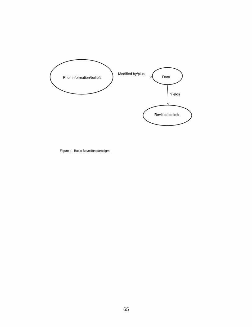
Figure 1. Basic Bayesian paradigm

Prior information/beliefs Data

Revised beliefs

Modified by/plus

Yields

65

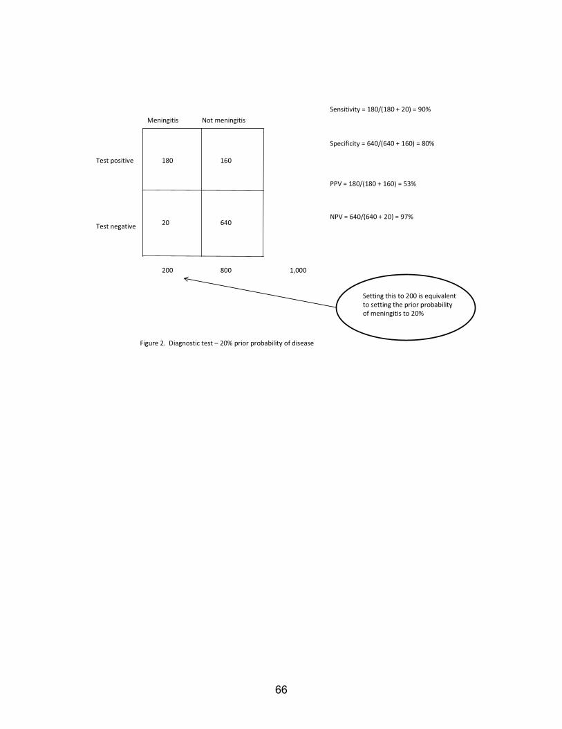
Figure 2.  Diagnostic test – 20% prior probability of disease

180 160

20 640

200 800 1,000

Meningitis              Not meningitis

Sensitivity = 180/(180 + 20) = 90%

Specificity = 640/(640 + 160) = 80%

PPV = 180/(180 + 160) = 53%

NPV = 640/(640 + 20) = 97%

Setting this to 200 is equivalent to setting the prior probability of meningitis to 20%

Test positive

Test negative

66

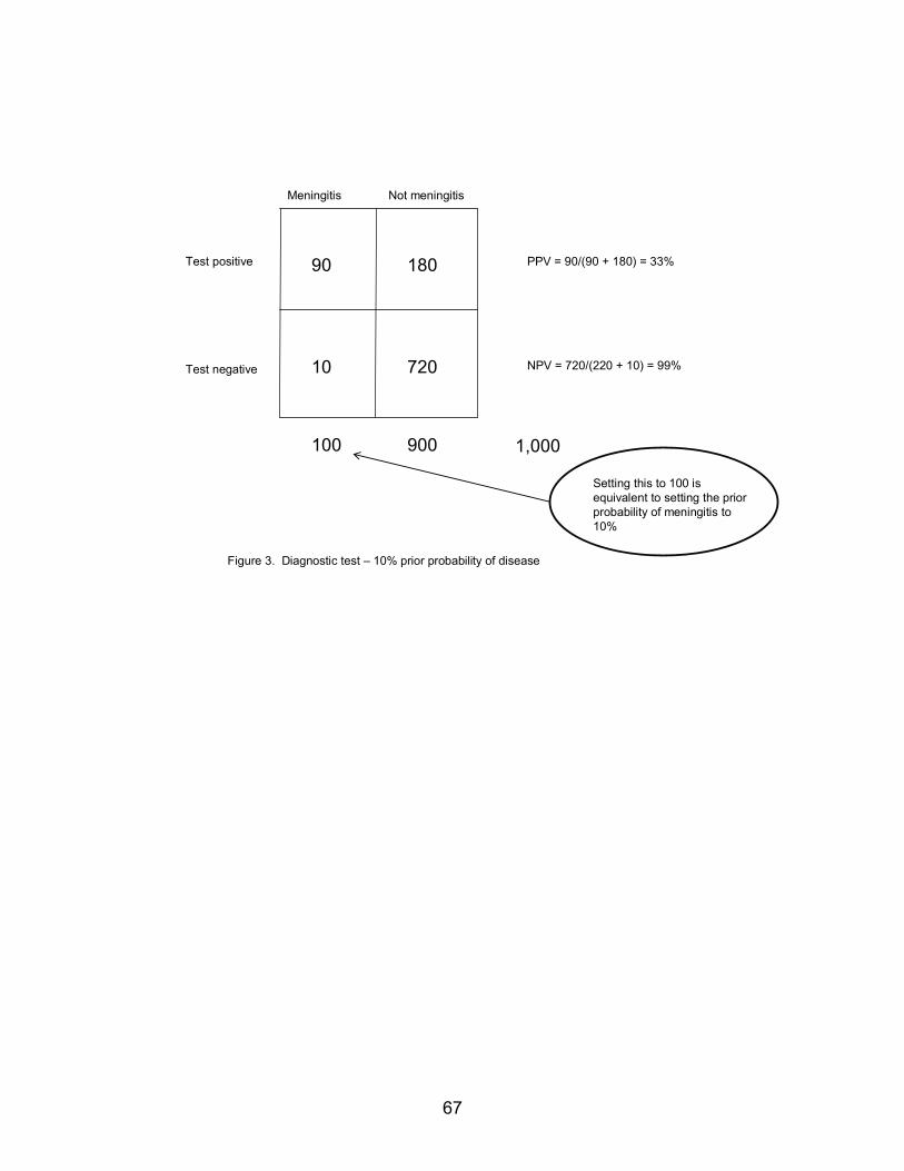
Figure 3. Diagnostic test – 10% prior probability of disease

90 180

10 720

100 900

Meningitis Not meningitis

PPV = 90/(90 + 180) = 33%

NPV = 720/(220 + 10) = 99%

Test positive

Test negative

1,000

Setting this to 100 is equivalent to setting the prior probability of meningitis to 10%

67

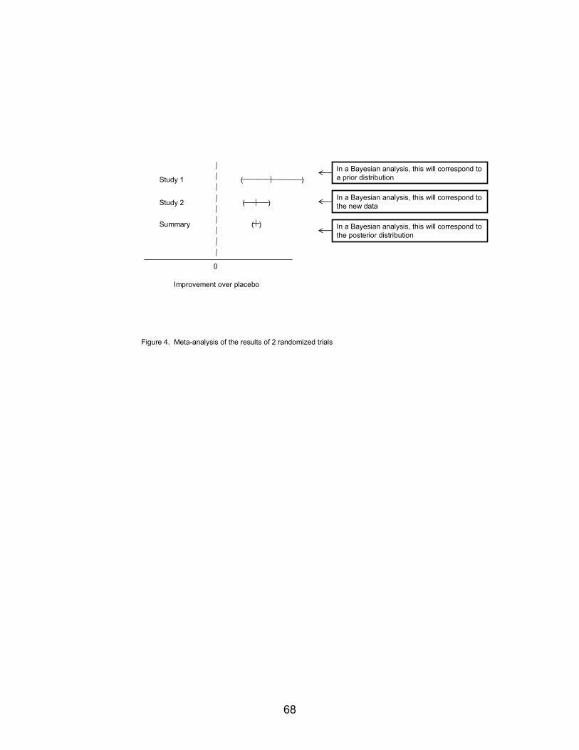
Figure 4. Meta-analysis of the results of 2 randomized trials

Improvement over placebo

0

Study 1

Study 2

Summary

In a Bayesian analysis, this will correspond to a prior distribution

In a Bayesian analysis, this will correspond to the new data

In a Bayesian analysis, this will correspond to the posterior distribution

( )

( )

( )

68

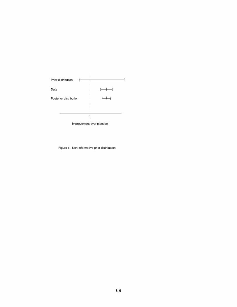
0

Prior distribution

Data

Posterior distribution

Figure 5. Non-informative prior distribution

)

)

)

(

(

(

Improvement over placebo

69

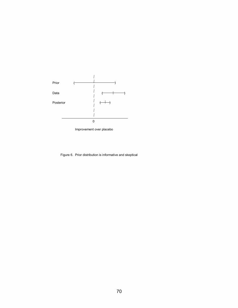
0

Prior

Data

Posterior

Figure 6. Prior distribution is informative and skeptical

)

)

)

(

(

(

Improvement over placebo

70

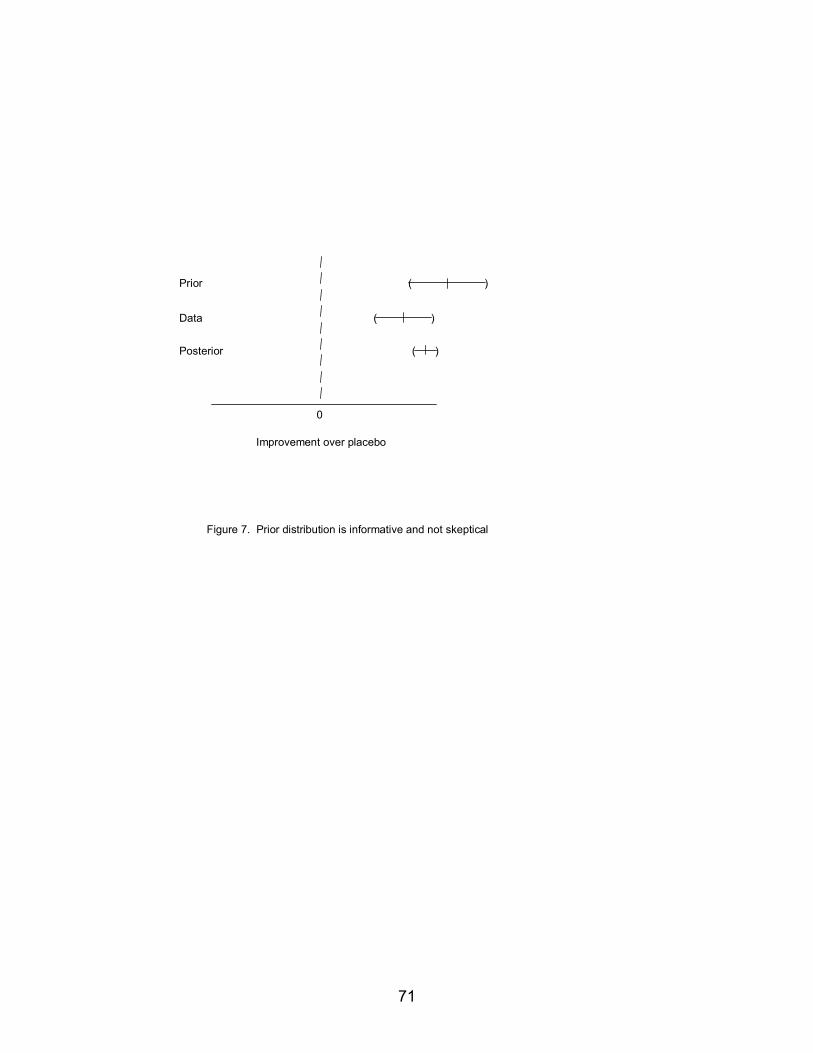
0

Prior

Data

Posterior

Figure 7. Prior distribution is informative and not skeptical

)(

)(

)(

Improvement over placebo

71

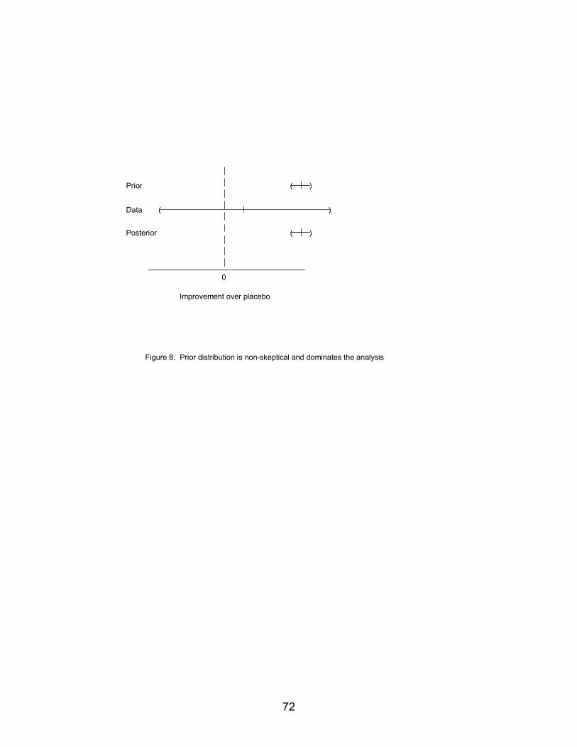
0

Prior

Data

Posterior

( )

Figure 8. Prior distribution is non-skeptical and dominates the analysis

( )

( )

Improvement over placebo

72

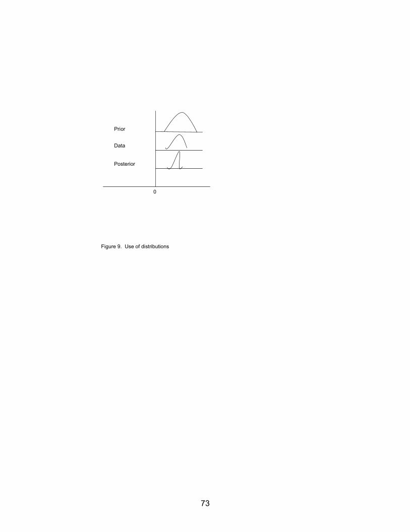
Figure 9. Use of distributions

0

Prior

Data

Posterior

73

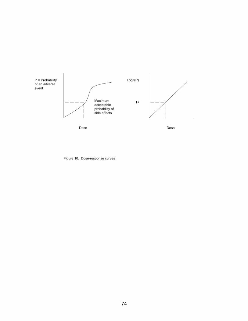
74

Figure 10. Dose-response curves

Dose Dose

P = Probability of an adverse event

Maximum acceptable probability of side effects

Logit(P)

1+

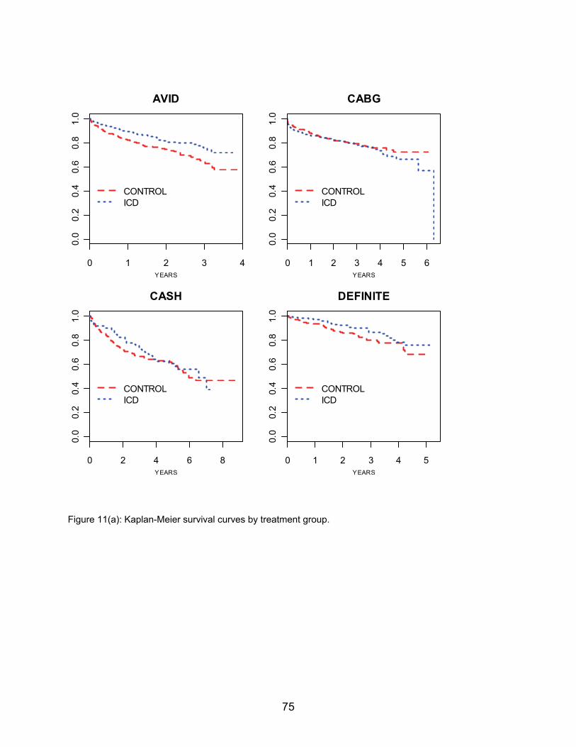
0 1 2 3 4

0.0

0.2

0.4

0.6

0.8

1.0

CONTROLICD

AVID

YEARS

0 1 2 3 4 5 60.

00.

20.

40.

60.

81.

0

CONTROLICD

CABG

YEARS

0 2 4 6 8

0.0

0.2

0.4

0.6

0.8

1.0

CONTROLICD

CASH

YEARS

0 1 2 3 4 5

0.0

0.2

0.4

0.6

0.8

1.0

CONTROLICD

DEFINITE

YEARS

Figure 11(a): Kaplan-Meier survival curves by treatment group.

75

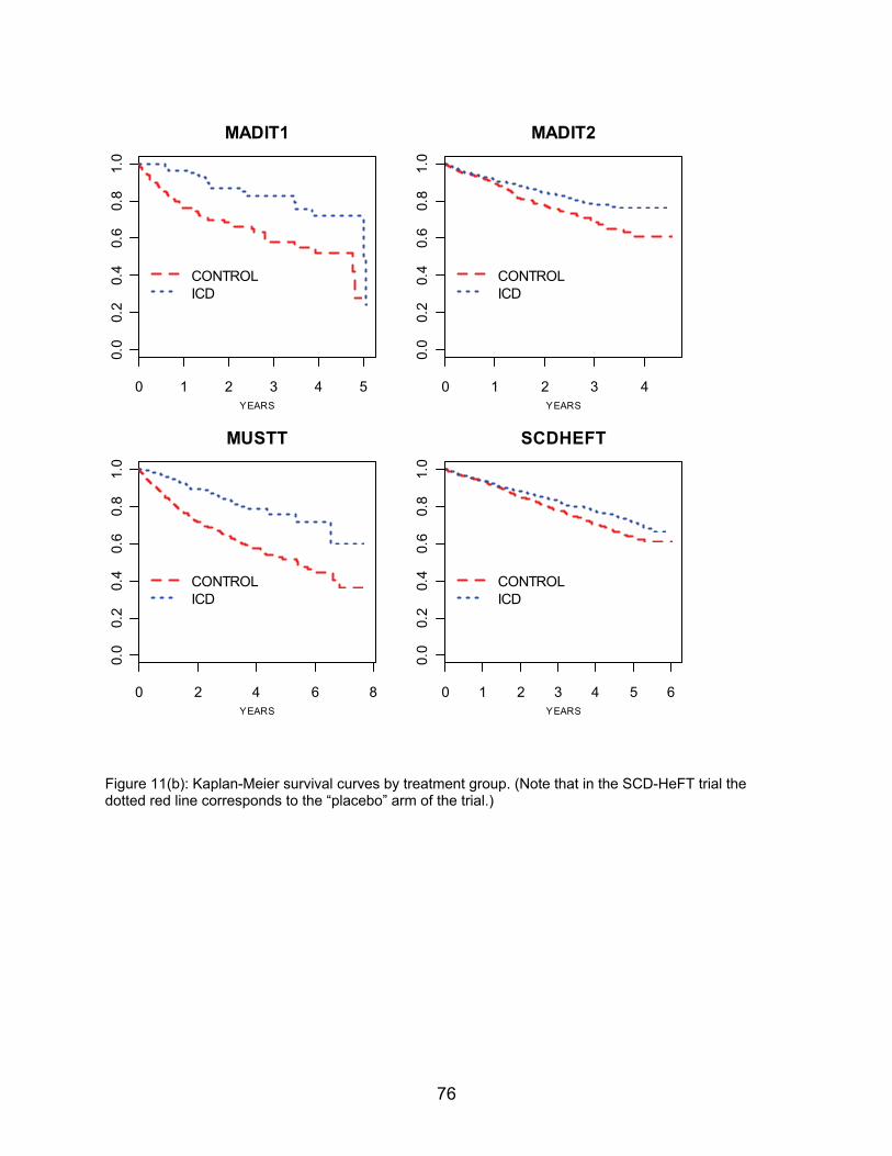
0 1 2 3 4 5

0.0

0.2

0.4

0.6

0.8

1.0

CONTROLICD

MADIT1

YEARS

0 1 2 3 4

0.0

0.2

0.4

0.6

0.8

1.0

CONTROLICD

MADIT2

YEARS

0 2 4 6 8

0.0

0.2

0.4

0.6

0.8

1.0

CONTROLICD

MUSTT

YEARS

0 1 2 3 4 5 6

0.0

0.2

0.4

0.6

0.8

1.0

CONTROLICD

SCDHEFT

YEARS

Figure 11(b): Kaplan-Meier survival curves by treatment group. (Note that in the SCD-HeFT trial the dotted red line corresponds to the “placebo” arm of the trial.)

76

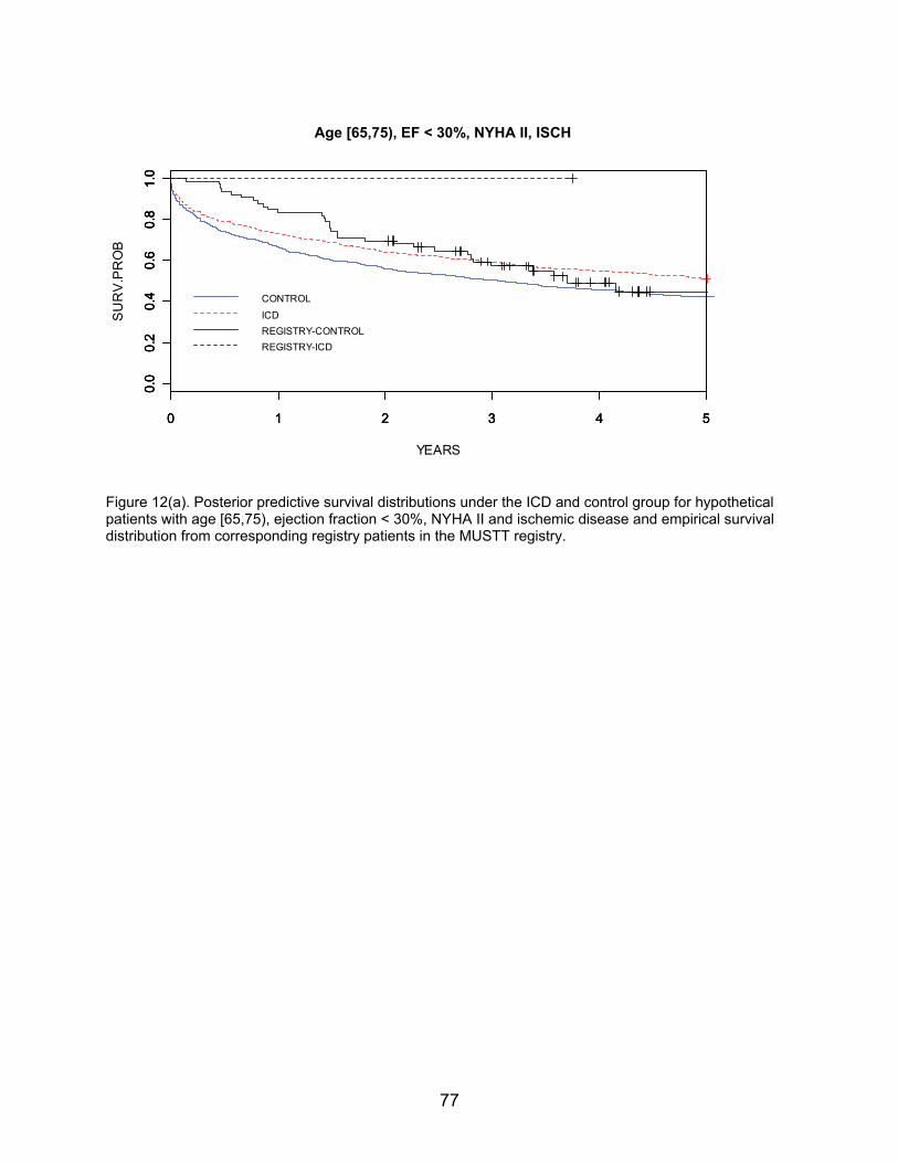
77

YEARS

SU

RV

.PR

OB

0 1 2 3 4 5

0.0

0.2

0.4

0.6

0.8

1.0

0 1 2 3 4 5

0.0

0.2

0.4

0.6

0.8

1.0

0 1 2 3 4 5

0.0

0.2

0.4

0.6

0.8

1.0

Age [65,75), EJ < 30%, NYHA2, ISCHAge [65,75), EF < 30%, NYHA II, ISCH

CONTROL

ICDREGISTRY-CONTROLREGISTRY-ICD

Figure 12(a). Posterior predictive survival distributions under the ICD and control group for hypothetical patients with age [65,75), ejection fraction < 30%, NYHA II and ischemic disease and empirical survival distribution from corresponding registry patients in the MUSTT registry.

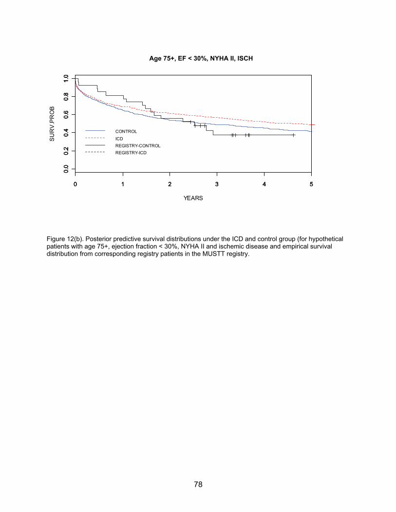
78

YEARS

SU

RV

.PR

OB

0 1 2 3 4 5

0.0

0.2

0.4

0.6

0.8

1.0

0 1 2 3 4 5

0.0

0.2

0.4

0.6

0.8

1.0

0 1 2 3 4 5

0.0

0.2

0.4

0.6

0.8

1.0

Age 75+, EJ < 30%, NYHA2, ISCHAge 75+, EF < 30%, NYHA II, ISCH

CONTROL

ICDREGISTRY-CONTROLREGISTRY-ICD

Figure 12(b). Posterior predictive survival distributions under the ICD and control group (for hypothetical patients with age 75+, ejection fraction < 30%, NYHA II and ischemic disease and empirical survival distribution from corresponding registry patients in the MUSTT registry.

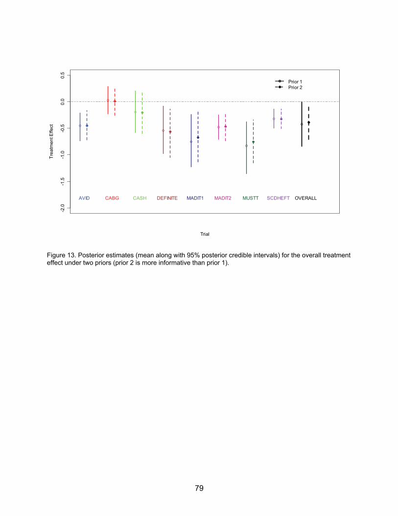
Trial

Trea

tmen

t Effe

ct

-2.0

-1.5

-1.0

-0.5

0.0

0.5

AVID CABG CASH DEFINITE MADIT1 MADIT2 MUSTT SCDHEFT

Prior 1Prior 2

OVERALL

Figure 13. Posterior estimates (mean along with 95% posterior credible intervals) for the overall treatment effect under two priors (prior 2 is more informative than prior 1).

79

80

0 2 4 6 8 10

0.0

0.2

0.4

0.6

0.8

1.0

YEARS

Bas

elin

e S

urvi

val

AVIDCABGCASHDEFINITEMADIT1MADIT2MUSTTSCDHEFTOVERALL

Figure 14. Estimated posterior baseline survival functions.

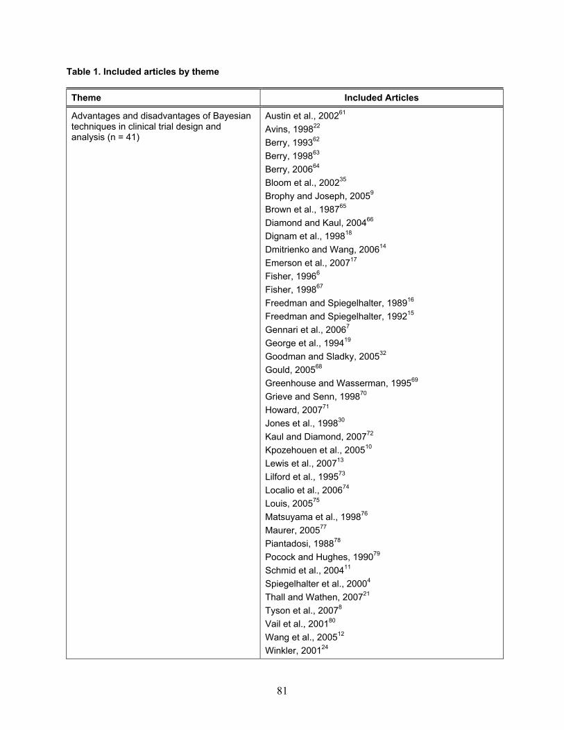
Table 1. Included articles by theme Theme Included Articles

Advantages and disadvantages of Bayesian techniques in clinical trial design and analysis (n = 41)

Austin et al., 200261 Avins, 199822 Berry, 199362 Berry, 199863 Berry, 200664 Bloom et al., 200235 Brophy and Joseph, 20059 Brown et al., 198765 Diamond and Kaul, 200466 Dignam et al., 199818 Dmitrienko and Wang, 200614 Emerson et al., 200717 Fisher, 19966 Fisher, 199867 Freedman and Spiegelhalter, 198916 Freedman and Spiegelhalter, 199215 Gennari et al., 20067 George et al., 199419 Goodman and Sladky, 200532 Gould, 200568 Greenhouse and Wasserman, 199569 Grieve and Senn, 199870 Howard, 200771 Jones et al., 199830 Kaul and Diamond, 200772 Kpozehouen et al., 200510 Lewis et al., 200713 Lilford et al., 199573 Localio et al., 200674 Louis, 200575 Matsuyama et al., 199876 Maurer, 200577 Piantadosi, 198878 Pocock and Hughes, 199079 Schmid et al., 200411 Spiegelhalter et al., 20004 Thall and Wathen, 200721 Tyson et al., 20078 Vail et al., 200180 Wang et al., 200512 Winkler, 200124

81

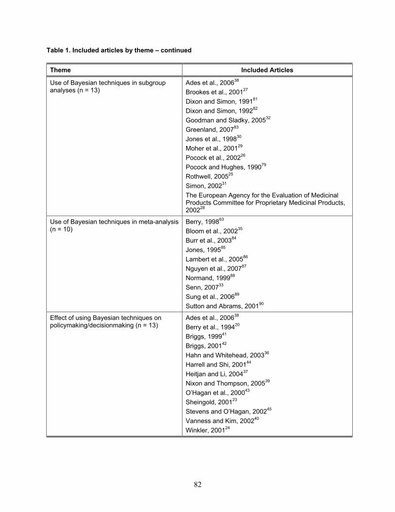
82

Table 1. Included articles by theme – continued Theme Included Articles

Use of Bayesian techniques in subgroup analyses (n = 13)

Ades et al., 200638 Brookes et al., 200127 Dixon and Simon, 199181 Dixon and Simon, 199282 Goodman and Sladky, 200532 Greenland, 200783 Jones et al., 199830 Moher et al., 200129 Pocock et al., 200226 Pocock and Hughes, 199079 Rothwell, 200525 Simon, 200231 The European Agency for the Evaluation of Medicinal Products Committee for Proprietary Medicinal Products, 200228

Use of Bayesian techniques in meta-analysis (n = 10)

Berry, 199863 Bloom et al., 200235 Burr et al., 200384 Jones, 199585 Lambert et al., 200586 Nguyen et al., 200787 Normand, 199988 Senn, 200733 Sung et al., 200689 Sutton and Abrams, 200190

Effect of using Bayesian techniques on policymaking/decisionmaking (n = 13)

Ades et al., 200638 Berry et al., 199420 Briggs, 199941 Briggs, 200142 Hahn and Whitehead, 200336 Harrell and Shi, 200144 Heitjan and Li, 200437 Nixon and Thompson, 200539 O’Hagan et al., 200043 Sheingold, 200123 Stevens and O’Hagan, 200245 Vanness and Kim, 200240 Winkler, 200124

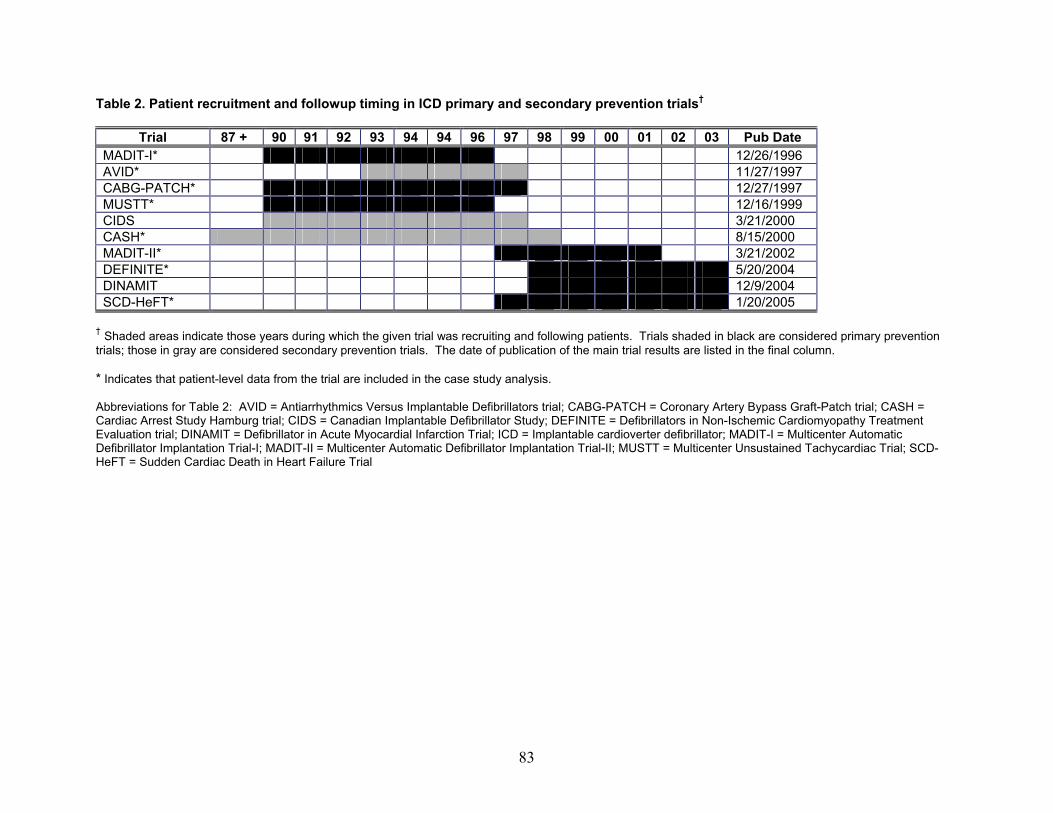
Table 2. Patient recruitment and followup timing in ICD primary and secondary prevention trials†

Trial 87 + 90 91 92 93 94 94 96 97 98 99 00 01 02 03 Pub Date MADIT-I* 12/26/1996 AVID* 11/27/1997 CABG-PATCH* 12/27/1997 MUSTT* 12/16/1999 CIDS 3/21/2000 CASH* 8/15/2000 MADIT-II* 3/21/2002 DEFINITE* 5/20/2004 DINAMIT 12/9/2004 SCD-HeFT* 1/20/2005

† Shaded areas indicate those years during which the given trial was recruiting and following patients. Trials shaded in black are considered primary prevention trials; those in gray are considered secondary prevention trials. The date of publication of the main trial results are listed in the final column. * Indicates that patient-level data from the trial are included in the case study analysis. Abbreviations for Table 2: AVID = Antiarrhythmics Versus Implantable Defibrillators trial; CABG-PATCH = Coronary Artery Bypass Graft-Patch trial; CASH = Cardiac Arrest Study Hamburg trial; CIDS = Canadian Implantable Defibrillator Study; DEFINITE = Defibrillators in Non-Ischemic Cardiomyopathy Treatment Evaluation trial; DINAMIT = Defibrillator in Acute Myocardial Infarction Trial; ICD = Implantable cardioverter defibrillator; MADIT-I = Multicenter Automatic Defibrillator Implantation Trial-I; MADIT-II = Multicenter Automatic Defibrillator Implantation Trial-II; MUSTT = Multicenter Unsustained Tachycardiac Trial; SCD-HeFT = Sudden Cardiac Death in Heart Failure Trial

83

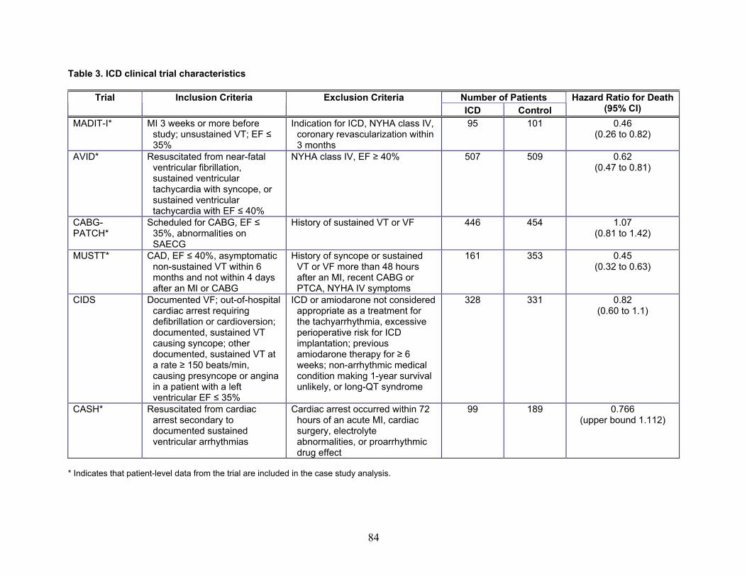
Table 3. ICD clinical trial characteristics

Number of Patients Trial Inclusion Criteria Exclusion Criteria ICD Control

Hazard Ratio for Death (95% CI)

MADIT-I* MI 3 weeks or more before study; unsustained VT; EF ≤ 35%

Indication for ICD, NYHA class IV, coronary revascularization within 3 months

95 101 0.46 (0.26 to 0.82)

AVID* Resuscitated from near-fatal ventricular fibrillation, sustained ventricular tachycardia with syncope, or sustained ventricular tachycardia with EF ≤ 40%

NYHA class IV, EF ≥ 40% 507 509 0.62 (0.47 to 0.81)

CABG-PATCH*

Scheduled for CABG, EF ≤ 35%, abnormalities on SAECG

History of sustained VT or VF 446 454 1.07 (0.81 to 1.42)

MUSTT* CAD, EF ≤ 40%, asymptomatic non-sustained VT within 6 months and not within 4 days after an MI or CABG

History of syncope or sustained VT or VF more than 48 hours after an MI, recent CABG or PTCA, NYHA IV symptoms

161 353 0.45 (0.32 to 0.63)

CIDS Documented VF; out-of-hospital cardiac arrest requiring defibrillation or cardioversion; documented, sustained VT causing syncope; other documented, sustained VT at a rate ≥ 150 beats/min, causing presyncope or angina in a patient with a left ventricular EF ≤ 35%

ICD or amiodarone not considered appropriate as a treatment for the tachyarrhythmia, excessive perioperative risk for ICD implantation; previous amiodarone therapy for ≥ 6 weeks; non-arrhythmic medical condition making 1-year survival unlikely, or long-QT syndrome

328 331 0.82 (0.60 to 1.1)

CASH* Resuscitated from cardiac arrest secondary to documented sustained ventricular arrhythmias

Cardiac arrest occurred within 72 hours of an acute MI, cardiac surgery, electrolyte abnormalities, or proarrhythmic drug effect

99 189 0.766 (upper bound 1.112)

* Indicates that patient-level data from the trial are included in the case study analysis.

84

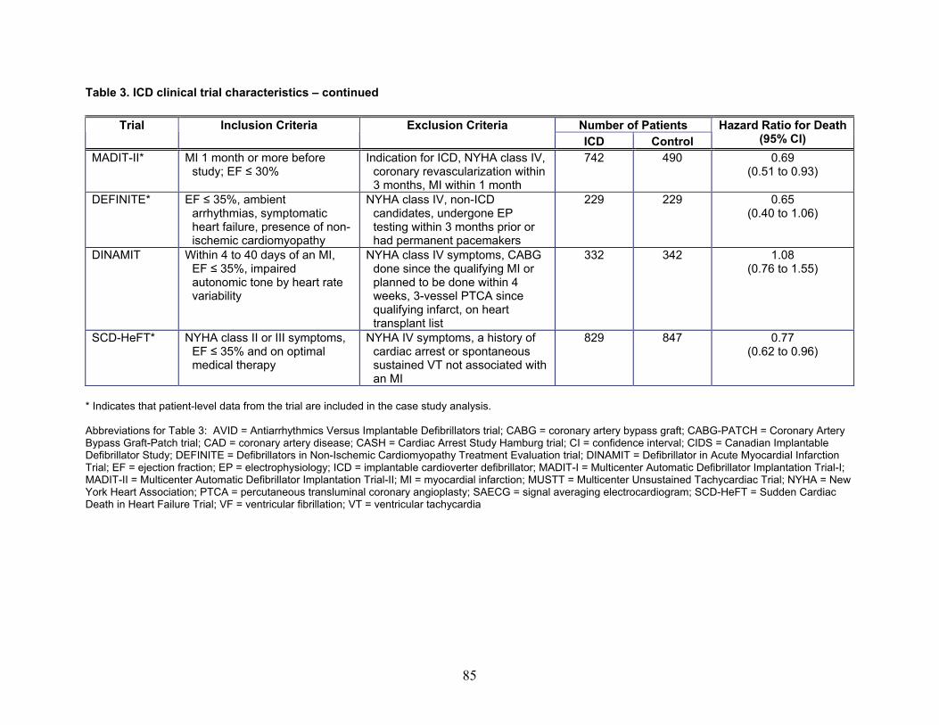
Table 3. ICD clinical trial characteristics – continued

Number of Patients Trial Inclusion Criteria Exclusion Criteria ICD Control

Hazard Ratio for Death (95% CI)

MADIT-II* MI 1 month or more before study; EF ≤ 30%

Indication for ICD, NYHA class IV, coronary revascularization within 3 months, MI within 1 month

742 490 0.69 (0.51 to 0.93)

DEFINITE* EF ≤ 35%, ambient arrhythmias, symptomatic heart failure, presence of non-ischemic cardiomyopathy

NYHA class IV, non-ICD candidates, undergone EP testing within 3 months prior or had permanent pacemakers

229 229 0.65 (0.40 to 1.06)

DINAMIT Within 4 to 40 days of an MI, EF ≤ 35%, impaired autonomic tone by heart rate variability

NYHA class IV symptoms, CABG done since the qualifying MI or planned to be done within 4 weeks, 3-vessel PTCA since qualifying infarct, on heart transplant list

332 342 1.08 (0.76 to 1.55)

SCD-HeFT* NYHA class II or III symptoms, EF ≤ 35% and on optimal medical therapy

NYHA IV symptoms, a history of cardiac arrest or spontaneous sustained VT not associated with an MI

829 847 0.77 (0.62 to 0.96)

* Indicates that patient-level data from the trial are included in the case study analysis. Abbreviations for Table 3: AVID = Antiarrhythmics Versus Implantable Defibrillators trial; CABG = coronary artery bypass graft; CABG-PATCH = Coronary Artery Bypass Graft-Patch trial; CAD = coronary artery disease; CASH = Cardiac Arrest Study Hamburg trial; CI = confidence interval; CIDS = Canadian Implantable Defibrillator Study; DEFINITE = Defibrillators in Non-Ischemic Cardiomyopathy Treatment Evaluation trial; DINAMIT = Defibrillator in Acute Myocardial Infarction Trial; EF = ejection fraction; EP = electrophysiology; ICD = implantable cardioverter defibrillator; MADIT-I = Multicenter Automatic Defibrillator Implantation Trial-I; MADIT-II = Multicenter Automatic Defibrillator Implantation Trial-II; MI = myocardial infarction; MUSTT = Multicenter Unsustained Tachycardiac Trial; NYHA = New York Heart Association; PTCA = percutaneous transluminal coronary angioplasty; SAECG = signal averaging electrocardiogram; SCD-HeFT = Sudden Cardiac Death in Heart Failure Trial; VF = ventricular fibrillation; VT = ventricular tachycardia

85

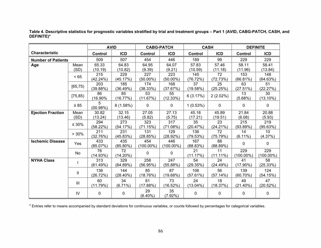
Table 4. Descriptive statistics for prognostic variables stratified by trial and treatment groups – Part 1 (AVID, CABG-PATCH, CASH, and DEFINITE)*

AVID CABG-PATCH CASH DEFINITE Characteristic Control ICD Control ICD Control ICD Control ICD Number of Patients 509 507 454 446 189 99 229 229

Mean (SD)

65.33 (10.19)

64.83 (10.82)

64.95 (9.39)

64.07 (9.21)

57.83 (10.59)

57.46 (11.18)

58.11 (11.96)

58.41 (13.84)

< 65 215 (42.24%)

229 (45.17%)

227 (50.00%)

223 (50.00%)

145 (76.72%)

72 (72.73%)

153 (66.81%)

148 (64.63%)

[65,75) 203 (39.88%)

185 (36.49%)

174 (38.33%)

168 (37.67%)

37 (19.58%)

25 (25.25%)

63 (27.51%)

51 (22.27%)

[75,85) 86 (16.90%

85 (16.77%)

53 (11.67%)

55 (12.33%) 6 (3.17%) 2 (2.02%) 13

(5.68%) 30

(13.10%)

Age

≥ 85 5 (00.98%) 8 (1.58%) 0 0 1 (0.53%) 0 0 0

Mean (SD)

30.82 (13.24)

32.15 (13.46)

27.05 (5.82)

27.13 (5.75)

45.18 (17.21)

45.89 (19.51)

21.84 (6.08)

20.88 (5.93)

≤ 30% 294 (58.22%)

273 (54.17%)

323 (71.15%)

317 (71.08%)

35 (20.47%)

23 (24.21%)

215 (93.89%)

219 (95.63%)

Ejection Fraction

> 30% 211 (32.76%)

231 (45.83%)

131 (28.85%)

129 (28.92%)

136 (79.53%)

72 (75.79%)

14 (6.11%)

10 (4.37%)

Yes 433 (85.07%)

435 (85.80%)

454 (100.00%)

446 (100.00%)

167 (88.83%)

88 (88.89%) 0 0 Ischemic Disease

No 76 (14.93%)

72 (14.20%) 0 0 21

(11.17%) 11

(11.11%) 229

(100.00%) 229

(100.00%)

I 313 (61.49%)

329 (64.89%)

258 (56.95%)

247 (55.88%)

54 (29.35%)

24 (24.49%)

41 (17.90%)

58 (25.33%)

II 136 (26.72%)

144 (28.40%)

85 (18.76%)

87 (19.68%)

106 (57.61%)

56 (57.14%)

139 (60.70%)

124 (54.15%)

III 60 (11.79%)

34 (6.71%)

81 (17.88%)

73 (16.52%)

24 (13.04%)

18 (18.37%)

49 (21.40%)

47 (20.52%)

NYHA Class

IV 0 0 29 (6.40%)

35 (7.92%) 0 0 0 0

* Entries refer to means accompanied by standard deviations for continuous variables, or counts followed by percentages for categorical variables.

86

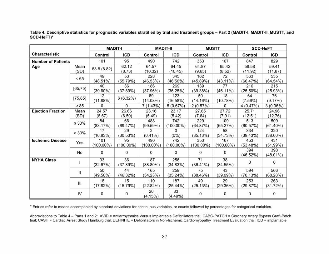
Table 4. Descriptive statistics for prognostic variables stratified by trial and treatment groups – Part 2 (MADIT-I, MADIT-II, MUSTT, and SCD-HeFT)*

MADIT-I MADIT-II MUSTT SCD-HeFT Characteristic Control ICD Control ICD Control ICD Control ICD Number of Patients 101 95 490 742 353 167 847 829

Mean (SD) 63.8 (8.82) 62.12

(8.73) 64.57

(10.32) 64.45

(10.45) 64.87 (9.65)

65.42 (8.52)

58.58 (11.92)

59.41 (11.87)

< 65 49 (48.51%)

53 (55.79%)

228 (46.53%)

345 (46.50%)

162 (45.89%)

72 (43.11%)

563 (66.47%)

535 (64.54%)

[65,75) 40 (39.60%)

36 (37.89%)

186 (37.96%)

269 (36.25%)

139 (39.38%)

77 (46.11%)

216 (25.50%)

215 (25.93%)

[75,85) 12 (11.88%) 6 (6.32%) 69

(14.08%) 123

(16.58%) 50

(14.16%) 18

(10.78%) 64

(7.56%) 76

(9.17%)

Age

≥ 85 0 0 7 (1.43%) 5 (0.67%) 2 (0.57%) 0 4 (0.47%) 3 (0.36%) Mean (SD)

24.57 (6.67)

26.66 (6.50)

23.16 (5.49)

23.17 (5.42)

27.65 (7.64)

27.72 (7.91)

25.71 (12.51)

24.96 (12.76)

≤ 30% 84 (83.17%)

66 (69.47%)

488 (99.59%)

742 (100.00%)

229 (64.87%)

109 (65.27%)

513 (60.57%)

509 (61.40%)

Ejection Fraction

> 30% 17 (16.83%)

29 (30.53%)

2 (0.41%)

0 (0%)

124 (35.13%)

58 (34.73%)

334 (39.43%)

320 (38.60%)

Yes 101 (100.00%)

95 (100.00%)

490 (100.00%)

742 (100.00%)

353 (100.00%)

167 (100.00%)

453 (53.48%)

431 (51.99%)

Ischemic Disease

No 0 0 0 0 0 0 394 (46.52%)

398 (48.01%)

I 33 (32.67%)

36 (37.89%)

187 (38.80%)

256 (34.83%)

71 (36.41%)

38 (34.55%) 0 0

II 50 (49.50%)

44 (46.32%)

165 (34.23%)

259 (35.24%)

75 (38.46%)

43 (39.09%)

594 (70.13%)

566 (68.28%)

III 18 (17.82%)

15 (15.79%)

110 (22.82%)

187 (25.44%)

49 (25.13%)

29 (29.36%)

253 (29.87%)

263 (31.72%)

NYHA Class

IV 0 0 20 (4.15%)

33 (4.49%) 0 0 0 0

* Entries refer to means accompanied by standard deviations for continuous variables, or counts followed by percentages for categorical variables. Abbreviations to Table 4 – Parts 1 and 2: AVID = Antiarrhythmics Versus Implantable Defibrillators trial; CABG-PATCH = Coronary Artery Bypass Graft-Patch trial; CASH = Cardiac Arrest Study Hamburg trial; DEFINITE = Defibrillators in Non-Ischemic Cardiomyopathy Treatment Evaluation trial; ICD = implantable

87

88

cardioverter defibrillator; MADIT-I = Multicenter Automatic Defibrillator Implantation Trial-I; MADIT-II = Multicenter Automatic Defibrillator Implantation Trial-II; MUSTT = Multicenter Unsustained Tachycardiac Trial; NYHA = New York Heart Association; SCD-HeFT = Sudden Cardiac Death in Heart Failure Trial; SD = standard deviation

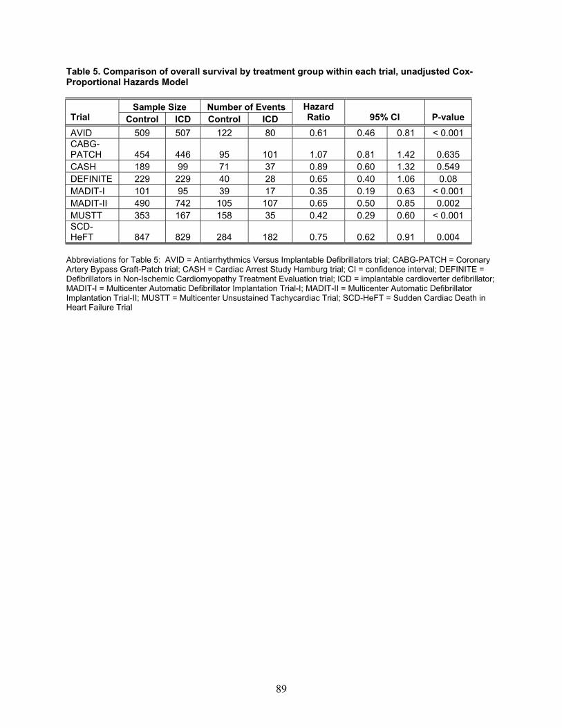
Table 5. Comparison of overall survival by treatment group within each trial, unadjusted Cox-Proportional Hazards Model

Sample Size Number of Events Trial Control ICD Control ICD

Hazard Ratio 95% CI P-value

AVID 509 507 122 80 0.61 0.46 0.81 < 0.001 CABG-PATCH 454 446 95 101 1.07 0.81 1.42 0.635 CASH 189 99 71 37 0.89 0.60 1.32 0.549 DEFINITE 229 229 40 28 0.65 0.40 1.06 0.08 MADIT-I 101 95 39 17 0.35 0.19 0.63 < 0.001 MADIT-II 490 742 105 107 0.65 0.50 0.85 0.002 MUSTT 353 167 158 35 0.42 0.29 0.60 < 0.001 SCD-HeFT 847 829 284 182 0.75 0.62 0.91 0.004

Abbreviations for Table 5: AVID = Antiarrhythmics Versus Implantable Defibrillators trial; CABG-PATCH = Coronary Artery Bypass Graft-Patch trial; CASH = Cardiac Arrest Study Hamburg trial; CI = confidence interval; DEFINITE = Defibrillators in Non-Ischemic Cardiomyopathy Treatment Evaluation trial; ICD = implantable cardioverter defibrillator; MADIT-I = Multicenter Automatic Defibrillator Implantation Trial-I; MADIT-II = Multicenter Automatic Defibrillator Implantation Trial-II; MUSTT = Multicenter Unsustained Tachycardiac Trial; SCD-HeFT = Sudden Cardiac Death in Heart Failure Trial

89

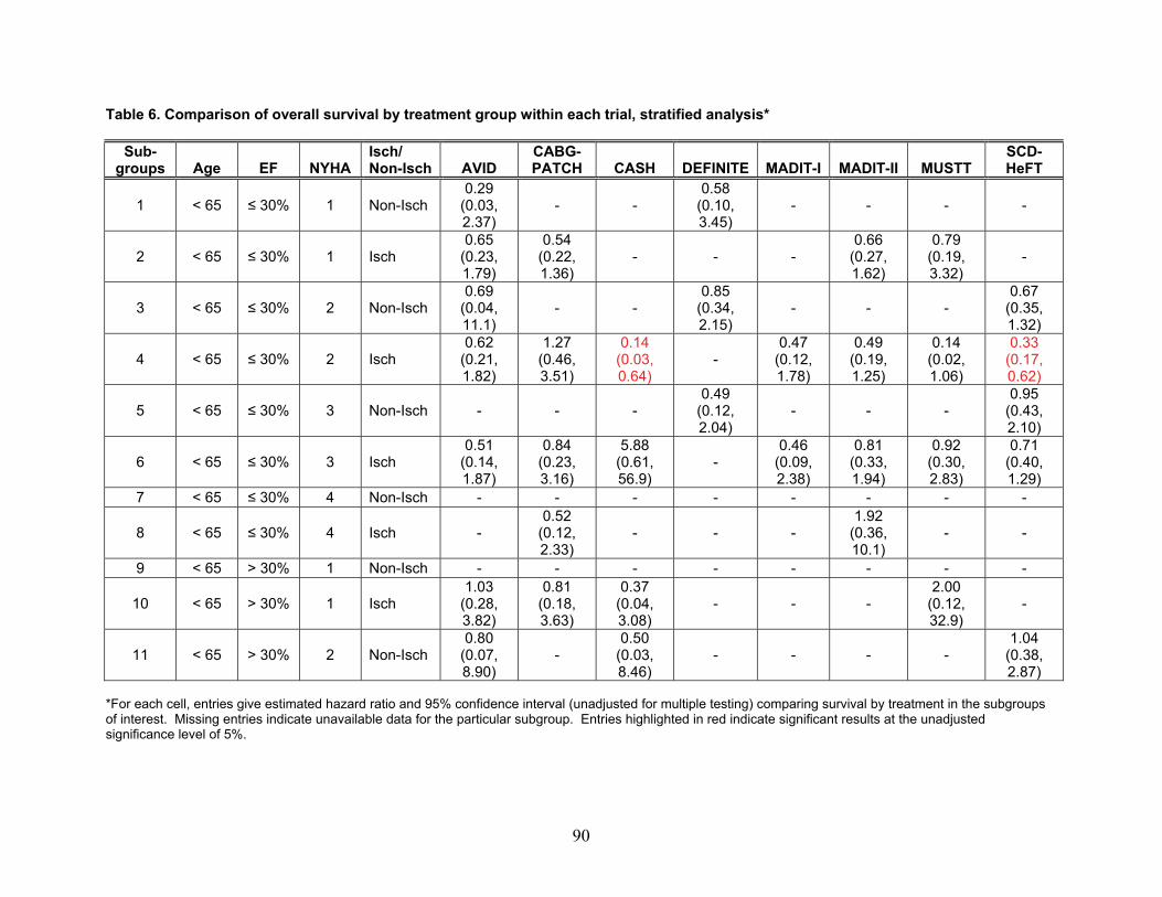
Table 6. Comparison of overall survival by treatment group within each trial, stratified analysis*

Sub-groups Age EF NYHA

Isch/ Non-Isch AVID

CABG-PATCH CASH DEFINITE MADIT-I MADIT-II MUSTT

SCD-HeFT

1 < 65 ≤ 30% 1 Non-Isch 0.29

(0.03, 2.37)

- - 0.58

(0.10, 3.45)

- - - -

2 < 65 ≤ 30% 1 Isch 0.65

(0.23, 1.79)

0.54 (0.22, 1.36)

- - - 0.66

(0.27, 1.62)

0.79 (0.19, 3.32)

-

3 < 65 ≤ 30% 2 Non-Isch 0.69

(0.04, 11.1)

- - 0.85

(0.34, 2.15)

- - - 0.67

(0.35, 1.32)

4 < 65 ≤ 30% 2 Isch 0.62

(0.21, 1.82)

1.27 (0.46, 3.51)

0.14 (0.03, 0.64)

- 0.47

(0.12, 1.78)

0.49 (0.19, 1.25)

0.14 (0.02, 1.06)

0.33 (0.17, 0.62)

5 < 65 ≤ 30% 3 Non-Isch - - - 0.49

(0.12, 2.04)

- - - 0.95

(0.43, 2.10)

6 < 65 ≤ 30% 3 Isch 0.51

(0.14, 1.87)

0.84 (0.23, 3.16)

5.88 (0.61, 56.9)

- 0.46

(0.09, 2.38)

0.81 (0.33, 1.94)

0.92 (0.30, 2.83)

0.71 (0.40, 1.29)

7 < 65 ≤ 30% 4 Non-Isch - - - - - - - -

8 < 65 ≤ 30% 4 Isch - 0.52

(0.12, 2.33)

- - - 1.92

(0.36, 10.1)

- -

9 < 65 > 30% 1 Non-Isch - - - - - - - -

10 < 65 > 30% 1 Isch 1.03

(0.28, 3.82)

0.81 (0.18, 3.63)

0.37 (0.04, 3.08)

- - - 2.00

(0.12, 32.9)

-

11 < 65 > 30% 2 Non-Isch 0.80

(0.07, 8.90)

- 0.50

(0.03, 8.46)

- - - - 1.04

(0.38, 2.87)

*For each cell, entries give estimated hazard ratio and 95% confidence interval (unadjusted for multiple testing) comparing survival by treatment in the subgroups of interest. Missing entries indicate unavailable data for the particular subgroup. Entries highlighted in red indicate significant results at the unadjusted significance level of 5%.

90

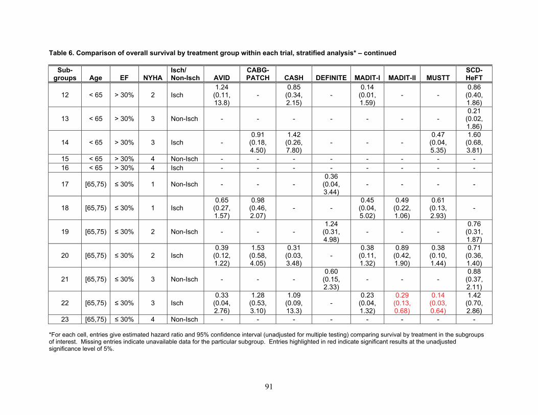
Table 6. Comparison of overall survival by treatment group within each trial, stratified analysis* – continued

Sub-groups Age EF NYHA

Isch/ Non-Isch AVID

CABG-PATCH CASH DEFINITE MADIT-I MADIT-II MUSTT

SCD-HeFT

12 < 65 > 30% 2 Isch 1.24

(0.11, 13.8)

- 0.85

(0.34, 2.15)

- 0.14

(0.01, 1.59)

- - 0.86

(0.40, 1.86)

13 < 65 > 30% 3 Non-Isch - - - - - - - 0.21

(0.02, 1.86)

14 < 65 > 30% 3 Isch - 0.91

(0.18, 4.50)

1.42 (0.26, 7.80)

- - - 0.47

(0.04, 5.35)

1.60 (0.68, 3.81)

15 < 65 > 30% 4 Non-Isch - - - - - - - - 16 < 65 > 30% 4 Isch - - - - - - - -

17 [65,75) ≤ 30% 1 Non-Isch - - - 0.36

(0.04, 3.44)

- - - -

18 [65,75) ≤ 30% 1 Isch 0.65

(0.27, 1.57)

0.98 (0.46, 2.07)

- - 0.45

(0.04, 5.02)

0.49 (0.22, 1.06)

0.61 (0.13, 2.93)

-

19 [65,75) ≤ 30% 2 Non-Isch - - - 1.24

(0.31, 4.98)

- - - 0.76

(0.31, 1.87)

20 [65,75) ≤ 30% 2 Isch 0.39

(0.12, 1.22)

1.53 (0.58, 4.05)

0.31 (0.03, 3.48)

- 0.38

(0.11, 1.32)

0.89 (0.42, 1.90)

0.38 (0.10, 1.44)

0.71 (0.36, 1.40)

21 [65,75) ≤ 30% 3 Non-Isch - - - 0.60

(0.15, 2.33)

- - - 0.88

(0.37, 2.11)

22 [65,75) ≤ 30% 3 Isch 0.33

(0.04, 2.76)

1.28 (0.53, 3.10)

1.09 (0.09, 13.3)

- 0.23

(0.04, 1.32)

0.29 (0.13, 0.68)

0.14 (0.03, 0.64)

1.42 (0.70, 2.86)

23 [65,75) ≤ 30% 4 Non-Isch - - - - - - - - *For each cell, entries give estimated hazard ratio and 95% confidence interval (unadjusted for multiple testing) comparing survival by treatment in the subgroups of interest. Missing entries indicate unavailable data for the particular subgroup. Entries highlighted in red indicate significant results at the unadjusted significance level of 5%.

91

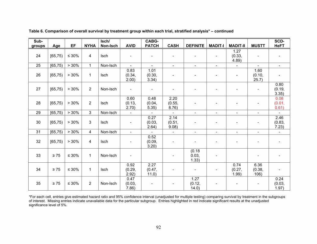
Table 6. Comparison of overall survival by treatment group within each trial, stratified analysis* – continued

Sub-groups Age EF NYHA

Isch/ Non-Isch AVID

CABG-PATCH CASH DEFINITE MADIT-I MADIT-II MUSTT

SCD-HeFT

24 [65,75) ≤ 30% 4 Isch - - - - - 1.27

(0.33, 4.89)

- -

25 [65,75) > 30% 1 Non-Isch - - - - - - - -

26 [65,75) > 30% 1 Isch 0.83

(0.34, 2.00)

1.01 (0.30, 3.34)

- - - - 1.60

(0.10, 25.7)

-

27 [65,75) > 30% 2 Non-Isch - - - - - - - 0.80

(0.19, 3.35)

28 [65,75) > 30% 2 Isch 0.60

(0.13, 2.70)

0.48 (0.04, 5.35)

2.20 (0.55, 8.76)

- - - - 0.08

(0.01, 0.61)

29 [65,75) > 30% 3 Non-Isch - - - - - - - -

30 [65,75) > 30% 3 Isch - 0.27

(0.03, 2.64)

2.14 (0.51, 9.08)

- - - - 2.46

(0.83, 7.23)

31 [65,75) > 30% 4 Non-Isch - - - - - - - -

32 [65,75) > 30% 4 Isch - 0.52

(0.09, 3.20)

- - - - - -

33 ≥ 75 ≤ 30% 1 Non-Isch - - (0.18 0.03, 1.33)

- - -

34 ≥ 75 ≤ 30% 1 Isch 0.92

(0.29, 2.92)

2.27 (0.47, 11.0)

- - - 0.74

(0.27, 1.99)

6.36 (0.38, 106)

-

35 ≥ 75 ≤ 30% 2 Non-Isch 0.47

(0.03, 7.86)

- - 1.27

(0.12, 14.0)

- - - 0.24

(0.03, 1.97)

*For each cell, entries give estimated hazard ratio and 95% confidence interval (unadjusted for multiple testing) comparing survival by treatment in the subgroups of interest. Missing entries indicate unavailable data for the particular subgroup. Entries highlighted in red indicate significant results at the unadjusted significance level of 5%.

92

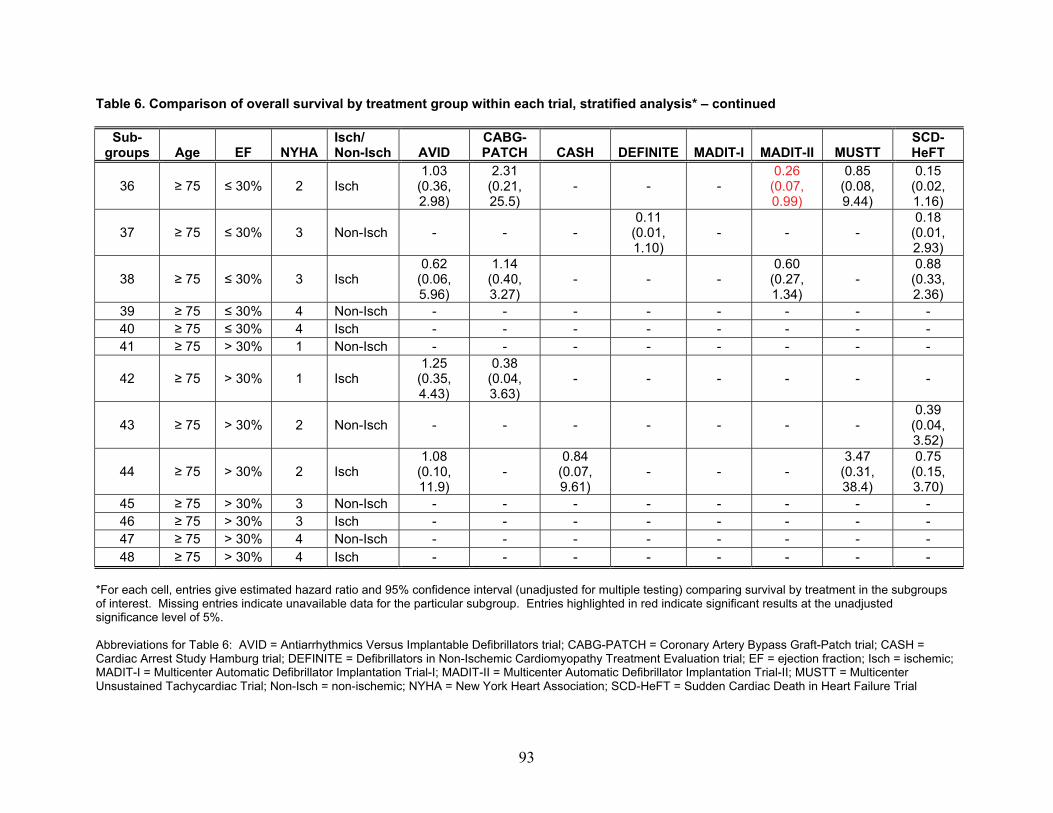
Table 6. Comparison of overall survival by treatment group within each trial, stratified analysis* – continued

Sub-groups Age EF NYHA

Isch/ Non-Isch AVID

CABG-PATCH CASH DEFINITE MADIT-I MADIT-II MUSTT

SCD-HeFT

36 ≥ 75 ≤ 30% 2 Isch 1.03

(0.36, 2.98)

2.31 (0.21, 25.5)

- - - 0.26

(0.07, 0.99)

0.85 (0.08, 9.44)

0.15 (0.02, 1.16)

37 ≥ 75 ≤ 30% 3 Non-Isch - - - 0.11

(0.01, 1.10)

- - - 0.18

(0.01, 2.93)

38 ≥ 75 ≤ 30% 3 Isch 0.62

(0.06, 5.96)

1.14 (0.40, 3.27)

- - - 0.60

(0.27, 1.34)

- 0.88

(0.33, 2.36)

39 ≥ 75 ≤ 30% 4 Non-Isch - - - - - - - - 40 ≥ 75 ≤ 30% 4 Isch - - - - - - - - 41 ≥ 75 > 30% 1 Non-Isch - - - - - - - -

42 ≥ 75 > 30% 1 Isch 1.25

(0.35, 4.43)

0.38 (0.04, 3.63)

- - - - - -

43 ≥ 75 > 30% 2 Non-Isch - - - - - - - 0.39

(0.04, 3.52)

44 ≥ 75 > 30% 2 Isch 1.08

(0.10, 11.9)

- 0.84

(0.07, 9.61)

- - - 3.47

(0.31, 38.4)

0.75 (0.15, 3.70)

45 ≥ 75 > 30% 3 Non-Isch - - - - - - - - 46 ≥ 75 > 30% 3 Isch - - - - - - - - 47 ≥ 75 > 30% 4 Non-Isch - - - - - - - - 48 ≥ 75 > 30% 4 Isch - - - - - - - -

*For each cell, entries give estimated hazard ratio and 95% confidence interval (unadjusted for multiple testing) comparing survival by treatment in the subgroups of interest. Missing entries indicate unavailable data for the particular subgroup. Entries highlighted in red indicate significant results at the unadjusted significance level of 5%. Abbreviations for Table 6: AVID = Antiarrhythmics Versus Implantable Defibrillators trial; CABG-PATCH = Coronary Artery Bypass Graft-Patch trial; CASH = Cardiac Arrest Study Hamburg trial; DEFINITE = Defibrillators in Non-Ischemic Cardiomyopathy Treatment Evaluation trial; EF = ejection fraction; Isch = ischemic; MADIT-I = Multicenter Automatic Defibrillator Implantation Trial-I; MADIT-II = Multicenter Automatic Defibrillator Implantation Trial-II; MUSTT = Multicenter Unsustained Tachycardiac Trial; Non-Isch = non-ischemic; NYHA = New York Heart Association; SCD-HeFT = Sudden Cardiac Death in Heart Failure Trial

93

Table 7. Subgroup composition by treatment group and trial – Part 1 (all trials)

All Trials Control ICD

Sub-groups Age EF NYHA

Isch/ Non-Isch

#Sub-jects #Events

#Sub-jects #Events

1 < 65 ≤ 30% 1 Non-Isch 45 9 42 32 < 65 ≤ 30% 1 Isch 247 39 295 283 < 65 ≤ 30% 2 Non-Isch 240 33 227 244 < 65 ≤ 30% 2 Isch 306 96 302 405 < 65 ≤ 30% 3 Non-Isch 92 21 82 176 < 65 ≤ 30% 3 Isch 171 68 188 517 < 65 ≤ 30% 4 Non-Isch 0 0 0 08 < 65 ≤ 30% 4 Isch 16 6 27 89 < 65 > 30% 1 Non-Isch 15 3 9 1

10 < 65 > 30% 1 Isch 173 15 156 1011 < 65 > 30% 2 Non-Isch 94 10 98 1012 < 65 > 30% 2 Isch 157 35 135 2213 < 65 > 30% 3 Non-Isch 23 6 30 114 < 65 > 30% 3 Isch 58 19 50 1915 < 65 > 30% 4 Non-Isch 0 0 0 016 < 65 > 30% 4 Isch 2 0 6 117 [65,75) ≤ 30% 1 Non-Isch 18 5 20 118 [65,75) ≤ 30% 1 Isch 222 53 211 3419 [65,75) ≤ 30% 2 Non-Isch 74 14 78 1420 [65,75) ≤ 30% 2 Isch 198 64 249 6121 [65,75) ≤ 30% 3 Non-Isch 37 17 32 1522 [65,75) ≤ 30% 3 Isch 128 65 133 4923 [65,75) ≤ 30% 4 Non-Isch 0 0 0 024 [65,75) ≤ 30% 4 Isch 20 4 24 825 [65,75) > 30% 1 Non-Isch 4 3 3 026 [65,75) > 30% 1 Isch 98 17 101 1627 [65,75) > 30% 2 Non-Isch 21 5 19 4

94

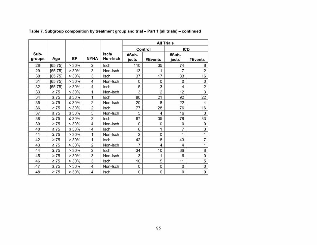
Table 7. Subgroup composition by treatment group and trial – Part 1 (all trials) – continued

All Trials Control ICD

Sub-groups Age EF NYHA

Isch/ Non-Isch

#Sub-jects #Events

#Sub-jects #Events

28 [65,75) > 30% 2 Isch 110 35 74 829 [65,75) > 30% 3 Non-Isch 13 1 7 230 [65,75) > 30% 3 Isch 37 17 33 1631 [65,75) > 30% 4 Non-Isch 0 0 0 032 [65,75) > 30% 4 Isch 5 3 4 233 ≥ 75 ≤ 30% 1 Non-Isch 3 2 12 334 ≥ 75 ≤ 30% 1 Isch 80 21 92 2235 ≥ 75 ≤ 30% 2 Non-Isch 20 8 22 436 ≥ 75 ≤ 30% 2 Isch 77 28 76 1637 ≥ 75 ≤ 30% 3 Non-Isch 5 4 16 338 ≥ 75 ≤ 30% 3 Isch 67 35 78 3339 ≥ 75 ≤ 30% 4 Non-Isch 0 0 0 040 ≥ 75 ≤ 30% 4 Isch 6 1 7 341 ≥ 75 > 30% 1 Non-Isch 2 0 1 142 ≥ 75 > 30% 1 Isch 42 8 43 743 ≥ 75 > 30% 2 Non-Isch 7 4 4 144 ≥ 75 > 30% 2 Isch 34 10 36 845 ≥ 75 > 30% 3 Non-Isch 3 1 6 046 ≥ 75 > 30% 3 Isch 10 5 11 547 ≥ 75 > 30% 4 Non-Isch 0 0 0 048 ≥ 75 > 30% 4 Isch 0 0 0 0

95

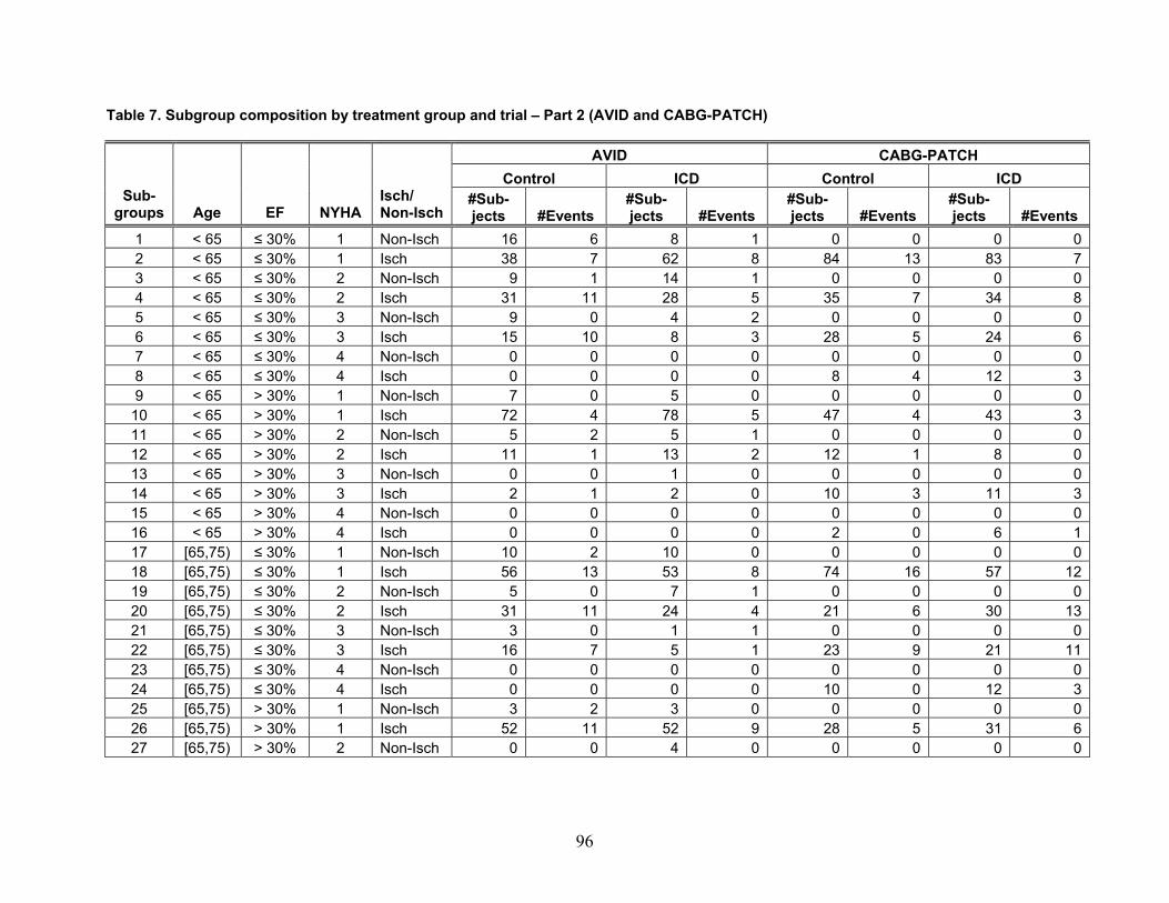
Table 7. Subgroup composition by treatment group and trial – Part 2 (AVID and CABG-PATCH)

AVID CABG-PATCH Control ICD Control ICD

Sub-groups Age EF NYHA

Isch/ Non-Isch

#Sub-jects #Events

#Sub-jects #Events

#Sub-jects #Events

#Sub-jects #Events

1 < 65 ≤ 30% 1 Non-Isch 16 6 8 1 0 0 0 02 < 65 ≤ 30% 1 Isch 38 7 62 8 84 13 83 73 < 65 ≤ 30% 2 Non-Isch 9 1 14 1 0 0 0 04 < 65 ≤ 30% 2 Isch 31 11 28 5 35 7 34 85 < 65 ≤ 30% 3 Non-Isch 9 0 4 2 0 0 0 06 < 65 ≤ 30% 3 Isch 15 10 8 3 28 5 24 67 < 65 ≤ 30% 4 Non-Isch 0 0 0 0 0 0 0 08 < 65 ≤ 30% 4 Isch 0 0 0 0 8 4 12 39 < 65 > 30% 1 Non-Isch 7 0 5 0 0 0 0 0

10 < 65 > 30% 1 Isch 72 4 78 5 47 4 43 311 < 65 > 30% 2 Non-Isch 5 2 5 1 0 0 0 012 < 65 > 30% 2 Isch 11 1 13 2 12 1 8 013 < 65 > 30% 3 Non-Isch 0 0 1 0 0 0 0 014 < 65 > 30% 3 Isch 2 1 2 0 10 3 11 315 < 65 > 30% 4 Non-Isch 0 0 0 0 0 0 0 016 < 65 > 30% 4 Isch 0 0 0 0 2 0 6 117 [65,75) ≤ 30% 1 Non-Isch 10 2 10 0 0 0 0 018 [65,75) ≤ 30% 1 Isch 56 13 53 8 74 16 57 1219 [65,75) ≤ 30% 2 Non-Isch 5 0 7 1 0 0 0 020 [65,75) ≤ 30% 2 Isch 31 11 24 4 21 6 30 1321 [65,75) ≤ 30% 3 Non-Isch 3 0 1 1 0 0 0 022 [65,75) ≤ 30% 3 Isch 16 7 5 1 23 9 21 1123 [65,75) ≤ 30% 4 Non-Isch 0 0 0 0 0 0 0 024 [65,75) ≤ 30% 4 Isch 0 0 0 0 10 0 12 325 [65,75) > 30% 1 Non-Isch 3 2 3 0 0 0 0 026 [65,75) > 30% 1 Isch 52 11 52 9 28 5 31 627 [65,75) > 30% 2 Non-Isch 0 0 4 0 0 0 0 0

96

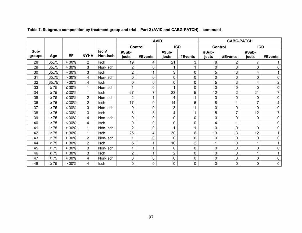
Table 7. Subgroup composition by treatment group and trial – Part 2 (AVID and CABG-PATCH) – continued

AVID CABG-PATCH Control ICD Control ICD

Sub-groups Age EF NYHA

Isch/ Non-Isch

#Sub-jects #Events

#Sub-jects #Events

#Sub-jects #Events

#Sub-jects #Events

28 [65,75) > 30% 2 Isch 19 4 21 3 8 2 7 129 [65,75) > 30% 3 Non-Isch 2 0 1 1 0 0 0 030 [65,75) > 30% 3 Isch 2 1 3 0 5 3 4 131 [65,75) > 30% 4 Non-Isch 0 0 0 0 0 0 0 032 [65,75) > 30% 4 Isch 0 0 0 0 5 3 4 233 ≥ 75 ≤ 30% 1 Non-Isch 1 0 1 0 0 0 0 034 ≥ 75 ≤ 30% 1 Isch 27 7 23 5 12 2 21 735 ≥ 75 ≤ 30% 2 Non-Isch 2 1 4 1 0 0 0 036 ≥ 75 ≤ 30% 2 Isch 17 9 14 6 8 1 7 437 ≥ 75 ≤ 30% 3 Non-Isch 0 0 3 1 0 0 0 038 ≥ 75 ≤ 30% 3 Isch 8 3 4 1 15 7 12 739 ≥ 75 ≤ 30% 4 Non-Isch 0 0 0 0 0 0 0 040 ≥ 75 ≤ 30% 4 Isch 0 0 0 0 4 1 1 041 ≥ 75 > 30% 1 Non-Isch 2 0 1 1 0 0 0 042 ≥ 75 > 30% 1 Isch 25 4 30 6 13 3 12 143 ≥ 75 > 30% 2 Non-Isch 1 0 0 0 0 0 0 044 ≥ 75 > 30% 2 Isch 5 1 10 2 1 0 1 145 ≥ 75 > 30% 3 Non-Isch 1 1 0 0 0 0 0 046 ≥ 75 > 30% 3 Isch 2 1 2 0 0 0 1 147 ≥ 75 > 30% 4 Non-Isch 0 0 0 0 0 0 0 048 ≥ 75 > 30% 4 Isch 0 0 0 0 0 0 0 0

97

Table 7. Subgroup composition by treatment group and trial – Part 3 (CASH and DEFINITE)

CASH DEFINITE Control ICD Control ICD

Sub-groups Age EF NYHA

Isch/ Non-Isch

#Sub-jects #Events

#Sub-jects #Events

#Sub-jects #Events

#Sub-jects #Events

1 < 65 ≤ 30% 1 Non-Isch 0 0 0 0 29 3 34 22 < 65 ≤ 30% 1 Isch 3 1 1 1 0 0 0 03 < 65 ≤ 30% 2 Non-Isch 1 0 2 1 89 10 78 84 < 65 ≤ 30% 2 Isch 16 11 9 2 0 0 0 05 < 65 ≤ 30% 3 Non-Isch 2 2 1 0 24 5 29 36 < 65 ≤ 30% 3 Isch 5 2 5 4 0 0 0 07 < 65 ≤ 30% 4 Non-Isch 0 0 0 0 0 0 0 08 < 65 ≤ 30% 4 Isch 0 0 0 0 0 0 0 09 < 65 > 30% 1 Non-Isch 7 3 1 0 1 0 3 1

10 < 65 > 30% 1 Isch 39 6 17 1 0 0 0 011 < 65 > 30% 2 Non-Isch 5 1 4 1 8 0 2 012 < 65 > 30% 2 Isch 45 13 26 7 0 0 0 013 < 65 > 30% 3 Non-Isch 1 1 0 0 2 1 2 014 < 65 > 30% 3 Isch 4 2 5 4 0 0 0 015 < 65 > 30% 4 Non-Isch 0 0 0 0 0 0 0 016 < 65 > 30% 4 Isch 0 0 0 0 0 0 0 017 [65,75) ≤ 30% 1 Non-Isch 0 0 0 0 8 3 10 118 [65,75) ≤ 30% 1 Isch 0 0 0 0 0 0 0 019 [65,75) ≤ 30% 2 Non-Isch 0 0 0 0 34 4 30 420 [65,75) ≤ 30% 2 Isch 3 2 4 3 0 0 0 021 [65,75) ≤ 30% 3 Non-Isch 0 0 0 0 18 7 9 322 [65,75) ≤ 30% 3 Isch 4 3 1 1 0 0 0 023 [65,75) ≤ 30% 4 Non-Isch 0 0 0 0 0 0 0 024 [65,75) ≤ 30% 4 Isch 0 0 0 0 0 0 0 025 [65,75) > 30% 1 Non-Isch 0 0 0 0 1 1 0 026 [65,75) > 30% 1 Isch 1 0 5 0 0 0 0 027 [65,75) > 30% 2 Non-Isch 0 0 1 1 1 0 2 0

98

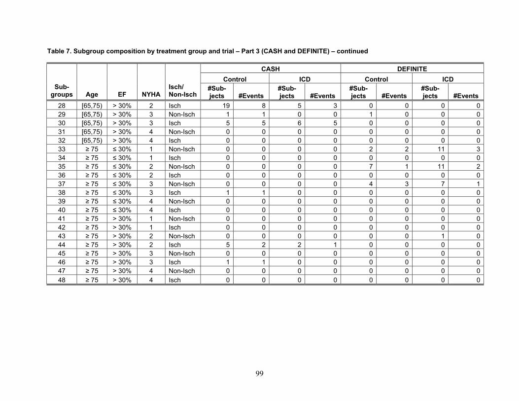
Table 7. Subgroup composition by treatment group and trial – Part 3 (CASH and DEFINITE) – continued

CASH DEFINITE Control ICD Control ICD

Sub-groups Age EF NYHA

Isch/ Non-Isch

#Sub-jects #Events

#Sub-jects #Events

#Sub-jects #Events

#Sub-jects #Events

28 [65,75) > 30% 2 Isch 19 8 5 3 0 0 0 029 [65,75) > 30% 3 Non-Isch 1 1 0 0 1 0 0 030 [65,75) > 30% 3 Isch 5 5 6 5 0 0 0 031 [65,75) > 30% 4 Non-Isch 0 0 0 0 0 0 0 032 [65,75) > 30% 4 Isch 0 0 0 0 0 0 0 033 ≥ 75 ≤ 30% 1 Non-Isch 0 0 0 0 2 2 11 334 ≥ 75 ≤ 30% 1 Isch 0 0 0 0 0 0 0 035 ≥ 75 ≤ 30% 2 Non-Isch 0 0 0 0 7 1 11 236 ≥ 75 ≤ 30% 2 Isch 0 0 0 0 0 0 0 037 ≥ 75 ≤ 30% 3 Non-Isch 0 0 0 0 4 3 7 138 ≥ 75 ≤ 30% 3 Isch 1 1 0 0 0 0 0 039 ≥ 75 ≤ 30% 4 Non-Isch 0 0 0 0 0 0 0 040 ≥ 75 ≤ 30% 4 Isch 0 0 0 0 0 0 0 041 ≥ 75 > 30% 1 Non-Isch 0 0 0 0 0 0 0 042 ≥ 75 > 30% 1 Isch 0 0 0 0 0 0 0 043 ≥ 75 > 30% 2 Non-Isch 0 0 0 0 0 0 1 044 ≥ 75 > 30% 2 Isch 5 2 2 1 0 0 0 045 ≥ 75 > 30% 3 Non-Isch 0 0 0 0 0 0 0 046 ≥ 75 > 30% 3 Isch 1 1 0 0 0 0 0 047 ≥ 75 > 30% 4 Non-Isch 0 0 0 0 0 0 0 048 ≥ 75 > 30% 4 Isch 0 0 0 0 0 0 0 0

99

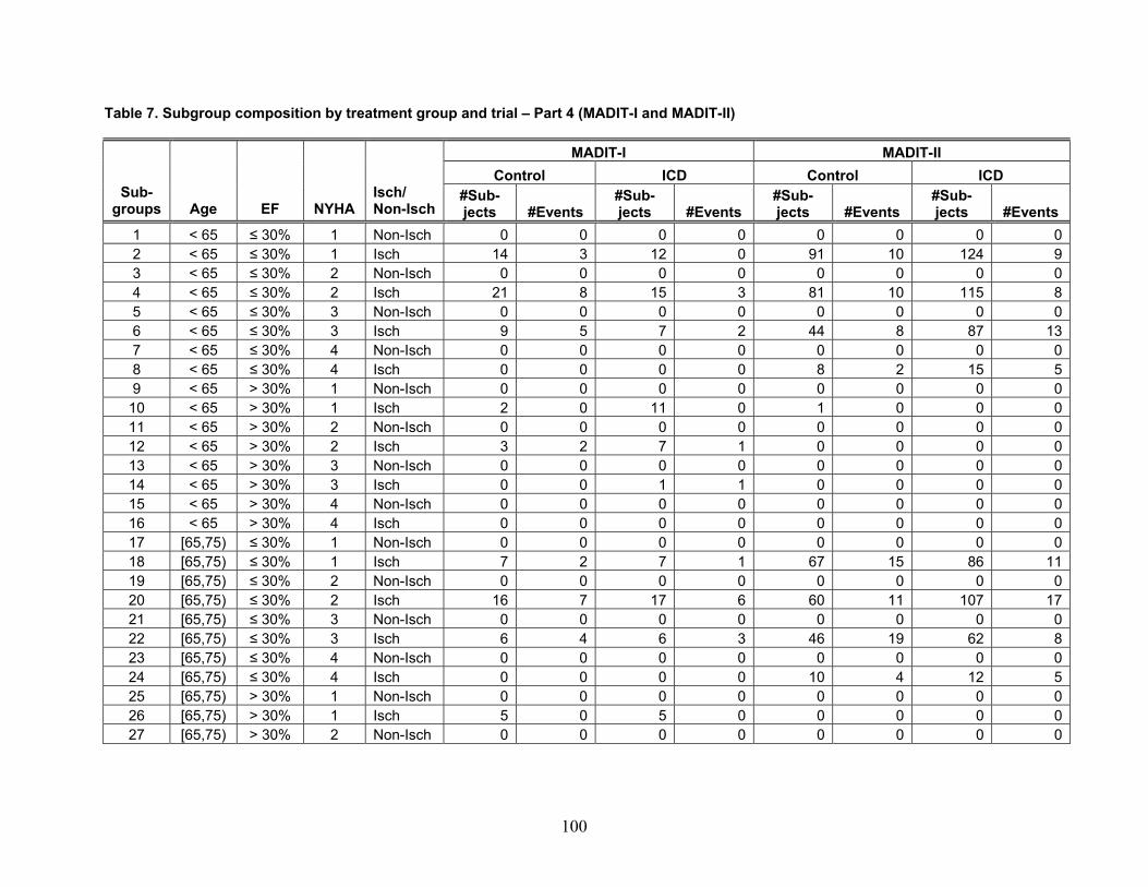
Table 7. Subgroup composition by treatment group and trial – Part 4 (MADIT-I and MADIT-II)

MADIT-I MADIT-II Control ICD Control ICD

Sub-groups Age EF NYHA

Isch/ Non-Isch

#Sub-jects #Events

#Sub-jects #Events

#Sub-jects #Events

#Sub-jects #Events

1 < 65 ≤ 30% 1 Non-Isch 0 0 0 0 0 0 0 02 < 65 ≤ 30% 1 Isch 14 3 12 0 91 10 124 93 < 65 ≤ 30% 2 Non-Isch 0 0 0 0 0 0 0 04 < 65 ≤ 30% 2 Isch 21 8 15 3 81 10 115 85 < 65 ≤ 30% 3 Non-Isch 0 0 0 0 0 0 0 06 < 65 ≤ 30% 3 Isch 9 5 7 2 44 8 87 137 < 65 ≤ 30% 4 Non-Isch 0 0 0 0 0 0 0 08 < 65 ≤ 30% 4 Isch 0 0 0 0 8 2 15 59 < 65 > 30% 1 Non-Isch 0 0 0 0 0 0 0 0

10 < 65 > 30% 1 Isch 2 0 11 0 1 0 0 011 < 65 > 30% 2 Non-Isch 0 0 0 0 0 0 0 012 < 65 > 30% 2 Isch 3 2 7 1 0 0 0 013 < 65 > 30% 3 Non-Isch 0 0 0 0 0 0 0 014 < 65 > 30% 3 Isch 0 0 1 1 0 0 0 015 < 65 > 30% 4 Non-Isch 0 0 0 0 0 0 0 016 < 65 > 30% 4 Isch 0 0 0 0 0 0 0 017 [65,75) ≤ 30% 1 Non-Isch 0 0 0 0 0 0 0 018 [65,75) ≤ 30% 1 Isch 7 2 7 1 67 15 86 1119 [65,75) ≤ 30% 2 Non-Isch 0 0 0 0 0 0 0 020 [65,75) ≤ 30% 2 Isch 16 7 17 6 60 11 107 1721 [65,75) ≤ 30% 3 Non-Isch 0 0 0 0 0 0 0 022 [65,75) ≤ 30% 3 Isch 6 4 6 3 46 19 62 823 [65,75) ≤ 30% 4 Non-Isch 0 0 0 0 0 0 0 024 [65,75) ≤ 30% 4 Isch 0 0 0 0 10 4 12 525 [65,75) > 30% 1 Non-Isch 0 0 0 0 0 0 0 026 [65,75) > 30% 1 Isch 5 0 5 0 0 0 0 027 [65,75) > 30% 2 Non-Isch 0 0 0 0 0 0 0 0

100

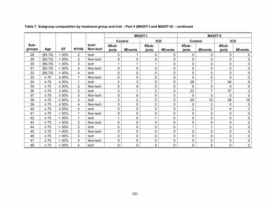
Table 7. Subgroup composition by treatment group and trial – Part 4 (MADIT-I and MADIT-II) – continued

MADIT-I MADIT-II Control ICD Control ICD

Sub-groups Age EF NYHA

Isch/ Non-Isch

#Sub-jects #Events

#Sub-jects #Events

#Sub-jects #Events

#Sub-jects #Events

28 [65,75) > 30% 2 Isch 5 1 0 0 0 0 0 029 [65,75) > 30% 3 Non-Isch 0 0 0 0 0 0 0 030 [65,75) > 30% 3 Isch 1 1 1 0 0 0 0 031 [65,75) > 30% 4 Non-Isch 0 0 0 0 0 0 0 032 [65,75) > 30% 4 Isch 0 0 0 0 0 0 0 033 ≥ 75 ≤ 30% 1 Non-Isch 0 0 0 0 0 0 0 034 ≥ 75 ≤ 30% 1 Isch 4 3 0 0 28 7 46 935 ≥ 75 ≤ 30% 2 Non-Isch 0 0 0 0 0 0 0 036 ≥ 75 ≤ 30% 2 Isch 5 1 2 0 23 7 37 337 ≥ 75 ≤ 30% 3 Non-Isch 0 0 0 0 0 0 0 038 ≥ 75 ≤ 30% 3 Isch 2 2 0 0 20 10 38 1639 ≥ 75 ≤ 30% 4 Non-Isch 0 0 0 0 0 0 0 040 ≥ 75 ≤ 30% 4 Isch 0 0 0 0 2 0 6 341 ≥ 75 > 30% 1 Non-Isch 0 0 0 0 0 0 0 042 ≥ 75 > 30% 1 Isch 1 0 1 0 0 0 0 043 ≥ 75 > 30% 2 Non-Isch 0 0 0 0 0 0 0 044 ≥ 75 > 30% 2 Isch 0 0 3 0 1 1 0 045 ≥ 75 > 30% 3 Non-Isch 0 0 0 0 0 0 0 046 ≥ 75 > 30% 3 Isch 0 0 0 0 0 0 0 047 ≥ 75 > 30% 4 Non-Isch 0 0 0 0 0 0 0 048 ≥ 75 > 30% 4 Isch 0 0 0 0 0 0 0 0

101

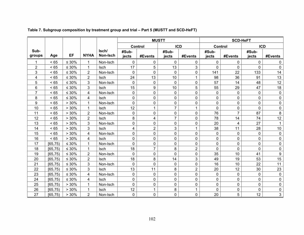
Table 7. Subgroup composition by treatment group and trial – Part 5 (MUSTT and SCD-HeFT)

MUSTT SCD-HeFT Control ICD Control ICD

Sub-groups Age EF NYHA

Isch/ Non-Isch

#Sub-jects #Events

#Sub-jects #Events

#Sub-jects #Events

#Sub-jects #Events

1 < 65 ≤ 30% 1 Non-Isch 0 0 0 0 0 0 0 02 < 65 ≤ 30% 1 Isch 17 5 13 3 0 0 0 03 < 65 ≤ 30% 2 Non-Isch 0 0 0 0 141 22 133 144 < 65 ≤ 30% 2 Isch 24 13 10 1 98 36 91 135 < 65 ≤ 30% 3 Non-Isch 0 0 0 0 57 14 48 126 < 65 ≤ 30% 3 Isch 15 9 10 5 55 29 47 187 < 65 ≤ 30% 4 Non-Isch 0 0 0 0 0 0 0 08 < 65 ≤ 30% 4 Isch 0 0 0 0 0 0 0 09 < 65 > 30% 1 Non-Isch 0 0 0 0 0 0 0 0

10 < 65 > 30% 1 Isch 12 1 7 1 0 0 0 011 < 65 > 30% 2 Non-Isch 0 0 0 0 76 7 87 812 < 65 > 30% 2 Isch 8 4 7 0 78 14 74 1213 < 65 > 30% 3 Non-Isch 0 0 0 0 20 4 27 114 < 65 > 30% 3 Isch 4 2 3 1 38 11 28 1015 < 65 > 30% 4 Non-Isch 0 0 0 0 0 0 0 016 < 65 > 30% 4 Isch 0 0 0 0 0 0 0 017 [65,75) ≤ 30% 1 Non-Isch 0 0 0 0 0 0 0 018 [65,75) ≤ 30% 1 Isch 18 7 8 2 0 0 0 019 [65,75) ≤ 30% 2 Non-Isch 0 0 0 0 35 10 41 920 [65,75) ≤ 30% 2 Isch 18 8 14 3 49 19 53 1521 [65,75) ≤ 30% 3 Non-Isch 0 0 0 0 16 10 22 1122 [65,75) ≤ 30% 3 Isch 13 11 8 2 20 12 30 2323 [65,75) ≤ 30% 4 Non-Isch 0 0 0 0 0 0 0 024 [65,75) ≤ 30% 4 Isch 0 0 0 0 0 0 0 025 [65,75) > 30% 1 Non-Isch 0 0 0 0 0 0 0 026 [65,75) > 30% 1 Isch 12 1 8 1 0 0 0 027 [65,75) > 30% 2 Non-Isch 0 0 0 0 20 5 12 3

102

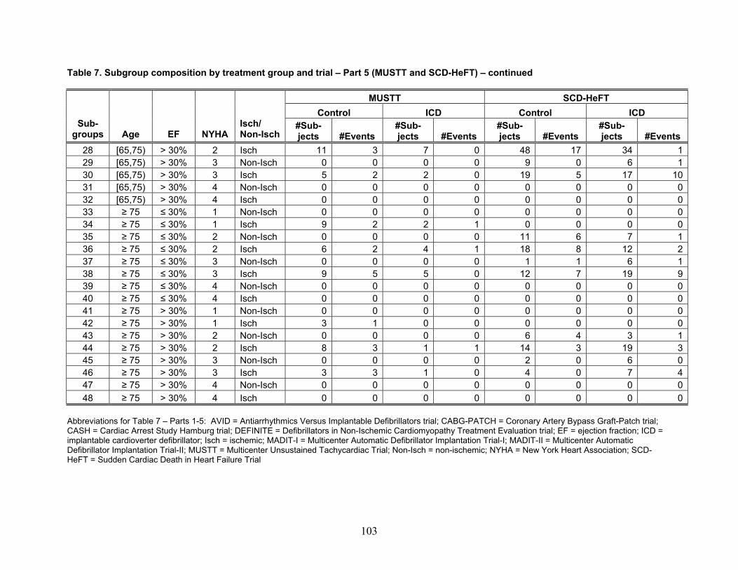
103

Table 7. Subgroup composition by treatment group and trial – Part 5 (MUSTT and SCD-HeFT) – continued

MUSTT SCD-HeFT Control ICD Control ICD

Sub-groups Age EF NYHA

Isch/ Non-Isch

#Sub-jects #Events

#Sub-jects #Events

#Sub-jects #Events

#Sub-jects #Events

28 [65,75) > 30% 2 Isch 11 3 7 0 48 17 34 129 [65,75) > 30% 3 0 Non-Isch 0 0 0 9 0 6 130 [65,75) > 30% 3 2 Isch 5 2 0 19 5 17 1031 [65,75) > 30% 4 0 Non-Isch 0 0 0 0 0 0 032 [65,75) > 30% 4 0 Isch 0 0 0 0 0 0 033 ≥ 75 ≤ 30% 1 Non-Isch 0 0 0 0 0 0 0 034 ≥ 75 ≤ 30% 1 Isch 9 2 2 1 0 0 0 035 ≥ 75 ≤ 30% 2 Non-Isch 0 0 0 0 11 6 7 136 ≥ 75 ≤ 30% 2 Isch 6 2 4 1 18 8 12 237 ≥ 75 ≤ 30% 3 Non-Isch 0 0 0 0 1 1 6 138 ≥ 75 ≤ 30% 3 Isch 9 5 5 0 12 7 19 939 ≥ 75 ≤ 30% 4 Non-Isch 0 0 0 0 0 0 0 040 ≥ 75 ≤ 30% 4 Isch 0 0 0 0 0 0 0 041 ≥ 75 > 30% 1 Non-Isch 0 0 0 0 0 0 0 042 ≥ 75 > 30% 1 Isch 3 1 0 0 0 0 0 043 ≥ 75 > 30% 2 Non-Isch 0 0 0 0 6 4 3 144 ≥ 75 > 30% 2 Isch 8 3 1 1 14 3 19 345 ≥ 75 > 30% 3 Non-Isch 0 0 0 0 2 0 6 046 ≥ 75 > 30% 3 Isch 3 3 1 0 4 0 7 447 ≥ 75 > 30% 4 Non-Isch 0 0 0 0 0 0 0 048 ≥ 75 > 30% 4 Isch 0 0 0 0 0 0 0 0

Abbreviations for Table 7 – Parts 1-5: AVID = Antiarrhythmics Versus Implantable Defibrillators trial; CABG-PATCH = Coronary Artery Bypass Graft-Patch trial; CASH = Cardiac Arrest Study Hamburg trial; DEFINITE = Defibrillators in Non-Ischemic Cardiomyopathy Treatment Evaluation trial; EF = ejection fraction; ICD = implantable cardioverter defibrillator; Isch = ischemic; MADIT-I = Multicenter Automatic Defibrillator Implantation Trial-I; MADIT-II = Multicenter Automatic Defibrillator Implantation Trial-II; MUSTT = Multicenter Unsustained Tachycardiac Trial; Non-Isch = non-ischemic; NYHA = New York Heart Association; SCD-HeFT = Sudden Cardiac Death in Heart Failure Trial

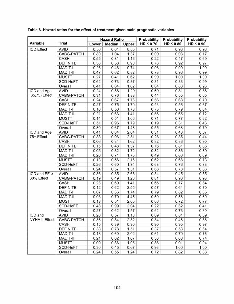
Table 8. Hazard ratios for the effect of treatment given main prognostic variables

Hazard Ratio Variable Trial Lower Median Upper

ProbabilityHR ≤ 0.70

Probability HR ≤ 0.80

ProbabilityHR ≤ 0.90

AVID 0.50 0.64 0.85 0.71 0.93 0.98CABG-PATCH 0.80 1.04 1.37 0.00 0.03 0.17CASH 0.55 0.81 1.16 0.22 0.47 0.69DEFINITE 0.36 0.58 0.90 0.78 0.92 0.97MADIT-I 0.26 0.46 0.74 0.96 0.99 1.00MADIT-II 0.47 0.62 0.82 0.78 0.96 0.99MUSTT 0.27 0.41 0.62 0.99 1.00 1.00SCD-HeFT 0.62 0.73 0.87 0.31 0.83 0.99

ICD Effect

Overall 0.41 0.64 1.02 0.64 0.83 0.93AVID 0.24 0.58 1.29 0.69 0.81 0.88CABG-PATCH 0.31 0.76 1.83 0.44 0.55 0.65CASH 0.24 0.67 1.76 0.56 0.63 0.70DEFINITE 0.27 0.75 1.70 0.43 0.56 0.67MADIT-I 0.16 0.50 1.73 0.73 0.79 0.84MADIT-II 0.21 0.63 1.41 0.56 0.65 0.72MUSTT 0.14 0.51 1.66 0.71 0.77 0.82SCD-HeFT 0.51 0.96 1.79 0.19 0.31 0.43

ICD and Age [65,75) Effect

Overall 0.30 0.67 1.48 0.55 0.68 0.79AVID 0.41 0.84 2.04 0.31 0.43 0.57CABG-PATCH 0.38 0.96 2.51 0.26 0.35 0.44CASH 0.06 0.34 1.62 0.82 0.86 0.90DEFINITE 0.15 0.48 1.37 0.76 0.81 0.86MADIT-I 0.05 0.32 1.72 0.82 0.86 0.89MADIT-II 0.20 0.71 1.75 0.49 0.60 0.69MUSTT 0.13 0.56 2.16 0.62 0.68 0.73SCD-HeFT 0.26 0.60 1.34 0.63 0.76 0.83

ICD and Age 75+ Effect

Overall 0.24 0.57 1.31 0.68 0.78 0.86AVID 0.36 0.85 2.68 0.34 0.45 0.55CABG-PATCH 0.19 0.49 1.20 0.81 0.90 0.93CASH 0.23 0.60 1.41 0.66 0.77 0.84DEFINITE 0.12 0.62 2.55 0.57 0.64 0.70MADIT-I 0.07 0.36 1.74 0.79 0.82 0.85MADIT-II 0.08 0.70 4.45 0.50 0.56 0.60MUSTT 0.13 0.51 2.05 0.66 0.72 0.77SCD-HeFT 0.48 0.99 2.04 0.22 0.32 0.41

ICD and EF ≥ 30% Effect

Overall 0.27 0.62 1.57 0.62 0.73 0.80AVID 0.26 0.57 1.18 0.69 0.81 0.89CABG-PATCH 0.36 0.84 2.32 0.34 0.46 0.56CASH 0.15 0.39 0.90 0.90 0.95 0.97DEFINITE 0.38 0.78 1.51 0.37 0.53 0.64MADIT-I 0.18 0.60 2.02 0.61 0.70 0.76MADIT-II 0.21 0.62 1.67 0.58 0.68 0.74MUSTT 0.09 0.36 1.05 0.86 0.91 0.94SCD-HeFT 0.30 0.45 0.67 0.98 1.00 1.00

ICD and NYHA II Effect

Overall 0.24 0.55 1.24 0.72 0.82 0.88

104

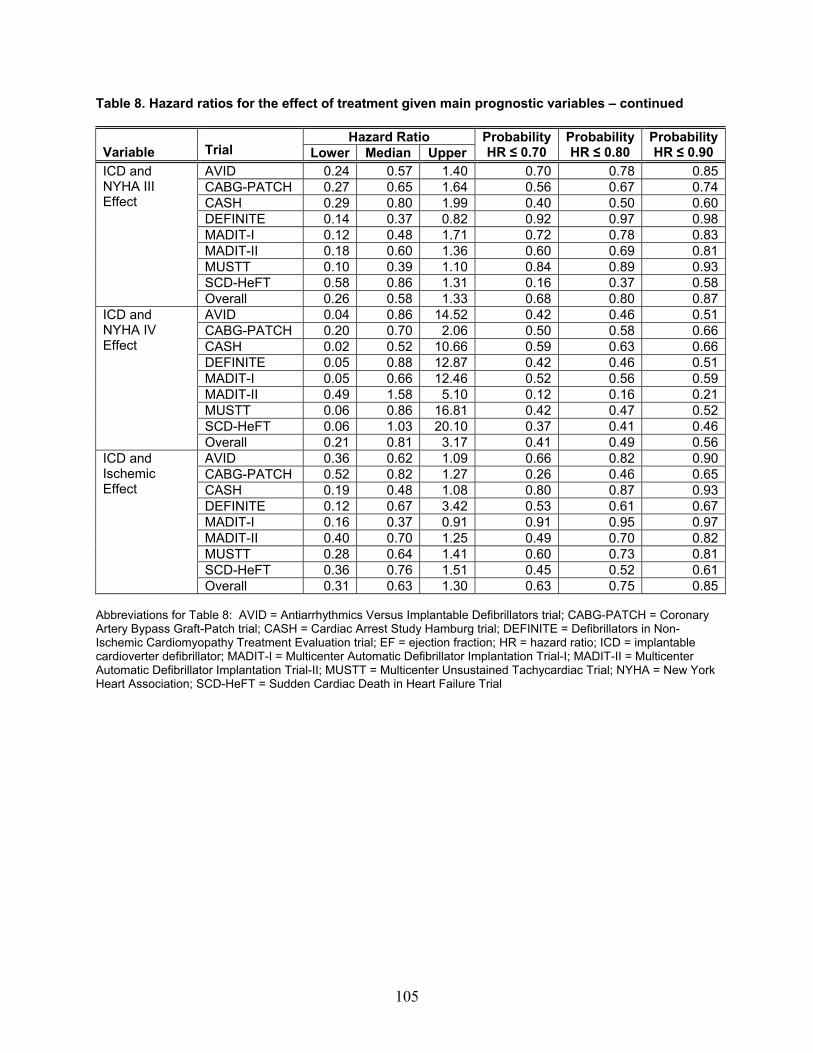
105

Table 8. Hazard ratios for the effect of treatment given main prognostic variables – continued

Hazard Ratio Variable Trial Lower Median Upper

ProbabilityHR ≤ 0.70

Probability HR ≤ 0.80

ProbabilityHR ≤ 0.90

AVID 0.24 0.57 1.40 0.70 0.78 0.85CABG-PATCH 0.27 0.65 1.64 0.56 0.67 0.74CASH 0.29 0.80 1.99 0.40 0.50 0.60DEFINITE 0.14 0.37 0.82 0.92 0.97 0.98MADIT-I 0.12 0.48 1.71 0.72 0.78 0.83MADIT-II 0.18 0.60 1.36 0.60 0.69 0.81MUSTT 0.10 0.39 1.10 0.84 0.89 0.93SCD-HeFT 0.58 0.86 1.31 0.16 0.37 0.58

ICD and NYHA III Effect

Overall 0.26 0.58 1.33 0.68 0.80 0.87AVID 0.04 0.86 14.52 0.42 0.46 0.51CABG-PATCH 0.20 0.70 2.06 0.50 0.58 0.66CASH 0.02 0.52 10.66 0.59 0.63 0.66DEFINITE 0.05 0.88 12.87 0.42 0.46 0.51MADIT-I 0.05 0.66 12.46 0.52 0.56 0.59MADIT-II 0.49 1.58 5.10 0.12 0.16 0.21MUSTT 0.06 0.86 16.81 0.42 0.47 0.52SCD-HeFT 0.06 1.03 20.10 0.37 0.41 0.46

ICD and NYHA IV Effect

Overall 0.21 0.81 3.17 0.41 0.49 0.56AVID 0.36 0.62 1.09 0.66 0.82 0.90CABG-PATCH 0.52 0.82 1.27 0.26 0.46 0.65CASH 0.19 0.48 1.08 0.80 0.87 0.93DEFINITE 0.12 0.67 3.42 0.53 0.61 0.67MADIT-I 0.16 0.37 0.91 0.91 0.95 0.97MADIT-II 0.40 0.70 1.25 0.49 0.70 0.82MUSTT 0.28 0.64 1.41 0.60 0.73 0.81SCD-HeFT 0.36 0.76 1.51 0.45 0.52 0.61

ICD and Ischemic Effect

Overall 0.31 0.63 1.30 0.63 0.75 0.85 Abbreviations for Table 8: AVID = Antiarrhythmics Versus Implantable Defibrillators trial; CABG-PATCH = Coronary Artery Bypass Graft-Patch trial; CASH = Cardiac Arrest Study Hamburg trial; DEFINITE = Defibrillators in Non-Ischemic Cardiomyopathy Treatment Evaluation trial; EF = ejection fraction; HR = hazard ratio; ICD = implantable cardioverter defibrillator; MADIT-I = Multicenter Automatic Defibrillator Implantation Trial-I; MADIT-II = Multicenter Automatic Defibrillator Implantation Trial-II; MUSTT = Multicenter Unsustained Tachycardiac Trial; NYHA = New York Heart Association; SCD-HeFT = Sudden Cardiac Death in Heart Failure Trial

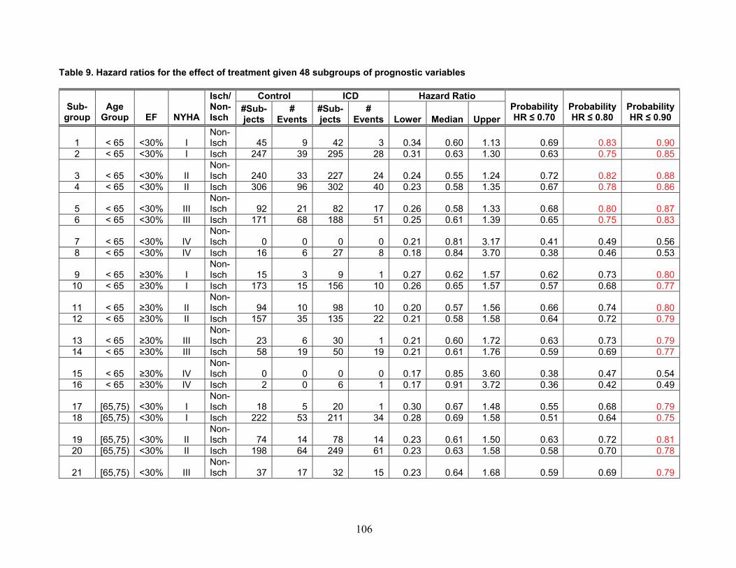
Table 9. Hazard ratios for the effect of treatment given 48 subgroups of prognostic variables

Control ICD Hazard Ratio Sub-

group Age

Group EF NYHA

Isch/ Non-Isch

#Sub-jects

# Events

#Sub-jects

# Events Lower Median Upper

Probability HR ≤ 0.70

Probability HR ≤ 0.80

Probability HR ≤ 0.90

1 < 65 <30% I Non-Isch 45 9 42 3 0.34 0.60 1.13 0.69 0.83 0.90

2 < 65 <30% I Isch 247 39 295 28 0.31 0.63 1.30 0.63 0.75 0.85

3 < 65 <30% II Non-Isch 240 33 227 24 0.24 0.55 1.24 0.72 0.82 0.88

4 < 65 <30% II Isch 306 96 302 40 0.23 0.58 1.35 0.67 0.78 0.86

5 < 65 <30% III Non-Isch 92 21 82 17 0.26 0.58 1.33 0.68 0.80 0.87

6 < 65 <30% III Isch 171 68 188 51 0.25 0.61 1.39 0.65 0.75 0.83

7 < 65 <30% IV Non-Isch 0 0 0 0 0.21 0.81 3.17 0.41 0.49 0.56

8 < 65 <30% IV Isch 16 6 27 8 0.18 0.84 3.70 0.38 0.46 0.53

9 < 65 ≥30% I Non-Isch 15 3 9 1 0.27 0.62 1.57 0.62 0.73 0.80

10 < 65 ≥30% I Isch 173 15 156 10 0.26 0.65 1.57 0.57 0.68 0.77

11 < 65 ≥30% II Non-Isch 94 10 98 10 0.20 0.57 1.56 0.66 0.74 0.80

12 < 65 ≥30% II Isch 157 35 135 22 0.21 0.58 1.58 0.64 0.72 0.79

13 < 65 ≥30% III Non-Isch 23 6 30 1 0.21 0.60 1.72 0.63 0.73 0.79

14 < 65 ≥30% III Isch 58 19 50 19 0.21 0.61 1.76 0.59 0.69 0.77

15 < 65 ≥30% IV Non-Isch 0 0 0 0 0.17 0.85 3.60 0.38 0.47 0.54

16 < 65 ≥30% IV Isch 2 0 6 1 0.17 0.91 3.72 0.36 0.42 0.49

17 [65,75) <30% I Non-Isch 18 5 20 1 0.30 0.67 1.48 0.55 0.68 0.79

18 [65,75) <30% I Isch 222 53 211 34 0.28 0.69 1.58 0.51 0.64 0.75

19 [65,75) <30% II Non-Isch 74 14 78 14 0.23 0.61 1.50 0.63 0.72 0.81

20 [65,75) <30% II Isch 198 64 249 61 0.23 0.63 1.58 0.58 0.70 0.78

21 [65,75) <30% III Non-Isch 37 17 32 15 0.23 0.64 1.68 0.59 0.69 0.79

106

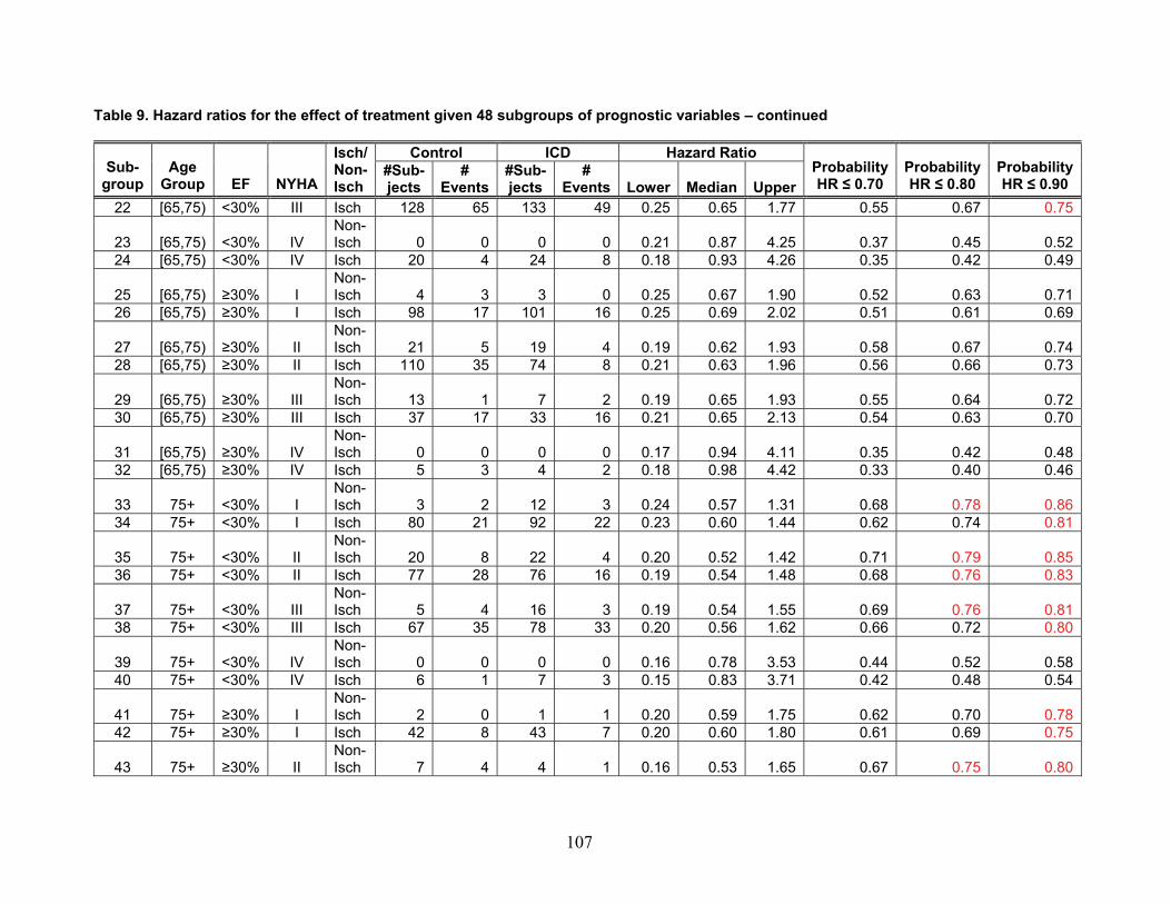
Table 9. Hazard ratios for the effect of treatment given 48 subgroups of prognostic variables – continued

Control ICD Hazard Ratio Sub-

group Age

Group EF NYHA

Isch/ Non-Isch

#Sub-jects

# #Sub-jects

# Events Lower Median Upper

Probability HR ≤ 0.70

Probability HR ≤ 0.80 Events

Probability HR ≤ 0.90

22 [65,75) <30% III Isch 128 65 133 49 0.25 0.65 1.77 0.55 0.67 0.75

23 [65,75) <30% Non-Isch 0 0 0 0 0.21 0.87 4.25 0.37IV 0.45 0.52

24 [65,75) <30% IV Isch 20 4 24 8 0.18 0.93 4.26 0.35 0.42 0.49

25 [65,75) ≥30% I Non-Isch 4 3 3 0 0.25 0.67 1.90 0.52 0.63 0.71

26 [65,75) ≥30% I Isch 98 17 101 16 0.25 0.69 2.02 0.51 0.61 0.69

27 [65,75) ≥30% II Non-Isch 21 5 19 4 0.19 0.62 1.93 0.58 0.67 0.74

28 [65,75) ≥30% II Isch 110 35 74 8 0.21 0.63 1.96 0.56 0.66 0.73

29 [65,75) ≥30% III Non-Isch 13 1 7 2 0.19 0.65 1.93 0.55 0.64 0.72

30 [65,75) ≥30% III Isch 37 17 33 16 0.21 0.65 2.13 0.54 0.63 0.70

31 [65,75) ≥30% IV Non-Isch 0 0 0 0 0.17 0.94 4.11 0.35 0.42 0.48

32 [65,75) ≥30% IV Isch 5 3 4 2 0.18 0.98 4.42 0.33 0.40 0.46

33 75+ <30% I Non-Isch 3 2 12 3 0.24 0.57 1.31 0.68 0.78 0.86

34 75+ <30% I Isch 80 21 92 22 0.23 0.60 1.44 0.62 0.74 0.81

35 75+ <30% II Non-Isch 20 8 22 4 0.20 0.52 1.42 0.71 0.79 0.85

36 75+ <30% II Isch 77 28 76 16 0.19 0.54 1.48 0.68 0.76 0.83

37 75+ <30% III Non-Isch 5 4 16 3 0.19 0.54 1.55 0.69 0.76 0.81

38 75+ <30% III Isch 67 35 78 33 0.20 0.56 1.62 0.66 0.72 0.80

39 75+ <30% IV Non-Isch 0 0 0 0 0.16 0.78 3.53 0.44 0.52 0.58

40 75+ <30% IV Isch 6 1 7 3 0.15 0.83 3.71 0.42 0.48 0.54

41 75+ ≥30% I Non-Isch 2 0 1 1 0.20 0.59 1.75 0.62 0.70 0.78

42 75+ ≥30% I Isch 42 8 43 7 0.20 0.60 1.80 0.61 0.69 0.75

43 75+ ≥30% II Non-Isch 7 4 4 1 0.16 0.53 1.65 0.67 0.75 0.80

107

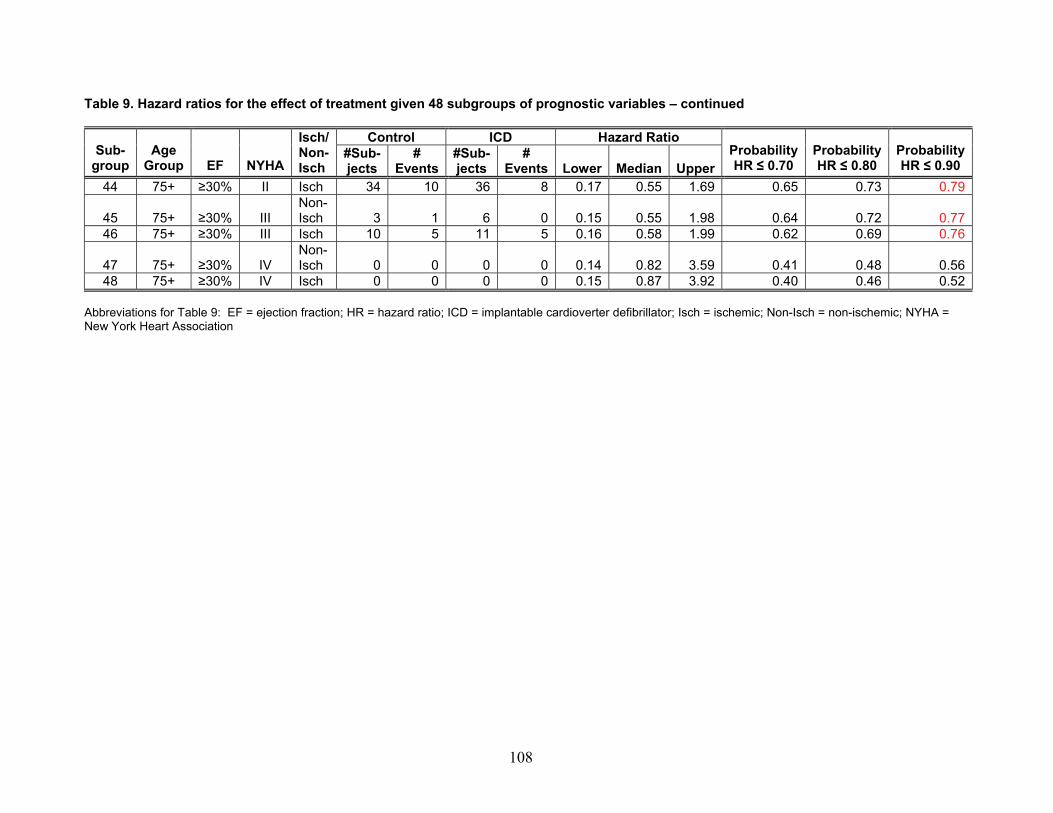
108

Table 9. Hazard ratios for the effect of treatment given 48 subgroups of prognostic variables – continued

Control ICD Hazard RatioSub-

group Age

Group EF NYHA

Isch/ Non-Isch

#Sub-jects

# Events

#Sub-jects

# Events Lower Median Upper

Probability HR ≤ 0.70

Probability HR ≤ 0.80

Probability HR ≤ 0.90

44 75+ ≥30% II Isch 34 10 36 8 0.17 0.55 1.69 0.65 0.73 0.79

45 75+ ≥30% III Isch 3Non-

1 6 0 0.15 0.55 1.98 0.64 0.72 0.7746 75+ ≥30% III Isch 10 5 11 5 0.16 0.58 1.99 0.62 0.69 0.76

47 75+ ≥30% IV Isch 0Non-

0 0 0 0.14 0.82 3.59 0.41 0.48 0.5648 75+ ≥30% IV Isch 0 0 0 0 0.15 0.87 3.92 0.40 0.46 0.52

Abbreviations for Table 9: EF = ejection fraction; HR = hazard ratio; ICD = implantable cardioverter defibrillator; Isch = ischemic; Non-Isch = non-ischemic; NYHA = New York Heart Association

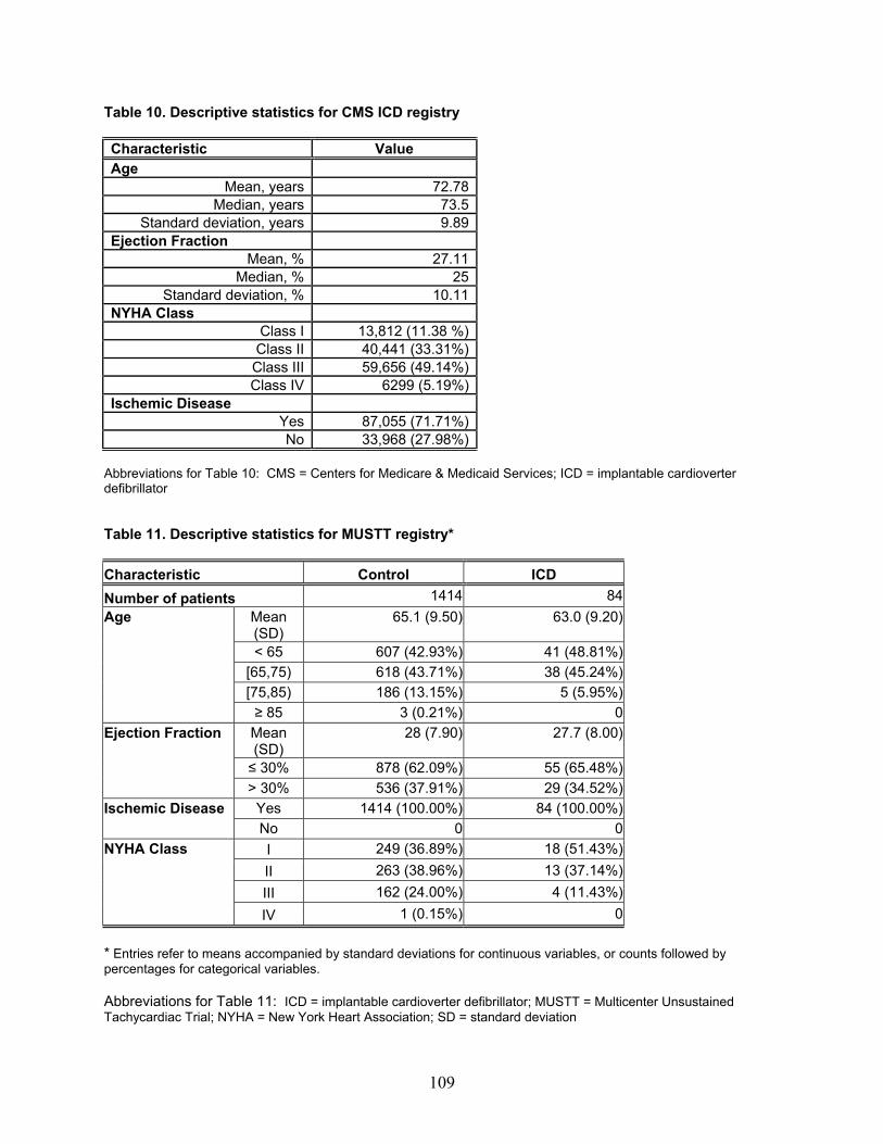
Table 10. Descriptive statistics for CMS ICD registry Characteristic Value Age

Mean, years 72.78Median, years 73.5

Standard deviation, years 9.89Ejection Fraction

Mean, % 27.11Median, % 25

Standard deviation, % 10.11NYHA Class

Class I 13,812 (11.38 %)Class II 40,441 (33.31%)Class III 59,656 (49.14%)Class IV 6299 (5.19%)

Ischemic Disease Yes 87,055 (71.71%)No 33,968 (27.98%)

Abbreviations for Table 10: CMS = Centers for Medicare & Medicaid Services; ICD = implantable cardioverter defibrillator Table 11. Descriptive statistics for MUSTT registry* Characteristic Control ICD Number of patients 1414 84

Mean (SD)

65.1 (9.50) 63.0 (9.20)

< 65 607 (42.93%) 41 (48.81%) [65,75) 618 (43.71%) 38 (45.24%) [75,85) 186 (13.15%) 5 (5.95%)

Age

≥ 85 3 (0.21%) 0 Mean (SD)

28 (7.90) 27.7 (8.00)

≤ 30% 878 (62.09%) 55 (65.48%)

Ejection Fraction

> 30% 536 (37.91%) 29 (34.52%) Yes 1414 (100.00%) 84 (100.00%) Ischemic Disease No 0 0 I 249 (36.89%) 18 (51.43%) II 263 (38.96%) 13 (37.14%) III 162 (24.00%) 4 (11.43%)

NYHA Class

IV 1 (0.15%) 0 * Entries refer to means accompanied by standard deviations for continuous variables, or counts followed by percentages for categorical variables. Abbreviations for Table 11: ICD = implantable cardioverter defibrillator; MUSTT = Multicenter Unsustained Tachycardiac Trial; NYHA = New York Heart Association; SD = standard deviation

109

Appendix. ICD Case Study

Introduction

In this Appendix we detail for the interested reader the case study and our findings. More details will be available in a statistical manuscript. An executive summary of these findings are included in the full report.

Prior to the case study described in this section, we performed substantial simulation studies to demonstrate that while single trials may be adequately powered to detect main treatment effects, they often have low power to detect treatment-covariate interactions. Furthermore, these studies demonstrated that combining data from trials improves the power to detect such treatment-covariate interactions. Details about the simulation studies and our findings may be obtained from the authors and will be published in a statistical manuscript. To explore the findings from our simulation studies and to provide evidence concerning the advantages and disadvantages of Bayesian techniques in clinical trial design and analysis, we performed a case study of the use of ICD therapy in the prevention of SCD using data from eight clinical trials.

Methods and Assumptions

For the purposes of this case study, we considered data from eight trials (AVID,

CABG-PATCH, CASH, DEFINITE, MADIT-I, MADIT-II, MUSTT and SCD-HeFT). For any trial, the overall survival (in years from randomization) is the primary outcome. There are two treatment groups (ICD versus control) and four baseline prognostic variables, namely, age (in years), ejection fraction (given as a percentage), NYHA class (classes I through IV) and ischemic disease (yes/no). Data were analyzed according to the intention-to-treat. Moreover, we assumed that the four prognostic variables also capture differences in the trial designs. We omitted from our analysis patients who had missing entries in any of the above covariates.

Besides the clinical trial data, we received data from the CMS on the CMS ICD Registry patients representing patients who have had an ICD implanted and are requesting coverage from CMS. The data represent 121,398 implants between 12/31/2004 and 6/30/2007. We note, however, that the registry data are only on ICD patients; that is, there is no control group. Moreover, the registry does not currently have follow-up information regarding patients’ overall survival. Thus, for the purpose of illustration, we utilized registry data from the MUSTT study to address survival comparisons considering clinical trial and registry data. Analysis of Individual Trials

We utilized Cox-Proportional hazards and Weibull regression models to compare overall survival by treatment groups. An introductory text describing these types of survival models can be found here.91 The findings from these two models were

A-110

qualitatively similar and so in our discussion here we only present those from the Weibull regression models. Although the Cox-Proportional hazards model is widely used, the Weibull regression model allows us to make comparisons of the estimation under Frequentist and Bayesian approaches on more similar modeling grounds. Details of the other models are available from the authors and will be published in a statistical manuscript.

First, we considered unadjusted analysis considering data from all patients in the trial as well as stratified analysis on subgroups. Second, we considered analysis that adjusted for the common set of baseline prognostic variables, both, with and without the interaction between each of the baseline prognostic variables and treatment. Analysis of Data Combining All Trials

We utilized Weibull regression models to compare overall survival by treatment groups in unadjusted and adjusted analysis. For the latter we considered models that included or not the interactions between baseline prognostic variables and treatment. To combine data from all trials we considered four model variations: 1) combining data from all trials, but without adjusting for (potential) trial effects; 2) combining data from all trials adjusting for trial effects assuming a fixed effect for trial; 3) combining data from all trials assuming a random effect for trial and 4) combining data from all trials assuming trial-specific baseline hazard functions. These models were estimated using maximum likelihood estimation.

Bayesian estimation was also performed in the above Weibull regression models. Moreover, we additionally considered a full hierarchical model utilizing random-effects for baseline hazard functions, main and interaction effects. We assumed normal priors for real-valued parameters (that is, parameters that can take on positive and negative values, such as the ICD effect). Precision parameters were assigned Gamma priors. Moreover, scale and shape parameters of the baseline hazard were assigned log-normal priors. Fixed effect parameters were assigned priors with mean zero and variance one. Random effects parameters were assigned priors with an overall population mean and population precision. Population means were assigned priors with mean zero and variance one, while precision parameters were assigned priors with mean and variance equal to one. Using Registry Data

We considered the random effects model (model 3 above) utilizing Bayesian estimation. This model formally accounts for the variability within and between trials. Using the posterior samples of the model parameters, we simulated the survival experience of hypothetical patients in a hypothetical new trial under the ICD and control groups in given prognostic subgroups. Using these samples we obtained the posterior predictive survival distributions for the ICD and control groups which can then be compared to the empirical survival distribution of the related subgroups in the registry data.

A-111

Analysis of Aggregate versus Patient-level Data

One critical aspect of our analysis is the availability of patient-level data from ICD trials. In practice, however, data analysts may face a situation in which only aggregate data are available; for example, in the form of estimates of the treatment effect along with estimated standard errors. Moreover, such data become available sequentially as trial results get published. We, thus, performed additional analyses to investigate two additional points:

1. What are the implications of using aggregate data as opposed to using patient-

level data in assessing overall ICD efficacy? 2. By considering the accumulated sequential evidence from trials, either using

aggregate or patient-level data, would we be able to reach a conclusive decision of overall ICD efficacy sooner?

To answer the above questions, we considered fixed and random effects models

and estimated these models under two different priors. Prior 2 has higher precision than prior 1. We set prior 2 to have different precisions when comparing the analysis for aggregate or patient-level data as we clarify below when we discuss our findings.

Finally, using patient-level data, we also considered the accumulated sequential evidence from trials to assess treatment-covariate interaction across prognostic subgroups.

All analyses were performed in R (version 2.7.2) and Winbugs (version 1.4.3). Convergence diagnosis of our Bayesian models was performed using the package BOA available in R. Additional details concerning the statistical models explored are available from the authors and will be published in a statistical manuscript.

Findings

Analysis of Individual Trials

Summary statistics for each trial by treatment group are shown in Appendix Table A1 (Parts 1 and 2). The table shows that the trials considered in this case study differ in sample size with the smallest trial having 196 patients (MADIT-I) and the largest with 1676 (SCD-HeFT) patients randomized to ICD and control. Moreover, participants have different compositions across trials. For example, some trials such as CABG-PATCH, MADIT-I, MADIT-II and MUSTT had only ischemic patients while the DEFINITE trial only included non-ischemic patients.

Appendix Figures A1(a) and A1(b) shows the Kaplan-Meier survival curves by trial and treatment group. In the analysis of individual trials, without adjusting for prognostic variables, there is evidence of treatment effect on overall survival in five trials (AVID, MADIT-I, MADIT-II, MUSTT and SCD-HeFT) (see Appendix Table A2). Among trials that showed treatment effect, the estimated hazard ratio (for death from all causes in the ICD group as compared to the control group) ranged from 0.35 to 0.75. Among

A-112

trials that did not show treatment effect, the estimated hazard ratio ranged from 0.65 to 1.07.

Comparisons of overall survival by treatment group within prognostic subgroups in general failed to show an association between treatment and overall survival (see Appendix Table A3). Moreover, most entries in the table with significant results were no longer significant when considering Bonferroni’s adjustment to account for multiple testing. The only exception was in subgroup 4 (age < 65, EF < 30 percent, NYHA 2 and ischemic disease) in the SCD-HeFT trial (Bonferroni’s adjusted p-value < 0.001). We note that these results are affected by the small sample sizes in each subgroup (Appendix Table A4 [Parts 1-5]).

To adjust for prognostic variables, we utilized the Weibull regression model. The model demonstrates evidence of treatment effect on overall survival in the trials previously identified as well as in the DEFINITE trial (Appendix Tables A5-A12). We also fitted Weibull regression models including the interaction between treatment and each of the prognostic variables. In general, there was no evidence of significant interactions. The exception was in CASH which showed significant treatment interaction with EF and NYHA class, MADIT 1 with a significant interaction between treatment and EF and SCD-HeFT with a significant interaction between treatment and AGE and NYHA class.

Before we move on to the next phase of the analysis we take a quick detour to explain in more detail the results we presented in Appendix Tables A5-A12. Because all these tables have similar format, we do not discuss them individually, but focus on the results in Appendix Table A5. The left side of the table shows results that only include main effects, while the right side of the table shows results that include main effects and interactions between treatment and prognostic variables. The results include estimates of the model parameters, standard errors and p-values. For example, for the model that utilizes only main effects, we estimate that the hazard of death from all causes for a patient in the ICD group is exp(-0.43) = 0.65 times the hazard of death for a patient in the control group.

Appendix Figure A2 summarizes the analysis of the individual trials displaying estimates, along with the respective 95 percent confidence intervals, of the log-hazard of treatment effect for each trial. The differences between estimates from models that do not adjust for covariates from those that do are, in general, relatively small. Without covariate adjustment there is evidence of treatment effect on overall survival in five trials (AVID, MADIT-I, MADIT-II, MUSTT and SCD-HeFT) as shown in the figure with the 95 percent CI excluding the null value (zero). When considering covariate adjustment, we also find a (borderline) treatment effect in the DEFINITE trial. We note, however, that the estimates vary from trial to trial. Moreover, the precisions for these estimates vary, with more precision attained in the largest trial (SCD-HeFT) with the narrowest 95 percent CI.

Key points: The analysis of the individual trials shows that, out of eight trials, five showed evidence of treatment effect, but there is also a lot of variation in the estimates of ICD effect across trials. Within any trial, the results are fairly robust to different model formulations. Moreover, generally, there is no evidence of significant treatment-covariate interactions in the prognostic subgroups.

A-113

Analysis of Data Combining All Trials

Under all model formulations considered here, there is evidence of treatment effect on overall survival (Appendix Tables A13-A17, with results presented in similar format to those discussed in the previous section).

Moreover, estimates from Bayesian models (Appendix Tables A18-A21) with priors as described before, are generally similar to those obtained under the frequentist Weibull regression models (compare results under Appendix Tables A18-A21 with those from Appendix Tables A13-A17). We note that in Appendix Tables A18-A21 we present the posterior mean, posterior standard deviation and 95 percent posterior credible intervals. Let us take the results under Appendix Table A18 for the model that only includes main effects for an example. We estimate that the hazard of death in the ICD is approximately exp(-0.38) = 0.68 times the hazard of death in the control group. Moreover, we estimate that with 95 percent posterior probability the hazard ratio lies between 0.61 and 0.76.

Appendix Figure A3 summarizes results displaying estimates, along with the corresponding 95 percent confidence/credible intervals, of the log-hazard of treatment effect across different models. The results show evidence of treatment effect on overall survival and are very similar across all models considered here, that is, with or without covariate adjustment, and across different specifications for how trial data are combined, with Weibull regression models using frequentist or Bayesian approaches to estimation. Moreover, the estimates have lower uncertainty as compared to those from the individual trials (compare Appendix Figure A3 with Appendix Figure A2).

The models that we discussed so far rely on strong assumptions as to how we accommodate trial differences. In one extreme end, we combine data assuming that trials are similar. Next, we relax this assumption and assume that trial differences are accommodated with fixed and random trial effects or allowing for trial-specific baseline hazard functions. However, we have allowed the effect of the prognostic variables, and the interactions to be similar across all trials. Next, we discuss results from a Bayesian hierarchical model that will relax this assumption. We note that an equivalent model, without priors in the population parameters, could not be estimated using classical frequentist approaches.

Appendix Table A22 shows estimates under the full Bayesian hierarchical model that accounts for trial variation in the baseline-hazard, main effects and interaction effects. To summarize the results we present the population estimates, as well as, the trial-specific estimates. From Appendix Table A22 we estimate, under the model that only includes main effects, that the hazard of death in the ICD is approximately exp(-0.43) = 0.65 times the hazard of death in the control group. Moreover, we estimate that with 95 percent posterior probability the hazard ratio lies between 0.40 and 1.03. This model also allows us to obtain the trial-specific effects. We find differential effect of ICD across trials. In particular, we find no treatment effect in the CABG-PATCH and CASH (95 percent posterior credible intervals include the null value) trials. There is no evidence of interactions between treatment and any of the prognostic variables.

For ease of interpretation, in Appendix Table A23 we provide the median hazard ratios and the 95 percent credible intervals for the effect of treatment within the main subgroups defined by the prognostic variables for the individual trials and then for the

A-114

entire population of trials. We also provide the posterior probability that the hazard ratio for the total mortality reduction from the ICD treatment would be 0.80 or less, as this was considered a clinically important reduction in mortality by members of our technical expert panel. For sensitivity analysis, we also present probabilities when using different clinical cutoffs, that is, of 0.70 and 0.90. So, for example, although the 95 percent credible interval for the overall hazard ratio for the reduction in mortality from ICD implant includes the value of no treatment efficacy (that is, a hazard ratio equal to 1), with 83 percent posterior probability the hazard ratio is 0.80 or less indicating a clinically significant reduction. However, if one looks at the findings for treatment and NHYA class 4 patients we observe that not only there is no evidence of a significant interaction, but that there is only a 49 percent probability that the hazard ratio is 0.80 or less. In Appendix Table A24, we provide the same information (median hazard ratios, 95 percent credible intervals, and posterior probability that the hazard ratio is less or equal to 0.70, 0.80 and 0.90) for each of the 48 subgroups. Again, note that there is no evidence of treatment benefit in the individual subgroups. The probability that the hazard ratio is 0.80 or less however is at least 75 percent in 11 of the subgroups indicated in red in the table.

While these results seem to contradict those arising from Appendix Tables A13-A17, we note that this full hierarchical model accounts for a variety of sources of variation not accounted for in the previous models; for example, that the interactions between treatment and say the presence of ischemia may not be the same across trials. But in doing so, we deal with yet another issue in that some prognostic subgroups were not observed in all trials. When accounting for all of these sources of variation, there is no longer evidential support for interactions.

We computed the Deviance Information Criterion (DIC) for all four models and including or not the interactions between treatment and baseline prognostic variables (Appendix Table A25). According to this criterion, models minimizing the DIC are preferred. We thus select the model with trial-specific baseline hazard functions. The full Bayesian hierarchical model is a close second best according to this criterion. Because the full Bayesian hierarchical model accounts for more sources of variation we will utilize it for the upcoming discussions.

Key points: Combining data from trials improves our inferences by increasing the precision of our estimates as well as the power to detect main effects and interactions. There is a variety of modeling approaches that allow us to combine data from different trials, but they do not necessarily lead to the same inference.

Understanding the underlying model assumptions and limitations is important when interpreting the results from the combined analysis. For example, in this section we observed that some models showed evidence for an interaction between treatment and AGE in the combined analysis. But this evidence arises from models that assume that this interaction is the same across all trials. If this assumption is regarded unreasonable, and we consider instead a model that accounts for the variation of the interaction across trials, then the interaction between treatment and AGE is no longer significant.

Finally, when considering Bayesian estimation, the role of priors should also be examined through a sensitivity analysis. We delay the discussion on the effect of priors to the section on “Analysis of Aggregate vs. Patient-level data,” below.

A-115

Using Registry Data

Appendix Table A26 provides descriptive characteristics of CMS ICD Registry patients. As compared to patients recruited to the actual ICD trials, we note that patients in the registry are older and with worse prognosis. Of particular note is that more than 87 percent of the patients in the CMS ICD Registry are NYHA Class II or greater while these patients represented approximately just two thirds of the trial patients.

As we discussed before, the current CMS registry does not have overall survival. Thus, we utilized the registry data from the MUSTT study for illustrative purposes. Appendix Table A27 has descriptive statistics for the MUSTT registry. We note that patients in the MUSTT registry also have different characteristics from those in the CMS registry. We also note that only approximately 35 percent of the patients in the MUSTT registry received beta-adrenergic blocking agents perhaps influencing the cohort’s mortality.

Appendix Figures A4(a) and A4(b) show the posterior predictive survival distribution for the ICD and control groups along with the empirical survival distribution from the registry data in two subgroups. For these subgroups, there are few patients in the MUSTT registry who received an ICD. Control patients in the MUSTT registry have better survival earlier on, but more comparable (to the posterior predictive survival) in later years.

Key points: The above analysis illustrates that we can utilize Bayesian hierarchical models to predict survival from patients in subgroups. This was an illustration and not a definitive examination of the strengths and weaknesses of the Bayesian approach to this problem. Indeed, in this data set we observed that the predictions from the Bayesian model were not always consistent with the survival observed in the registry. Various interpretations of this observation are possible, among them being the possibility (independent of the particular statistical model being employed) that patients in the registry had a different prognosis than patients in the clinical trials. Analysis of Aggregate versus Patient-level Data

Appendix Figure A5(a) (see also Appendix Table A28) shows the results from the analysis that combines aggregate data sequentially mimicking when the trials were completed and their data available. Trials were combined in the following order (based on their publication date): MADIT-I, AVID, CABG-PATCH, MUSTT, CASH, MADIT-II, DEFINITE, SCD-HeFT.

The figure shows that both fixed and random effects models give similar estimates. The estimates are lower and more precise when using the more informative prior 2. As we accumulate data from trials, the 95 percent posterior credible intervals under both priors get narrower. The gain of information with accumulated data is greater under the less informative prior 1 than under prior 2. Upon combining aggregate data from all trials, there is only a borderline evidence of overall ICD efficacy under prior 2. We do not rule out no efficacy under prior 1.

A-116

In contrast, Appendix Figure A5(b) (see also Appendix Table A29) shows the results from the analysis that combines patient-level data sequentially. Estimates from the fixed and random effects models are different when considering data from the first trial only (MADIT-1) which also has the smallest sample size. This shows sensitivity to both models and priors. However, as we combine data from more trials, the estimates become more similar and precise. Moreover, using the more informative prior we would have concluded overall ICD efficacy sooner with six trials.

Some additional comments are in order. The informative prior used in Appendix Figure A5(b) has precision 5 while the informative prior used to produce the results shown in Appendix Figure A5(a) has precision 20. Thus, to reach a conclusion of overall treatment effect using aggregate data would require an even more informative prior! However, Appendix Figure A5(a) also shows that the results are more sensitive to prior 2 as the estimates are pulled towards the prior mean (zero). Now, when using the patient-level data, the point estimates under both priors are similar, but with higher precision under prior 2.

Appendix Figure A6 (see also Appendix Table A30) shows the results from the analysis that combines patient-level data sequentially but accounting for covariates, under two priors, the same utilized to produce Appendix Figure A5(b), but considering the full Bayesian hierarchical model. Here too we can see that under the more informative prior we would have concluded overall ICD efficacy after six trials. However, under neither prior, we would be able to conclude treatment-covariate interactions across subgroups.

Key points: In this section we examined the use of patient-level data versus aggregate data as information accrues over time. Our analysis showed that the resulting inferences are not necessarily the same. Moreover, the analysis of aggregate data may be more sensitive to priors.

Finally, we note that the above analysis which assesses the interactions between treatment and covariates defining the subgroups of interest may not be feasible with aggregate data (see Pocock et al.26 for a review on issues with published subgroup analysis).

We now further examine the Bayesian hierarchical model that combines patient-level data from all eight trials. In what follows we will state a sample of questions of clinical interest that we can examine with this model. Question 1: Is there evidence that the devices used in the different trials differ in terms

of their efficacies? Answer: As we have discussed before, the Bayesian hierarchical model accounts for

the variability within and between trials. In particular, we assume that ICD efficacy is trial-specific, but allow for the borrowing of information about ICD efficacy across trials. Appendix Figure A7 shows the estimates of treatment effect for each trial and the overall effect across all trials. There is evidence that treatment efficacy differs across trials. Why this is the case is uncertain. The differences in treatment efficacy could be due to differences in the devices used in the trials, but they could also be due to the patient population being different across trials – even after controlling for age, EF, NYHA class, and ischemia. For example, additional information concerning the QRS interval, gender, or time from myocardial infarction could explain the differences in ICD efficacy. Accounting for these differences, under prior 1 we estimate that the hazard

A-117

of death in the ICD group is exp(-0.43) = 0.65 times the hazard in the control group. The 95 percent posterior credible interval is 0.41 to 1.02. Under prior 2 we estimate the hazard of death in the ICD group is 0.66 times that in the control group, with a 95 percent posterior credible interval of 0.49 to 0.90. That is, under the more informative prior 2, our analysis supports the evidence of overall ICD efficacy across all trials.

Question 2: Controlling for EF, ischemia, age, and NYHA class, are patients within the available trials similar?

Answer: Another feature of our Bayesian hierarchical model is that it allows for the baseline survival functions to vary from trial-to-trial. Appendix Figure A8 shows the estimated posterior baseline survival functions under each trial and overall trials. Even controlling for EF, ischemia, age, and NYHA class, the figure indicates that patients’ survival differs within the available trials. Patients in the SCDHEFT trial seem to have the best survival prognosis. Patients in CABG-PATCH, AVID and MUSTT have poorer survival prognosis. Again, as discussed under Question 1, there are several potential explanations for this difference. The variation across trials could be due to differences in the implanted devices, in the underlying medical care of the patient populations, or in patient characteristics that are currently not included in our analysis (e.g., gender, QRS interval, time from myocardial infarction). To gain further insight into these differences, additional patient-level data would be required from the trials, and the Bayesian hierarchical model would need to be updated to reflect this additional knowledge. Our group currently has a research grant starting 12/1/09 to gain access to these needed data and to update our Bayesian model so as to allow exploration of these described differences.

Also note that the variation across trials could be due in part to the fact that some of our trials were secondary prevention trials (CASH, AVID), while the remaining trials were primary prevention trials. As we described earlier, we chose to combine data from all ICD trials and explored the effects of the four prognostic characteristics across these populations. However, to explore the potential impact of a patient having previously experienced a sudden cardiac arrest, we have performed additional sensitivity analyses to assess whether treatment may have a different effect in the primary versus secondary patient populations.

First, we considered an analysis, using the Weibull regression model, combining only primary prevention trials or only secondary prevention trials without adjustment for other covariates or trial effects. For comparison purposes, we also combined all trials without adjustment for other covariates or trial effects. The results are reported in Appendix Table A31. The estimated log hazard ratio is essentially the same when combining either only primary prevention trials or only secondary prevention trials. As expected, there is more uncertainty in the estimate when combining secondary prevention trials due to the smaller sample.

Second, we considered an analysis that adjusted for our prognostic variables and included a term to indicate whether or not a trial was of primary or secondary prevention using a Weibull regression model with random trial effects. Appendix Table A32 shows the estimates from the model fit to the data. Our analysis indicated that adding the indicator of primary prevention improves the model fit (p < 0.001). However, while we estimate the hazard of death in primary prevention trials is exp(-0.65)=0.55 times the hazard in secondary prevention trials, the estimate for the hazard of death in the ICD

A-118

group is exp(-0.37) = 0.69 that for the control group – this estimate is essentially the same as that provided in Appendix Table A16 without adjusting for the indicator of primary prevention trials. Appendix Table A32 also shows that there is no evidence for significant interaction between treatment and the other prognostic variables – including the indicator of primary prevention trial.

Both analyses indicate that, even though the patient populations may be different, there is no evidence for differences in treatment effect. This supports our approach, which combined data from all trials. Question 3: Is there evidence that the ICD has different effects across patient

subgroups? Answer: The Bayesian hierarchical model also allows for trial-specific interactions.

From our analysis (see Appendix Table A30), there was no evidence for overall interactions between treatment and the covariates that define the subgroups of interest. In other words, there was no evidence for treatment-covariate interactions across prognostic subgroups.

Methodological and Clinical Implications of Findings

This case study illustrates Situations 1, 2 and 3 (described under CMS contexts).

For example, corresponding to Situation 1, in the CASH trial there was no overall efficacy of the ICD, but with a naïve analysis one could find efficacy within the subgroup with patients < 65 years-old, ≤ 30 percent, NYHA class II and ischemic disease. Illustrating Situation 2, the AVID trial supports overall efficacy of the device. However, concern may be raised in the subgroup of patients with < 65 years-old, ≤ 30 percent, NYHA class 3 and ischemic disease, even though the survival comparison within the subgroup was not significant. Finally, illustrating Situation 3, some trials do not have all subgroups represented. For example, the DEFINITE trial was only on non-ischemic patients.

Regarding Situations 1 and 2, testing for interactions at the individual trials often did not support the presence of treatment-covariate interactions. Combining data from the trials improves the power to detect interactions. However, in this case study, the analysis that combined data from the trials generally did not support the presence of interactions. Such conclusions are supported under different model formulations as well as different estimation approaches. In particular, we note that our Bayesian estimation of the models that combined data from trials gave similar estimates to those obtained under the classical frequentist approaches. This illustrates that for large studies, Bayesian inferences are less sensitive to prior choices.

Utilizing the full Bayesian hierarchical model, we simulated the survival experience of hypothetical patients in a new clinical trial. This accounts for both, the variation between and within clinical trials. Because of the borrowing of information across trials, this model allows us to predict survival even if an individual trial does not include some of the subgroups (thus, addressing Situation 3). Using this approach, we note that the survival in the registry data is better (relative to those predicted by our model) in early years. We note, however, that such analysis has an exploratory feature as confounding

A-119

A-120

might be present. We also note that this model could not be estimated using classical frequentist approaches.

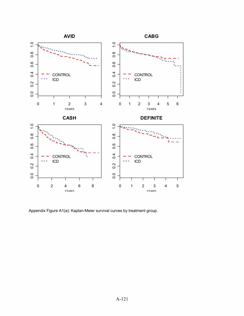
0 1 2 3 4

0.0

0.2

0.4

0.6

0.8

1.0

CONTROLICD

AVID

YEARS

0 1 2 3 4 5 6

0.0

0.2

0.4

0.6

0.8

1.0

CONTROLICD

CABG

YEARS

0 2 4 6 8

0.0

0.2

0.4

0.6

0.8

1.0

CONTROLICD

CASH

YEARS

0 1 2 3 4 5

0.0

0.2

0.4

0.6

0.8

1.0

CONTROLICD

DEFINITE

YEARS

Appendix Figure A1(a): Kaplan-Meier survival curves by treatment group.

A-121

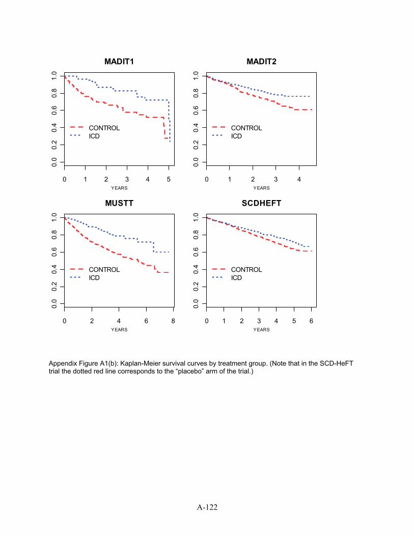
0 1 2 3 4 5

0.0

0.2

0.4

0.6

0.8

1.0

CONTROLICD

MADIT1

YEARS

0 1 2 3 4

0.0

0.2

0.4

0.6

0.8

1.0

CONTROLICD

MADIT2

YEARS

0 2 4 6 8

0.0

0.2

0.4

0.6

0.8

1.0

CONTROLICD

MUSTT

YEARS

0 1 2 3 4 5 6

0.0

0.2

0.4

0.6

0.8

1.0

CONTROLICD

SCDHEFT

YEARS

Appendix Figure A1(b): Kaplan-Meier survival curves by treatment group. (Note that in the SCD-HeFT trial the dotted red line corresponds to the “placebo” arm of the trial.)

A-122

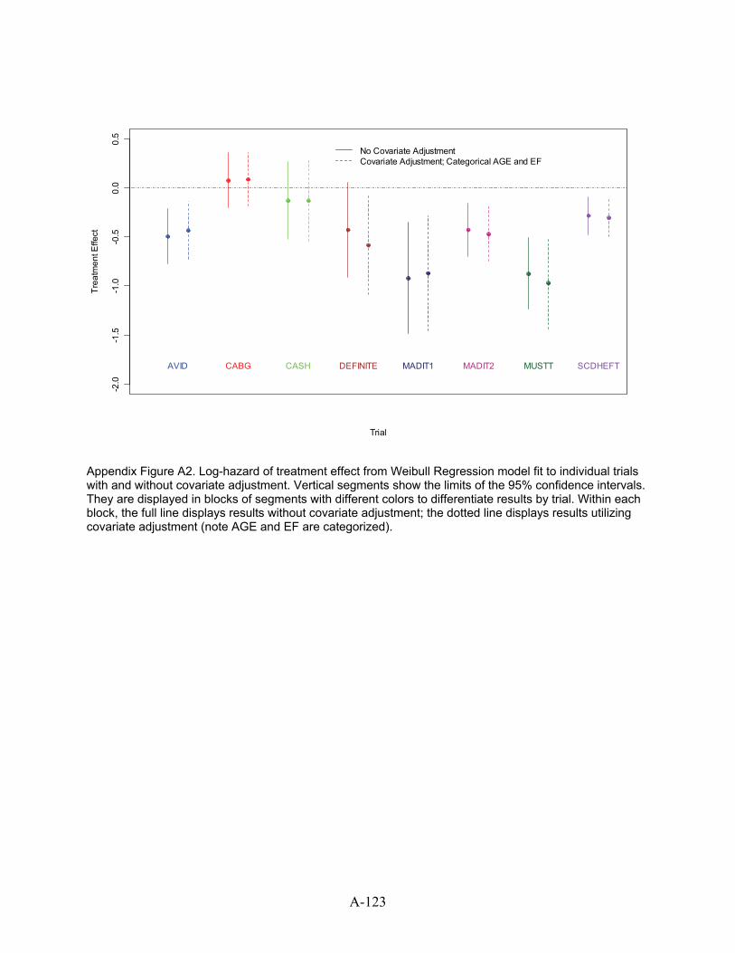
Trial

Trea

tmen

t Effe

ct

-2.0

-1.5

-1.0

-0.5

0.0

0.5

AVID CABG CASH

No Covariate AdjustmentCovariate Adjustment; Categorical AGE and EF

DEFINITE MADIT1 MADIT2 MUSTT SCDHEFT

Appendix Figure A2. Log-hazard of treatment effect from Weibull Regression model fit to individual trials with and without covariate adjustment. Vertical segments show the limits of the 95% confidence intervals. They are displayed in blocks of segments with different colors to differentiate results by trial. Within each block, the full line displays results without covariate adjustment; the dotted line displays results utilizing covariate adjustment (note AGE and EF are categorized).

A-123

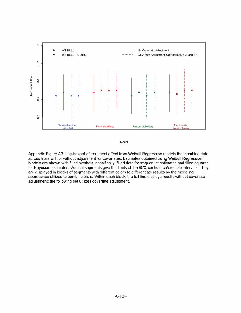
Model

Trea

tmen

t Effe

ct

-0.5

-0.4

-0.3

-0.2

-0.1

WEIBULLWEIBULL - BAYES

No Covariate AdjustmentCovariate Adjustment; Categorical AGE and EF

No adjustment for trial effect

Trial-Specific baseline hazardFixed trial effects Random trial effects

Appendix Figure A3. Log-hazard of treatment effect from Weibull Regression models that combine data across trials with or without adjustment for covariates. Estimates obtained using Weibull Regression Models are shown with filled symbols, specifically, filled dots for frequentist estimates and filled squares for Bayesian estimates. Vertical segments give the limits of the 95% confidence/credible intervals. They are displayed in blocks of segments with different colors to differentiate results by the modeling approaches utilized to combine trials. Within each block, the full line displays results without covariate adjustment; the following set utilizes covariate adjustment.

A-124

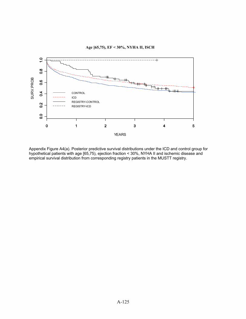
YEARS

SU

RV

.PR

OB

0 1 2 3 4 5

0.0

0.2

0.4

0.6

0.8

1.0

0 1 2 3 4 5

0.0

0.2

0.4

0.6

0.8

1.0

0 1 2 3 4 5

0.0

0.2

0.4

0.6

0.8

1.0

Age [65,75), EJ < 30%, NYHA2, ISCH

CONTROL

ICDREGISTRY-CONTROLREGISTRY-ICD

Age [65,75), EF < 30%, NYHA II, ISCH

Appendix Figure A4(a). Posterior predictive survival distributions under the ICD and control group for hypothetical patients with age [65,75), ejection fraction < 30%, NYHA II and ischemic disease and empirical survival distribution from corresponding registry patients in the MUSTT registry.

A-125

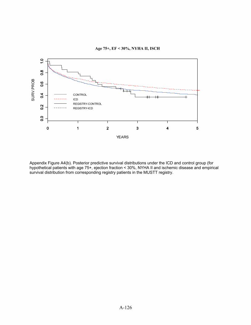
YEARS

SU

RV

.PR

OB

0 1 2 3 4 5

0.0

0.2

0.4

0.6

0.8

1.0

0 1 2 3 4 5

0.0

0.2

0.4

0.6

0.8

1.0

0 1 2 3 4 5

0.0

0.2

0.4

0.6

0.8

1.0

Age 75+, EJ < 30%, NYHA2, ISCH

CONTROL

ICDREGISTRY-CONTROLREGISTRY-ICD

Age 75+, EF < 30%, NYHA II, ISCH

Appendix Figure A4(b). Posterior predictive survival distributions under the ICD and control group (for hypothetical patients with age 75+, ejection fraction < 30%, NYHA II and ischemic disease and empirical survival distribution from corresponding registry patients in the MUSTT registry.

A-126

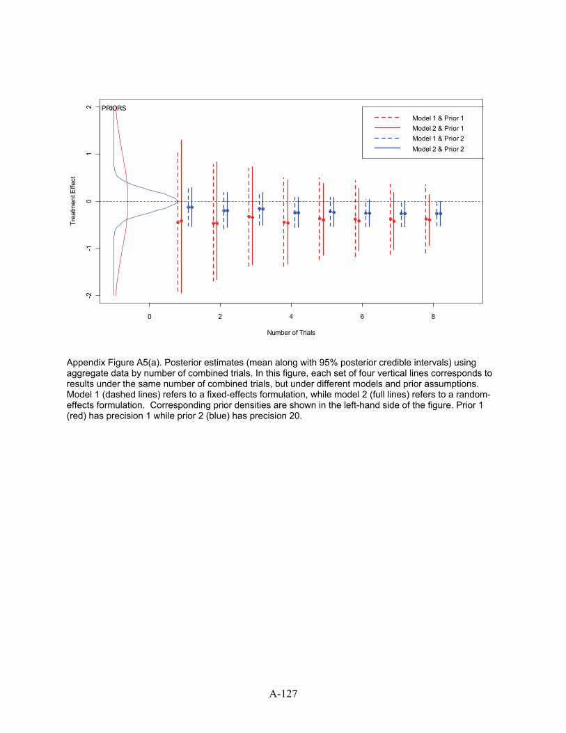
0 2 4 6 8

-2-1

01

2

Number of Trials

Trea

tmen

t Effe

ct

Model 1 & Prior 1Model 2 & Prior 1Model 1 & Prior 2Model 2 & Prior 2

PRIORS

Appendix Figure A5(a). Posterior estimates (mean along with 95% posterior credible intervals) using aggregate data by number of combined trials. In this figure, each set of four vertical lines corresponds to results under the same number of combined trials, but under different models and prior assumptions. Model 1 (dashed lines) refers to a fixed-effects formulation, while model 2 (full lines) refers to a random-effects formulation. Corresponding prior densities are shown in the left-hand side of the figure. Prior 1 (red) has precision 1 while prior 2 (blue) has precision 20.

A-127

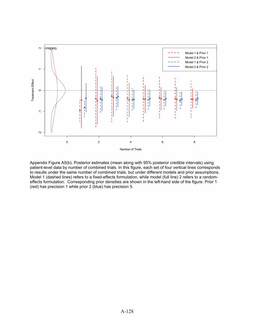
0 2 4 6 8

-2-1

01

2

Number of Trials

Trea

tmen

t Effe

ct

Model 1 & Prior 1Model 2 & Prior 1Model 1 & Prior 2Model 2 & Prior 2

PRIORS

Appendix Figure A5(b). Posterior estimates (mean along with 95% posterior credible intervals) using patient-level data by number of combined trials. In this figure, each set of four vertical lines corresponds to results under the same number of combined trials, but under different models and prior assumptions. Model 1 (dashed lines) refers to a fixed-effects formulation, while model (full line) 2 refers to a random-effects formulation. Corresponding prior densities are shown in the left-hand side of the figure. Prior 1 (red) has precision 1 while prior 2 (blue) has precision 5.

A-128

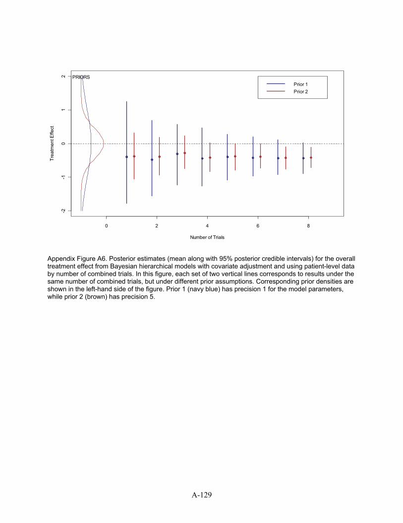
0 2 4 6 8

-2-1

01

2

Number of Trials

Trea

tmen

t Effe

ct

Prior 1Prior 2

PRIORS

Appendix Figure A6. Posterior estimates (mean along with 95% posterior credible intervals) for the overall treatment effect from Bayesian hierarchical models with covariate adjustment and using patient-level data by number of combined trials. In this figure, each set of two vertical lines corresponds to results under the same number of combined trials, but under different prior assumptions. Corresponding prior densities are shown in the left-hand side of the figure. Prior 1 (navy blue) has precision 1 for the model parameters, while prior 2 (brown) has precision 5.

A-129

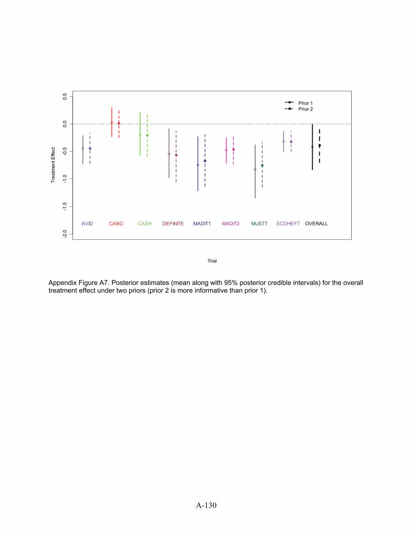
Trial

Trea

tmen

t Effe

ct

-2.0

-1.5

-1.0

-0.5

0.0

0.5

AVID CABG CASH DEFINITE MADIT1 MADIT2 MUSTT SCDHEFT

Prior 1Prior 2

OVERALL

Appendix Figure A7. Posterior estimates (mean along with 95% posterior credible intervals) for the overall treatment effect under two priors (prior 2 is more informative than prior 1).

A-130

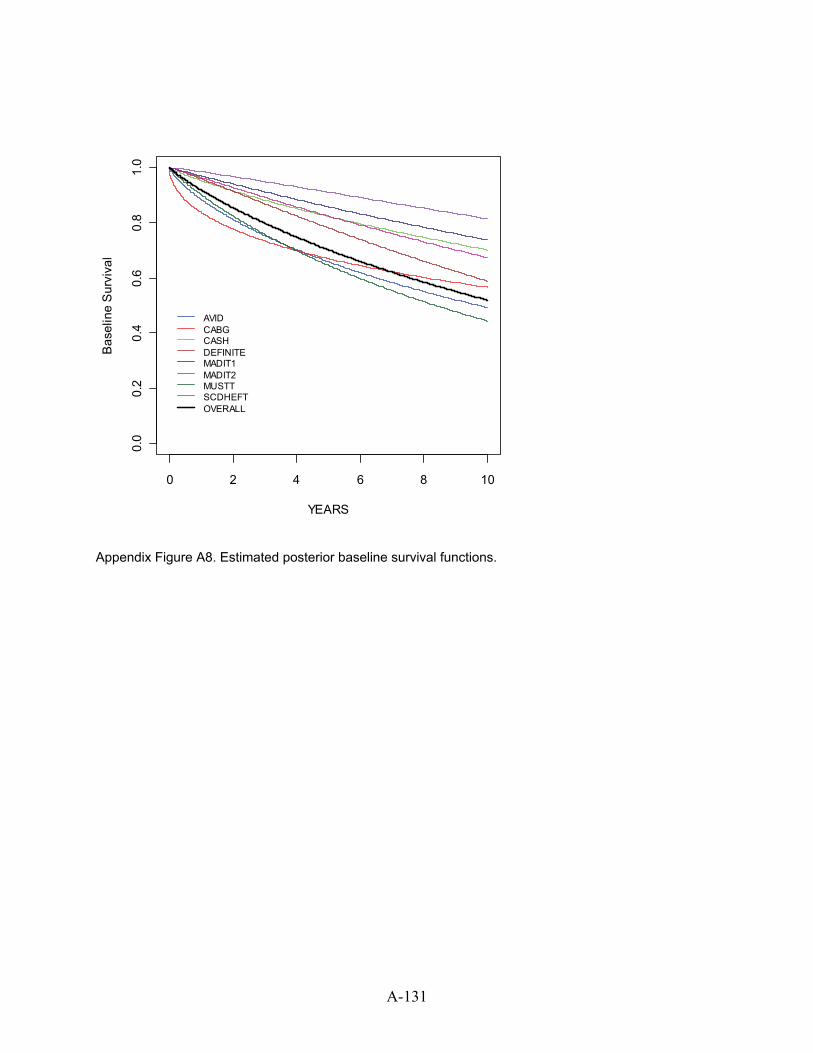
A-131

0 2 4 6 8 10

0.0

0.2

0.4

0.6

0.8

1.0

YEARS

Bas

elin

e S

urvi

val

AVIDCABGCASHDEFINITEMADIT1MADIT2MUSTTSCDHEFTOVERALL

Appendix Figure A8. Estimated posterior baseline survival functions.

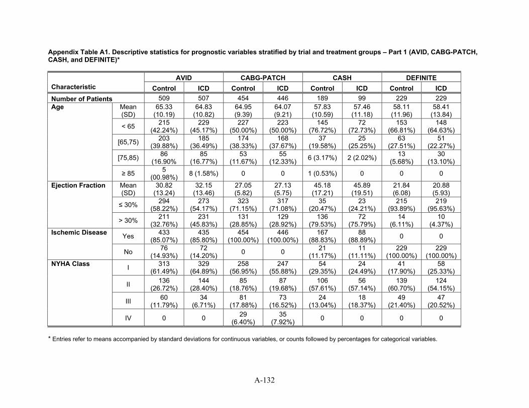
Appendix Table A1. Descriptive statistics for prognostic variables stratified by trial and treatment groups – Part 1 (AVID, CABG-PATCH, CASH, and DEFINITE)*

AVID CABG-PATCH CASH DEFINITE Characteristic Control ICD Control ICD Control ICD Control ICD Number of Patients 509 507 454 446 189 99 229 229

Mean (SD)

65.33 (10.19)

64.83 (10.82)

64.95 (9.39)

64.07 (9.21)

57.83 (10.59)

57.46 (11.18)

58.11 (11.96)

58.41 (13.84)

< 65 215 (42.24%)

229 (45.17%)

227 (50.00%)

223 (50.00%)

145 (76.72%)

72 (72.73%)

153 (66.81%)

148 (64.63%)

[65,75) 203 (39.88%)

185 (36.49%)

174 (38.33%)

168 (37.67%)

37 (19.58%)

25 (25.25%)

63 (27.51%)

51 (22.27%)

[75,85) 86 (16.90%

85 (16.77%)

53 (11.67%)

55 (12.33%) 6 (3.17%) 2 (2.02%) 13

(5.68%) 30

(13.10%)

Age

≥ 85 5 (00.98%) 8 (1.58%) 0 0 1 (0.53%) 0 0 0

Mean (SD)

30.82 (13.24)

32.15 (13.46)

27.05 (5.82)

27.13 (5.75)

45.18 (17.21)

45.89 (19.51)

21.84 (6.08)

20.88 (5.93)

≤ 30% 294 (58.22%)

273 (54.17%)

323 (71.15%)

317 (71.08%)

35 (20.47%)

23 (24.21%)

215 (93.89%)

219 (95.63%)

Ejection Fraction

> 30% 211 (32.76%)

231 (45.83%)

131 (28.85%)

129 (28.92%)

136 (79.53%)

72 (75.79%)

14 (6.11%)

10 (4.37%)

Yes 433 (85.07%)

435 (85.80%)

454 (100.00%)

446 (100.00%)

167 (88.83%)

88 (88.89%) 0 0 Ischemic Disease

No 76 (14.93%)

72 (14.20%) 0 0 21

(11.17%) 11

(11.11%) 229

(100.00%) 229

(100.00%)

I 313 (61.49%)

329 (64.89%)

258 (56.95%)

247 (55.88%)

54 (29.35%)

24 (24.49%)

41 (17.90%)

58 (25.33%)

II 136 (26.72%)

144 (28.40%)

85 (18.76%)

87 (19.68%)

106 (57.61%)

56 (57.14%)

139 (60.70%)

124 (54.15%)

III 60 (11.79%)

34 (6.71%)

81 (17.88%)

73 (16.52%)

24 (13.04%)

18 (18.37%)

49 (21.40%)

47 (20.52%)

NYHA Class

IV 0 0 29 (6.40%)

35 (7.92%) 0 0 0 0

* Entries refer to means accompanied by standard deviations for continuous variables, or counts followed by percentages for categorical variables.

A-132

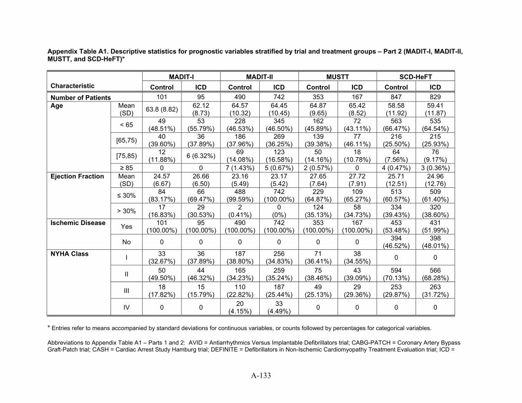
Appendix Table A1. Descriptive statistics for prognostic variables stratified by trial and treatment groups – Part 2 (MADIT-I, MADIT-II, MUSTT, and SCD-HeFT)*

MADIT-I MADIT-II MUSTT SCD-HeFT Characteristic Control ICD Control ICD Control ICD Control ICD Number of Patients 101 95 490 742 353 167 847 829

Mean (SD) 63.8 (8.82) 62.12

(8.73) 64.57

(10.32) 64.45

(10.45) 64.87 (9.65)

65.42 (8.52)

58.58 (11.92)

59.41 (11.87)

< 65 49 (48.51%)

53 (55.79%)

228 (46.53%)

345 (46.50%)

162 (45.89%)

72 (43.11%)

563 (66.47%)

535 (64.54%)

[65,75) 40 (39.60%)

36 (37.89%)

186 (37.96%)

269 (36.25%)

139 (39.38%)

77 (46.11%)

216 (25.50%)

215 (25.93%)

[75,85) 12 (11.88%) 6 (6.32%) 69

(14.08%) 123

(16.58%) 50

(14.16%) 18

(10.78%) 64

(7.56%) 76

(9.17%)

Age

≥ 85 0 0 7 (1.43%) 5 (0.67%) 2 (0.57%) 0 4 (0.47%) 3 (0.36%) Mean (SD)

24.57 (6.67)

26.66 (6.50)

23.16 (5.49)

23.17 (5.42)

27.65 (7.64)

27.72 (7.91)

25.71 (12.51)

24.96 (12.76)

≤ 30% 84 (83.17%)

66 (69.47%)

488 (99.59%)

742 (100.00%)

229 (64.87%)

109 (65.27%)

513 (60.57%)

509 (61.40%)

Ejection Fraction

> 30% 17 (16.83%)

29 (30.53%)

2 (0.41%)

0 (0%)

124 (35.13%)

58 (34.73%)

334 (39.43%)

320 (38.60%)

Yes 101 (100.00%)

95 (100.00%)

490 (100.00%)

742 (100.00%)

353 (100.00%)

167 (100.00%)

453 (53.48%)

431 (51.99%)

Ischemic Disease

No 0 0 0 0 0 0 394 (46.52%)

398 (48.01%)

I 33 (32.67%)

36 (37.89%)

187 (38.80%)

256 (34.83%)

71 (36.41%)

38 (34.55%) 0 0

II 50 (49.50%)

44 (46.32%)

165 (34.23%)

259 (35.24%)

75 (38.46%)

43 (39.09%)

594 (70.13%)

566 (68.28%)

III 18 (17.82%)

15 (15.79%)

110 (22.82%)

187 (25.44%)

49 (25.13%)

29 (29.36%)

253 (29.87%)

263 (31.72%)

NYHA Class

IV 0 0 20 (4.15%)

33 (4.49%) 0 0 0 0

* Entries refer to means accompanied by standard deviations for continuous variables, or counts followed by percentages for categorical variables. Abbreviations to Appendix Table A1 – Parts 1 and 2: AVID = Antiarrhythmics Versus Implantable Defibrillators trial; CABG-PATCH = Coronary Artery Bypass Graft-Patch trial; CASH = Cardiac Arrest Study Hamburg trial; DEFINITE = Defibrillators in Non-Ischemic Cardiomyopathy Treatment Evaluation trial; ICD =

A-133

A-134

implantable cardioverter defibrillator; MADIT-I = Multicenter Automatic Defibrillator Implantation Trial-I; MADIT-II = Multicenter Automatic Defibrillator Implantation Trial-II; MUSTT = Multicenter Unsustained Tachycardiac Trial; NYHA = New York Heart Association; SCD-HeFT = Sudden Cardiac Death in Heart Failure Trial; SD = standard deviation

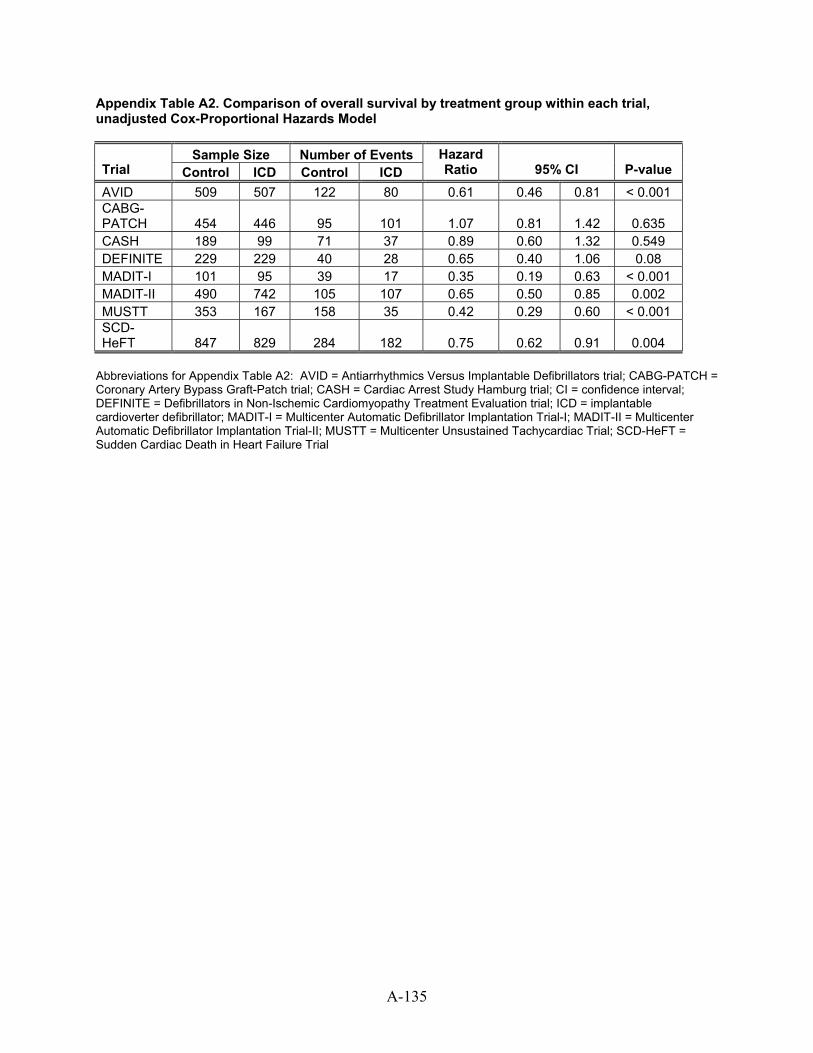
Appendix Table A2. Comparison of overall survival by treatment group within each trial, unadjusted Cox-Proportional Hazards Model

Sample Size Number of Events Trial Control ICD Control ICD

Hazard Ratio 95% CI P-value

AVID 509 507 122 80 0.61 0.46 0.81 < 0.001 CABG-PATCH 454 446 95 101 1.07 0.81 1.42 0.635 CASH 189 99 71 37 0.89 0.60 1.32 0.549 DEFINITE 229 229 40 28 0.65 0.40 1.06 0.08 MADIT-I 101 95 39 17 0.35 0.19 0.63 < 0.001 MADIT-II 490 742 105 107 0.65 0.50 0.85 0.002 MUSTT 353 167 158 35 0.42 0.29 0.60 < 0.001 SCD-HeFT 847 829 284 182 0.75 0.62 0.91 0.004

Abbreviations for Appendix Table A2: AVID = Antiarrhythmics Versus Implantable Defibrillators trial; CABG-PATCH = Coronary Artery Bypass Graft-Patch trial; CASH = Cardiac Arrest Study Hamburg trial; CI = confidence interval; DEFINITE = Defibrillators in Non-Ischemic Cardiomyopathy Treatment Evaluation trial; ICD = implantable cardioverter defibrillator; MADIT-I = Multicenter Automatic Defibrillator Implantation Trial-I; MADIT-II = Multicenter Automatic Defibrillator Implantation Trial-II; MUSTT = Multicenter Unsustained Tachycardiac Trial; SCD-HeFT = Sudden Cardiac Death in Heart Failure Trial

A-135

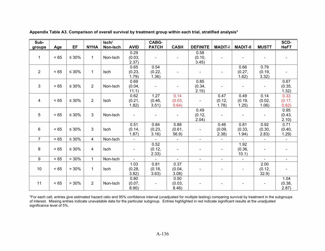
Appendix Table A3. Comparison of overall survival by treatment group within each trial, stratified analysis*

Sub-groups Age EF NYHA

Isch/ Non-Isch AVID

CABG-PATCH CASH DEFINITE MADIT-I MADIT-II MUSTT

SCD-HeFT

1 < 65 ≤ 30% 1 Non-Isch 0.29

(0.03, 2.37)

- - 0.58

(0.10, 3.45)

- - - -

2 < 65 ≤ 30% 1 Isch 0.65

(0.23, 1.79)

0.54 (0.22, 1.36)

- - - 0.66

(0.27, 1.62)

0.79 (0.19, 3.32)

-

3 < 65 ≤ 30% 2 Non-Isch 0.69

(0.04, 11.1)

- - 0.85

(0.34, 2.15)

- - - 0.67

(0.35, 1.32)

4 < 65 ≤ 30% 2 Isch 0.62

(0.21, 1.82)

1.27 (0.46, 3.51)

0.14 (0.03, 0.64)

- 0.47

(0.12, 1.78)

0.49 (0.19, 1.25)

0.14 (0.02, 1.06)

0.33 (0.17, 0.62)

5 < 65 ≤ 30% 3 Non-Isch - - - 0.49

(0.12, 2.04)

- - - 0.95

(0.43, 2.10)

6 < 65 ≤ 30% 3 Isch 0.51

(0.14, 1.87)

0.84 (0.23, 3.16)

5.88 (0.61, 56.9)

- 0.46

(0.09, 2.38)

0.81 (0.33, 1.94)

0.92 (0.30, 2.83)

0.71 (0.40, 1.29)

7 < 65 ≤ 30% 4 Non-Isch - - - - - - - -

8 < 65 ≤ 30% 4 Isch - 0.52

(0.12, 2.33)

- - - 1.92

(0.36, 10.1)

- -

9 < 65 > 30% 1 Non-Isch - - - - - - - -

10 < 65 > 30% 1 Isch 1.03

(0.28, 3.82)

0.81 (0.18, 3.63)

0.37 (0.04, 3.08)

- - - 2.00

(0.12, 32.9)

-

11 < 65 > 30% 2 Non-Isch 0.80

(0.07, 8.90)

- 0.50

(0.03, 8.46)

- - - - 1.04

(0.38, 2.87)

*For each cell, entries give estimated hazard ratio and 95% confidence interval (unadjusted for multiple testing) comparing survival by treatment in the subgroups of interest. Missing entries indicate unavailable data for the particular subgroup. Entries highlighted in red indicate significant results at the unadjusted significance level of 5%.

A-136

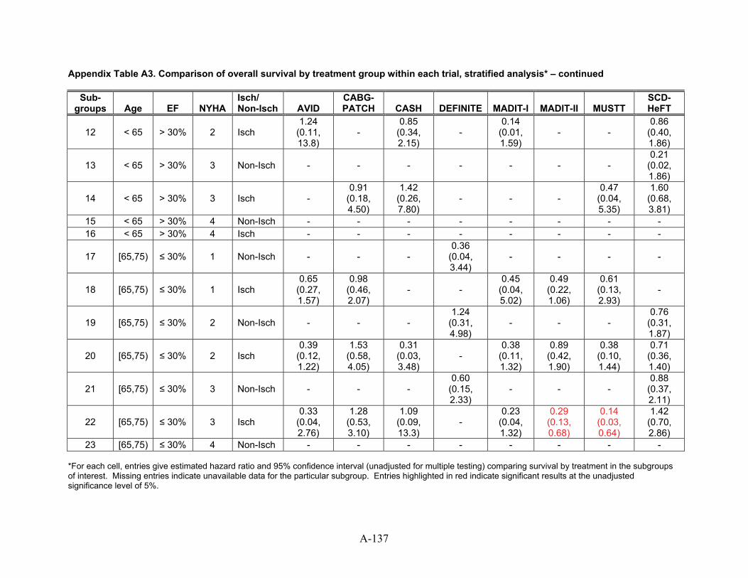
Appendix Table A3. Comparison of overall survival by treatment group within each trial, stratified analysis* – continued

Sub-groups Age EF NYHA

Isch/ Non-Isch AVID

CABG-PATCH CASH DEFINITE MADIT-I MADIT-II MUSTT

SCD-HeFT

12 < 65 > 30% 2 Isch 1.24

(0.11, 13.8)

- 0.85

(0.34, 2.15)

- 0.14

(0.01, 1.59)

- - 0.86

(0.40, 1.86)

13 < 65 > 30% 3 Non-Isch - - - - - - - 0.21

(0.02, 1.86)

14 < 65 > 30% 3 Isch - 0.91

(0.18, 4.50)

1.42 (0.26, 7.80)

- - - 0.47

(0.04, 5.35)

1.60 (0.68, 3.81)

15 < 65 > 30% 4 Non-Isch - - - - - - - - 16 < 65 > 30% 4 Isch - - - - - - - -

17 [65,75) ≤ 30% 1 Non-Isch - - - 0.36

(0.04, 3.44)

- - - -

18 [65,75) ≤ 30% 1 Isch 0.65

(0.27, 1.57)

0.98 (0.46, 2.07)

- - 0.45

(0.04, 5.02)

0.49 (0.22, 1.06)

0.61 (0.13, 2.93)

-

19 [65,75) ≤ 30% 2 Non-Isch - - - 1.24

(0.31, 4.98)

- - - 0.76

(0.31, 1.87)

20 [65,75) ≤ 30% 2 Isch 0.39

(0.12, 1.22)

1.53 (0.58, 4.05)

0.31 (0.03, 3.48)

- 0.38

(0.11, 1.32)

0.89 (0.42, 1.90)

0.38 (0.10, 1.44)

0.71 (0.36, 1.40)

21 [65,75) ≤ 30% 3 Non-Isch - - - 0.60

(0.15, 2.33)

- - - 0.88

(0.37, 2.11)

22 [65,75) ≤ 30% 3 Isch 0.33

(0.04, 2.76)

1.28 (0.53, 3.10)

1.09 (0.09, 13.3)

- 0.23

(0.04, 1.32)

0.29 (0.13, 0.68)

0.14 (0.03, 0.64)

1.42 (0.70, 2.86)

23 [65,75) ≤ 30% 4 Non-Isch - - - - - - - - *For each cell, entries give estimated hazard ratio and 95% confidence interval (unadjusted for multiple testing) comparing survival by treatment in the subgroups of interest. Missing entries indicate unavailable data for the particular subgroup. Entries highlighted in red indicate significant results at the unadjusted significance level of 5%.

A-137

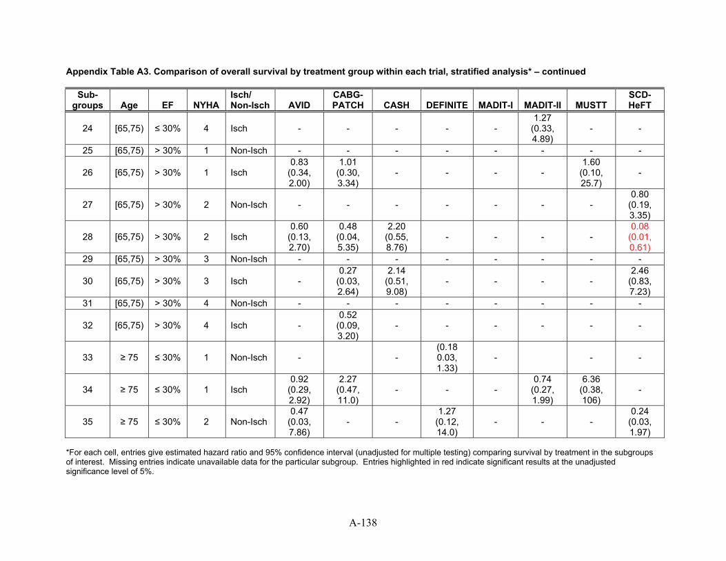
Appendix Table A3. Comparison of overall survival by treatment group within each trial, stratified analysis* – continued

Sub-groups Age EF NYHA

Isch/ Non-Isch AVID

CABG-PATCH CASH DEFINITE MADIT-I MADIT-II MUSTT

SCD-HeFT

24 [65,75) ≤ 30% 4 Isch - - - - - 1.27

(0.33, 4.89)

- -

25 [65,75) > 30% 1 Non-Isch - - - - - - - -

26 [65,75) > 30% 1 Isch 0.83

(0.34, 2.00)

1.01 (0.30, 3.34)

- - - - 1.60

(0.10, 25.7)

-

27 [65,75) > 30% 2 Non-Isch - - - - - - - 0.80

(0.19, 3.35)

28 [65,75) > 30% 2 Isch 0.60

(0.13, 2.70)

0.48 (0.04, 5.35)

2.20 (0.55, 8.76)

- - - - 0.08

(0.01, 0.61)

29 [65,75) > 30% 3 Non-Isch - - - - - - - -

30 [65,75) > 30% 3 Isch - 0.27

(0.03, 2.64)

2.14 (0.51, 9.08)

- - - - 2.46

(0.83, 7.23)

31 [65,75) > 30% 4 Non-Isch - - - - - - - -

32 [65,75) > 30% 4 Isch - 0.52

(0.09, 3.20)

- - - - - -

33 ≥ 75 ≤ 30% 1 Non-Isch - - (0.18 0.03, 1.33)

- - -

34 ≥ 75 ≤ 30% 1 Isch 0.92

(0.29, 2.92)

2.27 (0.47, 11.0)

- - - 0.74

(0.27, 1.99)

6.36 (0.38, 106)

-

35 ≥ 75 ≤ 30% 2 Non-Isch 0.47

(0.03, 7.86)

- - 1.27

(0.12, 14.0)

- - - 0.24

(0.03, 1.97)

*For each cell, entries give estimated hazard ratio and 95% confidence interval (unadjusted for multiple testing) comparing survival by treatment in the subgroups of interest. Missing entries indicate unavailable data for the particular subgroup. Entries highlighted in red indicate significant results at the unadjusted significance level of 5%.

A-138

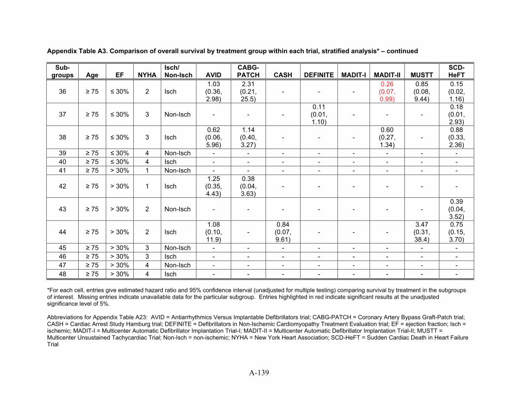
Appendix Table A3. Comparison of overall survival by treatment group within each trial, stratified analysis* – continued

Sub-groups Age EF NYHA

Isch/ Non-Isch AVID

CABG-PATCH CASH DEFINITE MADIT-I MADIT-II MUSTT

SCD-HeFT

36 ≥ 75 ≤ 30% 2 Isch 1.03

(0.36, 2.98)

2.31 (0.21, 25.5)

- - - 0.26

(0.07, 0.99)

0.85 (0.08, 9.44)

0.15 (0.02, 1.16)

37 ≥ 75 ≤ 30% 3 Non-Isch - - - 0.11

(0.01, 1.10)

- - - 0.18

(0.01, 2.93)

38 ≥ 75 ≤ 30% 3 Isch 0.62

(0.06, 5.96)

1.14 (0.40, 3.27)

- - - 0.60

(0.27, 1.34)

- 0.88

(0.33, 2.36)

39 ≥ 75 ≤ 30% 4 Non-Isch - - - - - - - - 40 ≥ 75 ≤ 30% 4 Isch - - - - - - - - 41 ≥ 75 > 30% 1 Non-Isch - - - - - - - -

42 ≥ 75 > 30% 1 Isch 1.25

(0.35, 4.43)

0.38 (0.04, 3.63)

- - - - - -

43 ≥ 75 > 30% 2 Non-Isch - - - - - - - 0.39

(0.04, 3.52)

44 ≥ 75 > 30% 2 Isch 1.08

(0.10, 11.9)

- 0.84

(0.07, 9.61)

- - - 3.47

(0.31, 38.4)

0.75 (0.15, 3.70)

45 ≥ 75 > 30% 3 Non-Isch - - - - - - - - 46 ≥ 75 > 30% 3 Isch - - - - - - - - 47 ≥ 75 > 30% 4 Non-Isch - - - - - - - - 48 ≥ 75 > 30% 4 Isch - - - - - - - -

*For each cell, entries give estimated hazard ratio and 95% confidence interval (unadjusted for multiple testing) comparing survival by treatment in the subgroups of interest. Missing entries indicate unavailable data for the particular subgroup. Entries highlighted in red indicate significant results at the unadjusted significance level of 5%. Abbreviations for Appendix Table A23: AVID = Antiarrhythmics Versus Implantable Defibrillators trial; CABG-PATCH = Coronary Artery Bypass Graft-Patch trial; CASH = Cardiac Arrest Study Hamburg trial; DEFINITE = Defibrillators in Non-Ischemic Cardiomyopathy Treatment Evaluation trial; EF = ejection fraction; Isch = ischemic; MADIT-I = Multicenter Automatic Defibrillator Implantation Trial-I; MADIT-II = Multicenter Automatic Defibrillator Implantation Trial-II; MUSTT = Multicenter Unsustained Tachycardiac Trial; Non-Isch = non-ischemic; NYHA = New York Heart Association; SCD-HeFT = Sudden Cardiac Death in Heart Failure Trial

A-139

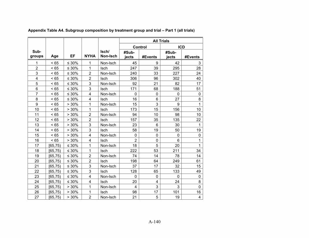
Appendix Table A4. Subgroup composition by treatment group and trial – Part 1 (all trials)

All Trials Control ICD

Sub-groups Age EF NYHA

Isch/ Non-Isch

#Sub-jects #Events

#Sub-jects #Events

1 < 65 ≤ 30% 1 Non-Isch 45 9 42 32 < 65 ≤ 30% 1 Isch 247 39 295 283 < 65 ≤ 30% 2 Non-Isch 240 33 227 244 < 65 ≤ 30% 2 Isch 306 96 302 405 < 65 ≤ 30% 3 Non-Isch 92 21 82 176 < 65 ≤ 30% 3 Isch 171 68 188 517 < 65 ≤ 30% 4 Non-Isch 0 0 0 08 < 65 ≤ 30% 4 Isch 16 6 27 89 < 65 > 30% 1 Non-Isch 15 3 9 1

10 < 65 > 30% 1 Isch 173 15 156 1011 < 65 > 30% 2 Non-Isch 94 10 98 1012 < 65 > 30% 2 Isch 157 35 135 2213 < 65 > 30% 3 Non-Isch 23 6 30 114 < 65 > 30% 3 Isch 58 19 50 1915 < 65 > 30% 4 Non-Isch 0 0 0 016 < 65 > 30% 4 Isch 2 0 6 117 [65,75) ≤ 30% 1 Non-Isch 18 5 20 118 [65,75) ≤ 30% 1 Isch 222 53 211 3419 [65,75) ≤ 30% 2 Non-Isch 74 14 78 1420 [65,75) ≤ 30% 2 Isch 198 64 249 6121 [65,75) ≤ 30% 3 Non-Isch 37 17 32 1522 [65,75) ≤ 30% 3 Isch 128 65 133 4923 [65,75) ≤ 30% 4 Non-Isch 0 0 0 024 [65,75) ≤ 30% 4 Isch 20 4 24 825 [65,75) > 30% 1 Non-Isch 4 3 3 026 [65,75) > 30% 1 Isch 98 17 101 1627 [65,75) > 30% 2 Non-Isch 21 5 19 4

A-140

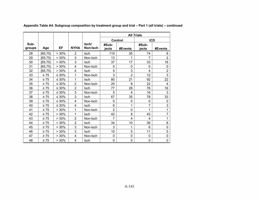
Appendix Table A4. Subgroup composition by treatment group and trial – Part 1 (all trials) – continued

All Trials Control ICD

Sub-groups Age EF NYHA

Isch/ Non-Isch

#Sub-jects #Events

#Sub-jects #Events

28 [65,75) > 30% 2 Isch 110 35 74 829 [65,75) > 30% 3 Non-Isch 13 1 7 230 [65,75) > 30% 3 Isch 37 17 33 1631 [65,75) > 30% 4 Non-Isch 0 0 0 032 [65,75) > 30% 4 Isch 5 3 4 233 ≥ 75 ≤ 30% 1 Non-Isch 3 2 12 334 ≥ 75 ≤ 30% 1 Isch 80 21 92 2235 ≥ 75 ≤ 30% 2 Non-Isch 20 8 22 436 ≥ 75 ≤ 30% 2 Isch 77 28 76 1637 ≥ 75 ≤ 30% 3 Non-Isch 5 4 16 338 ≥ 75 ≤ 30% 3 Isch 67 35 78 3339 ≥ 75 ≤ 30% 4 Non-Isch 0 0 0 040 ≥ 75 ≤ 30% 4 Isch 6 1 7 341 ≥ 75 > 30% 1 Non-Isch 2 0 1 142 ≥ 75 > 30% 1 Isch 42 8 43 743 ≥ 75 > 30% 2 Non-Isch 7 4 4 144 ≥ 75 > 30% 2 Isch 34 10 36 845 ≥ 75 > 30% 3 Non-Isch 3 1 6 046 ≥ 75 > 30% 3 Isch 10 5 11 547 ≥ 75 > 30% 4 Non-Isch 0 0 0 048 ≥ 75 > 30% 4 Isch 0 0 0 0

A-141

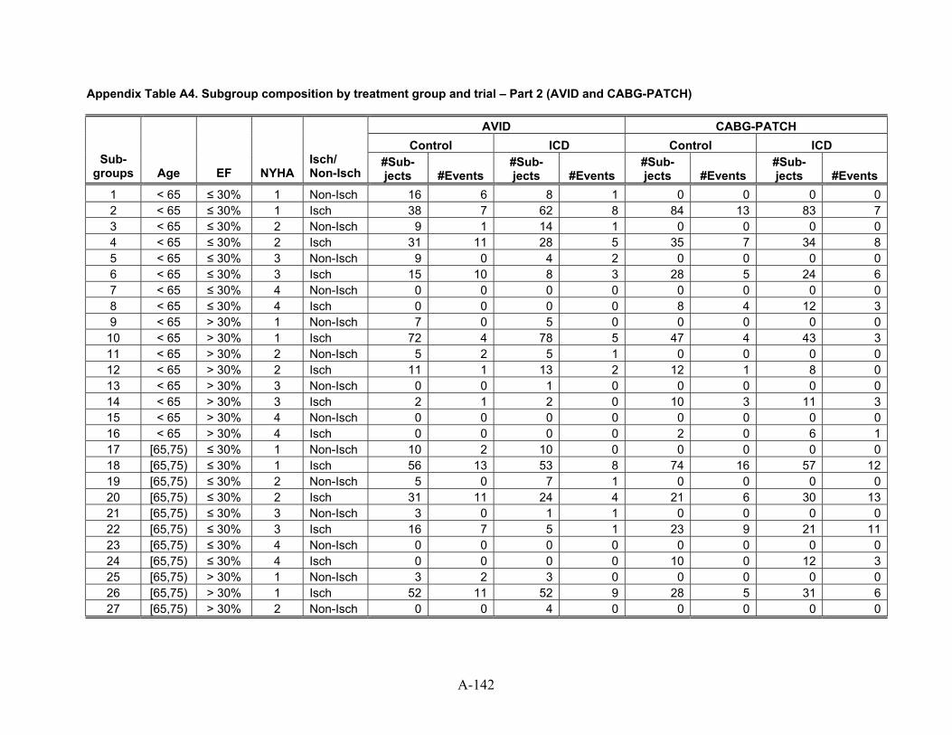
Appendix Table A4. Subgroup composition by treatment group and trial – Part 2 (AVID and CABG-PATCH)

AVID CABG-PATCH Control ICD Control ICD

Sub-groups Age EF NYHA

Isch/ Non-Isch

#Sub-jects #Events

#Sub-jects #Events

#Sub-jects #Events

#Sub-jects #Events

1 < 65 ≤ 30% 1 Non-Isch 16 6 8 1 0 0 0 02 < 65 ≤ 30% 1 Isch 38 7 62 8 84 13 83 73 < 65 ≤ 30% 2 Non-Isch 9 1 14 1 0 0 0 04 < 65 ≤ 30% 2 Isch 31 11 28 5 35 7 34 85 < 65 ≤ 30% 3 Non-Isch 9 0 4 2 0 0 0 06 < 65 ≤ 30% 3 Isch 15 10 8 3 28 5 24 67 < 65 ≤ 30% 4 Non-Isch 0 0 0 0 0 0 0 08 < 65 ≤ 30% 4 Isch 0 0 0 0 8 4 12 39 < 65 > 30% 1 Non-Isch 7 0 5 0 0 0 0 0

10 < 65 > 30% 1 Isch 72 4 78 5 47 4 43 311 < 65 > 30% 2 Non-Isch 5 2 5 1 0 0 0 012 < 65 > 30% 2 Isch 11 1 13 2 12 1 8 013 < 65 > 30% 3 Non-Isch 0 0 1 0 0 0 0 014 < 65 > 30% 3 Isch 2 1 2 0 10 3 11 315 < 65 > 30% 4 Non-Isch 0 0 0 0 0 0 0 016 < 65 > 30% 4 Isch 0 0 0 0 2 0 6 117 [65,75) ≤ 30% 1 Non-Isch 10 2 10 0 0 0 0 018 [65,75) ≤ 30% 1 Isch 56 13 53 8 74 16 57 1219 [65,75) ≤ 30% 2 Non-Isch 5 0 7 1 0 0 0 020 [65,75) ≤ 30% 2 Isch 31 11 24 4 21 6 30 1321 [65,75) ≤ 30% 3 Non-Isch 3 0 1 1 0 0 0 022 [65,75) ≤ 30% 3 Isch 16 7 5 1 23 9 21 1123 [65,75) ≤ 30% 4 Non-Isch 0 0 0 0 0 0 0 024 [65,75) ≤ 30% 4 Isch 0 0 0 0 10 0 12 325 [65,75) > 30% 1 Non-Isch 3 2 3 0 0 0 0 026 [65,75) > 30% 1 Isch 52 11 52 9 28 5 31 627 [65,75) > 30% 2 Non-Isch 0 0 4 0 0 0 0 0

A-142

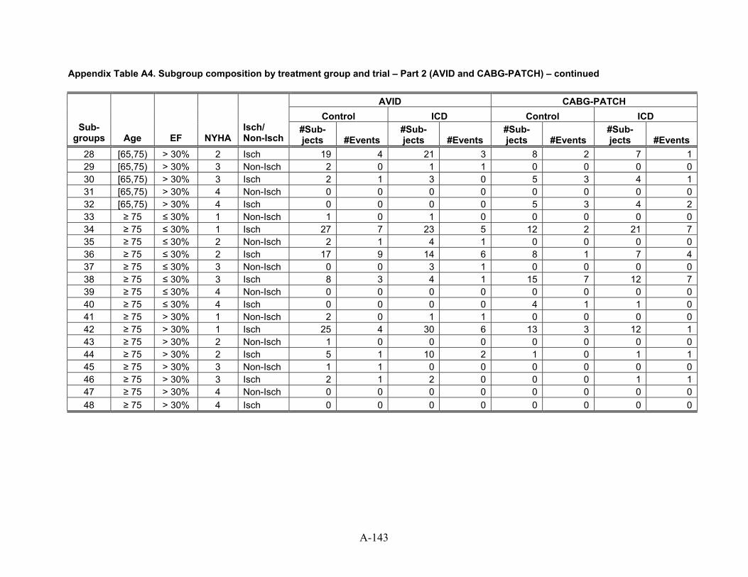
Appendix Table A4. Subgroup composition by treatment group and trial – Part 2 (AVID and CABG-PATCH) – continued

AVID CABG-PATCH Control ICD Control ICD

Sub-groups Age EF NYHA

Isch/ Non-Isch

#Sub-jects #Events

#Sub-jects #Events

#Sub-jects #Events

#Sub-jects #Events

28 [65,75) > 30% 2 Isch 19 4 21 3 8 2 7 129 [65,75) > 30% 3 Non-Isch 2 0 1 1 0 0 0 030 [65,75) > 30% 3 Isch 2 1 3 0 5 3 4 131 [65,75) > 30% 4 Non-Isch 0 0 0 0 0 0 0 032 [65,75) > 30% 4 Isch 0 0 0 0 5 3 4 233 ≥ 75 ≤ 30% 1 Non-Isch 1 0 1 0 0 0 0 034 ≥ 75 ≤ 30% 1 Isch 27 7 23 5 12 2 21 735 ≥ 75 ≤ 30% 2 Non-Isch 2 1 4 1 0 0 0 036 ≥ 75 ≤ 30% 2 Isch 17 9 14 6 8 1 7 437 ≥ 75 ≤ 30% 3 Non-Isch 0 0 3 1 0 0 0 038 ≥ 75 ≤ 30% 3 Isch 8 3 4 1 15 7 12 739 ≥ 75 ≤ 30% 4 Non-Isch 0 0 0 0 0 0 0 040 ≥ 75 ≤ 30% 4 Isch 0 0 0 0 4 1 1 041 ≥ 75 > 30% 1 Non-Isch 2 0 1 1 0 0 0 042 ≥ 75 > 30% 1 Isch 25 4 30 6 13 3 12 143 ≥ 75 > 30% 2 Non-Isch 1 0 0 0 0 0 0 044 ≥ 75 > 30% 2 Isch 5 1 10 2 1 0 1 145 ≥ 75 > 30% 3 Non-Isch 1 1 0 0 0 0 0 046 ≥ 75 > 30% 3 Isch 2 1 2 0 0 0 1 147 ≥ 75 > 30% 4 Non-Isch 0 0 0 0 0 0 0 048 ≥ 75 > 30% 4 Isch 0 0 0 0 0 0 0 0

A-143

Appendix Table A4. Subgroup composition by treatment group and trial – Part 3 (CASH and DEFINITE)

CASH DEFINITE Control ICD Control ICD

Sub-groups Age EF NYHA

Isch/ Non-Isch

#Sub-jects #Events

#Sub-jects #Events

#Sub-jects #Events

#Sub-jects #Events

1 < 65 ≤ 30% 1 Non-Isch 0 0 0 0 29 3 34 22 < 65 ≤ 30% 1 Isch 3 1 1 1 0 0 0 03 < 65 ≤ 30% 2 Non-Isch 1 0 2 1 89 10 78 84 < 65 ≤ 30% 2 Isch 16 11 9 2 0 0 0 05 < 65 ≤ 30% 3 Non-Isch 2 2 1 0 24 5 29 36 < 65 ≤ 30% 3 Isch 5 2 5 4 0 0 0 07 < 65 ≤ 30% 4 Non-Isch 0 0 0 0 0 0 0 08 < 65 ≤ 30% 4 Isch 0 0 0 0 0 0 0 09 < 65 > 30% 1 Non-Isch 7 3 1 0 1 0 3 1

10 < 65 > 30% 1 Isch 39 6 17 1 0 0 0 011 < 65 > 30% 2 Non-Isch 5 1 4 1 8 0 2 012 < 65 > 30% 2 Isch 45 13 26 7 0 0 0 013 < 65 > 30% 3 Non-Isch 1 1 0 0 2 1 2 014 < 65 > 30% 3 Isch 4 2 5 4 0 0 0 015 < 65 > 30% 4 Non-Isch 0 0 0 0 0 0 0 016 < 65 > 30% 4 Isch 0 0 0 0 0 0 0 017 [65,75) ≤ 30% 1 Non-Isch 0 0 0 0 8 3 10 118 [65,75) ≤ 30% 1 Isch 0 0 0 0 0 0 0 019 [65,75) ≤ 30% 2 Non-Isch 0 0 0 0 34 4 30 420 [65,75) ≤ 30% 2 Isch 3 2 4 3 0 0 0 021 [65,75) ≤ 30% 3 Non-Isch 0 0 0 0 18 7 9 322 [65,75) ≤ 30% 3 Isch 4 3 1 1 0 0 0 023 [65,75) ≤ 30% 4 Non-Isch 0 0 0 0 0 0 0 024 [65,75) ≤ 30% 4 Isch 0 0 0 0 0 0 0 025 [65,75) > 30% 1 Non-Isch 0 0 0 0 1 1 0 026 [65,75) > 30% 1 Isch 1 0 5 0 0 0 0 027 [65,75) > 30% 2 Non-Isch 0 0 1 1 1 0 2 0

A-144

Appendix Table A4. Subgroup composition by treatment group and trial – Part 3 (CASH and DEFINITE) – continued

CASH DEFINITE Control ICD Control ICD

Sub-groups Age EF NYHA

Isch/ Non-Isch

#Sub-jects #Events

#Sub-jects #Events

#Sub-jects #Events

#Sub-jects #Events

28 [65,75) > 30% 2 Isch 19 8 5 3 0 0 0 029 [65,75) > 30% 3 Non-Isch 1 1 0 0 1 0 0 030 [65,75) > 30% 3 Isch 5 5 6 5 0 0 0 031 [65,75) > 30% 4 Non-Isch 0 0 0 0 0 0 0 032 [65,75) > 30% 4 Isch 0 0 0 0 0 0 0 033 ≥ 75 ≤ 30% 1 Non-Isch 0 0 0 0 2 2 11 334 ≥ 75 ≤ 30% 1 Isch 0 0 0 0 0 0 0 035 ≥ 75 ≤ 30% 2 Non-Isch 0 0 0 0 7 1 11 236 ≥ 75 ≤ 30% 2 Isch 0 0 0 0 0 0 0 037 ≥ 75 ≤ 30% 3 Non-Isch 0 0 0 0 4 3 7 138 ≥ 75 ≤ 30% 3 Isch 1 1 0 0 0 0 0 039 ≥ 75 ≤ 30% 4 Non-Isch 0 0 0 0 0 0 0 040 ≥ 75 ≤ 30% 4 Isch 0 0 0 0 0 0 0 041 ≥ 75 > 30% 1 Non-Isch 0 0 0 0 0 0 0 042 ≥ 75 > 30% 1 Isch 0 0 0 0 0 0 0 043 ≥ 75 > 30% 2 Non-Isch 0 0 0 0 0 0 1 044 ≥ 75 > 30% 2 Isch 5 2 2 1 0 0 0 045 ≥ 75 > 30% 3 Non-Isch 0 0 0 0 0 0 0 046 ≥ 75 > 30% 3 Isch 1 1 0 0 0 0 0 047 ≥ 75 > 30% 4 Non-Isch 0 0 0 0 0 0 0 048 ≥ 75 > 30% 4 Isch 0 0 0 0 0 0 0 0

A-145

Appendix Table A4. Subgroup composition by treatment group and trial – Part 4 (MADIT-I and MADIT-II)

MADIT-I MADIT-II Control ICD Control ICD

Sub-groups Age EF NYHA

Isch/ Non-Isch

#Sub-jects #Events

#Sub-jects #Events

#Sub-jects #Events

#Sub-jects #Events

1 < 65 ≤ 30% 1 Non-Isch 0 0 0 0 0 0 0 02 < 65 ≤ 30% 1 Isch 14 3 12 0 91 10 124 93 < 65 ≤ 30% 2 Non-Isch 0 0 0 0 0 0 0 04 < 65 ≤ 30% 2 Isch 21 8 15 3 81 10 115 85 < 65 ≤ 30% 3 Non-Isch 0 0 0 0 0 0 0 06 < 65 ≤ 30% 3 Isch 9 5 7 2 44 8 87 137 < 65 ≤ 30% 4 Non-Isch 0 0 0 0 0 0 0 08 < 65 ≤ 30% 4 Isch 0 0 0 0 8 2 15 59 < 65 > 30% 1 Non-Isch 0 0 0 0 0 0 0 0

10 < 65 > 30% 1 Isch 2 0 11 0 1 0 0 011 < 65 > 30% 2 Non-Isch 0 0 0 0 0 0 0 012 < 65 > 30% 2 Isch 3 2 7 1 0 0 0 013 < 65 > 30% 3 Non-Isch 0 0 0 0 0 0 0 014 < 65 > 30% 3 Isch 0 0 1 1 0 0 0 015 < 65 > 30% 4 Non-Isch 0 0 0 0 0 0 0 016 < 65 > 30% 4 Isch 0 0 0 0 0 0 0 017 [65,75) ≤ 30% 1 Non-Isch 0 0 0 0 0 0 0 018 [65,75) ≤ 30% 1 Isch 7 2 7 1 67 15 86 1119 [65,75) ≤ 30% 2 Non-Isch 0 0 0 0 0 0 0 020 [65,75) ≤ 30% 2 Isch 16 7 17 6 60 11 107 1721 [65,75) ≤ 30% 3 Non-Isch 0 0 0 0 0 0 0 022 [65,75) ≤ 30% 3 Isch 6 4 6 3 46 19 62 823 [65,75) ≤ 30% 4 Non-Isch 0 0 0 0 0 0 0 024 [65,75) ≤ 30% 4 Isch 0 0 0 0 10 4 12 525 [65,75) > 30% 1 Non-Isch 0 0 0 0 0 0 0 026 [65,75) > 30% 1 Isch 5 0 5 0 0 0 0 027 [65,75) > 30% 2 Non-Isch 0 0 0 0 0 0 0 0

A-146

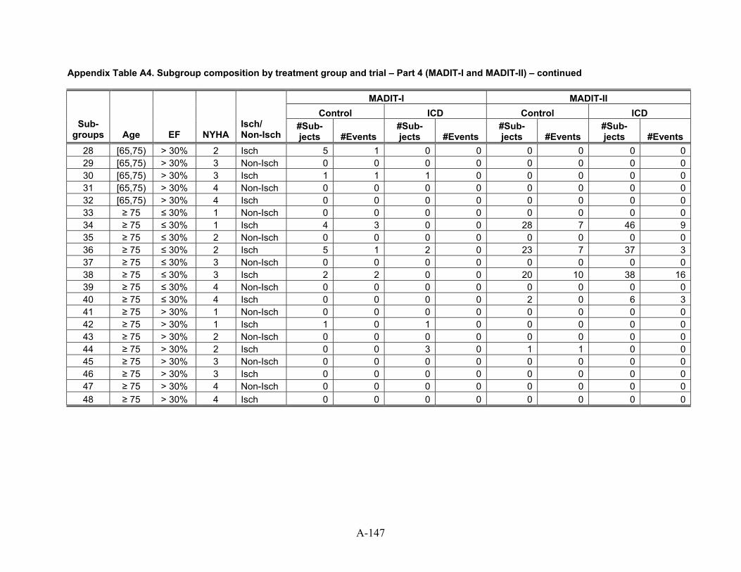
Appendix Table A4. Subgroup composition by treatment group and trial – Part 4 (MADIT-I and MADIT-II) – continued

MADIT-I MADIT-II Control ICD Control ICD

Sub-groups Age EF NYHA

Isch/ Non-Isch

#Sub-jects #Events

#Sub-jects #Events

#Sub-jects #Events

#Sub-jects #Events

28 [65,75) > 30% 2 Isch 5 1 0 0 0 0 0 029 [65,75) > 30% 3 Non-Isch 0 0 0 0 0 0 0 030 [65,75) > 30% 3 Isch 1 1 1 0 0 0 0 031 [65,75) > 30% 4 Non-Isch 0 0 0 0 0 0 0 032 [65,75) > 30% 4 Isch 0 0 0 0 0 0 0 033 ≥ 75 ≤ 30% 1 Non-Isch 0 0 0 0 0 0 0 034 ≥ 75 ≤ 30% 1 Isch 4 3 0 0 28 7 46 935 ≥ 75 ≤ 30% 2 Non-Isch 0 0 0 0 0 0 0 036 ≥ 75 ≤ 30% 2 Isch 5 1 2 0 23 7 37 337 ≥ 75 ≤ 30% 3 Non-Isch 0 0 0 0 0 0 0 038 ≥ 75 ≤ 30% 3 Isch 2 2 0 0 20 10 38 1639 ≥ 75 ≤ 30% 4 Non-Isch 0 0 0 0 0 0 0 040 ≥ 75 ≤ 30% 4 Isch 0 0 0 0 2 0 6 341 ≥ 75 > 30% 1 Non-Isch 0 0 0 0 0 0 0 042 ≥ 75 > 30% 1 Isch 1 0 1 0 0 0 0 043 ≥ 75 > 30% 2 Non-Isch 0 0 0 0 0 0 0 044 ≥ 75 > 30% 2 Isch 0 0 3 0 1 1 0 045 ≥ 75 > 30% 3 Non-Isch 0 0 0 0 0 0 0 046 ≥ 75 > 30% 3 Isch 0 0 0 0 0 0 0 047 ≥ 75 > 30% 4 Non-Isch 0 0 0 0 0 0 0 048 ≥ 75 > 30% 4 Isch 0 0 0 0 0 0 0 0

A-147

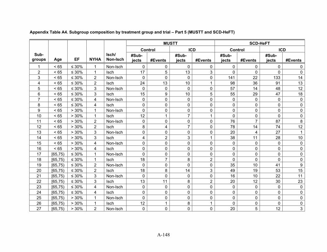
Appendix Table A4. Subgroup composition by treatment group and trial – Part 5 (MUSTT and SCD-HeFT)

MUSTT SCD-HeFT Control ICD Control ICD

Sub-groups Age EF NYHA

Isch/ Non-Isch

#Sub-jects #Events

#Sub-jects #Events

#Sub-jects #Events

#Sub-jects #Events

1 < 65 ≤ 30% 1 Non-Isch 0 0 0 0 0 0 0 02 < 65 ≤ 30% 1 Isch 17 5 13 3 0 0 0 03 < 65 ≤ 30% 2 Non-Isch 0 0 0 0 141 22 133 144 < 65 ≤ 30% 2 Isch 24 13 10 1 98 36 91 135 < 65 ≤ 30% 3 Non-Isch 0 0 0 0 57 14 48 126 < 65 ≤ 30% 3 Isch 15 9 10 5 55 29 47 187 < 65 ≤ 30% 4 Non-Isch 0 0 0 0 0 0 0 08 < 65 ≤ 30% 4 Isch 0 0 0 0 0 0 0 09 < 65 > 30% 1 Non-Isch 0 0 0 0 0 0 0 0

10 < 65 > 30% 1 Isch 12 1 7 1 0 0 0 011 < 65 > 30% 2 Non-Isch 0 0 0 0 76 7 87 812 < 65 > 30% 2 Isch 8 4 7 0 78 14 74 1213 < 65 > 30% 3 Non-Isch 0 0 0 0 20 4 27 114 < 65 > 30% 3 Isch 4 2 3 1 38 11 28 1015 < 65 > 30% 4 Non-Isch 0 0 0 0 0 0 0 016 < 65 > 30% 4 Isch 0 0 0 0 0 0 0 017 [65,75) ≤ 30% 1 Non-Isch 0 0 0 0 0 0 0 018 [65,75) ≤ 30% 1 Isch 18 7 8 2 0 0 0 019 [65,75) ≤ 30% 2 Non-Isch 0 0 0 0 35 10 41 920 [65,75) ≤ 30% 2 Isch 18 8 14 3 49 19 53 1521 [65,75) ≤ 30% 3 Non-Isch 0 0 0 0 16 10 22 1122 [65,75) ≤ 30% 3 Isch 13 11 8 2 20 12 30 2323 [65,75) ≤ 30% 4 Non-Isch 0 0 0 0 0 0 0 024 [65,75) ≤ 30% 4 Isch 0 0 0 0 0 0 0 025 [65,75) > 30% 1 Non-Isch 0 0 0 0 0 0 0 026 [65,75) > 30% 1 Isch 12 1 8 1 0 0 0 027 [65,75) > 30% 2 Non-Isch 0 0 0 0 20 5 12 3

A-148

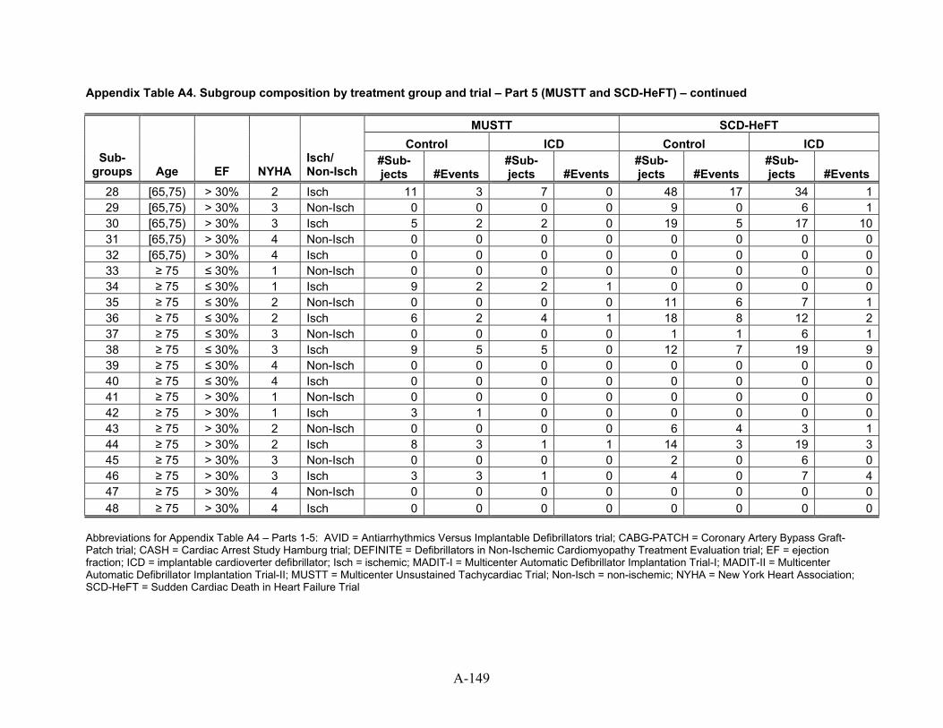
A-149

Appendix Table A4. Subgroup composition by treatment group and trial – Part 5 (MUSTT and SCD-HeFT) – continued

MUSTT SCD-HeFT Control ICD Control ICD

Sub-groups Age EF NYHA

Isch/ Non-Isch

#Sub-jects #Events

#Sub-jects #Events

#Sub-jects #Events

#Sub-jects #Events

28 [65,75) > 30% 2 Isch 11 3 7 0 48 17 34 129 [65,75) > 30% 3 0 Non-Isch 0 0 0 9 0 6 130 [65,75) > 30% 3 2 Isch 5 2 0 19 5 17 1031 [65,75) > 30% 4 0 Non-Isch 0 0 0 0 0 0 032 [65,75) > 30% 4 0 Isch 0 0 0 0 0 0 033 ≥ 75 ≤ 30% 1 Non-Isch 0 0 0 0 0 0 0 034 ≥ 75 ≤ 30% 1 Isch 9 2 2 1 0 0 0 035 ≥ 75 ≤ 30% 2 Non-Isch 0 0 0 0 11 6 7 136 ≥ 75 ≤ 30% 2 Isch 6 2 4 1 18 8 12 237 ≥ 75 ≤ 30% 3 Non-Isch 0 0 0 0 1 1 6 138 ≥ 75 ≤ 30% 3 Isch 9 5 5 0 12 7 19 939 ≥ 75 ≤ 30% 4 Non-Isch 0 0 0 0 0 0 0 040 ≥ 75 ≤ 30% 4 Isch 0 0 0 0 0 0 0 041 ≥ 75 > 30% 1 Non-Isch 0 0 0 0 0 0 0 042 ≥ 75 > 30% 1 Isch 3 1 0 0 0 0 0 043 ≥ 75 > 30% 2 Non-Isch 0 0 0 0 6 4 3 144 ≥ 75 > 30% 2 Isch 8 3 1 1 14 3 19 345 ≥ 75 > 30% 3 Non-Isch 0 0 0 0 2 0 6 046 ≥ 75 > 30% 3 Isch 3 3 1 0 4 0 7 447 ≥ 75 > 30% 4 Non-Isch 0 0 0 0 0 0 0 048 ≥ 75 > 30% 4 Isch 0 0 0 0 0 0 0 0

Abbreviations for Appendix Table A4 – Parts 1-5: AVID = Antiarrhythmics Versus Implantable Defibrillators trial; CABG-PATCH = Coronary Artery Bypass Graft-Patch trial; CASH = Cardiac Arrest Study Hamburg trial; DEFINITE = Defibrillators in Non-Ischemic Cardiomyopathy Treatment Evaluation trial; EF = ejection fraction; ICD = implantable cardioverter defibrillator; Isch = ischemic; MADIT-I = Multicenter Automatic Defibrillator Implantation Trial-I; MADIT-II = Multicenter Automatic Defibrillator Implantation Trial-II; MUSTT = Multicenter Unsustained Tachycardiac Trial; Non-Isch = non-ischemic; NYHA = New York Heart Association; SCD-HeFT = Sudden Cardiac Death in Heart Failure Trial

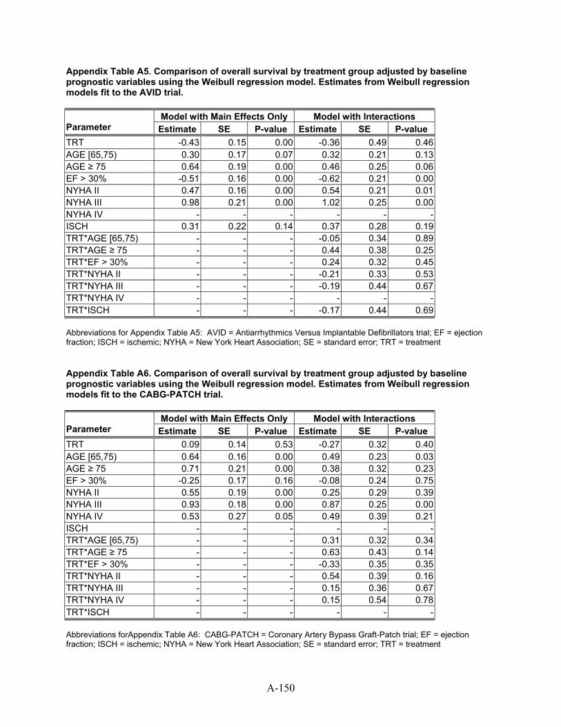
Appendix Table A5. Comparison of overall survival by treatment group adjusted by baseline prognostic variables using the Weibull regression model. Estimates from Weibull regression models fit to the AVID trial.

Model with Main Effects Only Model with Interactions Parameter Estimate SE P-value Estimate SE P-value TRT -0.43 0.15 0.00 -0.36 0.49 0.46 AGE [65,75) 0.30 0.17 0.07 0.32 0.21 0.13 AGE ≥ 75 0.64 0.19 0.00 0.46 0.25 0.06 EF > 30% -0.51 0.16 0.00 -0.62 0.21 0.00 NYHA II 0.47 0.16 0.00 0.54 0.21 0.01 NYHA III 0.98 0.21 0.00 1.02 0.25 0.00 NYHA IV - - - - - - ISCH 0.31 0.22 0.14 0.37 0.28 0.19 TRT*AGE [65,75) - - - -0.05 0.34 0.89 TRT*AGE ≥ 75 - - - 0.44 0.38 0.25 TRT*EF > 30% - - - 0.24 0.32 0.45 TRT*NYHA II - - - -0.21 0.33 0.53 TRT*NYHA III - - - -0.19 0.44 0.67 TRT*NYHA IV - - - - - - TRT*ISCH - - - -0.17 0.44 0.69 Abbreviations for Appendix Table A5: AVID = Antiarrhythmics Versus Implantable Defibrillators trial; EF = ejection fraction; ISCH = ischemic; NYHA = New York Heart Association; SE = standard error; TRT = treatment Appendix Table A6. Comparison of overall survival by treatment group adjusted by baseline prognostic variables using the Weibull regression model. Estimates from Weibull regression models fit to the CABG-PATCH trial.

Model with Main Effects Only Model with Interactions Parameter Estimate SE P-value Estimate SE P-value TRT 0.09 0.14 0.53 -0.27 0.32 0.40 AGE [65,75) 0.64 0.16 0.00 0.49 0.23 0.03 AGE ≥ 75 0.71 0.21 0.00 0.38 0.32 0.23 EF > 30% -0.25 0.17 0.16 -0.08 0.24 0.75 NYHA II 0.55 0.19 0.00 0.25 0.29 0.39 NYHA III 0.93 0.18 0.00 0.87 0.25 0.00 NYHA IV 0.53 0.27 0.05 0.49 0.39 0.21 ISCH - - - - - - TRT*AGE [65,75) - - - 0.31 0.32 0.34 TRT*AGE ≥ 75 - - - 0.63 0.43 0.14 TRT*EF > 30% - - - -0.33 0.35 0.35 TRT*NYHA II - - - 0.54 0.39 0.16 TRT*NYHA III - - - 0.15 0.36 0.67 TRT*NYHA IV - - - 0.15 0.54 0.78 TRT*ISCH - - - - - - Abbreviations forAppendix Table A6: CABG-PATCH = Coronary Artery Bypass Graft-Patch trial; EF = ejection fraction; ISCH = ischemic; NYHA = New York Heart Association; SE = standard error; TRT = treatment

A-150

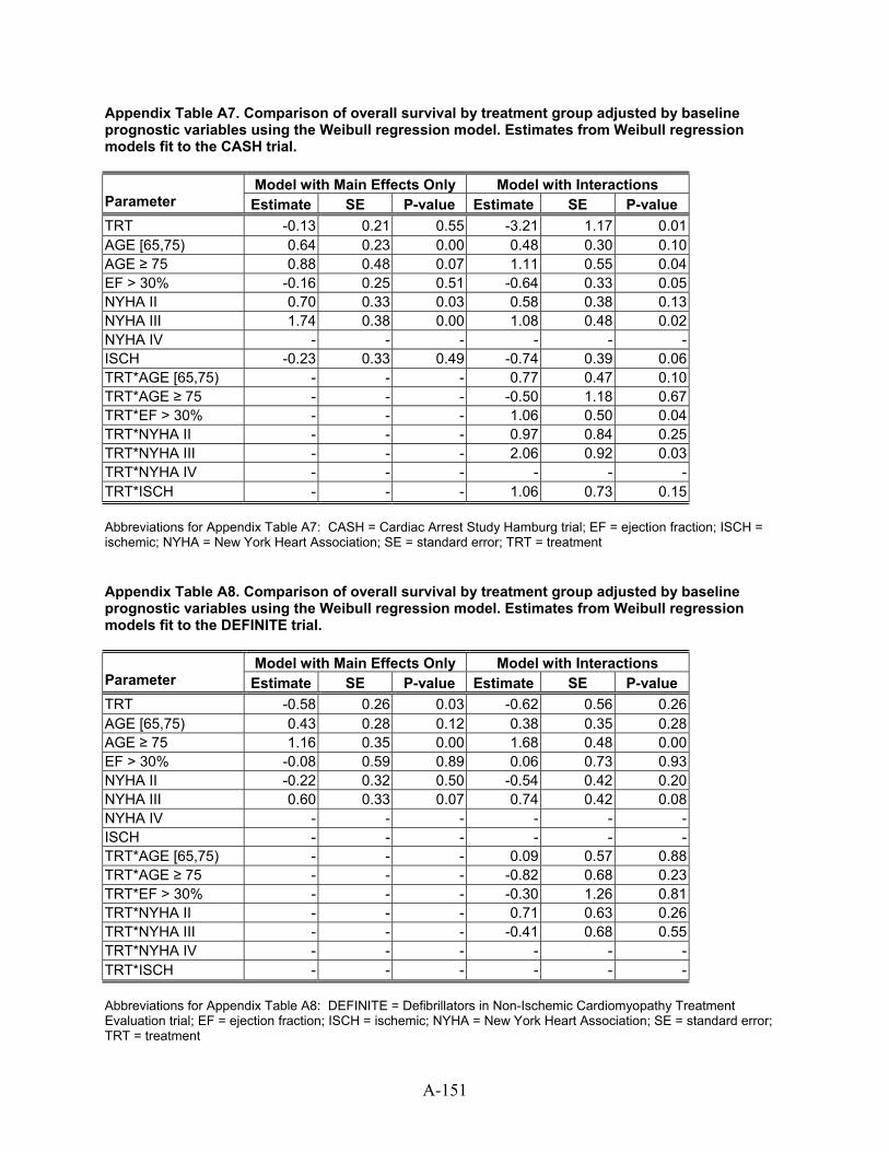
Appendix Table A7. Comparison of overall survival by treatment group adjusted by baseline prognostic variables using the Weibull regression model. Estimates from Weibull regression models fit to the CASH trial.

Model with Main Effects Only Model with Interactions Parameter Estimate SE P-value Estimate SE P-value TRT -0.13 0.21 0.55 -3.21 1.17 0.01 AGE [65,75) 0.64 0.23 0.00 0.48 0.30 0.10 AGE ≥ 75 0.88 0.48 0.07 1.11 0.55 0.04 EF > 30% -0.16 0.25 0.51 -0.64 0.33 0.05 NYHA II 0.70 0.33 0.03 0.58 0.38 0.13 NYHA III 1.74 0.38 0.00 1.08 0.48 0.02 NYHA IV - - - - - - ISCH -0.23 0.33 0.49 -0.74 0.39 0.06 TRT*AGE [65,75) - - - 0.77 0.47 0.10 TRT*AGE ≥ 75 - - - -0.50 1.18 0.67 TRT*EF > 30% - - - 1.06 0.50 0.04 TRT*NYHA II - - - 0.97 0.84 0.25 TRT*NYHA III - - - 2.06 0.92 0.03 TRT*NYHA IV - - - - - - TRT*ISCH - - - 1.06 0.73 0.15 Abbreviations for Appendix Table A7: CASH = Cardiac Arrest Study Hamburg trial; EF = ejection fraction; ISCH = ischemic; NYHA = New York Heart Association; SE = standard error; TRT = treatment Appendix Table A8. Comparison of overall survival by treatment group adjusted by baseline prognostic variables using the Weibull regression model. Estimates from Weibull regression models fit to the DEFINITE trial.

Model with Main Effects Only Model with Interactions Parameter Estimate SE P-value Estimate SE P-value TRT -0.58 0.26 0.03 -0.62 0.56 0.26 AGE [65,75) 0.43 0.28 0.12 0.38 0.35 0.28 AGE ≥ 75 1.16 0.35 0.00 1.68 0.48 0.00 EF > 30% -0.08 0.59 0.89 0.06 0.73 0.93 NYHA II -0.22 0.32 0.50 -0.54 0.42 0.20 NYHA III 0.60 0.33 0.07 0.74 0.42 0.08 NYHA IV - - - - - - ISCH - - - - - - TRT*AGE [65,75) - - - 0.09 0.57 0.88 TRT*AGE ≥ 75 - - - -0.82 0.68 0.23 TRT*EF > 30% - - - -0.30 1.26 0.81 TRT*NYHA II - - - 0.71 0.63 0.26 TRT*NYHA III - - - -0.41 0.68 0.55 TRT*NYHA IV - - - - - - TRT*ISCH - - - - - - Abbreviations for Appendix Table A8: DEFINITE = Defibrillators in Non-Ischemic Cardiomyopathy Treatment Evaluation trial; EF = ejection fraction; ISCH = ischemic; NYHA = New York Heart Association; SE = standard error; TRT = treatment

A-151

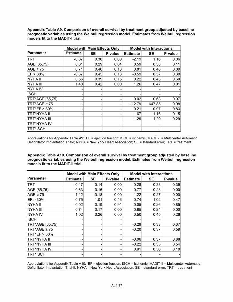
Appendix Table A9. Comparison of overall survival by treatment group adjusted by baseline prognostic variables using the Weibull regression model. Estimates from Weibull regression models fit to the MADIT-I trial.

Model with Main Effects Only Model with Interactions Parameter Estimate SE P-value Estimate SE P-value TRT -0.87 0.30 0.00 -2.19 1.16 0.06 AGE [65,75) 0.61 0.29 0.04 0.59 0.38 0.11 AGE ≥ 75 0.71 0.46 0.13 0.81 0.48 0.09 EF > 30% -0.67 0.45 0.13 -0.59 0.57 0.30 NYHA II 0.56 0.39 0.15 0.22 0.43 0.60 NYHA III 1.48 0.42 0.00 1.26 0.47 0.01 NYHA IV - - - - - - ISCH - - - - - - TRT*AGE [65,75) - - - 0.02 0.63 0.97 TRT*AGE ≥ 75 - - - -12.79 647.85 0.98 TRT*EF > 30% - - - 0.21 0.97 0.83 TRT*NYHA II - - - 1.67 1.16 0.15 TRT*NYHA III - - - 1.29 1.20 0.29 TRT*NYHA IV - - - - - - TRT*ISCH - - - - - - Abbreviations for Appendix Table A9: EF = ejection fraction; ISCH = ischemic; MADIT-I = Multicenter Automatic Defibrillator Implantation Trial-I; NYHA = New York Heart Association; SE = standard error; TRT = treatment Appendix Table A10. Comparison of overall survival by treatment group adjusted by baseline prognostic variables using the Weibull regression model. Estimates from Weibull regression models fit to the MADIT-II trial.

Model with Main Effects Only Model with Interactions Parameter Estimate SE P-value Estimate SE P-value TRT -0.47 0.14 0.00 -0.28 0.33 0.39 AGE [65,75) 0.63 0.16 0.00 0.77 0.23 0.00 AGE ≥ 75 1.12 0.18 0.00 1.22 0.27 0.00 EF > 30% 0.75 1.01 0.46 0.74 1.02 0.47 NYHA II 0.02 0.19 0.91 0.05 0.26 0.85 NYHA III 0.74 0.17 0.00 0.85 0.24 0.00 NYHA IV 1.02 0.26 0.00 0.50 0.45 0.26 ISCH - - - - - - TRT*AGE [65,75) - - - -0.29 0.33 0.37 TRT*AGE ≥ 75 - - - -0.20 0.37 0.59 TRT*EF > 30% - - - TRT*NYHA II - - - -0.06 0.37 0.88 TRT*NYHA III - - - -0.22 0.35 0.54 TRT*NYHA IV - - - 0.91 0.56 0.10 TRT*ISCH - - - - - - Abbreviations for Appendix Table A10: EF = ejection fraction; ISCH = ischemic; MADIT-II = Multicenter Automatic Defibrillator Implantation Trial-II; NYHA = New York Heart Association; SE = standard error; TRT = treatment

A-152

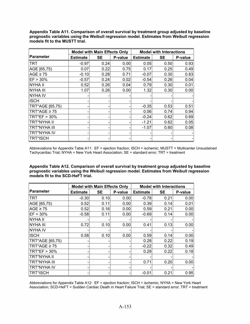
A-153

Appendix Table A11. Comparison of overall survival by treatment group adjusted by baseline prognostic variables using the Weibull regression model. Estimates from Weibull regression models fit to the MUSTT trial.

Model with Main Effects Only Model with Interactions Parameter Estimate SE P-value Estimate SE P-value TRT -0.97 0.24 0.00 0.05 0.50 0.93 AGE [65,75) 0.07 0.22 0.75 0.17 0.25 0.49 AGE ≥ 75 -0.10 0.28 0.71 -0.07 0.30 0.83 EF > 30% -0.57 0.24 0.02 -0.54 0.26 0.04 NYHA II 0.52 0.26 0.04 0.79 0.30 0.01 NYHA III 1.07 0.26 0.00 1.32 0.30 0.00 NYHA IV - - - - - - ISCH - - - - - - TRT*AGE [65,75) - - - -0.35 0.53 0.51 TRT*AGE ≥ 75 - - - 0.06 0.74 0.94 TRT*EF > 30% - - - -0.24 0.62 0.69 TRT*NYHA II - - - -1.21 0.62 0.05 TRT*NYHA III - - - -1.07 0.60 0.08 TRT*NYHA IV - - - - - - TRT*ISCH - - - - - - Abbreviations for Appendix Table A11: EF = ejection fraction; ISCH = ischemic; MUSTT = Multicenter Unsustained Tachycardiac Trial; NYHA = New York Heart Association; SE = standard error; TRT = treatment Appendix Table A12. Comparison of overall survival by treatment group adjusted by baseline prognostic variables using the Weibull regression model. Estimates from Weibull regression models fit to the SCD-HeFT trial.

Model with Main Effects Only Model with Interactions Parameter Estimate SE P-value Estimate SE P-value TRT -0.30 0.10 0.00 -0.78 0.21 0.00 AGE [65,75) 0.52 0.11 0.00 0.39 0.14 0.01 AGE ≥ 75 0.52 0.16 0.00 0.59 0.21 0.00 EF > 30% -0.58 0.11 0.00 -0.69 0.14 0.00 NYHA II - - - - - - NYHA III 0.72 0.10 0.00 0.41 0.13 0.00 NYHA IV - - - - - - ISCH 0.58 0.10 0.00 0.59 0.14 0.00 TRT*AGE [65,75) - - - 0.28 0.22 0.19 TRT*AGE ≥ 75 - - - -0.22 0.32 0.49 TRT*EF > 30% - - - 0.29 0.22 0.18 TRT*NYHA II - - - - - - TRT*NYHA III - - - 0.71 0.20 0.00 TRT*NYHA IV - - - - - - TRT*ISCH - - - -0.01 0.21 0.95 Abbreviations for Appendix Table A12: EF = ejection fraction; ISCH = ischemic; NYHA = New York Heart Association; SCD-HeFT = Sudden Cardiac Death in Heart Failure Trial; SE = standard error; TRT = treatment

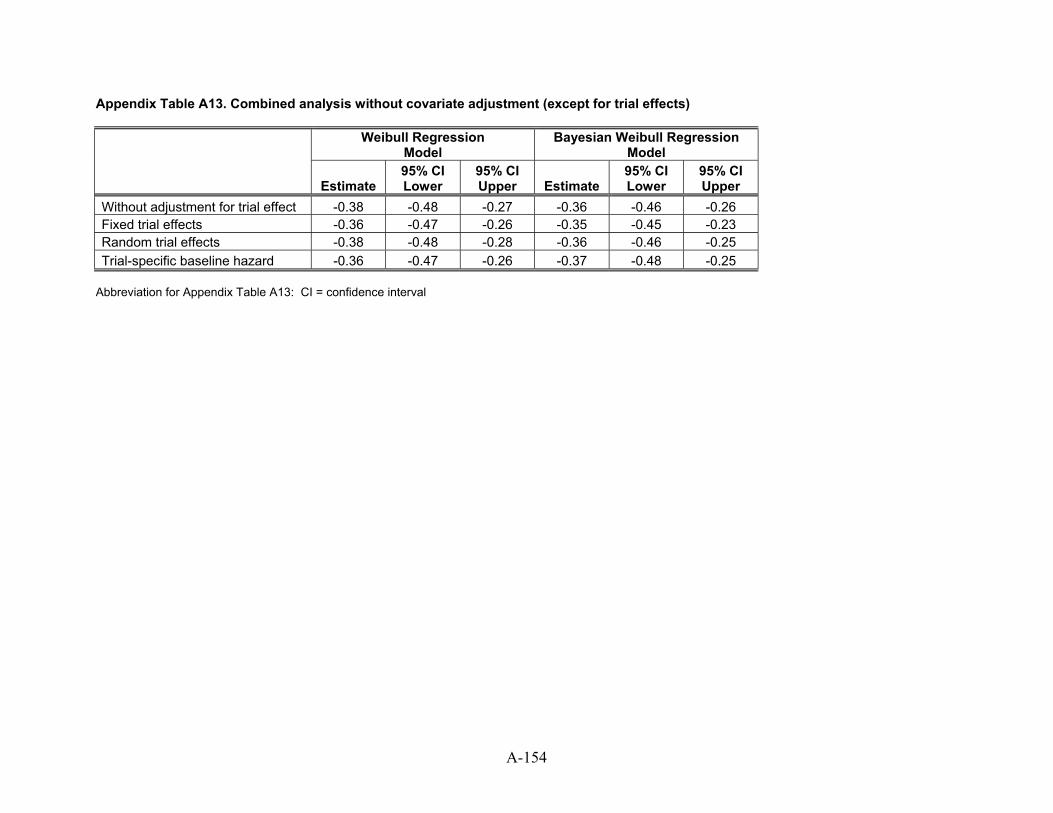
Appendix Table A13. Combined analysis without covariate adjustment (except for trial effects)

Weibull Regression Model

Bayesian Weibull Regression Model

Estimate

95% CI Lower

95% CI Upper Estimate

95% CI Lower

95% CI Upper

Without adjustment for trial effect -0.38 -0.48 -0.27 -0.36 -0.46 -0.26 Fixed trial effects -0.36 -0.47 -0.26 -0.35 -0.45 -0.23 Random trial effects -0.38 -0.48 -0.28 -0.36 -0.46 -0.25 Trial-specific baseline hazard -0.36 -0.47 -0.26 -0.37 -0.48 -0.25

Abbreviation for Appendix Table A13: CI = confidence interval

A-154

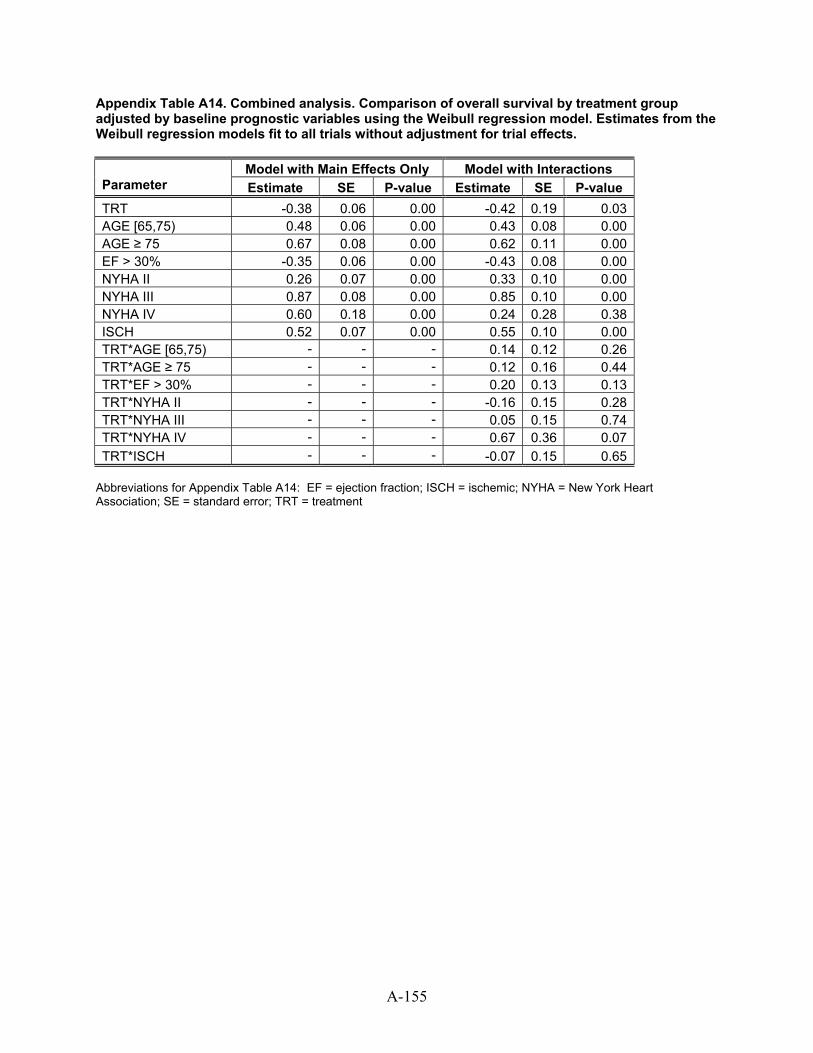
Appendix Table A14. Combined analysis. Comparison of overall survival by treatment group adjusted by baseline prognostic variables using the Weibull regression model. Estimates from the Weibull regression models fit to all trials without adjustment for trial effects.

Model with Main Effects Only Model with Interactions Parameter Estimate SE P-value Estimate SE P-value TRT -0.38 0.06 0.00 -0.42 0.19 0.03 AGE [65,75) 0.48 0.06 0.00 0.43 0.08 0.00 AGE ≥ 75 0.67 0.08 0.00 0.62 0.11 0.00 EF > 30% -0.35 0.06 0.00 -0.43 0.08 0.00 NYHA II 0.26 0.07 0.00 0.33 0.10 0.00 NYHA III 0.87 0.08 0.00 0.85 0.10 0.00 NYHA IV 0.60 0.18 0.00 0.24 0.28 0.38 ISCH 0.52 0.07 0.00 0.55 0.10 0.00 TRT*AGE [65,75) - - - 0.14 0.12 0.26 TRT*AGE ≥ 75 - - - 0.12 0.16 0.44 TRT*EF > 30% - - - 0.20 0.13 0.13 TRT*NYHA II - - - -0.16 0.15 0.28 TRT*NYHA III - - - 0.05 0.15 0.74 TRT*NYHA IV - - - 0.67 0.36 0.07 TRT*ISCH - - - -0.07 0.15 0.65

Abbreviations for Appendix Table A14: EF = ejection fraction; ISCH = ischemic; NYHA = New York Heart Association; SE = standard error; TRT = treatment

A-155

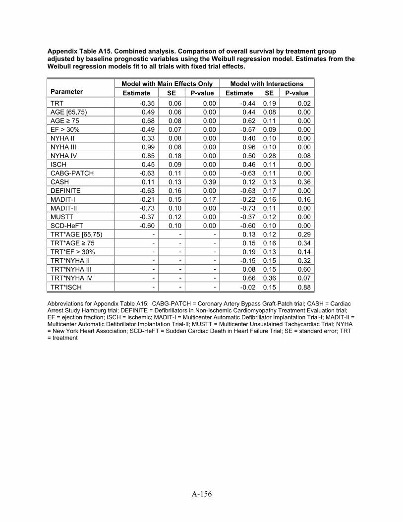
Appendix Table A15. Combined analysis. Comparison of overall survival by treatment group adjusted by baseline prognostic variables using the Weibull regression model. Estimates from the Weibull regression models fit to all trials with fixed trial effects.

Model with Main Effects Only Model with Interactions Parameter Estimate SE P-value Estimate SE P-value TRT -0.35 0.06 0.00 -0.44 0.19 0.02 AGE [65,75) 0.49 0.06 0.00 0.44 0.08 0.00 AGE ≥ 75 0.68 0.08 0.00 0.62 0.11 0.00 EF > 30% -0.49 0.07 0.00 -0.57 0.09 0.00 NYHA II 0.33 0.08 0.00 0.40 0.10 0.00 NYHA III 0.99 0.08 0.00 0.96 0.10 0.00 NYHA IV 0.85 0.18 0.00 0.50 0.28 0.08 ISCH 0.45 0.09 0.00 0.46 0.11 0.00 CABG-PATCH -0.63 0.11 0.00 -0.63 0.11 0.00 CASH 0.11 0.13 0.39 0.12 0.13 0.36 DEFINITE -0.63 0.16 0.00 -0.63 0.17 0.00 MADIT-I -0.21 0.15 0.17 -0.22 0.16 0.16 MADIT-II -0.73 0.10 0.00 -0.73 0.11 0.00 MUSTT -0.37 0.12 0.00 -0.37 0.12 0.00 SCD-HeFT -0.60 0.10 0.00 -0.60 0.10 0.00 TRT*AGE [65,75) - - - 0.13 0.12 0.29 TRT*AGE ≥ 75 - - - 0.15 0.16 0.34 TRT*EF > 30% - - - 0.19 0.13 0.14 TRT*NYHA II - - - -0.15 0.15 0.32 TRT*NYHA III - - - 0.08 0.15 0.60 TRT*NYHA IV - - - 0.66 0.36 0.07 TRT*ISCH - - - -0.02 0.15 0.88

Abbreviations for Appendix Table A15: CABG-PATCH = Coronary Artery Bypass Graft-Patch trial; CASH = Cardiac Arrest Study Hamburg trial; DEFINITE = Defibrillators in Non-Ischemic Cardiomyopathy Treatment Evaluation trial; EF = ejection fraction; ISCH = ischemic; MADIT-I = Multicenter Automatic Defibrillator Implantation Trial-I; MADIT-II = Multicenter Automatic Defibrillator Implantation Trial-II; MUSTT = Multicenter Unsustained Tachycardiac Trial; NYHA = New York Heart Association; SCD-HeFT = Sudden Cardiac Death in Heart Failure Trial; SE = standard error; TRT = treatment

A-156

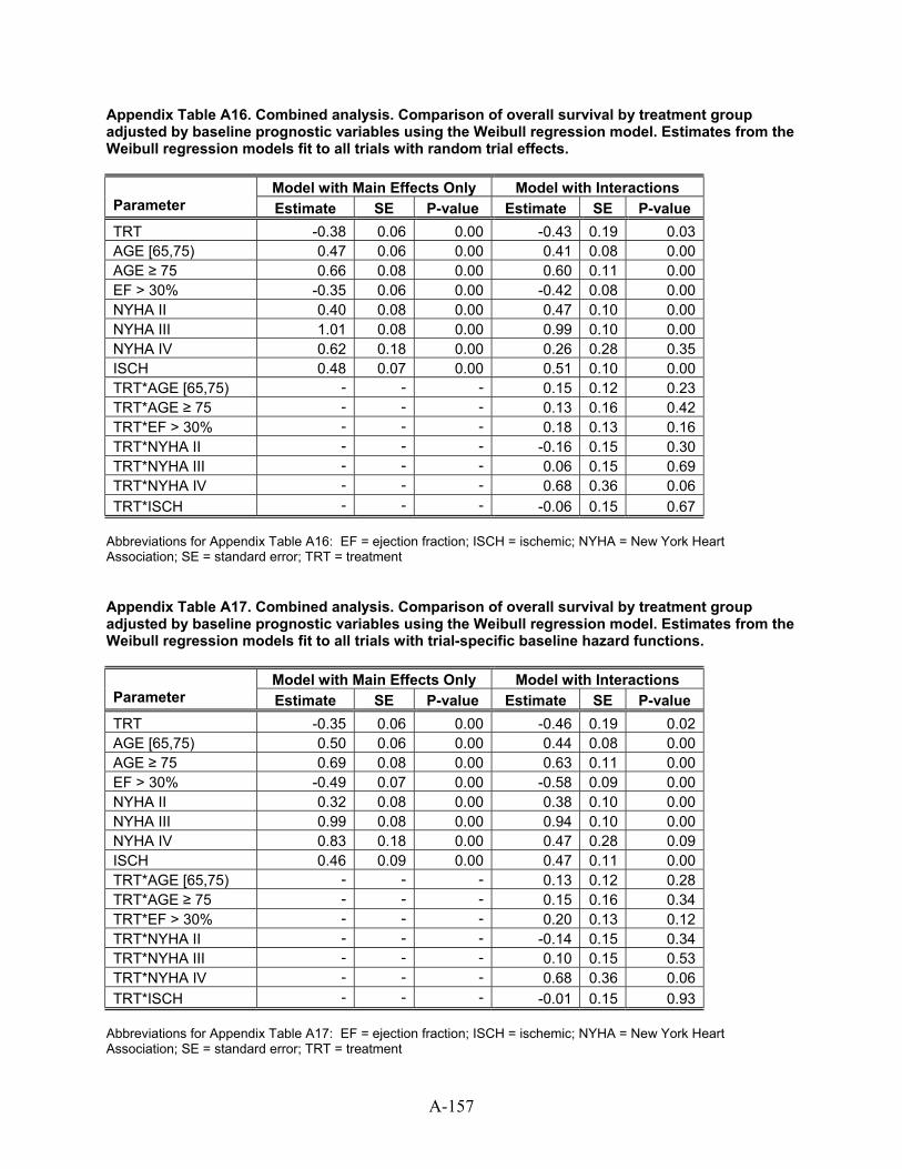
A-157

Appendix Table A16. Combined analysis. Comparison of overall survival by treatment group adjusted by baseline prognostic variables using the Weibull regression model. Estimates from the Weibull regression models fit to all trials with random trial effects.

Model with Main Effects Only Model with Interactions Parameter Estimate SE P-value Estimate SE P-value TRT -0.38 0.06 0.00 -0.43 0.19 0.03 AGE [65,75) 0.47 0.06 0.00 0.41 0.08 0.00 AGE ≥ 75 0.66 0.08 0.00 0.60 0.11 0.00 EF > 30% -0.35 0.06 0.00 -0.42 0.08 0.00 NYHA II 0.40 0.08 0.00 0.47 0.10 0.00 NYHA III 1.01 0.08 0.00 0.99 0.10 0.00 NYHA IV 0.62 0.18 0.00 0.26 0.28 0.35 ISCH 0.48 0.07 0.00 0.51 0.10 0.00 TRT*AGE [65,75) - - - 0.15 0.12 0.23 TRT*AGE ≥ 75 - - - 0.13 0.16 0.42 TRT*EF > 30% - - - 0.18 0.13 0.16 TRT*NYHA II - - - -0.16 0.15 0.30 TRT*NYHA III - - - 0.06 0.15 0.69 TRT*NYHA IV - - - 0.68 0.36 0.06 TRT*ISCH - - - -0.06 0.15 0.67

Abbreviations for Appendix Table A16: EF = ejection fraction; ISCH = ischemic; NYHA = New York Heart Association; SE = standard error; TRT = treatment Appendix Table A17. Combined analysis. Comparison of overall survival by treatment group adjusted by baseline prognostic variables using the Weibull regression model. Estimates from the Weibull regression models fit to all trials with trial-specific baseline hazard functions.

Model with Main Effects Only Model with Interactions Parameter Estimate SE P-value Estimate SE P-value TRT -0.35 0.06 0.00 -0.46 0.19 0.02 AGE [65,75) 0.50 0.06 0.00 0.44 0.08 0.00 AGE ≥ 75 0.69 0.08 0.00 0.63 0.11 0.00 EF > 30% -0.49 0.07 0.00 -0.58 0.09 0.00 NYHA II 0.32 0.08 0.00 0.38 0.10 0.00 NYHA III 0.99 0.08 0.00 0.94 0.10 0.00 NYHA IV 0.83 0.18 0.00 0.47 0.28 0.09 ISCH 0.46 0.09 0.00 0.47 0.11 0.00 TRT*AGE [65,75) - - - 0.13 0.12 0.28 TRT*AGE ≥ 75 - - - 0.15 0.16 0.34 TRT*EF > 30% - - - 0.20 0.13 0.12 TRT*NYHA II - - - -0.14 0.15 0.34 TRT*NYHA III - - - 0.10 0.15 0.53 TRT*NYHA IV - - - 0.68 0.36 0.06 TRT*ISCH - - - -0.01 0.15 0.93

Abbreviations for Appendix Table A17: EF = ejection fraction; ISCH = ischemic; NYHA = New York Heart Association; SE = standard error; TRT = treatment

Appendix Table A18. Combined analysis. Comparison of overall survival by treatment group adjusted by baseline prognostic variables using the Bayesian Weibull regression model. Estimates from the Bayesian Weibull regression models fit to all trials without adjustment for trial effects.

Model with Main Effects Only Model with Interactions

Parameter Estimate SD 95% Credible

Interval Estimate SD 95% Credible

Interval TRT -0.38 0.06 -0.50 -0.27 -0.35 0.20 -0.80 0.00AGE [65,75) 0.47 0.06 0.36 0.58 0.42 0.07 0.29 0.57AGE ≥ 75 0.66 0.08 0.50 0.81 0.61 0.10 0.39 0.80EF > 30% -0.35 0.06 -0.47 -0.23 -0.43 0.09 -0.61 -0.26NYHA II 0.23 0.07 0.10 0.39 0.33 0.09 0.13 0.50NYHA III 0.85 0.07 0.70 0.98 0.85 0.10 0.64 1.04NYHA IV 0.56 0.17 0.24 0.89 0.19 0.24 -0.32 0.66ISCH 0.51 0.07 0.36 0.65 0.55 0.09 0.35 0.72TRT*AGE [65,75) - - - - 0.13 0.12 -0.12 0.35TRT*AGE ≥ 75 - - - - 0.12 0.15 -0.16 0.40TRT*EF > 30% - - - - 0.16 0.13 -0.11 0.40TRT*NYHA II - - - - -0.21 0.15 -0.46 0.09TRT*NYHA III - - - - 0.00 0.15 -0.28 0.32TRT*NYHA IV - - - - 0.66 0.33 0.00 1.28TRT*ISCH - - - - -0.09 0.15 -0.40 0.17

Abbreviations for Appendix Table A18: EF = ejection fraction; ISCH = ischemic; NYHA = New York Heart Association; SD = standard deviation; TRT = treatment

A-158

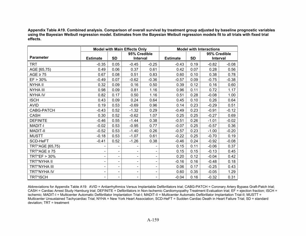
Appendix Table A19. Combined analysis. Comparison of overall survival by treatment group adjusted by baseline prognostic variables using the Bayesian Weibull regression model. Estimates from the Bayesian Weibull regression models fit to all trials with fixed trial effects.

Model with Main Effects Only Model with Interactions

Parameter Estimate SD 95% Credible

Interval Estimate SD 95% Credible

Interval TRT -0.35 0.05 -0.45 -0.25 -0.43 0.19 -0.82 -0.08AGE [65,75) 0.49 0.06 0.37 0.61 0.42 0.07 0.28 0.56AGE ≥ 75 0.67 0.08 0.51 0.83 0.60 0.10 0.38 0.78EF > 30% -0.49 0.07 -0.62 -0.36 -0.57 0.09 -0.75 -0.38NYHA II 0.32 0.09 0.16 0.50 0.39 0.12 0.16 0.60NYHA III 0.98 0.09 0.81 1.16 0.96 0.11 0.72 1.17NYHA IV 0.82 0.17 0.50 1.16 0.51 0.28 -0.08 1.00ISCH 0.43 0.09 0.24 0.64 0.45 0.10 0.26 0.64AVID 0.19 0.53 -0.69 0.96 0.14 0.23 -0.29 0.51CABG-PATCH -0.43 0.52 -1.32 0.29 -0.49 0.23 -0.91 -0.12CASH 0.30 0.52 -0.62 1.07 0.25 0.25 -0.27 0.69DEFINITE -0.46 0.55 -1.44 0.38 -0.51 0.26 -1.01 -0.02MADIT-I -0.02 0.53 -0.95 0.77 -0.07 0.25 -0.57 0.36MADIT-II -0.52 0.53 -1.40 0.26 -0.57 0.23 -1.00 -0.20MUSTT -0.18 0.53 -1.07 0.61 -0.22 0.25 -0.70 0.19SCD-HeFT -0.41 0.52 -1.26 0.38 -0.46 0.24 -0.92 -0.08TRT*AGE [65,75) - - - - 0.15 0.11 -0.06 0.37TRT*AGE ≥ 75 - - - - 0.15 0.15 -0.13 0.45TRT*EF > 30% - - - - 0.20 0.12 -0.04 0.42TRT*NYHA II - - - - -0.16 0.16 -0.48 0.18TRT*NYHA III - - - - 0.06 0.17 -0.25 0.43TRT*NYHA IV - - - - 0.60 0.35 -0.05 1.29TRT*ISCH - - - - -0.04 0.16 -0.32 0.31

Abbreviations for Appendix Table A19: AVID = Antiarrhythmics Versus Implantable Defibrillators trial; CABG-PATCH = Coronary Artery Bypass Graft-Patch trial; CASH = Cardiac Arrest Study Hamburg trial; DEFINITE = Defibrillators in Non-Ischemic Cardiomyopathy Treatment Evaluation trial; EF = ejection fraction; ISCH = ischemic; MADIT-I = Multicenter Automatic Defibrillator Implantation Trial-I; MADIT-II = Multicenter Automatic Defibrillator Implantation Trial-II; MUSTT = Multicenter Unsustained Tachycardiac Trial; NYHA = New York Heart Association; SCD-HeFT = Sudden Cardiac Death in Heart Failure Trial; SD = standard deviation; TRT = treatment

A-159

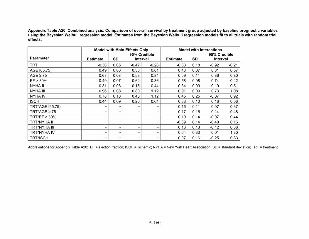
Appendix Table A20. Combined analysis. Comparison of overall survival by treatment group adjusted by baseline prognostic variables using the Bayesian Weibull regression model. Estimates from the Bayesian Weibull regression models fit to all trials with random trial effects.

Model with Main Effects Only Model with Interactions 95% Credible

Interval Parameter Estimate SD Estimate SD 95% Credible

Interval TRT -0.36 0.05 -0.47 -0.26 -0.58 0.18 -0.92 -0.21AGE [65,75) 0.49 0.06 0.38 0.61 0.43 0.07 0.31 0.57AGE ≥ 75 0.68 0.08 0.53 0.84 0.59 0.11 0.36 0.80EF > 30% -0.49 0.07 -0.62 -0.36 -0.58 0.08 -0.74 -0.42NYHA II 0.31 0.08 0.15 0.44 0.34 0.09 0.19 0.51NYHA III 0.96 0.08 0.80 1.12 0.91 0.09 0.73 1.08NYHA IV 0.78 0.18 0.43 1.12 0.45 0.25 -0.07 0.92ISCH 0.44 0.09 0.26 0.64 0.38 0.10 0.18 0.56TRT*AGE [65,75) - - - - 0.16 0.11 -0.07 0.37TRT*AGE ≥ 75 - - - - 0.17 0.16 -0.14 0.48TRT*EF > 30% - - - - 0.19 0.14 -0.07 0.44TRT*NYHA II - - - - -0.09 0.14 -0.40 0.16TRT*NYHA III - - - - 0.13 0.13 -0.12 0.38TRT*NYHA IV - - - - 0.64 0.33 0.01 1.30TRT*ISCH - - - - 0.07 0.16 -0.25 0.33

Abbreviations for Appendix Table A20: EF = ejection fraction; ISCH = ischemic; NYHA = New York Heart Association; SD = standard deviation; TRT = treatment

A-160

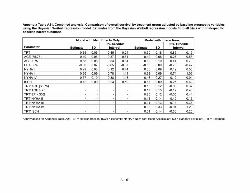
A-161

Appendix Table A21. Combined analysis. Comparison of overall survival by treatment group adjusted by baseline prognostic variables using the Bayesian Weibull regression model. Estimates from the Bayesian Weibull regression models fit to all trials with trial-specific baseline hazard functions.

Model with Main Effects Only Model with Interactions

Parameter Estimate SD 95% Credible

Interval Estimate SD 95% Credible

Interval TRT -0.35 0.06 -0.45 -0.24 -0.50 -0.850.18 -0.19AGE [65,75) 0.49 0.06 0.37 0.61 0.42 0.08 0.27 0.58AGE ≥ 75 0.68 0.08 0.53 0.84 0.60 0.10 0.41 0.79EF > 30% -0.50 0.07 -0.65 -0.37 -0.58 0.09 -0.76 -0.42NYHA II 0.29 0.08 0.12 0.44 0.36 0.09 0.19 0.55NYHA III 0.96 0.09 0.78 1.11 0.92 0.09 0.74 1.09NYHA IV 0.77 0.19 0.38 1.13 0.46 0.27 -0.12 0.94ISCH 0.42 0.43 0.090.09 0.23 0.59 0.25 0.62TRT*AGE [65,75) - - - - 0.16 0.12 -0.08 0.37TRT*AGE ≥ 75 - - - - 0.17 0.15 -0.12 0.48TRT*EF > 30% - - - - 0.20 0.12 -0.05 0.44TRT*NYHA II - - - - -0.13 0.14 -0.40 0.15TRT*NYHA III - - - - 0.11 0.13 -0.13 0.38TRT*NYHA IV - - - - 0.63 0.33 -0.01 1.29TRT*ISCH - - - - 0.01 0.14 -0.30 0.26

Abbreviations for Appendix Table A21: EF = ejection fraction; ISCH = ischemic; NYHA = New York Heart Association; SD = standard deviation; TRT = treatment

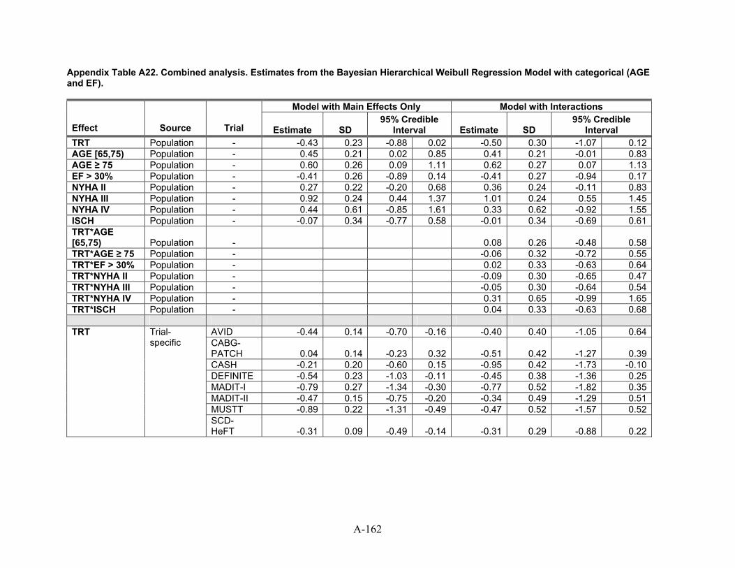
Appendix Table A22. Combined analysis. Estimates from the Bayesian Hierarchical Weibull Regression Model with categorical (AGE and EF).

Model with Main Effects Only Model with Interactions

Effect Source Trial Estimate SD 95% Credible

Interval Estimate SD 95% Credible

Interval TRT Population - -0.43 0.23 -0.88 0.02 -0.50 0.30 -1.07 0.12AGE [65,75) Population - 0.45 0.21 0.02 0.85 0.41 0.21 -0.01 0.83AGE ≥ 75 Population - 0.60 0.26 0.09 1.11 0.62 0.27 0.07 1.13EF > 30% Population - -0.41 0.26 -0.89 0.14 -0.41 0.27 -0.94 0.17NYHA II Population - 0.27 0.22 -0.20 0.68 0.36 0.24 -0.11 0.83NYHA III Population - 0.92 0.24 0.44 1.37 1.01 0.24 0.55 1.45NYHA IV Population - 0.44 0.61 -0.85 1.61 0.33 0.62 -0.92 1.55ISCH Population - -0.07 0.34 -0.77 0.58 -0.01 0.34 -0.69 0.61TRT*AGE [65,75) Population - 0.08 0.26 -0.48 0.58TRT*AGE ≥ 75 Population - -0.06 0.32 -0.72 0.55TRT*EF > 30% Population - 0.02 0.33 -0.63 0.64TRT*NYHA II Population - -0.09 0.30 -0.65 0.47TRT*NYHA III Population - -0.05 0.30 -0.64 0.54TRT*NYHA IV Population - 0.31 0.65 -0.99 1.65TRT*ISCH Population - 0.04 0.33 -0.63 0.68

AVID -0.44 0.14 -0.70 -0.16 -0.40 0.40 -1.05 0.64CABG-PATCH 0.04 0.14 -0.23 0.32 -0.51 0.42 -1.27 0.39CASH -0.21 0.20 -0.60 0.15 -0.95 0.42 -1.73 -0.10DEFINITE -0.54 0.23 -1.03 -0.11 -0.45 0.38 -1.36 0.25MADIT-I -0.79 0.27 -1.34 -0.30 -0.77 0.52 -1.82 0.35MADIT-II -0.47 0.15 -0.75 -0.20 -0.34 0.49 -1.29 0.51MUSTT -0.89 0.22 -1.31 -0.49 -0.47 0.52 -1.57 0.52

TRT

Trial-specific

SCD-HeFT -0.31 0.09 -0.49 -0.14 -0.31 0.29 -0.88 0.22

A-162

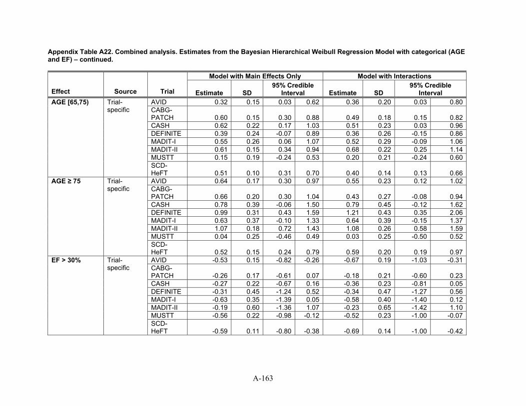
Appendix Table A22. Combined analysis. Estimates from the Bayesian Hierarchical Weibull Regression Model with categorical (AGE and EF) – continued.

Model with Main Effects Only Model with Interactions

Effect Source Trial Estimate SD 95% Credible

Interval Estimate SD 95% Credible

Interval AVID 0.32 0.15 0.03 0.62 0.36 0.20 0.03 0.80CABG-PATCH 0.60 0.15 0.30 0.88 0.49 0.18 0.15 0.82CASH 0.62 0.22 0.17 1.03 0.51 0.23 0.03 0.96DEFINITE 0.39 0.24 -0.07 0.89 0.36 0.26 -0.15 0.86MADIT-I 0.55 0.26 0.06 1.07 0.52 0.29 -0.09 1.06MADIT-II 0.61 0.15 0.34 0.94 0.68 0.22 0.25 1.14MUSTT 0.15 0.19 -0.24 0.53 0.20 0.21 -0.24 0.60

AGE [65,75)

Trial-specific

SCD-HeFT 0.51 0.10 0.31 0.70 0.40 0.14 0.13 0.66AVID 0.64 0.17 0.30 0.97 0.55 0.23 0.12 1.02CABG-PATCH 0.66 0.20 0.30 1.04 0.43 0.27 -0.08 0.94CASH 0.78 0.39 -0.06 1.50 0.79 0.45 -0.12 1.62DEFINITE 0.99 0.31 0.43 1.59 1.21 0.43 0.35 2.06MADIT-I 0.63 0.37 -0.10 1.33 0.64 0.39 -0.15 1.37MADIT-II 1.07 0.18 0.72 1.43 1.08 0.26 0.58 1.59MUSTT 0.04 0.25 -0.46 0.49 0.03 0.25 -0.50 0.52

AGE ≥ 75

Trial-specific

SCD-HeFT 0.52 0.15 0.24 0.79 0.59 0.20 0.19 0.97AVID -0.53 0.15 -0.82 -0.26 -0.67 0.19 -1.03 -0.31CABG-PATCH -0.26 0.17 -0.61 0.07 -0.18 0.21 -0.60 0.23CASH -0.27 0.22 -0.67 0.16 -0.36 0.23 -0.81 0.05DEFINITE -0.31 0.45 -1.24 0.52 -0.34 0.47 -1.27 0.56MADIT-I -0.63 0.35 -1.39 0.05 -0.58 0.40 -1.40 0.12MADIT-II -0.19 0.60 -1.36 1.07 -0.23 0.65 -1.42 1.10MUSTT -0.56 0.22 -0.98 -0.12 -0.52 0.23 -1.00 -0.07

EF > 30%

Trial-specific

SCD-HeFT -0.59 0.11 -0.80 -0.38 -0.69 0.14 -1.00 -0.42

A-163

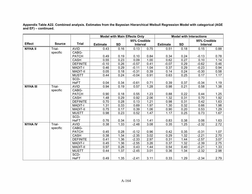
Appendix Table A22. Combined analysis. Estimates from the Bayesian Hierarchical Weibull Regression Model with categorical (AGE and EF) – continued.

Model with Main Effects Only Model with Interactions

Effect Source Trial Estimate SD 95% Credible

Interval Estimate SD 95% Credible

Interval AVID 0.43 0.16 0.13 0.75 0.51 0.18 0.15 0.88CABG-PATCH 0.49 0.19 0.10 0.84 0.34 0.24 -0.13 0.78CASH 0.55 0.23 0.09 1.00 0.62 0.27 0.10 1.14DEFINITE -0.10 0.26 -0.57 0.41 -0.07 0.29 -0.62 0.46MADIT-I 0.46 0.29 -0.11 1.04 0.37 0.29 -0.23 0.94MADIT-II 0.05 0.18 -0.31 0.39 0.14 0.24 -0.30 0.58MUSTT 0.44 0.24 -0.04 0.91 0.63 0.25 0.17 1.17

NYHA II

Trial-specific

SCD-HeFT 0.04 0.34 -0.61 0.71 0.39 0.37 -0.34 1.19AVID 0.94 0.19 0.57 1.28 0.98 0.21 0.58 1.38CABG-PATCH 0.90 0.18 0.55 1.23 0.88 0.22 0.44 1.25CASH 1.48 0.29 0.92 2.06 1.32 0.31 0.70 1.92DEFINITE 0.70 0.28 0.13 1.21 0.98 0.31 0.42 1.63MADIT-I 1.31 0.33 0.69 1.97 1.30 0.32 0.66 1.98MADIT-II 0.75 0.17 0.39 1.06 0.90 0.20 0.53 1.29MUSTT 0.98 0.23 0.52 1.47 1.17 0.25 0.73 1.67

NYHA III

Trial-specific

SCD-HeFT 0.76 0.34 0.13 1.41 0.83 0.38 0.06 1.63AVID 0.38 1.33 -2.48 3.08 0.35 1.25 -2.32 2.72CABG-PATCH 0.45 0.28 -0.12 0.96 0.42 0.35 -0.31 1.07CASH 0.38 1.34 -2.35 3.02 0.29 1.32 -2.21 2.70DEFINITE 0.41 1.36 -2.33 2.97 0.31 1.44 -2.57 3.07MADIT-I 0.45 1.36 -2.55 3.26 0.37 1.32 -2.39 2.75MADIT-II 0.97 0.26 0.43 1.44 0.54 0.40 -0.21 1.33MUSTT 0.44 1.37 -2.45 3.01 0.36 1.34 -2.32 2.98

NYHA IV

Trial-specific

SCD-HeFT 0.49 1.35 -2.41 3.11 0.33 1.29 -2.34 2.79

A-164

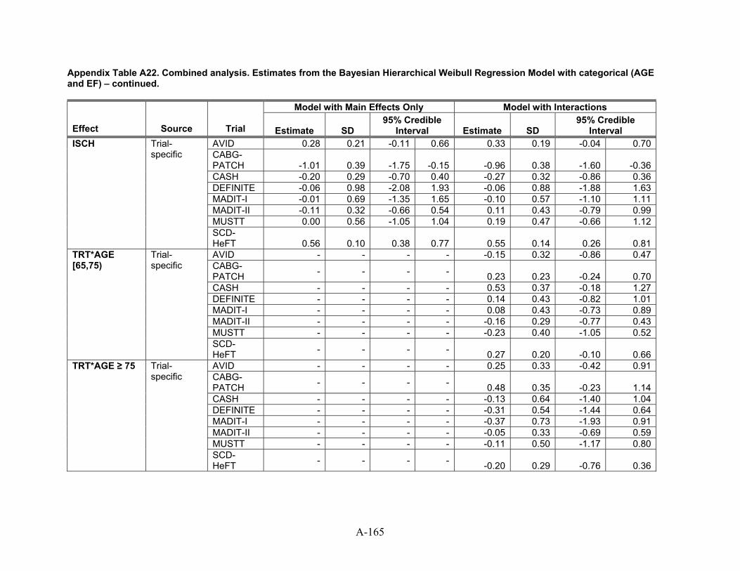
Appendix Table A22. Combined analysis. Estimates from the Bayesian Hierarchical Weibull Regression Model with categorical (AGE and EF) – continued.

Model with Main Effects Only Model with Interactions

Effect Source Trial Estimate SD 95% Credible

Interval Estimate SD 95% Credible

Interval AVID 0.28 0.21 -0.11 0.66 0.33 0.19 -0.04 0.70CABG-PATCH -1.01 0.39 -1.75 -0.15 -0.96 0.38 -1.60 -0.36CASH -0.20 0.29 -0.70 0.40 -0.27 0.32 -0.86 0.36DEFINITE -0.06 0.98 -2.08 1.93 -0.06 0.88 -1.88 1.63MADIT-I -0.01 0.69 -1.35 1.65 -0.10 0.57 -1.10 1.11MADIT-II -0.11 0.32 -0.66 0.54 0.11 0.43 -0.79 0.99MUSTT 0.00 0.56 -1.05 1.04 0.19 0.47 -0.66 1.12

ISCH

Trial-specific

SCD-HeFT 0.56 0.10 0.38 0.77 0.55 0.14 0.26 0.81AVID - - - - -0.15 0.32 -0.86 0.47CABG-PATCH - - - - 0.23 0.23 -0.24 0.70CASH - - - - 0.53 0.37 -0.18 1.27DEFINITE - - - - 0.14 0.43 -0.82 1.01MADIT-I - - - - 0.08 0.43 -0.73 0.89MADIT-II - - - - -0.16 0.29 -0.77 0.43MUSTT - - - - -0.23 0.40 -1.05 0.52

TRT*AGE [65,75)

Trial-specific

SCD-HeFT - - - - 0.27 0.20 -0.10 0.66AVID - - - - 0.25 0.33 -0.42 0.91CABG-PATCH - - - - 0.48 0.35 -0.23 1.14CASH - - - - -0.13 0.64 -1.40 1.04DEFINITE - - - - -0.31 0.54 -1.44 0.64MADIT-I - - - - -0.37 0.73 -1.93 0.91MADIT-II - - - - -0.05 0.33 -0.69 0.59MUSTT - - - - -0.11 0.50 -1.17 0.80

TRT*AGE ≥ 75

Trial-specific

SCD-HeFT - - - - -0.20 0.29 -0.76 0.36

A-165

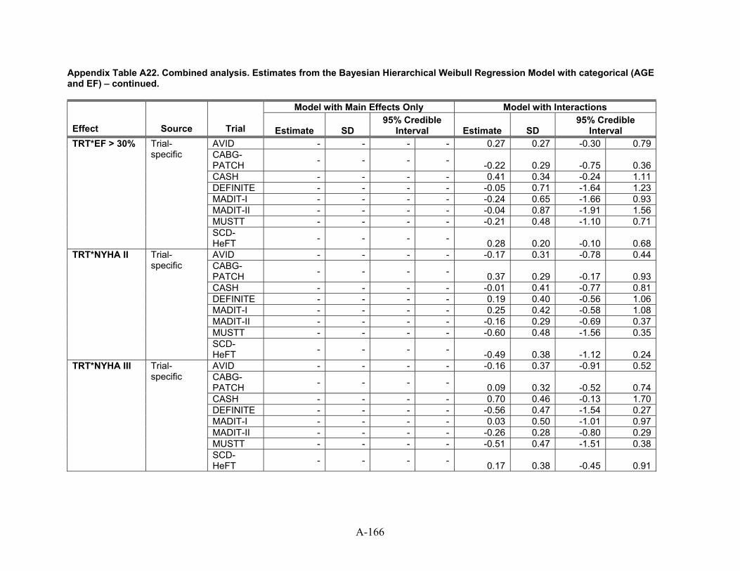
Appendix Table A22. Combined analysis. Estimates from the Bayesian Hierarchical Weibull Regression Model with categorical (AGE and EF) – continued.

Model with Main Effects Only Model with Interactions

Effect Source Trial Estimate SD 95% Credible

Interval Estimate SD 95% Credible

Interval AVID - - - - 0.27 0.27 -0.30 0.79CABG-PATCH - - - - -0.22 0.29 -0.75 0.36CASH - - - - 0.41 0.34 -0.24 1.11DEFINITE - - - - -0.05 0.71 -1.64 1.23MADIT-I - - - - -0.24 0.65 -1.66 0.93MADIT-II - - - - -0.04 0.87 -1.91 1.56MUSTT - - - - -0.21 0.48 -1.10 0.71

TRT*EF > 30%

Trial-specific

SCD-HeFT - - - - 0.28 0.20 -0.10 0.68AVID - - - - -0.17 0.31 -0.78 0.44CABG-PATCH - - - - 0.37 0.29 -0.17 0.93CASH - - - - -0.01 0.41 -0.77 0.81DEFINITE - - - - 0.19 0.40 -0.56 1.06MADIT-I - - - - 0.25 0.42 -0.58 1.08MADIT-II - - - - -0.16 0.29 -0.69 0.37MUSTT - - - - -0.60 0.48 -1.56 0.35

TRT*NYHA II

Trial-specific

SCD-HeFT - - - - -0.49 0.38 -1.12 0.24AVID - - - - -0.16 0.37 -0.91 0.52CABG-PATCH - - - - 0.09 0.32 -0.52 0.74CASH - - - - 0.70 0.46 -0.13 1.70DEFINITE - - - - -0.56 0.47 -1.54 0.27MADIT-I - - - - 0.03 0.50 -1.01 0.97MADIT-II - - - - -0.26 0.28 -0.80 0.29MUSTT - - - - -0.51 0.47 -1.51 0.38

TRT*NYHA III

Trial-specific

SCD-HeFT - - - - 0.17 0.38 -0.45 0.91

A-166

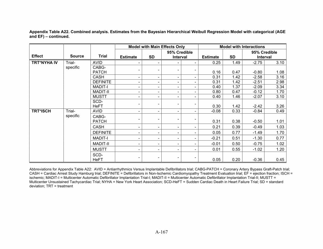
A-167

Appendix Table A22. Combined analysis. Estimates from the Bayesian Hierarchical Weibull Regression Model with categorical (AGE and EF) – continued.

Model with Main Effects Only Model with Interactions

Effect Source Trial Estimate SD 95% Credible

Interval Estimate SD 95% Credible

Interval AVID - - - - 0.25 1.49 -2.75 3.10CABG-PATCH - - - - 0.16 0.47 -0.80 1.08CASH - - - - 0.31 1.42 -2.58 3.16DEFINITE - - - - 0.31 1.42 -2.51 2.98MADIT-I - - - - 0.40 1.37 -2.09 3.34MADIT-II - - - - 0.80 0.47 -0.12 1.70MUSTT - - - - 0.40 1.46 -2.07 3.10

TRT*NYHA IV

Trial-specific

SCD-HeFT - - - - 0.30 1.42 -2.42 3.26AVID - - - - -0.08 0.33 -0.84 0.49CABG-PATCH - - - - 0.31 0.38 -0.50 1.01CASH - - - - 0.21 0.39 -0.49 1.03DEFINITE - - - - 0.05 0.77 -1.49 1.70MADIT-I - - - - -0.21 0.51 -1.30 0.77MADIT-II - - - - -0.01 0.50 -0.75 1.02MUSTT - - - - 0.01 0.55 -1.02 1.20

TRT*ISCH

Trial-specific

SCD-HeFT - - - - 0.05 0.20 -0.36 0.45

Abbreviations for Appendix Table A22: AVID = Antiarrhythmics Versus Implantable Defibrillators trial; CABG-PATCH = Coronary Artery Bypass Graft-Patch trial; CASH = Cardiac Arrest Study Hamburg trial; DEFINITE = Defibrillators in Non-Ischemic Cardiomyopathy Treatment Evaluation trial; EF = ejection fraction; ISCH = ischemic; MADIT-I = Multicenter Automatic Defibrillator Implantation Trial-I; MADIT-II = Multicenter Automatic Defibrillator Implantation Trial-II; MUSTT = Multicenter Unsustained Tachycardiac Trial; NYHA = New York Heart Association; SCD-HeFT = Sudden Cardiac Death in Heart Failure Trial; SD = standard deviation; TRT = treatment

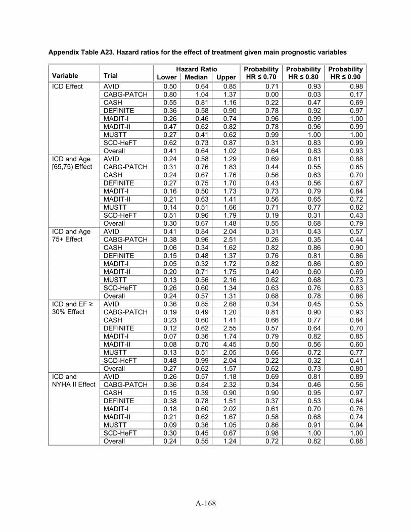
Appendix Table A23. Hazard ratios for the effect of treatment given main prognostic variables

Hazard Ratio Variable Trial Lower Median Upper

ProbabilityHR ≤ 0.70

Probability HR ≤ 0.80

ProbabilityHR ≤ 0.90

AVID 0.50 0.64 0.85 0.71 0.93 0.98CABG-PATCH 0.80 1.04 1.37 0.00 0.03 0.17

ICD Effect

CASH 0.55 0.81 1.16 0.22 0.47 0.69DEFINITE 0.36 0.58 0.90 0.78 0.92 0.97MADIT-I 0.26 0.46 0.74 0.96 0.99 1.00MADIT-II 0.47 0.62 0.82 0.78 0.96 0.99MUSTT 0.27 0.41 0.62 0.99 1.00 1.00SCD-HeFT 0.62 0.73 0.87 0.31 0.83 0.99Overall 0.41 0.64 1.02 0.64 0.83 0.93AVID 0.24 0.58 1.29 0.69 0.81 0.88CABG-PATCH 0.31 0.76 1.83 0.44 0.55 0.65CASH 0.24 0.67 1.76 0.56 0.63 0.70DEFINITE 0.27 0.75 1.70 0.43 0.56 0.67MADIT-I 0.16 0.50 1.73 0.73 0.79 0.84MADIT-II 0.21 0.63 1.41 0.56 0.65 0.72MUSTT 0.14 0.51 1.66 0.71 0.77 0.82SCD-HeFT 0.51 0.96 1.79 0.19 0.31 0.43

ICD and Age [65,75) Effect

Overall 0.30 0.67 1.48 0.55 0.68 0.79AVID 0.41 0.84 2.04 0.31 0.43 0.57CABG-PATCH 0.38 0.96 2.51 0.26 0.35 0.44CASH 0.06 0.34 1.62 0.82 0.86 0.90

ICD and Age 75+ Effect

DEFINITE 0.15 0.48 1.37 0.76 0.81 0.86MADIT-I 0.05 0.32 1.72 0.82 0.86 0.89MADIT-II 0.20 0.71 1.75 0.49 0.60 0.69MUSTT 0.13 0.56 2.16 0.62 0.68 0.73SCD-HeFT 0.26 0.60 1.34 0.63 0.76 0.83Overall 0.24 0.57 1.31 0.68 0.78 0.86AVID 0.36 0.85 2.68 0.34 0.45 0.55CABG-PATCH 0.19 0.49 1.20 0.81 0.90 0.93CASH 0.23 0.60 1.41 0.66 0.77 0.84DEFINITE 0.12 0.62 2.55 0.57 0.64 0.70MADIT-I 0.07 0.36 1.74 0.79 0.82 0.85MADIT-II 0.08 0.70 4.45 0.50 0.56 0.60MUSTT 0.13 0.51 2.05 0.66 0.72 0.77SCD-HeFT 0.48 0.99 2.04 0.22 0.32 0.41

ICD and EF ≥ 30% Effect

Overall 0.27 0.62 1.57 0.62 0.73 0.80AVID 0.26 0.57 1.18 0.69 0.81 0.89CABG-PATCH 0.36 0.84 2.32 0.34 0.46 0.56CASH 0.15 0.39 0.90 0.90 0.95 0.97DEFINITE 0.38 0.78 1.51 0.37 0.53 0.64MADIT-I 0.18 0.60 2.02 0.61 0.70 0.76MADIT-II 0.21 0.62 1.67 0.58 0.68 0.74MUSTT 0.09 0.36 1.05 0.86 0.91 0.94SCD-HeFT 0.30 0.45 0.67 0.98 1.00 1.00

ICD and NYHA II Effect

Overall 0.24 0.55 1.24 0.72 0.82 0.88

A-168

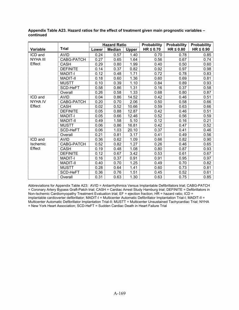
A-169

Appendix Table A23. Hazard ratios for the effect of treatment given main prognostic variables – continued

Hazard Ratio Variable Trial Lower Median Upper

ProbabilityHR ≤ 0.70

Probability HR ≤ 0.80

ProbabilityHR ≤ 0.90

AVID 0.24 0.57 1.40 0.70 0.78 0.85CABG-PATCH 0.27 0.65 1.64 0.56 0.67 0.74CASH 0.29 0.80 1.99 0.40 0.50 0.60DEFINITE 0.14 0.37 0.82 0.92 0.97 0.98MADIT-I 0.12 0.48 1.71 0.72 0.78 0.83MADIT-II 0.18 0.60 1.36 0.60 0.69 0.81MUSTT 0.10 0.39 1.10 0.84 0.89 0.93SCD-HeFT 0.58 0.86 1.31 0.16 0.37 0.58

ICD and NYHA III Effect

Overall 0.26 0.58 1.33 0.68 0.80 0.87AVID 0.04 0.86 14.52 0.42 0.46 0.51CABG-PATCH 0.20 0.70 2.06 0.50 0.58 0.66CASH 0.02 0.52 10.66 0.59 0.63 0.66DEFINITE 0.05 0.88 12.87 0.42 0.46 0.51MADIT-I 0.05 0.66 12.46 0.52 0.56 0.59MADIT-II 0.49 1.58 5.10 0.12 0.16 0.21MUSTT 0.06 0.86 16.81 0.42 0.47 0.52SCD-HeFT 0.06 1.03 20.10 0.37 0.41 0.46

ICD and NYHA IV Effect

Overall 0.21 0.81 3.17 0.41 0.49 0.56AVID 0.36 0.62 1.09 0.66 0.82 0.90CABG-PATCH 0.52 0.82 1.27 0.26 0.46 0.65CASH 0.19 0.48 1.08 0.80 0.87 0.93DEFINITE 0.12 0.67 3.42 0.53 0.61 0.67MADIT-I 0.16 0.37 0.91 0.91 0.95 0.97MADIT-II 0.40 0.70 1.25 0.49 0.70 0.82MUSTT 0.28 0.64 1.41 0.60 0.73 0.81SCD-HeFT 0.36 0.76 1.51 0.45 0.52 0.61

ICD and Ischemic Effect

Overall 0.31 0.63 1.30 0.63 0.75 0.85 Abbreviations for Appendix Table A23: AVID = Antiarrhythmics Versus Implantable Defibrillators trial; CABG-PATCH = Coronary Artery Bypass Graft-Patch trial; CASH = Cardiac Arrest Study Hamburg trial; DEFINITE = Defibrillators in Non-Ischemic Cardiomyopathy Treatment Evaluation trial; EF = ejection fraction; HR = hazard ratio; ICD = implantable cardioverter defibrillator; MADIT-I = Multicenter Automatic Defibrillator Implantation Trial-I; MADIT-II = Multicenter Automatic Defibrillator Implantation Trial-II; MUSTT = Multicenter Unsustained Tachycardiac Trial; NYHA = New York Heart Association; SCD-HeFT = Sudden Cardiac Death in Heart Failure Trial

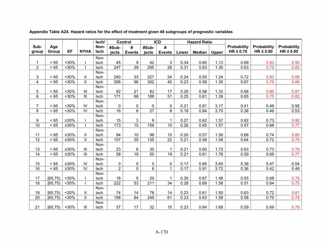
Appendix Table A24. Hazard ratios for the effect of treatment given 48 subgroups of prognostic variables

Control ICD Hazard Ratio Sub-

group Age

Group EF NYHA

Isch/ Non-Isch

#Sub-jects

# Events

#Sub-jects

# Events Lower Median Upper

Probability HR ≤ 0.70

Probability HR ≤ 0.80

Probability HR ≤ 0.90

1 < 65 <30% I Non-Isch 45 9 42 3 0.34 0.60 1.13 0.69 0.83 0.90

2 < 65 <30% I Isch 247 39 295 28 0.31 0.63 1.30 0.63 0.75 0.85

3 < 65 <30% II Non-Isch 240 33 227 24 0.24 0.55 1.24 0.72 0.82 0.88

4 < 65 <30% II Isch 306 96 302 40 0.23 0.58 1.35 0.67 0.78 0.86

5 < 65 <30% III Non-Isch 92 21 82 17 0.26 0.58 1.33 0.68 0.80 0.87

6 < 65 <30% III Isch 171 68 188 51 0.25 0.61 1.39 0.65 0.75 0.83

7 < 65 <30% IV Non-Isch 0 0 0 0 0.21 0.81 3.17 0.41 0.49 0.56

8 < 65 <30% IV Isch 16 6 27 8 0.18 0.84 3.70 0.38 0.46 0.53

9 < 65 ≥30% I Non-Isch 15 3 9 1 0.27 0.62 1.57 0.62 0.73 0.80

10 < 65 ≥30% I Isch 173 15 156 10 0.26 0.65 1.57 0.57 0.68 0.77

11 < 65 ≥30% II Non-Isch 94 10 98 10 0.20 0.57 1.56 0.66 0.74 0.80

12 < 65 ≥30% II Isch 157 35 135 22 0.21 0.58 1.58 0.64 0.72 0.79

13 < 65 ≥30% III Non-Isch 23 6 30 1 0.21 0.60 1.72 0.63 0.73 0.79

14 < 65 ≥30% III Isch 58 19 50 19 0.21 0.61 1.76 0.59 0.69 0.77

15 < 65 ≥30% IV Non-Isch 0 0 0 0 0.17 0.85 3.60 0.38 0.47 0.54

16 < 65 ≥30% IV Isch 2 0 6 1 0.17 0.91 3.72 0.36 0.42 0.49

17 [65,75) <30% I Non-Isch 18 5 20 1 0.30 0.67 1.48 0.55 0.68 0.79

18 [65,75) <30% I Isch 222 53 211 34 0.28 0.69 1.58 0.51 0.64 0.75

19 [65,75) <30% II Non-Isch 74 14 78 14 0.23 0.61 1.50 0.63 0.72 0.81

20 [65,75) <30% II Isch 198 64 249 61 0.23 0.63 1.58 0.58 0.70 0.78

21 [65,75) <30% III Non-Isch 37 17 32 15 0.23 0.64 1.68 0.59 0.69 0.79

A-170

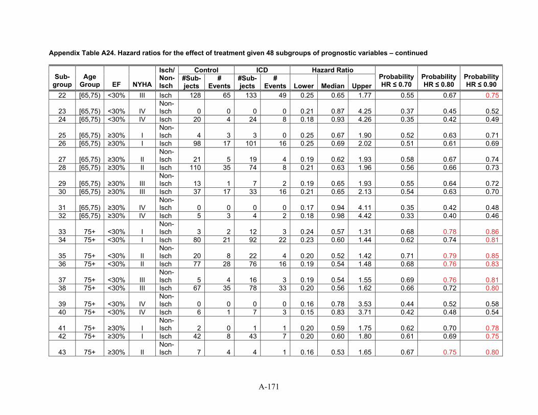
Appendix Table A24. Hazard ratios for the effect of treatment given 48 subgroups of prognostic variables – continued

Control ICD Hazard Ratio Sub-

group Age

Group EF NYHA

Isch/ Non-Isch

#Sub-jects

# Events

#Sub-jects

# Events Lower Median Upper

Probability HR ≤ 0.70

Probability HR ≤ 0.80

Probability HR ≤ 0.90

22 [65,75) <30% III Isch 128 65 133 49 0.25 0.65 1.77 0.55 0.67 0.75

23 [65,75) <30% IV Non-Isch 0 0 0 0 0.21 0.87 4.25 0.37 0.45 0.52

24 [65,75) <30% IV Isch 20 4 24 8 0.18 0.93 4.26 0.35 0.42 0.49

25 [65,75) ≥30% I Non-Isch 4 3 3 0 0.25 0.67 1.90 0.52 0.63 0.71

26 [65,75) ≥30% I Isch 98 17 101 16 0.25 0.69 2.02 0.51 0.61 0.69

27 [65,75) ≥30% II Non-Isch 21 5 19 4 0.19 0.62 1.93 0.58 0.67 0.74

28 [65,75) ≥30% II Isch 110 35 74 8 0.21 0.63 1.96 0.56 0.66 0.73

29 [65,75) ≥30% III Non-Isch 13 1 7 2 0.19 0.65 1.93 0.55 0.64 0.72

30 [65,75) ≥30% III Isch 37 17 33 16 0.21 0.65 2.13 0.54 0.63 0.70

31 [65,75) ≥30% IV Non-Isch 0 0 0 0 0.17 0.94 4.11 0.35 0.42 0.48

32 [65,75) ≥30% IV Isch 5 3 4 2 0.18 0.98 4.42 0.33 0.40 0.46

33 75+ <30% I Non-Isch 3 2 12 3 0.24 0.57 1.31 0.68 0.78 0.86

34 75+ <30% I Isch 80 21 92 22 0.23 0.60 1.44 0.62 0.74 0.81

35 75+ <30% II Non-Isch 20 8 22 4 0.20 0.52 1.42 0.71 0.79 0.85

36 75+ <30% II Isch 77 28 76 16 0.19 0.54 1.48 0.68 0.76 0.83

37 75+ <30% III Non-Isch 5 4 16 3 0.19 0.54 1.55 0.69 0.76 0.81

38 75+ <30% III Isch 67 35 78 33 0.20 0.56 1.62 0.66 0.72 0.80

39 75+ <30% IV Non-Isch 0 0 0 0 0.16 0.78 3.53 0.44 0.52 0.58

40 75+ <30% IV Isch 6 1 7 3 0.15 0.83 3.71 0.42 0.48 0.54

41 75+ ≥30% I Non-Isch 2 0 1 1 0.20 0.59 1.75 0.62 0.70 0.78

42 75+ ≥30% I Isch 42 8 43 7 0.20 0.60 1.80 0.61 0.69 0.75

43 75+ ≥30% II Non-Isch 7 4 4 1 0.16 0.53 1.65 0.67 0.75 0.80

A-171

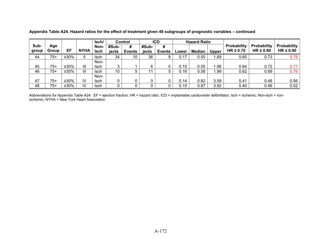
A-172

Appendix Table A24. Hazard ratios for the effect of treatment given 48 subgroups of prognostic variables – continued

Control ICD Hazard RatioSub-

group Age

Group EF NYHA

Isch/ Non-Isch

#Sub-jects

# Events

#Sub-jects

# Events Lower Median Upper

Probability HR ≤ 0.70

Probability HR ≤ 0.80

Probability HR ≤ 0.90

44 75+ ≥30% II Isch 34 10 36 8 0.17 0.55 1.69 0.65 0.73 0.79

45 75+ ≥30% III Isch 3 0.15 Non-

1 6 0 0.55 1.98 0.64 0.72 0.7746 75+ ≥30% III Isch 10 5 11 5 0.16 0.58 1.99 0.62 0.69 0.76

47 75+ ≥30% IV Isch 0 0.14 Non-

0 0 0 0.82 3.59 0.41 0.48 0.5648 75+ ≥30% IV Isch 0 0 0 0 0.15 0.87 3.92 0.40 0.46 0.52

Abbreviations for Appendix Table A24: EF = ejection fraction; HR = hazard ratio; ICD = implantable cardioverter defibrillator; Isch = ischemic; Non-Isch = non-ischemic; NYHA = New York Heart Association

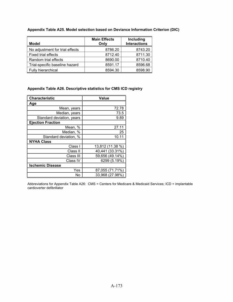
Appendix Table A25. Model selection based on Deviance Information Criterion (DIC)

Model Main Effects

Only Including

Interactions No adjustment for trial effects 8786.20 8743.20Fixed trial effects 8712.40 8711.30Random trial effects 8690.00 8710.40Trial-specific baseline hazard 8591.17 8596.68Fully hierarchical 8594.30 8598.90

Appendix Table A26. Descriptive statistics for CMS ICD registry Characteristic Value Age

Mean, years 72.78Median, years 73.5

Standard deviation, years 9.89Ejection Fraction

Mean, % 27.11Median, % 25

Standard deviation, % 10.11NYHA Class

Class I 13,812 (11.38 %)Class II 40,441 (33.31%)Class III 59,656 (49.14%)Class IV 6299 (5.19%)

Ischemic Disease Yes 87,055 (71.71%)No 33,968 (27.98%)

Abbreviations for Appendix Table A26: CMS = Centers for Medicare & Medicaid Services; ICD = implantable cardioverter defibrillator

A-173

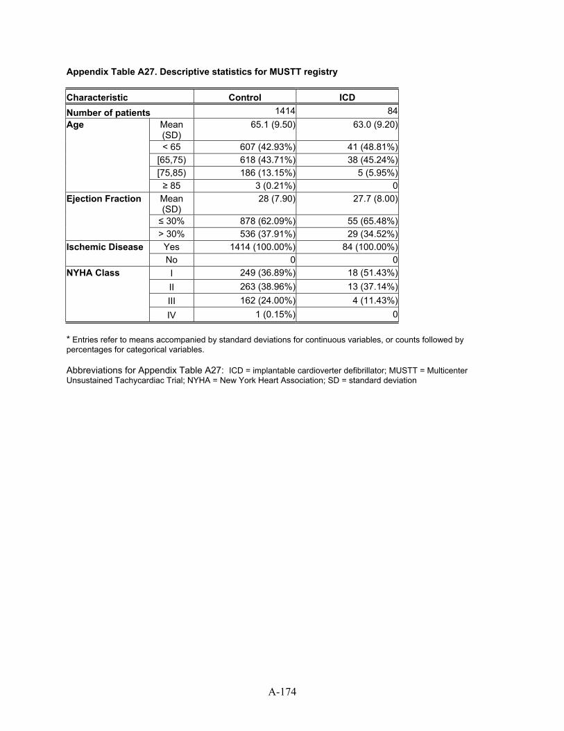
A-174

Appendix Table A27. Descriptive statistics for MUSTT registry Characteristic Control ICD Number of patients 1414 84

Mean (SD)

65.1 (9.50) 63.0 (9.20)

< 65 607 (42.93%) 41 (48.81%) [65,75) 618 (43.71%) 38 (45.24%) [75,85) 186 (13.15%) 5 (5.95%)

Age

≥ 85 3 (0.21%) 0 Mean (SD)

28 (7.90) 27.7 (8.00)

≤ 30% 878 (62.09%) 55 (65.48%)

Ejection Fraction

> 30% 536 (37.91%) 29 (34.52%) Yes 1414 (100.00%) 84 (100.00%) Ischemic Disease No 0 0 I 249 (36.89%) 18 (51.43%) II 263 (38.96%) 13 (37.14%) III 162 (24.00%) 4 (11.43%)

NYHA Class

IV 1 (0.15%) 0 * Entries refer to means accompanied by standard deviations for continuous variables, or counts followed by percentages for categorical variables. Abbreviations for Appendix Table A27: ICD = implantable cardioverter defibrillator; MUSTT = Multicenter Unsustained Tachycardiac Trial; NYHA = New York Heart Association; SD = standard deviation

Appendix Table A28. Posterior estimates from Bayesian models, with fixed-effect and random-effects formulation, using aggregate data by number of combined trials. We utilize two priors: prior 1 has precision 1, while prior 2 has precision 20. Trials were combined in the following order (based on their publication date): MADIT-I, AVID, CABG-PATCH, MUSTT, CASH, MADIT-II, DEFINITE, SCD-HeFT.

Prior 1 Prior 2 Fixed Effect Random Effects Fixed Effect Random Effects

Trials Combined

Esti-mate SD

95% Credible Interval

Esti-mate SD

95% Credible Interval

Esti-mate SD

95% Credible Interval

Esti-mate SD

95% Credible Interval

1 -0.45 0.75 -1.91 1.07 -0.41 0.81 -1.94 1.30 -0.13 0.21 -0.53 0.27 -0.13 0.21 -0.54 0.292 -0.47 0.63 -1.70 0.77 -0.47 0.62 -1.66 0.84 -0.20 0.19 -0.58 0.18 -0.20 0.19 -0.56 0.183 -0.32 0.53 -1.37 0.74 -0.34 0.53 -1.35 0.73 -0.15 0.18 -0.50 0.18 -0.16 0.17 -0.50 0.184 -0.44 0.48 -1.38 0.50 -0.46 0.45 -1.34 0.46 -0.24 0.16 -0.56 0.09 -0.24 0.17 -0.56 0.095 -0.37 0.44 -1.24 0.49 -0.40 0.39 -1.14 0.38 -0.22 0.16 -0.53 0.08 -0.23 0.16 -0.54 0.086 -0.38 0.41 -1.18 0.43 -0.41 0.34 -1.05 0.27 -0.25 0.15 -0.54 0.04 -0.25 0.15 -0.54 0.047 -0.38 0.38 -1.13 0.37 -0.42 0.30 -1.02 0.19 -0.26 0.14 -0.54 0.02 -0.26 0.14 -0.54 0.018 -0.38 0.36 -1.10 0.35 -0.40 0.27 -0.94 0.13 -0.26 0.13 -0.52 0.00 -0.26 0.13 -0.53 0.00

Abbreviations for Appendix Table A28: AVID = Antiarrhythmics Versus Implantable Defibrillators trial; CABG-PATCH = Coronary Artery Bypass Graft-Patch trial; CASH = Cardiac Arrest Study Hamburg trial; DEFINITE = Defibrillators in Non-Ischemic Cardiomyopathy Treatment Evaluation trial; MADIT-I = Multicenter Automatic Defibrillator Implantation Trial-I; MADIT-II = Multicenter Automatic Defibrillator Implantation Trial-II; MUSTT = Multicenter Unsustained Tachycardiac Trial; SCD-HeFT = Sudden Cardiac Death in Heart Failure Trial; SD = standard deviation

A-175

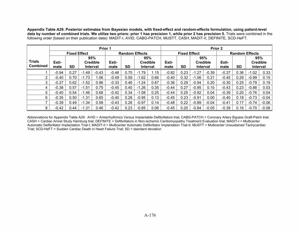
A-176

Appendix Table A29. Posterior estimates from Bayesian models, with fixed-effect and random-effects formulation, using patient-level data by number of combined trials. We utilize two priors: prior 1 has precision 1, while prior 2 has precision 5. Trials were combined in the following order (based on their publication date): MADIT-I, AVID, CABG-PATCH, MUSTT, CASH, MADIT-II, DEFINITE, SCD-HeFT.

Prior 1 Prior 2 Fixed Effect Random Effects Fixed Effect Random Effects

Trials Combined

Esti-mate SD SD SD

95% Credible Interval

Esti-mate

95% Credible Interval

Esti-mate

95% Credible Interval

Esti-mate SD

95% Credible Interval

1 -0.94 0.27 -1.49 -0.43 -0.46 0.75 -1.79 1.15 -0.82 0.23 -1.27 -0.39 -0.37 0.36 -1.02 0.332 -0.40 0.70 -1.73 1.06 -0.49 0.59 -1.62 0.66 -0.40 0.32 -1.06 0.21 -0.45 0.29 -0.99 0.153 -0.27 0.62 -1.52 0.96 -0.33 0.46 -1.24 0.67 -0.36 0.29 -0.94 0.20 -0.30 0.25 -0.79 0.194 -0.38 0.57 -1.51 0.75 -0.45 0.40 -1.26 0.35 -0.44 0.27 -0.95 0.10 -0.43 0.23 -0.88 0.035 -0.40 0.54 -1.46 0.68 -0.42 0.34 -1.08 0.25 -0.44 0.25 -0.92 0.04 -0.39 0.20 -0.76 0.046 -0.35 0.50 -1.31 0.65 -0.40 0.28 -0.95 0.13 -0.45 0.23 -0.91 0.00 -0.40 0.18 -0.73 -0.047 -0.39 0.49 -1.34 0.58 -0.43 0.26 -0.97 0.14 -0.48 0.22 -0.89 -0.04 -0.41 0.17 -0.74 -0.068 -0.42 0.44 -1.31 0.46 -0.42 0.23 -0.85 0.06 -0.45 0.20 -0.84 -0.05 -0.39 0.16 -0.70 -0.08

Abbreviations for Appendix Table A29: AVID = Antiarrhythmics Versus Implantable Defibrillators trial; CABG-PATCH = Coronary Artery Bypass Graft-Patch trial; CASH = Cardiac Arrest Study Hamburg trial; DEFINITE = Defibrillators in Non-Ischemic Cardiomyopathy Treatment Evaluation trial; MADIT-I = Multicenter Automatic Defibrillator Implantation Trial-I; MADIT-II = Multicenter Automatic Defibrillator Implantation Trial-II; MUSTT = Multicenter Unsustained Tachycardiac Trial; SCD-HeFT = Sudden Cardiac Death in Heart Failure Trial; SD = standard deviation

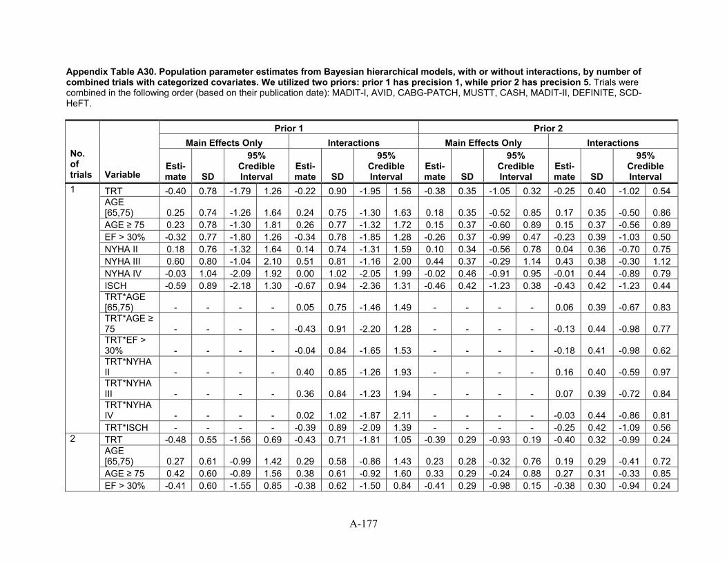
Appendix Table A30. Population parameter estimates from Bayesian hierarchical models, with or without interactions, by number of combined trials with categorized covariates. We utilized two priors: prior 1 has precision 1, while prior 2 has precision 5. Trials were combined in the following order (based on their publication date): MADIT-I, AVID, CABG-PATCH, MUSTT, CASH, MADIT-II, DEFINITE, SCD-HeFT.

Prior 1 Prior 2 Main Effects Only Interactions Main Effects Only Interactions

No. of trials Variable

Esti-mate SD

95% Credible Interval

Esti-mate SD

95% Credible Interval

Esti-mate SD

95% Credible Interval

Esti-mate SD

95% Credible Interval

TRT -0.40 0.78 -1.79 1.26 -0.22 0.90 -1.95 1.56 -0.38 0.35 -1.05 0.32 -0.25 0.40 -1.02 0.54 AGE [65,75) 0.25 0.74 -1.26 1.64 0.24 0.75 -1.30 1.63 0.18 0.35 -0.52 0.85 0.17 0.35 -0.50 0.86 AGE ≥ 75 0.23 0.78 -1.30 1.81 0.26 0.77 -1.32 1.72 0.15 0.37 -0.60 0.89 0.15 0.37 -0.56 0.89 EF > 30% -0.32 0.77 -1.80 1.26 -0.34 0.78 -1.85 1.28 -0.26 0.37 -0.99 0.47 -0.23 0.39 -1.03 0.50 NYHA II 0.18 0.76 -1.32 1.64 0.14 0.74 -1.31 1.59 0.10 0.34 -0.56 0.78 0.04 0.36 -0.70 0.75 NYHA III 0.60 0.80 -1.04 2.10 0.51 0.81 -1.16 2.00 0.44 0.37 -0.29 1.14 0.43 0.38 -0.30 1.12 NYHA IV -0.03 1.04 -2.09 1.92 0.00 1.02 -2.05 1.99 -0.02 0.46 -0.91 0.95 -0.01 0.44 -0.89 0.79 ISCH -0.59 0.89 -2.18 1.30 -0.67 0.94 -2.36 1.31 -0.46 0.42 -1.23 0.38 -0.43 0.42 -1.23 0.44 TRT*AGE [65,75) - - - - 0.05 0.75 -1.46 1.49 - - - - 0.06 0.39 -0.67 0.83 TRT*AGE ≥ 75 - - - - -0.43 0.91 -2.20 1.28 - - - - -0.13 0.44 -0.98 0.77 TRT*EF > 30% - - - - -0.04 0.84 -1.65 1.53 - - - - -0.18 0.41 -0.98 0.62 TRT*NYHA II - - - - 0.40 0.85 -1.26 1.93 - - - - 0.16 0.40 -0.59 0.97 TRT*NYHA III - - - - 0.36 0.84 -1.23 1.94 - - - - 0.07 0.39 -0.72 0.84 TRT*NYHA IV - - - - 0.02 1.02 -1.87 2.11 - - - - -0.03 0.44 -0.86 0.81

1

TRT*ISCH - - - - -0.39 0.89 -2.09 1.39 - - - - -0.25 0.42 -1.09 0.56 TRT -0.48 0.55 -1.56 0.69 -0.43 0.71 -1.81 1.05 -0.39 0.29 -0.93 0.19 -0.40 0.32 -0.99 0.24 AGE [65,75) 0.27 0.61 -0.99 1.42 0.29 0.58 -0.86 1.43 0.23 0.28 -0.32 0.76 0.19 0.29 -0.41 0.72 AGE ≥ 75 0.42 0.60 -0.89 1.56 0.38 0.61 -0.92 1.60 0.33 0.29 -0.24 0.88 0.27 0.31 -0.33 0.85

2

EF > 30% -0.41 0.60 -1.55 0.85 -0.38 0.62 -1.50 0.84 -0.41 0.29 -0.98 0.15 -0.38 0.30 -0.94 0.24

A-177

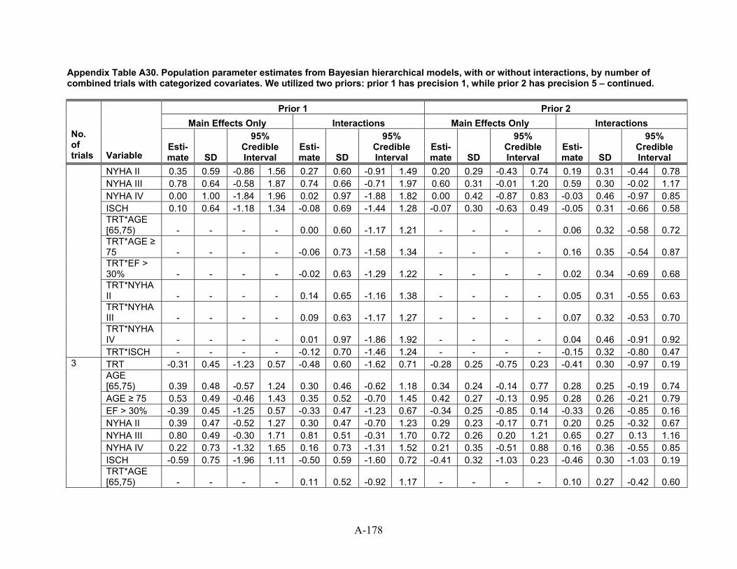
Appendix Table A30. Population parameter estimates from Bayesian hierarchical models, with or without interactions, by number of combined trials with categorized covariates. We utilized two priors: prior 1 has precision 1, while prior 2 has precision 5 – continued.

Prior 1 Prior 2 Main Effects Only Interactions Main Effects Only Interactions

No. of trials Variable

Esti-mate SD

95% Credible Interval

Esti-mate SD

95% Credible Interval

Esti-mate SD

95% Credible Interval

Esti-mate SD

95% Credible Interval

NYHA II 0.35 0.59 -0.86 1.56 0.27 0.60 -0.91 1.49 0.20 0.29 -0.43 0.74 0.19 0.31 -0.44 0.78 NYHA III 0.78 0.64 -0.58 1.87 0.74 0.66 -0.71 1.97 0.60 0.31 -0.01 1.20 0.59 0.30 -0.02 1.17 NYHA IV 0.00 1.00 -1.84 1.96 0.02 0.97 -1.88 1.82 0.00 0.42 -0.87 0.83 -0.03 0.46 -0.97 0.85 ISCH 0.10 0.64 -1.18 1.34 -0.08 0.69 -1.44 1.28 -0.07 0.30 -0.63 0.49 -0.05 0.31 -0.66 0.58 TRT*AGE [65,75) - - - - 0.00 0.60 -1.17 1.21 - - - - 0.06 0.32 -0.58 0.72 TRT*AGE ≥ 75 - - - - -0.06 0.73 -1.58 1.34 - - - - 0.16 0.35 -0.54 0.87 TRT*EF > 30% - - - - -0.02 0.63 -1.29 1.22 - - - - 0.02 0.34 -0.69 0.68 TRT*NYHA II - - - - 0.14 0.65 -1.16 1.38 - - - - 0.05 0.31 -0.55 0.63 TRT*NYHA III - - - - 0.09 0.63 -1.17 1.27 - - - - 0.07 0.32 -0.53 0.70 TRT*NYHA IV - - - - 0.01 0.97 -1.86 1.92 - - - - 0.04 0.46 -0.91 0.92

TRT*ISCH - - - - -0.12 0.70 -1.46 1.24 - - - - -0.15 0.32 -0.80 0.47 TRT -0.31 0.45 -1.23 0.57 -0.48 0.60 -1.62 0.71 -0.28 0.25 -0.75 0.23 -0.41 0.30 -0.97 0.19 AGE [65,75) 0.39 0.48 -0.57 1.24 0.30 0.46 -0.62 1.18 0.34 0.24 -0.14 0.77 0.28 0.25 -0.19 0.74 AGE ≥ 75 0.53 0.49 -0.46 1.43 0.35 0.52 -0.70 1.45 0.42 0.27 -0.13 0.95 0.28 0.26 -0.21 0.79 EF > 30% -0.39 0.45 -1.25 0.57 -0.33 0.47 -1.23 0.67 -0.34 0.25 -0.85 0.14 -0.33 0.26 -0.85 0.16 NYHA II 0.39 0.47 -0.52 1.27 0.30 0.47 -0.70 1.23 0.29 0.23 -0.17 0.71 0.20 0.25 -0.32 0.67 NYHA III 0.80 0.49 -0.30 1.71 0.81 0.51 -0.31 1.70 0.72 0.26 0.20 1.21 0.65 0.27 0.13 1.16 NYHA IV 0.22 0.73 -1.32 1.65 0.16 0.73 -1.31 1.52 0.21 0.35 -0.51 0.88 0.16 0.36 -0.55 0.85 ISCH -0.59 0.75 -1.96 1.11 -0.50 0.59 -1.60 0.72 -0.41 0.32 -1.03 0.23 -0.46 0.30 -1.03 0.19

3

TRT*AGE [65,75) - - - - 0.11 0.52 -0.92 1.17 - - - - 0.10 0.27 -0.42 0.60

A-178

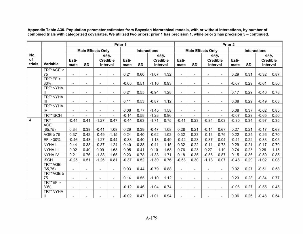
Appendix Table A30. Population parameter estimates from Bayesian hierarchical models, with or without interactions, by number of combined trials with categorized covariates. We utilized two priors: prior 1 has precision 1, while prior 2 has precision 5 – continued.

Prior 1 Prior 2 Main Effects Only Interactions Main Effects Only Interactions

No. of trials Variable

Esti-mate SD

95% Credible Interval

Esti-mate SD

95% Credible Interval

Esti-mate SD

95% Credible Interval

Esti-mate SD

95% Credible Interval

TRT*AGE ≥ 75 - - - - 0.21 0.60 -1.07 1.32 - - - - 0.29 0.31 -0.32 0.87 TRT*EF > 30% - - - - -0.05 0.51 -1.10 0.93 - - - - -0.07 0.29 -0.61 0.50 TRT*NYHA II - - - - 0.21 0.55 -0.94 1.28 - - - - 0.17 0.29 -0.40 0.73 TRT*NYHA III - - - - 0.11 0.53 -0.87 1.12 - - - - 0.08 0.29 -0.49 0.63 TRT*NYHA IV - - - - 0.06 0.77 -1.45 1.58 - - - - 0.08 0.37 -0.62 0.85

TRT*ISCH - - - - -0.14 0.58 -1.28 0.96 - - - - -0.07 0.29 -0.65 0.50 TRT -0.44 0.41 -1.27 0.47 -0.44 0.63 -1.71 0.75 -0.41 0.23 -0.84 0.03 -0.30 0.34 -0.97 0.35 AGE [65,75) 0.34 0.38 -0.41 1.08 0.29 0.39 -0.47 1.08 0.28 0.21 -0.14 0.67 0.27 0.21 -0.17 0.68 AGE ≥ 75 0.37 0.42 -0.49 1.15 0.24 0.40 -0.62 1.02 0.32 0.23 -0.13 0.76 0.22 0.24 -0.26 0.70 EF > 30% -0.46 0.43 -1.27 0.44 -0.38 0.40 -1.13 0.49 -0.42 0.23 -0.87 0.04 -0.41 0.22 -0.83 0.05 NYHA II 0.44 0.38 -0.37 1.24 0.40 0.38 -0.41 1.15 0.32 0.22 -0.11 0.73 0.29 0.21 -0.17 0.70 NYHA III 0.92 0.40 0.09 1.68 0.95 0.41 0.10 1.68 0.76 0.23 0.27 1.19 0.74 0.23 0.26 1.15 NYHA IV 0.21 0.76 -1.38 1.65 0.23 0.78 -1.33 1.71 0.18 0.35 -0.55 0.87 0.15 0.36 -0.59 0.85 ISCH -0.25 0.51 -1.26 0.81 -0.37 0.52 -1.39 0.76 -0.53 0.30 -1.13 0.07 -0.48 0.29 -1.02 0.08 TRT*AGE [65,75) - - - - 0.03 0.44 -0.79 0.88 - - - - 0.02 0.27 -0.51 0.58 TRT*AGE ≥ 75 - - - - 0.14 0.55 -1.10 1.12 - - - - 0.23 0.28 -0.34 0.77 TRT*EF > 30% - - - - -0.12 0.46 -1.04 0.74 - - - - -0.06 0.27 -0.55 0.45

4

TRT*NYHA II - - - - -0.02 0.47 -1.01 0.94 - - - - 0.06 0.26 -0.48 0.54

A-179

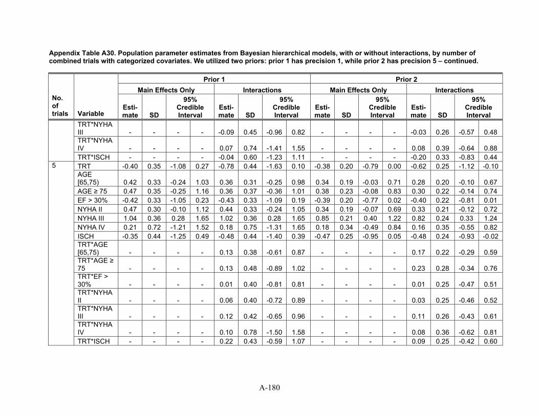
Appendix Table A30. Population parameter estimates from Bayesian hierarchical models, with or without interactions, by number of combined trials with categorized covariates. We utilized two priors: prior 1 has precision 1, while prior 2 has precision 5 – continued.

Prior 1 Prior 2 Main Effects Only Interactions Main Effects Only Interactions

No. of trials Variable

Esti-mate SD

95% Credible Interval

Esti-mate SD

95% Credible Interval

Esti-mate SD

95% Credible Interval

Esti-mate SD

95% Credible Interval

TRT*NYHA III - - - - -0.09 0.45 -0.96 0.82 - - - - -0.03 0.26 -0.57 0.48 TRT*NYHA IV - - - - 0.07 0.74 -1.41 1.55 - - - - 0.08 0.39 -0.64 0.88

TRT*ISCH - - - - -0.04 0.60 -1.23 1.11 - - - - -0.20 0.33 -0.83 0.44 TRT -0.40 0.35 -1.08 0.27 -0.78 0.44 -1.63 0.10 -0.38 0.20 -0.79 0.00 -0.62 0.25 -1.12 -0.10 AGE [65,75) 0.42 0.33 -0.24 1.03 0.36 0.31 -0.25 0.98 0.34 0.19 -0.03 0.71 0.28 0.20 -0.10 0.67 AGE ≥ 75 0.47 0.35 -0.25 1.16 0.36 0.37 -0.36 1.01 0.38 0.23 -0.08 0.83 0.30 0.22 -0.14 0.74 EF > 30% -0.42 0.33 -1.05 0.23 -0.43 0.33 -1.09 0.19 -0.39 0.20 -0.77 0.02 -0.40 0.22 -0.81 0.01 NYHA II 0.47 0.30 -0.10 1.12 0.44 0.33 -0.24 1.05 0.34 0.19 -0.07 0.69 0.33 0.21 -0.12 0.72 NYHA III 1.04 0.36 0.28 1.65 1.02 0.36 0.28 1.65 0.85 0.21 0.40 1.22 0.82 0.24 0.33 1.24 NYHA IV 0.21 0.72 -1.21 1.52 0.18 0.75 -1.31 1.65 0.18 0.34 -0.49 0.84 0.16 0.35 -0.55 0.82 ISCH -0.35 0.44 -1.25 0.49 -0.48 0.44 -1.40 0.39 -0.47 0.25 -0.95 0.05 -0.48 0.24 -0.93 -0.02 TRT*AGE [65,75) - - - - 0.13 0.38 -0.61 0.87 - - - - 0.17 0.22 -0.29 0.59 TRT*AGE ≥ 75 - - - - 0.13 0.48 -0.89 1.02 - - - - 0.23 0.28 -0.34 0.76 TRT*EF > 30% - - - - 0.01 0.40 -0.81 0.81 - - - - 0.01 0.25 -0.47 0.51 TRT*NYHA II - - - - 0.06 0.40 -0.72 0.89 - - - - 0.03 0.25 -0.46 0.52 TRT*NYHA III - - - - 0.12 0.42 -0.65 0.96 - - - - 0.11 0.26 -0.43 0.61 TRT*NYHA IV - - - - 0.10 0.78 -1.50 1.58 - - - - 0.08 0.36 -0.62 0.81

5

TRT*ISCH - - - - 0.22 0.43 -0.59 1.07 - - - - 0.09 0.25 -0.42 0.60

A-180

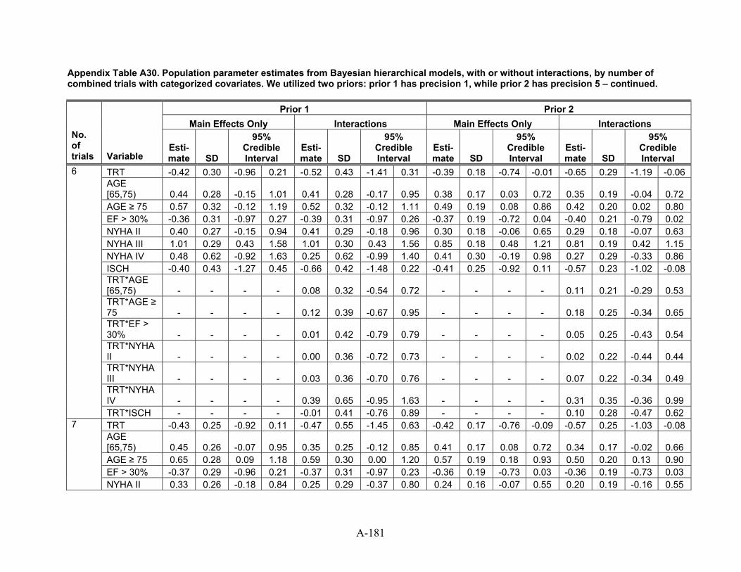
Appendix Table A30. Population parameter estimates from Bayesian hierarchical models, with or without interactions, by number of combined trials with categorized covariates. We utilized two priors: prior 1 has precision 1, while prior 2 has precision 5 – continued.

Prior 1 Prior 2 Main Effects Only Interactions Main Effects Only Interactions

No. of trials Variable

Esti-mate SD

95% Credible Interval

Esti-mate SD

95% Credible Interval

Esti-mate SD

95% Credible Interval

Esti-mate SD

95% Credible Interval

TRT -0.42 0.30 -0.96 0.21 -0.52 0.43 -1.41 0.31 -0.39 0.18 -0.74 -0.01 -0.65 0.29 -1.19 -0.06 AGE [65,75) 0.44 0.28 -0.15 1.01 0.41 0.28 -0.17 0.95 0.38 0.17 0.03 0.72 0.35 0.19 -0.04 0.72 AGE ≥ 75 0.57 0.32 -0.12 1.19 0.52 0.32 -0.12 1.11 0.49 0.19 0.08 0.86 0.42 0.20 0.02 0.80 EF > 30% -0.36 0.31 -0.97 0.27 -0.39 0.31 -0.97 0.26 -0.37 0.19 -0.72 0.04 -0.40 0.21 -0.79 0.02 NYHA II 0.40 0.27 -0.15 0.94 0.41 0.29 -0.18 0.96 0.30 0.18 -0.06 0.65 0.29 0.18 -0.07 0.63 NYHA III 1.01 0.29 0.43 1.58 1.01 0.30 0.43 1.56 0.85 0.18 0.48 1.21 0.81 0.19 0.42 1.15 NYHA IV 0.48 0.62 -0.92 1.63 0.25 0.62 -0.99 1.40 0.41 0.30 -0.19 0.98 0.27 0.29 -0.33 0.86 ISCH -0.40 0.43 -1.27 0.45 -0.66 0.42 -1.48 0.22 -0.41 0.25 -0.92 0.11 -0.57 0.23 -1.02 -0.08 TRT*AGE [65,75) - - - - 0.08 0.32 -0.54 0.72 - - - - 0.11 0.21 -0.29 0.53 TRT*AGE ≥ 75 - - - - 0.12 0.39 -0.67 0.95 - - - - 0.18 0.25 -0.34 0.65 TRT*EF > 30% - - - - 0.01 0.42 -0.79 0.79 - - - - 0.05 0.25 -0.43 0.54 TRT*NYHA II - - - - 0.00 0.36 -0.72 0.73 - - - - 0.02 0.22 -0.44 0.44 TRT*NYHA III - - - - 0.03 0.36 -0.70 0.76 - - - - 0.07 0.22 -0.34 0.49 TRT*NYHA IV - - - - 0.39 0.65 -0.95 1.63 - - - - 0.31 0.35 -0.36 0.99

6

TRT*ISCH - - - - -0.01 0.41 -0.76 0.89 - - - - 0.10 0.28 -0.47 0.62 TRT -0.43 0.25 -0.92 0.11 -0.47 0.55 -1.45 0.63 -0.42 0.17 -0.76 -0.09 -0.57 0.25 -1.03 -0.08 AGE [65,75) 0.45 0.26 -0.07 0.95 0.35 0.25 -0.12 0.85 0.41 0.17 0.08 0.72 0.34 0.17 -0.02 0.66 AGE ≥ 75 0.65 0.28 0.09 1.18 0.59 0.30 0.00 1.20 0.57 0.19 0.18 0.93 0.50 0.20 0.13 0.90 EF > 30% -0.37 0.29 -0.96 0.21 -0.37 0.31 -0.97 0.23 -0.36 0.19 -0.73 0.03 -0.36 0.19 -0.73 0.03

7

NYHA II 0.33 0.26 -0.18 0.84 0.25 0.29 -0.37 0.80 0.24 0.16 -0.07 0.55 0.20 0.19 -0.16 0.55

A-181

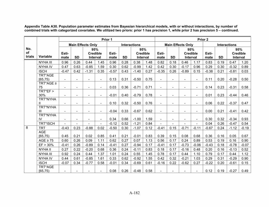
Appendix Table A30. Population parameter estimates from Bayesian hierarchical models, with or without interactions, by number of combined trials with categorized covariates. We utilized two priors: prior 1 has precision 1, while prior 2 has precision 5 – continued.

Prior 1 Prior 2 Main Effects Only Interactions Main Effects Only Interactions

No. of trials Variable

Esti-mate SD

95% Credible Interval

Esti-mate SD

95% Credible Interval

Esti-mate SD

95% Credible Interval

Esti-mate SD

95% Credible Interval

NYHA III 0.96 0.26 0.44 1.45 0.96 0.28 0.38 1.48 0.82 0.18 0.46 1.17 0.83 0.19 0.47 1.20 NYHA IV 0.47 0.63 -0.85 1.59 0.30 0.62 -0.99 1.42 0.42 0.30 -0.17 0.96 0.29 0.30 -0.32 0.89 ISCH -0.47 0.42 -1.31 0.35 -0.57 0.43 -1.40 0.27 -0.35 0.26 -0.89 0.15 -0.38 0.21 -0.81 0.03 TRT*AGE [65,75) - - - - 0.13 0.31 -0.50 0.75 - - - - 0.11 0.20 -0.28 0.50 TRT*AGE ≥ 75 - - - - 0.03 0.36 -0.71 0.71 - - - - 0.14 0.23 -0.31 0.58 TRT*EF > 30% - - - - -0.01 0.40 -0.79 0.78 - - - - 0.01 0.23 -0.44 0.46 TRT*NYHA II - - - - 0.10 0.32 -0.50 0.76 - - - - 0.06 0.22 -0.37 0.47 TRT*NYHA III - - - - -0.04 0.33 -0.67 0.62 - - - - 0.00 0.21 -0.41 0.42 TRT*NYHA IV - - - - 0.34 0.66 -1.00 1.59 - - - - 0.30 0.32 -0.34 0.93

TRT*ISCH - - - - -0.12 0.52 -1.21 0.84 - - - - 0.04 0.26 -0.47 0.54 TRT -0.43 0.23 -0.88 0.02 -0.50 0.30 -1.07 0.12 -0.41 0.15 -0.71 -0.11 -0.67 0.24 -1.12 -0.19 AGE [65,75) 0.45 0.21 0.02 0.85 0.41 0.21 -0.01 0.83 0.39 0.15 0.08 0.68 0.36 0.16 0.05 0.67 AGE ≥ 75 0.60 0.26 0.09 1.11 0.62 0.27 0.07 1.13 0.56 0.17 0.24 0.89 0.53 0.19 0.16 0.90 EF > 30% -0.41 0.26 -0.89 0.14 -0.41 0.27 -0.94 0.17 -0.41 0.17 -0.73 -0.06 -0.43 0.18 -0.78 -0.07 NYHA II 0.27 0.22 -0.20 0.68 0.36 0.24 -0.11 0.83 0.18 0.17 -0.16 0.48 0.20 0.16 -0.13 0.52 NYHA III 0.92 0.24 0.44 1.37 1.01 0.24 0.55 1.45 0.78 0.17 0.44 1.10 0.79 0.17 0.44 1.12 NYHA IV 0.44 0.61 -0.85 1.61 0.33 0.62 -0.92 1.55 0.42 0.32 -0.21 1.03 0.29 0.31 -0.29 0.90 ISCH -0.07 0.34 -0.77 0.58 -0.01 0.34 -0.69 0.61 -0.16 0.22 -0.62 0.27 -0.22 0.20 -0.61 0.15

8

TRT*AGE [65,75) - - - - 0.08 0.26 -0.48 0.58 - - - - 0.12 0.19 -0.27 0.49

A-182

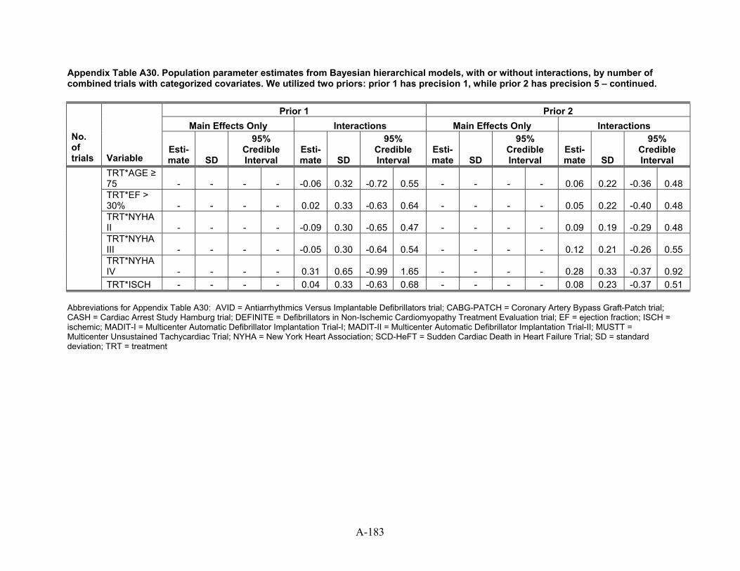
A-183

Appendix Table A30. Population parameter estimates from Bayesian hierarchical models, with or without interactions, by number of combined trials with categorized covariates. We utilized two priors: prior 1 has precision 1, while prior 2 has precision 5 – continued.

Prior 1 Prior 2 Main Effects Only Interactions Main Effects Only Interactions

No. of trials Variable

Esti-mate SD

95% Credible Interval

Esti-mate SD

95% Credible Interval

Esti-mate SD

95% Credible Interval

Esti-mate SD

95% Credible Interval

TRT*AGE ≥ 75 - - - - 0.32 55 - - - - 0.06 0.22 0.48 -0.06 -0.72 0. -0.36 TRT*EF > 30% - - - - 0.02 0.33 0.64 - - - - 0.05 0.22 0.48 -0.63 -0.40 TRT*NYHA II - - - - 0.30 47 - - - - 0.09 0.19 0.48 -0.09 -0.65 0. -0.29 TRT*NYHA III - - - - 0.30 0.54 - - - - 0.12 0.21 0.55 -0.05 -0.64 -0.26 TRT*NYHA IV - - - - 0.31 0.65 65 - - - - 0.28 0.33 0.92 -0.99 1. -0.37

TRT*ISCH - - - - 0.04 0.33 0.68 - - - - 0.08 0.23 0.51 -0.63 -0.37 Abbreviations for Appendix Table A30: AVID = Antiarrhythmics Versus Implantable Defibrillators trial; CABG-PATCH = Coronary Artery Bypass Graft-Patch trial; CASH = Cardiac Arrest Study Hamburg trial; DEFINITE = Defibrillators in Non-Ischemic Cardiomyopathy Treatment Evaluation trial; EF = ejection fraction; ISCH = ischemic; MADIT-I = Multicenter Automatic Defibrillator Implantation Trial-I; MADIT-II = Multicenter Automatic Defibrillator Implantation Trial-II; MUSTT = Multicenter Unsustained Tachycardiac Trial; NYHA = New York Heart Association; SCD-HeFT = Sudden Cardiac Death in Heart Failure Trial; SD = standard deviation; TRT = treatment

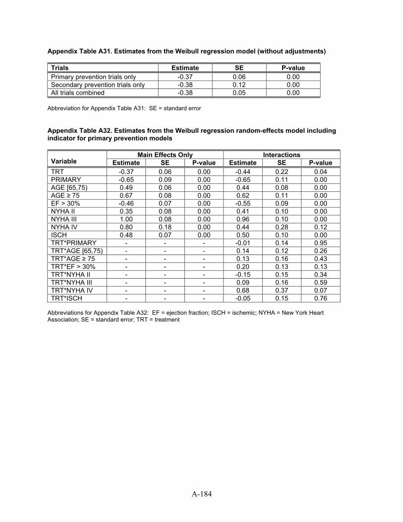
Appendix Table A31. Estimates from the Weibull regression model (without adjustments) Trials Estimate SE P-value Primary prevention trials only -0.37 0.06 0.00 Secondary prevention trials only -0.38 0.12 0.00 All trials combined -0.38 0.05 0.00

Abbreviation for Appendix Table A31: SE = standard error Appendix Table A32. Estimates from the Weibull regression random-effects model including indicator for primary prevention models

Main Effects Only Interactions Variable Estimate SE P-value Estimate SE P-value TRT -0.37 0.06 0.00 -0.44 0.22 0.04 PRIMARY -0.65 0.09 0.00 -0.65 0.11 0.00 AGE [65,75) 0.49 0.06 0.00 0.44 0.08 0.00 AGE ≥ 75 0.67 0.08 0.00 0.62 0.11 0.00 EF > 30% -0.46 0.07 0.00 -0.55 0.09 0.00 NYHA II 0.35 0.08 0.00 0.41 0.10 0.00 NYHA III 1.00 0.08 0.00 0.96 0.10 0.00 NYHA IV 0.80 0.18 0.00 0.44 0.28 0.12 ISCH 0.48 0.07 0.00 0.50 0.10 0.00 TRT*PRIMARY - - - -0.01 0.14 0.95 TRT*AGE [65,75) - - - 0.14 0.12 0.26 TRT*AGE ≥ 75 - - - 0.13 0.16 0.43 TRT*EF > 30% - - - 0.20 0.13 0.13 TRT*NYHA II - - - -0.15 0.15 0.34 TRT*NYHA III - - - 0.09 0.16 0.59 TRT*NYHA IV - - - 0.68 0.37 0.07 TRT*ISCH - - - -0.05 0.15 0.76

Abbreviations for Appendix Table A32: EF = ejection fraction; ISCH = ischemic; NYHA = New York Heart Association; SE = standard error; TRT = treatment

A-184