Embed Size (px)
Citation preview
Diss. ETH No. 16707
Use of FACTS Devices forPower Flow Control and
Damping of Oscillations inPower Systems
A dissertation submitted to the
SWISS FEDERAL INSTITUTE OF TECHNOLOGY
ZURICH
for the degree of
Doctor of Technical Sciences
presented by
RUSEJLA SADIKOVIC
Master of Science, Faculty of Electrical Engineering,
University of Tuzla
born October 14th, 1969
in Tuzla, Bosna and Hecegovina
accepted on the recommendation of
Prof. Dr. Goran Andersson, examiner
Prof. Dr. Caludio A. Canizares, co-examiner
2006


Acknowledgments
This dissertation presents the results of my research done at the Powersystem Laboratory of the Swiss Federal Institute of Technology (ETH)during the years 2002 − 2004.
First of all I would like to express my deep gratitude to my advisorProf. Goran Andersson for giving me the opportunity to work on thisproject. His valuable suggestions and his encouragement and patiencehave been a big help for me over the last for years.
I am very grateful to Dr. Petr Korba four his skilled guidance, valuablecomments, stimulating discussions and support throughout this project.
Special thanks go to Prof. Claudio A. Canizares for accepting to co-referee this thesis.
I also would like to thank my colleagues at the laboratory for the en-joyable discussions and friendly atmosphere. I particularly thank myoffice-mates Dr. Andrei Karpatchev and Mirjana Milosevic for the re-laxed work atmosphere in our office. I am very grateful as well to MariaLourdes Steiner-Igcasenza for proofreading this thesis.
Finally, I would like to extend my deepest gratitude and personal thanksto those closest to me. In particular, I would like to thank my husbandAdnan, my son Berin and my parents for their support, encouragementand understanding.
Rusejla Sadikovic
3

Abstract
Due to the deregulation of the electrical market, difficulty in acquiringrights-of-way to build new transmission lines, and steady increase inpower demand, maintaining power system stability becomes a difficultand very challenging problem. In large, interconnected power systems,power system damping is often reduced, leading to lightly damped elec-tromechanical modes of oscillations. Implementation of new equipmentconsisting high power electronics based technologies such as FlexibleAlternating Current Transmission Systems (FACTS) and proper con-troller design become essential for improvement of operation and con-trol of power systems.
The aim of this dissertation is to examine the ability of FACTS de-vices, such as Thyristor Controlled Series Capacitor (TCSC), UnifiedPower Flow Controller (UPFC) and Static VAr Compensator (SVC)for power flow control and damping of electromechanical oscillations ina power system. A power flow control strategy is based on linearizationof active and reactive power flows around an operating point. A controlstrategy for damping of oscillations, including several FACTS devicesand PSSs, is based on different approaches, both off-line and on-line,e.g. residue based method, pole shifting method and genetic algorithms.The robustness of each approach is discussed. One part of this disser-tation deals with location of FACTS devices considering multiple tasks,power flow control and damping of oscillations.
The results of the case studies demonstrate advantages and disadvan-tages of the considered control approaches.
5


Kurzfassung
Als Folge der Liberalisierung vieler Elektrizitatsmarkte ergeben sich furden Netzbetrieb zusatzliche anspruchsvolle Aufgaben. Die Erschwer-nis des Baus zusatzlicher Ubertragungsleitungen aufgrund langwierigerBewilligungsverfahren sowie ein starkes Wachstum der Nachfrage nachelektrischer Energie stellen an die Netzbetreiber hohe Anspruche bezu-glich der Gewahrleistung der Systemstabilitat. In grossen, stark ver-maschten Netzstrukturen werden Leistungspendelungen nur bedingt ge-dampft und konnen zu erheblichen elektromechanischen Schwingungenfuhren. Aus diesem Grund ist die Anwendung neuer Kontrollmecha-nismen basierend auf leistungselektronischen Technologien wie FlexibleAlternating Current Transmission Systems (FACTS) hinsichtlich einessicheren Netzbetriebs notwendig.
Das Ziel dieser Dissertation ist die Untersuchung der Eignung von FACTSGeraten, wie Thyristor Controlled Series Capacitor (TCSC), UnifiedPower Flow Controller (UPFC) sowie Static VAr Compensator (SVC) inBezug auf Lastfluss-Steuerung sowie Dampfung von Leistungspendelun-gen. Es wird ein auf der Linearisierung des Wirk- und Blindleistungs-flusses basierendes Verfahren zur Lastfluss-Regelung vorgestellt, welchesdie Dampfung von Leistungspendelungen mittels FACTS Geraten undPSS’s beinhaltet. Dabei setzt sich dieses Verfahren aus den folgendenoff- und on-line Methoden zusammen: Der Residuen basierten Meth-ode, der Pol-Verschiebungsmethode und den genetischen Algorithmen.Erlauterungen bezuglich der Robustheit dieser Methoden werden eben-falls diskutiert. Ein weiterer Bestandteil dieser Dissertation setzt sichmit der Bestimmung des Einsatzortes von FACTS-Geraten auseinander.
Als Resultat der untersuchten Fallstudien werden sowohl Vor- als auch
7

8 Kurzfassung
Nachteile der betrachteten Methoden zur Lastfluss-Steuerung aufgezeigt.
Contents
1 Introduction 13
1.1 Thesis outline . . . . . . . . . . . . . . . . . . . . . . . . 17
1.2 Contributions . . . . . . . . . . . . . . . . . . . . . . . . 17
1.3 List of Publications . . . . . . . . . . . . . . . . . . . . . 18
2 Modeling of FACTS devices 19
2.1 Thyristor Controlled Series Capacitor . . . . . . . . . . 19
2.2 Unified Power Flow Controller . . . . . . . . . . . . . . 23
2.3 Static VAr Compensator . . . . . . . . . . . . . . . . . . 30
3 Use of FACTS Devices for Damping of Power System
Oscillations 33
3.1 Introduction . . . . . . . . . . . . . . . . . . . . . . . . . 33
3.2 Modal Analysis . . . . . . . . . . . . . . . . . . . . . . . 34
3.3 FACTS POD Controller Design . . . . . . . . . . . . . . 38
3.4 Case Studies . . . . . . . . . . . . . . . . . . . . . . . . 40
3.4.1 Design of TCSC POD Controller . . . . . . . . . 41
3.4.2 Design of UPFC POD Controller . . . . . . . . . 45
3.4.3 Design of SVC POD Controller . . . . . . . . . . 51
3.5 Summary . . . . . . . . . . . . . . . . . . . . . . . . . . 53
9

10 Contents
4 On the Location of the TSCS 55
4.1 Dynamic Criterion . . . . . . . . . . . . . . . . . 56
4.2 Static Criterion . . . . . . . . . . . . . . . . . . . 56
4.3 Case Study . . . . . . . . . . . . . . . . . . . . . 58
4.4 Summary . . . . . . . . . . . . . . . . . . . . . . 62
5 Self-Tuning Controllers 65
5.1 Adaptive Model Identification . . . . . . . . . . . . . . . 66
5.2 Residue Based Adaptive Control . . . . . . . . . . . . . 69
5.3 Pole Shifting Adaptive Control . . . . . . . . . . . . . . 76
5.4 Summary . . . . . . . . . . . . . . . . . . . . . . . . . . 85
6 Coordinated Tuning of PSS and FACTS POD
Controllers 87
6.1 Genetic Algorithms . . . . . . . . . . . . . . . . . . . . . 88
6.1.1 Selection . . . . . . . . . . . . . . . . . . . . . . 88
6.1.2 Crossover . . . . . . . . . . . . . . . . . . . . . . 89
6.1.3 Mutation . . . . . . . . . . . . . . . . . . . . . . 89
6.2 PSS and FACTS POD Controller design . . . . . . . . . 90
6.3 Case study . . . . . . . . . . . . . . . . . . . . . . . . . 91
6.3.1 Case Study with the TCSC - Case Study I . . . 95
6.3.2 Case Study with the SVC - Case Study II . . . . 100
6.3.3 Case Study with the TCSC and the SVC - CaseStudy III . . . . . . . . . . . . . . . . . . . . . . 105
6.4 Summary . . . . . . . . . . . . . . . . . . . . . . . . . . 110

Contents 11
7 Concluding Remarks 111
A IEEE 39 Bus Test System Data 115
B IEEE 68 Bus Test System Data 121
C IEEE Sensitivity Analysis 129
Bibliography 133

Chapter 1
Introduction
Modern bulk power systems cover large geographic areas, e.g. the Eu-ropean UCTE system and the North American systems, and have alarge number of load buses and generators. Additionally, available gen-erating plants are often not situated near load centers and power mustconsequently be transmitted over long distances. To meet the load andelectric market demands, new lines should be added to the system, butdue to environmental reasons, the installation of electric power trans-mission lines must often be restricted. Hence, the utilities are forced torely on already existing infra-structure instead of building new trans-mission lines. In order to maximize the efficiency of generation, trans-mission and distribution of electric power, the transmission networksare very often pushed to their physical limits, where outage of lines orother equipment could result in the rapid failure of the entire system.With such increasing stress on the existing transmission lines the useof Flexible AC Transmission Systems (FACTS) devices becomes an im-portant and effective option.
FACTS technologies offer competitive solutions to today’s power sys-tems in terms of increased power flow transfer capability, enhancingcontinuous control over the voltage profile, improving system damping,minimizing losses, etc. FACTS technology consists of high power elec-tronics based equipment with its real-time operating control [1, 2, 6].There are two groups of FACTS controllers based on different techni-cal approaches, both resulting in controllers able to solve transmission
13
14 Chapter 1. Introduction
problems.
The first group employs reactive impedances or tap-changing trans-formers with thyristor switches as controlled elements; the second groupemploy self-commutated voltage-sourced switching converters. The so-phisticate control and fast response are common for both groups. TheStatic VAr Compensator (SVC), Thyristor Controlled Series Capacitor(TCSC) and Phase Shifter, belong to the first group of controllers whileStatic Synchronous Compensators (STATCOM), Static SynchronousSeries Compensators (SSSC), Unified Power Flow Controllers (UPFC)and Interline Power Flow Controllers (IPFC) belong to the other group.
The power system may be thought of as a large, interconnected non-linear system with many lightly damped electromechanical modes ofoscillation. If the damping of these modes become too small, or evenpositive, it can impose severe constraints on the system’s operation. Itis thus important to be able to determine the nature of those modes,find stability limits and in many cases use controls to prevent insta-bility. The poorly damped low frequency electromechanical oscillationsoccur due to inadequate damping torque in some generators, causingboth local-mode oscillations (1 Hz to 2 Hz) and inter-area oscillations(0.1 Hz to 1 Hz) [19]. The traditional approach employs power sys-tem stabilizers (PSS) on generator excitation control systems in orderto damp those oscillations. PSSs are effective but they are usually de-signed for damping local modes and in large power systems they maynot provide enough damping for inter-area modes. Hence, in order toimprove damping of these modes, it is of interest to study FACTS poweroscillation damping (POD) controllers [17]. In large power systems thenumber of inter-area modes is usually larger than the number of controldevices available [3]. Generally, damping of power system oscillationsis not the primary reason of placing FACTS devices in the power sys-tem, but rather power flow control [6, 7]. However, when installed,supplementary control lows can be applied to existing devices in orderto improve damping, as well as satisfy the primary requirements of thedevice.
One of the very important questions in the practical application of con-troller installation is whether to use local or remote input signals (oftenreferred to as global signals) as feedback signals. There are differentapproaches, [3, 13, 15, 17]. The advantages of the local signals are their
15
simplicity and reliability. On the other hand, they might not give ade-quate observability of some of the significant inter-area modes [4]. Theadvantage of the global signals is that they contain information aboutthe overall network dynamics in contrast to the local signals. But froman economic viewpoint, the implementation of a control scheme usingglobal signals may be more cost effective than installing new controldevices [3]. Since remote signals are often transmitted by the exist-ing communication channels, time delay is involved, which could be animpediment. In this thesis, the local signal is used as the controller’sfeedback signal.
A conventional damping control design considers a single operating con-dition of the system. In this kind of controller the feedback is fixed andamplifies the control error, which in turn determines the value of theinput signal u (controller output) to the system. The way in which theerror is processed is the same for all operating conditions. In Chapter 3,a conventional lead-lag controller designed for nominal operating pointis presented and applied on three different types of FACTS devices.This controller is simple, but works often only within a limited operat-ing range. In case of contingencies, changed operating conditions cancause poorly damped or even unstable oscillations since the controllerparameters yielding satisfactory damping for one operating conditionmay no longer provide sufficient damping for another one. In orderto address this issue, researchers, over the years, have proposed differ-ent approaches for adaptive control structures for PSSs as well as forFACTS devices. Some of them are reviewed in Chapter 5.
The primary idea is to overcome the problems that might be encoun-tered by conventionally tuned controllers with the changing of operatingconditions. Dealing with an adaptive on-line tuning, the identificationof the static and dynamic characteristics of the system plays an impor-tant role together with the control strategy itself. In Chapter 5, on-lineidentification based on the automatic detection of oscillations in powersystems using dynamic data such as currents, voltages and angle dif-ferences measured across transmission lines, provided on-line by phasormeasurement units, is presented [5]. The on-line collected measureddata are subjected to a further evaluation with the objective to esti-mate dominant modes (frequencies and damping) during any operationof the power system or to give reduced transfer function of the unknownpower system.
16 Chapter 1. Introduction
Based on two approaches of on-line identification of the power system, acontrol strategy for on-line tuning of the POD controllers is developed.The first approach is based on modal analysis, i.e. residue method,and the second employs self-tuning controllers (STC) based on the poleshifting method. The self-tuning controller is based on the idea of sep-arating the estimation of unknown parameters from the design of theoptimal controller, [29].
Although controllers tuned by the conventional design approach aresimple, lack of robustness of that kind of controllers is not the onlyproblem encountered. Conventional procedures become time consum-ing and difficult to implement for cases in which:
• there is a significant number of PSSs and FACTS POD controllersto be coordinated,
• coordination must be conducted for a variety of operating conditionsand
• certain performance specifications have to be satisfied.
As a consequence of the presence of different types of the stabilizers inthe system, e.g. the PSSs and FACTS POD controllers, the undesiredand detrimental interactions between them may occur [34]. To avoidthis a simultaneous optimization and coordination of the parameter set-tings of both stabilizers is required in order to enhance overall systemstability and minimizing possible adverse interactions. A solution tothis problem is the use of Genetic Algorithms (GA) methodology, andthis has been investigated in Chapter 6.
In [38] and [39], PSS tuning by means of GA is presented. These papersinvestigate the use of genetic algorithms to design robust PSS, in whichseveral operating conditions and system configurations are simultane-ously considered in the design process. In [38], simultaneous tuning ofnine PSSs in 14 operating conditions for the New England power sys-tem was performed. The objective function used for GA optimizationwas the sum of the damping ratios for all eigenvalues in all operatingconditions. Two additional objective functions that allowed some eigen-values to be shifted to the left-hand side of the complex plane or to a
1.1. Thesis outline 17
wedge-shape sector in the complex plane were further investigated in[39]. In [40], the authors propose the use of advanced techniques inGA for the optimal tuning of PSSs again for different operating condi-tions. The results obtained in these papers proved that GA could bea powerful tool for robust PSS damping controller design. ConsideringFACTS POD tuning, the GA approach is used in [36] in order to designSVC and TCSC damping controllers to enhance damping of inter-areamodes in a three-area six-machine system. In Chapter 6 of this thesis,the GA approach is used as well, as a tool for design of multiple PODcontrollers in a large, realistic system.
1.1 Thesis outline
Following the Introduction, Chapter 2 describes the injection models ofthe FACTS devices, and their use in power flow control.
Chapter 3 gives an overview of the conventional POD controller de-sign and their application on the TCSC, UPFC and SVC.
In Chapter 4, an approach for the optimal location of FACTS devicescombining the static (for optimal location of the power flow controller)and the dynamic criteria (for optimal location of the damping controller)is presented.
The concept of one-line tuning of the FACTS POD controllers is pre-sented in Chapter 5.
In Chapter 6 a method for simultaneous coordinated tuning of theFACTS POD controller and the PSS controllers is presented.
Chapter 7 summarizes the findings in this work with some suggestionsfor future research directions.
1.2 Contributions
The main contributions of this dissertation can be summarized as:

18 Chapter 1. Introduction
• Application of POD controller to Unified Power Flow Controllers(UPFC) based on residue approach, considering different local sig-nals as feedback signals.
• Proposal of an approach for location of FACTS devices for multi-ple control objectives, considering static and dynamic criteria.
• Application of self-tuning controllers based on residue method andon pole shifting method.
• Application of genetic algorithm methodology to coordination ofpower system controllers for robust damping of electromechanicaloscillations.
1.3 List of publications
The work presented in this dissertation has been reported by the fol-lowing publications:
1. R. Sadikovic and G. Andersson, Power Flow Control by SensitivityBased Facts Controllers, IPEC 2003, Singapore, November 2003.
2. R. Sadikovic, G. Andersson and P. Korba, A Power Flow ControlStrategy for FACTS Devices, WAC 2004, Spain, June 2004.
3. R. Sadikovic, P. Korba and G. Andersson, Application of FACTSDevices for Damping of Power System Oscillations, IEEE Pow-erTech 2005, Russia, June 2005.
4. R. Sadikovic, G. Andersson and P. Korba, Method for Location ofFACTS for Multiple Control Objectives, X SEPOPE, Brasil, May2006.
5. R. Sadikovic, P. Korba and G. Andersson, Self-tuning Controllerfor Damping of Power System Oscillations with FACTS Devices,IEEE PES General Meeting, Canada, June 2006.
6. R. Sadikovic, G. Andersson and P. Korba, Damping ControllerDesign for Power System Oscillations, Intelligent Automation &Soft Computing Journal, Vol. 12, No. 1, pp: 51-62, 2006.
Chapter 2
Modelling of FACTS
Devices
Flexible AC transmission systems (FACTS) devices are installed inpower systems to increase the power flow transfer capability of the trans-mission systems, to enhance continuous control over the voltage profileand/or to damp power system oscillations [6, 7]. The ability to controlpower rapidly can increase stability margins as well as the damping ofthe power system, to minimize losses, to work within the thermal limitsrange, etc.
In this chapter, injection models of the Thyristor Controlled Series Ca-pacitor (TCSC), Unified Power Flow Controller (UPFC) and Static VarCondensator (SVC), used in this dissertation, with appropriate controls,are presented.
2.1 Thyristor Controlled Series Capacitor
Model
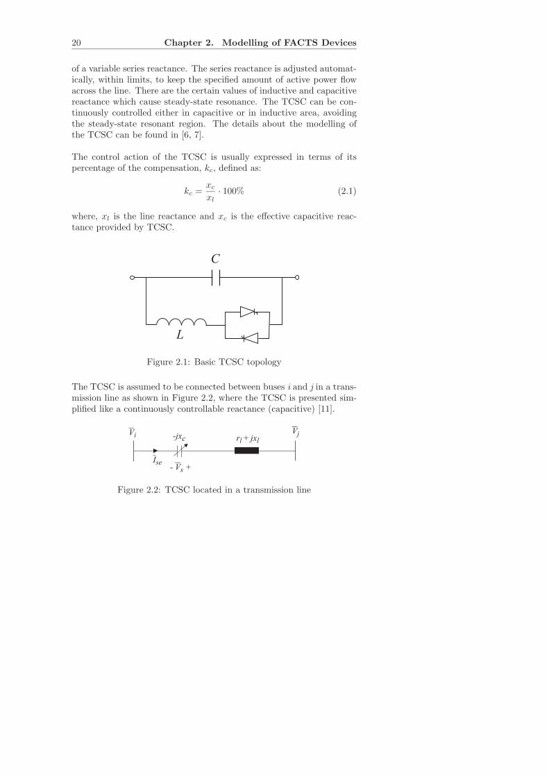
A Thyristor Controlled Series Capacitor (TCSC) configuration consistsof a series capacitor bank, C, in parallel with a thyristor-controlled re-actor, L, as shown in Figure 2.1. This simple model utilizes the concept
19
20 Chapter 2. Modelling of FACTS Devices
of a variable series reactance. The series reactance is adjusted automat-ically, within limits, to keep the specified amount of active power flowacross the line. There are the certain values of inductive and capacitivereactance which cause steady-state resonance. The TCSC can be con-tinuously controlled either in capacitive or in inductive area, avoidingthe steady-state resonant region. The details about the modelling ofthe TCSC can be found in [6, 7].
The control action of the TCSC is usually expressed in terms of itspercentage of the compensation, kc, defined as:
kc =xc
xl
· 100% (2.1)
where, xl is the line reactance and xc is the effective capacitive reac-tance provided by TCSC.
L
C
Figure 2.1: Basic TCSC topology
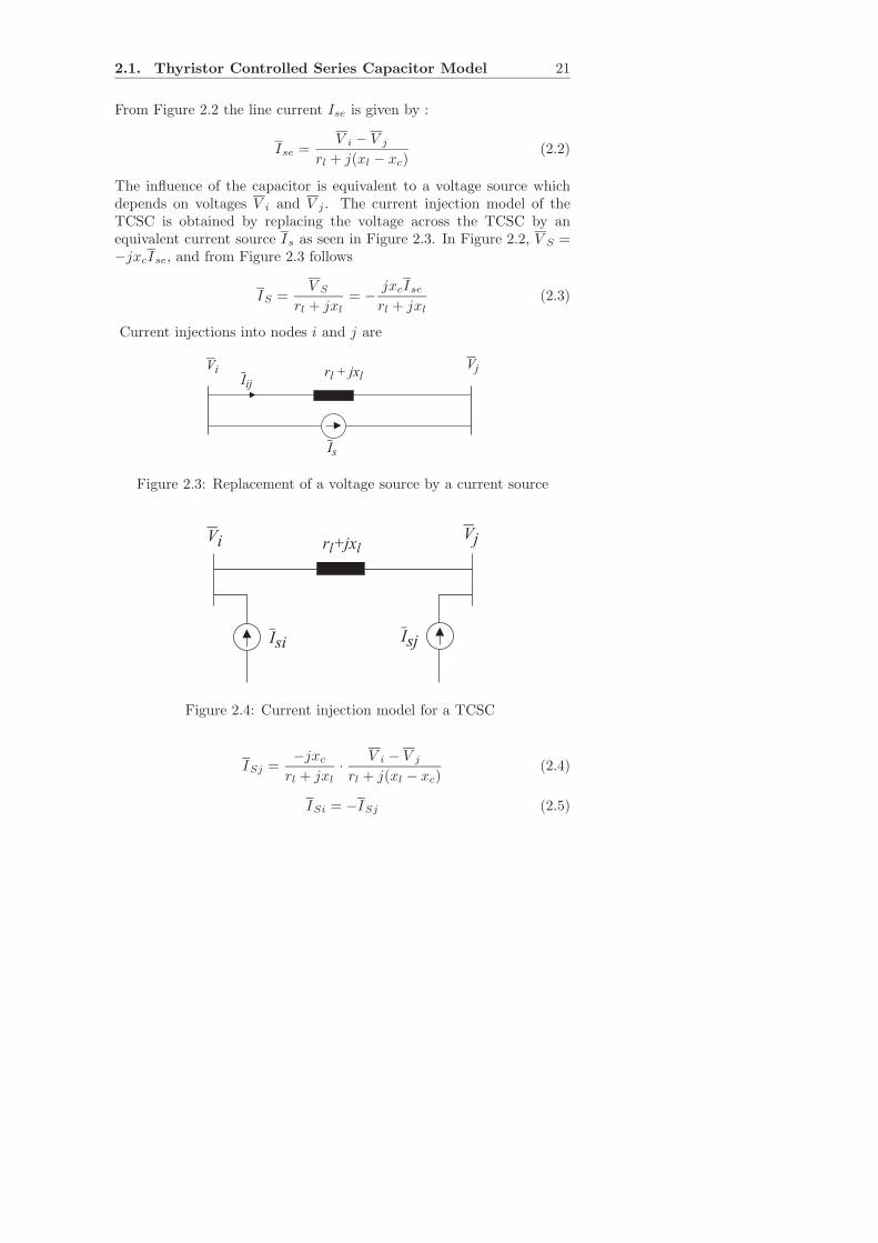
The TCSC is assumed to be connected between buses i and j in a trans-mission line as shown in Figure 2.2, where the TCSC is presented sim-plified like a continuously controllable reactance (capacitive) [11].
Vjr jx+ ll
-jxc
Ise- +Vs
Vi
Figure 2.2: TCSC located in a transmission line
2.1. Thyristor Controlled Series Capacitor Model 21
From Figure 2.2 the line current Ise is given by :
Ise =V i − V j
rl + j(xl − xc)(2.2)
The influence of the capacitor is equivalent to a voltage source whichdepends on voltages V i and V j . The current injection model of theTCSC is obtained by replacing the voltage across the TCSC by anequivalent current source Is as seen in Figure 2.3. In Figure 2.2, V S =−jxcIse, and from Figure 2.3 follows
IS =V S
rl + jxl
= − jxcIse
rl + jxl
(2.3)
Current injections into nodes i and j are
Vi Vjr + jxllIij
Is
Figure 2.3: Replacement of a voltage source by a current source
Vi Vjr +jxll
Isi Isj
Figure 2.4: Current injection model for a TCSC
ISj =−jxc
rl + jxl
· V i − V j
rl + j(xl − xc)(2.4)
ISi = −ISj (2.5)
22 Chapter 2. Modelling of FACTS Devices
and therefore the appropriate current injection model of the TCSC canbe presented as shown in Figure 2.4.
TCSC
ControlStrategy
Dkc
Kcd1
sTcd
-
+
P
Pref
Powernetwork
Isi
Isj1
Ts+1
kcDmax
kcDmin
++
+
Cdamp
DP
Figure 2.5: General form of the TCSC control system
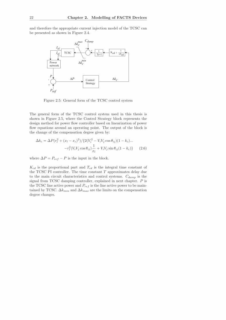
The general form of the TCSC control system used in this thesis isshown in Figure 2.5, where the Control Strategy block represents thedesign method for power flow controller based on linearization of powerflow equations around an operating point. The output of the block isthe change of the compensation degree given by:
∆kc = ∆P (r2l + (xl − xc)2)/2(V 2
i − ViVj cos θij)(1 − kc)...
−r2l (ViVj cos θij)1
xl
+ ViVj sin θij(1 − kc) (2.6)
where ∆P = Pref − P is the input in the block.
Kcd is the proportional part and Tcd is the integral time constant ofthe TCSC PI controller. The time constant T approximates delay dueto the main circuit characteristics and control systems. Cdamp is thesignal from TCSC damping controller, explained in next chapter. P isthe TCSC line active power and Pref is the line active power to be main-tained by TCSC. ∆kmin and ∆kmax are the limits on the compensationdegree changes.
2.2. Unified Power Flow Controller 23
2.2 Unified Power Flow Controller
The UPFC can provide simultaneous control of all basic power systemparameters (transmission voltage, impedance and phase angle). Thecontroller can fulfill functions of reactive shunt compensation, seriescompensation and phase shifting, meeting multiple control objectives.From a functional perspective, the objectives are met by applying a DCcapacitor, shunt connected transformer and voltage source converter inparallel branch and dc capacitor, voltage source convertor and seriesinjected transformer in the series branch.
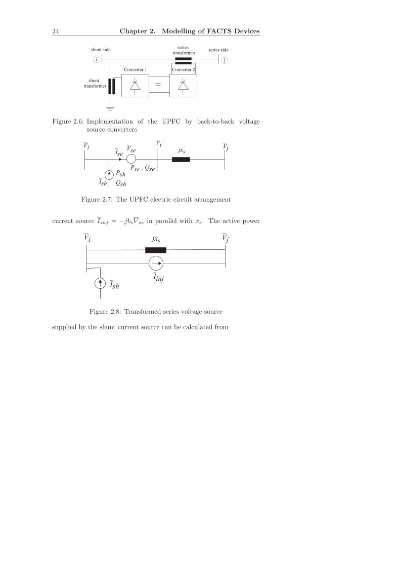
The two voltage source converters are a so called ”back to back” ACto DC voltage source converters operated from a common DC link ca-pacitor, Figure 2.6. The shunt converter is primarily used to provideactive power demand of the series converter through the common DClink. Converter 1 can also generate or absorb reactive power, if it isdesired, and thereby provides independent shunt reactive compensationfor the line. Converter 2 provides the main function of the UPFC by in-jecting a voltage with controllable magnitude and phase angle in serieswith the line, Figure 2.7. The reactance xs describes the reactance seenfrom terminals of the series transformer and is equal to (in p.u. base onsystem voltage and base power)
xS = xkr2max(SB/SS) (2.7)
where xk denotes the series transformer reactance, rmax the maximumper unit value of injected voltage magnitude, SB the system base power,and SS the nominal rating power of the series converter.
The UPFC injection model is derived enabling three parameters to be si-multaneously controlled [8]. They are namely the shunt reactive power,Qconv1, and the magnitude, r, and the angle, γ, of injected series voltageV se. Figure 2.7 shows the circuit representation of a UPFC, where theseries connected voltage source is modelled by an ideal series voltagewhich is controllable in magnitude and phase, and the shunt converteris modelled as an ideal shunt current source. In Figure 2.7,
Ish = It + Iq
= (It + jIq)ejθi (2.8)
where It is the current in phase with V i and Iq is the current in quadra-ture with V i. In Figure 2.8 the voltage source V se is replaced by the
24 Chapter 2. Modelling of FACTS Devices
i j
shunt side series sideseries
transformer
shunttransformer
Converter 1 Converter 2
Figure 2.6: Implementation of the UPFC by back-to-back voltagesource converters
Vi VjjxsIse
Ish
VseVi’
Psh
Qsh
Pse , Qse
Figure 2.7: The UPFC electric circuit arrangement
current source Iinj = −jbsV se in parallel with xs. The active power
Vi jxs
Iinj
Vj
Ish
Figure 2.8: Transformed series voltage source
supplied by the shunt current source can be calculated from
2.2. Unified Power Flow Controller 25
PCONV 1 = Re[V i(−I∗
sh)]
= −ViIt (2.9)
With the UPFC losses neglected,
PCONV 1 = PCONV 2 (2.10)
The apparent power supplied by the series voltage source converter iscalculated from
SCONV 2 = V seI∗
se
= rejγV i
(
V′
i − V j
jxs
)
∗
(2.11)
Active and reactive power supplied by Converter 2 are distinguished as
PCONV 2 = rbsViVj sin(θi − θj + γ) − rbsV2i sin γ (2.12)
QCONV 2 = rbsViVj cos(θi − θj + γ) + rbsV2i cos γ (2.13)
Substitution of (2.9) and (2.12) into (2.10) gives
It = −rbsViVj sin(θi − θj + γ) + rbsVi sin γ (2.14)
The current of the shunt source is then given by
Ish = (It + jIq)ejθi
= (−rbsVj sin(θij + γ) + rbsVi sin γ + jIq)ejθi (2.15)
From Figure 2.8 the bus current injections can be defined as
Ii = Ish − Iinj (2.16)
Ij = Iinj (2.17)
where
Iinj = −jbsV se
= −jbsrV iejγ (2.18)
Substituting (2.15) and (2.18) into (2.16) and (2.17) gives
Ii = (−ebsVj sin(θij + γ) + rbsVi sin γ + jIq)ejθi+
+jrbsViej(θi+γ)
(2.19)
26 Chapter 2. Modelling of FACTS Devices
Ij = −jbsViej(θi+γ) (2.20)
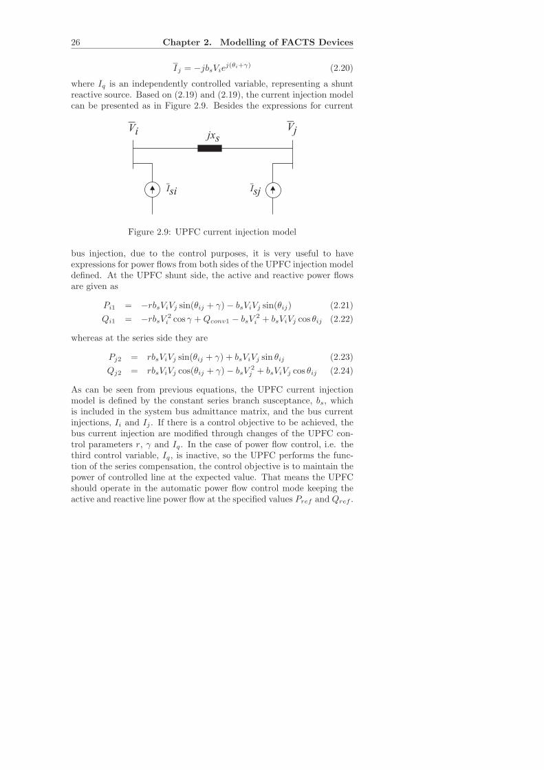
where Iq is an independently controlled variable, representing a shuntreactive source. Based on (2.19) and (2.19), the current injection modelcan be presented as in Figure 2.9. Besides the expressions for current
jxsVi Vj
Isi Isj
Figure 2.9: UPFC current injection model
bus injection, due to the control purposes, it is very useful to haveexpressions for power flows from both sides of the UPFC injection modeldefined. At the UPFC shunt side, the active and reactive power flowsare given as
Pi1 = −rbsViVj sin(θij + γ) − bsViVj sin(θij) (2.21)
Qi1 = −rbsV 2i cos γ +Qconv1 − bsV
2i + bsViVj cos θij (2.22)
whereas at the series side they are
Pj2 = rbsViVj sin(θij + γ) + bsViVj sin θij (2.23)
Qj2 = rbsViVj cos(θij + γ) − bsV2j + bsViVj cos θij (2.24)
As can be seen from previous equations, the UPFC current injectionmodel is defined by the constant series branch susceptance, bs, whichis included in the system bus admittance matrix, and the bus currentinjections, Ii and Ij . If there is a control objective to be achieved, thebus current injection are modified through changes of the UPFC con-trol parameters r, γ and Iq. In the case of power flow control, i.e. thethird control variable, Iq, is inactive, so the UPFC performs the func-tion of the series compensation, the control objective is to maintain thepower of controlled line at the expected value. That means the UPFCshould operate in the automatic power flow control mode keeping theactive and reactive line power flow at the specified values Pref and Qref .
2.2. Unified Power Flow Controller 27
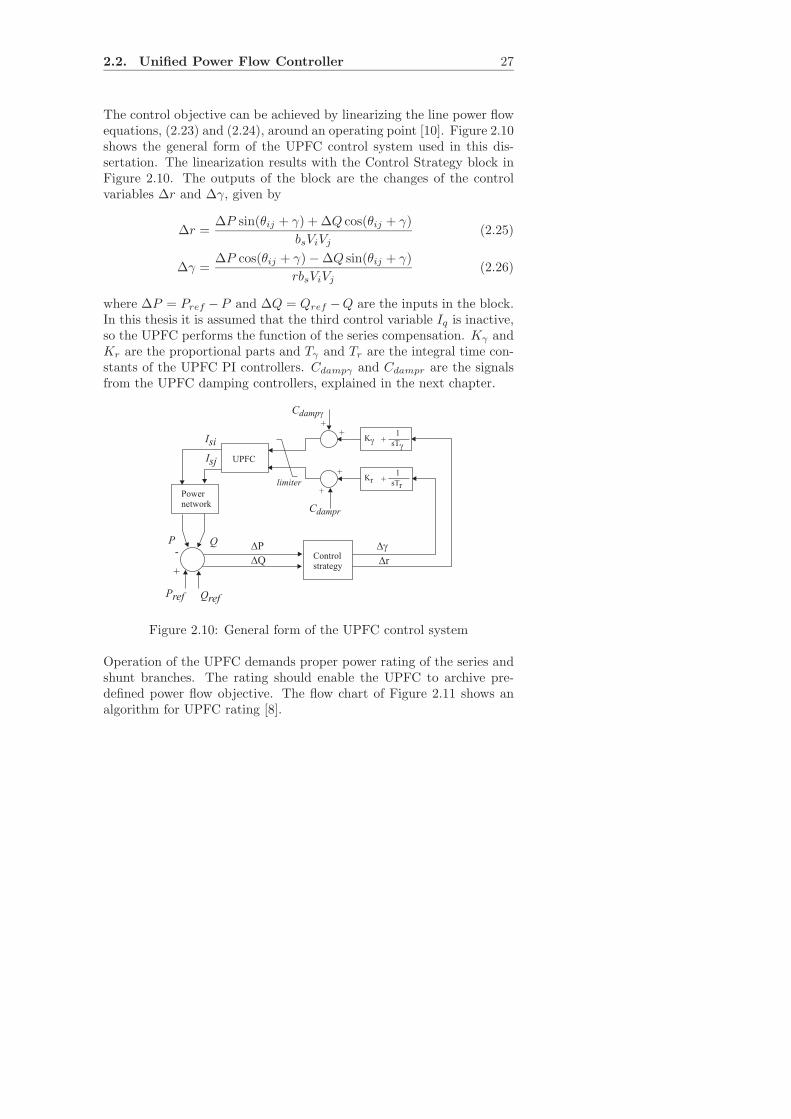
The control objective can be achieved by linearizing the line power flowequations, (2.23) and (2.24), around an operating point [10]. Figure 2.10shows the general form of the UPFC control system used in this dis-sertation. The linearization results with the Control Strategy block inFigure 2.10. The outputs of the block are the changes of the controlvariables ∆r and ∆γ, given by
∆r =∆P sin(θij + γ) + ∆Q cos(θij + γ)
bsViVj
(2.25)
∆γ =∆P cos(θij + γ) − ∆Q sin(θij + γ)
rbsViVj
(2.26)
where ∆P = Pref −P and ∆Q = Qref −Q are the inputs in the block.In this thesis it is assumed that the third control variable Iq is inactive,so the UPFC performs the function of the series compensation. Kγ andKr are the proportional parts and Tγ and Tr are the integral time con-stants of the UPFC PI controllers. Cdampγ and Cdampr are the signalsfrom the UPFC damping controllers, explained in the next chapter.
UPFC
Dg
Dr
Q
+
- Controlstrategy
Isi
Isj
Powernetwork
Kg1
sTg+
Kr1
sTr+
++
Cdampg
+
+
Cdampr
P
Pref Qref
limiter
DP
DQ
Figure 2.10: General form of the UPFC control system
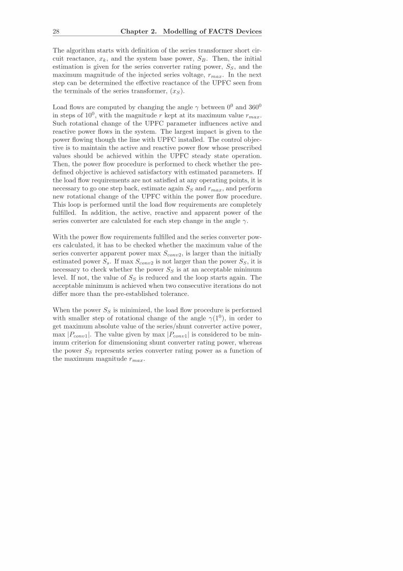
Operation of the UPFC demands proper power rating of the series andshunt branches. The rating should enable the UPFC to archive pre-defined power flow objective. The flow chart of Figure 2.11 shows analgorithm for UPFC rating [8].
28 Chapter 2. Modelling of FACTS Devices
The algorithm starts with definition of the series transformer short cir-cuit reactance, xk, and the system base power, SB . Then, the initialestimation is given for the series converter rating power, SS , and themaximum magnitude of the injected series voltage, rmax. In the nextstep can be determined the effective reactance of the UPFC seen fromthe terminals of the series transformer, (xS).
Load flows are computed by changing the angle γ between 00 and 3600
in steps of 100, with the magnitude r kept at its maximum value rmax.Such rotational change of the UPFC parameter influences active andreactive power flows in the system. The largest impact is given to thepower flowing though the line with UPFC installed. The control objec-tive is to maintain the active and reactive power flow whose prescribedvalues should be achieved within the UPFC steady state operation.Then, the power flow procedure is performed to check whether the pre-defined objective is achieved satisfactory with estimated parameters. Ifthe load flow requirements are not satisfied at any operating points, it isnecessary to go one step back, estimate again SS and rmax, and performnew rotational change of the UPFC within the power flow procedure.This loop is performed until the load flow requirements are completelyfulfilled. In addition, the active, reactive and apparent power of theseries converter are calculated for each step change in the angle γ.
With the power flow requirements fulfilled and the series converter pow-ers calculated, it has to be checked whether the maximum value of theseries converter apparent power max Sconv2, is larger than the initiallyestimated power Ss. If max Sconv2 is not larger than the power SS , it isnecessary to check whether the power SS is at an acceptable minimumlevel. If not, the value of SS is reduced and the loop starts again. Theacceptable minimum is achieved when two consecutive iterations do notdiffer more than the pre-established tolerance.
When the power SS is minimized, the load flow procedure is performedwith smaller step of rotational change of the angle γ(10), in order toget maximum absolute value of the series/shunt converter active power,max |Pconv1|. The value given by max |Pconv1| is considered to be min-imum criterion for dimensioning shunt converter rating power, whereasthe power SS represents series converter rating power as a function ofthe maximum magnitude rmax.
2.2. Unified Power Flow Controller 29
DEFINE xk, SB
rmax, Initial SS
CALCULATE
2
maxB
s k
S
Sx x r
S=
PERFORM LOAD FLOW
g 0 0 0[0 :10 : 360 ]=
ISLOAD FLOW
REQUIREMENTSFULFILLED?
NO
(INCREASE Ss)
YES
CALCULATEPconv2, Qconv2, Sconv2
IF
max Sconv2 > SS ?
YES
(INCREASE Ss)
IS
SS minimum?
YES
NO
PERFORM LOAD FLOW
g 0 0 0[0 :10 : 360 ]=
CALCULATE max |Pconv1|
OUTPUT SS, Sconv1, rmax
DECREASE Ss
Figure 2.11: Algorithm for optimal rating of the UPFC, [8]
30 Chapter 2. Modelling of FACTS Devices
2.3 Static VAr Compensator
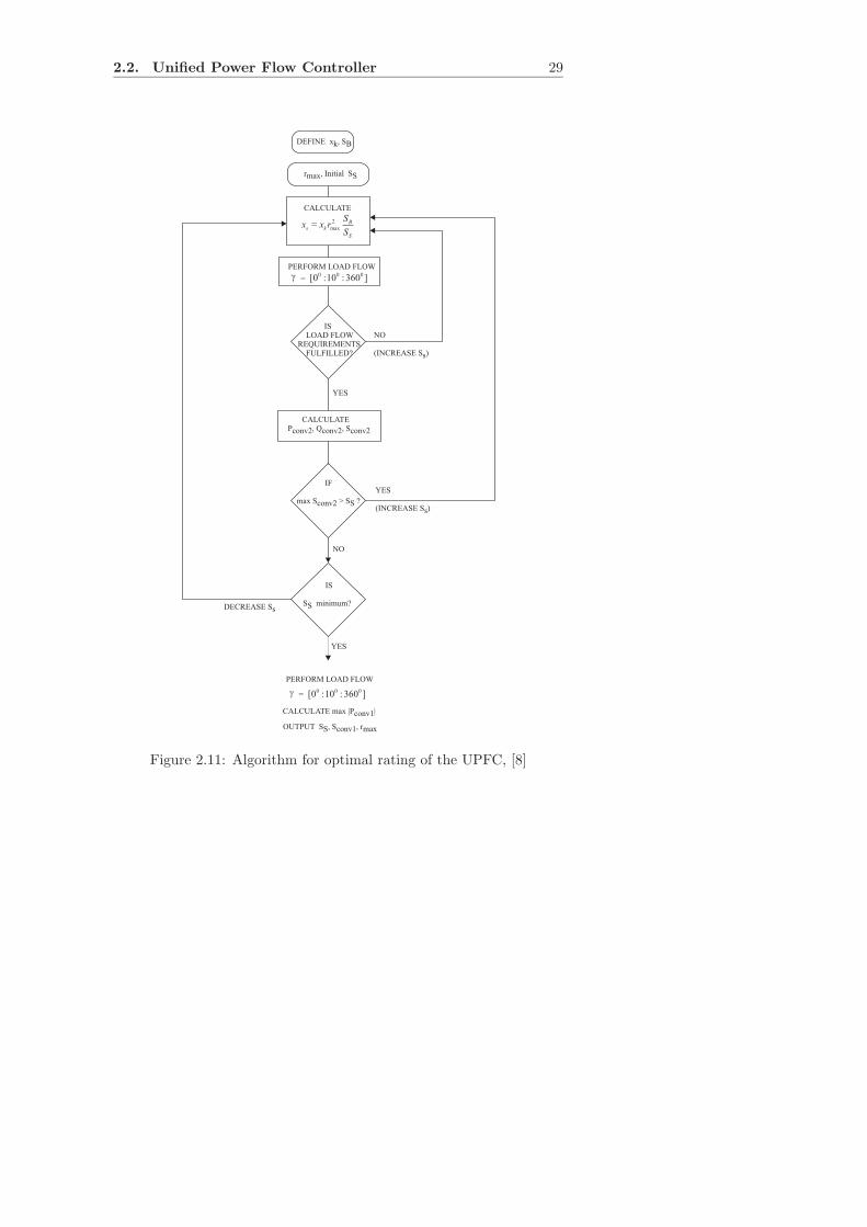
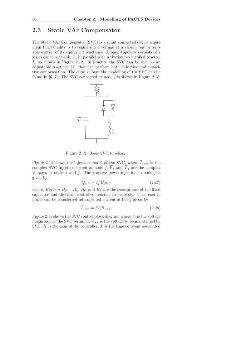
The Static VAr Compensator (SVC) is a shunt connected device whosemain functionality is to regulate the voltage at a chosen bus by suit-able control of its equivalent reactance. A basic topology consists of aseries capacitor bank, C, in parallel with a thyristor-controlled reactor,L, as shown in Figure 2.12. In practice the SVC can be seen as anadjustable reactance [1], that can perform both inductive and capaci-tive compensation. The details about the modelling of the SVC can befound in [6, 7]. The SVC connected at node j is shown in Figure 2.13.
L
C
Figure 2.12: Basic SVC topology
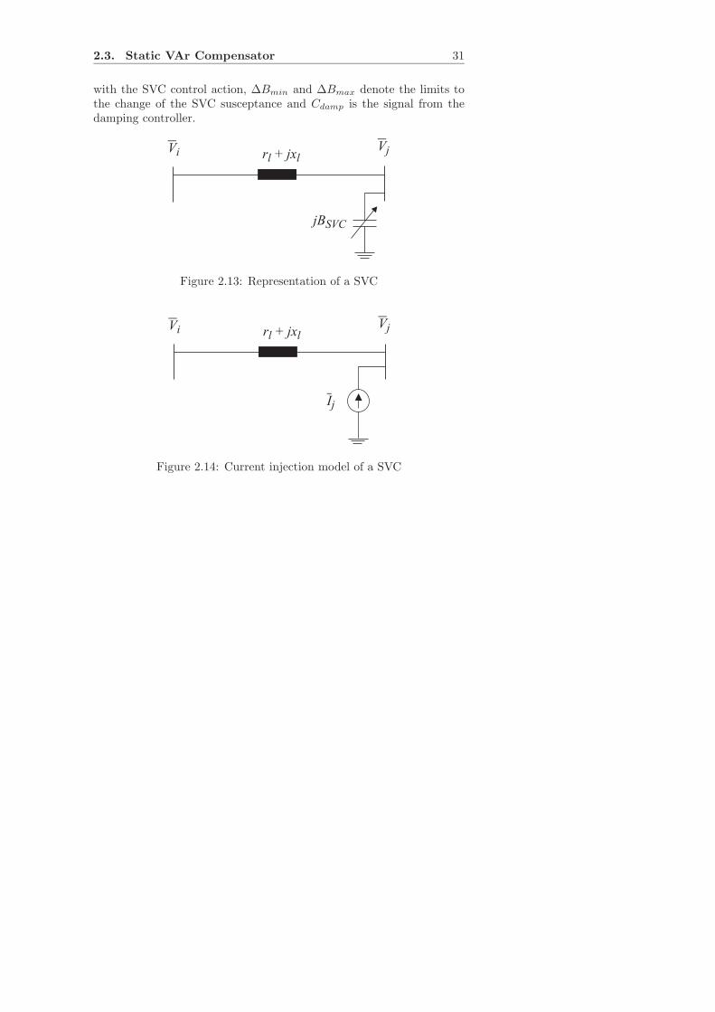
Figure 2.14 shows the injection model of the SVC, where Ijsvc is thecomplex SVC injected current at node j, V i and V j are the complexvoltages at nodes i and j. The reactive power injection in node j isgiven by:
Qj = −V 2j BSV C (2.27)
where, BSV C = BC −BL, BC and BL are the susceptance of the fixedcapacitor and thyristor controlled reactor, respectively. The reactivepower can be transferred into injected current at bus j given by
Ijsvc = jVjBSV C (2.28)
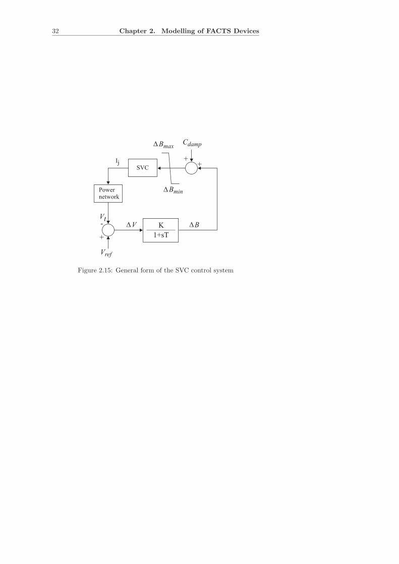
Figure 2.15 shows the SVC control block diagram where Vt is the voltagemagnitude at the SVC terminal, Vref is the voltage to be maintained bySVC, K is the gain of the controller, T is the time constant associated
2.3. Static VAr Compensator 31
with the SVC control action, ∆Bmin and ∆Bmax denote the limits tothe change of the SVC susceptance and Cdamp is the signal from thedamping controller.
Vi Vjr + jxll
jBSVC
Figure 2.13: Representation of a SVC
Ij
Vi Vjr + jxll
Figure 2.14: Current injection model of a SVC
32 Chapter 2. Modelling of FACTS Devices
K
1+sT
+
-
+
Vref
Cdamp
Vt
Bmax
Bmin
+
Powernetwork
SVCIj
D
D
BDVD
Figure 2.15: General form of the SVC control system
Chapter 3
Use of FACTS Devices
for Damping of Power
System Oscillations
3.1 Introduction
The power system may be thought of as a large, interconnected non-linear system with many lightly damped electromechanical modes ofoscillation. If the damping of these modes become too small or nega-tive, it can impose severe constraints on the system’s operation. It isthus important to be able to determine their nature, find stability limitsand in many cases use controls to prevent their instability. Electrome-chanical oscillations can be broadly classified into two main groups:
• Inter − area oscillations
• Local oscillations
Inter-area oscillations are observed when a group of machines in onearea swings against another group in another area normally with a fre-quency below 1 Hz. The study the inter-area modes is quite complicatedsince it requires detailed representation of the entire interconnected sys-
33
34 Chapter 3. Use of FACTS Devices for Damping...
tem and inter-area modes are influenced by several states of larger areasof the power network.
Local oscillations are observed when one particular plant swings againstthe rest of the system or several generators at frequencies of typically 1Hz to 2 Hz [12].
With the power industry moving toward deregulation, long-distancepower transfers are steadily increasing, outpacing the addition of newtransmission facilities and causing the inter-area oscillations to becomemore lightly damped [11]. During the last decade, FACTS devices havebeen employed to damp power system oscillations [13, 14, 15, 16]. Some-times, these controllers are placed in the power system for some otherreasons (to improve the voltage stability or to control power flow) [6, 7],then to damp power oscillations. However, when installed, supplemen-tary control can be applied to existing controllers in order to improvedamping, as well as satisfy the primary requirements of the device. PODcontrol can be applied as well through power system stabilizer (PSS)on generator excitation control systems. PSSs are effective but they areusually designed for damping local electromechanical oscillations andin large power systems tuning all of them might be very difficult. Inthis chapter, POD control has been applied to three FACTS devices,TCSC, UPFC and SVC in order to damp inter-area oscillations. Themain focus is on the TCSC, UPFC and SVC influence on power os-cillation damping when a large disturbance is applied. The controllerdesign method utilizes the residue approach [15, 16, 17]. The presentedapproach solves the optimal location of the FACTS devices, as well asthe selection of the proper feedback signals.
3.2 Modal Analysis
In order to identify oscillatory modes of a multi-machine system, thelinearized system model including PSS and FACTS devices system canbe used by
∆x = A∆x+B∆u
∆y = C∆x+D∆u (3.1)
where∆x is the state vector of length equal to the numbers of states n

3.2. Modal Analysis 35
∆y is the output vector of length m∆u is the input vector of length rA is the n by n state matrixB is the control or input matrix of size n by rC is the output matrix of size m by nD is the feed forward matrix of dimensions m by r.The equation
det(λI −A) = 0 (3.2)
is referred to as the characteristic equation of matrix A and the valuesof λ, which satisfy the characteristic equation, are the eigenvalues ofmatrix A. Because the matrix A is a n by n matrix, it has n solutionsof eigenvalues
λ = λ1, λ2, ...λn (3.3)
with assumption that λi 6= λj , i 6= j.
For every eigenvalue λi, there is an eigenvector φi which satisfies Equa-tion
Aφi = λiφi (3.4)
φi is called the right eigenvector of the state matrix A associated withthe eigenvalue λi. Each right eigenvector is a column vector with thelength equal to the number of the states.Left eigenvector associated with the eigenvalue λi is the n-row vectorwhich satisfies
ψiA = λiψi (3.5)
The right eigenvector describes how each mode of oscillation is dis-tributed among the system states. In other words, it indicates on whichsystem variables the mode is more observable. The right eigenvector iscalled mode shape.
The left eigenvector, together with the system’s initial state, determinesthe amplitude of the mode. A left eigenvector carries mode controlla-bility information.
Numerous indices, such as participation factors, transfer function residuesand mode sensitivities can be calculated from eigenvectors. Those in-dices are very useful in system analysis and controller design.
36 Chapter 3. Use of FACTS Devices for Damping...
For a particular eigenvalue λi = σi + jωi, the real part of the eigen-value gives the damping, and the imaginary part gives the frequency ofoscillation. The relative damping ratio is given by
ξ =−σi
√
σ2i + ω2
i
(3.6)
The oscillatory modes having damping ratio less than 3% are said tobe critical [18]. When designing damping controls one has to take careabout margin due to uncertainties or disturbances. Hence the damp-ing ratio of at least 5% should be the objective of the control design [19].
Participation factors
The sensitivity of a particular eigenvalue λi to the changes in the diag-onal elements of the state matrix A is given, [18], by
pki =∂λi
∂akk
= ψkiφki (3.7)
where ψki is the kth element in the ith row of the the left eigenvector ψi,and φki is the kth element in the ith column of the right eigenvector φi.The participation factor pki is a measure of the relative participation ofthe kth state variable in the ith mode, and vice versa. The participationfactor is used in this thesis for purpose of conventional tuning of PSSs,in Chapter 6.
Controllability and observability
In order to modify a selected oscillatory mode by a feedback controller,the chosen input of the controller must influence the behavior of thatmode and the mode must also be visible in the chosen feedback sig-nal i.e. the behavior of that mode should be reflected in the feedbacksignal. The measures for those two properties are the modal control-lability and observability, respectively. The modal controllability andmodal observability matrices are defined, [18], by
B′ = Φ−1B
C ′ = CΦ (3.8)
The mode is not controllable if the corresponding row of the matrix B′
is a zero vector, and the mode is not observable if the corresponding
3.2. Modal Analysis 37
column of the matrix C ′ is a zero vector. If a mode is either not con-trollable or not observable, feedback between the output and the inputwill have no effect on the mode.
Residues
Considering (3.1) with single input and single output (SISO) and as-suming D = 0, the open loop transfer function of the system can beobtained by
G(s) =∆y(s)
∆u(s)
= C(sI −A)−1B (3.9)
The transfer function G(s) can be expanded in partial fractions of theLaplace transform of y in terms of C and B matrices and the right andleft eigenvectors as
G(s) =
N∑
i=1
CφiψiB
(s− λi)
=N∑
i=1
Ri
(s− λi)(3.10)
Each term in the denominator, Ri, of the summation is a scalar calledresidue. The residue Ri of a particular mode i gives the measure ofthat mode’s sensitivity to a feedback between the output y and theinput u; it is the product of the mode’s observability and controllability.Figure 3.1 shows a system G(s) equipped with a feedback control H(s).When applying the feedback control, eigenvalues of the initial systemG(s) are changed. It can be proven, [17], that when the feedback controlis applied, the shift of an eigenvalue can be calculated by
∆λi = RiH(λi) (3.11)
It can be observed from (3.11) that the shift of the eigenvalue causedby the controller is proportional to the magnitude of the correspondingresidue. For a certain mode, the same type of feedback control H(s),regardless of its structure and parameters, can be tested at differentlocations. For the mode of the interest, residues at all locations haveto be calculated. The largest residue then indicates the most effectivelocation to apply the feedback control.
38 Chapter 3. Use of FACTS Devices for Damping...
3.3 FACTS POD Controller Design
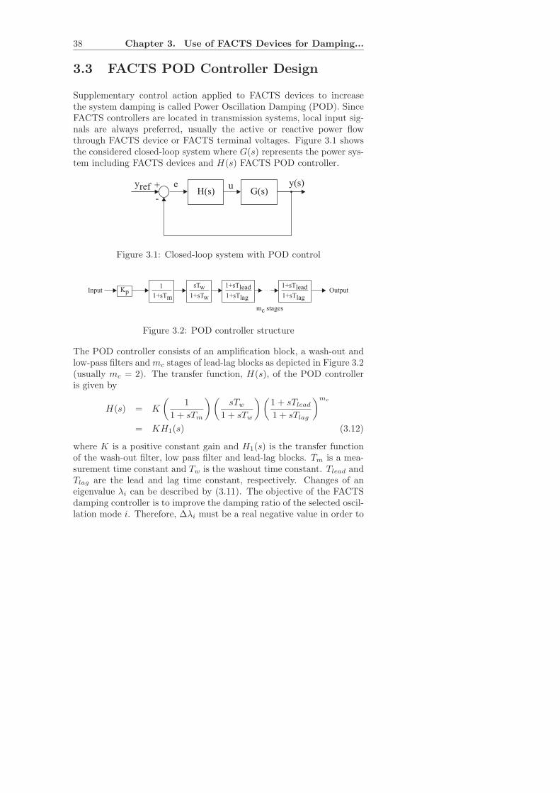
Supplementary control action applied to FACTS devices to increasethe system damping is called Power Oscillation Damping (POD). SinceFACTS controllers are located in transmission systems, local input sig-nals are always preferred, usually the active or reactive power flowthrough FACTS device or FACTS terminal voltages. Figure 3.1 showsthe considered closed-loop system where G(s) represents the power sys-tem including FACTS devices and H(s) FACTS POD controller.
G(s)yref y(s)+
-
ueH(s)
Figure 3.1: Closed-loop system with POD control
Input OutputsTw 1+sTlead 1+sTlead
1+sTw 1+sTlag 1+sTlagKp
mc stages
1
1+sTm
Figure 3.2: POD controller structure
The POD controller consists of an amplification block, a wash-out andlow-pass filters and mc stages of lead-lag blocks as depicted in Figure 3.2(usually mc = 2). The transfer function, H(s), of the POD controlleris given by
H(s) = K
(
1
1 + sTm
)(
sTw
1 + sTw
)(
1 + sTlead
1 + sTlag
)mc
= KH1(s) (3.12)
where K is a positive constant gain and H1(s) is the transfer functionof the wash-out filter, low pass filter and lead-lag blocks. Tm is a mea-surement time constant and Tw is the washout time constant. Tlead andTlag are the lead and lag time constant, respectively. Changes of aneigenvalue λi can be described by (3.11). The objective of the FACTSdamping controller is to improve the damping ratio of the selected oscil-lation mode i. Therefore, ∆λi must be a real negative value in order to
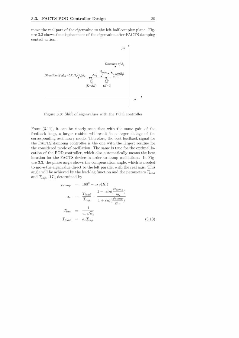
3.3. FACTS POD Controller Design 39
move the real part of the eigenvalue to the left half complex plane. Fig-ure 3.3 shows the displacement of the eigenvalue after FACTS dampingcontrol action.
jcomparg(Ri)
Direction of Ri
Dli
li(0)
li(1)
( )K=0( )K= KD
Direction of Dli = K H1 i RiD l( )
jw
s
Figure 3.3: Shift of eigenvalues with the POD controller
From (3.11), it can be clearly seen that with the same gain of thefeedback loop, a larger residue will result in a larger change of thecorresponding oscillatory mode. Therefore, the best feedback signal forthe FACTS damping controller is the one with the largest residue forthe considered mode of oscillation. The same is true for the optimal lo-cation of the POD controller, which also automatically means the bestlocation for the FACTS device in order to damp oscillations. In Fig-ure 3.3, the phase angle shows the compensation angle, which is neededto move the eigenvalue direct to the left parallel with the real axis. Thisangle will be achieved by the lead-lag function and the parameters Tlead
and Tlag, [17], determined by
ϕcomp = 1800 − arg(Ri)
αc =Tlead
Tlag
=1 − sin(
ϕcomp
mc
)
1 + sin(ϕcomp
mc
)
Tlag =1
wi
√αc
Tlead = αcTlag (3.13)
40 Chapter 3. Use of FACTS Devices for Damping...
where arg(Ri) denotes the phase angle of the residue Ri, wi is thefrequency of the mode of oscillation in rad/sec. The controller gain Kis computed as a function of the desired eigenvalue location accordingto (3.11):
K =
∣
∣
∣
∣
∣
λi,des − λi
RiH1(λi)
(3.14)
3.4 Case Studies
The FACTS POD controller location and the feedback signal should beselected in a such a way that the residues corresponding to each of thecritical modes are as high as possible [20]. Anyhow, it might not becost effective to place the FACTS device at a particular location just todamp oscillations. In order to satisfy the primarily requirements of theFACTS device as well as the damping of oscillations, a compromise hasto be made for each individual case. In this chapter, only damping isconsidered, i.e. the primary aim is to damp oscillations.
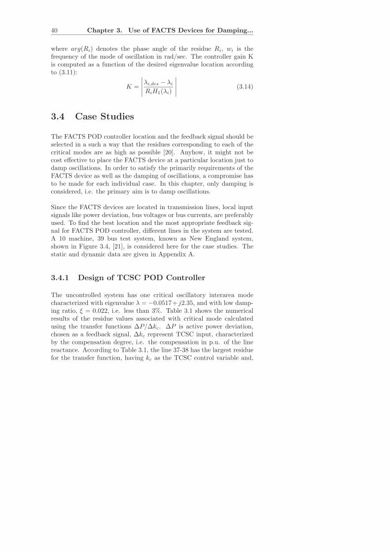
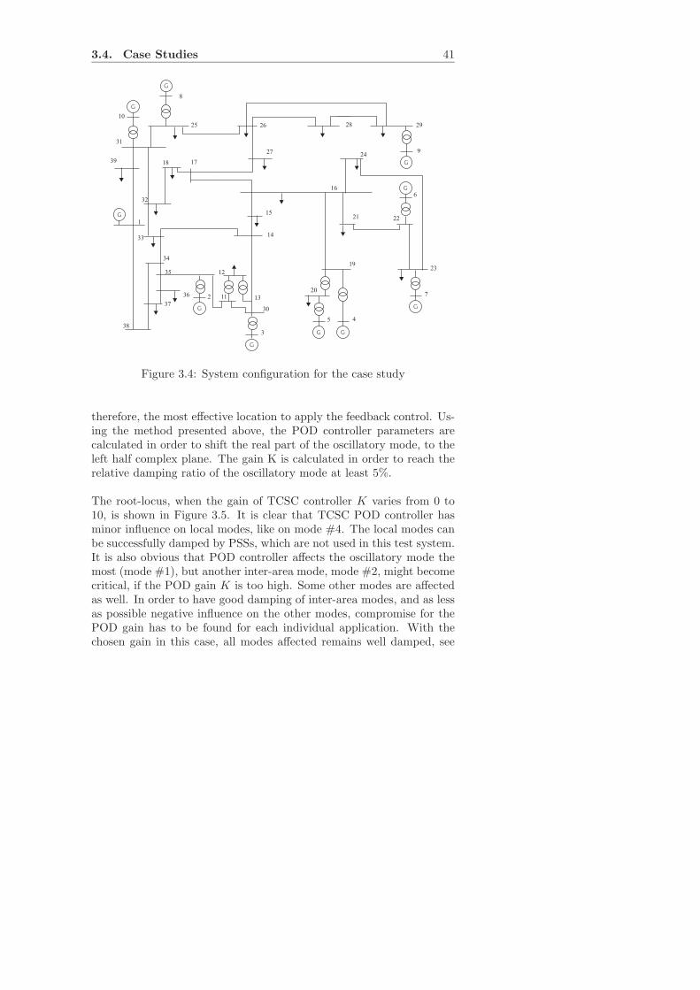
Since the FACTS devices are located in transmission lines, local inputsignals like power deviation, bus voltages or bus currents, are preferablyused. To find the best location and the most appropriate feedback sig-nal for FACTS POD controller, different lines in the system are tested.A 10 machine, 39 bus test system, known as New England system,shown in Figure 3.4, [21], is considered here for the case studies. Thestatic and dynamic data are given in Appendix A.
3.4.1 Design of TCSC POD Controller
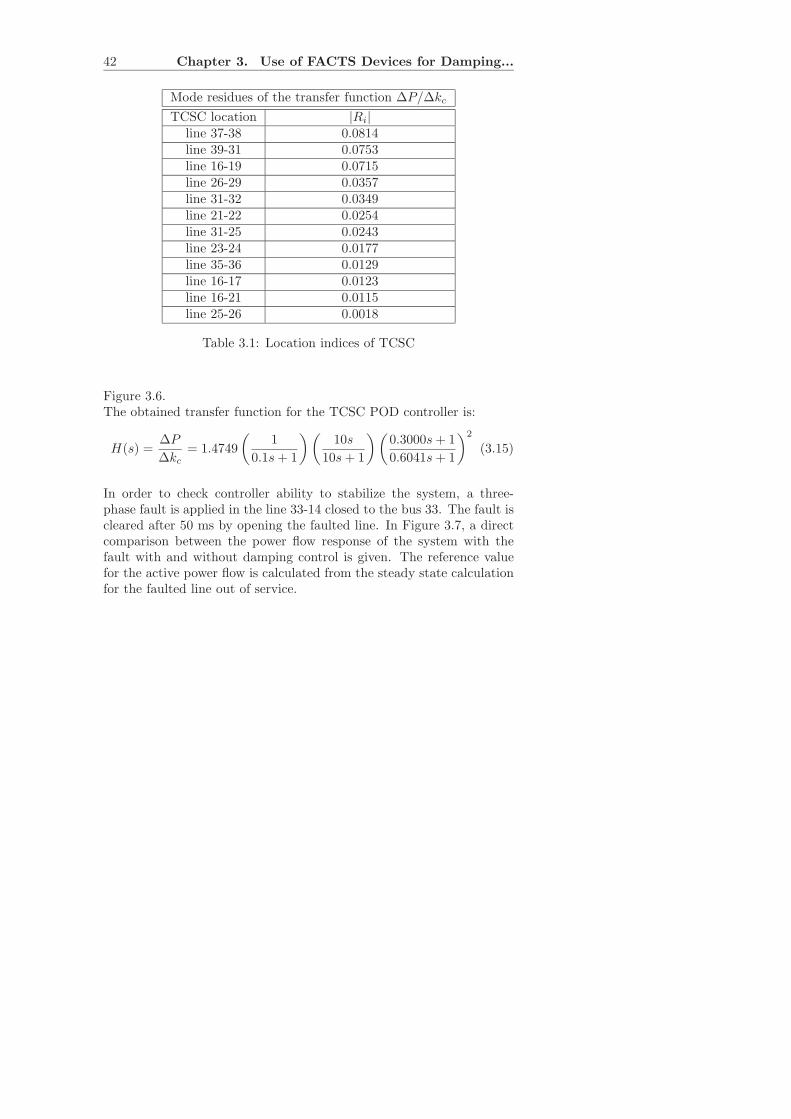
The uncontrolled system has one critical oscillatory interarea modecharacterized with eigenvalue λ = −0.0517+ j2.35, and with low damp-ing ratio, ξ = 0.022, i.e. less than 3%. Table 3.1 shows the numericalresults of the residue values associated with critical mode calculatedusing the transfer functions ∆P/∆kc. ∆P is active power deviation,chosen as a feedback signal, ∆kc represent TCSC input, characterizedby the compensation degree, i.e. the compensation in p.u. of the linereactance. According to Table 3.1, the line 37-38 has the largest residuefor the transfer function, having kc as the TCSC control variable and,
3.4. Case Studies 41
G
G
10
31
39
1
G
38
37
36
35
34
G
33
32
18 17
26
G
8
25 28 29
9
2
14
15
16
G
11 13
12
3
30
27 24
21
19
G G
5 4
20
23
22
G6
G
7
Figure 3.4: System configuration for the case study
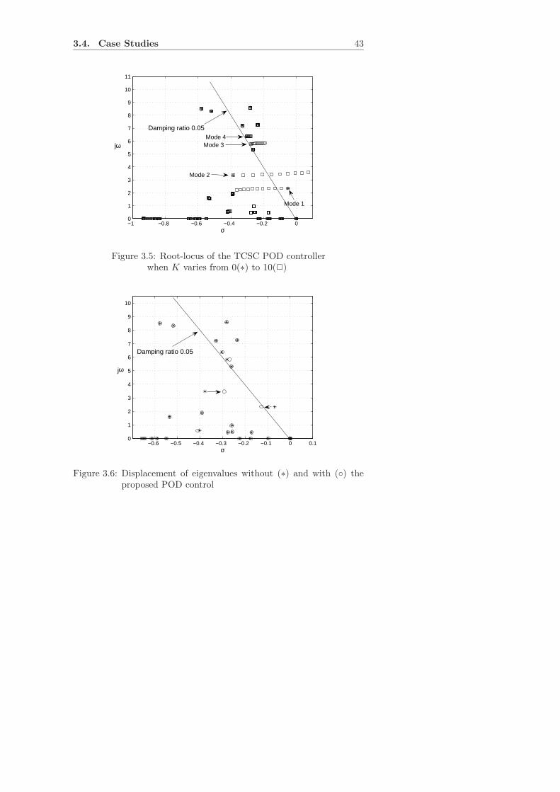
therefore, the most effective location to apply the feedback control. Us-ing the method presented above, the POD controller parameters arecalculated in order to shift the real part of the oscillatory mode, to theleft half complex plane. The gain K is calculated in order to reach therelative damping ratio of the oscillatory mode at least 5%.
The root-locus, when the gain of TCSC controller K varies from 0 to10, is shown in Figure 3.5. It is clear that TCSC POD controller hasminor influence on local modes, like on mode #4. The local modes canbe successfully damped by PSSs, which are not used in this test system.It is also obvious that POD controller affects the oscillatory mode themost (mode #1), but another inter-area mode, mode #2, might becomecritical, if the POD gain K is too high. Some other modes are affectedas well. In order to have good damping of inter-area modes, and as lessas possible negative influence on the other modes, compromise for thePOD gain has to be found for each individual application. With thechosen gain in this case, all modes affected remains well damped, see
42 Chapter 3. Use of FACTS Devices for Damping...
Mode residues of the transfer function ∆P/∆kc
TCSC location |Ri|line 37-38 0.0814line 39-31 0.0753line 16-19 0.0715line 26-29 0.0357line 31-32 0.0349line 21-22 0.0254line 31-25 0.0243line 23-24 0.0177line 35-36 0.0129line 16-17 0.0123line 16-21 0.0115line 25-26 0.0018
Table 3.1: Location indices of TCSC
Figure 3.6.The obtained transfer function for the TCSC POD controller is:
H(s) =∆P
∆kc
= 1.4749
(
1
0.1s+ 1
)(
10s
10s+ 1
)(
0.3000s+ 1
0.6041s+ 1
)2
(3.15)
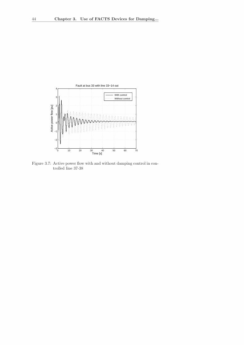
In order to check controller ability to stabilize the system, a three-phase fault is applied in the line 33-14 closed to the bus 33. The fault iscleared after 50 ms by opening the faulted line. In Figure 3.7, a directcomparison between the power flow response of the system with thefault with and without damping control is given. The reference valuefor the active power flow is calculated from the steady state calculationfor the faulted line out of service.
3.4. Case Studies 43
−1 −0.8 −0.6 −0.4 −0.2 00
1
2
3
4
5
6
7
8
9
10
11
σ
Damping ratio 0.05
jω
Mode 1
Mode 2
Mode 3 Mode 4
Figure 3.5: Root-locus of the TCSC POD controllerwhen K varies from 0(∗) to 10(2)
−0.6 −0.5 −0.4 −0.3 −0.2 −0.1 0 0.10
1
2
3
4
5
6
7
8
9
10
σ
Damping ratio 0.05
jω
Figure 3.6: Displacement of eigenvalues without (∗) and with () theproposed POD control
44 Chapter 3. Use of FACTS Devices for Damping...
0 10 20 30 40 50 60 70−3
−2
−1
0
1
2
3
4
Time [s]
Act
ive
pow
er fl
ow [p
u]
Fault at bus 33 with line 33−14 out
With control
Without control
Figure 3.7: Active power flow with and without damping control in con-trolled line 37-38
3.4. Case Studies 45
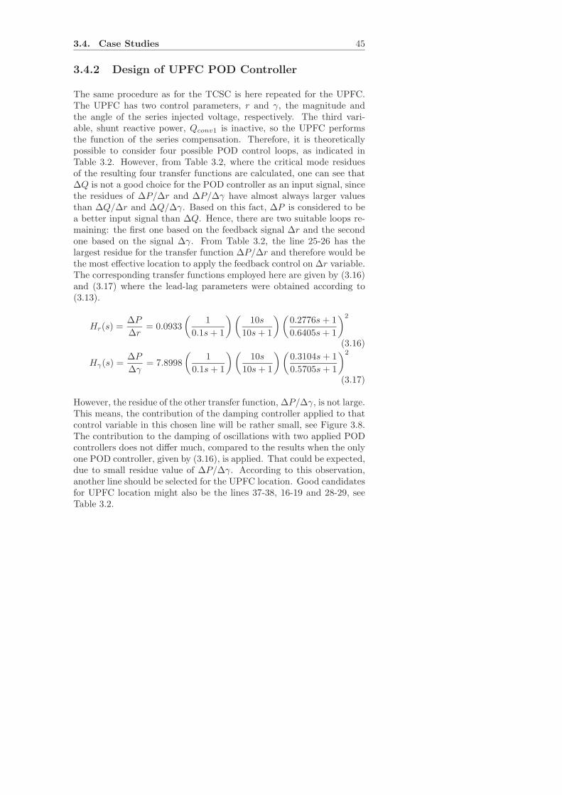
3.4.2 Design of UPFC POD Controller
The same procedure as for the TCSC is here repeated for the UPFC.The UPFC has two control parameters, r and γ, the magnitude andthe angle of the series injected voltage, respectively. The third vari-able, shunt reactive power, Qconv1 is inactive, so the UPFC performsthe function of the series compensation. Therefore, it is theoreticallypossible to consider four possible POD control loops, as indicated inTable 3.2. However, from Table 3.2, where the critical mode residuesof the resulting four transfer functions are calculated, one can see that∆Q is not a good choice for the POD controller as an input signal, sincethe residues of ∆P/∆r and ∆P/∆γ have almost always larger valuesthan ∆Q/∆r and ∆Q/∆γ. Based on this fact, ∆P is considered to bea better input signal than ∆Q. Hence, there are two suitable loops re-maining: the first one based on the feedback signal ∆r and the secondone based on the signal ∆γ. From Table 3.2, the line 25-26 has thelargest residue for the transfer function ∆P/∆r and therefore would bethe most effective location to apply the feedback control on ∆r variable.The corresponding transfer functions employed here are given by (3.16)and (3.17) where the lead-lag parameters were obtained according to(3.13).
Hr(s) =∆P
∆r= 0.0933
(
1
0.1s+ 1
)(
10s
10s+ 1
)(
0.2776s+ 1
0.6405s+ 1
)2
(3.16)
Hγ(s) =∆P
∆γ= 7.8998
(
1
0.1s+ 1
)(
10s
10s+ 1
)(
0.3104s+ 1
0.5705s+ 1
)2
(3.17)
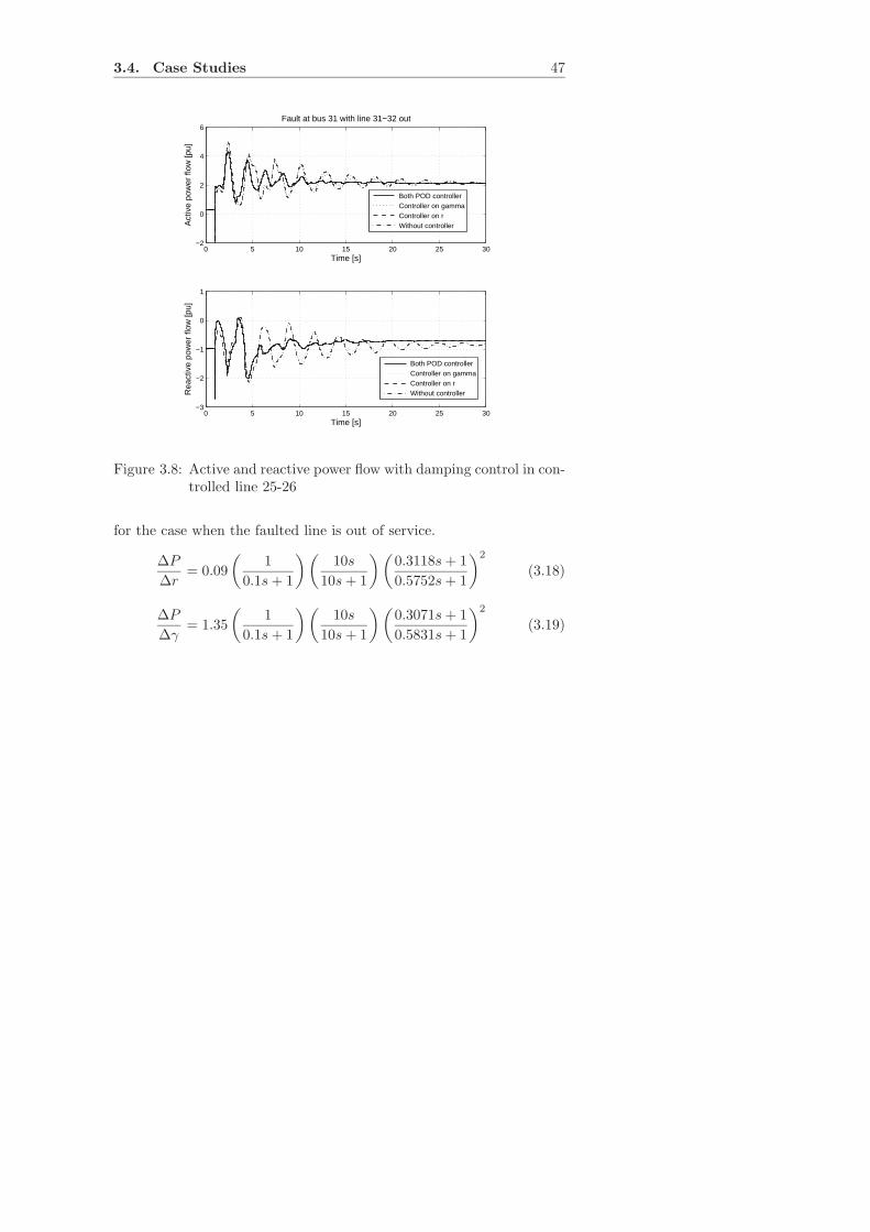
However, the residue of the other transfer function, ∆P/∆γ, is not large.This means, the contribution of the damping controller applied to thatcontrol variable in this chosen line will be rather small, see Figure 3.8.The contribution to the damping of oscillations with two applied PODcontrollers does not differ much, compared to the results when the onlyone POD controller, given by (3.16), is applied. That could be expected,due to small residue value of ∆P/∆γ. According to this observation,another line should be selected for the UPFC location. Good candidatesfor UPFC location might also be the lines 37-38, 16-19 and 28-29, seeTable 3.2.
46 Chapter 3. Use of FACTS Devices for Damping...
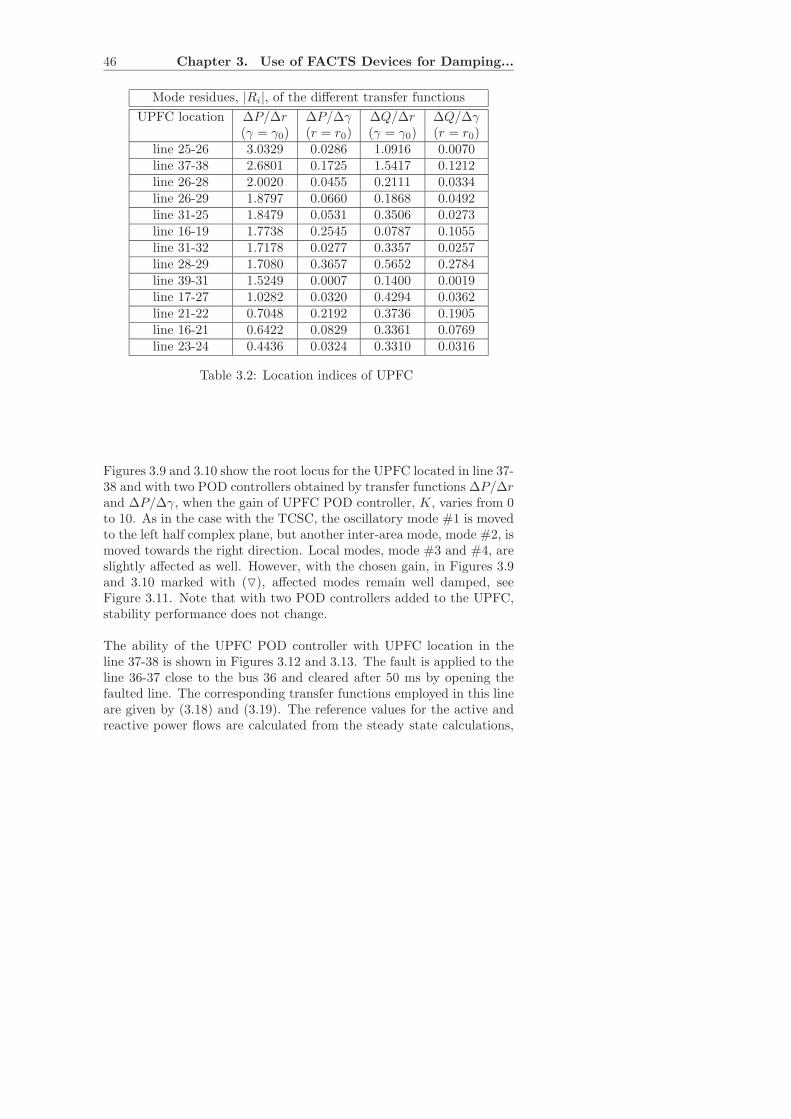
Mode residues, |Ri|, of the different transfer functions
UPFC location ∆P/∆r ∆P/∆γ ∆Q/∆r ∆Q/∆γ(γ = γ0) (r = r0) (γ = γ0) (r = r0)
line 25-26 3.0329 0.0286 1.0916 0.0070line 37-38 2.6801 0.1725 1.5417 0.1212line 26-28 2.0020 0.0455 0.2111 0.0334line 26-29 1.8797 0.0660 0.1868 0.0492line 31-25 1.8479 0.0531 0.3506 0.0273line 16-19 1.7738 0.2545 0.0787 0.1055line 31-32 1.7178 0.0277 0.3357 0.0257line 28-29 1.7080 0.3657 0.5652 0.2784line 39-31 1.5249 0.0007 0.1400 0.0019line 17-27 1.0282 0.0320 0.4294 0.0362line 21-22 0.7048 0.2192 0.3736 0.1905line 16-21 0.6422 0.0829 0.3361 0.0769line 23-24 0.4436 0.0324 0.3310 0.0316
Table 3.2: Location indices of UPFC
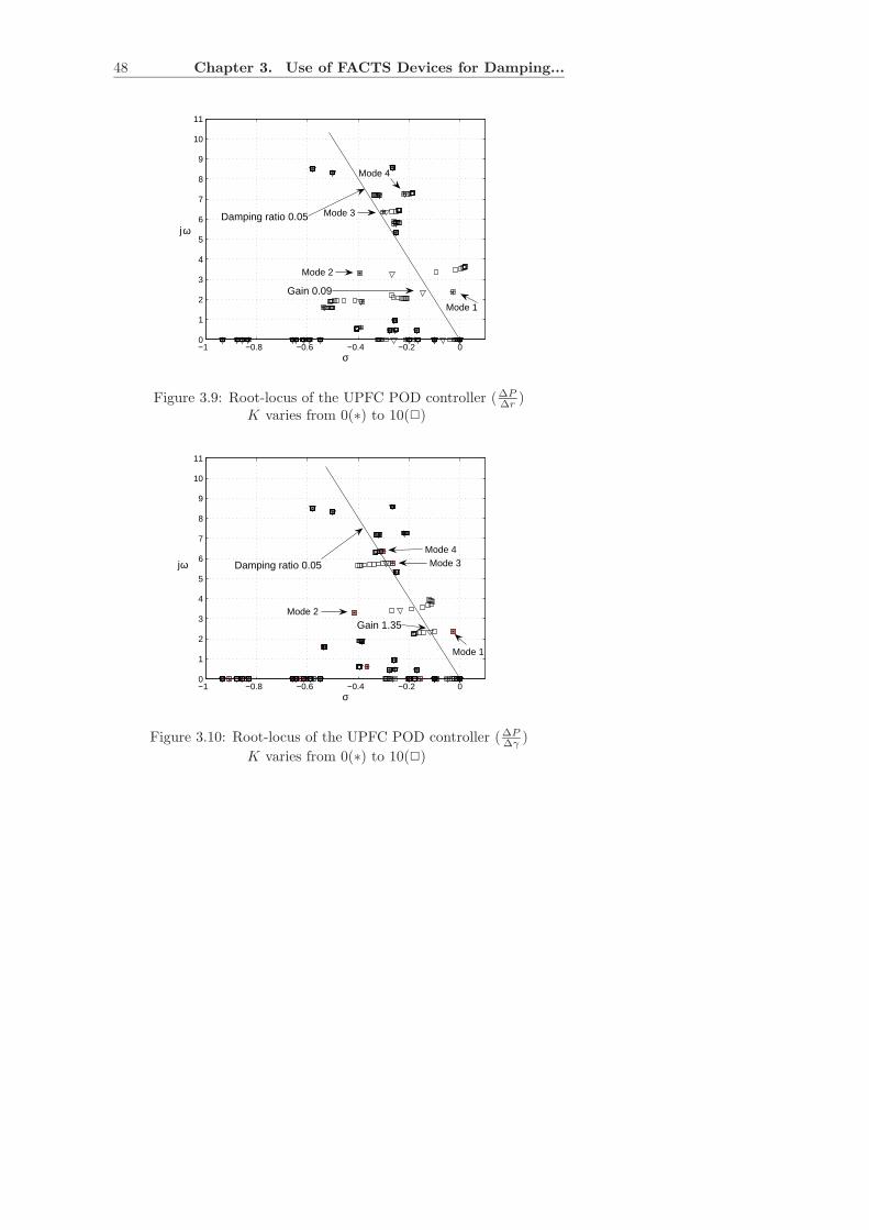
Figures 3.9 and 3.10 show the root locus for the UPFC located in line 37-38 and with two POD controllers obtained by transfer functions ∆P/∆rand ∆P/∆γ, when the gain of UPFC POD controller, K, varies from 0to 10. As in the case with the TCSC, the oscillatory mode #1 is movedto the left half complex plane, but another inter-area mode, mode #2, ismoved towards the right direction. Local modes, mode #3 and #4, areslightly affected as well. However, with the chosen gain, in Figures 3.9and 3.10 marked with (), affected modes remain well damped, seeFigure 3.11. Note that with two POD controllers added to the UPFC,stability performance does not change.
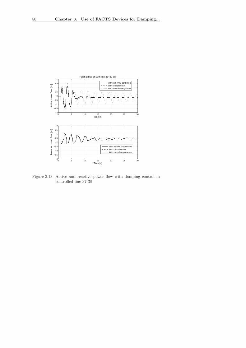
The ability of the UPFC POD controller with UPFC location in theline 37-38 is shown in Figures 3.12 and 3.13. The fault is applied to theline 36-37 close to the bus 36 and cleared after 50 ms by opening thefaulted line. The corresponding transfer functions employed in this lineare given by (3.18) and (3.19). The reference values for the active andreactive power flows are calculated from the steady state calculations,
3.4. Case Studies 47
0 5 10 15 20 25 30−2
0
2
4
6
Time [s]
Act
ive
pow
er fl
ow [p
u]
Fault at bus 31 with line 31−32 out
0 5 10 15 20 25 30−3
−2
−1
0
1
Time [s]
Rea
ctiv
e po
wer
flow
[pu]
Both POD controller Controller on gamma Controller on r Without controller
Both POD controller Controller on gamma Controller on r Without controller
Figure 3.8: Active and reactive power flow with damping control in con-trolled line 25-26
for the case when the faulted line is out of service.
∆P
∆r= 0.09
(
1
0.1s+ 1
)(
10s
10s+ 1
)(
0.3118s+ 1
0.5752s+ 1
)2
(3.18)
∆P
∆γ= 1.35
(
1
0.1s+ 1
)(
10s
10s+ 1
)(
0.3071s+ 1
0.5831s+ 1
)2
(3.19)
48 Chapter 3. Use of FACTS Devices for Damping...
−1 −0.8 −0.6 −0.4 −0.2 00
1
2
3
4
5
6
7
8
9
10
11
σ
Gain 0.09
Damping ratio 0.05jω
Mode 2
Mode 3
Mode 4
Mode 1
Figure 3.9: Root-locus of the UPFC POD controller (∆P∆r
)K varies from 0(∗) to 10(2)
−1 −0.8 −0.6 −0.4 −0.2 00
1
2
3
4
5
6
7
8
9
10
11
σ
Gain 1.35
Damping ratio 0.05jω
Mode 1
Mode 2
Mode 3 Mode 4
Figure 3.10: Root-locus of the UPFC POD controller (∆P∆γ
)
K varies from 0(∗) to 10(2)
3.4. Case Studies 49
−1 −0.8 −0.6 −0.4 −0.2 00
1
2
3
4
5
6
7
8
9
10
11
σ
Damping ratio 0.05jω
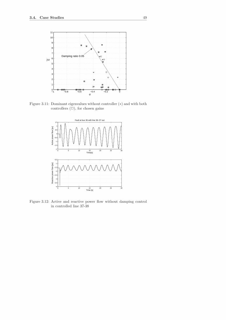
Figure 3.11: Dominant eigenvalues without controller (∗) and with bothcontrollers (2), for chosen gains
0 5 10 15 20 25 30−2
−1.5
−1
−0.5
0
0.5
1
1.5
Time[s]
Act
ive
pow
er fl
ow [p
u]
Fault at bus 36 with line 36−37 out
0 5 10 15 20 25 30−4
−3.5
−3
−2.5
−2
−1.5
−1
−0.5
Time [s]
Rea
ctiv
e po
wer
flow
[pu]
Figure 3.12: Active and reactive power flow without damping controlin controlled line 37-38
50 Chapter 3. Use of FACTS Devices for Damping...
0 5 10 15 20 25 30−2
−1.5
−1
−0.5
0
0.5
1
1.5
2
Time [s]
Act
ive
pow
er fl
ow [p
u]
Fault at bus 36 with line 36−37 out
0 5 10 15 20 25 30−4
−3.5
−3
−2.5
−2
−1.5
−1
−0.5
0
Time [s]
Rea
ctiv
e po
wer
flow
[pu]
With both POD controllers With controller on r With controller on gamma
With both POD controllers With controller on r With controller on gamma
Figure 3.13: Active and reactive power flow with damping control incontrolled line 37-38
3.4. Case Studies 51
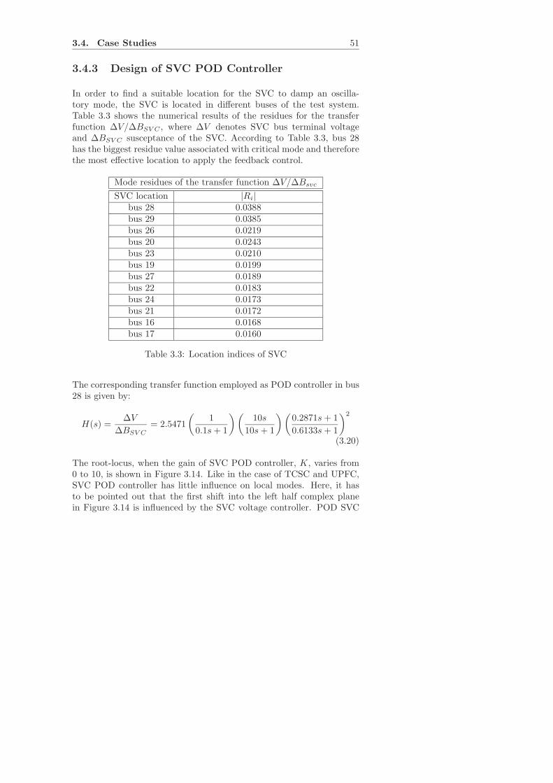
3.4.3 Design of SVC POD Controller
In order to find a suitable location for the SVC to damp an oscilla-tory mode, the SVC is located in different buses of the test system.Table 3.3 shows the numerical results of the residues for the transferfunction ∆V/∆BSV C , where ∆V denotes SVC bus terminal voltageand ∆BSV C susceptance of the SVC. According to Table 3.3, bus 28has the biggest residue value associated with critical mode and thereforethe most effective location to apply the feedback control.
Mode residues of the transfer function ∆V/∆Bsvc
SVC location |Ri|bus 28 0.0388bus 29 0.0385bus 26 0.0219bus 20 0.0243bus 23 0.0210bus 19 0.0199bus 27 0.0189bus 22 0.0183bus 24 0.0173bus 21 0.0172bus 16 0.0168bus 17 0.0160
Table 3.3: Location indices of SVC
The corresponding transfer function employed as POD controller in bus28 is given by:
H(s) =∆V
∆BSV C
= 2.5471
(
1
0.1s+ 1
)(
10s
10s+ 1
)(
0.2871s+ 1
0.6133s+ 1
)2
(3.20)
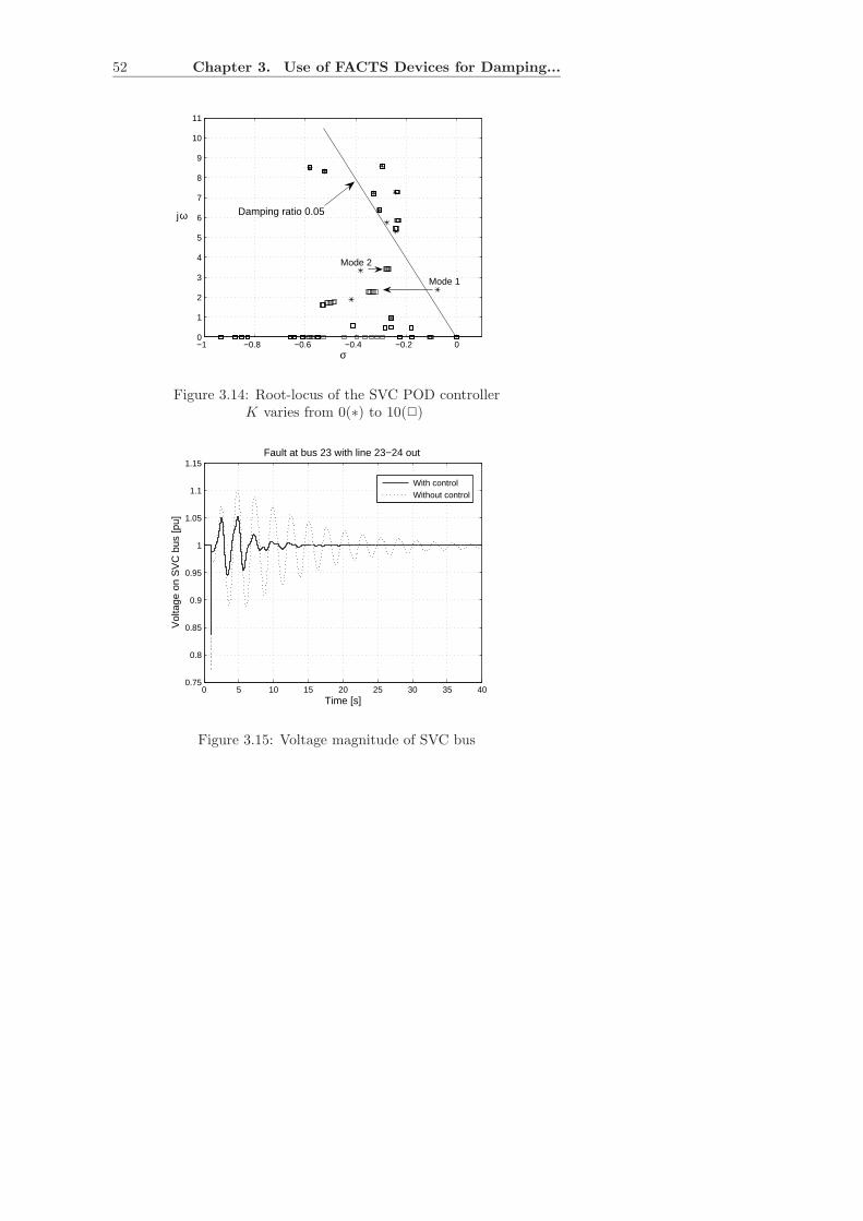
The root-locus, when the gain of SVC POD controller, K, varies from0 to 10, is shown in Figure 3.14. Like in the case of TCSC and UPFC,SVC POD controller has little influence on local modes. Here, it hasto be pointed out that the first shift into the left half complex planein Figure 3.14 is influenced by the SVC voltage controller. POD SVC
52 Chapter 3. Use of FACTS Devices for Damping...
−1 −0.8 −0.6 −0.4 −0.2 00
1
2
3
4
5
6
7
8
9
10
11
σ
Damping ratio 0.05jω
Mode 1
Mode 2
Figure 3.14: Root-locus of the SVC POD controllerK varies from 0(∗) to 10(2)
0 5 10 15 20 25 30 35 400.75
0.8
0.85
0.9
0.95
1
1.05
1.1
1.15
Time [s]
Vol
tage
on
SV
C b
us [p
u]
Fault at bus 23 with line 23−24 out
With control Without control
Figure 3.15: Voltage magnitude of SVC bus
3.5. Summary 53
0 5 10 15 20 25 30 35 400
0.2
0.4
0.6
0.8
1
1.2
1.4
Time [s]
Fau
lted
bus
volta
ge [p
u]
Fault at bus 23 with line 23−24 out
With control Without control
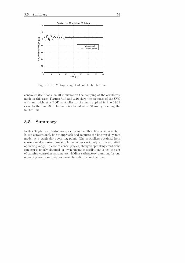
Figure 3.16: Voltage magnitude of the faulted bus
controller itself has a small influence on the damping of the oscillatorymode in this case. Figures 3.15 and 3.16 show the response of the SVCwith and without a POD controller to the fault applied in line 23-24close to the bus 23. The fault is cleared after 50 ms by opening thefaulted line.
3.5 Summary
In this chapter the residue controller design method has been presented.It is a conventional, linear approach and requires the linearized systemmodel at a particular operating point. The controllers obtained fromconventional approach are simple but often work only within a limitedoperating range. In case of contingencies, changed operating conditionscan cause poorly damped or even unstable oscillations since the setof existing controller parameters yielding satisfactory damping for oneoperating condition may no longer be valid for another one.

Chapter 4
On the Location of the
TCSC
Provided optimal locations, FACTS devices are capable of performingmultiple tasks; for example power flow control, voltage control, minimiz-ing the losses, damping of oscillations etc. The location of the FACTSdevice has a large impact on its performance with regard to the objec-tives to be fulfilled. A location being the best for one objective may beless suitable for another objective.
If the objective of the Thyristor Controlled Series Capacitor (TCSC),for example, is the power flow control, the most effective location is of-ten in highly loaded lines [11]. Applying the power flow control or anyother objective of FACTS devices in general, it is often desirable to havea control design which enables the operation of the controlled transmis-sion path without affecting the rest of the system. So far there is noFACTS controller that is able to satisfy the control objective without af-fecting the rest of the system, but it is possible to minimize its influence.
In this Chapter a procedure for placing a TCSC considering both powerflow control and damping of power oscillations is presented. A method-ology used to give the insight into the influence of the TCSC location inthe system, on the rest of the system, is power flow sensitivity analysis.Sensitivity analysis gives a direct measure of the controllability of the ac-tive power flow in the specified line by the chosen location of the TCSC.
55
56 Chapter 4. On the Location of the TCSC
Besides power flow control, satisfactory damping of power oscillationsis an important issue as well. In Chapter 3 damping control utilizes theresidue method and the presented approach solves the optimal locationof the TCSC device regarding damping of the oscillatory modes.
In this chapter both methodologies are used in order to find the suit-able location for both tasks, power flow control and damping control.The proposed algorithm has been demonstrated on the same test as inprevious Chapter.
4.1 Dynamic Criterion
Dynamic criteria is based on the residue method. This part is presentedin Chapter 3. According to this criteria, the most effective locationmeans the best location of the POD controller, while the compromisehas to be found for the location of both the power flow controller andPOD controller. In general, the optimal location of the TCSC controllerobtained from a dynamic criteria is not the same as that with a staticcriteria.
4.2 Static Criterion
The static criteria used for optimal location of the TCSC controlleris based on the sensitivity of the line flows with respect to the seriescompensation in a line. The sensitivity of the line flows determines theinfluence of an output variable to a control variable. In this case, it is adirect measure of the controllability of the active power flow in specifiedline by the TCSC located in the same, or in another line.
A power system in the steady state is modelled by the load flow equa-tions:
F (X,Z,D) = 0 (4.1)
where X is the (nx × 1) vector of state variables, Z is the (nz × 1)vector of control variables, i.e. input form FACTS devices, D is thevector of parameters, i.e. line reactances, loads. The first order Taylor
4.2. Static Criterion 57
expansion of (4.1) in the neighborhood of the nominal operating point(X0, Z0,D0) gives
0 = F (X0 + ∆X,Z0 + ∆Z,D0 + ∆D) ≈F (X0, Z0,D0) + Fx∆X + Fz∆Z + FD∆D (4.2)
with Jacobian matrices Fx, Fz, FD that are computed at the nominaloperating point (X0, Z0,D0). From (4.2) follows that
Fx∆X + Fz∆Z + FD∆D = 0 (4.3)
since F (X0, Z0,D0) = 0. Assuming that Fx is non-singular,
∆X = −F−1x Fz∆Z − F−1
x FD∆D
= Sxz∆Z + SxD∆D (4.4)
with
Sxz = −F−1x Fz
SxD = −F−1x FD (4.5)
At the operating point, the power flow vector W 0 is determined by afunction H,
W 0 = H(X0, Z0,D0) (4.6)
With a perturbation by ∆Z it becomes
W 0 + ∆W = H(X0 + ∆X,Z0 + ∆Z,D0 + ∆D) (4.7)
Linearization yields
∆W ≈Wx∆X +Wz∆Z +WD∆D (4.8)
Substituting (4.4) into (4.8) gives
∆W = [−WxF−1x Fz +Wz]∆Z + [−WxF
−1x FD]∆D (4.9)
Assuming ∆D = 0 leads to
∆W = [WxSxz +Wz]∆Z (4.10)
whereSwz = WxSxz +Wz (4.11)
58 Chapter 4. On the Location of the TCSC
Equation (4.11) represents the power flow sensitivities of output vari-ables with respect to control variables, i.e. it gives the direct measureof the controllability of the active power in the specified line l by thechosen location of the TCSC, w. In the line flow compensation system,W is the active line flow vector and Z is the vector of control variables,degree of compensation, Fx is the Jacobian matrix used in standardNewton-Raphson load flow computations. The Jacobian matrices Fz,Wz and Wx are derived in Appendix C.
4.3 Case Study
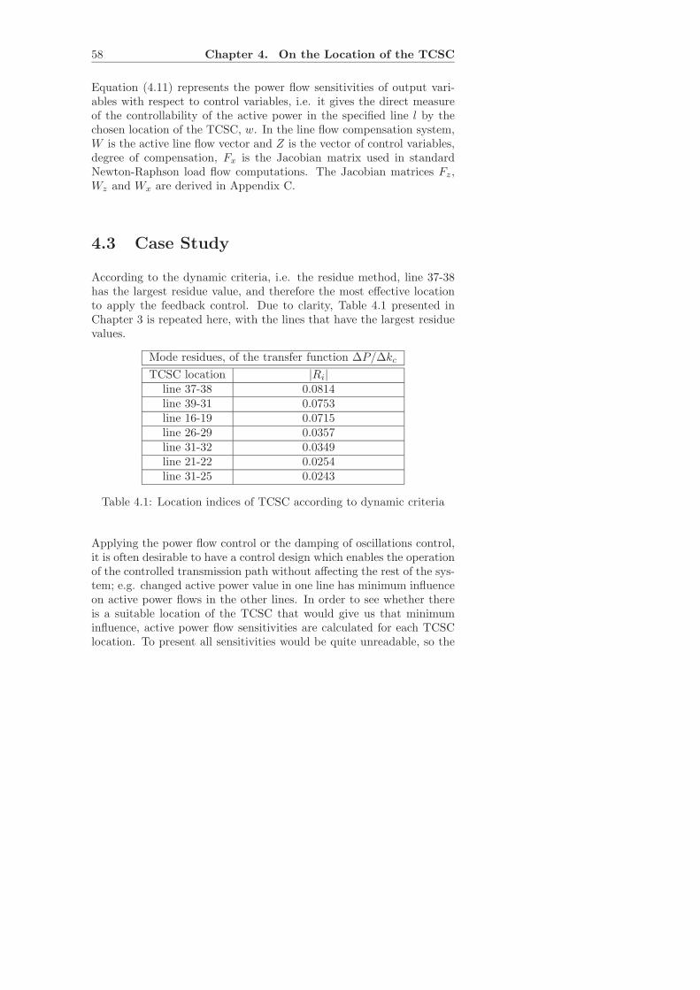
According to the dynamic criteria, i.e. the residue method, line 37-38has the largest residue value, and therefore the most effective locationto apply the feedback control. Due to clarity, Table 4.1 presented inChapter 3 is repeated here, with the lines that have the largest residuevalues.
Mode residues, of the transfer function ∆P/∆kc
TCSC location |Ri|line 37-38 0.0814line 39-31 0.0753line 16-19 0.0715line 26-29 0.0357line 31-32 0.0349line 21-22 0.0254line 31-25 0.0243
Table 4.1: Location indices of TCSC according to dynamic criteria
Applying the power flow control or the damping of oscillations control,it is often desirable to have a control design which enables the operationof the controlled transmission path without affecting the rest of the sys-tem; e.g. changed active power value in one line has minimum influenceon active power flows in the other lines. In order to see whether thereis a suitable location of the TCSC that would give us that minimuminfluence, active power flow sensitivities are calculated for each TCSClocation. To present all sensitivities would be quite unreadable, so the
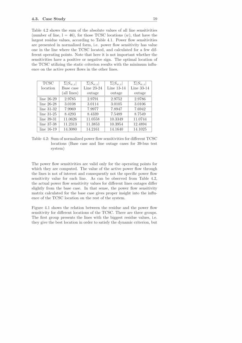
4.3. Case Study 59
Table 4.2 shows the sum of the absolute values of all line sensitivities(number of line, l = 46), for those TCSC locations (w), that have thelargest residue values, according to Table 4.1. Power flow sensitivitiesare presented in normalized form, i.e. power flow sensitivity has valueone in the line where the TCSC located, and calculated for a few dif-ferent operating points. Note that here it is not important whether thesensitivities have a positive or negative sign. The optimal location ofthe TCSC utilizing the static criterion results with the minimum influ-ence on the active power flows in the other lines.
TCSC Σ|Sw,z| Σ|Sw,z| Σ|Sw,z| Σ|Sw,z|location Base case Line 23-24 Line 13-14 Line 33-14
(all lines) outage outage outage
line 26-29 2.9785 2.9791 2.9752 2.9786line 26-28 3.0108 3.0114 3.0105 3.0106line 31-32 7.9969 7.9977 7.8947 7.6942line 31-25 8.4293 8.4339 7.5489 8.7549line 39-31 11.0626 11.0558 10.3349 11.0744line 37-38 11.2313 11.3853 10.3954 12.4894line 16-19 14.3080 14.2161 14.1640 14.1025
Table 4.2: Sum of normalized power flow sensitivities for different TCSClocations (Base case and line outage cases for 39-bus testsystem)
The power flow sensitivities are valid only for the operating points forwhich they are computed. The value of the active power flow throughthe lines is not of interest and consequently not the specific power flowsensitivity value for each line. As can be observed from Table 4.2,the actual power flow sensitivity values for different lines outages differslightly from the base case. In that sense, the power flow sensitivitymatrix calculated for the base case gives proper insight into the influ-ence of the TCSC location on the rest of the system.
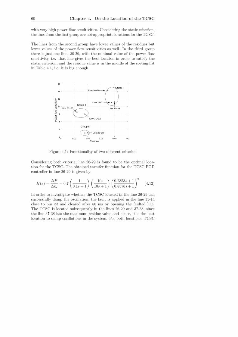
Figure 4.1 shows the relation between the residue and the power flowsensitivity for different locations of the TCSC. There are three groups.The first group presents the lines with the biggest residue values, i.e.they give the best location in order to satisfy the dynamic criterion, but
60 Chapter 4. On the Location of the TCSC
with very high power flow sensitivities. Considering the static criterion,the lines from the first group are not appropriate locations for the TCSC.
The lines from the second group have lower values of the residues butlower values of the power flow sensitivities as well. In the third groupthere is just one line, 26-29, with the minimal value of the power flowsensitivity, i.e. that line gives the best location in order to satisfy thestatic criterion, and the residue value is in the middle of the sorting listin Table 4.1, i.e. it is big enough.
0 0.02 0.04 0.06 0.08 0.12
4
6
8
10
12
14
16
Residue
Pow
er fl
ow s
ensi
tivity
Group I
Group II
Group III
Line 16−19
Line 39−31
Line 37−38Line 31−25
Line 31−32
Line 26−29
Figure 4.1: Functionality of two different criterion
Considering both criteria, line 26-29 is found to be the optimal loca-tion for the TCSC. The obtained transfer function for the TCSC PODcontroller in line 26-29 is given by:
H(s) =∆P
∆kc
= 0.7
(
1
0.1s+ 1
)(
10s
10s+ 1
)(
0.2353s+ 1
0.8576s+ 1
)2
(4.12)
In order to investigate whether the TCSC located in the line 26-29 cansuccessfully damp the oscillation, the fault is applied in the line 33-14close to bus 33 and cleared after 50 ms by opening the faulted line.The TCSC is located subsequently in the lines 26-29 and 37-38, sincethe line 37-38 has the maximum residue value and hence, it is the bestlocation to damp oscillations in the system. For both locations, TCSC
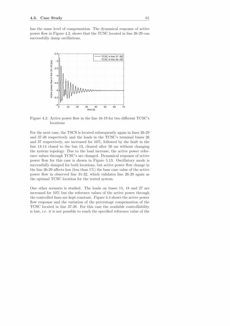
4.3. Case Study 61
has the same level of compensation. The dynamical response of activepower flow in Figure 4.2, shows that the TCSC located in line 26-29 cansuccessfully damp oscillations.
0 10 20 30 40 50 60 70−6
−5.5
−5
−4.5
−4
−3.5
−3
−2.5
time [s]
Act
ive
pow
er fl
ow in
line
16−
19 [p
u]
TCSC in line 37−38TCSC in line 26−29
Figure 4.2: Active power flow in the line 16-19 for two different TCSC’slocations
For the next case, the TSCS is located subsequently again in lines 26-29and 37-38 respectively and the loads in the TCSC’s terminal buses 26and 37 respectively, are increased for 10%, followed by the fault in theline 13-14 closed to the bus 13, cleared after 50 ms without changingthe system topology. Due to the load increase, the active power refer-ence values through TCSC’s are changed. Dynamical response of activepower flow for this case is shown in Figure 5.13. Oscillatory mode issuccessfully damped for both locations, but active power flow change inthe line 26-29 affects less (less than 1%) the base case value of the activepower flow in observed line 31-32, which validates line 26-29 again asthe optimal TCSC location for the tested system.
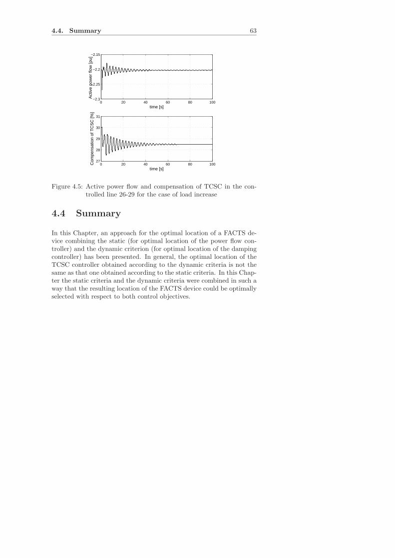
One other scenario is studied. The loads on buses 15, 18 and 27 areincreased for 10% but the reference values of the active power throughthe controlled lines are kept constant. Figure 4.4 shows the active powerflow response and the variation of the percentage compensation of theTCSC located in line 37-38. For this case the available controllabilityis lost, i.e. it is not possible to reach the specified reference value of the
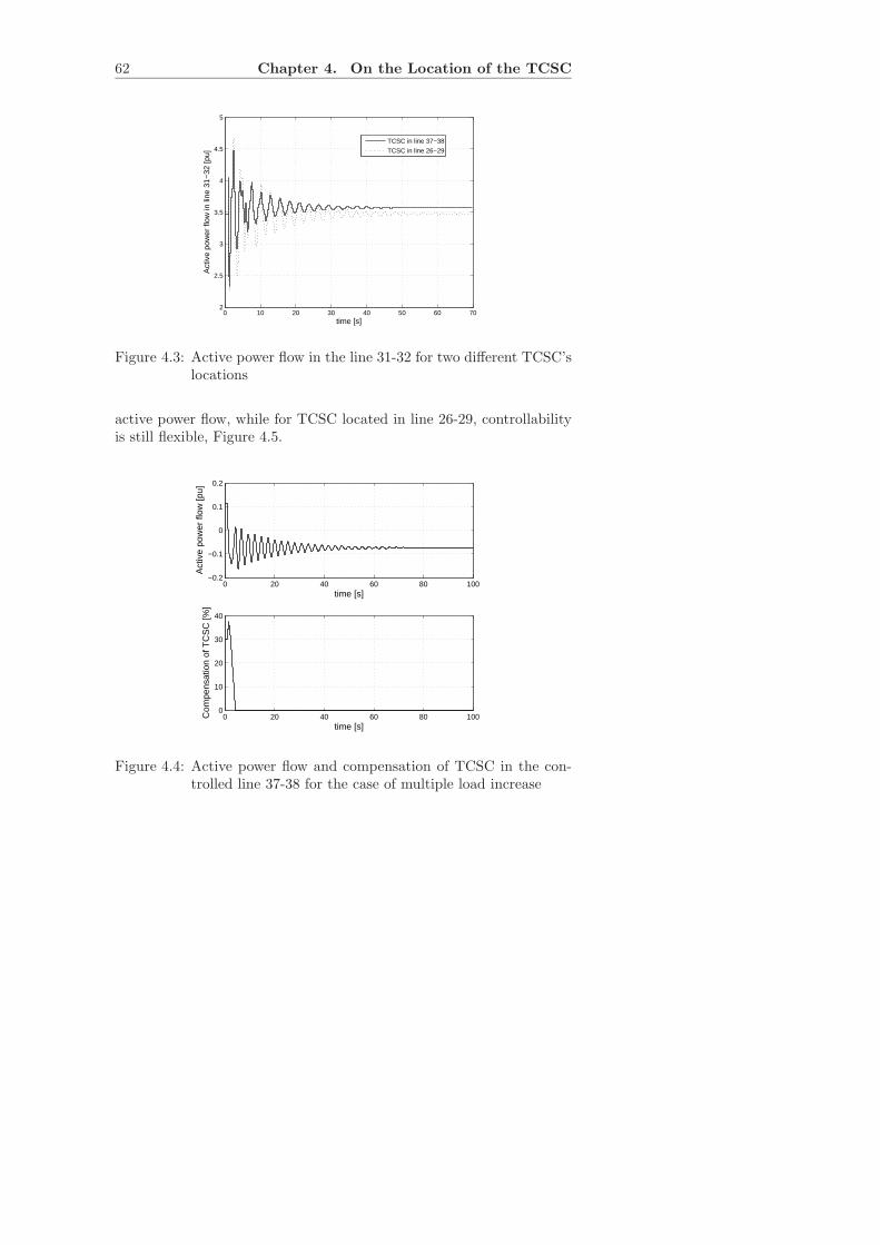
62 Chapter 4. On the Location of the TCSC
0 10 20 30 40 50 60 702
2.5
3
3.5
4
4.5
5
time [s]
Act
ive
pow
er fl
ow in
line
31−
32 [p
u]
TCSC in line 37−38
TCSC in line 26−29
Figure 4.3: Active power flow in the line 31-32 for two different TCSC’slocations
active power flow, while for TCSC located in line 26-29, controllabilityis still flexible, Figure 4.5.
0 20 40 60 80 100−0.2
−0.1
0
0.1
0.2
time [s]
Act
ive
pow
er fl
ow [p
u]
0 20 40 60 80 1000
10
20
30
40
time [s]
Com
pens
atio
n of
TC
SC
[%]
Figure 4.4: Active power flow and compensation of TCSC in the con-trolled line 37-38 for the case of multiple load increase
4.4. Summary 63
0 20 40 60 80 100−2.3
−2.25
−2.2
−2.15
time [s]
Act
ive
pow
er fl
ow [p
u]
0 20 40 60 80 10027
28
29
30
31
time [s]
Com
pens
atio
n of
TC
SC
[%]
Figure 4.5: Active power flow and compensation of TCSC in the con-trolled line 26-29 for the case of load increase
4.4 Summary
In this Chapter, an approach for the optimal location of a FACTS de-vice combining the static (for optimal location of the power flow con-troller) and the dynamic criterion (for optimal location of the dampingcontroller) has been presented. In general, the optimal location of theTCSC controller obtained according to the dynamic criteria is not thesame as that one obtained according to the static criteria. In this Chap-ter the static criteria and the dynamic criteria were combined in such away that the resulting location of the FACTS device could be optimallyselected with respect to both control objectives.


Chapter 5
Self-Tuning Controllers
A conventional damping control design considers a single operating con-dition of the system. In this kind of controllers, feedback is fixed andamplifies the error, which in turn determines the value of the input sig-nal u (controller output) for the system. The way in which the error isprocessed is the same for all operating conditions. The basis of the adap-tive system is that it influences the way in which the error is processed.There are three basic approaches to the problem of adaptive control;heuristic approach, self-tuning controllers (STC) and model adaptivereference systems (MRAS), [28].
The self-tuning controller is based on the idea of separating the estima-tion of unknown parameters from the design of the optimal controller,[29]. The unknown parameters are estimated on-line, using recursive es-timation of the characteristics of the system and its disturbances. Theapproach used in STCs was first mentioned in the work of Kalman in1958, [30] and then revived in the early 1970s by the work of Astromand Wittenmark, [31], and others. Researchers, over the years, havebeen developing this approach. A self-tuning controller for power sys-tem stabilizers (PSSs) has been reported in [22] where Prony analysisextracts oscillation modes from sequential data and estimates oscillationfrequency, damping, amplitude and phase of each mode. The authorsin [24, 25, 26] have done the work on PSS self-tuning controller basedon pole assignment where the amount of pole shifting is adjusted de-pending upon the changes of system operating conditions.
65
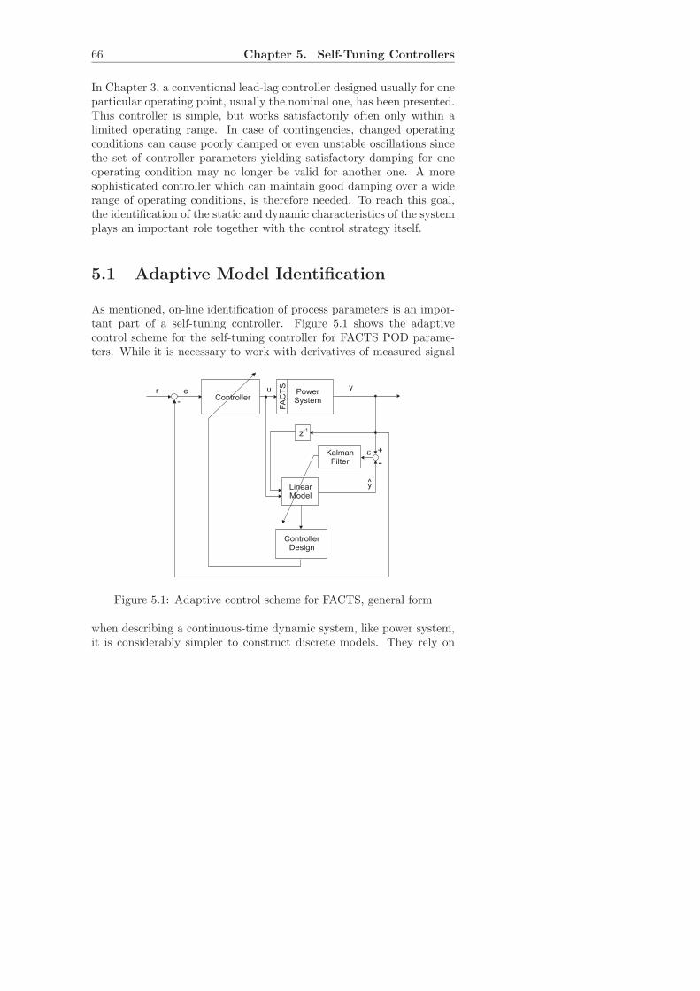
66 Chapter 5. Self-Tuning Controllers
In Chapter 3, a conventional lead-lag controller designed usually for oneparticular operating point, usually the nominal one, has been presented.This controller is simple, but works satisfactorily often only within alimited operating range. In case of contingencies, changed operatingconditions can cause poorly damped or even unstable oscillations sincethe set of controller parameters yielding satisfactory damping for oneoperating condition may no longer be valid for another one. A moresophisticated controller which can maintain good damping over a widerange of operating conditions, is therefore needed. To reach this goal,the identification of the static and dynamic characteristics of the systemplays an important role together with the control strategy itself.
5.1 Adaptive Model Identification
As mentioned, on-line identification of process parameters is an impor-tant part of a self-tuning controller. Figure 5.1 shows the adaptivecontrol scheme for the self-tuning controller for FACTS POD parame-ters. While it is necessary to work with derivatives of measured signal
+
y
LinearModel
y
ControllerDesign
z-1
e
-Kalman
Filter
Controllerr
-PowerSystem
FA
CT
Sue
Figure 5.1: Adaptive control scheme for FACTS, general form
when describing a continuous-time dynamic system, like power system,it is considerably simpler to construct discrete models. They rely on
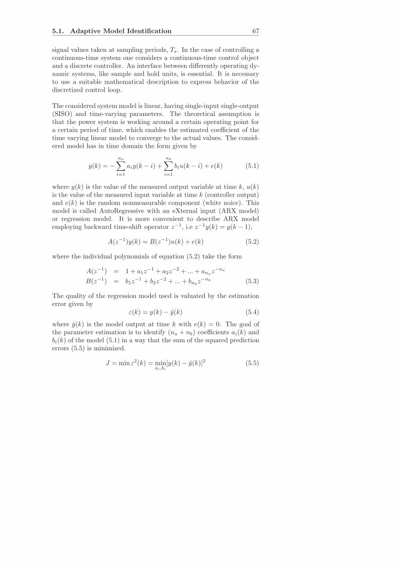
5.1. Adaptive Model Identification 67
signal values taken at sampling periods, Ts. In the case of controlling acontinuous-time system one considers a continuous-time control objectand a discrete controller. An interface between differently operating dy-namic systems, like sample and hold units, is essential. It is necessaryto use a suitable mathematical description to express behavior of thediscretized control loop.
The considered system model is linear, having single-input single-output(SISO) and time-varying parameters. The theoretical assumption isthat the power system is working around a certain operating point fora certain period of time, which enables the estimated coefficient of thetime varying linear model to converge to the actual values. The consid-ered model has in time domain the form given by
y(k) = −na∑
i=1
aiy(k − i) +
nb∑
i=1
biu(k − i) + e(k) (5.1)
where y(k) is the value of the measured output variable at time k, u(k)is the value of the measured input variable at time k (controller output)and e(k) is the random nonmeasurable component (white noice). Thismodel is called AutoRegressive with an eXternal input (ARX model)or regression model. It is more convenient to describe ARX modelemploying backward time-shift operator z−1, i.e z−1y(k) = y(k − 1),
A(z−1)y(k) = B(z−1)u(k) + e(k) (5.2)
where the individual polynomials of equation (5.2) take the form
A(z−1) = 1 + a1z−1 + a2z
−2 + ...+ anaz−na
B(z−1) = b1z−1 + b2z
−2 + ...+ bnbz−nb (5.3)
The quality of the regression model used is valuated by the estimationerror given by
ε(k) = y(k) − y(k) (5.4)
where y(k) is the model output at time k with e(k) = 0. The goal ofthe parameter estimation is to identify (na + nb) coefficients ai(k) andbi(k) of the model (5.1) in a way that the sum of the squared predictionerrors (5.5) is minimized.
J = min ε2(k) = minai,bi
[y(k) − y(k)]2 (5.5)
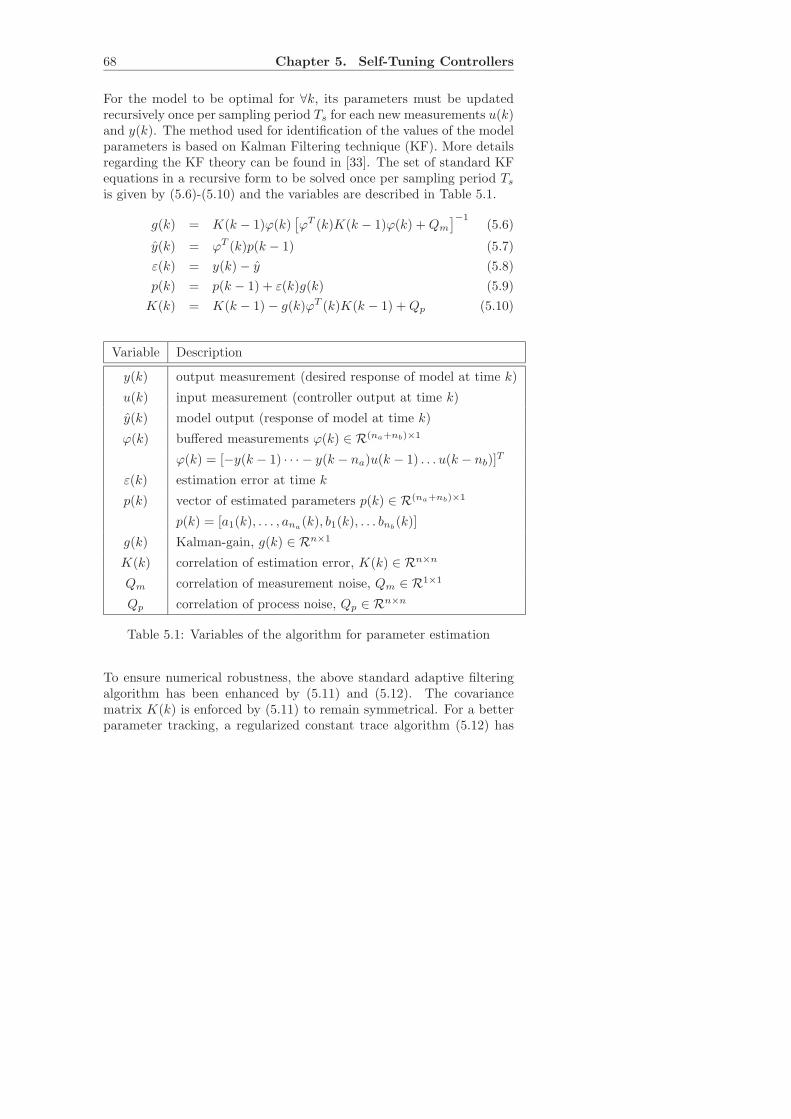
68 Chapter 5. Self-Tuning Controllers
For the model to be optimal for ∀k, its parameters must be updatedrecursively once per sampling period Ts for each new measurements u(k)and y(k). The method used for identification of the values of the modelparameters is based on Kalman Filtering technique (KF). More detailsregarding the KF theory can be found in [33]. The set of standard KFequations in a recursive form to be solved once per sampling period Ts
is given by (5.6)-(5.10) and the variables are described in Table 5.1.
g(k) = K(k − 1)ϕ(k)[
ϕT (k)K(k − 1)ϕ(k) +Qm
]−1(5.6)
y(k) = ϕT (k)p(k − 1) (5.7)
ε(k) = y(k) − y (5.8)
p(k) = p(k − 1) + ε(k)g(k) (5.9)
K(k) = K(k − 1) − g(k)ϕT (k)K(k − 1) +Qp (5.10)
Variable Description
y(k) output measurement (desired response of model at time k)
u(k) input measurement (controller output at time k)
y(k) model output (response of model at time k)
ϕ(k) buffered measurements ϕ(k) ∈ R(na+nb)×1
ϕ(k) = [−y(k − 1) · · · − y(k − na)u(k − 1) . . . u(k − nb)]T
ε(k) estimation error at time k
p(k) vector of estimated parameters p(k) ∈ R(na+nb)×1
p(k) = [a1(k), . . . , ana(k), b1(k), . . . bnb
(k)]
g(k) Kalman-gain, g(k) ∈ Rn×1
K(k) correlation of estimation error, K(k) ∈ Rn×n
Qm correlation of measurement noise, Qm ∈ R1×1
Qp correlation of process noise, Qp ∈ Rn×n
Table 5.1: Variables of the algorithm for parameter estimation
To ensure numerical robustness, the above standard adaptive filteringalgorithm has been enhanced by (5.11) and (5.12). The covariancematrix K(k) is enforced by (5.11) to remain symmetrical. For a betterparameter tracking, a regularized constant trace algorithm (5.12) has
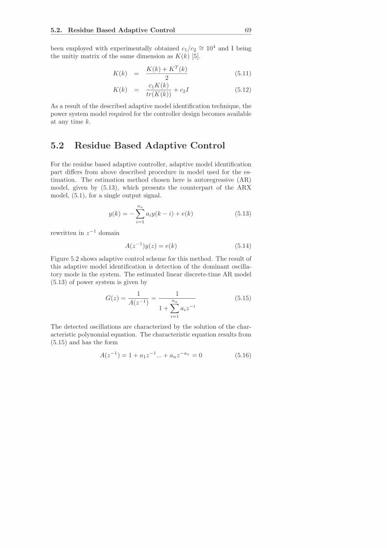
5.2. Residue Based Adaptive Control 69
been employed with experimentally obtained c1/c2 ∼= 104 and I beingthe unitiy matrix of the same dimension as K(k) [5].
K(k) =K(k) +KT (k)
2(5.11)
K(k) =c1K(k)
tr(K(k))+ c2I (5.12)
As a result of the described adaptive model identification technique, thepower system model required for the controller design becomes availableat any time k.
5.2 Residue Based Adaptive Control
For the residue based adaptive controller, adaptive model identificationpart differs from above described procedure in model used for the es-timation. The estimation method chosen here is autoregressive (AR)model, given by (5.13), which presents the counterpart of the ARXmodel, (5.1), for a single output signal.
y(k) = −na∑
i=1
aiy(k − i) + e(k) (5.13)
rewritten in z−1 domain
A(z−1)y(z) = e(k) (5.14)
Figure 5.2 shows adaptive control scheme for this method. The result ofthis adaptive model identification is detection of the dominant oscilla-tory mode in the system. The estimated linear discrete-time AR model(5.13) of power system is given by
G(z) =1
A(z−1)=
1
1 +
na∑
i=1
aiz−i
(5.15)
The detected oscillations are characterized by the solution of the char-acteristic polynomial equation. The characteristic equation results from(5.15) and has the form
A(z−1) = 1 + a1z−1...+ anz
−an = 0 (5.16)
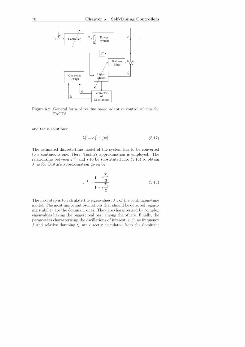
70 Chapter 5. Self-Tuning Controllers
+
y
LinearModel
y
z-1
e-
PowerSystem
FA
CT
Su
xi
fi
ControllerDesign
Controllerr -
e
KalmanFilter
Parametersof
Oscillations
Figure 5.2: General form of residue based adaptive control scheme forFACTS
and the n solutions:
λdi = αd
i ± jwdi (5.17)
The estimated discrete-time model of the system has to be convertedto a continuous one. Here, Tustin’s approximation is employed. Therelationship between z−1 and s to be substituted into (5.16) to obtainλi is for Tustin’s approximation given by
z−1 =1 − s
Ts
2
1 + sTs
2
(5.18)
The next step is to calculate the eigenvalues, λi, of the continuous-timemodel. The most important oscillations that should be detected regard-ing stability are the dominant ones. They are characterized by complexeigenvalues having the biggest real part among the others. Finally, theparameters characterizing the oscillations of interest, such as frequencyf and relative damping ξ, are directly calculated from the dominant
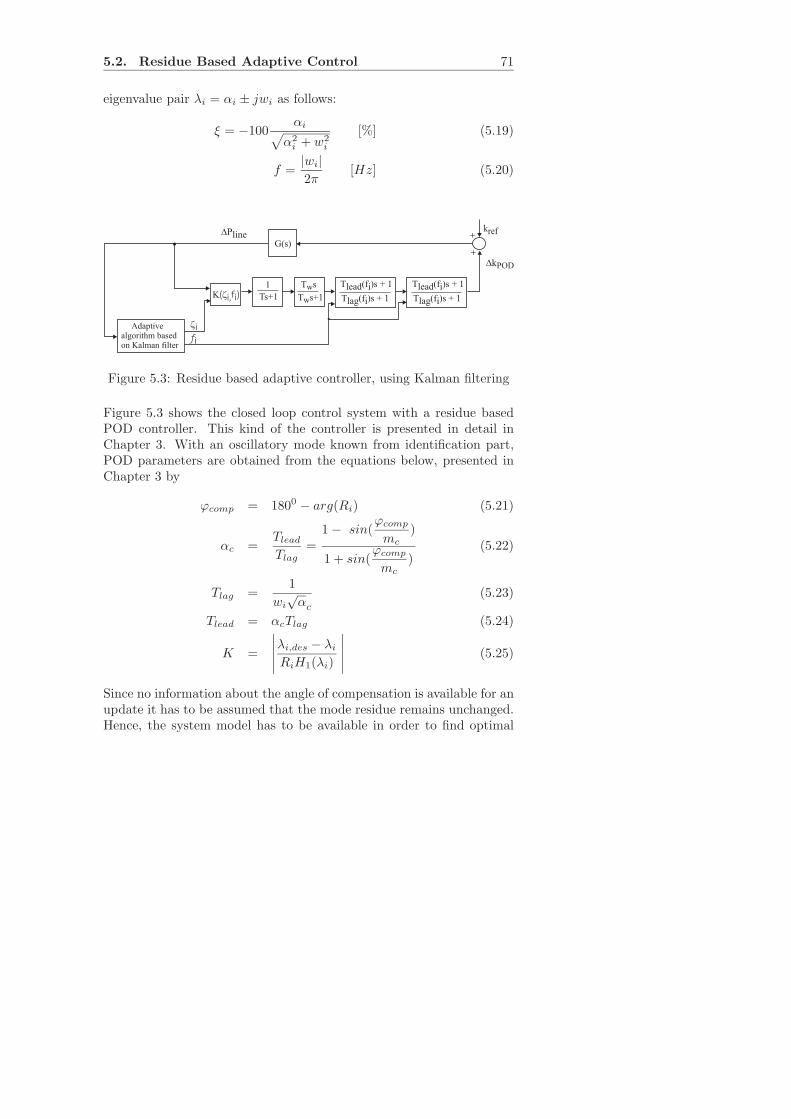
5.2. Residue Based Adaptive Control 71
eigenvalue pair λi = αi ± jwi as follows:
ξ = −100αi
√
α2i + w2
i
[%] (5.19)
f =|wi|2π
[Hz] (5.20)
G(s)
K( i,fi)z Ts+1
1
T s+1w
T sw Tlead(fi)s + 1
Tlag(fi)s + 1
DPline
Adaptivealgorithm basedon Kalman filter
zifi
Tlead(fi)s + 1
Tlag(fi)s + 1
DkPOD
+
+kref
Figure 5.3: Residue based adaptive controller, using Kalman filtering
Figure 5.3 shows the closed loop control system with a residue basedPOD controller. This kind of the controller is presented in detail inChapter 3. With an oscillatory mode known from identification part,POD parameters are obtained from the equations below, presented inChapter 3 by
ϕcomp = 1800 − arg(Ri) (5.21)
αc =Tlead
Tlag
=1 − sin(
ϕcomp
mc
)
1 + sin(ϕcomp
mc
)(5.22)
Tlag =1
wi
√αc
(5.23)
Tlead = αcTlag (5.24)
K =
∣
∣
∣
∣
∣
λi,des − λi
RiH1(λi)
(5.25)
Since no information about the angle of compensation is available for anupdate it has to be assumed that the mode residue remains unchanged.Hence, the system model has to be available in order to find optimal

72 Chapter 5. Self-Tuning Controllers
location for FACTS devices, in this case TCSC, and consequently to cal-culate the values of residues for the controller design. From Figure 5.3,one can see that Tlead, Tlag and the gain K are updated online at everysampling period, Ts, according to (5.23)-(5.25). A relatively simple andpowerful adaptive controller tuning has been achieved in considered testsystem using this approach.
The test system used for applying the residue based controller is theNew England 39 bus system, shown in Figure 3.4, Chapter 3. For thiscase study the dynamic data of some generators were modified in or-der to get illustrative results. The modified system has one oscillatory,inter-area mode characterized by λ = −0.0784 ± j5.3677 with dampingratio ξ = 1.46%. Performed residue and sensitivity analysis show thatthe line 26-29 is, again, the most suitable location for TCSC in order tosatisfy both, i.e. a power flow and damping control.
As mentioned, the problem with a set of fixed controller parametersi.e. tuned by conventional method, arises when the system topology ischanged. In such cases, the re-tuning of POD parameters is required.One solution of this problem is to re-tune the controller parameters forevery new operating condition based on a complete set of the modelparameters. In following Figures, dynamic responses obtained by thisapproach are denoted as ”re-tuned POD”, i.e. POD is re-tuned for ap-propriate operating condition, e.g. with the line out of service, whereas”fixed POD” means POD controller tuned as well by residue basedmethod, but for nominal condition.
In order to compare all approaches, the following disturbances are con-sidered for simulation with a fault for 100 ms close to the buses:
1. bus # 16 followed by outage of the line 16-17 and with line 25-26out of service
2. bus # 25 followed by outage of the line 25-26 and with lines 23-24and 32-18 out of service
Figures 5.4 and 5.5 show the active power flow dynamic response forthe first disturbance, with comparison of the results obtained for fixedtuned POD, re-tuned POD, and proposed adaptive tuned POD. It canbe noted that ”re-tuned” POD, tuned for system’s operating condition
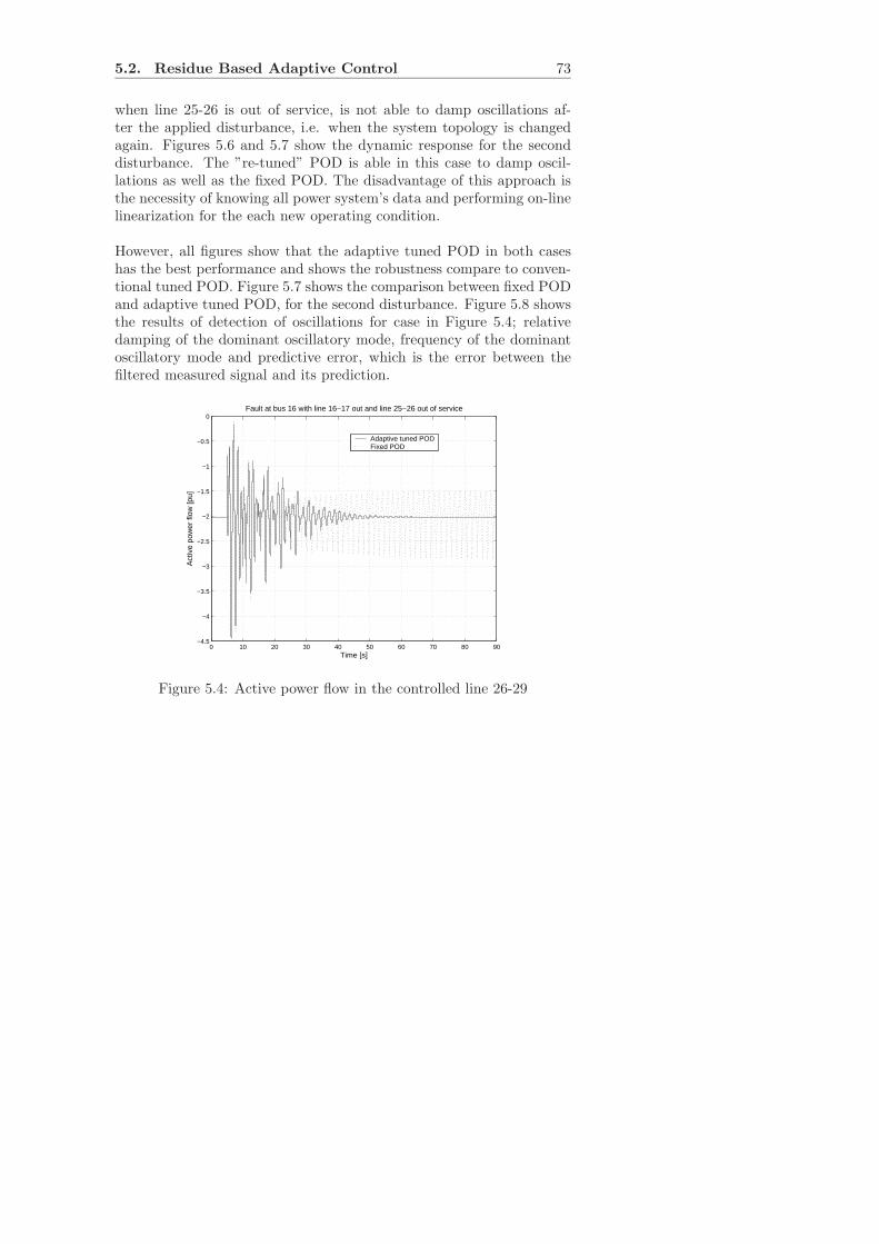
5.2. Residue Based Adaptive Control 73
when line 25-26 is out of service, is not able to damp oscillations af-ter the applied disturbance, i.e. when the system topology is changedagain. Figures 5.6 and 5.7 show the dynamic response for the seconddisturbance. The ”re-tuned” POD is able in this case to damp oscil-lations as well as the fixed POD. The disadvantage of this approach isthe necessity of knowing all power system’s data and performing on-linelinearization for the each new operating condition.
However, all figures show that the adaptive tuned POD in both caseshas the best performance and shows the robustness compare to conven-tional tuned POD. Figure 5.7 shows the comparison between fixed PODand adaptive tuned POD, for the second disturbance. Figure 5.8 showsthe results of detection of oscillations for case in Figure 5.4; relativedamping of the dominant oscillatory mode, frequency of the dominantoscillatory mode and predictive error, which is the error between thefiltered measured signal and its prediction.
0 10 20 30 40 50 60 70 80 90−4.5
−4
−3.5
−3
−2.5
−2
−1.5
−1
−0.5
0
Time [s]
Act
ive
pow
er fl
ow [p
u]
Fault at bus 16 with line 16−17 out and line 25−26 out of service
Adaptive tuned PODFixed POD
Figure 5.4: Active power flow in the controlled line 26-29
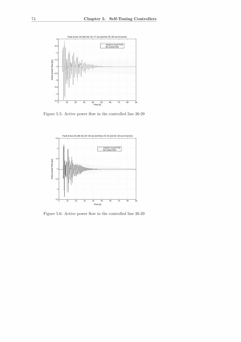
74 Chapter 5. Self-Tuning Controllers
0 10 20 30 40 50 60 70 80 90−4.5
−4
−3.5
−3
−2.5
−2
−1.5
−1
−0.5
0
Time [s]
Act
ive
pow
er fl
ow [p
u]
Fault at bus 16 with line 16−17 out and line 25−26 out of service
Adaptive tuned PODRe−tuned POD
Figure 5.5: Active power flow in the controlled line 26-29
0 10 20 30 40 50 60 70 80 90−3.5
−3
−2.5
−2
−1.5
−1
−0.5
Time [s]
Act
ive
pow
er fl
ow [p
u]
Fault at bus 25 with line 25−26 out and lines 23−24 and 32−18 out of service
Adaptive tuned PODRe−tuned POD
Figure 5.6: Active power flow in the controlled line 26-29
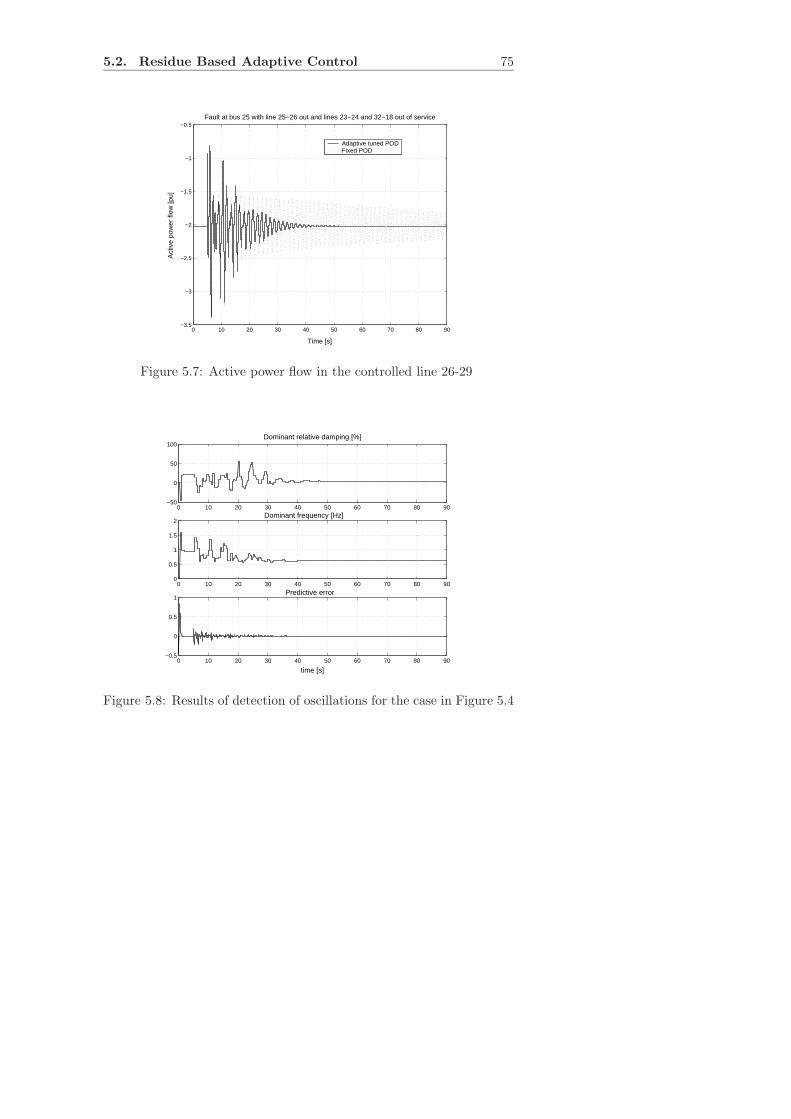
5.2. Residue Based Adaptive Control 75
0 10 20 30 40 50 60 70 80 90−3.5
−3
−2.5
−2
−1.5
−1
−0.5
Time [s]
Act
ive
pow
er fl
ow [p
u]
Fault at bus 25 with line 25−26 out and lines 23−24 and 32−18 out of service
Adaptive tuned PODFixed POD
Figure 5.7: Active power flow in the controlled line 26-29
0 10 20 30 40 50 60 70 80 90−50
0
50
100Dominant relative damping [%]
0 10 20 30 40 50 60 70 80 900
0.5
1
1.5
2Dominant frequency [Hz]
0 10 20 30 40 50 60 70 80 90−0.5
0
0.5
1Predictive error
time [s]
Figure 5.8: Results of detection of oscillations for the case in Figure 5.4
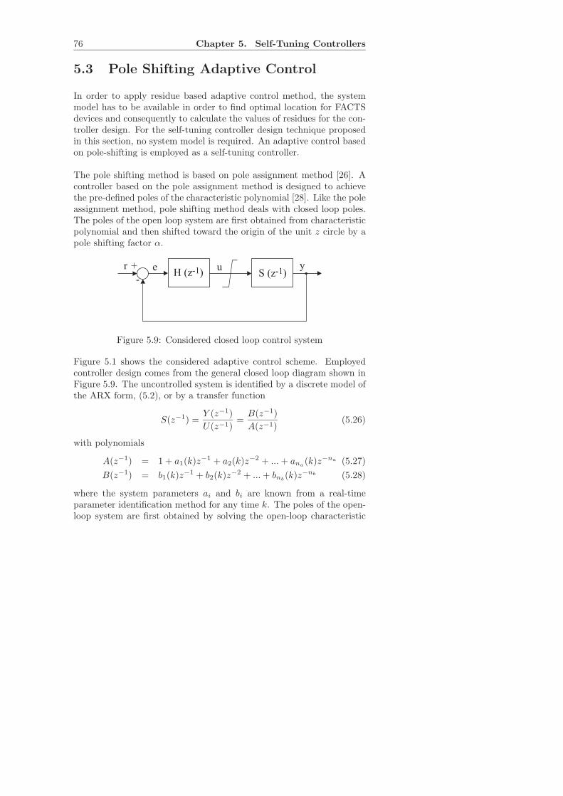
76 Chapter 5. Self-Tuning Controllers
5.3 Pole Shifting Adaptive Control
In order to apply residue based adaptive control method, the systemmodel has to be available in order to find optimal location for FACTSdevices and consequently to calculate the values of residues for the con-troller design. For the self-tuning controller design technique proposedin this section, no system model is required. An adaptive control basedon pole-shifting is employed as a self-tuning controller.
The pole shifting method is based on pole assignment method [26]. Acontroller based on the pole assignment method is designed to achievethe pre-defined poles of the characteristic polynomial [28]. Like the poleassignment method, pole shifting method deals with closed loop poles.The poles of the open loop system are first obtained from characteristicpolynomial and then shifted toward the origin of the unit z circle by apole shifting factor α.
S (z )-1y+
-
urH (z )-1e
Figure 5.9: Considered closed loop control system
Figure 5.1 shows the considered adaptive control scheme. Employedcontroller design comes from the general closed loop diagram shown inFigure 5.9. The uncontrolled system is identified by a discrete model ofthe ARX form, (5.2), or by a transfer function
S(z−1) =Y (z−1)
U(z−1)=B(z−1)
A(z−1)(5.26)
with polynomials
A(z−1) = 1 + a1(k)z−1 + a2(k)z
−2 + ...+ ana(k)z−na (5.27)
B(z−1) = b1(k)z−1 + b2(k)z
−2 + ...+ bnb(k)z−nb (5.28)
where the system parameters ai and bi are known from a real-timeparameter identification method for any time k. The poles of the open-loop system are first obtained by solving the open-loop characteristic
5.3. Pole Shifting Adaptive Control 77
equation from (5.27) frozen for the actual time k:
A(z−1) = 1 + a1z−1 + a2z
−2 + ...+ anaz−na = 0 (5.29)
The discrete transfer function of the considered controller is given by
H(z−1) =U(z−1)
E(z−1)=G(z−1)
F (z−1)(5.30)
where
F (z−1) = 1 + f1z−1 + ...+ fiz
−i + ...+ fnfz−nf (5.31)
G(z−1) = g0 + g1z−1 + ...+ giz
−i + ...+ gngz−nf (5.32)
and nf = nb − 1, ng = na − 1.The transfer function of the closed loop system, illustrated in the blockdiagram in Figure 5.9, then takes the form
Y (z−1)
R(z−1)=
B(z−1)G(z−1)
A(z−1)F (z−1) +B(z−1)G(z−1)(5.33)
The transfer function of the closed loop system has to be suitably ad-justed by choosing a controller transfer function to guarantee the over-all stability of the closed loop system. According to pole assignmentmethod, by choosing the characteristic polynomial
P (z−1) = 1 +
np∑
i=1
piz−i (5.34)
in the polynomial equation
P (z−1) = A(z−1)F (z−1) +B(z−1)G(z−1) (5.35)
where np = max(na + nf , nb + ng), one should achieve the pre-setpoles. As mentioned, the open loop poles of the system are obtained bysolving (5.29). If all the roots of (5.29) are within the unit circle in thez-domain, the system is stable. It is clear, the system is more stable asthe closer the poles are to the origin of the unit circle. The function ofthe pole shifting self-tuning control is to shift all roots of (5.29) towardsthe origin of the unit circle by a factor α. This implies that P (z−1)takes the form of a polynomial A(z−1) multiplied with an array of α,
P (z−1) = 1 +
np∑
i=1
piz−i = 1 +
np∑
i=1
αiaiz−i (5.36)
78 Chapter 5. Self-Tuning Controllers
where 0 < α < 1 and the prescribed coefficients pi = 0 for i > na.Hence, the resulting close-loop poles will be the roots of the character-istic equation given by
P (z−1) = 0 (5.37)
Substituting (5.27), (5.28), (5.31), (5.32) and (5.36) into (5.35) andcomparing the coefficients at the same power of z−1 on the both sides,gives:
M ·H = L (5.38)
where
M =
1 0 . 0 b1 0 . 0a1 1 . 0 b2 b1 . 0. a1 . . . b2 . .ana
. . 1 bnb. . b1
0 ana. a1 0 bnb
. b2. 0 . . . 0 . .. . . . . . . .0 0 . ana
0 0 . bnb
(5.39)
H =
f1..fnf
g0..gng
(5.40)
L =
a1(α− 1)a2(α
2 − 1)..ana
(αna − 1)0.0
(5.41)
If the variable α in matrix L is fixed, one has a special case of the poleassignment control algorithm where the coefficients of the controller
5.3. Pole Shifting Adaptive Control 79
transfer function, fi(i = 1, ...nf ) and gi(i = 1, ...ng), can be calculatedat every sample from (5.38) by
H = M−1L (5.42)
and the control u can be calculated, as shown in Fig. 5.9, by
U(z−1)
E(z−1)=G(z−1)
F (z−1)= H(z−1) (5.43)
or with zero reference value r
U(z−1)
Y (z−1)=G(z−1)
F (z−1)= H(z−1) (5.44)
From (5.44) follows
U(z−1)F (z−1) = Y (z−1)G(z−1) (5.45)
rewritten in time domain
u(k)+f1u(t−1)+...+fnfu(t−nf ) = g0y(t)+g1y(t−1)+...+gng
y(t−ng)(5.46)
oru(k) = ϕT (k)H(k) (5.47)
with ϕ(k) = [−u(k− 1), ...,−u(k− nf ), y(k), ..., y(k− ng)] and H givenby (5.40).
Proper value of the pole shifting factor depends on the operating condi-tions. For that reason it is desirable to adapt the parameter α on line.From (5.47), it is obvious that the control at time k, u(k), is a functionof pole shifting factor at that time, with constraint umin ≤ u ≤ umax.Sensitivity function can be calculated from (5.47) as
du
dα= ϕT · dH
dα(5.48)
Substituting (5.42) into (5.48) gives
du
dα= ϕT ·M−1 · dL
dα(5.49)
du
dα= ϕT ·M−1 · [a1, 2a2α, ..., naana
αna−1] (5.50)

80 Chapter 5. Self-Tuning Controllers
With the approximationdu
dα=
∆u
∆α(5.51)
the modification factor α is given by
∆α = K· | dudα
|−1 ·∆u (5.52)
where ∆u is the control margin defined as
∆u =
umax − u u ≥ 0u− umin u < 0
(5.53)
and K is a positive constant chosen to avoid excessive variation in α.The variable pole shifting factor, α(k), can be calculated by
α(k) = α(k0) + ∆α (5.54)
where α(k0) is any value between 0 and 1.
Figure 5.10 and Figure 5.13 show the direct comparison between theactive power flow response of the system to the fault with fixed PODparameters and adaptive tuned parameters of the POD controller, fortwo different cases. The simulations are carried out for two disturbancesfor 100 ms. The faults are created 1.0 s after the start of the simulationsand they are applied close to the following buses:
1. bus #16 followed by outage of the line 16-17
2. bus #21 followed by outage of the line 21-22 and with line 32-18and 33-14 out of service
The fixed POD parameters are tuned using the residue method. Theresults given in this Figures show that the oscillations of the systemare damped out efficiency and demonstrates the ability of the systemto adapt to a new operating conditions. Figure 5.12 shows the compar-ison of the active power flow for the case on Figure 5.10, with fixed andvariable pole shifting factor, α.
Variation of the pole shifting factor for two studied cases is shown inFigure 5.11 and Figure 5.14. It can be seen that pole shifting factoradapts itself to the dynamic of the system and it can converge either to
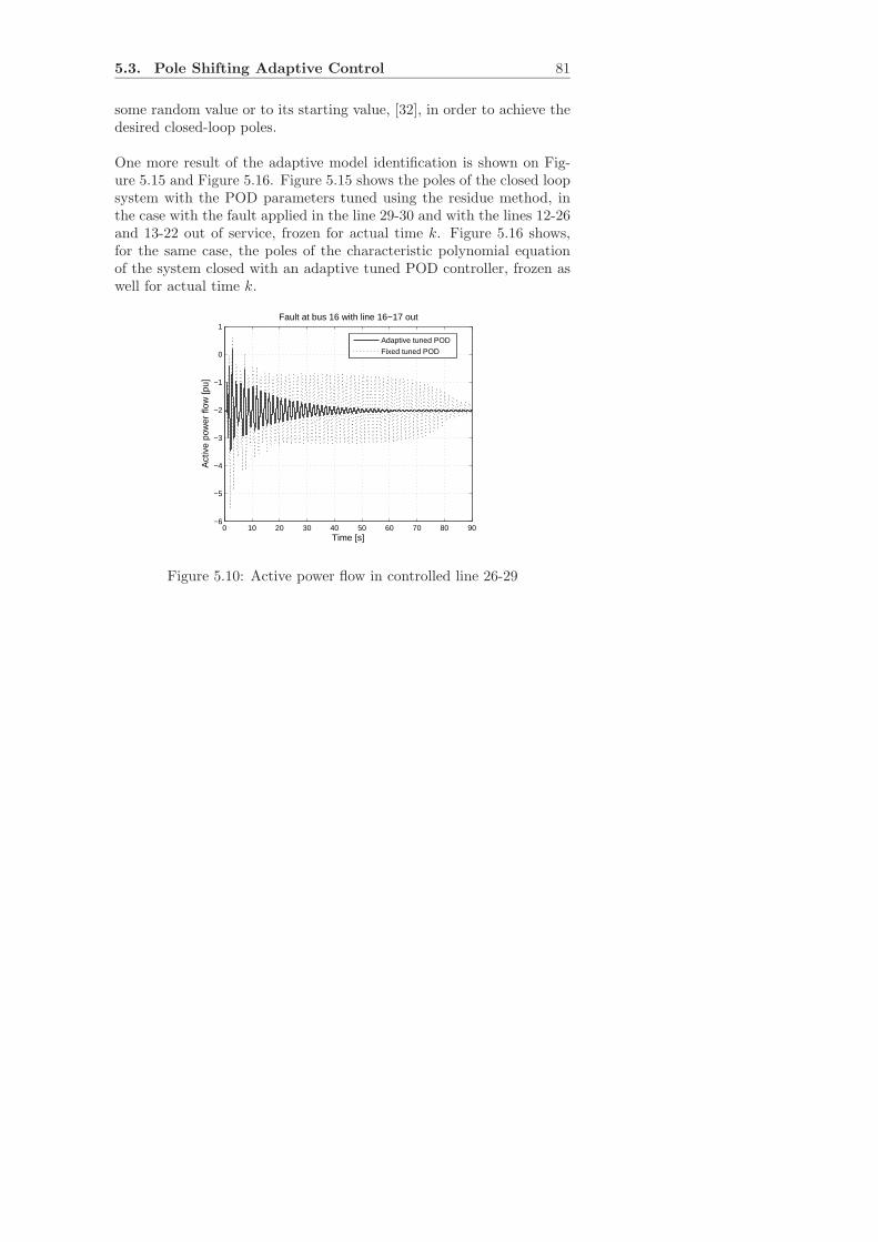
5.3. Pole Shifting Adaptive Control 81
some random value or to its starting value, [32], in order to achieve thedesired closed-loop poles.
One more result of the adaptive model identification is shown on Fig-ure 5.15 and Figure 5.16. Figure 5.15 shows the poles of the closed loopsystem with the POD parameters tuned using the residue method, inthe case with the fault applied in the line 29-30 and with the lines 12-26and 13-22 out of service, frozen for actual time k. Figure 5.16 shows,for the same case, the poles of the characteristic polynomial equationof the system closed with an adaptive tuned POD controller, frozen aswell for actual time k.
0 10 20 30 40 50 60 70 80 90−6
−5
−4
−3
−2
−1
0
1
Time [s]
Act
ive
pow
er fl
ow [p
u]
Fault at bus 16 with line 16−17 out
Adaptive tuned POD
Fixed tuned POD
Figure 5.10: Active power flow in controlled line 26-29
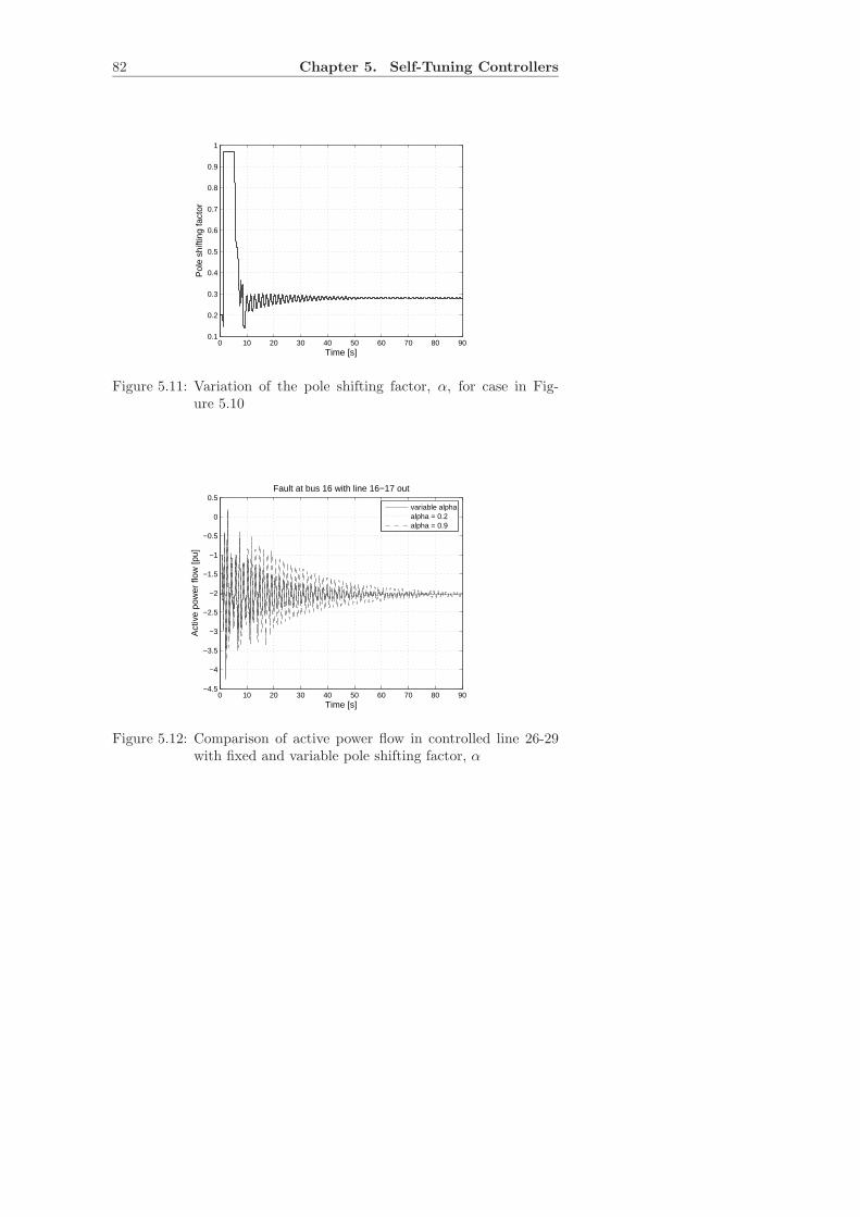
82 Chapter 5. Self-Tuning Controllers
0 10 20 30 40 50 60 70 80 900.1
0.2
0.3
0.4
0.5
0.6
0.7
0.8
0.9
1
Time [s]
Pol
e sh
iftin
g fa
ctor
Figure 5.11: Variation of the pole shifting factor, α, for case in Fig-ure 5.10
0 10 20 30 40 50 60 70 80 90−4.5
−4
−3.5
−3
−2.5
−2
−1.5
−1
−0.5
0
0.5
Time [s]
Act
ive
pow
er fl
ow [p
u]
Fault at bus 16 with line 16−17 out
variable alphaalpha = 0.2alpha = 0.9
Figure 5.12: Comparison of active power flow in controlled line 26-29with fixed and variable pole shifting factor, α
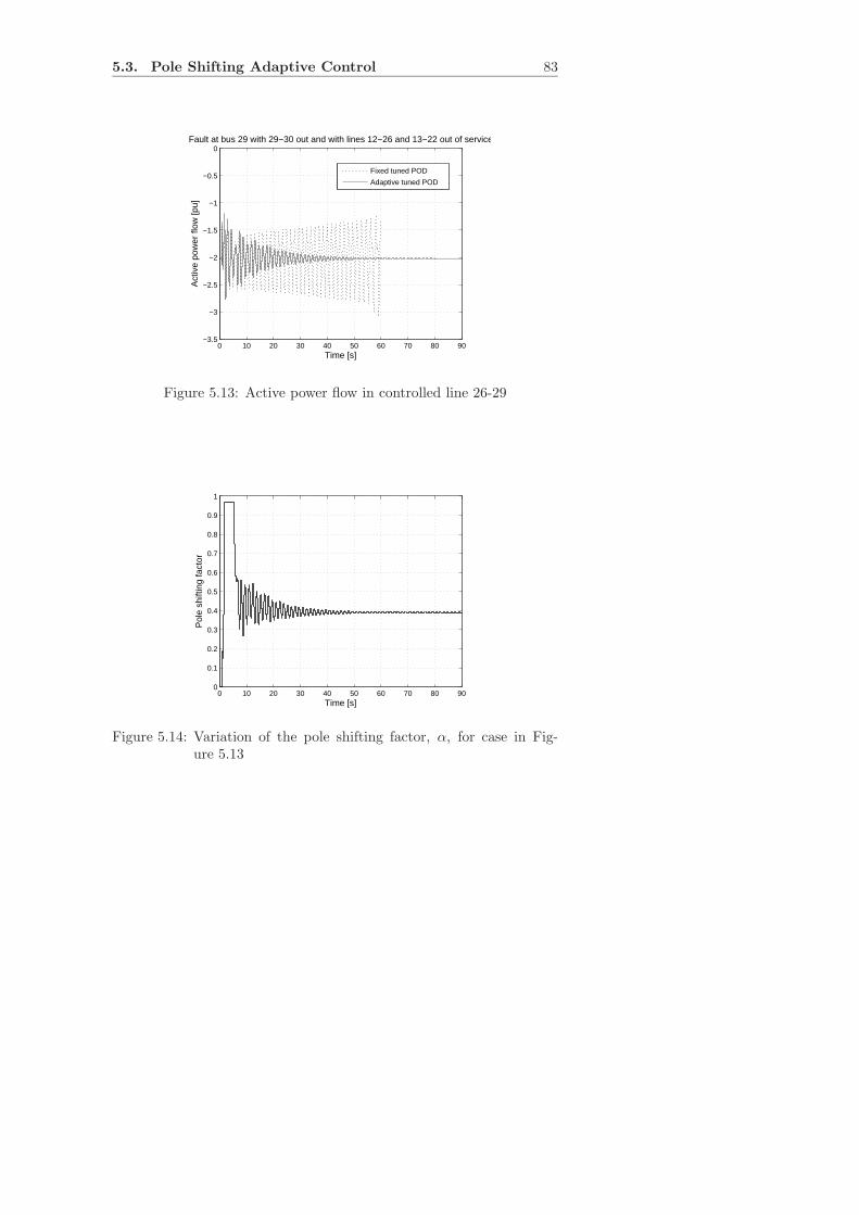
5.3. Pole Shifting Adaptive Control 83
0 10 20 30 40 50 60 70 80 90−3.5
−3
−2.5
−2
−1.5
−1
−0.5
0Fault at bus 29 with 29−30 out and with lines 12−26 and 13−22 out of service
Time [s]
Act
ive
pow
er fl
ow [p
u]
Fixed tuned POD
Adaptive tuned POD
Figure 5.13: Active power flow in controlled line 26-29
0 10 20 30 40 50 60 70 80 900
0.1
0.2
0.3
0.4
0.5
0.6
0.7
0.8
0.9
1
Time [s]
Pol
e sh
iftin
g fa
ctor
Figure 5.14: Variation of the pole shifting factor, α, for case in Fig-ure 5.13
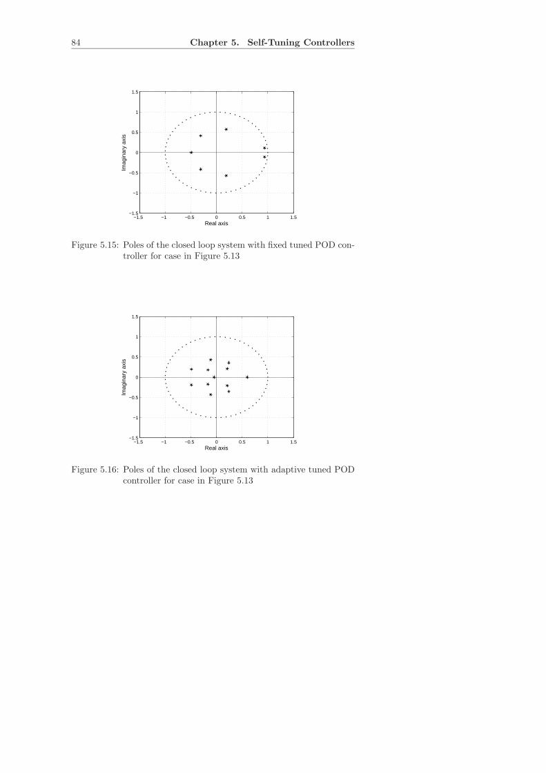
84 Chapter 5. Self-Tuning Controllers
−1.5 −1 −0.5 0 0.5 1 1.5−1.5
−1
−0.5
0
0.5
1
1.5
Imag
inar
y ax
is
Real axis
Figure 5.15: Poles of the closed loop system with fixed tuned POD con-troller for case in Figure 5.13
−1.5 −1 −0.5 0 0.5 1 1.5−1.5
−1
−0.5
0
0.5
1
1.5
Real axis
Imag
inar
y ax
is
Figure 5.16: Poles of the closed loop system with adaptive tuned PODcontroller for case in Figure 5.13
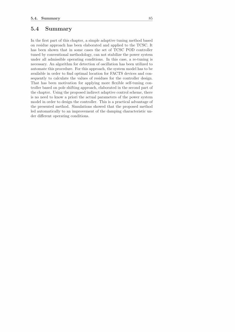
5.4. Summary 85
5.4 Summary
In the first part of this chapter, a simple adaptive tuning method basedon residue approach has been elaborated and applied to the TCSC. Ithas been shown that in some cases the set of TCSC POD controllertuned by conventional methodology, can not stabilize the power systemunder all admissible operating conditions. In this case, a re-tuning isnecessary. An algorithm for detection of oscillation has been utilized toautomate this procedure. For this approach, the system model has to beavailable in order to find optimal location for FACTS devices and con-sequently to calculate the values of residues for the controller design.That has been motivation for applying more flexible self-tuning con-troller based on pole shifting approach, elaborated in the second part ofthe chapter. Using the proposed indirect adaptive control scheme, thereis no need to know a priori the actual parameters of the power systemmodel in order to design the controller. This is a practical advantage ofthe presented method. Simulations showed that the proposed methodled automatically to an improvement of the damping characteristic un-der different operating conditions.

Chapter 6
Coordinated Tuning of
PSS and FACTS POD
Controllers
With a conventional design approach, it might be very difficult to prop-erly handle a coordinated design for multiple controllers and for a va-riety of operating conditions. Power oscillation damping controllers ofFACTS devices (FACTS POD) are effective in contribution to the damp-ing of poorly damped inter-area modes while power system stabilizers(PSSs) are an efficient tool for damping of the local modes, but theycan damp the inter-area modes as well [19]. The aim of tuning bothstabilizers is the same as for tuning the individual ones; to ensure thatthe power system operates with adequate damping over a wide range ofoperating conditions and system configurations.
As a consequence of the action of both stabilizers in the system, thePSSs and FACTS POD, undesired interactions between them may oc-cur [34]. This requires a simultaneous optimization and coordinationof the parameter settings of both stabilizers in order to enhance overallsystem stability and minimizing possible adverse interactions betweenstabilizers.
This chapter presents a method used for the coordinated tuning of POD
87
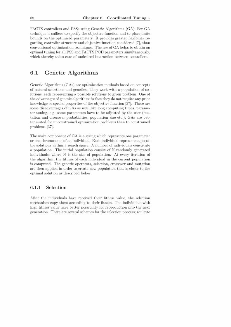
88 Chapter 6. Coordinated Tuning...
FACTS controllers and PSSs using Genetic Algorithms (GA). For GAtechnique it suffices to specify the objective function and to place finitebounds on the optimized parameters. It provides greater flexibility re-garding controller structure and objective function considered [?], thanconventional optimization techniques. The use of GA helps to obtain anoptimal tuning for all PSS and FACTS POD parameters simultaneously,which thereby takes care of undesired interaction between controllers.
6.1 Genetic Algorithms
Genetic Algorithms (GAs) are optimization methods based on conceptsof natural selections and genetics. They work with a population of so-lutions, each representing a possible solutions to given problem. One ofthe advantages of genetic algorithms is that they do not require any priorknowledge or special properties of the objective function [37]. There aresome disadvantages of GAs as well, like long computing times, parame-ter tuning, e.g. some parameters have to be adjusted by the user (mu-tation and crossover probabilities, population size etc.), GAs are bet-ter suited for unconstrained optimization problems than to constrainedproblems [37].
The main component of GA is a string which represents one parameteror one chromosome of an individual. Each individual represents a possi-ble solutions within a search space. A number of individuals constitutea population. The initial population consist of N randomly generatedindividuals, where N is the size of population. At every iteration ofthe algorithm, the fitness of each individual in the current populationis computed. The genetic operators, selection, crossover and mutationare then applied in order to create new population that is closer to theoptimal solution as described below.
6.1.1 Selection
After the individuals have received their fitness value, the selectionmechanism copy them according to their fitness. The individuals withhigh fitness value have better possibility for reproduction into the nextgeneration. There are several schemes for the selection process; roulette
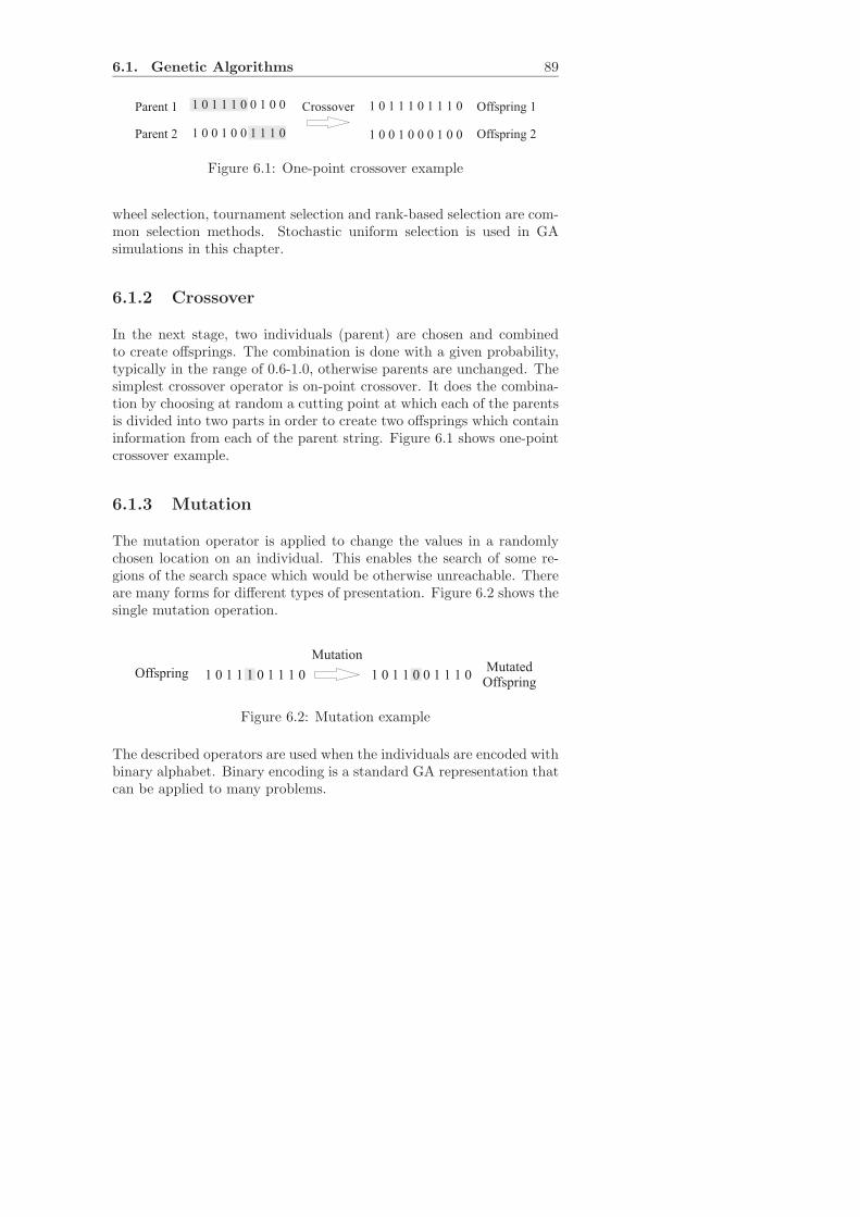
6.1. Genetic Algorithms 89
Figure 6.1: One-point crossover example
wheel selection, tournament selection and rank-based selection are com-mon selection methods. Stochastic uniform selection is used in GAsimulations in this chapter.
6.1.2 Crossover
In the next stage, two individuals (parent) are chosen and combinedto create offsprings. The combination is done with a given probability,typically in the range of 0.6-1.0, otherwise parents are unchanged. Thesimplest crossover operator is on-point crossover. It does the combina-tion by choosing at random a cutting point at which each of the parentsis divided into two parts in order to create two offsprings which containinformation from each of the parent string. Figure 6.1 shows one-pointcrossover example.
6.1.3 Mutation
The mutation operator is applied to change the values in a randomlychosen location on an individual. This enables the search of some re-gions of the search space which would be otherwise unreachable. Thereare many forms for different types of presentation. Figure 6.2 shows thesingle mutation operation.
Figure 6.2: Mutation example
The described operators are used when the individuals are encoded withbinary alphabet. Binary encoding is a standard GA representation thatcan be applied to many problems.
90 Chapter 6. Coordinated Tuning...
The GA requires an initial population to begin the search process. Themost common method is to randomly generate solutions for the entirepopulation. The GA moves from generation to generation selecting andreproducing the parents until a stopping criterion is met. The simpleststopping criterion is a specified maximum number of generations.
6.2 PSS and FACTS POD Controller De-
sign
PSS acts through the excitation system in order to produce an addi-tional damping torque proportional to speed change of the generator,[19], used as input signal for PSS for simulations in this chapter. Itinvolves transfer function consisting of an amplification block, a wash-out block and two lead-lag blocks. The following equation describes thestructure of the PSS used in this dissertation.
HPSS(s) = KPSS
(
sTw
1 + sTw
)(
1 + sT1
1 + sT2
)(
1 + sT3
1 + sT4
)
(6.1)
The lead-lag blocks provide the appropriate phase-lead characteristicsto compensate the phase lag between the exciter input and the generatorelectrical torque.As discussed in Chapter 3, the structure of FACTS POD controller hasa similar structure to that of the PSS controllers.
HFACTS(s) = KFACTS
(
sTw
1 + sTw
)(
1 + sT1
1 + sT2
)2
(6.2)
The time constant Tw is usually considered as a known parameter withsome predefined values.
The objective of the parameter tuning by the GA optimization pro-cedure is to achieve the minimum 5% damping for all oscillatory modesover all operating conditions under consideration, i.e. when all ξi ≥ 5%,the optimization procedure is stopped. Parameters to be determined bythe GA procedure are KPSSi, T1i, T2i, T3i and T4i for PSS controllers,and KFACTSj , T1j and T2j for FACTS POD controllers, where i and jare the numbers of PSS and FACTS POD controllers, respectively.
6.3. Case Study 91
Let Ω represent the set of selected operating points. For a certainoperating point, the power system is linearized around the operatingpoint, the eigenvalues of the closed loop system are computed, and theobjective function is evaluated using the eigenvalues whose have damp-ing ratio less than 5%. The optimization problem to be solved by theGA is formulated as a max-min optimization problem, where the ob-jective function maximizes the minimum damping ratio in all scenariosin Ω [35]. Hence the problem can be mathematically described as theoptimization problem
F = maxp
minn
ξ (6.3)
subject to
KPSSi, min ≤ KPSSi ≤ KPSSi, max
T1i, min ≤ T1i ≤ T1i, max
T2i, min ≤ T2i ≤ T2i, max
T3i, min ≤ T3i ≤ T3i, max
T4i, min ≤ T4i ≤ T4i, max
KFACTSj, min ≤ KFATCSj ≤ KFACTSj, max
T1j, min ≤ T1j ≤ T1j, max
T2j, min ≤ T2j ≤ T2j, max (6.4)
where p is total number of operating conditions under consideration, nis the number of eigenvalues with damping ratio less than 5% and ξ isthe closed-loop damping ratio.
6.3 Case Study
A 16-machine, 68 bus test system, shown in Figure 6.3, is consideredfor the case studies. This is a reduced order equivalent of the inter-connected New England test system (NETS) and New York power sys-tem (NYPS). The static and dynamic data are adopted from [19], andcan be found in Appendix B, but the buses are renumbered keeping thetopology and data the same. All generators except the slack generatorG13 are equipped with static excitation system and power system stabi-lizer (PSS), to ensure appropriate damping for its local modes. FACTS
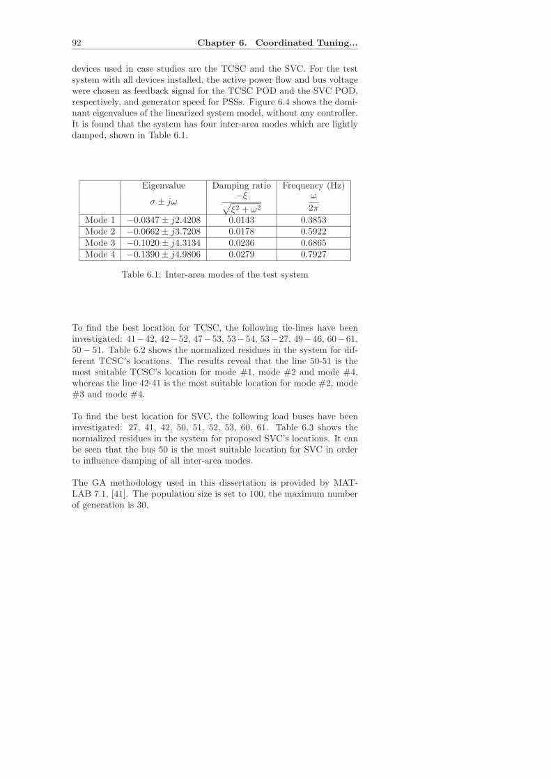
92 Chapter 6. Coordinated Tuning...
devices used in case studies are the TCSC and the SVC. For the testsystem with all devices installed, the active power flow and bus voltagewere chosen as feedback signal for the TCSC POD and the SVC POD,respectively, and generator speed for PSSs. Figure 6.4 shows the domi-nant eigenvalues of the linearized system model, without any controller.It is found that the system has four inter-area modes which are lightlydamped, shown in Table 6.1.
Eigenvalue Damping ratio Frequency (Hz)
σ ± jω−ξ
√
ξ2 + ω2
ω
2π
Mode 1 −0.0347 ± j2.4208 0.0143 0.3853Mode 2 −0.0662 ± j3.7208 0.0178 0.5922Mode 3 −0.1020 ± j4.3134 0.0236 0.6865Mode 4 −0.1390 ± j4.9806 0.0279 0.7927
Table 6.1: Inter-area modes of the test system
To find the best location for TCSC, the following tie-lines have beeninvestigated: 41−42, 42−52, 47−53, 53−54, 53−27, 49−46, 60−61,50 − 51. Table 6.2 shows the normalized residues in the system for dif-ferent TCSC’s locations. The results reveal that the line 50-51 is themost suitable TCSC’s location for mode #1, mode #2 and mode #4,whereas the line 42-41 is the most suitable location for mode #2, mode#3 and mode #4.
To find the best location for SVC, the following load buses have beeninvestigated: 27, 41, 42, 50, 51, 52, 53, 60, 61. Table 6.3 shows thenormalized residues in the system for proposed SVC’s locations. It canbe seen that the bus 50 is the most suitable location for SVC in orderto influence damping of all inter-area modes.
The GA methodology used in this dissertation is provided by MAT-LAB 7.1, [41]. The population size is set to 100, the maximum numberof generation is 30.
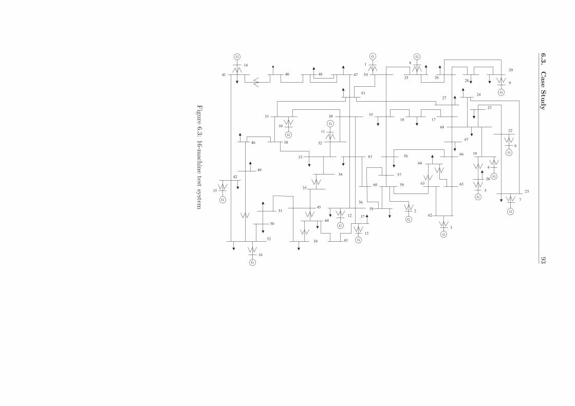
6.3
.C
ase
Stu
dy
93
41
14
40 48 47 54
1 8
25 2628
29
9
24
21
22
6
7
235
20
66
67
68
1718
5530
53
27
61 56
64
656358
57
60
592
62
3
13
37
36
43
44
45
35
34
33
32
10
3846
49
42
15
52
50
51
16
39
12
11
31
GG
G
G
G
G
G
G
G
19
G
4
G
G
G
G
G
G
Figu
re6.3:
16-mach
ine
testsy
stem
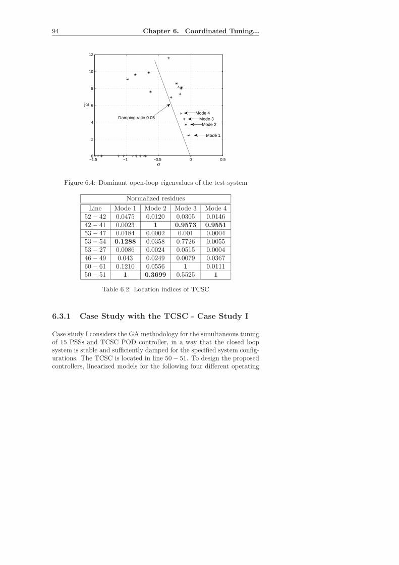
94 Chapter 6. Coordinated Tuning...
−1.5 −1 −0.5 0 0.50
2
4
6
8
10
12
σ
Mode 1
Mode 2Mode 3
Mode 4Damping ratio 0.05
jω
Figure 6.4: Dominant open-loop eigenvalues of the test system
Normalized residues
Line Mode 1 Mode 2 Mode 3 Mode 452 − 42 0.0475 0.0120 0.0305 0.014642 − 41 0.0023 1 0.9573 0.9551
53 − 47 0.0184 0.0002 0.001 0.000453 − 54 0.1288 0.0358 0.7726 0.005553 − 27 0.0086 0.0024 0.0515 0.000446 − 49 0.043 0.0249 0.0079 0.036760 − 61 0.1210 0.0556 1 0.011150 − 51 1 0.3699 0.5525 1
Table 6.2: Location indices of TCSC
6.3.1 Case Study with the TCSC - Case Study I
Case study I considers the GA methodology for the simultaneous tuningof 15 PSSs and TCSC POD controller, in a way that the closed loopsystem is stable and sufficiently damped for the specified system config-urations. The TCSC is located in line 50 − 51. To design the proposedcontrollers, linearized models for the following four different operating
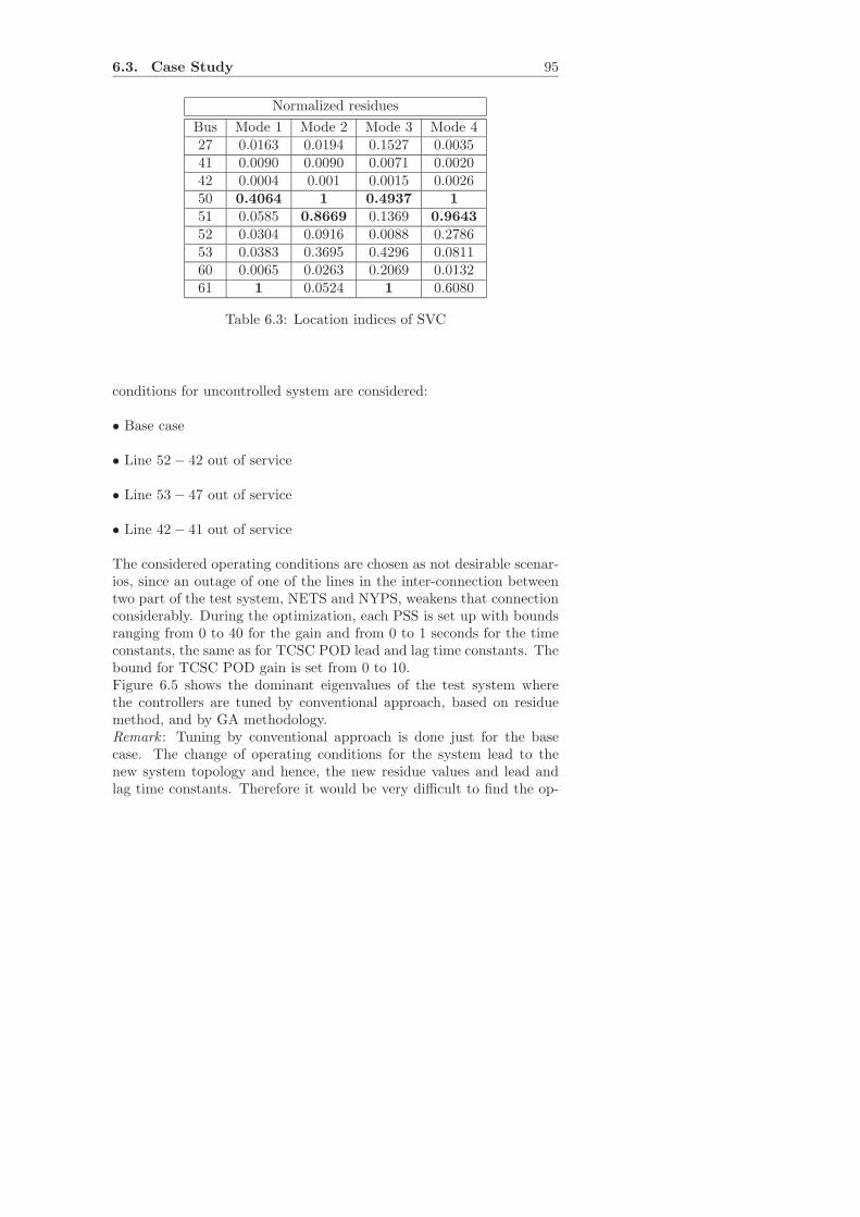
6.3. Case Study 95
Normalized residues
Bus Mode 1 Mode 2 Mode 3 Mode 427 0.0163 0.0194 0.1527 0.003541 0.0090 0.0090 0.0071 0.002042 0.0004 0.001 0.0015 0.002650 0.4064 1 0.4937 1
51 0.0585 0.8669 0.1369 0.9643
52 0.0304 0.0916 0.0088 0.278653 0.0383 0.3695 0.4296 0.081160 0.0065 0.0263 0.2069 0.013261 1 0.0524 1 0.6080
Table 6.3: Location indices of SVC
conditions for uncontrolled system are considered:
• Base case
• Line 52 − 42 out of service
• Line 53 − 47 out of service
• Line 42 − 41 out of service
The considered operating conditions are chosen as not desirable scenar-ios, since an outage of one of the lines in the inter-connection betweentwo part of the test system, NETS and NYPS, weakens that connectionconsiderably. During the optimization, each PSS is set up with boundsranging from 0 to 40 for the gain and from 0 to 1 seconds for the timeconstants, the same as for TCSC POD lead and lag time constants. Thebound for TCSC POD gain is set from 0 to 10.Figure 6.5 shows the dominant eigenvalues of the test system wherethe controllers are tuned by conventional approach, based on residuemethod, and by GA methodology.Remark : Tuning by conventional approach is done just for the basecase. The change of operating conditions for the system lead to thenew system topology and hence, the new residue values and lead andlag time constants. Therefore it would be very difficult to find the op-
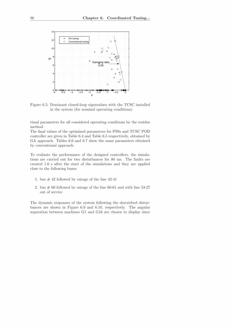
96 Chapter 6. Coordinated Tuning...
−4 −3.5 −3 −2.5 −2 −1.5 −1 −0.5 00
2
4
6
8
10
12
14
σ
GA tuningConventional tuning
Damping ratio0.05
jω
Figure 6.5: Dominant closed-loop eigenvalues with the TCSC installedin the system (for nominal operating conditions)
timal parameters for all considered operating conditions by the residuemethod.The final values of the optimized parameters for PSSs and TCSC PODcontroller are given in Table 6.4 and Table 6.5 respectively, obtained byGA approach. Tables 6.6 and 6.7 show the same parameters obtainedby conventional approach.
To evaluate the performance of the designed controllers, the simula-tions are carried out for two disturbances for 80 ms. The faults arecreated 1.0 s after the start of the simulations and they are appliedclose to the following buses:
1. bus # 42 followed by outage of the line 42-41
2. bus # 60 followed by outage of the line 60-61 and with line 53-27out of service
The dynamic responses of the system following the descriebed distur-bances are shown in Figure 6.9 and 6.10, respectively. The angularseparation between machines G1 and G16 are chosen to display since
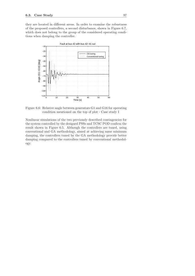
6.3. Case Study 97
they are located in different areas. In order to examine the robustnessof the proposed controllers, a second disturbance, shown in Figure 6.7,which does not belong to the group of the considered operating condi-tions when damping the controller.
0 10 20 30 40 50 60−110
−100
−90
−80
−70
−60
−50
−40
−30
−20
−10Fault at bus 42 with bus 42−41 out
Time [s]
Ang
le (
G1−
G16
) [d
eg]
GA tuning
Conventional tuning
Figure 6.6: Relative angle between generators G1 and G16 for operatingcondition mentioned on the top of plot - Case study I
Nonlinear simulations of the two previously described contingencies forthe system controlled by the designed PSSs and TCSC POD confirm theresult shown in Figure 6.5. Although the controllers are tuned, usingconventional and GA methodology, aimed at achieving same minimumdamping, the controllers tuned by the GA methodology provide betterdamping compared to the controllers tuned by conventional methodol-ogy.
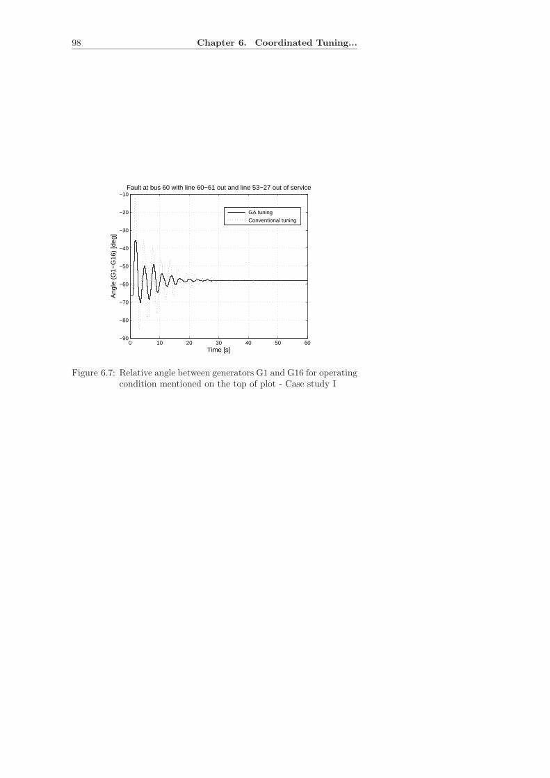
98 Chapter 6. Coordinated Tuning...
0 10 20 30 40 50 60−90
−80
−70
−60
−50
−40
−30
−20
−10
Time [s]
Ang
le (
G1−
G16
) [d
eg]
Fault at bus 60 with line 60−61 out and line 53−27 out of service
GA tuning
Conventional tuning
Figure 6.7: Relative angle between generators G1 and G16 for operatingcondition mentioned on the top of plot - Case study I
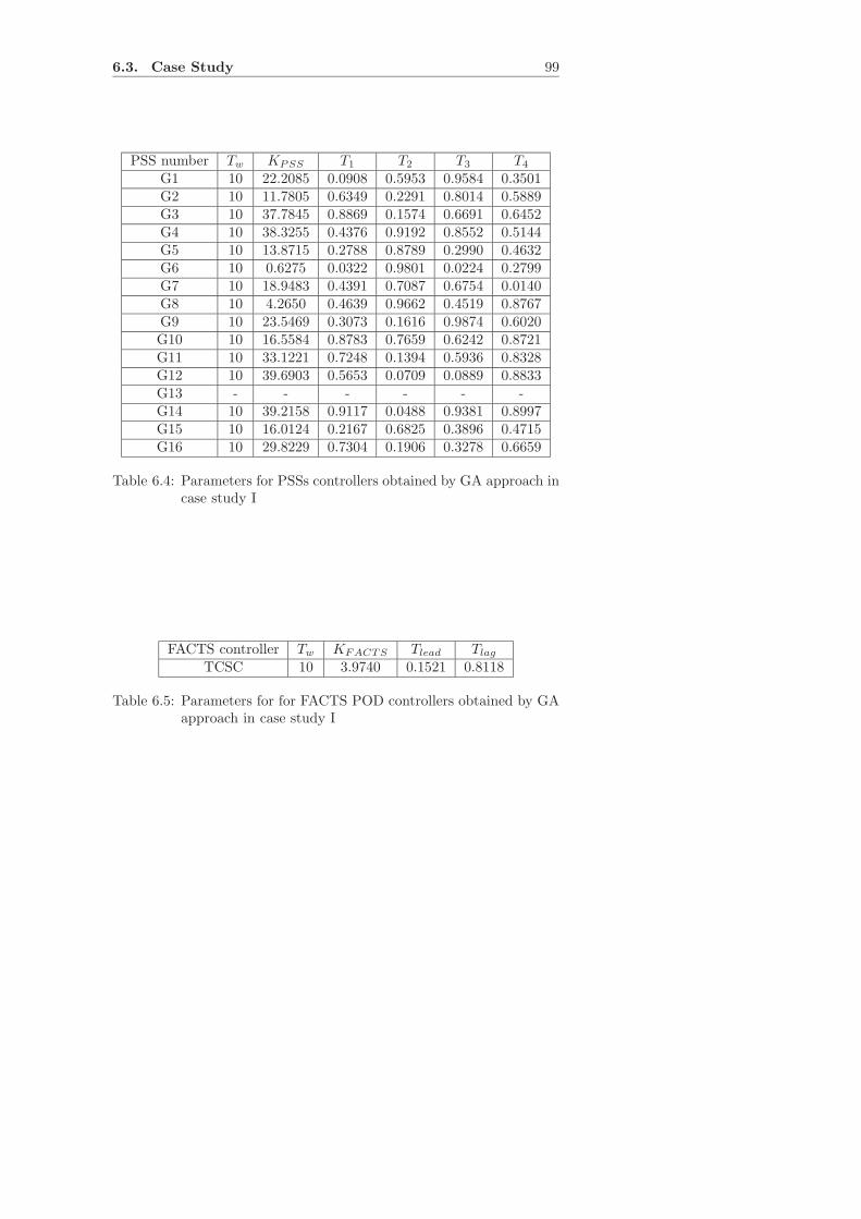
6.3. Case Study 99
PSS number Tw KPSS T1 T2 T3 T4
G1 10 22.2085 0.0908 0.5953 0.9584 0.3501G2 10 11.7805 0.6349 0.2291 0.8014 0.5889G3 10 37.7845 0.8869 0.1574 0.6691 0.6452G4 10 38.3255 0.4376 0.9192 0.8552 0.5144G5 10 13.8715 0.2788 0.8789 0.2990 0.4632G6 10 0.6275 0.0322 0.9801 0.0224 0.2799G7 10 18.9483 0.4391 0.7087 0.6754 0.0140G8 10 4.2650 0.4639 0.9662 0.4519 0.8767G9 10 23.5469 0.3073 0.1616 0.9874 0.6020G10 10 16.5584 0.8783 0.7659 0.6242 0.8721G11 10 33.1221 0.7248 0.1394 0.5936 0.8328G12 10 39.6903 0.5653 0.0709 0.0889 0.8833G13 - - - - - -G14 10 39.2158 0.9117 0.0488 0.9381 0.8997G15 10 16.0124 0.2167 0.6825 0.3896 0.4715G16 10 29.8229 0.7304 0.1906 0.3278 0.6659
Table 6.4: Parameters for PSSs controllers obtained by GA approach incase study I
FACTS controller Tw KFACTS Tlead Tlag
TCSC 10 3.9740 0.1521 0.8118
Table 6.5: Parameters for for FACTS POD controllers obtained by GAapproach in case study I

100 Chapter 6. Coordinated Tuning...
PSS number Tw KPSS T1 T2 T3 T4
G1 10 10 0.093 0.1695 0.0930 0.1695G2 10 15 0.0871 0.1179 0.0871 0.1179G3 10 20 0.1326 0.1405 0.1326 0.1405G4 10 20 0.0947 0.2214 0.0947 0.2214G5 10 20 0.0989 0.2121 0.0989 0.2121G6 10 20 0.1210 0.1734 0.1210 0.1734G7 10 25 0.0687 0.1492 0.0687 0.1492G8 10 20 0.0848 0.1859 0.0848 0.1859G9 10 28 0.1063 0.1483 0.1063 0.1483G10 10 20 0.1196 0.1275 0.1196 0.1275G11 10 10 0.0839 0.0892 0.0839 0.0892G12 10 10 0.1221 0.1348 0.1221 0.1348G13 - - - - - -G14 10 40 0.2613 0.2766 0.2613 0.2766G15 10 40 0.2145 0.2498 0.2145 0.2498G16 10 40 0.1951 0.2062 0.1951 0.2062
Table 6.6: Parameters for PSSs controllers obtained by conventional ap-proach in case study I
FACTS controller Tw KFACTS Tlead Tlag
TCSC 10 2 0.1470 0.9395
Table 6.7: Parameters for for FACTS POD controllers obtained by con-ventional approach in case study I
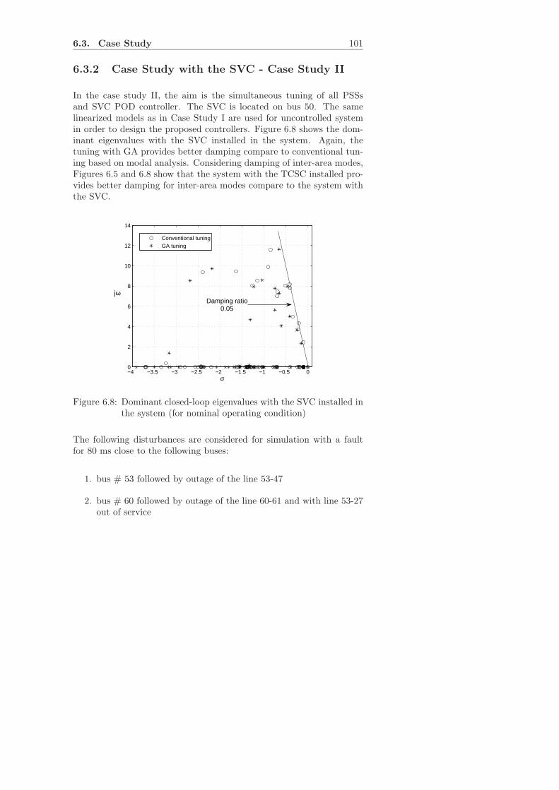
6.3. Case Study 101
6.3.2 Case Study with the SVC - Case Study II
In the case study II, the aim is the simultaneous tuning of all PSSsand SVC POD controller. The SVC is located on bus 50. The samelinearized models as in Case Study I are used for uncontrolled systemin order to design the proposed controllers. Figure 6.8 shows the dom-inant eigenvalues with the SVC installed in the system. Again, thetuning with GA provides better damping compare to conventional tun-ing based on modal analysis. Considering damping of inter-area modes,Figures 6.5 and 6.8 show that the system with the TCSC installed pro-vides better damping for inter-area modes compare to the system withthe SVC.
−4 −3.5 −3 −2.5 −2 −1.5 −1 −0.5 00
2
4
6
8
10
12
14
σ
Conventional tuningGA tuning
jωDamping ratio
0.05
Figure 6.8: Dominant closed-loop eigenvalues with the SVC installed inthe system (for nominal operating condition)
The following disturbances are considered for simulation with a faultfor 80 ms close to the following buses:
1. bus # 53 followed by outage of the line 53-47
2. bus # 60 followed by outage of the line 60-61 and with line 53-27out of service
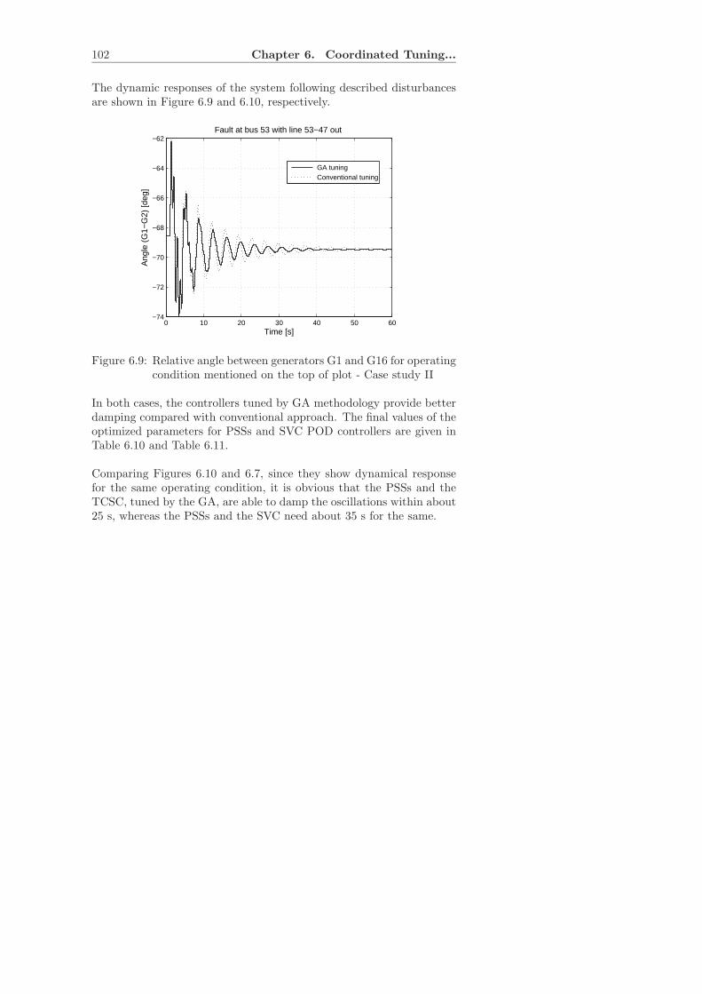
102 Chapter 6. Coordinated Tuning...
The dynamic responses of the system following described disturbancesare shown in Figure 6.9 and 6.10, respectively.
0 10 20 30 40 50 60−74
−72
−70
−68
−66
−64
−62
Time [s]
Ang
le (
G1−
G2)
[deg
]
Fault at bus 53 with line 53−47 out
GA tuning Conventional tuning
Figure 6.9: Relative angle between generators G1 and G16 for operatingcondition mentioned on the top of plot - Case study II
In both cases, the controllers tuned by GA methodology provide betterdamping compared with conventional approach. The final values of theoptimized parameters for PSSs and SVC POD controllers are given inTable 6.10 and Table 6.11.
Comparing Figures 6.10 and 6.7, since they show dynamical responsefor the same operating condition, it is obvious that the PSSs and theTCSC, tuned by the GA, are able to damp the oscillations within about25 s, whereas the PSSs and the SVC need about 35 s for the same.
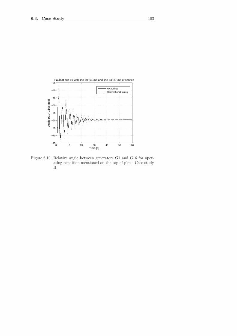
6.3. Case Study 103
0 10 20 30 40 50 60−75
−70
−65
−60
−55
−50
−45
−40
−35
Time [s]
Ang
le (
G1−
G16
) [d
eg]
Fault at bus 60 with line 60−61 out and line 53−27 out of service
GA tuning
Conventional tuning
Figure 6.10: Relative angle between generators G1 and G16 for oper-ating condition mentioned on the top of plot - Case studyII
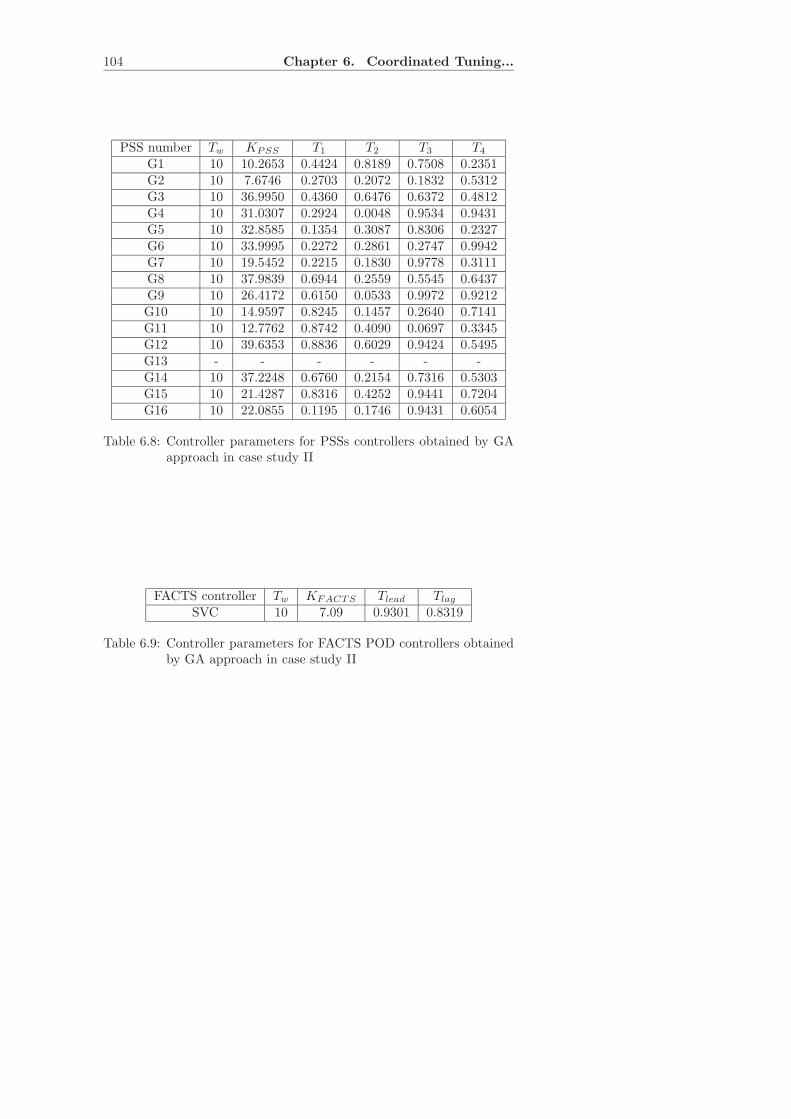
104 Chapter 6. Coordinated Tuning...
PSS number Tw KPSS T1 T2 T3 T4
G1 10 10.2653 0.4424 0.8189 0.7508 0.2351G2 10 7.6746 0.2703 0.2072 0.1832 0.5312G3 10 36.9950 0.4360 0.6476 0.6372 0.4812G4 10 31.0307 0.2924 0.0048 0.9534 0.9431G5 10 32.8585 0.1354 0.3087 0.8306 0.2327G6 10 33.9995 0.2272 0.2861 0.2747 0.9942G7 10 19.5452 0.2215 0.1830 0.9778 0.3111G8 10 37.9839 0.6944 0.2559 0.5545 0.6437G9 10 26.4172 0.6150 0.0533 0.9972 0.9212G10 10 14.9597 0.8245 0.1457 0.2640 0.7141G11 10 12.7762 0.8742 0.4090 0.0697 0.3345G12 10 39.6353 0.8836 0.6029 0.9424 0.5495G13 - - - - - -G14 10 37.2248 0.6760 0.2154 0.7316 0.5303G15 10 21.4287 0.8316 0.4252 0.9441 0.7204G16 10 22.0855 0.1195 0.1746 0.9431 0.6054
Table 6.8: Controller parameters for PSSs controllers obtained by GAapproach in case study II
FACTS controller Tw KFACTS Tlead Tlag
SVC 10 7.09 0.9301 0.8319
Table 6.9: Controller parameters for FACTS POD controllers obtainedby GA approach in case study II
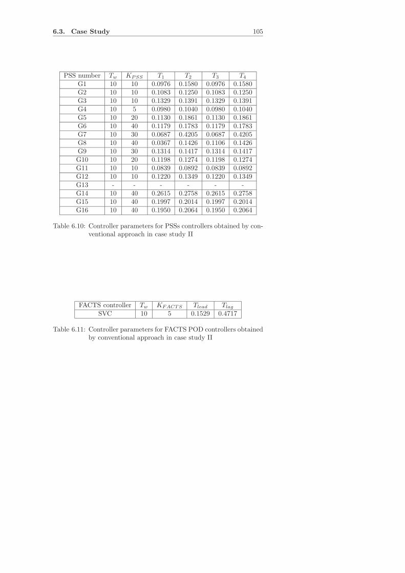
6.3. Case Study 105
PSS number Tw KPSS T1 T2 T3 T4
G1 10 10 0.0976 0.1580 0.0976 0.1580G2 10 10 0.1083 0.1250 0.1083 0.1250G3 10 10 0.1329 0.1391 0.1329 0.1391G4 10 5 0.0980 0.1040 0.0980 0.1040G5 10 20 0.1130 0.1861 0.1130 0.1861G6 10 40 0.1179 0.1783 0.1179 0.1783G7 10 30 0.0687 0.4205 0.0687 0.4205G8 10 40 0.0367 0.1426 0.1106 0.1426G9 10 30 0.1314 0.1417 0.1314 0.1417G10 10 20 0.1198 0.1274 0.1198 0.1274G11 10 10 0.0839 0.0892 0.0839 0.0892G12 10 10 0.1220 0.1349 0.1220 0.1349G13 - - - - - -G14 10 40 0.2615 0.2758 0.2615 0.2758G15 10 40 0.1997 0.2014 0.1997 0.2014G16 10 40 0.1950 0.2064 0.1950 0.2064
Table 6.10: Controller parameters for PSSs controllers obtained by con-ventional approach in case study II
FACTS controller Tw KFACTS Tlead Tlag
SVC 10 5 0.1529 0.4717
Table 6.11: Controller parameters for FACTS POD controllers obtainedby conventional approach in case study II

106 Chapter 6. Coordinated Tuning...
6.3.3 Case Study with the TCSC and the SVC -
Case Study III
This case study presents the results after applying GA methodologyto the simultaneous tuning of all PSSs, the SVC and the TCSC PODcontrollers in test system. Since there are two FACTS POD controllers,the aim is to achieve 7% damping for all oscillatory modes over all op-erating conditions under consideration. According to the results shownin Table 6.2 and Table 6.3, line 41 − 42 is chosen for TCSC location,whereas bus 50 is chosen for SVC location. To design the proposedcontrollers, linearized models for the following four different operatingconditions for uncontrolled system are considered:
• Base case
• Line 53 − 47 and line 60 − 61 out of service
• Line 53 − 54 and line 39 − 45 out of service
• Line 46 − 49 and line 53 − 47 out of service
The following disturbances are considered for simulation with a faultfor 80 ms close to the following buses:
1. bus # 46 followed by outage of the line 46-49 and with line 53-47out of service
2. bus # 60 followed by outage of the line 60-61 and with line 53-27out of service
Dynamic responses for above disturbances are shown in Figures 6.12and 6.13, respectively. These figures exhibit the relative angular sepa-ration between the generators located in separate geographical regions.The final values of the optimized parameters for PSSs and SVC PODcontrollers are given in Table 6.14 and Table 6.15.
As in case studies I and II, the GA methodology provides better damp-ing compared with conventional damping. To evaluate the performance
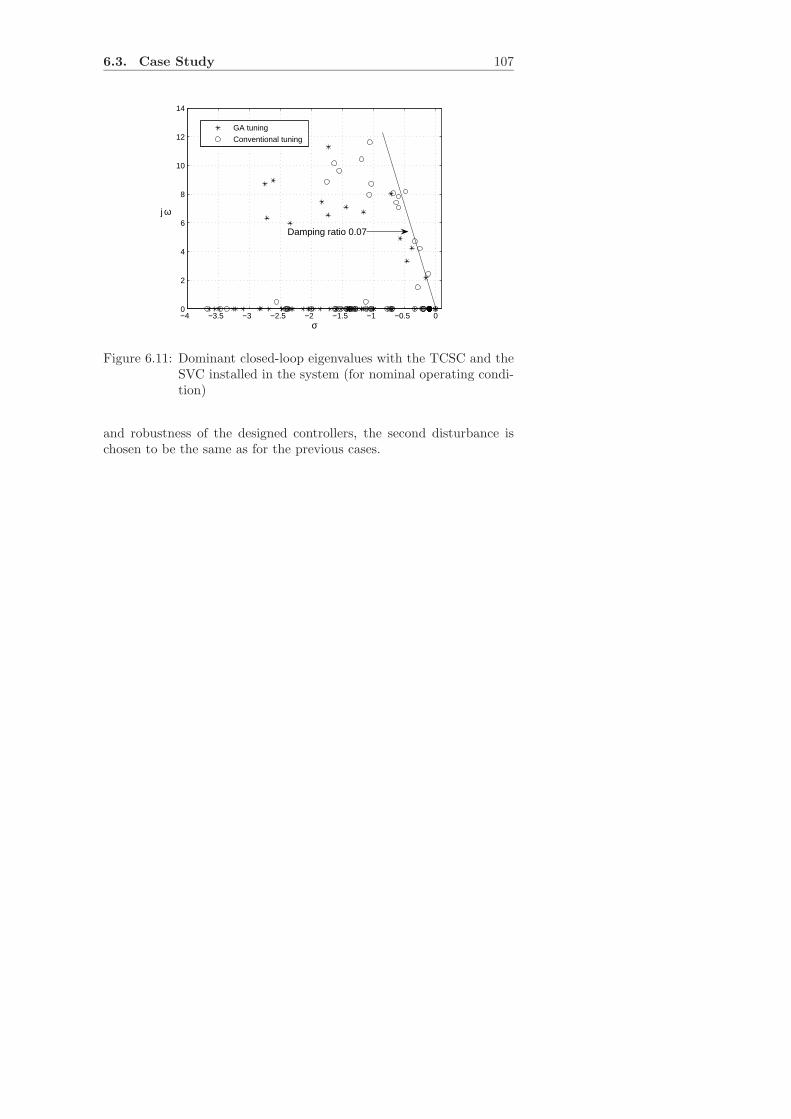
6.3. Case Study 107
−4 −3.5 −3 −2.5 −2 −1.5 −1 −0.5 00
2
4
6
8
10
12
14
σ
GA tuning
Conventional tuning
Damping ratio 0.07
j ω
Figure 6.11: Dominant closed-loop eigenvalues with the TCSC and theSVC installed in the system (for nominal operating condi-tion)
and robustness of the designed controllers, the second disturbance ischosen to be the same as for the previous cases.
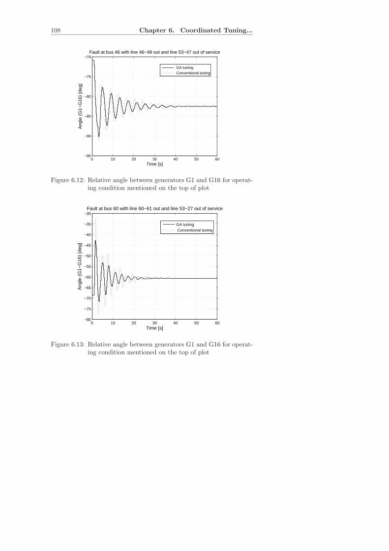
108 Chapter 6. Coordinated Tuning...
0 10 20 30 40 50 60−95
−90
−85
−80
−75
−70Fault at bus 46 with line 46−49 out and line 53−47 out of service
Time [s]
Ang
le (
G1−
G16
) [d
eg]
GA tuning Conventional tuning
Figure 6.12: Relative angle between generators G1 and G16 for operat-ing condition mentioned on the top of plot
0 10 20 30 40 50 60−80
−75
−70
−65
−60
−55
−50
−45
−40
−35
−30
Time [s]
Ang
le (
G1−
G16
) [d
eg]
Fault at bus 60 with line 60−61 out and line 53−27 out of service
GA tuning Conventional tuning
Figure 6.13: Relative angle between generators G1 and G16 for operat-ing condition mentioned on the top of plot
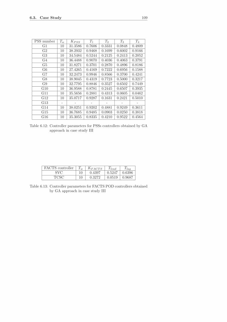
6.3. Case Study 109
PSS number Tw KPSS T1 T2 T3 T4
G1 10 31.3586 0.7606 0.3331 0.0848 0.4809G2 10 38.2932 0.9468 0.1699 0.6002 0.9166G3 10 34.5484 0.5244 0.2125 0.2413 0.2052G4 10 36.4488 0.9070 0.4036 0.4063 0.3791G5 10 31.8271 0.3701 0.2870 0.4896 0.8186G6 10 27.4265 0.4169 0.7222 0.6956 0.1588G7 10 32.2473 0.9946 0.8566 0.3700 0.4241G8 10 38.9045 0.4319 0.7723 0.5000 0.3217G9 10 32.7795 0.8846 0.3527 0.6502 0.7449G10 10 36.9588 0.8781 0.2445 0.6507 0.3935G11 10 35.5656 0.2881 0.4313 0.0605 0.0462G12 10 35.0717 0.9287 0.1631 0.2421 0.5010G13 - - - - - -G14 10 38.0251 0.9202 0.4881 0.9249 0.3611G15 10 36.7685 0.9485 0.0903 0.0250 0.3818G16 10 35.3055 0.8335 0.4210 0.9522 0.4564
Table 6.12: Controller parameters for PSSs controllers obtained by GAapproach in case study III
FACTS controller Tw KFACTS Tlead Tlag
SVC 10 0.4397 0.5247 0.6396TCSC 10 0.3272 0.0519 0.9687
Table 6.13: Controller parameters for FACTS POD controllers obtainedby GA approach in case study III

110 Chapter 6. Coordinated Tuning...
PSS number Tw KPSS T1 T2 T3 T4
G1 10 40 0.0929 0.1696 0.0929 0.1696G2 10 25 0.1083 0.1250 0.1083 0.1250G3 10 25 0.1118 0.1212 0.1118 0.1212G4 10 40 0.0947 0.2214 0.0947 0.2214G5 10 40 0.0989 0.2121 0.0989 0.2121G6 10 35 0.1210 0.1734 0.1210 0.1734G7 10 40 0.0687 0.1492 0.0687 0.1492G8 10 40 0.0850 0.1856 0.0850 0.1856G9 10 40 0.1065 0.1481 0.1065 0.1481G10 10 30 0.1198 0.1277 0.1198 0.1274G11 10 15 0.0839 0.0892 0.0839 0.0892G12 10 25 0.1220 0.1349 0.1220 0.1349G13 - - - - - -G14 10 40 0.4018 0.4174 0.4018 0.4174G15 10 40 0.1254 0.1412 0.1254 0.1412G16 10 40 0.2116 0.2124 0.2116 0.2124
Table 6.14: Controller parameters for PSSs controllers obtained by con-ventional approach in case study III
FACTS controller Tw KFACTS Tlead Tlag
SVC 10 2 0.1137 0.3954TCSC 10 0.5 0.0737 0.6098
Table 6.15: Controller parameters for FACTS POD controllers obtainedby conventional approach in case study III

6.4. Summary 111
6.4 Summary
In this chapter, simultaneous tuning of multiple PSSs and FACTS PODcontrollers has been illustrated using GA methodology. The controldesign methodology was illustrated by three case studies. In the firsttwo cases, the POD controllers were designed for 15 PSSs and a different,single FACTS POD controller. In the third case, the aim was to tune 15PSSs and two FACTS POD controllers. The performance of the designwas validate using non-linear simulations. Furthermore, comparisonwith the conventional tuning procedure showed that the performance ismore robust when damping controllers were designed by GA procedure.

Chapter 7
Concluding Remarks
In this thesis, different control design methodologies for designing FACTSpower flow controllers and power oscillations damping controllers inpower systems have been illustrated.
The injection models of the Thyristor Controlled Series Capacitor (TCSC),Unified Power Flow Controllers (UPFC) and Static VAR Compensator(SVC) with their power flow controllers have been demonstrated. Theinjection models are very simple to implement and they have been ap-propriate for the kind of investigation carried out in this dissertation.The software for both steady-state study and dynamic study of largepower systems embedded with FACTS devices have been developed.
The application of FACTS damping controllers, using conventional ap-proach based on the residue method turned out to lack robustness underchanged operating conditions. Poorly damped or even unstable oscilla-tions can result in instability, since the controller parameters yieldingsatisfactory damping for one operating condition may no longer be validfor another one. In those cases, a re-tuning is necessary. That providedthe motivation for developing an adaptive control strategy.
A simple adaptive tuning method based on the residue approach hasbeen developed and applied to the TCSC. The disadvantage of this sim-ple approach is that the system model has to be available in order tofind optimal location for FACTS devices and consequently to calculate
113
114 Chapter 7. Concluding Remarks
the values of residues for the controller design. This is the reason for theimplementation of a more flexible self-tuning controller. The pole shift-ing method was applied in the control design. As the system dynamicsare identified on-line, based on the automatic detection of oscillations inpower systems using dynamic data from the system, the most dominantoscillation mode present at any time is identified. Hence, the controlprovides maximum damping of the identified frequency all the time,under different operating conditions, leading to an improvement of thedamping characteristic.
In general, the optimal location of the FACTS controller obtained ac-cording to the dynamic criteria is not the same as the one obtainedaccording to the static criteria. A compromise has to be found for eachparticular case, considering multiple tasks, for example power flow con-trol and damping of oscillations. The procedure for considering theTCSC location in order to satisfy the mentioned requirements has beenpresented. As the static criteria (for optimal location of the power flowcontroller), power flow sensitivity analysis has been used; as the dy-namic criteria (for optimal location of the damping controller), residueanalysis has been used. Verification by simulation matched predictedlocation as optimally selected TCSC location with respect to both con-trol objectives.
The concept of simultaneous coordination of multiple controllers in thesystem, like PSS and FACTS POD controllers, has been applied. Theconcept has been based on Genetic Algorithm (GA) methodology, inwhich an optimization problem to be solved is to determine the con-troller parameters so that they provide required damping of the closed-loop system, under different operating conditions. Furthermore, com-parison with the conventional based tuning procedure showed that theperformance is more robust when damping controllers were designed byGAs procedure.
In this thesis, on-line tuning was applied just on the TCSC. It would bedesirable to apply all proposed on-line approaches to FACTS devices,e.g. SVC and UPFC. This task could be the subject of future research.
Designing POD controllers, local signals as a feedback signals were usedin this work. In general, the use of phasor measurement units (PMU)ensures transmission of remote signals in almost real time. Allowing the

115
controller to use multiple input signals, some of which might be remote,could prove as more effective in damping of oscillations. Moreover, itmight be possible to build a hierarchical control scheme in order toachieve better control of oscillations and, for example, optimization ofpower flow, especially in case of multiple contingencies. Future researchin this direction would provide more insight into these possibilities.


Appendix A
IEEE 39 Bus Test
System Data
The topology of the system is shown in Figure 6.3. All data here are inpu with a base power of 100 MVA.
Bus Nr. Voltage Power generation Real load Reactive load
1 1.03 10.00 11.04 2.502 0.982 - 0.092 0.0463 0.983 6.50 0.00 0.004 0.997 6.32 0.00 0.005 1.011 5.08 0.00 0.006 1.050 6.50 0.00 0.007 1.063 5.60 0.00 0.008 1.0278 5.40 0.00 0.009 1.0265 8.30 0.00 0.0010 1.045 2.50 0.00 0.00
Table A.1: Machine bus data
117
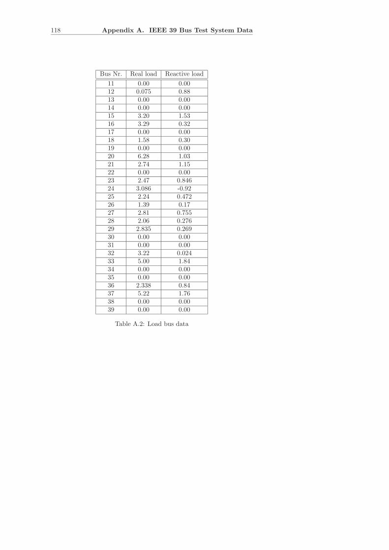
118 Appendix A. IEEE 39 Bus Test System Data
Bus Nr. Real load Reactive load
11 0.00 0.0012 0.075 0.8813 0.00 0.0014 0.00 0.0015 3.20 1.5316 3.29 0.3217 0.00 0.0018 1.58 0.3019 0.00 0.0020 6.28 1.0321 2.74 1.1522 0.00 0.0023 2.47 0.84624 3.086 -0.9225 2.24 0.47226 1.39 0.1727 2.81 0.75528 2.06 0.27629 2.835 0.26930 0.00 0.0031 0.00 0.0032 3.22 0.02433 5.00 1.8434 0.00 0.0035 0.00 0.0036 2.338 0.8437 5.22 1.7638 0.00 0.0039 0.00 0.00
Table A.2: Load bus data
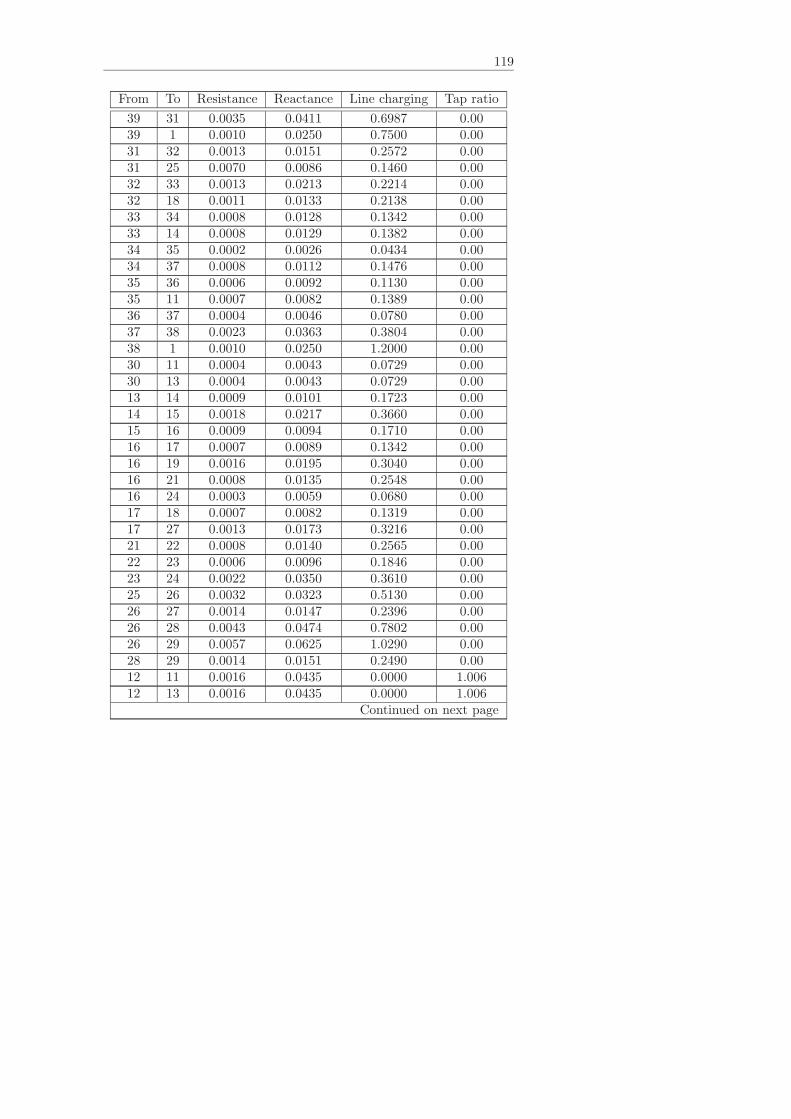
119
From To Resistance Reactance Line charging Tap ratio
39 31 0.0035 0.0411 0.6987 0.0039 1 0.0010 0.0250 0.7500 0.0031 32 0.0013 0.0151 0.2572 0.0031 25 0.0070 0.0086 0.1460 0.0032 33 0.0013 0.0213 0.2214 0.0032 18 0.0011 0.0133 0.2138 0.0033 34 0.0008 0.0128 0.1342 0.0033 14 0.0008 0.0129 0.1382 0.0034 35 0.0002 0.0026 0.0434 0.0034 37 0.0008 0.0112 0.1476 0.0035 36 0.0006 0.0092 0.1130 0.0035 11 0.0007 0.0082 0.1389 0.0036 37 0.0004 0.0046 0.0780 0.0037 38 0.0023 0.0363 0.3804 0.0038 1 0.0010 0.0250 1.2000 0.0030 11 0.0004 0.0043 0.0729 0.0030 13 0.0004 0.0043 0.0729 0.0013 14 0.0009 0.0101 0.1723 0.0014 15 0.0018 0.0217 0.3660 0.0015 16 0.0009 0.0094 0.1710 0.0016 17 0.0007 0.0089 0.1342 0.0016 19 0.0016 0.0195 0.3040 0.0016 21 0.0008 0.0135 0.2548 0.0016 24 0.0003 0.0059 0.0680 0.0017 18 0.0007 0.0082 0.1319 0.0017 27 0.0013 0.0173 0.3216 0.0021 22 0.0008 0.0140 0.2565 0.0022 23 0.0006 0.0096 0.1846 0.0023 24 0.0022 0.0350 0.3610 0.0025 26 0.0032 0.0323 0.5130 0.0026 27 0.0014 0.0147 0.2396 0.0026 28 0.0043 0.0474 0.7802 0.0026 29 0.0057 0.0625 1.0290 0.0028 29 0.0014 0.0151 0.2490 0.0012 11 0.0016 0.0435 0.0000 1.00612 13 0.0016 0.0435 0.0000 1.006
Continued on next page

120 Appendix A. IEEE 39 Bus Test System Data
Continued from previous pageFrom To Resistance Reactance Line charging Tap ratio
35 2 0.0000 0.0250 0.0000 1.07030 3 0.0000 0.0200 0.0000 1.07019 4 0.0007 0.0142 0.0000 1.07020 5 0.0009 0.0180 0.0000 1.00922 6 0.0000 0.0143 0.0000 1.02523 7 0.0005 0.0272 0.0000 0.0025 8 0.0006 0.0232 0.0000 1.02531 10 0.0000 0.0181 0.0000 1.02529 9 0.0008 0.0156 0.0000 1.02519 20 0.0007 0.0138 0.0000 1.060
Table A.3: Line data
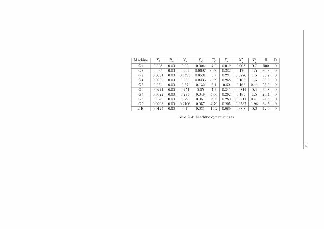
121
Machine Xl Ra Xd X ′
d T ′
d Xq X ′
q T ′
q H D
G1 0.003 0.00 0.02 0.006 7.0 0.019 0.008 0.7 500 0G2 0.035 0.00 0.295 0.0697 6.56 0.282 0.170 1.5 30.3 0G3 0.0304 0.00 0.2495 0.0531 5.7 0.237 0.0876 1.5 35.8 0G4 0.0295 0.00 0.262 0.0436 5.69 0.258 0.166 1.5 28.6 0G5 0.054 0.00 0.67 0.132 5.4 0.62 0.166 0.44 26.0 0G6 0.0224 0.00 0.254 0.05 7.3 0.241 0.0814 0.4 34.8 0G7 0.0322 0.00 0.295 0.049 5.66 0.292 0.186 1.5 26.4 0G8 0.028 0.00 0.29 0.057 6.7 0.280 0.0911 0.41 24.3 0G9 0.0298 0.00 0.2106 0.057 4.79 0.205 0.0587 1.96 34.5 0G10 0.0125 0.00 0.1 0.031 10.2 0.069 0.008 0.0 42.0 0
Table A.4: Machine dynamic data
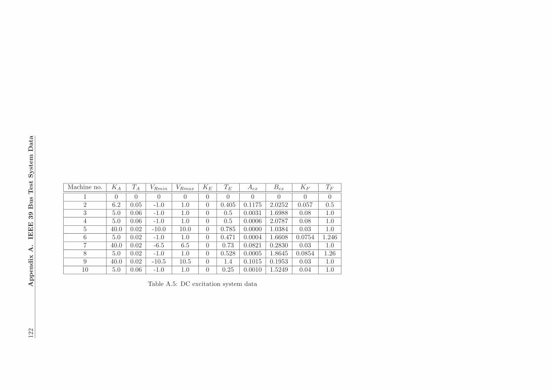
122
Appendix
A.
IEEE
39
Bus
Test
Syste
mD
ata
Machine no. KA TA VRmin VRmax KE TE Aex Bex KF TF
1 0 0 0 0 0 0 0 0 0 02 6.2 0.05 -1.0 1.0 0 0.405 0.1175 2.0252 0.057 0.53 5.0 0.06 -1.0 1.0 0 0.5 0.0031 1.6988 0.08 1.04 5.0 0.06 -1.0 1.0 0 0.5 0.0006 2.0787 0.08 1.05 40.0 0.02 -10.0 10.0 0 0.785 0.0000 1.0384 0.03 1.06 5.0 0.02 -1.0 1.0 0 0.471 0.0004 1.6608 0.0754 1.2467 40.0 0.02 -6.5 6.5 0 0.73 0.0821 0.2830 0.03 1.08 5.0 0.02 -1.0 1.0 0 0.528 0.0005 1.8645 0.0854 1.269 40.0 0.02 -10.5 10.5 0 1.4 0.1015 0.1953 0.03 1.010 5.0 0.06 -1.0 1.0 0 0.25 0.0010 1.5249 0.04 1.0
Table A.5: DC excitation system data

Appendix B
IEEE 68 Bus Test
System Data
The topology of the system is shown in Figure 6.3. All data here are inpu with a base power of 100 MVA.
Table B.1: Machine bus data
Bus Nr. Voltage Power generation
1 1.045 2.52 0.98 5.453 0.983 6.504 0.997 6.325 1.011 5.0526 1.050 7.007 1.063 5.608 1.03 5.409 1.025 8.0010 1.010 5.0011 1.000 10.0012 1.0156 13.5013 1.011 35.91
Continued on next page
123
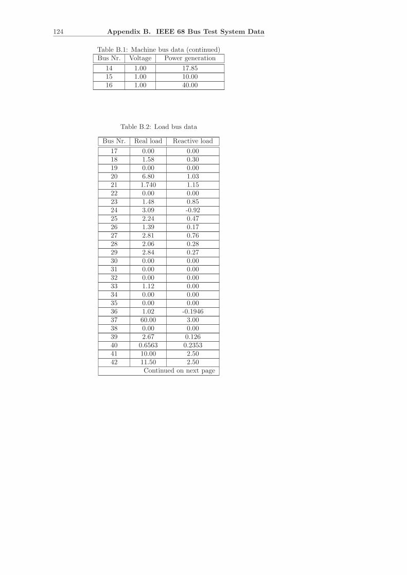
124 Appendix B. IEEE 68 Bus Test System Data
Table B.1: Machine bus data (continued)Bus Nr. Voltage Power generation
14 1.00 17.8515 1.00 10.0016 1.00 40.00
Table B.2: Load bus data
Bus Nr. Real load Reactive load
17 0.00 0.0018 1.58 0.3019 0.00 0.0020 6.80 1.0321 1.740 1.1522 0.00 0.0023 1.48 0.8524 3.09 -0.9225 2.24 0.4726 1.39 0.1727 2.81 0.7628 2.06 0.2829 2.84 0.2730 0.00 0.0031 0.00 0.0032 0.00 0.0033 1.12 0.0034 0.00 0.0035 0.00 0.0036 1.02 -0.194637 60.00 3.0038 0.00 0.0039 2.67 0.12640 0.6563 0.235341 10.00 2.5042 11.50 2.50
Continued on next page
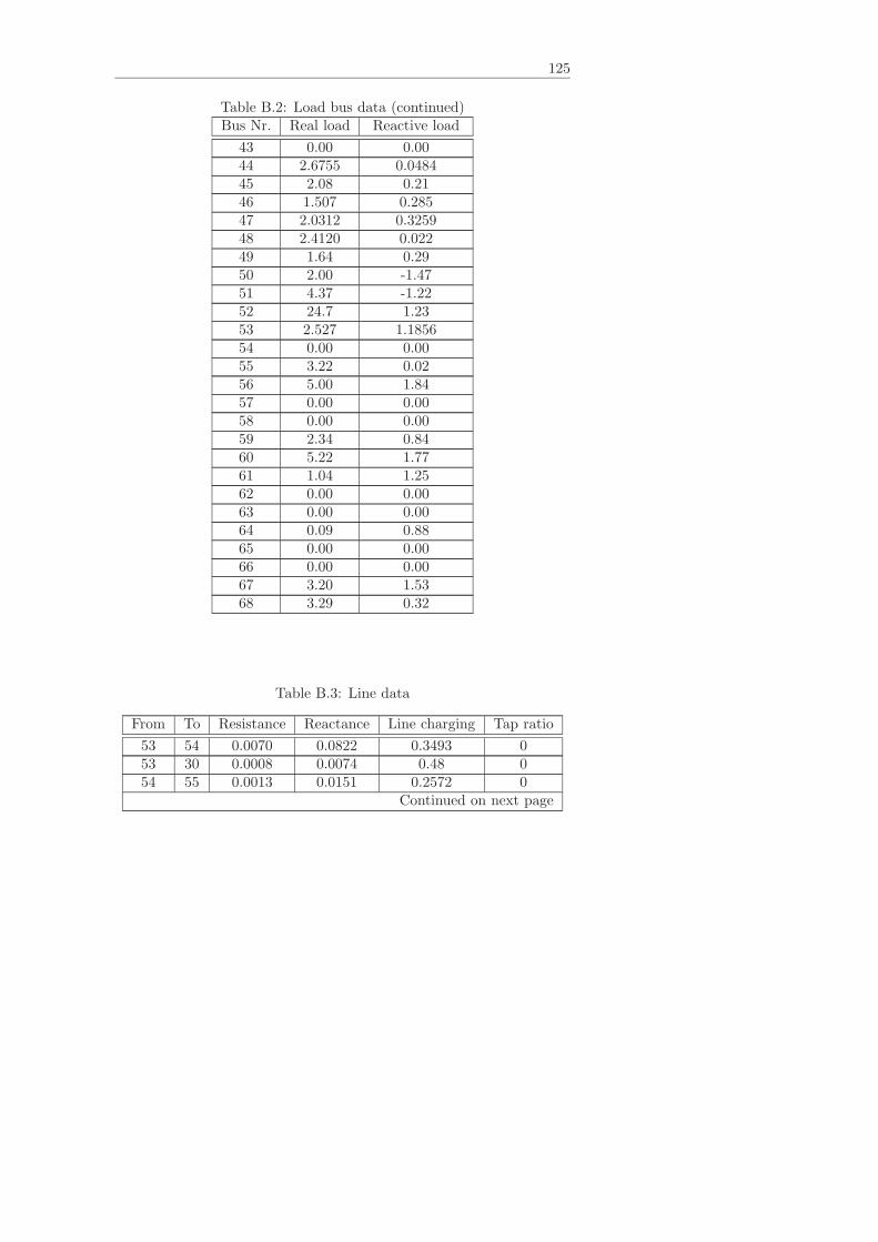
125
Table B.2: Load bus data (continued)Bus Nr. Real load Reactive load
43 0.00 0.0044 2.6755 0.048445 2.08 0.2146 1.507 0.28547 2.0312 0.325948 2.4120 0.02249 1.64 0.2950 2.00 -1.4751 4.37 -1.2252 24.7 1.2353 2.527 1.185654 0.00 0.0055 3.22 0.0256 5.00 1.8457 0.00 0.0058 0.00 0.0059 2.34 0.8460 5.22 1.7761 1.04 1.2562 0.00 0.0063 0.00 0.0064 0.09 0.8865 0.00 0.0066 0.00 0.0067 3.20 1.5368 3.29 0.32
Table B.3: Line data
From To Resistance Reactance Line charging Tap ratio
53 54 0.0070 0.0822 0.3493 053 30 0.0008 0.0074 0.48 054 55 0.0013 0.0151 0.2572 0
Continued on next page
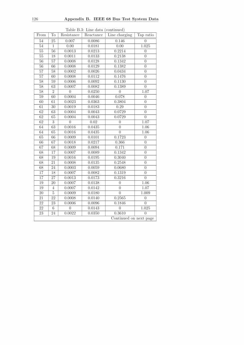
126 Appendix B. IEEE 68 Bus Test System Data
Table B.3: Line data (continued)From To Resistance Reactance Line charging Tap ratio
54 25 0.007 0.0086 0.146 054 1 0.00 0.0181 0.00 1.02555 56 0.0013 0.0213 0.2214 055 18 0.0011 0.0133 0.2138 056 57 0.0008 0.0128 0.1342 056 66 0.0008 0.0129 0.1382 057 58 0.0002 0.0026 0.0434 057 60 0.0008 0.0112 0.1476 058 59 0.0006 0.0092 0.1130 058 63 0.0007 0.0082 0.1389 058 2 0 0.0250 0 1.0759 60 0.0004 0.0046 0.078 060 61 0.0023 0.0363 0.3804 061 30 0.0019 0.0183 0.29 062 63 0.0004 0.0043 0.0729 062 65 0.0004 0.0043 0.0729 062 3 0 0.02 0 1.0764 63 0.0016 0.0435 0 1.0664 65 0.0016 0.0435 0 1.0665 66 0.0009 0.0101 0.1723 066 67 0.0018 0.0217 0.366 067 68 0.0009 0.0094 0.171 068 17 0.0007 0.0089 0.1342 068 19 0.0016 0.0195 0.3040 068 21 0.0008 0.0135 0.2548 068 24 0.0003 0.0059 0.0680 017 18 0.0007 0.0082 0.1319 017 27 0.0013 0.0173 0.3216 019 20 0.0007 0.0138 0 1.0619 4 0.0007 0.0142 0 1.0720 5 0.0009 0.0180 0 1.00921 22 0.0008 0.0140 0.2565 022 23 0.0006 0.0096 0.1846 022 6 0 0.0143 0 1.02523 24 0.0022 0.0350 0.3610 0
Continued on next page
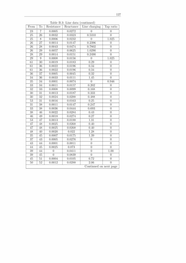
127
Table B.3: Line data (continued)From To Resistance Reactance Line charging Tap ratio
23 7 0.0005 0.0272 0 025 26 0.0032 0.0323 0.5310 025 8 0.0006 0.0232 0 1.02526 27 0.0014 0.0147 0.2396 026 28 0.0043 0.0474 0.7802 026 29 0.0057 0.0625 1.0290 028 29 0.0014 0.0151 0.2490 029 9 0.0008 0.0156 0 1.02561 30 0.0019 0.0183 0.29 061 36 0.0022 0.0196 0.34 061 36 0.0022 0.0196 0.34 036 37 0.0005 0.0045 0.32 034 36 0.0033 0.0111 1.45 035 34 0.0001 0.0074 0 0.94633 34 0.0011 0.0157 0.202 032 33 0.0008 0.0099 0.168 030 31 0.0013 0.0187 0.333 030 32 0.0024 0.0288 0.488 053 31 0.0016 0.0163 0.25 031 38 0.0011 0.0147 0.247 033 38 0.0036 0.0444 0.693 038 46 0.0022 0.0284 0.43 046 49 0.0018 0.0274 0.27 053 47 0.0013 0.0188 1.31 047 48 0.0025 0.0268 0.40 047 48 0.0025 0.0268 0.40 048 40 0.0020 0.022 1.28 035 45 0.0007 0.0175 1.39 037 43 0.0005 0.0276 0 043 44 0.0001 0.0011 0 044 45 0.0025 0.073 0 039 44 0 0.0411 0 1.0039 45 0 0.0839 0 045 51 0.0004 0.0105 0.72 050 52 0.0012 0.0288 2.06 0
Continued on next page
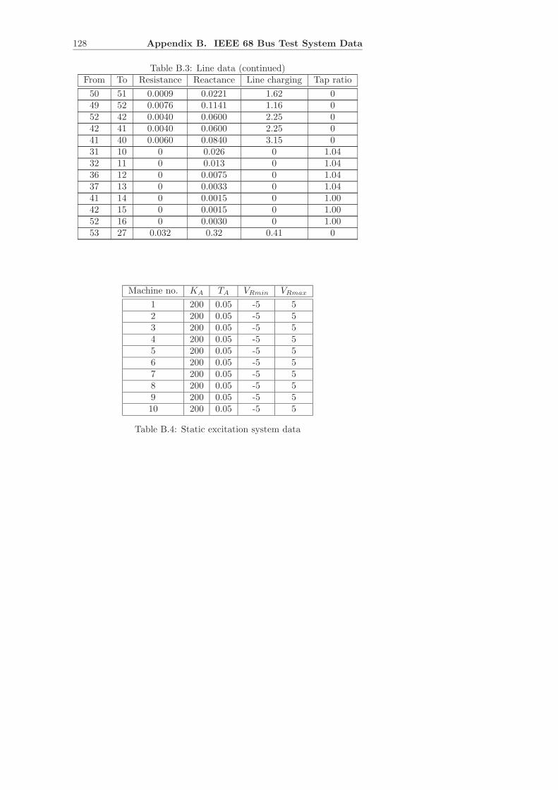
128 Appendix B. IEEE 68 Bus Test System Data
Table B.3: Line data (continued)From To Resistance Reactance Line charging Tap ratio
50 51 0.0009 0.0221 1.62 049 52 0.0076 0.1141 1.16 052 42 0.0040 0.0600 2.25 042 41 0.0040 0.0600 2.25 041 40 0.0060 0.0840 3.15 031 10 0 0.026 0 1.0432 11 0 0.013 0 1.0436 12 0 0.0075 0 1.0437 13 0 0.0033 0 1.0441 14 0 0.0015 0 1.0042 15 0 0.0015 0 1.0052 16 0 0.0030 0 1.0053 27 0.032 0.32 0.41 0
Machine no. KA TA VRmin VRmax
1 200 0.05 -5 52 200 0.05 -5 53 200 0.05 -5 54 200 0.05 -5 55 200 0.05 -5 56 200 0.05 -5 57 200 0.05 -5 58 200 0.05 -5 59 200 0.05 -5 510 200 0.05 -5 5
Table B.4: Static excitation system data
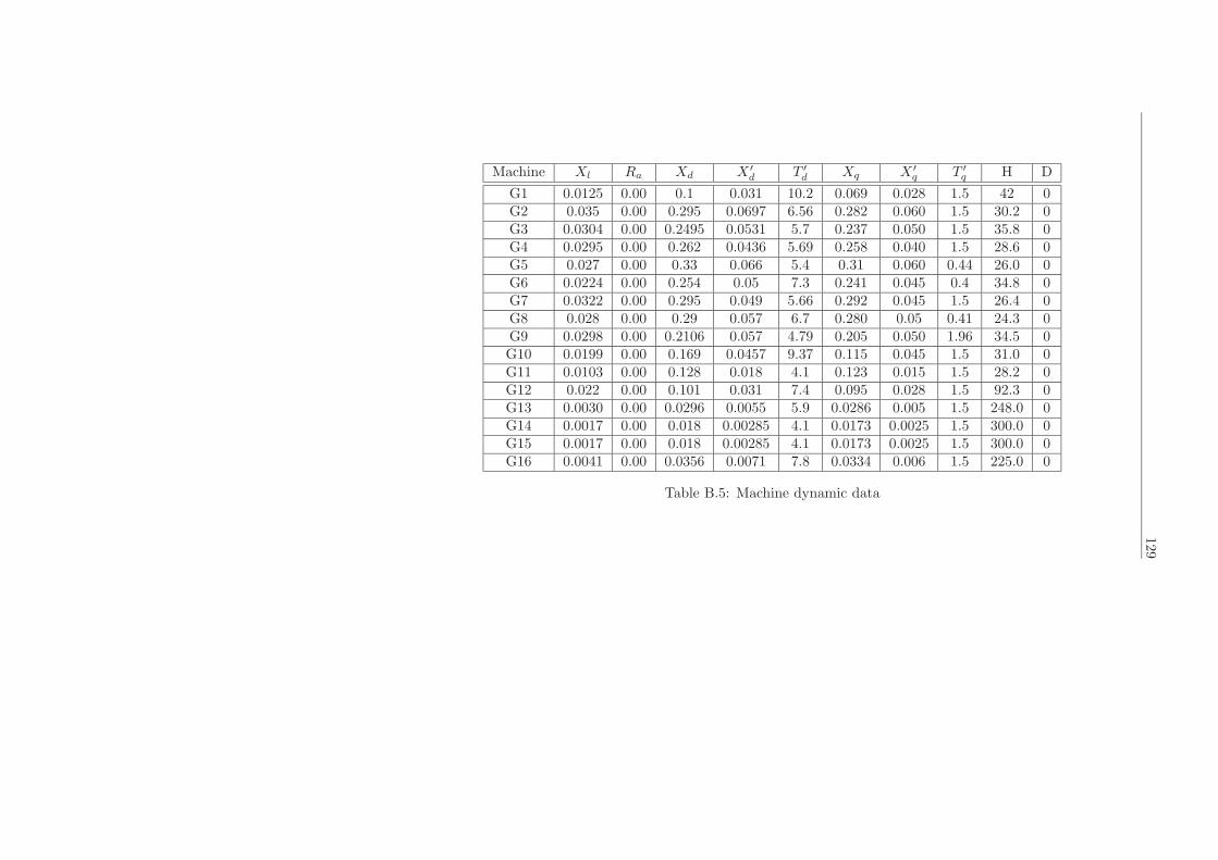
129
Machine Xl Ra Xd X ′
d T ′
d Xq X ′
q T ′
q H D
G1 0.0125 0.00 0.1 0.031 10.2 0.069 0.028 1.5 42 0G2 0.035 0.00 0.295 0.0697 6.56 0.282 0.060 1.5 30.2 0G3 0.0304 0.00 0.2495 0.0531 5.7 0.237 0.050 1.5 35.8 0G4 0.0295 0.00 0.262 0.0436 5.69 0.258 0.040 1.5 28.6 0G5 0.027 0.00 0.33 0.066 5.4 0.31 0.060 0.44 26.0 0G6 0.0224 0.00 0.254 0.05 7.3 0.241 0.045 0.4 34.8 0G7 0.0322 0.00 0.295 0.049 5.66 0.292 0.045 1.5 26.4 0G8 0.028 0.00 0.29 0.057 6.7 0.280 0.05 0.41 24.3 0G9 0.0298 0.00 0.2106 0.057 4.79 0.205 0.050 1.96 34.5 0G10 0.0199 0.00 0.169 0.0457 9.37 0.115 0.045 1.5 31.0 0G11 0.0103 0.00 0.128 0.018 4.1 0.123 0.015 1.5 28.2 0G12 0.022 0.00 0.101 0.031 7.4 0.095 0.028 1.5 92.3 0G13 0.0030 0.00 0.0296 0.0055 5.9 0.0286 0.005 1.5 248.0 0G14 0.0017 0.00 0.018 0.00285 4.1 0.0173 0.0025 1.5 300.0 0G15 0.0017 0.00 0.018 0.00285 4.1 0.0173 0.0025 1.5 300.0 0G16 0.0041 0.00 0.0356 0.0071 7.8 0.0334 0.006 1.5 225.0 0
Table B.5: Machine dynamic data


Appendix C
Sensitivity Analysis
Notation
In this part, the following notations and definitions are used:
• nℓ : number of transmission lines
• ℓ, ℓ′ : indices for transmission lines
• zℓ = rℓ + j(xℓ − xcℓ) : series impedance of line ℓ
• yℓ = gℓ + jbℓ : series admittance of line ℓ
• ZC = xcℓnℓ
1 : vector of series capacitive resistances
• P : vector of active power injections at all nodes except slack node
• Q : vector of reactive power injections at PQ-nodes
• W : vector of active power line flows
• SL(i) : set of lines connected to bus i
• SPV : set of PV−nodes
• SPQ : set of PQ−nodes
• SLK : slack node
131
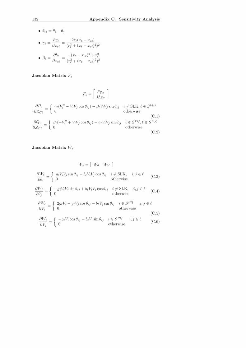
132 Appendix C. Sensitivity Analysis
• θij = θi − θj
• γℓ =∂gℓ
∂xcℓ
=2rℓ(xℓ − xcℓ)
(r2ℓ + (xℓ − xcℓ)2)2
• βℓ =∂bℓ∂xcℓ
=−(xℓ − xcℓ)
2 + r2ℓ(r2ℓ + (xℓ − xcℓ)
2)2
Jacobian Matrix Fz
Fz =
[
PZC
QZC
]
∂Pi
∂ZCℓ
=
γℓ(V2i − ViVj cos θij) − βℓViVj sin θij i 6= SLK, ℓ ∈ SL(i)
0 otherwise(C.1)
∂Qi
∂ZCℓ
=
βℓ(−V 2i + ViVj cos θij) − γℓViVj sin θij i ∈ SPQ, ℓ ∈ SL(i)
0 otherwise(C.2)
Jacobian Matrix Wx
Wx =[
Wθ WV
]
∂Wℓ
∂θi
=
gℓViVj sin θij − bℓViVj cos θij i 6= SLK, i, j ∈ ℓ0 otherwise
(C.3)
∂Wℓ
∂θj
=
−gℓViVj sin θij + bℓViVj cos θij i 6= SLK, i, j ∈ ℓ0 otherwise
(C.4)
∂Wℓ
∂Vi
=
2gℓVi − gℓVj cos θij − bℓVj sin θij i ∈ SPQ i, j ∈ ℓ0 otherwise
(C.5)
∂Wℓ
∂Vj
=
−gℓVi cos θij − bℓVi sin θij i ∈ SPQ i, j ∈ ℓ0 otherwise
(C.6)

133
Jacobian Matrix Wz
Wz = [WZC]
∂Wℓ
∂ZCℓ′=
γℓ(V2i − ViVj cos θij) − βℓViVj sin θij ℓ = ℓ′
0 ℓ 6= ℓ′(C.7)

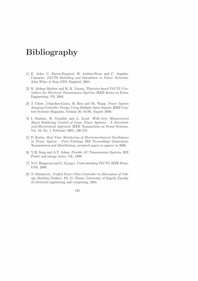
Bibliography
[1] E. Acha, C. Fuerte-Esquivel, H. Ambriz-Perez and C. Angeles-Camacho. FACTS Modelling and Simulation in Power Networks,John Wiley & Sons LTD, England, 2004.
[2] R. Mohan Mathur and R. K. Varma. Thyristor-based FACTS Con-trollers for Electrical Transmission Systems, IEEE Series on PowerEngineering, US, 2002.
[3] J. Chow, J.Sanchez-Gasca, H. Ren and Sh. Wang. Power Systemdamping Controller Design Using Multiple Input Signals. IEEE Con-trol Systems Magazine, Volume 20, 82-90, August 2000.
[4] I. Kamwa, R. Grondin and L. Loud. Wide-Area MeasurementBased Stabilizing Control of Large Power Systems - A Decentral-ized/Hierarchical Approach, IEEE Transactions on Power Systems,Vol. 16, No. 1, February 2001, 136-153.
[5] P. Korba. Real Time Monitoring of Electromechanical Oscillationsin Power System - First Findings. IEE Proceedings Generation,Transmission and Distribution, accepted paper to appear in 2006.
[6] Y.H. Song and A.T. Johns. Flexible AC Transmission Systems. IEEPower and energy series, UK, 1999.
[7] N.G. Hingorani and L. Gyugyi. Understanding FACTS. IEEE Press,USA, 2000.
[8] N. Dizdarevic, Unified Power Flow Controller in Alleviation of Volt-age Stability Problem. Ph. D. Thesis, University of Zagreb, Facultyof electrical engineering and computing, 2001.
135
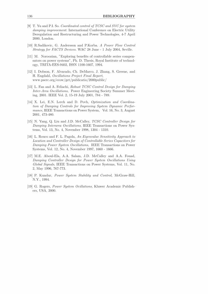
136 BIBLIOGRAPHY
[9] T. Yu and P.I. So. Coordinated control of TCSC and SVC for systemdamping improvement. International Conference on Electric UtilityDeregulation and Restructuring and Power Technologies, 4-7 April2000, London.
[10] R.Sadikovic, G. Andersson and P.Korba. A Power Flow ControlStrategy for FACTS Devices. WAC 28 June - 1 July 2004, Seville.
[11] M. Noroozian, ”Exploring benefits of controllable series compen-sators on power systems”, Ph. D. Thesis, Royal Institute of technol-ogy, TRITA-EES-9402, ISSN 1100-1607, 1994.
[12] I. Dobson, F. Alvarado, Ch. DeMarco, J. Zhang, S. Greene, andH. Engdahl, Oscillations Project Final Report,www.pserc.org/ecow/get/publicatio/2000public/
[13] L. Fan and A. Feliachi, Robust TCSC Control Design for DampingInter-Area Oscillations, Power Engineering Society Summer Meet-ing, 2001. IEEE Vol. 2, 15-19 July 2001, 784 - 789.
[14] X. Lei, E.N. Lerch and D. Povh, Optimization and Coordina-tion of Damping Controls for Improving System Dynamic Perfor-mance, IEEE Transactions on Power System, Vol. 16, No. 3, August2001, 473-480.
[15] N. Yang, Q. Liu and J.D. McCalley, TCSC Controller Design forDamping Interarea Oscillations, IEEE Transactions on Power Sys-tems, Vol. 13, No. 4, November 1998, 1304 - 1310.
[16] L. Rouco and F. L. Pagola, An Eigenvalue Sensitivity Approach toLocation and Controller Design of Controllable Series Capacitors forDamping Power System Oscillations, IEEE Transactions on PowerSystems, Vol. 12, No. 4, November 1997, 1660 - 1666.
[17] M.E. Aboul-Ela, A.A. Salam, J.D. McCalley and A.A. Fouad,Damping Controller Design for Power System Oscillations UsingGlobal Signals, IEEE Transactions on Power Systems, Vol. 11, No.2, May 1996, 767-773.
[18] P. Kundur, Power System Stability and Control, McGraw-Hill,N.Y., 1994.
[19] G. Rogers, Power System Ocillations, Kluwer Academic Publish-ers, USA, 2000.
BIBLIOGRAPHY 137
[20] N. Martins and L. Lima, Determination of Suitable Location forPower System Stabilizers and Static VAR Compensators for Damp-ing Electromechanical Oscillations in Large Scale Power Systems,IEEE Transactions on Power System, Vol. 5, No. 4, November 1990,1455-1469.
[21] M.A. Pai, Energy Function Analysis for Power System Stability,Kluwer Academic Publishers, 1989.
[22] M. Amano, M. Watanabe and M. Banjo, Self-Tuning of PowerSystem Stabilizers Using Prony Analysis, Power Engineering SocietyWinter Meeting, Vol. 1, February 1999, 655 - 660.
[23] P. Korba, M. Larsson and C. Rehtanz, Detection of oscillationsin power systems using Kalman fitlering techniques, Proceedings of2003 IEEE Conference on Control Applications, Vol.1, June 2003,183 - 188.
[24] Ch. Wu and Y. Hsu, Design of Self Tuning PID Power SystemStabilizer for Multimachine Power System, IEEE Transaction onPower Systems, Vol. 3, No. 3, August 1998.
[25] G.P. Chen, O.P. Malik, G.S. Hope, Y.H. Qin and G.Y. Xu, Anadaptive power system stabilizer based on the self-optimizing poleshifting control strategy, IEEE Transactions on Energy Conversion,Vol. 8, No. 4, December 1993, 639-645.
[26] O.P.Malik, G.P. Chen, G.S Hope,Y.H. Qin, and G.Y. Xu, AdaptiveSelf-optimising Pole Shifting Control Algorithm, IEE ProceedingsControl Theory and Applications, Vol. 139, No. 5, September 1992,429-438.
[27] S. Cheng, Y.S.Chow, O.P. Malik and G.S. Hope, An Adaptive Syn-chronous Machine Stabilizer, IEEE Transaction on Power Systems,Vol. PWRS-1(3), 1986, 101-109.
[28] V. Bobal, J.Bohm, J. Fessl and J. Machacek, Digital Self-tuningControllers, Springer, November 2005.
[29] K. J. Astrom and B. Wittenmark, Adaptive Control, Addison-Wesley, 1989.
[30] R.E. Kalman, Design of a Self Optimizing Control System, Trans.ASME, Vol. 80, 1958, 481-492.
138 BIBLIOGRAPHY
[31] K. J. Astrom and B. Wittenmark, On Self Tuning Regulators, Au-tomatica, Vol. 9, 1970, 185-199.
[32] R. Sadikovic, P. Korba and G. Andersson, Self-tuning Controllerfor Damping of Power System Oscillations with FACTS Devices,Accepted for presentation at the IEEE PES General Meeting, Mon-treal, Canada, 2006.
[33] S. Haykin, Adaptive Filter Theory,Pretince Hall, 1996.
[34] CIGRE TF 38-02-16, Impact of interactions among power systemcontrols, Report, September 1999
[35] A. Hasanovic and A. Feliachi. Genetic Algorithm Based Inter-area Oscillation Damping Controller Design Using MATLAB. IEEETransactions on Power System, Vol. 11, No. 2, May 2002, 1136-1141.
[36] Joe H. Chow, Felix F. Wu and James A. Momoh, (Eds.) AppliedMathematics for Restructured Electric Power Systems Optimiza-tion, Control, and Computational Intelligence, ISBN: 0-387-23470-5,Springer 2005.
[37] Y.H. Song, Modern Optimisation Techniques in Power Systems,Kluwer Academic Publishers, 1999.
[38] A. L. B. do Bomfim, G. N. Taranto and D. M. Falcao, Simulta-neous Tuning of Power System Damping Controllers Using GeneticAlgorithms, IEEE Transactions on Power Systems, Vol. 15, No. 1,February 2000, 163-169.
[39] Y. L. Abdel-Magid and M. A. Abido, Optimal Multiobjective De-sign of Robust Power Systems Stabilizers Using Genetic Algorithms,IEEE Transactions on Power Systems, Vol. 18, No. 3, August 2003,1125-1132.
[40] K. Hongesombut and Y. Mitani, Implementation of Advanced Ge-netic Algorithm to Modern Power System Stabilization Control,IEEE PES, Power Systems Conference and Exposition, Vol 2, Oc-tober 2004, 1050 - 1055.
[41] Math Works Inc.,MATLAB the language of technical computing co-mutation, visualisation, programming, The Math Works Inc., Nat-ick, version 7.1, 2005.
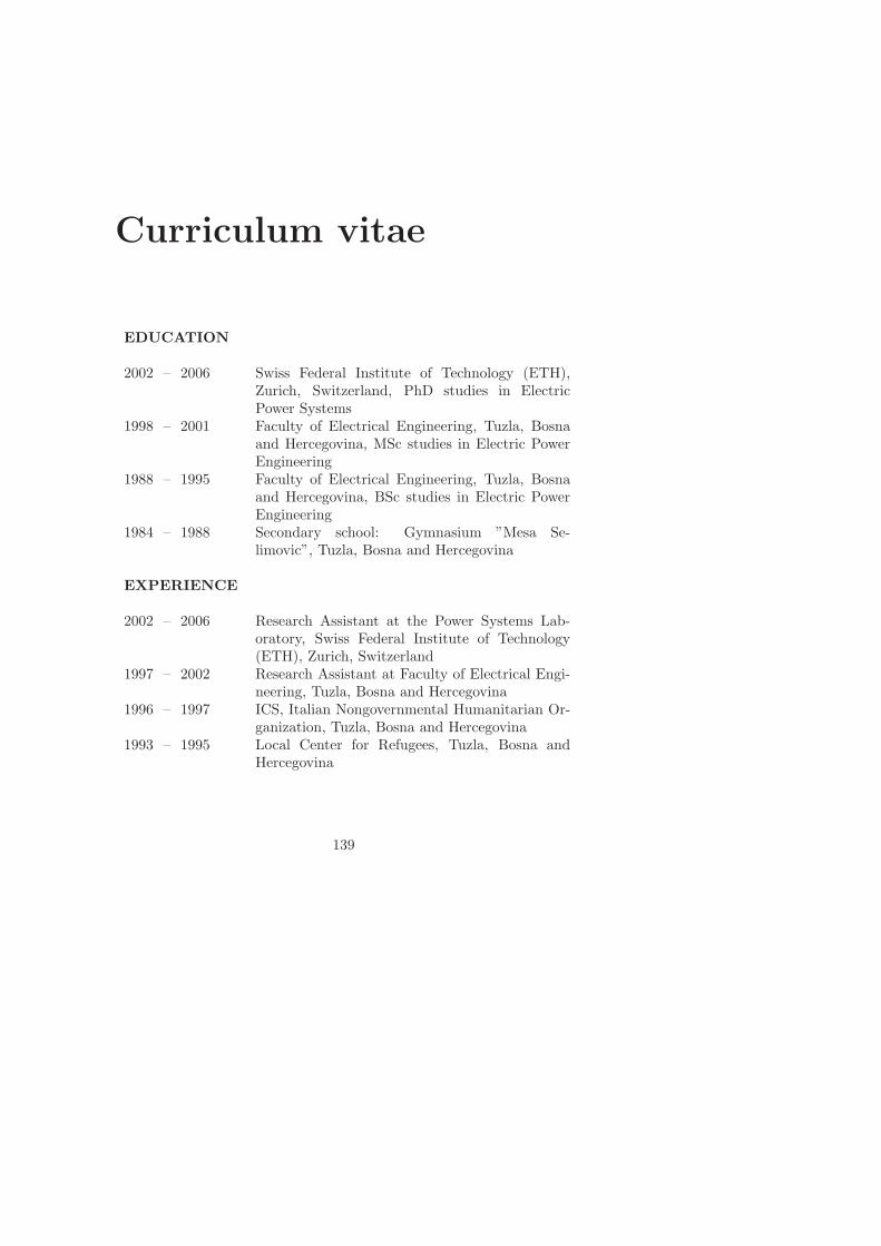
Curriculum vitae
EDUCATION
2002 – 2006 Swiss Federal Institute of Technology (ETH),Zurich, Switzerland, PhD studies in ElectricPower Systems
1998 – 2001 Faculty of Electrical Engineering, Tuzla, Bosnaand Hercegovina, MSc studies in Electric PowerEngineering
1988 – 1995 Faculty of Electrical Engineering, Tuzla, Bosnaand Hercegovina, BSc studies in Electric PowerEngineering
1984 – 1988 Secondary school: Gymnasium ”Mesa Se-limovic”, Tuzla, Bosna and Hercegovina
EXPERIENCE
2002 – 2006 Research Assistant at the Power Systems Lab-oratory, Swiss Federal Institute of Technology(ETH), Zurich, Switzerland
1997 – 2002 Research Assistant at Faculty of Electrical Engi-neering, Tuzla, Bosna and Hercegovina
1996 – 1997 ICS, Italian Nongovernmental Humanitarian Or-ganization, Tuzla, Bosna and Hercegovina
1993 – 1995 Local Center for Refugees, Tuzla, Bosna andHercegovina
139