1

Useful Estimations and Rules of Thumb for

Optomechanics

by

Katie Schwertz

A Report Submitted to the Faculty of the

DEPARTMENT OF OPTICAL SCIENCES

In Partial Fulfillment of the Requirements for the Degree of

MASTER OF SCIENCE

In the Graduate College

THE UNIVERSITY OF ARIZONA

May 7, 2010

2

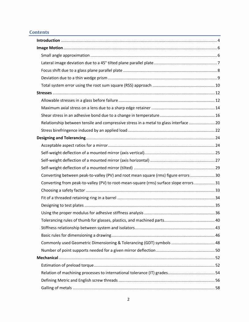
Contents

Introduction ..................................................................................................................................... 4

Image Motion ................................................................................................................................... 6

Small angle approximation ............................................................................................................ 6

Lateral image deviation due to a 45° tilted plane parallel plate ...................................................... 7

Focus shift due to a glass plane parallel plate ................................................................................ 8

Deviation due to a thin wedge prism ............................................................................................. 9

Total system error using the root sum square (RSS) approach ..................................................... 10

Stresses .......................................................................................................................................... 12

Allowable stresses in a glass before failure .................................................................................. 12

Maximum axial stress on a lens due to a sharp edge retainer ...................................................... 14

Shear stress in an adhesive bond due to a change in temperature ............................................... 16

Relationship between tensile and compressive stress in a metal to glass interface ...................... 20

Stress birefringence induced by an applied load .......................................................................... 22

Designing and Tolerancing .............................................................................................................. 24

Acceptable aspect ratios for a mirror ........................................................................................... 24

Self-weight deflection of a mounted mirror (axis vertical)............................................................ 25

Self-weight deflection of a mounted mirror (axis horizontal) ....................................................... 27

Self-weight deflection of a mounted mirror (tilted) ..................................................................... 29

Converting between peak-to-valley (PV) and root mean square (rms) figure errors ..................... 30

Converting from peak-to-valley (PV) to root-mean-square (rms) surface slope errors .................. 31

Choosing a safety factor .............................................................................................................. 33

Fit of a threaded retaining ring in a barrel ................................................................................... 34

Designing to test plates ............................................................................................................... 35

Using the proper modulus for adhesive stiffness analysis ............................................................ 36

Tolerancing rules of thumb for glasses, plastics, and machined parts........................................... 40

Stiffness relationship between system and isolators .................................................................... 43

Basic rules for dimensioning a drawing ........................................................................................ 46

Commonly used Geometric Dimensioning & Tolerancing (GDT) symbols ..................................... 48

Number of point supports needed for a given mirror deflection .................................................. 50

Mechanical ..................................................................................................................................... 52

Estimation of preload torque ....................................................................................................... 52

Relation of machining processes to international tolerance (IT) grades........................................ 54

Defining Metric and English screw threads .................................................................................. 56

Galling of metals ......................................................................................................................... 58

3

Choosing a tap drill size ............................................................................................................... 59

Using threaded inserts ................................................................................................................ 60

Damping factor for optomechanical systems ............................................................................... 61

Load distribution in screw threads ............................................................................................... 62

Cost and performance tradeoffs for commercially available linear stages .................................... 63

Material Properties ........................................................................................................................ 67

Material properties and uses of common optical glasses ............................................................. 67

Material properties and uses of common metals ......................................................................... 69

Material properties and uses of common adhesives .................................................................... 71

Miscellaneous Topics ...................................................................................................................... 73

Time to reach thermal equilibrium .............................................................................................. 73

Sag formula ................................................................................................................................. 76

Pencil bounce trick ...................................................................................................................... 77

Outgassing and use of cyanoacrylates (superglue) ....................................................................... 78

Shipping environments –drop heights ......................................................................................... 79

Shipping environments – vibration and the Miles equation ......................................................... 81

Machine shop talk and terminology............................................................................................. 84

Clean room classifications ........................................................................................................... 85

Change in the refractive index of air with temperature ................................................................ 87

Prefixes for orders of magnitude ................................................................................................. 89

Electromagnetic spectrum wavelength ranges............................................................................. 89

Decimal equivalents of fractions of an inch.................................................................................. 90

Quick conversions ....................................................................................................................... 92

4

Introduction

Frequently in technical fields, including that of optomechanics, preliminary design decisions and everyday choices are made based on experience. For those who have worked in a field for many years, it may seem second nature to determine if a design decision is feasible or if information presented to them is reasonable. For those who do not have significant experience in design, a more rigorous process is required before a design decision can be reached. It is crucial during each point in the design process that the question is asked, “does this make sense?” This applies to all stages of the engineering process: concept, design, fabrication, assembly, test, and maintenance. When presented with new information, it is advantageous to be able to quickly determine if it is reasonable or not. This report aims to provide a collection of easy-to-remember rules of thumb and useful estimations related to optomechanics that a practicing engineer of any level can employ for a quick check of sensibility. These estimations may be derived mathematically or conceptually, but all are based on a set of reasonable assumptions and years of experience from engineers in the field. They are in no way meant to replace a complete analysis of the situation or design at hand, but rather to provide quick, easy-to-remember relationships that can be used on a day to day basis. A similar collection of rules of thumb for Photonics has been published by Miller and Friedman (Photonics Rules of Thumb: Optics, Electro-Optics, Fiber Optics, and Lasers. New York: McGraw-Hill, 1996.). This book is an excellent reference for the practicing engineer and this report follows its format closely. The rules of thumb presented in this report are broken down into six categories: Image Motion, Stresses, Designing and Tolerancing, Mechanical, Material Properties, and Miscellaneous Topics. Within each category, a number of useful estimations relevant to the topic are presented. With the exception of some of the reference tables in the material property and miscellaneous sections, each rule of thumb is laid out in the following manner: Rule: The estimation or rule of thumb is concisely stated. A corresponding equation, if applicable, is also included. Explanation and Usefulness: Relevant background information is presented to the reader to give context as to when this rule can be applied. The details of how the rule should be applied and when it is useful are also discussed. Limitations: Qualitative and/or quantitative limitations on the estimation are discussed. An explanation of the major assumption(s) in the rule is provided to the reader to aid in determining when the estimation is valid, when the rule does not apply, and when a more rigorous analysis should be completed. Complete Analysis: This section intends to provide the reader with a detailed analysis that can be used for instances when the rule of thumb is outside its range of validity. References: Materials used in the derivation, explanation, or analysis of the specific rule of thumb are included here. Additional references are sometimes listed that are relevant to the topic and provide information beyond the discussion presented.

5

It is important to understand under what circumstances each estimation is valid before it is employed. Knowing these limitations, along with an understanding of where each estimation is derived from, these rules of thumb will allow for simplified calculations and decisions in a variety of everyday applications.

6

Image Motion

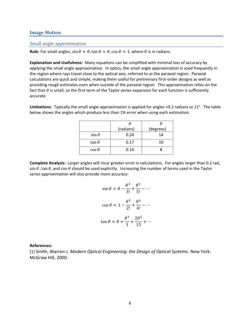
Small angle approximation

Rule: For small angles, where is in radians. Explanation and Usefulness: Many equations can be simplified with minimal loss of accuracy by applying the small angle approximation. In optics, the small angle approximation is used frequently in the region where rays travel close to the optical axis, referred to as the paraxial region. Paraxial calculations are quick and simple, making them useful for preliminary first-order designs as well as providing rough estimates even when outside of the paraxial region. This approximation relies on the fact that is small, so the first term of the Taylor series expansion for each function is sufficiently accurate. Limitations: Typically the small angle approximation is applied for angles <0.2 radians or 11°. The table below shows the angles which produce less than 1% error when using each estimation.

(radians)

(degrees)

0.24 14

0.17 10

0.14 8

Complete Analysis: Larger angles will incur greater error in calculations. For angles larger than 0.2 rad, and should be used explicitly. Increasing the number of terms used in the Taylor series approximation will also provide more accuracy:

References:

[1] Smith, Warren J. Modern Optical Engineering: the Design of Optical Systems. New York: McGraw Hill, 2000.

7

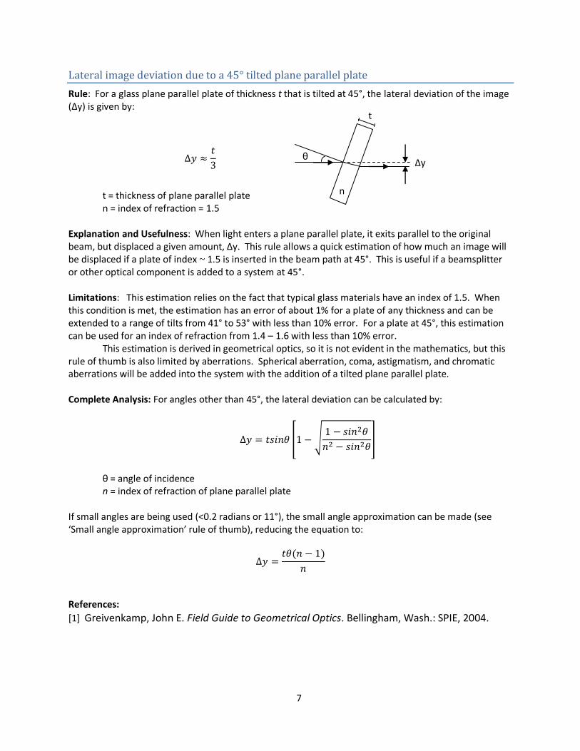
Lateral image deviation due to a 45° tilted plane parallel plate

Rule: For a glass plane parallel plate of thickness t that is tilted at 45°, the lateral deviation of the image (∆y) is given by:

t = thickness of plane parallel plate n = index of refraction = 1.5 Explanation and Usefulness: When light enters a plane parallel plate, it exits parallel to the original beam, but displaced a given amount, ∆y. This rule allows a quick estimation of how much an image will be displaced if a plate of index ~ 1.5 is inserted in the beam path at 45°. This is useful if a beamsplitter or other optical component is added to a system at 45°. Limitations: This estimation relies on the fact that typical glass materials have an index of 1.5. When this condition is met, the estimation has an error of about 1% for a plate of any thickness and can be extended to a range of tilts from 41° to 53° with less than 10% error. For a plate at 45°, this estimation can be used for an index of refraction from 1.4 – 1.6 with less than 10% error. This estimation is derived in geometrical optics, so it is not evident in the mathematics, but this rule of thumb is also limited by aberrations. Spherical aberration, coma, astigmatism, and chromatic aberrations will be added into the system with the addition of a tilted plane parallel plate. Complete Analysis: For angles other than 45°, the lateral deviation can be calculated by:

θ = angle of incidence

n = index of refraction of plane parallel plate If small angles are being used (<0.2 radians or 11°), the small angle approximation can be made (see ‘Small angle approximation’ rule of thumb), reducing the equation to:

References:

[1] Greivenkamp, John E. Field Guide to Geometrical Optics. Bellingham, Wash.: SPIE, 2004.

t

Δy

θ Δy

t

θ

n

8

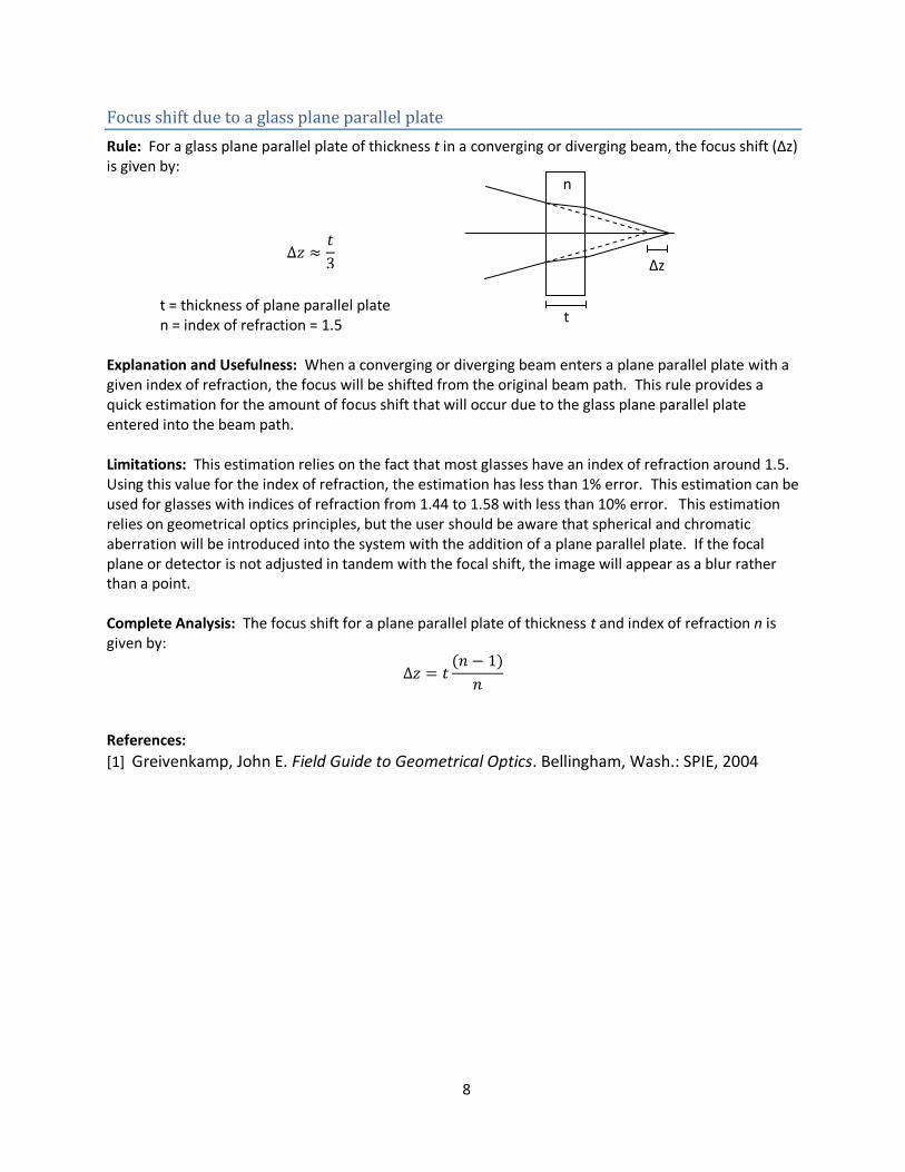
Focus shift due to a glass plane parallel plate

Rule: For a glass plane parallel plate of thickness t in a converging or diverging beam, the focus shift (Δz) is given by:

t = thickness of plane parallel plate

n = index of refraction = 1.5

Explanation and Usefulness: When a converging or diverging beam enters a plane parallel plate with a given index of refraction, the focus will be shifted from the original beam path. This rule provides a quick estimation for the amount of focus shift that will occur due to the glass plane parallel plate entered into the beam path. Limitations: This estimation relies on the fact that most glasses have an index of refraction around 1.5. Using this value for the index of refraction, the estimation has less than 1% error. This estimation can be used for glasses with indices of refraction from 1.44 to 1.58 with less than 10% error. This estimation relies on geometrical optics principles, but the user should be aware that spherical and chromatic aberration will be introduced into the system with the addition of a plane parallel plate. If the focal plane or detector is not adjusted in tandem with the focal shift, the image will appear as a blur rather than a point. Complete Analysis: The focus shift for a plane parallel plate of thickness t and index of refraction n is given by:

References:

[1] Greivenkamp, John E. Field Guide to Geometrical Optics. Bellingham, Wash.: SPIE, 2004

t

Δz

n

9

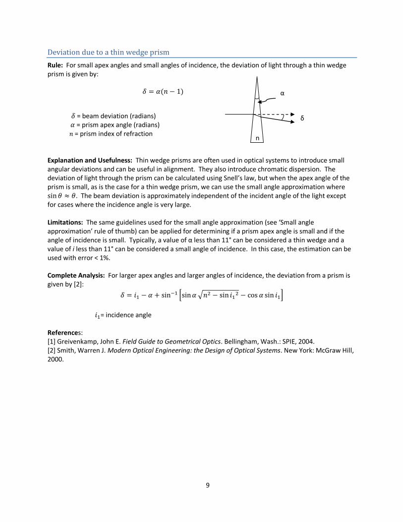
Deviation due to a thin wedge prism

Rule: For small apex angles and small angles of incidence, the deviation of light through a thin wedge prism is given by:

= beam deviation (radians) = prism apex angle (radians) = prism index of refraction

Explanation and Usefulness: Thin wedge prisms are often used in optical systems to introduce small angular deviations and can be useful in alignment. They also introduce chromatic dispersion. The deviation of light through the prism can be calculated using Snell’s law, but when the apex angle of the prism is small, as is the case for a thin wedge prism, we can use the small angle approximation where . The beam deviation is approximately independent of the incident angle of the light except for cases where the incidence angle is very large. Limitations: The same guidelines used for the small angle approximation (see ‘Small angle approximation’ rule of thumb) can be applied for determining if a prism apex angle is small and if the angle of incidence is small. Typically, a value of α less than 11° can be considered a thin wedge and a value of i less than 11° can be considered a small angle of incidence. In this case, the estimation can be used with error < 1%. Complete Analysis: For larger apex angles and larger angles of incidence, the deviation from a prism is given by [2]:

= incidence angle

References: [1] Greivenkamp, John E. Field Guide to Geometrical Optics. Bellingham, Wash.: SPIE, 2004. [2] Smith, Warren J. Modern Optical Engineering: the Design of Optical Systems. New York: McGraw Hill, 2000.

n

δ

α

10

Total system error using the root sum square (RSS) approach

Rule: For each given error in a system, , the total error can be found by: Explanation and Usefulness: In any system, there are multiple sources of error (e.g. angular, positional) that affect system performance. If each of these errors is independent, or approximately independent, the effects combine as a root sum square (RSS). Some examples of independent errors would be the radii of curvature for each lens, the tilt of one element, or the spacing between elements (as long as they are not referenced to a common surface). The total RSS error is dominated by the largest errors, and the smallest contributors are negligible. System performance can be improved most efficiently by reducing the largest contributors whereas the smallest contributors could be increased (by relaxing a requirement) to reduce cost without greatly affecting system performance [1]. A useful interpretation of this rule is that by knowing the tolerances ( ) to a certain confidence value, the RSS then represents the overall confidence level of the analysis. Typically tolerances are defined to a 95% confidence value (± 2σ for a Normal/Gaussian distribution), so the RSS would also represent a net 95% confidence level. Some special applications may apply a ± 3σ approach, providing a 99.7% confidence level. NIST provides very detailed explanations online for uncertainty analysis in measurements [2].

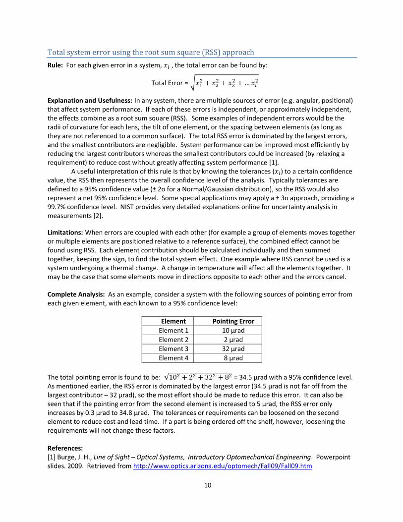
Limitations: When errors are coupled with each other (for example a group of elements moves together or multiple elements are positioned relative to a reference surface), the combined effect cannot be found using RSS. Each element contribution should be calculated individually and then summed together, keeping the sign, to find the total system effect. One example where RSS cannot be used is a system undergoing a thermal change. A change in temperature will affect all the elements together. It may be the case that some elements move in directions opposite to each other and the errors cancel. Complete Analysis: As an example, consider a system with the following sources of pointing error from each given element, with each known to a 95% confidence level:

Element Pointing Error

Element 1 10 μrad

Element 2 2 μrad

Element 3 32 μrad

Element 4 8 μrad

The total pointing error is found to be: = 34.5 μrad with a 95% confidence level. As mentioned earlier, the RSS error is dominated by the largest error (34.5 μrad is not far off from the largest contributor – 32 μrad), so the most effort should be made to reduce this error. It can also be seen that if the pointing error from the second element is increased to 5 μrad, the RSS error only increases by 0.3 μrad to 34.8 μrad. The tolerances or requirements can be loosened on the second element to reduce cost and lead time. If a part is being ordered off the shelf, however, loosening the requirements will not change these factors.

References: [1] Burge, J. H., Line of Sight – Optical Systems, Introductory Optomechanical Engineering. Powerpoint slides. 2009. Retrieved from http://www.optics.arizona.edu/optomech/Fall09/Fall09.htm

Total Error =

11

[2] NIST/SEMATECH, e-Handbook of Statistical Methods, http://www.itl.nist.gov/div898/handbook/mpc/section5/mpc5.htm , 12 April 2010. [3] ISO 9001:2008, Quality Management Systems.

12

Stresses

Allowable stresses in a glass before failure

Rule: Glass can withstand tensile stresses of 1,000 psi (6.9 MPa) and compressive stresses of 50,000 psi (345 MPa) before problems or failures occur [1]. Explanation and Usefulness: When designing a mount for a given optical system, it is critical to consider the stresses that will occur at any glass interface. Knowing the force that will be exerted on a metal-glass interface can drive the type of edge contact, the thermal operating range, and the overall tolerances of the system. Considering that failure in glass is typically catastrophic, a conservative approach should be taken to ensure a given glass can withstand the expected load in a system. This rule of thumb is considered very conservative. Looking at the examples given below, using this estimation for most glasses gives a very small or zero probability of failure. Limitations: Unfortunately, there is no characteristic strength value for a given glass, so this estimation should be used with caution. The actual tensile and compressive strength of any given optic depends on a large variety of factors. The area of the surface under stress, surface finish, size of internal flaws, glass composition, surrounding environment, and the amount and duration of the load all are important factors in determining the strength of glass. In general, glass is weaker with increasing moisture in the air and is able to withstand rapid, short loads better than slow lengthy loads [2]. Complete Analysis: Weibull statistics are commonly used to predict the probability of failure and strength of a glass. This approach allows for the characterization of the inert strength of glass but does not take time factors into account [3]. It assumes that flaws and loads remain constant over time. The mathematical distribution is given by:

exp

Probability of failure

Applied stress Characteristic strength (stress at which 63.2% of samples fail)

Weibull modulus (indicator of the scatter of the distribution of the data)

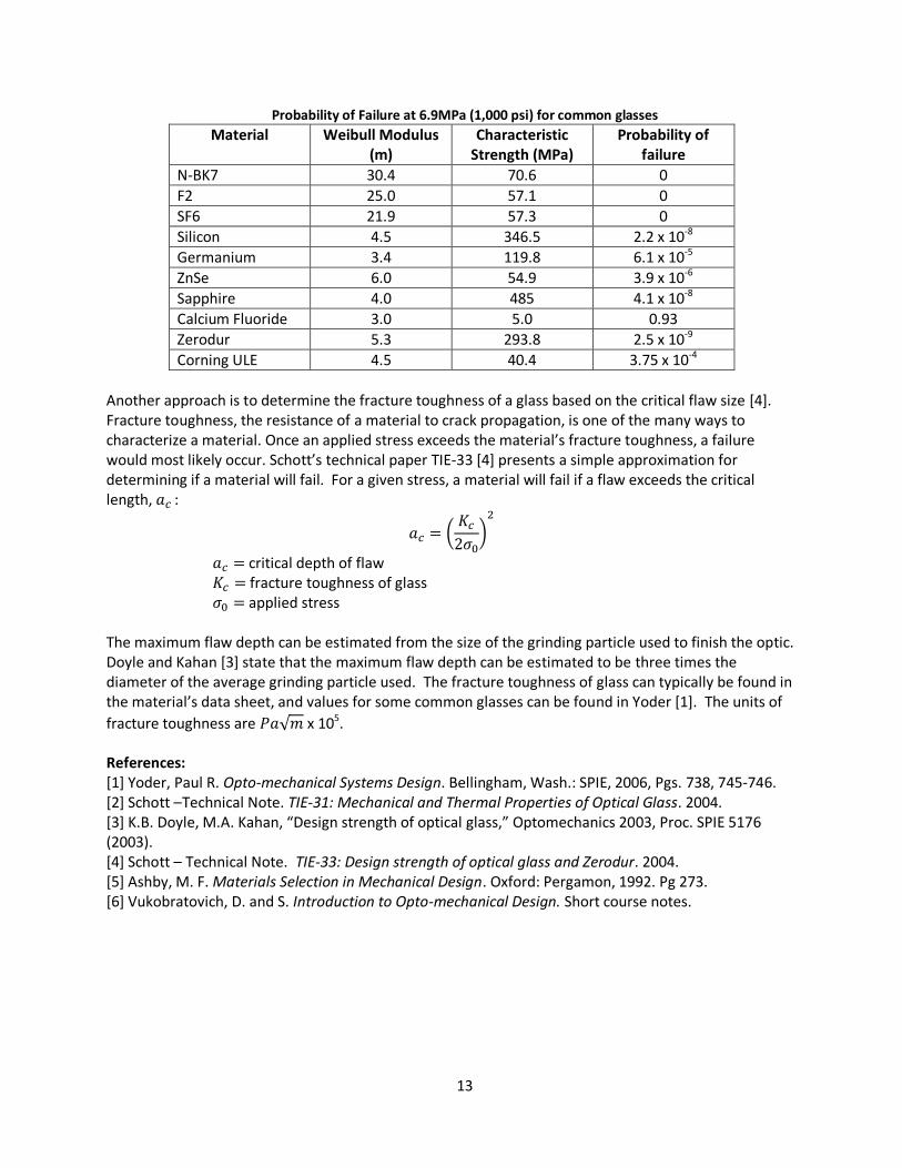
A list of Weibull parameters are shown below for some common glasses. The probability of failure is also displayed for an applied stress of 6.9MPa (1,000psi).

13

Probability of Failure at 6.9MPa (1,000 psi) for common glasses

Material Weibull Modulus (m)

Characteristic Strength (MPa)

Probability of failure

N-BK7 30.4 70.6 0

F2 25.0 57.1 0

SF6 21.9 57.3 0

Silicon 4.5 346.5 2.2 x 10-8

Germanium 3.4 119.8 6.1 x 10-5

ZnSe 6.0 54.9 3.9 x 10-6

Sapphire 4.0 485 4.1 x 10-8

Calcium Fluoride 3.0 5.0 0.93

Zerodur 5.3 293.8 2.5 x 10-9

Corning ULE 4.5 40.4 3.75 x 10-4

Another approach is to determine the fracture toughness of a glass based on the critical flaw size [4]. Fracture toughness, the resistance of a material to crack propagation, is one of the many ways to characterize a material. Once an applied stress exceeds the material’s fracture toughness, a failure would most likely occur. Schott’s technical paper TIE-33 [4] presents a simple approximation for determining if a material will fail. For a given stress, a material will fail if a flaw exceeds the critical length, :

critical depth of flaw fracture toughness of glass applied stress

The maximum flaw depth can be estimated from the size of the grinding particle used to finish the optic. Doyle and Kahan [3] state that the maximum flaw depth can be estimated to be three times the diameter of the average grinding particle used. The fracture toughness of glass can typically be found in the material’s data sheet, and values for some common glasses can be found in Yoder [1]. The units of

fracture toughness are x 105. References: [1] Yoder, Paul R. Opto-mechanical Systems Design. Bellingham, Wash.: SPIE, 2006, Pgs. 738, 745-746. [2] Schott –Technical Note. TIE-31: Mechanical and Thermal Properties of Optical Glass. 2004. [3] K.B. Doyle, M.A. Kahan, “Design strength of optical glass,” Optomechanics 2003, Proc. SPIE 5176 (2003). [4] Schott – Technical Note. TIE-33: Design strength of optical glass and Zerodur. 2004. [5] Ashby, M. F. Materials Selection in Mechanical Design. Oxford: Pergamon, 1992. Pg 273. [6] Vukobratovich, D. and S. Introduction to Opto-mechanical Design. Short course notes.

14

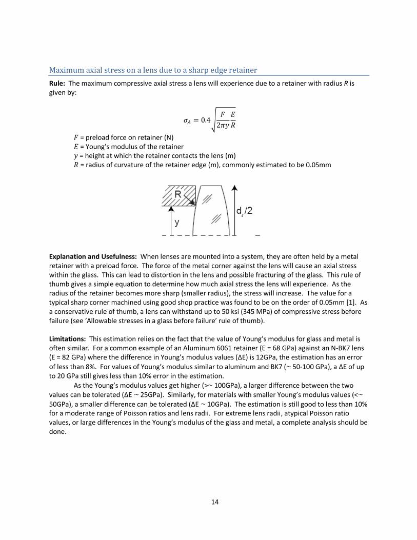
Maximum axial stress on a lens due to a sharp edge retainer

Rule: The maximum compressive axial stress a lens will experience due to a retainer with radius R is given by:

= preload force on retainer (N) = Young’s modulus of the retainer = height at which the retainer contacts the lens (m) = radius of curvature of the retainer edge (m), commonly estimated to be 0.05mm

Explanation and Usefulness: When lenses are mounted into a system, they are often held by a metal retainer with a preload force. The force of the metal corner against the lens will cause an axial stress within the glass. This can lead to distortion in the lens and possible fracturing of the glass. This rule of thumb gives a simple equation to determine how much axial stress the lens will experience. As the radius of the retainer becomes more sharp (smaller radius), the stress will increase. The value for a typical sharp corner machined using good shop practice was found to be on the order of 0.05mm [1]. As a conservative rule of thumb, a lens can withstand up to 50 ksi (345 MPa) of compressive stress before failure (see ‘Allowable stresses in a glass before failure’ rule of thumb). Limitations: This estimation relies on the fact that the value of Young’s modulus for glass and metal is often similar. For a common example of an Aluminum 6061 retainer (E = 68 GPa) against an N-BK7 lens (E = 82 GPa) where the difference in Young’s modulus values (ΔE) is 12GPa, the estimation has an error

of less than 8%. For values of Young’s modulus similar to aluminum and BK7 (~ 50-100 GPa), a ΔE of up to 20 GPa still gives less than 10% error in the estimation.

As the Young’s modulus values get higher (>~ 100GPa), a larger difference between the two values can be tolerated (ΔE ~ 25GPa). Similarly, for materials with smaller Young’s modulus values (<~

50GPa), a smaller difference can be tolerated (ΔE ~ 10GPa). The estimation is still good to less than 10% for a moderate range of Poisson ratios and lens radii. For extreme lens radii, atypical Poisson ratio values, or large differences in the Young’s modulus of the glass and metal, a complete analysis should be done.

15

Complete Analysis: The maximum axial stress due to a sharp edge retainer is given by [2]:

= preload force on retainer = height at which the retainer contacts the lens = Young’s modulus of the retainer = Young’s modulus of the lens = twice the lens radius of curvature = twice the retainer corner radius of curvature = Poisson’s ratio for the lens = Poisson’s ratio for the retainer

The sharp corner retainer radius is typically approximated as 0.05mm ( = 0.1mm), however if the corner is fabricated specifically to have a larger radius, the axial stress will be reduced. In the extreme case of going to infinity, a tangential edge contact would be the result. The numerator of the above

equation would simplify to:

.

References: [1] Delgado, R.F. and Hallinan, M., Mounting of lens elements, Optical Engineering, 14, S-11, 1975. Reprinted in SPIE Milestone Series, Vol. 770, 1988, pg. 173. [2] P.R. Yoder, Jr., Parametric investigations of mounting-induced axial contact stresses in individual lens elements," Proc. SPIE 1998, 8 (1993).

16

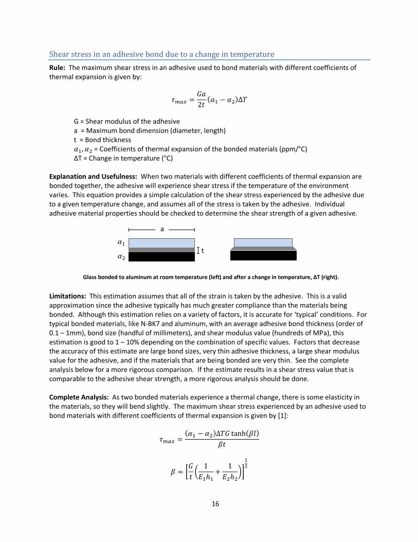
Shear stress in an adhesive bond due to a change in temperature

Rule: The maximum shear stress in an adhesive used to bond materials with different coefficients of thermal expansion is given by:

G = Shear modulus of the adhesive

a = Maximum bond dimension (diameter, length) t = Bond thickness = Coefficients of thermal expansion of the bonded materials (ppm/°C)

ΔT = Change in temperature (°C) Explanation and Usefulness: When two materials with different coefficients of thermal expansion are bonded together, the adhesive will experience shear stress if the temperature of the environment varies. This equation provides a simple calculation of the shear stress experienced by the adhesive due to a given temperature change, and assumes all of the stress is taken by the adhesive. Individual adhesive material properties should be checked to determine the shear strength of a given adhesive. Limitations: This estimation assumes that all of the strain is taken by the adhesive. This is a valid approximation since the adhesive typically has much greater compliance than the materials being bonded. Although this estimation relies on a variety of factors, it is accurate for ‘typical’ conditions. For typical bonded materials, like N-BK7 and aluminum, with an average adhesive bond thickness (order of 0.1 – 1mm), bond size (handful of millimeters), and shear modulus value (hundreds of MPa), this estimation is good to 1 – 10% depending on the combination of specific values. Factors that decrease the accuracy of this estimate are large bond sizes, very thin adhesive thickness, a large shear modulus value for the adhesive, and if the materials that are being bonded are very thin. See the complete analysis below for a more rigorous comparison. If the estimate results in a shear stress value that is comparable to the adhesive shear strength, a more rigorous analysis should be done. Complete Analysis: As two bonded materials experience a thermal change, there is some elasticity in the materials, so they will bend slightly. The maximum shear stress experienced by an adhesive used to bond materials with different coefficients of thermal expansion is given by [1]:

Glass bonded to aluminum at room temperature (left) and after a change in temperature, ΔT (right).

a

t

17

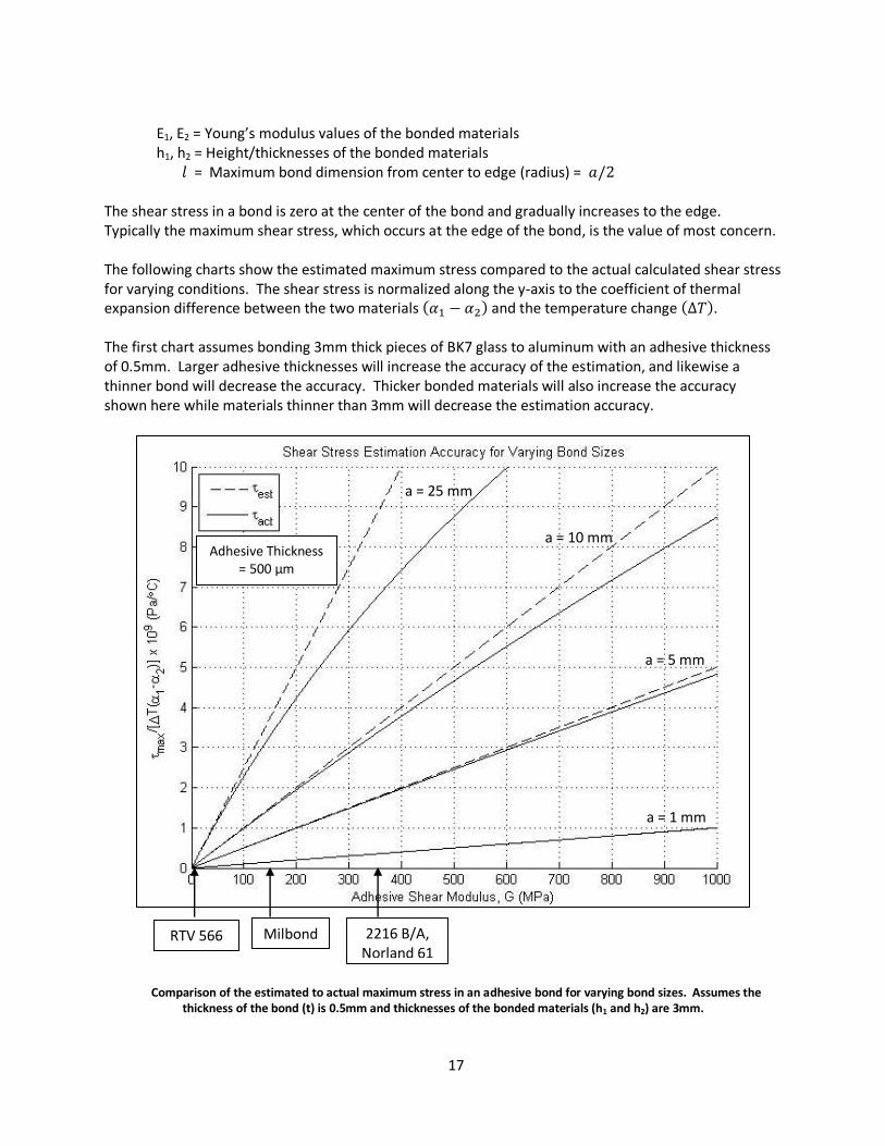
E1, E2 = Young’s modulus values of the bonded materials h1, h2 = Height/thicknesses of the bonded materials = Maximum bond dimension from center to edge (radius) = The shear stress in a bond is zero at the center of the bond and gradually increases to the edge. Typically the maximum shear stress, which occurs at the edge of the bond, is the value of most concern.

The following charts show the estimated maximum stress compared to the actual calculated shear stress for varying conditions. The shear stress is normalized along the y-axis to the coefficient of thermal expansion difference between the two materials and the temperature change . The first chart assumes bonding 3mm thick pieces of BK7 glass to aluminum with an adhesive thickness of 0.5mm. Larger adhesive thicknesses will increase the accuracy of the estimation, and likewise a thinner bond will decrease the accuracy. Thicker bonded materials will also increase the accuracy shown here while materials thinner than 3mm will decrease the estimation accuracy.

Comparison of the estimated to actual maximum stress in an adhesive bond for varying bond sizes. Assumes the

thickness of the bond (t) is 0.5mm and thicknesses of the bonded materials (h1 and h2) are 3mm.

a = 1 mm

a = 25 mm

a = 5 mm

a = 10 mm

2216 B/A, Norland 61

Milbond

Adhesive Thickness = 500 μm

RTV 566

18

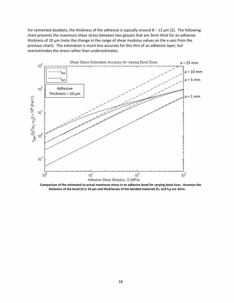
For cemented doublets, the thickness of the adhesive is typically around 8 – 13 μm *2+. The following chart presents the maximum shear stress between two glasses that are 3mm thick for an adhesive thickness of 10 μm (note the change in the range of shear modulus values on the x-axis from the previous chart). The estimation is much less accurate for this thin of an adhesive layer, but overestimates the stress rather than underestimates.

Comparison of the estimated to actual maximum stress in an adhesive bond for varying bond sizes. Assumes the

thickness of the bond (t) is 10 μm and thicknesses of the bonded materials (h1 and h2) are 3mm.

Adhesive Thickness = 10 μm

a = 25 mm

a = 10 mm

a = 5 mm

a = 1 mm

19

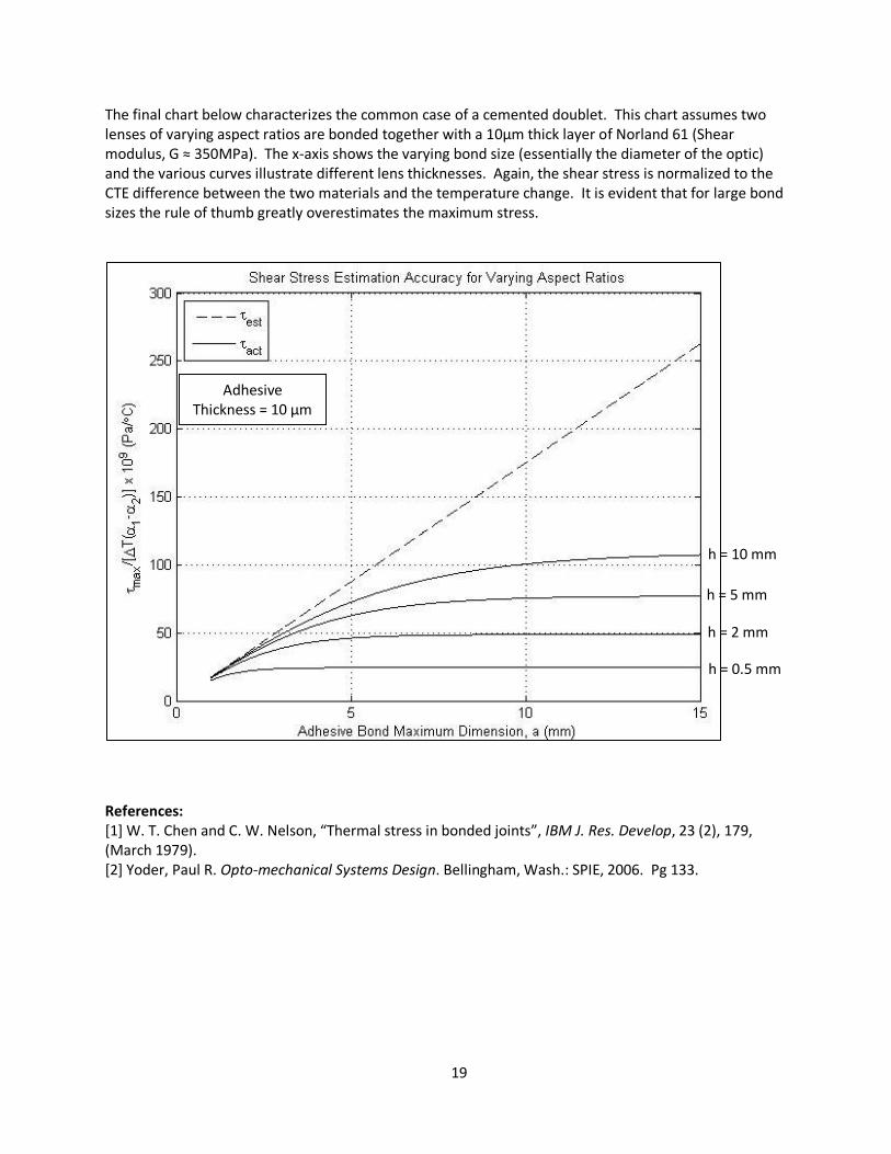
The final chart below characterizes the common case of a cemented doublet. This chart assumes two lenses of varying aspect ratios are bonded together with a 10μm thick layer of Norland 61 (Shear modulus, G ≈ 350MPa). The x-axis shows the varying bond size (essentially the diameter of the optic) and the various curves illustrate different lens thicknesses. Again, the shear stress is normalized to the CTE difference between the two materials and the temperature change. It is evident that for large bond sizes the rule of thumb greatly overestimates the maximum stress.

References: [1] W. T. Chen and C. W. Nelson, “Thermal stress in bonded joints”, IBM J. Res. Develop, 23 (2), 179, (March 1979). [2] Yoder, Paul R. Opto-mechanical Systems Design. Bellingham, Wash.: SPIE, 2006. Pg 133.

Adhesive Thickness = 10 μm

h = 0.5 mm

h = 2 mm

h = 10 mm

h = 5 mm

20

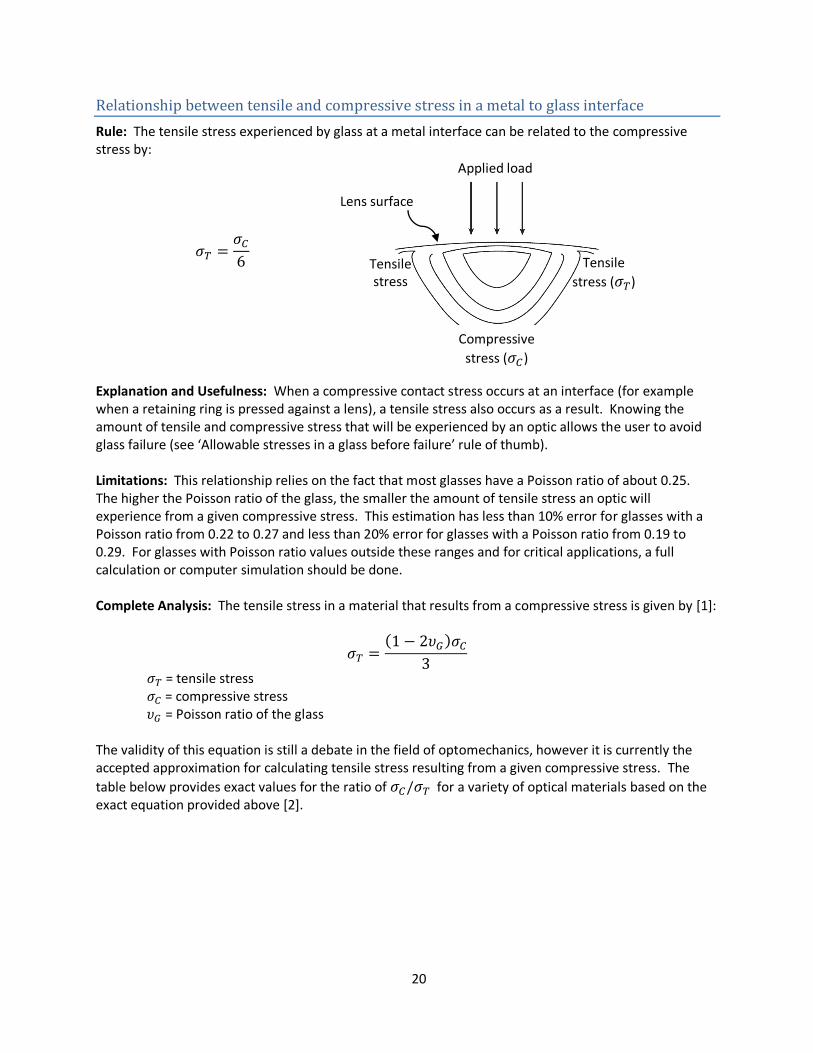
Relationship between tensile and compressive stress in a metal to glass interface

Rule: The tensile stress experienced by glass at a metal interface can be related to the compressive stress by:

Explanation and Usefulness: When a compressive contact stress occurs at an interface (for example when a retaining ring is pressed against a lens), a tensile stress also occurs as a result. Knowing the amount of tensile and compressive stress that will be experienced by an optic allows the user to avoid glass failure (see ‘Allowable stresses in a glass before failure’ rule of thumb). Limitations: This relationship relies on the fact that most glasses have a Poisson ratio of about 0.25. The higher the Poisson ratio of the glass, the smaller the amount of tensile stress an optic will experience from a given compressive stress. This estimation has less than 10% error for glasses with a Poisson ratio from 0.22 to 0.27 and less than 20% error for glasses with a Poisson ratio from 0.19 to 0.29. For glasses with Poisson ratio values outside these ranges and for critical applications, a full calculation or computer simulation should be done. Complete Analysis: The tensile stress in a material that results from a compressive stress is given by [1]:

= tensile stress = compressive stress = Poisson ratio of the glass

The validity of this equation is still a debate in the field of optomechanics, however it is currently the accepted approximation for calculating tensile stress resulting from a given compressive stress. The

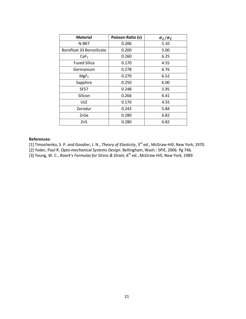
table below provides exact values for the ratio of for a variety of optical materials based on the exact equation provided above [2].

Applied load

Compressive

stress ( )

Tensile stress

Tensile

stress ( )

Lens surface

21

Material Poisson Ratio (ν)

N-BK7 0.206 5.10

Borofloat 33 Borosilicate 0.200 5.00

CaF2 0.260 6.25

Fused Silica 0.170 4.55

Germanium 0.278 6.76

MgF2 0.270 6.52

Sapphire 0.250 6.00

SF57 0.248 5.95

Silicon 0.266 6.41

ULE 0.170 4.55

Zerodur 0.243 5.84

ZnSe 0.280 6.82

ZnS 0.280 6.82

References: [1] Timoshenko, S. P. and Goodier, J. N., Theory of Elasticity, 3rd ed., McGraw-Hill, New York, 1970. [2] Yoder, Paul R. Opto-mechanical Systems Design. Bellingham, Wash.: SPIE, 2006. Pg 746. [3] Young, W. C., Roark’s Formulas for Stress & Strain, 6th ed., McGraw-Hill, New York, 1989.

22

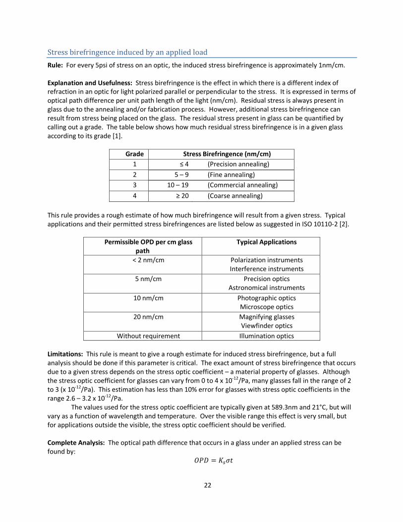
Stress birefringence induced by an applied load

Rule: For every 5psi of stress on an optic, the induced stress birefringence is approximately 1nm/cm. Explanation and Usefulness: Stress birefringence is the effect in which there is a different index of refraction in an optic for light polarized parallel or perpendicular to the stress. It is expressed in terms of optical path difference per unit path length of the light (nm/cm). Residual stress is always present in glass due to the annealing and/or fabrication process. However, additional stress birefringence can result from stress being placed on the glass. The residual stress present in glass can be quantified by calling out a grade. The table below shows how much residual stress birefringence is in a given glass according to its grade [1].

Grade Stress Birefringence (nm/cm)

1 ≤ 4 (Precision annealing)

2 5 – 9 (Fine annealing)

3 10 – 19 (Commercial annealing)

4 ≥ 20 (Coarse annealing)

This rule provides a rough estimate of how much birefringence will result from a given stress. Typical applications and their permitted stress birefringences are listed below as suggested in ISO 10110-2 [2].

Permissible OPD per cm glass path

Typical Applications

< 2 nm/cm Polarization instruments Interference instruments

5 nm/cm Precision optics Astronomical instruments

10 nm/cm Photographic optics Microscope optics

20 nm/cm Magnifying glasses Viewfinder optics

Without requirement Illumination optics

Limitations: This rule is meant to give a rough estimate for induced stress birefringence, but a full analysis should be done if this parameter is critical. The exact amount of stress birefringence that occurs due to a given stress depends on the stress optic coefficient – a material property of glasses. Although the stress optic coefficient for glasses can vary from 0 to 4 x 10-12/Pa, many glasses fall in the range of 2 to 3 (x 10-12/Pa). This estimation has less than 10% error for glasses with stress optic coefficients in the range 2.6 – 3.2 x 10-12/Pa.

The values used for the stress optic coefficient are typically given at 589.3nm and 21°C, but will vary as a function of wavelength and temperature. Over the visible range this effect is very small, but for applications outside the visible, the stress optic coefficient should be verified.

Complete Analysis: The optical path difference that occurs in a glass under an applied stress can be found by:

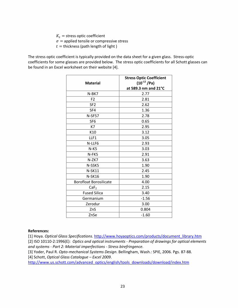
23

stress optic coefficient applied tensile or compressive stress thickness (path length of light )

The stress optic coefficient is typically provided on the data sheet for a given glass. Stress-optic coefficients for some glasses are provided below. The stress optic coefficients for all Schott glasses can be found in an Excel worksheet on their website [4].

Material

Stress Optic Coefficient (10-12 /Pa)

at 589.3 nm and 21°C

N-BK7 2.77

F2 2.81

SF2 2.62

SF4 1.36

N-SF57 2.78

SF6 0.65

K7 2.95

K10 3.12

LLF1 3.05

N-LLF6 2.93

N-K5 3.03

N-FK5 2.91

N-ZK7 3.63

N-SSK5 1.90

N-SK11 2.45

N-SK16 1.90

Borofloat Borosilicate 4.00

CaF2 2.15

Fused Silica 3.40

Germanium -1.56

Zerodur 3.00

ZnS 0.804

ZnSe -1.60

References: [1] Hoya. Optical Glass Specifications. http://www.hoyaoptics.com/products/document_library.htm [2] ISO 10110-2:1996(E): Optics and optical instruments - Preparation of drawings for optical elements and systems - Part 2: Material imperfections - Stress birefringence. [3] Yoder, Paul R. Opto-mechanical Systems Design. Bellingham, Wash.: SPIE, 2006. Pgs. 87-88. [4] Schott, Optical Glass Catalogue – Excel 2009. http://www.us.schott.com/advanced_optics/english/tools_downloads/download/index.htm

24

Designing and Tolerancing

Acceptable aspect ratios for a mirror

Rule: The diameter to thickness ratio for a mirror should be around 6, but can be acceptable from 4 to 20. Explanation and Usefulness: The aspect ratio of a mirror is defined as the ratio of the diameter to the thickness. Minimizing self-weight deflection in a mirror is a driving factor when designing a support system. Deflections are proportional to the square of the aspect ratio so as aspect ratios get larger, it becomes increasingly difficult to control self weight deflection. As aspect ratios move away from 6, fabrication becomes increasingly difficult.

Typically, mirrors with an aspect ratio larger than 8 to 10 are defined as thin mirrors and require complex mounting systems [1]. As the aspect ratio increases, the complexity of the support system will also greatly increase. A mirror with an aspect ratio of up to 20 can still be mounted, but only with a sophisticated mounting structure [2]. Limitations: Special applications may require aspect ratios outside this range but the designer should be aware of the added cost and complexity that will be required. Complete Analysis: For calculating the self-weight deflection of a mirror, refer to the rules of thumb ‘Self-weight deflection of a mounted mirror’. References:

[1] Yoder, Paul R. Opto-mechanical Systems Design. Bellingham, Wash.: SPIE, 2006, pg. 473. [2] Vukobratovich, D. and S. Introduction to Opto-mechanical Design. Short course notes. [3] Pearson, E.T., Thin mirror support systems, in Proceedings of Conference on Optical and Infrared Telescopes for the 1990’s, Vol. 1, Kitt Peak National Observatory, Tucson, AZ, 1980, pg. 555.

25

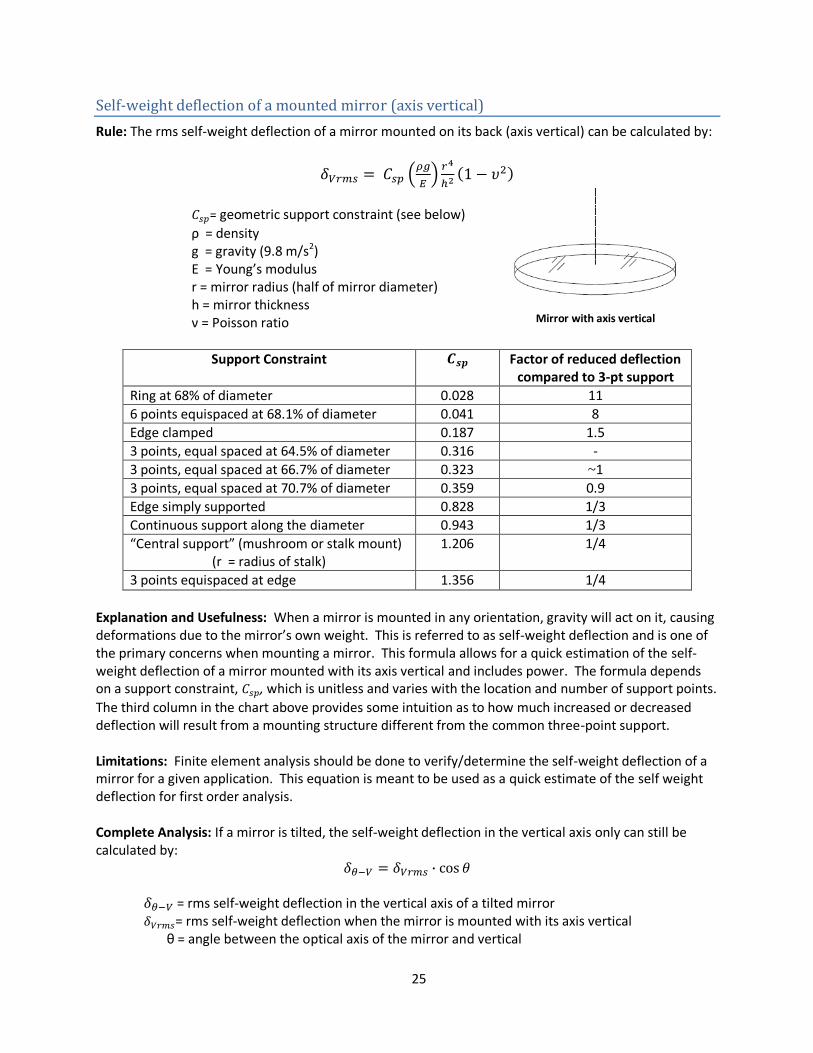
Self-weight deflection of a mounted mirror (axis vertical)

Rule: The rms self-weight deflection of a mirror mounted on its back (axis vertical) can be calculated by:

= geometric support constraint (see below)

ρ = density g = gravity (9.8 m/s2) E = Young’s modulus r = mirror radius (half of mirror diameter) h = mirror thickness ν = Poisson ratio

Support Constraint Factor of reduced deflection compared to 3-pt support

Ring at 68% of diameter 0.028 11

6 points equispaced at 68.1% of diameter 0.041 8

Edge clamped 0.187 1.5

3 points, equal spaced at 64.5% of diameter 0.316 -

3 points, equal spaced at 66.7% of diameter 0.323 ~1

3 points, equal spaced at 70.7% of diameter 0.359 0.9

Edge simply supported 0.828 1/3

Continuous support along the diameter 0.943 1/3

“Central support” (mushroom or stalk mount) (r = radius of stalk)

1.206 1/4

3 points equispaced at edge 1.356 1/4

Explanation and Usefulness: When a mirror is mounted in any orientation, gravity will act on it, causing deformations due to the mirror’s own weight. This is referred to as self-weight deflection and is one of the primary concerns when mounting a mirror. This formula allows for a quick estimation of the self-weight deflection of a mirror mounted with its axis vertical and includes power. The formula depends on a support constraint, , which is unitless and varies with the location and number of support points.

The third column in the chart above provides some intuition as to how much increased or decreased deflection will result from a mounting structure different from the common three-point support. Limitations: Finite element analysis should be done to verify/determine the self-weight deflection of a mirror for a given application. This equation is meant to be used as a quick estimate of the self weight deflection for first order analysis. Complete Analysis: If a mirror is tilted, the self-weight deflection in the vertical axis only can still be calculated by:

= rms self-weight deflection in the vertical axis of a tilted mirror = rms self-weight deflection when the mirror is mounted with its axis vertical θ = angle between the optical axis of the mirror and vertical

Mirror with axis vertical

26

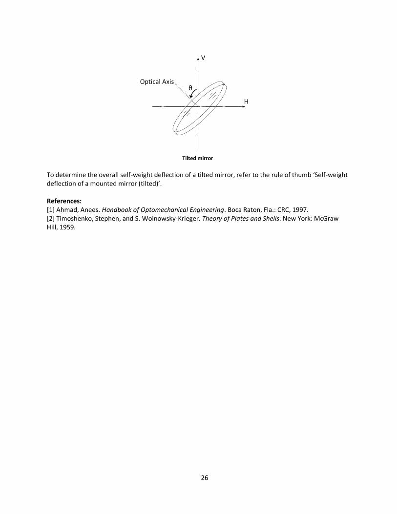
Tilted mirror

To determine the overall self-weight deflection of a tilted mirror, refer to the rule of thumb ‘Self-weight deflection of a mounted mirror (tilted)’. References: [1] Ahmad, Anees. Handbook of Optomechanical Engineering. Boca Raton, Fla.: CRC, 1997. [2] Timoshenko, Stephen, and S. Woinowsky-Krieger. Theory of Plates and Shells. New York: McGraw Hill, 1959.

Optical Axis

H

V

θ

27

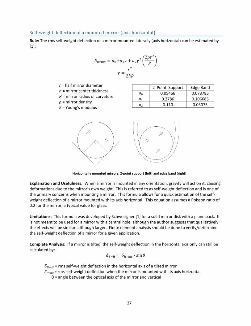
Self-weight deflection of a mounted mirror (axis horizontal)

Rule: The rms self-weight deflection of a mirror mounted laterally (axis horizontal) can be estimated by [1]:

r = half mirror diameter h = mirror center thickness R = mirror radius of curvature ρ = mirror density E = Young’s modulus

Horizontally mounted mirrors: 2-point support (left) and edge band (right)

Explanation and Usefulness: When a mirror is mounted in any orientation, gravity will act on it, causing deformations due to the mirror’s own weight. This is referred to as self-weight deflection and is one of the primary concerns when mounting a mirror. This formula allows for a quick estimation of the self-weight deflection of a mirror mounted with its axis horizontal. This equation assumes a Poisson ratio of 0.2 for the mirror, a typical value for glass. Limitations: This formula was developed by Schwesigner [1] for a solid mirror disk with a plane back. It is not meant to be used for a mirror with a central hole, although the author suggests that qualitatively the effects will be similar, although larger. Finite element analysis should be done to verify/determine the self-weight deflection of a mirror for a given application. Complete Analysis: If a mirror is tilted, the self-weight deflection in the horizontal axis only can still be calculated by:

= rms self-weight deflection in the horizontal axis of a tilted mirror = rms self-weight deflection when the mirror is mounted with its axis horizontal θ = angle between the optical axis of the mirror and vertical

2 Point Support Edge Band 0.05466 0.073785 0.2786 0.106685 0.110 0.03075

28

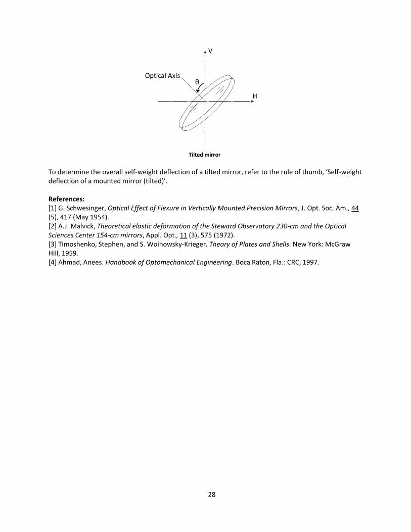
Tilted mirror

To determine the overall self-weight deflection of a tilted mirror, refer to the rule of thumb, ‘Self-weight deflection of a mounted mirror (tilted)’. References: [1] G. Schwesinger, Optical Effect of Flexure in Vertically Mounted Precision Mirrors, J. Opt. Soc. Am., 44 (5), 417 (May 1954). [2] A.J. Malvick, Theoretical elastic deformation of the Steward Observatory 230-cm and the Optical Sciences Center 154-cm mirrors, Appl. Opt., 11 (3), 575 (1972). [3] Timoshenko, Stephen, and S. Woinowsky-Krieger. Theory of Plates and Shells. New York: McGraw Hill, 1959. [4] Ahmad, Anees. Handbook of Optomechanical Engineering. Boca Raton, Fla.: CRC, 1997.

Optical Axis

H

V

θ

29

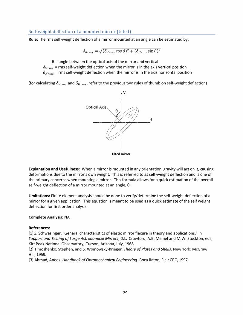
Self-weight deflection of a mounted mirror (tilted)

Rule: The rms self-weight deflection of a mirror mounted at an angle can be estimated by:

θ = angle between the optical axis of the mirror and vertical = rms self-weight deflection when the mirror is in the axis vertical position

= rms self-weight deflection when the mirror is in the axis horizontal position

(for calculating and , refer to the previous two rules of thumb on self-weight deflection)

Tilted mirror

Explanation and Usefulness: When a mirror is mounted in any orientation, gravity will act on it, causing deformations due to the mirror’s own weight. This is referred to as self-weight deflection and is one of the primary concerns when mounting a mirror. This formula allows for a quick estimation of the overall self-weight deflection of a mirror mounted at an angle, θ. Limitations: Finite element analysis should be done to verify/determine the self-weight deflection of a mirror for a given application. This equation is meant to be used as a quick estimate of the self weight deflection for first order analysis. Complete Analysis: NA References: [1]G. Schwesinger, "General characteristics of elastic mirror flexure in theory and applications," in Support and Testing of Large Astronomical Mirrors, D.L. Crawford, A.B. Meinel and M.W. Stockton, eds, Kitt Peak National Observatory, Tucson, Arizona, July, 1968. [2] Timoshenko, Stephen, and S. Woinowsky-Krieger. Theory of Plates and Shells. New York: McGraw Hill, 1959. [3] Ahmad, Anees. Handbook of Optomechanical Engineering. Boca Raton, Fla.: CRC, 1997.

Optical Axis

H

V

θ

30

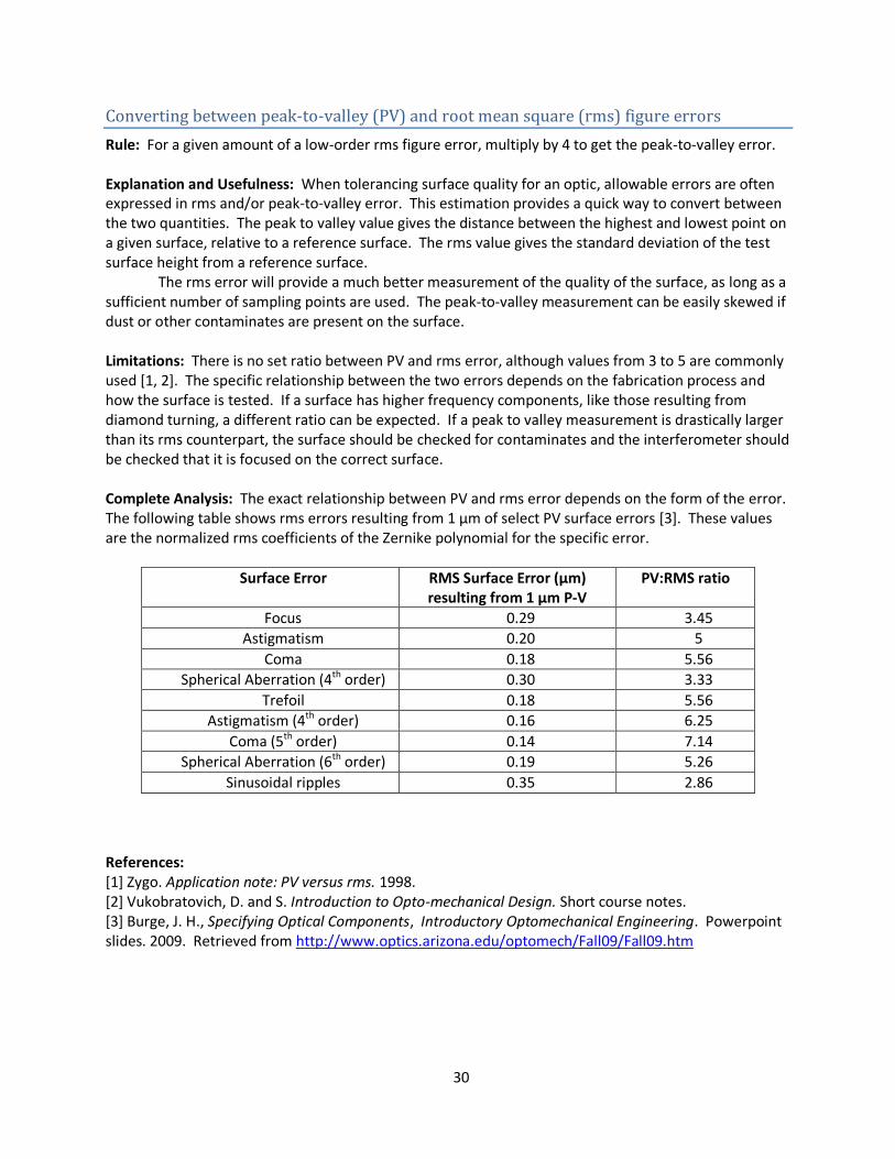
Converting between peak-to-valley (PV) and root mean square (rms) figure errors

Rule: For a given amount of a low-order rms figure error, multiply by 4 to get the peak-to-valley error. Explanation and Usefulness: When tolerancing surface quality for an optic, allowable errors are often expressed in rms and/or peak-to-valley error. This estimation provides a quick way to convert between the two quantities. The peak to valley value gives the distance between the highest and lowest point on a given surface, relative to a reference surface. The rms value gives the standard deviation of the test surface height from a reference surface.

The rms error will provide a much better measurement of the quality of the surface, as long as a sufficient number of sampling points are used. The peak-to-valley measurement can be easily skewed if dust or other contaminates are present on the surface. Limitations: There is no set ratio between PV and rms error, although values from 3 to 5 are commonly used [1, 2]. The specific relationship between the two errors depends on the fabrication process and how the surface is tested. If a surface has higher frequency components, like those resulting from diamond turning, a different ratio can be expected. If a peak to valley measurement is drastically larger than its rms counterpart, the surface should be checked for contaminates and the interferometer should be checked that it is focused on the correct surface. Complete Analysis: The exact relationship between PV and rms error depends on the form of the error. The following table shows rms errors resulting from 1 μm of select PV surface errors [3]. These values are the normalized rms coefficients of the Zernike polynomial for the specific error.

Surface Error RMS Surface Error (μm) resulting from 1 μm P-V

PV:RMS ratio

Focus 0.29 3.45

Astigmatism 0.20 5

Coma 0.18 5.56

Spherical Aberration (4th order) 0.30 3.33

Trefoil 0.18 5.56

Astigmatism (4th order) 0.16 6.25

Coma (5th order) 0.14 7.14

Spherical Aberration (6th order) 0.19 5.26

Sinusoidal ripples 0.35 2.86

References: [1] Zygo. Application note: PV versus rms. 1998. [2] Vukobratovich, D. and S. Introduction to Opto-mechanical Design. Short course notes. [3] Burge, J. H., Specifying Optical Components, Introductory Optomechanical Engineering. Powerpoint slides. 2009. Retrieved from http://www.optics.arizona.edu/optomech/Fall09/Fall09.htm

31

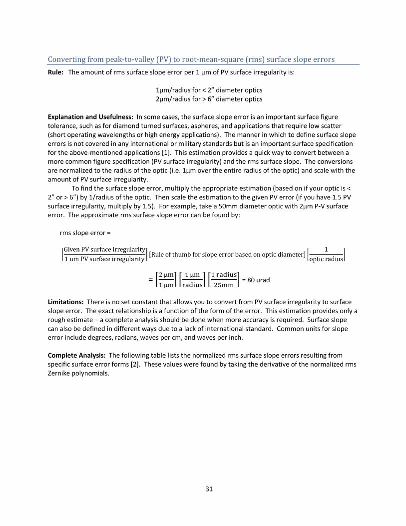
Converting from peak-to-valley (PV) to root-mean-square (rms) surface slope errors

Rule: The amount of rms surface slope error per 1 μm of PV surface irregularity is:

1μm/radius for < 2” diameter optics 2μm/radius for > 6” diameter optics

Explanation and Usefulness: In some cases, the surface slope error is an important surface figure tolerance, such as for diamond turned surfaces, aspheres, and applications that require low scatter (short operating wavelengths or high energy applications). The manner in which to define surface slope errors is not covered in any international or military standards but is an important surface specification for the above-mentioned applications [1]. This estimation provides a quick way to convert between a more common figure specification (PV surface irregularity) and the rms surface slope. The conversions are normalized to the radius of the optic (i.e. 1μm over the entire radius of the optic) and scale with the amount of PV surface irregularity.

To find the surface slope error, multiply the appropriate estimation (based on if your optic is < 2” or > 6”) by 1/radius of the optic. Then scale the estimation to the given PV error (if you have 1.5 PV surface irregularity, multiply by 1.5). For example, take a 50mm diameter optic with 2μm P-V surface error. The approximate rms surface slope error can be found by:

rms slope error =

= μ

μ

μ

= 80 urad

Limitations: There is no set constant that allows you to convert from PV surface irregularity to surface slope error. The exact relationship is a function of the form of the error. This estimation provides only a rough estimate – a complete analysis should be done when more accuracy is required. Surface slope can also be defined in different ways due to a lack of international standard. Common units for slope error include degrees, radians, waves per cm, and waves per inch. Complete Analysis: The following table lists the normalized rms surface slope errors resulting from specific surface error forms [2]. These values were found by taking the derivative of the normalized rms Zernike polynomials.

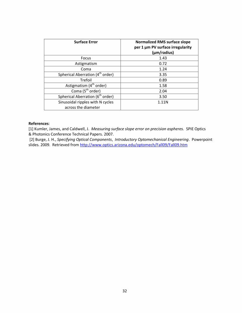
32

Surface Error Normalized RMS surface slope per 1 μm PV surface irregularity

(μm/radius)

Focus 1.43

Astigmatism 0.72

Coma 1.24

Spherical Aberration (4th order) 3.35

Trefoil 0.89

Astigmatism (4th order) 1.58

Coma (5th order) 2.04

Spherical Aberration (6th order) 3.50

Sinusoidal ripples with N cycles across the diameter

1.11N

References: [1] Kumler, James, and Caldwell, J. Measuring surface slope error on precision aspheres. SPIE Optics & Photonics Conference Technical Papers. 2007. [2] Burge, J. H., Specifying Optical Components, Introductory Optomechanical Engineering. Powerpoint slides. 2009. Retrieved from http://www.optics.arizona.edu/optomech/Fall09/Fall09.htm

33

Choosing a safety factor

Rule: For optics and optical systems, a safety factor of 2 to 4 should be applied. Safety Factor = allowed stress/applied stress

Explanation and Usefulness: A safety factor describes the ability of a system to withstand a certain load or stress compared to what it will actually experience. For example, if a system is expected to experience up to 3 G’s of shock loading during shipping, it can be designed to withstand 9G’s, providing a safety factor of 3. In general, a higher safety factor is preferred to allow for unforeseen errors, and is much higher for applications involving personal safety, but there is a trade-off. Larger safety factors provide less chance of system failure, but they will typically require more weight or tighter requirements and tolerances on the system. This in turn drives up cost and lead times. Limitations: This is a very generalized rule. Decisions about the safety factors should depend on how critical the application is and how familiar the materials and conditions are. Lower safety factors can be used when using very reliable materials in environmental conditions that are not severe. Higher safety factors should be used for materials that are not reliable or are unknown, for severe environmental conditions, and for critical applications involving personal safety [1]. Complete Analysis: NA

References: [1] Oberg, Erik, Franklin D. Jones, Holbrook L. Horton, and Henry H. Ryffel. Machinery's Handbook: a Reference Book for the Mechanical Engineer, Designer, Manufacturing Engineer, Draftsman, Toolmaker, and Machinist. 22nd Ed. Industrial, 1984. [2] Vukobratovich, D. and S. Introduction to Opto-mechanical Design. Short course notes.

34

Fit of a threaded retaining ring in a barrel

Rule: A retaining ring in a barrel should not be used to provide a position constraint for the lenses. Explanation and Usefulness: When designing an optical system that will be mounted in a barrel, the axial location of the lenses should not be determined by the retaining rings. Tightly fitted rings can cause stress in the lenses due to wedge error in the lenses. To avoid this problem, the fit of the retaining rings should be loose or some compliance should be provided. The lens position should then be defined by machined seats in the barrel or by precision spacers.

The class of fit is a tolerance standard on threads according to ASME B1.1 1989 [1]. The higher the class of thread, the tighter the tolerances, and therefore the fit, will be. For mounting lenses in a barrel with proper centering, a loose fit (Class 1 or 2) allows accommodation for wedge in the lens or against the barrel walls. The preload force is then also distributed uniformly around the lens. When a retaining ring is assembled in the barrel without the optics and shaken near the ear, the ring should rattle slightly in the barrel [2]. If a tight fit thread is being used for the retaining ring, an o-ring can be used between the retaining ring and the glass to provide some compliance. Limitations: NA Complete Analysis: NA References: [1] ASME Standard B1.1 – 1989: Unified Inch Screw Threads, UN and UNR Thread Form. [2] Yoder, Paul R. Opto-mechanical Systems Design. Bellingham, Wash.: SPIE, 2006. Pg. 189.

35

Designing to test plates

Rule: When designing an optical system, design to test plates whenever possible. Explanation and Usefulness: Many optical fabrication shops use test plates to control the radius and figure of an optic during the fabrication process. A test plate is a lens with a given radius that is controlled to a high degree of accuracy. It can be put in contact with a test part and the number of fringes counted to quickly determine the error in the test part. Manufacturers typically keep a large selection of test plates that are listed in test plate catalogs in optical design software.

When using optical design software, the radius of curvature of each optic in a system is typically optimized for best performance. It is advantageous to take the time to then fit as many radii in the design as possible to test plates listed in a given manufacturer’s test plate catalog. This will reduce both lead time and cost for the system. New test plates can cost $1,000 and upwards depending on the size of the optic and can require weeks for fabrication. Limitations: It is not always feasible to fit every surface to a test plate. This is just a suggestion to help reduce lead time and costs. Complete Analysis: NA References: [1] Smith, Warren J. Modern Optical Engineering: the Design of Optical Systems. New York: McGraw Hill, 2000.

36

Using the proper modulus for adhesive stiffness analysis

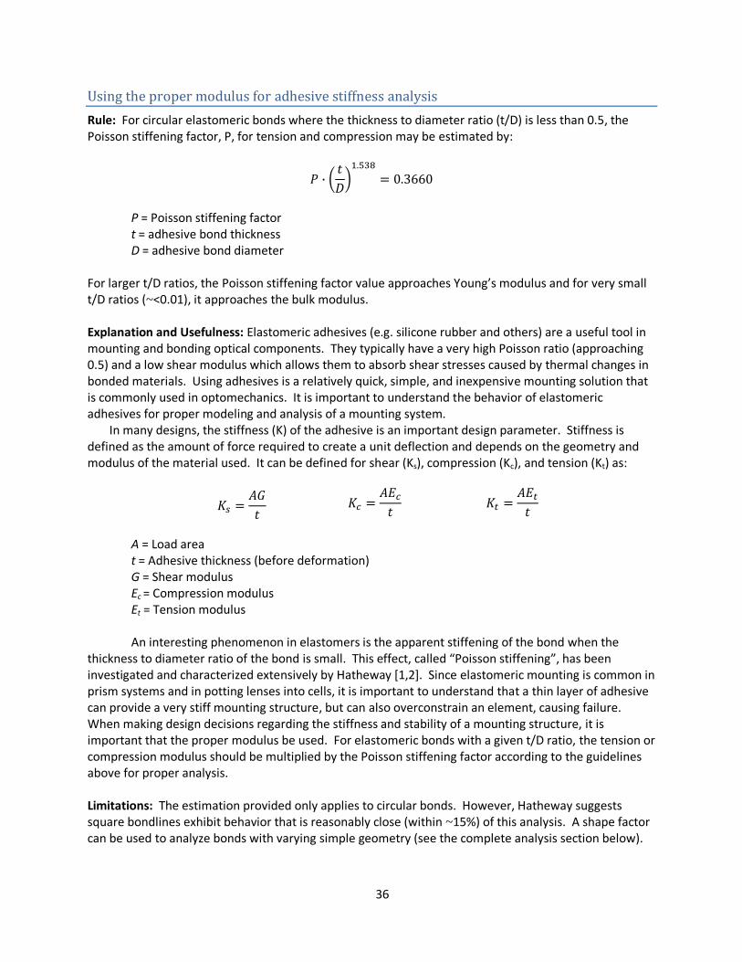
Rule: For circular elastomeric bonds where the thickness to diameter ratio (t/D) is less than 0.5, the Poisson stiffening factor, P, for tension and compression may be estimated by:

P = Poisson stiffening factor t = adhesive bond thickness D = adhesive bond diameter

For larger t/D ratios, the Poisson stiffening factor value approaches Young’s modulus and for very small t/D ratios (~<0.01), it approaches the bulk modulus. Explanation and Usefulness: Elastomeric adhesives (e.g. silicone rubber and others) are a useful tool in mounting and bonding optical components. They typically have a very high Poisson ratio (approaching 0.5) and a low shear modulus which allows them to absorb shear stresses caused by thermal changes in bonded materials. Using adhesives is a relatively quick, simple, and inexpensive mounting solution that is commonly used in optomechanics. It is important to understand the behavior of elastomeric adhesives for proper modeling and analysis of a mounting system.

In many designs, the stiffness (K) of the adhesive is an important design parameter. Stiffness is defined as the amount of force required to create a unit deflection and depends on the geometry and modulus of the material used. It can be defined for shear (Ks), compression (Kc), and tension (Kt) as:

A = Load area

t = Adhesive thickness (before deformation) G = Shear modulus Ec = Compression modulus Et = Tension modulus

An interesting phenomenon in elastomers is the apparent stiffening of the bond when the thickness to diameter ratio of the bond is small. This effect, called “Poisson stiffening”, has been investigated and characterized extensively by Hatheway [1,2]. Since elastomeric mounting is common in prism systems and in potting lenses into cells, it is important to understand that a thin layer of adhesive can provide a very stiff mounting structure, but can also overconstrain an element, causing failure. When making design decisions regarding the stiffness and stability of a mounting structure, it is important that the proper modulus be used. For elastomeric bonds with a given t/D ratio, the tension or compression modulus should be multiplied by the Poisson stiffening factor according to the guidelines above for proper analysis. Limitations: The estimation provided only applies to circular bonds. However, Hatheway suggests square bondlines exhibit behavior that is reasonably close (within ~15%) of this analysis. A shape factor can be used to analyze bonds with varying simple geometry (see the complete analysis section below).

37

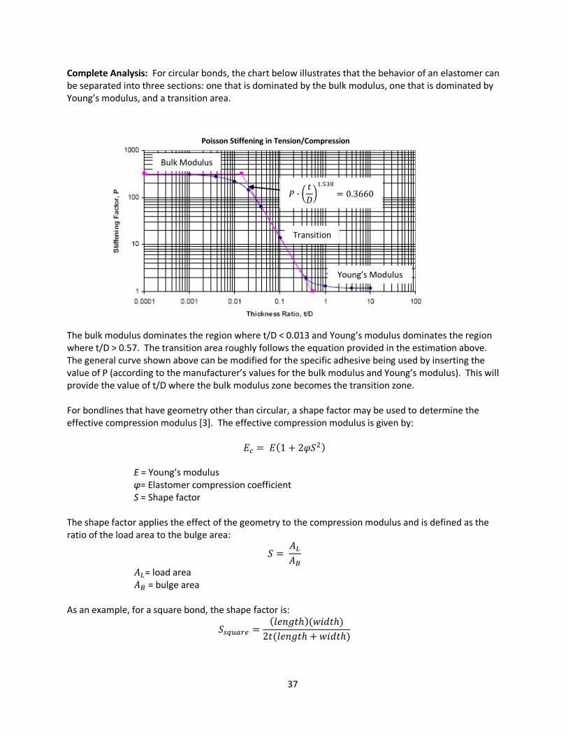
Complete Analysis: For circular bonds, the chart below illustrates that the behavior of an elastomer can be separated into three sections: one that is dominated by the bulk modulus, one that is dominated by Young’s modulus, and a transition area.

The bulk modulus dominates the region where t/D < 0.013 and Young’s modulus dominates the region where t/D > 0.57. The transition area roughly follows the equation provided in the estimation above. The general curve shown above can be modified for the specific adhesive being used by inserting the value of P (according to the manufacturer’s values for the bulk modulus and Young’s modulus). This will provide the value of t/D where the bulk modulus zone becomes the transition zone. For bondlines that have geometry other than circular, a shape factor may be used to determine the effective compression modulus [3]. The effective compression modulus is given by:

E = Young’s modulus φ= Elastomer compression coefficient S = Shape factor The shape factor applies the effect of the geometry to the compression modulus and is defined as the ratio of the load area to the bulge area:

= load area = bulge area As an example, for a square bond, the shape factor is:

Bulk Modulus

Transition

Young’s Modulus

Poisson Stiffening in Tension/Compression

38

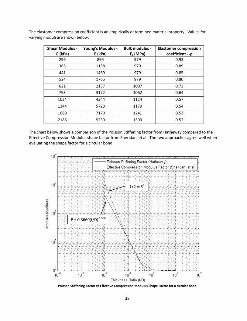
The elastomer compression coefficient is an empirically determined material property. Values for varying moduli are shown below:

Shear Modulus - G (kPa)

Young’s Modulus - E (kPa)

Bulk modulus - Eb (MPa)

Elastomer compression coefficient - φ

296 896 979 0.93

365 1158 979 0.89

441 1469 979 0.85

524 1765 979 0.80

621 2137 1007 0.73

793 3172 1062 0.64

1034 4344 1124 0.57

1344 5723 1179 0.54

1689 7170 1241 0.53

2186 9239 1303 0.52

The chart below shows a comparison of the Poisson Stiffening factor from Hatheway compared to the Effective Compression Modulus shape factor from Sheridan, et al. The two approaches agree well when evaluating the shape factor for a circular bond.

Poisson Stiffening Factor vs Effective Compression Modulus Shape Factor for a circular bond

P = 0.3660(t/D)-1.538

1+2 φ S2

39

References: [1] Hatheway, Alson E., “Designing elastomeric mirror mountings,” New Developments in Optomechanics, Proceedings of SPIE, 6665-03 (Bellingham: SPIE, 2007). [2] Hatheway, A. E., “Analysis of adhesive bonds in optics,” Optomechanical Design, Volume 1998 (Bellingham: SPIE, July, 1993). [3] P. M. Sheridan, F. O. James, and T. S. Miller, Design of components, in Engineering with Rubber, Munich:Hanser, 1992, pp. 209.

40

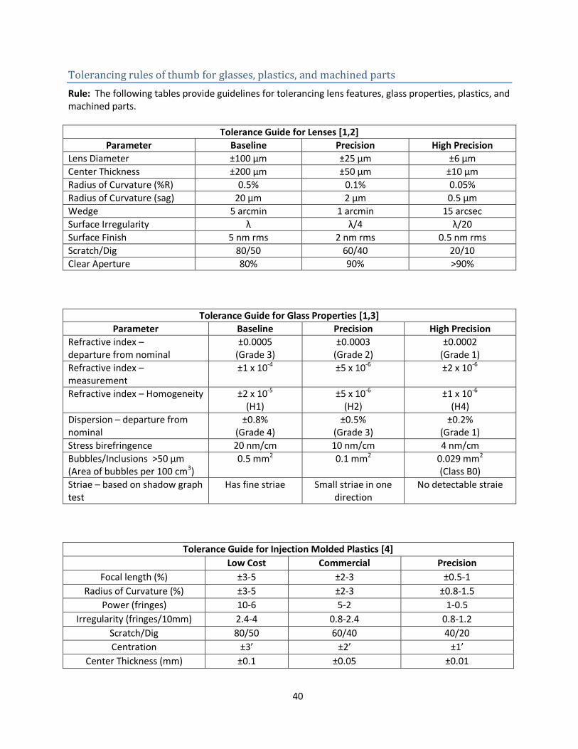
Tolerancing rules of thumb for glasses, plastics, and machined parts

Rule: The following tables provide guidelines for tolerancing lens features, glass properties, plastics, and machined parts.

Tolerance Guide for Lenses [1,2]

Parameter Baseline Precision High Precision

Lens Diameter ±100 μm ±25 μm ±6 μm

Center Thickness ±200 μm ±50 μm ±10 μm

Radius of Curvature (%R) 0.5% 0.1% 0.05%

Radius of Curvature (sag) 20 μm 2 μm 0.5 μm

Wedge 5 arcmin 1 arcmin 15 arcsec

Surface Irregularity λ λ/4 λ/20

Surface Finish 5 nm rms 2 nm rms 0.5 nm rms

Scratch/Dig 80/50 60/40 20/10

Clear Aperture 80% 90% >90%

Tolerance Guide for Glass Properties [1,3]

Parameter Baseline Precision High Precision

Refractive index – departure from nominal

±0.0005 (Grade 3)

±0.0003 (Grade 2)

±0.0002 (Grade 1)

Refractive index – measurement

±1 x 10-4 ±5 x 10-6

±2 x 10-6

Refractive index – Homogeneity ±2 x 10-5

(H1) ±5 x 10-6

(H2) ±1 x 10-6

(H4)

Dispersion – departure from nominal

±0.8% (Grade 4)

±0.5% (Grade 3)

±0.2% (Grade 1)

Stress birefringence 20 nm/cm 10 nm/cm 4 nm/cm

Bubbles/Inclusions >50 μm (Area of bubbles per 100 cm3)

0.5 mm2 0.1 mm2 0.029 mm2 (Class B0)

Striae – based on shadow graph test

Has fine striae Small striae in one direction

No detectable straie

Tolerance Guide for Injection Molded Plastics [4]

Low Cost Commercial Precision

Focal length (%) ±3-5 ±2-3 ±0.5-1

Radius of Curvature (%) ±3-5 ±2-3 ±0.8-1.5

Power (fringes) 10-6 5-2 1-0.5

Irregularity (fringes/10mm) 2.4-4 0.8-2.4 0.8-1.2

Scratch/Dig 80/50 60/40 40/20

Centration ±3’ ±2’ ±1’

Center Thickness (mm) ±0.1 ±0.05 ±0.01

41

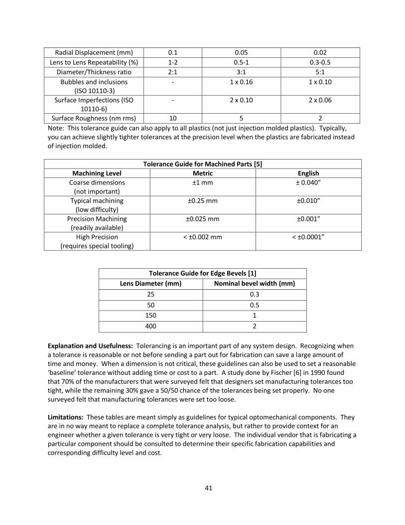
Radial Displacement (mm) 0.1 0.05 0.02

Lens to Lens Repeatability (%) 1-2 0.5-1 0.3-0.5

Diameter/Thickness ratio 2:1 3:1 5:1

Bubbles and inclusions (ISO 10110-3)

- 1 x 0.16 1 x 0.10

Surface Imperfections (ISO 10110-6)

- 2 x 0.10 2 x 0.06

Surface Roughness (nm rms) 10 5 2

Note: This tolerance guide can also apply to all plastics (not just injection molded plastics). Typically, you can achieve slightly tighter tolerances at the precision level when the plastics are fabricated instead of injection molded.

Tolerance Guide for Machined Parts [5]

Machining Level Metric English

Coarse dimensions (not important)

±1 mm ± 0.040”

Typical machining (low difficulty)

±0.25 mm ±0.010”

Precision Machining (readily available)

±0.025 mm ±0.001”

High Precision (requires special tooling)

< ±0.002 mm < ±0.0001”

Tolerance Guide for Edge Bevels [1]

Lens Diameter (mm) Nominal bevel width (mm)

25 0.3

50 0.5

150 1

400 2

Explanation and Usefulness: Tolerancing is an important part of any system design. Recognizing when a tolerance is reasonable or not before sending a part out for fabrication can save a large amount of time and money. When a dimension is not critical, these guidelines can also be used to set a reasonable ‘baseline’ tolerance without adding time or cost to a part. A study done by Fischer [6] in 1990 found that 70% of the manufacturers that were surveyed felt that designers set manufacturing tolerances too tight, while the remaining 30% gave a 50/50 chance of the tolerances being set properly. No one surveyed felt that manufacturing tolerances were set too loose. Limitations: These tables are meant simply as guidelines for typical optomechanical components. They are in no way meant to replace a complete tolerance analysis, but rather to provide context for an engineer whether a given tolerance is very tight or very loose. The individual vendor that is fabricating a particular component should be consulted to determine their specific fabrication capabilities and corresponding difficulty level and cost.

42

Complete Analysis: NA References: [1] Burge, J. H., Specifying Optical Components, Introductory Optomechanical Engineering. Powerpoint slides. 2009. Retrieved from http://www.optics.arizona.edu/optomech/Fall09/Fall09.htm [2] Optimax Systems, Inc. Manufacturing Tolerances chart. 2008. http://www.optimaxsi.com/Resources/ManufacturingChart.php [3] Schott. Optical Glass: Description of Properties 2009. Pocket catalog v1.8. 2009. www.schott.com [4] Bäumer, Stefan. Handbook of Plastic Optics. Weinheim: Wiley-VCH, 2005. [5] Burge, J. H., Mechanical Fabrication and Metrology, Introductory Optomechanical Engineering. Powerpoint slides. 2009. Retrieved from http://www.optics.arizona.edu/optomech/Fall09/Fall09.htm [6] Fischer, R. H., Optimization of Lens Designer to Manufacturer Communications, Proc. SPIE 1354, 506, 1990.

43

Stiffness relationship between system and isolators

Rule: When vibration isolators are used, their resonant frequency should be at least an order of magnitude less than the system they are isolating Explanation and Usefulness: When designing a system, the vibration environment the system will be operating in is an important consideration. Vibrations can occur from objects as large as a tall swaying building or passing cars and as small as someone walking in a room or a motor that drives the fan in a computer. Regardless of the source, vibration isolators can be used to reduce the amount of vibration that is transferred from the environment to a system.

The isolation of a system is accomplished by maintaining the proper relationship between the frequency of the environmental vibrations and the natural frequency of the system. A system’s natural frequency is the frequency at which it resonates, and depends on the mass of the system and the stiffness of the support structure (beam, spring, etc).

ω0= natural frequency (rad/sec)

f0 = natural frequency (Hz) k = stiffness of the beam/spring

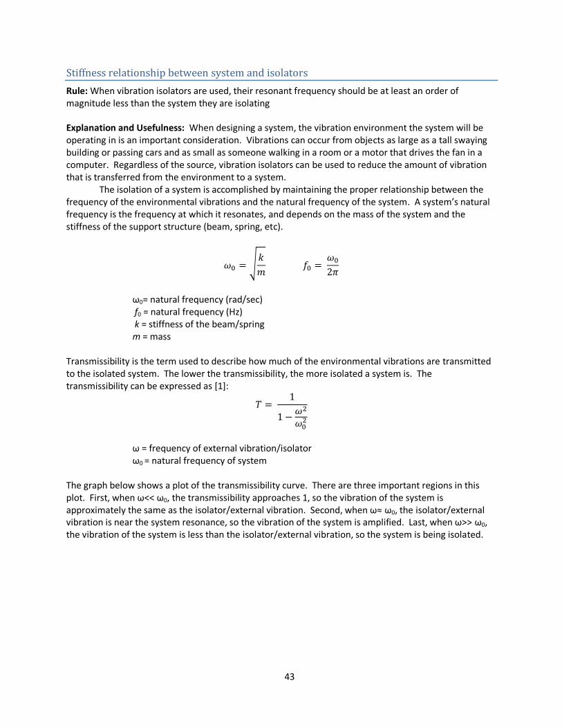
m = mass Transmissibility is the term used to describe how much of the environmental vibrations are transmitted to the isolated system. The lower the transmissibility, the more isolated a system is. The transmissibility can be expressed as [1]:

ω = frequency of external vibration/isolator

ω0 = natural frequency of system The graph below shows a plot of the transmissibility curve. There are three important regions in this plot. First, when ω<< ω0, the transmissibility approaches 1, so the vibration of the system is approximately the same as the isolator/external vibration. Second, when ω≈ ω0, the isolator/external vibration is near the system resonance, so the vibration of the system is amplified. Last, when ω>> ω0, the vibration of the system is less than the isolator/external vibration, so the system is being isolated.

44

From this graph, we can see it is important that the natural frequency of the isolator is much smaller than natural frequency of the system it is isolating. This estimation provides an approximate amount of how much lower the natural frequency of the isolator should be relative to the natural frequency of the

system to be effective (i.e.

).

Limitations: The requirements for any given system and isolator will be different, so this estimation is meant simply as a guideline. There are a wide variety of isolator materials and designs, and the specific isolator properties chosen will ultimately depend on the system requirements and vibration environment. Some of the common types of isolators include elastomeric isolators, springs, spring-friction dampers, springs with air dampings, springs with wire mesh, and pneumatic systems [2]. Each isolator type has different advantages, disadvantages, and uses which can be considered when choosing an isolator.

Complete Analysis: Isolation technically begins at the point where

since T < 1. At that point,

however, the isolation effect is very small and due to being at the border between isolation and amplification, any error may actually cause amplification instead of the intended isolation. As ω/ω0 increases, the transmissibility decreases proportional to 1/ ω2. The table below provides approximate frequency values for common sources of vibration.

Amplification

Isolation

Frequency Ratio,

Tran

smis

sib

ility

, T

45

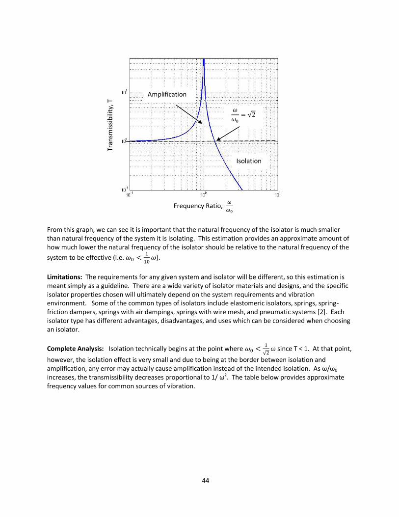
Common Environmental Noise Sources [1]

Vibration Type Frequency

Swaying of tall buildings 0.1 – 5 Hz

Machinery vibration 10 – 100 Hz

Building vibration 10 – 100 Hz

Microseisms (threshold of disturbance of interferometers and electron microscopes)

0.1 – 1 Hz

Atomic vibrations 1012 Hz

References: [1] Newport Corporation. Fundamentals of Vibration, www.newport.com . 2010. [2] Barry Controls. Isolator Selection. www.barrycontrols.com/engineering/shock.cfm. 2010.

46

Basic rules for dimensioning a drawing

Rule: 1. A feature can be located with fixed dimensional tolerances from one point only in a given straight line. 2. If an overall dimension is specified, one intermediate dimension should not be dimensioned. Dimensions should be given between those points that it is essential to hold in a specific relation to each other. 3. Dimensions should not be duplicated on a drawing to avoid inconsistencies. 4. As far as possible, the dimensions on companion parts/drawings should be given from the same relative locations. 5. Dimension lines should not pass through figures. 6. When there are several parallel dimension lines, they should be staggered. Explanation and Usefulness: When creating a drawing for a part, correct dimensioning and tolerancing practices are critical for a machinist to fabricate a part the way it was intended by the designer. These rules provide a few basic guidelines for the designer in order to aid in proper dimensioning. For a complete list of the conventions for dimensioning a drawing, ASME Y14.5M should be consulted [1]. Limitations: These rules are basic dimensioning guidelines, not an all inclusive list. Complete Analysis: An example of a common mistake in dimensioning is shown below [2]. The horizontal dimensions calling out the lengths of the body and the stem of the part violate the first and second rules stated above. Depending on the sequence which the features are machined, the tolerances for each dimension may not be met. It is also not clear from the dimensioning which lengths are most important.

Incorrect dimensioning of part

The following two drawings show correct dimensioning for the lengths of the body and stem of the part. Figure 1 shows the case where the individual lengths of the stem and body are more important than the overall length of the part. Figure 2 shows the case where the body and overall length of the part are more important features than the stem.

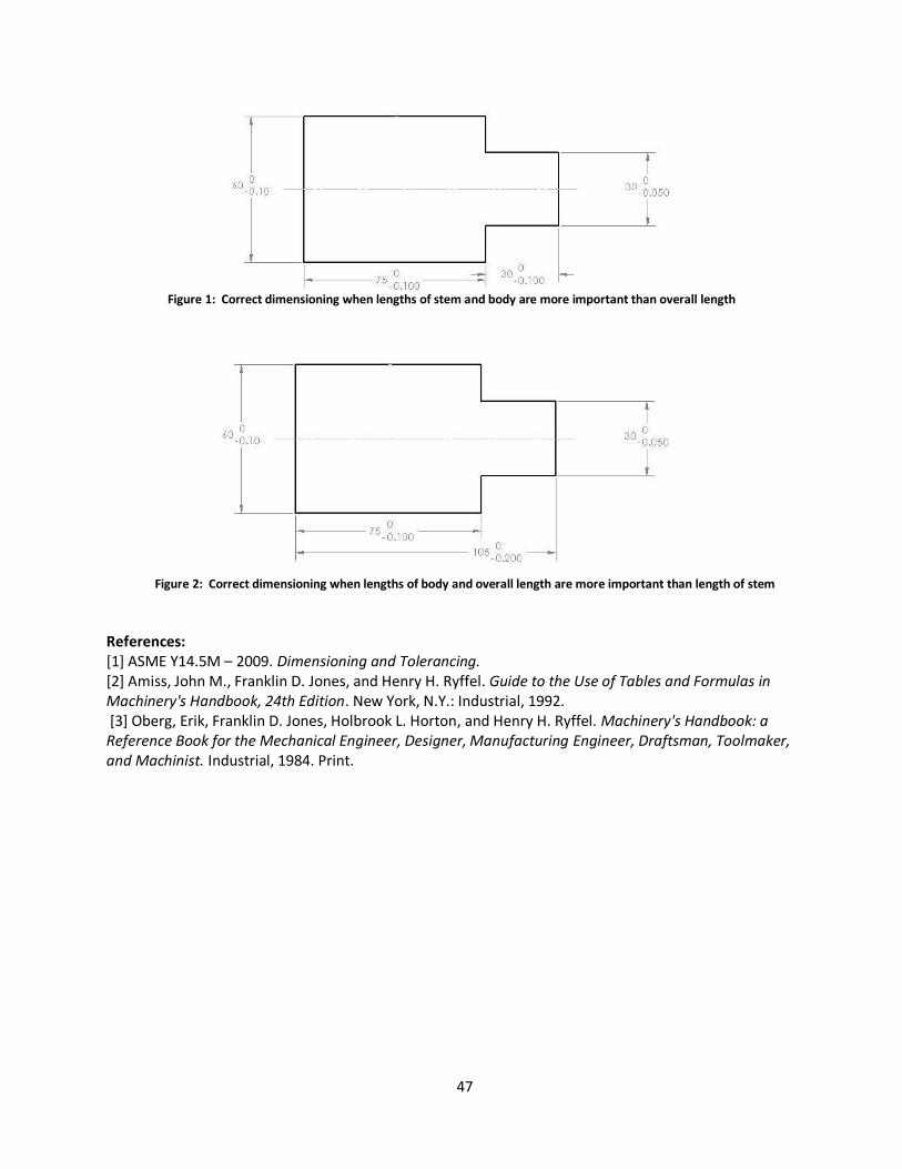
47

Figure 1: Correct dimensioning when lengths of stem and body are more important than overall length

Figure 2: Correct dimensioning when lengths of body and overall length are more important than length of stem

References: [1] ASME Y14.5M – 2009. Dimensioning and Tolerancing. [2] Amiss, John M., Franklin D. Jones, and Henry H. Ryffel. Guide to the Use of Tables and Formulas in Machinery's Handbook, 24th Edition. New York, N.Y.: Industrial, 1992. [3] Oberg, Erik, Franklin D. Jones, Holbrook L. Horton, and Henry H. Ryffel. Machinery's Handbook: a Reference Book for the Mechanical Engineer, Designer, Manufacturing Engineer, Draftsman, Toolmaker, and Machinist. Industrial, 1984. Print.

48

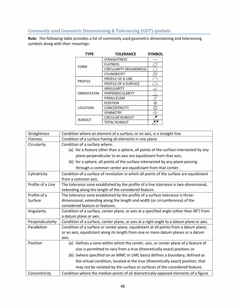
Commonly used Geometric Dimensioning & Tolerancing (GDT) symbols

Rule: The following table provides a list of commonly used geometric dimensioning and tolerancing symbols along with their meanings: TYPE TOLERANCE SYMBOL

STRAIGHTNESS

FLATNESS

CYLINDRICITY

CIRCULARITY (ROUNDNESS)

PROFILE OF A LINE

PROFILE OF A SURFACE

ANGULARITY

PERPENDICULARITY

PARALLELISM

POSITION

CONCENTRICITY

SYMMETRY

CIRCULAR RUNOUT

TOTAL RUNOUT

FORM

PROFILE

ORIENTATION

LOCATION

RUNOUT

Straightness Condition where an element of a surface, or an axis, is a straight line.

Flatness Condition of a surface having all elements in one plane.

Circularity Condition of a surface where: (a) for a feature other than a sphere, all points of the surface intersected by any

plane perpendicular to an axis are equidistant from that axis;

(b) for a sphere, all points of the surface intersected by any plane passing

through a common center are equidistant from that center.

Cylindricity Condition of a surface of revolution in which all points of the surface are equidistant from a common axis.

Profile of a Line The tolerance zone established by the profile of a line tolerance is two-dimensional, extending along the length of the considered feature.

Profile of a Surface

The tolerance zone established by the profile of a surface tolerance is three-dimensional, extending along the length and width (or circumference) of the considered feature or features.

Angularity Condition of a surface, center plane, or axis at a specified angle (other than 90°) from a datum plane or axis.

Perpendicularity Condition of a surface, center plane, or axis at a right angle to a datum plane or axis.

Parallelism Condition of a surface or center plane, equidistant at all points from a datum plane; or an axis, equidistant along its length from one or more datum planes or a datum axis.

Position (a) Defines a zone within which the center, axis, or center plane of a feature of

size is permitted to vary from a true (theoretically exact) position; or

(b) (where specified on an MMC or LMC basis) defines a boundary, defined as

the virtual condition, located at the true (theoretically exact) position, that

may not be violated by the surface or surfaces of the considered feature.

Concentricity Condition where the median points of all diametrically opposed elements of a figure

49

of revolution (or correspondingly-located elements of two or more radially-disposed features) are congruent with the axis (or center point) of a datum feature.

Symmetry Condition where the center plane of the actual mating envelope of one or more features is congruent with the axis or center plane of a datum feature within specified limits.

Circular Runout Provides control of circular elements of a surface. The tolerance is applied independently at each circular measuring position as the part is rotated 360°.

Total Runout Provides composite control of all surface elements. The tolerance is applied simultaneously to all circular and profile measuring positions as the part is rotated 360°.

Explanation and Usefulness: Geometric dimensioning and tolerancing (GD&T) is a way to provide tolerances on the geometry and fit of mechanical parts. It allows engineers to describe tolerances in a way other than simple maximum and minimum dimensions. Although some of the symbols provide an individual tolerance, many of the symbols provide a related tolerance (they have a tolerance in reference to a datum point). This chart provides a list of the most commonly used GD&T symbols. For a detailed list of GD&T symbols as well as how to use and interpret them, ASME Y14.5M can be referenced [1].

A common example of applying GD&T to optomechanical systems is on a lens barrel. The concentricity of the openings at both ends of the lens barrel is defined as well as the perpendicularity of the barrel edges to the barrel side. GD&T is also useful when defining a pattern of features on a part. Limitations: NA Complete Analysis: NA References: [1] ASME Y14.5M – 2009. Dimensioning and Tolerancing.

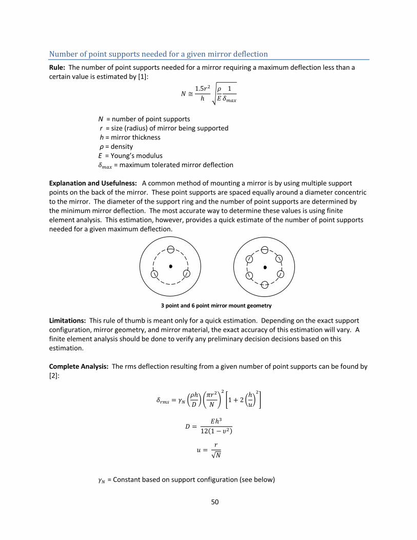
50

Number of point supports needed for a given mirror deflection

Rule: The number of point supports needed for a mirror requiring a maximum deflection less than a certain value is estimated by [1]:

N = number of point supports

r = size (radius) of mirror being supported h = mirror thickness ρ = density E = Young’s modulus = maximum tolerated mirror deflection Explanation and Usefulness: A common method of mounting a mirror is by using multiple support points on the back of the mirror. These point supports are spaced equally around a diameter concentric to the mirror. The diameter of the support ring and the number of point supports are determined by the minimum mirror deflection. The most accurate way to determine these values is using finite element analysis. This estimation, however, provides a quick estimate of the number of point supports needed for a given maximum deflection. Limitations: This rule of thumb is meant only for a quick estimation. Depending on the exact support configuration, mirror geometry, and mirror material, the exact accuracy of this estimation will vary. A finite element analysis should be done to verify any preliminary decision decisions based on this estimation. Complete Analysis: The rms deflection resulting from a given number of point supports can be found by [2]:

= Constant based on support configuration (see below)

3 point and 6 point mirror mount geometry

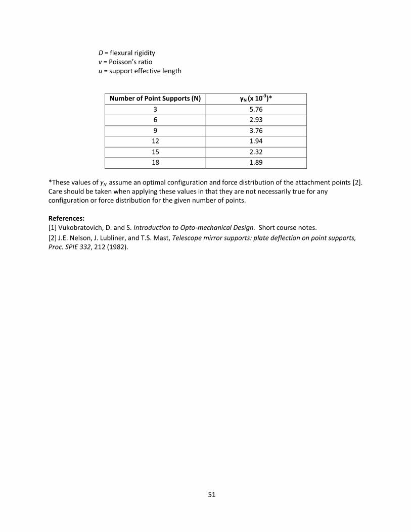
51

D = flexural rigidity v = Poisson’s ratio u = support effective length

Number of Point Supports (N) γN (x 10-3)*

3 5.76

6 2.93

9 3.76

12 1.94

15 2.32

18 1.89

*These values of assume an optimal configuration and force distribution of the attachment points [2]. Care should be taken when applying these values in that they are not necessarily true for any configuration or force distribution for the given number of points. References: [1] Vukobratovich, D. and S. Introduction to Opto-mechanical Design. Short course notes.

[2] J.E. Nelson, J. Lubliner, and T.S. Mast, Telescope mirror supports: plate deflection on point supports, Proc. SPIE 332, 212 (1982).

52

Mechanical

Estimation of preload torque

Rule: Preload torque can be estimated by:

P = preload torque Q = applied torque DT = thread pitch diameter

Explanation and Usefulness: Often times when assembling an optical system, a preload force is needed for a given element or mounting structure. It is important to know how much torque is necessary to provide a given preload. This equation provides a quick estimation of the preload torque given an applied torque and the diameter of the threads. This is commonly applied for determining the preload torque for a retaining ring lens mount or for a fastener. Limitations: This estimation relies on quantifying the friction effects that occur between the two materials, however there is often a large amount of uncertainty in the exact friction coefficient values. They are strongly dependent on the smoothness of the surfaces and whether the surfaces are dry or lubricated. This equation has less than 8% error when using estimated coefficients of sliding friction for aluminum-aluminum interfaces and aluminum-glass interfaces. For more than a rough estimate of the preload torque, the equations below should be used with the best-known coefficients of sliding friction. Complete Analysis: The preload torque for a retaining ring on glass is more accurately estimated by:

=coefficient of sliding for metal-to-metal =coefficient of sliding for glass-to-metal Q = applied torque DT = thread pitch diameter This equation takes into account the sliding friction of the metal threads against the metal retainer

and the metal retainer against the lens. Yoder [1] explains this is still an estimation due to small factors neglected in the equation derivation and the large uncertainties in the sliding coefficients. Black anodized aluminum has a value of about 0.19 while anodized aluminum against polished glass gives a value of about 0.15.

The torque required to produce a given preload for a metal fastener in a metal plate is estimated by [2]:

Q = applied torque P = preload torque

= thread pitch diameter = fastener head diameter

μ = coefficient of friction of plate

53

= coefficient of friction of fastener

= distance the fastener moves parallel to the screw axis in one turn (equal to the pitch for a single thread)

α = half-apex angle of the fastener compressed into a cone (pressure-cone method for stiffness calculations). Can assume α = 30°.

Again, this is still an estimation due to the fact that the coefficients of friction vary widely. On average, both μ and are taken to be 0.15.

References: [1] Yoder, Paul R. Opto-mechanical Systems Design. Bellingham, Wash.: SPIE, 2006. Pg. 189. [2] Shigley, Joseph Edward., and Charles R. Mischke. Mechanical Engineering Design. New York: McGraw-Hill, 1989.

54

Relation of machining processes to international tolerance (IT) grades

Rule: The following table provides general rules of thumb for which machining processes can produce items within a specific international tolerance (IT) grade [1].

Explanation and Usefulness: International tolerance (IT) grades define how precise a given machining process can produce a part or feature. They are specified in ISO 286 [2]. The lower the IT grade, the more precise a part or finish is. When designing a mount or mechanical structure, an IT grade may be specified for a particular feature to ensure a certain finish or fit is achieved. This chart allows an appropriate machining process to be specified to achieve a given tolerance grade. Limitations: Depending on the specific shop and procedure used for each machining process, a certain IT grade may be obtained outside the limits stated above. These are simply guidelines for what IT grades can be obtained by machining procedures in a typical shop. Complete Analysis: The chart on the next page shows the specific tolerances (in mm) for each international tolerance grades for a part of a given size [3]. The tolerances for IT grades larger than IT 16 can be calculated using the following formulas:

IT17 = IT12 x 10 IT18 = IT13 x 10

etc… References:

[1] Oberg, Erik, Franklin D. Jones, Holbrook L. Horton, and Henry H. Ryffel. Machinery's Handbook: a Reference Book for the Mechanical Engineer, Designer, Manufacturing Engineer, Draftsman, Toolmaker, and Machinist. Industrial, 1984. [2] ISO 286: 1988. System of Limits and Fits. [3] ANSI/ASME B4.2 – 1999, Preferred Metric Limits and Fits.

4 5 6 7 8 9 10 11 12 13

Machining Processes and Tolerance Grades

Cylindrical Grinding

Surface Grinding

Diamond Turning

Lapping/Honing

Milling

Planing and Shaping

Drilling

Diamond Boring

Broaching

Reaming

Turning

Boring

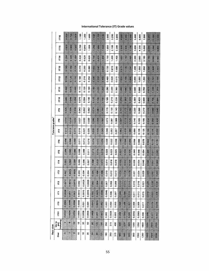
55

International Tolerance (IT) Grade values

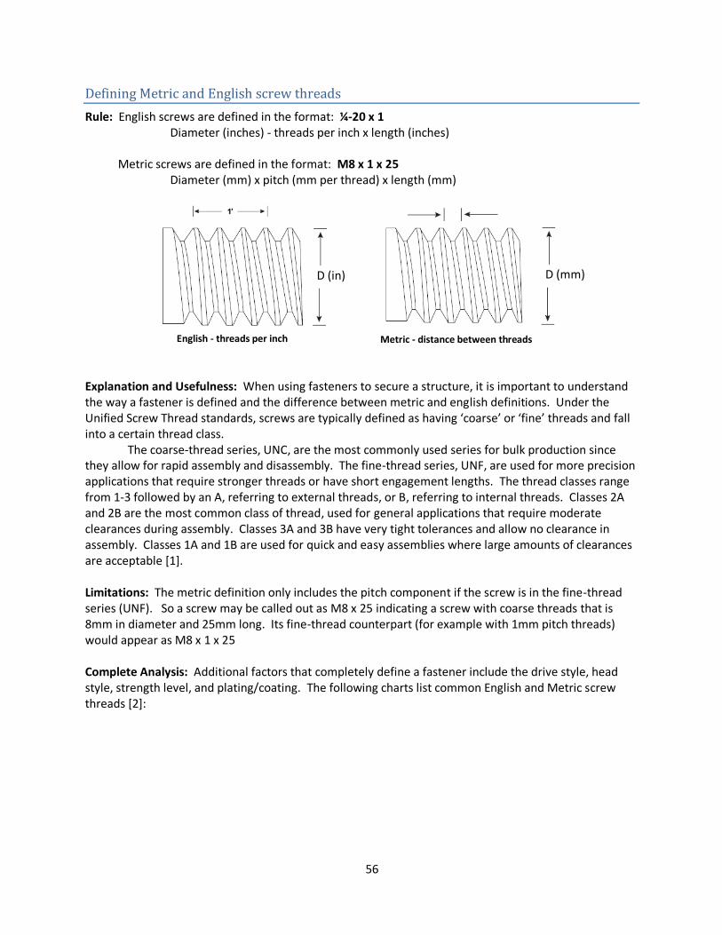
56

Defining Metric and English screw threads

Rule: English screws are defined in the format: ¼-20 x 1 Diameter (inches) - threads per inch x length (inches)

Metric screws are defined in the format: M8 x 1 x 25 Diameter (mm) x pitch (mm per thread) x length (mm)

Explanation and Usefulness: When using fasteners to secure a structure, it is important to understand the way a fastener is defined and the difference between metric and english definitions. Under the Unified Screw Thread standards, screws are typically defined as having ‘coarse’ or ‘fine’ threads and fall into a certain thread class.

The coarse-thread series, UNC, are the most commonly used series for bulk production since they allow for rapid assembly and disassembly. The fine-thread series, UNF, are used for more precision applications that require stronger threads or have short engagement lengths. The thread classes range from 1-3 followed by an A, referring to external threads, or B, referring to internal threads. Classes 2A and 2B are the most common class of thread, used for general applications that require moderate clearances during assembly. Classes 3A and 3B have very tight tolerances and allow no clearance in assembly. Classes 1A and 1B are used for quick and easy assemblies where large amounts of clearances are acceptable [1]. Limitations: The metric definition only includes the pitch component if the screw is in the fine-thread series (UNF). So a screw may be called out as M8 x 25 indicating a screw with coarse threads that is 8mm in diameter and 25mm long. Its fine-thread counterpart (for example with 1mm pitch threads) would appear as M8 x 1 x 25 Complete Analysis: Additional factors that completely define a fastener include the drive style, head style, strength level, and plating/coating. The following charts list common English and Metric screw threads [2]:

English - threads per inch Metric - distance between threads

D (in) D (mm)

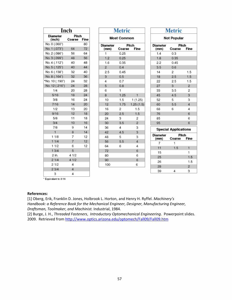
57

References: [1] Oberg, Erik, Franklin D. Jones, Holbrook L. Horton, and Henry H. Ryffel. Machinery's Handbook: a Reference Book for the Mechanical Engineer, Designer, Manufacturing Engineer, Draftsman, Toolmaker, and Machinist. Industrial, 1984. [2] Burge, J. H., Threaded Fasteners, Introductory Optomechanical Engineering. Powerpoint slides. 2009. Retrieved from http://www.optics.arizona.edu/optomech/Fall09/Fall09.htm

58

Galling of metals

Rule: Avoid using similar metals under load to prevent galling. Explanation and Usefulness: Galling is a form of surface damage in materials that occurs when solids are rubbed together. Material is transferred from one surface to another, creating abrasive surfaces and increasing adhesion between the two surfaces [1]. This is a common problem when two metal components of the same material are in contact without lubrication, for example, when a stainless steel fastener is used in a stainless steel part. Galling is particularly concerning because it cannot be remedied once it has occurred and will usually cause loss of functionality of the particular part.

The simplest way to avoid galling is to design with dissimilar metals or use lubrication at the interface of concern. There are also new ‘anti-galling’ alloys (e.g. Nitronic) that have high wear and gall-resistance [2], as well as companies that provide anti-galling coating services. Limitations: NA Complete Analysis: The only standard that exists for determining how resistant a material is to galling is the ‘button-on-block’ test defined by ASTM Standard G98 [3]. A button of the specimen under test is loaded against a large flat block of the same material and then rotated one revolution. An unaided visual inspection of the macroscopic roughness is done to determine if galling occurred according to the ASTM standard guidelines. The load can then be varied to determine the threshold galling stress (taken as the average of the lowest galled test and the highest non-galled test). A number of other methods have also been proposed and studied [4], but the button-on-block test is the only current standard. References: [1] ASTM G40 – 10: Standard Terminology Relating to Wear and Erosion. [2] U. Wiklund and I.M. Hutchings. Investigation of surface treatments for galling protection of titanium alloys, Wear 251 (2001), pp. 1034–1041 [3] ASTM G98 - 02(2009): Standard Test Method for Galling Resistance of Materials. [4] S.R. Hummel and B. Partlow, Comparison of Threshold Galling Results from Two Testing Methods, Tribol. Int., Vol 37, 2004, p 291–295.

59

Choosing a tap drill size

Rule: To obtain a tap drill size, use the following formula and drop all but the first decimal:

Root diameter = Screw diameter – thread spacing

Explanation and Usefulness: Tapping is the process in which threads are cut into the inside surface of a hole. The proper size tap must be chosen for a fastener of a given diameter and thread pitch. Choosing the correct size tap for a given fastener can be difficult given the number of factors that can influence the size of a drilled hole. This rule of thumb provides a quick way to determine an appropriate tap drill size for a given fastener. Limitations: Whether using this rule of thumb or a detailed calculation, there are a number of factors that can influence the size and accuracy of a drilled hole. These factors include, but are not limited to, the setup, the accuracy of the drill point, the size and length of the drill, the material, the runout on the machinery, and the lubrication, if any, that is used. For most materials, the resulting drill hole will be oversized, although there are some materials in which the hole may be undersized. The Machinery’s Handbook [1] provides a table of values for the amount diameters are typically oversized in drilling under normal shop conditions, as well as explanations of when a drill hole may be undersized. Complete Analysis: The following formulas provide the size of the tap drill hole for a given percentage of full thread (expressed as a decimal). The percentage of full thread refers to the amount of cross sectional thread engagement available in a tapped hole. The larger the drill size, the smaller the percentage of full thread and the weaker the thread. For most cases, a 50-60% thread engagement is satisfactory, although sometimes upwards of 75% is used as a safety factor.

For American Unified Threads: Root diameter = Screw diameter –

For ISO Metric Threads: Root diameter = Screw diameter – (1.08523 x Pitch x %full thread)

For American National Thread form: Root diameter = Screw diameter –

There are also many tap drill size selection charts available online or in machining reference books. References:

[1] Oberg, Erik, Franklin D. Jones, Holbrook L. Horton, and Henry H. Ryffel. Machinery's Handbook: a Reference Book for the Mechanical Engineer, Designer, Manufacturing Engineer, Draftsman, Toolmaker, and Machinist. 22nd Ed. Industrial, 1984.

60

Using threaded inserts

Rule: When using fasteners in soft materials, including aluminum, threaded inserts should be used for added robustness. Explanation and Usefulness: Threads in soft materials can be easily damaged in assembly and disassembly of a system. Aluminum is a common metal that this applies to, but there are a variety of metals, plastics, woods, and other materials that are considered softer materials. Threaded inserts are small coils of stronger metal material (e.g. stainless steel) that can be inserted into a tapped hole for added strength and robustness. They can also provide corrosion resistance and a repair for stripped threads. There are a large variety of different styles/types of threaded inserts as well as varying materials and lengths. Some common types of threaded inserts include helical, thread-locking, self-tapping, press-fit, and rivet nuts. Limitations: Care should be taken as to what metals are being used for the threaded inserts and the fastener that will come into contact with it. If a stainless steel fastener will be inserted into a stainless steel threaded insert, there is a higher likelihood that galling will occur (see ‘Galling of metals’ rule of thumb’). There are some ‘anti-galling’ threaded inserts available as well as special inserts for vacuum applications (e.g. Nitronic). Complete Analysis: NA References: [1] Yardley Products Corportation. 2010. www.yardleyproducts.com

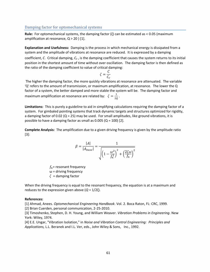
61

Damping factor for optomechanical systems

Rule: For optomechanical systems, the damping factor (ζ) can be estimated as < 0.05 (maximum amplification at resonance, Q > 20 ) [1]. Explanation and Usefulness: Damping is the process in which mechanical energy is dissipated from a system and the amplitude of vibrations at resonance are reduced. It is expressed by a damping

coefficient, C. Critical damping, Cr , is the damping coefficient that causes the system returns to its initial

position in the shortest amount of time without over oscillation. The damping factor is then defined as the ratio of the damping coefficient to value of critical damping:

The higher the damping factor, the more quickly vibrations at resonance are attenuated. The variable ‘Q' refers to the amount of transmission, or maximum amplification, at resonance. The lower the Q factor of a system, the better damped and more stable the system will be. The damping factor and

maximum amplification at resonance are related by:

.

Limitations: This is purely a guideline to aid in simplifying calculations requiring the damping factor of a system. For gimbaled pointing systems that track dynamic targets and structures optimized for rigidity, a damping factor of 0.02 (Q = 25) may be used. For small amplitudes, like ground vibrations, it is possible to have a damping factor as small as 0.005 (Q = 100) [2]. Complete Analysis: The amplification due to a given driving frequency is given by the amplitude ratio [3]:

= resonant frequency ω = driving frequency = damping factor When the driving frequency is equal to the resonant frequency, the equation is at a maximum and reduces to the expression given above (Q = 1/2ζ). References: [1] Ahmad, Anees. Optomechanical Engineering Handbook. Vol. 2. Boca Raton, FL: CRC, 1999. [2] Brian Cuerden, personal communication, 2-25-2010. [3] Timoshenko, Stephen, D. H. Young, and William Weaver. Vibration Problems in Engineering. New York: Wiley, 1974. [4] E.E. Ungar, "Vibration Isolation," in Noise and Vibration Control Engineering: Principles and Applications, L.L. Beranek and I.L. Ver, eds., John Wiley & Sons, Inc., 1992.

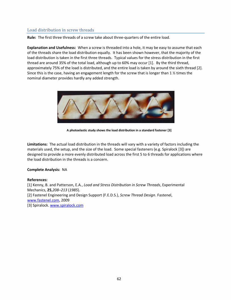
62

Load distribution in screw threads

Rule: The first three threads of a screw take about three-quarters of the entire load. Explanation and Usefulness: When a screw is threaded into a hole, it may be easy to assume that each of the threads share the load distribution equally. It has been shown however, that the majority of the load distribution is taken in the first three threads. Typical values for the stress distribution in the first thread are around 35% of the total load, although up to 60% may occur [1]. By the third thread, approximately 75% of the load is distributed, and the entire load is taken by around the sixth thread [2]. Since this is the case, having an engagement length for the screw that is longer than 1 ½ times the nominal diameter provides hardly any added strength.

A photoelastic study shows the load distribution in a standard fastener [3]

Limitations: The actual load distribution in the threads will vary with a variety of factors including the materials used, the setup, and the size of the load. Some special fasteners (e.g. Spiralock [3]) are designed to provide a more evenly distributed load across the first 5 to 6 threads for applications where the load distribution in the threads is a concern. Complete Analysis: NA References: [1] Kenny, B. and Patterson, E.A., Load and Stress Distribution in Screw Threads, Experimental Mechanics, 25,208–213 (1985). [2] Fastenel Engineering and Design Support (F.E.D.S.), Screw Thread Design. Fastenel, www.fastenel.com, 2009 [3] Spiralock. www.spiralock.com

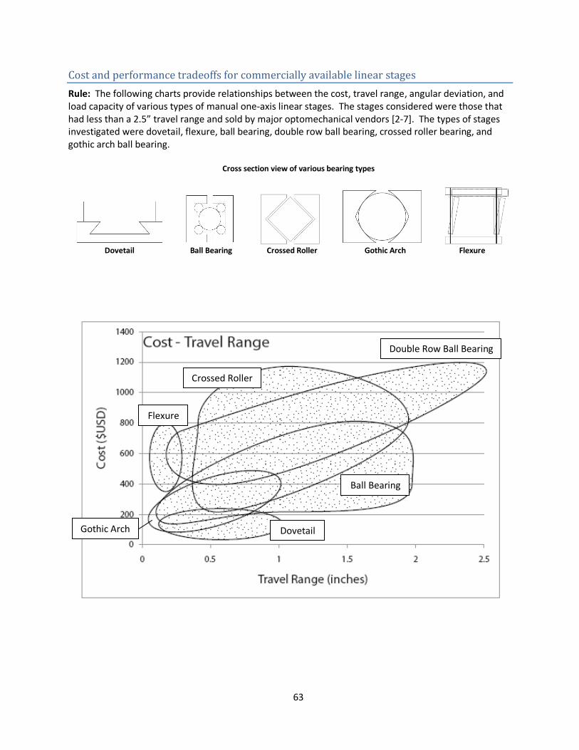
63

Cost and performance tradeoffs for commercially available linear stages

Rule: The following charts provide relationships between the cost, travel range, angular deviation, and load capacity of various types of manual one-axis linear stages. The stages considered were those that had less than a 2.5” travel range and sold by major optomechanical vendors [2-7]. The types of stages investigated were dovetail, flexure, ball bearing, double row ball bearing, crossed roller bearing, and gothic arch ball bearing.

Cross section view of various bearing types

Dovetail Ball Bearing Crossed Roller Gothic Arch Flexure

Ball Bearing

Dovetail

Double Row Ball Bearing

Crossed Roller

Flexure

Gothic Arch

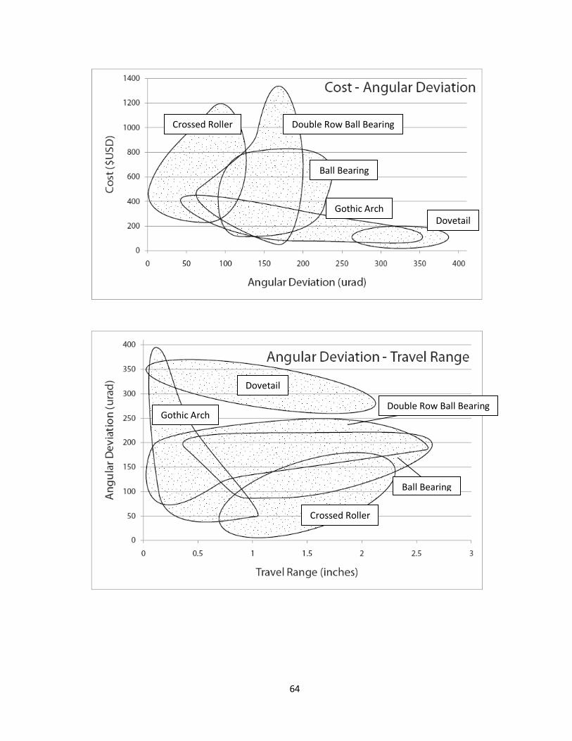
64

Crossed Roller

Ball Bearing

Double Row Ball Bearing

Gothic Arch Dovetail

Ball Bearing

Gothic Arch Double Row Ball Bearing

Crossed Roller

Dovetail

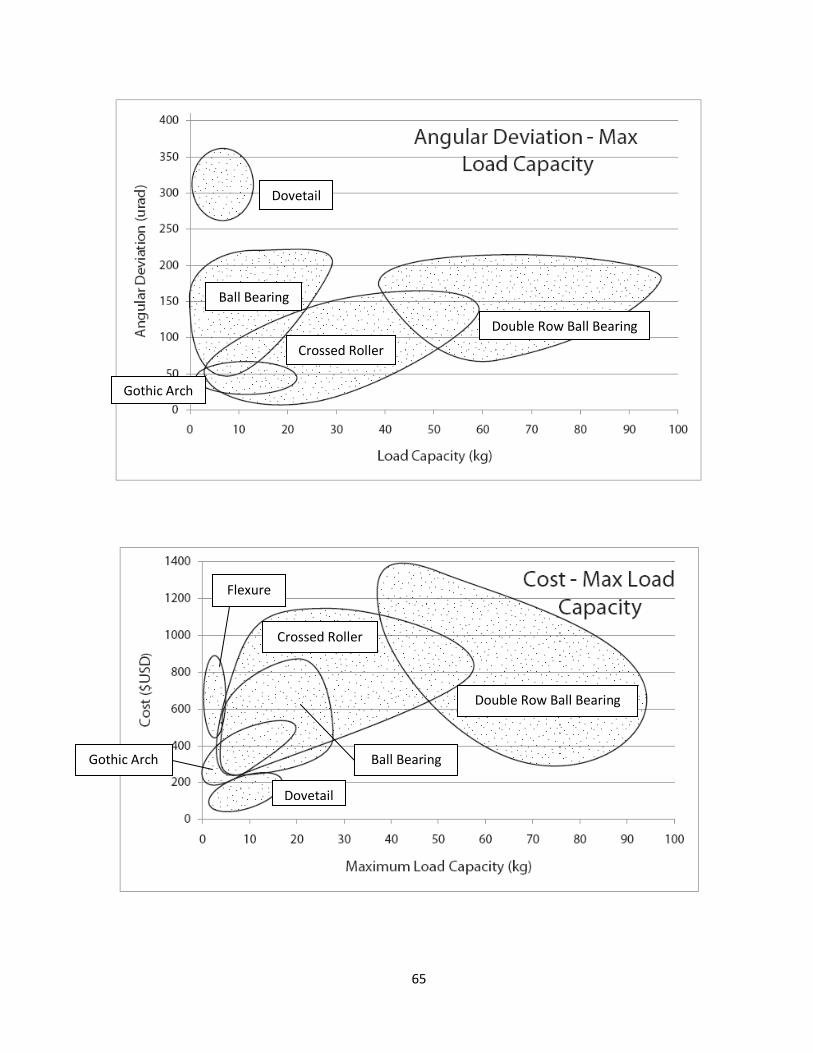
65

Crossed Roller

Ball Bearing

Double Row Ball Bearing

Gothic Arch

Dovetail

Crossed Roller

Ball Bearing

Dovetail

Flexure

Gothic Arch

Double Row Ball Bearing

66

Explanation and Usefulness: When multiple precise motions need to made in a system, stages are typically the solution. When choosing a stage for a specific application, some general factors that should be taken into account are repeatability, resolution, encoding accuracy, errors in motion, cost, load capacity, travel range, stiffness, stability, velocity of motion, environmental sensitivity, and additional features like over-travel protection and locking mechanisms. These charts aim to provide relationships between some of the main factors in choosing a stage for a specific application.

Limitations: These charts are meant to provide general relationships for the selection of an appropriate stage for a given application. Individual stage properties from a manufacturer should be verified before making any design decisions. Complete Analysis: The following table provides some additional general properties of the various types of linear stages [1,2].

Property Dovetail Ball Bearing Gothic Arch Ball Bearing

Crossed Roller

Bearing

Flexure

Cost Low Moderate Moderate High Moderate/High

Resolution Low Moderate Moderate High Very High

Travel Range Large Moderate Moderate Moderate Very Small

Load Capacity High Low Moderate High High

Angular Deviation High Moderate Low Low N/A

Stiffness High Low High High Moderate

Common Applications

Coarse positioning

General purpose precision

positioning

General purpose precision

positioning

Fiber optics positioning

Fiber optics positioning

References: [1] Dessau, Kathy Li and Arnone, David (New Focus Inc). Keeping it Straight. Lasers and Optronics, July 1993, pg 25-26. [2] Newport Corporation – Technical References. Translation Stage Design. 2010. www.newport.com [3] Melles Griot. www.cvimellesgriot.com [4] ThorLabs, Inc. www.thorlabs.com [5] Newport Corportation. www.newport.com [6] New Focus. www.newfocus.com [7] OptoSigma . www.optosigma.com

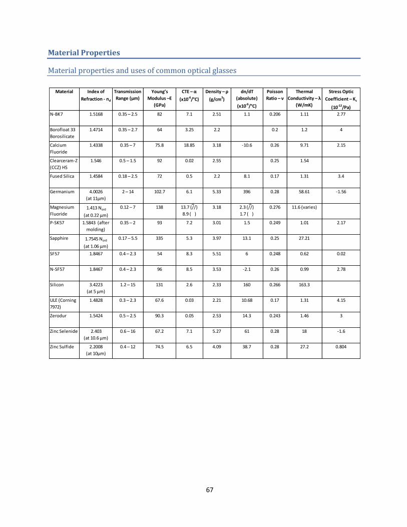
67

Material Properties

Material properties and uses of common optical glasses

Material Index of

Refraction - nd

Transmission

Range (μm)

Young’s

Modulus –E

(GPa)

CTE – α

(x10-6/°C)

Density – ρ

(g/cm3)

dn/dT

(absolute)

(x10-6/°C)

Poisson

Ratio – ν

Thermal

Conductivity – λ

(W/mK)

Stress Optic

Coefficient – Ks

(10-12/Pa)

N-BK7 1.5168 0.35 – 2.5 82 7.1 2.51 1.1 0.206 1.11 2.77

Borofloat 33

Borosilicate

1.4714 0.35 – 2.7 64 3.25 2.2 0.2 1.2 4

Calcium

Fluoride

1.4338 0.35 – 7 75.8 18.85 3.18 -10.6 0.26 9.71 2.15

Clearceram-Z

(CCZ) HS

1.546 0.5 – 1.5 92 0.02 2.55 0.25 1.54

Fused Silica 1.4584 0.18 – 2.5 72 0.5 2.2 8.1 0.17 1.31 3.4

Germanium 4.0026

(at 11μm)

2 – 14 102.7 6.1 5.33 396 0.28 58.61 -1.56

Magnesium

Fluoride1.413 Nord

(at 0.22 μm)

0.12 – 7 138 13.7 (//)

8.9 (

⊥

)

3.18 2.3 (//)

1.7 (

⊥

)

0.276 11.6 (varies)

P-SK57 1.5843 (after

molding)

0.35 – 2 93 7.2 3.01 1.5 0.249 1.01 2.17

Sapphire 1.7545 Nord

(at 1.06 μm)

0.17 – 5.5 335 5.3 3.97 13.1 0.25 27.21

SF57 1.8467 0.4 – 2.3 54 8.3 5.51 6 0.248 0.62 0.02

N-SF57 1.8467 0.4 – 2.3 96 8.5 3.53 -2.1 0.26 0.99 2.78

Silicon 3.4223

(at 5 μm)

1.2 – 15 131 2.6 2.33 160 0.266 163.3

ULE (Corning

7972)

1.4828 0.3 – 2.3 67.6 0.03 2.21 10.68 0.17 1.31 4.15

Zerodur 1.5424 0.5 – 2.5 90.3 0.05 2.53 14.3 0.243 1.46 3

Zinc Selenide 2.403

(at 10.6 μm)

0.6 – 16 67.2 7.1 5.27 61 0.28 18 -1.6

Zinc Sulfide 2.2008

(at 10μm)

0.4 – 12 74.5 6.5 4.09 38.7 0.28 27.2 0.804

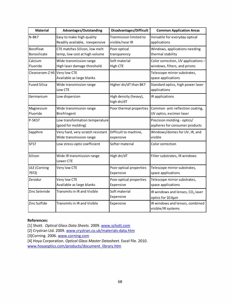
68

References: [1] Shott. Optical Glass Data Sheets. 2009. www.schott.com [2] Crystran Ltd. 2009. www.crystran.co.uk/materials-data.htm [3]Corning. 2006. www.corning.com [4] Hoya Corporation. Optical Glass Master Datasheet. Excel file. 2010. www.hoyaoptics.com/products/document_library.htm

Material Advantages/Outstanding

Properties

Disadvantages/Difficult

Properties

Common Application Areas

N-BK7 Easy to make high quality

Readily available, inexpensive

Tranmission limited to

visible/near IR

Versatile for everyday optical

applications

Borofloat

Borosilicate

CTE matches Silicon, low melt

temp, low cost at high volume

Poor optical

transparency

Windows, applications needing

thermal stability

Calcium

Fluoride

Wide transmission range

High laser damage threshold

Soft material

High CTE

Color correction, UV applications –

windows, filters, and prisms

Clearceram-Z HS Very low CTE

Available as large blanks

Telescope mirror substrates,

space applications

Fused Silica Wide transmission range

Low CTE

Higher dn/dT than BK7 Standard optics, high power laser

applications

Germanium Low dispersion High density (heavy),

high dn/dT

IR applications

Magnesium

Fluoride

Wide transmission range

Birefringent

Poor thermal properties Common anti-reflection coating,

UV optics, excimer laser

applicationsP-SK57 Low transformation temperature

(good for molding)

Precision molding - optics/

aspheres for consumer products

Sapphire Very hard, very scratch resistant

Wide transmission range

Difficult to machine,

expensive

Windows/domes for UV, IR, and

visible

SF57 Low stress-optic coefficient Softer material Color correction

Silicon Wide IR transmission range

Lower CTE

High dn/dT Filter substrates, IR windows

ULE (Corning

7972)

Very low CTE Poor optical properties

Expensive

Telescope mirror substrates,

space applications

Zerodur Very low CTE

Available as large blanks

Poor optical properties

Expensive

Telescope mirror substrates,

space applications

Zinc Selenide Transmits in IR and Visible Soft material

ExpensiveIR windows and lenses, CO2 laser

optics for 10.6μm

Zinc Sulfide Transmits in IR and Visible Expensive IR windows and lenses, combined

visible/IR systems

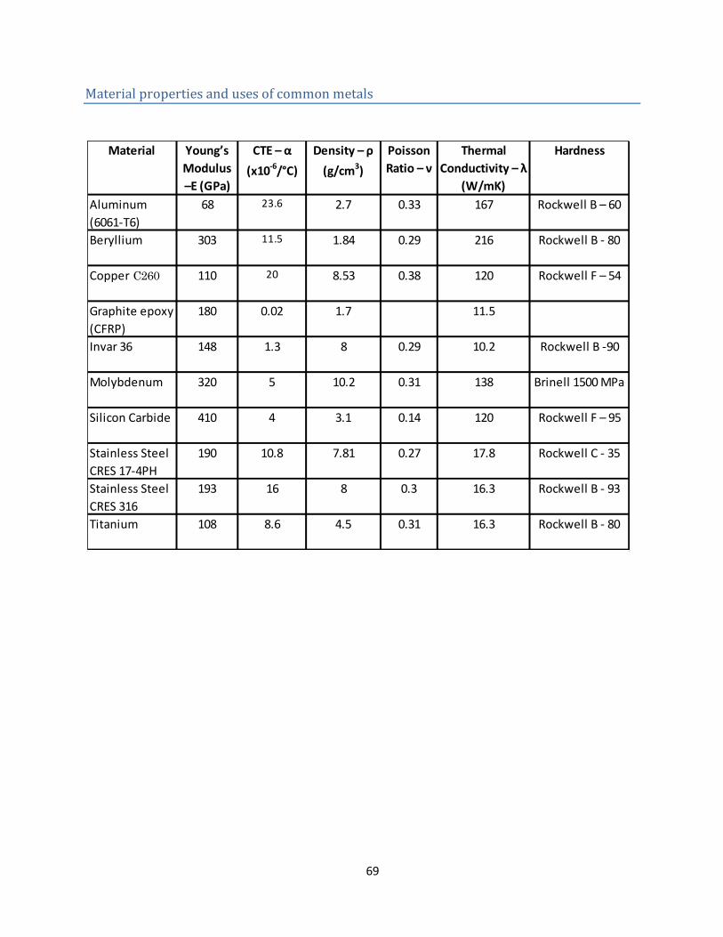
69

Material properties and uses of common metals

Material Young’s

Modulus

–E (GPa)

CTE – α

(x10-6/°C)

Density – ρ

(g/cm3)

Poisson

Ratio – ν

Thermal

Conductivity – λ

(W/mK)

Hardness

Aluminum

(6061-T6)

68 23.6 2.7 0.33 167 Rockwell B – 60

Beryllium 303 11.5 1.84 0.29 216 Rockwell B - 80

Copper C260 110 20 8.53 0.38 120 Rockwell F – 54

Graphite epoxy

(CFRP)

180 0.02 1.7 11.5

Invar 36 148 1.3 8 0.29 10.2 Rockwell B -90

Molybdenum 320 5 10.2 0.31 138 Brinell 1500 MPa

Silicon Carbide 410 4 3.1 0.14 120 Rockwell F – 95

Stainless Steel

CRES 17-4PH

190 10.8 7.81 0.27 17.8 Rockwell C - 35

Stainless Steel

CRES 316

193 16 8 0.3 16.3 Rockwell B - 93

Titanium 108 8.6 4.5 0.31 16.3 Rockwell B - 80

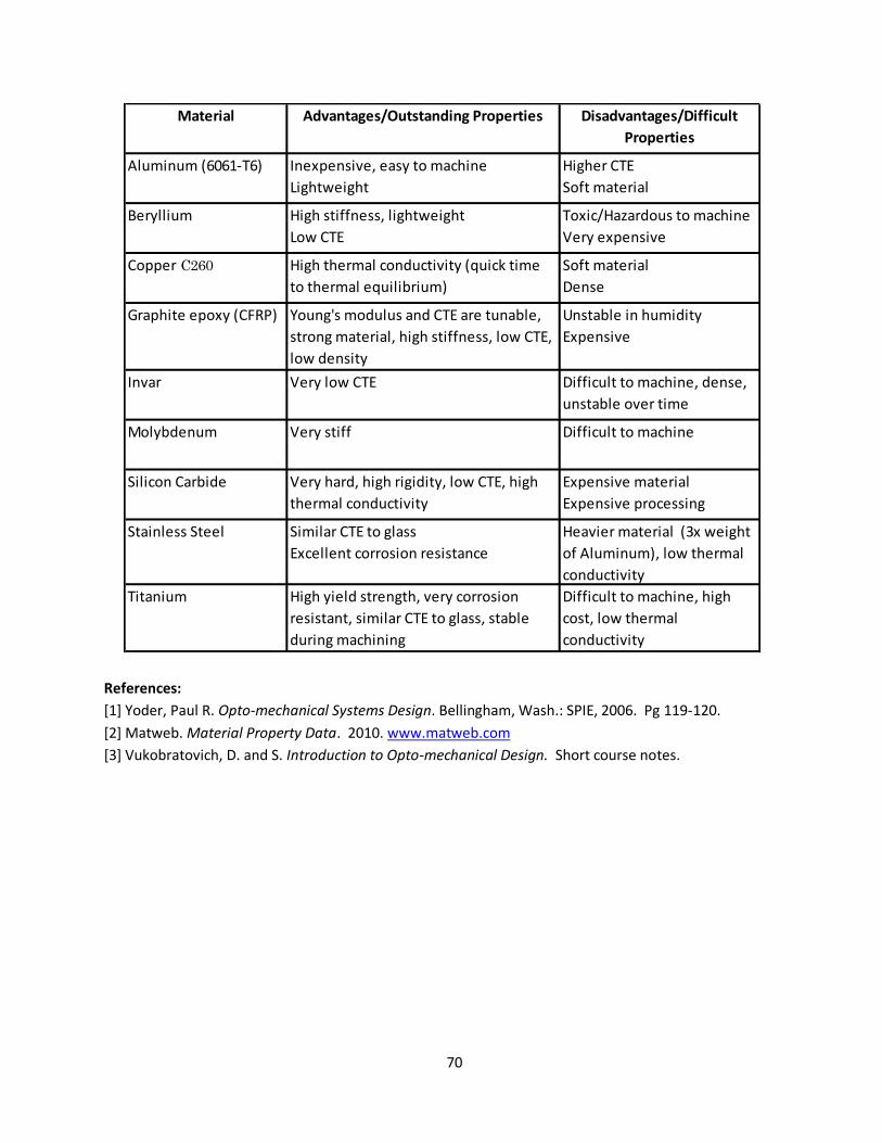
70

References:

[1] Yoder, Paul R. Opto-mechanical Systems Design. Bellingham, Wash.: SPIE, 2006. Pg 119-120.

[2] Matweb. Material Property Data. 2010. www.matweb.com

[3] Vukobratovich, D. and S. Introduction to Opto-mechanical Design. Short course notes.

Material Advantages/Outstanding Properties Disadvantages/Difficult

Properties

Aluminum (6061-T6) Inexpensive, easy to machine

Lightweight

Higher CTE

Soft material

Beryllium High stiffness, lightweight

Low CTE

Toxic/Hazardous to machine

Very expensive

Copper C260 High thermal conductivity (quick time

to thermal equilibrium)

Soft material

Dense

Graphite epoxy (CFRP) Young's modulus and CTE are tunable,

strong material, high stiffness, low CTE,

low density

Unstable in humidity

Expensive

Invar Very low CTE Difficult to machine, dense,

unstable over time

Molybdenum Very stiff Difficult to machine

Silicon Carbide Very hard, high rigidity, low CTE, high

thermal conductivity

Expensive material

Expensive processing

Stainless Steel Similar CTE to glass

Excellent corrosion resistance

Heavier material (3x weight

of Aluminum), low thermal

conductivity

Titanium High yield strength, very corrosion

resistant, similar CTE to glass, stable

during machining

Difficult to machine, high

cost, low thermal

conductivity

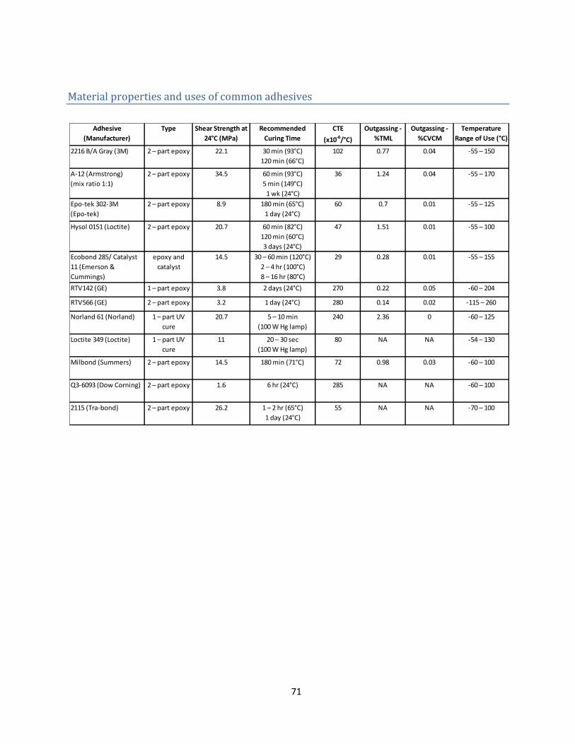
71

Material properties and uses of common adhesives

Adhesive

(Manufacturer)

Type Shear Strength at

24°C (MPa)

Recommended

Curing Time

CTE

(x10-6/°C)

Outgassing -

%TML

Outgassing -

%CVCM

Temperature

Range of Use (°C)

2216 B/A Gray (3M) 2 – part epoxy 22.1 30 min (93°C)

120 min (66°C)

102 0.77 0.04 -55 – 150

A-12 (Armstrong)

(mix ratio 1:1)

2 – part epoxy 34.5 60 min (93°C)

5 min (149°C)

1 wk (24°C)

36 1.24 0.04 -55 – 170

Epo-tek 302-3M

(Epo-tek)

2 – part epoxy 8.9 180 min (65°C)

1 day (24°C)

60 0.7 0.01 -55 – 125

Hysol 0151 (Loctite) 2 – part epoxy 20.7 60 min (82°C)

120 min (60°C)

3 days (24°C)

47 1.51 0.01 -55 – 100

Ecobond 285/ Catalyst

11 (Emerson &

Cummings)

epoxy and

catalyst

14.5 30 – 60 min (120°C)

2 – 4 hr (100°C)

8 – 16 hr (80°C)

29 0.28 0.01 -55 – 155

RTV142 (GE) 1 – part epoxy 3.8 2 days (24°C) 270 0.22 0.05 -60 – 204

RTV566 (GE) 2 – part epoxy 3.2 1 day (24°C) 280 0.14 0.02 -115 – 260

Norland 61 (Norland) 1 – part UV

cure

20.7 5 – 10 min

(100 W Hg lamp)

240 2.36 0 -60 – 125

Loctite 349 (Loctite) 1 – part UV

cure

11 20 – 30 sec

(100 W Hg lamp)

80 NA NA -54 – 130

Milbond (Summers) 2 – part epoxy 14.5 180 min (71°C) 72 0.98 0.03 -60 – 100

Q3-6093 (Dow Corning) 2 – part epoxy 1.6 6 hr (24°C) 285 NA NA -60 – 100

2115 (Tra-bond) 2 – part epoxy 26.2 1 – 2 hr (65°C)

1 day (24°C)

55 NA NA -70 – 100

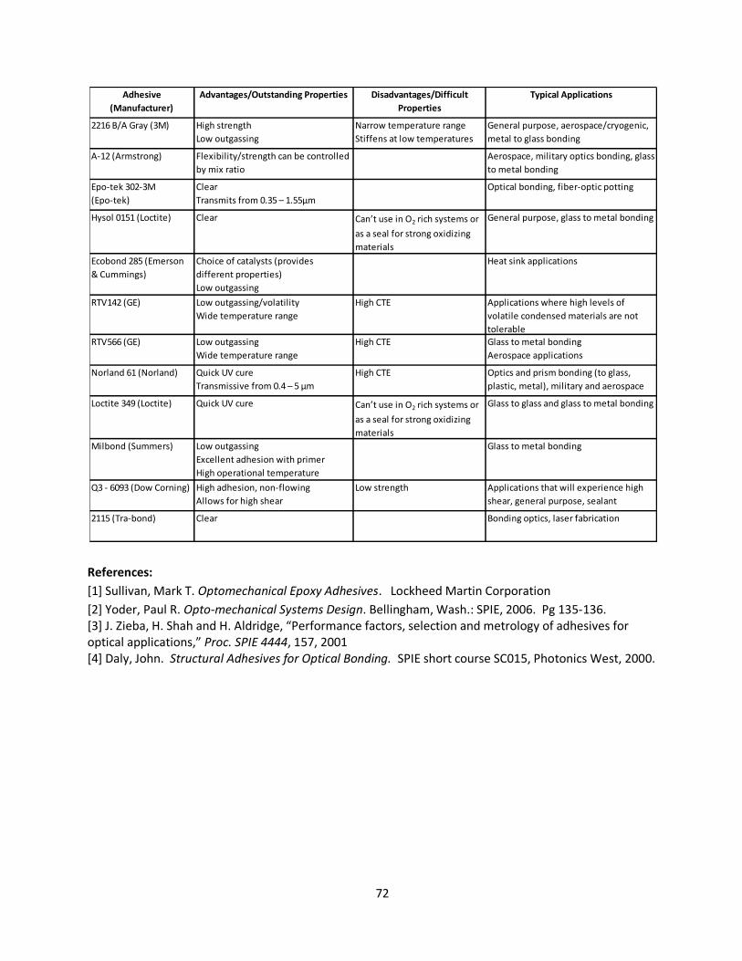
72

References:

[1] Sullivan, Mark T. Optomechanical Epoxy Adhesives. Lockheed Martin Corporation

[2] Yoder, Paul R. Opto-mechanical Systems Design. Bellingham, Wash.: SPIE, 2006. Pg 135-136. *3+ J. Zieba, H. Shah and H. Aldridge, “Performance factors, selection and metrology of adhesives for optical applications,” Proc. SPIE 4444, 157, 2001 [4] Daly, John. Structural Adhesives for Optical Bonding. SPIE short course SC015, Photonics West, 2000.

Adhesive

(Manufacturer)

Advantages/Outstanding Properties Disadvantages/Difficult

Properties

Typical Applications

2216 B/A Gray (3M) High strength

Low outgassing

Narrow temperature range

Stiffens at low temperatures

General purpose, aerospace/cryogenic,

metal to glass bonding

A-12 (Armstrong) Flexibility/strength can be controlled

by mix ratio

Aerospace, military optics bonding, glass

to metal bonding

Epo-tek 302-3M

(Epo-tek)

Clear

Transmits from 0.35 – 1.55μm

Optical bonding, fiber-optic potting

Hysol 0151 (Loctite) Clear Can’t use in O2 rich systems or

as a seal for strong oxidizing

materials

General purpose, glass to metal bonding

Ecobond 285 (Emerson

& Cummings)

Choice of catalysts (provides

different properties)

Low outgassing

Heat sink applications

RTV142 (GE) Low outgassing/volatility

Wide temperature range

High CTE Applications where high levels of

volatile condensed materials are not

tolerable

RTV566 (GE) Low outgassing

Wide temperature range

High CTE Glass to metal bonding

Aerospace applications

Norland 61 (Norland) Quick UV cure

Transmissive from 0.4 – 5 μm

High CTE Optics and prism bonding (to glass,

plastic, metal), military and aerospace

applicationsLoctite 349 (Loctite) Quick UV cure Can’t use in O2 rich systems or

as a seal for strong oxidizing

materials

Glass to glass and glass to metal bonding

Milbond (Summers) Low outgassing

Excellent adhesion with primer

High operational temperature

Glass to metal bonding

Q3 - 6093 (Dow Corning) High adhesion, non-flowing

Allows for high shear

Low strength Applications that will experience high

shear, general purpose, sealant

2115 (Tra-bond) Clear Bonding optics, laser fabrication

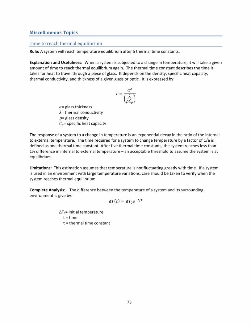
73

Miscellaneous Topics

Time to reach thermal equilibrium

Rule: A system will reach temperature equilibrium after 5 thermal time constants. Explanation and Usefulness: When a system is subjected to a change in temperature, it will take a given amount of time to reach thermal equilibrium again. The thermal time constant describes the time it takes for heat to travel through a piece of glass. It depends on the density, specific heat capacity, thermal conductivity, and thickness of a given glass or optic. It is expressed by:

= glass thickness = thermal conductivity = glass density = specific heat capacity

The response of a system to a change in temperature is an exponential decay in the ratio of the internal to external temperature. The time required for a system to change temperature by a factor of 1/e is defined as one thermal time constant. After five thermal time constants, the system reaches less than 1% difference in internal to external temperature – an acceptable threshold to assume the system is at equilibrium. Limitations: This estimation assumes that temperature is not fluctuating greatly with time. If a system is used in an environment with large temperature variations, care should be taken to verify when the system reaches thermal equilibrium. Complete Analysis: The difference between the temperature of a system and its surrounding environment is give by:

ΔT0= initial temperature t = time τ = thermal time constant

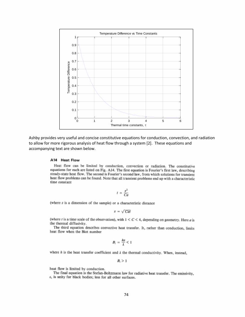
74

Ashby provides very useful and concise constitutive equations for conduction, convection, and radiation to allow for more rigorous analysis of heat flow through a system [2]. These equations and accompanying text are shown below.

0 1 2 3 4 5 60

0.1

0.2

0.3

0.4

0.5

0.6

0.7

0.8

0.9

1

Thermal time constants,

Tem

pera

ture

Diffe

rence

Temperature Difference vs Time Constants

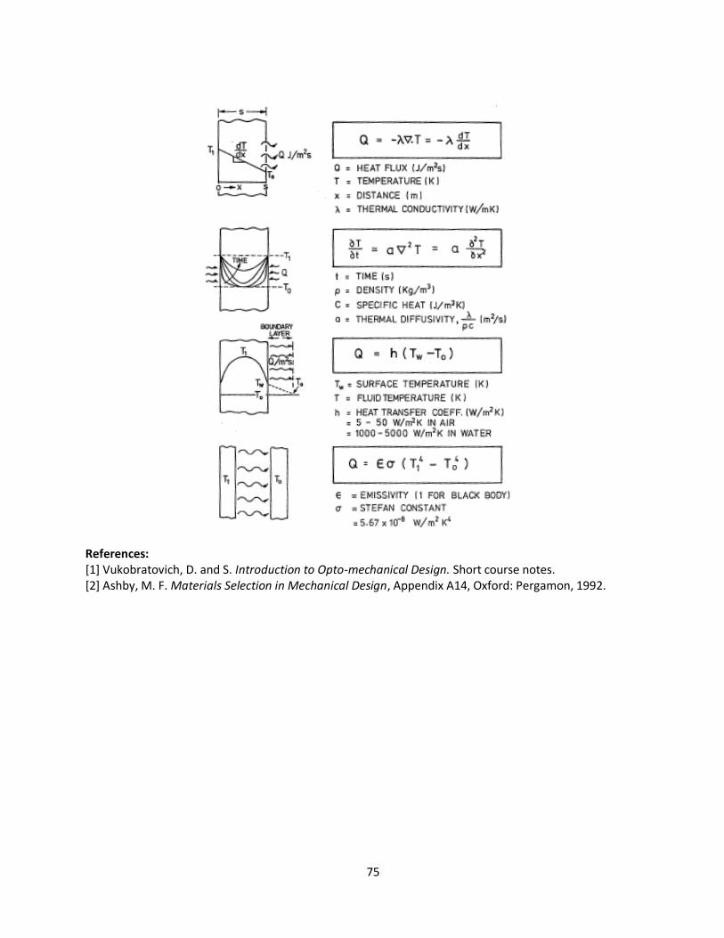
75

References: [1] Vukobratovich, D. and S. Introduction to Opto-mechanical Design. Short course notes. [2] Ashby, M. F. Materials Selection in Mechanical Design, Appendix A14, Oxford: Pergamon, 1992.

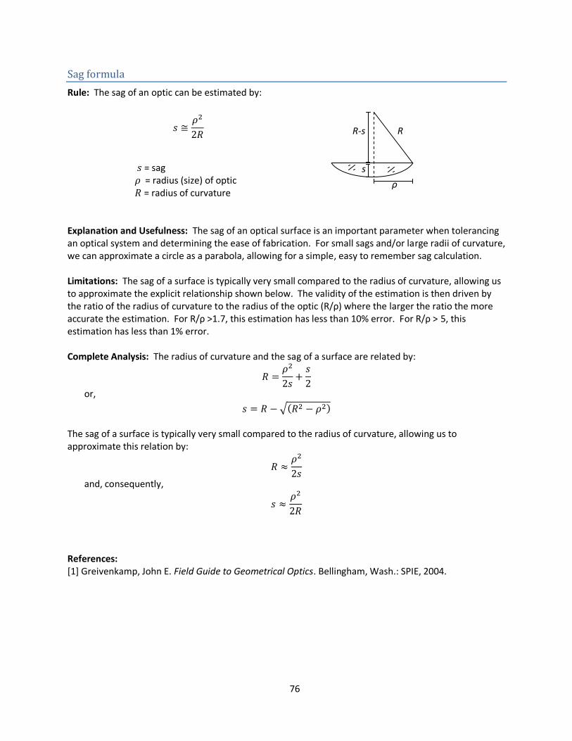
76

Sag formula

Rule: The sag of an optic can be estimated by:

= sag = radius (size) of optic = radius of curvature

Explanation and Usefulness: The sag of an optical surface is an important parameter when tolerancing an optical system and determining the ease of fabrication. For small sags and/or large radii of curvature, we can approximate a circle as a parabola, allowing for a simple, easy to remember sag calculation. Limitations: The sag of a surface is typically very small compared to the radius of curvature, allowing us to approximate the explicit relationship shown below. The validity of the estimation is then driven by the ratio of the radius of curvature to the radius of the optic (R/ρ) where the larger the ratio the more accurate the estimation. For R/ρ >1.7, this estimation has less than 10% error. For R/ρ > 5, this estimation has less than 1% error. Complete Analysis: The radius of curvature and the sag of a surface are related by:

or,

The sag of a surface is typically very small compared to the radius of curvature, allowing us to approximate this relation by:

and, consequently,

References: [1] Greivenkamp, John E. Field Guide to Geometrical Optics. Bellingham, Wash.: SPIE, 2004.

R R-s

ρ

s

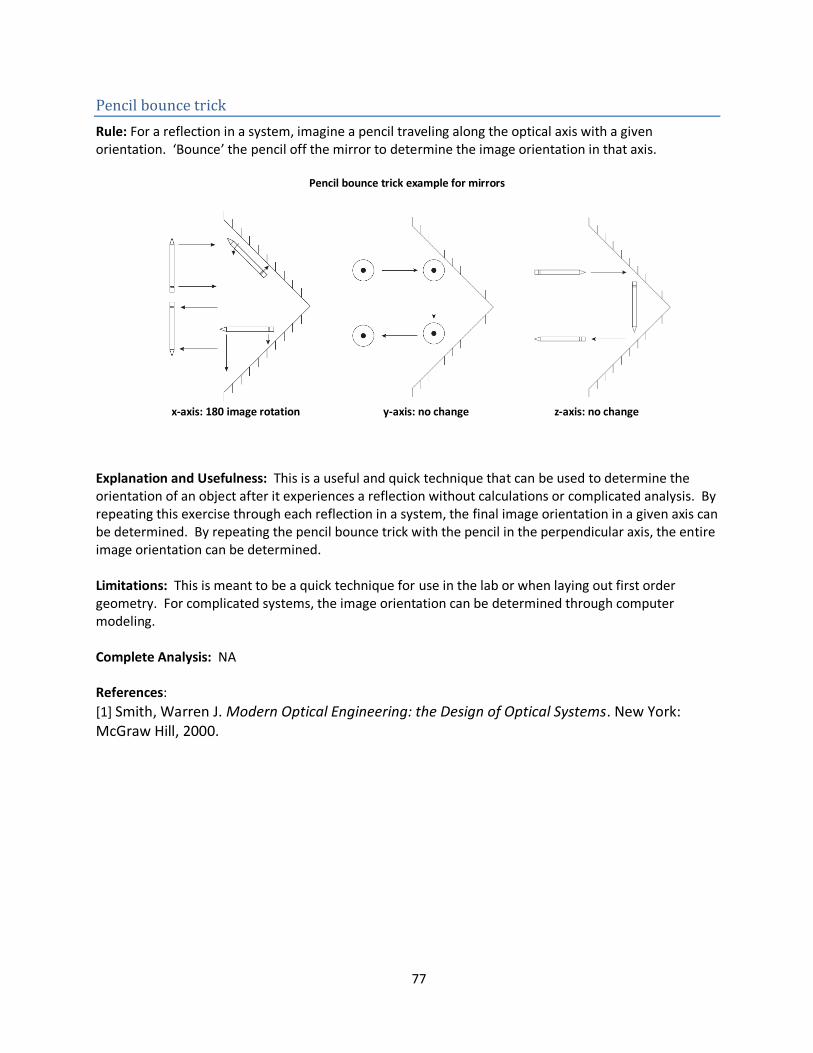
77

Pencil bounce trick

Rule: For a reflection in a system, imagine a pencil traveling along the optical axis with a given orientation. ‘Bounce’ the pencil off the mirror to determine the image orientation in that axis.

Pencil bounce trick example for mirrors

x-axis: 180 image rotation y-axis: no change z-axis: no change

Explanation and Usefulness: This is a useful and quick technique that can be used to determine the orientation of an object after it experiences a reflection without calculations or complicated analysis. By repeating this exercise through each reflection in a system, the final image orientation in a given axis can be determined. By repeating the pencil bounce trick with the pencil in the perpendicular axis, the entire image orientation can be determined. Limitations: This is meant to be a quick technique for use in the lab or when laying out first order geometry. For complicated systems, the image orientation can be determined through computer modeling. Complete Analysis: NA References:

[1] Smith, Warren J. Modern Optical Engineering: the Design of Optical Systems. New York: McGraw Hill, 2000.

78

Outgassing and use of cyanoacrylates (superglue)

Rule: When selecting an adhesive, avoid using cyanoacrylates (superglue) near lenses with coatings. Explanation and Usefulness: Cyanoacrylates are a common adhesive choice in optomechanics, especially for thread locking, due to their high strength, good adhesion to metal surfaces, and rapid cure time. They have the potential, however, to severely contaminate optical coatings [1]. When exposed to a vacuum or elevated temperatures, adhesives will release particles in gaseous form in a process called outgassing. These released particles can then condense and contaminate optical surfaces and coatings. Cyanoacrylates have very undesirable outgassing properties and should be avoided for space or other vacuum applications. Limitations: Outgassing is most severe in a vacuum or at elevated temperatures, but adhesives can also outgas at room temperature. Minimizing outgassing is critical for space applications but should be taken into consideration for any application. Complete Analysis: Outgassing is quantified by percent Total Mass Lost (%TML) and percent Collected Volatile Condensable Material (%CVCM). NASA provides requirements for these values of < 1% TML and <0.1% CVCM for space applications that should be followed for optical applications. NASA also maintains a very useful database of the outgassing properties of adhesives and other materials [2]. The cyanoacrylates listed in this database have around 2-3% TML and 0.01-0.02% CVCM. A ‘low outgassing’ section can be found on the website for an extensive list of low outgassing adhesives.

References: [1] Vukobratovich, D. and S. Introduction to Opto-mechanical Design. [2] http://outgassing.nasa.gov/ [3] MIL-A-46050C: Military specification, adhesives, cyanoacrylate, rapid room solventless temperature –curing. 1979. [4] J. Zieba, H. Shah and H. Aldridge, “Performance factors, selection and metrology of adhesives for optical applications,” Proc. SPIE 4444, 157 (2001).

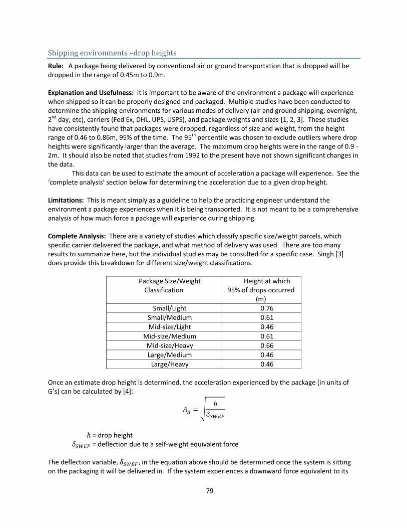
79

Shipping environments –drop heights

Rule: A package being delivered by conventional air or ground transportation that is dropped will be dropped in the range of 0.45m to 0.9m. Explanation and Usefulness: It is important to be aware of the environment a package will experience when shipped so it can be properly designed and packaged. Multiple studies have been conducted to determine the shipping environments for various modes of delivery (air and ground shipping, overnight, 2nd day, etc), carriers (Fed Ex, DHL, UPS, USPS), and package weights and sizes [1, 2, 3]. These studies have consistently found that packages were dropped, regardless of size and weight, from the height range of 0.46 to 0.86m, 95% of the time. The 95th percentile was chosen to exclude outliers where drop heights were significantly larger than the average. The maximum drop heights were in the range of 0.9 -2m. It should also be noted that studies from 1992 to the present have not shown significant changes in the data. This data can be used to estimate the amount of acceleration a package will experience. See the ‘complete analysis’ section below for determining the acceleration due to a given drop height. Limitations: This is meant simply as a guideline to help the practicing engineer understand the environment a package experiences when it is being transported. It is not meant to be a comprehensive analysis of how much force a package will experience during shipping. Complete Analysis: There are a variety of studies which classify specific size/weight parcels, which specific carrier delivered the package, and what method of delivery was used. There are too many results to summarize here, but the individual studies may be consulted for a specific case. Singh [3] does provide this breakdown for different size/weight classifications.

Package Size/Weight Classification

Height at which 95% of drops occurred

(m)

Small/Light 0.76

Small/Medium 0.61

Mid-size/Light 0.46

Mid-size/Medium 0.61

Mid-size/Heavy 0.66

Large/Medium 0.46

Large/Heavy 0.46

Once an estimate drop height is determined, the acceleration experienced by the package (in units of G’s) can be calculated by *4+:

= drop height = deflection due to a self-weight equivalent force The deflection variable, , in the equation above should be determined once the system is sitting on the packaging it will be delivered in. If the system experiences a downward force equivalent to its

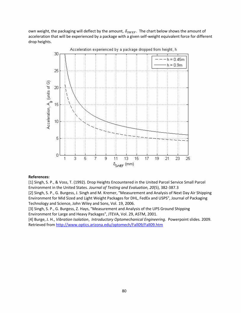
80

own weight, the packaging will deflect by the amount, . The chart below shows the amount of acceleration that will be experienced by a package with a given self-weight equivalent force for different drop heights.

References: [1] Singh, S. P., & Voss, T. (1992). Drop Heights Encountered in the United Parcel Service Small Parcel Environment in the United States. Journal of Testing and Evaluation, 20(5), 382-387.3 [2] Singh, S. P., G. Burgess, J. Singh and M. Kremer, "Measurement and Analysis of Next Day Air Shipping Environment for Mid Sized and Light Weight Packages for DHL, FedEx and USPS", Journal of Packaging Technology and Science, John Wiley and Sons, Vol. 19, 2006. [3] Singh, S. P., G. Burgess, Z. Hays, "Measurement and Analysis of the UPS Ground Shipping Environment for Large and Heavy Packages", JTEVA, Vol. 29, ASTM, 2001. [4] Burge, J. H., Vibration Isolation, Introductory Optomechanical Engineering. Powerpoint slides. 2009. Retrieved from http://www.optics.arizona.edu/optomech/Fall09/Fall09.htm

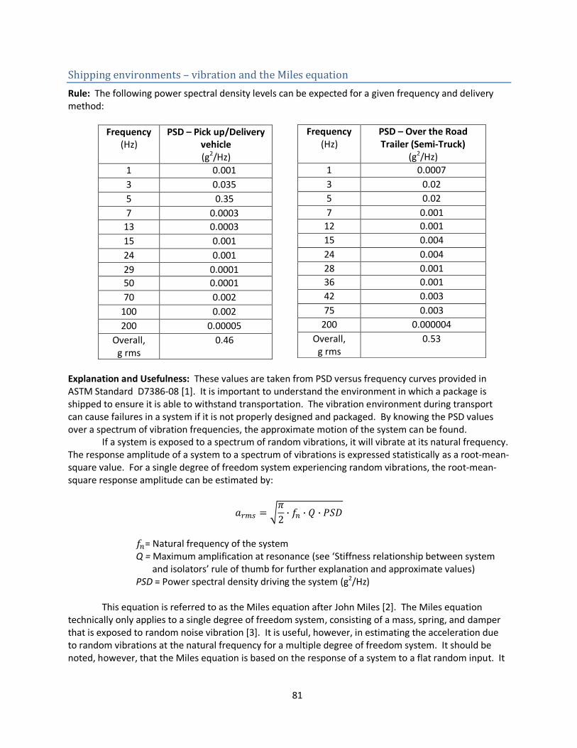
81

Shipping environments – vibration and the Miles equation

Rule: The following power spectral density levels can be expected for a given frequency and delivery method:

Frequency (Hz)

PSD – Pick up/Delivery vehicle (g2/Hz)

1 0.001

3 0.035

5 0.35

7 0.0003

13 0.0003

15 0.001

24 0.001

29 0.0001

50 0.0001

70 0.002

100 0.002

200 0.00005

Overall, g rms

0.46

Explanation and Usefulness: These values are taken from PSD versus frequency curves provided in ASTM Standard D7386-08 [1]. It is important to understand the environment in which a package is shipped to ensure it is able to withstand transportation. The vibration environment during transport can cause failures in a system if it is not properly designed and packaged. By knowing the PSD values over a spectrum of vibration frequencies, the approximate motion of the system can be found.

If a system is exposed to a spectrum of random vibrations, it will vibrate at its natural frequency. The response amplitude of a system to a spectrum of vibrations is expressed statistically as a root-mean-square value. For a single degree of freedom system experiencing random vibrations, the root-mean-square response amplitude can be estimated by:

= Natural frequency of the system Q = Maximum amplification at resonance (see ‘Stiffness relationship between system

and isolators’ rule of thumb for further explanation and approximate values) PSD = Power spectral density driving the system (g2/Hz) This equation is referred to as the Miles equation after John Miles [2]. The Miles equation technically only applies to a single degree of freedom system, consisting of a mass, spring, and damper that is exposed to random noise vibration [3]. It is useful, however, in estimating the acceleration due to random vibrations at the natural frequency for a multiple degree of freedom system. It should be noted, however, that the Miles equation is based on the response of a system to a flat random input. It

Frequency (Hz)

PSD – Over the Road Trailer (Semi-Truck)

(g2/Hz)

1 0.0007

3 0.02

5 0.02

7 0.001

12 0.001

15 0.004

24 0.004

28 0.001

36 0.001

42 0.003

75 0.003

200 0.000004

Overall, g rms

0.53

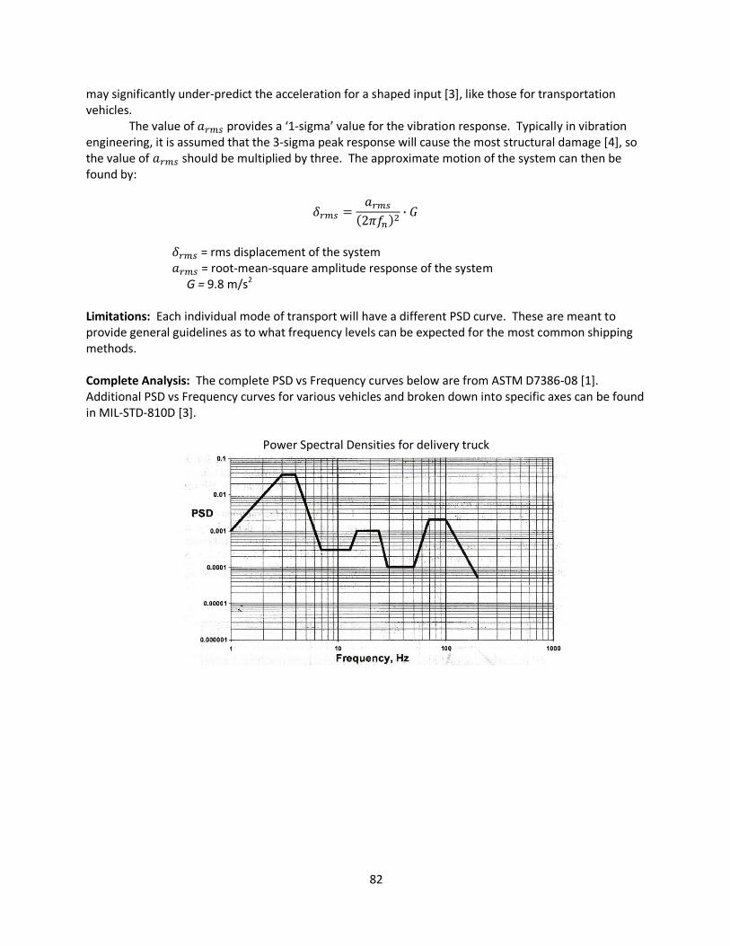
82

may significantly under-predict the acceleration for a shaped input [3], like those for transportation vehicles.

The value of provides a ‘1-sigma’ value for the vibration response. Typically in vibration engineering, it is assumed that the 3-sigma peak response will cause the most structural damage [4], so the value of should be multiplied by three. The approximate motion of the system can then be found by:

= rms displacement of the system = root-mean-square amplitude response of the system G = 9.8 m/s2 Limitations: Each individual mode of transport will have a different PSD curve. These are meant to provide general guidelines as to what frequency levels can be expected for the most common shipping methods. Complete Analysis: The complete PSD vs Frequency curves below are from ASTM D7386-08 [1]. Additional PSD vs Frequency curves for various vehicles and broken down into specific axes can be found in MIL-STD-810D [3].

Power Spectral Densities for delivery truck

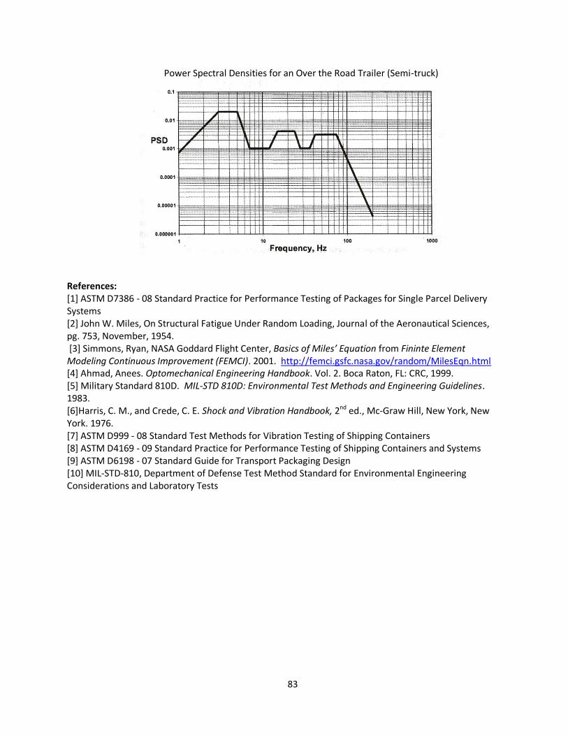
83

Power Spectral Densities for an Over the Road Trailer (Semi-truck)

References: [1] ASTM D7386 - 08 Standard Practice for Performance Testing of Packages for Single Parcel Delivery Systems [2] John W. Miles, On Structural Fatigue Under Random Loading, Journal of the Aeronautical Sciences, pg. 753, November, 1954. [3] Simmons, Ryan, NASA Goddard Flight Center, Basics of Miles’ Equation from Fininte Element Modeling Continuous Improvement (FEMCI). 2001. http://femci.gsfc.nasa.gov/random/MilesEqn.html [4] Ahmad, Anees. Optomechanical Engineering Handbook. Vol. 2. Boca Raton, FL: CRC, 1999. [5] Military Standard 810D. MIL-STD 810D: Environmental Test Methods and Engineering Guidelines. 1983. [6]Harris, C. M., and Crede, C. E. Shock and Vibration Handbook, 2nd ed., Mc-Graw Hill, New York, New York. 1976. [7] ASTM D999 - 08 Standard Test Methods for Vibration Testing of Shipping Containers [8] ASTM D4169 - 09 Standard Practice for Performance Testing of Shipping Containers and Systems [9] ASTM D6198 - 07 Standard Guide for Transport Packaging Design [10] MIL-STD-810, Department of Defense Test Method Standard for Environmental Engineering Considerations and Laboratory Tests

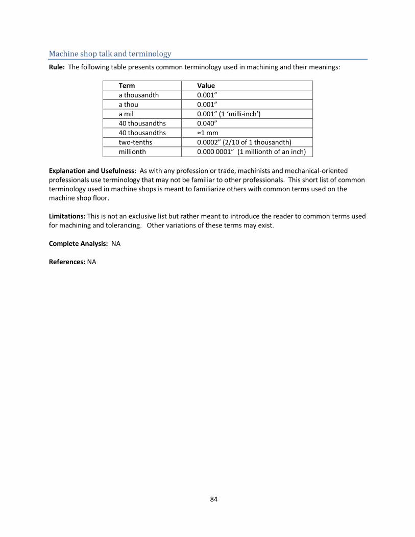
84

Machine shop talk and terminology

Rule: The following table presents common terminology used in machining and their meanings:

Term Value

a thousandth 0.001”

a thou 0.001”

a mil 0.001” (1 ‘milli-inch’)

40 thousandths 0.040”

40 thousandths ≈1 mm

two-tenths 0.0002” (2/10 of 1 thousandth)

millionth 0.000 0001” (1 millionth of an inch)

Explanation and Usefulness: As with any profession or trade, machinists and mechanical-oriented professionals use terminology that may not be familiar to other professionals. This short list of common terminology used in machine shops is meant to familiarize others with common terms used on the machine shop floor. Limitations: This is not an exclusive list but rather meant to introduce the reader to common terms used for machining and tolerancing. Other variations of these terms may exist. Complete Analysis: NA

References: NA

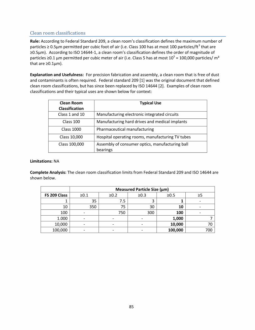
85

Clean room classifications

Rule: According to Federal Standard 209, a clean room’s classification defines the maximum number of particles ≥ 0.5μm permitted per cubic foot of air (i.e. Class 100 has at most 100 particles/ft3 that are ≥0.5μm). According to ISO 14644-1, a clean room’s classification defines the order of magnitude of particles ≥0.1 µm permitted per cubic meter of air (i.e. Class 5 has at most 105 = 100,000 particles/ m³ that are ≥0.1μm). Explanation and Usefulness: For precision fabrication and assembly, a clean room that is free of dust and contaminants is often required. Federal standard 209 [1] was the original document that defined clean room classifications, but has since been replaced by ISO 14644 [2]. Examples of clean room classifications and their typical uses are shown below for context:

Clean Room Classification

Typical Use

Class 1 and 10 Manufacturing electronic integrated circuits

Class 100 Manufacturing hard drives and medical implants

Class 1000 Pharmaceutical manufacturing

Class 10,000 Hospital operating rooms, manufacturing TV tubes

Class 100,000 Assembly of consumer optics, manufacturing ball bearings

Limitations: NA Complete Analysis: The clean room classification limits from Federal Standard 209 and ISO 14644 are shown below.

Measured Particle Size (μm)

FS 209 Class ≥0.1 ≥0.2 ≥0.3 ≥0.5 ≥5

1 35 7.5 3 1 -

10 350 75 30 10 -

100 - 750 300 100 -

1.000 - - - 1,000 7

10,000 - - - 10,000 70

100,000 - - - 100,000 700

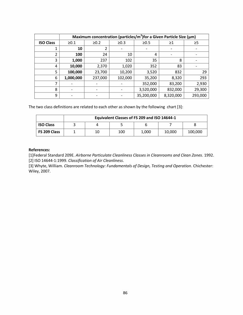
86

Maximum concentration (particles/m3)for a Given Particle Size (μm)

ISO Class ≥0.1 ≥0.2 ≥0.3 ≥0.5 ≥1 ≥5

1 10 2 - - - -

2 100 24 10 4 - -

3 1,000 237 102 35 8 -

4 10,000 2,370 1,020 352 83 -

5 100,000 23,700 10,200 3,520 832 29

6 1,000,000 237,000 102,000 35,200 8,320 293

7 - - - 352,000 83,200 2,930

8 - - - 3,520,000 832,000 29,300

9 - - - 35,200,000 8,320,000 293,000

The two class definitions are related to each other as shown by the following chart [3]:

Equivalent Classes of FS 209 and ISO 14644-1

ISO Class 3 4 5 6 7 8

FS 209 Class 1 10 100 1,000 10,000 100,000

References: [1]Federal Standard 209E. Airborne Particulate Cleanliness Classes in Cleanrooms and Clean Zones. 1992. [2] ISO 14644-1:1999. Classification of Air Cleanliness. [3] Whyte, William. Cleanroom Technology: Fundamentals of Design, Testing and Operation. Chichester: Wiley, 2007.

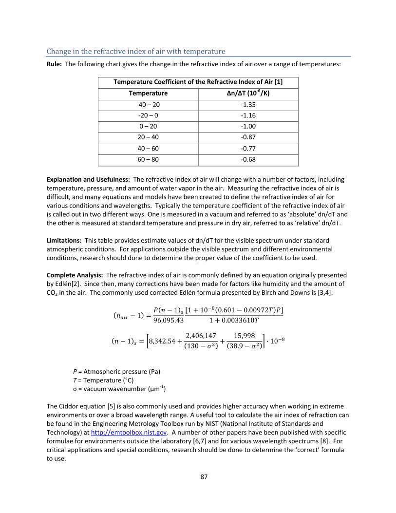
87

Change in the refractive index of air with temperature

Rule: The following chart gives the change in the refractive index of air over a range of temperatures:

Temperature Coefficient of the Refractive Index of Air [1]

Temperature ∆n/∆T (10-6/K)

-40 – 20 -1.35

-20 – 0 -1.16

0 – 20 -1.00

20 – 40 -0.87

40 – 60 -0.77

60 – 80 -0.68

Explanation and Usefulness: The refractive index of air will change with a number of factors, including temperature, pressure, and amount of water vapor in the air. Measuring the refractive index of air is difficult, and many equations and models have been created to define the refractive index of air for various conditions and wavelengths. Typically the temperature coefficient of the refractive index of air is called out in two different ways. One is measured in a vacuum and referred to as ‘absolute’ dn/dT and the other is measured at standard temperature and pressure in dry air, referred to as ‘relative’ dn/dT. Limitations: This table provides estimate values of dn/dT for the visible spectrum under standard atmospheric conditions. For applications outside the visible spectrum and different environmental conditions, research should done to determine the proper value of the coefficient to be used. Complete Analysis: The refractive index of air is commonly defined by an equation originally presented by Edlén[2]. Since then, many corrections have been made for factors like humidity and the amount of CO2 in the air. The commonly used corrected Edlén formula presented by Birch and Downs is [3,4]:

P = Atmospheric pressure (Pa) T = Temperature (°C)

σ = vacuum wavenumber (μm-1) The Ciddor equation [5] is also commonly used and provides higher accuracy when working in extreme environments or over a broad wavelength range. A useful tool to calculate the air index of refraction can be found in the Engineering Metrology Toolbox run by NIST (National Institute of Standards and Technology) at http://emtoolbox.nist.gov. A number of other papers have been published with specific formulae for environments outside the laboratory [6,7] and for various wavelength spectrums [8]. For critical applications and special conditions, research should be done to determine the ‘correct’ formula to use.

88

References: [1] Ohara Corporation. Optical Properties. http://www.oharacorp.com/o2.html [2] B. Edlén. The refractive index of air. Metrologia 2, 71–80 (1966). [3] K.P. Birch and M.J. Downs, "An updated Edlén equation for the refractive index of air," Metrologia 30, 155-162 (1993). [4] K.P. Birch and M.J. Downs, "Correction to the updated Edlén equation for the refractive index of air," Metrologia 31, 315-316 (1994). [5] P. E. Ciddor. Refractive index of air: new equations for the visible and near infrared, Appl. Opt. 35, 1566–1573 (1996). [6] K. P. Birch, M. J. Downs, The results of a comparison between calculated and measured values of the refractive index of air, J. Phys. E: Sci. Instrum. 21, 694–695 (1988). [7] G. Bönsch and E. Potulski, Measurement of the refractive index of air and comparison with modified Edlén's formulae, Metrologia 35, 133–139 (1998). [8] R. J. Mathar, Calculated refractivity of water vapor and moist air in the atmospheric window at 10 μm, Appl. Opt. 43, 928-932 (2004).

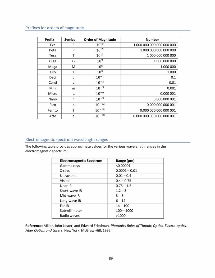
89

Prefixes for orders of magnitude

Prefix Symbol Order of Magnitude Number

Exa E 1 000 000 000 000 000 000

Peta P 1 000 000 000 000 000

Tera T 1 000 000 000 000

Giga G 1 000 000 000

Mega M 1 000 000

Kilo K 1 000

Deci d 0.1

Centi c 0.01

Milli m 0.001

Micro μ 0.000 001

Nano n 0.000 000 001

Pico p 0.000 000 000 001

Femto f 0.000 000 000 000 001

Atto a 0.000 000 000 000 000 001

Electromagnetic spectrum wavelength ranges

The following table provides approximate values for the various wavelength ranges in the electromagnetic spectrum:

Electromagnetic Spectrum Range (μm)

Gamma rays <0.00001

X-rays 0.0001 – 0.01

Ultraviolet 0.01 – 0.4

Visible 0.4 – 0.75

Near IR 0.75 – 1.2

Short-wave IR 1.2 – 3

Mid-wave IR 3 – 6

Long-wave IR 6 – 14

Far IR 14 – 100

Submillimeter 100 – 1000

Radio waves >1000

Reference: Miller, John Lester, and Edward Friedman. Photonics Rules of Thumb: Optics, Electro-optics, Fiber Optics, and Lasers. New York: McGraw-Hill, 1996.

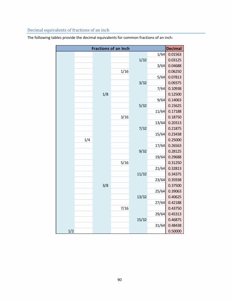
90

Decimal equivalents of fractions of an inch

The following tables provide the decimal equivalents for common fractions of an inch:

Decimal 1/64 0.01563

1/32 0.03125

3/64 0.04688

1/16 0.06250

5/64 0.07813

3/32 0.09375

7/64 0.10938

1/8 0.12500

9/64 0.14063

5/32 0.15625

11/64 0.17188

3/16 0.18750

13/64 0.20313

7/32 0.21875

15/64 0.23438

1/4 0.25000

17/64 0.26563

9/32 0.28125

19/64 0.29688

5/16 0.31250

21/64 0.32813

11/32 0.34375

23/64 0.35938

3/8 0.37500

25/64 0.39063

13/32 0.40625

27/64 0.42188

7/16 0.43750

29/64 0.45313

15/32 0.46875

31/64 0.48438

1/2 0.50000

Fractions of an Inch

91

Decimal33/64 0.51563

17/32 0.53125

35/64 0.54688

9/16 0.56250

37/64 0.57813

19/32 0.59375

39/64 0.60938

5/8 0.62500

41/64 0.64063

21/32 0.65625

43/64 0.67188

11/16 0.68750

45/64 0.70313

23/32 0.71875

47/64 0.73438

3/4 0.75000

49/64 0.76563

25/32 0.78125

51/64 0.79688

13/16 0.81250

53/64 0.82813

27/32 0.84375

55/64 0.85938

7/8 0.87500

57/64 0.89063

29/32 0.90625

59/64 0.92188

15/16 0.93750

61/64 0.95313

31/32 0.96875

63/64 0.98438

1 1.00000

Fractions of an Inch

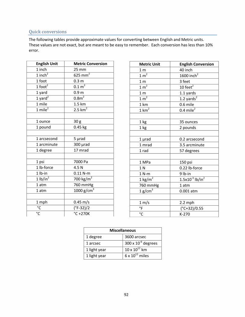
92

Quick conversions

The following tables provide approximate values for converting between English and Metric units. These values are not exact, but are meant to be easy to remember. Each conversion has less than 10% error.

Miscellaneous

1 degree 3600 arcsec

1 arcsec 300 x 10-6 degrees

1 light year 10 x 1012 km

1 light year 6 x 1012 miles

English Unit Metric Conversion

1 inch 25 mm

1 inch2 625 mm2

1 foot 0.3 m

1 foot2 0.1 m2

1 yard 0.9 m

1 yard2 0.8m2

1 mile 1.5 km

1 mile2 2.5 km2

1 ounce 30 g

1 pound 0.45 kg

1 arcsecond 5 μrad

1 arcminute 300 μrad

1 degree 17 mrad

1 psi 7000 Pa

1 lb-force 4.5 N

1 lb-in 0.11 N-m

1 lb/in2 700 kg/m2

1 atm 760 mmHg

1 atm 1000 g/cm3

1 mph 0.45 m/s

°C (°F-32)/2

°C °C +270K

Metric Unit English Conversion

1 m 40 inch

1 m2 1600 inch2

1 m 3 feet

1 m2 10 feet2

1 m 1.1 yards

1 m2 1.2 yards2

1 km 0.6 mile

1 km2 0.4 mile2

1 kg 35 ounces

1 kg 2 pounds

1 μrad 0.2 arcsecond

1 mrad 3.5 arcminute

1 rad 57 degrees

1 MPa 150 psi

1 N 0.22 lb-force

1 N-m 9 lb-in

1 kg/m2 1.5x10-3 lb/in2

760 mmHg 1 atm

1 g/cm3 0.001 atm

1 m/s 2.2 mph

°F (°C+32)/0.55

°C K-270