Embed Size (px)
Citation preview
NUREG/CR-7189 ANL/EVS/TM-14/2
User’s Guide for RESRAD-OFFSITE Manuscript Completed: September 2014 Date Published: April 2015 Prepared by: E.K. Gnanapragasam C. Yu Argonne National Laboratory 9700 South Cass Avenue Argonne, IL 60439 M. Fuhrmann, NRC Project Manager NRC Job Code V6467


iii
ABSTRACT The RESRAD-OFFSITE code can be used to model the radiological dose or risk to an offsite receptor. This User’s Guide for RESRAD-OFFSITE Version 3.1 is an update of the User’s Guide for RESRAD-OFFSITE Version 2 contained in the Appendix A of the User’s Manual for RESRAD-OFFSITE Version 2 (ANL/EVS/TM/07-1, DOE/HS-0005, NUREG/CR-6937). This user’s guide presents the basic information necessary to use Version 3.1 of the code. It also points to the help file and other documents that provide more detailed information about the inputs, the input forms and features/tools in the code; two of the features (overriding the source term and computing area factors) are discussed in the appendices to this guide. Section 2 describes how to download and install the code and then verify the installation of the code. Section 3 shows ways to navigate through the input screens to simulate various exposure scenarios and to view the results in graphics and text reports. Section 4 has screen shots of each input form in the code and provides basic information about each parameter to increase the user’s understanding of the code. Section 5 outlines the contents of all the text reports and the graphical output. It also describes the commands in the two output viewers. Section 6 deals with the probabilistic and sensitivity analysis tools available in the code. Section 7 details the various ways of obtaining help in the code.

v
CONTENTS
ABSTRACT ........................................................................................................................ iii
CONTENTS..….……………………………………………………………………………………v
FIGURES..….………………………………………………………………………………………ix
TABLES…….……………………………………………………………………………………...xv
1 INTRODUCTION ....................................................................................................... 1
1.1 Purpose Of User’s Guide .................................................................................. 1
1.2 Organization Of User’s Guide ........................................................................... 1
2 INSTALLATION ........................................................................................................ 3
2.1 Installing From The RESRAD Website .............................................................. 3
2.2 Checking The Installation .................................................................................. 3
2.3 Uninstalling ....................................................................................................... 3
3 NAVIGATION ............................................................................................................ 5
3.1 Menus and Toolbars ......................................................................................... 6
3.1.1 Menus ..................................................................................................... 6
3.1.2 Toolbars ................................................................................................ 11
3.2 RESRAD DOS-Emulator ................................................................................. 12
3.3 Iconic Navigator Window ................................................................................. 13
3.4 Linked Input Forms ......................................................................................... 15
4 INPUT FORMS ....................................................................................................... 17
4.1 Title ................................................................................................................. 20
4.2 Preliminary Inputs ........................................................................................... 23
4.3 Site Layout ...................................................................................................... 25
4.4 Map Interface .................................................................................................. 27
4.5 Source (Initial Concentrations of Radionuclides at Site) .................................. 40
4.6 Source Release and Deposition Velocity ......................................................... 43
4.7 Distribution Coefficients .................................................................................. 52
4.8 Transfer Factors .............................................................................................. 54
4.9 Set Pathways .................................................................................................. 56
vi
4.10 Reporting Times ............................................................................................ 57
4.11 Storage Times ............................................................................................... 59
4.12 Physical and Hydrological Parameters .......................................................... 60
4.13 Primary Contamination (Contaminated Zone and Cover): Physical and Hydrological Data .................................................................................. 62
4.14 Agricultural Areas and Livestock Feed Growing Areas: Physical and Hydrological Data .................................................................................. 66
4.15 Offsite Dwelling Area: Physical and Hydrological Data .................................. 69
4.16 Atmospheric Transport Parameters ............................................................... 70
4.17 Unsaturated Zone Hydrology ........................................................................ 73
4.18 Saturated Zone Hydrology ............................................................................ 75
4.19 Water Use ..................................................................................................... 77
4.20 Surface Water Body ...................................................................................... 79
4.21 Groundwater Transport Parameters .............................................................. 80
4.22 Ingestion Rates ............................................................................................. 84
4.23 Livestock Intakes (Factors) ........................................................................... 86
4.24 Livestock Feed Factors and Plant Factors .................................................... 87
4.25 Inhalation and External Gamma .................................................................... 88
4.26 External Radiation Shape and Area Factors ................................................. 90
4.27 Occupancy Factors ....................................................................................... 93
4.28 Radon Data ................................................................................................... 95
4.29 Carbon-14 Data ............................................................................................ 97
4.30 Tritium (H-3) Data ......................................................................................... 98
5 RESULTS .......................................................................................................... 99
5.1 Report Viewer ............................................................................................... 102
5.2 Graph Viewer (Deterministic and Sensitivity Analysis) .................................. 106
6 ENHANCEMENTS ................................................................................................ 111
6.1 One-Parameter-at-a-Time Sensitivity Analysis .............................................. 111
6.2 Uncertainty and Probabilistic Analysis ........................................................... 114
6.2.1 Parameter Distributions Tab ............................................................... 117
6.2.2 Sample Specifications Tab ................................................................. 119
6.2.3 Input Rank Correlations Tab ............................................................... 121
6.2.4 Output Specifications Tab ................................................................... 122
vii
6.2.5 Step-by-Step Analysis Tab.................................................................. 123
6.2.6 Post Run Regression Tab ................................................................... 129
6.3 Multiparameter Sensitivity Analysis ............................................................... 130
7 HELP………. ........................................................................................................ 133
7.1 Application Help (on Input Parameters) ......................................................... 134
7.2 Message Log ................................................................................................ 135
7.3 Website ......................................................................................................... 136
7.4 Run Time Feedback Form............................................................................. 138
8 REFERENCES ...................................................................................................... 139
APPENDIX A: Overriding the Source Term and Specifying Releases from Primary Contamination ................................................................................... A-1
A.1 Nuclides with No Progeny ................................................................................. A-3
A.1.1 RESRAD-OFFSITE Source Module Output ........................................... A-3
A.1.2 Checklist of Steps to Override the RESRAD-OFFSITE Source Model ... A-9
A.2 Nuclides with Progeny in a Simple Transformation Chain ............................... A-16
A.3 Nuclides with Progeny in a Transformation Chain with Branches .................. A-20
A.4 Reference for Appendix A ............................................................................... A-23
APPENDIX B: Computing Area Factors for Offsite Exposure Scenarios ................. B-1
B.1 Range of the X Dimension of the Small Area of Elevated Contamination .......... B-2
B.2 Range of the Y Dimension of the Small Area of Elevated Contamination .......... B-2
B.3 Distribution of the X and Y Dimensions of the Small Area of Elevated
Contamination ................................................................................................... B-3
B.4 Location of the Center of the Small Area of Elevated Contamination ................ B-5
B.5 Number of Points on the Dose—Area Plot ........................................................ B-5
B.6 Generate Dimensions ....................................................................................... B-5
B.7 Generate Dose—Area Plot ............................................................................... B-6
B.8 Table of Area Factors........................................................................................ B-7
B.9 Reference for Appendix B ............................................................................... B-16

ix
FIGURES
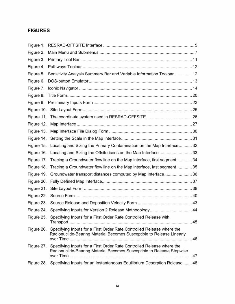
Figure 1. RESRAD-OFFSITE Interface ............................................................................ 5
Figure 2. Main Menu and Submenus ............................................................................... 7
Figure 3. Primary Tool Bar ............................................................................................. 11
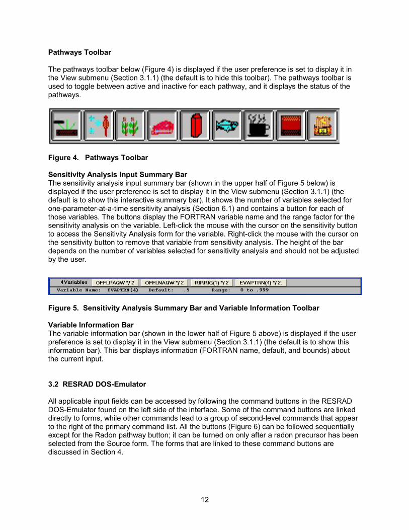
Figure 4. Pathways Toolbar ........................................................................................... 12
Figure 5. Sensitivity Analysis Summary Bar and Variable Information Toolbar ............... 12
Figure 6. DOS-button Emulator ...................................................................................... 13
Figure 7. Iconic Navigator .............................................................................................. 14
Figure 8. Title Form ........................................................................................................ 20
Figure 9. Preliminary Inputs Form .................................................................................. 23
Figure 10. Site Layout Form ........................................................................................... 25
Figure 11. The coordinate system used in RESRAD-OFFSITE. ..................................... 26
Figure 12. Map Interface ................................................................................................ 27
Figure 13. Map Interface File Dialog Form ..................................................................... 30
Figure 14. Setting the Scale in the Map Interface ........................................................... 31
Figure 15. Locating and Sizing the Primary Contamination on the Map Interface ........... 32
Figure 16. Locating and Sizing the Offsite icons on the Map Interface ........................... 33
Figure 17. Tracing a Groundwater flow line on the Map interface, first segment ............. 34
Figure 18. Tracing a Groundwater flow line on the Map interface, last segment ............. 35
Figure 19. Groundwater transport distances computed by Map Interface ....................... 36
Figure 20. Fully Defined Map Interface........................................................................... 37
Figure 21. Site Layout Form. .......................................................................................... 38
Figure 22. Source Form ................................................................................................. 40
Figure 23. Source Release and Deposition Velocity Form ............................................. 43
Figure 24. Specifying Inputs for Version 2 Release Methodology ................................... 44
Figure 25. Specifying Inputs for a First Order Rate Controlled Release with Transport ....................................................................................................... 45
Figure 26. Specifying Inputs for a First Order Rate Controlled Release where the Radionuclide-Bearing Material Becomes Susceptible to Release Linearly over Time ...................................................................................................... 46
Figure 27. Specifying Inputs for a First Order Rate Controlled Release where the Radionuclide-Bearing Material Becomes Susceptible to Release Stepwise over Time ...................................................................................................... 47
Figure 28. Specifying Inputs for an Instantaneous Equilibrium Desorption Release ....... 48
x
Figure 29. Specifying Inputs for an Instantaneous Release where the Radionuclide-Bearing Material Becomes Susceptible to Release Linearly over Time ......................................................................................... 49
Figure 30. Specifying Inputs for an Instantaneous Release where the Radionuclide-Bearing Material Becomes Susceptible to Release Stepwise over Time ....................................................................................... 50
Figure 31. Distribution Coefficients Form for Version 2 Release..................................... 52
Figure 32. Distribution Coefficients Form for Version 3 Releases ................................... 53
Figure 33. Transfer Factors Form ................................................................................... 54
Figure 34. Transfer Factors Form for H-3 and C-14 ....................................................... 55
Figure 35. Set Pathways DOS-Emulator. ....................................................................... 56
Figure 36. Reporting Times Form ................................................................................... 57
Figure 37. Storage Time Form ....................................................................................... 59
Figure 38. Physical and Hydrological Properties Form ................................................... 60
Figure 39. Primary Contamination Form ......................................................................... 62
Figure 40. Agricultural Area Form .................................................................................. 66
Figure 41. Livestock Feed Growing Areas Form ............................................................ 67
Figure 42. Offsite Dwelling Area Form ........................................................................... 69
Figure 43. Atmospheric Transport Form ......................................................................... 70
Figure 44. Unsaturated Zone Hydrology Form ............................................................... 73
Figure 45. Saturated Zone Hydrology Form ................................................................... 75
Figure 46. Water Use Form ............................................................................................ 77
Figure 47. Surface Water Body Form ............................................................................. 79
Figure 48. Groundwater Transport Form ........................................................................ 80
Figure 49. Ingestion Rates Form .................................................................................... 84
Figure 50. Livestock Intakes Form ................................................................................. 86
Figure 51. Plant Factors and Livestock Feed Factors Forms .......................................... 87
Figure 52. Inhalation and External Gamma Form ........................................................... 88
Figure 53. External Radiation Shape and Area Factors Form ........................................ 90
Figure 54. Non-Rectangular Primary Contamination in External Radiation Shape and Area Factors Form .................................................................................. 91
Figure 55. Occupancy Factor Form ................................................................................ 93
Figure 56. Radon Form .................................................................................................. 95
Figure 57. Carbon-14 and Carbon-12 Forms ................................................................. 97
Figure 58. Tritium Form .................................................................................................. 98
Figure 59. Report Viewer ............................................................................................. 102
xi
Figure 60. File Dialog box of Report Viewer ................................................................. 103
Figure 61. Graph Viewer .............................................................................................. 106
Figure 62. Set Sensitivity Analysis Range Form ........................................................... 111
Figure 63. Uncertainty and Probabilistic Analysis Form ................................................ 114
Figure 64. Parameter Distributions Tab of the Uncertainty and Probabilistic Analysis Form ............................................................................................. 117
Figure 65. Help on Statistical Distributions Form .......................................................... 118
Figure 66. Sample Specification Tab of the Uncertainty and Probabilistic Analysis Form ............................................................................................ 119
Figure 67. Input Rank Correlations Tab of the Uncertainty and Probabilistic Analysis Form ............................................................................................. 121
Figure 68. Output Specifications Tab of the Uncertainty and Probabilistic Analysis Form ............................................................................................. 122
Figure 69. Step by Step Analysis Tab of the Uncertainty and Probabilistic Analysis Form ............................................................................................ 123
Figure 70. Step by Step Analysis Tab of the Uncertainty and Probabilistic Analysis Form when a Previously Executed Input File is Opened .............................. 124
Figure 71. The CDF of Output view of the Probabilistic/Uncertainty Graphics Output ... 125
Figure 72. Scatter Plot of Output against Input view of the Probabilistic/Uncertainty Graphics Output .......................................................................................... 126
Figure 73. Scatter Plot of Output against Output view of the Probabilistic/Uncertainty Graphics Output .......................................................................................... 127
Figure 74. Probabilistic Temporal Plots ........................................................................ 128
Figure 75. Regression Analysis Tab of the Uncertainty and Probabilistic Analysis Form ........................................................................................................... 129
Figure 76. Multi-Parameter Sensitivity Analysis View of Parameter Distributions Tab of the Uncertainty and Probabilistic Analysis Form ............................... 130
Figure 77. Regression Output ...................................................................................... 131
Figure 78. Output against Input Scatter plot Showing the Variation of Output with One Input at Different Values of Another Input ............................................ 132
Figure 79. Context Sensitive Help ................................................................................ 134
Figure 80. Message Log Generated by the Computational Code ................................. 135
Figure 81. RESRAD Website ....................................................................................... 136
Figure 82. A portion of the Documents Page of the RESRAD Website ........................ 137
Figure 83. Run Time Feedback Form ........................................................................... 138
xii
Appendix Figures
Figure A.1 Examples of SFSIN.DAT and CZTHICK3.DAT Files Created by the Source Term Model of RESRAD-OFFSITE under the Traditional RESRAD Leach Model .............................................................................. A-2
Figure A.2 Examples of AQFLUXIN.DAT, AIFLUXIN.DAT, and SWFLUXIN.DAT Files Created by the Source Term Model of RESRAD-OFFSITE under the Traditional RESRAD Leach Model ............................................. A-3
Figure A.3 Temporal Profile of Activity in the Primary Contamination under the Traditional RESRAD First-Order Leach Rate Release Model .................... A-4
Figure A.4 Temporal Profile of Release to Groundwater under the Traditional RESRAD First-Order Leach Rate Model................................................. A-4
Figure A.5 Temporal Profile of Release to Atmosphere under the Traditional RESRAD First-Order Leach Rate Model .................................................. A-5
Figure A.6 Temporal Profile of Release to Surface Erosion under the Traditional RESRAD First-Order Leach Rate Model ................................................... A-5
Figure A.7 Temporal Profile of Release to Groundwater under the Equilibrium Desorption Release Model ........................................................................ A-6
Figure A.8 Temporal Profile of Release to Groundwater under the First-Order Leach Rate with Transport Release Model ................................................ A-6
Figure A.9 Input Files AQFLUXIN.DAT, AIFLUXIN.DAT, and SWFLUXIN.DAT Created to Specify the Releases of This Example to RESRAD-OFFSITE .......................................................................... ……..A-9
Figure A.10 RESRAD-OFFSITE Input File Showing the Locations Where the Numbers of Time Points at which the Different Releases Are to Be Read Are Specified ................................................................................. A-10
Figure A.11 Comparison of the Input Flux Specified in This Example Case for AQFLUXIN.DAT and the Flux Interpolated by RESRAD Using Different Numbers of Computational Time Points .................................... A-11
Figure A.12 Comparison of the Input Flux Specified in This Example Case for AIFLUXIN.DAT and the Flux Interpolated by RESRAD Using Different Numbers of Computational Time Points .................................... A-12
Figure A.13 Comparison of the Input Flux Specified in This Example Case for SWFLUXIN.DAT and the Flux Interpolated by RESRAD Using Different Numbers of Computational Time Points .................................... A-13
Figure A.14 Automatic Selection of All Progeny with a Half-Life Greater Than the Cutoff Half-Life, When a Nuclide Is Specified To Be Initially Present in the Contamination ............................................................................... A-14
Figure A.15 Selection of Cutoff Half-Life ..................................................................... A-16
Figure A.16 Source Term Output Files for Case with only 230Th Initially Present ......... A-16
xiii
Figure A.17 Long-Lived Progeny Are at the Same Concentration as the Parent in the Initial Contamination ...................................................................... A-17
Figure A.18 Source Term Output Files for Case in which 230Th and Its Long-Lived Progeny Are Initially Present ................................................. A-18
Figure A.19 Progeny of 242mAm Modeled Explicitly by RESRAD-OFFSITE When a Cutoff Half-Life of 30 Days Is Specified ...................................... A-19
Figure A.20 Chain File Generated by RESRAD-OFFSITE Showing the Branches and Threads of the 242mAm Transformation Chain ................................... A-20
Figure B.1 Area Factors Form—Default Options ......................................................... B-2
Figure B.2 Area Factors Form—Option to Specify the Range of the Y Dimension of the Small Area of Elevated Contamination ............................................ B-3
Figure B.3 Distribution of Area of the Small Area of Elevated Contamination under Three Distributions Options for Sampling the Dimensions of the Small Area of Elevated Contamination: Triangular Skewed to the High End, Uniform, and Triangular Skewed to the Low End ....................................... B-4
Figure B.4 Area Factors Form—Generate Dose-Area Plot Command Button Activated ........................................................................................ B-7
Figure B.5 Scatter Plot of Dose against Area of Contamination for Cs-137 Where the Direct External Exposure from the Primary Contamination is the Dominant Pathway.. ......................................................................... B-9
Figure B.6 Scatter Plot of Dose against Area of Contamination for Pu-239 for Which Atmospheric Transport Is the Dominant Route of Exposure ......... B-10
Figure B.7 Scatter Plot of Dose against Area of Contamination for Tc-99 for Which Groundwater Transport Is the Dominant Route of Exposure ......... B-11
Figure B.8 Sample of Area Factor Text Report for Cs-137 ........................................ B-13
Figure B.9 Sample of Area Factor Text Report for Pu-239 ........................................ B-14
Figure B.10 Sample of Area Factor Text Report for Tc-99 .......................................... B-15
TABLES
Table 1 Icon Identification. .......................................................................................... 28
Table A.1 Release to Be Input to RESRAD-OFFSITE .................................................... A-8


1
1 INTRODUCTION The RESRAD-OFFSITE code was initially developed to extend the capability of the RESRAD (onsite) code for modeling offsite receptor exposure scenarios (Yu et al. 2007). The transition from RESRAD (onsite) to RESRAD-OFFSITE, including benchmarking of RESRAD-OFFSITE code against peer codes, was documented in DOE/EH-0708 (Yu et al. 2006). The capability of RESRAD-OFFSITE code was further enhanced in the modeling of the source release term for handling containerized waste materials. This new source term model was documented in NUREG/CR-7127 (Yu et al. 2013) for potential application to low-level radioactive waste disposal facility performance assessment. A new version of RESRAD-OFFSITE (Version 3.1) was released following the incorporation of this new source term model. Version 3.1 includes additional features such as time-distributed source release and computation of area factors for offsite exposure scenarios. 1.1 Purpose Of User’s Guide The primary purpose of this user’s guide is to help users understand and use the RESRAD-OFFSITE code Version 3.1. It describes how to download and install the code, as well as how to navigate through the input screens to simulate various exposure scenarios and view the results in graphics and text reports. This user’s guide not only describes the features of RESRAD-OFFSITE, Version 3.1, it also provides additional information about the input parameters to increase the user’s understanding of the code. Some advanced features, such as overriding the source term model, use of probabilistic and sensitivity analysis, and computing the area factors, are also included in this user’s guide. 1.2 Organization Of User’s Guide This information is organized into the following major sections:
Section 2. Installation: Installation procedures and system requirements. • Section 3. Navigation: Instructions for moving around the interface to •
accomplish various tasks and to save input and output. Section 4. Input forms: Description of each input form, information on how to •
use each form, and parameters in the input forms. Section 5. Outputs: Instructions on how to find results in the textual and •
graphical output. Section 6. Enhancements: Explanation of the probabilistic/uncertainty •
analysis and sensitivity analysis features. Section 7. Help: Various ways of obtaining help. • Section 8. References: List of references. • Appendix A. Overriding the source term module: Description of how to •
override the source and release module of the computational code, as well as how to specify temporal information about the primary contamination and the release.
Appendix B. Computing the area factors: Description of a menu option that •facilitates the calculation of area factors of small areas with elevated contamination for offsite exposure scenarios.

3
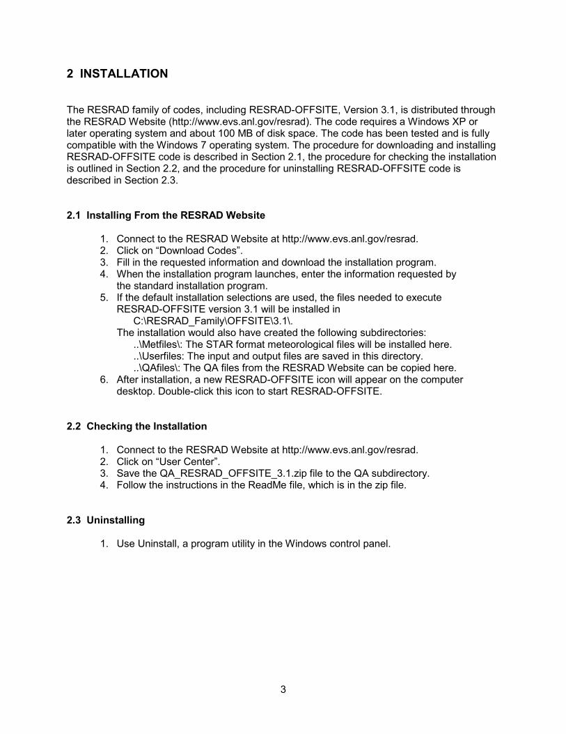
2 INSTALLATION The RESRAD family of codes, including RESRAD-OFFSITE, Version 3.1, is distributed through the RESRAD Website (http://www.evs.anl.gov/resrad). The code requires a Windows XP or later operating system and about 100 MB of disk space. The code has been tested and is fully compatible with the Windows 7 operating system. The procedure for downloading and installing RESRAD-OFFSITE code is described in Section 2.1, the procedure for checking the installation is outlined in Section 2.2, and the procedure for uninstalling RESRAD-OFFSITE code is described in Section 2.3. 2.1 Installing From the RESRAD Website
1. Connect to the RESRAD Website at http://www.evs.anl.gov/resrad. 2. Click on “Download Codes”. 3. Fill in the requested information and download the installation program. 4. When the installation program launches, enter the information requested by
the standard installation program. 5. If the default installation selections are used, the files needed to execute
RESRAD-OFFSITE version 3.1 will be installed in C:\RESRAD_Family\OFFSITE\3.1\. The installation would also have created the following subdirectories: ..\Metfiles\: The STAR format meteorological files will be installed here. ..\Userfiles: The input and output files are saved in this directory. ..\QAfiles\: The QA files from the RESRAD Website can be copied here. 6. After installation, a new RESRAD-OFFSITE icon will appear on the computer
desktop. Double-click this icon to start RESRAD-OFFSITE. 2.2 Checking the Installation
1. Connect to the RESRAD Website at http://www.evs.anl.gov/resrad. 2. Click on “User Center”. 3. Save the QA_RESRAD_OFFSITE_3.1.zip file to the QA subdirectory. 4. Follow the instructions in the ReadMe file, which is in the zip file.
2.3 Uninstalling
1. Use Uninstall, a program utility in the Windows control panel.

5
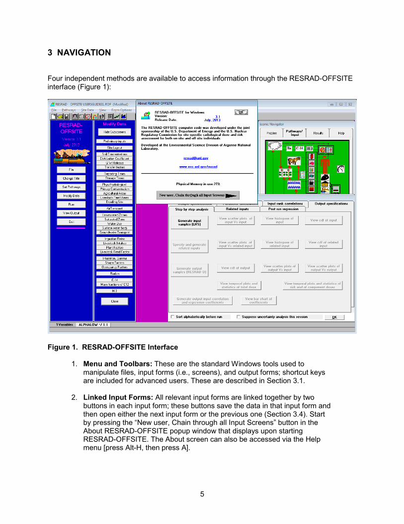
3 NAVIGATION Four independent methods are available to access information through the RESRAD-OFFSITE interface (Figure 1):
Figure 1. RESRAD-OFFSITE Interface
1. Menu and Toolbars: These are the standard Windows tools used to manipulate files, input forms (i.e., screens), and output forms; shortcut keys are included for advanced users. These are described in Section 3.1.
2. Linked Input Forms: All relevant input forms are linked together by two
buttons in each input form; these buttons save the data in that input form and then open either the next input form or the previous one (Section 3.4). Start by pressing the “New user, Chain through all Input Screens” button in the About RESRAD-OFFSITE popup window that displays upon starting RESRAD-OFFSITE. The About screen can also be accessed via the Help menu [press Alt-H, then press A].

6
3. RESRAD DOS-Emulator: This set of textual command buttons is similar to the buttons used in RESRAD for the DOS interface (Section 3.2).
4. Iconic Navigator Window: This tabbed window provides access to the
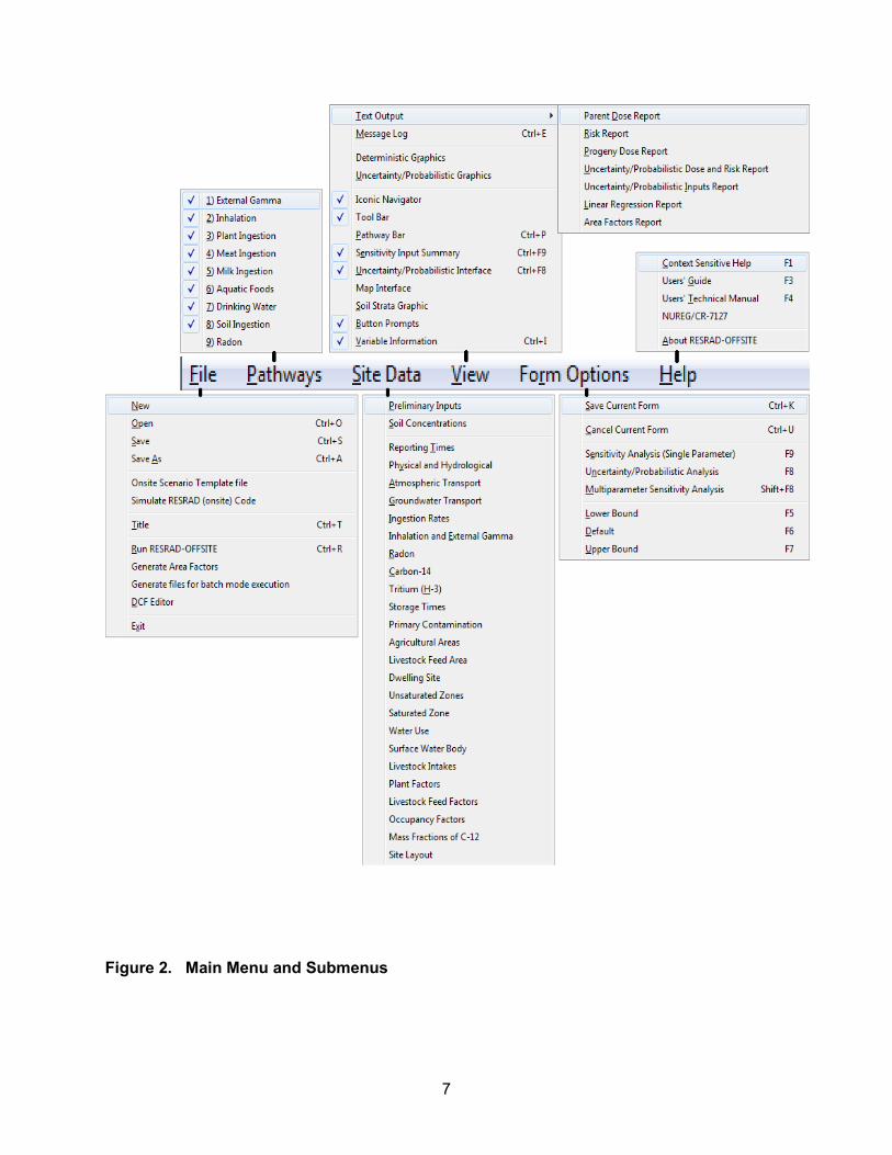
information through more graphical cues (Section 3.3). 3.1 Menus and Toolbars 3.1.1 Menus The menu on the main RESRAD-OFFSITE window (i.e., the Main Menu) gives complete access to all the forms, functions, and features of the code. The Main Menu and the submenus that branch from it are shown below (Figure 2).
7
Figure 2. Main Menu and Submenus
8
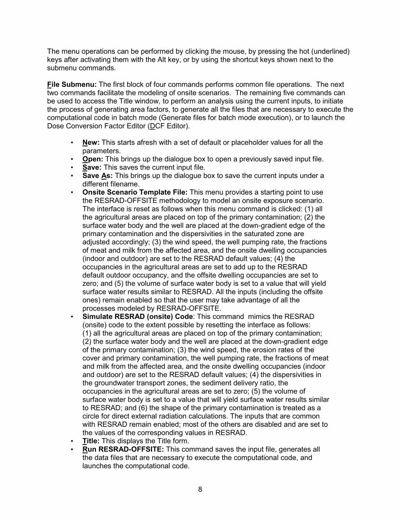
The menu operations can be performed by clicking the mouse, by pressing the hot (underlined) keys after activating them with the Alt key, or by using the shortcut keys shown next to the submenu commands. File Submenu: The first block of four commands performs common file operations. The next two commands facilitate the modeling of onsite scenarios. The remaining five commands can be used to access the Title window, to perform an analysis using the current inputs, to initiate the process of generating area factors, to generate all the files that are necessary to execute the computational code in batch mode (Generate files for batch mode execution), or to launch the Dose Conversion Factor Editor (DCF Editor).
New: This starts afresh with a set of default or placeholder values for all the •parameters.
Open: This brings up the dialogue box to open a previously saved input file. • Save: This saves the current input file. • Save As: This brings up the dialogue box to save the current inputs under a •
different filename. Onsite Scenario Template File: This menu provides a starting point to use •
the RESRAD-OFFSITE methodology to model an onsite exposure scenario. The interface is reset as follows when this menu command is clicked: (1) all the agricultural areas are placed on top of the primary contamination; (2) the surface water body and the well are placed at the down-gradient edge of the primary contamination and the dispersivities in the saturated zone are adjusted accordingly; (3) the wind speed, the well pumping rate, the fractions of meat and milk from the affected area, and the onsite dwelling occupancies (indoor and outdoor) are set to the RESRAD default values; (4) the occupancies in the agricultural areas are set to add up to the RESRAD default outdoor occupancy, and the offsite dwelling occupancies are set to zero; and (5) the volume of surface water body is set to a value that will yield surface water results similar to RESRAD. All the inputs (including the offsite ones) remain enabled so that the user may take advantage of all the processes modeled by RESRAD-OFFSITE.
Simulate RESRAD (onsite) Code: This command mimics the RESRAD •(onsite) code to the extent possible by resetting the interface as follows: (1) all the agricultural areas are placed on top of the primary contamination; (2) the surface water body and the well are placed at the down-gradient edge of the primary contamination; (3) the wind speed, the erosion rates of the cover and primary contamination, the well pumping rate, the fractions of meat and milk from the affected area, and the onsite dwelling occupancies (indoor and outdoor) are set to the RESRAD default values; (4) the dispersivities in the groundwater transport zones, the sediment delivery ratio, the occupancies in the agricultural areas are set to zero; (5) the volume of surface water body is set to a value that will yield surface water results similar to RESRAD; and (6) the shape of the primary contamination is treated as a circle for direct external radiation calculations. The inputs that are common with RESRAD remain enabled; most of the others are disabled and are set to the values of the corresponding values in RESRAD.
Title: This displays the Title form. • Run RESRAD-OFFSITE: This command saves the input file, generates all •
the data files that are necessary to execute the computational code, and launches the computational code.
9
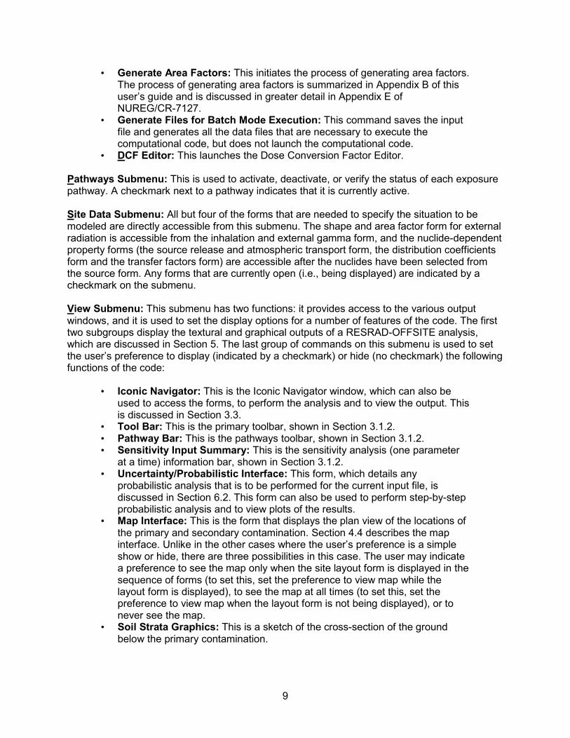
Generate Area Factors: This initiates the process of generating area factors. •The process of generating area factors is summarized in Appendix B of this user’s guide and is discussed in greater detail in Appendix E of NUREG/CR-7127.
Generate Files for Batch Mode Execution: This command saves the input •file and generates all the data files that are necessary to execute the computational code, but does not launch the computational code.
DCF Editor: This launches the Dose Conversion Factor Editor. • Pathways Submenu: This is used to activate, deactivate, or verify the status of each exposure pathway. A checkmark next to a pathway indicates that it is currently active. Site Data Submenu: All but four of the forms that are needed to specify the situation to be modeled are directly accessible from this submenu. The shape and area factor form for external radiation is accessible from the inhalation and external gamma form, and the nuclide-dependent property forms (the source release and atmospheric transport form, the distribution coefficients form and the transfer factors form) are accessible after the nuclides have been selected from the source form. Any forms that are currently open (i.e., being displayed) are indicated by a checkmark on the submenu. View Submenu: This submenu has two functions: it provides access to the various output windows, and it is used to set the display options for a number of features of the code. The first two subgroups display the textural and graphical outputs of a RESRAD-OFFSITE analysis, which are discussed in Section 5. The last group of commands on this submenu is used to set the user’s preference to display (indicated by a checkmark) or hide (no checkmark) the following functions of the code:
Iconic Navigator: This is the Iconic Navigator window, which can also be •used to access the forms, to perform the analysis and to view the output. This is discussed in Section 3.3.
Tool Bar: This is the primary toolbar, shown in Section 3.1.2. • Pathway Bar: This is the pathways toolbar, shown in Section 3.1.2. • Sensitivity Input Summary: This is the sensitivity analysis (one parameter •
at a time) information bar, shown in Section 3.1.2. Uncertainty/Probabilistic Interface: This form, which details any •
probabilistic analysis that is to be performed for the current input file, is discussed in Section 6.2. This form can also be used to perform step-by-step probabilistic analysis and to view plots of the results.
Map Interface: This is the form that displays the plan view of the locations of •the primary and secondary contamination. Section 4.4 describes the map interface. Unlike in the other cases where the user’s preference is a simple show or hide, there are three possibilities in this case. The user may indicate a preference to see the map only when the site layout form is displayed in the sequence of forms (to set this, set the preference to view map while the layout form is displayed), to see the map at all times (to set this, set the preference to view map when the layout form is not being displayed), or to never see the map.
Soil Strata Graphics: This is a sketch of the cross-section of the ground •below the primary contamination.
10
Button Prompts: A button prompt is a short descriptive name for a control •on the toolbar or on the Pathways/Inputs tab of the Iconic Navigator window. A prompt is displayed when the mouse cursor moves over the control and lingers there for a short while. The descriptions of the objects in the map interface are also displayed as the mouse lingers over the different objects in the map interface.
Variable Information: This is the variable information bar, shown in •Section 3.1.2.
Form Options Submenu: The first two commands on the Form Options submenu, Save current form and Cancel current form, are used to save or cancel the changes made to an open form (Section 4). The remaining six commands perform operations on the input boxes contained in the forms, as follows:
Sensitivity Analysis (single parameter): This is used to activate “one •parameter at a time sensitivity analysis” (Section 6.1) on the input parameter and to set the range of the parameter for the analysis.
Uncertainty/Probabilistic Analysis: This is used to include the input •parameter in the probabilistic or uncertainty analysis (Section 6.2). It can also be used to display the uncertainty/probabilistic analysis form if it is not visible.
Multi-parameter Sensitivity Analysis: This is used to include the input •parameter in the probabilistic or uncertainty analysis with uniform or log-uniform distribution of a selectable range about its current value and to display the uncertainty/probabilistic analysis form if it is not visible.
Lower Bound: This is used to set the input to the lowest value accepted by •RESRAD-OFFSITE. The lowest value may be a physical bound (i.e., the lowest value that is applicable for the parameter because of physical considerations) or simply a numerical bound imposed to prevent the code from crashing.
Default: This is used to set the input to the default value assigned in the •RESRAD-OFFSITE code. While some default values (e.g., ingestion rates, inhalation rates) are generally accepted values, others (e.g., field capacity, distribution coefficient) are merely placeholder values.
Upper Bound: This is used to set the input to the highest value accepted by •RESRAD-OFFSITE. The highest value may be a physical bound (i.e., the highest value that is applicable for the parameter because of physical considerations) or simply a numerical bound imposed to prevent the code from crashing.
Help submenu: This is used to obtain context-sensitive information about the inputs, forms, and features in RESRAD-OFFSITE; to access PDF versions of this user’s guide and the user’s technical manual; and to display the About RESRAD-OFFSITE form.
Context-Sensitive Help: Information about a specific input parameter, form, •or feature in RESRAD-OFFSITE can be obtained by pressing the F1 function key while the input control is in focus (box, option buttons, dropdown box, etc.). The input control is in focus when the cursor is in the field of the control.
User’s Guide: This opens the PDF version of this document. • User’s Technical Manual: This opens the PDF version of the user’s manual. •
11
NUREG/CR-7127: This opens the PDF version of NUREG/CR-7127, which •deals with the source release options added to Version 3.1 of RESRAD-OFFSITE and with performing sensitivity analysis.
About RESRAD-OFFSITE: This displays the About RESRAD-OFFSITE form •(i.e., the About form). This form shows the version and release date of the RESRAD-OFFSITE software installed on the computer, the amount of physical memory that is available on the computer, and the e-mail contact for the RESRAD team; it also provides a link to access the RESRAD Website.
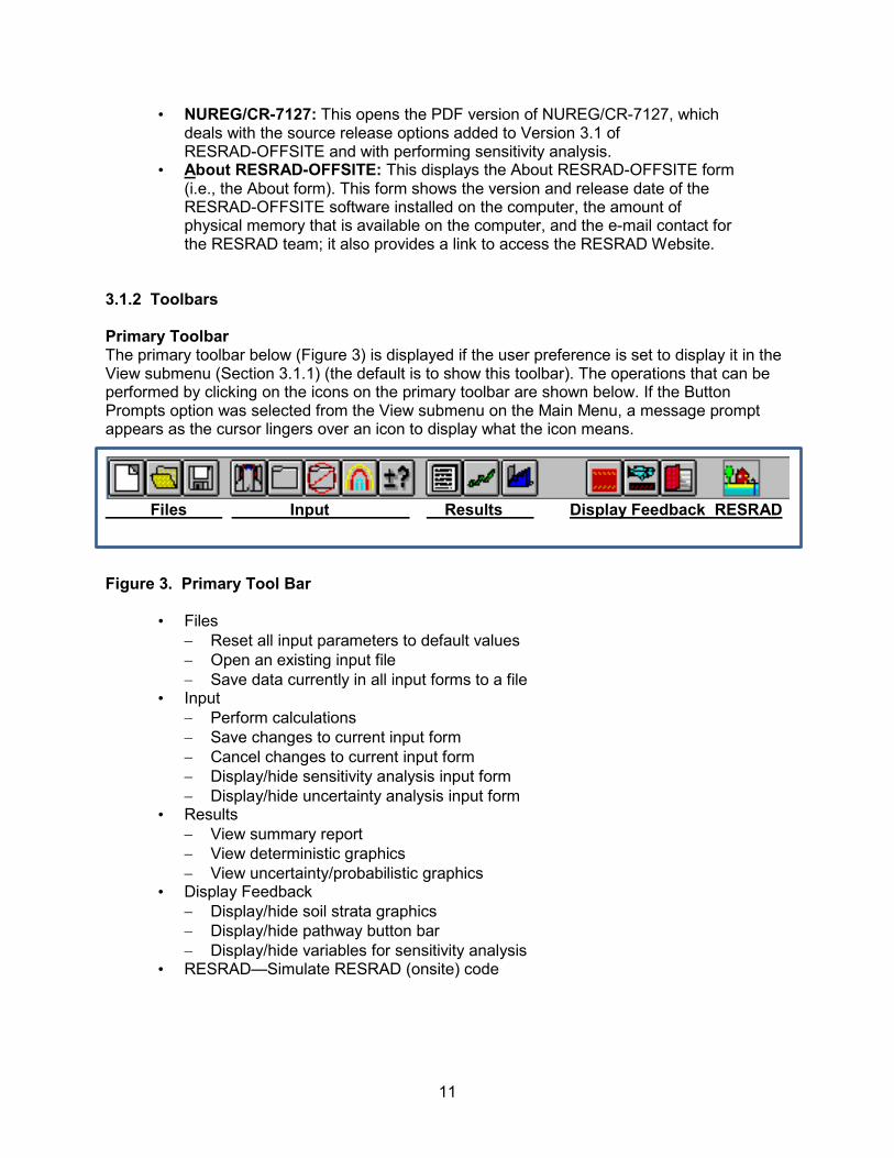
3.1.2 Toolbars Primary Toolbar The primary toolbar below (Figure 3) is displayed if the user preference is set to display it in the View submenu (Section 3.1.1) (the default is to show this toolbar). The operations that can be performed by clicking on the icons on the primary toolbar are shown below. If the Button Prompts option was selected from the View submenu on the Main Menu, a message prompt appears as the cursor lingers over an icon to display what the icon means.
Files Input Results Display Feedback RESRAD Figure 3. Primary Tool Bar
Files •− Reset all input parameters to default values − Open an existing input file − Save data currently in all input forms to a file
Input •− Perform calculations − Save changes to current input form − Cancel changes to current input form − Display/hide sensitivity analysis input form − Display/hide uncertainty analysis input form
Results •− View summary report − View deterministic graphics − View uncertainty/probabilistic graphics
Display Feedback •− Display/hide soil strata graphics − Display/hide pathway button bar − Display/hide variables for sensitivity analysis
RESRAD—Simulate RESRAD (onsite) code •
12
Pathways Toolbar The pathways toolbar below (Figure 4) is displayed if the user preference is set to display it in the View submenu (Section 3.1.1) (the default is to hide this toolbar). The pathways toolbar is used to toggle between active and inactive for each pathway, and it displays the status of the pathways.
Figure 4. Pathways Toolbar Sensitivity Analysis Input Summary Bar The sensitivity analysis input summary bar (shown in the upper half of Figure 5 below) is displayed if the user preference is set to display it in the View submenu (Section 3.1.1) (the default is to show this interactive summary bar). It shows the number of variables selected for one-parameter-at-a-time sensitivity analysis (Section 6.1) and contains a button for each of those variables. The buttons display the FORTRAN variable name and the range factor for the sensitivity analysis on the variable. Left-click the mouse with the cursor on the sensitivity button to access the Sensitivity Analysis form for the variable. Right-click the mouse with the cursor on the sensitivity button to remove that variable from sensitivity analysis. The height of the bar depends on the number of variables selected for sensitivity analysis and should not be adjusted by the user.
Figure 5. Sensitivity Analysis Summary Bar and Variable Information Toolbar Variable Information Bar The variable information bar (shown in the lower half of Figure 5 above) is displayed if the user preference is set to display it in the View submenu (Section 3.1.1) (the default is to show this information bar). This bar displays information (FORTRAN name, default, and bounds) about the current input. 3.2 RESRAD DOS-Emulator All applicable input fields can be accessed by following the command buttons in the RESRAD DOS-Emulator found on the left side of the interface. Some of the command buttons are linked directly to forms, while other commands lead to a group of second-level commands that appear to the right of the primary command list. All the buttons (Figure 6) can be followed sequentially except for the Radon pathway button; it can be turned on only after a radon precursor has been selected from the Source form. The forms that are linked to these command buttons are discussed in Section 4.
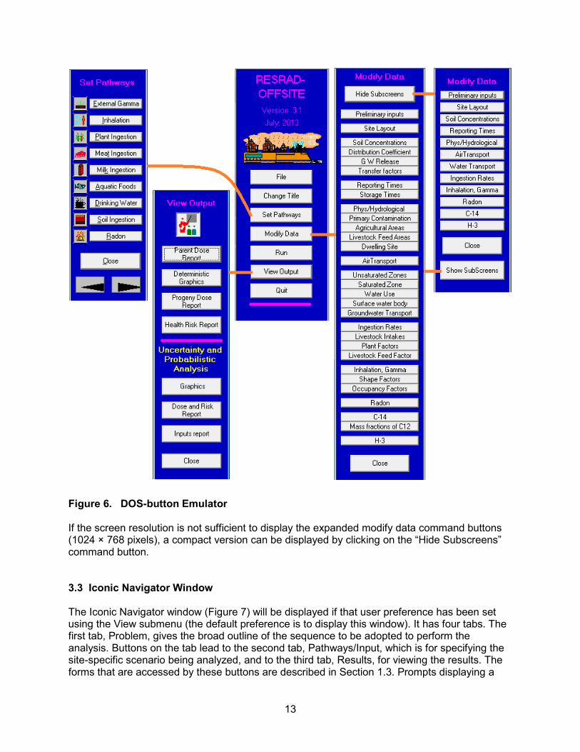
13
Figure 6. DOS-button Emulator If the screen resolution is not sufficient to display the expanded modify data command buttons (1024 × 768 pixels), a compact version can be displayed by clicking on the “Hide Subscreens” command button. 3.3 Iconic Navigator Window The Iconic Navigator window (Figure 7) will be displayed if that user preference has been set using the View submenu (the default preference is to display this window). It has four tabs. The first tab, Problem, gives the broad outline of the sequence to be adopted to perform the analysis. Buttons on the tab lead to the second tab, Pathways/Input, which is for specifying the site-specific scenario being analyzed, and to the third tab, Results, for viewing the results. The forms that are accessed by these buttons are described in Section 1.3. Prompts displaying a
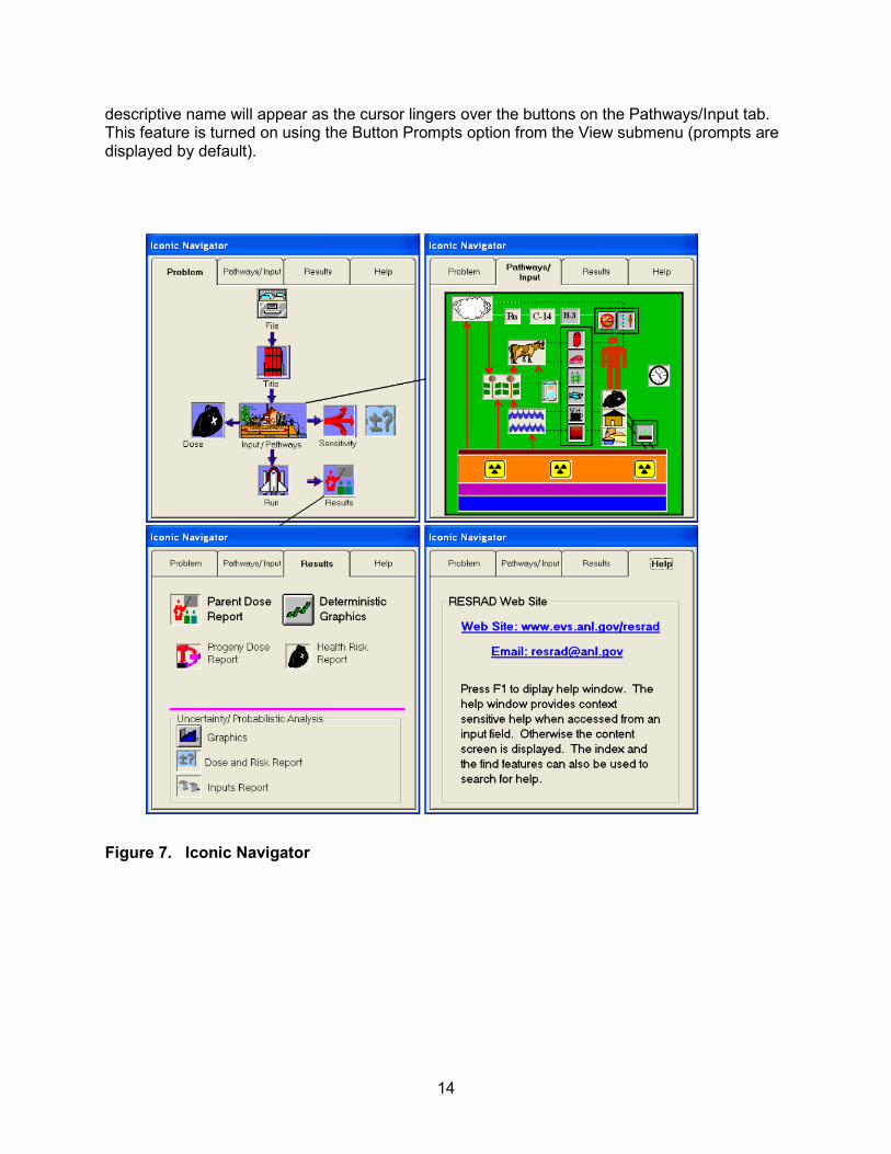
14
descriptive name will appear as the cursor lingers over the buttons on the Pathways/Input tab. This feature is turned on using the Button Prompts option from the View submenu (prompts are displayed by default).
Figure 7. Iconic Navigator

15
Problem: This tab guides the user to set up a case in RESRAD-OFFSITE. •Each button brings up windows or forms to continue with the process.
Pathways/Input: This tab allows the user to view and activate pathways. •
Buttons for the pathways can be found in the three black boxes. Inhalation pathways are above the person, and ingestion pathways are to the left. The single external pathway is at the lower right. Input windows are accessed by clicking on icons. Prompts appear to display what the icon means if the Button Prompts option was selected from the View submenu.
Results: The top two buttons give access to the main deterministic results in •
report and graphical formats. The next two buttons open supplementary reports. If an uncertainty analysis was run, three more buttons below the purple line to provide access to the two reports and a set of graphics.
Help: If the user operating system is connected to the Internet, this tab gives •
the user access to the RESRAD Website and provides the address to which users can e-mail questions for the RESRAD team.
3.4 Linked Input Forms All the input forms that are relevant to the current analysis can be displayed in sequence by using the forward and backward arrows in each form. The linked sequence begins in the About RESRAD-OFFSITE window, which is displayed every time RESRAD-OFFSITE is launched. This window is also accessible from the Help submenu (press Alt-H, then press A). The last form in the sequence has the run command instead of a forward arrow; it issues the command to perform the RESRAD-OFFSITE analysis using the current set of inputs. The sequence of the forms is as follows: Title, Preliminary Inputs, Site Layout (and map interface), Source, Source Release and Deposition Velocity, Distribution Coefficients, Transfer Factors, Set Pathways, Reporting Times, Storage Times, Physical and Hydrological, Primary Contamination, Agricultural Areas, Livestock Feed Growing Areas, Offsite Dwelling Area, Atmospheric Transport, Unsaturated Zone Hydrology, Saturated Zone Hydrology, Water Use, Surface Water Body, Groundwater Transport, Ingestion Rates, Livestock Intakes, Livestock Feed Factors, Plant Factors, Inhalation and External Gamma, External Radiation Shape and Area Factors, Occupancy, Radon, Carbon-14, Mass Fractions of Carbon-12, and Tritium. The last four forms are displayed only if they are relevant to the current selection of nuclides. The forms are described in the linked sequence in Section 4.

17
4 INPUT FORMS There are more than 30 input forms for entering the parameters that define the site data, assumptions, site identification, and calculation specifications. Sections 4.1 through 4.30 describe each form in detail and have a description of each input on the form. Additional information about each input can also be obtained by clicking the help command, F1, when the cursor is in that input field. The RESRAD-OFFSITE predictions of dose and risk, dependent on the values specified for the inputs on these forms. The sensitivity of the predictions to the value of an input depends on the scenario being considered and the values of the other inputs. Hence it is imperative that site-specific or site-appropriate values be used for all the inputs except for those that are defined by the standard receptor. Most input is entered by keying numbers into boxes, but some input is entered through list boxes, check boxes, and option boxes. Some features common to all input forms are described here. Saving Information to Memory There are two levels at which information can be saved in RESRAD-OFFSITE. The first level is to temporarily save the information to memory. This can be done with any of the following commands:
Command Buttons: Click on the Save button, Forward button, or Backward •button on the form.
Menu: Select Form Options, then Save current form (Ctrl-K). •
Toolbar: Click on the Folder button. •
Saving Information to File The second level is to save the settings to a file. This can be done with any of the following commands:
DOS-Emulator: Press the File button on the DOS-Emulator to activate the •File Options form. Then select Save or Save As.
Menu: Select File, then either Save (Ctrl-S) or Save As (Ctrl-A). •
Toolbar: Press the Disk button to save to a file. •
Run: If any input form was exited with a save operation (as opposed to a •
cancel operation), then the file will need to be saved to disk before calculations are performed. This will perform a save, but not a save as.
Canceling Changes Made to a Form The changes to the inputs in a form can be canceled if they have not yet been saved to memory.
Function Keys: Press the Esc key. •

18
Command button: Click on the Cancel button on the form. •
Menu: Select Form Options, then Cancel current form (Ctrl-U). •
Toolbar: Click on the Canceled Folder button. • Saving Information to Memory and Opening Next or Previous Form The information in a form can be saved to memory, and the next or previous form can be opened by pressing the forward arrow or the backward arrow on each form, as appropriate. Entering Numbers Some input boxes may be grayed out (disabled) because they are not applicable to the current case, either because some pathways have been turned off or because the pertinent radionuclide was not chosen. Values representative of the site should be entered in all input boxes that are active. The default value and the bounds (upper and lower) of the selected parameter will be displayed in the variable information bar. The value in the input box may be set to the default value or to an upper or lower bound, as described below.
Defaults: To set the selected parameter to its default, either select Form •Options and then Default from the Main Menu, or press the F6 function key. While some default values (e.g., ingestion rates, inhalation rates) are generally accepted values, others (e.g., field capacity, distribution coefficient) are merely placeholder values.
Bounds: To set the selected parameter to its upper (or lower) bound, either •
select Form Options and then UpperBound (or LowerBound) from the Main menu, or press the F7 (F5) function key. These may be a physical bound (i.e., the highest or lowest value that is applicable for the parameter because of physical considerations) or simply a numerical bound imposed to prevent the code from crashing.
Obtaining Help Context-specific help will be shown anytime the F1 function key is pressed. For additional sources of help, please refer to the Help section (Section 7) of this user’s guide.
Selecting a Parameter for Probabilistic or Uncertainty Analysis Input parameters can be selected for inclusion in a probabilistic or uncertainty analysis by pressing the F8 key while the cursor is in the input box for that parameter (see Section 6.2, Uncertainty and Probabilistic Analysis). Some parameters are ineligible for uncertainty analysis, either because it does not make sense to perform the analysis on those parameters, or because of the unmanageable constraints imposed by interrelationships with other parameters.
19
Selecting a Parameter for One-Parameter-at-a-Time Sensitivity Analysis Input parameters can be selected for one-parameter-at-a-time sensitivity analysis by pressing the F9 key while the cursor is in the input box for that parameter (see Section 6.1, Sensitivity Analysis). Some parameters are ineligible for sensitivity analysis because it does not make sense to perform a sensitivity analysis on those parameters.
Selecting a Parameter for Multi-parameter Sensitivity Analysis Input parameters can be selected for inclusion in a multi parameter sensitivity analysis by pressing Shift-F8 while the cursor is in the input box for that parameter. The selected parameters can have a uniform distribution with a half range of 50%, 25%, 10%, 5%, or 0.1% of the deterministic value on either side of the deterministic value, or a log-uniform distribution ranging from 1/10 to 10, 1/5 to 5, 1/3 to 3, 1/2 to 2, or 1/1.001 to 1.001 times the deterministic value (see Section 6.2, Uncertainty and Probabilistic Analysis). Only the parameters that are eligible for uncertainty analysis can be included in the Multi-parameter Sensitivity Analysis. The sensitive parameters can be ranked using the standardized regression coefficient or the standardized rank regression coefficient. Multi-parameter Sensitivity Analysis is discussed in section 6.3 of this guide.
20
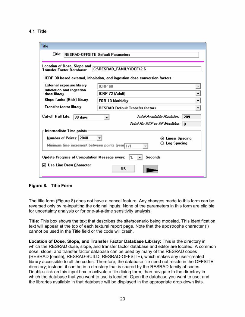
4.1 Title
Figure 8. Title Form The title form (Figure 8) does not have a cancel feature. Any changes made to this form can be reversed only by re-inputting the original inputs. None of the parameters in this form are eligible for uncertainty analysis or for one-at-a-time sensitivity analysis. Title: This box shows the text that describes the site/scenario being modeled. This identification text will appear at the top of each textural report page. Note that the apostrophe character (‘) cannot be used in the Title field or the code will crash. Location of Dose, Slope, and Transfer Factor Database Library: This is the directory in which the RESRAD dose, slope, and transfer factor database and editor are located. A common dose, slope, and transfer factor database can be used by many of the RESRAD codes (RESRAD [onsite], RESRAD-BUILD, RESRAD-OFFSITE), which makes any user-created library accessible to all the codes. Therefore, the database file need not reside in the OFFSITE directory; instead, it can be in a directory that is shared by the RESRAD family of codes. Double-click on this input box to activate a file dialog form, then navigate to the directory in which the database that you want to use is located. Open the database you want to use, and the libraries available in that database will be displayed in the appropriate drop-down lists.
21
External Exposure Library and the Inhalation and Ingestion Dose Library: The dose conversion factors in these libraries will be used for the current analysis. Libraries of dose conversion factors can be set up by using the RESRAD Dose Conversion Factors Editor, which is a standalone utility program common to the RESRAD family of codes. The libraries are stored in a database file. The second drop-down list contains all the internal exposure dose conversion factor libraries that are available in the current database; these include the standard RESRAD FGR11 (Eckerman et al. 1988) and age-dependent ICRP72 (ICRP 1996) libraries and any libraries created by the user. The library displayed in the first drop-down box for external exposure depends on the library chosen in the second drop-down box for internal exposure. If the ICRP 30 based internal exposure library, FGR 11, is chosen, then the external exposure dose factors will be from FGR 12. The external exposure dose factors will be from ICRP 60 if an ICRP60-based age-dependent internal dose library from ICRP72 is chosen. Both the internal and external exposure dose factors will come from the user-created library when a user-created library is selected. Slope Factor Library: The slope factors (risk) in this library will be used for the current analysis. Libraries of slope factors can be set up by using the RESRAD Dose Conversion Factors Editor, which is a standalone utility program common to the RESRAD family of codes. The libraries are stored in a database file. The drop-down list contains all the slope-factor libraries that are available in the current database: the standard RESRAD FGR13 morbidity (Eckerman et al. 1999), FGR13 mortality, the HEAST2001 morbidity libraries (EPA 2001), and any created by the user. Transfer Factor Library: The transfer factors in this library will be used for the current analysis unless the values are changed in the nuclide-specific transfer factor form (Section 4.8). Libraries of transfer factors can be set up using the RESRAD Dose Conversion Factors Editor, which is a standalone utility program common to the RESRAD family of codes. The libraries are stored in a database file. The drop-down list contains all the dose conversion factor libraries that are available in the current database, including the standard RESRAD default transfer factor library and any libraries created by the user. The RESRAD transfer factor library contains only one soil-to-plant transfer factor for each nuclide, whereas the RESRAD-OFFSITE code can accept and use different factors for the vegetation in each of the four different agricultural and farmed areas. The transfer factors are site and species specific; the transfer factor form (Section 4.8) allows these values to be changed for each input file without having to create a different library for each site. Cutoff Half-Life: The fate and transport of nuclides with half-lives larger than the specified half-life are modeled explicitly by the code. Progeny nuclides with a half-life shorter than the specified value are assumed to be in secular equilibrium with their immediate parent. The user can select from the values in the list (180, 30, 7, or 1 day[s]) or type in any value that is not less than 10 minutes. Only the nuclides that have a half-life greater than the cutoff half-life are listed in the right scroll box on the Source form. Informational Boxes: There are two informational boxes in this form. The first shows the number of radionuclides in the current ICRP38 (ICRP 1983) database that have a half-life greater than or equal to the current cutoff half-life. The second shows the number of such nuclides that are lacking at one or more dose conversion or slope factors.
22
Intermediate Time Points
Number of Points: This shows the number of time points at which •concentrations, doses, and risks are computed. Because RESRAD-OFFSITE can compute concentration and flux at any time on the basis of the concentrations and fluxes computed at preceding times, and because the code uses all the time points that fall within the appropriate exposure duration to perform time integration of dose and risk, this parameter determines the accuracy of the computed values. The number of points in the temporal graphics will be set to this number. Straight line segments connect the points in the curve. A larger number of times enables the code to compute offsite accumulation, groundwater transport, and time integration of dose and risk more accurately and will result in smoother plots. However, a larger number will also increase the execution time. For most radionuclides, a number of time points equal to about one-tenth to one-fifth of the prediction time horizon should give results of sufficient accuracy. A greater number of intermediate time points are required if the rate of release of a radionuclide changes rapidly over time. The number of points shown must be such that a linear approximation between the values of flux at those times is a good representation of the actual temporal variation of the flux. The interval of time between the intermediate time points must also not exceed the travel time in any of the groundwater transport zones.
Linear Spacing or Log Spacing: The spacing shows the manner in which •
the intermediate time points are distributed over the time horizon. The time horizon is the sum of the maximum user-specified reporting time (Section 4.10, Reporting Times) and the exposure duration (Section 4.2, Preliminary Inputs). The spacing may be linear or log.
1. Linear: If linear is chosen, the intermediate time points are spaced
uniformly (in an arithmetic sequence) between 0 and the time horizon. 2. Log: If log is chosen, the intermediate time points are spaced in a
geometric sequence (uniformly on a logarithmic scale) between the specified minimum time increment and the time horizon. The spacing in this case may be adjusted by the minimum time increment, as described below.
Minimum Time Increment: In addition to being the first intermediate time •
point under the choice of log spacing, as described above, this is also the lower bound for spacing between intermediate time points of a geometric sequence. Depending on the time horizon and the number of points, the spacing between the intermediate time points can be very small at the beginning of the geometric sequence. In order to avoid unnecessary calculations, if the spacing is less than the specified minimum value, the sequence of time points will then be modified to a linear sequence with the minimum time increment, followed by a geometric sequence with a time increment that is never less than the specified minimum.
Update Progress of Computation Message: The time needed to perform the RESRAD-OFFSITE computations can range from a few minutes to a couple of hours, depending on the number of intermediate time points, number of radionuclides, number and lengths of
23
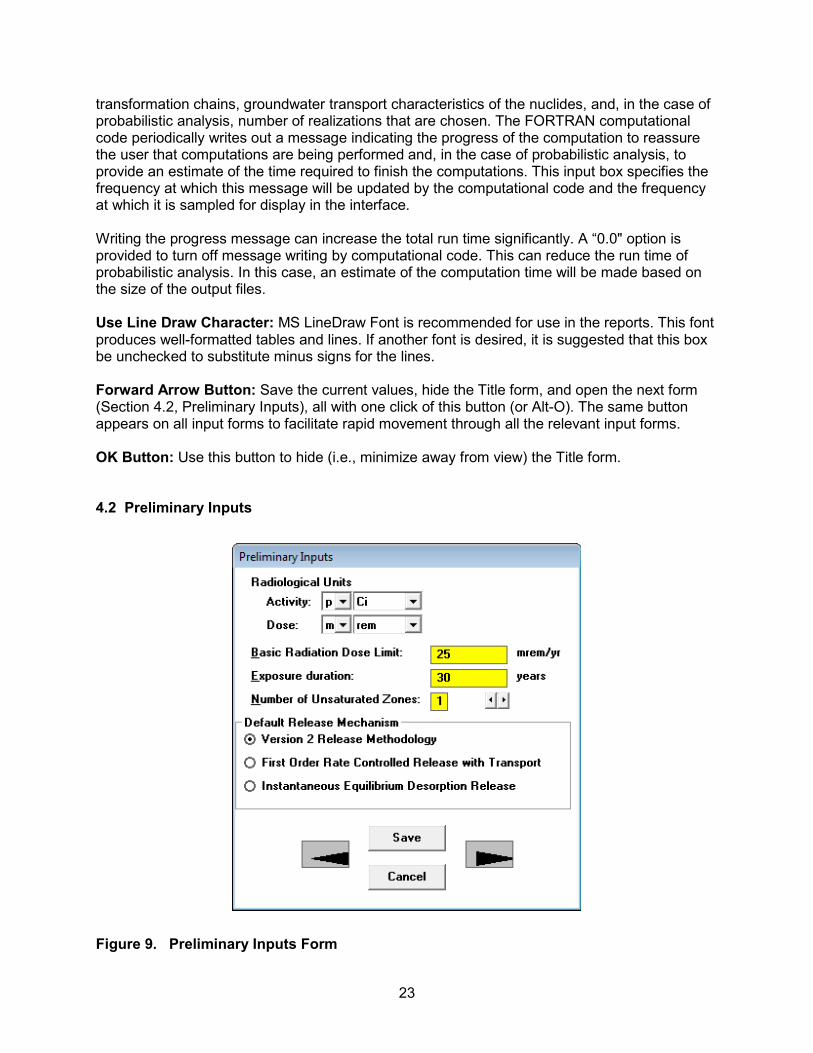
transformation chains, groundwater transport characteristics of the nuclides, and, in the case of probabilistic analysis, number of realizations that are chosen. The FORTRAN computational code periodically writes out a message indicating the progress of the computation to reassure the user that computations are being performed and, in the case of probabilistic analysis, to provide an estimate of the time required to finish the computations. This input box specifies the frequency at which this message will be updated by the computational code and the frequency at which it is sampled for display in the interface. Writing the progress message can increase the total run time significantly. A “0.0" option is provided to turn off message writing by computational code. This can reduce the run time of probabilistic analysis. In this case, an estimate of the computation time will be made based on the size of the output files. Use Line Draw Character: MS LineDraw Font is recommended for use in the reports. This font produces well-formatted tables and lines. If another font is desired, it is suggested that this box be unchecked to substitute minus signs for the lines. Forward Arrow Button: Save the current values, hide the Title form, and open the next form (Section 4.2, Preliminary Inputs), all with one click of this button (or Alt-O). The same button appears on all input forms to facilitate rapid movement through all the relevant input forms. OK Button: Use this button to hide (i.e., minimize away from view) the Title form. 4.2 Preliminary Inputs
Figure 9. Preliminary Inputs Form

24
The preliminary inputs form (Figure 9) allows selection of dose units, the default release mechanism and other parameters that determine the appearance of other input forms. It also contains the two inputs which do not belong in any of the other input forms. None of the parameters in this form are eligible for uncertainty analysis or for one-at-a-time sensitivity analysis. Radiological Units
Activity: The drop-down boxes allow the user to choose the desired unit of •radiological activity. Available choices are curie (Ci), becquerel (Bq), disintegrations per second (dps), and disintegrations per minute (dpm); the first two can be combined with metric prefixes ranging from atto (10-18) through exa (1018).
Dose: The drop-down boxes allow the user to choose the desired unit of •
radiological dose. Available choices are roentgen equivalent man (rem) and sievert (Sv); these can be combined with metric prefixes ranging from atto (10-18) through exa (1018).
Basic Radiation Dose Limit: This is the annual radiation dose limit used to derive all site-specific soil guidelines. Exposure Duration: This is the length of time that the receptor is exposed to radiation at this site. Values reported for risk are time-integrated over this exposure duration. The risk is calculated by using the trapezoidal formula on contaminated intakes computed at all the intermediate time points falling within the exposure duration and at the intermediate time point that is just outside the exposure duration. Dose is time integrated over 1 year or the exposure duration, whichever is less. (Given the current lower bound of 1 year on the exposure duration, dose is currently integrated over a 1-year period.) Number of Unsaturated Zones: This is the number of partially saturated layers between the primary contamination and the saturated zone. The code has provisions for up to five different horizontal strata.
Default Release Mechanism: Two additional release mechanisms were introduced in Version 3.1. These release mechanisms are discussed in Section 4.6. The default mechanism specified in this form when a nuclide is selected for analysis will be used as the release mechanism for that nuclide. Changing the release mechanism for each nuclide after adding all the nuclides is tedious. If a file contains many nuclides it would be more convenient for the user to specify a release mechanism here and then add in the source form all the nuclides that will use the selected release mechanism. Then a different release mechanism can be selected in this form before continuing to add the nuclides that will use the newly selected release mechanism.
25
4.3 Site Layout
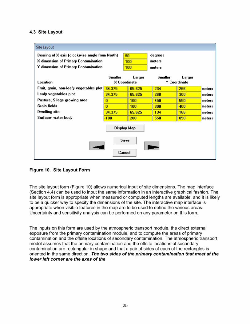
Figure 10. Site Layout Form
The site layout form (Figure 10) allows numerical input of site dimensions. The map interface (Section 4.4) can be used to input the same information in an interactive graphical fashion. The site layout form is appropriate when measured or computed lengths are available, and it is likely to be a quicker way to specify the dimensions of the site. The interactive map interface is appropriate when visible features in the map are to be used to define the various areas. Uncertainty and sensitivity analysis can be performed on any parameter on this form.
The inputs on this form are used by the atmospheric transport module, the direct external exposure from the primary contamination module, and to compute the areas of primary contamination and the offsite locations of secondary contamination. The atmospheric transport model assumes that the primary contamination and the offsite locations of secondary contamination are rectangular in shape and that a pair of sides of each of the rectangles is oriented in the same direction. The two sides of the primary contamination that meet at the lower left corner are the axes of the
26
coordinate system. Each offsite area is defined by the four coordinates as shown in figure 11. These can be thought of as the coordinates of the sides of the offsite area.
Bearing of X-axis: This is the clockwise angle from north to the direction of the positive X-axis.
X Dimension of the Primary Contamination: This is the length of the side of the idealized primary contamination that is parallel to the X-axis, the length of the lower side.
Y Dimension of the Primary Contamination: This is the length of the side of the idealized primary contamination that is parallel to the Y-axis, the length of the left side.
The X Coordinates of an Offsite Area: These are the X coordinates of the two sides that are parallel to the Y-axis. When the save command or one of the form linking arrow commands is issued, the code will compare the two X coordinates of each area and interchange them if the larger value is entered in the column for the smaller value, and vice versa.
The Y Coordinates of an Offsite Area: These are the Y coordinates of the two sides that are parallel to the X-axis. When the save command or one of the form linking arrow commands is issued, the code will compare the two Y coordinates of each area and interchange them if the larger value is entered in the column for the smaller value and vice versa.
All the information that has been entered and saved in the site layout form will be reflected in the display map. Conversely, the position and size that have been set and accepted in the map interface will be reflected in the site layout form.
Figure 11. The coordinate system used in
RESRAD-OFFSITE.
Y axis
X axis
X dimension of primary contamination
Larger Y coordinate of offsite area
(0,0)
Y dimension of primary contamination
Smaller Y coordinate of offsite area
Smaller X coordinate of offsite areaLarger X coordinate of offsite area
27
4.4 Map Interface
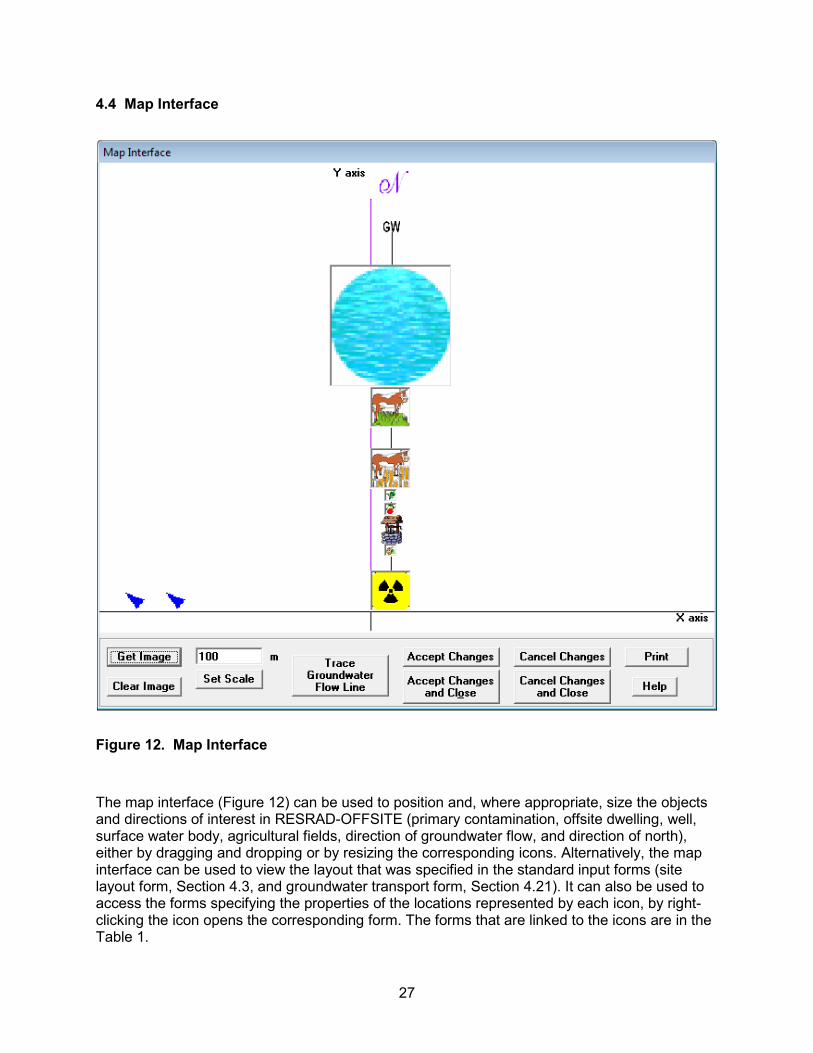
Figure 12. Map Interface
The map interface (Figure 12) can be used to position and, where appropriate, size the objects and directions of interest in RESRAD-OFFSITE (primary contamination, offsite dwelling, well, surface water body, agricultural fields, direction of groundwater flow, and direction of north), either by dragging and dropping or by resizing the corresponding icons. Alternatively, the map interface can be used to view the layout that was specified in the standard input forms (site layout form, Section 4.3, and groundwater transport form, Section 4.21). It can also be used to access the forms specifying the properties of the locations represented by each icon, by right-clicking the icon opens the corresponding form. The forms that are linked to the icons are in the Table 1.
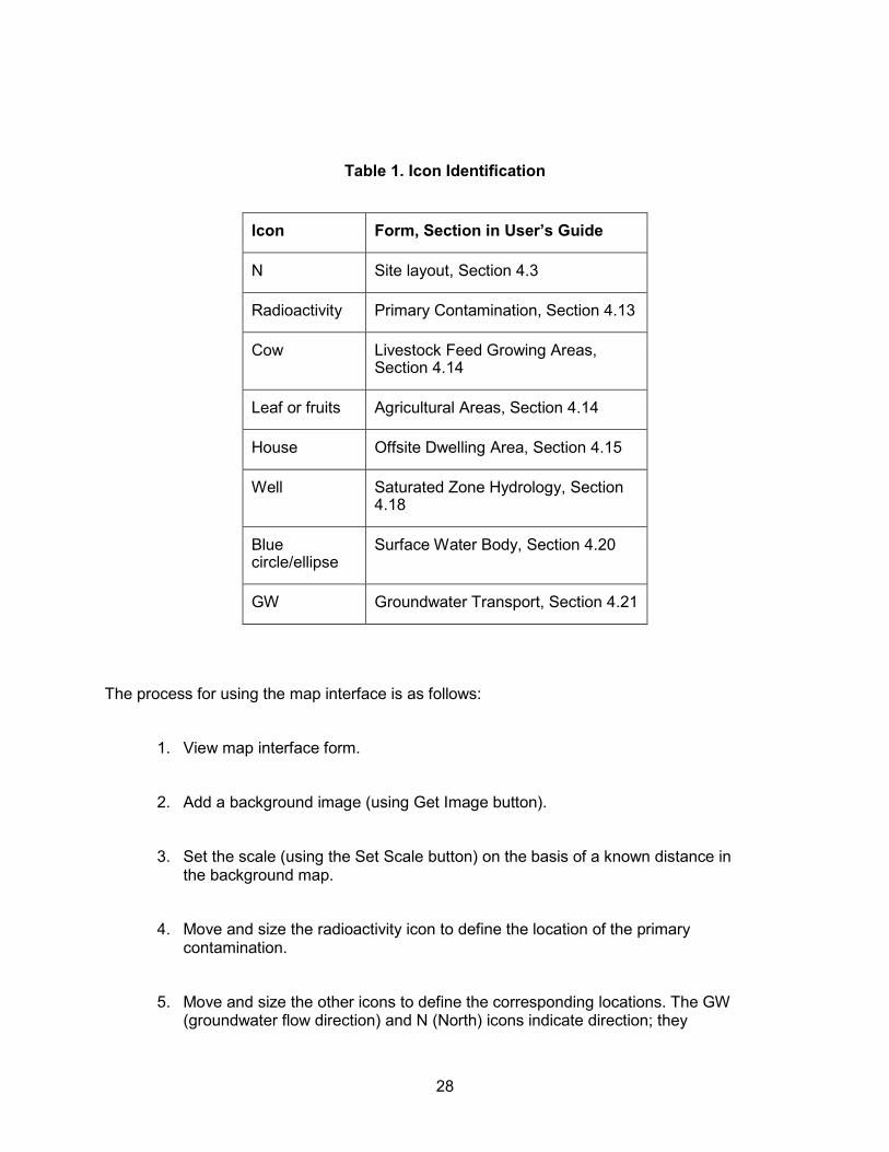
28
Table 1. Icon Identification
Icon Form, Section in User’s Guide
N Site layout, Section 4.3
Radioactivity Primary Contamination, Section 4.13
Cow Livestock Feed Growing Areas, Section 4.14
Leaf or fruits Agricultural Areas, Section 4.14
House Offsite Dwelling Area, Section 4.15
Well Saturated Zone Hydrology, Section 4.18
Blue circle/ellipse
Surface Water Body, Section 4.20
GW Groundwater Transport, Section 4.21
The process for using the map interface is as follows:
1. View map interface form.
2. Add a background image (using Get Image button).
3. Set the scale (using the Set Scale button) on the basis of a known distance in the background map.
4. Move and size the radioactivity icon to define the location of the primary contamination.
5. Move and size the other icons to define the corresponding locations. The GW (groundwater flow direction) and N (North) icons indicate direction; they

29
cannot be resized, because size has no meaning for the direction. The well cannot be resized because the diameter of the well is not an input.
6. Trace the groundwater flow line passing through the center of the primary contamination, if that information is available.
7. Click on the Accept Changes button.
8. The image location, scale, and object locations will be written to the input file when the RESRAD-OFFSITE file is saved. This information is used to display the map image and the icons when the input file is opened at a later time.
Details on Using Map Interface
Steps 2 through 8 are described in greater detail below.
Step 2 (in detail): To get an image, click on the Get Image button and navigate to an image (bitmap, metafile, enhanced metafile, JPEG, or GIF file) of the site that is large enough to contain all the objects of interest and open it.
Click on the Get Image button on the map interface. A file dialog box will pop •up (Figure 13).
Use the file dialog box to navigate to the directory containing the image, •typically the same folder that contains the RESRAD-OFFISTE input files (for example, the highlighted folder, “Userfiles,” in the figure 13).
Double-click the file to be opened (for example, the highlighted file, •“HypotheticalSuburbanResidentGroundwaterFlog.jpg,” in the figure 13).
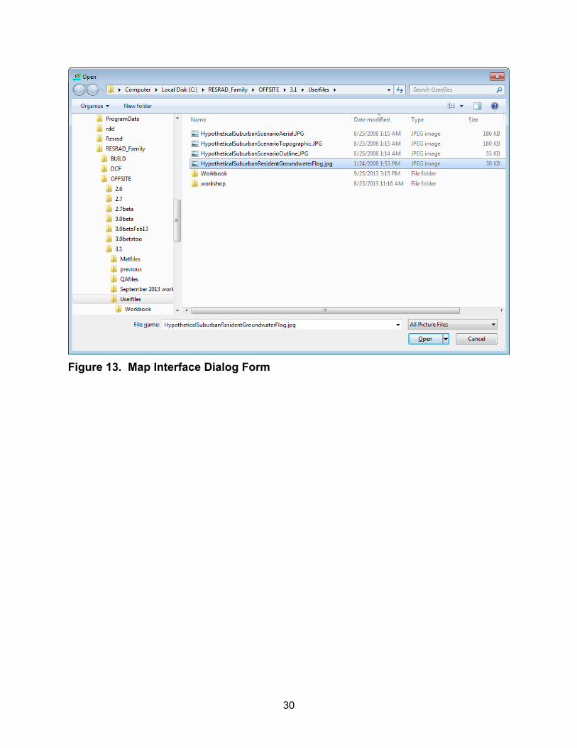
30
Figure 13. Map Interface Dialog Form
31
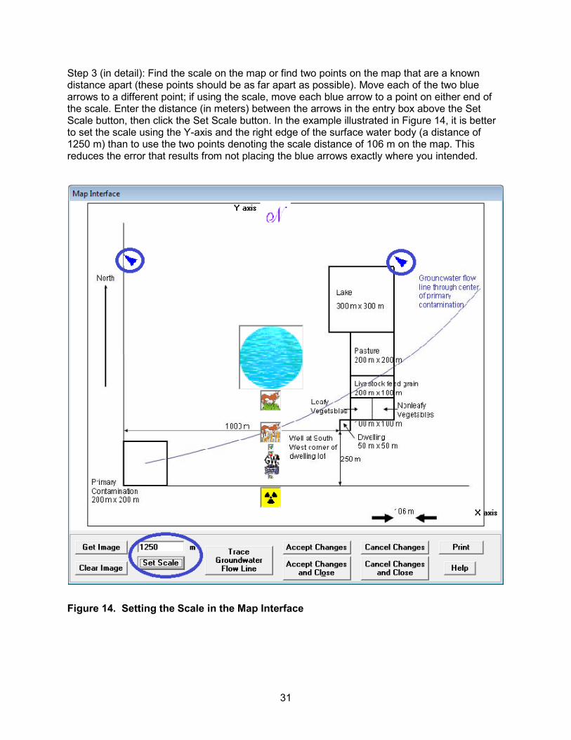
Step 3 (in detail): Find the scale on the map or find two points on the map that are a known distance apart (these points should be as far apart as possible). Move each of the two blue arrows to a different point; if using the scale, move each blue arrow to a point on either end of the scale. Enter the distance (in meters) between the arrows in the entry box above the Set Scale button, then click the Set Scale button. In the example illustrated in Figure 14, it is better to set the scale using the Y-axis and the right edge of the surface water body (a distance of 1250 m) than to use the two points denoting the scale distance of 106 m on the map. This reduces the error that results from not placing the blue arrows exactly where you intended.
Figure 14. Setting the Scale in the Map Interface
32
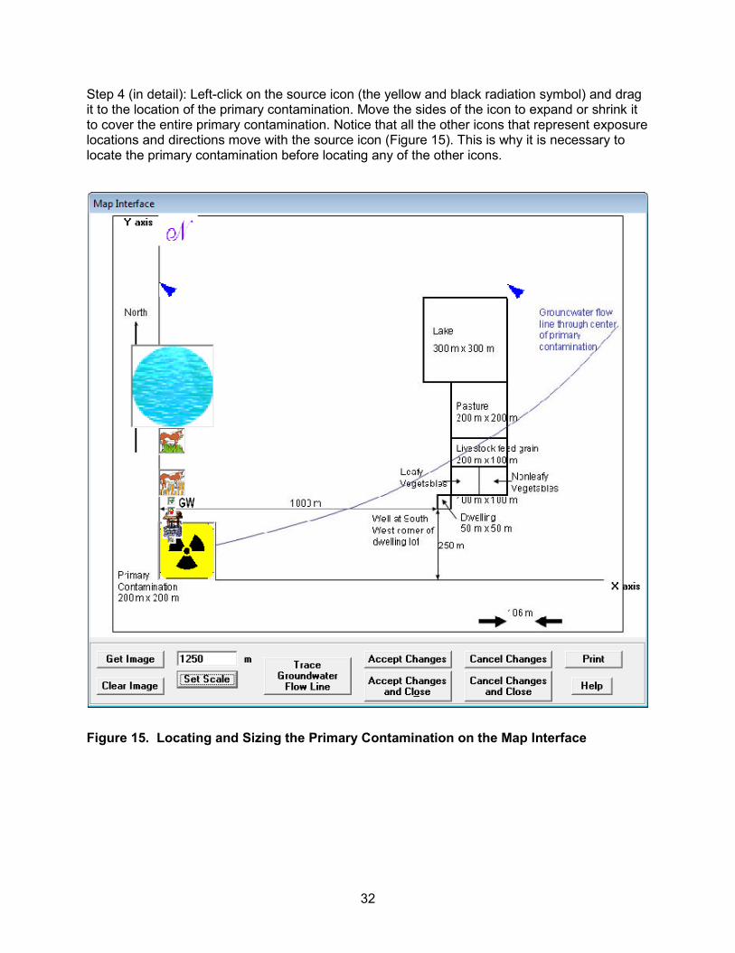
Step 4 (in detail): Left-click on the source icon (the yellow and black radiation symbol) and drag it to the location of the primary contamination. Move the sides of the icon to expand or shrink it to cover the entire primary contamination. Notice that all the other icons that represent exposure locations and directions move with the source icon (Figure 15). This is why it is necessary to locate the primary contamination before locating any of the other icons.
Figure 15. Locating and Sizing the Primary Contamination on the Map Interface
33
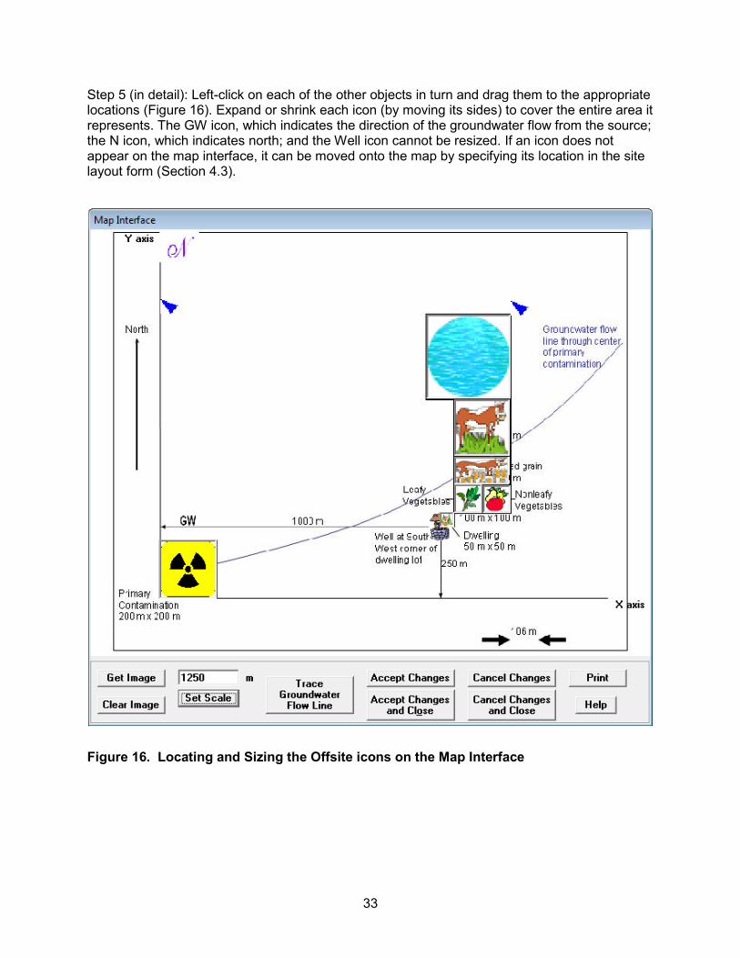
Step 5 (in detail): Left-click on each of the other objects in turn and drag them to the appropriate locations (Figure 16). Expand or shrink each icon (by moving its sides) to cover the entire area it represents. The GW icon, which indicates the direction of the groundwater flow from the source; the N icon, which indicates north; and the Well icon cannot be resized. If an icon does not appear on the map interface, it can be moved onto the map by specifying its location in the site layout form (Section 4.3).
Figure 16. Locating and Sizing the Offsite icons on the Map Interface
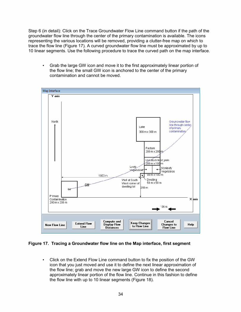
34
Step 6 (in detail): Click on the Trace Groundwater Flow Line command button if the path of the groundwater flow line through the center of the primary contamination is available. The icons representing the various locations will be removed, providing a clutter-free map on which to trace the flow line (Figure 17). A curved groundwater flow line must be approximated by up to 10 linear segments. Use the following procedure to trace the curved path on the map interface.
Grab the large GW icon and move it to the first approximately linear portion of •the flow line; the small GW icon is anchored to the center of the primary contamination and cannot be moved.
Figure 17. Tracing a Groundwater flow line on the Map interface, first segment
Click on the Extend Flow Line command button to fix the position of the GW •icon that you just moved and use it to define the next linear approximation of the flow line; grab and move the new large GW icon to define the second approximately linear portion of the flow line. Continue in this fashion to define the flow line with up to 10 linear segments (Figure 18).
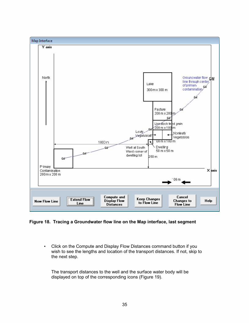
35
Figure 18. Tracing a Groundwater flow line on the Map interface, last segment
Click on the Compute and Display Flow Distances command button if you •wish to see the lengths and location of the transport distances. If not, skip to the next step.
The transport distances to the well and the surface water body will be displayed on top of the corresponding icons (Figure 19).
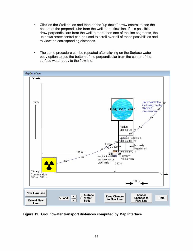
36
Click on the Well option and then on the “up down” arrow control to see the •bottom of the perpendicular from the well to the flow line. If it is possible to draw perpendiculars from the well to more than one of the line segments, the up down arrow control can be used to scroll over all of these possibilities and to view the corresponding distances.
The same procedure can be repeated after clicking on the Surface water •body option to see the bottom of the perpendicular from the center of the surface water body to the flow line.
Figure 19. Groundwater transport distances computed by Map Interface
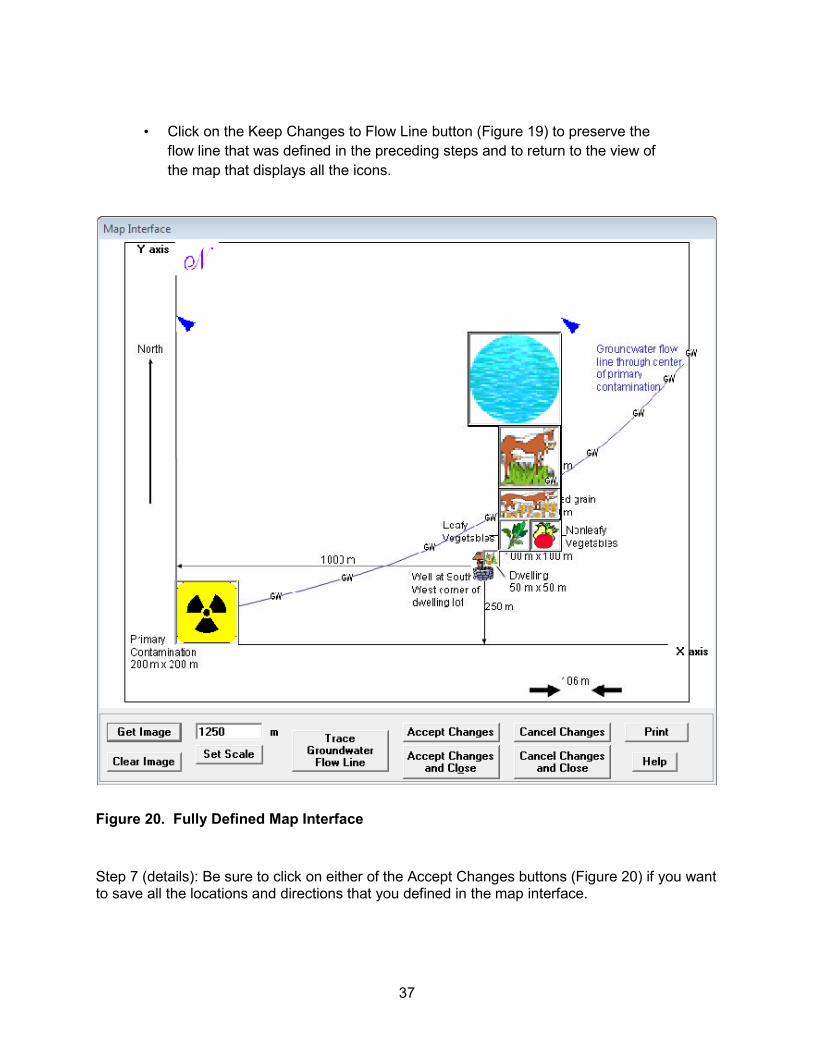
37
Click on the Keep Changes to Flow Line button (Figure 19) to preserve the •flow line that was defined in the preceding steps and to return to the view of the map that displays all the icons.
Figure 20. Fully Defined Map Interface
Step 7 (details): Be sure to click on either of the Accept Changes buttons (Figure 20) if you want to save all the locations and directions that you defined in the map interface.
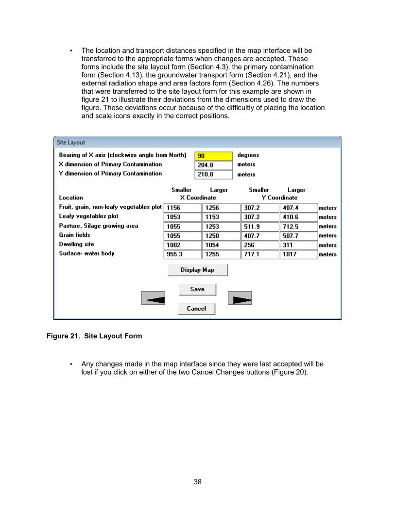
38
The location and transport distances specified in the map interface will be •transferred to the appropriate forms when changes are accepted. These forms include the site layout form (Section 4.3), the primary contamination form (Section 4.13), the groundwater transport form (Section 4.21), and the external radiation shape and area factors form (Section 4.26). The numbers that were transferred to the site layout form for this example are shown in figure 21 to illustrate their deviations from the dimensions used to draw the figure. These deviations occur because of the difficultly of placing the location and scale icons exactly in the correct positions.
Figure 21. Site Layout Form
Any changes made in the map interface since they were last accepted will be •lost if you click on either of the two Cancel Changes buttons (Figure 20).

39
Step 8 (details): The image location, scale, and object locations will be written to the input file when the RESRAD-OFFSITE file is saved. This information is used to display the map image and the icons when the input file is opened at a later time. If the input file is being sent to a different computer, the image files should also be sent in order for it to be displayed on that computer. The Get Image command may need to be used on the receiving computer after opening the input file if the structures and/or the names of the RESRAD-OFFSITE directories are different on the two computers. If the image file is not sent, the image of the map cannot be displayed; however, the icons will be in their specified locations, so the analysis will yield the same results.
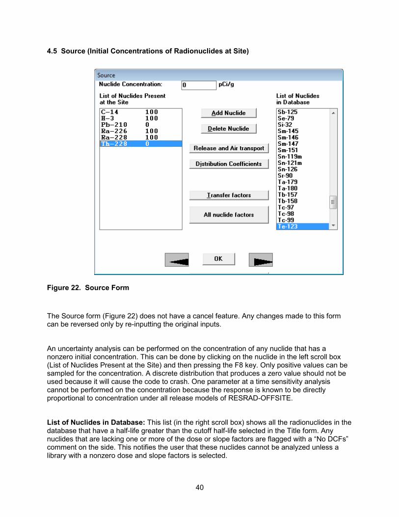
40
4.5 Source (Initial Concentrations of Radionuclides at Site)
Figure 22. Source Form
The Source form (Figure 22) does not have a cancel feature. Any changes made to this form can be reversed only by re-inputting the original inputs.
An uncertainty analysis can be performed on the concentration of any nuclide that has a nonzero initial concentration. This can be done by clicking on the nuclide in the left scroll box (List of Nuclides Present at the Site) and then pressing the F8 key. Only positive values can be sampled for the concentration. A discrete distribution that produces a zero value should not be used because it will cause the code to crash. One parameter at a time sensitivity analysis cannot be performed on the concentration because the response is known to be directly proportional to concentration under all release models of RESRAD-OFFSITE.
List of Nuclides in Database: This list (in the right scroll box) shows all the radionuclides in the database that have a half-life greater than the cutoff half-life selected in the Title form. Any nuclides that are lacking one or more of the dose or slope factors are flagged with a “No DCFs” comment on the side. This notifies the user that these nuclides cannot be analyzed unless a library with a nonzero dose and slope factors is selected.
41
List of Nuclides Present at the Site: This list (in the left scroll box) shows radionuclides that will be explicitly considered in the current analysis. It includes all radionuclides that were specified to be initially present at the site and their principal nuclide progeny (see cutoff half-life in the Title form). Although the fate and transport of any associated radionuclides will not be modeled explicitly, their contributions to dose and risk will be included on the basis of the assumption that they are in secular equilibrium with their principal radionuclide parent.
Add Nuclide: To add a radionuclide, either click on its name in the right scroll box and then click the Add Nuclide button, or just double-click on its name in the right scroll box. The radionuclide will be added to the left scroll box with a concentration specified in the top center input box. All potential decay products will be added to the left scroll box with a default concentration of zero if they are not already present.
Delete Nuclide: To delete a radionuclide, click on its name in the left scroll box and then click on the Delete Nuclide button. All potential decay products that arise only from the deleted radionuclide and have an initial concentration of zero will also be deleted automatically.
Nuclide Concentration: This is the radionuclide concentration averaged over an appropriate depth and area. See Section 3.3 of the RESRAD (onsite) Manual and the RESRAD Data Collection Handbook for more details.
To change the concentration of a radionuclide that is in the left scroll box: •Click on the radionuclide in the left scroll box and type in the concentration.
To change the default concentration when adding new radionuclides: Click on •the right scroll box, then enter the concentration in the top center box. To add radionuclides with this concentration, see above description.
Accessing Other Related Forms
The three command buttons on this form, which are listed below, provide access to the three forms that contain the radionuclide-dependent inputs. Alternatively, the first form can be opened by clicking on the forward arrow button on this form, and then the other two forms can be accessed by continuing to use the forward arrow buttons on the successive forms. If the computer monitor is large enough (17 inches or more diagonally), all of these forms can be viewed simultaneously by clicking on the All Nuclide Factors button. All three forms can also be accessed by double-clicking on the radionuclide name in the left scroll box.
Source Release and Deposition Velocity: Use this button to specify the release mechanism, the parameters of the release mechanism, and the temporal variation of nuclides eligible for release, as well as to specify the deposition velocity of the material with which the nuclide is being transported in the atmosphere. This opens the Source Release and Deposition Velocity

42
form (Section 4.6). As discussed in Appendix A, it is also possible to override the source term module of RESRAD-OFFSITE.
Distribution Coefficients: Use this button to open the Distribution Coefficients form (Section 4.7).
Transfer Factors: Use this button to access the Transfer Factors form (Section 4.8).
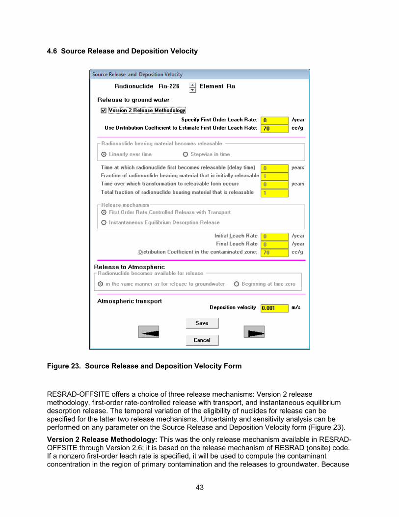
43
4.6 Source Release and Deposition Velocity
Figure 23. Source Release and Deposition Velocity Form
RESRAD-OFFSITE offers a choice of three release mechanisms: Version 2 release methodology, first-order rate-controlled release with transport, and instantaneous equilibrium desorption release. The temporal variation of the eligibility of nuclides for release can be specified for the latter two release mechanisms. Uncertainty and sensitivity analysis can be performed on any parameter on the Source Release and Deposition Velocity form (Figure 23).
Version 2 Release Methodology: This was the only release mechanism available in RESRAD-OFFSITE through Version 2.6; it is based on the release mechanism of RESRAD (onsite) code. If a nonzero first-order leach rate is specified, it will be used to compute the contaminant concentration in the region of primary contamination and the releases to groundwater. Because
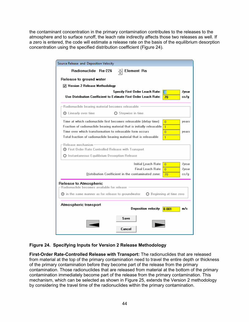
44
the contaminant concentration in the primary contamination contributes to the releases to the atmosphere and to surface runoff, the leach rate indirectly affects those two releases as well. If a zero is entered, the code will estimate a release rate on the basis of the equilibrium desorption concentration using the specified distribution coefficient (Figure 24).
Figure 24. Specifying Inputs for Version 2 Release Methodology
First-Order Rate-Controlled Release with Transport: The radionuclides that are released from material at the top of the primary contamination need to travel the entire depth or thickness of the primary contamination before they become part of the release from the primary contamination. Those radionuclides that are released from material at the bottom of the primary contamination immediately become part of the release from the primary contamination. This mechanism, which can be selected as shown in Figure 25, extends the Version 2 methodology by considering the travel time of the radionuclides within the primary contamination.
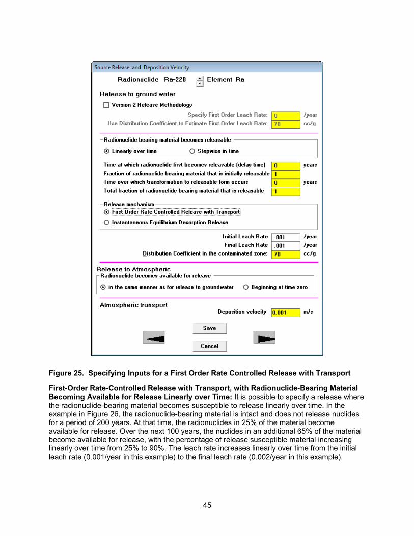
45
Figure 25. Specifying Inputs for a First Order Rate Controlled Release with Transport
First-Order Rate-Controlled Release with Transport, with Radionuclide-Bearing Material Becoming Available for Release Linearly over Time: It is possible to specify a release where the radionuclide-bearing material becomes susceptible to release linearly over time. In the example in Figure 26, the radionuclide-bearing material is intact and does not release nuclides for a period of 200 years. At that time, the radionuclides in 25% of the material become available for release. Over the next 100 years, the nuclides in an additional 65% of the material become available for release, with the percentage of release susceptible material increasing linearly over time from 25% to 90%. The leach rate increases linearly over time from the initial leach rate (0.001/year in this example) to the final leach rate (0.002/year in this example).
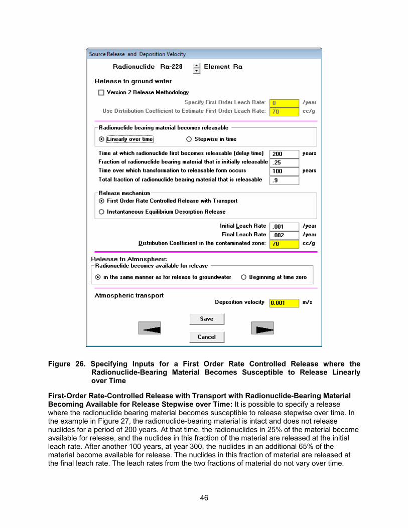
46
Figure 26. Specifying Inputs for a First Order Rate Controlled Release where the
Radionuclide-Bearing Material Becomes Susceptible to Release Linearly over Time
First-Order Rate-Controlled Release with Transport with Radionuclide-Bearing Material Becoming Available for Release Stepwise over Time: It is possible to specify a release where the radionuclide bearing material becomes susceptible to release stepwise over time. In the example in Figure 27, the radionuclide-bearing material is intact and does not release nuclides for a period of 200 years. At that time, the radionuclides in 25% of the material become available for release, and the nuclides in this fraction of the material are released at the initial leach rate. After another 100 years, at year 300, the nuclides in an additional 65% of the material become available for release. The nuclides in this fraction of material are released at the final leach rate. The leach rates from the two fractions of material do not vary over time.
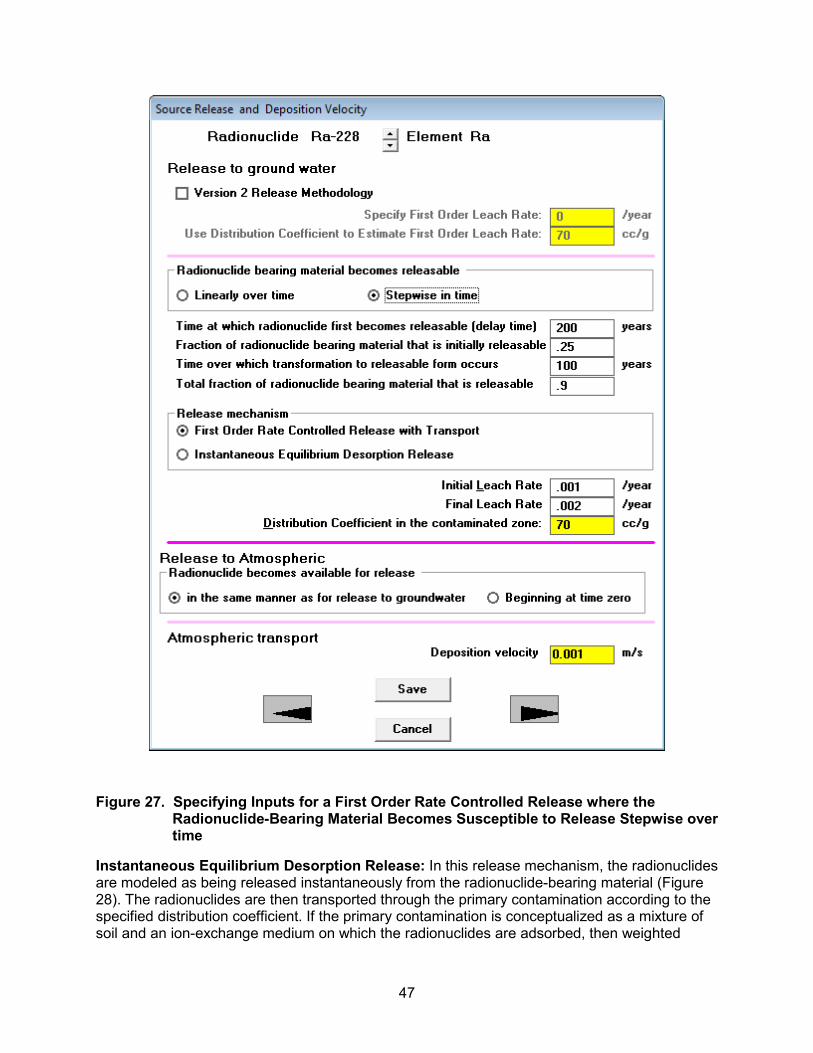
47
Figure 27. Specifying Inputs for a First Order Rate Controlled Release where the
Radionuclide-Bearing Material Becomes Susceptible to Release Stepwise over time
Instantaneous Equilibrium Desorption Release: In this release mechanism, the radionuclides are modeled as being released instantaneously from the radionuclide-bearing material (Figure 28). The radionuclides are then transported through the primary contamination according to the specified distribution coefficient. If the primary contamination is conceptualized as a mixture of soil and an ion-exchange medium on which the radionuclides are adsorbed, then weighted
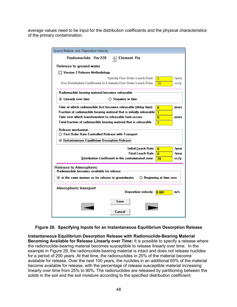
48
average values need to be input for the distribution coefficients and the physical characteristics of the primary contamination.
Figure 28. Specifying Inputs for an Instantaneous Equilibrium Desorption Release
Instantaneous Equilibrium Desorption Release with Radionuclide-Bearing Material Becoming Available for Release Linearly over Time: It is possible to specify a release where the radionuclide-bearing material becomes susceptible to release linearly over time. In the example in Figure 29, the radionuclide-bearing material is intact and does not release nuclides for a period of 200 years. At that time, the radionuclides in 25% of the material become available for release. Over the next 100 years, the nuclides in an additional 65% of the material become available for release, with the percentage of release susceptible material increasing linearly over time from 25% to 90%. The radionuclides are released by partitioning between the solids in the soil and the soil moisture according to the specified distribution coefficient.
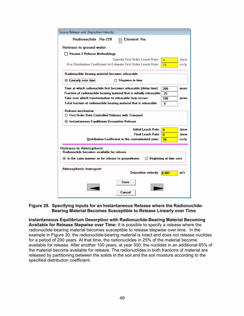
49
Figure 29. Specifying Inputs for an Instantaneous Release where the Radionuclide-
Bearing Material Becomes Susceptible to Release Linearly over Time
Instantaneous Equilibrium Desorption with Radionuclide-Bearing Material Becoming Available for Release Stepwise over Time: It is possible to specify a release where the radionuclide-bearing material becomes susceptible to release stepwise over time. In the example in Figure 30, the radionuclide-bearing material is intact and does not release nuclides for a period of 200 years. At that time, the radionuclides in 25% of the material become available for release. After another 100 years, at year 300, the nuclides in an additional 65% of the material become available for release. The radionuclides in both fractions of material are released by partitioning between the solids in the soil and the soil moisture according to the specified distribution coefficient.
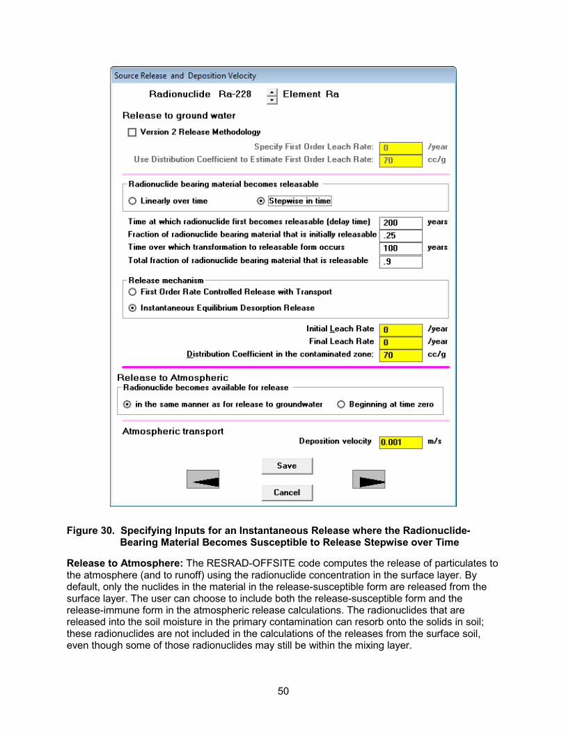
50
Figure 30. Specifying Inputs for an Instantaneous Release where the Radionuclide-Bearing Material Becomes Susceptible to Release Stepwise over Time
Release to Atmosphere: The RESRAD-OFFSITE code computes the release of particulates to the atmosphere (and to runoff) using the radionuclide concentration in the surface layer. By default, only the nuclides in the material in the release-susceptible form are released from the surface layer. The user can choose to include both the release-susceptible form and the release-immune form in the atmospheric release calculations. The radionuclides that are released into the soil moisture in the primary contamination can resorb onto the solids in soil; these radionuclides are not included in the calculations of the releases from the surface soil, even though some of those radionuclides may still be within the mixing layer.

51
Deposition Velocity: The deposition velocity of the material with which the nuclide is being transported is used by the code to account for loss from dry deposition along the atmospheric transport path and to compute the deposition flux at the offsite locations.
Click on the up or down arrow next to the radionuclide name to save the inputs for the currently displayed radionuclide and to view the inputs for the next or previous radionuclide.
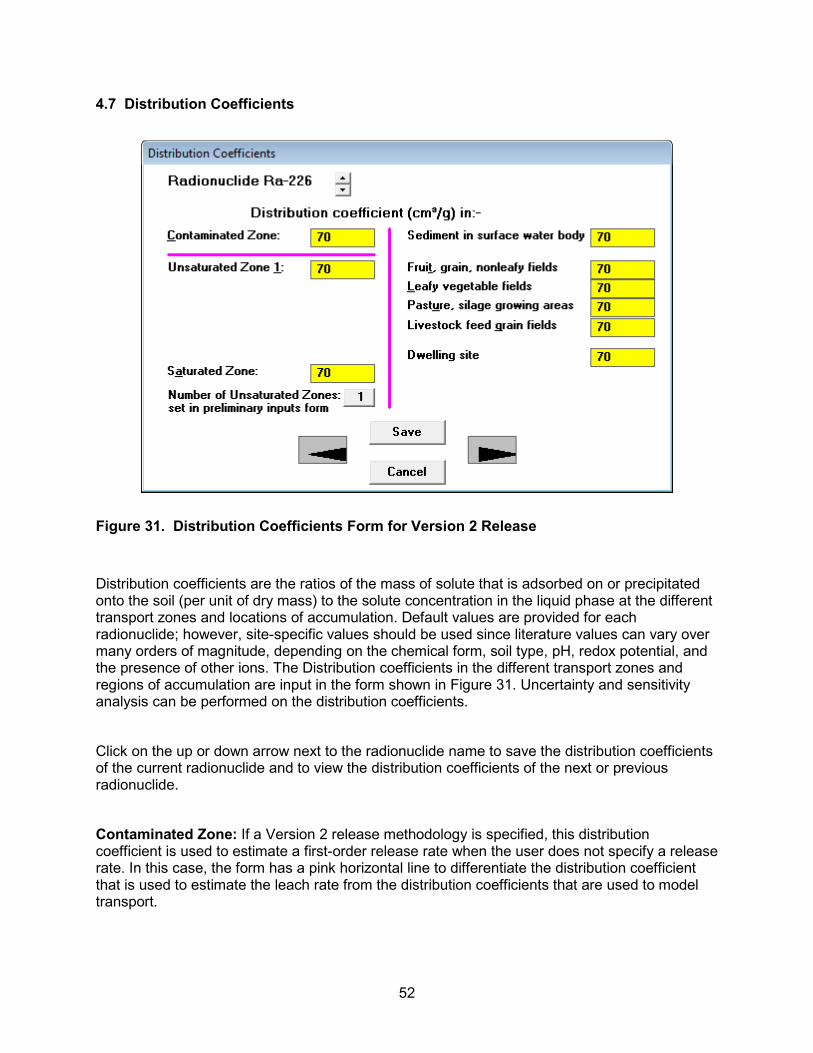
52
4.7 Distribution Coefficients
Figure 31. Distribution Coefficients Form for Version 2 Release
Distribution coefficients are the ratios of the mass of solute that is adsorbed on or precipitated onto the soil (per unit of dry mass) to the solute concentration in the liquid phase at the different transport zones and locations of accumulation. Default values are provided for each radionuclide; however, site-specific values should be used since literature values can vary over many orders of magnitude, depending on the chemical form, soil type, pH, redox potential, and the presence of other ions. The Distribution coefficients in the different transport zones and regions of accumulation are input in the form shown in Figure 31. Uncertainty and sensitivity analysis can be performed on the distribution coefficients.
Click on the up or down arrow next to the radionuclide name to save the distribution coefficients of the current radionuclide and to view the distribution coefficients of the next or previous radionuclide.
Contaminated Zone: If a Version 2 release methodology is specified, this distribution coefficient is used to estimate a first-order release rate when the user does not specify a release rate. In this case, the form has a pink horizontal line to differentiate the distribution coefficient that is used to estimate the leach rate from the distribution coefficients that are used to model transport.
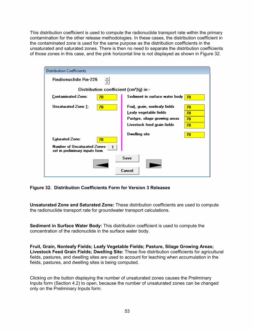
53
This distribution coefficient is used to compute the radionuclide transport rate within the primary contamination for the other release methodologies. In these cases, the distribution coefficient in the contaminated zone is used for the same purpose as the distribution coefficients in the unsaturated and saturated zones. There is then no need to separate the distribution coefficients of those zones in this case, and the pink horizontal line is not displayed as shown in Figure 32.
Figure 32. Distribution Coefficients Form for Version 3 Releases
Unsaturated Zone and Saturated Zone: These distribution coefficients are used to compute the radionuclide transport rate for groundwater transport calculations.
Sediment in Surface Water Body: This distribution coefficient is used to compute the concentration of the radionuclide in the surface water body.
Fruit, Grain, Nonleafy Fields; Leafy Vegetable Fields; Pasture, Silage Growing Areas; Livestock Feed Grain Fields; Dwelling Site: These five distribution coefficients for agricultural fields, pastures, and dwelling sites are used to account for leaching when accumulation in the fields, pastures, and dwelling sites is being computed.
Clicking on the button displaying the number of unsaturated zones causes the Preliminary Inputs form (Section 4.2) to open, because the number of unsaturated zones can be changed only on the Preliminary Inputs form.
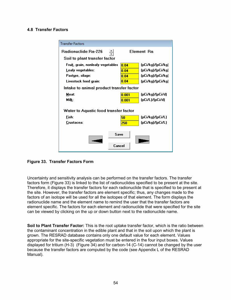
54
4.8 Transfer Factors
Figure 33. Transfer Factors Form
Uncertainty and sensitivity analysis can be performed on the transfer factors. The transfer factors form (Figure 33) is linked to the list of radionuclides specified to be present at the site. Therefore, it displays the transfer factors for each radionuclide that is specified to be present at the site. However, the transfer factors are element specific; thus, any changes made to the factors of an isotope will be used for all the isotopes of that element. The form displays the radionuclide name and the element name to remind the user that the transfer factors are element specific. The factors for each element and radionuclide that were specified for the site can be viewed by clicking on the up or down button next to the radionuclide name.
Soil to Plant Transfer Factor: This is the root uptake transfer factor, which is the ratio between the contaminant concentration in the edible plant and that in the soil upon which the plant is grown. The RESRAD database contains only one default value for each element. Values appropriate for the site-specific vegetation must be entered in the four input boxes. Values displayed for tritium (H-3) (Figure 34) and for carbon-14 (C-14) cannot be changed by the user because the transfer factors are computed by the code (see Appendix L of the RESRAD Manual).
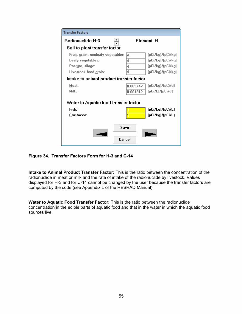
55
Figure 34. Transfer Factors Form for H-3 and C-14
Intake to Animal Product Transfer Factor: This is the ratio between the concentration of the radionuclide in meat or milk and the rate of intake of the radionuclide by livestock. Values displayed for H-3 and for C-14 cannot be changed by the user because the transfer factors are computed by the code (see Appendix L of the RESRAD Manual).
Water to Aquatic Food Transfer Factor: This is the ratio between the radionuclide concentration in the edible parts of aquatic food and that in the water in which the aquatic food sources live.
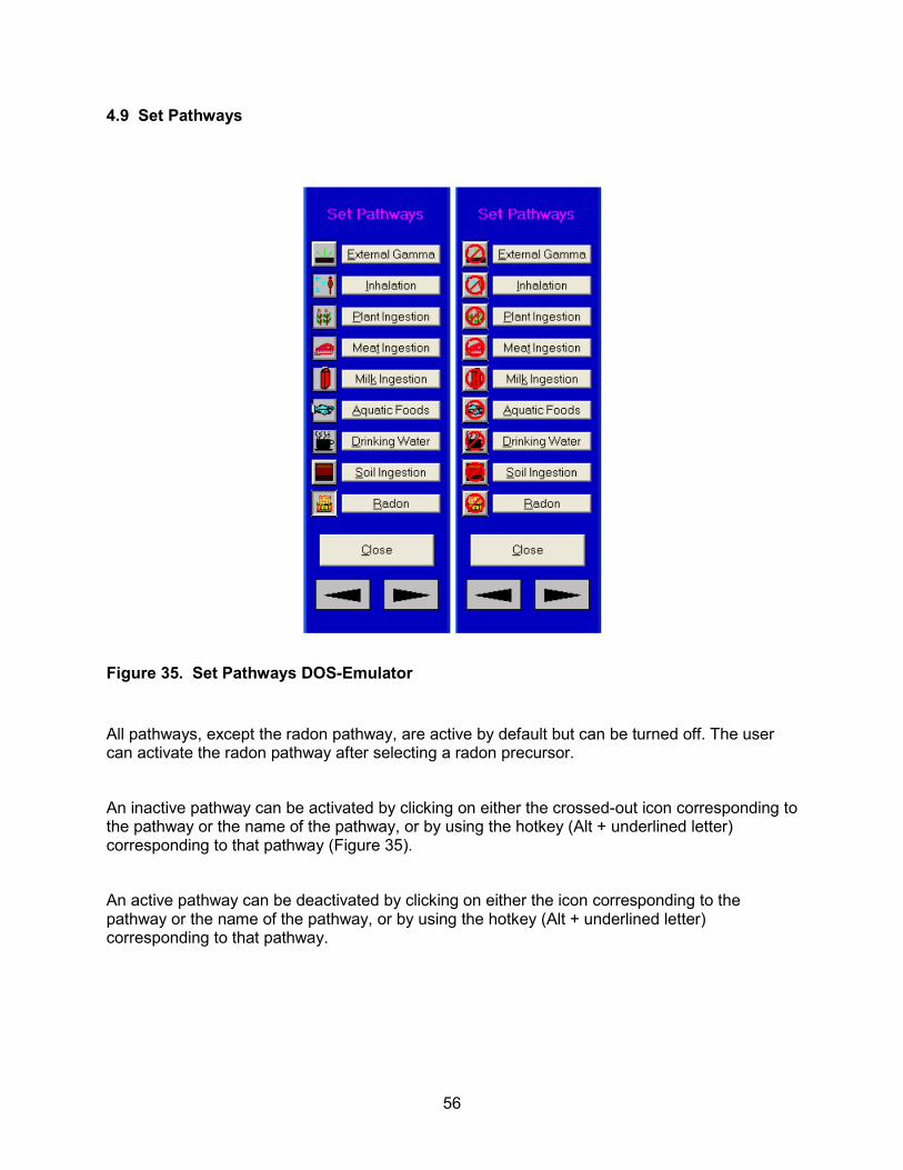
56
4.9 Set Pathways
Figure 35. Set Pathways DOS-Emulator
All pathways, except the radon pathway, are active by default but can be turned off. The user can activate the radon pathway after selecting a radon precursor.
An inactive pathway can be activated by clicking on either the crossed-out icon corresponding to the pathway or the name of the pathway, or by using the hotkey (Alt + underlined letter) corresponding to that pathway (Figure 35).
An active pathway can be deactivated by clicking on either the icon corresponding to the pathway or the name of the pathway, or by using the hotkey (Alt + underlined letter) corresponding to that pathway.
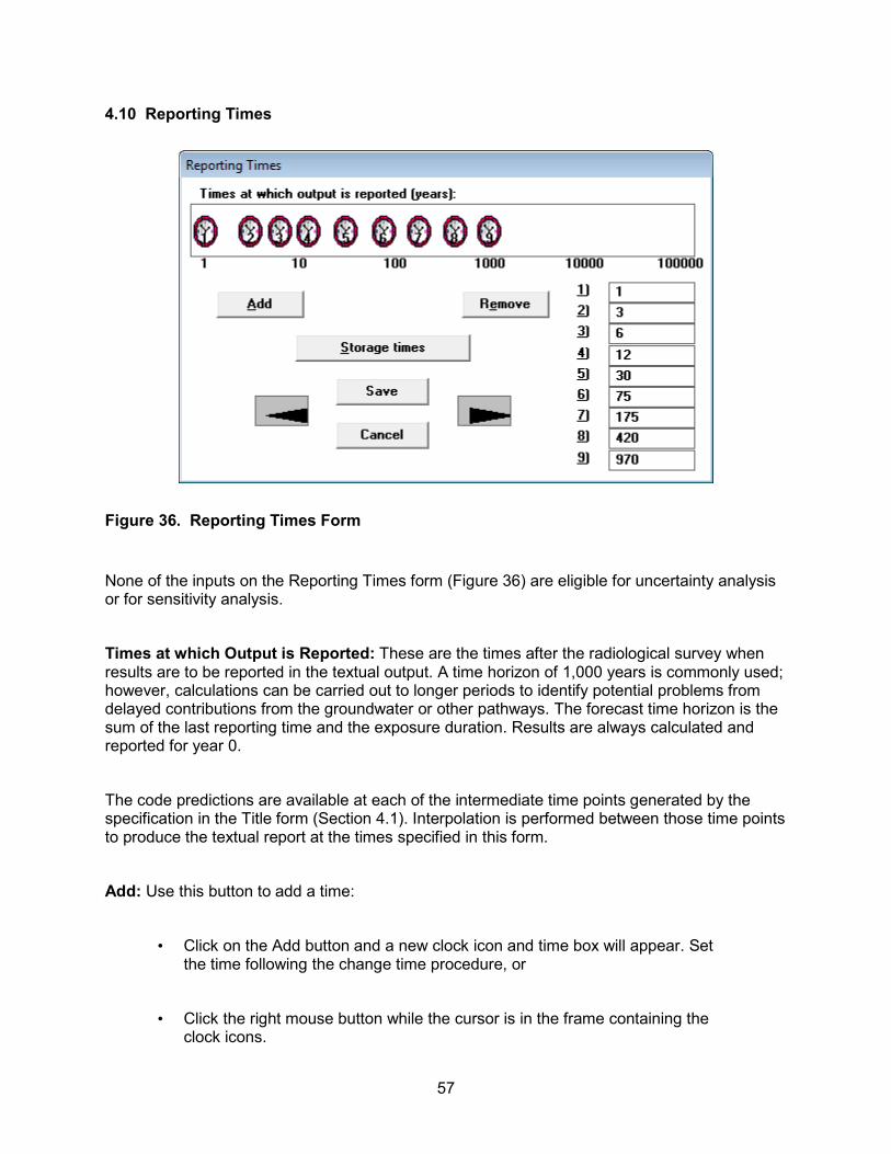
57
4.10 Reporting Times
Figure 36. Reporting Times Form
None of the inputs on the Reporting Times form (Figure 36) are eligible for uncertainty analysis or for sensitivity analysis.
Times at which Output is Reported: These are the times after the radiological survey when results are to be reported in the textual output. A time horizon of 1,000 years is commonly used; however, calculations can be carried out to longer periods to identify potential problems from delayed contributions from the groundwater or other pathways. The forecast time horizon is the sum of the last reporting time and the exposure duration. Results are always calculated and reported for year 0.
The code predictions are available at each of the intermediate time points generated by the specification in the Title form (Section 4.1). Interpolation is performed between those time points to produce the textual report at the times specified in this form.
Add: Use this button to add a time:
Click on the Add button and a new clock icon and time box will appear. Set •the time following the change time procedure, or
Click the right mouse button while the cursor is in the frame containing the •clock icons.

58
Remove: Use this button to remove a time:
Click on the appropriate time box or clock icon, then click on the Remove •button.
To change a time:
Click on the appropriate time box and enter new value, or •
Click on the appropriate clock icon and drag to desired time location. •
Storage Times: The Storage Times form can be assessed by clicking on this button. The Storage Times form is the next linked form, so the forward arrow can also be used to get to it.
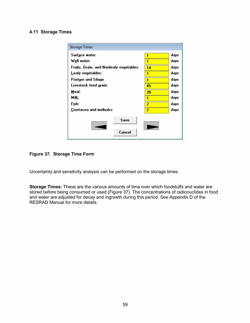
59
4.11 Storage Times
Figure 37. Storage Time Form
Uncertainty and sensitivity analysis can be performed on the storage times.
Storage Times: These are the various amounts of time over which foodstuffs and water are stored before being consumed or used (Figure 37). The concentrations of radionuclides in food and water are adjusted for decay and ingrowth during this period. See Appendix D of the RESRAD Manual for more details.
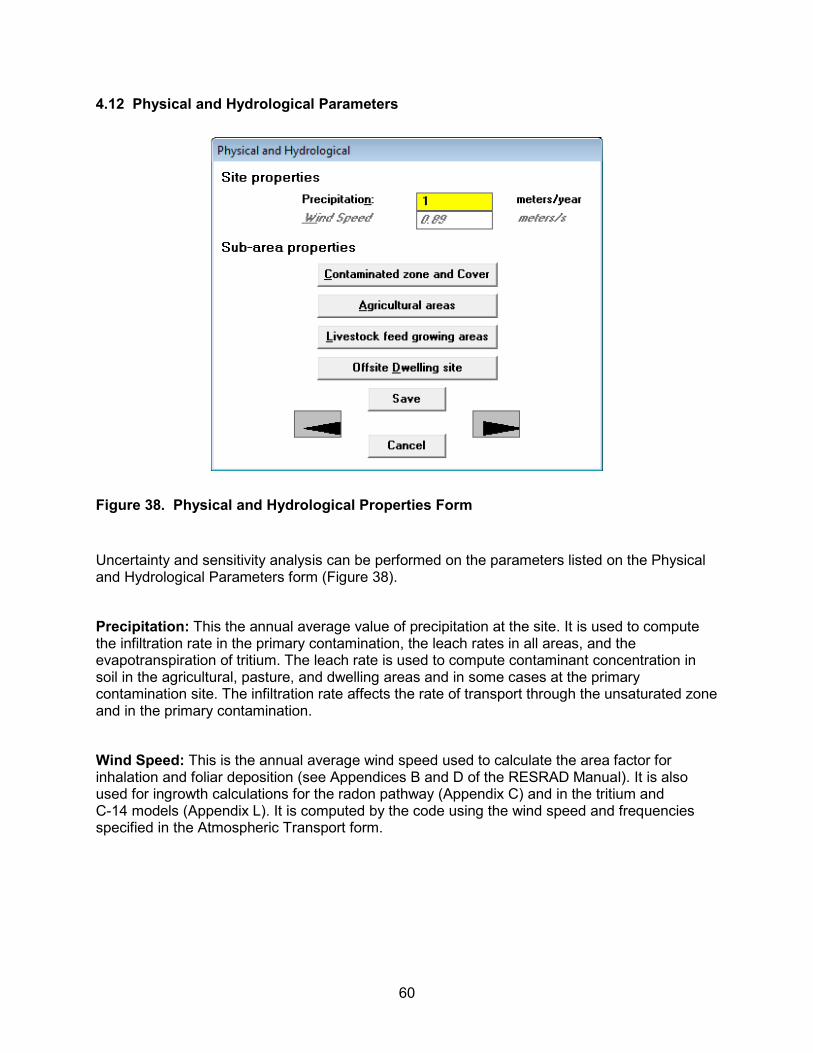
60
4.12 Physical and Hydrological Parameters
Figure 38. Physical and Hydrological Properties Form
Uncertainty and sensitivity analysis can be performed on the parameters listed on the Physical and Hydrological Parameters form (Figure 38).
Precipitation: This the annual average value of precipitation at the site. It is used to compute the infiltration rate in the primary contamination, the leach rates in all areas, and the evapotranspiration of tritium. The leach rate is used to compute contaminant concentration in soil in the agricultural, pasture, and dwelling areas and in some cases at the primary contamination site. The infiltration rate affects the rate of transport through the unsaturated zone and in the primary contamination.
Wind Speed: This is the annual average wind speed used to calculate the area factor for inhalation and foliar deposition (see Appendices B and D of the RESRAD Manual). It is also used for ingrowth calculations for the radon pathway (Appendix C) and in the tritium and C-14 models (Appendix L). It is computed by the code using the wind speed and frequencies specified in the Atmospheric Transport form.

61
Accessing Other Related Forms
The four command buttons on this form (Figure 38), Contaminated Zone and Cover, Agricultural Areas, Livestock Feed Growing Areas, and Offsite Dwelling Site, provide access to the four forms that provide physical and hydrological data on four subarea properties (see Sections 4.13, 4.14, and 4.15). Clicking on any of these four buttons opens the respective form. The current parent form will not be closed and will remain in the background, and it will appear again when the other form is exited. Alternatively, the first form can be opened by clicking on the forward arrow button on this form; the other three forms can be accessed by continuing to use the forward arrow buttons on the successive forms.
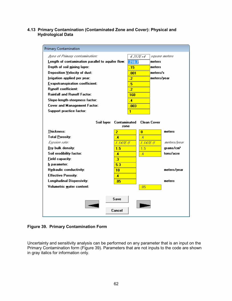
62
4.13 Primary Contamination (Contaminated Zone and Cover): Physical and Hydrological Data
Figure 39. Primary Contamination Form
Uncertainty and sensitivity analysis can be performed on any parameter that is an input on the Primary Contamination form (Figure 39). Parameters that are not inputs to the code are shown in gray italics for information only.
63
Area of Primary Contamination: This is not a direct input; it is computed using the information input in the Site Layout form. The primary contamination is a compact area that contains the locations of all soil samples with radionuclide concentrations that are clearly (i.e., two standard deviations) above background.
Length of Contamination Parallel to Aquifer Flow: This is the distance between two parallel lines that are perpendicular to the direction of the aquifer flow: one at the up-gradient edge of the contaminated zone, and the other at the down-gradient edge. It is used in groundwater transport calculations. The code computes this value from the information input in the map interface. The user can change the value computed by the code. The connection between this form and the map interface is one-directional; the information entered in this form will not affect the map interface.
Depth of Soil Mixing Layer: This is the thickness of the surface soil at the location of the primary contamination, which may be assumed to be mixed uniformly from time to time as a result of anthropogenic or physical processes. It is used to calculate the concentration of contaminants in surface soil.
Deposition Velocity of Dust: This is the representative deposition velocity of dust at the location of primary contamination. It is used to compute the release to the atmosphere on the basis of the assumption that there is no net deposition of particulates at the site.
The next three inputs and the precipitation rate are used to compute the infiltration rate and to compute the evapotranspiration of tritium from the primary contamination. They affect all releases from the primary contamination as well as the transport rate through the unsaturated layers.
Irrigation Applied per Year: This is the volume of irrigation water that is applied over a period of 1 year per unit area of land. It is not the actual rate of irrigation during the growing season; instead, it is the irrigation rate averaged over 1 year.
Evapotranspiration Coefficient: This is the fraction of precipitation and irrigation water that penetrates the topsoil, which is lost to the atmosphere by evaporation and by transpiration by vegetation.
Runoff Coefficient: This is the fraction of precipitation that does not penetrate the topsoil, and instead leaves the area of concern as surface runoff; no loss is assumed for irrigation water.
The next six inputs are used to compute the rate of erosion. Erosion Rate is not an input in RESRAD-OFFSITE; it is displayed for the information of users.

64
Rainfall and Runoff Index: This is a measure of the energy of the rainfall. It is used to compute the erosion rate.
Slope-Length-Steepness Factor: This factor accounts for the effect the profile of the terrain has on the erosion rate.
Cover and Management Factor: This factor (formerly called the Cropping-Management Factor) accounts for the effects land use, vegetation, and management have on the erosion rate.
Support Practice Factor: This factor (formerly called the Conservation Practice Factor) accounts for the effects conservation practices have on the erosion rate.
Dry Bulk Density (of Soil in the Contaminated Zone and in Clean Cover): This is the mass of (dry) solids in a unit volume of soil in the respective layers of soil. In addition to being used to compute the erosion rate, this is also used to compute the exposure to external radiation. The density in the contaminated zone is also used to compute the release to groundwater, and thus the concentration in the primary contamination.
Soil Erodibility Factor: This is a measure of the susceptibility of the soil to erosion.
Thickness (of Contaminated Zone): This is the distance (in meters [m]), between the uppermost and lowermost soil samples with radionuclide concentrations that are clearly (i.e., two standard deviations) above background.
Thickness (of Clean Cover): This is the distance from the ground surface to the location of the uppermost soil sample with radionuclide concentrations that are clearly above background.
Total Porosity (of Contaminated Zone and Clean Cover): This is the fraction of soil (by volume) that is occupied by liquid and gaseous phases in the respective layers.
Field Capacity (of Contaminated Zone): This is the volumetric moisture content of soil at which (free) gravity drainage ceases. This is the amount of moisture that will be retained in a column of soil against the force of gravity.
b Parameter (of Contaminated Zone): The soil-specific exponential b parameter relates the hydraulic conductivity of partially saturated soil to its moisture content.

65
Hydraulic Conductivity (of Contaminated Zone): This is the apparent flow velocity through the contaminated zone under a unit hydraulic gradient.
Effective Porosity: This is the fraction of soil (by volume) through which water flows. Part of the soil moisture may not contribute to the movement of contaminants. Therefore, the effective porosity will be less than or equal to the total porosity.
Longitudinal Dispersivity: This is the ratio between the longitudinal dispersion coefficient and pore water velocity. It has the dimension of length. This parameter depends on the thickness of the zone and ranges from one one-hundredth of the thickness to the order of the thickness.
Volumetric Water Content (of Clean Cover): This is the fraction of soil (by volume) that is occupied by water.
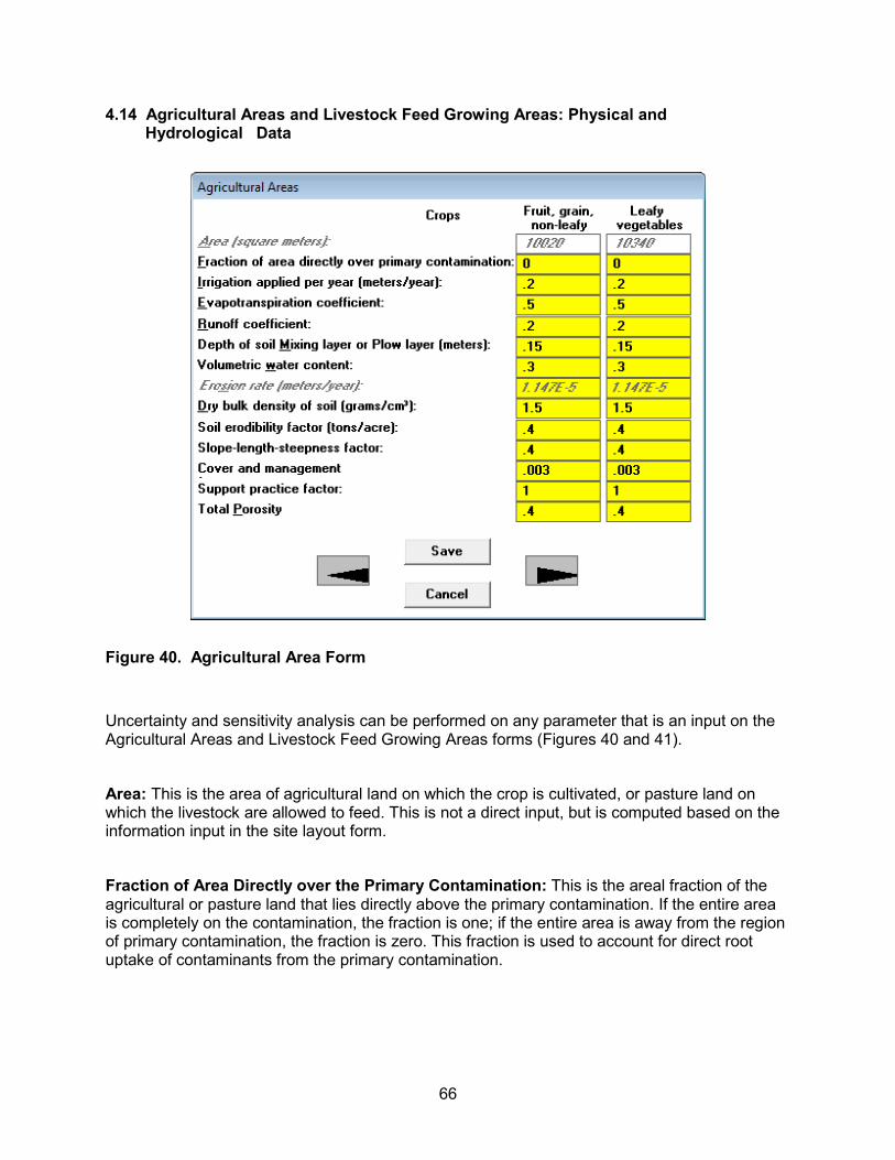
66
4.14 Agricultural Areas and Livestock Feed Growing Areas: Physical and Hydrological Data
Figure 40. Agricultural Area Form
Uncertainty and sensitivity analysis can be performed on any parameter that is an input on the Agricultural Areas and Livestock Feed Growing Areas forms (Figures 40 and 41).
Area: This is the area of agricultural land on which the crop is cultivated, or pasture land on which the livestock are allowed to feed. This is not a direct input, but is computed based on the information input in the site layout form.
Fraction of Area Directly over the Primary Contamination: This is the areal fraction of the agricultural or pasture land that lies directly above the primary contamination. If the entire area is completely on the contamination, the fraction is one; if the entire area is away from the region of primary contamination, the fraction is zero. This fraction is used to account for direct root uptake of contaminants from the primary contamination.
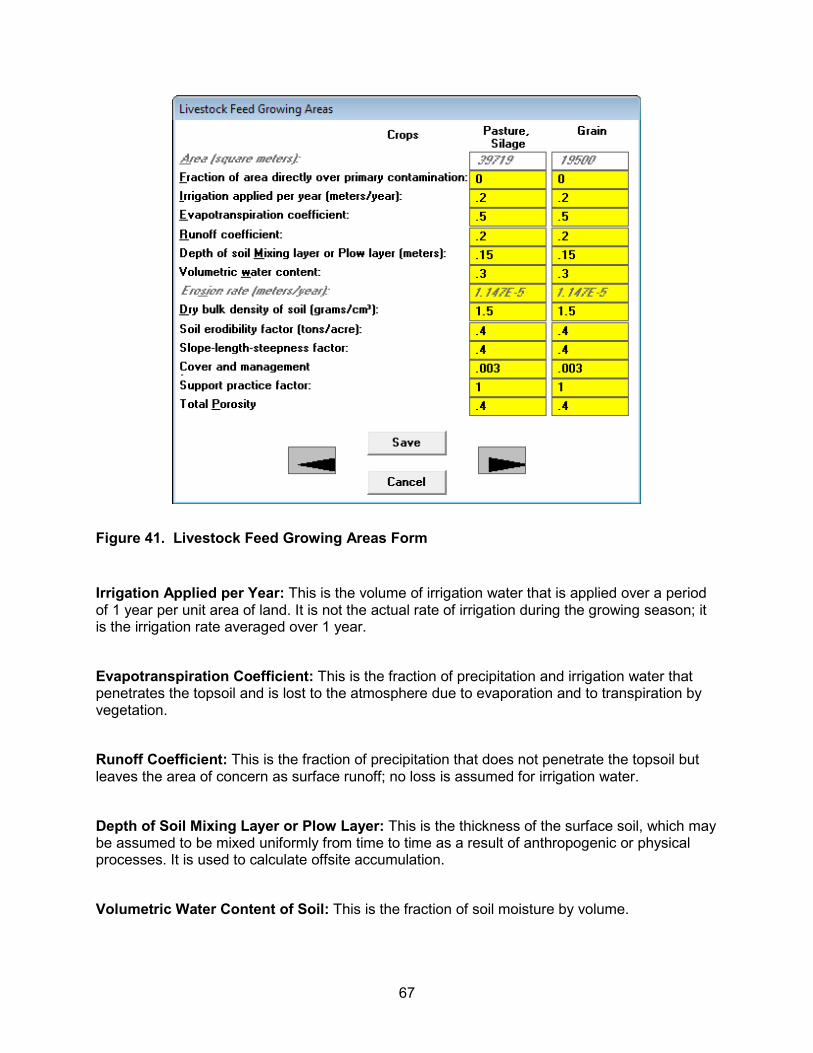
67
Figure 41. Livestock Feed Growing Areas Form
Irrigation Applied per Year: This is the volume of irrigation water that is applied over a period of 1 year per unit area of land. It is not the actual rate of irrigation during the growing season; it is the irrigation rate averaged over 1 year.
Evapotranspiration Coefficient: This is the fraction of precipitation and irrigation water that penetrates the topsoil and is lost to the atmosphere due to evaporation and to transpiration by vegetation.
Runoff Coefficient: This is the fraction of precipitation that does not penetrate the topsoil but leaves the area of concern as surface runoff; no loss is assumed for irrigation water.
Depth of Soil Mixing Layer or Plow Layer: This is the thickness of the surface soil, which may be assumed to be mixed uniformly from time to time as a result of anthropogenic or physical processes. It is used to calculate offsite accumulation.
Volumetric Water Content of Soil: This is the fraction of soil moisture by volume.

68
Dry Bulk Density of Soil: This is the mass of solids in a unit volume of soil.
Soil Erodibility Factor: This is a measure of the susceptibility of the soil to erosion.
Slope-Length-Steepness Factor: This factor accounts for the effect the profile of the terrain has on the erosion rate.
Cover and Management Factor: This factor (formerly called the Cropping-Management Factor) accounts for the effects land use, vegetation, and management have on the erosion rate.
Support Practice Factor: This factor (formerly called the Conservation Practice Factor) accounts for the effects conservation practices have on the erosion rate.
Total Porosity: This is the fraction of soil (by volume) that is occupied by liquid and gaseous phases.
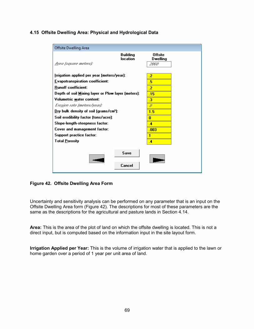
69
4.15 Offsite Dwelling Area: Physical and Hydrological Data
Figure 42. Offsite Dwelling Area Form
Uncertainty and sensitivity analysis can be performed on any parameter that is an input on the Offsite Dwelling Area form (Figure 42). The descriptions for most of these parameters are the same as the descriptions for the agricultural and pasture lands in Section 4.14.
Area: This is the area of the plot of land on which the offsite dwelling is located. This is not a direct input, but is computed based on the information input in the site layout form.
Irrigation Applied per Year: This is the volume of irrigation water that is applied to the lawn or home garden over a period of 1 year per unit area of land.
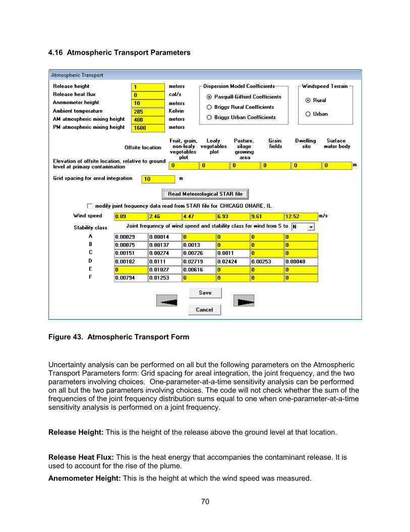
70
4.16 Atmospheric Transport Parameters
Figure 43. Atmospheric Transport Form
Uncertainty analysis can be performed on all but the following parameters on the Atmospheric Transport Parameters form: Grid spacing for areal integration, the joint frequency, and the two parameters involving choices. One-parameter-at-a-time sensitivity analysis can be performed on all but the two parameters involving choices. The code will not check whether the sum of the frequencies of the joint frequency distribution sums equal to one when one-parameter-at-a-time sensitivity analysis is performed on a joint frequency.
Release Height: This is the height of the release above the ground level at that location.
Release Heat Flux: This is the heat energy that accompanies the contaminant release. It is used to account for the rise of the plume.
Anemometer Height: This is the height at which the wind speed was measured.
71
Ambient Temperature: This is the temperature of the air at the location of release.
AM and PM Atmospheric Mixing Heights: The atmospheric mixing height is the thickness of the layer of air that is bounded by the ground surface and a layer of stable air above it. The spreading of the contaminants is limited to the thickness of the mixing layer. AM and PM refer to the portion of the day during which the measurement was taken.
Dispersion Model Coefficients: This is the formulation used to generate the dispersion coefficients for the atmospheric transport model.
Wind Speed Terrain: The choice of terrain determines the relationship between the wind speed and the elevation above the ground surface.
Elevation of Offsite Location, relative to the Ground Level at Primary Contamination: When the ground level at the offsite location is above the ground level at the site of primary contamination, the code adjusts for the upward deflection of the wind. It is the difference in the height of the ground surface at the offsite location of contaminant accumulation and the height of the ground surface at the site of primary contamination.
Grid Spacing for Areal Integration: The primary contamination and the offsite receptor areas are assumed to be rectangular in shape (as defined in Section 4.3), when modeling the atmospheric transport. Rather than use a single transport distance from the center of the source to the center of the receptor, the code provides the option to subdivide the source and receptor areas into smaller squares or rectangles. The transport from each subdivision of the source to each subdivision of the offsite receptor area is computed and summed together to produce a better estimate of the atmospheric transport. Smaller grid spacings improve the accuracy of the calculations, but they require a longer computation time. This input is the maximum dimension of each subdivided rectangle.
Read Meteorological STAR File: This button is used to select the data file that contains the joint frequency distribution of the wind speed and stability class in STAR format. Files containing the meteorological data at a number of airports are placed in the .\metfiles\ subdirectory during installation.
Modify Joint Frequency Data Read from STAR File: The data read from a STAR file is locked to prevent accidental alteration. This box must be checked if the user wants to change the data (joint frequencies, wind speed) that were read. This label also shows the name of the metrological data STAR file that was read.
Wind Speed: This is the average wind speed for the wind speed interval.

72
Joint Frequency (of Wind Speed, Wind Direction and Stability Class): This is the joint frequency distribution (i.e., it is the fraction of the time during which the atmospheric conditions fall within each wind speed interval, wind direction, and stability class combination). There are six atmospheric stability classes (A through F), six wind speed intervals, and 16 wind directions. The form displays the joint frequency for the direction specified in the drop-down box. The information for each wind direction can be viewed and edited by selecting the desired direction from the drop-down box. Both the direction from which wind blows and the direction toward which it blows are shown in order to avoid confusion; customarily, wind is identified by the direction from which it blows rather than by the direction toward which it blows.
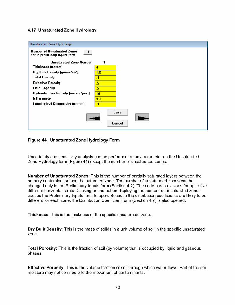
73
4.17 Unsaturated Zone Hydrology
Figure 44. Unsaturated Zone Hydrology Form
Uncertainty and sensitivity analysis can be performed on any parameter on the Unsaturated Zone Hydrology form (Figure 44) except the number of unsaturated zones.
Number of Unsaturated Zones: This is the number of partially saturated layers between the primary contamination and the saturated zone. The number of unsaturated zones can be changed only in the Preliminary Inputs form (Section 4.2). The code has provisions for up to five different horizontal strata. Clicking on the button displaying the number of unsaturated zones causes the Preliminary Inputs form to open. Because the distribution coefficients are likely to be different for each zone, the Distribution Coefficient form (Section 4.7) is also opened.
Thickness: This is the thickness of the specific unsaturated zone.
Dry Bulk Density: This is the mass of solids in a unit volume of soil in the specific unsaturated zone.
Total Porosity: This is the fraction of soil (by volume) that is occupied by liquid and gaseous phases.
Effective Porosity: This is the volume fraction of soil through which water flows. Part of the soil moisture may not contribute to the movement of contaminants.

74
Field Capacity: This is the volumetric moisture content of soil at which (free) gravity drainage ceases, or the amount of moisture that will be retained in a column of soil against the force of gravity. This is the minimum moisture content of the unsaturated layer in the absence of evapotranspiration and root uptake.
Hydraulic Conductivity: This is the apparent flow velocity of water through the contaminated zone under a unit hydraulic gradient.
b Parameter: The soil-specific exponential b parameter relates the hydraulic conductivity of partially saturated soil to its moisture content.
Longitudinal Dispersivity: This is the ratio between the longitudinal dispersion coefficient and pore water velocity. It has the dimension of length. This parameter depends on the thickness of the zone and ranges from one one-hundredth of the thickness to the order of the thickness.
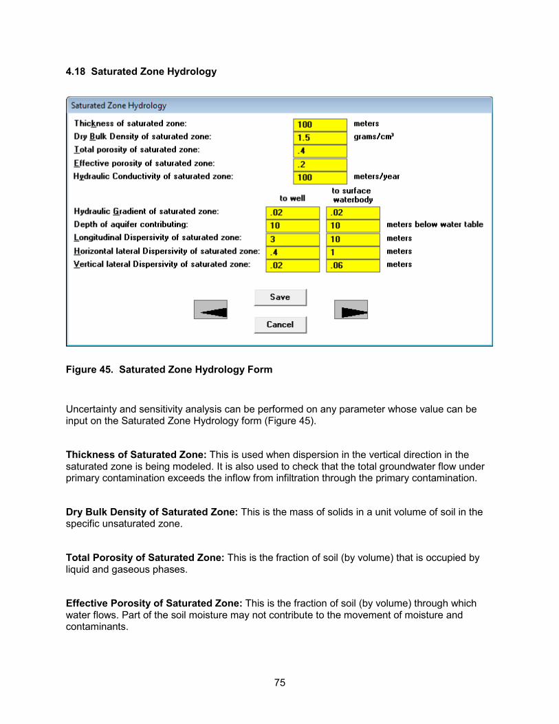
75
4.18 Saturated Zone Hydrology
Figure 45. Saturated Zone Hydrology Form
Uncertainty and sensitivity analysis can be performed on any parameter whose value can be input on the Saturated Zone Hydrology form (Figure 45).
Thickness of Saturated Zone: This is used when dispersion in the vertical direction in the saturated zone is being modeled. It is also used to check that the total groundwater flow under primary contamination exceeds the inflow from infiltration through the primary contamination.
Dry Bulk Density of Saturated Zone: This is the mass of solids in a unit volume of soil in the specific unsaturated zone.
Total Porosity of Saturated Zone: This is the fraction of soil (by volume) that is occupied by liquid and gaseous phases.
Effective Porosity of Saturated Zone: This is the fraction of soil (by volume) through which water flows. Part of the soil moisture may not contribute to the movement of moisture and contaminants.

76
Hydraulic Conductivity of Saturated Zone: This is the apparent flow velocity of water through the contaminated zone under a unit hydraulic gradient.
There are two columns for the remaining properties specified in the form, the first for transport from the primary contamination to the well and the second for transport to the surface water body.
Hydraulic Gradient of Saturated Zone: This is the slope of the surface of the water table.
Depth of Aquifer Contributing: Water flowing through the specified depth of the aquifer is assumed to be intercepted by the well or surface water body. This parameter is used to calculate the contaminant concentration in well water or the contaminated flux into the surface water body.
Longitudinal Dispersivity of Saturated Zone: This is the ratio between the longitudinal dispersion coefficient and pore water velocity. It has the dimension of length. This parameter depends on the length of the saturated zone.
Horizontal Lateral Dispersivity of Saturated Zone: This is the ratio between the horizontal lateral dispersion coefficient and pore water velocity. It has the dimension of length.
Vertical Lateral Dispersivity of Saturated Zone: This is the ratio between the vertical lateral dispersion coefficient and pore water velocity. It has the dimension of length.
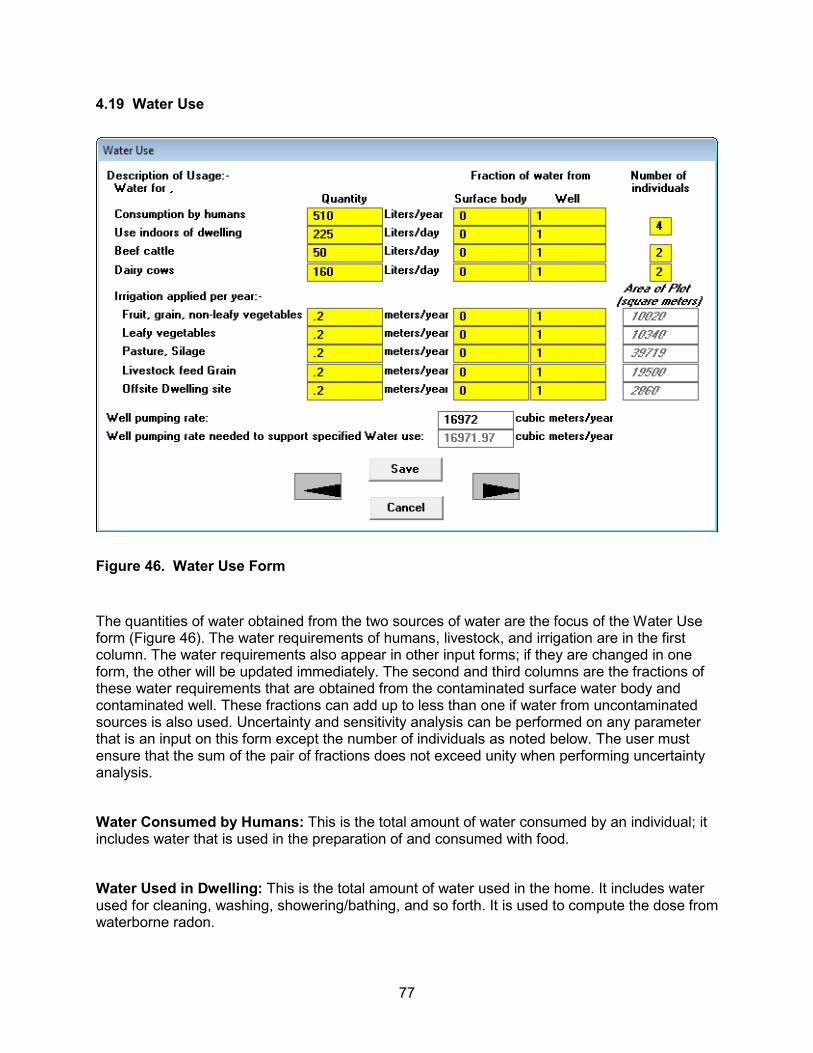
77
4.19 Water Use
Figure 46. Water Use Form
The quantities of water obtained from the two sources of water are the focus of the Water Use form (Figure 46). The water requirements of humans, livestock, and irrigation are in the first column. The water requirements also appear in other input forms; if they are changed in one form, the other will be updated immediately. The second and third columns are the fractions of these water requirements that are obtained from the contaminated surface water body and contaminated well. These fractions can add up to less than one if water from uncontaminated sources is also used. Uncertainty and sensitivity analysis can be performed on any parameter that is an input on this form except the number of individuals as noted below. The user must ensure that the sum of the pair of fractions does not exceed unity when performing uncertainty analysis.
Water Consumed by Humans: This is the total amount of water consumed by an individual; it includes water that is used in the preparation of and consumed with food.
Water Used in Dwelling: This is the total amount of water used in the home. It includes water used for cleaning, washing, showering/bathing, and so forth. It is used to compute the dose from waterborne radon.

78
Water for Beef Cattle: This is the amount of water consumed by each individual animal raised for meat.
Water for Dairy Cows: This is the amount of water consumed by each individual animal raised for milk production.
Number of Individuals: These are the number of humans or livestock that obtain the specified water needs from the water source. These inputs are used only to compute the required minimum well pumping rate and are not used by the computational code. These inputs are not eligible for uncertainty analysis.
Irrigation Applied per Year: This is the volume of irrigation water that is applied over a period of 1 year per unit area of land. It is not the actual rate of irrigation during the growing season; it is the irrigation rate averaged over 1 year.
Well Pumping Rate Needed To Support Specified Water Use: This is the total volume of water that needs to be withdrawn from the well to satisfy the demand described in this form. It is provided to help the user select an appropriate well pumping rate. This value is computed every time a change is made to an input in this form. The well pumping rate is increased automatically, so it will never be less than this minimum required rate.
Well Pumping Rate: This is the rate at which water is extracted from the well. The interface will not accept a well pumping rate that is insufficient to meet the needs specified in this form. While the code performs this check for the deterministic case, the user is responsible for ensuring that this condition is not violated when performing sensitivity or probabilistic/uncertainty analysis.
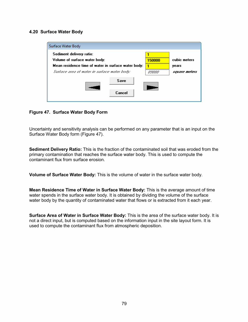
79
4.20 Surface Water Body
Figure 47. Surface Water Body Form
Uncertainty and sensitivity analysis can be performed on any parameter that is an input on the Surface Water Body form (Figure 47).
Sediment Delivery Ratio: This is the fraction of the contaminated soil that was eroded from the primary contamination that reaches the surface water body. This is used to compute the contaminant flux from surface erosion.
Volume of Surface Water Body: This is the volume of water in the surface water body.
Mean Residence Time of Water in Surface Water Body: This is the average amount of time water spends in the surface water body. It is obtained by dividing the volume of the surface water body by the quantity of contaminated water that flows or is extracted from it each year.
Surface Area of Water in Surface Water Body: This is the area of the surface water body. It is not a direct input, but is computed based on the information input in the site layout form. It is used to compute the contaminant flux from atmospheric deposition.
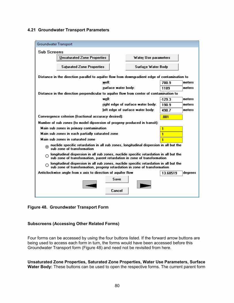
80
4.21 Groundwater Transport Parameters
Figure 48. Groundwater Transport Form
Subscreens (Accessing Other Related Forms)
Four forms can be accessed by using the four buttons listed. If the forward arrow buttons are being used to access each form in turn, the forms would have been accessed before this Groundwater Transport form (Figure 48) and need not be revisited from here.
Unsaturated Zone Properties, Saturated Zone Properties, Water Use Parameters, Surface Water Body: These buttons can be used to open the respective forms. The current parent form
81
will not be closed and will remain in the background. It will reappear when the other forms have been exited.
Uncertainty and sensitivity analysis can be performed on the distances that are inputs on this form. One-at-a-time sensitivity analysis can also be performed on the number of subzones, but not uncertainty analysis. Neither uncertainty analysis nor one-parameter-at-a-time sensitivity analysis can be performed on the convergence criteria. The code will compute the five groundwater transport distances if the locations of the well and the surface water body relative to the primary contamination were specified in the map interface. The user can change the values computed by the code. The connection between this form and the map interface is one-directional; the information entered in this form will not affect the map interface.
Distance in the Direction Parallel to Aquifer Flow from Contamination to Well: This is the distance (in meters [m]) along a groundwater flow line from the down-gradient edge of the primary contamination to the well. It is used in the computation of transport in the saturated zone to the well. A negative value indicates that the well is either up-gradient of or within the primary contamination. If this value is negative or if the combination of water and land usage and exposure pathways indicates that well water has no influence on dose, the computational code will skip the well water concentration computations in order to reduce computational time.
Distance in the Direction Parallel to Aquifer Flow from Contamination to Surface Water Body: This is the distance (in meters [m]) along a groundwater flow line from the down-gradient edge of the primary contamination to the up-gradient edge of the surface water body. It is used in the computation of transport in the saturated zone to the surface water body. A negative value indicates that the surface water body is up-gradient of the primary contamination. If this value is negative or if the combination of water and land usage and exposure pathways indicates that water from the surface water body has no influence on dose, the computational code will skip the surface water computations in order to reduce computational time.
Distance in the Direction Perpendicular to Aquifer Flow from Contamination to Well: This is the distance (in meters [m]) between two groundwater flow lines, one through the center of the contamination and the other thorough the well. It is used in the computation of dilution due to dispersion in the saturated zone, and it applies to water extracted from a well.
Distance in the Direction Perpendicular to Aquifer Flow from Contamination to Right Edge of Surface Water Body: This is the distance (in meters [m]) between two groundwater flow lines, one through the center of the contamination and the other through the right edge of the surface contamination. It is used to compute the contamination flux from the groundwater into the surface water body.
Distance in the Direction Perpendicular to the Aquifer Flow from Contamination to Left Edge of Surface Water Body: This is the distance (in meters [m]) between two groundwater flow lines, one through the center of the contamination and the other thorough the left edge of the surface contamination. It is used to compute the contamination flux from the groundwater into the surface water body.
82
Convergence Criterion: This is the fractional accuracy desired in the Romberg integration used to calculate the contaminant flux or concentration in groundwater. A lower value will likely require the use of a larger number of points in this numerical integration technique, and will thus have a longer computation time. For each Romberg refinement or cycle number, the number of integrand function evaluations is 2N, where N is the cycle number. Therefore, if the convergence criterion is set too low, the computation time becomes excessive, and convergence may not be achieved. If convergence is not achieved, RESRAD will indicate the failure in the QRFAIL.LOG file, and the last estimate of the integral using 32,769 points will be used. If the convergence criterion is set at zero, Simpson’s rule with 32 integration intervals will be used.
Modeling Transport of Progeny Produced in Transit
RESRAD-OFFSITE has two groundwater transport algorithms. One models the effects of the differences in the water-to-soil interaction of the parent nuclide and the progeny nuclides, and the other models the longitudinal dispersion. When one of these processes is clearly dominant, the user can choose the appropriate algorithm to model the transport of the progeny produced in transit. When both the longitudinal dispersion and the differences in the water-to-soil interaction are of comparable importance, the prediction of progeny nuclides produced in transit in the transport zones can be improved by breaking up the transport zones into a number of subzones; then both processes will be modeled over most of the transport path. Additional run time will be needed to do this.
Main Subzones in Primary Contamination: This is the number of subzones into which the saturated zone is to be divided in order to improve the predictions of progeny nuclides produced in transit.
Main Subzones in Each Partially Saturated Zone: This is the number of subzones into which the partially saturated zone is to be divided in order to improve the predictions of progeny nuclides produced in transit.
Main Subzones in Saturated Zone: This is the number of subzones into which the saturated zone is to be divided in order to improve the predictions of progeny nuclides produced in transit.
Modeling Nuclide -Specific Retardation or Dispersion
The two transport algorithms give rise to three choices for the algorithm to be used in the zones where the specific atom undergoes transformations. One of three options can be selected to do the following:
Model the effects of the nuclide-specific distribution coefficients of the parent •and progeny in the zone of transformation and ignore the effects of longitudinal dispersion,

83
Model the effects of longitudinal dispersion and use the retardation factor of •the parent nuclide for both the parent and the progeny produced in that zone and ignore the retardation factor of the progeny, or
Model the effects of longitudinal dispersion and use the retardation factor of •the progeny nuclide for both the parent and the progeny produced in that zone and ignore the retardation factor of the parent.
Anticlockwise Angle from X-axis to Direction of Groundwater Flow: This input will appear only if the GW icon in the map interface was used to specify the direction of groundwater flow.
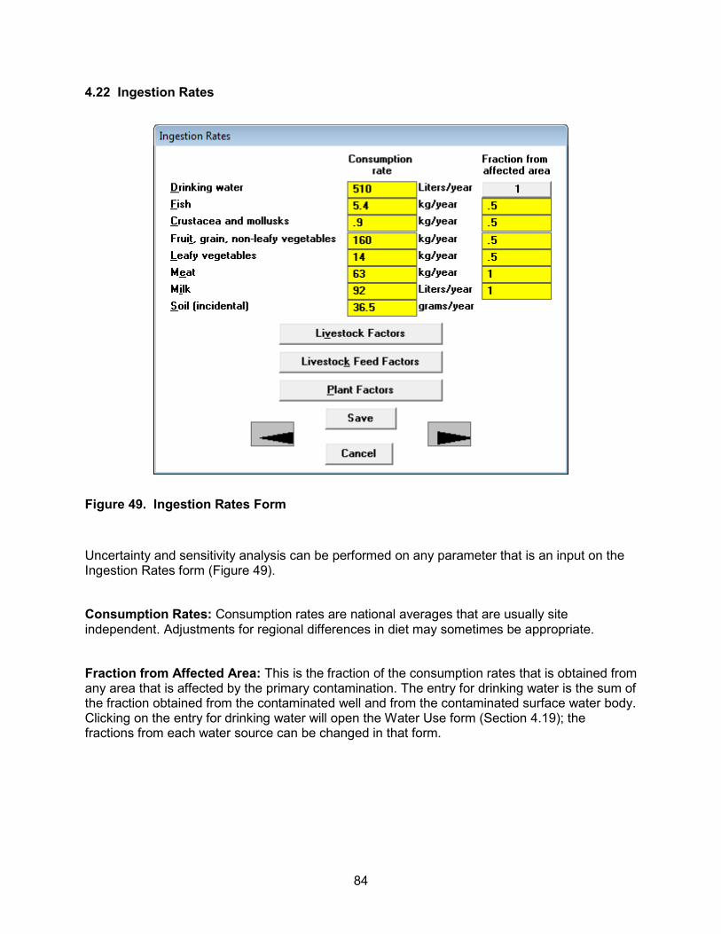
84
4.22 Ingestion Rates
Figure 49. Ingestion Rates Form
Uncertainty and sensitivity analysis can be performed on any parameter that is an input on the Ingestion Rates form (Figure 49).
Consumption Rates: Consumption rates are national averages that are usually site independent. Adjustments for regional differences in diet may sometimes be appropriate.
Fraction from Affected Area: This is the fraction of the consumption rates that is obtained from any area that is affected by the primary contamination. The entry for drinking water is the sum of the fraction obtained from the contaminated well and from the contaminated surface water body. Clicking on the entry for drinking water will open the Water Use form (Section 4.19); the fractions from each water source can be changed in that form.

85
Accessing Other Related Forms Three forms can be accessed by using the three buttons listed below. Alternatively, the first form can be opened by clicking on the forward arrow button on this form; after that, the other forms can be opened by continuing to use the forward arrow buttons on the successive forms.
Livestock Factors, Livestock Feed Factors, and Plant Factors: These buttons can be used to open the respective forms. The current parent form will not be closed and will remain in the background; it will reappear when the form has been exited.
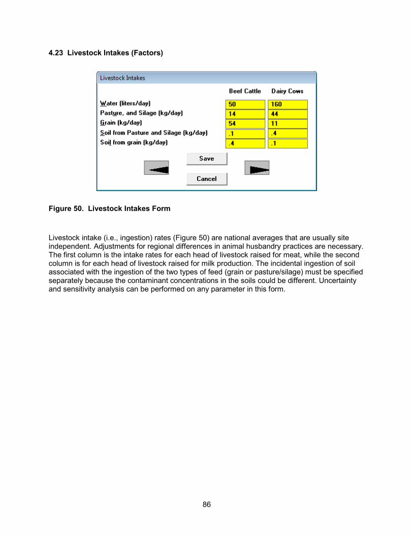
86
4.23 Livestock Intakes (Factors)
Figure 50. Livestock Intakes Form
Livestock intake (i.e., ingestion) rates (Figure 50) are national averages that are usually site independent. Adjustments for regional differences in animal husbandry practices are necessary. The first column is the intake rates for each head of livestock raised for meat, while the second column is for each head of livestock raised for milk production. The incidental ingestion of soil associated with the ingestion of the two types of feed (grain or pasture/silage) must be specified separately because the contaminant concentrations in the soils could be different. Uncertainty and sensitivity analysis can be performed on any parameter in this form.

87
4.24 Livestock Feed Factors and Plant Factors
Figure 51. Plant Factors and Livestock Feed Factors Forms
Plant (i.e., vegetable and livestock feed) factors (Figure 51) are related to growth and contaminant transfer. They depend on the mix of crops and on regional farming practices. Uncertainty and sensitivity analysis can be performed on any parameter that is an input on these forms.
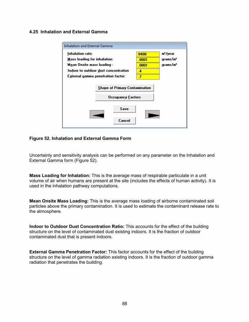
88
4.25 Inhalation and External Gamma
Figure 52. Inhalation and External Gamma Form
Uncertainty and sensitivity analysis can be performed on any parameter on the Inhalation and External Gamma form (Figure 52).
Mass Loading for Inhalation: This is the average mass of respirable particulate in a unit volume of air when humans are present at the site (includes the effects of human activity). It is used in the inhalation pathway computations.
Mean Onsite Mass Loading: This is the average mass loading of airborne contaminated soil particles above the primary contamination. It is used to estimate the contaminant release rate to the atmosphere.
Indoor to Outdoor Dust Concentration Ratio: This accounts for the effect of the building structure on the level of contaminated dust existing indoors. It is the fraction of outdoor contaminated dust that is present indoors.
External Gamma Penetration Factor: This factor accounts for the effect of the building structure on the level of gamma radiation existing indoors. It is the fraction of outdoor gamma radiation that penetrates the building.

89
Accessing Other Related Forms Two forms can be accessed by using the two buttons listed below. Alternatively, the first form can be opened by clicking on the forward arrow button on this form, and then the other form can be opened by continuing to use the forward arrow button on the first form.
Shape of Primary Contamination, Occupancy Factors: These buttons can be used to open the respective forms. The current parent form will not be closed and will remain in the background; it will reappear when the form has been exited.
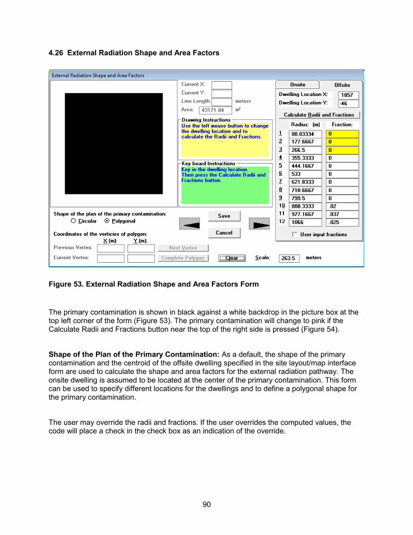
90
4.26 External Radiation Shape and Area Factors
Figure 53. External Radiation Shape and Area Factors Form
The primary contamination is shown in black against a white backdrop in the picture box at the top left corner of the form (Figure 53). The primary contamination will change to pink if the Calculate Radii and Fractions button near the top of the right side is pressed (Figure 54).
Shape of the Plan of the Primary Contamination: As a default, the shape of the primary contamination and the centroid of the offsite dwelling specified in the site layout/map interface form are used to calculate the shape and area factors for the external radiation pathway. The onsite dwelling is assumed to be located at the center of the primary contamination. This form can be used to specify different locations for the dwellings and to define a polygonal shape for the primary contamination.
The user may override the radii and fractions. If the user overrides the computed values, the code will place a check in the check box as an indication of the override.
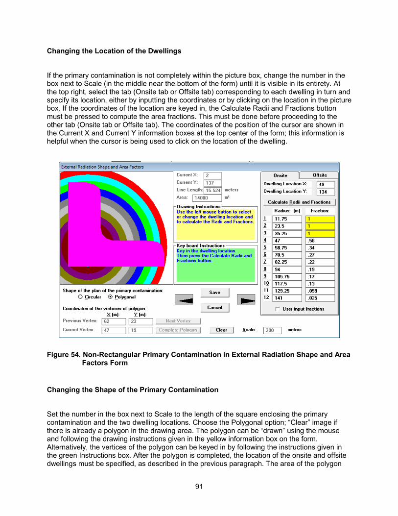
91
Changing the Location of the Dwellings
If the primary contamination is not completely within the picture box, change the number in the box next to Scale (in the middle near the bottom of the form) until it is visible in its entirety. At the top right, select the tab (Onsite tab or Offsite tab) corresponding to each dwelling in turn and specify its location, either by inputting the coordinates or by clicking on the location in the picture box. If the coordinates of the location are keyed in, the Calculate Radii and Fractions button must be pressed to compute the area fractions. This must be done before proceeding to the other tab (Onsite tab or Offsite tab). The coordinates of the position of the cursor are shown in the Current X and Current Y information boxes at the top center of the form; this information is helpful when the cursor is being used to click on the location of the dwelling.
Figure 54. Non-Rectangular Primary Contamination in External Radiation Shape and Area Factors Form
Changing the Shape of the Primary Contamination
Set the number in the box next to Scale to the length of the square enclosing the primary contamination and the two dwelling locations. Choose the Polygonal option; “Clear” image if there is already a polygon in the drawing area. The polygon can be “drawn” using the mouse and following the drawing instructions given in the yellow information box on the form. Alternatively, the vertices of the polygon can be keyed in by following the instructions given in the green Instructions box. After the polygon is completed, the location of the onsite and offsite dwellings must be specified, as described in the previous paragraph. The area of the polygon

92
will be computed when the radii and area fractions are computed. The area is displayed in the box at the top center of the form (Figure 54).
Because the fraction of each annular area that is contaminated is computed graphically in the interface, it is not possible to perform uncertainty or sensitivity analysis on any of the parameters on this form. However, it is possible to perform probabilistic analysis on the input on the site layout form (Section 4.3). The FORTRAN computational code will compute the appropriate radii and fractions for all exposure locations (onsite and offsite dwellings, agricultural areas, livestock feed growing area, and pasture) for the probabilistic runs using the rectangular shapes specified in the site layout form.
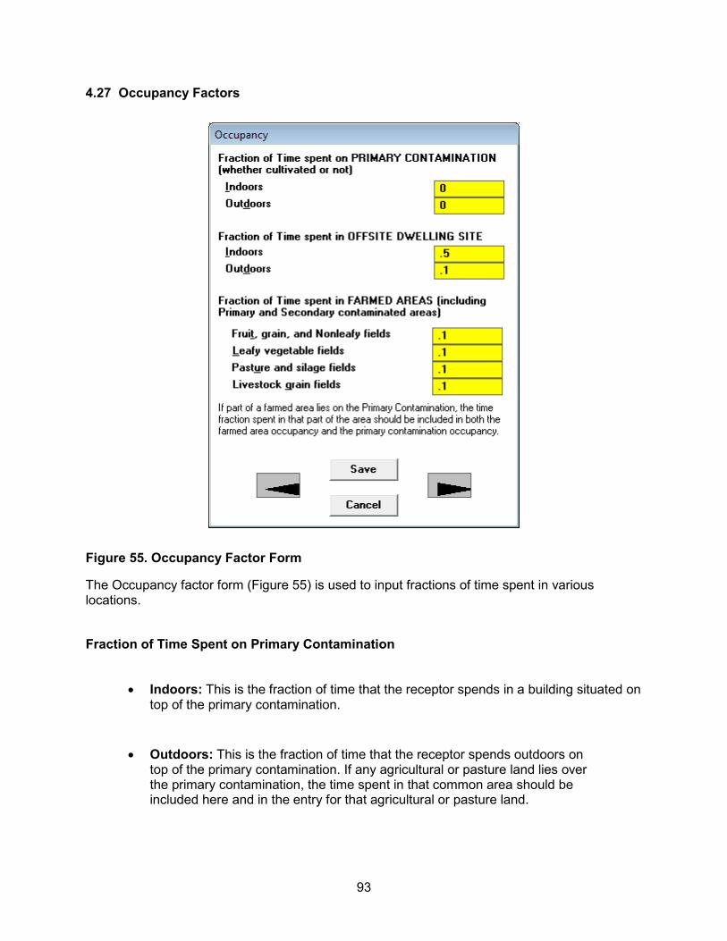
93
4.27 Occupancy Factors
Figure 55. Occupancy Factor Form
The Occupancy factor form (Figure 55) is used to input fractions of time spent in various locations.
Fraction of Time Spent on Primary Contamination
• Indoors: This is the fraction of time that the receptor spends in a building situated on top of the primary contamination.
• Outdoors: This is the fraction of time that the receptor spends outdoors on top of the primary contamination. If any agricultural or pasture land lies over the primary contamination, the time spent in that common area should be included here and in the entry for that agricultural or pasture land.

94
Fraction of Time Spent in Offsite Dwelling Site
• Indoors: This is the fraction of time that the receptor spends in a building situated away from the primary contamination.
• Outdoors: This is the fraction of time that the receptor spends outdoors of the offsite dwelling that is located away from the primary contamination.
Fraction of Time Spent in Farmed Areas: This is the fraction of time that the receptor spends outside in agricultural land and pasture land contaminated by irrigation or by atmospheric deposition. If any agricultural or pasture land overlies the primary contamination, the time spent in that common area should be included in the entry for the agricultural or pasture land and in the outdoor time fraction above the primary contamination.
Note: The sum of the time fractions spent indoors and outdoors on the primary contamination and in the offsite dwelling site cannot exceed unity. Because of the way the time fractions are defined here, it is possible for the sum of all the time fractions of a single individual to exceed unity. However, the sum of the time fractions will not exceed 2. (The sum will equal 2 if an individual spends all the time outdoors in an agricultural or pasture land that overlies the primary contamination.) In addition, the time fractions spent indoors on the primary contamination and indoors and outdoors in the offsite dwelling site, and in the farmed areas, cannot exceed unity.
Uncertainty and sensitivity analysis can be performed on any parameter on this form. The user must ensure that the combined occupancy limits discussed in the preceding paragraph are not violated during uncertainty analysis.
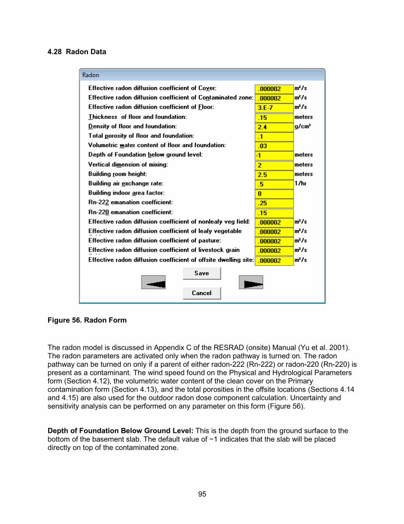
95
4.28 Radon Data
Figure 56. Radon Form
The radon model is discussed in Appendix C of the RESRAD (onsite) Manual (Yu et al. 2001). The radon parameters are activated only when the radon pathway is turned on. The radon pathway can be turned on only if a parent of either radon-222 (Rn-222) or radon-220 (Rn-220) is present as a contaminant. The wind speed found on the Physical and Hydrological Parameters form (Section 4.12), the volumetric water content of the clean cover on the Primary contamination form (Section 4.13), and the total porosities in the offsite locations (Sections 4.14 and 4.15) are also used for the outdoor radon dose component calculation. Uncertainty and sensitivity analysis can be performed on any parameter on this form (Figure 56).
Depth of Foundation Below Ground Level: This is the depth from the ground surface to the bottom of the basement slab. The default value of −1 indicates that the slab will be placed directly on top of the contaminated zone.

96
Onsite Vertical Dimension of Mixing: This is used to define the mixing volume used to compute the onsite concentrations of radon, C-14, and H-3.
Building Indoor Area Factor: This is the fraction of the floor area built on the contaminated area. Values greater than 1.0 indicate a contribution from walls penetrating the contaminated zone. The default value of 0 indicates that the time-dependent area factor is derived from an assumed floor area of 100 m2 and the amount of wall extending into the contaminated zone.

97
4.29 Carbon-14 Data
Figure 57. Carbon-14 and Carbon-12 Forms
Appendix L of the RESRAD (onsite) Manual contains a description of the C-14 parameters and their use in the C-14 model. The vertical dimension of mixing parameter on the Radon Data form (Section 4.28) is also used to compute the onsite concentrations of C-14 and H-3. Uncertainty and sensitivity analysis can be performed on any parameter on these forms (Figure 57).
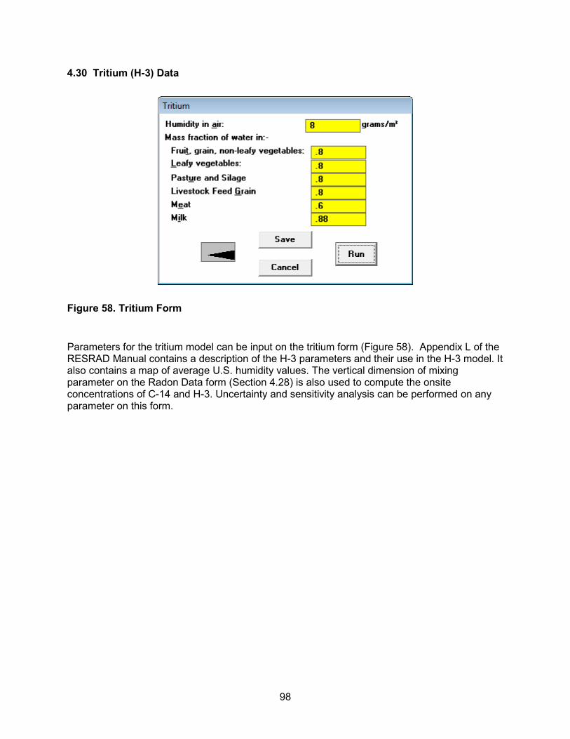
98
4.30 Tritium (H-3) Data
Figure 58. Tritium Form
Parameters for the tritium model can be input on the tritium form (Figure 58). Appendix L of the RESRAD Manual contains a description of the H-3 parameters and their use in the H-3 model. It also contains a map of average U.S. humidity values. The vertical dimension of mixing parameter on the Radon Data form (Section 4.28) is also used to compute the onsite concentrations of C-14 and H-3. Uncertainty and sensitivity analysis can be performed on any parameter on this form.
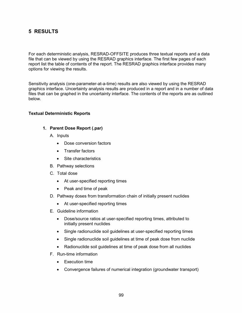
99
5 RESULTS
For each deterministic analysis, RESRAD-OFFSITE produces three textual reports and a data file that can be viewed by using the RESRAD graphics interface. The first few pages of each report list the table of contents of the report. The RESRAD graphics interface provides many options for viewing the results.
Sensitivity analysis (one-parameter-at-a-time) results are also viewed by using the RESRAD graphics interface. Uncertainty analysis results are produced in a report and in a number of data files that can be graphed in the uncertainty interface. The contents of the reports are as outlined below.
Textual Deterministic Reports
1. Parent Dose Report (.par) A. Inputs
• Dose conversion factors
• Transfer factors
• Site characteristics
B. Pathway selections
C. Total dose
• At user-specified reporting times
• Peak and time of peak
D. Pathway doses from transformation chain of initially present nuclides
• At user-specified reporting times
E. Guideline information
• Dose/source ratios at user-specified reporting times, attributed to initially present nuclides
• Single radionuclide soil guidelines at user-specified reporting times
• Single radionuclide soil guidelines at time of peak dose from nuclide
• Radionuclide soil guidelines at time of peak dose from all nuclides
F. Run-time information
• Execution time
• Convergence failures of numerical integration (groundwater transport)
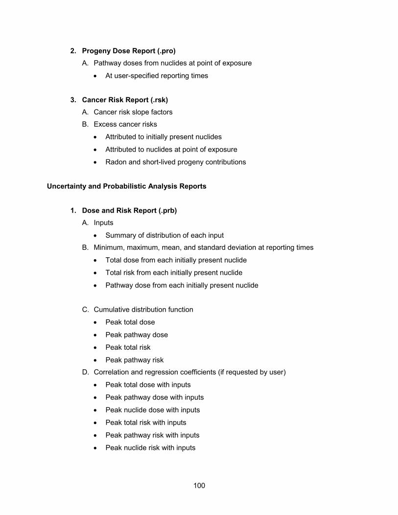
100
2. Progeny Dose Report (.pro) A. Pathway doses from nuclides at point of exposure
• At user-specified reporting times
3. Cancer Risk Report (.rsk) A. Cancer risk slope factors
B. Excess cancer risks
• Attributed to initially present nuclides
• Attributed to nuclides at point of exposure
• Radon and short-lived progeny contributions
Uncertainty and Probabilistic Analysis Reports
1. Dose and Risk Report (.prb) A. Inputs
• Summary of distribution of each input
B. Minimum, maximum, mean, and standard deviation at reporting times
• Total dose from each initially present nuclide
• Total risk from each initially present nuclide
• Pathway dose from each initially present nuclide
C. Cumulative distribution function
• Peak total dose
• Peak pathway dose
• Peak total risk
• Peak pathway risk
D. Correlation and regression coefficients (if requested by user)
• Peak total dose with inputs
• Peak pathway dose with inputs
• Peak nuclide dose with inputs
• Peak total risk with inputs
• Peak pathway risk with inputs
• Peak nuclide risk with inputs

101
2. Probabilistic Input Report (.smp) A. Input specification
• Distribution of each input
• RCC
• Warnings of incompatible input correlations
B. Input samples
• Input vectors
• Rank of input vectors
• Correlation coefficients of raw data
• Correlation coefficients of rank data
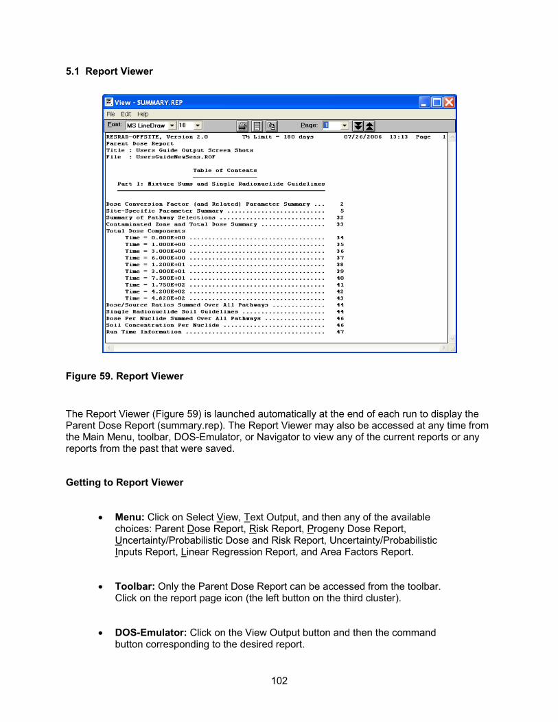
102
5.1 Report Viewer
Figure 59. Report Viewer
The Report Viewer (Figure 59) is launched automatically at the end of each run to display the Parent Dose Report (summary.rep). The Report Viewer may also be accessed at any time from the Main Menu, toolbar, DOS-Emulator, or Navigator to view any of the current reports or any reports from the past that were saved.
Getting to Report Viewer
• Menu: Click on Select View, Text Output, and then any of the available choices: Parent Dose Report, Risk Report, Progeny Dose Report, Uncertainty/Probabilistic Dose and Risk Report, Uncertainty/Probabilistic Inputs Report, Linear Regression Report, and Area Factors Report.
• Toolbar: Only the Parent Dose Report can be accessed from the toolbar. Click on the report page icon (the left button on the third cluster).
• DOS-Emulator: Click on the View Output button and then the command button corresponding to the desired report.
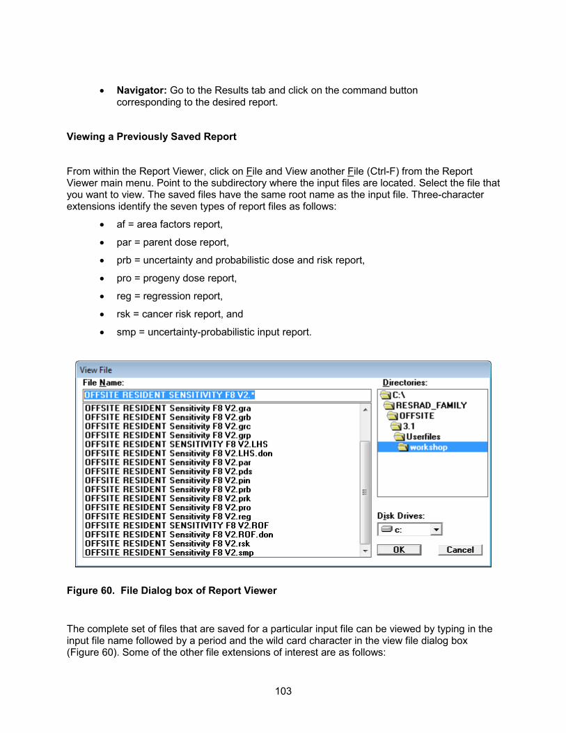
103
• Navigator: Go to the Results tab and click on the command button corresponding to the desired report.
Viewing a Previously Saved Report
From within the Report Viewer, click on File and View another File (Ctrl-F) from the Report Viewer main menu. Point to the subdirectory where the input files are located. Select the file that you want to view. The saved files have the same root name as the input file. Three-character extensions identify the seven types of report files as follows:
• af = area factors report,
• par = parent dose report,
• prb = uncertainty and probabilistic dose and risk report,
• pro = progeny dose report,
• reg = regression report,
• rsk = cancer risk report, and
• smp = uncertainty-probabilistic input report.
Figure 60. File Dialog box of Report Viewer
The complete set of files that are saved for a particular input file can be viewed by typing in the input file name followed by a period and the wild card character in the view file dialog box (Figure 60). Some of the other file extensions of interest are as follows:
104
• chn = a file listing the transformation threads and principal nuclides for each initially present nuclide.
• pds or prk = formatted data file of peak probabilistic dose or risk for each simulation, and
• pin = data file of probabilistic samples for each simulation.
Moving Around
• Pages: To go to another page, choose one of the following methods:
− Enter the page number in the page text box and hit Enter.
− Pull down the page list and click on the desired page.
− Advance a page by pressing the “Page Down” key or by clicking on the double down arrows.
− Go back a page by pressing the “Page Up” key or by clicking on the double up arrows.
• Within a Page: Use scroll bars to position text.
• Between Reports: Click on File and View another File (Ctrl-F) from the Report Viewer main menu to view another report. You can also close the Report Viewer and go back to the Main Menu to select a different file.
Saving Files
Every time a calculation is run, the previous reports and graphics files are overwritten. The results can be saved under different names, which allows for their retrieval later.
• Saving All Files: Click on File and Save All under the Report Viewer main menu. This will save all textual reports to files. If the input filename is xxxx.rad, the reports will be saved as xxxx.yyy, where the extension yyy identifies the report as described in “Viewing a Previously Saved Report” above.
• Saving the Open Report: Click on File and Save under the Report Viewer main menu. This will prompt the user for a name under which to save the currently displayed report.

105
Copying Selections
• Copy Highlighted Section: Click on Edit/Copy under the Report Viewer main menu. The selected text will be placed on the Windows clipboard and can be placed into any document, such as a spreadsheet or word-processed text.
• Copy the Current Page: Click on Edit/Select All, followed by Edit/Copy. Another option is to click on the icon that looks like two pages.
Printing
• Setting up the Printer: RESRAD-OFFSITE uses the standard Windows printer. The setup for the printer can be accessed through the File/Printer/Setup menu option. Options that can be selected include printer, paper size, and orientation.
• Setting up the Report for Printing: Click on the icon that looks like a single page to automatically select the best font size that will fit the report to a single page width.
• Printing: Select the File/Print menu option or click on the printer icon button. A dialogue box will appear for printing the whole report, sets of pages, or the current highlighted text.
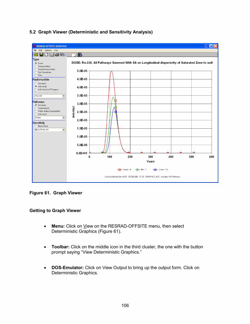
106
5.2 Graph Viewer (Deterministic and Sensitivity Analysis)
Figure 61. Graph Viewer
Getting to Graph Viewer
• Menu: Click on View on the RESRAD-OFFSITE menu, then select Deterministic Graphics (Figure 61).
• Toolbar: Click on the middle icon in the third cluster, the one with the button prompt saying “View Deterministic Graphics.”
• DOS-Emulator: Click on View Output to bring up the output form. Click on Deterministic Graphics.

107
• Windows Navigator: Click on the Results tab, then click on the Deterministic Graphics icon.
Choosing from the Plot Selection Pallet
All dose, risk, and concentration data produced by RESRAD-OFFSITE for each radionuclide and pathway or media combination are available to the Graph Viewer. Thus a wide choice of plots is available. The plots are selected by specifying the following:
• Type (of Plot)
− Dose: Select Dose to view a graphical representation of the radiological dose over the user-specified time horizon.
− Concentration: This displays a plot of the concentration of the selected radionuclide in various media over the user-specified time horizon.
− Dose/Source Ratio: This displays a graph of the ratio of an individual radionuclide’s dose contribution to its initial concentration in soil in the primary contamination, over the user-specified time horizon.
− Soil Guidelines: Select Soil Guidelines to view a graph of the initial radionuclide concentration in soil that will produce the specified basic radiation dose limit at that specific time as a function of time.
− Risk: Select Risk to view a graphical representation of the excess cancer risk over the user-specified time horizon.
• Radionuclide
− Summed: This option is available for Dose and Risk plots; it displays the dose or risk due to all the radionuclides specified to be present at the site.
− Individual: This option is available for all five types of plots, but its definition depends on the type of plot. Select the radionuclide by using the drop-down scroll box.
When used with the concentration plots, it displays the concentration of the selected radionuclide (either an initially present nuclide or a progeny) in the selected media.
When used with the other four types of plots, it displays the total quantity due to the selected radionuclide (initially present nuclide) and its progeny.
− Individual and Progeny: This option is available for Dose, Dose/Source Ratio, and Risk plots. It displays the individual dose, dose-to-source ratio, or risk due to the selected radionuclide (initially present nuclide) and each of its progeny.
− Individual and Threads: This option is available for Dose, Dose/Source Ratio, and Risk plots. It displays the individual dose, dose-to-source ratio,
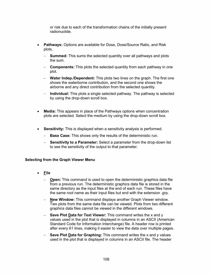
108
or risk due to each of the transformation chains of the initially present radionuclide.
• Pathways: Options are available for Dose, Dose/Source Ratio, and Risk plots.
− Summed: This sums the selected quantity over all pathways and plots the sum.
− Components: This plots the selected quantity from each pathway in one plot.
− Water Indep./Dependent: This plots two lines on the graph. The first one shows the waterborne contribution, and the second one shows the airborne and any direct contribution from the selected quantity.
− Individual: This plots a single selected pathway. The pathway is selected by using the drop-down scroll box.
• Media: This appears in place of the Pathways options when concentration plots are selected. Select the medium by using the drop-down scroll box.
• Sensitivity: This is displayed when a sensitivity analysis is performed.
− Base Case: This shows only the results of the deterministic run.
− Sensitivity to a Parameter: Select a parameter from the drop-down list to see the sensitivity of the output to that parameter.
Selecting from the Graph Viewer Menu
• File
− Open: This command is used to open the deterministic graphics data file from a previous run. The deterministic graphics data file is stored in the same directory as the input files at the end of each run. These files have the same root name as their input files but end with the extension .grp.
− New Window: This command displays another Graph Viewer window. Two plots from the same data file can be viewed. Plots from two different graphics data files cannot be viewed in the different windows.
− Save Plot Data for Text Viewer: This command writes the x and y values used in the plot that is displayed in columns in an ASCII (American Standard Code for Information Interchange) file. A header row is printed after every 61 lines, making it easier to view the data over multiple pages.
− Save Plot Data for Graphing: This command writes the x and y values used in the plot that is displayed in columns in an ASCII file. The header
109
row is printed once at the beginning of the file, making it easier to use these data in other graphing programs.
− Print: This command is used to produce a hard (paper) copy of the current plot.
− Print Setup: This opens a window displaying the list of available printers and printing specifications.
− Close Window: When multiple Graph Viewer windows are open, this command is used to close an individual window.
− Exit: This closes all Graph Viewer windows.
• Edit
− Copy: This command saves the plot in a metafile. The print screen (Print Scrn) key on the keyboard produces a much better quality image.
− Export to Excel: This command opens a new Excel file and transfers the x and y values used in the plot. If multiple lines are displayed in the plot, a pair of columns is output for each line that is displayed. The first three rows contain the plot title, plot footer, and column headers.
• Options: This menu is used to change the appearance of the plot. The following choices can be made: display either axis in linear or logarithmic scale, display or suppress grid lines, use different colors for different plots or use black for all plots, and use the same or different line styles for the different plots. This menu is also used to hide or show the prompts for the buttons on the toolbar.
• View: This menu is used to view the plot data. The plot data must have been saved previously by using the Save Plot Data command described above under the first option, File.

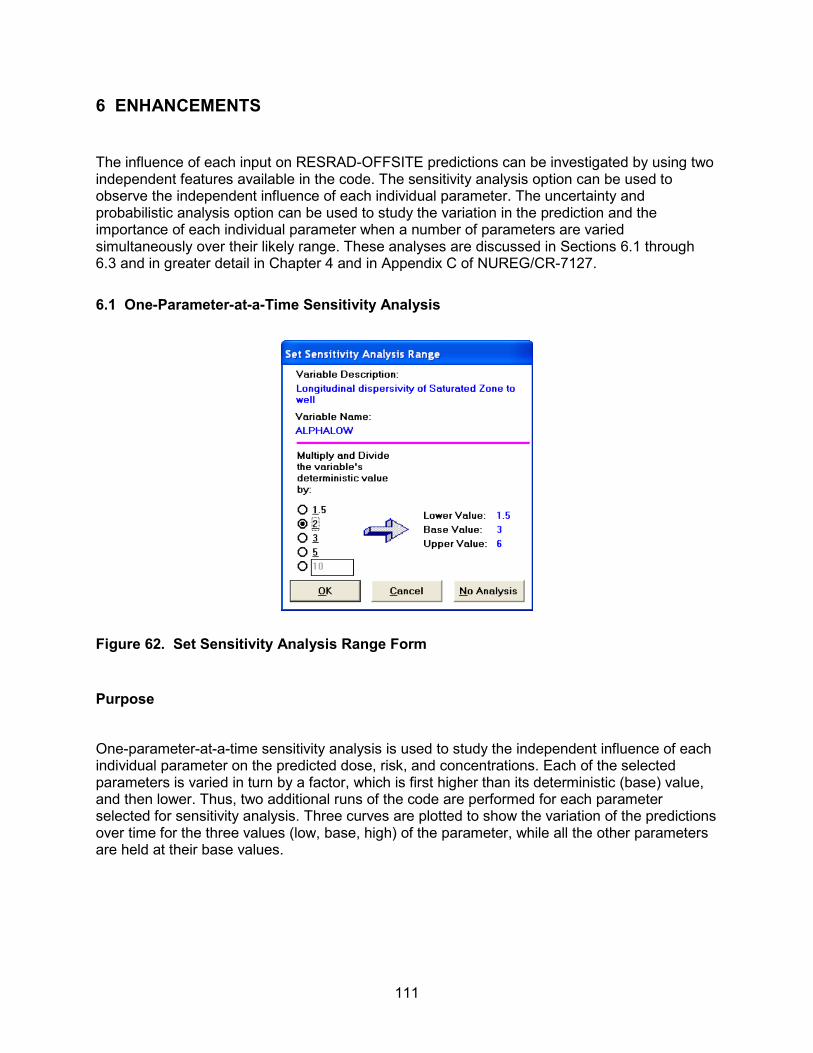
111
6 ENHANCEMENTS
The influence of each input on RESRAD-OFFSITE predictions can be investigated by using two independent features available in the code. The sensitivity analysis option can be used to observe the independent influence of each individual parameter. The uncertainty and probabilistic analysis option can be used to study the variation in the prediction and the importance of each individual parameter when a number of parameters are varied simultaneously over their likely range. These analyses are discussed in Sections 6.1 through 6.3 and in greater detail in Chapter 4 and in Appendix C of NUREG/CR-7127.
6.1 One-Parameter-at-a-Time Sensitivity Analysis
Figure 62. Set Sensitivity Analysis Range Form
Purpose
One-parameter-at-a-time sensitivity analysis is used to study the independent influence of each individual parameter on the predicted dose, risk, and concentrations. Each of the selected parameters is varied in turn by a factor, which is first higher than its deterministic (base) value, and then lower. Thus, two additional runs of the code are performed for each parameter selected for sensitivity analysis. Three curves are plotted to show the variation of the predictions over time for the three values (low, base, high) of the parameter, while all the other parameters are held at their base values.
112
Displaying the Sensitivity Analysis Range
• Menu: First click on the input box of the parameter of interest to put it in focus. Then click on Form Options on the RESRAD-OFFSITE menu and Sensitivity Analysis (F9 key).
• Toolbar: First click on the input box of the parameter of interest to put it in focus. Then click on the Set Sensitivity Button (fourth button in the second cluster on the toolbar).
• Input Window: First click on the parameter of interest, then press the F9 key.
• Sensitivity Input Summary Bar: The sensitivity input summary bar (shown if Sensitivity Input Summary under the View option is checked) will include a button for each parameter selected for sensitivity analysis. The title of the button includes the variable name, the symbols */, and the factor by which to multiply and divide. Right Click on any of these buttons to review, change, or remove a sensitivity analysis on the corresponding parameter.
Selecting a Parameter for Sensitivity Analysis
First display the Set Sensitivity Analysis Range form (Figure 62) while the cursor is in the input box corresponding to the desired parameter. Then set the multiplication and division factor as described below.
Choose one of the options for the multiplication and division factor. The resultant values for the two sensitivity runs will be shown at the right along with the base value. If you choose the last option, you can enter any value greater than 1 or accept the value of 10. If the selected factor causes a parameter value to exceed its bounds, a warning message will be displayed with the option to set the factor to the maximum allowable value. If the base value specified for any variable selected for sensitivity analysis is changed, the sensitivity button corresponding to that factor should be revisited to ensure that the values for the sensitivity analysis will still be within the bounds.
Click on the OK button to include the parameter in the sensitivity analysis. A button for this parameter will be added on the sensitivity input summary bar, and the parameter will be selected for sensitivity analysis.

113
Removing a Parameter from Sensitivity Analysis
If a parameter has already been selected for sensitivity analysis, the button corresponding to it will be on the sensitivity input summary bar. Either right-click on that button, or left-click and choose No Analysis to remove the sensitivity analysis. Clicking on Cancel will not remove the parameter from the sensitivity analysis in this case.
If the parameter has not yet been selected, simply click Cancel on the Set Sensitivity Analysis Range form to disregard the information in the form.
Viewing Results of Sensitivity Analysis
Sensitivity analysis results are shown only in a graphic format, not in any textual report. Launch the deterministic Graph Viewer after performing a sensitivity analysis on the selected parameters; the Sensitivity option will be displayed at the bottom of the plot selection pallet (Section 5.2). Select a parameter from the drop-down box to see the sensitivity of the output to that parameter.
More information on performing sensitivity analysis using RESRAD-OFFSITE is available in Chapter 4 and in Appendix C of NUREG/CR-7127.
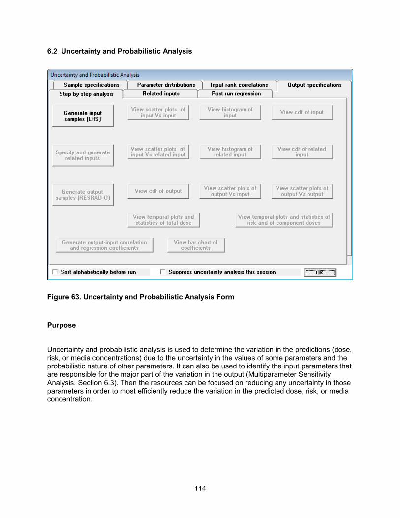
114
6.2 Uncertainty and Probabilistic Analysis
Figure 63. Uncertainty and Probabilistic Analysis Form
Purpose
Uncertainty and probabilistic analysis is used to determine the variation in the predictions (dose, risk, or media concentrations) due to the uncertainty in the values of some parameters and the probabilistic nature of other parameters. It can also be used to identify the input parameters that are responsible for the major part of the variation in the output (Multiparameter Sensitivity Analysis, Section 6.3). Then the resources can be focused on reducing any uncertainty in those parameters in order to most efficiently reduce the variation in the predicted dose, risk, or media concentration.
115
Selecting an Input Parameter for Uncertainty and Probabilistic Analysis
• Menu: First click on the input box of the parameter of interest to put it in focus. Then click on Form Options and Uncertainty/Probabilistic Analysis (F8 key) (Figure 63).
• Toolbar: First click on the input box of the parameter of interest to put it in focus. Then click on the Uncertainty/Probabilistic Analysis button (farthest button on the right in the second cluster on the toolbar; it has a ±? symbol on it).
• Input Window: Press the F8 function key while the focus is on the input parameter to be included for uncertainty or probabilistic analysis.
The distribution of the selected variable is specified in the Parameter distributions tab (Section 6.2.1) of the Uncertainty and Probabilistic Analysis interface form.
Displaying the Uncertainty and Probabilistic Analysis (Interface) Form
• Menu: Click on View and then Uncertainty/Probabilistic interface (Ctrl-F8). This displays the form and sets the user preference to always display the form when the RESRAD-OFFSITE interface is launched.
The methods just described (Selecting an Input Parameter for Uncertainty and Probabilistic Analysis) will also display the form if it is not already visible. They are not included here because they also select the input that is in focus at the time they were invoked for uncertainty or probabilistic analysis.
The Uncertainty and Probabilistic Analysis form currently has one tab (Related inputs) under development and six active tabs as follows.
1. Parameter distributions: The uncertainty in the value of an input or the probabilistic nature of an input is specified in the form of a probabilistic distribution on this tab.
2. Sample specifications: This tab is used to specify how the probabilistic input sets will be generated from the distributions specified in the previous tab.

116
3. Input rank correlations: This tab accepts the specification of correlations between pairs of uncertain/probabilistic inputs if the appropriate choice is made in the Sample specifications tab.
4. Output specifications: This tab describes the different types of probabilistic display and analysis options that are available for the various outputs and is used to specify whether the component doses, risks, and concentrations for each realization of a probabilistic run need to be saved. It is also used to specify the desired output-input correlation and regression coefficients.
5. Step-by-step analysis: This tab allows the analysis to be carried out in sequence and provides an option to view the results of each step before proceeding to the next. It also allows viewing of the probabilistic graphics from a previous analysis.
6. Post run regression: This tab is used to obtain a specific selection of output-input correlation and regression coefficients.
These six tabs are described more fully in Sections 6.2.1 through 6.2.6.
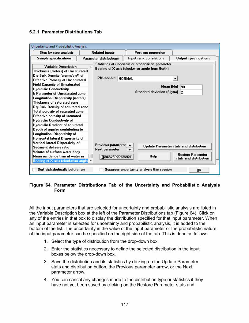
117
6.2.1 Parameter Distributions Tab
Figure 64. Parameter Distributions Tab of the Uncertainty and Probabilistic Analysis Form
All the input parameters that are selected for uncertainty and probabilistic analysis are listed in the Variable Description box at the left of the Parameter Distributions tab (Figure 64). Click on any of the entries in that box to display the distribution specified for that input parameter. When an input parameter is selected for uncertainty and probabilistic analysis, it is added to the bottom of the list. The uncertainty in the value of the input parameter or the probabilistic nature of the input parameter can be specified on the right side of the tab. This is done as follows:
1. Select the type of distribution from the drop-down box.
2. Enter the statistics necessary to define the selected distribution in the input boxes below the drop-down box.
3. Save the distribution and its statistics by clicking on the Update Parameter stats and distribution button, the Previous parameter arrow, or the Next parameter arrow.
4. You can cancel any changes made to the distribution type or statistics if they have not yet been saved by clicking on the Restore Parameter stats and
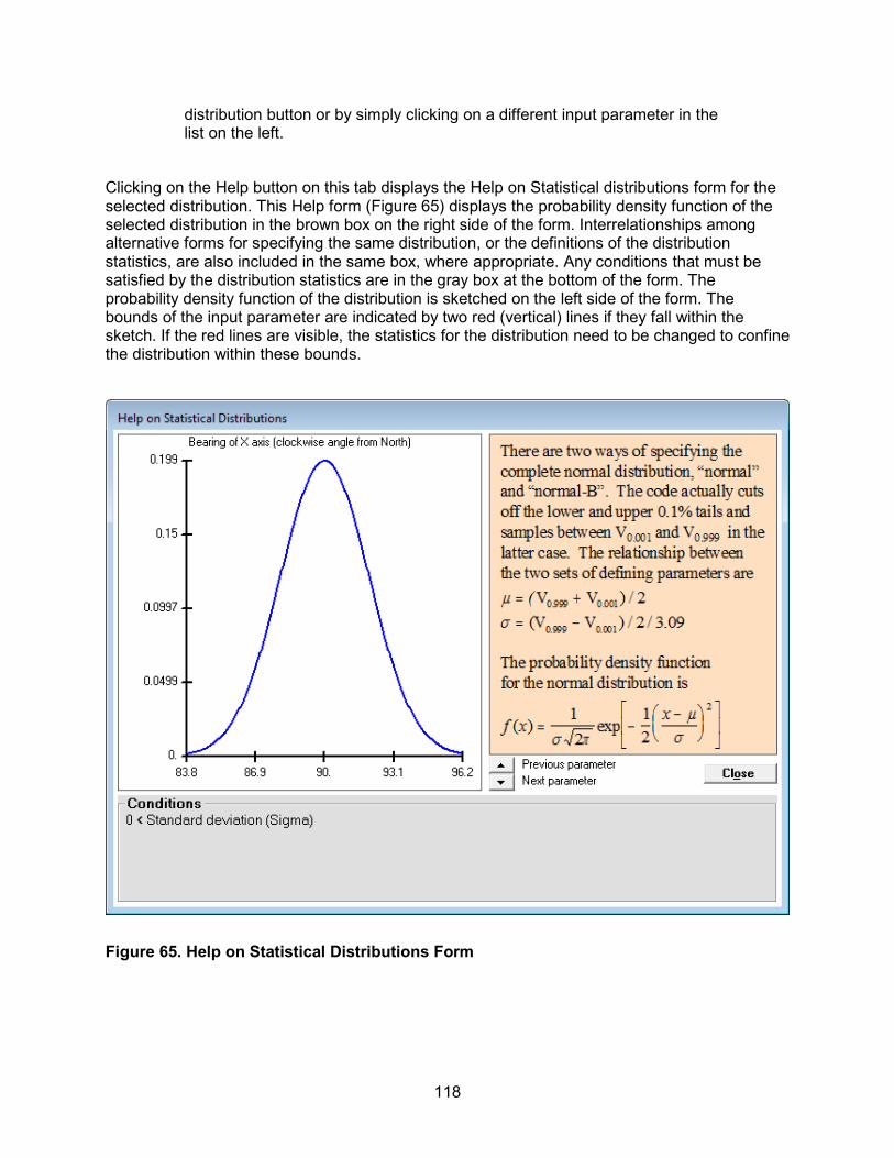
118
distribution button or by simply clicking on a different input parameter in the list on the left.
Clicking on the Help button on this tab displays the Help on Statistical distributions form for the selected distribution. This Help form (Figure 65) displays the probability density function of the selected distribution in the brown box on the right side of the form. Interrelationships among alternative forms for specifying the same distribution, or the definitions of the distribution statistics, are also included in the same box, where appropriate. Any conditions that must be satisfied by the distribution statistics are in the gray box at the bottom of the form. The probability density function of the distribution is sketched on the left side of the form. The bounds of the input parameter are indicated by two red (vertical) lines if they fall within the sketch. If the red lines are visible, the statistics for the distribution need to be changed to confine the distribution within these bounds.
Figure 65. Help on Statistical Distributions Form
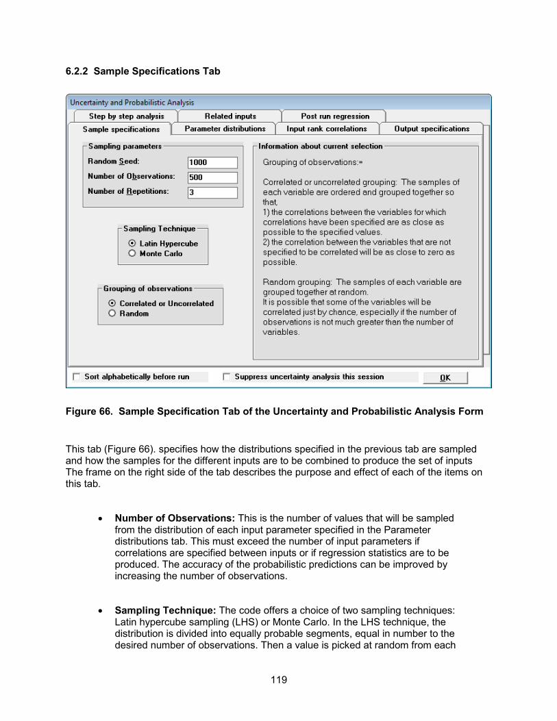
119
6.2.2 Sample Specifications Tab
Figure 66. Sample Specification Tab of the Uncertainty and Probabilistic Analysis Form
This tab (Figure 66). specifies how the distributions specified in the previous tab are sampled and how the samples for the different inputs are to be combined to produce the set of inputs The frame on the right side of the tab describes the purpose and effect of each of the items on this tab.
• Number of Observations: This is the number of values that will be sampled from the distribution of each input parameter specified in the Parameter distributions tab. This must exceed the number of input parameters if correlations are specified between inputs or if regression statistics are to be produced. The accuracy of the probabilistic predictions can be improved by increasing the number of observations.
• Sampling Technique: The code offers a choice of two sampling techniques: Latin hypercube sampling (LHS) or Monte Carlo. In the LHS technique, the distribution is divided into equally probable segments, equal in number to the desired number of observations. Then a value is picked at random from each
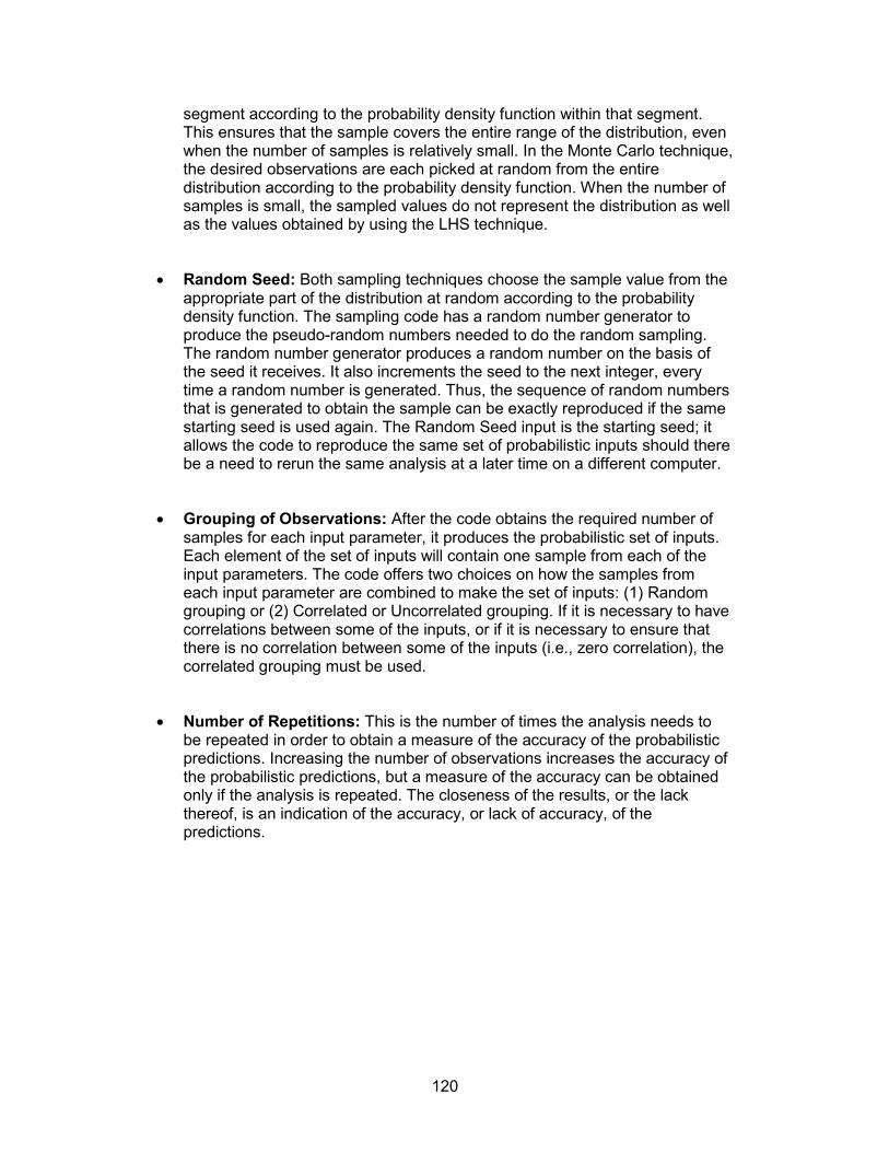
120
segment according to the probability density function within that segment. This ensures that the sample covers the entire range of the distribution, even when the number of samples is relatively small. In the Monte Carlo technique, the desired observations are each picked at random from the entire distribution according to the probability density function. When the number of samples is small, the sampled values do not represent the distribution as well as the values obtained by using the LHS technique.
• Random Seed: Both sampling techniques choose the sample value from the appropriate part of the distribution at random according to the probability density function. The sampling code has a random number generator to produce the pseudo-random numbers needed to do the random sampling. The random number generator produces a random number on the basis of the seed it receives. It also increments the seed to the next integer, every time a random number is generated. Thus, the sequence of random numbers that is generated to obtain the sample can be exactly reproduced if the same starting seed is used again. The Random Seed input is the starting seed; it allows the code to reproduce the same set of probabilistic inputs should there be a need to rerun the same analysis at a later time on a different computer.
• Grouping of Observations: After the code obtains the required number of samples for each input parameter, it produces the probabilistic set of inputs. Each element of the set of inputs will contain one sample from each of the input parameters. The code offers two choices on how the samples from each input parameter are combined to make the set of inputs: (1) Random grouping or (2) Correlated or Uncorrelated grouping. If it is necessary to have correlations between some of the inputs, or if it is necessary to ensure that there is no correlation between some of the inputs (i.e., zero correlation), the correlated grouping must be used.
• Number of Repetitions: This is the number of times the analysis needs to be repeated in order to obtain a measure of the accuracy of the probabilistic predictions. Increasing the number of observations increases the accuracy of the probabilistic predictions, but a measure of the accuracy can be obtained only if the analysis is repeated. The closeness of the results, or the lack thereof, is an indication of the accuracy, or lack of accuracy, of the predictions.
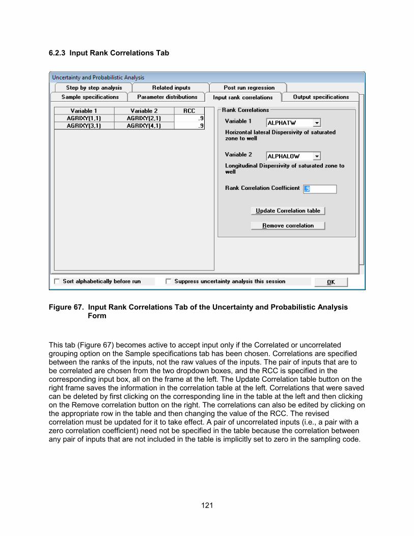
121
6.2.3 Input Rank Correlations Tab
Figure 67. Input Rank Correlations Tab of the Uncertainty and Probabilistic Analysis Form
This tab (Figure 67) becomes active to accept input only if the Correlated or uncorrelated grouping option on the Sample specifications tab has been chosen. Correlations are specified between the ranks of the inputs, not the raw values of the inputs. The pair of inputs that are to be correlated are chosen from the two dropdown boxes, and the RCC is specified in the corresponding input box, all on the frame at the left. The Update Correlation table button on the right frame saves the information in the correlation table at the left. Correlations that were saved can be deleted by first clicking on the corresponding line in the table at the left and then clicking on the Remove correlation button on the right. The correlations can also be edited by clicking on the appropriate row in the table and then changing the value of the RCC. The revised correlation must be updated for it to take effect. A pair of uncorrelated inputs (i.e., a pair with a zero correlation coefficient) need not be specified in the table because the correlation between any pair of inputs that are not included in the table is implicitly set to zero in the sampling code.
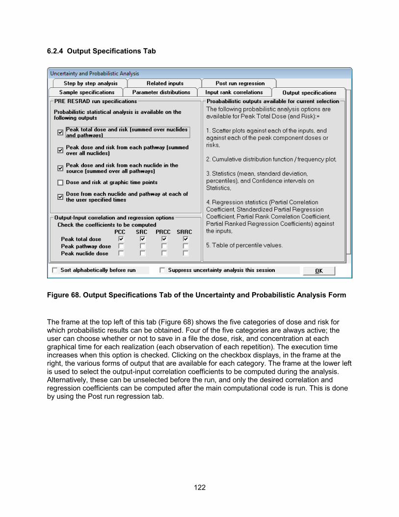
122
6.2.4 Output Specifications Tab
Figure 68. Output Specifications Tab of the Uncertainty and Probabilistic Analysis Form
The frame at the top left of this tab (Figure 68) shows the five categories of dose and risk for which probabilistic results can be obtained. Four of the five categories are always active; the user can choose whether or not to save in a file the dose, risk, and concentration at each graphical time for each realization (each observation of each repetition). The execution time increases when this option is checked. Clicking on the checkbox displays, in the frame at the right, the various forms of output that are available for each category. The frame at the lower left is used to select the output-input correlation coefficients to be computed during the analysis. Alternatively, these can be unselected before the run, and only the desired correlation and regression coefficients can be computed after the main computational code is run. This is done by using the Post run regression tab.
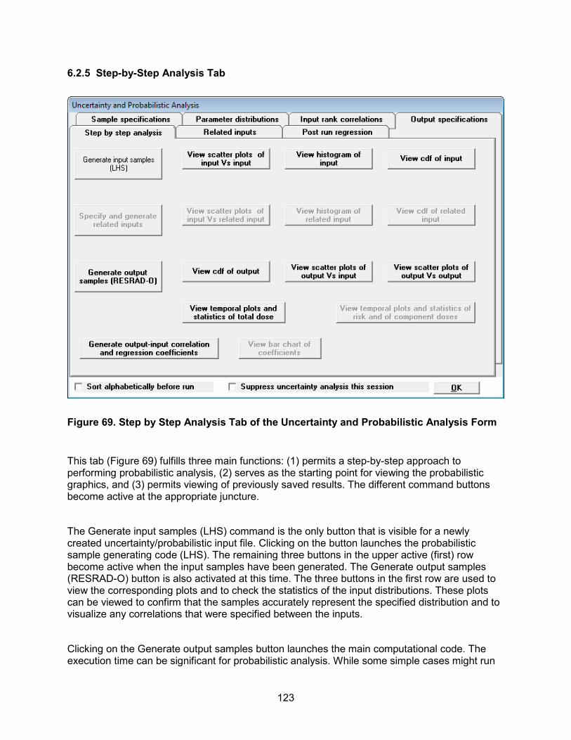
123
6.2.5 Step-by-Step Analysis Tab
Figure 69. Step by Step Analysis Tab of the Uncertainty and Probabilistic Analysis Form
This tab (Figure 69) fulfills three main functions: (1) permits a step-by-step approach to performing probabilistic analysis, (2) serves as the starting point for viewing the probabilistic graphics, and (3) permits viewing of previously saved results. The different command buttons become active at the appropriate juncture.
The Generate input samples (LHS) command is the only button that is visible for a newly created uncertainty/probabilistic input file. Clicking on the button launches the probabilistic sample generating code (LHS). The remaining three buttons in the upper active (first) row become active when the input samples have been generated. The Generate output samples (RESRAD-O) button is also activated at this time. The three buttons in the first row are used to view the corresponding plots and to check the statistics of the input distributions. These plots can be viewed to confirm that the samples accurately represent the specified distribution and to visualize any correlations that were specified between the inputs.
Clicking on the Generate output samples button launches the main computational code. The execution time can be significant for probabilistic analysis. While some simple cases might run
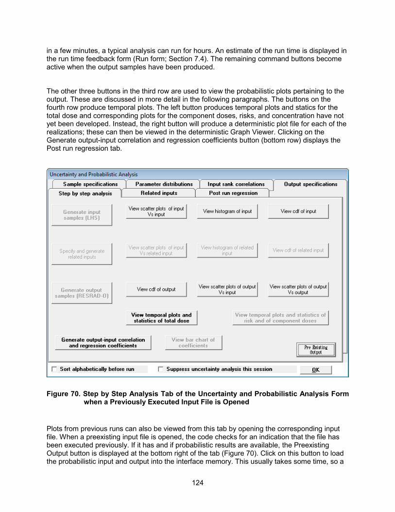
124
in a few minutes, a typical analysis can run for hours. An estimate of the run time is displayed in the run time feedback form (Run form; Section 7.4). The remaining command buttons become active when the output samples have been produced.
The other three buttons in the third row are used to view the probabilistic plots pertaining to the output. These are discussed in more detail in the following paragraphs. The buttons on the fourth row produce temporal plots. The left button produces temporal plots and statics for the total dose and corresponding plots for the component doses, risks, and concentration have not yet been developed. Instead, the right button will produce a deterministic plot file for each of the realizations; these can then be viewed in the deterministic Graph Viewer. Clicking on the Generate output-input correlation and regression coefficients button (bottom row) displays the Post run regression tab.
Figure 70. Step by Step Analysis Tab of the Uncertainty and Probabilistic Analysis Form
when a Previously Executed Input File is Opened
Plots from previous runs can also be viewed from this tab by opening the corresponding input file. When a preexisting input file is opened, the code checks for an indication that the file has been executed previously. If it has and if probabilistic results are available, the Preexisting Output button is displayed at the bottom right of the tab (Figure 70). Click on this button to load the probabilistic input and output into the interface memory. This usually takes some time, so a
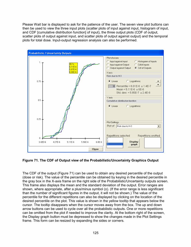
125
Please Wait bar is displayed to ask for the patience of the user. The seven view plot buttons can then be used to view the three input plots (scatter plots of input against input, histogram of input, and CDF [cumulative distribution function] of input), the three output plots (CDF of output, scatter plots of output against input, and scatter plots of output against output) and the temporal plots for total dose. Input-output regression analysis can also be performed.
Figure 71. The CDF of Output view of the Probabilistic/Uncertainty Graphics Output
The CDF of the output (Figure 71) can be used to obtain any desired percentile of the output (dose or risk). The value of the percentile can be obtained by keying in the desired percentile in the gray box in the X-axis frame on the right side of the Probabilistic/Uncertainty outputs screen. This frame also displays the mean and the standard deviation of the output. Error ranges are shown, where appropriate, after a plus/minus symbol (±). (If the error range is less significant than the number of significant figures in the output, it will not be shown.) The value of the percentile for the different repetitions can also be displayed by clicking on the location of the desired percentile on the plot. This value is shown in the yellow tooltip that appears below the cursor. The tooltip disappears when the cursor moves away from the box. The up and down arrow buttons can be used to cycle over all the probabilistic outputs. One or more repetitions can be omitted from the plot if needed to improve the clarity. At the bottom right of the screen, the Display graph button must be depressed to show the changes made in the Plot Settings frame. This form can be resized by expanding the sides or corners.
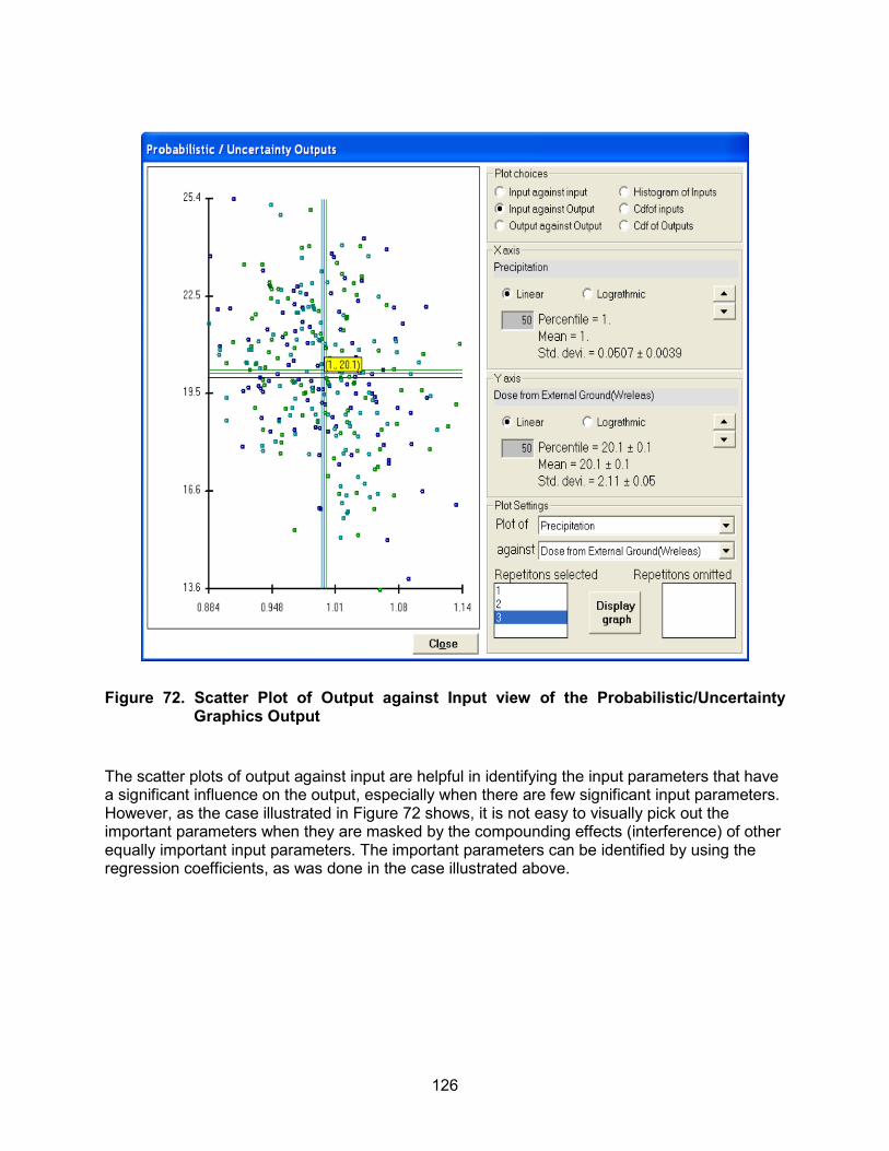
126
Figure 72. Scatter Plot of Output against Input view of the Probabilistic/Uncertainty
Graphics Output
The scatter plots of output against input are helpful in identifying the input parameters that have a significant influence on the output, especially when there are few significant input parameters. However, as the case illustrated in Figure 72 shows, it is not easy to visually pick out the important parameters when they are masked by the compounding effects (interference) of other equally important input parameters. The important parameters can be identified by using the regression coefficients, as was done in the case illustrated above.
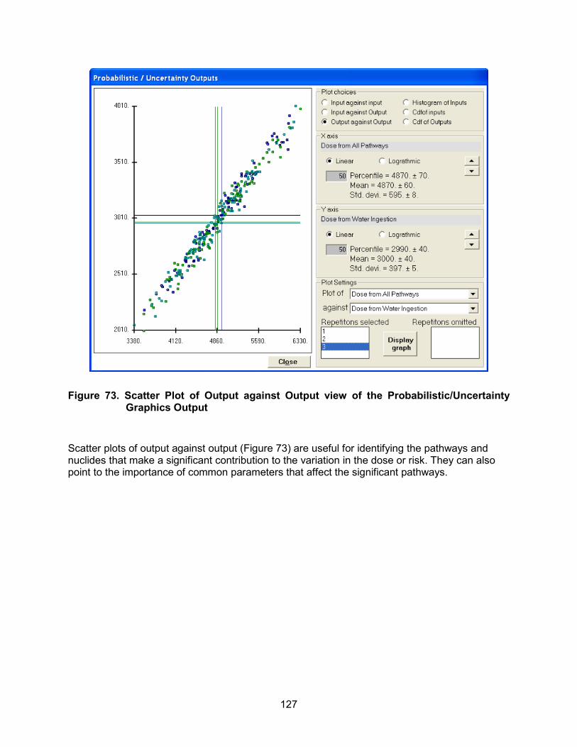
127
Figure 73. Scatter Plot of Output against Output view of the Probabilistic/Uncertainty
Graphics Output
Scatter plots of output against output (Figure 73) are useful for identifying the pathways and nuclides that make a significant contribution to the variation in the dose or risk. They can also point to the importance of common parameters that affect the significant pathways.
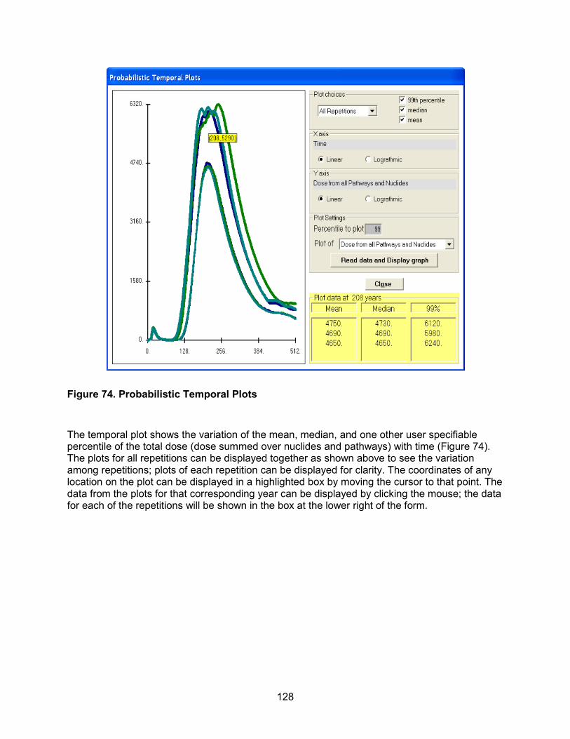
128
Figure 74. Probabilistic Temporal Plots
The temporal plot shows the variation of the mean, median, and one other user specifiable percentile of the total dose (dose summed over nuclides and pathways) with time (Figure 74). The plots for all repetitions can be displayed together as shown above to see the variation among repetitions; plots of each repetition can be displayed for clarity. The coordinates of any location on the plot can be displayed in a highlighted box by moving the cursor to that point. The data from the plots for that corresponding year can be displayed by clicking the mouse; the data for each of the repetitions will be shown in the box at the lower right of the form.
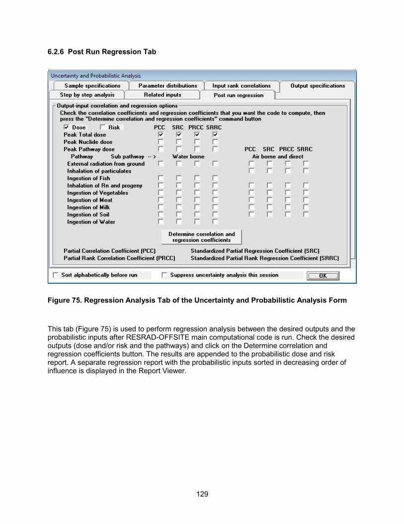
129
6.2.6 Post Run Regression Tab
Figure 75. Regression Analysis Tab of the Uncertainty and Probabilistic Analysis Form
This tab (Figure 75) is used to perform regression analysis between the desired outputs and the probabilistic inputs after RESRAD-OFFSITE main computational code is run. Check the desired outputs (dose and/or risk and the pathways) and click on the Determine correlation and regression coefficients button. The results are appended to the probabilistic dose and risk report. A separate regression report with the probabilistic inputs sorted in decreasing order of influence is displayed in the Report Viewer.
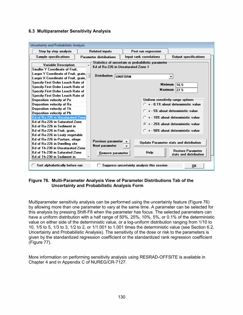
130
6.3 Multiparameter Sensitivity Analysis
Figure 76. Multi-Parameter Analysis View of Parameter Distributions Tab of the Uncertainty and Probabilistic Analysis Form
Multiparameter sensitivity analysis can be performed using the uncertainty feature (Figure 76) by allowing more than one parameter to vary at the same time. A parameter can be selected for this analysis by pressing Shift-F8 when the parameter has focus. The selected parameters can have a uniform distribution with a half range of 50%, 25%, 10%, 5%, or 0.1% of the deterministic value on either side of the deterministic value, or a log-uniform distribution ranging from 1/10 to 10, 1/5 to 5, 1/3 to 3, 1/2 to 2, or 1/1.001 to 1.001 times the deterministic value (see Section 6.2, Uncertainty and Probabilistic Analysis). The sensitivity of the dose or risk to the parameters is given by the standardized regression coefficient or the standardized rank regression coefficient (Figure 77).
More information on performing sensitivity analysis using RESRAD-OFFSITE is available in Chapter 4 and in Appendix C of NUREG/CR-7127.
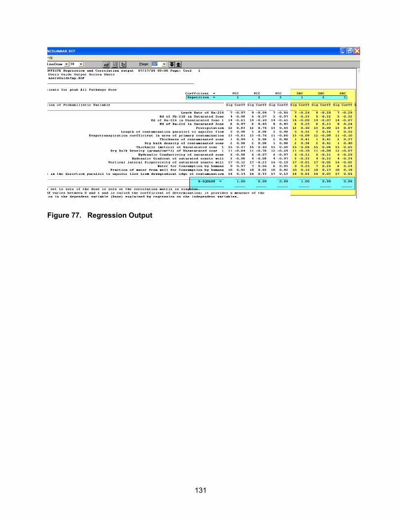
131
Figure 77. Regression Output
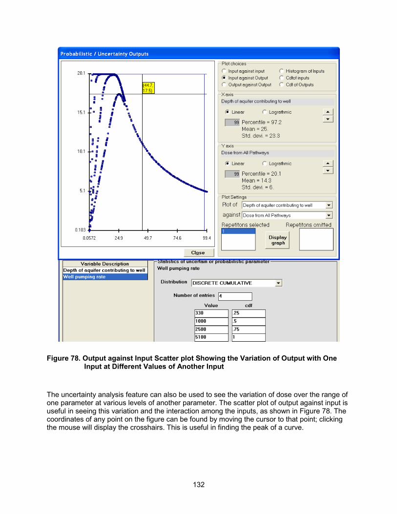
132
Figure 78. Output against Input Scatter plot Showing the Variation of Output with One Input at Different Values of Another Input
The uncertainty analysis feature can also be used to see the variation of dose over the range of one parameter at various levels of another parameter. The scatter plot of output against input is useful in seeing this variation and the interaction among the inputs, as shown in Figure 78. The coordinates of any point on the figure can be found by moving the cursor to that point; clicking the mouse will display the crosshairs. This is useful in finding the peak of a curve.
133
7 HELP
Various levels of help are available in RESRAD-OFFSITE:
• Application Help Form: A help file that is accessible from the code gives a description of each input and explains how the parameter is used in the code.
• Message Log (View - OUTPUT.FIL) Form: A message log that is produced during the execution of the computational code is useful for debugging if the code should terminate before completion.
• RESRAD Website: The RESRAD Website has documents that relate to the RESRAD family of codes. The latest code is available for downloading from the site. The About RESRAD-OFFSITE form from the Help menu of the code contains a link to the RESRAD Website and e-mail address of the RESRAD team.
• Run Time Feedback Form: This gives information about the progress of the computation and a dynamic estimate of the run time for probabilistic cases.
• PDF Versions of the User’s Guide, the User’s Manual, and other Documents: This guide, the technical manual, and the other reports that are listed in the menu can be accessed in PDF form.
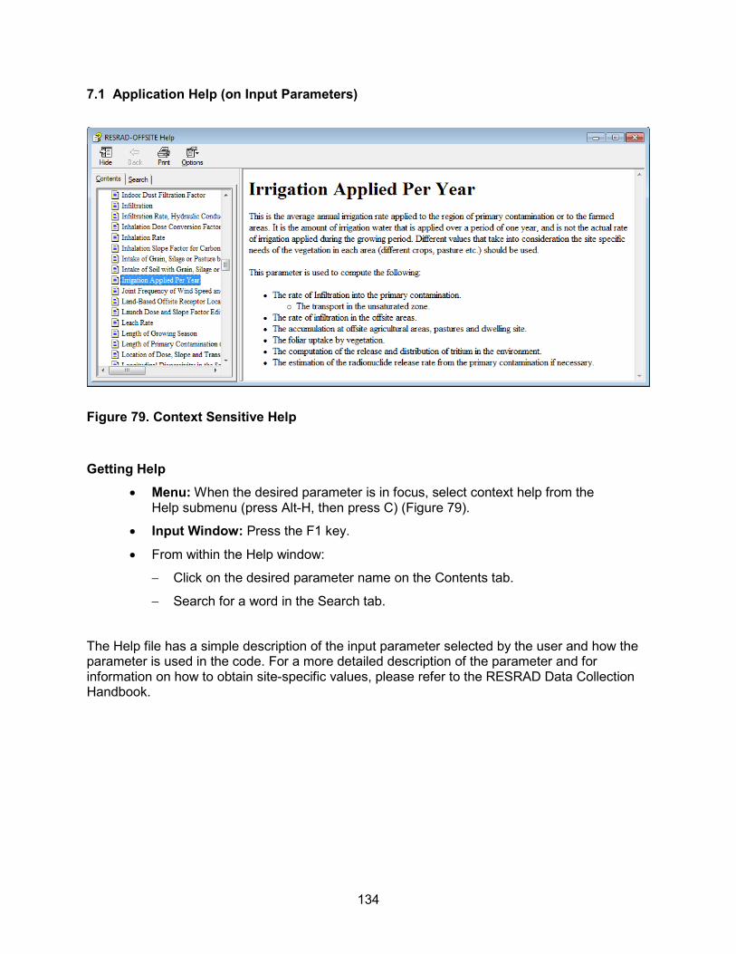
134
7.1 Application Help (on Input Parameters)
Figure 79. Context Sensitive Help
Getting Help
• Menu: When the desired parameter is in focus, select context help from the Help submenu (press Alt-H, then press C) (Figure 79).
• Input Window: Press the F1 key.
• From within the Help window:
− Click on the desired parameter name on the Contents tab.
− Search for a word in the Search tab.
The Help file has a simple description of the input parameter selected by the user and how the parameter is used in the code. For a more detailed description of the parameter and for information on how to obtain site-specific values, please refer to the RESRAD Data Collection Handbook.
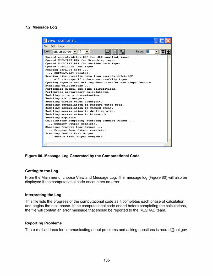
135
7.2 Message Log
Figure 80. Message Log Generated by the Computational Code
Getting to the Log From the Main menu, choose View and Message Log. The message log (Figure 80) will also be displayed if the computational code encounters an error.
Interpreting the Log This file lists the progress of the computational code as it completes each phase of calculation and begins the next phase. If the computational code ended before completing the calculations, the file will contain an error message that should be reported to the RESRAD team.
Reporting Problems The e-mail address for communicating about problems and asking questions is [email protected].
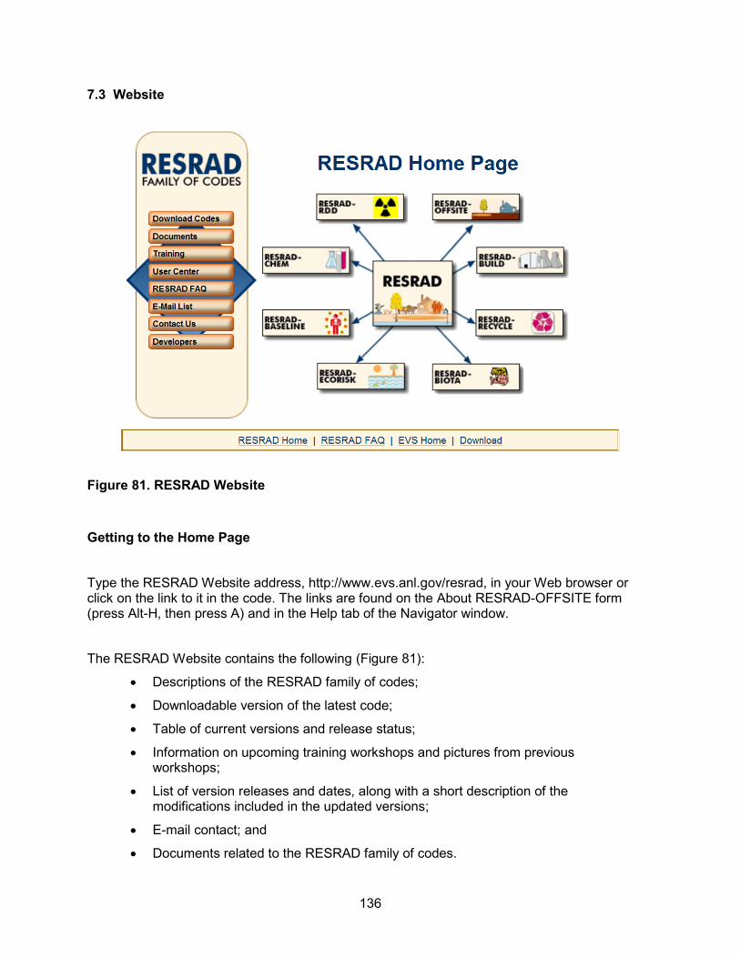
136
7.3 Website
Figure 81. RESRAD Website
Getting to the Home Page
Type the RESRAD Website address, http://www.evs.anl.gov/resrad, in your Web browser or click on the link to it in the code. The links are found on the About RESRAD-OFFSITE form (press Alt-H, then press A) and in the Help tab of the Navigator window.
The RESRAD Website contains the following (Figure 81):
• Descriptions of the RESRAD family of codes;
• Downloadable version of the latest code;
• Table of current versions and release status;
• Information on upcoming training workshops and pictures from previous workshops;
• List of version releases and dates, along with a short description of the modifications included in the updated versions;
• E-mail contact; and
• Documents related to the RESRAD family of codes.
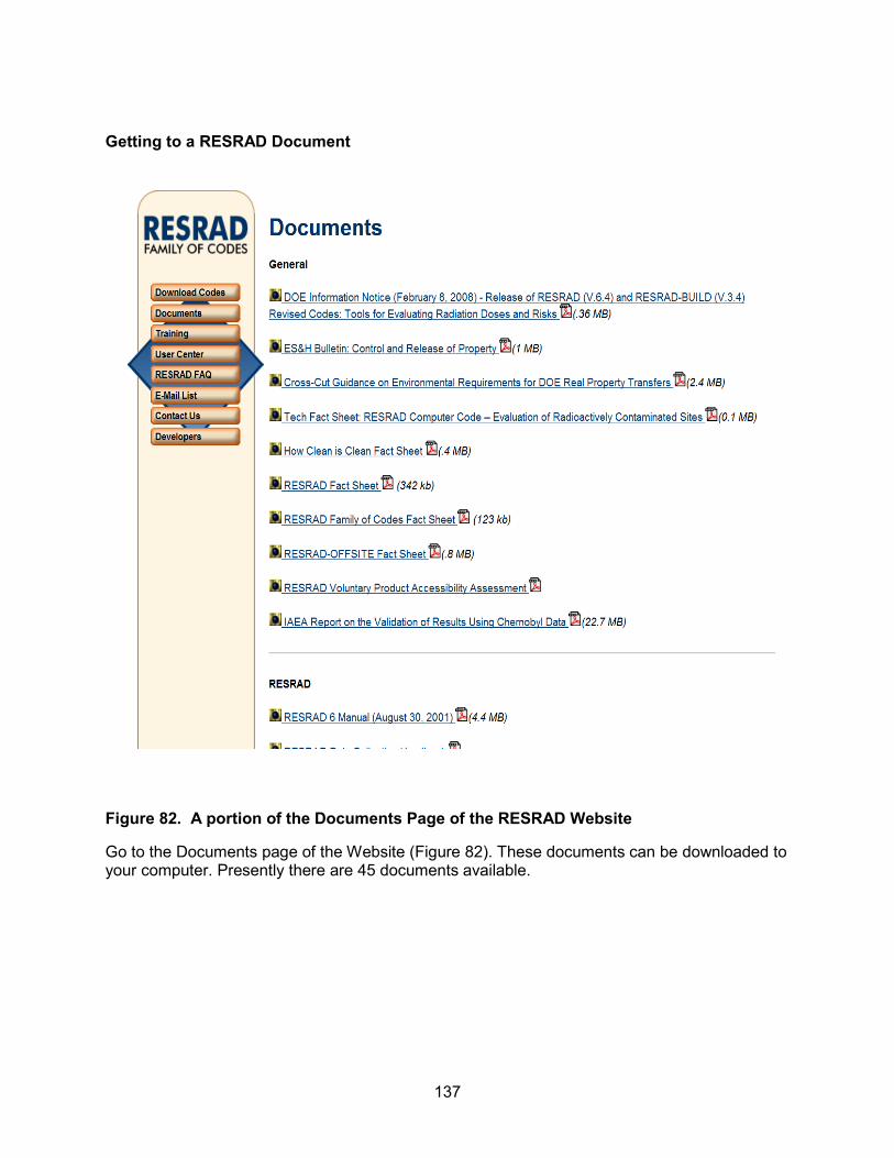
137
Getting to a RESRAD Document
Figure 82. A portion of the Documents Page of the RESRAD Website
Go to the Documents page of the Website (Figure 82). These documents can be downloaded to your computer. Presently there are 45 documents available.
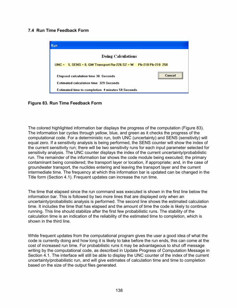
138
7.4 Run Time Feedback Form
Figure 83. Run Time Feedback Form
The colored highlighted information bar displays the progress of the computation (Figure 83). The information bar cycles through yellow, blue, and green as it checks the progress of the computational code. For a deterministic run, both UNC (uncertainty) and SENS (sensitivity) will equal zero. If a sensitivity analysis is being performed, the SENS counter will show the index of the current sensitivity run; there will be two sensitivity runs for each input parameter selected for sensitivity analysis. The UNC counter displays the index of the current uncertainty/probabilistic run. The remainder of the information bar shows the code module being executed; the primary contaminant being considered; the transport layer or location, if appropriate; and, in the case of groundwater transport, the nuclides entering and leaving the transport layer and the current intermediate time. The frequency at which this information bar is updated can be changed in the Title form (Section 4.1). Frequent updates can increase the run time.
The time that elapsed since the run command was executed is shown in the first line below the information bar. This is followed by two more lines that are displayed only when an uncertainty/probabilistic analysis is performed. The second line shows the estimated calculation time. It includes the time that has elapsed and the amount of time the code is likely to continue running. This line should stabilize after the first few probabilistic runs. The stability of the calculation time is an indication of the reliability of the estimated time to completion, which is shown in the third line.
While frequent updates from the computational program gives the user a good idea of what the code is currently doing and how long it is likely to take before the run ends, this can come at the cost of increased run time. For probabilistic runs it may be advantageous to shut off message writing by the computational code, as described in Update Progress of Computation Message in Section 4.1. The interface will still be able to display the UNC counter of the index of the current uncertainty/probabilistic run, and will give estimates of calculation time and time to completion based on the size of the output files generated.
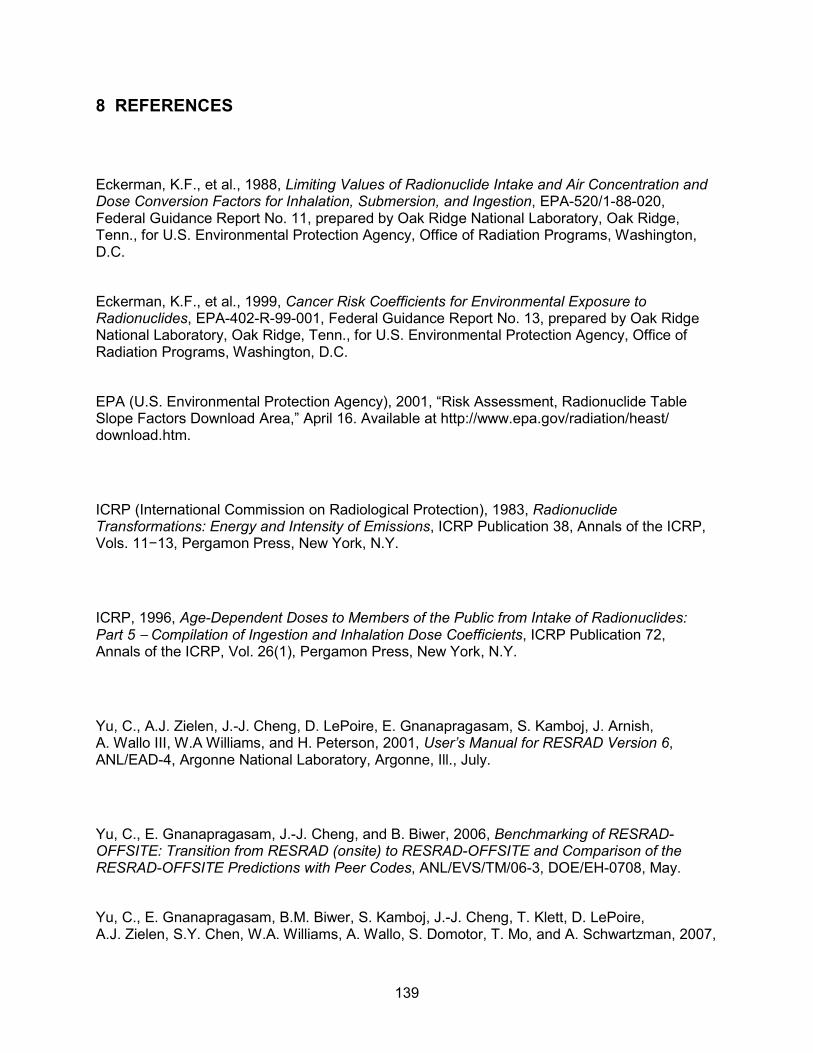
139
8 REFERENCES
Eckerman, K.F., et al., 1988, Limiting Values of Radionuclide Intake and Air Concentration and Dose Conversion Factors for Inhalation, Submersion, and Ingestion, EPA-520/1-88-020, Federal Guidance Report No. 11, prepared by Oak Ridge National Laboratory, Oak Ridge, Tenn., for U.S. Environmental Protection Agency, Office of Radiation Programs, Washington, D.C.
Eckerman, K.F., et al., 1999, Cancer Risk Coefficients for Environmental Exposure to Radionuclides, EPA-402-R-99-001, Federal Guidance Report No. 13, prepared by Oak Ridge National Laboratory, Oak Ridge, Tenn., for U.S. Environmental Protection Agency, Office of Radiation Programs, Washington, D.C.
EPA (U.S. Environmental Protection Agency), 2001, “Risk Assessment, Radionuclide Table Slope Factors Download Area,” April 16. Available at http://www.epa.gov/radiation/heast/ download.htm.
ICRP (International Commission on Radiological Protection), 1983, Radionuclide Transformations: Energy and Intensity of Emissions, ICRP Publication 38, Annals of the ICRP, Vols. 11−13, Pergamon Press, New York, N.Y.
ICRP, 1996, Age-Dependent Doses to Members of the Public from Intake of Radionuclides: Part 5 ⎯ Compilation of Ingestion and Inhalation Dose Coefficients, ICRP Publication 72, Annals of the ICRP, Vol. 26(1), Pergamon Press, New York, N.Y.
Yu, C., A.J. Zielen, J.-J. Cheng, D. LePoire, E. Gnanapragasam, S. Kamboj, J. Arnish, A. Wallo III, W.A Williams, and H. Peterson, 2001, User’s Manual for RESRAD Version 6, ANL/EAD-4, Argonne National Laboratory, Argonne, Ill., July.
Yu, C., E. Gnanapragasam, J.-J. Cheng, and B. Biwer, 2006, Benchmarking of RESRAD-OFFSITE: Transition from RESRAD (onsite) to RESRAD-OFFSITE and Comparison of the RESRAD-OFFSITE Predictions with Peer Codes, ANL/EVS/TM/06-3, DOE/EH-0708, May.
Yu, C., E. Gnanapragasam, B.M. Biwer, S. Kamboj, J.-J. Cheng, T. Klett, D. LePoire, A.J. Zielen, S.Y. Chen, W.A. Williams, A. Wallo, S. Domotor, T. Mo, and A. Schwartzman, 2007,

140
User’s Manual for RESRAD-OFFSITE Version 2, ANL/EVS/TM/07-1, DOE/HS-0005, NUREG/CR-6937, June.
Yu, C., E.K. Gnanapragasam, J.-J. Cheng, S. Kamboj, and S.Y. Chen, 2013, Revised New Source Term Model for the RESRAD-OFFSITE Code Version 3, ANL/EVS/TM/11-5, NUREG/CR-7127, prepared by Argonne National Laboratory for U.S. Nuclear Regulatory Commission, June.

APPENDIX A:
OVERRIDING THE SOURCE TERM AND SPECIFYING RELEASES FROM PRIMARY CONTAMINATION
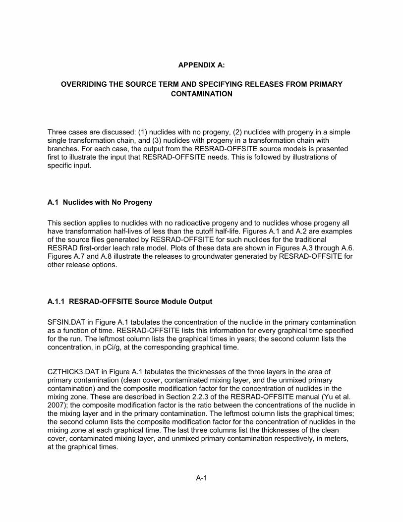
A-1
APPENDIX A:
OVERRIDING THE SOURCE TERM AND SPECIFYING RELEASES FROM PRIMARY CONTAMINATION
Three cases are discussed: (1) nuclides with no progeny, (2) nuclides with progeny in a simple single transformation chain, and (3) nuclides with progeny in a transformation chain with branches. For each case, the output from the RESRAD-OFFSITE source models is presented first to illustrate the input that RESRAD-OFFSITE needs. This is followed by illustrations of specific input.
A.1 Nuclides with No Progeny
This section applies to nuclides with no radioactive progeny and to nuclides whose progeny all have transformation half-lives of less than the cutoff half-life. Figures A.1 and A.2 are examples of the source files generated by RESRAD-OFFSITE for such nuclides for the traditional RESRAD first-order leach rate model. Plots of these data are shown in Figures A.3 through A.6. Figures A.7 and A.8 illustrate the releases to groundwater generated by RESRAD-OFFSITE for other release options.
A.1.1 RESRAD-OFFSITE Source Module Output
SFSIN.DAT in Figure A.1 tabulates the concentration of the nuclide in the primary contamination as a function of time. RESRAD-OFFSITE lists this information for every graphical time specified for the run. The leftmost column lists the graphical times in years; the second column lists the concentration, in pCi/g, at the corresponding graphical time.
CZTHICK3.DAT in Figure A.1 tabulates the thicknesses of the three layers in the area of primary contamination (clean cover, contaminated mixing layer, and the unmixed primary contamination) and the composite modification factor for the concentration of nuclides in the mixing zone. These are described in Section 2.2.3 of the RESRAD-OFFSITE manual (Yu et al. 2007); the composite modification factor is the ratio between the concentrations of the nuclide in the mixing layer and in the primary contamination. The leftmost column lists the graphical times; the second column lists the composite modification factor for the concentration of nuclides in the mixing zone at each graphical time. The last three columns list the thicknesses of the clean cover, contaminated mixing layer, and unmixed primary contamination respectively, in meters, at the graphical times.
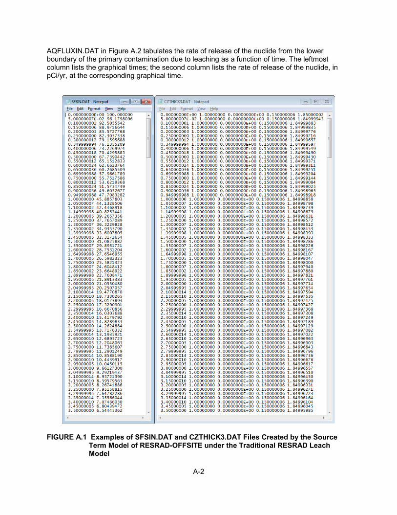
A-2
AQFLUXIN.DAT in Figure A.2 tabulates the rate of release of the nuclide from the lower boundary of the primary contamination due to leaching as a function of time. The leftmost column lists the graphical times; the second column lists the rate of release of the nuclide, in pCi/yr, at the corresponding graphical time.
FIGURE A.1 Examples of SFSIN.DAT and CZTHICK3.DAT Files Created by the Source Term Model of RESRAD-OFFSITE under the Traditional RESRAD Leach Model
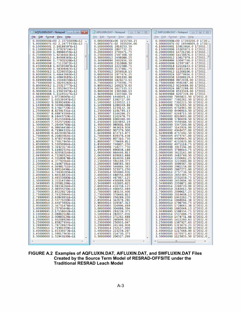
A-3
FIGURE A.2 Examples of AQFLUXIN.DAT, AIFLUXIN.DAT, and SWFLUXIN.DAT Files Created by the Source Term Model of RESRAD-OFFSITE under the Traditional RESRAD Leach Model
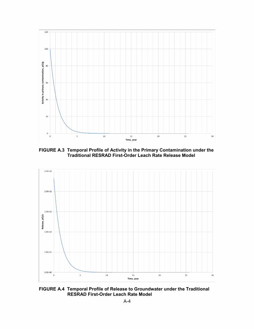
A-4
FIGURE A.3 Temporal Profile of Activity in the Primary Contamination under the Traditional RESRAD First-Order Leach Rate Release Model
FIGURE A.4 Temporal Profile of Release to Groundwater under the Traditional RESRAD First-Order Leach Rate Model
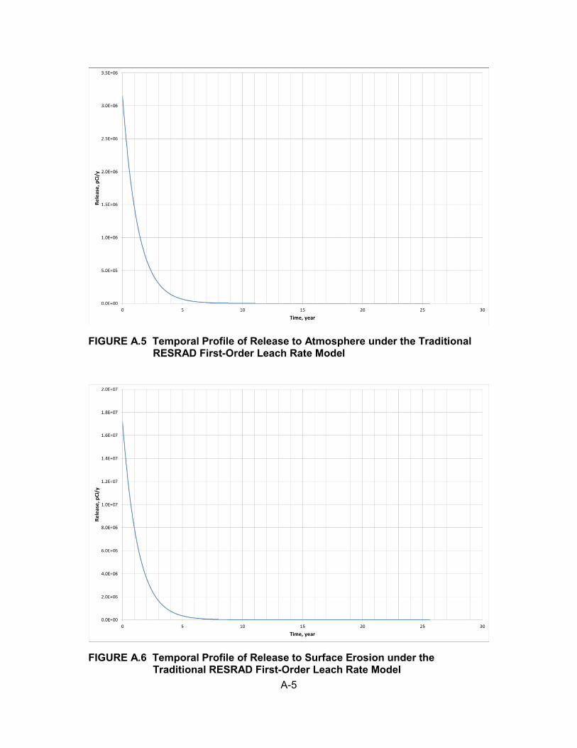
A-5
FIGURE A.5 Temporal Profile of Release to Atmosphere under the Traditional RESRAD First-Order Leach Rate Model
FIGURE A.6 Temporal Profile of Release to Surface Erosion under the Traditional RESRAD First-Order Leach Rate Model
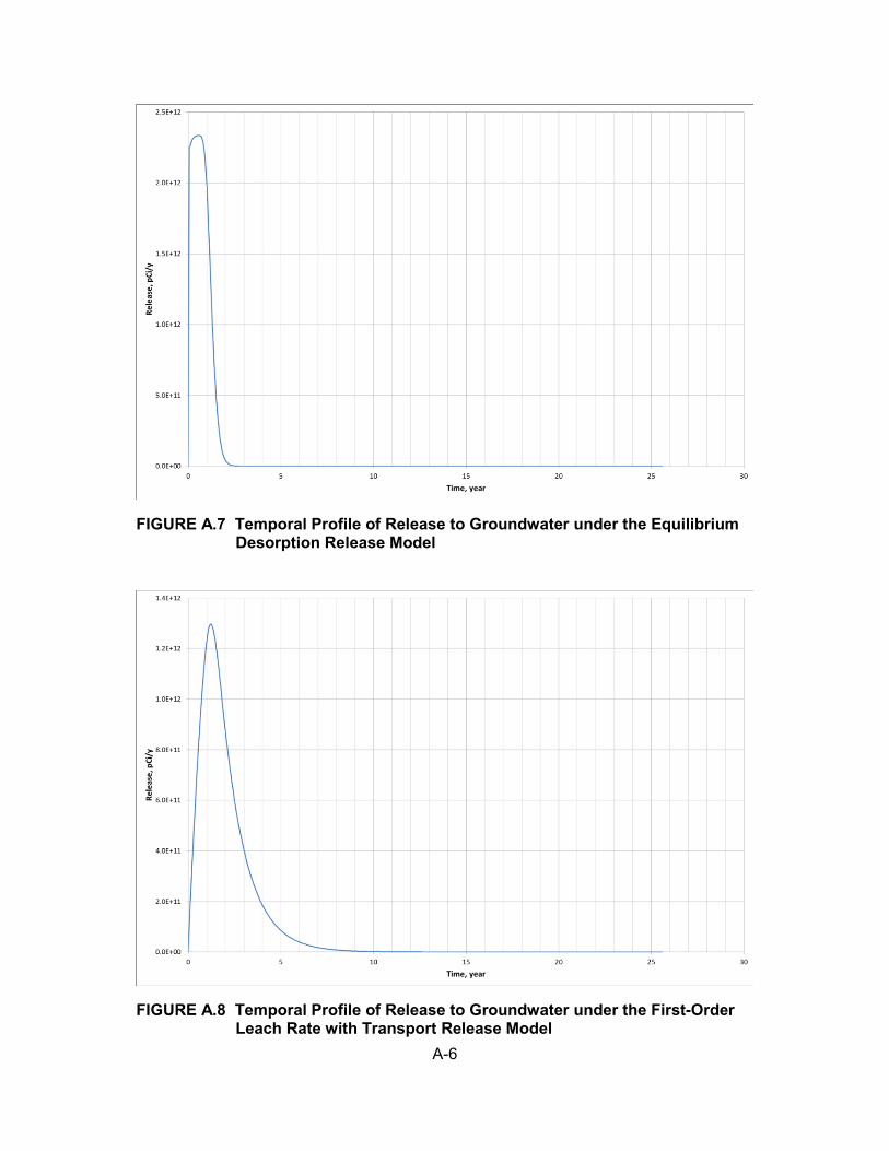
A-6
FIGURE A.7 Temporal Profile of Release to Groundwater under the Equilibrium Desorption Release Model
FIGURE A.8 Temporal Profile of Release to Groundwater under the First-Order Leach Rate with Transport Release Model
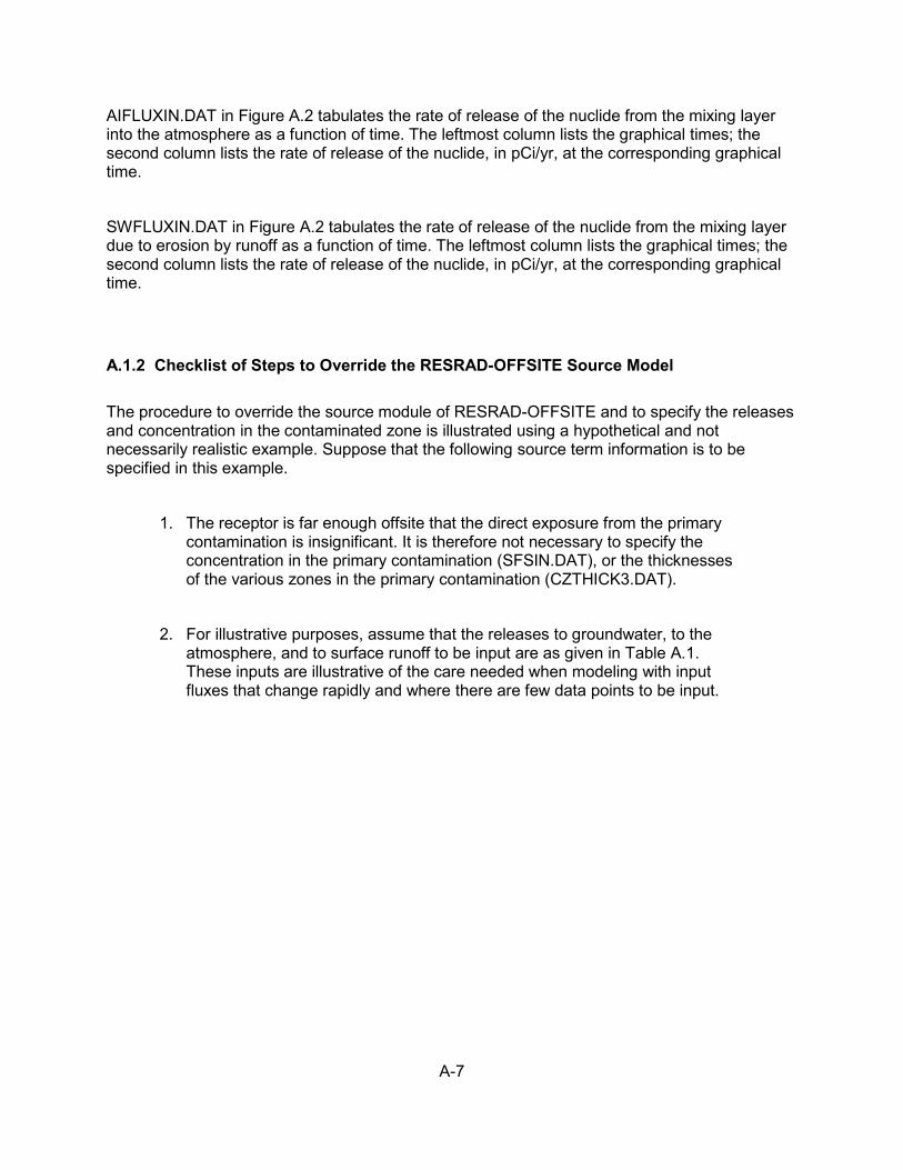
A-7
AIFLUXIN.DAT in Figure A.2 tabulates the rate of release of the nuclide from the mixing layer into the atmosphere as a function of time. The leftmost column lists the graphical times; the second column lists the rate of release of the nuclide, in pCi/yr, at the corresponding graphical time.
SWFLUXIN.DAT in Figure A.2 tabulates the rate of release of the nuclide from the mixing layer due to erosion by runoff as a function of time. The leftmost column lists the graphical times; the second column lists the rate of release of the nuclide, in pCi/yr, at the corresponding graphical time.
A.1.2 Checklist of Steps to Override the RESRAD-OFFSITE Source Model
The procedure to override the source module of RESRAD-OFFSITE and to specify the releases and concentration in the contaminated zone is illustrated using a hypothetical and not necessarily realistic example. Suppose that the following source term information is to be specified in this example.
1. The receptor is far enough offsite that the direct exposure from the primary contamination is insignificant. It is therefore not necessary to specify the concentration in the primary contamination (SFSIN.DAT), or the thicknesses of the various zones in the primary contamination (CZTHICK3.DAT).
2. For illustrative purposes, assume that the releases to groundwater, to the atmosphere, and to surface runoff to be input are as given in Table A.1. These inputs are illustrative of the care needed when modeling with input fluxes that change rapidly and where there are few data points to be input.
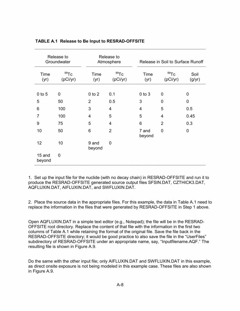
A-8
TABLE A.1 Release to Be Input to RESRAD-OFFSITE
Release to
Groundwater Release to
Atmosphere Release in Soil to Surface Runoff
Time (yr)
99Tc (pCi/yr)
Time (yr)
99Tc (pCi/yr)
Time (yr)
99Tc (pCi/yr)
Soil (g/yr)
0 to 5 0 0 to 2 0.1 0 to 3 0 0
5 50 2 0.5 3 0 0
6 100 3 4 4 5 0.5
7 100 4 5 5 4 0.45
9 75 5 4 6 2 0.3
10 50 6 2 7 and beyond
0 0
12 10 9 and beyond
0
15 and beyond
0
1. Set up the input file for the nuclide (with no decay chain) in RESRAD-OFFSITE and run it to produce the RESRAD-OFFSITE generated source output files SFSIN.DAT, CZTHICK3.DAT, AQFLUXIN.DAT, AIFLUXIN.DAT, and SWFLUXIN.DAT.
2. Place the source data in the appropriate files. For this example, the data in Table A.1 need to replace the information in the files that were generated by RESRAD-OFFSITE in Step 1 above.
Open AQFLUXIN.DAT in a simple text editor (e.g., Notepad); the file will be in the RESRAD-OFFSITE root directory. Replace the content of that file with the information in the first two columns of Table A.1 while retaining the format of the original file. Save the file back in the RESRAD-OFFSITE directory; it would be good practice to also save the file in the “UserFiles” subdirectory of RESRAD-OFFSITE under an appropriate name, say, “Inputfilename.AQF.” The resulting file is shown in Figure A.9.
Do the same with the other input file; only AIFLUXIN.DAT and SWFLUXIN.DAT in this example, as direct onsite exposure is not being modeled in this example case. These files are also shown in Figure A.9.
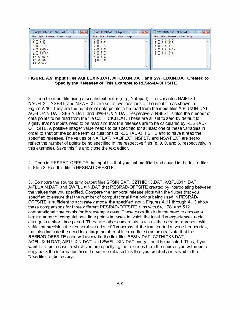
A-9
FIGURE A.9 Input Files AQFLUXIN.DAT, AIFLUXIN.DAT, and SWFLUXIN.DAT Created to Specify the Releases of This Example to RESRAD-OFFSITE
3. Open the input file using a simple text editor (e.g., Notepad). The variables NAIFLXT, NAQFLXT, NSFST, and NSWFLXT are set at two locations of the input file as shown in Figure A.10. They are the number of data points to be read from the input files AIFLUXIN.DAT, AQFLUZIN.DAT, SFSIN.DAT, and SWFLUXIN.DAT, respectively. NSFST is also the number of data points to be read from the file CZTHICK3.DAT. These are all set to zero by default to signify that no inputs need to be read and that the releases are to be calculated by RESRAD-OFFSITE. A positive integer value needs to be specified for at least one of these variables in order to shut off the source term calculations of RESRAD-OFFSITE and to have it read the specified releases. The values of NAIFLXT, NAQFLXT, NSFST, and NSWFLXT are set to reflect the number of points being specified in the respective files (8, 9, 0, and 6, respectively, in this example). Save this file and close the text editor.
4. Open in RESRAD-OFFSITE the input file that you just modified and saved in the text editor in Step 3. Run this file in RESRAD-OFFSITE.
5. Compare the source term output files SFSIN.DAT, CZTHICK3.DAT, AQFLUXIN.DAT, AIFLUXIN.DAT, and SWFLUXIN.DAT that RESRAD-OFFSITE created by interpolating between the values that you specified. Compare the temporal release plots with the fluxes that you specified to ensure that the number of computational time points being used in RESRAD-OFFSITE is sufficient to accurately model the specified input. Figures A.11 through A.13 show these comparisons for three different RESRAD-OFFSITE runs with 64, 128, and 512 computational time points for this example case. These plots illustrate the need to choose a large number of computational time points in cases in which the input flux experiences rapid change in a short time period. There are other constraints, such as the need to represent with sufficient precision the temporal variation of flux across all the transportation zone boundaries, that also indicate the need for a large number of intermediate time points. Note that the RESRAD-OFFSITE code will overwrite the flux files SFSIN.DAT, CZTHICK3.DAT, AQFLUXIN.DAT, AIFLUXIN.DAT, and SWFLUXIN.DAT every time it is executed. Thus, if you want to rerun a case in which you are specifying the releases from the source, you will need to copy back the information from the source release files that you created and saved in the “Userfiles” subdirectory.
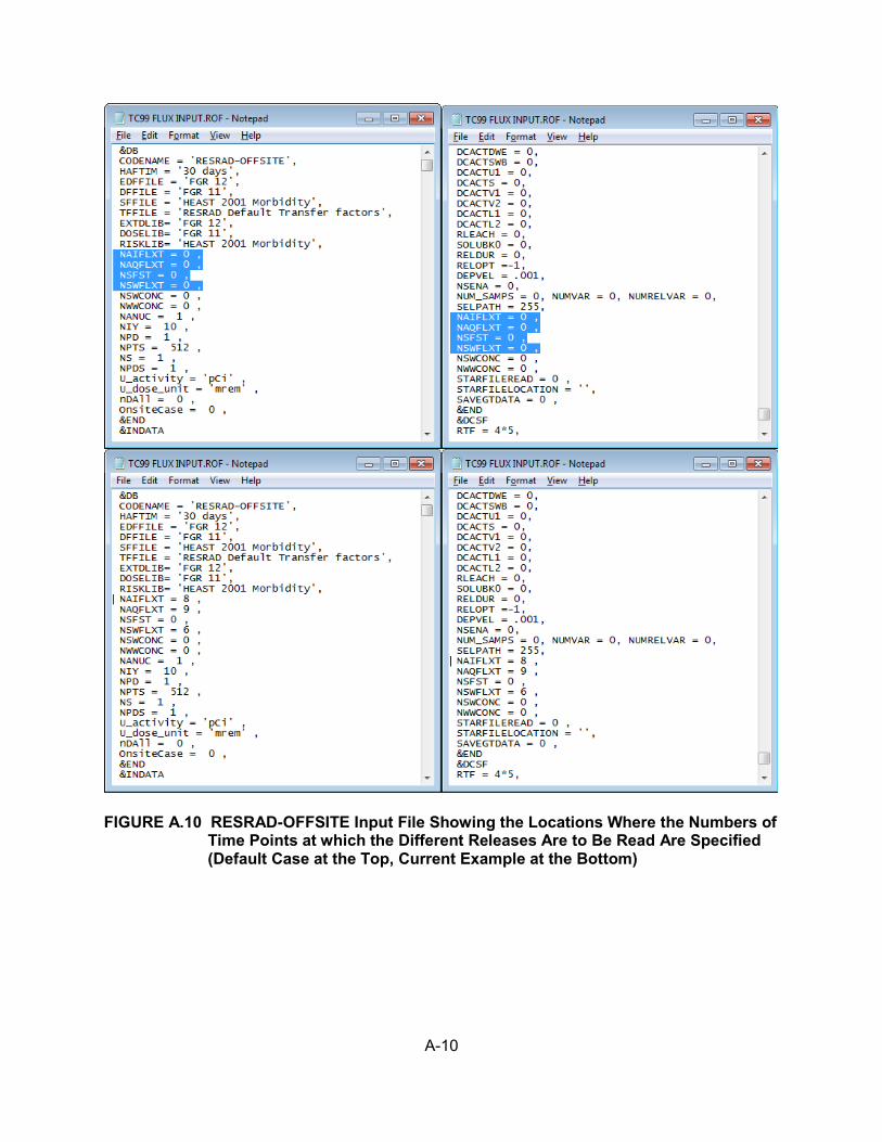
A-10
FIGURE A.10 RESRAD-OFFSITE Input File Showing the Locations Where the Numbers of Time Points at which the Different Releases Are to Be Read Are Specified (Default Case at the Top, Current Example at the Bottom)
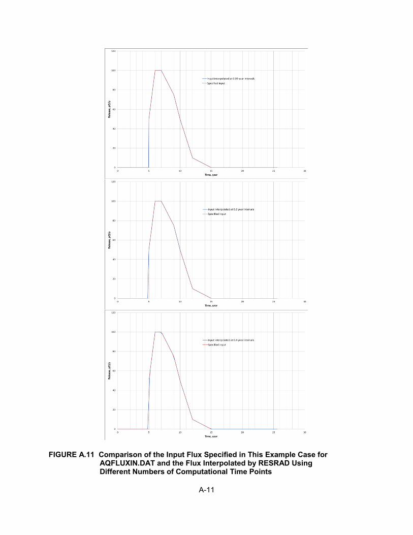
A-11
FIGURE A.11 Comparison of the Input Flux Specified in This Example Case for AQFLUXIN.DAT and the Flux Interpolated by RESRAD Using Different Numbers of Computational Time Points

A-12
FIGURE A.12 Comparison of the Input Flux Specified in This Example Case for AIFLUXIN.DAT and the Flux Interpolated by RESRAD Using Different Numbers of Computational Time Points
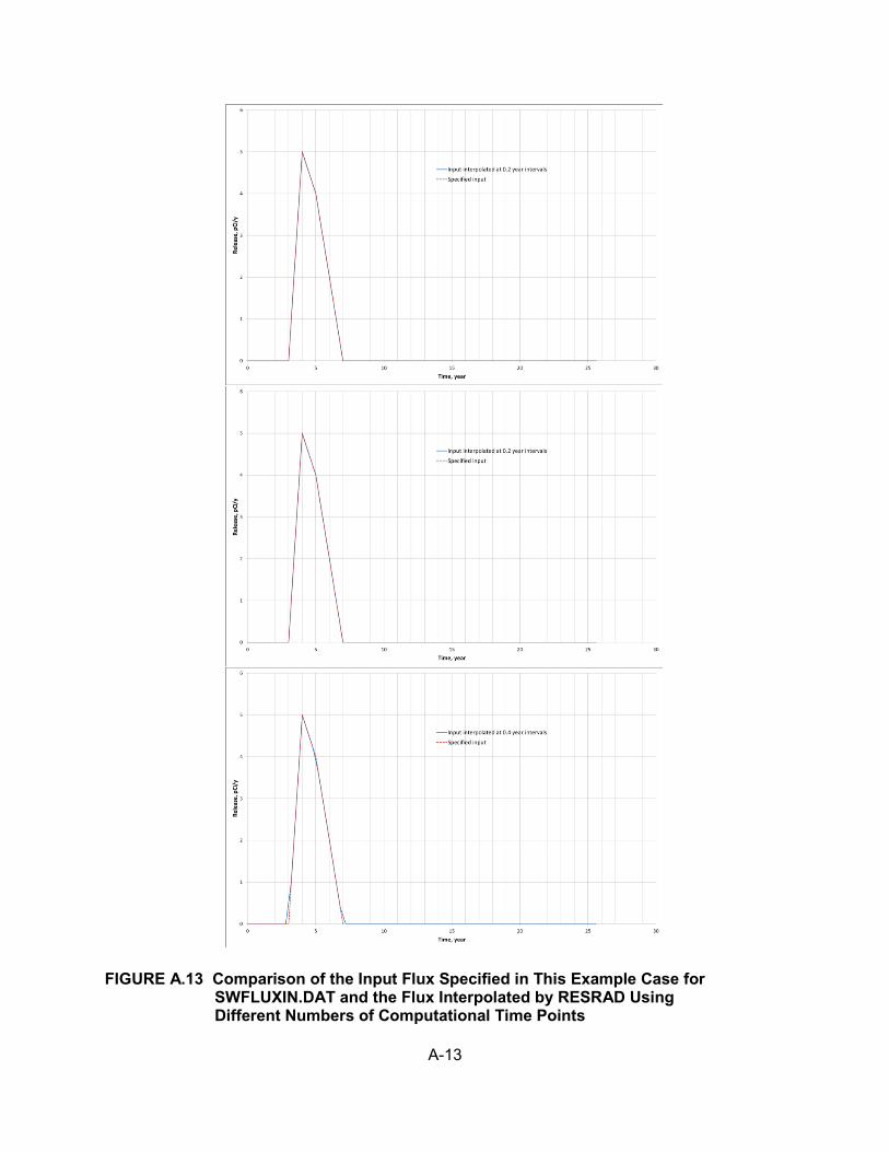
A-13
FIGURE A.13 Comparison of the Input Flux Specified in This Example Case for SWFLUXIN.DAT and the Flux Interpolated by RESRAD Using Different Numbers of Computational Time Points
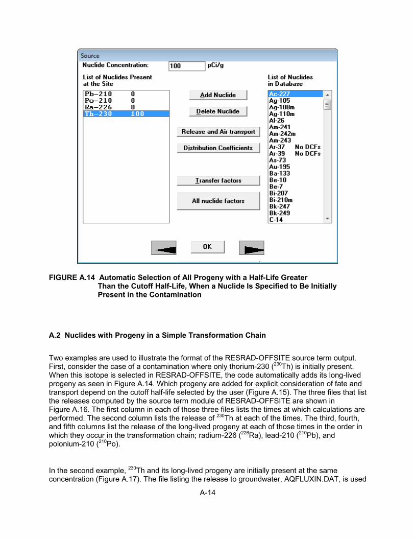
A-14
FIGURE A.14 Automatic Selection of All Progeny with a Half-Life Greater Than the Cutoff Half-Life, When a Nuclide Is Specified to Be Initially Present in the Contamination
A.2 Nuclides with Progeny in a Simple Transformation Chain
Two examples are used to illustrate the format of the RESRAD-OFFSITE source term output. First, consider the case of a contamination where only thorium-230 (230Th) is initially present. When this isotope is selected in RESRAD-OFFSITE, the code automatically adds its long-lived progeny as seen in Figure A.14. Which progeny are added for explicit consideration of fate and transport depend on the cutoff half-life selected by the user (Figure A.15). The three files that list the releases computed by the source term module of RESRAD-OFFSITE are shown in Figure A.16. The first column in each of those three files lists the times at which calculations are performed. The second column lists the release of 230Th at each of the times. The third, fourth, and fifth columns list the release of the long-lived progeny at each of those times in the order in which they occur in the transformation chain; radium-226 (226Ra), lead-210 (210Pb), and polonium-210 (210Po).
In the second example, 230Th and its long-lived progeny are initially present at the same concentration (Figure A.17). The file listing the release to groundwater, AQFLUXIN.DAT, is used
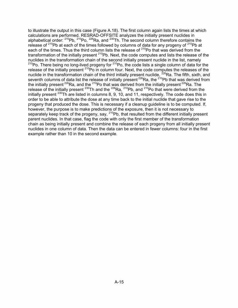
A-15
to illustrate the output in this case (Figure A.18). The first column again lists the times at which calculations are performed. RESRAD-OFFSITE analyzes the initially present nuclides in alphabetical order: 210Pb, 210Po, 226Ra, and 230Th. The second column therefore contains the release of 210Pb at each of the times followed by columns of data for any progeny of 210Pb at each of the times. Thus the third column lists the release of 210Po that was derived from the transformation of the initially present 210Pb. Next, the code computes and lists the release of the nuclides in the transformation chain of the second initially present nuclide in the list, namely 210Po. There being no long-lived progeny for 210Po, the code lists a single column of data for the release of the initially present 210Po in column four. Next, the code computes the releases of the nuclide in the transformation chain of the third initially present nuclide, 226Ra. The fifth, sixth, and seventh columns of data list the release of initially present 226Ra, the 210Pb that was derived from the initially present 226Ra, and the 210Po that was derived from the initially present 226Ra. The release of the initially present 230Th and the 226Ra, 210Pb, and 210Po that were derived from the initially present 230Th are listed in columns 8, 9, 10, and 11, respectively. The code does this in order to be able to attribute the dose at any time back to the initial nuclide that gave rise to the progeny that produced the dose. This is necessary if a cleanup guideline is to be computed. If, however, the purpose is to make predictions of the exposure, then it is not necessary to separately keep track of the progeny, say, 210Pb, that resulted from the different initially present parent nuclides. In that case, flag the code with only the first member of the transformation chain as being initially present and combine the release of each progeny from all initially present nuclides in one column of data. Then the data can be entered in fewer columns: four in the first example rather than 10 in the second example.
A-16
FIGURE A.15 Selection of Cutoff Half-Life
FIGURE A.16 Source Term Output Files for Case with Only 230Th Initially Present
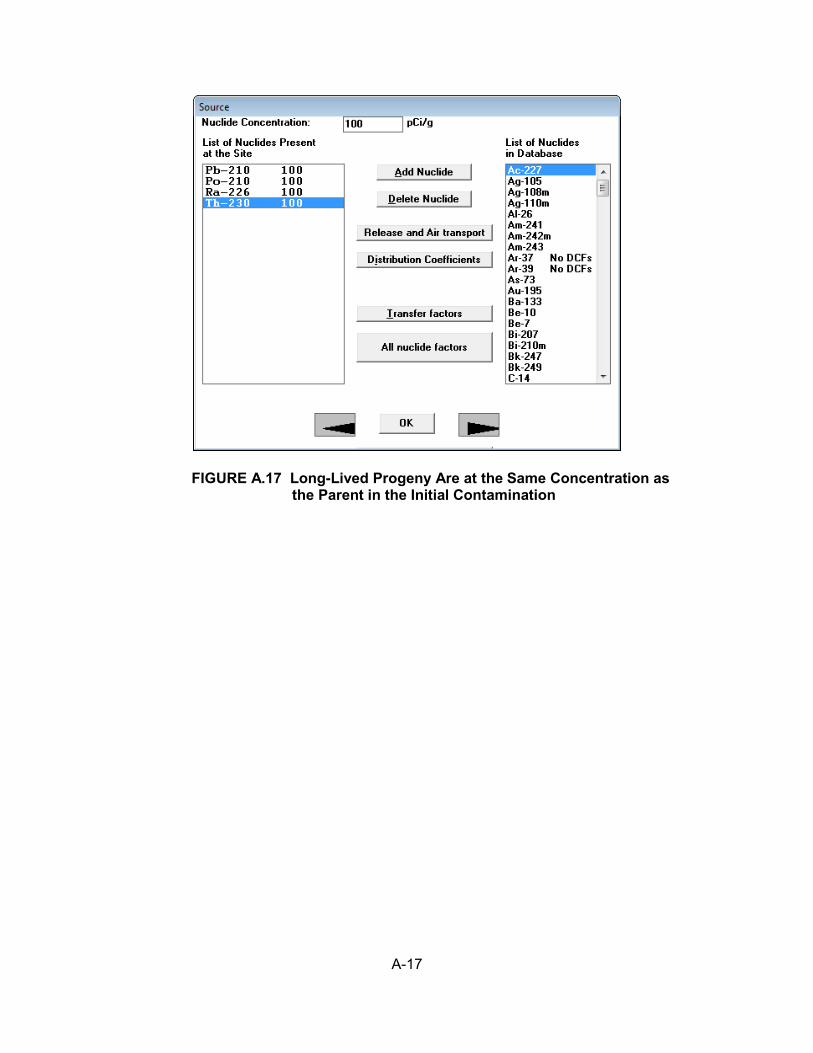
A-17
FIGURE A.17 Long-Lived Progeny Are at the Same Concentration as the Parent in the Initial Contamination
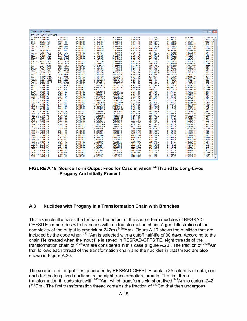
A-18
FIGURE A.18 Source Term Output Files for Case in which 230Th and Its Long-Lived Progeny Are Initially Present
A.3 Nuclides with Progeny in a Transformation Chain with Branches
This example illustrates the format of the output of the source term modules of RESRAD-OFFSITE for nuclides with branches within a transformation chain. A good illustration of the complexity of the output is americium-242m (242mAm). Figure A.19 shows the nuclides that are included by the code when 242mAm is selected with a cutoff half-life of 30 days. According to the chain file created when the input file is saved in RESRAD-OFFSITE, eight threads of the transformation chain of 242mAm are considered in this case (Figure A.20). The fraction of 242mAm that follows each thread of the transformation chain and the nuclides in that thread are also shown in Figure A.20.
The source term output files generated by RESRAD-OFFSITE contain 35 columns of data, one each for the long-lived nuclides in the eight transformation threads. The first three transformation threads start with 242mAm, which transforms via short-lived 242Am to curium-242 (242Cm). The first transformation thread contains the fraction of 242Cm that then undergoes
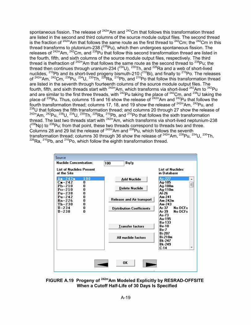
A-19
spontaneous fission. The release of 242mAm and 242Cm that follows this transformation thread are listed in the second and third columns of the source module output files. The second thread is the fraction of 242mAm that follows the same route as the first thread to 242Cm; the 242Cm in this thread transforms to plutonium-238 (238Pu), which then undergoes spontaneous fission. The releases of 242mAm, 242Cm, and 238Pu that follow this second transformation thread are listed in the fourth, fifth, and sixth columns of the source module output files, respectively. The third thread is thefraction of 242mAm that follows the same route as the second thread to 238Pu; the thread then continues through uranium-234 (234U), 230Th, and 226Ra and a web of short-lived nuclides, 210Pb and its short-lived progeny bismuth-210 (210Bi), and finally to 210Po. The releases of 242mAm, 242Cm, 238Pu, 234U, 230Th, 226Ra, 210Pb, and 210Po that follow this transformation thread are listed in the seventh through fourteenth columns of the source module output files. The fourth, fifth, and sixth threads start with 242mAm, which transforms via short-lived 242Am to 242Pu and are similar to the first three threads, with 242Pu taking the place of 242Cm, and 238U taking the place of 238Pu. Thus, columns 15 and 16 show the release of 242mAm and 242Pu that follows the fourth transformation thread; columns 17, 18, and 19 show the release of 242mAm, 242Pu, and 238U that follows the fifth transformation thread; and columns 20 through 27 show the release of 242mAm, 242Pu, 238U, 234U, 230Th, 226Ra, 210Pb, and 210Po that follows the sixth transformation thread. The last two threads start with 242mAm, which transforms via short-lived neptunium-238 (238Np) to 238Pu; from that point, these two threads correspond to threads two and three. Columns 28 and 29 list the release of 242mAm and 238Pu, which follows the seventh transformation thread; columns 30 through 36 show the release of 242mAm, 238Pu, 234U, 230Th, 226Ra, 210Pb, and 210Po, which follow the eighth transformation thread.
FIGURE A.19 Progeny of 242mAm Modeled Explicitly by RESRAD-OFFSITE When a Cutoff Half-Life of 30 Days Is Specified
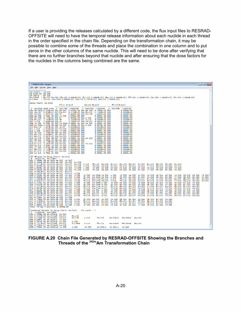
A-20
If a user is providing the releases calculated by a different code, the flux input files to RESRAD-OFFSITE will need to have the temporal release information about each nuclide in each thread in the order specified in the chain file. Depending on the transformation chain, it may be possible to combine some of the threads and place the combination in one column and to put zeros in the other columns of the same nuclide. This will need to be done after verifying that there are no further branches beyond that nuclide and after ensuring that the dose factors for the nuclides in the columns being combined are the same.
FIGURE A.20 Chain File Generated by RESRAD-OFFSITE Showing the Branches and Threads of the 242mAm Transformation Chain

A-21
A.4 Reference for Appendix A
Yu, C., E. Gnanapragasam, B.M. Biwer, S. Kamboj, J.-J. Cheng, T. Klett, D. LePoire, A.J. Zielen, S.Y. Chen, W.A. Williams, A. Wallo, S. Domotor, T. Mo, and A. Schwartzman, 2007, User’s Manual for RESRAD-OFFSITE Version 2, ANL/EVS/TM/07-1, DOE/HS-0005, NUREG/CR-6937, June.


APPENDIX B:
COMPUTING AREA FACTORS FOR OFFSITE EXPOSURE SCENARIOS
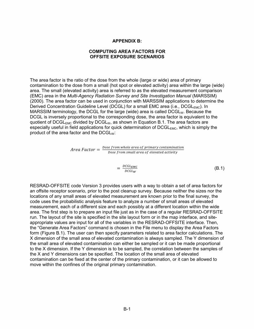
B-1
APPENDIX B:
COMPUTING AREA FACTORS FOR OFFSITE EXPOSURE SCENARIOS
The area factor is the ratio of the dose from the whole (large or wide) area of primary contamination to the dose from a small (hot spot or elevated activity) area within the large (wide) area. The small (elevated activity) area is referred to as the elevated measurement comparison (EMC) area in the Multi-Agency Radiation Survey and Site Investigation Manual (MARSSIM) (2000). The area factor can be used in conjunction with MARSSIM applications to determine the Derived Concentration Guideline Level (DCGL) for a small EMC area (i.e., DCGLEMC). In MARSSIM terminology, the DCGL for the large (wide) area is called DCGLW. Because the DCGL is inversely proportional to the corresponding dose, the area factor is equivalent to the quotient of DCGLEMC divided by DCGLW, as shown in Equation B.1. The area factors are especially useful in field applications for quick determination of DCGLEMC, which is simply the product of the area factor and the DCGLW:
𝐴𝐴𝐴𝐴𝐴𝐴𝐴𝐴 𝐹𝐹𝐴𝐴𝐹𝐹𝐹𝐹𝐹𝐹𝐴𝐴 = 𝐷𝐷𝐷𝐷𝐷𝐷𝐷𝐷 𝑓𝑓𝑓𝑓𝐷𝐷𝑓𝑓 𝑤𝑤ℎ𝐷𝐷𝑜𝑜𝐷𝐷 𝑎𝑎𝑓𝑓𝐷𝐷𝑎𝑎 𝐷𝐷𝑓𝑓 𝑝𝑝𝑓𝑓𝑖𝑖𝑓𝑓𝑎𝑎𝑓𝑓𝑖𝑖 𝑐𝑐𝐷𝐷𝑐𝑐𝑐𝑐𝑎𝑎𝑓𝑓𝑖𝑖𝑐𝑐𝑎𝑎𝑐𝑐𝑖𝑖𝐷𝐷𝑐𝑐𝐷𝐷𝐷𝐷𝐷𝐷𝐷𝐷 𝑓𝑓𝑓𝑓𝐷𝐷𝑓𝑓 𝐷𝐷𝑓𝑓𝑎𝑎𝑜𝑜𝑜𝑜 𝑎𝑎𝑓𝑓𝐷𝐷𝑎𝑎 𝐷𝐷𝑓𝑓 𝐷𝐷𝑜𝑜𝐷𝐷𝑒𝑒𝑎𝑎𝑐𝑐𝐷𝐷𝑒𝑒 𝑎𝑎𝑐𝑐𝑐𝑐𝑖𝑖𝑒𝑒𝑖𝑖𝑐𝑐𝑖𝑖
= 𝐷𝐷𝐷𝐷𝐷𝐷𝐷𝐷𝐸𝐸𝐸𝐸𝐸𝐸 𝐷𝐷𝐷𝐷𝐷𝐷𝐷𝐷𝑊𝑊
(B.1)
RESRAD-OFFSITE code Version 3 provides users with a way to obtain a set of area factors for an offsite receptor scenario, prior to the post cleanup survey. Because neither the sizes nor the locations of any small areas of elevated measurement are known prior to the final survey, the code uses the probabilistic analysis feature to analyze a number of small areas of elevated measurement, each of a different size and each possibly at a different location within the wide area. The first step is to prepare an input file just as in the case of a regular RESRAD-OFFSITE run. The layout of the site is specified in the site layout form or in the map interface, and site-appropriate values are input for all of the variables in the RESRAD-OFFSITE interface. Then, the “Generate Area Factors” command is chosen in the File menu to display the Area Factors form (Figure B.1). The user can then specify parameters related to area factor calculations. The X dimension of the small area of elevated contamination is always sampled. The Y dimension of the small area of elevated contamination can either be sampled or it can be made proportional to the X dimension. If the Y dimension is to be sampled, the correlation between the samples of the X and Y dimensions can be specified. The location of the small area of elevated contamination can be fixed at the center of the primary contamination, or it can be allowed to move within the confines of the original primary contamination.
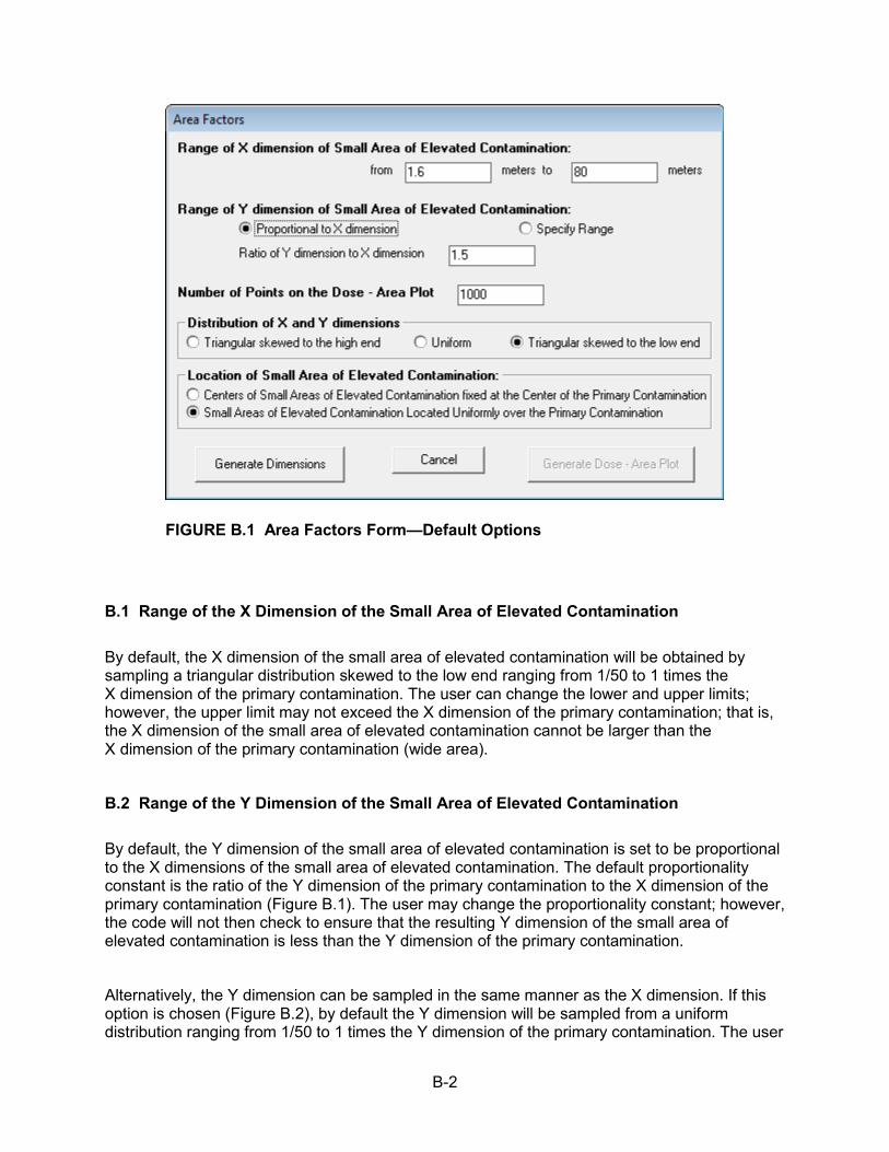
B-2
FIGURE B.1 Area Factors Form—Default Options
B.1 Range of the X Dimension of the Small Area of Elevated Contamination
By default, the X dimension of the small area of elevated contamination will be obtained by sampling a triangular distribution skewed to the low end ranging from 1/50 to 1 times the X dimension of the primary contamination. The user can change the lower and upper limits; however, the upper limit may not exceed the X dimension of the primary contamination; that is, the X dimension of the small area of elevated contamination cannot be larger than the X dimension of the primary contamination (wide area).
B.2 Range of the Y Dimension of the Small Area of Elevated Contamination
By default, the Y dimension of the small area of elevated contamination is set to be proportional to the X dimensions of the small area of elevated contamination. The default proportionality constant is the ratio of the Y dimension of the primary contamination to the X dimension of the primary contamination (Figure B.1). The user may change the proportionality constant; however, the code will not then check to ensure that the resulting Y dimension of the small area of elevated contamination is less than the Y dimension of the primary contamination.
Alternatively, the Y dimension can be sampled in the same manner as the X dimension. If this option is chosen (Figure B.2), by default the Y dimension will be sampled from a uniform distribution ranging from 1/50 to 1 times the Y dimension of the primary contamination. The user
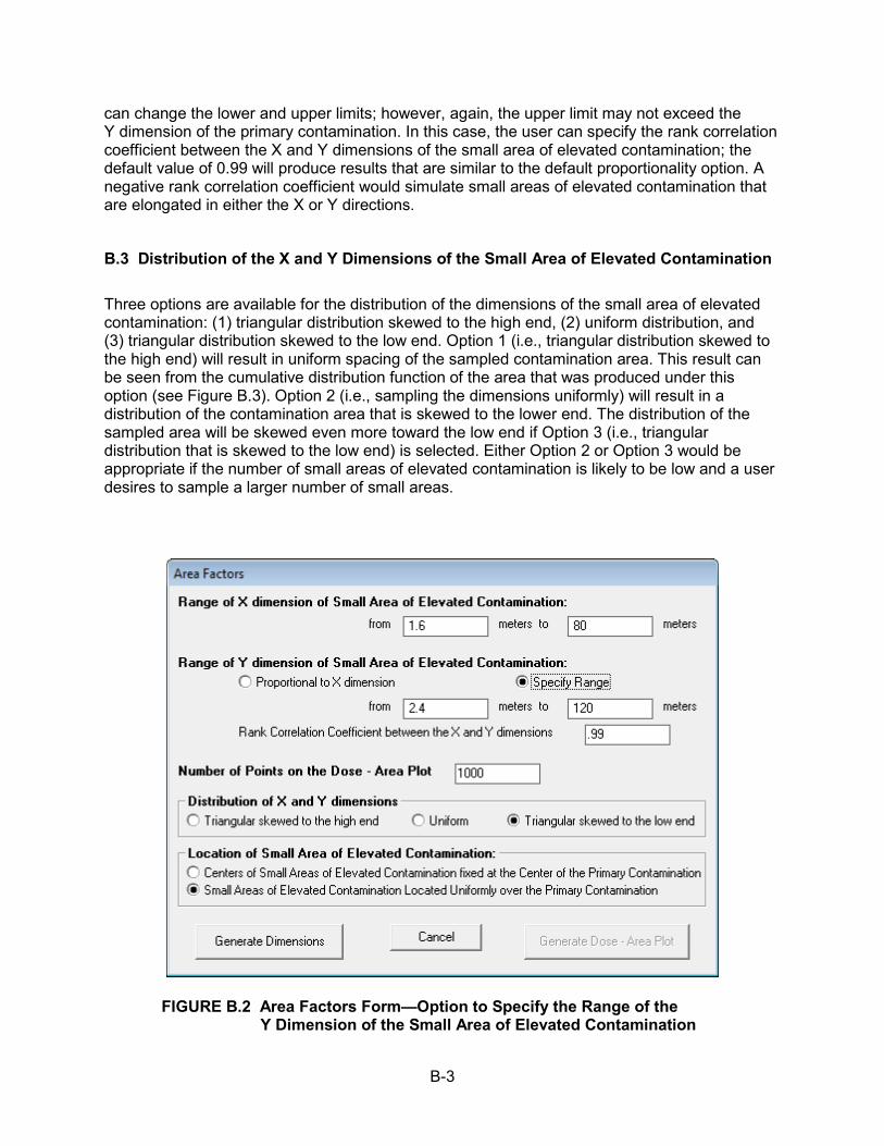
B-3
can change the lower and upper limits; however, again, the upper limit may not exceed the Y dimension of the primary contamination. In this case, the user can specify the rank correlation coefficient between the X and Y dimensions of the small area of elevated contamination; the default value of 0.99 will produce results that are similar to the default proportionality option. A negative rank correlation coefficient would simulate small areas of elevated contamination that are elongated in either the X or Y directions.
B.3 Distribution of the X and Y Dimensions of the Small Area of Elevated Contamination
Three options are available for the distribution of the dimensions of the small area of elevated contamination: (1) triangular distribution skewed to the high end, (2) uniform distribution, and (3) triangular distribution skewed to the low end. Option 1 (i.e., triangular distribution skewed to the high end) will result in uniform spacing of the sampled contamination area. This result can be seen from the cumulative distribution function of the area that was produced under this option (see Figure B.3). Option 2 (i.e., sampling the dimensions uniformly) will result in a distribution of the contamination area that is skewed to the lower end. The distribution of the sampled area will be skewed even more toward the low end if Option 3 (i.e., triangular distribution that is skewed to the low end) is selected. Either Option 2 or Option 3 would be appropriate if the number of small areas of elevated contamination is likely to be low and a user desires to sample a larger number of small areas.
FIGURE B.2 Area Factors Form—Option to Specify the Range of the Y Dimension of the Small Area of Elevated Contamination
B-4
FIGURE B.3 Distribution of Area of the Small Area of Elevated Contamination under Three Distributions Options for Sampling the Dimensions of the Small Area of Elevated Contamination: Triangular Skewed to the High End (top), Uniform (bottom left), and Triangular Skewed to the Low End (bottom right)
B-5
B.4 Location of the Center of the Small Area of Elevated Contamination
There are two choices for the location of the center (or centroid) of the small area of elevated contamination: it can be fixed at the center of the primary contamination, or it can be allowed to vary. The fixed option will produce a tighter curve between the dose and the small area of elevated contamination. Under the variable option, the small area of elevated contamination is constrained to be within the primary contamination. Thus, the center has to lie within a rectangle with dimensions that are the difference between the corresponding dimensions of the primary contamination and the small area of elevated contamination. The code samples two unit uniform distributions and uses those samples to locate the center of the small area of elevated contamination. A sample value of zero for the X location would place the left edge of the small area of elevated contamination on the left boundary of the primary contamination; a unit value would place the right edge of the small area of elevated contamination on the right boundary of the primary contamination. Likewise, a sample value of zero for the Y location would place the lower edge of the small area of elevated contamination on the lower boundary of the primary contamination; a unit value would place the top edge of the small area of elevated contamination on the upper boundary of the primary contamination. Because the calculated dose will vary with the location of the small area of elevated contamination, the first option (centers fixed) could produce area factors that are higher than reasonable, whereas the second option (moving centers) will produce conservative area factors.
B.5 Number of Points on the Dose—Area Plot
This specifies the number of times the distribution of the dimensions of the small area of elevated contamination is to be sampled. The default value is 1,000. A smaller value can be used if the dose–area relationship is expected to be in a tight band or a single curve. This result would be the case if the Y dimension of the small area of elevated contamination is set to be proportional to the X dimension and the center is fixed. A larger value might be required if the dose–area relationship is expected to be in the shape of a wide band. This result could be the case when both dimensions of the small area of elevated contamination are sampled and/or the location of these small areas of elevated contamination was allowed to vary.
B.6 Generate Dimensions
The Generate Dimensions command button is used to generate the layout—dimensions and location—of each sample of small area of elevated contamination and the offsite transport distances from each sample of small area of elevated contamination to the offsite receptor locations. The Generate Dimension command must be clicked after the user does the following: specifies the limits and type of distribution for the X dimension of the small area of elevated contamination, chooses the method of determining the Y dimension and specifies the required values for that method, selects the desired location option for the centers of the small areas of elevated contamination, and sets the number of samples. This command button first launches the probabilistic sampling code to sample all of the specified distributions. That information is then read by the interface, which uses the sampling results to develop the relationships for the offsite transport distances. Three types of plots of the dimension that were generated can be
B-6
viewed before proceeding to generate the dose from each small area of elevated contamination: scatter plots, histograms, and cumulative distribution functions. These plots are used to verify that the desired layout and transport distances have been generated. The Generate Dose-Area Plot command button becomes active after the layout and transport distances have been generated (Figure B.4).
B.7 Generate Dose—Area Plot
This command launches the computational code of RESRAD-OFFSITE to process the inputs for each of the sampled small areas of elevated contamination to generate the dose from each of those small areas of elevated contamination. A scatter plot of dose against the area of elevated contamination and a text report of area factors are displayed at the end of the run. Four sample plots, obtained by using four options for sizing and locating the small area, for three different radionuclides (i.e., cesium-137 [Cs-137], plutonium-239 [Pu-239], and technetium-99 [Tc-99]) are shown in Figures B.5 through B.7. The four options are case (a) the Y dimensions of the small areas of elevated contamination are proportional to the X dimensions of the small areas of elevated contamination, and the centers of the small areas of elevated contamination coincide with the center of the whole contamination; case (b) the Y dimensions of the small areas of elevated contamination are proportional to the X dimensions, and the small areas of elevated contamination are located within the whole contamination but are not constrained to be concentric; case (c) the Y dimensions of the small areas of elevated contamination are sampled and paired with the samples of the X dimension at a specified correlation, and the centers of the small areas of elevated contamination coincide with the center of the whole contamination; and case (d) the Y dimensions of the small area of elevated contamination are sampled and paired with the samples of the X dimension at a specified correlation, and the small area of elevated contamination is located within the whole contamination but is not constrained to be concentric.
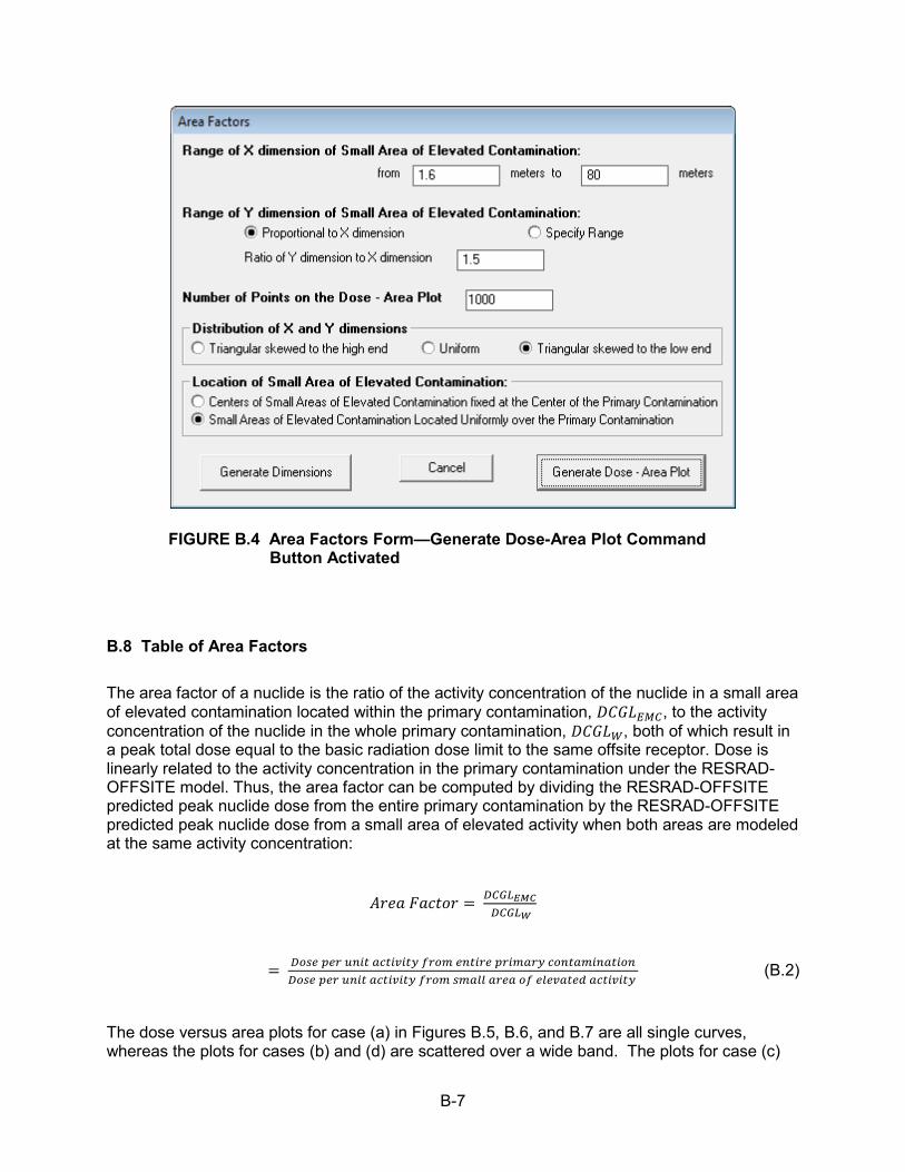
B-7
FIGURE B.4 Area Factors Form—Generate Dose-Area Plot Command Button Activated
B.8 Table of Area Factors
The area factor of a nuclide is the ratio of the activity concentration of the nuclide in a small area of elevated contamination located within the primary contamination, 𝐷𝐷𝐷𝐷𝐷𝐷𝐷𝐷𝐸𝐸𝐸𝐸𝐷𝐷, to the activity concentration of the nuclide in the whole primary contamination, 𝐷𝐷𝐷𝐷𝐷𝐷𝐷𝐷𝑊𝑊, both of which result in a peak total dose equal to the basic radiation dose limit to the same offsite receptor. Dose is linearly related to the activity concentration in the primary contamination under the RESRAD-OFFSITE model. Thus, the area factor can be computed by dividing the RESRAD-OFFSITE predicted peak nuclide dose from the entire primary contamination by the RESRAD-OFFSITE predicted peak nuclide dose from a small area of elevated activity when both areas are modeled at the same activity concentration:
𝐴𝐴𝐴𝐴𝐴𝐴𝐴𝐴 𝐹𝐹𝐴𝐴𝐹𝐹𝐹𝐹𝐹𝐹𝐴𝐴 = 𝐷𝐷𝐷𝐷𝐷𝐷𝐷𝐷𝐸𝐸𝐸𝐸𝐸𝐸 𝐷𝐷𝐷𝐷𝐷𝐷𝐷𝐷𝑊𝑊
= 𝐷𝐷𝐷𝐷𝐷𝐷𝐷𝐷 𝑝𝑝𝐷𝐷𝑓𝑓 𝑢𝑢𝑐𝑐𝑖𝑖𝑐𝑐 𝑎𝑎𝑐𝑐𝑐𝑐𝑖𝑖𝑒𝑒𝑖𝑖𝑐𝑐𝑖𝑖 𝑓𝑓𝑓𝑓𝐷𝐷𝑓𝑓 𝐷𝐷𝑐𝑐𝑐𝑐𝑖𝑖𝑓𝑓𝐷𝐷 𝑝𝑝𝑓𝑓𝑖𝑖𝑓𝑓𝑎𝑎𝑓𝑓𝑖𝑖 𝑐𝑐𝐷𝐷𝑐𝑐𝑐𝑐𝑎𝑎𝑓𝑓𝑖𝑖𝑐𝑐𝑎𝑎𝑐𝑐𝑖𝑖𝐷𝐷𝑐𝑐𝐷𝐷𝐷𝐷𝐷𝐷𝐷𝐷 𝑝𝑝𝐷𝐷𝑓𝑓 𝑢𝑢𝑐𝑐𝑖𝑖𝑐𝑐 𝑎𝑎𝑐𝑐𝑐𝑐𝑖𝑖𝑒𝑒𝑖𝑖𝑐𝑐𝑖𝑖 𝑓𝑓𝑓𝑓𝐷𝐷𝑓𝑓 𝐷𝐷𝑓𝑓𝑎𝑎𝑜𝑜𝑜𝑜 𝑎𝑎𝑓𝑓𝐷𝐷𝑎𝑎 𝐷𝐷𝑓𝑓 𝐷𝐷𝑜𝑜𝐷𝐷𝑒𝑒𝑎𝑎𝑐𝑐𝐷𝐷𝑒𝑒 𝑎𝑎𝑐𝑐𝑐𝑐𝑖𝑖𝑒𝑒𝑖𝑖𝑐𝑐𝑖𝑖
(B.2)
The dose versus area plots for case (a) in Figures B.5, B.6, and B.7 are all single curves, whereas the plots for cases (b) and (d) are scattered over a wide band. The plots for case (c)

B-8
are similar to case (a), with some scatter that is noticeable at higher doses. In cases (a) and (c), the small area of elevated contamination is constrained to be concentric with the primary contamination. In cases (b) and (d), the small area of elevated contamination is constrained to be within the primary contamination, but it does not have to be concentric with it. The dose from the small area of elevated contamination will be influenced by its location relative to the receptor for almost all exposure pathways. For example, in Figure B.5, where the direct external exposure pathway dominates, a small area of elevated contamination that is located closer to the receptor will subject the receptor to a greater dose than one that is located farther away, all other conditions being equal. Similarly in Figure B.6, where the atmospheric transport is the dominant exposure pathway, a small area of elevated contamination that is located in an unfavorable location with respect to atmospheric stability, wind speed, and distance will subject the receptor to a greater dose than one that is located at a favorable location, all other conditions being equal. Likewise in Figure B.7, where groundwater transport is the dominant exposure pathway, a small area of elevated contamination that has considerable overlap of flow lines with the source of water will subject the receptor to a greater dose than one that has little overlap of flow lines, all other conditions being equal. The transport distance will also influence the dose depending on the relative effects of ingrowth, decay, and dispersion. In cases (a) and (b), the small area of elevated contamination is constrained to be similar in shape to the primary contamination. In cases (c) and (d), the small area of elevated contamination is of a different shape, because its two dimensions are sampled separately and paired according to a user-specified correlation. The small area of elevated contamination will more closely resemble the shape of the primary contamination if the dimensions are directly correlated to a high degree (rank correlation coefficient of almost 1). The dose from the small area of elevated contamination will be influenced by its shape for almost all exposure pathways; the relationship between shape and dose is complex.
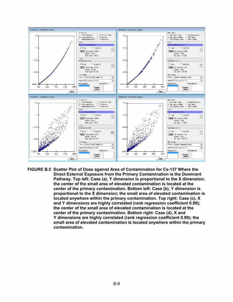
B-9
FIGURE B.5 Scatter Plot of Dose against Area of Contamination for Cs-137 Where the Direct External Exposure from the Primary Contamination is the Dominant Pathway. Top left: Case (a), Y dimension is proportional to the X dimension; the center of the small area of elevated contamination is located at the center of the primary contamination. Bottom left: Case (b), Y dimension is proportional to the X dimension; the small area of elevated contamination is located anywhere within the primary contamination. Top right: Case (c), X and Y dimensions are highly correlated (rank regression coefficient 0.99); the center of the small area of elevated contamination is located at the center of the primary contamination. Bottom right: Case (d), X and Y dimensions are highly correlated (rank regression coefficient 0.99); the small area of elevated contamination is located anywhere within the primary contamination.
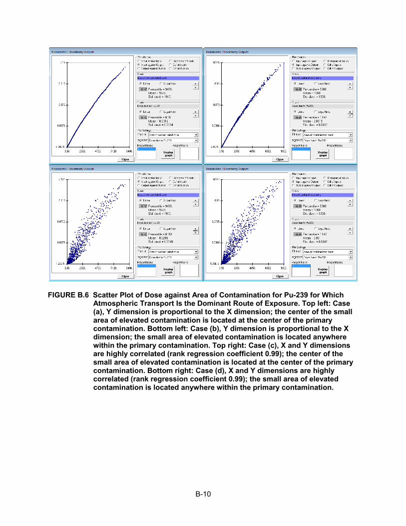
B-10
FIGURE B.6 Scatter Plot of Dose against Area of Contamination for Pu-239 for Which Atmospheric Transport Is the Dominant Route of Exposure. Top left: Case (a), Y dimension is proportional to the X dimension; the center of the small area of elevated contamination is located at the center of the primary contamination. Bottom left: Case (b), Y dimension is proportional to the X dimension; the small area of elevated contamination is located anywhere within the primary contamination. Top right: Case (c), X and Y dimensions are highly correlated (rank regression coefficient 0.99); the center of the small area of elevated contamination is located at the center of the primary contamination. Bottom right: Case (d), X and Y dimensions are highly correlated (rank regression coefficient 0.99); the small area of elevated contamination is located anywhere within the primary contamination.
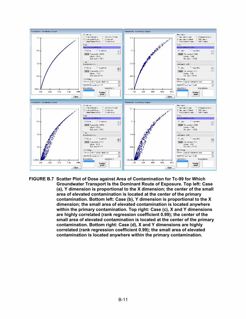
B-11
FIGURE B.7 Scatter Plot of Dose against Area of Contamination for Tc-99 for Which Groundwater Transport Is the Dominant Route of Exposure. Top left: Case (a), Y dimension is proportional to the X dimension; the center of the small area of elevated contamination is located at the center of the primary contamination. Bottom left: Case (b), Y dimension is proportional to the X dimension; the small area of elevated contamination is located anywhere within the primary contamination. Top right: Case (c), X and Y dimensions are highly correlated (rank regression coefficient 0.99); the center of the small area of elevated contamination is located at the center of the primary contamination. Bottom right: Case (d), X and Y dimensions are highly correlated (rank regression coefficient 0.99); the small area of elevated contamination is located anywhere within the primary contamination.

B-12
Thus, the area factor depends not only on the size of the small area of elevated measurement but also on its shape and its location within the primary contamination. Because neither the dimensions nor the location of any potential small area of elevated contamination are known prior to the final site survey, the area factor table generated by RESRAD-OFFSITE must be that for the most detrimental location and dimensions. The code will be better able to find the most detrimental location if a sufficiently large number of simulations are performed. The code groups the simulations (the default is 1,000 simulations) into 20 intervals based on the area of the small area of elevated contamination. Then the code determines the simulation within each interval for which the dose/area ratio is the greatest. This method generally allows the code to find the 20 points from the simulations that are closest to the upper boundary of the dose-area curve. The areas and doses of these 20 simulations are used to generate the area factor text report.
The RESRAD-OFFSITE code calculates area factors, and the corresponding small areas are output to the file named “AreaFactorText.REP” in the RESRAD-OFFSITE directory. A copy of this file is saved as “inputfilename.AF” to the directory where the input file is saved. This file contains a list of up to 21 pairs of areas and area factors for each radionuclide analyzed; the 20 from the probabilistic run and the whole area deterministic run. The area factors for different radionuclides are listed on separate pages of the text report. Figures B.8 through B.10 show the text reports derived from the information shown in the scatter plots in Figures B.5 through B.7. These area factors are for the specific scenario analyzed. They are derived on the basis of pathways selected and parameter values used for that particular case. Therefore, for different scenarios, the calculated area factors will most likely be different. The user must check the area factor table to see whether the number of simulations was sufficient for the code to determine the upper boundary of the scatter plot. One way to do this is to check whether the area factors are increasing as the area decreases. If they do not, the user could rerun the analysis with a larger number of simulations.
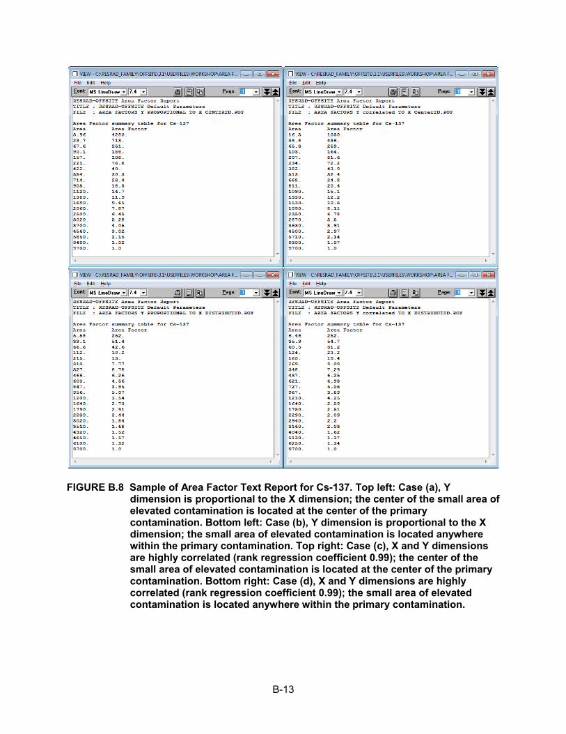
B-13
FIGURE B.8 Sample of Area Factor Text Report for Cs-137. Top left: Case (a), Y dimension is proportional to the X dimension; the center of the small area of elevated contamination is located at the center of the primary contamination. Bottom left: Case (b), Y dimension is proportional to the X dimension; the small area of elevated contamination is located anywhere within the primary contamination. Top right: Case (c), X and Y dimensions are highly correlated (rank regression coefficient 0.99); the center of the small area of elevated contamination is located at the center of the primary contamination. Bottom right: Case (d), X and Y dimensions are highly correlated (rank regression coefficient 0.99); the small area of elevated contamination is located anywhere within the primary contamination.
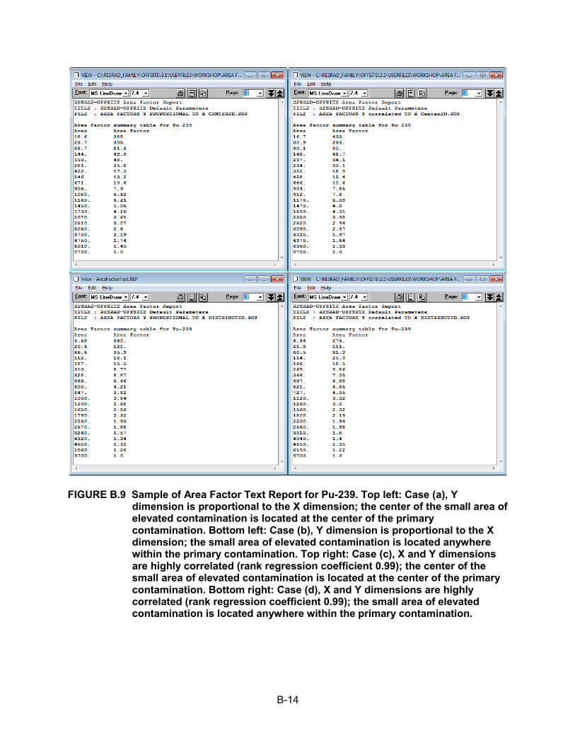
B-14
FIGURE B.9 Sample of Area Factor Text Report for Pu-239. Top left: Case (a), Y dimension is proportional to the X dimension; the center of the small area of elevated contamination is located at the center of the primary contamination. Bottom left: Case (b), Y dimension is proportional to the X dimension; the small area of elevated contamination is located anywhere within the primary contamination. Top right: Case (c), X and Y dimensions are highly correlated (rank regression coefficient 0.99); the center of the small area of elevated contamination is located at the center of the primary contamination. Bottom right: Case (d), X and Y dimensions are highly correlated (rank regression coefficient 0.99); the small area of elevated contamination is located anywhere within the primary contamination.
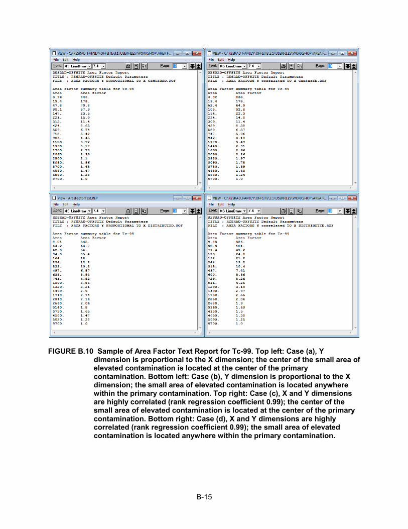
B-15
FIGURE B.10 Sample of Area Factor Text Report for Tc-99. Top left: Case (a), Y dimension is proportional to the X dimension; the center of the small area of elevated contamination is located at the center of the primary contamination. Bottom left: Case (b), Y dimension is proportional to the X dimension; the small area of elevated contamination is located anywhere within the primary contamination. Top right: Case (c), X and Y dimensions are highly correlated (rank regression coefficient 0.99); the center of the small area of elevated contamination is located at the center of the primary contamination. Bottom right: Case (d), X and Y dimensions are highly correlated (rank regression coefficient 0.99); the small area of elevated contamination is located anywhere within the primary contamination.
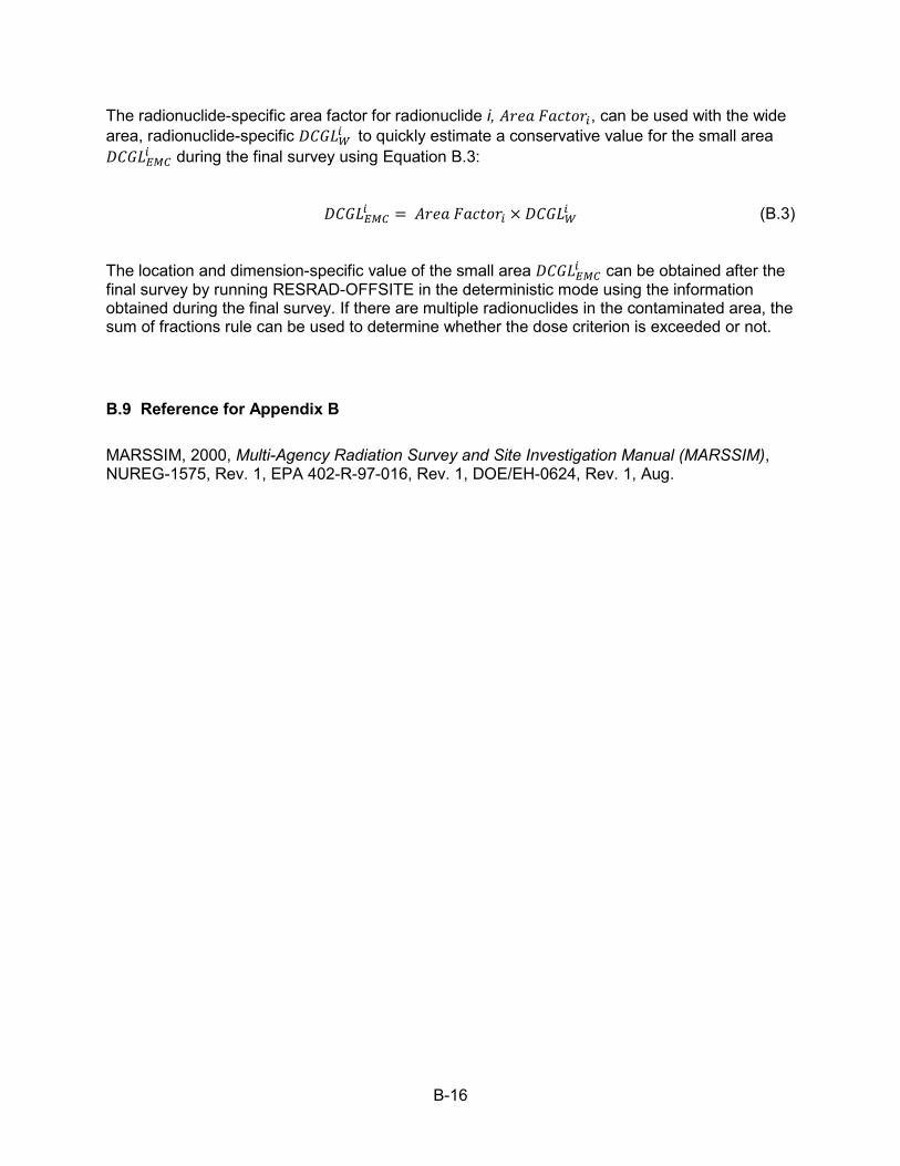
B-16
The radionuclide-specific area factor for radionuclide i, 𝐴𝐴𝐴𝐴𝐴𝐴𝐴𝐴 𝐹𝐹𝐴𝐴𝐹𝐹𝐹𝐹𝐹𝐹𝐴𝐴𝑖𝑖, can be used with the wide area, radionuclide-specific 𝐷𝐷𝐷𝐷𝐷𝐷𝐷𝐷𝑊𝑊𝑖𝑖 to quickly estimate a conservative value for the small area 𝐷𝐷𝐷𝐷𝐷𝐷𝐷𝐷𝐸𝐸𝐸𝐸𝐷𝐷𝑖𝑖 during the final survey using Equation B.3:
𝐷𝐷𝐷𝐷𝐷𝐷𝐷𝐷𝐸𝐸𝐸𝐸𝐷𝐷𝑖𝑖 = 𝐴𝐴𝐴𝐴𝐴𝐴𝐴𝐴 𝐹𝐹𝐴𝐴𝐹𝐹𝐹𝐹𝐹𝐹𝐴𝐴𝑖𝑖 × 𝐷𝐷𝐷𝐷𝐷𝐷𝐷𝐷𝑊𝑊𝑖𝑖 (B.3)
The location and dimension-specific value of the small area 𝐷𝐷𝐷𝐷𝐷𝐷𝐷𝐷𝐸𝐸𝐸𝐸𝐷𝐷𝑖𝑖 can be obtained after the final survey by running RESRAD-OFFSITE in the deterministic mode using the information obtained during the final survey. If there are multiple radionuclides in the contaminated area, the sum of fractions rule can be used to determine whether the dose criterion is exceeded or not.
B.9 Reference for Appendix B
MARSSIM, 2000, Multi-Agency Radiation Survey and Site Investigation Manual (MARSSIM), NUREG-1575, Rev. 1, EPA 402-R-97-016, Rev. 1, DOE/EH-0624, Rev. 1, Aug.