Using Bayesian networks to incorporate uncertainty in habitat suitability index models

Tools and Technology Article

Using Bayesian Networks to IncorporateUncertainty in Habitat SuitabilityIndex Models

GEORGE F. WILHERE,1 Washington Department of Fish and Wildlife, Habitat Program, 600 Capitol Way N., Olympia, WA 98501-1091, USA

ABSTRACT Habitat suitability index (HSI) models rarely characterize the uncertainty associated with theirestimates of habitat quality despite the fact that uncertainty can have important management implications.The purpose of this paper was to explore the use of Bayesian belief networks (BBNs) for representing andpropagating 3 types of uncertainty in HSI models—uncertainty in the suitability index relationships, theparameters of the HSI equation, and measurement of habitat variables (i.e., model inputs). I constructed aBBN–HSI model, based on an existing HSI model, using NeticaTM software. I parameterized the BBN’sconditional probability tables via Monte Carlo methods, and developed a discretization scheme that metspecifications for numerical error. I applied the model to both real and dummy sites in order to demonstratethe utility of the BBN–HSI model for 1) determining whether sites with different habitat types hadstatistically significant differences in HSI, and 2) making decisions based on rules that reflect differentattitudes toward risk—maximum expected value, maximin, and maximax. I also examined effects ofuncertainty in the habitat variables on the model’s output. Some sites with different habitat types haddifferent values for E[HSI], the expected value of HSI, but habitat suitability was not significantly differentbased on the overlap of 90% confidence intervals forE[HSI]. The different decision rules resulted in differentrankings of sites, and hence, different decisions based on risk. As measurement uncertainty in habitatvariables increased, sites with significantly different (a ¼ 0.1) E[HSI] became statistically more similar.Incorporating uncertainty in HSI models enables explicit consideration of risk and more robust habitatmanagement decisions. � 2012 The Wildlife Society.

KEY WORDS Bayesian network, habitat modeling, habitat suitability index, HSI, risk.

Uncertainty is inherent to every management decision af-fecting wildlife and their habitats. Uncertainty is pervasivebecause ecosystems are wickedly complex (Ludwig 2001) andthey exhibit irreducible natural variability at multiple spatialand temporal scales. Natural resource managers who ignoreuncertainty may adopt overly optimistic or pessimisticbeliefs; leading to decisions that ultimately result in environ-mental degradation or forgone economic opportunities(Ludwig et al. 1993, Reckhow 1994). Managers who ap-proach decisions with resolute certainty may fail to anticipateproblems or recognize potential risks. In contrast, dealingwith uncertainty enables managers to plan for contingenciesand minimize potential losses (Morgan and Henrion1990:2). Management decisions should be well informedabout the uncertainty of consequent outcomes, and therisk of undesirable outcomes should be evaluated and dealtwith appropriately (Murphy and Noon 1991, Burgman et al.2005).

Scientists should characterize uncertainties associated withinformation they provide managers. In fact, Morgan andHenrion (1990:44) believe scientists have a professional andethical responsibility to do so. Despite repeated calls tocharacterize uncertainty and incorporate it into managementdecisions (Hilborn 1987, Murphy and Noon 1991,McCarthy and Burgman 1995, Harwood and Stokes2003, Steel et al. 2009), it is still not a universal practice.This failing is especially prevalent in the construction and useof habitat suitability index (HSI) models.The concepts and methodology for HSI models were

developed over 30 years ago (U.S. Fish and WildlifeService [USFWS] 1980, 1981). Habitat suitability indexmodels are based on the assumption that habitat qualitycan be described through an index. The index ranges from0 to 1, with 0 being non-habitat and 1 being optimal habitat.Habitat quality is described in terms of carrying capacity(USFWS 1980), where optimal habitat has maximal carryingcapacity and a site’s HSI value is the ratio of the site’s carryingcapacity to maximal carrying capacity (USFWS 1981). Theinputs to an HSI model are measurable habitat variables.Suitability index (SI) relationships, which also range from 0to 1, relate each habitat variable to habitat quality. Suitabilityindices are typically constructed through expert knowledge

Received: 21 December 2010; Accepted: 9 December 2011

Additional supporting information may be found in the online version ofthis article.1E-mail: [email protected]

The Journal of Wildlife Management; DOI: 10.1002/jwmg.366

Wilhere � Building HSI Models With Bayesian Networks 1

informed by a review of the scientific literature. The SIrelationships usually take the form of piece-wise linear func-tions represented graphically, as opposed to analytical for-mulations, but the HSI methodology places no constraintson SI relationships and more complex functions are also used(e.g., Spies et al. 2007). Suitability indices are mathematicallycombined via the HSI equation. The equation is typically aweighted arithmetic or geometric mean of the SIs, althoughminimum, maximum, and logical functions are occasionallyemployed. Parameter values (i.e., weights) and the equation’sstructure are invariably based on expert knowledge, again,informed by the scientific literature.Habitat suitability index models are regularly employed for

assessing the effects of forest management (Marzluff et al.2002, Spies et al. 2007) and environmental mitigationrequirements (Duberstein et al. 2007, Ashley and Muse2008). Hence, the reliability of HSI models and the natureof their outputs affect decisions with real consequences forwildlife habitats (Brooks 1997, Roloff and Kernohan 1999).Well over 150 HSI models for fish and wildlife species werepublished before 1990 (Terrell and Carpenter 1997), andmany others have been developed since then (e.g., McCombet al. 2002, Dussault et al. 2006, Kroll and Haufler 2006,Burnett et al. 2007, Spies et al. 2007). All the aforemen-tioned models have a major shortcoming in common—theydo not characterize the uncertainty associated with their HSIestimates.An HSI model has 4 main sources of uncertainty: 1) SI

relationships, 2) parameters of theHSI equation, 3) structureof theHSI equation, and 4) habitat variables. The first 3 stemfrom the lack of knowledge (epistemic uncertainty) about aspecies’ autecology and the natural variability (aleatory un-certainty) in a species’ demographic response to habitatconditions. The fourth is the result of measurement uncer-tainty. VanHorne andWiens (1991) were the first to suggestthat SI relationships could be structured to account foruncertainty. They proposed an approach whereby uncertain-ty would be represented in 3 dimensions via a triangulardistribution defined by piece-wise linear relationships: theupper and lower limits and a central tendency. Burgman et al.(2001) implemented this idea with triangular fuzzy numbers,which are typically used to deal with conceptual vagueness(Regan et al. 2002) and in Burgman et al. (2001), fuzzynumbers quantified expert opinion about ‘‘agreement’’ be-tween a particular value of a habitat variable and ‘‘the conceptof suitable habitat.’’ The result is not a probability distribu-tion over the domain of SI values, but rather possibility levelsfor suitable habitat.Uncertainty has been incorporated into HSI models in

other ways as well. Johnson and Gillingham (2004) usedMonte Carlo methods to incorporate uncertainty in the 4factors of an HSI equation. Uncertainty was represented aseither a triangular or uniform probability distribution, withthe center and limits of each distribution based on expertopinion. The model’s output was a probability distribution ofHSI values. Larson et al. (2004) incorporated uncertaintyinto their SI relationships with 3 different sets of relation-ships that yielded 3 separate HSI values—upper, lower, and

best estimates, and Ray and Burgman (2006) dealt withuncertainty in the parameters and structure of their modelby constructing 22 equally plausible models and boundingthe ‘‘range of subjective uncertainty’’ by the HSI values at theupper and lower extremes. Neither of these approachesgenerated a probability distribution for HSI values, whichis problematic because extreme values could have extremelysmall probabilities of being the true HSI value. Bender et al.(1996) dealt with uncertainty of habitat variables (i.e., modelinputs) through Monte Carlo and bootstrapping methods.Using empirically derived estimates of habitat variables, theygenerated 90% confidence intervals for the mean HSIs of 6different habitat types. If confidence intervals of differenthabitat types did not overlap, then they concluded that themeanHSIs of those habitat types were significantly different.Although various approaches have been explored for in-

corporating uncertainty in HSI models, most have addressedonly 1 source of uncertainty; only Ray and Burgman (2006)dealt with more than 1 source. Furthermore, several of theseapproaches did not produce a probability distribution overHSI values, and therefore, could not generate particular typesof information useful for management decisions: expectedvalue of HSI, the probability of extreme HSI values, andwhether differences in HSI values between sites or betweenhabitat types were significantly different.Perhaps a practical modeling framework that facilitates the

representation and propagation of uncertainty would encour-age HSI models that provide a fuller and more useful char-acterization of uncertainty. One such modeling framework isBayesian belief networks (BBNs). Bayesian belief networksare a type of probabilistic graphical model (Jensen andNielsen 2007), which have proven utility for ecologicalmodeling (Marcot et al. 2006, Uusitalo 2007), and havebeen used for numerous assessments of wildlife habitats(e.g., Raphael et al. 2001, Lee and Irwin 2005, McNayet al. 2006, Smith et al. 2007).Bayesian belief networks possess 3 useful features for build-

ing HSI models that incorporate uncertainty. First, all var-iables in a BBN are represented as random variables (i.e., asprobability distributions). Second, BBNs enable uncertaintyto be explicitly incorporated into each functional relationshipof an HSI model. These uncertainties propagate through thenetwork and are expressed at the model output as a randomvariable. And third, the graphical nature of BBNs enablesstraightforward translation of an HSI model to a BBNthrough a computer-user interface typical of software appli-cations such as NeticaTM (Norsys Software Corp.,Vancouver, British Columbia) or Hugin ExpertTM (HuginExpert A/S, Aalborg, Denmark).BBNs may be a practical modeling framework for repre-

senting and propagating uncertainty in HSI models. Thepurpose of this paper is to explore the use of BBNs for theimplementation of HSI models. My objectives are to 1)explain the translation of an HSI model to a BBN–HSImodel, 2) explain how to incorporate HSI model uncertain-ties into a BBN, and 3) demonstrate how the output of aBBN–HSI model can be used to make more informedmanagement decisions. The scope of my exploration is

2 The Journal of Wildlife Management

confined to 3 of the 4 types of uncertainty: SI relationships,HSI equation parameters, and measurement of habitatvariables.

METHODS

The methods consist of 2 stages: 1) construction of a BBN–HSI model and 2) a demonstration of the model’s utility forrepresenting and propagating uncertainty in HSI models.

Construction of a BBN–HSI ModelThe initial steps of constructing a BBN–HSI model are thesame as an ordinary HSI model: 1) selecting habitat variables(i.e., model inputs), 2) constructing SI relationships for eachhabitat variable, and 3) formulating an equation that com-bines SIs into the HSI (USFWS 1981). Additional stepsnecessary to construct a BBN–HSI are: 4) quantifyinguncertainty in each SI relationship, 5) assembling the net-work, 6) discretizing input variables, 7) discretizing inter-mediate and output variables, 8) quantifying uncertaintyin parameters of the HSI equation, and 9) parameterizingthe BBN.For steps 1 through 4, I used an existing HSI model that

quantified uncertainty in its SI relationships (Burgman et al.2001). This model, for the Florida scrub-jay (Aphelocomacoerulescens), is described by the following equations:

SI1a ¼ G1aðpercent shrub canopy comprised of scrub oaksÞð1Þ

SI1b ¼ G1bðdistance from scrub oak ridgeÞ ð2Þ

SI2a ¼ G2aðpercent of cover comprised of sand or herbsÞð3Þ

SI2b ¼ G2bðdistance to ruderal areaÞ ð4Þ

SI3a ¼ G3aðpercentage of pine canopy coverÞ ð5Þ

SI3b ¼ G3bðdistance to forestÞ ð6Þ

SI4a ¼ G4aðmean height of oak scrubÞ ð7Þ

SI4b ¼ G4bðmean height of palmetto scrubÞ ð8Þ

SI1 ¼ maxðSI1a; SI1bÞ ð9Þ

SI2 ¼ maxðSI2a; SI2bÞ ð10Þ

SI3 ¼ minðSI3a; SI3bÞ ð11Þ

SI4 ¼ SI4a if scrub oak cover > 30%; else SI4 ¼ SI4b

ð12Þ

HSI ¼ ðSIw11 SIw2

2 SIw33 SIw4

4 Þ1=ðw1þw2þw3þw4Þ ð13Þwhere each Gz is a graphical function depicting the relation-ship between a suitability index and a habitat variable; z

denotes 1a, 1b, 2a, 2b, 3a, 3b, 4a, 4a, or 4b; and w1, w2, w3,and w4 are parameters that determine the relative influenceof SI1, SI2, SI3, and SI4, respectively, in the calculation ofHSI. The ecological basis for the HSI model is explained inBreininger (1992) and Breininger et al. (1998).The model of Burgman et al. (2001) represents expert

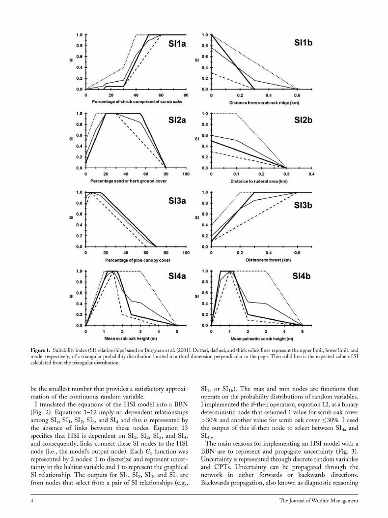
uncertainty in each SI relationship, equations 1–8, by meansof 3 piece-wise linear functions corresponding to the bestguess, lower bound and upper bound of a triangular fuzzynumber (Fig. 1). I assumed that these graphical representa-tions of uncertainty corresponded to the mode, lower bound,and upper bound of a triangular probability distribution(sensu Van Horne and Wiens 1991). In effect, each SIz isa random variable described by a probability distribution andthe shape of that distribution is determined by Gz and thevalue of the habitat variable.Equation 13 is a weighted geometric mean. The model of

Burgman et al. (2001) and Breininger et al. (1998) usedan unweighted geometric mean, which is equivalent tow1 ¼ w2 ¼ w3 ¼ w4 ¼ 1. The assertion that SI1, SI2,SI3, and SI4 are equally influential was an expert judgment,and like the expert judgments made to construct the graphi-cal SI relationships, there certainly was uncertainty associat-ed with that judgment. However, Burgman et al. (2001) didnot incorporate this parameter uncertainty in their model. Imodeled uncertainty in w1, w2, w3, and w4 by treating themas random variables described by probability distributions(explained below).I assembled the network, step 5, with NeticaTM (version

4.08). This software provides all the functionality neededto construct and run BBN models. A BBN consists ofnodes and links. Variables are represented as nodes.Nodes can be inputs to the model, outputs of the model,or intermediate variables. A link between nodes indicates acause-and-effect relationship, and hence, is always uni-directional. No link between nodes implies no cause-and-effect relationship exists and is equivalent to statistical inde-pendence. At the beginning of a link is a parent node andat the end of a link is a child node. Every child node holdsthe probabilistic relationship between its output and itsparent nodes. The relationship is stored as a conditionalprobability table (CPT) with each row corresponding to aunique combination of the parent’s states and each columncorresponding to the child’s output states. Nodes and linksare well suited for representing HSI models, which can bedecomposed into modular components and do not possessfeedback loops.All variables in a BBNmust be either categorical or binned,

and therefore, continuous variables must be discretized.Discretization partitions the domain of a continuous randomvariable into a finite number of intervals (or states). Theresulting discrete random variable assumes the intervals’center values: x1, x2, x3, . . ., xN. Discretization results innumerical errors, and if too coarse will cause linear relation-ships to behave nonlinearly. These problems can be avoidedthrough finer discretization, but with a practical limitation—computer memory and computational burdens increase ex-ponentially with N. Therefore, the number of states should


be the smallest number that provides a satisfactory approxi-mation of the continuous random variable.I translated the equations of the HSI model into a BBN

(Fig. 2). Equations 1–12 imply no dependent relationshipsamong SIz, SI1, SI2, SI3, and SI4 and this is represented bythe absence of links between these nodes. Equation 13specifies that HSI is dependent on SI1, SI2, SI3, and SI4,and consequently, links connect these SI nodes to the HSInode (i.e., the model’s output node). Each Gz function wasrepresented by 2 nodes: 1 to discretize and represent uncer-tainty in the habitat variable and 1 to represent the graphicalSI relationship. The outputs for SI1, SI2, SI3, and SI4 arefrom nodes that select from a pair of SI relationships (e.g.,

SI1a or SI1b). The max and min nodes are functions thatoperate on the probability distributions of random variables.I implemented the if-then operation, equation 12, as a binarydeterministic node that assumed 1 value for scrub oak cover>30% and another value for scrub oak cover �30%. I usedthe output of this if-then node to select between SI4a andSI4b.The main reasons for implementing an HSI model with a

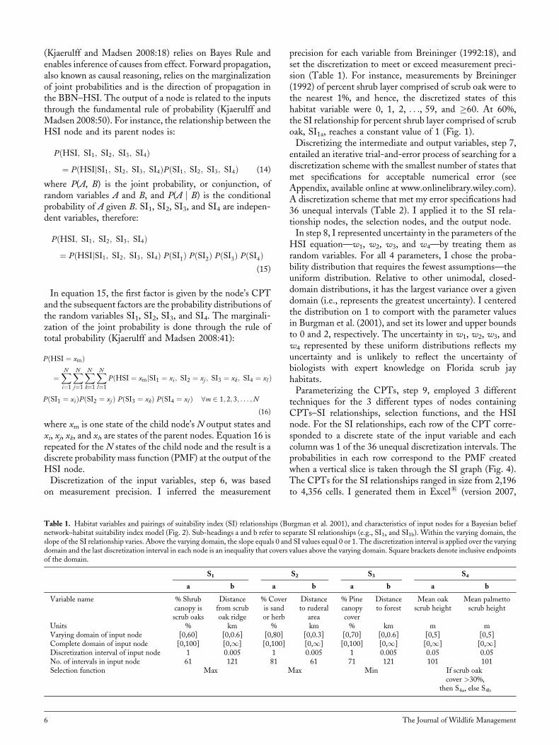
BBN are to represent and propagate uncertainty (Fig. 3).Uncertainty is represented through discrete random variablesand CPTs. Uncertainty can be propagated through thenetwork in either forwards or backwards directions.Backwards propagation, also known as diagnostic reasoning

Figure 1. Suitability index (SI) relationships based on Burgman et al. (2001). Dotted, dashed, and thick solids lines represent the upper limit, lower limit, andmode, respectively, of a triangular probability distribution located in a third dimension perpendicular to the page. Thin solid line is the expected value of SIcalculated from the triangular distribution.


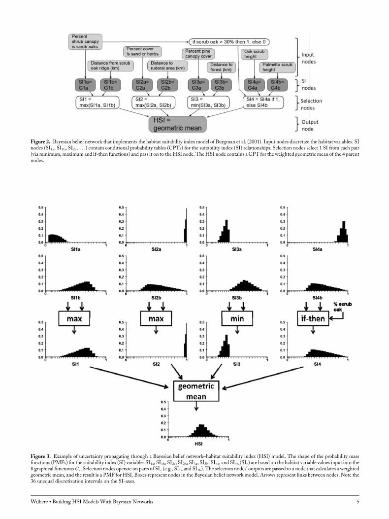
Figure 2. Bayesian belief network that implements the habitat suitability index model of Burgman et al. (2001). Input nodes discretize the habitat variables. SInodes (SI1a, SI1b, SI2a, . . .) contain conditional probability tables (CPTs) for the suitability index (SI) relationships. Selection nodes select 1 SI from each pair(via minimum,maximum and if-then functions) and pass it on to theHSI node. TheHSI node contains a CPT for the weighted geometric mean of the 4 parentnodes.

Figure 3. Example of uncertainty propagating through a Bayesian belief network–habitat suitability index (HSI) model. The shape of the probability massfunctions (PMFs) for the suitability index (SI) variables SI1a, SI1b, SI2a, SI2b, SI3a, SI3b, SI4a, and SI4b (SIz) are based on the habitat variable values input into the8 graphical functionsGz. Selection nodes operate on pairs of SIz (e.g., SI1a and SI1b). The selection nodes’ outputs are passed to a node that calculates a weightedgeometric mean, and the result is a PMF for HSI. Boxes represent nodes in the Bayesian belief network model. Arrows represent links between nodes. Note the36 unequal discretization intervals on the SI-axes.


(Kjaerulff and Madsen 2008:18) relies on Bayes Rule andenables inference of causes from effect. Forward propagation,also known as causal reasoning, relies on the marginalizationof joint probabilities and is the direction of propagation inthe BBN–HSI. The output of a node is related to the inputsthrough the fundamental rule of probability (Kjaerulff andMadsen 2008:50). For instance, the relationship between theHSI node and its parent nodes is:

PðHSI; SI1; SI2; SI3; SI4Þ¼ PðHSIjSI1; SI2; SI3; SI4ÞPðSI1; SI2; SI3; SI4Þ (14)

where P(A, B) is the joint probability, or conjunction, ofrandom variables A and B, and P(A j B) is the conditionalprobability of A given B. SI1, SI2, SI3, and SI4 are indepen-dent variables, therefore:

PðHSI; SI1; SI2; SI3; SI4Þ¼ PðHSIjSI1; SI2; SI3; SI4Þ PðSI1Þ PðSI2Þ PðSI3Þ PðSI4Þ

(15)

In equation 15, the first factor is given by the node’s CPTand the subsequent factors are the probability distributions ofthe random variables SI1, SI2, SI3, and SI4. The marginali-zation of the joint probability is done through the rule oftotal probability (Kjaerulff and Madsen 2008:41):

PðHSI ¼ xmÞ

¼XN

i¼1

XN

j¼1

XN

k¼1

XN

l¼1

PðHSI ¼ xmjSI1 ¼ xi; SI2 ¼ xj ; SI3 ¼ xk; SI4 ¼ xl Þ

PðSI1 ¼ xiÞPðSI2 ¼ xj Þ PðSI3 ¼ xkÞ PðSI4 ¼ xl Þ 8m 2 1; 2; 3; . . . ;N

(16)

where xm is one state of the child node’s N output states andxi, xj, xk, and xl, are states of the parent nodes. Equation 16 isrepeated for the N states of the child node and the result is adiscrete probability mass function (PMF) at the output of theHSI node.Discretization of the input variables, step 6, was based

on measurement precision. I inferred the measurement

precision for each variable from Breininger (1992:18), andset the discretization to meet or exceed measurement preci-sion (Table 1). For instance, measurements by Breininger(1992) of percent shrub layer comprised of scrub oak were tothe nearest 1%, and hence, the discretized states of thishabitat variable were 0, 1, 2, . . ., 59, and �60. At 60%,the SI relationship for percent shrub layer comprised of scruboak, SI1a, reaches a constant value of 1 (Fig. 1).Discretizing the intermediate and output variables, step 7,

entailed an iterative trial-and-error process of searching for adiscretization scheme with the smallest number of states thatmet specifications for acceptable numerical error (seeAppendix, available online at www.onlinelibrary.wiley.com).A discretization scheme that met my error specifications had36 unequal intervals (Table 2). I applied it to the SI rela-tionship nodes, the selection nodes, and the output node.In step 8, I represented uncertainty in the parameters of the

HSI equation—w1, w2, w3, and w4—by treating them asrandom variables. For all 4 parameters, I chose the proba-bility distribution that requires the fewest assumptions—theuniform distribution. Relative to other unimodal, closed-domain distributions, it has the largest variance over a givendomain (i.e., represents the greatest uncertainty). I centeredthe distribution on 1 to comport with the parameter valuesin Burgman et al. (2001), and set its lower and upper boundsto 0 and 2, respectively. The uncertainty in w1, w2, w3, andw4 represented by these uniform distributions reflects myuncertainty and is unlikely to reflect the uncertainty ofbiologists with expert knowledge on Florida scrub jayhabitats.Parameterizing the CPTs, step 9, employed 3 different

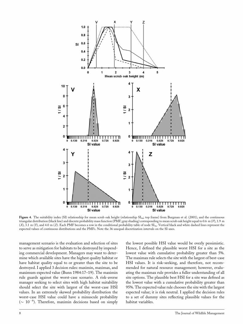
techniques for the 3 different types of nodes containingCPTs–SI relationships, selection functions, and the HSInode. For the SI relationships, each row of the CPT corre-sponded to a discrete state of the input variable and eachcolumn was 1 of the 36 unequal discretization intervals. Theprobabilities in each row correspond to the PMF createdwhen a vertical slice is taken through the SI graph (Fig. 4).The CPTs for the SI relationships ranged in size from 2,196to 4,356 cells. I generated them in Excel1 (version 2007,

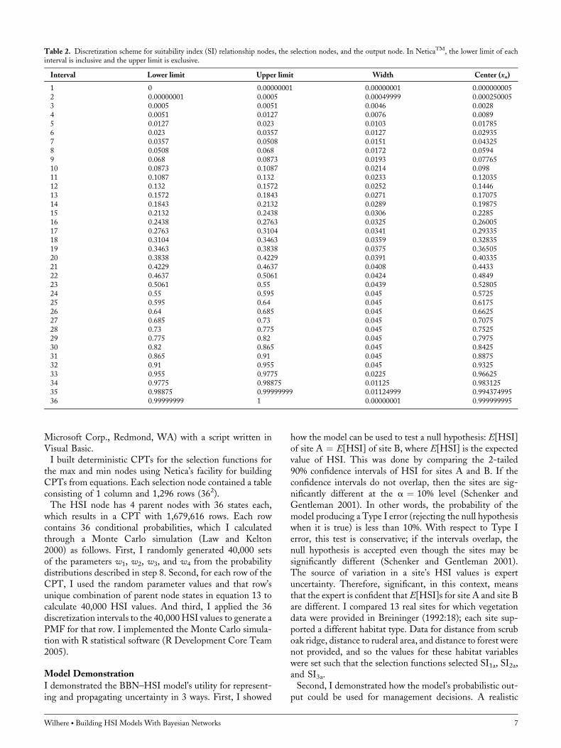
Table 1. Habitat variables and pairings of suitability index (SI) relationships (Burgman et al. 2001), and characteristics of input nodes for a Bayesian beliefnetwork–habitat suitability index model (Fig. 2). Sub-headings a and b refer to separate SI relationships (e.g., SI1a and SI1b). Within the varying domain, theslope of the SI relationship varies. Above the varying domain, the slope equals 0 and SI values equal 0 or 1. The discretization interval is applied over the varyingdomain and the last discretization interval in each node is an inequality that covers values above the varying domain. Square brackets denote inclusive endpointsof the domain.

S1 S2 S3 S4

a b a b a b a b

Variable name % Shrubcanopy isscrub oaks

Distancefrom scruboak ridge

% Coveris sandor herb

Distanceto ruderal

area

% Pinecanopycover

Distanceto forest

Mean oakscrub height

Mean palmettoscrub height

Units % km % km % km m mVarying domain of input node [0,60] [0,0.6] [0,80] [0,0.3] [0,70] [0,0.6] [0,5] [0,5]Complete domain of input node [0,100] [0,1] [0,100] [0,1] [0,100] [0,1] [0,1] [0,1]Discretization interval of input node 1 0.005 1 0.005 1 0.005 0.05 0.05No. of intervals in input node 61 121 81 61 71 121 101 101Selection function Max Max Min If scrub oak

cover >30%,then S4a, else S4b


Microsoft Corp., Redmond, WA) with a script written inVisual Basic.I built deterministic CPTs for the selection functions for

the max and min nodes using Netica’s facility for buildingCPTs from equations. Each selection node contained a tableconsisting of 1 column and 1,296 rows (362).The HSI node has 4 parent nodes with 36 states each,

which results in a CPT with 1,679,616 rows. Each rowcontains 36 conditional probabilities, which I calculatedthrough a Monte Carlo simulation (Law and Kelton2000) as follows. First, I randomly generated 40,000 setsof the parameters w1, w2, w3, and w4 from the probabilitydistributions described in step 8. Second, for each row of theCPT, I used the random parameter values and that row’sunique combination of parent node states in equation 13 tocalculate 40,000 HSI values. And third, I applied the 36discretization intervals to the 40,000HSI values to generate aPMF for that row. I implemented the Monte Carlo simula-tion with R statistical software (R Development Core Team2005).

Model Demonstration

I demonstrated the BBN–HSI model’s utility for represent-ing and propagating uncertainty in 3 ways. First, I showed

how the model can be used to test a null hypothesis: E[HSI]of site A ¼ E[HSI] of site B, where E[HSI] is the expectedvalue of HSI. This was done by comparing the 2-tailed90% confidence intervals of HSI for sites A and B. If theconfidence intervals do not overlap, then the sites are sig-nificantly different at the a ¼ 10% level (Schenker andGentleman 2001). In other words, the probability of themodel producing a Type I error (rejecting the null hypothesiswhen it is true) is less than 10%. With respect to Type Ierror, this test is conservative; if the intervals overlap, thenull hypothesis is accepted even though the sites may besignificantly different (Schenker and Gentleman 2001).The source of variation in a site’s HSI values is expertuncertainty. Therefore, significant, in this context, meansthat the expert is confident that E[HSI]s for site A and site Bare different. I compared 13 real sites for which vegetationdata were provided in Breininger (1992:18); each site sup-ported a different habitat type. Data for distance from scruboak ridge, distance to ruderal area, and distance to forest werenot provided, and so the values for these habitat variableswere set such that the selection functions selected SI1a, SI2a,and SI3a.Second, I demonstrated how the model’s probabilistic out-

put could be used for management decisions. A realistic

Table 2. Discretization scheme for suitability index (SI) relationship nodes, the selection nodes, and the output node. In NeticaTM, the lower limit of eachinterval is inclusive and the upper limit is exclusive.

Interval Lower limit Upper limit Width Center (xn)

1 0 0.00000001 0.00000001 0.0000000052 0.00000001 0.0005 0.00049999 0.0002500053 0.0005 0.0051 0.0046 0.00284 0.0051 0.0127 0.0076 0.00895 0.0127 0.023 0.0103 0.017856 0.023 0.0357 0.0127 0.029357 0.0357 0.0508 0.0151 0.043258 0.0508 0.068 0.0172 0.05949 0.068 0.0873 0.0193 0.0776510 0.0873 0.1087 0.0214 0.09811 0.1087 0.132 0.0233 0.1203512 0.132 0.1572 0.0252 0.144613 0.1572 0.1843 0.0271 0.1707514 0.1843 0.2132 0.0289 0.1987515 0.2132 0.2438 0.0306 0.228516 0.2438 0.2763 0.0325 0.2600517 0.2763 0.3104 0.0341 0.2933518 0.3104 0.3463 0.0359 0.3283519 0.3463 0.3838 0.0375 0.3650520 0.3838 0.4229 0.0391 0.4033521 0.4229 0.4637 0.0408 0.443322 0.4637 0.5061 0.0424 0.484923 0.5061 0.55 0.0439 0.5280524 0.55 0.595 0.045 0.572525 0.595 0.64 0.045 0.617526 0.64 0.685 0.045 0.662527 0.685 0.73 0.045 0.707528 0.73 0.775 0.045 0.752529 0.775 0.82 0.045 0.797530 0.82 0.865 0.045 0.842531 0.865 0.91 0.045 0.887532 0.91 0.955 0.045 0.932533 0.955 0.9775 0.0225 0.9662534 0.9775 0.98875 0.01125 0.98312535 0.98875 0.99999999 0.01124999 0.99437499536 0.99999999 1 0.00000001 0.999999995


management scenario is the evaluation and selection of sitesto serve as mitigation for habitats to be destroyed by impend-ing commercial development. Managers may want to deter-mine which available sites have the highest quality habitat orhave habitat quality equal to or greater than the site to bedestroyed. I applied 3 decision rules: maximin, maximax, andmaximum expected value (Bunn 1984:17–19). The maximinrule guards against the worst-case scenario. A risk-aversemanager seeking to select sites with high habitat suitabilityshould select the site with largest of the worst-case HSIvalues. In an extremely skewed probability distribution theworst-case HSI value could have a minuscule probability(� 10�6). Therefore, maximin decisions based on simply

the lowest possible HSI value would be overly pessimistic.Hence, I defined the plausible worst HSI for a site as thelowest value with cumulative probability greater than 5%.The maximax rule selects the site with the largest of best-caseHSI values. It is risk-seeking, and therefore, not recom-mended for natural resource management; however, evalu-ating the maximax rule provides a fuller understanding of allsite options. The plausible best HSI for a site was defined asthe lowest value with a cumulative probability greater than95%. The expected value rule chooses the site with the largestexpected value; it is risk neutral. I applied the decision rulesto a set of dummy sites reflecting plausible values for thehabitat variables.

Figure 4. The suitability index (SI) relationship for mean scrub oak height (relationship SI4a; top frame) from Burgman et al. (2001), and the continuoustriangular distribution (black line) and discrete probabilitymass function (PMF; gray shading) corresponding tomean scrub oak height equal to 0.6 m (V), 1.9 m(X), 3.1 m (Y), and 4.0 m (Z). Each PMF becomes a row in the conditional probability table of node SI4a. Vertical black and white dashed lines represent theexpected values of continuous distributions and the PMFs. Note the 36 unequal discretization intervals on the SI-axes.


The first 2 demonstrations ignored uncertainty in themeasurement of habitat variables. The third demonstrationincorporated measurement uncertainty of habitat variables,and examined its affect on the model output and consequentdecisions based on that output. Uncertainty in modelinputs refers to the statistical variance of each habitatvariable that results from taking measurements at multipleplots within a site. Because of spatial heterogeneity ofhabitat conditions within a site, a habitat variable is not asingle value, but a variety of values described by a meanand standard deviation and can be represented as a proba-bility distribution. To explore the affects of uncertainty inthe model inputs, for each habitat variable I created proba-bility distributions with coefficients of variation equal to5%, 10%, 20%, 40%, and 60%. A larger coefficient ofvariation corresponded to greater spatial heterogeneity.The probability distributions were approximately symmetric,unimodal beta distributions, and the expected values ofthe probability distributions for each habitat variableremained constant. I completed these steps for each of the13 real sites.

RESULTS

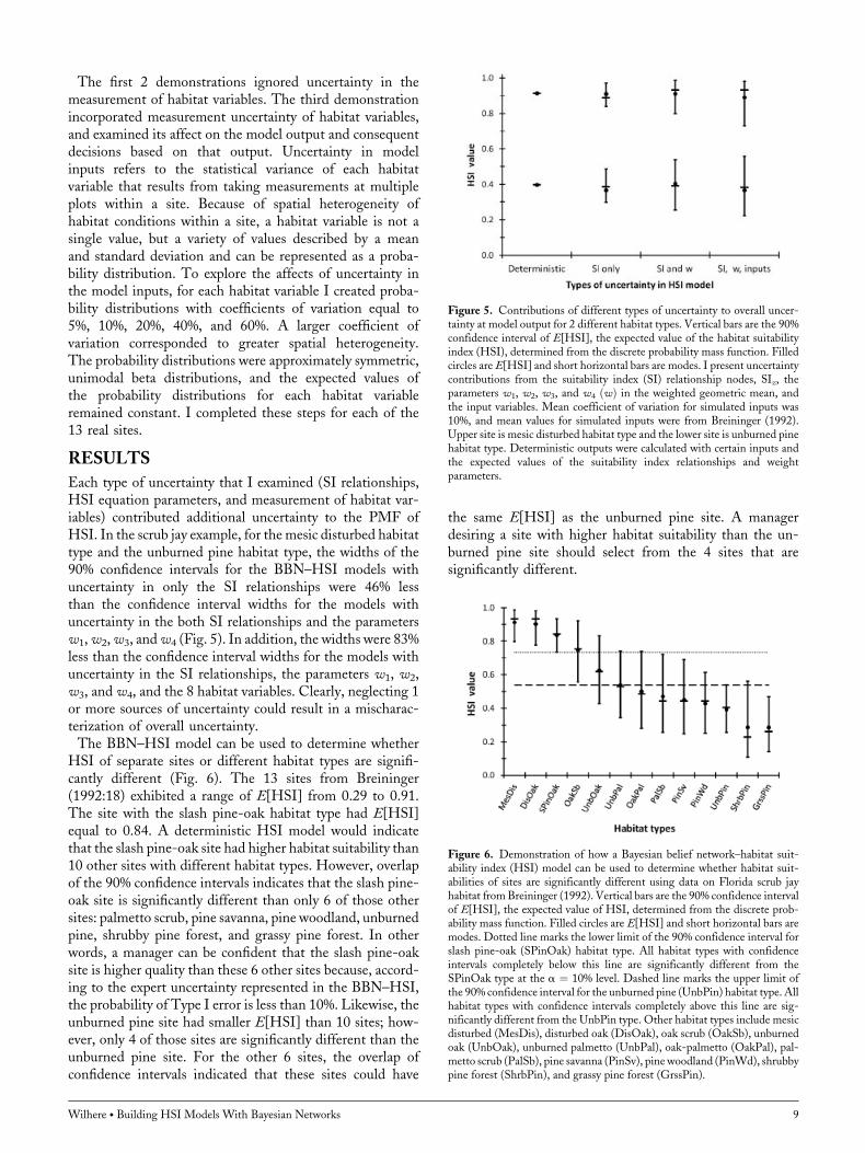
Each type of uncertainty that I examined (SI relationships,HSI equation parameters, and measurement of habitat var-iables) contributed additional uncertainty to the PMF ofHSI. In the scrub jay example, for the mesic disturbed habitattype and the unburned pine habitat type, the widths of the90% confidence intervals for the BBN–HSI models withuncertainty in only the SI relationships were 46% lessthan the confidence interval widths for the models withuncertainty in the both SI relationships and the parametersw1,w2,w3, andw4 (Fig. 5). In addition, the widths were 83%less than the confidence interval widths for the models withuncertainty in the SI relationships, the parameters w1, w2,w3, and w4, and the 8 habitat variables. Clearly, neglecting 1or more sources of uncertainty could result in a mischarac-terization of overall uncertainty.The BBN–HSI model can be used to determine whether

HSI of separate sites or different habitat types are signifi-cantly different (Fig. 6). The 13 sites from Breininger(1992:18) exhibited a range of E[HSI] from 0.29 to 0.91.The site with the slash pine-oak habitat type had E[HSI]equal to 0.84. A deterministic HSI model would indicatethat the slash pine-oak site had higher habitat suitability than10 other sites with different habitat types. However, overlapof the 90% confidence intervals indicates that the slash pine-oak site is significantly different than only 6 of those othersites: palmetto scrub, pine savanna, pine woodland, unburnedpine, shrubby pine forest, and grassy pine forest. In otherwords, a manager can be confident that the slash pine-oaksite is higher quality than these 6 other sites because, accord-ing to the expert uncertainty represented in the BBN–HSI,the probability of Type I error is less than 10%. Likewise, theunburned pine site had smaller E[HSI] than 10 sites; how-ever, only 4 of those sites are significantly different than theunburned pine site. For the other 6 sites, the overlap ofconfidence intervals indicated that these sites could have

the same E[HSI] as the unburned pine site. A managerdesiring a site with higher habitat suitability than the un-burned pine site should select from the 4 sites that aresignificantly different.

Figure 5. Contributions of different types of uncertainty to overall uncer-tainty at model output for 2 different habitat types. Vertical bars are the 90%confidence interval of E[HSI], the expected value of the habitat suitabilityindex (HSI), determined from the discrete probability mass function. Filledcircles are E[HSI] and short horizontal bars are modes. I present uncertaintycontributions from the suitability index (SI) relationship nodes, SIz, theparameters w1, w2, w3, and w4 ðwÞ in the weighted geometric mean, andthe input variables. Mean coefficient of variation for simulated inputs was10%, and mean values for simulated inputs were from Breininger (1992).Upper site is mesic disturbed habitat type and the lower site is unburned pinehabitat type. Deterministic outputs were calculated with certain inputs andthe expected values of the suitability index relationships and weightparameters.

Figure 6. Demonstration of how a Bayesian belief network–habitat suit-ability index (HSI) model can be used to determine whether habitat suit-abilities of sites are significantly different using data on Florida scrub jayhabitat from Breininger (1992). Vertical bars are the 90% confidence intervalof E[HSI], the expected value of HSI, determined from the discrete prob-ability mass function. Filled circles are E[HSI] and short horizontal bars aremodes. Dotted line marks the lower limit of the 90% confidence interval forslash pine-oak (SPinOak) habitat type. All habitat types with confidenceintervals completely below this line are significantly different from theSPinOak type at the a ¼ 10% level. Dashed line marks the upper limit ofthe 90% confidence interval for the unburned pine (UnbPin) habitat type. Allhabitat types with confidence intervals completely above this line are sig-nificantly different from the UnbPin type. Other habitat types include mesicdisturbed (MesDis), disturbed oak (DisOak), oak scrub (OakSb), unburnedoak (UnbOak), unburned palmetto (UnbPal), oak-palmetto (OakPal), pal-metto scrub (PalSb), pine savanna (PinSv), pine woodland (PinWd), shrubbypine forest (ShrbPin), and grassy pine forest (GrssPin).


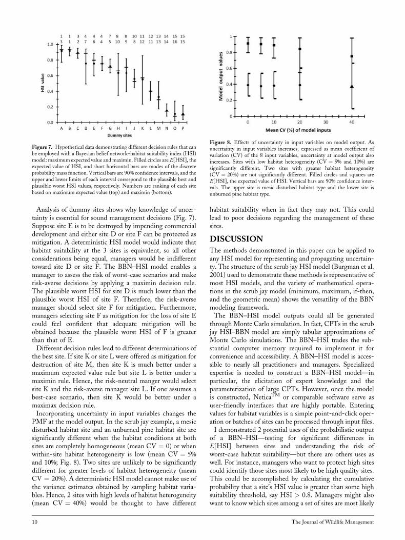
Analysis of dummy sites shows why knowledge of uncer-tainty is essential for sound management decisions (Fig. 7).Suppose site E is to be destroyed by impending commercialdevelopment and either site D or site F can be protected asmitigation. A deterministic HSI model would indicate thathabitat suitability at the 3 sites is equivalent, so all otherconsiderations being equal, managers would be indifferenttoward site D or site F. The BBN–HSI model enables amanager to assess the risk of worst-case scenarios and makerisk-averse decisions by applying a maximin decision rule.The plausible worst HSI for site D is much lower than theplausible worst HSI of site F. Therefore, the risk-aversemanager should select site F for mitigation. Furthermore,managers selecting site F as mitigation for the loss of site Ecould feel confident that adequate mitigation will beobtained because the plausible worst HSI of F is greaterthan that of E.Different decision rules lead to different determinations of

the best site. If site K or site L were offered as mitigation fordestruction of site M, then site K is much better under amaximum expected value rule but site L is better under amaximin rule. Hence, the risk-neutral manger would selectsite K and the risk-averse manager site L. If one assumes abest-case scenario, then site K would be better under amaximax decision rule.Incorporating uncertainty in input variables changes the

PMF at the model output. In the scrub jay example, a mesicdisturbed habitat site and an unburned pine habitat site aresignificantly different when the habitat conditions at bothsites are completely homogeneous (mean CV ¼ 0) or whenwithin-site habitat heterogeneity is low (mean CV ¼ 5%and 10%; Fig. 8). Two sites are unlikely to be significantlydifferent for greater levels of habitat heterogeneity (meanCV ¼ 20%). A deterministic HSI model cannot make use ofthe variance estimates obtained by sampling habitat varia-bles. Hence, 2 sites with high levels of habitat heterogeneity(mean CV ¼ 40%) would be thought to have different

habitat suitability when in fact they may not. This couldlead to poor decisions regarding the management of thesesites.

DISCUSSION

The methods demonstrated in this paper can be applied toany HSI model for representing and propagating uncertain-ty. The structure of the scrub jay HSI model (Burgman et al.2001) used to demonstrate these methods is representative ofmost HSI models, and the variety of mathematical opera-tions in the scrub jay model (minimum, maximum, if-then,and the geometric mean) shows the versatility of the BBNmodeling framework.The BBN–HSI model outputs could all be generated

through Monte Carlo simulation. In fact, CPTs in the scrubjay HSI–BBN model are simply tabular approximations ofMonte Carlo simulations. The BBN–HSI trades the sub-stantial computer memory required to implement it forconvenience and accessibility. A BBN–HSI model is acces-sible to nearly all practitioners and managers. Specializedexpertise is needed to construct a BBN–HSI model—inparticular, the elicitation of expert knowledge and theparameterization of large CPTs. However, once the modelis constructed, NeticaTM or comparable software serve asuser-friendly interfaces that are highly portable. Enteringvalues for habitat variables is a simple point-and-click oper-ation or batches of sites can be processed through input files.I demonstrated 2 potential uses of the probabilistic output

of a BBN–HSI—testing for significant differences inE[HSI] between sites and understanding the risk ofworst-case habitat suitability—but there are others uses aswell. For instance, managers who want to protect high sitescould identify those sites most likely to be high quality sites.This could be accomplished by calculating the cumulativeprobability that a site’s HSI value is greater than some highsuitability threshold, say HSI > 0.8. Managers might alsowant to know which sites among a set of sites are most likely

Figure 8. Effects of uncertainty in input variables on model output. Asuncertainty in input variables increases, expressed as mean coefficient ofvariation (CV) of the 8 input variables, uncertainty at model output alsoincreases. Sites with low habitat heterogeneity (CV ¼ 5% and 10%) aresignificantly different. Two sites with greater habitat heterogeneity(CV ¼ 20%) are not significantly different. Filled circles and squares areE[HSI], the expected value of HSI. Vertical bars are 90% confidence inter-vals. The upper site is mesic disturbed habitat type and the lower site isunburned pine habitat type.

Figure 7. Hypothetical data demonstrating different decision rules that canbe employed with a Bayesian belief network–habitat suitability index (HSI)model: maximum expected value andmaximin. Filled circles areE[HSI], theexpected value of HSI, and short horizontal bars are modes of the discreteprobability mass function. Vertical bars are 90% confidence intervals, and theupper and lower limits of each interval correspond to the plausible best andplausible worst HSI values, respectively. Numbers are ranking of each sitebased on maximum expected value (top) and maximin (bottom).


to have similar habitat suitability. The probability that 2 siteshave equivalent HSI values can be estimated by the overlap oftheir PMFs.This demonstration neglected 1 major form of uncertainty

in HSI models—the structure of the HSI equation. Thisuncertainty could be incorporated in the model by expandingthe Monte Carlo method used to generate the CPT of theHSI output node. Experts could construct plausible HSIequations and assign a subjective probability to each.These probabilities would reflect the expert’s degree of beliefthat an equation is the 1 that most accurately estimateshabitat suitability. The probabilities would be used to calcu-late a weighted arithmetic mean of the HSI values generatedby each of the plausible HSI models within each iteration ofthe simulation process.The proper interpretation of the model’s probabilistic out-

put is a Bayesian interpretation. That is, the probabilitiesrepresent an expert’s degree of belief that a particular value isthe true HSI value of a site. An expert’s belief is an amalgamof direct knowledge (i.e., observations or measurements inthe field) and indirect knowledge (e.g., the literature andinteractions with other experts). Direct knowledge and in-direct knowledge conflate both irreducible aleatory and re-ducible epistemic uncertainties. As the ideal expert gainsknowledge, the uncertainty of his or her beliefs will convergetoward purely aleatory uncertainty. In the real expert, cog-nitive and motivational biases affect his or her interpretationof their accumulated knowledge (Cleaves 1994) and no suchconvergence may occur. Hence, when using expert-basedmodels, we should remember this caveat: such models donot represent ecological relationships; the best we can hopefor is a model that accurately represents the knowledge of theexperts (Garthwaite et al. 2005).Despite their obvious shortcomings, models based on ex-

pert knowledge are often the only practical alternative whenassessments of habitat quality are needed. This situation isexpected to continue for the foreseeable future. Expert-basedmodels should characterize an expert’s uncertainty about hisor her knowledge. I presented a modeling framework withwhich to incorporate expert uncertainty in HSI models,however, I avoided the more difficult task of eliciting expertuncertainty. Such avoidance is apparently endemic to naturalresource management; serious attention to elicitation ofexpert uncertainty has received scant attention in the naturalresource management literature (although see Choy et al.2009). In contrast, engineering has recognized the impor-tance of rigorous elicitation methods and developed a sub-stantial body of research (e.g., Merkenhofer 1987, Kenny andvon Winterfeldt 1991, Chhibber et al. 1992). Improving thereliability of expert-based models ultimately depends onenforcing more demanding standards for the elicitation ofexpert knowledge and uncertainty. Developing and testingsuch standards should be an active area of research.

MANAGEMENT IMPLICATIONS

When an outcome is uncertain and a possible outcomeimposes a cost, then there is risk. The precautionary principleof natural resource management mandates a risk-averse ap-

proach to management (Gullet 1997). Therefore, managersneed to be aware of risks, and for them to be fully informed,scientists must provide estimates of uncertainty. Habitatsuitability index models are still used to assess the effectsof forest management and environmental mitigation require-ments, and yet, nearly all HSI models fail to incorporateuncertainty in their HSI estimates. Lacking information onuncertainty, managers will be unaware of the risk incurredwith some management options, and make decisions thatinadvertently cause the loss or degradation of wildlife hab-itats. Model uncertainty is often misinterpreted as lack ofknowledge, however, models that report uncertainty, such asa BBN–HSI, provide information on not only the most likelyoutcome but also on all other possible outcomes (Steel et al.2009). Understanding the likelihood of the full range ofpossible outcomes enriches a manager’s understanding,thereby leading to more robust management decisions.This paper demonstrates 1 method for incorporating uncer-tainty in HSI models.

ACKNOWLEDGMENTS

I thank T. Quinn for his encouragement and support, B.Marcot for his knowledgeable feedback, and B. Collier andan anonymous reviewer for helpful criticism and thoroughreviews. Product or company names mentioned in this pub-lication are for reader information only and do not implyendorsement by the Washington Department of Fish andWildlife of any product or service.

LITERATURE CITEDAshley, P., and A.Muse. 2008.Habitat evaluation procedures report: GravesProperty—Yakama Nation. Columbia Basin Fish andWildlife Authority,Portland, Oregon, USA.

Bender, L. C., G. J. Roloff, and J. B. Haufler. 1996. Evaluating confidenceintervals for habitat suitability models. Wildlife Society Bulletin 24:347–352.

Brooks, R. P. 1997. Improving habitat suitability index models. WildlifeSociety Bulletin 25:163–167.

Breininger, D. R. 1992. Habitat model for the Florida scrub jay on John F.Kennedy Space Center. NASA Technical Memorandum 107543.Kennedy Space Center, Florida, USA.

Breininger, D. R., V. L. Larson, B. W. Duncan, and R. B. Smith. 1998.Linking habitat suitability to demographic success in Florida scrub-jays.Wildlife Society Bulletin 26:118–128.

Bunn, D. W. 1984. Applied decision analysis. McGraw-Hill, New York,New York, USA.

Burgman, M. A., D. R. Breininger, B. W. Duncan, and S. Ferson. 2001.Setting reliability bounds on habitat suitability indices. EcologicalApplications 11:70–78.

Burgman, M. A., D. B. Lindenmayer, and J. Elith. 2005. Managing land-scapes for conservation under uncertainty. Ecology 86:2007–2017.

Burnett, K. M., G. H. Reeves, D. J. Miller, S. Clark, K. Vance-Borland, andK. Christiansen. 2007. Distribution of salmon-habitat potential relative tolandscape characteristics and implications for conservation. EcologicalApplications 17:66–80.

Chhibber, S., G. Apostolakis, and D. Okrent. 1992. A taxonomy of issuesrelated to the use of expert judgments in probabilistic safety studies.Reliability Engineering and System Safety 38:27–45.

Choy, S. L., R. O’Leary, and K. Mengersen. 2009. Elicitation by design inecology: using expert opinion to inform priors for Bayesian statisticalmodels. Ecology 90:265–277.

Cleaves, D. A. 1994. Assessing uncertainty in expert judgments aboutnatural resources. GTR-SO-110. USDA Forest Service, SouthernForest Experimental Station, New Orleans, Louisiana, USA.


Duberstein, C. A., M. A. Simmons, M. R. Sackschewsky, and J. M. Becker.2007. Development of a habitat suitability index model for the sagesparrow on the Hanford Site. PNNL-16885. Pacific NorthwestNational Laboratory, Richland, Washington, USA.

Dussault, C., R. Courtois, and J. P. Ouellet. 2006. A habitat suitability indexmodel to assess moose habitat selection at multiple spatial scales. CanadianJournal of Forest Research 36:1097–1110.

Garthwaite, P. H., J. B. Kadane, and A. O’Hagan. 2005. Statistical methodsfor eliciting probability distributions. Journal of the American StatisticalAssociation 100:680–700.

Gullet, W. 1997. Environmental protection and the ‘‘precautionary princi-ple’’: a response to scientific uncertainty in environmental management.Environmental Planning and Law Journal 14:52–69.

Harwood, J., and K. Stokes. 2003. Coping with uncertainty in ecologicaladvice: lessons from fisheries. Trends in Ecology and Evolution 18:617–622.

Hilborn, R. 1987. Living with uncertainty in resource management. NorthAmerican Journal of Fisheries Management 7:1–5.

Jensen, F. V., and T. D. Nielsen. 2007. Bayesian networks and decisiongraphs. Springer, New York, New York, USA.

Johnson, C. J., and M. P. Gillingham. 2004. Mapping uncertainty: sensi-tivity of wildlife habitat ratings to expert opinion. Journal of AppliedEcology 41:1032–1041.

Kenny, R. L., and D. von Winterfeldt. 1991. Eliciting probabilitiesfrom experts in complex technical problems. IEEE Transactions onEngineering Management 38:191–201.

Kjaerulff, U. B., and A. L. Madsen. 2008. Bayesian networks and influencediagrams. Springer, New York, New York, USA.

Kroll, A. J., and J. B. Haufler. 2006. Development and evaluation of habitatmodels at multiple spatial scales: a case study with the dusky flycatcher.Forest Ecology and Management 229:161–169.

Larson,M. A., F. R. Thompson, III, J. J.Millspaugh,W.D.Dijak, and S. R.Shifley. 2004. Linking population viability, habitat suitability, and land-scape simulation models for conservation planning. Ecological Modelling180:103–118.

Law, A. M., and W. D. Kelton. 2000. Simulation modeling and analysis.McGraw-Hill, New York, New York, USA.

Lee, D. C., and L. L. Irwin. 2005. Assessing risks to spotted owls from forestthinning in fire-adapted forest of the western United States. ForestEcology and Management 211:191–209.

Ludwig, D. 2001. The era of management is over. Ecosystems 4:758–764.

Ludwig, D., R. Hilborn, and C. Walters. 1993. Uncertainty, resourceexploitation, and conservation: lessons from history. Science 260:17–36.

Marcot, B. G., J. D. Steventon, G. D. Sutherland, and R. K.McCann. 2006.Guidelines for developing and updating Bayesian belief networks appliedto ecological modeling and conservation. Canadian Journal of ForestResearch 36:3063–3074.

Marzluff, J. M., J. J. Millspaugh, K. R. Ceder, C. D. Oliver, J. Withey, J. B.McCarter, C. L. Mason, and J. Comnick. 2002. Modeling changes inwildlife habitat and timber revenues in response to forest management.Forest Science 48:191–202.

McCarthy, M. A., and M. A. Burgman. 1995. Coping with uncertainty inforest wildlife planning. Forest Ecology and Management 74:23–36.

McComb, W. C., M. T. McGrath, T. A. Spies, and D. Vesely. 2002.Models for mapping potential habitat at landscape scales: an example usingnorthern spotted owls. Forest Science 48:204–216.

McNay, R. S., B. G. Marcot, V. Brumovsky, and R. Ellis. 2006. A Bayesianapproach to evaluating habitat for woodland caribou in north-central

British Columbia. Canadian Journal of Forest Research 36:3117–3133.

Merkenhofer, M. W. 1987. Quantifying judgmental uncertainty: method-ology, experiences, and insights. IEEE Transactions on Systems, Man,and Cybernetics 17:741–751.

Morgan,M. G., andM.Henrion. 1990. Uncertainty: a guide to dealing withuncertainty in quantitative risk and policy analysis. Cambridge UniversityPress, Cambridge, United Kingdom.

Murphy, D. D., and B. D. Noon. 1991. Coping with uncertainty in wildlifebiology. Journal of Wildlife Management 55:773–778.

R Development Core Team. 2005. R: a language and environment forstatistical computing. R Foundation for Statistical Computing, Vienna,Austria.

Raphael, M. G., M. J. Wisdom, M. M. Rowland, R. S. Holthausen, B. C.Wales, B. G. Marcot, and T. D. Rich. 2001. Status and trends of habitatsof terrestrial vertebrates in relation to land management in the interiorColumbia River Basin. Forest Ecology and Management 153:63–88.

Ray, N., and M. A. Burgman. 2006. Subjective uncertainties in habitatsuitability maps. Ecological Modelling 195:172–186.

Reckhow, K. H. 1994. Importance of scientific uncertainty in decisionmaking. Environmental Management 18:161–166.

Regan, H. M., M. Colyvan, and M. A. Burgman. 2002. A taxonomy andtreatment of uncertainty for ecology and conservation biology. EcologicalApplications 12:618–628.

Roloff, G. J., and B. J. Kernohan. 1999. Evaluating reliability of habitatsuitability index models. Wildlife Society Bulletin 27:973–985.

Schenker, N., and J. F. Gentleman. 2001. On judging the significance ofdifferences by examining the overlap between confidence intervals.American Statistician 55:182–186.

Smith, C. S., A. L. Howes, B. Price, and C. A. McAlpine. 2007. Using aBayesian belief network to predict suitable habitat for an endangeredmammal—the Julia Creek dunnart (Sminthopsis douglasi). BiologicalConservation 139:333–347.

Spies, T. A., B. C. McComb, R. S. H. Kennedy, M. T. McGrath, K. Olsen,and R. J. Pabst. 2007. Potential effects of forest policies on terrestrialbiodiversity in a multi-ownership province. Ecological Applications17:48–65.

Steel, E. A., T. J. Beechie, M. H. Ruckelshaus, A. H. Fullerton, P.McElhany, and P. Roni. 2009. Mind the gap: uncertainty and modelcommunication between mangers and scientists. American FisheriesSociety Symposium 71:357–372.

Terrell, J. W., and J. Carpenter. 1997. Selected habitat suitability indexmodel evaluations. USGS/BRD/ITR-1997-0005. U.S. GeologicalSurvey, Washington, D.C., USA.

Uusitalo, L. 2007. Advantages and challenges of Bayesian networks inenvironmental modeling. Ecological Modelling 203:312–318.

U.S. Fish and Wildlife Service [USFWS]. 1980. Habitat as a basis forenvironmental assessment. ESM 101. U.S. Fish and Wildlife Service,Department of Interior, Washington, D.C., USA.

U.S. Fish and Wildlife Service [USFWS]. 1981. Standards for the devel-opment of habitat suitability index models. ESM 103. U.S. Fish andWildlife Service, Department of Interior, Washington, D.C., USA.

Van Horne, B., and J. A.Wiens. 1991. Forest bird habitat suitability modelsand the development of general habitat models. Fish and WildlifeResearch Report 8. U.S. Fish and Wildlife Service, Washington, D.C.,USA.

Associate Editor: Bret Collier.


Documents

Using Bayesian networks to incorporate uncertainty in habitat suitability index models