EDUCATION AND EXAMINATION COMMITTEE

OF THE

SOCIETY OF ACTUARIES

FINANCIAL MATHEMATICS STUDY NOTE

USING DURATION AND CONVEXITY TO APPROXIMATE

CHANGE IN PRESENT VALUE

by

Robert Alps, ASA, MAAA

Copyright 2017 by the Society of Actuaries The Education and Examination Committee provides study notes to persons preparing for the examinations of the Society of Actuaries. They are intended to acquaint candidates with some of the theoretical and practical considerations involved in the various subjects. While varying opinions are presented where appropriate, limits on the length of the material and other considerations sometimes prevent the inclusion of all possible opinions. These study notes do not, however, represent any official opinion, interpretations or endorsement of the Society of Actuaries or its Education and Examination Committee. The Society is grateful to the authors for their contributions in preparing the study notes.

FM-24-17

1

Using Duration and Convexity to Approximate Change in Present Value Robert Alps

February 1, 2017

Contents 1 Introduction ............................................................................................................................. 2

2 Cash Flow Series and Present Value ....................................................................................... 3

3 Macaulay and Modified Duration ............................................................................................ 4

4 First-Order Approximations of Present Value ......................................................................... 5

5 Modified and Macaulay Convexity ......................................................................................... 6

6 Second-Order Approximations of Present Value .................................................................... 7

Appendix A: Derivation of First-Order Macaulay Approximation ................................................ 9

Appendix B: Comparisons of Approximations............................................................................. 10

Appendix C: Demonstration that the First-Order Macaulay Approximation is More Accurate

than the First-Order Modified Approximation ............................................................................. 13

Appendix D: Derivation of Second-Order Macaulay Approximation .......................................... 17

2

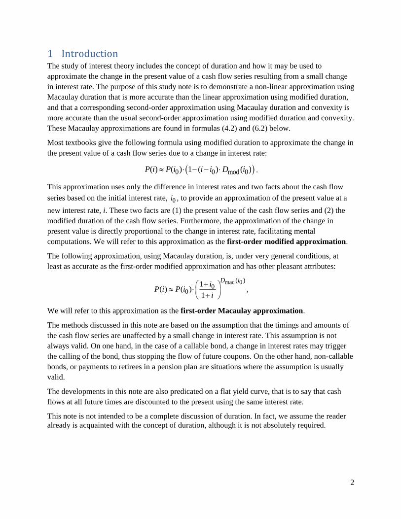
1 Introduction The study of interest theory includes the concept of duration and how it may be used to

approximate the change in the present value of a cash flow series resulting from a small change

in interest rate. The purpose of this study note is to demonstrate a non-linear approximation using

Macaulay duration that is more accurate than the linear approximation using modified duration,

and that a corresponding second-order approximation using Macaulay duration and convexity is

more accurate than the usual second-order approximation using modified duration and convexity.

These Macaulay approximations are found in formulas (4.2) and (6.2) below.

Most textbooks give the following formula using modified duration to approximate the change in

the present value of a cash flow series due to a change in interest rate:

0 0 mod 0( ) ( ) 1 ( ) ( )P i P i i i D i .

This approximation uses only the difference in interest rates and two facts about the cash flow

series based on the initial interest rate, 0i , to provide an approximation of the present value at a

new interest rate, i. These two facts are (1) the present value of the cash flow series and (2) the

modified duration of the cash flow series. Furthermore, the approximation of the change in

present value is directly proportional to the change in interest rate, facilitating mental

computations. We will refer to this approximation as the first-order modified approximation.

The following approximation, using Macaulay duration, is, under very general conditions, at

least as accurate as the first-order modified approximation and has other pleasant attributes:

mac 0( )0

01

( ) ( )1

D ii

P i P ii

,

We will refer to this approximation as the first-order Macaulay approximation.

The methods discussed in this note are based on the assumption that the timings and amounts of

the cash flow series are unaffected by a small change in interest rate. This assumption is not

always valid. On one hand, in the case of a callable bond, a change in interest rates may trigger

the calling of the bond, thus stopping the flow of future coupons. On the other hand, non-callable

bonds, or payments to retirees in a pension plan are situations where the assumption is usually

valid.

The developments in this note are also predicated on a flat yield curve, that is to say that cash

flows at all future times are discounted to the present using the same interest rate.

This note is not intended to be a complete discussion of duration. In fact, we assume the reader

already is acquainted with the concept of duration, although it is not absolutely required.

3

2 Cash Flow Series and Present Value A cash flow is a pair, ( , )a t , where a is a real number, and t is a non-negative real number. Given

a cash flow ( , )a t , the amount of the cash flow is a and the time of the cash flow is t . Notice

that we have allowed the amount to be negative, although the time is non-negative. A cash flow

series is a sequence (finite or infinite) of cash flows ( , )k ka t defined for k N , where N is a

subset of the set of non-negative integers.

For the purpose of calculating present values and durations, we introduce a periodic effective

interest rate, i, where the period of time is the same time unit used to measure the times of the

cash flows. For example, if the times are measured in months, then the interest rate, i, is a

monthly effective interest rate. We define P to represent the present value of the cash flow series

as a function of the interest rate as follows.

( ) (1 ) ktk

k N

P i a i

(2.1)

If the cash flow series is infinite, the sum in (2.1) may not converge or be finite. In what follows,

we implicitly make the assumption that any sums so represented converge. In the case that N is a

finite set of the form {1,..., }n , we may choose to write the sum as

1

(1 ) kn

tk

k

a i

.

The following examples show the present value of a 10-year annuity immediate calculated at an

annual effective interest rate of 7.0% and at an annual effective interest rate of interest of 6.5%.

We will use this same cash flow series as an example throughout this note.

Suppose ( , ) (1000, )k ka t k and 1,...,10N . Then,

10 0.07

(0.07) 1000 7023.5815P a (2.2)

and

10 0.065

(0.065) 1000 7188.8302.P a (2.3)

We would like to approximate the change in the present value of a cash flow series resulting

from a small change in the interest rate. This is a valuable technique for several reasons. First,

much of actuarial science involves the use of mathematical models of various levels of

complexity and sophistication. To be able to use a model effectively, one needs to understand the

dynamics of the model, i.e., how one variable changes based on a change to a different variable.

The present value formula is such a mathematical model. An actuary should understand how

present value changes when the amounts change, when the times change, and when the interest

rate changes.

4

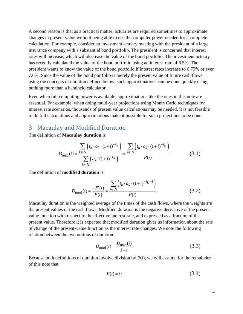
A second reason is that as a practical matter, actuaries are required sometimes to approximate

changes in present value without being able to use the computer power needed for a complete

calculation. For example, consider an investment actuary meeting with the president of a large

insurance company with a substantial bond portfolio. The president is concerned that interest

rates will increase, which will decrease the value of the bond portfolio. The investment actuary

has recently calculated the value of the bond portfolio using an interest rate of 6.5%. The

president wants to know the value of the bond portfolio if interest rates increase to 6.75% or even

7.0%. Since the value of the bond portfolio is merely the present value of future cash flows,

using the concepts of duration defined below, such approximations can be done quickly using

nothing more than a handheld calculator.

Even when full computing power is available, approximations like the ones in this note are

essential. For example, when doing multi-year projections using Monte Carlo techniques for

interest rate scenarios, thousands of present value calculations may be needed. It is not feasible

to do full calculations and approximations make it possible for such projections to be done.

3 Macaulay and Modified Duration The definition of Macaulay duration is

mac

(1 ) (1 )

( ) .( )(1 )

k k

k

t tk k k k

k N k N

tk

k N

t a i t a i

D iP ia i

(3.1)

The definition of modified duration is

1

mod

(1 )( )

( ) .( ) ( )

ktk k

k N

t a iP i

D iP i P i

(3.2)

Macaulay duration is the weighted average of the times of the cash flows, where the weights are

the present values of the cash flows. Modified duration is the negative derivative of the present-

value function with respect to the effective interest rate, and expressed as a fraction of the

present value. Therefore it is expected that modified duration gives us information about the rate

of change of the present-value function as the interest rate changes. We note the following

relation between the two notions of duration:

macmod

( )( ) .

1

D iD i

i

(3.3)

Because both definitions of duration involve division by P(i), we will assume for the remainder

of this note that

( ) 0.P i (3.4)

5

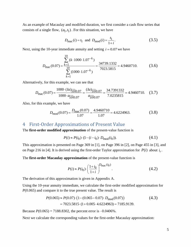
As an example of Macaulay and modified duration, we first consider a cash flow series that

consists of a single flow, 1 1( , )a t . For this situation, we have

1mac 1 mod( ) and ( ) .

1

tD i t D i

i

(3.5)

Next, using the 10-year immediate annuity and setting 0.07i we have

10

1mac 10

1

( 1000 1.07 )34739.1332

(0.07) 4.9460710.7023.5815

(1000 1.07 )

k

k

k

k

k

D

(3.6)

Alternatively, for this example, we can see that

mac10 0.07 10 0.07

10 0.07 10 0.07

1000 ( ) ( ) 34.7391332(0.07) 4.9460710.

1000 7.0235815

Ia IaD

a a

(3.7)

Also, for this example, we have

macmod

(0.07) 4.9460710(0.07) 4.6224963.

1.07 1.07

DD (3.8)

4 First-Order Approximations of Present Value The first-order modified approximation of the present-value function is

0 0 mod 0( ) ( ) (1 ( ) ( )).P i P i i i D i (4.1)

This approximation is presented on Page 369 in [1], on Page 396 in [2], on Page 455 in [3], and

on Page 216 in [4]. It is derived using the first-order Taylor approximation for ( )P i about 0i .

The first-order Macaulay approximation of the present-value function is

mac 0( )

00

1( ) ( ) .

1

D ii

P i P ii

(4.2)

The derivation of this approximation is given in Appendix A.

Using the 10-year annuity immediate, we calculate the first-order modified approximation for

P(0.065) and compare it to the true present value. The result is

mod(0.065) (0.07) 1 (0.065 0.07) (0.07)

7023.5815 (1 0.005 4.6224963) 7185.9139.

P P D

(4.3)

Because P(0.065) = 7188.8302, the percent error is –0.0406%.

Next we calculate the corresponding values for the first-order Macaulay approximation:

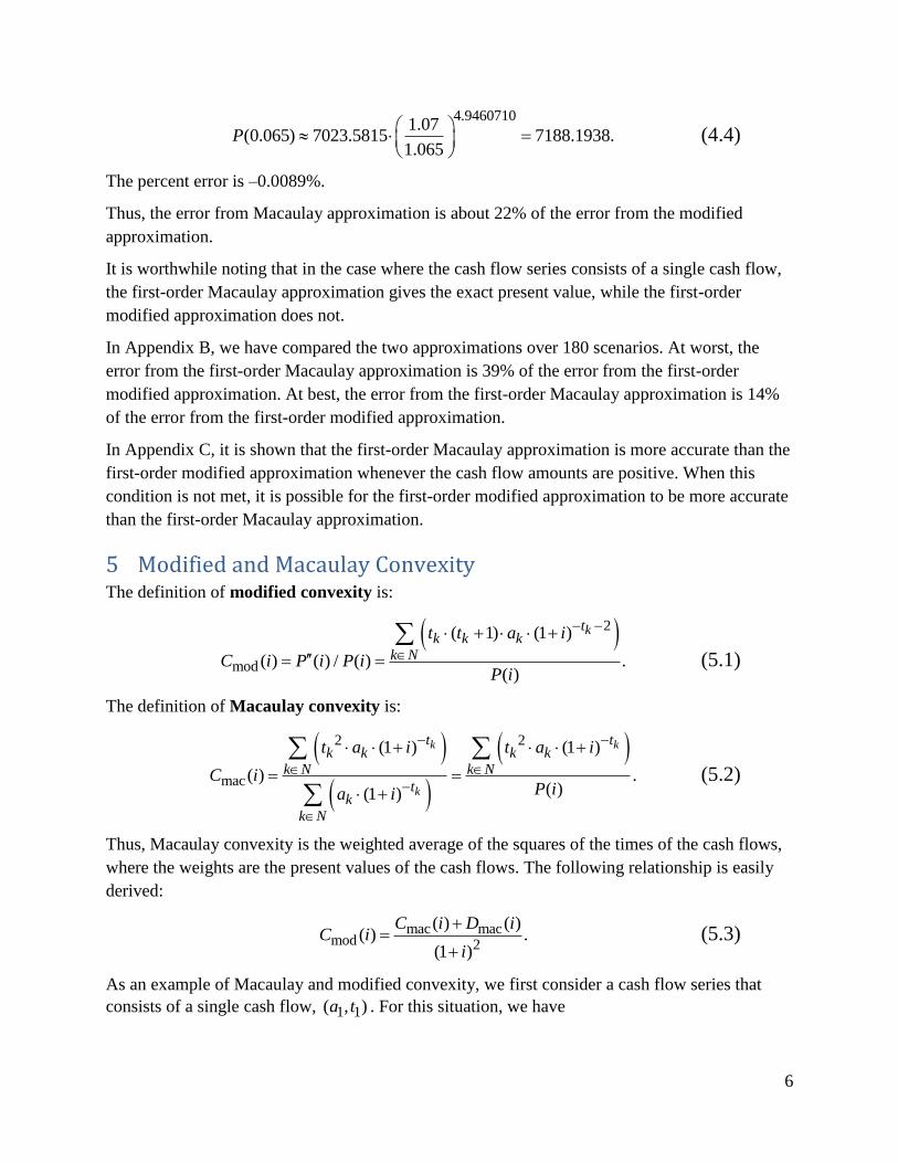
6

4.9460710

1.07(0.065) 7023.5815 7188.1938.

1.065P

(4.4)

The percent error is –0.0089%.

Thus, the error from Macaulay approximation is about 22% of the error from the modified

approximation.

It is worthwhile noting that in the case where the cash flow series consists of a single cash flow,

the first-order Macaulay approximation gives the exact present value, while the first-order

modified approximation does not.

In Appendix B, we have compared the two approximations over 180 scenarios. At worst, the

error from the first-order Macaulay approximation is 39% of the error from the first-order

modified approximation. At best, the error from the first-order Macaulay approximation is 14%

of the error from the first-order modified approximation.

In Appendix C, it is shown that the first-order Macaulay approximation is more accurate than the

first-order modified approximation whenever the cash flow amounts are positive. When this

condition is not met, it is possible for the first-order modified approximation to be more accurate

than the first-order Macaulay approximation.

5 Modified and Macaulay Convexity The definition of modified convexity is:

2

mod

( 1) (1 )

( ) ( ) / ( ) .( )

ktk k k

k N

t t a i

C i P i P iP i

(5.1)

The definition of Macaulay convexity is:

2 2

mac

(1 ) (1 )

( ) .( )(1 )

k k

k

t tk k k k

k N k N

tk

k N

t a i t a i

C iP ia i

(5.2)

Thus, Macaulay convexity is the weighted average of the squares of the times of the cash flows,

where the weights are the present values of the cash flows. The following relationship is easily

derived:

mac macmod 2

( ) ( )( ) .

(1 )

C i D iC i

i

(5.3)

As an example of Macaulay and modified convexity, we first consider a cash flow series that

consists of a single cash flow, 1 1( , )a t . For this situation, we have

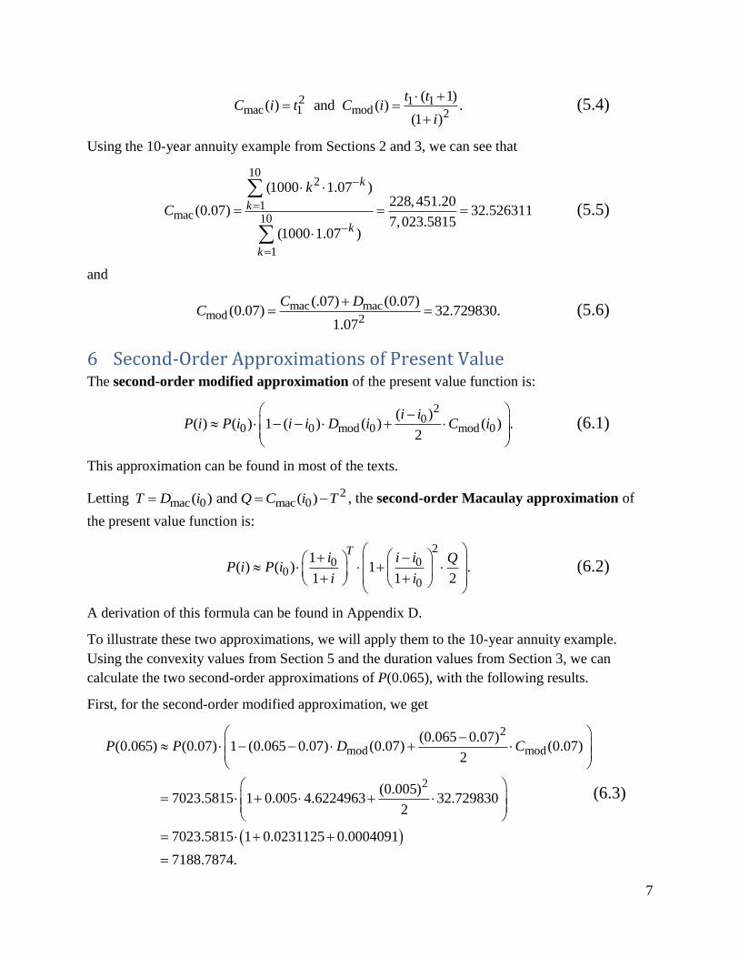
7

2 1 1mac 1 mod 2

( 1)( ) and ( ) .

(1 )

t tC i t C i

i

(5.4)

Using the 10-year annuity example from Sections 2 and 3, we can see that

102

1mac 10

1

(1000 1.07 )228,451.20

(0.07) 32.5263117,023.5815

(1000 1.07 )

k

k

k

k

k

C

(5.5)

and

mac macmod 2

(.07) (0.07)(0.07) 32.729830.

1.07

C DC

(5.6)

6 Second-Order Approximations of Present Value The second-order modified approximation of the present value function is:

2

00 0 mod 0 mod 0

( )( ) ( ) 1 ( ) ( ) ( ) .

2

i iP i P i i i D i C i

(6.1)

This approximation can be found in most of the texts.

Letting 2mac 0 mac 0 ( ) and ( )T D i Q C i T , the second-order Macaulay approximation of

the present value function is:

2

0 00

0

1( ) ( ) 1 .

1 1 2

Ti i i Q

P i P ii i

(6.2)

A derivation of this formula can be found in Appendix D.

To illustrate these two approximations, we will apply them to the 10-year annuity example.

Using the convexity values from Section 5 and the duration values from Section 3, we can

calculate the two second-order approximations of P(0.065), with the following results.

First, for the second-order modified approximation, we get

2

mod mod

2

(0.065 0.07)(0.065) (0.07) 1 (0.065 0.07) (0.07) (0.07)

2

(0.005)7023.5815 1 0.005 4.6224963 32.729830

2

7023.5815 1 0.0231125 0.0004091

7188.7874.

P P D C

(6.3)

8

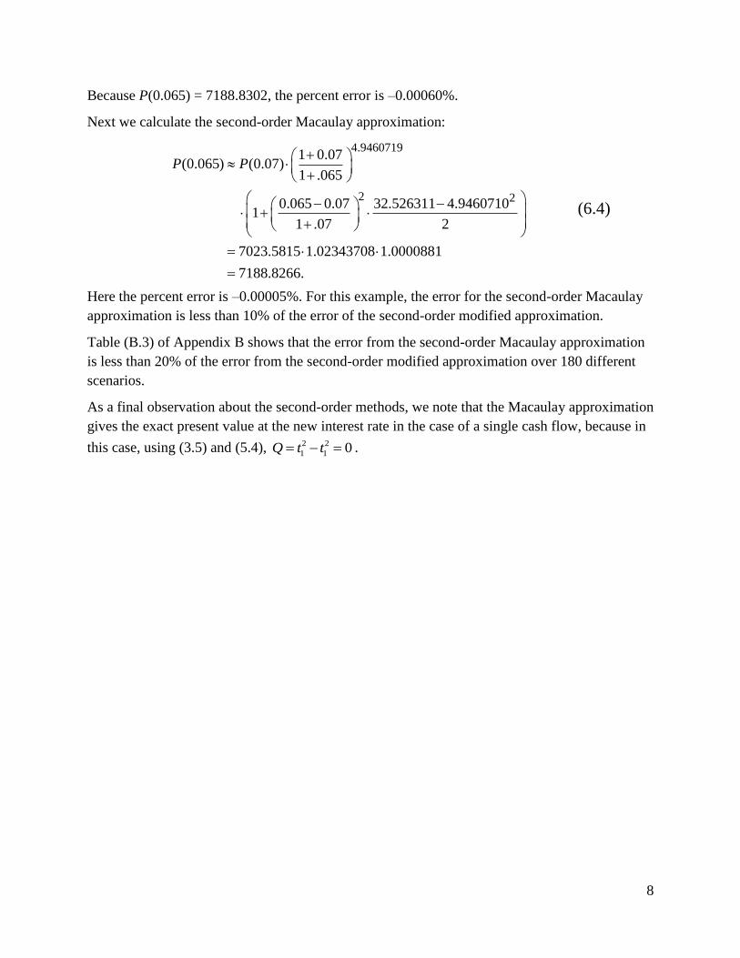
Because P(0.065) = 7188.8302, the percent error is –0.00060%.

Next we calculate the second-order Macaulay approximation:

4.9460719

2 2

1 0.07(0.065) (0.07)

1 .065

0.065 0.07 32.526311 4.9460710 1

1 .07 2

7023.5815 1.02343708 1.0000881

7188.8266.

P P

(6.4)

Here the percent error is –0.00005%. For this example, the error for the second-order Macaulay

approximation is less than 10% of the error of the second-order modified approximation.

Table (B.3) of Appendix B shows that the error from the second-order Macaulay approximation

is less than 20% of the error from the second-order modified approximation over 180 different

scenarios.

As a final observation about the second-order methods, we note that the Macaulay approximation

gives the exact present value at the new interest rate in the case of a single cash flow, because in

this case, using (3.5) and (5.4), 2 2

1 1 0Q t t .

9

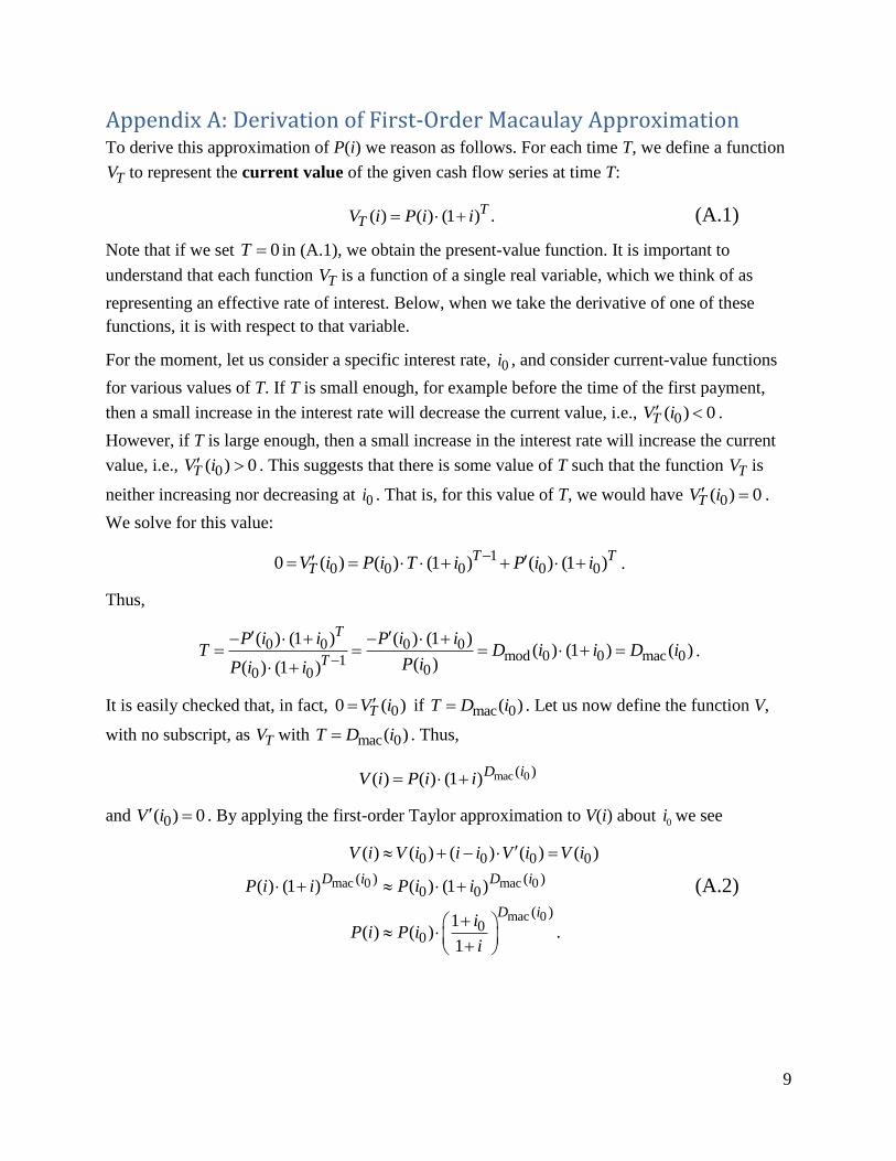
Appendix A: Derivation of First-Order Macaulay Approximation To derive this approximation of P(i) we reason as follows. For each time T, we define a function

TV to represent the current value of the given cash flow series at time T:

( ) ( ) (1 ) .TTV i P i i (A.1)

Note that if we set 0T in (A.1), we obtain the present-value function. It is important to

understand that each function TV is a function of a single real variable, which we think of as

representing an effective rate of interest. Below, when we take the derivative of one of these

functions, it is with respect to that variable.

For the moment, let us consider a specific interest rate, 0i , and consider current-value functions

for various values of T. If T is small enough, for example before the time of the first payment,

then a small increase in the interest rate will decrease the current value, i.e., 0( ) 0TV i .

However, if T is large enough, then a small increase in the interest rate will increase the current

value, i.e., 0( ) 0TV i . This suggests that there is some value of T such that the function TV is

neither increasing nor decreasing at 0i . That is, for this value of T, we would have 0( ) 0TV i .

We solve for this value:

10 0 0 0 00 ( ) ( ) (1 ) ( ) (1 )T T

TV i P i T i P i i .

Thus,

0 0 0 0mod 0 0 mac 01

00 0

( ) (1 ) ( ) (1 )( ) (1 ) ( )

( )( ) (1 )

T

T

P i i P i iT D i i D i

P iP i i

.

It is easily checked that, in fact, 00 ( )TV i if mac 0( )T D i . Let us now define the function V,

with no subscript, as TV with mac 0( )T D i . Thus,

mac 0( )( ) ( ) (1 )

D iV i P i i

and 0( ) 0V i . By applying the first-order Taylor approximation to V(i) about 0i we see

mac 0 mac 0

mac 0

0 0 0 0

( ) ( )0 0

( )0

0

( ) ( ) ( ) ( ) ( )

( ) (1 ) ( ) (1 )

1( ) ( ) .

1

D i D i

D i

V i V i i i V i V i

P i i P i i

iP i P i

i

(A.2)

10

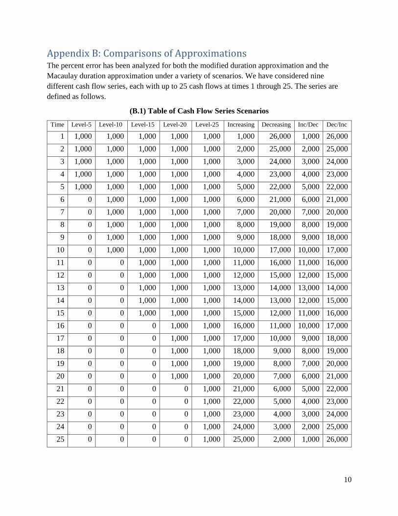
Appendix B: Comparisons of Approximations The percent error has been analyzed for both the modified duration approximation and the

Macaulay duration approximation under a variety of scenarios. We have considered nine

different cash flow series, each with up to 25 cash flows at times 1 through 25. The series are

defined as follows.

(B.1) Table of Cash Flow Series Scenarios

Time Level-5 Level-10 Level-15 Level-20 Level-25 Increasing Decreasing Inc/Dec Dec/Inc

1 1,000 1,000 1,000 1,000 1,000 1,000 26,000 1,000 26,000

2 1,000 1,000 1,000 1,000 1,000 2,000 25,000 2,000 25,000

3 1,000 1,000 1,000 1,000 1,000 3,000 24,000 3,000 24,000

4 1,000 1,000 1,000 1,000 1,000 4,000 23,000 4,000 23,000

5 1,000 1,000 1,000 1,000 1,000 5,000 22,000 5,000 22,000

6 0 1,000 1,000 1,000 1,000 6,000 21,000 6,000 21,000

7 0 1,000 1,000 1,000 1,000 7,000 20,000 7,000 20,000

8 0 1,000 1,000 1,000 1,000 8,000 19,000 8,000 19,000

9 0 1,000 1,000 1,000 1,000 9,000 18,000 9,000 18,000

10 0 1,000 1,000 1,000 1,000 10,000 17,000 10,000 17,000

11 0 0 1,000 1,000 1,000 11,000 16,000 11,000 16,000

12 0 0 1,000 1,000 1,000 12,000 15,000 12,000 15,000

13 0 0 1,000 1,000 1,000 13,000 14,000 13,000 14,000

14 0 0 1,000 1,000 1,000 14,000 13,000 12,000 15,000

15 0 0 1,000 1,000 1,000 15,000 12,000 11,000 16,000

16 0 0 0 1,000 1,000 16,000 11,000 10,000 17,000

17 0 0 0 1,000 1,000 17,000 10,000 9,000 18,000

18 0 0 0 1,000 1,000 18,000 9,000 8,000 19,000

19 0 0 0 1,000 1,000 19,000 8,000 7,000 20,000

20 0 0 0 1,000 1,000 20,000 7,000 6,000 21,000

21 0 0 0 0 1,000 21,000 6,000 5,000 22,000

22 0 0 0 0 1,000 22,000 5,000 4,000 23,000

23 0 0 0 0 1,000 23,000 4,000 3,000 24,000

24 0 0 0 0 1,000 24,000 3,000 2,000 25,000

25 0 0 0 0 1,000 25,000 2,000 1,000 26,000

11

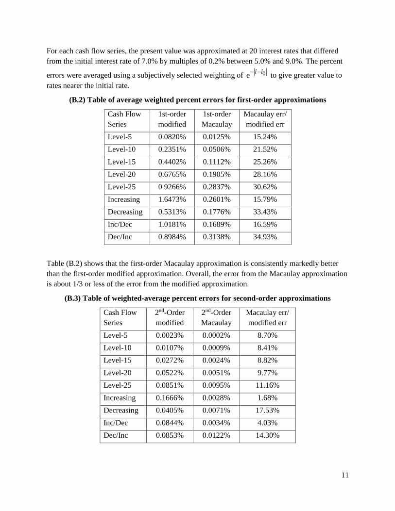
For each cash flow series, the present value was approximated at 20 interest rates that differed

from the initial interest rate of 7.0% by multiples of 0.2% between 5.0% and 9.0%. The percent

errors were averaged using a subjectively selected weighting of 0ei i

to give greater value to

rates nearer the initial rate.

(B.2) Table of average weighted percent errors for first-order approximations

Cash Flow

Series

1st-order

modified

1st-order

Macaulay

Macaulay err/

modified err

Level-5 0.0820% 0.0125% 15.24%

Level-10 0.2351% 0.0506% 21.52%

Level-15 0.4402% 0.1112% 25.26%

Level-20 0.6765% 0.1905% 28.16%

Level-25 0.9266% 0.2837% 30.62%

Increasing 1.6473% 0.2601% 15.79%

Decreasing 0.5313% 0.1776% 33.43%

Inc/Dec 1.0181% 0.1689% 16.59%

Dec/Inc 0.8984% 0.3138% 34.93%

Table (B.2) shows that the first-order Macaulay approximation is consistently markedly better

than the first-order modified approximation. Overall, the error from the Macaulay approximation

is about 1/3 or less of the error from the modified approximation.

(B.3) Table of weighted-average percent errors for second-order approximations

Cash Flow

Series

2nd-Order

modified

2nd-Order

Macaulay

Macaulay err/

modified err

Level-5 0.0023% 0.0002% 8.70%

Level-10 0.0107% 0.0009% 8.41%

Level-15 0.0272% 0.0024% 8.82%

Level-20 0.0522% 0.0051% 9.77%

Level-25 0.0851% 0.0095% 11.16%

Increasing 0.1666% 0.0028% 1.68%

Decreasing 0.0405% 0.0071% 17.53%

Inc/Dec 0.0844% 0.0034% 4.03%

Dec/Inc 0.0853% 0.0122% 14.30%

12

Table (B.3) shows that the second-order Macaulay approximation is consistently markedly better

than the second-order modified approximation. Overall, the error from the Macaulay

approximation is about 1/5 or less of the error from the modified approximation.

We can use the second-order results to measure the success of the Macaulay first-order

approximation. For the Level-5 cash flow series, the difference between the first-order modified

average error and the second-order modified average error is 0.0820% - 0.0023%, or 0.0797%.

The difference between the first-order modified average error and the first-order Macaulay

average error is 0.0820% – 0.0125%, or 0.0695%. Thus the first-order Macaulay approximation

takes you 87% of the way from the first-order modified to the second-order modified

approximation. This percentage varies between 72% and 94% over the nine different cash flow

series studied.

13

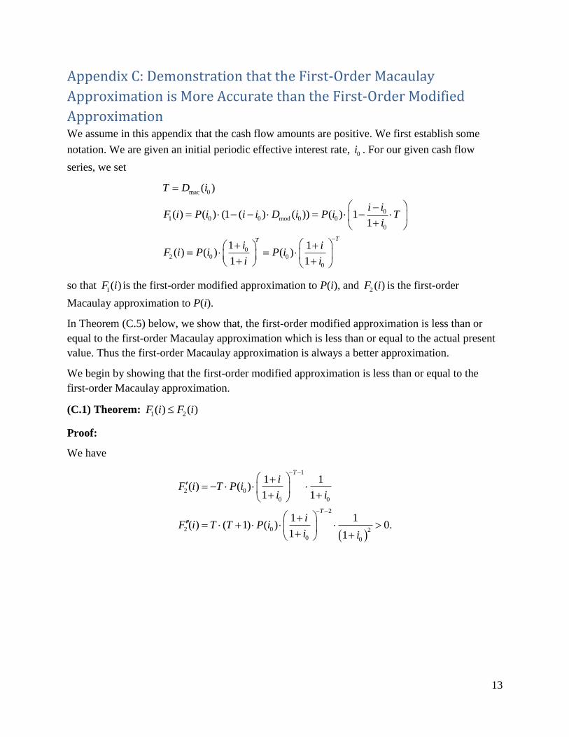
Appendix C: Demonstration that the First-Order Macaulay

Approximation is More Accurate than the First-Order Modified

Approximation We assume in this appendix that the cash flow amounts are positive. We first establish some

notation. We are given an initial periodic effective interest rate, 0i . For our given cash flow

series, we set

mac 0

01 0 0 mod 0 0

0

02 0 0

0

( )

( ) ( ) (1 ( ) ( )) ( ) 11

1 1( ) ( ) ( )

1 1

TT

T D i

i iF i P i i i D i P i T

i

i iF i P i P i

i i

so that 1( )F i is the first-order modified approximation to P(i), and 2 ( )F i is the first-order

Macaulay approximation to P(i).

In Theorem (C.5) below, we show that, the first-order modified approximation is less than or

equal to the first-order Macaulay approximation which is less than or equal to the actual present

value. Thus the first-order Macaulay approximation is always a better approximation.

We begin by showing that the first-order modified approximation is less than or equal to the

first-order Macaulay approximation.

(C.1) Theorem: 1 2( ) ( )F i F i

Proof:

We have

1

2 0

0 0

2

2 0 2

0 0

1 1( ) ( )

1 1

1 1( ) ( 1) ( ) 0.

1 1

T

T

iF i T P i

i i

iF i T T P i

i i

14

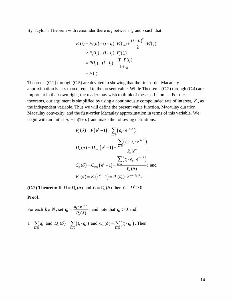
By Taylor’s Theorem with remainder there is j between 0i and i such that

2

02 2 0 0 2 0 2

2 0 0 2 0

00 0

0

1

( )( ) ( ) ( ) ( ) ( )

2

( ) ( ) ( )

( )( ) ( )

1

( ).

i iF i F i i i F i F j

F i i i F i

T P iP i i i

i

F i

Theorems (C.2) through (C.5) are devoted to showing that the first-order Macaulay

approximation is less than or equal to the present value. While Theorems (C.2) through (C.4) are

important in their own right, the reader may wish to think of these as Lemmas. For these

theorems, our argument is simplified by using a continuously compounded rate of interest, , as

the independent variable. Thus we will define the present value function, Macaulay duration,

Macaulay convexity, and the first-order Macaulay approximation in terms of this variable. We

begin with an initial 0 0ln(1 )i and make the following definitions.

0

mac

2

mac

( )

2 0

( ) e 1 e ;

e

( ) e 1 ;( )

e

( ) e 1 ; and( )

( ) e 1 ( ) e .

k

k

k

t

k

k N

t

k k

k N

t

k k

k N

T

P P a

t a

D DP

t a

C CP

F F P

(C.2) Theorem: If ( )D D and ( )C C then 2 0C D .

Proof:

For each k N , set e

( )

kt

kk

aq

P

, and note that 0kq and

1 k

k N

q

and ( ) k k

k N

D t q

and 2( ) k k

k N

C t q

. Then

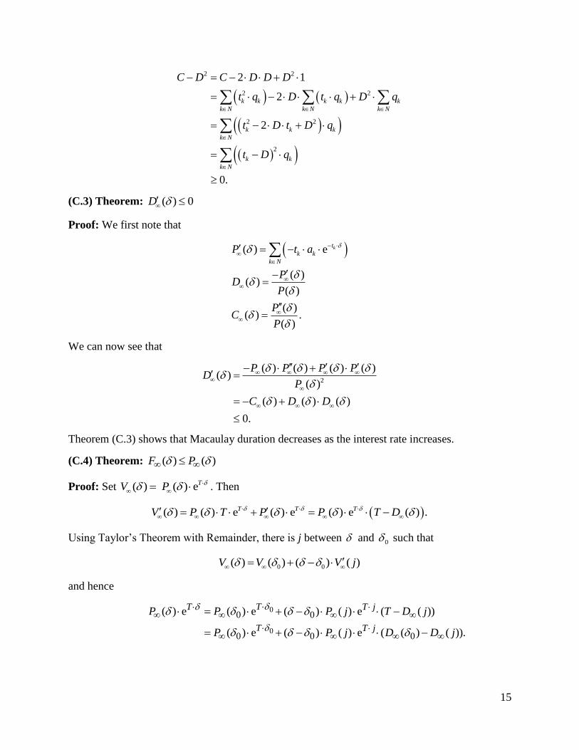
15

2 2

2 2

2 2

2

2 1

2

2

0.

k k k k k

k N k N k N

k k k

k N

k k

k N

C D C D D D

t q D t q D q

t D t D q

t D q

(C.3) Theorem: ( ) 0D

Proof: We first note that

( ) e

( )( )

( )

( )( ) .

( )

kt

k k

k N

P t a

PD

P

PC

P

We can now see that

2

( ) ( ) ( ) ( )( )

( )

( ) ( ) ( )

0.

P P P PD

P

C D D

Theorem (C.3) shows that Macaulay duration decreases as the interest rate increases.

(C.4) Theorem: ( ) ( )F P

Proof: Set ( ) ( ) eTV P

. Then

( ) ( ) e ( ) e ( ) e ( ) .T T TV P T P P T D

Using Taylor’s Theorem with Remainder, there is j between and 0 such that

0 0( ) ( ) ( ) ( )V V V j

and hence

0

0

0 0

0 0 0

( ) e ( ) e ( ) ( ) e ( ( ))

( ) e ( ) ( ) e ( ( ) ( )).

TT T j

T T j

P P P j T D j

P P j D D j

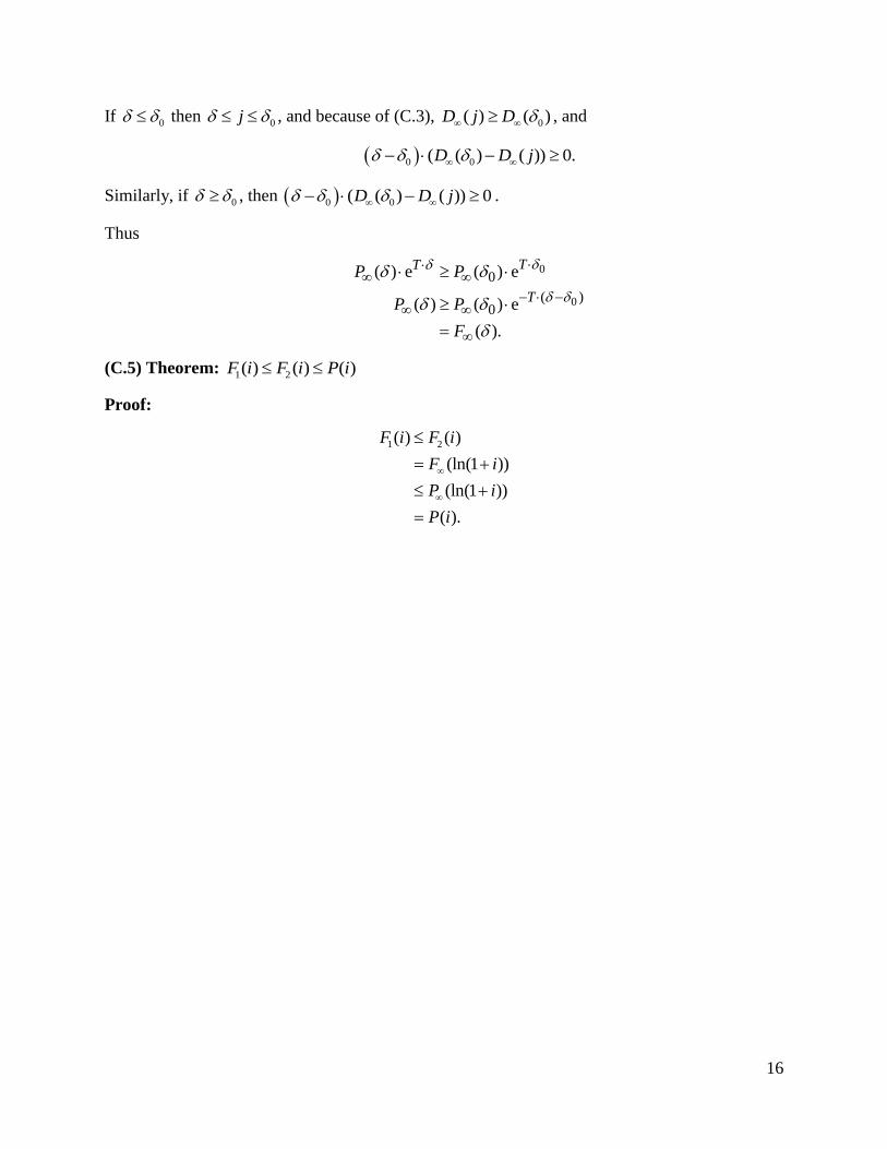
16

If 0 then

0j , and because of (C.3), 0( ) ( )D j D , and

0 0( ( ) ( )) 0.D D j

Similarly, if 0 , then 0 0( ( ) ( )) 0D D j .

Thus

0

0

0

( )0

( ) e ( ) e

( ) ( ) e

( ).

TT

T

P P

P P

F

(C.5) Theorem: 1 2( ) ( ) ( )F i F i P i

Proof:

1 2( ) ( )

(ln(1 ))

(ln(1 ))

( ).

F i F i

F i

P i

P i

17

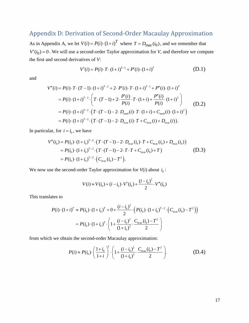
Appendix D: Derivation of Second-Order Macaulay Approximation

As in Appendix A, we let ( ) ( ) (1 )TV i P i i where mac 0( )T D i , and we remember that

0( ) 0V i . We will use a second-order Taylor approximation for V, and therefore we compute

the first and second derivatives of V:

1( ) ( ) (1 ) ( ) (1 )T TV i P i T i P i i (D.1)

and

2 1

2 2

2 2

mod mod

2

( ) ( ) ( 1) (1 ) 2 ( ) (1 ) ( ) (1 )

( ) ( )( ) (1 ) ( 1) 2 (1 ) (1 )

( ) ( )

( ) (1 ) ( 1) 2 ( ) (1 ) ( ) (1 )

( ) (1 ) (

T T T

T

T

T

V i P i T T i P i T i P i i

P i P iP i i T T T i i

P i P i

P i i T T D i T i C i i

P i i T

mac mac mac1) 2 ( ) ( ) ( ) .T D i T C i D i

(D.2)

In particular, for 0i i , we have

2

0 0 0 mac 0 mac 0 mac 0

2

0 0 mac 0

2 2

0 0 mac 0

( ) ( ) (1 ) ( 1) 2 ( ) ( ) ( )

( ) (1 ) ( 1) 2 ( )

( ) (1 ) ( ) .

T

T

T

V i P i i T T D i T C i D i

P i i T T T T C i T

P i i C i T

(D.3)

We now use the second-order Taylor approximation for V(i) about 0i :

2

00 0 0 0

( )( ) ( ) ( ) ( ) ( )

2

i iV i V i i i V i V i

This translates to

2

2 200 0 0 0 mac 0

2 2

0 mac 00 0 2

0

( )( ) (1 ) ( ) (1 ) 0 ( ) (1 ) ( )

2

( ) ( )( ) (1 ) 1

(1 ) 2

T T T

T

i iP i i P i i P i i C i T

i i C i TP i i

i

from which we obtain the second-order Macaulay approximation:

2 2

0 0 mac 00 2

0

1 ( ) ( )( ) ( ) 1 .

1 (1 ) 2

Ti i i C i T

P i P ii i

(D.4)

18

Acknowledgements

The author thanks Steve Kossman, David Cummings, and Stephen Meskin for their suggestions

during the preparation of this note and for their review of drafts containing various errors. Of

course, any errors that remain in the note are the responsibility of the author.

References

[1] Broverman, Samuel A., Mathematics of Investment and Credit, Sixth Edition, Actex

Publications, Inc., 2015

[2] Vaaler, Leslie Jane Federer and Daniel, James W., Mathematical Interest Theory, Second

Edition, Pearson Prentice Hall, 2009

[3] Kellison, Stephen G., The Theory of Interest, Third Edition, McGraw Hill Irwin, 2009

[4] Ruckman, Chris and Francis, Joe, Financial Mathematics, Second Edition, BPP Professional

Education, Inc., 2005