t 106 (2007) 480–491www.elsevier.com/locate/rse

Remote Sensing of Environmen

Validation of a large area land cover product usingpurpose-acquired airborne video

M.A. Wulder ⁎, J.C. White, S. Magnussen, S. McDonald

Canadian Forest Service (Pacific Forestry Centre), Natural Resources Canada, Victoria, British Columbia, Canada

Received 3 April 2006; received in revised form 14 September 2006; accepted 16 September 2006

Abstract

Large area land cover products generated from remotely sensed data are difficult to validate in a timely and cost effective manner. As a result, pre-existing data are often used for validation. Temporal, spatial, and attribute differences between the land cover product and pre-existing validation datacan result in inconclusive depictions of map accuracy. This approach may therefore misrepresent the true accuracy of the land cover product, as wellas the accuracy of the validation data, which is not assumed to be without error. Hence, purpose-acquired validation data is preferred; however,logistical constraints often preclude its use— especially for large area land cover products. Airborne digital video provides a cost-effective tool forcollecting purpose-acquired validation data over large areas. An operational trial was conducted, involving the collection of airborne video for thevalidation of a 31,000 km2 sub-sample of the Canadian large area Earth Observation for Sustainable Development of Forests (EOSD) land cover map(Vancouver Island, British Columbia, Canada). In this trial, one form of agreement between the EOSD product and the airborne video data wasdefined as a match between the mode land cover class of a 3 by 3 pixel neighbourhood surrounding the sample pixel and the primary or secondarychoice of land cover for the interpreted video. This scenario produced the highest level of overall accuracy at 77% for level 4 of classificationhierarchy (13 classes). The coniferous treed class, which represented 71% of Vancouver Island, had an estimated user's accuracy of 86%. Purposeacquired video was found to be a useful and cost-effective data source for validation of the EOSD land cover product. The impact of using multipleinterpreters was also tested and documented. Improvements to the sampling and response designs that emerged from this trial will benefit a full-scaleaccuracy assessment of the EOSD product and also provides insights for other regional and global land cover mapping programs.© 2006 Elsevier Inc. All rights reserved.

Keywords: Land cover; Forest; Mapping; Landsat; Validation; Airborne video; Large area land cover; Sample design; Monitoring

1. Introduction

The classification of land cover over large geographic areaswith remotely sensed data is increasingly common; regions(Homer et al., 1997), nations (Loveland et al., 1991; Fuller et al.,1994; Cihlar & Beaubien, 1998), continents (Stone et al., 1994),and the globe (Loveland & Belward, 1997; Loveland et al., 2000;Hansen et al., 2000) have been mapped with a variety of satellitedata types. This surge of interest in large area land cover mappingprojects may be explained by an increase in image availability, aneed for national- and global-scale land cover products formodelling and monitoring activities, and political obligationsrelated to international treaties such as the Convention on Climate

⁎ Corresponding author. 506 West Burnside Rd., Victoria, BC, Canada V8Z1M5. Tel.: +1 250 363 6090; fax: +1 250 363 0775.

E-mail address: mike.wulder@pfc.cfs.nrcan.gc.ca (M.A. Wulder).

0034-4257/$ - see front matter © 2006 Elsevier Inc. All rights reserved.doi:10.1016/j.rse.2006.09.012

Change (Kyoto Protocol). Standard operational protocols for thevalidation of these products are emerging (Loveland et al., 1999;Justice et al., 2000; Strahler et al., 2006; Wulder, Franklin et al.,2006), and a new initiative is addressing both the harmonizationand validation of large area land cover products (Herold et al.,2006).

A sufficient level of accuracy is assumed in order to rationalizethe applied use of these large area land cover products for a widevariety of applications (Morisette et al., 2002; Stehman &Czaplewski, 2003). Accuracy assessment protocols requirevalidation data that is independent from information used inmap development; however, validation data is expensive andlogistically challenging to collect for large area land coverproducts (Cihlar, 2000). As a result, pre-existing data are oftenused for validation of large area land cover products generatedfrom remotely sensed data. Unfortunately, temporal, spatial, andattribute differences between the land cover product and the pre-

481M.A. Wulder et al. / Remote Sensing of Environment 106 (2007) 480–491

existing validation data can result in poor levels of apparentaccuracy (Remmel et al., 2005). Furthermore, the use of pre-existing validation data may misrepresent the true accuracy of theland cover product, while at the same time, revealing problemsinherent in the validation data (Wulder, White et al. 2006). Aerialvideography is one means of obtaining purpose-acquiredvalidation data for land cover products extending over largeareas (Slaymaker, 2003).

Airborne videography became known as a flexible and costeffective remote sensing tool in the early 1980s (Meisner, 1986;Mausel et al., 1992; King, 1995), and has demonstrated utility for awide range of applications including species identification andvegetation mapping (Nixon et al., 1985; Bobbe et al., 1993;Frazier, 1998; Suzuki et al., 2004), forest health and damageassessment (Jacobs and Eggen-McIntosh, 1993; Jacobs, 2000);forest inventory update (Brownlie et al., 1996; Davis et al., 2002);and validation of vegetation maps generated from medium reso-lution remotely sensed data (Graham, 1993; Marsh et al., 1994;Slaymaker et al., 1996; Hepinstall et al., 1999; Hess et al., 2002).Marsh et al. (1994) compared the use of systematically acquiredaerial colour photography and airborne video for the validation ofland cover products generated from Landsat TM imagery. Thesimilarity between the accuracies measured by the photographyand video sources was statistically significant (α=0.01), suggest-ing that video could provide validation data of similar quality andutility to that of traditional aerial photography, with the advantageof collecting a larger volume of data with the same level of effort.

Aerial videography gained additional momentum in the1990s as a result of the GAP analysis programs implemented inthe United States (Slaymaker, 2003). GAP programs operated atthe state level and were initiated to assess the extent to whichnative animal and plant species were being protected. GAP landcover maps generated from Landsat TM data required a sourceof calibration data to facilitate the classification of the imagery,as well as a source of validation data to assess the accuracy of theoutput vegetation maps (Scott et al., 1993; Slaymaker, 2003).Aerial point sampling methods developed by Norton-Griffiths(1982) for aerial photography were adapted to aerial videogra-phy by Graham (1993) and implemented in the Arizona GAPprogram. The automatic labelling of video frames with GlobalPositioning System (GPS) coordinates was a major technolog-ical advancement, “providing a way to precisely and automat-ically match video-recorded GPS time with the positioninformation in the GPS data file” (Graham, 1993: 29).Slaymaker et al. (1996) modified this approach for the GAPprogram in New England. Aerial video for calibration andvalidation of Landsat-based land cover maps was subsequentlyadopted by many other state-wide GAP programs (Schlagel,1995; Driese et al., 1997; Hepinstall et al., 1999; Reiners et al.,2000), as well as for other land cover products (Skirvin et al.,2000; Hess et al., 2002; Maingi et al., 2002; Skirvin et al., 2004).Technological advances in the 1990s led to the development ofdigital video cameras and powerful multi-media capabilities indesktop computers, further enhancing the quality and afford-ability of video options (Hess et al., 2002).

The advantages and disadvantages of airborne video for vali-dation of land cover maps are summarized in Slaymaker (2003).

One of the main advantages of video is data redundancy (Mauselet al., 1992), which facilitates the collection of large samples ofvalidation (and calibration) points at specified intervals (of time ordistance). In the early 1990s, the inferior resolution of video (240lines for colour, 300 lines for panchromatic) compared to that of35 mm photo film (1500 lines) was an impediment to the wide-spread adoption of video for land cover applications (Slaymaker,2003). Since this time, the quality of video has improved dra-matically; with current consumer grade digital video camerastypically having more than 500 lines (colour) (Jack, 2005).

The main goal of the Earth Observation for Sustainable Devel-opment of Forests (EOSD) program is the creation of a land covermap of the forested area of Canada, produced to represent year2000 conditions, and on track for completion in 2006 (Wulder et al.,2003). There are many areas in the north of Canada being mappedfor the EOSD project that are inaccessible, have no pre-existingdetailed forest or vegetation inventories, and minimal or out-datedaerial photography. While a framework for validating the EOSDproduct has been developed (Wulder, Franklin et al., 2006), analternative data source, along with a protocol for using this datasource to validate the EOSD product, is required. The objective ofthis study was to develop a protocol and demonstrate the use ofairborne video as a source of validation data for large area landcover products generated from remotely sensed data, specificallythe EOSD land cover product. The rationale and approachesdemonstrated here are intended to be portable to other large areamapping programs.

To fully explore the potential of airborne video for validationof the EOSD product, an operational trial was conducted onVancouver Island, British Columbia, Canada. Video data wasused for validation and the accuracy estimates were compared tothe estimates obtained using pre-existing forest inventory datafor validation. Pre-existing data is often considered a viablesource of validation data, despite fundamental differences thatoften exist between the pre-existing data and the product beingvalidated. This communication details the protocol developedthrough this operational trial, the results of the accuracyassessment using the airborne video, the impact of multipleinterpreters, and suggested improvements for future implemen-tation of the video system for validation.

2. Study area

Vancouver Island has a total land area of 31,284 km2 (Fig. 1).Much of the island (85%) lies in the Coastal Western Hemlockbiogeoclimatic zone (Klinka et al., 1991). This zone is cha-racterized as one of Canada's wettest climates and mostproductive forest areas, with cool summers and mild winters.The rugged physical features of Vancouver Island include longmountain-draped fjords on the west coast, coastal plains on theeastern coast, and a chain of glaciated mountains running alongthe north–south axis of the island. Elevations range from 0 to2200 m. Forests cover 91% of Vancouver Island and forestspecies, in order of prevalence, include Hemlock (Tsuga spp.),Western red cedar (Thuja plicata Donn ex. Don), Westernhemlock (Tsuga heterophylla (Raf.) Sarg.), Yellow cedar(Chamaecyparis nootkatensis (D. Don) Spach.), and Douglas-

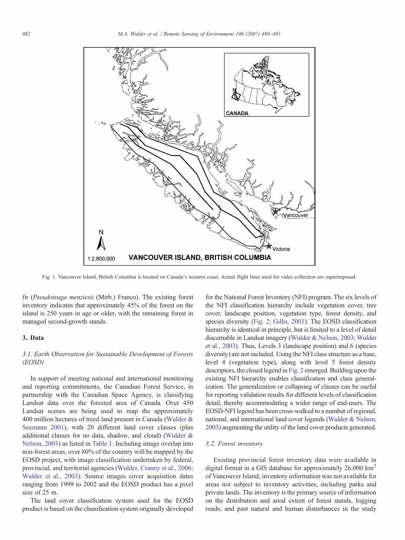
Fig. 1. Vancouver Island, British Columbia is located on Canada's western coast. Actual flight lines used for video collection are superimposed.

482 M.A. Wulder et al. / Remote Sensing of Environment 106 (2007) 480–491

fir (Pseudotsuga menziesii (Mirb.) Franco). The existing forestinventory indicates that approximately 45% of the forest on theisland is 250 years in age or older, with the remaining forest inmanaged second-growth stands.

3. Data

3.1. Earth Observation for Sustainable Development of Forests(EOSD)

In support of meeting national and international monitoringand reporting commitments, the Canadian Forest Service, inpartnership with the Canadian Space Agency, is classifyingLandsat data over the forested area of Canada. Over 450Landsat scenes are being used to map the approximately400 million hectares of treed land present in Canada (Wulder &Seemann 2001), with 20 different land cover classes (plusadditional classes for no data, shadow, and cloud) (Wulder &Nelson, 2003) as listed in Table 1. Including image overlap intonon-forest areas, over 80% of the country will be mapped by theEOSD project, with image classification undertaken by federal,provincial, and territorial agencies (Wulder, Cranny et al., 2006;Wulder et al., 2003). Source images cover acquisition datesranging from 1999 to 2002 and the EOSD product has a pixelsize of 25 m.

The land cover classification system used for the EOSDproduct is based on the classification system originally developed

for the National Forest Inventory (NFI) program. The six levels ofthe NFI classification hierarchy include vegetation cover, treecover, landscape position, vegetation type, forest density, andspecies diversity (Fig. 2; Gillis, 2001). The EOSD classificationhierarchy is identical in principle, but is limited to a level of detaildiscernable in Landsat imagery (Wulder & Nelson, 2003; Wulderet al., 2003). Thus, Levels 3 (landscape position) and 6 (speciesdiversity) are not included. Using the NFI class structure as a base,level 4 (vegetation type), along with level 5 forest densitydescriptors, the closed legend in Fig. 2 emerged. Building upon theexisting NFI hierarchy enables classification and class general-ization. The generalization or collapsing of classes can be usefulfor reporting validation results for different levels of classificationdetail, thereby accommodating a wider range of end-users. TheEOSD-NFI legend has been cross-walked to a number of regional,national, and international land cover legends (Wulder & Nelson,2003) augmenting the utility of the land cover products generated.

3.2. Forest inventory

Existing provincial forest inventory data were available indigital format in a GIS database for approximately 26,000 km2

of Vancouver Island; inventory informationwas not available forareas not subject to inventory activities, including parks andprivate lands. The inventory is the primary source of informationon the distribution and areal extent of forest stands, loggingroads, and past natural and human disturbances in the study

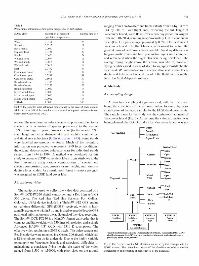
Fig. 2. The five levels of the NFI classification hierarchy that correspond to theEOSD classes. The hierarchical nature of the classification scheme enablesgeneralization and reporting at higher levels of the hierarchy.

Table 1Proportional allocation of first phase samples by EOSD stratum

EOSD class Proportion of sampledpopulation mapped as x

Sample size of x

Water 0.0461 25Snow/ice 0.0217 19Rock/rubble 0.0000 14Exposed land 0.0324 22Shrub 0.0420 24Wetland treed 0.0074 16Wetland shrub 0.0016 14Wetland herb 0.0013 14Herb 0.0792 34Coniferous dense 0.0705 32Coniferous open 0.5391 149Coniferous sparse 0.1015 39Broadleaf dense 0.0185 19Broadleaf open 0.0377 23Broadleaf sparse 0.0007 14Mixed wood dense 0.0000 14Mixed wood open 0.0000 14Mixed wood sparse 0.0002 14TOTAL 1.0000 500

Half of the samples were allocated proportional to the area of each stratum,while the other half of the samples were allocated to improve estimates for rareclasses (see Czaplewski, 2003).

483M.A. Wulder et al. / Remote Sensing of Environment 106 (2007) 480–491

region. The inventory includes species composition (of up to sixspecies, with estimates of species prevalence to the nearest10%), stand age in years, crown closure (to the nearest 5%),stand height in metres, diameter at breast height in centimetres,and stand area in hectares (Gillis & Leckie, 1993). Some standswere labelled non-productive forest. Much of the inventoryinformation was projected to represent 1999 forest conditions;the original data collection reference years for individual standsranged from 1954 to 1999. A method was developed for thisstudy to generate EOSD-equivalent labels from attributes in theforest inventory using various combinations of species andspecies composition, age, crown closure, height, and non-pro-ductive forest codes. As a result, each forest inventory polygonwas assigned an EOSD land cover label.

3.3. Airborne video

The equipment used to collect the video data consisted of aSony™ DCR-PC330 digital camcorder and a Red Hen A-VMS300 device. The Red Hen (Red Hen Systems, Fort Collins,Colorado, USA) device included a Thales™ B12 GPS engine(a real-time differential GPS (DGPS) receiver), which is hori-zontally accurate to within 3m, and is used to encode/decodeGPSpositional information onto the audio track of the video recording.The Sony™ DCR-PC330 is a MiniDV format camcorder that iscompact and lightweight, with 530 lines of resolution and a singleAdvanced HAD™ 1/3″ CCD with 3310 K total pixels. Theeffective video resolution is 2048 K pixels. The video camera andRed Hen device were mounted in a Cessna 206 aircraft, which hada 12-inch photo port on its underside. Due to the highly variabletopography on Vancouver Island, and associated difficulties inmaintaining a consistent flying height, the scale of the videoranged from 1:500 to 1:30000, with pixel sizes on the ground

ranging from 1 cm to 60 cm and frame extents from2.4 by 1.8m to144 by 108 m. Four flight lines, extending the full length ofVancouver Island, were flown over a two day period on August10th and 11th 2004, resulting in approximately 11 h of continuousvideo (Fig. 1), representing approximately 0.5% of the land area ofVancouver Island. The flight lines were designed to capture thegreatest range of land cover classes possible.Ancillary data such asbiogeoclimatic zones and base planimetric layers were compiledand referenced when the flight plan was being developed. Theaverage flying height above the terrain, was 585 m; however,flying heights varied in areas of steep topography. Post-flight, thevideo and GPS information were integrated to create a completelydigital and fully georeferenced record of the flight lines using theRed Hen MediaMapper® software.

4. Methods

4.1. Sampling design

A two-phase sampling design was used, with the first phasebeing the collection of the airborne video, followed by post-stratification of the video samples by the EOSD land cover strata.The sample frame for the study was the contiguous landmass ofVancouver Island (Fig. 1). At the time the video acquisition wasbeing planned, the EOSD product for Vancouver Island was not

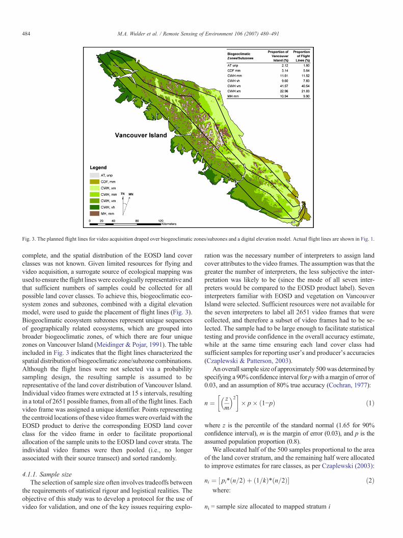
Fig. 3. The planned flight lines for video acquisition draped over biogeoclimatic zones/subzones and a digital elevation model. Actual flight lines are shown in Fig. 1.

484 M.A. Wulder et al. / Remote Sensing of Environment 106 (2007) 480–491

complete, and the spatial distribution of the EOSD land coverclasses was not known. Given limited resources for flying andvideo acquisition, a surrogate source of ecological mapping wasused to ensure the flight lineswere ecologically representative andthat sufficient numbers of samples could be collected for allpossible land cover classes. To achieve this, biogeoclimatic eco-system zones and subzones, combined with a digital elevationmodel, were used to guide the placement of flight lines (Fig. 3).Biogeoclimatic ecosystem subzones represent unique sequencesof geographically related ecosystems, which are grouped intobroader biogeoclimatic zones, of which there are four uniquezones on Vancouver Island (Meidinger & Pojar, 1991). The tableincluded in Fig. 3 indicates that the flight lines characterized thespatial distribution of biogeoclimatic zone/subzone combinations.Although the flight lines were not selected via a probabilitysampling design, the resulting sample is assumed to berepresentative of the land cover distribution of Vancouver Island.Individual video frames were extracted at 15 s intervals, resultingin a total of 2651 possible frames, from all of the flight lines. Eachvideo frame was assigned a unique identifier. Points representingthe centroid locations of these video frameswere overlaidwith theEOSD product to derive the corresponding EOSD land coverclass for the video frame in order to facilitate proportionalallocation of the sample units to the EOSD land cover strata. Theindividual video frames were then pooled (i.e., no longerassociated with their source transect) and sorted randomly.

4.1.1. Sample sizeThe selection of sample size often involves tradeoffs between

the requirements of statistical rigour and logistical realities. Theobjective of this study was to develop a protocol for the use ofvideo for validation, and one of the key issues requiring explo-

ration was the necessary number of interpreters to assign landcover attributes to the video frames. The assumption was that thegreater the number of interpreters, the less subjective the inter-pretation was likely to be (since the mode of all seven inter-preters would be compared to the EOSD product label). Seveninterpreters familiar with EOSD and vegetation on VancouverIsland were selected. Sufficient resources were not available forthe seven interpreters to label all 2651 video frames that werecollected, and therefore a subset of video frames had to be se-lected. The sample had to be large enough to facilitate statisticaltesting and provide confidence in the overall accuracy estimate,while at the same time ensuring each land cover class hadsufficient samples for reporting user's and producer's accuracies(Czaplewski & Patterson, 2003).

An overall sample size of approximately 500was determined byspecifying a 90% confidence interval forpwith amargin of error of0.03, and an assumption of 80% true accuracy (Cochran, 1977):

n ¼ zm

� �2� �

� p� ð1−pÞ ð1Þ

where z is the percentile of the standard normal (1.65 for 90%confidence interval), m is the margin of error (0.03), and p is theassumed population proportion (0.8).

We allocated half of the 500 samples proportional to the areaof the land cover stratum, and the remaining half were allocatedto improve estimates for rare classes, as per Czaplewski (2003):

ni ¼ ½ piTðn=2Þ þ ð1=kÞTðn=2Þ� ð2Þwhere:

ni = sample size allocated to mapped stratum i

485M.A. Wulder et al. / Remote Sensing of Environment 106 (2007) 480–491

pi = proportion of sample population mapped as in = total sample sizek = # of map categories

Under a strictly proportional allocation scheme, severalclasses present in the EOSD product would have had nosamples allocated to them. Recall that the video frames werepreviously tagged with their associated land cover strata, andthe number of samples required for each land cover stratum, aslisted in Table 1, was then selected at random from the 2651available video frames.

4.2. Response design

4.2.1. Evaluation protocolThe evaluation protocol is the procedure used to collect the

reference information (Stehman & Czaplewski, 1998). In de-fining the evaluation protocol, the spatial support region (SSR) ischosen. The SSR is defined as “the size, geometry, and orien-tation of the space on which an observation is defined”(Atkinson & Curran, 1995: 768). Given the variability in flyingheights, the area of the instantaneous field of view of each videoframe varied. Therefore, it was not practical to specify an SSR asa fixed areal unit. The centroid of the frame, whose location wascaptured by the GPS unit during flight, was selected as an easilyunderstood reference point for all interpreters. The centre of thevideo frame, determined by the collected GPS UTM easting andnorthing, was assigned a land cover class by the interpreters.

4.2.2. Video attributionInterpreters were given a land cover class key which pro-

vided samples of the video for each of the EOSD land coverclasses. The key was intended to improve consistency betweeninterpreters, who manually assigned a land cover label to thecentroid of the selected video samples. Interpreters wereselected based on their familiarity with the EOSD product andthe EOSD classification scheme, their understanding of forestinventory, and their experience in interpreting aerial photogra-phy. The interpreters had differing levels of field experience onVancouver Island; including two of the interpreters who wereinvolved in the acquisition of the video and therefore had someadditional understanding of the spatial distribution and visualrepresentation of the land cover classes. Strand et al. (2002)demonstrated that direct field experience did not improve theaccuracy with which photo interpreters could label land covertypes; however, Drake (1996) demonstrated that even a mini-mum amount of training can improve the interpretation ofvegetation classes from airborne video.

The key points communicated to the interpreters included(Wulder et al., 2004):

• Tall and low shrubswould be grouped into a single shrub class.• Density classes, particularly the distinction between denseand open classes, are known to be problematic. Interpreterswere advised when not certain of the density class to selectboth a primary and secondary class label (e.g. primary label:dense conifer, secondary label: open conifer).

• Guidelines for defining mixed wood stands were provided(i.e., when neither coniferous nor broadleaf species accountfor more than 75% of the total basal area in the stand).

• Several examples of video frames were provided for eachland cover class to promote consistent interpretations.

4.2.3. Labelling protocolThe interpreters were provided with a listing of the sample

video frames. Recall that the sample video frames had beenpooled and sorted randomly by their unique identifier. Theinterpreters did not know the geographic location of the videoframe, or the flight line that the video frame originated from.The interpreters were also not privy to the EOSD land coverstratum from which the video frame was selected. Each inter-preter independently determined an appropriate label for theland cover type existing at the centre of the video frame. As perStehman et al. (2003), the interpreters selected the most likelyclass (primary choice) with an option to specify a second choiceif necessary. The secondary choice captures the confusionbetween classes when the frame falls in the transition betweentwo cover-type classes (Fig. 4), thereby acknowledging the-matic and non-thematic errors (Foody, 2002).

4.2.4. Defining agreementSeveral scenarios for defining agreement between the EOSD

product and the interpreted video frames were explored:

1. If the land cover class of the EOSD product matched theprimary land cover choice of the interpreted video.

2. If the land cover class of the EOSD product matched either theprimary or secondary land cover choice of the interpretedvideo.

3. If the modal class of a 3 by 3 pixel SSR around the targetEOSD pixel matched either the primary or secondary landcover choice of the interpreted video.

The first scenario is a direct comparison between the inter-preted video and the EOSD product, making no allowances forpossible errors in attribution and/or positional accuracy. Thesecond scenario listed above accommodates thematic ambiguity,while the third choice accommodates both thematic ambiguityand positional uncertainty (Stehman et al., 2003). Under the thirdscenario, if more than one modal class existed, the sample wasdropped. For the scenario where the pre-existing forest inventorydata is used for validation, the land cover of the EOSD pixel iscompared directly to the label of the inventory polygon withinwhich the EOSD pixel falls (see Wulder, White et al. 2006 fordetails).

4.3. Analysis

The EOSD land cover class had previously been extracted foreach of the sample video frames, based on the GPS position of thevideo frame centroid. Similarly, the mode land cover class of a 3by 3 pixel neighbourhood surrounding the centroid pixel wasgenerated and extracted for the centroid of each video frame. TheEOSD classifications for each of the samples were then compared

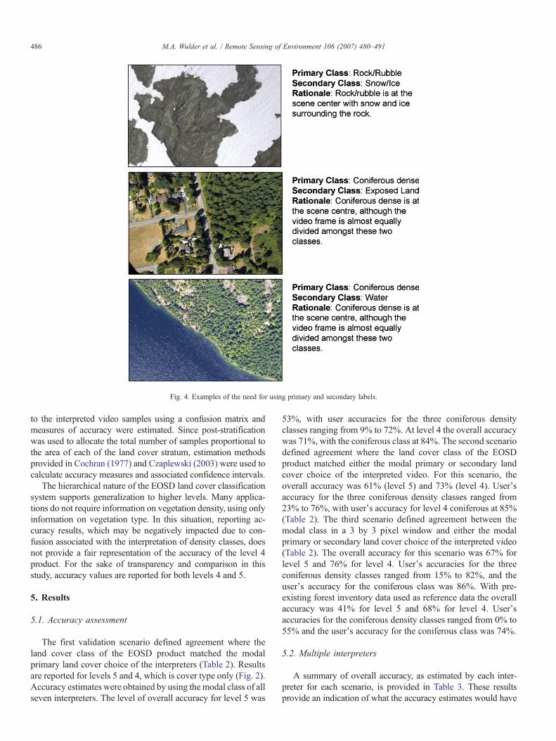
Fig. 4. Examples of the need for using primary and secondary labels.

486 M.A. Wulder et al. / Remote Sensing of Environment 106 (2007) 480–491

to the interpreted video samples using a confusion matrix andmeasures of accuracy were estimated. Since post-stratificationwas used to allocate the total number of samples proportional tothe area of each of the land cover stratum, estimation methodsprovided in Cochran (1977) and Czaplewski (2003) were used tocalculate accuracy measures and associated confidence intervals.

The hierarchical nature of the EOSD land cover classificationsystem supports generalization to higher levels. Many applica-tions do not require information on vegetation density, using onlyinformation on vegetation type. In this situation, reporting ac-curacy results, which may be negatively impacted due to con-fusion associated with the interpretation of density classes, doesnot provide a fair representation of the accuracy of the level 4product. For the sake of transparency and comparison in thisstudy, accuracy values are reported for both levels 4 and 5.

5. Results

5.1. Accuracy assessment

The first validation scenario defined agreement where theland cover class of the EOSD product matched the modalprimary land cover choice of the interpreters (Table 2). Resultsare reported for levels 5 and 4, which is cover type only (Fig. 2).Accuracy estimates were obtained by using the modal class of allseven interpreters. The level of overall accuracy for level 5 was

53%, with user accuracies for the three coniferous densityclasses ranging from 9% to 72%. At level 4 the overall accuracywas 71%, with the coniferous class at 84%. The second scenariodefined agreement where the land cover class of the EOSDproduct matched either the modal primary or secondary landcover choice of the interpreted video. For this scenario, theoverall accuracy was 61% (level 5) and 73% (level 4). User'saccuracy for the three coniferous density classes ranged from23% to 76%, with user's accuracy for level 4 coniferous at 85%(Table 2). The third scenario defined agreement between themodal class in a 3 by 3 pixel window and either the modalprimary or secondary land cover choice of the interpreted video(Table 2). The overall accuracy for this scenario was 67% forlevel 5 and 76% for level 4. User's accuracies for the threeconiferous density classes ranged from 15% to 82%, and theuser's accuracy for the coniferous class was 86%. With pre-existing forest inventory data used as reference data the overallaccuracy was 41% for level 5 and 68% for level 4. User'saccuracies for the coniferous density classes ranged from 0% to55% and the user's accuracy for the coniferous class was 74%.

5.2. Multiple interpreters

A summary of overall accuracy, as estimated by each inter-preter for each scenario, is provided in Table 3. These resultsprovide an indication of what the accuracy estimates would have

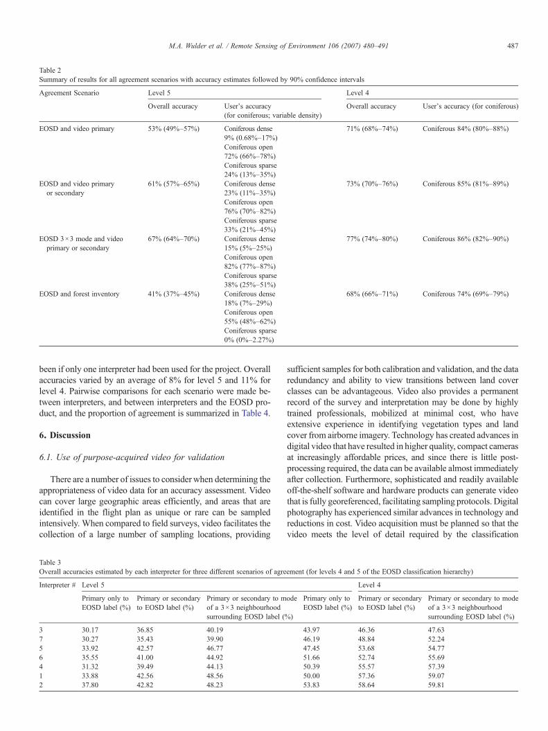
Table 2Summary of results for all agreement scenarios with accuracy estimates followed by 90% confidence intervals

Agreement Scenario Level 5 Level 4

Overall accuracy User's accuracy(for coniferous; variable density)

Overall accuracy User's accuracy (for coniferous)

EOSD and video primary 53% (49%–57%) Coniferous dense 71% (68%–74%) Coniferous 84% (80%–88%)9% (0.68%–17%)Coniferous open72% (66%–78%)Coniferous sparse24% (13%–35%)

EOSD and video primaryor secondary

61% (57%–65%) Coniferous dense 73% (70%–76%) Coniferous 85% (81%–89%)23% (11%–35%)Coniferous open76% (70%–82%)Coniferous sparse33% (21%–45%)

EOSD 3×3 mode and videoprimary or secondary

67% (64%–70%) Coniferous dense 77% (74%–80%) Coniferous 86% (82%–90%)15% (5%–25%)Coniferous open82% (77%–87%)Coniferous sparse38% (25%–51%)

EOSD and forest inventory 41% (37%–45%) Coniferous dense 68% (66%–71%) Coniferous 74% (69%–79%)18% (7%–29%)Coniferous open55% (48%–62%)Coniferous sparse0% (0%–2.27%)

487M.A. Wulder et al. / Remote Sensing of Environment 106 (2007) 480–491

been if only one interpreter had been used for the project. Overallaccuracies varied by an average of 8% for level 5 and 11% forlevel 4. Pairwise comparisons for each scenario were made be-tween interpreters, and between interpreters and the EOSD pro-duct, and the proportion of agreement is summarized in Table 4.

6. Discussion

6.1. Use of purpose-acquired video for validation

There are a number of issues to consider when determining theappropriateness of video data for an accuracy assessment. Videocan cover large geographic areas efficiently, and areas that areidentified in the flight plan as unique or rare can be sampledintensively. When compared to field surveys, video facilitates thecollection of a large number of sampling locations, providing

Table 3Overall accuracies estimated by each interpreter for three different scenarios of agre

Interpreter # Level 5

Primary only toEOSD label (%)

Primary or secondaryto EOSD label (%)

Primary or secondary to mof a 3×3 neighbourhoodsurrounding EOSD label (%

3 30.17 36.85 40.197 30.27 35.43 39.905 33.92 42.57 46.776 35.55 41.00 44.924 31.32 39.49 44.131 33.88 42.56 48.562 37.80 42.82 48.23

sufficient samples for both calibration and validation, and the dataredundancy and ability to view transitions between land coverclasses can be advantageous. Video also provides a permanentrecord of the survey and interpretation may be done by highlytrained professionals, mobilized at minimal cost, who haveextensive experience in identifying vegetation types and landcover from airborne imagery. Technology has created advances indigital video that have resulted in higher quality, compact camerasat increasingly affordable prices, and since there is little post-processing required, the data can be available almost immediatelyafter collection. Furthermore, sophisticated and readily availableoff-the-shelf software and hardware products can generate videothat is fully georeferenced, facilitating sampling protocols. Digitalphotography has experienced similar advances in technology andreductions in cost. Video acquisition must be planned so that thevideo meets the level of detail required by the classification

ement (for levels 4 and 5 of the EOSD classification hierarchy)

Level 4

ode

)

Primary only toEOSD label (%)

Primary or secondaryto EOSD label (%)

Primary or secondary to modeof a 3×3 neighbourhoodsurrounding EOSD label (%)

43.97 46.36 47.6346.19 48.84 52.2447.45 53.68 54.7751.66 52.74 55.6950.39 55.57 57.3950.00 57.36 59.0753.83 58.64 59.81

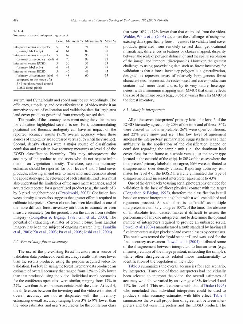
Table 4Summary of overall interpreter agreement

Level Minimum % Maximum % Mean %

Interpreter versus interpreter(primary label only)

5 51 71 604 61 82 70

Interpreter versus interpreter(primary or secondary label)

5 67 90 774 70 92 81

Interpreter versus EOSD(primary label only)

5 30 37 334 44 54 49

Interpreter versus EOSD(primary or secondary labelcompared to the mode of a3×3 neighbourhood aroundEOSD target pixel)

5 40 49 454 48 60 55

488 M.A. Wulder et al. / Remote Sensing of Environment 106 (2007) 480–491

system, and flying height and speed must be set accordingly. Theefficiency, simplicity, and cost effectiveness of video make it anattractive source of calibration and validation data for large arealand cover products generated from remotely sensed data.

The results of the accuracy assessment using the video framesfor validation highlighted several issues. First, accommodatingpositional and thematic ambiguity can have an impact on thereported accuracy results (75% overall accuracy when thesesources of ambiguity are addressed versus 53%when they are not).Second, density classes were a major source of classificationconfusion and result in low accuracy measures at level 5 of theEOSD classification hierarchy. This may misrepresent theaccuracy of the product to end users who do not require infor-mation on vegetation density. Therefore, separate accuracyestimates should be reported for both levels 4 and 5 land coverproducts, allowing an end user to make informed decisions aboutthe application-specific relevance of each estimate. End usersmustalso understand the limitations of the agreement scenarios, and ofaccuracies reported for a generalized product (e.g., the mode of 3by 3 pixel neighbourhood) (Czaplewski, 2003). Confusion bet-ween density classes also suggests that greater effort is required tocalibrate interpreters. Crown closure has been identified as one ofthe more difficult forest inventory attributes to estimate or evenmeasure accurately (on the ground, from the air, or from satelliteimagery) (Congalton & Biging, 1992; Gill et al., 2000). Thepotential of extracting estimates of crown closure from Landsatimagery has been the subject of ongoing research (e.g., Franklinet al., 2003; Xu et al., 2003; Pu et al., 2005; Joshi et al., 2006).

6.2. Pre-existing forest inventory

The use of the pre-existing forest inventory as a source ofvalidation data produced overall accuracy results that were lowerthan the results produced using the purpose acquired video forvalidation. For level 5, using the forest inventory data produced anestimate of overall accuracy that ranged from 12% to 26% lowerthan that produced using the video. Individual user's accuraciesfor the coniferous open class were similar, ranging from 17% to27% lower than the estimates associatedwith the video.At level 4,the differences between the inventory and the video estimates ofoverall accuracy are not as disparate, with the inventoryestimating overall accuracy ranging from 3% to 9% lower thanthe video estimates, and user's accuracies for the coniferous class

that were 10% to 12% lower than that estimated from the video.Wulder,White et al. (2006) document the challenges of using pre-existing data (specifically forest inventory) to validate land coverproducts generated from remotely sensed data: geolocationalmismatches, differences in features or classes mapped, disparitybetween the scale of polygon delineation and the spatial resolutionof the image, and temporal discrepancies. However, the greatestchallenge to using pre-existing data such as forest inventory forvalidation is that a forest inventory polygon is a generalization,designed to represent areas of relatively homogenous forestcharacteristics. In contrast, the raster based land cover product cancontain much more detail and is, by its very nature, heteroge-neous, with a minimum mapping unit (MMU) that often reflectsthe size of the image pixels (e.g., 0.06 ha) versus the 2 haMMUofthe forest inventory.

6.3. Multiple interpreters

All of the seven interpreters' primary labels for level 5 of theEOSD hierarchy agreed only 20% of the time and of these, 36%were classed as not interpretable; 26% were open coniferous;and 22% were snow and ice. This low level of agreementamongst the interpreters' primary label suggests there was eitherambiguity in the application of the classification legend orconfusion regarding the sample unit (i.e., the dominant landcover class for the frame as a whole versus just the cover typelocated at the centroid of the chip). In 80% of the cases where theinterpreters' primary labels did not agree, 66%were attributed todisagreements over density classes. Reporting accuracy esti-mates for level 4 of the EOSD hierarchy eliminated this type ofdisagreement and increased interpreter agreement to 43%.

One of the drawbacks to using aerial photography or video forvalidation is the lack of direct physical contact with the target(Congalton & Biging, 1992), therefore the classification is stillbased on remote interpretation (albeit with a well established andrigourous process). As such, there is no “truth”, as multipleinterpreters are unlikely to agree 100% of the time. The absenceof an absolute truth dataset makes it difficult to assess theperformance of any one interpreter, and to determine the optimalnumber of interpreters required to provide an unbiased result.Powell et al. (2004) manufactured a truth standard by having allfive interpreters assign pixels to land cover classes by consensus.The result was termed the “gold standard” and was used for thefinal accuracy assessment. Powell et al. (2004) attributed someof the disagreement between interpreters to human error (e.g.,misinterpretation of the image printout, miscoding the sample),while other disagreements related more fundamentally toidentification of the vegetation in the video.

Table 3 summarizes the overall accuracies for each scenario,by interpreter. If any one of these interpreters had individuallybeen selected to interpret the video, the overall estimates ofaccuracy would have varied by an average of 8% for level 5 and11% for level 4. This result contrasts with that of Drake (1996)who concluded that individual interpreters could be used toproduce similar accuracy estimates, with little effect. Table 4summarizes the overall proportion of agreement between inter-preters and between interpreters and the EOSD product. The

489M.A. Wulder et al. / Remote Sensing of Environment 106 (2007) 480–491

results indicate that there was more agreement amongst indivi-dual interpreters than there was between individual interpretersand the EOSD product. For level 5, agreement between primarylabels of any two interpreters ranged by 20%, with an averageoverall agreement of 60%. If both the primary and secondarylabels are considered, agreement between any two interpretersranged by 23%, with an average overall agreement of 77% andthe highest agreement at 90%. Comparisons between individualinterpreters and the EOSD output were markedly lower. If onlythe primary label of a single interpreter is considered, thenoverall agreement averaged 40% (range 8%). If both primaryand secondary label are compared to the modal land cover classof a 3 by 3 pixel neighbourhood, overall agreement increased to45% (range 9%). For level 4, the patterns in accuracy estimatesare similar. Agreement amongst interpreters was greater at moregeneralized levels of the EOSD hierarchy (70% at level 4 versus60% at level 5), and if thematic ambiguity was accounted for(77% for both primary and secondary labels at level 5 versus60% for primary label only at level 5).

These results suggest that the use of multiple interpreters canbe important for reducing bias and improving consistency in classlabeling. The number of interpreters required likely varies byapplication and depends on the complexity of the land coverclasses. For the method whereby the modal class of interpreters isused, a minimum of three interpreters would be practical, and isrecommended. An evaluation protocol that incorporates indepen-dent classification by each interpreter, followed by cross cali-bration, and revisit of problematic classes would be the mosteffective way to use fewer interpreters (and fewer resources),while still taking advantage of the benefits ofmultiple interpreters.

6.4. Lessons learned

Themain objective of this studywas to develop a protocol anddemonstrate the use of airborne video as a source of validationdata for large area land cover products, specifically the EOSD.Over the course of conducting this operational trial, severalissues arose, providing opportunities to improve upon themethodology for future implementation. First, a fully probabi-listic sample design is clearly more important than therepresentation of all potential classes — particularly sinceresources for the accuracy assessment are scarce and a keyobjective of the EOSD accuracy assessment is to generate robustestimates of overall accuracy and producer's and user'saccuracies for the dominant forest classes. To that end, flightlines should be placed so that they traverse the study area at fixedintervals of distance in both north–south and east–westorientations. Samples should be allocated proportional to strataarea, with no accounting for rare classes that have a very limitedspatial extent. The video camera should be set to a fixed zoom,facilitating an increase in the consistency of the scale of videoframes. In addition, the pilot should be instructed to try tomaintain a consistent altitude above ground level (rather thanfocussing on maintaining a consistent altitude). An attitude andheading reference system device (digital gyroscope) is critical toensure that the accurate GPS locations recorded by the Red Hensystem can be used to their full potential. With a known pitch,

roll, and heading, combined with the GPS position of the plane,it is relatively simple to calculate the coordinates of the centre ofthe image on the ground. Finally, with over 60% of the dis-agreement between interpreters caused by differences in densityestimates, greater effort must be made to calibrate interpretersand improve consistency in estimation of density classes. Drake(1996) demonstrated the utility of training in improving theinterpretation accuracy of vegetation classes from airborne video.

7. Conclusion

This operational trial explored the use of purpose-acquiredairborne video data for validation of an EOSD land coverproduct. Results indicate that airborne video is an efficient andcost-effective medium for validation of large area land coverproducts generated from remotely sensed data. The results alsoconfirm that accuracy estimates generated using purpose-acquired data will be different from estimates generated usingpre-existing forest inventory data as a reference source. In thisstudy, the use of forest inventory for validation would haveresulted in an underestimation of EOSD product accuracy.Furthermore, pre-existing data may not be the most appropriatedata source for validation, and may be unavailable in remote orinaccessible areas. Airborne video provides a viable validationdata source; the hardware, software, and expertise required toacquire the video data, generate a fully georeferenced data set,select a representative sample, and interpret land cover classes iswidely available and affordable.

A full implementation of the protocol developed hererequires a carefully selected sampling strategy that successfullybalances the requirements of statistical rigour while at the sametime accommodating logistical realities and fulfilling theprimary objectives of the accuracy assessment. Multipleinterpreters were found to be an effective means to improveconsistency and reduce bias in the assignment of land coverclasses to the video samples, although a minimum of threeinterpreters would likely be sufficient. Substantial effort shouldbe directed at calibrating interpreters and improving consistencyin labelling. Finally, the importance of reporting accuracyestimates and the details of the sample design in a transparentmanner, for both levels 4 and 5 of the EOSD classificationhierarchy, will provide the end user with the informationrequired to assess whether the product is sufficiently accuratefor a specific application. The lessons learned from this trial willcontribute to a robust assessment of EOSD product accuracyand provide insights for other regional and global land covermapping programs.

Acknowledgements

This research is enabled through funding of the GovernmentRelated Initiatives Program of the Canadian Space Plan of theCanadian Space Agency and Natural Resources Canada–Canadian Forest Service. David Seemann, of the Canadian ForestService, and Jamie Heath, of Terrasaurus Aerial Photography, arethanked for their assistance with collection of the video data. PaulBoudewyn, Morgan Cranny, Mike Heneley, David Seemann, and

490 M.A. Wulder et al. / Remote Sensing of Environment 106 (2007) 480–491

David Tammadge are thanked for their assistance with theinterpretation of the video samples.

References

Atkinson, P., & Curran, P. J. (1995). Defining an optimal size of support for remotesensing investigations. IEEE Transactions onGeoscience and Remote Sensing,33, 768−776.

Bobbe, T., Reed, D., & Schramek, J. (1993). Georeferenced Airborne VideoImagery: Natural resource applications on the Tongass. Journal of Forestry,91, 34−37.

Brownlie, R. K., Firth, J. G., & Hosking, G. (1996). Potential of airborne videofor updating forest maps. New Zealand Forestry, 41, 37−40.

Cihlar, J. (2000). Land cover mapping of large areas from satellites: status andresearch priorities. International Journal of Remote Sensing, 21, 1093−1114.

Cihlar, J., & Beaubien, J. (1998). Land cover of Canada version 1.1. Specialpublication, NBIOME Project. Produced by the Canada Centre for RemoteSensing and theCanadianForest Service, Natural Resources Canada.Ottawa,Ontario, Canada.

Cochran, W. G. (1977). Sampling techniques, 3rd Edition New York: JohnWiley & Sons 428 pp.

Congalton, R. G., & Biging, G. S. (1992). A pilot study evaluating groundreference data collection efforts for use in forest inventory. Photogram-metric Engineering and Remote Sensing, 58, 1669−1671.

Czaplewski, R. L. (2003). Statistical design and methodological considerations forthe accuracy assessment of maps of forest condition. In M. A. Wulder, & S. E.Franklin (Eds.), Remote sensing of forest environments: Concepts and casestudies (pp. 115−141). Boston MA: Kluwer Academic Publishers 519 pp.

Czaplewski, R. L., & Patterson, P. L. (2003). Classification accuracy forstratification with remotely sensed data. Forest Science, 49, 402−408.

Davis, T. J., Klinkenberg, B., & Keller, C. P. (2002). Updating inventory usingoblique videogrammetry and data fusion. Journal of Forestry, 2, 45−50.

Drake, S. (1996). Visual interpretation of vegetation classes from airbornevideography: an evaluation of observer proficiency with minimal training.Photogrammetry and Remote Sensing, 62, 969−978.

Driese, K. L., Reiners, W. A., Merrill, E. H., & Gerow, K. G. (1997). A digitalland cover map of Wyoming, USA: a tool for vegetation analysis. Journal ofVegetation Science, 8, 133−146.

Foody, G. M. (2002). Status of land cover classification accuracy assessment.Remote Sensing of Environment, 80, 185−201.

Franklin, S. E., Hall, R. J., Smith, L., & Gerylo, G. R. (2003). Discrimination ofconifer height, age, and crown closure classes using Landsat-5 TM imagery inthe Canadian Northwest Territories. International Journal of Remote Sensing,24, 1823−1834.

Frazier, P. (1998). Mapping blackberry thickets in the Kosciuszko National Parkusing airborne video data. Plant Protection Quarterly, 13, 145−148.

Fuller, R., Groom, G., & Jones, A. (1994). The land cover map of Great Britain:An automated classification of Landsat Thematic Mapper data. Photo-grammetric Engineering and Remote Sensing, 60, 553−562.

Gill, S. J., Milliken, J., Beardsley, D., & Warbington, R. (2000). Using amensuration approach with FIAvegetation plot data to assess the accuracy oftree size and crown closure classes in a vegetation map of NortheasternCalifornia. Remote Sensing of Environment, 73, 298−306.

Gillis, M. D. (2001). Canada's National Forest Inventory (responding to currentinformation needs). Environmental Monitoring and Assessment, 67, 121−129.

Gillis, M. D., & Leckie, D. G. (1993). Forest inventory mapping proceduresacross Canada. Information Report PI–X–114 Forestry Canada: PetawawaNational Forestry Institute.

Graham, Lee A. (1993). Airborne video for near-real-time vegetation mapping.Journal of Forestry, 8, 28−32.

Hansen, M. C., Defries, R. S., Townshend, J. R. G., & Sohlberg, R. (2000).Global land cover classification at 1 km spatial resolution using a classi-fication tree approach. International Journal of Remote Sensing, 21,1331−1364.

Hepinstall, J. A., Sader, S. A., Krohn, W. B., Boone, R. B., & Bartlett, R. I.(1999). Development and testing of a vegetation and land cover map of

Maine.Maine Agriculture and Forest Experiment Station Technical Bulletin,Vol. 173. (pp. )Orono: University of Maine 104 pp.

Herold, M., Woodcock, C., di Gregorio, A., Mayaux, P., Belward, A., Latham,J., & Schmullius, C. C. (2006). A joint initiative for harmonization andvalidation of land cover datasets. IEEE Transaction on GeoScience andRemote Sensing, 44, 1719−1727.

Hess, L. L., Novo, E. M. L. M., Slaymaker, D. M., Holt, J., Steffen, C.,Valeriano, D. M., et al. (2002). Geocoded digital videography for validationof land cover mapping in the Amazon basin. International Journal ofRemote Sensing, 23, 1527−1556.

Homer, C., Ramsey, R., Edwards, T., Jr., & Falconer, A. (1997). Landscapecover-type modeling using a multi-scene thematic mapper mosaic. Photo-grammetric Engineering and Remote Sensing, 63, 59−67.

Jack, K. (2005). Video demystified, 4th Edition Eagle Rock, VA: LLHTechnology Publishing 733 pp.

Jacobs, D. M. (2000). February 1994 Ice Storm: forest resource damageassessment in northern Mississippi.United States Department of Agricul-ture, Forest Service, Southern Research Station, Resource Bulletin SRS-54.Asheville, NC 11 pp.

Jacobs, D. M., & Eggen-McIntosh, S. (1993). Airborne videography and GPSfor assessment of forest damage in southern Louisiana from HurricaneAndrew. Proceedings of the IUFRO conference on inventory andmanagement techniques in the context of catastrophic events; 1993 June21–24 PA: University Park 12 pp.

Joshi, C., DeLeeuw, J., Skidmore, A. K., van Duren, I. C., & van Oosten, H.(2006). Remotely sensed estimation of forest canopy density: A comparisonof the performance of four methods. International Journal of Applied EarthObservation and Geoinformation, 8, 84−95.

Justice, C., Belward, A., Morisette, J., Lewis, P., Privette, J., & Baret, F. (2000).Developments in the ‘validation’ of satellite sensor products for the study ofthe land surface. International Journal of Remote Sensing, 21, 3383−3390.

King, D. J. (1995). Airborne multispectral digital camera and video sensors: acritical review of system designs and applications. Canadian Journal ofRemote Sensing, 21, 245−273.

Klinka, K., Pojar, J., & Meidinger, D. V. (1991). Revision of biogeoclimaticunits of coastal British Columbia. Northwest Science, 65, 32−47.

Loveland, T. R., & Belward, A. S. (1997). The International GeosphereBiosphere Programme Data and Information System global land cover dataset (DISCover). Acta Astronautica, 41, 681−689.

Loveland, T. R., Merchant, J. W., Ohlen, D. O., & Brown, J. F. (1991).Development of a land-cover characteristics database for the conterminousU. S.. Photogrammetric Engineering and Remote Sensing, 57, 1453−1463.

Loveland, T. R., Reed, B. C., Brown, J. F., Ohlen, D. O., Zhu, Z., Yang, L., et al.(2000). Development of a global land cover characteristic database andIGBP DISCover from 1 km AVHRR data. International Journal of RemoteSensing, 21, 1303−1330.

Loveland, T. R., Zhu, Z., Ohlen, D. O., Brown, J. F., Reed, B. C., & Yang, L.(1999). An analysis of the IGBP global land-cover characterisation process.Photogrammetric Engineering and Remote Sensing, 65, 1021−1032.

Maingi, J. K., Marsh, S. E., Kepner, W. G., & Edmonds, C. M. (2002). Anaccuracy assessment of 1992 Landsat-MSS derived land cover for the UpperSan Pedro Watershed (US/Mexico).United States Environmental ProtectionAgency, EPA/600/R-02/040 21 pp.

Marsh, S. E., Walsh, J. L., & Sobrevila, C. (1994). Evaluation of airborne videodata for land-cover classification accuracy assessment in an isolatedBrazilian forest. Remote Sensing of Environment, 48, 61−69.

Mausel, P. W., Everitt, J. H., Escobar, E. E., & King, D. J. (1992). Airbornevideography: current status and future perspectives. PhotogrammetricEngineering and Remote Sensing, 58, 1189−1195.

Meidinger, D., & Pojar, J. (Eds.). (1991). Ecosystems of British ColumbiaVictoria, British Columbia, Canada: Research Branch, Ministry of Forests330 pp.

Meisner, D. E. (1986). Fundamentals of airborne video remote sensing. RemoteSensing of Environment, 19, 63−79.

Morisette, J. T., Privette, J. L., & Justice, C. O. (2002). A framework for thevalidation of MODIS land products. Remote Sensing of Environment, 83,77−96.

491M.A. Wulder et al. / Remote Sensing of Environment 106 (2007) 480–491

Nixon, P., Escobar, D., & Menges, R. (1985). Use of multiband video system forquick assessment of vegetation condition and discrimination of plantspecies. Remote Sensing of Environment, 17, 203−208.

Norton-Griffiths, M. (1982). Aerial point sampling for land use surveys. Journalof Biogeography, 15, 149−156.

Powell, R. L., Matzke, N., de Souza, C., Jr., Clark, M., Numata, I., Hess, L. L.,et al. (2004). Sources of error in accuracy assessment of thematic land-covermaps in the Brazillian Amazon. Remote Sensing of Environment, 90,221−234.

Pu, R., Yu, Q., Gong, P., & Biging, G. S. (2005). EO-1 Hyperion, ALI, andLandsat ETM+ data comparison for estimating forest crown closure and leafarea index. International Journal of Remote Sensing, 26, 457−474.

Reiners, W. A., Driese, K. L., & Schrupp, D. (2000). Statistical evaluation of theWyoming and Colorado landcover map thematic accuracy using aerialvideography techniques: Final report.Laramie, Wyoming: Department ofBotany, University of Wyoming Available online: http://ndis1.nrel.colostate.edu/cogap/report/colandcov_acc.pdf

Remmel, T. K., Csillag, F., Mitchell, S., & Wulder, M. (2005). Integration offorest inventory and satellite imagery: A Canadian status assessment andresearch issues. Forest Ecology and Management, 207, 405−428.

Schlagel, J. (1995). Integrating aerial-videography with ArcInfo for satelliteimage interpretation and accuracy assessment in Vermont. Proceedings ofthe 15th Annual ESRI User Conference, May 22–26, 1995 California: PalmSprings.

Scott, J. M., Davis, F., Csuti, B., Noss, Reed, Butterfield, B., Groves, C., et al.(1993). Gap analysis: A geographic approach to protection of biologicaldiversity.Journal of Wildlife Management, 57 (Supplement: WildlifeMonographs No. 123.).

Skirvin, S. M., Drake, S. E., Maingi, J. K., Marsh, S. E., & Kepner, W. G.(2000). An accuracy assessment of 1997 Landsat Thematic Mapper derivedland cover for the Upper San Pedro Watershed (U.S./Mexico). EPA/600/R-00/097. Washington, DC: Office of Research and Development.

Skirvin, S. M., Kepner, W. G., Marsh, S. E., Drake, S. E., Maingi, J. K.,Edmonds, C. M., et al. (2004). Assessing the accuracy of satellite-derivedland-cover classification using historical aerial photography, digitalorthophoto quadrangles, and airborne video data. In R. S. Lunetta, & J. G.Lyon (Eds.), Remote Sensing and GIS Accuracy Assessment (pp. 115−131).Boca Raton FL: CRC Press.

Slaymaker, D. M. (2003). Using georeferenced large-scale aerial videography asa surrogate for ground validation data. In M. A. Wulder, & S. E. Franklin(Eds.), Remote sensing of forest environments: Concepts and case studies(pp. 469−489). Boston MA: Kluwer Academic Publishers 519 pp.

Slaymaker, D. M., Jones, K. M. L., Griffin, C. R., & Finn, J. T. (1996). Mappingdeciduous forests in southern New England using aerial videography andhyperclustered multi-temporal Landsat TM imagery. In J. M. Planning, T. H.Scott, & F. W. Davids (Eds.), Gap analysis: a landscape approach tobiodiversity planning (pp. 87−101). Bethesda MD: American Society ofPhotogrammetry and Remote Sensing.

Stehman, S. V., & Czaplewski, R. L. (1998). Design and analysis for thematicmap accuracy assessment: Fundamental principles. Remote Sensing ofEnvironment, 64, 331−344.

Stehman, S. V., & Czaplewski, R. L. (2003). Introduction to special issue onmap accuracy. Environmental and Ecological Statistics, 10, 301−308.

Stehman, S. V., Wickham, J. D., Smith, J. H., & Yang, L. (2003). Thematicaccuracy of the 1992 national land-cover data for the eastern United States:Statistical methodology and regional results. Remote Sensing of Environ-ment, 86, 500−516.

Stone, T., Schlesinger, P., Houghton, T., & Woodwell, G. (1994). A map of thevegetation of South America based on satellite imagery. PhotogrammetricEngineering and Remote Sensing, 60, 541−551.

Strahler, A. H., Boschetti, L., Foody, G. M., Friedl, M. A., Hansen, M. C.,Herold, M., et al. (2006). Global land cover validation: Recommendationsfor evaluation and accuracy assessment of global land cover maps.Luxembourg: Office for the Official Publications of the EuropeanCommunities.

Strand, G. H., Dramstad, W., & Engan, G. (2002). The effect of field experienceon the accuracy of identifying land cover types in aerial photographs. In-ternational Journal of Applied Earth Observation and Geoinformation, 4,137−146.

Suzuki, R., Hiyama, T., Asanuma, J., & Ohata, T. (2004). Land surfaceidentification near Yakutsk in eastern Siberia using video images taken froma hedgehopping aircraft. International Journal of Remote Sensing, 25,4015−4028.

Wulder, M. A., Cranny, M., Hall, R. J., Luther, J. E., Beaudoin, A., & Dechka, J.(2006). Satellite land cover mapping of Canada's forest, SPIE Newsroom.The International Society for Optical Engineering, 2p (Available fromhttp://newsroom.spie.org/documents/Imported/296/2006070296.pdf).

Wulder, M. A., Dechka, J. A., Gillis, M. A., Luther, J. E., Hall, R. J., Beaudoin,A., et al. (2003). Operational mapping of the land cover of the forested areaof Canada with Landsat data: EOSD land cover program. ForestryChronicle, 79, 1075−1083.

Wulder, M. A., Franklin, S. E., White, J. C., Linke, J., & Magnussen, S. (2006).An accuracy assessment framework for large area land cover classificationproducts derived from medium resolution satellite data. InternationalJournal of Remote Sensing, 27, 663−683.

Wulder, M. A., McDonald, S., & White, J.C. (2004). Protocols for attribution ofEOSD classes to video tiles. Example application using Vancouver Island asthe population.Version 1,Natural Resources Canada, Canadian Forest Service,Pacific Forestry Centre, Victoria, BC, Canada, January 13, 2005, 57 p.

Wulder, M., & Nelson, T. (2003). EOSD Land Cover Classification LegendReport, Version 1, Natural Resources Canada, Canadian Forest Service, PacificForestry Centre, Victoria, British Columbia, Canada, March 2003. Availablefrom http://www.pfc.forestry.ca/eosd/cover/EOSD_Legend_Report.pdf. 81 pp.

Wulder, M., & Seemann, D. (2001). Spatially partitioning Canada with theLandsat Worldwide Reference System. Canadian Journal of RemoteSensing, 27, 225−231.

Wulder, M. A., White, J. C., Luther, J. E., Strickland, G., Remmel, T. K., &Mitchell, S. (2006). Use of vector polygons for the accuracy assessment ofpixel-based land cover maps. Canadian Journal of Remote Sensing, 32,268−279.

Xu, B., Gong, P., & Pu, R. L. (2003). Crown closure estimation of oak savannahin a dry season with Landsat TM imagery: Comparison of various indicesthrough correlation analysis. International Journal of Remote Sensing, 24,1811−1822.