Embed Size (px)
Citation preview

Value of Component Commonality in Managing Uncertainty in a Supply
Chain
Northern Illinois University Department of Technology
Shun Takai
Role of Safety Inventory in a Supply Chain
Role of Safety Inventory in a Supply Chain
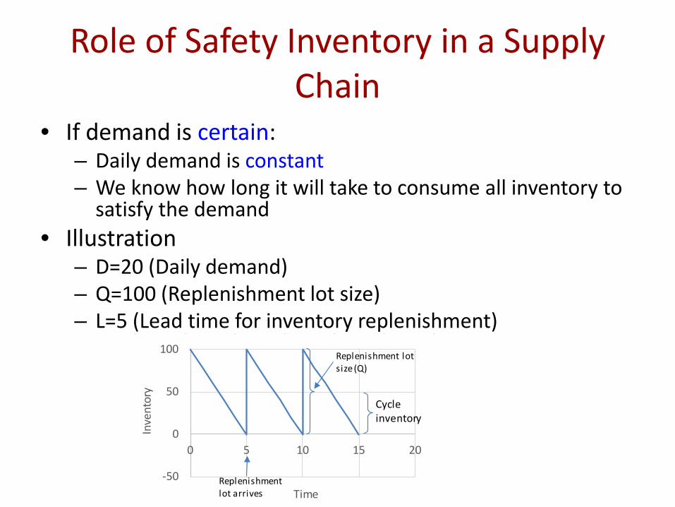
• If demand is certain: – Daily demand is constant – We know how long it will take to consume all inventory to
satisfy the demand • Illustration
– D=20 (Daily demand) – Q=100 (Replenishment lot size) – L=5 (Lead time for inventory replenishment)
• -50
0
50
100
0 5 10 15 20
Inve
ntor
y
TimeReplenishment lot arrives
Replenishment lot size (Q)
Cycle inventory
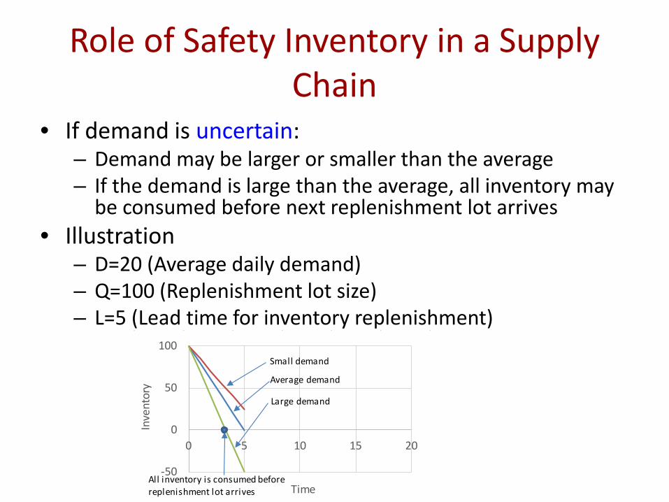
Role of Safety Inventory in a Supply Chain
• If demand is uncertain: – Demand may be larger or smaller than the average – If the demand is large than the average, all inventory may
be consumed before next replenishment lot arrives • Illustration
– D=20 (Average daily demand) – Q=100 (Replenishment lot size) – L=5 (Lead time for inventory replenishment)
• -50
0
50
100
0 5 10 15 20
Inve
ntor
y
TimeAll inventory is consumed before replenishment lot arrives
Small demand
Average demand
Large demand
Role of Safety Inventory in a Supply Chain
• Safety inventory is used to account for uncertainty that: – Demand may be larger than the average (or forecasted)
• Illustration – D=20 (Average daily demand) – Q=100 (Replenishment lot size) – L=5 (Lead time for inventory replenishment) – ss=50 (Safety inventory)
• 0
50
100
150
0 5 10 15 20
Inve
ntor
y
Time
Safety inventory to account for demand uncertainty
Cycle inventory
Determining Appropriate Level of Safety Inventory
Trade-Off in Safety Inventory Decisions
• Large amount of safety inventory – Increases product availability (reduces product
shortage); thus increases profit – Increases inventory holding costs; thus reduces profit
• Key questions in safety inventory decisions are: 1. What is the appropriate level of safety inventory? 2. What actions to take to reduce safety inventory
while maintaining product availability?
(Reference) Supply Chain Management: Strategy, Planning, and Operation. Sunil Chopra and Peter Meindl. (2013) 5th Edition. Boston, MA: Pearson Prentice-Hall.
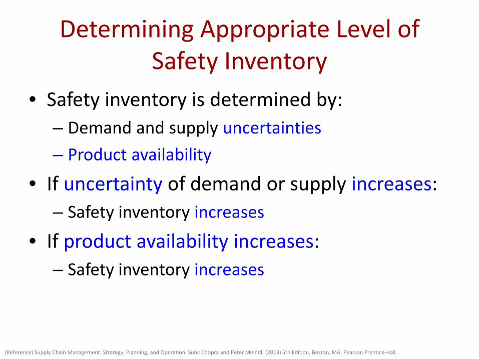
Determining Appropriate Level of Safety Inventory
• Safety inventory is determined by: – Demand and supply uncertainties – Product availability
• If uncertainty of demand or supply increases: – Safety inventory increases
• If product availability increases: – Safety inventory increases
(Reference) Supply Chain Management: Strategy, Planning, and Operation. Sunil Chopra and Peter Meindl. (2013) 5th Edition. Boston, MA: Pearson Prentice-Hall.
Demand Uncertainty
Measuring Demand Uncertainty • Demand in each period (e.g., daily or weekly demand) is
modeled by: – Di: average demand per period – σi: standard deviation of demand per period (e.g., forecast
error) – i = 1, 2, 3, …, L
• Notation is simplified if uncertainty of demand in each period is identical – D: average demand per period – σD: standard deviation of demand per period
• Lead time is the time between when an order is placed and when the order is received – L: lead time
(Reference) Supply Chain Management: Strategy, Planning, and Operation. Sunil Chopra and Peter Meindl. (2013) 5th Edition. Boston, MA: Pearson Prentice-Hall.
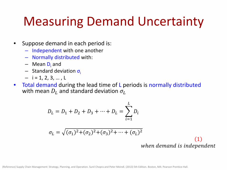
Measuring Demand Uncertainty • Suppose demand in each period is:
– Independent with one another – Normally distributed with: – Mean Di and – Standard deviation σi – i = 1, 2, 3, … , L
• Total demand during the lead time of L periods is normally distributed with mean 𝐷𝐷𝐿𝐿 and standard deviation 𝜎𝜎𝐿𝐿
𝐷𝐷𝐿𝐿 = 𝐷𝐷1 + 𝐷𝐷2 + 𝐷𝐷3 + ⋯+ 𝐷𝐷𝐿𝐿 = �𝐷𝐷𝑖𝑖
𝐿𝐿
𝑖𝑖=1
𝜎𝜎𝐿𝐿 = (𝜎𝜎1)2+(𝜎𝜎2)2+(𝜎𝜎3)2+⋯+ (𝜎𝜎𝐿𝐿)2
1 𝑤𝑤𝑤𝑤𝑤𝑤𝑤 𝑑𝑑𝑤𝑤𝑑𝑑𝑑𝑑𝑤𝑤𝑑𝑑 𝑖𝑖𝑖𝑖 𝑖𝑖𝑤𝑤𝑑𝑑𝑤𝑤𝑖𝑖𝑤𝑤𝑤𝑤𝑑𝑑𝑤𝑤𝑤𝑤𝑖𝑖
(Reference) Supply Chain Management: Strategy, Planning, and Operation. Sunil Chopra and Peter Meindl. (2013) 5th Edition. Boston, MA: Pearson Prentice-Hall.
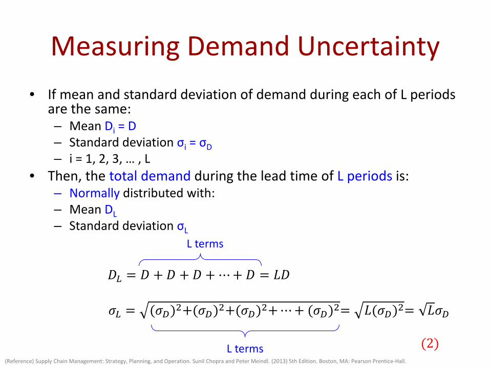
Measuring Demand Uncertainty • If mean and standard deviation of demand during each of L periods
are the same: – Mean Di = D – Standard deviation σi = σD – i = 1, 2, 3, … , L
• Then, the total demand during the lead time of L periods is: – Normally distributed with: – Mean DL – Standard deviation σL
𝐷𝐷𝐿𝐿 = 𝐷𝐷 + 𝐷𝐷 + 𝐷𝐷 + ⋯+ 𝐷𝐷 = 𝐿𝐿𝐷𝐷 𝜎𝜎𝐿𝐿 = (𝜎𝜎𝐷𝐷)2+(𝜎𝜎𝐷𝐷)2+(𝜎𝜎𝐷𝐷)2+⋯+ (𝜎𝜎𝐷𝐷)2= 𝐿𝐿(𝜎𝜎𝐷𝐷)2= 𝐿𝐿𝜎𝜎𝐷𝐷 (2)
(Reference) Supply Chain Management: Strategy, Planning, and Operation. Sunil Chopra and Peter Meindl. (2013) 5th Edition. Boston, MA: Pearson Prentice-Hall.
L terms
L terms
Product Availability and Replenishment Policy
Product Availability and Replenishment Policy
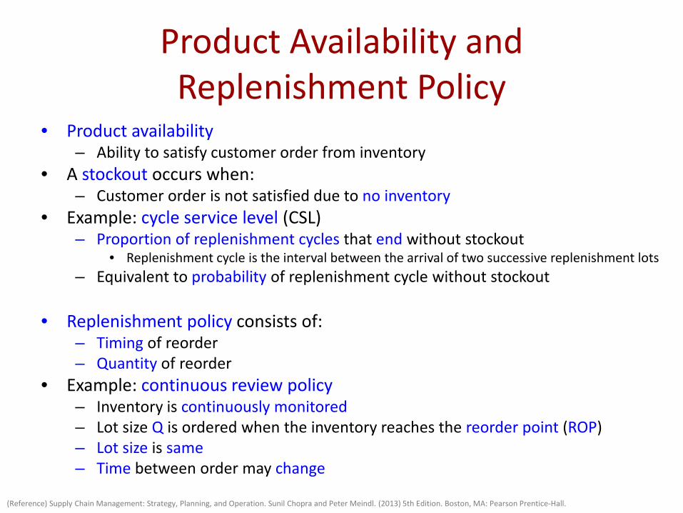
• Product availability – Ability to satisfy customer order from inventory
• A stockout occurs when: – Customer order is not satisfied due to no inventory
• Example: cycle service level (CSL) – Proportion of replenishment cycles that end without stockout
• Replenishment cycle is the interval between the arrival of two successive replenishment lots – Equivalent to probability of replenishment cycle without stockout
• Replenishment policy consists of:
– Timing of reorder – Quantity of reorder
• Example: continuous review policy – Inventory is continuously monitored – Lot size Q is ordered when the inventory reaches the reorder point (ROP) – Lot size is same – Time between order may change
(Reference) Supply Chain Management: Strategy, Planning, and Operation. Sunil Chopra and Peter Meindl. (2013) 5th Edition. Boston, MA: Pearson Prentice-Hall.
Evaluating CSL Given a Replenishment Policy
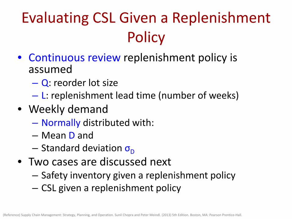
• Continuous review replenishment policy is assumed – Q: reorder lot size – L: replenishment lead time (number of weeks)
• Weekly demand – Normally distributed with: – Mean D and – Standard deviation σD
• Two cases are discussed next – Safety inventory given a replenishment policy – CSL given a replenishment policy
(Reference) Supply Chain Management: Strategy, Planning, and Operation. Sunil Chopra and Peter Meindl. (2013) 5th Edition. Boston, MA: Pearson Prentice-Hall.
0
50
100
150
0 5 10 15 20
Inve
ntor
y
Time
Lot is ordered Lot arrives
Safety inventory
LD
ROP
Lead time L
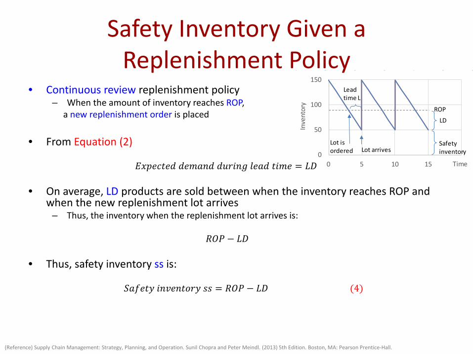
Safety Inventory Given a Replenishment Policy
• Continuous review replenishment policy – When the amount of inventory reaches ROP, a new replenishment order is placed
• From Equation (2)
𝐸𝐸𝐸𝐸𝑖𝑖𝑤𝑤𝐸𝐸𝑖𝑖𝑤𝑤𝑑𝑑 𝑑𝑑𝑤𝑤𝑑𝑑𝑑𝑑𝑤𝑤𝑑𝑑 𝑑𝑑𝑑𝑑𝑑𝑑𝑖𝑖𝑤𝑤𝑑𝑑 𝑙𝑙𝑤𝑤𝑑𝑑𝑑𝑑 𝑖𝑖𝑖𝑖𝑑𝑑𝑤𝑤 = 𝐿𝐿𝐷𝐷
• On average, LD products are sold between when the inventory reaches ROP and
when the new replenishment lot arrives – Thus, the inventory when the replenishment lot arrives is:
𝑅𝑅𝑅𝑅𝑅𝑅 − 𝐿𝐿𝐷𝐷
• Thus, safety inventory ss is:
𝑆𝑆𝑑𝑑𝑆𝑆𝑤𝑤𝑖𝑖𝑆𝑆 𝑖𝑖𝑤𝑤𝑖𝑖𝑤𝑤𝑤𝑤𝑖𝑖𝑖𝑖𝑑𝑑𝑆𝑆 𝑖𝑖𝑖𝑖 = 𝑅𝑅𝑅𝑅𝑅𝑅 − 𝐿𝐿𝐷𝐷 (4)
(Reference) Supply Chain Management: Strategy, Planning, and Operation. Sunil Chopra and Peter Meindl. (2013) 5th Edition. Boston, MA: Pearson Prentice-Hall.
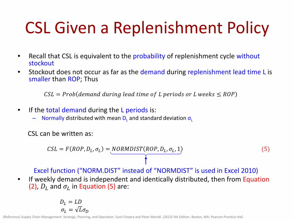
CSL Given a Replenishment Policy • Recall that CSL is equivalent to the probability of replenishment cycle without
stockout • Stockout does not occur as far as the demand during replenishment lead time L is
smaller than ROP; Thus 𝐶𝐶𝑆𝑆𝐿𝐿 = 𝑅𝑅𝑑𝑑𝑖𝑖𝑃𝑃 𝑑𝑑𝑤𝑤𝑑𝑑𝑑𝑑𝑤𝑤𝑑𝑑 𝑑𝑑𝑑𝑑𝑑𝑑𝑖𝑖𝑤𝑤𝑑𝑑 𝑙𝑙𝑤𝑤𝑑𝑑𝑑𝑑 𝑖𝑖𝑖𝑖𝑑𝑑𝑤𝑤 𝑖𝑖𝑆𝑆 𝐿𝐿 𝑖𝑖𝑤𝑤𝑑𝑑𝑖𝑖𝑖𝑖𝑑𝑑𝑖𝑖 𝑖𝑖𝑑𝑑 𝐿𝐿 𝑤𝑤𝑤𝑤𝑤𝑤𝑤𝑤𝑖𝑖 ≤ 𝑅𝑅𝑅𝑅𝑅𝑅
• If the total demand during the L periods is:
– Normally distributed with mean DL and standard deviation σL
CSL can be written as:
𝐶𝐶𝑆𝑆𝐿𝐿 = 𝐹𝐹 𝑅𝑅𝑅𝑅𝑅𝑅,𝐷𝐷𝐿𝐿,𝜎𝜎𝐿𝐿 = 𝑁𝑁𝑅𝑅𝑅𝑅𝑁𝑁𝐷𝐷𝑁𝑁𝑆𝑆𝑁𝑁 𝑅𝑅𝑅𝑅𝑅𝑅,𝐷𝐷𝐿𝐿,𝜎𝜎𝐿𝐿 , 1 (5)
• If weekly demand is independent and identically distributed, then from Equation (2), 𝐷𝐷𝐿𝐿 and 𝜎𝜎𝐿𝐿 in Equation (5) are:
𝐷𝐷𝐿𝐿 = 𝐿𝐿𝐷𝐷 𝜎𝜎𝐿𝐿 = 𝐿𝐿𝜎𝜎𝐷𝐷
(Reference) Supply Chain Management: Strategy, Planning, and Operation. Sunil Chopra and Peter Meindl. (2013) 5th Edition. Boston, MA: Pearson Prentice-Hall.
Excel function (“NORM.DIST” instead of “NORMDIST” is used in Excel 2010)
Safety Inventory Given Desired CSL
• Companies often choose replenishment policies to achieve desired levels of product availability
• Thus, appropriate level of safety inventory needs to be calculated to achieve the desired level of product availability (e.g., in terms of CSL)
• Next – Safety inventory given desired CSL is discussed
(Reference) Supply Chain Management: Strategy, Planning, and Operation. Sunil Chopra and Peter Meindl. (2013) 5th Edition. Boston, MA: Pearson Prentice-Hall.
Safety Inventory Given Desired CSL
• Goal – For continuous review replenishment policy, – Calculate appropriate safety inventory that
achieves the desired CSL • Assumption
– L: lead time – CSL: desired cycle service level – DL: mean demand during lead time – σL: standard deviation of demand during lead time
(Reference) Supply Chain Management: Strategy, Planning, and Operation. Sunil Chopra and Peter Meindl. (2013) 5th Edition. Boston, MA: Pearson Prentice-Hall.
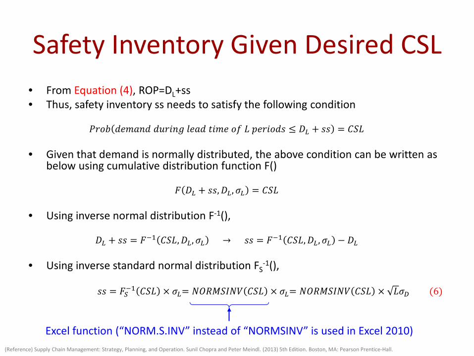
Safety Inventory Given Desired CSL • From Equation (4), ROP=DL+ss • Thus, safety inventory ss needs to satisfy the following condition
𝑅𝑅𝑑𝑑𝑖𝑖𝑃𝑃 𝑑𝑑𝑤𝑤𝑑𝑑𝑑𝑑𝑤𝑤𝑑𝑑 𝑑𝑑𝑑𝑑𝑑𝑑𝑖𝑖𝑤𝑤𝑑𝑑 𝑙𝑙𝑤𝑤𝑑𝑑𝑑𝑑 𝑖𝑖𝑖𝑖𝑑𝑑𝑤𝑤 𝑖𝑖𝑆𝑆 𝐿𝐿 𝑖𝑖𝑤𝑤𝑑𝑑𝑖𝑖𝑖𝑖𝑑𝑑𝑖𝑖 ≤ 𝐷𝐷𝐿𝐿 + 𝑖𝑖𝑖𝑖 = 𝐶𝐶𝑆𝑆𝐿𝐿
• Given that demand is normally distributed, the above condition can be written as
below using cumulative distribution function F()
𝐹𝐹 𝐷𝐷𝐿𝐿 + 𝑖𝑖𝑖𝑖,𝐷𝐷𝐿𝐿,𝜎𝜎𝐿𝐿 = 𝐶𝐶𝑆𝑆𝐿𝐿
• Using inverse normal distribution F-1(),
𝐷𝐷𝐿𝐿 + 𝑖𝑖𝑖𝑖 = 𝐹𝐹−1 𝐶𝐶𝑆𝑆𝐿𝐿,𝐷𝐷𝐿𝐿,𝜎𝜎𝐿𝐿 → 𝑖𝑖𝑖𝑖 = 𝐹𝐹−1 𝐶𝐶𝑆𝑆𝐿𝐿,𝐷𝐷𝐿𝐿,𝜎𝜎𝐿𝐿 − 𝐷𝐷𝐿𝐿
• Using inverse standard normal distribution FS-1(),
𝑖𝑖𝑖𝑖 = 𝐹𝐹𝑆𝑆−1 𝐶𝐶𝑆𝑆𝐿𝐿 × 𝜎𝜎𝐿𝐿= 𝑁𝑁𝑅𝑅𝑅𝑅𝑁𝑁𝑆𝑆𝑁𝑁𝑁𝑁𝑁𝑁 𝐶𝐶𝑆𝑆𝐿𝐿 × 𝜎𝜎𝐿𝐿= 𝑁𝑁𝑅𝑅𝑅𝑅𝑁𝑁𝑆𝑆𝑁𝑁𝑁𝑁𝑁𝑁 𝐶𝐶𝑆𝑆𝐿𝐿 × 𝐿𝐿𝜎𝜎𝐷𝐷 (6)
(Reference) Supply Chain Management: Strategy, Planning, and Operation. Sunil Chopra and Peter Meindl. (2013) 5th Edition. Boston, MA: Pearson Prentice-Hall.
Excel function (“NORM.S.INV” instead of “NORMSINV” is used in Excel 2010)
Impact of Product Design on Safety Inventory – Value of Component
Commonality
Component Commonality • Component commonality is a key to increasing product variety
without reducing product availability or without increasing component inventory too much
• If product variety in a supply chain is large, the variety and amount of components in the supply chain can be significantly large
• Use of common components in multiple products enables a company to: – Aggregate component demand and – Reduce component inventory
• If a distinct component is used in each product: – Demand for the component is the same as demand for the finished
product in which the component is used • If the same component is used in multiple products:
– Demand for the component is the same as the aggregate demand of all the finished products in which the component is used
(Reference) Supply Chain Management: Strategy, Planning, and Operation. Sunil Chopra and Peter Meindl. (2013) 5th Edition. Boston, MA: Pearson Prentice-Hall.
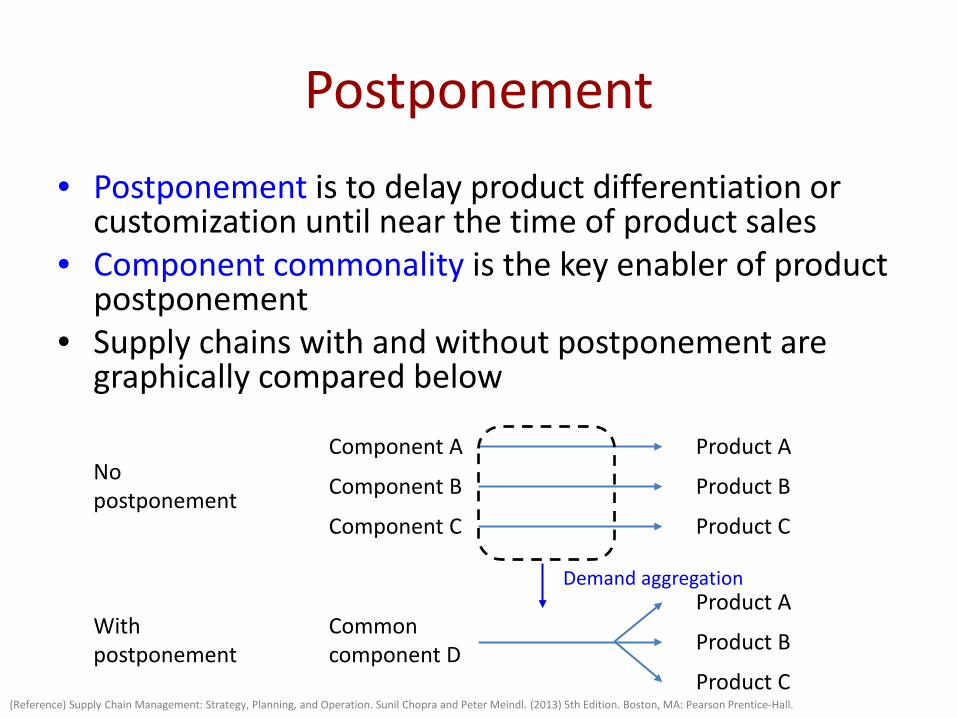
Postponement • Postponement is to delay product differentiation or
customization until near the time of product sales • Component commonality is the key enabler of product
postponement • Supply chains with and without postponement are
graphically compared below
•
(Reference) Supply Chain Management: Strategy, Planning, and Operation. Sunil Chopra and Peter Meindl. (2013) 5th Edition. Boston, MA: Pearson Prentice-Hall.
Product A
Product B
Product C
Component A
Component B
Component C
Product A
Product B
Product C
No postponement
Common component D
With postponement
Demand aggregation
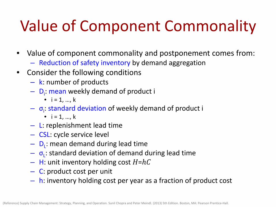
Value of Component Commonality • Value of component commonality and postponement comes from:
– Reduction of safety inventory by demand aggregation • Consider the following conditions
– k: number of products – Di: mean weekly demand of product i
• i = 1, …, k – σi: standard deviation of weekly demand of product i
• i = 1, …, k – L: replenishment lead time – CSL: cycle service level – DL: mean demand during lead time – σL: standard deviation of demand during lead time – H: unit inventory holding cost 𝐻𝐻=𝑤𝐶𝐶 – C: product cost per unit – h: inventory holding cost per year as a fraction of product cost
(Reference) Supply Chain Management: Strategy, Planning, and Operation. Sunil Chopra and Peter Meindl. (2013) 5th Edition. Boston, MA: Pearson Prentice-Hall.
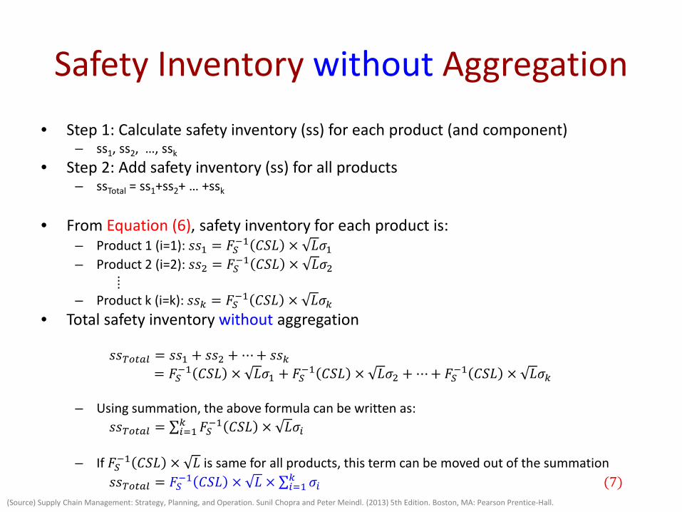
Safety Inventory without Aggregation • Step 1: Calculate safety inventory (ss) for each product (and component)
– ss1, ss2, …, ssk • Step 2: Add safety inventory (ss) for all products
– ssTotal = ss1+ss2+ … +ssk
• From Equation (6), safety inventory for each product is: – Product 1 (i=1): 𝑖𝑖𝑖𝑖1 = 𝐹𝐹𝑆𝑆−1 𝐶𝐶𝑆𝑆𝐿𝐿 × 𝐿𝐿𝜎𝜎1 – Product 2 (i=2): 𝑖𝑖𝑖𝑖2 = 𝐹𝐹𝑆𝑆−1 𝐶𝐶𝑆𝑆𝐿𝐿 × 𝐿𝐿𝜎𝜎2 ⁞ – Product k (i=k): 𝑖𝑖𝑖𝑖𝑘𝑘 = 𝐹𝐹𝑆𝑆−1 𝐶𝐶𝑆𝑆𝐿𝐿 × 𝐿𝐿𝜎𝜎𝑘𝑘
• Total safety inventory without aggregation
𝑖𝑖𝑖𝑖𝑇𝑇𝑇𝑇𝑇𝑇𝑇𝑇𝑇𝑇 = 𝑖𝑖𝑖𝑖1 + 𝑖𝑖𝑖𝑖2 + ⋯+ 𝑖𝑖𝑖𝑖𝑘𝑘 = 𝐹𝐹𝑆𝑆−1 𝐶𝐶𝑆𝑆𝐿𝐿 × 𝐿𝐿𝜎𝜎1 + 𝐹𝐹𝑆𝑆−1 𝐶𝐶𝑆𝑆𝐿𝐿 × 𝐿𝐿𝜎𝜎2 + ⋯+ 𝐹𝐹𝑆𝑆−1 𝐶𝐶𝑆𝑆𝐿𝐿 × 𝐿𝐿𝜎𝜎𝑘𝑘
– Using summation, the above formula can be written as: 𝑖𝑖𝑖𝑖𝑇𝑇𝑇𝑇𝑇𝑇𝑇𝑇𝑇𝑇 = ∑ 𝐹𝐹𝑆𝑆−1 𝐶𝐶𝑆𝑆𝐿𝐿 × 𝐿𝐿𝜎𝜎𝑖𝑖𝑘𝑘
𝑖𝑖=1
– If 𝐹𝐹𝑆𝑆−1 𝐶𝐶𝑆𝑆𝐿𝐿 × 𝐿𝐿 is same for all products, this term can be moved out of the summation 𝑖𝑖𝑖𝑖𝑇𝑇𝑇𝑇𝑇𝑇𝑇𝑇𝑇𝑇 = 𝐹𝐹𝑆𝑆−1 𝐶𝐶𝑆𝑆𝐿𝐿 × 𝐿𝐿 × ∑ 𝜎𝜎𝑖𝑖𝑘𝑘
𝑖𝑖=1 (7)
(Source) Supply Chain Management: Strategy, Planning, and Operation. Sunil Chopra and Peter Meindl. (2013) 5th Edition. Boston, MA: Pearson Prentice-Hall.
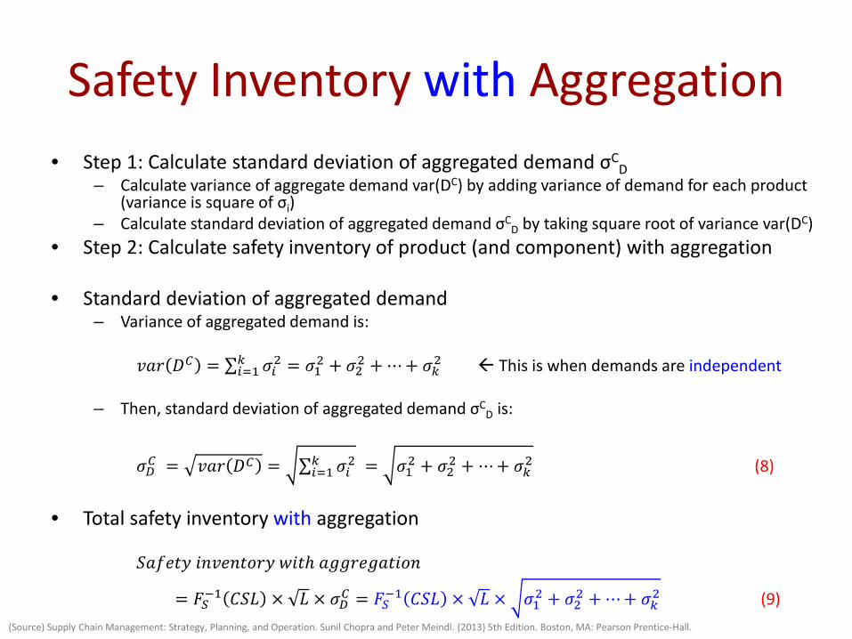
Safety Inventory with Aggregation • Step 1: Calculate standard deviation of aggregated demand σC
D – Calculate variance of aggregate demand var(DC) by adding variance of demand for each product
(variance is square of σi) – Calculate standard deviation of aggregated demand σC
D by taking square root of variance var(DC) • Step 2: Calculate safety inventory of product (and component) with aggregation
• Standard deviation of aggregated demand
– Variance of aggregated demand is: 𝑖𝑖𝑑𝑑𝑑𝑑 𝐷𝐷𝐶𝐶 = ∑ 𝜎𝜎𝑖𝑖2𝑘𝑘
𝑖𝑖=1 = 𝜎𝜎12 + 𝜎𝜎22 + ⋯+ 𝜎𝜎𝑘𝑘2 This is when demands are independent
– Then, standard deviation of aggregated demand σCD is:
𝜎𝜎𝐷𝐷𝐶𝐶 = 𝑖𝑖𝑑𝑑𝑑𝑑 𝐷𝐷𝐶𝐶 = ∑ 𝜎𝜎𝑖𝑖2𝑘𝑘𝑖𝑖=1 = 𝜎𝜎12 + 𝜎𝜎22 + ⋯+ 𝜎𝜎𝑘𝑘2 (8)
• Total safety inventory with aggregation
𝑆𝑆𝑑𝑑𝑆𝑆𝑤𝑤𝑖𝑖𝑆𝑆 𝑖𝑖𝑤𝑤𝑖𝑖𝑤𝑤𝑤𝑤𝑖𝑖𝑖𝑖𝑑𝑑𝑆𝑆 𝑤𝑤𝑖𝑖𝑖𝑖𝑤 𝑑𝑑𝑑𝑑𝑑𝑑𝑑𝑑𝑤𝑤𝑑𝑑𝑑𝑑𝑖𝑖𝑖𝑖𝑖𝑖𝑤𝑤
= 𝐹𝐹𝑆𝑆−1 𝐶𝐶𝑆𝑆𝐿𝐿 × 𝐿𝐿 × 𝜎𝜎𝐷𝐷𝐶𝐶 = 𝐹𝐹𝑆𝑆−1 𝐶𝐶𝑆𝑆𝐿𝐿 × 𝐿𝐿 × 𝜎𝜎12 + 𝜎𝜎22 + ⋯+ 𝜎𝜎𝑘𝑘2 (9)
(Source) Supply Chain Management: Strategy, Planning, and Operation. Sunil Chopra and Peter Meindl. (2013) 5th Edition. Boston, MA: Pearson Prentice-Hall.
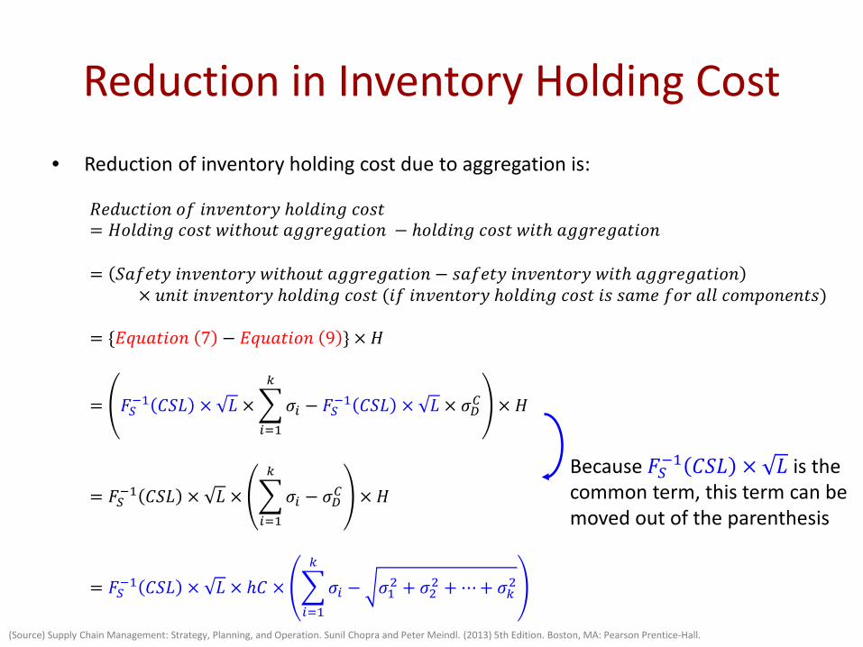
Reduction in Inventory Holding Cost • Reduction of inventory holding cost due to aggregation is:
𝑅𝑅𝑤𝑤𝑑𝑑𝑑𝑑𝐸𝐸𝑖𝑖𝑖𝑖𝑖𝑖𝑤𝑤 𝑖𝑖𝑆𝑆 𝑖𝑖𝑤𝑤𝑖𝑖𝑤𝑤𝑤𝑤𝑖𝑖𝑖𝑖𝑑𝑑𝑆𝑆 𝑤𝑖𝑖𝑙𝑙𝑑𝑑𝑖𝑖𝑤𝑤𝑑𝑑 𝐸𝐸𝑖𝑖𝑖𝑖𝑖𝑖 = 𝐻𝐻𝑖𝑖𝑙𝑙𝑑𝑑𝑖𝑖𝑤𝑤𝑑𝑑 𝐸𝐸𝑖𝑖𝑖𝑖𝑖𝑖 𝑤𝑤𝑖𝑖𝑖𝑖𝑤𝑖𝑖𝑑𝑑𝑖𝑖 𝑑𝑑𝑑𝑑𝑑𝑑𝑑𝑑𝑤𝑤𝑑𝑑𝑑𝑑𝑖𝑖𝑖𝑖𝑖𝑖𝑤𝑤 − 𝑤𝑖𝑖𝑙𝑙𝑑𝑑𝑖𝑖𝑤𝑤𝑑𝑑 𝐸𝐸𝑖𝑖𝑖𝑖𝑖𝑖 𝑤𝑤𝑖𝑖𝑖𝑖𝑤 𝑑𝑑𝑑𝑑𝑑𝑑𝑑𝑑𝑤𝑤𝑑𝑑𝑑𝑑𝑖𝑖𝑖𝑖𝑖𝑖𝑤𝑤
= 𝑆𝑆𝑑𝑑𝑆𝑆𝑤𝑤𝑖𝑖𝑆𝑆 𝑖𝑖𝑤𝑤𝑖𝑖𝑤𝑤𝑤𝑤𝑖𝑖𝑖𝑖𝑑𝑑𝑆𝑆 𝑤𝑤𝑖𝑖𝑖𝑖𝑤𝑖𝑖𝑑𝑑𝑖𝑖 𝑑𝑑𝑑𝑑𝑑𝑑𝑑𝑑𝑤𝑤𝑑𝑑𝑑𝑑𝑖𝑖𝑖𝑖𝑖𝑖𝑤𝑤 − 𝑖𝑖𝑑𝑑𝑆𝑆𝑤𝑤𝑖𝑖𝑆𝑆 𝑖𝑖𝑤𝑤𝑖𝑖𝑤𝑤𝑤𝑤𝑖𝑖𝑖𝑖𝑑𝑑𝑆𝑆 𝑤𝑤𝑖𝑖𝑖𝑖𝑤 𝑑𝑑𝑑𝑑𝑑𝑑𝑑𝑑𝑤𝑤𝑑𝑑𝑑𝑑𝑖𝑖𝑖𝑖𝑖𝑖𝑤𝑤 × 𝑑𝑑𝑤𝑤𝑖𝑖𝑖𝑖 𝑖𝑖𝑤𝑤𝑖𝑖𝑤𝑤𝑤𝑤𝑖𝑖𝑖𝑖𝑑𝑑𝑆𝑆 𝑤𝑖𝑖𝑙𝑙𝑑𝑑𝑖𝑖𝑤𝑤𝑑𝑑 𝐸𝐸𝑖𝑖𝑖𝑖𝑖𝑖 (𝑖𝑖𝑆𝑆 𝑖𝑖𝑤𝑤𝑖𝑖𝑤𝑤𝑤𝑤𝑖𝑖𝑖𝑖𝑑𝑑𝑆𝑆 𝑤𝑖𝑖𝑙𝑙𝑑𝑑𝑖𝑖𝑤𝑤𝑑𝑑 𝐸𝐸𝑖𝑖𝑖𝑖𝑖𝑖 𝑖𝑖𝑖𝑖 𝑖𝑖𝑑𝑑𝑑𝑑𝑤𝑤 𝑆𝑆𝑖𝑖𝑑𝑑 𝑑𝑑𝑙𝑙𝑙𝑙 𝐸𝐸𝑖𝑖𝑑𝑑𝑖𝑖𝑖𝑖𝑤𝑤𝑤𝑤𝑤𝑤𝑖𝑖𝑖𝑖)
= {𝐸𝐸𝐸𝐸𝑑𝑑𝑑𝑑𝑖𝑖𝑖𝑖𝑖𝑖𝑤𝑤 7 − 𝐸𝐸𝐸𝐸𝑑𝑑𝑑𝑑𝑖𝑖𝑖𝑖𝑖𝑖𝑤𝑤 9 } × 𝐻𝐻
= 𝐹𝐹𝑆𝑆−1 𝐶𝐶𝑆𝑆𝐿𝐿 × 𝐿𝐿 × �𝜎𝜎𝑖𝑖
𝑘𝑘
𝑖𝑖=1
− 𝐹𝐹𝑆𝑆−1 𝐶𝐶𝑆𝑆𝐿𝐿 × 𝐿𝐿 × 𝜎𝜎𝐷𝐷𝐶𝐶 × 𝐻𝐻
= 𝐹𝐹𝑆𝑆−1 𝐶𝐶𝑆𝑆𝐿𝐿 × 𝐿𝐿 × �𝜎𝜎𝑖𝑖
𝑘𝑘
𝑖𝑖=1
− 𝜎𝜎𝐷𝐷𝐶𝐶 × 𝐻𝐻
= 𝐹𝐹𝑆𝑆−1 𝐶𝐶𝑆𝑆𝐿𝐿 × 𝐿𝐿 × 𝑤𝐶𝐶 × �𝜎𝜎𝑖𝑖
𝑘𝑘
𝑖𝑖=1
− 𝜎𝜎12 + 𝜎𝜎22 + ⋯+ 𝜎𝜎𝑘𝑘2
(Source) Supply Chain Management: Strategy, Planning, and Operation. Sunil Chopra and Peter Meindl. (2013) 5th Edition. Boston, MA: Pearson Prentice-Hall.
Because 𝐹𝐹𝑆𝑆−1 𝐶𝐶𝑆𝑆𝐿𝐿 × 𝐿𝐿 is the common term, this term can be moved out of the parenthesis
Problem
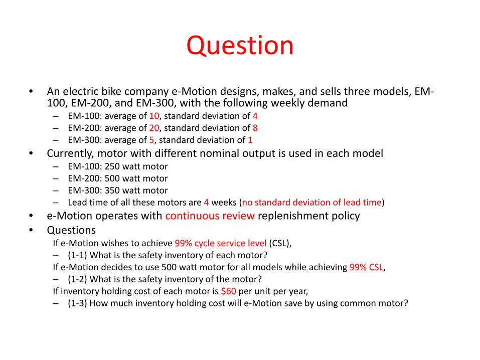
Question • An electric bike company e-Motion designs, makes, and sells three models, EM-
100, EM-200, and EM-300, with the following weekly demand – EM-100: average of 10, standard deviation of 4 – EM-200: average of 20, standard deviation of 8 – EM-300: average of 5, standard deviation of 1
• Currently, motor with different nominal output is used in each model – EM-100: 250 watt motor – EM-200: 500 watt motor – EM-300: 350 watt motor – Lead time of all these motors are 4 weeks (no standard deviation of lead time)
• e-Motion operates with continuous review replenishment policy • Questions
If e-Motion wishes to achieve 99% cycle service level (CSL), – (1-1) What is the safety inventory of each motor? If e-Motion decides to use 500 watt motor for all models while achieving 99% CSL, – (1-2) What is the safety inventory of the motor? If inventory holding cost of each motor is $60 per unit per year, – (1-3) How much inventory holding cost will e-Motion save by using common motor?
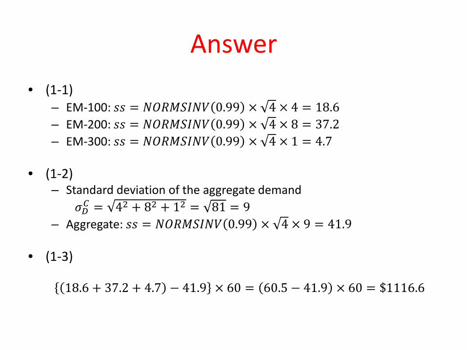
Answer • (1-1)
– EM-100: 𝑖𝑖𝑖𝑖 = 𝑁𝑁𝑅𝑅𝑅𝑅𝑁𝑁𝑆𝑆𝑁𝑁𝑁𝑁𝑁𝑁 0.99 × 4 × 4 = 18.6 – EM-200: 𝑖𝑖𝑖𝑖 = 𝑁𝑁𝑅𝑅𝑅𝑅𝑁𝑁𝑆𝑆𝑁𝑁𝑁𝑁𝑁𝑁 0.99 × 4 × 8 = 37.2 – EM-300: 𝑖𝑖𝑖𝑖 = 𝑁𝑁𝑅𝑅𝑅𝑅𝑁𝑁𝑆𝑆𝑁𝑁𝑁𝑁𝑁𝑁 0.99 × 4 × 1 = 4.7
• (1-2)
– Standard deviation of the aggregate demand 𝜎𝜎𝐷𝐷𝐶𝐶 = 42 + 82 + 12 = 81 = 9 – Aggregate: 𝑖𝑖𝑖𝑖 = 𝑁𝑁𝑅𝑅𝑅𝑅𝑁𝑁𝑆𝑆𝑁𝑁𝑁𝑁𝑁𝑁 0.99 × 4 × 9 = 41.9
• (1-3)
18.6 + 37.2 + 4.7 − 41.9 × 60 = 60.5 − 41.9 × 60 = $1116.6


![Commonality and Individuality in Writing[1]](https://img.pdfslide.net/doc/110x75/577ce72f1a28abf1039487c6/commonality-and-individuality-in-writing1.jpg)