Embed Size (px)
Citation preview
van den Berg, M., Buttazzo, G., & Velichkov, B. (2015). Optimizationproblems involving the first Dirichlet eigenvalue and the torsional rigidity. InA. Pratelli, & G. Leugering (Eds.), New Trends in Shape Optimization (pp.19-41). (International Series of Numerical Mathematics; Vol. 166). Springer.https://doi.org/10.1007/978-3-319-17563-8_2
Peer reviewed version
Link to published version (if available):10.1007/978-3-319-17563-8_2
Link to publication record in Explore Bristol ResearchPDF-document
University of Bristol - Explore Bristol ResearchGeneral rights
This document is made available in accordance with publisher policies. Please cite only the publishedversion using the reference above. Full terms of use are available:http://www.bristol.ac.uk/pure/about/ebr-terms
Optimization problems involvingthe first Dirichlet eigenvalueand the torsional rigidity
Michiel van den Berg, Giuseppe Buttazzo and BozhidarVelichkov
Abstract. We present some open problems and obtain some partial re-sults for spectral optimization problems involving measure, torsionalrigidity and first Dirichlet eigenvalue.
Mathematics Subject Classification (2010). Primary 49J45, 49R05; Sec-ondary 35P15, 47A75, 35J25.
Keywords. Torsional rigidity, Dirichlet eigenvalues, spectral optimiza-tion.
1. Introduction
A shape optimization problem can be written in the very general form
minF (Ω) : Ω ∈ A
,
where A is a class of admissible domains and F is a cost functional definedon A. We consider in the present paper the case where the cost functionalF is related to the solution of an elliptic equation and involves the spectrumof the related elliptic operator. We speak in this case of spectral optimizationproblems. Shape optimization problems of spectral type have been widelyconsidered in the literature; we mention for instance the papers [14], [18],[17], [20], [21], [22], [23], [30], and we refer to the books [16], [27], [28], andto the survey papers [2], [19], [26], where the reader can find a complete listof references and details.
In the present paper we restrict ourselves for simplicity to the Laplaceoperator −∆ with Dirichlet boundary conditions. Furthermore we shall as-sume that the admissible domains Ω are a priori contained in a given boundeddomain D ⊂ Rd. This assumption greatly simplifies several existence resultsthat otherwise would require additional considerations in terms of concentra-tion-compactness arguments [14], [32].
2 M. van den Berg, G. Buttazzo and B. Velichkov
The most natural constraint to consider on the class of admissible do-mains is a bound on their Lebesgue measure. Our admissible class A is then
A =
Ω ⊂ D : |Ω| ≤ 1.
Other kinds of constraints are also possible, but we concentrate here to theone above, referring the reader interested in possible variants to the booksand papers quoted above.
The following two classes of cost functionals are the main ones consid-ered in the literature.
Integral functionals. Given a right-hand side f ∈ L2(D), for every Ω ∈ Alet uΩ be the unique solution of the elliptic PDE
−∆u = f in Ω, u ∈ H10 (Ω).
The integral cost functionals are of the form
F (Ω) =
∫Ω
j(x, uΩ(x),∇uΩ(x)
)dx,
where j is a suitable integrand that we assume convex in the gradient variable.We also assume that j is bounded from below by
j(x, s, z) ≥ −a(x)− c|s|2,
with a ∈ L1(D) and c smaller than the first Dirichlet eigenvalue of the Laplaceoperator −∆ in D. For instance, the energy Ef (Ω) defined by
Ef (Ω) = inf
∫D
(1
2|∇u|2 − f(x)u
)dx : u ∈ H1
0 (Ω)
,
belongs to this class since, integrating by parts its Euler-Lagrange equation,we have that
Ef (Ω) = −1
2
∫D
f(x)uΩ dx,
which corresponds to the integral functional above with
j(x, s, z) = −1
2f(x)s.
The case f = 1 is particularly interesting for our purposes. We denote by wΩ
the torsion function, that is the solution of the PDE
−∆u = 1 in Ω, u ∈ H10 (Ω),
and by the torsional rigidity T (Ω) the L1 norm of wΩ,
T (Ω) =
∫Ω
wΩ dx = −2E1(Ω).
Spectral functionals. For every admissible domain Ω ∈ A we considerthe spectrum Λ(Ω) of the Laplace operator −∆ on H1
0 (Ω). Since Ω has afinite measure, the operator −∆ has a compact resolvent and so its spectrumΛ(Ω) is discrete:
Λ(Ω) =(λ1(Ω), λ2(Ω), . . .
),
Optimization problems for torsion and eigenvalues 3
where λk(Ω) are the eigenvalues counted with their multiplicity. The spectralcost functionals we may consider are of the form
F (Ω) = Φ(Λ(Ω)
),
for a suitable function Φ : RN → R. For instance, taking Φ(Λ) = λk(Ω) weobtain
F (Ω) = λk(Ω).
We take the torsional rigidity T (Ω) and the first eigenvalue λ1(Ω) asprototypes of the two classes above and we concentrate our attention on costfunctionals that depend on both of them. We note that, by the maximumprinciple, when Ω increases T (Ω) increases, while λ1(Ω) decreases.
2. Statement of the problem
The optimization problems we want to consider are of the form
min
Φ(λ1(Ω), T (Ω)
): Ω ⊂ D, |Ω| ≤ 1
, (2.1)
where we have normalized the constraint on the Lebesgue measure of Ω, andwhere Φ is a given continuous (or lower semi-continuous) and non-negativefunction. In the rest of this paper we often take for simplicity D = Rd,even if most of the results are valid in the general case. For instance, takingΦ(a, b) = ka + b with k a fixed positive constant, the quantity we aim tominimize becomes
kλ1(Ω) + T (Ω) with Ω ⊂ D, and |Ω| ≤ 1.
Remark 2.1. If the function Φ(a, b) is increasing with respect to a and de-creasing with respect to b, then the cost functional
F (Ω) = Φ(λ1(Ω), T (Ω)
)turns out to be decreasing with respect to the set inclusion. Since both thetorsional rigidity and the first eigenvalue are γ-continuous functionals andthe function Φ is assumed lower semi-continuous, we can apply the existenceresult of [21], which provides the existence of an optimal domain.
In general, if the function Φ does not verify the monotonicity property ofRemark 2.1, then the existence of an optimal domain is an open problem, andthe aim of this paper is to discuss this issue. For simplicity of the presentationwe limit ourselves to the two-dimensional case d = 2. The case of general ddoes not present particular difficulties but requires the use of several d−dependent exponents.
Remark 2.2. The following facts are well known.
i) If B is a disk in R2 we have
T (B) =1
8π|B|2.
4 M. van den Berg, G. Buttazzo and B. Velichkov
ii) If j0,1 ≈ 2.405 is the first positive zero of the Bessel functions J0(x) andB is a disk of R2 we have
λ1(B) =π
|B|j20,1.
iii) The torsional rigidity T (Ω) scales as
T (tΩ) = t4T (Ω), ∀t > 0.
iv) The first eigenvalue λ1(Ω) scales as
λ1(tΩ) = t−2λ1(Ω), ∀t > 0.
v) For every domain Ω of R2 and any disk B we have
|Ω|−2T (Ω) ≤ |B|−2T (B) =1
8π.
vi) For every domain Ω of R2 and any disk B we have (Faber-Krahn in-equality)
|Ω|λ1(Ω) ≥ |B|λ1(B) = πj20,1.
vii) A more delicate inequality is the so-called Kohler-Jobin inequality (see[29], [11]): for any domain Ω of R2 and any disk B we have
λ21(Ω)T (Ω) ≥ λ2
1(B)T (B) =π
8j40,1.
This had been previously conjectured by G. Polya and G.Szego [31].
We recall the following inequality, well known for planar regions (Section5.4 in [31]), between torsional rigidity and first eigenvalue.
Proposition 2.3. For every domain Ω ⊂ Rd we have
λ1(Ω)T (Ω) ≤ |Ω|.
Proof. By definition, λ1(Ω) is the infimum of the Rayleigh quotient∫Ω
|∇u|2 dx/∫
Ω
u2 dx over all u ∈ H10 (Ω), u 6= 0.
Taking as u the torsion function wΩ, we have
λ1(Ω) ≤∫
Ω
|∇wΩ|2 dx/∫
Ω
w2Ω dx.
Since −∆wΩ = 1, an integration by parts gives∫Ω
|∇wΩ|2 dx =
∫Ω
wΩ dx = T (Ω),
while the Holder inequality gives∫Ω
w2Ω dx ≥
1
|Ω|
(∫Ω
wΩ dx
)2
=1
|Ω|(T (Ω)
)2.
Summarizing, we have
λ1(Ω) ≤ |Ω|T (Ω)
as required.
Optimization problems for torsion and eigenvalues 5
Remark 2.4. The infimum of λ1(Ω)T (Ω) over open sets Ω of prescribed mea-sure is zero. To see this, let Ωn be the disjoint union of one ball of volume1/n and n(n − 1) balls of volume 1/n2. Then the radius Rn of the ball ofvolume 1/n is (nωd)
−1/d while the radius rn of the balls of volume 1/n2 is(n2ωd)
−1/d, so that |Ωn| = 1,
λ1(Ωn) = λ1(BRn) =1
R2n
λ1(B1) = (nωd)2/dλ1(B1),
and
T (Ωn) = T (BRn) + n(n− 1)T (Brn) = T (B1)
(Rd+2n + n(n− 1)rd+2
n
)= T (B1)ω
−1−2/dd
(n−1−2/d + (n− 1)n−1−4/d
).
Therefore
λ1(Ωn)T (Ωn) =λ1(B1)T (B1)
ωd
n2/d + n− 1
n1+2/d,
which vanishes as n→∞.
In the next section we investigate the inequality of Proposition 2.3.
3. A sharp inequality between torsion and first eigenvalue
We define the constant
Kd = sup
λ1(Ω)T (Ω)
|Ω|: Ω open in Rd, |Ω| <∞
.
We have seen in Proposition 2.3 that Kd ≤ 1. The question is if the constant1 can be improved.
Consider a ball B; performing the shape derivative as in [28], keepingthe volume of the perturbed shapes constant, we obtain for every field V (x)
∂[λ1(B)T (B)](V ) = T (B)∂[λ1(B)](V ) + λ1(B)∂[T (B)](V )
= CB
∫∂B
V · ndHd−1
for a suitable constant CB . Since the volume of the perturbed shapes isconstant, we have ∫
∂B
V · ndHd−1 = 0,
where Hd−1 denotes (d−1)-dimensional Hausdorff measure. This shows thatballs are stationary for the functional
F (Ω) =λ1(Ω)T (Ω)
|Ω|.
Below we will show, by considering rectangles, that balls are not optimal. Todo so we shall obtain a lower bound for the torsional rigidity of a rectangle.
6 M. van den Berg, G. Buttazzo and B. Velichkov
Proposition 3.1. In a rectangle Ra,b = (−b/2, b/2) × (−a/2, a/2) with a ≤ bwe have
T (Ra,b) ≥a3b
12− 11a4
180.
Proof. Let us estimate the energy
E1(Ra,b) = inf
∫Ra,b
(1
2|∇u|2 − u
)dx dy : u ∈ H1
0 (Ra,b)
by taking the function
u(x, y) =a2 − 4y2
8θ(x),
where θ(x) is defined by
θ(x) =
1 ,if |x| ≤ (b− a)/2
(b− 2|x|)/a ,otherwise.
We have
|∇u|2 =
(a2 − 4y2
8
)2
|θ′(x)|2 + y2|θ(x)|2,
so that
E1(Ra,b) ≤ 2
∫ a/2
0
(a2 − 4y2
8
)2
dy
∫ b/2
0
|θ′(x)|2 dx
+ 2
∫ a/2
0
y2 dy
∫ b/2
0
|θ(x)|2 dx
− 4
∫ a/2
0
a2 − 4y2
8dy
∫ b/2
0
θ(x) dx
=a4
60+a3
12
(b− a
2+a
6
)− a3
6
(b− a
2+a
4
)= −a
3b
24+
11a4
360.
The desired inequality follows since T (Ra,b) = −2E1(Ra,b).
In d-dimensions we have the following.
Proposition 3.2. If Ωε = ω × (−ε/2, ε, 2), where ω is a convex set in Rd−1
with |ω| <∞, then
T (Ωε) =ε3
12|ω|+O(ε4), ε ↓ 0.
We defer the proof to Section 5.For a ball of radius R we have
λ1(B) =j2d/2−1,1
R2, T (B) =
ωdRd+2
d(d+ 2), |B| = ωdR
d, (3.1)
Optimization problems for torsion and eigenvalues 7
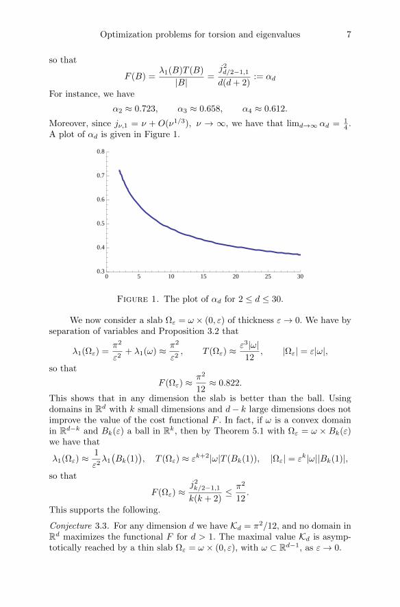
so that
F (B) =λ1(B)T (B)
|B|=j2d/2−1,1
d(d+ 2):= αd
For instance, we have
α2 ≈ 0.723, α3 ≈ 0.658, α4 ≈ 0.612.
Moreover, since jν,1 = ν + O(ν1/3), ν → ∞, we have that limd→∞ αd = 14 .
A plot of αd is given in Figure 1.
0 5 10 15 20 25 300.3
0.4
0.5
0.6
0.7
0.8
Figure 1. The plot of αd for 2 ≤ d ≤ 30.
We now consider a slab Ωε = ω × (0, ε) of thickness ε→ 0. We have byseparation of variables and Proposition 3.2 that
λ1(Ωε) =π2
ε2+ λ1(ω) ≈ π2
ε2, T (Ωε) ≈
ε3|ω|12
, |Ωε| = ε|ω|,
so that
F (Ωε) ≈π2
12≈ 0.822.
This shows that in any dimension the slab is better than the ball. Usingdomains in Rd with k small dimensions and d− k large dimensions does notimprove the value of the cost functional F . In fact, if ω is a convex domainin Rd−k and Bk(ε) a ball in Rk, then by Theorem 5.1 with Ωε = ω × Bk(ε)we have that
λ1(Ωε) ≈1
ε2λ1
(Bk(1)
), T (Ωε) ≈ εk+2|ω|T (Bk(1)), |Ωε| = εk|ω||Bk(1)|,
so that
F (Ωε) ≈j2k/2−1,1
k(k + 2)≤ π2
12.
This supports the following.
Conjecture 3.3. For any dimension d we have Kd = π2/12, and no domain inRd maximizes the functional F for d > 1. The maximal value Kd is asymp-totically reached by a thin slab Ωε = ω × (0, ε), with ω ⊂ Rd−1, as ε→ 0.
8 M. van den Berg, G. Buttazzo and B. Velichkov
4. The attainable set
In this section we bound the measure by |Ω| ≤ 1. Our goal is to plot the subsetof R2 whose coordinates are the eigenvalue λ1(Ω) and the torsion T (Ω). It isconvenient to change coordinates and to set for any admissible domain Ω,
x = λ1(Ω), y =(λ1(Ω)T (Ω)
)−1.
In addition, define
E =
(x, y) ∈ R2 : x = λ1(Ω), y =(λ1(Ω)T (Ω)
)−1for some Ω, |Ω| ≤ 1
.
Therefore, the optimization problem (2.1) can be rewritten as
min
Φ(x, 1/(xy)
): (x, y) ∈ E
.
Conjecture 4.1. The set E is closed.
We remark that the conjecture above, if true, would imply the existenceof a solution of the optimization problem (2.1) for many functions Φ. Belowwe will analyze the variational problem in case Φ(x, y) = kx + 1
xy , where
k > 0.
Theorem 4.2. Let d = 2, 3, · · · , and let
k∗d =1
2dω4/dd j2
d/2−1,1
.
Consider the optimization problem
min kλ1(Ω) + T (Ω) : |Ω| ≤ 1 . (4.1)
If 0 < k ≤ k∗d then the ball with radius
Rk =
(2kdj2
d/2−1,1
ωd
)1/(d+4)
(4.2)
is the unique minimizer (modulo translations and sets of capacity 0).If k > k∗d then the ball B with measure 1 is the unique minimizer.
Proof. Consider the problem (4.1) without the measure constraint
minkλ1(Ω) + T (Ω) : Ω ⊂ Rd
. (4.3)
Taking tΩ instead of Ω gives that
kλ1(tΩ) + T (tΩ) = kt−2λ1(Ω) + td+2T (Ω).
The optimal t which minimizes this expression is given by
t =
(2kλ1(Ω)
(d+ 2)T (Ω)
)1/(d+4)
.
Hence (4.3) equals
min
(d+ 4)
(kd+2
4(d+ 2)d+2T 2(Ω)λd+2
1 (Ω)
)1/(d+4)
: Ω ⊂ Rd. (4.4)
Optimization problems for torsion and eigenvalues 9
By the Kohler-Jobin inequality in Rd, the minimum in (4.4) is attained byany ball. Therefore the minimum in (4.3) is given by a ball BR such that(
2kλ1(BR)
(d+ 2)T (BR)
)1/(d+4)
= 1.
This gives (4.2). We conclude that the measure constrained problem (4.1)admits the ball BRk
as a solution whenever ωdRdk ≤ 1. That is k ≤ k∗d.
Next consider the case k > k∗d. Let B be the open ball with measure 1.It is clear that
minkλ1(Ω) + T (Ω) : |Ω| ≤ 1 ≤ kλ1(B) + T (B).
To prove the converse we note that for k > k∗d,
minkλ1(Ω) + T (Ω) : |Ω| ≤ 1
≥ min
(k − k∗d)λ1(Ω) : |Ω| ≤ 1
+ min
k∗dλ1(Ω) + T (Ω) : |Ω| ≤ 1
.
(4.5)
The minimum in the first term in the right hand side of (4.5) is attainedfor B by Faber-Krahn, whereas the minimum in second term is attained forBRk∗
dby our previous unconstrained calculation. Since |BRk∗
d| = |B| = 1 we
have by (4.5) that
minkλ1(Ω) + T (Ω) : |Ω| ≤ 1
≥ (k − k∗d)λ1(B) + k∗dλ1(B) + T (B)
= kλ1(B) + T (B).
Uniqueness of the above minimizers follows by uniqueness of Faber-Krahnand Kohler-Jobin.
It is interesting to replace the first eigenvalue in (4.1) be a higher eigen-value. We have the following for the second eigenvalue.
Theorem 4.3. Let d = 2, 3, · · · , and let
l∗d =1
2d(2ωd)4/dj2d/2−1,1
.
Consider the optimization problem
min lλ2(Ω) + T (Ω) : |Ω| ≤ 1 . (4.6)
If 0 < l ≤ l∗d then the union of two disjoint balls with radii
Rl =
(ldj2
d/2−1,1
ωd
)1/(d+4)
(4.7)
is the unique minimizer (modulo translations and sets of capacity 0).If l > l∗d then union of two disjoint balls with measure 1/2 each is the uniqueminimizer.
10 M. van den Berg, G. Buttazzo and B. Velichkov
Proof. First consider the unconstrained problem
minlλ1(Ω) + T (Ω) : Ω ⊂ Rd
. (4.8)
Taking tΩ instead of Ω gives that
lλ2(tΩ) + T (tΩ) = lt−2λ2(Ω) + td+2T (Ω).
The optimal t which minimizes this expression is given by
t =
(2lλ2(Ω)
(d+ 2)T (Ω)
)1/(d+4)
.
Hence (4.8) equals
min
(d+ 4)
(ld+2
4(d+ 2)d+2T 2(Ω)λd+2
2 (Ω)
)1/(d+4)
: Ω ⊂ Rd. (4.9)
It follows by the Kohler-Jobin inequality, see for example Lemma 6 in [9], thatthe minimizer of (4.9) is attained by the union of two disjoint balls BR andB′R with the same radius. Since λ2(BR ∪B′R) = λ1(BR) and T (BR ∪B′R) =2T (BR) we have, using (3.1), that the radii of these balls are given by (4.7).We conclude that the measure constrained problem (4.6) admits the unionof two disjoint balls with equal radius Rl as a solution whenever 2ωdR
dl ≤ 1.
That is l ≤ l∗d.Next consider the case l > l∗d. Let Ω be the union of two disjoint balls
B and B′ with measure 1/2 each. Then
minlλ2(Ω) + T (Ω) : |Ω| ≤ 1 ≤ lλ1(B) + 2T (B).
To prove the converse we note that for l > l∗d,
minlλ2(Ω) + T (Ω) : |Ω| ≤ 1
≥ min
(l − l∗d)λ2(Ω) : |Ω| ≤ 1
+ min
l∗dλ2(Ω) + T (Ω) : |Ω| ≤ 1
.
(4.10)
The minimum in the first term in the right hand side of (4.10) is attainedfor B ∪ B′ by the Krahn-Szego inequality, whereas the minimum in secondterm is attained for the union of two disjoint balls with radius Rl∗d by ourprevious unconstrained calculation. Since |BRl∗
d| = 1/2 = |B| = |B′| we have
by (4.10) that
minlλ2(Ω) + T (Ω) : |Ω| ≤ 1 ≥ (l − l∗d)λ1(B) + l∗dλ1(B) + 2T (B)
= lλ1(B) + 2T (B).
Uniqueness of the above minimizers follows by uniqueness of Krahn-Szego andKohler-Jobin for the second eigenvalue.
To replace the first eigenvalue in (4.1) be the j’th eigenvalue (j > 2)is a very difficult problem since we do not know the minimizers of the j’thDirichlet eigenvalue with a measure constraint nor the minimizer of the j’th
Optimization problems for torsion and eigenvalues 11
Dirichlet eigenvalue a torsional rigidity constraint. However, if these two prob-lems have a common minimizer then information similar to the above can beobtained.
Putting together the facts listed in Remark 2.2 we obtain the followinginequalities.
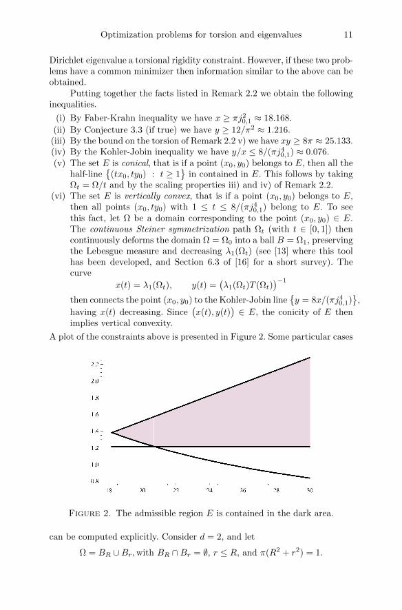
(i) By Faber-Krahn inequality we have x ≥ πj20,1 ≈ 18.168.
(ii) By Conjecture 3.3 (if true) we have y ≥ 12/π2 ≈ 1.216.(iii) By the bound on the torsion of Remark 2.2 v) we have xy ≥ 8π ≈ 25.133.(iv) By the Kohler-Jobin inequality we have y/x ≤ 8/(πj4
0,1) ≈ 0.076.(v) The set E is conical, that is if a point (x0, y0) belongs to E, then all the
half-line
(tx0, ty0) : t ≥ 1
in contained in E. This follows by takingΩt = Ω/t and by the scaling properties iii) and iv) of Remark 2.2.
(vi) The set E is vertically convex, that is if a point (x0, y0) belongs to E,then all points (x0, ty0) with 1 ≤ t ≤ 8/(πj4
0,1) belong to E. To seethis fact, let Ω be a domain corresponding to the point (x0, y0) ∈ E.The continuous Steiner symmetrization path Ωt (with t ∈ [0, 1]) thencontinuously deforms the domain Ω = Ω0 into a ball B = Ω1, preservingthe Lebesgue measure and decreasing λ1(Ωt) (see [13] where this toolhas been developed, and Section 6.3 of [16] for a short survey). Thecurve
x(t) = λ1(Ωt), y(t) =(λ1(Ωt)T (Ωt)
)−1
then connects the point (x0, y0) to the Kohler-Jobin liney = 8x/(πj4
0,1)
,
having x(t) decreasing. Since(x(t), y(t)
)∈ E, the conicity of E then
implies vertical convexity.
A plot of the constraints above is presented in Figure 2. Some particular cases
Figure 2. The admissible region E is contained in the dark area.
can be computed explicitly. Consider d = 2, and let
Ω = BR ∪Br,with BR ∩Br = ∅, r ≤ R, and π(R2 + r2) = 1.
12 M. van den Berg, G. Buttazzo and B. Velichkov
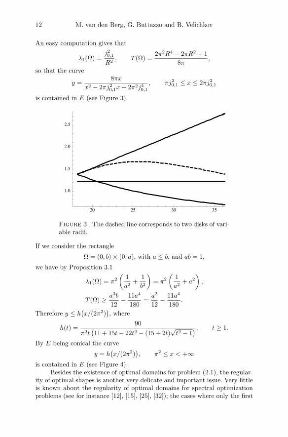
An easy computation gives that
λ1(Ω) =j20,1
R2, T (Ω) =
2π2R4 − 2πR2 + 1
8π,
so that the curve
y =8πx
x2 − 2πj20,1x+ 2π2j4
0,1
, πj20,1 ≤ x ≤ 2πj2
0,1
is contained in E (see Figure 3).
20 25 30 35
1.0
1.5
2.0
2.5
Figure 3. The dashed line corresponds to two disks of vari-able radii.
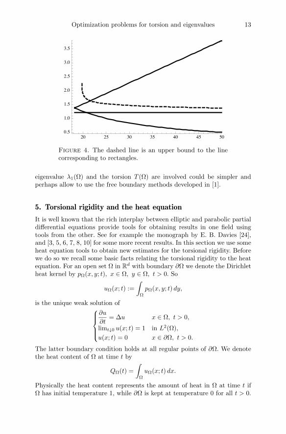
If we consider the rectangle
Ω = (0, b)× (0, a), with a ≤ b, and ab = 1,
we have by Proposition 3.1
λ1(Ω) = π2
(1
a2+
1
b2
)= π2
(1
a2+ a2
),
T (Ω) ≥ a3b
12− 11a4
180=a2
12− 11a4
180.
Therefore y ≤ h(x/(2π2)
), where
h(t) =90
π2t(11 + 15t− 22t2 − (15 + 2t)
√t2 − 1
) , t ≥ 1.
By E being conical the curve
y = h(x/(2π2)
), π2 ≤ x < +∞
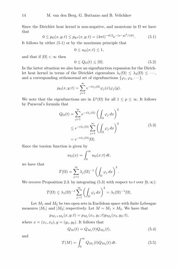
is contained in E (see Figure 4).Besides the existence of optimal domains for problem (2.1), the regular-
ity of optimal shapes is another very delicate and important issue. Very littleis known about the regularity of optimal domains for spectral optimizationproblems (see for instance [12], [15], [25], [32]); the cases where only the first
Optimization problems for torsion and eigenvalues 13
20 25 30 35 40 45 500.5
1.0
1.5
2.0
2.5
3.0
3.5
Figure 4. The dashed line is an upper bound to the linecorresponding to rectangles.
eigenvalue λ1(Ω) and the torsion T (Ω) are involved could be simpler andperhaps allow to use the free boundary methods developed in [1].
5. Torsional rigidity and the heat equation
It is well known that the rich interplay between elliptic and parabolic partialdifferential equations provide tools for obtaining results in one field usingtools from the other. See for example the monograph by E. B. Davies [24],and [3, 5, 6, 7, 8, 10] for some more recent results. In this section we use someheat equation tools to obtain new estimates for the torsional rigidity. Beforewe do so we recall some basic facts relating the torsional rigidity to the heatequation. For an open set Ω in Rd with boundary ∂Ω we denote the Dirichletheat kernel by pΩ(x, y; t), x ∈ Ω, y ∈ Ω, t > 0. So
uΩ(x; t) :=
∫Ω
pΩ(x, y; t) dy,
is the unique weak solution of∂u
∂t= ∆u x ∈ Ω, t > 0,
limt↓0 u(x; t) = 1 in L2(Ω),
u(x; t) = 0 x ∈ ∂Ω, t > 0.
The latter boundary condition holds at all regular points of ∂Ω. We denotethe heat content of Ω at time t by
QΩ(t) =
∫Ω
uΩ(x; t) dx.
Physically the heat content represents the amount of heat in Ω at time t ifΩ has initial temperature 1, while ∂Ω is kept at temperature 0 for all t > 0.
14 M. van den Berg, G. Buttazzo and B. Velichkov
Since the Dirichlet heat kernel is non-negative, and monotone in Ω we havethat
0 ≤ pΩ(x, y; t) ≤ pRd(x, y; t) = (4πt)−d/2e−|x−y|2/(4t). (5.1)
It follows by either (5.1) or by the maximum principle that
0 ≤ uΩ(x; t) ≤ 1,
and that if |Ω| <∞ then
0 ≤ QΩ(t) ≤ |Ω|. (5.2)
In the latter situation we also have an eigenfunction expansion for the Dirich-let heat kernel in terms of the Dirichlet eigenvalues λ1(Ω) ≤ λ2(Ω) ≤ · · · ,and a corresponding orthonormal set of eigenfunctions ϕ1, ϕ2, · · · ,
pΩ(x, y; t) =
∞∑j=1
e−tλj(Ω)ϕj(x)ϕj(y).
We note that the eigenfunctions are in Lp(Ω) for all 1 ≤ p ≤ ∞. It followsby Parseval’s formula that
QΩ(t) =
∞∑j=1
e−tλj(Ω)
(∫Ω
ϕj dx
)2
≤ e−tλ1(Ω)∞∑j=1
(∫Ω
ϕj dx
)2
= e−tλ1(Ω)|Ω|.
(5.3)
Since the torsion function is given by
wΩ(x) =
∫ ∞0
uΩ(x; t) dt,
we have that
T (Ω) =
∞∑j=1
λj(Ω)−1
(∫Ω
ϕj dx
)2
.
We recover Proposition 2.3. by integrating (5.3) with respect to t over [0,∞):
T (Ω) ≤ λ1(Ω)−1∞∑j=1
(∫Ω
ϕj dx
)2
= λ1(Ω)−1|Ω|.
Let M1 and M2 be two open sets in Euclidean space with finite Lebesguemeasures |M1| and |M2| respectively. Let M = M1 ×M2. We have that
pM1×M2(x, y; t) = pM1
(x1, y1; t)pM2(x2, y2; t),
where x = (x1, x2), y = (y1, y2). It follows that
QM (t) = QM1(t)QM2
(t), (5.4)
and
T (M) =
∫ ∞0
QM1(t)QM2
(t) dt. (5.5)
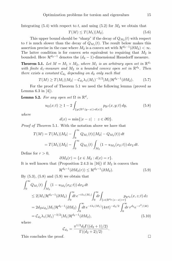
Optimization problems for torsion and eigenvalues 15
Integrating (5.4) with respect to t, and using (5.2) for M2 we obtain that
T (M) ≤ T (M1)|M2|. (5.6)
This upper bound should be “sharp” if the decay of QM2(t) with respect
to t is much slower than the decay of QM1(t). The result below makes thisassertion precise in the case where M2 is a convex set with Hd2−1(∂M2) <∞.The latter condition is for convex sets equivalent to requiring that M2 isbounded. Here Hd2−1 denotes the (d2 − 1)-dimensional Hausdorff measure.
Theorem 5.1. Let M = M1 ×M2, where M1 is an arbitrary open set in Rd1with finite d1-measure and M2 is a bounded convex open set in Rd2 . Thenthere exists a constant Cd2 depending on d2 only such that
T (M) ≥ T (M1)|M2| − Cd2λ1(M1)−3/2|M1|Hd2−1(∂M2). (5.7)
For the proof of Theorem 5.1 we need the following lemma (proved asLemma 6.3 in [4]).
Lemma 5.2. For any open set Ω in Rd,
uΩ(x; t) ≥ 1− 2
∫y∈Rd:|y−x|>d(x)
pRd(x, y; t) dy, (5.8)
whered(x) = min|x− z| : z ∈ ∂Ω.
Proof of Theorem 5.1. With the notation above we have that
T (M) = T (M1)|M2| −∫ ∞
0
QM1(t)(|M2| −QM2
(t)) dt
= T (M1)|M2| −∫ ∞
0
QM1(t)
∫M2
(1− uM2(x2; t)) dx2 dt.
Define for r > 0,∂M2(r) = x ∈M2 : d(x) = r.
It is well known that (Proposition 2.4.3 in [16]) if M2 is convex then
Hd2−1(∂M2(r)) ≤ Hd2−1(∂M2). (5.9)
By (5.3), (5.8) and (5.9) we obtain that∫ ∞0
QM1(t)
∫M2
(1− uM2(x2; t)) dx2 dt
≤ 2|M1|Hd2−1(∂M2)
∫ ∞0
dt e−tλ1(M1)
∫ ∞0
dr
∫z∈Rd2 :|z−x|>r
pRd2 (x, z; t) dz
= 2d2ωd2 |M1|Hd2−1(∂M2)
∫ ∞0
dt e−tλ1(M1)(4πt)−d2/2∫ ∞
0
dr rd2e−r2/(4t)
= Cd2λ1(M1)−3/2|M1|Hd2−1(∂M2), (5.10)
where
Cd2 =π1/2d2Γ((d2 + 1)/2)
Γ((d2 + 2)/2).
This concludes the proof.
16 M. van den Berg, G. Buttazzo and B. Velichkov
Proof of Proposition 3.2. Let M1 = (0, ε) ⊂ R, M2 = ω ⊂ Rd−1. Since thetorsion function for M1 is given by x(ε − x)/2, 0 ≤ x ≤ ε we have thatT (M1) = ε3/12. Then (5.6) proves the upper bound. The lower bound followsfrom (5.7) since λ1(M1) = π2/ε2, |M1| = ε.
It is of course possible, using the Faber-Krahn inequality for λ1(M1),to obtain a bound for the right-hand side of (5.10) in terms of the quantity|M1|(d1+3)/d1Hd2−1(∂M2).
Our next result is an improvement of Proposition 3.1. The torsionalrigidity for a rectangle follows by substituting the formulae for Q(0,a)(t) andQ(0,b)(t) given in (5.12) below into (5.5). We recover the expression given onp.108 in [31]:
T (Ra,b) =64ab
π6
∑k=1,3,···
∑l=1,3,···
k−2l−2
(k2
a2+l2
b2
)−1
.
Nevertheless the following result is not immediately obvious.
Theorem 5.3. ∣∣∣∣T (Ra,b)−a3b
12+
31ζ(5)a4
2π5
∣∣∣∣ ≤ a5
15b, (5.11)
where
ζ(5) =
∞∑k=1
1
k5.
Proof. A straightforward computation using the eigenvalues and eigenfunc-tions of the Dirichlet Laplacian on the interval together with the first identityin (5.3) shows that
Q(0,a)(t) =8a
π2
∑k=1,3,...
k−2e−tπ2k2/a2 . (5.12)
We write
Q(0,b)(t) = b− 4t1/2
π1/2+
(Q(0,b)(t) +
4t1/2
π1/2− b). (5.13)
The constant term b in the right-hand side of (5.13) gives, using (5.12), acontribution
8ab
π2
∫[0,∞)
dt∑
k=1,3,...
k−2e−tπ2k2/a2 =
8a3b
π4
∑k=1,3,...
k−4
=8a3b
π4
∞∑k=1
k−4 −∑
k=2,4,...
k−4
=15a3b
2π4ζ(4)
=a3b
12,
Optimization problems for torsion and eigenvalues 17
which jibes with the corresponding term in (5.11). In a very similar calcula-
tion we have that the − 4t1/2
π1/2 term in the right-hand side of (5.13) contributes
− 32a
π5/2
∫[0,∞)
dt t1/2∑
k=1,3,...
k−2e−tπ2k2/a2 = −31ζ(5)a4
2π5,
which jibes with the corresponding term in (5.11). It remains to bound thecontribution from the expression in the large round brackets in (5.11). Ap-plying formula (5.12) to the interval (0, b) instead and using the fact that∑k=1,3,··· k
−2 = π2/8 gives that
Q(0,b)(t)− b+4t1/2
π1/2=
8b
π2
∑k=1,3,...
k−2(e−tπ
2k2/b2 − 1)
+4t1/2
π1/2
= −8
b
∑k=1,3,...
∫[0,t]
dτe−τπ2k2/b2 +
4t1/2
π1/2
= −8
b
∫[0,t]
dτ
( ∞∑k=1
e−τπ2k2/b2 −
∞∑k=1
e−4τπ2k2/b2
)
+4t1/2
π1/2.
(5.14)
In order to bound the right-hand side of (5.14) we use the following instanceof the Poisson summation formula.∑
k∈Ze−tπk
2
= t−1/2∑k∈Z
e−πk2/t, t > 0.
We obtain that
∞∑k=1
e−tπk2
=1
(4t)1/2− 1
2+ t−1/2
∞∑k=1
e−πk2/t, t > 0.
Applying this identity twice (with t = πτ/b2 and t = 4πτ/b2 respectively)gives that the right-hand side of (5.14) equals
− 8
π1/2
∫[0,t]
dτ
(τ−1/2
∞∑k=1
e−k2b2/τ − (4τ)−1/2
∞∑k=1
e−k2b2/(4τ)
).
Since k 7→ e−k2b2/τ is non-negative and decreasing,
∞∑k=1
τ−1/2e−k2b2/τ ≤ τ−1/2
∫[0,∞)
dke−k2b2/τ = π1/2(2b)−1.
It follows that ∣∣∣∣Q(0,b)(t)− b+4t1/2
π1/2
∣∣∣∣ ≤ 8t
b, t > 0.
18 M. van den Berg, G. Buttazzo and B. Velichkov
So the contribution of the third term in (5.13) to T (Ra,b) is bounded inabsolute value by
64a
π2b
∫[0,∞)
dt t∑
k=1,3,...
k−2e−tπ2k2/a2 =
64a5
π6b
∑k=1,3,...
k−6
=63a5
π6bζ(6)
=a5
15b.
This completes the proof of Theorem 5.3.
The Kohler-Jobin theorem mentioned in Section 2 generalizes to d-dimensions: for any open set Ω with finite measure the ball minimizes thequantity T (Ω)λ1(Ω)(d+2)/2. Moreover, in the spirit of Theorem 5.1, the fol-lowing inequality is proved in [9] through an elementary heat equation proof.
Theorem 5.4. If T (Ω) < ∞ then the spectrum of the Dirichlet Laplacianacting in L2(Ω) is discrete, and
T (Ω) ≥(
2
d+ 2
)(4πd
d+ 2
)d/2 ∞∑k=1
λk(Ω)−(d+2)/2.
We obtain, using the Ashbaugh-Benguria theorem (p.86 in [27]) forλ1(Ω)/λ2(Ω), that
T (Ω)λ1(Ω)(d+2)/2
≥(
2
d+ 2
)(4πd
d+ 2
)d/2Γ
(1 +
d
2
)(1 +
(λ1(B)
λ2(B)
)(d+2)/2).
(5.15)
The constant in the right-hand side of (5.15) is for d = 2 off by a factorj40,1j
41,1
8(j40,1+j41,1)≈ 3.62 if compared with the sharp Kohler-Jobin constant. We
also note the missing factor mm/(m+2) in the right-hand side of (57) in [9].
Acknowledgment
A large part of this paper was written during a visit of the first two authorsat the Isaac Newton Institute for Mathematical Sciences of Cambridge (UK).GB and MvdB gratefully acknowledge the Institute for the excellent workingatmosphere provided. The authors also wish to thank Pedro Antunes helpfuldiscussions. The work of GB is part of the project 2010A2TFX2 “Calcolodelle Variazioni” funded by the Italian Ministry of Research and University.
References
[1] H.W. Alt, L.A. Caffarelli: Existence and regularity for a minimum problemwith free boundary. J. Reine Angew. Math., 325 (1981), 105–144.
Optimization problems for torsion and eigenvalues 19
[2] M.S. Ashbaugh: Open problems on eigenvalues of the Laplacian. In “Analyticand Geometric Inequalities and Applications”, Math. Appl. 478, Kluwer Acad.Publ., Dordrecht (1999), 13–28.
[3] M. van den Berg: On the spectrum of the Dirichlet Laplacian for horn-shapedregions in Rn with infinite volume. J. Funct. Anal., 58 (1984), 150–156.
[4] M. van den Berg, E.B. Davies: Heat flow out of regions in Rm. Math. Z.,202 (1989), 463–482.
[5] M. van den Berg, R. Banuelos: Dirichlet eigenfunctions for horn-shapedregions and Laplacians on cross sections. J. Lond. Math. Soc., 53 (1996), 503–511.
[6] M. van den Berg, E. Bolthausen: Estimates for Dirichlet eigenfunctions. J.Lond. Math. Soc., 59 (1999), 607–619.
[7] M. van den Berg, T. Carroll: Hardy inequality and Lp estimates for thetorsion function. Bull. Lond. Math. Soc., 41 (2009), 980–986.
[8] M. van den Berg: Estimates for the torsion function and Sobolev constants.Potential Anal., 36 (2012), 607–616.
[9] M. van den Berg, M. Iversen: On the minimization of Dirichlet eigenvaluesof the Laplace operator. J. Geom. Anal., 23 (2013), 660–676.
[10] M. van den Berg, D. Bucur: On the torsion function with Robin or Dirichletboundary conditions. J. Funct. Anal., 266 (2014), 1647–1666.
[11] L. Brasco: On torsional rigidity and principal frequencies: an invitation tothe Kohler-Jobin rearrangement technique. ESAIM Control Optim. Calc. Var.,20 (2014), no. 2, 315–338.
[12] T. Briancon, J. Lamboley: Regularity of the optimal shape for the firsteigenvalue of the Laplacian with volume and inclusion constraints. Ann. Inst.H. Poincare Anal. Non Lineaire, 26 (2009), 1149–1163.
[13] F. Brock: Continuous Steiner symmetrization. Math. Nachr., 172 (1995), 25–48.
[14] D. Bucur: Minimization of the k-th eigenvalue of the Dirichlet Laplacian.Arch. Rational Mech. Anal., 206 (2012), 1073–1083.
[15] D. Bucur: Regularity of optimal convex shapes. J. Convex Anal., 10 (2003),501–516.
[16] D. Bucur, G. Buttazzo: Variational Methods in Shape Optimization Prob-lems. Progress in Nonlinear Differential Equations 65, Birkhauser Verlag, Basel(2005).
[17] D. Bucur, G. Buttazzo, I. Figueiredo: On the attainable eigenvalues ofthe Laplace operator. SIAM J. Math. Anal., 30 (1999), 527–536.
[18] D. Bucur, G. Buttazzo, B. Velichkov: Spectral optimization problems withinternal constraint. Ann. Inst. H. Poincare Anal. Non Lineaire, 30 (2013), 477–495.
[19] G. Buttazzo: Spectral optimization problems. Rev. Mat. Complut., 24 (2011),277–322.
[20] G. Buttazzo, G. Dal Maso: Shape optimization for Dirichlet problems: re-laxed formulation and optimality conditions. Appl. Math. Optim., 23 (1991),17–49.
20 M. van den Berg, G. Buttazzo and B. Velichkov
[21] G. Buttazzo, G. Dal Maso: An existence result for a class of shape opti-mization problems.. Arch. Rational Mech. Anal., 122 (1993), 183–195.
[22] G. Buttazzo, B. Velichkov: Shape optimization problems on metric measurespaces. J. Funct. Anal., 264 (2013), 1–33.
[23] G. Buttazzo, B. Velichkov: Some new problems in spectral optimization.In “Calculus of Variations and PDEs”, Banach Center Publications 101, PolishAcademy of Sciences, Warszawa (2014), 19–35.
[24] E.B. Davies: Heat kernels and spectral theory. Cambridge University Press,Cambridge (1989).
[25] G. De Philippis, B. Velichkov: Existence and regularity of minimizers forsome spectral optimization problems with perimeter constraint. Appl. Math. Op-tim., 69 (2014), 199–231.
[26] A. Henrot: Minimization problems for eigenvalues of the Laplacian. J. Evol.Equ., 3 (2003), 443–461.
[27] A. Henrot: Extremum Problems for Eigenvalues of Elliptic Operators. Fron-tiers in Mathematics, Birkhauser Verlag, Basel (2006).
[28] A. Henrot, M. Pierre: Variation et Optimisation de Formes. Une AnalyseGeometrique. Mathematiques & Applications 48, Springer-Verlag, Berlin (2005).
[29] M.T. Kohler-Jobin: Une methode de comparaison isoperimetrique de fonc-tionnelles de domaines de la physique mathematique. I. Une demonstration dela conjecture isoperimetrique Pλ2 ≥ πj40/2 de Polya et Szego. Z. Angew. Math.Phys., 29 (1978), 757–766.
[30] D. Mazzoleni, A. Pratelli: Existence of minimizers for spectral problems.J. Math. Pures Appl., 100 (2013), 433–453.
[31] G. Polya, G.Szego: Isoperimetric inequalities in mathematical physics. Ann.of Math. Stud. 27, Princeton University Press, Princeton (1951).
[32] B. Velichkov: Existence and regularity results for some shape optimizationproblems. PhD Thesis available at http://cvgmt.sns.it.
Michiel van den BergSchool of Mathematics, University of BristolUniversity Walk, Bristol BS8 1TW - UKe-mail: [email protected]://www.maths.bris.ac.uk/ mamvdb/
Giuseppe ButtazzoDipartimento di Matematica, Universita di PisaLargo B. Pontecorvo 5, 56127 Pisa - ITALYe-mail: [email protected]://www.dm.unipi.it/pages/buttazzo/
Bozhidar VelichkovLaboratoire Jean Kuntzmann (LJK), Universite Joseph FourierTour IRMA, BP 53, 51 rue des Mathematiques, 38041 Grenoble Cedex 9 - FRANCEe-mail: [email protected]://www.velichkov.it

![buttazzo.ppt [modalità compatibilità] - ArtistDesign NoE ... · Overview of Real-Time Scheduling Giorgio Buttazzo Scuola Superiore Sant’Anna, Pisa E-mail: buttazzo@sssup.it Goal](https://img.pdfslide.net/doc/110x75/5c69a67709d3f2e4258d2ec5/modalita-compatibilita-artistdesign-noe-overview-of-real-time-scheduling.jpg)