Embed Size (px)
Citation preview
“Metode de optimizare Riemanniene pentru învățare profundă”Proiect cofinanțat din Fondul European de Dezvoltare Regională prin
Programul Operațional Competitivitate 2014-2020
Variational AutoEncoder:
An Introduction and Recent Perspectives
Luigi Malagò, Alexandra Peste, and Septimia Sarbu
Romanian Institute of Science and Technology
Politecnico di Milano 23 February 2018
Outline
1 Plan of the presentation
2 General View of Variational AutoencodersIntroductionResearch Directions
3 Work-in-progressUsing Gaussian Graphical ModelsGeometry of the Latent Space
4 Future Work
L.Malago, A.Peste (RIST) Variational Autoencoders 2 / 36
Plan of the presentation
Overview of variational inference in deep learning: general algorithm,research directions and fast review of the existing literature
Present some of the work we have done so far:the use of graphical models for introducing correlations between the latentvariablesanalysis of the geometry of the latent space
Present some ideas and questions that we have been thinking about, alongwith possible research directions
L.Malago, A.Peste (RIST) Variational Autoencoders 3 / 36
Outline
1 Plan of the presentation
2 General View of Variational AutoencodersIntroductionResearch Directions
3 Work-in-progressUsing Gaussian Graphical ModelsGeometry of the Latent Space
4 Future Work
L.Malago, A.Peste (RIST) Variational Autoencoders 4 / 36

Generative Models in Deep Learning
Real images Generated images [12]
L.Malago, A.Peste (RIST) Variational Autoencoders 5 / 36
Notations for Bayesian Inference
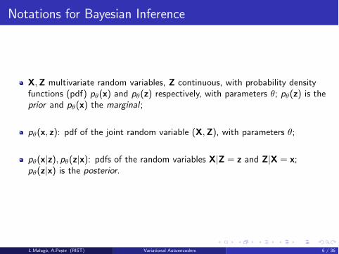
X,Z multivariate random variables, Z continuous, with probability densityfunctions (pdf) p✓(x) and p✓(z) respectively, with parameters ✓; p✓(z) is theprior and p✓(x) the marginal ;
p✓(x, z): pdf of the joint random variable (X,Z), with parameters ✓;
p✓(x|z), p✓(z|x): pdfs of the random variables X|Z = z and Z|X = x;p✓(z|x) is the posterior.
L.Malago, A.Peste (RIST) Variational Autoencoders 6 / 36
General Setting
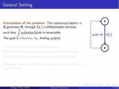
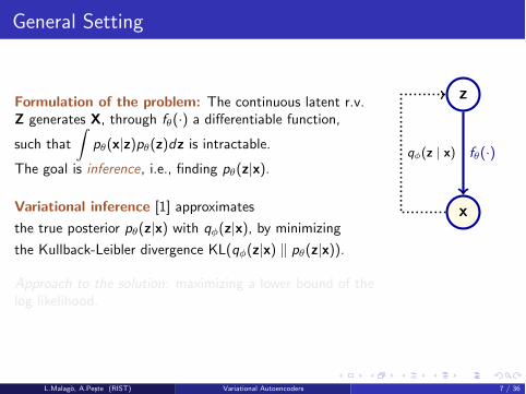
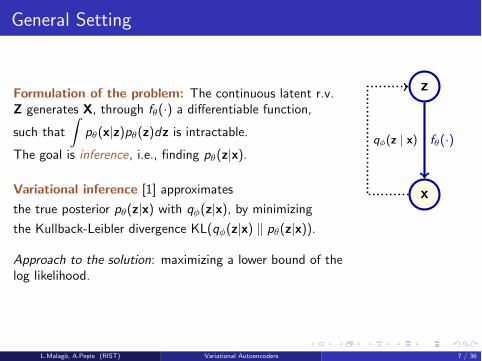
Formulation of the problem: The continuous latent r.v.Z generates X, through f✓(·) a di↵erentiable function,
such that
Zp✓(x|z)p✓(z)dz is intractable.
The goal is inference, i.e., finding p✓(z|x).
z
x
f✓(·)q�(z | x)
Variational inference [1] approximates
the true posterior p✓(z|x) with q�(z|x), by minimizing
the Kullback-Leibler divergence KL(q�(z|x) k p✓(z|x)).
Approach to the solution: maximizing a lower bound of thelog likelihood.
L.Malago, A.Peste (RIST) Variational Autoencoders 7 / 36
General Setting
Formulation of the problem: The continuous latent r.v.Z generates X, through f✓(·) a di↵erentiable function,
such that
Zp✓(x|z)p✓(z)dz is intractable.
The goal is inference, i.e., finding p✓(z|x).
z
x
f✓(·)q�(z | x)
Variational inference [1] approximates
the true posterior p✓(z|x) with q�(z|x), by minimizing
the Kullback-Leibler divergence KL(q�(z|x) k p✓(z|x)).
Approach to the solution: maximizing a lower bound of thelog likelihood.
L.Malago, A.Peste (RIST) Variational Autoencoders 7 / 36
Variational Inference I
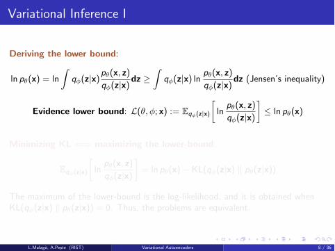
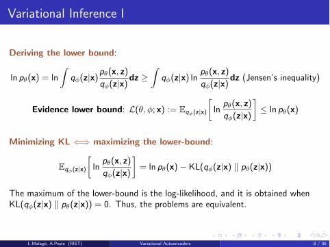
Deriving the lower bound:
ln p✓(x) = ln
Zq�(z|x)
p✓(x, z)
q�(z|x)dz �
Zq�(z|x) ln
p✓(x, z)
q�(z|x)dz (Jensen’s inequality)
Evidence lower bound: L(✓,�; x) := Eq�(z|x)
ln
p✓(x, z)
q�(z|x)
� ln p✓(x)
Minimizing KL () maximizing the lower-bound:
Eq�(z|x)
ln
p✓(x, z)
q�(z|x)
�= ln p✓(x)� KL(q�(z|x) k p✓(z|x))
The maximum of the lower-bound is the log-likelihood, and it is obtained whenKL(q�(z|x) k p✓(z|x)) = 0. Thus, the problems are equivalent.
L.Malago, A.Peste (RIST) Variational Autoencoders 8 / 36
Variational Inference I
Deriving the lower bound:
ln p✓(x) = ln
Zq�(z|x)
p✓(x, z)
q�(z|x)dz �
Zq�(z|x) ln
p✓(x, z)
q�(z|x)dz (Jensen’s inequality)
Evidence lower bound: L(✓,�; x) := Eq�(z|x)
ln
p✓(x, z)
q�(z|x)
� ln p✓(x)
Minimizing KL () maximizing the lower-bound:
Eq�(z|x)
ln
p✓(x, z)
q�(z|x)
�= ln p✓(x)� KL(q�(z|x) k p✓(z|x))
The maximum of the lower-bound is the log-likelihood, and it is obtained whenKL(q�(z|x) k p✓(z|x)) = 0. Thus, the problems are equivalent.
L.Malago, A.Peste (RIST) Variational Autoencoders 8 / 36
Variational Inference II
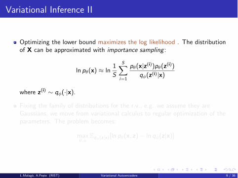
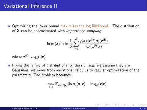
Optimizing the lower bound maximizes the log likelihood . The distributionof X can be approximated with importance sampling :
ln p✓(x) ⇡ ln1
S
SX
i=1
p✓(x|z(i))p✓(z(i))q�(z(i)|x)
where z(i) ⇠ q�(·|x).
Fixing the family of distributions for the r.v., e.g. we assume they areGaussians, we move from variational calculus to regular optimization of theparameters. The problem becomes:
max✓,�
Eq�(z|x)[ln p✓(x, z)� ln q�(z|x)]
L.Malago, A.Peste (RIST) Variational Autoencoders 9 / 36
Variational Inference II
Optimizing the lower bound maximizes the log likelihood . The distributionof X can be approximated with importance sampling :
ln p✓(x) ⇡ ln1
S
SX
i=1
p✓(x|z(i))p✓(z(i))q�(z(i)|x)
where z(i) ⇠ q�(·|x).
Fixing the family of distributions for the r.v., e.g. we assume they areGaussians, we move from variational calculus to regular optimization of theparameters. The problem becomes:
max✓,�
Eq�(z|x)[ln p✓(x, z)� ln q�(z|x)]
L.Malago, A.Peste (RIST) Variational Autoencoders 9 / 36
Variational Autoencoders
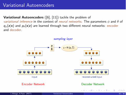
Variational Autoencoders ([6], [11]) tackle the problem ofvariational inference in the context of neural networks. The parameters � and ✓ ofq�(z|x) and p✓(x|z) are learned through two di↵erent neural networks: encoderand decoder.
sampling layer
Encoder Network Decoder Network
L.Malago, A.Peste (RIST) Variational Autoencoders 10 / 36
Applications
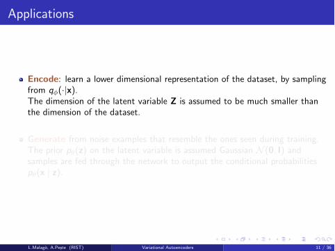
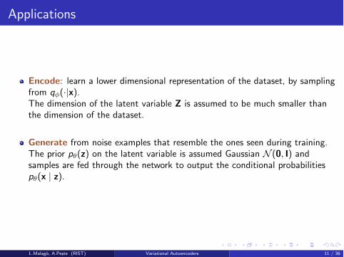
Encode: learn a lower dimensional representation of the dataset, by samplingfrom q�(·|x).The dimension of the latent variable Z is assumed to be much smaller thanthe dimension of the dataset.
Generate from noise examples that resemble the ones seen during training.The prior p✓(z) on the latent variable is assumed Gaussian N (0, I) andsamples are fed through the network to output the conditional probabilitiesp✓(x | z).
L.Malago, A.Peste (RIST) Variational Autoencoders 11 / 36
Applications
Encode: learn a lower dimensional representation of the dataset, by samplingfrom q�(·|x).The dimension of the latent variable Z is assumed to be much smaller thanthe dimension of the dataset.
Generate from noise examples that resemble the ones seen during training.The prior p✓(z) on the latent variable is assumed Gaussian N (0, I) andsamples are fed through the network to output the conditional probabilitiesp✓(x | z).
L.Malago, A.Peste (RIST) Variational Autoencoders 11 / 36
Details of the Algorithm
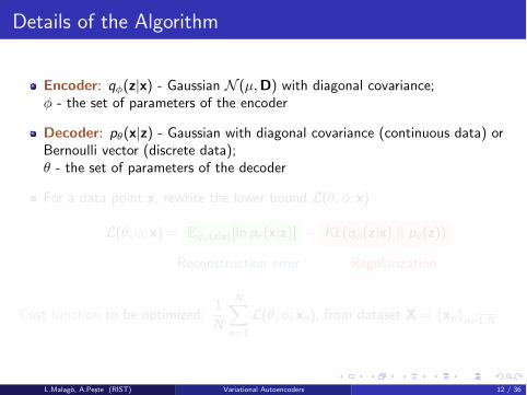
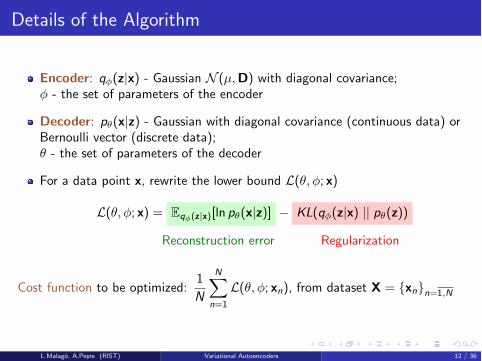
Encoder: q�(z|x) - Gaussian N (µ,D) with diagonal covariance;� - the set of parameters of the encoder
Decoder: p✓(x|z) - Gaussian with diagonal covariance (continuous data) orBernoulli vector (discrete data);✓ - the set of parameters of the decoder
For a data point x, rewrite the lower bound L(✓,�; x)
L(✓,�; x) = Eq�(z|x)[ln p✓(x|z)] � KL(q�(z|x) || p✓(z))
Reconstruction error Regularization
Cost function to be optimized:1
N
NX
n=1
L(✓,�; xn), from dataset X = {xn}n=1,N
L.Malago, A.Peste (RIST) Variational Autoencoders 12 / 36
Details of the Algorithm
Encoder: q�(z|x) - Gaussian N (µ,D) with diagonal covariance;� - the set of parameters of the encoder
Decoder: p✓(x|z) - Gaussian with diagonal covariance (continuous data) orBernoulli vector (discrete data);✓ - the set of parameters of the decoder
For a data point x, rewrite the lower bound L(✓,�; x)
L(✓,�; x) = Eq�(z|x)[ln p✓(x|z)] � KL(q�(z|x) || p✓(z))
Reconstruction error Regularization
Cost function to be optimized:1
N
NX
n=1
L(✓,�; xn), from dataset X = {xn}n=1,N
L.Malago, A.Peste (RIST) Variational Autoencoders 12 / 36
Backpropagating through Stochastic Layers
Training neural networks requires computing the gradient of the costfunction, using backpropagation
Di�culty when computing r�Eq�(z|x)[ln p✓(x|z)] - Monte Carlo estimation ofthe gradient has high variance
The reparameterization trick: find g�(·) di↵erentiable transformation andrandom variable � with pdf p(·), such that Z = g�(� ).
Eq�(z|x)[ln p✓(x|z)] = Ep(�)[ln p✓(x |g�(�))]r�Eq�(z|x)[ln p✓(x|z)] = Ep(�)[r� ln p✓(x |g�(�)]
Example for X ⇠ N(µ,⌃), with ⌃ = LL
T Cholesky decomposition:X = µ+ L� , with � ⇠ N (0, I).
L.Malago, A.Peste (RIST) Variational Autoencoders 13 / 36
Backpropagating through Stochastic Layers
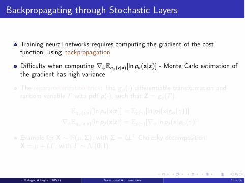
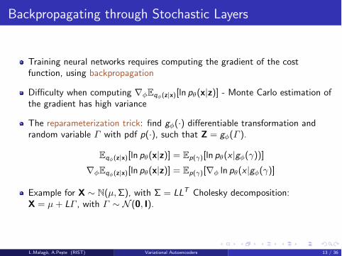
Training neural networks requires computing the gradient of the costfunction, using backpropagation
Di�culty when computing r�Eq�(z|x)[ln p✓(x|z)] - Monte Carlo estimation ofthe gradient has high variance
The reparameterization trick: find g�(·) di↵erentiable transformation andrandom variable � with pdf p(·), such that Z = g�(� ).
Eq�(z|x)[ln p✓(x|z)] = Ep(�)[ln p✓(x |g�(�))]r�Eq�(z|x)[ln p✓(x|z)] = Ep(�)[r� ln p✓(x |g�(�)]
Example for X ⇠ N(µ,⌃), with ⌃ = LL
T Cholesky decomposition:X = µ+ L� , with � ⇠ N (0, I).
L.Malago, A.Peste (RIST) Variational Autoencoders 13 / 36
Limitations and Challenges
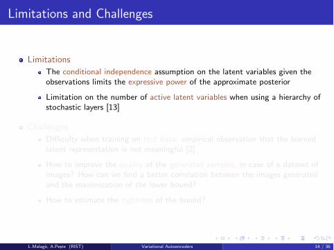
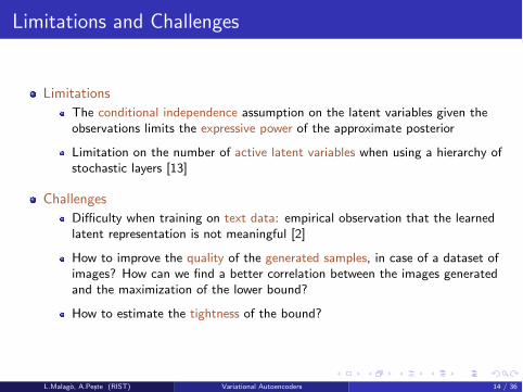
LimitationsThe conditional independence assumption on the latent variables given theobservations limits the expressive power of the approximate posterior
Limitation on the number of active latent variables when using a hierarchy ofstochastic layers [13]
ChallengesDi�culty when training on text data: empirical observation that the learnedlatent representation is not meaningful [2]
How to improve the quality of the generated samples, in case of a dataset ofimages? How can we find a better correlation between the images generatedand the maximization of the lower bound?
How to estimate the tightness of the bound?
L.Malago, A.Peste (RIST) Variational Autoencoders 14 / 36
Limitations and Challenges
LimitationsThe conditional independence assumption on the latent variables given theobservations limits the expressive power of the approximate posterior
Limitation on the number of active latent variables when using a hierarchy ofstochastic layers [13]
ChallengesDi�culty when training on text data: empirical observation that the learnedlatent representation is not meaningful [2]
How to improve the quality of the generated samples, in case of a dataset ofimages? How can we find a better correlation between the images generatedand the maximization of the lower bound?
How to estimate the tightness of the bound?
L.Malago, A.Peste (RIST) Variational Autoencoders 14 / 36
Research Directions
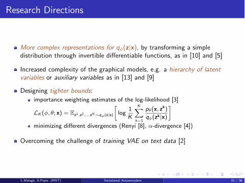
More complex representations for q�(z|x), by transforming a simpledistribution through invertible di↵erentiable functions, as in [10] and [5]
Increased complexity of the graphical models, e.g. a hierarchy of latent
variables or auxiliary variables as in [13] and [9]
Designing tighter bounds:importance weighting estimates of the log-likelihood [3]
LK (�, ✓; x) = Ez1,z2,...zK⇠q�(z|x)
log
1
K
KX
k=1
p✓(x, zk)
q�(zk|x)
�
minimizing di↵erent divergences (Renyi [8], ↵-divergence [4])
Overcoming the challenge of training VAE on text data [2]
L.Malago, A.Peste (RIST) Variational Autoencoders 15 / 36
Research Directions
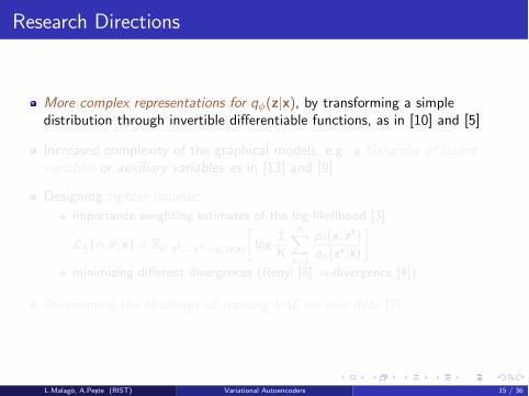
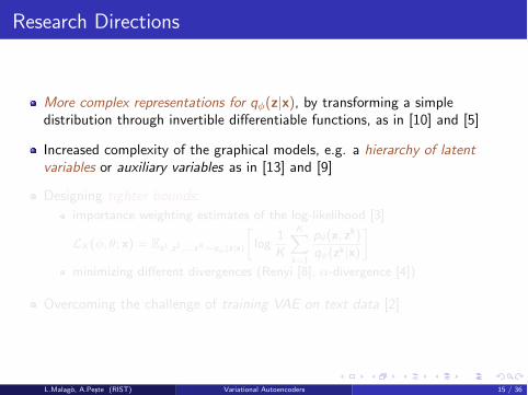
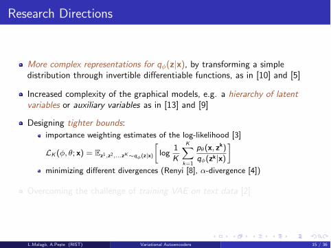
More complex representations for q�(z|x), by transforming a simpledistribution through invertible di↵erentiable functions, as in [10] and [5]
Increased complexity of the graphical models, e.g. a hierarchy of latent
variables or auxiliary variables as in [13] and [9]
Designing tighter bounds:importance weighting estimates of the log-likelihood [3]
LK (�, ✓; x) = Ez1,z2,...zK⇠q�(z|x)
log
1
K
KX
k=1
p✓(x, zk)
q�(zk|x)
�
minimizing di↵erent divergences (Renyi [8], ↵-divergence [4])
Overcoming the challenge of training VAE on text data [2]
L.Malago, A.Peste (RIST) Variational Autoencoders 15 / 36
Outline
1 Plan of the presentation
2 General View of Variational AutoencodersIntroductionResearch Directions
3 Work-in-progressUsing Gaussian Graphical ModelsGeometry of the Latent Space
4 Future Work
L.Malago, A.Peste (RIST) Variational Autoencoders 16 / 36
Gaussian Graphical Models for VAE
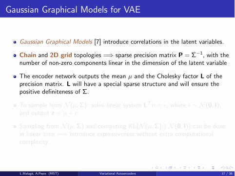
Gaussian Graphical Models [7] introduce correlations in the latent variables.
Chain and 2D grid topologies =) sparse precision matrix P = ⌃�1, with thenumber of non-zero components linear in the dimension of the latent variable
The encoder network outputs the mean µ and the Cholesky factor L of theprecision matrix. L will have a special sparse structure and will ensure thepositive definiteness of ⌃.
To sample from N (µ,⌃): solve linear system LT⌫ = ✏, where ✏ ⇠ N (0, I),and output z = µ+ ⌫.
Sampling from N (µ,⌃) and computing KL(N (µ,⌃) k N (0, I)) can be donein linear time =) introduce expressiveness without extra computationalcomplexity.
L.Malago, A.Peste (RIST) Variational Autoencoders 17 / 36
Gaussian Graphical Models for VAE
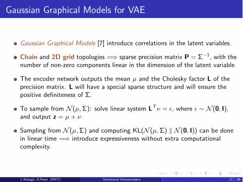
Gaussian Graphical Models [7] introduce correlations in the latent variables.
Chain and 2D grid topologies =) sparse precision matrix P = ⌃�1, with thenumber of non-zero components linear in the dimension of the latent variable
The encoder network outputs the mean µ and the Cholesky factor L of theprecision matrix. L will have a special sparse structure and will ensure thepositive definiteness of ⌃.
To sample from N (µ,⌃): solve linear system LT⌫ = ✏, where ✏ ⇠ N (0, I),and output z = µ+ ⌫.
Sampling from N (µ,⌃) and computing KL(N (µ,⌃) k N (0, I)) can be donein linear time =) introduce expressiveness without extra computationalcomplexity.
L.Malago, A.Peste (RIST) Variational Autoencoders 17 / 36
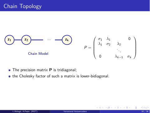
Chain Topology
z1 z2 ... zk
Chain Model
P =
0
BBB@
�1 �1 0�1 �2 �2
. . .0 �k�1 �k
1
CCCA
The precision matrix P is tridiagonal;
the Cholesky factor of such a matrix is lower-bidiagonal.
L.Malago, A.Peste (RIST) Variational Autoencoders 18 / 36
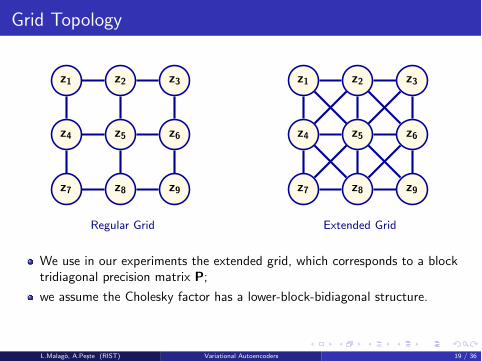
Grid Topology
z1 z2 z3
z4 z5 z6
z7 z8 z9
Regular Grid
z1 z2 z3
z4 z5 z6
z7 z8 z9
Extended Grid
We use in our experiments the extended grid, which corresponds to a blocktridiagonal precision matrix P;
we assume the Cholesky factor has a lower-block-bidiagonal structure.
L.Malago, A.Peste (RIST) Variational Autoencoders 19 / 36
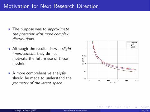
Motivation for Next Research Direction
The purpose was to approximate
the posterior with more complex
distributions.
Although the results show a slight
improvement, they do notmotivate the future use of thesemodels.
A more comprehensive analysisshould be made to understand thegeometry of the latent space.
L.Malago, A.Peste (RIST) Variational Autoencoders 20 / 36
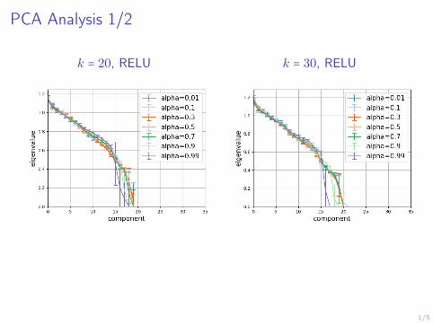
Analysis of the Representations in the Latent Space
Experiments on MNIST dataset to understand the representation of the
images in the learned latent space.
Principal Components Analysis of the latent means will give us insights aboutwhich components are relevant for the representation.
Claim: components with a low variation along the dataset are the ones notmeaningful.
PCA eigenvalues of the posterior samples are very close to 1 =) the KLminimization forces some components to be N (0, I).
L.Malago, A.Peste (RIST) Variational Autoencoders 21 / 36
1/5
PCA Analysis 1/2
k = 20, RELU k = 30, RELU
2/5
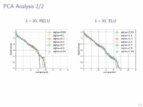
PCA Analysis 2/2
k = 30, RELU k = 30, ELU
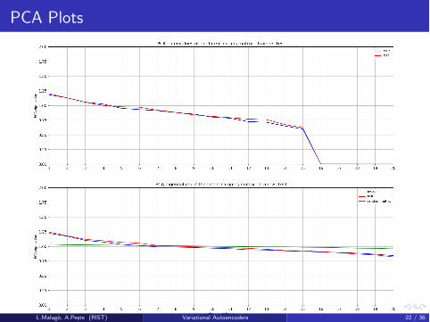
PCA Plots
L.Malago, A.Peste (RIST) Variational Autoencoders 22 / 36
Interpretation of the Plot
When training a VAE with latent size 20 on MNIST, only around 15 of thelatent variables are relevant for the representation.
The number remains constant when training with a larger latent size.
This is a consequence of the KL regularization term in the cost function,which forces some components to be Gaussian noise.
Is this number a particularity of the dataset?
What is the impact on this number when using more complicated networkarchitectures?
Would we observe the same behavior with other bounds derived fromdi↵erent divergences (e.g. Renyi)?
L.Malago, A.Peste (RIST) Variational Autoencoders 23 / 36
Correlations Plot
L.Malago, A.Peste (RIST) Variational Autoencoders 24 / 36
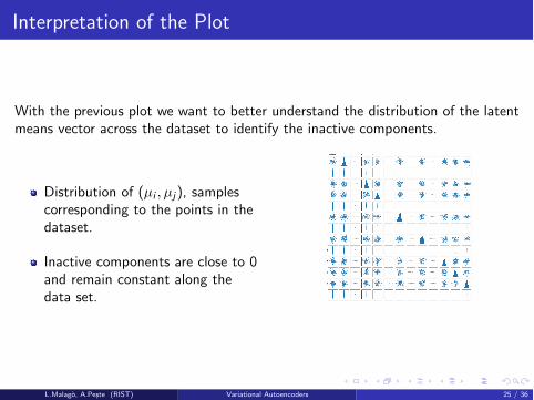
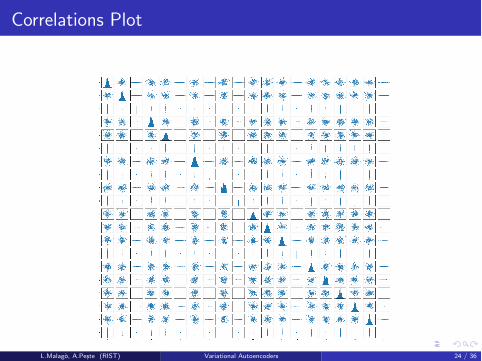
Interpretation of the Plot
With the previous plot we want to better understand the distribution of the latentmeans vector across the dataset to identify the inactive components.
Distribution of (µi , µj), samplescorresponding to the points in thedataset.
Inactive components are close to 0and remain constant along thedata set.
L.Malago, A.Peste (RIST) Variational Autoencoders 25 / 36
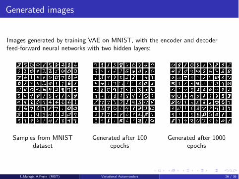
Generated images
Images generated by training VAE on MNIST, with the encoder and decoderfeed-forward neural networks with two hidden layers:
Samples from MNISTdataset
Generated after 100epochs
Generated after 1000epochs
L.Malago, A.Peste (RIST) Variational Autoencoders 26 / 36
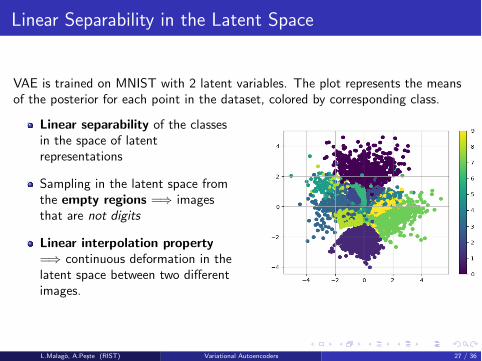
Linear Separability in the Latent Space
VAE is trained on MNIST with 2 latent variables. The plot represents the meansof the posterior for each point in the dataset, colored by corresponding class.
Linear separability of the classesin the space of latentrepresentations
Sampling in the latent space fromthe empty regions =) imagesthat are not digits
Linear interpolation property=) continuous deformation in thelatent space between two di↵erentimages.
L.Malago, A.Peste (RIST) Variational Autoencoders 27 / 36
4/5
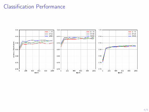
Classification Performance
Outline
1 Plan of the presentation
2 General View of Variational AutoencodersIntroductionResearch Directions
3 Work-in-progressUsing Gaussian Graphical ModelsGeometry of the Latent Space
4 Future Work
L.Malago, A.Peste (RIST) Variational Autoencoders 28 / 36
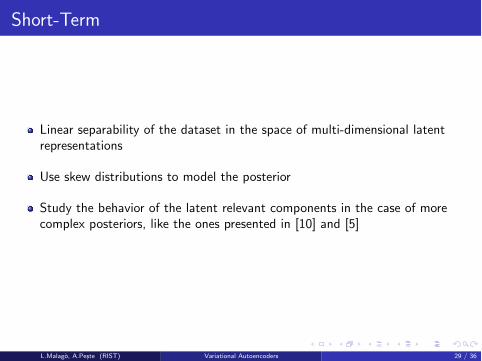
Short-Term
Linear separability of the dataset in the space of multi-dimensional latentrepresentations
Use skew distributions to model the posterior
Study the behavior of the latent relevant components in the case of morecomplex posteriors, like the ones presented in [10] and [5]
L.Malago, A.Peste (RIST) Variational Autoencoders 29 / 36
Medium-Term
Bounds derived from di↵erent divergences (e.g. Renyi, ↵-divergence)impact of the ↵ parameter on the tightness of the boundsrelevant components in the latent space and see how their number changes
Geometric methods for training VAEthe use of natural gradientstudy the geometry of the latent spaceuse Riemannian optimization methods that exploit some properties of thespace of the latent variables
Extend the study to di↵erent types of generative models, e.g. GenerativeAdversarial Networks (GANs), Restricted Boltzmann Machines (RBMs).
L.Malago, A.Peste (RIST) Variational Autoencoders 30 / 36
References I
[1] David M Blei, Alp Kucukelbir, and Jon D McAuli↵e.Variational inference: A review for statisticians.Journal of the American Statistical Association, 2017.
[2] Samuel R Bowman, Luke Vilnis, Oriol Vinyals, Andrew M Dai, RafalJozefowicz, and Samy Bengio.Generating sentences from a continuous space.arXiv preprint arXiv:1511.06349, 2015.
[3] Yuri Burda, Roger Grosse, and Ruslan Salakhutdinov.Importance weighted autoencoders.arXiv preprint arXiv:1509.00519, 2015.
[4] Jose Miguel Hernandez-Lobato, Yingzhen Li, Mark Rowland, DanielHernandez-Lobato, Thang D Bui, and Richard E Turner.Black-box ↵-divergence minimization.2016.
L.Malago, A.Peste (RIST) Variational Autoencoders 31 / 36
References II
[5] Diederik P Kingma, Tim Salimans, Rafal Jozefowicz, Xi Chen, Ilya Sutskever,and Max Welling.Improving variational autoencoders with inverse autoregressive flow.In Advances In Neural Information Processing Systems, pages 4736–4744,2016.
[6] Diederik P Kingma and Max Welling.Auto-encoding variational bayes.2013.
[7] Ste↵en L Lauritzen.Graphical models, volume 17.Clarendon Press, 1996.
[8] Yingzhen Li and Richard E Turner.Renyi divergence variational inference.In Advances in Neural Information Processing Systems, pages 1073–1081,2016.
L.Malago, A.Peste (RIST) Variational Autoencoders 32 / 36
References III
[9] Lars Maaløe, Casper Kaae Sønderby, Søren Kaae Sønderby, and Ole Winther.Auxiliary deep generative models.arXiv preprint arXiv:1602.05473, 2016.
[10] Danilo Jimenez Rezende and Shakir Mohamed.Variational inference with normalizing flows.arXiv preprint arXiv:1505.05770, 2015.
[11] Danilo Jimenez Rezende, Shakir Mohamed, and Daan Wierstra.Stochastic backpropagation and approximate inference in deep generativemodels.2014.
[12] Tim Salimans, Ian Goodfellow, Wojciech Zaremba, Vicki Cheung, AlecRadford, and Xi Chen.Improved techniques for training gans.In Advances in Neural Information Processing Systems, pages 2234–2242,2016.
L.Malago, A.Peste (RIST) Variational Autoencoders 33 / 36
References IV
[13] Casper Kaae Sønderby, Tapani Raiko, Lars Maaløe, Søren Kaae Sønderby,and Ole Winther.Ladder variational autoencoders.In D. D. Lee, M. Sugiyama, U. V. Luxburg, I. Guyon, and R. Garnett, editors,Advances in Neural Information Processing Systems 29, pages 3738–3746.Curran Associates, Inc., 2016.
L.Malago, A.Peste (RIST) Variational Autoencoders 34 / 36

Questions?
L.Malago, A.Peste (RIST) Variational Autoencoders 35 / 36
5/5
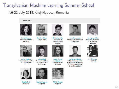
Transylvanian Machine Learning Summer School
16-22 July 2018, Cluj-Napoca, Romania

5/5
Transylvanian Machine Learning Summer School
16-22 July 2018, Cluj-Napoca, Romania
Registration Deadline: 30 March 2018
More details at www.tmlss.ro
Thank You!
L.Malago, A.Peste (RIST) Variational Autoencoders 36 / 36