Embed Size (px)
Citation preview
Kay H. Brodersen
Translational Neuromodeling Unit (TNU) Institute of Biomedical Engineering
University of Zurich & ETH Zurich
Variational Bayesian inference
HOMO VARIATIONIS
≈
Illu
stra
tio
n a
dap
ted
fro
m:
Mik
e W
est
Variational Bayesian inference
“An approximate answer to the right problem is worth a good deal more than
an exact answer to an approximate problem.”
John W. Tukey, 1915 – 2000
3
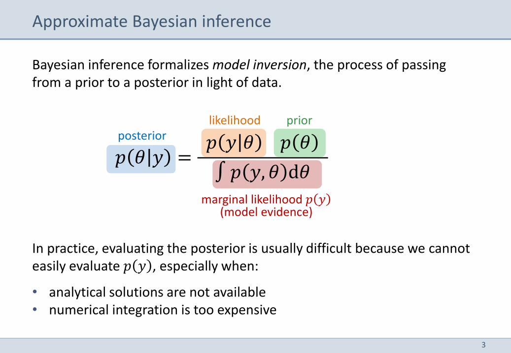
marginal likelihood 𝑝 𝑦 (model evidence)
prior likelihood posterior
Bayesian inference formalizes model inversion, the process of passing from a prior to a posterior in light of data.
Approximate Bayesian inference
In practice, evaluating the posterior is usually difficult because we cannot easily evaluate 𝑝 𝑦 , especially when:
• analytical solutions are not available • numerical integration is too expensive
𝑝 𝜃 𝑦 = 𝑝 𝑦 𝜃 𝑝 𝜃
∫ 𝑝 𝑦, 𝜃 d𝜃
4
Approximate Bayesian inference
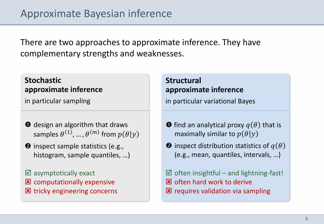
There are two approaches to approximate inference. They have complementary strengths and weaknesses.
5
Approximate Bayesian inference
Stochastic approximate inference
in particular sampling
design an algorithm that draws
samples 𝜃 1 , … , 𝜃 𝑚 from 𝑝 𝜃 𝑦
inspect sample statistics (e.g., histogram, sample quantiles, …)
Structural approximate inference
in particular variational Bayes
find an analytical proxy 𝑞 𝜃 that is maximally similar to 𝑝 𝜃 𝑦
inspect distribution statistics of 𝑞 𝜃 (e.g., mean, quantiles, intervals, …)
There are two approaches to approximate inference. They have complementary strengths and weaknesses.
asymptotically exact computationally expensive tricky engineering concerns
often insightful – and lightning-fast! often hard work to derive requires validation via sampling
6
Overview
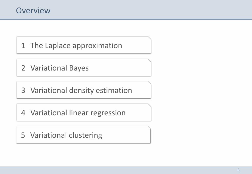
1 The Laplace approximation
2 Variational Bayes
3 Variational density estimation
4 Variational linear regression
5 Variational clustering
7
Overview
1 The Laplace approximation
2 Variational Bayes
3 Variational density estimation
4 Variational linear regression
5 Variational clustering
8
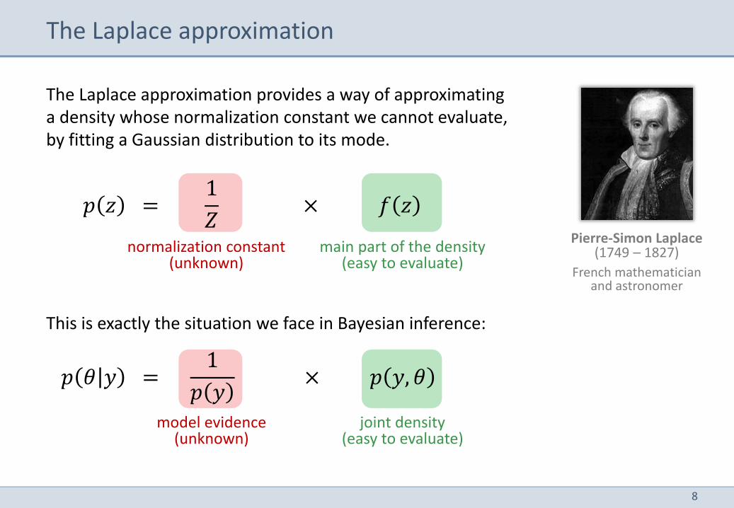
The Laplace approximation provides a way of approximating a density whose normalization constant we cannot evaluate, by fitting a Gaussian distribution to its mode.
The Laplace approximation
normalization constant (unknown)
main part of the density (easy to evaluate)
Pierre-Simon Laplace (1749 – 1827)
French mathematician and astronomer
This is exactly the situation we face in Bayesian inference:
𝑝 𝑧 = 1
𝑍 × 𝑓 𝑧
𝑝 𝜃 𝑦 = 1
𝑝 𝑦 × 𝑝 𝑦, 𝜃
model evidence (unknown)
joint density (easy to evaluate)
9
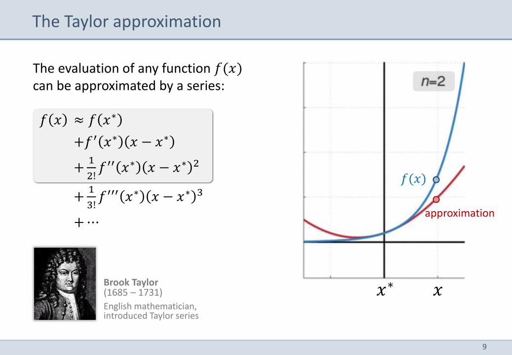
The evaluation of any function 𝑓(𝑥) can be approximated by a series:
The Taylor approximation
𝑥∗ 𝑥
approximation
𝑓(𝑥)
Brook Taylor (1685 – 1731)
English mathematician, introduced Taylor series
𝑓 𝑥 ≈ 𝑓 𝑥∗
+𝑓′ 𝑥∗ 𝑥 − 𝑥∗
+1
2!𝑓′′ 𝑥∗ 𝑥 − 𝑥∗ 2
+1
3!𝑓′′′ 𝑥∗ 𝑥 − 𝑥∗ 3
+ ⋯
10
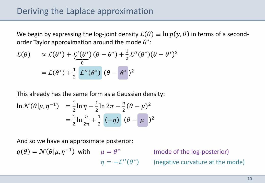
We begin by expressing the log-joint density ℒ 𝜃 ≡ ln 𝑝 𝑦, 𝜃 in terms of a second-order Taylor approximation around the mode 𝜃∗:
ℒ 𝜃 ≈ ℒ 𝜃∗ + ℒ′ 𝜃∗
0
𝜃 − 𝜃∗ +1
2ℒ′′ 𝜃∗ 𝜃 − 𝜃∗ 2
= ℒ 𝜃∗ +1
2 ℒ′′ 𝜃∗ 𝜃 − 𝜃∗ 2
This already has the same form as a Gaussian density:
ln 𝒩 𝜃 𝜇, 𝜂−1 =1
2ln 𝜂 −
1
2ln 2𝜋 −
𝜂
2𝜃 − 𝜇 2
=1
2ln
𝜂
2𝜋+
1
2 −𝜂 𝜃 − 𝜇 2
And so we have an approximate posterior:
𝑞 𝜃 = 𝒩 𝜃 𝜇, 𝜂−1 with 𝜇 = 𝜃∗ (mode of the log-posterior)
𝜂 = −ℒ′′ 𝜃∗ (negative curvature at the mode)
Deriving the Laplace approximation

11
Given a model with parameters 𝜃 = 𝜃1, … , 𝜃𝑝 , the Laplace approximation
reduces to a simple three-step procedure:
Applying the Laplace approximation
Find the mode of the log-joint:
𝜃∗ = arg max𝜃
ln 𝑝 𝑦, 𝜃
Evaluate the curvature of the log-joint at the mode:
∇∇ ln 𝑝 𝑦, 𝜃∗
We obtain a Gaussian approximation: 𝒩 𝜃 𝜇, Λ−1 with 𝜇 = 𝜃∗ Λ = −∇∇ ln 𝑝 𝑦, 𝜃∗
12
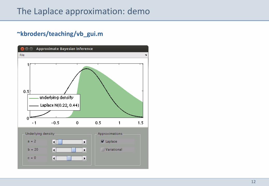
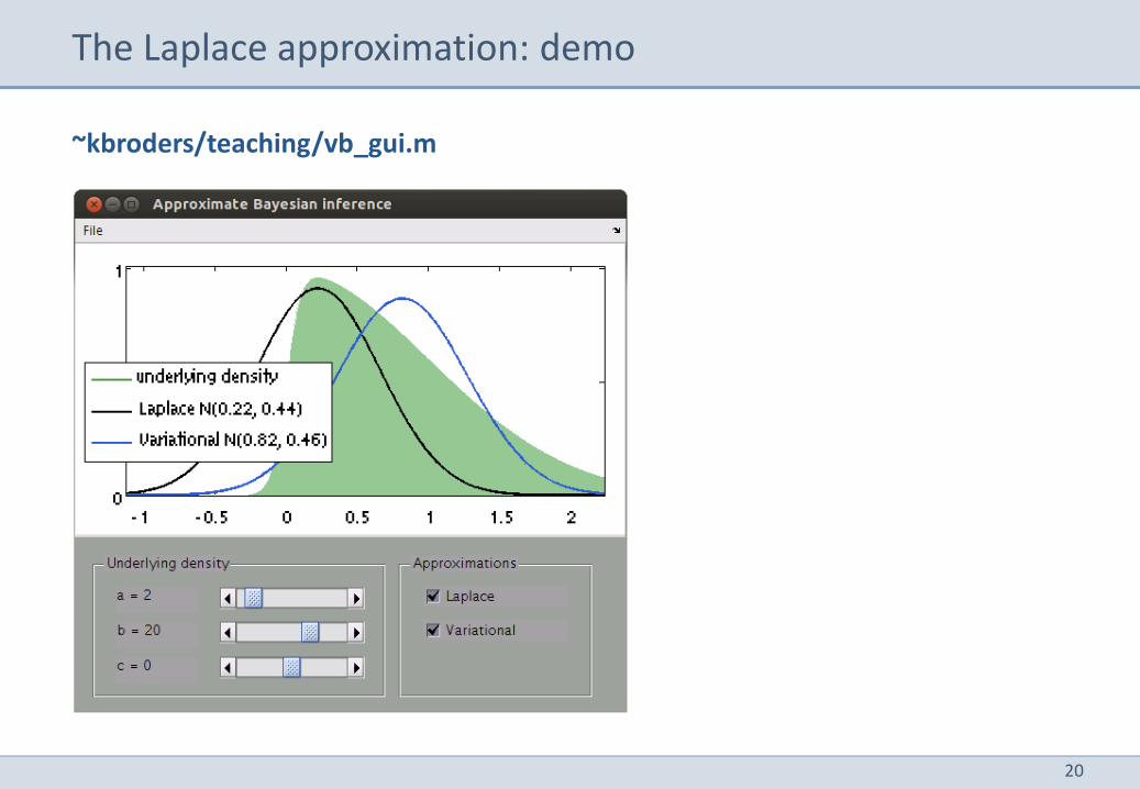
The Laplace approximation: demo
~kbroders/teaching/vb_gui.m
13
-10 0 10 200
0.05
0.1
0.15
0.2
0.25
The Laplace approximation
-10 0 10 200
0.05
0.1
0.15
0.2
0.25
The Laplace approximation
log joint
approximation
-10 0 10 200
0.05
0.1
0.15
0.2
0.25
The Laplace approximation
-10 0 10 200
0.05
0.1
0.15
0.2
0.25
The Laplace approximation
log joint
approximation
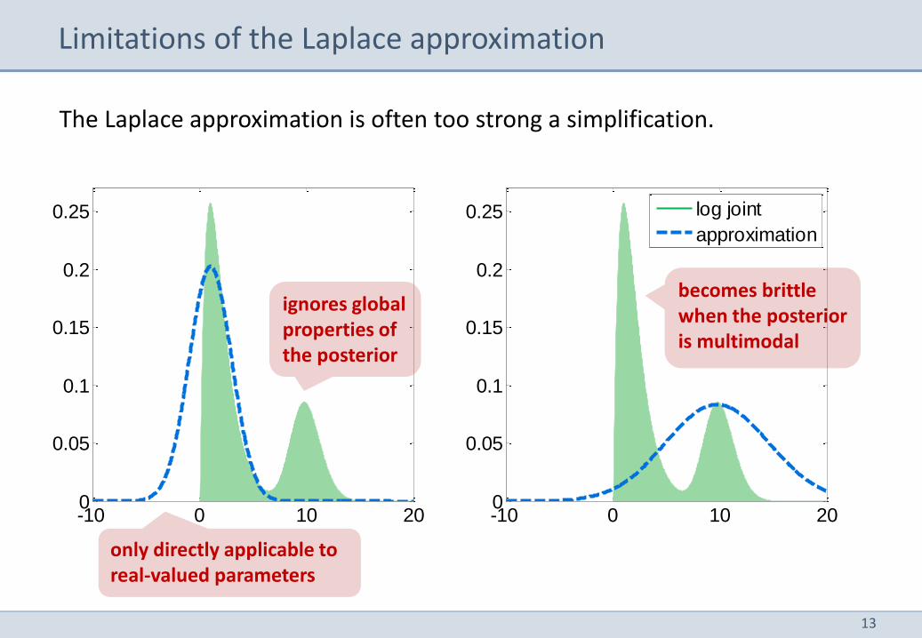
Limitations of the Laplace approximation
ignores global properties of the posterior
becomes brittle when the posterior is multimodal
only directly applicable to real-valued parameters
The Laplace approximation is often too strong a simplification.
14
Overview
1 The Laplace approximation
2 Variational Bayes
3 Variational density estimation
4 Variational linear regression
5 Variational clustering
15
best proxy 𝑞 𝜃
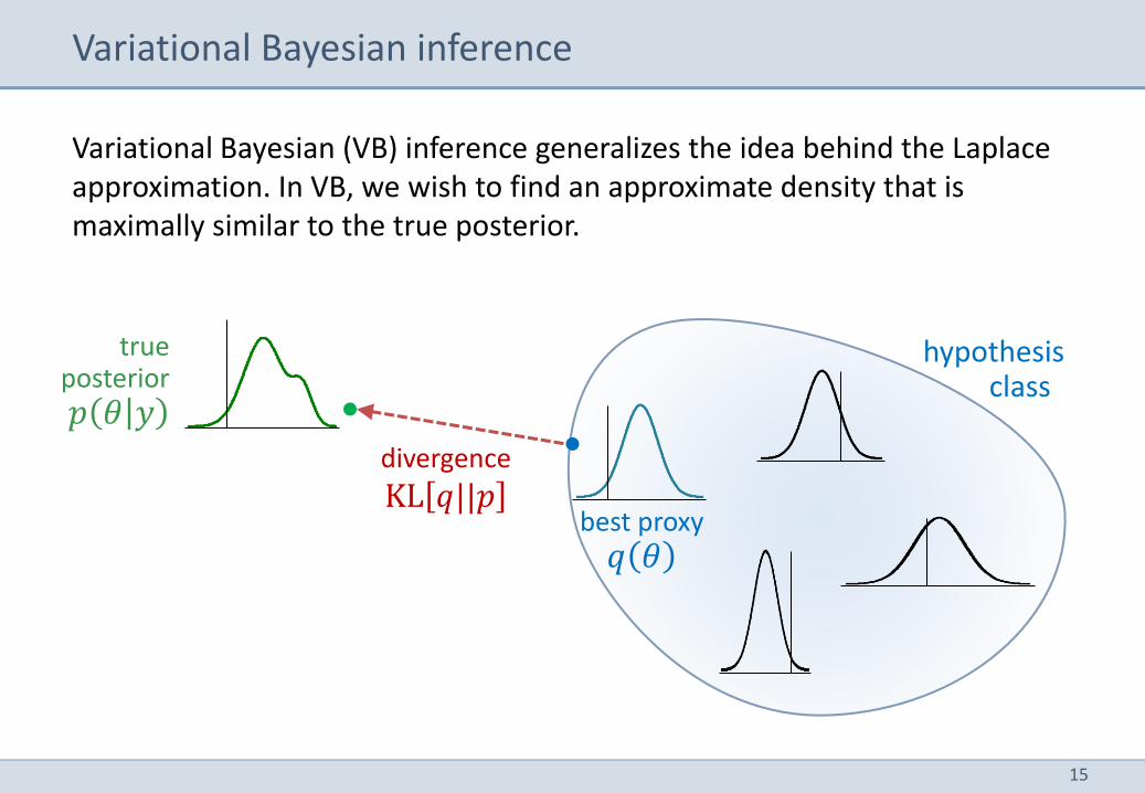
Variational Bayesian inference
true posterior 𝑝 𝜃 𝑦
hypothesis class
divergence
KL 𝑞||𝑝
Variational Bayesian (VB) inference generalizes the idea behind the Laplace approximation. In VB, we wish to find an approximate density that is maximally similar to the true posterior.
16
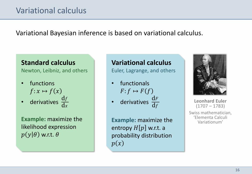
Variational Bayesian inference is based on variational calculus.
Variational calculus
Standard calculus Newton, Leibniz, and others
• functions 𝑓: 𝑥 ↦ 𝑓 𝑥
• derivatives d𝑓
d𝑥
Example: maximize the likelihood expression 𝑝 𝑦 𝜃 w.r.t. 𝜃
Variational calculus Euler, Lagrange, and others
• functionals 𝐹: 𝑓 ↦ 𝐹 𝑓
• derivatives d𝐹
d𝑓
Example: maximize the entropy 𝐻 𝑝 w.r.t. a probability distribution 𝑝 𝑥
Leonhard Euler (1707 – 1783)
Swiss mathematician, ‘Elementa Calculi
Variationum’
17
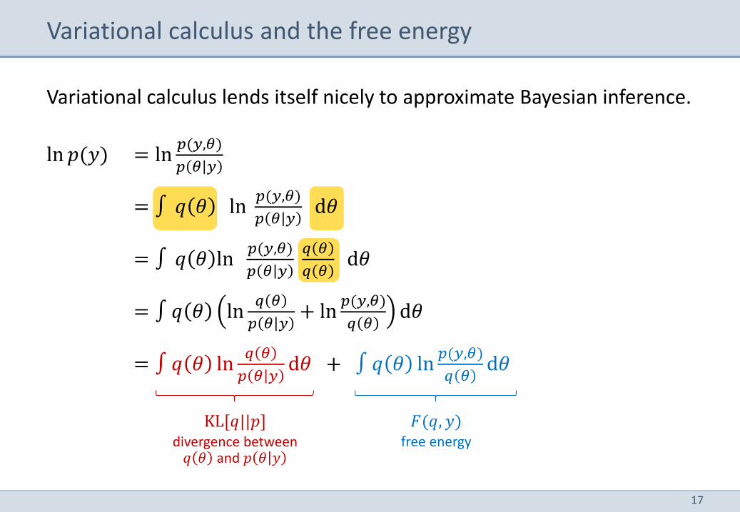
Variational calculus lends itself nicely to approximate Bayesian inference.
Variational calculus and the free energy
ln 𝑝(𝑦) = ln𝑝(𝑦,𝜃)
𝑝 𝜃 𝑦
= ∫ 𝑞 𝜃 ln 𝑝(𝑦,𝜃)
𝑝 𝜃 𝑦 d𝜃
= ∫ 𝑞 𝜃 ln 𝑝(𝑦,𝜃)
𝑝 𝜃 𝑦 𝑞 𝜃
𝑞 𝜃 d𝜃
= ∫ 𝑞 𝜃 ln𝑞 𝜃
𝑝 𝜃 𝑦+ ln
𝑝(𝑦,𝜃)
𝑞 𝜃d𝜃
= ∫ 𝑞 𝜃 ln𝑞 𝜃
𝑝 𝜃 𝑦d𝜃 + ∫ 𝑞 𝜃 ln
𝑝(𝑦,𝜃)
𝑞 𝜃d𝜃
KL[𝑞||𝑝] divergence between
𝑞 𝜃 and 𝑝 𝜃 𝑦
𝐹(𝑞, 𝑦) free energy
18
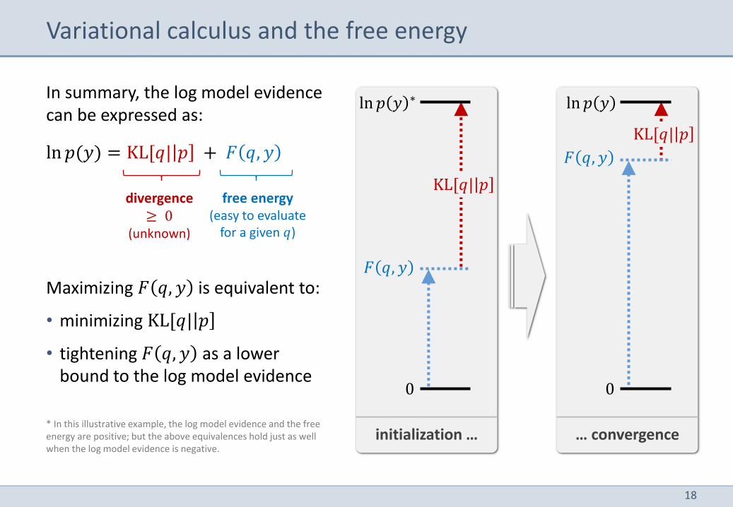
Variational calculus and the free energy
Maximizing 𝐹 𝑞, 𝑦 is equivalent to:
• minimizing KL[𝑞| 𝑝
• tightening 𝐹 𝑞, 𝑦 as a lower bound to the log model evidence
* In this illustrative example, the log model evidence and the free energy are positive; but the above equivalences hold just as well when the log model evidence is negative.
In summary, the log model evidence can be expressed as:
ln 𝑝(𝑦) = KL[𝑞| 𝑝 + 𝐹 𝑞, 𝑦
divergence ≥ 0
(unknown)
free energy (easy to evaluate
for a given 𝑞)
KL[𝑞| 𝑝
ln 𝑝 𝑦 ∗
𝐹 𝑞, 𝑦
0
KL[𝑞| 𝑝
ln 𝑝 𝑦
𝐹 𝑞, 𝑦
0
initialization … … convergence
19
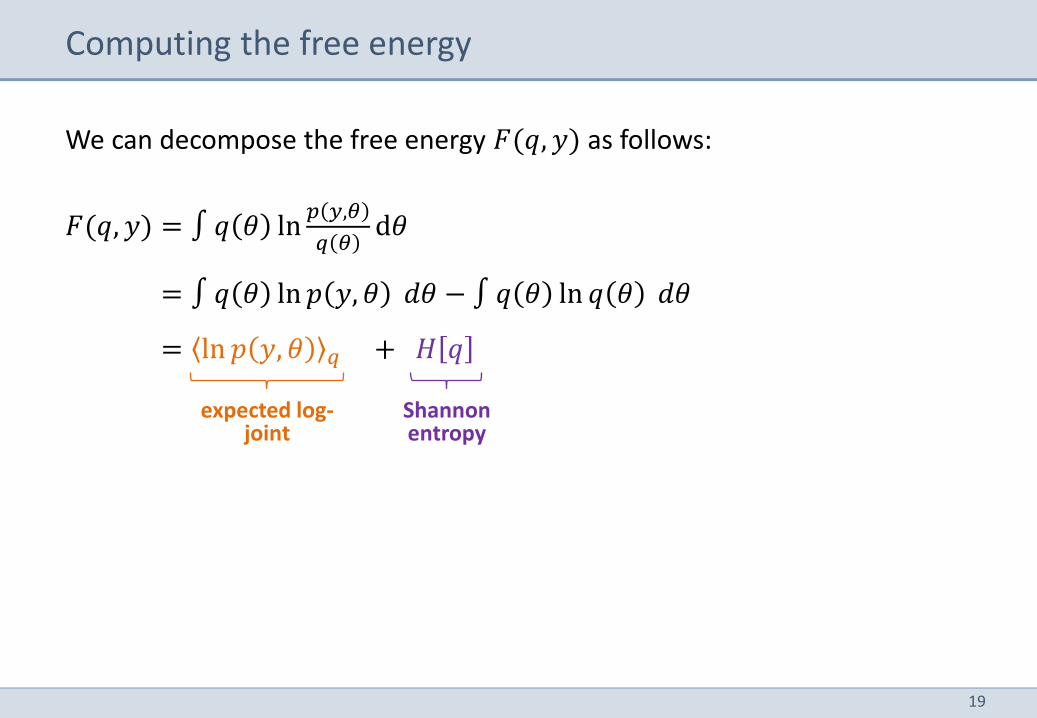
Computing the free energy
We can decompose the free energy 𝐹(𝑞, 𝑦) as follows:
𝐹(𝑞, 𝑦) = ∫ 𝑞 𝜃 ln𝑝 𝑦,𝜃
𝑞 𝜃d𝜃
= ∫ 𝑞 𝜃 ln 𝑝 𝑦, 𝜃 𝑑𝜃 − ∫ 𝑞 𝜃 ln 𝑞 𝜃 𝑑𝜃
= ln 𝑝 𝑦, 𝜃 𝑞 + 𝐻 𝑞
expected log-joint
Shannon entropy
20
The Laplace approximation: demo
~kbroders/teaching/vb_gui.m
21
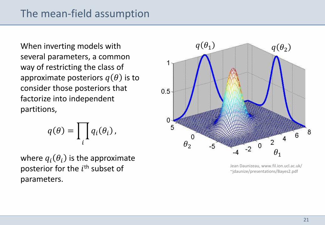
When inverting models with several parameters, a common way of restricting the class of approximate posteriors 𝑞 𝜃 is to consider those posteriors that factorize into independent partitions,
𝑞 𝜃 = 𝑞𝑖 𝜃𝑖
𝑖
,
where 𝑞𝑖 𝜃𝑖 is the approximate posterior for the 𝑖th subset of parameters.
The mean-field assumption
𝜃1 𝜃2
𝑞 𝜃1 𝑞 𝜃2
Jean Daunizeau, www.fil.ion.ucl.ac.uk/ ~jdaunize/presentations/Bayes2.pdf
22
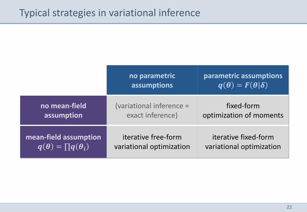
Typical strategies in variational inference
no parametric assumptions
parametric assumptions 𝒒 𝜽 = 𝑭 𝜽 𝜹
no mean-field assumption
(variational inference = exact inference)
fixed-form optimization of moments
mean-field assumption 𝒒 𝜽 = ∏𝒒 𝜽𝒊
iterative free-form variational optimization
iterative fixed-form variational optimization
23
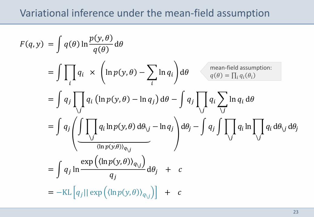
= 𝑞 𝜃 ln𝑝 𝑦, 𝜃
𝑞 𝜃d𝜃
= 𝑞𝑖 × ln 𝑝 𝑦, 𝜃 − ln 𝑞𝑖
𝑖𝑖
d𝜃
= 𝑞𝑗 𝑞𝑖 ln 𝑝 𝑦, 𝜃 − ln 𝑞𝑗
\𝑗
d𝜃 − 𝑞𝑗 𝑞𝑖 ln 𝑞𝑖
\𝑗\𝑗
d𝜃
= 𝑞𝑗 𝑞𝑖 ln𝑝 𝑦,𝜃
\𝑗
d𝜃\𝑗
ln 𝑝 𝑦,𝜃 𝑞\𝑗
− ln𝑞𝑗 d𝜃𝑗 − 𝑞𝑗 𝑞𝑖
\𝑗
ln 𝑞𝑖
\𝑗
d𝜃\𝑗 d𝜃𝑗
= 𝑞𝑗 lnexp ln𝑝 𝑦,𝜃 𝑞\𝑗
𝑞𝑗d𝜃𝑗 + 𝑐
= −KL 𝑞𝑗|| exp ln𝑝 𝑦,𝜃 𝑞\𝑗 + 𝑐
Variational inference under the mean-field assumption
𝐹 𝑞, 𝑦
mean-field assumption: 𝑞 𝜃 = ∏ 𝑞𝑖 𝜃𝑖𝑖
24
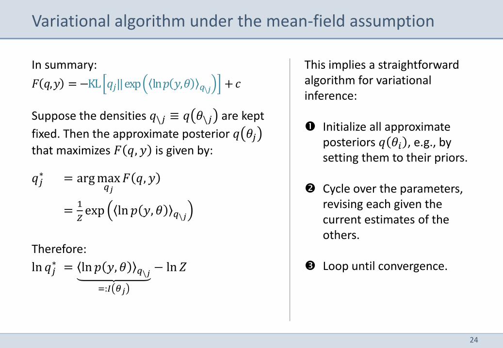
In summary:
𝐹 𝑞,𝑦 = −KL 𝑞𝑗||exp ln𝑝 𝑦,𝜃 𝑞\𝑗+𝑐
Suppose the densities 𝑞\𝑗 ≡ 𝑞 𝜃\𝑗 are kept
fixed. Then the approximate posterior 𝑞 𝜃𝑗
that maximizes 𝐹 𝑞, 𝑦 is given by:
𝑞𝑗∗ = arg max
𝑞𝑗
𝐹 𝑞, 𝑦
=1
𝑍exp ln 𝑝 𝑦, 𝜃 𝑞\𝑗
Therefore:
ln 𝑞𝑗∗ = ln 𝑝 𝑦, 𝜃 𝑞\𝑗
=:𝐼 𝜃𝑗
− ln 𝑍
Variational algorithm under the mean-field assumption
This implies a straightforward algorithm for variational inference: Initialize all approximate
posteriors 𝑞 𝜃𝑖 , e.g., by setting them to their priors.
Cycle over the parameters,
revising each given the current estimates of the others.
Loop until convergence.
25
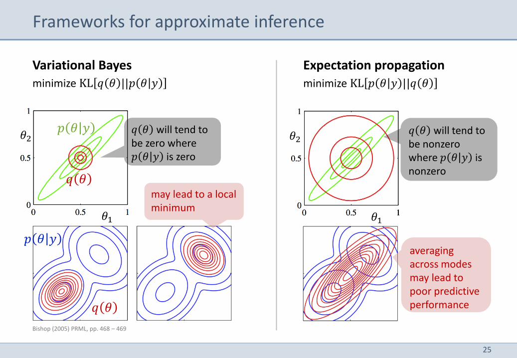
Frameworks for approximate inference
Variational Bayes
minimize KL 𝑞 𝜃 ||𝑝 𝜃 𝑦
Expectation propagation
minimize KL 𝑝 𝜃 𝑦 ||𝑞 𝜃
𝜃1
𝜃2
𝜃1
𝜃2
𝑞 𝜃
𝑝 𝜃 𝑦 𝑞 𝜃 will tend to be zero where 𝑝 𝜃 𝑦 is zero
may lead to a local minimum
𝑞 𝜃
𝑝 𝜃 𝑦 averaging across modes may lead to poor predictive performance
𝑞 𝜃 will tend to be nonzero where 𝑝 𝜃 𝑦 is nonzero
Bishop (2005) PRML, pp. 468 – 469
26
Overview
1 The Laplace approximation
2 Variational Bayes
3 Variational density estimation
4 Variational linear regression
5 Variational clustering
27
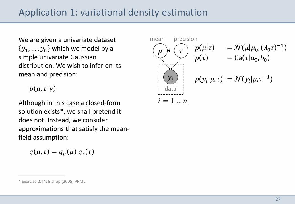
We are given a univariate dataset 𝑦1, … , 𝑦𝑛 which we model by a
simple univariate Gaussian distribution. We wish to infer on its mean and precision:
𝑝 𝜇, 𝜏 𝑦
Although in this case a closed-form solution exists*, we shall pretend it does not. Instead, we consider approximations that satisfy the mean-field assumption:
𝑞 𝜇, 𝜏 = 𝑞𝜇 𝜇 𝑞𝜏 𝜏
Application 1: variational density estimation
𝜇
𝑦𝑖
𝜏 𝑝 𝜇 𝜏 = 𝒩 𝜇 𝜇0, 𝜆0𝜏 −1
𝑝 𝜏 = Ga 𝜏 𝑎0, 𝑏0
𝑝 𝑦𝑖 𝜇,𝜏 = 𝒩 𝑦𝑖 𝜇,𝜏−1
𝑖 = 1 … 𝑛
mean precision
data
* Exercise 2.44; Bishop (2005) PRML
28
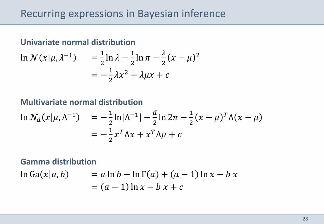
Univariate normal distribution
ln 𝒩 𝑥 𝜇, 𝜆−1 =1
2ln 𝜆 −
1
2ln 𝜋 −
𝜆
2𝑥 − 𝜇 2
= −1
2𝜆𝑥2 + 𝜆𝜇𝑥 + 𝑐
Multivariate normal distribution
ln 𝒩𝑑 𝑥 𝜇, Λ−1 = −1
2ln Λ−1 −
𝑑
2ln 2𝜋 −
1
2𝑥 − 𝜇 𝑇Λ 𝑥 − 𝜇
= −1
2𝑥𝑇Λ𝑥 + 𝑥𝑇Λ𝜇 + 𝑐
Gamma distribution
ln Ga 𝑥 𝑎, 𝑏 = 𝑎 ln 𝑏 − ln Γ 𝑎 + 𝑎 − 1 ln 𝑥 − 𝑏 𝑥
= 𝑎 − 1 ln 𝑥 − 𝑏 𝑥 + 𝑐
Recurring expressions in Bayesian inference
29
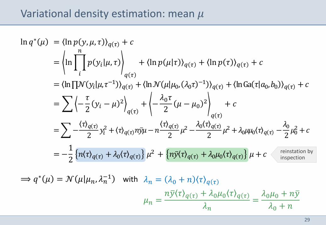
𝜆𝑛 = 𝜆0 + 𝑛 𝜏 𝑞 𝜏
Variational density estimation: mean 𝜇
= ln 𝑝 𝑦, 𝜇, 𝜏 𝑞 𝜏 + 𝑐
= ln 𝑝 𝑦𝑖 𝜇, 𝜏
𝑛
𝑖 𝑞 𝜏
+ ln 𝑝 𝜇 𝜏 𝑞 𝜏 + ln 𝑝 𝜏 𝑞 𝜏 + 𝑐
= ln∏𝒩 𝑦𝑖 𝜇,𝜏−1𝑞 𝜏 + ln𝒩 𝜇 𝜇0, 𝜆0𝜏
−1𝑞 𝜏 + lnGa 𝜏 𝑎0,𝑏0 𝑞 𝜏 + 𝑐
= −𝜏
2𝑦𝑖 − 𝜇 2
𝑞 𝜏+ −
𝜆0𝜏
2𝜇 − 𝜇0
2
𝑞 𝜏
+ 𝑐
= −𝜏 𝑞 𝜏
2𝑦𝑖
2 + 𝜏 𝑞 𝜏 𝑛𝑦 𝜇−𝑛𝜏 𝑞 𝜏
2𝜇2 −
𝜆0 𝜏 𝑞 𝜏
2𝜇2 +𝜆0𝜇𝜇0 𝜏 𝑞 𝜏 −
𝜆0
2𝜇0
2 +𝑐
= −1
2 𝑛 𝜏 𝑞 𝜏 + 𝜆0 𝜏 𝑞 𝜏 𝜇2 + 𝑛𝑦 𝜏 𝑞 𝜏 +𝜆0𝜇0 𝜏 𝑞 𝜏 𝜇 + 𝑐
ln 𝑞∗ 𝜇
𝜇𝑛 =𝑛𝑦 𝜏 𝑞 𝜏 + 𝜆0𝜇0 𝜏 𝑞 𝜏
𝜆𝑛=
𝜆0𝜇0 + 𝑛𝑦
𝜆0 + 𝑛
reinstation by inspection
⟹ 𝑞∗ 𝜇 = 𝒩 𝜇 𝜇𝑛, 𝜆𝑛−1 with
30
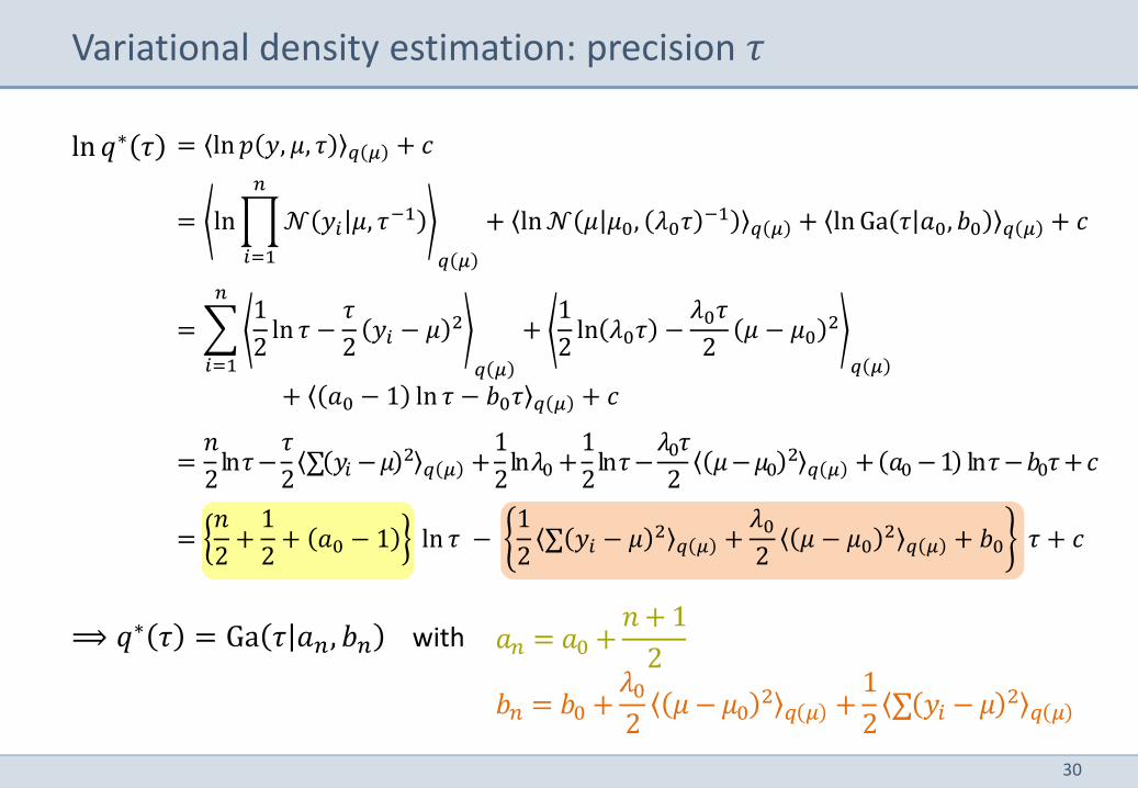
𝑎𝑛 = 𝑎0 +𝑛 + 1
2
𝑏𝑛 = 𝑏0 +𝜆0
2𝜇 − 𝜇0
2𝑞 𝜇 +
1
2∑ 𝑦𝑖 − 𝜇 2
𝑞 𝜇
⟹ 𝑞∗ 𝜏 = Ga 𝜏 𝑎𝑛, 𝑏𝑛 with
Variational density estimation: precision 𝜏
= ln 𝑝 𝑦, 𝜇, 𝜏 𝑞 𝜇 + 𝑐
= ln 𝒩 𝑦𝑖 𝜇, 𝜏−1
𝑛
𝑖=1 𝑞 𝜇
+ ln 𝒩 𝜇 𝜇0, 𝜆0𝜏 −1𝑞 𝜇 + ln Ga 𝜏 𝑎0, 𝑏0 𝑞 𝜇 + 𝑐
= 1
2ln 𝜏 −
𝜏
2𝑦𝑖 − 𝜇 2
𝑛
𝑖=1 𝑞 𝜇
+1
2ln 𝜆0𝜏 −
𝜆0𝜏
2𝜇 − 𝜇0
2
𝑞 𝜇
+ 𝑎0 − 1 ln 𝜏 − 𝑏0𝜏 𝑞 𝜇 + 𝑐
=𝑛
2ln𝜏−
𝜏
2∑ 𝑦𝑖 −𝜇 2
𝑞 𝜇 +1
2ln𝜆0 +
1
2ln𝜏−
𝜆0𝜏
2𝜇−𝜇0
2𝑞 𝜇 + 𝑎0 −1 ln𝜏 −𝑏0𝜏+𝑐
=𝑛
2+
1
2+ 𝑎0 − 1 ln 𝜏 −
1
2∑ 𝑦𝑖 − 𝜇 2
𝑞 𝜇 +𝜆0
2𝜇 − 𝜇0
2𝑞 𝜇 + 𝑏0 𝜏 + 𝑐
ln 𝑞∗ 𝜏
31
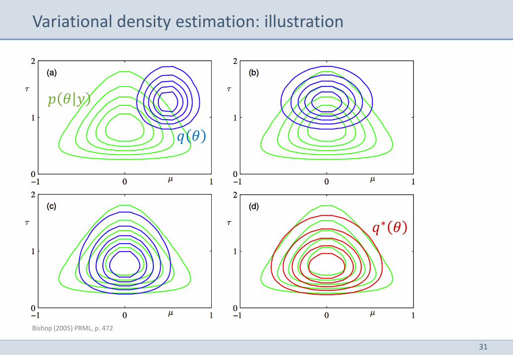
Variational density estimation: illustration
Bishop (2005) PRML, p. 472
𝑞 𝜃
𝑝 𝜃 𝑦
𝑞∗ 𝜃
32
Overview
1 The Laplace approximation
2 Variational Bayes
3 Variational density estimation
4 Variational linear regression
5 Variational clustering
33
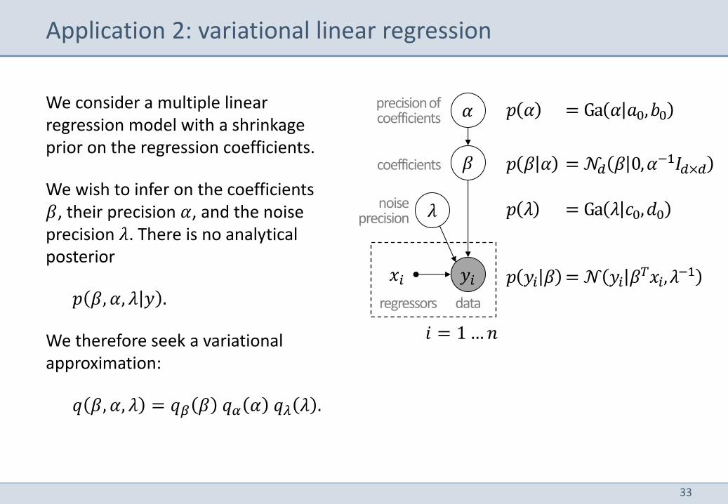
Application 2: variational linear regression
We consider a multiple linear regression model with a shrinkage prior on the regression coefficients.
We wish to infer on the coefficients 𝛽, their precision 𝛼, and the noise precision 𝜆. There is no analytical posterior
𝑝 𝛽, 𝛼, 𝜆 𝑦 .
We therefore seek a variational approximation:
𝑞 𝛽, 𝛼, 𝜆 = 𝑞𝛽 𝛽 𝑞𝛼 𝛼 𝑞𝜆 𝜆 .
𝛽
𝑦𝑖
𝛼
𝑝 𝛽 𝛼 = 𝒩𝑑 𝛽 0,𝛼−1𝐼𝑑×𝑑
𝑝 𝛼 = Ga 𝛼 𝑎0,𝑏0
𝑝 𝑦𝑖 𝛽 = 𝒩 𝑦𝑖 𝛽𝑇𝑥𝑖, 𝜆−1
𝑖 = 1 … 𝑛
coefficients
precision of coefficients
data
𝑥𝑖
regressors
noise precision 𝜆 𝑝 𝜆 = Ga 𝜆 𝑐0,𝑑0
34
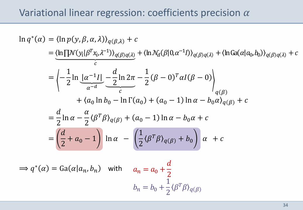
𝑎𝑛 = 𝑎0 +𝑑
2
𝑏𝑛 = 𝑏0 +1
2𝛽𝑇𝛽 𝑞 𝛽
Variational linear regression: coefficients precision 𝛼
= ln 𝑝 𝑦, 𝛽, 𝛼, 𝜆 𝑞 𝛽,𝜆 + 𝑐
= ln∏𝒩 𝑦𝑖 𝛽𝑇𝑥𝑖,𝜆−1
𝑞 𝛽 𝑞 𝜆
𝑐
+ ln𝒩𝑑 𝛽 0,𝛼−1𝐼 𝑞 𝛽 𝑞 𝜆 + lnGa 𝛼 𝑎0,𝑏0 𝑞 𝛽 𝑞 𝜆 +𝑐
= −1
2ln 𝛼−1𝐼
𝛼−𝑑
−𝑑
2ln 2𝜋
𝑐
−1
2𝛽 − 0 𝑇𝛼𝐼 𝛽 − 0
𝑞 𝛽
+ 𝑎0 ln 𝑏0 − ln Γ 𝑎0 + 𝑎0 − 1 ln 𝛼 − 𝑏0𝛼 𝑞 𝛽 + 𝑐
=𝑑
2ln 𝛼 −
𝛼
2𝛽𝑇𝛽 𝑞 𝛽 + 𝑎0 − 1 ln 𝛼 − 𝑏0𝛼 + 𝑐
=𝑑
2+ 𝑎0 − 1 ln 𝛼 −
1
2𝛽𝑇𝛽 𝑞 𝛽 + 𝑏0 𝛼 + 𝑐
ln 𝑞∗ 𝛼
⟹ 𝑞∗ 𝛼 = Ga 𝛼 𝑎𝑛, 𝑏𝑛 with
35
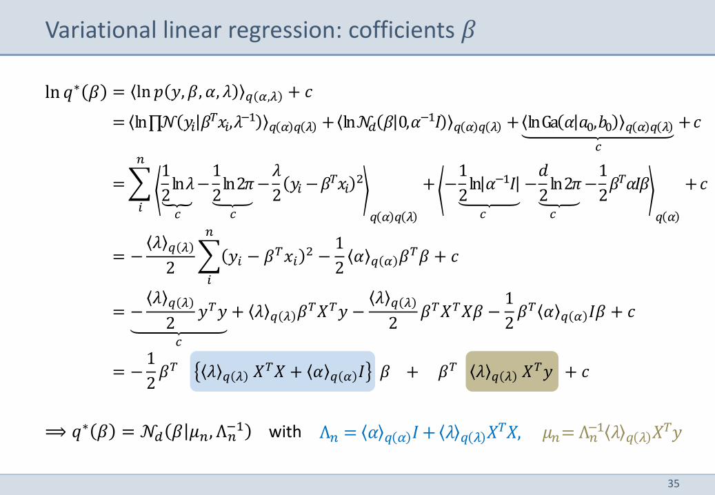
Variational linear regression: cofficients 𝛽
= ln 𝑝 𝑦, 𝛽, 𝛼, 𝜆 𝑞 𝛼,𝜆 + 𝑐
= ln∏𝒩 𝑦𝑖 𝛽𝑇𝑥𝑖,𝜆−1
𝑞 𝛼 𝑞 𝜆 + ln𝒩𝑑 𝛽 0,𝛼−1𝐼 𝑞 𝛼 𝑞 𝜆 + lnGa 𝛼 𝑎0,𝑏0 𝑞 𝛼 𝑞 𝜆
𝑐
+𝑐
= 1
2ln𝜆
𝑐
−1
2ln2𝜋
𝑐
−𝜆
2𝑦𝑖 −𝛽𝑇𝑥𝑖
2
𝑞 𝛼 𝑞 𝜆
𝑛
𝑖
+ −1
2ln 𝛼−1𝐼
𝑐
−𝑑
2ln2𝜋
𝑐
−1
2𝛽𝑇𝛼𝐼𝛽
𝑞 𝛼
+𝑐
= −𝜆 𝑞 𝜆
2 𝑦𝑖 − 𝛽𝑇𝑥𝑖
2
𝑛
𝑖
−1
2𝛼 𝑞 𝛼 𝛽𝑇𝛽 + 𝑐
= −𝜆 𝑞 𝜆
2𝑦𝑇𝑦
𝑐
+ 𝜆 𝑞 𝜆 𝛽𝑇𝑋𝑇𝑦 −𝜆 𝑞 𝜆
2𝛽𝑇𝑋𝑇𝑋𝛽 −
1
2𝛽𝑇 𝛼 𝑞 𝛼 𝐼𝛽 + 𝑐
= −1
2𝛽𝑇 𝜆 𝑞 𝜆 𝑋𝑇𝑋 + 𝛼 𝑞 𝛼 𝐼 𝛽 + 𝛽𝑇 𝜆 𝑞 𝜆 𝑋𝑇𝑦 + 𝑐
ln 𝑞∗ 𝛽
Λ𝑛 = 𝛼 𝑞 𝛼 𝐼 + 𝜆 𝑞 𝜆 𝑋𝑇𝑋, 𝜇𝑛= Λ𝑛−1 𝜆 𝑞 𝜆 𝑋𝑇𝑦
⟹ 𝑞∗ 𝛽 = 𝒩𝑑 𝛽 𝜇𝑛, Λ𝑛
−1 with
36
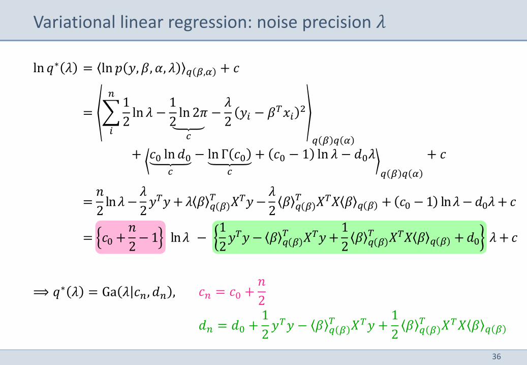
Variational linear regression: noise precision 𝜆
= ln 𝑝 𝑦, 𝛽, 𝛼, 𝜆 𝑞 𝛽,𝛼 + 𝑐
= 1
2ln 𝜆 −
1
2ln 2𝜋
𝑐
−𝜆
2𝑦𝑖 − 𝛽𝑇𝑥𝑖
2
𝑛
𝑖𝑞 𝛽 𝑞 𝛼
+ 𝑐0 ln 𝑑0
𝑐
− ln Γ 𝑐0
𝑐
+ 𝑐0 − 1 ln 𝜆 − 𝑑0𝜆
𝑞 𝛽 𝑞 𝛼
+ 𝑐
=𝑛
2ln𝜆 −
𝜆
2𝑦𝑇𝑦 + 𝜆 𝛽 𝑞 𝛽
𝑇 𝑋𝑇𝑦 −𝜆
2𝛽 𝑞 𝛽
𝑇 𝑋𝑇𝑋 𝛽 𝑞 𝛽 + 𝑐0 − 1 ln𝜆 − 𝑑0𝜆 + 𝑐
= 𝑐0 +𝑛
2− 1 ln𝜆 −
1
2𝑦𝑇𝑦 − 𝛽 𝑞 𝛽
𝑇 𝑋𝑇𝑦 +1
2𝛽 𝑞 𝛽
𝑇 𝑋𝑇𝑋 𝛽 𝑞 𝛽 + 𝑑0 𝜆 + 𝑐
ln 𝑞∗ 𝜆
⟹ 𝑞∗ 𝜆 = Ga 𝜆 𝑐𝑛, 𝑑𝑛 , 𝑐𝑛 = 𝑐0 +𝑛
2
𝑑𝑛 = 𝑑0 +1
2𝑦𝑇𝑦 − 𝛽 𝑞 𝛽
𝑇 𝑋𝑇𝑦 +1
2𝛽 𝑞 𝛽
𝑇 𝑋𝑇𝑋 𝛽 𝑞 𝛽
37
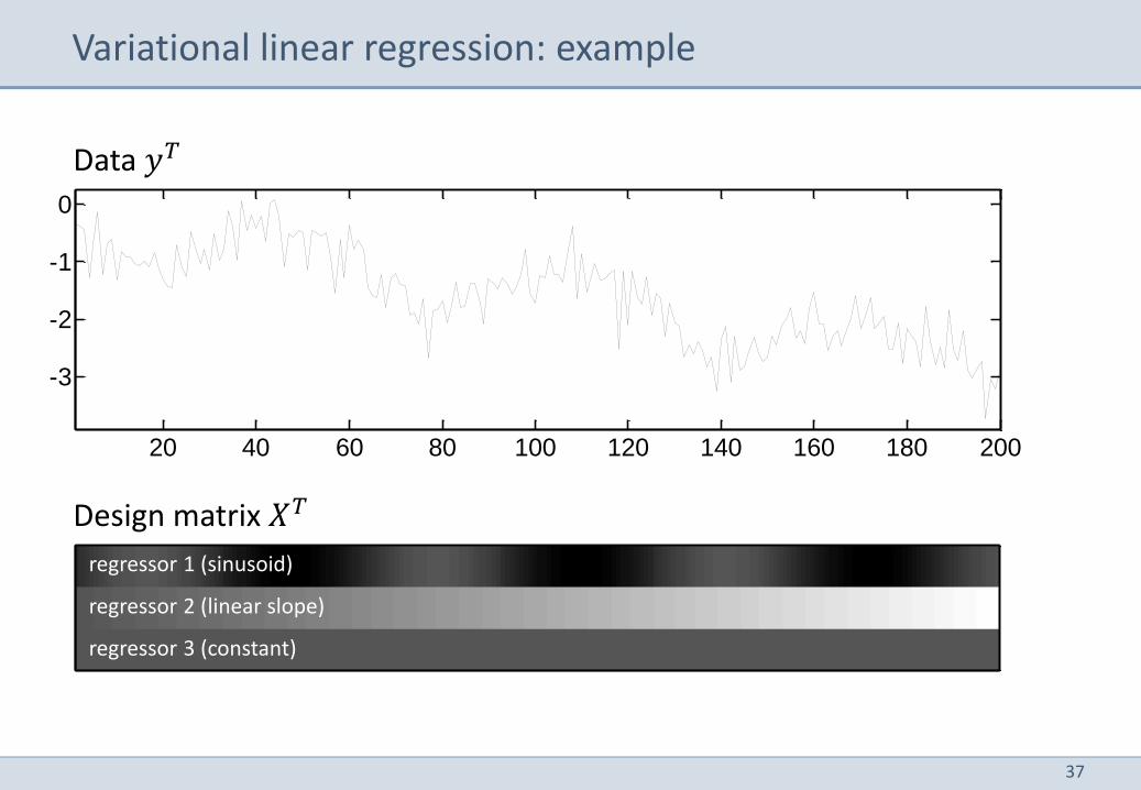
Variational linear regression: example
20 40 60 80 100 120 140 160 180 200
-3
-2
-1
0
Data 𝑦𝑇
Design matrix 𝑋𝑇
regressor 1 (sinusoid)
regressor 2 (linear slope)
regressor 3 (constant)
38
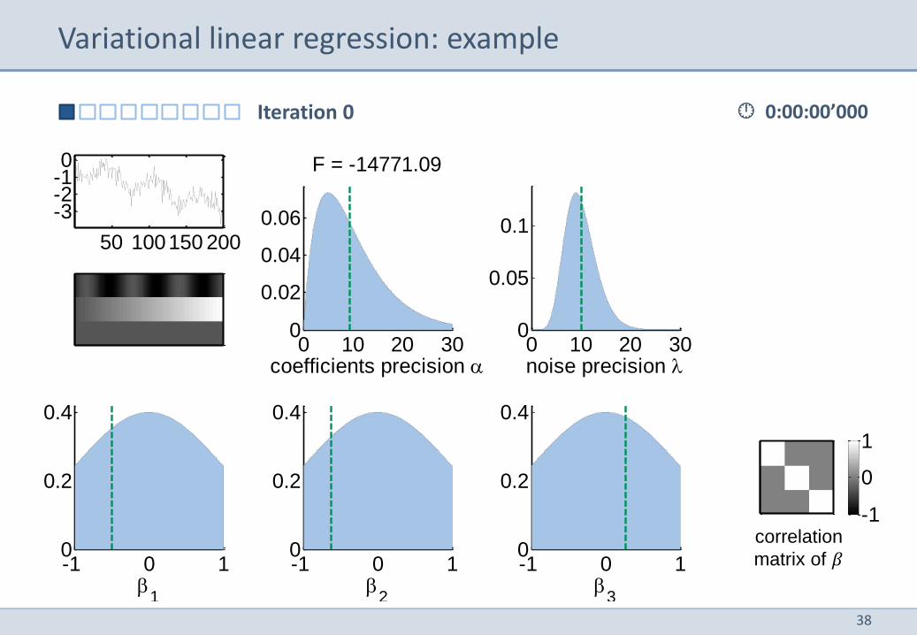
Variational linear regression: example
50 100150 200
-3-2-10
0 10 20 300
0.02
0.04
0.06
coefficients precision
F = -14771.09
0 10 20 300
0.05
0.1
noise precision
-1 0 10
0.2
0.4
1
-1 0 10
0.2
0.4
2
-1 0 10
0.2
0.4
3
-1
0
1
Iteration 0
50 100150 200
-3-2-10
0 10 20 300
0.02
0.04
0.06
coefficients precision
F = -14771.09
0 10 20 300
0.05
0.1
noise precision
-1 0 10
0.2
0.4
1
-1 0 10
0.2
0.4
2
-1 0 10
0.2
0.4
3
-1
0
1
50 100150 200
-3-2-10
0 10 20 300
0.02
0.04
0.06
coefficients precision
F = -14771.09
0 10 20 300
0.05
0.1
noise precision
-1 0 10
0.2
0.4
1
-1 0 10
0.2
0.4
2
-1 0 10
0.2
0.4
3
-1
0
1
50 100150 200
-3-2-10
0 10 20 300
0.02
0.04
0.06
coefficients precision
F = -14771.09
0 10 20 300
0.05
0.1
noise precision
-1 0 10
0.2
0.4
1
-1 0 10
0.2
0.4
2
-1 0 10
0.2
0.4
3
-1
0
1
50 100150 200
-3-2-10
0 10 20 300
0.02
0.04
0.06
coefficients precision
F = -14771.09
0 10 20 300
0.05
0.1
noise precision
-1 0 10
0.2
0.4
1
-1 0 10
0.2
0.4
2
-1 0 10
0.2
0.4
3
-1
0
1
50 100150 200
-3-2-10
0 10 20 300
0.02
0.04
0.06
coefficients precision
F = -14771.09
0 10 20 300
0.05
0.1
noise precision
-1 0 10
0.2
0.4
1
-1 0 10
0.2
0.4
2
-1 0 10
0.2
0.4
3
-1
0
1
0:00:00’000
correlation
matrix of 𝛽

39
50 100150 200
-3-2-10
0 10 20 300
0.05
0.1
coefficients precision
F = 95.95
0 10 20 300
0.2
0.4
noise precision
-1 0 10
5
10
1
-1 0 10
10
20
2
-1 0 10
2
4
6
3
-1
0
1
Variational linear regression: example
correlation
matrix of 𝛽
0:00:00’002 Iteration 1
40
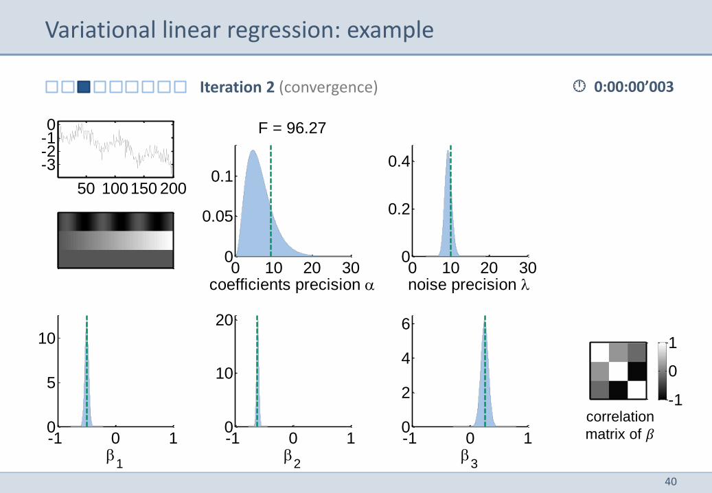
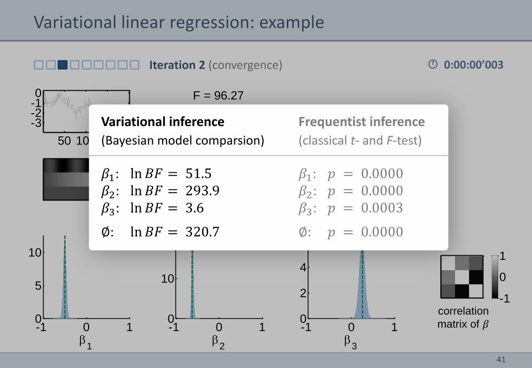
Iteration 2 (convergence)
50 100150 200
-3-2-10
0 10 20 300
0.05
0.1
coefficients precision
F = 96.27
0 10 20 300
0.2
0.4
noise precision
-1 0 10
5
10
1
-1 0 10
10
20
2
-1 0 10
2
4
6
3
-1
0
1
Variational linear regression: example
correlation
matrix of 𝛽
0:00:00’003
41
Iteration 2 (convergence)
50 100150 200
-3-2-10
0 10 20 300
0.05
0.1
coefficients precision
F = 96.27
0 10 20 300
0.2
0.4
noise precision
-1 0 10
5
10
1
-1 0 10
10
20
2
-1 0 10
2
4
6
3
-1
0
1
Variational linear regression: example
Variational inference
(Bayesian model comparsion)
𝛽1: ln 𝐵𝐹 = 51.5 𝛽2: ln 𝐵𝐹 = 293.9 𝛽3: ln 𝐵𝐹 = 3.6
∅: ln 𝐵𝐹 = 320.7
Frequentist inference
(classical t- and F-test)
𝛽1: 𝑝 = 0.0000 𝛽2: 𝑝 = 0.0000 𝛽3: 𝑝 = 0.0003
∅: 𝑝 = 0.0000
correlation
matrix of 𝛽
0:00:00’003
42
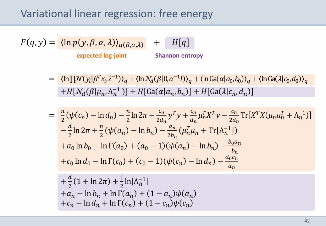
Variational linear regression: free energy
= ln 𝑝 𝑦, 𝛽, 𝛼, 𝜆 𝑞 𝛽,𝛼,𝜆 + 𝐻 𝑞 𝐹 𝑞, 𝑦
= ln∏𝒩 𝑦𝑖 𝛽𝑇𝑥𝑖,𝜆−1
𝑞 + ln𝒩𝑑 𝛽 0,𝛼−1𝐼 𝑞 + lnGa 𝛼 𝑎0,𝑏0 𝑞 + lnGa 𝜆 𝑐0,𝑑0 𝑞
+𝐻 𝒩𝑑 𝛽 𝜇𝑛, Λ𝑛−1 + 𝐻 Ga 𝛼 𝑎𝑛, 𝑏𝑛 + 𝐻 Ga 𝜆 𝑐𝑛, 𝑑𝑛
= 𝑛
2𝜓 𝑐𝑛 − ln𝑑𝑛 −
𝑛
2ln2𝜋 −
𝑐𝑛
2𝑑𝑛𝑦𝑇𝑦 +
𝑐𝑛
𝑑𝑛𝜇𝑛
𝑇𝑋𝑇𝑦 −𝑐𝑛
2𝑑𝑛Tr 𝑋𝑇𝑋 𝜇𝑛𝜇𝑛
𝑇 + Λ𝑛−1
−𝑑
2ln2𝜋 +
𝑛
2𝜓 𝑎𝑛 − ln𝑏𝑛 −
𝑎𝑛
2𝑏𝑛𝜇𝑛
𝑇𝜇𝑛 + Tr Λ𝑛−1
+𝑎0 ln𝑏0 − lnΓ 𝑎0 + 𝑎0 − 1 𝜓 𝑎𝑛 − ln𝑏𝑛 −𝑏0𝑎𝑛
𝑏𝑛
+𝑐0 ln𝑑0 − lnΓ 𝑐0 + 𝑐0 − 1 𝜓 𝑐𝑛 − ln𝑑𝑛 −𝑑0𝑐𝑛
𝑑𝑛
+𝑑
21 + ln2𝜋 +
1
2ln Λ𝑛
−1
+𝑎𝑛 − ln𝑏𝑛 + lnΓ 𝑎𝑛 + 1 − 𝑎𝑛 𝜓 𝑎𝑛 +𝑐𝑛 − ln𝑑𝑛 + lnΓ 𝑐𝑛 + 1 − 𝑐𝑛 𝜓 𝑐𝑛
expected log-joint Shannon entropy
43
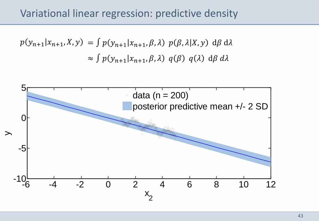
Variational linear regression: predictive density
= ∫ 𝑝 𝑦𝑛+1 𝑥𝑛+1, 𝛽, 𝜆 𝑝 𝛽, 𝜆 𝑋, 𝑦 d𝛽 d𝜆
≈ ∫ 𝑝 𝑦𝑛+1 𝑥𝑛+1, 𝛽, 𝜆 𝑞 𝛽 𝑞 𝜆 d𝛽 𝑑𝜆
𝑝 𝑦𝑛+1 𝑥𝑛+1, 𝑋, 𝑦
-6 -4 -2 0 2 4 6 8 10 12-10
-5
0
5
x2
y
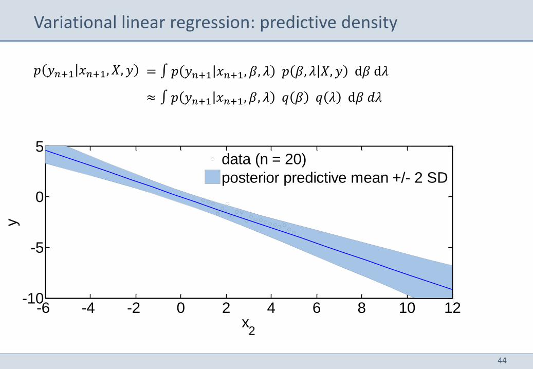
data (n = 20)
posterior predictive mean +/- 2 SD
-6 -4 -2 0 2 4 6 8 10 12-10
-5
0
5
x2
y
data (n = 200)
posterior predictive mean +/- 2 SD
44
Variational linear regression: predictive density
= ∫ 𝑝 𝑦𝑛+1 𝑥𝑛+1, 𝛽, 𝜆 𝑝 𝛽, 𝜆 𝑋, 𝑦 d𝛽 d𝜆
≈ ∫ 𝑝 𝑦𝑛+1 𝑥𝑛+1, 𝛽, 𝜆 𝑞 𝛽 𝑞 𝜆 d𝛽 𝑑𝜆
𝑝 𝑦𝑛+1 𝑥𝑛+1, 𝑋, 𝑦
-6 -4 -2 0 2 4 6 8 10 12-10
-5
0
5
x2
y
data (n = 20)
posterior predictive mean +/- 2 SD
45
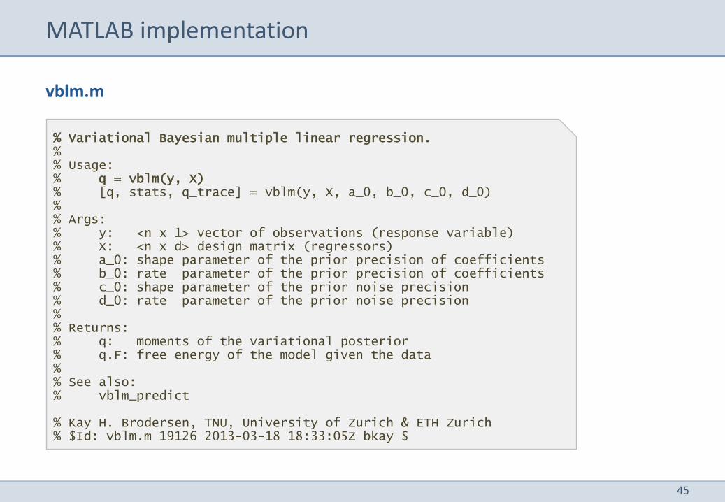
% Variational Bayesian multiple linear regression. % % Usage: % q = vblm(y, X) % [q, stats, q_trace] = vblm(y, X, a_0, b_0, c_0, d_0) % % Args: % y: <n x 1> vector of observations (response variable) % X: <n x d> design matrix (regressors) % a_0: shape parameter of the prior precision of coefficients % b_0: rate parameter of the prior precision of coefficients % c_0: shape parameter of the prior noise precision % d_0: rate parameter of the prior noise precision % % Returns: % q: moments of the variational posterior % q.F: free energy of the model given the data % % See also: % vblm_predict % Kay H. Brodersen, TNU, University of Zurich & ETH Zurich % $Id: vblm.m 19126 2013-03-18 18:33:05Z bkay $
vblm.m
MATLAB implementation
46
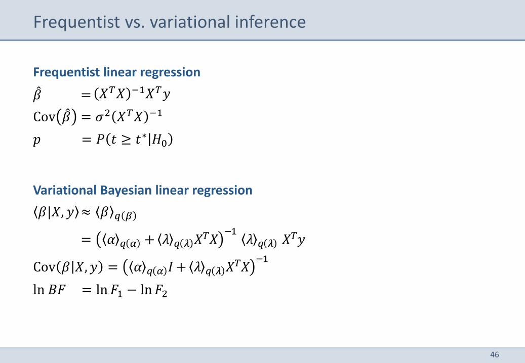
Frequentist linear regression
𝑋𝑇𝑋 −1𝑋𝑇𝑦
Cov 𝛽 = 𝜎2 𝑋𝑇𝑋 −1
𝑝 = 𝑃 𝑡 ≥ 𝑡∗ 𝐻0
Variational Bayesian linear regression
𝛽|𝑋, 𝑦 ≈ 𝛽 𝑞 𝛽
= 𝛼 𝑞 𝛼 + 𝜆 𝑞 𝜆 𝑋𝑇𝑋−1
𝜆 𝑞 𝜆 𝑋𝑇𝑦
Cov 𝛽 𝑋, 𝑦 = 𝛼 𝑞 𝛼 𝐼 + 𝜆 𝑞 𝜆 𝑋𝑇𝑋−1
ln 𝐵𝐹 = ln 𝐹1 − ln 𝐹2
Frequentist vs. variational inference
𝛽 =
47
Overview
1 The Laplace approximation
2 Variational Bayes
3 Variational density estimation
4 Variational linear regression
5 Variational clustering
48
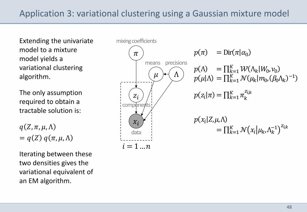
Extending the univariate model to a mixture model yields a variational clustering algorithm.
The only assumption required to obtain a tractable solution is:
𝑞 𝑍, 𝜋, 𝜇, Λ
= 𝑞 𝑍 𝑞 𝜋, 𝜇, Λ
Iterating between these two densities gives the variational equivalent of an EM algorithm.
Application 3: variational clustering using a Gaussian mixture model
𝑧𝑖
𝑥𝑖
𝜋
𝑝 Λ = ∏ 𝒲 Λ𝑘 𝑊0,𝜈0𝐾𝑘=1
𝑝 𝜇 Λ = ∏ 𝒩 𝜇𝑘 𝑚0, 𝛽0Λ𝑘−1𝐾
𝑘=1
𝑝 𝜋 = Dir 𝜋 𝛼0
𝑝 𝑥𝑖 𝑍,𝜇,Λ
= ∏ 𝒩 𝑥𝑖 𝜇𝑘,Λ𝑘−1 𝑧𝑖,𝑘𝐾
𝑘=1
𝑖 = 1…𝑛
mixing coefficients
data
components
𝑝 𝑧𝑖 𝜋 = ∏ 𝜋𝑘
𝑧𝑖,𝑘𝐾𝑘=1
means precisions
𝜇 Λ
49
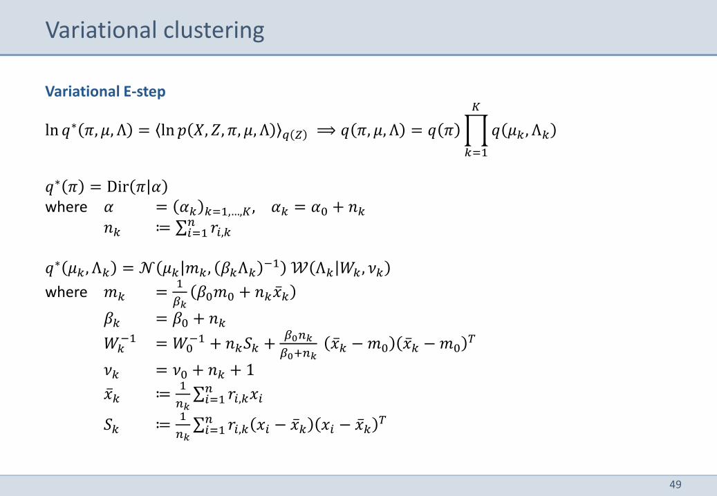
Variational clustering
Variational E-step
ln 𝑞∗ 𝜋, 𝜇, Λ = ln 𝑝 𝑋, 𝑍, 𝜋, 𝜇, Λ 𝑞 𝑍 ⟹ 𝑞 𝜋, 𝜇, Λ = 𝑞 𝜋 𝑞 𝜇𝑘 , Λ𝑘
𝐾
𝑘=1
𝑞∗ 𝜋 = Dir 𝜋 𝛼 where 𝛼 = 𝛼𝑘 𝑘=1,…,𝐾, 𝛼𝑘 = 𝛼0 + 𝑛𝑘
𝑛𝑘 ≔ ∑ 𝑟𝑖,𝑘𝑛𝑖=1
𝑞∗ 𝜇𝑘 , Λ𝑘 = 𝒩 𝜇𝑘 𝑚𝑘 , 𝛽𝑘Λ𝑘
−1 𝒲 Λ𝑘 𝑊𝑘 , 𝜈𝑘
where 𝑚𝑘 =1
𝛽𝑘𝛽0𝑚0 + 𝑛𝑘𝑥 𝑘
𝛽𝑘 = 𝛽0 + 𝑛𝑘
𝑊𝑘−1 = 𝑊0
−1 + 𝑛𝑘𝑆𝑘 +𝛽0𝑛𝑘
𝛽0+𝑛𝑘 𝑥 𝑘 − 𝑚0 𝑥 𝑘 − 𝑚0
𝑇
𝜈𝑘 = 𝜈0 + 𝑛𝑘 + 1
𝑥 𝑘 ≔1
𝑛𝑘∑ 𝑟𝑖,𝑘𝑥𝑖
𝑛𝑖=1
𝑆𝑘 ≔1
𝑛𝑘∑ 𝑟𝑖,𝑘 𝑥𝑖 − 𝑥 𝑘 𝑥𝑖 − 𝑥 𝑘
𝑇𝑛𝑖=1
50
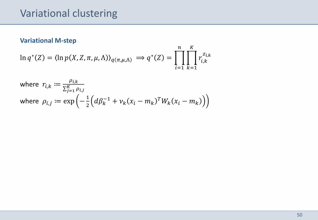
Variational clustering
Variational M-step
ln 𝑞∗ 𝑍 = ln 𝑝 𝑋, 𝑍, 𝜋, 𝜇, Λ 𝑞 𝜋,𝜇,Λ ⟹ 𝑞∗ 𝑍 = 𝑟𝑖,𝑘𝑧𝑖,𝑘
𝐾
𝑘=1
𝑛
𝑖=1
where 𝑟𝑖,𝑘 ≔𝜌𝑖,𝑘
∑ 𝜌𝑖,𝑗𝐾𝑗=1
where 𝜌𝑖,𝑗 ≔ exp −1
2𝑑𝛽𝑘
−1 + 𝜈𝑘 𝑥𝑖 − 𝑚𝑘𝑇𝑊𝑘 𝑥𝑖 − 𝑚𝑘
51
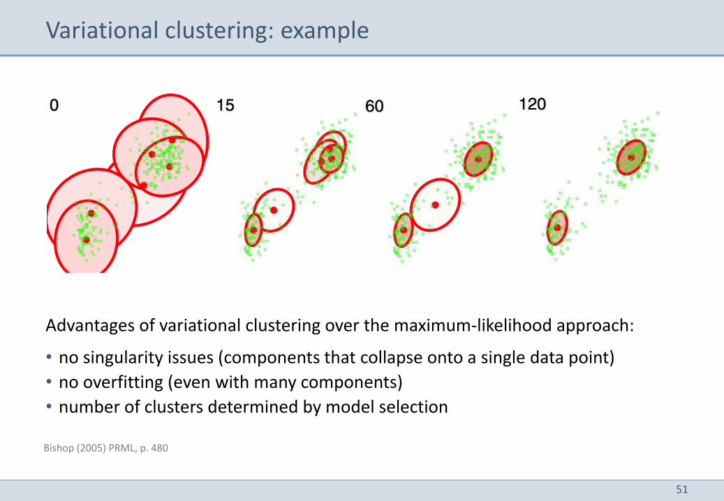
Variational clustering: example
Bishop (2005) PRML, p. 480
Advantages of variational clustering over the maximum-likelihood approach:
• no singularity issues (components that collapse onto a single data point)
• no overfitting (even with many components)
• number of clusters determined by model selection
52
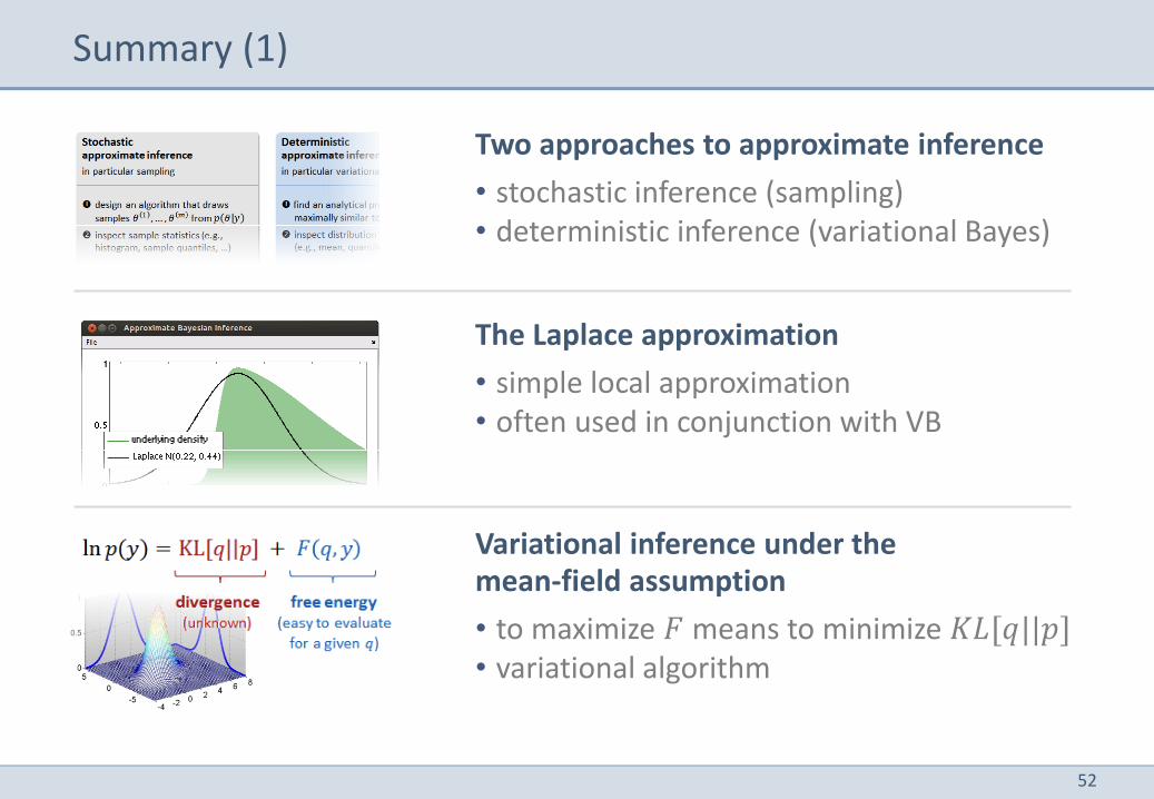
Summary (1)
Two approaches to approximate inference
• stochastic inference (sampling) • deterministic inference (variational Bayes)
The Laplace approximation
• simple local approximation • often used in conjunction with VB
Variational inference under the mean-field assumption
• to maximize 𝐹 means to minimize 𝐾𝐿[𝑞||𝑝] • variational algorithm
53
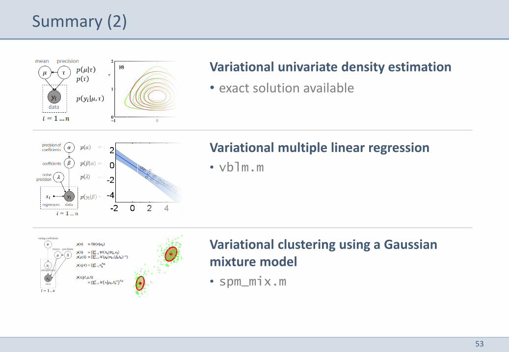
Summary (2)
Variational univariate density estimation
• exact solution available
Variational multiple linear regression
• vblm.m
Variational clustering using a Gaussian mixture model
• spm_mix.m