Embed Size (px)
Citation preview
NeuroImage 76 (2013) 345–361
Contents lists available at SciVerse ScienceDirect
NeuroImage
j ourna l homepage: www.e lsev ie r .com/ locate /yn img
Variational Bayesian mixed-effects inference for classification studies
Kay H. Brodersen a,b,c,⁎, Jean Daunizeau c,d, Christoph Mathys a,c, Justin R. Chumbley c,Joachim M. Buhmann b, Klaas E. Stephan a,c,e
a Translational Neuromodeling Unit (TNU), Institute for Biomedical Engineering, University of Zurich & ETH Zurich, Switzerlandb Machine Learning Laboratory, Department of Computer Science, ETH Zurich, Switzerlandc Laboratory for Social and Neural Systems Research (SNS), Department of Economics, University of Zurich, Switzerlandd Institut du Cerveau et de la Moelle Épinière (ICM), Hôpital Pitié Salpêtrière, Paris, Francee Wellcome Trust Centre for Neuroimaging, University College London, UK
⁎ Corresponding author at: Translational NeuromodeBiomedical Engineering, University of Zurich & ETH ZurZurich, Switzerland.
E-mail address: [email protected] (K.H.
1053-8119/$ – see front matter © 2013 Elsevier Inc. Allhttp://dx.doi.org/10.1016/j.neuroimage.2013.03.008
a b s t r a c t
a r t i c l e i n f oArticle history:Accepted 9 March 2013Available online 16 March 2013
Keywords:Variational BayesFixed effectsRandom effectsNormal-binomialBalanced accuracyBayesian inferenceGroup studies
Multivariate classification algorithms are powerful tools for predicting cognitive or pathophysiological states fromneuroimaging data. Assessing the utility of a classifier in application domains such as cognitive neuroscience,brain–computer interfaces, or clinical diagnostics necessitates inference on classification performance at morethan one level, i.e., both in individual subjects and in the population from which these subjects were sampled.Such inference requires models that explicitly account for both fixed-effects (within-subjects) and random-effects (between-subjects) variance components.Whilemodels of this sort are standard inmass-univariate analysesof fMRI data, they have not yet receivedmuch attention in multivariate classification studies of neuroimaging data,presumably because of the high computational costs they entail. This paper extends a recently developed hierarchi-cal model for mixed-effects inference in multivariate classification studies and introduces an efficient variationalBayes approach to inference. Using both synthetic and empirical fMRI data, we show that this approach is equallysimple to use as, yetmore powerful than, a conventional t-test on subject-specific sample accuracies, and computa-tionally much more efficient than previous sampling algorithms and permutation tests. Our approach is indepen-dent of the type of underlying classifier and thus widely applicable. The present framework may help establishmixed-effects inference as a future standard for classification group analyses.
© 2013 Elsevier Inc. All rights reserved.
Introduction
Multivariate classification algorithms have emerged from thefield ofmachine learning as powerful tools for predicting cognitive or patho-physiological states from neuroimaging data (Haynes and Rees, 2006).Classifiers are based on decoding models that differ in two ways fromconventional mass-univariate encoding analyses based on the generallinear model (GLM; Friston et al., 1995). First, multivariate approachesexplicitly account for dependencies among voxels. Second, they reversethe direction of inference, predicting a contextual variable from brainactivity (decoding) rather than the other way around (encoding).There are three related areas of application in which these two charac-teristics have sparked most interest.
In cognitive neuroscience, and in particular neuroimaging, classifiershave been employed to decode subject-specific cognitive or perceptualstates frommultivariatemeasures of brain activity, such as those obtainedby fMRI (Brodersen et al., 2012b; Cox and Savoy, 2003; Haynes and Rees,2006; Norman et al., 2006; Tong and Pratte, 2012). A second area is the
ling Unit (TNU), Institute forich,Wilfriedstrasse 6, CH 8032
Brodersen).
rights reserved.
design of brain–machine interfaces which aim at decoding subjectivecognitive states (e.g., intentions or decisions) from trial-wise measure-ments of neuronal activity in individual subjects (Blankertz et al., 2011;Sitaram et al., 2008). A third important domain concerns clinical applica-tions that explore the utility of multivariate decoding approaches fordiagnostic purposes (Davatzikos et al., 2008; Klöppel et al., 2008, 2012;Marquand et al., 2010). Recently, decoding models have also been inte-grated with biophysical models of brain function, such as dynamic causalmodels (Friston et al., 2003), to afford mechanistically interpretableclassifications (Brodersen et al., 2011a,b).
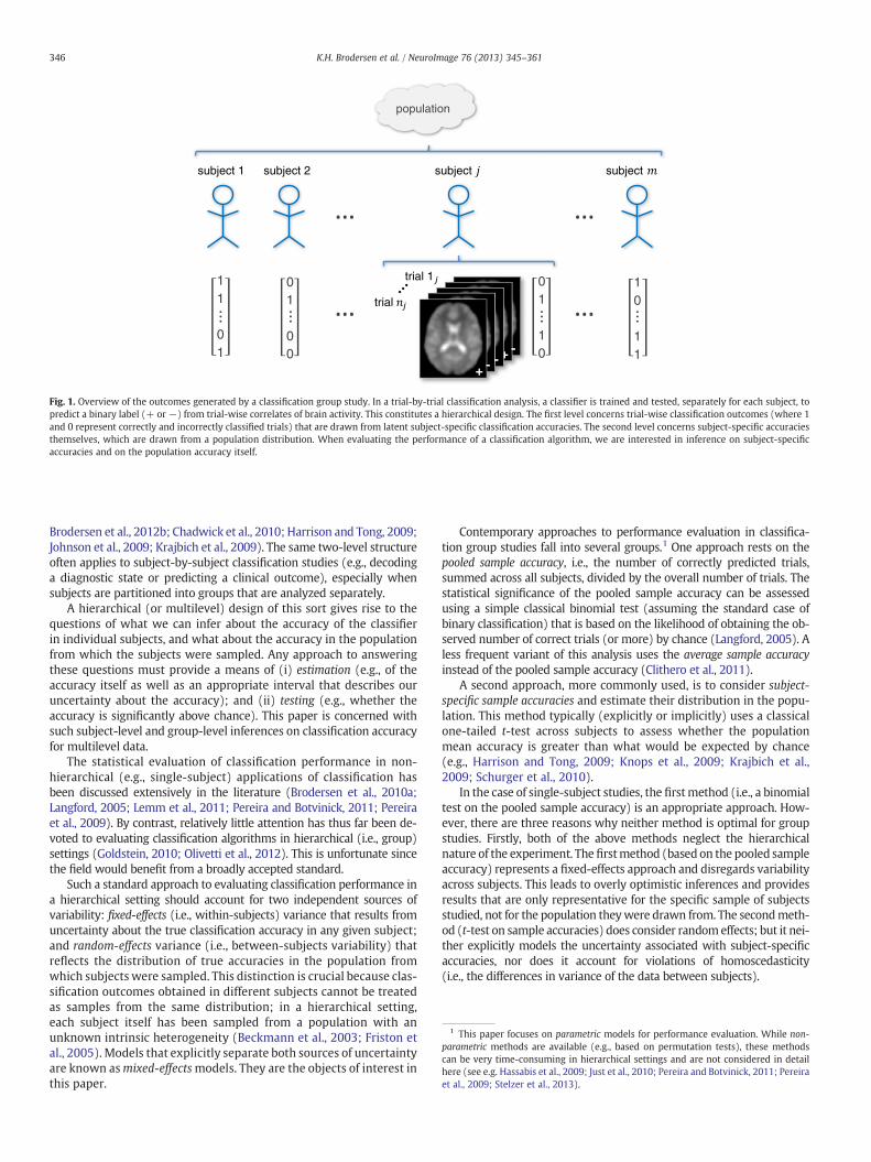
Many applications ofmultivariate classification operate on datawitha two-level hierarchical structure. Consider, for example, a study inwhich a classification algorithm is used to decode from fMRI datawhether a subject chose option A or B on each of n experimental repeti-tions or trials. This analysis gives rise to n estimated labels (representingwhich choice the classifier predicted on each trial) and n true labels(indicating which option was truly chosen). Comparing predicted totrue labels yields a sequence of classification outcomes (indicating foreach trial whether the prediction was correct or incorrect). Repeatingthis analysis for each member of a group ofm subjects yields the typicaltwo-level structure (m subjects times n trials each) that is illustrated inFig. 1; for a concrete example see Figs. 7a,e. A two-level structure under-lies virtually all trial-by-trial decoding studies (see, amongmany others,
1 This paper focuses on parametric models for performance evaluation. While non-parametric methods are available (e.g., based on permutation tests), these methodscan be very time-consuming in hierarchical settings and are not considered in detailhere (see e.g. Hassabis et al., 2009; Just et al., 2010; Pereira and Botvinick, 2011; Pereiraet al., 2009; Stelzer et al., 2013).
subject
---+
trial
trial 1
subject 1 subject 2 subject
population
01
10
11
01
01
00
10
11
Fig. 1. Overview of the outcomes generated by a classification group study. In a trial-by-trial classification analysis, a classifier is trained and tested, separately for each subject, topredict a binary label (+ or−) from trial-wise correlates of brain activity. This constitutes a hierarchical design. The first level concerns trial-wise classification outcomes (where 1and 0 represent correctly and incorrectly classified trials) that are drawn from latent subject-specific classification accuracies. The second level concerns subject-specific accuraciesthemselves, which are drawn from a population distribution. When evaluating the performance of a classification algorithm, we are interested in inference on subject-specificaccuracies and on the population accuracy itself.
346 K.H. Brodersen et al. / NeuroImage 76 (2013) 345–361
Brodersen et al., 2012b; Chadwick et al., 2010; Harrison and Tong, 2009;Johnson et al., 2009; Krajbich et al., 2009). The same two-level structureoften applies to subject-by-subject classification studies (e.g., decodinga diagnostic state or predicting a clinical outcome), especially whensubjects are partitioned into groups that are analyzed separately.
A hierarchical (or multilevel) design of this sort gives rise to thequestions of what we can infer about the accuracy of the classifierin individual subjects, and what about the accuracy in the populationfrom which the subjects were sampled. Any approach to answeringthese questions must provide a means of (i) estimation (e.g., of theaccuracy itself as well as an appropriate interval that describes ouruncertainty about the accuracy); and (ii) testing (e.g., whether theaccuracy is significantly above chance). This paper is concerned withsuch subject-level and group-level inferences on classification accuracyfor multilevel data.
The statistical evaluation of classification performance in non-hierarchical (e.g., single-subject) applications of classification hasbeen discussed extensively in the literature (Brodersen et al., 2010a;Langford, 2005; Lemm et al., 2011; Pereira and Botvinick, 2011; Pereiraet al., 2009). By contrast, relatively little attention has thus far been de-voted to evaluating classification algorithms in hierarchical (i.e., group)settings (Goldstein, 2010; Olivetti et al., 2012). This is unfortunate sincethe field would benefit from a broadly accepted standard.
Such a standard approach to evaluating classification performance ina hierarchical setting should account for two independent sources ofvariability: fixed-effects (i.e., within-subjects) variance that results fromuncertainty about the true classification accuracy in any given subject;and random-effects variance (i.e., between-subjects variability) thatreflects the distribution of true accuracies in the population fromwhich subjects were sampled. This distinction is crucial because clas-sification outcomes obtained in different subjects cannot be treatedas samples from the same distribution; in a hierarchical setting,each subject itself has been sampled from a population with anunknown intrinsic heterogeneity (Beckmann et al., 2003; Friston etal., 2005). Models that explicitly separate both sources of uncertaintyare known asmixed-effectsmodels. They are the objects of interest inthis paper.
Contemporary approaches to performance evaluation in classifica-tion group studies fall into several groups.1 One approach rests on thepooled sample accuracy, i.e., the number of correctly predicted trials,summed across all subjects, divided by the overall number of trials. Thestatistical significance of the pooled sample accuracy can be assessedusing a simple classical binomial test (assuming the standard case ofbinary classification) that is based on the likelihood of obtaining the ob-served number of correct trials (or more) by chance (Langford, 2005). Aless frequent variant of this analysis uses the average sample accuracyinstead of the pooled sample accuracy (Clithero et al., 2011).
A second approach, more commonly used, is to consider subject-specific sample accuracies and estimate their distribution in the popu-lation. This method typically (explicitly or implicitly) uses a classicalone-tailed t-test across subjects to assess whether the populationmean accuracy is greater than what would be expected by chance(e.g., Harrison and Tong, 2009; Knops et al., 2009; Krajbich et al.,2009; Schurger et al., 2010).
In the case of single-subject studies, the firstmethod (i.e., a binomialtest on the pooled sample accuracy) is an appropriate approach. How-ever, there are three reasons why neither method is optimal for groupstudies. Firstly, both of the above methods neglect the hierarchicalnature of the experiment. The firstmethod (based on the pooled sampleaccuracy) represents a fixed-effects approach and disregards variabilityacross subjects. This leads to overly optimistic inferences and providesresults that are only representative for the specific sample of subjectsstudied, not for the population theywere drawn from. The secondmeth-od (t-test on sample accuracies) does consider randomeffects; but it nei-ther explicitly models the uncertainty associated with subject-specificaccuracies, nor does it account for violations of homoscedasticity(i.e., the differences in variance of the data between subjects).
347K.H. Brodersen et al. / NeuroImage 76 (2013) 345–361
The second limitation of the abovemethods is rooted in their distribu-tional assumptions. In the standard case of binary classification, it is rea-sonable to assume individual classification outcomes to follow binomialdistributions (justifying the binomial test in single-subject studies). How-ever, it is not well founded to assume that sample accuracies follow aGaussian distribution (which, in this particular case, is the implicit as-sumption of a classical t-test on sample accuracies). This is because aGaussian has infinite support, which means it inevitably places probabil-ity mass on values below 0% and above 100% (for an alternative, seeDixon, 2008).
A third problem, albeit not an intrinsic characteristic of the abovemethods, is their typical focus on classification accuracy, which isknown to be a poor indicator of performance when classes are notperfectly balanced. Specifically, a classifier trained on an imbalanceddataset may acquire a bias in favor of the majority class, resulting inan overoptimistic accuracy. This motivates the use of an alternativeperformance measure, the balanced accuracy, which removes thisbias from performance evaluation.
We recently proposed a solution to the three above limitations usingBayesian hierarchical models for mixed-effects inference on classifica-tion performance. In particular, we introduced the beta-binomial modeland the normal-binomial model for inferring on both accuracies andbalanced accuracies (Brodersen et al., 2012a). Both models use a fullyBayesian framework for mixed-effects inference, are based on naturaldistributional assumptions, and enable more accurate inferences thanthe two conventional approaches described earlier. Themodels are inde-pendent of the type of underlying classifier, which makes them widelyapplicable.
The practical utility of our models, however, has been limited bythe high computational complexity of the underlying Markov chainMonte Carlo (MCMC) sampling algorithms required for model inver-sion (i.e., the process of passing from a prior to a posterior distributionover model parameters, given the data). MCMC is asymptoticallyexact; but it is also exceedingly slow, especially when performing infer-ence in a voxel-by-voxel fashion, as is common, for example, in ‘search-light’ approaches (Kriegeskorte et al., 2006; Nandy and Cordes, 2003).
In this paper, we present a variational Bayes (VB) algorithm toovercome this critical limitation.2 Our approach has three main fea-tures. First, we present a mixed-effects model that explicitly respectsthe hierarchical structure of the data. Second, the model can be equallyused for inference on the accuracy and the balanced accuracy. Third, ournovel variational inference scheme dramatically reduces the computa-tional complexity (i.e., runtime) compared to our previous samplingapproach based on MCMC.
The paper is organized as follows. In the Theory section, wepresent variations of our recently developed normal-binomial modelfor mixed-effects inference (Brodersen et al., 2012a). These are theunivariate normal-binomial model (for inference on the accuracy) andthe twofold normal-binomial model (for inference on the balancedaccuracy).3 We then describe a novel VB algorithm for model inversionand compare it to an MCMC sampler. In the Applications section, weprovide a set of illustrative results on both synthetic data and empiricalfMRImeasurements. Finally, in theDiscussion,we review the key charac-teristics of our approach, compare it to similar models in other analysisdomains, and discuss its role in future classification studies.
Theory
In a hierarchical setting, a classifier is typically used to predict aclass label for each trial, where trials are further structured into sets,
2 The approach proposed in this paper has been implemented as open-source soft-ware for both MATLAB and R. The code can be downloaded from: http://www.translationalneuromodeling.org/software/.
3 Note that the terms ‘univariate’ and ‘twofold’ are used to characterize the numberand structure of model parameters in each subject; these differences are unrelated tothe distinction between univariate and multivariate analyses.
for instance because they were recorded from different subjects.The most common situation is binary classification, where class labelsare taken from {+1,−1}, denoting ‘positive’ and ‘negative’ trials,respectively. Less common, but equally amenable to the approachpresented in this paper, are multiclass settings in which trials fallinto more than two classes (see Discussion).
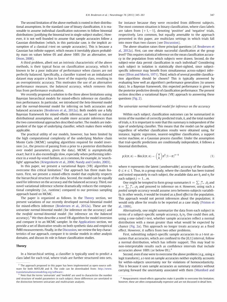
The above situation raises three principal questions (cf. Brodersen etal., 2012a). First, can one obtain successful classification at the grouplevel? This requires statistical inference on themean classification accura-cy in the population from which subjects were drawn. Second, do thesubject-wise data permit classification in each individual? Consideringeach subject in isolation is statistically short-sighted, since subject-specific inference may benefit from simultaneous across-subject infer-ence (Efron andMorris, 1971). Third, which of several possible classifica-tion algorithms should be chosen? This is typically answered byevaluating how well an algorithm's performance generalizes (to unseendata). In a Bayesian framework, this expected performance is given bythe posterior predictive density of classification performance. The presentsection describes a variational Bayes (VB) approach to answering thesequestions (Fig. 2).
The univariate normal-binomial model for inference on the accuracy
Within each subject, classification outcomes can be summarized interms of the number of correctly predicted trials, k, and the total numberof trials, n. It is important to note that this summary is independent of thetype of underlying classifier. This means that the model can be appliedregardless of whether classification results were obtained using, forinstance, logistic regression, nearest-neighbor classification, a supportvector machine, or a Gaussian process classifier. Under the assumptionthat trial-specific predictions are conditionally independent, k follows abinomial distribution,
p kjπ;nð Þ ¼ Bin kjπ;nð Þ ¼ nk
� �πk 1−πð Þn−k ð1Þ
where π represents the latent (unobservable) accuracy of the classifier,0 ≤ π ≤ 1. Thus, in a group study, where the classifier has been trainedand tested separately in each subject, the available data are kj and nj foreach subject j = 1…m.
Onemight be tempted to form group summaries k = ∑ j = 1m kj and
n = ∑ j = 1m nj and proceed to inference on π. However, using such a
pooled sample accuracywould assume zero between-subjects variabili-ty. In other words, πwould be treated as a fixed effect in the population.This approach would not permit inferences about the population; itwould only allow for results to be reported as a case study (Friston etal., 1999).
Alternatively, one might summarize the data from each subject interms of a subject-specific sample accuracy, kj/nj. One could then ask,using a one-tailed t-test, whether sample accuracies reflect a normaldistribution with a mean greater than what would be expected bychance (Fig. 2a). This approach no longer treats accuracy as a fixedeffect. However, it suffers from two other problems.
First, submitting subject-specific sample accuracies to a t-test as-sumes that accuracies, which are confined to the [0,1] interval, followa normal distribution, which has infinite support. This may lead tonon-interpretable results such as confidence intervals that includeaccuracies above 100% (or below 0%).4
Second, even if onewere to overcome the above problem (e.g., using alogit transform), a t-test on sample accuracies neither explicitly accountsfor within-subjects uncertainty nor for violations of homoscedasticity.This is because it uses sample accuracies as summary statistics withoutcarrying forward the uncertainty associated with them (Mumford and
4 Nonparametric mixed-effects approaches make it possible to overcome this limitation;however, these are often computationally expensive and are not discussed in detail here.
b Bayesian mixed-effects inference (univariate normal-binomial model)
c Variational Bayesapproximation
iterative conditional optimizationof posterior moments
a Conventional maximum-likelihood estimation
Fig. 2. Inference on classification accuracies. (a) Conventional maximum-likelihood estimation does not explicitly model within-subjects (fixed-effects) variance components and isbased on an ill-justified normality assumption. It is therefore inadequate for the statistical evaluation of classification group studies. (b) The normal-binomial model respects thehierarchical structure of the study and makes natural distributional assumptions, thus enabling mixed-effects inference, which makes it suitable for group studies. The model usesthe sigmoid transform σ(ρj) := (1 + exp(−ρj))−1 which turns log-odds with real support (−∞,∞) into accuracies on the [0,1] interval. (b) Model inversion can be implementedefficiently using a variational Bayes approximation to the posterior densities of the model parameters (see Fig. 3 for details).
348 K.H. Brodersen et al. / NeuroImage 76 (2013) 345–361
Nichols, 2009). For example, sample accuracies do not distinguish be-tween an accuracy of 80% thatwas obtained as 80 correct out of 100 trials(i.e., an estimate with high confidence) and the same accuracy obtainedas 8 out of 10 trials (i.e., an estimate with low confidence). Furthermore,nodistinction regarding the confidence in the inference is beingmade be-tween 80 correct out of 100 trials (i.e., high confidence) and 50 correctout of 100 trials (lower confidence, since the variance of a binomial distri-bution depends on its mean and becomes maximal at a mean of 0.5).
In order to explicitly capture bothwithin-subjects (fixed-effects) andbetween-subjects (random-effects) variance components, we must in-stead use a hierarchicalmodel inwhich separate levels account for differ-ent sources of variability (Fig. 2b). At the level of individual subjects, foreach subject j, the number of correctly classified trials kj is modeled as
p kjjπj;nj
� �¼ Bin kjjπj;nj
� �ð2Þ
where πj represents the latent classification accuracy in subject j.5 Next,at the group level, we account for variability between subjects bymodel-ing subject-specific accuracies as drawn from a population distribution.
The natural parameter of the binomial density is ln π1−π
. Thus, one possi-
ble parameterization is to assume accuracies to be logit-normally distrib-uted and conditionally independent given the population parameters. In
other words, each logit accuracy ρj : ¼ σ−1 πj
� �: ¼ ln
πj
1−πjis drawn
from a normal distribution. The inverse-sigmoid (or logit) transformσ−1(πj) turns accuracies with support on the [0,1] interval intolog-odds with support on the real line (−∞,+∞). Thus,
p ρjjμ;λ� �
¼ N ρjjμ;λ� �
¼ffiffiffiffiffiffiλ2π
rexp −λ
2ρj−μ� �2� �
ð3Þ
where μ and λ represent the population mean and the populationprecision (i.e., inverse variance), respectively.
Since neuroimaging studies are typically confined to relatively smallsample sizes, an adequate expression of our prior ignorance about thepopulation parameters is critical (cf. Woolrich et al., 2004). We usea diffuse prior on μ and λ such that the posterior will be dominated bythe data (for a validation of this prior, see Applications). A
5 From now on, we will omit nj unless this introduces ambiguity.
straightforward parameterization is to use independent conjugatedensities:
p μ μ0;η0�� � ¼ N μ μ0;η0
�� � ð4Þ
p λ a0; b0j Þ ¼ Ga λ a0; b0j Þ:ðð ð5Þ
In the above densities, μ0 and η0 encode the prior mean and pre-cision of the populationmean, and a0 and b0 represent the shape andscale parameter,6 respectively, that specify the prior distribution ofthe population precision (for an alternative, see Leonard, 1972). Insummary, the univariate normal-binomial model uses a binomialdistribution at the level of individual subjects and a logit-normaldistribution at the group level (Fig. 2b).
In principle, inverting the above model immediately yields thedesired posterior density over parameters,
p μ;λ;ρjkð Þ ¼∏m
j¼1
Bin kjjσ ρj
� �� �N ρj μ;λ
������ �
N μjμ0; η0 �
Ga λja0; b0ð Þp kð Þ :
ð6Þ
In practice, however, integrating the expression in the denomina-tor of the above expression, which provides the normalizationconstant for the posterior density, is prohibitively difficult. We previ-ously described a stochastic approximation based on MCMC algo-rithms; however, the practical use of these algorithms was limitedby their considerable computational complexity (Brodersen et al.,2012a). Here, we propose to invert the above model using a deter-ministic VB approximation (Fig. 2c). This approximation is no longerasymptotically exact, but it conveys considerable computationaladvantages. The remainder of this section describes its derivation(see Fig. 3 for a summary).
Variational inference
The difficult problem of finding the exact posterior p(μ,λ,ρ|k) can betransformed into the easier problem of finding an approximate para-metric posterior q(μ,λ,ρ|δ) with moments (i.e., parameters) δ. (Wewill omit δ to simplify the notation.) Inference then reduces to finding
6 Under the Gamma parameterization used here, the prior expectation of λ is⟨λ⟩ = a0b0.
349K.H. Brodersen et al. / NeuroImage 76 (2013) 345–361
a density q that minimizes a measure of dissimilarity between q and p.This can be achieved by maximizing the so-called negative free energyF of the model, a lower-bound approximation to the log model evi-dence, with respect to (the moments of) q. For details, see MacKay(1995), Attias (2000), Ghahramani and Beal (2001), Bishop et al.(2002), and Fox andRoberts (2012).Maximizing thenegative free ener-gy minimizes the Kullback–Leibler (KL) divergence between the ap-proximate and the true posterior, q and p:
KL qjjp½ � : ¼ ∭q μ;λ;ρð Þ ln q μ;λ;ρð Þp μ;λ;ρjkð Þdμdλdρ ð7Þ
¼ ∭q μ;λ;ρð Þln q μ;λ;ρð Þp k; μ;λ;ρð Þdμdλdρþ lnp kð Þ ð8Þ
⇔ ln p kð Þ ¼ KL qjjp½ � þ lnp k; μ;λ;ρð Þq μ;λ;ρð Þ
� q μ;λ;ρð Þ|fflfflfflfflfflfflfflfflfflfflfflfflfflfflfflfflfflfflfflfflffl{zfflfflfflfflfflfflfflfflfflfflfflfflfflfflfflfflfflfflfflfflffl}
¼:F q;kð Þ
: ð9Þ
This means that the log-model evidence ln p(k) can be expressedas the sum of (i) the KL-divergence between the approximate and thetrue posterior and (ii) the negative free energy F(q,k). Because theKL-divergence cannot be negative, maximizing the negative free en-ergy with respect to q minimizes the KL-divergence and thus resultsin an approximate posterior that is maximally similar to the true pos-terior. At the same time, maximizing the negative free energy pro-vides a lower-bound approximation to the log-model evidence,which permits Bayesian model comparison (Bishop, 2007; Penny etal., 2004). In summary, maximizing the negative free energy F(q,k)in Eq. (9) enables both inference on the posterior density over param-eters and model comparison. In this paper, we are primarily interest-ed in the posterior density.
In trying to maximize F(q,k), variational calculus tells us that
∂F q; kð Þ∂q ¼ 0⇒q μ;λ;ρð Þ∝ exp½ ln p k; μ;λ;ρð Þ|fflfflfflfflfflfflfflfflfflfflffl{zfflfflfflfflfflfflfflfflfflfflffl}
negative variational energy
� ð10Þ
This means that the approximate posterior which maximizes thenegative free energy is equal to the true posterior and thus propor-tional to the joint density over data and parameters7 (with the nor-malization constant being given by the model evidence). In otherwords, the VB approach is complete in the sense that, in the absenceof any other approximations, optimizing Fwith respect to q yields theexact posterior density and model evidence.
Mean-field approximation
To make the optimization on the l.h.s. in Eq. (10) tractable, we as-sume that the joint posterior over all model parameters factorizesinto specific parts. Using one density for each variable,
q μ;λ;ρð Þ ¼ q μð Þq λð Þq ρð Þ ð11Þ
the mean-field assumption turns the problem of maximizing F(q,k)into the problem of deriving three expectations:
I1 μð Þ ¼ ln p k; μ;λ;ρð Þh iq λ;ρð Þ ð12Þ
I2 λð Þ ¼ ln p k; μ;λ;ρð Þh iq μ;ρð Þ ð13Þ
I3 ρð Þ ¼ ln p k; μ;λ;ρð Þh iq μ;λð Þ: ð14Þ
7 The dependence of the joint probability in Eq. (10) on the prior (μ0,η0,a0,b0) hasbeen omitted for brevity.
This transformation has several advantages over working with Eq.(10) directly: it makes it more likely that we can find the exact distri-butional form of a marginal approximate posterior (as will be the casefor μ and λ); it may make the Laplace assumption more appropriate inthose cases where we cannot identify a fixed form (as will be the casefor ρ); and it often provides us with interpretable update equations(as will be the case, in particular, for μ and λ).
Parametric assumptions
Due to the structure of the model, the posteriors on the populationparameters μ and λ are conditionally independent given the data. Inaddition, owing to the conjugacy of their priors, the posteriors on μand λ follow the same distributions and do not require any additionalparametric assumptions:
q μð Þ ¼ N μjμμ ;ημ� �
ð15Þ
q λð Þ ¼ Ga λ aλ; bλj Þ:ð ð16Þ
Subject-specific (logit) accuracies q ≡ (ρ1,…,ρm) are also condi-tionally independent given the data. This is a consequence of thefact that the posterior for each subject only depends on its Markovblanket, i.e., the subject's data and the population parameters (butnot the other subject's logit accuracies). This can be seen from thefact that
q μ;λ;ρð Þ ¼ q μð Þq λð Þq ρð Þ ð17Þ
¼ q μð Þq λð Þ∏mj¼1q ρj
� �: ð18Þ
However, we do require a distributional assumption for the abovesubject-specific posteriors to make model inversion feasible. Here, weassume posterior subject-specific (logit) accuracies to be normallydistributed:
q ρð Þ ¼ ∏mj¼1N ρjjμμ j
; ηρj
� �: ð19Þ
The conditional independence in Eq. (19) differs in a subtle butimportant way from the assumption of unconditional independencethat is implicit in random-effects analyses on the basis of a t-test onsubject-specific sample accuracies (see Introduction). In the case ofsuch t-tests, estimation in each subject only ever uses data fromthat same subject. By contrast, the subject-specific posteriors in Eq.(20) borrow strength from all observations. This can be seen fromthe fact that the subject-specific posteriors q(ρ) are computed withrespect to the population posteriors q(μ) and q(λ) which are them-selves informed by observations from the entire group (seeEqs. (12)–(14)).
Derivation of variational densities
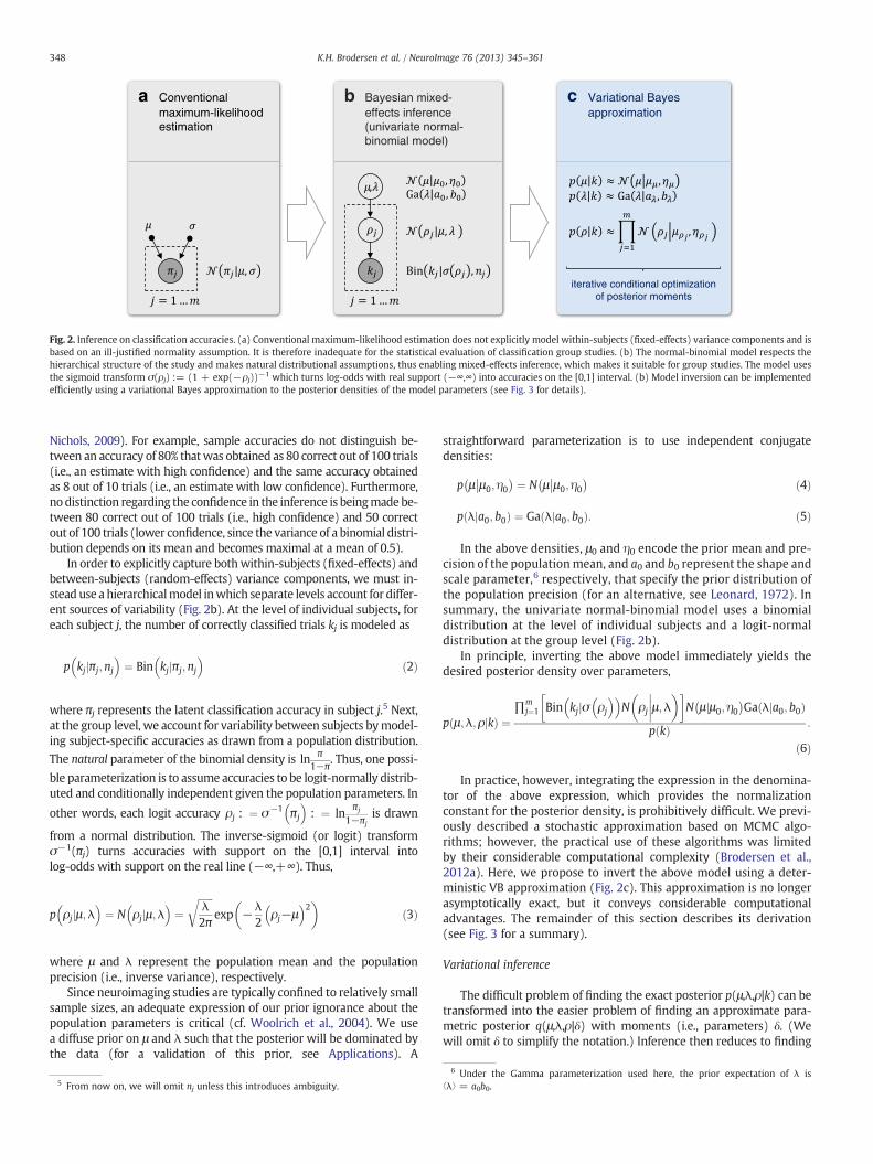
For each mean-field part in Eq. (11), the variational density q(⋅)can be obtained by evaluating the variational energy I(⋅), as describednext. The first variational energy concerns the posterior density overthe population mean μ. It is given by
I1 μð Þ ¼ ln p k; μ;λ;ρð Þh iq λ;ρð Þ ð20Þ
¼ ln p kjρð Þh iq λ;ρð Þ þ ln p ρjμ;λð Þh iq λ;ρð Þ þ ln p μ;λð Þh iq λ;ρð Þ ð21Þ
¼ ∑mj¼1 lnN ρjjμ;λ
� �D Eq λ;ρð Þ
þ ln N μjμ0; η0 �
Ga λja0; b0ð Þ �� �q λ;ρð Þ þ c ð22Þ
conditional maximization until convergence
(negative) free energy
Newton-Raphson
variational algorithm with Laplace approximations
parametric assumptions
mean-field approximation
variational inference
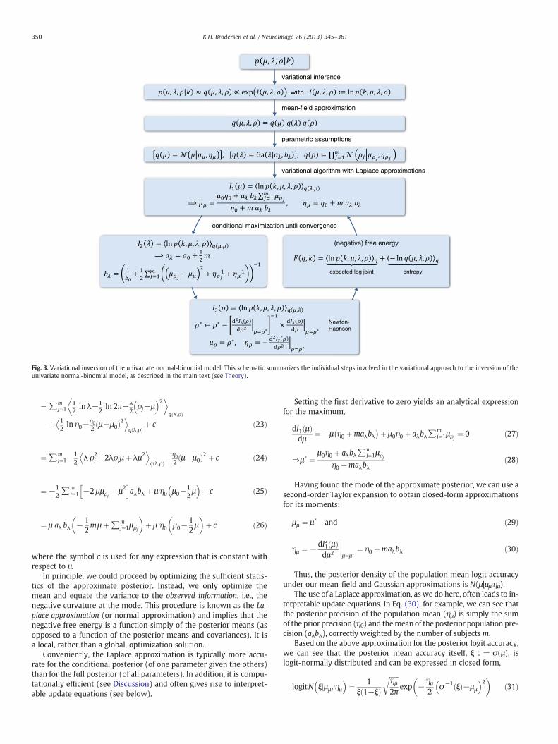
Fig. 3. Variational inversion of the univariate normal-binomial model. This schematic summarizes the individual steps involved in the variational approach to the inversion of theunivariate normal-binomial model, as described in the main text (see Theory).
350 K.H. Brodersen et al. / NeuroImage 76 (2013) 345–361
¼ ∑mj¼1
12ln λ−1
2ln 2π−λ
2ρj−μ� �2�
q λ;ρð Þþ 1
2ln η0−
η02
μ−μ0ð Þ2D E
q λ;ρð Þþ c ð23Þ
¼ ∑mj¼1−
12
λ ρ2j −2λρjμ þ λμ2
D Eq λ;ρð Þ
−η02
μ−μ0ð Þ2 þ c ð24Þ
¼ −12∑m
j¼1 −2 μμρjþ μ2
h iaλbλ þ μ η0 μ0−
12μ
� �þ c ð25Þ
¼ μ aλ bλ −12mμ þ∑m
j¼1μρj
� �þ μ η0 μ0−
12μ
� �þ c ð26Þ
where the symbol c is used for any expression that is constant withrespect to μ.
In principle, we could proceed by optimizing the sufficient statis-tics of the approximate posterior. Instead, we only optimize themean and equate the variance to the observed information, i.e., thenegative curvature at the mode. This procedure is known as the La-place approximation (or normal approximation) and implies that thenegative free energy is a function simply of the posterior means (asopposed to a function of the posterior means and covariances). It isa local, rather than a global, optimization solution.
Conveniently, the Laplace approximation is typically more accu-rate for the conditional posterior (of one parameter given the others)than for the full posterior (of all parameters). In addition, it is compu-tationally efficient (see Discussion) and often gives rise to interpret-able update equations (see below).
Setting the first derivative to zero yields an analytical expressionfor the maximum,
dI1 μð Þdμ
¼ −μ η0 þmaλbλ �þ μ0η0 þ aλbλ∑
mj¼1μρj
¼ 0 ð27Þ
⇒μ� ¼μ0η0 þ aλbλ∑
mj¼1μρj
η0 þmaλbλ: ð28Þ
Having found the mode of the approximate posterior, we can use asecond-order Taylor expansion to obtain closed-form approximationsfor its moments:
μμ ¼ μ� and ð29Þ
ημ ¼ −dI21 μð Þdμ2
����μ¼μ�
¼ η0 þmaλbλ: ð30Þ
Thus, the posterior density of the population mean logit accuracyunder our mean-field and Gaussian approximations is N(μ|μμ,ημ).
The use of a Laplace approximation, as we do here, often leads to in-terpretable update equations. In Eq. (30), for example, we can see thatthe posterior precision of the population mean (ημ) is simply the sumof the prior precision (η0) and themean of the posterior population pre-cision (aλbλ), correctly weighted by the number of subjects m.
Based on the above approximation for the posterior logit accuracy,we can see that the posterior mean accuracy itself, ξ : = σ(μ), islogit-normally distributed and can be expressed in closed form,
logitN ξjμμ ; ημ� �
¼ 1ξ 1−ξð Þ
ffiffiffiffiffiffiημ2π
rexp −
ημ2
σ−1 ξð Þ−μμ
� �2� �ð31Þ

351K.H. Brodersen et al. / NeuroImage 76 (2013) 345–361
where μμ and ημ represent the posterior mean and precision, respec-tively, of the population mean logit accuracy.
The second variational energy concerns the population precision λand is given by
I2 λð Þ ¼ ln p k; μ;λ;ρð Þh iq μ;ρð Þ ð32Þ
¼ m2
ln λ−λ2∑m
j¼1 μρj−μμ
� �2 þ η−1ρj
þ η−1μ
� �þ a0−1ð Þ ln λ− λ
b0þ c
ð33Þ
where c represents a term that is constant with respect to λ. Theabove expression already has the form of a log-Gamma distributionwith parameters
aλ ¼ a0 þ12m and ð34Þ
bλ ¼ 1b0
þ 12∑m
j¼1 μρj−μμ
� �2 þ η−1ρj
þ η−1μ
� �� �−1: ð35Þ
From this we can see that the shape parameter aλ is a weighted sumof prior shape a0 and datam. When viewing the second parameter as a‘rate’ coefficient bλ−1 (as opposed to a shape coefficient bλ), it becomesclear that the posterior rate really is a weighted sum of: the prior rate(b0−1); the dispersion of subject-specific means; their variances (η−1
ρj);
and our uncertainty about the population mean (ημ−1).The variational energy of the third partition concerns the model
parameters representing subject-specific latent accuracies. This ener-gy is given by
I3 ρð Þ ¼ ln p k; μ;λ;ρð Þh iq μ;λð Þ ð36Þ
¼ ∑mj¼1 kj lnσ ρj
� �þ nj−kj� �
ln 1−σ ρj
� �� �−1
2aλbλ ρj−μμ
� �2� �þ c: ð37Þ
Since an analytical expression for the maximum of this energydoes not exist, we resort to an iterative Newton–Raphson schemebased on a quadratic Taylor-series approximation to the variationalenergy I3(ρ). For this, we begin by considering the Jacobian
dI3 ρð Þdρ
� �j¼ ∂I3 ρð Þ
∂ρj¼ kj−njσ ρj
� �þ aλbλ μμ−ρ
� �ð38Þ
and the Hessian
d2I3 ρð Þdρ2
!jk
¼ ∂2I3 ρð Þ∂ρj∂ρk
¼ −δjk njσ ρj
� �1−σ ρj
� �� �þ aλbλ
� �ð39Þ
where the Kronecker delta operator δjk is 1 if j = k and 0 otherwise.As noted before, the absence of off-diagonal elements in the Hessianis not based on an assumption of conditional independence ofsubject-specific posteriors; it is a consequence of the mean-field sep-aration in Eq. (11). Each GN iteration performs the update
ρ� ← ρ�− d2I3 ρð Þdρ2
�����ρ¼ρ�
24
35−1
� dI3 ρð Þdρ
�����ρ¼ρ�
ð40Þ
until the vector ρ* converges, i.e., ‖ρ⁎current − ρ⁎previous‖2 b 10−3. Usingthismaximum,we can use a second-order Taylor expansion (i.e., the La-place approximation) to set themoments of the approximate posterior:
μρ ¼ ρ� and ð41Þ
ηρ ¼ −d2I3 ρð Þdρ2
�����ρ¼ρ�
: ð42Þ
Variational algorithm and free energy
The expressions for the three variational energies depend on oneanother. This circularity can be resolved by iterating over the expres-sions sequentially and updating the moments of each approximatemarginal given the current moments of the other marginals. This ap-proach of conditional maximization (or stepwise ascent) maximizesthe (negative) free energy F ≡ F(q,k) and leads to approximate mar-ginals that are maximally similar to the exact marginals.
The free energy itself can be expressed as the sum of the expectedlog-joint density (over the data and the model parameters) and theShannon entropy of the approximate posterior:
F ¼ ln p k; μ;λ;ρð Þh iq|fflfflfflfflfflfflfflfflfflfflfflfflfflffl{zfflfflfflfflfflfflfflfflfflfflfflfflfflffl}expected log joint
þ − ln q μ;λ;ρð Þh iq|fflfflfflfflfflfflfflfflfflfflfflfflfflffl{zfflfflfflfflfflfflfflfflfflfflfflfflfflffl}entropy H q½ �
: ð43Þ
We begin by considering the expectation of the log joint w.r.t. thevariational posterior:
ln p k; μ;λ;ρð Þh iq ¼∑mj¼1 ln Bin kjjσ ρj
� �� �þ lnN ρjjμ;λ
� �D Eq μð Þ
� q λð Þ|fflfflfflfflfflfflfflfflfflfflfflfflfflfflfflfflfflfflfflfflfflfflfflfflfflfflfflfflfflfflfflfflfflfflfflfflfflfflfflfflfflfflfflfflffl{zfflfflfflfflfflfflfflfflfflfflfflfflfflfflfflfflfflfflfflfflfflfflfflfflfflfflfflfflfflfflfflfflfflfflfflfflfflfflfflfflfflfflfflfflffl}
≡I ρjð Þ
* +q ρjð Þ
þ lnN μjμ0;η0 �� �
q þ ln Ga λja0; b0ð Þh iq:
ð44Þ
The above expression contains the variational energy of ρj,
I ρj
� �¼ ln Bin kjjσ ρj
� �� �þ 12
ψ aλð Þ þ ln bλð Þ
−12ln 2π−1
2aλbλ ρj−μμ
� �2 þ η−1μ
� � ð45Þ
where ψ(⋅) is the digamma function. I(ρj) is the only term in Eq. (44)whose expectation [w.r.t. q(ρj)] cannot be derived analytically. Underthe Laplace approximation, however, it is replaced by a second-orderTaylor expansion around the variational posterior mode μρj
,
I ρj
� �≈ I μρj
� �þ I ′ μρj
� �ρj−μρj
� �þ 12I ″ μρj
� �ρj−μρj
� �2: ð46Þ
This allows us to approximate the expectation of I(ρj) by
I ρj
� �D Eq ρjð Þ≈ I μρj
� �D Eq ρjð Þ|fflfflfflfflfflfflfflfflfflffl{zfflfflfflfflfflfflfflfflfflffl}
I μρj
� �þI ′ μρj
� �ρj−μρj
D Eq ρjð Þ|fflfflfflfflfflfflfflfflfflfflffl{zfflfflfflfflfflfflfflfflfflfflffl}
0
þ12I ″ μρj
� �|fflfflfflffl{zfflfflfflffl}
−ηρj
ρj−μρj
� �2� q ρjð Þ|fflfflfflfflfflfflfflfflfflfflfflfflfflfflffl{zfflfflfflfflfflfflfflfflfflfflfflfflfflfflffl}
η−1ρj
ð47Þ
¼ I μρj
� �−1
2ð48Þ
where the equality I″ μρj
� �¼ −ηρj
follows directly from Eq. (42).Hence, the expected log joint is:
ln p k; μ;λ;ρð Þh iq≈12ln
η02π
−η02
μμ−μ0
� �2 þ η−1μ
� �zfflfflfflfflfflfflfflfflfflfflfflfflfflfflfflfflfflfflfflfflfflfflfflfflfflfflfflfflfflfflffl}|fflfflfflfflfflfflfflfflfflfflfflfflfflfflfflfflfflfflfflfflfflfflfflfflfflfflfflfflfflfflffl{ln N μjμ0 ;η0ð Þh iq
− ln Γ a0ð Þ−a0 ln b0 þ a0−1ð Þ ψ aλð Þ þ ln bλð Þ− aλbλb0
zfflfflfflfflfflfflfflfflfflfflfflfflfflfflfflfflfflfflfflfflfflfflfflfflfflfflfflfflfflfflfflfflfflfflfflfflfflfflfflfflfflfflfflfflfflfflfflfflfflfflfflffl}|fflfflfflfflfflfflfflfflfflfflfflfflfflfflfflfflfflfflfflfflfflfflfflfflfflfflfflfflfflfflfflfflfflfflfflfflfflfflfflfflfflfflfflfflfflfflfflfflfflfflfflffl{lnGa λja0 ;b0ð Þh iq
þXmj¼1
ln Bin kjjσ μρj
� �� �
þ12
ψ aλð Þ þ lnbλð Þ−12ln 2π
−12aλbλ μρj
−μμ
� �2 þ η−1μ
� �−1
2
�ð49Þ
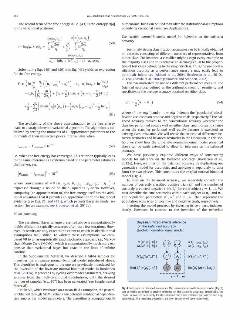
Bayesian mixed-effects inference on the balanced accuracy (twofold normal-binomial model)
Fig. 4. Inference on balanced accuracies. The univariate normal-binomial model (Fig. 2)can be easily extended to enable inference on the balanced accuracy. Specifically, themodel is inverted separately for classification outcomes obtained on positive and neg-ative trials. The resulting posteriors are then recombined (see main text).
352 K.H. Brodersen et al. / NeuroImage 76 (2013) 345–361
The second term of the free energy in Eq. (43) is the entropy H[q]of the variational posterior:
− ln q μ;λ;ρð Þh iq ¼12ln
2πeημ
zfflfflfflfflffl}|fflfflfflfflffl{H N μjμμ ;ημð Þ½ �
þXmj¼1
12ln
2πeηρj
zfflfflfflfflffl}|fflfflfflfflffl{H N ρj jμρj;ηρj
� �h i
þ aλ þ lnbλ þ lnΓ aλð Þ þ 1−aλð Þψ aλð Þzfflfflfflfflfflfflfflfflfflfflfflfflfflfflfflfflfflfflfflfflfflfflfflfflfflfflfflfflfflfflfflfflfflffl}|fflfflfflfflfflfflfflfflfflfflfflfflfflfflfflfflfflfflfflfflfflfflfflfflfflfflfflfflfflfflfflfflfflffl{H Ga λ aλ ;bλj Þð �½
ð50Þ
Substituting Eqs. (49) and (50) into Eq. (43) yields an expressionfor the free energy,
F ≈ 12ln
η0ημ
− η02
μμ−μ0
� �2 þ η−1μ
� �þ aλ−a0 ln b0 þ ln
Γ aλð ÞΓ a0ð Þ
−aλbλ1b0
þ m2ημ
!þ a0 þ
m2
� �ln bλ þ a0−aλ þ
m2
� �ψ aλð Þ
þ 12þXmj¼1
ln Bin kj σ μρj
� ���� �−1
2aλbλ μρj
−μμ
� �2−12ln ηρj
� �:
ð51Þ
The availability of the above approximation to the free energyleads to a straightforward variational algorithm. The algorithm is ini-tialized by setting the moments of all approximate posteriors to themoments of their respective priors. It terminates when
Fcurrent − Fprevious b 10−3 ð52Þ
i.e., when the free energy has converged. This criterion typically leadsto the same inference as a criterion based on the parameter estimatesthemselves, e.g.,
θcurrent − θprevious��� ���2 b 10−3 ð53Þ
where convergence of θ ≡ μμ ;ημ ; aλ; bλ; μρ1;…; μρm
; ηρ1;…;ηρm
� �is
expressed through a bound on their (squared) ‘2-norm. However,computing (an approximation to) the free energy itself has the addi-tional advantage that it provides an approximation to the log modelevidence (see Eqs. (9) and (43)), which permits Bayesian model se-lection (for an example, see Brodersen et al., 2012a).
MCMC sampling
The variational Bayes scheme presented above is computationallyhighly efficient; it typically converges after just a few iterations. How-ever, its results are only exact to the extent to which its distributionalassumptions are justified. To validate these assumptions, we com-pared VB to an asymptotically exact stochastic approach, i.e., Markovchain Monte Carlo (MCMC), which is computationally much more ex-pensive than variational Bayes but exact in the limit of infiniteruntime.
In the Supplemental Material, we describe a Gibbs sampler forinverting the univariate normal-binomial model introduced above.This algorithm is analogous to the one we previously introduced forthe inversion of the bivariate normal-binomial model in Brodersenet al. (2012a). It proceeds by cycling over model parameters, drawingsamples from their full-conditional distributions, until the desirednumber of samples (e.g., 106) has been generated (see SupplementalMaterial).
Unlike VB, which was based on amean-field assumption, the posteri-or obtained through MCMC retains any potential conditional dependen-cies among the model parameters. The algorithm is computationally
burdensome; but it canbe used to validate the distributional assumptionsunderlying variational Bayes (see Applications).
The twofold normal-binomial model for inference on the balancedaccuracy
Seemingly strong classification accuracies can be trivially obtainedon datasets consisting of different numbers of representatives fromeither class. For instance, a classifier might assign every example tothe majority class and thus achieve an accuracy equal to the propor-tion of test cases belonging to the majority class. Thus, the use of clas-sification accuracy as a performance measure may easily lead tooptimistic inferences (Akbani et al., 2004; Brodersen et al., 2010a,2012a; Chawla et al., 2002; Japkowicz and Stephen, 2002).
This has motivated the use of a different performance measure: thebalanced accuracy, defined as the arithmetic mean of sensitivity andspecificity, or the average accuracy obtained on either class,
φ : ¼ 12
πþ þ π−� �
ð54Þ
where π+ : = σ(μ+) and π− : = σ(μ−) denote the (population) classi-fication accuracies on positive and negative trials, respectively.8 The bal-anced accuracy reduces to the conventional accuracy whenever theclassifier performed equally well on either class; and it drops to chancewhen the classifier performed well purely because it exploited anexisting class imbalance. We will revisit the conceptual differences be-tween accuracies and balanced accuracies in the Discussion. In this sec-tion, we show how the univariate normal-binomial model presentedabove can be easily extended to allow for inference on the balancedaccuracy.
We have previously explored different ways of constructingmodels for inference on the balanced accuracy (Brodersen et al.,2012a). Here, we infer on the balanced accuracy by duplicating ourgenerative model for accuracies and applying it separately to datafrom the two classes. This constitutes the twofold normal-binomialmodel (Fig. 4).
To infer on the balanced accuracy, we separately consider thenumber of correctly classified positive trials kj
+ and the number ofcorrectly predicted negative trials kj
− for each subject j = 1…m. Wenext describe the true accuracies within each subject as πj+ and πj−.The population parameters μ+, λ+ and μ−, λ− then represent thepopulation accuracies on positive and negative trials, respectively.
Inverting the model proceeds by inverting its two parts indepen-dently. However, in contrast to the inversion of the univariate
9 Note that the heteroscedasticity in this dataset results both from the fact that sub-jects have different numbers of trials and from their different sample accuracies.
353K.H. Brodersen et al. / NeuroImage 76 (2013) 345–361
normal-binomial model, we are no longer interested in the posteriordensities over the population mean accuracies μ+ and μ− themselves.Rather, we wish to obtain the posterior density of the balanced accura-cy,
p ϕjkþ; k−� �
¼ p12
σ μþ� �þ σ μ−ð Þ
� �kþ; k−��� �
:
�ð55Þ
Unlike the population mean accuracy (Eq. (29)), which waslogit-normally distributed, the posteriormean of the population balancedaccuracy can no longer be expressed in closed form. The same applies tosubject-specific posterior balanced accuracies. We therefore approxi-mate the respective integrals by (one-dimensional) numerical integra-tion. If we were interested in the sum of the two class-specificaccuracies, s : = σ(μ+) + σ(μ−), we would consider the convolutionof the distributions for σ(μ+) and σ(μ−),
p s kþ; k−��� �
¼ ∫s0pσ μþð Þ s−z kþ
��� �pσ μ−ð Þ z k−j Þdzð
��ð56Þ
wherepσ μþð Þ andpσ μ−ð Þ represent the individual posterior distributions ofthe population accuracy on positive and negative trials, respectively. Inthe same spirit, the modified convolution
p ϕjkþ; k−� �
¼ ∫2φ0 pσ μþð Þ 2ϕ−zjkþ
� �pσ μ−ð Þ z k−j Þdzð ð57Þ
yields the posterior distribution of the arithmetic mean of twoclass-specific accuracies, i.e., the balanced accuracy.
Applications
This section illustrates the sort of inferences that can be made usingVB in a classification study of a group of subjects.We begin by consider-ing synthetic classification outcomes to evaluate the consistency of ourapproach and illustrate its link to classical fixed-effects and random-effects analyses. We then apply our approach to empirical fMRI dataobtained from a trial-by-trial classification analysis.
Application to synthetic data
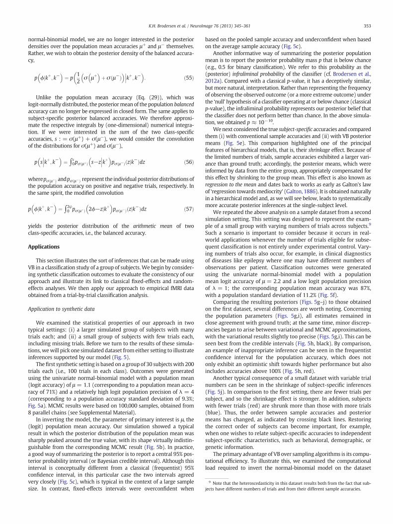
We examined the statistical properties of our approach in twotypical settings: (i) a larger simulated group of subjects with manytrials each; and (ii) a small group of subjects with few trials each,including missing trials. Before we turn to the results of these simula-tions, wewill pick one simulated dataset from either setting to illustrateinferences supported by our model (Fig. 5).
Thefirst synthetic setting is based on a group of 30 subjectswith 200trials each (i.e., 100 trials in each class). Outcomes were generatedusing the univariate normal-binomial model with a population mean(logit accuracy) of μ = 1.1 (corresponding to a population mean accu-racy of 71%) and a relatively high logit population precision of λ = 4(corresponding to a population accuracy standard deviation of 9.3%;Fig. 5a). MCMC results were based on 100,000 samples, obtained from8 parallel chains (see Supplemental Material).
In inverting the model, the parameter of primary interest is μ, the(logit) population mean accuracy. Our simulation showed a typicalresult in which the posterior distribution of the population mean wassharply peaked around the true value, with its shape virtually indistin-guishable from the corresponding MCMC result (Fig. 5b). In practice,a good way of summarizing the posterior is to report a central 95% pos-terior probability interval (or Bayesian credible interval). Although thisinterval is conceptually different from a classical (frequentist) 95%confidence interval, in this particular case the two intervals agreedvery closely (Fig. 5c), which is typical in the context of a large samplesize. In contrast, fixed-effects intervals were overconfident when
based on the pooled sample accuracy and underconfident when basedon the average sample accuracy (Fig. 5c).
Another informative way of summarizing the posterior populationmean is to report the posterior probability mass p that is below chance(e.g., 0.5 for binary classification). We refer to this probability as the(posterior) infraliminal probability of the classifier (cf. Brodersen et al.,2012a). Compared with a classical p-value, it has a deceptively similar,butmore natural, interpretation. Rather than representing the frequencyof observing the observed outcome (or a more extreme outcome) underthe ‘null’ hypothesis of a classifier operating at or below chance (classicalp-value), the infraliminal probability represents our posterior belief thatthe classifier does not perform better than chance. In the above simula-tion, we obtained p ≈ 10−10.
Wenext considered the true subject-specific accuracies and comparedthem (i) with conventional sample accuracies and (ii) with VB posteriormeans (Fig. 5e). This comparison highlighted one of the principalfeatures of hierarchical models, that is, their shrinkage effect. Because ofthe limited numbers of trials, sample accuracies exhibited a larger vari-ance than ground truth; accordingly, the posterior means, which wereinformed by data from the entire group, appropriately compensated forthis effect by shrinking to the group mean. This effect is also known asregression to the mean and dates back to works as early as Galton's lawof ‘regression towardsmediocrity’ (Galton, 1886). It is obtained naturallyin a hierarchical model and, as wewill see below, leads to systematicallymore accurate posterior inferences at the single-subject level.
We repeated the above analysis on a sample dataset from a secondsimulation setting. This setting was designed to represent the exam-ple of a small group with varying numbers of trials across subjects.9
Such a scenario is important to consider because it occurs in real-world applications whenever the number of trials eligible for subse-quent classification is not entirely under experimental control. Vary-ing numbers of trials also occur, for example, in clinical diagnosticsof diseases like epilepsy where one may have different numbers ofobservations per patient. Classification outcomes were generatedusing the univariate normal-binomial model with a populationmean logit accuracy of μ = 2.2 and a low logit population precisionof λ = 1; the corresponding population mean accuracy was 87%,with a population standard deviation of 11.2% (Fig. 5f).
Comparing the resulting posteriors (Figs. 5g–j) to those obtainedon the first dataset, several differences are worth noting. Concerningthe population parameters (Figs. 5g,i), all estimates remained inclose agreement with ground truth; at the same time, minor discrep-ancies began to arise between variational and MCMC approximations,with the variational results slightly too precise (Figs. 5g,i). This can beseen best from the credible intervals (Fig. 5h, black). By comparison,an example of inappropriate inference can be seen in the frequentistconfidence interval for the population accuracy, which does notonly exhibit an optimistic shift towards higher performance but alsoincludes accuracies above 100% (Fig. 5h, red).
Another typical consequence of a small dataset with variable trialnumbers can be seen in the shrinkage of subject-specific inferences(Fig. 5j). In comparison to the first setting, there are fewer trials persubject, and so the shrinkage effect is stronger. In addition, subjectswith fewer trials (red) are shrunk more than those with more trials(blue). Thus, the order between sample accuracies and posteriormeans has changed, as indicated by crossing black lines. Restoringthe correct order of subjects can become important, for example,when one wishes to relate subject-specific accuracies to independentsubject-specific characteristics, such as behavioral, demographic, orgenetic information.
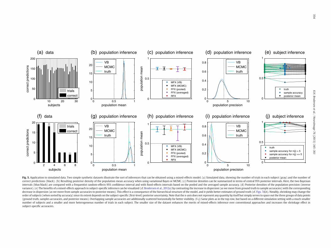
The primary advantage of VB over sampling algorithms is its compu-tational efficiency. To illustrate this, we examined the computationalload required to invert the normal-binomial model on the dataset
10 20 300
50
100
150
200
subjects
corr
ect p
redi
ctio
ns
(a) data
trialscorrect
0 0.5 10
5
10
15
20
population mean
(b) population inference
VBMCMCtruth
0
0.5
1
(c) population inference
popu
latio
n m
ean
MFX (VB)MFX (MCMC)FFX (pooled)FFX (averaged)RFX
0 5 100
0.2
0.4
0.6
0.8
population precision
(d) population inference
VBMCMCtruth
0
0.5
1
(e) subject inference
truthsample accuracyposterior mean
2 4 6 80
5
10
15
20
subjects
corr
ect p
redi
ctio
ns
(f) data
trialscorrect
0 0.5 10
5
10
15
20
population mean
(g) population inference
VBMCMCtruth
0
0.5
1
(h) population inference
popu
latio
n m
ean
MFX (VB)MFX (MCMC)FFX (pooled)FFX (averaged)RFX
0 5 100
0.2
0.4
0.6
0.8
population precision
(i) population inference
VBMCMCtruth
0
0.5
1
(j) subject inference
truthsample accuracy for n(j) > 5sample accuracy for n(j) <= 5posterior mean
Fig. 5. Application to simulated data. Two simple synthetic datasets illustrate the sort of inferences that can be obtained using a mixed-effects model. (a) Simulated data, showing the number of trials in each subject (gray) and the number ofcorrect predictions (black). (b) Resulting posterior density of the population mean accuracy when using variational Bayes or MCMC. (c) Posterior densities can be summarized in terms of central 95% posterior intervals. Here, the two Bayesianintervals (blue/black) are compared with a frequentist random-effects 95% confidence interval and with fixed-effects intervals based on the pooled and the averaged sample accuracy. (d) Posterior densities of the population precision (inversevariance). (e) The benefits of amixed-effects approach in subject-specific inference can be visualized (cf. Brodersen et al., 2012a) by contrasting the increase in dispersion (aswemove from ground truth to sample accuracies)with the correspondingdecrease in dispersion (as wemove from sample accuracies to posterior means). This effect is a consequence of the hierarchical structure of the model, and it yields better estimates of ground truth (cf. Figs. 7d,h). Notably, shrinkingmay change theorder of subjects (when sorted by accuracy) since its extent depends on the subject-specific (first-level) posterior uncertainty. Note that the x-axis does not represent any quantity by itself but simply serves to space out the three groups of data points(ground truth, samples accuracies, and posterior means). Overlapping sample accuracies are additionally scattered horizontally for better visibility. (f–j) Same plots as in the top row, but based on a different simulation setting with a much smallernumber of subjects and a smaller and more heterogeneous number of trials in each subject. The smaller size of the dataset enhances the merits of mixed-effects inference over conventional approaches and increases the shrinkage effect insubject-specific accuracies.
354K.H.Brodersen
etal./
NeuroIm
age76
(2013)345
–361
105 106 107 108 10910-2
100
102
FLOPs
abso
lute
err
or (
% p
oint
s) MCMCVB
0.01 s 4:18 min
Fig. 6. Estimation error and computational complexity. VB andMCMCdiffer in theway es-timation error and computational complexity are traded off. The plot shows estimationerror in terms of the absolute difference of the posterior mean of the populationmean ac-curacy in percentage points (y-axis). Computational complexity is shown in terms of thenumber of floating point operations (FLOPs) consumed. VB converged after 370,000FLOPs (iterative update b 10−6) to a posterior mean of the population mean accuracy of73.5%. Given a true population mean of 73.9%, the estimation error of VB was −0.4 per-centage points. In contrast, MCMC used up 1.47 × 10⁹ FLOPs to draw 10,000 samples(excluding 100 burn-in samples). Its posterior mean estimate was 73.6%, implying anerror of −0.26 percentage points. Thus, while MCMC ultimately achieved a marginallylower error, VB was computationally more efficient by more than 3 orders of magnitude.It should be noted that the plot uses log–log axes for readability; the difference betweenthe two algorithms would be visually even more striking on a linear scale.
355K.H. Brodersen et al. / NeuroImage 76 (2013) 345–361
shown in Fig. 5a. Rather than measuring computation time (which isplatform-dependent), we considered the number of floating-pointoperations (FLOPs), which we related to the absolute error of the in-ferred posterior mean of the mean population accuracy (in percentagepoints; Fig. 6). We found that MCMC used 4000 times more arithmeticoperations to achieve an estimate that was better than VB by no morethan 0.13 percentage points.
10 20 300
50
100
150
200
subjects
corr
ect p
redi
ctio
ns
(a) example data
trialscorrect
0 0.5 10
0.2
0.4
0.6
0.8
1
p(re
ject
| π
= 0
.5;
α)
test size α
(b) specificity
2 4 6 80
5
10
15
20
subjects
corr
ect p
redi
ctio
ns
(e) example data
trialscorrect
0 0.5 10
0.2
0.4
0.6
0.8
1
p(re
ject
| π
= 0
.5;
α)
test size a
(f) specificity
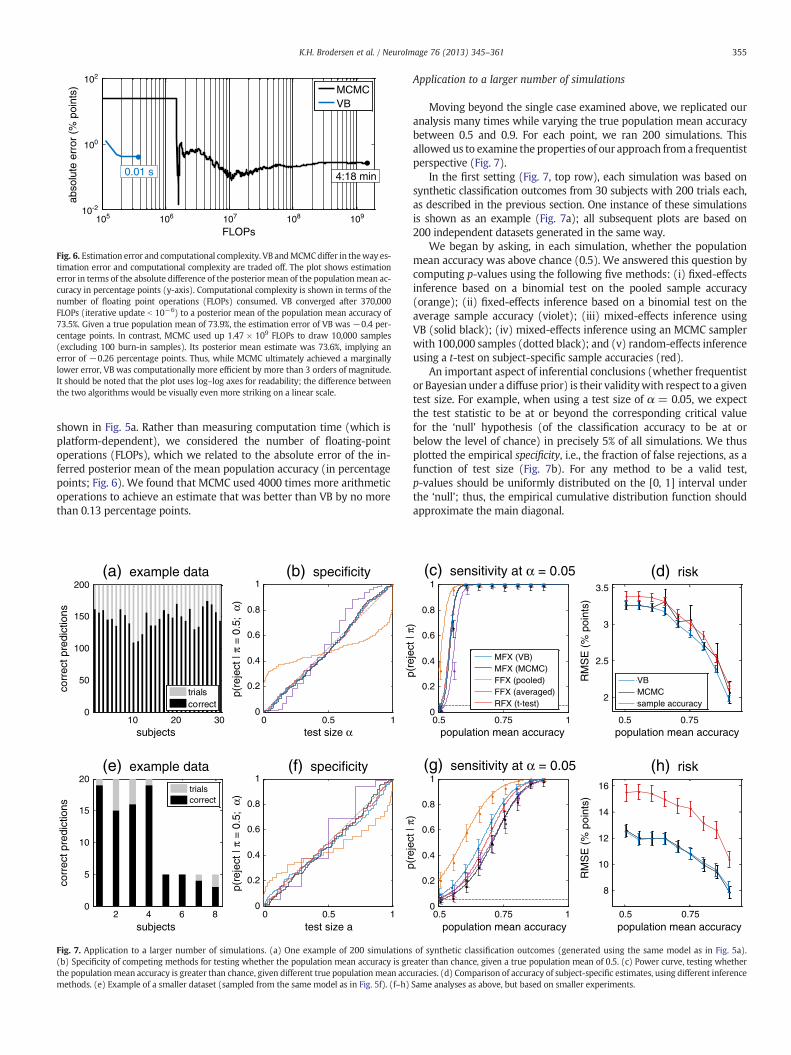
Fig. 7. Application to a larger number of simulations. (a) One example of 200 simulations(b) Specificity of competing methods for testing whether the population mean accuracy is grethe populationmean accuracy is greater than chance, given different true population mean accmethods. (e) Example of a smaller dataset (sampled from the same model as in Fig. 5f). (f–h)
Application to a larger number of simulations
Moving beyond the single case examined above, we replicated ouranalysis many times while varying the true population mean accuracybetween 0.5 and 0.9. For each point, we ran 200 simulations. Thisallowed us to examine the properties of our approach froma frequentistperspective (Fig. 7).
In the first setting (Fig. 7, top row), each simulation was based onsynthetic classification outcomes from 30 subjects with 200 trials each,as described in the previous section. One instance of these simulationsis shown as an example (Fig. 7a); all subsequent plots are based on200 independent datasets generated in the same way.
We began by asking, in each simulation, whether the populationmean accuracy was above chance (0.5). We answered this question bycomputing p-values using the following five methods: (i) fixed-effectsinference based on a binomial test on the pooled sample accuracy(orange); (ii) fixed-effects inference based on a binomial test on theaverage sample accuracy (violet); (iii) mixed-effects inference usingVB (solid black); (iv) mixed-effects inference using an MCMC samplerwith 100,000 samples (dotted black); and (v) random-effects inferenceusing a t-test on subject-specific sample accuracies (red).
An important aspect of inferential conclusions (whether frequentistor Bayesian under a diffuse prior) is their validitywith respect to a giventest size. For example, when using a test size of α = 0.05, we expectthe test statistic to be at or beyond the corresponding critical valuefor the ‘null’ hypothesis (of the classification accuracy to be at orbelow the level of chance) in precisely 5% of all simulations. We thusplotted the empirical specificity, i.e., the fraction of false rejections, as afunction of test size (Fig. 7b). For any method to be a valid test,p-values should be uniformly distributed on the [0, 1] interval underthe ‘null’; thus, the empirical cumulative distribution function shouldapproximate the main diagonal.
0.5 0.75 10
0.2
0.4
0.6
0.8
1
population mean accuracy
p(re
ject
| π)
(c) sensitivity at α = 0.05
MFX (VB)MFX (MCMC)FFX (pooled)FFX (averaged)RFX (t-test)
0.5 0.75
2
2.5
3
3.5
population mean accuracy
RM
SE
(%
poi
nts)
(d) risk
VBMCMCsample accuracy
0.5 0.75 10
0.2
0.4
0.6
0.8
1
population mean accuracy
p(re
ject
| π)
(g) sensitivity at α = 0.05
0.5 0.75
8
10
12
14
16
population mean accuracy
RM
SE
(%
poi
nts)
(h) risk
of synthetic classification outcomes (generated using the same model as in Fig. 5a).ater than chance, given a true population mean of 0.5. (c) Power curve, testing whetheruracies. (d) Comparison of accuracy of subject-specific estimates, using different inferenceSame analyses as above, but based on smaller experiments.
5 10 15 200
20
40
60
subjects
corr
ect p
redi
ctio
ns
(a) data
0 0.5 10
0.2
0.4
0.6
0.8
1
TNR
TP
R
(b) data and ground truth
0
0.2
0.4
0.6
0.8
1
(c) population inference
popu
latio
n m
ean
posterior accuracy
posterior balanced accuracy
ground truthchance
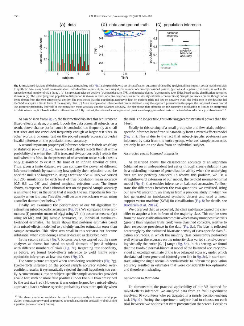
Fig. 8. Imbalanceddata and the balanced accuracy. (a) In analogywith Fig. 7a, the panel shows a set of classification outcomes obtainedby applying a linear support vectormachine (SVM)to synthetic data, using 5-fold cross-validation. Individual bars represent, for each subject, the number of correctly classified positive (green) and negative (red) trials, as well as therespective total number of trials (gray). (b) Sample accuracies on positive (true positive rate, TPR) and negative classes (true negative rate, TNR), based on the classification outcomesshown in (a). The underlying true population distribution is shown in terms of a bivariate Gaussian kernel density estimate (contour lines). Sample accuracies can be thought of asbeing drawn from this two-dimensional density. The plot shows that the population accuracy is high on positive trials and low on negative trials; the imbalance in the data has ledthe SVM to acquire a bias in favor of the majority class. (c) As an example of an inference that can be obtained using the approach presented in this paper, the last panel shows central95% posterior probability intervals of the population mean accuracy and the balanced accuracy. The plot shows that inference on the accuracy is misleading as it must be interpretedin relation to an implicit baseline that is different from 0.5. By contrast, the balanced accuracy interval provides a sharply peaked estimate of the true balanced accuracy; its baseline is 0.5.
356 K.H. Brodersen et al. / NeuroImage 76 (2013) 345–361
As can be seen fromFig. 7b, thefirstmethod violates this requirement(fixed-effects analysis, orange). It pools the data across all subjects; as aresult, above-chance performance is concluded too frequently at smalltest sizes and not concluded frequently enough at larger test sizes. Inother words, a binomial test on the pooled sample accuracy providesinvalid inference on the population mean accuracy.
A second important property of inference schemes is their sensitivityor statistical power (Fig. 7c). An ideal test (falsely) rejects the null with aprobability of αwhen the null is true, and always (correctly) rejects thenull when it is false. In the presence of observation noise, such a test isonly guaranteed to exist in the limit of an infinite amount of data.Thus, given a finite dataset, we can compare the power of differentinference methods by examining how quickly their rejection rates riseonce the null is no longer true. Using a test size of α = 0.05, we carriedout 200 simulations for each level of true population mean accuracy(0.5, 0.6, …, 0.9) and plotted empirical rejection rates. The figureshows, as expected, that a Binomial test on the pooled sample accuracyis an invalid test, in the sense that it rejects the null hypothesis too fre-quently when it is true. This effect will become even clearer when usinga smaller dataset (see below).10
Finally, we examined the performance of our VB algorithm forestimating subject-specific accuracies (Fig. 7d). We compared three esti-mators: (i) posterior means of σ(ρj) using VB; (ii) posterior means σ(ρj)using MCMC; and (iii) sample accuracies, i.e., individual maximum-likelihood estimates. The figure shows that posterior estimates basedon a mixed-effects model led to a slightly smaller estimation error thansample accuracies. This effect was small in this scenario but becamesubstantial when considering a smaller dataset, as described next.
In the second setting (Fig. 7, bottom row), we carried out the sameanalyses as above, but based on small datasets of just 8 subjectswith different numbers of trials (Fig. 7e). Regarding test specificity,as before, we found fixed-effects inference to yield highly over-optimistic inferences at low test sizes (Fig. 7f).
The same picture emerged when considering sensitivities (Fig. 7g).Fixed-effects inference on the pooled sample accuracy yielded over-confident results; it systematically rejected the null hypothesis too eas-ily. A conventional t-test on subject-specific sample accuracies provideda valid test, with nomore false positives under the null than prescribedby the test size (red). However, it was outperformed by a mixed-effectsapproach (black), whose rejection probability rises more quickly when
10 The above simulation could also be used for a power analysis to assess what pop-ulation mean accuracy would be required to reach a particular probability of obtaininga positive (above-chance) finding.
the null is no longer true, thus offering greater statistical power than thet-test.
Finally, in this setting of a small group size and few trials, subject-specific inference benefitted substantially from a mixed-effects model(Fig. 7h). This is due to the fact that subject-specific posteriors areinformed by data from the entire group, whereas sample accuraciesare only based on the data from an individual subject.
Accuracies versus balanced accuracies
As described above, the classification accuracy of an algorithm(obtained on an independent test set or through cross-validation) canbe a misleading measure of generalization ability when the underlyingdata are not perfectly balanced. To resolve this problem, we use astraightforward extension of our model, the twofold normal-binomialmodel (Fig. 4), that enables inference on balanced accuracies. To illus-trate the differences between the two quantities, we revisited, usingour new VB algorithm, an analysis from a previous study in which wehad generated an imbalanced synthetic dataset and used a linearsupport vector machine (SVM) for classification (Fig. 8; for details, seeBrodersen et al., 2012a).
We observed that, as expected, the class imbalance caused the clas-sifier to acquire a bias in favor of the majority class. This can be seenfrom the raw classificationoutcomes inwhichmanymore positive trials(green) than negative trials (red) were classified correctly, relative totheir respective prevalence in the data (Fig. 8a). The bias is reflectedaccordingly by the estimated bivariate density of class-specific classifi-cation accuracies, in which the majority class consistently performedwell whereas the accuracy on the minority class varied strongly, cover-ing virtually the entire [0, 1] range (Fig. 8b). In this setting, we foundthat the twofold normal-binomial model of the balanced accuracy pro-vided an excellent estimate of the true balanced accuracy under whichthe data had been generated (dotted green line in Fig. 8c). In stark con-trast, using the single normal-binomialmodel to infer on the populationaccuracy resulted in estimates that were considerably too optimisticand therefore misleading.
Application to fMRI data
To demonstrate the practical applicability of our VB method formixed-effects inference, we analyzed data from an fMRI experimentinvolving 16 volunteers who participated in a simple decision-makingtask (Fig. 9). During the experiment, subjects had to choose, on eachtrial, between two options that were presented on the screen. Decisions
5 10 150
20
40
60
subjects
corr
ect p
redi
ctio
ns(a) data
0 0.5 10
0.2
0.4
0.6
0.8
1
TNRT
PR
(b) data
0 0.5 10
5
10
15
20
25
population mean
(c) population inference
balanced acc.chance
0 5 10 150
0.2
0.4
0.6
0.8
1(d) subject inference
subjects (sorted)
accu
racy
sample balanced acc.posterior mean
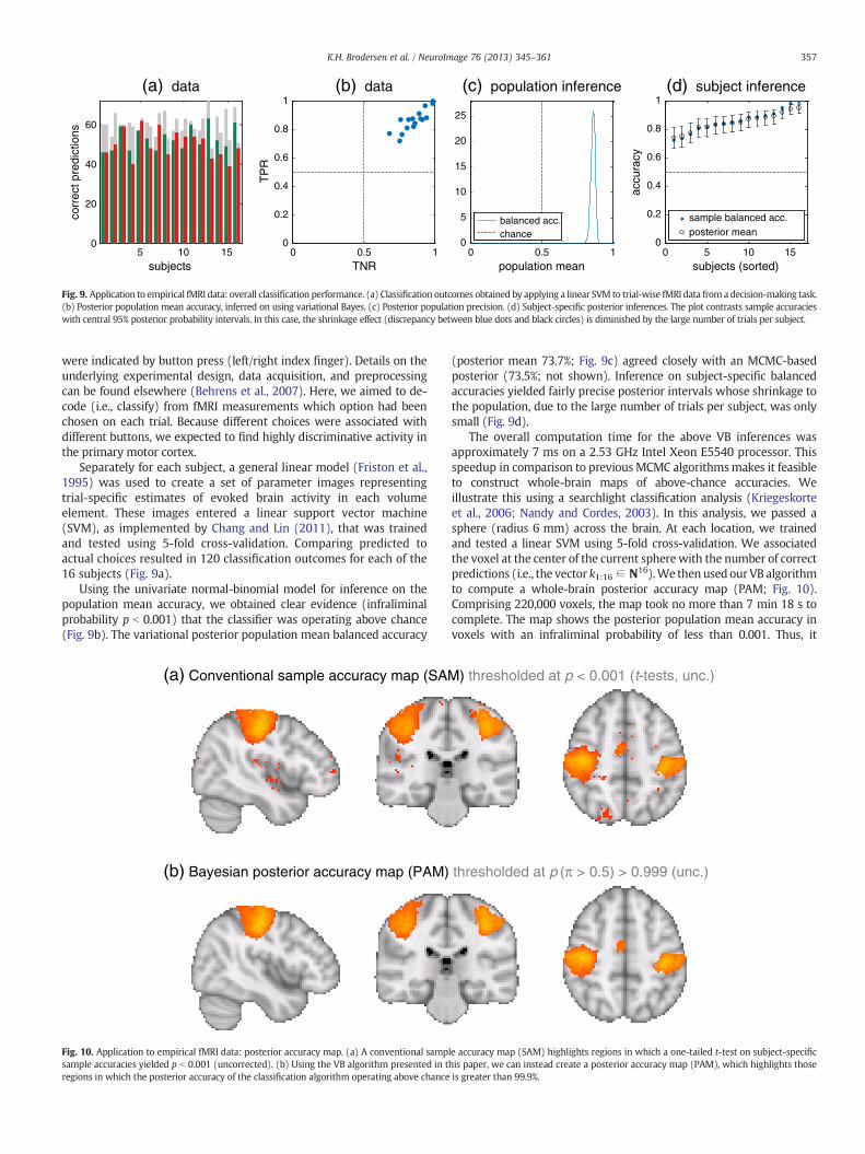
Fig. 9. Application to empirical fMRI data: overall classification performance. (a) Classification outcomes obtained by applying a linear SVM to trial-wise fMRI data from a decision-making task.(b) Posterior population mean accuracy, inferred on using variational Bayes. (c) Posterior population precision. (d) Subject-specific posterior inferences. The plot contrasts sample accuracieswith central 95% posterior probability intervals. In this case, the shrinkage effect (discrepancy between blue dots and black circles) is diminished by the large number of trials per subject.
357K.H. Brodersen et al. / NeuroImage 76 (2013) 345–361
were indicated by button press (left/right index finger). Details on theunderlying experimental design, data acquisition, and preprocessingcan be found elsewhere (Behrens et al., 2007). Here, we aimed to de-code (i.e., classify) from fMRI measurements which option had beenchosen on each trial. Because different choices were associated withdifferent buttons, we expected to find highly discriminative activity inthe primary motor cortex.
Separately for each subject, a general linear model (Friston et al.,1995) was used to create a set of parameter images representingtrial-specific estimates of evoked brain activity in each volumeelement. These images entered a linear support vector machine(SVM), as implemented by Chang and Lin (2011), that was trainedand tested using 5-fold cross-validation. Comparing predicted toactual choices resulted in 120 classification outcomes for each of the16 subjects (Fig. 9a).
Using the univariate normal-binomial model for inference on thepopulation mean accuracy, we obtained clear evidence (infraliminalprobability p b 0.001) that the classifier was operating above chance(Fig. 9b). The variational posterior population mean balanced accuracy
(a) Conventional sample accuracy map (SAM
(b) Bayesian posterior accuracy map (PAM)
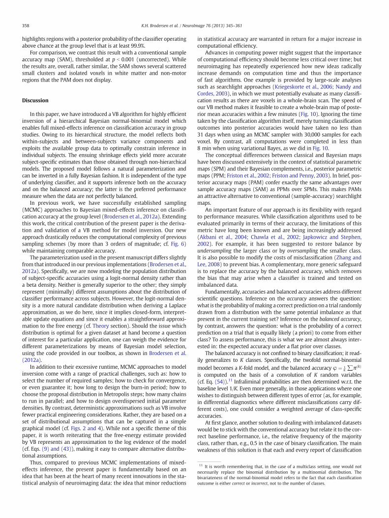
Fig. 10. Application to empirical fMRI data: posterior accuracy map. (a) A conventional sampsample accuracies yielded p b 0.001 (uncorrected). (b) Using the VB algorithm presented in tregions in which the posterior accuracy of the classification algorithm operating above chance
(posterior mean 73.7%; Fig. 9c) agreed closely with an MCMC-basedposterior (73.5%; not shown). Inference on subject-specific balancedaccuracies yielded fairly precise posterior intervals whose shrinkage tothe population, due to the large number of trials per subject, was onlysmall (Fig. 9d).
The overall computation time for the above VB inferences wasapproximately 7 ms on a 2.53 GHz Intel Xeon E5540 processor. Thisspeedup in comparison to previous MCMC algorithmsmakes it feasibleto construct whole-brain maps of above-chance accuracies. Weillustrate this using a searchlight classification analysis (Kriegeskorteet al., 2006; Nandy and Cordes, 2003). In this analysis, we passed asphere (radius 6 mm) across the brain. At each location, we trainedand tested a linear SVM using 5-fold cross-validation. We associatedthe voxel at the center of the current spherewith the number of correctpredictions (i.e., the vector k1:16 ∈ N16).We then used ourVB algorithmto compute a whole-brain posterior accuracy map (PAM; Fig. 10).Comprising 220,000 voxels, the map took no more than 7 min 18 s tocomplete. The map shows the posterior population mean accuracy invoxels with an infraliminal probability of less than 0.001. Thus, it
) thresholded at p < 0.001 (t-tests, unc.)
thresholded at p (π > 0.5) > 0.999 (unc.)
le accuracy map (SAM) highlights regions in which a one-tailed t-test on subject-specifichis paper, we can instead create a posterior accuracy map (PAM), which highlights thoseis greater than 99.9%.
358 K.H. Brodersen et al. / NeuroImage 76 (2013) 345–361
highlights regionswith a posterior probability of the classifier operatingabove chance at the group level that is at least 99.9%.
For comparison, we contrast this result with a conventional sampleaccuracy map (SAM), thresholded at p b 0.001 (uncorrected). Whilethe results are, overall, rather similar, the SAM shows several scatteredsmall clusters and isolated voxels in white matter and non-motorregions that the PAM does not display.
11 It is worth remembering that, in the case of a multiclass setting, one would notnecessarily replace the binomial distribution by a multinomial distribution. Thebivariateness of the normal-binomial model refers to the fact that each classificationoutcome is either correct or incorrect, not to the number of classes.
Discussion
In this paper, we have introduced a VB algorithm for highly efficientinversion of a hierarchical Bayesian normal-binomial model whichenables full mixed-effects inference on classification accuracy in groupstudies. Owing to its hierarchical structure, the model reflects bothwithin-subjects and between-subjects variance components andexploits the available group data to optimally constrain inference inindividual subjects. The ensuing shrinkage effects yield more accuratesubject-specific estimates than those obtained through non-hierarchicalmodels. The proposed model follows a natural parameterization andcan be inverted in a fully Bayesian fashion. It is independent of the typeof underlying classifier, and it supports inference both on the accuracyand on the balanced accuracy; the latter is the preferred performancemeasure when the data are not perfectly balanced.
In previous work, we have successfully established sampling(MCMC) approaches to Bayesian mixed-effects inference on classifi-cation accuracy at the group level (Brodersen et al., 2012a). Extendingthis work, the critical contribution of the present paper is the deriva-tion and validation of a VB method for model inversion. Our newapproach drastically reduces the computational complexity of previoussampling schemes (by more than 3 orders of magnitude; cf. Fig. 6)while maintaining comparable accuracy.
The parameterization used in the presentmanuscript differs slightlyfrom that introduced in our previous implementations (Brodersen et al.,2012a). Specifically, we are now modeling the population distributionof subject-specific accuracies using a logit-normal density rather thana beta density. Neither is generally superior to the other; they simplyrepresent (minimally) different assumptions about the distribution ofclassifier performance across subjects. However, the logit-normal den-sity is a more natural candidate distribution when deriving a Laplaceapproximation, as we do here, since it implies closed-form, interpret-able update equations and since it enables a straightforward approxi-mation to the free energy (cf. Theory section). Should the issue whichdistribution is optimal for a given dataset at hand become a questionof interest for a particular application, one can weigh the evidence fordifferent parameterizations by means of Bayesian model selection,using the code provided in our toolbox, as shown in Brodersen et al.(2012a).
In addition to their excessive runtime, MCMC approaches to modelinversion come with a range of practical challenges, such as: how toselect the number of required samples; how to check for convergence,or even guarantee it; how long to design the burn-in period; how tochoose the proposal distribution in Metropolis steps; howmany chainsto run in parallel; and how to design overdispersed initial parameterdensities. By contrast, deterministic approximations such as VB involvefewer practical engineering considerations. Rather, they are based on aset of distributional assumptions that can be captured in a simplegraphical model (cf. Figs. 2 and 4). While not a specific theme of thispaper, it is worth reiterating that the free-energy estimate providedby VB represents an approximation to the log evidence of the model(cf. Eqs. (9) and (43)), making it easy to compare alternative distribu-tional assumptions.
Thus, compared to previous MCMC implementations of mixed-effects inference, the present paper is fundamentally based on anidea that has been at the heart of many recent innovations in the sta-tistical analysis of neuroimaging data: the idea that minor reductions
in statistical accuracy are warranted in return for a major increase incomputational efficiency.
Advances in computing power might suggest that the importanceof computational efficiency should become less critical over time; butneuroimaging has repeatedly experienced how new ideas radicallyincrease demands on computation time and thus the importanceof fast algorithms. One example is provided by large-scale analysessuch as searchlight approaches (Kriegeskorte et al., 2006; Nandy andCordes, 2003), in which we must potentially evaluate as many classifi-cation results as there are voxels in a whole-brain scan. The speed ofour VB method makes it feasible to create a whole-brain map of poste-rior mean accuracies within a few minutes (Fig. 10). Ignoring the timetaken by the classification algorithm itself, merely turning classificationoutcomes into posterior accuracies would have taken no less than31 days when using an MCMC sampler with 30,000 samples for eachvoxel. By contrast, all computations were completed in less than8 min when using variational Bayes, as we did in Fig. 10.
The conceptual differences between classical and Bayesian mapshave been discussed extensively in the context of statistical parametricmaps (SPM) and their Bayesian complements, i.e., posterior parametricmaps (PPM; Friston et al., 2002; Friston and Penny, 2003). In brief, pos-terior accuracy maps (PAM) confer exactly the same advantages oversample accuracy maps (SAM) as PPMs over SPMs. This makes PAMsan attractive alternative to conventional (sample-accuracy) searchlightmaps.
An important feature of our approach is its flexibility with regardto performance measures. While classification algorithms used to beevaluated primarily in terms of their accuracy, the limitations of thismetric have long been known and are being increasingly addressed(Akbani et al., 2004; Chawla et al., 2002; Japkowicz and Stephen,2002). For example, it has been suggested to restore balance byundersampling the larger class or by oversampling the smaller class.It is also possible to modify the costs of misclassification (Zhang andLee, 2008) to prevent bias. A complementary, more generic safeguardis to replace the accuracy by the balanced accuracy, which removesthe bias that may arise when a classifier is trained and tested onimbalanced data.
Fundamentally, accuracies and balanced accuracies address differentscientific questions. Inference on the accuracy answers the question:what is the probability ofmaking a correct prediction on a trial randomlydrawn from a distribution with the same potential imbalance as thatpresent in the current training set? Inference on the balanced accuracy,by contrast, answers the question: what is the probability of a correctprediction on a trial that is equally likely (a priori) to come from eitherclass? To assess performance, this is what we are almost always inter-ested in: the expected accuracy under a flat prior over classes.
The balanced accuracy is not confined to binary classification; it read-ily generalizes to K classes. Specifically, the twofold normal-binomialmodel becomes a K-fold model, and the balanced accuracy φ ¼ 1
K ∑π kð Þ
is computed on the basis of a convolution of K random variables(cf. Eq. (54)).11 Infraliminal probabilities are then determined w.r.t. thebaseline level 1/K. Even more generally, in those applications where onewishes to distinguish between different types of error (as, for example,in differential diagnostics where different misclassifications carry dif-ferent costs), one could consider a weighted average of class-specificaccuracies.
At first glance, another solution to dealingwith imbalanced datasetswould be to stickwith the conventional accuracy but relate it to the cor-rect baseline performance, i.e., the relative frequency of the majorityclass, rather than, e.g., 0.5 in the case of binary classification. The mainweakness of this solution is that each and every report of classification
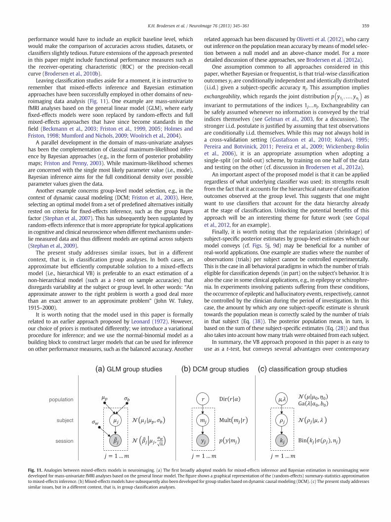
359K.H. Brodersen et al. / NeuroImage 76 (2013) 345–361
performance would have to include an explicit baseline level, whichwould make the comparison of accuracies across studies, datasets, orclassifiers slightly tedious. Future extensions of the approach presentedin this paper might include functional performance measures such asthe receiver-operating characteristic (ROC) or the precision-recallcurve (Brodersen et al., 2010b).
Leaving classification studies aside for a moment, it is instructive toremember that mixed-effects inference and Bayesian estimationapproaches have been successfully employed in other domains of neu-roimaging data analysis (Fig. 11). One example are mass-univariatefMRI analyses based on the general linear model (GLM), where earlyfixed-effects models were soon replaced by random-effects and fullmixed-effects approaches that have since become standards in thefield (Beckmann et al., 2003; Friston et al., 1999, 2005; Holmes andFriston, 1998; Mumford and Nichols, 2009; Woolrich et al., 2004).
A parallel development in the domain of mass-univariate analyseshas been the complementation of classical maximum-likelihood infer-ence by Bayesian approaches (e.g., in the form of posterior probabilitymaps; Friston and Penny, 2003). While maximum-likelihood schemesare concerned with the single most likely parameter value (i.e., mode),Bayesian inference aims for the full conditional density over possibleparameter values given the data.
Another example concerns group-level model selection, e.g., in thecontext of dynamic causal modeling (DCM; Friston et al., 2003). Here,selecting an optimal model from a set of predefined alternatives initiallyrested on criteria for fixed-effects inference, such as the group Bayesfactor (Stephan et al., 2007). This has subsequently been supplanted byrandom-effects inference that ismore appropriate for typical applicationsin cognitive and clinical neurosciencewhen differentmechanisms under-lie measured data and thus different models are optimal across subjects(Stephan et al., 2009).
The present study addresses similar issues, but in a differentcontext, that is, in classification group analyses. In both cases, anapproximate but efficiently computable solution to a mixed-effectsmodel (i.e., hierarchical VB) is preferable to an exact estimation of anon-hierarchical model (such as a t-test on sample accuracies) thatdisregards variability at the subject or group level. In other words: “Anapproximate answer to the right problem is worth a good deal morethan an exact answer to an approximate problem” (John W. Tukey,1915–2000).
It is worth noting that the model used in this paper is formallyrelated to an earlier approach proposed by Leonard (1972). However,our choice of priors is motivated differently; we introduce a variationalprocedure for inference; and we use the normal-binomial model as abuilding block to construct larger models that can be used for inferenceon other performancemeasures, such as the balanced accuracy. Another
(a) GLM group studies (b) DCM
population
subject
session
Fig. 11. Analogies between mixed-effects models in neuroimaging. (a) The first broadly adodeveloped for mass-univariate fMRI analyses based on the general linear model. The figure shotomixed-effects inference. (b)Mixed-effectsmodels have subsequently also been developed fosimilar issues, but in a different context, that is, in group classification analyses.
related approach has been discussed by Olivetti et al. (2012), who carryout inference on the populationmean accuracy bymeans ofmodel selec-tion between a null model and an above-chance model. For a moredetailed discussion of these approaches, see Brodersen et al. (2012a).
One assumption common to all approaches considered in thispaper, whether Bayesian or frequentist, is that trial-wise classificationoutcomes yi are conditionally independent and identically distributed(i.i.d.) given a subject-specific accuracy πj. This assumption implies
exchangeability, which regards the joint distribution p y1j;…; ynj
� �as
invariant to permutations of the indices 1j…nj. Exchangeability canbe safely assumed whenever no information is conveyed by the trialindices themselves (see Gelman et al., 2003, for a discussion). Thestronger i.i.d. postulate is justified by assuming that test observationsare conditionally i.i.d. themselves. While this may not always hold ina cross-validation setting (Gustafsson et al., 2010; Kohavi, 1995;Pereira and Botvinick, 2011; Pereira et al., 2009; Wickenberg-Bolinet al., 2006), it is an appropriate assumption when adopting asingle-split (or hold-out) scheme, by training on one half of the dataand testing on the other (cf. discussion in Brodersen et al., 2012a).
An important aspect of the proposed model is that it can be appliedregardless of what underlying classifier was used; its strengths resultfrom the fact that it accounts for the hierarchical nature of classificationoutcomes observed at the group level. This suggests that one mightwant to use classifiers that account for the data hierarchy alreadyat the stage of classification. Unlocking the potential benefits of thisapproach will be an interesting theme for future work (see Gopalet al., 2012, for an example).
Finally, it is worth noting that the regularization (shrinkage) ofsubject-specific posterior estimates by group-level estimates which ourmodel conveys (cf. Figs. 5j, 9d) may be beneficial for a number ofreal-world applications. One example are studies where the number ofobservations (trials) per subject cannot be controlled experimentally.This is the case in all behavioral paradigms in which the number of trialseligible for classification depends (in part) on the subject's behavior. It isalso the case in some clinical applications, e.g., in epilepsy or schizophre-nia. In experiments involving patients suffering from these conditions,the occurrence of epileptic and hallucinatory events, respectively, cannotbe controlled by the clinician during the period of investigation. In thiscase, the amount by which any one subject-specific estimate is shrunktowards the population mean is correctly scaled by the number of trialsin that subject (Eq. (38)). The posterior population mean, in turn, isbased on the sum of these subject-specific estimates (Eq. (28)) and thusalso takes into account howmany trials were obtained from each subject.
In summary, the VB approach proposed in this paper is as easy touse as a t-test, but conveys several advantages over contemporary
group studies (c) classification group studies
pted models for mixed-effects inference and Bayesian estimation in neuroimaging werews a graphical representation of the (random-effects) summary-statistics approximationr group studies based on dynamic causalmodeling (DCM). (c) The present study addresses
360 K.H. Brodersen et al. / NeuroImage 76 (2013) 345–361
fixed-effects and random-effects analyses. These advantages include:(i) posterior densities as opposed to point estimates of parameters;(ii) increased sensitivity (statistical power), i.e., a higher probability ofdetecting a positive result, especially with small sample sizes; (iii) ashrinking-to-the-population (or regression-to-the-mean) effect whoseregularization leads to more precise subject-specific accuracy estimates;and (iv) posterior accuracy maps (PAM) which provide a mixed-effectsalternative to conventional sample accuracy maps (SAM).
In order to facilitate its use and dissemination, the VB approach intro-duced in this paper has been implemented as open-source softwarefor both MATLAB and R. The code is freely available for download(http://www.translationalneuromodeling.org/software/). With thissoftware we hope to assist in improving the statistical sensitivity andinterpretation of results in future classification group studies.
Acknowledgments
The authors wish to thank Tom Nichols, Tim Behrens, MarkWoolrich, Adrian Groves, Ged Ridgway, and Falk Lieder for insightfuldiscussions, and additionally Tim Behrens for sharing fMRI data. Thisresearch was supported by the University Research Priority Program‘Foundations of Human Social Behaviour’ at the University of Zurich(KHB, KES), the SystemsX.ch project ‘Neurochoice’ (KHB, KES), andthe René and Susanne Braginsky Foundation (KES).
Conflict of interest
The authors declare no conflict of interest.
Appendix A. Supplementary data
Supplementary data to this article can be found online at http://dx.doi.org/10.1016/j.neuroimage.2013.03.008.
References
Akbani, R., Kwek, S., Japkowicz, N., 2004. Applying support vector machines to imbalanceddatasets. Machine Learning: ECML 2004, pp. 39–50.
Attias, H., 2000. A variational Bayesian framework for graphical models. Adv. NeuralInf. Process. Syst. 12, 209–215.
Beckmann, C.F., Jenkinson, M., Smith, S.M., 2003. General multilevel linear modeling forgroup analysis in fMRI. Neuroimage 20, 1052–1063.
Behrens, T.E.J., Woolrich, M.W., Walton, M.E., Rushworth, M.F.S., 2007. Learning thevalue of information in an uncertain world. Nat. Neurosci. 10, 1214–1221.
Bishop, C.M., 2007. Pattern Recognition and Machine Learning. Springer, New York.Bishop, C.M., Spiegelhalter, D., Winn, J., 2002. VIBES: a variational inference engine for
Bayesian networks. Adv. Neural Inf. Process. Syst. 15, 777–784.Blankertz, B., Lemm, S., Treder, M., Haufe, S., Müller, K.-R., 2011. Single-trial analysis
and classification of ERP components—a tutorial. Neuroimage 15, 814–825.Brodersen, K.H., Ong, C.S., Stephan, K.E., Buhmann, J.M., 2010a. The balanced accuracy
and its posterior distribution. Proceedings of the 20th International Conferenceon Pattern Recognition. IEEE Computer Society, pp. 3121–3124.
Brodersen, K.H., Ong, C.S., Stephan, K.E., Buhmann, J.M., 2010b. The binormal assumptionon precision-recall curves. Proceedings of the 20th International Conference on PatternRecognition. IEEE Computer Society, pp. 4263–4266.
Brodersen, K.H., Haiss, F., Ong, C.S., Jung, F., Tittgemeyer, M., Buhmann, J.M., Weber, B.,Stephan, K.E., 2011a. Model-based feature construction for multivariate decoding.Neuroimage 56, 601–615.
Brodersen, K.H., Schofield, T.M., Leff, A.P., Ong, C.S., Lomakina, E.I., Buhmann, J.M.,Stephan, K.E., 2011b. Generative embedding for model-based classification of fMRIdata. PLoS Comput. Biol. 7, e1002079.
Brodersen, K.H., Mathys, C., Chumbley, J.R., Daunizeau, J., Ong, C.S., Buhmann, J.M.,Stephan, K.E., 2012a. Bayesian mixed-effects inference on classification performancein hierarchical data sets. J. Mach. Learn. Res. 13, 3133–3176.
Brodersen, K.H., Wiech, K., Lomakina, E.I., Lin, C., Buhmann, J.M., Bingel, U., Ploner, M.,Stephan, K.E., Tracey, I., 2012b. Decoding the perception of pain from fMRI usingmultivariate pattern analysis. Neuroimage 63, 1162–1170.
Chadwick, M.J., Hassabis, D., Weiskopf, N., Maguire, E.A., 2010. Decoding individualepisodic memory traces in the human hippocampus. Curr. Biol. 20, 544–547.
Chang, C.-C., Lin, C.-J., 2011. LIBSVM: a library for support vector machines. ACM Trans.Intell. Syst. Technol. 2, 27:1–27:27.
Chawla, N.V., Bowyer, K.W., Hall, L.O., Kegelmeyer, W.P., 2002. SMOTE: syntheticminority over-sampling technique. J. Artif. Intell. Res. 16, 321–357.
Clithero, J.A., Smith, D.V., Carter, R.M., Huettel, S.A., 2011. Within- and cross-participantclassifiers reveal different neural coding of information. Neuroimage 56, 699–708.
Cox, D.D., Savoy, R.L., 2003. Functional magnetic resonance imaging (fMRI) “brain reading”:detecting and classifying distributed patterns of fMRI activity in human visual cortex.Neuroimage 19, 261–270.
Davatzikos, C., Resnick, S.M., Wu, X., Parmpi, P., Clark, C.M., 2008. Individual patientdiagnosis of AD and FTD via high-dimensional pattern classification ofMRI. Neuroimage41, 1220–1227.
Dixon, P., 2008. Models of accuracy in repeated-measures designs. J. Mem. Lang. 59,447–456.
Efron, B., Morris, C., 1971. Limiting the risk of Bayes and empirical Bayes estimators—part I: the Bayes case. J. Am. Stat. Assoc. 807–815.
Fox, C.W., Roberts, S.J., 2012. A tutorial on variational Bayesian inference. Artif. Intell.Rev. 38, 85–95.
Friston, K.J., Penny, W., 2003. Posterior probability maps and {SPMs}. Neuroimage 19,1240–1249.
Friston, K.J., Holmes, A.P., Worsley, K.J., Poline, J.P., Frith, C.D., Frackowiak, R.S.J., 1995.Statistical parametric maps in functional imaging: a general linear approach. Hum.Brain Mapp. 2, 189–210.
Friston, K.J., Holmes, A.P., Worsley, K.J., 1999. How many subjects constitute a study?Neuroimage 10, 1–5.
Friston, K.J., Penny, W., Phillips, C., Kiebel, S., Hinton, G., Ashburner, J., 2002. Classicaland Bayesian inference in neuroimaging: theory. Neuroimage 16, 465–483.
Friston, K.J., Harrison, L., Penny, W., 2003. Dynamic causal modelling. Neuroimage 19,1273–1302.
Friston, K.J., Stephan, K.E., Lund, T.E., Morcom, A., Kiebel, S., 2005. Mixed-effects andfMRI studies. Neuroimage 24, 244–252.
Galton, F., 1886. Regression towards mediocrity in hereditary stature. J. Anthropol. Inst.Great Brit. Ireland 15, 246–263.
Gelman, A., Carlin, J.B., Stern, H.S., Rubin, D.B., 2003. Bayesian Data Analysis, 2nd ed.Chapman and Hall/CRC.
Ghahramani, Z., Beal, M.J., 2001. Propagation algorithms for variational Bayesian learning.Adv. Neural Inf. Process. Syst. 507–513.
Goldstein, H., 2010. Multilevel Statistical Models. Wiley.Gopal, S., Yang, Y., Bai, B., Niculescu-Mizil, A., 2012. Bayesian models for Large-scale
Hierarchical Classification. Adv. Neural Inf. Process. Syst. 25, 2420–2428.Gustafsson, M.G.,Wallman, M.,Wickenberg Bolin, U., Göransson, H., Fryknäs, M., Andersson,
C.R., Isaksson, A., 2010. Improving Bayesian credibility intervals for classifier error ratesusing maximum entropy empirical priors. Artif. Intell. Med. 49, 93–104.
Harrison, S.A., Tong, F., 2009. Decoding reveals the contents of visual working memoryin early visual areas. Nature 458, 632–635.
Hassabis, D., Chu, C., Rees, G., Weiskopf, N., Molyneux, P.D., Maguire, E.A., 2009.Decoding neuronal ensembles in the human hippocampus. Curr. Biol. 19, 546–554.
Haynes, J.-D., Rees, G., 2006. Decoding mental states from brain activity in humans. Nat.Rev. Neurosci. 7, 523–534.
Holmes, A.P., Friston, K.J., 1998. Generalisability, random effects and population inference.Fourth Int Conf on Functional Mapping of the Human Brain. Neuroimage 7, S754.
Japkowicz, N., Stephen, S., 2002. The class imbalance problem: a systematic study.Intell. Data Anal. 6, 429–449.
Johnson, J.D., McDuff, S.G.R., Rugg, M.D., Norman, K.A., 2009. Recollection, familiarity,and cortical reinstatement: a multivoxel pattern analysis. Neuron 63, 697–708.
Just, M.A., Cherkassky, V.L., Aryal, S., Mitchell, T.M., 2010. A neurosemantic theory ofconcrete noun representation based on the underlying brain codes. PLoS One 5,e8622.
Klöppel, S., Stonnington, C.M., Chu, C., Draganski, B., Scahill, R.I., Rohrer, J.D., Fox, N.C.,Jack, C.R., Ashburner, J., Frackowiak, R.S.J., 2008. Automatic classification of MRscans in Alzheimer's disease. Brain 131, 681–689.
Klöppel, S., Abdulkadir, A., Jack Jr., C.R., Koutsouleris, N., Mourão-Miranda, J., Vemuri, P.,2012. Diagnostic neuroimaging across diseases. Neuroimage 61, 457–463.
Knops, A., Thirion, B., Hubbard, E.M., Michel, V., Dehaene, S., 2009. Recruitment of an areainvolved in eye movements during mental arithmetic. Science 324, 1583–1585.
Kohavi, R., 1995. A study of cross-validation and bootstrap for accuracy estimation andmodel selection. International Joint Conference on Artificial Intelligence. LawrenceErlbaum Associates Ltd., pp. 1137–1145.
Krajbich, I., Camerer, C., Ledyard, J., Rangel, A., 2009. Using neural measures of economicvalue to solve the public goods free-rider problem. Science 326, 596–599.
Kriegeskorte, N., Goebel, R., Bandettini, P., 2006. Information-based functional brainmapping. Proc. Natl. Acad. Sci. U. S. A. 103, 3863–3868.
Langford, J., 2005. Tutorial on practical prediction theory for classification. J. Mach. Learn.Res. 6, 273–306.
Lemm, S., Blankertz, B., Dickhaus, T., Müller, K.-R., 2011. Introduction to machine learningfor brain imaging. Neuroimage 56, 387–399.
Leonard, T., 1972. Bayesian methods for binomial data. Biometrika 59, 581–589.MacKay, D.J.C., 1995. Ensemble learning and evidence maximization. Proc. NIPS
(Available at: http://citeseerx.ist.psu.edu/viewdoc/download?doi=10.1.1.54.4083&rep=rep1&type=pdf [Accessed January 4, 2013]).
Marquand, A., Howard, M., Brammer, M., Chu, C., Coen, S., Mourão-Miranda, J., 2010.Quantitative prediction of subjective pain intensity from whole-brain fMRI datausing Gaussian processes. Neuroimage 49, 2178–2189.
Mumford, J.A., Nichols, T., 2009. Simple group fMRI modeling and inference. Neuroimage47, 1469–1475.
Nandy, R.R., Cordes, D., 2003. Novel nonparametric approach to canonical correlationanalysis with applications to low CNR functional MRI data. Magn. Reson. Med.50, 354–365.
Norman, K.A., Polyn, S.M., Detre, G.J., Haxby, J.V., 2006. Beyondmind-reading:multi-voxelpattern analysis of fMRI data. Trends Cogn. Sci. 10, 424–430.
Olivetti, E., Veeramachaneni, S., Nowakowska, E., 2012. Bayesian hypothesis testing forpattern discrimination in brain decoding. Pattern Recognit. 45, 2075–2084.

361K.H. Brodersen et al. / NeuroImage 76 (2013) 345–361
Penny, W.D., Stephan, K.E., Mechelli, A., Friston, K.J., 2004. Comparing dynamic causalmodels. Neuroimage 22, 1157–1172.
Pereira, F., Botvinick, M., 2011. Informationmappingwith pattern classifiers: a comparativestudy. Neuroimage 56, 476–496.
Pereira, F., Mitchell, T., Botvinick, M., 2009. Machine learning classifiers and fMRI: atutorial overview. Neuroimage 45, S199–S209.
Schurger, A., Pereira, F., Treisman, A., Cohen, J.D., 2010. Reproducibility distinguishesconscious from nonconscious neural representations. Science 327, 97–99.
Sitaram, R., Weiskopf, N., Caria, A., Veit, R., Erb, M., Birbaumer, N., 2008. fMRI brain–computer interfaces: a tutorial on methods and applications. IEEE Signal Process.Mag. 25, 95–106.
Stelzer, J., Chen, Y., Turner, R., 2013. Statistical inference andmultiple testing correctionin classification-based multi-voxel pattern analysis (MVPA): random permutationsand cluster size control. Neuroimage 65, 69–82.
Stephan, K.E., Weiskopf, N., Drysdale, P.M., Robinson, P.A., Friston, K.J., 2007. Comparinghemodynamic models with DCM. Neuroimage 38, 387–401.
Stephan, K.E., Penny, W.D., Daunizeau, J., Moran, R.J., Friston, K.J., 2009. Bayesian modelselection for group studies. Neuroimage 46, 1004–1017.
Tong, F., Pratte, M.S., 2012. Decoding patterns of human brain activity. Annu. Rev. Psychol.63, 483–509.
Wickenberg-Bolin, U., Goransson, H., Fryknas, M., Gustafsson, M., Isaksson, A., 2006.Improved variance estimation of classification performance via reduction of biascaused by small sample size. BMC Bioinformatics 7, 127.
Woolrich, M.W., Behrens, T.E.J., Beckmann, C.F., Jenkinson, M., Smith, S.M., 2004.Multilevel linear modelling for FMRI group analysis using Bayesian inference.Neuroimage 21, 1732–1747.
Zhang, D., Lee, W.S., 2008. Learning classifiers without negative examples: A reductionapproach. International Conference on Digital, Information Management (ICDIM).


![Walsh-Hadamard Variational Inference for Bayesian Deep ......Bayesian neural networks [35, 38] represent a good example of models for which inference is intractable, and for which](https://img.pdfslide.net/doc/110x75/60e941f8bc8d6a14cd22a870/walsh-hadamard-variational-inference-for-bayesian-deep-bayesian-neural-networks.jpg)