Variational Learning and Variational Inference

Ian Goodfellow

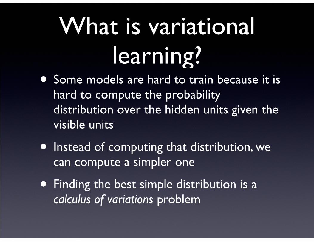
What is variational learning?

• Some models are hard to train because it is hard to compute the probability distribution over the hidden units given the visible units

• Instead of computing that distribution, we can compute a simpler one

• Finding the best simple distribution is a calculus of variations problem

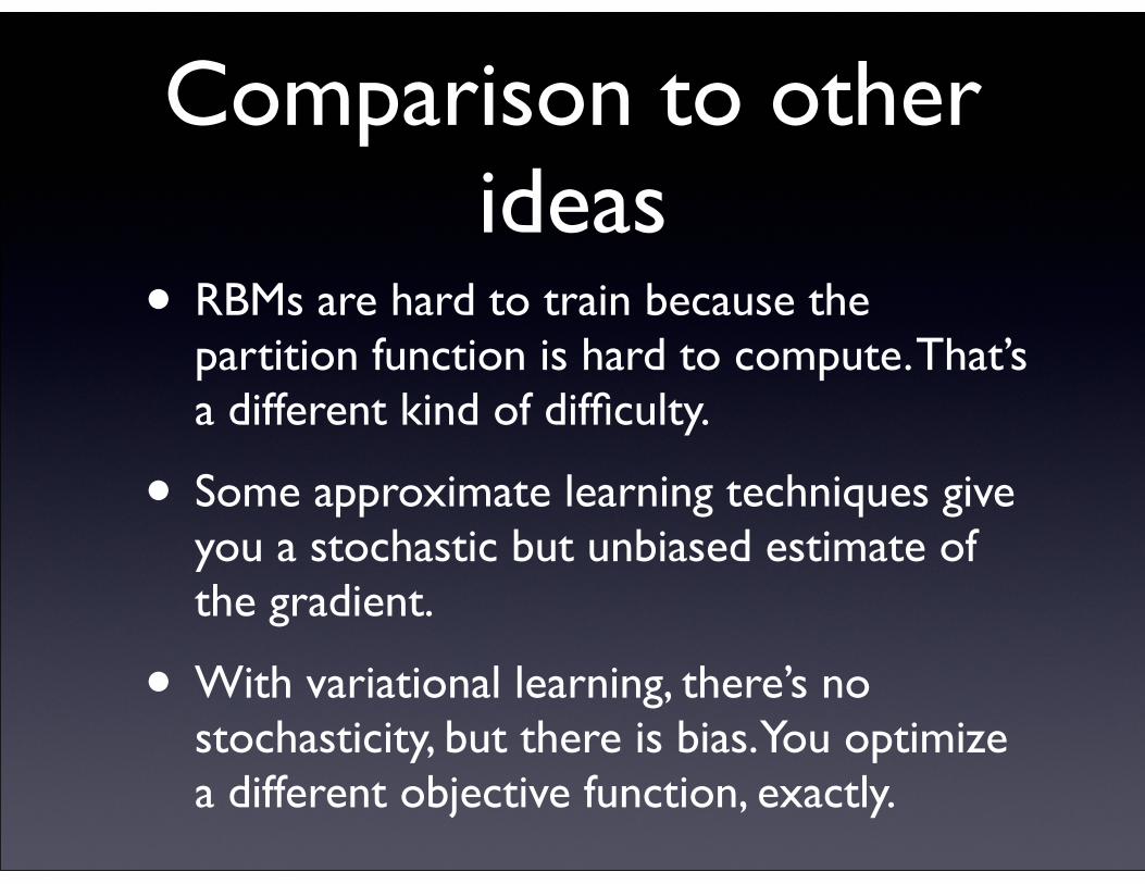
Comparison to other ideas

• RBMs are hard to train because the partition function is hard to compute. That’s a different kind of difficulty.

• Some approximate learning techniques give you a stochastic but unbiased estimate of the gradient.

• With variational learning, there’s no stochasticity, but there is bias. You optimize a different objective function, exactly.

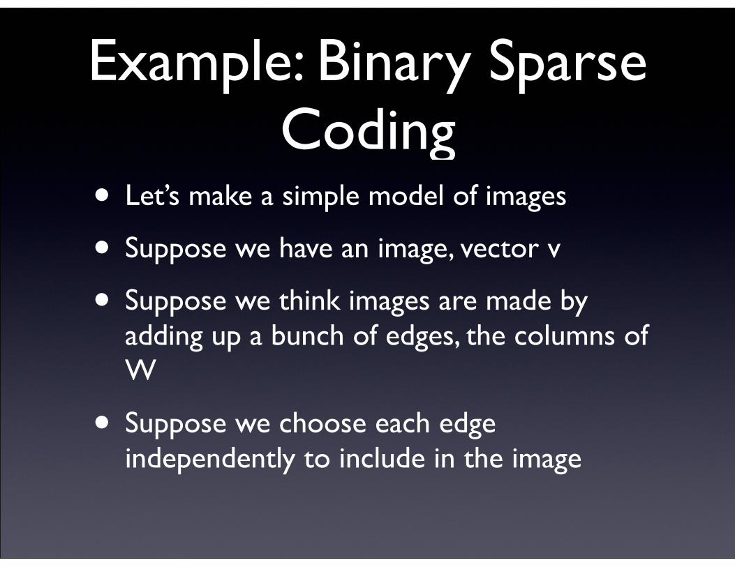
Example: Binary Sparse Coding

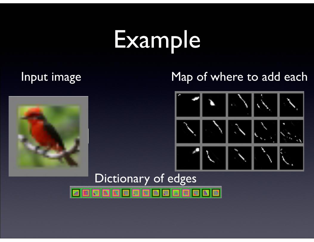
• Let’s make a simple model of images

• Suppose we have an image, vector v

• Suppose we think images are made by adding up a bunch of edges, the columns of W

• Suppose we choose each edge independently to include in the image

Example

Feature Extraction:Inference

Filters demonstrated here:

Infer EQ[h]

for each patch

32x32x3

27x27 of 6x6x327x27xN (N=1600 or 6000)

Input image Map of where to add each

Dictionary of edges

Feature Extraction:Inference

Filters demonstrated here:

Infer EQ[h]

for each patch

32x32x3

27x27 of 6x6x327x27xN (N=1600 or 6000)

Feature Extraction:Inference

Filters demonstrated here:

Infer EQ[h]

for each patch

32x32x3

27x27 of 6x6x327x27xN (N=1600 or 6000)

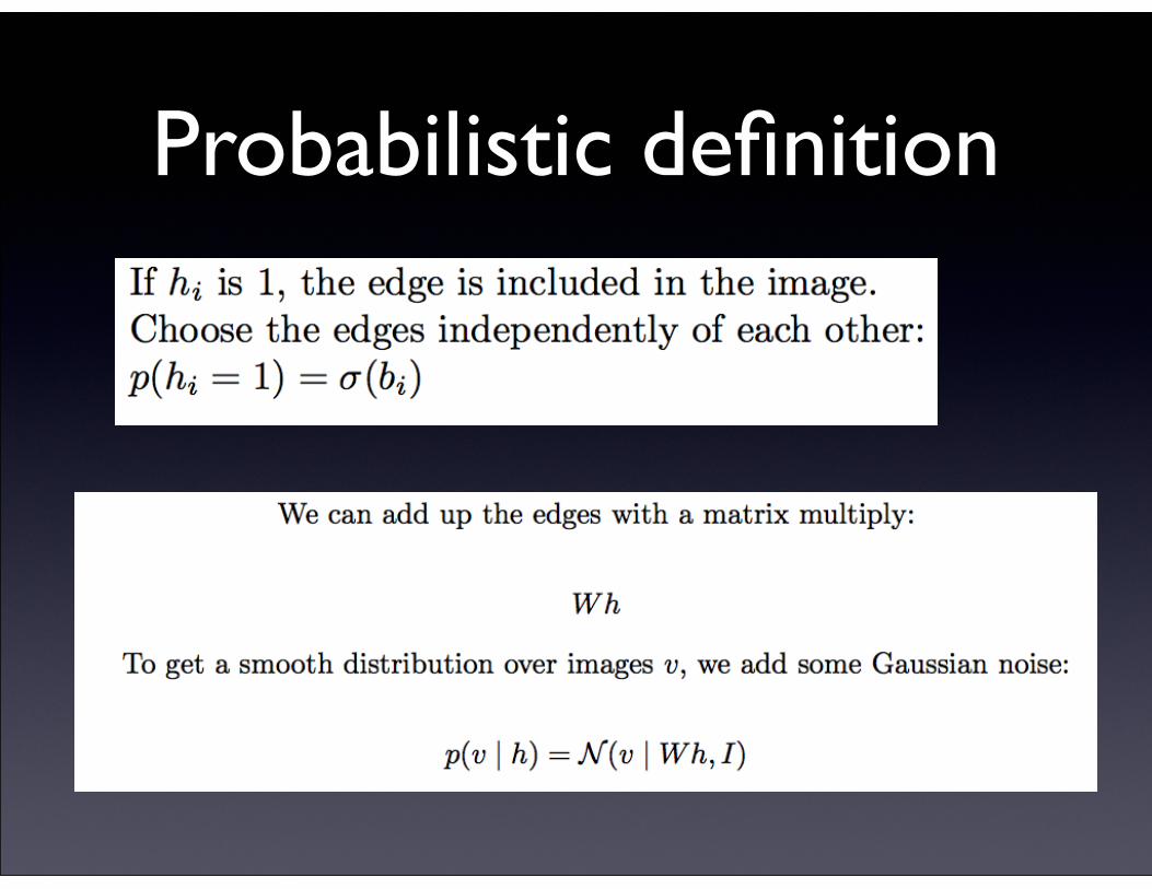
Probabilistic definition

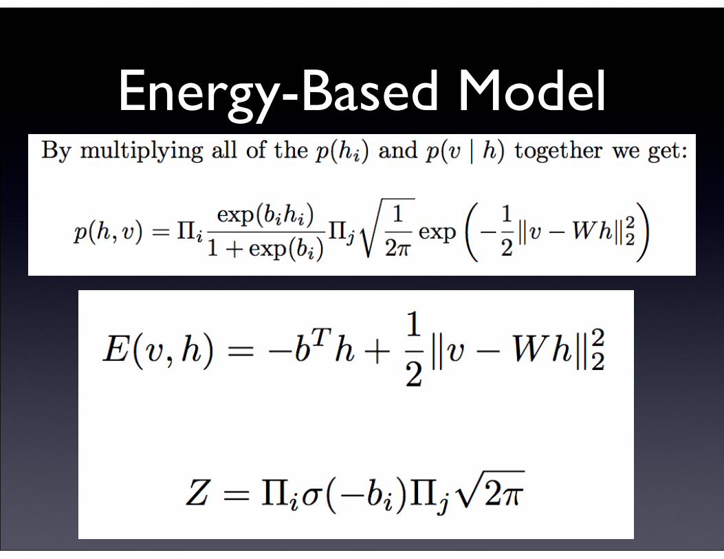
Energy-Based Model

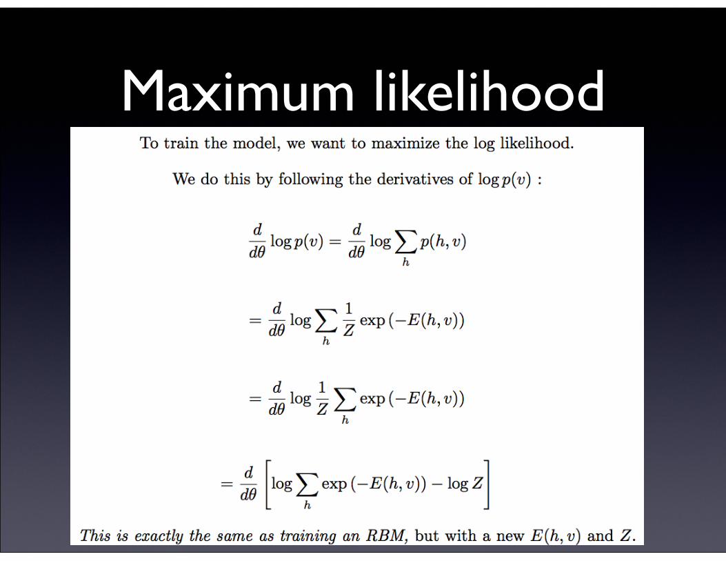
Maximum likelihood

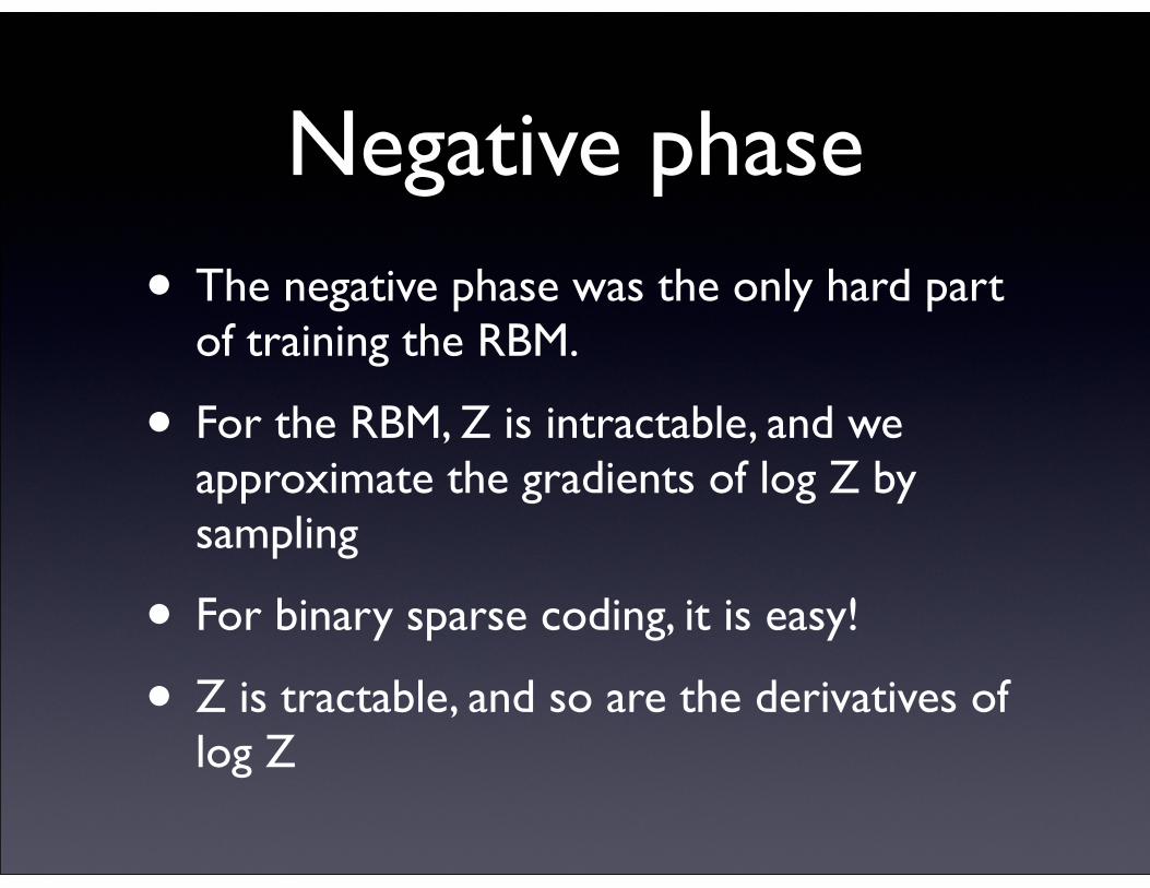
Negative phase

• The negative phase was the only hard part of training the RBM.

• For the RBM, Z is intractable, and we approximate the gradients of log Z by sampling

• For binary sparse coding, it is easy!

• Z is tractable, and so are the derivatives of log Z

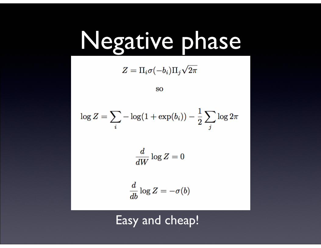
Negative phase

Easy and cheap!

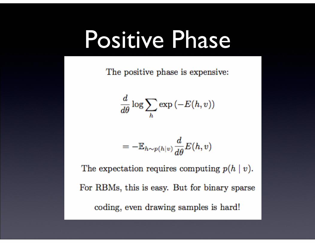
Positive Phase

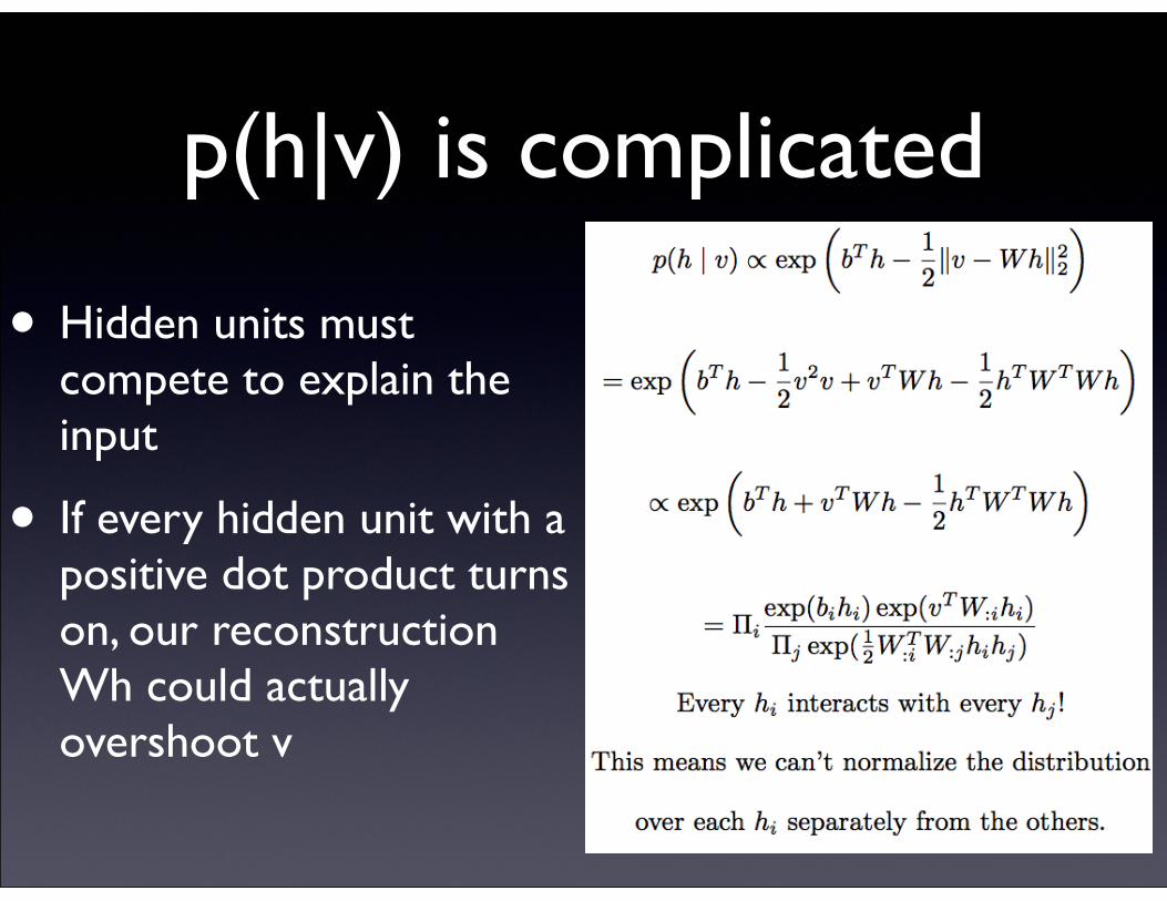
p(h|v) is complicated

• Hidden units must compete to explain the input

• If every hidden unit with a positive dot product turns on, our reconstruction Wh could actually overshoot v

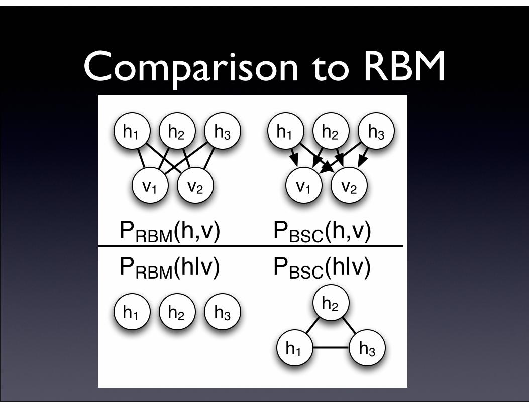
Comparison to RBMh1 h2

v1 v2

h3 h1 h2

v1 v2

h3

h1 h2 h3

h1

h2

h3

PRBM(h,v) PBSC(h,v)PRBM(h|v) PBSC(h|v)

Let’s simplify things

• p(h|v) is just plain too hard to work with

• Let’s make a new distribution q(h)

• We want q(h) to be simple. It should be cheap to compute expectations over q(h)

• We want q(h) to be close to p(h|v) somehow

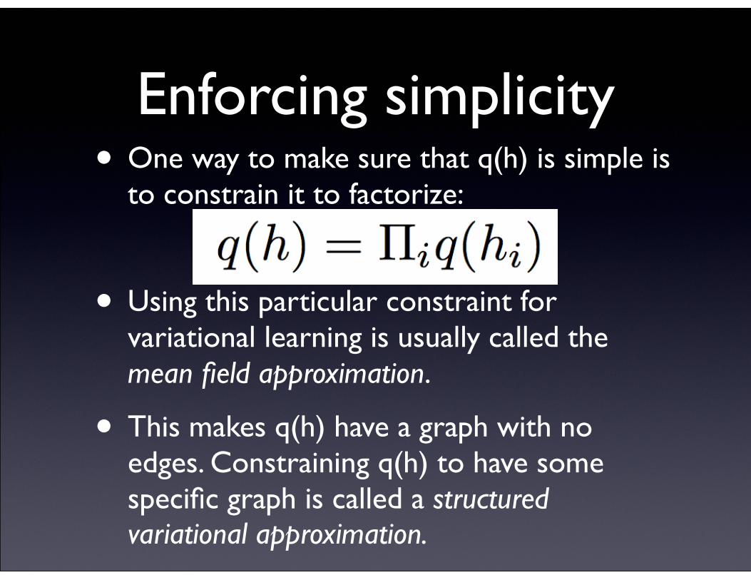
Enforcing simplicity• One way to make sure that q(h) is simple is

to constrain it to factorize:

• Using this particular constraint for variational learning is usually called the mean field approximation.

• This makes q(h) have a graph with no edges. Constraining q(h) to have some specific graph is called a structured variational approximation.

Variational lower bound

Variational learning

● Approximate intractable P(h|v) with tractable Q(h)

● Use Q to construct a lower bound on the log likelihood

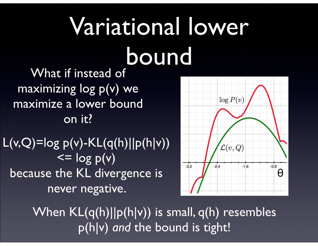
What if instead of maximizing log p(v) we

maximize a lower bound on it?

L(v,Q)=log p(v)-KL(q(h)||p(h|v))<= log p(v)

because the KL divergence is never negative.

When KL(q(h)||p(h|v)) is small, q(h) resembles p(h|v) and the bound is tight!

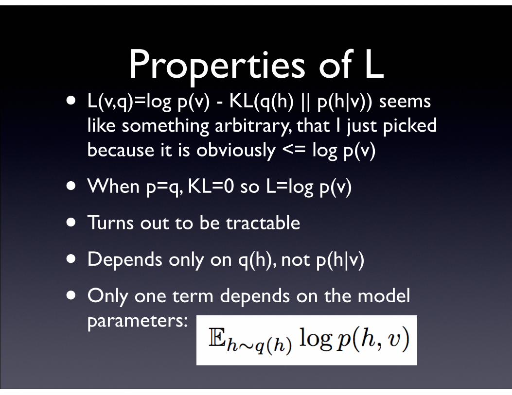
Properties of L• L(v,q)=log p(v) - KL(q(h) || p(h|v)) seems

like something arbitrary, that I just picked because it is obviously <= log p(v)

• When p=q, KL=0 so L=log p(v)

• Turns out to be tractable

• Depends only on q(h), not p(h|v)

• Only one term depends on the model parameters:

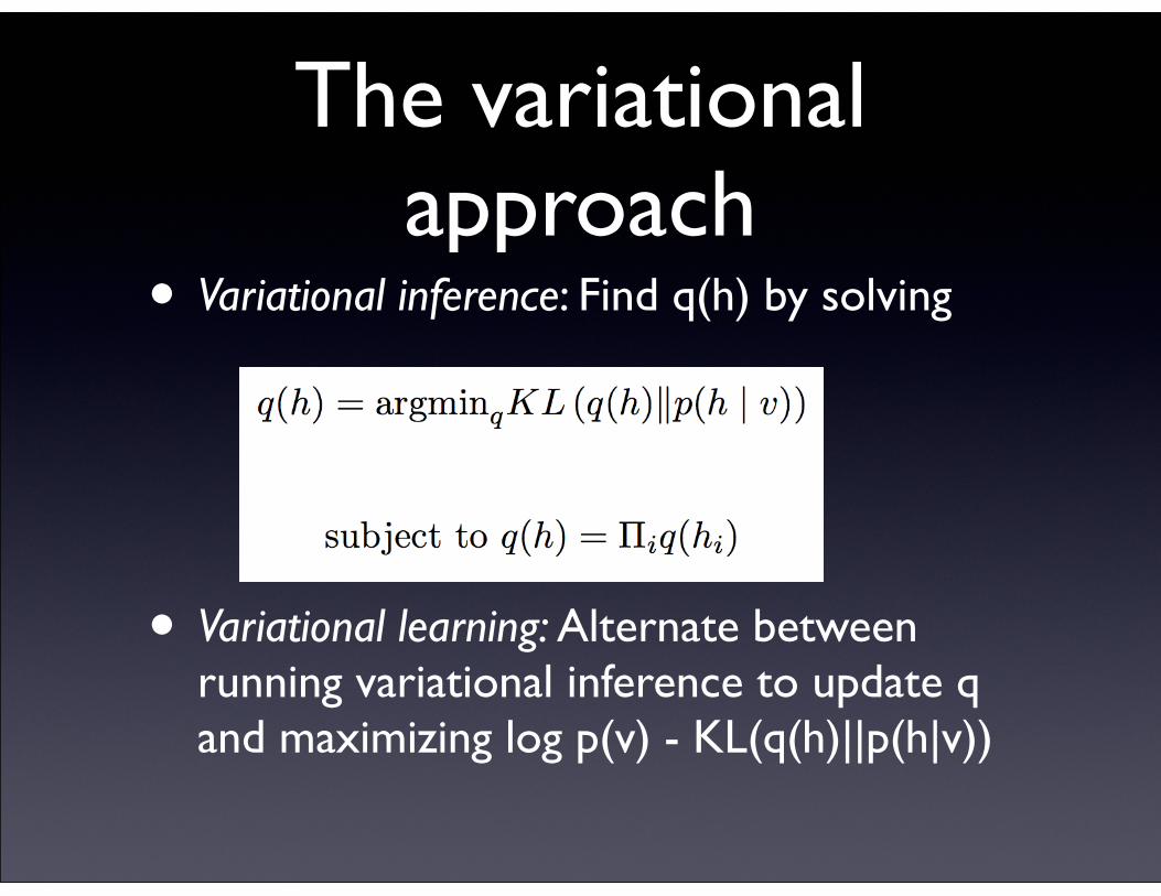
The variational approach

• Variational inference: Find q(h) by solving

• Variational learning: Alternate between running variational inference to update q and maximizing log p(v) - KL(q(h)||p(h|v))

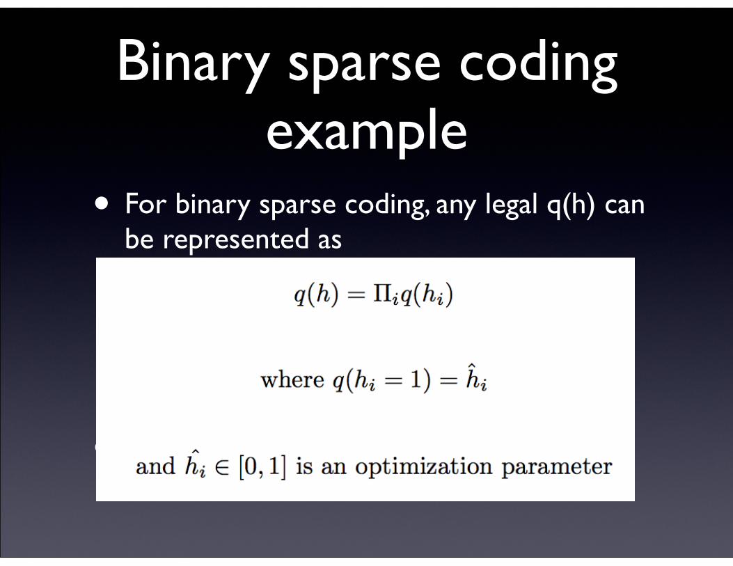
Binary sparse coding example

• For binary sparse coding, any legal q(h) can be represented as

•

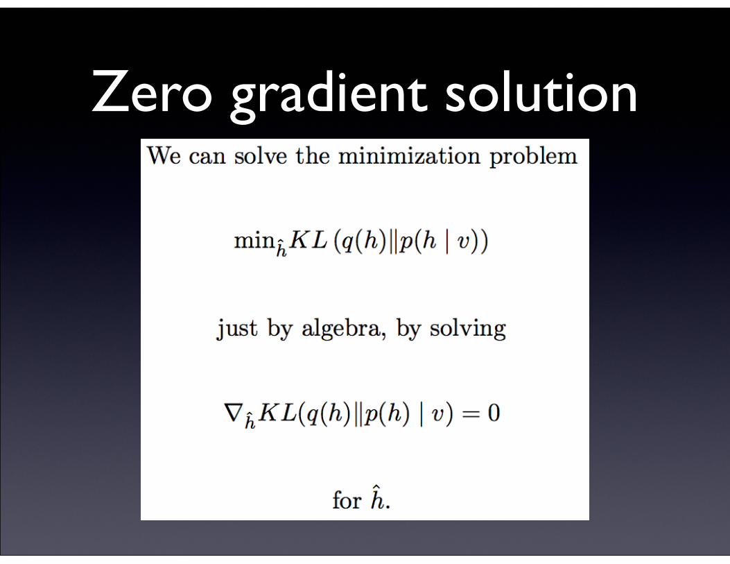
Zero gradient solution

Fixed point equations

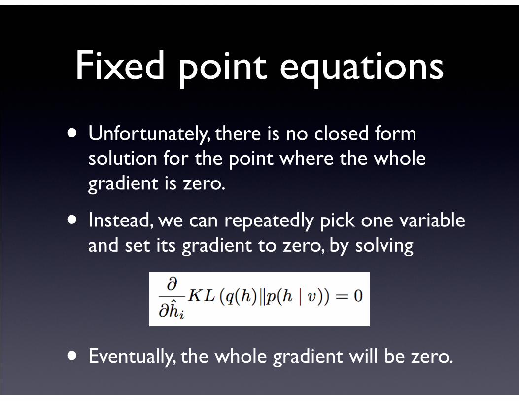
• Unfortunately, there is no closed form solution for the point where the whole gradient is zero.

• Instead, we can repeatedly pick one variable and set its gradient to zero, by solving

• Eventually, the whole gradient will be zero.

Fixed point update• After doing a bunch of calculus and

algebra, we get that the fixed point update is

• It looks a lot like p(h|v) in an RBM, but now the different hidden units get to inhibit each other.

Parallel updates

• These equations just say how to update one equation at a time

• What if you want to update several?

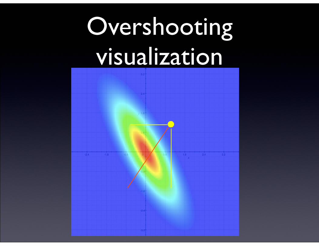
• Updating each variable to its individually optimal value doesn’t reach the global optimum. You have to scale back the step to avoid overshooting.

Overshooting visualization

Diagnosing Variational Model Problems

• Most important technical skill as a researcher, engineer, or consultant is deciding what to try next.

• Probabilistic methods are nice because you can isolate failures of inference from failures of learning or failures of representation

• What are some tests you could do to verify that variational inference is working?

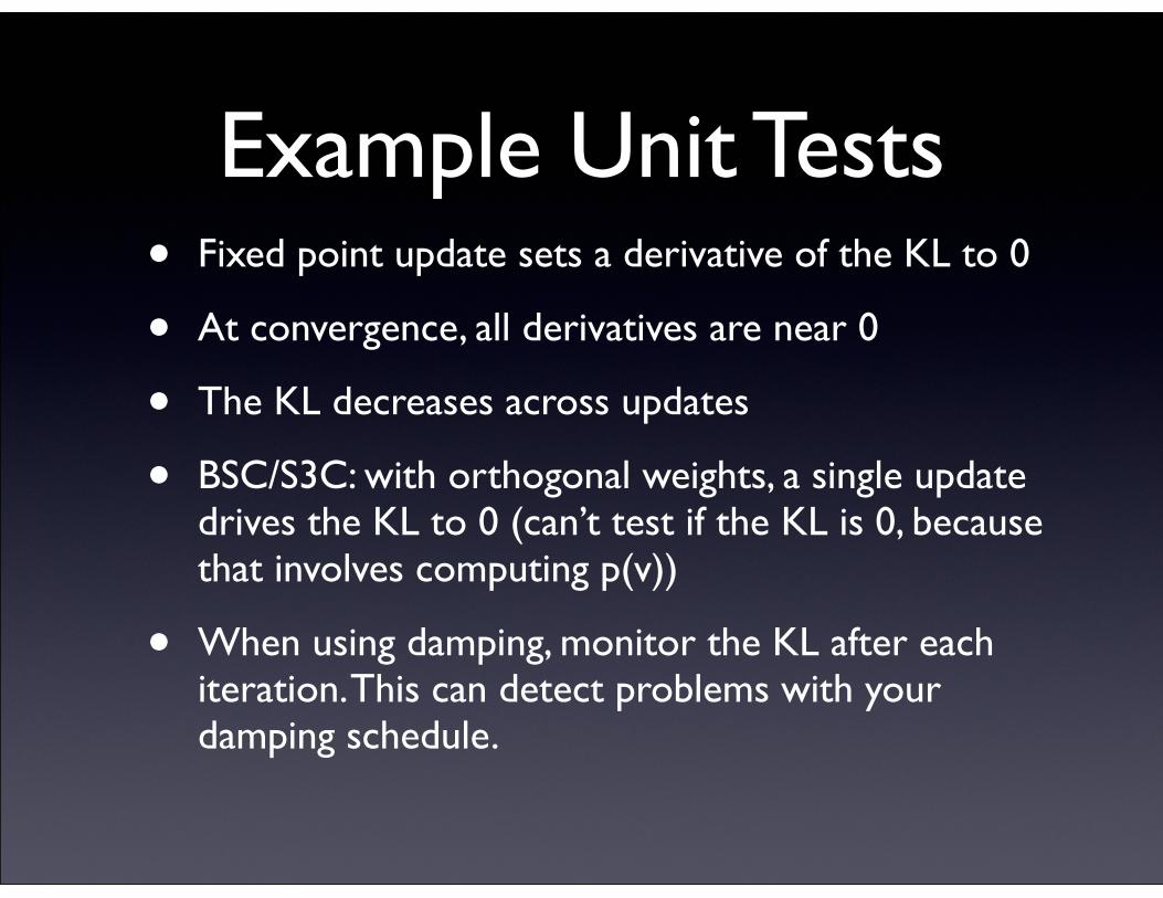
Example Unit Tests• Fixed point update sets a derivative of the KL to 0

• At convergence, all derivatives are near 0

• The KL decreases across updates

• BSC/S3C: with orthogonal weights, a single update drives the KL to 0 (can’t test if the KL is 0, because that involves computing p(v))

• When using damping, monitor the KL after each iteration. This can detect problems with your damping schedule.

Continuous variables

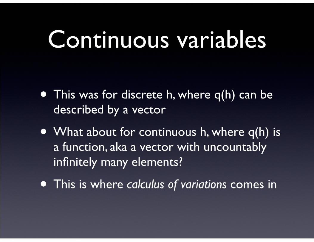
• This was for discrete h, where q(h) can be described by a vector

• What about for continuous h, where q(h) is a function, aka a vector with uncountably infinitely many elements?

• This is where calculus of variations comes in

Calculus of variations

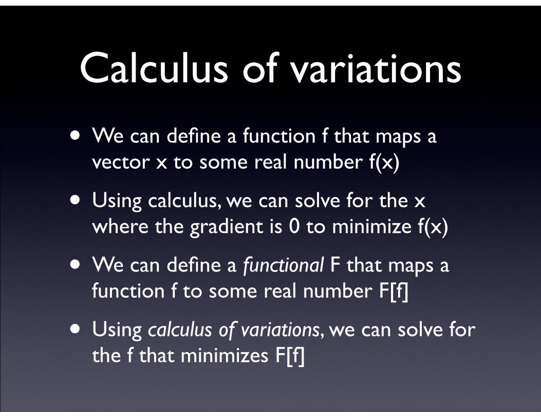
• We can define a function f that maps a vector x to some real number f(x)

• Using calculus, we can solve for the x where the gradient is 0 to minimize f(x)

• We can define a functional F that maps a function f to some real number F[f]

• Using calculus of variations, we can solve for the f that minimizes F[f]

Calculus of variations for variational inference

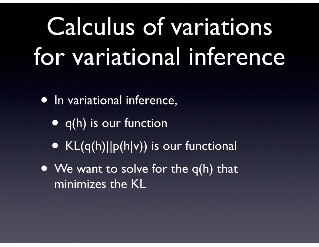
• In variational inference,

• q(h) is our function

• KL(q(h)||p(h|v)) is our functional

• We want to solve for the q(h) that minimizes the KL

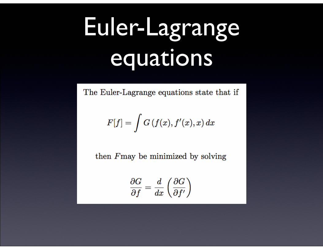
Euler-Lagrange equations

Applications of Euler-Lagrange

• We can use the Euler-Lagrange equation to solve for the minimum of a functional

• When f is a probability distribution, we need to also add a Lagrange multiplier to make sure f is normalized

• You can use this to prove stuff like that the Gaussian distribution has the highest entropy of any distribution with fixed variance v

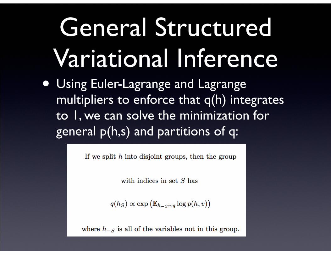
General Structured Variational Inference

• Using Euler-Lagrange and Lagrange multipliers to enforce that q(h) integrates to 1, we can solve the minimization for general p(h,s) and partitions of q:

More complicated structures

• You could also imagine making q(h) have a richer structure

• chain

• tree

• any structure for which expectations of log p(h,s) are tractable

• It doesn’t have to be a partition. But I don’t cover that here.

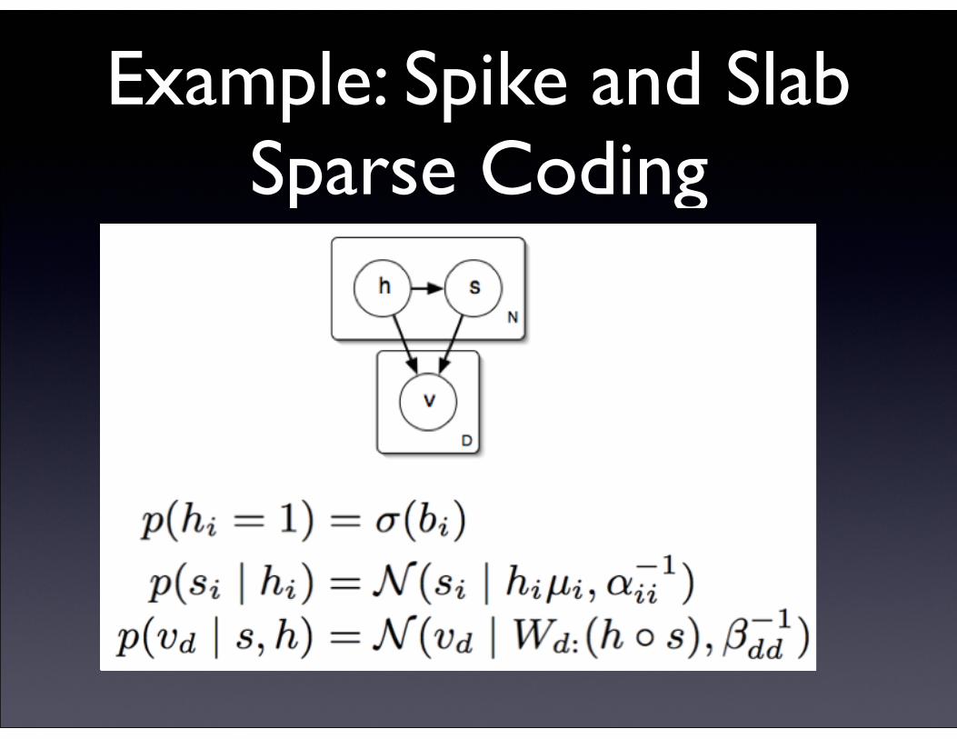
Example: Spike and Slab Sparse Coding

Large-Scale Feature Learning With Spike-and-Slab Sparse CodingIan J. Goodfellow Aaron Courville Yoshua Bengio

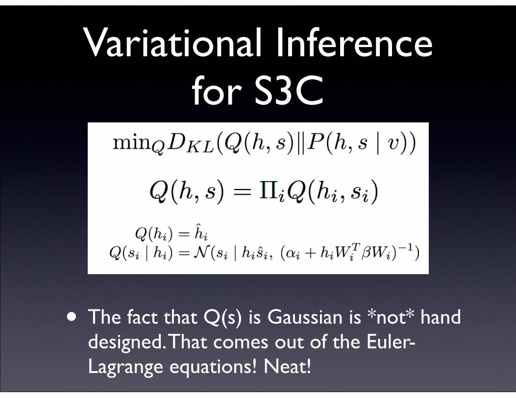
Variational Inference for S3C

• The fact that Q(s) is Gaussian is *not* hand designed. That comes out of the Euler-Lagrange equations! Neat!

Large-Scale Feature Learning With Spike-and-Slab Sparse CodingIan J. Goodfellow Aaron Courville Yoshua Bengio

Optimization

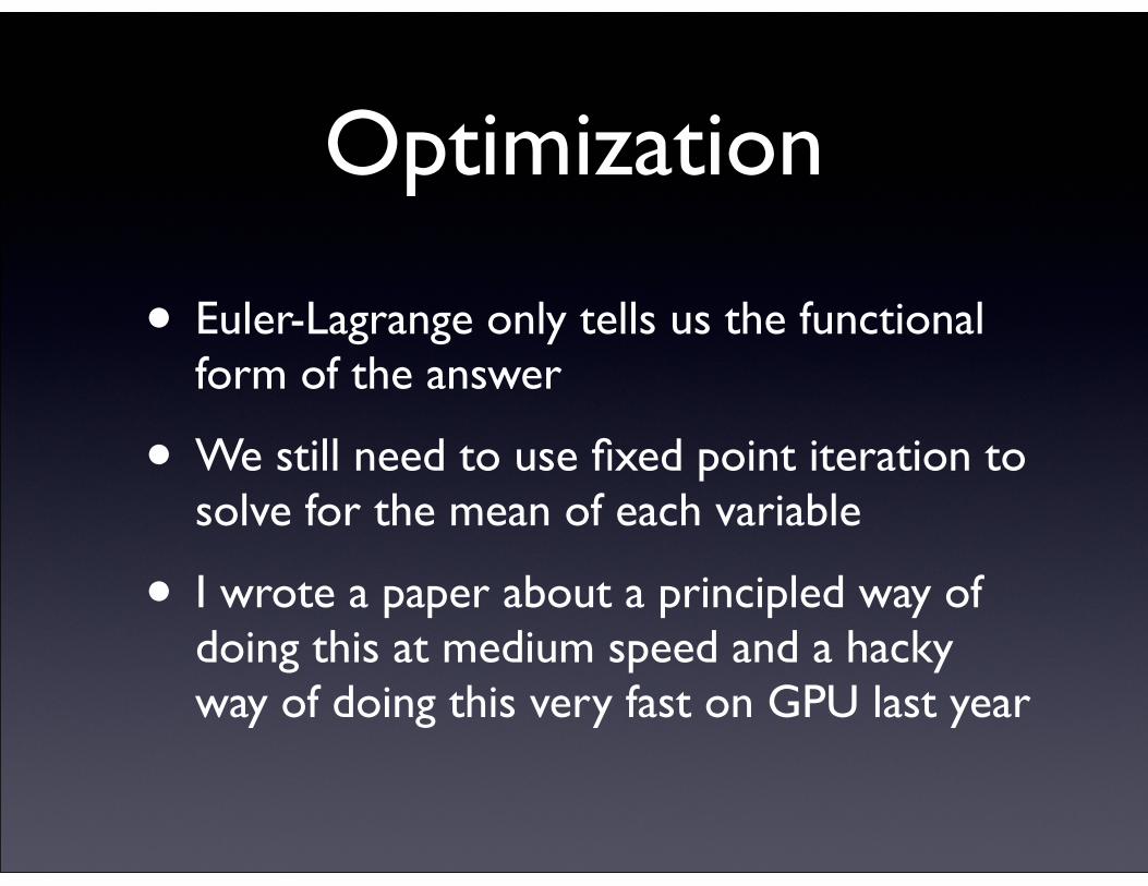
• Euler-Lagrange only tells us the functional form of the answer

• We still need to use fixed point iteration to solve for the mean of each variable

• I wrote a paper about a principled way of doing this at medium speed and a hacky way of doing this very fast on GPU last year

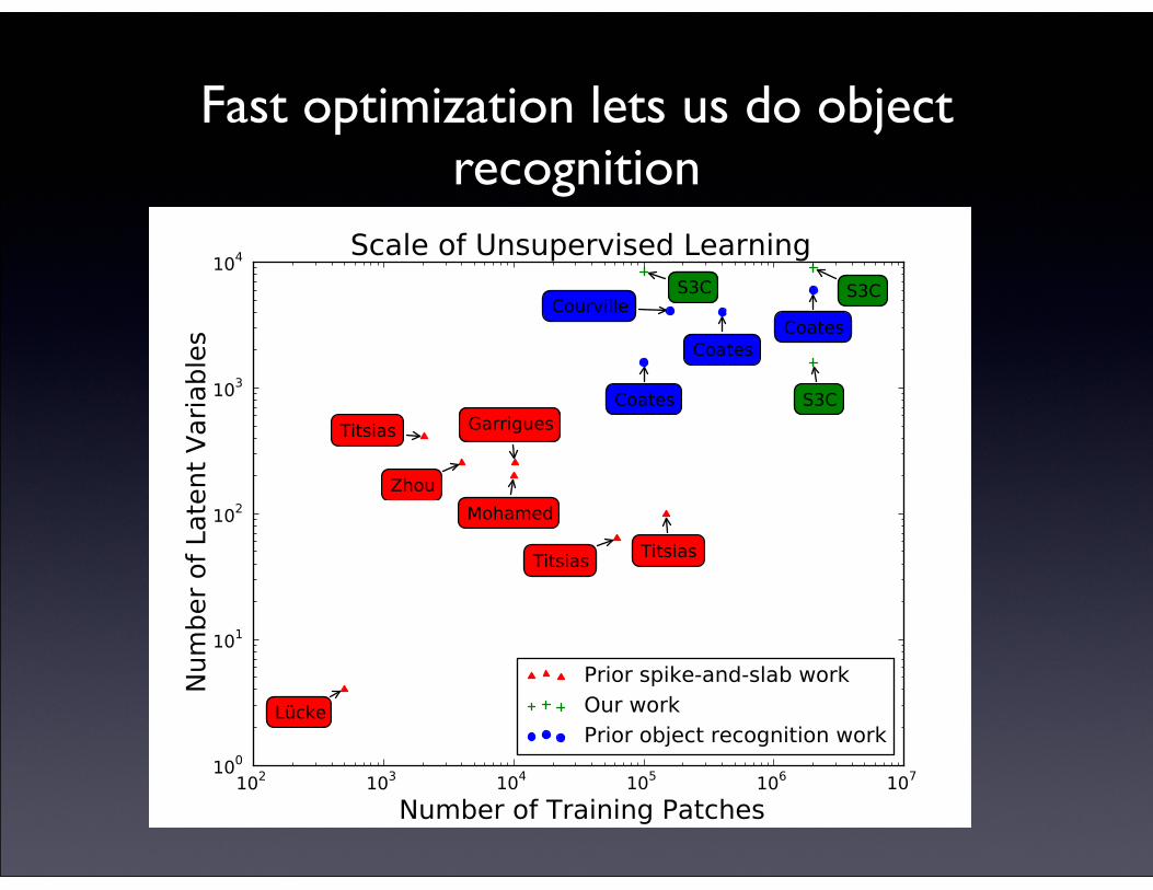
Fast optimization lets us do object recognition

TPAMI SPECIAL ISSUE SUBMISSION UNDER REVIEW 9

Fig. 5. Our inference scheme enables us to extendspike-and-slab modeling from small problems to the scaleneeded for object recognition. Previous object recognitionwork is from (Coates and Ng, 2011; Courville et al.,2011b). Previous spike-and-slab work is from (Mohamedet al., 2012; Zhou et al., 2009; Garrigues and Olshausen,2008; Lucke and Sheikh, 2011; Titsias and Lazaro-Gredilla, 2011).

For each inference scheme considered, we found thefastest possible variant obtainable via a two-dimensionalgrid search over ⌘h and either ⌘s in the case of the heuris-tic method or the number of conjugate gradient steps toapply per s update in the case of the conjugate gradientmethod. We used the same value of these parameters onevery pair of update steps. It may be possible to obtainfaster results by varying the parameters throughout thecourse of inference.

For these timing experiments, it is necessary to makesure that each algorithm is not able to appear fasterby converging early to an incorrect solution. We thusreplace the standard convergence criterion based on thesize of the change in the variational parameters with arequirement that the KL divergence reach within 0.05 onaverage of our best estimate of the true minimum valueof the KL divergence found by batch gradient descent.

All experiments were performed on an Nvidia Ge-Force GTX-580.

The results are summarized in Fig. 7.

7 CLASSIFICATION RESULTSBecause S3C forms the basis of all further model de-velopment in this line of research, we concentrate onvalidating its value as a feature discovery algorithm.We conducted experiments to evaluate the usefulness ofS3C features for supervised learning on the CIFAR-10and CIFAR-100 (Krizhevsky and Hinton, 2009) datasets.Both datasets consist of color images of objects suchas animals and vehicles. Each contains 50,000 train and

Fig. 6. Example filters from a dictionary of over 8,000learned on full 32x32 images.

Fig. 7. The inference speed for each method was com-puted based on the inference time for the same set 100examples from each dataset. The heuristic method isconsistently faster than the conjugate gradient method.The conjugate gradient method is slowed more by prob-lem size than the heuristic method is, as shown by theconjugate gradient method’s low speed on the CIFAR-100 full image task. The heuristic method has a very lowcost per iteration but is strongly affected by the strengthof explaining-away interactions–moving from CIFAR-100full images to CIFAR-100 patches actually slows it downbecause the degree of overcompleteness increases.

10,000 test examples. CIFAR-10 contains 10 classes whileCIFAR-100 contains 100 classes, so there are fewer la-beled examples per class in the case of CIFAR-100.

For all experiments, we used the same overall proce-dure as Coates and Ng (2011) except for feature learn-ing. CIFAR-10 consists of 32 ⇥ 32 images. We train ourfeature extractor on 6⇥6 contrast-normalized and ZCA-whitened patches from the training set (this preprocess-ing step is not necessary to obtain good performancewith S3C; we included it primarily to facilitate compar-ison with other work). At test time, we extract featuresfrom all 6 ⇥ 6 patches on an image, then average-poolthem. The average-pooling regions are arranged on anon-overlapping grid. Finally, we train an L2-SVM witha linear kernel on the pooled features.

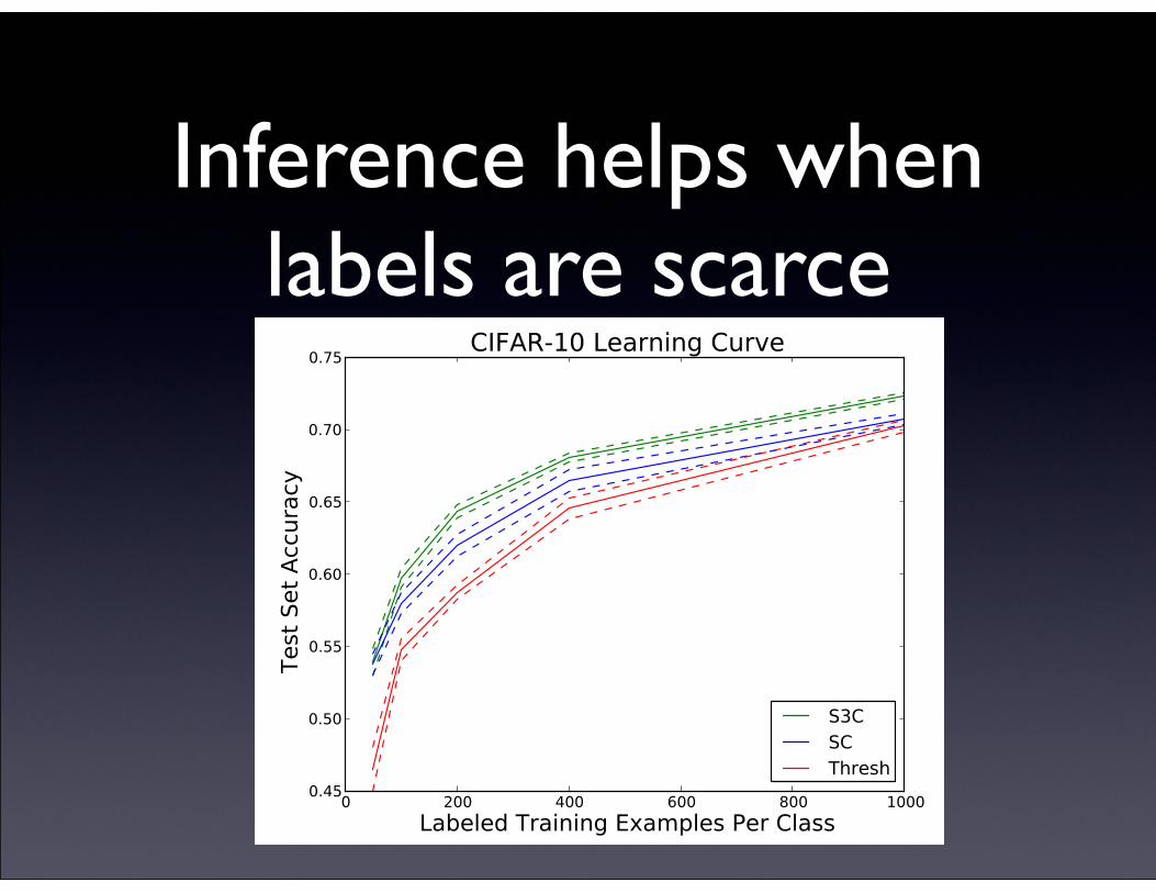
Inference helps when labels are scarceTPAMI SPECIAL ISSUE SUBMISSION UNDER REVIEW 10

Fig. 8. Semi-supervised classification accuracy on sub-sets of CIFAR-10. Thresholding, the best feature extractoron the full dataset, performs worse than sparse codingwhen few labels are available. S3C improves upon sparsecoding’s advantage.

Sheet1

Page 1

Model Validation accuracyTest Accuracy ErrorK-means+L 54.8 1S3C+P 53.7 1S3C+3 51.3SC+3 50.6OMP-1+3 48.7

K-means+L

S3C+P

S3C+3

SC+3

OMP-1+3

44 46 48 50 52 54 56

CIFAR-100 Results

Validation accuracy

Test Accuracy

Fig. 9. CIFAR-100 classification accuracy for variousmodels. As expected, S3C outperforms SC (sparse cod-ing) and and OMP-1. S3C with spatial pyramid poolingis near the state-of-the-art method, which uses a learnedpooling structure.

7.1 CIFAR-10

We use CIFAR-10 to evaluate our hypothesis that S3C issimilar to a more regularized version of sparse coding.

Coates and Ng (2011) used 1600 basis vectors in allof their sparse coding experiments. They post-processedthe sparse coding feature vectors by splitting them intothe positive and negative part for a total of 3200 featuresper average-pooling region. They average-pool on a 2⇥2

grid for a total of 12,800 features per image (i.e. eachelement of the 2 ⇥ 2 grid averages over a block withsides d(32 � 6 + 1)/2e or b(32 � 6 + 1)/2c). We usedEQ[h] as our feature vector. Unlike the output of sparsecoding, this does not have a negative part, so using a2 ⇥ 2 grid we would have only 6,400 features. In orderto compare with similar sizes of feature vectors we used

a 3⇥3 pooling grid for a total of 14,400 features (i.e. eachelement of the 3 ⇥ 3 grid averages over 9 ⇥ 9 locations)when evaluating S3C. To ensure this is a fair means ofcomparison, we confirmed that running sparse codingwith a 3⇥3 grid and absolute value rectification performsworse than sparse coding with a 2 ⇥ 2 grid and signsplitting (76.8% versus 77.9% on the validation set).

We tested the regularizing effect of S3C by training theSVM on small subsets of the CIFAR-10 training set, butusing features that were learned on patches drawn fromthe entire CIFAR-10 train set. The results, summarizedin Figure 8, show that S3C has the advantage over boththresholding and sparse coding for a wide range ofamounts of labeled data. (In the extreme low-data limit,the confidence interval becomes too large to distinguishsparse coding from S3C).

On the full dataset, S3C achieves a test set accuracy of78.3± 0.9 % with 95% confidence. Coates and Ng (2011)do not report test set accuracy for sparse coding with“natural encoding” (i.e., extracting features in a modelwhose parameters are all the same as in the model usedfor training) but sparse coding with different parametersfor feature extraction than training achieves an accuracyof 78.8 ± 0.9% (Coates and Ng, 2011). Since we havenot enhanced our performance by modifying parametersat feature extraction time these results seem to indicatethat S3C is roughly equivalent to sparse coding forthis classification task. S3C also outperforms ssRBMs,which require 4,096 basis vectors per patch and a 3 ⇥ 3

pooling grid to achieve 76.7±0.9% accuracy. All of theseapproaches are close to the best result, using the pipelinefrom Coates and Ng (2011), of 81.5% achieved usingthresholding of linear features learned with OMP-1.These results show that S3C is a useful feature extractorthat performs comparably to the best approaches whenlarge amounts of labeled data are available.

7.2 CIFAR-100Having verified that S3C features help to regularize aclassifier, we proceed to use them to improve perfor-mance on the CIFAR-100 dataset, which has ten timesas many classes and ten times fewer labeled examplesper class. We compare S3C to two other feature extrac-tion methods: OMP-1 with thresholding, which Coatesand Ng (2011) found to be the best feature extractoron CIFAR-10, and sparse coding, which is known toperform well when less labeled data is available. Weevaluated only a single set of hyperparameters for S3C.For sparse coding and OMP-1 we searched over the sameset of hyperparameters as Coates and Ng (2011) did:{0.5, 0.75, 1.0, 1.25, 1.25} for the sparse coding penaltyand {0.1, 0.25, 0.5, 1.0} for the thresholding value. Inorder to use a comparable amount of computationalresources in all cases, we used at most 1600 hidden unitsand a 3⇥ 3 pooling grid for all three methods. For S3C,this was the only feature encoding we evaluated. For SC(sparse coding) and OMP-1, which double their number

Transfer Learning Challenge

• Won the “NIPS 2011 Workshop on Challenges in Hierarchical Learning: Transfer Learning Challenge”... without using transfer learning

• Train on a large amount of unlabeled data

• Optionally train on a medium amount of labeled data, of other object categories

• Train on just 5-20 examples per category for 10 new categories, and test on those

Further reading• Probabilistic Graphical Models: Principals and

Techniques by Daphne Koller and Nir Friedman. Chapter 11

• Pattern Recognition and Machine Learning by Christopher M. Bishop, Chapter 10.1 and Appendix D

• “Scaling Spike-and-Slab Models for Unsupervised Feature Learning” Ian J. Goodfellow, Aaron Courville, Yoshua Bengio. To appear in IEEE TPAMI special issue on deep learning. http://www-etud.iro.umontreal.ca/~goodfeli/tpami.pdf