Variations in relaxation labeling techniques

COMPUTER GRAPHICS AND IMAGE PROCESSING 17, 33-51 (1981)

Variations in Relaxation Labeling Techniques

PAUL A. NAGIN

DePartment of Ophthalmology, Tufts New England Medical Center, Boston, Massachusetts

ALLEN R. HANSON

School of Language and Communication, Hampshire College, Amherst, Massachusetts

AND

EDWARD M. RISEMAN

Computer and Information Science Department, University of Massachusetts, Amherst, Massachusetts

Received September 16, 1980; revised December 8, 1980

Several issues concerning the behavior of relaxation labeling processes are examined in this paper. The performance of region relaxation is shown to be affected by the form of compatibility coefficients and the configuration of local neighborhoods. Three variants of the algorithm are explored on an artificially generated test image: relaxation with simple unary compatibility coefficients, probabilistic relaxation with piecewise-linear compatibility coefficients derived from conditional probabilities, and a form of discrete relaxation without compatibility coefficients. The compatibilities based upon conditional probabilities yield the only version that preserves image detail associated with spatially thin structures.

1. INTRODUCTION

The focus of this paper is on algorithms that employ spatial context to organize pixel labels based upon global histogram clustering techniques. Although there has been significant interest in relaxation labeling algorithms, there are many unexplored variations of these algorithms. In particular we still do not understand the mecha- nisms that allow stability of fine image detail in the updating procedures.

Three variants of relaxation updating algorithms are explored in an effort to gain some insight into segmentation processes on an image that has some fine image structure. The experiments presented in this paper illustrate the effects of compatibility coefficients, neighborhood configuration, and probabilistic labeling on segmentation error rates. These results will be quantified through the use of an artificially generated test image with known characteristics.

2. RELAXATION LABELING PROCESSES

The general formulation of a probabilistic RLP requires the specification of a set of probabilities representing the degree of membership associated with a set of "object" classes. For our purposes, the classes correspond to clusters detected in feature space and the objects correspond to the pixels in the image. At each

*This research was supported by the Office of Naval Research under Contract ONR N00014-75-C-0459, and by the National Eye Institute under Grant NIH 2 R01 EY00936.

33

0146-664X/81/090033-19502.00/0 Copyright �9 1981 by Academic Press, Inc.

All rights of reproduction in any form reserved.

34 NAGIN, HANSON, AND RISEMAN

iteration, the probabilities of duster membership associated with each pixel are adjusted according to the degree of support received from the probabilities at neighboring pixels. The updating process is iterated with the expectation that the influence of the spatial context will produce a marked reduction in the ambiguity of the initial classifications.

2.1. Formal Definitions

Let us formally define the RLP as in [1], and for further general discussion of RLPs also refer to [2-6]. Let A1, A 2 . . . . . A N be the pixels in the image and Ca, Ca . . . . . C M be the labels associated with the clusters detected in feature space. Next, we must initially associate with each pixel A i an m-dimensional probability vector ( P,A, Pis . . . . , Pro) whose component Pg~ indicates the probability that A i E

C~. Note that

M

O< Pi,~<-- 1 and ~ Pi, = 1. e~=l

At each iteration t, we independently compute a new P,~ in the following heuristic manner:

P i l l = Pit(1 + qt ) / X p i ~ ( 1 + qti~), t~

where

qt = X X r ( i , a, j , f l ) , p j t J

and wherej is an index over pixels in N o. The compatibility coefficients are specified as a mapping r from the set of quadruples (i, a, j , fl) into [ - 1, + 1]. The denomina- tor is a normalizing factor computed across the new probabilities of the m labels, so that the new values for P,~ will sum to 1.

2.2. Initial Probabilistic Labeling

Before applying the RLP, it is necessary to assign an initial probabilistic labeling to each pixel. The generation of initial values is dependent upon the task domain and is not the focus of this paper; labels associated with dusters in feature space have been used in varying ways [2, 7, 8]. The object distributions are well defined in the artificial test images employed in this paper, and therefore duster peak detection will not be difficult. We will assume a simple model in which the cluster peaks are the classes, and membership in a class is a function of the gray level difference between a pixel and the peak representing that class. Thus, for each pixel A,,

P(A , is labeled a) -- 1//dia

E (1/d,.)'

where d,~ is the Euclidean distance in feature space from A, to cluster a.

VARIATIONS IN RELAXATION LABELING 35

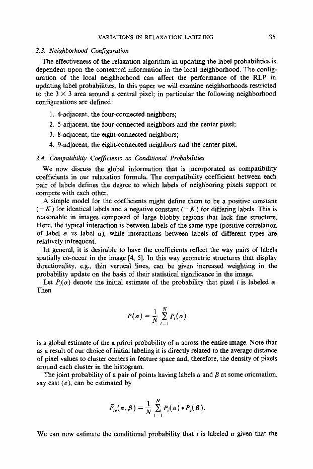
2.3. Neighborhood Configuration

The effectiveness of the relaxation algorithm in updating the label probabilities is dependent upon the contextual information in the local neighborhood. The configuration of the local neighborhood can affect the performance of the RLP in updating label probabilities. In this paper we will examine neighborhoods restricted to the 3 • 3 area around a central pixel; in particular the following neighborhood configurations are defined:

1. 4-adjacent, the four-connected neighbors;

2. 5-adjacent, the four-connected neighbors and the center pixel;

3. 8-adjacent, the eight-connected neighbors;

4. 9-adjacent, the eight-connected neighbors and the center pixel.

2.4. Compatibility Coefficients as Conditional Probabilities

We now discuss the global information that is incorporated as compatibility coefficients in our relaxation formula. The compatibility coefficient between each pair of labels defines the degree to which labels of neighboring pixels support or compete with each other.

A simple model for the coefficients might define them to be a positive constant (+ K) for identical labels and a negative constant ( - K ) for differing labels. This is reasonable in images composed of large blobby regions that lack fine structure. Here, the typical interaction is between labels of the same type (positive correlation of label a vs label a), while interactions between labels of different types are relatively infrequent.

In general, it is desirable to have the coefficients reflect the way pairs of labels spatially co-occur in the image [4, 5]. In this way geometric structures that display directionality, e.g., thin vertical lines, can be given increased weighting in the probability update on the basis of their statistical significance in the image.

Let Pi(a) denote the initial estimate of the probability that pixel i is labeled a. Then

| N

P(- ) = ,Z P+(-) l : l

is a global estimate of the a priori probability of a across the entire image. Note that as a result of our choice of initial labeling it is directly related to the average distance of pixel values to cluster centers in feature space and, therefore, the density of pixels around each cluster in the histogram.

The joint probability of a pair of points having labels a and/3 at some orientation, say east (e), can be estimated by

1 N ff/e(Ot, fl) = ' N E P i ( ~ t ) * P e ( f l ) "

i=1

We can now estimate the conditional probability that i is labeled a given that the


east pixel e is labeled/3 by

p , , ( < # ) -

N Z 1,,(.).t,.(.)

/l~e(~ # ) /=l N

Pi(#) i=I

Two labels are independent in direction 0 if the pair of labels co-occur with the same probability as the product of their individual probabilities,

/~ fl) = P(ot)zP(#), and in terms of conditional probabilities,

e , , ( - l # )

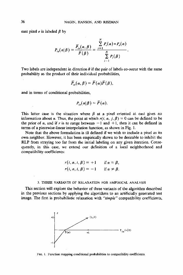
This latter case is the situation where fl at a pixel oriented at east gives no information about a. Thus, the point at which r(i, a, j , fl) = 0 can be defined to be the prior of a, and if r is to range between - 1 and + 1, then it can be defined in terms of a piecewise-linear interpolation function, as shown in Fig. 1.

Note that the above formulation is ill defined if we wish to include a pixel as its own neighbor. However, it has been empirically shown to be desirable to inhibit the RLP from straying too far from the initial labeling on any given iteration. Conse- quently, in this case, we extend our definition of a local neighborhood and compatibility coefficients:

r ( i , a , i , fl) = + 1

r ( i , . , i , # ) = --1

i f a = /3 ,

if a =# ft.

3. THREE VARIANTS OF RELAXATION FOR EMPIRICAL ANALYSIS

This section will explore the behavior of three variants of the algorithm described in the previous sections by applying the algorithms to an artificially generated test image. The first is probabilistic relaxation with "simple" compatibility coefficients,

+i

-i,

r

~ (z,1)

J Pie(~ I S)

FIo. 1. Function mapping conditional probabilities to compatibility coefficients.


namely, for all neighbors j:

r ( i , a , j , f l )= +1 i f a = f l ,

r ( i , a , j , f l ) = - - I i f a ~ ~8.

The second variant uses probabilistic relaxation with modified conditional probabilities for coefficients (as defined in Section 2.4). Finally, a degenerate form of discrete relaxation will be presented, called plurality update. In this scheme, both the label probabilities and the label compatibilities are discarded. The algorithm initially assigns the most likely label to each pixel, e.g., via a minimum distance classifier. Next, an update rule is applied which consists simply of selecting the most frequently occurring label in the neighborhood of each pixel. This is equivalent to a mode filter [9] except that it is applied to labels instead of pixel intensities. This algorithm has the advantage of simplicity and speed of execution while retaining some of the flavor of the probabilistic schemes.

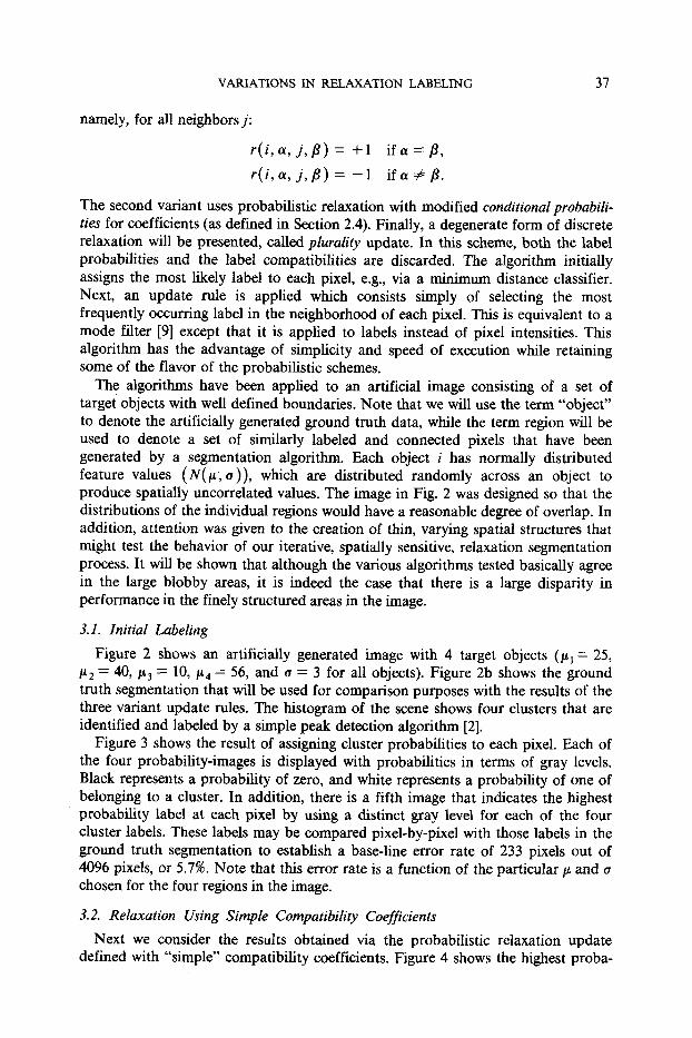
The algorithms have been applied to an artificial image consisting of a set of target objects with well defined boundaries. Note that we will use the term "object" to denote the artificially generated ground truth data, while the term region will be used to denote a set of similarly labeled and connected pixels that have been generated by a segmentation algorithm. Each object i has normally distributed feature values ( N ( ~ ; o ) ) , which are distributed randomly across an object to produce spatially uncorrelated values. The image in Fig. 2 was designed so that the distributions of the individual regions would have a reasonable degree of overlap. In addition, attention was given to the creation of thin, varying spatial structures that might test the behavior of our iterative, spatially sensitive, relaxation segmentation process. It will be shown that although the various algorithms tested basically agree in the large blobby areas, it is indeed the case that there is a large disparity in performance in the finely structured areas in the image.

3.1. Initial Labeling

Figure 2 shows an artificially generated image with 4 target objects (/~l = 25, /~2 = 40,/~3 = 10, k~4 = 56, and a -~ 3 for all objects). Figure 2b shows the ground truth segmentation that will be used for comparison purposes with the results of the three variant update rules. The histogram of the scene shows four clusters that are identified and labeled by a simple peak detection algorithm [2].

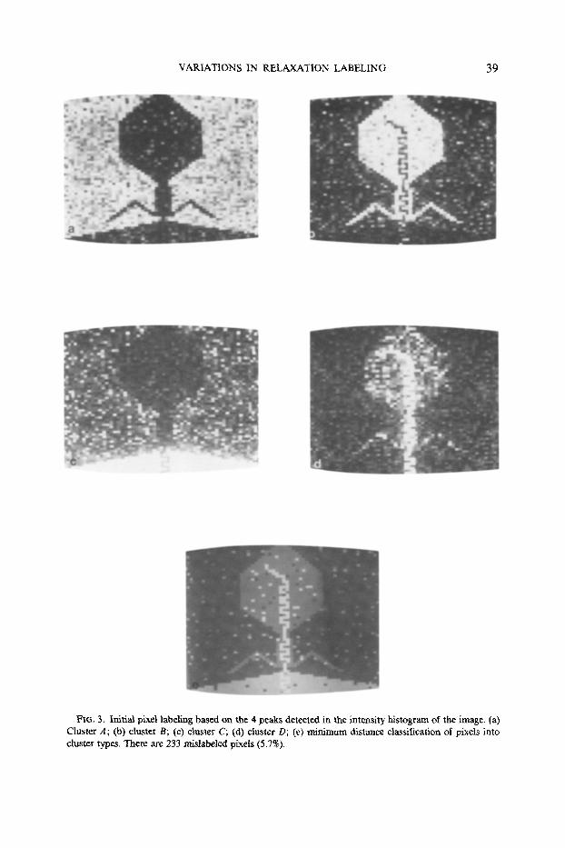
Figure 3 shows the result of assigning duster probabilities to each pixel. Each of the four probability-images is displayed with probabilities in terms of gray levels. Black represents a probability of zero, and white represents a probability of one of belonging to a cluster. In addition, there is a fifth image that indicates the highest probability label at each pixel by using a distinct gray level for each of the four cluster labels. These labels may be compared pixel-by-pixel with those labels in the ground truth segmentation to establish a base-line error rate of 233 pixels out of 4096 pixels, or 5.7%. Note that this error rate is a function of the particular # and chosen for the four regions in the image.

3.2. Relaxation Using Simple Compatibility Coefficients Next we consider the results obtained via the probabilistic relaxation update

defined with "simple" compatibility coefficients. Figure 4 shows the highest proba-


02

01

a

03 04

C C C A C B C D

# of points

i0 25 40 56 gray level

C

FIG. 2. Artificial image used in the next set of experiments. All objects have normal distributions and the pixds have a spatially random distribution within each object. Note that there is a 1-1 correspon- dence between the numeric ordering of the objects and the alphabetic ordering of the dusters. (a) Image containing 4 objects (#t = 25, /tz = 40, ~3 = 10, /~4 = 56, o = 3 for all objects). Co) Ground truth segmentation. (c) Overall histogram reveals 4 partially overlapped clusters.


FIG. 3. Initial pixel labeling based on the 4 peaks detected in the intensity histogram of the image. (a) Cluster A; (b) duster B; (c) cluster C; (d) cluster D; (e) minimum distance classification of pixels into duster types. There are 233 mislabeled pixeis (5.7%).



"o

G

, ~ eL0

..> ,~

r

t'~ 8.&=

" ~ e9 ~,~

0

,~ ~ ~ ~ . ~ ~


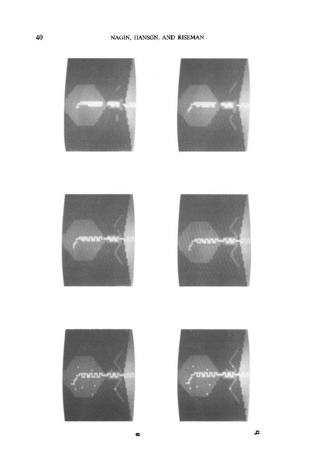
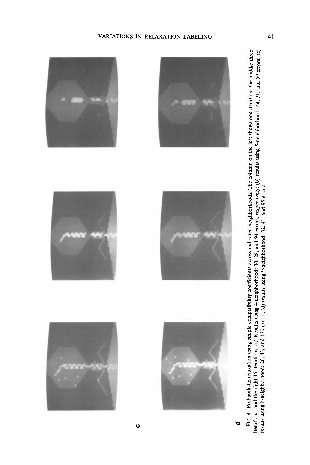
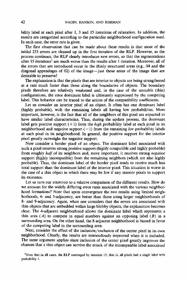
bility label at each pixel after 1, 3 and 15 iterations of relaxation. In addition, the results are categorized according to the particular neighborhood configuration used. In each case, the error rate is given.

The first observation that can be made about these results is that most of the initial 233 errors are cleaned up in the first iteration of the RLP. However, as the process continues, the RLP clearly introduces new errors, so that the segmentations after 15 iterations 1 are much worse than the results after 1 iteration. Moreover, all of the errors that are introduced occur in the thinly structured areas (e.g., 04 and the diagonal appendages of 02) of the image--just those areas of the image that are desirable to preserve!

The explanation is that the pixels that are interior to objects are being strengthened at a rate much faster than those along the boundaries of objects. The boundary pixels therefore are relatively weakened and, in the case of the unstable (thin) configurations, the once dominant label is ultimately suppressed by the competing label. This behavior can be traced to the action of the compatibility coefficients.

Let us consider an interior pixel of an object. It often has one dominant label (highly probable), with the remaining labels all having low probabilities. More important, however, is the fact that all of the neighbors of this pixel are expected to have similar label characteristics. Thus, during the update process, the dominant label gets positive support (+ 1) from the high probability label at each pixel in its neighborhood and negative support ( - 1) from the remaining low probability labels at each pixel in its neighborhood. In general, the positive support for the interior pixel greatly outweighs the negative support.

Now consider a border pixel of an object. The dominant label associated with such a pixel receives strong positive support (highly compatible and highly probable) from roughly half of its neighbors and, more important, it receives strong negative support (highly incompatible) from the remaining neighbors (which are also highly probable). Thus, the dominant label of the border pixel tends to receive much less total support than the dominant label of the interior pixel. This situation is worse in the case of a thin object in which there may be few if any interior pixels to support its existence.

Let us turn our attention to a relative comparison of the different results. How do we account for the widely differing error rates associated with the various neighborhood formations? Note that upon convergence the two results using limited neighborhoods, 4- and 5-adjacency, are better than those using larger neighborhoods of 8- and 9-adjacency. Again, when one considers that the errors are associated with thin objects that are embedded within large blobby objects, the explanation becomes dear. The 4-adjacent neighborhood allows the dominant label which represents a thin area (A) to compete in equal numbers against an opposing label (B) in a surrounding area. On the other hand, the 8-adjacent neighborhood is biased in favor of the competing label in the surrounding area.

Next, consider the effect of the inclusion/exclusion of the center pixel in its own neighborhood. Clearly, the results are tremendously improved when it is included. The same argument applies since inclusion of the center pixel greatly improves the chances that a thin object can survive the attack of the incompatible label associated

INote that in all cases, the RLP converged by iteration 15; that is, all pixels had a single label with probability 1.


with the many pixels of the surrounding object. It is a form of "inertia" of resting probabilities and helps to some degree, but unfortunately it is not a very sound general solution.

All of these results suffer from a similar deficiency. The "simple" compatibility coefficients are inadequate to represent label dependencies that occur within the image. Therefore, the quality of a segmentation is driven by the geometry (shape) of objects with respect to the geometry of the pixel neighborhood that is defined for the RLP. This is clearly unsatisfactory, since the two-dimensional geometry of an object is in general arbitrary.

3.3. Relaxation Using Conditional Probabilities as Compatibility Coefficients

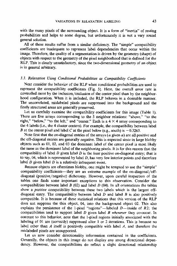
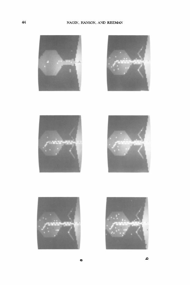
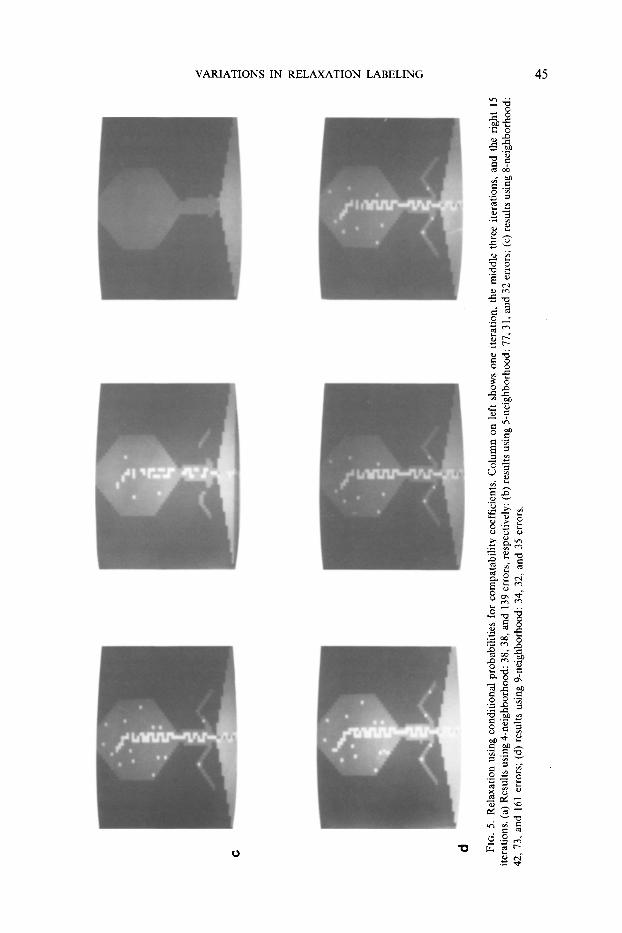
Next consider the behavior of the RLP when conditional probabilities are used to represent the compatibility coefficients (Fig. 5). Here, the overall error rate is controlled more by the inclusion/exclusion of the center pixel than by the neighborhood configuration. When it is included, the RLP behaves in a desirable manner. The uncorrelated, mislabeled pixels are suppressed into the background and the finely structured areas are generally preserved.

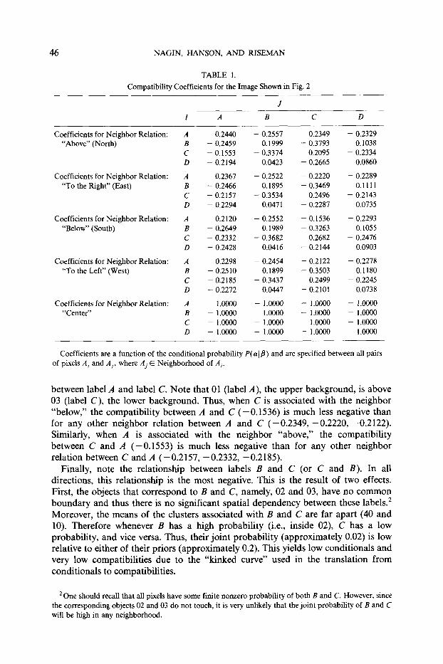
Let us carefully examine the compatibility coefficients for this image (Table 1). There are five arrays corresponding to the 5 neighbor relations: "above," "to the right," "below," "to the left," and "center." Each is a 4 • 4 array corresponding to the 4 labels (i.e., the 4 cluster centers). For example, the compatibility between label B at the center pixel and label C at the pixel below (e.g., south) is -0.3263.

Note first that the on-diagonal entries of the arrays (a given a) are all positive and the off-diagonal entries are generally negative. This is expected since in large blobby objects such as 01, 02, and 03 the dominant label of the center pixel is most likely the same as the dominant label of the neighboring pixels. It is for this reason that the compatibility of label D given label D is the least positive on-diagonal entry; that is to say, 04, which is represented by label D, has very few interior points and therefore label D given label D is a relatively infrequent event.

Because objects are oftentimes blobby, one might be tempted to use the "simple" compatibility coefficients--they are an extreme example of the on-diagonal/off- diagonal (positive/negative) dichotomy. However, upon careful inspection of the tables one finds some important exceptions to this observation. Consider the compatibilities between label B (02) and label D (04). In all orientations the tables show a positive compatibility between these two labels which is the largest off- diagonal entry. The compatibility between label D and label B is also positively compatible. It is because of these statistical relations that this version of the RLP does not suppress the thin object, 04, into the background object 02. This also explains the persistence of the 1-pixel "regions"--labeled D--inside of R2; the compatibilities tend to support label D given label B whenever they co-occur. In contrast to this behavior, note that the 1-pixel regions initially associated with the labeling of 01 are (correctly) suppressed after 1 or 2 iterations. This is because no label other than A itself is positively compatible with label A, and therefore the mislabeled pixels are unsupported.

Let us now consider directionality information contained in the coefficients. Generally, the objects in this image do not display any strong directional dependency. However, the compatibilities do reflect a slight directional relationship


, ~ ~!~iii~!!i~(~ ~ ~ ~ ~


O

O O

"~ O

_~a2 "~ O

.s .-~

0 0 0

~,~

~ 7 7

~

~ ~

46 NAG/N, HANSON, A N D RISEMAN

TABLE 1.

Compatibility Coefficients for the Image Shown in Fig. 2

I A B C D

Coefficients for Neighbor Relation: "Above" (North)

Coefficients for Neighbor Relation: "To the Right" (East)

Coefficients for Neighbor Relationi "Below" (South)

Coefficients for Neighbor Relation: "To the Left" (West)

Coefficients for Neighbor Relation: "Center"

A 0.2440 -0 .2557 - 0 . 2349 -0 .2329 B - 0 . 2 ~ 9 0.1999 -0 .3793 0.1038 C - 0.1553 - 0.3374 0.2095 - 0.2334 D - 0.2194 0.0423 - 0.2665 0.0860

A 0.2367 - 0.2522 - 0.2220 -0 .2289 B -0 .2466 0.1895 - 0.3469 0.1111 C - 0.2157 - 0 . 3534 0.2496 -0 .2143 D -0 .2294 0.~71 -0 .2287 0.0735

A 0.2120 - 0 . 2552 - 0.1536 - 0.2293 B - 0.2649 0.1989 - 0.3263 0.1055 C - 0.2332 - 0.3682 0.2682 - 0.2476 D -0 .2428 0.~16 - 0 . 2 1 ~ 0.0903

A 0.2298 - 0.2454 - 0.2122 --0.2278 B - 0.2510 0.1899 --0.3503 0.1180 C -0 .2185 -0 .3437 0.2499 -0 .2245 D -0 .2272 0.0447 --0.2101 0.0738

A 1.0000 -1 .0000 --1.0000 -1 .0000 B -1 .0000 1.0000 -1 .0000 -1 .0000 C -1 .0000 -1 .0000 1.0000 -1 .0000 D - I . 0 0 0 0 - 1 . 0000 -1 .0000 1.13000

Coefficients are a function of the conditional probability P(atf l ) and are specified between all pairs of pixels A i and A j , where Aj ~ Neighborhood of A i.

between label A and label C. Note that 01 (label A), the upper background, is above 03 (label C), the lower background. Thus, when C is associated with the neighbor "below," the compatibility between A and C ( -0 .1536) is much less negative than for any other neighbor relation between A and C ( -0 .2349 , -0 .2220 , -0 .2122) . Similarly, when A is associated with the neighbor "above," the compatibility between C and A (-0 .1553) is much less negative than for any other neighbor relation between C and A (-0 .2157, -0.2332, -0.2185).

Finally, note the relationship between labels B and C (or C and B). In all directions, this relationship is the most negative. This is the result of two effects. First, the objects that correspond to B and C, namely, 02 and 03, have no common boundary and thus there is no significant spatial dependency between these labels. 2 Moreover, the means of the dusters associated with B and C are far apart (40 and 10). Therefore whenever B has a high probability (i.e., inside 02), C has a low probability, and vice versa. Thus, their joint probability (approximately 0.02) is low relative to either of their priors (approximately 0.2). This yields low conditionals and very low compatibilities due to the "kinked curve" used in the translation from conditionals to compatibilities.

2One should recall that all pixels have some finite nonzero probability of both B and C. However, since the corresponding objects 02 and 03 do not touch, it is very unlikely that the joint probability of B and C will be high in any neighborhood.


3.4. Relaxation Using Plurality Update

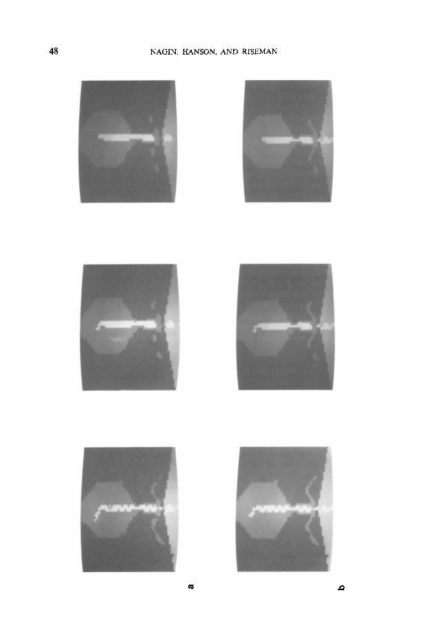
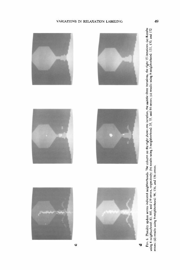
Finally, consider the third update scheme--the plurality rule-- in which the label probabilities and label compatibilities are not employed at all. Instead, a minimum distance classifier is used to assign an initial label to each pixel. The label is then updated by replacing it with the most frequently occurring label in its neighborhood. Therefore, this scheme favors geometrically stable configurations of labels, e.g., blobs that contain interior points.

After 15 iterations, the results (Fig. 6) using a 4-adjacent neighborhood are not much worse than the results obtained via the probabilistic relaxation update using simple compatibility coefficients. This is not surprising since neither technique incorporates information that is based on structural dependencies between labels. Both schemes are implicitly biased toward structures that have interior points and, thus, neither is able to preserve thin regions. The plurality results using an 8-adjacent neighborhood are considerably worse than those with the 4-adjacent neighborhood. This is also to be expected since increasing the number of neighbors works against maintaining the fragile structures that we have been examining.

In defense of the plurality relaxation scheme, note that this computationally inexpensive technique performs very well in areas lacking spatial structure. Here, it yields the desired effect of suppressing sparse, randomly located "noise" labels. Moreover, we have found that its application to natural scenes that mostly contain "blobby" regions yields results that are remarkably similar to the results using probabilistic relaxation--even when the latter used compatibility coefficients that are based on spatial dependencies of labels in the image.

3.5. Summary of Test Results

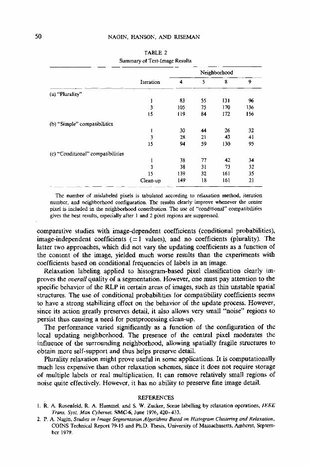
According to Table 2 the "simple" relaxation scheme gives the best results in the short run. However, the converged results show a significant degradation of performance. On the other hand, relaxation with conditional probabilities has only slightly worse minimum error rates than the simple scheme and importantly, it does not degrade significantly over time. Moreover, by referring to the segmentations using conditional probabilities (Fig. 5) one notes that the 5-neighborhood and 9- neighborhood results can be improved by a very simple clean-up scheme. The images show a large number of 1 and 2 pixel "regions" that are counted as errors. 3 Clearly, these regions are too small to carry any "meaning," and it is therefore justifiable to suppress them into the background. When this is done the error rates reduce to 18 and 21 pixels, respectively, or approximately 0.4%. We conclude that the conditional probabilities are necessary to prevent the relaxation process from destroying fragile structures.

3.6. Conclusions

This paper has covered a range of issues concerning the behavior of relaxation labeling processes. The performance of these algorithms is affected by the form of compatibility coefficients and the configuration of local neighborhoods. Let us now make some recommendations and evaluations based on the work presented.

When appropriately specified, compatibility coefficients can allow stability in the RLP and prevent destruction of fine detail in an image. This was shown by

3 Note that the results based on the other relaxation schemes do not leave any such noise regions.



r "O

u~

~=.-

�9 ~ O O

~ o o

g ~

" O *-,

='-o

O

O

" O 0 0

"~ 0a


TABLE 2

Summary of Test-Image Results

Neighborhood

Iteration 4 5 8 9

(a) "Plurality"

(b) "Simple" compatibilities

(c) "Conditional" compatibilities

1 83 55 131 96 3 105 75 170 136

15 l l9 84 172 156

1 30 44 26 32 3 28 21 43 41

15 94 59 130 95

1 38 77 42 34 3 38 31 73 32

15 139 32 161 35 Clean-up 149 18 161 21

The number of mislabeled pixels is tabulated according to relaxation method, iteration number, and neighborhood configuration. The results clearly improve whenever the center pixel is included in the neighborhood contribution. The use of "conditional" compatibilities gives the best results, especially after 1 and 2 pixel regions are suppressed.

comparative studies with image-dependent coefficients (conditional probabifities), image-independent coefficients (-+ 1 values), and no coefficients (plurality). The latter two approaches, which did not vary the updating coefficients as a function of the content of the image, yielded much worse results than the experiments with coefficients based on conditional frequencies of labels in an image.

Relaxation labeling applied to histogram-based pixel classification clearly improves the overall quality of a segmentation. However, one must pay attention to the specific behavior of the RLP in certain areas of images, such as thin unstable spatial structures. The use of conditional probabilities for compatibility coefficients seems to have a strong stabilizing effect on the behavior of the update process. However, since its action greatly preserves detail, it also allows very small "noise" regions to persist thus causing a need for postprocessing clean-up.

The performance varied significantly as a function of the configuration of the local updating neighborhood. The presence of the central pixel moderates the influence of the surrounding neighborhood, allowing spatially fragile structures to obtain more self-support and thus helps preserve detail.

Plurality relaxation might prove useful in some applications. It is computationally much less expensive than other relaxation schemes, since it does not require storage of multiple labels or real multiplication. It can remove relatively small regions of noise quite effectively. However, it has no ability to preserve fine image detail.

REFERENCES

1. R. A. Rosenfeld, R. A. Hummel, and S. W. Zucker, Scene labelling by relaxation operations, IEEE Trans. Syst. Man Cybernet. SMC-6, June I976, 420-433.

2. P. A. Nagin, Studies in Image Segmentation Algorithms Based on Histogram Clustering and Relaxation, COINS Technical Report 79-15 and Ph.D. Thesis, University of Massachusetts, Amherst, Septem- ber 1979.


3. A. Rosenfeld and L. S. Davis, Iterative Histogram Modification, TR-519, Computer Science Center, University of Maryland, April 1977.

4. S. W. Zucker and J. L. Mohammed, Analysis of probabilistic relaxation labelling processes, Proc. PRIP, Chicago, Illinois, May 1978.

5. S. Peleg and A. Rosenfeld, Determining compatibility coefficients for curve enhancement relaxation processes, IEEE Trans. Syst. Man Cybernet. SMC-8, July 1978, 548-555.

6. A. R. Hanson, E. M. Riseman, and F. C. Glazer, Edge relaxation and boundary continuity, in Consistent Labeling Problems in Pattern Recognition (R. M. Haralick, Ed.), Plenum, New York, in press; also COINS Technical Report 80-11, University of Massachusetts, Amherst, May 1980.

7. G. B. Coleman, Image Segmentation by Clustering, USCIPI Report 750, Image Processing Institute, University of Southern California, July 1977.

8. R. R. Kohler, Ph.D. Thesis, University of Massachusetts, Amherst, in preparation. 9. J. Eklundh and A. Rosenfeld, Peak detection using difference operators, IEEE Trans. Pattern Anal.

Mach. Intell. PAMI-I, July 1979, 317-325.

Documents

Variations in relaxation labeling techniques