Sec. 1.4

1.4 MODELING AND ENERGY METHODS

L4odeling and Energy Methods

In terms of g = 9.31 m/s2, this becomest )

Sximum acceterat ion : ' : : : " T ' : 's - 7 .68 e 's

9.81 m/s ' o

,1ry : .{ ' . ' ("#* sino,,/ * 'o.or.ur,)

23

Example 1.3.3

Compute the form of the response of an underdamped system using the Cartesian formof the solution given in Window 1.5.

Solution Frombasictrigonometrysin(x + y) : sinxcosy * cosxsiny.Applyingthisto equation (1.36) with x = a7t and y : $ yields

x(t) : 4"-t '" sin(or7t + 0) : r-{ ' '(ArsinoT/ * A2cosuat)

where,41 : cosS andA2 = sin0,asindicatedinWindowl.5.Evaluatingtheinit ialcon-ditions yields

x(0) : xo: eo(Ars in0 + A2cos0)

Solving yields ,42 : xo. Next differentiate .r(r) to get

.i: -(6,s-(', '(Arsin<,rrl + lrcosorrt) + aoe-L',,t(Arcostodt - ,42sinorTl)

Applying the initial velocity condition yields

'uo = i(0) : -La,(ArsinO + x6cos0) + ao(A1cos0 - rosin0)

Solving this last expression yields

u0 I (anxsA -

^ 1 -

(D4

Thus the free response in Cartesian form becomes

tr

Modeling is the art or process of writing down an equation, or system of equations,to describe the motion of a physical device. For example, equation (1.2) was-gbtainedby modeling the spring-mass system of Figure 1".4.8y summing the forces acting onthe mass in the x direction and employing the experimental evidence of the mathe-matical model of the force in a spring given by Figure 1.3, equation (1..2) can be ob-tained. The success of this model is determined by how well the solution of equation(1.2) predicts the observed behavior of the system. This comparison between the vi-bration response of a device and the response predicted by the analytical model is dis-cussed in Section 1.6.The majority of this book is devoted to the analysis of vibration

24 Introduction to Vibration and the Free Response Chao. 1

models. However, two methods of modeling-Newton's law and energy methods-are presented in this section. More comprehensive treatments of modeling can befound in Doebelin (1980), Shames (1980, 1989), and Cannon (1967),ryxample.

The force summation method is used in the previous sectionsVd should befamiliar to the reader from introductory dynamics (see, e.g., Shames, 1980). Newton'slaw of moticn (called Newton's second /aw) states that the rate of change of the ab-solute momentum of the mass center is proportional to the net applied force vectorand acts in a direction of the net force. For systems with constant mass (such as thoseconsidered here) moving in only one direction, the rate of change of momentum be-comes the scalar relation

: m x

which is often called the inertia force. The physical device of interest is examined bynoting the forces acting on the center of mass. The forces are then summed (as vec-tors) to produce a dynamic equation following Newton's law. For motion in the x di-rection only, this becomes the scalar equation

(1.4e)

where f, denotes the ith force acting on the mass r.tx in the x direction and the sum-mation is over the number of such forces. In the first three chapters, only single-degree-of-freedom systems moving in one direction are considered; thus Newton's lawtakes on a scalar nature. In more practical problems with many degrees of freedom,energy considerations can be combined with the concepts of virtual work to produceLagrange's equations, as discussed in Section 4.7.Lagrange's equations also providean energy-based alternative to summing forces to derive equations of motion.

For bodies that are free to rotate about a fixed axis, the sum of the torquesabout the rotation axis through the center of mass of the object must equal the rateof change of angular momentum of the mass. This is expressed as

(1.s0)

where M6i are the torques acting on the object through point 0, -/ is the moment ofinertia (sometimes denoted 1s) about the rotation axis, and 0 is the angle of rotation.This is discussed in more detail in Example 1.5.1.

If the forces or torques acting on an object or mechanical part are difficult todetermine, an energy approach may be more efficient. In this method the differen-tial equation of motion is established by using the principle of energy conservation.This principle is equivalent to Newton's law for conservative systems and states thatthe sum of the potential energy and kinetic energy of a particle remains constant ateach instant of time throughout the particle's motion. Integrating Newton's law

d , . \- l m x ldt

2f, , : ^*

) ruo, : "'g

Sec. '1.4 Modeling and Energy Methods 25

(F : mi) over an increment of displacement and identifying the work done in aconservative field as the change in potential energy yields

U r - U r : T z - T t ( 1 .s1)

where U1 and {./2 represent the particle's potential energy at the times /r and /t, re-spectively, and T1 and T2 represent the particle's kinetic energy at times t, and t2,re-spectively. Equation (1.51) can be rearranged to yield

T + U : c o n s t a n t ( 7 . 5 2 )

where T and U denote the total kinetic and potential energy, respectively.For periodic motion, if rt is chosen to be the time at which the moving mass

passes through its static equilibrium position, Ul can be set to zero at that time, andif 12 is chosen as the time at which the mass undergoes its maximum displacement sothat its velocity is zero (f, : O), equation (1.51) yields

T r : U z (1.s3)

Since tlre reference potential energy Uliszero, U2 in equation (1.53) is the maximumvalue of potential energy in the system. Because the energy in this system is con-served, Z2 must also be a maximum value so that equation (1.53) yields

Z-u" : U-u* (1.54)

for conservative systems undergoing periodic motion. Since energy is a scalar quan-

tity, using the conservation of energy yields a possibility of obtaining the equation ofmotion of a system without using vectors.

Equations (1.52), (1.53), and (1.54) are three statements of the conservation ofenergy. Each of these can be used to determine the equation of motion of aspring-mass syslem. As an illustration, consider the energy of the spring-mass system

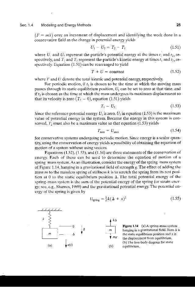
of Figure 1.1-4, hanging in a gravitational field of strength g. The effect of adding the

mass /11 to the massless spring of stiffness k is to stretch the spring from its rest posi-

tion at 0 to the static equil ibrium position A. The total potential energy of thespring-mass system is the sum of the potential energy of the spring (or strain ener-gy; see, e.g., Shames, 1989) and the gravitational potential energy. The potential en-ergy of the spring is given by

u ,p , i ng : l t 1n+x12 (1.ss)

Figure 1,14 (a)A spring-mass systemhanging in a gravitational field. Here A isthe static equilibrium position and x isthe displacement from equilibrium.(b) The free-body diagram for staticequilibrium.

l oV

(b)

25 Introduction to Vibration and the Free Response Chap. 1

The gravitational potential energy is

Ugro, : -mgx (1.56)

where the minus sign indicates that the mass is located below the rcference point xsThe kinetic energy of the system is

7 : !m*2

Substituting these energy expressions into equation (1.52) yields

i**' - mgx I )t<11, + r)2 : constant

Differentiating this expression with respect to time yields

* ( m i + k x ) + * ( k L - m s ) : 0

Since the static force balance on the mass from Figure 1.14(b) yieldskL, : mg, equation (1.59) becomes

i ( m i + k x ) : g (1.60)

The velocity i cannot be zero for all time; otherwise, x(t) : constant and no vibra-

tion would be possible. Hence equation (1.60) yields the standard equation of motion

m i * k x : 0 (1 .61)

This procedure is called the energy method of obtaining the equation of motion.

The energy method can also be used to obtain the frequency of vibration directly

for conservative systems that are oscillatory. The maximum value of sine (and co-

sine) is 1. Hence, from equations (1.3) and (1.a), the maximum displacement is ,4 and

the maximum velocity is o,A. Substitution of these maximum values into the ex-

pression for U-u* and Z*u* and using the energy equation (1.54) yields

lm(.,A)2 : it ,4 (r.62)

Solving this for on yields the standard natural frequency relation ,^ : {t /^ .

Example 1.4.1

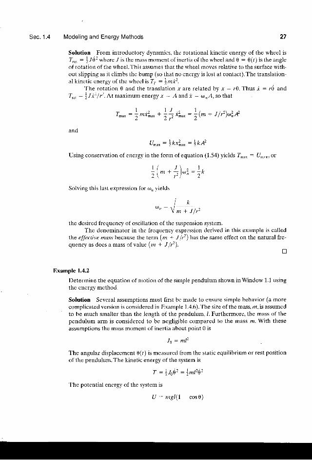
Figure L.15 is a crude model of a vehicle suspension system hitting a bump. Calculate thenatural frequency of oscillation using the energy method. Assume that no energy is lostduring the contact.

Figure 1,15 Simple model of an

automobile suspension system. The

rotation of the wheel relative to the

horizontal as it hits a bump is given by 0.

It is assumed that the wheel roils without

slipping as the car hits the bump.

(r.s7)

(1.s8)

(1.se)the fact that

Sec. 1.4 Modeling and Energy Methods

Solution From introductory dynamics, the rotational kinetic energy of the wheel isT*, : lJ02 where -/ is the mass moment of inertia of the wheel and 0 : 0(l) is the angleof rotation of the wheel. This assumes that the wheel moves relative to the surface with-out slipping as it climbs the bump (so that no energy is lost at contact). The translation-al kinetic energy of the wheel is T7 : lm*2.

The rotation 0 and the translation x are related by x : r0. Thus i : rd andT,o. : |J *21 12. At maximum energy x : A and * : a,,A,so that

T _' max + l lrz)af,*

and

U.u* : t 1 t< *2^ - : l t c t

Using conservation of energy in the form of equation (1.54) yields Z.u* = f/-.^, or

Solving this last expression for o,, vields

the desired frequency of oscillation of the suspension system.The denominator in the frequency expression derived in this example is called

the effectivenass because the term (m + J lr2) has the same effect on the natural fre-quency as does a mass cf valu e (m + J lr2).

!

Example 1.4.2

Determine the equation of motion of the simple pendulum shown in Window 1.1 usingthe energy method.

Solution Several assumptions must first be made to ensure simple behavior (a more

complicated version is considered in Example 1.4.6).The size of the mass, z, is assumedto be much smaller than the length of the pendulum, /. Furthermore, the mass of thependulum arm is considered to be negligible compared to the mass rz. With these

assumptions the mass moment of inertia about point 0 is

Jo : mlz

The angular displacement 0(r) is measuled from the static equilibrium or rest position

of the pendulum. The kinetic energy of the system is

7 : ) J s a 2 : ) m 1 2 6 2

The potential energy of the system is

27

1 . , l J . , 1i^i '*^-

* ,7 f '^^^ =

t(^

1 ( / \ , 1 ,; l m + - l / U . J ; : ; Kz \ r - / / -

U : m g l ( I - c o s 0 )

28 lntroduction to Vibration and the Free Response Chap' 1

0 + - n

(lto' + it s') : (rd + to)e : o

since I ( 1 - cos 0 ) is the geometric change in elevation of the pendulum mass' Substitu-

tion of these expressions for the kinetic and potential energy into equation (1.52) and

differentiating yields

)* l i m t ' { + m s t ( t - c o s o l ] : so t -

m l 2 e 6 + r z g l ( s i n 0 ) 0 : 0

o(mtzo + ngl sinO) = 6

Since 6 (r) cannot be zero for all time, this becomes

m l 2 0 + m g l s i n 0 : 0

or

or

Factoring out 0 yields

] s i n 0t

This is a nonlinear equation in 0 and is discussed in Section 1.10. However, here, since

sin 0 can be approximated by 0 for small angles, the linear equation of motion for the pen-

dulum becomes

= 0

This corresponds to an oscillation with natural frequency . , .: filt for initial condi-

tions such that 0 remains small, as defined by the approximation sin 0 = 0.

Example 1.4.3

Determine the equation of motion of the shaft and disk illustrated in Window 1.1 using

the energ.v method.

Solution The shaft and disk of Window 1.1 are modeled as a rod st i f fness in twist-

ing, result ing in torsional motion. The shaft, or rod, exhibits a tolque in twist ing pro-

port ional tolhe angle of twist 0(t).The potential energy associated with the torsional

spring stiffne.s is U - jke2, where the stiffness coefficient k is determined much like

tire metnoO used to determine the spring stiffness in translation, as discussed in Sec-

t ion 1.1.The angle 0(r) is measured from the stat ic equi l ibr ium, or rest, posit ion.The

kinetic energy associated with the disk of mass moment of inertia "r is T : I le2. rnis

assumes that the inertia of the rod is much smaller than that of the disk and can be

neglected.Substitution of these expressions for the kinetic and potential energy into equa-

tion (1.52) and differentiating yields

q

e + ; oI

d

dt

so that the equation of motion becomes (because 0 + 0)

, 1 6 + k o : 0

Sec. 1.4 Modeling and Energy Methods 29

This is the equation of motion fo1lqrsional vibration of a disk on a shaft. The natural

frequency of vibration is o, : V klJ .I

ExamPle 1.4.4

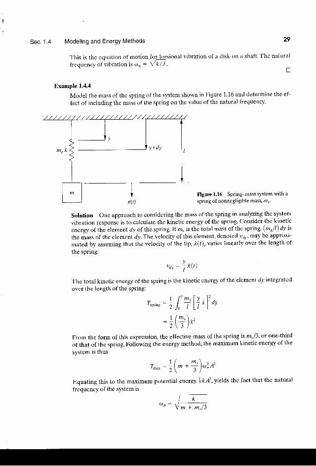
Model the mass of the spring of the system shown in Figure 1.16 and determine the ef-

fect of including the mass of the spring on the value of the natural frequency'

Figure 1.16 Spring-mass system with aspring of nonnegligible mass, m'.

Solution One approach to considering the mass of the spring in analyzing the system

vibration response is to calculate the kinetic energy of the spring. Consider the kinetic

energy of the element dy of the spring. If n" is the total mass of the spring, \nt"[) dy is

the mass of the element zly. The velocity of this element, denoted 't)d,may be approxi-

mated by assuming that the velocity of the tip, i(r), varies linearly over the length of

the spring:

oo, :

The total kinetic energy of the spring is the kinetic energy of the element dy integtated

over the length of the spring:

T_ spfmg

From the form of this expression, the effective mass of the spring is m,f3, or one-third

of that of the spring. Following the energy method, the maximum kinetic energy of the

svstem is thus

Equating this to the maximum potential energy, |k'4,yields the fact that the natural

frequency of the system is

i rt'l

r^* : : ( * * ) ) , ; *

I f t m , [ r . l ' ,,J , t l7 r )o 'r l m ' \ . ,2 \ 3 t

30 lntroduction to Vibration and the Free Response Chap' 1

Thus including the effects of the mass of the spring in the system decreases the natural

frequency. Note that if the mass of spring is much smaller than the system mass n, the

effect of the spring mass on the natural frequency is negligible'

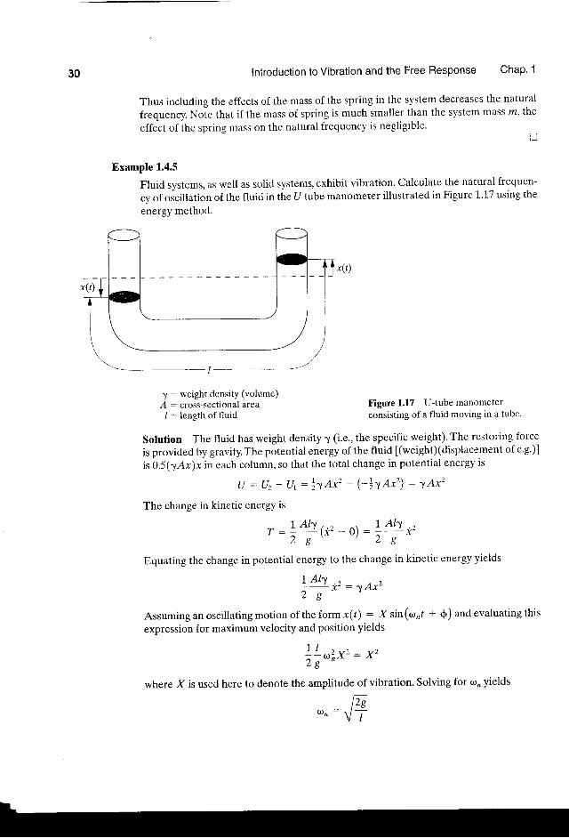
Example 1.4.5

Fluid systems, as well as solid systerrrs, cxhibit vibration. Calculate the natural frequen-

cy of oicillation of the fluici in the U tube manometer illustrated in Figure L.17 using the

energy method.

^y : weight density (volume)A : cross-sectional area

/ : Iength of fluidFigure L.17 U-tube manometerconsisting of a fluid moving in a tube

Solution The fluid has weight density 1 (i.e., the specific weight). The restoring force

is provided by gravity.The potential energy of the fluid [(weight)(displacement of c.g.)]

is 0.5("y,4x)x in each column, so that the total change in potential energy is

U : Uz - Ur : Lt Ar, - (-lt at ) : 1 Axz

The change in kinetic energy is

1 AI'v I Ahr : r s

( i ' -0) : tTr-

Equating the change in potential energy to the change in kinetic energy yields

I A \ . ) 1; ;

* : l A x z

Assuming an oscillating motion of the form x(t) : y sin(onl + $) and evaluating this

expression for maximum velocity and position yields

1 I

i ' r u 2 ' x 2 : Y z

where X is used here to denote the amplituAe of vibration. Solving for orn yields

tr, , : v7

fiI

II

3 lSec. 1.4 Modeling and Energy Methods

which is the natural frequency of oscillation of the fluid in the tube. Note that it dependsonly on the acceleration due to gravity and the length of the fluid. Vibration of fluids in-side mechanical containers (called sloshing) occurs in gas tanks in both automobiles andairplanes and forms an important application of vibration analysis.

!

Example 1.4.6

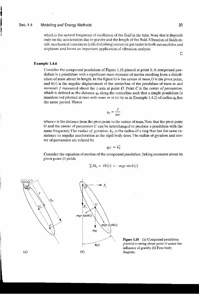
Consider the compound pendulum of Figure 1.18 pinned at point 0. A compound pen-dulum is a pendulum with a significant mass moment of inertia resulting from a distrib-ution of mass about its length. In the figure G is the center of mass, O is the pivot point,and 0(t) is the angular displacement of the centerline of the pendulum of mass rn andmoment / measured about the z-axis at point O. Point C is the center of percussion,which is defined as the distance 46 along the centerline such that a simple pendulum (amassless rod pivoted at zero with mass m at its tip as in Example 1.4.2) of radius 46 hasthe same period. Hence

where r is the distance from the pivot point to the center of mass Note that the pivot pointO and the center of percussion C can be interchanged to produce a pendulum with thesame frequency. The radius of gyration, ku, is the radius of a ring that has the same re-sistance to angular acceleration as the rigid body does.The radius of gyration and cen-ter of percussion are related by

eor : k2o

Consider the equation of motion of the compound pendulum.Taking moments about itspivot point O yields

2Mo : /0 (r) : -mgr sinl(t)

Figure 1.18 (a) Compound pendulumpivoted to swing about point O under theinfluence of gravity. (b) Free-bodydiagram.

JQ n = -

mr

l Ei a x

(b)

32 ntroduction to Vibration and the Free Response Chap' 1

For small 0(/) this nonlinear equation becomes

" 1 6 1 r ; + m g r \ ( t ) = 0

The natural frequency of oscillation becomes

t^8'u , ,= ! " /

This frequency can be expressed in terms of the center of percussion as

a- : rE" Y q o

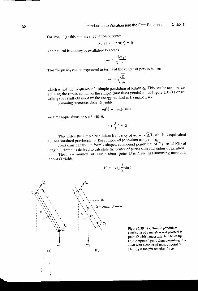
which is just the frequency of a simple pendulum of length 4o' This can be seen by ex-

aminingihe forces acting-on the simple (massless) pendulum of Figure 1.19(a) or re-

calling ihe result obtained by the energy method in Example 1"4'2'

Summing moments about O Yields

ml26 : -mgl sin0

or after approximating sin 0 with 0'

e+

This yields the simple pendulum frequency of orn : 'fglt 'which is equivalent

to that obtained previously for the compound pendulum using / : qs'

Nextconsider theuni formlyshapedcompoundpendulumofFigure l . l9(b)oflength /. Here it is desired to calculate the center of percussion and radius of gyration'

. I . hemassmomen to f i ne r t i aabou tpo in to i s l , so tha tsummingmomen ts

about O vields

o

; o : 0I

-^s f,"ine"r0 :

G = center of mass

Figure 1.19 (a) SimPle Pendulumconsisting of a massless rod pivoted at

point O with a mass attached to its tip.(b) Compound pendulum consisting of a

shaft with a center of mass at point G.

Here /6 is the pin reaction force.

Sec. 1.4 Modeling and Energy Methods

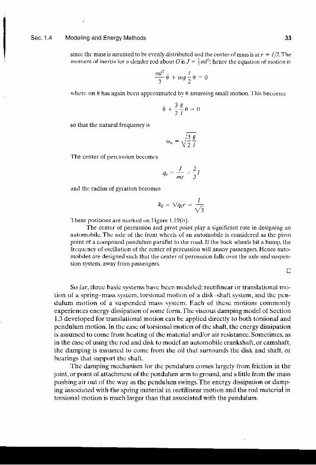
since the mass is assumed to be evenly distributed and the center of mass is at r : I p.Themomento f iner t ia fo ras lender rodabout O isJ : \m lz ;hencetheequat ionof mot ion is

n 1 1 2 , l -

; u " ms10 :0

where sin 0 has again been approximated by 0 assuming small motion. This becomes

so that the natural frequency is

The center of percussion becomes

4 o =

and the radius of gyration becomes

k o : l w

These positions are marked on Figure 1.19(b).The center of percussion and pivot point play a significant role in designing an

automobile. The axle of the front wheels of an automobile is considered as the pivotpoint of a compound pendulum parallel to the road. If the back wheels hit a bump, thefrequency of oscillation of the center of percussion will annoy passengers. Hence auto-mobiles are designed such that the center of percussion falls over the axle and suspen-sion system. away from passengers.

u

So far, three basic systems have been modeled: rectilinear or translational mo-tion of a spring-mass system, torsional motion of a disk-shaft system, and the pen-dulum motion of a suspended mass system. Each of these motions commonlyexperiences energy dissipation of some form.The viscous damping model of Section1.3 developed for translational motion can be applied directly to both torsional andpendulum motion. In the case of torsional motion of the shaft, the energy dissipationis assumed to come from heating of the material and/or air resistance. Sometimes, asin the case of using the rod and disk to model an automobile crankshaft, or camshaft,the damping is assumed to come from the oil that surrounds the disk and shaft, orbearings that support the shaft.

The damping mechanism for the pendulum comes largely from friction in thejoint, or point of attachment of the pendulum arm to ground, and a little from the masspushing air out of the way as the pendulum swings.The energy dissipation or damp-ing associated with the spring material in rectilinear motion and the rod material intorsional motion is much larger than that associated with the pendulum.

33

tri'": lr7

i i + - - " 0 : o2 l

I . ,

m r J

I

V 3

34 Introduction to Vibration and the Free Response Chap. 1

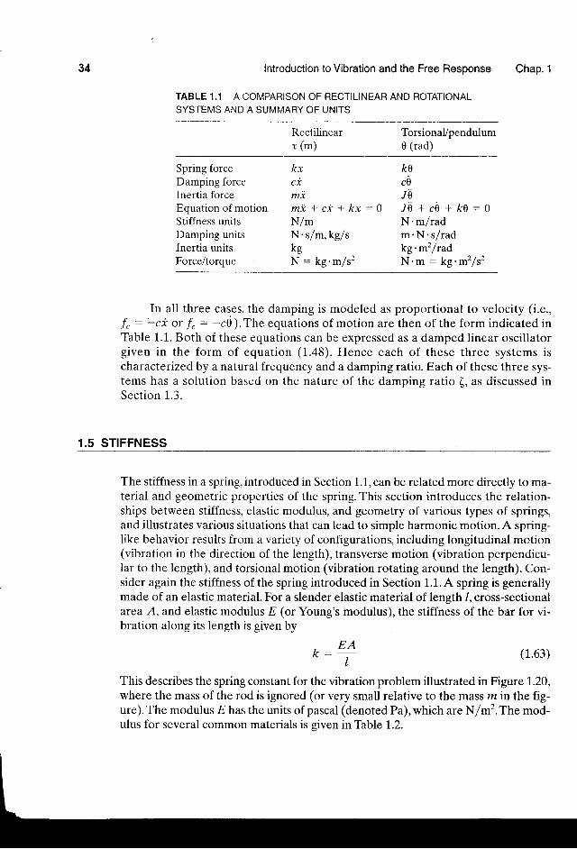
TABLE 1.1 A COMPARISON OF RECTILINEAR AND ROTATIONALSYSTEMS AND A SUMMARY OF UNITS

Rectilinearx (m)

Torsional/pendulum0 (rad)

Spring forceDamping forceInertia forceEquation of motionStiffness unitsDamping unitsInertia unitsForce/torque

kxc*mim i * c * + k x : 0N/mN's/m, kglskgN : kg.m/s2

koCH

JOt 6+cg+ to=oN.m/radm.N .s / radkg.m2/radN.m : kg .m2 ls2

In all three cases, the damping is modeled as proportional to velocity (i.e.,f, : -c* or f,. : -c0 ). The equations of motion are then of the form indicated inTable 1.1. Both of these equations can be expressed as a damped linear oscillatorgiven in the form of equation (1.48). Hence each of these three systems ischaracterized by a natural frequency and a damping ratio. Each of these three sys-tems has a solution based on the nature of the damping ratio (, as discussed inSect ion 1.3.

1.5 STIFFNESS

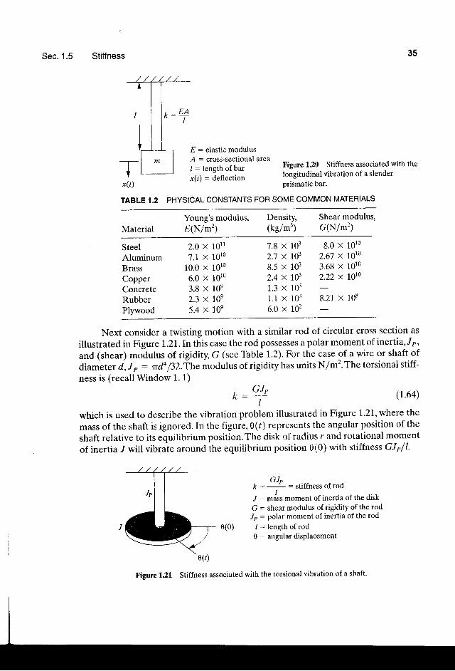
The stiffness in a spring, introduced in Section 1.1, can be related more directly to ma-terial and geometric properties of the spring. This section introduces the relation-ships between stiffness, elastic modulus, and geometry of various types of springs,and illustrates various situations that can lead to simple harmonic motion. A spring-like behavior results from a variety of configurations, including longitudinal motion(vibration in the direction of the length), transverse motion (vibration perpendicu-lar to the length), and torsional motion (vibration rotating around the length). Con-sider again the stiffness of the spring introduced in Section 1.1. A spring is generallymade of an elastic material. For a slender elastic material of length /, cross-sectionalarea A, and elastic modulus E (or Young's modulus), the stiffness of the bar for vi-bration along its length is given by

. E AI

(1.63)

This describes the spring constant for the vibration problem illustrated in Figure 1.20,where the mass of the rod is ignored (or very small relative to the mass ,?? in the fig-ure). The modulus E has the units of pascal (denoted Pa), which are N/m2. The mod-ulus for several common materials is siven in Thble 1.2.

Sec. 1.5 Stiffness 35

E = elastic modulus

,4 : cross-sectional area

/ : length of bar

x(t) = deflect'on

Figure 1.20 Stiffness associated with thelongitudinal vibration of a sler.derprismatic bar.

TABLE 1.2 PHYSICAL CONSTANTS FOR SOME COMMON MATERIALS

MaterialYoung's modulus,E(N/m'z)

Density, Shear modulus,(kgl-') G(N/m'z)

SteelAluminumBrassCopperConcreteRubberPlywood

2.0 x 10117.1 x 1010

10.0 x 10106.0 x 10103.8 x 10e2.3 x 1,0e5.4 x 10e

7.8 x 1032.7 x 1,038.5 x 1032.4 x I031.3 x 1031.1 x 1036.0 x 102

g.0 x 10102.67 x 10103.68 x 10102.22 x r0r0

8.21 x 108

Next consider a twisting motion with a similar rod of circular cross section as

illustrated in F'igure 1,.2l.Inthis case the rod possesses a polar moment of inertia,"Ip,

and (shear) modulus of rigidity, G (see Table 1.2). For the case of a wire or shaft of

diameter d', J p : naa llZ.ihe modulus of rigidity has units N/m2. The torsional stiff-

ness is (recall Window 1. 1)

, GJ,I

(1,.64)

which is used to describe the vibration problem illustrated in Figure 1.21, where the

mass of the shaft is ignored. In the figure, 0(/) represents the angular position of the

shaft relative to its equilibrium position.The disk of radius r and rotational moment

of inertia ,I will vibrate around the equilibrium position 0(0) with stiffness GJ P/1.

GJ"k - : =s t i f f nesso f rod

J : miss moment of inertia of the disk

G = shear modulus of rigidity of the rod

J p : polar moment of inertia of the rod

/ = length of rod

0 : angular displacemente(0)

Figure 1.21 Stiffness associated with the torsional vibration of a shaft

36 Introduction to Vibration and the Free Response Chap. 1

Example 1.5.1

Calculate the natural frequency of oscillation of the torsional system given in Figure 1.21.

Solution Using the noment equation (1.50), the equation of motion for this system is

16@ : -ko?)

This may be wrilten as

t-

t i l r y + )o ( r ) :o

This agrees with the result obtained using the energy method as indicated in Example1.4.3. This indicates an oscillatory motion with frequency

li IGi' , :vi: lnSuppose that the shaft is made of steel and is 2 m long with a diameter of 0.5 cm. If thedisk has mass moment of inertia "/ : 0.5 kg.m2 and considering that the shear modu-lus of steel is G : 8 x 1010 N/m2, the frequency can be calculated by

, _k *G lp _ (B x1010N/m2) [1 r ' ( 0 .5x t o *zm)4 /sz ](r) : = -

J t . t (2 m) (0 .5 kg . - r )

:4 .9 ( ra r l2 /s2)

Thus the natural frequency is orn : 2.2 rad/s.

n

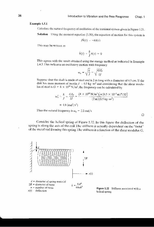
Consider the helical spring of Figure I.22.In this figure the deflection of thespring is along the axis of the coil. The stiffness is actually dependent on the "twist',of the metal rod forming this spring.The stiffness is a function of the shear modulus G.

l,^{

l_*,,,r/ : diameter of spring material

2R : diameter of turnsn : number of turns

x(4 : deflect on

, t J O '

64nRr Figure 1.22 Stiffness associated with ahelical spring.

37Sec. 1.5 Stiffness

x(o)

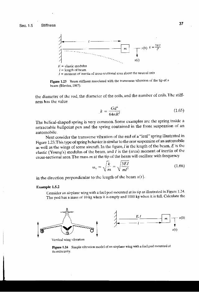
E : elastic modulusI : length of beam1 : moment of inertia of cross-sectional area about the neutral axis

Figure 1.23 Beam stiffness associated with the transverse vibration of the tip of a

beam (Blevins,1987).

the diameter of the rod, the diameter of the coils, and the number of coils. The stiff-

ness has the value

(1.6s)

@ r : (1.66)

L"

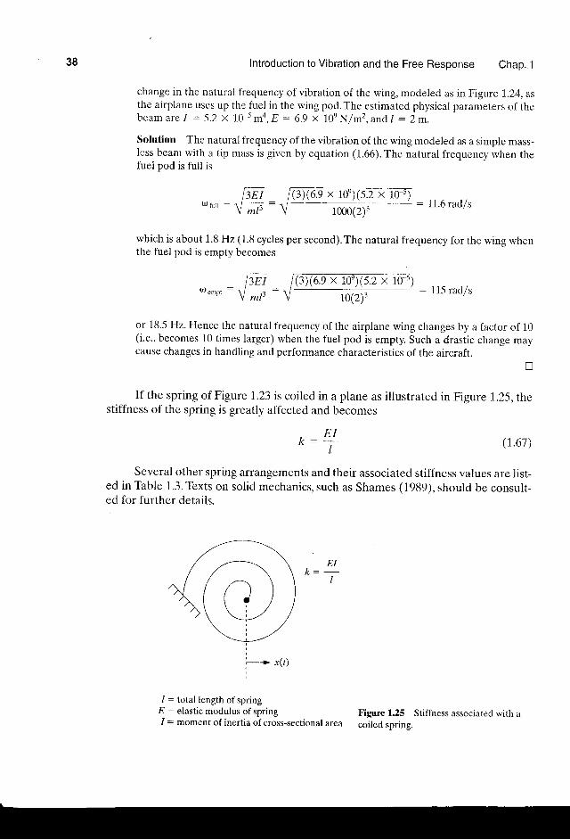
r#rVertical wing vibration

Figure 1.2 Simple vibration model of an airplane wing with a fuel pod mounted at

its extremity.

-T-- "(o)

IV

r(t)

Tx(t)

, Gd4''

64nR3

The helical-shaped spring is very common. Some examples are the spring inside a

retractable balfpoinfpen and the spring contained in the front suspension of an

automobile.Next consider the transverse vibration of the end of a "leaf " spring illustrated in

Figure 1.23.This type of spring behavior is similar to the rear suspension of an automobile

as well as the wings of some aircraft. In the figure, / is the length of the beam, E is the

elastic (Young's) hodulus of the beam, and 1 is the (area) moment of inertia of the

cross-sectional area. The mass r?? at the tip of the beam will oscillate with frequency

EEIt -- \,1 mF

in the direction perpendicular to the length of the beam x(t)'

Example 1.5.2

Consider an airplane wing with a fuel pod mounte<l at its tip as illustrated in Egure 1.24'

The pod has a mass of 10 kg when it is empty and 1000 kg when it is full' calculate the

38 Introduction to Vibrat ion and the Free Response Chap. 1

change in the natural frequency of vibration of the wing, modeled as in Figure 1.24, asthe airplane uses up the fuel in the wing pod. The estimated physical parameters of theb e a m a r e I - 5 . 2 x 1 0 5 m a , E - - 6 . 9 x 1 0 e N / m 2 , a n d l : 2 m .

Solution The natural frequency of the vibration of the wing modeled as a simple mass-less beam with a tip mass is given by equation (1.66).The natural frequency when thefuei pod is fuil is

EEI ffi. u r ' r r : V

^ p : l : l l ' 6 r a d / s

which is about 1.8 Hz (.L8 cycles per second). The natural frequency for the wing whenthe fuel pod is empty becomes

ItEr f i jxest loTs2 x ro'roe_pr :V ; r , -V ro (a f

: [5 rad /s

or 18.5 Hz. Hence the natural frequency of the airplane wing changes by a factor of 10(i.e., becomes 10 times larger) when the fuel pod is empty. Such a drastic change mavcause changes in handling and performance characteristics of the aircraft.

!

If the spring of Figure 1.23 is coiled in a plane as illustrated in Figure 1,.25,thestiffness of the spring is greatly affected and becomes

( r .61)

Several other spring arrangements and their associated stiffness values are list-ed in Thble 1.3. Texts on solid mechanics, such as Shames (1989), should be consult-ed for further details.

, E IK : t

EI, - -I

; , ,--> xlt l

/ : total length of springE : elastic modulus of spring1 = moment of inertia of cross-sectional area

Figure 1,25 Stiffness associated with acoiled spring.

Sec. 1 .5 Stiffness

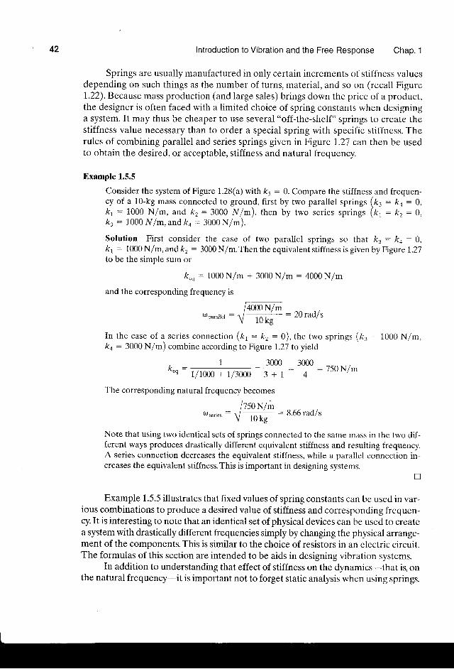
TABLE 1.3 SAMPLE SPRING CONSTANTS

39

Axial stiffness of a tapered bar of length /, modulus E, and end diame-ters d1 and d,

Torsional stiffness on a hollow uniform shaft of shearlength /, inside diameter dt, and outside diameter d2

Tiansverse stiffness of a pinned-pinned beam of modulusment of inertia 1, and length / for a load applied at point a

Tiansverse stiffness of a clamped-clamped beam of modulus, E, areamoment of inertia /, and length / for a load applied at its cenier

modulus G,

,E, area mo-from its end

n Ed,d"4I

nc(d1 - dl\, - -" - 3a. 3EII' -

a2U - d2

, I92EI' '

13

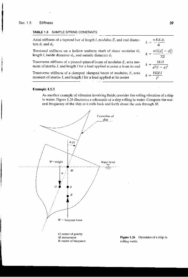
Example 1.5.3

As another example of vibration involving fluids, consider the rolling vibration of a shipin water. Figure 1.26 illustrates a schematic of a ship rolling in water. Compute the nat-ural frequency of the ship as it rolls back and forth about the axis through M.

17: buoyant force

G: center of gravityM: metacenterB: center of buoyance

Figure 1.26 Dynamics of a ship inrolling water.

40 Introduction to Vibration and the Free Response Chap. 1

In the figure, G denotes the center of gravity, B denotes the center of buoyancy,M is the point of intersection of the buoyant force before and after the roll (called themetacenter), and ft is the iength of GM.The perpendicular line from the center of grav-ity to the iine of action of the buoyant force is marked by the point Z.Here W denotesthe weight of the ship,"/ denotes the mass moment of the ship about the roll axis, and 0(t)denotes the angle of roll.

Solution Summing moments about M yields:

/6(r ) : -wGZ : -whsing(r )

Again for small enough values of 0, this nonlinear equation can be approximated by

/ 6 ( / ) +who ( t ) : 0

Thus the natural frequencv of the svstem tt

*, r : \ /

,

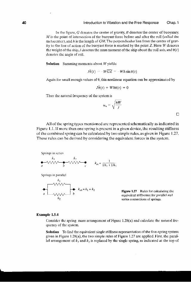
All of the spring types mentioned are represented schematically as indicated inFigure 1.1. If more than one spring is present in a given device, the resulting stiffnessof the combined spring can be calculated by two simple rules, as given in Figurel.27.These rules can be derived by considering the equivalent forces in the system.

Springs in series

K1 k2

ffia b c

Springs in parallel

k1

, , - 7*o" -

l l k ,+L lk ,

Figure 1.27 Rules for calculating theequivalent stiffnesses for parallel andseries connections of springs.

+- i * koo=kt+ kz, ,qnn!b

t.L2

Example 1.5.4

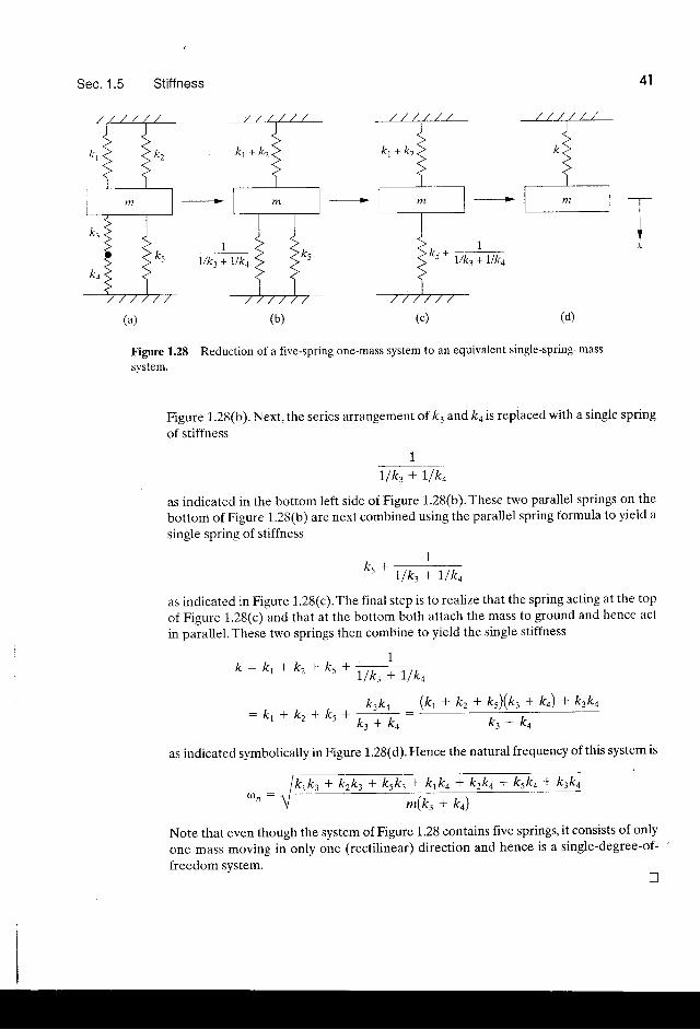
Consider the spring-mass arrangement of Figure I.28(a) and calculate the natural fre-quency of the system.

Solution To tind the equivalent single stiffness representation of the five-spring systemgiven in Figure 1.28(a), the two simple rules of Figure !.27 are applied. First, the paral-lel arrangement of k1 and k2 is replaced by the single spring, as indicated at the top of

Sec . 1 .5 Stiffness

+ + +

(a) (b) (c.) (d)

Figure 1..28 Reduction of a five-spring one-mass system to an equivalent single-spring-mass

svstem.

Figure 1.28(b). Next, the series arrangement of k3 and ka is replaced with a single springof stiffness

1

uh+ was indicated in the bottom left side of Figure 1.28(b). These two parallel springs on the

bottom of Figure 1.2S(b) are next combined usirrg the parallel spring formula to yield a

single spring of stiffness

1

k tu t l t , +w

as indicated in Figure 1.28(c).The final step is to realize that the spring acting at the top

ofFigure 1.28(c) and that at the bottom both attach the mass to ground and hence act

in parallel. These two springs then combine to yield the single stiffness

4 l

':{-

-3-l ^ l

1k - k , * k ) + k . I , - . - , ,-

l / k t + t / K 4

: k t - t k 2 + k s +k tko _ (k t+ t< r+ t< r ) ( k t+ ko ) + k t t co

b + k 4 h + k 4

as indicated symbolically in Figure 1.28(d). Hence the natural frequency of this system is

- ' - ! m ( t < r + t c o )

Note that even though the system of Figure 1.28 contains five springs, it consists of only

one mass moving in only one (rectilinear) direction and hence is a single-degree-of-freedom system.

-T-

+

42 lntroduction to Vibration and the Free Response Chap. 1

Springs are usually manufactured in only certain increments of stiffness valuesdepending on such things as the number of turns, material, and so on (recall Figure1.22).Because mass production (and large sales) brings down the price of a product,the designer is often faced with a limited choice of spring constants when designinga system. It may thus be cheaper to use several "off-the-shelf" springs to create thestiffness value necessary than to order a special spring with specific stiffness. Therules of combining parallel and series springs given in Figure 1..27 can then be usedto obtain the desired, or acceptable, stiffness and natural frequency

Example 1.5.5

Consider the system of Figure 1.28(a) with kt : 0. Compare the stiffness and frequen-cy of a 10-kg mass connected to ground, first by two parallel springs (k. : ko : 0,kr : 1000 N/m, and kz : 3000 lf/-), then by two series springs (tc, : tc, : O,k: : 1000 N/m. and ko : 3000 N/m).

Solulion First consider the case of two paraliel springs so that fu : ko : 0,k1 : 1000 N/m, and k, : 3000 N/m.Then the equivalent stiffness is given by Figure 1.27to be the simple sum or

k"o : 1000 N/m + 3000 N/m : 4000 N/m

and the corresponding frequency is

* pd i l te l: 20 rad/s

750 N/m

In the case of a series connection (kr: kr: 0), ttre two springs (t, : 1OOO N7mk+ : 3000 N/m) combine according to Figure 1.27 to yield

t - _ 1 _ 3 0 0 0" " u - V l o o 0 + t l l o o o - 3 + l

The corresponding natural frequency becomes

,ry50 r.t^"osc.i.s :

V rO, : 8'66rad/s

Note that using two identical sets of springs connected to the same mass in the two dif-ferent ways produces drastically different equivalent stiffness and resulting frequency.A series connection decreases the equivalent stiffness, while a parallel connection in-creases the equivalent stiffness.This is important in designing systems.

Example 1.5.5 illustrates that fixed values of spring constants can be used in var-ious combinations to produce a desired value of stiffness and corresponding frequen-cy. It is interesting to note that an identical set ofphysical devices can be used to createa system with drastically different frequencies simply by changing the physical arrange-ment of the components. This is similar to the choice of resistors in an electric circuit.The formulas of this section are intended to be aids in designing vibration systems.

In addition to understanding that effect of stiffness on the dynamics-that ig onthe natural frequency-it is important not to forget static analysis when using springs.

30004

Sec. 1.6 Measurement 43

In particular, the static deflection of each spring system needs to be checked to makesure that the dynamic analysis is correctlf interpreted. Recall from the discussion ofFigure 1.14 that the static deflection has the value

A:rywhere m is themass supported by a spnng Jf rtiffn"r, k in a gravitational field pro-viding acceleration of gravity g. Static deflection is often ignored in introduciorytreatments but is.used extensively in spring design and is essential in nonlinear analy-sis. Static deflection is denoted by a variety of symbols. The symbols 6, a, 6", and xqare all used in vibration publications to denote the deflection of a spring caused bythe weight of the mass attached to it.

1.6 MEASUREMENT

Measurements associated with vibration are used for several purposes. First, the quan-tities required to analyze the vibrating motion of a system all require measurement.The mathematical models proposed in previous sections all require knowledge ofthe mass, damping, and stiffness coefficients of the device under itudy. These coeffi-cients can be measured in a variety of ways, as discussed in this section. Vibrationmeasurements are also used to verify and improve analytical models.This is discussedi1 some detail in Chapter 7. Other uses of vibration testing techniques include relia-bility and durability studies, searching for damage, and testing for acceptability interms of vibration parameters. These topics are also discussed briefly in -haptei Z.

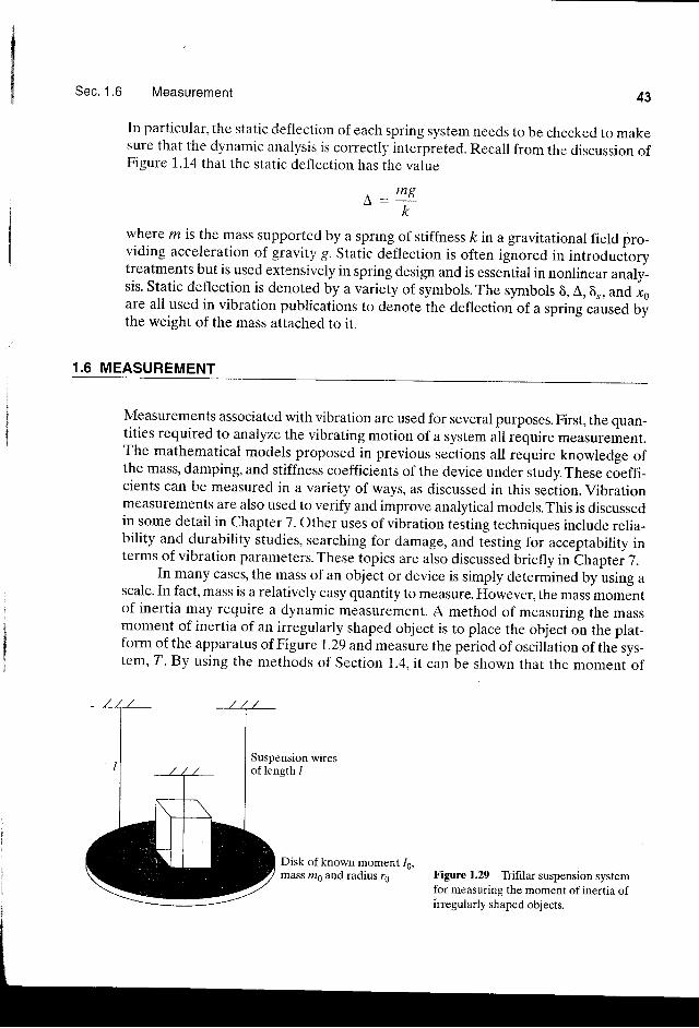
In many cases, the mass of an object or device is simply determined by using ascale. In fact, mass is a relatively easy quantity to measure. However, the mass momentof inertia may require a dynamic measurement. A method of measuring the massmoment of inertia of an irregularly shaped object is to place the object on the plat-form of the apparatus of Figure 1..29 andmeasure the period of osciliation of the sys-tem, z. By using the methods of Section r.4,it can be shown that the moment of

Suspension wiresof length /

Disk of known moment 16,mass rno and radius rg Figure 1,29 Tiifilar suspension system

for measuring the moment of inertia ofirregularly shaped objects.

44 Introduction to Vibration and the Free Response Chap. 1

inertia of an object, l (about a vertical axis), placed on the disk of Figure 1.29 rvithits mass center aligned vertically with that of the disk, is given by

I -t -

gTzrf,(ms + m)(1.68)

412 l

Here m is the mass of the part being measured, ms is the mass of the disk, rs the ra-dius of the disk, / the length of the wires, 1s the moment of inertia of the disk, and gthe acceleration due to gravity.

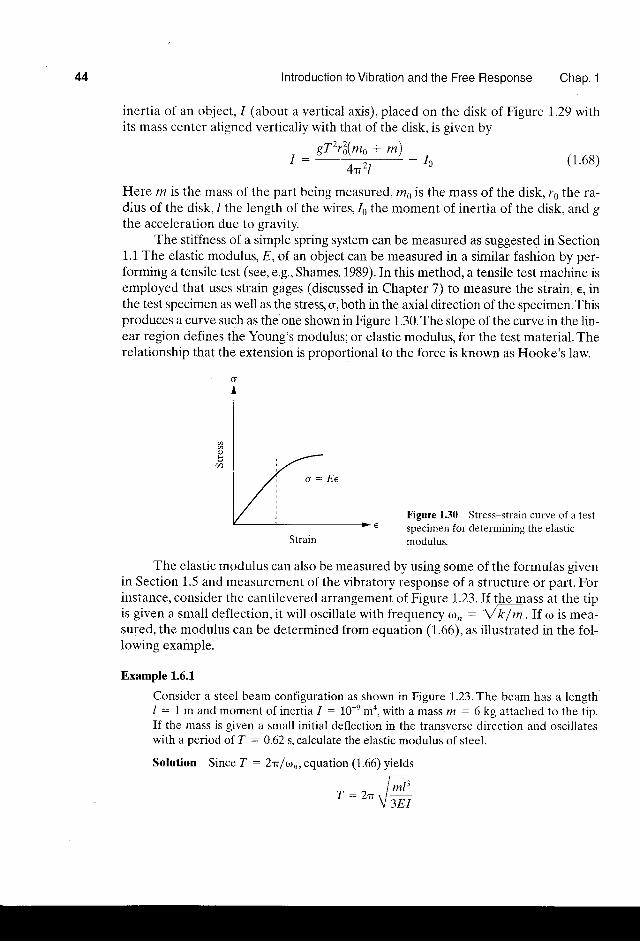
The stiffness of a simple spring system can be measured as suggested in Section1.1 The elastic modulus, E, of an object can be measured in a similar fashion by per-forming a tensile test (see, e.g., Shames, 1989). In this method, a tensile test machine isemployed that uses strain gages (discussed in Chapter 7) to measure the strain, e, inthe test specimen as well as the stress, o, both in the axial direction of the specimen.Thisproduces a curve such as the one shown in Figure 1.30. The slope of the curve in the lin-ear region defines the Young's modulus; or elastic modulus, for the test material. Therelationship that the extension is proportional to the force is known as Ftrooke's law.

Figure 1.30 Stress-strain curve of a test€ specimen for determining the elastic

modulus.

The elastic modulus can also be measured by using some of the formulas givenin Section 1.5 and measurement of the vibratory response of a structure or part. Forinsiance, consider thc cantilevered arrangement of Figure I.23.If tlggrass at the tipis given a snrall deflection, it witl oscillate with frequency a, : V k/m. If o is mea-sured, the modulus can be determined from equation (1.66), as illustrated in the fol-lowing example.

Example 1.6.L

Consider a steel beam configuration as shown in Figure L23.-the beam has a length/ : 1 m and moment of inertia 1 : 10-ema,with a mass rrz : 6 kg attached to the tip.If the mass is given a small initial deflection in the transverse direction and oscillateswith a period of T : 0.62 s, calculate the elastic modulus of steel.

Sofution Since Z : 2rf otn,equation (1.66) yields

Io

Strain

mt -

3EIT :Z t r

Sec. 1.6

Displacement (mm)

1.0

Measurement

Solving for -E yields

45

E :4r2ml3 _ 4T 'z (6 kg) (1m)3

: 205 x 10e N/m23T2I 3(0.62 s)2(1oi m4)

The period 7, and hence the frequency c'ln, can be measured with a stopwatchfor vibrations that are large enough and last long enough to see. However, many vi-brations of interest have very small amplitudes and happen very quickly. Hence sev-eral very sophisticated devices for measuring time and frequenry have been developedand are discussed in Chapter 7.

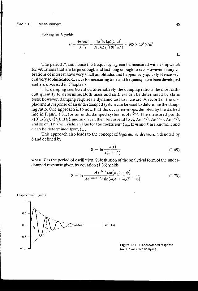
The damping coefficient or, alternatively, the damping ratio is the most diffi-cult quantity to determine. Both mass and stiffness can be determined by statictests; however, damping requires a dynamic test to measure. A record of the dis-placement response of an underdamped system can be used to determine the damp-ing ratio. One approach is to note that the decay envelope, denoted by the dashedline in Figure 1.31, for an underdamped system is Ae-t', '. The measured pointsr(0), x(rr), x(t.r), x(tr),and so on can then be curve fit to A, As-tu^\, Ae-('ntz, n"-tu"tt,and so on.This will yield a value for the coefficient (a,.If. m and /c are known, ( andc can be determined from (con.

This approach also leads to the concept of logarithmic decrement, denoted by6 and defined by

x( t \E : l n : :

x ( t + T)(1.6e)

where Z is the period of oscillation. Substitution of the analytical form of the under-damped response given by equation (1.36) yields

E : l n^r-La"t sin(oar + g)

( i .70)4"-La"o+r) sin(orar + oaT + g)

0.5

Time (s)

Figure 1.31 Underdamped responseused to measure damping.

46 Introduction to Vibration and the Free Response Chap. 1

Sinceo2? :2n,thedenominatorbecomes e-{a"(J+r) sin(oar + $),andtheexpressionfor the decrement reduces to

E : l n e ( ' , r : L @ , 7

The period Z in this case is the damped period \2n /<,:a) so that')- 2rL

6 : itr,. ----:+- ' - -4 , , f t - ( {1=

Solving this expression for ( yields

2.t972

(1 .71)

(1.72)

5 -\/4;';E

(1..73)

which determines the damping ratio given the value of the logarithmic decrement.Thus if the value of x(r) is measured off the plot of Figure 1.3I at any two suc-

cessive peaks, say x(rr) and x(rr), equation (1.69) can be used to produce a measuredvalue of b, and equation (1,73) can be used to determine the damping ratio. The for-mula for the damping ratio, equations (1.29) and (1.30), and knowledge of m and ksubsequently yield the value of the damping coefficient c. Note that peak measure-ments can be used over any integer multiple of the period (see Problem 66) to increasethe accuracy over measurements taken at adjacent peaks.

The computation in Problem 1.66 yields

E:! ,n( , ' i ' )=,)n \x( t + nT) /

where n is any integer number of successive (positive) peaks. While this does tend to

increase the accuracy of computing 6, the majority of damping measurements per-

formed today are based on modal analysis methods, as discussed in Chapter 7.

Example 1.6.2

The free response of the system of Figure 1.9 with a mass of 2 kg is recorded to be of theform given in Figure 1.31.A static deflection test is performed and the stiffness is de-termined to be 1.5 x 103 N/m.The displacements at tr and f2 are measured to be 9 and1 mm, respectively. Calculate the damping coefficient.

Solution From the definition of the logarithmic decrement

f r ( r , ) .1 . Isn* l6 : l n l . - : l : l n l - l : 2 . 1 e 1 2L x ( I 2 ) J L I m m l

From equation (1.73),

5

Also,

{G,itIefi= 0.33 or 33%

,,, : 2fk^: 2@ : 1.095 x 1o2kgls

Sec . 1 .6 Measurement

and from equation (1.30) the damping coefficient becomes

c : c , ,L : ( t .o ls x 1c 'z) (0.33) : 36.15 kg/s

Example 1.6.3

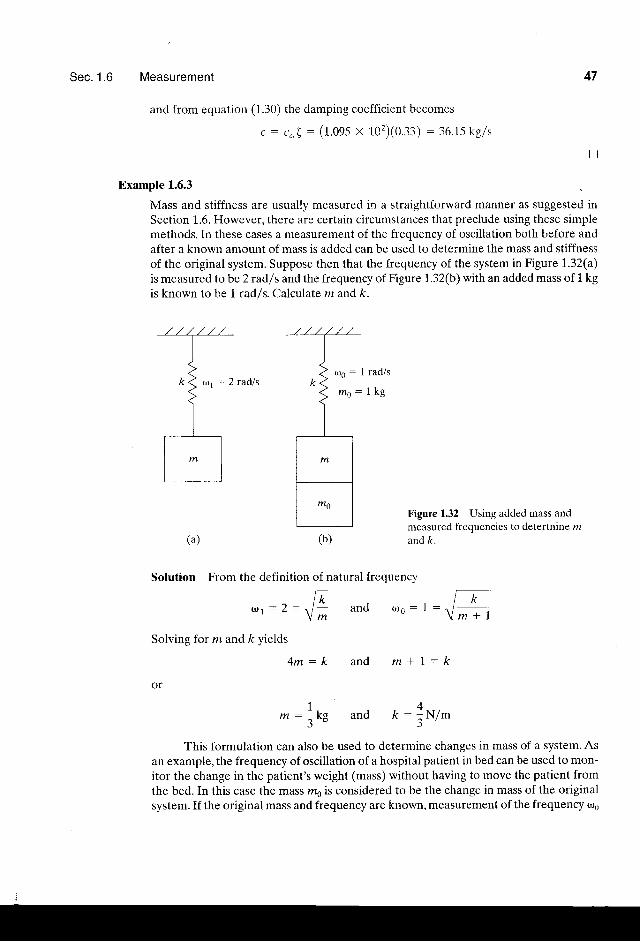
Mass and stiffness are usually measured in a straightforward manner as suggested inSection 1.6. However, there are certain circumstances that preclude using these simplemethods. In these cases a measurement of the frequency of oscillation both before andafter a known amount of mass is added can be used to determine the mass and stiffnessof the original system. Suppose then that the frequency of the system in Figure 1,.32(a)is measured tobe?radf s and the frequency of Figure I.32(b) with an added mass of 1 kgis known to be I radls. Calculate m and k.

Figure 1.32 Using added mass and

measured frequencies to detertnine n

and k.

Solution From the definition of natural frequency

. . - I -@ 1 - L - - . - I -

@ 0 - r -

47

(4.)

Solving for m and k yields

4 m : k

or

and

and m + 1 , : k

*: tut and r=lNz-

This formulation can also be used to determine changes in mass of a system. Asan example, the frequency of oscillation of a hospital patient in bed can be used to mon-itor the change in the patient's weight (mass) without having to move the patient fromthe bed. In this case the mass 1116 is considered to be the change in mass of the originalsystem. If the original mass and frequency are known, measurement of the frequency <os

km

k^ + I

48 Introduction to Vibration and the Free Response Chap. 1

can be used to determine the change in mass ne. Given that the original weight is 120 lb,the original frequency is 100.4 Hz,and the frequency of the patient-bed system changesto 100 Hz, determine the change in the patient's weight.

From the two frequency relations

a21m : k

and

a $ ( m + * o ) : k

Thus, olrru : ,?,(m + no). Solving for the change in mass trs yields

l ' l . \m o : m l , - L l

\ ( 06 /

or

wo -- l2orb I r 'o!.4 ry)' - r I' " ' " 1 \ t ooHz ) ' )

: 0 .96 lb

Since the frequency decreased, the patient gained almost a pound. An increase in tie-quency would indicate a loss of weight.

n

Measurement of m, c, k. <,s,,and ( is used to verify the mathematical model ofa system and for a variety of other reasons. Measurement of vibrating systems formsan important aspect of the activity in industry related to vibration technology. Chap-ter 7 is specifically devoted to measurement, and comments on vibration measure-ments are mentioned throughout the remaining chapters.

1.7 DESIGN CONSIDERATIONS

Design in vibration refers to adjusting the physical parameters of a device to causeits vibration response to meet a specified shape or performance criterion. For in-stance, consider the response of the single-degree-of-freedom system of Figure 1 .9.The shape of the response is somewhat determined by the value of the dampingratio in the sense that the response is either overdamped, underdamped, or criticallydamped (( > 1, ( < 1, L

-- l,respectively).The damping ratio in turn depends onthe values of m, c, and k. A designer may choose these values to produce the de-sired response.

Multiplying by g and converting the frequency to hertz yields

w,: w\fi,_ t)

Sec. 1.7 Design Considerations

Section 1.5 on stiffness considerations is actually an introduction to design aswell. The formulas given there for stiffness in terms of modulus and geometric di-mensions can be used to design a system that has a given natural frequency. Exam-ple I.5.2 points out one of the important problems in design, that often the propertiesthat we are interested in designing for (frequency in this case) are very sensitive tooperational changes. In Example 1,.5.2,the frequency changes a great deal as the zrir-plane uses up fuel.

Another important issue in design often focuses on using devices that are al-ready available. For example, the rules given in Figure I.27 are design rules for pro-ducing a desired value of spring constant from a set of "available" springs by placingthem in certain combinations, as illustrated in Example 1.5.5. Often design work inengineering involves using available products to produce configurations (or designs)that suit your particular application. In the case of spring stiffness, springs are usual-ly mass produced, and hence inexpensive, in only certain discrete values of stiffness.The formulas given for parallel and series connections of springs are then used toproduce the desired stiffness. If cost is not a restriction, then formulas such as giveninTable 1.3 may be used to design a single spring to fit the stated stiffness require-ments. Of course, designing a spring-mass system to have a desired natural frequen-cy may not produce a system with an acceptable static deflection. Thus, the designprocess becomes complicated. Design is one of the most active and exciting disci-plines in engineering because it often involves compromise and choice with manyacceptable solutions.

Unfortunately, the values of m, c,and k have other constraints. In particular, thesize and material of which the device is made determines these parameters. Hence thedesign procedure becomes a compromise. For example, for geometric reasons, themass of a device may be limited to be between 2 and 3 kg, and for static displace-ment conditions, the stiffness may be required to be greater than 200 N/m. In this case,the natural frequency must be in the interval

8.16 rad/s = 0), S 10 rad/s (r.14)

This severely limits the design of the vibration response, 4s illustrated in the follow-ing example.

Example 1.7.1

Consider the system of Figure 1.9 with mass and stiffness properties as summarized byinequality (1.74). Suppose that the system is subject to an initial velocity that is alwaysless than 300 mm/s, and to an initial displacement of zero (i.e., x6 : 0, ?ro - 300 mm/s).For this range of mass and stiffness, choose a value of the damping coefficient such thatthe amplitude of vibration is always less than 25 mm.

Solution This is a design-oriented example, and hence as typical of design calculationsthere is not a nice, clean formula to follow. Rather, the solution must be obtained using

49

50 Introduction to Vibration and the Free Response Chap. 1

theory and parameter studies. First, note that for zero initial displacement, the responsemay be written from equation (1.38) as

x ( / ) e-( ' , tsin(orat)

Also note that the amplitude of this periodic function is

1)^

t'-"'Thus, for small o2 the amplitude is larger than for larger or7. Hence for the range of fre-quencies of interest, it appears that the worst case (largest amplitude) will occur for thesmallest value of the frequency (o, : 8.16 rad/s). Also, the amplitude increases with ooso that using oo : 300 mm/s will ensure that amplitude is a large as possible. Now, o6 andr,rn are fixed, so it remains to investigate how the maximum value of .r(t) varies as thedamping ratio is varied. One approach is to compute the amplitude of the response atthe first peak. From Figure 1.10 the largest amplitude occurs at the first time the deriv-ativeof -r(r) iszero.Takingthederivativeof x(l) andsettingitequal tozero yieldstheexpression for the time to the first peak:

s)de*Lant cos(o;t) - (ans-|'^t sin(co,r) : 0

Solving this for I and denoting this value of time by T- yields

r^: -t-ra"-'13) = Itun-,ryL--L)@ 7 \ E o " / 6 4 \ ( /

The value of the amplitude of the first (and largest) peak is calculated by substitutingthe value of T- into .x(t), resulting in

A ^ ( ( ) = x \ T ^ ) : i l - r - - - r - t u " - ( v ' " - ( ' ) / - ' l f t - ( 2 \ \

, , \ / t - ( 2 ( / s i n \ t " - ' \ - - a - / /

Simplifying yields

uo

A7

A.(L) : ?t;1|4'^"-'l''4-\\ s )

For fixed initial velocity (the largest possible) and frequency (the lowest possible), thisvalue of ,4-(() determines the largest value that the highest peak will have as ( varies.The exact value of ( that will keep this peak, and hence the response, at or below 25 mmcanbedeterminedbynumericallysolvingA.(():0.025(m)foravalueof(.Thisyields( : 0.281. Using the upper limit of the mass values (rn : 3 kg) then yields the value ofthe required damping coefficient:

c :Zma,( : 2(3X8.16X0.281) : 14.1,5kg/s

For this value of the damping the response is never larger than 25 mm. Note that if thereis no damping, the same initial conditions produce a response of amplitudeA : us fan : 37 mm.

n

Sec. 1.7 Design Considerations

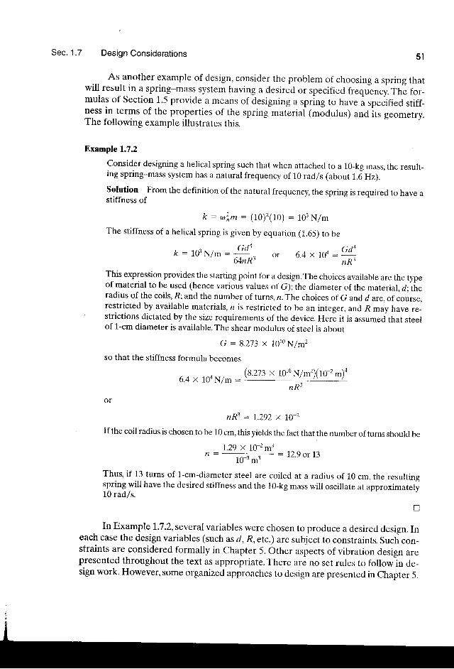
As another example of design, consider the problem of choosing a spring thatwill result in a spring-mass system having a desired or specified frequency. The for_mulas of Section 1.5 provide a means of clesigning a rpting to have a specified stiff-ness in terms of the properties of the spring material (modulus) and its geometry.The following example illustrates this.

Example 1.7.2

Consider designing a helical spring such that when attached to a 10-kg mass, the result-ing spring-mass system has a narural frequency of 10 rad/s (about 1.6 Hz).

Solution From the definition of the natural frequency, the spring is required to have astiffness of

k: lo2,m: (10) 'z(10) = 103N/m

The stiffness of a helical spring is given by equation (i.65) to be

5 t

k : r G N / * = G d o .

' 64nR'

or 6.4 x I0o : Gd:nR'

This expression provides the starting point for a design.The choices avaiiable are the typeof material to be used (hence various values of G); the diameter of the material. d: theradius of the coils, R; and the number of turns, n. The choices of G and d are, ofcourse,restricted by available materials, n is restricted to be an integer, and R may have re_strictions dictated by the size requirements of the device. Here it is assumed that steelof l.-cm diameter is available. The shear modulus of steel is about

G : 9.273 x 1010 N/m2

so that the stiffness formula becomes

6.4 x 704 N/m :(s .z t t x IoroN/m2)( lo-r m)4

nR3

nR3 = I.292 x l0 2

If the coil radius is chosen to be 10 crn, this yields the fact that the number of tums should be

, = l '29 ]<- lo-2 mj : r2.9 or 13I U " M '

Thus, if 13 turns of l-cm-diameter steel are coiled at a radius of 10 cm, the resultinsspring will have the desired stiffness and the 10-kg mass will oscillate at approximatel!10 radls.

tr

In Example 1'.7.2,several variables were chosen to produce a desired design. Ineach case the design variables (such as d, R,etc.) are sub.iect to constraints. Such con_straints are considered formally in Chapter 5. Other aspects of vibration design arepresented throughout the text as appropriate. There are no set rules to follow in de-sign work. However, some organized approaches to design are presented in chapter 5.

52 lntroduction to Vibration and the Free Response Chap. ' l

The following example illustrates another difficulty in design, by examining whathappens when operating conditions are changed after the design is over.

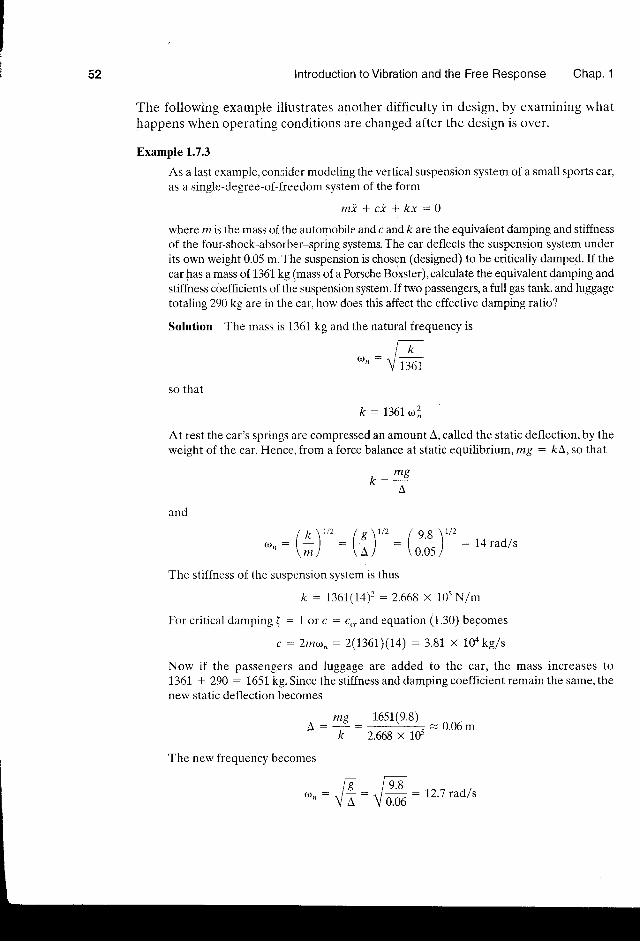
Example 1.7.3

As a last exampie, consider modeling the vertical suspension system of a small sports car,as a single-degree-of-freedom system of the form

m i * c * + k x = 0

where m is the mass of the automobile and c and k are the equivalent damping and stiffnessof the four-shock-absorber-spring systems. The car deflects the suspension system underits own weight 0.05 m. The suspension is chosen (designed) to be criticaliy damped. If thecar has a mass of 1361 kg (mass of a Porsche Boxster), calculate the equivalent damping andstiffness coefficients of the suspension system. If fwo passengers, a full gas tank, and luggagetotaling 290 kg are in the car, how does this affect the effective damping ratio?

Solution The mass is 1361 ks and the natural frequencv is

so that

k: 136ltL'f,

At rest the car's springs are compressed an amount A, called the static deflection, by theweight of the car. Hence, from a force balance at static equilibrium, mE : kL',so that

k - - -gA

and

i k i t : i 8 \ ' ' / q . 8 \ ' '' " : \ ; / : \ - r / = \ 0 . 0 5 / : r 4 r a c r l s

I he s t i l l ness o f the suspens ion sysrem is rhus

k - 1361(14)2 : 2 .668 x 10s N/m

For cri t ical damping ( : I or c : c,,and equation (1.30) becomes

c : 2man : 2(1361)(14) : 3.81 x 104 kgls

Now if the passengers and luggage are added to the car, the mass increases to136l + 290 : 165l kg. Since the stiffness and damping coefficient remain the same, thenew static deflection becomes

mF 1651(9.8)I : -: - = 0.06m

k 2.668 x It'

frequency

Sec. 1.8 Stabil ity 53

From equations (L29) and (I.30) the damping ratio becomes

_ c 3.81 x 104Zma,

3.81 x 100: - : i l L ,

2(1.65r)(r2.7)

Thus the car with passengers, fuel, and luggage is no longer critically damped and willexhibit some oscillatorv motion in the vertical direction.

Note that this illustrates a difficulty in design problems, in the sense that thecar cannot be exactly critically damped for all passenger situations.In this case, ifcritical damping is desirable, it really cannot be achieved. Designs that change dra-matically when one parameter changes a small amount are said not to be robust.Thisis discussed in greater detail in Chapter 5.

1.8 STABILITY

In the preceding sections, the physical parameters m, c,and k are allconsidered to bepositive in equation (1,.25).This allows the treatment of the solutions of equation(1,.25) to be classified into three groups: overdamped, underdamped, or criticallydamped. The case with c : 0 provides a fourth class, called undamped. These four so-lutions are all well behaved in the sense that they do not grow with time and their am-plitudes are finite. There are many situations, however, in which the coefficients arenot positive, and in these cases the motion is not well behaved. This situation refersto the stabiliry of solutions of a system.

Recalling that the solution of the undamped case (c : 0) is of the form,4 sin (co,r + +), it is easy to see that the undamped response is bounded. That is, if

lr(t)l denotes the absolute value of x, then

l ' ( r) l = Alsin(o,r + o)l : e: Lr,T*o * ,1 (1..7s)

for every value of r. Thus lr(r)l is always less than some finite number for all timeand for all finite choices of initial conditions. In this case the response is well be-haved and said to be stable (sometimes called marginally stable).If, on the otherhand, the value of k in equatio n (1, .2) is negative and m is positive, the solutions areof the form

x(t) : ,4 sinh a,t I B cosh ornt (1.76)

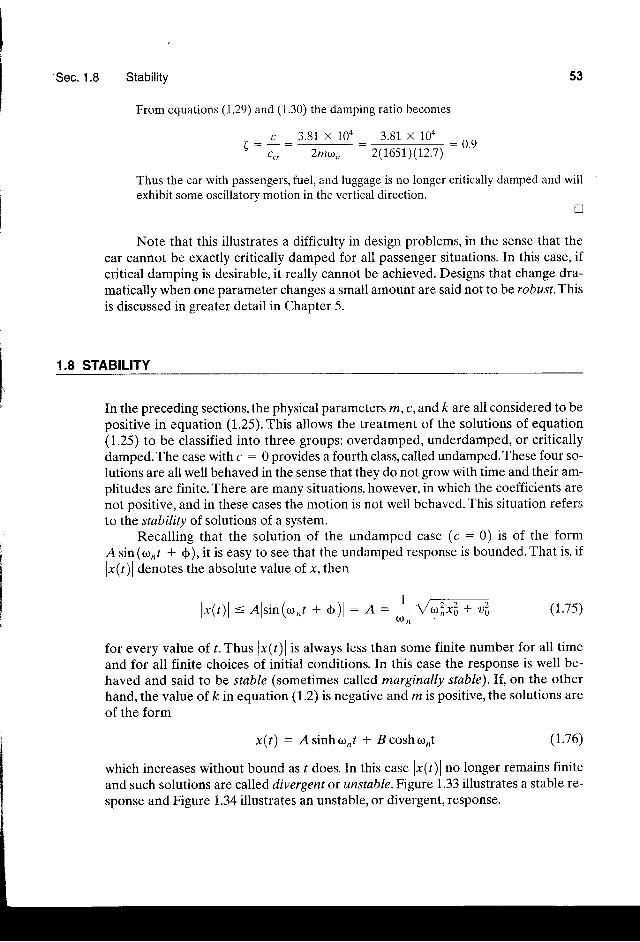
which increases without bound as t does. In this case lx(t)l no longer remains finiteand such solutions are called divergent or unstable.Figure 1.33 illustrates a stable re-sponse and Figure 1.34 illustrates an unstable, or divergent, response.

54 Introduction to Vibration and the Free Response Chap.

Time (s)

Displacement (mm)

0.0

-0.5

- 1.0

1 .0

0.5

Figure 1.33 Example of a stable response.

Displacernent (mm)

Figure 1.34 Example of an unstable, orTime(s) divergent,response.

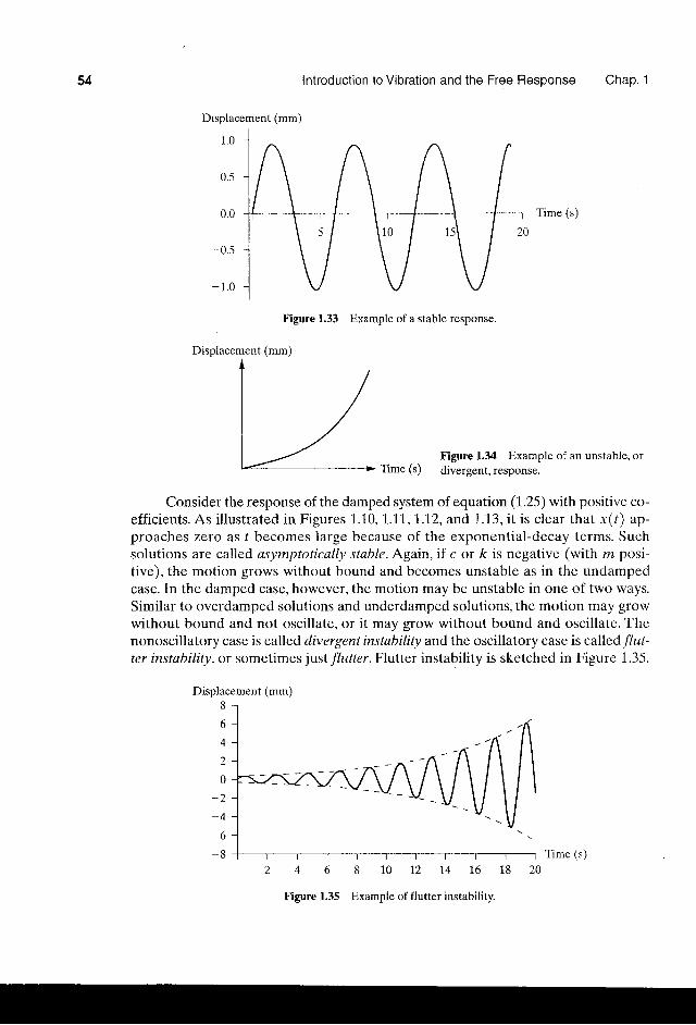
Consider the response of the damped system of equation (1.25) with positive co-efficients. As i l lustrated in Figures 1.10, 1.11, 1.12, and 1.13,it is clear that x(t) ap-proaches zero as I becomes large because of the exponential-decay terms. Suchsolutions are called asymptotically stable. Again, if c or k is negative (with m posi-tive), the motion grows without bound and becomes unstable as in the undampedcase. In the damped case, however, the motion may be unstable in one of two ways.Similar to overdamped solutions and underdamped solutions, the motion may growwithout bound and not oscillate, or it may grow without bound and oscillate. Thenonoscillatory case is called divergent instability and the oscillatory case is called flut-ter instability, or sometimes just flutter. Flutter instability is sketched in Figure 1.35.

Displacement (mm)8

o

4

2

0

-6

-8

4 6 8 1 0 t 2 1 4 1 6

Figure 1.35 Example of flutter instability.

10 ' \ / ) .

Time (s)

Sec . 1 .8 Stability 55

The trend of growing without bound for large r contirrues in Figures 1.34 and 1.35,even though the figure stops. These types of instability occur in a variety of situa-tions, often called self-excited vibratiorzs, and require some source of energy. The fol-lowing example illustrates such instabilities.

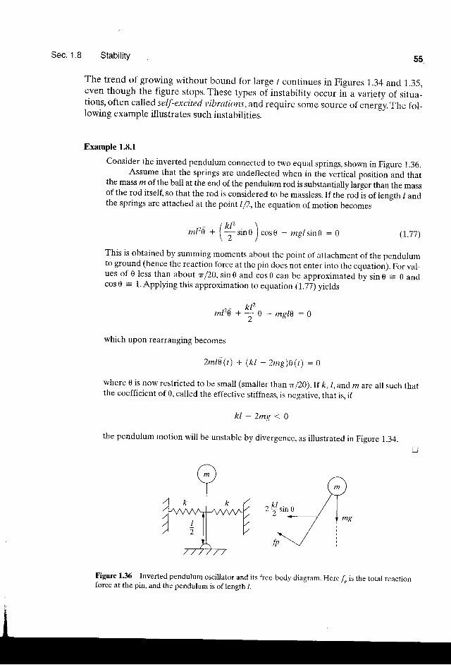
Example 1.8.1

Consider the inverted pendulum connected to two equal springs, shown in Figure 1.36.Assume that the springs are undeflected when in the vertical position and that

the mass m of the ball at the end of the pendulum rod is substantially larger than the massof the rod itself, so that the rod is considered to be massless. If the rod is of length / andthe springs are attached at the point I p,the equation of motion becomes

This is obtained by summing moments about the point of attachment of the pendulumto ground (hence the reaction force at the pin does not enter into the equation). For val-ues of 0 less than about r f20.s in0 and cos0 can be approximated by s in0 = 0 andcos 0 = 1. Applying this approximation to equation (1.77) yields

ml26 + cosO - rng l s i n0 :0 (r.77)

ml26 - mg l \ : 0

which upon rearranging becomes

2mt6\) + (k t - zms)o( t ) : o

where 0 is now restricted to be small (smaller than r 120).If ft, /, and m are allsuch thatthe coefficient of 0, called the effective stiffness, is negative, that is, if

k l - Z m g < 0

the pendulum motion will be unstable by divergence, as illustrated in Figure 1.34.

/k t2 \

\ t ' 'u /

k12+ - 0

z

Figure 1.36 Inverted pendulum oscillator and its free-body diagram. Heref is the total reactionforce at the pin, and the pendulum is of length /.

56 Introduction to Vibration and the Free Response Chap. 1

Example L.8.2

The vibration of an aircraft wing can be crudely modeled as

m i * c i + k x : 1 *

where m, c and k are the mass, damping, and stiffness values of the wing, respectively,modeled as a single-degree-of-freedom system, and where 1i is an approximate modelof the aerodynamic forces on the wing (ry > 0 for high speed). Rearranging this ex-pression yields

m i + ( c - " 1 , ) t + k x : 0

I f landcaresuchthatc - 1> 0, thesystemisasymptot ica l lystable.However, i f 1 issuch tha tc - 1< 0 , t hen ( : ( c - 1 )pma^ < 0and theso lu t i onsa reo f t he fo rm

xv ) = Ae-tu' 'sin(urrl + s)

where -(or,/ > 0 for all r > 0. Such solutions increase exponentially with time, as indi-cated in Figure 1.35. This is an example of flutter instability and self-excited oscillation.

n

1.9 NUMERICAL SIMULATION OFTHETIME RESPONSE

So far the vibration problems examined have all been cast as linear differential equa-tions that have solutions that can be determined analytically. These solutions areoften plotted versus time in order to visualize the physical vibration and obtain an ideaof the nature of the response. However, there are many more complex systems thatcannot be solved analytically.The pendulum equation given in Example 1.4.2 is sucha system. In order to solve ihe pendulum equation analytically, the approximation ofsin ( 0 ) : 0 was used. This allowed the analytical determination of an approximate so-lution that holds only for those initial conditions for which 0 remains less than about10 degrees. For cases with larger initial conditions, a numerical integration routinemay be used to compute and plot a solution to the equation of motion.

The free response of any single-degree-of-freedom systen may be easily com-puted by simple numerical means such as Euler's method or Runge-Kutta methods.This section examines the use of these common numerical methods for solving vi-bration problems that are difficult to solve in closed form. Runge-Kutta schemes canbe found on calculators and in most common mathematical software packages suchas Mathematica, Mathcad, Maple, and Mant-as, or they may be programmed in moretraditional languages, such as FORTRAN, or into spreadsheets. This section reviewsthe use of numerical methods for solving differential equations and then applies thesemethods to the solution of several vibration problems considered in the previous sec-tions.These techniques are then used in the following section to analyze the responseof nonlinear systems. Appendix F introduces the use of Mathematica, Mathcad, andMert-ae for numerical integration and plotting. Many modern curriculums introducethese methods and codes early in the engineering curriculum, in which case this sec-tion can be skipped, or used as a quick review

Sec. 1 .9 Numerical Simulation of the Time Response 57

There are many schemes for numerically solving ordinary differential equa-tions, such as those of vibration analysis. Two numerical solution schemes are pre-sented here. The basis of numerical solutions of ordinary differential equations is toessentially undo calculus by representing each derivative by a small but finite differ-ence (recall the definition of a derivative from calculus given in Window 1.6). A nu-merical solution of an ordinary differential equation is a procedure for constructingapproximate values: x1, xz, . . . , x,, of the solution x(r) at the discrete values of time:to 4 tt 1tz"'. < 1,. Effectively, a numerical procedure produces a list of discretevalues xt : xlt,) that approximate the solution rather than a continuous functionx(t), which is the exact solution.The initial conditions of the vibration problem of in-terest form the starting point. For a single-degree-of-freedom system of the form

mi * c i * kx :0 r(0) : xe . i (0) : uo (1.78)the initial values xo and oe form the first two points of the numerical solution .Let Tybe the total length of time over which the solution is of interest (i.e., the equation istobesolvedforvaluesof lbetweenr : 0and t : T).Thetimeinterval T, - }isthendivided up into n intervals (so that L,t : Trln).Thbn equarion (1.78) is ialculated atthe values of /0 : 0, / r : At, t r : 2L,t , . . . , tn: nLt : Tytoproduce an approximaterepresentation, or simulation, of the solution.

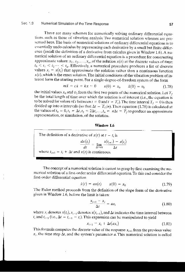
Window 1.6

The definit ion of a derivative of x(r) at t : t, is

dx\t). : l l m

d t A1+0

x(t,*r) * x(t,)

Ltwhere ti+t : tr * Ar and x(r) is continuous.

The concept of a numerical solution is easiest to grasp by first examining the nu-merical solution of a first-order scalar differential equation. To this end consider thefirst-order differential eouation

*( t ) : ax( t ) x(0) : xe (r.7e)The Euler method proceeds from the definition of the slope form of the derivativegiven in Window 1.6, before the limit is taken:

xt+r - xi

N : o * , (1.80)

where rr denotes x(ti), xi+t denotes x(t,*r),and Ar indicates the time interval betweent, and t,*, (i.e., Ar : ti+t - r;). This expression can be manipulated to yield

This formula computes the discrete value of the response x,n, from the previous valuex;, the time step A/, and the system's parameter a.This numerical solution is called

xi+l : x, I Ltlaxi) (1 .81)

58 lntroduction to Vibration and the Free Response Chap. 1

an Euler or tangent line method.The following example illustrates the use of the Euler

formula for computing a solution using vtbl-Z.

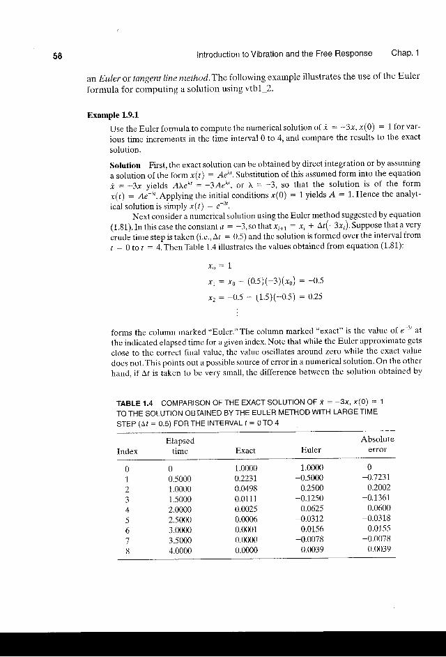
Example 1.9.1

Use the Euler formula to compute the numerical solution of i : -3x, t(0) = 1 for var-

ious time increments in the time interval 0 to 4, and compare the results to the exact

solution.

Solution First, the exact solution can be obtained by direct integration or by assuming

a solution of the form x(t) : Arxt. Substitution of this assumed form into the equation

* : -3x yields , tr'er' : -3Ae\', or \ = -3, so that the solution is of the form

x(,t) : 4r-zt.Applying the initial conditions ;r(0) = 1 yields A : L. Hence the analyt-

ical solution is simply x(t) : ,-' 'Next consider a numerical solution using the Euler method suggested by equation

(1.81) . Inth iscasetheconstanta: -3,sothatx;n i : l r + A/( -3x; ) .Supposethataverycrude time step is taken (i.e., Al : 0.5) and the solution is formed over the interval fiom

/ : 0 to r : 4. Then Table 1.4 illustrates the values obtained from equation (1.81):

x o : 1

xr = ro + (o.s)(-3)(.ro) : -0.5

xz: -05 - (1.s)(-0.s) :0.25

forms the column marked "Euler." The column marked "exact" is the value of e-'' at

the indicated elapsed tin.re for a given index. Note that while the Euler approxlmate gets

close to the correct final value, the value oscillates around zero while the exact value

does not.This points out a possible source of error in a numerical solution. On the other

hand, if Ar is taken to be very small, the difference between the solution obtained by

TABLE 1.4 COMPARISON OFTHE EXACT SOLUTION OF * : -3x' x(0) : 1

TO THE SOLUTION OBTAINED BY THE EULER METHOD WITH LARGE TIME

STEP (Af : 0.5) FOR THE INTERVAL f : O TO 4

ElapsedIndex time Exact Euler

Absoluteerror

0 01 0.50002 1.00003 1.50004 2.00005 2.50006 3.00007 3.50008 4.0000

1.00000.22310.04980.01110.00250.00060.00010.00000.0000

1.0000-0.5000

0.2500-0.12500.062s

-0.03120.0156

-0.00780.0039

0-0.72310.2002

-0.13610.0600

-0.03180.0155

-0.00780.0039

S E c 1 . 9 Numerical Simulation of the Time Resoonse

Time (s)

0.5 1 1.5 2 2.s 3 3.5 4

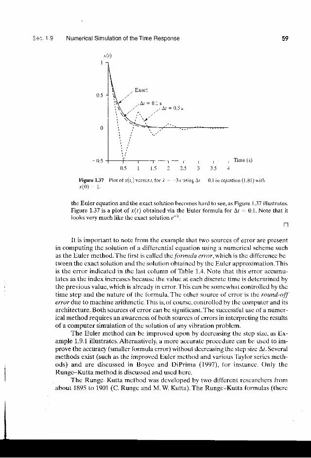
F igu re1 .37 P lo to f x (1 , ) ve r sus t , f o r i : - 3 rus i ngA / - 0 . l i nequa t i on (1 .81 )w i t h. r ( 0 ) : 1 .

the Euler equation and the exact solution becomes hard to see, as Figure 1.37 illustrates.Figure 1.37 is a plot of x(r) obtained via the Euler formula for At : 0.1. Note that itlooks very much like the exact solution e-3'.

!

It is important to note from the example that two sources of error are presentin computing the solution of a differential equation using a numerical scheme suchas the Euler method. The first is called the /o rmula error, which is the difference be-tween the exact solution and the solution obtained by the Euler approximation.Thisis the error indicated in the last column of Table 1.4. Note that this error accumu-Iates as the index increases because the value at each discrete time is determined bythe previous value, which is already in error. This can be somewhat controlled by thetime step and the nature of the formula. The other source of error is the round-offeruor due to machine arithmetic. This is, of course, controlled by the computer and itsarchitecture. Both sources of error can be significant. The successful use of a numer-ical method requires an awareness of both sources of errors in interpreting the resultsof a computer simulation of the solution of any vibration problem.

The Euler method can be improved upon by decreasing the step size, as Ex-ample 1.9.1 illustrates. Alternatively, a more accurate procedure can be used to im-prove the accuracy (smaller formula error) without decreasing the step size Lt. Severalmethods exist (such as the improved Euler method and various Taylor series meth-ods) and are discussed in Boyce and DiPrima (1997), for instance. Only theRunge-Kutta method js discussed and used here.

The Runge-Kutta method was developed by two different researchers fromabout 1895 to 1901 (C. Runge and M. W. Kutta). The Runge-Kutta formulas (there

59

A r : 0 . 1 s, A r : 0 . 5 s

60 lntroduction to Vibration and the Free Response Chap' 1

are several) involve a weighted average of values of the right-hand side of the dif-

ferential equation taken at different points between the time intervals /, and l' + A/.

The derivations of various Runge-Kutta formulas are tedious but straightforward

and are not presented here (see Boyce and DiPrima,1991). One useful formulation

canbes ta ted fo r the f i r s t -o rde rp rob lem t : f ( x , r ) , x (0 ) : xn ,whe re / i sanysca la r

function (linear or nonlinear) as

xn+t :r, , * +

(k,,t * zk,z + 2k,3 + k,4) (1.82)

where

k, ,q: f (xu + Ltkn, t , + Lt )

The sum in parentheses in equation (1.82) represents the average of six numbers

each of which looks like a slope at a different time; for instance, the term ft,1 is the

slope of the function at the "left" end of the time interval.

Such formulas can be errhanced by treating At as a variable, A/r. At each time

step /,, the value of Ar, is adjusted based on how rapidly the solution x(r) is chang-

ing. If the solution is not changing very rapidly, a large value of A/r is allowed with-

out increasing the formula error. On the other hand, if x(r) is changing rapidly, a

small Ar, must be chosen to keep the formula error small. Such step sizes can be cho-

sen automatically as part of the computer code for implementing the numerical so-

lution. The Runge-Kutta and Euler forrnulas just listed can be applied to vibration

problems by noting that the most general (damped) vibration problem can be put

in to a f i rs t -ordcr fotm.Returning to a damped system of the form

mi ( t ) + c i ( t ) + kx ( t ) : 0 x (0 ) - x0 , t ( 0 ) : i 0 (1 ' 83 )

the Euler method of equation (1.81) can be applied by writing this expression as two

first-order equations.To this end, divide equation (1.83) by the mass m and define two

new variables by x1 : x(t) and 12 : t(/).Then differentiate the definit ion of 11(r),

rearrange equation (1.83), and replace x and its derivative with .rr and "t2 to get

i1Q) : x2( t )

* r ( r ) : - k * 'U) - * * ' ( t )

subject to the init ial conditions r,(0) : ro and xz(O) : i6. The nvo coupled first-

order differential equations given in (1.8a) may be written as a single expression by

k6 : f \ x , , t , )

k,,r: f (r, * I0,r,,, * +)

k,.: f(,,r, * I o,r,t" * +)

(1.84)

Sec. 1.9 Numerical Simulation of the Time Response 6l

using a vector and matrix form determined by first defining the vector 2 x 1 x(/)and the 2 x 2matrix Aby

x ( / ) : [ ; ; [ ; ] ]

The matrix ,4 defined in this way is called the state matrix and the vector x is calledthe state vector. The position xt and the velocity x2 lre called the state variables.Using these definitions (see Appendix C), the rules of vector differentiation (ele-ment by element) and multiplication of a matrix times a vector, equations (1.84) maybe written as

* ( r ) : Ax( t ) (1.86)

subject to the initial condition x(0). Now the Euler method of numerical solutiongiven in equation (1.81) can be applied directly to this vector-matrix formulation ofequation (1.86), by simply calling the scalar x, the vector x, and replacing the scalara with the matrix,4 to produce

*(r,*,) :x(r,) + A,tAx(r,) (1.87)

This, along with the initial condition x(0), defines the Euler formula for integratingthe general single-degree-of-freedom vibration problem described in equation (1.82)for computing and plotting the time response.

As suggested, the Euler-formula method can be greatly improved by using aRunge-Kutta program. For instance, Merree has two different Runge-Kutta-basedsimuiations: ode23 and ode45.These are automatic step-size integration methods (i.e.,A/ is chosen automatically). The Engineering Vibration Toolbox has one fixed-stepRunge-Kutta-based method, vtbl_3, for comparison.The M-file ode23 uses a simplesecond- and third-order pair of formulas for medium accuracy and ode45 uses a fourth-and fifth-order pair for greater accuracy. Each of these corresponds to a formulationsimilar to that expressed in equations (1.82) with more terms and a variable step sizeAr. In general, the Runge-Kutta simulations are of a higher quality than those ob-tained by the Euler method.

Example 1.9.2

Use the ode45 function to simulate the response to 3; + i + 2x : 0 subject to the ini-tial conditions x(0) : 0, t(0) : 0.25 over the time interval 0 < t < 20.

x t =

Next an M-file is created to store the equations of motion.An M-file is created by choos-ing a name, say sdof . m, and entering

x(o) : [ ; ; lS]]

(18s)t o 1lA: l k c I

L- * -;)

Solution The first step is to write the equation of motion in first-order form.This yields

62 Introduction to Vibration and the Free Resoonse Chap. 1

0

-0.1

*0.2

Ilme

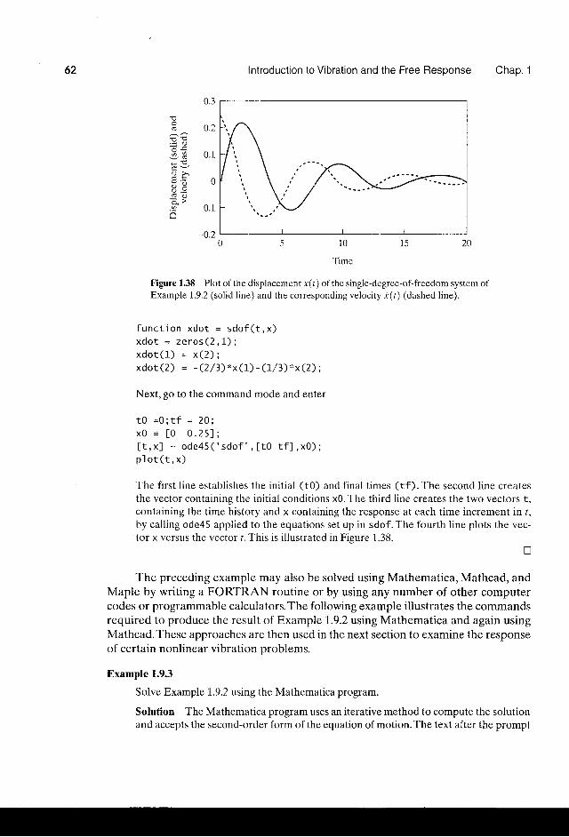
Figure 1.38 Plot of the displacement x(t) of the single-degree-of-freedom system ofExample 1.9.2 (solid line) and the corresponding velocity i(t) (dashed line).

f u n c t i o n x d o t = s d o f ( t , x )x d o t = z e r o s ( 2 , I ) ;x d o t ( 1 ) = x ( 2 ) ;xdo t (2 ) = - (2 /11"* rL ) - ( t /3 ) ' , x (2 ) ;

Next, go to the command mode and enter

t 0 = 0 ; t f = 2 0 ;x 0 = [ 0 0 . 2 5 ] ;

[ t , x ] = ode45 ( ' sdo f ' , [ t0 t f ] , x0) ;p l o t ( t , x )

The first line establishes the initial (t0) and final times (tf).The second line createsthe vector containing the initial conditions x0. The third line creates the two vectors t,containing the time history and x containing the response at each time increment in r,by calling ode45 applied to the equations set up in sdof.The fourth line plots the vec-tor x versus the vector t. This is illustrated in Fieure 1.38.

The preceding example may also be solved using Mathematica, Mathcad, and

Maple by writing a FORTRAN routine or by using any number of other computercodes or programmable calculators.The following example illustrates the commandsrequired to produce the result of Example 1.9.2 using Mathematica and again usingMathcad.These approaches are then used in the next section to examine the responseof certain nonlinear vibration Droblems.

Example 1.9.3

Solve Example 1.9.2 using the Mathematica program.

Solution The Mathematica program uses an iterative method to compute the solutionand accepts the second-order form of the equation of motion. The text after the prompt

0.2

0.1

!

^ 5

- . ! _

0 > ,

E >

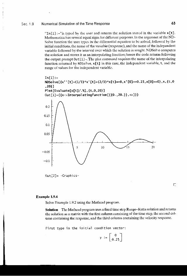
Sec. 1 .9 Numerical Simulation of the Time Response

"Inl1l:="is typed by the user and returns the solution stored in the variable x[t].Mathematica has several equal signs for different purposes. In the argument of the ND-Solve function the user types in the differential equation to be solved, followed by theinitial conditions, the name of the variable (response), and the name of the independentvariable followed by the interval over which the solution is sought. NDSoI','e computesthe solution and stores it as an interpolating function; hence the code returns follorvingthe output prompt Out [1] =. The plot command requires the name of the interpolatingfunction returned by NDSolve, x[t] in this case, the independent variable, t, and therange of values for the independent variable.

In [1-] : =NDSo lve [ { x " [ t ] + (1 , / 3 ) ' ! x ' [ t ] + (2 /3 ) *x [ t ] = -0 , x ' [ 0 ]==0 .25 ,x [0 ]==91 ,x , { t , 0,20 l lP l ot [EvaI uate[x[ t ] / . %1, { t , 0 , 20} l0ut [1 ] ={{x->Interpol at ' i ngFunct i on t { t0 . , 20. } } , + l } }

0.15

0.1

-0.1

O u t [ 2 ] = - C r a p h i c s -

Example 1.9.4

Solve Example 1.9.2 using the Mathcad program.

Solution The Mathcad program uses a fixed time step Runge-Kutta solution and returnsthe solution as a matrix with the first column consisting of the time step, the second col-umn containing the response, and the third column containing the velocity response.

F i r s t t ype i n t he i n i t i a l cond i t i on vec to i - :

63

u

[01L0 .2s I

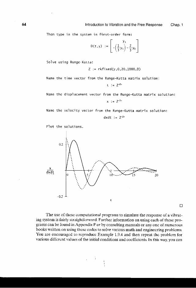
64 Introduction to Vibration and the Free Resoonse Chao. 1

T h e n t y p e i n t h e

S o l v e u s i n g Runge-Kut ta :

Z : = r k f i x e d ( y , 0 , 2 0 , 1 0 0 0 , D )

Name the t ime vector f rom the Runge-Kut ta matr ix so lut ion:

+ . - 7 < 0 >

Name the d isp lacement vec tor f rom the Runge-Kut ta mat r ix so lu t ion :

x i= Z '1 '

N a m e t h e v e l o c i t y v e c t o r f r o m t h e R u n g e - K u t t a m a t r i x s o l u t i o n :

dxdt := Z'2'

P l o t the so l u t ' i ons .

D

The use of these computationa! programs to simulate the response of a vibrat-ing system is fairly straightforward. Further information on using each of these pro-grams can be found in Appendix F or by consulting manuals or any one of numerousbooks written on using these codes to soive various math and engineering problems.You are encouraged to reproduce Example I.9.4 and then repeat the problem forvarious different values of the initial conditions and coefficients. In this way, you can

s y s t e m i n f i r s t - o r d e r f o r m :

tYr - lD(t,y) ,= | _r+r,)_ 1r, IL \3 _)

X

d-xdt

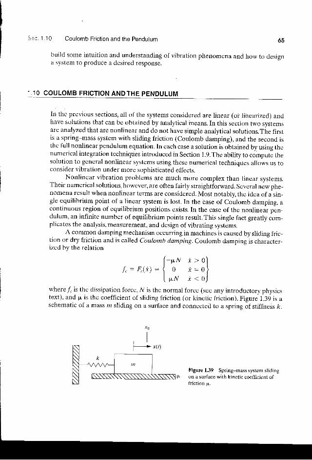
S:c. 1 .10 Coulomb Frict ion and the Pendulum

build some intuition and understanding of vibration phenomena and how to designa svstem to produce a desired response.

. .10 COULOMB FRICTION ANDTHE PENDULUM

In the previous sections, all of the systems considered are linear (oi linearized) andhave solutions that can be obtained by analytical means. In this section two systemsare analyzed that are nonlinear and do not have simple analytical solutions. The firstis a spring-mass system with sliding friction (coulomb damping), and the second isthe full nonlinear pendulum equation. In each case a solution is obtained by using thenumerical integration techniques introduced in Section 1.9.The ability to compute thesolution to general nonlinear systems using these numerical techniques allows us toconsider vibration under more sophisticated effects.

Nonlinear vibration problems are much more complex than linear systems.Their numerical solutions, however, are often fairly straightforward. Several new phe-nomena result when nonlinear terms are considered. Most notably, the idea of a sin-gle equilibrium point of a linear system is lost. In the case of coulomb damping, acontinuous region of equilibrium positions exists. In the case of the nonlinear pen-dulum, an infinite number of equilibrium points result. This single fact greatly Com-plicates the analysis, measurement, and design of vibrating systems.

A common damping mechanism occurring in machines is caused by sliding fric-tion or dry friction and is called Coulomb damping. Coulomb damping is character-ized bv the relation

f , : F , ( *1 :

where f, is the dissipation force, l/ is the normal force (see any introductory physicstext), and p is the coefficient of sliding friction (or kinetic friction). Figure 1.39 is aschematic of a mass ru sliding on a surface and connected to a spring of stiffness k.

Figure 1.39 Spring-mass system slidingon a surface with kinetic coefficient offriction u.

65

{lJ ;:3}

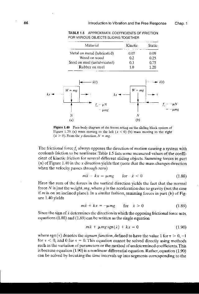
66 Introduction to Vibrat ion and the Free Response Chap. 1

TABLE 1,5 APPROXIMATE COEFFICIENTS OF FRICTIONFOR VARIOUS OBJECTS SLIDING TOGETHER

Material Kinetic Static

Metal on metal (lubricated)Wood on wood

Steel on steel (unlubricated)Rubber on steel

0.070.20.31.0

0.090.250.751 a n

F- r(r)

/ . : pN

: pmq

(b)

Figure 1.40 Free-body diagram of the forces acting on the sliding block system ofFigure 1.39: (a) mass moving to the left (t < 0) (b) mass moving to the right( i > 0) .Fromthey di rect ion, N - mg.

The frictionalforce f, always opposes the direction of motion causing a system withcoulomb friction to be nonlinear. Table 1.5 lists some measured values of the coeffi-cient of kinetic friction for several different sliding objects. Summing forces in part(a) of Figure 1.40 in the x direction yields that (note that the mass changes directionwhen the velocity passes through zero)

m I I k x : W m g f o r i < 0 (1.88)

Here the sum of the forces in the vertical direction yields the fact that the normalforce ,4y' is just the weight, mg, where g is the acceleration due to gravity (not the caseif rz is on an inclined plane). In a similar fashion, summing forces in part (b) of Fig-ure 1.40 yields

m i * k x : _ p m g f o r i > 0 (1.8e)

Since the sign of i determines the direction in which the opposing frictional force acts,equations (1.88) and (1.89) can be written as the single equation

m i * p m g s g n ( i ) + k x : 0 (1.e0)

where sgn (r) denotes the signum function,defined to have the value 1 for r > 0, -1for t { 0, and 0 for t : 0. This equation cannot be solved directly using methodssuch as the variation of parameters or the method of undetermined coefficients. Thisis because equation (1.90) is a nonlinear differential equation. Rather, equation (1.90)can be solved by breaking the time intervals up into segments corresponding to the

(4.)

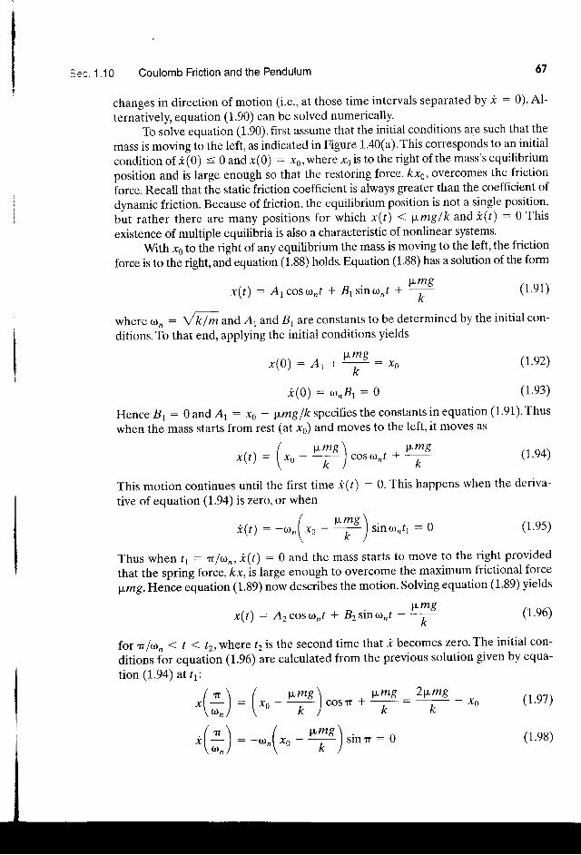
Sec. 1 . '1 0 Coulomb Friction and the Pendulum

changes in direction of motion (i.e., at those time intervals separated by i : 0). Al-

ternatively, equation (1.90) can be solved numerically.To solve equation (1.90), first assume that the initial conditions are such that the

mass is moving to the left, as indicated in Figure 1.40(a).This corresponds to an initial

condit ionof i (0) < 0andx(0) : xo,wherexgistotherightof themass,sequi l ibr iumposition and is large enough so that the restoring force,kxs, overcomes the friction

iorce. Recall that the static friction coefficient is always greater than the coefficient of

dynamic friction. Because of friction, the equilibrium position is not a single position,

but rather there are many positions for which r(/) < pmclk andi(r) :0This

existence of multiple equilibria is also a characteristic of nonlinear systems.With xs to the right of any equilibrium the mass is moving to the left, the friction

force is to the right, and equation (1.88) holds. Equation (1.88) has a solution of the form

x( / ) : ,41cos ,on t * B ls in ror / . ry

where .^ : f kJ^and A1 and 81 are constants to be determined by the initial con-

ditions. To that end, applying the initial conditions yields

L m gx (0 ) :A '+ f=xs

i ( 0 ) : o n B 1 : 0

Hence Br : 0 and Ay- -rs ILmg lkspecifiesthe constantsinequation (1.91).Thus

when the mass starts from rest (at rs) and moves to the left, it moves as

/ t t^g \ wmgx \ t ) :

\ " 0 - L / c o s ( l ) n t(1..e4)

This motion continues until the first time *(t) :0. This happens when the deriva-

tive of equation (1.94) is zero, or when

t ( / ) : - ' " ( ' o - " f ) s i no rn /1 :o

67

(1.e1)

(1,.92)

(1.e3)

Thus when t1 : 11 f11.,, *(t) :0 and the mass starts to move to the right provided

that the spring force,kx,is large enough to overcome the maximum frictional force

p,mg.Henceequation (1.89) now describes the motion. Solving equation (1.89) yields

,r(t) : A2cos .;.nt * B2sino,t - ry

(1.es)

(1.e6)

for r f a, < t < /r, where /2 is the second time that i becomes zero. T'he initial con-

ditions for equation (1.96) are calculated from the previous solution given by equa-

tion (L.94) au1:

/ n \x l - l

\ o " , /

. / " r \x t - l

\ to",/

: (ro - flcosn * pmg :

k

f lsint: o

- X g (r.e7)

(1.e8)= - " ( to -

2wmg

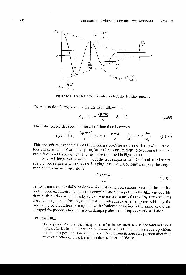
68 Introduction to Vibration and the Free Response Chap. 1

4pN\- - l

K I

/ \ 'oo":(4#1)/ 2 p N \- \ 'Yo-

t /

Figure 1.41 Free response of a svstem with Coulomb friction present.

From equation (1.96) and its derivatives it follows that

3pmgA z : x o - B z : 0 (1.ee)

The solution for the second interval of time then becomes

( 3w*S \ p-g n Znx( r ) : \ " - ; /coso, r

_ T * . , . i l

(1 .100)

This procedure is repeated unti l the motion stops.The motion wil l stop when the ve-locity is zero (* : 0) and the spring force (ftr) is insufficient to overcome the maxi-mum frictional force ( pmg ) . The response is plotted in Figure 1.41 ,

Several things can be noted about the free response with Coulomb friction ver-sus the free response with viscous darnping. First, with Coulomb damping the ampli-tude decays l inearly with slope

2p"mga,( 1 . 1 0 1 )

rather than exponentially as does a viscously damped system. Second, the motionunder Coulomb friction comes to a complete stop, at a potentially different equilib-rium position than when initially at rest, whereas a viscorrsly damped system oscillutesaround a single equilibrium, r : 0, with infinitesimally small amplitude. Finally, thefrequency of oscillation of a system with coulomb damping is the same as the un-damped frequency, whereas viscous damping alters the frequency of oscillation.

Example L.10.1

The response of a mass oscillating on a surface is measured to be of the form indicatedin Figure 1.41. The initial position is measured to be 30 mm from its zero rest position,and the final position is measured to be 3.5 mm from its zero rest position after fourcycles of oscillation in 1 s. Determine the coefficient of friction.

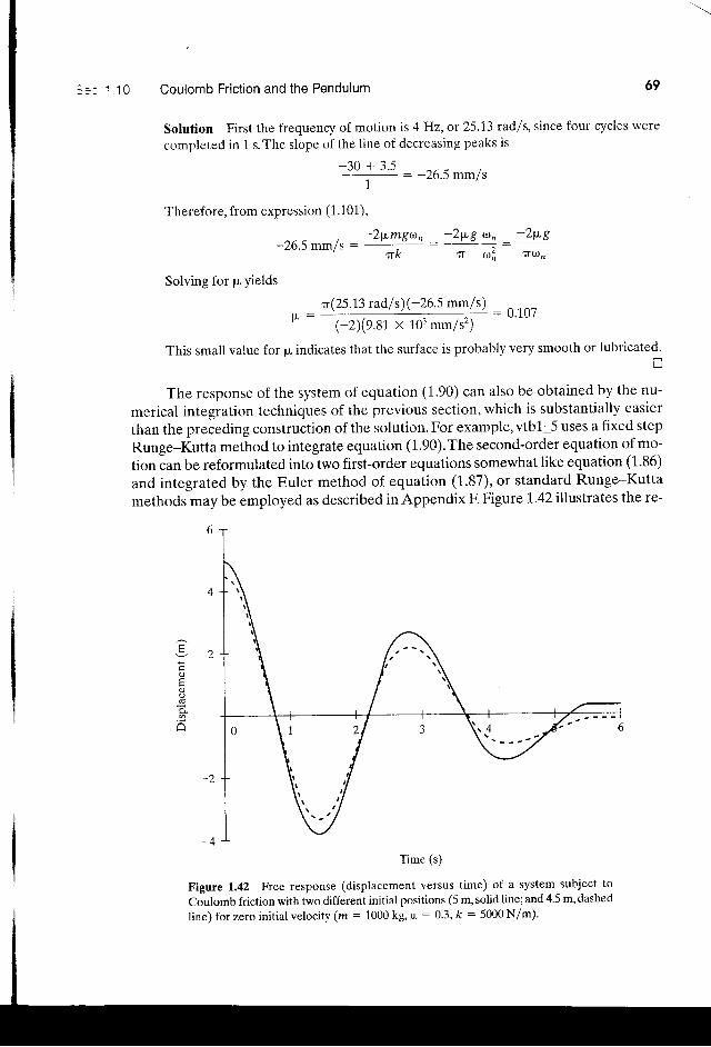
1 0 Coulomb Friction and the Pendulum 69

Solution First the frequency of motion ts 4 Hz, or 25.1"3 rad/s, since four cycles were

completed in 1, s. The slope of the line of decreasing peaks is

- { t t + 1 a

T: -26 .5mm/s

Therefore. from expression (:l . l0l).

-26'5 mm/s : -21"ry'8"

- -2wg a: :

-2t"g'

1tk 7t a'. T0"

Solving for p yields

n (25.13 rud / s) (-26.5 mm/s ) = 0.107(-2X9.81 x 103 mm/s2)

This small value for p indicates that the surface is probably very smooth or lubricated

The response of the system of equation (1.90) can also be obtained by the nu-

merical integration techniques of the previous section, which is substantially easier

than the preceding construction of the solution. For example, vtbl-5 uses a fixed step

Runge-Kutta method to integrate equation (1.90).The second-order equation of mo-

tion can be reformulated into two first-order equations somewhat like equation (1.86)

and integrated by the Euler method of equation (1.87), or standard Runge-Kutta

methods may be employed as described in Appendix F. Figure 1.42 illustrates the re-

Time (s)

Figure 1.42 Free response (displacement versus time) of a system subject to

coulomb friction with two different initial positions (5 m, solid line;and 4.5 m, dashed

line) for zero initial velocity (m : 1000 kg, p : 0.3, k : 5000 N/m)'

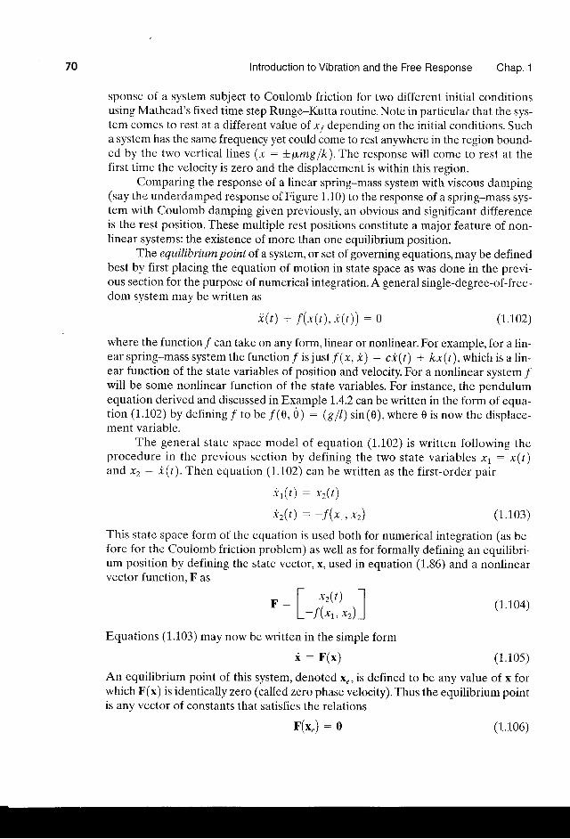
Introduction to Vibration and the Free Response Chap. 1

sponse of a system subject to Coulomb friction for two different initial conditionsusing Mathcad's fixed time step Runge-Kutta routine. Note in particular that the sys-tem comes to rest at a different value of 11 depending on the initial conditions. Sucha system has the same frequency yet could come to rest anyvhere in the region bound-ed by the two vertical lines (x : +p,mg lk). The response will come to rest at thefirst time the velocity is zero and the displacement is within this region.

Comparing the response of a linear spring-mass system with viscous damping(say the underdarnped response of Figure 1.10) to the response of a spring-mass sys-tem with Coulomb damping given previously, an obvious and signiticant differenceis the rest position.'fhese multiple rest positions constitute a major feature of non-linear systems; the existence of more than one equilibrium position.

The equilibrium point of a system, or set of governing equations, may be definedbest by first placing the equation of motion in state space as was done in the previ-ous section for the purpose of numerical integration. A general single-degree-of-free-dom svstem mav be written as

i ( r ) + f ( *@. * ( r ) ) : 0 (1.102)

where the function / can take on any form, linear or nonlinear. For example, for a lin-earspring-masssystemthefunct ion/ is just f (* , i ) : c ic(t) + kx(t) ,whichisal in-ear function of the state variables of position and velocity. For a nonlinear system /will be some nonlinear function of the state variables. For instance, the pendulumequation derived and discussed in Exampl e 1.4.2 can be written in the form of equa-t i o n ( 1 . 1 0 2 ) b y d e f i n i n g " f t o b e / ( 0 , 0 ) : ( S l t ) s i n ( 0 ) , w h e r e 0 i s n o w t h e d i s p l a c e -ment variable.

The general state space model of equation (1.102) is written following theprocedure in the previous section by defining the two state variables x, : x(r)and x2: *U). Then equation (1.102) can be written as the first-order pair

i r ( t ) : x r ( t )

*r( t) : - f (* , , *r) ( 1 . 1 0 3 )

This state space form of the equation is used both for numerical integration (as be-fore for the Coulomb friction problem) as well as for formally defining an equilibri-um position by defining the state vector, x, used in equation (1.86) and a nonlinearvector function, F as

(1 .104)

Equations (1.103) may now be written in the simple form

* : F(x) (1.10s)An equilibrium point of this system, denoted x", is defined to be any value of x forwhich F(x) is identically zero (called zero phase velocity).Thus the equilibrium pointis any vector of constants that satisfies the relations

F: I xzu) , lL- I \x r , xz ) )

F(x") : o (1.106)

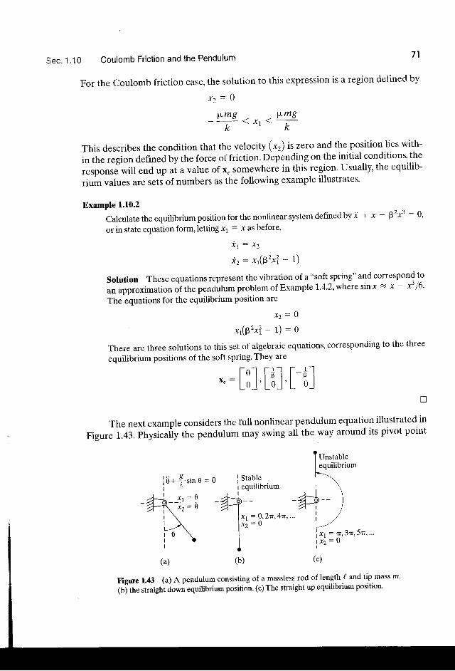
Sec. 1.10 Coulomb Friction and the Pendulum 71

For the Coulomb friction case, the solution to this expression is a region defined by

x z : 0

wmg wmg- k : < x t < k

This describes the condition that the velocity (xt) is zero and the position lies with-

in the region defined by the force of friction. Depending on the initial conditions, the

response"will end up ai a value of x, somewhere in this region. Usually, the equilib-

rium values are sets of numbers as the following example illustrates.

Example 1.10.2

calculatetheequilibriumpositionforthenonlinearsystemdefinedbyi * x- Bzxr:0'or in state equation form,letting x1 : x as before,

* t = x z

*r : x t (Bzxl - t )

Solution These equations represent the vibration of a "soft spring" and correspond to

an approximation oithe pendutumproblem of Example 1.4.2'wheresinx = x - x' f6'

The equations for the equilibrium position are

x z : 0

t , ( 9 ' * ? -1 ) : o

There are three solutions to this set of algebraic equations, corresponding to the three

equilibrium positions of the soft spring'They are

tol l-,1-l t-+l*" = Lol Lol ' L o-l

!

The next example considers the full nonlinear pendulum equation illustrated in

Figure 1.43. physicaliy the pendulum may swing all the way around its pivot point

l 6 + 4 s i n o = o l S t a b l ei | | equil ibrium

Unstableequilibrium

, - - )

(a) (b)

l__--/t ^

i xl = 1T. Jlr, )rr.t x 2 : v

(c)

Figure 1.43 (a) A pendulum consisting of a massless rod of length / and tip mass /r?

iti,fr" toulgiti Oown equilibrium position' (c) The straight up equilibrium position'

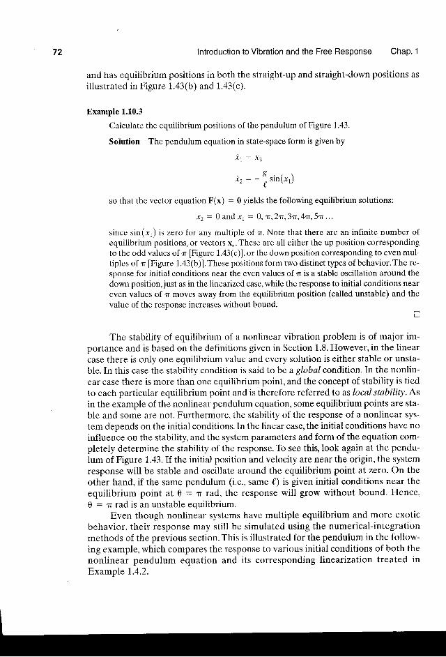
72 lntroduction to Vibration and the Free Response Chap. 'l

and has equiiibrium positions in both the straight-up and straight-down positions asi l lust rated in F igure 1.43(b) and 1.43(c) .

Example 1.L0.3

Calculate the equilibrium positions of the pendulum of Figure 1.43.

Solution The pendulum equation in state-space form is given by

x t : r z

o. 6 , / \xz : -

7sm\ j r1 l

so that the vector equation F(t) : 0 yields the following equilibrium solutions:

xz : 0 and xr = 0, r ,2r ,3n,4r ,5r . . .

since sin(x1) is zero for any multiple of n. Note that there are an infinite number ofequiiibrium positions, or vectors x,. These are all either the up position correspondingto the odd values of n [Figure 1.43(c)], or the down position corresponding to even mul-tiples of tr [Figure 1.43(b)]. These positions form two distinct types of behavior. The re-sponse for initial conditions near the even values of n is a stable oscillation around thedown position, just as in the linearized case, while the response to initial conditions neareven values of T moves away from the equilibrium position (called unstable) and thevalue of the response increases without bound.

I

The stability of equilibrium of a nonlinear vibration problem is of major im-portance and is based on the definitions given in Section 1.8. However, in the Iinear

case there is only one equilibrium value and every solution is either stable or unsta-

ble.In this case the stability condition is said to be a global condition.In the nonlin-

ear case there is more than one equilibrium point, and the concept of stability is tied

to each particular equilibrium point and is therefore referred to as local stability. As

in the example of the nonlinear pendulum equation, some equilibrium points are sta-

ble and some are not. Furthermore, the stability of the response of a nonlinear sys-

tem depends on the initial conditions. In the linear case, the initial conditions have no

influence on the stability, and the system parameters and form of the equation com-pletely determine the stability of the response. To see this, look again at the pendu-

lum of Figure 1.43. If the initial position and velocity are near the origin, the system

response will be stable and oscillate around the equilibrium point at zero. On the

other hand, if the same pendulum (i.e., same /) is given initial conditions near the

equil ibrium point at 0 : Tr rad, the response wil l grow without bound. Hence,

0 : tr rad is an unstable equilibrium.Even though nonlinear systems have multiple equilibrium and more exotic

behavior, their response may sti l l be simulated using the numerical-integrationmethods of the previous section. This is illustrated for the pendulum in the follow-

ing example, which compares the response to various initial conditions of both thenonlinear pendulum equation and its corresponding l inearization treated in

Example 1,4.2.

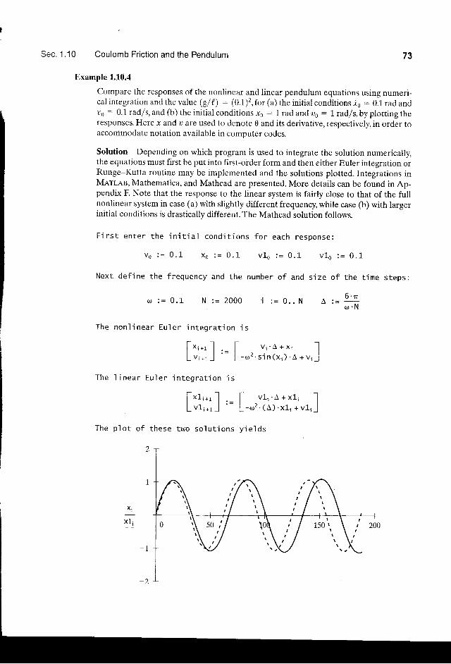
Sec. 1 .10 Coulomb Friction and the Pendulum

Example 1.10.4

Compare the responses of the nonlinbar and linear pendulum equations using numeri-cal integration and the value (gl {) : (0.1)'z, for (a) the initial conditions xo = 0.1 rad andoo : 0.1 radT's, and (b) the initial conditions x0 : 1 rad and oo = L rad/s, by plotting theresponses. Here x and r,' are used to denote 0 and its derivative, respectively, in order toaccommodate notation available in computer codes.

Solution Depending on which program is used to integrate the solution numerically,the equations must first be put into first-order form and then either Euler integration orRunge-Kutta routine may be irrrplemented and the solutions plotted. Integrations inMerLee, Mathematica, and Mathcad are presented. More details can be found in Ap-pendix F. Note that the response to the linear system is fairly close to that of the fullnonlinear system in case (a) with slightly different frequency, while case (b) with largerinitial conditions is drastically different. The Mathcad solution follows.

F ins t en te r t he i n i t i a l cond i t . i ons f o r each response :

v e : = 0 . 1 x o : = 0 . 1 v 1 o : = 0 . 1 - v 1 o : = 0 . 1

Next def ine the f i 'equency and the number of and s ize of the t ime steps:

i : = 0 . . N

The non l i nea r Eu le r i n teg ra t i on i s

[ * r - ' 1 . _ [ v i . l + x i IL u ' ' ' _ . J

' - L - r ' . s i n ( x i ) . A + v 1 _ l

The " l i nea r Eu le r i n teg ra t i on i s

o : = 0 . 1 N := 2000

T h e p l o t o f t h e s e t w o s o l u t i o n s y i e l d s

. 6 ' no t = r +

f * 1 , , r 1 . _ t v1 ; .A+x1 -1 IL v 1 , - , I

' - L - . t ( A ) . x 1 r + v 1 1 J

74 Introduction to Vibration and the Free Resoonse Chao. 1

i s t h e l i n e a r s o l u t i o n . N e x t c o m p u t e t h e s ei n i t i a l c o n d i t i o n s c l o s e t o u n s t a b l e

v lo : =

._t' - | ?

L-( , ) -

nei n g

T

s i n

H e r e t h e d aso ' l u t i ons ae q u i l i b r i u m

[ ' ' . ' - ]L v r + r l

0 . t "

v1- i .A + x l1 I. (A ) . x1 r + v11 I

v 6 : = 0 . 1 x 1 s : = T

A + x 1 I [ x r 1 + r l(x i ) 'A + v1_ l f v l1 + 1J

Xt

Iir

The Marlen code for running the solutions (using Runge-Kutta this time) and plottingis obtained by f irst creating the appropriate M-f i les (named 1 i n*pend-dot. m andNL-pend-dot. m, defining the linear and nonlinear pendulum equations, respectively):

f u n c t i o n x d o t = l i n _ p e n d _ d o t ( t , x )omega = 0 .1 ; n /o de f ine the na tura l fnequencyx d o t ( 1 , 1 ) = x ( 2 ) ;xdo t (2 , 1 ) = -omega, r2*x (1) ;

func t ion xdot = NL_pend_dot ( t ,x )o m e g a = 0 . 1 ; % d e f i n e t h e n a t u r a l f r e q u e n c yx d o t ( 1 , 1 ) = x ( 2 ) ;x d o t ( 2 , 1 ) = - o m e 9 a , r 2 * s i n ( x ( 1 ) ) ;

In the command mode type the following:

% O v e r p l o t ' l i n e a r

& n o n ' l i n e a r s i m u l a t i o n s o f t h e f r e e% response o f a pendu lum.

x 0 = 0 . 1 ; v 0 = 0 . 1 ;t i = 0 ; t f = 2 0 0 ;

% . l

i near

l t i m e - l i n , s o l - l i n ] = e i s 4 5 1 ' 1 i n - p e n d - d o t ' , [ t i t f ] , [ x 0 v 0 ] ) ;

% non l i near

[ t ' i m e - N L , s o l - N L ] = o d e 4 5 ( ' N L - p e n d - d o t ' , [ t i t f ] , [ x 0 v 0 ] ) ;

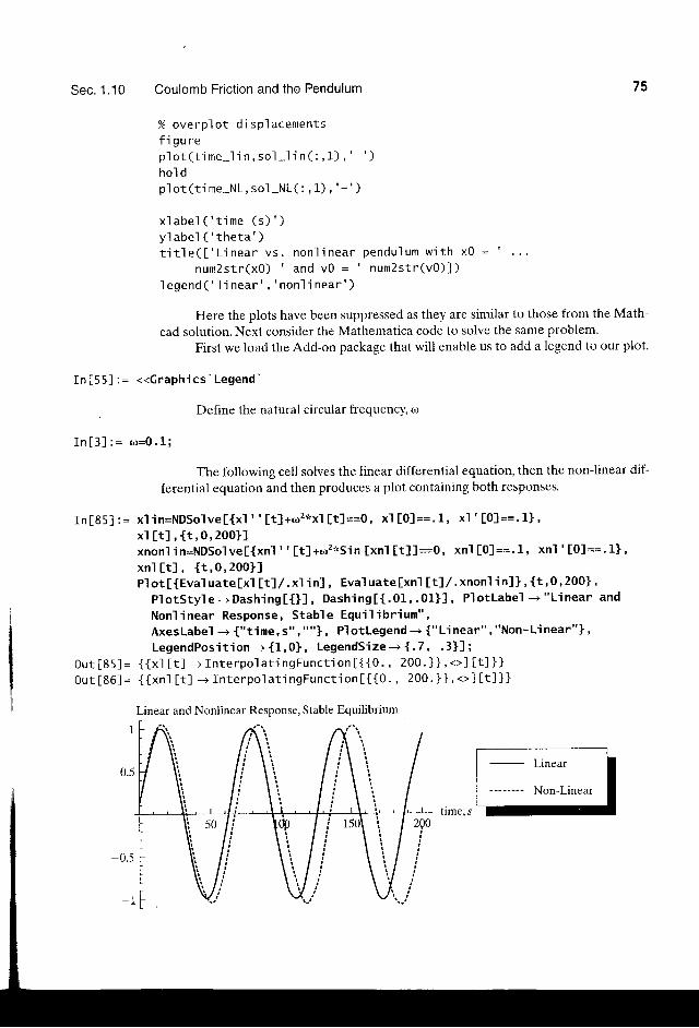
Sec. 1.' l 0 Coulomb Friction and the Pendulum

% o v e r p l o t d i s p l a c e m e n t sf i gu rep l o t ( t i m e - l i n , s o l - l i n ( : , 1 ) ,

' - ' )

ho l dp l o t ( t i m e - N L , s o l - N L ( : , 1 ) , ' - ' )

x l a b e l ( ' t i m e ( s ) ' )

y l abe ' l ( ' the ta ' )t i t l e ( [ ' L i n e a r v s . n o n l i n e a r p e n d u l u m w i t h x 0 = ' . . .

n u m 2 s t r ( x 0 ) ' a n d v 0 = ' n u m 2 s t r ( v 0 ) l )

l e g e n d ( ' I i n e a r ' , ' n o n l i n e a r ' )

Here the plots have been suppressed as they are similar to those from the Math-

cad solution. Next consider the Mathematica code to solve the same problem.

First we load the Add-on package that will enable us to add a legend to our plot.

In [55 ] := <<Graph ics ' Legend '

. Define the natural circular frequency, tr

I n [ 3 ] : = o = 0 . 1 ;

The following cell solves the linear differential equation, then the non-lir.rear dif'

ferential equation and then produces a plot containing both responses.

In t85 l : = x l i n=NDSo' l ve [ {x ] " t t l+ to2" "x l [ t ]==9, x1 [0 ]==. 1 , x ' l ' [0 ]== ' 1 ] '

x l [ t ] , { t , 0 , 2 0 0 } lx n o n l i n = N D S o l v e [ { x n ] " [ t ] + r o z ' r $ - i n t x n l [ t ] l = = 0 , x n 1 [ 0 ] = = . 1 , x n l ' [ 0 1 = = ' 1 1 '

xn l [ t ] , { t ,0 , 200} lP ' lo t [ {Eva lua te [x l [ t ] / . x l in l , Eva ' lua te lxn l [ t ] , / . xnon] in l ] ' { t ' 0 '200} ,

P l o tS ty ' l e -+ Dash i ng [ { } ] , Dash ing [ { . 01 , . 0 I } ] , P l o t labe l - -+ "L i near and

Non l inear Response, S tab le Equ ' i l i b r ium" '

AxesLabe l -+ { " t ime, s " , " " } , P l o tLegend - -+ { " L i near " , "Non- L i near " } ,

LegendPos ' i t ion- -+ {1 ,0 } , LegendSize-+ { .7 , .3 } l ;O u t [ 8 5 ] = { { x l i t J - - + I n t e r p o l a t ' i n g F u n c t i o n [ { { 0 . , 2 0 0 . } } , + ] t t l } }

O u t [ 8 6 ] = { { x n ] [ t ] - + I n t e n p o l a t i n g F u n c t i o n t { { 0 . , 2 0 0 . } i , < > l [ t ] ] ]

Linear and Nonlinear Response, Stable Equilibrium

\Linear

Non-Linear

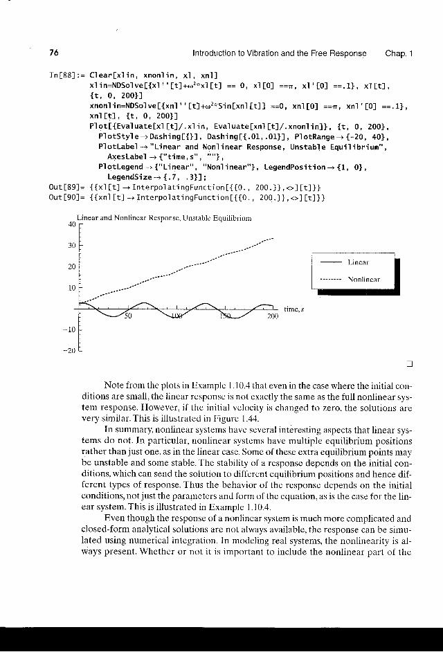
76 Introduction to Vibration and the Free Response Chao. 1

I n [ 8 8 ] : = C l e a r [ x l i n , x n o n l i n , x l , x n ] lx ' l in=NDSolve [ {x l ' ' [ t ]41o2 ' :x1

t t l == 0 , x l [0 ] == l r , x l ' [0 ] == .1 ] , x1 [ t ] ,{ t , 0 , 2 0 0 } lx n o n l i n = N D S o l v e [ { x n l " [ t ] + < o 2 ' i S i n l x n l [ t ] l = = 0 , x n l [ 0 ] = - t r , x n l ' [ 0 ] = = . 1 ] ,x n l [ t ] , { t , 0 , 2 0 0 } lP l o t [ { E v a l u a t e l x l [ t ] / . x ] i n , E v a l u a t e [ x n ' l [ t ] / . x n o n l i n l ] , { t , 0 , 2 0 0 } ,

P1 o tSty l e -+ Dash ing [ { } ] , Dash ing [ { . 01 , . 01} ] , P ' lo tRange -+ { -20 , 40} ,F lo tLabe l -+ "L inear and Non l inear Response, Unstab le Equ ' i1 ib r ium" ,

A x e s L a b e l - - + { " t i m e , s " , " " } ,P lo tLegend-+ { "L inear " , "Non1 inear " } , LegendPos i t ' i on-+ {1 , 0 } ,

LegendSize -+ { . 7 , . 3 } l ;0 u t [ 8 9 ] = { i x l I t ] - + I n t e r p o l a t i n g F u n c t ' i o n [ { { 0 . , 2 0 0 . } } , + ] [ t ] ] ]O u t [ 9 0 ] = { { x n l [ t ] - + I n t e r p o l a t i n g F u n c t i o n [ { { 0 . , 2 0 0 . } } , + ] [ t ] ] ]

Linear and Nonlinear Response, Unstable Equilibrium40

- Linear

-'-----' Nonlinear

t ime,s

Note from the plots in Example 1.10.4 that even in the case where the initial con-ditions are small, the linear response is not exactly the same as the full nonlinear sys-tem response. Ilowever, if the initial velocity is changed to zero, the solutions arevery similar. This is illustrated in Figure 1.44.

In summary, nonlinear systems have several interesting aspects that linear sys-tems do not. In particular, nonlinear systems have multiple equil ibrium positionsrather than just one, as in the linear case. Some of these extra equilibrium points maybe unstable and some stable. The stability of a response depends on the initial con-ditions, which can send the solution to different equilibrium positions and hence dif-ferent types of response. Thus the behavior of the response depends on the initialconditions, not just the parameters and form of the equation, as is the case for the lin-ear system. This is i l lustrated in Example 1.10.4.

Even though the response of a nonlinear system is much more complicated andclosed-form analytical solutions are not always available, the response can be simu-lated using numerical integration. In modeling real systems, the nonlinearity is al-ways present. Whether or not it is important to include the nonlinear part of the

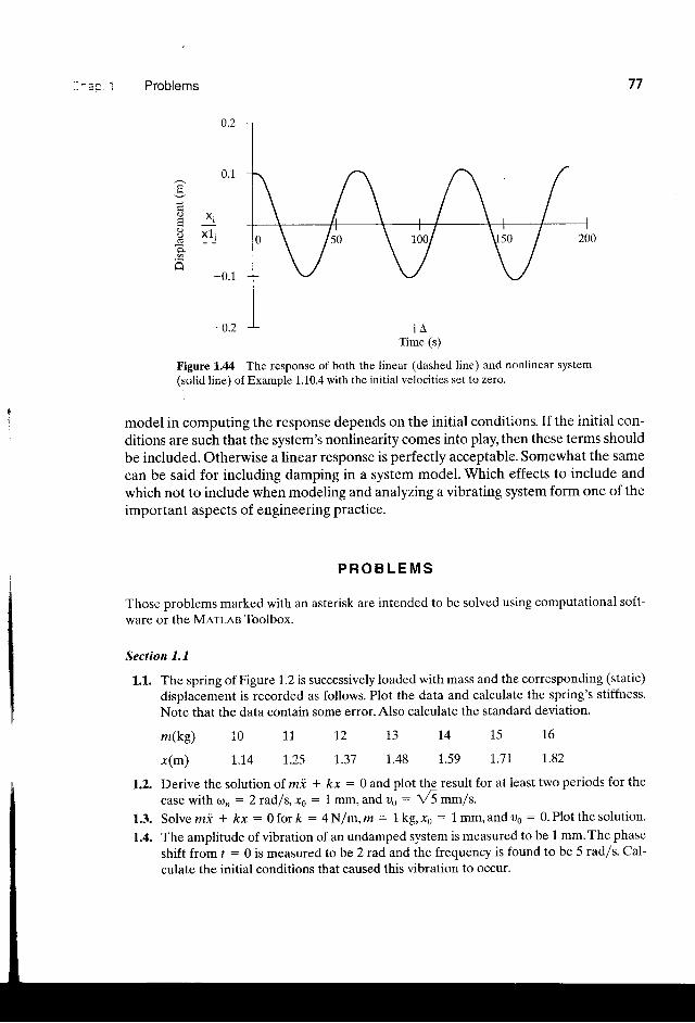
Problems

-0.1

-0.2

Figure 1.44 The response of both the linear (dashed line) and nonlinear system(solid line) of Example 1.10.4 with the initial velocities set to zero'

model in computing the response depends on the initial conditions. If the initial con-ditions are such that the system's nonlinearity comes into play, then these terms shouldbe included. Otherwise a linear response is perfectly acceptable. Somewhat the samecan be said for including damping in a system model. Which effects to include andwhich not to include when modeling and analyzinga vibrating system form one of theimportant aspects of engineering practice.

P R O B L E M S

Those problems marked with an asterisk are intended to be solved using computational soft-ware or the Merlan Toolbox.

Section 1.1

1.1. The spring of Figure 1.2 is successively loaded with mass and the corresponding (static)displacement is recorded as follows. Plot the data and calculate the spring's stiffness.Note that the data contain some error. Also calculate the standard deviation.

77

a Y .

8 x1,

m(kd 10 1.1 12

x(m) 1..I4 1.25 I.37

L.2. Derive the solution of mi * kx : 0 and plot the result for at least two periods for thecase with @n : 2rad/s, xs : 1 mm, and oe : \6 m-/s.

1.3. Solve mi * kx : 0fork : 4Nlm,m : 1kg,x6 : 1 mm,andoo : 0.Plotthesolution.

1.4. The amplitude of vibration of an undamped system is measured to be 1 mm. The phase

shift from r : 0 is measured tobe? rad and the frequency is found to be 5 rad/s. Cal-culate the initial conditions that caused this vibration to occur.

L3 14 15 16

i.48 1.59 I.7r I.82

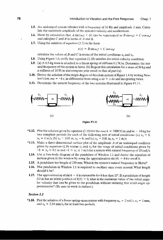
78 Introduction to Vibration and the Free Response Chap. 1

1.5. An undamped system vibrates with a frequency of 10 Hz and amplitude 1 mm. Calcu-late the maximum amplitude of the system's velocity and acceleration.

L.6. Show by calculation that -4sin(<,.r,t + $) can be represented as -Bsinco,r * Ccosto,tand calctilate C and B in terms of A and S.

L.7. Using the solution of equation (1.2) in the form

x(t ) : Bs inron/ * Ccoso, /

calculate the values of B and C in terms of the initial conditions rs and o6.1.8' Using Figure 1.6, verify that equation (1.10) satisfies the initial-velocity condition.1.9. (a) A 0.5-kg mass is attached to a linear spring of stiffness 0.1 N/m. Determine the nat-

ural frequency of the system in hertz. (b) Repeat this calculation for a mass of 50 kg anda stiffness of 10 N/m and compare your result to that of part (a).

1.10. Derive the solution of the single-degree-of-freedom system of Egure 1.4 by writing New-ton's law, ma : -kx,in differential form using a dx = u du and integrating twice.

1.11. Determine the natural frequency of the two systems illustrated in Figure P1.11.

Figure P1.11

*1.12. Plot thesolut iongivenbyequat ion(1.10) for thecasek = 1000N/m andm:10kgfortwo complete periods for each of the following sets of initial conditions: (a) xo : 0,'u6 : 1 m/q(b) to = 0.01 m,uo = 0,and (c) ro : 0.01m,tre : 1 m/s.

*1.13. Make a three-dimensional surface plot of the amplitude A of an undamped oscillatorgiven by equation (1.9) versus x0 and or for the range of initial conditions given by-1 < rn < 0.1 mand-1 < ?.)0 < 1m/sforasystemwithnaturalfrequencyof 10rad/s.

1.14. Use a free-body diagram of the pendulum of Window 1.1 and derive the equation ofmotion given in the window by using the approximation sin(0) : 0 for small 0.

1,.15. A pendulum has length of 250 mm. What is the system's natural frequency inHertz?1.16. The pendulum in Window 1.1 is required to oscillate once every second. What length

should it be?L.17. The approximation of sin 0 : 0 is reasonable for 0 less than 10'. If a pendulum of length

0.5 m has an initial position of 0(0) : 0, what is the maximum value of the initial angu-lar velocity that can be given to the pendulum without violating this small-angle ap-proximation? (Be sure to work in radians.)

Section 1.2

*1.1.8. Plotthesolutionof alinearspring-masssystemwithfrequencycon = 2radfs,xo: 1mm,and oo : 2.34 mm/s, for at least two periods.

(b)(a )

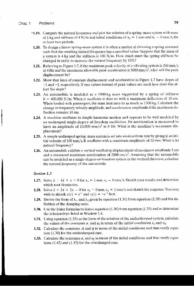
Chap. 1 Problems

*L.L9. Compute the natural frequency and plot the solution of a spring-mass system with massof 1 kg and stiffness of 4 N/m and initial conditions of xe : 1 mm and uo : 0 mm/s. forat leasl two periods.

1.20. To design a linear spring-mass system it is often a matter of choosing a spring constantsuch that the resulting natural frequency has a specified value. Suppose that the mass ofa system is 4 kg and the stiffness is 100 N/m. How much must the spring stiffness bechanged in order to increase the natural frequency by 10%?

1.21. Referring to Figure 1.7, if the maximum peak velocity of a vibrating system is 200 mm/sat 4Hz and the maximum allowable peak acceleration is 5000 mm/s2, what wiil the peakdisplacement be?

1.22. Show that lines of constant displacement and acceleration in Figure 1.7 have slopes of*1 and -1, respectively. If rms values instead of peak values are used, how does this af-fect the slope?

1.23. An automobile is modeled as a 1000-kg mass supported by a spring of stiffnessft : 400,000 N/m. When it oscillates it does so with a maximum deflection of 10 cm.When loaded with passengers, the mass increases to as much as 1300 kg. Calculate thechange in frequency, velocity amplitude, and acceleration amplitude if the maximum de-flection remains 10 cm.

1.24. A machine oscillates in simple harmonic motion and appears to be well modeled byan undamped single-degree-of-freedom oscillation. Its acceleration is measured tohave an amplitude of 10,000 mm/sz at 8 Hz. What is the machine's maximum dis-placement?

1.25. A simple undamped spring-mass system is set into motion from rest by giving it an ini-tial velocity of L00 mm/s. It oscillates with a maximum amplitude of L0 mm. What is itsnatural frequency?

1.26. An automobile exhibits a vertical oscillating displacement of maximum amplitude 5 cmand a measured maximum acceleration of 2000 cm/s'. Assuming that the automobilecan be modeled as a single-degree-of-freedom systern in the vertical direction, calculatethe natural frequency of the automobile.

Section 1.3

1.27. Solve i + 4 i * , r = 0forxn: 1mm.un:0mm/s.Sketchyourresul tsanddeterr ' , . r inewhich root dominates.

1 , . 28 . So l ve i + 2 t * 2x :O fo rxs :Omm,oo : 1mm/sandske tch the response .Youmaywish to sketch x(t) : e"' and x(l) : -t-' ttttr.

1.29. Derive the form of tr1, and \2 given by equation (1.31) from equation (i.28) and the de-finition of the damping ratio.

1.30. Use the Euler formulas to derive equation (1.36) from equation (1.35) and to determinethe relationships listed in Window 1.4.

1.31. Using equation (1.35) as the form of the solution of the underdamped system, calculatethe values of the constants a1 and a2 in terms of the initial conditions xe and z'0.

1.32. Calculate the constants -4 and S in terms of the initial conditions and thus verify equa-tion (1.38) for the underdamped case.

1.33. Calculate the constants a1 and a2 in terms of the initial conditions and thus verify equa-tions (1.42) and (1.43) for the overdamped case.

79

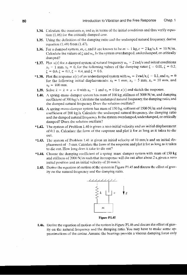
80 Introduction to Vibration and the Free Response Chap. 1

L.34. Calculate the constants a1 and a2 in terms of the initial conditions anci thus verify equa-tion (1.46) for the critically damDed case.

1.35. Using the definition of the damping ratio and the undamped natural frequency, deriveequation (1.48) from (1.47).

1.36. For a damped system, m,c,andt are known tobe nr = 1 kg, c : Zkg/s,k = 10N/m.Calculate the values of ( and cu,,. Is the system overdamped, underdamped, or criticallydamped?

*1.37. Plot x(r) for a damped system of natural frequency an = 2 rad/s and initial conditionsxo : 1 mm,

"o : 0, for the following values of the damping ratio: ( : 0.01, ( : 0.2,

( : 0 .6 , ( : 0 .1 ,L - 0 .4 ,and ( : 9 .3 .*1.38. Plot the response x(r) of an underdamped system with <,r , : 2radf s'( : 0.1", and oo : 0

for the following init ial displacements: xs : L mm, xs : 5 mm, ro : 10 mm, andxo : 100 mm'

1 .39 . So l ve i - i + x :0w i thx6 : l andus :0 fo rx ( t )andske tch the resPonse .

1.40. A spring-mass-damper system has mass of 100 kg, stiffness of 3000 N/m, and dampingcoefficient of 300 kg/s. Calculate the undamped natural frequenry, the damping ratio, andthe damped natural frequency. Does the solution oscillate?

L.41. A spring-mass-damper system has mass of 150 kg, stiffness of 1500 N/m and dampingcoefficient of 200 kg/s. Calculate the undamped natural frequency, the damping ratioand the damped natural freqrrency. Is the system overdamped, underdamped, or criticallydamped? Does the solution osciilate?

*1.42. "the system of Problem 1.40 is given a zero initial velocity and an initial displacementof 0.1 m. Calculate the form of the response and plot it for as long as it takes to dieout .

*L.43. The system of Problem 1.41 is given an initial velocity of 10 mm/s and an initial dis-placement of -5 mm. Calculate the form of the response and plot it for as long as it takesto die out. FIow long does it take to die out?

*1.44. Choose the damping coefficient of a spring-mass-damper system with mass of 150 kgand stiffness of 2000 N/m such that its response will die out after about 2 s, given a zeroinitial position and an initial velocity of 10 mm/s.

1.45. Derive the equation of motion of the system in Figure P1.45 and discuss the effect of grav-ity on the natural frequency and the damping ratio.

t,

Figure P1'45

1.46. Derive the equation of motion of the system in Figure P1.46 and discuss the effect of grav-

ity on the natural frequency and the damping ratio. You may have to make some ap-proximations of the cosine. Assume the bearings provide a viscous damping force only

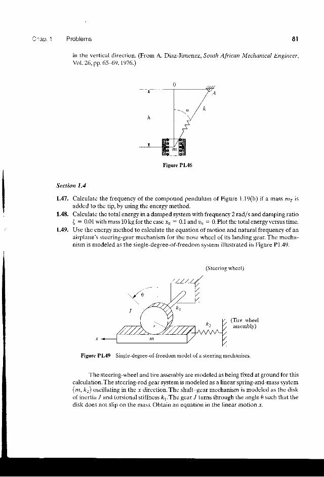
/ - h r n I Problems

in the vertical direction. (From AYol. 26, pp. 65 -69, I97 6.)

8 l

Diaz-Jimenez, S outh African M echanical Engine er,

Figure P1.46

Section 1.4

1.47. Calculate the frequency of the compound pendulum of Figure 1.19(b) if a mass m. isadded to the tip, by using the energy method.

1.48. Calculate the total energy in a damped system with frequency 2 rad/s and damping ratio( : 0.01 with mass 10 kg for the case "r0 = 0.1 and oo : 0. Plot the total energy versus time.

1.49. Use the energy method to calculate the equation of motion and natural frequency of anairplane's steering-gear mechanism for the nose wheel of its landing gear. The mecha-nism is modeled as the single-degree-of-freedom system illustrated in Figure P1.49.

(Steering wheel)

(Tire-wheelassembly)

Figure P1.49 Single-degree-of-freedom model of a steering mechanism.

The steering-wheel and tire assembly are modeled as being fixed at ground for thiscalculation. The steering-rod gear system is modeled as a linear spring-and-mass system(^, kt) oscillating in the -r direction. The shaft-gear mechanism is modeled as the diskof inertia .I and torsional stiffness k1. The gear / turns through the angle 0 such that thedisk does not slip on the mass. Obtain an equation in the linear motion.r.

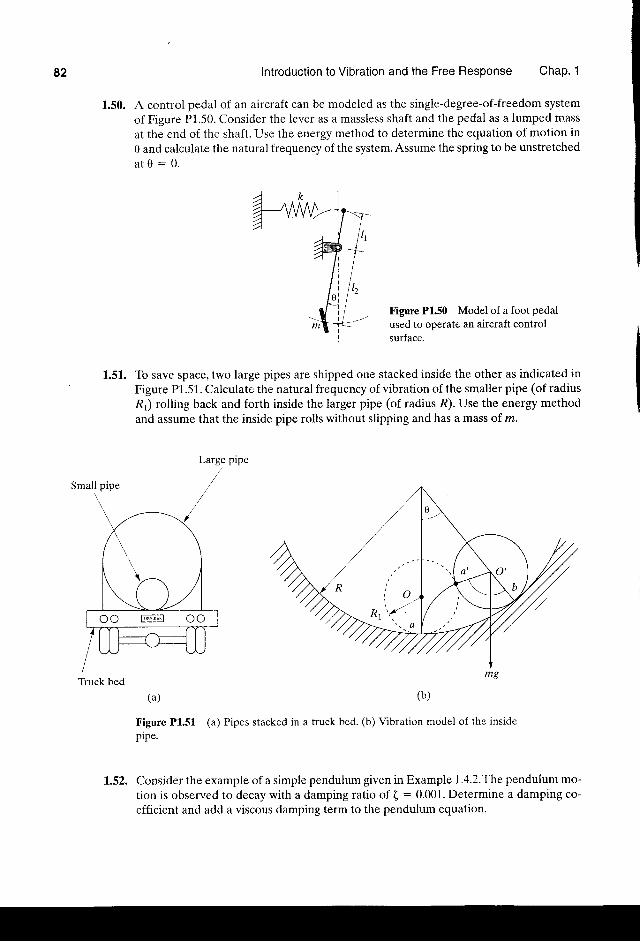
82 Introduction to Vibration and the Free Response Chap. 1

1.50. A control pedal of an aircraft can be modeled as the single-degree-of-freedom systemof Figure P1.50. Consider the lever as a massless shaft and the pedal as a lumped massat the end of the shaft. Use the energy method to determine the equation of motion in0 and calculate the natural frequency of the system. Assume the spring to be unstretcheda t O : 0 .

Figure P1.50 Model of a foot pedalused to operate an aircraft controlsurface.

1.51. To save space, two large pipes are shipped one stacked inside the other as indicated inFigure P1.51. Calculate the natural frequency of vibration of the smaller pipe (of radiusR1) rolling back and forth inside the larger pipe (of radius R). Use the energy methodand assume that the inside pipe rolls without slipping and has a mass of rn.

Large pipe

(u) (b)

Figure P1.51 (a) Pipes stacked in a truck bed. (b) Vibration model of the inside

pipe.

1.52. Consider the example of a simple pendulum given in Example l.4.Z.The pendulum mo-tion is observed to decay with a damping ratio of ( : 0.001. Determine a damping co-efficient and add a viscous damping term to the pendulum equation.

Tiuck bed

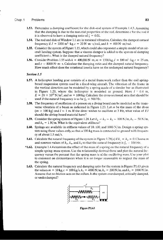
L l h : n 1 Problems

L.53. Determine a damping coefficient for the disk-rod system of Example 1.4.3. Assumingthat the damping is due to the material properties of the rod, determine c for the rod ifit is observed to have a damping ratio of ( : 0.01.

1.54. The rod and disk of Window L.L are in torsional vibration. Calculate the damped naturaifrequency if "r : 1000 m2.kg. c : 20 N.m.s/rad, and ft : 400 N.m/rad.

1.55. Consider the system of Figure 1.15, which could also represent a simple model of an air-craft landing system. Suppose that a viscous damper is added to the system of dampingcoefficient c. What is the damped natural frequency?

1..56. Consider Problem 1.55 with k = 400,000 N. n,ffi = 1500 kg, "/ : 100 m2 .kg, r : 25 cm.and c = 8000 N'm's. Calculate the darnping ratio and the damped natural frequency.How much effect does the rotational inertia have on the undamDed natural frequencv?

Section 1.5

1.57. A helicopter landing gear consists of a metal framework rather than the coil spring-based suspension system used in a fixed-wing aircraft. The vibration of the frame inthe vertical direction can be modeled by a spring made of a slender bar as illustratedin Figure 1.20, where the helicopter is modeled as ground. Here / : 0.4 m,E : 20 x 1010 N/mz, and m : 100 kg. Calculate the cross-sectional area that should be

. used if the natural frequency is to be fi : 500 Hz.1.58. The frequency of oscillation of a person on a diving board can be modeled as the trans-

verse vibration of a beam as indicated in Figure 1.23.Let mbe the mass of the diver(rn : 100 kg) and / - 1 m. If the diver wishes to oscillate at 3 Hz, what value of EIshould the diving-board material have?

1.59. Consider the spring system of Figure l.28.Let kt : ks * kz : 100 N/m, ft: : 50 N/m.and ko : 1 N/m. What is the equivalent stiff'ness?

1.60. Springs are available in stiffness values of 10, 100, and i000 N/m. Design a spring sys-tem using these values only, so that a 100-kg mass is connected to ground with frequen-cy of about 1.5 rad/s.

1.61. Calculate the natural frequency ofthe system in Figure 1.28(a) it ky : k2: 0. Choose nzand nonzero values of kt, ko,and ft5 so that the natural frequency isJ, : 1gg ttr.

*1.62. Example 1.4.4 examines the effect of the mass of a spring on the natural frequency of asimple spring-mass system. Use the relationship derived there and plot the natural fre-quency versus the percent that the spring mass is of the oscillating mass. [Jse your plotto comment on circumstances when it is no lonser reasohable to neslect the mass ofthe spring.

1.63. Calculate the natural frequency and damping ratio for the system in Figure P1.63 giventhevalues m: l0 kg,c = 100kg/s,k1 : 4000N/m,kz : 200N/m,andk. = 1000N/m.Assume that no friction acts on the rollers. Is the system overdamped, critically damped,or underdamped?

83

Figure P1.63

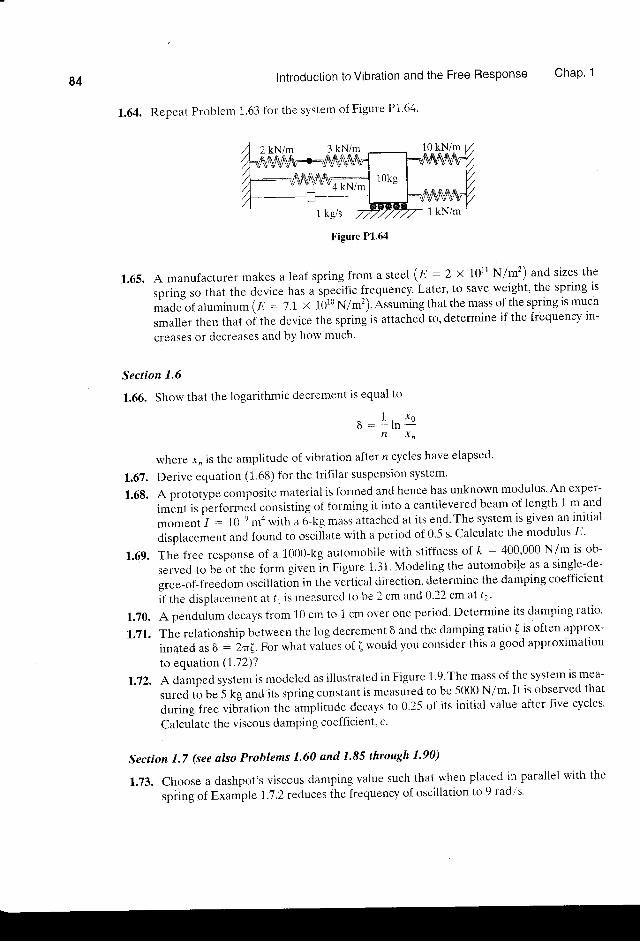
84 lntroduction to Vibration and the Free Response Chap' 1

1.64. Repeat Problem 1.63 for the system of Figure P1'64'

Figure P1.64

1.65. A manufacturer makes a leaf spring from a steel (E : 2 x 1011 N/m2) and sizes the

spring so that the device has u .p""iti. frequency. Later, to save weight, the spring is

made of aluminum (E : '7.L x ttito N7m2). assuming that the mass oJ the spring is much

smaller then that oi th" device the spring is attached to, determine if the frequency in-

creases or ciecteases and by how much'

Section 7.6

1.66. Show that the logarithmic decremetrt is equal to

a :L tn !fr xn

where x, is the amplitude of vibration after n cycles have elapsed'

1.67. Derive equation (1.68) for the trifilar suspension system'

1.6g. A prototype composite material is formed and hence has unknown modulus. An exper-

imlnt is performed consisting of forming it into a cantilevered beam of length 1 m and

moment 1 : 10 , ma with u d-kg ,nos attached at its end. The system is given an initial

displacement and found to oscillate with a period of 0.5 s' Calculate the modulus E'

L.69. The free response of a 1000-kg automobile with stiffness of k : 400,000 N/m is ob-

served to be of the form givenin Figure 1.31. Modeling the autornobile as a single-de-

gree-of-freedom oscillation in the vertical clirection, determine the damping coefficient

i f the displa.ement at / , is measured to be 2 crn and0'22 cm at 12'

1.70. A pendulum decays from 10 crr to 1 cm over one period. Determine its damping ratio'

1.71. The reiationship between the log decrement E and the darnping ratio ( is often approx-

imated as 6 : 2rr(. For what values of ( would you consider this a good approximation

to equation (1.72)?

I.72. Adamped system is modeled as illustrated in Figure 1.9.The mass of the system ls mea-

sured to be 5 kg and its spring constant is measured to be 5000 N/m. It is observed that

during free vibration the amplitude decavs to 0.25 of its initial value after five cycles'

Calculate the viscous damping coefficient, c'

Section 1.7 (see also Problems 1.60 and 1'85 through 1'90)

1.73. Choose a dashpot's visccus damping value such that when placed in parallel with the

spring of Example 1.7.2 reduces the frequency of oscillation to 9 rad,i s.

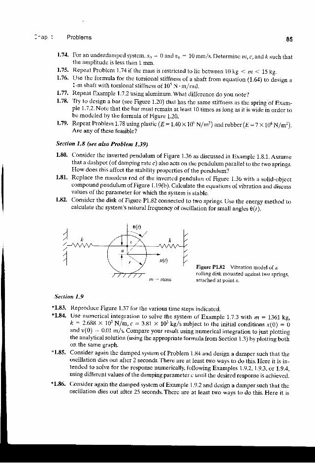
^ 2 n I Problems

1.74. For an underdamped system,.ro : 0 and ?ro : 10 mm/s. Determ jne m, c,and ft such thatthe amplitude is less than L mm.

1.75. Repeat Problem 1.74 if the mass is restricted to lie between 10 kg < m < 1.5 kg.1.76. Use the formula for the torsional stiffness of a shaft from equation (1.6a) to design a

1-m shaft with torsional stiffness of 105 N. m/rad..1.77. Repeat Example 1.7.2 using aluminum. What difference do you note?1.78. Tiy to design a bar (see Figure 1.20) that has the same stiffness as the spring of Exam-

ple 1.7.2. Note that the bar must remain at least 10 times as long as it is wide in order tobe modeled by the formula of Figure 1..20.

1.79. Repeat Problem 1.78 using plastic (E:1.40 x 10e N/m2) and rubber (E'= 7 x 106 N/m2).Are any of these feasible?

Section 1.8 (see also Problem 1.39)

1.80. Consider the inverted pendulum of Figure 1.36 as discussed in Example 1.8.1. Assumethat a dashpot (of damping rate c) also acts on the pendulum parallel to the two springs.How does this affect the stability properties of the pendulum?

1.81. Replace the massless rod of the inverted pendulun of Figure 1.36 with a solid-objectcompound pendulum ofFigure f.i9(b). Calculate the equations of vibration and discnssvalues of the parameter for which the system is stable.

1.82. Consider the disk of Figure P1.82 connected to two springs. Use the energy method tocalculate the system's natural frequency of oscillation for small angles 0(r).

Figure P1.82 Vibration model of arolling disk mounted against two springs,attached at point s.

Section 7.9

*1.83. Reproduce Figure 1.37 for the various time steps indicated.*1.84. use numerical integration to solve the system of Example 1.7.3 with m : 1.36r kg,

k : 2-688 x 105 N/m, c : 3.81 x 103 kgls subject to th; initial conditions x(0) = band o(0) : 0.01 m/s. Compare your result using numerical integration to just plottingthe analytical solution (using the appropriate formula from Section 1.3) by plotting bothon the same graph.

*1.85. Consider again the damped system of Problem 1.84 and design a damper such that theoscillation dies out after 2 seconds. There are at least two ways to do this. Here it is in-tended to solve for the response numerically, following Examples !.9.2,1.9.3, or 1.9.4,using different values of the damping parameter c until the desired response is achieved.

*L.86. Consider again the damped system of Example 7.9.2 and design a damper such that theoscillation dies out after 25 seconds. There are at least two ways to do this. Here it is

85

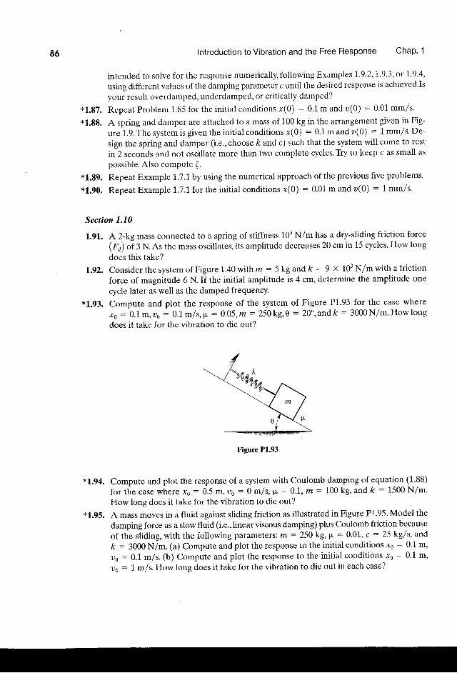
86 lntroduction to Vibration and the Free Response Chap. 1

intended to solve for the response numerically, following Examples t.9.2'1'.9.3,ot 1.9.4,

using different values of the damping parameter c until the desired response is achieved.Isyour result overdamped, underdamped, or critically damped?

*1.87. Repeat Problem 1.85 for the initial conditions 'r(0) : 0.1 m and ?r(0) : 0.01 mm/s'

*1.88. A spring and damper are attached to a mass of 100 kg in the arrangement given in Fig-

ure L.9.The system is given the initial conditions x(0) : 0.1 m and ?r(0) = 1 mm/s. De-

sign the spring and damper (i.e., choose ft and c) such that the system will come tc rest

in 2 seconds and not oscillate more than two complete cycles. Tiy to keep c as small aspossible. Also compute (.

*1.89. Repeat Example I.7.lby using the numerical approach of the previous five problems.

*1.90. Repeat Example 1.7.1 for the initial conditions x(0) : 0.01 m and r;(0) = I mm/s.

Section l.I0

1.91. A 2-kg mass connected to a spring of stiffness 103 N/m has a dry-sliding friction force(,f'r) of f N. As the mass oscillates, its amplitude decreases 20 cm in 15 cycles. How long

does this take?

1.92. Consider thesystemof F igure l .40wi th m:Skgandk:9 x 103N/mwithafr ic t ionforce of magnitude 6 N. If the initial amplitude is 4 cm, determine the amplitude one

cycle later as well as the damped frequency.*1.93. Compute and plot the response of the system of Figure P1.93 for the case where

to = 0.1 r l ,o0 : 0 .1 m/s, $:0.05,m:250kg,0 :Z}" ,andf t = 3000N/m'Howlongdoes it take for the vibration to die out?

Figure P1.93

*L.94. Compute and plot the response of a system with Coulomb damping of equation (1.88)

forthe case where ro : 0.5 ltr,oo : 0m/s, p : 0.1, m: 100kg, and t : 1500N/m'How long does it take for the vibration to die out?

*1.95. A mass moves in a fluid against sliding friction as illustrated in Figure P1.95. Model the

damping force as a slow fluid (i.e.,linear viscous damping) plus Coulomb friction because

of ttre sliding, with the following parameters: m : 250 kg, p = 0.01, c : 25 kg/s, and

k : 3000 N/m. (a) Compute and plot the response to the initial conditions xo : 0.1 m,

oo : 0.1 m/s (b) Compute and plot the response to the initial conditions ro : 0.1 m,

a6 : I mf s.How long does it take for the vibration to die out in each case?

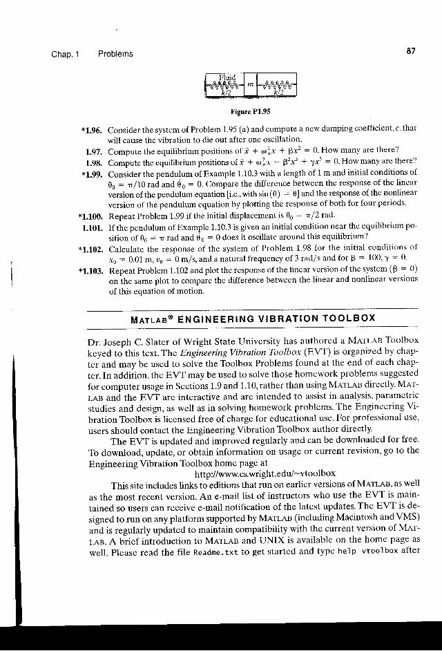
Chap .1 Problems

Fluidffi

kt2m A A f , \ A A

vv \ y \ yv \ vkt2

Figure P1.95

*1.96. ConsiderthesystemofProbleml.g5(a)andcomputeanewdampingccefficient,c,thatwill cause the vibration to die out after one oscillation.

Compute the equilibrium positions of i + 62,,x * $x2 : 0. How many are there?

Compute the equilibrium positions of i + (t)2,r - Fzxt + 1x5 = 0. How many are there?

Consider the pendulum of Example 1.10.3 with a length of i. m and initial conditions of

0o: rll1rad and do = 0. Compare the difference between the response of the linear

version of the pendulum equation [i.e., with sin (0) : 0] and the response of the nonlinear

version of the pendulum equation by plotting the response of both for four periods'

Repeat Problem 1.99 if the initial displacement is 8s : T f 2 rad.

If the pendulum of Example 1.10.3 is given an initial condition near the equilibrium po-

sition of 0o = n rad and d o : 0 does it oscillate around this equilibrium?*1.102. Calculate the response of the system of Problem 1.98 for the initial conditions of

xo : 0.0L fiI,oo : 0 m/s,and a natural frequency of 3 rad/s and for F : fOO,l = g'

*1.103. RepeatProblem1.L02andplottheresponseofthelinearversionofthesystem(p = 0)

on the same plot to compare the difference between the linear and nonlinear versions

of this equation of motion.

M n r L n g @ E N G I N E E R I N G V I B R A T I O N T O O L B O X

Dr. Joseph C. Slater of Wright State Llniversity has authored a Mnrlas Toolbox

keyed to this text. The Engineering Vibration Toolbox (EVT) is organized by chap-

ter and may be used to solve the Toolbox Problems found at the end of each chap-

ter. In addition, the EVT may be used to solve those homework problems suggested

for computer usage in Sections 1.9 and 1.L0, rather than using M.cTI-ae directly. Mar-

LAB and the EVT are interactive and are intended to assist in analysis, parametric

studies and design, as well as in solving homework problems. The Engineering Vi-

bration Toolbox is licensed free of charge for educational use. For professional use,

users should contact the Engineering Vibration Toolbox author directly.The EVT is updated and improved regularly and can be downloaded for free.

To download, update, or obtain information on usage or current revision, go to the

Engineering Vibration Toolbox home page athttp://www.cs.wright. edu/-vtoolbox

This site includes links to editions that run on earlier versions of Menan, as well

as the most recent version. An e-mail list of instructors who use the EVT is main-

tained so users can receive e-mail notification of the latest updates. The EVT is de-

signed to run on any platform supported by Merlen (including Macintosh andVMS)

and is regularly updated to maintain compatibility with the current version of Mer-

LAB. A brief introduction to Merles and UNIX is available on the home page as

well. Please read the file Readme.txt to get started and type help vtoolbox after

87

L.97.1.98.

*1.99.

*1.100.

1.101..

88 lntroduction to Vibration and the Free Response Chap' 1

installation to obtain an overview. Once installed, typing vtbud will display the cur-

rent revision status of your installation and attempt to download the current revi-

sion status from the anonymous FTP site. Updates can then be downloaded

incrementally as desired. Please see Appendix G for further information.

T O O L B O X P R O B L E M S

T81.1. Fix [your choice or use the values from Example 1.3.1 with x(0) : 1 mm] the values

of m, c,k, and .r(0) and plot the responses x(t) for a range of values of the initial ve-

locity i(0) to see how the response depends on the initial velocity. Remember to use

numbers with consistent units.

TBl.2. Using the values from ProblemTBi..1 and i(0) : 0, plot the response x(l) for a range

ofvalues ofx(0) to see how the response depends on the initial displacement'

TB1.3. Reproduce Figures 1.10, 1'11, andl'.72.

. T81.4. Consider solving Problem L.32 and compare the time for each response to reach and

stay below 0.01 mm.

T81.5. Solve Problems 1.88, 1.89, and 1.90 using the Engineering vibration Toolbox.

T8,1.6. Solve Problems 1.93, 1.94, and 1.95 using the Engineering Vibration Toolbox.

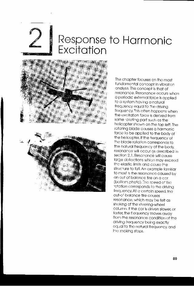
Response to HormonicExcitotion

Thls chcpter focuses on the mostfundomentol concept in vibroiiononolysis, This concept is thot ofresononce. Resoncnce occurs wheno periodic externolforce is oppliedto o system hoving o nolurolfrequency equol to tfre drivingfrequency. This oflen hcppens whenthe excitoiion force is derived fromsome rototing pcrt sucl-r os thehelicopier shovyn on the top left. Therototing blode couses o hormonicforce to be opplied to the body ofthe helicopter. lf the frequency ofthe blode rotction corresponds tothe noturol frequency of the body,resononce will occur os described insection 2, L Resononce will ccuselorge deflections which moy exceedthe elosiic limits ond couse thestructure to foil, An exomple fomiliorto most is the resononce coused byon out of bolonce tire on o cor(bottom photo). The speed of tirerotction conesponds to the drivingfrequency. At o certoin speed, theout-of-bolonce tire cousesresononce, which mcy be felt osshcking of the steering-wheelcolumn. lf ihe cor is driven slower, orfoster, the frequency moves owoyfrom the resoncnce condition of ihedriving frequency being exocflyequol to the noturol frequencv ondthe shoking slops.

89