Vintage Article: Consumption and Saving overthe Life Cycle:

How Important are Consumer Durables?∗

Jesús Fernández-VillaverdeUniversity of Pennsylvania, CEPR and NBER

Dirk KruegerUniversity of Pennsylvania, CEPR and NBER

February 16, 2010

Abstract

In this paper we investigate whether a standard life cycle model inwhich households purchase nondurable consumption and consumer durablesand face idiosyncratic income and mortality risk as well as endogenousborrowing constraints can account for two key patterns of consumptionand asset holdings over the life cycle. First, consumption expenditureson both durable and nondurable goods are hump-shaped. Second, younghouseholds keep very few liquid assets and hold most of their wealth inconsumer durables. The first pattern persists even after controlling forfamily size and constitutes a puzzle from the perspective of complete mar-ket models, in which individuals smooth consumption over their lifetime.The second pattern suggests that we need to explicitly model durablesto understand households’life cycle consumption and portfolio allocation.In our model durables play a dual role: they provide both consumptionservices and act as collateral for loans. A plausibly parameterized ver-sion of the model predicts that the interaction of consumer durables andendogenous borrowing constraints induces durables accumulation early inlife and higher consumption of nondurables and accumulation of financialassets later in the life cycle, in an order of magnitude consistent withobserved data. We thus conclude that durables are a key feature to ex-plain both the hump in consumption of durables and nondurables and theoptimal asset allocation of households.

∗All comments are welcomed to jesusfv@econ.upenn.edu or dkrueger@econ.upenn.edu. Wewould like to thank Andrew Atkeson, Michele Boldrin, Hal Cole, MariaCristina De Nardi,Narayana Kocherlakota, Lee Ohanian, Luigi Pistaferri and Edward Prescott for many helpfulcomments. All remaining errors are our own.

1

PreambleWhen we wrote this paper in 2000-2001, we wanted to stress the triple role

of consumer durables in life cycle models as an asset, as a long-lived good gen-erating utility flows, and as collateral for borrowing. To do so, we incorporateddurable goods serving these three roles into an otherwise standard overlappinggenerations, life cycle consumption savings model with an endogenous borrow-ing constraint. We calibrated the model to match U.S. macro and micro ob-servations and evaluated the importance of consumer durables for life cycleconsumption and asset choices.After the completion of this paper, substantial new work in three areas

related to our work has emerged. We structure our brief discussion of this liter-ature along the lines of the three main roles consumer durables play in our ownresearch, while of course recognizing that in most of the literature durables andhousing play multiple roles. In order to keep this discussion brief and concise, wewill not discuss the large literature modeling house prices endogenously becauseour own work maintains the assumption of exogenous and constant prices fordurables and thus does not contribute to this literature. To leave the integrityof the paper intact from its original state, we opted to review the subsequentliterature here, rather than incorporating the literature review into the originalpaper.First, a substantial empirical and theoretical-quantitative literature stud-

ies the interaction of household nondurable consumption choices and consumerdurables (especially housing), often in a life cycle context. Our own compan-ion paper, Fernández-Villaverde and Krueger (2007) and Yang (2009) provideempirical evidence on expenditures for consumer durables over the life cycle.Other relevant papers include Martin (2003), Ortalo-Magne and Rady (2006),Li and Yao (2007), Diaz and Luengo-Prado (2008), Kiyotaki et al. (2008), andIacoviello and Pavan (2009).The importance of housing for the accumulation of wealth and its portfolio

composition is the theme of an important body of work, starting from Grossmanand Laroque (1990) and Berkovec and Fullerton (1992), to the recent contribu-tions by Gervais (2002), Gruber and Martin (2003), Martin and Gruber (2004),Cocco (2005), Nakajima (2005), Yao and Zhang (2005), Silos (2007a, b), Diazand Luengo-Prado (2009), and Hintermaier and Koeniger (2009).Third, the role as collateral of consumer durables in general and housing

in particular in the main theme of a recent literature that focuses on the jointhousing and mortgage choice. Important examples of this work include Hurstand Stafford (2004), Luengo-Prado (2006), and Chambers et al. (2009a, b). Therecent increase in default on mortgages has motivated a small but growing liter-ature on structural models of foreclosures within this context. See, for instance,Jeske and Krueger (2005) and Garriga and Schlagenhauf (2009). The same issueis analyzed empirically, among others, by Carroll and Li (2008). Finally, a fewrecent papers have attempted to estimate models of housing choice (Sanchez,2007, is an important example), often with the focus on quantifying key struc-tural parameters, especially the elasticity of substitution between nondurable

2

consumption and services from consumer durables or housing. Examples of thisline of work include Bajari et al. (2008) and Li et al. (2009).This paper was last substantially revised in 2001 and prior to the solicitation

from Macroeconomics Dynamics had not been submitted for publication to anyjournal.

1 Introduction

In this paper we investigate whether a standard life cycle model in which house-holds purchase nondurable consumption and consumer durables and face idio-syncratic income and mortality risk as well as endogenous borrowing constraintscan account for two key patterns of consumption and asset holdings over the lifecycle. First, consumption expenditures on both durable and nondurable goodsare hump-shaped: expenditures are low early in life, then rise considerably untilabout age 50, and fall again. The average household in the Survey of ConsumerExpenditures spends 63% more when the head of the household is 50 than whenshe is 25 and around 70% more than when she is 65. Second, young householdskeep very few liquid assets and hold most of their wealth in consumer durables1 .Later in life, then, families accumulate significant amounts of financial assetsfor retirement. The importance of durables is also mirrored in the aggregatecomposition of wealth: households hold 35% of their total assets in real estateand other consumer durables and only 28% in equity2 .As we will discuss below, the first fact, the hump in consumption expen-

ditures persists even after controlling for family size and constitutes a puzzlefrom the perspective of the standard life-cycle model with complete financialmarkets, according to which individuals smooth consumption over their lifetimeand across states of the world. Understanding this puzzle is not only interestingfrom a theoretical perspective, but also crucial for applied policy analysis. Asindividual behavior changes over the life cycle, so will the effects of social secu-rity reform, the public provision of saving incentives or the welfare consequencesof progressive taxation vary by age groups. For an accurate quantitative assess-ment of policy reforms is thus essential to establish a coherent explanation forchanges in consumption and savings behavior over the life cycle that gives riseto the hump in consumption.The second fact, the life-cycle pattern of households portfolio composition,

suggests that it is required to explicitly model the purchase decision of con-sumer durables to understand households’consumption and portfolio allocationdecisions. This constitutes a departure from the tradition in the life-cycle con-sumption literature which has largely ignored the presence of durables. Thisomission is problematic if the purchase of durables and the flow of services gen-erated by them interacts with nondurable consumption in a nonseparable way.

1>From now on we will use the term consumer durables or, more simply, durables toinclude houses and other consumer durable goods. See Section 2 for detailed data on thesetwo empirical observations.

2See Flow of Funds Accounts, second quarter 1998.

3

For example, recent explanations of the life cycle hump in nondurable consump-tion provided by Carroll (1997) or Gourinchas and Parker (2002) rely cruciallyon households consuming, up to the age of 40, all of their income, apart fromsome small buffer stock used to insure against future bad income shocks. Wewill argue that, in the presence of consumer durables in the model, householdsbehave quite differently: they accumulate durables early in life and consume therest of disposable income, without any saving in financial assets. In this periodof their lives durables not only provide consumption service flows, but are alsoused as collateralizable insurance against uninsurable idiosyncratic income risk.Our model also distinguishes itself from standard household portfolio choice

model that, on one hand, explicitly include the presence of durables such ashousing, but on the other hand usually ignore the life cycle dimension of ahousehold.3 Thus these models by construction cannot explain the observationof little accumulation of liquid assets early in life in the data. Instead of in-terpreting this fact as indicating that young households do not to save, as oneis forced to when considering a standard life-cycle model of consumption with-out durables, we will demonstrate that it is optimal for households to save indurables early in life and to shift to the accumulation of financial assets onlylater on in the life cycle.In order to substantiate our claims we construct a dynamic general equilib-

rium life cycle model of consumption and saving with labor income uncertaintyand borrowing constraints to formally evaluate whether such a model can ex-plain the two empirical observations mentioned above in a unified framework.The crucial elements of our model are a) a highly persistent stochastic idiosyn-cratic labor income process with b) a hump-shaped mean over the life cycle;c) the presence of durables that yield consumption services and can be usedas collateral, in addition to a standard one-period bond whose short sales aresubject to a borrowing constraint; d) endogenous determination of the interestrate in general equilibrium.We now justify the key elements of our model. The first two elements are

fairly standard in the literature on life cycle consumption and mainly motivatedby the empirical observation that, even if households face substantial idiosyn-cratic labor income risk (see e.g. Gottschalk and Moffi tt (1994)), on averagelabor income follows a hump-shaped pattern over the life cycle with peak aroundthe age of 50 (see Hansen (1993)). The third and fourth elements of the modelare novel features to the literature we wish to contribute to. The presence of con-sumer durables is motivated by the empirical observation that they constitute alarge fraction of households asset holdings. Furthermore, as mentioned above,the life-cycle pattern of nondurable consumption may be intimately related tothe life cycle pattern of the accumulation of durables, so that abstracting fromthem may severely bias any study of the life cycle profile of nondurable con-sumption and asset accumulation. Finally, we determine the interest rate ofthe economy endogenously in general equilibrium because the life cycle profileof consumption and asset accumulation depends crucially on the ratio between

3A notable exception is Cocco, Gomes and Maenhout (2002).

4

the subjective time discount factor and the interest rate. The discipline of gen-eral equilibrium determines this ratio endogenously in our model and thereforerestricts our possibility to predetermine the results by appropriate choice of boththe interest rate and the time discount factor 4 . In addition, since we want toextend our line of research to the study of the interactions between durablesand the business cycle and to evaluations of the welfare effects of different fiscalpolicies, we view endogenous price and interest rate determination not only asattractive from a theoretical perspective, but also as quantitatively crucial foraddressing these questions.Our main findings are summarized as follows. In the empirical part of the

paper we use data from the Consumer Expenditure Survey to show that con-sumption expenditure of both durables and nondurables follows a hump-shapepattern over the life cycle. We also use data from the Survey of ConsumerFinances to document that young households virtually own no liquid financialassets, but hold a major fraction of their wealth portfolio as durables, while onlylater in life the composition of household portfolios shifts in favor of financialassets.Our second contribution is to demonstrate that a plausibly parametrized

version of our model can quantitatively explain these empirical findings as aris-ing from rational choices of consumers facing an increasing wage profile andincome uncertainty. The interaction between consumer durables that provideboth consumption and collateral services, and endogenous borrowing constraintsgives rise to accumulation of durables (and no accumulation of financial assets)early in life and substitution towards higher consumption of nondurables andthe accumulation of financial assets later in life.This work is related to several strands of the literature. On the empirical

side it adds to the discussion about the life cycle profile of consumption ob-served in cross sectional micro data. Important references include Attanasioand Browning (1995), Attanasio and Weber (1995), Blundell et al. (1994) andGourinchas and Parker (2002). The key question in the context of our paper iswhether, once changes in family size are controlled for, consumption still followsa hump-shaped life cycle profile. The key empirical finding of our paper is thepresence of a hump-shape profile not only for nondurable consumption, but alsofor expenditures on consumer durables.On the theoretical side, the basic building block of our model is the clas-

sic income fluctuation problem in which a consumer faces a stochastic incomeprocess and decides how much to consume and how much to save. Contributorsto this literature include Deaton (1991), Carroll (1992 and 1997) and Gourinchasand Parker (2002). Following Bewley (1986) the income fluctuation problemhas been embedded by Huggett (1993) and Aiyagari (1994) into general equilib-rium, giving rise to the endogenous determination of the interest rate as well as anontrivial income, wealth and consumption distribution in equilibrium. Our pa-

4A complementary approach, taken by Gourinchas and Parker (2002), fixes the interestrate and estimates the time discount factor from cross-section micro data using the SimulatedMethods of Moments. In contrast to Gourinchas and Parker’s partial equilibrium model, inour general equilibrium model all markets clear at each point of time.

5

per incorporates consumer durables and endogenous borrowing constraints intoAiyagari’s framework; the specification of the borrowing constraint is adaptedfrom the recent endogenous incomplete markets literature (see Alvarez and Jer-mann (2000) Kehoe and Levine (1993), Kocherlakota (1993), and Krueger andPerri (1999, 2005)). Lustig (2004) also presents a model with a durable assetand endogenous borrowing constraints to explain the equity premium puzzle; inhis model, however, agents have access to a full set of Arrow securities and areinfinitely lived. Our model shares some of his elements, but our focus is on thelife-cycle consumption and asset allocation whereas Lustig studies the pricingimplications of endogenous borrowing constraints.Although our focus is on the life cycle pattern of consumption of durables and

nondurables, our model also has implications for the optimal portfolio allocationbetween financial assets and durables at each point of the life cycle. Thereforethe paper makes contact to the literature on optimal portfolio choice in thepresence of consumer durables, as Chah et al. (1995), Eberly (1994), Flavinand Yamashita (2002) and Grossman and Laroque (1990). Finally, the paperalso relates to the literature of Real Business Cycles with a household productionsector (see Greenwood et al. (1995) for a review). We share their focus on anexplicit treatment of the household sector in dynamic general equilibrium andits dynamic behavior; we do not, however, model aggregate uncertainty.The paper is organized as follows. In Section 2 we present empirical re-

sults from the Consumer Expenditure Survey documenting a hump-shape inboth nondurable and durable consumption expenditures even after controllingfor household size. We also discuss the evidence on the life cycle pattern ofwealth composition derived from the Survey of Consumer Finances. In Section3 we present our model and define equilibrium. Section 4 is devoted to a dis-cussion of the model calibration and Section 5 presents the quantitative resultsobtained from the benchmark calibration of the model. Section 6 performssensitivity analysis and Section 7 concludes. Technical discussions about ourempirical methods, the data used, the computational algorithm and all figuresare contained in the appendix.

2 Empirical Findings

This section presents our empirical findings on consumption and wealth accu-mulation over the life cycle. We first document life cycle profile of consumptionusing data from the Consumer Expenditure Survey (CEX), dealing explicitlywith the issue of changing household size over the life-cycle. A more extensivediscussion of the results in this section can be found in our empirical companionpaper, Fernández-Villaverde and Krueger (2007). We then turn to the Surveyof Consumer Finances (SCF) in order to document life-cycle pattern of wealthand portfolio allocation. We point out that the structure of household port-folios changes with age, and that housing and other consumer durables play aquantitatively crucial role in most of households’portfolios.

6

2.1 Life Cycle Profiles of Consumption

A basic prediction of the life-cycle model with complete financial markets is thatthe life-cycle consumption profiles should be smooth. If the period utility func-tion is time-invariant and the time discount factor is constant, then householdschoose consumption plans to equate marginal utility across time and states ofthe world, possibly with some growth rate, depending on the relative size of thereal interest rate and the discount factor. Under CRRA period utility consump-tion growth itself should be constant across time. With complete markets, con-sumption smoothing can be achieved through the transfer of contingent claimsacross periods and states5 . The first empirical question, motivated by standardeconomic theory, we want to answer is therefore whether smooth consumptionprofiles are indeed observed over the life cycle in household-level consumptiondata.During the eighties some agreement arose that the answer to this question

was negative (see Deaton (1992) for an overview). The main stylized fact emerg-ing from this literature was that consumption seems to track income over thelife cycle, changing only when income changes, and not already when it becomesknown that income will change, as economic theory predicts. This evidence wasinterpreted as indicating the presence of liquidity constraints or other financialmarket imperfections. Since labor income follows a hump over the life cycle,these imperfections then imply the consumption hump over the life cycle in thedata.Recently this view has been disputed by Blundell et al. (1994), Attanasio

and Browning (1995) and especially Attanasio et al. (1999). These authorsargue that once the consumption data are appropriately adjusted for changes inhousehold size (which is also hump-shaped over the life cycle) and compositionthe hump in life cycle consumption disappears. We will challenge this view andargue that consumption follows a hump even after controlling for demographics.For that we will use 1980-2001 data from the Consumer Expenditure Survey(CEX).

2.1.1 The CEX Data

During the last few years, the CEX has become one of the main sources forempirical work on consumption (see Attanasio, 1999 for a survey). The CEX isa rotating panel of about 5000 households, where each household is interviewedevery three months over five calendar quarters, and every quarter 20 percent ofthe sample is replaced by new households.In order to document life cycle profile for consumption in the way economic

theory envisions it there exist two main problems arising from the CEX. First,

5This statement relies on the further assumption that leisure and consumption are separablein the period utility function. For instance Ghez and Becker (1973) propose a model whereconsumption services are produced with time and consumption goods as inputs. When timebecomes more expensive (i.e. labor income is higher), agents substitute time with goods inthe production function of consumer services, generating a correlation between labor incomeand consumption.

7

the CEX only measures consumption expenditures, and not the consumptionservice flows from these expenditures. Second, the CEX only contains a verylimited panel dimension, as households provide at most four subsequent quartersof consumption data. In Fernandez-Villaverde and Krueger (2007) we discussin detail how we address both issues. Here we provide a short summary of ourdiscussion.

2.1.2 Expenditures versus Consumption

Since the CEX does not report a measure of consumption services we are leftwith analyzing expenditures on consumption goods. While this distinction is notvery relevant for nondurable goods it is crucial in the case of consumer durables.However, the CEX does not allow us to reliably impute service flows from infor-mation on the stock of consumer durables. Nevertheless, our theoretical modelbelow has implications for the life-cycle profile of expenditures on nondurablesand durables, and thus it is useful to document the empirical profiles from theCEX here. Our empirical results may serve as a benchmark against which thequantitative predictions of our model as well as other models can be evaluated.

2.1.3 Constructing a Pseudopanel

Since the CEX does not have a significant panel dimension, we construct apseudopanel or synthetic cohort panel (see Deaton, 1985) to document life-cycle consumption profiles. We use the age of the reference person to associatea household with a cohort and define 10 cohorts with a length of five years. Inorder to generate a balanced Panel with consumption data over the life cyclewe compute the means of cohort consumption, using CEX-provided populationweights.

2.1.4 Specification and Estimation of Life-Cycle Profiles

We propose to estimate life cycle consumption expenditure profiles by a simpleand flexible seminonparametric regression that controls for cohort and timeeffect with dummy variables and puts relatively little parametric structure onthe dependence of consumption on age. In particular, we specify the partiallylinear model:

cit = πicohorti + πtγt +m (ageit) + εit (1)

where cit is the cohort i average of log-consumption at time t, cohorti is a dummyfor each cohort (except the youngest one), γt a dummy for each quarter, ageitis the age of cohort i at time t, measured in years, m (ageit) = E (cit|ageit) is asmooth function of ageit, and εit is an independent, zero mean, random error.The random term captures multiplicative measurement error in consumptionexpenditures (since the dependent variable is log-consumption) as well as un-observed cross-sectional heterogeneity. We estimate the partially linear modelusing the two-step estimator proposed by Speckman (1988). This estimatorcombines ordinary least squares to estimate the parametric component with

8

a standard kernel smoothing estimator to estimate the nonparametric compo-nent.6 In order to separately identify time, age, and cohort effects we followDeaton (1997) and assume that time effects are orthogonal to a time trend andthat their sum is normalized to zero.

2.1.5 Controlling for Family Size: Household Equivalence Scales

Before carrying out the estimation of consumption profiles we need to quan-tify how much of the hump in consumption over the life cycle is explained bychanges in household size and composition. For this purpose we employ house-hold equivalence scales, which measure the change in consumption expendituresneeded to keep the welfare of a family constant when its size varies.7 In ourcompanion paper we survey the large literature on household equivalence scalesbefore settling on a particular scale.8

We now deflate consumption expenditure measures Cjt from the CEX forhousehold j at quarter t by the equivalence scale esjt obtained from the de-mographic information of the household. This results in adjusted householdconsumption cjt = log

Cjtesjt

. Let cit denote the synthetic cohort i average of cjt,which we now use to estimate the partially linear model in equation (1).

2.1.6 Results

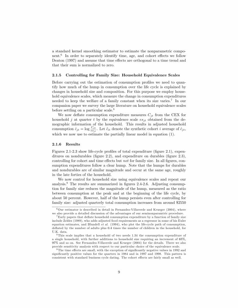
Figures 2.1-2.3 show life-cycle profiles of total expenditure (figure 2.1), expen-ditures on nondurables (figure 2.2), and expenditure on durables (figure 2.3),controlling for cohort and time effects but not for family size. In all figures, con-sumption expenditures follow a clear hump. Note that the humps for durablesand nondurables are of similar magnitude and occur at the same age, roughlyin the late forties of the household.We now control for household size using equivalence scales and repeat our

analysis.9 The results are summarized in figures 2.4-2.6. Adjusting consump-tion for family size reduces the magnitude of the hump, measured as the ratiobetween consumption at the peak and at the beginning of the life cycle, byabout 50 percent. However, half of the hump persists even after controlling forfamily size: adjusted quarterly total consumption increases from around $2550

6Our estimator is described in detail in Fernandez-Villaverde and Krueger (2004), wherewe also provide a detailed discussion of the advantages of our seminonparamtric procedure.

7Early papers that deflate household consumption expenditure by a function of family sizeinclude Zeldes (1989), who adds adjusted food requirements as a regressor in some of his Eulerequation estimates, and Blundell et al. (1994), who plot the life-cycle path of consumption,deflated by the number of adults plus 0.4 times the number of children in the household, forU.K. data.

8This scale implies that a household of two needs 1.34 the consumption expenditure ofa single household, with further additions to household size requiring an increment of 65%,97% and so on. See Fernandez-Villaverde and Krueger (2004) for the details. There we alsoprovide sensitivity analysis with respect to our particular choice of the equivalence scale.

9The time effects are small, with the exception of significantly negative values in 1992 andsignificantly positive values for the quarters in 1984 and in 1997 and 1998. This pattern isconsistent with standard business cycle dating. The cohort effects are fairly small as well.

9

to nearly $3300 and then decreases to about $1800 (see figure 2.4). Relative tothe unadjusted data we also observe that the peak in life-cycle consumption ispostponed, roughly to the age of 50.In figure 2.5 we show adjusted nondurable consumption. Again the size of

the hump is reduced by 50%, as a comparison with figure 2.2 reveals. Withrespect to expenditures of consumer durables, figure 2.6 yet again displays aclear hump. Now, however, expenditures are already fairly high at the beginningof the life cycle, capturing first purchases of durable goods by young households.Comparing figures 2.5 and 2.6 we observe that the reduction of the hump dueto adjustment for household size is quite similar for nondurables and durables.Furthermore, both profiles peak at around the same household age.10

In summary, our analysis demonstrates that even though changes in house-hold size can account for around half of the hump in life cycle consumption andthus are crucial in understanding life-cycle profiles, the other half remains a puz-zle from the perspective of the standard life-cycle model with complete financialmarkets. This is especially true for the profile of expenditures on consumerdurables. If the period utility function is separable in nondurable consumptionand services from durables, the real interest rate is equal to the time discountfactor and constant over time, then it is optimal to simply purchase the de-sired stock of durables early in life and to only replace depreciation from thereon. In contrast, our data display that the process of durables accumulationis incremental over the life cycle, consistent with other work that has docu-mented liquidity constraints in the purchases of consumption durables (Alessieet al., 1997, Attanasio et al., 2005, Barrow and McGranahan, 2000, and Eberly,1994) or argued for the importance of nonseparabilities in the utility function(Attanasio and Weber, 1995).

2.2 Life Cycle Profiles of Wealth

How do the findings in the previous subsection relate to observed patterns ofwealth accumulation and portfolio composition over the life cycle? One of themost authoritative sources on households’asset holdings is the Survey of Con-sumer Finances (SCF), a triennial survey of U.S. households undertaken by theFederal Reserve System. The SCF interviews a representative cross section ofover 4000 households, and collects data about their demographics characteris-tics, assets and debts. Since the short number of repeated surveys (six, of whichonly four are directly comparable) precludes the building of a pseudo-panel, wewill focus on the cross-sectional aspect of the data. We will use the 1995 surveyinformation to document several important aspects of the life cycle profile ofhouseholds assets.The pattern of life cycle wealth is shown in Figure 2.7. We plot the house-

holds mean and median net worth along the life cycle11 . Two main points arise

10 In Fernandez-Villaverde and Krueger (2004) we perform an extended bootstrap analysisto document that the confidence bands around our point estimates for life-cycle consumptionprofiles are tight. Thus our findings are not due to sampling uncertainty in the CEX data.11The age used is the age of the “head” of the family as defined by the SCF: the male

10

from this figure. First, as for consumption expenditures, wealth also follows ahump-shaped pattern over the life cycle. Households accumulate wealth fromthe beginning of their lives until retirement, the moment at which they beginto run down their wealth. It is noticeable, however, that wealth stays relativelyhigh even after the age of 80. Second, wealth is highly unequally distributed,as can be seen from the large ratio between household mean and median networth; this ratio attains its maximum over the life cycle at around 400 per centjust before retirement.Additional interesting information is contained in data on the composition

of household wealth. Figure 2.812 shows the importance of durables in mosthouseholds’portfolios. We order households along the dimension of total wealthand plot the percentage of their portfolio held in real estate (which consistsof the primary residence for most households) and the percentage invested incorporate equity. For 60 per cent of all families, those between the thirtiethand ninetieth percentile, real estate represents most of their total assets whilevehicles and other durables are an important part of the remaining portfolio.Below the thirtieth percentile, households have none or low wealth, most ofit in vehicles and other durables. For example, note that 65.4 per cent of thehouseholds in the lowest quartile of the net worth distribution own vehicles withmedian value of $4800 while only 7.9 per cent of this group have financial assetsbeyond a transaction account. If we include the transaction accounts as financialassets, 78 per cent of these last quartile households have some financial assets,but with a median value of only $1100. These facts leave the highest 10 percent of the wealth distribution as the only households for which financial assetsare a fundamentally important part of their portfolio. A theory of life cycleconsumption and saving should account for the low levels of financial wealth ofmost households.Even more important, given our focus on life cycle consumption, is the port-

folio composition of assets along the life cycle. Figure 2.9 shows that the primaryresidence is a basic component of the median assets of households over theirlives. Before households reach the age of 40, the median value of a homeown-ers’primary residence exceeds the median value of total assets for householdsholding some assets. After the age of 40, the median primary residence valuestays always above 50 percent of the median of total assets. The same picturearises in a percentile decomposition of homeowners’portfolios. Up to the age of45, the portion of homeowners’assets in real estate is around two thirds. Afterthat time and until retirement it decreases, but never falls below 57 per cent13 .

in a mixed-sex couple, the older person in a same-sex couple or the main individual earnerotherwise.12The data on asset composition by wealth percentiles was kindly supplied to us by Joseph

Tracy. See Tracy et al. (1999) for the study in which these data were first used.13 It can be argued that concentrating on homeowners’portfolios does introduce a selection

bias in favor of primary residences. However, since most non-homeowners households holdvery little wealth, including these non-homeowners in Figure 2.8 will reduce the level of thecurves, but not necessarily the relation between them. We do not include non-homeowners toavoid the jump in primary residence value associated with the median households acquiringits first home.

11

Again, theory needs to explain why housing and other durable goods have sucha primary role in the life cycle accumulation of wealth for the median wealthhousehold.To summarize the empirical part of this paper: expenditures on nondurable

and durable consumption goods follow a hump over the life cycle and the stockof durables seem to accumulate only progressively. At the same time younghouseholds hold most of their wealth in consumer durables, with financial assetsgaining importance in later periods of a household’s life. We now present a modelto jointly reproduce these stylized facts of life cycle consumption and portfoliodecisions.

3 The Environment

In this section we present a dynamic general equilibrium model of life cycleconsumption. We use a standard dynamic general equilibrium, life cycle modelwith income uncertainty, with two novel features: first we will introduce serviceflows of consumer durables into the utility function and second, we will restrictintertemporal trade by endogenous borrowing constraints, as explained belowin detail.

3.1 Demographics

There is a continuum of individuals of measure 1 at each point of time in oureconomy. Each individual lives at most J periods. In each period j ≤ Jof his life the conditional probability of surviving and living in period j + 1is denoted by αj ∈ (0, 1). Define α0 = 1 and αJ = 0. The probability ofsurvival, assumed to be equal across individuals of the same cohort, is beyondthe control of the individual and independent of other characteristics of theindividual (such as income or wealth). We assume that αj is not only theprobability for a particular individual of survival, but also the (deterministic)fraction of agents14 that, having survived until age j, will survive to age j + 1.Annuity markets are assumed to be absent and accidental bequests are assumedto be uniformly distributed among all agents currently alive. In each period a

number µ1 =(

1 +∑J−1j=1

∏ji=1 αi

)−1of newborns enter the economy, and the

fraction of people in the economy of age j is defined recursively as µj+1 = αjµj ,with µJ+1 = αJ = 0. Let J = {0, 1, . . . , J} denote the set of possible ages of anindividual.

3.2 Technology

There is one good produced according to the aggregate production functionF (Kt, Lt) where Kt is the aggregate capital stock and Lt is the aggregate labor

14 In other words, we assume a law of large numbers to hold in our economy. See Feldmanand Gilles (1985) for a justification; note that we do not require realizations of the underlyingstochastic process to be independent across agents.

12

input. We assume that F is strictly increasing in both inputs, strictly concave,has decreasing marginal products which obey the Inada conditions and is ho-mogeneous of degree one. As usual with constant returns to scale productiontechnologies, in equilibrium the number of firms is indeterminate and withoutloss of generality we assume that there is a single representative firm.The final good can be either consumed or invested into physical capital or

consumer durables. Let by Kdt denote the aggregate stock of consumer durables

in period t. The aggregate resource constraint then reads as:

Ct +Kt+1 − (1− δ)Kt +Kdt+1 − (1− δd)Kd

t = F (Kt, Lt) (2)

where Ct are aggregate consumption expenditures and δ and δd are the depre-

ciation rates on physical capital and consumer durables, respectively.

3.3 Preferences and Endowments

Individuals are endowed with one unit of time in each period that they supplyinelastically in the labor market. Individuals differ in their labor productiv-ity due to differences in age and realizations of idiosyncratic uncertainty. Thelabor productivity of an individual of age j is given by εjη, where {εj}Jj=1 de-notes the age profile of average labor productivity. The stochastic componentof labor productivity, η, follows a finite state Markov chain with state spaceη ∈ E = {η1, . . . ηN} and transition probabilities given by the matrix π(η′|η).Let Π denote the unique invariant measure associated with π. The initial real-ization of the stochastic part of labor productivity is assumed to be drawn fromΠ for all agents.We assume that all agents, independent of age and other characteristics face

the same Markov transition probabilities and that the fraction of the populationexperiencing a transition from η to η′ is also given by π. This law of largenumbers and the model demographic structure assure that the aggregate laborinput is constant. As with lifetime uncertainty we assume that individualscannot insure against idiosyncratic labor productivity by trading contingentclaims. Moral hazard problems may be invoked to justify the absence of thesemarkets.In addition to her time endowment an individual also possesses an initial

endowment of the durable consumption good, kd1 ≥ 0 and an initial position ofcapital, k1 ≥ 0. In most of our applications we will assume that k1 = kd1 = 0.

Individuals derive utility from consumption of the nondurable good, c, andfrom the services of the stock kd of durable good. Individuals value streams ofconsumption and durables

{cj , k

dj

}Jj=1

according to

E0

J∑j=1

βj−1u(cj , kdj )

(3)

where β is the time discount factor and E0 is the expectation operator, con-ditional on information available at time 0. The period utility function u is

13

assumed to be strictly increasing in both arguments, strictly concave, with di-minishing marginal utility from both arguments and obeying the Inada condi-tions with respect to nondurable consumption. The instantaneous utility frombeing dead is normalized to zero and expectations are taken with respect to thestochastic processes governing survival and labor productivity.

3.4 Timing and Information

The timing of events in a given period is as follows. Households observe theiridiosyncratic shock η and receive transfers from accidental bequests. Then laborand capital is supplied to firms and production takes place. Next households re-ceive factor payments and make their consumption and asset allocation decision.Finally uncertainty about early death is revealed. Durables are not transferreduntil the end of the period. In that way, even if the household sells its stock ofdurables and use the payment to finance present consumption of nondurables,it will hold the durables (and receive utility from the service flow) until the endof the period. Analogously, the addition or subtraction to the stock will notinfluence the present period service flow. All information is publicly held andthe idiosyncratic labor productivity status (as well as survival status) becomescommon knowledge upon realization.

3.5 Equilibrium

We will limit our attention to stationary equilibria in which prices, wages andinterest rates are constant across time. Individuals are assumed to be pricetakers in the goods and factor markets they participate in. In each moment oftime individuals are characterized by their position of capital and holdings ofconsumer durables, as well as their age and labor productivity status (k, kd, η, j).Let by Φ(k, kd, η, j) denote the measure of agents of type (k, kd, η, j), constantin a stationary equilibrium.We normalize the price of the final good to 1 and let by r and w denote the

interest rate and wage rate for one effi ciency unit of labor, respectively. Also letby Tr denote transfers from accidental bequests. The consumer problem cannow be formulated recursively as

V (k, kd, η, j) = maxc,k′kd′

u(c, kd) + βαj∑η′

π(η′|η)V (k′, kd′, η′, j + 1) (4)

s.t

c+ k′ + kd′ = wηεj + (1 + r)k + (1− δd)kd + Tr

k′ ≥ b(kd′, η, j)

c ≥ 0, kd′≥ 0

Several specifications of the constraints b that limit short-sales of capitalwill be discussed below. Note that these constraints are allowed to vary by age

14

and current labor productivity status15 to reflect differences in future earningpotentials among agents, and are allowed to vary by durable holdings nextperiod to allow for collateralized borrowing.We are now ready to define a stationary equilibrium. Let J and E be

the power sets of J and E, respectively and B be the Borel sets of R LetS = R×R×E×J and S = B × B × E × J andM be the set of finite measuresover the measurable space (S,S).

Definition 1 A stationary equilibrium is a value function V, policy functionsfor the household,

(c, k′, kd′

), labor and capital demand for the representative

firm, (K,L), prices (w, r), transfers Tr, and a finite measure Φ ∈M such that

1. Given (w, r) and Tr, V solves the functional equation (4) and(c, k′, kd′

)are the associated policy functions

2. Input prices satisfy

r = FK(K,L)− δw = FL(K,L)

3. Markets clear:∫c(k, kd, η, j)dΦ+δ

∫k′(k, kd, η, j)dΦ+δd

∫kd′(k, kd, η, j)dΦ = F (K,L) (Goods Market)∫

k′(k, kd, η, j)dΦ = K (Capital Market)∫ηεjdΦ = L (Labor Market)

4. Transfers are given by

Tr =

∫ [k′(k, kd, η, j)− k

]dΦ +

∫ [kd′(k, kd, η, j)− kd

]dΦ

5. The measure follows:Φ = T (Φ)

where T is the law of motion generated by π and the policies k′ and kd,′

as described below.

This definition is standard, possibly apart form the definition of transfers.The distribution of agents at the beginning of the period, Φ does not include theindividuals that died at the end of last period. Hence total accidental bequestsof capital from deceased households at the end of last period equal∫ [

k′(k, kd, η, j)− k]dΦ (5)

15As markets for contingent claims are assumed to be inoperative the borrowing constraintscannot depend on the realization of the productivity shock next period.

15

where we also used the fact that the total number of agents in the economy isnormalized to 1. A similar argument holds for bequests of consumer durables.We now describe what we mean by the law of motion T being generated by

π and the policies k′ and kd′. The operator T maps M into M in the followingway. Define the transition function Q : (S,S)→ [0, 1] by:

Definition 2 For all S′ = R′ × Z ′ × E′ × J ′ ∈ B × B × E × J and all s =(k, kd, η, j) ∈ S

Q(s, S′) =∑η′∈E′

{αjπ(η′|η) if j + 1 ∈ J ′, k′(k, kd, η, j) ∈ R′, kd′(k, kd, η, j) ∈ Z ′

0 else

Then for all J ′ ∈ J such that 0 /∈ J ′ we have

T (Φ)(S′) =

∫Q(s, S′)dΦ

For J ′ = 0 we have

T (Φ)(R′ × Z ′ × E′ × {0}) =∑η′∈E′

{Π(η′)µ1 if 0 ∈ R′, 0 ∈ Z ′

0 else

Note that this definition implicitly assumes that individuals are born withzero assets (capital and consumer durables).To complete the description of the model, our specifications of the borrowing

limits are as follows. In our benchmark economy we specify the borrowing limitsb(kd

′, η, j) to be the smallest number to satisfy

V (b(kd′, η, j), kd

′, η′, j + 1) ≥ V (0, 0, η′, j + 1) for all η′ ∈ E

i.e. households can borrow up to the point at which, for all possible realizationsof the stochastic labor productivity shock tomorrow, they have an incentiveto repay their debt rather than to default, with the default consequence beingspecified as losing their debt, but also their consumer durables. Thus consumerdurables play an important role not only in generating consumption services,but also as collateralizable assets against which agents can borrow.We will also report results for economies in which borrowing limits are spec-

ified asb(kd

′, η, j) = 0

and asb(kd

′, η, j) = −κkd

′

The first specification prevents borrowing altogether. Although we do not viewthis specification as reasonable in an economy with collateralizable assets, sincea large fraction of previous work on life-cycle consumption (in the absence ofdurables) has explicitly or implicitly (via judicious choice of the income process)used this specification we want to present similar results for comparison. The

16

second specification allows households to borrow up to a percentage κ againsttheir stock of consumer durables.We finish this section by discussing an important element of our model: the

absence of a durable goods rental market. Suppose households, in addition tobuying durable goods, can also rent them from competitive providers of durableservices for a rental rate of pr. Consistent with the timing of the model, supposea unit of durables rented today yields consumption services tomorrow. Thenthe rental price has to satisfy pr = r + δd, and the net cost of renting oneunit of services for tomorrow is r + δd whereas the net cost of obtaining oneunit of durables services via buying is 1 − 1−δd

1+r = r+δd

1+r < r + δd as long asthe interest rate is positive.16 In addition, purchased consumer durables relaxthe borrowing constraint and thus make buying instead of renting even moreattractive. Therefore our modeling choices (households can buy and sell durableswithout adjustment cost) would imply that the option to rent the durable isstrictly dominated by purchasing it, using it and selling it afterwards.Obviously the introduction of transactions and agency costs associated with

purchases of consumer durables (but also for repeatedly renting them) changesthe argument; in our model with cross-sectional heterogeneity both positiverentals and purchases of durables would potentially occur in equilibrium.17 Arethese effects important? Our answer is that, even if they may be of some impor-tance, the insights of including an explicit rental market may not compensatefor the additional computational burden involved. Note also that the existenceof collateralized loans reduce the theoretical role of rental markets. Households,by judicious choice of when and how much to borrow will be able to repro-duce nearly the same intertemporal allocation of consumption in our model ascompared to a model with an explicit rental market.

4 Calibration

We choose the benchmark parametrization of our economy partly on the basisof microeconomic evidence and partly so that the stationary equilibrium for oureconomy matches selected long-run averages of US data.

4.1 Demographics

We define a year as our unit of time. Then, with respect to demographics, wewill have J = 81 generations. Therefore we can interpret our model as one inwhich households become economically active at age 20, and live up to age 100.

16Note that if the providers of the durable rental could rent the durable in the same period

in which it is acquired by them, then the rental price would satisfy pr = r+δd

1+rand both the

rent and buy option have the same cost associated with it. Still, since consumer durables havecollateral value (they relax the borrowing constraint) for agents that face binding borrowingconstraints, at least for these agents buying strictly dominates the renting option.17See Platania and Schlagenhauf (2000) for an explicit life-cycle analysis of the purchase vs.

renting decision for housing.

17

The conditional survival probabilities {αj}Jj=1 are taken from Faber (1982)18 .We plot these survival probabilities in Figure 4.1.

4.2 Technology

We select a Cobb-Douglas production function F (Kt, Lt) = AKαt L

1−αt as a

representation of the technology that produces the final good. We normalizeA = 1 and set α = 0.3 so that the equilibrium of our economy matches the long-run labor share of national income for the US of approximately 1− α = 0.7.We choose the depreciation rates δ and δd of physical capital and consumer

durables to match investment shares of output and capital-output ratios for theUS economy. In the steady state of our model I = δK and Id = δdKd andhence δ = I/Y

K/Y and δd = Id/YKd/Y

.We use data from the 2000 comprehensive revision of NIPA and Fixed As-

sets and Consumer Durable Goods of the Bureau of Economic Analysis (seehttp://www.bea.doc.gov for detailed information and downloadable tables) tocompute K defined as Private Nonresidential Fixed Assets (equipment, softwareand nonresidential structures) and Kd defined as Private Residential Structuresand Consumer Durable goods. Since the NIPA are somewhat inconsistent inthe treatment of the household sector (the accounts do include the imputedflow of services from owner-occupied housing as part of GDP but not the ser-vices from other durables), we adjust NIPA data when needed to reflect themeasurement definitions in our economy: final, physical goods produced in theperiod. We use as our benchmark calibration δ = I/Y

K/Y = 0.1351.2 = 0.1125 and

δd = Id/YKd/Y

= 0.121.45 = 0.0857.

4.3 Preferences and Endowments

In each period agents supply one unit of time, the productivity of which isgiven by εjη. The deterministic age profile of the unconditional mean of laborproductivity {εj}Jj=1 is taken from Hansen (1993). We take εj = 0 for j ≥ 46,in effect imposing mandatory retirement at the age of 65.In the parametrization of the stochastic idiosyncratic labor productivity

process we follow Storesletten et al. (1999). They build a rotating panel fromthe Panel Study of Income Dynamics (PSID) to estimate the stochastic partuit = ln(ηit) of the labor income process for household i at time t

uit = zit + εit (6)

zit = ρzit−1 + νit

where εit ∼ N(0, σ2ε

)and νit ∼ N

(0, σ2ν

)are innovation processes. Their point

estimates are ρ = 0.935, σ2ε = 0.017 and σ2ν = 0.061.

18Since we care about the life cycle consumption of households after demographic adjust-ments we do not need to worry about the different mortality rates in the household. Faber’snumbers refer to women survival probabilities.

18

This process differs from other specifications in the literature (see Abowd andCard (1989), Carroll (1992) or Gourinchas and Parker (2002) among others) intwo aspects. First we do not allow labor income to go to zero. Even if this eventhas a very low probability (Carroll (1992) estimates this probability as 0.003 fora year), its effects are substantial on intertemporal allocations: households willnot borrow any positive amount since they may face a life-long sequence of zerolabor income and may be unable to consume a positive amount and repay theirdebt in some period. This implication seems debatable, in particular in lightof the existence of a collection of public income support programs in the U.S.,given that the notion of labor income in the model should be interpreted as aftertax, after government transfer labor income. Second, we do not impose a unitroot in the autoregressive process for zit since Storesletten et al. (2001) are ableto reject the null of a unit root19 . This choice remains, however, an open anddebated issue. In small samples it is very diffi cult to separate a unit root fromour value ρ = 0.935, especially since with finitely lived families, the stochasticprocess can not drift away too much from its initial condition.20 Fortunately, ourresults are not very sensitive to this choice, as shown below when we performsensitivity analysis by increasing ρ towards unity.

Using the method proposed by Tauchen and Hussey (1991), we approximatethis continuous state AR(1) process with a three state Markov chain21 , whichresults in:

E = {0.57, 0.93, 1.51} (7)

π =

0.75 0.24 0.010.19 0.62 0.190.01 0.24 0.75

(8)

Π = [0.31, 0.38, 0.31] (9)

As initial endowments of physical capital and durables we assume k1 = kd1 = 0.With respect to preferences we assume that the period utility function is of

CRRA type:

u(c, kd) =

(g(c, kd

))1−σ − 1

1− σ (10)

where g (·, ·) is an aggregator function of the services flows from durables andnondurables. A simple but quite general choice for the aggregator is an CESaggregator of the form:

g(c, kd) =[θcτ + (1− θ)

(kd + ε

)τ] 1τ(11)

19Part of the appeal of the unit root assumption derives from the fact that, as pointedout by Deaton (1991), it simplifies the computation of the household problem since one statevariable can be eliminated.20We performed Monte Carlo simulations to check that, when indiviudal wages generated

with our chosen process are estimated with a unit root process we in general cannot rejectthe null of nonstationarity.21An approximation with more than three states would be desirable; computational con-

straints prevents this at the moment.

19

where ε is a number small enough to be irrelevant for our quantitative exercises,but makes the utility function finite for kd = 0 (the intuition being that one cansurvive without a house and other consumer durables, but one cannot survivewithout food).Unfortunately, we do not have conclusive empirical evidence about the value

of τ . Eichenbaum and Hansen (1990) find that the substitutability betweendurables and nondurables is highly sensitive to the overall specification of pref-erences. McGrattan et al. (1997) use aggregate data to estimate, in a modelwhere labor input is needed to complement durables to produce consumptionservices, a value of τ = 0.429 with standard error of 0.116. Rupert et al. (1995)explore a number of different specifications of a model similar to McGrattanet al. (1997) using PSID data. They find that the estimated values of τ differgreatly with changes in the sample composition and that overall, their resultsare not particularly informative. For example, they estimate τ = −0.065 withstandard error of 0.471 for single males while the equivalent estimates for singlefemales are 0.445 and 0.121 and for couples 0.083 and 0.292. It is interestingthat two of the three results are not significantly different from zero. Ogakiand Reinhart (1998), using aggregate data and a similar specification to ours,estimate τ = 0.143, not significantly different from zero at the 5% level. Giventhis range of estimates, we find it reasonable to adopt as a benchmark the caseτ = 0 (the aggregator function takes a Cobb-Douglas form) and test later forsensitivity of the results to our choice. The resulting period utility function isthen given by

u(c, kd) =

(cθ(kd + ε

)1−θ)1−σ − 1

1− σ (12)

Also, for our benchmark calibration we choose a coeffi cient of relative risk aver-sion σ = 2, a value in the middle of the range commonly used in the literature.We jointly pick the parameters θ and the time discount factor β so that the

steady state equilibrium for our benchmark calibration has an interest rate ofr = 4% (see McGrattan and Prescott (2001) for a justification of this numberbased on their measure of the return on capital and on the risk-free rate ofinflation-protected U.S. Treasury bonds) and a ratio of expenditures on non-durables and durables of C

Id= C/Y

Id/Y= 6.2, the long-run average for US data.

This results in choices β = 0.9375 and θ = 0.81.

5 Results

5.1 Aggregate Variables

In Table 5.1 we report values for aggregate variables for our benchmark economy.

Table 5.1

20

Variable Steady State Value

r 4%CY 0.67IY 0.22Id

Y 0.11wY 0.54L 1.29KY 1.97Kd

Y 1.26CId

6.2

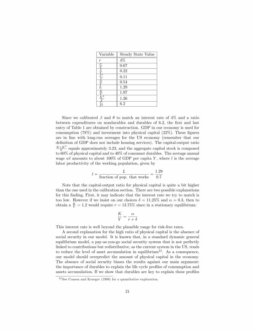
Since we calibrated β and θ to match an interest rate of 4% and a ratiobetween expenditures on nondurables and durables of 6.2, the first and lastentry of Table 1 are obtained by construction. GDP in our economy is used forconsumption (78%) and investment into physical capital (22%). These figuresare in line with long-run averages for the US economy (remember that ourdefinition of GDP does not include housing services). The capital-output ratioK+Kd

Y equals approximately 3.23, and the aggregate capital stock is composedto 60% of physical capital and to 40% of consumer durables. The average annualwage wl amounts to about 100% of GDP per capita Y , where l is the averagelabor productivity of the working population, given by

l =L

fraction of pop. that works=

1.29

0.7

Note that the capital-output ratio for physical capital is quite a bit higherthan the one used in the calibration section. There are two possible explanationsfor this finding. First, it may indicate that the interest rate we try to match istoo low. However if we insist on our choices δ = 11.25% and α = 0.3, then toobtain a K

Y = 1.2 would require r = 13.75% since in a stationary equilibrium:

K

Y=

α

r + δ

This interest rate is well beyond the plausible range for risk-free rates.A second explanation for the high ratio of physical capital is the absence of

social security in our model. It is known that, in a standard dynamic generalequilibrium model, a pay-as-you-go social security system that is not perfectlylinked to contributions but redistributive, as the current system in the US, tendsto reduce the level of asset accumulation in equilibrium22 . As a consequence,our model should overpredict the amount of physical capital in the economy.The absence of social security biases the results against our main argument:the importance of durables to explain the life cycle profiles of consumption andassets accumulation. If we show that durables are key to explain these profiles

22See Conesa and Krueger (1999) for a quantitative exploration.

21

even when no social security exists and the incentive for financial accumulationis higher, the result will hold even more tightly with a redistributive socialsecurity system. The size of this bias is, however, uncertain and the effects ofsocial security in an economy with durables deserve further research.

5.2 Life Cycle Profiles

Figures 5.1 and 5.2 show the average life-cycle pattern of labor income, non-durable consumption expenditures and the stocks of consumer durables, finan-cial assets and total net worth. We plot age on the x-axis, following our inter-pretation that agents start their economic life at the age of 20 and live up tothe age of 100.These averages are obtained by integrating the policy functions with respect

to the equilibrium measure of agents, holding age fixed. For example, averagenondurable consumption expenditures by cohort j is given by

Cj =

∫c(k, kd, η, j)Φ(dk × dkd × dη × {j})

Note that due to stochastic death cohorts are not of the same size, so thatpopulation averages are weighted averages of cohort averages.>From Figure 5.1 we see the hump shape of average labor income. This

hump shape arises by construction since the life cycle profile for labor incomeparallels the life cycle profile of average labor productivity {εj}Jj=1 which obeysa hump-shape over the life cycle, with peak around the age of 50. Also note thatat the age of 65 agents retire in our model, which is induced by assuming εj = 0for j ≥ 46.Also, in Figure 5.1 we can see that expenditures on nondurable consump-

tion obey a hump-shaped life cycle pattern, with peak around the age of 4523

and a pattern and, more importantly a size ( about 40% bigger than age 20),quite similar to the one reported in Figure 2.5. The increase in nondurableconsumption in the early part of life is due to two factors in our model, both ofwhich are crucially dependent on the presence of consumer durables. First, sincedurables generate service flows, early in life it is optimal to build up the stockof consumer durables and compromise on consumption of nondurables. Second,once the stock of nondurables is built up, due to the nonseparabilities in theutility function the marginal utility from nondurable consumption is higher, dueto a higher stock of durables. The hump shape in nondurable consumption isnot due to buffer stock behavior per se as in Carroll (1992) or Gourinchas andParker (2002): households in our model, once they have accumulated consumerdurables, can use these as collateralizable insurance against unfavorable laborproductivity shocks as their borrowing capacity increases with their holding ofdurables.23The spike in the first period is due to the fact that agents start with kd = 0. To avoid very

low utility households choose a high consumption of nondurables. A possible remedy wouldbe to endow agents with a small positive stock of consumer durables at birth.

22

It is important to note the increase of consumption late in life. This smallincrease is due to lifetime uncertainty. Households want to buffer until almostthe end of their life; then they consume in the last periods since survival proba-bilities are low or zero. Also, from Figure 5.1 we see how average consumptiontracks deterministic average labor income. Since this income increase is perfectlyforecastable, our model displays excess sensitivity of consumption to income assuggested by empirical data and contrary to the predictions of the basic LifeCycle-Permanent Income model (see Deaton (1992) for a review).In Figure 5.2 we show how the average wealth portfolio evolves over the life

cycle. Early in life households borrow as much as possible to buy houses andother consumer durables. As time goes by, the stock of durables is built upand holdings of financial assets as well as nondurable consumption increases.Since households can borrow against their durable assets, the accumulation offinancial assets occurs for life-cycle, and not for insurance purposes. Our modelreproduces important facts about the life cycle composition of wealth: younghouseholds do save (net worth becomes significantly positive by the age of 35),but they do not save in financial assets, but rather in consumer durables. Ashouseholds become older, financial assets become a more important part of thehousehold’s wealth portfolio, with these assets being accumulated primarily tofinance consumption in retirement. Note that total net worth peaks at age 64,the year prior to retirement. Also note that households hold substantial networth until high ages, mainly for insurance purposes against living too long.This correspond to the observation that elderly households seem to overaccu-mulate assets (or more precisely they do not run down their wealth fast enough).This peak in net worth at age 64 would be far less pronounced in the presenceof a pay-as-you go social security system, because part of the life cycle motiveof savings and the precautionary savings motive due to stochastic mortalitydisappears.In Figure 5.3 we plot the total stock of consumer durables. The stock follows

a hump shape, differing from a complete markets model where the desired stockis built up in the first period and only an amount equal to depreciation is spenteach period thereafter. We plot the average expenditure on durables in Figure5.4. From this graph we notice that the model generates a pattern of consumerdurables that somehow diverges from the observed pattern: there is a big peakin the first years and then it falls, even though it is possible to see somewhatof a hump after the first spike. One possible explanation is that in the datayoung families obtain bequests, which in large part come as consumer durables.A second possible explanation is the endogenous formation of households in thedata. In our model, all households enter their active economic life at age 20,a time period where they want to build up the desired stock of capital. In thedata, however, economically active (in the sense of our model) households arecreated endogenously due to differences in marriage timing and education. Thisendogeneity smooths out the first big spike of durable expenditures in the dataand leads to a pattern of life cycle durables expenditure reported in Section 2.24

24This divergence between data a model may also indicate that our borrowing constraint is

23

In Figure 5.5 we plot several simulated life cycle patterns, from which weobserve how households adjust their consumption decisions to labor incomeshocks. These shocks, although quantitatively important, are not able to over-come, however, the general pattern of a life cycle hump in consumption onaverage.The stochastic patterns in Figure 5.5 raise the question of the role of idiosyn-

cratic income uncertainty. To address this issue we solve the model setting thevariances of the labor income innovations to zero, i.e. computing the model with-out labor income uncertainty. The results are plotted in Figures 5.6-5.7. Tworesults are worth mentioning. First, from the life cycle pattern of nondurableconsumption in Figure 5.6 we can see that, once uncertainty is eliminated, halfof the hump in nondurable consumption disappears: the new profile is sub-stantially smoother than before (see Figure 5.1). With uncertainty borrowingconstraints are tighter because default has to be prevented in all income statestomorrow, in particular in the high income states. A tighter borrowing con-straint makes consumption co-move more with income. In addition risk aversehouseholds postpone a larger fraction of consumption until an important degreeof uncertainty is revealed. In contrast, without labor income uncertainty thiseffect is absent and higher nondurable consumption sets in earlier in life.Second, the average holding of durables is smaller. As explained before,

in an environment with uninsurable stochastic labor income, durables are alsoaccumulated because the collateral services they provide in allowing borrowingto smooth nondurable consumption. Comparing the stock of durables fromFigure 5.7 with the stock of durables from Figure 5.2 we can see that, for primeage households, the average holding of durables is reduced by around 15%.Finally our model is also able to cast some light on two other important

issues. First, the model predicts that only 58% of the households hold any fi-nancial wealth in equilibrium, and these are households in later periods of theirlife. This low participation corresponds to the evidence on financial assets fromthe Survey of Consumer Finances and is obtained without the need of model ele-ments such as a very high elasticity of intertemporal substitution or transactioncosts commonly used in the literature to generate similar results. The presenceof an alternative asset that also generates consumption and collateral services isenough to discourage 42% of households from participating in financial markets.Second, consumer durables can help to explain why households with higher

life cycle income save proportionally more than poor households (see the empir-ical evidence presented in Dynan et al. (2004)). Figure 5.8 plots the life-cycleprofile of financial assets for the average household, for a household that al-ways enjoys the high labor income shock, ex-post, and for a household thatalways suffers the low income shock, also ex-post. We can see from this plothow the high income household, despite of having a realized lifetime incomethat is only 2.6 times higher than the low income households, has accumulatedover six times more financial assets at age 65. This result comes from the strong

specified too loosely, allowing households to invest into consumer durables at too rapid pacewhen young.

24

nonhomogeneity introduced by the dual role of durables as a saving instrumentand a consumption good: as the household becomes richer the marginal util-ity of durables decreases and financial assets become relatively more attractive.Quantitatively, around 50, the high income household only has around twice asmany durables as the low income household but has accumulated already animportant stock of financial assets while the poor household still has negativefinancial wealth.

6 Sensitivity Analysis

In this section we will consider two different issues. First, subsection A andB will study the behavior of the model under the alternative two borrowingconstraints outlined in Section 3. Second, in Subsection C we will check therobustness of our calibration to different changes in parameter values.

6.1 Ad-Hoc Borrowing Constraints

In this subsection we describe how our main results change as we adopt a dif-ferent form of borrowing constraint. The case on which most of the literatureon life cycle consumption without durable goods has focused is an ad-hoc spec-ification limiting short-sales of bonds to a fixed number b. Often this numberis set to b = 0 (see Aiyagari (1994) and Krusell and Smith (1998) among oth-ers).25 Although such a specification of the borrowing constraint in the presenceof a collateralizable asset seems somewhat unreasonable we want to relate ourresults to the existing literature and hence adopt the constraint b = 0. Then,durables, while still providing services and hence utility to households, lose theirrole as collateralizable assets. We leave all other parameters unchanged fromthe benchmark calibration.

Table 6.225Other important contributors to the life-cycle consumption literature specify income

processes with positive probability of zero lifetime income. The Inada condition on the utilityfunction then leads to a self-imposed borrowing constraint at 0: no agent facing a chanceof zero lifetime income would ever borrow and risk zero or negative consumption for certainrealizations of the stochastic income process. See, e.g., Carroll (1992, 1997) and Gourinchasand Parker (2002).

25

Variable Steady State Value

r 2.25%CY 0.65IY 0.25Id

Y 0.1wY 0.54L 1.29KY 2.21Kd

Y 1.17CId

6.5

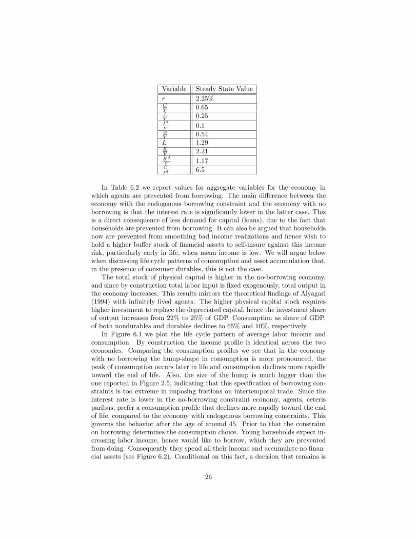
In Table 6.2 we report values for aggregate variables for the economy inwhich agents are prevented from borrowing. The main difference between theeconomy with the endogenous borrowing constraint and the economy with noborrowing is that the interest rate is significantly lower in the latter case. Thisis a direct consequence of less demand for capital (loans), due to the fact thathouseholds are prevented from borrowing. It can also be argued that householdsnow are prevented from smoothing bad income realizations and hence wish tohold a higher buffer stock of financial assets to self-insure against this incomerisk, particularly early in life, when mean income is low. We will argue belowwhen discussing life cycle patterns of consumption and asset accumulation that,in the presence of consumer durables, this is not the case.The total stock of physical capital is higher in the no-borrowing economy,

and since by construction total labor input is fixed exogenously, total output inthe economy increases. This results mirrors the theoretical findings of Aiyagari(1994) with infinitely lived agents. The higher physical capital stock requireshigher investment to replace the depreciated capital, hence the investment shareof output increases from 22% to 25% of GDP. Consumption as share of GDP,of both nondurables and durables declines to 65% and 10%, respectivelyIn Figure 6.1 we plot the life cycle pattern of average labor income and

consumption. By construction the income profile is identical across the twoeconomies. Comparing the consumption profiles we see that in the economywith no borrowing the hump-shape in consumption is more pronounced, thepeak of consumption occurs later in life and consumption declines more rapidlytoward the end of life. Also, the size of the hump is much bigger than theone reported in Figure 2.5, indicating that this specification of borrowing con-straints is too extreme in imposing frictions on intertemporal trade. Since theinterest rate is lower in the no-borrowing constraint economy, agents, ceterisparibus, prefer a consumption profile that declines more rapidly toward the endof life, compared to the economy with endogenous borrowing constraints. Thisgoverns the behavior after the age of around 45. Prior to that the constrainton borrowing determines the consumption choice. Young households expect in-creasing labor income, hence would like to borrow, which they are preventedfrom doing. Consequently they spend all their income and accumulate no finan-cial assets (see Figure 6.2). Conditional on this fact, a decision that remains is

26

the allocation of income between expenditures on nondurables and investmentinto consumer durables. Figure 6.1 shows that between the age of 20 and 30 anincreasing fraction of income is devoted to nondurables: at the beginning of lifeagents build up the stock of consumer durables as with endogenous borrowingconstraints. Since this accumulation cannot be credit-financed and hence comesat the expense of nondurable consumption, however, this process is slower inthe economy with borrowing constraints that prevent all borrowing.>From Figure 6.2 we also see that financial assets are not used to buffer

bad income shocks early in life; this is accomplished by holding durables whichboth yield services and can be sold if necessary. Financial assets are used forretirement saving, as they become the dominant asset in the average household’sportfolio after the age of 40.One important difference between the two economies is that with endogenous

borrowing constraints the net worth of the average young generation is (slightly)negative: even when taking account of consumer durables, households up to theage of 30 borrow, on net, against their higher expected future labor income;mostly to finance the accumulation of durables, but also to smooth consumptionover time and states (in equilibrium the low interest rate relative to the timediscount factor implies that a declining consumption profile is optimal).

6.2 Consumer Durables and Fixed Down Payment

As argued before, the presence of durables suggests that, using them as collat-eral, households should be able to borrow up to some amount. This consid-eration motivates a borrowing constraint of the form b(kd

′, η, j) = −κkd′ . We

pick κ = 0.8 which corresponds to a down payment requirement for purchasesof consumer durables of 20%, following the real estate market practices.26 Weleave all the remaining parameters of the benchmark calibration unchanged.

Table 6.3

Variable Steady State Value

r 2.24%CY 0.63IY 0.25Id

Y 0.12wY 0.54L 1.29KY 2.15Kd

Y 1.37CId

5.25

26Grossman and Laroque (1990) justify this practice based on liquidity costs associatedwith durables.

27

We present the results for aggregate variables for this economy in Table 6.3.As in the previous case, the main difference, compared to the endogenous bor-rowing constraint economy, is that the interest rate is substantially lower. Alsothe stocks of physical capital and durables are higher. In fact, the stock ofdurables is even higher than in our benchmark economy. The result is closelyrelated with the dual role of durables as collateral and as a generator of util-ity. The use of durables as collateral also reduces the importance of physicalcapital as a buffer to smooth income fluctuations and, as a consequence thestock of physical capital is lower than in the case in borrowing is not permittedaltogether.In Figure 6.3 we plot the life cycle pattern of average labor income and

consumption. The possibility to partially finance the acquisition of durablesreduces the hump with respect to the case of no borrowing, but it is still biggerthan in our benchmark economy. In Figure 6.4 we plot the life cycle patterns ofconsumer durables, financial wealth and total wealth. In this picture we can seehow households take advantage of durables as a collateral and how they havenegative financial wealth until their mid-forties, a point at which they beginto save for retirement. However, in comparison to the benchmark case withendogenous borrowing constraint, total wealth is always strictly positive sinceall borrowing has to be fully collateralized.

6.3 Changes in Parameters

In this subsection we will check the robustness of the results to changes inparameters. First we study the effects of increasing the persistence parame-ter ρ. The main consequence of this increment is a bigger hump in nondurableconsumption. Here the reverse arguments we used to discuss the effects of uncer-tainty apply. A higher persistence of labor income makes borrowing constraintstighter. High shock households have a higher incentive to default on debts whenthe shock is more persistent: they can leave behind their debts and rebuild theirdurables stock under the better labor income perspectives. Also, as a higherdegree of uncertainty needs to be revealed through life when shocks are morepersistence (the reversion to the mean of a particular realization of the shockis lower or nonexistent if a unit root is present), risk-adverse households willwait until more of this uncertainty is revealed before increasing their consump-tion. Quantitatively we found that the effects of moving ρ from our benchmarkcalibration to 0.99 are small.Also small are the effects of changing the elasticity of substitution between

durables and nondurables. Even if this elasticity is crucial in the case of realbusiness cycles models with household production (see Greenwood et al. (1995))since it governs the margin of substitution between the two sectors in the econ-omy, in our model without endogenous labor choice it is of minor quantitativeimportance. Higher elasticities of substitution help to slightly delay the buildingof a stock of durables, improving the performance of the model to match thehump in durables but they decrease the hump in nondurables consumption.Finally, to assess the importance of durables we drive the weight of durables

28

in the utility function to zero. In this case our models nests a dynamic gen-eral equilibrium version of Carroll (1997) and Gourinchas and Parker (2002)27 .We find two main differences with respect to our benchmark calibration. Firstthe hump in consumption is too big in size. Second households accumulate abuffer stock of financial assets at the beginning of their lives. With our bench-mark choice of endogenous debt constraints, in the absence of durables, theconstraints collapses to a standard positive borrowing condition because with-out the punishment associated with the loss of durables, households do not haveany incentive to pay back any negative amount of debt28 . This highlights theimportance of durables: they interact with nondurables to get the profile of lifecycle right, they serve as a self-insurance device and they are key to properlyaccount for the size and composition of household wealth.

7 Conclusion

In this paper we demonstrate that consumer durables are crucial to explainthe life cycle profiles of consumption and savings. Households begin their eco-nomic life without a stock of durables and they are precluded from buildingthis stock immediately because of the presence of limited intertemporal mar-kets. As a consequence, during the first part of their life cycle, households areforced to progressively accumulate durables and compromise on their consump-tion of nondurables and accumulation of financial assets. This phenomenon canexplain why we observe that empirical life cycle consumption profiles, both ofdurables and nondurables, are hump shaped, even after controlling for demo-graphics characteristics and why most households do not hold any substantialfinancial wealth until they enter into their forties.To quantitatively explore this mechanism, we build a dynamic general equi-

librium life cycle model with exogenous and uninsurable labor income risk andborrowing constraints. We parametrize the model using long run considera-tions and microeconomic evidence and we use it to generate life cycle profiles ofdurables and nondurables consumption.The model is able to match two basic aspects of the data: the hump in non-

durables consumption and the life cycle component of wealth level and compo-sition. The model also accounts for most of the hump in durables expendituresalthough some improvements still remain along this dimension. In addition,the model casts some light on several other important issues such as a) thetracking of income by consumption, b) the amount of savings undertaken byyoung households, c) the importance of insurable labor risk, d) the low par-ticipation of households in financial markets and e) the higher savings rate of

27Even if some details in the labor income process or the treatment of retirement are dif-ferent, the households problems are esentially equivalent.28A specification like Alvarez and Jermann’s (2000) borrowing constraints would allow some

borrowing since there is an effective punishment to default: agents are forced to autarchy fromthe moment of default on. The quantitative effect of this specification in a life cycle model isan open question and deferred to future research. See Azariadis and Lambertini (2003) for atreatment in a three period OLG economy.

29

households with higher life cycle income. An interesting final point is that,checking the behavior of the model under different borrowing constraints, wefind that our choice of endogenous borrowing constraint outperforms the morecommonly used exogenous specification of the constraint.

30

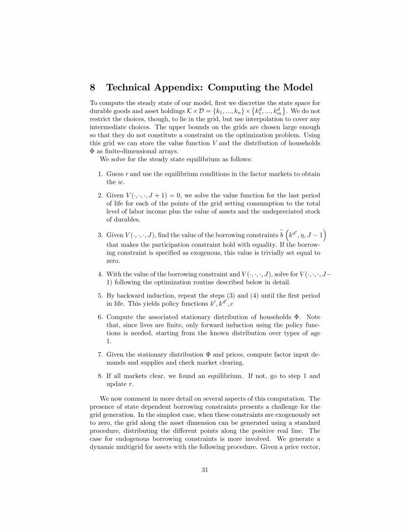
8 Technical Appendix: Computing the Model

To compute the steady state of our model, first we discretize the state space fordurable goods and asset holdings K×D = {k1, ..., kn}×

{kd1 , ..., k

dm

}. We do not

restrict the choices, though, to lie in the grid, but use interpolation to cover anyintermediate choices. The upper bounds on the grids are chosen large enoughso that they do not constitute a constraint on the optimization problem. Usingthis grid we can store the value function V and the distribution of householdsΦ as finite-dimensional arrays.We solve for the steady state equilibrium as follows:

1. Guess r and use the equilibrium conditions in the factor markets to obtainthe w.

2. Given V (·, ·, ·, J + 1) = 0, we solve the value function for the last periodof life for each of the points of the grid setting consumption to the totallevel of labor income plus the value of assets and the undepreciated stockof durables.

3. Given V (·, ·, ·, J), find the value of the borrowing constraints−b(kd

′, η, J − 1

)that makes the participation constraint hold with equality. If the borrow-ing constraint is specified as exogenous, this value is trivially set equal tozero.

4. With the value of the borrowing constraint and V (·, ·, ·, J), solve for V (·, ·, ·, J−1) following the optimization routine described below in detail.

5. By backward induction, repeat the steps (3) and (4) until the first periodin life. This yields policy functions k′, kd

′, c

6. Compute the associated stationary distribution of households Φ. Notethat, since lives are finite, only forward induction using the policy func-tions is needed, starting from the known distribution over types of age1.

7. Given the stationary distribution Φ and prices, compute factor input de-mands and supplies and check market clearing.

8. If all markets clear, we found an equilibrium. If not, go to step 1 andupdate r.

We now comment in more detail on several aspects of this computation. Thepresence of state dependent borrowing constraints presents a challenge for thegrid generation. In the simplest case, when these constraints are exogenously setto zero, the grid along the asset dimension can be generated using a standardprocedure, distributing the different points along the positive real line. Thecase for endogenous borrowing constraints is more involved. We generate adynamic multigrid for assets with the following procedure. Given a price vector,

31

we compute the “natural debt” limit implied by the discounted value of theremaining life cycle income at the worst possible realization of the shock. Withthese limits, we generate a different grid for each period of life, ranging fromthis lower limit to some arbitrary, age dependent, positive number29 . Since ingeneral these “natural debt”limits will be lower than the borrowing constraintlimit, the household may face the situation that, for a particular point of thegrid, no positive consumption is feasible. Because for negative consumption, theutility function is not defined, we address this issue numerically using a penaltycorrection in the utility function: negative consumption implies such a hugenegative utility that the household will never visit the areas of the multigridthat imply this negative consumption even after an arbitrary sequence of theworst possible realizations of the stochastic shock. The highest points in thegrid for all type of borrowing constraints were chosen in such a way that thestationary distribution Φ does not put mass in these points. The distributionof point in the grid is uniform.

Finding the level of the borrowing constraint−b at time j amounts to invert

the value function V (·, ·, η′, j + 1) along its first dimension. To do so, we solve

the root of the linear equation V(·, kd′ , η′, j + 1

)− V (0, 0, η′, j + 1) at each

point of the grid of durables and each possible point η′. Then, since we arelooking for the tightest of borrowing constraint values in the stochastic incomeprocess, we find the vector of maximum values in η′ for each possible choiceof durables stock. This vector contains the value of the borrowing constraint−b(kd

′, η, j + 1

)evaluated at each point in the durables grid, for each η and each

age.With this vector as an input, the optimization routine searches on the grid

of durables and performs a Quasi-Newton update30 on asset holdings condi-tional on each point of the durables grid except for values of the asset holdingclose to the borrowing constraints. For these values we substitute the Quasi-Newton with a variant of the bisection method. This change allows for a correcttreatment of the borrowing constraint in which the derivative of the objectivefunction is not zero. We computed the needed numerical derivatives using a for-ward scheme. To improve effi ciency, we tried a two dimensional Newton searchinstead of the combination of grid search and Quasi-Newton. This alternative,however, was not adopted because of numerical instability problems.Where needed, we use a simple linear or bilinear interpolation scheme. As

a robustness check, we also tried a cubic spline interpolation with a “not-a-

29The presence of durables makes the computation of this “natural debt”limit dependent onthe stock of durables. To avoid this problem we take the limit implied by the first point in thegrid of durables. This limit is strictly above the real “natural debt” limit for households withhigher quantities of durables and was chosen to avoid optimizing in highly negative points ofassets holdings. We check that in the optimization routine the borrowing constraint is alwaysequal or higher than the lower bound of the grid.30Our most important deviation from the standard Newton-Raphson is that we impose

relatively conservative bounds in the size of the update to avoid overshotings. These boundsproved more reliable than cooling down the algorithm because of the discontinuity in thecomputable objective function caused by the penalty correction.

32

knot” condition. Cubic splines match exactly the function values at the gridpoints with continuous first and second derivatives. The “not-a-knot” condi-tion requires that the third derivative of the spline be continuous in the lastn − 1 and n − 2 points of the grid. We found that this more sophisticated in-terpolation scheme implied outcomes that were virtually indistinguishable fromthe ones reported in the text and resulted in an important degradation of timeperformance.In order to simulate the stationary distribution Φ and life cycle profiles and

since we store only finite-dimensional arrays, an individual choice k′(k, kd, η, j

)is interpreted to choose asset holdings k1 and k2 with probabilities ν and 1− ν.These probabilities solve the linear equation k′

(k, kd, η, j

)= νk1 + (1− ν) k2.

A similar procedure is followed for the durable stock choice. We build averagelife-cycles with a simulation of a cross-section of individuals and check the lawof large numbers with the first two moments of the distribution.All the programs needed for the computation of the model were programed

in Fortran 95 and compiled in Compaq Visual Fortran 6.1 to run on WindowsPC. The computational materials are available upon request from the authors.

33

References

[1] Abowd, J.M. and D. Card (1989), “On the Covariance Structure of Earn-ings and Hours Changes”. Econometrica 57, 411-445.

[2] Aiyagari, R. (1994), “Uninsured Idiosyncratic Risk and Aggregate Saving”.Quarterly Journal of Economics 109, 659-684.

[3] Alessie, R., M. Devereux and G. Weber (1997), “Intertemporal Consump-tion, Durables and Liquidity Constraints: A Cohort Analysis”. EuropeanEconomic Review 41, 37-59.

[4] Alvarez, F. and U. Jermann (2000), “Effi ciency, Equilibrium and AssetPricing with Risk of Default”. Econometrica 68, 775-797.

[5] Attanasio, O. P. and M. Browning (1995), “Consumption over the LifeCycle and over the Business Cycle”. American Economic Review 85, 1118-1137.

[6] Attanasio, O.P., J. Banks, C. Meghir and G. Weber (1999), “Humps andBumps in Lifetime Consumption”. Journal of Business and Economics 17,22-35.

[7] Attanasio, O., P.K. Goldberg and E. Kyriazidou (2005), “Credit Con-straints in the Market for Consumer Durables; Evidence from Microdataon Car Loans”. Mimeo, UCL.

[8] Attanasio, O. and G. Weber (1995), “Is Consumption Growth Consistentwith Intertemporal Optimization? Evidence for the Consumer ExpenditureSurvey”. Journal of Political Economy 103, 1121-1157.

[9] Azariadis, C. and L. Lambertini (2003), “Endogenous Debt Constraints inLifecycle Economies”. Review of Economic Studies 70, 1-27.

[10] Bajari, P., P. Chan, D. Krueger and D. Miller (2008), “A Dynamic Modelof Housing Demand: Estimation and Policy Implications,”Working paper,University of Minnesota.

[11] Barrow, L. and L. McGranahan (2000), “The Effects of the Earned In-come Credit on the Seasonality of Household Expenditures”. National TaxJournal, 53, 1211-1244.

[12] Berkovec, J and D. Fullerton (1992), “A General Equilibrium Model ofHousing, Taxes and Portfolio Choice,”Journal of Political Economy, 100,390-429.

[13] Bewley, T. (1986), “Stationary Monetary Equilibrium with a Continuumof Independently Fluctuating Consumers”, in W. Hildenbrand and A. Mas-Colell (eds) Contributions to Mathematical Economics in Honor of GerardDebreu, North Holland.

34

[14] Blundell, R., M. Browning and C. Meghir (1994), “Consumer Demand andthe Life-Cycle Allocation of Household Expenditures”. Review of EconomicStudies 61, 57-80.

[15] Carroll, C. (1992), “The Buffer-Stock Theory of Saving: Some Macroeco-nomic Evidence”. Brookings Papers on Economic Activity, 23, 61-156.

[16] Carroll, C. (1997), “Buffer-Stuck Saving and the Life Cycle/PermanentIncome Hypothesis”. Quarterly Journal of Economics, 112, 1-55.

[17] Carroll, S. and W. Li (2008), “The Homeownership Experience of House-holds in Bankruptcy,”Working paper, Federal Reserve Bank of Philadelphia

[18] Chah, E., V. Ramey and R. Starr (1995), “Liquidity Constraints and In-tertemporal Consumer Optimization: Theory and Evidence from DurableGoods”. Journal of Money, Credit and Banking 27, 272-287.

[19] Chambers, M., C. Garriga and D. Schlagenhauf (2009a), “Accounting forChanges in the Homeownership Rate,”International Economic Review, 50,677-726.

[20] Chambers, M., C. Garriga and D. Schlagenhauf (2009b) “The Loan Struc-ture and Housing Tenure Decisions in an Equilibrium Model of MortgageChoice,”Review of Economic Dynamics, 12, 444-468.

[21] Cocco, J. (2005), “Portfolio Choice in the Presence of Housing,”Review ofFinancial Studies, 18, 535-567.

[22] Cocco, J., F. Gomes and P. Maenhout (2002): “Consumption and PortfolioChoice over the Life-Cycle,”forthcoming, Review of Financial Studies.

[23] Conesa, J.C. and D. Krueger (1999), “Social Security Reform with Hetero-geneous Agents”. Review of Economic Dynamics 2, 757-795.

[24] Deaton, A. (1985), ”Panel Data from Time Series of Cross-Sections”. Jour-nal of Econometrics 30, 109-126.

[25] Deaton, A. (1991), “Saving and Liquidity Constraints”. Econometrica, 59,1221-1248.

[26] Deaton, A. (1992), Understanding Consumption. Oxford University Press.

[27] Deaton. A. (1997), The Analysis of Households Surveys. John Hopkins Uni-versity.

[28] Diaz, A. and M. Luengo-Prado (2008), “On the User Cost and Homeown-ership,”Review of Economic Dynamics, 11, 584-613.

[29] Diaz, A. and M. Luengo-Prado (2009), “The Wealth Distribution withDurable Goods,”International Economic Review, forthcoming.

35

[30] Dynan, K. E., J. Skinner and S. Zeldes (2004), “Do the Rich Save More?”.Journal of Political Economy 112, 397-444.

[31] Eberly, J. (1994), “Adjustment of Consumers’Durables Stocks: Evidencefrom Automobile Purchases”. Journal of Political Economy 102, 403-436.

[32] Eichenbaum, M. and L.P. Hansen (1990), “Estimating Models with In-tertemporal Substitution Using Aggregate Time Series Data”. Journal ofBusiness and Economic Statistics 8, 53-69.

[33] Faber, J. F. (1982), “Life tables for the United States: 1900-2050”, Actu-arial Study No 87, U.S. Department of Health and Human Services.

[34] Feldman, M. and C. Gilles (1985), “An Expository Note on Individual Riskwithout Aggregate Uncertainty”. Journal of Economic Theory 35(1), 26-32.

[35] Fernández-Villaverde, J. and D. Krueger (2007), “Consumption over theLife Cycle: Facts from the Consumer Expenditure Survey,”Review of Eco-nomics and Statistics, 89, 552-565.

[36] Flavin, M. and T. Yamashita (2002), “Owner-Occupied Housing and theComposition of the Household Portfolio”. American Economic Review´ 92,345-362.

[37] Garriga, C. and D. Schlagenhauf (2009), “Home Equity, Foreclosures, andBailouts,”Working paper, Federal Reserve Bank of St. Louis.

[38] Gervais, M. (2002), “Housing Taxation and Capital Accumulation,”Jour-nal of Monetary Economics, 40, 1461-1489.

[39] Ghez, G.R. and G. Becker, (1975), The Allocation of Time and Goods overthe Life Cycle. Columbia University Press for the NBER.

[40] Gottschalk, P. and R. Moffi tt (1994). “The Growth of Earnings Instabilityin the U.S. Labor Market”. Brookings Papers on Economic Activity, 217-272.

[41] Gourinchas, P.O. and J. A. Parker (2002), “Consumption over the LifeCycle”. Econometrica, 70, 47-91.

[42] Greenwood, J., R. Rogerson and R. Wright (1995), “Household Productionin Real Business Cycle Theory”in T.F. Cooley (ed) Frontiers of BusinessCycle Research. Princeton University Press.

[43] Grossman, S. and G. Laroque (1990), “Asset Pricing and Optimal PortfolioChoice in the Presence of Illiquid Durable Consumption Goods”. Econo-metrica, 58, 25-51.

[44] Gruber, J. and R. Martin (2003) “Precautionary Savings and the WealthDistribution with Illiquid Durables,”International Finance Discussion Pa-pers 773, Board of Governors of the Federal Reserve System

36

[45] Hansen, G. D. (1993), “The Cyclical and Secular Behavior of the LaborInput: Comparing Effi ciency Units and Hours Worked”. Journal of AppliedEconometrics, 8, 71-80.

[46] Hintermaier, T. andW. Koeniger (2009), “Debt Portfolios,”Working paper,Queen Mary College.

[47] Huggett, M. (1993), “The Risk-Free Rate in Heterogeneous-AgentIncomplete-Insurance Economies”. Journal of Economic Dynamics andControl, 17, 953-969.

[48] Hurst, E. and F. Stafford (2004), “Home is where the Equity is: MortgageRefinancing and Household Consumption,”Journal of Money, Credit andBanking, 36, 985-1014.

[49] Iacoviello, M. and M. Pavan (2009), “Housing and Debt over the Life Cycleand over the Business Cycle,”Working paper, Boston College.

[50] Jeske, K and D. Krueger (2005), “Housing and the Macroeconomy: TheRole of Implicit Guarantees for Government Sponsored Enterprises,”Work-ing paper, Federal Reserve Bank of Atlanta.

[51] Kehoe, T. and D. Levine (1993), “Debt Constrained Asset Markets”. Re-view of Economic Studies, 60, 865-888.

[52] Kiyotaki, N., A. Michaelides, and K. Nikolov (2008), “Winners and Losersin the Housing Market,”Working paper, London School of Economics.

[53] Kocherlakota, N. (1996), “Implications of Effi cient Risk Sharing withoutCommitment”. Review of Economic Studies 63, 595-609.

[54] Krueger, D. and F. Perri (1999), “Risk Sharing: Private Insurance Mar-kets or Redistributive Taxes?”. Federal Reserve Bank of Minneapolis StaffReport 262.

[55] Krueger, D. and F. Perri (2005), “Does Income Inequality Lead to Con-sumption Inequality? Empirical Findings and a Theoretical Explanation,”forthcoming in Review of Economic Studies..

[56] Krusell, P. and A. Smith (1998), “Income and Wealth Heterogeneity in theMacroeconomy”. Journal of Political Economy 106, 867-96.

[57] Li, W., H. Liu and R. Yao (2009), “Housing over Time and over the LifeCycle: A Structural Estimation,”Working paper, Federal Reserve Bank ofPhiladelphia (2009)

[58] Li, W. and R. Yao (2007), “The Life-Cycle Effects of House Price Changes,”Journal of Money, Credit, and Banking, 39, 1375-1409

[59] Luengo-Prado, M. (2006), “Durables, Nondurables, Down Payments andConsumption Excesses,”Journal of Monetary Economics, 5

37

[60] Lustig, H. (2004), “The Market Price of Risk and the Wealth Distribution,”mimeo, UCLA.

[61] Martin R. (2003) “Consumption, Durable Goods, and Transaction Costs,”International Finance Discussion Papers 756, Board of Governors of theFederal Reserve System.

[62] Martin, R. and J. Gruber (2004) “Does Housing Wealth Make Us LessEqual? The Role of Durable Goods in the Distribution of Wealth,”Workingpaper, Federal Reserve Board.

[63] McGrattan, E. R. Rogerson and R. Wright (1997), “An Equilibrium Modelof Business Cycle with Household Production and Fiscal Policy”. Interna-tional Economic Review 38, 267-290.

[64] McGrattan, E. and E.C. Prescott (2001), “Is the Stock Market Overval-ued?”. NBER Working Paper 8077.

[65] Nakajima, M. (2005) “Rising Earnings Instability, Portfolio Choice andHousing Prices,”Working paper, Federal Reserve Bank of Philadelphia.

[66] Ogaki, M. and C.M. Reinhart (1998), “Measuring Intertemporal Substi-tution: The Role of Durable Goods”. Journal of Political Economy 106,1078-1098.

[67] Ortalo-Magne, F. and S. Rady (2006) “Housing Market Dynamics: Onthe Contribution of Income Shocks and Credit Constraints,” Review ofEconomic Studies, 78, 459-485.

[68] Platania, J. and D. Schlagenhauf (2000), “Housing and Asset Holding in aDynamic General Equilibrium Model,”mimeo.

[69] Rupert, P., R. Rogerson and Randall Wright (1995), “Estimating Substi-tution Elasticities in Household Production Models”. Economic Theory 6,179-193.

[70] Sanchez, J. (2007) “An Estimable Dynamic Model of Housing TenureChoice,”Working paper, Pontifica Universidad Catolica de Chile.

[71] Silos, P. (2007a), “Housing Tenure and Wealth Distribution in Life-CycleEconomies,”B.E. Journals in Macroeconomics, 7.

[72] Silos, P. (2007b), “Housing, Portfolio Choice and the Macroeconomy,”Journal of Economic Dynamics and Control, 31, 2774-2801

[73] Speckman, P. (1988), “Kernel Smoothing in Partial Linear Models”. Jour-nal of the Royal Statistical Society B 50, 413-436.

[74] Storesletten, K., C. Telmer and A. Yaron (2001), “Asset Pricing with Idio-syncratic Risk and Overlapping Generations”. Mimeo.

38

[75] Tauchen, G. and R. Hussey (1991), “Quadrature-Based Methods for Ob-taining Approximate Solutions to Nonlinear Asset Pricing Models”. Econo-metrica 59, 371-396.

[76] Tracy, J., H. Schneider and S. Chan (1999), “Are Stocks Overtaking RealEstate in Household Portfolios?”. Current Issues in Economics and Fi-nance, Federal Reserve Bank of New York, 5(5).

[77] Yang, F. (2009), “Consumption over the Life Cycle: How Different is Hous-ing?,”Review of Economic Dynamics, 12, 423-443.

[78] Yao, R. and H. Zhang (2005) “Optimal Consumption and Portfolio Choiceswith risky Housing and Borrowing Constraints,”Review of Financial Stud-ies, 18, 197-239.

[79] Zeldes, S. (1989), “Consumption and Liquidity Constraints: An EmpiricalInvestigation”. Journal of Political Economy 97, 305-346.3, 1509-1539.

39

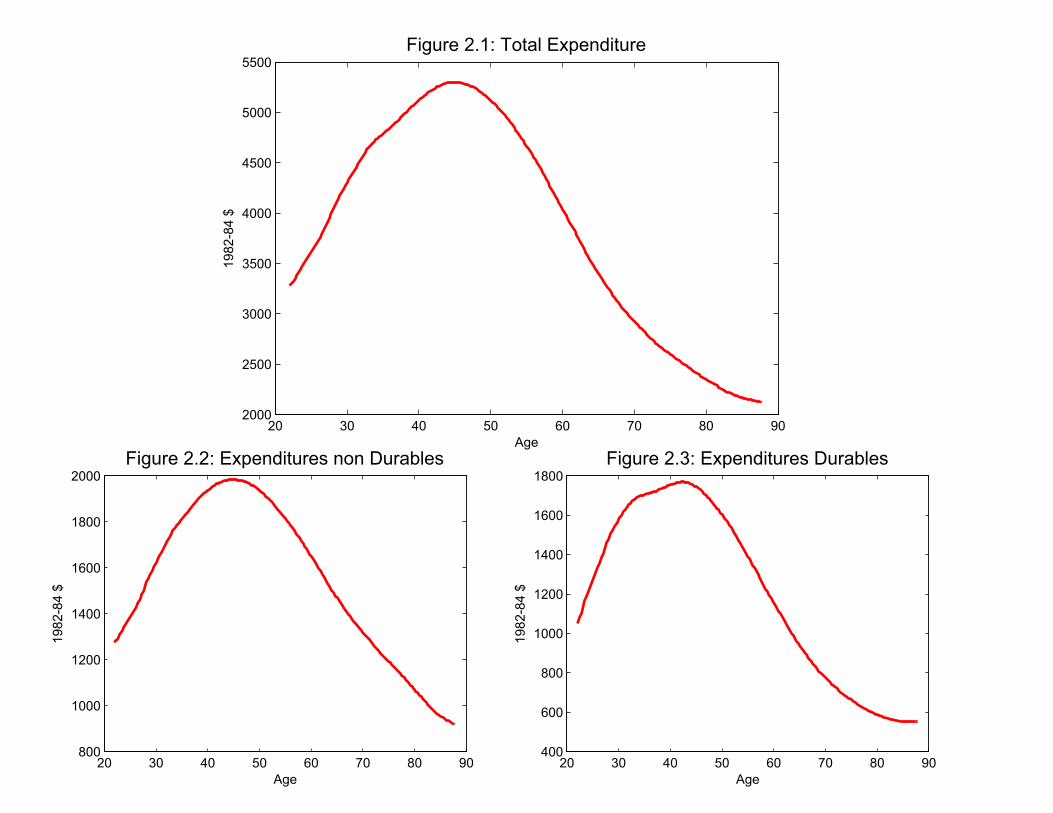
20 30 40 50 60 70 80 902000

2500

3000

3500

4000

4500

5000

5500Figure 2.1: Total Expenditure

Age

1982

-84

$

20 30 40 50 60 70 80 90800

1000

1200

1400

1600

1800

2000Figure 2.2: Expenditures non Durables

Age

1982

-84

$

20 30 40 50 60 70 80 90400

600

800

1000

1200

1400

1600

1800Figure 2.3: Expenditures Durables

Age

1982

-84

$

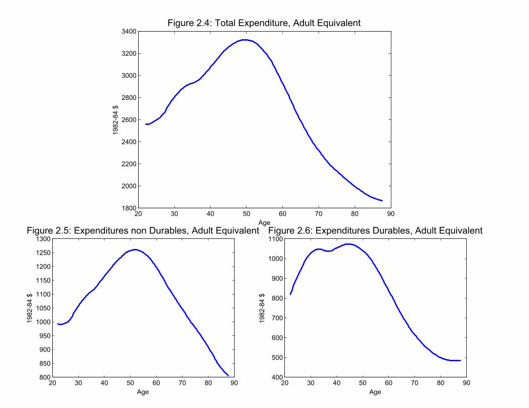
20 30 40 50 60 70 80 901800

2000

2200

2400

2600

2800

3000

3200

3400Figure 2.4: Total Expenditure, Adult Equivalent

Age

1982

-84

$

20 30 40 50 60 70 80 90800

850

900

950

1000

1050

1100

1150

1200

1250

1300Figure 2.5: Expenditures non Durables, Adult Equivalent

Age

1982

-84

$

20 30 40 50 60 70 80 90400

500

600

700

800

900

1000

1100Figure 2.6: Expenditures Durables, Adult Equivalent

Age

1982

-84

$

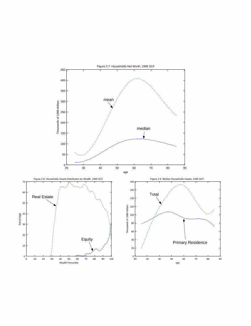
20 30 40 50 60 70 80 900

50

100

150

200

250

300

350

400

450Figure 2.7: Households Net Worth, 1995 SCF

age

Tho

usan

ds o

f 199

8 do

llars

20 30 40 50 60 70 80 900

20

40

60

80

100

120

140

160

180Figure 2.9: Median Households Assets, 1995 SCF

age

Tho

usan

ds o

f 199

8 do

llars

0 10 20 30 40 50 60 70 80 90 1000

10

20

30

40

50

60

70Figure 2.8: Households Assets Distribution by Wealth, 1995 SCF

Wealth Percentile

Per

cent

age

mean

median

Real Estate

Equity Primary Residence

Total

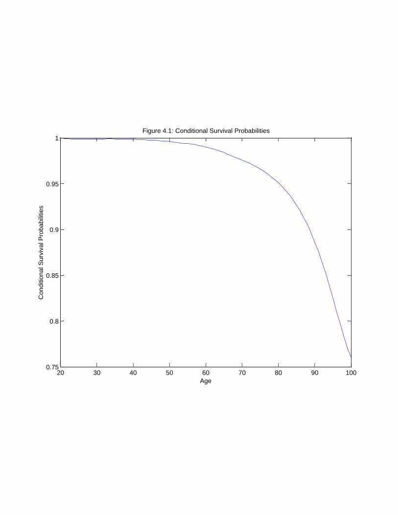
20 30 40 50 60 70 80 90 1000.75

0.8

0.85

0.9

0.95

1Figure 4.1: Conditional Survival Probabilities

Age

Con

ditio

nal S

urvi

val P

roba

bilit

ies

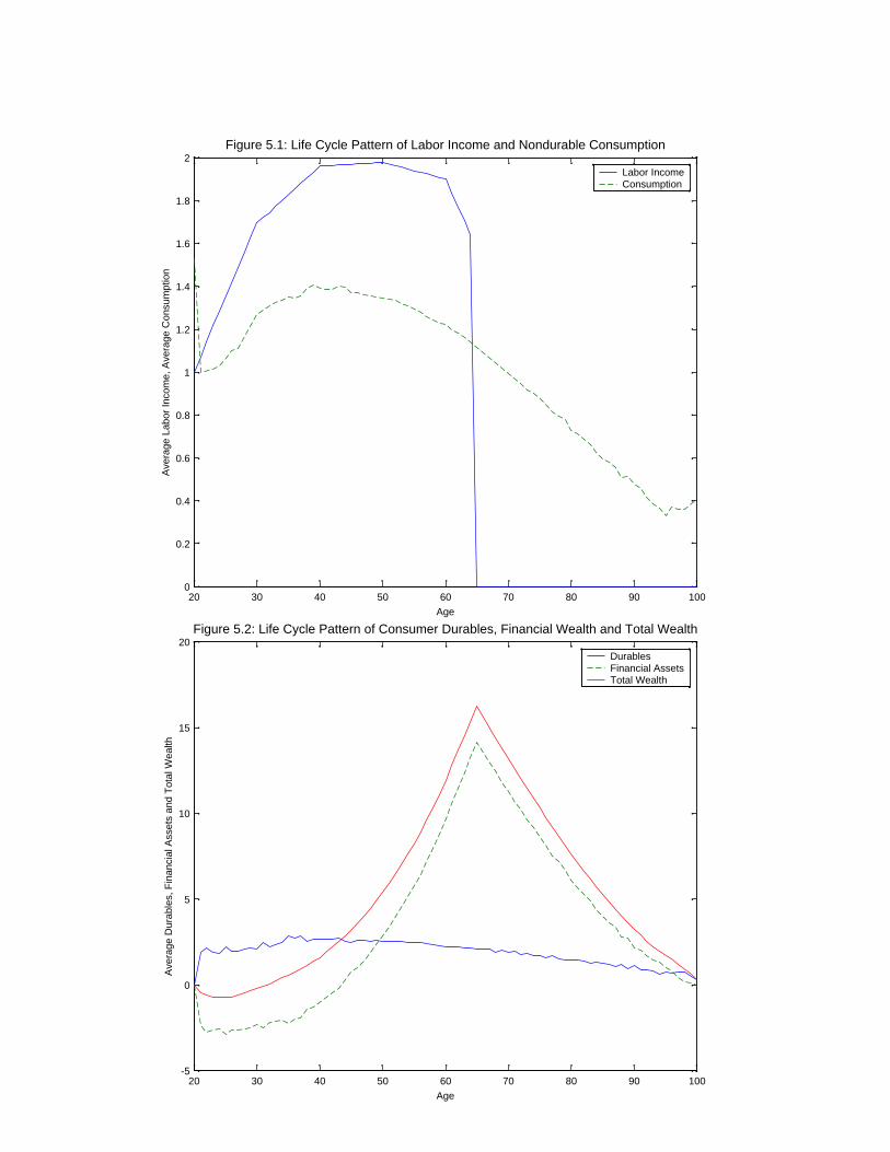
20 30 40 50 60 70 80 90 1000

0.2

0.4

0.6

0.8

1

1.2

1.4

1.6

1.8

2

Age

Ave

rage

Lab

or In

com

e, A

vera

ge C

onsu

mpt

ion

Figure 5.1: Life Cycle Pattern of Labor Income and Nondurable Consumption

Labor IncomeConsumption

20 30 40 50 60 70 80 90 100-5

0

5

10

15

20

Age

Ave

rage

Dur

able

s, F

inan

cial

Ass

ets

and

Tot

al W

ealth

Figure 5.2: Life Cycle Pattern of Consumer Durables, Financial Wealth and Total Wealth

Durables Financial AssetsTotal Wealth

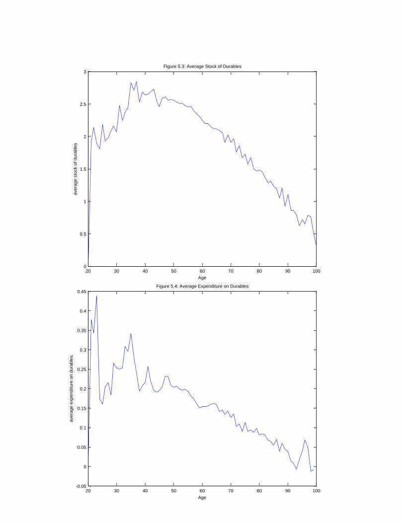
20 30 40 50 60 70 80 90 1000

0.5

1

1.5

2

2.5

3Figure 5.3: Average Stock of Durables

Age

aver

age

stoc

k of

dur

able

s

20 30 40 50 60 70 80 90 100-0.05

0

0.05

0.1

0.15

0.2

0.25

0.3

0.35

0.4

0.45Figure 5.4: Average Expenditure on Durables

Age

aver

age

expe

nditu

re o

n du

rabl

es

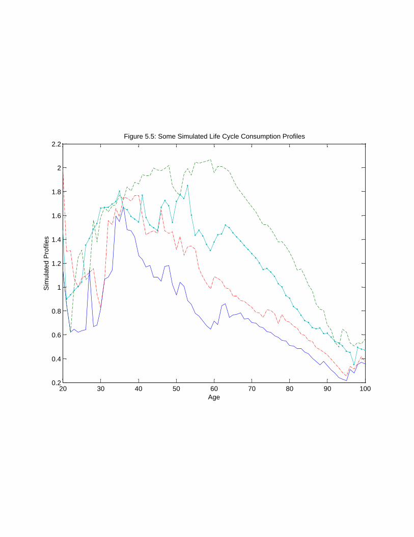
20 30 40 50 60 70 80 90 1000.2

0.4

0.6

0.8

1

1.2

1.4

1.6

1.8

2

2.2Figure 5.5: Some Simulated Life Cycle Consumption Profiles

Age

Sim

ulat

ed P

rofil

es

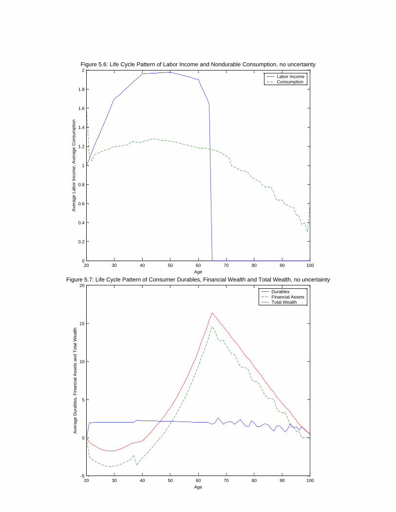
20 30 40 50 60 70 80 90 1000

0.2

0.4

0.6

0.8

1

1.2

1.4

1.6

1.8

2

Age

Ave

rage

Lab

or In

com

e, A

vera

ge C

onsu

mpt

ion

Figure 5.6: Life Cycle Pattern of Labor Income and Nondurable Consumption, no uncertainty

Labor IncomeConsumption

20 30 40 50 60 70 80 90 100-5

0

5

10

15

20

Age

Ave

rage

Dur

able

s, F

inan

cial

Ass

ets

and

Tot

al W

ealth

Figure 5.7: Life Cycle Pattern of Consumer Durables, Financial Wealth and Total Wealth, no uncertainty

Durables Financial AssetsTotal Wealth

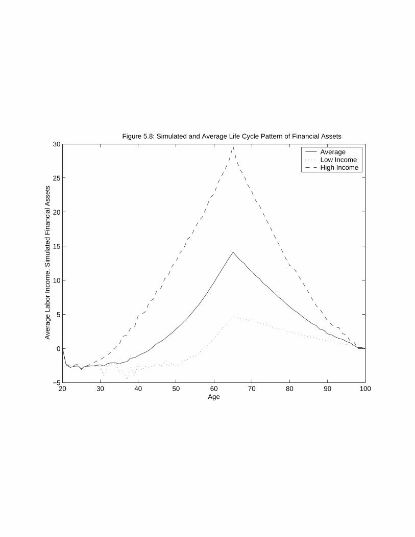
20 30 40 50 60 70 80 90 100−5

0

5

10

15

20

25

30Figure 5.8: Simulated and Average Life Cycle Pattern of Financial Assets

Age

Ave

rage

Lab

or In

com

e, S

imul

ated

Fin

anci

al A

sset

s

Average Low Income High Income

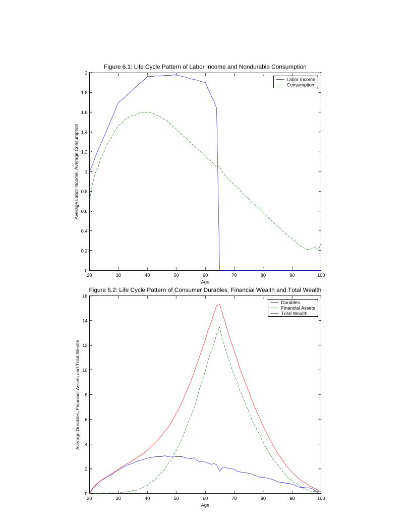
20 30 40 50 60 70 80 90 1000

0.2

0.4

0.6

0.8

1

1.2

1.4

1.6

1.8

2

Age

Ave

rage

Lab

or In

com

e, A

vera

ge C

onsu

mpt

ion

Figure 6.1: Life Cycle Pattern of Labor Income and Nondurable Consumption

Labor IncomeConsumption

20 30 40 50 60 70 80 90 1000

2

4

6

8

10

12

14

16

Age

Ave

rage

Dur

able

s, F

inan

cial

Ass

ets

and

Tot

al W

ealth

Figure 6.2: Life Cycle Pattern of Consumer Durables, Financial Wealth and Total Wealth

Durables Financial AssetsTotal Wealth

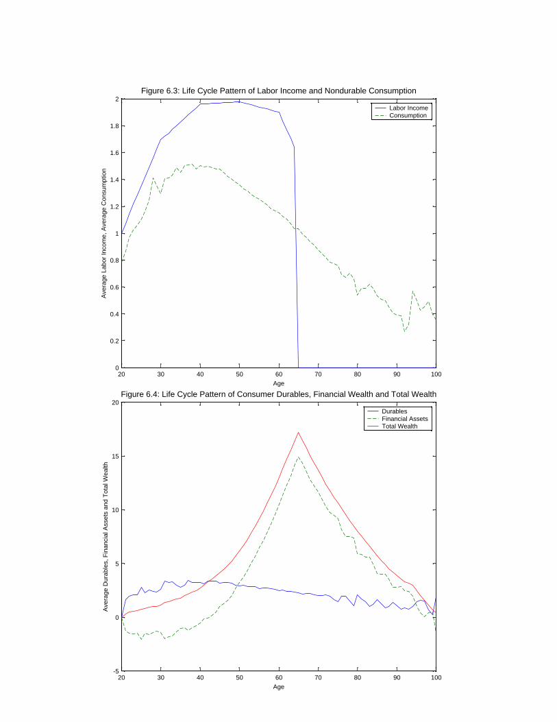
20 30 40 50 60 70 80 90 1000

0.2

0.4

0.6

0.8

1

1.2

1.4

1.6

1.8

2

Age

Ave

rage

Lab

or In

com

e, A

vera

ge C

onsu

mpt

ion

Figure 6.3: Life Cycle Pattern of Labor Income and Nondurable Consumption

Labor IncomeConsumption

20 30 40 50 60 70 80 90 100-5

0

5

10

15

20

Age

Ave

rage

Dur

able

s, F

inan

cial

Ass

ets

and

Tot

al W

ealth

Figure 6.4: Life Cycle Pattern of Consumer Durables, Financial Wealth and Total Wealth

Durables Financial AssetsTotal Wealth