Virtual Indicative Broadband over Power Lines Topologies

Trends in Renewable Energy OPEN ACCESS ISSN: 2376-2144

Peer-Reviewed Article futureenergysp.com/index.php/tre

*Corresponding author: [email protected] 258

Tr Ren Energy, 2019, Vol.5, No.3, 258-281. doi: 10.17737/tre.2019.5.3.00100

Virtual Indicative Broadband over Power Lines Topologies for Respective Subclasses by Adjusting Channel Attenuation Statistical Distribution Parameters of Statistical Hybrid Models (Class Maps) – Part 2: Numerical Results for the Overhead and Underground Medium-Voltage Power Grids

Athanasios G. Lazaropoulos*

School of Electrical and Computer Engineering / National Technical University of Athens /

9 Iroon Polytechniou Street / Zografou, GR 15780

Received June 21, 2019; Accepted August 12, 2019; Published August 16, 2019

With reference to the initial statistical hybrid model (iSHM) and modified statistical hybrid model (mSHM), the theory of the definition procedure of new virtual indicative distribution BPL topologies by appropriately adjusting the channel attenuation statistical distributions (CASDs) parameters of iSHM and mSHM has been presented in [1]. In this paper, the results of the definition procedure for the OV and UN MV BPL networks are first presented through the prism of the proposed class maps of iSHM and mSHM.

Keywords: Smart Grid; Broadband over Power Lines (BPL) networks; Power Line Communications

(PLC); Distribution Power Grids; Capacity; Statistics; Modeling

1. Introduction

This set of papers deals with two fervent issues of the broadband over power lines

(BPL) statistical channel modelling, say: (i) the underrepresentation of the BPL topology

classes during the BPL statistical channel modelling through the insertion of

virtual indicative BPL topologies and their respective subclasses; and

(ii) the graphical representation of the BPL topology classes and subclasses in terms of

their average capacity through the proposed class maps of the first paper [1].

First, as the BPL statistical channel modelling is concerned, two versions of the hybrid

statistical model have already been proposed, say the initial statistical hybrid model

(iSHM), which has been presented in [2], [3], and the modified statistical hybrid model

(mSHM), which has been presented in [4]. The basic component of both hybrid statistical

models is the deterministic hybrid model that has exhaustively been validated in a

plethora of transmission and distribution BPL network cases [5]-[15]. Apart from the

deterministic hybrid model, iSHM applies five well-known channel attenuation statistical

distribution (CASDs) of the communications literature, say, Gaussian, Lognormal, Wald,

Weibull and Gumbel ones [2], [3], while mSHM applies the Empirical CASD [4] so that

BPL topology classes –i.e., rural, suburban, urban and aggravated urban subclass– and

CORE Metadata, citation and similar papers at core.ac.uk

Provided by Trends in Renewable Energy

https://core.ac.uk/display/300330399?utm_source=pdf&utm_medium=banner&utm_campaign=pdf-decoration-v1

Peer-Reviewed Article Trends in Renewable Energy, 5

Tr Ren Energy, 2019, Vol.5, No.3, 258-281. doi: 10.17737/tre.2019.5.3.00100 259

respective subclasses can be defined. Second, as the underrepresentation of the

BPL topology classes is concerned, by appropriately adjusting the CASD parameters of

iSHM and mSHM –i.e., CASD maximum likelihood estimators (MLEs) and Empirical

cumulative density function (CDF) for iSHM and mSHM, respectively–, new virtual

indicative distribution BPL topologies can be proposed that are added to the existing real

ones and further define their respective distribution BPL topology subclasses enriched

with corresponding statistically equivalent BPL topologies. In [1], the theoretical

framework for the definition procedure of the virtual indicative BPL topologies and their

respective virtual subclasses, briefly denoted as definition procedure hereafter, has been

detailed. Third, as the graphical capacity representation of the real and virtual subclasses

is concerned, the main output of the definition procedure of [1] is the class map, which is

a 2D contour plot for given power grid type, coupling scheme, injected power spectral

density (IPSD) limits and noise levels, that is the graphical synthesis of the CASD

parameter and subclass map; say, real and virtual distribution BPL subclasses are

graphically categorized into suitable BPL topology class areas in terms of their

corresponding average capacities where the axes of the contour plot are proper

adjustments of CASD parameters of iSHM and mSHM. The numerical results of the full

deployment of class mapping are first presented in this paper for overhead medium

voltage (OV MV) and underground medium voltage (UN MV) BPL networks while the

BPL statistical channel modelling concept along with the class map is first applied to OV

high-voltage (HV) BPL networks in [16].

The rest of this paper is organized as follows: Section II synopsizes the default

settings that are required for the fine operation of the deterministic hybrid model, iSHM,

mSHM and the definition procedure. In Section III, the numerical results of the definition

procedure of iSHM and mSHM are demonstrated on the basis of the class maps of the

OV MV and UN MV BPL networks. Section IV concludes this paper.

2. The Operation Settings of Class Mapping

To coexist the deterministic hybrid model, iSHM and mSHM with the definition

procedure, a set of operation settings, which have already been reported in [2]-[4], should

be assumed. In this Section, a synopsis of these assumptions is given as well as the set of

scenarios that is studied in this paper.

2.1 Operation Settings Concerning the Operation of the Deterministic Hybrid Model With reference to Fig. 1 of [1], the five indicative OV MV and UN MV BPL

topologies, which are reported in Tables 1 and 2 of [1], respectively, are considered as the

representative ones of the respective main OV MV and UN MV BPL topology

subclasses. Note that with reference to [5], [8], [10], [17], the indicative OV MV and UN

MV BPL topologies concern average long end-to-end connections of 1000m and 200m,

respectively.

As the the circuital parameters of the above indicative OV MV and UN MV BPL

topologies are concerned for the operation of the deterministic hybrid model, these are

detailed in [5], [7]-[15], [18]-[33]. Synoptically, the required assumptions can be



synopsized as follows: (i) the branching cables are assumed identical to the distribution

cables; (ii) the interconnections between the distribution and branch conductors are fully

activated; say all the phase and the neutral conductors of the branching cables are

connected to the respective ones of the distribution cables; (iii) the transmitting and the

receiving ends are assumed matched to the characteristic impedance of the modal

channels; and (iv) the branch terminations are assumed open circuit since MV/LV

transformers are assumed to be installed.

2.2 iSHM Operation Settings

Already been identified in [3], the distribution power grid type,

the BPL topology class, CASD, electromagnetic interference (EMI) policy, noise level

and applied coupling scheme are factors that should be carefully selected during the

operation of the deterministic hybrid model and iSHM. Hence, additional details should

be given for iSHM operation settings as reported in this subsection.

First, the BPL operation frequency range and the flat-fading subchannel

frequency spacing are assumed to be equal to 3-30 MHz and 0.1 MHz (i.e, 0.1 MHz),

respectively. Hence, there are 270 subchannels in the frequency range of interest

(i.e., 270). In accordance with [8], [10], [11], [19], [21], [34], the assumption of the

flat-fading subchannels, which is a typical scenario, remains a crucial element towards

the capacity computation of the examined distribution BPL topologies, that is anyway the

output measure of iSHM.

Second, to compute coupling scheme channel attenuations of the distribution BPL

topologies, CS2 module, which has been detailed in [35], [36], is applied as the default

coupling scheme system of the deterministic hybrid model. Among the available coupling

schemes that are supported by CS2 module, WtG1 and StP1 coupling schemes are

assumed to be the default ones for the assessment of OV MV and UN MV BPL topology

subclasses, respectively, so that a direct comparison between the results of this paper and

those of [3] and [4], can be achieved.

Third, during the computation of the coupling scheme channel attenuation

differences in the Phase B of [2], values that are greater or equal to zero are expected in

the vast majority of the cases. However, in the scarce cases of negative coupling scheme

channel attenuation differences and in “LOS” cases, the coupling scheme channel

attenuation differences are assumed to be equal to an arbitrarily low value, say 1×10-11.

This assumption is made in order to prevent the presence of infinite terms due to the

natural logarithms and denominators of Lognormal, Wald and Weibull channel

attenuation distributions in iSHM.

Fourth, as the members of each BPL topology subclass are concerned in Phase D,

100 member distribution BPL topologies (i.e., P=100) are assumed to be added in each

BPL topology subclass per CASD through the statistical hybrid model procedure

described in [2].

Fifth, during the capacity computations of iSHM, FCC Part 15 is considered as

the default IPSD limit proposal concerning EMI policies for BPL systems in this paper.

Among the available EMI policies, which are FCC Part 15, German Reg TP NB30 and

the BBC / NATO Proposal and their impact on the performance of hybrid statistical

models has already been studied in [3], [4], FCC Part 15 is assumed to be the default EMI

policy in this paper due to its proneness to the broadband character of BPL networks and



its high performance results of statistical hybrid models. In the frequency range 3-30

MHz of this paper, -60 dBm/Hz and -40 dBm/Hz are the FCC Part 15 IPSD limits

suitable for the operation of OV MV and UN MV BPL topologies, respectively [8],

[10], [37].

Sixth, during the capacity computations, uniform additive white Gaussian noise

(AWGN) PSD levels are assumed in accordance with the FL noise model of [38], [39].

As it regards the noise properties of OV MV and UN MV BPL networks in the 3-30MHz

frequency range [8], [10], [19], [34], [40], -105dBm/Hz and -135dBm/Hz are the

appropriate AWGN PSD limit levels for OV MV and UN MV BPL networks,

respectively.

Seventh, in accordance with [3], [4], the performance of iSHM and the accuracy

of its capacity results significantly depend on the selection of the CASD. Based on the

findings of Table 3 of [3], it has been demonstrated for the iSHM that Weibull and Wald

CASDs perform the best capacity estimations in OV MV and UN MV power grid types,

respectively, regardless of the examined BPL topology subclass when the aforementioned

operation settings concerning EMI policy, noise level and applied coupling scheme are

assumed. These two CASDs are going to be only adopted by the following definition

procedure and during the iSHM study in this paper.

2.3 mSHM Operation Settings

Similarly to iSHM, the distribution power grid type, the BPL topology class,

the reference indicative distribution BPL topology, EMI policy, noise level and applied

coupling scheme are factors that are involved during the operation of the deterministic

hybrid model and mSHM [4]. In contrast with iSHM operation settings, only one CASD,

say, the Empirical CASD, is adopted by mSHM by default and, hence, CASD selection is

not considered among the mSHM operation settings.

As the BPL operation frequency range, flat-fading subchannel spacing,

coupling scheme system, the member number of each BPL topology subclass,

EMI policy and noise level are considered, their properties described in Sec. 2.2 for

iSHM are assumed to be the same with the ones of mSHM. For comparison reasons

between iSHM and mSHM and in accordance with [2], [3], [4], the infinity prevention

assumption remains for the mSHM.

In general, each indicative distribution BPL topology is characterized by a set of

parameters regarding either iSHM (i.e., MLEs) or mSHM (i.e., Empirical CDF).

As already been mentioned in Sec.2.2 for iSHM, Weibull and Wald CASD MLEs

perform the best capacity estimations in OV MV and UN MV power grid types,

respectively, and these MLEs are going to be adopted for the rest of this paper.

As mSHM CASD parameters are concerned, the Empirical CDF of a reference

distribution BPL topology among the indicative distribution BPL topologies of the main

subclasses acts as the mSHM CASD parameter that is going to be delivered to the

following definition procedure.

2.4 Operation Settings for the Definition Procedure

In accordance with [1], the BPMN diagrams of iSHM and mSHM flowchart are

presented in Figs. 2(a) and 2(b) of [1], respectively. With reference to the aforementioned

figures, the additional BPMN elements (i.e., the virtual topology modules and their



corresponding outputs), which will allow the application of the definition procedure, are

shown in red color. Apart from the BPMN diagrams, the interaction of the virtual

topology modules with the remaining iSHM and mSHM steps is depicted through the

flowcharts of Figs. 3(a) and 3(b) of [1], respectively. By comparing Figs. 3(a) and 3(b) of

[1], several differences concerning these flowcharts can be observed, especially:

(i) between steps FL1.04 and FL2.04; and (ii) between steps FL1.05 and FL2.05.

Due to the previous differences, the operation settings concerning the definition

procedure can be divided into two groups, namely:

1. iSHM definition procedure: With reference to [2], [3], since Weibull CASD

performs the best capacity estimations in OV MV BPL networks, and

are Weibull CASD MLEs that are used in FL1.04 of Fig. 3(a) of [1].

When UN MV BPL topologies are studied, and are the Wald CASD

MLEs that are used in FL1.04 of Fig. 3(a) of [1]. In accordance with FL1.04 of

Fig. 3(a) of [1], MLEs of the indicative distribution BPL topologies of main

subclasses are computed. To compute the MLE spacings per distribution power

grid type in FL1.05 of Fig. 3(a) of [1], and , which are the number of

spacings for the horizontal and vertical axis, respectively, should be assumed.

In this paper, the number of spacings for the horizontal and vertical axis is

assumed to be equal to 10 in both cases regardless of the distribution power grid

type while this selection is going to be proven critical for the simulation time of

class mapping (see Sec.3.5).

2. mSHM definition procedure: In contrast with iSHM definition procedure, there is

only one CASD that is used across the mSHM definition procedure, say Empirical

CASD, but Empirical CASD is characterized by its CDF and not by

corresponding MLEs [4]. In accordance with FL2.04 of Fig. 3(b) of [1],

Empirical CDFs of the indicative distribution BPL topologies of main subclasses

are computed. Conversely to iSHM, mSHM definition procedure demands the

assumption of a reference indicative distribution BPL topology among the

indicative ones so that suitable horizontal and vertical shifts can be added and the

class map can be plotted. To compute the horizontal and vertical shift spacings in

FL2.05 of Fig. 3(b) of [1] given the reference indicative distribution BPL

topology, and , which are the number of spacings for the horizontal and

vertical axis, respectively, should be assumed. In this paper, the number of

spacings for the horizontal and vertical axis is assumed to be equal to 10 in both

cases regardless of the distribution power grid type examined. At this step of the

definition procedure, same number of horizontal and vertical spacings is

considered between iSHM and mSHM definition procedures for duration

comparison reasons. Note that the maximum and minimum horizontal shift is

assumed to be equal to 30 dB and -30 dB, respectively, while the maximum and

minimum vertical shift is assumed to be equal to 1 and 0, respectively.

Since all the required assumptions concerning the operation settings of iSHM,

mSHM and definition procedure have been reported in this Section, the numerical results

of iSHM and mSHM definition procedure are presented in the following Section for the

OV MV and UN MV BPL topologies as well as the class maps.



3. Numerical Results and Discussion

In this Section, numerical results concerning the definition procedure of iSHM

and mSHM are presented. Taking into account the already identified default operation

settings of Secs.2.1-2.4, four different scenarios concerning the class mapping are

presented, namely: (i) iSHM definition procedure for OV MV BPL topologies;

(ii) iSHM definition procedure for UN MV BPL topologies;

(iii) mSHM definition procedure for OV MV BPL topologies; and

(iv) mSHM definition procedure for UN MV BPL topologies. This Section ends with

observations concerning the simulation time of the aforementioned four scenarios.

3.1 iSHM Definition Procedure for OV MV BPL topologies

With reference to Table 3 of [3], Weibull CASD achieves the best capacity

estimations in OV MV BPL topologies with average absolute percentage change that is

equal to 0.47% and remains the smallest one among the five examined CASDs.

For the five indicative OV MV BPL topologies of the main subclasses of Table 1 of [1],

the respective and , which are the Weibull CASD MLEs, are reported in

Table 1 of [3] while the respective capacities are given in Table 3 of [3]. On the basis of

the Weibull CASD MLEs and capacities of the five indicative OV MV BPL topologies of

the main subclasses of Table 1 of [1], the spacings for the horizontal and vertical axis, as

dictated by FL1.05 of Fig. 3(a) of [1], are equal to and

, respectively, while the capacity borders between the adjacent distribution

BPL topology classes , as dictated by FL1.03 of

Fig. 3(a) of [1], are equal to 245Mbps, 289Mbps, 332Mbps and 379Mbps, respectively.

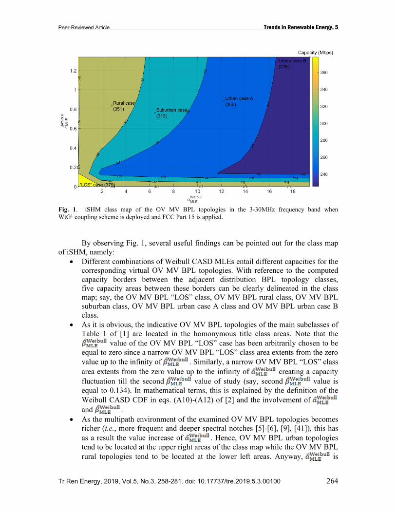
Summarizing the aforementioned analysis, the class map of OV MV BPL topologies is

plotted in Fig. 1 with respect to and when the operation settings of

Sec.2 are assumed. In the same 2D contour plot, the Weibull CASD MLEs of the five

indicative OV MV BPL topologies of the main subclasses of Table 1 of [1] with the

corresponding capacities are also shown.



Fig. 1. iSHM class map of the OV MV BPL topologies in the 3-30MHz frequency band when

WtG1 coupling scheme is deployed and FCC Part 15 is applied.

By observing Fig. 1, several useful findings can be pointed out for the class map

of iSHM, namely:

• Different combinations of Weibull CASD MLEs entail different capacities for the

corresponding virtual OV MV BPL topologies. With reference to the computed

capacity borders between the adjacent distribution BPL topology classes,

five capacity areas between these borders can be clearly delineated in the class

map; say, the OV MV BPL “LOS” class, OV MV BPL rural class, OV MV BPL

suburban class, OV MV BPL urban case A class and OV MV BPL urban case B

class.

• As it is obvious, the indicative OV MV BPL topologies of the main subclasses of

Table 1 of [1] are located in the homonymous title class areas. Note that the

value of the OV MV BPL “LOS” case has been arbitrarily chosen to be

equal to zero since a narrow OV MV BPL “LOS” class area extents from the zero

value up to the infinity of . Similarly, a narrow OV MV BPL “LOS” class

area extents from the zero value up to the infinity of creating a capacity

fluctuation till the second value of study (say, second value is

equal to 0.134). In mathematical terms, this is explained by the definition of the

Weibull CASD CDF in eqs. (A10)-(A12) of [2] and the involvement of

and .

• As the multipath environment of the examined OV MV BPL topologies becomes

richer (i.e., more frequent and deeper spectral notches [5]-[6], [9], [41]), this has

as a result the value increase of . Hence, OV MV BPL urban topologies

tend to be located at the upper right areas of the class map while the OV MV BPL

rural topologies tend to be located at the lower left areas. Anyway, is



more sensitive to the multipath environment aggravation in contrast with

that remains relatively insensitive. The last remark is validated by the fact that

indicative OV MV BPL rural, OV MV BPL suburban and OV MV BPL urban

case A topologies of Table 1 of [1] are characterized by approximately equal

values of .

• Note that for given , the capacity of the virtual OV MV BPL topologies

increases with respect to the . This is explained by studying Fig. (2) of

[4], eq. (A10) of [2] and the behavior of Weibull CASD CDF; since

receives values that are significantly greater than 1 for the practical cases of

interest, the term of eq. (10) of [2] can be considered to be greater than 1 in

the majority of the cases examined in Fig. (2) of [4] where is the coupling

scheme channel attenuation difference between the examined OV MV BPL

topology and its respective “LOS” case at q flat-fading subchannel.

As increases, increases from -1 to infinity and, thus,

starts from and fast tends to 1.

The last observation has as a result the improvement of the capacities of the

virtual OV MV BPL topologies that are characterized by greater values

for given . Anyway, the capacity improvement is more evident for the

cases of low because the term remains significantly greater than 1

and this explains the appearance of the class area edges at the bottom of the class

map and the steep and almost vertical class area borders for greater than

1.2.

3.2 iSHM Definition Procedure for UN MV BPL topologies

With reference to Table 3 of [3], Wald CASD achieves the best capacity

estimations in UN MV BPL topologies with average absolute percentage change that is

equal to 0.01% and remains the smallest one among the five examined CASDs. For the

five indicative UN MV BPL topologies of the main subclasses of Table 2 of [1],

the respective and , which are the Wald CASD MLEs, are reported in

Table 1 of [3] while the respective capacities are given in Table 3 of [3].

By observing the extent of values of Table 2 of [1], which ranges from 20.93 to

2.62×103, and taking under consideration the number of spacings that is equal to 10, the

proper selection for the vertical axis is the representation of and the

corresponding vertical spacings. Therefore, on the basis of the Wald CASD MLEs and

capacities of the five indicative OV MV BPL topologies of the main subclasses of Table

2 of [1], the spacings for the horizontal and vertical axis, as dictated by FL1.05 of Fig.

3(a) of [1], are equal to and , respectively,

while the capacity borders between the adjacent distribution BPL topology classes

, as dictated by FL1.03 of Fig. 3(a) of [1], are equal to 561Mbps,

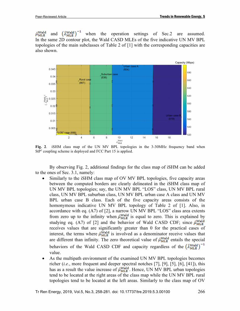
619Mbps, 651Mbps and 699Mbps, respectively. Summarizing the aforementioned

analysis, the class map of UN MV BPL topologies is plotted in Fig. 2 with respect to



and when the operation settings of Sec.2 are assumed.

In the same 2D contour plot, the Wald CASD MLEs of the five indicative UN MV BPL

topologies of the main subclasses of Table 2 of [1] with the corresponding capacities are

also shown.

Fig. 2. iSHM class map of the UN MV BPL topologies in the 3-30MHz frequency band when

StP1 coupling scheme is deployed and FCC Part 15 is applied.

By observing Fig. 2, additional findings for the class map of iSHM can be added

to the ones of Sec. 3.1, namely:

• Similarly to the iSHM class map of OV MV BPL topologies, five capacity areas

between the computed borders are clearly delineated in the iSHM class map of

UN MV BPL topologies; say, the UN MV BPL “LOS” class, UN MV BPL rural

class, UN MV BPL suburban class, UN MV BPL urban case A class and UN MV

BPL urban case B class. Each of the five capacity areas consists of the

homonymous indicative UN MV BPL topology of Table 2 of [1]. Also, in

accordance with eq. (A7) of [2], a narrow UN MV BPL “LOS” class area extents

from zero up to the infinity when is equal to zero. This is explained by

studying eq. (A7) of [2] and the behavior of Wald CASD CDF; since

receives values that are significantly greater than 0 for the practical cases of

interest, the terms where is involved as a denominator receive values that

are different than infinity. The zero theoretical value of entails the special

behaviors of the Wald CASD CDF and capacity regardless of the

value.

• As the multipath environment of the examined UN MV BPL topologies becomes

richer (i.e., more frequent and deeper spectral notches [7], [9], [5], [6], [41]), this

has as a result the value increase of . Hence, UN MV BPL urban topologies

tend to be located at the right areas of the class map while the UN MV BPL rural

topologies tend to be located at the left areas. Similarly to the class map of OV



MV BPL topologies, behaves similarly to (i.e., CASD MLEs that

are sensitive to the multipath environment aggravation) while behaves

similarly to (i.e., CASD MLEs that do not depend on the multipath

environment aggravation). Conversely to iSHM class map of OV MV BPL

topologies, iSHM class map of UN MV BPL topologies does not comprise class

area edges of the extent demonstrated in OV MV BPL topologies.

3.3 mSHM Definition Procedure for OV MV BPL topologies

With reference to Table 3 of [4], Empirical CASD of mSHM achieves better

capacity estimations than the ones of Weibull CASD of iSHM in OV MV BPL topologies

when OV MV BPL urban case A, OV MV BPL suburban case and OV MV BPL rural

case are examined while the capacity estimation difference between Empirical and

Weibull CASDs remains relatively small when OV MV BPL urban case B is examined.

In total, Empirical CASD of mSHM achieves better average absolute percentage change

(i.e., 0.09%) than Weibull CASD of iSHM (i.e., 0.47%).

In accordance with [1], similarly to the role of CASD selection of iSHM, the

selection of the reference distribution BPL topology among the available indicative

distribution BPL topologies of the main subclasses defines the class map of mSHM. In

contrast with iSHM where one CASD excels over the others in terms of the capacity

estimation performance (say, Weibull CASD and Wald CASD for the OV MV and UN

MV BPL topologies, respectively) and is finally selected, all the four indicative OV MV

BPL topologies of the main subclasses of Table 1 of [1], except for the OV MV “LOS”

case, should be examined separately during the preparation of mSHM class maps.

For the reference indicative OV MV BPL urban case A of Table 1 of [1],

the horizontal shift and vertical shift of its corresponding

Empirical CDF, hereafter denoted simply as and , respectively, are

assumed to be both equal to zero while the respective capacity is given in Table 3 of [3].

On the basis of the horizontal and vertical shifts of the Empirical CDF and the capacity of

the reference indicative OV MV BPL urban case A, the spacing for the horizontal axis

and the spacing for the vertical axis , as dictated by FL2.05 of

Fig. 3(b) of [1], are equal to and , respectively, while the

capacity borders between the adjacent distribution BPL topology classes

, as dictated by FL2.03 of Fig. 3(a) of [1], are equal to 245Mbps,

289Mbps, 332Mbps and 379Mbps, respectively. Note that the capacity borders between

the adjacent distribution BPL topology classes remain the same during the design of

iSHM and mSHM class maps. Summarizing the aforementioned analysis, the class map

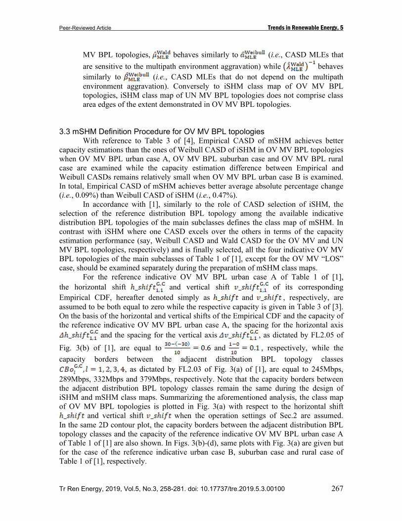
of OV MV BPL topologies is plotted in Fig. 3(a) with respect to the horizontal shift

and vertical shift when the operation settings of Sec.2 are assumed.

In the same 2D contour plot, the capacity borders between the adjacent distribution BPL

topology classes and the capacity of the reference indicative OV MV BPL urban case A

of Table 1 of [1] are also shown. In Figs. 3(b)-(d), same plots with Fig. 3(a) are given but

for the case of the reference indicative urban case B, suburban case and rural case of

Table 1 of [1], respectively.





Fig. 3. mSHM class map of the OV MV BPL topologies in the 3-30MHz frequency band when

WtG1 coupling scheme is deployed and FCC Part 15 is applied for different reference indicative OV MV

BPL topologies. (a) OV MV BPL urban case A. (b) OV MV BPL urban case B. (c) OV MV BPL suburban

case. (d) OV MV BPL rural case.

From Figs. 3(a)-(d), several interesting remarks can be pointed out concerning the

mSHM class maps, namely:

• Similarly to the iSHM class map of OV MV BPL topologies, five capacity areas

between the computed borders can be clearly delineated in the mSHM class map



of OV MV BPL topologies; say, the OV MV BPL “LOS” class, OV MV BPL

rural class, OV MV BPL suburban class, OV MV BPL urban case A class and

UN MV BPL urban case B class. The virtual OV MV BPL topologies that are

members of the aforementioned OV MV BPL topology classes can be defined by

the suitable combined horizontal and vertical shift adjustment of the reference

indicative OV MV BPL topology with reference to Figs. 3(a)-(d).

• As the procedure of the Empirical CDF shifting is concerned in this paper,

the vertical shift is first taken into account and the horizontal shift is second

executed. This sequence of shifts ensures that the shape of the Empirical CDF

retains its characteristics as reported in eq.(11) of [1] and its accompanying two

restrictions regarding the definition of valid shift pair combinations. Anyway,

since the vertical and horizontal shifts can be considered as linear transformations

of the Empirical CDFs, the sequence of shifts can be reversed without class map

modifications if the new horizontal values are not modified during the vertical

shifts.

• The vertical shifts that are assumed during the preparation of the mSHM class

maps are considered to be positive and range from 0 to 1 while the horizontal

shifts are assumed to range from -30 dB to 30 dB regardless of the examined

distribution BPL topology. As the vertical shifts are concerned, the positive

values up to 1, which are combined with the CDF maximum value restriction of 1,

imply that the virtual Empirical CDF that is produced after the valid shift pair

combination reaches up to 1. As the horizontal shifts are concerned, since

coupling scheme channel attenuation differences of the reference indicative OV

MV BPL topology take values greater than 1×10-11 dB, the negative horizontal

shifts imply that the virtual OV MV BPL topology is characterized by lower

channel attenuation than the one of the reference indicative OV MV BPL

topology while the positive horizontal shifts imply the opposite result. Anyway,

after the horizontal shift, the virtual coupling scheme channel attenuation

difference always remains lower bounded by 1×10-11 dB.

• Regardless of the examined reference indicative OV MV BPL topology, higher

capacities are observed in the upper left areas of the mSHM class map. Since

restrictions concerning the virtual Empirical CDF and virtual coupling scheme

channel attenuation differences have been already reported, the great areas of the

OV MV BPL “LOS” topology class are observed in the upper left areas of the

mSHM class map. As the examined reference indicative OV MV BPL topology is

characterized by high capacity, there is no need for high boost of the Empirical

CDF (i.e., vertical shift) so that the capacity of the virtual OV MV BPL topology

reaches up to the capacity maximum that is the capacity of OV MV BPL “LOS”

topology class. The latter explanation justifies the area expansion of the OV MV

BPL “LOS” topology class up to the lower left areas of the mSHM class maps

when OV MV BPL rural and OV MV BPL suburban topology classes are

illustrated in Figs. 3(c) and 3(d), respectively.

• Regardless of the examined reference indicative OV MV BPL topology, lower

capacities are observed especially in the lower right areas of the mSHM class map

but also, in a certain extent, in upper right areas of the mSHM class map. As the

lower right areas of the mSHM class map are examined, the high imposed



coupling scheme channel attenuation differences by the high values of the

horizontal shifts that are combined with the relatively low increase of Empirical

CDF due to the low values of the vertical shifts normally reduce the capacities of

the virtual OV MV BPL topologies. Here, there is no restriction to the imposed

coupling scheme channel attenuation differences and, therefore, the capacities of

the virtual OV MV BPL topologies tend to zero as the horizontal shifts

significantly increase. As the upper right of the mSHM class map, which can be

treated as a special case of the low capacity behavior, are investigated, the

capacities of the virtual OV MV BPL topologies are observed to be decreased but

remain higher than the capacities observed in the lower right areas of the mSHM

class map when vertical shifts exceed 0.9. The behavior of the capacities of the

virtual OV MV BPL topologies in the upper right areas of the mSHM class map is

explained by the fact that, for given the maximum vertical shift (e.g., 1), as the

horizontal shift increases above 0dB this implies that the virtual Empirical CDF is

characterized by a step function of magnitude 1 while the step position is located

at the examined horizontal step value. Due to the shape of the virtual Empirical

CDF, the virtual coupling scheme channel attenuation difference is fixed and

equal to the examined horizontal step value. As the examined horizontal shift

increases, so does the fixed virtual coupling scheme channel attenuation

difference, thus having an effect of the reduction of the capacity of the examined

virtual OV MV BPL topology.

• By identifying the five capacity areas between the computed borders in each of

the mSHM class maps of Figs. 3(a)-(d), it is obvious that a plethora of virtual OV

MV BPL topologies can enrich the different OV MV BPL topology classes by

adopting different reference indicative OV MV BPL topologies when suitable

combined horizontal and vertical shift adjustments that comply with the

respective mSHM class map areas and Empirical CDFs are followed.

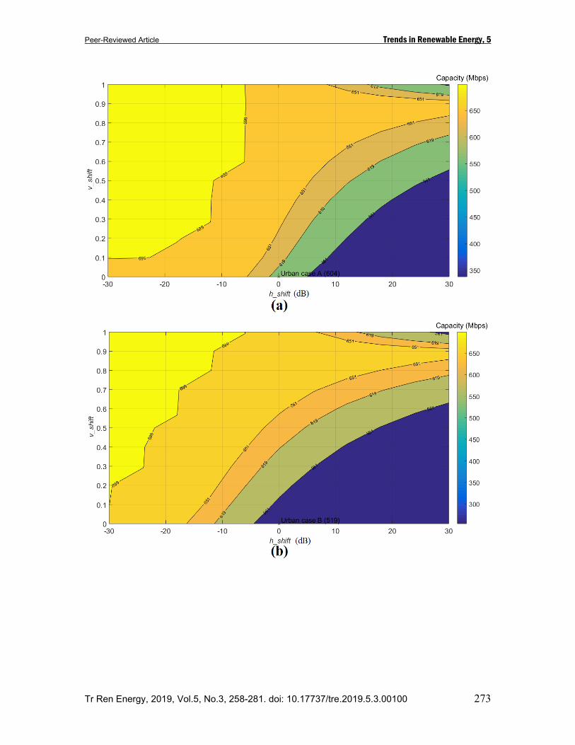
3.4 mSHM Definition Procedure for UN MV BPL topologies

With reference to Table 3 of [4], Empirical CASD of mSHM does not achieve

better capacity estimations than the ones of Wald CASD of iSHM in UN MV BPL

topologies but the percentage change differences in all the examined cases remain

significantly low. Anyway, the average absolute percentage change between the

Empirical CASD of mSHM (i.e., 0.07%) and Wald CASD of iSHM (i.e., 0.01%) again

remains significantly low while the main advantage of the Empirical CASD against Wald

CASD remains its execution time (as reported in Sec.3.5).

In accordance with [1] and similarly to Sec.3.3, all the four indicative UN MV

BPL topologies of the main subclasses of Table 2 of [1], except for the UN MV “LOS”

case, are examined separately during the preparation of mSHM class maps. As the

horizontal shifts, vertical shifts, horizontal shift spacings and vertical shift spacings of the

mSHM class maps of UN MV BPL topologies are considered, these are assumed to

receive the same values with the respective ones of the mSHM class maps of OV MV

BPL topologies. Also, the capacity borders between the adjacent distribution BPL

topology classes , which are adopted during the preparation of the

mSHM class maps, are equal to 561 Mbps, 619 Mbps, 651 Mbps and 699 Mbps,



respectively, and remain the same ones with the respective capacity borders during the

preparation of the iSHM class maps already presented in Sec.3.2. The class map of UN

MV BPL topologies is plotted in Fig. 4(a) with respect to the horizontal shift and

vertical shift when the operation settings of Sec.2 are assumed.

In the same 2D contour plot, the capacity borders between the adjacent distribution BPL

topology classes and the capacity of the reference indicative UN MV BPL urban case A

of Table 2 of [1] are also shown. In Figs. 4(b)-(d), same plots with Fig. 4(a) are given but

for the case of the reference indicative UN MV BPL urban case B, UN MV BPL

suburban case and UN MV BPL rural case of Table 2 of [1], respectively.





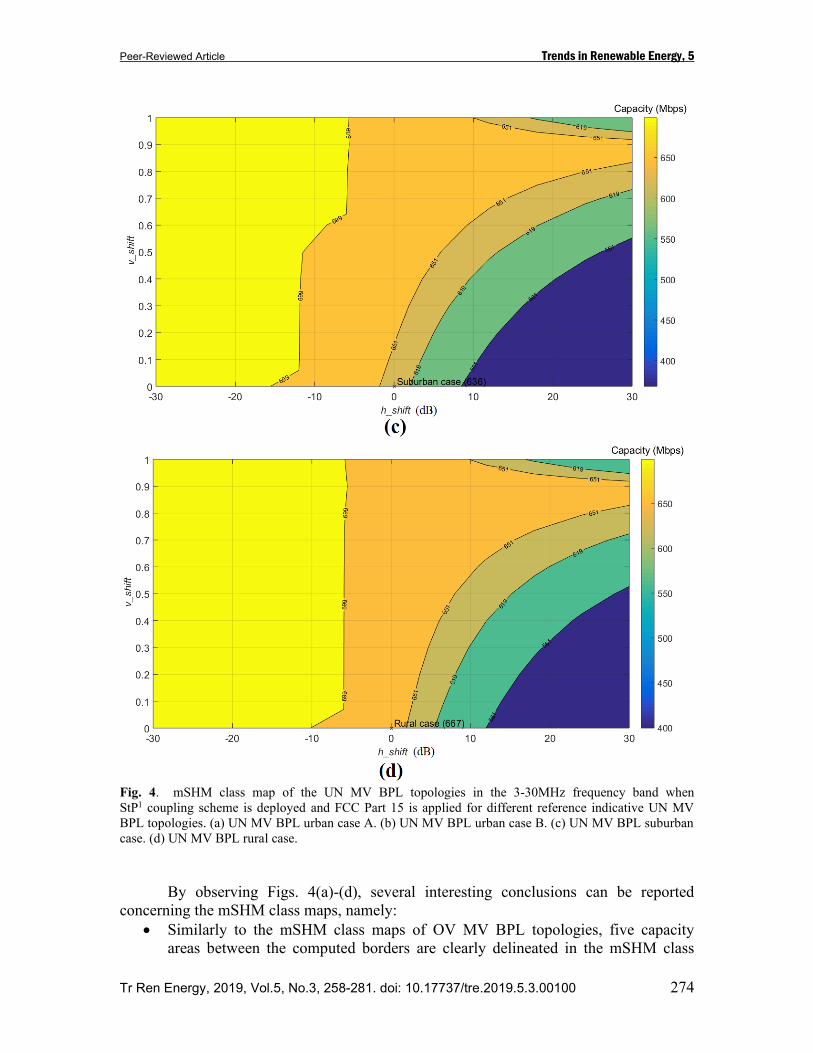
Fig. 4. mSHM class map of the UN MV BPL topologies in the 3-30MHz frequency band when

StP1 coupling scheme is deployed and FCC Part 15 is applied for different reference indicative UN MV

BPL topologies. (a) UN MV BPL urban case A. (b) UN MV BPL urban case B. (c) UN MV BPL suburban

case. (d) UN MV BPL rural case.

By observing Figs. 4(a)-(d), several interesting conclusions can be reported

concerning the mSHM class maps, namely:

• Similarly to the mSHM class maps of OV MV BPL topologies, five capacity

areas between the computed borders are clearly delineated in the mSHM class



map of UN MV BPL topologies whose planning remains the same as that of

mSHM class maps of OV MV BPL topologies in Figs. 3(a)-(d).

• Similarly to mSHM class maps of the OV MV BPL topologies, the reference

indicative UN MV BPL topology of each of the illustrated mSHM class maps is

located at the axis center of each class map while the capacities of the virtual UN

MV BPL topologies, which are defined with reference to the Empirical CDF of

the reference indicative UN MV BPL topology, increase as the horizontal shift

decreases (i.e., coupling scheme channel attenuation differences decrease) or the

vertical shift increases (i.e., Empirical CDF shifts upward).

• By comparing the OV MV BPL “LOS” class areas of Figs. 3(a)-(d) against the

UN MV BPL “LOS” class areas of Figs. 4(a)-(d), differences concerning the

location of the right borderline of these areas, which are more clear when high

values of vertical shifts are adopted, are here mentioned. By comparing Figs. 2

and 3 of [4], the coupling scheme channel attenuation differences of the UN MV

BPL topologies are characterized by a fixed difference (i.e., the minimum of the

coupling scheme channel attenuation difference remains above a channel

attenuation difference threshold) across the examined frequency range in contrast

with the coupling scheme channel attenuation differences of the OV MV BPL

topologies whose minima are equal to zero. This behavior of the coupling scheme

channel attenuation differences of the UN MV BPL topologies is reflected on the

class maps where the upper right UN MV BPL “LOS” class area borderline is

located at the horizontal shift that is equal to the aforementioned channel

attenuation difference threshold. As it is evident this channel attenuation

difference threshold is included across the entire right UN MV BPL “LOS” class

area borderline which is not so evident when the vertical shift is significantly

lower than 1.

• Similarly to the mSHM class map of OV MV BPL topologies, by identifying the

five capacity areas between the computed borders in each of the mSHM class

maps of Figs. 4(a)-(d), it is obvious that a plethora of virtual UN MV BPL

topologies can again be defined in order to enrich the different UN MV BPL

topology classes. By selecting among the different reference indicative OV MV

BPL topologies and applying suitable combined horizontal and vertical shift

adjustments in compliance with the respective mSHM class maps, virtual UN MV

BPL topologies of different Empirical CDF forms that anyway are members of

the same UN MV BPL topology class can be defined.

3.5 Class Mapping and Simulation Time

With reference to Table 3 of [4], different CASDs and power grid types are

characterized by different capacity estimation performances (i.e., different percentage and

average absolute percentage changes). Apart from the different capacity estimation

performances, class mapping of Secs. 3.1-3.4 requires different simulation times that

depend primarily on the applied CASD and secondarily on the power grid type given the

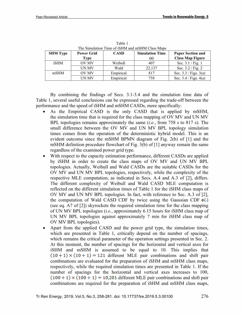
operation settings of Sec. 2. More analytically, in Table 1, the required simulation times

for the class mapping of Secs. 3.1-3.4, which have been recorded during the class map

implementation, are reported.



Table 1

The Simulation Time of iSHM and mSHM Class Maps

SHM Type Power Grid

Type

CASD Simulation Time

(s)

Paper Section and

Class Map Figure

iSHM OV MV Weibull 407 Sec. 3.1 / Fig. 1

UN MV Wald 22,137 Sec. 3.2 / Fig. 2

mSHM OV MV Empirical 817 Sec. 3.3 / Figs. 3(a)

UN MV Empirical 758 Sec. 3.4 / Figs. 4(a)

By combining the findings of Secs. 3.1-3.4 and the simulation time data of

Table 1, several useful conclusions can be expressed regarding the trade-off between the

performance and the speed of iSHM and mSHM CASDs, more specifically:

• As the Empirical CASD is the only CASD that is applied by mSHM,

the simulation time that is required for the class mapping of OV MV and UN MV

BPL topologies remains approximately the same (i.e., from 758 s to 817 s). The

small difference between the OV MV and UN MV BPL topology simulation

times comes from the operation of the deterministic hybrid model. This is an

evident outcome since the mSHM BPMN diagram of Fig. 2(b) of [1] and the

mSHM definition procedure flowchart of Fig. 3(b) of [1] anyway remain the same

regardless of the examined power grid type.

• With respect to the capacity estimation performance, different CASDs are applied

by iSHM in order to create the class maps of OV MV and UN MV BPL

topologies. Actually, Weibull and Wald CASDs are the suitable CASDs for the

OV MV and UN MV BPL topologies, respectively, while the complexity of the

respective MLE computation, as indicated in Secs. A.4 and A.3 of [2], differs.

The different complexity of Weibull and Wald CASD MLE computation is

reflected on the different simulation times of Table 1 for the iSHM class maps of

OV MV and UN MV BPL topologies. In fact, with reference to Sec. A.3 of [2],

the computation of Wald CASD CDF by twice using the Gaussian CDF

(see eq. A7 of [2]) skyrockets the required simulation time for the class mapping

of UN MV BPL topologies (i.e., approximately 6.15 hours for iSHM class map of

UN MV BPL topologies against approximately 7 min for iSHM class map of

OV MV BPL topologies).

• Apart from the applied CASD and the power grid type, the simulation times,

which are presented in Table 1, critically depend on the number of spacings,

which remains the critical parameter of the operation settings presented in Sec. 2.

At this moment, the number of spacings for the horizontal and vertical axes for

iSHM and mSHM is assumed to be equal to 10. This implies that

different MLE pair combinations and shift pair

combinations are evaluated for the preparation of iSHM and mSHM class maps,

respectively, while the required simulation times are presented in Table 1. If the

number of spacings for the horizontal and vertical axes increases to 100,

different MLE pair combinations and shift pair

combinations are required for the preparation of iSHM and mSHM class maps,



respectively,

while the simulation times are expected to be increased by approximately

84 times. By analyzing the simulation time data of Table 1, this becomes a

prohibitive task for the iSHM class mapping of UN MV BPL topologies

(i.e., the simulation time is expected to be equal to approximately 21.5 days).

• By considering the capacity estimation performance and the simulation data of the

different CASDs for the class mapping of UN MV BPL topologies, an interesting

trade-off can be established between Empirical CASD of mSHM and the

Wald CASD of iSHM. Although the capacity estimation performance of Wald

CASD of iSHM presents slightly improved results with respect to the capacity

estimation performance in relation with the Empirical CASD of mSHM,

the simulation time of Wald CASD is six times greater than the one of Empirical

CASD. Therefore, the slight improved capacity estimation performance is

exchanged at significantly worse simulation times. Conversely, the same trade-off

issue holds in OV MV BPL topologies between the Empirical CASD of mSHM

and the Weibull CASD of iSHM.

By concluding this Section, it is evident that the definition of class maps of

distribution BPL topologies can successfully enrich the existing distribution BPL

topology classes with a plethora of statistically equivalent virtual distribution BPL

topologies. However, the selection among different CASDs and different SHM types

offers a diversity regarding the capacity estimation performance and the simulation time.

4. Conclusions

In this paper, the numerical results concerning the class mapping of OV MV and

UN MV BPL topologies have been presented on the basis of iSHM and mSHM

flowcharts and definition procedures, which have been analyzed in [1]. In accordance

with the proposed class maps, it has been verified that distribution BPL topology classes

can be further enriched with respective distribution BPL topology subclasses that further

consist of a plethora of corresponding distribution BPL topologies that remain

statistically equivalent with the indicative distribution BPL topology of the examined

subclass. Apart from the definition of virtual distribution BPL topologies in terms of

their capacity by simply selecting appropriate CASD parameters, the capacity estimation

performance and the simulation time of iSHM and mSHM CASDs have been examined

revealing an interesting trade-off between the aforementioned two parameters. After the

class map definition, the statistical approach of SHM can be considered to be more

robust since a great number of indicative distribution BPL topologies, which can act as

representative topologies of respective distribution BPL topology subclasses, can be

assumed.

CONFLICTS OF INTEREST

The author declares that there is no conflict of interests regarding the publication

of this paper.



References [1] A. G. Lazaropoulos, “Virtual Indicative Broadband over Power Lines Topologies

for Respective Subclasses by Adjusting Channel Attenuation Statistical

Distribution Parameters of Statistical Hybrid Models – Part 1: Theory,” Trends in

Renewable Energy, vol. 5, no. 3, pp 237-257, Aug. 2019. DOI:

10.17737/tre.2019.5.3.0099

[2] A. G. Lazaropoulos, “Statistical Broadband over Power Lines Channel Modeling

– Part 1: The Theory of the Statistical Hybrid Model,” Progress in

Electromagnetics Research C, vol. 92, pp. 1-16, 2019. [Online]. Available:

http://www.jpier.org/PIERC/pierc92/01.19012902.pdf

[3] A. G. Lazaropoulos, “Statistical Broadband over Power Lines (BPL) Channel

Modeling – Part 2: The Numerical Results of the Statistical Hybrid Model,”

Progress in Electromagnetics Research C, vol. 92, pp. 17-30, 2019. [Online].

Available: http://www.jpier.org/PIERC/pierc92/02.19012903.pdf

[4] A. G. Lazaropoulos, “Enhancing the Statistical Hybrid Model Performance in

Overhead and Underground Medium Voltage Broadband over Power Lines

Channels by Adopting Empirical Channel Attenuation Statistical Distribution,”

Trends in Renewable Energy, vol. 5, no. 2, pp. 181-217, 2019. [Online].

Available: http://futureenergysp.com/index.php/tre/article/view/96/pdf

[5] A. G. Lazaropoulos, “Towards Modal Integration of Overhead and Underground

Low-Voltage and Medium-Voltage Power Line Communication Channels in the

Smart Grid Landscape: Model Expansion, Broadband Signal Transmission

Characteristics, and Statistical Performance Metrics (Invited Paper),” ISRN Signal

Processing, vol. 2012, Article ID 121628, pp. 1-17, 2012. [Online]. Available:

http://www.hindawi.com/isrn/sp/2012/121628/

[6] A. G. Lazaropoulos, “Towards Broadband over Power Lines Systems Integration:

Transmission Characteristics of Underground Low-Voltage Distribution Power

Lines,” Progress in Electromagnetics Research B, vol. 39, pp. 89-114, 2012.

[Online]. Available: http://www.jpier.org/PIERB/pierb39/05.12012409.pdf

[7] A. G. Lazaropoulos and P. G. Cottis, “Transmission characteristics of overhead

medium voltage power line communication channels,” IEEE Trans. Power Del.,

vol. 24, no. 3, pp. 1164-1173, Jul. 2009.

[8] A. G. Lazaropoulos and P. G. Cottis, “Capacity of overhead medium voltage

power line communication channels,” IEEE Trans. Power Del., vol. 25, no. 2, pp.

723-733, Apr. 2010.

[9] A. G. Lazaropoulos and P. G. Cottis, “Broadband transmission via underground

medium-voltage power lines-Part I: transmission characteristics,” IEEE Trans.

Power Del., vol. 25, no. 4, pp. 2414-2424, Oct. 2010.

[10] A. G. Lazaropoulos and P. G. Cottis, “Broadband transmission via underground

medium-voltage power lines-Part II: capacity,” IEEE Trans. Power Del., vol. 25,

no. 4, pp. 2425-2434, Oct. 2010.

[11] A. G. Lazaropoulos, “Broadband transmission and statistical performance

properties of overhead high-voltage transmission networks,” Hindawi Journal of



http://futureenergysp.com/index.php/tre/article/view/96/pdf

http://www.hindawi.com/isrn/sp/2012/121628/

http://www.jpier.org/PIERB/pierb39/05.12012409.pdf



Computer Networks and Commun., 2012, article ID 875632, 2012. [Online].

Available: http://www.hindawi.com/journals/jcnc/aip/875632/

[12] P. Amirshahi and M. Kavehrad, “High-frequency characteristics of overhead

multiconductor power lines for broadband communications,” IEEE J. Sel. Areas

Commun., vol. 24, no. 7, pp. 1292-1303, Jul. 2006.

[13] T. Sartenaer, “Multiuser communications over frequency selective wired channels

and applications to the powerline access network” Ph.D. dissertation, Univ.

Catholique Louvain, Louvain-la-Neuve, Belgium, Sep. 2004.

[14] T. Calliacoudas and F. Issa, ““Multiconductor transmission lines and cables

solver,” An efficient simulation tool for plc channel networks development,”

presented at the IEEE Int. Conf. Power Line Communications and Its

Applications, Athens, Greece, Mar. 2002.

[15] T. Sartenaer and P. Delogne, “Deterministic modelling of the (Shielded) outdoor

powerline channel based on the multiconductor transmission line equations,”

IEEE J. Sel. Areas Commun., vol. 24, no. 7, pp. 1277-1291, Jul. 2006.

[16] A. G. Lazaropoulos, “Virtual Indicative Broadband over Power Lines Topologies

for Respective Subclasses by Adjusting Channel Attenuation Statistical

Distribution Parameters of Statistical Hybrid Models – Part 3: The Case of

Overhead Transmission Power Grids,” Trends in Renewable Energy, vol. 5, no. 3,

pp 282-306, Aug. 2019. DOI: 10.17737/tre.2019.5.3.00101

[17] S. Liu and L. J. Greenstein, “Emission characteristics and interference constraint

of overhead medium-voltage broadband power line (BPL) systems,” in Proc.

IEEE Global Telecommunications Conf., New Orleans, LA, USA, Nov./Dec.

2008, pp. 1-5.

[18] A. G. Lazaropoulos, “Underground Distribution BPL Connections with (N + 1)-

hop Repeater Systems: A Novel Capacity Mitigation Technique,” Elsevier

Computers and Electrical Engineering, vol. 40, pp. 1813-1826, 2014.

[19] A. G. Lazaropoulos, “Review and Progress towards the Capacity Boost of

Overhead and Underground Medium-Voltage and Low-Voltage Broadband over

Power Lines Networks: Cooperative Communications through Two- and Three-

Hop Repeater Systems,” ISRN Electronics, vol. 2013, Article ID 472190, pp. 1-

19, 2013. [Online]. Available:

http://www.hindawi.com/isrn/electronics/aip/472190/

[20] A. G. Lazaropoulos, “Broadband over Power Lines (BPL) Systems Convergence:

Multiple-Input Multiple-Output (MIMO) Communications Analysis of Overhead

and Underground Low-Voltage and Medium-Voltage BPL Networks (Invited

Paper),” ISRN Power Engineering, vol. 2013, Article ID 517940, pp. 1-30, 2013.

[Online]. Available:

http://www.hindawi.com/isrn/power.engineering/2013/517940/

[21] A. G. Lazaropoulos, “Deployment Concepts for Overhead High Voltage

Broadband over Power Lines Connections with Two-Hop Repeater System:

Capacity Countermeasures against Aggravated Topologies and High Noise

Environments,” Progress in Electromagnetics Research B, vol. 44, pp. 283-307,

2012. [Online]. Available: http://www.jpier.org/PIERB/pierb44/13.12081104.pdf

[22] N. Suljanović, A. Mujčić, M. Zajc, and J. F. Tasič, “Approximate computation of

high-frequency characteristics for power line with horizontal disposition and

http://www.hindawi.com/journals/jcnc/aip/875632/

http://www.hindawi.com/isrn/electronics/aip/472190/

http://www.hindawi.com/isrn/power.engineering/2013/517940/




middle-phase to ground coupling,” Elsevier Electr. Power Syst. Res., vol. 69, pp.

17-24, Jan. 2004.

[23] OPERA1, D5: Pathloss as a function of frequency, distance and network topology

for various LV and MV European powerline networks. IST Integrated Project No

507667, Apr. 2005.

[24] N. Suljanović, A. Mujčić, M. Zajc, and J. F. Tasič, “High-frequency

characteristics of high-voltage power line,” in Proc. IEEE Int. Conf. on Computer

as a Tool, Ljubljana, Slovenia, Sep. 2003, pp. 310-314.

[25] N. Suljanović, A. Mujčić, M. Zajc, and J. F. Tasič, “Power-line high-frequency

characteristics: analytical formulation,” in Proc. Joint 1st Workshop on Mobile

Future & Symposium on Trends in Communications, Bratislava, Slovakia, Oct.

2003, pp. 106-109.

[26] W. Villiers, J. H. Cloete, and R. Herman, “The feasibility of ampacity control on

HV transmission lines using the PLC system,” in Proc. IEEE Conf. Africon,

George, South Africa, Oct. 2002, vol. 2, pp. 865-870.

[27] P. Amirshahi, “Broadband access and home networking through powerline

networks” Ph.D. dissertation, Pennsylvania State Univ., University Park, PA, May

2006.

[28] OPERA1, D44: Report presenting the architecture of plc system, the electricity

network topologies, the operating modes and the equipment over which PLC

access system will be installed, IST Integr. Project No 507667, Dec. 2005.

[29] J. Anatory, N. Theethayi, R. Thottappillil, M. M. Kissaka, and N. H. Mvungi,

“The influence of load impedance, line length, and branches on underground

cable Power-Line Communications (PLC) systems,” IEEE Trans. Power Del.,

vol. 23, no. 1, pp. 180-187, Jan. 2008.

[30] J. Anatory, N. Theethayi, and R. Thottappillil, “Power-line communication

channel model for interconnected networks-Part II: Multiconductor system,”

IEEE Trans. Power Del., vol. 24, no. 1, pp. 124-128, Jan. 2009.

[31] J. Anatory, N. Theethayi, R. Thottappillil, M. M. Kissaka, and N. H. Mvungi,

“The effects of load impedance, line length, and branches in typical low-voltage

channels of the BPLC systems of developing countries: transmission-line

analyses,” IEEE Trans. Power Del., vol. 24, no. 2, pp. 621-629, Apr. 2009.

[32] T. Banwell and S. Galli, “A novel approach to accurate modeling of the indoor

power line channel—Part I: Circuit analysis and companion model,” IEEE Trans.

Power Del., vol. 20, no. 2, pp. 655-663, Apr. 2005.

[33] W. Villiers, J. H. Cloete, L. M. Wedepohl, and A. Burger, “Real-time sag

monitoring system for high-voltage overhead transmission lines based on power-

line carrier signal behavior,” IEEE Trans. Power Del., vol. 23, no. 1, pp. 389-395,

Jan. 2008.

[34] A. G. Lazaropoulos, “Smart Energy and Spectral Efficiency (SE) of Distribution

Broadband over Power Lines (BPL) Networks – Part 1: The Impact of

Measurement Differences on SE Metrics,” Trends in Renewable Energy, vol. 4,

no. 2, pp. 125-184, Aug. 2018. [Online]. Available:


[35] A. G. Lazaropoulos, “Broadband Performance Metrics and Regression

Approximations of the New Coupling Schemes for Distribution Broadband over




Power Lines (BPL) Networks,” Trends in Renewable Energy, vol. 4, no. 1, pp.

43-73, Jan. 2018. [Online]. Available:


[36] A. G. Lazaropoulos, “New Coupling Schemes for Distribution Broadband over

Power Lines (BPL) Networks,” Progress in Electromagnetics Research B, vol.

71, pp. 39-54, 2016. [Online]. Available:


[37] A. G. Lazaropoulos, “A Panacea to Inherent BPL Technology Deficiencies by

Deploying Broadband over Power Lines (BPL) Connections with Multi-Hop

Repeater Systems,” Bentham Recent Advances in Electrical & Electronic

Engineering, vol. 10, no. 1, pp. 30-46, 2017.

[38] A. G. Lazaropoulos, “The Impact of Noise Models on Capacity Performance of

Distribution Broadband over Power Lines Networks,” Hindawi Computer

Networks and Communications, vol. 2016, Article ID 5680850, 14 pages, 2016.

doi:10.1155/2016/5680850. [Online]. Available:

http://www.hindawi.com/journals/jcnc/2016/5680850/

[39] A. G. Lazaropoulos, “Capacity Performance of Overhead Transmission Multiple-

Input Multiple-Output Broadband over Power Lines Networks: The Insidious

Effect of Noise and the Role of Noise Models (Invited Paper),” Trends in

Renewable Energy, vol. 2, no. 2, pp. 61-82, Jun. 2016. [Online]. Available:

http://futureenergysp.com/index.php/tre/article/view/23

[40] A. G. Lazaropoulos, “Smart Energy and Spectral Efficiency (SE) of Distribution

Broadband over Power Lines (BPL) Networks – Part 2: L1PMA, L2WPMA and

L2CXCV for SE against Measurement Differences in Overhead Medium-Voltage

BPL Networks,” Trends in Renewable Energy, vol. 4, no. 2, pp. 185-212, Aug.

2018. [Online]. Available:


[41] A. G. Lazaropoulos, “Factors Influencing Broadband Transmission

Characteristics of Underground Low-Voltage Distribution Networks,” IET

Commun., vol. 6, no. 17, pp. 2886-2893, Nov. 2012.

Article copyright: © 2019 Athanasios G. Lazaropoulos. This is an open access article

distributed under the terms of the Creative Commons Attribution 4.0 International

License, which permits unrestricted use and distribution provided the original author and

source are credited.



http://www.hindawi.com/journals/jcnc/2016/5680850/

http://futureenergysp.com/index.php/tre/article/view/23


http://creativecommons.org/licenses/by/4.0/



Documents

Virtual Indicative Broadband over Power Lines Topologies