Embed Size (px)
Citation preview
Fluid Dynamics I-1ANSYS, Inc. Proprietary
© 2009 ANSYS, Inc. All rights reserved.
Introduction to CFD using Ansys CFX
Fluid Dynamics I:Viscous Incompressible Flow
Fluid Dynamics I-2ANSYS, Inc. Proprietary
© 2009 ANSYS, Inc. All rights reserved.
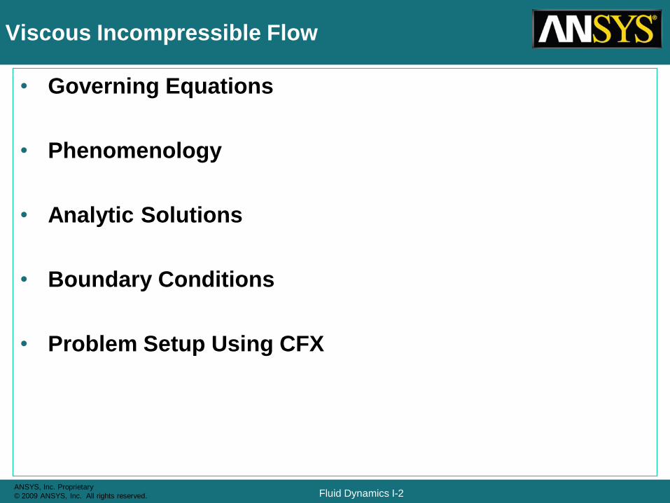
Viscous Incompressible Flow
• Governing Equations
• Phenomenology
• Analytic Solutions
• Boundary Conditions
• Problem Setup Using CFX
Fluid Dynamics I-3ANSYS, Inc. Proprietary
© 2009 ANSYS, Inc. All rights reserved.
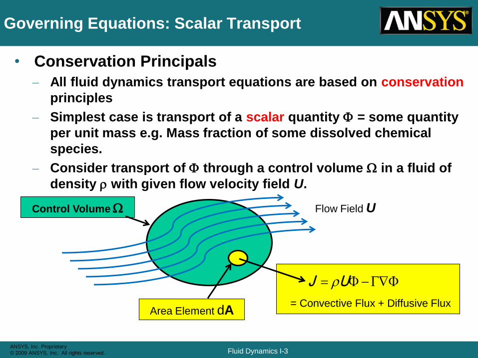
= Convective Flux + Diffusive Flux
Governing Equations: Scalar Transport
• Conservation Principals
– All fluid dynamics transport equations are based on conservation
principles
– Simplest case is transport of a scalar quantity F = some quantity
per unit mass e.g. Mass fraction of some dissolved chemical
species.
– Consider transport of F through a control volume W in a fluid of
density r with given flow velocity field U.
Flow Field UControl Volume W
Area Element dA
FF UJ r
Fluid Dynamics I-4ANSYS, Inc. Proprietary
© 2009 ANSYS, Inc. All rights reserved.
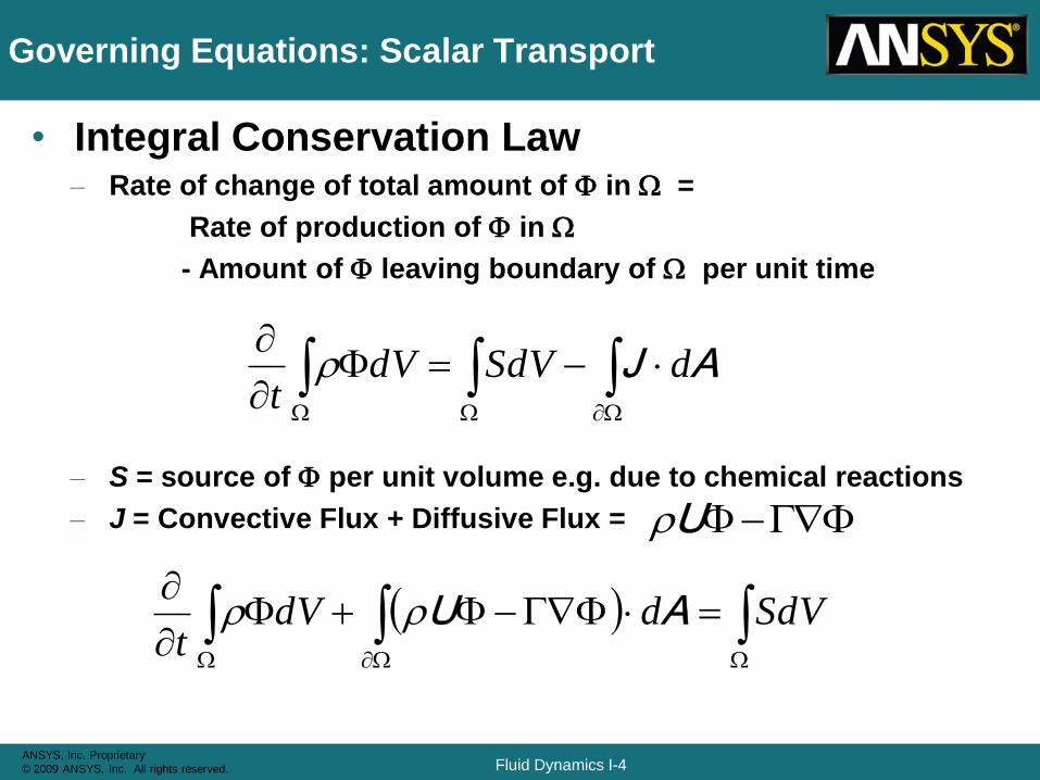
Governing Equations: Scalar Transport
• Integral Conservation Law– Rate of change of total amount of F in W =
Rate of production of F in W
- Amount of F leaving boundary of W per unit time
– S = source of F per unit volume e.g. due to chemical reactions
– J = Convective Flux + Diffusive Flux =
AJ ddVSdVt
F
WWW
r
FFUr
dVSddVt
WWW
FFF
AUrr
Fluid Dynamics I-5ANSYS, Inc. Proprietary
© 2009 ANSYS, Inc. All rights reserved.
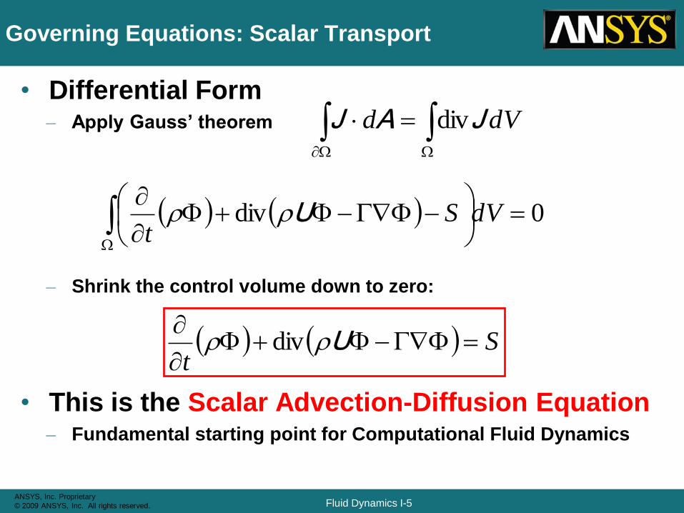
Governing Equations: Scalar Transport
• Differential Form– Apply Gauss’ theorem
– Shrink the control volume down to zero:
• This is the Scalar Advection-Diffusion Equation– Fundamental starting point for Computational Fluid Dynamics
0div
FFF
W
dVSt
Urr
dVd WW
JAJ div
St
FFF
Urr div
Fluid Dynamics I-6ANSYS, Inc. Proprietary
© 2009 ANSYS, Inc. All rights reserved.
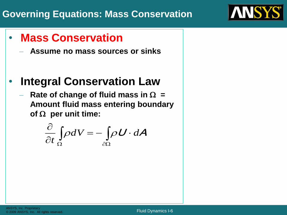
Governing Equations: Mass Conservation
• Mass Conservation– Assume no mass sources or sinks
• Integral Conservation Law– Rate of change of fluid mass in W =
Amount fluid mass entering boundary
of W per unit time:
AU ddVt
WW
rr
Fluid Dynamics I-7ANSYS, Inc. Proprietary
© 2009 ANSYS, Inc. All rights reserved.
Governing Equations: Mass Conservation
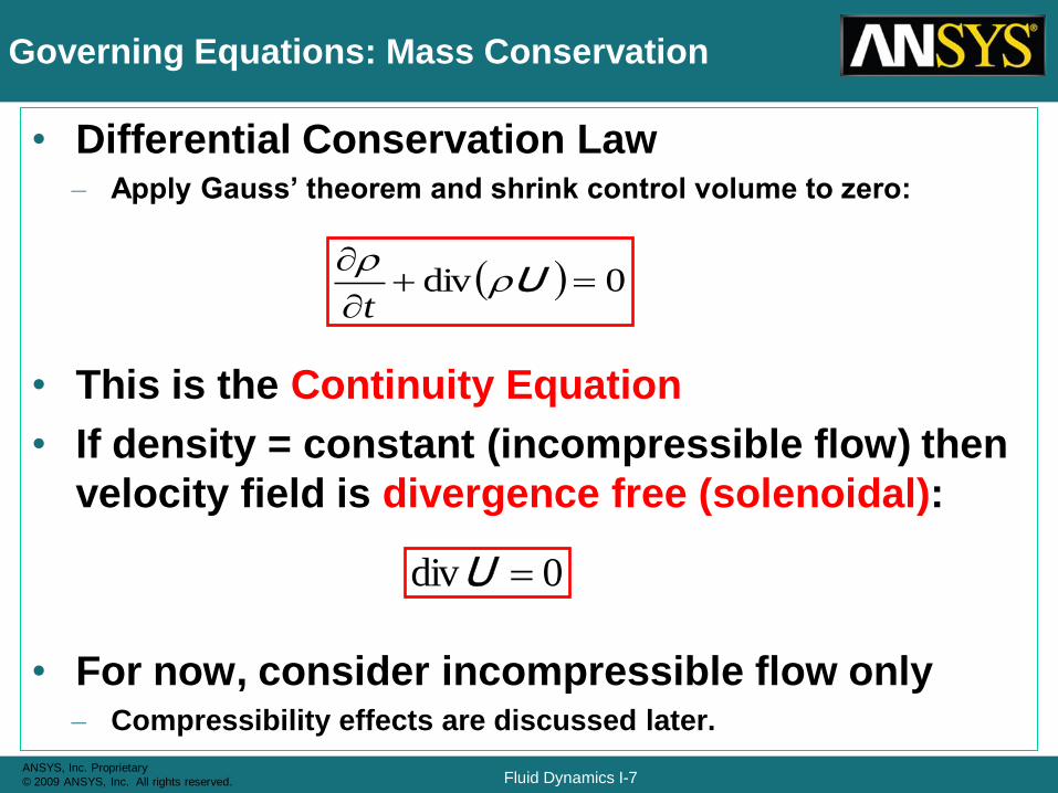
• Differential Conservation Law – Apply Gauss’ theorem and shrink control volume to zero:
• This is the Continuity Equation
• If density = constant (incompressible flow) then
velocity field is divergence free (solenoidal):
• For now, consider incompressible flow only– Compressibility effects are discussed later.
0div
Ur
r
t
0div U
Fluid Dynamics I-8ANSYS, Inc. Proprietary
© 2009 ANSYS, Inc. All rights reserved.
Governing Equations: Momentum Conservation
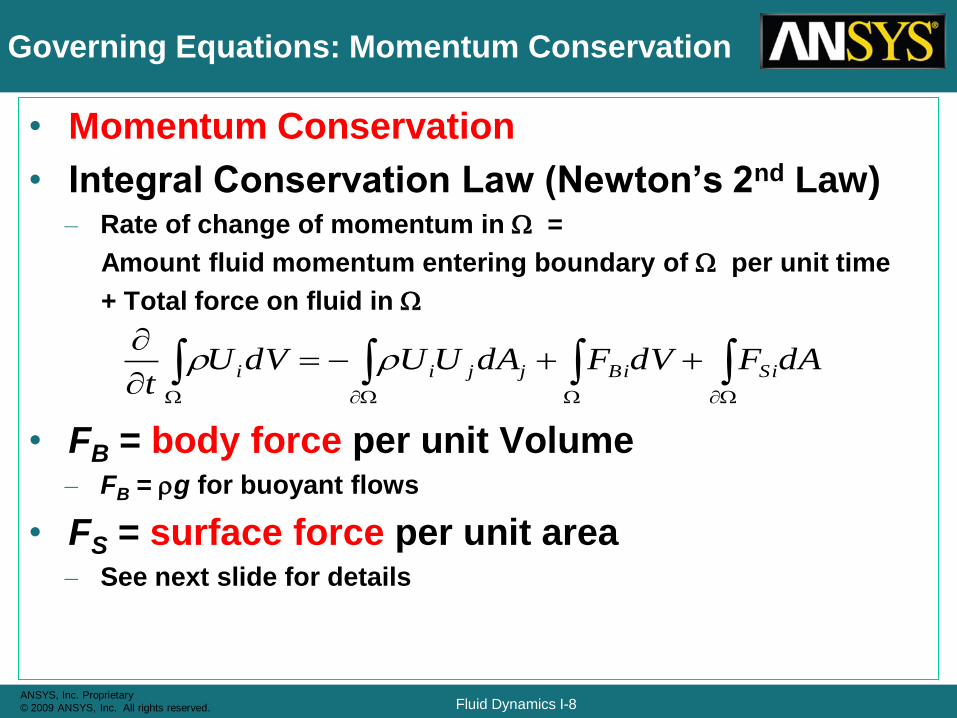
• Momentum Conservation
• Integral Conservation Law (Newton’s 2nd Law)– Rate of change of momentum in W =
Amount fluid momentum entering boundary of W per unit time
+ Total force on fluid in W
• FB = body force per unit Volume– FB = rg for buoyant flows
• FS = surface force per unit area – See next slide for details
dAFdVFdAUUdVUt
SiBijjii WWWW
rr
Fluid Dynamics I-9ANSYS, Inc. Proprietary
© 2009 ANSYS, Inc. All rights reserved.
Governing Equations: Momentum Conservation
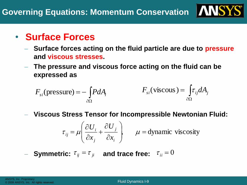
• Surface Forces– Surface forces acting on the fluid particle are due to pressure
and viscous stresses.
– The pressure and viscous force acting on the fluid can be
expressed as
– Viscous Stress Tensor for Incompressible Newtonian Fluid:
– Symmetric: and trace free:
W
isi PdAF )pressure( W
jijsi dAF )viscous(
viscositydynamic ,
i
j
j
iij
x
U
x
U
jiij 0ii
Fluid Dynamics I-10ANSYS, Inc. Proprietary
© 2009 ANSYS, Inc. All rights reserved.
Governing Equations: Momentum Conservation
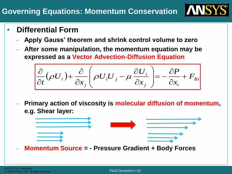
• Differential Form
– Apply Gauss’ theorem and shrink control volume to zero
– After some manipulation, the momentum equation may be
expressed as a Vector Advection-Diffusion Equation
– Primary action of viscosity is molecular diffusion of momentum,
e.g. Shear layer:
– Momentum Source = - Pressure Gradient + Body Forces
Bi
ij
iji
j
i Fx
P
x
UUU
xU
t
rr
Fluid Dynamics I-11ANSYS, Inc. Proprietary
© 2009 ANSYS, Inc. All rights reserved.
Pressure Field Definitions (1):
Absolute, Reference and Static Pressure
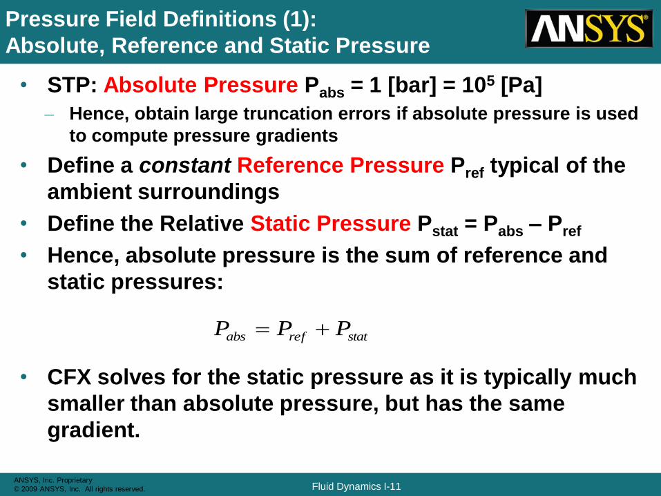
• STP: Absolute Pressure Pabs = 1 [bar] = 105 [Pa]
– Hence, obtain large truncation errors if absolute pressure is used
to compute pressure gradients
• Define a constant Reference Pressure Pref typical of the
ambient surroundings
• Define the Relative Static Pressure Pstat = Pabs – Pref
• Hence, absolute pressure is the sum of reference and
static pressures:
• CFX solves for the static pressure as it is typically much
smaller than absolute pressure, but has the same
gradient.
statrefabs PPP
Fluid Dynamics I-12ANSYS, Inc. Proprietary
© 2009 ANSYS, Inc. All rights reserved.
Pressure Field Definitions (2):
Hydrostatic and Modified Pressure
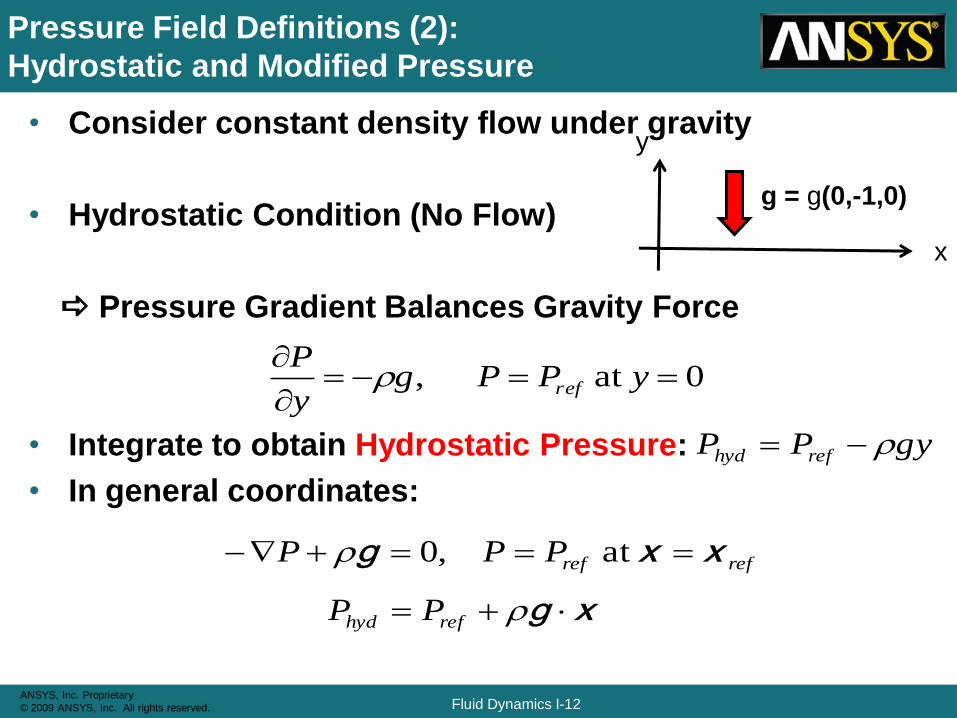
• Consider constant density flow under gravity
• Hydrostatic Condition (No Flow)
a Pressure Gradient Balances Gravity Force
• Integrate to obtain Hydrostatic Pressure:
• In general coordinates:
0at ,
yPPg
y
Prefr
y
x
g = g(0,-1,0)
gyPP refhyd r
refrefPPP xxg at ,0r
xg rrefhyd PP
Fluid Dynamics I-13ANSYS, Inc. Proprietary
© 2009 ANSYS, Inc. All rights reserved.
Pressure Field Definitions (3):
Hydrostatic and Modified Pressure
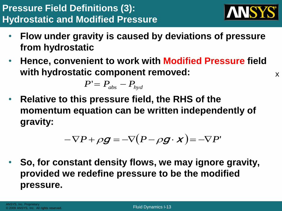
• Flow under gravity is caused by deviations of pressure
from hydrostatic
• Hence, convenient to work with Modified Pressure field
with hydrostatic component removed:
• Relative to this pressure field, the RHS of the
momentum equation can be written independently of
gravity:
• So, for constant density flows, we may ignore gravity,
provided we redefine pressure to be the modified
pressure.
x
hydabs PPP '
'PPP xgg rr
Fluid Dynamics I-14ANSYS, Inc. Proprietary
© 2009 ANSYS, Inc. All rights reserved.
Summary: Navier Stokes Equations
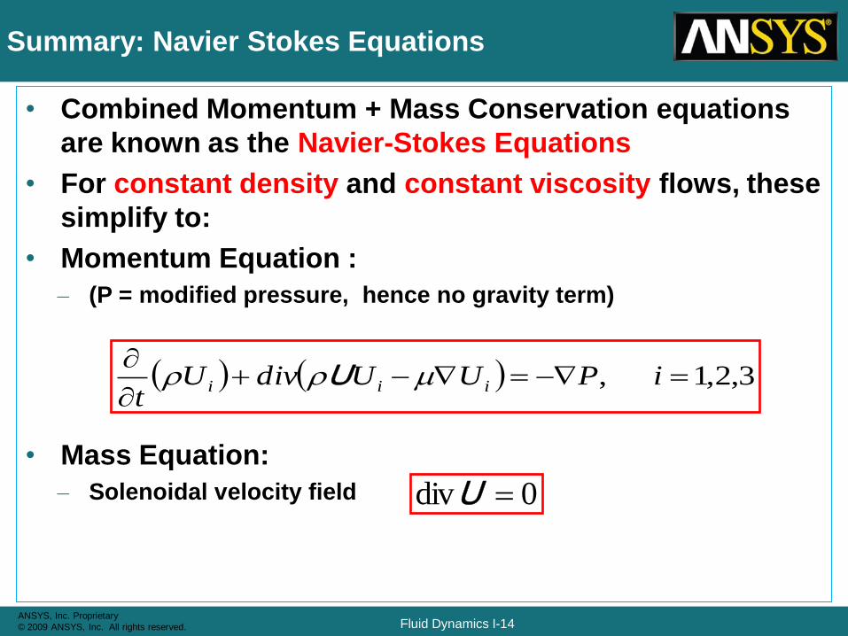
• Combined Momentum + Mass Conservation equations
are known as the Navier-Stokes Equations
• For constant density and constant viscosity flows, these
simplify to:
• Momentum Equation :
– (P = modified pressure, hence no gravity term)
• Mass Equation:
– Solenoidal velocity field
3,2,1 ,
iPUUdivU
tiii rr U
0div U
Fluid Dynamics I-15ANSYS, Inc. Proprietary
© 2009 ANSYS, Inc. All rights reserved.
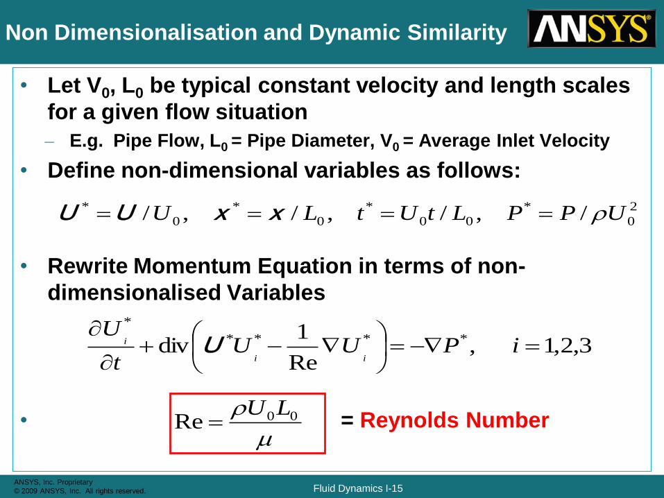
Non Dimensionalisation and Dynamic Similarity
• Let V0, L0 be typical constant velocity and length scales
for a given flow situation
– E.g. Pipe Flow, L0 = Pipe Diameter, V0 = Average Inlet Velocity
• Define non-dimensional variables as follows:
• Rewrite Momentum Equation in terms of non-
dimensionalised Variables
• = Reynolds Number
/ ,/ ,/ ,/ 2
0
*
00
*
0
*
0
* UPPLtUtLU r xxUU
3,2,1 ,Re
1div ****
*
iPUU
t
U
ii
i U
Re 00
r LU
Fluid Dynamics I-16ANSYS, Inc. Proprietary
© 2009 ANSYS, Inc. All rights reserved.
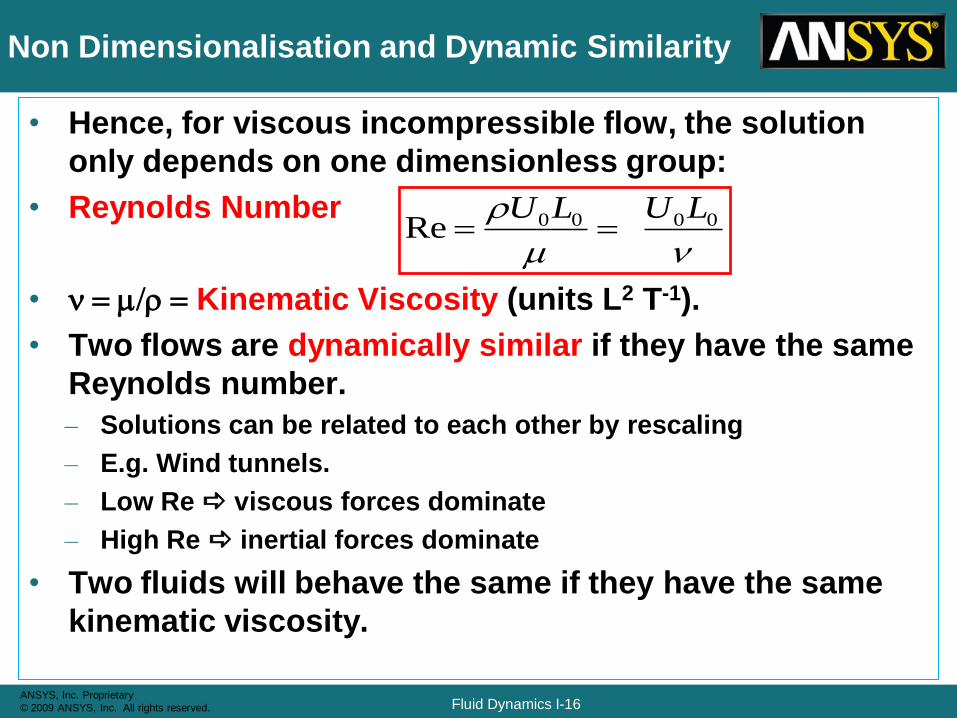
Non Dimensionalisation and Dynamic Similarity
• Hence, for viscous incompressible flow, the solution
only depends on one dimensionless group:
• Reynolds Number
• n /r Kinematic Viscosity (units L2 T-1).
• Two flows are dynamically similar if they have the same
Reynolds number.
– Solutions can be related to each other by rescaling
– E.g. Wind tunnels.
– Low Re a viscous forces dominate
– High Re a inertial forces dominate
• Two fluids will behave the same if they have the same
kinematic viscosity.
n
r 0000 ReLULU
Fluid Dynamics I-17ANSYS, Inc. Proprietary
© 2009 ANSYS, Inc. All rights reserved.
Viscous Incompressible Flow:
Phenomenology and Some Useful Analytic Solutions
Fluid Dynamics I-18ANSYS, Inc. Proprietary
© 2009 ANSYS, Inc. All rights reserved.
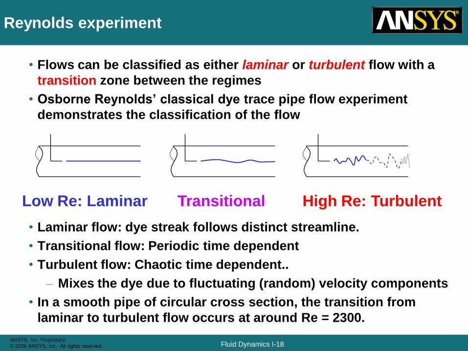
Reynolds experiment
• Flows can be classified as either laminar or turbulent flow with a
transition zone between the regimes
• Osborne Reynolds’ classical dye trace pipe flow experiment
demonstrates the classification of the flow
• Laminar flow: dye streak follows distinct streamline.
• Transitional flow: Periodic time dependent
• Turbulent flow: Chaotic time dependent..
– Mixes the dye due to fluctuating (random) velocity components
• In a smooth pipe of circular cross section, the transition from
laminar to turbulent flow occurs at around Re = 2300.
Low Re: Laminar Transitional High Re: Turbulent
Fluid Dynamics I-19ANSYS, Inc. Proprietary
© 2009 ANSYS, Inc. All rights reserved.
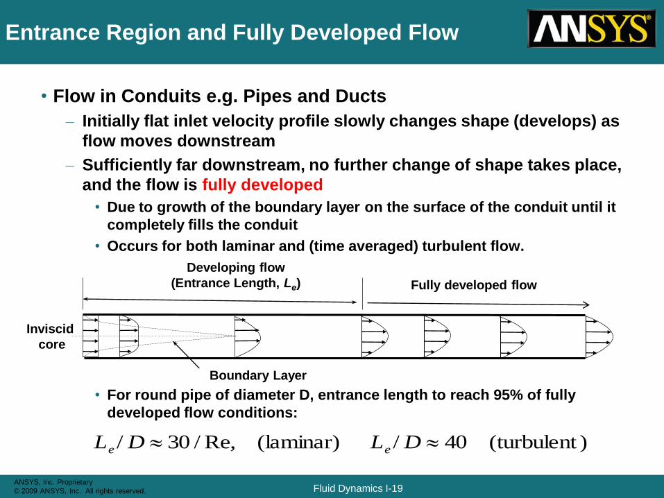
Entrance Region and Fully Developed Flow
• Flow in Conduits e.g. Pipes and Ducts
– Initially flat inlet velocity profile slowly changes shape (develops) as
flow moves downstream
– Sufficiently far downstream, no further change of shape takes place,
and the flow is fully developed
• Due to growth of the boundary layer on the surface of the conduit until it
completely fills the conduit
• Occurs for both laminar and (time averaged) turbulent flow.
• For round pipe of diameter D, entrance length to reach 95% of fully
developed flow conditions:
Inviscid
core
Boundary Layer
Developing flow
(Entrance Length, Le) Fully developed flow
)(turbulent 40/ (laminar) ,Re/30/ DLDL ee
Fluid Dynamics I-20ANSYS, Inc. Proprietary
© 2009 ANSYS, Inc. All rights reserved.
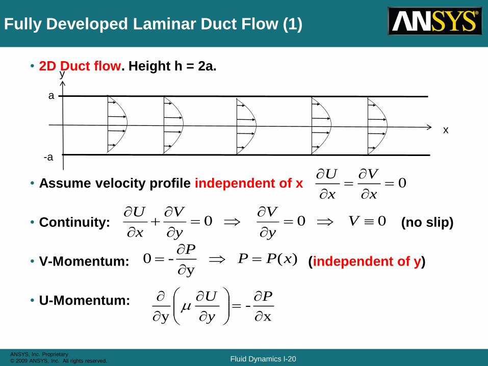
Fully Developed Laminar Duct Flow (1)
• 2D Duct flow. Height h = 2a.
• Assume velocity profile independent of x
• Continuity: (no slip)
• V-Momentum: (independent of y)
• U-Momentum:
y
x
a
-a
0
x
V
x
U
0 0 0
V
y
V
y
V
x
U
x
-y
P
y
U
)( y
-0 xPPP
Fluid Dynamics I-21ANSYS, Inc. Proprietary
© 2009 ANSYS, Inc. All rights reserved.
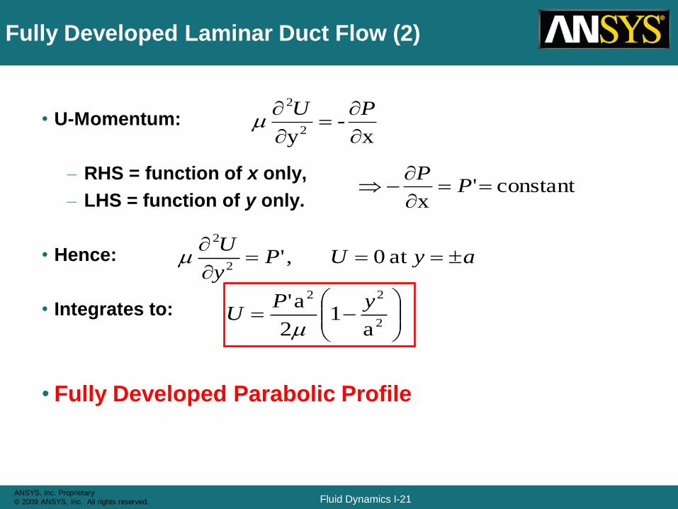
Fully Developed Laminar Duct Flow (2)
• U-Momentum:
– RHS = function of x only,
– LHS = function of y only.
• Hence:
• Integrates to:
• Fully Developed Parabolic Profile
x
-y2
2
PU
constant 'x
P
P
at 0 ,'2
2
ayUPy
U
a
12
a'2
22
yPU
Fluid Dynamics I-22ANSYS, Inc. Proprietary
© 2009 ANSYS, Inc. All rights reserved.
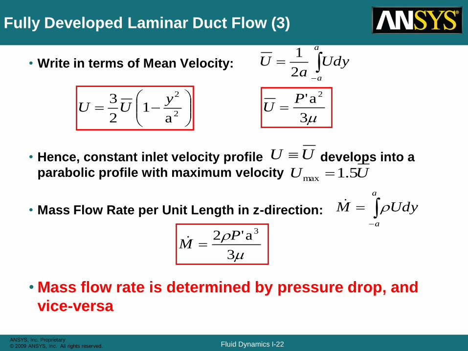
Fully Developed Laminar Duct Flow (3)
• Write in terms of Mean Velocity:
• Hence, constant inlet velocity profile develops into a
parabolic profile with maximum velocity
• Mass Flow Rate per Unit Length in z-direction:
• Mass flow rate is determined by pressure drop, and
vice-versa
2
2
a1
2
3 yUU
UU
2
1
a
a
Udya
U
3
a' 2
PU
UU 5.1 max
a
a
UdyM r
3
a'2 3
rPM
Fluid Dynamics I-23ANSYS, Inc. Proprietary
© 2009 ANSYS, Inc. All rights reserved.
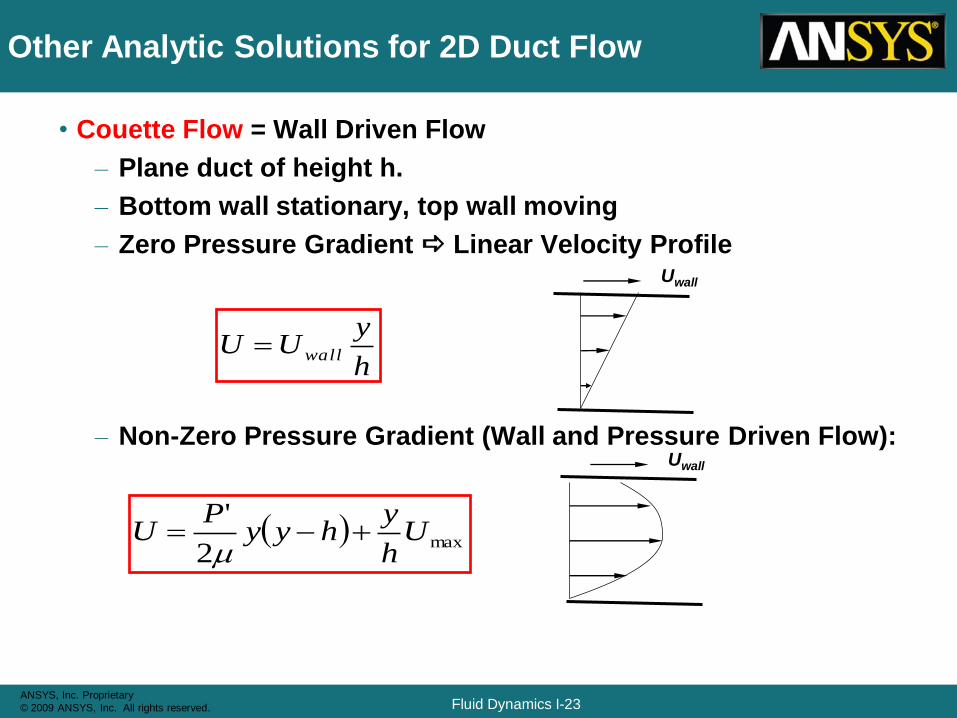
Other Analytic Solutions for 2D Duct Flow
• Couette Flow = Wall Driven Flow
– Plane duct of height h.
– Bottom wall stationary, top wall moving
– Zero Pressure Gradient a Linear Velocity Profile
– Non-Zero Pressure Gradient (Wall and Pressure Driven Flow):
h
yUU wall
Uwall
max2
'U
h
yhyy
PU
Uwall
Fluid Dynamics I-24ANSYS, Inc. Proprietary
© 2009 ANSYS, Inc. All rights reserved.
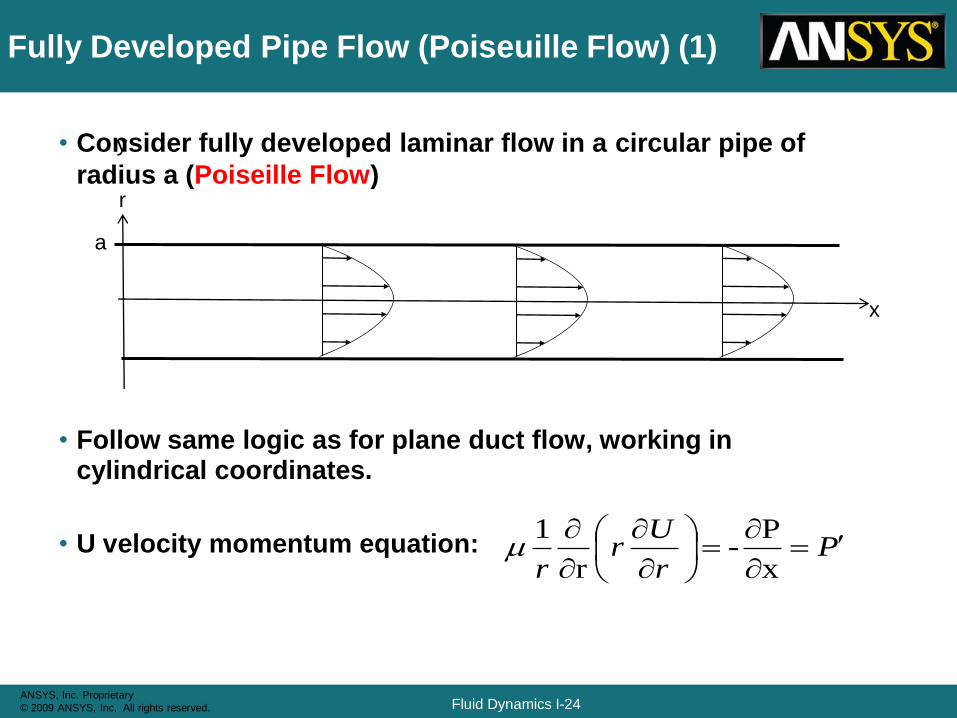
Fully Developed Pipe Flow (Poiseuille Flow) (1)
• Consider fully developed laminar flow in a circular pipe of
radius a (Poiseille Flow)
• Follow same logic as for plane duct flow, working in cylindrical coordinates.
• U velocity momentum equation:
y
x
a
r
x
P-
r
1P
r
Ur
r
Fluid Dynamics I-25ANSYS, Inc. Proprietary
© 2009 ANSYS, Inc. All rights reserved.
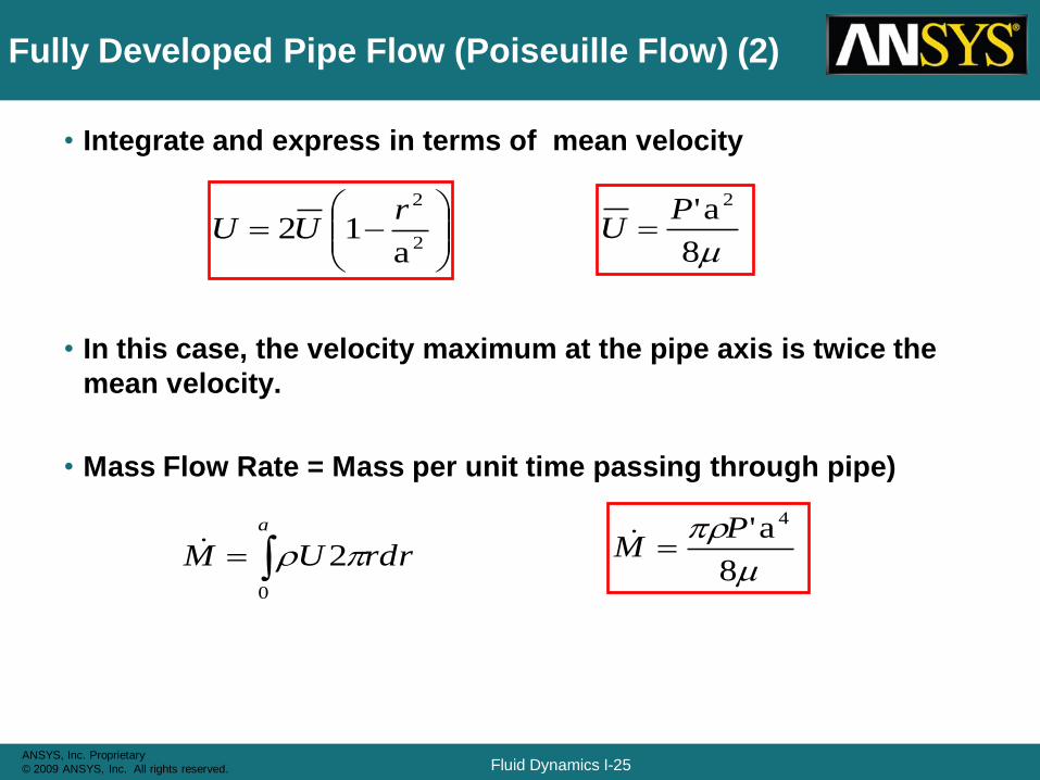
Fully Developed Pipe Flow (Poiseuille Flow) (2)
• Integrate and express in terms of mean velocity
• In this case, the velocity maximum at the pipe axis is twice the
mean velocity.
• Mass Flow Rate = Mass per unit time passing through pipe)
2
2
a1 2
rUU
8
a' 2
PU
20
a
rdrUM r 8
a' 4
rPM
Fluid Dynamics I-26ANSYS, Inc. Proprietary
© 2009 ANSYS, Inc. All rights reserved.
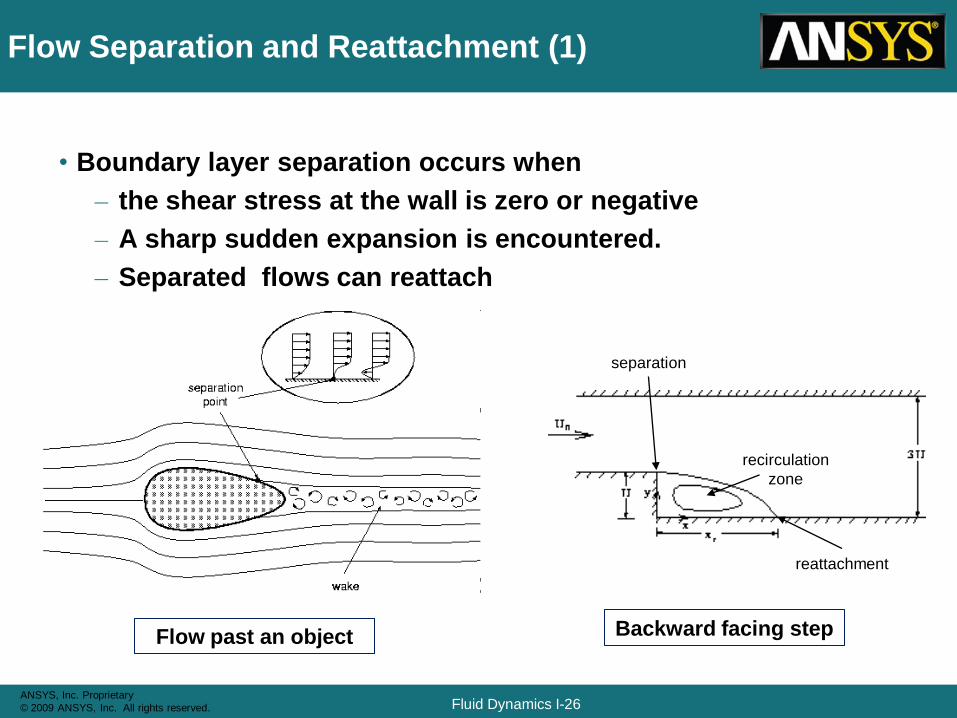
Flow Separation and Reattachment (1)
• Boundary layer separation occurs when
– the shear stress at the wall is zero or negative
– A sharp sudden expansion is encountered.
– Separated flows can reattach
Flow past an object Backward facing step
separation
reattachment
recirculation
zone

Fluid Dynamics I-27ANSYS, Inc. Proprietary
© 2009 ANSYS, Inc. All rights reserved.
CFX Setup:Fluid Domains
Fluid Dynamics I-28ANSYS, Inc. Proprietary
© 2009 ANSYS, Inc. All rights reserved.
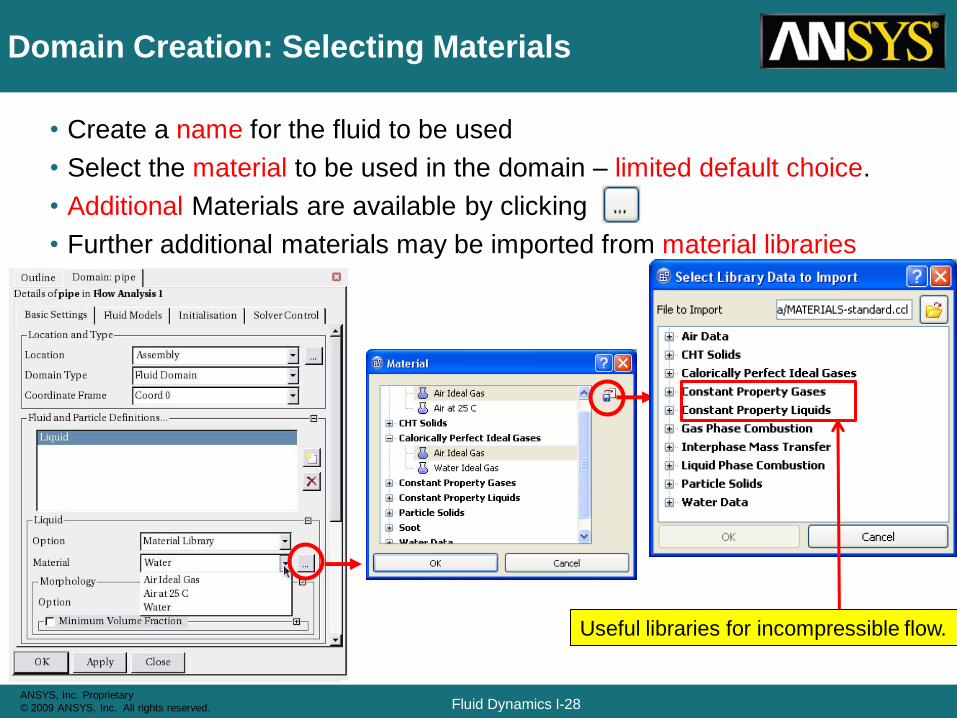
Domain Creation: Selecting Materials
• Create a name for the fluid to be used
• Select the material to be used in the domain – limited default choice.
• Additional Materials are available by clicking
• Further additional materials may be imported from material libraries
Useful libraries for incompressible flow.
Fluid Dynamics I-29ANSYS, Inc. Proprietary
© 2009 ANSYS, Inc. All rights reserved.
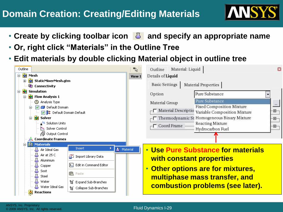
Domain Creation: Creating/Editing Materials
• Create by clicking toolbar icon and specify an appropriate name
• Or, right click “Materials” in the Outline Tree
• Edit materials by double clicking Material object in outline tree
• Use Pure Substance for materials
with constant properties
• Other options are for mixtures,
multiphase mass transfer, and
combustion problems (see later).
Fluid Dynamics I-30ANSYS, Inc. Proprietary
© 2009 ANSYS, Inc. All rights reserved.
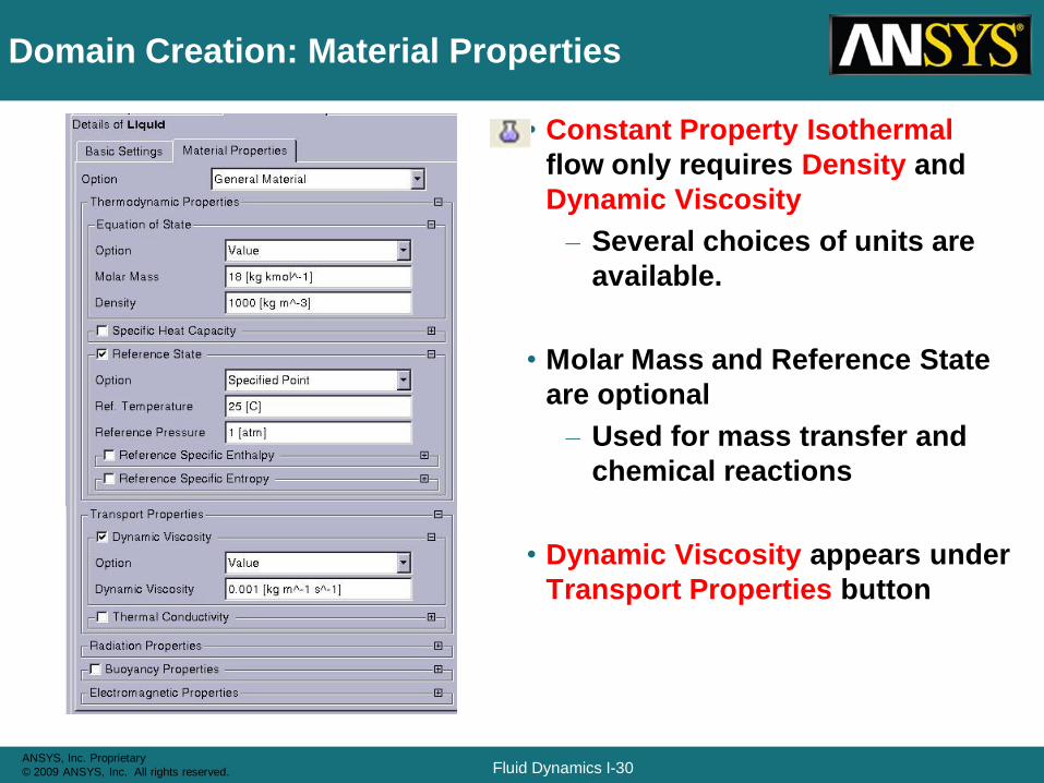
Domain Creation: Material Properties
• Constant Property Isothermal
flow only requires Density and
Dynamic Viscosity
– Several choices of units are
available.
• Molar Mass and Reference State
are optional
– Used for mass transfer and
chemical reactions
• Dynamic Viscosity appears under
Transport Properties button
Fluid Dynamics I-31ANSYS, Inc. Proprietary
© 2009 ANSYS, Inc. All rights reserved.
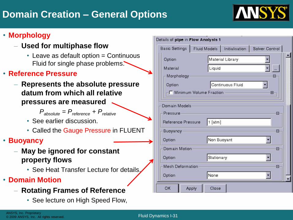
Domain Creation – General Options
• Morphology
– Used for multiphase flow
• Leave as default option = Continuous
Fluid for single phase problems.
• Reference Pressure
– Represents the absolute pressure
datum from which all relative
pressures are measured
Pabsolute = Preference + Prelative
• See earlier discussion.
• Called the Gauge Pressure in FLUENT
• Buoyancy
– May be ignored for constant
property flows
• See Heat Transfer Lecture for details.
• Domain Motion
– Rotating Frames of Reference
• See lecture on High Speed Flow,
Fluid Dynamics I-32ANSYS, Inc. Proprietary
© 2009 ANSYS, Inc. All rights reserved.
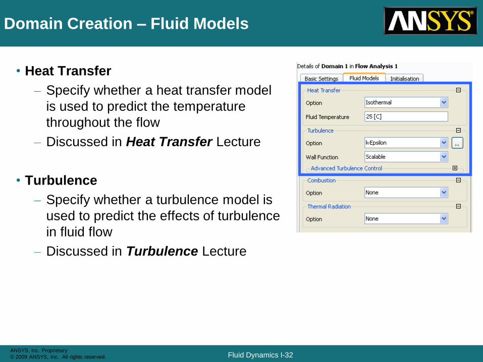
Domain Creation – Fluid Models
• Heat Transfer
– Specify whether a heat transfer model
is used to predict the temperature
throughout the flow
– Discussed in Heat Transfer Lecture
• Turbulence
– Specify whether a turbulence model is
used to predict the effects of turbulence
in fluid flow
– Discussed in Turbulence Lecture
Fluid Dynamics I-33ANSYS, Inc. Proprietary
© 2009 ANSYS, Inc. All rights reserved.
CFX Setup:Boundary Conditions
Fluid Dynamics I-34ANSYS, Inc. Proprietary
© 2009 ANSYS, Inc. All rights reserved.
Defining Boundary Conditions
• Defining Boundary Conditions involves:
– Identifying the location of the boundaries
• e.g., inlets, outlets, walls, symmetry
– Supplying information on the variables at the boundaries
• Variable Values and/or Flux Values
• Data required at a boundary depends upon the boundary condition
type and the physical models employed
• You must be aware of types of the boundary condition available and
locate the boundaries where the flow variables have known values or
can be reasonably approximated
Poorly defined boundary conditions can have a
significant impact on your solution
Fluid Dynamics I-35ANSYS, Inc. Proprietary
© 2009 ANSYS, Inc. All rights reserved.
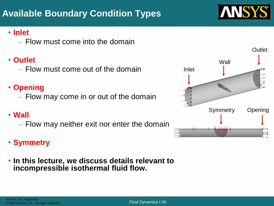
Available Boundary Condition Types
• Inlet
– Flow must come into the domain
• Outlet
– Flow must come out of the domain
• Opening
– Flow may come in or out of the domain
• Wall
– Flow may neither exit nor enter the domain
• Symmetry
• In this lecture, we discuss details relevant to incompressible isothermal fluid flow.
Inlet
Opening
Outlet
Wall
Symmetry
Fluid Dynamics I-36ANSYS, Inc. Proprietary
© 2009 ANSYS, Inc. All rights reserved.
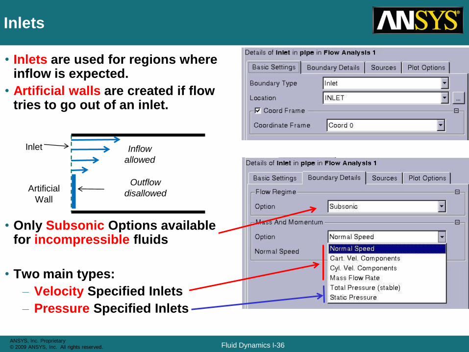
Inlets
• Inlets are used for regions where inflow is expected.
• Artificial walls are created if flow tries to go out of an inlet.
• Only Subsonic Options available for incompressible fluids
• Two main types:
– Velocity Specified Inlets
– Pressure Specified Inlets
Inlet Inflow
allowed
Outflow
disallowedArtificial
Wall
Fluid Dynamics I-37ANSYS, Inc. Proprietary
© 2009 ANSYS, Inc. All rights reserved.
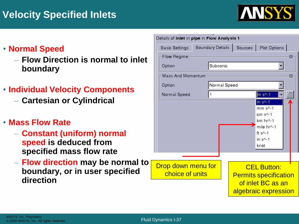
Velocity Specified Inlets
• Normal Speed
– Flow Direction is normal to inlet boundary
• Individual Velocity Components
– Cartesian or Cylindrical
• Mass Flow Rate
– Constant (uniform) normal speed is deduced from specified mass flow rate
– Flow direction may be normal to boundary, or in user specified direction
Drop down menu for
choice of unitsCEL Button:
Permits specification
of inlet BC as an
algebraic expression
Fluid Dynamics I-38ANSYS, Inc. Proprietary
© 2009 ANSYS, Inc. All rights reserved.
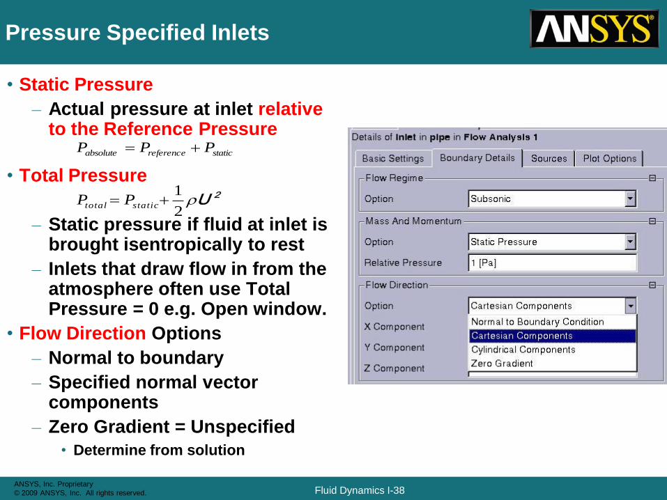
Pressure Specified Inlets
• Static Pressure
– Actual pressure at inlet relative to the Reference Pressure
• Total Pressure
– Static pressure if fluid at inlet is brought isentropically to rest
– Inlets that draw flow in from the atmosphere often use Total Pressure = 0 e.g. Open window.
• Flow Direction Options
– Normal to boundary
– Specified normal vector components
– Zero Gradient = Unspecified
• Determine from solution
2
1 2Ur statictotal PP
staticreferenceabsolute PPP
Fluid Dynamics I-39ANSYS, Inc. Proprietary
© 2009 ANSYS, Inc. All rights reserved.
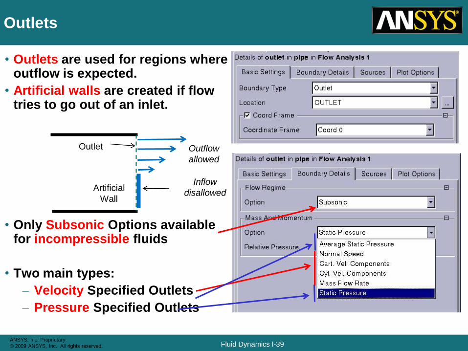
Outlets
• Outlets are used for regions where outflow is expected.
• Artificial walls are created if flow tries to go out of an inlet.
• Only Subsonic Options available for incompressible fluids
• Two main types:
– Velocity Specified Outlets
– Pressure Specified Outlets
Outlet Outflow
allowed
Inflow
disallowedArtificial
Wall
Fluid Dynamics I-40ANSYS, Inc. Proprietary
© 2009 ANSYS, Inc. All rights reserved.
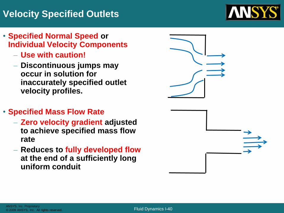
Velocity Specified Outlets
• Specified Normal Speed or Individual Velocity Components
– Use with caution!
– Discontinuous jumps may occur in solution for inaccurately specified outlet velocity profiles.
• Specified Mass Flow Rate
– Zero velocity gradient adjusted to achieve specified mass flow rate
– Reduces to fully developed flow at the end of a sufficiently long uniform conduit
Fluid Dynamics I-41ANSYS, Inc. Proprietary
© 2009 ANSYS, Inc. All rights reserved.
Pressure Specified Outlets
• Static Pressure
– Pressure at outlet relative to the Reference Pressure
– Zero Gradient Conditions applied to velocity
– Fully developed flow at end of a sufficiently long uniform conduit
• Average Static Pressure
– Use when you know the mean outlet pressure, but the outlet pressure distribution is not uniform
– Allows the outlet pressure profile to vary, with the average value constrained to a specific value
• Total Pressure
– Disallowed
– Unconditionally unstable as an outlet BC
• Flow Direction
– Unspecified
– Determined from solution
Fluid Dynamics I-42ANSYS, Inc. Proprietary
© 2009 ANSYS, Inc. All rights reserved.
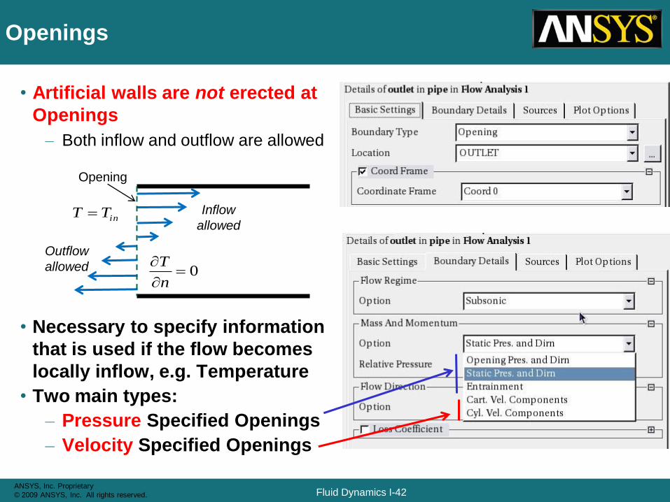
Openings
• Artificial walls are not erected at
Openings
– Both inflow and outflow are allowed
• Necessary to specify information
that is used if the flow becomes
locally inflow, e.g. Temperature
• Two main types:
– Pressure Specified Openings
– Velocity Specified Openings
Opening
Inflow
allowed
Outflow
allowed
inTT
0
n
T
Fluid Dynamics I-43ANSYS, Inc. Proprietary
© 2009 ANSYS, Inc. All rights reserved.
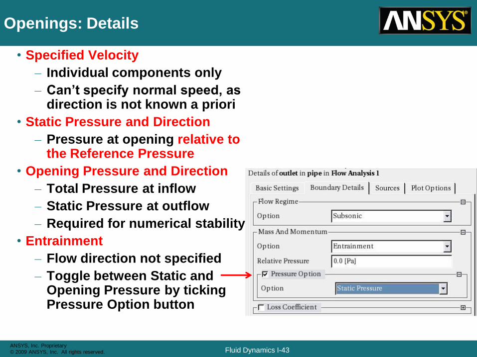
Openings: Details
• Specified Velocity
– Individual components only
– Can’t specify normal speed, as direction is not known a priori
• Static Pressure and Direction
– Pressure at opening relative to the Reference Pressure
• Opening Pressure and Direction
– Total Pressure at inflow
– Static Pressure at outflow
– Required for numerical stability
• Entrainment
– Flow direction not specified
– Toggle between Static and Opening Pressure by ticking Pressure Option button
Fluid Dynamics I-44ANSYS, Inc. Proprietary
© 2009 ANSYS, Inc. All rights reserved.
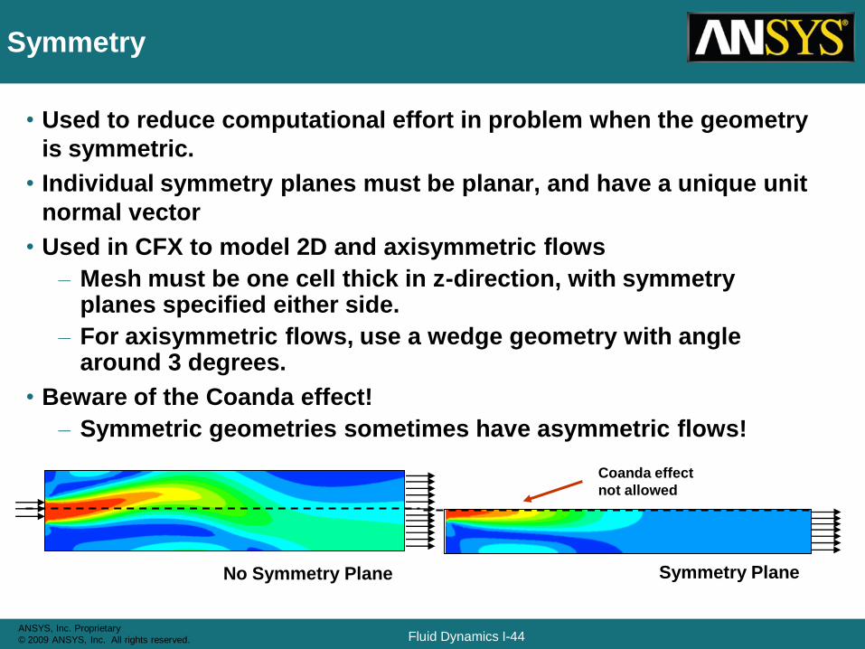
Symmetry
• Used to reduce computational effort in problem when the geometry
is symmetric.
• Individual symmetry planes must be planar, and have a unique unit
normal vector
• Used in CFX to model 2D and axisymmetric flows
– Mesh must be one cell thick in z-direction, with symmetry planes specified either side.
– For axisymmetric flows, use a wedge geometry with angle around 3 degrees.
• Beware of the Coanda effect!
– Symmetric geometries sometimes have asymmetric flows!
No Symmetry Plane Symmetry Plane
Coanda effect
not allowed
Fluid Dynamics I-45ANSYS, Inc. Proprietary
© 2009 ANSYS, Inc. All rights reserved.
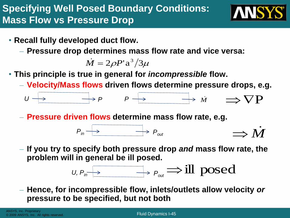
Specifying Well Posed Boundary Conditions:
Mass Flow vs Pressure Drop
• Recall fully developed duct flow.
– Pressure drop determines mass flow rate and vice versa:
• This principle is true in general for incompressible flow.
– Velocity/Mass flows driven flows determine pressure drops, e.g.
– Pressure driven flows determine mass flow rate, e.g.
– If you try to specify both pressure drop and mass flow rate, the problem will in general be ill posed.
– Hence, for incompressible flow, inlets/outlets allow velocity orpressure to be specified, but not both
3a'2 3 rPM
U P P M P
Pin Pout M
U, Pin Pout posed ill
Fluid Dynamics I-46ANSYS, Inc. Proprietary
© 2009 ANSYS, Inc. All rights reserved.
• When there is 1 Inlet and 1 Outlet
– Most Robust: Velocity/Mass Driven Inlet
• Velocity/Mass Flow at Inlet;
• Static Pressure at outlet.
• The inlet pressure is an implicit result of the prediction
– Robust: Velocity/Mass Driven Outlet
• Total or Static Pressure at Inlet;
• Velocity/Mass Flow at outlet.
• The outlet pressure and inlet velocity are determined by the solution.
– Less Robust: Pressure Driven Flow
• Total or Static Pressure at Inlet;
• Static pressure at outlet.
• The system mass flow is part of the solution.
• Ideally, at least one boundary should specify Pressure (either Total
or Static)
Specifying Well Posed Boundary Conditions:
Robustness
Fluid Dynamics I-47ANSYS, Inc. Proprietary
© 2009 ANSYS, Inc. All rights reserved.
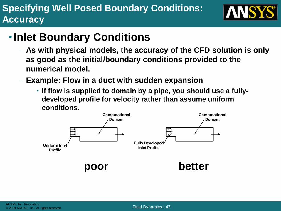
Specifying Well Posed Boundary Conditions:
Accuracy
• Inlet Boundary Conditions– As with physical models, the accuracy of the CFD solution is only
as good as the initial/boundary conditions provided to the
numerical model.
– Example: Flow in a duct with sudden expansion
• If flow is supplied to domain by a pipe, you should use a fully-
developed profile for velocity rather than assume uniform
conditions.
poor better
Fully Developed
Inlet Profile
Computational
Domain
Computational
Domain
Uniform Inlet
Profile
Fluid Dynamics I-48ANSYS, Inc. Proprietary
© 2009 ANSYS, Inc. All rights reserved.
Specifying Well Posed Boundary Conditions:
Accuracy
• Mass flow inlets result in a uniform velocity profile over
the inlet
– Fully developed flow is not achieved
– You cannot specify a mass flow profile
• Mass flow outlets allow a natural velocity profile to
develop based on the upstream conditions
• Pressure specified boundary conditions allow a natural
velocity profile to develop
Fluid Dynamics I-49ANSYS, Inc. Proprietary
© 2009 ANSYS, Inc. All rights reserved.
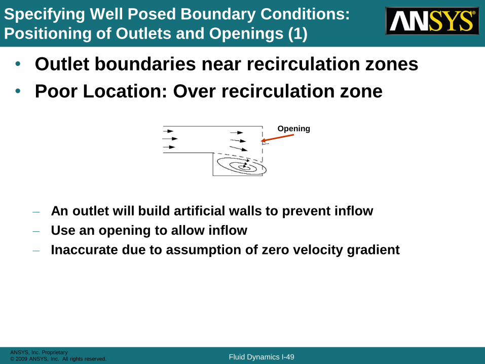
• Outlet boundaries near recirculation zones
• Poor Location: Over recirculation zone
– An outlet will build artificial walls to prevent inflow
– Use an opening to allow inflow
– Inaccurate due to assumption of zero velocity gradient
Specifying Well Posed Boundary Conditions:
Positioning of Outlets and Openings (1)
Opening
Fluid Dynamics I-50ANSYS, Inc. Proprietary
© 2009 ANSYS, Inc. All rights reserved.
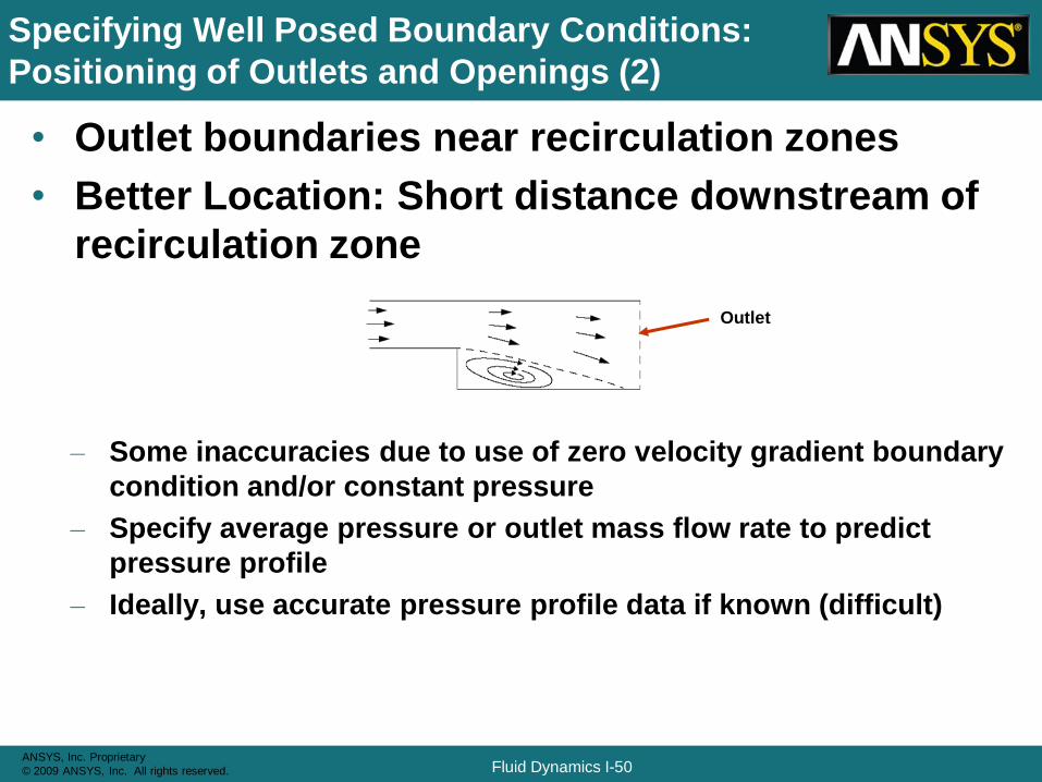
• Outlet boundaries near recirculation zones
• Better Location: Short distance downstream of
recirculation zone
– Some inaccuracies due to use of zero velocity gradient boundary
condition and/or constant pressure
– Specify average pressure or outlet mass flow rate to predict
pressure profile
– Ideally, use accurate pressure profile data if known (difficult)
Specifying Well Posed Boundary Conditions:
Positioning of Outlets and Openings (2)
Outlet
Fluid Dynamics I-51ANSYS, Inc. Proprietary
© 2009 ANSYS, Inc. All rights reserved.
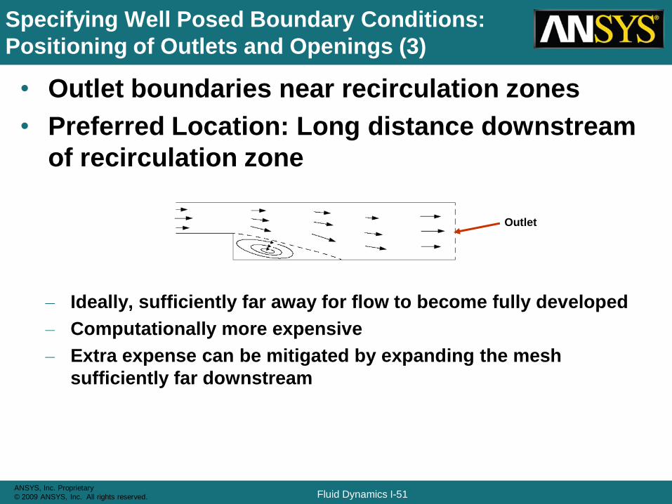
• Outlet boundaries near recirculation zones
• Preferred Location: Long distance downstream
of recirculation zone
– Ideally, sufficiently far away for flow to become fully developed
– Computationally more expensive
– Extra expense can be mitigated by expanding the mesh
sufficiently far downstream
Specifying Well Posed Boundary Conditions:
Positioning of Outlets and Openings (3)
Outlet
Fluid Dynamics I-52ANSYS, Inc. Proprietary
© 2009 ANSYS, Inc. All rights reserved.
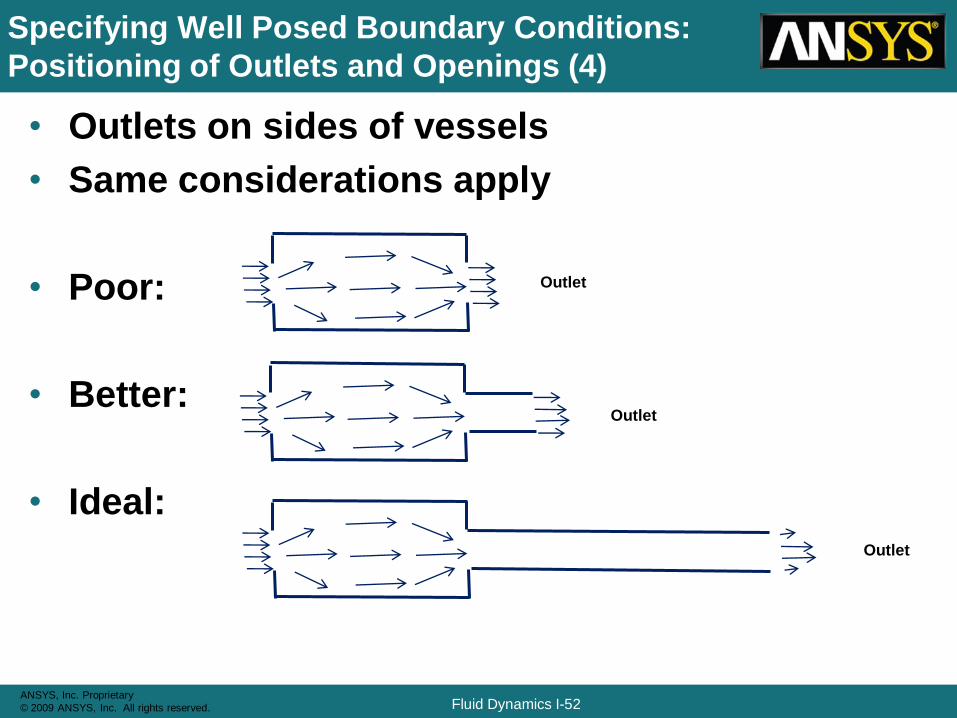
• Outlets on sides of vessels
• Same considerations apply
• Poor:
• Better:
• Ideal:
Specifying Well Posed Boundary Conditions:
Positioning of Outlets and Openings (4)
Outlet
Outlet
Outlet