Visibility of noisy point cloud data

ARTICLE IN PRESS

Computers & Graphics 34 (2010) 219–230

Contents lists available at ScienceDirect

Computers & Graphics

0097-84

doi:10.1

� Corr

E-m

journal homepage: www.elsevier.com/locate/cag

Technical Section

Visibility of noisy point cloud data

Ravish Mehra a,b,�, Pushkar Tripathi a,c, Alla Sheffer d, Niloy J. Mitra a,e

a IIT Delhi, Indiab UNC, Chapel Hill, USAc GaTech, USAd UBC, Canadae KAUST, Saudi Arabia

a r t i c l e i n f o

Article history:

Received 4 December 2009

Received in revised form

12 February 2010

Accepted 7 March 2010

Keywords:

Computer graphics

Point cloud

Visibility

Line and curve generation

Surface reconstruction

Noise smoothing

93/$ - see front matter & 2010 Elsevier Ltd. A

016/j.cag.2010.03.002

esponding author at: UNC, Chapel Hill, USA.

ail address: [email protected] (R. M

a b s t r a c t

We present a robust algorithm for estimating visibility from a given viewpoint for a point set containing

concavities, non-uniformly spaced samples, and possibly corrupted with noise. Instead of performing an

explicit surface reconstruction for the points set, visibility is computed based on a construction

involving convex hull in a dual space, an idea inspired by the work of Katz et al. [26]. We derive

theoretical bounds on the behavior of the method in the presence of noise and concavities, and use the

derivations to develop a robust visibility estimation algorithm. In addition, computing visibility from a

set of adaptively placed viewpoints allows us to generate locally consistent partial reconstructions.

Using a graph based approximation algorithm we couple such reconstructions to extract globally

consistent reconstructions. We test our method on a variety of 2D and 3D point sets of varying

complexity and noise content.

& 2010 Elsevier Ltd. All rights reserved.

1. Introduction

Unorganized point cloud data (PCD) is the natural output ofmany 3D scanning systems. Despite its simplicity, recent research[1,33,22] demonstrates that PCD can be an effective and powerfulshape representation, suitable for model editing and manipula-tion. The simplicity of PCD data-structures, the easy availability of3D scanners as its source, and the promise of generalization tohigher dimensions have all contributed to the popularity of thisrepresentation.

Unlike with other surface representations, the notion ofvisibility for a point set is ambiguous. However, once we have awell defined surface based on a point set, we can uniquely definethe notion of visibility and identify its hidden points, from anyviewpoint. The problem of reconstructing a (smooth) surface froma noisy point set, under moderate sampling requirements, hasbeen extensively studied by the computer graphics [23,27] and bythe computational geometry community (see recent monograph[11]).

Recently Katz et al. [26] introduced the hidden point removal(HPR) operator (see Fig. 1), a simple and elegant algorithm fordetermining point set visibility without explicitly reconstructing

ll rights reserved.

ehra).

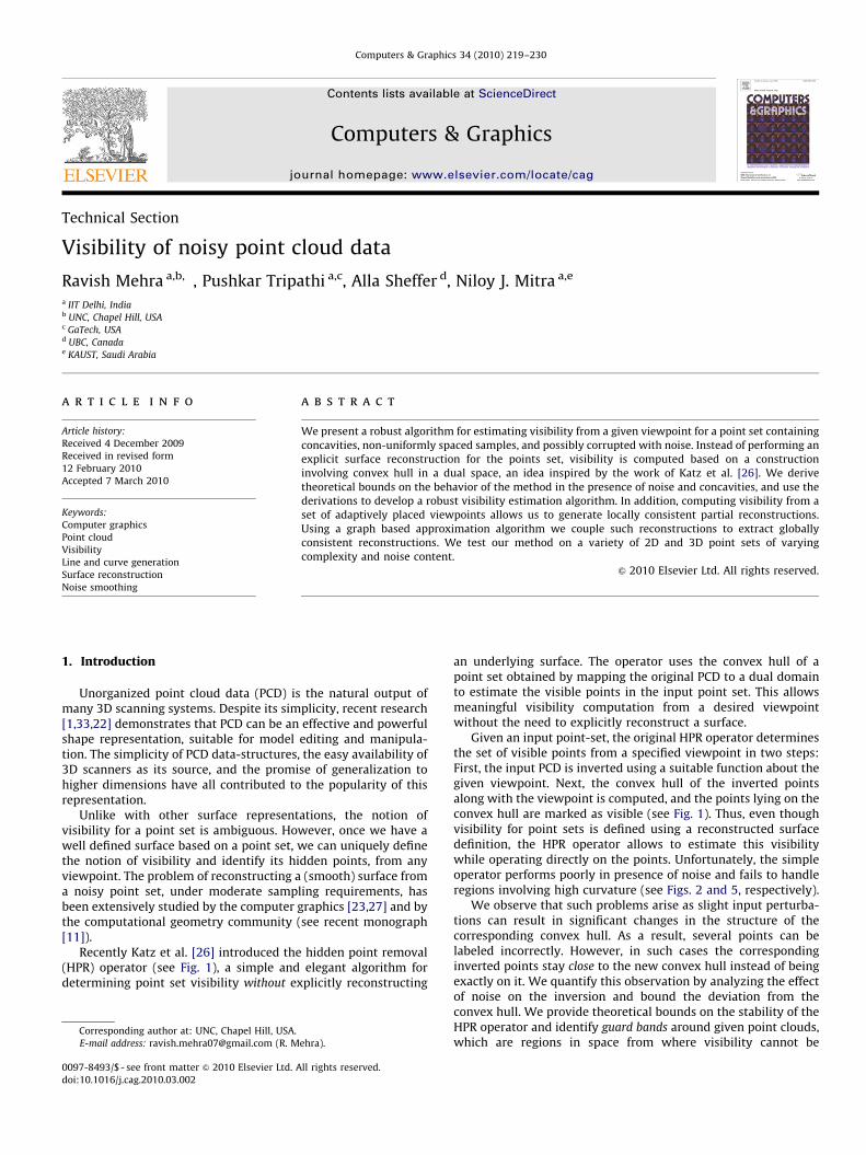
an underlying surface. The operator uses the convex hull of apoint set obtained by mapping the original PCD to a dual domainto estimate the visible points in the input point set. This allowsmeaningful visibility computation from a desired viewpointwithout the need to explicitly reconstruct a surface.

Given an input point-set, the original HPR operator determinesthe set of visible points from a specified viewpoint in two steps:First, the input PCD is inverted using a suitable function about thegiven viewpoint. Next, the convex hull of the inverted pointsalong with the viewpoint is computed, and the points lying on theconvex hull are marked as visible (see Fig. 1). Thus, even thoughvisibility for point sets is defined using a reconstructed surfacedefinition, the HPR operator allows to estimate this visibilitywhile operating directly on the points. Unfortunately, the simpleoperator performs poorly in presence of noise and fails to handleregions involving high curvature (see Figs. 2 and 5, respectively).

We observe that such problems arise as slight input perturba-tions can result in significant changes in the structure of thecorresponding convex hull. As a result, several points can belabeled incorrectly. However, in such cases the correspondinginverted points stay close to the new convex hull instead of beingexactly on it. We quantify this observation by analyzing the effectof noise on the inversion and bound the deviation from theconvex hull. We provide theoretical bounds on the stability of theHPR operator and identify guard bands around given point clouds,which are regions in space from where visibility cannot be

www.elsevier.com/locate/cag

dx.doi.org/10.1016/j.cag.2010.03.002

mailto:[email protected]

ARTICLE IN PRESS

amax

amin C R

Fig. 1. Stages of the basic HPR operator [26]. Figures have been suitably scaled for

illustration: (a) input PCD and viewpoint (in orange); (b) inverted pointset; (c)

convex hull and (d) estimated visible points (in blue).

R. Mehra et al. / Computers & Graphics 34 (2010) 219–230220

reliably estimated using the algorithm. By suitably relaxing thecondition of points lying on the convex hull to include points nearthe convex hull, we arrive at a robust visibility operator.

Using this understanding, we propose simple algorithms forconsistent curve and surface reconstructions. The ability toreliably extract local connectivity information, enables the directapplication of various geometry processing tools on the inputPCD. Piecing together local connectivity inferred from variousadaptively placed viewpoints we build a connectivity graph. Aspecial sub-graph of this graph implicitly encodes a reconstruc-tion for the input PCD. Since extracting this sub-graph turns out tobe an instance of the maximal weight-cycle problem, known to beNP hard, we propose an approximate solution. Besides curve orsurface reconstructions, the connectivity graphs can also be usedfor smoothing the noisy input point set.

Contributions: We analyze the effect of noise in the inverteddomain and obtain a bound for the distortion of the convex hullfor HPR operator. We introduce the concept of guard bands aroundthe point set from where visibility cannot be reliably estimated.This understanding leads to a robust HPR operator, for 2D and 3Dpoint sets, that is used to infer local connectivity, which issubsequently collated using a graph based approximation algo-rithm to extract a consistent manifold.

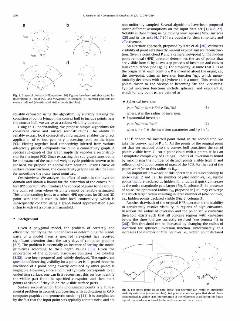
Fig. 2. For noisy point cloud data, basic HPR operator can result in unreliable

visibility estimates (shown in blue). Red points denote samples that should have

been marked as visible. (For interpretation of the references to colour in this figure

legend, the reader is referred to the web version of this article.)

2. Background

Given a polygonal model, the problem of correctly andefficiently identifying the hidden faces or determining the visibleparts of a model from a specified viewpoint has receivedsignificant attention since the early days of computer graphics[5,7]. The problem is essentially an instance of sorting the modelprimitives according to their depth values [36]. Given theimportance of the problem, hardware solutions like z-buffer[8,35] have been proposed and widely deployed. The equivalentquestion of detecting visibility for a point set is ill-posed since thelikelihood of a point being exactly occluded by other points isnegligible. However, since a point set typically corresponds to anunderlying surface, one can first reconstruct this surface, identifythe visible part from the specified viewpoint, and then markpoints as visible if they lie on the visible surface parts.

Surface reconstruction from unorganized points is a funda-mental problem in geometry processing with applications in CAD,computer graphics and geometric modeling [11]. It is complicatedby the fact that the input point sets typically contain noise and are

non-uniformly sampled. Several algorithms have been proposedunder different assumptions on the input data set [3,14,29,27].Notably surface fitting using moving least square (MLS) surfaces[28] and its variants [4,17,24] are popular for their simplicity andeffectiveness.

An alternate approach, proposed by Katz et al. [26], estimatesvisibility of point sets directly without explicit surface reconstruc-tion. Given a point cloud P and a camera viewpoint C, the hiddenpoint removal (HPR) operator determines the set of points thatare visible from C by a two step process of inversion and convexhull computation (see Fig. 1). For simplicity, assume that C is atthe origin. First, each point piAP is inverted about the origin, i.e.,the viewpoint, using an inversion function f ðpiÞ, which mono-tonically decreases with JpiJ (where J:J is a norm). This results inpoints closer to the viewpoint becoming far and vice-versa.Typical inversion functions include spherical and exponential,which for any point pi, are defined as:

�
Spherical inversion
p̂ i :¼ f ðpiÞ ¼ piþ2ðR�JpiJÞpi=JpiJ ð1Þ

where, R is the radius of inversion.
� Exponential inversion
p̂ i :¼ f ðpiÞ ¼ pi=JpiJg

ð2Þ

where, g41 is the inversion parameter and JpiJo1.

Let P̂ denote the inverted point cloud. In the second step, wetake the convex hull of P̂ [C. All the points of the original pointset that get mapped onto the convex hull constitute the set ofpoints visible from C. For a point cloud with n points, it has anasymptotic complexity of O(nlogn). Radius of inversion is foundby maximizing the number of distinct points visible from C andreflection of C about center of mass of the PCD. For the rest of thepaper we refer to this radius as Ropt.

An important drawback of this operator is its susceptibility tonoise (Figs. 2 and 3). The number of false negatives, i.e., visiblepoints that are declared as hidden, for a radius R quickly increaseas the noise magnitude gets larger (Fig. 3, column 2). In presenceof noise, the optimized radius Ropt proposed in [26] may convergeat a much larger radius resulting in large number of false positives,i.e., hidden points declared visible (Fig. 3, column 3).

Another drawback of the original HPR operator is the inabilityto consistently resolve visibility in regions of high curvature.Based on the radius of inversion and the point set, a curvaturethreshold exists such that all concave regions with curvaturebelow the threshold are correctly resolved (see Lemma 4.3 in[26]). This threshold can be increased by changing the radius ofinversion for spherical inversion function. Unfortunately, thisincreases the number of false positives i.e., hidden point declared

ARTICLE IN PRESS

ground truth HPR R = 300amax HPR R = Ropt robust HPR

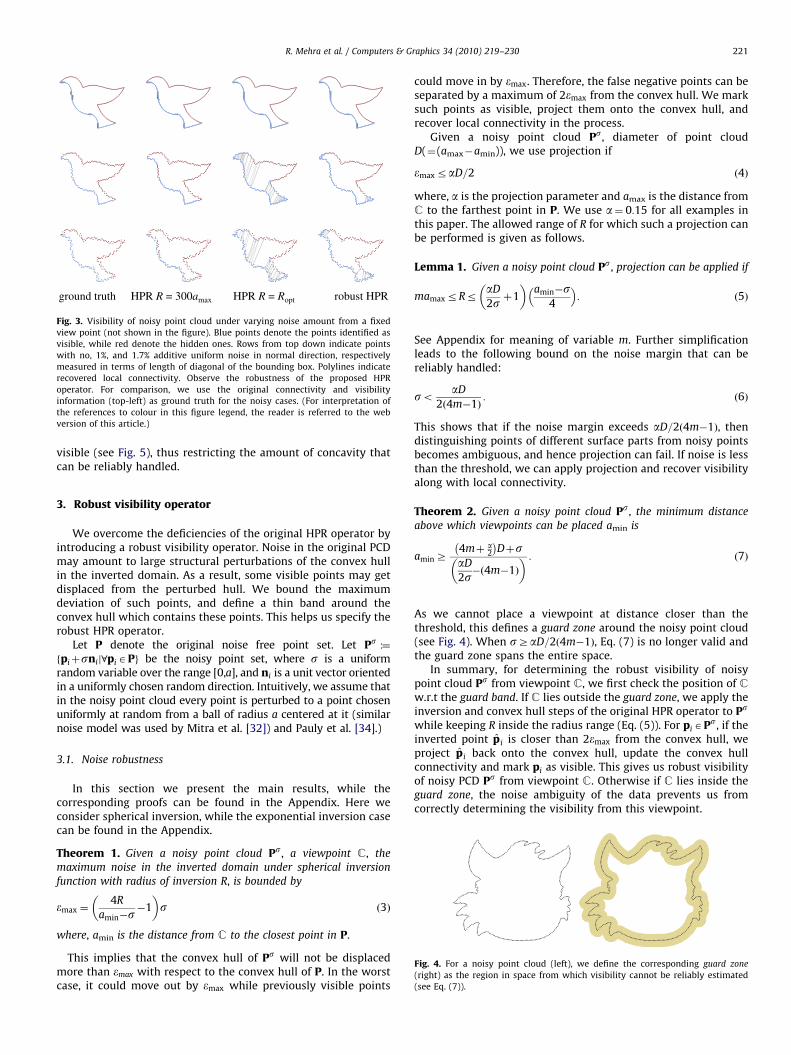
Fig. 3. Visibility of noisy point cloud under varying noise amount from a fixed

view point (not shown in the figure). Blue points denote the points identified as

visible, while red denote the hidden ones. Rows from top down indicate points

with no, 1%, and 1.7% additive uniform noise in normal direction, respectively

measured in terms of length of diagonal of the bounding box. Polylines indicate

recovered local connectivity. Observe the robustness of the proposed HPR

operator. For comparison, we use the original connectivity and visibility

information (top-left) as ground truth for the noisy cases. (For interpretation of

the references to colour in this figure legend, the reader is referred to the web

version of this article.)

R. Mehra et al. / Computers & Graphics 34 (2010) 219–230 221

visible (see Fig. 5), thus restricting the amount of concavity thatcan be reliably handled.

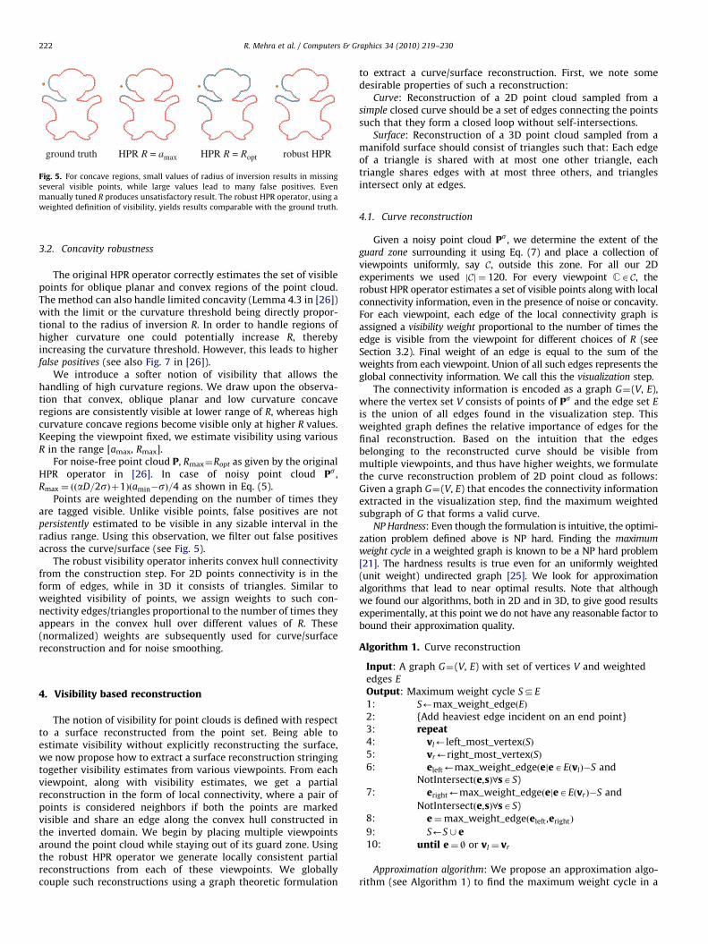
Fig. 4. For a noisy point cloud (left), we define the corresponding guard zone

(right) as the region in space from which visibility cannot be reliably estimated

(see Eq. (7)).

3. Robust visibility operator

We overcome the deficiencies of the original HPR operator byintroducing a robust visibility operator. Noise in the original PCDmay amount to large structural perturbations of the convex hullin the inverted domain. As a result, some visible points may getdisplaced from the perturbed hull. We bound the maximumdeviation of such points, and define a thin band around theconvex hull which contains these points. This helps us specify therobust HPR operator.

Let P denote the original noise free point set. Let Ps :¼fpiþsnij8piAPg be the noisy point set, where s is a uniformrandom variable over the range [0,a], and ni is a unit vector orientedin a uniformly chosen random direction. Intuitively, we assume thatin the noisy point cloud every point is perturbed to a point chosenuniformly at random from a ball of radius a centered at it (similarnoise model was used by Mitra et al. [32]) and Pauly et al. [34].)

3.1. Noise robustness

In this section we present the main results, while thecorresponding proofs can be found in the Appendix. Here weconsider spherical inversion, while the exponential inversion casecan be found in the Appendix.

Theorem 1. Given a noisy point cloud Ps, a viewpoint C, the

maximum noise in the inverted domain under spherical inversion

function with radius of inversion R, is bounded by

emax ¼4R

amin�s�1

� �s ð3Þ

where, amin is the distance from C to the closest point in P.

This implies that the convex hull of Ps will not be displacedmore than emax with respect to the convex hull of P. In the worstcase, it could move out by emax while previously visible points

could move in by emax. Therefore, the false negative points can beseparated by a maximum of 2emax from the convex hull. We marksuch points as visible, project them onto the convex hull, andrecover local connectivity in the process.

Given a noisy point cloud Ps, diameter of point cloudD(¼(amax�amin)), we use projection if

emaxraD=2 ð4Þ

where, a is the projection parameter and amax is the distance fromC to the farthest point in P. We use a¼ 0:15 for all examples inthis paper. The allowed range of R for which such a projection canbe performed is given as follows.

Lemma 1. Given a noisy point cloud Ps, projection can be applied if

mamaxrRraD

2s þ1

� �amin�s

4

� �: ð5Þ

See Appendix for meaning of variable m. Further simplificationleads to the following bound on the noise margin that can bereliably handled:

so aD

2ð4m�1Þ: ð6Þ

This shows that if the noise margin exceeds aD=2ð4m�1Þ, thendistinguishing points of different surface parts from noisy pointsbecomes ambiguous, and hence projection can fail. If noise is lessthan the threshold, we can apply projection and recover visibilityalong with local connectivity.

Theorem 2. Given a noisy point cloud Ps, the minimum distance

above which viewpoints can be placed amin is

aminZ4mþ a

2

� �Dþs

aD

2s�ð4m�1Þ

� � : ð7Þ

As we cannot place a viewpoint at distance closer than thethreshold, this defines a guard zone around the noisy point cloud(see Fig. 4). When sZaD=2ð4m�1Þ, Eq. (7) is no longer valid andthe guard zone spans the entire space.

In summary, for determining the robust visibility of noisypoint cloud Ps from viewpoint C, we first check the position of Cw.r.t the guard band. If C lies outside the guard zone, we apply theinversion and convex hull steps of the original HPR operator to Ps

while keeping R inside the radius range (Eq. (5)). For piAPs, if theinverted point p̂ i is closer than 2emax from the convex hull, weproject p̂i back onto the convex hull, update the convex hullconnectivity and mark pi as visible. This gives us robust visibilityof noisy PCD Ps from viewpoint C. Otherwise if C lies inside theguard zone, the noise ambiguity of the data prevents us fromcorrectly determining the visibility from this viewpoint.

ARTICLE IN PRESS

ground truth HPR R = Ropt robust HPRHPR R = amax

Fig. 5. For concave regions, small values of radius of inversion results in missing

several visible points, while large values lead to many false positives. Even

manually tuned R produces unsatisfactory result. The robust HPR operator, using a

weighted definition of visibility, yields results comparable with the ground truth.


3.2. Concavity robustness

The original HPR operator correctly estimates the set of visiblepoints for oblique planar and convex regions of the point cloud.The method can also handle limited concavity (Lemma 4.3 in [26])with the limit or the curvature threshold being directly propor-tional to the radius of inversion R. In order to handle regions ofhigher curvature one could potentially increase R, therebyincreasing the curvature threshold. However, this leads to higherfalse positives (see also Fig. 7 in [26]).

We introduce a softer notion of visibility that allows thehandling of high curvature regions. We draw upon the observa-tion that convex, oblique planar and low curvature concaveregions are consistently visible at lower range of R, whereas highcurvature concave regions become visible only at higher R values.Keeping the viewpoint fixed, we estimate visibility using variousR in the range [amax, Rmax].

For noise-free point cloud P, Rmax¼Ropt as given by the originalHPR operator in [26]. In case of noisy point cloud Ps,Rmax ¼ ððaD=2sÞþ1Þðamin�sÞ=4 as shown in Eq. (5).

Points are weighted depending on the number of times theyare tagged visible. Unlike visible points, false positives are notpersistently estimated to be visible in any sizable interval in theradius range. Using this observation, we filter out false positivesacross the curve/surface (see Fig. 5).

The robust visibility operator inherits convex hull connectivityfrom the construction step. For 2D points connectivity is in theform of edges, while in 3D it consists of triangles. Similar toweighted visibility of points, we assign weights to such con-nectivity edges/triangles proportional to the number of times theyappears in the convex hull over different values of R. These(normalized) weights are subsequently used for curve/surfacereconstruction and for noise smoothing.

4. Visibility based reconstruction

The notion of visibility for point clouds is defined with respectto a surface reconstructed from the point set. Being able toestimate visibility without explicitly reconstructing the surface,we now propose how to extract a surface reconstruction stringingtogether visibility estimates from various viewpoints. From eachviewpoint, along with visibility estimates, we get a partialreconstruction in the form of local connectivity, where a pair ofpoints is considered neighbors if both the points are markedvisible and share an edge along the convex hull constructed inthe inverted domain. We begin by placing multiple viewpointsaround the point cloud while staying out of its guard zone. Usingthe robust HPR operator we generate locally consistent partialreconstructions from each of these viewpoints. We globallycouple such reconstructions using a graph theoretic formulation

to extract a curve/surface reconstruction. First, we note somedesirable properties of such a reconstruction:

Curve: Reconstruction of a 2D point cloud sampled from asimple closed curve should be a set of edges connecting the pointssuch that they form a closed loop without self-intersections.

Surface: Reconstruction of a 3D point cloud sampled from amanifold surface should consist of triangles such that: Each edgeof a triangle is shared with at most one other triangle, eachtriangle shares edges with at most three others, and trianglesintersect only at edges.

4.1. Curve reconstruction

Given a noisy point cloud Ps, we determine the extent of theguard zone surrounding it using Eq. (7) and place a collection ofviewpoints uniformly, say C, outside this zone. For all our 2Dexperiments we used jCj ¼ 120. For every viewpoint CAC, therobust HPR operator estimates a set of visible points along with localconnectivity information, even in the presence of noise or concavity.For each viewpoint, each edge of the local connectivity graph isassigned a visibility weight proportional to the number of times theedge is visible from the viewpoint for different choices of R (seeSection 3.2). Final weight of an edge is equal to the sum of theweights from each viewpoint. Union of all such edges represents theglobal connectivity information. We call this the visualization step.

The connectivity information is encoded as a graph G¼(V, E),where the vertex set V consists of points of Ps and the edge set E

is the union of all edges found in the visualization step. Thisweighted graph defines the relative importance of edges for thefinal reconstruction. Based on the intuition that the edgesbelonging to the reconstructed curve should be visible frommultiple viewpoints, and thus have higher weights, we formulatethe curve reconstruction problem of 2D point cloud as follows:Given a graph G¼(V, E) that encodes the connectivity informationextracted in the visualization step, find the maximum weightedsubgraph of G that forms a valid curve.

NP Hardness: Even though the formulation is intuitive, the optimi-zation problem defined above is NP hard. Finding the maximum

weight cycle in a weighted graph is known to be a NP hard problem[21]. The hardness results is true even for an uniformly weighted(unit weight) undirected graph [25]. We look for approximationalgorithms that lead to near optimal results. Note that althoughwe found our algorithms, both in 2D and in 3D, to give good resultsexperimentally, at this point we do not have any reasonable factor tobound their approximation quality.

Algorithm 1. Curve reconstruction

Input: A graph G¼(V, E) with set of vertices V and weightededges E

Output: Maximum weight cycle SDE

1:
S’max_weight_edgeðEÞ 2: {Add heaviest edge incident on an end point} 3: repeat 4: vl’left_most_vertexðSÞ 5: vr’right_most_vertexðSÞ 6: eleft’max_weight_edgeðejeAEðvlÞ�S and
NotIntersectðe,sÞ8sAS)
7: eright’max_weight_edgeðejeAEðvrÞ�S and
NotIntersectðe,sÞ8sAS)
8: e¼max_weight_edgeðeleft,erightÞ
9:
S’S [ e 10: until e¼ | or vl ¼ vr
Approximation algorithm: We propose an approximation algo-
rithm (see Algorithm 1) to find the maximum weight cycle in a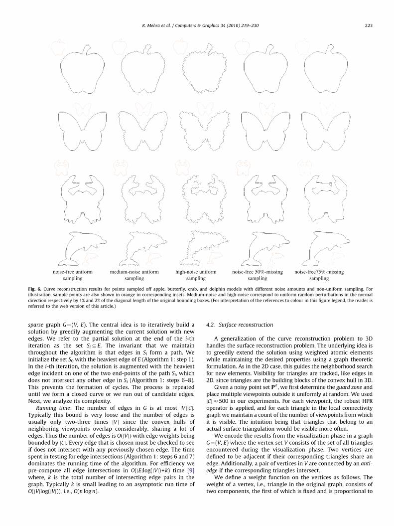

ARTICLE IN PRESS

noise-free uniformsampling

high-noise uniformsampling

noise-free 50%-missingsampling

noise-free75%-missingsampling

medium-noise uniformsampling

Fig. 6. Curve reconstruction results for points sampled off apple, butterfly, crab, and dolphin models with different noise amounts and non-uniform sampling. For

illustration, sample points are also shown in orange in corresponding insets. Medium-noise and high-noise correspond to uniform random perturbations in the normal

direction respectively by 1% and 2% of the diagonal length of the original bounding boxes. (For interpretation of the references to colour in this figure legend, the reader is

referred to the web version of this article.)


sparse graph G¼(V, E). The central idea is to iteratively build asolution by greedily augmenting the current solution with newedges. We refer to the partial solution at the end of the i-thiteration as the set SiDE. The invariant that we maintainthroughout the algorithm is that edges in Si form a path. Weinitialize the set S0 with the heaviest edge of E (Algorithm 1: step 1).In the i-th iteration, the solution is augmented with the heaviestedge incident on one of the two end-points of the path Si, whichdoes not intersect any other edge in Si (Algorithm 1: steps 6–8).This prevents the formation of cycles. The process is repeateduntil we form a closed curve or we run out of candidate edges.Next, we analyze its complexity.

Running time: The number of edges in G is at most jV jjCj.Typically this bound is very loose and the number of edges isusually only two-three times jV j since the convex hulls ofneighboring viewpoints overlap considerably, sharing a lot ofedges. Thus the number of edges is OðjV jÞwith edge weights beingbounded by jCj. Every edge that is chosen must be checked to seeif does not intersect with any previously chosen edge. The timespent in testing for edge intersections (Algorithm 1: steps 6 and 7)dominates the running time of the algorithm. For efficiency wepre-compute all edge intersections in O(jEjlog(jVj)+k) time [9]where, k is the total number of intersecting edge pairs in thegraph. Typically k is small leading to an asymptotic run time ofO(jVjlog(jVj)), i.e., O(n log n).

4.2. Surface reconstruction

A generalization of the curve reconstruction problem to 3Dhandles the surface reconstruction problem. The underlying idea isto greedily extend the solution using weighted atomic elementswhile maintaining the desired properties using a graph theoreticformulation. As in the 2D case, this guides the neighborhood searchfor new elements. Visibility for triangles are tracked, like edges in2D, since triangles are the building blocks of the convex hull in 3D.

Given a noisy point set Ps, we first determine the guard zone andplace multiple viewpoints outside it uniformly at random. We usedjCj � 500 in our experiments. For each viewpoint, the robust HPRoperator is applied, and for each triangle in the local connectivitygraph we maintain a count of the number of viewpoints from whichit is visible. The intuition being that triangles that belong to anactual surface triangulation would be visible more often.

We encode the results from the visualization phase in a graphG¼(V, E) where the vertex set V consists of the set of all trianglesencountered during the visualization phase. Two vertices aredefined to be adjacent if their corresponding triangles share anedge. Additionally, a pair of vertices in V are connected by an anti-

edge if the corresponding triangles intersect.We define a weight function on the vertices as follows. The

weight of a vertex, i.e., triangle in the original graph, consists oftwo components, the first of which is fixed and is proportional to

ARTICLE IN PRESS

noise-free uniformsampling

medium-noise uniformsampling

high-noise uniformsampling



new

Gat

han

crus

tC

C-c

rust

robu

st H

PR

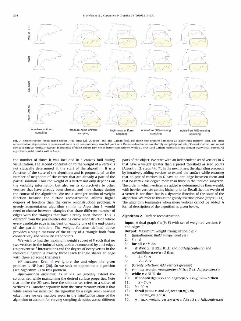
Fig. 7. Reconstruction result using robust HPR, crust [2], CC-crust [16], and Gathan [19]. For noise-free uniform sampling all algorithms perform well. The crust

reconstruction degenerates in presence of noise or on non-uniformly sampled point sets. On noise-free but non-uniformly sampled point sets, CC-crust, Gathan, and robust

HPR give similar results. However, in presence of noise, robust HPR yields better connectivity, while CC-crust and Gathan reconstructions contain many small curves. All

algorithms yield results within 1–2 s.


the number of times it was included in a convex hull duringvisualization. The second contribution to the weight of a vertex isnot statically determined at the start of the algorithm. It is afunction of the state of the algorithm and is proportional to thenumber of neighbors of the vertex that are already a part of thepartial solution. Thus the weight of a vertex not only depends onthe visibility information but also on its connectivity to othervertices that have already been chosen, and may change duringthe course of the algorithm. We use a stronger notion of weightfunction because the surface reconstruction affords higherdegrees of freedom than the curve reconstruction problem. Agreedy augmentation algorithm similar to Algorithm 1, wouldneed to choose between triangles that share different number ofedges with the triangles that have already been chosen. This isdifferent from the possibilities during curve reconstruction whereevery candidate edge is incident on exactly one of the end-pointsof the partial solution. The weight function defined aboveprovides a single measure of the utility of a triangle both fromconnectivity and visibility standpoints.

We wish to find the maximum weight subset of V such that notwo vertices in the induced subgraph are connected by anti-edges(to prevent self-intersection) and the degree of every vertex in theinduced subgraph is exactly three (each triangle shares an edgewith three adjacent triangles).

NP hardness: Even if we ignore the anti-edges the givenproblem is NP hard [20]. So we seek an approximate algorithm(see Algorithm 2) to this problem.

Approximation algorithm: As in 2D, we greedily extend thesolution set, while maintaining the desired surface properties. Notethat unlike the 2D case, here the solution set refers to a subset ofvertices in G. Another departure from the curve reconstruction is thatwhile earlier we initialized the algorithm by a single seed (heaviestedge), here we use multiple seeds in the initialization phase of thealgorithm to account for varying sampling densities across different

parts of the object. We start with an independent set of vertices in G

that have a weight greater than a preset threshold as seed points(Algorithm 2: steps 4 to 7). In the next phase, the algorithm proceedsby iteratively adding vertices to extend the surface while ensuringthat no pair of vertices in G have an anti-edge between them andthat no vertex has degree more than three in the induced subgraph.The order in which vertices are added is determined by their weight,with heavier vertices getting higher priority. Recall that the weight ofa vertex is not fixed but is a dynamic function of the state of thealgorithm. We refer to this as the greedy selection phase (steps 9–13).The algorithm terminates when more vertices cannot be added. Aformal description of the algorithm is given below.

Algorithm 2. Surface reconstruction

Input: A dual graph G¼(V, E) with set of weighted vertices V

and edges E

Output: Maximum weight triangulation SDV

1:
{Initialization: Build independent set} 2: S f 3: for all vAV do 4: if WðvÞZ THRESHOLD and notAdjacentðu,vÞ and
noAntiEdgeðu,vÞ8uAS then
5: S’S [ v 6: V’V�v 7: {Greedy Selection: Add vertices greedily} 8: v’max_weight_vertexðwjwAV ,(sAS s:t: Adjacentðw,sÞÞ 9: while vaNULL do 10: if noAntiEdgeðu,vÞ and degreeðu,S [ vÞr38uAS then 11: S’S [ v 12: V’V�v 13: forall (ujuAV and Adjacentðu,vÞ)) do 14: update_weight(u) 15: v’max_weight_vertexðwjwAV ,(sAS s:t: Adjacentðw,sÞÞ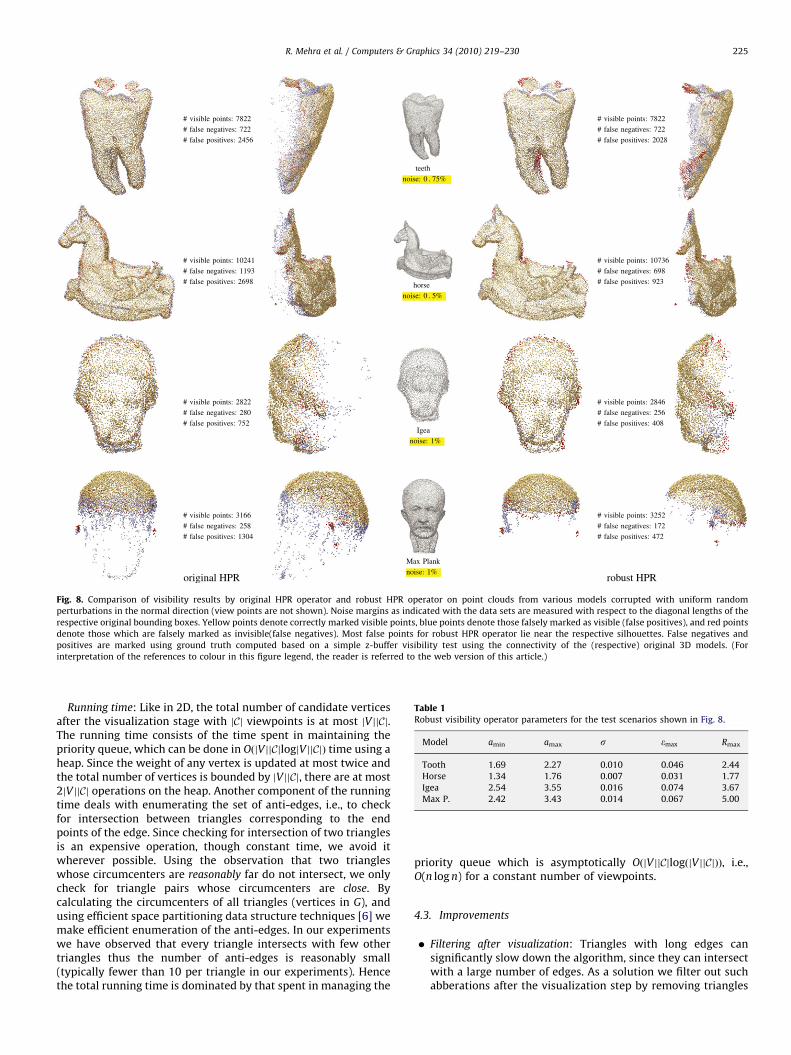

ARTICLE IN PRESS

original HPR robust HPR

# visible points: 7822

# false negatives: 722

# false positives: 2456






















teeth

noise: 0 . 75%

horse

noise: 0 . 5%

Igea

noise: 1%

Max Plank

noise: 1%

Fig. 8. Comparison of visibility results by original HPR operator and robust HPR operator on point clouds from various models corrupted with uniform random

perturbations in the normal direction (view points are not shown). Noise margins as indicated with the data sets are measured with respect to the diagonal lengths of the

respective original bounding boxes. Yellow points denote correctly marked visible points, blue points denote those falsely marked as visible (false positives), and red points

denote those which are falsely marked as invisible(false negatives). Most false points for robust HPR operator lie near the respective silhouettes. False negatives and

positives are marked using ground truth computed based on a simple z-buffer visibility test using the connectivity of the (respective) original 3D models. (For

interpretation of the references to colour in this figure legend, the reader is referred to the web version of this article.)

Table 1Robust visibility operator parameters for the test scenarios shown in Fig. 8.

Model amin amax s emax Rmax

Tooth 1.69 2.27 0.010 0.046 2.44

Horse 1.34 1.76 0.007 0.031 1.77

Igea 2.54 3.55 0.016 0.074 3.67

Max P. 2.42 3.43 0.014 0.067 5.00


Running time: Like in 2D, the total number of candidate verticesafter the visualization stage with jCj viewpoints is at most jV jjCj.The running time consists of the time spent in maintaining thepriority queue, which can be done in OðjV jjCjlogjV jjCjÞ time using aheap. Since the weight of any vertex is updated at most twice andthe total number of vertices is bounded by jV jjCj, there are at most2jV jjCj operations on the heap. Another component of the runningtime deals with enumerating the set of anti-edges, i.e., to checkfor intersection between triangles corresponding to the endpoints of the edge. Since checking for intersection of two trianglesis an expensive operation, though constant time, we avoid itwherever possible. Using the observation that two triangleswhose circumcenters are reasonably far do not intersect, we onlycheck for triangle pairs whose circumcenters are close. Bycalculating the circumcenters of all triangles (vertices in G), andusing efficient space partitioning data structure techniques [6] wemake efficient enumeration of the anti-edges. In our experimentswe have observed that every triangle intersects with few othertriangles thus the number of anti-edges is reasonably small(typically fewer than 10 per triangle in our experiments). Hencethe total running time is dominated by that spent in managing the

priority queue which is asymptotically OðjV jjCjlogðjV jjCjÞÞ, i.e.,O(n log n) for a constant number of viewpoints.

4.3. Improvements

�
Filtering after visualization: Triangles with long edges cansignificantly slow down the algorithm, since they can intersectwith a large number of edges. As a solution we filter out suchabberations after the visualization step by removing triangles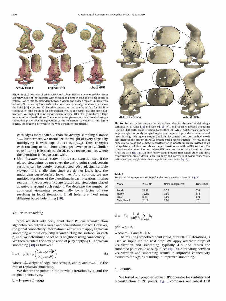

ARTICLE IN PRESS

Fig. 10. Reconstruction outputs on raw scanned data for the coati model using a

combination of AMLS [18] and cocone [12] (left), and robust HPR based smoothing

(Section 4.4) with reconstruction (Algorithm 2). While AMLS-cocone generate

large triangles in poorly sampled regions our approach provides a more natural

result leaving such regions empty. Similarly, by construction, our method avoids

self intersections present in AMLS-cocone based reconstruction. The raw scan is

thick due to noise and a direct reconstruction is unnatural. Hence instead of an

interpolatory solution, we choose approximation as with AMLS method. For

smoothing the point cloud for robust HPR, we use connectivity based on robust

HPR (see also Fig. 14). On such noisy scans original HPR based quick-and-dirty

reconstruction breaks down, since visibility and convex-hull based connectivity

Fig. 9. Typical behavior of original HPR and robust HPR on raw scanned data from

a given viewpoint (not shown), with the hidden points in pink and visible points in

yellow. Notice that the boundary between visible and hidden regions is sharp with

robust HPR, indicating few misclassifications. In absence of ground truth, we show

the AMLS [18] + cocone [12] based reconstruction and use the surface for visibility

computation (left column) for comparison. Notice the result also has misclassi-

fications. We highlight some regions where original HPR clearly produces a large

number of misclassifications. The scanner noise parameter s is estimated using a

calibration plane. (For interpretation of the references to colour in this figure



with edges more than 5� than the average sampling distancesavg. Furthermore, we normalize the weight of every edge e bymultiplying it with expð�2 � jJeJ�savgj=savgÞ. Thus, triangleswith too long or too short edges get lower priority. Similaredge filtering is less critical for 2D curve reconstruction, wherethe algorithm is fast to start with.

estimates from single views have significant errors (see Fig. 9).
�
Table 2Robust visibility operator timings for the test scenarios shown in Fig. 8.

Model # Points Noise margin (%) Time (ms)

Tooth 21.9k 0.75 531

Horse 32.3k 0.50 681

Igea 8.3k 1.00 171

Max Planck 20.0k 1.00 375

Multi-iteration reconstruction: In the reconstruction step, if theplaced viewpoints do not cover the entire point cloud, certainsections can be poorly reconstructed. Also placing suitableviewpoints is challenging since we do not know how theunderlying curve/surface looks like. As a solution, we usemultiple iterations of the algorithm. In each iteration, missingregions in the curve/surface are located and viewpoints placedadaptively around such regions. We decrease the number ofadditional viewpoints exponentially by a factor of tworesulting in logjCj iterations. Small holes are fixed usingdiffusion based hole filling [10].

4.4. Noise-smoothing

Since we start with noisy point cloud Ps, our reconstructionalgorithm can output a rough and non-uniform surface. However,the global connectivity information E allows us to apply Laplaciansmoothing without explicitly reconstructing the surface. For eachpiAPs, we determine the set of its neighbors using connectivity E.We then calculate the new position of pi by applying HC Laplaciansmoothing [30] as follows :

li ¼ ð1�rÞpiþrP

jAAdjðiÞwijpjP

jAAdjðiÞwij

!ð8Þ

where wji¼weight of edge connecting pi and pj and r¼ 0:1 is the

rate of Laplacian smoothing.We denote the points in the previous iteration by qi and the

original points by oi.

bi ¼ li�ðaoiþð1�aÞqiÞ

di ¼�bbi�1�bjAdjðiÞj

XjAAdjðiÞ

bj

pnewi ¼ piþdi

where a¼ 1 and b¼ 0:6.The resulting smoothed point cloud, after 80–100 iterations, is

used as input for the next step. We apply alternate steps ofvisualization and smoothing, typically 4–5, and return thesmoothed point cloud as output (see Fig. 14). Alternating betweenvisualization and smoothing results in improved connectivityestimates for G(V, E) resulting in improved smoothing.

5. Results

We tested our proposed robust HPR operator for visibility andreconstruction of 2D points. Fig. 3 compares our robust HPR

ARTICLE IN PRESS

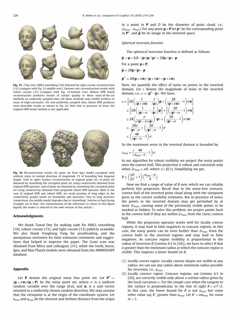
Fig. 12. (Top row) Input noisy point sets are smoothed and reconstructed using the robust HPR operator on torus, Igea, kitten, duck and Pierrot models, respectively.

Connectivity information from the smoothed reconstructions (middle row) are mapped back to the original noisy data sets (bottom row). Insets highlight artifacts due to

poor sampling or concavity.

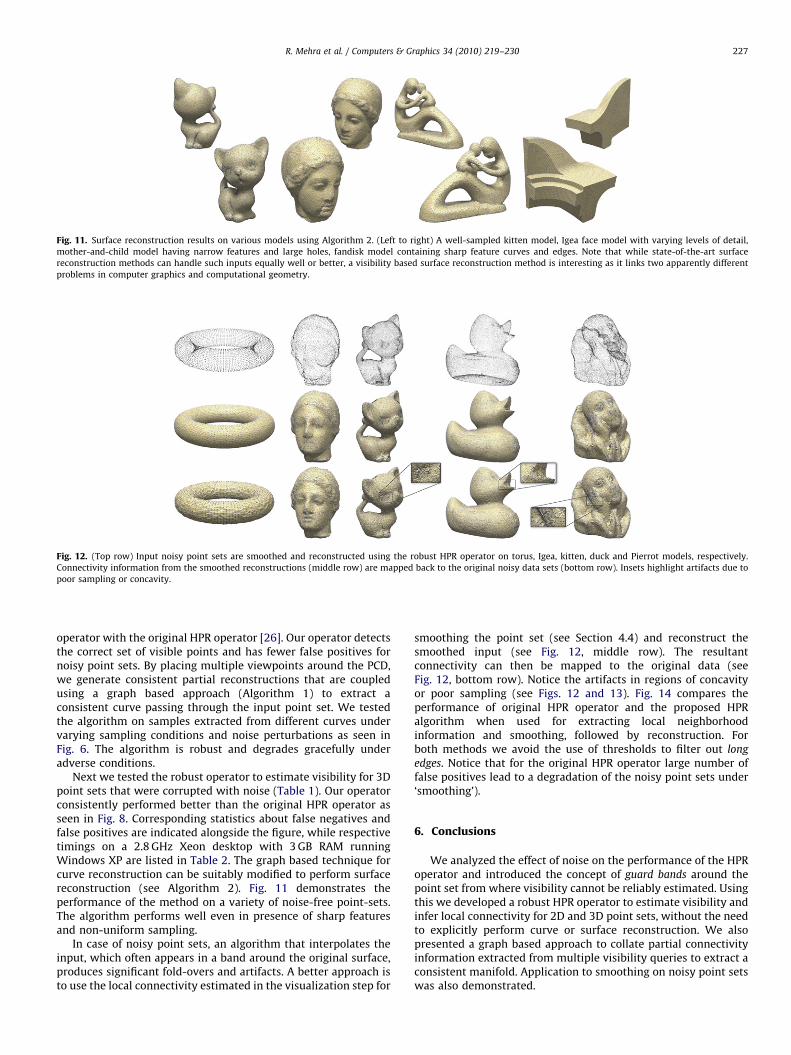
Fig. 11. Surface reconstruction results on various models using Algorithm 2. (Left to right) A well-sampled kitten model, Igea face model with varying levels of detail,

mother-and-child model having narrow features and large holes, fandisk model containing sharp feature curves and edges. Note that while state-of-the-art surface

reconstruction methods can handle such inputs equally well or better, a visibility based surface reconstruction method is interesting as it links two apparently different

problems in computer graphics and computational geometry.


operator with the original HPR operator [26]. Our operator detectsthe correct set of visible points and has fewer false positives fornoisy point sets. By placing multiple viewpoints around the PCD,we generate consistent partial reconstructions that are coupledusing a graph based approach (Algorithm 1) to extract aconsistent curve passing through the input point set. We testedthe algorithm on samples extracted from different curves undervarying sampling conditions and noise perturbations as seen inFig. 6. The algorithm is robust and degrades gracefully underadverse conditions.

Next we tested the robust operator to estimate visibility for 3Dpoint sets that were corrupted with noise (Table 1). Our operatorconsistently performed better than the original HPR operator asseen in Fig. 8. Corresponding statistics about false negatives andfalse positives are indicated alongside the figure, while respectivetimings on a 2.8 GHz Xeon desktop with 3 GB RAM runningWindows XP are listed in Table 2. The graph based technique forcurve reconstruction can be suitably modified to perform surfacereconstruction (see Algorithm 2). Fig. 11 demonstrates theperformance of the method on a variety of noise-free point-sets.The algorithm performs well even in presence of sharp featuresand non-uniform sampling.

In case of noisy point sets, an algorithm that interpolates theinput, which often appears in a band around the original surface,produces significant fold-overs and artifacts. A better approach isto use the local connectivity estimated in the visualization step for

smoothing the point set (see Section 4.4) and reconstruct thesmoothed input (see Fig. 12, middle row). The resultantconnectivity can then be mapped to the original data (seeFig. 12, bottom row). Notice the artifacts in regions of concavityor poor sampling (see Figs. 12 and 13). Fig. 14 compares theperformance of original HPR operator and the proposed HPRalgorithm when used for extracting local neighborhoodinformation and smoothing, followed by reconstruction. Forboth methods we avoid the use of thresholds to filter out long

edges. Notice that for the original HPR operator large number offalse positives lead to a degradation of the noisy point sets under‘smoothing’).

6. Conclusions

We analyzed the effect of noise on the performance of the HPRoperator and introduced the concept of guard bands around thepoint set from where visibility cannot be reliably estimated. Usingthis we developed a robust HPR operator to estimate visibility andinfer local connectivity for 2D and 3D point sets, without the needto explicitly perform curve or surface reconstruction. We alsopresented a graph based approach to collate partial connectivityinformation extracted from multiple visibility queries to extract aconsistent manifold. Application to smoothing on noisy point setswas also demonstrated.

ARTICLE IN PRESS

Fig. 14. Reconstruction results for point set from Igea model corrupted with

uniform noise in normal direction of magnitude 1% of bounding box diagonal

length. (Left to right) Surface reconstruction of original point set, of point set

obtained by smoothing the corrupted point set using connectivity obtained from

original HPR operator, and of point set obtained by smoothing the corrupted point

set using connectivity obtained from proposed robust HPR operator. Both in the

case of original HPR and robust HPR, we avoid pruning of long edges in the

connectivity graphs based on thresholds and heuristics. Due to long incorrect

connections, the middle model degrades due to ‘smoothing’. Interior or back facing

triangles are in blue. (For interpretation of the references to colour in this figure


Fig. 13. (Top row) AMLS smoothing [18] followed by tight cocone reconstruction

[13] (compare with Fig. 12-middle row); (bottom row) reconstruction results with

robust cocone [15] (compare with Fig. 12-bottom row). Robust HPR based

reconstruction produces results of similar quality to these state-of-the-art

methods on uniformly sampled data (all these methods may exhibit artifacts in

areas of high-curvature). On non-uniformly sampled data robust HPR produces

more desirable results as shown in Fig. 10. Note that in presence of noise, the

original HPR based method is not applicable.


Acknowledgments

We thank Tamal Dey for making code for AMLS smoothing[18], robust cocone [15], and tight cocone [13] publicly available.We also thank Yongliang Yang for proofreading, and theanonymous reviewers for their extensive comments and sugges-tions that helped to improve the paper. The Coati scan wasobtained from Mitra and colleagues [31], while the tooth, horse,Igea, and Max Planck models were obtained from the AIM@SHAPEdatabase.

Appendix

Let P denote the original noise free point set. Let Ps :¼fpiþsnij8piAPg be the noisy point set, where s is a uniformrandom variable over the range [0,a], and ni is a unit vectororiented in a uniformly chosen random direction. We may assumethat the viewpoint is at the origin of the coordinate system. Letamin and amax be the shortest and farthest distance from the origin

to a point in P and D be the diameter of point cloud, i.e.,(amax�amin). For any point pAP let ps be the corresponding pointin Ps, and p̂ be its image in the inverted space.

Spherical inversion function

The spherical inversion function is defined as follows.

p̂ ¼ pþ2ðR�JpJÞp=JpJ¼ 2Rp=JpJ�p

For a point pAP,

p̂ ¼ 2Rp=JpJ�p

p̂s¼ 2RðpþsnÞ=JpþsnJ�ðpþsnÞ:

Next, we quantify the effect of noise on points in the inverteddomain. Let e denote the magnitude of noise in the inverteddomain, i.e., e¼ Jp̂

s�p̂J. We have,

e¼ 2R1

JpþsnJ�

1

JpJ

� �pþ

2R

JpþsnJ�1

� �sn

��

r 2R1

JpJ�s�1

JpJ

� �p

��þ 2R

JpJ�s�1

� �sn

��

r2Rs

ðJpJ�sÞJpJ

� �JpJþ

2R

JpJ�s�1

� �sJnJ

r2Rs

JpJ�sþ

2R

JpJ�s�1

� �s

r4R

JpJ�s�1

� �s:

So the maximum noise in the inverted domain is bounded by

emax ¼4R

amin�s�1

� �s:

In our algorithm for robust visibility we project the noisy pointsonto the convex hull. This projection is robust and consistent onlywhen 2emaxraD, where aA ½0,1�. Simplifying we get,

RraD

2s þ1

� �amin�s

4

� �:

Now we find a range of value of R over which we can reliablyperform this projection. Recall that in the noise-free scenario,convex hull of the inverted point cloud along with the viewpointgives us the correct visibility estimates. But in presence of noise,the points in the inverted domain may get perturbed by atmost 2emax, causing some of the previously visible points to bemarked as hidden. To solve this problem, we project points backto the convex hull if they are within 2emax from the (new) convexhull.

While the projection operator works well for locally convexregions, it may lead to false negatives in concave regions. In thiscase, the noisy points can be even farther than 2emax from theconvex hulls in the inverted regions and may lead to falsenegatives. As concave region visibility is proportional to theradius of inversion R (Lemma 4.3 in [26]), we have to select R thatis greater than the minimum radius at which the concave region isvisible. This imposes a lower bound on R.

(1)
Locally convex region: Locally convex shapes are visible at anyradius, we can use any radius above minimum radius possiblefor inversion, i.e., amax.
(2)
Locally concave region: Concave regions, see Lemma 4.3 in[26], are correctly visible only above a certain radius given bythe local curvature k. For the simple case when the tangent tothe surface is perpendicular to the line of sight R4kr2=2.In this case, the lower bound for R is not amax but someother value say R0, greater than amax. Let R0 ¼mamax for somem41.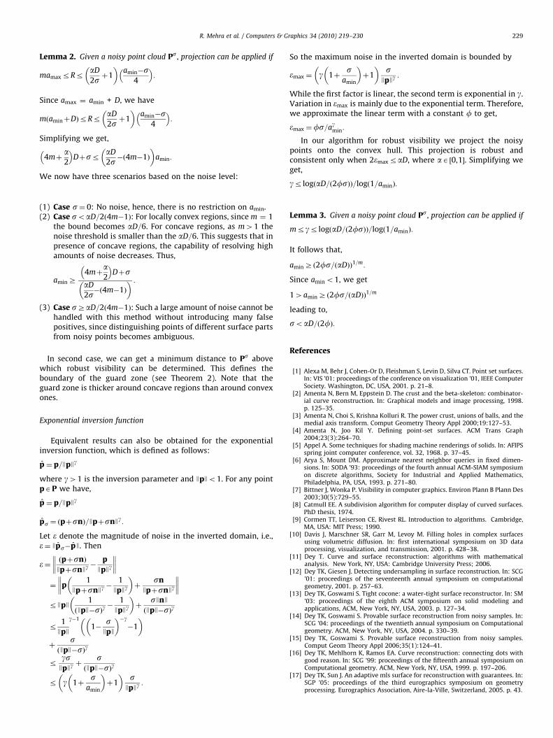

ARTICLE IN PRESS



mamaxrRraD

2sþ1

� �amin�s

4

� �:

Since amax ¼ amin + D, we have

mðaminþDÞrRraD

2sþ1

� �amin�s

4

� �:

Simplifying we get,

4mþa2

� �Dþsr aD

2s�ð4m�1Þ

� �amin:

We now have three scenarios based on the noise level:

(1)
Case s¼ 0: No noise, hence, there is no restriction on amin. (2) Case soaD=2ð4m�1Þ: For locally convex regions, since m ¼ 1
the bound becomes aD=6. For concave regions, as m41 thenoise threshold is smaller than the aD=6. This suggests that inpresence of concave regions, the capability of resolving highamounts of noise decreases. Thus,

aminZ

4mþa2

� �Dþs

aD

2s�ð4m�1Þ

� � :Case sZaD=2ð4m�1Þ: Such a large amount of noise cannot be
(3) handled with this method without introducing many falsepositives, since distinguishing points of different surface partsfrom noisy points becomes ambiguous.
In second case, we can get a minimum distance to Ps abovewhich robust visibility can be determined. This defines theboundary of the guard zone (see Theorem 2). Note that theguard zone is thicker around concave regions than around convexones.

Exponential inversion function

Equivalent results can also be obtained for the exponentialinversion function, which is defined as follows:

p̂ ¼ p=JpJg

where g41 is the inversion parameter and JpJo1. For any pointpAP we have,

p̂ ¼ p=JpJg

p̂s ¼ ðpþsnÞ=JpþsnJg:

Let e denote the magnitude of noise in the inverted domain, i.e.,e¼ Jp̂s�p̂J. Then

e¼ ðpþsnÞ

JpþsnJg�

p

JpJg

��

¼ p1

JpþsnJg�

1

JpJg

� �þ

sn

JpþsnJg

��

rJpJ1

ðJpJ�sÞg�

1

JpJg

� �þ

sJnJ

ðJpJ�sÞg

r1

JpJ

g�1

1�sJpJ

� ��g�1

� �

þs

ðJpJ�sÞg

rgsJpJgþ

sðJpJ�sÞg

r g 1þs

amin

� �þ1

� �s

JpJg:

So the maximum noise in the inverted domain is bounded by

emax ¼ g 1þs

amin

� �þ1

� �s

JpJg:

While the first factor is linear, the second term is exponential in g.Variation in emax is mainly due to the exponential term. Therefore,we approximate the linear term with a constant f to get,

emax ¼fs=agmin:

In our algorithm for robust visibility we project the noisypoints onto the convex hull. This projection is robust andconsistent only when 2emaxraD, where aA ½0,1�. Simplifying weget,

gr logðaD=ð2fsÞÞ=logð1=aminÞ:


mrgr logðaD=ð2fsÞÞ=logð1=aminÞ:

It follows that,

aminZ ð2fs=ðaDÞÞ1=m:

Since amino1, we get

14aminZ ð2fs=ðaDÞÞ1=m

leading to,

soaD=ð2fÞ:

References

[1] Alexa M, Behr J, Cohen-Or D, Fleishman S, Levin D, Silva CT. Point set surfaces.In: VIS ’01: proceedings of the conference on visualization ’01, IEEE ComputerSociety. Washington, DC, USA, 2001. p. 21–8.

[2] Amenta N, Bern M, Eppstein D. The crust and the beta-skeleton: combinator-ial curve reconstruction. In: Graphical models and image processing, 1998.p. 125–35.

[3] Amenta N, Choi S, Krishna Kolluri R. The power crust, unions of balls, and themedial axis transform. Comput Geometry Theory Appl 2000;19:127–53.

[4] Amenta N, Joo Kil Y. Defining point-set surfaces. ACM Trans Graph2004;23(3):264–70.

[5] Appel A. Some techniques for shading machine renderings of solids. In: AFIPSspring joint computer conference, vol. 32, 1968. p. 37–45.

[6] Arya S, Mount DM. Approximate nearest neighbor queries in fixed dimen-sions. In: SODA ’93: proceedings of the fourth annual ACM-SIAM symposiumon discrete algorithms, Society for Industrial and Applied Mathematics,Philadelphia, PA, USA, 1993. p. 271–80.

[7] Bittner J, Wonka P. Visibility in computer graphics. Environ Plann B Plann Des2003;30(5):729–55.

[8] Catmull EE. A subdivision algorithm for computer display of curved surfaces.PhD thesis, 1974.

[9] Cormen TT, Leiserson CE, Rivest RL. Introduction to algorithms. Cambridge,MA, USA: MIT Press; 1990.

[10] Davis J, Marschner SR, Garr M, Levoy M. Filling holes in complex surfacesusing volumetric diffusion. In: first international symposium on 3D dataprocessing, visualization, and transmission, 2001. p. 428–38.

[11] Dey T. Curve and surface reconstruction: algorithms with mathematicalanalysis. New York, NY, USA: Cambridge University Press; 2006.

[12] Dey TK, Giesen J. Detecting undersampling in surface reconstruction. In: SCG’01: proceedings of the seventeenth annual symposium on computationalgeometry, 2001. p. 257–63.

[13] Dey TK, Goswami S. Tight cocone: a water-tight surface reconstructor. In: SM’03: proceedings of the eighth ACM symposium on solid modeling andapplications, ACM, New York, NY, USA, 2003. p. 127–34.

[14] Dey TK, Goswami S. Provable surface reconstruction from noisy samples. In:SCG ’04: proceedings of the twentieth annual symposium on Computationalgeometry. ACM, New York, NY, USA, 2004. p. 330–39.

[15] Dey TK, Goswami S. Provable surface reconstruction from noisy samples.Comput Geom Theory Appl 2006;35(1):124–41.

[16] Dey TK, Mehlhorn K, Ramos EA. Curve reconstruction: connecting dots withgood reason. In: SCG ’99: proceedings of the fifteenth annual symposium onComputational geometry. ACM, New York, NY, USA, 1999. p. 197–206.

[17] Dey TK, Sun J. An adaptive mls surface for reconstruction with guarantees. In:SGP ’05: proceedings of the third eurographics symposium on geometryprocessing. Eurographics Association, Aire-la-Ville, Switzerland, 2005. p. 43.

ARTICLE IN PRESS


[18] Dey TK, Sun J. An adaptive mls surface for reconstruction with guarantees. In:SGP ’05: proceedings of the third eurographics symposium on geometryprocessing, Eurographics Association. Aire-la-Ville, Switzerland, 2005. p. 43.

[19] Dey TK, Wenger R. Fast reconstruction of curves with sharp corners. Int JComput Geometry Appl 2002;12(5):353–400.

[20] Francke A, Hoffmann M. The euclidean degree-4 minimum spanning treeproblem is np-hard. In: SCG ’09: proceedings of the 25th annual symposiumon computational geometry. ACM, New York, NY, USA, 2009. p. 179–188.

[21] Garey MR, Johnson DS. Computers and intractability: a guide to the theory ofnp-completeness (series of books in the mathematical sciences). New York,NY, USA: W.H. Freeman; 1979.

[22] Gross M, Pfister H, editors. Point-based graphics. Elsevier Science andTechnology Books, 2007.

[23] Hoppe H, Derose T, Duchamp T, McDonald JA, Stuetzle W. Surfacereconstruction from unorganized points, 1992.

[24] Huang H, Li D, Zhang H, Ascher U, Cohen-Or D. Consolidation of unorganizedpoint clouds for surface reconstruction. ACM Trans Graphics 2009;28(5) toappear.

[25] Karp RM. Reducibility among combinatorial problems. In: Miller RE, ThatcherJW, editors. Complexity of Computer Computations. New York, NY, USA:Plenum Press; 1972. p. 85–103.

[26] Katz S, Tal A, Basri R. Direct visibility of point sets. In: SIGGRAPH ’07: ACMSIGGRAPH 2007 papers. ACM, New York, NY, USA, 2007. p. 24.

[27] Kazhdan M, Bolitho M, Hoppe H. Poisson surface reconstruction. In: SGP ’06:proceedings of the fourth eurographics symposium on geometry processing.Eurographics Association, Aire-la-Ville, Switzerland, 2006. p. 61–70.

[28] Levin D. The approximation power of moving least-squares. Math Comput1998;67(224):1517–31.

[29] Mederos B, Amenta N, Velho L, Henrique de Figueiredo L. Surfacereconstruction from noisy point clouds. In: SGP ’05: proceedings of the thirdeurographics symposium on geometry processing. Eurographics Association,Aire-la-Ville, Switzerland, 2005. p. 53.

[30] Vollmer J, Mencl, R. Muller H. Improved laplacian smoothing of noisy surfacemeshes, 1999.

[31] Mitra NJ, Flory S, Ovsjanikov M, Gelfand N, Guibas L, Pottmann H. Dynamicgeometry registration. In: Symposium on geometry processing, 2007. p. 173–82.

[32] Mitra NJ, Nguyen A, Guibas L. Estimating surface normals in noisy point clouddata. Int J Comput Geometry Appl 2004;14: 261–76. (special issue).

[33] Pauly M, Kobbelt LP, Gross M. Point-based multiscale surface representation.ACM Trans Graph 2006;25(2):177–93.

[34] Pauly M, Mitra NJ, Guibas L. Uncertainty and variability in point cloud surfacedata. In: Symposium on point-based graphics, 2004.

[35] Schnelle Kurven Straer Wolfgang. Flchendarstellung auf graphischen Sicht-gerten. PhD thesis, 1974.

[36] Sutherland IE, Sproull RF, Robert, Schumacker A. A characterization of tenhidden-surface algorithms. ACM Comput Surv 1974;6:1–55.

Documents

Visibility of noisy point cloud data