Visibility PreprocessingFor Interactive Walkthroughs

Seth J. TellerCarlo H. Sequin

University of California at BerkeleyzAbstract

The number of polygons comprising interesting architectural mod-els is many more than can be rendered at interactive frame rates.However, due to occlusion by opaque surfaces (e.g., walls), only asmall fraction of a typical model is visible from most viewpoints.

We describe a method of visibility preprocessing that is effi-cient and effective for axis-aligned or axial architectural models. Amodel is subdivided into rectangular cells whose boundaries coin-cide with major opaque surfaces. Non-opaque portals are identifiedon cell boundaries, and used to form an adjacency graph connect-ing the cells of the subdivision. Next, the cell-to-cell visibility iscomputed for each cell of the subdivision, by linking pairs of cellsbetween which unobstructed sightlines exist.

During an interactive walkthrough phase, an observer with aknown position and view cone moves through the model. At eachframe, the cell containing the observer is identified, and the con-tents of potentially visible cells are retrieved from storage. The setof potentially visible cells is further reduced by culling it againstthe observer’s view cone, producing the eye-to-cell visibility. Thecontents of the remaining visible cells are then sent to a graphicspipeline for hidden-surface removal and rendering.

Tests on moderately complex 2-D and 3-D axial models revealsubstantially reduced rendering loads.

CR Categories and Subject Descriptors: [Computer Graph-ics]: I.3.5 Computational Geometry and Object Modeling – geomet-ric algorithms, languages, and systems; I.3.7 Three-DimensionalGraphics and Realism – visible line/surface algorithms.

Additional Key Words and Phrases: architectural simulation,linear programming, superset visibility.zComputer Science Department, Berkeley, CA 94720

1 Introduction

Interesting architectural models of furnished buildings may consistof several million polygons. This is many more than today’s work-stations can render in a fraction of a second, as is necessary forsmooth interactive walkthroughs.

However, such scenes typically consist of large connected ele-ments of opaque material (e.g., walls), so that from most vantagepoints only a small fraction of the model can be seen. The scenecan be spatially subdivided into cells, and the model partitioned intosets of polygons attached to each cell. Approximate visibility infor-mation can then be computed offline, and associated with each cellfor later use in an interactive rendering phase. This approximate in-formation must contain a superset of the polygons visible from anyviewpoint in the cell. If this “potentially visible set” or PVS [1] ex-cluded some visible polygon for an observer position, the interac-tive rendering phase would exhibit flashing or holes there, detract-ing from the simulation’s accuracy and realism.

1.1 Visibility Precomputation

Several researchers have proposed spatial subdivision techniquesfor rendering acceleration. We broadly refer to these methods as“visibility precomputations,” since by performing work offline theyreduce the effort involved in solving the hidden-surface problem.Much attention has focused on computing exact visibility (e.g., [5,12, 16, 19, 22]); that is, computing an exact description of the vis-ible elements of the scene data for every qualitatively distinct re-gion of viewpoints. Such complete descriptions may be combinato-rially complex and difficult to implement [16, 18], even for highlyrestricted viewpoint regions (e.g., viewpoints at infinity).

The binary space partition or BSP tree data structure [8] obviatesthe hidden-surface computation by producing a back-to-front order-ing of polygons from any viewpoint. This technique has the draw-back that, for an n-polygon scene, the splitting operations neededto construct the BSP tree may generate O(n2) new polygons [17].Fixed-grid and octree spatial subdivisions [9, 11] accelerate ray-traced rendering by efficiently answering queries about rays propa-gating through ordered sets of parallelepipedal cells. To our knowl-edge, these ray-propagation techniques have not been used in inter-active display systems.

Given the wide availability of fast polygon-rendering hardware[3, 14], it seems reasonable to search for simpler, faster algorithmswhich may overestimate the set of visible polygons, computing asuperset of the true answer. Graphics hardware can then solve the

1

eye

obstacle

invisible object

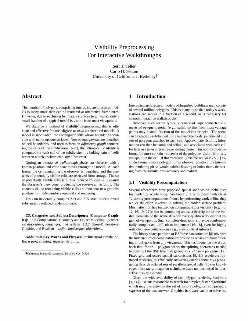
Figure 1: Cone-octree culling: the boxed object is reported visible.

hidden-surface problem for this polygon superset in screen-space.One approach involves intersecting a view cone with an octree-based spatial subdivision of the input [10]. This method has the un-desirable property that it can report as visible an arbitrarily large partof the scene when, in fact, only a tiny portion can be seen (Figure 1).The algorithm may also have poor average case behavior for sceneswith high depth complexity; i.e., many viewpoints for which a largenumber of overlapping polygons paint the same screen pixel.

Another overestimation method involves finding portals, or non-opaque regions, in otherwise opaque model elements, and treatingthese as lineal (in 2-D) or areal (in 3-D) light sources [1]. Opaquepolygons in the model then cause shadow volumes [6] to arise withrespect to the light sources; those parts of the model inside theshadow volumes can be marked invisible for any observer on theoriginating portal. This portal-polygon occlusion algorithm has notfound use in practice due to implementation difficulties and highcomputational complexity [1, 2].

obstacles

cell

visibleobject

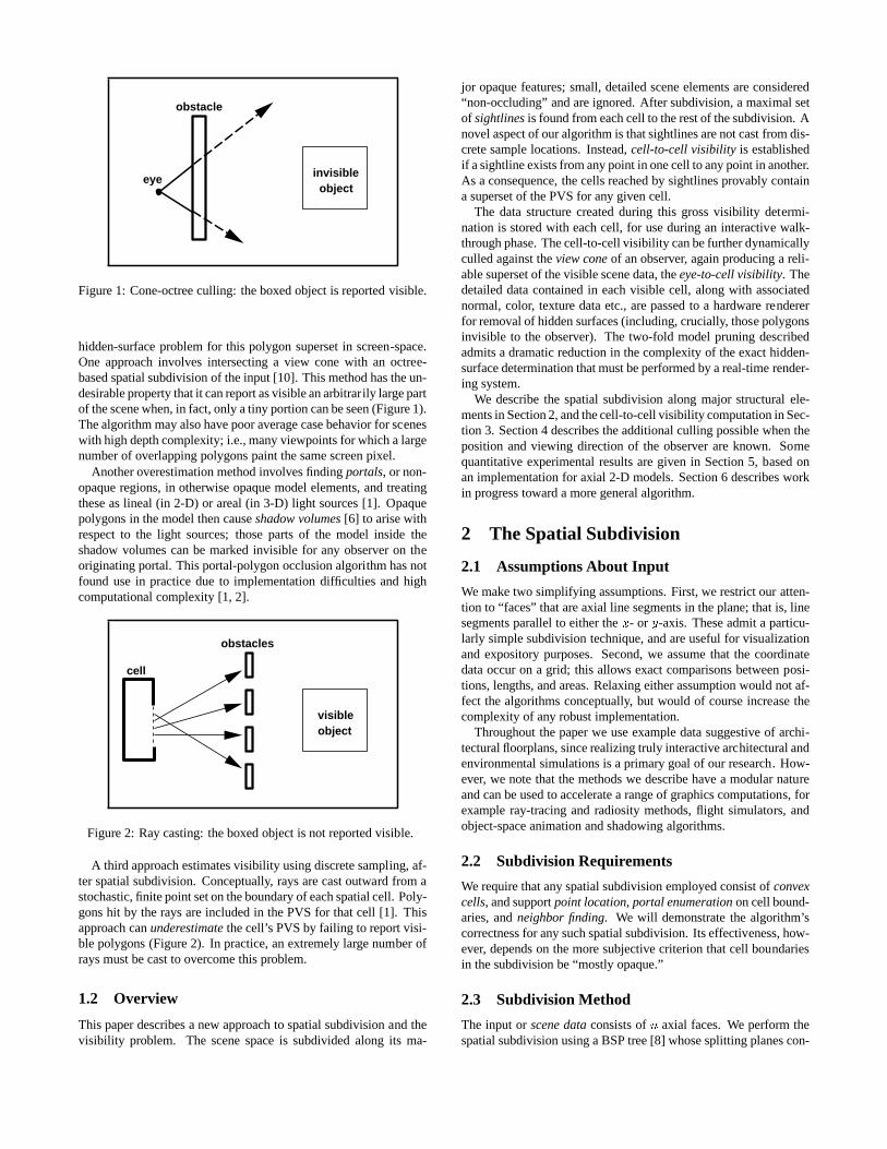
Figure 2: Ray casting: the boxed object is not reported visible.

A third approach estimates visibility using discrete sampling, af-ter spatial subdivision. Conceptually, rays are cast outward from astochastic, finite point set on the boundary of each spatial cell. Poly-gons hit by the rays are included in the PVS for that cell [1]. Thisapproach can underestimate the cell’s PVS by failing to report visi-ble polygons (Figure 2). In practice, an extremely large number ofrays must be cast to overcome this problem.

1.2 Overview

This paper describes a new approach to spatial subdivision and thevisibility problem. The scene space is subdivided along its ma-

jor opaque features; small, detailed scene elements are considered“non-occluding” and are ignored. After subdivision, a maximal setof sightlines is found from each cell to the rest of the subdivision. Anovel aspect of our algorithm is that sightlines are not cast from dis-crete sample locations. Instead, cell-to-cell visibility is establishedif a sightline exists from any point in one cell to any point in another.As a consequence, the cells reached by sightlines provably containa superset of the PVS for any given cell.

The data structure created during this gross visibility determi-nation is stored with each cell, for use during an interactive walk-through phase. The cell-to-cell visibility can be further dynamicallyculled against the view cone of an observer, again producing a reli-able superset of the visible scene data, the eye-to-cell visibility. Thedetailed data contained in each visible cell, along with associatednormal, color, texture data etc., are passed to a hardware rendererfor removal of hidden surfaces (including, crucially, those polygonsinvisible to the observer). The two-fold model pruning describedadmits a dramatic reduction in the complexity of the exact hidden-surface determination that must be performed by a real-time render-ing system.

We describe the spatial subdivision along major structural ele-ments in Section 2, and the cell-to-cell visibility computation in Sec-tion 3. Section 4 describes the additional culling possible when theposition and viewing direction of the observer are known. Somequantitative experimental results are given in Section 5, based onan implementation for axial 2-D models. Section 6 describes workin progress toward a more general algorithm.

2 The Spatial Subdivision

2.1 Assumptions About Input

We make two simplifying assumptions. First, we restrict our atten-tion to “faces” that are axial line segments in the plane; that is, linesegments parallel to either the x- or y-axis. These admit a particu-larly simple subdivision technique, and are useful for visualizationand expository purposes. Second, we assume that the coordinatedata occur on a grid; this allows exact comparisons between posi-tions, lengths, and areas. Relaxing either assumption would not af-fect the algorithms conceptually, but would of course increase thecomplexity of any robust implementation.

Throughout the paper we use example data suggestive of archi-tectural floorplans, since realizing truly interactive architectural andenvironmental simulations is a primary goal of our research. How-ever, we note that the methods we describe have a modular natureand can be used to accelerate a range of graphics computations, forexample ray-tracing and radiosity methods, flight simulators, andobject-space animation and shadowing algorithms.

2.2 Subdivision Requirements

We require that any spatial subdivision employed consist of convexcells, and support point location, portal enumeration on cell bound-aries, and neighbor finding. We will demonstrate the algorithm’scorrectness for any such spatial subdivision. Its effectiveness, how-ever, depends on the more subjective criterion that cell boundariesin the subdivision be “mostly opaque.”

2.3 Subdivision Method

The input or scene data consists of n axial faces. We perform thespatial subdivision using a BSP tree [8] whose splitting planes con-

tain the major axial faces. For the special case of planar, axial data,the BSP tree becomes an instance of a k-D tree [4] with k = 2. Ev-ery node of a k-D tree is associated with a spatial cell bounded byk half-open extents [x0;min ::: x0;max); :::; [xk�1;min ::: xk�1;max).If a k-D node is not a leaf, it has a split dimension s such that0 � s < k; a split abscissa a such that xs;min < a < xs;max;and low and high child nodes with extents equivalent to that of theparent in every dimension except k = s, for which the extentsare [xs;min:::a) and [a:::xs;max), respectively. A balanced k-D treesupports logarithmic-time point location and linear-time neighborqueries.

The k-D tree root cell’s extent is initialized to the bounding boxof the input (Fig. 3-a). Each input face F is classified with respectto the root cell as:� disjoint if F has no intersection with the cell;� spanning if F partitions the cell interior into components that

intersect only on their boundaries;� covering if F lies on the cell boundary and intersects theboundary’s relative interior;� incident otherwise.

Spanning, covering, and incident faces, but not disjoint faces, arestored with each node. Clearly no face can be disjoint from the rootcell. The disjoint class becomes relevant after subdivision, when aparent may contain faces disjoint from one or the other of its chil-dren.

x = m

(a)

(b)

x = m

CCCCCCCCCCCCCCCCCCCCCCCCCCCCCCCCCCCCCCCCCCCCCCCCCCCCCCCCCCCCCCCCCCCCCCCCCCCCCCCCCCCCCCCCCCCCCCCCCCCCCCCCCCCCCCCCCCCCCCCCCCCCCCCCCCCCCCCCCCCCCCCCCCCCCCCCCCCCCCCCCCCCCCCCCCCCCCCCCCCCCCCCCCCCCCCCCCCCCCCCCCCCCCCCCCCCCCCCCCCCCCCCCCCCCCCCCCCCCCCCCCCCCCCCCCCCCCCCCCCC

incident

coveringcovering

spanning

y=AA

B

CCCCCCCCCCCCCCCCCCCCCCCCCCCCCCCCCCCCCCCCCCCCCCCCCCCCCCCCCCCCCCCCCCCCCCCCCCCCCCCCCCCCCCCCCCCCCCCCCCCCCCCCCCCCCCCCCCCCCCCCCCCCCCCCCCCCCCCCCCCCCCCCCCCCCCCCCCCC

incident

coveringdisjoint

input faces

k-d cells

CCCCCCCCCCCCCCCCCC

Figure 3: (a): A k-D tree root cell and input face classifications.(b): The right-hand cell and contents after the first split at x = m.

We say that face A cleaves face B if the line supporting A inter-sects B at a point in B’s relative interior (Fig. 3-a). We recursivelysubdivide the root node, repeatedly subjecting each leaf cell of thek-D tree to the following procedure:� If the k-D cell has no incident faces (its interior is empty), do

nothing;

� if any spanning faces exist, split on the median spanning face;� otherwise, split on a sufficiently obscured minimum cleavingabscissa; i.e., along a face A cleaving a minimal set of facesorthogonal to A.

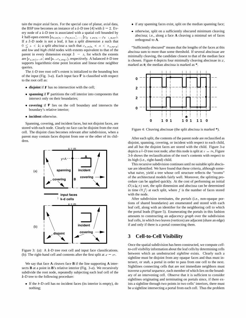
“Sufficiently obscured” means that the lengths of the faces at thisabscissa sum to more than some threshold. If several abscissae areminimally cleaving, the candidate closest to that of the median faceis chosen. Figure 4 depicts four minimally cleaving abscissae in x,marked as 0; the median abscissa is marked as *.

0

2

2

0

0 1 0 1 1 * 1 01 10

Figure 4: Cleaving abscissae (the split abscissa is marked *).

After each split, the contents of the parent node are reclassified asdisjoint, spanning, covering, or incident with respect to each child,and all but the disjoint faces are stored with the child. Figure 3-adepicts a k-D tree root node; after this node is split at x = m, Figure3-b shows the reclassification of the root’s contents with respect toits high (i.e., right-hand) child.

This recursive subdivision continues until no suitable split abscis-sae are identified. We have found that these criteria, although some-what naive, yield a tree whose cell structure reflects the “rooms”of the architectural models fairly well. Moreover, the splitting pro-cedure can be applied quickly. At the cost of performing an initialO(n lg n) sort, the split dimension and abscissa can be determinedin time O(f) at each split, where f is the number of faces storedwith the node.

After subdivision terminates, the portals (i.e., non-opaque por-tions of shared boundaries) are enumerated and stored with eachleaf cell, along with an identifier for the neighboring cell to whichthe portal leads (Figure 5). Enumerating the portals in this fashionamounts to constructing an adjacency graph over the subdivisionleaf cells, in which two leaves (vertices) are adjacent (share an edge)if and only if there is a portal connecting them.

3 Cell-to-Cell Visibility

Once the spatial subdivision has been constructed, we compute cell-to-cell visibility information about the leaf cells by determining cellsbetween which an unobstructed sightline exists. Clearly such asightline must be disjoint from any opaque faces and thus must in-tersect, or stab, a portal in order to pass from one cell to the next.Sightlines connecting cells that are not immediate neighbors musttraverse a portal sequence, each member of which lies on the bound-ary of an intervening cell. Observe that it is sufficient to considersightlines originating and terminating on portals since, if there ex-ists a sightline through two points in two cells’ interiors, there mustbe a sightline intersecting a portal from each cell. Thus the problem

input faces portalscell boundariesadjacency graph vertices adjacency graph edges

Figure 5: Subdivision, with portals and adjacency graph.

of finding sightlines between cell areas reduces to finding sightlinesbetween line segments on cell boundaries.

A

B

C

D

L

R RL L

R

L

R

LR

L

R

(a)

(b) (c)

Figure 6: Oriented portal sequences, and separable sets L and R.

We say that a portal sequence admits a sightline if there exists aline that stabs every portal of the sequence. Figure 6 depicts fourcells A, B, C, and D. There are four portal sequences originatingat A that admit sightlines: [A/B, B/C, C/D], [A/C, C/B, B/D],[A/B, B/D], and [A/C, C/D], where P=Q denotes a portal fromcell P to cell Q. Thus A, B, C, and D are mutually visible.

3.1 Generating Portal Sequences

To find sightlines, we must generate candidate portal sequences,and identify those sequences that admit sightlines. We find candi-date portal sequences with a graph traversal on the cell adjacencygraph. Two cells P and Q are neighbors if their shared boundary isnot completely opaque. Each connected non-opaque region of thisshared boundary is a portal from P to Q. Given any starting cell Cfor which we wish to compute visible cells, a recursive depth-firstsearch (DFS) ofC’s neighbors, rooted atC, produces candidate por-tal sequences. Searching proceeds incrementally; when a candidateportal sequence no longer admits a sightline (according to the crite-rion described below), the depth-first search on that portal sequenceterminates. The cells reached by the DFS are stored in a stab tree(see below) as they are encountered.

3.2 Finding Sightlines Through Portal Sequences

The fact that portal sequences arise from directed paths in the sub-division adjacency graph allows us to orient each portal in the se-quence and find sightlines easily. As the DFS encounters each por-tal, it places the portal endpoints in a set L or R, according to theportal’s orientation (Figure 6). A sightline can stab this portal se-quence if and only if the point sets L and R are linearly separable;that is, iff there exists a line S such thatS � L � 0; 8 L 2 LS �R � 0; 8R 2 R: (1)

For a portal sequence of length m, this is a linear programmingproblem of 2m constraints. Both deterministic [15] and randomized[20] algorithms exist to solve this linear program (i.e., find a linestabbing the portal sequence) in linear time; that is, time O(m). Ifno such stabbing line exists, the algorithms report this fact.

3.3 The Algorithm

Assume the existence of a routine Stabbing Line(P) that, given aportal sequence P, determines either a stabbing line for P or de-termines that no such stabbing line exists. All cells visible from asource cell C can then be found with the recursive procedure:

Find Visible Cells (cell C, portal sequence P, visible cell set V)V = V [ Cfor each neighbor N of C

for each portal p connecting C and Norient p from C to NP0 = P concatenate pif Stabbing Line (P0) exists then

Find Visible Cells (N , P0, V)

CCCCCCCCCCCCCCCCCCCCCCCCCCCCCCCCCCCCCCCCCCCCCCCCCCCCCCCCCCCCCCCCCCCCCCCCCCCCCCCCCCCCCCCCCCCCCCCCCCCCCCCCCCCCCC

I J

H

GA

E

F

D

C

B

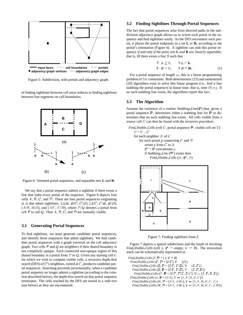
Figure 7: Finding sightlines from I .

Figure 7 depicts a spatial subdivision and the result of invokingFind Visible Cells (cell I , P = empty, V = ;). The invocationstack can be schematically represented as

Find Visible Cells (I, P = [ ], V = ;)Find Visible Cells (F ,P = [I/F ], V = fIg)

Find Visible Cells (B, P = [I/F , F /B], V = fI; Fg)Find Visible Cells (E,P = [I/F , F /E], V = fI; F; Bg)

Find Visible Cells (C, P = [I/F , F /E, E/C], V = fI; F; B;Eg)Find Visible Cells (J , P = [I/J], V = fI; F; B;E; Cg)

Find Visible Cells (H, P = [I/J , J /H1], V = fI; F; B;E; C; Jg)Find Visible Cells (H, P = [I/J , J /H2], V = fI; F; B;E; C; J;Hg)

The last line shows that the cell-to-cell visibility V returned isfI; F;B;E;C; J;Hg.The recursive nature of Find Visible Cells() suggests an efficient

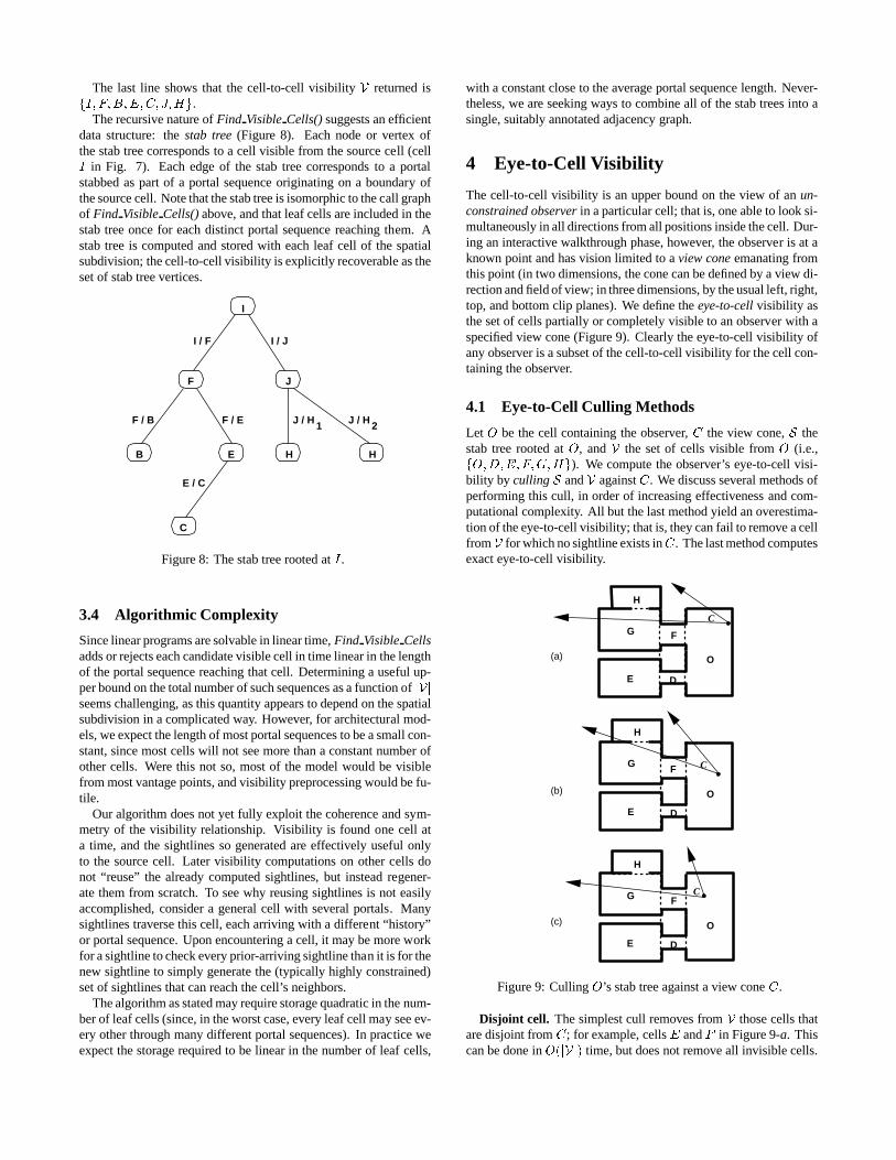
data structure: the stab tree (Figure 8). Each node or vertex ofthe stab tree corresponds to a cell visible from the source cell (cellI in Fig. 7). Each edge of the stab tree corresponds to a portalstabbed as part of a portal sequence originating on a boundary ofthe source cell. Note that the stab tree is isomorphic to the call graphof Find Visible Cells() above, and that leaf cells are included in thestab tree once for each distinct portal sequence reaching them. Astab tree is computed and stored with each leaf cell of the spatialsubdivision; the cell-to-cell visibility is explicitly recoverable as theset of stab tree vertices.

I

F J

B E

C

H

I / F I / J

F / B F / E

E / C

J / H

H

J / H1 2

Figure 8: The stab tree rooted at I .

3.4 Algorithmic Complexity

Since linear programs are solvable in linear time, Find Visible Cellsadds or rejects each candidate visible cell in time linear in the lengthof the portal sequence reaching that cell. Determining a useful up-per bound on the total number of such sequences as a function of jVjseems challenging, as this quantity appears to depend on the spatialsubdivision in a complicated way. However, for architectural mod-els, we expect the length of most portal sequences to be a small con-stant, since most cells will not see more than a constant number ofother cells. Were this not so, most of the model would be visiblefrom most vantage points, and visibility preprocessing would be fu-tile.

Our algorithm does not yet fully exploit the coherence and sym-metry of the visibility relationship. Visibility is found one cell ata time, and the sightlines so generated are effectively useful onlyto the source cell. Later visibility computations on other cells donot “reuse” the already computed sightlines, but instead regener-ate them from scratch. To see why reusing sightlines is not easilyaccomplished, consider a general cell with several portals. Manysightlines traverse this cell, each arriving with a different “history”or portal sequence. Upon encountering a cell, it may be more workfor a sightline to check every prior-arriving sightline than it is for thenew sightline to simply generate the (typically highly constrained)set of sightlines that can reach the cell’s neighbors.

The algorithm as stated may require storage quadratic in the num-ber of leaf cells (since, in the worst case, every leaf cell may see ev-ery other through many different portal sequences). In practice weexpect the storage required to be linear in the number of leaf cells,

with a constant close to the average portal sequence length. Never-theless, we are seeking ways to combine all of the stab trees into asingle, suitably annotated adjacency graph.

4 Eye-to-Cell Visibility

The cell-to-cell visibility is an upper bound on the view of an un-constrained observer in a particular cell; that is, one able to look si-multaneously in all directions from all positions inside the cell. Dur-ing an interactive walkthrough phase, however, the observer is at aknown point and has vision limited to a view cone emanating fromthis point (in two dimensions, the cone can be defined by a view di-rection and field of view; in three dimensions, by the usual left, right,top, and bottom clip planes). We define the eye-to-cell visibility asthe set of cells partially or completely visible to an observer with aspecified view cone (Figure 9). Clearly the eye-to-cell visibility ofany observer is a subset of the cell-to-cell visibility for the cell con-taining the observer.

4.1 Eye-to-Cell Culling Methods

Let O be the cell containing the observer, C the view cone, S thestab tree rooted at O, and V the set of cells visible from O (i.e.,fO;D;E;F;G;Hg). We compute the observer’s eye-to-cell visi-bility by culling S and V against C. We discuss several methods ofperforming this cull, in order of increasing effectiveness and com-putational complexity. All but the last method yield an overestima-tion of the eye-to-cell visibility; that is, they can fail to remove a cellfromV for which no sightline exists inC. The last method computesexact eye-to-cell visibility.

E

G F

(a)

(b)

(c)

H

O

O

O

E

G F

H

E

G F

H

D

D

D

C

C

C

Figure 9: Culling O’s stab tree against a view cone C.

Disjoint cell. The simplest cull removes from V those cells thatare disjoint from C; for example, cells E and F in Figure 9-a. Thiscan be done in O(jVj) time, but does not remove all invisible cells.

CellG in Figure 9-a has a non-empty intersection with C, but is notvisible; any sightline to it must traverse the cell F , which is disjointfromC. More generally, in the cell adjacency graph, the visible cellsmust form a single connected component, each cell of which hasa non-empty intersection with C. This connected component mustalso, of course, contain the cell O.

Connected component. Thus, a more effective cull employs adepth-first search from O in S , subject to the constraint that everycell traversed must intersect the interior of C. This requires timeO(jSj), and removes cell G in Figure 9-a. However, it fails to re-move G in Figure 9-b, even though G is invisible from the observer(because all sightlines in C from the observer to G must traversesome opaque input face).

Incident portals. The culling method can be refined further bysearching only through cells reachable via portals that intersect C’sinterior. Figure 9-c shows that this is still not sufficient to obtain anaccurate list of visible cells; cell H passes this test, but is not visiblein C, since no sightline from the observer can stab the three portalsnecessary to reach H .

Exact eye-to-cell. The important observation is that for a cell tobe visible, some portal sequence to that cell must admit a sightlinethat lies inside C and contains the view position. Retaining the stabtree S permits an efficient implementation of this sufficient crite-rion, since S stores with O every portal sequence originating at O.Suppose the portal sequence to some cell has length m. As before,this sequence implies 2m linear constraints on any stabbing line. Tothese we add three linear constraints: one demanding that the stab-bing line contain the observer’s view point, and two demanding thatthe stabbing ray lie inside the two halfspaces whose intersection de-finesC (in two dimensions). The resulting linear program of 2m+3constraints can be solved in time O(m), i.e., O(jVj) for each portalsequence.

This final refinement of the culling algorithm computes exact eye-to-cell visibility. Figure 9-c shows that the cull removes H fromthe observer’s eye-to-cell visibility since the portal sequence [O/F ,F /G, G/H] does not admit a sightline through the view point.

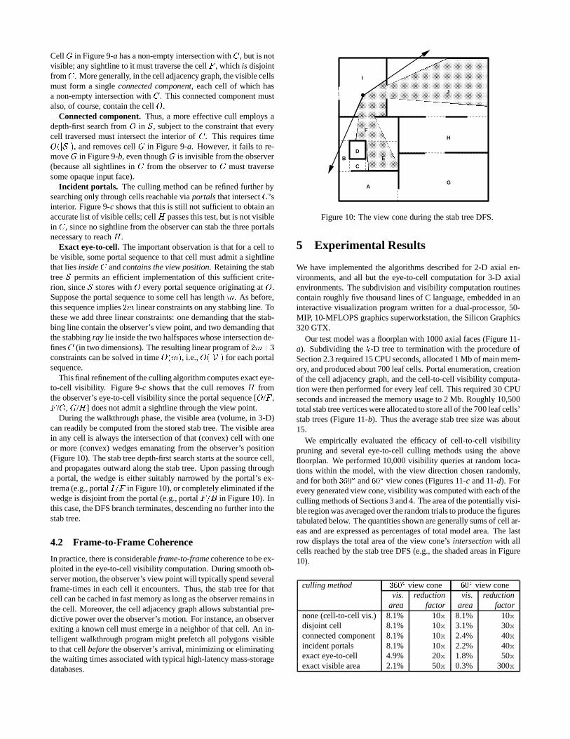
During the walkthrough phase, the visible area (volume, in 3-D)can readily be computed from the stored stab tree. The visible areain any cell is always the intersection of that (convex) cell with oneor more (convex) wedges emanating from the observer’s position(Figure 10). The stab tree depth-first search starts at the source cell,and propagates outward along the stab tree. Upon passing througha portal, the wedge is either suitably narrowed by the portal’s ex-trema (e.g., portal I=F in Figure 10), or completely eliminated if thewedge is disjoint from the portal (e.g., portal F=B in Figure 10). Inthis case, the DFS branch terminates, descending no further into thestab tree.

4.2 Frame-to-Frame Coherence

In practice, there is considerable frame-to-frame coherence to be ex-ploited in the eye-to-cell visibility computation. During smooth ob-server motion, the observer’s view point will typically spend severalframe-times in each cell it encounters. Thus, the stab tree for thatcell can be cached in fast memory as long as the observer remains inthe cell. Moreover, the cell adjacency graph allows substantial pre-dictive power over the observer’s motion. For instance, an observerexiting a known cell must emerge in a neighbor of that cell. An in-telligent walkthrough program might prefetch all polygons visibleto that cell before the observer’s arrival, minimizing or eliminatingthe waiting times associated with typical high-latency mass-storagedatabases.

CCCCCCCCCCCCCCCCCCCCCCCCCCCCCCCCCCCCCCCCCCCCCCCCCCCCCCCCCCCCCCCCCCCCCCCCCCCCCCCCCCCCCCCCCCCCCCCCCCCCCCCCCCCCCCCCCCCCCCCCCCCCCCCCCCCCCCCCCCCCCCCCCCCCCCCCCCCCCCCCCCCCCCCCCCCCCCCCCCCCCCCCCCCCCCCCCCCCCCCCCCCCCCCCCCCCCCCCCCCCCCCCCCCCCCCCCCCCCCCCCCCCCCCCCCCCCCCCCCCCCCCCCCCCCCCCCCCCCCCCCCCCCCCCCCCCCCCCCCCCCCCCCCCCCCCCCCCCCCCCCCCCCCCCCCCCCCCCCCCCCCCCCCCCCCCCCCCCCCCCCCCCCCCCCCCCCCCCCCCCCCCCCCCCCCCCCCCCCCCCCCCCCCCCCCCCCCCCCCCCCCCCCCCCCCCCCCCCCCCCCCCCCCCCCCCCCCCCCCCCCCCCCCCCCCCCCCCCCCCCCCCCCCCCCCCCCCCCCCCCCCCCCCCCCCCCCCCCCCCCCCCCC

I

J

H

GA

E

F

D

C

B

Figure 10: The view cone during the stab tree DFS.

5 Experimental Results

We have implemented the algorithms described for 2-D axial en-vironments, and all but the eye-to-cell computation for 3-D axialenvironments. The subdivision and visibility computation routinescontain roughly five thousand lines of C language, embedded in aninteractive visualization program written for a dual-processor, 50-MIP, 10-MFLOPS graphics superworkstation, the Silicon Graphics320 GTX.

Our test model was a floorplan with 1000 axial faces (Figure 11-a). Subdividing the k-D tree to termination with the procedure ofSection 2.3 required 15 CPU seconds, allocated 1 Mb of main mem-ory, and produced about 700 leaf cells. Portal enumeration, creationof the cell adjacency graph, and the cell-to-cell visibility computa-tion were then performed for every leaf cell. This required 30 CPUseconds and increased the memory usage to 2 Mb. Roughly 10,500total stab tree vertices were allocated to store all of the 700 leaf cells’stab trees (Figure 11-b). Thus the average stab tree size was about15.

We empirically evaluated the efficacy of cell-to-cell visibilitypruning and several eye-to-cell culling methods using the abovefloorplan. We performed 10,000 visibility queries at random loca-tions within the model, with the view direction chosen randomly,and for both 360� and 60� view cones (Figures 11-c and 11-d). Forevery generated view cone, visibility was computed with each of theculling methods of Sections 3 and 4. The area of the potentially visi-ble region was averaged over the random trials to produce the figurestabulated below. The quantities shown are generally sums of cell ar-eas and are expressed as percentages of total model area. The lastrow displays the total area of the view cone’s intersection with allcells reached by the stab tree DFS (e.g., the shaded areas in Figure10).

culling method 360� view cone 60� view conevis. reduction vis. reduction

area factor area factornone (cell-to-cell vis.) 8.1% 10x 8.1% 10xdisjoint cell 8.1% 10x 3.1% 30xconnected component 8.1% 10x 2.4% 40xincident portals 8.1% 10x 2.2% 40xexact eye-to-cell 4.9% 20x 1.8% 50xexact visible area 2.1% 50x 0.3% 300x

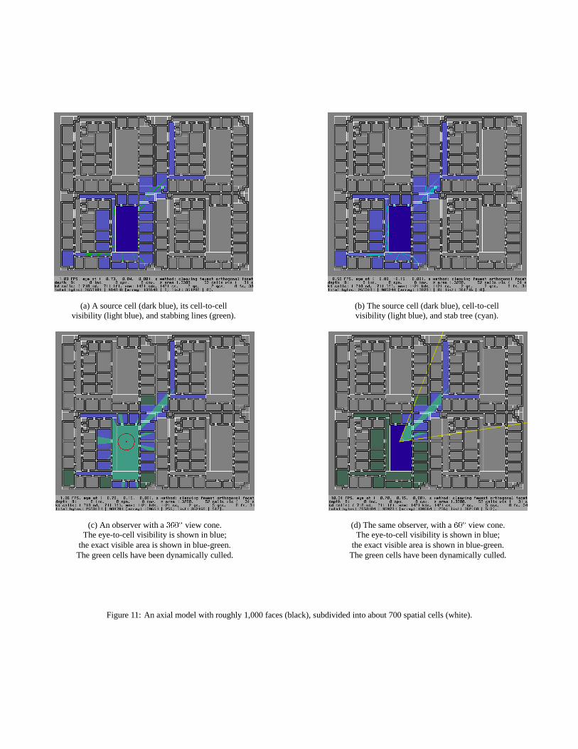
(a) A source cell (dark blue), its cell-to-cellvisibility (light blue), and stabbing lines (green).

(b) The source cell (dark blue), cell-to-cellvisibility (light blue), and stab tree (cyan).

(c) An observer with a 360� view cone.The eye-to-cell visibility is shown in blue;

the exact visible area is shown in blue-green.The green cells have been dynamically culled.

(d) The same observer, with a 60� view cone.The eye-to-cell visibility is shown in blue;

the exact visible area is shown in blue-green.The green cells have been dynamically culled.

Figure 11: An axial model with roughly 1,000 faces (black), subdivided into about 700 spatial cells (white).

6 Extensions and Discussion

We briefly discuss extensions of the visibility computation algo-rithms to three-dimensional scenes.

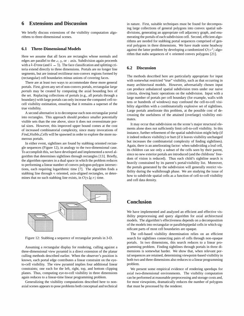
6.1 Three-Dimensional Models

Here we assume that all faces are rectangles whose normals andedges are parallel to the x, y, or z axis. Subdivision again proceedswith a k-D tree (and k = 3). The face classification and splitting cri-teria extend directly to three dimensions. Portals are no longer linesegments, but are instead rectilinear non-convex regions formed by(rectangular) cell boundaries minus unions of covering faces.

There are at least two ways to accommodate these more generalportals. First, given any set of non-convex portals, rectangular largeportals may be created by computing the axial bounding box ofthe set. Replacing collections of portals (e.g., all portals through aboundary) with large portals can only increase the computed cell-to-cell visibility estimation, ensuring that it remains a superset of thetrue visibility.

A second alternative is to decompose each non-rectangular portalinto rectangles. This approach should produce smaller potentiallyvisible sets than the one above, since it does not overestimate por-tal sizes. However, this improved upper bound comes at the costof increased combinatorial complexity, since many invocations ofFind Visible Cells will be spawned in order to explore the more nu-merous portals.

In either event, sightlines are found by stabbing oriented rectan-gle sequences (Figure 12), in analogy to the two-dimensional case.To accomplish this, we have developed and implemented a novel al-gorithm that determines sightlines through rectangles [13]. Briefly,the algorithm operates in a dual space in which the problem reducesto performing a linear number of convex polygon-polygon intersec-tions, each requiring logarithmic time [7]. The algorithm finds astabbing line through n oriented, axis-aligned rectangles, or deter-mines that no such stabbing line exists, in O(n lg n) time.

CCCCCCCCCCCCCCCCCCCCCCCCCCCCCCCCCCCCCCCC

++++++++++++++++++++++++++++++++++++++++++++++++

****************************************

!!!!!!!!!!!!!!!!!!

++++++++++++++++++++++++++++++++++++++++++++++++++++++

CCCCCCCCCCCCCCCCCCCCCCCCCCCCCCCCCCCCCCCC

++++++++++++++++++++++++++++++++++++++++++++++++++++++

*******************************************************

********************************************

CCCCCCCCCCCCCCCCCCCCCCCCCCCCCCCCCCCCCCCC

!!!!!!!!!!!!!!!!!!!!!!!!!!!!!!!!!!!!! !!!!!!

!!!!!!!!!!!!!!!!!!!!!!!!

Figure 12: Stabbing a sequence of rectangular portals in 3-D.

Assuming a rectangular display for rendering, culling against athree-dimensional view pyramid is a direct extension of the planarculling methods described earlier. When the observer’s position isknown, each portal edge contributes a linear constraint on the eye-to-cell visibility. The view pyramid implies four additional linearconstraints; one each for the left, right, top, and bottom clippingplanes. Thus, computing eye-to-cell visibility in three dimensionsagain reduces to a linear-time linear programming problem.

Generalizing the visibility computations described here to non-axial scenes appears to pose problems both conceptual and technical

in nature. First, suitable techniques must be found for decompos-ing large collections of general polygons into convex spatial sub-divisions, generating an appropriate cell adjacency graph, and enu-merating the portals of each subdivision cell. Second, efficient algo-rithms are needed for stabbing portal sequences comprised of gen-eral polygons in three dimensions. We have made some headwayagainst the latter problem by developing a randomized O(n2) algo-rithm that stabs sequences of n oriented convex polygons [21].

6.2 Discussion

The methods described here are particularly appropriate for inputwith somewhat restricted “true” visibility, such as that occurring inmany architectural models. However, adversarially chosen inputcan produce unbalanced spatial subdivision trees under our naivecriteria, slowing basic operations on the subdivision. Input with alarge number of portals per cell boundary (for example, walls withtens or hundreds of windows) may confound the cell-to-cell visi-bility algorithm with a combinatorially explosive set of sightlines.Large portals ameliorate this problem, at the possible cost of de-creasing the usefulness of the attained (overlarge) visibility esti-mates.

It may occur that subdivision on the scene’s major structural ele-ments alone does not sufficiently limit cell-to-cell visibility. In thisinstance, further refinement of the spatial subdivision might help (ifit indeed reduces visibility) or hurt (if it leaves visibility unchangedbut increases the combinatorial complexity of finding sightlines).Again, there is an ameliorating factor: when subdividing a leaf cell,its children can see only a subset of the cells seen by their parent,since no new exterior portals are introduced (and the childrens’ free-dom of vision is reduced). Thus each child’s sightline search isheavily constrained by its parent’s portal/visibility list. Moreover,the portals generated by the subdivision will generally restrict vis-ibility during the walkthrough phase. We are studying the issue ofhow to subdivide spatial cells as a function of cell-to-cell visibilityand cell data density.

Conclusion

We have implemented and analyzed an efficient and effective vis-ibility preprocessing and query algorithm for axial architecturalmodels. The algorithm’s effectiveness depends on a decompositionof the models into rectangular or parallelepipedal cells in which sig-nificant parts of most cell boundaries are opaque.

The cell-based visibility determination relies on an efficientsearch for sightlines connecting pairs of cells through non-opaqueportals. In two dimensions, this search reduces to a linear pro-gramming problem. Finding sightlines through portals in three di-mensions is somewhat harder. We show that, when relevant por-tal sequences are retained, determining viewpoint-based visibility inboth two and three dimensions also reduces to a linear programmingproblem.

We present some empirical evidence of rendering speedups foraxial two-dimensional environments. The visibility computationcan be performed at reasonable preprocessing and storage costs and,for most viewpoints, dramatically reduces the number of polygonsthat must be processed by the renderer.

Acknowledgments

Our special thanks go to Jim Winget, who has always held an ac-tive, supportive role in our research. We gratefully acknowledge thesupport of Silicon Graphics, Inc., and particularly thank Paul Hae-berli for his help in preparing this material for submission and pub-lication. Michael Hohmeyer contributed much valuable insight andan implementation of Raimund Seidel’s randomized linear program-ming algorithm. Finally we thank Mark Segal, Efi Fogel, and theSIGGRAPH referees for their many helpful comments and sugges-tions.

References

[1] John M. Airey. Increasing Update Rates in the Building Walk-through System with Automatic Model-Space Subdivision andPotentially Visible Set Calculations. PhD thesis, UNC ChapelHill, 1990.

[2] John M. Airey, John H. Rohlf, and Frederick P. Brooks, Jr. To-wards image realism with interactive update rates in complexvirtual building environments. ACM Siggraph Special Issueon 1990 Symposium on Interactive 3D Graphics, 24(2):41–50,1990.

[3] Kurt Akeley. The Silicon Graphics 4D/240GTX superwork-station. IEEE Computer Graphics and Applications, 9(4):71–83, July 1989.

[4] J.L. Bentley. Multidimensional binary search trees used forassociative searching. Communications of the ACM, 18:509–517, 1975.

[5] B. Chazelle and L.J. Guibas. Visibility and intersection prob-lems in plane geometry. In Proc. 1st ACM Symposium onComputational Geometry, pages 135–146, 1985.

[6] Frank C. Crow. Shadow algorithms for computer graph-ics. Computer Graphics (Proc. Siggraph ’77), 11(2):242–248,1977.

[7] David P. Dobkin and Diane L. Souvaine. Detecting the inter-section of convex objects in the plane. Technical Report No.89-9, DIMACS, 1989.

[8] H. Fuchs, Z. Kedem, and B. Naylor. On visible surface genera-tion by a priori tree structures. Computer Graphics (Proc. Sig-graph ’80), 14(3):124–133, 1980.

[9] Akira Fujimoto and Kansei Iwata. Accelerated ray tracing.Computer Graphics: Visual Technology and Art (Proc. Com-puter Graphics Tokyo ’85), pages 41–65, 1985.

[10] Benjamin Garlick, Daniel R. Baum, and James M. Winget.Interactive viewing of large geometric databases using multi-processor graphics workstations. Siggraph ’90 Course Notes(Parallel Algorithms and Architectures for 3D Image Genera-tion), 1990.

[11] Andrew S. Glassner. Space subdivision for fast ray trac-ing. IEEE Computer Graphics and Applications, 4(10):15–22,1984.

[12] John E. Hershberger. Efficient Algorithms for Shortest Pathand Visibility Problems. PhD thesis, Stanford University,1987.

[13] Michael E. Hohmeyer and Seth Teller. Stabbing isotheticrectangles and boxes in O(n lg n) time. Technical ReportUCB/CSD 91/634, CS Department, UC Berkeley, 1991.

[14] David Kirk and Douglas Voorhies. The rendering architectureof the DN10000VS. Computer Graphics (Proc. Siggraph ’90),24(4):299–307, 1990.

[15] N. Megiddo. Linear-time algorithms for linear program-ming in R3 and related problems. SIAM Journal Computing,12:759–776, 1983.

[16] Joseph O’Rourke. Art Gallery Theorems and Algorithms. Ox-ford University Press, 1987.

[17] Michael S. Paterson and F. Frances Yao. Efficient binary spacepartitions for hidden-surface removal and solid modeling. Dis-crete and Computational Geometry, 5(5):485–503, 1990.

[18] W.H. Plantinga and C.R. Dyer. An algorithm for constructingthe aspect graph. In Proc. 27th Annual IEEE Symposium onFoundations of Computer Science, pages 123–131, 1986.

[19] Franco P. Preparata and Michael Ian Shamos. ComputationalGeometry: an Introduction. Springer-Verlag, 1985.

[20] Raimund Seidel. Linear programming and convex hulls madeeasy. In Proc. 6th ACM Symposium on Computational Geom-etry, pages 211–215, 1990.

[21] Seth Teller and Michael E. Hohmeyer. Stabbing oriented con-vex polygons in randomized O(n2) time. Technical ReportUCB/CSD 91/669, CS Department, UC Berkeley, July 1991.

[22] Gert Vegter. The visibility diagram: a data structure for visibil-ity problems and motion planning. In Proc. 2nd ScandinavianWorkshop on Algorithm Theory, pages 97–110, 1990.