Embed Size (px)
Citation preview

Visualization and Navigation of Document Information Spaces Using a
Self-Organizing Map
Daniel X. PapeCommunity Architectures for Network Information Systems
CSNA’98 6/18/98

Overview
• Self-Organizing Map (SOM) Algorithm
• U-Matrix Algorithm for SOM Visualization
• SOM Navigation Application
• Document Representation and Collection Examples
• Problems and Optimizations
• Future Work
Basic SOM Algorithm
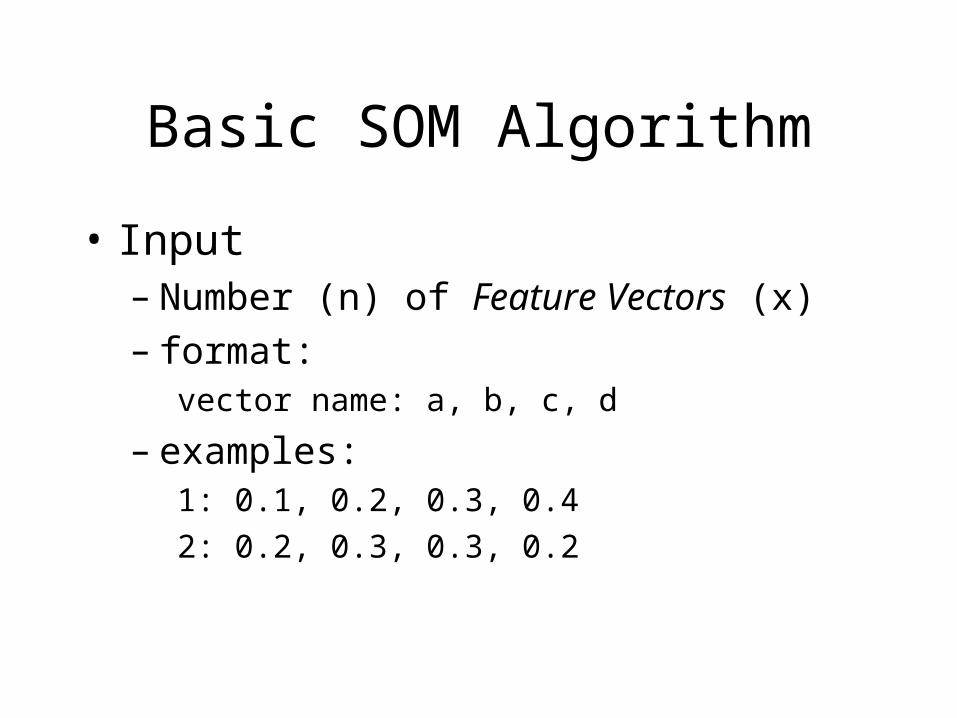
• Input– Number (n) of Feature Vectors (x)– format:
vector name: a, b, c, d
– examples:1: 0.1, 0.2, 0.3, 0.4
2: 0.2, 0.3, 0.3, 0.2
Basic SOM Algorithm
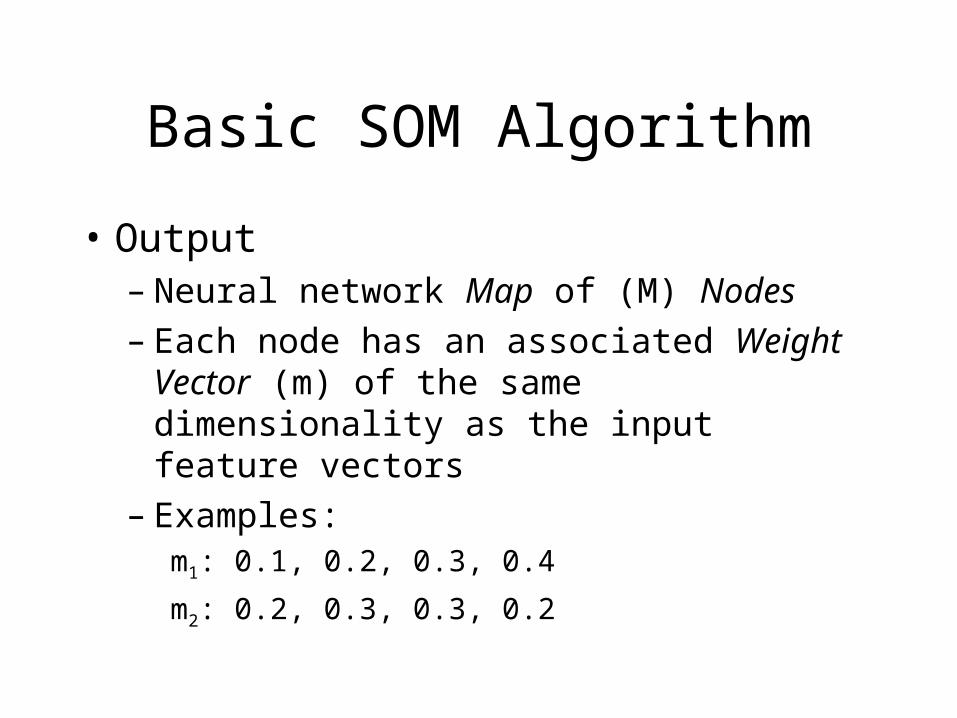
• Output– Neural network Map of (M) Nodes– Each node has an associated Weight Vector (m)
of the same dimensionality as the input feature vectors
– Examples:m1: 0.1, 0.2, 0.3, 0.4
m2: 0.2, 0.3, 0.3, 0.2
Basic SOM Algorithm
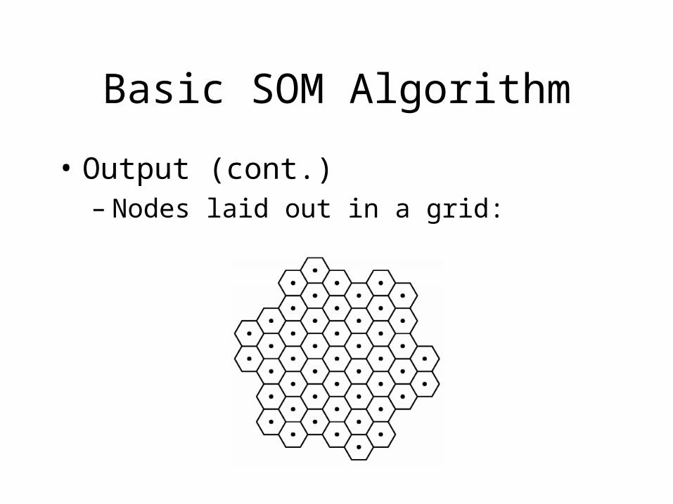
• Output (cont.)– Nodes laid out in a grid:
Basic SOM Algorithm
• Other Parameters– Number of timesteps (T)– Learning Rate (eta)
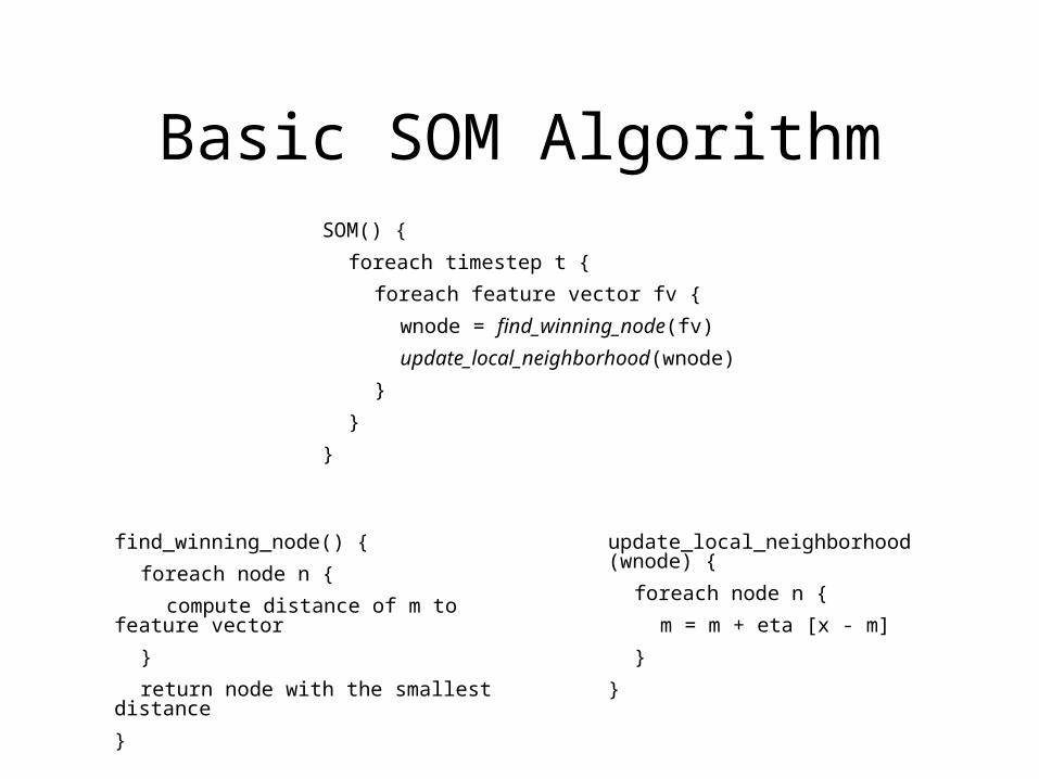
Basic SOM AlgorithmSOM() {
foreach timestep t {
foreach feature vector fv {
wnode = find_winning_node(fv)
update_local_neighborhood(wnode)
}
}
}
find_winning_node() {
foreach node n {
compute distance of m to feature vector
}
return node with the smallest distance
}
update_local_neighborhood(wnode) {
foreach node n {
m = m + eta [x - m]
}
}
U-Matrix Visualization
• Provides a simple way to visualize cluster boundaries on the map
• Simple algorithm:– for each node in the map, compute the average
of the distances between its weight vector and those of its immediate neighbors
• Average distance is a measure of a node’s similarity between it and its neighbors
U-Matrix Visualization
• Interpretation– one can encode the U-Matrix measurements as
greyscale values in an image, or as altitudes on a terrain
– landscape that represents the document space: the valleys, or dark areas are the clusters of data, and the mountains, or light areas are the boundaries between the clusters
U-Matrix Visualization
• Example:– dataset of random three dimensional points,
arranged in four obvious clusters
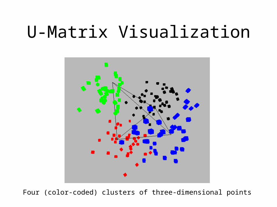
U-Matrix Visualization
Four (color-coded) clusters of three-dimensional points
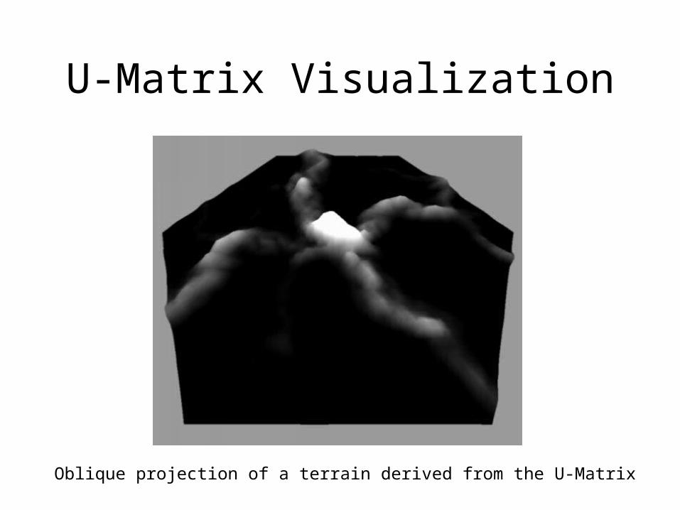
U-Matrix Visualization
Oblique projection of a terrain derived from the U-Matrix
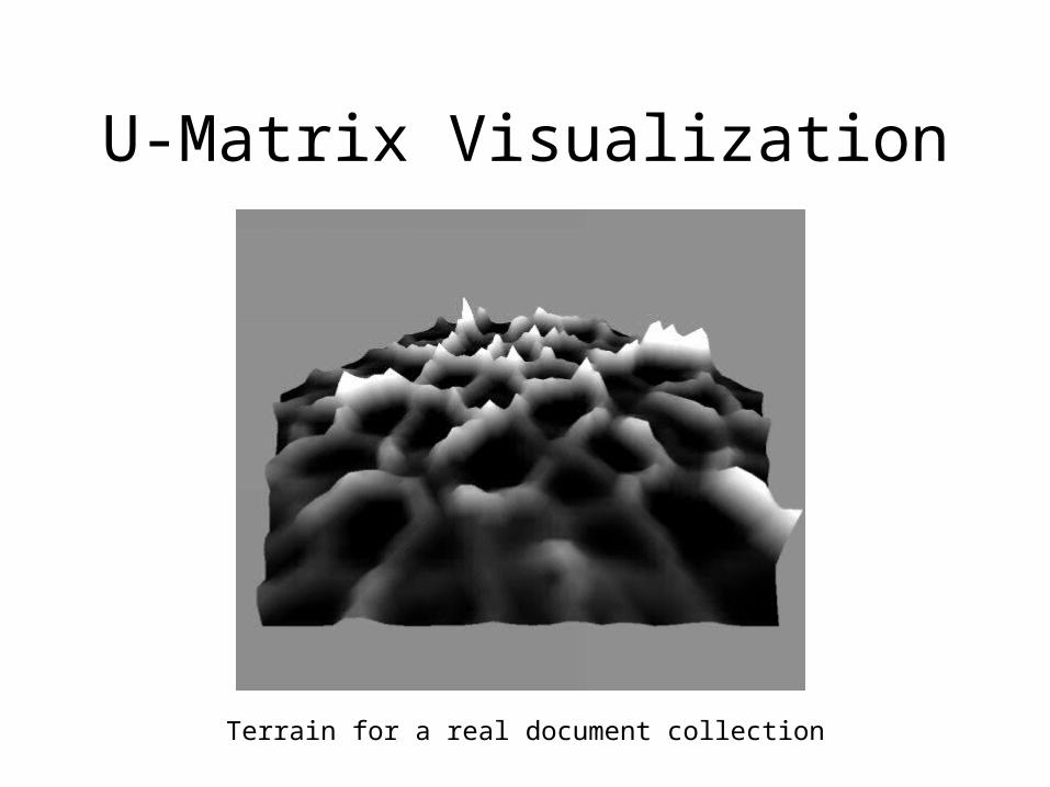
U-Matrix Visualization
Terrain for a real document collection
Current Labeling Procedure
• Feature vectors are encoded as 0’s and 1’s
• Weight vectors have real values from 0 to 1
• Sort weight vector dimensions by element value– dimension with greatest value is “best” noun
phrase for that node
• Aggregate nodes with the same “best” noun phrase into groups

Umatrix Navigation
• 3D Space-Flight
• Hierarchical Navigation
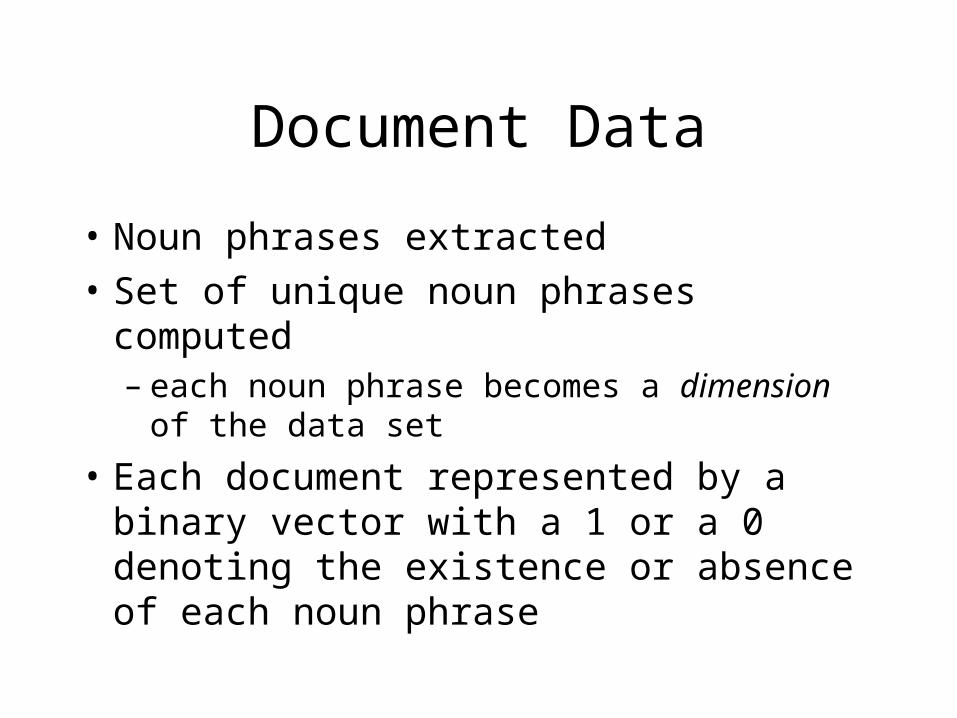
Document Data
• Noun phrases extracted
• Set of unique noun phrases computed– each noun phrase becomes a dimension of the
data set
• Each document represented by a binary vector with a 1 or a 0 denoting the existence or absence of each noun phrase
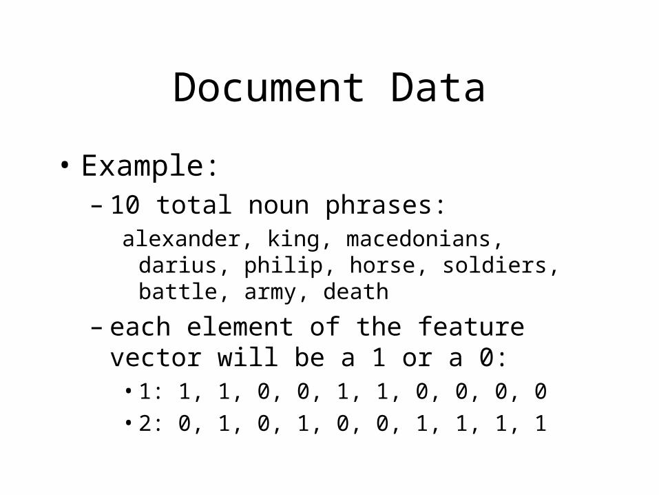
Document Data
• Example:– 10 total noun phrases:
alexander, king, macedonians, darius, philip, horse, soldiers, battle, army, death
– each element of the feature vector will be a 1 or a 0:
• 1: 1, 1, 0, 0, 1, 1, 0, 0, 0, 0
• 2: 0, 1, 0, 1, 0, 0, 1, 1, 1, 1
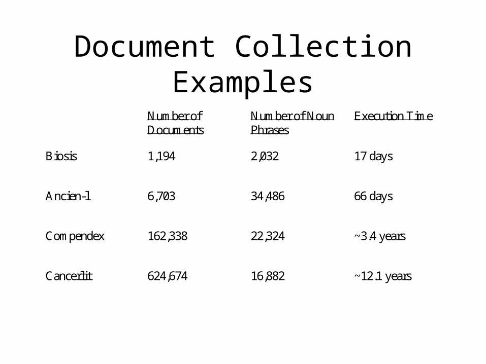
Document Collection Examples
Number ofDocuments
Number of NounPhrases
Execution Time
Biosis 1,194 2,032 17 days
Ancien-l 6,703 34,486 66 days
Compendex 162,338 22,324 ~3.4 years
Cancerlit 624,674 16,882 ~12.1 years

Problems
• As document sets get larger, the feature vectors get longer, use more memory, etc.
• Execution time grows to unrealistic lengths
Solutions?
• Need algorithm refinements for sparse feature vectors
• Need a faster way to do the find_winning_node() computation
• Need a better way to do the update_local_neighborhood() computation

Sparse Vector Optimization
• Intelligent support for sparse feature vectors– saves on memory usage– greatly improves speed of the weight vector
update computation
Faster find_winning_node()
• SOM weight vectors become partially ordered very quickly
Faster find_winning_node()
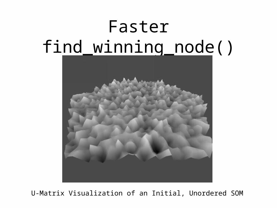
U-Matrix Visualization of an Initial, Unordered SOM
Faster find_winning_node()
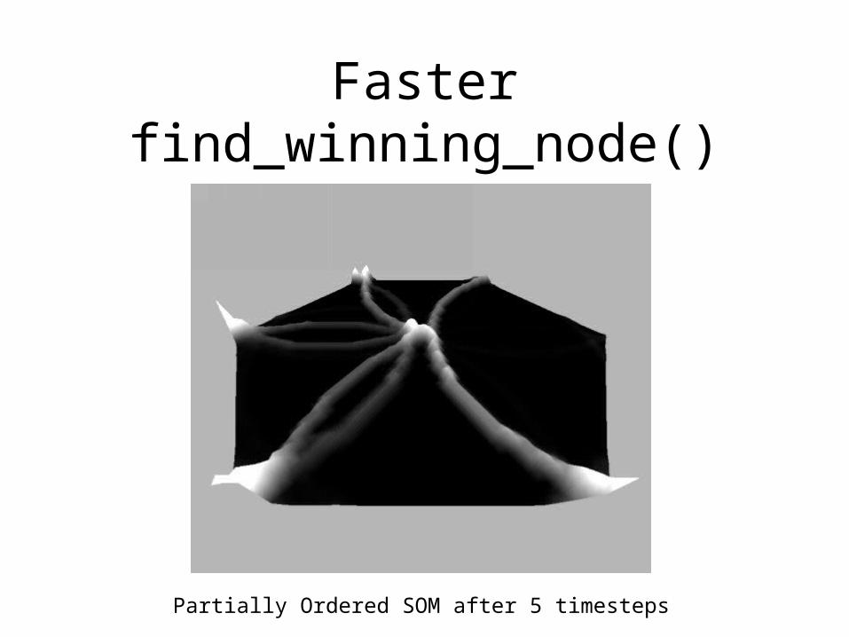
Partially Ordered SOM after 5 timesteps
Faster find_winning_node()
• Don’t do a global search for the winner
• Start search from last known winner position
• Pro:– usually finds a new winner very quickly
• Con:– this new search for a winner can sometimes get
stuck in a local minima
Better Neighborhood Update
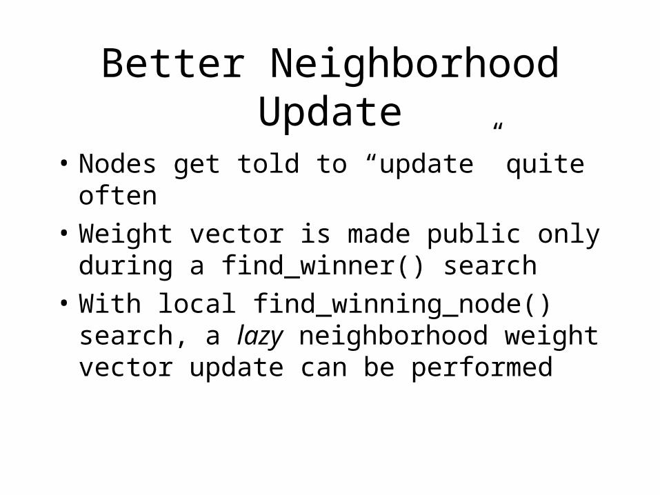
• Nodes get told to “update” quite often
• Weight vector is made public only during a find_winner() search
• With local find_winning_node() search, a lazy neighborhood weight vector update can be performed
Better Neighborhood Update
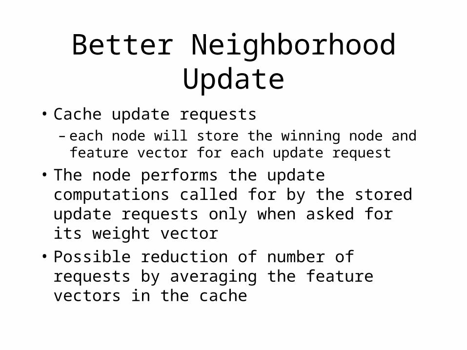
• Cache update requests– each node will store the winning node and
feature vector for each update request
• The node performs the update computations called for by the stored update requests only when asked for its weight vector
• Possible reduction of number of requests by averaging the feature vectors in the cache
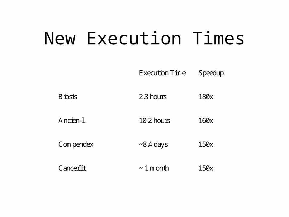
New Execution Times
Execution Time Speedup
Biosis 2.3 hours 180x
Ancien-l 10.2 hours 160x
Compendex ~8.4 days 150x
Cancerlit ~ 1 month 150x

Future Work
• Parallelization
• Label Problem
Label Problem
• Current Procedure not very good
• Cluster boundaries
• Term selection
Cluster Boundaries
• Image processing
• Geometric
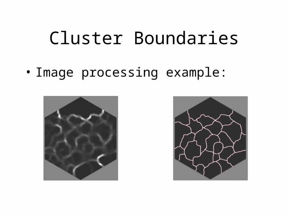
Cluster Boundaries
• Image processing example:

Term Selection
• Too many unique noun phrases– Too many dimensions in the feature vector data
• “Knee” of frequency curve