Embed Size (px)
Citation preview

Vivado Design Suite User Guide
Implementation
UG904 (v2016.4) December 19, 2016
Implementation 2UG904 (v2016.4) December 19, 2016 www.xilinx.com
Revision HistoryThe following table shows the revision history for this document.
Date Version Revision
12/19/2016 2016.4 Additional updates for the Vivado® Design Suite v.2016.4 release. Changes include:
• Added BUFG Optimization to link_design.
• In BUFG Optimization, added note about clock_Buffer_insertion occurring in mandatory logic optimization.
• Updated Table 2-4.
10/05/2016 2016.3 Updated for the Vivado Design Suite v.2016.3 release. Changes include:
• Added Table 2-3, Optimization Ordering for Multiple Options.
• Added information about additional logic optimizations:
° Mux Optimization
° Control Set Merging
° BUFG Optimization
° Module-Based Fanout Optimization
• Added Table 2-4, Optimization Phases for Directives.
• Added new directive: EarlyBlockPlacement, page 62.
• Added list of options for routing ECO changes, page 155.
06/08/2016 2016.2 Updated for the Vivado Design Suite v.2016.2 release.
04/06/2016 2016.1 Updated for the Vivado Design Suite v.2016.1 release. Changes include the following:
• Chapter 2:
° Corrected descriptions of AltSpreadLogic_medium and AltSpreadLogic_low.
° Corrected some options that didn’t have the leading “-”.
° Added information about CLOCK_BUFFER_TYPE to BUFG Optimization, page 52.
° Updated list of directives in Available Directives, page 62
° Added information about Summary of Physical Synthesis Optimizations in Physical Optimization Messages, page 71.
° Added Physical Optimization Reports, page 74.
° Added Router Messaging, page 88
• Chapter 3: Added Vivado ECO Flow, page 144.
• Appendix C: Updated all tables with Implementation Strategy descriptions.
Send Feedback
Table of ContentsRevision History . . . . . . . . . . . . . . . . . . . . . . . . . . . . . . . . . . . . . . . . . . . . . . . . . . . . . . . . . . . . . . . . . . . . 2
Chapter 1: Preparing for ImplementationAbout the Vivado Implementation Process . . . . . . . . . . . . . . . . . . . . . . . . . . . . . . . . . . . . . . . . . . . . . 5Managing Implementation . . . . . . . . . . . . . . . . . . . . . . . . . . . . . . . . . . . . . . . . . . . . . . . . . . . . . . . . . . 8Configuring, Implementing, and Verifying IP . . . . . . . . . . . . . . . . . . . . . . . . . . . . . . . . . . . . . . . . . . . 13Guiding Implementation with Design Constraints. . . . . . . . . . . . . . . . . . . . . . . . . . . . . . . . . . . . . . . 14Using Checkpoints to Save and Restore Design Snapshots. . . . . . . . . . . . . . . . . . . . . . . . . . . . . . . . 16
Chapter 2: Implementing the DesignRunning Implementation in Non-Project Mode . . . . . . . . . . . . . . . . . . . . . . . . . . . . . . . . . . . . . . . . 18Running Implementation in Project Mode. . . . . . . . . . . . . . . . . . . . . . . . . . . . . . . . . . . . . . . . . . . . . 22Customizing Implementation Strategies . . . . . . . . . . . . . . . . . . . . . . . . . . . . . . . . . . . . . . . . . . . . . . 33Launching Implementation Runs . . . . . . . . . . . . . . . . . . . . . . . . . . . . . . . . . . . . . . . . . . . . . . . . . . . . 39Moving Processes to the Background. . . . . . . . . . . . . . . . . . . . . . . . . . . . . . . . . . . . . . . . . . . . . . . . . 41Running Implementation in Steps . . . . . . . . . . . . . . . . . . . . . . . . . . . . . . . . . . . . . . . . . . . . . . . . . . . 41About Implementation Commands . . . . . . . . . . . . . . . . . . . . . . . . . . . . . . . . . . . . . . . . . . . . . . . . . . 43Implementation Sub-Processes . . . . . . . . . . . . . . . . . . . . . . . . . . . . . . . . . . . . . . . . . . . . . . . . . . . . . 43Opening the Synthesized Design. . . . . . . . . . . . . . . . . . . . . . . . . . . . . . . . . . . . . . . . . . . . . . . . . . . . . 45Logic Optimization . . . . . . . . . . . . . . . . . . . . . . . . . . . . . . . . . . . . . . . . . . . . . . . . . . . . . . . . . . . . . . . . 50Power Optimization. . . . . . . . . . . . . . . . . . . . . . . . . . . . . . . . . . . . . . . . . . . . . . . . . . . . . . . . . . . . . . . 57Placement. . . . . . . . . . . . . . . . . . . . . . . . . . . . . . . . . . . . . . . . . . . . . . . . . . . . . . . . . . . . . . . . . . . . . . . 59Physical Optimization . . . . . . . . . . . . . . . . . . . . . . . . . . . . . . . . . . . . . . . . . . . . . . . . . . . . . . . . . . . . . 66Routing . . . . . . . . . . . . . . . . . . . . . . . . . . . . . . . . . . . . . . . . . . . . . . . . . . . . . . . . . . . . . . . . . . . . . . . . . 79Incremental Compile . . . . . . . . . . . . . . . . . . . . . . . . . . . . . . . . . . . . . . . . . . . . . . . . . . . . . . . . . . . . . . 90
Chapter 3: Analyzing and Viewing Implementation ResultsMonitoring the Implementation Run . . . . . . . . . . . . . . . . . . . . . . . . . . . . . . . . . . . . . . . . . . . . . . . . 106Moving Forward After Implementation . . . . . . . . . . . . . . . . . . . . . . . . . . . . . . . . . . . . . . . . . . . . . . 109Viewing Messages . . . . . . . . . . . . . . . . . . . . . . . . . . . . . . . . . . . . . . . . . . . . . . . . . . . . . . . . . . . . . . . 111Viewing Implementation Reports. . . . . . . . . . . . . . . . . . . . . . . . . . . . . . . . . . . . . . . . . . . . . . . . . . . 113Modifying Implementation Results . . . . . . . . . . . . . . . . . . . . . . . . . . . . . . . . . . . . . . . . . . . . . . . . . 118Vivado ECO Flow . . . . . . . . . . . . . . . . . . . . . . . . . . . . . . . . . . . . . . . . . . . . . . . . . . . . . . . . . . . . . . . . 144
Implementation 3UG904 (v2016.4) December 19, 2016 www.xilinx.com
Send Feedback
Appendix A: Using Remote Hosts and LSFLaunching Runs on Remote Linux Hosts. . . . . . . . . . . . . . . . . . . . . . . . . . . . . . . . . . . . . . . . . . . . . . 162Setting Up SSH Key Agent Forward. . . . . . . . . . . . . . . . . . . . . . . . . . . . . . . . . . . . . . . . . . . . . . . . . . 167
Appendix B: ISE Command MapTcl Commands and Options. . . . . . . . . . . . . . . . . . . . . . . . . . . . . . . . . . . . . . . . . . . . . . . . . . . . . . . . 168
Appendix C: Implementation Categories, Strategy Descriptions, and Directive MappingImplementation Categories. . . . . . . . . . . . . . . . . . . . . . . . . . . . . . . . . . . . . . . . . . . . . . . . . . . . . . . . 169Implementation Strategy Descriptions. . . . . . . . . . . . . . . . . . . . . . . . . . . . . . . . . . . . . . . . . . . . . . . 169Directives Used By opt_design and place_design in Implementation Strategies . . . . . . . . . . . . . 171Directives Used by phys_opt_design and route_design in Implementation Strategies . . . . . . . . 172
Appendix D: Additional Resources and Legal NoticesXilinx Resources . . . . . . . . . . . . . . . . . . . . . . . . . . . . . . . . . . . . . . . . . . . . . . . . . . . . . . . . . . . . . . . . . 173Solution Centers. . . . . . . . . . . . . . . . . . . . . . . . . . . . . . . . . . . . . . . . . . . . . . . . . . . . . . . . . . . . . . . . . 173Documentation Navigator and Design Hubs . . . . . . . . . . . . . . . . . . . . . . . . . . . . . . . . . . . . . . . . . . 173References . . . . . . . . . . . . . . . . . . . . . . . . . . . . . . . . . . . . . . . . . . . . . . . . . . . . . . . . . . . . . . . . . . . . . 174Training Resources. . . . . . . . . . . . . . . . . . . . . . . . . . . . . . . . . . . . . . . . . . . . . . . . . . . . . . . . . . . . . . . 175Please Read: Important Legal Notices . . . . . . . . . . . . . . . . . . . . . . . . . . . . . . . . . . . . . . . . . . . . . . . 175
Implementation 4UG904 (v2016.4) December 19, 2016 www.xilinx.com
Send Feedback
Chapter 1
Preparing for Implementation
About the Vivado Implementation ProcessThe Xilinx® Vivado® Design Suite enables implementation of UltraScale™ FPGA and Xilinx 7 series FPGA designs from a variety of design sources, including:
• RTL designs
• Netlist designs
• IP-centric design flows
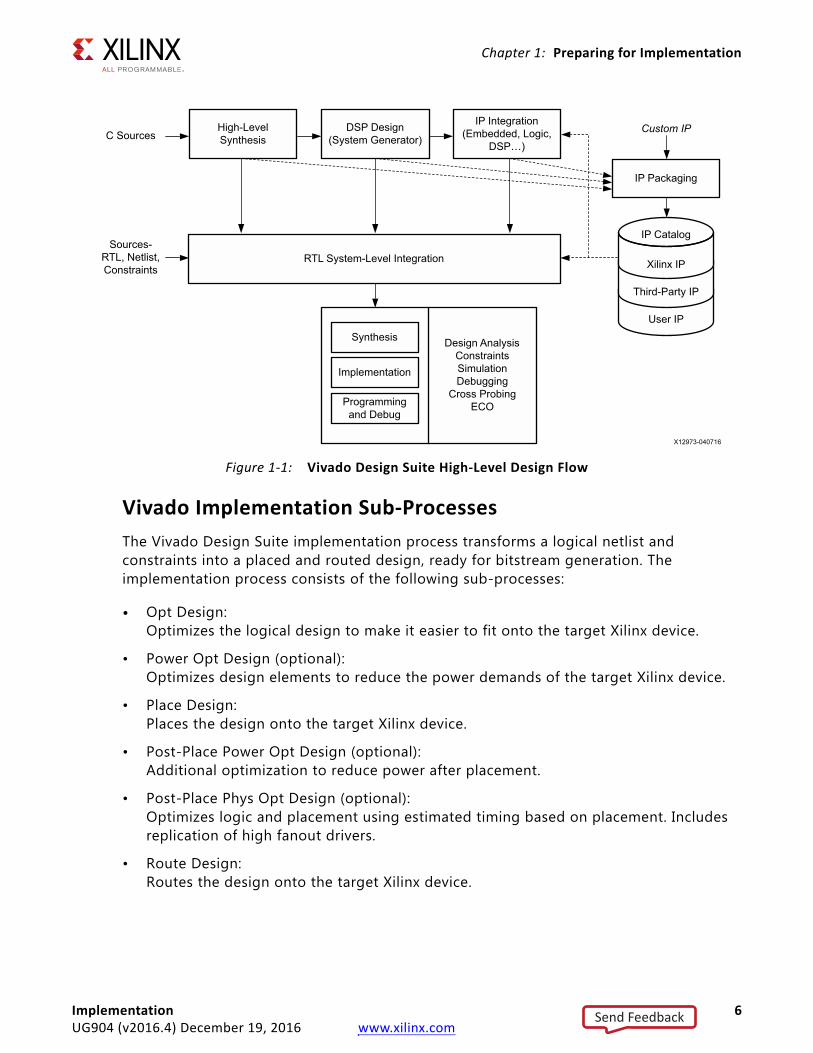
Figure 1-1 shows the Vivado tools flow.
Vivado implementation includes all steps necessary to place and route the netlist onto device resources, within the logical, physical, and timing constraints of the design.
For more information about the design flows supported by the Vivado tools, see the Vivado Design Suite User Guide: Design Flows Overview (UG892) [Ref 1].
SDC and XDC Constraint SupportThe Vivado Design Suite implementation is a timing-driven flow. It supports industry standard Synopsys Design Constraints (SDC) commands to specify design requirements and restrictions, as well as additional commands in the Xilinx Design Constraints format (XDC).
Implementation 5UG904 (v2016.4) December 19, 2016 www.xilinx.com
Send Feedback
Chapter 1: Preparing for Implementation
Vivado Implementation Sub-ProcessesThe Vivado Design Suite implementation process transforms a logical netlist and constraints into a placed and routed design, ready for bitstream generation. The implementation process consists of the following sub-processes:
• Opt Design: Optimizes the logical design to make it easier to fit onto the target Xilinx device.
• Power Opt Design (optional): Optimizes design elements to reduce the power demands of the target Xilinx device.
• Place Design: Places the design onto the target Xilinx device.
• Post-Place Power Opt Design (optional): Additional optimization to reduce power after placement.
• Post-Place Phys Opt Design (optional): Optimizes logic and placement using estimated timing based on placement. Includes replication of high fanout drivers.
• Route Design: Routes the design onto the target Xilinx device.
X-Ref Target - Figure 1-1
Figure 1-1: Vivado Design Suite High-Level Design Flow
High-Level SynthesisC Sources
DSP Design (System Generator)
IP Integration (Embedded, Logic,
DSP…)
IP Packaging
RTL System-Level IntegrationSources-
RTL, Netlist, Constraints
IP Catalog
Xilinx IP
Third-Party IP
User IP
Custom IP
Synthesis
Implementation
Programming and Debug
Design Analysis Constraints Simulation Debugging
Cross Probing ECO
Implementation 6UG904 (v2016.4) December 19, 2016 www.xilinx.com
Send Feedback
Chapter 1: Preparing for Implementation
• Post-Route Phys Opt Design (optional): Optimizes logic, placement, and routing using actual routed delays.
• Write Bitstream: Generates a bitstream for Xilinx device configuration. Typically, bitstream generation follows implementation.
For more information about writing the bitstream, see this link in the Vivado Design Suite User Guide: Programming and Debugging (UG908) [Ref 12].
Note: The Vivado Design Suite supports Module Analysis, which is the implementation of a part of a design to estimate performance. I/O buffer insertion is skipped for this flow to prevent over-utilization of I/O. For more information, search for “module analysis” in the Vivado Design Suite User Guide: Hierarchical Design (UG905) [Ref 2].
Multithreading with the Vivado ToolsOn multiprocessor systems, Vivado tools use multithreading to speed up certain processes, including DRC reporting, static timing analysis, placement, and routing. The maximum number of simultaneous threads varies, depending on the number of processors and task. The maximum number of threads by task is:
• DRC reporting: 8
• Static timing analysis: 8
• Placement: 8
• Routing: 8
• Physical optimization: 8
The default number of maximum simultaneous threads is based on the OS. For Windows systems, the limit is 2; for Linux systems the default is 8. The limit can be changed using a parameter called general.maxThreads. To change the limit use the following Tcl command:
Vivado% set_param general.maxThreads <new limit>
where the new limit must be an integer from 1 to 8, inclusive.
Tcl example on a Windows system:
Vivado% get_param general.maxThreads 2
This means all tasks are limited to 2 threads regardless of number of processors or the task being executed. If the system has at least 8 processors, you can set the limit to 8 and allow each task to use the maximum number of threads.
Vivado% set_param general.maxThreads 8
Implementation 7UG904 (v2016.4) December 19, 2016 www.xilinx.com
Send Feedback

Chapter 1: Preparing for Implementation
To summarize, the number of simultaneous threads is the smallest of the following values:
• Maximum number of processors
• Limit of threads for the task
• General limit of threads
Tcl API Supports ScriptingThe Vivado Design Suite includes a Tool Command Language (Tcl) Application Programming Interface (API). The Tcl API supports scripting for all design flows, allowing you to customize the design flow to meet your specific requirements.
Note: For more information about Tcl commands, see the Vivado Design Suite Tcl Command Reference Guide (UG835) [Ref 17] or type <command> -help.
Managing ImplementationThe Vivado Design Suite includes a variety of design flows and supports an array of design sources. To generate a bitstream that can be downloaded onto a Xilinx device, the design must pass through implementation.
Implementation is a series of steps that takes the logical netlist and maps it into the physical array of the target Xilinx device. Implementation comprises:
• Logic optimization
• Placement of logic cells
• Routing of connections between cells
Project Mode and Non-Project ModesThe Vivado Design Suite lets you run implementation with a project file (Project Mode) or without a project file (Non-Project Mode).
Project Mode
The Vivado Design Suite lets you create a project file (.xpr) and directory structure that allows you to:
• Manage the design source files.
• Store the results of the synthesis and implementation runs.
• Track the project status through the design flow.
Implementation 8UG904 (v2016.4) December 19, 2016 www.xilinx.com
Send Feedback
Chapter 1: Preparing for Implementation
Working in Project Mode
In Project Mode, a directory structure is created on disk to help you manage design sources, run results and reports, as well as project status.
The automated management of the design data, process, and status requires a project infrastructure that is stored in the Vivado project file (.xpr).
In Project Mode, the Vivado tools automatically write checkpoint files into the local project directory at key points in the design flow.
To run implementation in Project Mode, you click the Run Implementation button in the IDE or use the launch_runs Tcl command. See this link in the Vivado Design Suite User Guide: Design Flows Overview (UG892) [Ref 1] for more information about using projects in the Vivado Design Suite.
Flow Navigator
The complete design flow is integrated in the Vivado Integrated Design Environment (IDE). The Vivado IDE includes a standardized interface called the Flow Navigator.
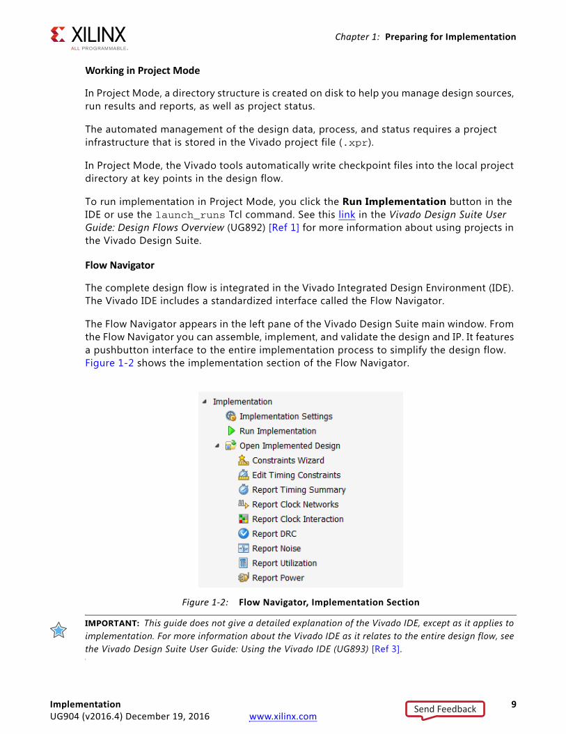
The Flow Navigator appears in the left pane of the Vivado Design Suite main window. From the Flow Navigator you can assemble, implement, and validate the design and IP. It features a pushbutton interface to the entire implementation process to simplify the design flow. Figure 1-2 shows the implementation section of the Flow Navigator.
IMPORTANT: This guide does not give a detailed explanation of the Vivado IDE, except as it applies to implementation. For more information about the Vivado IDE as it relates to the entire design flow, see the Vivado Design Suite User Guide: Using the Vivado IDE (UG893) [Ref 3].
X-Ref Target - Figure 1-2
Figure 1-2: Flow Navigator, Implementation Section
Implementation 9UG904 (v2016.4) December 19, 2016 www.xilinx.com
Send Feedback

Chapter 1: Preparing for Implementation
Non-Project Mode
The Vivado tools also let you work with the design in memory, without the need for a project file and local directory. Working without a project file in the compilation style flow is called Non-Project Mode. Source files and design constraints are read into memory from their current locations. The in-memory design is stepped through the design flow without being written to intermediate files.
In Non-Project Mode, you must run each design step individually, with the appropriate options for each implementation Tcl command.
Non-Project Mode allows you to apply design changes and proceed through the design flow without needing to save changes and rerun steps. You can run reports and save design checkpoints (.dcp) at any stage of the design flow.
IMPORTANT: In Non-Project Mode, when you exit the Vivado design tools, the in-memory design is lost. For this reason, Xilinx recommends that you write design checkpoints after major steps such as synthesis, placement, and routing.
You can save design checkpoints in both Project Mode and Non-Project Mode. You can only open design checkpoints in Non-Project Mode.
Similarities and Differences Between Project Mode and Non-Project Mode
Vivado implementation can be run in either Project Mode or Non-Project Mode. The Vivado IDE and Tcl API can be used in both Project Mode and Non-Project Mode.
There are many differences between Project Mode and Non-Project Mode. Features not available in Non-Project Mode include:
• Flow Navigator
• Design status indicators
• IP catalog
• Implementation runs and run strategies
• Design Runs window
• Messages window
• Reports window
Note: This list illustrates features that are not supported in Non-Project Mode. It is not exhaustive.
Implementation 10UG904 (v2016.4) December 19, 2016 www.xilinx.com
Send Feedback
Chapter 1: Preparing for Implementation
You must implement the non-project based design by running the individual Tcl commands:
• opt_design
• power_opt_design (optional)
• place_design
• phys_opt_design (optional)
• route_design
• phys_opt_design (optional)
• write_bitstream
You can run implementation steps interactively in the Tcl Console, in the Vivado IDE, or by using a custom Tcl script. You can customize the design flow as needed to include reporting commands and additional optimizations. For more information, see Running Implementation in Non-Project Mode.
The details of running implementation in Project Mode and Non-Project Mode are described in this guide.
For more information on running the Vivado Design Suite using either Project Mode or Non-Project Mode, see:
• Vivado Design Suite User Guide: Design Flows Overview (UG892) [Ref 1]
• Vivado Design Suite User Guide: Using the Vivado IDE (UG893) [Ref 3]
Beginning the Implementation Flow
The implementation flow typically begins by loading a synthesized design into memory. Then the implementation flow can run, or the design can be analyzed and refined along with its constraints and the design can be reloaded after updates.
There are two ways to begin the implementation flow with a synthesized design:
• Run Vivado synthesis. In Project Mode, the synthesis run contains the synthesis results and those results are automatically used as the input for implementation run. In Non-Project Mode, the synthesis results are in memory after synth_design completes, and implementation can continue from that point.
• Load a synthesized netlist. Synthesized netlists can be used as the input design source, for example when using a third-party tool for synthesis.
To initiate implementation:
• In Project Mode, launch the implementation run.
• In Non-Project Mode run a script or interactive commands.
Implementation 11UG904 (v2016.4) December 19, 2016 www.xilinx.com
Send Feedback
Chapter 1: Preparing for Implementation
To analyze and refine constraints, the synthesized design is loaded without running implementation.
• In Project Mode, you accomplish this by opening the Synthesized Design, which is the result of the synthesis run.
• In Non-Project Mode, you use the link_design command to load the design.
You can also drive the implementation flow using design checkpoints in Non-Project Mode. Opening a checkpoint loads the design and restores it to its original state, which might include placement and routing data. This enables re-entrant implementation flows, such as loading a routed design and editing the routing, or loading a placed design and running multiple routes with different options.
Importing Previously Synthesized Netlists
The Vivado Design Suite supports netlist-driven design by importing previously synthesized netlists from Xilinx or third-party tools. The netlist input formats include:
• Structural Verilog
• Structural SystemVerilog
• EDIF
• Xilinx NGC
• Synthesized Design Checkpoint (DCP)
IMPORTANT: NGC format files are not supported in the Vivado Design Suite for UltraScale devices. It is recommended that you regenerate the IP using the Vivado Design Suite IP customization tools with native output products. Alternatively, convert_ngc Tcl utility to convert NGC files to EDIF or Verilog formats. However, Xilinx recommends using native Vivado IP rather than XST-generated NGC format files going forward.
IMPORTANT: When using IP in Project Mode or Non-Project Mode, always use the XCI file not the DCP file. This ensures that IP output products are used consistently during all stages of the design flow. If the IP was synthesized out-of-context and already has an associated DCP file, the DCP file is automatically used and the IP is not re-synthesized. For more information, this link in the Vivado Design Suite User Guide: Designing with IP (UG896) [Ref 4].
For more information on the source files and project types supported by the Vivado Design Suite, see the Vivado Design Suite User Guide: System-Level Design Entry (UG895) [Ref 6].
Implementation 12UG904 (v2016.4) December 19, 2016 www.xilinx.com
Send Feedback
Chapter 1: Preparing for Implementation
Starting From RTL Sources
At a minimum, Vivado implementation requires a synthesized netlist. A design can start from a synthesized netlist, or from RTL source files.
IMPORTANT: If you start from RTL sources, you must first run Vivado synthesis before implementation can begin. The Vivado IDE manages this automatically if you attempt to run implementation on an un-synthesized design. The tools allow you to run synthesis first.
For information on running Vivado synthesis, see the Vivado Design Suite User Guide: Synthesis (UG901) [Ref 8].
Creating and Opening the Synthesized Design in Non-Project Mode
In Non-Project Mode, you must run the Tcl command synth_design to create and open the synthesized design. You can also run the Tcl command link_design to open a synthesized netlist in any supported input format. You can open a synthesized design checkpoint file using the open_checkpoint command.
For more information, see Opening the Synthesized Design in Chapter 2, Implementing the Design.
Loading the Design Netlist in Project Mode Before Implementation
In Project Mode, after synthesis of an RTL design, or with a netlist-based project open, you can load the design netlist for analysis before implementation.
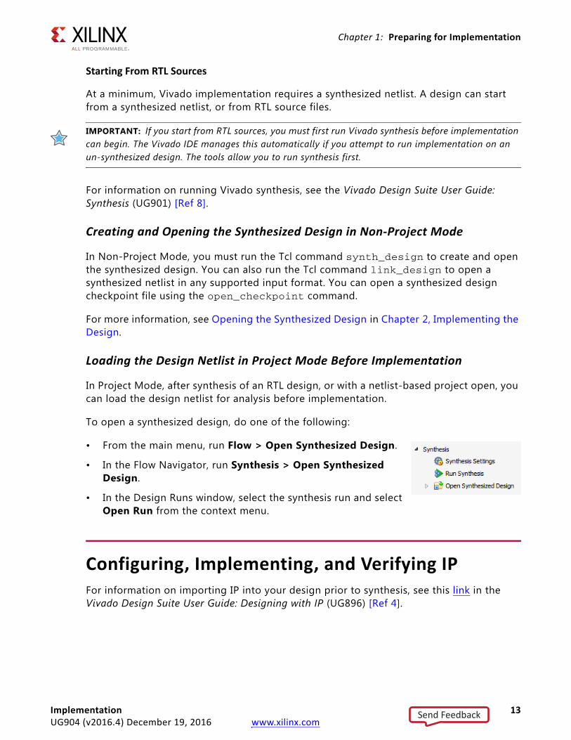
To open a synthesized design, do one of the following:
• From the main menu, run Flow > Open Synthesized Design.
• In the Flow Navigator, run Synthesis > Open Synthesized Design.
• In the Design Runs window, select the synthesis run and select Open Run from the context menu.
Configuring, Implementing, and Verifying IPFor information on importing IP into your design prior to synthesis, see this link in the Vivado Design Suite User Guide: Designing with IP (UG896) [Ref 4].
Implementation 13UG904 (v2016.4) December 19, 2016 www.xilinx.com
Send Feedback
Chapter 1: Preparing for Implementation
Guiding Implementation with Design ConstraintsRECOMMENDED: Include design constraints to guide implementation. There are two types of design constraints, physical constraints and timing constraints.
There are two types of design constraints, physical constraints and timing constraints. These are defined below.
Physical Constraints Definition Physical constraints define a relationship between logical design objects and device resources such as:
• Package pin placement.
• Absolute or relative placement of cells, including Block RAM, DSP, LUT, and flip-flops.
• Floorplanning constraints that assign cells to general regions of a device.
• Device configuration settings.
Timing Constraints DefinitionTiming constraints define the frequency requirements for the design, and are written in industry standard SDC.
Without timing constraints, the Vivado Design Suite optimizes the design solely for wire length and routing congestion, and makes no effort to assess or improve design performance.
UCF Format Not SupportedIMPORTANT: The Vivado Design Suite does not support the UCF format.
For information on migrating UCF constraints to XDC commands, see this link in the ISE to Vivado Design Suite Migration Guide (UG911) [Ref 18].
Constraint Sets Apply Lists of Constraint Files to Your DesignA constraint set is a list of constraint files that can be applied to your design in Project Mode. The set contains design constraints captured in XDC or Tcl files.
Implementation 14UG904 (v2016.4) December 19, 2016 www.xilinx.com
Send Feedback
Chapter 1: Preparing for Implementation
Allowed Constraint Set Structures
The following constraint set structures are allowed:
• Multiple constraint files within a constraint set
• Constraint sets with separate physical and timing constraint files
• A master constraint file
• A new constraint file that accepts constraint changes
• Multiple constraint sets
TIP: Separate constraints by function into different constraint files to (a) make your constraint strategy clearer, and (b) to facilitate targeting timing and implementation changes.
Multiple Constraint Sets Are Allowed
You can have multiple constraint sets for a project. Multiple constraint sets allow you to use different implementation runs to test different approaches.
For example, you can have one constraint set for synthesis, and a second constraint set for implementation. Having two constraint sets allows you to experiment by applying different constraints during synthesis, simulation, and implementation.
Organizing design constraints into multiple constraint sets can help you:
• Target various Xilinx devices for the same project. Different physical and timing constraints might be needed for different target devices.
• Perform what-if design exploration. Use constraint sets to explore various scenarios for floorplanning and over-constraining the design.
• Manage constraint changes. Override master constraints with local changes in a separate constraint file.
TIP: To validate the timing constraints, run report_timing_summary on the synthesized design. Fix problematic constraints before implementation!
For more information on defining and working with constraints that affect placement and routing, see this link in the Vivado Design Suite User Guide: Using Constraints (UG903) [Ref 9].
Implementation 15UG904 (v2016.4) December 19, 2016 www.xilinx.com
Send Feedback
Chapter 1: Preparing for Implementation
Adding Constraints as Attribute StatementsConstraints can be added to HDL sources as attribute statements. Attributes can be added to both Verilog and VHDL sources to pass through to Vivado synthesis or Vivado implementation.
In some cases, constraints are available only as HDL attributes, and are not available in XDC. In those cases, the constraint must be specified as an attribute in the HDL source file. For example, Relatively Placed Macros (RPMs) must be defined using HDL attributes. An RPM is a set of logic elements (such as FF, LUT, DSP, and RAM) with relative placements.
You can define RPMs using U_SET and HU_SET attributes and define relative placements using Relative Location Attributes.
For more information about Relative Location Constraints, see this link in the Vivado Design Suite User Guide: Using Constraints (UG903) [Ref 9].
For more information on constraints that are not supported in XDC, see the ISE to Vivado Design Suite Migration Guide (UG911) [Ref 18].
Using Checkpoints to Save and Restore Design SnapshotsThe Vivado Design Suite uses a physical design database to store placement and routing information. Design checkpoint files (.dcp) allow you to save and restore this physical database at key points in the design flow. A checkpoint is a snapshot of a design at a specific point in the flow.
This design checkpoint file includes:
• Current netlist, including any optimizations made during implementation
• Design constraints
• Implementation results
Checkpoint designs can be run through the remainder of the design flow using Tcl commands. They cannot be modified with new design sources.
IMPORTANT: In Project Mode, the Vivado design tools automatically save and restore checkpoints as the design progresses. In Non-Project Mode, you must save checkpoints at appropriate stages of the design flow, otherwise, progress is lost.
Implementation 16UG904 (v2016.4) December 19, 2016 www.xilinx.com
Send Feedback

Chapter 1: Preparing for Implementation
Writing Checkpoint Files Run File > Write Checkpoint to capture a snapshot of the design database at any point in the flow. This creates a file with a dcp extension.
The related Tcl command is write_checkpoint.
Reading Checkpoint Files Run File > Open Checkpoint to open the checkpoint in the Vivado Design Suite.
The design checkpoint is opened as a separate in-memory design.
The related Tcl command is open_checkpoint.
Implementation 17UG904 (v2016.4) December 19, 2016 www.xilinx.com
Send Feedback
Chapter 2
Implementing the Design
Running Implementation in Non-Project ModeTo implement the synthesized design or netlist onto the targeted Xilinx® devices in Non-Project Mode, you must run the Tcl commands corresponding to the Implementation sub-processes:
• Opt Design: Optimizes the logical design to make it easier to fit onto the target Xilinx device.
• Power Opt Design (optional): Optimizes design elements to reduce the power demands of the target Xilinx device.
• Place Design: Places the design onto the target Xilinx device.
• Post-Place Power Opt Design (optional): Additional optimization to reduce power after placement.
• Post-Place Phys Opt Design (optional): Optimizes logic and placement using estimated timing based on placement. Includes replication of high fanout drivers.
• Route Design: Routes the design onto the target Xilinx device.
• Post-Route Phys Opt Design (optional): Optimizes logic, placement, and routing using actual routed delays.
• Write Bitstream: Generates a bitstream for Xilinx device configuration. Typically, bitstream generation follows implementation.
For more information about writing the bitstream, see this link in the Vivado Design Suite User Guide: Programming and Debugging (UG908) [Ref 12].
These steps are collectively known as implementation.
Enter the commands in any of the following ways:
• In the Tcl Console from the Vivado® IDE.
• From the Tcl prompt in the Vivado Design Suite Tcl shell.
• Using a Tcl script with the implementation commands and source the script in the Vivado Design Suite.
Implementation 18UG904 (v2016.4) December 19, 2016 www.xilinx.com
Send Feedback
Chapter 2: Implementing the Design
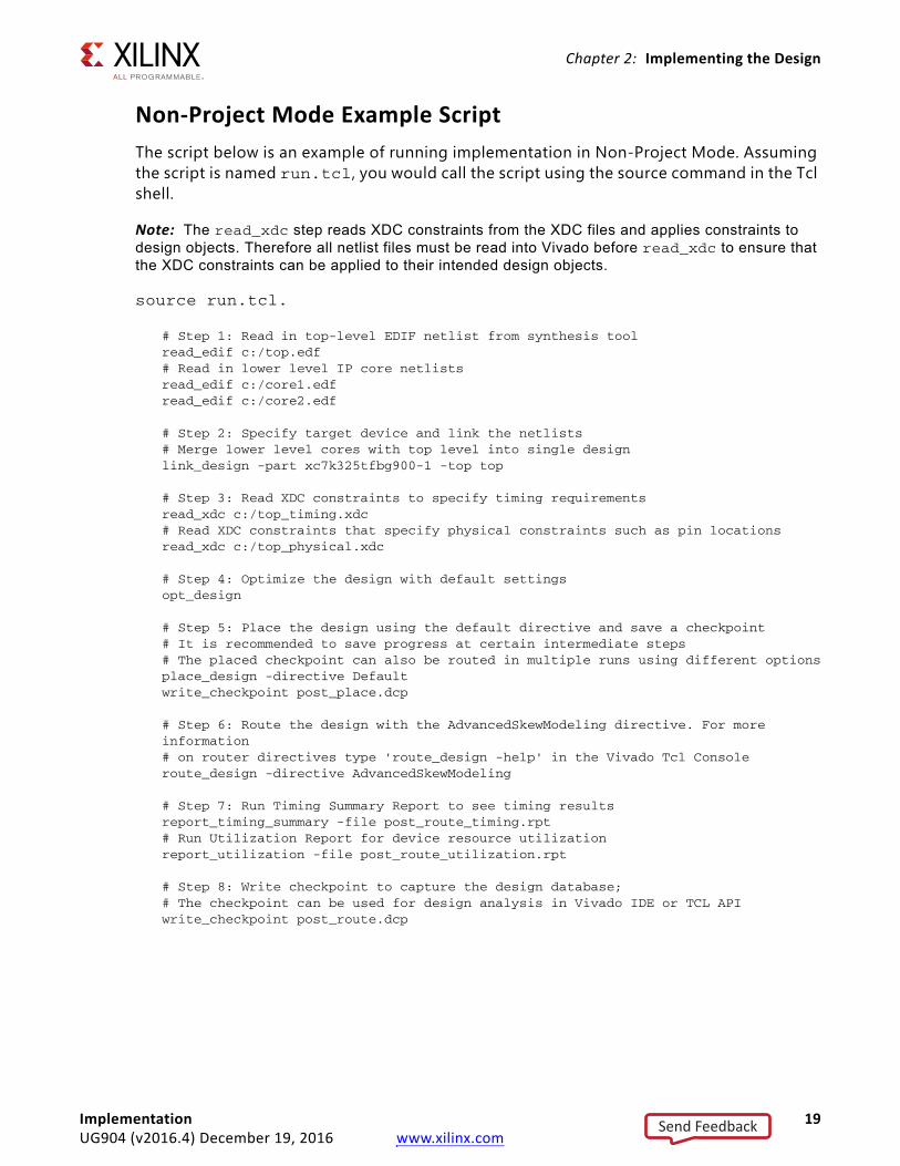
Non-Project Mode Example ScriptThe script below is an example of running implementation in Non-Project Mode. Assuming the script is named run.tcl, you would call the script using the source command in the Tcl shell.
Note: The read_xdc step reads XDC constraints from the XDC files and applies constraints to design objects. Therefore all netlist files must be read into Vivado before read_xdc to ensure that the XDC constraints can be applied to their intended design objects.
source run.tcl.
# Step 1: Read in top-level EDIF netlist from synthesis toolread_edif c:/top.edf # Read in lower level IP core netlistsread_edif c:/core1.edfread_edif c:/core2.edf
# Step 2: Specify target device and link the netlists# Merge lower level cores with top level into single designlink_design -part xc7k325tfbg900-1 -top top
# Step 3: Read XDC constraints to specify timing requirementsread_xdc c:/top_timing.xdc # Read XDC constraints that specify physical constraints such as pin locationsread_xdc c:/top_physical.xdc
# Step 4: Optimize the design with default settingsopt_design
# Step 5: Place the design using the default directive and save a checkpoint# It is recommended to save progress at certain intermediate steps# The placed checkpoint can also be routed in multiple runs using different optionsplace_design -directive Defaultwrite_checkpoint post_place.dcp
# Step 6: Route the design with the AdvancedSkewModeling directive. For more information # on router directives type 'route_design -help' in the Vivado Tcl Console route_design -directive AdvancedSkewModeling
# Step 7: Run Timing Summary Report to see timing resultsreport_timing_summary -file post_route_timing.rpt # Run Utilization Report for device resource utilizationreport_utilization -file post_route_utilization.rpt
# Step 8: Write checkpoint to capture the design database; # The checkpoint can be used for design analysis in Vivado IDE or TCL APIwrite_checkpoint post_route.dcp
Implementation 19UG904 (v2016.4) December 19, 2016 www.xilinx.com
Send Feedback

Chapter 2: Implementing the Design
Key Steps in Non-Project Mode Example ScriptThe key steps in the Non-Project Mode Example Script, page 19 above, are:
• Step 1: Read Design Source Files
• Step 2: Build the In-Memory Design
• Step 3: Read Design Constraints
• Step 4: Perform Logic Optimization
• Step 5: Place the Design
• Step 6: Route the Design
• Step 7: Run Required Reports
• Step 8: Save the Design Checkpoint
Step 1: Read Design Source Files
EDIF netlist design sources are read into memory through use of the read_edif command. Non-Project Mode also supports an RTL design flow, which allows you to read source files and run synthesis before implementation.
Use the read_checkpoint command to add synthesized design checkpoint files as sources.
The read_* Tcl commands are designed for use with Non-Project Mode. The read_* Tcl commands allow the Vivado tools to read a file on the disk and build the in-memory design without copying the file or creating a dependency on the file.
This approach makes Non-Project Mode highly flexible with regard to design.
IMPORTANT: You must monitor any changes to the source design files, and update the design as needed.
Step 2: Build the In-Memory Design
The Vivado tools build an in-memory view of the design using link_design. The link_design command combines the netlist based source files read into the tools with the Xilinx part information, to create a design database in memory.
All actions taken in Non-Project Mode are directed at the in-memory database within the Vivado tools.
The in-memory design resides in the Vivado tools, whether running in batch mode, Tcl shell mode for interactive Tcl commands, or in the Vivado IDE for interaction with the design data in a graphical form.
Implementation 20UG904 (v2016.4) December 19, 2016 www.xilinx.com
Send Feedback
Chapter 2: Implementing the Design
Step 3: Read Design Constraints
The Vivado Design Suite uses design constraints to define requirements for both the physical and timing characteristics of the design.
For more information, see Guiding Implementation with Design Constraints, page 14.
The read_xdc command reads an XDC constraint file, then applies it to the in-memory design.
TIP: Although Project Mode supports the definition of constraint sets, containing multiple constraint files for different purposes, Non-Project Mode uses multiple read_xdc commands to achieve the same effect.
Step 4: Perform Logic Optimization
Logic optimization is run in preparation for placement and routing. Optimization simplifies the logic design before committing to physical resources on the target part.
The Vivado netlist optimizer includes many different types of optimizations to meet varying design requirements. For more information, see Logic Optimization, page 50.
Step 5: Place the Design
The place_design command places the design. For more information, see Placement, page 59. After placement, the progress is saved to a design checkpoint file using the write_checkpoint command.
Step 6: Route the Design
The route_design command routes the design. For more information, see Routing, page 79.
Step 7: Run Required Reports
The report_timing_summary command runs timing analysis and generates a timing report with details of timing violations. The report_utilization command generates a summary of the percentage of device resources used along with other utilization statistics. In Non-Project Mode, you must use the appropriate Tcl command to specify each report that you want to create. Each reporting command supports the -file option to direct output to a file.
See this link the Vivado Design Suite Tcl Command Reference Guide (UG835) [Ref 17] for further information on the report_timing_summary command and this link for further information on report_utilization command.
Implementation 21UG904 (v2016.4) December 19, 2016 www.xilinx.com
Send Feedback
Chapter 2: Implementing the Design
You can output reports to files for later review, or you can send the reports directly to the Vivado IDE to review now. For more information, see Viewing Implementation Reports, page 113.
Step 8: Save the Design Checkpoint
Saves the in-memory design into a design checkpoint file. The saved in-memory design includes the following:
• Logical netlist
• Physical and timing related constraints
• Xilinx part data
• Placement and routing information
In Non-Project Mode, the design checkpoint file saves the design and allows it to be reloaded for further analysis and modification.
For more information, see Using Checkpoints to Save and Restore Design Snapshots.
Running Implementation in Project ModeIn Project Mode, the Vivado IDE allows you to:
• Define implementation runs that are configured to use specific synthesis results and design constraints.
• Run multiple strategies on a single design.
• Customize implementation strategies to meet specific design requirements.
• Save customized implementation strategies to use in other designs.
IMPORTANT: Non-Project Mode does not support predefined implementation runs and strategies. Non-project based designs must be manually moved through each step of the implementation process using Tcl commands. For more information, see Running Implementation in Non-Project Mode.
Creating Implementation RunsYou can create and launch new implementation runs to explore design alternatives and find the best results. You can queue and launch the runs serially or in parallel using multiple, local CPUs.
On Linux systems, you can launch runs on remote servers. For more information, see Appendix A, Using Remote Hosts and LSF.
Implementation 22UG904 (v2016.4) December 19, 2016 www.xilinx.com
Send Feedback
Chapter 2: Implementing the Design
Defining Implementation Runs
To define an implementation run:
1. From the main menu, select Flow > Create Runs.
(Alternatively, in the Flow Navigator, select Create Implementation Runs from the Implementation popup menu. Or, in the Design Runs window, select Create Runs from the popup menu.)
The Create New Runs wizard opens.
2. Select Implementation on the first page of the Create New Runs wizard, and click Next.
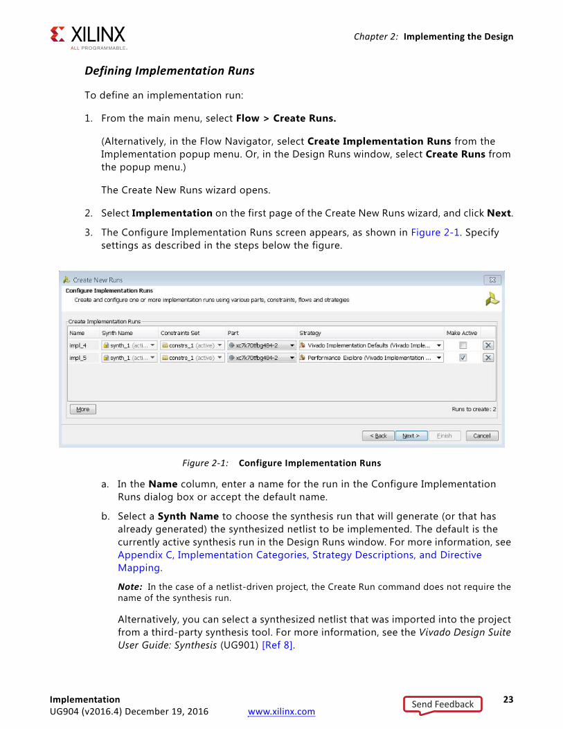
3. The Configure Implementation Runs screen appears, as shown in Figure 2-1. Specify settings as described in the steps below the figure.
a. In the Name column, enter a name for the run in the Configure Implementation Runs dialog box or accept the default name.
b. Select a Synth Name to choose the synthesis run that will generate (or that has already generated) the synthesized netlist to be implemented. The default is the currently active synthesis run in the Design Runs window. For more information, see Appendix C, Implementation Categories, Strategy Descriptions, and Directive Mapping.
Note: In the case of a netlist-driven project, the Create Run command does not require the name of the synthesis run.
Alternatively, you can select a synthesized netlist that was imported into the project from a third-party synthesis tool. For more information, see the Vivado Design Suite User Guide: Synthesis (UG901) [Ref 8].
X-Ref Target - Figure 2-1
Figure 2-1: Configure Implementation Runs
Implementation 23UG904 (v2016.4) December 19, 2016 www.xilinx.com
Send Feedback
Chapter 2: Implementing the Design
c. Select a Constraints Set to apply during implementation. The optimization, placement, and routing are largely directed by the physical and timing constraints in the specified constraint set.
For more information on constraint sets, see the Vivado Design Suite User Guide: Using Constraints (UG903) [Ref 9].
d. Select a target Part.
The default values for Constraints Set and Part are defined by the Project Settings when the Create New Runs command is executed.
For more information on the Project Settings, see this link in the Vivado Design Suite User Guide: System-Level Design Entry (UG895) [Ref 6].
TIP: To create runs with different constraint sets or target parts, use the Create New Runs command. To change these values on existing runs, select the run in the Design Runs window and edit the Run Properties.
For more information, see Changing Implementation Run Settings, page 28.
e. Select a Strategy.
Strategies are a defined set of Vivado implementation feature options that control the implementation results. Vivado Design Suite includes a set of pre-defined strategies. You can also create your own implementation strategies.
Select from among the strategies shown in Appendix C, Implementation Categories, Strategy Descriptions, and Directive Mapping. The strategies are broken into categories according to their purposes, with the category name as a prefix. The categories are shown in Appendix C.
For more information see Defining Strategies, page 34.
TIP: The optimal strategy can change between designs and software releases.
The purpose of using Performance strategies is to improve design performance at the expense of run time. You should always try to meet timing goals, using the Vivado implementation defaults first, before choosing a Performance strategy. This ensures that your design has sufficient margin for absorbing timing closure impact due to design changes. But if your design goals cannot be met, and if increased run time is acceptable, the Performance_Explore strategy is a good first choice. It covers all types design types.
IMPORTANT: Strategies containing the terms SLL or SLR are for use with SSI devices only.
Implementation 24UG904 (v2016.4) December 19, 2016 www.xilinx.com
Send Feedback
Chapter 2: Implementing the Design
TIP: Before launching a run, you can change the settings for each step in the implementation process, overriding the default settings for the selected strategy. You can also save those new settings as a new strategy. For more information, see Changing Implementation Run Settings, page 28.
f. Click More to define additional runs. By default, the next strategy in the sequence is automatically chosen. Specify names and strategies for the added runs. See Figure 2-1, above.
g. Use the Make Active check box to select the runs you wish to initiate.
h. Click Next.
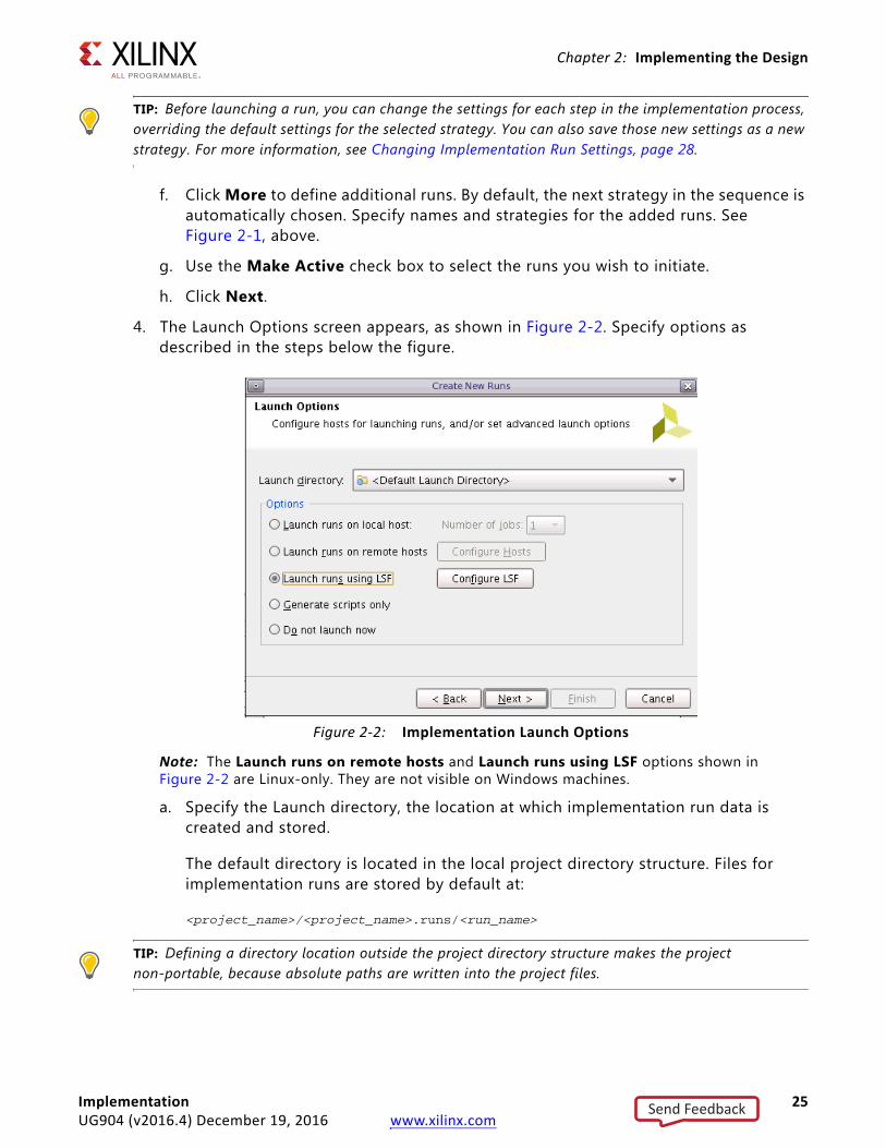
4. The Launch Options screen appears, as shown in Figure 2-2. Specify options as described in the steps below the figure.
Note: The Launch runs on remote hosts and Launch runs using LSF options shown in Figure 2-2 are Linux-only. They are not visible on Windows machines.
a. Specify the Launch directory, the location at which implementation run data is created and stored.
The default directory is located in the local project directory structure. Files for implementation runs are stored by default at:
<project_name>/<project_name>.runs/<run_name>
TIP: Defining a directory location outside the project directory structure makes the project non-portable, because absolute paths are written into the project files.
X-Ref Target - Figure 2-2
Figure 2-2: Implementation Launch Options
Implementation 25UG904 (v2016.4) December 19, 2016 www.xilinx.com
Send Feedback
Chapter 2: Implementing the Design
b. Use the radio buttons and drop-down options to specify settings appropriate to your project. Choose from the following:
- Select the Launch runs on local host option if you want to launch the run on the local machine.
- Use the Number of jobs drop-down menu to define the number of local processors to use when launching multiple runs simultaneously.
- Select Launch runs on remote hosts (Linux only) if you want to use remote hosts to launch one or more jobs.
- Use the Configure Hosts button to configure remote hosts. For more information, see Appendix A, Using Remote Hosts and LSF.
- Select Launch runs using LSF (Linux only) if you want to use LSF (Load Sharing Facility) bsub command to launch one or more jobs. Use the Configure LSF button to set up the bsub command options and test your LSF connection.
TIP: LSF, the Load Sharing Facility, is a subsystem for submitting, scheduling, executing, monitoring, and controlling a workload of batch jobs across compute servers in a cluster.
- Select the Generate scripts only option if you want to export and create the run directory and run script but do not want the run script to launch at this time. The script can be run later outside the Vivado IDE tools.
- Select do not launch now if you want to save the new runs, but you do not want to launch or create run scripts at this time.
5. Click Next to review the Create New Runs Summary.
6. Click Finish to create the defined runs and execute the specified launch options.
New runs are added to the Design Runs window. See Using the Design Runs Window.
Using the Design Runs WindowThe Design Runs window displays all synthesis and implementation runs created in the project. It includes commands to configure, manage, and launch the runs.
Opening the Design Runs Window
Select Window > Design Runs to open the Design Runs window (see Figure 2-3) if it is not already open.
Implementation 26UG904 (v2016.4) December 19, 2016 www.xilinx.com
Send Feedback
Chapter 2: Implementing the Design
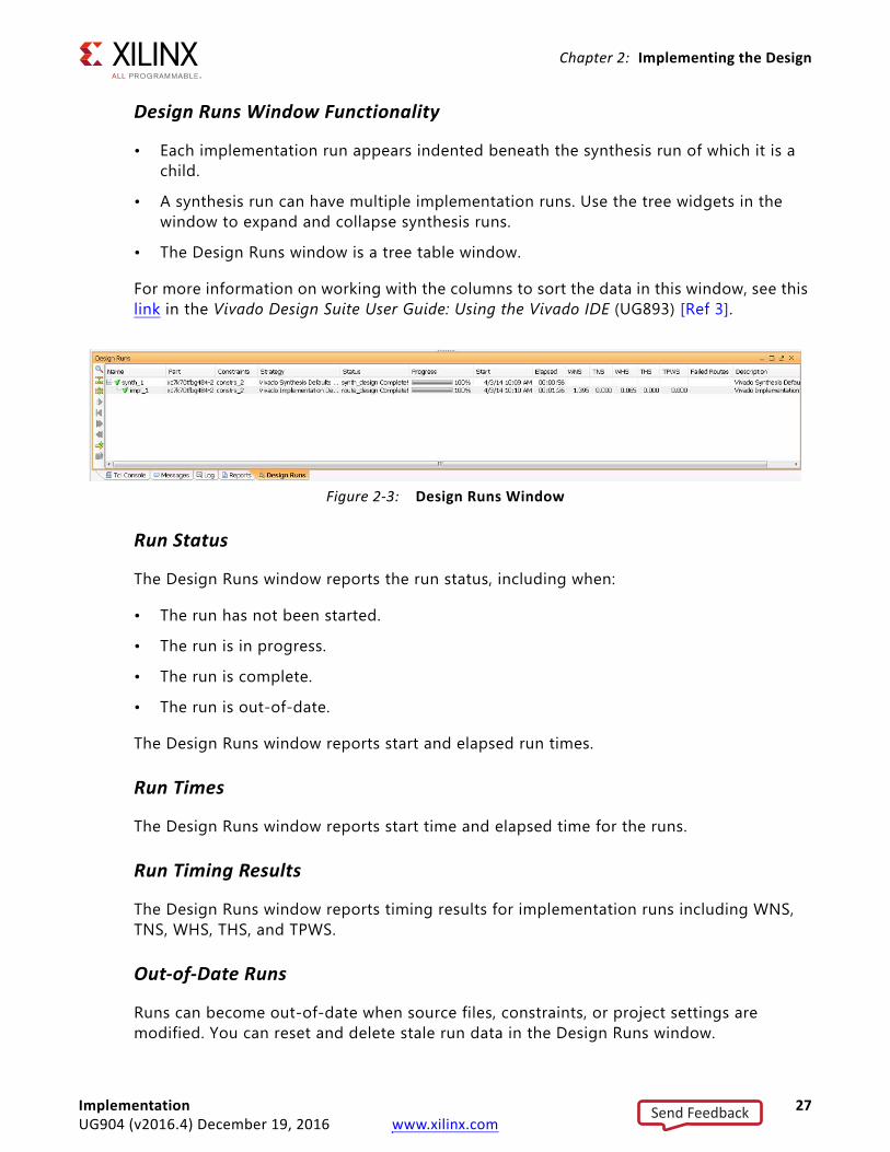
Design Runs Window Functionality
• Each implementation run appears indented beneath the synthesis run of which it is a child.
• A synthesis run can have multiple implementation runs. Use the tree widgets in the window to expand and collapse synthesis runs.
• The Design Runs window is a tree table window.
For more information on working with the columns to sort the data in this window, see this link in the Vivado Design Suite User Guide: Using the Vivado IDE (UG893) [Ref 3].
Run Status
The Design Runs window reports the run status, including when:
• The run has not been started.
• The run is in progress.
• The run is complete.
• The run is out-of-date.
The Design Runs window reports start and elapsed run times.
Run Times
The Design Runs window reports start time and elapsed time for the runs.
Run Timing Results
The Design Runs window reports timing results for implementation runs including WNS, TNS, WHS, THS, and TPWS.
Out-of-Date Runs
Runs can become out-of-date when source files, constraints, or project settings are modified. You can reset and delete stale run data in the Design Runs window.
X-Ref Target - Figure 2-3
Figure 2-3: Design Runs Window
Implementation 27UG904 (v2016.4) December 19, 2016 www.xilinx.com
Send Feedback
Chapter 2: Implementing the Design
Active Run
All views in the Vivado IDE reference the active run. The Log view, Report view, Status Bar, and Project Summary display information for the active run. The Project Summary window displays only compilation, resource, and summary information for the active run.
TIP: Only one synthesis run and one implementation run can be active in the Vivado IDE at any time.
The active run is displayed in bold text.
To make a run active:
1. Select the run in the Design Runs window.
2. Select Make Active from the popup menu.
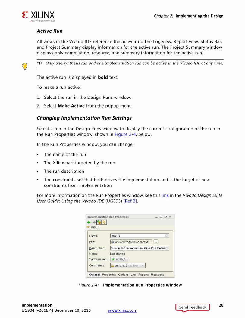
Changing Implementation Run Settings
Select a run in the Design Runs window to display the current configuration of the run in the Run Properties window, shown in Figure 2-4, below.
In the Run Properties window, you can change:
• The name of the run
• The Xilinx part targeted by the run
• The run description
• The constraints set that both drives the implementation and is the target of new constraints from implementation
For more information on the Run Properties window, see this link in the Vivado Design Suite User Guide: Using the Vivado IDE (UG893) [Ref 3].
X-Ref Target - Figure 2-4
Figure 2-4: Implementation Run Properties Window
Implementation 28UG904 (v2016.4) December 19, 2016 www.xilinx.com
Send Feedback
Chapter 2: Implementing the Design
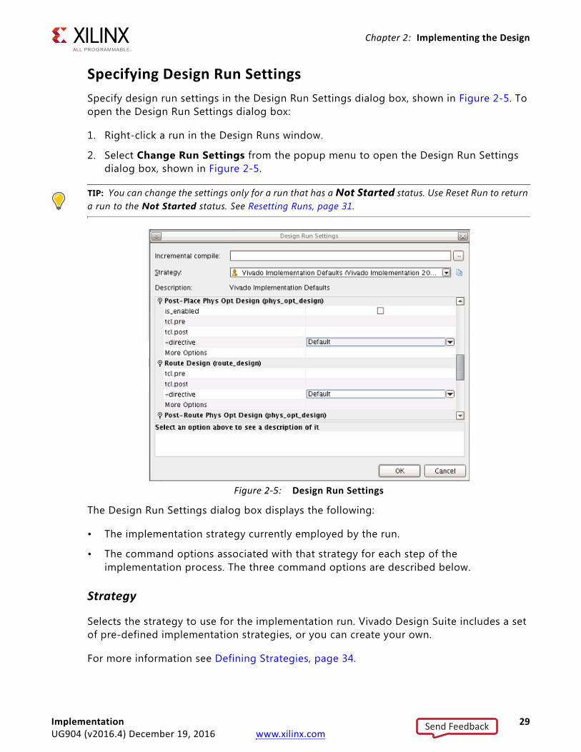
Specifying Design Run SettingsSpecify design run settings in the Design Run Settings dialog box, shown in Figure 2-5. To open the Design Run Settings dialog box:
1. Right-click a run in the Design Runs window.
2. Select Change Run Settings from the popup menu to open the Design Run Settings dialog box, shown in Figure 2-5.
TIP: You can change the settings only for a run that has a Not Started status. Use Reset Run to return a run to the Not Started status. See Resetting Runs, page 31.
The Design Run Settings dialog box displays the following:
• The implementation strategy currently employed by the run.
• The command options associated with that strategy for each step of the implementation process. The three command options are described below.
Strategy
Selects the strategy to use for the implementation run. Vivado Design Suite includes a set of pre-defined implementation strategies, or you can create your own.
For more information see Defining Strategies, page 34.
X-Ref Target - Figure 2-5
Figure 2-5: Design Run Settings
Implementation 29UG904 (v2016.4) December 19, 2016 www.xilinx.com
Send Feedback
Chapter 2: Implementing the Design
Description
Describes the selected implementation strategy.
Options
When you select a strategy, each step of the Vivado implementation process displays in a table in the lower part of the dialog box:
• Opt Design (opt_design)
• Power Opt Design (power_opt_design) (optional)
• Place Design (place_design)
• Post-Place Power Opt Design (power_opt_design) (optional)
• Post-Place Phys Opt Design (phys_opt_design) (optional)
• Route Design (route_design)
• Post-Route Phys Opt Design (phys_opt_design) (optional)
• Write Bitstream (write_bitstream)
Click the command option to view a brief description of the option at the bottom of the Design Run Settings dialog box.
For more information about the implementation steps and their available options, see Chapter 2, Implementing the Design.
Modifying Command Options
To modify command options, click the right-side column of a specific option. You can do the following:
• Select options with predefined settings from the pull down menu.
• Select or deselect a check box to enable or disable options.
Note: The most common options for each implementation command are available through the check boxes. Add other supported command options using the More Options field. Syntax: precede option names with a hyphen and separate options from each other with a space.
• Type a value to define options that accept a user-defined value.
• Options accepting a file name and path open a file browser to let you locate and specify the file.
• Insert a custom Tcl script (called a hook script) before and after each step in the implementation process (tcl.pre and tcl.post).
Implementation 30UG904 (v2016.4) December 19, 2016 www.xilinx.com
Send Feedback
Chapter 2: Implementing the Design
Inserting a hook script lets you perform specific tasks before or after each implementation step (for example, generate a timing report before and after Place Design to compare timing results).
For more information on defining Tcl hook scripts, see this link in the Vivado Design Suite User Guide: Using Tcl Scripting (UG894) [Ref 5].
TIP: Relative paths in the tcl.pre and tcl.post scripts are relative to the appropriate run directory of the project they are applied to: <project>/<project.runs>/<run_name>
Use the DIRECTORY property of the current project or current run to define the relative paths in your Tcl scripts:
get_property DIRECTORY [current_project]get_property DIRECTORY [current_run]
Save Strategy As
Select the Save Strategy As icon next to the Strategy field to save any changes to the strategy as a new strategy for future use.
CAUTION! If you do not select Save Strategy As, changes are saved to the current implementation run, but are not preserved for future use.
Verifying Run StatusThe Vivado IDE processes the run and launches implementation, depending on the status of the run. The status is displayed in the Design Runs window (shown in Figure 2-3).
• If the status of the run is Not Started, the run begins immediately.
• If the status of the run is Error, the tools reset the run to remove any incomplete run data, then restarts the run.
• If the status of the run is Complete (or Out-of-Date), the tools prompt you to confirm that the run should be reset before proceeding with the run.
Resetting Runs
To reset a run:
1. Select a run in the Design Runs window.
2. Select Reset Runs from the popup menu.
Resetting an implementation run returns it to the first step of implementation (opt_design) for the selected run.
Implementation 31UG904 (v2016.4) December 19, 2016 www.xilinx.com
Send Feedback
Chapter 2: Implementing the Design
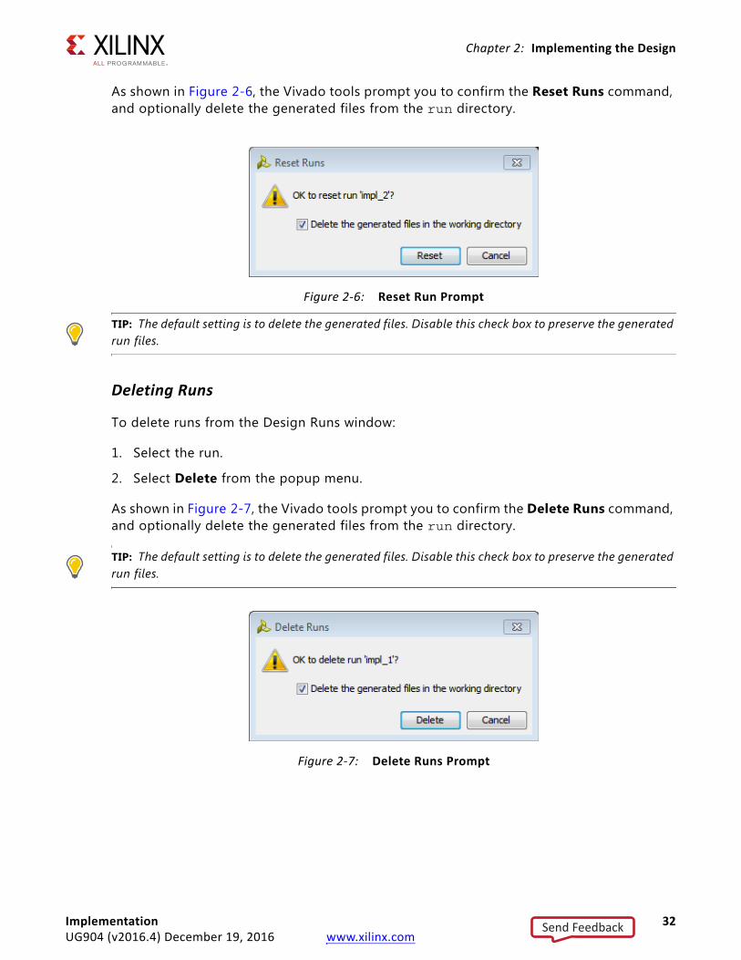
As shown in Figure 2-6, the Vivado tools prompt you to confirm the Reset Runs command, and optionally delete the generated files from the run directory.
TIP: The default setting is to delete the generated files. Disable this check box to preserve the generated run files.
Deleting Runs
To delete runs from the Design Runs window:
1. Select the run.
2. Select Delete from the popup menu.
As shown in Figure 2-7, the Vivado tools prompt you to confirm the Delete Runs command, and optionally delete the generated files from the run directory.
TIP: The default setting is to delete the generated files. Disable this check box to preserve the generated run files.
X-Ref Target - Figure 2-6
Figure 2-6: Reset Run Prompt
X-Ref Target - Figure 2-7
Figure 2-7: Delete Runs Prompt
Implementation 32UG904 (v2016.4) December 19, 2016 www.xilinx.com
Send Feedback
Chapter 2: Implementing the Design
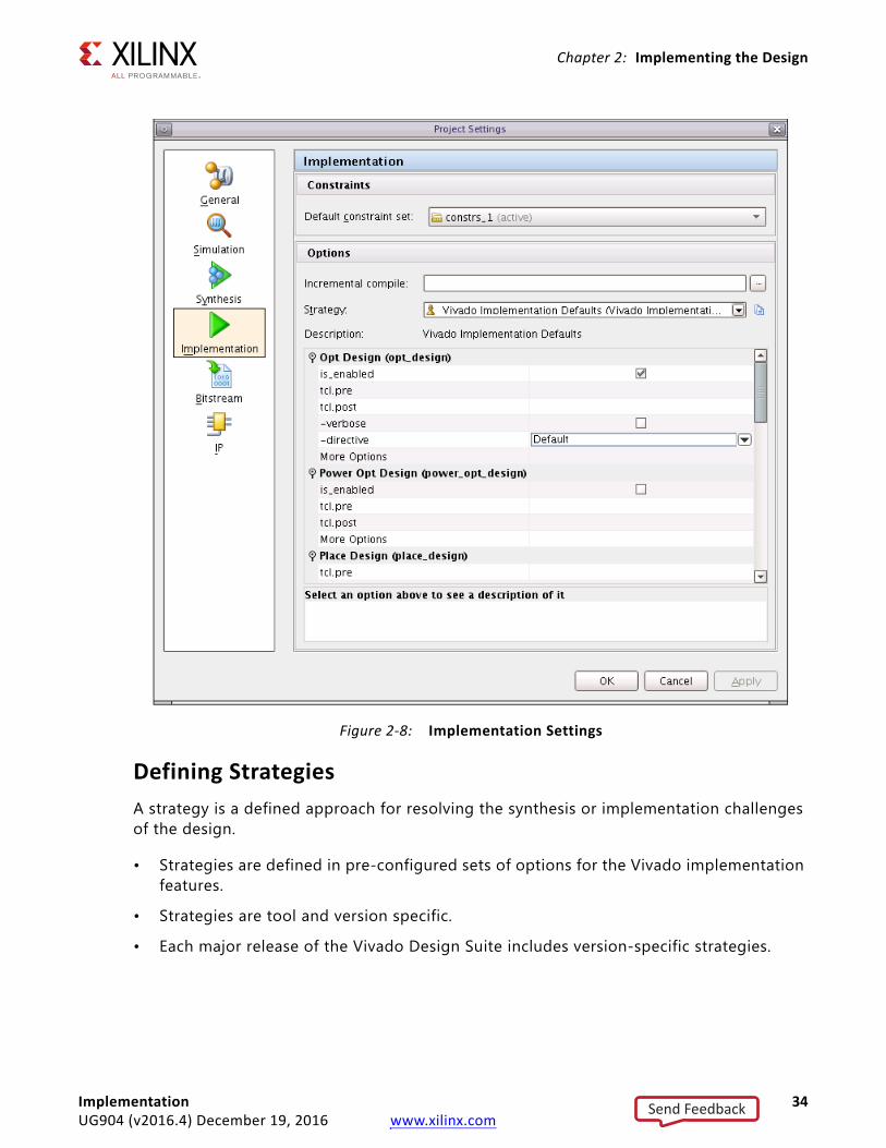
Customizing Implementation StrategiesImplementation Settings define the default options used when you define new implementation runs. Configure these options in the Vivado IDE.
Figure 2-8 shows the Implementation Settings view in the Project Settings dialog box. To open this dialog box from the Vivado IDE, select Tools > Project Settings from the main menu.
TIP: The Project Settings command is not available in the Vivado IDE when running in Non-Project Mode. In this case, you can define and preserve implementation strategies as Tcl scripts that can be used in batch mode, or interactively in the Vivado IDE.
Accessing Implementation Settings for the Active Run from Flow NavigatorYou can also access Implementation Settings for the active implementation run directly from the Flow Navigator.
The Implementation Settings dialog box, shown in Figure 2-8, contains the following fields:
• Default Constraint Set:Select the constraint set to be used by default for the implementation run.
• Incremental Compile:Specify the Incremental Compile checkpoint, if desired.
• Strategy:Select the strategy to use for the implementation run. The Vivado Design Suite includes a set of pre-defined strategies. You can also create your own implementation strategies and save changes as new strategies for future use. For more information see Defining Strategies.
• Description:Describes the selected implementation strategy. The description of user-defined strategies can be changed by entering a new descriptions. The description of Vivado tools standard implementation strategies cannot be changed.
Implementation 33UG904 (v2016.4) December 19, 2016 www.xilinx.com
Send Feedback
Chapter 2: Implementing the Design
Defining StrategiesA strategy is a defined approach for resolving the synthesis or implementation challenges of the design.
• Strategies are defined in pre-configured sets of options for the Vivado implementation features.
• Strategies are tool and version specific.
• Each major release of the Vivado Design Suite includes version-specific strategies.
X-Ref Target - Figure 2-8
Figure 2-8: Implementation Settings
Implementation 34UG904 (v2016.4) December 19, 2016 www.xilinx.com
Send Feedback
Chapter 2: Implementing the Design
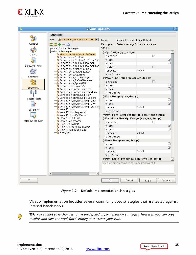
Vivado implementation includes several commonly used strategies that are tested against internal benchmarks.
TIP: You cannot save changes to the predefined implementation strategies. However, you can copy, modify, and save the predefined strategies to create your own.
X-Ref Target - Figure 2-9
Figure 2-9: Default Implementation Strategies
Implementation 35UG904 (v2016.4) December 19, 2016 www.xilinx.com
Send Feedback
Chapter 2: Implementing the Design
Accessing Currently Defined StrategiesTo access the currently defined strategies, select Tools > Options in the Vivado IDE main menu.
Reviewing, Copying, and Modifying StrategiesTo review, copy, and modify strategies:
1. Select Tools > Options from the main menu.
2. Select Strategies in the left-side panel.
The Strategies dialog box (shown in Figure 2-9, above) contains a list of pre-defined strategies for various tools and release versions.
3. In the Flow pull-down menu, select the appropriate Vivado Implementation version for the available strategies. A list of included strategies is displayed.
4. Create a new strategy or copy an existing strategy.
° To create a new strategy, click the Create New Strategy button on the toolbar or select it from the right-click menu.
° To copy an existing strategy, select Create a copy of this strategy from the toolbar or from the popup menu. The Vivado design tools:
a.Create a copy of the currently selected strategy.
b.Add it to the User Defined Strategies list.
c.Display the strategy options on the right side of the dialog box for you to modify.
5. Provide a name and description for the new strategy as follows:
° Name: Enter a strategy name to assign to a run.
° Type: Specify Synthesis or Implementation.
° Tool Version: Specify the tool version.
° Description: Enter the strategy description displayed in the Design Run results table.
Implementation 36UG904 (v2016.4) December 19, 2016 www.xilinx.com
Send Feedback
Chapter 2: Implementing the Design
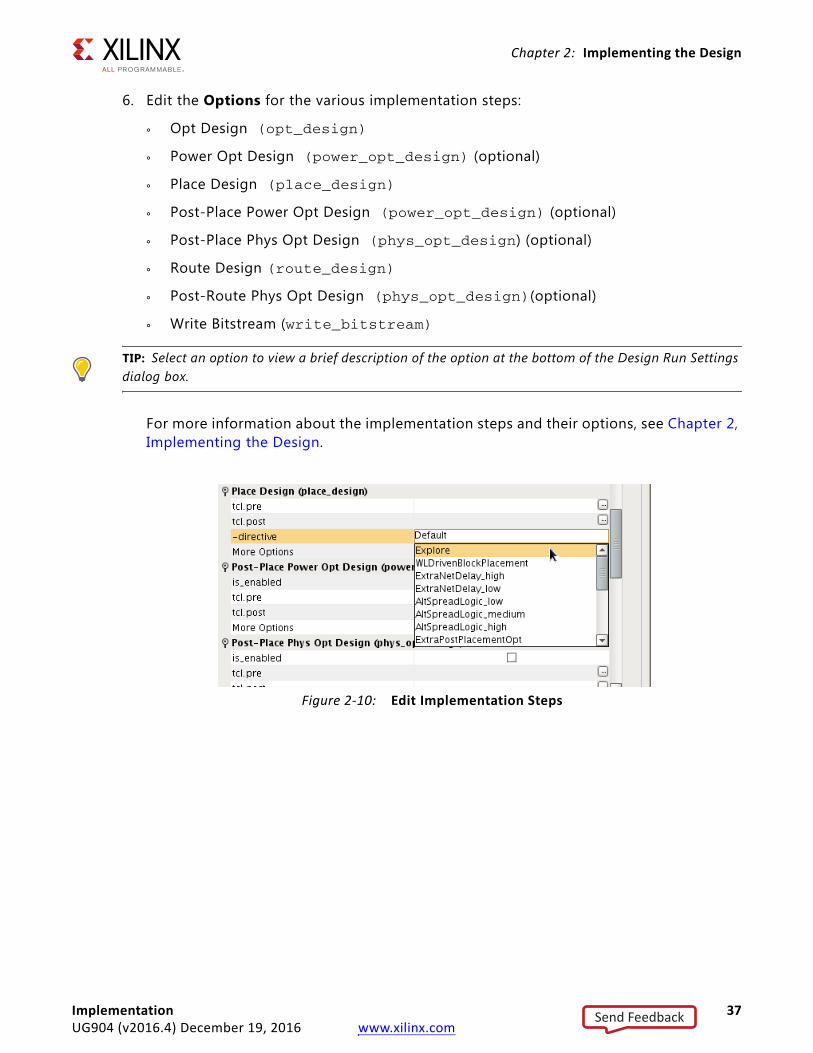
6. Edit the Options for the various implementation steps:
° Opt Design (opt_design)
° Power Opt Design (power_opt_design) (optional)
° Place Design (place_design)
° Post-Place Power Opt Design (power_opt_design) (optional)
° Post-Place Phys Opt Design (phys_opt_design) (optional)
° Route Design (route_design)
° Post-Route Phys Opt Design (phys_opt_design)(optional)
° Write Bitstream (write_bitstream)
TIP: Select an option to view a brief description of the option at the bottom of the Design Run Settings dialog box.
For more information about the implementation steps and their options, see Chapter 2, Implementing the Design.
X-Ref Target - Figure 2-10
Figure 2-10: Edit Implementation Steps
Implementation 37UG904 (v2016.4) December 19, 2016 www.xilinx.com
Send Feedback

Chapter 2: Implementing the Design
7. Click the right-side column of a specific option to modify command options. See Figure 2-10, Edit Implementation Steps, immediately above for an example.
You can then:
° Select predefined options from the pull down menu.
° Enable or disable some options with a check box.
° Type a user-defined value for options with a text entry field.
° Use the file browser to specify a file for options accepting a file name and path.
° Insert a custom Tcl script (called a hook script) before and after each step in the implementation process (tcl.pre and tcl.post). This lets you perform specific tasks either before or after each implementation step (for example, generating a timing report before and after Place Design to compare timing results).
For more information on defining Tcl hook scripts, see this link in the Vivado Design Suite User Guide: Using Tcl Scripting (UG894) [Ref 5].
Note: Relative paths in the tcl.pre and tcl.post scripts are relative to the appropriate run directory of the project they are applied to: <project>/<project.runs>/<run_name>
You can use the DIRECTORY property of the current project or current run to define the relative paths in your scripts:
get_property DIRECTORY [current_project]get_property DIRECTORY [current_run]
8. Click OK to save the new strategy.
The new strategy is listed under User Defined Strategy. The Vivado tools save user-defined strategies to the following locations:
• Linux OS
$HOME/.Xilinx/Vivado/strategies
• Windows 7
C:\Users\<username>\AppData\Roaming\Xilinx\Vivado\strategies
Sharing StrategiesDesign teams that want to create and share strategies can copy any user-defined strategy from the user directory to the <InstallDir>/Vivado/<version>/strategies directory, where <InstallDir> is the installation directory of the Xilinx software, and <version> is the release version.
Implementation 38UG904 (v2016.4) December 19, 2016 www.xilinx.com
Send Feedback
Chapter 2: Implementing the Design
Launching Implementation RunsDo any of the following to launch the active implementation run in the Design Runs window:
• Select Run Implementation in the Flow Navigator.
• Select Flow > Run Implementation from the main menu.
• Select Run Implementation from the toolbar menu.
• Select a run in the Design Runs window and select Launch Runs from the popup menu.
Launching a single implementation run initiates a separate process for the implementation.
TIP: Select a run in the Design Runs window to launch a run other than the active run. Select two or more runs in the Design Runs window to launch multiple runs at the same time.
1. Use Shift+click or Ctrl+click to select multiple runs.
Note: You can choose both synthesis and implementation runs when selecting multiple runs in the Design Runs window. The Vivado IDE manages run dependencies and launches runs in the correct order.
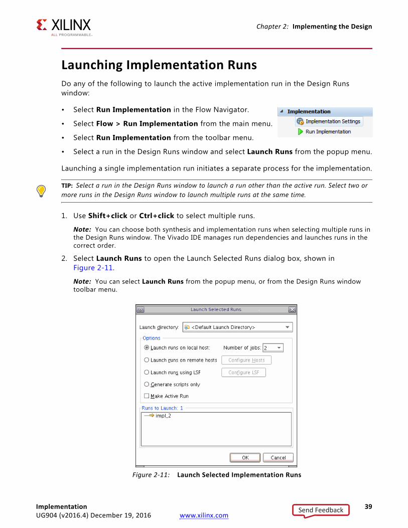
2. Select Launch Runs to open the Launch Selected Runs dialog box, shown in Figure 2-11.
Note: You can select Launch Runs from the popup menu, or from the Design Runs window toolbar menu.
X-Ref Target - Figure 2-11
Figure 2-11: Launch Selected Implementation Runs
Implementation 39UG904 (v2016.4) December 19, 2016 www.xilinx.com
Send Feedback
Chapter 2: Implementing the Design
3. Select Launch Directory.
The default launch directory is in the local project directory structure. Files for implementation runs are stored at:
<project_name>/<project_name>.runs/<run_name>
TIP: Defining any non-default location outside the project directory structure makes the project non-portable because absolute paths are written into the project files.
4. Specify Options.
° Select the Launch runs on local host option if you want to launch the run on the local machine.
° Use the Number of jobs drop-down menu to define the number of local processors to use when launching multiple runs simultaneously.
° Select Launch runs on remote hosts (Linux only) if you want to use remote hosts to launch one or more jobs.
° Use the Configure Hosts button to configure remote hosts. For more information, see Appendix A, Using Remote Hosts and LSF.
° Select Launch runs using LSF (Linux only) if you want to use LSF (Load Sharing Facility) bsub command to launch one or more jobs. Use the Configure LSF button to set up the bsub command options and test your LSF connection.
TIP: LSF, the Load Sharing Facility, is a subsystem for submitting, scheduling, executing, monitoring, and controlling a workload of batch jobs across compute servers in a cluster.
° Select the Generate scripts only option if you want to export and create the run directory and run script but do not want the run script to launch at this time. The script can be run later outside the Vivado IDE tools.
° Select do not launch now if you want to save the new runs, but you do not want to launch or create run scripts at this time.
Implementation 40UG904 (v2016.4) December 19, 2016 www.xilinx.com
Send Feedback
Chapter 2: Implementing the Design
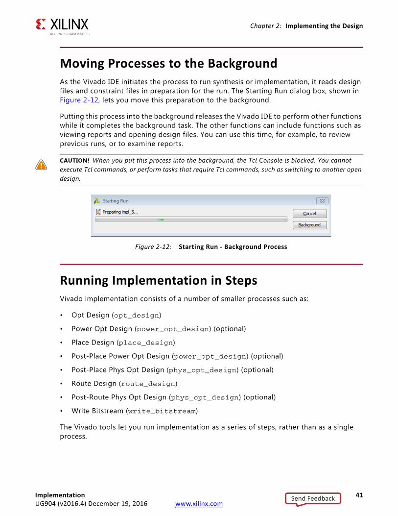
Moving Processes to the BackgroundAs the Vivado IDE initiates the process to run synthesis or implementation, it reads design files and constraint files in preparation for the run. The Starting Run dialog box, shown in Figure 2-12, lets you move this preparation to the background.
Putting this process into the background releases the Vivado IDE to perform other functions while it completes the background task. The other functions can include functions such as viewing reports and opening design files. You can use this time, for example, to review previous runs, or to examine reports.
CAUTION! When you put this process into the background, the Tcl Console is blocked. You cannot execute Tcl commands, or perform tasks that require Tcl commands, such as switching to another open design.
Running Implementation in StepsVivado implementation consists of a number of smaller processes such as:
• Opt Design (opt_design)
• Power Opt Design (power_opt_design) (optional)
• Place Design (place_design)
• Post-Place Power Opt Design (power_opt_design) (optional)
• Post-Place Phys Opt Design (phys_opt_design) (optional)
• Route Design (route_design)
• Post-Route Phys Opt Design (phys_opt_design) (optional)
• Write Bitstream (write_bitstream)
The Vivado tools let you run implementation as a series of steps, rather than as a single process.
X-Ref Target - Figure 2-12
Figure 2-12: Starting Run - Background Process
Implementation 41UG904 (v2016.4) December 19, 2016 www.xilinx.com
Send Feedback
Chapter 2: Implementing the Design
How to Run Implementation in StepsTo run implementation in steps:
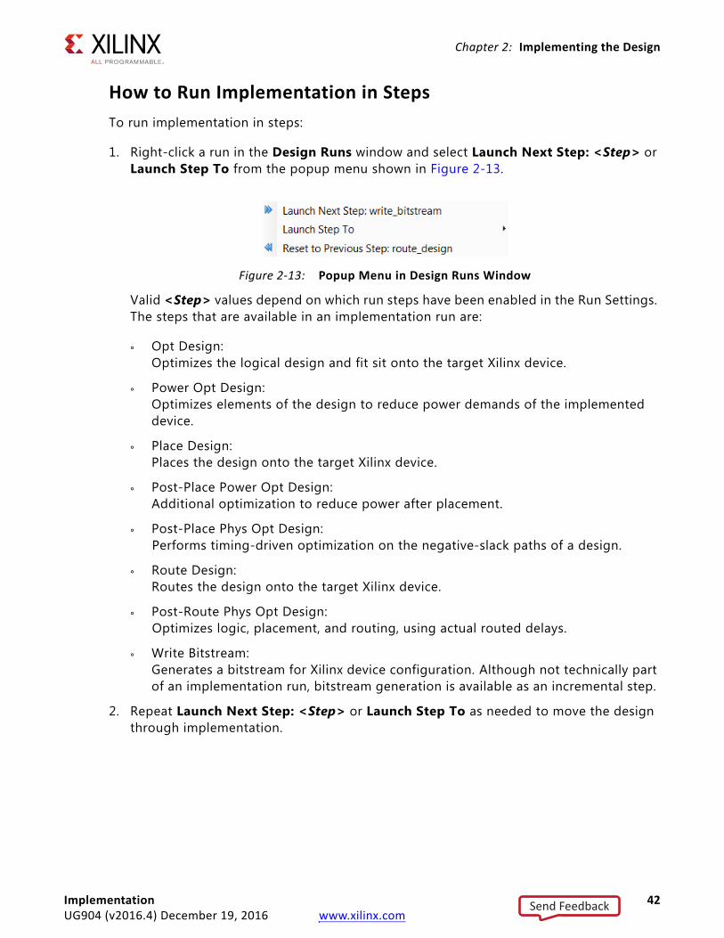
1. Right-click a run in the Design Runs window and select Launch Next Step: <Step> or Launch Step To from the popup menu shown in Figure 2-13.
Valid <Step> values depend on which run steps have been enabled in the Run Settings. The steps that are available in an implementation run are:
° Opt Design:Optimizes the logical design and fit sit onto the target Xilinx device.
° Power Opt Design:Optimizes elements of the design to reduce power demands of the implemented device.
° Place Design:Places the design onto the target Xilinx device.
° Post-Place Power Opt Design:Additional optimization to reduce power after placement.
° Post-Place Phys Opt Design:Performs timing-driven optimization on the negative-slack paths of a design.
° Route Design:Routes the design onto the target Xilinx device.
° Post-Route Phys Opt Design:Optimizes logic, placement, and routing, using actual routed delays.
° Write Bitstream:Generates a bitstream for Xilinx device configuration. Although not technically part of an implementation run, bitstream generation is available as an incremental step.
2. Repeat Launch Next Step: <Step> or Launch Step To as needed to move the design through implementation.
X-Ref Target - Figure 2-13
Figure 2-13: Popup Menu in Design Runs Window
Implementation 42UG904 (v2016.4) December 19, 2016 www.xilinx.com
Send Feedback
Chapter 2: Implementing the Design
3. To back up from a completed step, select Reset to Previous Step: <Step> from the Design Runs window popup menu.
Select Reset to Previous Step to reset the selected run from its current state to the prior incremental step. This allows you to:
° Step backward through a run.
° Make any needed changes.
° Step forward again to incrementally complete the run.
About Implementation CommandsThe Xilinx® Vivado® Design Suite includes many features to manage and simplify the implementation process for project-based designs. These features include the ability to step manually through the implementation process.
For more information, see Running Implementation in Project Mode, page 22.
Non-Project based designs must be manually taken through each step of the implementation process using Tcl commands or Tcl scripts.
Note: For more information about Tcl commands, see the Vivado Design Suite Tcl Command Reference Guide (UG835) [Ref 17], or type <command> -help.
For more information, see Running Implementation in Non-Project Mode, page 18.
Implementation Sub-ProcessesIn Project Mode, the implementation commands are run in a fixed order. In Non-Project Mode the commands can be run in a similar order, but can also be run repeatedly, iteratively, and in a different sequence than in Project Mode.
IMPORTANT: Implementation Commands are re-entrant
Implementation commands are re-entrant, which means that when an implementation command is called in Non-Project Mode, it reads the design in memory, performs its tasks, and writes the resulting design back into memory. This provides more flexibility when running in Non-Project Mode.
Implementation 43UG904 (v2016.4) December 19, 2016 www.xilinx.com
Send Feedback
Chapter 2: Implementing the Design
Examples:
• opt_design followed by opt_design -remapThe Remap operation occurs on the opt_design results.
• place_design called on a design that contains some placed cellsThe existing cell placement is used as a starting point for place_design.
• route_design called on a design that contains some routingThe existing routing is used as a starting point for route_design.
• route_design called on a design with unplaced cellsRouting fails because cells must be placed first.
• opt_design called on a fully-placed and routed designLogic optimization might optimize the logical netlist, creating new cells that are unplaced, and new nets that are unrouted. Placement and routing might need to be rerun to finish implementation.
Putting a design through the Vivado implementation process, whether in Project Mode or Non-Project Mode, consists of several sub-processes:
• Open Synthesized Design:Combines the netlist, the design constraints, and Xilinx target part data, to build the in-memory design to drive implementation.
• Opt Design:Optimizes the logical design to make it easier to fit onto the target Xilinx device.
• Power Opt Design (optional):Optimizes design elements to reduce the power demands of the target Xilinx device.
• Place Design:Places the design onto the target Xilinx device.
• Post-Place Power Opt Design (optional):Additional optimization to reduce power after placement.
• Post-Place Phys Opt Design (optional):Optimizes logic and placement using estimated timing based on placement. Includes replication of high fanout drivers.
• Route Design:Routes the design onto the target Xilinx device.
• Post-Route Phys Opt Design:Optimizes logic, placement, and routing using actual routed delays (optional).
• Write Bitstream:Generates a bitstream for Xilinx device configuration.
Note: Although not technically part of an implementation run, Write Bitstream is available as a separate step.
Implementation 44UG904 (v2016.4) December 19, 2016 www.xilinx.com
Send Feedback
Chapter 2: Implementing the Design
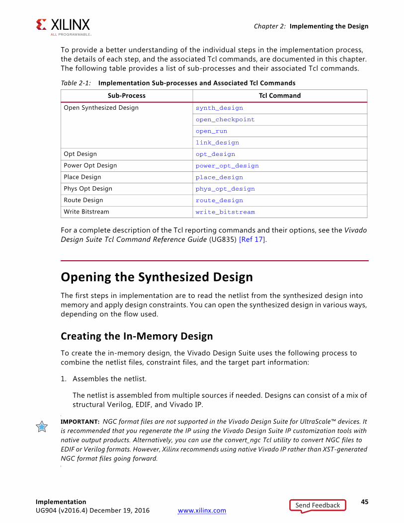
To provide a better understanding of the individual steps in the implementation process, the details of each step, and the associated Tcl commands, are documented in this chapter. The following table provides a list of sub-processes and their associated Tcl commands.
For a complete description of the Tcl reporting commands and their options, see the Vivado Design Suite Tcl Command Reference Guide (UG835) [Ref 17].
Opening the Synthesized DesignThe first steps in implementation are to read the netlist from the synthesized design into memory and apply design constraints. You can open the synthesized design in various ways, depending on the flow used.
Creating the In-Memory DesignTo create the in-memory design, the Vivado Design Suite uses the following process to combine the netlist files, constraint files, and the target part information:
1. Assembles the netlist.
The netlist is assembled from multiple sources if needed. Designs can consist of a mix of structural Verilog, EDIF, and Vivado IP.
IMPORTANT: NGC format files are not supported in the Vivado Design Suite for UltraScale™ devices. It is recommended that you regenerate the IP using the Vivado Design Suite IP customization tools with native output products. Alternatively, you can use the convert_ngc Tcl utility to convert NGC files to EDIF or Verilog formats. However, Xilinx recommends using native Vivado IP rather than XST-generated NGC format files going forward.
Table 2-1: Implementation Sub-processes and Associated Tcl Commands
Sub-Process Tcl Command
Open Synthesized Design synth_design
open_checkpoint
open_run
link_design
Opt Design opt_design
Power Opt Design power_opt_design
Place Design place_design
Phys Opt Design phys_opt_design
Route Design route_design
Write Bitstream write_bitstream
Implementation 45UG904 (v2016.4) December 19, 2016 www.xilinx.com
Send Feedback
Chapter 2: Implementing the Design
2. Transforms legacy netlist primitives to the currently supported subset of Unisim primitives.
TIP: Use report_transformed_primitives to generate a list of transformed cells.
3. Processes constraints from XDC files.
These constraints include both timing constraints and physical constraints such as package pin assignments and Pblocks for floorplanning.
IMPORTANT: Review critical warnings that identify failed constraints. Constraints might be placed on design objects that have been optimized or no longer exist. The Tcl command 'write_xdc -constraints INVALID' also captures invalid XDC constraints.
4. Builds placement macros.
The Vivado tools create placement macros of cells, based on their connectivity or placement constraints to simplify placement.
Examples of placement macros include:
° An XDC-based macro.
° A relatively placed macro (RPM).
Note: RPMs are placed as a group rather than as individual cells.
° A long carry chain that needs to be placed in multiple CLBs.
Note: The primitives making up the carry chains must belong to a single macro to ensure that downstream placement aligns it into vertical slices.
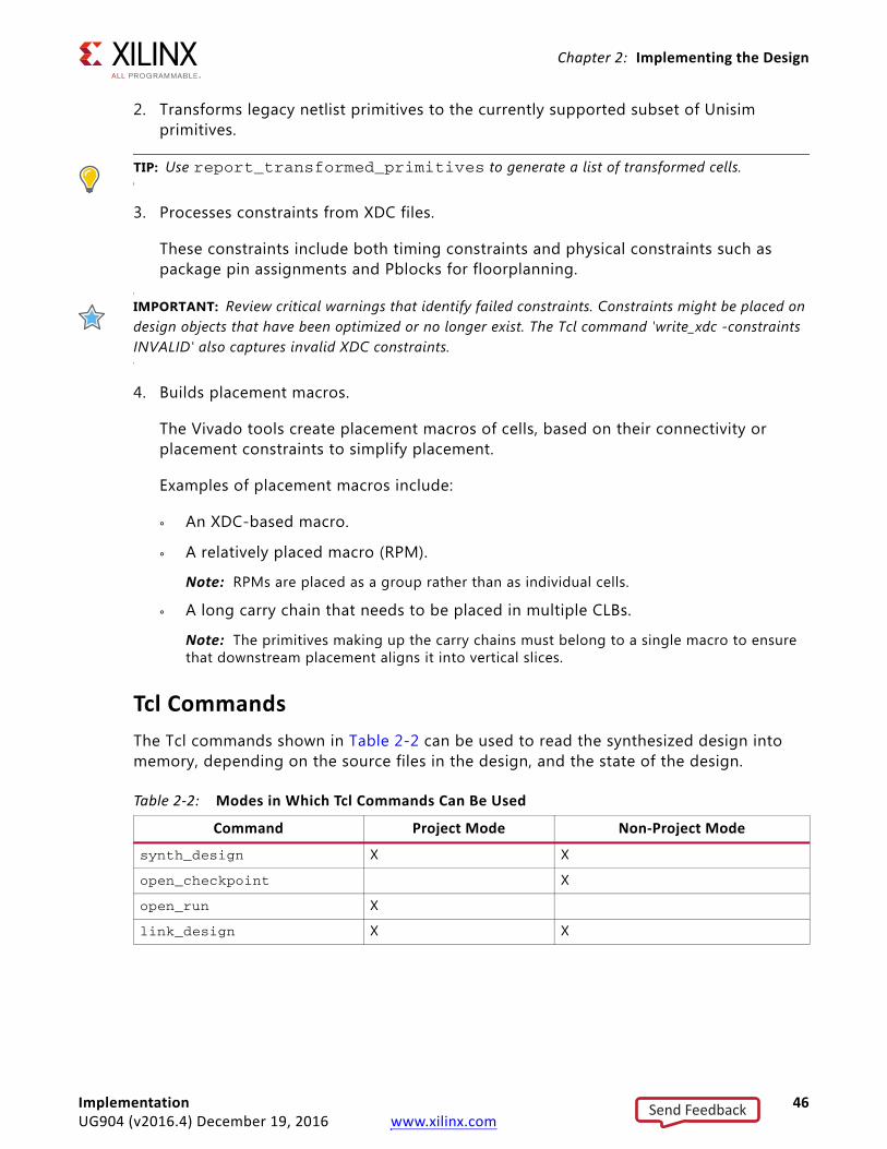
Tcl CommandsThe Tcl commands shown in Table 2-2 can be used to read the synthesized design into memory, depending on the source files in the design, and the state of the design.
Table 2-2: Modes in Which Tcl Commands Can Be Used
Command Project Mode Non-Project Mode
synth_design X X
open_checkpoint X
open_run X
link_design X X
Implementation 46UG904 (v2016.4) December 19, 2016 www.xilinx.com
Send Feedback
Chapter 2: Implementing the Design
synth_design
The synth_design command can be used in both Project Mode and Non-Project Mode. It runs Vivado synthesis on RTL sources with the specified options, and reads the design into memory after synthesis.
synth_design [-name <arg>] [-part <arg>] [-constrset <arg>] [-top <arg>] [-include_dirs <args>] [-generic <args>] [-verilog_define <args>] [-flatten_hierarchy <arg>] [-gated_clock_conversion <arg>] [-directive <arg>] [-rtl] [-bufg <arg>] [-no_lc] [-fanout_limit <arg>] [-shreg_min_size <arg>] [-mode <arg>] [-fsm_extraction <arg>] [-keep_equivalent_registers] [-resource_sharing <arg>] [-control_set_opt_threshold <arg>] [-max_bram <arg>] [-max_dsp <arg>] [-quiet] [-verbose]
synth_design Example Script
The following is an excerpt from the create_bft_batch.tcl script found in the examples/Vivado_Tutorials directory of the software installation.
# Setup design sources and constraintsread_vhdl -library bftLib [ glob ./Sources/hdl/bftLib/*.vhdl ] read_vhdl ./Sources/hdl/bft.vhdlread_verilog [ glob ./Sources/hdl/*.v ] read_xdc ./Sources/bft_full.xdc
# Run synthesis, report utilization and timing estimates, write design checkpointsynth_design -top bft -part xc7k70tfbg484-2 -flatten rebuilt write_checkpoint -force $outputDir/post_synth
For more information on using the synth_design example script, see the Vivado Design Suite Tutorial: Design Flows Overview (UG888) [Ref 19] and the Vivado Design Suite User Guide: Synthesis (UG901) [Ref 8].
The synth_design example script reads VHDL and Verilog files; reads a constraint file; and synthesizes the design on the specified part. The design is opened by the Vivado tools into memory when synth_design completes. A design checkpoint is written after completing synthesis.
For more information on the synth_design Tcl command, see this link in the Vivado Design Suite Tcl Command Reference Guide (UG835) [Ref 17]. This reference guide also provides a complete description of the Tcl commands and their options.
open_checkpoint
The open_checkpoint command opens a design checkpoint file (DCP), creates a new in-memory project and initializes a design immediately in the new project with the contents of the checkpoint. This command can be used to open a top-level design checkpoint, or the checkpoint created for an out-of-context module.
Implementation 47UG904 (v2016.4) December 19, 2016 www.xilinx.com
Send Feedback

Chapter 2: Implementing the Design
Note: In previous releases, the read_checkpoint command was used to read and initialize checkpoint designs. Beginning in version 2014.1, this function is provided by the open_checkpoint command.The behavior of read_checkpoint has been changed such that it only adds the checkpoint file to the list of source files. This is consistent with other read commands such as read_verilog, read_vhdl, and read_xdc. A separate link_design command is required to initialize the design and load it into memory when using read_checkpoint.
When opening a checkpoint, there is no need to create a project first. The open_checkpoint command reads the design data into memory, opening the design in Non-Project Mode. Refer to this link in the Vivado Design Suite User Guide: Design Flows Overview (UG892) [Ref 1] for more information on Project Mode and Non-Project Mode.
IMPORTANT: In the incremental compile flow, the read_checkpoint command is still used to specify the reference design checkpoint.
open_checkpoint Syntax
open_checkpoint [-part <arg>] [-quiet] [-verbose] <file>
open_checkpoint Example Script
# Read the specified design checkpoint and create an in-memory design.open_checkpoint C:/Data/post_synth.dcp
The open_checkpoint example script opens the post synthesis design checkpoint file.
open_run
The open_run command opens a previously completed synthesis or implementation run, then loads the in-memory design of the Vivado tools.
IMPORTANT: The open_run command works in Project Mode only. Design runs are not supported in Non-Project Mode.
Use open_run before implementation on an RTL design in order to open a previously completed Vivado synthesis run then load the synthesized netlist into memory.
TIP: Because the in-memory design is updated automatically, you do not need to use open_run after synth_design. You need to use open_run only to open a previously completed synthesis run from an earlier design session.
The open_run command is for use with RTL designs only. To open a netlist-based design, use link_design.
open_run Syntax
open_run [-name <arg>] [-quiet] [-verbose] <run>
Implementation 48UG904 (v2016.4) December 19, 2016 www.xilinx.com
Send Feedback
Chapter 2: Implementing the Design
open_run Example Script
# Open named design from completed synthesis runopen_run -name synth_1 synth_1
The open_run example script opens a design (synth_1) into the Vivado tools memory from the completed synthesis run (also named synth_1).
If you use open_run while a design is already in memory, the Vivado tools prompt you to save any changes to the current design before opening the new design.
link_design
The link_design command creates an in-memory design from netlist sources (such as from a third-party synthesis tool), and links the netlists and design constraints with the target part.
TIP: The link_design command supports both Project Mode and Non-Project Mode to create the netlist design. Use link_design -part <arg> without a netlist loaded, to open a blank design for device exploration.
link_design Syntax
link_design [-name <arg>] [-part <arg>] [-constrset <arg>] [-top <arg>] [-mode <arg>] [-quiet] [-verbose]
link_design Example Script
# Open named design from netlist sources.link_design -name netDriven -constrset constrs_1 -part xc7k325tfbg900-1
If you use link_design while a design is already in memory, the Vivado tools prompt you to save any changes to the current design before opening the new design.
RECOMMENDED: After creating the in-memory synthesized design in the Vivado tools, review Errors and Critical Warnings for missing or incorrect constraints. After the design is successfully created, you can begin running analysis, generating reports, applying new constraints, or running implementation.
Immediately after opening the in-memory synthesized design, run report_timing_summary to check timing constraints. This ensures that the design goals are complete and reasonable. For more detailed descriptions of the report_timing_summary command, see this link in the Vivado Design Suite Tcl Command Reference Guide (UG835) [Ref 17].
Implementation 49UG904 (v2016.4) December 19, 2016 www.xilinx.com
Send Feedback
Chapter 2: Implementing the Design
BUFG Optimization
Mandatory logic optimization (MLO), which occurs at the beginning of link design, supports the use of the CLOCK_BUFFER_TYPE property to insert global clock buffers. Supported values are BUFG for 7 series, and BUFG and BUFGCE for UltraScale. The value NONE can be used for all architectures to suppress global clock buffer insertion through MLO and opt_design. For BUFG and BUFGCE, MLO inserts the corresponding buffer type to drive the specified net.
Use of CLOCK_BUFFER_TYPE provides the advantage of controlling buffer insertion using XDC constraints so that no design source or netlist modifications are required. Buffers inserted using CLOCK_BUFFER_TYPE are not subject to any limits, so the property must be used cautiously to avoid introducing too many global clocks into the design, which may result in placement failures. For more information, see the Vivado Design Suite Properties Reference Guide (UG912) [Ref 14].
Logic OptimizationLogic optimization ensures the most efficient logic design before attempting placement. It performs a netlist connectivity check to warn of potential design problems such as nets with multiple drivers and un-driven inputs. Logic optimization also performs block RAM power optimization.
Often design connectivity errors are propagated to the logic optimization step where the flow fails. It is important to ensure valid connectivity using DRC Reports before running implementation.
Logic optimization skips optimization of cells and nets that have DONT_TOUCH properties set to a value of TRUE.
The Tcl command used to run Logic Optimization is opt_design.
Common Design ErrorsOne common error that can cause logic optimization to fail is using undriven LUT inputs, where the input is used by the LUT logic equation. This results in an error such as:
ERROR: [Opt 31-67] Problem: A LUT6 cell in the design is missing a connection on input pin I0, which is used by the LUT equation.
This error often occurs when the connection was omitted while assembling logic from multiple sources. Logic optimization identifies both the cell name and the pin, so that it can be traced back to its source definition.
Implementation 50UG904 (v2016.4) December 19, 2016 www.xilinx.com
Send Feedback
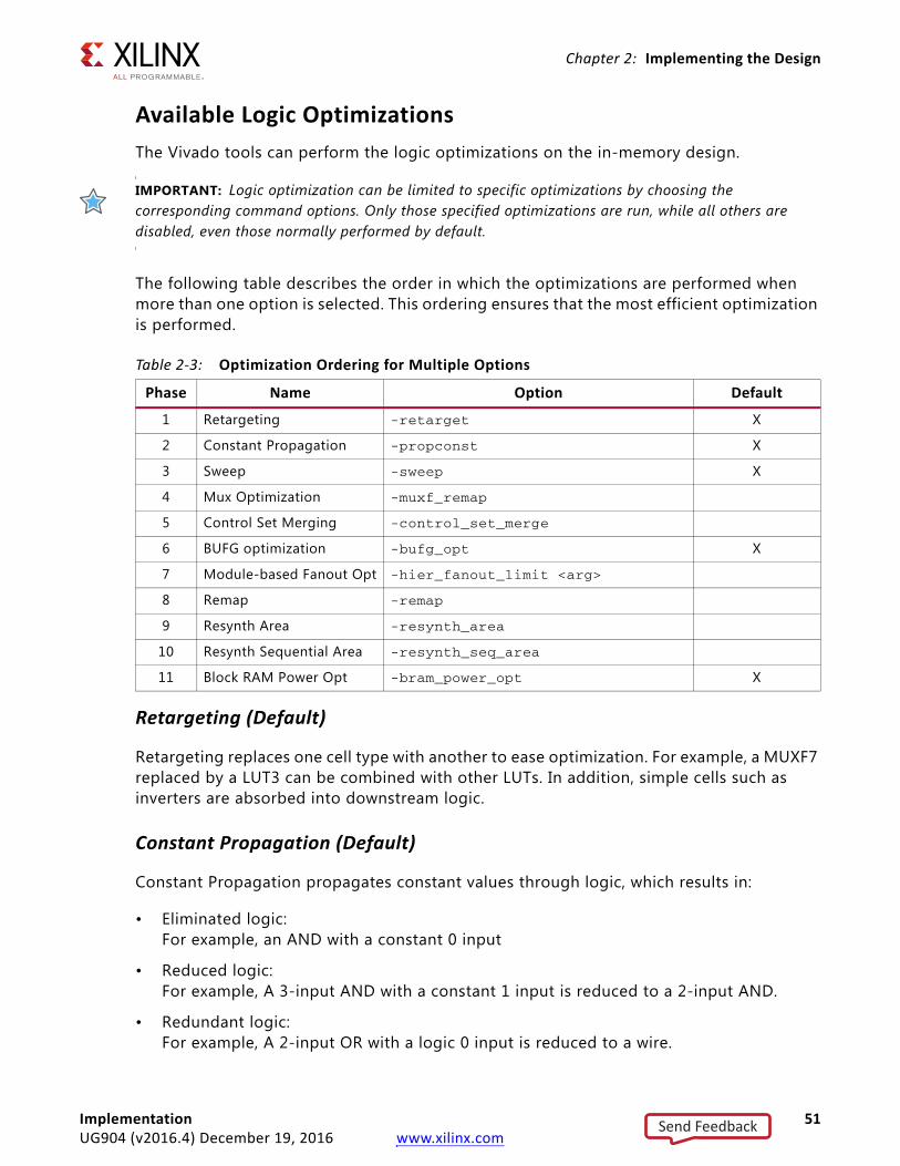
Chapter 2: Implementing the Design
Available Logic OptimizationsThe Vivado tools can perform the logic optimizations on the in-memory design.
IMPORTANT: Logic optimization can be limited to specific optimizations by choosing the corresponding command options. Only those specified optimizations are run, while all others are disabled, even those normally performed by default.
The following table describes the order in which the optimizations are performed when more than one option is selected. This ordering ensures that the most efficient optimization is performed.
Retargeting (Default)
Retargeting replaces one cell type with another to ease optimization. For example, a MUXF7 replaced by a LUT3 can be combined with other LUTs. In addition, simple cells such as inverters are absorbed into downstream logic.
Constant Propagation (Default)
Constant Propagation propagates constant values through logic, which results in:
• Eliminated logic:For example, an AND with a constant 0 input
• Reduced logic:For example, A 3-input AND with a constant 1 input is reduced to a 2-input AND.
• Redundant logic:For example, A 2-input OR with a logic 0 input is reduced to a wire.
Table 2-3: Optimization Ordering for Multiple Options
Phase Name Option Default
1 Retargeting -retarget X
2 Constant Propagation -propconst X
3 Sweep -sweep X
4 Mux Optimization -muxf_remap
5 Control Set Merging -control_set_merge
6 BUFG optimization -bufg_opt X
7 Module-based Fanout Opt -hier_fanout_limit <arg>
8 Remap -remap
9 Resynth Area -resynth_area
10 Resynth Sequential Area -resynth_seq_area
11 Block RAM Power Opt -bram_power_opt X
Implementation 51UG904 (v2016.4) December 19, 2016 www.xilinx.com
Send Feedback
Chapter 2: Implementing the Design
Sweep (Default)
Sweep removes cells that have no loads.
Block RAM Power Optimization (Default)
Block RAM Power Optimization enables power optimization on block RAM cells including:
• Changing the WRITE_MODE on unread ports of true dual-port RAMs to NO_CHANGE.
• Applying intelligent clock gating to block RAM outputs.
Remap
Remap combines multiple LUTs into a single LUT to reduce the depth of the logic.
Resynth Area
Resynth Area performs re-synthesis in area mode to reduce the number of LUTs.
Resynth Sequential Area
Resynth Sequential Area performs re-synthesis to reduce both combinational and sequential logic. Performs a superset of the optimization of Resynth Area.
Mux Optimization
Remaps MUXF7, MUXF8, and MUXF9 primitives to LUT3 to improve route-ability.
TIP: To further optimize the netlist after the mux optimization is performed, combine the mux optimization with remap (opt_design -muxf_remap -remap)
Control Set Merging
Reduce the drivers of logically-equivalent control signals to a single driver. This is like a reverse fanout replication, and results in nets that are better suited for module-based replication.
BUFG Optimization
Logic optimization conservatively inserts global clock buffers on clock nets and high-fanout non-clock nets such as device-wide resets.
For 7 series designs, clock buffers are inserted as long as 12 total global clock buffers are not exceeded.
Implementation 52UG904 (v2016.4) December 19, 2016 www.xilinx.com
Send Feedback
Chapter 2: Implementing the Design
For UltraScale designs, there is no limit for clock buffers inserted on clock nets.
For non-clock nets:
• Global clock buffers are only inserted as long as 24 total clock buffers are not exceeded, not including BUFG_GT buffers.
• The fanout must be above 25,000.
For fabric-driven clock nets, the fanout must be 30 or greater.
Note: To prevent BUFG Optimization on a net, assign the value NONE to the CLOCK_BUFFER_TYPE property of the net. Some clock buffer insertion that is required to legalize the design can also occur in mandatory logic optimization.
Module-Based Fanout Optimization
Net drivers with fanout greater than the specified limit, provided as an argument with this option, will be replicated according to the logical hierarchy.
For each hierarchical instance driven by the high-fanout net, if the fanout within the hierarchy is greater than the specified limit, then the net within the hierarchy is driven by a replica of the driver of the high-fanout net.
IMPORTANT: Each use of logic optimization affects the in-memory design, not the synthesized design that was originally opened.
opt_design
The opt_design command runs Logic Optimization.
opt_design Syntax
opt_design [-retarget] [-propconst] [-sweep] [-bram_power_opt] [-remap] [-resynth_area] [-resynth_seq_area] [-directive <arg>] [-muxf_remap] [-hier_fanout_limit <arg>] [-bufg_opt] [-control_set_merge] [-quiet] [-verbose]
opt_design Example Script
# Run logic optimization with block RAM Power Optimization disabled, save results in a checkpoint, report timing estimatesopt_design -directive NoBramPowerOptwrite_checkpoint -force $outputDir/post_optreport_timing_summary -file $outputDir/post_opt_timing_summary.rpt
The opt_design example script performs logic optimization on the in-memory design, rewriting it in the process. It also writes a design checkpoint after completing optimization, and generates a timing summary report and writes the report to the specified file.
Implementation 53UG904 (v2016.4) December 19, 2016 www.xilinx.com
Send Feedback
Chapter 2: Implementing the Design
Restrict Optimization to Listed Types
Use command line options to restrict optimization to one or more of the listed types. For example, the following is another method for skipping the block RAM optimization that is run by default:
opt_design -retarget -propconst -sweep
Using Directives
Directives provide different modes of behavior for the opt_design command. Only one directive can be specified at a time. The directive option is incompatible with other options. The following directives are available:
• Explore:Runs multiple passes of optimization.
• ExploreArea:Runs multiple passes of optimization with emphasis on reducing combinational logic.
• AddRemap:Runs the default logic optimization flow and includes LUT remapping to reduce logic levels.
• ExploreSequentialArea:Runs multiple passes of optimization with emphasis on reducing registers and related combinational logic.
• RuntimeOptimized:Runs minimal passes of optimization, trading design performance for faster run time.
• NoBramPowerOpt:Runs all the default opt_design optimizations except block RAM Power Optimization.
• ExploreWithRemap:Same as the Explore directive but includes the Remap optimization.
• Default:Runs opt_design with default settings.
Table 2-4 provides an overview of the optimization phase for the different directives.
Implementation 54UG904 (v2016.4) December 19, 2016 www.xilinx.com
Send Feedback
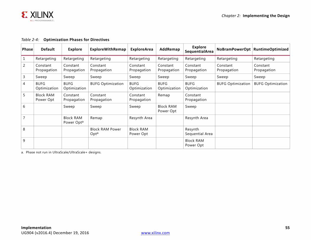
Chapter 2: Implementing the Design
Im 55UG
Ta
Ph NoBramPowerOpt RuntimeOptimized
1 Retargeting Retargeting
2 Constant Propagation
Constant Propagation
3 Sweep Sweep
4 BUFG Optimization BUFG Optimization
5
6
7
8
9
a.
plementation904 (v2016.4) December 19, 2016 www.xilinx.com
ble 2-4: Optimization Phases for Directives
ase Default Explore ExploreWithRemap ExploreArea AddRemap ExploreSequentialArea
Retargeting Retargeting Retargeting Retargeting Retargeting Retargeting
Constant Propagation
Constant Propagation
Constant Propagation
Constant Propagation
Constant Propagation
Constant Propagation
Sweep Sweep Sweep Sweep Sweep Sweep
BUFG Optimization
BUFG Optimization
BUFG Optimization BUFG Optimization
BUFG Optimization
BUFG Optimization
Block RAM Power Opt
Constant Propagation
Constant Propagation
Constant Propagation
Remap Constant Propagation
Sweep Sweep Sweep Block RAM Power Opt
Sweep
Block RAM Power Opta
Remap Resynth Area Resynth Area
Block RAM Power Opta
Block RAM Power Opt
Resynth Sequential Area
Block RAM Power Opt
Phase not run in UltraScale/UltraScale+ designs.
Chapter 2: Implementing the Design
Using the -verbose Option
To better analyze optimization results, use the -verbose option to see additional details of the logic affected by opt_design optimization.
The -verbose option is off by default due to the potential for a large volume of additional messages. Use the -verbose option if you believe it might be helpful.
RECOMMENDED: To improve tool run time for large designs, use the -verbose option only in shell or batch mode and not in the GUI mode.
IMPORTANT: The opt_design command operates on the in-memory design. If run multiple times, the subsequent run optimizes the results of the previous run. Therefore you might need to reload the implemented design before adding the -verbose option.
Logic Optimization ConstraintsThe Vivado Design Suite respects the DONT_TOUCH property during logic optimization. It does not optimize away nets or cells with these properties. For more information, see this link in the Vivado Design Suite User Guide: Synthesis (UG901) [Ref 8].
You would typically apply the DONT_TOUCH property to leaf cells to prevent them from being optimized. DONT_TOUCH on a hierarchical cell preserves the cell boundary, but optimization might still occur within the cell and constants can still be propagated across the boundary. To preserve a hierarchical net, apply the DONT_TOUCH property to all net segments using the -segments option of get_nets.
The tools automatically add DONT_TOUCH properties of value TRUE to nets that have MARK_DEBUG properties of value TRUE. This is done to keep the nets intact throughout the implementation flow so that they can be probed at any design stage. This is the recommended use of MARK_DEBUG. However, on rare occasions DONT_TOUCH might be too restrictive and could prevent optimization such as constant propagation, sweep, or remap, leading to more difficult timing closure. In such cases, you can set DONT_TOUCH to a value of FALSE, while keeping MARK_DEBUG TRUE. The risk in doing this is that nets with MARK_DEBUG can be optimized away and no longer probed.
Implementation 56UG904 (v2016.4) December 19, 2016 www.xilinx.com
Send Feedback

Chapter 2: Implementing the Design
Power OptimizationPower optimization optimizes dynamic power using clock gating (optional). It can be used in both Project Mode and Non-Project Mode, and can be run after logic optimization or after placement to reduce power demand in the design. Power optimization includes Xilinx intelligent clock gating solutions that can reduce dynamic power in your design, but do not change the clocks or logic of the design.
For more information, see the Vivado Design Suite User Guide: Power Analysis and Optimization (UG907) [Ref 11].
Vivado Tools Power AnalysisThe Vivado tools analyze all portions of the design, including legacy and third-party IP blocks. It also identifies output logic from sourcing registers that does not contribute to the result for each clock cycle.
Using Clock Enables (CEs)
The Vivado power optimizer takes advantage of the abundant supply of Clock Enables (CEs) available in the logic of Xilinx 7 series devices. The tools create fine-grain clock gating, or logic gating signals, that eliminate unnecessary switching activity in the register.
In addition, at the flip-flop level, CEs are actually gating the clock rather than selecting between the D input and feedback Q output of the flip-flop. This increases the performance of the CE input but also reduces clock power.
Intelligent Clock Gating
Intelligent clock gating also reduces power for dedicated block RAMs in either simple dual-port or true dual-port mode, as shown in Figure 2-15.
X-Ref Target - Figure 2-14
Figure 2-14: Intelligent Clock Gating
Implementation 57UG904 (v2016.4) December 19, 2016 www.xilinx.com
Send Feedback
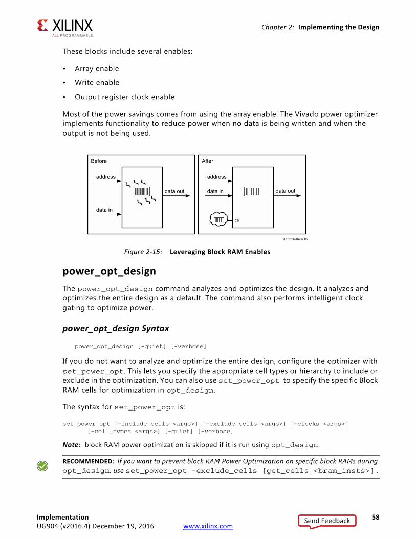
Chapter 2: Implementing the Design
These blocks include several enables:
• Array enable
• Write enable
• Output register clock enable
Most of the power savings comes from using the array enable. The Vivado power optimizer implements functionality to reduce power when no data is being written and when the output is not being used.
power_opt_designThe power_opt_design command analyzes and optimizes the design. It analyzes and optimizes the entire design as a default. The command also performs intelligent clock gating to optimize power.
power_opt_design Syntax
power_opt_design [-quiet] [-verbose]
If you do not want to analyze and optimize the entire design, configure the optimizer with set_power_opt. This lets you specify the appropriate cell types or hierarchy to include or exclude in the optimization. You can also use set_power_opt to specify the specific Block RAM cells for optimization in opt_design.
The syntax for set_power_opt is:
set_power_opt [-include_cells <args>] [-exclude_cells <args>] [-clocks <args>][-cell_types <args>] [-quiet] [-verbose]
Note: block RAM power optimization is skipped if it is run using opt_design.
RECOMMENDED: If you want to prevent block RAM Power Optimization on specific block RAMs during opt_design, use set_power_opt -exclude_cells [get_cells <bram_insts>].
X-Ref Target - Figure 2-15
Figure 2-15: Leveraging Block RAM Enables
Before
address
data in
data out
After
address
data in data out
ce
Implementation 58UG904 (v2016.4) December 19, 2016 www.xilinx.com
Send Feedback
Chapter 2: Implementing the Design
PlacementThe Vivado Design Suite placer places cells from the netlist onto specific sites in the target Xilinx device. Like the other implementation commands, the Vivado placer works from, and updates, the in-memory design.
Design Placement OptimizationThe Vivado placer simultaneously optimizes the design placement for:
• Timing slack: Placement of cells in timing-critical paths is chosen to minimize negative slack.
• Wirelength: Overall placement is driven to minimize the overall wirelength of connections.
• Congestion: The Vivado placer monitors pin density and spreads cells to reduce potential routing congestion.
Design Rule ChecksBefore starting placement, Vivado implementation runs Design Rule Checks (DRCs), including user-selected DRCs from report_drc, and built-in DRCs internal to the Vivado placer. Internal DRCs check for illegal placement, such as Memory IP cells without LOC constraints and I/O banks with conflicting IOSTANDARDs.
Clock and I/O PlacementAfter design rule checking, the Vivado placer places clock and I/O cells before placing other logic cells. Clock and I/O cells are placed concurrently because they are often related through complex placement rules specific to the targeted Xilinx device. For UltraScale devices, the placer also assigns clock tracks and pre-routes the clocks. Register cells with IOB properties are processed during this phase to determine which registers with an IOB value of TRUE should be mapped to I/O logic sites. If the placer fails to honor an IOB property of TRUE, a critical warning is issued.
Placer Targets
The placer targets at this stage of placement are:
• I/O ports and their related logic
• Global and local clock buffers
• Clock management tiles (MMCMs and PLLs)
• Gigabit Transceiver (GT) cells
Implementation 59UG904 (v2016.4) December 19, 2016 www.xilinx.com
Send Feedback
Chapter 2: Implementing the Design
Placing Unfixed Logic
When placing unfixed logic during this stage of placement, the placer adheres to physical constraints, such as LOC properties and Pblock assignments. It also validates existing LOC constraints against the netlist connectivity and device sites. Certain IP (such as Memory IP and GTs) are generated with device-specific placement constraints.
IMPORTANT: Due to the device I/O architecture, a LOC property often constrains cells other than the cell to which LOC has been applied. A LOC on an input port also fixes the location of its related I/O buffer, IDELAY, and ILOGIC. Conflicting LOC constraints cannot be applied to individual cells in the input path. The same applies for outputs and GT-related cells.
Clock Resources Placement Rules
Clock resources must follow the placement rules described in the 7 Series FPGAs Clocking Resources User Guide (UG472) [Ref 15] and UltraScale Architecture Clocking Resources User Guide (UG572) [Ref 16]. For example, an input that drives a global clock buffer must be located at a clock-capable I/O site, must be located in the same upper or lower half of the device for 7 series devices, and in the same clock region for UltraScale devices. These clock placement rules are also validated against the logical netlist connectivity and device sites.
When Clock and I/O Placement Fails
If the Vivado placer fails to find a solution for the clock and I/O placement, the placer reports the placement rules that were violated, and briefly describes the affected cells.
Placement can fail because of several reasons, including:
• Clock tree issues caused by conflicting constraints
• Clock tree issues that are too complex for the placer to resolve
• RAM and DSP block placement conflicts with other constraints, such as Pblocks
• Over-utilization of resources
• I/O bank requirements and rules
In some cases, the Vivado placer provisionally places cells at sites, and attempts to place other cells as it tries to solve the placement problem. The provisional placements often pinpoint the source of clock and I/O placement failure. Manually placing a cell that failed provisional placement might help placement converge.
TIP: Use place_ports to run the clock and I/O placement step first. Then run place_design. If port placement fails, the placement is saved to memory to allow failure analysis. For more information, run place_ports -help from the Vivado Tcl command prompt.
Implementation 60UG904 (v2016.4) December 19, 2016 www.xilinx.com
Send Feedback
Chapter 2: Implementing the Design
For more information about UltraScale clock tree placement and routing, see the UltraFast Design Methodology Guide for the Vivado Design Suite (UG949) [Ref 13].
Global Placement, Detailed Placement, and Packing and LegalizationAfter Clock and I/O placement, the remaining placement phases consist of global placement, detailed placement, and packing and legalization.
RECOMMENDED: Run report_timing_summary after placement to check the critical paths. Paths with very large negative setup slack might need manual placement, further constraining, or logic restructuring to achieve timing closure.
place_designThe place_design command runs placement on the design. Like the other implementation commands, place_design is re-entrant in nature. For a partially placed design, the Vivado placer uses the existing placement as the starting point instead of starting from scratch.
place_design Syntax
place_design [-directive <arg>] [-no_timing_driven] [-timing_summary] [-unplace] [-post_place_opt] [-quiet] [-verbose]
place_design Example Script
# Run placement, save results to checkpoint, report timing estimatesplace_designwrite_checkpoint -force $outputDir/post_placereport_timing_summary -file $outputDir/post_place_timing_summary.rpt
The place_design example script places the in-memory design. It then writes a design checkpoint after completing placement, generates a timing summary report, and writes the report to the specified file.
Using DirectivesDirectives provide different modes of behavior for the place_design command. Only one directive can be specified at a time. The directive option is incompatible with other options.
Placer Directives
Because placement typically has the greatest impact on overall design performance, the Placer has the most directives of all commands. Table 2-5 shows which directives might benefit which types of designs.
Implementation 61UG904 (v2016.4) December 19, 2016 www.xilinx.com
Send Feedback
Chapter 2: Implementing the Design
Available Directives
• Explore:Higher placer effort in detail placement and post-placement optimization.
• WLDrivenBlockPlacement:Wirelength-driven placement of RAM and DSP blocks. Override timing-driven placement by directing the Placer to minimize the distance of connections to and from blocks. This directive can improve timing to and from RAM and DSP blocks.
• EarlyBlockPlacement:Timing-driven placement of RAM and DSP blocks. The RAM and DSP block locations are finalized early in the placement process and are used as anchors to place the remaining logic.
• ExtraNetDelay_high:Increases estimated delay of high fanout and long-distance nets. This directive can improve timing of critical paths that meet timing after place_design but fail timing in route_design due to overly optimistic estimated delays. Three levels of pessimism are supported: high, medium, and low. ExtraNetDelay_high applies the highest level of pessimism.
• ExtraNetDelay_low:Increases estimated delay of high fanout and long-distance nets. This directive can improve timing of critical paths that meet timing after place_design but fail timing in route_design due to overly optimistic estimated delays. Three levels of pessimism are supported: high, medium, and low. ExtraNetDelay_low applies the lowest level of pessimism.
• SSI_SpreadLogic_high:Spreads logic throughout the SSI device to avoid creating congested regions. Two levels are supported: high and low. SpreadLogic_high achieves the highest level of spreading.
Table 2-5: Directive Guidelines
Directive Designs Benefitted
BlockPlacement Designs with many block RAM, DSP blocks, or both
ExtraNetDelay Designs that anticipate many long-distance net connections and nets that fan out to many different modules
SpreadLogic Designs with very high connectivity that tend to create congestion
ExtraPostPlacementOpt All design types
SSI SSI designs that might benefit from different styles of partitioning to relieve congestion or improve timing.
Implementation 62UG904 (v2016.4) December 19, 2016 www.xilinx.com
Send Feedback
Chapter 2: Implementing the Design
• SSI_SpreadLogic_low:Spreads logic throughout the SSI device to avoid creating congested regions. Two levels are supported: high and low. SpreadLogic_low achieves a minimal level of spreading.
• AltSpreadLogic_high:Spreads logic throughout the device to avoid creating congested regions. Three levels are supported: high, medium, and low. AltSpreadLogic_high achieves the highest level of spreading.
• AltSpreadLogic_medium:Spreads logic throughout the device to avoid creating congested regions. Three levels are supported: high, medium, and low. AltSpreadLogic_medium achieves a nominal level of spreading.
• AltSpreadLogic_low:Spreads logic throughout the device to avoid creating congested regions. Three levels are supported: high, medium, and low. AltSpreadLogic_low achieves a minimal level of spreading.
• ExtraPostPlacementOpt:Higher placer effort in post-placement optimization.
• ExtraTimingOpt:Use an alternate set of algorithms for timing-driven placement during the later stages.
• SSI_SpreadSLLs:Partition across SLRs and allocate extra area for regions of higher connectivity.
• SSI_BalanceSLLs:Partition across SLRs while attempting to balance SLLs between SLRs.
• SSI_BalanceSLRs:Partition across SLRs to balance number of cells between SLRs.
• SSI_HighUtilSLRs:Force the placer to attempt to place logic closer together in each SLR.
• RuntimeOptimized:Run fewest iterations, trade higher design performance for faster run time.
• Quick:Absolute, fastest run time, non-timing-driven, performs the minimum required for a legal design.
• Default:Run place_design with default settings.
TIP: Use the -directive option to explore different placement options for your design.
Implementation 63UG904 (v2016.4) December 19, 2016 www.xilinx.com
Send Feedback
Chapter 2: Implementing the Design
Using the -unplace Option
The -unplace option unplaces all cells and all ports in a design that do not have fixed locations. An object with fixed location has an IS_LOC_FIXED property value of TRUE.
Using the -no_timing_driven Option
The -no_timing_driven option disables the default timing driven placement algorithm. This results in a faster placement based on wire lengths, but ignores any timing constraints during the placement process.
Using the -timing_summary Option
After placement, an estimated timing summary is output to the log file. By default, the number reflects the internal estimates of the placer. For example:
INFO: [Place 30-746] Post Placement Timing Summary WNS=0.022. For the most accurate timing information please run report_timing.
For greater accuracy at the expense of slightly longer run time, you can use the -timing_summary option to force the placer to report the timing summary based on the results from the static timing engine.
INFO: [Place 30-100] Post Placement Timing Summary | WNS=0.236 | TNS=0.000 |
where
° WNS = Worst Negative Slack
° TNS = Total Negative Slack
Using the -verbose Option
To better analyze placement results, use the -verbose option to see additional details of the cell and I/O placement by the place_design command.
The -verbose option is off by default due to the potential for a large volume of additional messages. Use the -verbose option if you believe it might be helpful.
Using the -post_place_opt Option
Post placement optimization is a placement optimization that can potentially improve critical path timing at the expense of additional run time. The optimization is performed on a fully placed design with timing violations. For each of the top few critical paths, the placer tries moving critical cells to improve delay and commits new cell placements if they improve estimated delay. For designs with longer run times and relatively more critical paths, these placement passes might further improve timing.
Implementation 64UG904 (v2016.4) December 19, 2016 www.xilinx.com
Send Feedback
Chapter 2: Implementing the Design
This optimization can be run at any stage after placement, and can be particularly effective on a routed design. Be aware of the following when running this optimization on a routed design:
• Because the timing data reflects the actual routed delays, it ensures the optimization considers the most critical paths.
• When evaluating cell movements, the placer must estimate delays based on cell placements. It does not have access to the actual route delays.
• If new cell placements are committed, the related nets become unrouted and it is required to run route_design to route those nets.
See the following examples:
1. Run post placement optimization after placement:
place_designplace_design -post_place_opt
2. Run post placement optimization after routing:
place_designphys_opt_designroute_designplace_design -post_place_optroute_design
3. Run multiple iterations of post placement optimization in a loop, after routing. For convenience, the implementation commands are wrapped in a Tcl proc called runPPO with arguments to choose the number of iterations and whether or not to enable phys_opt_design in each iteration:
proc runPPO { {numIters 1} {enablePhysOpt 1} } { for {set i 0} {$i < $numIters} {incr i} { place_design -post_place_opt if {$enablePhysOpt != 0} { phys_opt_design } route_design if {[get_property SLACK [get_timing_paths ]] >= 0} {break}; #stop if timing is met }}
. . .place_designphys_opt_designroute_designrunPPO 4 1 ; # run 4 post-route iterations and enable phys_opt_design
Implementation 65UG904 (v2016.4) December 19, 2016 www.xilinx.com
Send Feedback
Chapter 2: Implementing the Design
Physical OptimizationPhysical optimization performs timing-driven optimization on the negative-slack paths of a design. Physical optimization has two modes of operation: post-place and post-route.
In post-place mode, optimization occurs based on timing estimates based on cell placement. Physical optimization automatically incorporates netlist changes due to logic optimizations and places cells as needed.
In post-route mode, optimization occurs based on actual routing delays. In addition to automatically updating the netlist on logic changes and placing cells, physical optimization also automatically updates routing as needed.
IMPORTANT: Post-route physical optimization is most effectively used on designs that have a few failing paths. Using post-route physical optimization on designs with WNS<-0.200 ns or more than 200 failing end points can result in long run time with little improvement to QOR.
Overall physical optimization is more aggressive in post-place mode, where there is more opportunity for logic optimization. In post-route mode, physical optimization tends to be more conservative to avoid disrupting timing-closed routing. Before running, physical optimization checks the routing status of the design to determine which mode to use, post-place or post-route.
If a design does not have negative slack, and a physical optimization with a timing based optimization option is requested, the command exits quickly without performing optimization. To balance runtime and design performance, physical optimization does not automatically attempt to optimize all failing paths in a design. Only the top few percent of failing paths are considered for optimization. So it is possible to use multiple consecutive runs of physical optimization to gradually reduce the number of failing paths in the design.
Available Physical OptimizationsThe Vivado tools perform the physical optimizations on the in-memory design, as shown in the following table.
IMPORTANT: Physical optimization can be limited to specific optimizations by choosing the corresponding command options. Only those specified optimizations are run, while all others are disabled, even those normally performed by default.
Implementation 66UG904 (v2016.4) December 19, 2016 www.xilinx.com
Send Feedback
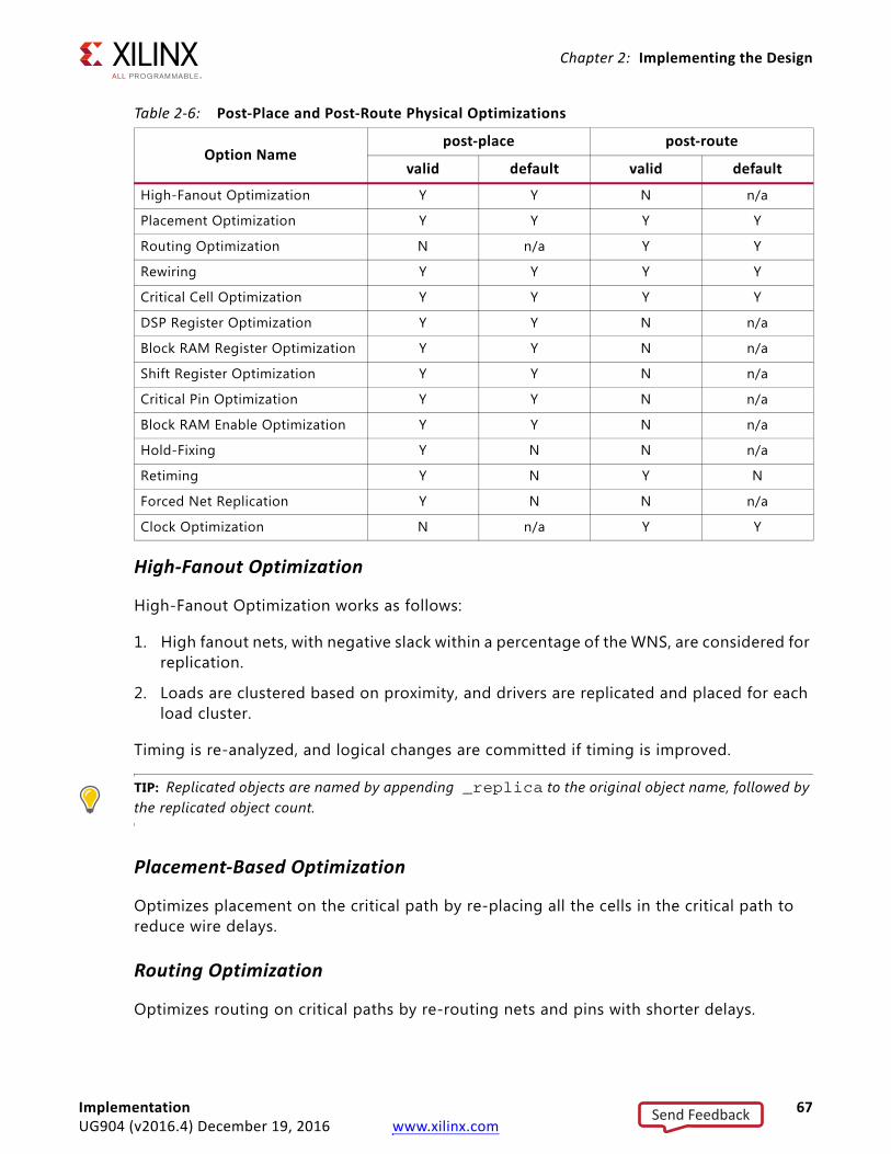
Chapter 2: Implementing the Design
High-Fanout Optimization
High-Fanout Optimization works as follows:
1. High fanout nets, with negative slack within a percentage of the WNS, are considered for replication.
2. Loads are clustered based on proximity, and drivers are replicated and placed for each load cluster.
Timing is re-analyzed, and logical changes are committed if timing is improved.
TIP: Replicated objects are named by appending _replica to the original object name, followed by the replicated object count.
Placement-Based Optimization
Optimizes placement on the critical path by re-placing all the cells in the critical path to reduce wire delays.
Routing Optimization
Optimizes routing on critical paths by re-routing nets and pins with shorter delays.
Table 2-6: Post-Place and Post-Route Physical Optimizations
Option Namepost-place post-route
valid default valid default
High-Fanout Optimization Y Y N n/a
Placement Optimization Y Y Y Y
Routing Optimization N n/a Y Y
Rewiring Y Y Y Y
Critical Cell Optimization Y Y Y Y
DSP Register Optimization Y Y N n/a
Block RAM Register Optimization Y Y N n/a
Shift Register Optimization Y Y N n/a
Critical Pin Optimization Y Y N n/a
Block RAM Enable Optimization Y Y N n/a
Hold-Fixing Y N N n/a
Retiming Y N Y N
Forced Net Replication Y N N n/a
Clock Optimization N n/a Y Y
Implementation 67UG904 (v2016.4) December 19, 2016 www.xilinx.com
Send Feedback
Chapter 2: Implementing the Design
Rewiring
Optimizes the critical path by swapping connections on LUTs to reduce the number of logic levels for critical signals. LUT equations are modified to maintain design functionality.
Critical-Cell Optimization
Critical-Cell Optimization replicates cells in failing paths. If the loads on a specific cell are placed far apart, the cell might be replicated with new drivers placed closer to load clusters. High fanout is not a requirement for this optimization to occur, but the path must fail timing with slack within a percentage of the worst negative slack.
DSP Register Optimization
DSP Register Optimization can move registers out of the DSP cell into the logic array or from logic to DSP cells if it improves the delay on the critical path.
Block RAM Register Optimization
Block RAM Register Optimization can move registers out of the block RAM cell into the logic array or from logic to block RAM cells if it improves the delay on the critical path.
Shift Register Optimization
The shift register optimization improves timing on negative slack paths between shift register cells (SRLs) and other logic cells.
If there are timing violations to or from shift register cells (SRL16E or SRLC32E), the optimization extracts a register from the beginning or end of the SRL register chain and places it into the logic fabric to improve timing. The optimization shortens the wirelength of the original critical path.
The optimization only moves registers from a shift register to logic fabric, but never from logic fabric into a shift register, because the latter never improves timing.
The prerequisites for this optimization to occur are:
• The SRL address must be one or greater, such that there are register stages that can be moved out of the SRL.
• The SRL address must be a constant value, driven by logic 1 or logic 0.
• There must be a timing violation ending or beginning from the SRL cell that is among the worst critical paths.
Implementation 68UG904 (v2016.4) December 19, 2016 www.xilinx.com
Send Feedback
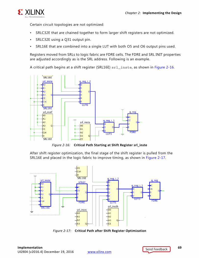
Chapter 2: Implementing the Design
Certain circuit topologies are not optimized:
• SRLC32E that are chained together to form larger shift registers are not optimized.
• SRLC32E using a Q31 output pin.
• SRL16E that are combined into a single LUT with both O5 and O6 output pins used.
Registers moved from SRLs to logic fabric are FDRE cells. The FDRE and SRL INIT properties are adjusted accordingly as is the SRL address. Following is an example.
A critical path begins at a shift register (SRL16E) srl_inste, as shown in Figure 2-16.
After shift register optimization, the final stage of the shift register is pulled from the SRL16E and placed in the logic fabric to improve timing, as shown in Figure 2-17.
X-Ref Target - Figure 2-16
Figure 2-16: Critical Path Starting at Shift Register srl_inste
X-Ref Target - Figure 2-17
Figure 2-17: Critical Path after Shift Register Optimization
Implementation 69UG904 (v2016.4) December 19, 2016 www.xilinx.com
Send Feedback
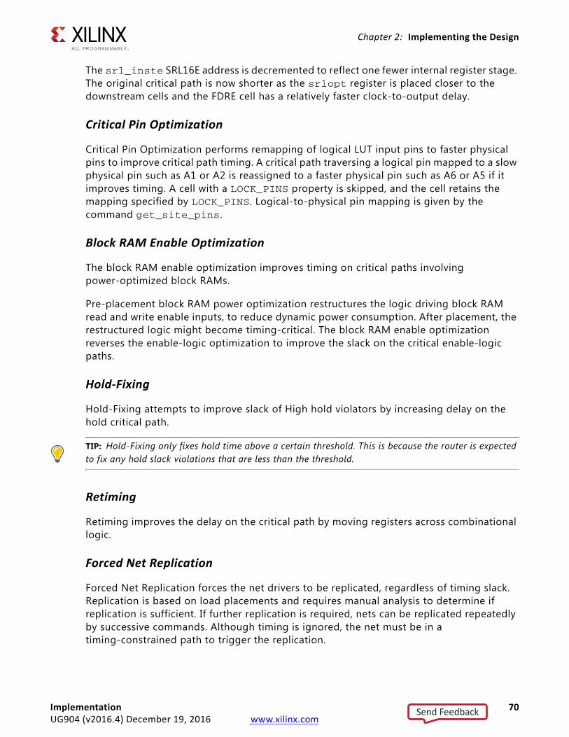
Chapter 2: Implementing the Design
The srl_inste SRL16E address is decremented to reflect one fewer internal register stage. The original critical path is now shorter as the srlopt register is placed closer to the downstream cells and the FDRE cell has a relatively faster clock-to-output delay.
Critical Pin Optimization
Critical Pin Optimization performs remapping of logical LUT input pins to faster physical pins to improve critical path timing. A critical path traversing a logical pin mapped to a slow physical pin such as A1 or A2 is reassigned to a faster physical pin such as A6 or A5 if it improves timing. A cell with a LOCK_PINS property is skipped, and the cell retains the mapping specified by LOCK_PINS. Logical-to-physical pin mapping is given by the command get_site_pins.
Block RAM Enable Optimization
The block RAM enable optimization improves timing on critical paths involving power-optimized block RAMs.
Pre-placement block RAM power optimization restructures the logic driving block RAM read and write enable inputs, to reduce dynamic power consumption. After placement, the restructured logic might become timing-critical. The block RAM enable optimization reverses the enable-logic optimization to improve the slack on the critical enable-logic paths.
Hold-Fixing
Hold-Fixing attempts to improve slack of High hold violators by increasing delay on the hold critical path.
TIP: Hold-Fixing only fixes hold time above a certain threshold. This is because the router is expected to fix any hold slack violations that are less than the threshold.
Retiming
Retiming improves the delay on the critical path by moving registers across combinational logic.
Forced Net Replication
Forced Net Replication forces the net drivers to be replicated, regardless of timing slack. Replication is based on load placements and requires manual analysis to determine if replication is sufficient. If further replication is required, nets can be replicated repeatedly by successive commands. Although timing is ignored, the net must be in a timing-constrained path to trigger the replication.
Implementation 70UG904 (v2016.4) December 19, 2016 www.xilinx.com
Send Feedback
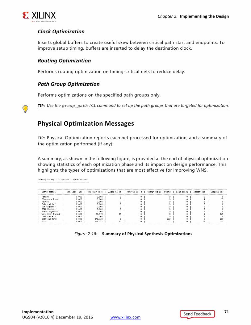
Chapter 2: Implementing the Design
Clock Optimization
Inserts global buffers to create useful skew between critical path start and endpoints. To improve setup timing, buffers are inserted to delay the destination clock.
Routing Optimization
Performs routing optimization on timing-critical nets to reduce delay.
Path Group Optimization
Performs optimizations on the specified path groups only.
TIP: Use the group_path TCL command to set up the path groups that are targeted for optimization.
Physical Optimization Messages
TIP: Physical Optimization reports each net processed for optimization, and a summary of the optimization performed (if any).
A summary, as shown in the following figure, is provided at the end of physical optimization showing statistics of each optimization phase and its impact on design performance. This highlights the types of optimizations that are most effective for improving WNS.X-Ref Target - Figure 2-18
Figure 2-18: Summary of Physical Synthesis Optimizations
Implementation 71UG904 (v2016.4) December 19, 2016 www.xilinx.com
Send Feedback
Chapter 2: Implementing the Design
phys_opt_designThe phys_opt_design command runs physical optimization on the design. It can be run in post-place mode after placement and in post-route mode after the design is fully-routed.
phys_opt_design Syntax
phys_opt_design [-fanout_opt] [-placement_opt] [-routing_opt] [-rewire] [-critical_cell_opt] [-dsp_register_opt] [-bram_register_opt] [-bram_enable_opt] [-shift_register_opt] [-hold_fix] [-retime] [-force_replication_on_nets <args>] [-directive <arg>] [-critical_pin_opt][-clock_opt][-path_groups][-quiet][-verbose]
phys_opt_design Example Script
open_checkpoint top_placed.dcp
# Run post-place phys_opt_design and save resultsphys_opt_designwrite_checkpoint -force $outputDir/top_placed_phys_opt.dcpreport_timing_summary -file $outputDir/top_placed_phys_opt_timing.rpt
# Route the design and save resultsroute_designwrite_checkpoint -force $outputDir/top_routed.dcpreport_timing_summary -file $outputDir/top_routed_timing.rpt
# Run post-route phys_opt_design and save resultsphys_opt_designwrite_checkpoint -force $outputDir/top_routed_phys_opt.dcpreport_timing_summary -file $outputDir/top_routed_phys_opt_timing.rpt
The phys_opt_design example script runs both post-place and post-route physical optimization. First, the placed design is loaded from a checkpoint, followed by post-place phys_opt_design. The checkpoint and timing results are saved. Next the design is routed, with progress saved afterwards. That is followed by post-route phys_opt_design and saving the results. Note that the same command phys_opt_design is used for both post-place and post-route physical optimization. No explicit options are used to specify the mode.
Implementation 72UG904 (v2016.4) December 19, 2016 www.xilinx.com
Send Feedback
Chapter 2: Implementing the Design
Using DirectivesDirectives provide different modes of behavior for the phys_opt_design command. Only one directive can be specified at a time, and the directive option is incompatible with other options. The available directives are described below.
• Explore:Run different algorithms in multiple passes of optimization, including replication for very high fanout nets, and a final phase called Critical Path Optimization where a subset of physical optimizations are run on the top critical paths of all endpoint clocks, regardless of slack.
• ExploreWithHoldFix:Run different algorithms in multiple passes of optimization, including hold violation fixing and replication for very high fanout nets.
TIP: Hold-Fixing only fixes hold time above a certain threshold. This is because the router is expected to fix any hold slack violations that are less than the threshold.
• AggressiveExplore:Similar to Explore but with different optimization algorithms and more aggressive goals.
• AlternateReplication:Use different algorithms for performing critical cell replication.
• AggressiveFanoutOpt:Uses different algorithms for fanout-related optimizations with more aggressive goals.
• AddRetime:Performs the default phys_opt_design flow and adds register retiming.
• AlternateFlowWithRetiming:Perform more aggressive replication and DSP and block RAM optimization, and enable register retiming.
• Default:Run phys_opt_design with default settings.
TIP: All directives are compatible with both post-place and post-route versions of phys_opt_design.
Implementation 73UG904 (v2016.4) December 19, 2016 www.xilinx.com
Send Feedback
Chapter 2: Implementing the Design
Using the -verbose OptionTo better analyze physical optimization results, use the -verbose option to see additional details of the optimizations performed by the phys_opt_design command.
The -verbose option is off by default due to the potential for a large volume of additional messages. Use the -verbose option if you believe it might be helpful.
IMPORTANT: The phys_opt_design command operates on the in-memory design. If run twice, the second run optimizes the results of the first run.
Physical Optimization ConstraintsThe Vivado Design Suite respects the DONT_TOUCH property during physical optimization. It does not perform physical optimization on nets or cells with these properties. Additionally, Pblock assignments are obeyed such that replicated logic inherits the Pblock assignments of the original logic. Timing exceptions are also copied from original to replicated cells.
For more information, see this link in the Vivado Design Suite User Guide: Synthesis (UG901) [Ref 8].
The DONT_TOUCH property is typically placed on leaf cells to prevent them from being optimized. DONT_TOUCH on a hierarchical cell preserves the cell boundary, but optimization can still occur within the cell.
The tools automatically add DONT_TOUCH properties of value TRUE to nets that have MARK_DEBUG properties of value TRUE. This is done to keep the nets intact throughout the implementation flow so that they can be probed at any design stage. This is the recommended use of MARK_DEBUG. However there might be rare occasions on which the DONT_TOUCH is too restrictive and prevents optimizations such as replication and retiming, leading to more difficult timing closure. In those cases DONT_TOUCH can be set to a value of FALSE while keeping MARK_DEBUG TRUE. The consequence of removing the DONT_TOUCH properties is that nets with MARK_DEBUG can be optimized away and no longer probed. If a MARK_DEBUG net is replicated, only the original net retains MARK_DEBUG, not the replicated nets.
Physical Optimization ReportsThe Tcl reporting command report_phys_opt provides details of each optimization performed by phys_opt_design at a very fine level of detail. It must be run in the same Vivado session as phys_opt_design while the optimization history resides in memory. Therefore, if a report is desired, it is recommended to include the report_phys_opt command in Tcl scripts immediately following the last phys_opt_design command.
Implementation 74UG904 (v2016.4) December 19, 2016 www.xilinx.com
Send Feedback
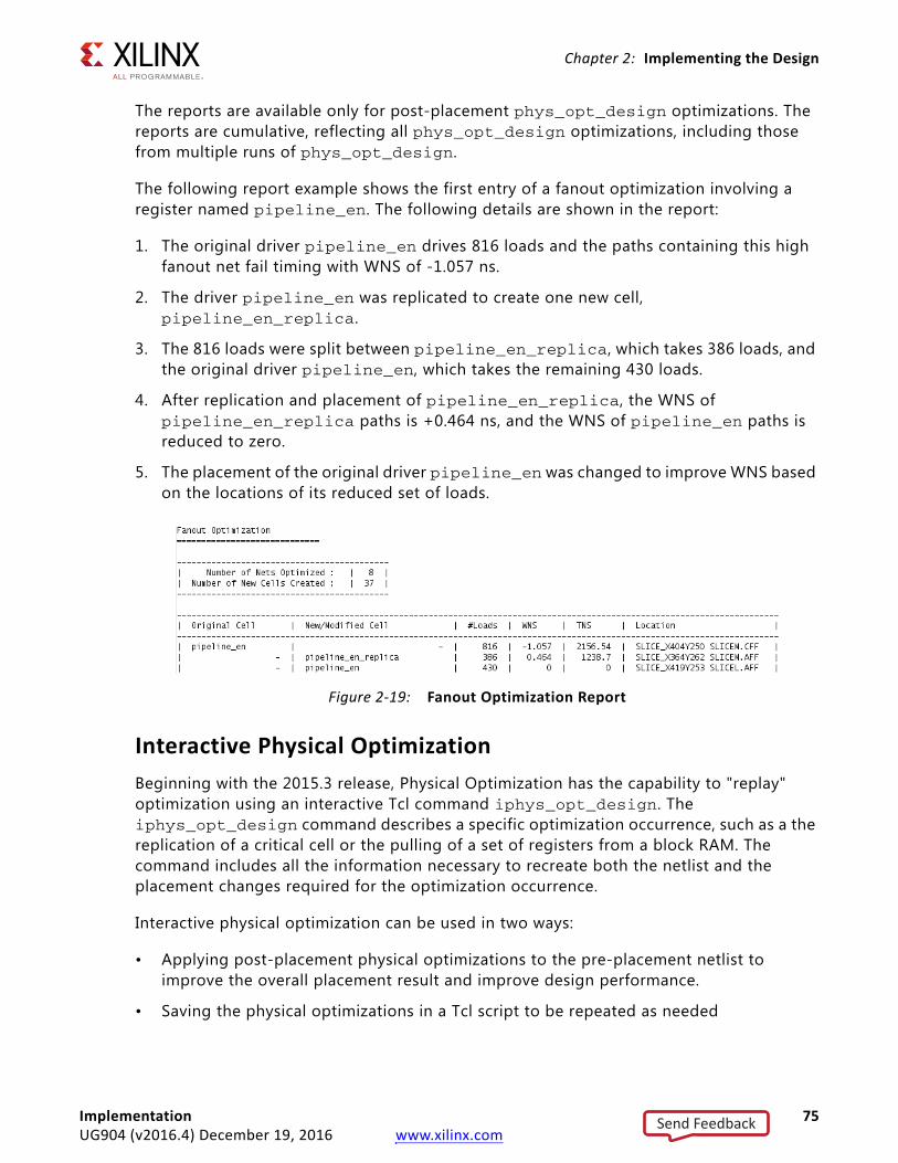
Chapter 2: Implementing the Design
The reports are available only for post-placement phys_opt_design optimizations. The reports are cumulative, reflecting all phys_opt_design optimizations, including those from multiple runs of phys_opt_design.
The following report example shows the first entry of a fanout optimization involving a register named pipeline_en. The following details are shown in the report:
1. The original driver pipeline_en drives 816 loads and the paths containing this high fanout net fail timing with WNS of -1.057 ns.
2. The driver pipeline_en was replicated to create one new cell, pipeline_en_replica.
3. The 816 loads were split between pipeline_en_replica, which takes 386 loads, and the original driver pipeline_en, which takes the remaining 430 loads.
4. After replication and placement of pipeline_en_replica, the WNS of pipeline_en_replica paths is +0.464 ns, and the WNS of pipeline_en paths is reduced to zero.
5. The placement of the original driver pipeline_en was changed to improve WNS based on the locations of its reduced set of loads.
Interactive Physical OptimizationBeginning with the 2015.3 release, Physical Optimization has the capability to "replay" optimization using an interactive Tcl command iphys_opt_design. The iphys_opt_design command describes a specific optimization occurrence, such as a the replication of a critical cell or the pulling of a set of registers from a block RAM. The command includes all the information necessary to recreate both the netlist and the placement changes required for the optimization occurrence.
Interactive physical optimization can be used in two ways:
• Applying post-placement physical optimizations to the pre-placement netlist to improve the overall placement result and improve design performance.
• Saving the physical optimizations in a Tcl script to be repeated as needed
X-Ref Target - Figure 2-19
Figure 2-19: Fanout Optimization Report
Implementation 75UG904 (v2016.4) December 19, 2016 www.xilinx.com
Send Feedback
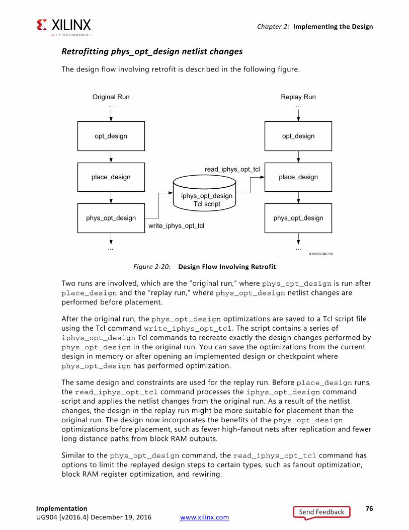
Chapter 2: Implementing the Design
Retrofitting phys_opt_design netlist changes
The design flow involving retrofit is described in the following figure.
Two runs are involved, which are the “original run,” where phys_opt_design is run after place_design and the “replay run,” where phys_opt_design netlist changes are performed before placement.
After the original run, the phys_opt_design optimizations are saved to a Tcl script file using the Tcl command write_iphys_opt_tcl. The script contains a series of iphys_opt_design Tcl commands to recreate exactly the design changes performed by phys_opt_design in the original run. You can save the optimizations from the current design in memory or after opening an implemented design or checkpoint where phys_opt_design has performed optimization.
The same design and constraints are used for the replay run. Before place_design runs, the read_iphys_opt_tcl command processes the iphys_opt_design command script and applies the netlist changes from the original run. As a result of the netlist changes, the design in the replay run might be more suitable for placement than the original run. The design now incorporates the benefits of the phys_opt_design optimizations before placement, such as fewer high-fanout nets after replication and fewer long distance paths from block RAM outputs.
Similar to the phys_opt_design command, the read_iphys_opt_tcl command has options to limit the replayed design steps to certain types, such as fanout optimization, block RAM register optimization, and rewiring.
X-Ref Target - Figure 2-20
Figure 2-20: Design Flow Involving Retrofit
Implementation 76UG904 (v2016.4) December 19, 2016 www.xilinx.com
Send Feedback
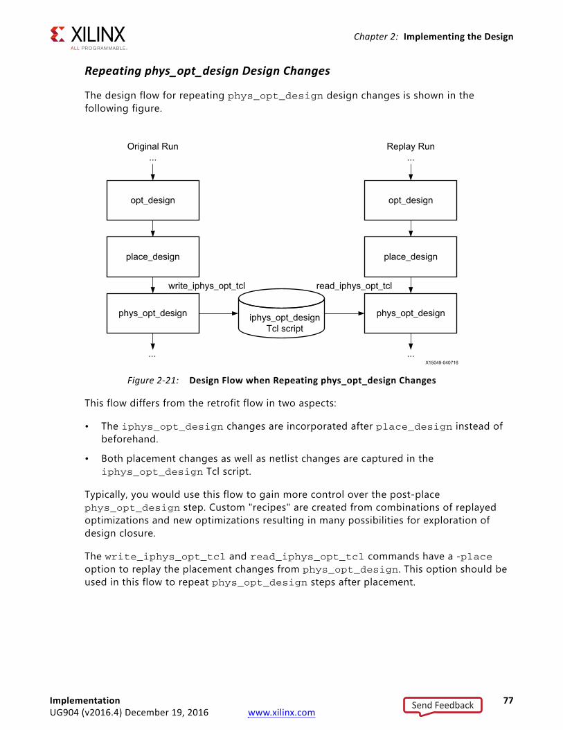
Chapter 2: Implementing the Design
Repeating phys_opt_design Design Changes
The design flow for repeating phys_opt_design design changes is shown in the following figure.
This flow differs from the retrofit flow in two aspects:
• The iphys_opt_design changes are incorporated after place_design instead of beforehand.
• Both placement changes as well as netlist changes are captured in the iphys_opt_design Tcl script.
Typically, you would use this flow to gain more control over the post-place phys_opt_design step. Custom "recipes" are created from combinations of replayed optimizations and new optimizations resulting in many possibilities for exploration of design closure.
The write_iphys_opt_tcl and read_iphys_opt_tcl commands have a -place option to replay the placement changes from phys_opt_design. This option should be used in this flow to repeat phys_opt_design steps after placement.
X-Ref Target - Figure 2-21
Figure 2-21: Design Flow when Repeating phys_opt_design Changes
Implementation 77UG904 (v2016.4) December 19, 2016 www.xilinx.com
Send Feedback
Chapter 2: Implementing the Design
Interactive Physical Optimization Command Reference
The interactive physical optimization commands, along with corresponding options, are described below.
write_iphys_opt_tcl
This command writes a file containing the iphys_opt_design Tcl commands corresponding to the physical optimizations performed in the current design.
Syntax:
write_iphys_opt_tcl [-place] [-quiet] [-verbose] <output file>
The -place option directs the command to include placement information with the iphys_opt_tcl commands. Use this option when you intend to apply placement with netlist changes during iphys_opt_design command replay.
The write_iphys_opt_tcl command can be used any time after phys_opt_design has been run.
read_iphys_opt_tcl
This command reads a file containing the iphys_opt_design Tcl commands corresponding to the physical optimizations performed in a previous run.
Syntax:
read_iphys_opt_tcl [-fanout_opt] [-critical_cell_opt] [-placement_opt] [-rewire] [-dsp_register_opt] [-bram_register_opt] [-shift_register_opt] [-critical_pin_opt] [-clock_opt] [-include_skipped_optimizations] [-place] [-quiet] [-verbose] <input file>
The read_iphys_opt_design command has many of the same options as phys_opt_design to limit the scope of replayed optimizations to only those specified. These options include -fanout_opt, -critical_cell_opt, -placement_opt, -rewire, -dsp_register_opt, -bram_register_opt, -shift_register_opt, -critical_pin_opt, and -clock_opt.
Apply the skipped optimizations that are defined in the input Tcl script, as well as the standard optimizations. These are optimizations identified by phys_opt_design that are skipped because suitable locations for optimized logic cannot be found. When this option is specified, the iphys_opt_design command will attempt to use the included skipped optimizations in the pre-placement netlist.
Implementation 78UG904 (v2016.4) December 19, 2016 www.xilinx.com
Send Feedback
Chapter 2: Implementing the Design
iphys_opt_design
The iphys_opt_design command is a low-level Tcl command that performs a physical optimization. All default phys_opt_design optimizations can be performed using iphys_opt_design. Although it is possible to modify iphys_opt_design commands, and even to create them from scratch, you would typically write them to a script and replay them in a separate run.
RECOMMENDED: Avoid using the Tcl source command to execute a script of iphys_opt_design commands. For most efficient processing of commands and for fastest runtime, use the read_iphys_opt_tcl command instead.
Syntax:
iphys_opt_design [-fanout_opt] [-critical_cell_opt] [-placement_opt] [-rewire] [-net <arg>] -cluster <args> -place_cell <args> [-place] [-dsp_register_opt] [-bram_register_opt] [-shift_register_opt] [-cell <arg>] [-packing] [-unpacking] [-port <arg>] [-critical_pin_opt] [-clock_opt] [-skipped_optimization] [-quiet] [-verbose]
RoutingThe Vivado router performs routing on the placed design, and performs optimization on the routed design to resolve hold time violations.
The Vivado router starts with a placed design and attempts to route all nets. It can start with a placed design that is unrouted, partially routed, or fully routed.
For a partially routed design, the Vivado router uses the existing routes as the starting point, instead of starting from scratch. For a fully-routed design, the router checks for timing violations and attempts to re-route critical portions to meet timing.
Note: The re-routing process is commonly referred to as "rip-up and re-route."
The router provides options to route the entire design or to route individual nets and pins.
When routing the entire design, the flow is timing-driven, using automatic timing budgeting based on the timing constraints.
Routing individual nets and pins can be performed using two distinct modes:
• Interactive Router mode
• Auto-Delay mode
Implementation 79UG904 (v2016.4) December 19, 2016 www.xilinx.com
Send Feedback
Chapter 2: Implementing the Design
The Interactive Router mode uses fast, lightweight timing modeling for greater responsiveness in an interactive session. Some delay accuracy is sacrificed with the estimated delays being pessimistic. Timing constraints are ignored in this mode, but there are several choices to influence the routing:
• Resource-based routing (default): The router chooses from the available routing resources, resulting in the fastest router runtime.
• Smallest delay (the -delay option): The router tries to achieve the smallest possible delay from the available routing resources.
• Delay-driven (the -max_delay and -min_delay options): Specify timing requirements based on a maximum delay, minimum delay, or both. The router tries to route the net with a delay that meets the specified requirements.
In Auto-Delay mode, the router runs the timing-driven flow with automatic timing budgeting based on the timing constraints, but unlike the default flow, only the specified nets or pins are routed. This mode is used to route critical nets and pins before routing the remainder of the design. This includes nets and pins that are setup-critical, hold-critical, or both. Auto-Delay mode is not intended for routing individual nets in a design containing a significant amount of routing. Interactive routing should be used instead.
For best results when routing many individual nets and pins, prioritize and route these individually. This avoids contention for critical routing resources.
Routing requires a one-time “run time hit” for initialization, even when editing routes of nets and pins. The initialization time increases with the size of the design and with the size of the device. The router does not need to be re-initialized unless the design is closed and reopened.
Design Rule Checks Before starting routing, the Vivado tools run Design Rule Checks (DRC), including:
• User-selected DRCs from report_drc
• Built-in DRCs internal to the Vivado router engine
Routing PrioritiesThe Vivado Design Suite routes global resources first, such as clocks, resets, I/O, and other dedicated resources.
This default priority is built into the Vivado router. The router then prioritizes data signals according to timing criticality.
Implementation 80UG904 (v2016.4) December 19, 2016 www.xilinx.com
Send Feedback
Chapter 2: Implementing the Design
Impact of Poor Timing ConstraintsPost-routing timing violations are sometimes the result of incorrect timing constraints. Before you experiment with router settings, make sure that you have validated the constraints and the timing picture seen by the router. Validate timing and constraints by reviewing timing reports from the placed design before routing.
Common examples of the impact of poor timing constraints include:
• Cross-clock paths and multi-cycle paths in which hold timing causes route delay insertion
• Congested areas, which can be addressed by targeted fanout optimization in RTL synthesis or through physical optimization
RECOMMENDED: Review timing constraints and correct those that are invalid (or consider RTL changes) before exploring multiple routing options.
Router Timing SummaryAt the end of the routing process, the router reports an estimated timing summary calculated using actual routing delays. However, to improve run time, the router uses incremental timing updates rather than doing the full timing computation to calculate the timing summary. Consequently, the estimated WNS can be more pessimistic (by a few ps) than actual timing. It is therefore possible for the router WNS to be negative while the actual WNS is positive. If the router reports estimated WNS that is negative, the message is a warning, not a critical warning.
TIP: When you run route_design -directive Explore, the router timing summary is based on signoff timing.
IMPORTANT: You must check the actual signoff timing using report_timing_summary or run route_design with the -timing_summary option.
route_designThe route_design command runs routing on the design.
route_design Syntax
route_design [-unroute] [-release_memory] [-nets <args>] [-physical_nets] [-pins <arg>] [-directive <arg>] [-tns_cleanup] [-no_timing_driven] [-preserve] [-delay] [-auto_delay] -max_delay <arg> -min_delay <arg> [-timing_summary] [-finalize] [-quiet] [-verbose]
Implementation 81UG904 (v2016.4) December 19, 2016 www.xilinx.com
Send Feedback
Chapter 2: Implementing the Design
Using DirectivesWhen routing the entire design, directives provide different modes of behavior for the route_design command. Only one directive can be specified at a time. The directive option is incompatible with most other options to prevent conflicting optimizations. The following directives are available:
• Explore:Allows the router to explore different critical path placements after an initial route.
• NoTimingRelaxation:Prevents the router from relaxing timing to complete routing. If the router has difficulty meeting timing, it runs longer to try to meet the original timing constraints.
• MoreGlobalIterations:Uses detailed timing analysis throughout all stages instead of just the final stages, and runs more global iterations even when timing improves only slightly.
• HigherDelayCost:Adjusts the internal cost functions of the router to emphasize delay over iterations, allowing a tradeoff of run time for better performance.
• RuntimeOptimized:Run fewest iterations, trade higher design performance for faster run time.
• AlternateCLBRouting:Chooses alternate routing algorithms that require extra runtime but may help resolve routing congestion.
• Quick:Absolute, fastest run time, non-timing-driven, performs the minimum required for a legal design.
• Default:Run route_design with default settings.
Trading Run Time for Better Routing
The following directives are methods of trading run time for potentially better routing results:
• NoTimingRelaxation
• MoreGlobalIterations
• HigherDelayCost
• AdvancedSkewModeling
Implementation 82UG904 (v2016.4) December 19, 2016 www.xilinx.com
Send Feedback

Chapter 2: Implementing the Design
Using Other route_design Options
Following are more details on the route_design options and option values where applicable.
• Using -nets
This limits operation to only the list of nets specified. The option requires an argument that is a Tcl list of net objects. Note that the argument must be a net object, the value returned by get_nets, as opposed to the string value of the net names.
• Using -pins
This limits operation only to the specified pins. The option requires an argument, which is a Tcl list of pin objects. Note that the argument must be a pin object, the value returned by get_pins, as opposed to the string value of the pin names.
• Using -delay
By default, the router routes individual nets and pins with the fastest run time, using available resources without regard to timing criticality. The -delay option directs the router to find the route with the smallest possible delay.
• Using -min_delay and -max_delay
These options can be used only with the pin option and to specify a desired target delay in picoseconds. The -max_delay option specifies the maximum desired slow-max corner delay for the routing of the specified pin. Similarly the -min_delay option specifies the minimum fast-min corner delay. The two options can be specified simultaneously to create a desired delay range.
• Using -auto_delay
Use with -nets or -pins option to route in timing constraint-driven mode. Timing budgets are automatically derived from the timing constraints so this option is not compatible with -min_delay, -max_delay, or -delay.
Implementation 83UG904 (v2016.4) December 19, 2016 www.xilinx.com
Send Feedback

Chapter 2: Implementing the Design
• Using -preserve
This option routes the entire design while preserving existing routing. Without -preserve, the existing routing is subject to being unrouted and re-routed to improve critical-path timing. This option is most commonly used when "pre-routing" critical nets, that is, routing certain nets first to ensure that they have best access to routing resources. After achieving those routes, the -preserve option ensures they are not disrupted while routing the remainder of the design. Note that -preserve is completely independent of the FIXED_ROUTE and IS_ROUTE_FIXED net properties. The route preservation lasts only for the duration of the route_design operation in which is it used. The -preserve option can be used with -directive, with one exception, the -directive Explore option, which modifies placement, which in turn modifies routing.
• Using -unroute
The -unroute option removes routing for the entire design or for nets and pins, when combined with the nets or pin options. The option does not remove routing for nets with FIXED_ROUTE properties. Removing routing on nets with FIXED_ROUTE properties requires the properties to be removed first.
• Using -timing_summary
The router outputs a final timing summary to the log, based on its internal estimated timing which might differ slightly from the actual routed timing due to pessimism in the delay estimates. The -timing_summary option forces the router to call the Vivado static timing analyzer to report the timing summary based on the actual routed delays. This incurs additional run time for the static timing analysis. The -timing_summary is ignored when the -directive Explore option is used.
When the -directive Explore option is used, routing always calls the Vivado static timing analyzer for the most accurate timing updates, whether or not the -timing_summary option is used.
• Using -tns_cleanup
For optimal run time, the router focuses on improving the Worst Negative Slack (WNS) path as opposed to reducing the Total Negative Slack (TNS). The -tns_cleanup option invokes an optional phase at the end of routing, during which the router attempts to fix all failing paths to reduce the TNS. Consequently, this option might reduce TNS at the expense of run time but might not affect WNS. Use the -tns_cleanup option during routing when you intend to follow router runs with post-route physical optimization. Use of this option during routing ensures that physical optimization focuses on the WNS path and that effort is not wasted on non-critical paths that can be fixed by the router. This option is compatible with -directive.
Implementation 84UG904 (v2016.4) December 19, 2016 www.xilinx.com
Send Feedback
Chapter 2: Implementing the Design
• Using -physical_nets
The -physical_nets option operates only on logic 0 and logic 1 routes. The option covers all logic constant values in the design and is compatible with the -unroute option. Because constant 0 and 1 tie-offs in the physical device have no exact correlation to logical nets, these nets cannot be routed and unrouted reliably using the -nets and -pins options.
• Using -release_memoryAfter router initialization, router data is kept in memory to ensure optimal performance. This option forces the router to delete its data from memory and release the memory back to the operating system. This option should not be required for mainstream use and is provided in case router memory must be manually managed, for example, with extremely large designs.
• Using -finalize
When routing interactively you can specify route_design -finalize to complete any partially routed connections.
For UltraScale+ designs, this step is required if placement and routing of registers was changed as part of an ECO task.
• Using -no_timing_driven
This option disables timing-driven routing and is used primarily for testing the routing feasibility of a design.
TIP: If a clock net is unrouted in an UltraScale design, place_design must be run before the clock net is re-routed. This ensures that the clock net is legally routed. This restriction is planned to be removed in a future release
Routing Example Script 1
# Route design, save results to checkpoint, report timing estimates route_designwrite_checkpoint -force $outputDir/post_routereport_timing_summary -file $outputDir/post_route_timing_summary.rpt
The route_design example script performs the following steps:
1. Routes the design
2. Writes a design checkpoint after completing routing
3. Generates a timing summary report
4. Writes the report to the specified file.
Implementation 85UG904 (v2016.4) December 19, 2016 www.xilinx.com
Send Feedback
Chapter 2: Implementing the Design
Routing is performed as part of an implementation run, or by running route_design after place_design as part of a Tcl script.
The router provides info in the log to indicate progress, such as the current phase (initialization, global routing iterations, and timing updates). At the end of global routing, the log includes periodic updates showing the current number of overlapping nets as the router attempts to achieve a fully legalized design. For example:
Phase 4.1 Global Iteration 0 Number of Nodes with overlaps = 435 Number of Nodes with overlaps = 3 Number of Nodes with overlaps = 1 Number of Nodes with overlaps = 0
The timing updates are provided throughout the flow showing timing closure progress.
Timing Summary
[Route 35-57] Estimated Timing Summary | WNS=0.105 | TNS=0 | WHS=0.051 | THS=0
where:
° WNS = Worst Negative Slack
° TNS = Total Negative Slack
° WHS = Worst Hold Slack
° THS = Total Hold Slack
Note: Hold time analysis can be skipped during intermediate routing phases. If hold time is not performed, the router shows a value of "N/A" for WHS and THS.
After routing is complete, the router reports a routing utilization summary and a final estimated timing summary. An example of the Router Utilization Summary is shown below.
Router Utilization Summary
Global Vertical Routing Utilization = 15.3424 % Global Horizontal Routing Utilization = 16.3981 % Routable Net Status* *Does not include unroutable nets such as driverless and loadless. Run report_route_status for detailed report. Number of Failed Nets = 0 Number of Unrouted Nets = 0 Number of Partially Routed Nets = 0 Number of Node Overlaps = 0
Implementation 86UG904 (v2016.4) December 19, 2016 www.xilinx.com
Send Feedback
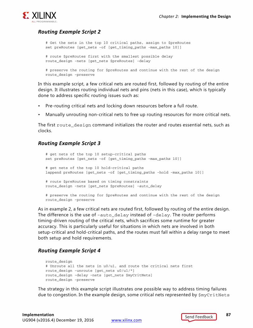
Chapter 2: Implementing the Design
Routing Example Script 2
# Get the nets in the top 10 critical paths, assign to $preRoutesset preRoutes [get_nets -of [get_timing_paths -max_paths 10]]
# route $preRoutes first with the smallest possible delayroute_design -nets [get_nets $preRoutes] -delay
# preserve the routing for $preRoutes and continue with the rest of the designroute_design -preserve
In this example script, a few critical nets are routed first, followed by routing of the entire design. It illustrates routing individual nets and pins (nets in this case), which is typically done to address specific routing issues such as:
• Pre-routing critical nets and locking down resources before a full route.
• Manually unrouting non-critical nets to free up routing resources for more critical nets.
The first route_design command initializes the router and routes essential nets, such as clocks.
Routing Example Script 3
# get nets of the top 10 setup-critical pathsset preRoutes [get_nets -of [get_timing_paths -max_paths 10]]
# get nets of the top 10 hold-critical pathslappend preRoutes [get_nets -of [get_timing_paths -hold -max_paths 10]]
# route $preRoutes based on timing constraintsroute_design -nets [get_nets $preRoutes] -auto_delay
# preserve the routing for $preRoutes and continue with the rest of the designroute_design -preserve
As in example 2, a few critical nets are routed first, followed by routing of the entire design. The difference is the use of -auto_delay instead of -delay. The router performs timing-driven routing of the critical nets, which sacrifices some runtime for greater accuracy. This is particularly useful for situations in which nets are involved in both setup-critical and hold-critical paths, and the routes must fall within a delay range to meet both setup and hold requirements.
Routing Example Script 4
route_design# Unroute all the nets in u0/u1, and route the critical nets firstroute_design -unroute [get_nets u0/u1/*] route_design -delay -nets [get_nets $myCritNets]route_design -preserve
The strategy in this example script illustrates one possible way to address timing failures due to congestion. In the example design, some critical nets represented by $myCritNets
Implementation 87UG904 (v2016.4) December 19, 2016 www.xilinx.com
Send Feedback
Chapter 2: Implementing the Design
need routing resources in the same device region as the nets in instance u0/u1. The nets in u0/u1 are not as timing-critical, so they are unrouted to allow the critical nets $myCritNets to be routed first, with the smallest possible delay. Then route_design -preserve routes the entire design. The -preserve switch preserves the routing of $myCritNets while the unrouted u0/u1 nets are re-routed. Table 2-7 summarizes the commands in the example.
Router Messaging
The router provides helpful messages when it struggles to meet timing goals due to congestion or excessive hold violation fixing. The router commonly exhibits these symptoms when it struggles:
• Excessive runtimes, on the order of hours per iteration
• Large number of overlaps reported, in the hundreds of thousands
• Setup and hold slacks become progressively worse, as seen in the Estimated Timing Summaries
The router might provide further warning messages when any of the following occurs:
• Congestion is expected to have negative timing closure impact, which typically occurs when the congestion level is 5 or greater. Level 5 indicates a congested region measuring 32x32 (2^5 = 32).
• The overall router hold-fix effort is expected to be very high, which impacts the ability to meet overall setup requirements.
• Specific endpoint pins become both setup-critical and hold-critical and it is difficult or impossible to satisfy both. The message includes the names of up to ten pins for design analysis.
• Specific CLBs experience high pin utilization or high routing resource utilization which results in local congestion. The messages will include the names of up to ten of the most congested CLBs.
• In extreme cases with severe congestion, the router warns that congestion is preventing the router from routing all nets, and the router will prioritize the successful completion of routing all nets over timing optimizations.
When targeting UltraScale devices, the router generates a table showing initial estimated congestion when congestion might affect timing closure. The table does not show specific regions but gives a measure of different types of congestion for an overall assessment. The congestion is categorized into bins of Global (design-wide), Long (connections spanning several CLBs), and Short Congestion. The tables of different runs can be compared to determine which have better chances of meeting performance goals without being too negatively impacted by congestion.
INFO: [Route 35-449] Initial Estimated Congestion
Implementation 88UG904 (v2016.4) December 19, 2016 www.xilinx.com
Send Feedback
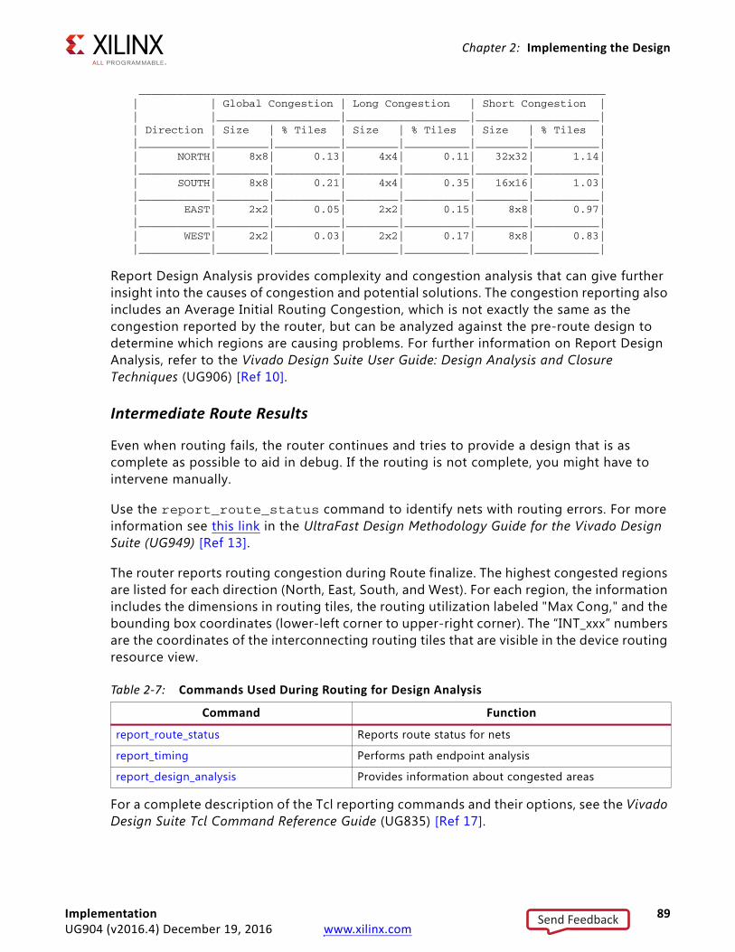
Chapter 2: Implementing the Design
________________________________________________________________________| | Global Congestion | Long Congestion | Short Congestion || |___________________|___________________|___________________|| Direction | Size | % Tiles | Size | % Tiles | Size | % Tiles ||___________|________|__________|________|__________|________|__________|| NORTH| 8x8| 0.13| 4x4| 0.11| 32x32| 1.14||___________|________|__________|________|__________|________|__________|| SOUTH| 8x8| 0.21| 4x4| 0.35| 16x16| 1.03||___________|________|__________|________|__________|________|__________|| EAST| 2x2| 0.05| 2x2| 0.15| 8x8| 0.97||___________|________|__________|________|__________|________|__________|| WEST| 2x2| 0.03| 2x2| 0.17| 8x8| 0.83||___________|________|__________|________|__________|________|__________|
Report Design Analysis provides complexity and congestion analysis that can give further insight into the causes of congestion and potential solutions. The congestion reporting also includes an Average Initial Routing Congestion, which is not exactly the same as the congestion reported by the router, but can be analyzed against the pre-route design to determine which regions are causing problems. For further information on Report Design Analysis, refer to the Vivado Design Suite User Guide: Design Analysis and Closure Techniques (UG906) [Ref 10].
Intermediate Route Results
Even when routing fails, the router continues and tries to provide a design that is as complete as possible to aid in debug. If the routing is not complete, you might have to intervene manually.
Use the report_route_status command to identify nets with routing errors. For more information see this link in the UltraFast Design Methodology Guide for the Vivado Design Suite (UG949) [Ref 13].
The router reports routing congestion during Route finalize. The highest congested regions are listed for each direction (North, East, South, and West). For each region, the information includes the dimensions in routing tiles, the routing utilization labeled "Max Cong," and the bounding box coordinates (lower-left corner to upper-right corner). The “INT_xxx” numbers are the coordinates of the interconnecting routing tiles that are visible in the device routing resource view.
For a complete description of the Tcl reporting commands and their options, see the Vivado Design Suite Tcl Command Reference Guide (UG835) [Ref 17].
Table 2-7: Commands Used During Routing for Design Analysis
Command Function
report_route_status Reports route status for nets
report_timing Performs path endpoint analysis
report_design_analysis Provides information about congested areas
Implementation 89UG904 (v2016.4) December 19, 2016 www.xilinx.com
Send Feedback
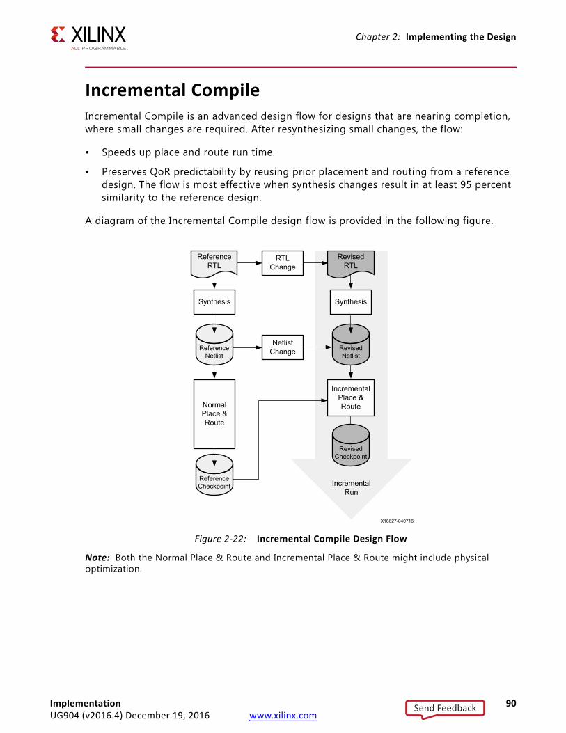
Chapter 2: Implementing the Design
Incremental CompileIncremental Compile is an advanced design flow for designs that are nearing completion, where small changes are required. After resynthesizing small changes, the flow:
• Speeds up place and route run time.
• Preserves QoR predictability by reusing prior placement and routing from a reference design. The flow is most effective when synthesis changes result in at least 95 percent similarity to the reference design.
A diagram of the Incremental Compile design flow is provided in the following figure.
Note: Both the Normal Place & Route and Incremental Place & Route might include physical optimization.
X-Ref Target - Figure 2-22
Figure 2-22: Incremental Compile Design Flow
Reference RTL
Synthesis
Normal Place & Route
Reference Checkpoint
RTLChange
NetlistChangeReference
Netlist
Revised RTL
Synthesis
Revised Netlist
Incremental Place & Route
Revised Checkpoint
Incremental Run
Implementation 90UG904 (v2016.4) December 19, 2016 www.xilinx.com
Send Feedback
Chapter 2: Implementing the Design
Incremental Compile Flow DesignsThe Incremental Compile flow, shown in Figure 2-22, involves two different designs, the reference design and the current design.
Reference Design
The reference design is usually an earlier iteration or variation of the current design that has been synthesized, placed, and routed.
However, you can use a checkpoint that has any amount of placement, routing, or both.The reference design checkpoint (DCP) might be the product of many design iterations involving code changes, floorplanning, and revised constraints necessary to close timing.
After the current design is loaded, load the reference design checkpoint using the read_checkpoint -incremental <dcp> command. Loading the reference design checkpoint with the -incremental option enables the Incremental Compile design flow for subsequent place and route operations. For more information, see Examining the Similarity Between the Reference Design and the Current Design, page 93.
IMPORTANT: For the incremental flow to work properly, the device and speed grade of the reference design checkpoint (DCP) must match the device and speed grade of the current design.
Current Design
The current design incorporates small design changes or variations from the reference design. These changes or variations can include:
• RTL changes
• Netlist changes
• Both RTL changes and netlist changes
Running Incremental Place and RouteThe updated, current design is first loaded into memory. The reference design checkpoint is then loaded incrementally.
The key component of the Incremental Compile process is incremental place and route. From the reference checkpoint only, the physical data of place and route is inspected. Netlist and constraints for the updated current design are used.
• The netlist in the current design is compared to the reference design to identify matching cells and nets.
• Placement from the reference design checkpoint is reused to place matching cells in the current design.
Implementation 91UG904 (v2016.4) December 19, 2016 www.xilinx.com
Send Feedback
Chapter 2: Implementing the Design
• Routing is reused to route matching nets on a per-load-pin basis. If a load pin disappears due to netlist changes, then its routing is discarded, otherwise it is reused. Therefore it is possible to have partially-reused routes.
Incremental placement and incremental routing might discard cell placements and net routes instead of reusing them, if it helps improve routability of the netlist or helps maintain performance comparable to that of the reference design.
Design objects that do not match between the reference design and the current design are placed after incremental placement is complete and routed after routing is complete.
Nets with Multiple Fanouts
The Vivado router performs fine-grained matching for nets with multiple fanouts, in which each routing segment can be reused or discarded as appropriate.
Effectively Reusing Placement and Routing
Effective reuse of the placement and routing from the reference design depends on the differences between the two designs. Even small differences can have a large impact.
Impact of Small RTL Changes
Although synthesis tries to minimize netlist name changes, sometimes small RTL changes such as the following can lead to very large changes in the synthesized netlist:
• Changing a constant value in the HDL code
• Increasing the size of an inferred memory
• Widening an internal bus
Impact of Changing Constraints and Synthesis Options
Similarly, changing constraints and synthesis options such as the following can also have a large impact on incremental placement and routing run time:
• Changing timing constraints and resynthesizing
• Preserving or dissolving logical hierarchy
• Enabling register re-timing
Using phys_opt_design
Physical Optimization (phys_opt_design) can also be used in the Incremental Compile flow, as in the normal place and route flow. If a reference checkpoint contains physical optimizations, and if it is generated with Vivado Design Suite version 2015.3 or later, Incremental Compile implicitly runs read_iphys_opt_design to process the iphys_opt_design commands from the reference checkpoint. Incremental Compile
Implementation 92UG904 (v2016.4) December 19, 2016 www.xilinx.com
Send Feedback

Chapter 2: Implementing the Design
applies both netlist and placement changes for matching cells and restores the results of the original physical optimizations. This improves both runtime and predictability when phys_opt_design is used.
If the reference checkpoint is generated from versions of the Vivado tools prior to 2015.3, and if it contains optimizations performed by phys_opt_design, ensure that the incremental run also uses phys_opt_design. This captures the placement optimizations performed by phys_opt_design in the reference design and allows related routes to be reused. Unlike place_design and route_design, phys_opt_design does not have an incremental mode, but it does perform logic transformations in the revised design that are very similar to those of the reference design.
Note the netlist similarity between the post-route Reference Design and the Current Design. If the netlist matching seems suboptimal, it might be due to significant amounts of logic optimization from phys_opt_design. Therefore the post-place checkpoint might be a better reference design than the post-route checkpoint.
Examining the Similarity Between the Reference Design and the Current Design
Run report_incremental_reuse to examine and report the similarity between a reference design checkpoint file and the current design. The report_incremental_reuse command compares the netlist from the reference design checkpoint with the current in-memory design, and reports the percentage of matching of cells, nets, and ports.
A higher degree of design similarity results in more effective reuse of placement and routing from the reference design. The greater the percentage of similarity between the reference design and current design, the greater the opportunity for placement and routing reuse.
Incremental Reuse Summary
The reuse report is divided into two sections, the Netlist Similarity Summary and the Implementation Reuse Summary. The Netlist Similarity Summary shows how many logical objects in the current design match objects in the reference design. This indicates how logically similar the design is after updating it with small changes.
The Implementation Reuse Summary shows physical data reuse of matching logical objects, including what percentage of cells, ports, and nets are reused, along with their placement and routing information from the reference design. For cells that are not reused, it provides a breakdown of which cells are new cells in the netlist, those cells that do not exist in the reference design, and which cells have placements that must be discarded because their placements become illegal after updating the design. For nets, the report provides a breakdown of fully-reused routes, partially-reused routes, and nets that are new (that is, those nets that do not exist in the reference design).
Implementation 93UG904 (v2016.4) December 19, 2016 www.xilinx.com
Send Feedback
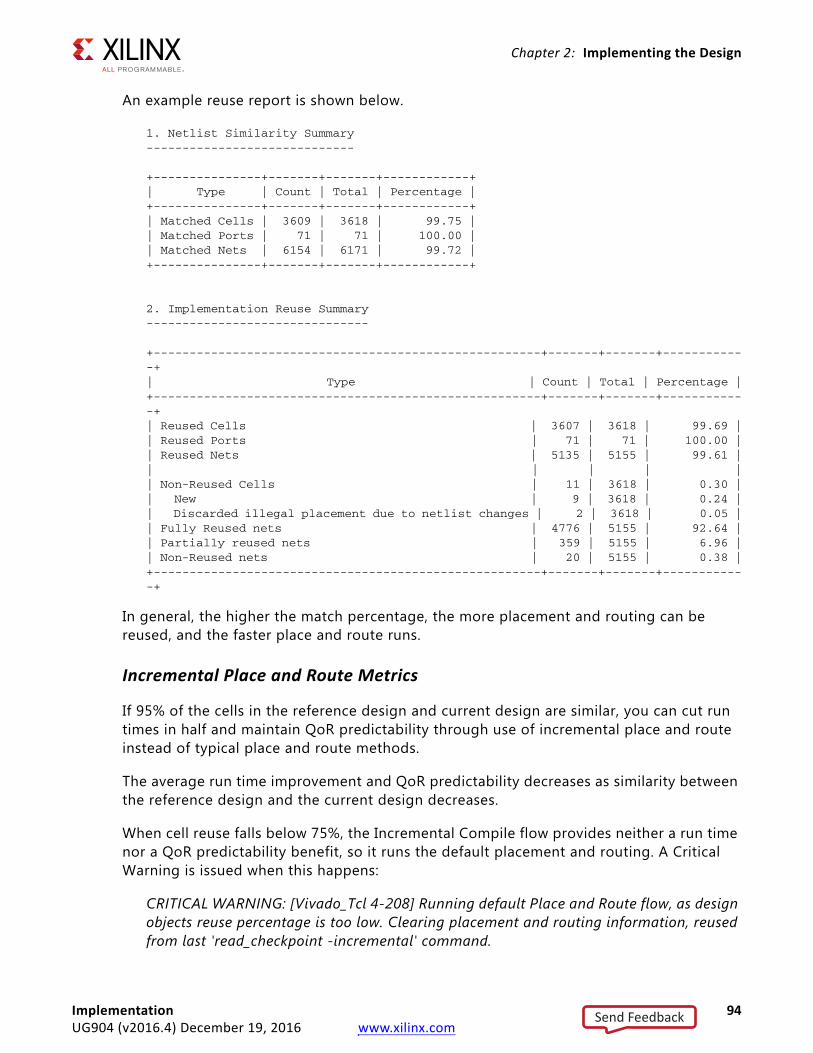
Chapter 2: Implementing the Design
An example reuse report is shown below.
1. Netlist Similarity Summary-----------------------------
+---------------+-------+-------+------------+| Type | Count | Total | Percentage |+---------------+-------+-------+------------+| Matched Cells | 3609 | 3618 | 99.75 || Matched Ports | 71 | 71 | 100.00 || Matched Nets | 6154 | 6171 | 99.72 |+---------------+-------+-------+------------+
2. Implementation Reuse Summary-------------------------------
+------------------------------------------------------+-------+-------+------------+| Type | Count | Total | Percentage |+------------------------------------------------------+-------+-------+------------+| Reused Cells | 3607 | 3618 | 99.69 || Reused Ports | 71 | 71 | 100.00 || Reused Nets | 5135 | 5155 | 99.61 || | | | || Non-Reused Cells | 11 | 3618 | 0.30 || New | 9 | 3618 | 0.24 || Discarded illegal placement due to netlist changes | 2 | 3618 | 0.05 || Fully Reused nets | 4776 | 5155 | 92.64 || Partially reused nets | 359 | 5155 | 6.96 || Non-Reused nets | 20 | 5155 | 0.38 |+------------------------------------------------------+-------+-------+------------+
In general, the higher the match percentage, the more placement and routing can be reused, and the faster place and route runs.
Incremental Place and Route Metrics
If 95% of the cells in the reference design and current design are similar, you can cut run times in half and maintain QoR predictability through use of incremental place and route instead of typical place and route methods.
The average run time improvement and QoR predictability decreases as similarity between the reference design and the current design decreases.
When cell reuse falls below 75%, the Incremental Compile flow provides neither a run time nor a QoR predictability benefit, so it runs the default placement and routing. A Critical Warning is issued when this happens:
CRITICAL WARNING: [Vivado_Tcl 4-208] Running default Place and Route flow, as design objects reuse percentage is too low. Clearing placement and routing information, reused from last 'read_checkpoint -incremental' command.
Implementation 94UG904 (v2016.4) December 19, 2016 www.xilinx.com
Send Feedback
Chapter 2: Implementing the Design
Factors Affecting Run Time Improvement
Factors that can affect run time improvement include:
• The amount of change in timing-critical areas. If critical path placement and routing cannot be reused, more effort is required to preserve timing. Also, if the small design changes introduce new timing problems that did not exist in the reference design, higher effort and run time might be required, and the design might not meet timing.
• The initialization portion of the place and route run time. In short place and route runs, the initialization overhead of the Vivado placer and router might eliminate any gain from the incremental place and route process. For designs with longer run times, initialization becomes a small percentage of the run time.
Using Incremental CompileIn both Project Mode and Non-Project Mode, incremental place and route mode is entered when you load the reference design checkpoint using the read_checkpoint -incremental <dcp_file> command where <dcp_file> specifies the path and file name of the reference design checkpoint. Loading the reference design checkpoint with the -incremental option enables the Incremental Compile design flow for subsequent place and route operations. In Non-Project Mode, read_checkpoint -incremental should follow opt_design and precede place_design.
Using Incremental Compile in Non-Project Mode
To specify a design checkpoint file (DCP) to use as the reference design, and to run incremental place in Non-Project Mode:
1. Load the current design.
2. Run opt_design.
3. Run read_checkpoint -incremental <dcp_file>.
4. Run place_design.
5. Run phys_opt_design (optional). Run phys_opt_design if it was used in the reference design.
6. Run route_design.
link_design; # to load the current designopt_designread_checkpoint -incremental <dcp_file>place_design phys_opt_design; #if used in reference designroute_design
Implementation 95UG904 (v2016.4) December 19, 2016 www.xilinx.com
Send Feedback
Chapter 2: Implementing the Design
Incremental placement relies on the ability of the Vivado tools to match design objects in the current design with design objects in the reference design. However, use of the following opt_design command options typically results in poor cell-name matching between the reference and current designs (which, in turn, results in poor matching of placement and routing data):
• -resynth_area
• -resynth_seq_area
• -directive ExploreArea
• -directive ExploreAreaSequential
Using Incremental Compile in Project Mode
In Project Mode, you can set the incremental compile option in the Design Runs window. To set the incremental compile option:
1. Select a run in the Design Runs window.
2. Click Set Incremental Compile from the context menu.
3. In the Set Incremental Compile window, select a reference design checkpoint.
This enables incremental compile mode for the run.
IMPORTANT: When you choose a checkpoint from a design run, it is deleted if the design run is reset. If you want to choose a checkpoint from a design run, copy it into a separate directory before selecting it as your reference checkpoint.
For an example of the Implementation dialog box showing Incremental Compile settings, see Figure 2-23.
Implementation 96UG904 (v2016.4) December 19, 2016 www.xilinx.com
Send Feedback
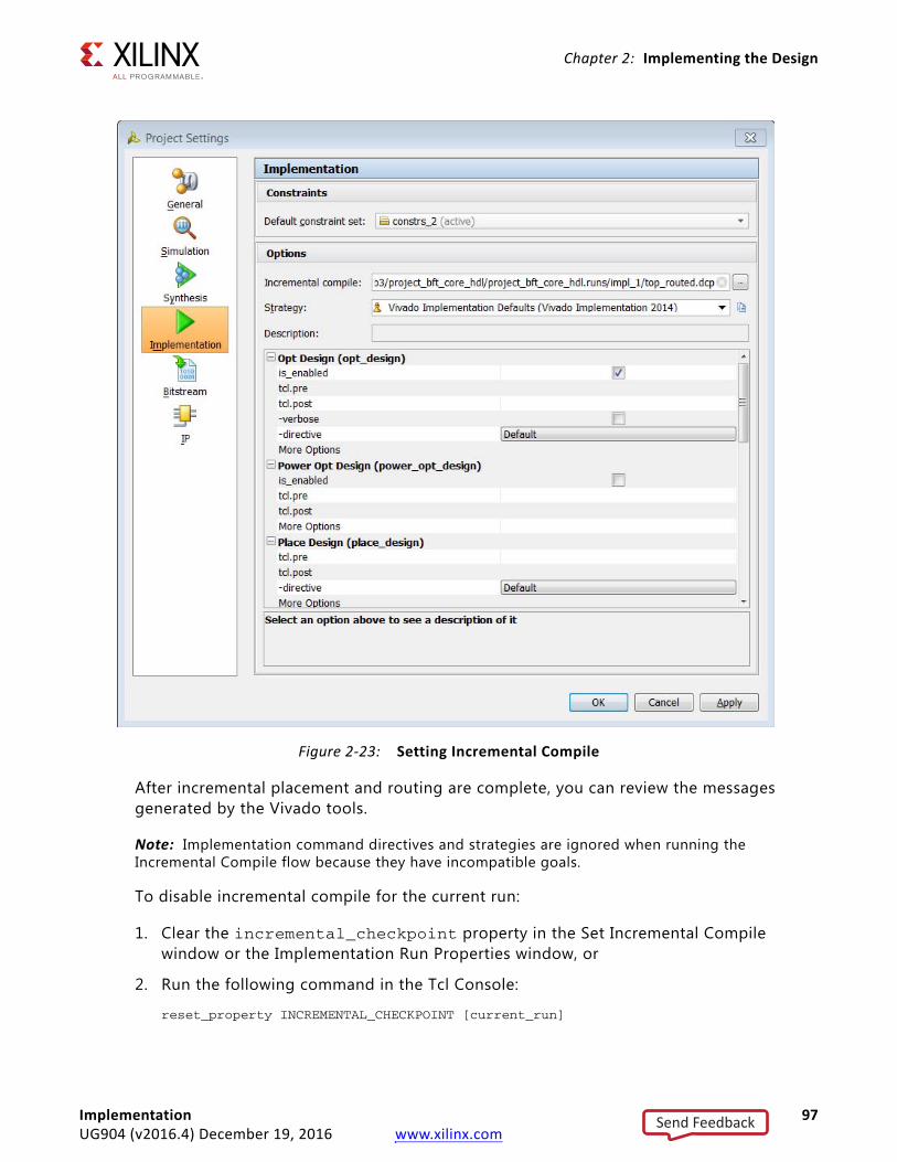
Chapter 2: Implementing the Design
After incremental placement and routing are complete, you can review the messages generated by the Vivado tools.
Note: Implementation command directives and strategies are ignored when running the Incremental Compile flow because they have incompatible goals.
To disable incremental compile for the current run:
1. Clear the incremental_checkpoint property in the Set Incremental Compile window or the Implementation Run Properties window, or
2. Run the following command in the Tcl Console:
reset_property INCREMENTAL_CHECKPOINT [current_run]
X-Ref Target - Figure 2-23
Figure 2-23: Setting Incremental Compile
Implementation 97UG904 (v2016.4) December 19, 2016 www.xilinx.com
Send Feedback
Chapter 2: Implementing the Design
Orphaned Route Segments
Some cells might have been eliminated from the current design, or moved during placement, leaving orphaned route segments from the reference design. If you are running in the Vivado IDE, you might see potentially problematic nets. These orphaned or improperly connected route segments are cleaned up during incremental routing by the Vivado router.
The following INFO message appears during placement.
INFO: [Place 46-2] During incremental compilation, routing data from the original checkpoint is applied during place_design. As a result, dangling route segments and route conflicts may appear in the post place_design implementation due to changes between the original and incremental netlists. These routes can be ignored as they will be subsequently resolved by route_design. This issue will be cleaned up automatically in place_design in a future software release.
Using Synplify Compile PointsThe Incremental Compile flow is most effective when the revised and reference designs are most similar, preferably with at least 95 percent of the cells matching. Synthesis flows such as Synplify Compile Points minimize the amount of netlist changes resulting from RTL changes. Compile points are logical boundaries across which no optimization might occur. This sacrifices some design performance for predictability, but when combined with Incremental Compile, the resulting flow yields even more run time savings and predictability.
Synplify provides two different compile point flows, which are automatic and manual. In the automatic compile point mode, compile points are automatically chosen by synthesis, based on existing hierarchy and utilization estimates. This is a pushbutton mode. Aside from enabling the flow, there is no action required on your part. To enable, check the Auto Compile Point check box in the GUI or add the following setting to the Synplify project:
set_option -automatic_compile_point 1
The manual compile point flow offers more flexibility, but requires more interaction to choose compile points. The flow involves compiling the design, then using either the SCOPE editor Compile Points tab or the define_compile_point setting. For further information on compile point flows, see the Synplify online help.
Implementation 98UG904 (v2016.4) December 19, 2016 www.xilinx.com
Send Feedback
Chapter 2: Implementing the Design
Saving Post-Reuse CheckpointsAfter read_checkpoint -incremental applies the reference checkpoint to the current design, the incremental reuse data is retained throughout the flow. If a checkpoint is saved, then reloaded in the same or a separate Vivado Design Suite session, it remains in incremental compile mode. Consider the following command sequence:
opt_design; # optimize the current designread_checkpoint -incremental reference.dcp; # apply reference data to current designwrite_checkpoint incr.dcp; # save a snapshot of the current designread_checkpoint incr.dcpplace_designwrite_checkpoint top_placed.dcp; # save incremental placement resultroute_design
Upon read_checkpoint incr.dcp, the Vivado tools determine that incremental data exists, and the subsequent place_design and route_design commands run incrementally.
Even if you exit and restart the Vivado Design Suite, in the following command sequence the route_design command is run in incremental mode, using the routing data from the original reference checkpoint reference.dcp:
read_checkpoint top_placed.dcpphys_opt_designroute_design
Constraint ConflictsConstraints of the revised design can conflict with the physical data of the reference checkpoint. When conflicts occur, constraints of the revised design take precedence. This is illustrated in the following example.
Constraint Conflict Example
A constraint assigns a fixed location RAMB36_X0Y0 for a cell cell_A. However in the reference checkpoint reference.dcp, cell_A is placed at RAMB36_X0Y1 and a different cell cell_B is placed at RAMB36_X0Y0.
After running read_checkpoint -incremental reference.dcp, cell_A is placed at RAMB36_X0Y0 and cell_B is unplaced. The cell cell_B is placed during incremental placement.
IMPORTANT: You cannot use Pblocks when using incremental compile. Pblocks can create unmanageable placement conflicts.
Implementation 99UG904 (v2016.4) December 19, 2016 www.xilinx.com
Send Feedback
Chapter 2: Implementing the Design
Incremental Compile Advanced ControlsThere are three read_checkpoint options that provide control over cell placement reuse from a reference checkpoint. These options must be specified with the read_checkpoint -incremental option, as shown below.
-only_reuse option
-only_reuse <cell objects>
The -only_reuse option limits the cell placement reuse to the list of specified cells. The cells could be leaf cells or hierarchical cells.
Examples:
• Only reuse the placement from a top-level instance mem_ctrl_inst within routed.dcp:
read_checkpoint -incremental routed.dcp -only_reuse [get_cells mem_ctrl_inst]
• Only reuse the block RAM placement within routed.dcp:
read_checkpoint -incremental routed.dcp -only_reuse [get_cells -hier -filter { PRIMITIVE_TYPE =~ BMEM.bram.* } ]
-dont_reuse option
-dont_reuse <cell objects>
The -dont_reuse option reuses all cell placement except for those in the specified list. The cells could be leaf cells or hierarchical cells.
Examples:
• Reuse all placement from routed.dcp except for the cell placements from top-level instance mem_ctrl_inst:
read_checkpoint -incremental routed.dcp -dont_reuse [get_cells mem_ctrl_inst]
• Reuse all placement from routed.dcp except for the block RAM placement:
read_checkpoint -incremental routed.dcp -dont_reuse [get_cells -hier -filter { PRIMITIVE_TYPE =~ BMEM.bram.* } ]
Implementation 100UG904 (v2016.4) December 19, 2016 www.xilinx.com
Send Feedback
Chapter 2: Implementing the Design
-fix_reuse option
The -fix_reuse option can be used with -only_reuse or -dont_reuse to lock down the placement of the reused cells automatically.
Example:
• Only reuse the block RAM placement within routed.dcp, and lock down the reused cell placement:
read_checkpoint -incremental routed.dcp -only_reuse [get_cells -hier -filter { PRIMITIVE_TYPE =~ BMEM.bram.* } ] -fix_reuse
As a reminder, in general, reused placement and routing can be modified. Therefore, -fix_reuse should be specified if modification is not desired.
After applying the RAM cell locations, the cells are affixed with IS_LOC_FIXED properties with value TRUE.
Incremental Compile Advanced AnalysisThe Vivado tools provide reporting, timing labels, and object properties for advanced reuse analysis.
Reuse Reporting
The report_incremental_reuse command provides options for more detailed analysis, similar to report_utilization.
-cells <list of cells>
The -cells option limits the reuse reporting to the list of given cells instead of reporting reuse of the entire design.
For example, limit the reuse reporting to only block RAM:
report_incremental_reuse -cells [get_cells -hierarchical -filter { PRIMITIVE_TYPE =~ BMEM.bram.* } ]
Implementation 101UG904 (v2016.4) December 19, 2016 www.xilinx.com
Send Feedback
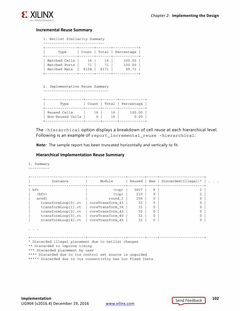
Chapter 2: Implementing the Design
Incremental Reuse Summary
1. Netlist Similarity Summary-----------------------------+---------------+-------+-------+------------+| Type | Count | Total | Percentage |+---------------+-------+-------+------------+| Matched Cells | 16 | 16 | 100.00 || Matched Ports | 71 | 71 | 100.00 || Matched Nets | 6154 | 6171 | 99.72 |+---------------+-------+-------+------------+
2. Implementation Reuse Summary-------------------------------
+------------------+-------+-------+------------+| Type | Count | Total | Percentage |+------------------+-------+-------+------------+| Reused Cells | 16 | 16 | 100.00 || Non-Reused Cells | 0 | 16 | 0.00 |+------------------+-------+-------+------------+
The -hierarchical option displays a breakdown of cell reuse at each hierarchical level. Following is an example of report_incremental_reuse -hierarchical:
Note: The sample report has been truncated horizontally and vertically to fit.
Hierarchical Implementation Reuse Summary
1. Summary----------
+--------------------------+------------------+--------+-----+---------------------+| Instance | Module | Reused | New | Discarded(Illegal)* | . . .+--------------------------+------------------+--------+-----+---------------------+| bft | (top) | 3607 | 9 | 2 || (bft) | (top) | 210 | 9 | 2 || arnd1 | round_1 | 256 | 0 | 0 || transformLoop[0].ct | coreTransform_43 | 32 | 0 | 0 || transformLoop[1].ct | coreTransform_38 | 32 | 0 | 0 || transformLoop[2].ct | coreTransform_42 | 32 | 0 | 0 || transformLoop[3].ct | coreTransform_40 | 32 | 0 | 0 || transformLoop[4].ct | coreTransform_45 | 32 | 0 | 0 |
. . .
+--------------------------+------------------+--------+-----+---------------------+* Discarded illegal placement due to netlist changes** Discarded to improve timing*** Discarded placement by user**** Discarded due to its control set source is unguided***** Discarded due to its connectivity has Loc Fixed Insts
Implementation 102UG904 (v2016.4) December 19, 2016 www.xilinx.com
Send Feedback
Chapter 2: Implementing the Design
The reuse status of each cell is reported, beginning with the top-level hierarchy, then covering each level hierarchy contained within that level. The report progresses to the lowest level of hierarchy contained within the first submodule, then moves on to the next one.
In this example, the top level cell is bft with a cumulative reuse total of 3,607 cells with 9 new cells. The row with bft in parentheses show the cell reuse status contained within bft and but not its submodules. Of the 3,607 cells, only 210 are within bft and the remainder are within its submodules. However all 9 new cells are within bft. Within bft is a submodule arnd1 containing 256 reused cells, and no cells within arnd1 itself, only in submodules transformLoop[0].ct, transformLoop[1].ct, and so on.
There are 5 columns indicating cell reuse status at each level, although only the first one Discarded(Illegal) is shown. These columns have footnote references in the report with further reasons for discarding reused placement.
* Discarded illegal placement due to netlist changes
** Discarded to improve timing
*** Discarded placement by user
**** Discarded due to its control set source is unguided
***** Discarded due to its connectivity has Loc Fixed Insts
Instead of reporting all hierarchical levels, you can use the -hierarchical_depth option to limit the number of submodules to an exact number of levels. The following is the previous example, adding -hierarchical_depth of 1:
report_incremental_reuse -hierarchical -hierarchical_depth 1
1. Summary----------
+----------+--------+--------+-----+---------------------+| Instance | Module | Reused | New | Discarded(Illegal)* | . . .+----------+--------+--------+-----+---------------------+| bft | (top) | 3607 | 9 | 2 |+----------+--------+--------+-----+---------------------+
This limits reporting to the top level bft. If you had used a -hierarchical_depth of 2, the top and each level of hierarchy contained within bft would be reported, but nothing below those hierarchical cells.
Implementation 103UG904 (v2016.4) December 19, 2016 www.xilinx.com
Send Feedback
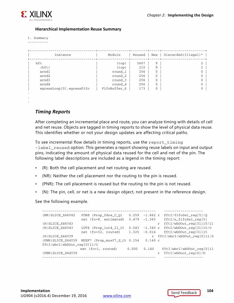
Chapter 2: Implementing the Design
Hierarchical Implementation Reuse Summary
1. Summary----------
+--------------------------------+---------------+--------+-----+---------------------+| Instance | Module | Reused | New | Discarded(Illegal)* |+--------------------------------+---------------+--------+-----+---------------------+| bft | (top) | 3607 | 9 | 2 || (bft) | (top) | 210 | 9 | 2 || arnd1 | round_1 | 256 | 0 | 0 || arnd2 | round_2 | 256 | 0 | 0 || arnd3 | round_3 | 256 | 0 | 0 || arnd4 | round_4 | 256 | 0 | 0 || egressLoop[0].egressFifo | FifoBuffer_6 | 173 | 0 | 0 |...
Timing Reports
After completing an incremental place and route, you can analyze timing with details of cell and net reuse. Objects are tagged in timing reports to show the level of physical data reuse. This identifies whether or not your design updates are affecting critical paths.
To see incremental flow details in timing reports, use the report_timing -label_reused option. This generates a report showing reuse labels on input and output pins, indicating the amount of physical data reused for the cell and net of the pin. The following label descriptions are included as a legend in the timing report:
• (R): Both the cell placement and net routing are reused.
• (NR): Neither the cell placement nor the routing to the pin is reused.
• (PNR): The cell placement is reused but the routing to the pin is not reused.
• (N): The pin, cell, or net is a new design object, not present in the reference design.
See the following example.
------------------------------------------------------- -------------------(NR)SLICE_X46Y42 FDRE (Prop_fdre_C_Q) 0.259 -1.862 r fftI/fifoSel_reg[5]/Q net (fo=8, estimated) 0.479 -1.383 fftI/n_fifoSel_reg[5](R)SLICE_X46Y43 r fftI/wbDOut_reg[31]i5/I1(R)SLICE_X46Y43 LUT4 (Prop_lut4_I1_O) 0.043 -1.340 r fftI/wbDOut_reg[31]i5/O net (fo=32, routed) 1.325 -0.014 fftI/wbDOut_reg[31]i5(R)SLICE_X44Y39 r fftI/wbcI/wbDOut_reg[0]i1/S(PNR)SLICE_X44Y39 MUXF7 (Prop_muxf7_S_O) 0.154 0.140 r fftI/wbcI/wbDOut_reg[0]i1/O net (fo=1, routed) 0.000 0.140 fftI/wbcI/wbDOut_reg[0]i1(PNR)SLICE_X44Y39 r fftI/wbDout_reg[0]/D------------------------------------------------------- -------------------
Implementation 104UG904 (v2016.4) December 19, 2016 www.xilinx.com
Send Feedback
Chapter 2: Implementing the Design
Object Properties
The read_checkpoint -incremental command assigns two cell properties which are useful for analyzing incremental flow results using scripts or interactive Tcl commands.
• IS_REUSED: A boolean property on cell, port, net, and pin objects. The property is set to TRUE on the respective object if any of the following incremental data is reused:
° A cell placement
° A package pin assignment for a port
° Any portion of the routing for a net
° Routing to a pin
• REUSE_STATUS: A string property on cells and nets denoting the reuse status after incremental placement and routing.
Possible values for cells are:
° New
° Reused
° Discarded placement to improve timing
° Discarded illegal placement due to netlist changes
Possible values for nets are:
° REUSED
° NON_REUSED
° PARTIALLY_REUSED
TIP: Xilinx has published several applications in the Xilinx Tcl Store, in the Incremental Compile package. These applications include visualization of placement and routing reuse when analyzing critical path and other design views. Also included is an application for automatic Incremental Compile for the project flow, which automatically manages reference checkpoints for incremental design runs.
Implementation 105UG904 (v2016.4) December 19, 2016 www.xilinx.com
Send Feedback
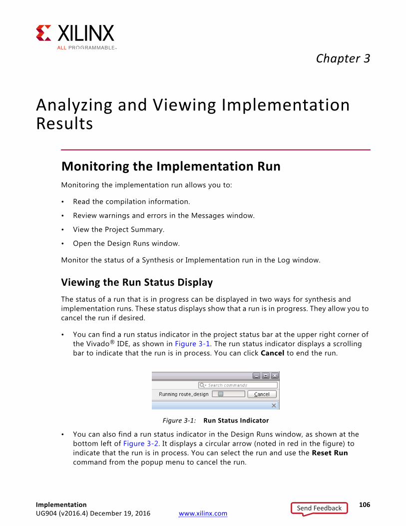
Chapter 3
Analyzing and Viewing Implementation Results
Monitoring the Implementation RunMonitoring the implementation run allows you to:
• Read the compilation information.
• Review warnings and errors in the Messages window.
• View the Project Summary.
• Open the Design Runs window.
Monitor the status of a Synthesis or Implementation run in the Log window.
Viewing the Run Status DisplayThe status of a run that is in progress can be displayed in two ways for synthesis and implementation runs. These status displays show that a run is in progress. They allow you to cancel the run if desired.
• You can find a run status indicator in the project status bar at the upper right corner of the Vivado® IDE, as shown in Figure 3-1. The run status indicator displays a scrolling bar to indicate that the run is in process. You can click Cancel to end the run.
• You can also find a run status indicator in the Design Runs window, as shown at the bottom left of Figure 3-2. It displays a circular arrow (noted in red in the figure) to indicate that the run is in process. You can select the run and use the Reset Run command from the popup menu to cancel the run.
X-Ref Target - Figure 3-1
Figure 3-1: Run Status Indicator
Implementation 106UG904 (v2016.4) December 19, 2016 www.xilinx.com
Send Feedback
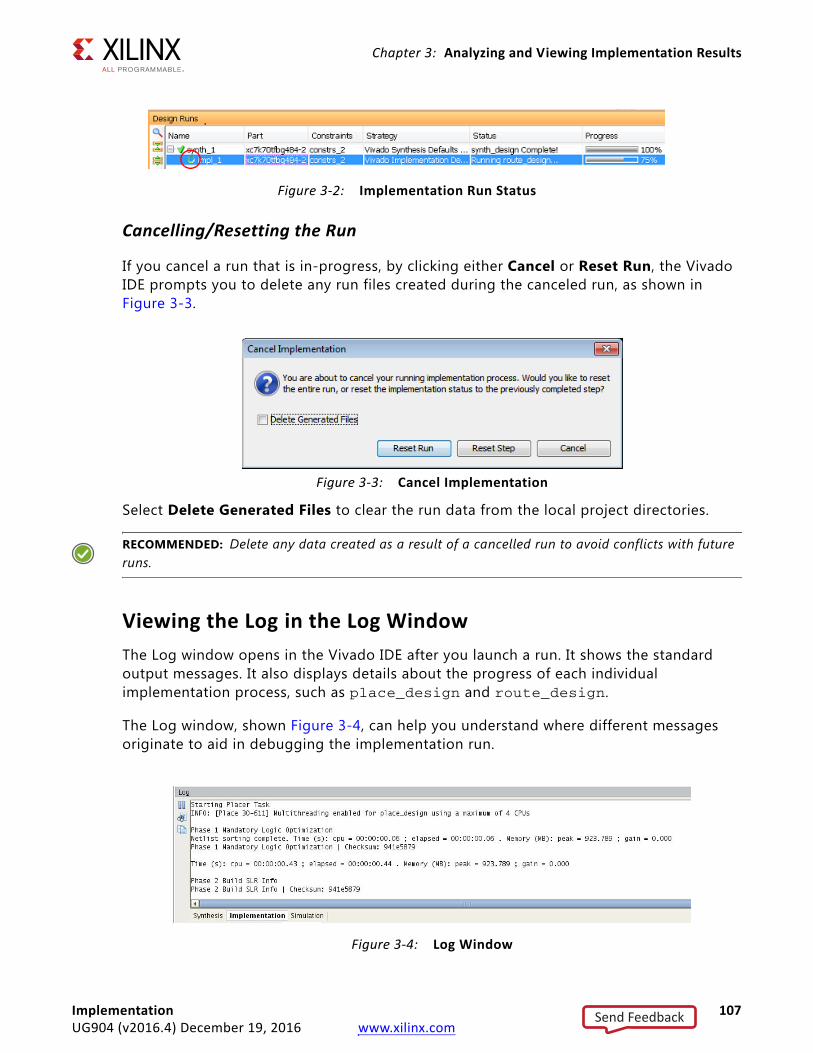
Chapter 3: Analyzing and Viewing Implementation Results
Cancelling/Resetting the Run
If you cancel a run that is in-progress, by clicking either Cancel or Reset Run, the Vivado IDE prompts you to delete any run files created during the canceled run, as shown in Figure 3-3.
Select Delete Generated Files to clear the run data from the local project directories.
RECOMMENDED: Delete any data created as a result of a cancelled run to avoid conflicts with future runs.
Viewing the Log in the Log WindowThe Log window opens in the Vivado IDE after you launch a run. It shows the standard output messages. It also displays details about the progress of each individual implementation process, such as place_design and route_design.
The Log window, shown Figure 3-4, can help you understand where different messages originate to aid in debugging the implementation run.
X-Ref Target - Figure 3-2
Figure 3-2: Implementation Run Status
X-Ref Target - Figure 3-3
Figure 3-3: Cancel Implementation
X-Ref Target - Figure 3-4
Figure 3-4: Log Window
Implementation 107UG904 (v2016.4) December 19, 2016 www.xilinx.com
Send Feedback
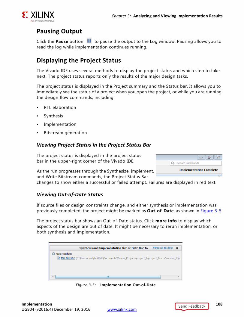
Chapter 3: Analyzing and Viewing Implementation Results
Pausing OutputClick the Pause button to pause the output to the Log window. Pausing allows you to read the log while implementation continues running.
Displaying the Project StatusThe Vivado IDE uses several methods to display the project status and which step to take next. The project status reports only the results of the major design tasks.
The project status is displayed in the Project summary and the Status bar. It allows you to immediately see the status of a project when you open the project, or while you are running the design flow commands, including:
• RTL elaboration
• Synthesis
• Implementation
• Bitstream generation
Viewing Project Status in the Project Status Bar
The project status is displayed in the project status bar in the upper-right corner of the Vivado IDE.
As the run progresses through the Synthesize, Implement, and Write Bitstream commands, the Project Status Bar changes to show either a successful or failed attempt. Failures are displayed in red text.
Viewing Out-of-Date Status
If source files or design constraints change, and either synthesis or implementation was previously completed, the project might be marked as Out-of-Date, as shown in Figure 3-5.
The project status bar shows an Out-of-Date status. Click more info to display which aspects of the design are out of date. It might be necessary to rerun implementation, or both synthesis and implementation.
X-Ref Target - Figure 3-5
Figure 3-5: Implementation Out-of-Date
Implementation 108UG904 (v2016.4) December 19, 2016 www.xilinx.com
Send Feedback
Chapter 3: Analyzing and Viewing Implementation Results
Forcing Runs Up-to-Date
Click Force-up-to-date to force the implementation or synthesis runs up to date. Use Force-up-to-date if you changed the design or constraints, but still want to analyze the results of the current run.
TIP: The Force-up-to-date command is also available from the popup menu of the Design Runs window when an out-of-date run is selected.
Moving Forward After ImplementationAfter implementation has completed, for both Project Mode and Non-Project Mode, the direction you take the design next depends on the results of the implementation.
• Is the design fully placed and routed, or are there issues that need to be resolved?
• Have the timing constraints and design requirements been met, or are their additional changes required to complete the design?
• Are you ready to generate the bitstream for the Xilinx part?
Recommended Steps After ImplementationThe recommended steps after implementation are:
1. Review the implementation messages.
2. Review the implementation reports to validate key aspects of the design:
° Timing constraints are met (report_timing_summary).
° Utilization is as expected (report_utilization).
° Power is as expected (report_power).
3. Write the bitstream file.
Writing the bitstream file includes a final DRC to ensure that the design does not violate any hardware rules.
4. If any design requirements have not been met:
a. In Project Mode, open the implemented design for further analysis.
b. In Non-Project Mode, open a post-implementation design checkpoint.
For more information on analysis of the implemented design, see this link in the Vivado Design Suite User Guide: Design Analysis and Closure Techniques (UG906) [Ref 10].
Implementation 109UG904 (v2016.4) December 19, 2016 www.xilinx.com
Send Feedback
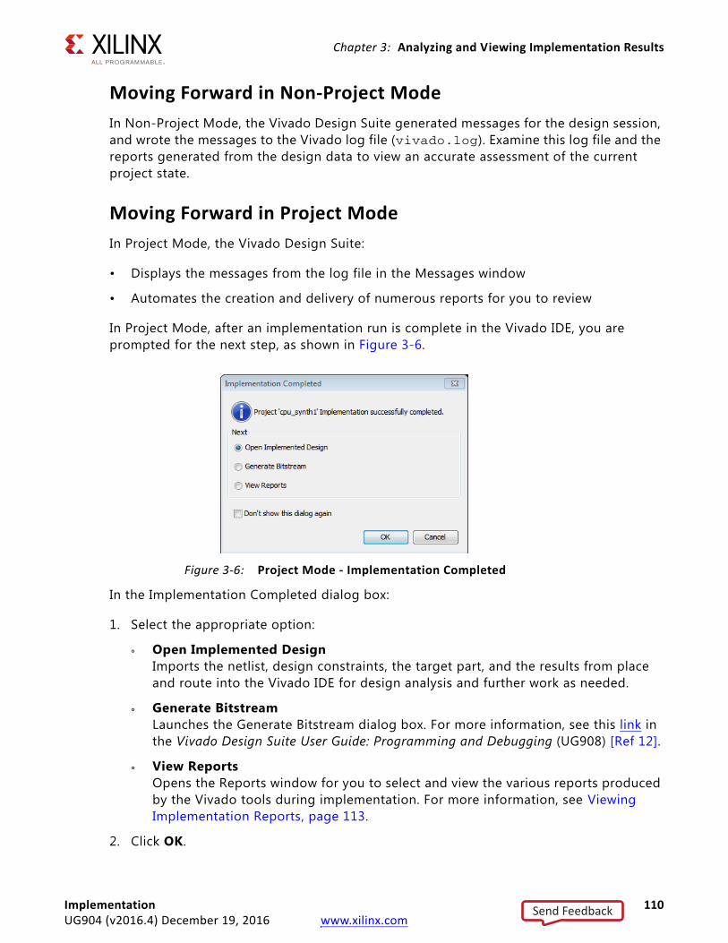
Chapter 3: Analyzing and Viewing Implementation Results
Moving Forward in Non-Project ModeIn Non-Project Mode, the Vivado Design Suite generated messages for the design session, and wrote the messages to the Vivado log file (vivado.log). Examine this log file and the reports generated from the design data to view an accurate assessment of the current project state.
Moving Forward in Project ModeIn Project Mode, the Vivado Design Suite:
• Displays the messages from the log file in the Messages window
• Automates the creation and delivery of numerous reports for you to review
In Project Mode, after an implementation run is complete in the Vivado IDE, you are prompted for the next step, as shown in Figure 3-6.
In the Implementation Completed dialog box:
1. Select the appropriate option:
° Open Implemented DesignImports the netlist, design constraints, the target part, and the results from place and route into the Vivado IDE for design analysis and further work as needed.
° Generate BitstreamLaunches the Generate Bitstream dialog box. For more information, see this link in the Vivado Design Suite User Guide: Programming and Debugging (UG908) [Ref 12].
° View ReportsOpens the Reports window for you to select and view the various reports produced by the Vivado tools during implementation. For more information, see Viewing Implementation Reports, page 113.
2. Click OK.
X-Ref Target - Figure 3-6
Figure 3-6: Project Mode - Implementation Completed
Implementation 110UG904 (v2016.4) December 19, 2016 www.xilinx.com
Send Feedback
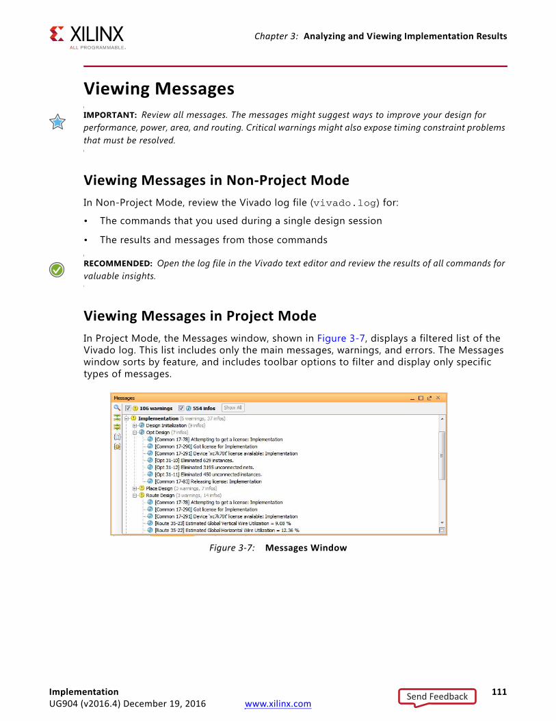
Chapter 3: Analyzing and Viewing Implementation Results
Viewing MessagesIMPORTANT: Review all messages. The messages might suggest ways to improve your design for performance, power, area, and routing. Critical warnings might also expose timing constraint problems that must be resolved.
Viewing Messages in Non-Project ModeIn Non-Project Mode, review the Vivado log file (vivado.log) for:
• The commands that you used during a single design session
• The results and messages from those commands
RECOMMENDED: Open the log file in the Vivado text editor and review the results of all commands for valuable insights.
Viewing Messages in Project ModeIn Project Mode, the Messages window, shown in Figure 3-7, displays a filtered list of the Vivado log. This list includes only the main messages, warnings, and errors. The Messages window sorts by feature, and includes toolbar options to filter and display only specific types of messages.
X-Ref Target - Figure 3-7
Figure 3-7: Messages Window
Implementation 111UG904 (v2016.4) December 19, 2016 www.xilinx.com
Send Feedback
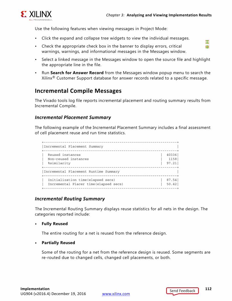
Chapter 3: Analyzing and Viewing Implementation Results
Use the following features when viewing messages in Project Mode:
• Click the expand and collapse tree widgets to view the individual messages.
• Check the appropriate check box in the banner to display errors, critical warnings, warnings, and informational messages in the Messages window.
• Select a linked message in the Messages window to open the source file and highlight the appropriate line in the file.
• Run Search for Answer Record from the Messages window popup menu to search the Xilinx® Customer Support database for answer records related to a specific message.
Incremental Compile Messages The Vivado tools log file reports incremental placement and routing summary results from Incremental Compile.
Incremental Placement Summary
The following example of the Incremental Placement Summary includes a final assessment of cell placement reuse and run time statistics.
+-----------------------------------------------------------------+|Incremental Placement Summary |+-----------------------------------------------------------------+| Reused instances | 40336|| Non-reused instances | 1158|| %similarity | 97.21|+-----------------------------------------------------------------+|Incremental Placement Runtime Summary |+-----------------------------------------------------------------+| Initialization time(elapsed secs) | 87.54|| Incremental Placer time(elapsed secs) | 50.42|+-----------------------------------------------------------------+
Incremental Routing Summary
The Incremental Routing Summary displays reuse statistics for all nets in the design. The categories reported include:
• Fully Reused
The entire routing for a net is reused from the reference design.
• Partially Reused
Some of the routing for a net from the reference design is reused. Some segments are re-routed due to changed cells, changed cell placements, or both.
Implementation 112UG904 (v2016.4) December 19, 2016 www.xilinx.com
Send Feedback
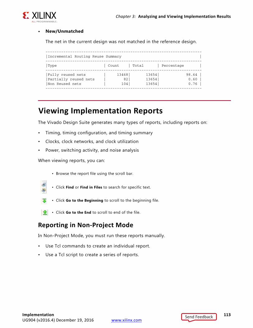
Chapter 3: Analyzing and Viewing Implementation Results
• New/Unmatched
The net in the current design was not matched in the reference design.
----------------------------------------------------------------------|Incremental Routing Reuse Summary |----------------------------------------------------------------------|Type | Count | Total | Percentage |----------------------------------------------------------------------|Fully reused nets | 13468| 13654| 98.64 ||Partially reused nets | 82| 13654| 0.60 ||Non Reused nets | 104| 13654| 0.76 |----------------------------------------------------------------------
Viewing Implementation ReportsThe Vivado Design Suite generates many types of reports, including reports on:
• Timing, timing configuration, and timing summary
• Clocks, clock networks, and clock utilization
• Power, switching activity, and noise analysis
When viewing reports, you can:
Reporting in Non-Project ModeIn Non-Project Mode, you must run these reports manually.
• Use Tcl commands to create an individual report.
• Use a Tcl script to create a series of reports.
• Browse the report file using the scroll bar.
• Click Find or Find in Files to search for specific text.
• Click Go to the Beginning to scroll to the beginning file.
• Click Go to the End to scroll to end of the file.
Implementation 113UG904 (v2016.4) December 19, 2016 www.xilinx.com
Send Feedback
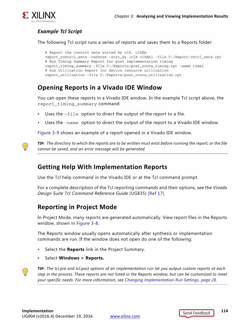
Chapter 3: Analyzing and Viewing Implementation Results
Example Tcl Script
The following Tcl script runs a series of reports and saves them to a Reports folder:
# Report the control sets sorted by clk, clkEnreport_control_sets -verbose -sort_by {clk clkEn} -file C:/Report/cntrl_sets.rpt# Run Timing Summary Report for post implementation timing report_timing_summary -file C:/Reports/post_route_timing.rpt -name time1# Run Utilization Report for device resource utilization report_utilization -file C:/Reports/post_route_utilization.rpt
Opening Reports in a Vivado IDE WindowYou can open these reports in a Vivado IDE window. In the example Tcl script above, the report_timing_summary command:
• Uses the -file option to direct the output of the report to a file.
• Uses the -name option to direct the output of the report to a Vivado IDE window.
Figure 3-9 shows an example of a report opened in a Vivado IDE window.
TIP: The directory to which the reports are to be written must exist before running the report, or the file cannot be saved, and an error message will be generated.
Getting Help With Implementation ReportsUse the Tcl help command in the Vivado IDE or at the Tcl command prompt.
For a complete description of the Tcl reporting commands and their options, see the Vivado Design Suite Tcl Command Reference Guide (UG835) [Ref 17].
Reporting in Project ModeIn Project Mode, many reports are generated automatically. View report files in the Reports window, shown in Figure 3-8.
The Reports window usually opens automatically after synthesis or implementation commands are run. If the window does not open do one of the following:
• Select the Reports link in the Project Summary.
• Select Windows > Reports.
TIP: The tcl.pre and tcl.post options of an implementation run let you output custom reports at each step in the process. These reports are not listed in the Reports window, but can be customized to meet your specific needs. For more information, see Changing Implementation Run Settings, page 28.
Implementation 114UG904 (v2016.4) December 19, 2016 www.xilinx.com
Send Feedback
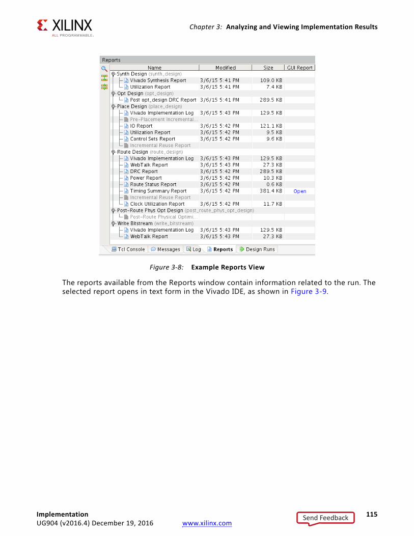
Chapter 3: Analyzing and Viewing Implementation Results
The reports available from the Reports window contain information related to the run. The selected report opens in text form in the Vivado IDE, as shown in Figure 3-9.
X-Ref Target - Figure 3-8
Figure 3-8: Example Reports View
Implementation 115UG904 (v2016.4) December 19, 2016 www.xilinx.com
Send Feedback
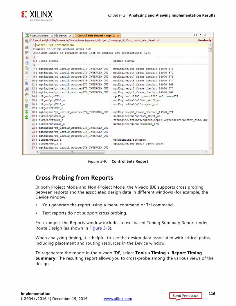
Chapter 3: Analyzing and Viewing Implementation Results
Cross Probing from ReportsIn both Project Mode and Non-Project Mode, the Vivado IDE supports cross probing between reports and the associated design data in different windows (for example, the Device window).
• You generate the report using a menu command or Tcl command.
• Text reports do not support cross probing.
For example, the Reports window includes a text-based Timing Summary Report under Route Design (as shown in Figure 3-8).
When analyzing timing, it is helpful to see the design data associated with critical paths, including placement and routing resources in the Device window.
To regenerate the report in the Vivado IDE, select Tools >Timing > Report Timing Summary. The resulting report allows you to cross-probe among the various views of the design.
X-Ref Target - Figure 3-9
Figure 3-9: Control Sets Report
Implementation 116UG904 (v2016.4) December 19, 2016 www.xilinx.com
Send Feedback
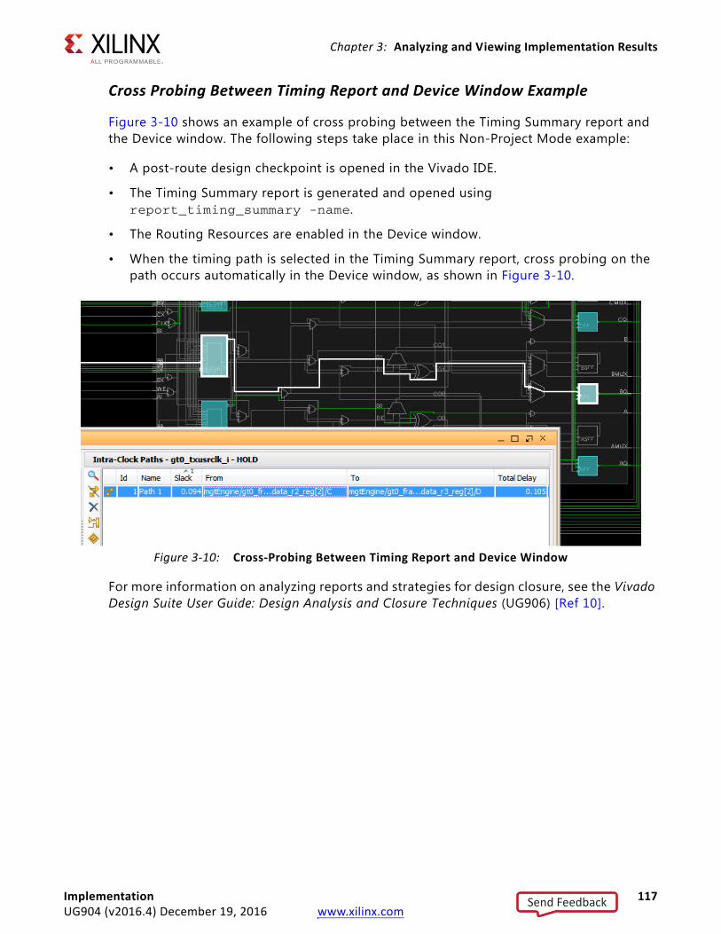
Chapter 3: Analyzing and Viewing Implementation Results
Cross Probing Between Timing Report and Device Window Example
Figure 3-10 shows an example of cross probing between the Timing Summary report and the Device window. The following steps take place in this Non-Project Mode example:
• A post-route design checkpoint is opened in the Vivado IDE.
• The Timing Summary report is generated and opened using report_timing_summary -name.
• The Routing Resources are enabled in the Device window.
• When the timing path is selected in the Timing Summary report, cross probing on the path occurs automatically in the Device window, as shown in Figure 3-10.
For more information on analyzing reports and strategies for design closure, see the Vivado Design Suite User Guide: Design Analysis and Closure Techniques (UG906) [Ref 10].
X-Ref Target - Figure 3-10
Figure 3-10: Cross-Probing Between Timing Report and Device Window
Implementation 117UG904 (v2016.4) December 19, 2016 www.xilinx.com
Send Feedback
Chapter 3: Analyzing and Viewing Implementation Results
Modifying Implementation ResultsThis section describes how to modify placement, routing, and logic for your design.
Modifying PlacementThe Vivado tools track two states for placed cells, Fixed and Unfixed, which describes the way in which the Vivado tools view placed cells in the design.
Fixed Cells
Fixed cells are those that you have placed yourself, or the location constraints for the cells have been imported from an XDC file.
• The Vivado Design Suite treats these placed cells as Fixed.
• Fixed cells are not moved unless directed to do so.
• The FF in Figure 3-11 is shown in orange (default) to indicate that it is Fixed.
Unfixed Cells
Unfixed cells have been placed by the Vivado tools in implementation, during the place_design command, or on execution of one of optimization commands.
• The Vivado Design Suite treats these placed cells as Unfixed (or loosely placed).
• These cells can be moved by the implementation tools as needed in design iterations.
• The LUT in Figure 3-11 is shown in blue (default) to indicate that it is Unfixed.
Implementation 118UG904 (v2016.4) December 19, 2016 www.xilinx.com
Send Feedback
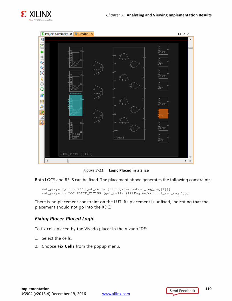
Chapter 3: Analyzing and Viewing Implementation Results
Both LOCS and BELS can be fixed. The placement above generates the following constraints:
set_property BEL BFF [get_cells {fftEngine/control_reg_reg[1]}]set_property LOC SLICE_X1Y199 [get_cells {fftEngine/control_reg_reg[1]}]
There is no placement constraint on the LUT. Its placement is unfixed, indicating that the placement should not go into the XDC.
Fixing Placer-Placed Logic
To fix cells placed by the Vivado placer in the Vivado IDE:
1. Select the cells.
2. Choose Fix Cells from the popup menu.
X-Ref Target - Figure 3-11
Figure 3-11: Logic Placed in a Slice
Implementation 119UG904 (v2016.4) December 19, 2016 www.xilinx.com
Send Feedback
Chapter 3: Analyzing and Viewing Implementation Results
To fix cell placement with Tcl, use a command of this form:
set_property is_bel_fixed TRUE [get_cells [list {fftEngine/control_reg_reg[1]_i_1}]]set_property is_loc_fixed TRUE [get_cells [list {fftEngine/control_reg_reg[1]_i_1}]]
For more information on Tcl commands, see the Vivado Design Suite Tcl Command Reference Guide (UG835) [Ref 17], or type <command> -help.
Placing and Moving Logic by Hand
You can place and move logic by hand.
• If the cell is already placed, drag and drop it to a new location.
• If the cell is unplaced:
a. Enter Create BEL Constraint Instance Drag & Drop mode.
b. Drag the logic from the Netlist window, or from the Timing Report window, onto the Device window.
The logic snaps to a new legal location.
TIP: When dragging logic to a location in the Device Window, the GUI allows you to drop the logic only on legal locations. If the location is illegal (for example, because of control set restriction for Slice FFs), the logic does not "snap" to the new location in the Device view, and it cannot be assigned.
Hand-placing logic can be slow, and used in specific situations only. The constraints are fragile with respect to design changes because the cell name is used in the constraint.
Placing Logic using a Tcl Command
You can place logic onto device resources of the target part using the place_cell Tcl command. Cells can be placed onto specific BEL sites (for example, SLICE_X49Y60/A6LUT) or into available sites (for example, SLICE_X49Y60). If you specify the site but not the BEL, the tool determines an appropriate BEL within the specified site if one is available. You can use the place_cell command to place cells or to move placed cells from one site on the device to another site. The command syntax is the same for placing an unplaced cell or for moving a placed cell.
TIP: When assigning logic to an illegal location (for example, because of control set restriction for Slice FFs), the Tcl Console issues an error message, and the assignment is ignored.
Cells that have been placed using the place_cell Tcl command are treated as Fixed by the Vivado tool.
Implementation 120UG904 (v2016.4) December 19, 2016 www.xilinx.com
Send Feedback
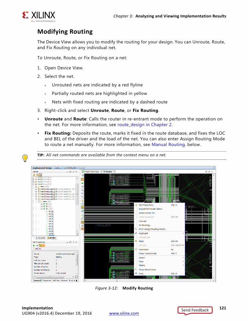
Chapter 3: Analyzing and Viewing Implementation Results
Modifying RoutingThe Device View allows you to modify the routing for your design. You can Unroute, Route, and Fix Routing on any individual net.
To Unroute, Route, or Fix Routing on a net:
1. Open Device View.
2. Select the net.
° Unrouted nets are indicated by a red flyline
° Partially routed nets are highlighted in yellow
° Nets with fixed routing are indicated by a dashed route
3. Right-click and select Unroute, Route, or Fix Routing.
• Unroute and Route: Calls the router in re-entrant mode to perform the operation on the net. For more information, see route_design in Chapter 2.
• Fix Routing: Deposits the route, marks it fixed in the route database, and fixes the LOC and BEL of the driver and the load of the net. You can also enter Assign Routing Mode to route a net manually. For more information, see Manual Routing, below.
TIP: All net commands are available from the context menu on a net.
X-Ref Target - Figure 3-12
Figure 3-12: Modify Routing
Implementation 121UG904 (v2016.4) December 19, 2016 www.xilinx.com
Send Feedback
Chapter 3: Analyzing and Viewing Implementation Results
Manual RoutingManual routing allows you to select specific routing resources for your nets. This gives you complete control over the routing paths that a signal is going to take. Manual routing does not invoke route_design. Routes are directly updated in the route database.
You might want to use manual routing when you want to precisely control the delay for a net. For example, assume a source synchronous interface, in which you want to minimize routing delay variation to the capture registers in the device. To accomplish this, you can assign LOC and BEL constraints to the registers and I/Os, and then precisely control the route delay from the IOB to the register by manual routing the nets.
Manual routing requires detailed knowledge of the device interconnect architecture. It is best used for a limited number of signals and for short connections.
Manual Routing Rules
Observe these rules during manual routing:
• The driver and the load require a LOC constraint and a BEL constraint.
• Branching is not allowed during manual routing, but you can implement branches by starting a new manual route from a branch point.
• LUT loads must have their pins locked.
• You must route to loads that are not already connected to a driver.
• Only complete connections are permitted. Antennas are not allowed.
• Overlap with existing unfixed routed nets is allowed. Run route_design after manual routing to resolve any conflicts due to overlapping nets.
Entering Assign Routing Mode
To enter Assign Routing Mode:
1. Open Device View.
2. Be sure that Routing Resources in the Device window is selected.
3. Enable the Layers for Unrouted Net and Partially Routed Net in the Device Options Layers view, shown in Figure 3-13.
Implementation 122UG904 (v2016.4) December 19, 2016 www.xilinx.com
Send Feedback
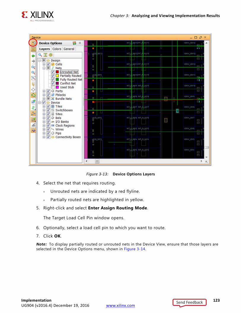
Chapter 3: Analyzing and Viewing Implementation Results
,
4. Select the net that requires routing.
° Unrouted nets are indicated by a red flyline.
° Partially routed nets are highlighted in yellow.
5. Right-click and select Enter Assign Routing Mode.
The Target Load Cell Pin window opens.
6. Optionally, select a load cell pin to which you want to route.
7. Click OK.
Note: To display partially routed or unrouted nets in the Device View, ensure that those layers are selected in the Device Options menu, shown in Figure 3-14.
X-Ref Target - Figure 3-13
Figure 3-13: Device Options Layers
Implementation 123UG904 (v2016.4) December 19, 2016 www.xilinx.com
Send Feedback
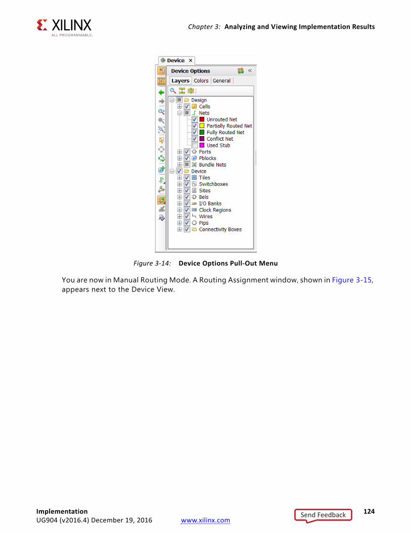
Chapter 3: Analyzing and Viewing Implementation Results
You are now in Manual Routing Mode. A Routing Assignment window, shown in Figure 3-15, appears next to the Device View.
X-Ref Target - Figure 3-14
Figure 3-14: Device Options Pull-Out Menu
Implementation 124UG904 (v2016.4) December 19, 2016 www.xilinx.com
Send Feedback
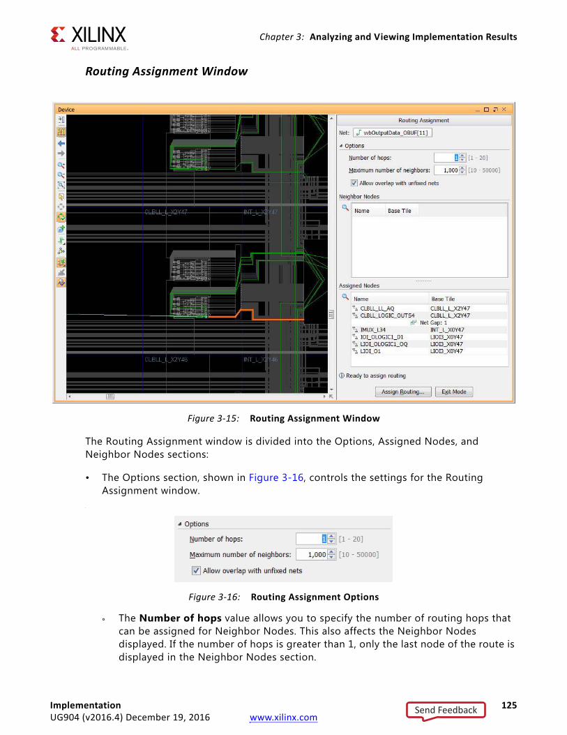
Chapter 3: Analyzing and Viewing Implementation Results
Routing Assignment Window
The Routing Assignment window is divided into the Options, Assigned Nodes, and Neighbor Nodes sections:
• The Options section, shown in Figure 3-16, controls the settings for the Routing Assignment window.
,
° The Number of hops value allows you to specify the number of routing hops that can be assigned for Neighbor Nodes. This also affects the Neighbor Nodes displayed. If the number of hops is greater than 1, only the last node of the route is displayed in the Neighbor Nodes section.
X-Ref Target - Figure 3-15
Figure 3-15: Routing Assignment Window
X-Ref Target - Figure 3-16
Figure 3-16: Routing Assignment Options
Implementation 125UG904 (v2016.4) December 19, 2016 www.xilinx.com
Send Feedback
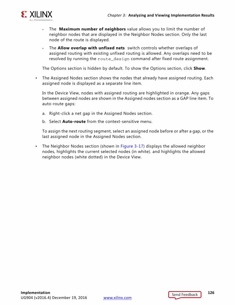
Chapter 3: Analyzing and Viewing Implementation Results
° The Maximum number of neighbors value allows you to limit the number of neighbor nodes that are displayed in the Neighbor Nodes section. Only the last node of the route is displayed.
° The Allow overlap with unfixed nets switch controls whether overlaps of assigned routing with existing unfixed routing is allowed. Any overlaps need to be resolved by running the route_design command after fixed route assignment.
The Options section is hidden by default. To show the Options section, click Show.
• The Assigned Nodes section shows the nodes that already have assigned routing. Each assigned node is displayed as a separate line item.
In the Device View, nodes with assigned routing are highlighted in orange. Any gaps between assigned nodes are shown in the Assigned nodes section as a GAP line item. To auto-route gaps:
a. Right-click a net gap in the Assigned Nodes section.
b. Select Auto-route from the context-sensitive menu.
To assign the next routing segment, select an assigned node before or after a gap, or the last assigned node in the Assigned Nodes section.
• The Neighbor Nodes section (shown in Figure 3-17) displays the allowed neighbor nodes, highlights the current selected nodes (in white). and highlights the allowed neighbor nodes (white dotted) in the Device View.
Implementation 126UG904 (v2016.4) December 19, 2016 www.xilinx.com
Send Feedback
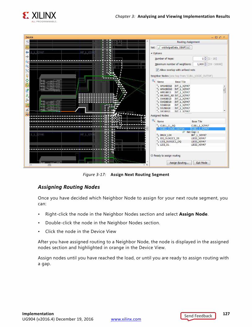
Chapter 3: Analyzing and Viewing Implementation Results
,
Assigning Routing Nodes
Once you have decided which Neighbor Node to assign for your next route segment, you can:
• Right-click the node in the Neighbor Nodes section and select Assign Node.
• Double-click the node in the Neighbor Nodes section.
• Click the node in the Device View
After you have assigned routing to a Neighbor Node, the node is displayed in the assigned nodes section and highlighted in orange in the Device View.
Assign nodes until you have reached the load, or until you are ready to assign routing with a gap.
X-Ref Target - Figure 3-17
Figure 3-17: Assign Next Routing Segment
Implementation 127UG904 (v2016.4) December 19, 2016 www.xilinx.com
Send Feedback
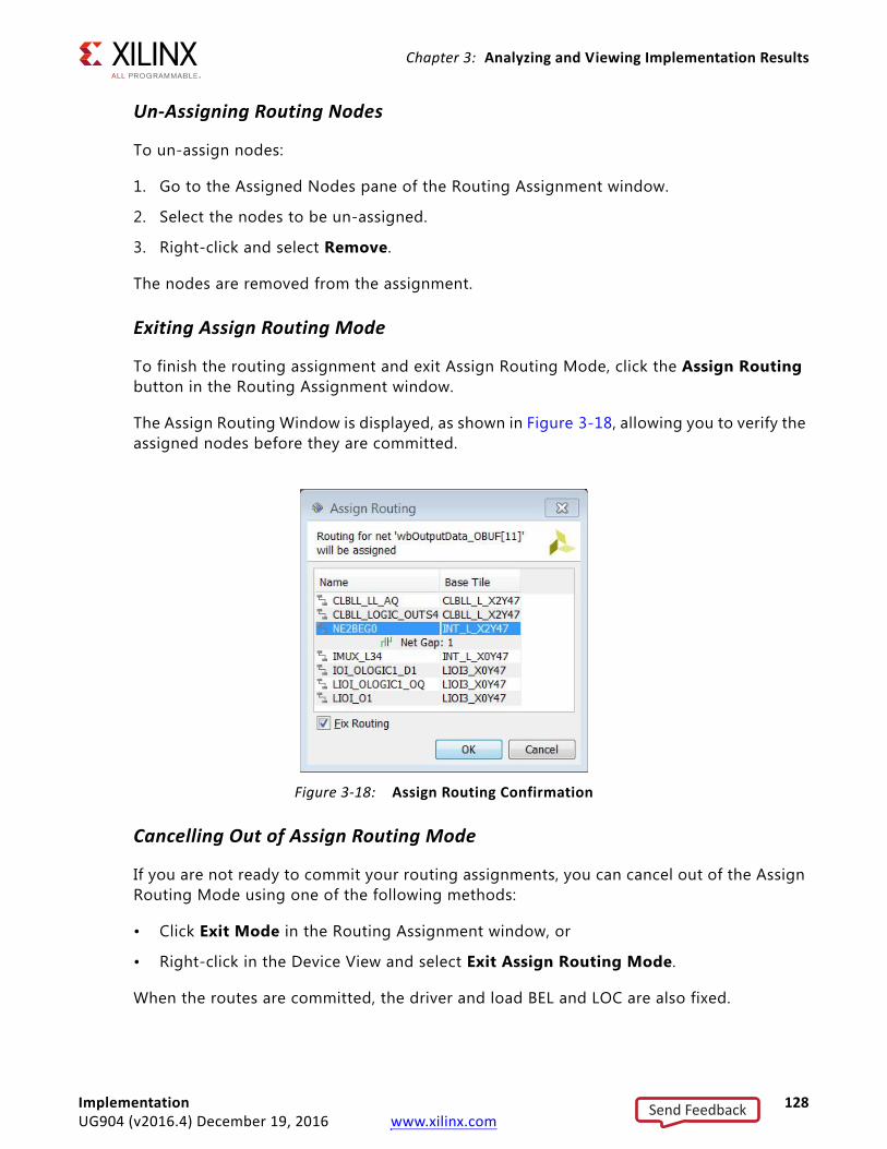
Chapter 3: Analyzing and Viewing Implementation Results
Un-Assigning Routing Nodes
To un-assign nodes:
1. Go to the Assigned Nodes pane of the Routing Assignment window.
2. Select the nodes to be un-assigned.
3. Right-click and select Remove.
The nodes are removed from the assignment.
Exiting Assign Routing Mode
To finish the routing assignment and exit Assign Routing Mode, click the Assign Routing button in the Routing Assignment window.
The Assign Routing Window is displayed, as shown in Figure 3-18, allowing you to verify the assigned nodes before they are committed.
Cancelling Out of Assign Routing Mode
If you are not ready to commit your routing assignments, you can cancel out of the Assign Routing Mode using one of the following methods:
• Click Exit Mode in the Routing Assignment window, or
• Right-click in the Device View and select Exit Assign Routing Mode.
When the routes are committed, the driver and load BEL and LOC are also fixed.
X-Ref Target - Figure 3-18
Figure 3-18: Assign Routing Confirmation
Implementation 128UG904 (v2016.4) December 19, 2016 www.xilinx.com
Send Feedback
Chapter 3: Analyzing and Viewing Implementation Results
Verifying Assigned Routes
• Assigned routes appear as dotted green lines in the Device View.
• Partially assigned routes appear as dotted yellow lines in the Device view.
Figure 3-19 shows an example of an assigned and partially assigned route.
Branching
When assigning routing to a net with more than one load, you must route the net in the following steps:
1. Assign routing to one load following the steps provided in Entering Assign Routing Mode, page 122, above.
2. Assign routing to all the branches of the net.
Figure 3-20 shows an example of a net that has assigned routing to one load and requires routing to two additional loads.
X-Ref Target - Figure 3-19
Figure 3-19: Assigned Partially Assigned Routing
Implementation 129UG904 (v2016.4) December 19, 2016 www.xilinx.com
Send Feedback
Chapter 3: Analyzing and Viewing Implementation Results
Assigning Routing to a Branch
To assign routing to a branch:
1. Go to Device View.
2. Select the net to be routed.
3. Right-click and select Enter Assign Routing Mode.
The Target Load Cell Pin window opens, showing all loads.
Note: The loads that already have assigned routing have a checkmark in the Routed column of the table.
X-Ref Target - Figure 3-20
Figure 3-20: Assign Branching Route
Implementation 130UG904 (v2016.4) December 19, 2016 www.xilinx.com
Send Feedback
Chapter 3: Analyzing and Viewing Implementation Results
4. Select the load to which you want to route.
5. Click OK. The Branch Start window (shown in Figure 3-22) opens.
6. Select the node from which you want to branch off the route for your selected load.
7. Click OK.
8. Follow the steps shown in Assigning Routing Nodes, page 127.
X-Ref Target - Figure 3-21
Figure 3-21: Target Load Cell Pin (Multiple Loads)
X-Ref Target - Figure 3-22
Figure 3-22: Branch Start
Implementation 131UG904 (v2016.4) December 19, 2016 www.xilinx.com
Send Feedback
Chapter 3: Analyzing and Viewing Implementation Results
Locking Cell Inputs on LUT Loads
You must ensure that the inputs of LUT loads to which you are routing are not being swapped with other inputs on those LUTs. To do so, lock the cell inputs of LUT loads as follows:
1. Open Device View.
2. Select the load LUT.
3. Right-click and select Lock Cell Input Pins.
The equivalent Tcl command is:
set_property LOCK_PINS {NAME:BEL_PIN} <cell object>
For nets that have fixed routing and multiple LUT loads, the following Tcl script can be used to lock the cell inputs of all the LUT loads.
set fixed_nets [get_nets -hierarchical -filter IS_ROUTE_FIXED]foreach LUT_load_pin [get_pins -leaf -of [get_nets $fixed_nets] \-filter DIRECTION==IN&&REF_NAME=~LUT*] {set pin [get_property REF_PIN_NAME $LUT_load_pin]set BEL_pin [file tail [get_bel_pins -of [get_pins $LUT_load_pin]]]set LUT_name [get_property PARENT_CELL $LUT_load_pin]# need to handle condition when LOCK_pins property already exists on LUTset existing_LOCK_PIN [get_property LOCK_PINS [get_cells $LUT_name]]if { $existing_LOCK_PIN ne "" } {
reset_property LOCK_PINS [get_cells $LUT_name]}set_property LOCK_PINS \[lsort -unique [concat $existing_LOCK_PIN $pin:$BEL_pin]] [get_cells $LUT_name]
}
Directed Routing ConstraintsFixed route assignments are stored as Directed Routing Strings in the route database. In a Directed Routing String, branching is indicated by nested {curly braces}.
For example, consider the route described in Figure 3-23, below. In this simplified illustration of a route, the various elements are indicated as shown in the following table (Directed Routing Constraints).
Table 3-1: Directed Routing Constraints
Elements Indicated By
Driver and Loads Orange Rectangles
Nodes Red lines
Switchboxes Blue rectangles
Implementation 132UG904 (v2016.4) December 19, 2016 www.xilinx.com
Send Feedback
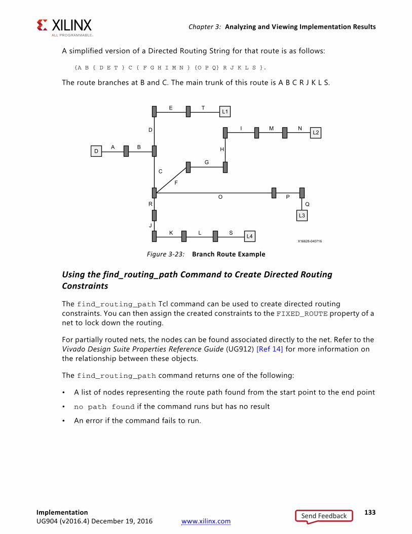
Chapter 3: Analyzing and Viewing Implementation Results
A simplified version of a Directed Routing String for that route is as follows:
{A B { D E T } C { F G H I M N } {O P Q} R J K L S }.
The route branches at B and C. The main trunk of this route is A B C R J K L S.
Using the find_routing_path Command to Create Directed Routing Constraints
The find_routing_path Tcl command can be used to create directed routing constraints. You can then assign the created constraints to the FIXED_ROUTE property of a net to lock down the routing.
For partially routed nets, the nodes can be found associated directly to the net. Refer to the Vivado Design Suite Properties Reference Guide (UG912) [Ref 14] for more information on the relationship between these objects.
The find_routing_path command returns one of the following:
• A list of nodes representing the route path found from the start point to the end point
• no path found if the command runs but has no result
• An error if the command fails to run.
X-Ref Target - Figure 3-23
Figure 3-23: Branch Route Example
D
L1
L2
L4
L3
A B
E T
I M N
QPO
G
H
F
D
C
R
JK L S
Implementation 133UG904 (v2016.4) December 19, 2016 www.xilinx.com
Send Feedback
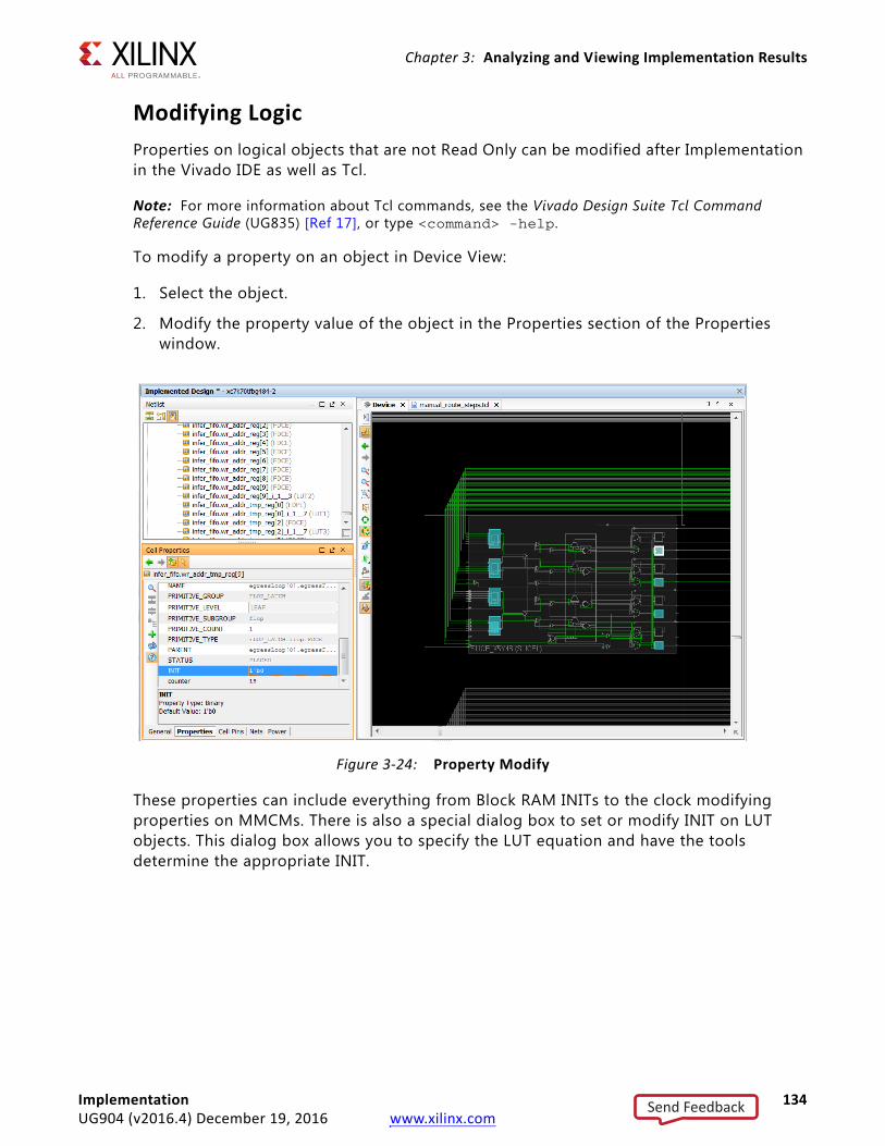
Chapter 3: Analyzing and Viewing Implementation Results
Modifying LogicProperties on logical objects that are not Read Only can be modified after Implementation in the Vivado IDE as well as Tcl.
Note: For more information about Tcl commands, see the Vivado Design Suite Tcl Command Reference Guide (UG835) [Ref 17], or type <command> -help.
To modify a property on an object in Device View:
1. Select the object.
2. Modify the property value of the object in the Properties section of the Properties window.
These properties can include everything from Block RAM INITs to the clock modifying properties on MMCMs. There is also a special dialog box to set or modify INIT on LUT objects. This dialog box allows you to specify the LUT equation and have the tools determine the appropriate INIT.
X-Ref Target - Figure 3-24
Figure 3-24: Property Modify
Implementation 134UG904 (v2016.4) December 19, 2016 www.xilinx.com
Send Feedback
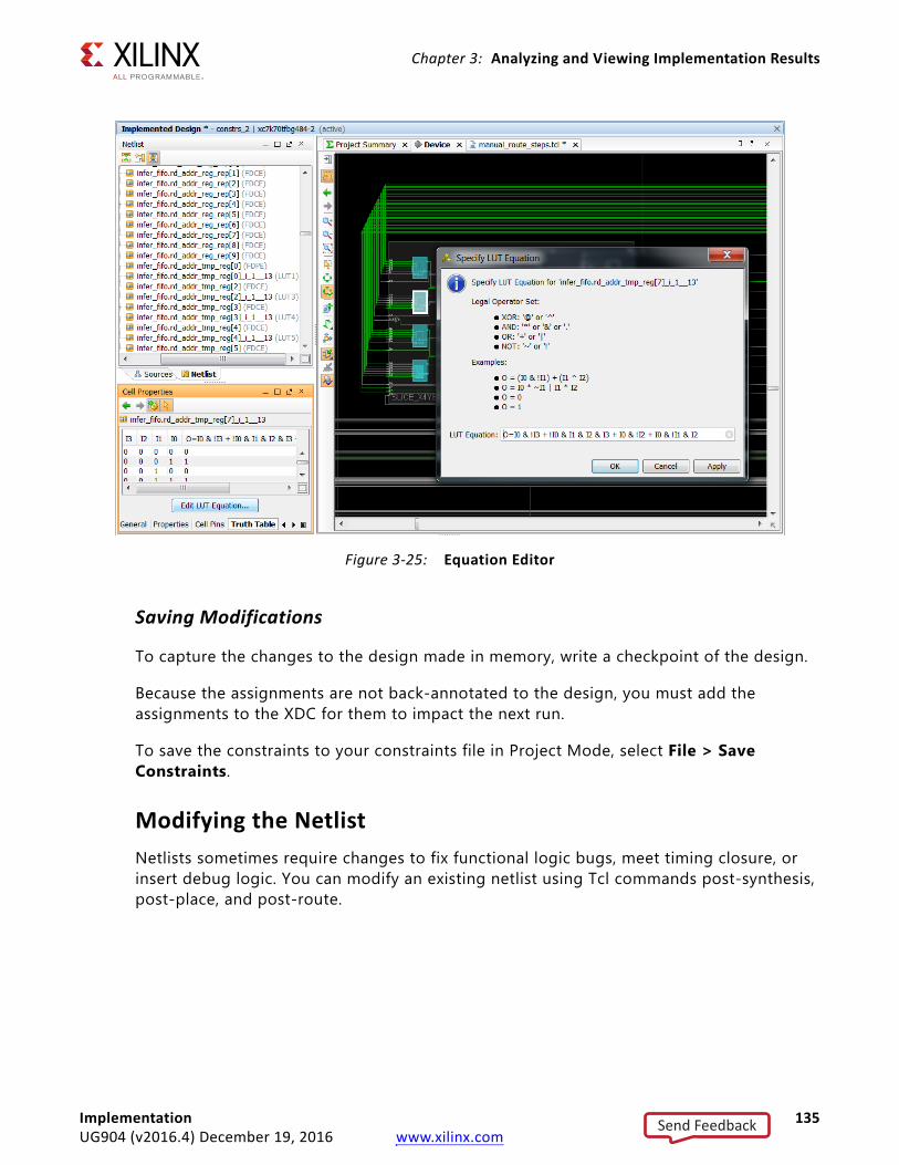
Chapter 3: Analyzing and Viewing Implementation Results
Saving Modifications
To capture the changes to the design made in memory, write a checkpoint of the design.
Because the assignments are not back-annotated to the design, you must add the assignments to the XDC for them to impact the next run.
To save the constraints to your constraints file in Project Mode, select File > Save Constraints.
Modifying the NetlistNetlists sometimes require changes to fix functional logic bugs, meet timing closure, or insert debug logic. You can modify an existing netlist using Tcl commands post-synthesis, post-place, and post-route.
X-Ref Target - Figure 3-25
Figure 3-25: Equation Editor
Implementation 135UG904 (v2016.4) December 19, 2016 www.xilinx.com
Send Feedback
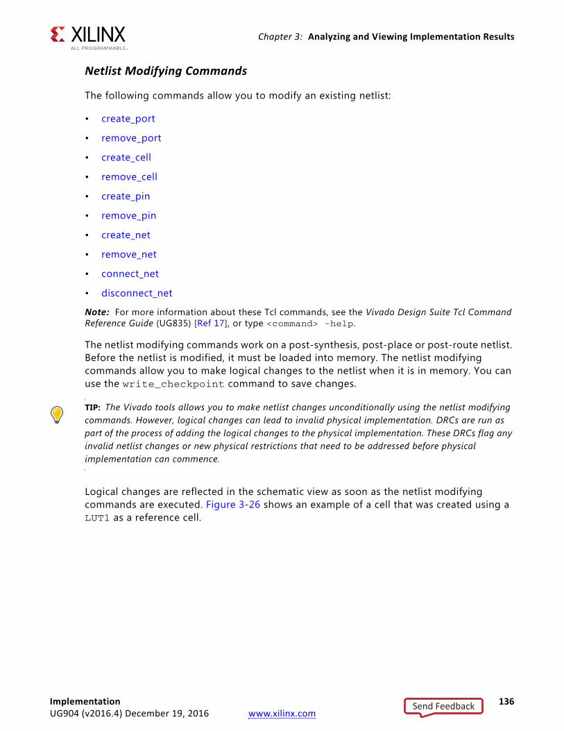
Chapter 3: Analyzing and Viewing Implementation Results
Netlist Modifying Commands
The following commands allow you to modify an existing netlist:
• create_port
• remove_port
• create_cell
• remove_cell
• create_pin
• remove_pin
• create_net
• remove_net
• connect_net
• disconnect_net
Note: For more information about these Tcl commands, see the Vivado Design Suite Tcl Command Reference Guide (UG835) [Ref 17], or type <command> -help.
The netlist modifying commands work on a post-synthesis, post-place or post-route netlist. Before the netlist is modified, it must be loaded into memory. The netlist modifying commands allow you to make logical changes to the netlist when it is in memory. You can use the write_checkpoint command to save changes.
TIP: The Vivado tools allows you to make netlist changes unconditionally using the netlist modifying commands. However, logical changes can lead to invalid physical implementation. DRCs are run as part of the process of adding the logical changes to the physical implementation. These DRCs flag any invalid netlist changes or new physical restrictions that need to be addressed before physical implementation can commence.
Logical changes are reflected in the schematic view as soon as the netlist modifying commands are executed. Figure 3-26 shows an example of a cell that was created using a LUT1 as a reference cell.
Implementation 136UG904 (v2016.4) December 19, 2016 www.xilinx.com
Send Feedback
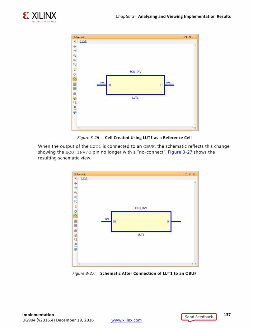
Chapter 3: Analyzing and Viewing Implementation Results
When the output of the LUT1 is connected to an OBUF, the schematic reflects this change showing the ECO_INV/O pin no longer with a "no-connect". Figure 3-27 shows the resulting schematic view.
X-Ref Target - Figure 3-26
Figure 3-26: Cell Created Using LUT1 as a Reference Cell
X-Ref Target - Figure 3-27
Figure 3-27: Schematic After Connection of LUT1 to an OBUF
Implementation 137UG904 (v2016.4) December 19, 2016 www.xilinx.com
Send Feedback
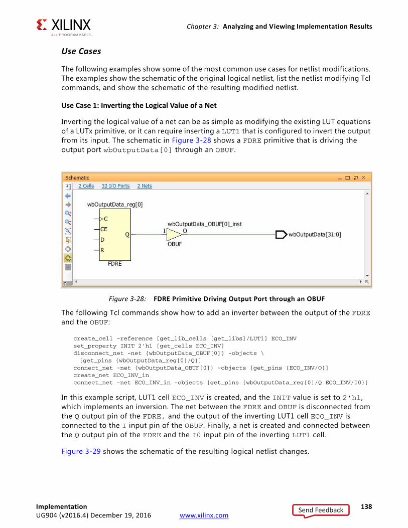
Chapter 3: Analyzing and Viewing Implementation Results
Use Cases
The following examples show some of the most common use cases for netlist modifications. The examples show the schematic of the original logical netlist, list the netlist modifying Tcl commands, and show the schematic of the resulting modified netlist.
Use Case 1: Inverting the Logical Value of a Net
Inverting the logical value of a net can be as simple as modifying the existing LUT equations of a LUTx primitive, or it can require inserting a LUT1 that is configured to invert the output from its input. The schematic in Figure 3-28 shows a FDRE primitive that is driving the output port wbOutputData[0] through an OBUF.
The following Tcl commands show how to add an inverter between the output of the FDRE and the OBUF:
create_cell -reference [get_lib_cells [get_libs]/LUT1] ECO_INVset_property INIT 2'h1 [get_cells ECO_INV]disconnect_net -net {wbOutputData_OBUF[0]} -objects \[get_pins {wbOutputData_reg[0]/Q}]
connect_net -net {wbOutputData_OBUF[0]} -objects [get_pins {ECO_INV/O}]create_net ECO_INV_inconnect_net -net ECO_INV_in -objects [get_pins {wbOutputData_reg[0]/Q ECO_INV/I0}]
In this example script, LUT1 cell ECO_INV is created, and the INIT value is set to 2'h1, which implements an inversion. The net between the FDRE and OBUF is disconnected from the Q output pin of the FDRE, and the output of the inverting LUT1 cell ECO_INV is connected to the I input pin of the OBUF. Finally, a net is created and connected between the Q output pin of the FDRE and the I0 input pin of the inverting LUT1 cell.
Figure 3-29 shows the schematic of the resulting logical netlist changes.
X-Ref Target - Figure 3-28
Figure 3-28: FDRE Primitive Driving Output Port through an OBUF
Implementation 138UG904 (v2016.4) December 19, 2016 www.xilinx.com
Send Feedback
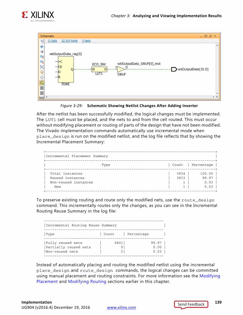
Chapter 3: Analyzing and Viewing Implementation Results
After the netlist has been successfully modified, the logical changes must be implemented. The LUT1 cell must be placed, and the nets to and from the cell routed. This must occur without modifying placement or routing of parts of the design that have not been modified. The Vivado implementation commands automatically use incremental mode when place_design is run on the modified netlist, and the log file reflects that by showing the Incremental Placement Summary:
+-------------------------------------------------------------------------------+|Incremental Placement Summary |+-------------------------------------------------------------------------------+| Type | Count | Percentage |+-------------------------------------------------------------------------------+| Total instances | 3834 | 100.00 || Reused instances | 3833 | 99.97 || Non-reused instances | 1 | 0.03 || New | 1 | 0.03 |+-------------------------------------------------------------------------------+
To preserve existing routing and route only the modified nets, use the route_design command. This incrementally routes only the changes, as you can see in the Incremental Routing Reuse Summary in the log file:
--------------------------------------------------------|Incremental Routing Reuse Summary |--------------------------------------------------------|Type | Count | Percentage |--------------------------------------------------------|Fully reused nets | 6401| 99.97 ||Partially reused nets | 0| 0.00 ||Non-reused nets | 2| 0.03 |--------------------------------------------------------
Instead of automatically placing and routing the modified netlist using the incremental place_design and route_design commands, the logical changes can be committed using manual placement and routing constraints. For more information see the Modifying Placement and Modifying Routing sections earlier in this chapter.
X-Ref Target - Figure 3-29
Figure 3-29: Schematic Showing Netlist Changes After Adding Inverter
Implementation 139UG904 (v2016.4) December 19, 2016 www.xilinx.com
Send Feedback
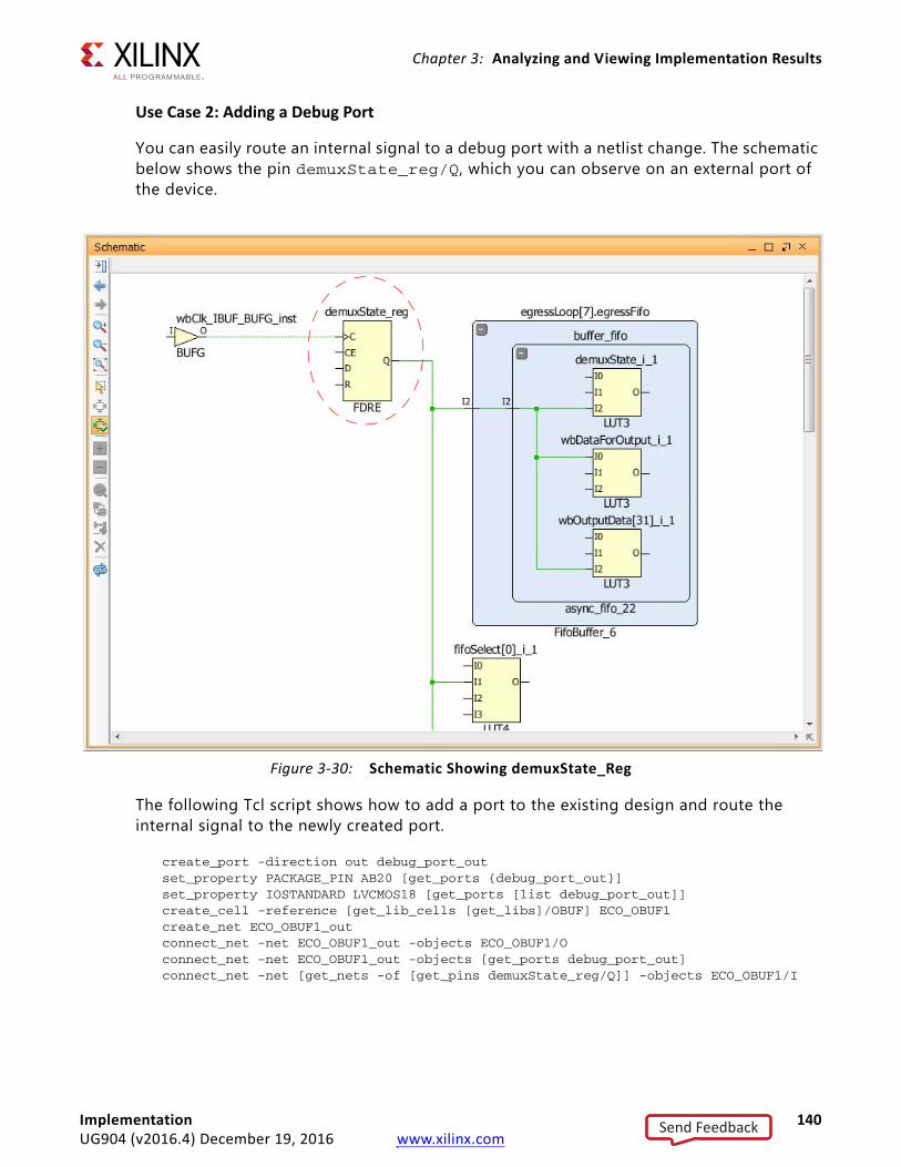
Chapter 3: Analyzing and Viewing Implementation Results
Use Case 2: Adding a Debug Port
You can easily route an internal signal to a debug port with a netlist change. The schematic below shows the pin demuxState_reg/Q, which you can observe on an external port of the device.
The following Tcl script shows how to add a port to the existing design and route the internal signal to the newly created port.
create_port -direction out debug_port_outset_property PACKAGE_PIN AB20 [get_ports {debug_port_out}]set_property IOSTANDARD LVCMOS18 [get_ports [list debug_port_out]]create_cell -reference [get_lib_cells [get_libs]/OBUF] ECO_OBUF1create_net ECO_OBUF1_outconnect_net -net ECO_OBUF1_out -objects ECO_OBUF1/Oconnect_net -net ECO_OBUF1_out -objects [get_ports debug_port_out]connect_net -net [get_nets -of [get_pins demuxState_reg/Q]] -objects ECO_OBUF1/I
X-Ref Target - Figure 3-30
Figure 3-30: Schematic Showing demuxState_Reg
Implementation 140UG904 (v2016.4) December 19, 2016 www.xilinx.com
Send Feedback
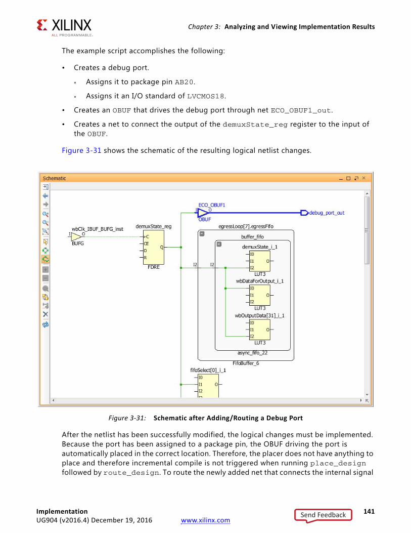
Chapter 3: Analyzing and Viewing Implementation Results
The example script accomplishes the following:
• Creates a debug port.
° Assigns it to package pin AB20.
° Assigns it an I/O standard of LVCMOS18.
• Creates an OBUF that drives the debug port through net ECO_OBUF1_out.
• Creates a net to connect the output of the demuxState_reg register to the input of the OBUF.
Figure 3-31 shows the schematic of the resulting logical netlist changes.
After the netlist has been successfully modified, the logical changes must be implemented. Because the port has been assigned to a package pin, the OBUF driving the port is automatically placed in the correct location. Therefore, the placer does not have anything to place and therefore incremental compile is not triggered when running place_design followed by route_design. To route the newly added net that connects the internal signal
X-Ref Target - Figure 3-31
Figure 3-31: Schematic after Adding/Routing a Debug Port
Implementation 141UG904 (v2016.4) December 19, 2016 www.xilinx.com
Send Feedback
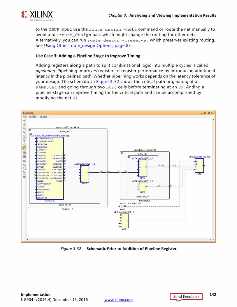
Chapter 3: Analyzing and Viewing Implementation Results
to the OBUF input, use the route_design -nets command or route the net manually to avoid a full route_design pass which might change the routing for other nets. Alternatively, you can run route_design -preserve, which preserves existing routing. See Using Other route_design Options, page 83.
Use Case 3: Adding a Pipeline Stage to Improve Timing
Adding registers along a path to split combinational logic into multiple cycles is called pipelining. Pipelining improves register-to-register performance by introducing additional latency in the pipelined path. Whether pipelining works depends on the latency tolerance of your design. The schematic in Figure 3-32 shows the critical path originating at a RAMB36E1 and going through two LUT6 cells before terminating at an FF. Adding a pipeline stage can improve timing for the critical path and can be accomplished by modifying the netlist.
X-Ref Target - Figure 3-32
Figure 3-32: Schematic Prior to Addition of Pipeline Register
Implementation 142UG904 (v2016.4) December 19, 2016 www.xilinx.com
Send Feedback
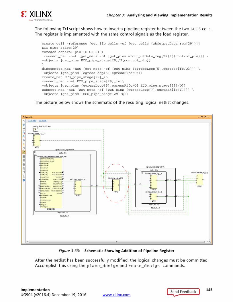
Chapter 3: Analyzing and Viewing Implementation Results
The following Tcl script shows how to insert a pipeline register between the two LUT6 cells. The register is implemented with the same control signals as the load register.
create_cell -reference [get_lib_cells -of [get_cells {wbOutputData_reg[29]}]] ECO_pipe_stage[29]foreach control_pin {C CE R} { connect_net -net [get_nets -of [get_pins wbOutputData_reg[29]/${control_pin}]] \-objects [get_pins ECO_pipe_stage[29]/${control_pin}]}disconnect_net -net [get_nets -of [get_pins {egressLoop[5].egressFifo/O3}]] \-objects [get_pins {egressLoop[5].egressFifo/O3}]create_net ECO_pipe_stage[29]_inconnect_net -net ECO_pipe_stage[29]_in \-objects [get_pins {egressLoop[5].egressFifo/O3 ECO_pipe_stage[29]/D}]connect_net -net [get_nets -of [get_pins {egressLoop[7].egressFifo/I7}]] \-objects [get_pins {ECO_pipe_stage[29]/Q}]
The picture below shows the schematic of the resulting logical netlist changes.
After the netlist has been successfully modified, the logical changes must be committed. Accomplish this using the place_design and route_design commands.
X-Ref Target - Figure 3-33
Figure 3-33: Schematic Showing Addition of Pipeline Register
Implementation 143UG904 (v2016.4) December 19, 2016 www.xilinx.com
Send Feedback
Chapter 3: Analyzing and Viewing Implementation Results
Vivado ECO FlowIMPORTANT: ECOs only work on design checkpoints. The ECO Layout is only available after a design checkpoint has been opened in the Vivado IDE.
Engineering change orders (ECOs) are modifications to the post implementation netlist with the intent to implement the changes with minimal impact to the original design. Vivado provides an ECO flow, which allows you to modify a design checkpoint, implement the changes, run reports on the changed netlist, and generate programming files.
Common use cases for the ECO flow are:
• Modifying debug probes of ILA and/or VIO cores in the design
• Routing an internal net to a package pin for external probing
• Evaluating what-if scenarios (improving timing, fixing logic bugs, and so on)
The advantage of the ECO flow is fast turn-around time by taking advantage of the incremental place and route features of the Vivado tool.
The Vivado IDE provides a predefined layout to support the ECO flow.
To access the ECO Layout, select Layout > ECO.
ECO Navigator
The ECO Navigator provides access to the commands that are required to complete an ECO.
Implementation 144UG904 (v2016.4) December 19, 2016 www.xilinx.com
Send Feedback
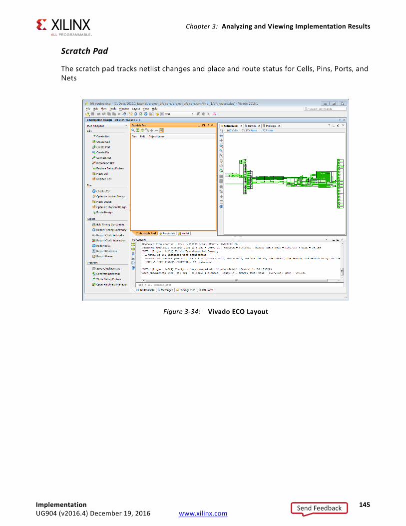
Chapter 3: Analyzing and Viewing Implementation Results
Scratch Pad
The scratch pad tracks netlist changes and place and route status for Cells, Pins, Ports, and Nets
X-Ref Target - Figure 3-34
Figure 3-34: Vivado ECO Layout
Implementation 145UG904 (v2016.4) December 19, 2016 www.xilinx.com
Send Feedback
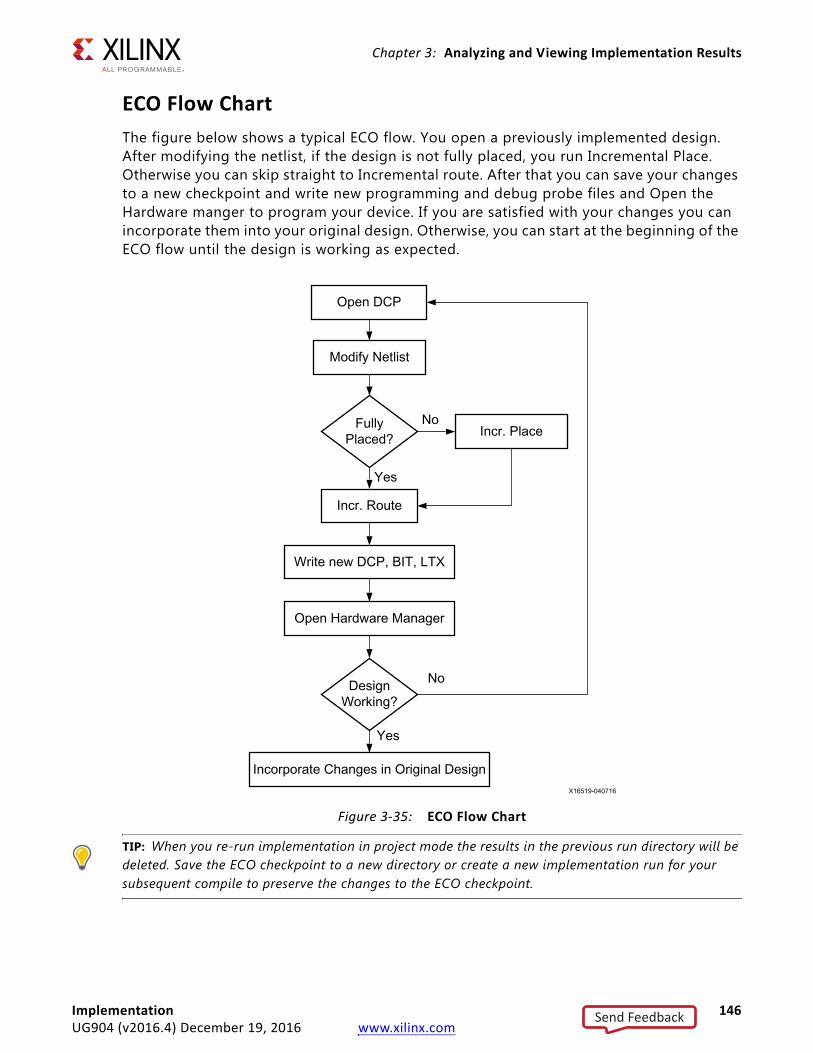
Chapter 3: Analyzing and Viewing Implementation Results
ECO Flow ChartThe figure below shows a typical ECO flow. You open a previously implemented design. After modifying the netlist, if the design is not fully placed, you run Incremental Place. Otherwise you can skip straight to Incremental route. After that you can save your changes to a new checkpoint and write new programming and debug probe files and Open the Hardware manger to program your device. If you are satisfied with your changes you can incorporate them into your original design. Otherwise, you can start at the beginning of the ECO flow until the design is working as expected.
TIP: When you re-run implementation in project mode the results in the previous run directory will be deleted. Save the ECO checkpoint to a new directory or create a new implementation run for your subsequent compile to preserve the changes to the ECO checkpoint.
X-Ref Target - Figure 3-35
Figure 3-35: ECO Flow Chart
Implementation 146UG904 (v2016.4) December 19, 2016 www.xilinx.com
Send Feedback
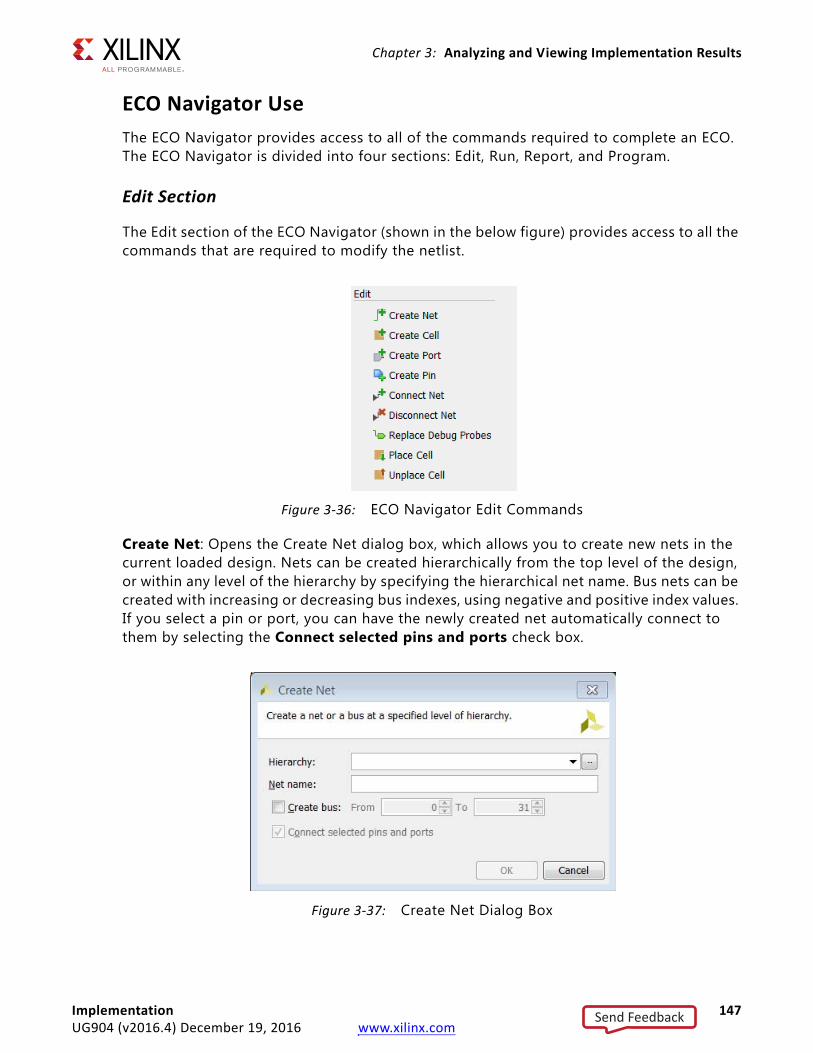
Chapter 3: Analyzing and Viewing Implementation Results
ECO Navigator UseThe ECO Navigator provides access to all of the commands required to complete an ECO. The ECO Navigator is divided into four sections: Edit, Run, Report, and Program.
Edit Section
The Edit section of the ECO Navigator (shown in the below figure) provides access to all the commands that are required to modify the netlist.
Create Net: Opens the Create Net dialog box, which allows you to create new nets in the current loaded design. Nets can be created hierarchically from the top level of the design, or within any level of the hierarchy by specifying the hierarchical net name. Bus nets can be created with increasing or decreasing bus indexes, using negative and positive index values. If you select a pin or port, you can have the newly created net automatically connect to them by selecting the Connect selected pins and ports check box.
X-Ref Target - Figure 3-36
Figure 3-36: ECO Navigator Edit Commands
X-Ref Target - Figure 3-37
Figure 3-37: Create Net Dialog Box
Implementation 147UG904 (v2016.4) December 19, 2016 www.xilinx.com
Send Feedback
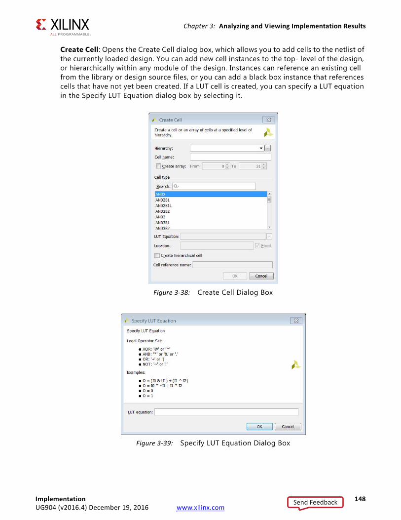
Chapter 3: Analyzing and Viewing Implementation Results
Create Cell: Opens the Create Cell dialog box, which allows you to add cells to the netlist of the currently loaded design. You can add new cell instances to the top- level of the design, or hierarchically within any module of the design. Instances can reference an existing cell from the library or design source files, or you can add a black box instance that references cells that have not yet been created. If a LUT cell is created, you can specify a LUT equation in the Specify LUT Equation dialog box by selecting it.X-Ref Target - Figure 3-38
Figure 3-38: Create Cell Dialog Box
X-Ref Target - Figure 3-39
Figure 3-39: Specify LUT Equation Dialog Box
Implementation 148UG904 (v2016.4) December 19, 2016 www.xilinx.com
Send Feedback
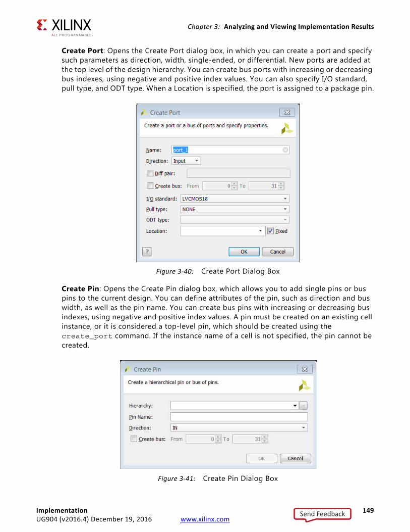
Chapter 3: Analyzing and Viewing Implementation Results
Create Port: Opens the Create Port dialog box, in which you can create a port and specify such parameters as direction, width, single-ended, or differential. New ports are added at the top level of the design hierarchy. You can create bus ports with increasing or decreasing bus indexes, using negative and positive index values. You can also specify I/O standard, pull type, and ODT type. When a Location is specified, the port is assigned to a package pin.
Create Pin: Opens the Create Pin dialog box, which allows you to add single pins or bus pins to the current design. You can define attributes of the pin, such as direction and bus width, as well as the pin name. You can create bus pins with increasing or decreasing bus indexes, using negative and positive index values. A pin must be created on an existing cell instance, or it is considered a top-level pin, which should be created using the create_port command. If the instance name of a cell is not specified, the pin cannot be created.
X-Ref Target - Figure 3-40
Figure 3-40: Create Port Dialog Box
X-Ref Target - Figure 3-41
Figure 3-41: Create Pin Dialog Box
Implementation 149UG904 (v2016.4) December 19, 2016 www.xilinx.com
Send Feedback
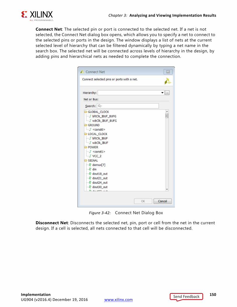
Chapter 3: Analyzing and Viewing Implementation Results
Connect Net: The selected pin or port is connected to the selected net. If a net is not selected, the Connect Net dialog box opens, which allows you to specify a net to connect to the selected pins or ports in the design. The window displays a list of nets at the current selected level of hierarchy that can be filtered dynamically by typing a net name in the search box. The selected net will be connected across levels of hierarchy in the design, by adding pins and hierarchical nets as needed to complete the connection.
Disconnect Net: Disconnects the selected net, pin, port or cell from the net in the current design. If a cell is selected, all nets connected to that cell will be disconnected.
X-Ref Target - Figure 3-42
Figure 3-42: Connect Net Dialog Box
Implementation 150UG904 (v2016.4) December 19, 2016 www.xilinx.com
Send Feedback
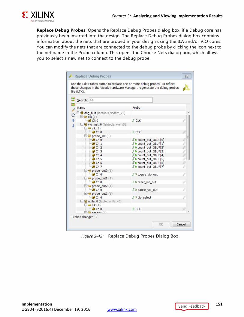
Chapter 3: Analyzing and Viewing Implementation Results
Replace Debug Probes: Opens the Replace Debug Probes dialog box, if a Debug core has previously been inserted into the design. The Replace Debug Probes dialog box contains information about the nets that are probed in your design using the ILA and/or VIO cores. You can modify the nets that are connected to the debug probe by clicking the icon next to the net name in the Probe column. This opens the Choose Nets dialog box, which allows you to select a new net to connect to the debug probe.
X-Ref Target - Figure 3-43
Figure 3-43: Replace Debug Probes Dialog Box
Implementation 151UG904 (v2016.4) December 19, 2016 www.xilinx.com
Send Feedback
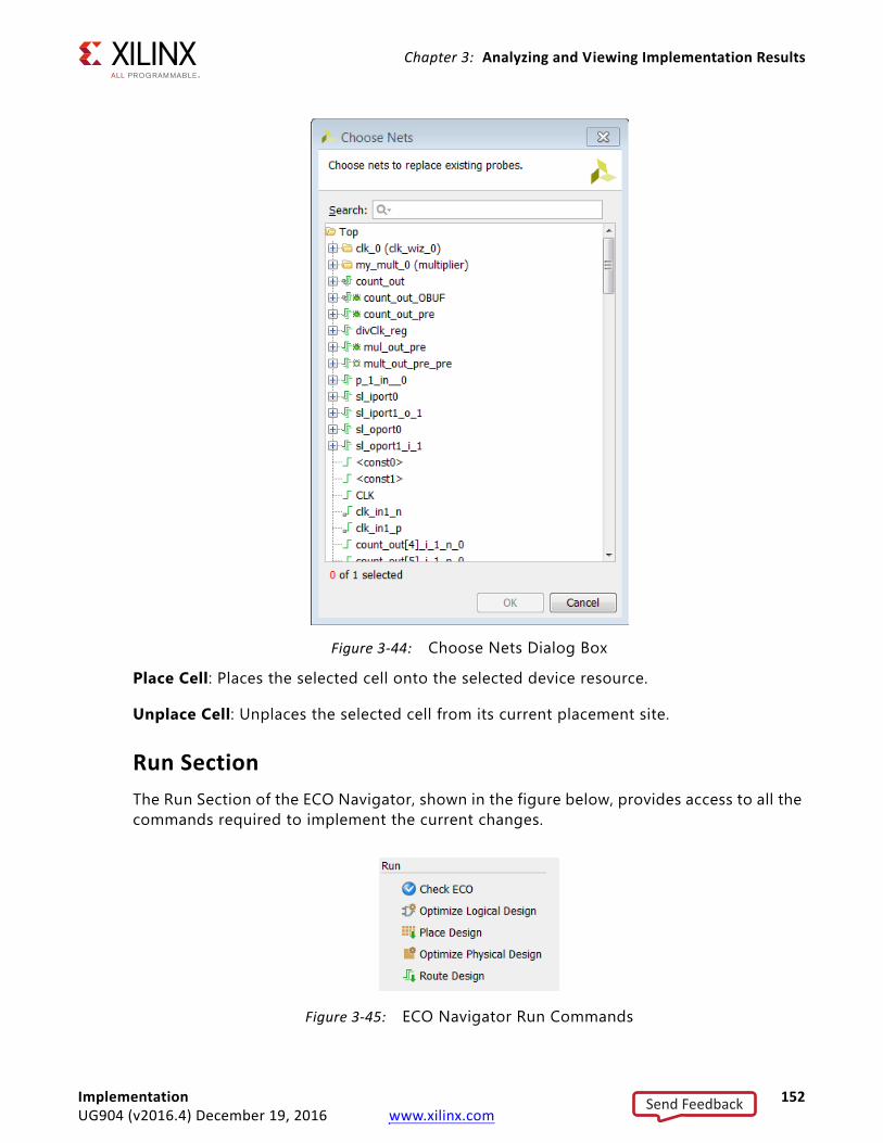
Chapter 3: Analyzing and Viewing Implementation Results
Place Cell: Places the selected cell onto the selected device resource.
Unplace Cell: Unplaces the selected cell from its current placement site.
Run SectionThe Run Section of the ECO Navigator, shown in the figure below, provides access to all the commands required to implement the current changes.
X-Ref Target - Figure 3-44
Figure 3-44: Choose Nets Dialog Box
X-Ref Target - Figure 3-45
Figure 3-45: ECO Navigator Run Commands
Implementation 152UG904 (v2016.4) December 19, 2016 www.xilinx.com
Send Feedback
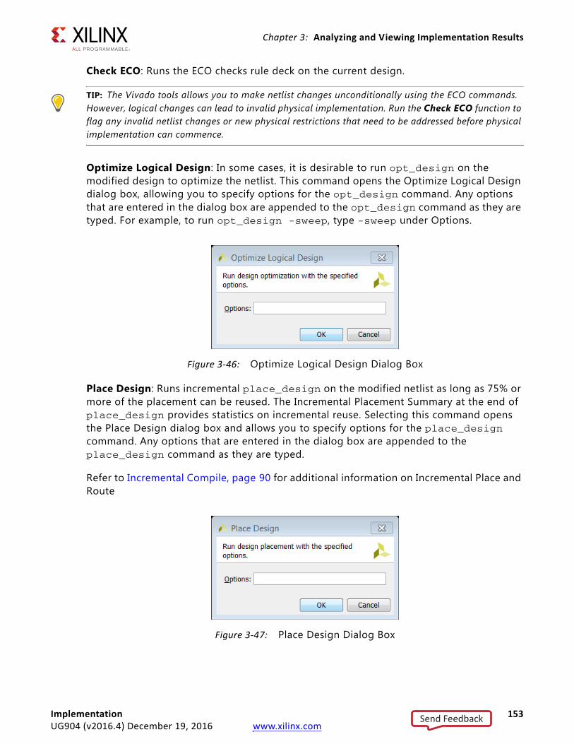
Chapter 3: Analyzing and Viewing Implementation Results
Check ECO: Runs the ECO checks rule deck on the current design.
TIP: The Vivado tools allows you to make netlist changes unconditionally using the ECO commands. However, logical changes can lead to invalid physical implementation. Run the Check ECO function to flag any invalid netlist changes or new physical restrictions that need to be addressed before physical implementation can commence.
Optimize Logical Design: In some cases, it is desirable to run opt_design on the modified design to optimize the netlist. This command opens the Optimize Logical Design dialog box, allowing you to specify options for the opt_design command. Any options that are entered in the dialog box are appended to the opt_design command as they are typed. For example, to run opt_design -sweep, type -sweep under Options.
Place Design: Runs incremental place_design on the modified netlist as long as 75% or more of the placement can be reused. The Incremental Placement Summary at the end of place_design provides statistics on incremental reuse. Selecting this command opens the Place Design dialog box and allows you to specify options for the place_design command. Any options that are entered in the dialog box are appended to the place_design command as they are typed.
Refer to Incremental Compile, page 90 for additional information on Incremental Place and Route
X-Ref Target - Figure 3-46
Figure 3-46: Optimize Logical Design Dialog Box
X-Ref Target - Figure 3-47
Figure 3-47: Place Design Dialog Box
Implementation 153UG904 (v2016.4) December 19, 2016 www.xilinx.com
Send Feedback
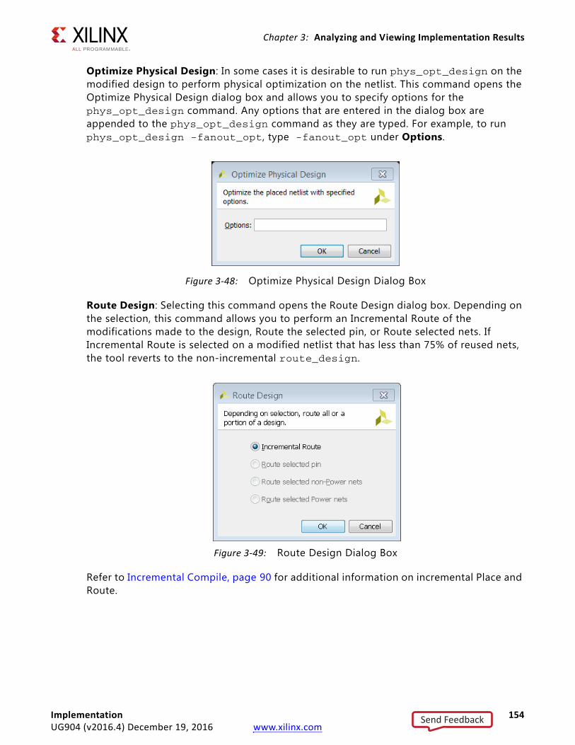
Chapter 3: Analyzing and Viewing Implementation Results
Optimize Physical Design: In some cases it is desirable to run phys_opt_design on the modified design to perform physical optimization on the netlist. This command opens the Optimize Physical Design dialog box and allows you to specify options for the phys_opt_design command. Any options that are entered in the dialog box are appended to the phys_opt_design command as they are typed. For example, to run phys_opt_design -fanout_opt, type -fanout_opt under Options.
Route Design: Selecting this command opens the Route Design dialog box. Depending on the selection, this command allows you to perform an Incremental Route of the modifications made to the design, Route the selected pin, or Route selected nets. If Incremental Route is selected on a modified netlist that has less than 75% of reused nets, the tool reverts to the non-incremental route_design.
Refer to Incremental Compile, page 90 for additional information on incremental Place and Route.
X-Ref Target - Figure 3-48
Figure 3-48: Optimize Physical Design Dialog Box
X-Ref Target - Figure 3-49
Figure 3-49: Route Design Dialog Box
Implementation 154UG904 (v2016.4) December 19, 2016 www.xilinx.com
Send Feedback
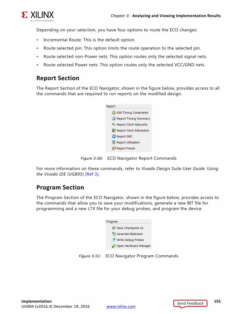
Chapter 3: Analyzing and Viewing Implementation Results
Depending on your selection, you have four options to route the ECO changes:
• Incremental Route: This is the default option.
• Route selected pin: This option limits the route operation to the selected pin.
• Route selected non-Power nets: This option routes only the selected signal nets.
• Route selected Power nets: This option routes only the selected VCC/GND nets.
Report SectionThe Report Section of the ECO Navigator, shown in the figure below, provides access to all the commands that are required to run reports on the modified design.
For more information on these commands, refer to Vivado Design Suite User Guide: Using the Vivado IDE (UG893) [Ref 3].
Program SectionThe Program Section of the ECO Navigator, shown in the figure below, provides access to the commands that allow you to save your modifications, generate a new BIT file for programming and a new LTX file for your debug probes, and program the device.
X-Ref Target - Figure 3-50
Figure 3-50: ECO Navigator Report Commands
X-Ref Target - Figure 3-51
Figure 3-51: ECO Navigator Program Commands
Implementation 155UG904 (v2016.4) December 19, 2016 www.xilinx.com
Send Feedback
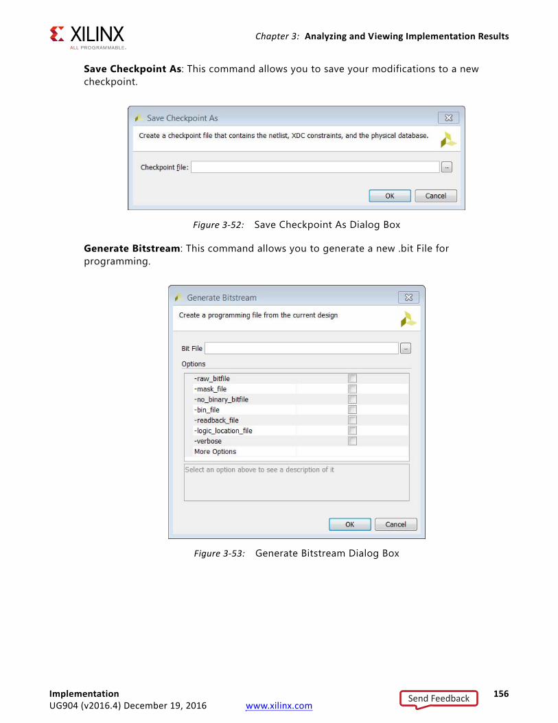
Chapter 3: Analyzing and Viewing Implementation Results
Save Checkpoint As: This command allows you to save your modifications to a new checkpoint.
Generate Bitstream: This command allows you to generate a new .bit File for programming.
X-Ref Target - Figure 3-52
Figure 3-52: Save Checkpoint As Dialog Box
X-Ref Target - Figure 3-53
Figure 3-53: Generate Bitstream Dialog Box
Implementation 156UG904 (v2016.4) December 19, 2016 www.xilinx.com
Send Feedback
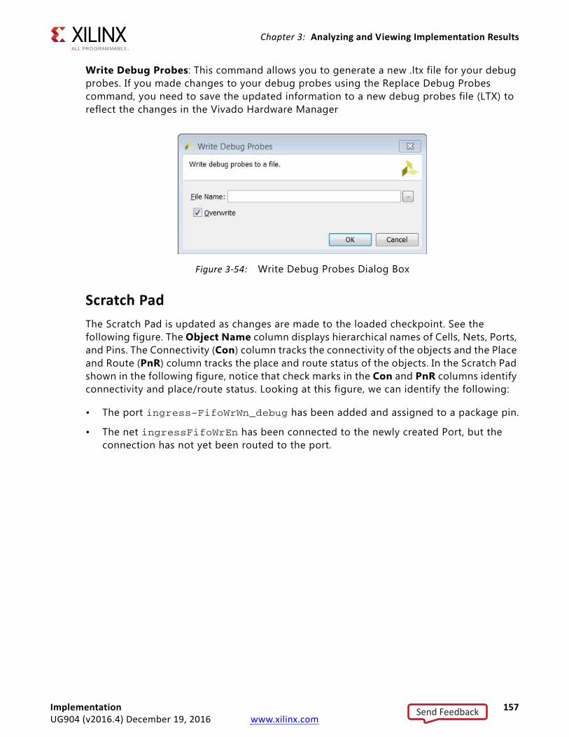
Chapter 3: Analyzing and Viewing Implementation Results
Write Debug Probes: This command allows you to generate a new .ltx file for your debug probes. If you made changes to your debug probes using the Replace Debug Probes command, you need to save the updated information to a new debug probes file (LTX) to reflect the changes in the Vivado Hardware Manager
Scratch PadThe Scratch Pad is updated as changes are made to the loaded checkpoint. See the following figure. The Object Name column displays hierarchical names of Cells, Nets, Ports, and Pins. The Connectivity (Con) column tracks the connectivity of the objects and the Place and Route (PnR) column tracks the place and route status of the objects. In the Scratch Pad shown in the following figure, notice that check marks in the Con and PnR columns identify connectivity and place/route status. Looking at this figure, we can identify the following:
• The port ingress-FifoWrWn_debug has been added and assigned to a package pin.
• The net ingressFifoWrEn has been connected to the newly created Port, but the connection has not yet been routed to the port.
X-Ref Target - Figure 3-54
Figure 3-54: Write Debug Probes Dialog Box
Implementation 157UG904 (v2016.4) December 19, 2016 www.xilinx.com
Send Feedback
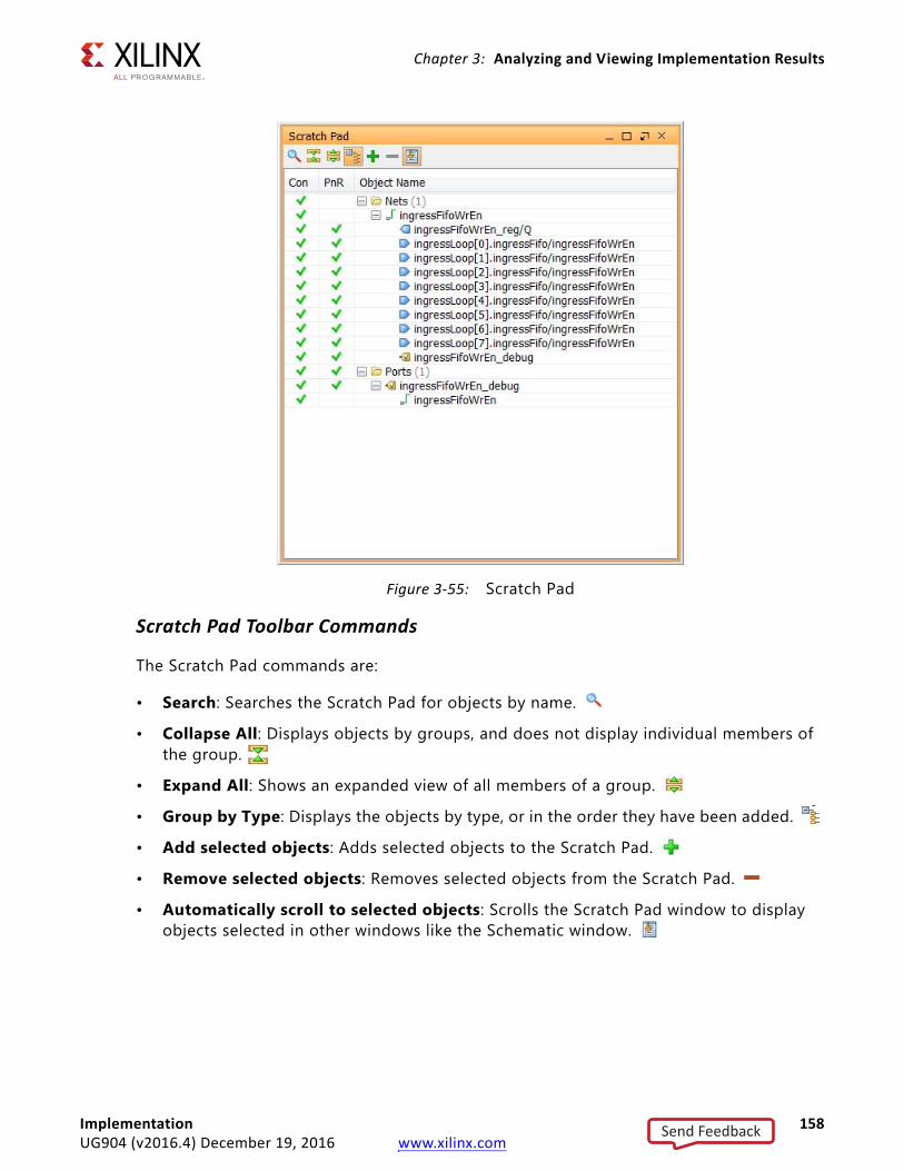
Chapter 3: Analyzing and Viewing Implementation Results
Scratch Pad Toolbar Commands
The Scratch Pad commands are:
• Search: Searches the Scratch Pad for objects by name.
• Collapse All: Displays objects by groups, and does not display individual members of the group.
• Expand All: Shows an expanded view of all members of a group.
• Group by Type: Displays the objects by type, or in the order they have been added.
• Add selected objects: Adds selected objects to the Scratch Pad.
• Remove selected objects: Removes selected objects from the Scratch Pad.
• Automatically scroll to selected objects: Scrolls the Scratch Pad window to display objects selected in other windows like the Schematic window.
X-Ref Target - Figure 3-55
Figure 3-55: Scratch Pad
Implementation 158UG904 (v2016.4) December 19, 2016 www.xilinx.com
Send Feedback

Chapter 3: Analyzing and Viewing Implementation Results
Scratch Pad Pop-up Menu
When you right-click in the Scratch Pad, the following pop-up menu commands are available:
• Clear Scratch Pad: Clears the contents of the Scratch Pad.
• Add Objects to Scratch Pad: Adds unconnected, unplaced, or unrouted objects to the Scratch Pad.
• Select Array Elements: Selects all the elements in an array if one element has been selected.
• Clone: Creates a copy of the selected object.
• Connect Net to Output Port: Opens the Connect Net to Output Port dialog box, which allows you to connect the selected net to an external port. See Figure 3-56.
• Elide Setting: Specifies how to truncate long object names that don't fit in the Object Name column. Choices are Left, Middle, and Right.
• Object Properties: Opens the Object Properties dialog box.
• Report Net Route Status: Reports the route status of the selected net.
• Select Driver Pin: Selects the driver pin of the selected net.
• Unplace: Unplaces the selected I/O ports.
• Configure I/O Ports: Assigns various properties of the selected I/O ports.
• Split Diff Pair: Removes the differential pair association from the selected port.
• Auto-place I/O Ports: Places I/O ports using the Autoplace I/O Ports wizard.
• Place I/O Ports in Area: Assigns the currently selected ports onto pins in the specified area.
• Place I/O Ports Sequentially: Assigns the currently selected ports individually onto package pins.
• Fix Ports: Fixes the selected placed I/O ports.
• Unfix Ports: Unfixes the selected placed I/O ports.
• Floorplanning: Assign selected cells to Pblock.
• Highlight Leaf Cells: Highlights the primitive logic for the selected cell.
• Unhighlight Leaf Cells: Unhighlights the primitive logic for the selected cell.
• Delete: Deletes the selected objects.
• Highlight: Highlights the selected objects.
• Unhighlight: Unhighlights the selected objects.
• Mark: Draws a marker for the selected object.
Implementation 159UG904 (v2016.4) December 19, 2016 www.xilinx.com
Send Feedback
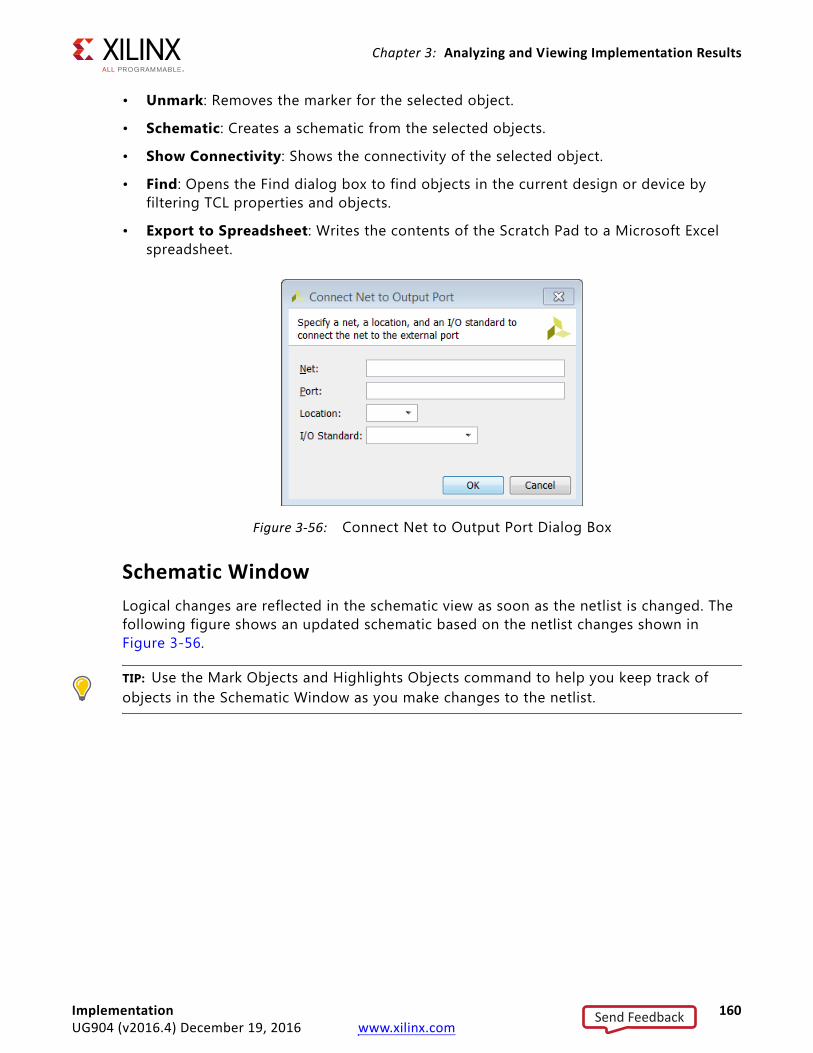
Chapter 3: Analyzing and Viewing Implementation Results
• Unmark: Removes the marker for the selected object.
• Schematic: Creates a schematic from the selected objects.
• Show Connectivity: Shows the connectivity of the selected object.
• Find: Opens the Find dialog box to find objects in the current design or device by filtering TCL properties and objects.
• Export to Spreadsheet: Writes the contents of the Scratch Pad to a Microsoft Excel spreadsheet.
Schematic WindowLogical changes are reflected in the schematic view as soon as the netlist is changed. The following figure shows an updated schematic based on the netlist changes shown in Figure 3-56.
TIP: Use the Mark Objects and Highlights Objects command to help you keep track of objects in the Schematic Window as you make changes to the netlist.
X-Ref Target - Figure 3-56
Figure 3-56: Connect Net to Output Port Dialog Box
Implementation 160UG904 (v2016.4) December 19, 2016 www.xilinx.com
Send Feedback
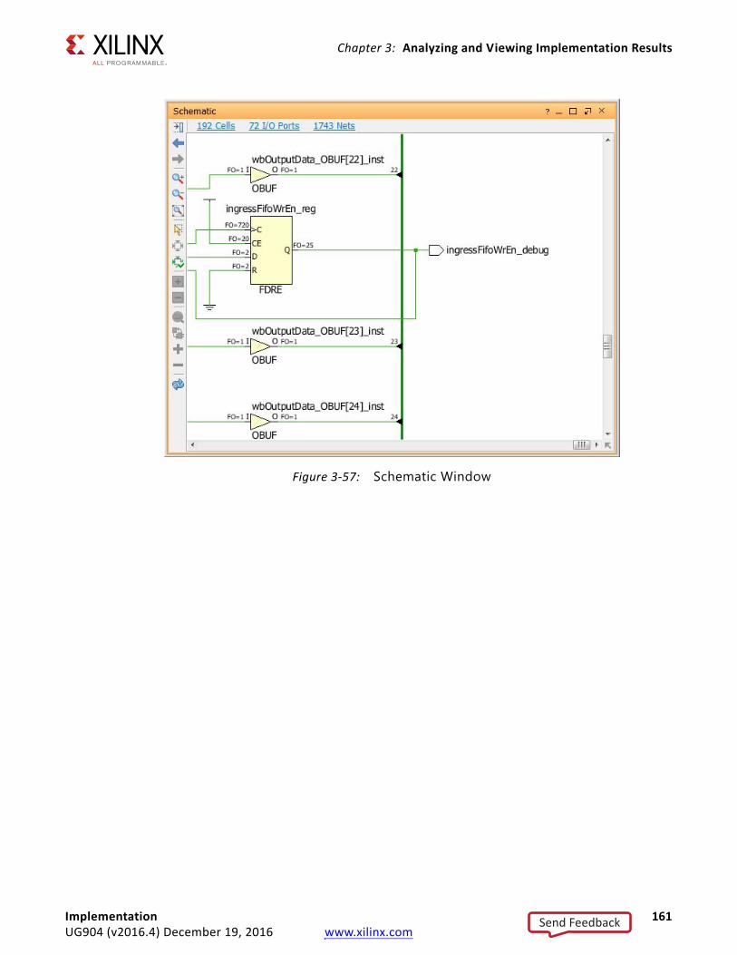
Chapter 3: Analyzing and Viewing Implementation Results
X-Ref Target - Figure 3-57
Figure 3-57: Schematic Window
Implementation 161UG904 (v2016.4) December 19, 2016 www.xilinx.com
Send Feedback
Appendix A
Using Remote Hosts and LSF
Launching Runs on Remote Linux Hosts
OverviewThe Xilinx® Vivado® Integrated Design Environment (IDE) supports simultaneous parallel execution of synthesis and implementation runs on multiple Linux hosts. You can accomplish this using LSF (Load Sharing Facility) or through manual host configuration.
For instructions on configuring remote hosts with LSF, see Configuring Remote Hosts Using LSF, page 163.
For instructions on configuring remote hosts manually, see Configuring Remote Hosts Manually, page 165.
About LSF
LSF is a subsystem for submitting, scheduling, executing, monitoring, and controlling a workload of batch jobs across compute servers in a cluster. You use the bsub command to launch synthesis and implementation runs in the Vivado Design Suite through LSF.
Linux and Remote Host Support
Linux is the only operating system supporting remote hosts because of superior security handling in Linux and the lack of remote-shell capabilities on Microsoft Windows systems.
Job Submission Algorithms and SSH
Job submission algorithms are implemented using a “greedy,” round-robin style with Tcl pipes within Secure Shell (SSH), a service within the Linux operating system.
RECOMMENDED: Before launching runs on multiple Linux hosts using manual configuration in the Vivado IDE, configure SSH so that the host does not require a password each time you launch a remote run.
For instructions on configuring SSH, see Setting Up SSH Key Agent Forward, page 167.
Implementation 162UG904 (v2016.4) December 19, 2016 www.xilinx.com
Send Feedback
Appendix A: Using Remote Hosts and LSF
Launch RequirementsThe requirements for launching synthesis and implementation runs on remote Linux hosts are:
• Vivado tools installation is assumed to be available from the login shell, which means that $XILINX_VIVADO and $PATH are configured correctly in your .cshrc/.bashrc setup scripts.
For Manual Configuration, if you do not have Vivado set up upon login (CSHRC or BASHRC), use the Run pre-launch script option, as described below, to define an environment setup script to be run prior to all jobs.
• Vivado IDE installation must be visible from the mounted file systems on remote machines. If the Vivado IDE installation is stored on a local disk on your own machine, it might not be visible from remote machines.
• Vivado IDE project files (.xpr) and directories (.data and .runs) must be visible from the mounted file systems on remote machines. If the design data is saved to a local disk, it might not be visible from remote machines.
Configuring Remote Hosts Using LSFTo configure the Vivado IDE to run synthesis or implementation on a remote Linux host using LSF configuration:
1. Select one of the following commands:
° From the main menu, click Tools > Options > Remote Hosts
° From the Launch Selected Runs dialog box, Configure LSF
° From the Create New Runs dialog box, Configure LSF
Implementation 163UG904 (v2016.4) December 19, 2016 www.xilinx.com
Send Feedback
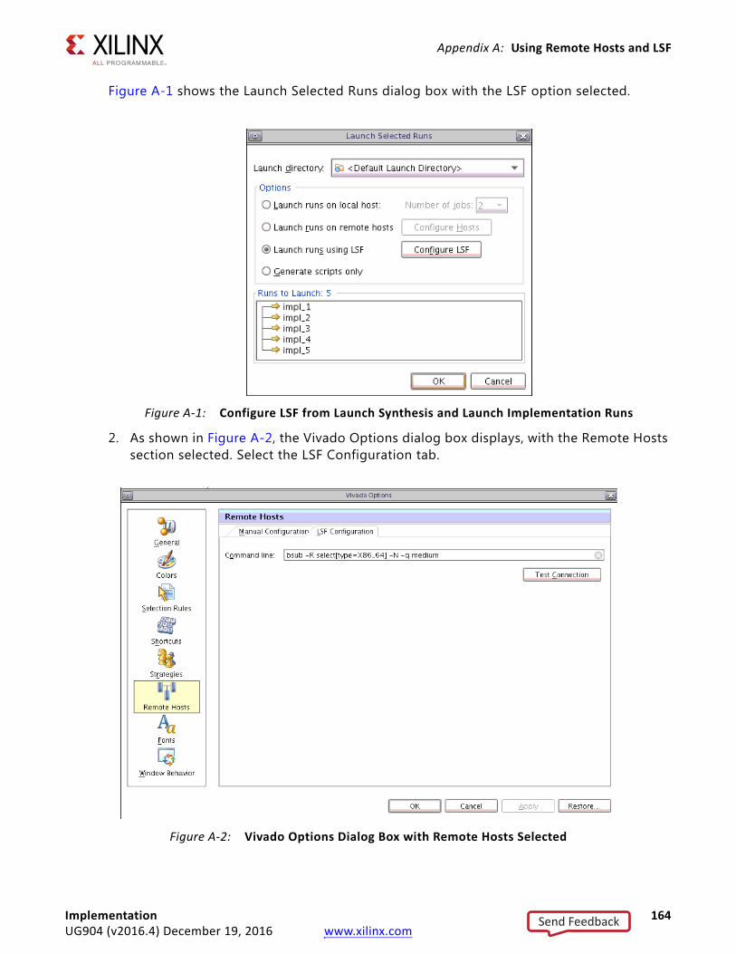
Appendix A: Using Remote Hosts and LSF
Figure A-1 shows the Launch Selected Runs dialog box with the LSF option selected.
2. As shown in Figure A-2, the Vivado Options dialog box displays, with the Remote Hosts section selected. Select the LSF Configuration tab.
X-Ref Target - Figure A-1
Figure A-1: Configure LSF from Launch Synthesis and Launch Implementation Runs
X-Ref Target - Figure A-2
Figure A-2: Vivado Options Dialog Box with Remote Hosts Selected
Implementation 164UG904 (v2016.4) December 19, 2016 www.xilinx.com
Send Feedback
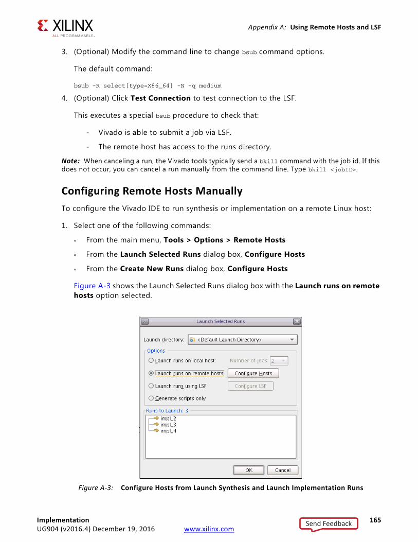
Appendix A: Using Remote Hosts and LSF
3. (Optional) Modify the command line to change bsub command options.
The default command:
bsub -R select[type=X86_64] -N -q medium
4. (Optional) Click Test Connection to test connection to the LSF.
This executes a special bsub procedure to check that:
- Vivado is able to submit a job via LSF.
- The remote host has access to the runs directory.
Note: When canceling a run, the Vivado tools typically send a bkill command with the job id. If this does not occur, you can cancel a run manually from the command line. Type bkill <jobID>.
Configuring Remote Hosts ManuallyTo configure the Vivado IDE to run synthesis or implementation on a remote Linux host:
1. Select one of the following commands:
° From the main menu, Tools > Options > Remote Hosts
° From the Launch Selected Runs dialog box, Configure Hosts
° From the Create New Runs dialog box, Configure Hosts
Figure A-3 shows the Launch Selected Runs dialog box with the Launch runs on remote hosts option selected.
X-Ref Target - Figure A-3
Figure A-3: Configure Hosts from Launch Synthesis and Launch Implementation Runs
Implementation 165UG904 (v2016.4) December 19, 2016 www.xilinx.com
Send Feedback
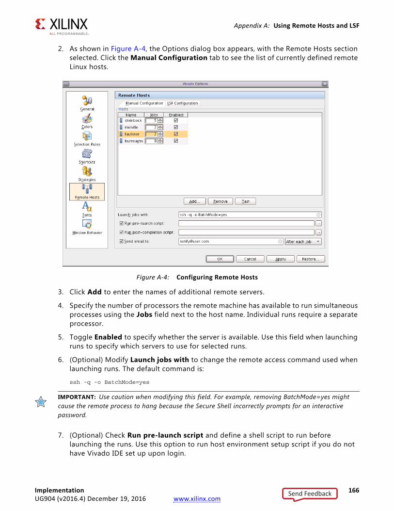
Appendix A: Using Remote Hosts and LSF
2. As shown in Figure A-4, the Options dialog box appears, with the Remote Hosts section selected. Click the Manual Configuration tab to see the list of currently defined remote Linux hosts.
3. Click Add to enter the names of additional remote servers.
4. Specify the number of processors the remote machine has available to run simultaneous processes using the Jobs field next to the host name. Individual runs require a separate processor.
5. Toggle Enabled to specify whether the server is available. Use this field when launching runs to specify which servers to use for selected runs.
6. (Optional) Modify Launch jobs with to change the remote access command used when launching runs. The default command is:
ssh -q -o BatchMode=yes
IMPORTANT: Use caution when modifying this field. For example, removing BatchMode=yes might cause the remote process to hang because the Secure Shell incorrectly prompts for an interactive password.
7. (Optional) Check Run pre-launch script and define a shell script to run before launching the runs. Use this option to run host environment setup script if you do not have Vivado IDE set up upon login.
X-Ref Target - Figure A-4
Figure A-4: Configuring Remote Hosts
Implementation 166UG904 (v2016.4) December 19, 2016 www.xilinx.com
Send Feedback
Appendix A: Using Remote Hosts and LSF
8. (Optional) Check Run post-completion script and define a custom script to run after the run completes, to move or copy the results for example.
9. (Optional) Check Send email to and enter an Email address to send a notification when the runs complete. You can have notifications sent After each Job, or After all jobs.
10. Click OK to accept the Remote Host configuration settings.
11. Select one or more hosts.
12. Click Test.
The tools verify that the server is available and that the configuration is properly set.
RECOMMENDED: Test each host to ensure proper setup before submitting runs to the host.
Removing Remote HostsTo remove a remote host, select it and click Remove.
Setting Up SSH Key Agent ForwardYou can configure SSH with the following commands at a Linux terminal or shell.
Note: This is a one-time step. When successfully set-up, this step does not need to be repeated.
1. Run the following command at a Linux terminal or shell to generate a public key on your primary machine. Though not required, it is a good practice to enter (and remember) a private key phrase when prompted for maximum security.
ssh-keygen -t rsa
2. Append the contents of your publish key to an authorized_keys file on the remote machine. Change remote_server to a valid host name:
cat ~/.ssh/id_rsa.pub | ssh remote_server “cat - >> ~/.ssh/authorized_keys”
3. Run the following command to prompt for your private key pass phrase, and enable key forwarding:
ssh-add
You should now be able to ssh to any machine without typing a password. The first time you access a new machine, it prompts you for a password. It does not prompt upon subsequent access.
TIP: If you are always prompted for a password, contact your System Administrator.
Implementation 167UG904 (v2016.4) December 19, 2016 www.xilinx.com
Send Feedback
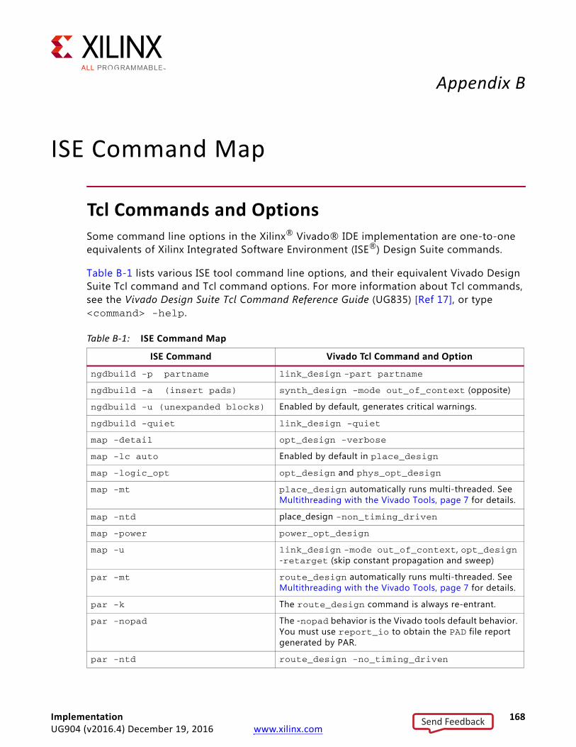
Implementation 168UG904 (v2016.4) December 19, 2016 www.xilinx.com
Appendix B
ISE Command Map
Tcl Commands and OptionsSome command line options in the Xilinx® Vivado® IDE implementation are one-to-one equivalents of Xilinx Integrated Software Environment (ISE®) Design Suite commands.
Table B-1 lists various ISE tool command line options, and their equivalent Vivado Design Suite Tcl command and Tcl command options. For more information about Tcl commands, see the Vivado Design Suite Tcl Command Reference Guide (UG835) [Ref 17], or type <command> -help.
Table B-1: ISE Command Map
ISE Command Vivado Tcl Command and Option
ngdbuild -p partname link_design -part partname
ngdbuild -a (insert pads) synth_design -mode out_of_context (opposite)
ngdbuild -u (unexpanded blocks) Enabled by default, generates critical warnings.
ngdbuild -quiet link_design -quiet
map -detail opt_design -verbose
map -lc auto Enabled by default in place_design
map -logic_opt opt_design and phys_opt_design
map -mt place_design automatically runs multi-threaded. See Multithreading with the Vivado Tools, page 7 for details.
map -ntd place_design -non_timing_driven
map -power power_opt_design
map -u link_design -mode out_of_context, opt_design -retarget (skip constant propagation and sweep)
par -mt route_design automatically runs multi-threaded. See Multithreading with the Vivado Tools, page 7 for details.
par -k The route_design command is always re-entrant.
par -nopad The -nopad behavior is the Vivado tools default behavior. You must use report_io to obtain the PAD file report generated by PAR.
par -ntd route_design -no_timing_driven
Send Feedback
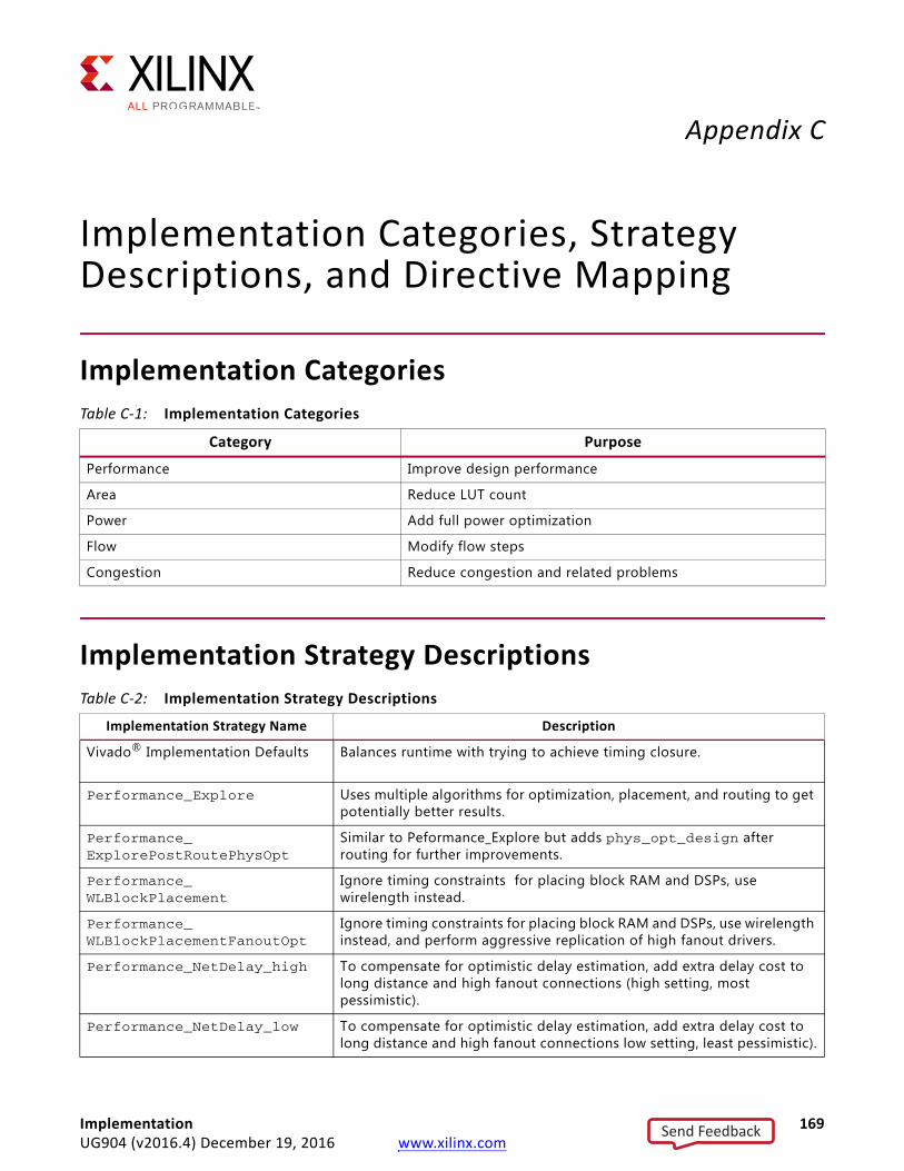
Appendix C
Implementation Categories, Strategy Descriptions, and Directive Mapping
Implementation CategoriesI
Implementation Strategy Descriptions
Table C-1: Implementation Categories
Category Purpose
Performance Improve design performance
Area Reduce LUT count
Power Add full power optimization
Flow Modify flow steps
Congestion Reduce congestion and related problems
Table C-2: Implementation Strategy Descriptions
Implementation Strategy Name Description
Vivado® Implementation Defaults Balances runtime with trying to achieve timing closure.
Performance_Explore Uses multiple algorithms for optimization, placement, and routing to get potentially better results.
Performance_ExplorePostRoutePhysOpt
Similar to Peformance_Explore but adds phys_opt_design after routing for further improvements.
Performance_WLBlockPlacement
Ignore timing constraints for placing block RAM and DSPs, use wirelength instead.
Performance_WLBlockPlacementFanoutOpt
Ignore timing constraints for placing block RAM and DSPs, use wirelength instead, and perform aggressive replication of high fanout drivers.
Performance_NetDelay_high To compensate for optimistic delay estimation, add extra delay cost to long distance and high fanout connections (high setting, most pessimistic).
Performance_NetDelay_low To compensate for optimistic delay estimation, add extra delay cost to long distance and high fanout connections low setting, least pessimistic).
Implementation 169UG904 (v2016.4) December 19, 2016 www.xilinx.com
Send Feedback
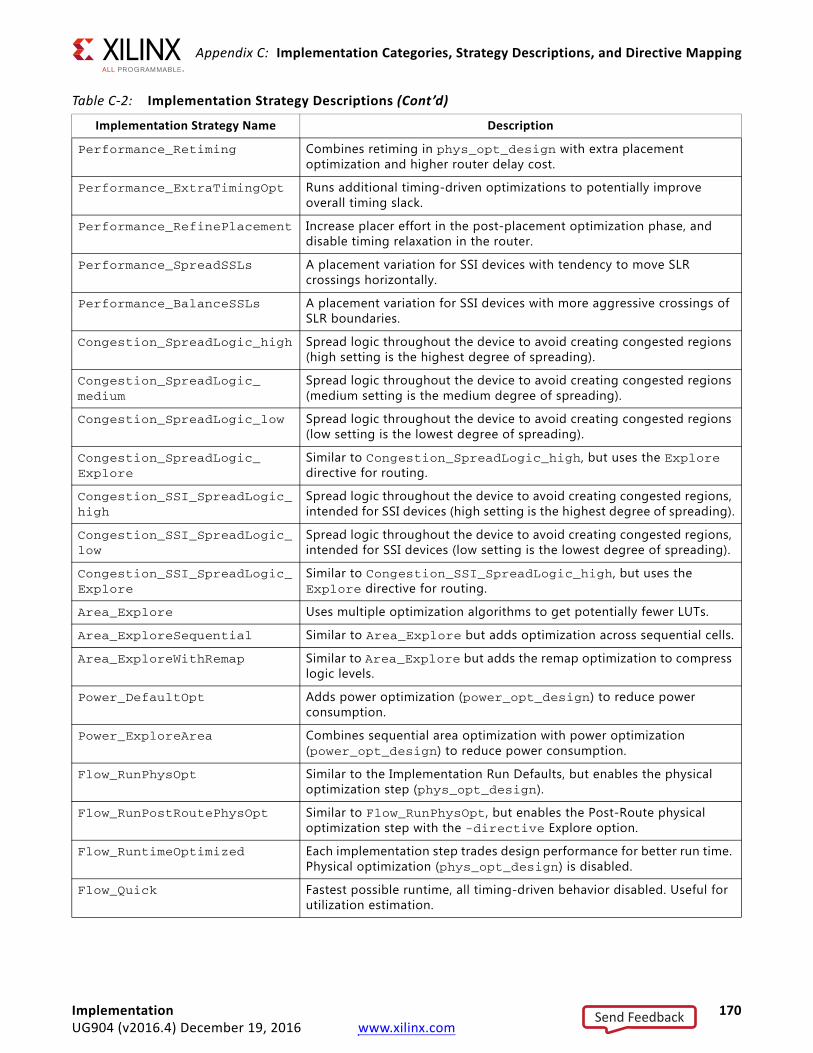
Appendix C: Implementation Categories, Strategy Descriptions, and Directive Mapping
Performance_Retiming Combines retiming in phys_opt_design with extra placement optimization and higher router delay cost.
Performance_ExtraTimingOpt Runs additional timing-driven optimizations to potentially improve overall timing slack.
Performance_RefinePlacement Increase placer effort in the post-placement optimization phase, and disable timing relaxation in the router.
Performance_SpreadSSLs A placement variation for SSI devices with tendency to move SLR crossings horizontally.
Performance_BalanceSSLs A placement variation for SSI devices with more aggressive crossings of SLR boundaries.
Congestion_SpreadLogic_high Spread logic throughout the device to avoid creating congested regions (high setting is the highest degree of spreading).
Congestion_SpreadLogic_medium
Spread logic throughout the device to avoid creating congested regions (medium setting is the medium degree of spreading).
Congestion_SpreadLogic_low Spread logic throughout the device to avoid creating congested regions (low setting is the lowest degree of spreading).
Congestion_SpreadLogic_Explore
Similar to Congestion_SpreadLogic_high, but uses the Explore directive for routing.
Congestion_SSI_SpreadLogic_high
Spread logic throughout the device to avoid creating congested regions, intended for SSI devices (high setting is the highest degree of spreading).
Congestion_SSI_SpreadLogic_low
Spread logic throughout the device to avoid creating congested regions, intended for SSI devices (low setting is the lowest degree of spreading).
Congestion_SSI_SpreadLogic_Explore
Similar to Congestion_SSI_SpreadLogic_high, but uses the Explore directive for routing.
Area_Explore Uses multiple optimization algorithms to get potentially fewer LUTs.
Area_ExploreSequential Similar to Area_Explore but adds optimization across sequential cells.
Area_ExploreWithRemap Similar to Area_Explore but adds the remap optimization to compress logic levels.
Power_DefaultOpt Adds power optimization (power_opt_design) to reduce power consumption.
Power_ExploreArea Combines sequential area optimization with power optimization (power_opt_design) to reduce power consumption.
Flow_RunPhysOpt Similar to the Implementation Run Defaults, but enables the physical optimization step (phys_opt_design).
Flow_RunPostRoutePhysOpt Similar to Flow_RunPhysOpt, but enables the Post-Route physical optimization step with the -directive Explore option.
Flow_RuntimeOptimized Each implementation step trades design performance for better run time. Physical optimization (phys_opt_design) is disabled.
Flow_Quick Fastest possible runtime, all timing-driven behavior disabled. Useful for utilization estimation.
Table C-2: Implementation Strategy Descriptions (Cont’d)
Implementation Strategy Name Description
Implementation 170UG904 (v2016.4) December 19, 2016 www.xilinx.com
Send Feedback
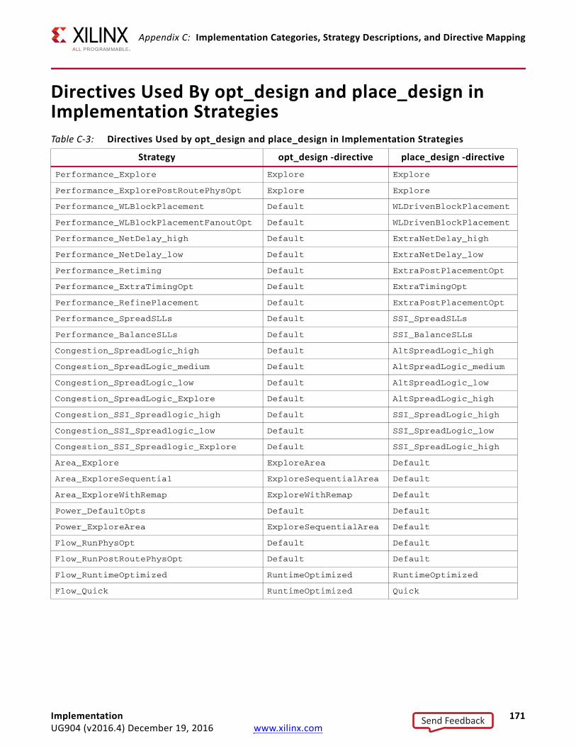
Appendix C: Implementation Categories, Strategy Descriptions, and Directive Mapping
Directives Used By opt_design and place_design in Implementation StrategiesTable C-3: Directives Used by opt_design and place_design in Implementation Strategies
Strategy opt_design -directive place_design -directive
Performance_Explore Explore Explore
Performance_ExplorePostRoutePhysOpt Explore Explore
Performance_WLBlockPlacement Default WLDrivenBlockPlacement
Performance_WLBlockPlacementFanoutOpt Default WLDrivenBlockPlacement
Performance_NetDelay_high Default ExtraNetDelay_high
Performance_NetDelay_low Default ExtraNetDelay_low
Performance_Retiming Default ExtraPostPlacementOpt
Performance_ExtraTimingOpt Default ExtraTimingOpt
Performance_RefinePlacement Default ExtraPostPlacementOpt
Performance_SpreadSLLs Default SSI_SpreadSLLs
Performance_BalanceSLLs Default SSI_BalanceSLLs
Congestion_SpreadLogic_high Default AltSpreadLogic_high
Congestion_SpreadLogic_medium Default AltSpreadLogic_medium
Congestion_SpreadLogic_low Default AltSpreadLogic_low
Congestion_SpreadLogic_Explore Default AltSpreadLogic_high
Congestion_SSI_Spreadlogic_high Default SSI_SpreadLogic_high
Congestion_SSI_Spreadlogic_low Default SSI_SpreadLogic_low
Congestion_SSI_Spreadlogic_Explore Default SSI_SpreadLogic_high
Area_Explore ExploreArea Default
Area_ExploreSequential ExploreSequentialArea Default
Area_ExploreWithRemap ExploreWithRemap Default
Power_DefaultOpts Default Default
Power_ExploreArea ExploreSequentialArea Default
Flow_RunPhysOpt Default Default
Flow_RunPostRoutePhysOpt Default Default
Flow_RuntimeOptimized RuntimeOptimized RuntimeOptimized
Flow_Quick RuntimeOptimized Quick
Implementation 171UG904 (v2016.4) December 19, 2016 www.xilinx.com
Send Feedback
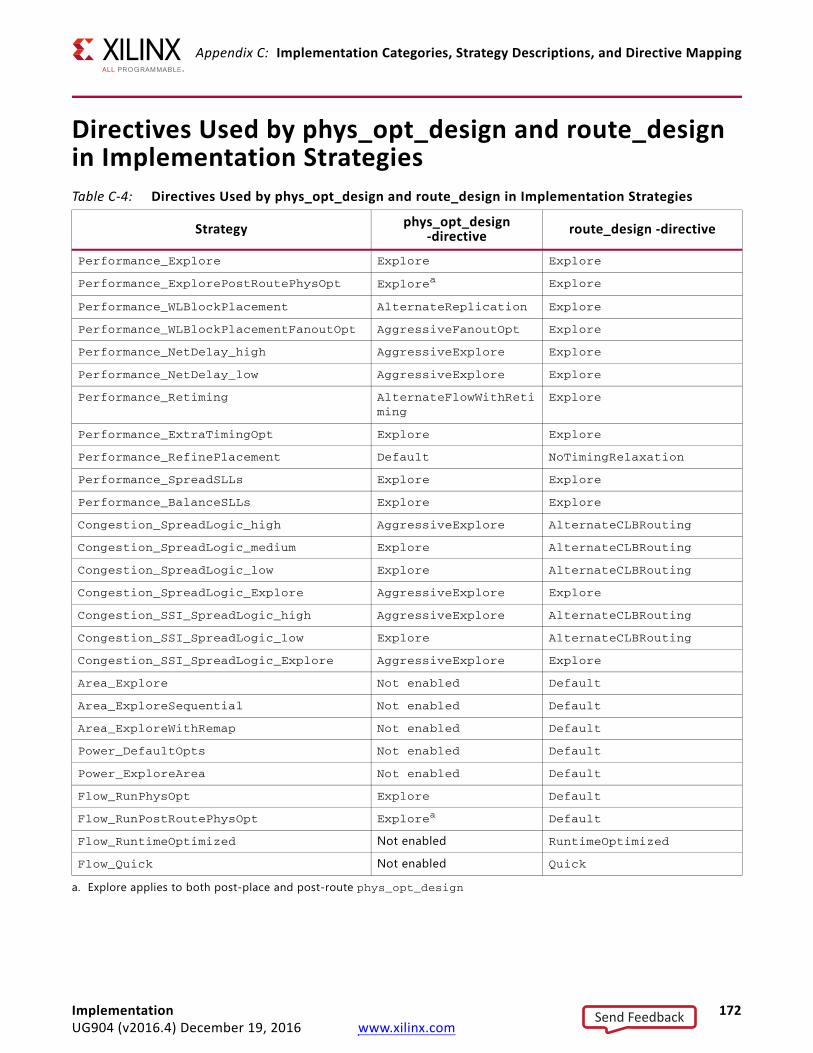
Appendix C: Implementation Categories, Strategy Descriptions, and Directive Mapping
Directives Used by phys_opt_design and route_design in Implementation StrategiesTable C-4: Directives Used by phys_opt_design and route_design in Implementation Strategies
Strategy phys_opt_design -directive route_design -directive
Performance_Explore Explore Explore
Performance_ExplorePostRoutePhysOpt Explorea Explore
Performance_WLBlockPlacement AlternateReplication Explore
Performance_WLBlockPlacementFanoutOpt AggressiveFanoutOpt Explore
Performance_NetDelay_high AggressiveExplore Explore
Performance_NetDelay_low AggressiveExplore Explore
Performance_Retiming AlternateFlowWithRetiming
Explore
Performance_ExtraTimingOpt Explore Explore
Performance_RefinePlacement Default NoTimingRelaxation
Performance_SpreadSLLs Explore Explore
Performance_BalanceSLLs Explore Explore
Congestion_SpreadLogic_high AggressiveExplore AlternateCLBRouting
Congestion_SpreadLogic_medium Explore AlternateCLBRouting
Congestion_SpreadLogic_low Explore AlternateCLBRouting
Congestion_SpreadLogic_Explore AggressiveExplore Explore
Congestion_SSI_SpreadLogic_high AggressiveExplore AlternateCLBRouting
Congestion_SSI_SpreadLogic_low Explore AlternateCLBRouting
Congestion_SSI_SpreadLogic_Explore AggressiveExplore Explore
Area_Explore Not enabled Default
Area_ExploreSequential Not enabled Default
Area_ExploreWithRemap Not enabled Default
Power_DefaultOpts Not enabled Default
Power_ExploreArea Not enabled Default
Flow_RunPhysOpt Explore Default
Flow_RunPostRoutePhysOpt Explorea Default
Flow_RuntimeOptimized Not enabled RuntimeOptimized
Flow_Quick Not enabled Quick
a. Explore applies to both post-place and post-route phys_opt_design
Implementation 172UG904 (v2016.4) December 19, 2016 www.xilinx.com
Send Feedback
Appendix D
Additional Resources and Legal Notices
Xilinx ResourcesFor support resources such as Answers, Documentation, Downloads, and Forums, see Xilinx® Support.
Solution CentersSee the Xilinx Solution Centers for support on devices, software tools, and intellectual property at all stages of the design cycle. Topics include design assistance, advisories, and troubleshooting tips.
Documentation Navigator and Design HubsXilinx Documentation Navigator provides access to Xilinx documents, videos, and support resources, which you can filter and search to find information. To open the Xilinx Documentation Navigator (DocNav):
• From the Vivado IDE, select Help > Documentation and Tutorials.
• On Windows, select Start > All Programs > Xilinx Design Tools > DocNav.
• At the Linux command prompt, enter docnav.
Xilinx Design Hubs provide links to documentation organized by design tasks and other topics, which you can use to learn key concepts and address frequently asked questions. To access the Design Hubs:
• In the Xilinx Documentation Navigator, click the Design Hubs View tab.
• On the Xilinx website, see the Design Hubs page.
Note: For more information on Documentation Navigator, see the Documentation Navigator page on the Xilinx website.
Implementation 173UG904 (v2016.4) December 19, 2016 www.xilinx.com
Send Feedback
Appendix D: Additional Resources and Legal Notices
References
Vivado Design Suite User Guides1. Vivado Design Suite User Guide: Design Flows Overview (UG892)
2. Vivado Design Suite User Guide: Hierarchical Design (UG905)
3. Vivado Design Suite User Guide: Using the Vivado IDE (UG893)
4. Vivado Design Suite User Guide: Designing with IP (UG896)
5. Vivado Design Suite User Guide: Using Tcl Scripting (UG894)
6. Vivado Design Suite User Guide: System-Level Design Entry (UG895)
7. Vivado Design Suite User Guide: Designing IP Subsystems Using IP Integrator (UG994)
8. Vivado Design Suite User Guide: Synthesis (UG901)
9. Vivado Design Suite User Guide: Using Constraints (UG903)
10. Vivado Design Suite User Guide: Design Analysis and Closure Techniques (UG906)
11. Vivado Design Suite User Guide: Power Analysis and Optimization (UG907)
12. Vivado Design Suite User Guide: Programming and Debugging (UG908)
13. UltraFast Design Methodology Guide for the Vivado Design Suite (UG949)
14. Vivado Design Suite Properties Reference Guide (UG912)
Other Vivado Design Suite Documents15. 7 Series FPGAs Clocking Resources User Guide (UG472)
16. UltraScale™ Architecture Clocking Resources Advanced Specification User Guide (UG572)
17. Vivado Design Suite Tcl Command Reference Guide (UG835)
18. Vivado Design Suite ISE to Vivado Design Suite Migration Guide (UG911)
19. Vivado Design Suite Tutorial: Design Flows Overview (UG888)
Vivado Design Suite Documentation Site20. Vivado Design Suite Documentation
Implementation 174UG904 (v2016.4) December 19, 2016 www.xilinx.com
Send Feedback

Appendix D: Additional Resources and Legal Notices
Training ResourcesXilinx provides a variety of training courses and QuickTake videos to help you learn more about the concepts presented in this document. Use these links to explore related training resources:
1. Essentials of FPGA Design Training Course
2. Vivado Design Suite Static Timing Analysis and Xilinx Design Constraints Training Course
3. Advanced Tools and Techniques of the Vivado Design Suite Training Course
4. Vivado Design Suite QuickTake Video Tutorials
Please Read: Important Legal NoticesThe information disclosed to you hereunder (the “Materials”) is provided solely for the selection and use of Xilinx products. To the maximum extent permitted by applicable law: (1) Materials are made available "AS IS" and with all faults, Xilinx hereby DISCLAIMS ALL WARRANTIES AND CONDITIONS, EXPRESS, IMPLIED, OR STATUTORY, INCLUDING BUT NOT LIMITED TO WARRANTIES OF MERCHANTABILITY, NON-INFRINGEMENT, OR FITNESS FOR ANY PARTICULAR PURPOSE; and (2) Xilinx shall not be liable (whether in contract or tort, including negligence, or under any other theory of liability) for any loss or damage of any kind or nature related to, arising under, or in connection with, the Materials (including your use of the Materials), including for any direct, indirect, special, incidental, or consequential loss or damage (including loss of data, profits, goodwill, or any type of loss or damage suffered as a result of any action brought by a third party) even if such damage or loss was reasonably foreseeable or Xilinx had been advised of the possibility of the same. Xilinx assumes no obligation to correct any errors contained in the Materials or to notify you of updates to the Materials or to product specifications. You may not reproduce, modify, distribute, or publicly display the Materials without prior written consent. Certain products are subject to the terms and conditions of Xilinx’s limited warranty, please refer to Xilinx’s Terms of Sale which can be viewed at https://www.xilinx.com/legal.htm#tos; IP cores may be subject to warranty and support terms contained in a license issued to you by Xilinx. Xilinx products are not designed or intended to be fail-safe or for use in any application requiring fail-safe performance; you assume sole risk and liability for use of Xilinx products in such critical applications, please refer to Xilinx’s Terms of Sale which can be viewed at https://www.xilinx.com/legal.htm#tos.AUTOMOTIVE APPLICATIONS DISCLAIMERAUTOMOTIVE PRODUCTS (IDENTIFIED AS “XA” IN THE PART NUMBER) ARE NOT WARRANTED FOR USE IN THE DEPLOYMENT OF AIRBAGS OR FOR USE IN APPLICATIONS THAT AFFECT CONTROL OF A VEHICLE (“SAFETY APPLICATION”) UNLESS THERE IS A SAFETY CONCEPT OR REDUNDANCY FEATURE CONSISTENT WITH THE ISO 26262 AUTOMOTIVE SAFETY STANDARD (“SAFETY DESIGN”). CUSTOMER SHALL, PRIOR TO USING OR DISTRIBUTING ANY SYSTEMS THAT INCORPORATE PRODUCTS, THOROUGHLY TEST SUCH SYSTEMS FOR SAFETY PURPOSES. USE OF PRODUCTS IN A SAFETY APPLICATION WITHOUT A SAFETY DESIGN IS FULLY AT THE RISK OF CUSTOMER, SUBJECT ONLY TO APPLICABLE LAWS AND REGULATIONS GOVERNING LIMITATIONS ON PRODUCT LIABILITY.© Copyright 2012-2016 Xilinx, Inc. Xilinx, the Xilinx logo, Artix, ISE, Kintex, Spartan, Virtex, Vivado, Zynq, and other designated brands included herein are trademarks of Xilinx in the United States and other countries. All other trademarks are the property of their respective owners.
Implementation 175UG904 (v2016.4) December 19, 2016 www.xilinx.com
Send Feedback


![Vivado Design Suite User Guide - Xilinx 89 for Even and Odd with Verilog and VHDL examples. ... See the Vivado Design Suite User Guide: Design Flows Overview (UG892) [Ref 8] for more](https://img.pdfslide.net/doc/110x75/5aabc62f7f8b9a8f498c6305/vivado-design-suite-user-guide-xilinx-89-for-even-and-odd-with-verilog-and-vhdl.jpg)