Volume Illumination - Ed · PDF fileTaku Komura Volume Illumination & Vector Vis. 26 Visualisation : Lecture 11 Illumination : storing normal vectors ... – perform interactive shading

Taku Komura Volume Illumination & Vector Vis. 1

Visualisation : Lecture 11

Visualisation – Lecture 11

Taku Komura

Institute for Perception, Action & BehaviourSchool of Informatics

Volume Illumination



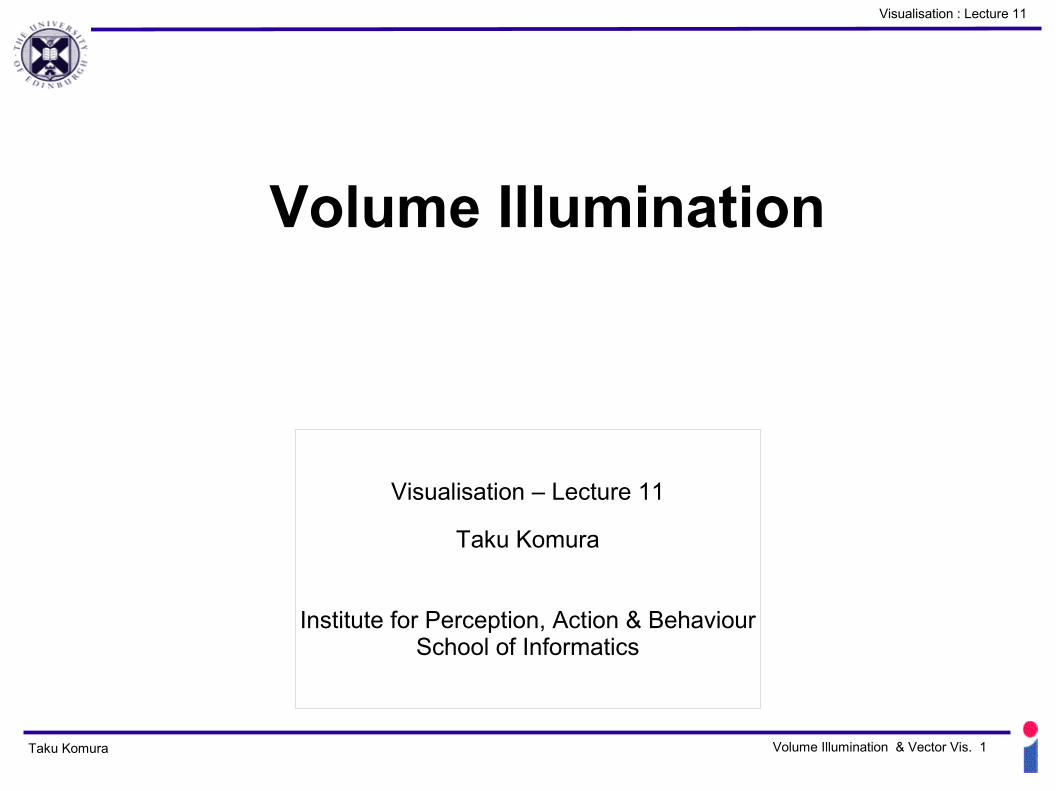
Previously : Volume Rendering● Image Order Volume Rendering

– ray casting / intensity transfer function / opacity transfer function

● Artifacts caused by the sampling method, step size etc.



Shear-warp Algorithm● An efficient method to traverse the volume data

[Lacroute '94]

● Assumes a orthographic camera model– projection perpendicular to image plane



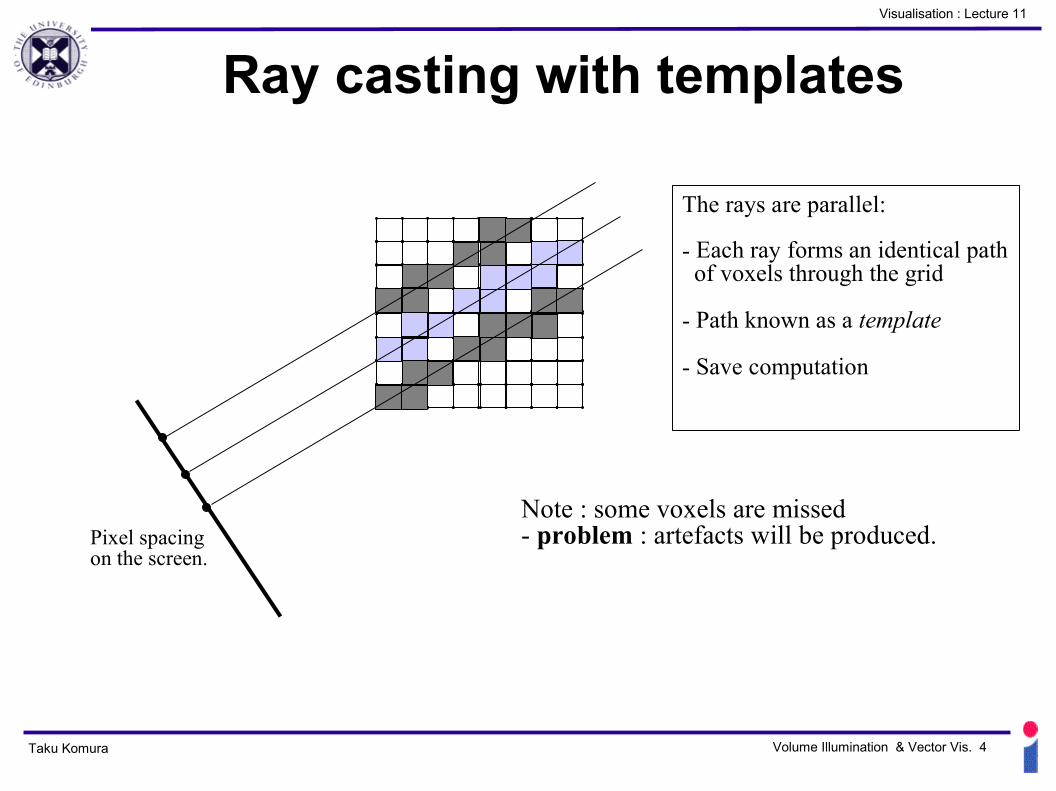
Ray casting with templates

Pixel spacing on the screen.

Note : some voxels are missed- problem : artefacts will be produced.

The rays are parallel:

- Each ray forms an identical path of voxels through the grid

- Path known as a template

- Save computation



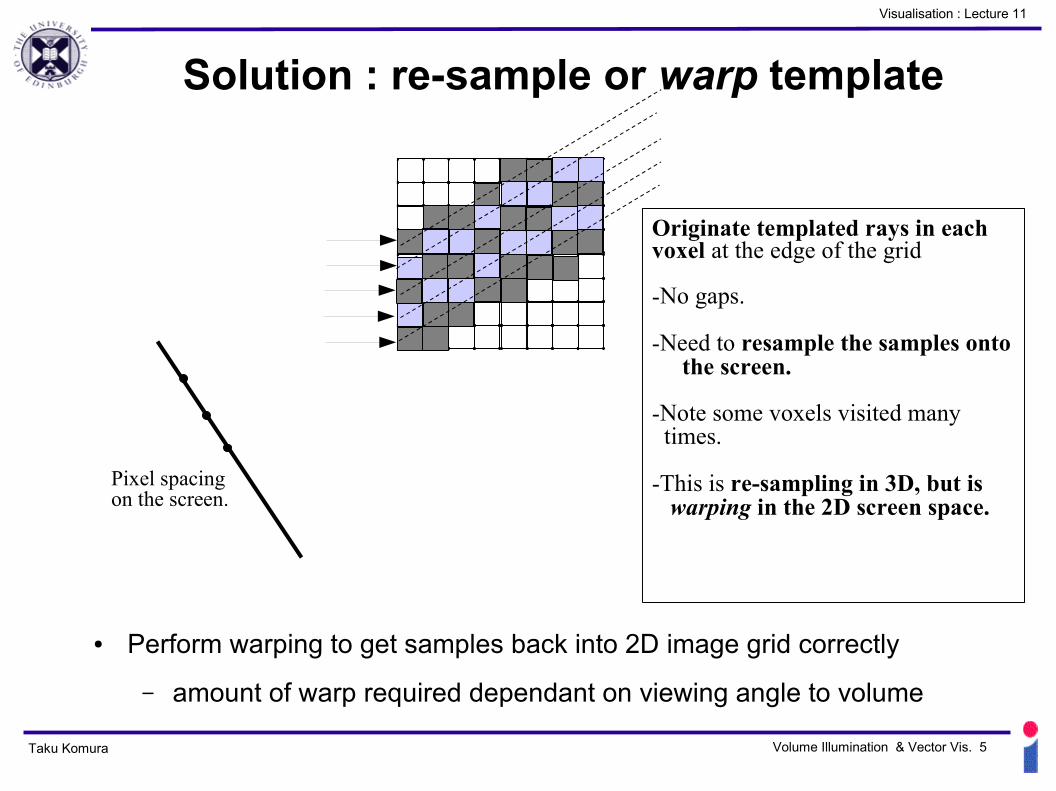
Solution : re-sample or warp template

● Perform warping to get samples back into 2D image grid correctly

– amount of warp required dependant on viewing angle to volume

Originate templated rays in each voxel at the edge of the grid

-No gaps.

-Need to resample the samples onto the screen.

-Note some voxels visited many times.

-This is re-sampling in 3D, but is warping in the 2D screen space.

Pixel spacing on the screen.



Shear-warp factorisation● Instead of traversing along rays, visit voxels in a plane

– regardless of camera viewing angle● Use front-to-back ordering

– support early termination (last lecture) ● Perform final warp on the image due to the shear process

● Improve efficiency using run-length encoding of voxels– Skipping the transparent voxels



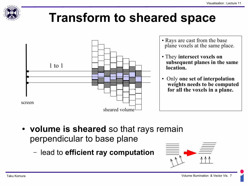
Transform to sheared space

● volume is sheared so that rays remain perpendicular to base plane– lead to efficient ray computation

screen

• Rays are cast from the base plane voxels at the same place.

• They intersect voxels on subsequent planes in the same location.

• Only one set of interpolation weights needs to be computed for all the voxels in a plane.

1 to 1

sheared volume



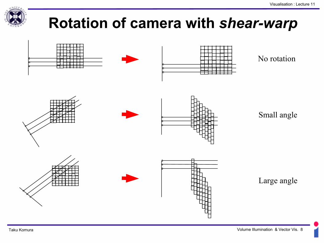
Rotation of camera with shear-warp

No rotation

Small angle

Large angle



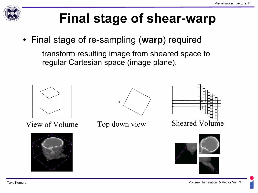
Final stage of shear-warp● Final stage of re-sampling (warp) required

– transform resulting image from sheared space to regular Cartesian space (image plane).

View of Volume Top down view Sheared Volume



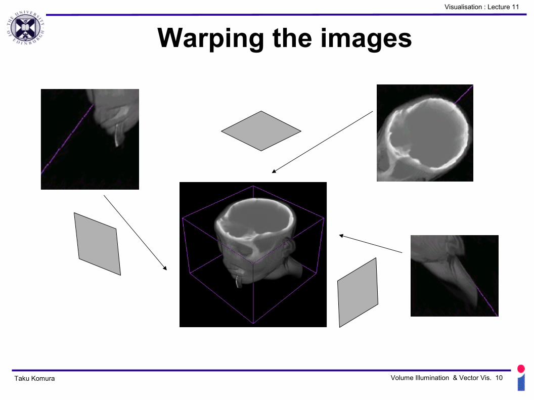
Warping the images



Light Propagation in Volumes● Lighting in volume

– only transmission and emission considered (until now)– can also:

— reflect light— scatter light into different directions



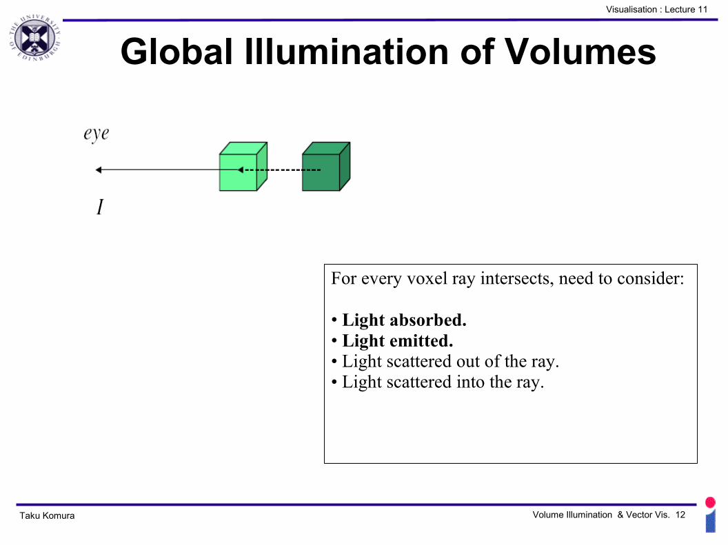
Global Illumination of Volumes

For every voxel ray intersects, need to consider:

• Light absorbed.• Light emitted.• Light scattered out of the ray.• Light scattered into the ray.



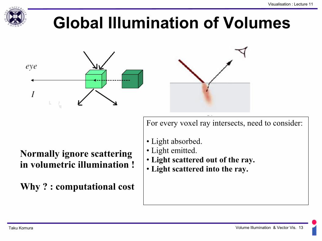
Global Illumination of Volumes

For every voxel ray intersects, need to consider:

• Light absorbed.• Light emitted.• Light scattered out of the ray.• Light scattered into the ray.

Normally ignore scattering in volumetric illumination !

Why ? : computational cost



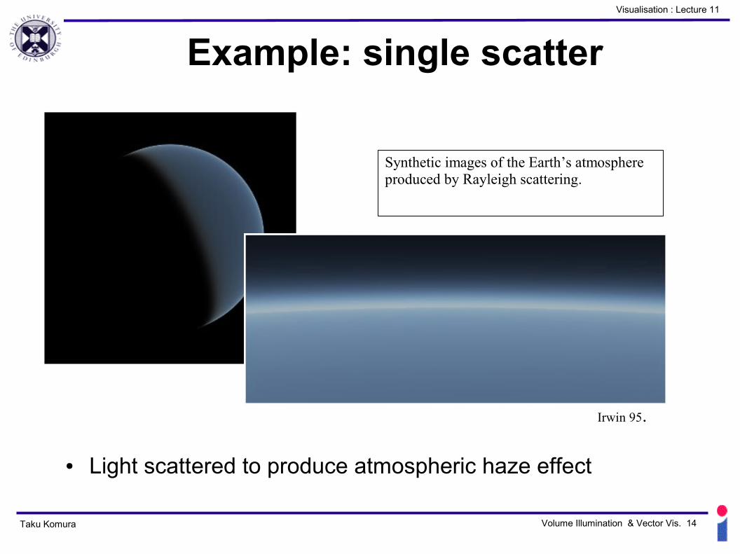
Example: single scatter

● Light scattered to produce atmospheric haze effect

Irwin 95.

Synthetic images of the Earth’s atmosphere produced by Rayleigh scattering.



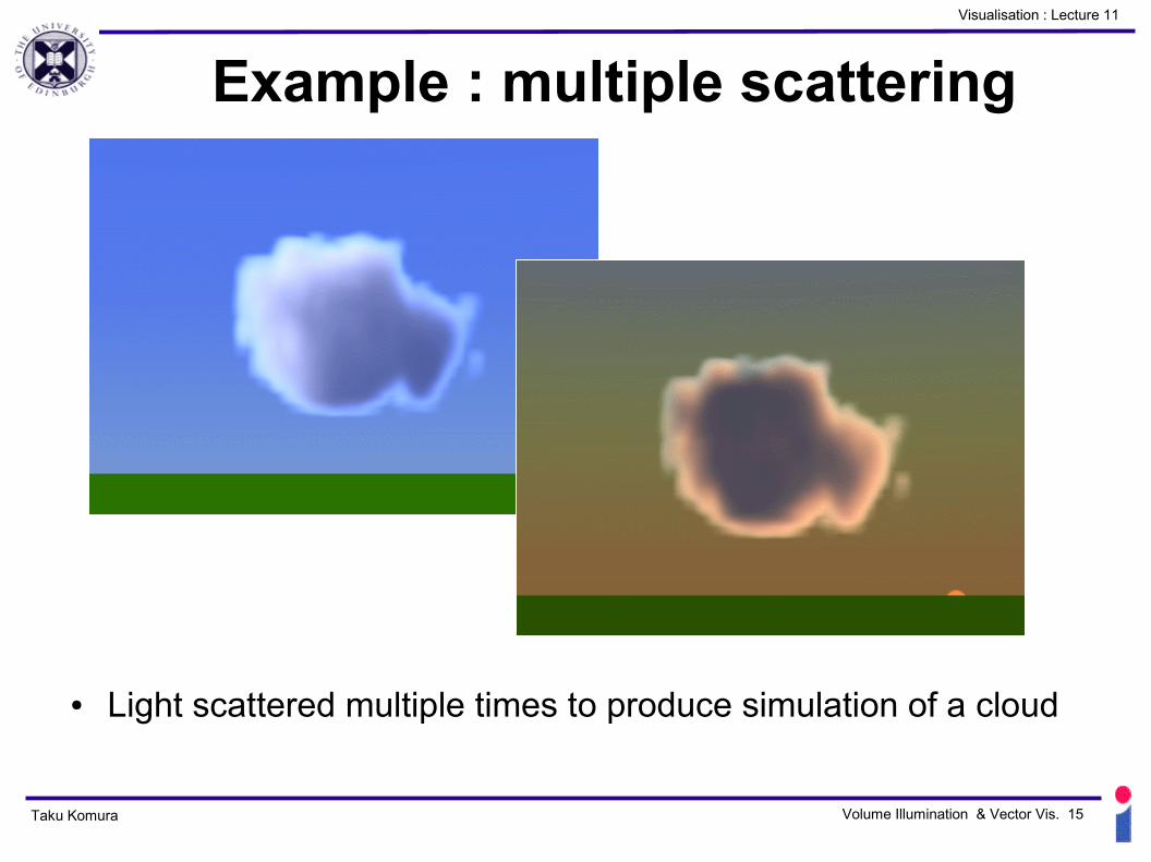
Example : multiple scattering

● Light scattered multiple times to produce simulation of a cloud



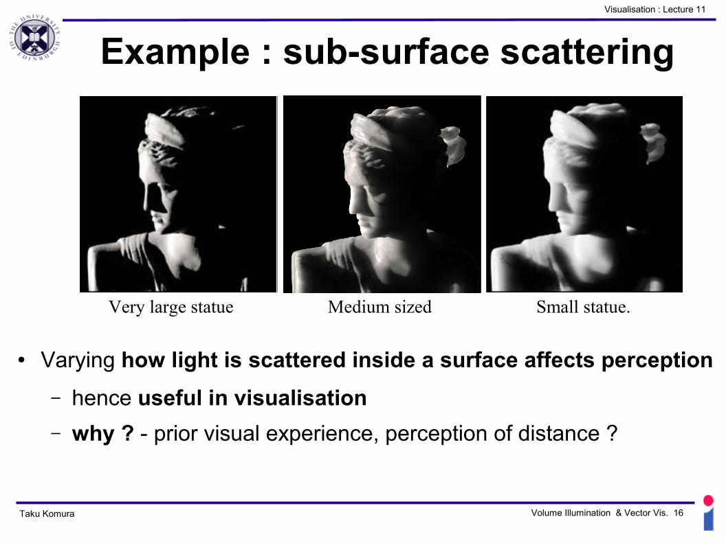
Example : sub-surface scattering

● Varying how light is scattered inside a surface affects perception– hence useful in visualisation– why ? - prior visual experience, perception of distance ?

Very large statue Medium sized Small statue.



Volume Illumination - ?● Scattering is too costly so we usually do not

take them into account when doing volume rendering

● But we still can add slight shadows to the volume by illuminating them



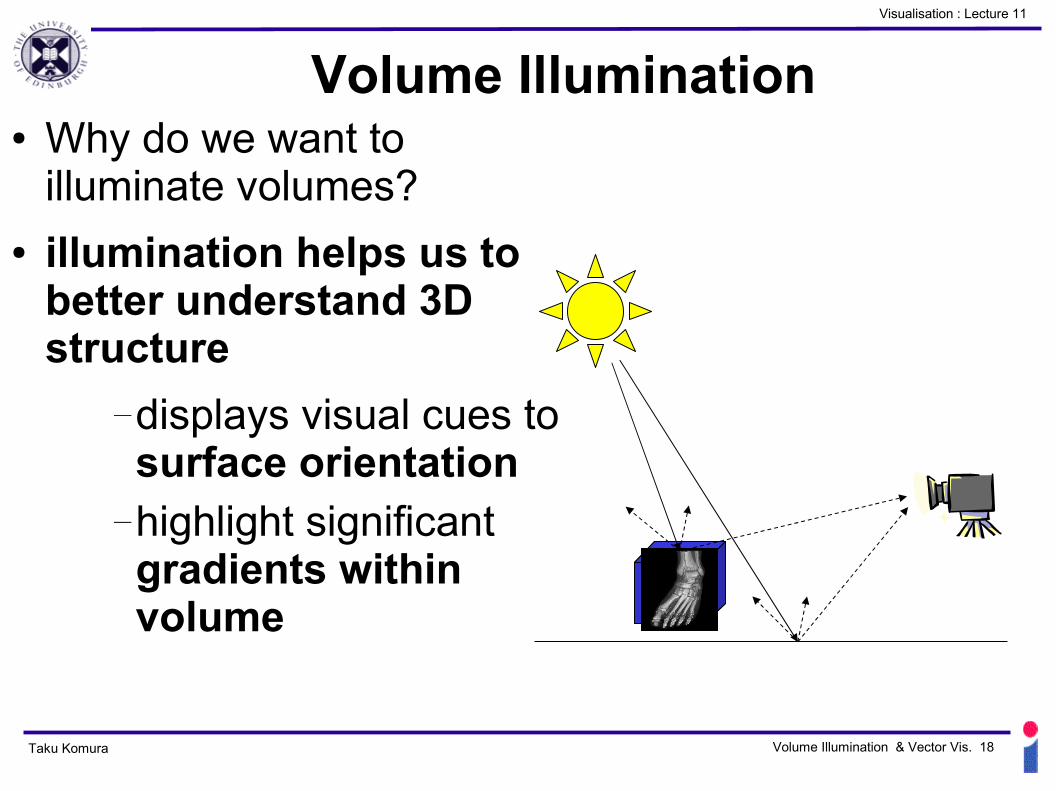
Volume Illumination● Why do we want to

illuminate volumes?● illumination helps us to

better understand 3D structure

—displays visual cues to surface orientation

—highlight significant gradients within volume



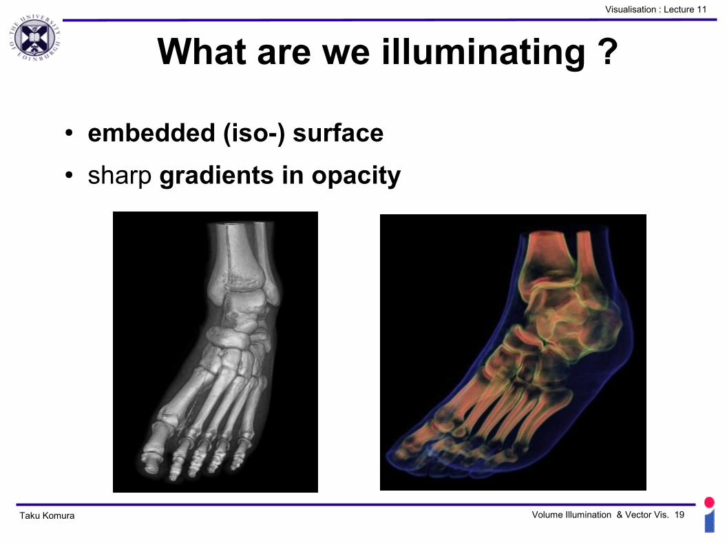
What are we illuminating ?

● embedded (iso-) surface● sharp gradients in opacity



Shading an Embedded iso-surface

● classify volume with a step function● use regular specular / diffuse surface shading● Remember for lighting equations of lecture 2

require– illumination direction– camera model (position)– surface orientation– need to calculate and store surface normal



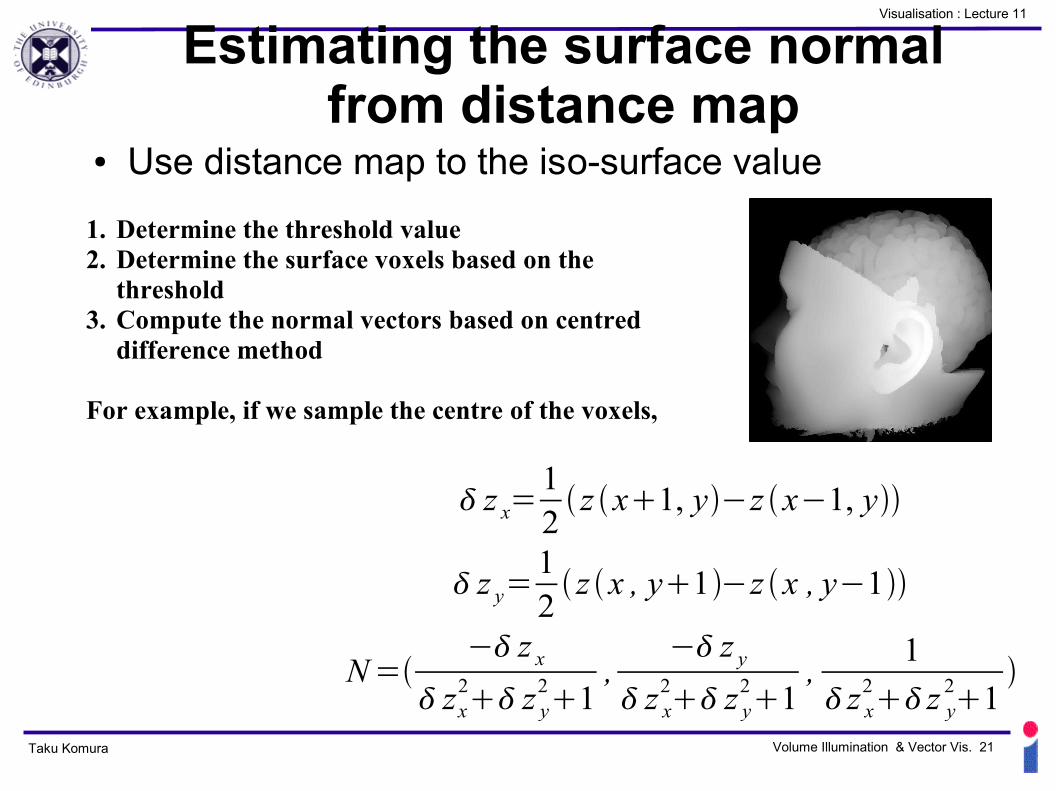
Estimating the surface normal from distance map

● Use distance map to the iso-surface value

1. Determine the threshold value2. Determine the surface voxels based on the

threshold3. Compute the normal vectors based on centred

difference method

For example, if we sample the centre of the voxels,

z x=12 z x1, y−z x−1, y

z y=12 z x , y1−z x , y−1

N=− z x

zx2 z y

21,

− z y

z x2 z y

21, 1 z x

2 z y21



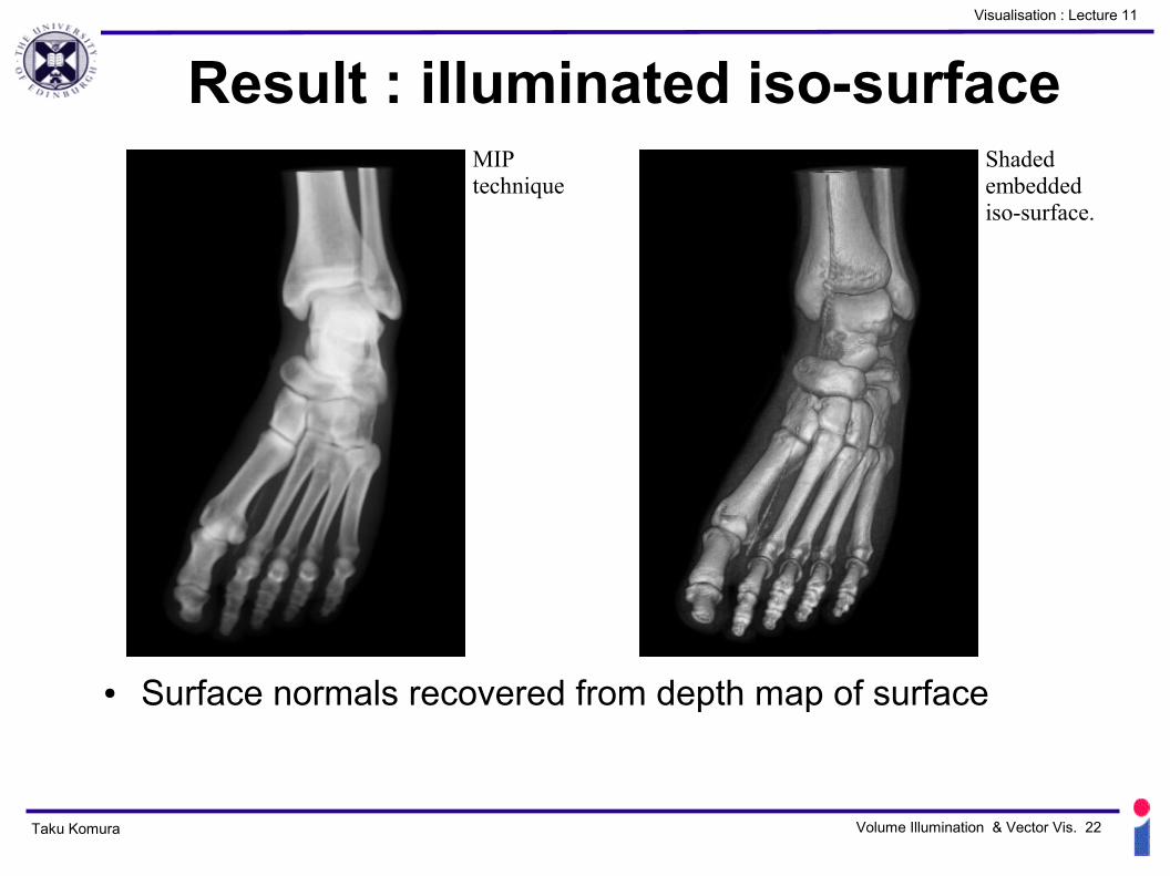
Result : illuminated iso-surface

● Surface normals recovered from depth map of surface

MIP technique

Shaded embedded iso-surface.



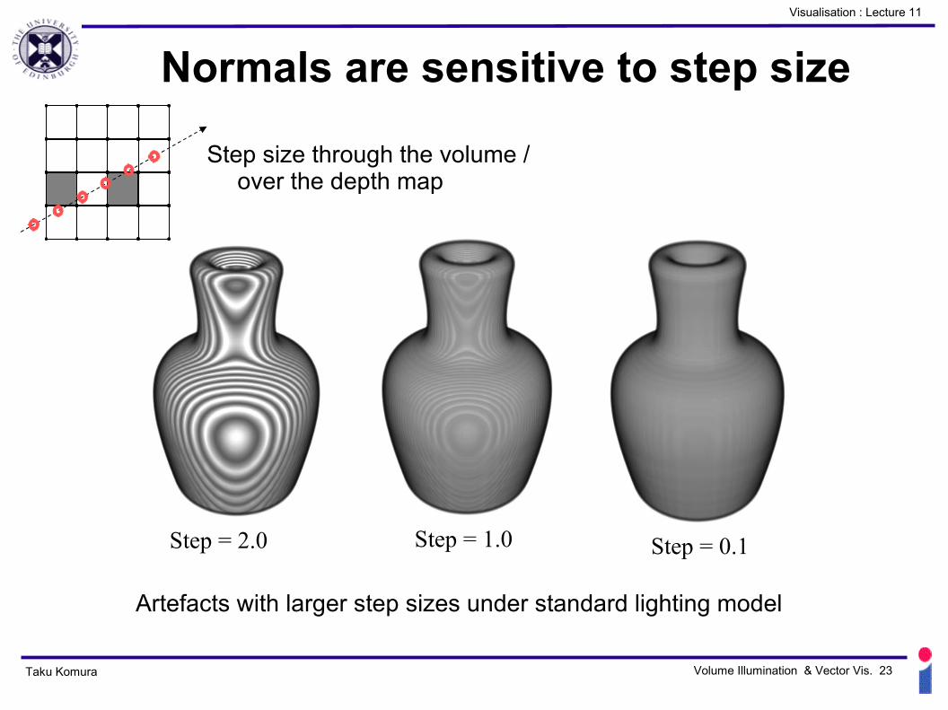
Normals are sensitive to step size

Artefacts with larger step sizes under standard lighting model

Step = 2.0 Step = 1.0 Step = 0.1

Step size through the volume / over the depth map



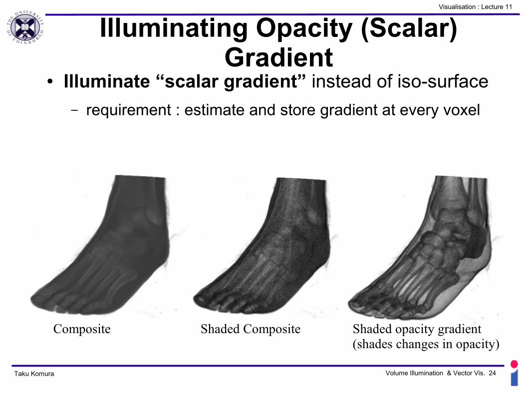
Illuminating Opacity (Scalar) Gradient

● Illuminate “scalar gradient” instead of iso-surface– requirement : estimate and store gradient at every voxel

Composite Shaded Composite Shaded opacity gradient(shades changes in opacity)



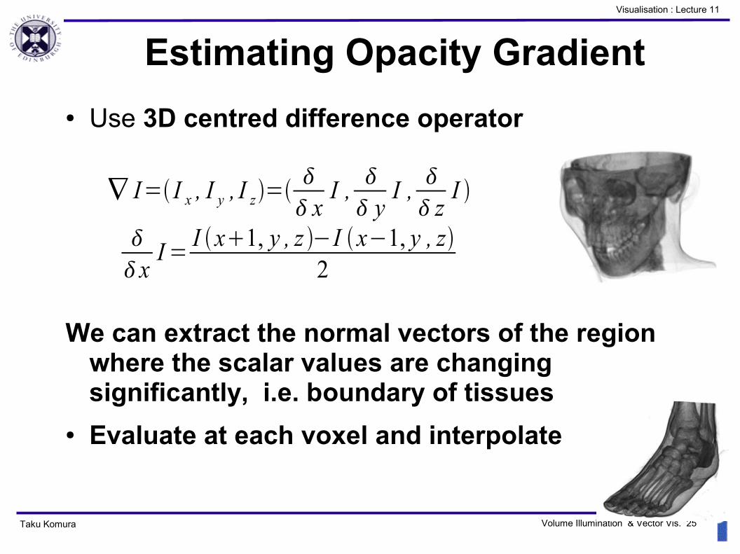
Estimating Opacity Gradient● Use 3D centred difference operator

We can extract the normal vectors of the region where the scalar values are changing significantly, i.e. boundary of tissues

● Evaluate at each voxel and interpolate

∇ I= I x , I y , I z= x

I , y

I , z

I

x

I= I x1, y , z −I x−1, y , z2



Illumination : storing normal vectors

● Visualisation is interactive– compute normal vectors for surface/gradient once– store normal– perform interactive shading calculations

● Storage :– 2563 data set of 1-byte scalars ~16Mb – normal vector (stored as floating point(4-byte)) ~ 200Mb!– Solution : quantise direction & magnitude as small

number of bits



Illumination : storing normal vectors

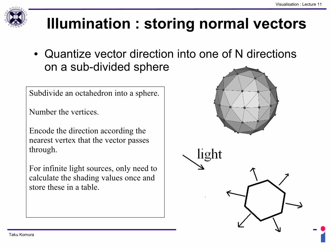
Subdivide an octahedron into a sphere.

Number the vertices.

Encode the direction according the nearest vertex that the vector passes through.

For infinite light sources, only need to calculate the shading values once and store these in a table.

● Quantize vector direction into one of N directions on a sub-divided sphere



Summary

● Shear-Warping● Light scattering● Volume illumination

Documents

Volume Illumination - Ed · PDF fileTaku Komura Volume Illumination & Vector Vis. 26 Visualisation : Lecture 11 Illumination : storing normal vectors ... – perform interactive shading