VOXEL APPROACH TO LANDSCAPE MODELLING - ISPRS

VOXEL APPROACH TO LANDSCAPE MODELLING

Ulla Pyysalo, Tapani Sarjakoski

Finnish Geodetic Institute, Department of Geoinformatics and Cartography – [email protected], [email protected]

Commission IV, WG IV/4

KEY WORDS: Voxel Model, Airborne Laser Scanning, Intensity, Resolution ABSTRACT: In this paper, we present a method for 3D volumetric reconstruction of landscape from airborne laser scanner data. The method applies a voxel model, where volume is divided to sub-volume particles, voxels, associated with a scalar or vector value. In the presented study the voxel model is generated from airborne laser scanner data, which enables measurement of large areas. Laser scanning provides simultaneously 3D co-ordinates and intensity-values for the laser pulses reflected from the surfaces. The typical density of laser data is several points per square meter and instruments are able to register more than one echo of the returning signal. Therefore, airborne laser scanning provides information not just about the ground surface, but also about the objects on top of the ground surface. In the study, several voxel models are derived from two different laser measurement data sets covering the same area. The models are compared and analysed.

1. INTRODUCTION

The use of 3D databases of landscape has increased during last ten years, partly because the need for more detailed and accurate analysis, and partly because the availability of 3D data have increased. Therefore, the research of data models enabling new ways of data usage is of great importance. Typically, in 3D geospatial databases vector or raster data structures are used. Objects in vector data model are represented with x, y and z-co-ordinates, while in raster model the z-co-ordinate is stored as an attribute of each pixel. Alternative type of 3D representation is the volumetric tessellation making use of e.g. voxels. A voxel is a sub-volume particle, associated with a scalar or vector value. This is analogous to a pixel, which represents 2D image data. Applicability and method development for airborne laser data has been under intensive research during last eight years, and developed methods have already replaced traditional photogrammetry in certain processes, such as production of the elevation model. In Finland, there is a production plan to compile a countrywide elevation model, and the data collection has already been initiated. However, the data containing 3D point cloud with reflection intensity could serve the needs for more advanced geospatial products than only digital elevation models. Importance of advanced methods for laser data will increase in the future, because the amount of available data will increase. Voxel models have traditionally been used in virtual reality applications and computer graphics, for example in game industry. One reason for this is that adjacency and connectivity of voxel particles is implicit in a voxel model. However, in many of these examples the environment to be modelled is virtual. In the presented study, the voxel model will be based on airborne laser scanning of real landscape. Therefore, the model provides input for large number of geospatial landscape analysis purposes.

In the proposed study airborne laser scanner data is used to produce a 3D voxel model of a terrain.

2. BACKGROUND

2.1 Previous studies

The voxel structures have been applied in geospatial application for about two decades already, since the analysis of 3D processes and the study of volume domains are in interest of many scientific fields (Karssenberg, 2005). Applications include environmental modelling for purposes such as geology (Jones, 1989), archaeology (Losiera et al., 2007) and change monitoring. The voxel models have been typically used for visualization (Marschallinger, 1996). Nowadays also some open-source GIS software packages support voxel structures (Neteier, Mitasova, 2002). Since the introduction of airborne laser scanning, the laser derived voxel models have been used in several purposes. Forest structure has been studied by calculating the laser point distribution in different canopy layers within each voxel (Chasmer et al., 2004; Lee et al., 2004; Lucas et al., 2005). A tree shape reconstruction using voxels has been carried out, and mathematical morphology operations introduced for 2D grid have been tested (Gorte and Pfeifer, 2004). The new airborne measurement mode, full waveform scanning, has been applied for visualization purposes (Persson et al., 2005; Töpel, 2005) and tree canopy representation (Litkey et al., 2007). Usage for other purposes has been introduced as well. The landmark based navigation system for cars was studied using voxels and visibility analysis (Brenner and Elias, 2003). The reconstruction of buildings using voxels has been carried for airborne laser data (Tarsha-Kurdi et al., 2007). Methods developed for reconstruction of surfaces and shapes for terrestrial laser data have been tested for airborne data as well (Vosselman et al., 2004).

563

The International Archives of the Photogrammetry, Remote Sensing and Spatial Information Sciences. Vol. XXXVII. Part B4. Beijing 2008

2.2 Objectives

The objective of the study is to develop methods for producing 3D voxel model representation of real landscape using airborne laser scanner data as input. The detailed research objectives are:

• to create voxel models with different resolutions and to compare models generated from two different measurement data

• to define several attributes for each voxel, based on the laser points and their intensities

• to test the classified voxel model approach

3. MATERIALS

3.1 Test area and measurement campaign

Finnish Geodetic Institute has set up an extensive test environment for research purposes in the area located in Nuuksio lake uplands, southern Finland, covering currently about 240 km2 (Sarjakoski et al., 2007). The area has been laser scanned in two parts, in 2006 and 2007. For both scans the geometry and other key parameters were the same (see Table 1).

Platform Aeroplane Flying height 1000 m

Maximum scanning angle ± 10 ° Point density Minimum 3/m2

Intensity Yes Echoes First, last, middle

Trajectory information Yes Table 1. Measurement parameters for the Nuuksio laser

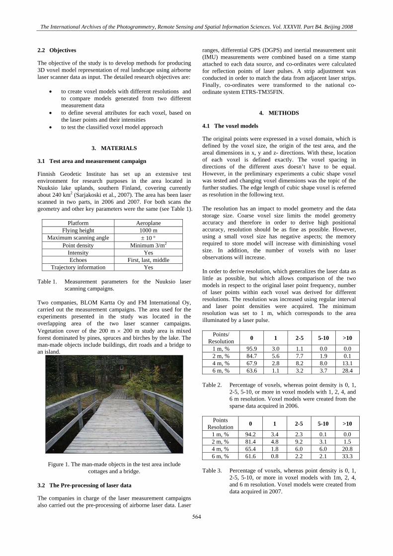
scanning campaigns. Two companies, BLOM Kartta Oy and FM International Oy, carried out the measurement campaigns. The area used for the experiments presented in the study was located in the overlapping area of the two laser scanner campaigns. Vegetation cover of the 200 m × 200 m study area is mixed forest dominated by pines, spruces and birches by the lake. The man-made objects include buildings, dirt roads and a bridge to an island.

Figure 1. The man-made objects in the test area include cottages and a bridge.

3.2 The Pre-processing of laser data

The companies in charge of the laser measurement campaigns also carried out the pre-processing of airborne laser data. Laser

ranges, differential GPS (DGPS) and inertial measurement unit (IMU) measurements were combined based on a time stamp attached to each data source, and co-ordinates were calculated for reflection points of laser pulses. A strip adjustment was conducted in order to match the data from adjacent laser strips. Finally, co-ordinates were transformed to the national co-ordinate system ETRS-TM35FIN.

4. METHODS

4.1 The voxel models

The original points were expressed in a voxel domain, which is defined by the voxel size, the origin of the test area, and the areal dimensions in x, y and z- directions. With these, location of each voxel is defined exactly. The voxel spacing in directions of the different axes doesn’t have to be equal. However, in the preliminary experiments a cubic shape voxel was tested and changing voxel dimensions was the topic of the further studies. The edge length of cubic shape voxel is referred as resolution in the following text. The resolution has an impact to model geometry and the data storage size. Coarse voxel size limits the model geometry accuracy and therefore in order to derive high positional accuracy, resolution should be as fine as possible. However, using a small voxel size has negative aspects; the memory required to store model will increase with diminishing voxel size. In addition, the number of voxels with no laser observations will increase. In order to derive resolution, which generalizes the laser data as little as possible, but which allows comparison of the two models in respect to the original laser point frequency, number of laser points within each voxel was derived for different resolutions. The resolution was increased using regular interval and laser point densities were acquired. The minimum resolution was set to 1 m, which corresponds to the area illuminated by a laser pulse.

Points/

Resolution 0 1 2-5 5-10 >10

1 m, % 95.9 3.0 1.1 0.0 0.0 2 m, % 84.7 5.6 7.7 1.9 0.1 4 m, % 67.9 2.8 8.2 8.0 13.1 6 m, % 63.6 1.1 3.2 3.7 28.4

Table 2. Percentage of voxels, whereas point density is 0, 1,

2-5, 5-10, or more in voxel models with 1, 2, 4, and 6 m resolution. Voxel models were created from the sparse data acquired in 2006.

Points

Resolution 0 1 2-5 5-10 >10

1 m, % 94.2 3.4 2.3 0.1 0.0 2 m, % 81.4 4.8 9.2 3.1 1.5 4 m, % 65.4 1.8 6.0 6.0 20.8 6 m, % 61.6 0.8 2.2 2.1 33.3

Table 3. Percentage of voxels, whereas point density is 0, 1,

2-5, 5-10, or more in voxel models with 1m, 2, 4, and 6 m resolution. Voxel models were created from data acquired in 2007.

564


Tables 2 and 3 show that portion of 1 point/voxel density reaches maximum using 2 m resolution. The small point density was favoured, since in a fusion of several measurements into a single voxel, co-ordinate information of measurements is lost. With 2 m resolution, the >10 class is still relatively small. Also the different characteristics of the two data sets can be observed from Tables 2 and 3. Since the second data was acquired with different laser scanning implementation, the average point density was higher, approximately 8 points/m2. However, this value contains the areas with overlapping measurement stripes. Without these areas, the average density is approximately 4 points/m2. The same parameter for the previous measurement is 2 points/m2. In all models, which were formed from 2006 acquired data, portion of voxels without any laser points is larger than in models created in 2007. By increasing the resolution, the point density obviously increases for all voxel models. 4.2 The voxel attributes

Two different representations were generated based on the two data sets, namely a binary model and a density model. The most simple one, binary model, was formed by addressing all voxels with one or more laser hits inside as 1 and the others, voxels without any hits, as 0 (Figure 2, upper row). The density model was formed, as explained previously, by counting the number of laser points within each voxel (Figure 2, lower row).

• 0/1, binary model • point count, density model

Three intensity attributes for voxels were formed by taking into account intensities of echoes within each voxel. The statistical parameters derived from these were:

• sum of intensities • mean of intensities • standard deviation of intensities

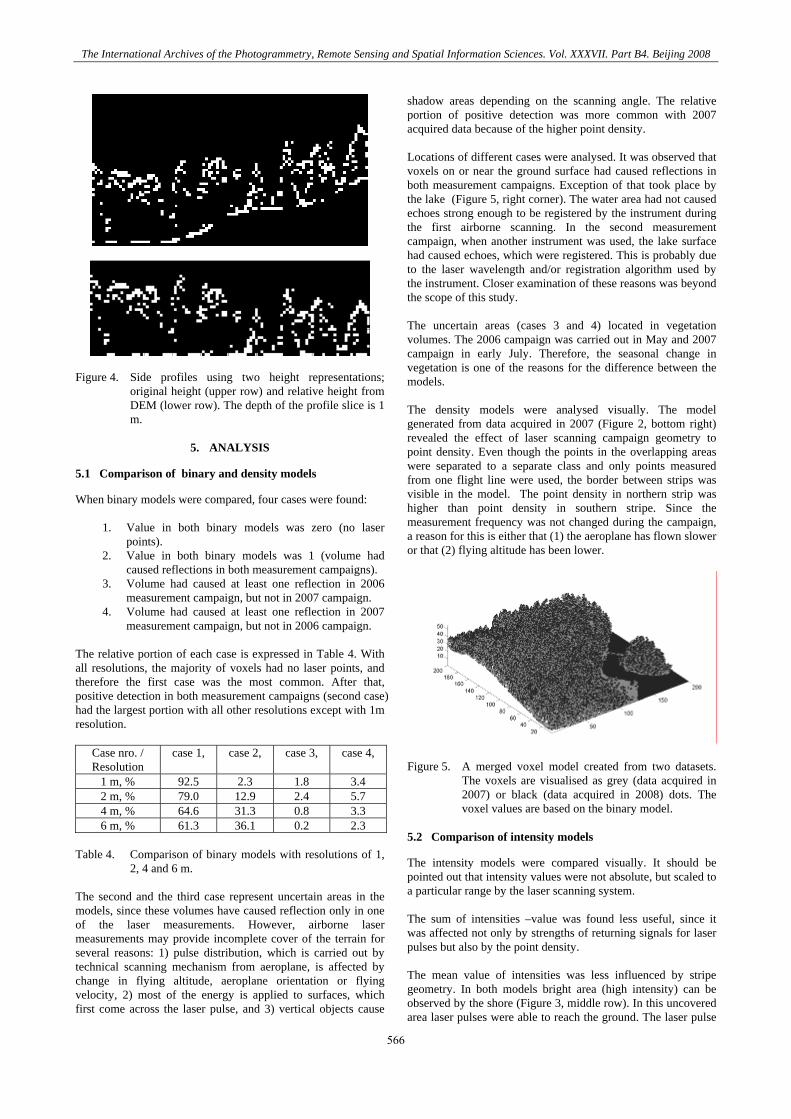
Figure 2. Binary models (upper) and density models (lower) created from datasets acquired in 2006 (left column) and dataset acquired in 2007 (right column). In these top view illustrations, one voxel layer is represented.

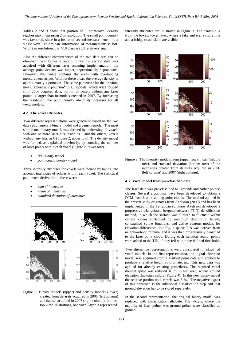
Intensity attributes are illustrated in Figure 3. The example is from the lowest voxel layer, where a lake surface, a shore line and a bridge to an island are visible.

Figure 3. The intensity models: sum (upper row), mean (middle

row), and standard deviation (bottom row) of the intensities created from datasets acquired in 2006 (left column) and 2007 (right column).

4.3 Voxel model from pre-classified data

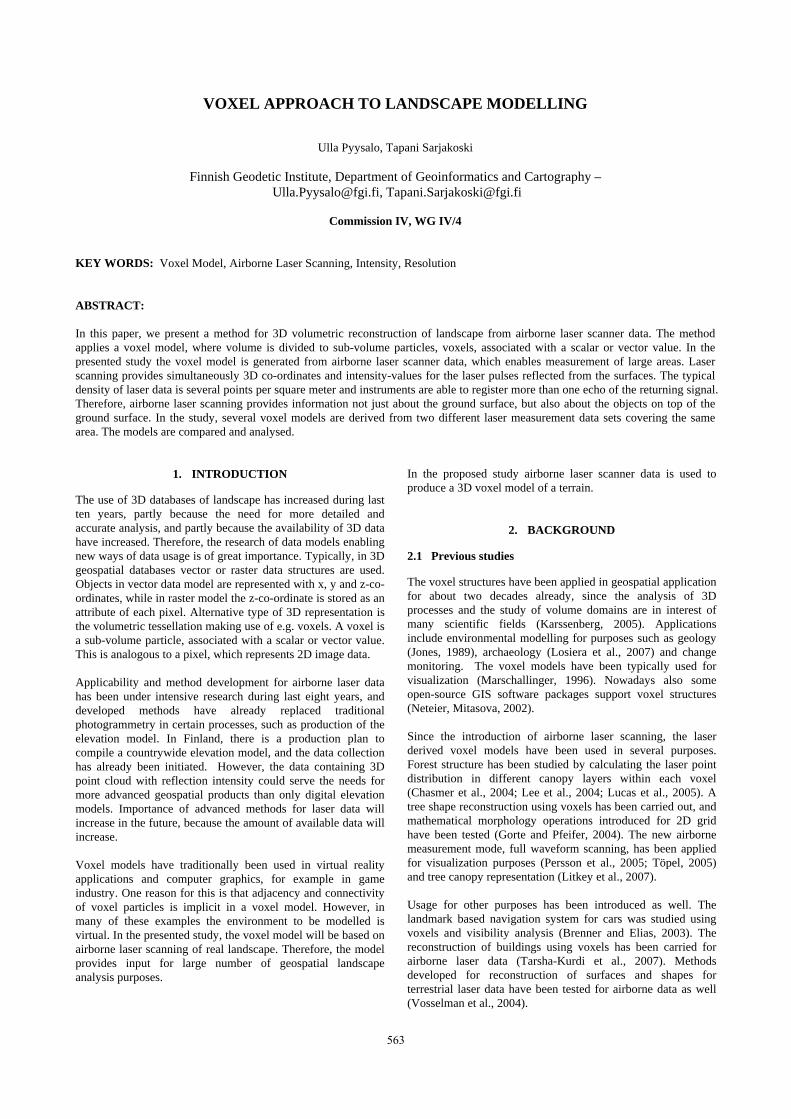
The laser data was pre-classified to ‘ground’ and ‘other points’ classes. Several algorithms have been developed to obtain a DTM from laser scanning point clouds. The method applied in the present study originates from Axelsson (2000) and has been implemented in the TerraScan software. Axelsson developed a progressive triangulated irregular network (TIN) densification method, in which the surface was allowed to fluctuate within certain values controlled by minimum description length, constrained spline functions, and active contour models for elevation differences. Initially, a sparse TIN was derived from neighbourhood minima, and it was then progressively densified to the laser point cloud. During each iteration round, points were added to the TIN, if they fell within the defined thresholds. Two alternative representations were considered for classified voxel models. In the first representation, the digital elevation model was acquired from classified point data and applied to produce a relative height co-ordinate, hzh. This new data was applied for already existing procedures. The required voxel domain space was reduced 40 % in test area, where ground elevation fluctuates mildly (Figure 4). In this new binary model the relative portion on 1-voxels was 5 %. The negative aspect of this approach is the additional classification step and that ground elevation has to be stored separately. In the second representation, the original binary model was replaced with classification attribute. The voxels, where the majority of laser points was ground points were classified as ground.

565


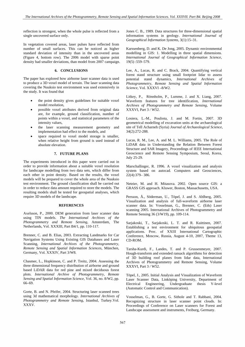
Figure 4. Side profiles using two height representations; original height (upper row) and relative height from DEM (lower row). The depth of the profile slice is 1 m.

5. ANALYSIS

5.1 Comparison of binary and density models

When binary models were compared, four cases were found:

1. Value in both binary models was zero (no laser points).

2. Value in both binary models was 1 (volume had caused reflections in both measurement campaigns).

3. Volume had caused at least one reflection in 2006 measurement campaign, but not in 2007 campaign.

4. Volume had caused at least one reflection in 2007 measurement campaign, but not in 2006 campaign.

The relative portion of each case is expressed in Table 4. With all resolutions, the majority of voxels had no laser points, and therefore the first case was the most common. After that, positive detection in both measurement campaigns (second case) had the largest portion with all other resolutions except with 1m resolution.

Case nro. / Resolution

case 1,

case 2,

case 3,

case 4,

1 m, % 92.5 2.3 1.8 3.4 2 m, % 79.0 12.9 2.4 5.7 4 m, % 64.6 31.3 0.8 3.3 6 m, % 61.3 36.1 0.2 2.3

Table 4. Comparison of binary models with resolutions of 1,

2, 4 and 6 m. The second and the third case represent uncertain areas in the models, since these volumes have caused reflection only in one of the laser measurements. However, airborne laser measurements may provide incomplete cover of the terrain for several reasons: 1) pulse distribution, which is carried out by technical scanning mechanism from aeroplane, is affected by change in flying altitude, aeroplane orientation or flying velocity, 2) most of the energy is applied to surfaces, which first come across the laser pulse, and 3) vertical objects cause

shadow areas depending on the scanning angle. The relative portion of positive detection was more common with 2007 acquired data because of the higher point density. Locations of different cases were analysed. It was observed that voxels on or near the ground surface had caused reflections in both measurement campaigns. Exception of that took place by the lake (Figure 5, right corner). The water area had not caused echoes strong enough to be registered by the instrument during the first airborne scanning. In the second measurement campaign, when another instrument was used, the lake surface had caused echoes, which were registered. This is probably due to the laser wavelength and/or registration algorithm used by the instrument. Closer examination of these reasons was beyond the scope of this study. The uncertain areas (cases 3 and 4) located in vegetation volumes. The 2006 campaign was carried out in May and 2007 campaign in early July. Therefore, the seasonal change in vegetation is one of the reasons for the difference between the models. The density models were analysed visually. The model generated from data acquired in 2007 (Figure 2, bottom right) revealed the effect of laser scanning campaign geometry to point density. Even though the points in the overlapping areas were separated to a separate class and only points measured from one flight line were used, the border between strips was visible in the model. The point density in northern strip was higher than point density in southern stripe. Since the measurement frequency was not changed during the campaign, a reason for this is either that (1) the aeroplane has flown slower or that (2) flying altitude has been lower.

Figure 5. A merged voxel model created from two datasets.

The voxels are visualised as grey (data acquired in 2007) or black (data acquired in 2008) dots. The voxel values are based on the binary model.

5.2 Comparison of intensity models

The intensity models were compared visually. It should be pointed out that intensity values were not absolute, but scaled to a particular range by the laser scanning system. The sum of intensities –value was found less useful, since it was affected not only by strengths of returning signals for laser pulses but also by the point density. The mean value of intensities was less influenced by stripe geometry. In both models bright area (high intensity) can be observed by the shore (Figure 3, middle row). In this uncovered area laser pulses were able to reach the ground. The laser pulse

566


reflection is strongest, when the whole pulse is reflected from a single uncovered surface only. In vegetation covered areas, laser pulses have reflected from number of small surfaces. This can be noticed as higher standard deviation of intensity than in the uncovered areas (Figure 4, bottom row). The 2006 model with sparse point density had smaller deviations, than model from 2007 campaign.

6. CONCLUSIONS

The paper has explored how airborne laser scanner data is used to produce a 3D voxel model of terrain. The laser scanning data covering the Nuuksio test environment was used extensively in the study. It was found that

• the point density gives guidelines for suitable voxel model resolution,

• possible voxel attributes derived from original data are, for example, ground classification, number of points within a voxel, and statistical parameters of the intensity values,

• the laser scanning measurement geometry and implementation had effect to the models, and

• space required to voxel model storage is smaller, when relative height from ground is used instead of absolute elevation.

7. FUTURE PLANS

The experiments introduced in this paper were carried out in order to provide information about a suitable voxel resolution for landscape modelling from two data sets, which differ from each other in point density. Based on the results, the voxel models will be prepared to cover the whole area of the Nuuksio test environment. The ground classification shall be carried out in order to reduce data amount required to store the models. The resulting models shall be tested for geospatial analyses, which require 3D models of the landscape.

REFERENCES

Axelsson, P., 2000. DEM generation from laser scanner data using TIN models. The International Archives of the Photogrammetry and Remote Sensing, Amsterdam, The Netherlands, Vol. XXXIII, Part B4/1, pp. 110-117. Brenner, C. and B. Elias, 2003. Extracting Landmarks for Car Navigation Systems Using Existing GIS Databases and Laser Scanning, International Archives of the Photogrammetry, Remote Sensing and Spatial Information Sciences, München, Germany, Vol. XXXIV, Part 3/W8. Chasmer, L., Hopkinson, C. and P. Treitz, 2004. Assessing the three dimensional frequency distribution of airborne and ground based LiDAR data for red pine and mixed deciduous forest plots. International Archive of Photogrammetry, Remote Sensing and Spatial Information Science, Vol. 36, no. 8/W2, pp. 66–69. Gorte, B. and N. Pfeifer, 2004. Structuring laser scanned trees using 3d mathematical morphology. International Archives of Photogrammetry and Remote Sensing, Istanbul, Turkey.Vol. XXXV.

Jones C. B., 1989. Data structures for three-dimensional spatial information systems in geology. International Journal of Geographical Information Systems, 3(1):15–31. Karssenberg, D. and K. De Jong, 2005. Dynamic environmental modelling in GIS: 1. Modelling in three spatial dimensions. International Journal of Geographical Information Science, 19(5) :559–579. Lee, A., Lucas, R. and C. Brack, 2004. Quantifying vertical forest stand structure using small footprint lidar to assess potential stand dynamics, International Archives of Photogrammetry, Remote Sensing and Spatial Information Science, Vol. XXXVI –8/W2. Litkey, P., Rönnholm, P., Lumme, J. and X. Liang, 2007. Waveform features for tree identification, International Archives of Photogrammetry and Remote Sensing, Volume XXXVI, Part 3 / W52. Losiera, L.-M., Pouliota, J. and M. Fortin, 2007. 3D geometrical modelling of excavation units at the archaeological site of Tell Acharneh (Syria) Journal of Archaeological Science, 34(2):272-288. Lucas, R. M., Lee, A. and M. L. Williams, 2005. The Role of LiDAR data in Understanding the Relation Between Forest Structure and SAR Imagery, Proceedings of IEEE International Geoscience and Remote Sensing Symposium, Seoul, Korea, July 25-29. Marschallinger, R. 1996. A voxel visualization and analysis system based on autocad. Computers and Geosciences, 22(4):379– 386. Neteier, M. and H. Mitasova. 2002. Open source GIS: a GRASS GIS approach. Kluwer, Boston, Massachusetts, USA. Persson, Å., Söderman, U., Töpel, J. and S. Ahlberg, 2005. Visualization and analysis of full-waveform airborne laser scanner data. In: Vosselman, G., Brenner, C. (Eds) Laser scanning 2005. International Archives of Photogrammetry and Remote Sensing 36 (3/W19), pp. 109-114. Sarjakoski, T., Sarjakoski, L. T. and R. Kuittinen, 2007. Establishing a test environment for ubiquitous geospatial applications. Proc. of XXIII International Cartographic Conference, Moscow, Russia, August 4-10, 2007, Theme 13, CD-ROM. Tarsha-Kurdi, F., Landes, T. and P. Grussenmeyer, 2007. Hough-transform and extended ransack algorithms for detection of 3D building roof planes from lidar data, International Archives of Photogrammetry and Remote Sensing, Volume XXXVI, Part 3 / W52. Töpel, J., 2005. Initial Analysis and Visualization of Waveform Laser Scanner Data, Linköping University, Department of Electrical Engineering, Undergraduate thesis Y-level (Automatic Control and Communication). Vosselman, G., B. Gorte, G. Sithole and T. Rabbani, 2004. Recognizing structure in laser scanner point clouds. In: Proceedings of Conference on Laser scanners for Forest and Landscape assessment and instruments, Freiburg, Germany.

567


568

Documents

VOXEL APPROACH TO LANDSCAPE MODELLING - ISPRS