Embed Size (px)
DESCRIPTION
Water Vapor in the Air. How do we compute the dewpoint temperature, the relative humidity, or the temperature of a rising air parcel inside a cloud? Here we investigate parameters that describe water in our atmosphere. Water Vapor in the Air. Outline: - PowerPoint PPT Presentation
Citation preview
Thermodynamics M. D. Eastin
Water Vapor in the Air
How do we compute the dewpoint temperature, the relative humidity, or the temperature of a rising air parcel inside a cloud?
Here we investigate parameters that describe water in our atmosphere
Thermodynamics M. D. Eastin
Outline:
Review of the Clausius-Clapeyron Equation Review of our Atmosphere as a System
Basic parameters that describe moist air Definitions Application: Use of Skew-T Diagrams
Parameters that describe atmospheric processes for moist air Isobaric Cooling Adiabatic – Isobaric processes Adiabatic expansion (or compression)
Unsaturated Saturated
Application: Use of Skew-T Diagrams
Additional useful parameters Summary
Water Vapor in the Air
Thermodynamics M. D. Eastin
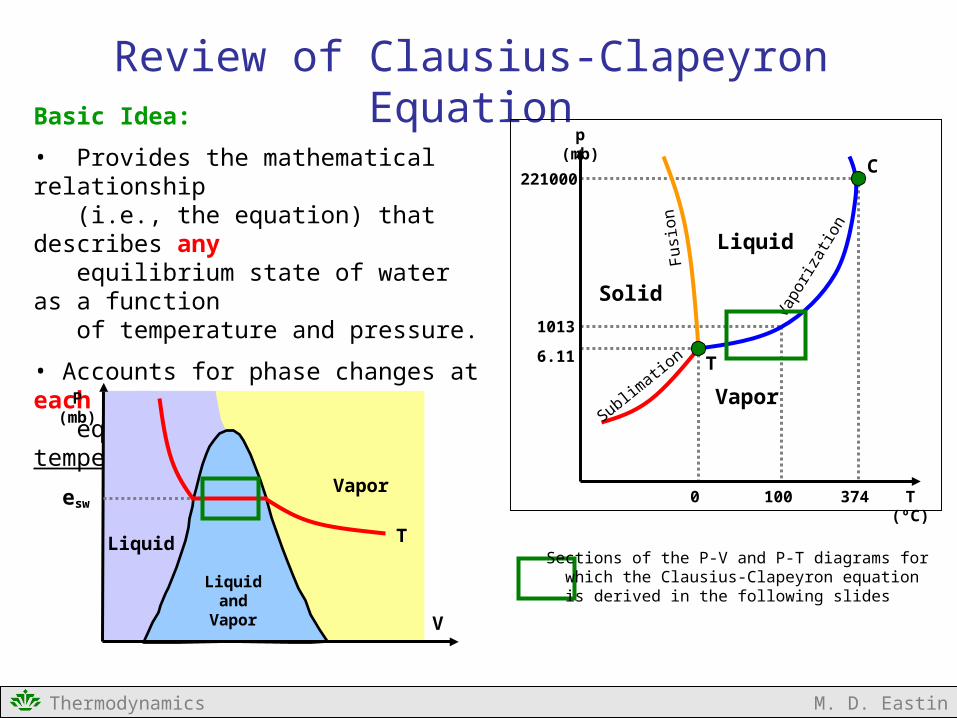
Basic Idea:
• Provides the mathematical relationship (i.e., the equation) that describes any equilibrium state of water as a function of temperature and pressure.
• Accounts for phase changes at each equilibrium state (each temperature)
Review of Clausius-Clapeyron Equation
Sublimatio
n
Fus
ion
Vap
oriz
atio
n
T
C
T (ºC)
p (mb)
3741000
6.11
1013
221000
Liquid
Vapor
Solid
V
P(mb)
Vapor
Liquid
Liquidand
Vapor
T
esw
Sections of the P-V and P-T diagrams for which the Clausius-Clapeyron equation is derived in the following slides
Thermodynamics M. D. Eastin
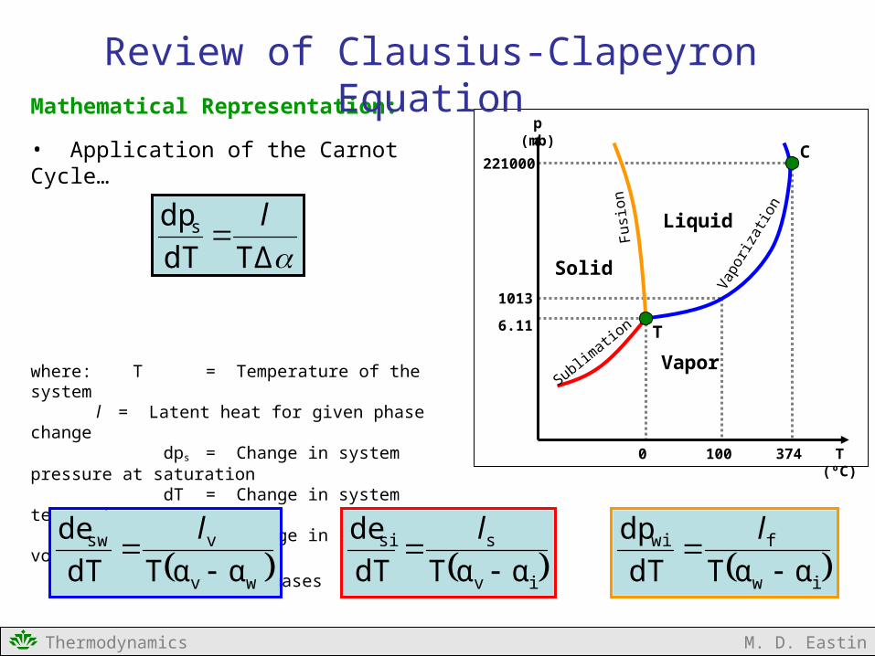
Mathematical Representation:
• Application of the Carnot Cycle…
where: T = Temperature of the system l = Latent heat for given phase change dps= Change in system pressure at saturation dT = Change in system temperature Δα = Change in specific volumes between
the two phases
wv
vsw
ααTdT
de
l
Sublimatio
n
Fus
ion
Vap
oriz
atio
n
T
C
T (ºC)
p (mb)
3741000
6.11
1013
221000
Liquid
Vapor
Solid
iv
ssi
ααTdT
de
l
iw
fwi
ααTdT
dp
l
TΔdT
dps l
Review of Clausius-Clapeyron Equation
Thermodynamics M. D. Eastin
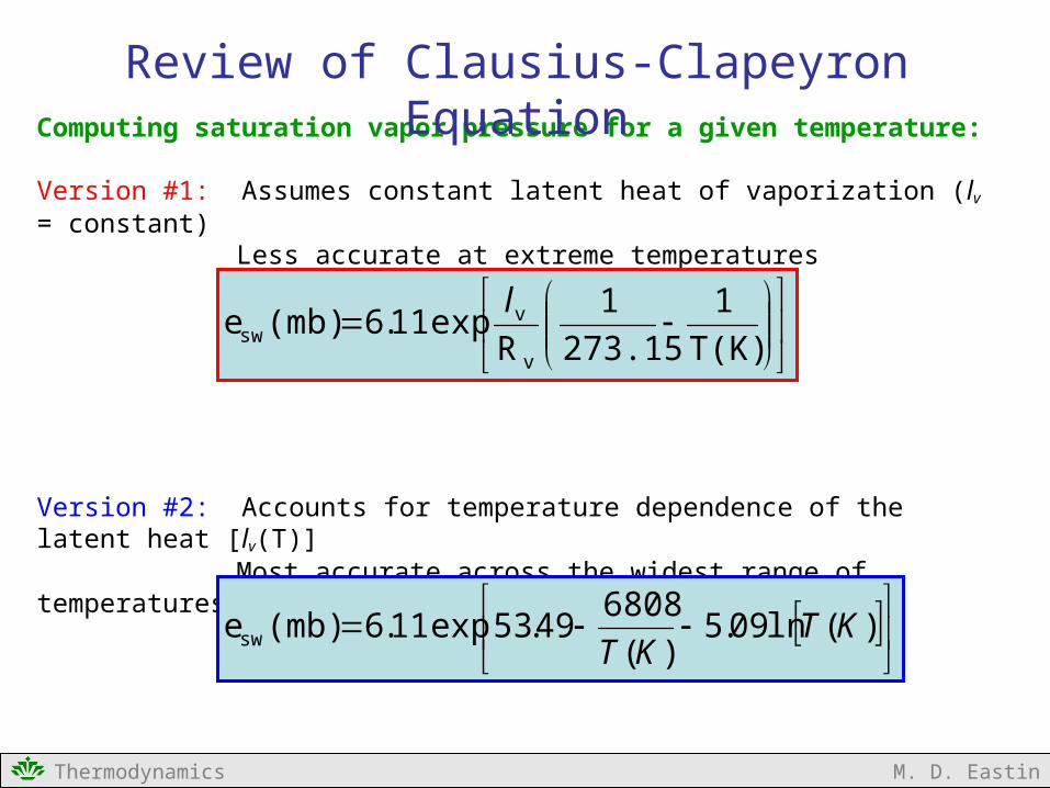
Computing saturation vapor pressure for a given temperature:
Version #1: Assumes constant latent heat of vaporization (lv = constant) Less accurate at extreme temperatures
Version #2: Accounts for temperature dependence of the latent heat [lv(T)] Most accurate across the widest range of temperatures
T(K)
1
273.15
1
Rexp11.6(mb)e
v
vsw
l
)(ln09.5
)(
680849.53exp11.6(mb)esw KT
KT
Review of Clausius-Clapeyron Equation
Thermodynamics M. D. Eastin
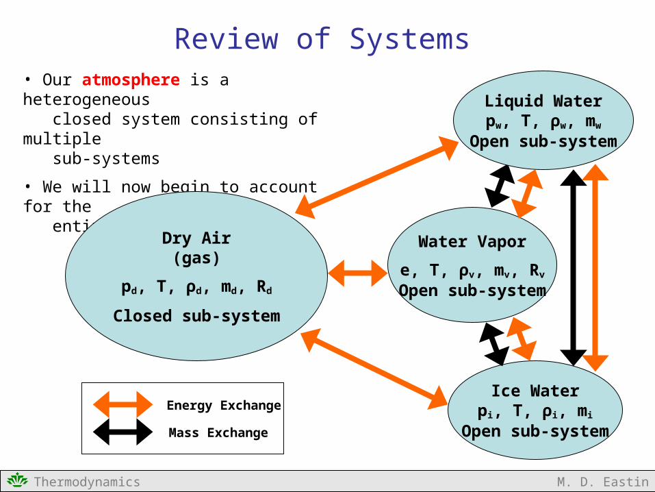
• Our atmosphere is a heterogeneous closed system consisting of multiple sub-systems
• We will now begin to account for the entire system…
Review of Systems
Water Vapor
e, T, ρv, mv, Rv
Open sub-system
Ice Waterpi, T, ρi, mi
Open sub-system
Dry Air(gas)
pd, T, ρd, md, Rd
Closed sub-system
Liquid Waterpw, T, ρw, mw
Open sub-system
Energy Exchange
Mass Exchange
Thermodynamics M. D. Eastin
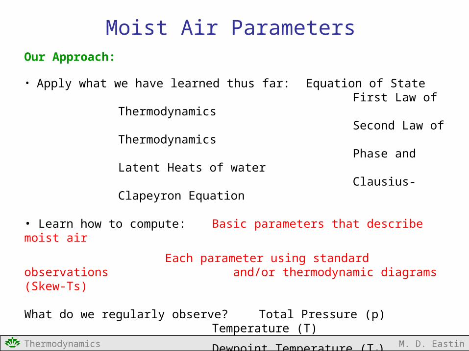
Our Approach:
• Apply what we have learned thus far: Equation of StateFirst Law of
ThermodynamicsSecond Law of
ThermodynamicsPhase and Latent
Heats of waterClausius-
Clapeyron Equation
• Learn how to compute: Basic parameters that describe moist air
Each parameter using standard observations and/or thermodynamic diagrams (Skew-Ts)
What do we regularly observe? Total Pressure (p)Temperature (T)
Dewpoint Temperature (Td) or
Relative Humidity (r)
Moist Air Parameters
Thermodynamics M. D. Eastin
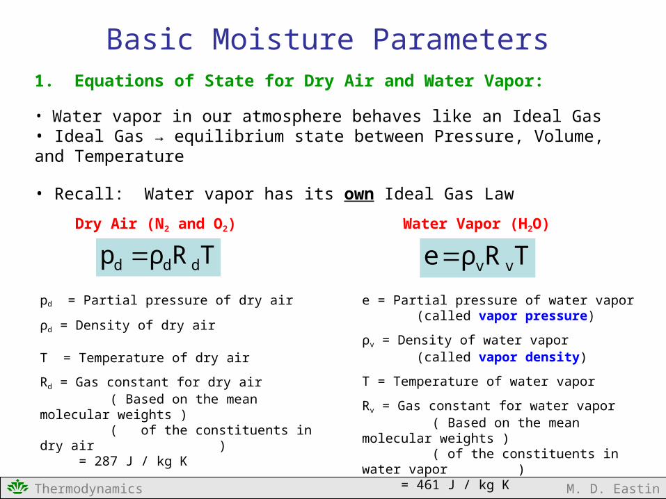
1. Equations of State for Dry Air and Water Vapor:
• Water vapor in our atmosphere behaves like an Ideal Gas • Ideal Gas → equilibrium state between Pressure, Volume, and Temperature
• Recall: Water vapor has its own Ideal Gas Law
Basic Moisture Parameters
TRρp ddd TRρe vvDry Air (N2 and O2) Water Vapor (H2O)
pd = Partial pressure of dry air
ρd = Density of dry air
T = Temperature of dry air
Rd = Gas constant for dry air ( Based on the mean molecular weights ) ( of the constituents in dry air ) = 287 J / kg K
e = Partial pressure of water vapor (called vapor pressure)
ρv = Density of water vapor (called vapor density)
T = Temperature of water vapor
Rv = Gas constant for water vapor ( Based on the mean molecular weights ) ( of the constituents in water vapor ) = 461 J / kg K
Thermodynamics M. D. Eastin
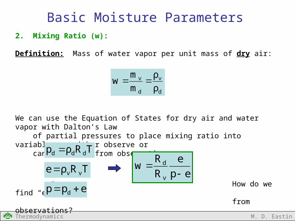
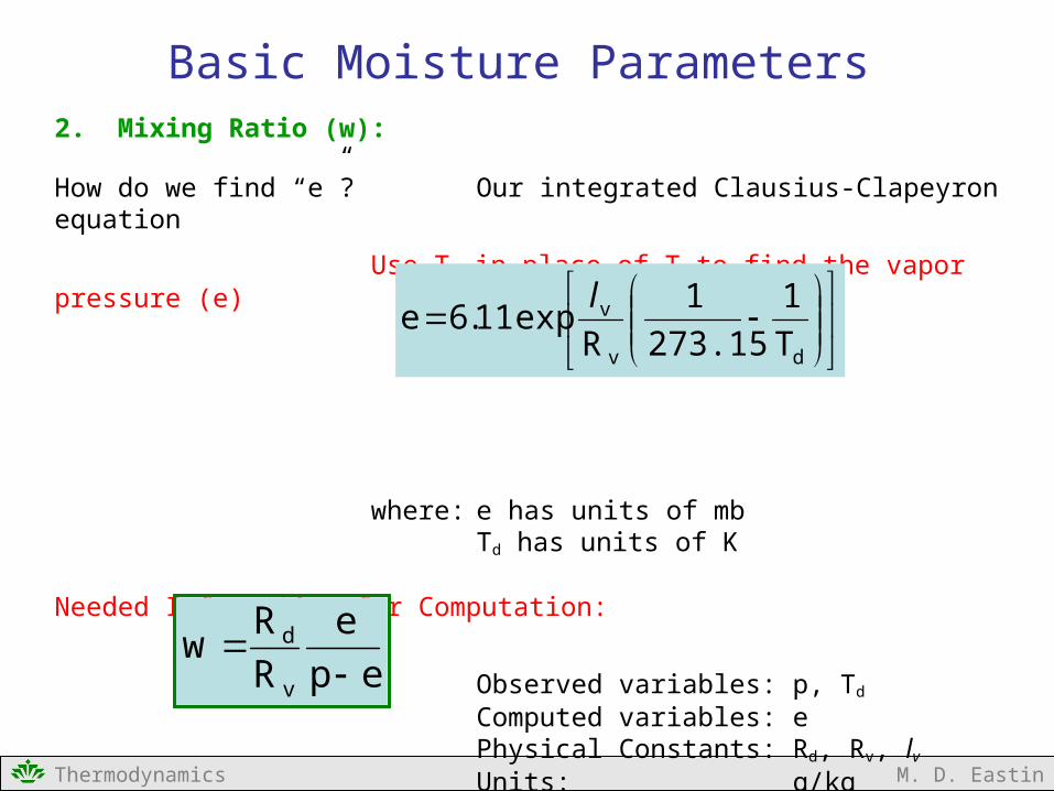
2. Mixing Ratio (w):
Definition: Mass of water vapor per unit mass of dry air:
We can use the Equation of States for dry air and water vapor with Dalton’s Law of partial pressures to place mixing ratio into variables we either observe or can calculate from observations:
How do we find “e” from observations?
d
v
d
v
ρ
ρ
m
mw
ep
e
R
Rw
v
d
TRρp ddd
TRρe vv
ep p d
Basic Moisture Parameters
Thermodynamics M. D. Eastin
2. Mixing Ratio (w):
How do we find “e”? Our integrated Clausius-Clapeyron equation
Use Td in place of T to find the vapor pressure (e)
where: e has units of mbTd has units of K
Needed Information for Computation:
Observed variables: p, Td
Computed variables: ePhysical Constants: Rd, Rv, lv
Units: g/kg
dv
v
T
1
273.15
1
Rexp11.6e
l
ep
e
R
Rw
v
d
Basic Moisture Parameters
Thermodynamics M. D. Eastin
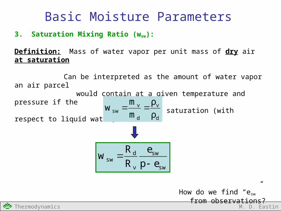
3. Saturation Mixing Ratio (wsw):
Definition: Mass of water vapor per unit mass of dry air at saturation
Can be interpreted as the amount of water vapor an air parcel would contain at a given temperature and pressure if the
parcel was at saturation (with respect to liquid water)
How do we find “esw” from observations?
sw
sw
v
dsw ep
e
R
Rw
d
v
d
vsw ρ
ρ
m
mw
Basic Moisture Parameters
Thermodynamics M. D. Eastin
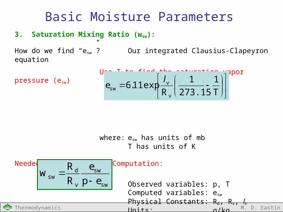
3. Saturation Mixing Ratio (wsw):
How do we find “esw”? Our integrated Clausius-Clapeyron equation
Use T to find the saturation vapor pressure (esw)
where: esw has units of mbT has units of K
Needed Information for Computation:
Observed variables: p, TComputed variables: esw
Physical Constants: Rd, Rv, lv
Units: g/kgsw
sw
v
dsw ep
e
R
Rw
T
1
273.15
1
Rexp11.6e
v
vsw
l
Basic Moisture Parameters
Thermodynamics M. D. Eastin
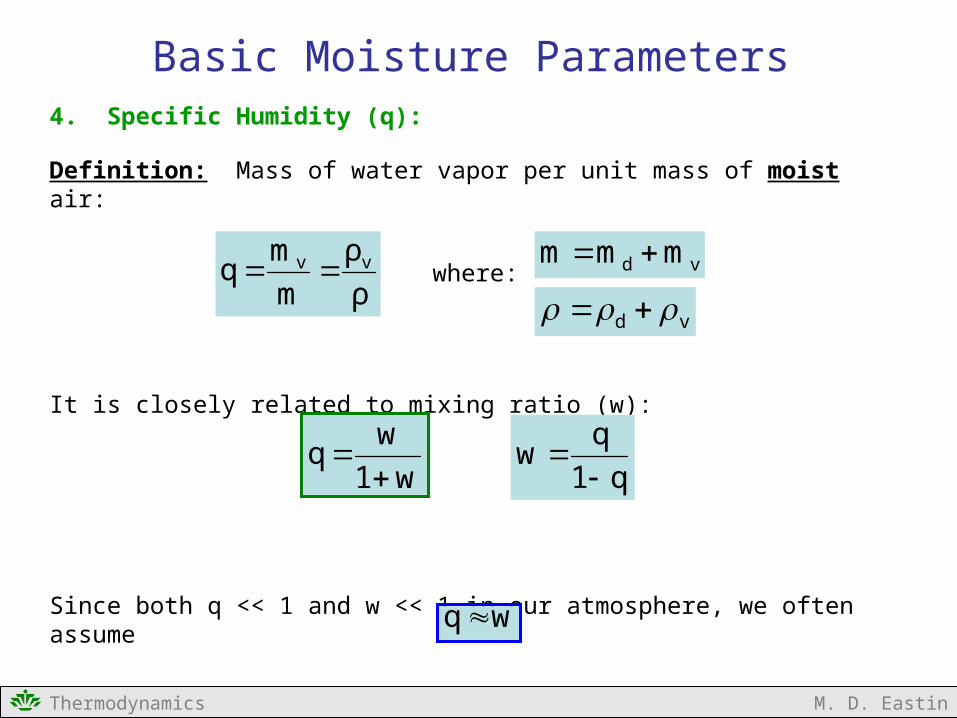
4. Specific Humidity (q):
Definition: Mass of water vapor per unit mass of moist air:
where:
It is closely related to mixing ratio (w):
Since both q << 1 and w << 1 in our atmosphere, we often assume
ρ
ρ
m
mq vv vd mmm
vd
w1
wq
q1
qw
wq
Basic Moisture Parameters
Thermodynamics M. D. Eastin
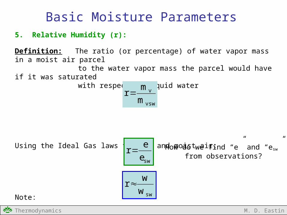
5. Relative Humidity (r):
Definition: The ratio (or percentage) of water vapor mass in a moist air parcel to the water vapor mass the parcel would have if it was saturated with respect to liquid water
Using the Ideal Gas laws for dry and moist air:
Note:
vsw
v
m
mr
swe
er How do we find “e” and “esw”
from observations?
sww
wr
Basic Moisture Parameters
Thermodynamics M. D. Eastin
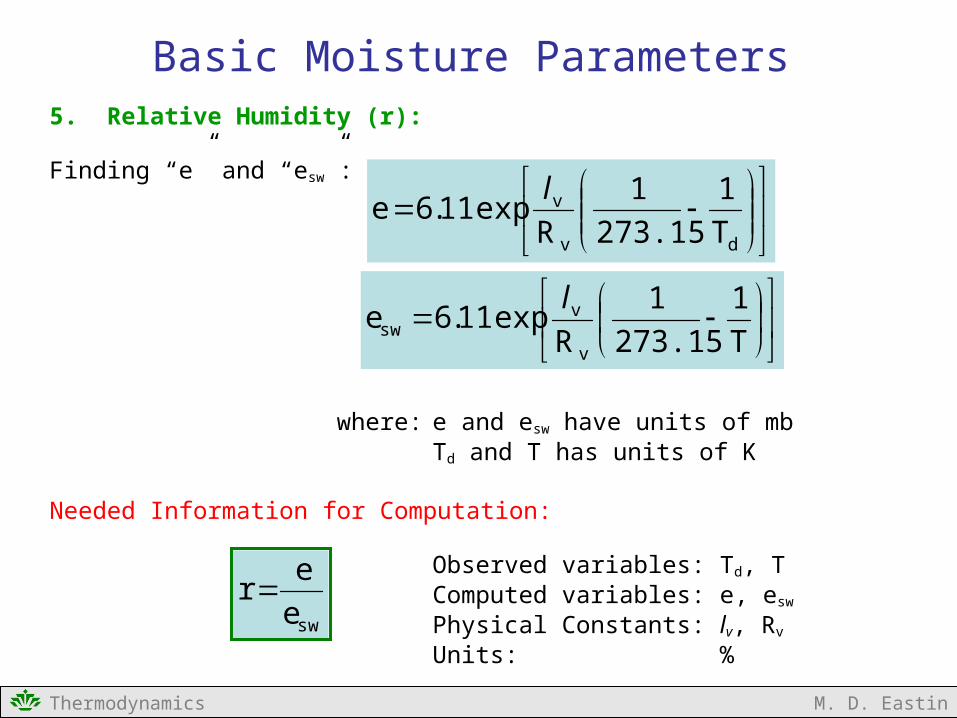
5. Relative Humidity (r):
Finding “e” and “esw”:
where: e and esw have units of mbTd and T has units of K
Needed Information for Computation:
Observed variables: Td, TComputed variables: e, esw
Physical Constants: lv, Rv
Units: %
T
1
273.15
1
Rexp11.6e
v
vsw
l
dv
v
T
1
273.15
1
Rexp11.6e
l
swe
er
Basic Moisture Parameters
Thermodynamics M. D. Eastin
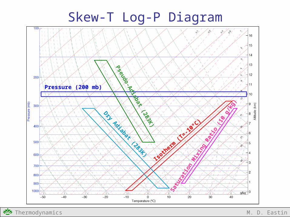
Skew-T Log-P Diagram
Isotherm
(T=-1
0ºC)
Satu
ratio
n M
ixin
g R
atio
(10
g/kg
)
Pressure (200 mb)
Dry Adiabat (283K)
Pseudo-A
diabat (283K)
Thermodynamics M. D. Eastin
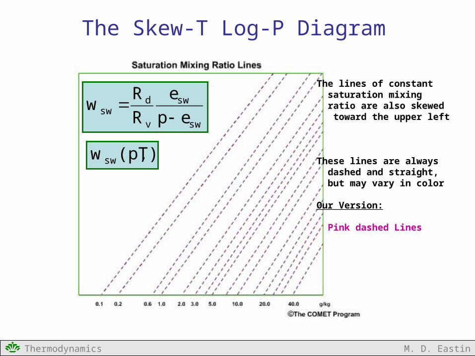
The Skew-T Log-P Diagram
The lines of constant saturation mixing ratio are also skewed toward the upper left
These lines are always dashed and straight, but may vary in color
Our Version:
Pink dashed Lines
sw
sw
v
dsw ep
e
R
Rw
T)(p,w sw
Thermodynamics M. D. Eastin
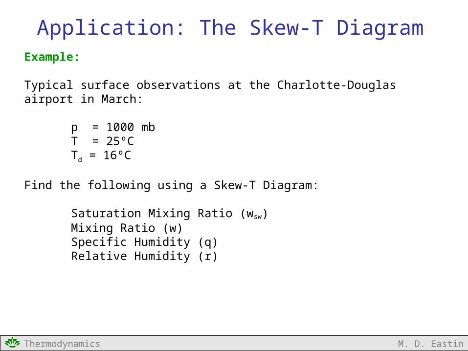
Example:
Typical surface observations at the Charlotte-Douglas airport in March:
p = 1000 mbT = 25ºCTd = 16ºC
Find the following using a Skew-T Diagram:
Saturation Mixing Ratio (wsw)Mixing Ratio (w)Specific Humidity (q)Relative Humidity (r)
Application: The Skew-T Diagram
Thermodynamics M. D. Eastin
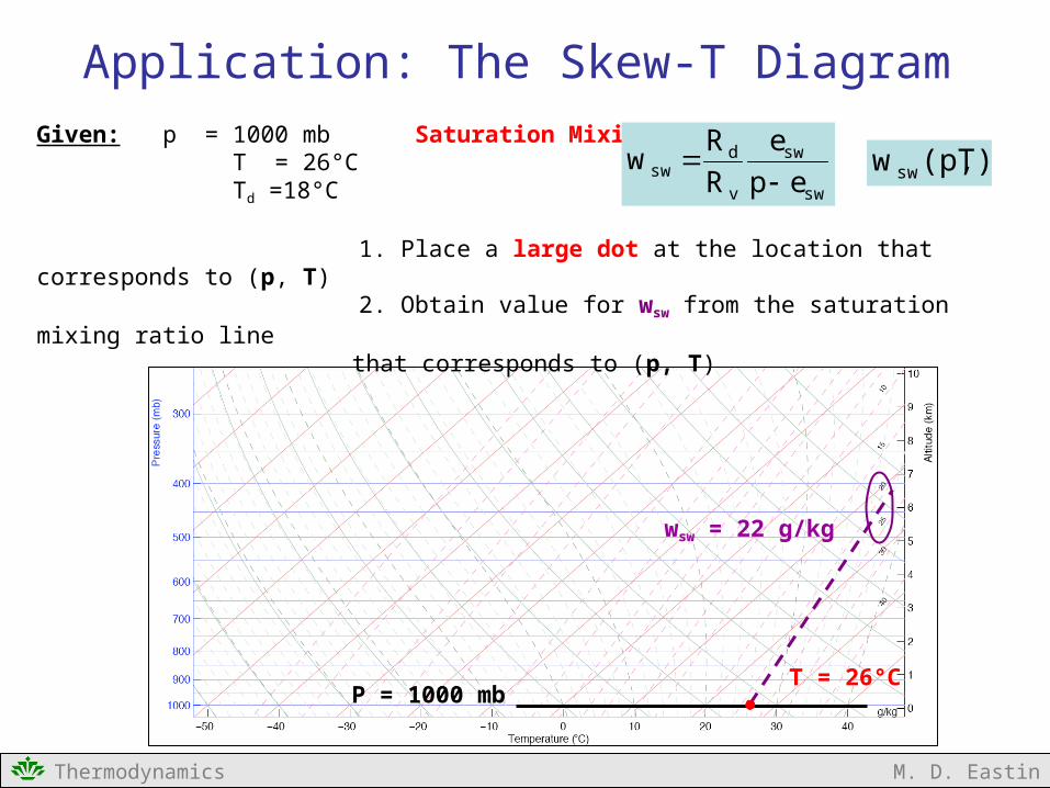
Given: p = 1000 mb Saturation Mixing Ratio: T = 26°C Td =18°C
1. Place a large dot at the location that corresponds to (p, T) 2. Obtain value for wsw from the saturation mixing ratio line
that corresponds to (p, T)
T = 26°CP = 1000 mb
wsw = 22 g/kg
Application: The Skew-T Diagram
sw
sw
v
dsw ep
e
R
Rw
T)(p,w sw
Thermodynamics M. D. Eastin
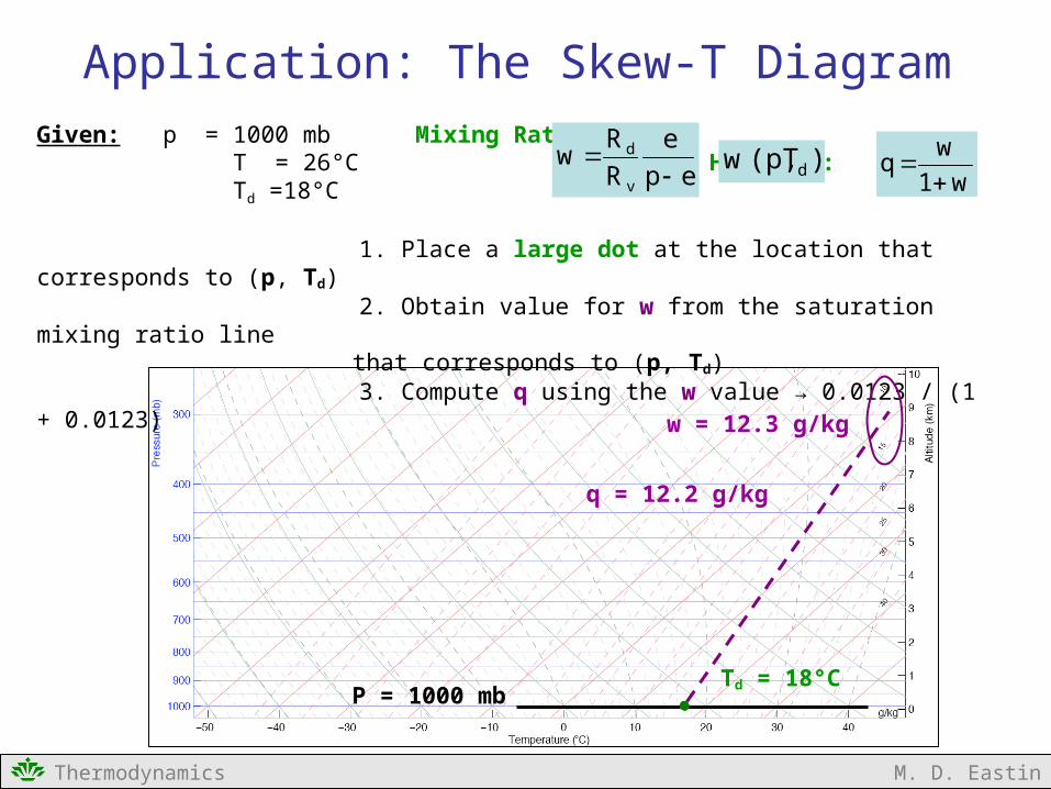
Given: p = 1000 mb Mixing Ratio: T = 26°C Specific Humidity: Td =18°C
1. Place a large dot at the location that corresponds to (p, Td) 2. Obtain value for w from the saturation mixing ratio line
that corresponds to (p, Td) 3. Compute q using the w value → 0.0123 / (1 + 0.0123)
Td = 18°CP = 1000 mb
w = 12.3 g/kg
ep
e
R
Rw
v
d
)T(p,w d
w1
wq
q = 12.2 g/kg
Application: The Skew-T Diagram
Thermodynamics M. D. Eastin
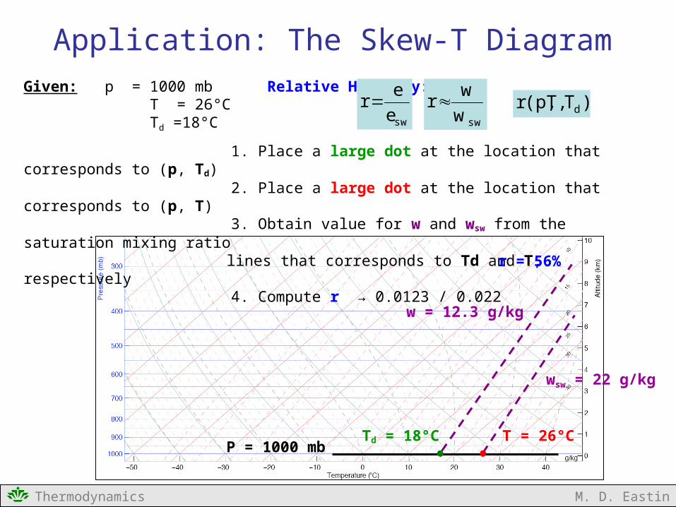
Given: p = 1000 mb Relative Humidity: T = 26°C Td =18°C
1. Place a large dot at the location that corresponds to (p, Td) 2. Place a large dot at the location that corresponds to (p, T) 3. Obtain value for w and wsw from the saturation mixing ratio
lines that corresponds to Td and T, respectively 4. Compute r → 0.0123 / 0.022
)TT,(p,r dswe
er
sww
wr
Application: The Skew-T Diagram
Td = 18°CP = 1000 mb
T = 26°C
wsw = 22 g/kg
r = 56%
w = 12.3 g/kg
Thermodynamics M. D. Eastin
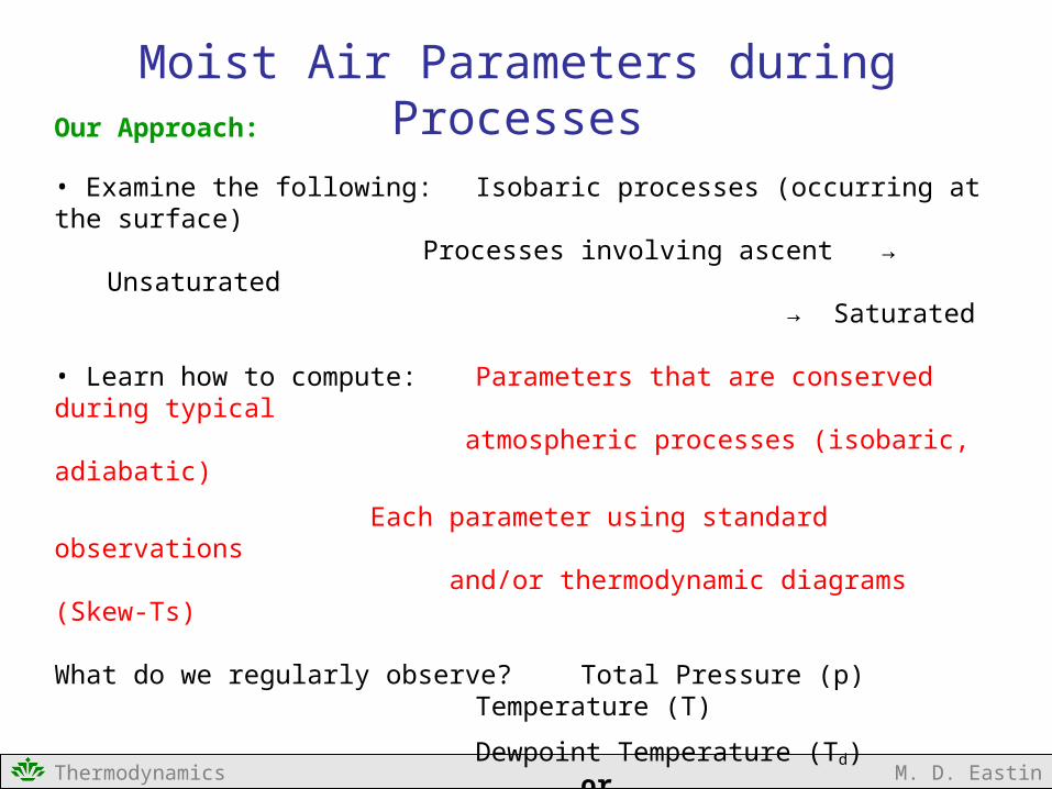
Our Approach:
• Examine the following: Isobaric processes (occurring at the surface)Processes involving ascent → Unsaturated
→ Saturated
• Learn how to compute: Parameters that are conserved during typical atmospheric processes (isobaric, adiabatic)
Each parameter using standard observations and/or thermodynamic diagrams (Skew-Ts)
What do we regularly observe? Total Pressure (p)Temperature (T)
Dewpoint Temperature (Td) or
Relative Humidity (r)
Moist Air Parameters during Processes
Thermodynamics M. D. Eastin
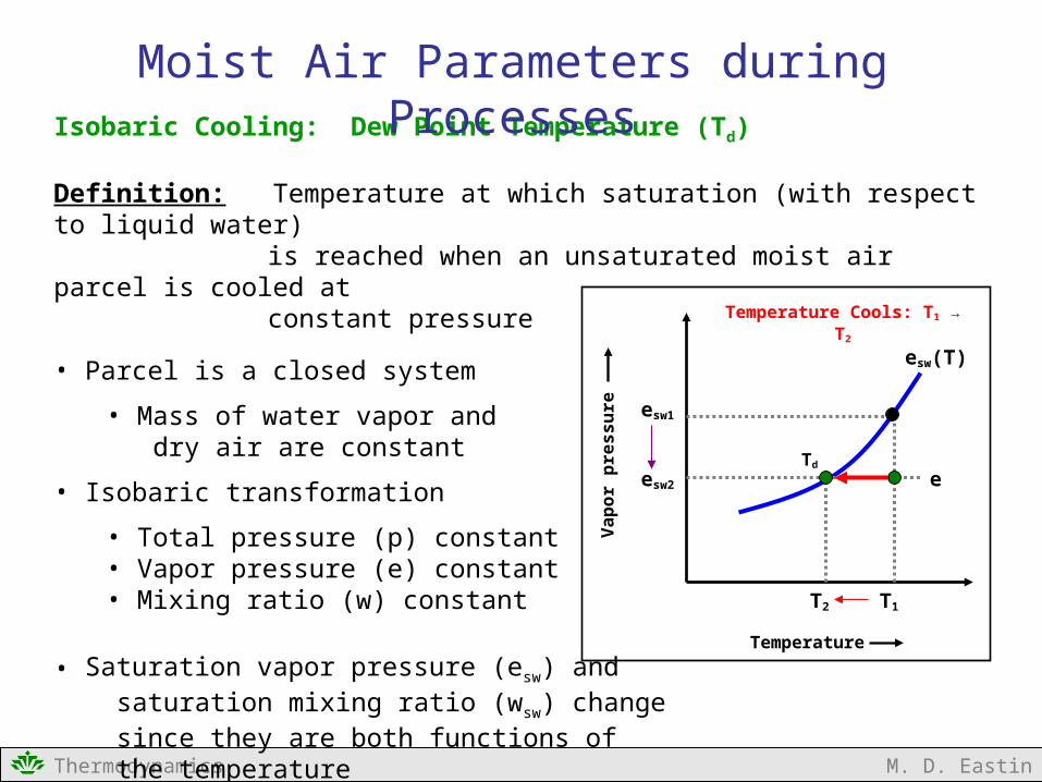
Isobaric Cooling: Dew Point Temperature (Td)
Definition: Temperature at which saturation (with respect to liquid water) is reached when an unsaturated moist air parcel is cooled at constant pressure
• Parcel is a closed system
• Mass of water vapor and dry air are constant
• Isobaric transformation
• Total pressure (p) constant• Vapor pressure (e) constant • Mixing ratio (w) constant
• Saturation vapor pressure (esw) and saturation mixing ratio (wsw) change since they are both functions of the temperature
Moist Air Parameters during Processes
Temperature
T2 T1
esw1
Va
po
r p
res
su
re
Td
Temperature Cools: T1 → T2
esw2 e
esw(T)
Thermodynamics M. D. Eastin
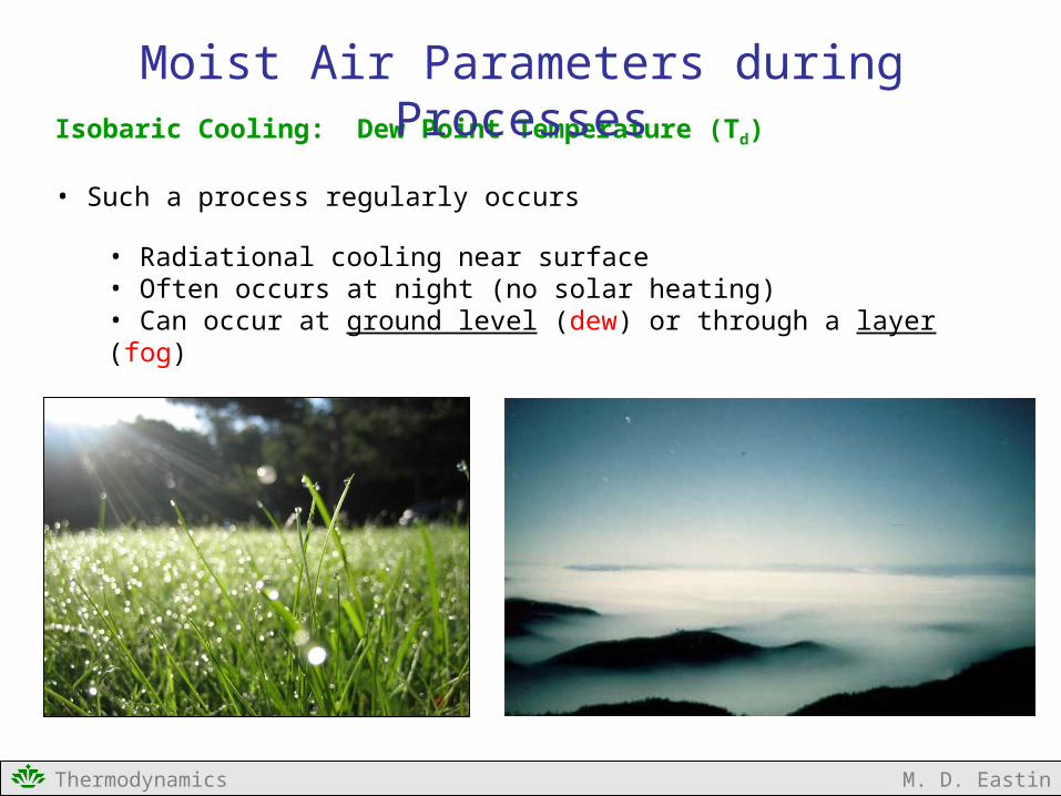
Isobaric Cooling: Dew Point Temperature (Td)
• Such a process regularly occurs
• Radiational cooling near surface• Often occurs at night (no solar heating)• Can occur at ground level (dew) or through a layer (fog)
Moist Air Parameters during Processes
Thermodynamics M. D. Eastin
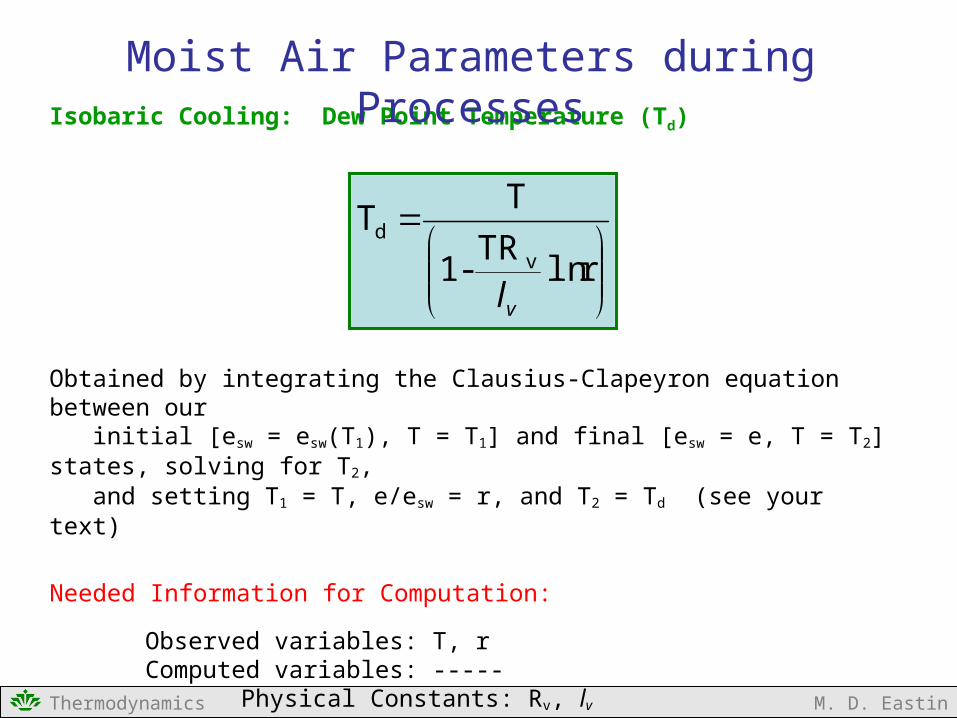
Isobaric Cooling: Dew Point Temperature (Td)
Obtained by integrating the Clausius-Clapeyron equation between our initial [esw = esw(T1), T = T1] and final [esw = e, T = T2] states, solving for T2, and setting T1 = T, e/esw = r, and T2 = Td (see your text)
Needed Information for Computation:
Observed variables: T, rComputed variables: -----
Physical Constants: Rv, lv
Units: K
Moist Air Parameters during Processes
rlnTR
-1
TT
v
d
vl
Thermodynamics M. D. Eastin
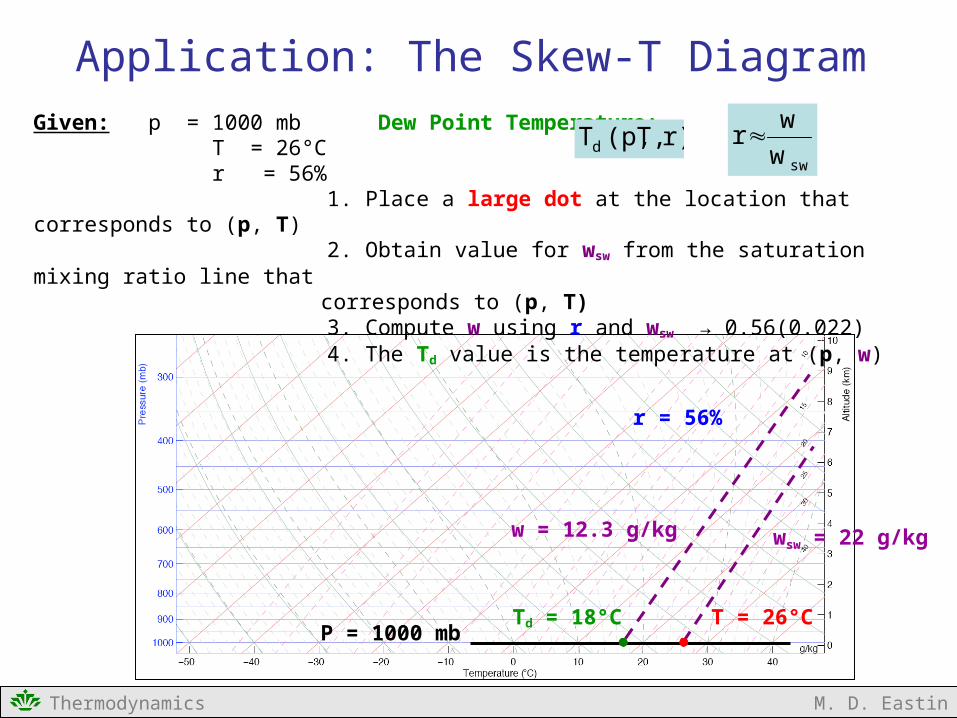
Given: p = 1000 mb Dew Point Temperature: T = 26°C r = 56%
1. Place a large dot at the location that corresponds to (p, T) 2. Obtain value for wsw from the saturation mixing ratio line that
corresponds to (p, T) 3. Compute w using r and wsw → 0.56(0.022) 4. The Td value is the temperature at (p, w)
r)T,(p,Tdsww
wr
Application: The Skew-T Diagram
Td = 18°CP = 1000 mb
T = 26°C
wsw = 22 g/kg
r = 56%
w = 12.3 g/kg
Thermodynamics M. D. Eastin
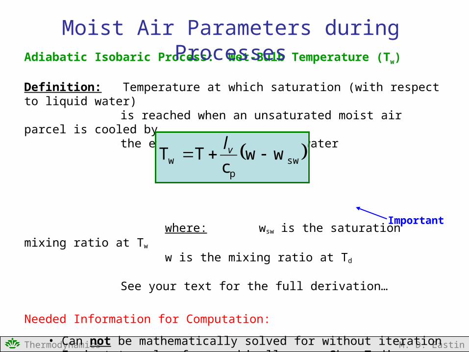
Adiabatic Isobaric Process: Wet-Bulb Temperature (Tw)
Definition: Temperature at which saturation (with respect to liquid water) is reached when an unsaturated moist air parcel is cooled by the evaporation of liquid water
where: wsw is the saturation mixing ratio at Tw
w is the mixing ratio at Td
See your text for the full derivation…
Needed Information for Computation:
• Can not be mathematically solved for without iteration• Easiest to solve for graphically on a Skew-T diagram
Moist Air Parameters during Processes
swp
w wwc
TT vl
Important
Thermodynamics M. D. Eastin
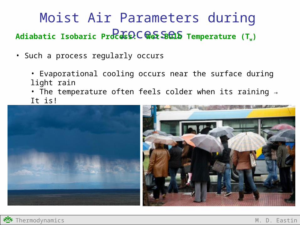
Moist Air Parameters during ProcessesAdiabatic Isobaric Process: Wet-Bulb Temperature (Tw)
• Such a process regularly occurs
• Evaporational cooling occurs near the surface during light rain• The temperature often feels colder when its raining → It is!

Thermodynamics M. D. Eastin
Wet-bulb Temperature (Tw):
1. Place a large dot at the location that corresponds to (p, Td) 2. Place a large dot at the location that corresponds to (p, T)
3. Draw a line from (p, Td) upward along a saturation mixing ratio line 4. Draw a line from (p, T) upward along a dry adiabat 5. From the intersection point of the two lines, draw another line downward along a pseudo-adiabat to the original pressure (p) 6. The Tw is the resulting temperature at that pressure
Application: The Skew-T Diagram
Td = 6°CP = 1000 mb
T = 26°C
Tw = 15ºC
Given:
p = 1000 mb T = 26ºC Td = 6ºC
Thermodynamics M. D. Eastin
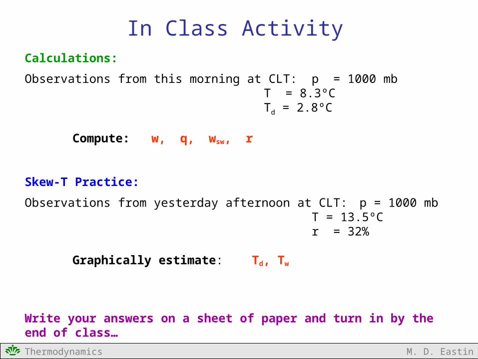
In Class ActivityCalculations:
Observations from this morning at CLT: p = 1000 mbT = 8.3ºCTd = 2.8ºC
Compute: w, q, wsw, r
Skew-T Practice:
Observations from yesterday afternoon at CLT: p = 1000 mbT = 13.5ºCr = 32%
Graphically estimate: Td, Tw
Write your answers on a sheet of paper and turn in by the end of class…
Thermodynamics M. D. Eastin
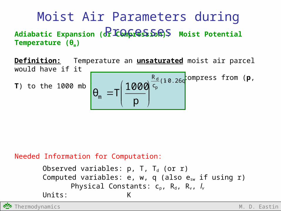
Adiabatic Expansion (or Compression): Moist Potential Temperature (θm)
Definition: Temperature an unsaturated moist air parcel would have if it were to expand or compress from (p, T) to the 1000 mb level
Needed Information for Computation:
Observed variables: p, T, Td (or r) Computed variables: e, w, q (also esw if using r)
Physical Constants: cp, Rd, Rv, lv
Units: K
Moist Air Parameters during Processes
0.26q)(1c
R
m
p
d
p
1000Tθ
Thermodynamics M. D. Eastin
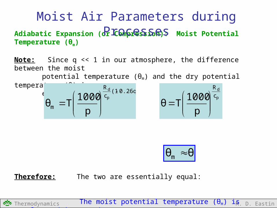
Adiabatic Expansion (or Compression): Moist Potential Temperature (θm)
Note: Since q << 1 in our atmosphere, the difference between the moistpotential temperature (θm) and the dry potential temperature (θ) isextremely small
Therefore: The two are essentially equal:
The moist potential temperature (θm) is rarely used in practice Rather, the dry potential temperature (θ) is used
Moist Air Parameters during Processes
0.26q)(1c
R
m
p
d
p
1000Tθ
θθm
p
d
c
R
p
1000Tθ
Thermodynamics M. D. Eastin
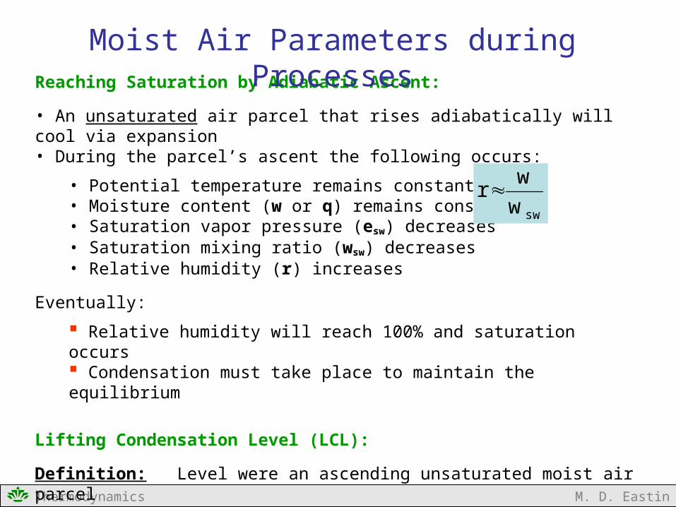
Reaching Saturation by Adiabatic Ascent:
• An unsaturated air parcel that rises adiabatically will cool via expansion• During the parcel’s ascent the following occurs:
• Potential temperature remains constant• Moisture content (w or q) remains constant• Saturation vapor pressure (esw) decreases• Saturation mixing ratio (wsw) decreases• Relative humidity (r) increases
Eventually:
Relative humidity will reach 100% and saturation occurs Condensation must take place to maintain the equilibrium
Lifting Condensation Level (LCL):
Definition: Level were an ascending unsaturated moist air parcel first achieves saturation due to adiabatic cooling and condensation begins to occur
Moist Air Parameters during Processes
sww
wr
Thermodynamics M. D. Eastin
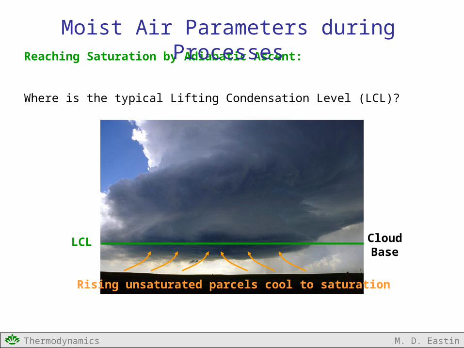
Reaching Saturation by Adiabatic Ascent:
Where is the typical Lifting Condensation Level (LCL)?
Moist Air Parameters during Processes
LCL CloudBase
Rising unsaturated parcels cool to saturation
Thermodynamics M. D. Eastin
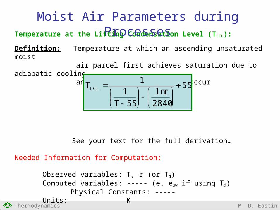
Temperature at the Lifting Condensation Level (TLCL):
Definition: Temperature at which an ascending unsaturated moist air parcel first achieves saturation due to adiabatic cooling and condensation begins to occur
See your text for the full derivation…
Needed Information for Computation:
Observed variables: T, r (or Td)Computed variables: ----- (e, esw if using Td)
Physical Constants: -----Units: K
Moist Air Parameters during Processes
55
2840rln
55T1
1TLCL
Thermodynamics M. D. Eastin
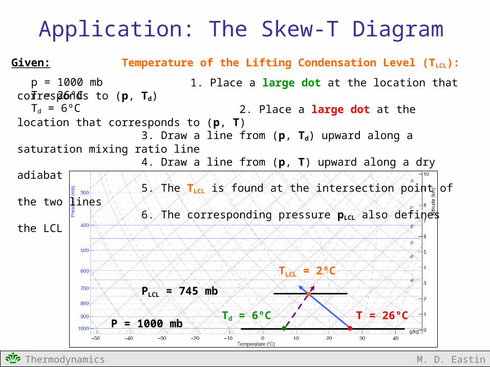
Temperature of the Lifting Condensation Level (TLCL):
1. Place a large dot at the location that corresponds to (p, Td) 2. Place a large dot at the location that corresponds to (p, T)
3. Draw a line from (p, Td) upward along a saturation mixing ratio line 4. Draw a line from (p, T) upward along a dry adiabat 5. The TLCL is found at the intersection point of the two lines 6. The corresponding pressure pLCL also defines the LCL
Application: The Skew-T Diagram
Td = 6°CP = 1000 mb
T = 26°C
TLCL = 2ºC
Given:
p = 1000 mb T = 26ºC Td = 6ºC
PLCL = 745 mb
Thermodynamics M. D. Eastin
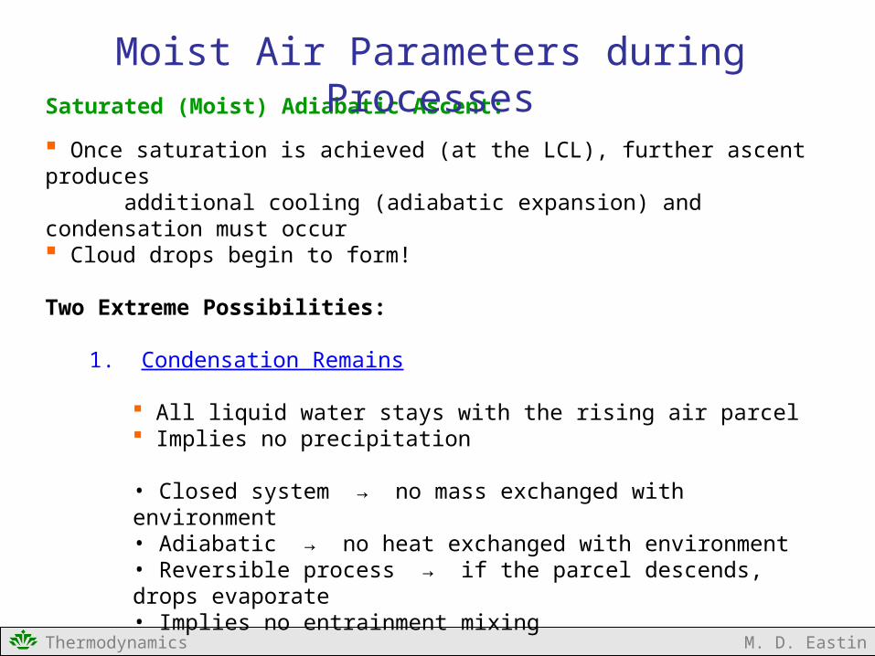
Saturated (Moist) Adiabatic Ascent:
Once saturation is achieved (at the LCL), further ascent produces additional cooling (adiabatic expansion) and condensation must occur Cloud drops begin to form!
Two Extreme Possibilities:
1. Condensation Remains
All liquid water stays with the rising air parcel Implies no precipitation
• Closed system → no mass exchanged with environment• Adiabatic → no heat exchanged with environment• Reversible process → if the parcel descends, drops evaporate• Implies no entrainment mixing
Moist Air Parameters during Processes
Thermodynamics M. D. Eastin
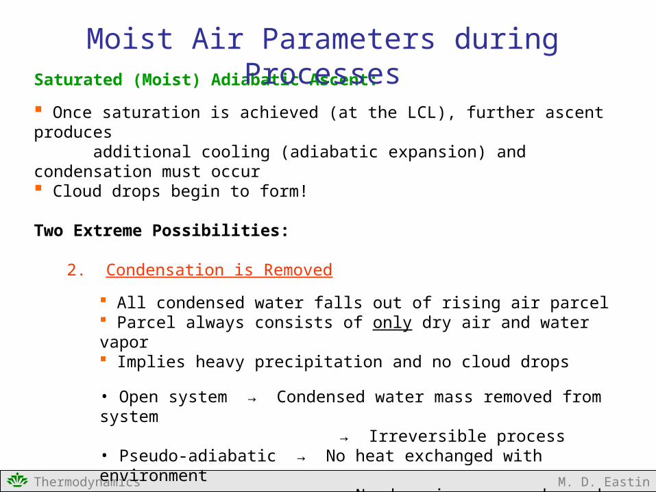
Saturated (Moist) Adiabatic Ascent:
Once saturation is achieved (at the LCL), further ascent produces additional cooling (adiabatic expansion) and condensation must occur Cloud drops begin to form!
Two Extreme Possibilities:
2. Condensation is Removed
All condensed water falls out of rising air parcel Parcel always consists of only dry air and water vapor Implies heavy precipitation and no cloud drops
• Open system → Condensed water mass removed from system → Irreversible process
• Pseudo-adiabatic → No heat exchanged with environment → No dry air mass exchanged → No water vapor exchanged
• Implies no entrainment mixing
Moist Air Parameters during Processes
Thermodynamics M. D. Eastin
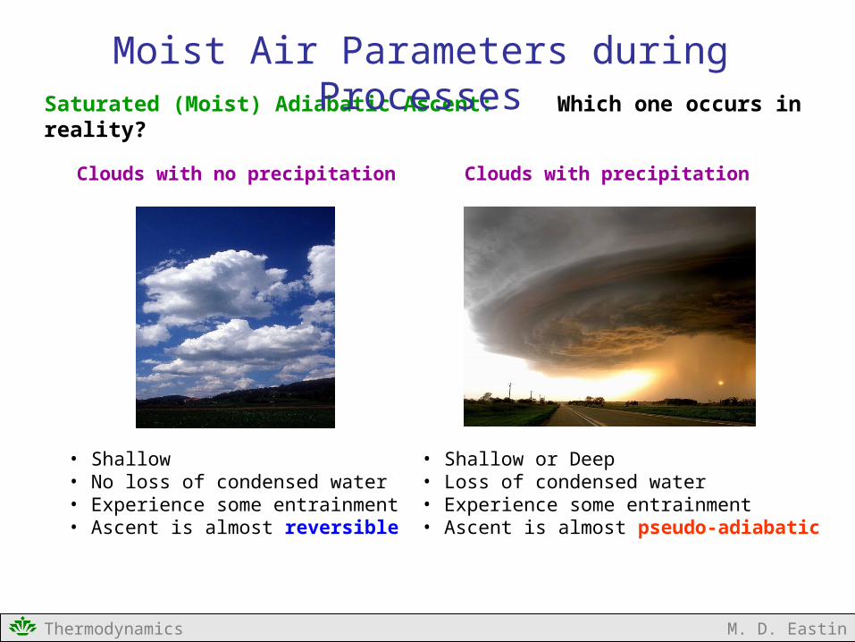
Saturated (Moist) Adiabatic Ascent: Which one occurs in reality?
Moist Air Parameters during Processes
Clouds with no precipitation
• Shallow• No loss of condensed water• Experience some entrainment• Ascent is almost reversible
Clouds with precipitation
• Shallow or Deep• Loss of condensed water• Experience some entrainment• Ascent is almost pseudo-adiabatic
Thermodynamics M. D. Eastin
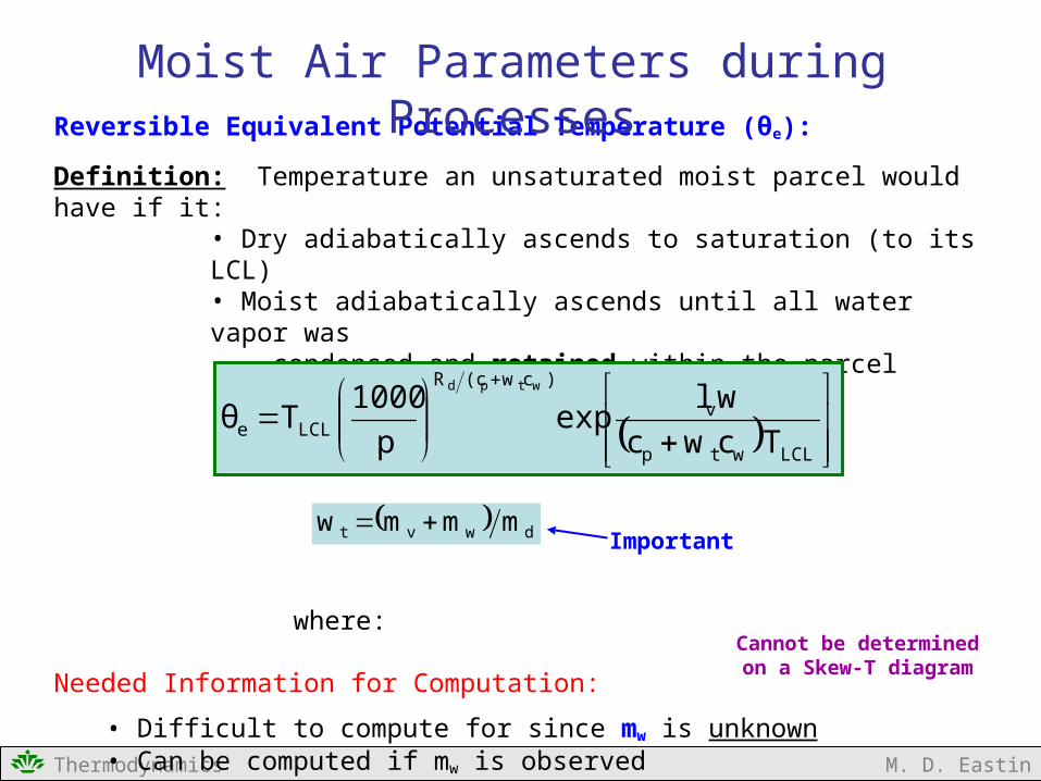
Reversible Equivalent Potential Temperature (θe):
Definition: Temperature an unsaturated moist parcel would have if it:• Dry adiabatically ascends to saturation (to its LCL)• Moist adiabatically ascends until all water vapor was condensed and retained within the parcel• Dry adiabatically descends to 1000 mb
where:
Needed Information for Computation:
• Difficult to compute for since mw is unknown• Can be computed if mw is observed (e.g. by radar) or estimated
Moist Air Parameters during Processes
LCLwtp
v
)cw(cR
LCLe Tcwc
wlexp
p
1000Tθ
wtpd
dwvt mmmw Important
Cannot be determinedon a Skew-T diagram
Thermodynamics M. D. Eastin
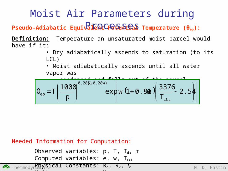
Pseudo-Adiabatic Equivalent Potential Temperature (θep):
Definition: Temperature an unsaturated moist parcel would have if it:• Dry adiabatically ascends to saturation (to its LCL)• Moist adiabatically ascends until all water vapor was condensed and falls out of the parcel• Dry adiabatically descends to 1000 mb
Needed Information for Computation:
Observed variables: p, T, Td, rComputed variables: e, w, TLCL
Physical Constants: Rd, Rv, lv
Units: K
Moist Air Parameters during Processes
2.54T
3376w0.811wexp
p
1000Tθ
LCL
0.28w)(10.285
ep
Thermodynamics M. D. Eastin
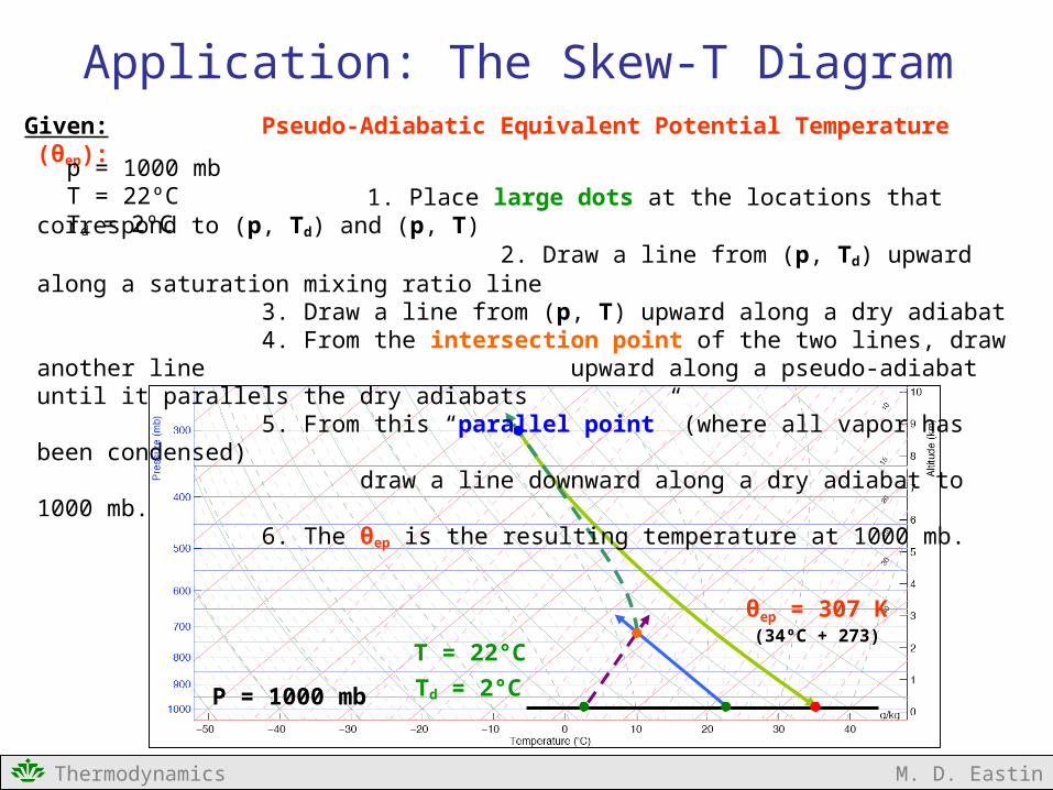
Pseudo-Adiabatic Equivalent Potential Temperature (θep):
1. Place large dots at the locations that correspond to (p, Td) and (p, T) 2. Draw a line from (p, Td) upward along a saturation mixing ratio line
3. Draw a line from (p, T) upward along a dry adiabat 4. From the intersection point of the two lines, draw another line upward along a pseudo-adiabat until it parallels the dry adiabats 5. From this “parallel point” (where all vapor has been condensed) draw a line downward along a dry adiabat to 1000 mb. 6. The θep is the resulting temperature at 1000 mb.
Application: The Skew-T Diagram
Td = 2°CP = 1000 mb
T = 22°C
θep = 307 K(34ºC + 273)
Given:
p = 1000 mb T = 22ºC Td = 2ºC
Thermodynamics M. D. Eastin
Saturated (Moist) Adiabatic Descent:
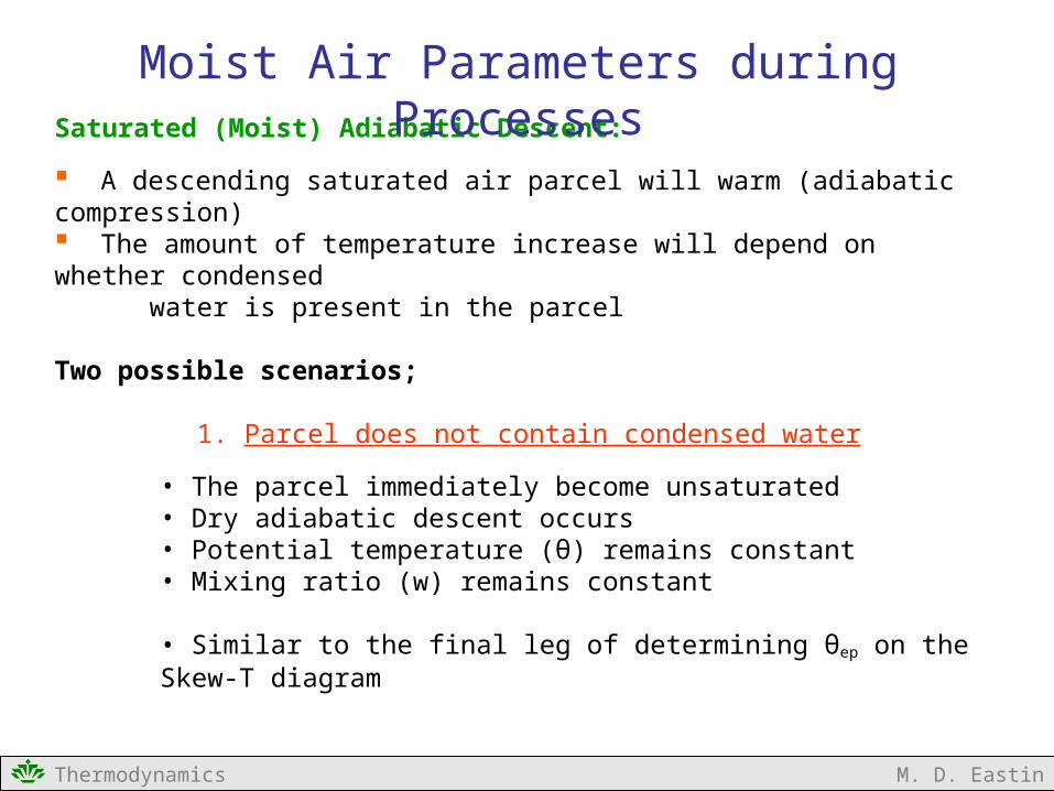
A descending saturated air parcel will warm (adiabatic compression) The amount of temperature increase will depend on whether condensed water is present in the parcel
Two possible scenarios;
1. Parcel does not contain condensed water
• The parcel immediately become unsaturated• Dry adiabatic descent occurs• Potential temperature (θ) remains constant• Mixing ratio (w) remains constant
• Similar to the final leg of determining θep on the Skew-T diagram
Moist Air Parameters during Processes
Thermodynamics M. D. Eastin
Saturated (Moist) Adiabatic Descent:
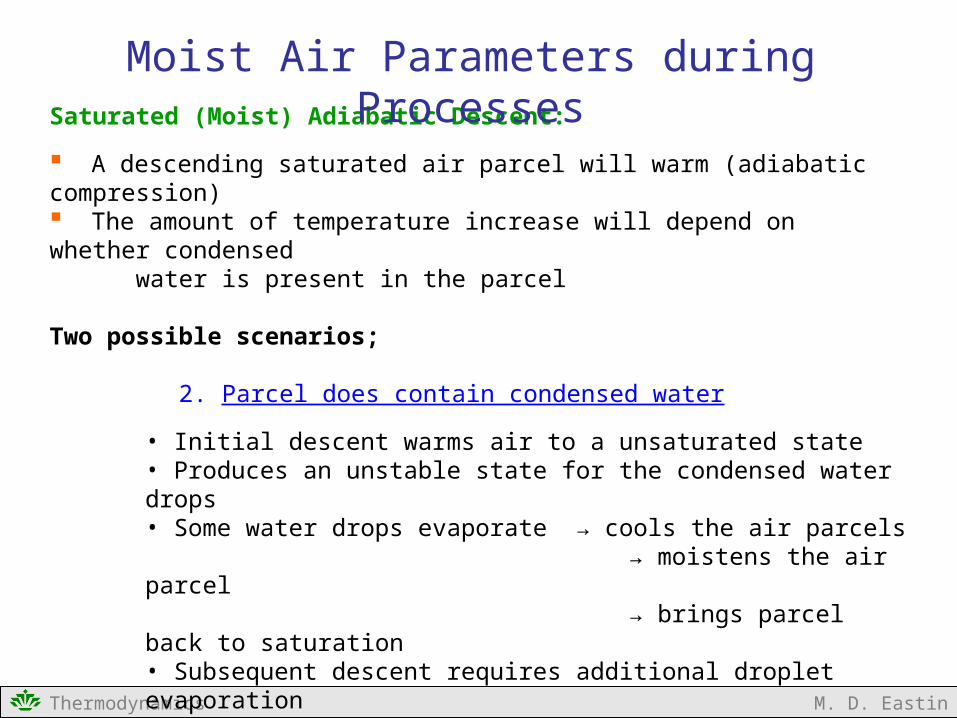
A descending saturated air parcel will warm (adiabatic compression) The amount of temperature increase will depend on whether condensed water is present in the parcel
Two possible scenarios;
2. Parcel does contain condensed water
• Initial descent warms air to a unsaturated state• Produces an unstable state for the condensed water drops• Some water drops evaporate → cools the air parcels
→ moistens the air parcel → brings parcel back to
saturation• Subsequent descent requires additional droplet evaporation in order to maintain the saturated state
Saturated descent can occur as long as condensed water is present Once all the condensed water evaporates → dry-adiabatic descent
Moist Air Parameters during Processes
Thermodynamics M. D. Eastin
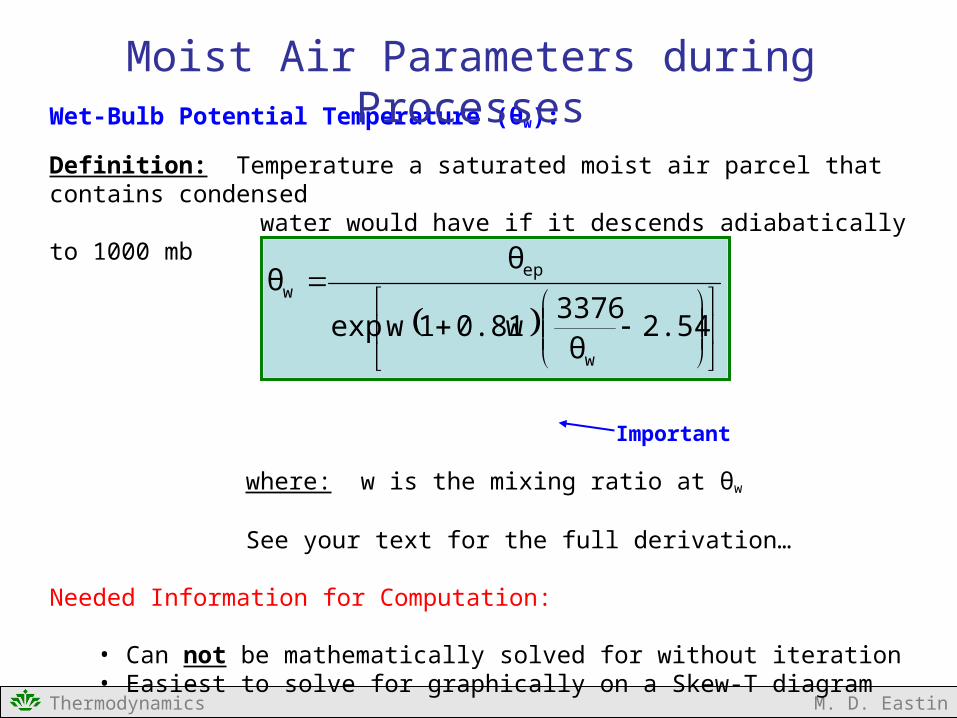
Wet-Bulb Potential Temperature (θw):
Definition: Temperature a saturated moist air parcel that contains condensed water would have if it descends adiabatically to 1000 mb
where: w is the mixing ratio at θw
See your text for the full derivation…
Needed Information for Computation:
• Can not be mathematically solved for without iteration• Easiest to solve for graphically on a Skew-T diagram
Moist Air Parameters during Processes
2.54θ
3376w0.811wexp
θθ
w
epw
Important
Thermodynamics M. D. Eastin
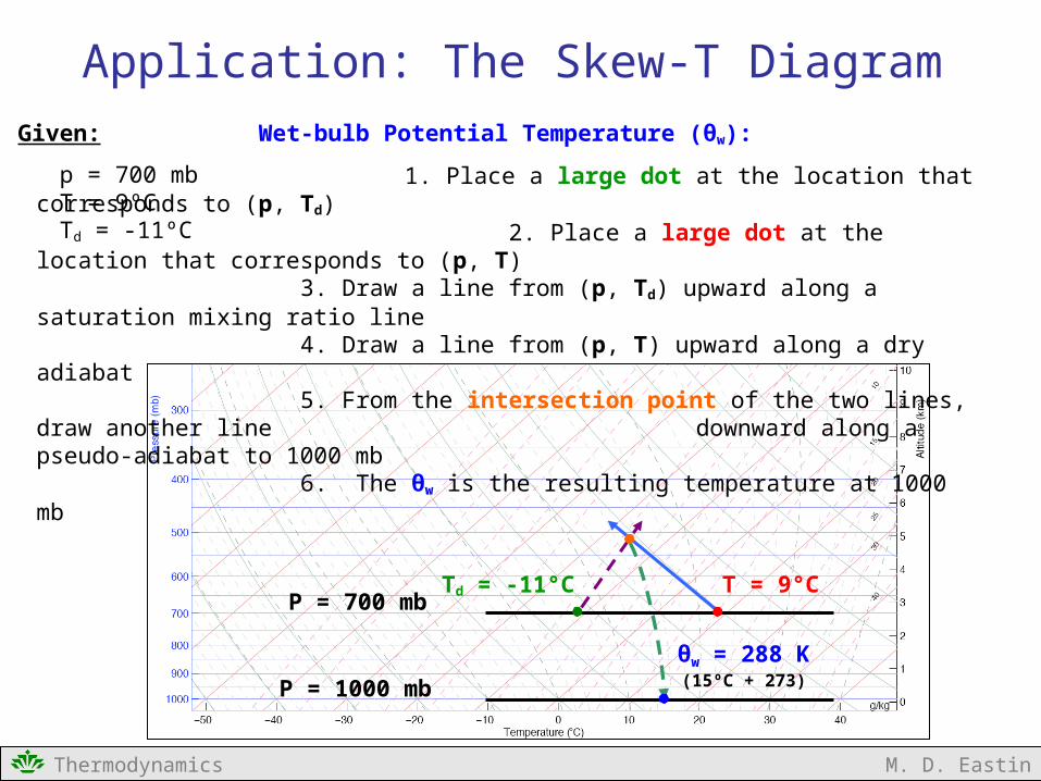
Wet-bulb Potential Temperature (θw):
1. Place a large dot at the location that corresponds to (p, Td) 2. Place a large dot at the location that corresponds to (p, T)
3. Draw a line from (p, Td) upward along a saturation mixing ratio line 4. Draw a line from (p, T) upward along a dry adiabat 5. From the intersection point of the two lines, draw another line downward along a pseudo-adiabat to 1000 mb 6. The θw is the resulting temperature at 1000 mb
Application: The Skew-T Diagram
Td = -11°C
P = 1000 mb
T = 9°C
Given:
p = 700 mb T = 9ºC Td = -11ºC
P = 700 mb
θw = 288 K(15ºC + 273)
Thermodynamics M. D. Eastin
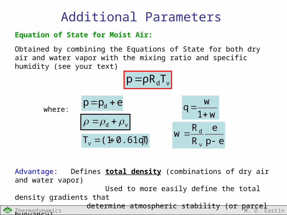
Equation of State for Moist Air:
Obtained by combining the Equations of State for both dry air and water vapor with the mixing ratio and specific humidity (see your text)
where:
Advantage: Defines total density (combinations of dry air and water vapor) Used to more easily define the total density gradients that
determine atmospheric stability (or parcel buoyancy)
Will use more in next chapter…
vdTρRp
vd
ep p d
T0.61q)(1Tv
w1
wq
ep
e
R
Rw
v
d
Additional Parameters
Thermodynamics M. D. Eastin
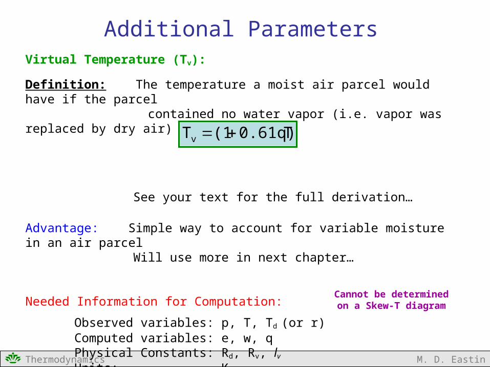
Virtual Temperature (Tv):
Definition: The temperature a moist air parcel would have if the parcel contained no water vapor (i.e. vapor was replaced by dry air)
See your text for the full derivation…
Advantage: Simple way to account for variable moisture in an air parcel Will use more in next chapter…
Needed Information for Computation:
Observed variables: p, T, Td (or r)Computed variables: e, w, qPhysical Constants: Rd, Rv, lv
Units: K
T0.61q)(1Tv
Additional Parameters
Cannot be determinedon a Skew-T diagram
Thermodynamics M. D. Eastin
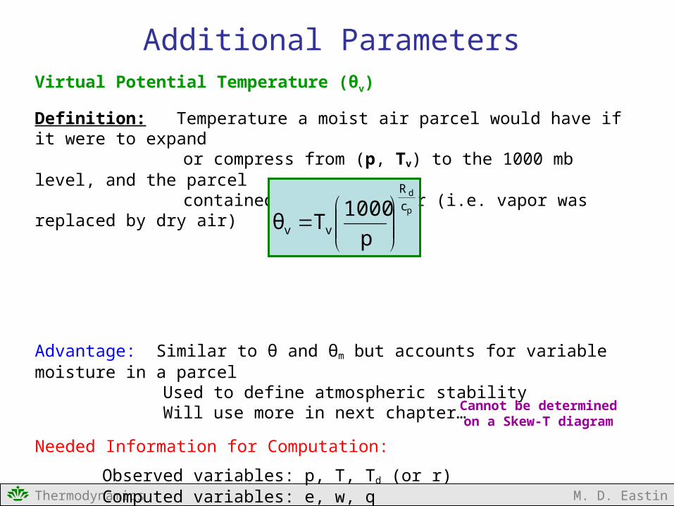
Virtual Potential Temperature (θv)
Definition: Temperature a moist air parcel would have if it were to expand or compress from (p, Tv) to the 1000 mb level, and the parcel
contained no water vapor (i.e. vapor was replaced by dry air)
Advantage: Similar to θ and θm but accounts for variable moisture in a parcel Used to define atmospheric stability Will use more in next chapter…
Needed Information for Computation:
Observed variables: p, T, Td (or r) Computed variables: e, w, q
Physical Constants: cp, Rd, Rv, lv
Units: K
p
d
c
R
vv p
1000Tθ
Additional Parameters
Cannot be determinedon a Skew-T diagram
Thermodynamics M. D. Eastin
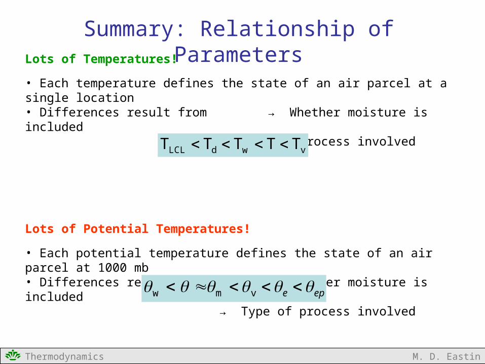
Summary: Relationship of ParametersLots of Temperatures!
• Each temperature defines the state of an air parcel at a single location• Differences result from → Whether moisture is included
→ Type of process involved
Lots of Potential Temperatures!
• Each potential temperature defines the state of an air parcel at 1000 mb• Differences result from → Whether moisture is included
→ Type of process involved
vwdLCL TTTTT
epe vmw
Thermodynamics M. D. Eastin
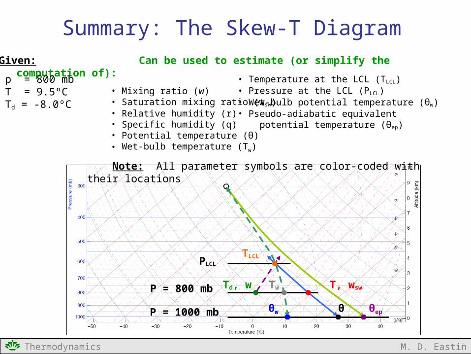
Can be used to estimate (or simplify the computation of):
• Mixing ratio (w)• Saturation mixing ratio (wsw)• Relative humidity (r)• Specific humidity (q)• Potential temperature (θ)• Wet-bulb temperature (Tw)
Note: All parameter symbols are color-coded with their locations
Summary: The Skew-T Diagram
Td, w
P = 1000 mb
T, wsw
Given:
p = 800 mb T = 9.5ºC Td = -8.0ºC
P = 800 mb
θw
TLCL
θepθ
Tw
PLCL
• Temperature at the LCL (TLCL)• Pressure at the LCL (PLCL)• Wet-bulb potential temperature (θw)• Pseudo-adiabatic equivalent potential temperature (θep)
Thermodynamics M. D. Eastin
Review:
• Review of the Clausius-Clapeyron Equation• Review of our Atmosphere as a System
• Basic parameters that describe moist air• Definitions• Application: Use of Skew-T Diagrams
• Parameters that describe atmospheric processes for moist air• Isobaric Cooling• Adiabatic – Isobaric processes• Adiabatic expansion (or compression)
• Unsaturated• Saturated
• Application: Use of Skew-T Diagrams
• Additional useful parameters• Summary
Water Vapor in the Air
Thermodynamics M. D. Eastin
ReferencesPetty, G. W., 2008: A First Course in Atmospheric Thermodynamics, Sundog Publishing, 336 pp.
Tsonis, A. A., 2007: An Introduction to Atmospheric Thermodynamics, Cambridge Press, 197 pp. Wallace, J. M., and P. V. Hobbs, 1977: Atmospheric Science: An Introductory Survey, Academic Press, New York, 467 pp.
Also (from course website):
NWSTC Skew-T Log-P Diagram and Sounding Analysis, National Weather Service, 2000
The Use of the Skew-T Log-P Diagram in Analysis and Forecasting, Air Weather Service, 1990