Wave Energy Propulsion for Pure Car and Truck Carriers …618333/FULLTEXT01.pdf · Pure Car and Truck Carriers (PCTCs) ... Wave Energy Propulsion for Pure Car and Truck Carriers

Wave Energy Propulsion forPure Car and Truck Carriers

(PCTCs)

Master thesis

by

Ludvig af Klinteberg

Supervisor: Mikael Huss, Wallenius Marine

Examiner: Anders Rosen, KTH Centre forNaval Architecture

Stockholm, 2009

KTH Centre forNaval Architecture

Abstract

Wave Energy Propulsion for Pure Car and Truck Carriers (PCTC’s)The development of ocean wave energy technology has in recent years seena revival due to increased climate concerns and interest in sustainable en-ergy. This thesis investigates whether ocean wave energy could also beused for propulsion of commercial ships, with Pure Car and Truck Carriers(PCTC’s) being the model ship type used. Based on current wave energyresearch four technologies are selected as candidates for wave energy propul-sion: bow overtopping, thrust generating foils, moving multi-point absorberand turbine-fitted anti-roll tanks.

Analyses of the selected technologies indicate that the generated propulsivepower does the overcome the added resistance from the system at the shipdesign speed and size used in the study. Conclusions are that further waveenergy propulsion research should focus on systems for ships that are slowerand smaller than current PCTC’s.

Vagenergiframdrivning av biltransportfartyg (PCTC’s)Utvecklingen av vagenergiteknik har pa senare ar fatt ett uppsving i sam-band med okande klimatoro och intresse for fornyelsebar energi. Detta exam-ensarbete utreder huruvida vagenergi aven skulle kunna anvandas till fram-drivning av kommersiella fartyg, och anvander moderna biltransportfartyg(PCTC’s - Pure Car and Truck Carriers) som fartygstyp for utredningen.Med utgangspunkt i aktuell vagenergiforskning tas fyra potentiella teknikerfor vagenergiframdrivning fram: ”overtopping” i foren, passiva fenor, ”mov-ing multi-point absorber” samt antirullningstankar med turbiner.

Analys av de valda teknikerna indikerar att den genererade framdrivandekraften blir mindre an systemets adderade framdrivningsmotstand vid denfartygshastighet och -langd som anvands. Slutsatserna ar att framtida forskn-ing om vagenergiframdrivning borde fokusera pa fartyg som ar mindre ochlangsammare an dagens PCTC-fartyg.

Contents

Contents ii

1 Introduction 1

2 Theory of ocean waves 2

2.1 Surface gravity waves . . . . . . . . . . . . . . . . . . . . . . . . . 22.1.1 Basic equations . . . . . . . . . . . . . . . . . . . . . . . . . 22.1.2 Deep water approximation . . . . . . . . . . . . . . . . . . . 52.1.3 Energy transport . . . . . . . . . . . . . . . . . . . . . . . . 6

2.2 Ocean wave spectra . . . . . . . . . . . . . . . . . . . . . . . . . . 7

3 Wave energy on worldwide route 9

4 Wave energy conversion 12

4.1 Overtopping devices . . . . . . . . . . . . . . . . . . . . . . . . . . 124.1.1 Wave Dragon . . . . . . . . . . . . . . . . . . . . . . . . . . 134.1.2 Sea Slot-cone Generator . . . . . . . . . . . . . . . . . . . . 15

4.2 Oscillating water column . . . . . . . . . . . . . . . . . . . . . . . . 164.3 Oscillating bodies . . . . . . . . . . . . . . . . . . . . . . . . . . . . 174.4 Thrust generating foils . . . . . . . . . . . . . . . . . . . . . . . . . 20

5 Proposed technologies 21

5.1 Bow overtopping . . . . . . . . . . . . . . . . . . . . . . . . . . . . 215.1.1 Ship motions . . . . . . . . . . . . . . . . . . . . . . . . . . 225.1.2 Overtopping model . . . . . . . . . . . . . . . . . . . . . . . 235.1.3 Water acceleration effect . . . . . . . . . . . . . . . . . . . . 275.1.4 Conclusions . . . . . . . . . . . . . . . . . . . . . . . . . . . 31

5.2 Thrust generating foils . . . . . . . . . . . . . . . . . . . . . . . . . 325.2.1 Modelling . . . . . . . . . . . . . . . . . . . . . . . . . . . . 325.2.2 Studies . . . . . . . . . . . . . . . . . . . . . . . . . . . . . 33

ii

CONTENTS iii

5.2.3 Numerical experiment . . . . . . . . . . . . . . . . . . . . . 335.2.4 Conclusions . . . . . . . . . . . . . . . . . . . . . . . . . . . 35

5.3 Moving Multi-Point Absorber . . . . . . . . . . . . . . . . . . . . . 365.3.1 Modelling . . . . . . . . . . . . . . . . . . . . . . . . . . . . 375.3.2 Numerical solution . . . . . . . . . . . . . . . . . . . . . . . 385.3.3 Conclusions . . . . . . . . . . . . . . . . . . . . . . . . . . . 39

5.4 Turbine-fitted anti-roll tanks . . . . . . . . . . . . . . . . . . . . . 40

6 Conclusions 41

Bibliography 42

Nomenclature 45

Abbreviations 49

List of Figures 50

List of Tables 51

Chapter 1

Introduction

This master thesis project has been carried out at Wallenius Marine in Stockholm,

and the purpose of it has been to investigate the possibility of reducing the fuel

consumption of Wallenius Lines’ Pure Car and Truck Carriers (PCTC’s) by extracting

energy from sea waves.

Wallenius works with a strong environmental vision, which in 2005 was expressed in

the conceptual emission-free E/S Orcelle. The Orcelle would be driven by fuel cells

together with a combination of solar, wind and wave energy systems. This project

has started off from this vision, in order to investigate if wave energy propulsion really

is a future possibility for the shipping industry.

In the 1970’s and early 1980’s extensive research was made in wave energy conversion,

including wave energy ship propulsion, motivated by high oil prices. Most projects

however lost their funding when oil prices dropped again in the mid 1980’s. In the

last few years there has been a revival in wave energy technology and several wave

energy conversion methods are now ready for large-scale implementation.

This thesis summarises current wave energy research, with the purpose of identifying

which techniques can be transferred onto a moving ship. Based on this summary

a number of techniques have been chosen as possible candidates and investigated

further, to evaluate if they could successfully be implemented on a PCTC.

1

Chapter 2

Theory of ocean waves

2.1 Surface gravity waves

This chapter provides a brief introduction to the theory necessary for the analysis of

ocean waves and the energy they transport.

2.1.1 Basic equations

The equations governing ocean waves can be derived from the basic principles of

fluid dynamics, the Navier-Stokes equations1. For a Newtonian fluid the equations

for conservation of mass and momentum can be written on Cartesian tensor form

(using the Einstein summation convention) as

∂ρ

∂t+

∂

∂xj(ρuj) = 0 (2.1)

∂ui∂t

+ uj∂ui∂xj

= −1ρ

∂p

∂xi+

1ρ

∂τij∂xj

+ fi (2.2)

where ui is the velocity vector, ρ is the density of the fluid, p is the total pressure,

fi is the external force and τij is the viscous stress tensor

1For a complete treatment of Navier-Stokes equations and surface gravity waves, see [14].

2

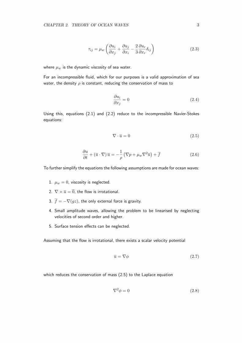
CHAPTER 2. THEORY OF OCEAN WAVES 3

τij = µw

(∂ui∂xj

+∂uj∂xi− 2

3∂ur∂xr

δij

)(2.3)

where µw is the dynamic viscosity of sea water.

For an incompressible fluid, which for our purposes is a valid approximation of sea

water, the density ρ is constant, reducing the conservation of mass to

∂ui∂xj

= 0 (2.4)

Using this, equations (2.1) and (2.2) reduce to the incompressible Navier-Stokes

equations:

∇ · u = 0 (2.5)

∂u

∂t+ (u · ∇)u = −1

ρ

(∇p+ µw∇2u

)+ f (2.6)

To further simplify the equations the following assumptions are made for ocean waves:

1. µw = 0, viscosity is neglected.

2. ∇× u = 0, the flow is irrotational.

3. f = −∇(gz), the only external force is gravity.

4. Small amplitude waves, allowing the problem to be linearised by neglecting

velocities of second order and higher.

5. Surface tension effects can be neglected.

Assuming that the flow is irrotational, there exists a scalar velocity potential

u = ∇φ (2.7)

which reduces the conservation of mass (2.5) to the Laplace equation

∇2φ = 0 (2.8)


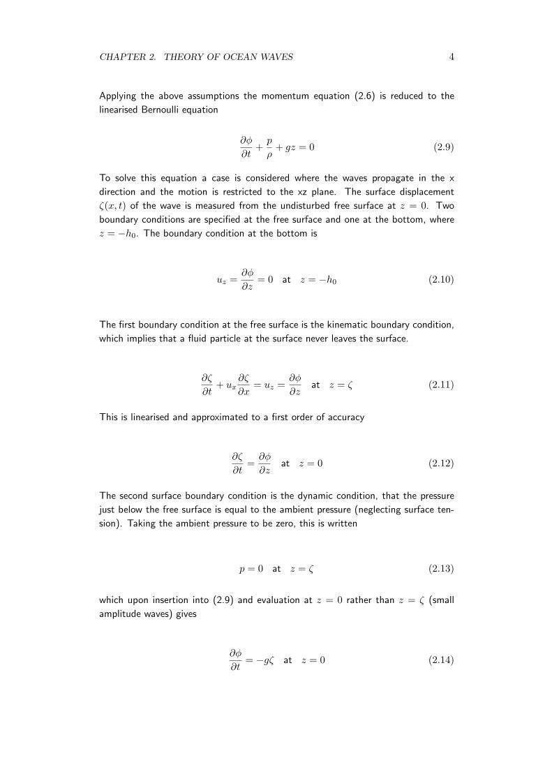
Applying the above assumptions the momentum equation (2.6) is reduced to the

linearised Bernoulli equation

∂φ

∂t+p

ρ+ gz = 0 (2.9)

To solve this equation a case is considered where the waves propagate in the x

direction and the motion is restricted to the xz plane. The surface displacement

ζ(x, t) of the wave is measured from the undisturbed free surface at z = 0. Two

boundary conditions are specified at the free surface and one at the bottom, where

z = −h0. The boundary condition at the bottom is

uz =∂φ

∂z= 0 at z = −h0 (2.10)

The first boundary condition at the free surface is the kinematic boundary condition,

which implies that a fluid particle at the surface never leaves the surface.

∂ζ

∂t+ ux

∂ζ

∂x= uz =

∂φ

∂zat z = ζ (2.11)

This is linearised and approximated to a first order of accuracy

∂ζ

∂t=∂φ

∂zat z = 0 (2.12)

The second surface boundary condition is the dynamic condition, that the pressure

just below the free surface is equal to the ambient pressure (neglecting surface ten-

sion). Taking the ambient pressure to be zero, this is written

p = 0 at z = ζ (2.13)

which upon insertion into (2.9) and evaluation at z = 0 rather than z = ζ (small

amplitude waves) gives

∂φ

∂t= −gζ at z = 0 (2.14)


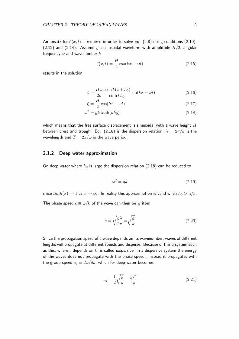
An ansatz for ζ(x, t) is required in order to solve Eq. (2.8) using conditions (2.10),

(2.12) and (2.14). Assuming a sinusoidal waveform with amplitude H/2, angular

frequency ω and wavenumber k

ζ(x, t) =H

2cos(kx− ωt) (2.15)

results in the solution

φ =Hω

2kcosh k(z + h0)

sinh kh0sin(kx− ωt) (2.16)

ζ =H

2cos(kx− ωt) (2.17)

ω2 = gk tanh(kh0) (2.18)

which means that the free surface displacement is sinusoidal with a wave height H

between crest and trough. Eq. (2.18) is the dispersion relation, λ = 2π/k is the

wavelength and T = 2π/ω is the wave period.

2.1.2 Deep water approximation

On deep water where h0 is large the dispersion relation (2.18) can be reduced to

ω2 = gk (2.19)

since tanh(x)→ 1 as x→∞. In reality this approximation is valid when h0 > λ/3.

The phase speed c ≡ ω/k of the wave can then be written

c =

√gλ

2π=√g

k(2.20)

Since the propagation speed of a wave depends on its wavenumber, waves of different

lengths will propagate at different speeds and disperse. Because of this a system such

as this, where c depends on k, is called dispersive. In a dispersive system the energy

of the waves does not propagate with the phase speed. Instead it propagates with

the group speed cg ≡ dω/dk, which for deep water becomes

cg =12

√g

k=gT

4π(2.21)


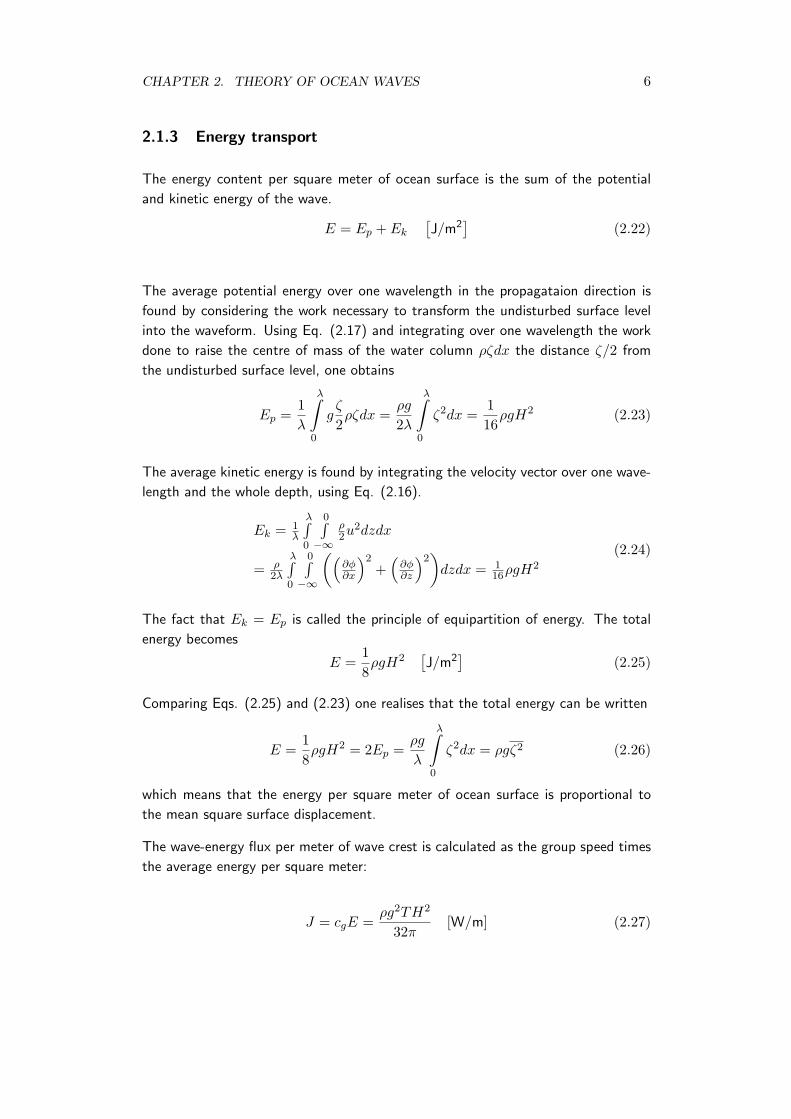
2.1.3 Energy transport

The energy content per square meter of ocean surface is the sum of the potential

and kinetic energy of the wave.

E = Ep + Ek[J/m2

](2.22)

The average potential energy over one wavelength in the propagataion direction is

found by considering the work necessary to transform the undisturbed surface level

into the waveform. Using Eq. (2.17) and integrating over one wavelength the work

done to raise the centre of mass of the water column ρζdx the distance ζ/2 from

the undisturbed surface level, one obtains

Ep =1λ

λ∫0

gζ

2ρζdx =

ρg

2λ

λ∫0

ζ2dx =116ρgH2 (2.23)

The average kinetic energy is found by integrating the velocity vector over one wave-

length and the whole depth, using Eq. (2.16).

Ek = 1λ

λ∫0

0∫−∞

ρ2u

2dzdx

= ρ2λ

λ∫0

0∫−∞

((∂φ∂x

)2+(∂φ∂z

)2)dzdx = 1

16ρgH2

(2.24)

The fact that Ek = Ep is called the principle of equipartition of energy. The total

energy becomes

E =18ρgH2

[J/m2

](2.25)

Comparing Eqs. (2.25) and (2.23) one realises that the total energy can be written

E =18ρgH2 = 2Ep =

ρg

λ

λ∫0

ζ2dx = ρgζ2 (2.26)

which means that the energy per square meter of ocean surface is proportional to

the mean square surface displacement.

The wave-energy flux per meter of wave crest is calculated as the group speed times

the average energy per square meter:

J = cgE =ρg2TH2

32π[W/m] (2.27)


2.2 Ocean wave spectra

The sea surface is not regular and can never be described as a neat sine wave of

constant wavelength and wave height going in one direction. It is a complex process,

where waves of many different wavelengths, sizes and directions together form a

surface that at first sight appears completely random. To describe this process it

is common to use an energy spectrum function S(ω) that describes how the wave

energy is distributed over different frequency components2:

E = ρg

∫ ∞0

S(ω)dω (2.28)

Where S(ω) is a Bretschneider spectrum, defined as

S(ω) = Aω−5e−Bω−4

(2.29)

A and B are constants that are empirically determined to describe a specific sea

state.

Based on the sea spectrum the spectral moment of order j is defined as

mj =∫ ∞

0ωjS(ω)dω (2.30)

Using the spectral moments several useful statistical variables can be calculated. One

is the significant wave height Hs, defined as

Hs = Hm0 = 4√m0 [m] (2.31)

This measure is used because it corresponds well to the traditional measure of sig-

nificant wave height, which is the average of the 1/3 highest waves in the spectrum

(Hs = H1/3). Sometimes Hs is also referred to as Hm0 because it is based on m0,

the spectral moment of order 0.

When working with wave energy another useful variable is the energy period Te [9],

which is the average period of all the waves in the spectrum:

Te =

∫∞0 TS(T )dT∫∞0 S(T )dT

=2π∫∞0 ω−1S(ω)dω∫∞0 S(ω)dω

= 2πm−1

m0[s] (2.32)

2See [17] for a complete introduction to sea spectra.


For fully developed seas a fairly accurate spectrum is the ISSC spectrum, which is a

two parameter spectrum based on significant wave height and period. Expressed in

terms of energy period it is written3 [17]

A = 4π4Γ(5/4)4T−4e H2

s

B = 16π4Γ(5/4)4T−4e

(2.33)

The average energy density of the sea state can be expressed in terms of Hs as

E = ρgm0 =ρg

16H2s [J/m2] (2.34)

In analogy with the energy flux J = cgE of a single wave, the energy flux of the whole

system (assuming deep water) can be calculated using the relations cg = g/(2ω),

(2.31) and (2.32) [9].

J = ρg

∫ ∞0

cg(ω)S(ω)dω =12ρg2m−1 =

ρg2

64πH2sTe [W/m] (2.35)

3Γ is the Gamma function, defined as Γ (x) =∞∫0

sx−1e−sds.

Chapter 3

Wave energy on worldwide route

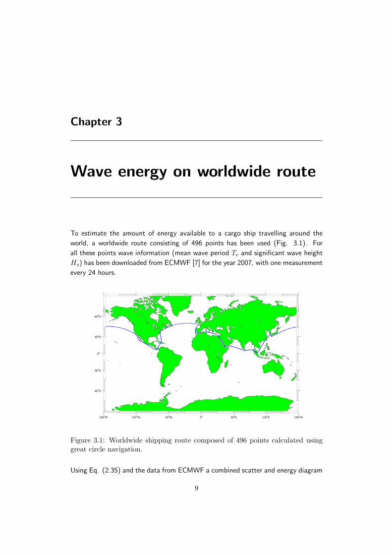
To estimate the amount of energy available to a cargo ship travelling around the

world, a worldwide route consisting of 496 points has been used (Fig. 3.1). For

all these points wave information (mean wave period Te and significant wave height

Hs) has been downloaded from ECMWF [7] for the year 2007, with one measurement

every 24 hours.

180oW 120oW 60oW 0o 60oE 120oE 180oW

60oS

30oS

0o

30oN

60oN

Figure 3.1: Worldwide shipping route composed of 496 points calculated usinggreat circle navigation.

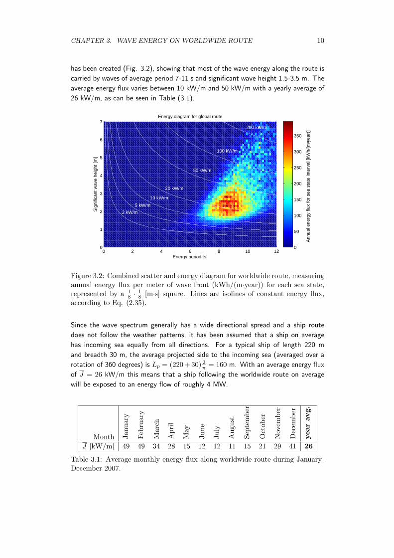
Using Eq. (2.35) and the data from ECMWF a combined scatter and energy diagram

9

CHAPTER 3. WAVE ENERGY ON WORLDWIDE ROUTE 10

has been created (Fig. 3.2), showing that most of the wave energy along the route is

carried by waves of average period 7-11 s and significant wave height 1.5-3.5 m. The

average energy flux varies between 10 kW/m and 50 kW/m with a yearly average of

26 kW/m, as can be seen in Table (3.1).

0 2 4 6 8 10 120

1

2

3

4

5

6

7

Ann

ual e

nerg

y flu

x fo

r se

a st

ate

inte

rval

[kW

h/(m

×yea

r)]

200 kW/m

100 kW/m

50 kW/m

Energy period [s]

Energy diagram for global route

20 kW/m

10 kW/m

5 kW/m

2 kW/m

Sig

nific

ant w

ave

heig

ht [m

]

0

50

100

150

200

250

300

350

Figure 3.2: Combined scatter and energy diagram for worldwide route, measuringannual energy flux per meter of wave front (kWh/(m·year)) for each sea state,represented by a 1

8 ·18 [m·s] square. Lines are isolines of constant energy flux,

according to Eq. (2.35).

Since the wave spectrum generally has a wide directional spread and a ship route

does not follow the weather patterns, it has been assumed that a ship on average

has incoming sea equally from all directions. For a typical ship of length 220 m

and breadth 30 m, the average projected side to the incoming sea (averaged over a

rotation of 360 degrees) is Lp = (220 + 30) 2π = 160 m. With an average energy flux

of J = 26 kW/m this means that a ship following the worldwide route on average

will be exposed to an energy flow of roughly 4 MW.

Month Janu

ary

Febr

uary

Mar

ch

Apr

il

May

June

July

Aug

ust

Sept

embe

r

Oct

ober

Nov

embe

r

Dec

embe

r

year

avg.

J [kW/m] 49 49 34 28 15 12 12 11 15 21 29 41 26

Table 3.1: Average monthly energy flux along worldwide route during January-December 2007.

CHAPTER 3. WAVE ENERGY ON WORLDWIDE ROUTE 11

One of the motivations for this thesis work has been that large amounts of fuel could

be saved by capturing as little as one tenth of this available energy. For further

analyses the sea state Te 9 s, Hs 2.5 m has been chosen as a reference state for this

thesis, since it lies in the centre of the most dense region of Fig. 3.2.

Chapter 4

Wave energy conversion

Wave energy conversion (WEC) is the term for the conversion of ocean wave energy

into a desired form, usually electrical or mechanical energy. Numerous strategies for

wave energy conversion have over the years been proposed. Almost all of them can

be categorised into one of the following categories; overtopping devices, oscillating

bodies and oscillating water column. [4, 5, 16]

This chapter attempts to give a brief summary of the state of the art of WEC by

describing the working principles and listing the devices that have reached farthest in

their development. The purpose is to give an overview of the technology that exists

today, in order to evaluate what could possibly be fitted onboard a ship.

4.1 Overtopping devices

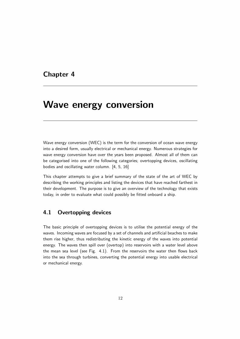
The basic principle of overtopping devices is to utilise the potential energy of the

waves. Incoming waves are focused by a set of channels and artificial beaches to make

them rise higher, thus redistributing the kinetic energy of the waves into potential

energy. The waves then spill over (overtop) into reservoirs with a water level above

the mean sea level (see Fig. 4.1). From the reservoirs the water then flows back

into the sea through turbines, converting the potential energy into usable electrical

or mechanical energy.

12

CHAPTER 4. WAVE ENERGY CONVERSION 13

4.1.1 Wave Dragon

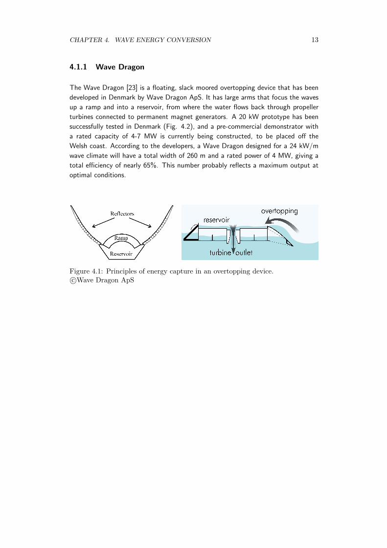
The Wave Dragon [23] is a floating, slack moored overtopping device that has been

developed in Denmark by Wave Dragon ApS. It has large arms that focus the waves

up a ramp and into a reservoir, from where the water flows back through propeller

turbines connected to permanent magnet generators. A 20 kW prototype has been

successfully tested in Denmark (Fig. 4.2), and a pre-commercial demonstrator with

a rated capacity of 4-7 MW is currently being constructed, to be placed off the

Welsh coast. According to the developers, a Wave Dragon designed for a 24 kW/m

wave climate will have a total width of 260 m and a rated power of 4 MW, giving a

total efficiency of nearly 65%. This number probably reflects a maximum output at

optimal conditions.

Figure 4.1: Principles of energy capture in an overtopping device.c©Wave Dragon ApS


Figure 4.2: Wave Dragon overtopping device prototype. The wave reflectors (top,bottom left) focus the waves onto the ramp and into the reservoir (bottom right).c©Wave Dragon ApS & Earth-vision.biz


4.1.2 Sea Slot-cone Generator

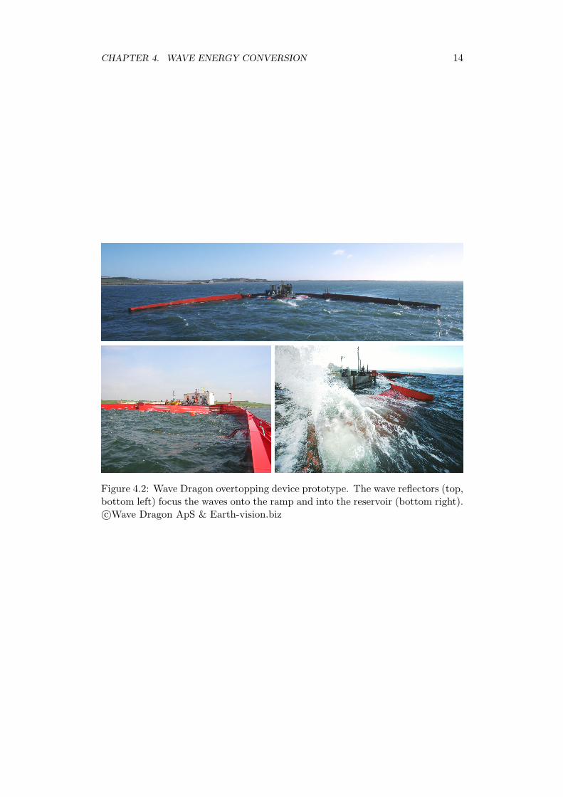
Another type of overtopping device is the Sea Slot-cone Generator (SSG) [15], which

is a shore-based installation that uses reservoirs at several levels to extract energy

from waves of different heights. The water is collected in the reservoirs and then flows

out through a Multi-Stage Turbine (MST) that consists of several turbines staggered

concentrically inside each other, driving a common shaft. The MST makes use of

the different levels of water head in the reservoirs, and is able to extract power even

at low water heads. Estimated overall efficiency of the SSG is 10-26% depending on

wave conditions.

Figure 4.3: The Sea Slot-cone Generator developed in Norway. It allows wavesof different height to overtop into reservoirs at three different levels (left). Waterthen flows out through a multi-stage turbine (right). From [15].


4.2 Oscillating water column

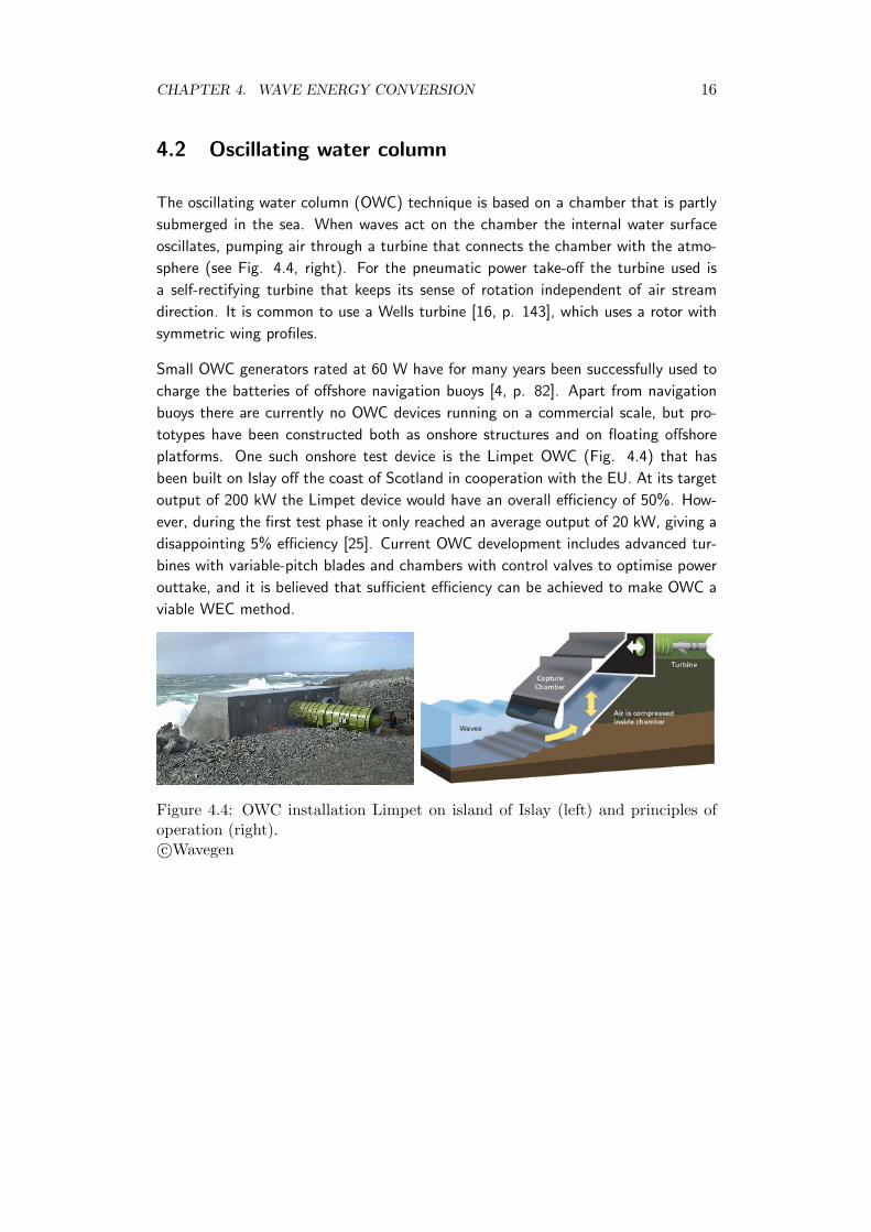
The oscillating water column (OWC) technique is based on a chamber that is partly

submerged in the sea. When waves act on the chamber the internal water surface

oscillates, pumping air through a turbine that connects the chamber with the atmo-

sphere (see Fig. 4.4, right). For the pneumatic power take-off the turbine used is

a self-rectifying turbine that keeps its sense of rotation independent of air stream

direction. It is common to use a Wells turbine [16, p. 143], which uses a rotor with

symmetric wing profiles.

Small OWC generators rated at 60 W have for many years been successfully used to

charge the batteries of offshore navigation buoys [4, p. 82]. Apart from navigation

buoys there are currently no OWC devices running on a commercial scale, but pro-

totypes have been constructed both as onshore structures and on floating offshore

platforms. One such onshore test device is the Limpet OWC (Fig. 4.4) that has

been built on Islay off the coast of Scotland in cooperation with the EU. At its target

output of 200 kW the Limpet device would have an overall efficiency of 50%. How-

ever, during the first test phase it only reached an average output of 20 kW, giving a

disappointing 5% efficiency [25]. Current OWC development includes advanced tur-

bines with variable-pitch blades and chambers with control valves to optimise power

outtake, and it is believed that sufficient efficiency can be achieved to make OWC a

viable WEC method.

Figure 4.4: OWC installation Limpet on island of Islay (left) and principles ofoperation (right).c©Wavegen


4.3 Oscillating bodies

Most of the WEC concepts being developed today consist of bodies that move in

one or more degrees of freedom in the sea, absorbing the energy of the waves.

Physically, to absorb energy from a wave means to generate a wave that interferes

destructively with the original wave [8, p. 196], thereby reducing its amplitude.

Hence, an oscillating body WEC device must be an efficient wave maker that creates

a cancelling wave with its motion.

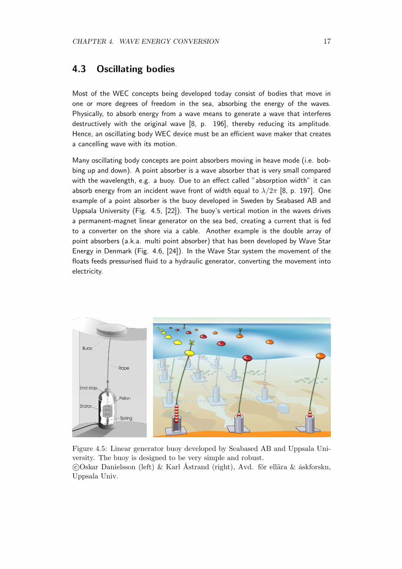
Many oscillating body concepts are point absorbers moving in heave mode (i.e. bob-

bing up and down). A point absorber is a wave absorber that is very small compared

with the wavelength, e.g. a buoy. Due to an effect called ”absorption width” it can

absorb energy from an incident wave front of width equal to λ/2π [8, p. 197]. One

example of a point absorber is the buoy developed in Sweden by Seabased AB and

Uppsala University (Fig. 4.5, [22]). The buoy’s vertical motion in the waves drives

a permanent-magnet linear generator on the sea bed, creating a current that is fed

to a converter on the shore via a cable. Another example is the double array of

point absorbers (a.k.a. multi point absorber) that has been developed by Wave Star

Energy in Denmark (Fig. 4.6, [24]). In the Wave Star system the movement of the

floats feeds pressurised fluid to a hydraulic generator, converting the movement into

electricity.

Figure 4.5: Linear generator buoy developed by Seabased AB and Uppsala Uni-versity. The buoy is designed to be very simple and robust.c©Oskar Danielsson (left) & Karl Astrand (right), Avd. for ellara & askforskn,

Uppsala Univ.


Other examples of oscillating body devices that have come far in their development

are the Pelamis (Fig. 4.7, [19]) and the Oyster (Fig. 4.8, [2]). The Pelamis is the

first WEC device in the world to be commercialised, with three 750 kW-devices now

operating off the Portuguese coast and more being planned. The Oyster has suc-

cessfully been tested in full scale at the New and Renewable Energy Centre (NaREC)

near Newcastle.


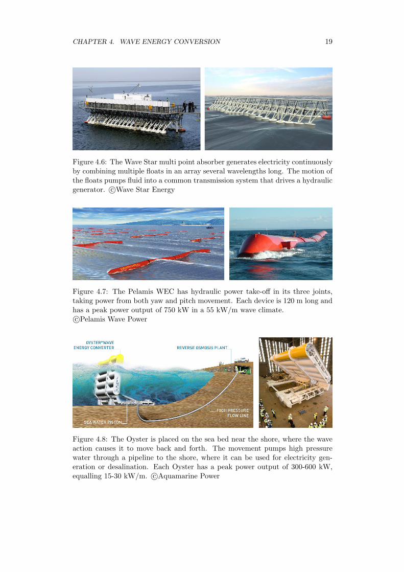
Figure 4.6: The Wave Star multi point absorber generates electricity continuouslyby combining multiple floats in an array several wavelengths long. The motion ofthe floats pumps fluid into a common transmission system that drives a hydraulicgenerator. c©Wave Star Energy

Figure 4.7: The Pelamis WEC has hydraulic power take-off in its three joints,taking power from both yaw and pitch movement. Each device is 120 m long andhas a peak power output of 750 kW in a 55 kW/m wave climate.c©Pelamis Wave Power

Figure 4.8: The Oyster is placed on the sea bed near the shore, where the waveaction causes it to move back and forth. The movement pumps high pressurewater through a pipeline to the shore, where it can be used for electricity gen-eration or desalination. Each Oyster has a peak power output of 300-600 kW,equalling 15-30 kW/m. c©Aquamarine Power


4.4 Thrust generating foils

One method of wave energy propulsion that has received a lot of attention is by using

a hydrofoil that undergoes an oscillating motion below the surface, thus generating

thrust. This mimics the way that birds, fishes and insects generate thrust by moving

wings and fins. The difference is that the thrust generation by the hydrofoil is

completely passive; wave energy is absorbed as ship motion kinetic energy, which in

turn is converted into thrust by the hydrofoil that moves with the ship.

The conversion of wave energy into thrust by a foil was named ”wave devouring

propulsion” (WDP) by Terao [12]. Another term for the same technology is ”passive

foil propeller”. Early experimental and analytical studies in the 1980’s suggested

that a WDP system on a ship could generate thrust in both following and head sea

[12, 21].

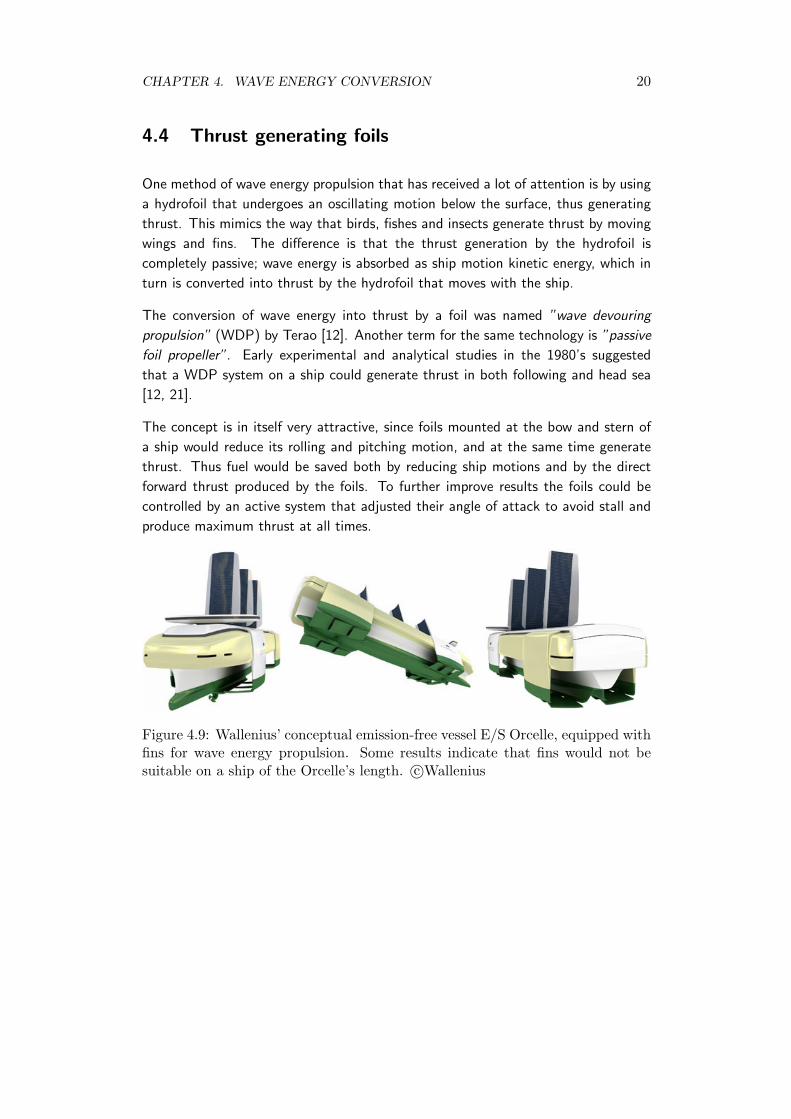
The concept is in itself very attractive, since foils mounted at the bow and stern of

a ship would reduce its rolling and pitching motion, and at the same time generate

thrust. Thus fuel would be saved both by reducing ship motions and by the direct

forward thrust produced by the foils. To further improve results the foils could be

controlled by an active system that adjusted their angle of attack to avoid stall and

produce maximum thrust at all times.

Figure 4.9: Wallenius’ conceptual emission-free vessel E/S Orcelle, equipped withfins for wave energy propulsion. Some results indicate that fins would not besuitable on a ship of the Orcelle’s length. c©Wallenius

Chapter 5

Proposed technologies

This chapter presents the different concepts for wave energy propulsion that have

been considered during this thesis work. All the concepts are adaptations of existing

technologies, and all have been chosen in discussion with engineers at Wallenius as

concepts that could be feasible to install on a PCTC. A total of 4 concepts have

been studied, but the bow overtopping is the one that has been most thoroughly

analysed. The analyses have been carried out with main ship data from Wallenius’

PCTC M/V Fedora, described in Table 5.1.

Lpp Breadth Draft CB U PE216 m 32.3 m 9.5 m 0.62 18 kts 8.5 MW

Table 5.1: Ship data for M/V Fedora used in study. PE is the engine powerrequired at 18 knots.

5.1 Bow overtopping

The motion of the sea surface relative the side of the ship is a superposition of the

motion of the sea surface and the pitch and heave motions of the ship. This relative

motion is at its largest at the bow of the ship. By installing an overtopping device

at the bow, this large motion amplitude could be used to generate electrical power.

A possible positive side-effect could be a slight damping of the pitching motion.

In this thesis work an overtopping device installed at the bow of a Wallenius PCTC has

21

CHAPTER 5. PROPOSED TECHNOLOGIES 22

been modelled by using the response amplitude operators1 (i.e. transfer functions)

Y3(ω) for heave and Y5(ω) for pitch in an ISSC sea state S(ω) (see Eqs. 2.29 and

2.33). The transfer functions have been calculated by using the linear strip method,

as implemented in the software package Tribon M3.

5.1.1 Ship motions

The transfer function for motion in the i-th d.o.f. (degree of freedom) is defined as

Yi(ω) = η0i (ω)/ζ0(ω) (5.1)

where ζ0(ω) is the oscillation amplitude of the particular frequency in the exciting

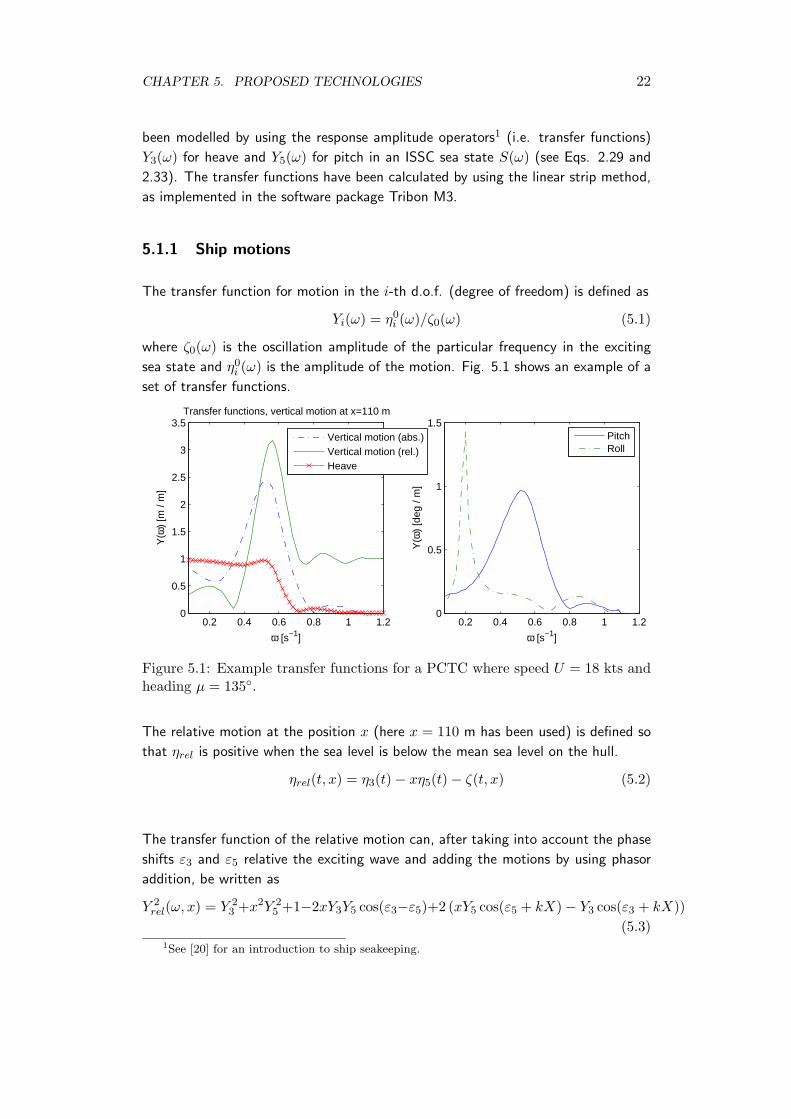
sea state and η0i (ω) is the amplitude of the motion. Fig. 5.1 shows an example of a

set of transfer functions.

0.2 0.4 0.6 0.8 1 1.20

0.5

1

1.5

2

2.5

3

3.5Transfer functions, vertical motion at x=110 m

ω [s−1]

Y(ω

) [m

/ m

]

Vertical motion (abs.)Vertical motion (rel.)Heave

0.2 0.4 0.6 0.8 1 1.20

0.5

1

1.5Y

(ω)

[deg

/ m

]

ω [s−1]

PitchRoll

Figure 5.1: Example transfer functions for a PCTC where speed U = 18 kts andheading µ = 135◦.

The relative motion at the position x (here x = 110 m has been used) is defined so

that ηrel is positive when the sea level is below the mean sea level on the hull.

ηrel(t, x) = η3(t)− xη5(t)− ζ(t, x) (5.2)

The transfer function of the relative motion can, after taking into account the phase

shifts ε3 and ε5 relative the exciting wave and adding the motions by using phasor

addition, be written as

Y 2rel(ω, x) = Y 2

3 +x2Y 25 +1−2xY3Y5 cos(ε3−ε5)+2 (xY5 cos(ε5 + kX)− Y3 cos(ε3 + kX))

(5.3)1See [20] for an introduction to ship seakeeping.


0.3 0.4 0.5 0.6 0.7 0.8 0.9 1 1.1 1.2 1.30

10

20

30

Sη (ω

)

ω [s−1]

Response energy spectrum, vertical motion at x=110 m

Absolute motionRelative motion

0.3 0.4 0.5 0.6 0.7 0.8 0.9 1 1.1 1.2 1.30

1

2

3

Sζ(ω

)

ω [s−1]

Sea state energy spectrum Hs=4.0, T

w=9.0

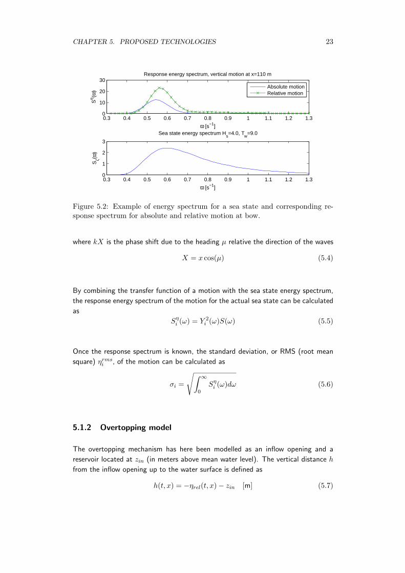
Figure 5.2: Example of energy spectrum for a sea state and corresponding re-sponse spectrum for absolute and relative motion at bow.

where kX is the phase shift due to the heading µ relative the direction of the waves

X = x cos(µ) (5.4)

By combining the transfer function of a motion with the sea state energy spectrum,

the response energy spectrum of the motion for the actual sea state can be calculated

as

Sηi (ω) = Y 2i (ω)S(ω) (5.5)

Once the response spectrum is known, the standard deviation, or RMS (root mean

square) ηrmsi , of the motion can be calculated as

σi =

√∫ ∞0

Sηi (ω)dω (5.6)

5.1.2 Overtopping model

The overtopping mechanism has here been modelled as an inflow opening and a

reservoir located at zin (in meters above mean water level). The vertical distance h

from the inflow opening up to the water surface is defined as

h(t, x) = −ηrel(t, x)− zin [m] (5.7)


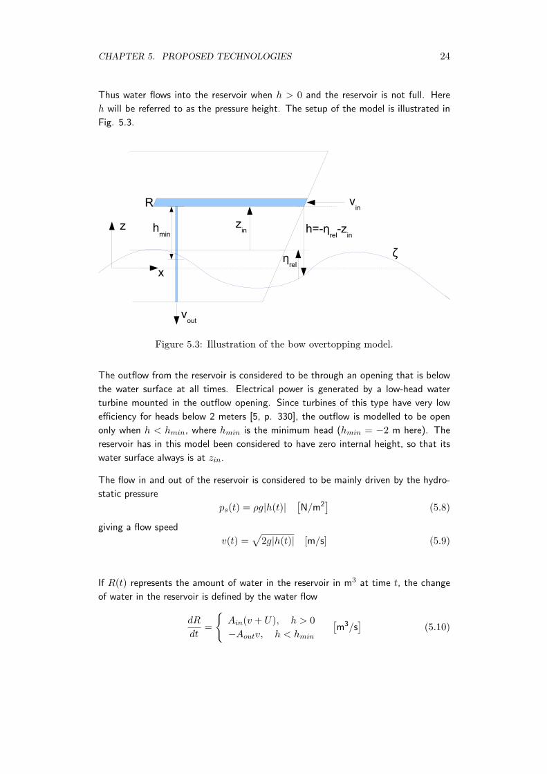
Thus water flows into the reservoir when h > 0 and the reservoir is not full. Here

h will be referred to as the pressure height. The setup of the model is illustrated in

Fig. 5.3.

Figure 5.3: Illustration of the bow overtopping model.

The outflow from the reservoir is considered to be through an opening that is below

the water surface at all times. Electrical power is generated by a low-head water

turbine mounted in the outflow opening. Since turbines of this type have very low

efficiency for heads below 2 meters [5, p. 330], the outflow is modelled to be open

only when h < hmin, where hmin is the minimum head (hmin = −2 m here). The

reservoir has in this model been considered to have zero internal height, so that its

water surface always is at zin.

The flow in and out of the reservoir is considered to be mainly driven by the hydro-

static pressure

ps(t) = ρg|h(t)|[N/m2

](5.8)

giving a flow speed

v(t) =√

2g|h(t)| [m/s] (5.9)

If R(t) represents the amount of water in the reservoir in m3 at time t, the change

of water in the reservoir is defined by the water flow

dR

dt=

{Ain(v + U), h > 0−Aoutv, h < hmin

[m3/s

](5.10)


The ship speed U has been added to the inflow speed driven by hydrostatic pressure

to include the effect of the ship’s forward speed relative to the sea water. Ain/out is

the area of the inflow and outflow openings, respectively, here set to 10 m2 each.

The available power of the outflow, before considering efficiency of power take-off

systems, is calculated as the volume outflow times the driving pressure

P (t) = Aoutv(t)ps(t) [W], h < hmin (5.11)

In terms of the pressure height

P = ρg√

2gAouth3/2 (5.12)

The relative motion ηrel between the surface and the inflow opening is normally

distributed, and therefore the probability density function (pdf) of h can be obtained

from the normal distribution by substituting ηrel using Eq. 5.7

f(h) =1

σrel√

2πexp

(−(h+ zin)2

2σ2rel

)(5.13)

Using f(h) the probabilities of in- and outflow can be written as2

Πin =∫ ∞

0f(h)dh =

12

(1− erf

(zin

σrel√

2

))(5.14)

Πout =∫ hmin

−∞f(h)dh =

12

(1 + erf

(zin − hmin

σrel√

2

))(5.15)

The outflow power depends on h3/2, here defined as the power height w

w = h3/2, h < hmin (5.16)

The pdf f(w) is obtained from (5.13) by variable substitution with (5.16) and nor-

malising with Πout

f(w) =1

Πout

√2

9πw−1/3

σrelexp

(−(w2/3 − zin)2

2σ2rel

)(5.17)

Similarly, the probability distribution functions for the inflow and outflow speeds are

obtained by substituting (5.9) into (5.13)

f(vin) =1

Πin

vin − Uσrelg

√2π

exp

−(

(vin − U)2 /2g − zin)2

2σ2rel

, U ≤ vin ≤ ∞ (5.18)

f(vout) =1

Πout

vout

σrelg√

2πexp

(−(v2

out/2g − zin)2

2σ2rel

),√

2ghmin ≤ vout ≤ ∞ (5.19)

2erf(x) is the error function, defined as erf(x) = 2√π

∫ x0

e−t2dt.


The in- and outflow pdf’s are only defined when h > 0 and h < hmin, respectively,

and therefore normalised with Πin and Πout.

Using the distribution functions mentioned above, important time averages for the

overtopping process can be calculated by noting that a variable x with pdf f(x),

defined ∀x ∈ R, has an average value

x =∫ ∞−∞

xf(x)dx (5.20)

The time average of the flow changing the reservoir level can thus be calculated as

dR

dt= ΠinAinvin −ΠoutAoutvout (5.21)

The reservoir water level will build up to its maximum if dRdt > 0. In that case there

will always be water in the reservoir, and the mean power production will only depend

on the outflow

P = Πoutρg√

2gAoutw (5.22)

If dRdt < 0, the reservoir will empty faster then it gets filled, and the power production

will depend on the inflow. Numerically, this means that the outflow area must be

adjusted so that dRdt = 0, since water cannot flow out from an empty reservoir. This

gives

P = Πoutρg√

2gAoutw (5.23)

where Aout is the adjusted outflow area

Aout =Πinvin

ΠoutvoutAin (5.24)

Therefore, the power production can be expressed as

P =

{ρg√

2gΠoutAoutw , ΠinAinvin > ΠoutAoutvoutρg√

2gΠinAin (vin/vout)w , ΠinAinvin < ΠoutAoutvout(5.25)

As can be observed in Fig. 5.4 (line ”Calculated”), this function is piecewise smooth

with a sharp maximum. The maximum occurs at the point where dRdt = 0, i.e. when

the average outflow is of the same magnitude as the average inflow. A time-domain

simulation of the same model has also been run (Fig. 5.4, line ”Simulated”), by

modelling the behaviour of the reservoir for a time series of the relative motion. The

results coincide well with the analytic model except for a slight underestimation in the

second half of the curve, probably because of effects that occur when the reservoir

is completely empty for some time periods.


0 0.5 1 1.5 2 2.5 3 3.5 40

100

200

300

400

500

600

zin

[m]

Tim

e av

erag

e of

out

flow

pow

er [k

W]

Power vs zin

. Ship speed U=18 kts. Sea state Hs=2.5 m, T

e=9.0 s.

SimulatedCalculated

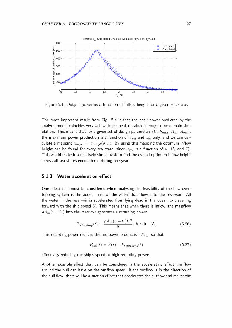
Figure 5.4: Output power as a function of inflow height for a given sea state.

The most important result from Fig. 5.4 is that the peak power predicted by the

analytic model coincides very well with the peak obtained through time-domain sim-

ulation. This means that for a given set of design parameters (U , hmin, Ain, Aout),

the maximum power production is a function of σrel and zin only, and we can cal-

culate a mapping zin,opt = zin,opt(σrel). By using this mapping the optimum inflow

height can be found for every sea state, since σrel is a function of µ, Hs and Te.

This would make it a relatively simple task to find the overall optimum inflow height

across all sea states encountered during one year.

5.1.3 Water acceleration effect

One effect that must be considered when analysing the feasibility of the bow over-

topping system is the added mass of the water that flows into the reservoir. All

the water in the reservoir is accelerated from lying dead in the ocean to travelling

forward with the ship speed U . This means that when there is inflow, the massflow

ρAin(v + U) into the reservoir generates a retarding power

Pretarding(t) =ρAin(v + U)U2

2, h > 0 [W] (5.26)

This retarding power reduces the net power production Pnet, so that

Pnet(t) = P (t)− Pretarding(t) (5.27)

effectively reducing the ship’s speed at high retarding powers.

Another possible effect that can be considered is the accelerating effect the flow

around the hull can have on the outflow speed. If the outflow is in the direction of

the hull flow, there will be a suction effect that accelerates the outflow and makes the


water flow out of the reservoir faster than when driven by hydrostatic pressure, thus

increasing the produced power. The theoretical maximum occurs when the outflow

is accelerated by the ship speed U

P (t) = Aout(v + U)ps, h < hmin [W] (5.28)


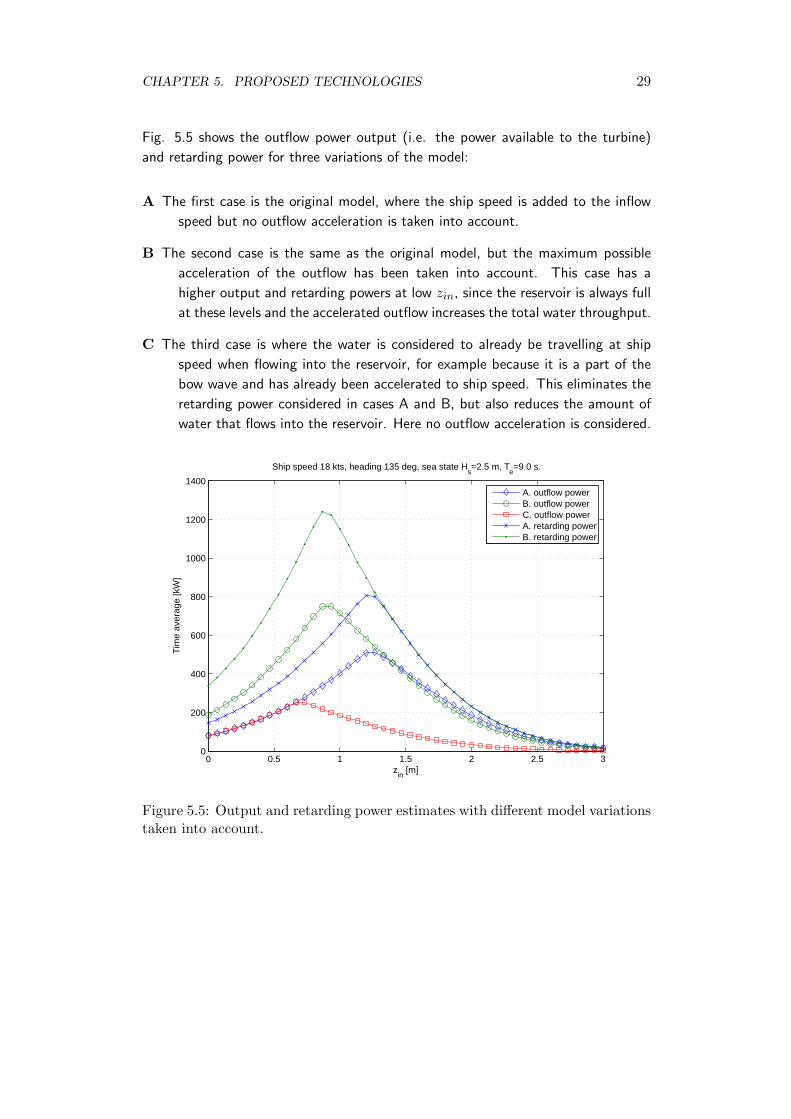
Fig. 5.5 shows the outflow power output (i.e. the power available to the turbine)

and retarding power for three variations of the model:

A The first case is the original model, where the ship speed is added to the inflow

speed but no outflow acceleration is taken into account.

B The second case is the same as the original model, but the maximum possible

acceleration of the outflow has been taken into account. This case has a

higher output and retarding powers at low zin, since the reservoir is always full

at these levels and the accelerated outflow increases the total water throughput.

C The third case is where the water is considered to already be travelling at ship

speed when flowing into the reservoir, for example because it is a part of the

bow wave and has already been accelerated to ship speed. This eliminates the

retarding power considered in cases A and B, but also reduces the amount of

water that flows into the reservoir. Here no outflow acceleration is considered.

0 0.5 1 1.5 2 2.5 30

200

400

600

800

1000

1200

1400

zin

[m]

Tim

e av

erag

e [k

W]

Ship speed 18 kts, heading 135 deg, sea state Hs=2.5 m, T

e=9.0 s.

A. outflow powerB. outflow powerC. outflow powerA. retarding powerB. retarding power

Figure 5.5: Output and retarding power estimates with different model variationstaken into account.


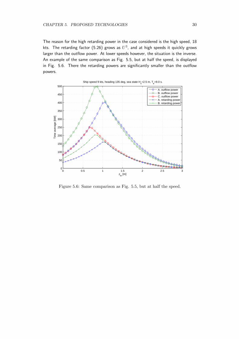
The reason for the high retarding power in the case considered is the high speed, 18

kts. The retarding factor (5.26) grows as U3, and at high speeds it quickly grows

larger than the outflow power. At lower speeds however, the situation is the inverse.

An example of the same comparison as Fig. 5.5, but at half the speed, is displayed

in Fig. 5.6. There the retarding powers are significantly smaller than the outflow

powers.

0 0.5 1 1.5 2 2.5 30

50

100

150

200

250

300

350

400

450

500

zin

[m]

Tim

e av

erag

e [k

W]

Ship speed 9 kts, heading 135 deg, sea state Hs=2.5 m, T

e=9.0 s.

A. outflow powerB. outflow powerC. outflow powerA. retarding powerB. retarding power

Figure 5.6: Same comparison as Fig. 5.5, but at half the speed.


5.1.4 Conclusions

As Fig. 5.5 clearly shows, the retarding power considered is significantly larger than

the outflow power regardless of outflow acceleration. This is a clear overestimate,

partly because some of the water has already been accelerated by the hull before

flowing in, and partly because the original added mass of the bow is reduced since

there is a reduction of the area that pushes water forward and to the side. However,

the outflow power is also a theoretical maximum that will be greatly reduced once

turbines and generators are included in the model.

One can interpret the results of the model by considering a floating overtopping

device, such as the Wave Dragon, that is equipped with an electric motor driven

by the generators on the device. At speeds close to zero the output power will be

larger than the retarding power, and the device will accelerate. But at a certain (and

probably very low) speed there will be an equilibrium, and the device will not move

any faster.


5.2 Thrust generating foils

The WDP concept described in section 4.4 has been analysed both by a literature

survey of earlier studies and by a numerical study using the simplified model described

below.

5.2.1 Modelling

To fully model a ship equipped with WDP, one must couple the equations of motions

of the ship with the behaviour of the oscillating foil, which is a fairly complicated

task. The hydrodynamics of foils oscillating in heave and pitch near a free surface is a

subject of ongoing research, and beyond the scope of this study. (One treatment of a

rigid oscillating foil near a free surface can be found in [10].) A simplified approach is

to model the foil by using steady-state foil theory, with fluid speed and angle of attack

determined by using linear wave theory together with the ship’s transfer functions for

heave and pitch. This approach disregards the foil’s damping effect on ship motions

and the wave-making effects of the oscillating foil, but is still interesting because of

its simple implementation.

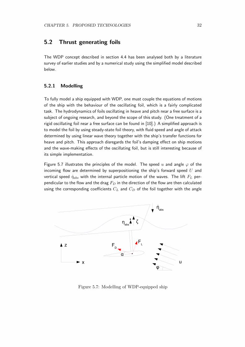
Figure 5.7 illustrates the principles of the model. The speed u and angle ϕ of the

incoming flow are determined by superpositioning the ship’s forward speed U and

vertical speed ηabs with the internal particle motion of the waves. The lift FL per-

pendicular to the flow and the drag FD in the direction of the flow are then calculated

using the corresponding coefficients CL and CD of the foil together with the angle

-0.50

0.51

1.5

-0.5

0

0.5

u

FLF

D

ζηabs

α

ηabs

φx

z

Figure 5.7: Modelling of WDP-equipped ship


of attack α, determined by the foil’s control system. The horizontal components of

FL and FD are then used to calculate the thrust and drag of the foil in the direction

of travel. The lift and drag are calculated as

FL =12ρu2AfCL (α) (5.29)

FD =12ρu2AfCD (α) (5.30)

where Af is the area of the foil [1].

5.2.2 Studies

One implementation of the simplified approach described above is a DNV study from

1989 [13], which considers a 300 m vessel sailing the route Chile-Japan at 13 knots.

The vessel in the study is equipped with bow and stern foils with areas 2.0% and

1.5% of the total water plane area (WPA), respectively. According to the study, the

foils would give a propulsive effect of 1.6 MW and a fuel saving of 21%, on average

for all headings. However, this study does not analyse the resistance increase due

to the appended foils or the motions of the ship in waves, but rather adds 15% (1

MW) to the still water resistance to account for all factors. A quick estimate of the

foil drag alone (based on CD) sets it at minimum 0.4 MW without waves, i.e at 0◦

angle of attack, and it would definitely be larger in waves. The fuel saving of 21%

is calculated as the ratio of the foil propulsive power at 13 knots and the effective

power normally needed to maintain that speed (with the 15% increase). Thus it

does not take into account the resistance increase from the foils. On the other hand,

the foils will most likely dampen the pitching of the ship, reducing the wave-induced

resistance compared to the original configuration.

More recently, WDP in the form of bow wings has been extensively studied by Naito

[18]. However, this wave energy conversion system seems to be ineffective when the

wavelength is shorter than the ship’s length (λ/L < 1), according to Naito. A typical

PCTC has a length of about 200 meters, meaning that WDP would only be effective

for wave periods above 11 seconds. Mean wave periods above 11 seconds occur less

than 5% of the year on the worldwide route [7, 11], and thus WDP seems to be

unsuitable for ships this large. An experimental study from CUT by Bergholtz and

Stocks [3] also concludes that when λ/L < 1 the foil thrust is too small to overcome

the added resistance due to the foils.

5.2.3 Numerical experiment

An implementation of the simplified model described in 5.2.1 has been made in

MATLAB during this thesis work, simulating a T-shaped foil mounted 10 meters


below the surface at the bow of a PCTC. The depth of 10 meters was chosen so

that the risk of foil slamming would be small even in large waves. It has some effect

on the results since the particle motions of the waves are largest near the surface,

making deep mounted foils slightly less effective. A symmetrical NACA 0012 profile

with aspect ratio 4 was used, since it is the kind used in [18] and [13]. It is also

similar to the NACA 0018 profile used by [3]. The total foil area was set to 1% of

the WPA, and the foil was considered to be controlled by an optimal control system.

Optimality was here defined as the angle of attack that maximised the net propulsive

force.

The 2D panel code XFoil [6] was used to derive the section lift and drag coefficients

(cl and cd) of the profile. The foil coefficients (CL and CD) where then derived from

the section coefficients by applying aspect ratio effects, as described in [1]. XFoil

is considered to give relatively accurate lift and drag predictions, but it is likely to

overestimate the stall angle. No experimental results were however available for the

high Reynolds number encountered here (Re 3e7), which is why the XFoil coefficients

have been applied without modification. Since the foil was considered to have an

optimal control system it would not come near the stall angle anyway, since the

optimal lift/drag ration of the foil was observed to be well below the stall angle.

The ship motions for different ISSC sea states with Te = 9 s and varying Hs were

obtained from the ship’s transfer function, as described in 5.1.1. By adding together

the ship motions with the particle motions of the waves, a time series of the speed

and direction of the flow around the foil was then obtained. The foil’s angle of attack

was set to the one that gave the largest net propulsive force, and the forces acting

on the foil were calculated using steady state foil theory and the coefficients CL and

CD. A time average of the horizontal forces acting on the foil at different significant

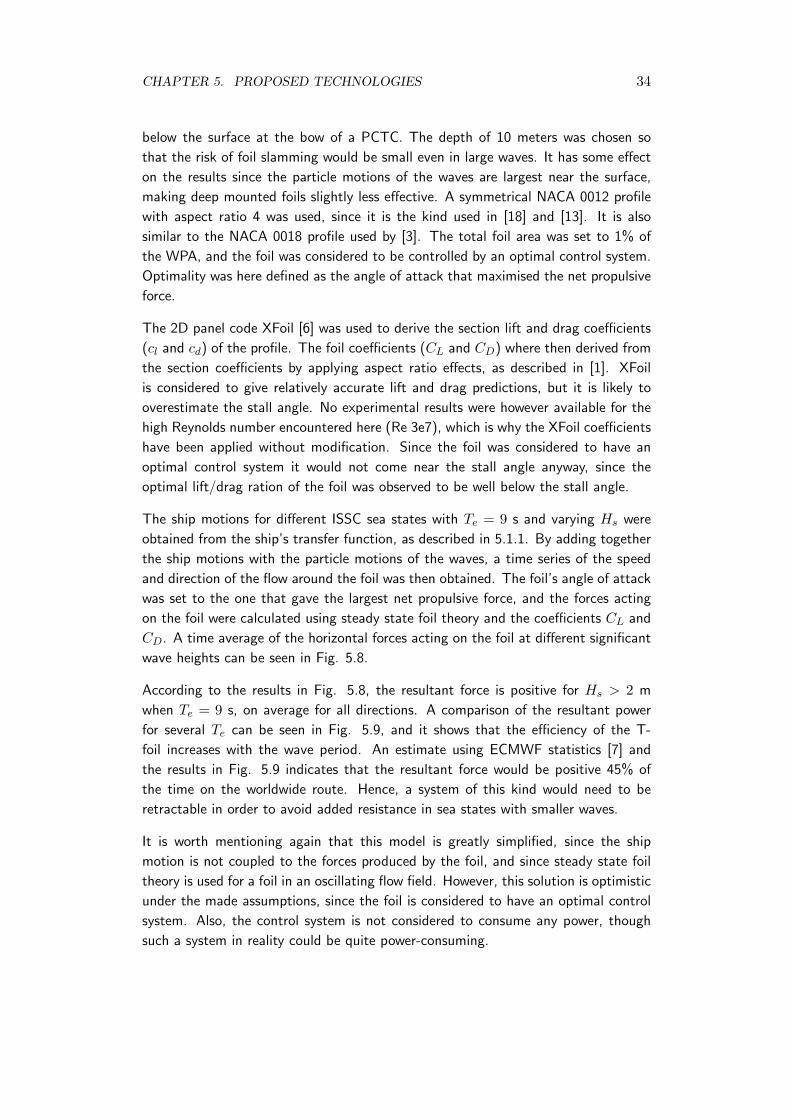
wave heights can be seen in Fig. 5.8.

According to the results in Fig. 5.8, the resultant force is positive for Hs > 2 m

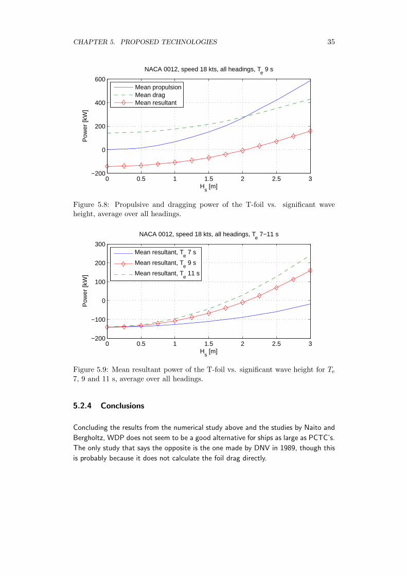
when Te = 9 s, on average for all directions. A comparison of the resultant power

for several Te can be seen in Fig. 5.9, and it shows that the efficiency of the T-

foil increases with the wave period. An estimate using ECMWF statistics [7] and

the results in Fig. 5.9 indicates that the resultant force would be positive 45% of

the time on the worldwide route. Hence, a system of this kind would need to be

retractable in order to avoid added resistance in sea states with smaller waves.

It is worth mentioning again that this model is greatly simplified, since the ship

motion is not coupled to the forces produced by the foil, and since steady state foil

theory is used for a foil in an oscillating flow field. However, this solution is optimistic

under the made assumptions, since the foil is considered to have an optimal control

system. Also, the control system is not considered to consume any power, though

such a system in reality could be quite power-consuming.


0 0.5 1 1.5 2 2.5 3−200

0

200

400

600

NACA 0012, speed 18 kts, all headings, Te 9 s

Hs [m]

Pow

er [k

W]

Mean propulsionMean dragMean resultant

Figure 5.8: Propulsive and dragging power of the T-foil vs. significant waveheight, average over all headings.

0 0.5 1 1.5 2 2.5 3−200

−100

0

100

200

300

Hs [m]

Pow

er [k

W]

NACA 0012, speed 18 kts, all headings, Te 7−11 s

Mean resultant, T

e 7 s

Mean resultant, Te 9 s

Mean resultant, Te 11 s

Figure 5.9: Mean resultant power of the T-foil vs. significant wave height for Te7, 9 and 11 s, average over all headings.

5.2.4 Conclusions

Concluding the results from the numerical study above and the studies by Naito and

Bergholtz, WDP does not seem to be a good alternative for ships as large as PCTC’s.

The only study that says the opposite is the one made by DNV in 1989, though this

is probably because it does not calculate the foil drag directly.


5.3 Moving Multi-Point Absorber

Another concept that has been considered during the work with this thesis is a

variation of the Wave Star multi point absorber (Figure 4.6) that can be installed on

a moving ship. The technology has here been named Moving Multi Point Absorber

(MMPA).

The idea is to use several surface-following point absorbers that lie outside of the

ship hull. The relative motion between the absorbers and their attachment points

on the ship would then be used, drawing energy from the sea waves both through

the absorbers’ and the ship’s movement. At the same time the rolling and pitching

movements of the ship would be damped.

The point absorbers used by the Wave Star are half spheres, and would probably

not be suitable for the MMPA because of their large propulsion resistance. Instead,

absorbers with a good ratio between drag and developed power would have to be

used. The absorbers could be displacing, semi-displacing or planing hulls. Hydrofoils

could also be a possibility.

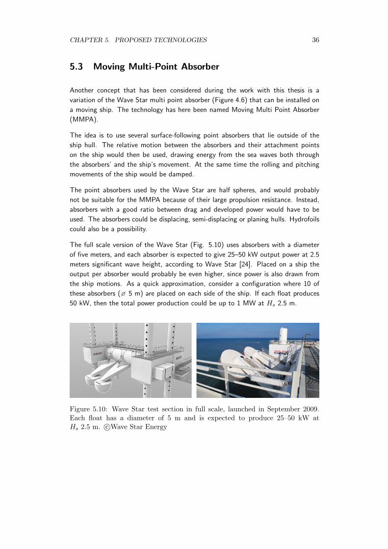
The full scale version of the Wave Star (Fig. 5.10) uses absorbers with a diameter

of five meters, and each absorber is expected to give 25–50 kW output power at 2.5

meters significant wave height, according to Wave Star [24]. Placed on a ship the

output per absorber would probably be even higher, since power is also drawn from

the ship motions. As a quick approximation, consider a configuration where 10 of

these absorbers (� 5 m) are placed on each side of the ship. If each float produces

50 kW, then the total power production could be up to 1 MW at Hs 2.5 m.

Figure 5.10: Wave Star test section in full scale, launched in September 2009.Each float has a diameter of 5 m and is expected to produce 25–50 kW atHs 2.5 m. c©Wave Star Energy


5.3.1 Modelling

The MMPA concept has not been thoroughly studied in this thesis, but a simplified

model of how to do it has been created. The model is based on the following

assumptions:

1. Linear theory is used.

2. The motions of the ship are not influenced by the motions of the absorber,

except for the resistance increase due to the absorber. Therefore the absolute3

vertical motion of the ship ηabs(ζ0, ω, t) at the position of the absorber, obtained

by linear strip theory, is an input variable in the model.

3. Only one absorber is modelled. An advanced model that captures the wave

interaction between many absorbers should also include absorber-ship interac-

tions.

4. The power take-off system is modelled as a spring CS (e.g. a linear generator)

and a damper CR, which are controllable via a control system.

The vertical movement r of the absorber is governed by the equation

mr = FR + Fs + Ff (5.31)

where FR and FS are the damper and spring forces:

FR = −CRzrFS = −CSzr

(5.32)

and zr is the relative motion between the ship and the absorber

zr = r − ηabs (5.33)

The fluid forces on the absorber are represented by Ff ,

Ff = −(Ar +Br + Cr) + Fe (5.34)

where A, B and C are hydrodynamic coefficients of the absorber and Fe is the

exciting wave force, Fe = Fe (ζ0, ω, t). These four variables depend on the absorber

shape, and can be calculated once the geometry has been decided, e.g. using the

linear strip method.

The governing equation finally becomes

(m+A) r + (CR +B) r + (CS + C) r = −CRηabs − CSηabs + Fe (5.35)3Absolute as compared to the relative motion, which is measured between surface and ship.


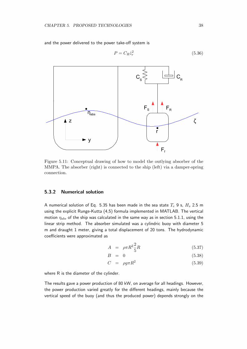
and the power delivered to the power take-off system is

P = CRz2r (5.36)

Figure 5.11: Conceptual drawing of how to model the outlying absorber of theMMPA. The absorber (right) is connected to the ship (left) via a damper-springconnection.

5.3.2 Numerical solution

A numerical solution of Eq. 5.35 has been made in the sea state Te 9 s, Hs 2.5 m

using the explicit Runge-Kutta (4,5) formula implemented in MATLAB. The vertical

motion ηabs of the ship was calculated in the same way as in section 5.1.1, using the

linear strip method. The absorber simulated was a cylindric buoy with diameter 5

m and draught 1 meter, giving a total displacement of 20 tons. The hydrodynamic

coefficients were approximated as

A = ρπR2 25R (5.37)

B = 0 (5.38)

C = ρgπR2 (5.39)

where R is the diameter of the cylinder.

The results gave a power production of 80 kW, on average for all headings. However,

the power production varied greatly for the different headings, mainly because the

vertical speed of the buoy (and thus the produced power) depends strongly on the


encounter frequency of the waves. When the ship heads into the waves the encounter

frequency increases, and thus the power production also increases.

5.3.3 Conclusions

An MMPA system could probably be able to produce a substantial amount of power,

but it is unclear if it could be done without the absorbers giving a resistance increase

larger than the produced power. It would most certainly be difficult at speeds as high

as 18 knots.


5.4 Turbine-fitted anti-roll tanks

In an M.Sc thesis work at Wallenius by Bjorn Winden [26], the possibility of fitting

roll damping U tanks on a PCTC has been investigated. The tanks work by letting

a fluid (usually water) flow between port and starboard tanks as the ship rolls, thus

counteracting the rolling motion. To improve damping performance in random sea

states, the duct between the tanks is fitted with some type of control valve or flow

damping device. Alternatively, the tank tops are connected by a closed air duct that

contains the control system.

Together with Bjorn Winden the possibility of extracting energy from the ship motions

by fitting a generator turbine to the roll tank system has been investigated. The idea

was to tap energy from the flow between the tanks with a variable resistance, thus

optimising the roll damping and extracting flow energy at the same time. However, a

simulation of the described system on a PCTC in rough weather showed that the tank

motions needed to stabilise the ship were so small that the possible power outtake

would be less than 1 kW. The reason for this is that the tanks already are tuned

to the ship’s roll eigenfrequency, and the adjustments needed to maintain optimal

roll damping in an irregular sea state are very small. One could increase the power

output by deliberately designing the tanks to be out of tune, but the increase would

probably not be large enough to justify this.

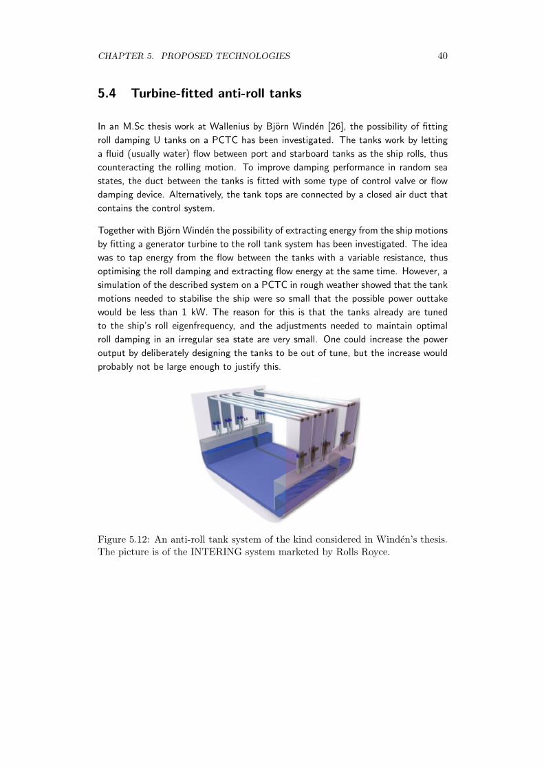
Figure 5.12: An anti-roll tank system of the kind considered in Winden’s thesis.The picture is of the INTERING system marketed by Rolls Royce.

Chapter 6

Conclusions

Looking at the technologies evaluated in chapter 5, a first conclusion is that none

has proved to be the future solution for wave energy propulsion of PCTC’s. The

main problem encountered in both the bow overtopping and WDP studies was the

resistance associated with the relatively high speed of 18 knots used, though in the

WDP case the length of the ship also had a negative impact on the results. In

the MMPA study no resistance estimate was made, but at 18 knots the increased

resistance would most likely pose a problem.

Noting that ship speed and size in this study have proved to be the main factors

against feasible wave energy propulsion, a justified question is if it would be possible

to construct shorter and slower ships that were at least partially propelled by wave

energy? The answer is, as it often is in science and engineering, that it depends

on what you need. It would, most likely, be possible to construct a wave-powered

vessel that moved at a very low speed, since a regular wave power device such as

the Wave Star or the Wave Dragon probably could move by its own power. The

question is rather if the speed and cargo-carrying capacity of such a vessel would

make it economically viable? This thesis does however not answer that question,

it only concludes that wave energy propulsion does not seem to be feasible for the

PCTC’s that are in Wallenius’ fleet today.

For future work in this field, a first recommendation would be to study systems for

shorter and slower ships than in this study, maybe 100 m long ships travelling at 10

knots. Secondly, I think that both the WDP and MMPA concepts could be further

studied beyond what has been done in this study. MMPA could be studied with

relative ease by using the linear strip method, while a thorough study of WDP would

have to use quite advanced fluid dynamics to be reliable.

41

Bibliography

[1] I.H. Abbott and A.E. Von Doenhoff. Theory of wing sections : including a

summary of airfoil data. Dover Publications, New York, 2nd ed., 1976. ISBN

0-486-60586-8. [cited at p. 33, 34]

[2] Aquamarine Power. Aquamarine Power Website. Accessed 2009-05-05.

URL http://www.aquamarinepower.com/technologies [cited at p. 18]

[3] J. Bergholtz and P. Stocks. Model testing of a passive foil propeller in

waves. Master’s thesis, Department of Naval Architecture and Ocean Engineer-

ing, Chalmers University of Technology, Goteborg, 1990. Report no. X-90/7.

[cited at p. 33, 34]

[4] J. Brooke. Wave energy conversion. Elsevier Science, Oxford, 2003. ISBN

0-08-044212-9. [cited at p. 12, 16]

[5] J. Cruz (ed.). Ocean wave energy : current status and future prepectives [i.e.

perspectives]. Springer, Berlin, 2008. ISBN 978-3-540-74894-6. [cited at p. 12, 24]

[6] M. Drela. XFoil - Subsonic Airfoil Development System. Accessed 2009-07-15.

URL http://web.mit.edu/drela/Public/web/xfoil/ [cited at p. 34]

[7] ECMWF, European Centre for Medium-Range Weather Forecasts. Interim

Re-Analysis wave statistics for 2007. Downloaded 2009-03-18.

URL http://data-portal.ecmwf.int/data/d/interim_daily/

[cited at p. 9, 33, 34]

[8] J. Falnes. Ocean waves and oscillating systems: linear interactions including

wave-energy extraction. Cambridge University Press, Cambridge, 2002. ISBN

0-521-01749-1. [cited at p. 17]

[9] J. Falnes. A review of wave-energy extraction. Marine Structures, 20(4):185–

201, 2007. [cited at p. 7, 8]

42

http://www.aquamarinepower.com/technologies

http://web.mit.edu/drela/Public/web/xfoil/

http://data-portal.ecmwf.int/data/d/interim_daily/

BIBLIOGRAPHY 43

[10] J. Grue, A. Mo, and E. Palm. Propulsion of a foil moving in water waves.

Journal of Fluid Mechanics, 186:393–417, 1988. [cited at p. 32]

[11] N. Hogben, N.M.C. Dacunha, G.F. Olliver, and British Maritime Technology

Ltd. Global wave statistics. Unwin Brothers, London, 1986. ISBN 0-946653-

38-9. [cited at p. 33]

[12] H. Isshiki, M. Murakami, and Y. Terao. Utilization of wave energy into propul-

sion of ships – wave devouring propulsion. In 15th Symposium on Naval Hy-

drodynamics, pp. 539–552. National Academy Press, Washington, DC, 1984.

[cited at p. 20]

[13] F. Korbijn. Analysis of a foil propeller system on a vessel of 300m length

sailing between chile and japan. Tech. Rep. 89-0034, Det Norske Veritas, Hovik,

Norway, 1989. [cited at p. 33, 34]

[14] P.K. Kundu and I.M. Cohen. Fluid mechanics. Academic Press, San Diego, 2nd

ed., 2002. ISBN 0-12-178251-4. [cited at p. 2]

[15] L. Margheritini, D. Vicinanza, and P. Frigaard. Ssg wave energy converter: De-

sign, reliability and hydraulic performance of an innovative overtopping device.

Renewable Energy, 34(5):1371–1380, 2009. [cited at p. 15]

[16] M.E. McCormick. Ocean wave energy conversion. Wiley, New York, 1981. ISBN

0-471-08543-X. [cited at p. 12, 16]

[17] W.H. Michel. Sea Spectra Revisited. Marine Technology, 36(4):211–227, 1999.

[cited at p. 7, 8]

[18] S. Naito and H. Isshiki. Effect of bow wings on ship propulsion and motions.

Applied Mechanics Reviews, 58(1-6):253–267, 2005. [cited at p. 33, 34]

[19] Pelamis Wave Power Ltd. Pelamis Wave Power Website. Accessed 2009-05-05.

URL http://www.pelamiswave.com [cited at p. 18]

[20] A. Rosen. Introduktion till fartygs sjoegenskaper. KTH Marina System, Stock-

holm, 2007. [cited at p. 22]

[21] K.V. Rozhdestvensky and V.A. Ryzhov. Aerohydrodynamics of flapping-wing

propulsors. Progress in Aerospace Sciences, 39(8):585–633, 2003. [cited at p. 20]

[22] Seabased AB. Seabased Website. Accessed 2009-05-05.

URL http://www.seabased.com [cited at p. 17]

[23] Wave Dragon ApS. Wave Dragon Website. Accessed 2009-04-21.

URL http://www.wavedragon.net [cited at p. 13]

http://www.pelamiswave.com

http://www.seabased.com

http://www.wavedragon.net

BIBLIOGRAPHY 44

[24] Wave Star Energy. Wave Star Website. Accessed 2009-05-05.

URL http://www.wavestarenergy.com [cited at p. 17, 36]

[25] Wavegen. Islay Limpet Project Monitoring Final Report, 2002. Downloaded

2009-05-04.

URL http://www.wavegen.co.uk/research_papers.htm [cited at p. 16]

[26] B. Winden. Anti roll tanks in pure car and truck carriers, 2009. M.Sc Thesis at

KTH Center for Naval Architecture, Stockholm. [cited at p. 40]

http://www.wavestarenergy.com

http://www.wavegen.co.uk/research_papers.htm

Nomenclature

α [ - ] Angle of attack . . . . . . . . . . . . . . . . . . . . . . . . . . . . . . . . . . . . . . . . . . . page 33

� [m] Float diameter . . . . . . . . . . . . . . . . . . . . . . . . . . . . . . . . . . . . . . . . . . . . page 36

η0i (ω) [m] Amplitude frequency component of motion in direction i . . page 22

ηi(t, x) [m] Motion in direction i . . . . . . . . . . . . . . . . . . . . . . . . . . . . . . . . . . . . . . page 22

ηabs [m] Vertical motion . . . . . . . . . . . . . . . . . . . . . . . . . . . . . . . . . . . . . . . . . . . page 33

ηrel(t, x) [m] Relative motion . . . . . . . . . . . . . . . . . . . . . . . . . . . . . . . . . . . . . . . . . . page 22

λ [m] Wavelength . . . . . . . . . . . . . . . . . . . . . . . . . . . . . . . . . . . . . . . . . . . . . . . . page 5

µ [ - ] Heading relative the direction of the waves . . . . . . . . . . . . . . . . page 23

µw [Ns/m2] Dynamic viscosity of sea water . . . . . . . . . . . . . . . . . . . . . . . . . . . . . page 3

ω [s−1] Angular frequency . . . . . . . . . . . . . . . . . . . . . . . . . . . . . . . . . . . . . . . . . page 5

φ [m2/s] Velocity potential . . . . . . . . . . . . . . . . . . . . . . . . . . . . . . . . . . . . . . . . . . page 3

Π [ - ] Probability. . . . . . . . . . . . . . . . . . . . . . . . . . . . . . . . . . . . . . . . . . . . . . . .page 25

ρ [kg/m3] Density of fluid . . . . . . . . . . . . . . . . . . . . . . . . . . . . . . . . . . . . . . . . . . . . page 2

σi [m] RMS of motion in direction i . . . . . . . . . . . . . . . . . . . . . . . . . . . . . .page 23

τ [N/m2] Viscous stress . . . . . . . . . . . . . . . . . . . . . . . . . . . . . . . . . . . . . . . . . . . . . . page 2

εi(ω) [ - ] Phase shift in direction i . . . . . . . . . . . . . . . . . . . . . . . . . . . . . . . . . . page 23

ϕ [ - ] Flow angle . . . . . . . . . . . . . . . . . . . . . . . . . . . . . . . . . . . . . . . . . . . . . . . . page 33

ζ [m] Free surface displacement . . . . . . . . . . . . . . . . . . . . . . . . . . . . . . . . . . page 4

45

BIBLIOGRAPHY 46

ζ0i (ω) [m] Amplitude of sea state frequency component . . . . . . . . . . . . . . page 22

A [m2s−4] Spectrum constant . . . . . . . . . . . . . . . . . . . . . . . . . . . . . . . . . . . . . . . . . page 7

A [Ns2/m] Added mass coefficient of absorber . . . . . . . . . . . . . . . . . . . . . . . . page 37

Af [m2] Foil area . . . . . . . . . . . . . . . . . . . . . . . . . . . . . . . . . . . . . . . . . . . . . . . . . . page 33

Ain [m2] Inflow opening area . . . . . . . . . . . . . . . . . . . . . . . . . . . . . . . . . . . . . . . page 25

Aout [m2] Outflow opening area . . . . . . . . . . . . . . . . . . . . . . . . . . . . . . . . . . . . . page 25

B [Ns/m] Damping coefficient of absorber . . . . . . . . . . . . . . . . . . . . . . . . . . . page 37

B [s−4] Spectrum constant . . . . . . . . . . . . . . . . . . . . . . . . . . . . . . . . . . . . . . . . . page 7

c [m/s] Phase speed . . . . . . . . . . . . . . . . . . . . . . . . . . . . . . . . . . . . . . . . . . . . . . . .page 5

C [N/m] Buoyancy coefficient of absorber . . . . . . . . . . . . . . . . . . . . . . . . . . page 37

CB [ - ] Block coefficient . . . . . . . . . . . . . . . . . . . . . . . . . . . . . . . . . . . . . . . . . . page 21

CD [ - ] Foil drag coefficient . . . . . . . . . . . . . . . . . . . . . . . . . . . . . . . . . . . . . . . page 33

cd [ - ] Section drag coefficient . . . . . . . . . . . . . . . . . . . . . . . . . . . . . . . . . . . .page 34

cg [m/s] Group speed . . . . . . . . . . . . . . . . . . . . . . . . . . . . . . . . . . . . . . . . . . . . . . . page 5

CL [ - ] Foil lift coefficient . . . . . . . . . . . . . . . . . . . . . . . . . . . . . . . . . . . . . . . . . page 33

cl [ - ] Section lift coefficient . . . . . . . . . . . . . . . . . . . . . . . . . . . . . . . . . . . . . page 34

CR [Ns/m] Damper constant. . . . . . . . . . . . . . . . . . . . . . . . . . . . . . . . . . . . . . . . . .page 37

CS [N/m] Spring constant . . . . . . . . . . . . . . . . . . . . . . . . . . . . . . . . . . . . . . . . . . . page 37

E [J/m2] Energy density . . . . . . . . . . . . . . . . . . . . . . . . . . . . . . . . . . . . . . . . . . . . . page 6

Ek [J/m2] Kinetic energy density. . . . . . . . . . . . . . . . . . . . . . . . . . . . . . . . . . . . . .page 6

Ep [J/m2] Potential energy density . . . . . . . . . . . . . . . . . . . . . . . . . . . . . . . . . . . . page 6

f [ - ] Probability density function . . . . . . . . . . . . . . . . . . . . . . . . . . . . . . . page 25

f [N/kg] External force . . . . . . . . . . . . . . . . . . . . . . . . . . . . . . . . . . . . . . . . . . . . . . page 2

FD [N] Drag force . . . . . . . . . . . . . . . . . . . . . . . . . . . . . . . . . . . . . . . . . . . . . . . . page 33

Fe [N] Exciting wave force on absorber . . . . . . . . . . . . . . . . . . . . . . . . . . . page 37

Ff [m] Fluid force . . . . . . . . . . . . . . . . . . . . . . . . . . . . . . . . . . . . . . . . . . . . . . . . page 37

BIBLIOGRAPHY 47

FL [N] Lift force. . . . . . . . . . . . . . . . . . . . . . . . . . . . . . . . . . . . . . . . . . . . . . . . . .page 33

FR [N] Damper force . . . . . . . . . . . . . . . . . . . . . . . . . . . . . . . . . . . . . . . . . . . . . page 37

FS [N] Spring force . . . . . . . . . . . . . . . . . . . . . . . . . . . . . . . . . . . . . . . . . . . . . . . page 37

g [m/s2] Acceleration of gravity . . . . . . . . . . . . . . . . . . . . . . . . . . . . . . . . . . . . . page 3

H [m] Wave height. . . . . . . . . . . . . . . . . . . . . . . . . . . . . . . . . . . . . . . . . . . . . . . .page 5

h [m] Pressure height . . . . . . . . . . . . . . . . . . . . . . . . . . . . . . . . . . . . . . . . . . . page 24

h0 [m] Water depth . . . . . . . . . . . . . . . . . . . . . . . . . . . . . . . . . . . . . . . . . . . . . . . page 4

Hs [m] Significant wave height . . . . . . . . . . . . . . . . . . . . . . . . . . . . . . . . . . . . . page 7

H1/3 [m] Significant wave height . . . . . . . . . . . . . . . . . . . . . . . . . . . . . . . . . . . . . page 7

Hm0 [m] Significant wave height . . . . . . . . . . . . . . . . . . . . . . . . . . . . . . . . . . . . . page 7

hmin [m] Minimum head . . . . . . . . . . . . . . . . . . . . . . . . . . . . . . . . . . . . . . . . . . . page 24

J [W/m] Energy flux . . . . . . . . . . . . . . . . . . . . . . . . . . . . . . . . . . . . . . . . . . . . . . . . page 6

k [m−1] Wavenumber . . . . . . . . . . . . . . . . . . . . . . . . . . . . . . . . . . . . . . . . . . . . . . . page 5

kX [ - ] Phase shift due to heading and position . . . . . . . . . . . . . . . . . . . page 23

L [m] Ship length . . . . . . . . . . . . . . . . . . . . . . . . . . . . . . . . . . . . . . . . . . . . . . . page 33

Lpp [m] Length between perpendiculars . . . . . . . . . . . . . . . . . . . . . . . . . . . .page 21

mj [m4s−j ] Spectral moment . . . . . . . . . . . . . . . . . . . . . . . . . . . . . . . . . . . . . . . . . . . page 7

p [N/m2] Total pressure . . . . . . . . . . . . . . . . . . . . . . . . . . . . . . . . . . . . . . . . . . . . . .page 2

P [W] Power . . . . . . . . . . . . . . . . . . . . . . . . . . . . . . . . . . . . . . . . . . . . . . . . . . . . .page 25

PE [W] Required engine power . . . . . . . . . . . . . . . . . . . . . . . . . . . . . . . . . . . . page 21

ps [N/m2] Hydrostatic pressure . . . . . . . . . . . . . . . . . . . . . . . . . . . . . . . . . . . . . . page 24

R [m3] Reservoir level . . . . . . . . . . . . . . . . . . . . . . . . . . . . . . . . . . . . . . . . . . . . page 24

r [m] Vertical motion of absorber . . . . . . . . . . . . . . . . . . . . . . . . . . . . . . . page 37

S [m4s] Energy spectrum function . . . . . . . . . . . . . . . . . . . . . . . . . . . . . . . . . . page 7

Sηi [m4s] Response energy spectrum . . . . . . . . . . . . . . . . . . . . . . . . . . . . . . . . page 23

T [s] Waveperiod . . . . . . . . . . . . . . . . . . . . . . . . . . . . . . . . . . . . . . . . . . . . . . . . page 5

BIBLIOGRAPHY 48

t [s] Time. . . . . . . . . . . . . . . . . . . . . . . . . . . . . . . . . . . . . . . . . . . . . . . . . . . . . . .page 2

Te [s] Wave energy period . . . . . . . . . . . . . . . . . . . . . . . . . . . . . . . . . . . . . . . . page 7

U [m/s] Ship speed . . . . . . . . . . . . . . . . . . . . . . . . . . . . . . . . . . . . . . . . . . . . . . . . page 25

u [m/s] Flow velocity. . . . . . . . . . . . . . . . . . . . . . . . . . . . . . . . . . . . . . . . . . . . . . .page 2

v [m/s] Flow speed. . . . . . . . . . . . . . . . . . . . . . . . . . . . . . . . . . . . . . . . . . . . . . . .page 24

w [m3/2] Power height . . . . . . . . . . . . . . . . . . . . . . . . . . . . . . . . . . . . . . . . . . . . . . page 25

Yi(ω) [ - ] Transfer function in direction i . . . . . . . . . . . . . . . . . . . . . . . . . . . . page 22

z [m] Vertical position . . . . . . . . . . . . . . . . . . . . . . . . . . . . . . . . . . . . . . . . . . . page 3

zin [m] Inflow height . . . . . . . . . . . . . . . . . . . . . . . . . . . . . . . . . . . . . . . . . . . . . . page 24

Abbreviations

Abbreviation Description Definition

ECMWF European Centre for Medium-Range WeatherForecasts

page 9

kts knots, 1 knot = 1.852 km/h page 21MMPA Moving Multi Point Absorber page 36MST Multi-Stage Turbine page 15OWC Oscillating Water Column page 16PCTC Pure Car and Truck Carrier page 1pdf Probability Density Function page 25SSG Sea Slot-cone Generator page 15WDP Wave Devouring Propulsion page 20WEC Wave Energy Conversion page 12WPA Water Plane Area page 33

49

List of Figures

3.1 Worldwide shipping route . . . . . . . . . . . . . . . . . . . . . . . . . . . . . 93.2 Combined scatter and energy diagram for worldwide route . . . . . . . . . . 10

4.1 Principles of energy capture in an overtopping device . . . . . . . . . . . . . 134.2 Wave Dragon prototype . . . . . . . . . . . . . . . . . . . . . . . . . . . . . . 144.3 Sea Slot-cone Generator . . . . . . . . . . . . . . . . . . . . . . . . . . . . . . 154.4 Limpet oscillating water column . . . . . . . . . . . . . . . . . . . . . . . . . 164.5 Linear generator buoy. . . . . . . . . . . . . . . . . . . . . . . . . . . . . . . . 174.6 Wave Star multi point absorber . . . . . . . . . . . . . . . . . . . . . . . . . 194.7 Pelamis WEC . . . . . . . . . . . . . . . . . . . . . . . . . . . . . . . . . . . 194.8 Oyster WEC . . . . . . . . . . . . . . . . . . . . . . . . . . . . . . . . . . . . 194.9 Wallenius’ E/S Orcelle, equipped with fins for wave energy propulsion . . . . 20

5.1 Example transfer functions for a PCTC . . . . . . . . . . . . . . . . . . . . . 225.2 Example of energy spectrum . . . . . . . . . . . . . . . . . . . . . . . . . . . 235.3 Illustration of the bow overtopping model. . . . . . . . . . . . . . . . . . . . 245.4 Output power as a function of inflow height for a given sea state. . . . . . . . 275.5 Output and retarding power estimates for model variations . . . . . . . . . . 295.6 Same comparison as Fig. 5.5, but at half the speed. . . . . . . . . . . . . . . 305.7 Modelling of WDP-equipped ship . . . . . . . . . . . . . . . . . . . . . . . . 325.8 Propulsive and dragging power of the T-foil, all headings . . . . . . . . . . . 355.9 Mean resultant of the T-foil for multiple Te, all headings . . . . . . . . . . . 355.10 Wave Star test section in full scale . . . . . . . . . . . . . . . . . . . . . . . . 365.11 Conceptual drawing of how to model the outlying absorber of the MMPA. . 385.12 An anti-roll tank system . . . . . . . . . . . . . . . . . . . . . . . . . . . . . 40

50

List of Tables

3.1 Average monthly energy flux . . . . . . . . . . . . . . . . . . . . . . . . . . . 10

5.1 Ship data for M/V Fedora used in study. . . . . . . . . . . . . . . . . . . . . 21

51

Documents

Wave Energy Propulsion for Pure Car and Truck Carriers …618333/FULLTEXT01.pdf · Pure Car and Truck Carriers (PCTCs) ... Wave Energy Propulsion for Pure Car and Truck Carriers