Wavelet based seismic signal de-noising using Shannon and Tsallis entropy

Computers and Mathematics with Applications 64 (2012) 3580–3593

Contents lists available at SciVerse ScienceDirect

Computers and Mathematics with Applications

journal homepage: www.elsevier.com/locate/camwa

Wavelet based seismic signal de-noising using Shannon andTsallis entropyM. Beenamol ∗, S. Prabavathy, J. MohanalinDepartment of Civil Engineering, St. Xavier’s Catholic College of Engineering, TN, India

a r t i c l e i n f o

Article history:Received 15 June 2012Received in revised form 25 August 2012Accepted 30 September 2012

Keywords:WaveletSeismic signalVisu shrinkNormal shrinkShannon entropy and Tsallis entropy

a b s t r a c t

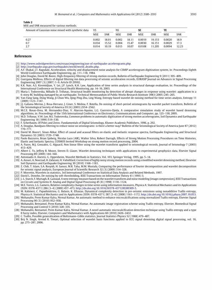
Seismograms are the vital sources of information in seismic engineering. But, these recordsare always contaminated with noise which has to be removed before using them inseismic applications. Recently, wavelet based techniques proved to be very effective inde-noising by achieving high SNR. However, selection of the correct threshold plays acrucial role in deciding the SNR value. It is strange that only very few thresholders existin seismic and non-seismic studies. In this paper, we have proposed a set of novel entropybased thresholders through 2 experiments. In experiment 1, we have proposed a Shannonentropy based algorithm which has produced 11.205 SNR. In experiment 2, we usedTsallis entropywhich hasmoderately improved the result by providing 12.23 SNR. Existingthresholders like visu and normal shrink have managed to produce 10.19 and 10.07 SNRrespectively. Through our experiments, we observed that for low frequency problems(σ = 0.27), the performance of both entropies matched appreciably. However, for highfrequency (σ = 2.7) Tsallis produced slightly better SNR and is more feasible in detectingthe occurrence of P and S waves by smoothing the accelerograms.

© 2012 Elsevier Ltd. All rights reserved.

1. Introduction

An earthquake is one of the most lethal natural disasters and it claims millions of lives apart from the destruction ofproperties. In fact, an estimate from the United States Geographical Survey (USGS) suggests that several million earthquakesoccur in the world each year, but only a few are getting noticed [1]. Further, the national earthquake information centerhas pointed out that about 50 earthquakes happen each day, or about 20,000 a year. According to an official estimate [2],316,000 people were killed, 300,000 injured, 1.3 million displaced, 97,294 houses destroyed and 188,383 were damaged inthe Port-au-Prince earthquake. A USGS report suggests that from 2000 to 2010 there was an average of 63,000 deaths peryear globally, which is much worse than the death rate for many types of cancers. The mortality rate and the destruction ofthese valuable properties are due to reaction of structures to the cyclic loads of earthquakes.

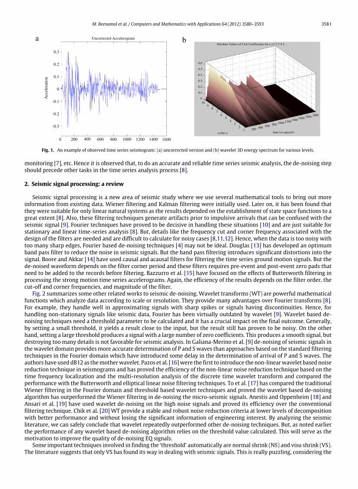
Structural engineers are expected to give more emphasis on designing structures based on design and responsespectra developed from accelerograms (which are expected to be earthquake resistant). This is possible by the use ofaccelerograms as it provides critical information about the earthquake source and is an asset for the progress in earthquakeand seismological engineering. Processing of the accelerograms [3] is often needed to bring out this valuable information andis often not straightforward due to the presence of complex characteristics like non-stationary and non-linear componentsof ground shaking. Moreover, due to the influence of many random and uncertain natural factors, the observed time seriesaccelerogram data always include many high frequency noises (Fig. 1) [4,5] which contaminate the real series data. Thiscausesmany difficulties in period identification, parameter estimation,modeling, system identification [6], structural health

∗ Corresponding author. Tel.: +91 9578930932.E-mail address: [email protected] (M. Beenamol).

0898-1221/$ – see front matter© 2012 Elsevier Ltd. All rights reserved.doi:10.1016/j.camwa.2012.09.009

http://dx.doi.org/10.1016/j.camwa.2012.09.009

http://www.elsevier.com/locate/camwa

http://www.elsevier.com/locate/camwa

mailto:[email protected]

http://dx.doi.org/10.1016/j.camwa.2012.09.009

M. Beenamol et al. / Computers and Mathematics with Applications 64 (2012) 3580–3593 3581

200 400 600 800 1000 1200 14001600 1800 2000

109

87

65

43

21

0.6

0.5

0.4

0.3

0.2

0.1

0

scales a

Absolute Values of Ca,b Coefficients for a =1 2 3 4 5 ...

time (or space)b

0 200 400 600 800 1000 1200 1400 1600

0.2

0.1

0.3

0

-0.1

-0.2

-0.3

Acc

eler

atio

n

Uncorrected Accelerogram ba

Fig. 1. An example of observed time series seismogram: (a) uncorrected version and (b) wavelet 3D energy spectrum for various levels.

monitoring [7], etc. Hence it is observed that, to do an accurate and reliable time series seismic analysis, the de-noising stepshould precede other tasks in the time series analysis process [8].

2. Seismic signal processing: a review

Seismic signal processing is a new area of seismic study where we use several mathematical tools to bring out moreinformation from existing data. Wiener filtering and Kalman filtering were initially used. Later on, it has been found thatthey were suitable for only linear natural systems as the results depended on the establishment of state space functions to agreat extent [8]. Also, these filtering techniques generate artifacts prior to impulsive arrivals that can be confused with theseismic signal [9]. Fourier techniques have proved to be decisive in handling these situations [10] and are just suitable forstationary and linear time-series analysis [8]. But, details like the frequency cut and corner frequency associated with thedesign of the filters are needed and are difficult to calculate for noisy cases [8,11,12]. Hence, when the data is too noisy withtoo many sharp edges, Fourier based de-noising techniques [4] may not be ideal. Douglas [13] has developed an optimumband pass filter to reduce the noise in seismic signals. But the band pass filtering introduces significant distortions into thesignal. Boore and Akkar [14] have used causal and acausal filters for filtering the time series ground motion signals. But thede-noised waveform depends on the filter corner period and these filters requires pre-event and post-event zero pads thatneed to be added to the records before filtering. Bazzurro et al. [15] have focused on the effects of Butterworth filtering inprocessing the strong motion time series accelerograms. Again, the efficiency of the results depends on the filter order, thecut-off and corner frequencies, and magnitude of the filter.

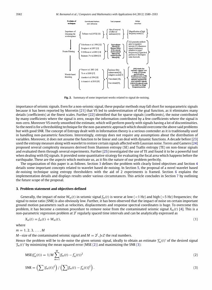
Fig. 2 summarizes some other related works to seismic de-noising. Wavelet transforms (WT) are powerful mathematicalfunctions which analyze data according to scale or resolution. They provide many advantages over Fourier transforms [8].For example, they handle well in approximating signals with sharp spikes or signals having discontinuities. Hence, forhandling non-stationary signals like seismic data, Fourier has been virtually outdated by wavelet [9]. Wavelet based de-noising techniques need a threshold parameter to be calculated and it has a crucial impact on the final outcome. Generally,by setting a small threshold, it yields a result close to the input, but the result still has proven to be noisy. On the otherhand, setting a large threshold produces a signal with a large number of zero coefficients. This produces a smooth signal, butdestroying too many details is not favorable for seismic analysis. In Galiana-Merino et al. [9] de-noising of seismic signals inthewavelet domain providesmore accurate determination of P and Swaves than approaches based on the standard filteringtechniques in the Fourier domain which have introduced some delay in the determination of arrival of P and S waves. Theauthors have used dB12 as themotherwavelet. Pazos et al. [16]were the first to introduce the non-linearwavelet basednoisereduction technique in seismograms and has proved the efficiency of the non-linear noise reduction technique based on thetime frequency localization and the multi-resolution analysis of the discrete time wavelet transform and compared theperformance with the Butterworth and elliptical linear noise filtering techniques. To et al. [17] has compared the traditionalWiener filtering in the Fourier domain and threshold based wavelet techniques and proved the wavelet based de-noisingalgorithm has outperformed the Wiener filtering in de-noising the micro-seismic signals. Anestis and Oppenheim [18] andAnsari et al. [19] have used wavelet de-noising on the high noise signals and proved its efficiency over the conventionalfiltering technique. Chik et al. [20] WT provide a stable and robust noise reduction criteria at lower levels of decompositionwith better performance and without losing the significant information of engineering interest. By analyzing the seismicliterature, we can safely conclude that wavelet repeatedly outperformed other de-noising techniques. But, as noted earlierthe performance of any wavelet based de-noising algorithm relies on the threshold value calculated. This will serve as themotivation to improve the quality of de-noising EQ signals.

Some important techniques involved in finding the ‘threshold’ automatically are normal shrink (NS) and visu shrink (VS).The literature suggests that only VS has found its way in dealing with seismic signals. This is really puzzling, considering the

3582 M. Beenamol et al. / Computers and Mathematics with Applications 64 (2012) 3580–3593

Fig. 2. Summary of some important works related to signal de-noising.

importance of seismic signals. Even for a non-seismic signal, these popularmethodsmay fall short for nonparametric signalsbecause it has been reported by Morretin [21] that VS led to underestimation of the goal function, as it eliminates manydetails (coefficients) at the finest scales. Further [22] identified that for sparse signals (coefficients), the noise contributedby many coefficients where the signal is zero, swaps the information contributed by a few coefficients where the signal isnon-zero. Moreover VS overly smoothed the estimate, whichwill perform poorly with signals having a lot of discontinuities.So theneed is for a thresholding technique for the non-parametric approachwhich should overcome the above said problemsbut with good SNR. The concept of Entropy dealt with in Information theory is a serious contender as it is traditionally usedin handling non-parametric functions. Interestingly, entropy does not require any assumptions about the distribution ofvariables. Moreover, it does not assume the function to be linear and can deal with dynamic functions. A decade before [23]used the entropymeasure alongwithwavelet to restore certain signals affectedwithGaussian noise. Torres andGamero [24]proposed several complexity measures derived from Shannon entropy (SE) and Tsallis entropy (TE) on non-linear signalsand evaluated them through several experiments. Further [25] investigated the use of TE and found it to be a powerful toolwhen dealing with EQ signals. It provided some quantitative strategy for evaluating the focal area which happens before theearthquake. These are the aspects which motivate us, as it fits the nature of our problem perfectly.

The organization of this paper is as follows. Section 3 defines the problem with clearly listed objectives and Section 4details some important concepts related to wavelet based de-noising. In Section 5, the proposal of a novel wavelet basedde-noising technique using entropy thresholders with the aid of 2 experiments is framed. Section 6 explains theimplementation details and displays results under various circumstances. This article concludes in Section 7 by outliningthe future scope of the proposal.

3. Problem statement and objectives defined

Generally, the impact of noise Wm(t) in seismic signal fm(t) is worse at low (<1 Hz) and high (>5 Hz) frequencies; thesignal to noise ratio (SNR) is also obviously low. Further, it has been observed that the impact of noise on certain importantground motion parameters such as velocities, displacements and response spectral coordinates is huge. To overcome thisproblem, it has become a common procedure to remove noise from the contaminated seismic signal Xm(t) [4]. This is anon-parametric regression problem at 2J regularly spaced time intervals and can be analytically expressed as

Xm(t) = fm(t) + Wm(t), (1)

wherem = 1, 2, 3, . . . ,MM—size of the contaminated seismic signal andM = 2J , JϵZ the real numbers.Hence the problem will be to de-noise the given seismic signal, ideally to obtain an estimate ‘f ′

m(t)’ of the desired signal‘fm(t)’ by minimizing the mean squared error (MSE (2)) and maximizing the SNR (3):

MSE(f ′

m(t)) = 1/MM

m=1

(fm(t) − f ′

m(t))2 (2)

SNR =

|fm(t)|2

/

[fm(t) − f ′

m(t)]2

. (3)


xm(t) Mathemetical Model(Denoising model)

fm(t)

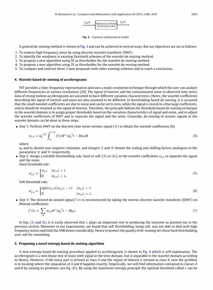
Fig. 3. A general mathematical model.

A general de-noisingmethod is shown in Fig. 3 and can be achieved in several ways. But our objectives are set as follows:

1. To remove high frequency noise by using discrete wavelet transform (DWT).2. To identify the weakness in existing threshold schemes of the wavelet de-noising method.3. To propose a new algorithm using SE as thresholder for the wavelet de-noising method.4. To propose a new algorithm using TE as thresholder for the wavelet de-noising method.5. To compare and contrast these 2 new proposals with other existing schemes and to reach a conclusion.

4. Wavelet based de-noising of accelerograms

WT provides a time-frequency representation and uses amulti-resolution technique throughwhich the user can analyzedifferent frequencies at various resolutions [20]. The signal of interest and the contaminated noise in observed time seriesdata of strongmotion accelerograms are assumed to have different variation characteristics. Hence, the wavelet coefficientsdescribing the signal of interest and noise are also assumed to be different. In thresholding based de-noising, it is assumedthat the small wavelet coefficients are due to noise and can be set to zero, while the signal is stored in a few large coefficients,which should be retained as the signal of interest. Therefore, the principle behind the threshold based de-noising techniquein the wavelet domain is to assign proper thresholds based on the variation characteristics of signal and noise, and to adjustthe wavelet coefficients of DWT and to separate the signal and the noise. Generally, de-noising of seismic signals in thewavelet domain can be done in three steps.

• Step 1: Perform DWT on the discrete time series seismic signal f (t) to obtain the wavelet coefficients [8]:

wj,k = a−j/20

+∞

∞

f (t)Ψ ∗(a−j0 t − kb0)dt (4)

wherea0 and b0 denote non-negative constants, and integers ‘j’ and ‘k’ denote the scaling and shifting factors analogous to theparameters ‘a’ and ‘b’ respectively.

• Step 2: Assign a suitable thresholding rule, hard or soft ((5) or (6)), to the wavelet coefficients wj,k to separate the signaland the noise.Hard threshold rule:

w′

j,k =

wj,k |wj,k| > λ

0 |wj,k| < λ.(5)

Soft threshold rule:

w′

j,k =

sgn(wj,k)(|wj,k| − λ) |wj,k| > λ

0 |wj,k| < λ.(6)

• Step 3: The desired de-noised signal f ′(t) is reconstructed by taking the inverse discrete wavelet transform (IDWT) onfiltered coefficients:

f ′(t) =

j,k

wj,kΨ∗(a−j

0 t − kb0). (7)

In Eqs. (5) and (6), it is easily observed that λ plays an important role in producing the outcome as pointed out in theprevious section. Moreover in our experiments, we found that soft thresholding, being soft, was not able to deal with highfrequency noises and took the SNRdown considerably. Hence to protect the quality of de-noisingwe chose hard thresholdingover soft for smoothing.

5. Proposing a novel entropy based de-noising algorithm

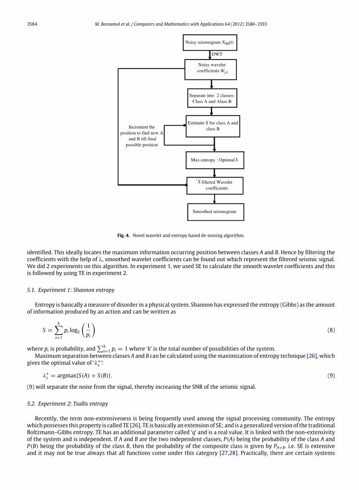
A new entropy based de-noising procedure applied to accelerograms is shown in Fig. 4 which is self-explanatory. Theaccelerogram is a non-linear mix of noise with signal in the time domain, but is separable in the wavelet domain accordingto theory. However, if the noisy part is termed as class A and the region of interest is termed as class B, now the problemis in locating where the separation of A and B happens exactly. Empirically, we will find information contained in classes Aand B by varying its positions (see Eq. (8)). By using the maximum entropy principle the optimal threshold called λ can be


Noisy seismogram Xm(t)

DWT

Noisy waveletcoefficients Wj,k

Separate into 2 classes:Class A and Alass B

Estimate S for class A and class B

Max entropy : Optimal

' ' filtered Waveletcoefficients

Smoothed seismogram

Increment the position to find new A

and B till finalpossible position

Fig. 4. Novel wavelet and entropy based de-noising algorithm.

identified. This ideally locates the maximum information occurring position between classes A and B. Hence by filtering thecoefficients with the help of λ, smoothed wavelet coefficients can be found out which represent the filtered seismic signal.We did 2 experiments on this algorithm. In experiment 1, we used SE to calculate the smooth wavelet coefficients and thisis followed by using TE in experiment 2.

5.1. Experiment 1: Shannon entropy

Entropy is basically ameasure of disorder in a physical system. Shannon has expressed the entropy (Gibbs) as the amountof information produced by an action and can be written as

S =

ki=1

pi log2

1pi

(8)

where pi is probability, andk

i=1 pi = 1 where ‘k’ is the total number of possibilities of the system.Maximum separation between classes A and B can be calculated using themaximization of entropy technique [26], which

gives the optimal value of ‘λ∗s ’:

λ∗

s = argmax{S(A) + S(B)}. (9)

(9) will separate the noise from the signal, thereby increasing the SNR of the seismic signal.

5.2. Experiment 2: Tsallis entropy

Recently, the term non-extensiveness is being frequently used among the signal processing community. The entropywhichpossesses this property is called TE [26]. TE is basically an extension of SE; and is a generalized version of the traditionalBoltzmann–Gibbs entropy. TE has an additional parameter called ‘q’ and is a real value. It is linked with the non-extensivityof the system and is independent. If A and B are the two independent classes, P(A) being the probability of the class A andP(B) being the probability of the class B, then the probability of the composite class is given by PA+B. i.e. SE is extensiveand it may not be true always that all functions come under this category [27,28]. Practically, there are certain systems


Table 1Characteristic details of SGM records.

Details 1 2

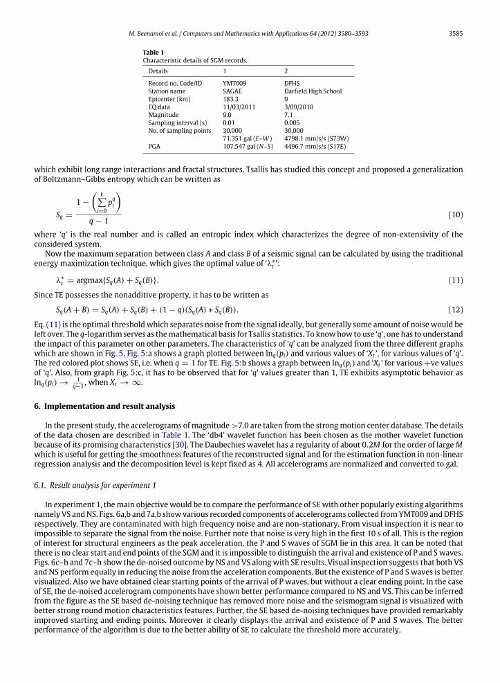
Record no. Code/ID YMT009 DFHSStation name SAGAE Darfield High SchoolEpicenter (km) 183.3 9EQ data 11/03/2011 3/09/2010Magnitude 9.0 7.1Sampling interval (s) 0.01 0.005No. of sampling points 30,000 30,000

71.351 gal (E–W ) 4798.1 mm/s/s (S73W)PGA 107.547 gal (N–S) 4496.7 mm/s/s (S17E)

which exhibit long range interactions and fractal structures. Tsallis has studied this concept and proposed a generalizationof Boltzmann–Gibbs entropy which can be written as

Sq =

1 −

k

i=0pqi

q − 1

(10)

where ‘q’ is the real number and is called an entropic index which characterizes the degree of non-extensivity of theconsidered system.

Now the maximum separation between class A and class B of a seismic signal can be calculated by using the traditionalenergy maximization technique, which gives the optimal value of ‘λ∗

t ’:

λ∗

t = argmax{Sq(A) + Sq(B)}. (11)

Since TE possesses the nonadditive property, it has to be written as

Sq(A + B) = Sq(A) + Sq(B) + (1 − q)(Sq(A) ∗ Sq(B)). (12)

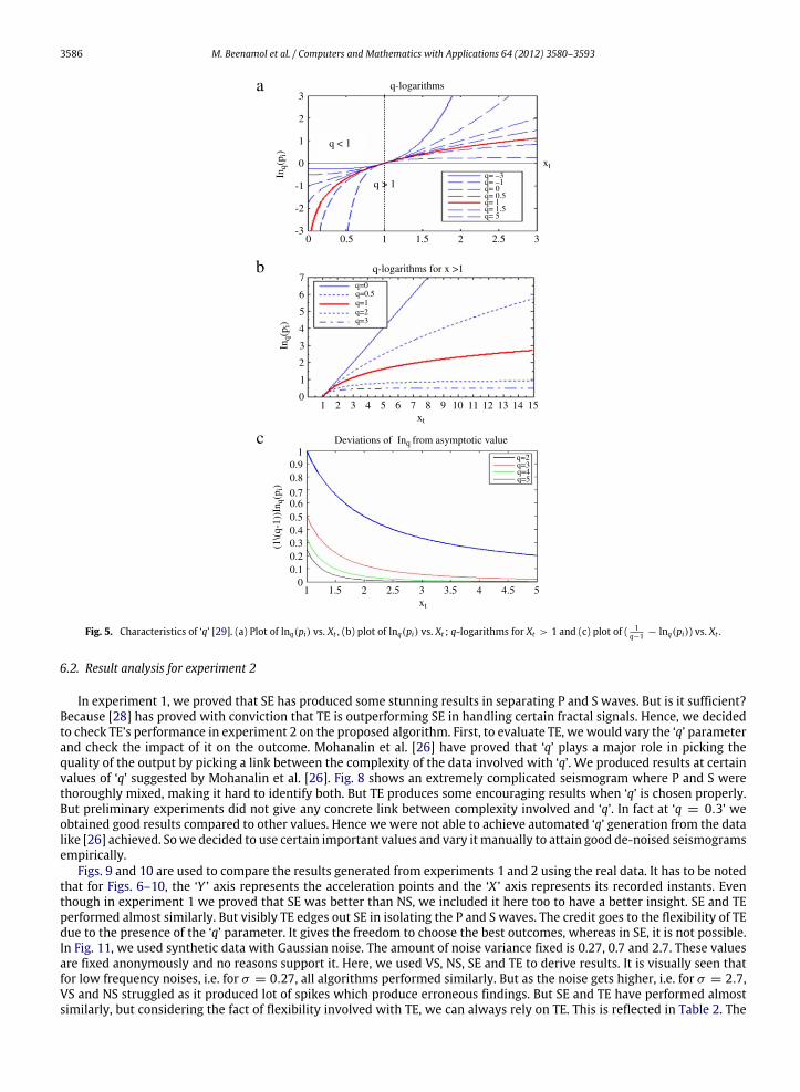
Eq. (11) is the optimal thresholdwhich separates noise from the signal ideally, but generally some amount of noise would beleft over. The q-logarithm serves as themathematical basis for Tsallis statistics. To knowhow to use ‘q’, one has to understandthe impact of this parameter on other parameters. The characteristics of ‘q’ can be analyzed from the three different graphswhich are shown in Fig. 5. Fig. 5:a shows a graph plotted between lnq(pi) and various values of ‘Xt ’, for various values of ‘q’.The red colored plot shows SE, i.e. when q = 1 for TE. Fig. 5:b shows a graph between lnq(pi) and ‘Xt ’ for various +ve valuesof ‘q’. Also, from graph Fig. 5:c, it has to be observed that for ‘q’ values greater than 1, TE exhibits asymptotic behavior aslnq(pi) →

1q−1 , when Xt → ∞.

6. Implementation and result analysis

In the present study, the accelerograms of magnitude>7.0 are taken from the strongmotion center database. The detailsof the data chosen are described in Table 1. The ‘db4’ wavelet function has been chosen as the mother wavelet functionbecause of its promising characteristics [30]. The Daubechies wavelet has a regularity of about 0.2M for the order of largeMwhich is useful for getting the smoothness features of the reconstructed signal and for the estimation function in non-linearregression analysis and the decomposition level is kept fixed as 4. All accelerograms are normalized and converted to gal.

6.1. Result analysis for experiment 1

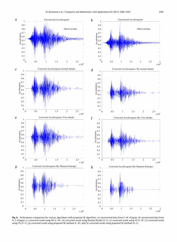
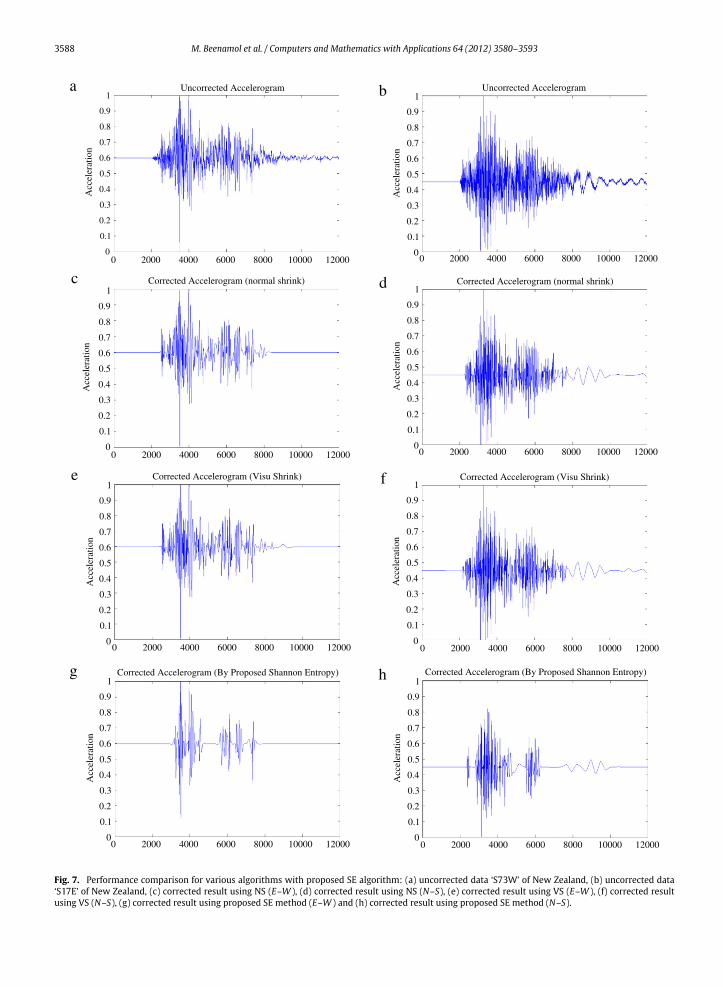
In experiment 1, themain objectivewould be to compare the performance of SEwith other popularly existing algorithmsnamely VS andNS. Figs. 6a,b and 7a,b showvarious recorded components of accelerograms collected fromYMT009 andDFHSrespectively. They are contaminated with high frequency noise and are non-stationary. From visual inspection it is near toimpossible to separate the signal from the noise. Further note that noise is very high in the first 10 s of all. This is the regionof interest for structural engineers as the peak acceleration, the P and S waves of SGM lie in this area. It can be noted thatthere is no clear start and end points of the SGM and it is impossible to distinguish the arrival and existence of P and Swaves.Figs. 6c–h and 7c–h show the de-noised outcome by NS and VS alongwith SE results. Visual inspection suggests that both VSand NS perform equally in reducing the noise from the acceleration components. But the existence of P and Swaves is bettervisualized. Also we have obtained clear starting points of the arrival of P waves, but without a clear ending point. In the caseof SE, the de-noised accelerogram components have shown better performance compared to NS and VS. This can be inferredfrom the figure as the SE based de-noising technique has removed more noise and the seismogram signal is visualized withbetter strong round motion characteristics features. Further, the SE based de-noising techniques have provided remarkablyimproved starting and ending points. Moreover it clearly displays the arrival and existence of P and S waves. The betterperformance of the algorithm is due to the better ability of SE to calculate the threshold more accurately.


q-logarithms for x >1

q-logarithms

xt

a

b

c

3

2

1

0

-1

-2

-3

Inq(

p i)

7

6

5

4

3

2

1

0

Inq(

p i)

10.90.8

0.70.60.50.40.30.20.1

0

(1\(

q-1)

)In q

(pi)

1 1.5 2 2.5 3 3.5 4 4.5 5xt

q=2q=3q=4q=5

Deviations of Inq from asymptotic value

1 2 3 4 5 6 7 8 9 10 11 12 13 14 15xt

q=0

q=1q=2q=3

q=0.

q= –3q= –1q= 0q= 0.5q= 1q= 1.5q= 5

5

0 0.5 1 1.5 2 2.5 3

q < 1

q > 1

Fig. 5. Characteristics of ‘q’ [29]. (a) Plot of lnq(pi) vs. Xt , (b) plot of lnq(pi) vs. Xt ; q-logarithms for Xt > 1 and (c) plot of ( 1q−1 − lnq(pi)) vs. Xt .

6.2. Result analysis for experiment 2

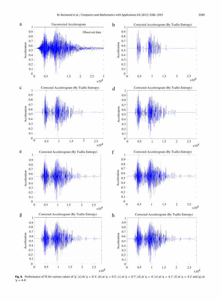
In experiment 1, we proved that SE has produced some stunning results in separating P and S waves. But is it sufficient?Because [28] has proved with conviction that TE is outperforming SE in handling certain fractal signals. Hence, we decidedto check TE’s performance in experiment 2 on the proposed algorithm. First, to evaluate TE, wewould vary the ‘q’ parameterand check the impact of it on the outcome. Mohanalin et al. [26] have proved that ‘q’ plays a major role in picking thequality of the output by picking a link between the complexity of the data involved with ‘q’. We produced results at certainvalues of ‘q’ suggested by Mohanalin et al. [26]. Fig. 8 shows an extremely complicated seismogram where P and S werethoroughly mixed, making it hard to identify both. But TE produces some encouraging results when ‘q’ is chosen properly.But preliminary experiments did not give any concrete link between complexity involved and ‘q’. In fact at ‘q = 0.3’ weobtained good results compared to other values. Hence we were not able to achieve automated ‘q’ generation from the datalike [26] achieved. Sowe decided to use certain important values and vary itmanually to attain good de-noised seismogramsempirically.

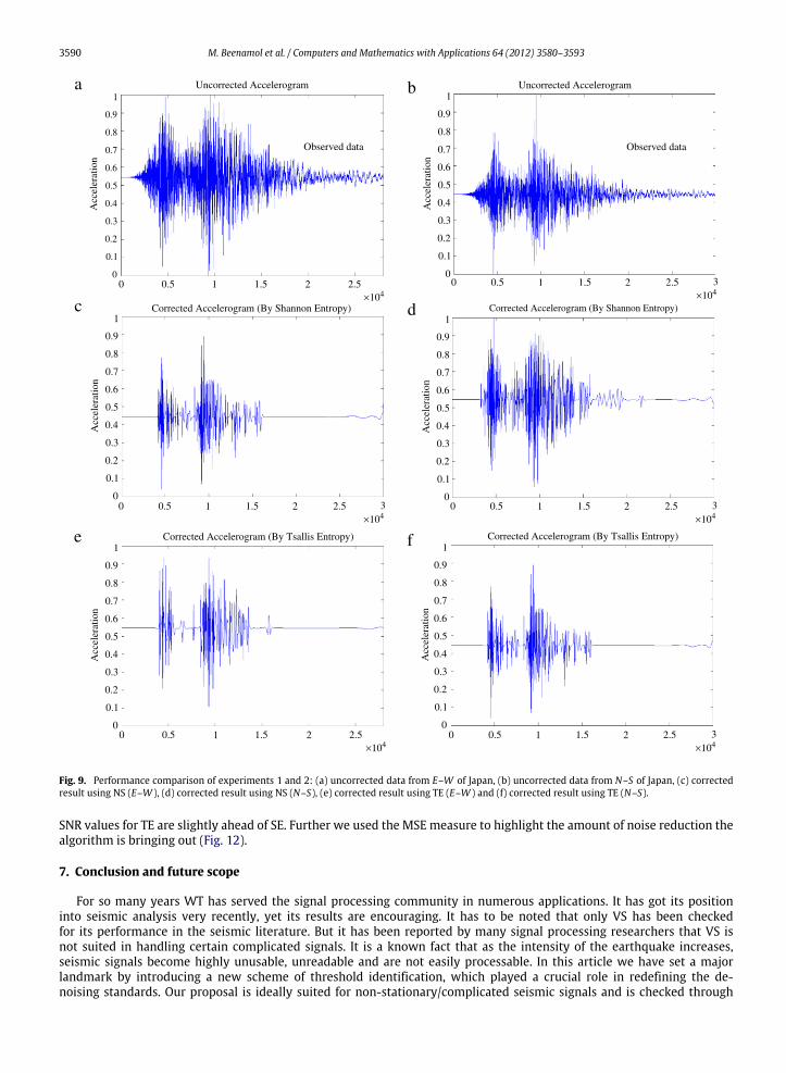
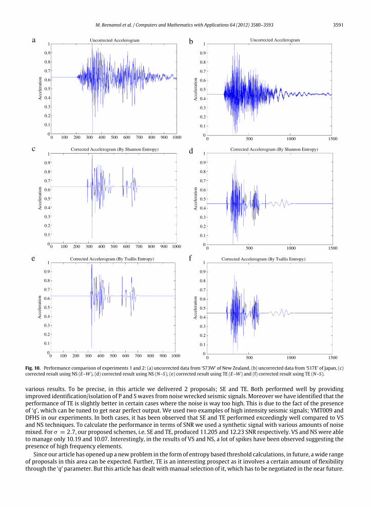
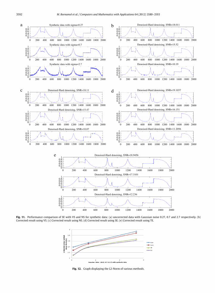
Figs. 9 and 10 are used to compare the results generated from experiments 1 and 2 using the real data. It has to be notedthat for Figs. 6–10, the ‘Y ’ axis represents the acceleration points and the ‘X ’ axis represents its recorded instants. Eventhough in experiment 1 we proved that SE was better than NS, we included it here too to have a better insight. SE and TEperformed almost similarly. But visibly TE edges out SE in isolating the P and S waves. The credit goes to the flexibility of TEdue to the presence of the ‘q’ parameter. It gives the freedom to choose the best outcomes, whereas in SE, it is not possible.In Fig. 11, we used synthetic data with Gaussian noise. The amount of noise variance fixed is 0.27, 0.7 and 2.7. These valuesare fixed anonymously and no reasons support it. Here, we used VS, NS, SE and TE to derive results. It is visually seen thatfor low frequency noises, i.e. for σ = 0.27, all algorithms performed similarly. But as the noise gets higher, i.e. for σ = 2.7,VS and NS struggled as it produced lot of spikes which produce erroneous findings. But SE and TE have performed almostsimilarly, but considering the fact of flexibility involved with TE, we can always rely on TE. This is reflected in Table 2. The


1

0.9

0.8

0.7

0.6

0.5

0.4

0.3

0.2

0.1

0

Acc

eler

atio

na Uncorrected Accelerogram

Observed data

0 0.5 1 1.5 2 2.5104

1

0.9

0.8

0.7

0.6

0.5

0.4

0.3

0.2

0.1

0

Acc

eler

atio

n

b

c d

e f

g h

0 0.5 1 1.5 2 2.5104

3

Observed data

Uncorrected Accelerogram

1

0.9

0.8

0.7

0.6

0.5

0.4

0.3

0.2

0.1

0

Acc

eler

atio

n

Corrected Accelerogram (normal shrink)

0 0.5 1 1.5 2 2.5104

1

0.9

0.8

0.7

0.6

0.5

0.4

0.3

0.2

0.1

0

Acc

eler

atio

n

0 0.5 1 1.5 2 2.5104

Corrected Accelerogram ( By normal shrink)

1

0.9

0.8

0.7

0.6

0.5

0.4

0.3

0.2

0.1

0

Acc

eler

atio

n

0 0.5 1 1.5 2 2.5104

Corrected Accelerogram (Visu shrink)1

0.9

0.8

0.7

0.6

0.5

0.4

0.3

0.2

0.1

0

Acc

eler

atio

n

0 0.5 1 1.5 2 2.5104

Corrected Accelerogram (By Visu shrink)

1

0.9

0.8

0.7

0.6

0.5

0.4

0.3

0.2

0.1

0

Acc

eler

atio

n

0 0.5 1 1.5 2 2.5104

Corrected Accelerogram (By Shannon Entropy)1

0.9

0.8

0.7

0.6

0.5

0.4

0.3

0.2

0.1

0

Acc

eler

atio

n

0 0.5 1 1.5 2 2.5104

3

Corrected Accelerogram (By Shannon Entropy)

Fig. 6. Performance comparison for various algorithms with proposed SE algorithm: (a) uncorrected data from E–W of Japan, (b) uncorrected data fromN–S of Japan, (c) corrected result using NS (E–W ), (d) corrected result using Normal Shrink (N–S), (e) corrected result using VS (E–W ), (f) corrected resultusing VS (N–S), (g) corrected result using proposed SE method (E–W ) and (h) corrected result using proposed SE method (N–S).


1

0.9

0.8

0.7

0.6

0.5

0.4

0.3

0.2

0.1

0

Acc

eler

atio

n

0 2000 4000 6000 8000 10000 12000

Uncorrected Accelerogram1

0.9

0.8

0.7

0.6

0.5

0.4

0.3

0.2

0.1

0

Acc

eler

atio

n

0 2000 4000 6000 8000 10000 12000

Uncorrected Accelerograma b

1

0.9

0.8

0.7

0.6

0.5

0.4

0.3

0.2

0.1

0

Acc

eler

atio

n

c

0 2000 4000 6000 8000 10000 12000

Corrected Accelerogram (normal shrink)1

0.9

0.8

0.7

0.6

0.5

0.4

0.3

0.2

0.1

0

Acc

eler

atio

n

d

0 2000 4000 6000 8000 10000 12000

Corrected Accelerogram (normal shrink)

1

0.9

0.8

0.7

0.6

0.5

0.4

0.3

0.2

0.1

0

Acc

eler

atio

n

e Corrected Accelerogram (Visu Shrink)

0 2000 4000 6000 8000 10000 12000

1

0.9

0.8

0.7

0.6

0.5

0.4

0.3

0.2

0.1

0

Acc

eler

atio

n

f

0 2000 4000 6000 8000 10000 12000

Corrected Accelerogram (Visu Shrink)

1

0.9

0.8

0.7

0.6

0.5

0.4

0.3

0.2

0.1

0

Acc

eler

atio

n

g

0 2000 4000 6000 8000 10000 12000

Corrected Accelerogram (By Proposed Shannon Entropy)1

0.9

0.8

0.7

0.6

0.5

0.4

0.3

0.2

0.1

0

Acc

eler

atio

n

h

0 2000 4000 6000 8000 10000 12000

Corrected Accelerogram (By Proposed Shannon Entropy)

Fig. 7. Performance comparison for various algorithms with proposed SE algorithm: (a) uncorrected data ‘S73W’ of New Zealand, (b) uncorrected data‘S17E’ of New Zealand, (c) corrected result using NS (E–W ), (d) corrected result using NS (N–S), (e) corrected result using VS (E–W ), (f) corrected resultusing VS (N–S), (g) corrected result using proposed SE method (E–W ) and (h) corrected result using proposed SE method (N–S).


Corrected Accelerogram (By Tsallis Entropy)



Corrected Accelerogram (By Tsallis Entropy)Uncorrected Accelerogram

Observed data




1

0.9

0.8

0.7

0.6

0.5

0.4

0.3

0.2

0.1

0

1

0.9

0.8

0.7

0.6

0.5

0.4

0.3

0.2

0.1

0

Acc

eler

atio

n

Acc

eler

atio

n

0 0.5

1

1.5 2 2.5 3

x1040 0.5 1 1.5 2 2.5

x104

1

0.9

0.8

0.7

0.6

0.5

0.4

0.3

0.2

0.1

0

Acc

eler

atio

n

0 0.5 1 1.5 2 2.5x104

1

0.9

0.8

0.7

0.6

0.5

0.4

0.3

0.2

0.1

0

Acc

eler

atio

n

0 0.5 1 1.5 2 2.5x104

1

0.9

0.8

0.7

0.6

0.5

0.4

0.3

0.2

0.1

0

Acc

eler

atio

n

0 0.5 1 1.5 2 2.5x104

1

0.9

0.8

0.7

0.6

0.5

0.4

0.3

0.2

0.1

0

Acc

eler

atio

n

0 0.5 1 1.5 2 2.5x104

1

0.90.8

0.7

0.6

0.5

0.4

0.3

0.20.1

0

Acc

eler

atio

n

10.9

0.8

0.7

0.6

0.5

0.4

0.3

0.2

0.1

0

Acc

eler

atio

n

0 0.5 1 1.5 2 2.5x104

0 0.5 1 1.5 2 2.5x104

a b

c d

e f

g h

Fig. 8. Performance of TE for various values of ‘q’. (a) At ‘q = 0.3’, (b) at ‘q = 0.5’, (c) at ‘q = 0.7’, (d) at ‘q = 4’, (e) at ‘q = 4.1’, (f) at ‘q = 4.3’ and (g) at‘q = 4.4’.


1

0.9

0.8

0.7

0.6

0.5

0.4

0.3

0.2

0.1

0

Acc

eler

atio

n

0 0.5 1 1.5 2 2.5104


Observed data

a1

0.9

0.8

0.7

0.6

0.5

0.4

0.3

0.2

0.1

0

Acc

eler

atio

n

b

c d

e f

0 0.5 1 1.5 2 2.5104

3


Observed data

1

0.9

0.8

0.7

0.6

0.5

0.4

0.3

0.2

0.1

0

Acc

eler

atio

n

0 0.5 1 1.5 2 2.5104

3

Corrected Accelerogram (By Shannon Entropy)1

0.9

0.8

0.7

0.6

0.5

0.4

0.3

0.2

0.1

0

Acc

eler

atio

n

0 0.5 1 1.5 2 2.5104

3

Corrected Accelerogram (By Shannon Entropy)

1

0.9

0.8

0.7

0.6

0.5

0.4

0.3

0.2

0.1

0

Acc

eler

atio

n

0 0.5 1 1.5 2 2.5104

Corrected Accelerogram (By Tsallis Entropy)1

0.9

0.8

0.7

0.6

0.5

0.4

0.3

0.2

0.1

0

Acc

eler

atio

n

0 0.5 1 1.5 2 2.5104

3


Fig. 9. Performance comparison of experiments 1 and 2: (a) uncorrected data from E–W of Japan, (b) uncorrected data from N–S of Japan, (c) correctedresult using NS (E–W ), (d) corrected result using NS (N–S), (e) corrected result using TE (E–W ) and (f) corrected result using TE (N–S).

SNR values for TE are slightly ahead of SE. Further we used the MSE measure to highlight the amount of noise reduction thealgorithm is bringing out (Fig. 12).

7. Conclusion and future scope

For so many years WT has served the signal processing community in numerous applications. It has got its positioninto seismic analysis very recently, yet its results are encouraging. It has to be noted that only VS has been checkedfor its performance in the seismic literature. But it has been reported by many signal processing researchers that VS isnot suited in handling certain complicated signals. It is a known fact that as the intensity of the earthquake increases,seismic signals become highly unusable, unreadable and are not easily processable. In this article we have set a majorlandmark by introducing a new scheme of threshold identification, which played a crucial role in redefining the de-noising standards. Our proposal is ideally suited for non-stationary/complicated seismic signals and is checked through


Uncorrected Accelerogram Uncorrected Accelerogram1

0.9

0.8

0.7

0.6

0.5

0.4

0.3

0.2

0.1

00 100 200 300 400 500 600 700 800 900 500 1000 15001000

0 100 200 300 400 500 600 700 800 900 1000

0 100 200 300 400 500 600 700 800 900 1000

Acc

eler

atio

na

1

0.9

0.8

0.7

0.6

0.5

0.4

0.3

0.2

0.1

0

Acc

eler

atio

n

c

1

0.9

0.8

0.7

0.6

0.5

0.4

0.3

0.2

0.1

0

Acc

eler

atio

n

e

1

0.9

0.8

0.7

0.6

0.5

0.4

0.3

0.2

0.1

00

500 1000 15000

500 1000 15000

Acc

eler

atio

n

b

1

0.9

0.8

0.7

0.6

0.5

0.4

0.3

0.2

0.1

0

Acc

eler

atio

n

d

1

0.9

0.8

0.7

0.6

0.5

0.4

0.3

0.2

0.1

0

Acc

eler

atio

n

f

Corrected Accelerogram (By Shannon Entropy) Corrected Accelerogram (By Shannon Entropy)

Corrected Accelerogram (By Tsallis Entropy) Corrected Accelerogram (By Tsallis Entropy)

Fig. 10. Performance comparison of experiments 1 and 2: (a) uncorrected data from ‘S73W’ of New Zealand, (b) uncorrected data from ‘S17E’ of Japan, (c)corrected result using NS (E–W ), (d) corrected result using NS (N–S), (e) corrected result using TE (E–W ) and (f) corrected result using TE (N–S).

various results. To be precise, in this article we delivered 2 proposals; SE and TE. Both performed well by providingimproved identification/isolation of P and Swaves fromnoisewrecked seismic signals. Moreoverwe have identified that theperformance of TE is slightly better in certain cases where the noise is way too high. This is due to the fact of the presenceof ‘q’, which can be tuned to get near perfect output. We used two examples of high intensity seismic signals; YMT009 andDFHS in our experiments. In both cases, it has been observed that SE and TE performed exceedingly well compared to VSand NS techniques. To calculate the performance in terms of SNR we used a synthetic signal with various amounts of noisemixed. For σ = 2.7, our proposed schemes, i.e. SE and TE, produced 11.205 and 12.23 SNR respectively. VS and NSwere ableto manage only 10.19 and 10.07. Interestingly, in the results of VS and NS, a lot of spikes have been observed suggesting thepresence of high frequency elements.

Since our article has opened up a newproblem in the formof entropy based threshold calculations, in future, awide rangeof proposals in this area can be expected. Further, TE is an interesting prospect as it involves a certain amount of flexibilitythrough the ‘q’ parameter. But this article has dealt withmanual selection of it, which has to be negotiated in the near future.


Synthetic data with sigma=0.27



1

00

0.80.60.40.2

1

0

0.80.60.40.2

1

0

0.80.60.40.2

1

0

0.80.60.40.2

1

0

0.80.60.40.2

1

0

0.80.60.40.2

1

0

0.80.60.40.2

1

0

0.80.60.40.2

1

0

0.80.60.40.2

200 400 600 800 1000 1200 1400 1600 1800 2000 0 200 400 600 800 1000 1200 1400 1600 1800 2000

0 200 400 600 800 1000 1200 1400 1600 1800 2000

0 200 400 600 800 1000 1200 1400 1600 1800 2000

0 200 400 600 800 1000 1200 1400 1600 1800 2000

0 200 400 600 800 1000 1200 1400 1600 1800 2000

0 200 400 600 800 1000 1200 1400 1600 1800 2000

0 200 400 600 800 1000 1200 1400 1600 1800 2000

0 200 400 600 800 1000 1200 1400 1600 1800 2000

a

c

1

0

0.80.60.40.2

1

0

0.80.60.40.2

1

0

0.80.60.40.2

1

0

0.80.60.40.2

1

0

0.80.60.40.2

1

0

0.80.60.40.2

b

d

Denoised-Hard denoising, SNR=18.011





Denoised-Hard denoising, SNR=19.1037Denoised-Hard denoising, SNR=18.11


0 200 400 600 800 1000 1200 1400 1600 1800 2000

0 200 400 600 800 1000 1200 1400 1600 1800 2000

0 200 400 600 800 1000 1200 1400 1600 1800 2000

0 200 400 600 800 1000 1200 1400 1600 1800 2000

0 200 400 600 800 1000 1200 1400 1600 1800 2000

0 200 400 600 800 1000 1200 1400 1600 1800 2000





e

Fig. 11. Performance comparison of SE with VS and NS for synthetic data: (a) uncorrected data with Gaussian noise 0.27, 0.7 and 2.7 respectively. (b)Corrected result using VS. (c) Corrected result using NS. (d) Corrected result using SE. (e) Corrected result using TE.

Fig. 12. Graph displaying the L2-Norm of various methods.


Table 2MSE and SNR measured for various methods.

Amount of Gaussian noise mixed with synthetic data VS NS SE TEMSE SNR MSE SNR MSE SNR MSE SNR

0.27 0.002 18.01 0.002 18.11 0.0019 19.153 0.0020 18.90.7 0.034 15.52 0.004 15.47 0.0030 16.151 0.0029 17.32.7 0.014 10.19 0.015 10.07 0.0108 11.205 0.0094 12.23

References

[1] http://www.oxbridgewriters.com/essays/engineering/use-of-earthquake-accelerograms.php.[2] http://earthquake.usgs.gov/earthquakes/world/world_deaths.php.[3] A.F. Shakal, J.T. Ragsdale, Acceleration, velocity and displacement noise analysis for CSMIP accelerogram digitization system, in: Proceedings Eighth

World Conference Earthquake Engineering, pp. 111–118, 1984.[4] John Douglas, David M. Boore, High-frequency filtering of strong-motion records, Bulletin of Earthquake Engineering 9 (2011) 395–409.[5] Guergana Mollova, Effects of digital filtering inn data processing of seismic acceleration records, EURASIP Journal on Advances in Signal Processing

Engineering 2007 (3) (2007) 1–9. Article ID 29502.[6] K.K. Nair, A.S. Kiremidjian, Y. Lei, J.P. Lynch, K.H. Law, Application of time series analysis in structural damage evaluation, in: Proceedings of the

International Conference on Structural Health Monitoring, pp. 14–16, 2003.[7] Maria I. Todorovska, Mihailo D. Trifunac, Structural health monitoring by detection of abrupt changes in response using wavelet: application to a

6-story RC building damaged by an earthquake, Technical Memorandum of Public Works Research Institute 3983 (2005) 245–265.[8] Yan-Fang Sang, Dong Wang, Ji-Chun Wu, Qing-Ping Zhu, Ling Wang, Entropy-based wavelet de-noising method for time series analysis, Entropy 11

(2009) 1123–1147.[9] J.J. Galiana-Merino, J. Rosa-Herranz, J. Giner, S. Molina, F. Botella, De-noising of short-period seismograms by wavelet packet transform, Bulletin of

the Seismological Society of America 93 (6) (2003) 2554–2562.[10] M.C.E. Rosas-Orea, M. Hernandez-Diaz, V. Alarcon-Aquino, L.G. Guerrero-Ojeda, A comparative simulation study of wavelet based denoising

algorithms, in: Proceedings of the 15th International Conference on Electronics, Communications and Computer, pp. 125–130, 2005.[11] M.D. Trifunac, V.W. Lee, M.I. Todorovska, Common problems in automatic digitization of strongmotion accelerograms, Soil Dynamics and Earthquake

Engineering 18 (1999) 519–530.[12] F. Scherbaum, Of Poles and Zeros: Fundamentals of Digital Seismology, Kluwer Academic Publishers, 1996, p. 292.[13] A. Douglas, Bandpass filtering to reduce noise on seismograms: is there a better way? Bulletin of the Seismological Society of America June 87 (2012)

770–777.[14] David M. Boore1, Sinan Akkar, Effect of causal and acausal filters on elastic and inelastic response spectra, Earthquake Engineering and Structural

Dynamics 32 (2003) 1729–1748.[15] Paolo Bazzurro, Brian Sjoberg, Nicolas Luco (AIR), Walter Silva, Robert Darragh, Effects of Strong Motion Processing Procedures on Time Histories,

Elastic and Inelastic Spectra, COSMOS Invited Workshop on strong motion record processing, 2004.[16] A. Pazos, M.J. Gonzalez, G. Alguacil, Non linear filter using the wavelet transform applied to seismological records, Journal of Seismology 7 (2003)

413–429.[17] Albert C. To, Jeffrey R. Moore, Steven D. Glaser, Wavelet denoising techniques with applications to experimental geophysics data, Elsevier Signal

Processing 89 (2009) 144–160.[18] Antoniadis A. Anestis, G. Oppenheim, Wavelet Methods in Statistics, Vol. 103, Springer Verlag, 1995, pp. 5–14.[19] A. Ansari, A. Noorzad, H. Zafarani, H. Vahidifard, Correction of highly noisy strongmotion records using amodifiedwavelet denoisingmethod, Elesevier

Soil Dynamics and Earthquake Engineering 30 (2010) 1168–1181.[20] Z. Chik, T. Islam, S.A. Rosyidi, H. Sanusi, M.R. Taha, M.M. Mustafa, Comparing the performance of fourier decomposition and wavelet decomposition

for seismic signal analysis, European Journal of Scientific Research 32 (3) (2009) 314–328.[21] P. Morretin, Wavelets in statistics, 3rd International Conference on Statistical Data Analysis and Related Methods, 1997.[22] David L. Donoho, De-noising by soft-thresholding, IEEE Transactions on Information Theory 41 (1995) 3.[23] J.-L. Starck, F.Murtagh, R. Gastaud, Anewentropymeasure basedon thewavelet transformandnoisemodeling [image compression], IEEE Transactions

on Circuits and Systems II: Analog and Digital Signal Processing 45 (8) (1998) 1118–1124.[24] M.E. Torres, L.G. Gamero, Relative complexity changes in time series using informationmeasures, Physica A: Statistical Mechanics and its Applications

(ISSN: 0378-4371) 286 (3–4) (2000) 457–473. http://dx.doi.org/10.1016/S0378-4371(00)00309-5.[25] M. Kalimeri, C. Papadimitriou, G. Balasis, K. Eftaxias, Dynamical complexity detection in pre-seismic emissions using nonadditive Tsallis entropy,

Physica A: Statistical Mechanics and its Applications (ISSN: 0378-4371) 387 (5–6) (2008) 1161–1172. http://dx.doi.org/10.1016/j.physa.2007.10.053.[26] Mohanalin, Prem Kumar Kalra, Nirmal Kumar, An automatic method to enhance microcalcifications using normalized Tsallis entropy, Elsevier Signal

Processing 90 (3) (2010) 952–958.[27] Mohanalin, Beenamol, Prem Kumar Kalra, Nirmal Kumar, An automatic image registration scheme using Tsallis entropy, Elsevier, Biomedical Signal

Processing and Control 5 (2010) 328–335.[28] Mohanalin, Beenamol, Prem Kumar Kalra, Nirmal Kumar, A novel automatic microcalcification detection technique using Tsallis entropy and a type

II fuzzy index, Elsevier, Computers and Mathematics with Applications 60 (2010) 2426–2432.[29] C. Tsallis, Possible generalization of Boltzmann–Gibbs statistics, Journal Statistics Physics 52 (1988) 479–487.[30] Brij N. Singh, Arvind K. Tiwari, Optimal selection of wavelet basis functions applied to ECG signal denoising digital signal processing, vol. 16,

pp. 275–287, 2006.

http://www.oxbridgewriters.com/essays/engineering/use-of-earthquake-accelerograms.php

http://earthquake.usgs.gov/earthquakes/world/world_deaths.php

http://dx.doi.org/doi:10.1016/S0378-4371(00)00309-5

http://dx.doi.org/doi:10.1016/j.physa.2007.10.053

Documents

Wavelet based seismic signal de-noising using Shannon and Tsallis entropy