Wavelet bases and entropy numbers in weighted function spaces

Math. Nachr. 278, No. 1–2, 108 – 132 (2005) / DOI 10.1002/mana.200410229

Wavelet bases and entropy numbers in weighted function spaces

Dorothee D. Haroske ∗1 and Hans Triebel∗∗1

1 Mathematical Institute, Friedrich-Schiller-University Jena, 07737 Jena, Germany

Received 4 February 2004, accepted 12 July 2004Published online 15 December 2004

Key words Wavelet bases, weighted function spaces, entropy numbersMSC (2000) 46E35, 42C40, 42B35, 41A46, 47B06

The aim of this paper is twofold. First we prove that inhomogeneous wavelets of Daubechies type are uncon-ditional Schauder bases in weighted function spaces of Bs

pq and F spq type. Secondly we use these results to

estimate entropy numbers of compact embeddings between these spaces.

c© 2005 WILEY-VCH Verlag GmbH & Co. KGaA, Weinheim

1 Introduction

This paper is the direct continuation of [32]. LetBspq(R

n, wα) be the weighted generalisation of the (unweighted)Besov spaces Bs

pq(Rn) in euclidean n-space R

n where

0 < p ≤ ∞ , 0 < q ≤ ∞ , s ∈ R , wα(x) =(1 + |x|2)α

2

with α > 0. One of the main results in [32] deals with the entropy numbers ek(id), k ∈ N, of the compactembedding

id : Bs1p1q1

(Rn, wα) ↪→ Bs2p2q2

(Rn) (1.1)

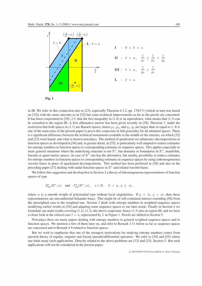
under the natural restrictions for the parameters as indicated in Figure 1, in particular,

−∞ < s2 < s1 < ∞ , δ = s1 − n

p1−(s2 − n

p2

)> 0 ,

with

p0 < p2 ≤ ∞ where1p0

=1p1

+α

n.

Subdividing the admitted(

1p2, s2)-region for given

(1p1, s1)

according to Figure 1 into three regions I, II, III, andthe critical line L we got the satisfactory equivalences

ek(id) ∼ k−s1−s2

n , k ∈ N , in I , (1.2)

and

ek(id) ∼ k−αn + 1

p2− 1

p1 , k ∈ N , in II . (1.3)

Furthermore we obtained some estimates for ek(id) on the critical line L, and for any ε > 0 and suitably chosennumbers c > 0 and cε > 0,

c k−αn + 1

p2− 1

p1 ≤ ek(id) ≤ cε k−α

n + 1p2

− 1p1 (log k)ε− 1

p2+ 1

p1 , 1 < k ∈ N , (1.4)

∗ email: [email protected], Phone: +49 3641 946123, Fax: +49 3641 946102∗∗ Corresponding author: e-mail: [email protected], Phone: +49 3641 946120, Fax: +49 3641 946102


Math. Nachr. 278, No. 1–2 (2005) / www.mn-journal.com 109

1p

δ = 0 L : δ = α

s

II

•III

(1p0, s1)(

1p1, s1)

(1p2, s2)

I

I : 0 < δ < α

II : δ > α ,1p1

≤ 1p2

<1p0

III : δ > α ,1p2

<1p1

L : δ = α

Fig. 1

in III. We refer in this connection also to [23], especially Theorem 4.3.2, pp. 170/171 (which in turn was basedon [32]) with the same outcome as in [32] but some technical improvements as far as the proofs are concerned.It has been conjectured in [29], 2.5, that the first inequality in (1.4) is an equivalence, what means that (1.3) canbe extended to the region III. A first affirmative answer has been given recently in [38], Theorem 7, under therestriction that both spaces in (1.1) are Banach spaces, hence p1, p2, and q1, q2 are larger than or equal to 1. It isone of the main aims of the present paper to prove this conjecture in full generality for all admitted spaces. Thereis a significant difference between the technical instruments available in the middle of the nineties, on which [32]and [23] were based, and what is known nowadays. The method of quarkonial (or subatomic) decompositions infunction spaces as developed in [54] and, in greater detail, in [55], is particularly well adapted to reduce estimatesfor entropy numbers in function spaces to corresponding estimates in sequence spaces. This applies especially tomore general situations where the underlying structure is not R

n, but domains or boundaries in Rn, manifolds,

fractals or quasi-metric spaces. In case of Rn one has the alternative, but nearby, possibility to reduce estimates

for entropy numbers in function spaces to corresponding estimates in sequence spaces by using (inhomogeneous)wavelet bases in place of quarkonial decompositions. This method has been preferred in [38] and also in thepreceding paper [37] dealing with radial function spaces in R

n and related wavelet bases.

We follow this suggestion and develop first in Section 2 a theory of inhomogeneous representations of functionspaces of type

Bspq(R

n, w) and F spq(R

n, w) , s ∈ R , 0 < p , q ≤ ∞ ,

where w is a smooth weight of polynomial type without local singularities. If p < ∞, q < ∞, then theserepresentations are unconditional Schauder bases. This might be of self-contained interest extending [56] fromthe unweighted case to the weighted one. Section 3 deals with entropy numbers in weighted sequence spacesmodifying earlier results in [54] and adapting some sequence spaces to our later needs. Finally in Section 4 weformulate our main results covering (1.2), (1.3), the above conjecture, hence (1.3) also in region III, and we havea closer look at the critical case δ = α, represented by L in Figure 1. Proofs are shifted to Section 5.

Nowadays there are many papers dealing with entropy numbers in general weighted sequence spaces and infunction spaces. We mention a few of them later on, and refer to Remark 3.11 below as far as sequence spacesare concerned and to Remark 4.9 related to function spaces.

But we wish to emphasise that one of the strongest motivations for studying entropy numbers comes fromspectral theory of regular, singular and fractal (pseudo)differential operators. We refer to [54] and [55] whereone finds many such applications. Directly related to the above problems are [33] and [23], Section 5. But suchapplications will not be considered in the present paper.


110 Haroske and Triebel: Weighted function spaces

2 Function spaces and wavelets

2.1 Basic notation

We use standard notation. Let N be the collection of all natural numbers and let N0 = N ∪ {0}. Let Rn be

euclidean n-space, where n ∈ N; put R = R1, whereas C is the complex plane. Let S(Rn) be the Schwartz

space of all complex-valued rapidly decreasing, infinitely differentiable functions on Rn. By S′(Rn) we denote

its topological dual, the space of tempered distributions on Rn. Furthermore, Lp(Rn) with 0 < p ≤ ∞, is the

standard quasi-Banach space with respect to the Lebesgue measure, quasi-normed by

‖f |Lp(Rn)‖ =( ∫

Rn

|f(x)|p dx)1

p

with the obvious modification if p = ∞. As usual, Z is the collection of all integers; and Zn where n ∈ N,

denotes the lattice of all points m = (m1, . . . ,mn) ∈ Rn with mj ∈ Z. Let N

n0 , where n ∈ N, be the set of all

multi-indices

γ = (γ1, . . . , γn) with γj ∈ N0 and |γ| =n∑

j=1

γj .

Let C(Rn) be the Banach space of all complex-valued uniformly continuous bounded functions in Rn and let for

r ∈ N,

Cr(Rn) = { f ∈ C(Rn) : Dγf ∈ C(Rn), |γ| ≤ r} , (2.1)

obviously normed, where we used the standard abbreviationDγ for derivatives.

Definition 2.1 The class Wn of admissible weight functions is the collection of all positive C∞ functions won R

n with the following properties:

(i) for all γ ∈ Nn0 there exists a positive constant cγ with

|Dγw(x)| ≤ cγ w(x) for all x ∈ Rn ;

(ii) there exist two constants c > 0 and α ≥ 0 such that

0 < w(x) ≤ cw(y)(1 + |x− y|2)α

2 for all x , y ∈ Rn .

Remark 2.2 These are the weights we dealt with in [32], [33] and [23], Chapter 4. If α ≥ 0 then we put

wα(x) =(1 + |x|2)α

2 , x ∈ Rn . (2.2)

Furthermore, Lp(Rn, w) with 0 < p ≤ ∞ and w ∈ Wn is the usual quasi-Banach space quasi-normed by

‖f |Lp(Rn, w)‖ = ‖wf |Lp(Rn)‖ .

2.2 Function spaces

If ϕ ∈ S(Rn) then

ϕ(ξ) = (Fϕ)(ξ) = (2π)−n2

∫Rn

e−iξxϕ(x) dx , ξ ∈ Rn, (2.3)

denotes the Fourier transform of ϕ. Here ξx is the scalar product in Rn. As usual, F−1ϕ or ϕ∨, stands for

the inverse Fourier transform, given by the right-hand side of (2.3) with i in place of −i. Both F and F−1 areextended to S′(Rn) in the standard way.

Let ϕ ∈ S(Rn) with

ϕ(x) = 1 if |x| ≤ 1 and ϕ(y) = 0 if |y| ≥ 32.



We put ϕ0 = ϕ. Let ϕ1(x) = ϕ(

x2

)− ϕ(x) and

ϕk(x) = ϕ1

(2−k+1x

), x ∈ R

n, k ∈ N .

Then∑∞

j=0 ϕj(x) = 1 for all x ∈ Rn is a dyadic resolution of unity. Recall that

(ϕj f

)∨is an entire analytic

function and hence(ϕj f

)∨(x) makes sense pointwise.

Definition 2.3 Let ϕ and ϕj be the above functions. Let w ∈Wn according to Definition 2.1. Let s ∈ R and0 < q ≤ ∞.

(i) Let 0 < p ≤ ∞. The space Bspq(R

n, w) is the collection of all f ∈ S′(Rn) such that

∥∥f |Bspq(R

n, w)∥∥

ϕ=

( ∞∑j=0

2jsq∥∥∥(ϕj f

)∨ |Lp(Rn, w)∥∥∥q)1

q

(2.4)

(with the usual modification if q = ∞) is finite.(ii) Let 0 < p <∞. The space F s

pq(Rn, w) is the collection of all f ∈ S′(Rn) such that

∥∥f |F spq(R

n, w)∥∥

ϕ=

∥∥∥∥∥( ∞∑

j=0

2jsq∣∣(ϕj f

)∨(·)|q)1

q ∣∣∣Lp(Rn, w)

∥∥∥∥∥ (2.5)

(with the usual modification if q = ∞) is finite.

Remark 2.4 If w = 1 then we have the unweighted spaces denoted as usual by Bspq(R

n) and F spq(R

n), hencethey are defined by (2.4) and (2.5) with Lp(Rn) in place of Lp(Rn, w), respectively. Weighted spaces of theabove type have been considered in detail in [32], [33] and, based on these papers, in [23], Chapter 4. Thereone finds also references to the substantial history of diverse types of weighted function spaces which will not berepeated here. We mention only a few properties of the above spaces:

(i) Bspq(R

n, w) and F spq(R

n, w) are quasi-Banach spaces (Banach spaces if p ≥ 1 and q ≥ 1), and they areindependent of ϕ. In particular, for different choices of ϕ the respective quasi-norms in (2.4) are equivalent toeach other. This justifies our omission of the subscript ϕ in the sequel. Similarly for (2.5).

(ii) The operator f → wf is an isomorphic mapping from Bspq(R

n, w) onto Bspq(R

n) and from F spq(R

n, w)onto F s

pq(Rn). In particular,∥∥wf |Bs

pq(Rn)∥∥ ∼ ∥∥f |Bs

pq(Rn, w)

∥∥ (2.6)

and ∥∥wf |F spq(R

n)∥∥ ∼ ∥∥f |F s

pq(Rn, w)

∥∥ (2.7)

(equivalent quasi-norms).Especially (2.6) and (2.7) are substantial assertions with their own history. We refer to [23], Remark 1 on

pp. 156/157. The shortest available proofs may be found in [32] and [23], pp. 156–158.

Remark 2.5 By the above isomorphism the weighted spaces can be reduced to the unweighted ones. Thetheory of the (unweighted) spaces Bs

pq(Rn) and F s

pq(Rn) in its full extent has been developed in [51] and [52].

But they have a long history, including their forerunners and special cases. The interested reader may consultChapter 1 in [52] which is a historically-minded survey from the beginnings up to the early nineties. The theory ofthese spaces as it stood in the middle of the nineties may be found in [1], [23] and [49]. As for more recent aspectswe refer to [54] and [55]. Although we assume that the reader is familiar with the theory of the (unweighted)spaces Bs

pq(Rn) and F s

pq(Rn) it might be useful to list a few special cases. Recall that for any σ ∈ R,

Iσ : f −→((

1 + |ξ|2)σ2 f)∨

is a one-to-one map of S(Rn) onto itself and of S′(Rn) onto itself. Then

Hsp(Rn) = I−sLp(Rn) , s ∈ R , 1 < p < ∞ , (2.8)



are the (fractional) Sobolev spaces with the classical Sobolev spaces

W kp (Rn) = Hk

p (Rn) , k ∈ N0 , 1 < p < ∞ , (2.9)

as a subclass, where the latter spaces can be equivalently normed by∥∥f |W kp (Rn)

∥∥ =∑|γ|≤k

‖Dγf |Lp(Rn)‖ . (2.10)

For these spaces one has the Littlewood-Paley characterisation

Hsp(Rn) = F s

p,2(Rn) , s ∈ R , 1 < p < ∞ . (2.11)

Furthermore,

Bspq(R

n) , s > 0 , 1 < p < ∞ , 1 ≤ q ≤ ∞ ,

are the classical Besov spaces. Let

Cs(Rn) = Bs∞,∞(Rn) , s ∈ R . (2.12)

Then Cs(Rn) with s > 0 are the Holder-Zygmund spaces. If 0 < p ≤ 1 then hp(Rn) = F 0p,2(R

n) are the(inhomogeneous) Hardy spaces.

2.3 Wavelet bases

Recall thatCr(Rn) with r ∈ N are the classical spaces according to (2.1). Furthermore if x = (x1, . . . , xn) ∈ Rn

and α = (α1, . . . , αn) ∈ Nn0 then we put

xα = xα11 . . . xαn

n (monomials).

Let Lj = L = 2n − 1 if j ∈ N and L0 = 1.

For any r ∈ N there are real compactly supported functions

ψ0(·) ∈ Cr(Rn) and ψl(·) ∈ Cr(Rn) where l = 1 , . . . , L ,

with ∫Rn

xαψl(x) dx = 0 , α ∈ Nn0 , |α| ≤ r ,

such that {2j n

2 ψljm(·) : j ∈ N0, 1 ≤ l ≤ Lj , m ∈ Z

n}

with

ψljm(x) =

{ψ0(x−m) if j = 0 , m ∈ Z

n , l = 1 ,

ψl(2j−1x−m) if j ∈ N , m ∈ Zn , 1 ≤ l ≤ L ,

is an orthonormal basis in L2(Rn).The best known example of such a system of functions is the (inhomogeneous) Daubechies wavelet basis.

We refer for details to [46], 3.8, pp. 96/97, formula (8.2), for the one-dimensional case, including that the fatherwavelet ψ0 and the mother wavelets ψl are real, and 3.9, pp. 107/108, formula (9.1), for its n-dimensionalextension. The original version goes back to I. Daubechies, [12] and [13], Chapter 6. We refer also to [57],



Chapter 4, and [34], Chapter 2. It is well-known that this system remains to be an unconditional Schauder basisin Lp(Rn) with 1 < p <∞, in the Sobolev spaces

Hsp(Rn) with 1 < p < ∞ , |s| < r , (2.13)

according to (2.8) and in the Besov spaces

Bspq(R

n) with 1 ≤ p < ∞ , 1 ≤ q < ∞ , |s| < r . (2.14)

Details may be found in [46], Chapter 6, but also in the other books and papers mentioned above. It was the mainaim of [56] to extend this theory to all (unweighted) spaces Bs

pq(Rn) and F s

pq(Rn) according to Definition 2.3

and Remark 2.4. Now we are doing the next step generalising this theory to the weighted spaces as introduced inDefinition 2.3. For this purpose we need some sequence spaces.

Let χjm with j ∈ N0 and m ∈ Zn be the characteristic function of the cube Qjm in R

n with sides parallel tothe axes of coordinates, centred at 2−jm, and with side-length 2−j . Let

s ∈ R , 0 < p ≤ ∞ , 0 < q ≤ ∞ , and w ∈Wn (2.15)

according to Definition 2.1. Then the sequence spaces bspq(w) and fspq(w) consist of all sequences

λ ={λl

jm ∈ C : j ∈ N0; 1 ≤ l ≤ Lj ; m ∈ Zn}

such that the respective quasi-norms

∥∥λ | bspq(w)∥∥ =

(∑l,j

2j(

s−np

)q

(∑m

w(2−jm

)p ∣∣λljm

∣∣p)qp)1

q

(2.16)

and ∥∥λ | fspq(w)

∥∥ =

∥∥∥∥∥( ∑

l,j,m

2jsqw(2−jm

)q ∣∣λljmχjm(·)∣∣q )1

q ∣∣∣Lp(Rn)

∥∥∥∥∥(with the usual modification if p = ∞ and/or q = ∞) are finite. If w = 1 then we write bspq and fs

pq . Sequencespaces of this type were introduced in [24], [25] in connection with atomic decompositions of the spacesBs

pq(Rn)

and F spq(R

n) and have been used afterwards by many authors.

We agree that Aspq(R

n, w) stands both for Bspq(R

n, w) and F spq(R

n, w), and similarly aspq(w) stands for

bspq(w) and fspq(w), respectively. If w = 1 (the unweighted case) we write correspondinglyAs

pq(Rn) and as

pq .

Theorem 2.6 Let s, p, q and w ∈Wn be given by (2.15) with p <∞ in the F -case. Let

r(s, p) = max(s,

2np

+n

2− s

)and

r(s, p, q) = max(s,

2nmin(p, q)

+n

2− s

).

(i) Let r ∈ N with r > r(s, p) in the B-case and r > r(s, p, q) in the F -case. Let f ∈ S′(Rn). Thenf ∈ As

pq(Rn, w) if, and only if, it can be represented as

f =∑l,j,m

λljm ψl

jm with∥∥λ | as

pq(w)∥∥ < ∞ , (2.17)

unconditional convergence in S′(Rn) and in any space Aσpq(R

n, w) with σ < s and w(x)w−1(x) → 0 if|x| → ∞. Furthermore, the representation (2.17) is unique,

λljm = 2jn

(f, ψl

jm

); (2.18)

I : f −→ {2jn(f, ψl

jm

)}(2.19)



is an isomorphic map of Aspq(R

n, w) onto aspq(w) and∥∥f |As

pq(Rn, w)

∥∥ ∼ ∥∥λ | aspq(w)

∥∥ (2.20)

(equivalent quasi-norms).(ii) In addition, let p <∞ and q <∞. Then (2.17) with (2.18) converges unconditionally in As

pq(Rn, w) and{

ψljm

}is an unconditional Schauder basis in As

pq(Rn, w).

Remark 2.7 The unweighted case, this means w = 1, is covered by the Theorem and Corollaries 5 and 7 in[56]. As mentioned above,

{ψl

jm

}is also an unconditional Schauder basis in the spaces Hs

p(Rn) and Bspq(R

n)with (2.13), (2.14) where one needs only ψl

jm ∈ Cr(Rn). There are a few assertions of this type in literature formore general (unweighted) spaces Bs

pq(Rn) and F s

pq(Rn) with respect to the Lemarie–Meyer wavelets (having

no compact supports). We refer to [26], Section 7, and [5], [6]. In case of weighted spaces it makes apparentlya big difference whether one deals with inhomogeneous wavelet bases of Daubechies type (or Lemarie–Meyertype) on the one hand or with related homogeneous wavelet bases on the other hand. In [40] the question istreated under which conditions for a positive Borel measure µ on R the homogeneous Daubechies wavelets arean unconditional Schauder basis in Lp(R, µ) with 1 < p < ∞. It comes out that this is the case if, and only if,µ = vµL, where µL is the Lebesgue measure on R and v belongs to the Muckenhoupt class Ap, what restrictsthe growth of v(x) if |x| → ∞. According to the above Theorem 2.6 the outcome is different if one deals withinhomogeneous Daubechies wavelets (as far as the necessity is concerned). An extension of [40] to R

n and tomore general, not necessarily compactly supported, homogeneous wavelet bases in Lp(Rn, µ) with 1 < p < ∞,has been given recently in [2]; there one finds also further references. Finally we refer to [48], dealing withmatrix-valued generalisations of weighted homogeneous Besov spaces

Bspq(R

n, w) , s ∈ R , 1 ≤ p < ∞ , 0 < q ≤ ∞ ,

where againw is related to Muckenhoupt weights (but also some more general weights are treated). Equivalencesof type (2.20) are obtained, also in terms of homogeneous wavelet bases of Lemarie–Meyer and Daubechies type.We refer in particular to [48], Corollary 10.3, p. 309.

A proof of (2.20) restricted to spacesBspq(R

n, w) with s > 0, 1 ≤ p ≤ ∞, 1 ≤ q ≤ ∞ has been given in [38],Theorem 1. There one finds also further references. We shift the proof of the above theorem to Subsection 5.1,reducing it to the unweighted case.

3 Sequence spaces and entropy numbers

3.1 Entropy numbers

By Theorem 2.6 some problems for function spaces can be transferred to corresponding problems for sequencespaces. This applies in particular to assertions about entropy numbers of compact embeddings between functionspaces and is postponed to Section 4. The present section deals with respective sequence spaces. But we hopethat the main results of this section, formulated in Theorems 3.5 and 3.9, are also of self-contained interest. Firstwe recall the definition of entropy numbers in an abstract setting.

Definition 3.1 LetA andB be two complex quasi-Banach spaces and let T be a linear and compact map fromA into B. Then for all k ∈ N, the kth entropy number ek(T : A ↪→ B) is the infimum of all ε > 0 such thatthe image of the unit ball UA = {a : ‖a |A‖ ≤ 1} under the mapping T can be covered by 2k−1 balls in B ofradius ε.

Remark 3.2 Entropy numbers in abstract and concrete (quasi-)Banach spaces have a long history which willnot be repeated here. As for the abstract theory, including the use of entropy numbers in spectral theory ofcompact operators, we refer to [16], [9], [23] and the literature mentioned there. Otherwise we recall that thepresent paper might be considered as the direct continuation of [32], [33], where one also finds additional materialconcerning the theory of entropy numbers.



3.2 Sequence spaces I

We split our considerations on sequence spaces into two parts. We always use the equivalence sign ∼ for twopositive functions a(x) and b(x) or for two sequences of positive numbers ak and bk (say, k ∈ N) if there are twopositive numbers c and C such that

c a(x) ≤ b(x) ≤ C a(x) or c ak ≤ bk ≤ C ak

for all admitted variables x or k.

Definition 3.3 Let d > 0, δ ≥ 0, 0 < p ≤ ∞, and 0 < q ≤ ∞. Let

Mj ∈ N such that Mj ∼ 2jd where j ∈ N0 . (3.1)

Then q(2jδ

Mjp

)is the linear space of all sequences

λ = {λjr ∈ C : j ∈ N0; r = 1, . . . ,Mj}

such that the quasi-norm

∥∥λ | q(2jδ Mjp

)∥∥ =

⎛⎝ ∞∑j=0

2jδq

( Mj∑r=1

∣∣λjr

∣∣p)qp

⎞⎠1q

is finite (with the obvious modifications if p = ∞ and/or q = ∞).

Remark 3.4 In case of δ = 0 we write q( Mjp

). It is quite obvious that q

(2jδ

Mjp

)is a quasi-Banach space

(Banach space if p ≥ 1 and q ≥ 1). These spaces have been introduced in [54], Section 8. They played in [54]and also in [55] a decisive role in connection with spectral theory of fractal elliptic operators. Here we need anextension of [54], Theorem 8.2 on p. 39, which reads as follows.

Theorem 3.5 Let d > 0, δ > 0, and Mj ∈ N according to (3.1). Let 0 < p1 ≤ ∞,

1p∗

=1p1

+δ

d, (3.2)

p∗ < p2 ≤ ∞, 0 < q1 ≤ ∞ and 0 < q2 ≤ ∞. Then

id : q1

(2jδ Mj

p1

)↪→ q2

( Mjp2

)(3.3)

is compact and

ek(id) ∼ k− δ

d + 1p2

− 1p1 , k ∈ N . (3.4)

Remark 3.6 If p2 ≥ p1 then the above theorem coincides with [54], Theorem 8.2. In other words we have toshow that this assertion remains valid if p∗ < p2 < p1. It is just this extension which is needed for a full proof ofthe results outlined so far in the Introduction. We shift the short direct proof to Subsection 5.2. But we wish tomention that this theorem follows also from the more general Theorems 3 and 4 in [41].

3.3 Sequence spaces II

We modify the sequence spaces from the preceding subsection such that they are better adapted to the spacesbspq(wα) according to (2.16) where wα is given by (2.2).

Definition 3.7 Let δ ≥ 0, α ≥ 0, 0 < p ≤ ∞, and 0 < q ≤ ∞. Then q(2jδ p(α)

)is the linear space of all

sequences

λ = {λjr ∈ C : j ∈ N0; r ∈ N}c© 2005 WILEY-VCH Verlag GmbH & Co. KGaA, Weinheim


such that the quasi-norm

∥∥λ | q(2jδ p(α))∥∥ =

⎛⎝ ∞∑j=0

2jδq

( ∞∑r=1

rαp |λjr |p)q

p

⎞⎠1q

(3.5)

is finite (with the usual modifications if p = ∞ and/or q = ∞).

Remark 3.8 In case of δ = α = 0 we write q( p). It is quite obvious that q(2jδ p(α)

)is a quasi-Banach

space (Banach space if p ≥ 1 and q ≥ 1).

Theorem 3.9 Let δ > 0 and α > 0. Let 0 < p1 ≤ ∞,

1p∗

=1p1

+ α , (3.6)

p∗ < p2 ≤ ∞, 0 < q1 ≤ ∞ and 0 < q2 ≤ ∞. Then

id : q1

(2jδ p1(α)

)↪→ q2( p2) (3.7)

is compact and

ek(id) ∼ k−α+ 1

p2− 1

p1 , k ∈ N . (3.8)

Remark 3.10 We shift the short proof of this assertion to Subsection 5.3 reducing it to Theorem 3.5.

Remark 3.11 In recent times several generalisations of the sequence spaces q(2jδ

Mjp

)and q

(2jδ p(α)

)were considered replacing 2jδ by some sequences of positive numbers βj , modifying 2jδ in (3.1) and rα in(3.5). Of interest are estimates or equivalences of entropy numbers of related compact embeddings. We refer to[44], [35], and more recently to [17], [18], and the series of papers by Leopold [41], [43], [42]. This refreshedinterest in the subject led to further studies in [3], [11], [39], [36]. The so far latest results in this directionwere received in [37] and [38]; here partly sophisticated arguments from the theory of operator ideals were usedwith the consequence that at least in some cases the considered sequence spaces must be Banach spaces, hencep ≥ 1, q ≥ 1. But this restriction does not apply to those assertions in [38] which we shall use later on. As far assequence spaces are concerned our aim here is different. We give short straightforward proofs of the Theorems 3.5and 3.9 avoiding any complication which may occur when dealing with the indicated generalisations. On theother hand, Theorem 3.9 generalises [37], Theorem 3, p. 262/263, where (3.8) was proved under the restrictions1 ≤ p1 < p2 ≤ ∞ and 1 ≤ q1 ≤ ∞, 1 ≤ q2 ≤ ∞. In this context we refer also to [38], Theorem 3, where thecorresponding sequence spaces are nearer to the spaces bspq(wα) according to (2.16) with (2.2) than to the spacesin Definition 3.7 and Theorem 3.9.

4 Function spaces and entropy numbers

4.1 The non-limiting case

Recall that we agreed in connection with Theorem 2.6 that Aspq(R

n, wα) stands both for Bspq(R

n, wα) andF s

pq(Rn, wα) where again wα is the special weight

wα(x) =(1 + |x|2)α

2 , x ∈ Rn , α ≥ 0 ,

according to (2.2); the respective function spaces were introduced in Definition 2.3.

Theorem 4.1 Let

s1 ∈ R , 0 < p1 ≤ ∞ , 0 < q1 ≤ ∞ and α > 0 (4.1)

with p1 <∞ in the F -case. Let

1p0

=1p1

+α

n, (4.2)



−∞ < s2 < s1 < ∞ , p0 < p2 ≤ ∞ , 0 < q2 ≤ ∞ , (4.3)

again with p2 <∞ in the F -case, and

δ = s1 − n

p1−(s2 − n

p2

)> 0 . (4.4)

Then the embedding

id : As1p1q1

(Rn, wα) ↪→ As2p2q2

(Rn) (4.5)

is compact.(i) If, in addition, δ < α, then


n , k ∈ N , (4.6)

region I in Figure 1.(ii) If, in addition, δ > α, then

ek(id) ∼ k−α

n + 1p2

− 1p1 , k ∈ N , (4.7)

regions II and III in Figure 1.

Remark 4.2 Since both (4.6) and (4.7) are independent of q1 and q2 the above assertions follow immediatelyfrom the case A = B and

Bspu(Rn, wα) ↪→ F s

pq(Rn, wα) ↪→ Bs

pv(Rn, wα)

with u = min(p, q) and v = max(p, q). This embedding is a consequence of Remark 2.4(ii), (2.6), (2.7) and thecorresponding assertions for the unweighted case according to [51], 2.3.2, Proposition 2(iii), p. 47. Hence it issufficient to prove the above theorem for A = B. This will be done in Subsection 5.4 combining and modifyingTheorems 2.6 and 3.9. Otherwise we refer to the above Introduction. In particular we again derive (1.2) and (1.3),originally proved in [32] and, based on this paper, in [23], Theorem 4.3.2, pp. 170/171. Furthermore we improve(1.4) confirming the conjecture in [29] that (4.7) is also valid in region III in Figure 1. A partial affirmative answerof this conjecture has also been given recently in [38], Theorem 7, under the assumption that the function spacesinvolved are Banach spaces, hence, p1, q1, p2, q2 are larger than or equal to 1. Further references will be given atthe end of Subsection 4.2 in Remark 4.9.

4.2 The limiting case

Let K and 2K be open balls in Rn, centred at the origin, of radius 1 and 2, respectively. Let As

pq(K) be therestriction of As

pq(Rn) on K , quasi-normed in the usual way. Let ext,

ext : Aspq(K) ↪→ As

pq(Rn, wα) , supp ext f ⊂ 2K

if f ∈ Aspq(K), be a linear and bounded extension operator, where wα is the above weight according to (2.2).

Let id be the compact embedding according to (4.5) and let idK be its counterpart with respect to K , hence,

idK : As1p1q1

(K) ↪→ As2p2q2

(K) .

Then

idK = re ◦ id ◦ ext ,

where re is the above restriction operator. Then

k−s1−s2

n ∼ ek

(idK

) ≤ c ek(id) , k ∈ N , (4.8)



where the left-hand side may be found in [23], Theorem 2 on p. 118, or [54], Section 23. We compare (4.8) withTheorem 4.1. For strong weights, i.e. if δ < α then ek(id) has the same behaviour as ek

(idK

)(and for respective

compact embeddings in arbitrary bounded domains in Rn). If δ > α, hence

s1 − s2 > α+n

p1− n

p2,

then the decay of ek(id) in (4.7) is less rapid than ek

(idK

). It remains the limiting case

δ = α ⇐⇒ s1 − s2 = α+n

p1− n

p2, (4.9)

where the situation is more complicated. Then we are on the line L in Figure 1. First assertions were obtainedin [32] which may also be found in [23], Theorem 4.3.2, pp. 170/171. These results had been complementedafterwards in [27], [28], and [29]. A decisive progress has been made quite recently in [38]. But there is no finalanswer so far. We wish to contribute to this challenging problem in the following theorem and in the subsequentcorollary, preferably based on [32], [23] and the above techniques. As usual we write ak � bk for two sequencesof positive numbers ak and bk if there is some c > 0 such that ak ≤ c bk. Similarly ak � bk.

Theorem 4.3 Let

s1 ∈ R , 0 < p1 ≤ ∞ , 0 < q1 ≤ ∞ , and α > 0


1p0

=1p1

+α

n(4.10)

and

−∞ < s2 < s1 < ∞ , p0 < p2 ≤ ∞ , 0 < q2 ≤ ∞ ,


α = δ = s1 − n

p1−(s2 − n

p2

)(4.11)

be the line L in Figure 1, and let

id : As1p1q1

(Rn, wα) ↪→ As2p2q2

(Rn) (4.12)

be the compact embedding according to (4.5).(i) Then for all 1 < k ∈ N,

ek

(id : F s1

p1q1(Rn, wα) ↪→ F s2

p2q2(Rn)

)� k−

s1−s2n (log k)

αn . (4.13)

Let, in addition, q1 ≤ p1 and q2 ≥ p2. Then for all 1 < k ∈ N,

ek

(id : F s1

p1q1(Rn, wα) ↪→ F s2

p2q2(Rn)

) ∼ k−s1−s2

n (log k)αn . (4.14)

(ii) Let, in addition,

� =s1 − s2n

+1q2

− 1q1

> 0 . (4.15)

Then for all 1 < k ∈ N,

ek

(id : Bs1

p1q1(Rn, wα) ↪→ Bs2

p2q2(Rn)

) ∼ k−s1−s2

n (log k)� . (4.16)



Remark 4.4 We discuss part (i). First we remark that (4.13) is known and will not be proved again. We referto [32] and [23], Theorem 4.3.2, p. 171. By (4.11) and (4.15) we have

� =s1 − s2n

+1q2

− 1q1

=α

n+(

1p1

− 1q1

)−(

1p2

− 1q2

). (4.17)

Since Bspp = F s

pp one has for 1 < k ∈ N,

ek

(id : F s1

p1p1(Rn, wα) ↪→ F s2

p2p2(Rn)

) ∼ k−s1−s2

n (log k)αn (4.18)

as a special case of (4.16). If q1 ≤ p1 and q2 ≥ p2 then (4.14) follows from (4.13), (4.18), elementary propertiesof entropy numbers and the embeddings

F s1p1q1

(Rn, wα) ↪→ F s1p1p1

(Rn, wα) , F s2p2p2

(Rn) ↪→ F s2p2q2

(Rn) . (4.19)

Unweighted embeddings of type (4.19) may be found in [51], 2.3.2, p. 47. The weighted counterpart followsafterwards from the isomorphic map mentioned in Remark 2.4(ii). Hence it remains to prove part (ii).

Remark 4.5 We discuss part (ii). Assertions of type (4.16) have a little history. The genuine q-dependence ofthe exponent � in (4.16) came out first in [27], [28], [29] somewhat surprisingly. In these papers, [32] was taken asa starting point, now combined with interpolation and duality properties for entropy numbers and a comparison ofapproximation numbers with entropy numbers. In the proofs given later on we again use interpolation arguments,relations between approximation numbers and entropy numbers, and duality. These instruments resulted in [27],[28], [29] in assertions of type (4.16) for some fixed p1, p2 (preferably between 1 and ∞) and q-parametersvarying typically in some intervals of type

q01 < q1 ≤ p1 and p2 ≤ q2 < q02 . (4.20)

But as far as the covered cases are concerned the outcome was not very satisfactory. The main point was the ob-servation that (4.16) with (4.15) can really happen for varying parameters q1 and q2 as in (4.20). More handsomeconditions have been found quite recently in [38], Theorem 10, under the assumption that the spaces in (4.16) areBanach spaces and the respective parameters p1, p2, q1, q2 satisfy some further restrictions in addition to � > 0.We shift the proof of part (ii) to Subsection 5.5. For this purpose we combine Theorem 2.6 with the followingsubstantial observation in [38]. First we recall that bspq(wα) and bspq are the weighted and unweighted sequencespaces according to Subsection 2.3, especially (2.16), with respect to the weight wα given by (2.2). As usual weput a+ = max(a, 0) for a ∈ R.

Assume

s1 ∈ R , 0 < p1 ≤ ∞ , 0 < q1 ≤ ∞ and α > 0 , (4.21)

with1p0

=1p1

+α

n(4.22)

and

−∞ < s2 < s1 < ∞ , p0 < p2 ≤ ∞ , 0 < q2 ≤ ∞ . (4.23)

Let

α = δ = s1 − n

p1−(s2 − n

p2

)and � =

s1 − s2n

+1q2

− 1q1. (4.24)

Then

id : bs1p1q1

(wα) ↪→ bs2p2q2

(4.25)

is compact. If, in addition,

α

n>

(1q1

− 1p1

)+

+(

1p2

− 1q2

)+

+(

1max(p2, q2)

− 1min(p1, q1)

)+

(4.26)



then


n (log k)� , 1 < k ∈ N . (4.27)

As said this remarkable result may be found in [38], especially in Lemma 2 and in Propositions 2 and 4. Incontrast to the function spaces of Besov type treated in [38] there is no restriction to the case of Banach spacesas far as the above sequence spaces are concerned. Furthermore if α satisfies (4.26) then it follows by (4.17) that� > 0. However the converse is not correct. There are admitted cases with � > 0 which are not covered by (4.24),(4.26); see also Figure 2 in Section 5.5 below. To get a full proof of part (ii) of the above theorem we translate firstthe above-mentioned assertion for sequence spaces with the help of Theorem 2.6 into a corresponding assertionfor Besov spaces and apply afterwards complex interpolation for quasi-Banach spaces according to [45].

Remark 4.6 We mention two special cases. First we recall that Cs(Rn) are the Holder-Zygmund spacesaccording to (2.12). Let

−∞ < s2 < s1 < ∞ and α = s1 − s2 .

Then it follows by (4.16) and (4.11) that

ek (id : Cs1(Rn, wα) ↪→ Cs2(Rn)) ∼(

k

log k

)− s1−s2n

where 1 < k ∈ N. But this is known, [32] or [23], p. 179. Secondly, let Hsp(Rn) be the Sobolev spaces according

to (2.8) with (2.11). Let

max(1, p0) < p2 ≤ 2 ≤ p1 < ∞ , −∞ < s2 < s1 < ∞ ,

α = s1 − n

p1−(s2 − n

p2

).

(4.28)

Then

ek

(id : Hs1

p1(Rn, wα) ↪→ Hs2

p2(Rn)

) ∼ k−s1−s2

n (log k)αn (4.29)

where 1 < k ∈ N. This follows from (4.14) and (2.11). In this case the somewhat sinister role of 2 in (4.28),(4.29) can be removed.

Corollary 4.7 Let −∞ < s2 < s1 <∞, 1 < p1 <∞, α > 0, 1p0

= 1p1

+ αn , max(1, p0) < p2 ≤ p1 <∞,

and

α = s1 − n

p1−(s2 − n

p2

).

Then

ek

(id : Hs1

p1(Rn, wα) ↪→ Hs2

p2(Rn)

) ∼ k−s1−s2

n (log k)αn (4.30)

where 1 < k ∈ N.

Remark 4.8 We shift the proof of this corollary to Subsection 5.6. It improves (4.28). But it is not clear whathappens if p1 < p2. However compared with Theorem 4.3(i) it makes clear that q1 ≤ p1, q2 ≥ p2 is sufficient toget (4.14), but not necessary.

Remark 4.9 Recall that we already gave some references of related work in Remark 3.11, which partiallyconcerns entropy numbers in function spaces, too. Thus we can restrict ourselves now to mention some closelyrelated papers not covered by Remark 3.11. Forerunners (in our sense) are certainly the papers [20], [21] (con-tained in [23]); see also [14], [15]. Later, concerning also some “limiting” situation (but now with δ = 0) werefer to [53], [22], [19], [30], [31], and [8].

Remark 4.10 The non-limiting cases α �= δ are settled now completely by Theorem 4.1. As for the limitingcase α = δ there remain some gaps. By Theorem 4.3(ii) we have (4.16) if � > 0. If � ≤ 0 then there isonly the estimate (4.8) from below so far. For the F -spaces we obtained in special cases the equivalences (4.14)and (4.30), otherwise there is only the estimate (4.13) from below. However, by the results achieved so far thefollowing conjecture seems to be natural.



Conjecture 4.11 Let the general assumptions of Theorem 4.3 be satisfied.(i) Then the equivalence (4.14) for F -spaces is valid for all admitted parameters p1, q1, p2, q2.

(ii) If

� =s1 − s2n

+1q2

− 1q1

< 0 ,

then for k ∈ N,

ek

(id : Bs1


p2q2(Rn)

) ∼ k−s1−s2

n .

Remark 4.12 By Theorem 2.6 we have an isomorphic map between function spaces and related sequencespaces. Hence any assertion for sequence spaces can be transferred to a corresponding assertion for functionspaces and vice versa. In particular using Theorem 4.3(ii) one can improve the assertion from [38] quoted inRemark 4.5 replacing p0 < p2 and (4.26) by

α

n> max

(1p2

− 1p1,

1p2

− 1q2

− 1p1

+1q1

),

where again δ = α > 0. We used � > 0 and (4.17).

5 Proofs

5.1 Proof of Theorem 2.6

Step 1. First we collect some prerequisites. As mentioned in Remark 2.7 the unweighted case of the theorem,this means w = 1, is covered by [56]. In particular, f ∈ S′(Rn) is an element of As

pq(Rn) if, and only if, it can

be represented as

f =∑l,j,m

λljmψ

ljm with

∥∥λ | aspq

∥∥ < ∞ ,

where this representation is unique,

λljm = 2jn

(f, ψl

jm

),

and I , given by

I : f −→ {2jn(f, ψl

jm

)},

is an isomorphic map of Aspq(R

n) onto aspq,

I : Aspq(R

n) ⇐⇒ aspq , (5.1)

including the equivalence of the quasi-norms∥∥f |Aspq(R

n)∥∥ ∼ ∥∥λ | as

pq

∥∥ .We wish to reduce the weighted case to the unweighted one using the localisation principle for the F -spacesand some interpolation as far as the B-spaces are concerned. We give a description of the localisation principleadapted to our needs. Let � be a non-negative compactly supported C∞ function in R

n such that∑k∈Zn

�k(x) ∼ 1 , x ∈ Rn , where �k(x) = �(x− k) .

We claim that for s ∈ R, 0 < p <∞, 0 < q ≤ ∞ and w ∈Wn,∥∥f |F spq(R

n, w)∥∥p ∼

∑k∈Zn

wp(k)∥∥�kf |F s

pq(Rn)∥∥p,



and a corresponding equivalence for Bs∞∞(Rn, w). The unweighted case, this means w = 1, is covered by [52],Theorem 2.4.7, pp. 124/125. The weighted case follows from Remark 2.4(ii), (2.6), (2.7), and∥∥w�kf |As

pq(Rn)∥∥ ∼ w(k)

∥∥�kf |Aspq(R

n)∥∥ , k ∈ Z

n ,

as a consequence of the properties of w according to Definition 2.1, and some pointwise multiplier assertionswhich may be found in [52], 4.2.2, p. 203. We complement these preparations by the following observations. Let

f =∑

k∈Zn

fk , supp fk ⊂ {y : |y − k| ≤ a} (5.2)

for some a > 0. Then, again by the localisation principle and pointwise multiplier assertions,∥∥f |F spq(R

n, w)∥∥p ≤ c

∑k∈Zn

wp(k)∥∥fk |F s

pq(Rn)∥∥p

(5.3)

(with a counterpart for Bs∞∞(Rn)). If, in addition, for some � with the above properties and some c > 0,∥∥fk |F spq(R

n)∥∥ ≤ c

∥∥�kf |F spq(R

n)∥∥ , k ∈ Z

n , (5.4)

then one has equivalence in (5.3), hence∥∥f |F spq(R

n, w)∥∥p ∼

∑k∈Zn

wp(k)∥∥fk |F s

pq(Rn)∥∥p

(5.5)

(with a counterpart for Bs∞∞(Rn)) as a characterisation (this means, either both sides are finite or infinite).

Step 2. We prove the theorem for the F spq-spaces. Let f be given by (2.17) and let

f =∑l,j,m

λljm ψl

jm =∑

k∈Zn

fk

where fk collects terms of the preceding sum with (5.2). By the corresponding assertion for the unweightedspaces we have the uniqueness (2.18) and, together with (5.3),∥∥f |F s

pq(Rn, w)

∥∥ ≤ c∥∥λ | fs

pq(w)∥∥ (5.6)

incorporating wp(k) appropriately. As for the converse we choose a non-negative compactly supported C∞

function � in Rn with �(x) = 1 if |x| ≤ C. If C is large then(f, ψl

jm

)=(�kf, ψ

ljm

)for those ψl

jm which contribute to fk. Then we have (5.4) by the unweighted case. We can apply (5.5) resultingin an equivalence in (5.6). The remaining assertions are now the same as in the unweighted case: unconditionalconvergence of (2.17) in S′(Rn) and in F σ

pq(Rn, w) with σ < s and that

{ψl

jm

}in case of q < ∞ is an

unconditional Schauder basis in F spq(R

n, w). This proves both parts of the theorem for the spaces F spq(R

n, w).As mentioned the above arguments apply also to part (i) with Bs∞∞(Rn, w).

Step 3. It remains to prove the theorem for the Bspq-spaces with 0 < p ≤ ∞, 0 < q ≤ ∞ and p �= q. This will

be done by real interpolation. By Remark 2.4(ii) the operator f → wf is an isomorphic map from Bspq(R

n, w)onto Bs

pq(Rn). Then it follows(Bs0

pp(Rn, w), Bs1

pp(Rn, w)

)θ,q

= Bspq(R

n, w) (5.7)

where

s0 �= s1 , 0 < θ < 1 , s = (1 − θ)s0 + θs1 , (5.8)



from the corresponding real interpolation for the unweighted spaces according to [51], Theorem 2.4.2, p. 64. By(5.7) with w = 1 and the isomorphism (5.1) we obtain(

bs0pp , b

s1pp

)θ,q

= bspq

and afterwards, again by an isomorphism between the respective sequence spaces,(bs0pp(w), bs1

pp(w))

θ,q= bspq(w) (5.9)

where the parameters have the same meaning as in (5.8). However by (5.7), (5.9) and the arguments from Step 2we get all assertions of the theorem for the spaces Bs

pq(Rn, w), including part (ii) if p <∞ and q <∞.


Step 1. For p2 ≥ p1 a proof of this theorem may be found in [54], Theorem 8.2, pp. 39–41. In other words, wehave to extend this assertion to p∗ < p2 < p1.

Step 2. Let p∗ < p2 < p1. We decompose id given by (3.3) as

id = id2 ◦ id1

with

id1 : q1

(2jδ Mj

p1

)↪→ q2

(2jδ Mj

p1

), δ = d

(1p2

− 1p1

),

and

id2 : q2

(2jδ Mj

p1

)↪→ q2

( Mjp2

).

By Holder’s inequality id2 is a linear and bounded map. Hence by Step 1 (or [54], Theorem 8.2)

ek(id) ≤ c ek(id1) ≤ c′ k−1d (δ−δ) = c′ k−

δd + 1

p2− 1

p1 , (5.10)

where c and c′ are independent of k ∈ N.

Step 3. It remains to prove that the inequalities in (5.10) are equivalences, again under the hypothesis p∗ <p2 < p1. For this purpose we recall the following property of entropy numbers proved in [32], Theorem 3.2,p. 139, and [23], Theorem 1.3.2, p. 13: Let A be a quasi-Banach space and let {B0, B1} be an interpolationcouple of quasi-Banach spaces. Let 0 < θ < 1 and let Bθ be a quasi-Banach space such that

B0 ∩B1 ↪→ Bθ ↪→ B0 +B1 (naturally quasi-normed)

and

‖b |Bθ‖ ≤ ‖b |B0‖1−θ ‖b |B1‖θ for all b ∈ B0 ∩B1 . (5.11)

Let T ∈ L(A,B0 ∩B1). Then there is a number c > 0 such that for all k ∈ N,

e2k(T : A ↪→ Bθ) ≤ c e1−θk (T : A ↪→ B0) eθ

k(T : A ↪→ B1) . (5.12)

Now we assume that for given d, δ, p1, q1 the converse of (5.10) (estimate from below) is wrong for some p2 withp∗ < p2 < p1 and some q2. Let A and B0 be the spaces on the left-hand side and the right-hand side of (3.3),respectively, i.e.

A = q1

(2jδ Mj

p1

), B0 = q2

( Mjp2

).

Let, in addition, p1 <∞ and

B1 = q2

( Mjp3

)for some p3 > p1 . (5.13)



Then Holder’s inequality leads to (5.11) for

Bθ = q2

( Mjp1

)with

1p1

=1 − θ

p2+

θ

p3. (5.14)

By assumption there is a sequence kj ∈ N with kj → ∞ if j → ∞ and

ekj (id : A ↪→ B0) · kδd− 1

p2+ 1

p1j −→ 0 for j −→ ∞ . (5.15)

We apply Theorem 3.5 to id : A ↪→ B1; then it follows by (3.4) (with p3 in place of p2), (5.12)–(5.15) that

e2kj (id : A ↪→ Bθ) · kδd

j −→ 0 if j −→ ∞ .

But this contradicts (3.4) with p2 in place of p1. If p1 = ∞ then there is no p3 with (5.13). But by the samereferences [32] and [23] as above there is a counterpart of (5.12) with respect to an interpolation couple {A0, A1}on the source side and a fixed space B on the target side. Let for d

δ = p∗ < p2 < p1 = ∞,

A0 = q1

(2jδ Mj∞

)and B = q2

( Mjp2

)where we may assume q1 <∞ (since we wish to disprove the counterpart of (5.15)). Let

A1 = q1

(2jδ

Mj

q1θ

)with 0 < θ < 1 .

By the above remarks real interpolation

(A0, A1)θ,q1= q1

(2jδ( Mj∞ ,

Mj

q1θ

)θ,q1

)= q1

(2jδ Mj

q1

)reduces the problem to what we already know. As for the real interpolation of p-spaces we refer to [50], Theo-rem 1.18.3/2, p. 127 (Banach spaces) and [4], Theorem 5.6.1, p. 122 (quasi-Banach spaces).


Step 1. Let α > 0 and 0 < q = p < ∞ in (3.5) (if p = q = ∞ then one has to modify what followsappropriately). One obtains

∞∑j=0

2jδp∞∑

r=1

rαp |λjr |p ∼∞∑

j,l=0

2(j+l)δp∑r∈Kl

|λjr |p ∼∞∑

j=0

2jδp

j∑l=0

∑r∈Kl

|λj−l,r |p , (5.16)

where r ∈ Kl means r ∼ 2l δα . Hence

p(2jδ p(α)

) ∼= p(2jδ Mj

p

)with Mj ∼ 2jd , d =

δ

α, (5.17)

in the interpretation of (5.16). Obviously, (3.6) coincides with (3.2). Now (3.8) with q1 = p1 and q2 = p2 followsfrom (3.4).

Step 2. Since (3.8) is independent of δ > 0 (only the equivalence constants may depend upon δ) one canreplace q1 = p1 in (3.7) by any q1 with 0 < q1 ≤ ∞ (embeddings for upper estimate, and at the expense of thepositive δ for the lower one). The same argument applies on the target side, since (3.7) with the outcome (3.8)can be generalised by

id : q1

(2jδ1 p1(α)

)↪→ q2

(2jδ2 p2

)with δ1 > δ2.




Step 1. By Remark 4.2 it is sufficient to prove the theorem for the B-spaces. We may assume that r ∈ N

in Theorem 2.6(i) is chosen sufficiently large such that the isomorphism I in (2.19) applies to both spaces in(4.5) with A = B. Hence the considered problem can be reduced to the estimate of the entropy numbers ofembeddings between related sequence spaces of type bspq(wα) according to (2.16). We adapt these sequencespaces notationally to the sequence spaces considered in Subsections 3.2 and 3.3 where we may neglect the finitesummation over l. Let δ ≥ 0, α ≥ 0, 0 < p ≤ ∞, and 0 < q ≤ ∞. In modification of Definition 3.7 we denoteby q

(2jδ p(α)

)n

the linear space of all sequences

λ = {λjm ∈ C : j ∈ N0; m ∈ Zn}

such that the quasi-norms

∥∥λ | q(2jδ p(α))

n

∥∥ =

( ∞∑j=0

2jδq

( ∑m∈Zn

(1 + 2−j |m|)αp |λjm|p

)qp)1

q

(5.18)

is finite (with obvious modification if p = ∞ and/or q = ∞). If δ = α = 0 then we write q( p)n. Underthe assumptions of the theorem, in particular (4.1)–(4.4), the above remarks and an additional lifting argument,the estimate for the entropy numbers for id in (4.5) can be reduced to a corresponding estimate for the entropynumbers of

id : q1

(2jδ p1(α)

)n↪→ q2 ( p2)n .

Step 2. We adapt the arguments from the proof of Theorem 3.9 in Subsection 5.3 to this slightly differentsituation. Let 0 < q = p <∞ in (5.18) (if p = q = ∞ then one has to modify what follows appropriately). Onehas (in analogy to (5.16)),

∞∑j=0

2jδp∑

m∈Zn

(1 + 2−j |m|)αp |λjm|p ∼

∞∑j=0

2jδp∞∑

l=0

2lδp∑

m∈Kjl

|λjm|p , (5.19)

where Kjl collects terms with 1 + 2−j |m| ∼ 2l δ

α . The cardinal number of Kjl is ∼ 2(j+l δ

α )n. Hence theexpression in (5.19) is equivalent to

∞∑j=0

2jδp

j∑l=0

∑m∈Kj−l

l

|λj−l,m|p

where the cardinal number of the last two sums is

Mj ∼ 2jn

j∑l=0

2ln(

δα−1

), j ∈ N0 .

Step 3. Let δ > α. Then

Mj ∼ 2jd with d =δn

α, j ∈ N0 ,

and we are in a similar situation as in (5.17). Again (4.2) coincides with (3.2). Now (4.7) with q1 = p1 andq2 = p2 follows from (3.4). The extension to all q1 and all q2 follows by the same arguments as in Step 2 inSubsection 5.3.

Step 4. Let δ < α. Then Mj ∼ 2jn. We have in modification of (3.2),

1pδ∗

=1p1

+δ

n=

1p1

+s1 − s2n

− 1p1

+1p2

=s1 − s2n

+1p2



in view of (4.4). Hence p2 > pδ∗ what corresponds to the broken line in Figure 1. Application of Theorem 3.5with pδ

∗ and n in place of p∗ and d, respectively, and δ given by (4.4) results in


n , k ∈ N , (5.20)

for

id : Bs1p1p1

(Rn, wα) ↪→ Bs2p2p2

(Rn) . (5.21)

Next we use first the interpolation (5.7) with p = p1 on the source side and afterwards on the target side (nowwith w = 1). Then one gets by the interpolation property for entropy numbers according to [32], Theorem 3.2,p. 139 or [23], Theorem 1.3.2, pp. 13/14, that

ek(id) ≤ c k−s1−s2

n , k ∈ N , (5.22)

for

id : Bs1p1q1

(Rn, wα) ↪→ Bs2p2q2

(Rn) . (5.23)

By (4.8) one has a corresponding estimate from below. Hence the inequality in (5.22) is also an equivalence for(5.23).


Step 1. By the Remarks 4.4 and 4.5 it remains to prove part (ii) of the theorem. We rely on the observations in[38] quoted in the above Remark 4.5 combined with Theorem 2.6. For this purpose we compare the assumptions(4.21)–(4.26) with the corresponding conditions in part (ii) of the theorem. This means by (4.15), (4.17) andp0 < p2,

α

n> max

(0,

1p2

− 1p1,

1p2

− 1q2

− 1p1

+1q1

). (5.24)

There are four cases in dependence on whether q1 is larger or smaller than p1, and q2 is larger or smaller than p2.First we deal with those two cases which are covered by (4.21)–(4.26).

Step 2. Let p1 ≤ q1 and q2 ≤ p2. Then (4.26) reduces to

α

n>

(1p2

− 1p1

)+

.

But this is the same as (5.24). Then (4.27) and Theorem 2.6 result in (4.16).

Step 3. Let q1 ≤ p1 and p2 ≤ q2. Then (4.26) means

α

n>

1q1

− 1p1

+1p2

− 1q2

+(

1q2

− 1q1

)+

.

Again this is the same as (5.24) and we get (4.16) also in this case.

Step 4. Let q1 ≤ p1 and q2 < p2. Then (4.26) reduces to

α

n>

1q1

− 1p1

+(

1p2

− 1q1

)+

. (5.25)

If, in addition, 1p2

≥ 1q1

then (5.25) coincides with (5.24). If 1p2< 1

q1then (5.25) covers the cases with

1p0

=α

n+

1p1

>1q1, hence q1 > p0 . (5.26)



For fixed α > 0 and the fixed target spaceBs2

p2q2(Rn), characterised by

(1p2, 1

q2

), we

described in Figure 2 the admitted sourcespaces, indicated by

(1p1, 1

q1

). Since q2 <

p2 there are further combinations satisfying(5.24), but not (5.26), see Figure 2. To catchthe remaining cases we apply the classicalcomplex interpolation method extended tosome classes of quasi-Banach spaces accord-ing to [45]. This is especially well adapted tosequence spaces of the type bspq and fs

pq and(as a consequence) to corresponding spacesBs

pq and F spq . In [45] the unweighted cases

are treated. But there is no problem by stan-dard arguments of complex interpolation toextend these assertions to related weightedspaces with weights as considered here.

��

��

1p2− α

n

1p2

1p2

covered by (5.25)

1q1

= 1p1

1q2

( 1p1, 1

q1)

coveredby (5.24)

1q1

= 1p0

+ 1q2

− 1p2

1q1

= 1p0

1p1

1q1

Fig. 2 : q1 ≤ p1, q2 < p2

(assuming α < n

p2

)Assume now 1

p0≤ 1

q1< 1

p0+ 1

q2− 1

p2according to (5.24), not covered by (5.26) as indicated in Figure 2. We

wish to apply the interpolation property for entropy numbers for source spaces with respect to the interpolation

Bs1p1q1

(Rn, wα) =[Bs3

p3q3

(R

n, w α1−θ

), Bs2

p2q2(Rn)

]θ, (5.27)

where 0 < θ < 1, and 0 < p3, q3 ≤ ∞, s2 < s3 < s1 are chosen such that

s1 = (1 − θ)s3 + θs2 ,1p1

=1 − θ

p3+

θ

p2, and

1q1

=1 − θ

q3+

θ

q2. (5.28)

Here Bs3p3q3

(R

n, w α1−θ

)acts as an auxiliary source space to which the above considerations can be applied; in

particular, the counterpart of (5.26) is given by

1p3

≤ 1q3

<1p3

+α

n(1 − θ). (5.29)

Note that (5.28) and (4.15) imply

(1 − θ)(s3 − s2) = s1 − s2 ,

(1 − θ)(s3 − s2n

+1q2

− 1q3

)=

s1 − s2n

+1q2

− 1q1

= � ,(5.30)

and

s3 − s2 − n

p3+n

p2=

α

1 − θ. (5.31)

Hence we are again in a limiting case. By (5.29) and the above considerations we conclude

ek

(id : Bs3

p3q3

(R

n, w α1−θ

)↪→ Bs2

p2q2(Rn)

) ≤ c k−s3−s2

n (log k)s3−s2

n + 1q2

− 1q3 (5.32)

for 1 < k ∈ N. Now the above mentioned interpolation property for entropy numbers for source spaces, see(5.27), applies in the same way as at the end of Subsection 5.2; we take this temporarily for granted and add arespective remark at the end of this proof in Step 6. Then we get by (5.30), (5.32) that

ek

(id : Bs1


p2q2(Rn)

) ≤ c k−(1−θ)s3−s2

n (log k)(1−θ)(

s3−s2n + 1

q2− 1

q3

)

= c k−s1−s2

n (log k)�



with 1 < k ∈ N. We claim that (together with some additional interpolation) any admitted source spaceBs1

p1q1(Rn, wα) can be reached in this way. Assume first p1 < p2 and q1 < q2. Then p3 → 0, θ → 1 is

possible. Note that (5.28), (5.29) imply

θ

q2+

1p1

− θ

p2≤ 1

q1<

1p1

− θ

p2+α

n+

θ

q2. (5.33)

If θ → 1, then the right-hand side in (5.33) tends to the upper line in Figure 2, restricted to p1 < p2 so far, where� = 0 on the borderline (a case not covered by our considerations). To remove the remaining restriction p1 < p2

we recall the embedding in the weak (unweighted) Besov spaces

Bs1p1q1

(Rn, wα) ↪→ weak-Bs1p0q1

(Rn) , (5.34)

according to [32] or [23], Theorem 4.2.4, p. 163. The space on the right-hand side of (5.34) corresponds to theupper right corner point in Figure 1 and to the bold empty circle o on the upper left corner of the coloured areain Figure 2. (Again we had � = 0 there.) Now one can use the interpolation property for entropy numbers on thetarget side in the same way as in [23], pp. 177/178, resulting in

ek

(id : Bs1


p2q2(Rn)

) ≤ c k−s1−s2

n (log k)� (5.35)

for all cases, corresponding to the coloured interior of Figure 2.Finally we have to prove that (5.35) is an equivalence. However here we can again rely on interpolation in

a similar way as at the end of Subsection 5.2, especially in connection with (5.15), and the fact that we alreadyknow that (5.35) is an equivalence in some cases treated in this step.

Step 5. Let finally p1 < q1 and p2 < q2. Then (4.26) reduces to

α

n>

1p2

− 1q2

+(

1q2

− 1p1

)+

. (5.36)

If, in addition, 1q2

≥ 1p1

, then (5.36) coincides with (5.24). If 1q2< 1

p1then (5.36) reduces to

α

n>

1p2

− 1q2. (5.37)

However since p1 < q1 there are admitted combinations satisfying (5.24), but not (5.37), i.e. when

1p2

− α

n≥ 1

q2>

1p2

− α

n−(

1p1

− 1q1

).

But now one can argue very much in the same way as in the preceding step usingBs3p3q3

(R

n, w α1−θ

)as an auxiliary

source space such that we have (5.27) with (5.28) and, additionally,

1p2

− 1q2

<α

n(1 − θ)(5.38)

as the adequate substitute of (5.29) and also of (5.37). The desired result follows in the same way as in theprevious step. Again one has to check that all cases admitted by (4.15) in this situation are covered; but this canbe done in a similar way as above. Starting with p1 < p2, q1 < q2, one catches the borderline having the sameequation as the upper line in Figure 2. The other borderline is now q1 = ∞. If q2 = ∞ then the argument isparallel to what was done before (with q3 = ∞). Otherwise, interpolating the outcome on the target side witha case already treated, say, p2 = q2 in Step 2, leads to all admitted values of q2 in the borderline case q1 = ∞.Consequently one obtains the desired estimate in the case p1 < p2. Finally one applies (5.34) again to extend theresult to all admitted p0 < p2 ≤ p1; we omit the details. The interested reader might produce the counterpart ofFigure 2 first.

Step 6. In Steps 4 and 5 we left open the point whether the interpolation property for entropy numbers onthe source side applies to the complex interpolation for quasi-Banach spaces according to [45]. Let {A0, A1}



be a respective interpolation couple on the source side. According to [32], Theorem 3.2, p. 139, and [23],Theorem 1.3.2, p. 13, it is sufficient to check the continuous embedding

[A0, A1]θ ↪→ (A0, A1)θ,∞ , 0 < θ < 1 .

In the classical case of complex interpolation for Banach spaces this is covered by [50], Sect. 1.10.3, pp. 64–66.However this proof works also in the above case of admitted quasi-Banach spaces. Hence one has the desiredinterpolation property for entropy numbers.

5.6 Proof of Corollary 4.7

Step 1. Let s1 = α = l ∈ N and 1 < p <∞. First we wish to prove the special case of (4.30),

ek(id) ∼(

k

log k

)− ln

, 1 < k ∈ N , (5.39)

where

id : H lp(R

n, wl) ↪→ Lp(Rn) . (5.40)

Recall that H lp(R

n, wα) = W lp(R

n, wα) are the weighted counterparts of the classical Sobolev spaces accordingto (2.9), (2.10). Let ak(id) be the approximation numbers of the compact embedding in (5.40). It follows from[47], V, §3, Theorem 9, p. 165 (and p. 104 as far as notation is concerned) that

ak(id) ∼(

k

log k

)− ln

, 1 < k ∈ N .

This distribution of the approximation numbers gives the possibility to apply [23], Theorem 1.3.3, p. 15, result-ing in

ek(id) ≤ c ak(id) ∼(

k

log k

)− ln

, 1 < k ∈ N . (5.41)

Together with (4.13) one gets (5.39).

Step 2. We extend (5.39), (5.40) to the case

−∞ < s2 < s1 < ∞ , α = s1 − s2 , 1 < p < ∞ ,

hence

ek(id) ∼(

k

log k

)− s1−s2n

, 1 < k ∈ N ,

where now

id : Hs1p (Rn, wα) ↪→ Hs2

p (Rn) .

By lifting according to [23], p. 158, we may assume s2 = 0. Let 0 < s = s1 < l ∈ N. Again by complexinterpolation similar as in Step 4 in Subsection 5.5 we have

Hsp(Rn, ws) =

[H l

p(Rn, wl), Lp(Rn)

]θ↪→ Bs

p∞(Rn, ws)

where 0 < θ < 1 and s = lθ. Now by the above Step 1 and the same arguments as in Steps 4 and 6 inSubsection 5.5 one gets

ek(id) ≤ c

(k

log k

)− sn

, 1 < k ∈ N .

Together with (4.13) and the indicated lifting one arrives at (5.41).



Step 3. Let 2 ≤ p1 = p < ∞. We combine (4.28), (4.29) with Step 2. Again by complex interpolationon the target side (or Holder’s inequality) and the same arguments as above one gets (4.30) under the additionalassumption p1 ≥ 2.

Step 4. In order to remove the restriction p1 ≥ 2 in Step 3 we rely on the following duality for entropynumbers: Let A be a uniformly convex Banach space, let B be a Banach space and let T : A ↪→ B be linear andcompact. Then one has for the dual operator T ′ : B′ ↪→ A′ and for any κ > 0,

sup kκek(T ′) ∼ sup kκek(T ) , (5.42)

where the suprema are taken over l = 1, . . . ,m and the equivalence constants are independent of m ∈ N. Werefer to [7] and [28], Lemma on p. 10. By [10] any Sobolev space Hs

p(Rn) with 1 < p < ∞ and s ∈ R satisfiesthe Clarkson inequality. As a consequence, Hs

p(Rn) and by (2.7) also Hsp(Rn, w) are uniformly convex. Recall

the duality assertion,

Hsp(Rn, w)′ = H−s

p′(R

n, w−1), s ∈ R ,

1p

+1p′

= 1 .

Now application of (5.42) with κ = s1−s2n and (4.30) according to Step 3 gives finally a full proof of (4.30).

Acknowledgements We wish to thank our colleagues Thomas Kuhn (Leipzig), Hans-Gerd Leopold (Jena), Winfried Sickel(Jena), and Leszek Skrzypczak (Poznan) for stimulating discussions, especially in connection with their joint paper [38].

Added in proof. In a modified version of [38] (2004) the authors gave a direct proof of (4.16) and confirmed Conjec-ture 4.11.

References

[1] D. R. Adams and L. I. Hedberg, Function Spaces and Potential Theory (Springer-Verlag, Berlin, 1996).[2] H. A. Aimar, A. L. Bernardis, and F. J. Martın-Reyes, Multiresolution approximations and wavelet bases of weighted

Lp spaces, J. Fourier Anal. Appl. 9, 497–510 (2003).[3] E. S. Belinsky, Entropy numbers of vector-valued diagonal operators, J. Approx. Theory 117, 132–139 (2002).[4] J. Bergh and J. Lofstrom, Interpolation Spaces (Springer-Verlag, Berlin, 1976).[5] M. Z. Berkolaiko and I. Ya. Novikov, Unconditional bases in spaces of functions of anisotropic smoothness, Trudy Mat.

Inst. Steklov 204, 35–51 (1993) (Russian); Engl. translation: Proc. Steklov Inst. Math. 204, 27–41 (1994).[6] M. Z. Berkolaiko and I. Ya. Novikov, Bases of splashes and linear operators in anisotropic Lizorkin-Triebel spaces,

Trudy Mat. Inst. Steklov 210, 5–30 (1995) (Russian); Engl. translation: Proc. Steklov Inst. Math. 210, 2–21 (1995).[7] J. Bourgain, A. Pajor, S. J. Szarek, and N. Tomczak-Jaegermann, On the duality problem for entropy numbers of opera-

tors, in: Geometric Aspects of Functional Analysis (1987–88), Lect. Notes Math. 1376 (Springer-Verlag, Berlin, 1989),pp. 50–63.

[8] A. Caetano, Entropy numbers of embeddings between logarithmic Sobolev spaces, Port. Math. 57 (3), 355–379 (2000).[9] B. Carl and I. Stephani, Entropy, Compactness and the Approximation of Operators (Cambridge Univ. Press, Cambridge,

1990).[10] F. Cobos and D. E. Edmunds, Clarkson’s inequality, Besov spaces and Triebel-Lizorkin spaces, Z. Anal. Anwendungen

7, 229–232 (1988).[11] F. Cobos and Th. Kuhn, Entropy numbers of embeddings of Besov spaces in generalized Lipschitz spaces, J. Approx.

Theory 112, 73–92 (2001).[12] I. Daubechies, Orthonormal bases of compactly supported wavelets, Comm. Pure Appl. Math. 41, 909–996 (1988).[13] I. Daubechies, Ten Lectures on Wavelets, CBMS-NSF Regional Conf. Series Appl. Math. SIAM (Philadelphia, 1992).[14] D. E. Edmunds and R. M. Edmunds, Entropy and approximation numbers of embeddings in Orlicz spaces, J. London

Math. Soc. 32 (2), 528–538, (1985).[15] D. E. Edmunds, R. M. Edmunds, and H. Triebel, Entropy numbers of embeddings of fractional Besov-Sobolev spaces

in Orlicz spaces, J. London Math. Soc. 35 (2), 121–134 (1987).[16] D. E. Edmunds and W. D. Evans, Spectral Theory and Differential Operators (Oxford Univ. Press, Oxford, 1987).[17] D. E. Edmunds and D. D. Haroske, Spaces of Lipschitz type, embeddings and entropy numbers, Dissertationes Math.

380 (1999).[18] D. E. Edmunds and D. D. Haroske, Embeddings in spaces of Lipschitz type, entropy and approximation numbers, and

applications, J. Approx. Theory 104 (2), 226–271 (2000).



[19] D. E. Edmunds and Yu. Netrusov, Entropy numbers of embeddings of Sobolev spaces in Zygmund spaces, Studia Math.128 (1), 71–102 (1998).

[20] D. E. Edmunds and H. Triebel, Entropy numbers and approximation numbers in function spaces, Proc. London Math.Soc. 58 (3), 137–152 (1989).

[21] D. E. Edmunds and H. Triebel, Entropy numbers and approximation numbers in function spaces II, Proc. London Math.Soc. 64 (3), 153–169 (1992).

[22] D. E. Edmunds and H. Triebel, Logarithmic Sobolev spaces and their applications to spectral theory, Proc. LondonMath. Soc. 71 (3), 333–371 (1995).

[23] D. E. Edmunds and H. Triebel, Function Spaces, Entropy Numbers, Differential Operators (Cambridge Univ. Press,Cambridge, 1996).

[24] M. Frazier and B. Jawerth, Decompositions of Besov spaces, Indiana Univ. Math. J. 34, 777–799 (1985).[25] M. Frazier and B. Jawerth, A discrete transform and decompositions of distribution spaces, J. Funct. Anal. 93, 34–170

(1990).[26] M. Frazier, B. Jawerth, and G. Weiss, Littlewood-Paley Theory and the Study of Function Spaces, CBMS Regional

Conf. Series Math. (AMS, Providence, 1991).[27] D. D. Haroske, Entropy numbers and approximation numbers in weighted function spaces of type Bs

p,q and F sp,q, eigen-

value distributions of some degenerate pseudodifferential operators, Ph.D. thesis, Jena (1995).[28] D. D. Haroske, Some limiting embeddings in weighted function spaces and related entropy numbers, Forschungsergeb-

nisse, Fak. Mathematik Informatik, Univ. Jena, Math/Inf/97/04, Jena (1997).[29] D. D. Haroske, Embeddings of some weighted functions spaces on R

n; entropy and approximation numbers, An. Univ.Craiova, Ser. Mat. Inform. XXIV, 1–44 (1997).

[30] D. Haroske, Some logarithmic function spaces, entropy numbers, applications to spectral theory, Dissertationes Math.373 (1998).

[31] D. D. Haroske, Logarithmic Sobolev spaces on Rn; entropy numbers, and some application, Forum Math. 12 (3),

257–313 (2000).[32] D. Haroske and H. Triebel, Entropy numbers in weighted function spaces and eigenvalue distributions of some degen-

erate pseudodifferential operators I, Math. Nachr. 167, 131–156 (1994).[33] D. Haroske and H. Triebel, Entropy numbers in weighted function spaces and eigenvalue distributions of some degen-

erate pseudodifferential operators II, Math. Nachr. 168, 109–137 (1994).[34] E. Hernandez and G. Weiss, A First Course on Wavelets (CRC Press, Boca Raton, 1996).[35] Th. Kuhn, Entropy numbers of matrix operators in Besov sequence spaces, Math. Nachr. 119, 165–174 (1984).[36] Th. Kuhn, Compact embeddings of Besov spaces in exponential Orlicz spaces, J. London Math. Soc. 67 (1), 235–244

(2003).[37] Th. Kuhn, H.-G. Leopold, W. Sickel, and L. Skrzypczak, Entropy numbers of Sobolev embeddings of radial Besov

spaces, J. Approx. Theory 121, 244–268 (2003).[38] Th. Kuhn, H.-G. Leopold, W. Sickel, and L. Skrzypczak, Entropy numbers of embeddings of weighted Besov spaces,

Jenaer Schriften Mathematik Informatik, Math/Inf/13/03, Jena (2003).[39] Th. Kuhn and T. P. Schonbek, Entropy numbers of diagonal operators between vector-valued sequence spaces, J. London

Math. Soc. 64 (3), 739–754 (2001).[40] P. G. Lemarie-Rieusset, Ondelettes et poids de Muckenhoupt, Studia Math. 108 (2), 127–147 (1994).[41] H.-G. Leopold, Embeddings and entropy numbers for general weighted sequence spaces: The non-limiting case, Geor-

gian Math. J. 7, 731–743 (2000).[42] H.-G. Leopold, Embeddings and entropy numbers in Besov spaces of generalized smoothness, in: Function Spaces,

edited by H. Hudzik and L. Skrzypczak, Lecture Notes in Pure and Applied Math. 213 (Marcel Dekker, 2000),pp. 323–336.

[43] H.-G. Leopold, Embeddings for general weighted sequence spaces and entropy numbers, in: Function Spaces, Differ-ential Operators and Nonlinear Analysis, edited by V. Mustonen and J. Rakosnık, Proceedings of the Conference heldin Syote, June, 1999 (Math. Inst. Acad. Sci. Czech Republic, 2000), pp. 170–186.

[44] J. S. Martins, Entropy numbers of diagonal operators on Besov sequence spaces, J. London Math. Soc. 37 (2), 351–361(1988).

[45] O. Mendez and M. Mitrea, The Banach envelopes of Besov and Triebel-Lizorkin spaces and applications to partialdifferential equations, J. Fourier Anal. Appl. 6, 503–531 (2000).

[46] Y. Meyer, Wavelets and Operators (Cambridge Univ. Press, Cambridge, 1992).[47] K. T. Mynbaev and M. O. Otelbaev, Weighted Function Spaces and the Spectrum of Differential Operators (Nauka,

Moskva, 1988) (Russian).[48] S. Roudenko, Matrix-weighted Besov spaces, Trans. AMS 355, 273–314 (2002).[49] Th. Runst and W. Sickel, Sobolev Spaces of Fractional Order, Nemytskij Operators, and Nonlinear Partial Differential

Equations (W. de Gruyter, Berlin, 1996).[50] H. Triebel, Interpolation Theory, Function Spaces, Differential Operators (North-Holland, Amsterdam, 1978); Sec. ed.:

Barth (Heidelberg, 1995).



[51] H. Triebel, Theory of Function Spaces (Birkhauser, Basel, 1983).[52] H. Triebel, Theory of Function Spaces II (Birkhauser, Basel, 1992).[53] H. Triebel, Approximation numbers and entropy numbers of embeddings of fractional Besov-Sobolev spaces in Orlicz

spaces, Proc. London Math. Soc. 66 (3), 589–618 (1993).[54] H. Triebel, Fractals and Spectra (Birkhauser, Basel, 1997).[55] H. Triebel, The Structure of Functions (Birkhauser, Basel, 2001).[56] H. Triebel, A note on wavelet bases in function spaces, in: Orlicz Centenary Vol., Banach Center Publications 64,

193–206 (2004).[57] P. Wojtaszczyk, A Mathematical Introduction to Wavelets (Cambridge Univ. Press, Cambridge, 1997).


Documents

Wavelet bases and entropy numbers in weighted function spaces