A Survey of Web Document Clustering

Wenyi Ni

Southern Methodist University

Department of computer of Computer science and Engineering

Abstract.

This survey presents the research advances in web document clustering field in recent years. Several

algorithms are introduced, including agglomerative hierarchical clustering, K-means, suffix tree

clustering, link-based clustering, frequent item based clustering and some other refined approaches.

This survey also introduces the methods (Entropy and F measure) to evaluate the quality of clusters.

Some algorithm comparisons are made in this paper based on them.

Introduction.

With the booming of the Internet, the number of the web pages is incremented in an explosive rate.

According to the statistics from Google, there are about 3 billion web pages in the year of 2003.

Efficiently retrieval of information has become a challenge. Dozens of Internet search engines have

been designed to help users retrieve valuable information, while there are still a lot of issues to be

researched and improved. This survey will address on researches that have been done on web

document clustering technology in recent years.

Web document clustering is the core topic in the information retrieval field. It uses unsupervised

algorithms to cluster a large amount web pages into several groups. Let’s take an example to

1

illustrate why web document clustering is necessary. Everyone has experienced Google search for

information from Internet. In response to a query of a web client, Google will send back tons of web

pages. Although they are listed by the order of its importance, users still sometimes have to browse

hundreds of web page to find what they want. If we can group the web pages into groups, users can

skip the group they are not interested in. They will not have to browse too many web pages before

reaching their targets. This will help users to do their queries efficiently. However the problem is

How to group web pages? The answer is using web document clustering. In this survey, we will

review the following aspects of web document clustering technology that are developed in recent

years.

Key requirements for Web document clustering.

How to present a document in the mathematical model

Different kinds of web document cluster algorithms.

Some refinements to the clustering algorithm

How to choose an appropriate topic to present the clusters.

How to evaluate the algorithms and resulting clusters.

Evaluate and compare different algorithms.

A real world web document clustering application

1. Key requirements for Web document clustering:

1.1 Relevance

The algorithm should produce clusters that group documents relevant to the user’s query from

irrelevant ones. The documents in one cluster should talk about the same topic.

2

1.2 Browsable Summary

The user can determine which cluster he is interested in by a glance. So we need to give a topic

name to each cluster. The topic name should be representative.

1.3 CPU and Memory

The algorithm should be efficient to deal with a large amount of documents. The user need not wait

a long time for the result. And the method should be approachable by real world application.

1.4 Overlap:

Each document may have multiple topics, it is important to avoid confining each document to only

one cluster.

2 Mathematical models of web document

Different approaches use different mathematical models to calculate web documents. Here, we will

discuss four common models that are used in recent research papers.

2.1. tf-idf model

The full name of tf-idf is term frequency-inverse document frequency. In this model, each document

D is consider to be represented by a feature of the form (d1, d2,…,dn), where di is a word in D. The

order of the di is based on the weight of each word. The formula below is the common weight

calculating formula that is widely used, while in different approaches, the formula is not exactly the

same. Some extra parameters may be added to optimize the whole clustering performance. Such as

in [8], the term weigh is determined by the formula, which combines Okapi’s tf score and IN-

QuERY’s normalized idf score.

Weight calculating formula in tf-idf:

3

In the above formula, each factor is explained below:

tfij is number of occurrences of the term tj in the Web page Pi

idfj is Inverse document frequency.

dfj is the number of Web pages in which term tj occurs in the web document collection.

n is the total number of Web pages in the database.

From this formula, we can see that the weight of each term is based on its inverse document

frequency (IDF) in the document collection and the occurrences of this term in the document..

Normally we have a word dictionary to strip out the very common words. Also we just select the n

(zemir[1] uses 500) highest-weighted terms as the feature.

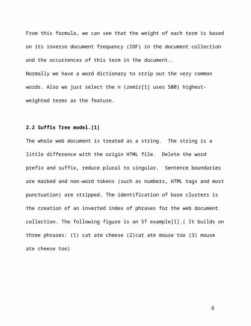
2.2 Suffix Tree model.[1]

The whole web document is treated as a string. The string is a little difference with the origin

HTML file. Delete the word prefix and suffix, reduce plural to singular. Sentence boundaries are

marked and non-word tokens (such as numbers, HTML tags and most punctuation) are stripped. The

identification of base clusters is the creation of an inverted index of phrases for the web document

collection. The following figure is an ST example[1].( It builds on three phrases: (1) cat ate cheese

(2)cat ate mouse too (3) mouse ate cheese too)

4

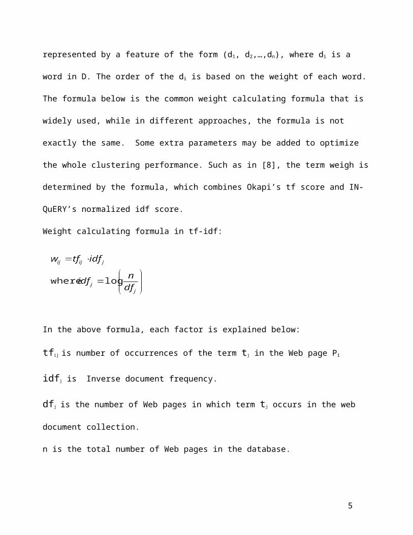
Figure1. Sample of Suffix Tree (courtesy of zemir[1])

The algorithm of suffix tree clustering will be introduced in the next section of this survey.

2.3 Link based model [18]:

From each web document in search result R, we extract all its out-links and in-links. Finally we get

N out-links and M in-links for all URLs.

Each web document P is represented as 2 vectors: Pout(N-dimension)and Pin(M-dimension). Pout,i

represents whether the web document P has a out-link in the ith item of vector Pout. If has, the ith

item is 1, else 0. Identical meaning for Pin,j

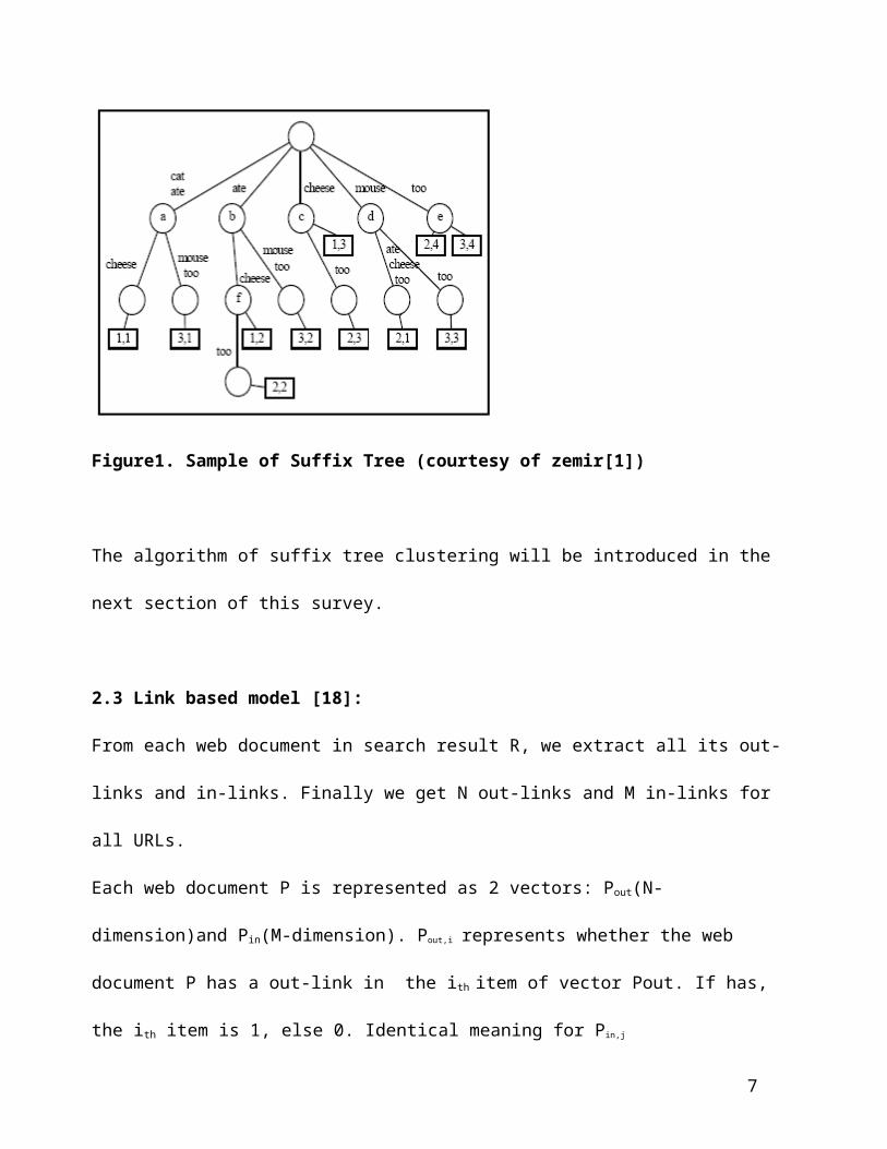
2.4 Frequent item set model [4]:

In this model, each document corresponds to an item and each possible feature corresponds to a

transaction. The entries in the table (domain of document attribute) represent the frequency of

occurrence of a specified feature (word) in that document.

5

Doc1 Doc2 Doc3 … Doc nSports 3 4 5 … 5Olympics 2 4 2 … 3race 0 1 0 … 3… … … … … …bike 2 1 0 … 1F-1 3 7 2 … 4

Figure 2. A collection document present as a transactional database

3.Different kinds of web document clustering approach:

3.1 algorithms with using tf-idf model

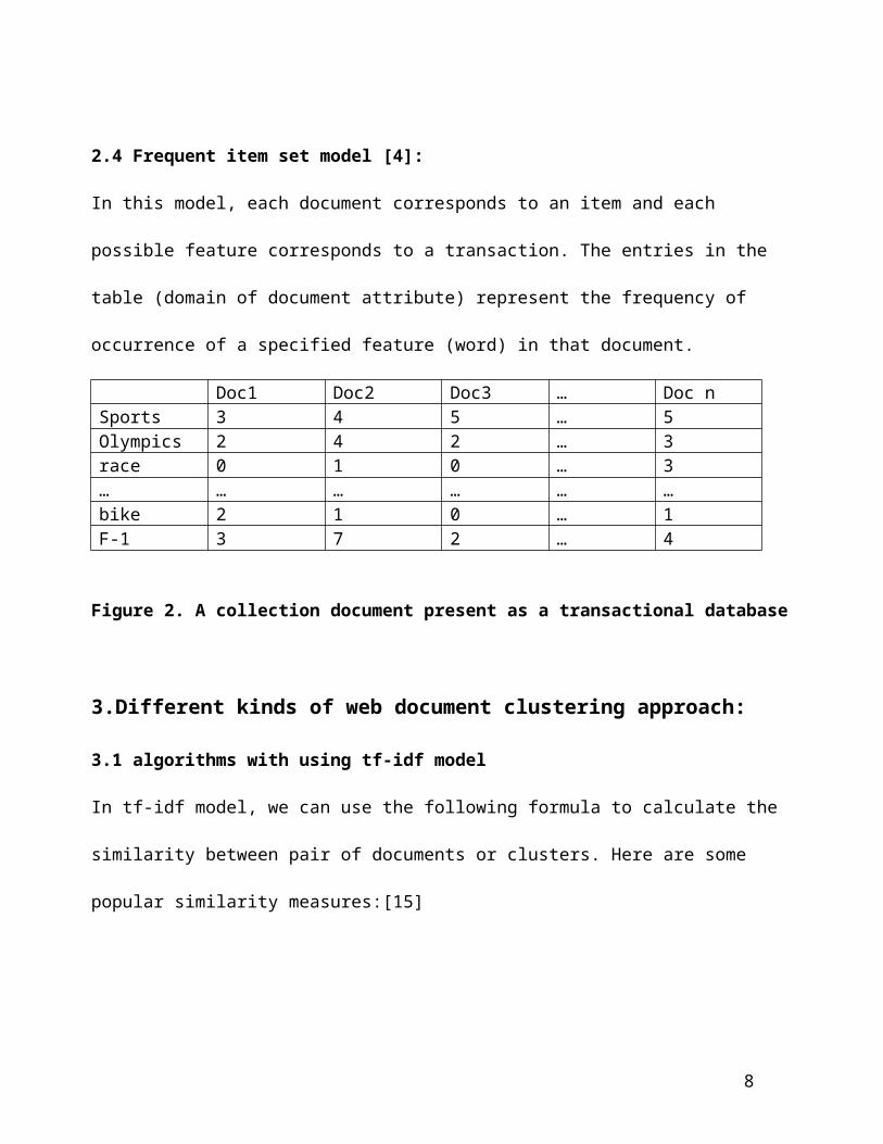
In tf-idf model, we can use the following formula to calculate the similarity between pair of

documents or clusters. Here are some popular similarity measures:[15]

Figure3. Common similarity measurements.

Where ti and tj represent a pair of documents or clusters. tih represent the hth term in document i.

Using one of those formulas and a proper threshold, we can easily determine whether the documents

are similar.

6

The idea to use tf-idf model to represent document is that the more common words between two

documents, the more likely they are similar.

Agglomerative hierarchical clustering and Partition (K-means) clustering are two clustering

techniques that are commonly used for document clustering with tf-idf model.

3.1.1 Algorithm for agglomerative hierarchical clustering.

1. Start with regarding each document as an individual cluster

2. Merge the most similar or closest pair of clusters.(use the similarity or distance measure

above)

3. Step 2 is iteratively executed until all objects are contained within a single cluster, which

become the root of the tree.

4. Instead of step 3, we can set a threshold to determine the number of clusters as step 2 stop

criterion.

3.1.2 Algorithm for K-means clustering.

1. Arbitrary select K web documents as seeds, they are the initial centroids of each

cluster.

2. Assign all other web documents to the closest centroid.

3. Computer the centroid of each cluster again. Get new centroid of each cluster

4. Repeat step2,3, until the centroid of each cluster doesn’t change.

3.1.3 A variant of K-means clustering—bisecting K-means

1. Select a cluster to split (There are several ways to select which cluster to split.

7

No significant difference exists in terms of clustering accuracy). We normally

choose the largest cluster or the one with the least overall similarity.

2. Employ the basic k-means algorithm to subdivide the chosen cluster.

3. Repeat step 2 for a constant number of times. Then perform the split that

produces clusters with the highest overall similarity.

4. Repeat the above step1,2,3, until the desired number of clusters is reached.

3.1.4 Principal direction divisive partitioning [4].

In this algorithm, we use tf-idf model to calculate the distance of pair documents or clusters. All the

documents are in a single large cluster at the beginning. Then proceeds by splitting it. Split the

original cluster into subclusters in recursive fashion. At each stage, do the following:

1.selects an unsplit cluster to split

2.splits that cluster into two subclusters.

The split criteria is the a threshold that measuring the average distance for the documents in a cluster

to the mean of the cluster size if it is desired to keep the resulting clusters in approximately the same

size.

The entire cycle is repeated as many times as desired resulting in a binary tree. The leaf nodes

constitute a partitioning of the entire documents set.

3.2 Suffix Tree Clustering algorithm [1]:

The idea is that each document is an order sequence of words, the tf-idf model lose this valuable

information. With suffix tree, we can exploit this document attribute to improve the quality of

cluster.

STC algorithm includes the following 5 steps:

8

1. Document cleaning.

The string of text representing each web documents transformed using a light stemming algorithm.

As I mentioned before (in model section), we transform the origin document to a standard STC

model document.

2. Identifying Base Cluster.

Create an inverted index of phrases from the web document collection with using a suffix tree. The

suffix tree of a collection of strings is a compact trie containing all the suffixes of all the strings in

the collection. Each node of the suffix tree represents a group of documents and a phrase that is

common to all of them. The label of the node represents the common phrase. Each node represents a

base cluster.

3. Each base cluster is assigned a score that is a function of the number of documents it contains,

and the words that make up its phrase. For example:

S(B)=|B|*f(|P|)

Where |B| is the number of documents in base cluster B. |P| is the number of words in phrase P that

has a non-zero score. Words are in stop list, or the number of appearances in too few (3 or less) or

too many (more than 40% of the web document collection) documents receive a score 0. The

function f penalizes single word, linear for phrase that is two to six words long. And become

constant for longer phrases.

4. Combine base clusters

A binary similarity measure between base clusters based on the overlap of their document sets. For

example: two base clusters Bm and Bn with size |Bm| and |Bn|. |BmBn| represent the number of

documents common to both base clusters. Define the similarity of Bm and Bn to be 1 if: |

BmBn|/Bm>0.5 and |BmBn|/Bn>0.5. Otherwise is 0.

9

So two base clusters are connected if they have similarity of 1. Using a single-link clustering

algorithm, all the connected base clusters are clustering together. All the documents in these base

clusters constitute a web document cluster.

5. The clusters are scored based on the scores of their base clusters that are calculated in step 3.

Report the top score clusters (for example 10 clusters)

3.3 Link based algorithm.[18]

The idea is web pages that share common links each other are very likely to be tightly related. In this

approach [16], we use the link state model for document and Cosine similarity measure:

For document P and Q, Similarity is calculated with the following formula:

Cosine(P,Q)=(P*Q)/(||P||* ||Q||)

Where P*Q=Pout*Qout + Pin*Qin,

||P||² =(Pout,i² + Pin,j²) (Total number of out-links and in-links of document P)

||Q||² =(Qout,i² + Qin,j²) (Total number of out-links and in-links of document Q)

For document P and cluster S, Similarity(P,S) = Cosine(P,C)= (P*C)/(||P|| ||C||) = (P*C)/ )/(||P||*||

C||)= ((Pout*Cout + Pin*Cin))/( ||P||* ||C||)

Where C is the centroid of cluster S, Cout= 1/|S|*Pout,i, Cin= 1/|S|*Pin,j.

||C||² =(Cout,i² + Cin,j²)

|S| is number of documents in cluster S.

Term “near-common Link of cluster” means links shared by majority members of one cluster. If link

is shared by 50%members of the cluster, we call it “50% near common link”.

Link based algorithm include 4 steps:

1. Filter irrelevant web documents:

10

A web document is regarded as irrelevant if the sum of in-links and out-links less than 2.

2. Use near-command link of cluster to grantee intra-cluster cohesiveness.

With the test of [16], they found 30% near-command link is appropriate. They require that

every cluster should have at least one 30% near common link.

3. Assign each web document to cluster, generate base clusters.

Each web document is assigned to an existing cluster if (a) similarity between the document

and the correspondent cluster is above the similarity threshold and (b) the document has a link

in common with near common links of the correspondent cluster.

If no such cluster meet the demands, the document will become a new cluster it self.

Centroid vector is used when calculated the similarity between document and cluster. It is

recalculated after a new document joins the cluster.

4. Generate final clusters by merging base clusters.

Recursively merging two base clusters if they share majority members. Merging threshold is

used to control merging procedure.

3.4 Association Rule Hypergraph Partitioning (ARHP)[4].

In this algorithm, we use a hyper graph H=(V,E) consists of a set of vertices and asset of hyperedges

where V corresponds to the set of documents being clustered, and each hyperedge corresponds to a

set of related documents. We use association rule discovery algorithm to find the frequent item set.

Association rules capture the relationships among items that are present in a transaction. The

algorithm is composed of two steps:

1. Discover all the frequent item-set.

2. Generate association rules from theses frequent item-sets.

11

Support (C) is the number of transactions that contain C where C is the subset of item set I. An

association rule is an expression for form xy where x,y belong to I. The support S of the rule xy

is defined as Support(xy)/|T|, where T is the set of transaction. And the confidence is defined as

Support(xy) / Support(x). The task of discovering an association rule is to find all rules xy,

Support S is greater than a given minimum support threshold and confidence is greater than a given

minimum confidence threshold.

Apriori is such an association rule algorithm to find related items(web documents).

3.5 DC-tree algorithm [2]

This algorithm is implemented by building a document cluster tree (DC-tree). In the DC-tree, every

leaf node represents a cluster that is made up of its entries(documents) . Every non-leaf node

represents a cluster that is made up of all its entries( subclusters or documents). It’s an incremental

algorithm. Every incoming document is guided to its corresponding cluster that is a leaf node.

In the DC-tree, there are four parameters:

1. Branching factor (B): Each non-leaf node contains at most B entries. Each entry is a sub-cluster or

a document.

2. Two similarity threshold (S1 and S2): 0<= S1<S2<=1

3. Minimum number of children in a DC leaf node (M).

Algorithm for Document insertion:

1. Identify the corresponding leaf node.

Start from the node. The document iteratively descends the DC three by choosing the most similar

child node and the similarity value is higher than threshold S1. If no similarity value is higher than

12

S1, inset as a new document leaf node to an empty entry of the node. If there is no empty entry in

this node (>B), than split the node to two groups.

2. Modify the leaf node:

If the document reaches a DC leaf node and the closest leaf entry (X) satisfies the similarity

threshold requirement (S2), it will combined with X. The DC entry for X is updated for the

combination. If no such X is found and there is an empty entry in the leaf node, then just insert the

document to this entry. Otherwise split the node to two groups.

3. Modify the path from the leaf node to the root:

After a document is inserted into a leaf node, update all the non-leaf nodes that are included in the

path from the root to the leaf node. If no split, just add the entry to this node. If splitting, two entries

will be added to the parent node instead of one entry. If there is no room in the parent, split will

cascade to it until reaching the root.

4.Some refinements to the clustering algorithm.

4.1. A grammar based phrase extraction algorithm [10].

Most document clustering techniques treat document as a list of words, ignoring the order or context

of the words. This algorithm captures some context of the words by using phrases rather individual

words as the features.

4.1.1 Parameters in the algorithm

1. N(wi) and N(wi,wj): The frequency count of a word wi and a bigram<wi,wj> where bigram

means a pair of adjacent words.

2. The mutual information association measure between words wi and wj:

13

AMI(wi, wj) = log2((N(wi, wj)/Nb)/(N(wi)N(wj)/Nw²))

Using this formula, the association weight is calculated for each of the bigrams in the training corpus

with a new non-terminal symbol wk, and association weight A(wi, wj) are stored in the grammar

table.

4.1.2 The grammar generation algorithm is as follows:

1. Make a frequency table for all the words and bigrams in the training corpus.

2. From the frequency table calculate the association weight for each bigram.

3. Find a bigram<wi, wj> with the maximum positive association weight A(wi, wj). Quit the

algorithm if none found.

4. In the training corpus, replace all the instances of the bigram<wi , wj> with a new symbol wk. This

is now the new corpus.

5. Add<wi, wj>, wk, and A(wi, wj) to the grammar.

6. Update the frequency table of all the words and bigrams.

7. Go to step 2.

The merge operation creates a new symbol wk that can be used in subsequent merge. This approach

achieves better performance than traditional words approach. It’s running result is more accurate

with the proof of Entropy and F-measure.

4.2 Feature coverage method:

Recall in tf-idf mode, we select the n terms with highest weight in the document selection. But for

web document clustering, a web document usually just contains ten words or less, and these words

are not included in the n highest rank list. It leads to a situation that some documents are all zero

14

weight in its feature vector. Let’ s say coverage is the percentage of documents containing at least

no zero weight in its feature vector. We need to improve the coverage percentage.

K is the approximate number of the cluster size. So the number of clusters is N/K, where N the

number of documents in the collection. The algorithm includes the following steps:

1. Randomly select a subset of documents with size m from the corpus.

2. Extract all the words in the documents. Remove stop words from dictionary. Combine words with

the same root. Count the document frequency of these words.

3. Set lower = k and higher = k

4. Select all words with document frequency in the range from lower to upper

5. If the coverage of these words is larger than the target coverage threshold, quit the iteration.

Otherwise set lower = lower –1 and upper = upper +1, goto step 4.

After the execution of this method, we get the variables “ lower” and “higher”. Use them as the two

bounds in the document frequency table. Select all the words between these two bounds to represent

the document with its corresponding feature vector.

4.3 Scatter/Gather [20].

It’s a mixed clustering algorithm. The whole algorithm is made up of three major steps. Every step

has some sub algorithm. The major steps include:

1.Find k centers

2.Assigh each document in this collection to each center.

4. Optimize the partitions.

4.3.1 Find k centers.

15

We can use either of the two following algorithm to find the k centers.

1. Buckshot

This is linear algorithm to find K approximate centers from a web documents collection. The idea is

straightforward. Choose a small random sample of the documents (the number of the documents is

kn^1/2) from the collection. With the cluster subroutine (AHC), we can get K approximate cluster

centers in O(kn). Although this method is not deterministic, several random collections of sample

documents often get similar partition according to the statistics theory.

2. Fractionation.

This algorithm is another linear time method to find k approximate centers from . It iteratively

breaks a collection C of N documents into N/m buckets, where m>k. Then the cluster subroutine is

applied to each bucket. Since the collection is much smaller than original one and each sub

collection document clustering need at most m² time. The total time for this sub clustering is N/m *

m², that is Nm. We iteratively partition the C with N/m, until the number of cluster is less than k.

Recall that the number of cluster decrease rate is N/m = p<1, then the overall time needed for this

algorithm is O((1+P+P²+…)mN). So it’s a linear algorithm.

4.3.2. Assign documents to the K centers

After we get the K centers, we use the assign- to- nearest neighbor algorithm to assign each

document in Collection C to its nearest center.

In this case, we need at most kn time to finish this step.

4.3.3.Refine the partition

16

1.Split groups that score poorly. The can be the average similarity between documents in the cluster,

as well as to the average similarity of a document to the cluster centroid.

2. Join.

The join refinement is to merge documents groups in a partition P to the another most similar group.

3. Assign to the nearest

4. Iterate the 1,2,3 in this step to improve the quality of clusters.

Each step in this algorithm is O(kn), So it’s linear.

Since all the three major steps in the Scatter/Gather algorithm is linear. The whole algorithm is

linear.

5.How to choose an appropriate topic to present the clusters.

After the cluster algorithm creating the clusters, we ordered the documents with their original rank in

each cluster. One important thing is that we should show users the clusters with meaningful titles.

For different cluster approach, we use different method. With documents similarity approach with tf-

idf, we use the most representative word of all documents. In phrase based or STC, we can use a

representative phrase.

As an alternative we can use a representative document in the cluster. We can choose:

1. The cluster centroid, or the document that is most similar to the actual centroid.

2. The highest ranked document in the cluster. the reason is if this document is non-relevant,

then the rest of the cluster is very likely non-relevant.

3. Use the lowest ranked document. If the lowest is relevant, then it is very likely all documents

in this cluster is relevant.

17

6. How to evaluate the quality of the result clusters.

Validating clustering algorithms and comparing performance of different algorithms are complex

because it is difficult to find an objective measure of quality of clusters.

There are two common measures to evaluate the quality. One type of measure allows us to compare

different sets of clusters without reference to external knowledge. It is called an internal quality

measure. We can use a measure of “overall similarity” base on the similarity of pair documents in a

cluster. The other type of measure is external quality measure. Evaluating the quality of the cluster

is based on comparing the clusters produced by the clustering technology to known classes.

There are two common external quality measures. One is entropy [13]. Which provides a measure of

good ness for un-nested cluster of for the clusters at one level of a hierarchical clustering. The other

is F-measure, which is more oriented toward measuring the effectiveness of the hierarchical

clustering.

6.1. Entropy

For each cluster, the class distribution of the data is calculated first. For example, for cluster j we

calculate pij, where pij is the probability that a document in cluster j belongs to class i. Then using

this class distribution, the entropy of each cluster j is calculated using the following formula:

Ej = -pijlog(pij)

Where the sum is taken over all classes

The total entropy for a set of clusters is calculated as the sum of the entropies of each cluster

weighted by the size of each cluster:

Ecs = (nj*Ej /n )

Where nj is the size of cluster j, m is the number of clusters, and n is the total number of documents.

18

So from the formula, we can see the best quality is that all the documents in the cluster fall into the

same class that is known before clustering.

6.2. F measure

It’s a measure that combines the precision and recall ideas. We treat each cluster as if it were the

result of a query and each class as if it were the desired set of documents for a query. We then

calculate the recall and precision of that cluster for each given class. More specifically, for cluster j

and class i:

Recall(i, j) = nij/ni

Percision(i, j) = nij/nj

Where nij is the number of members of class I in cluster j, nj is the number of members of cluster j

and ni is the number of members of class i.

The F measure of cluster j and class i is then calculated by the following:

F(i, j) = ( 2 * Recall(i, j) * Precision(i, j)) / ((Precision(i, j) + Recall(i, j))

For an entire hierarchical clustering the F measure of any class is the maximum value it attains at

any node in the tree and an overall value for the F measure is computed by taking the weighted

average of all values for the F measure as given by the following:

F = (ni * F(i, j)) / ni

Where ni is the number of documents and F(i,j) is the F measure of cluster j and class i.

7. Evaluation and comparison of different algorithm.

19

Agglomerative Hierarchical Clustering (AHC) algorithms are probably most commonly used. They

are typically slow when applied to large document collections. Single-link and group-average

methods typically take O(n²) time, while complete-link methods typically take O(n³)time. AHC also

need several halting criteria. They are based on predetermined constants (for example: halt when 10

clusters remain). So AHC is very sensitive to the halting criterion. If it mistakenly merges multiple

“good” clusters, the resulting cluster will be meaningless to the user. In web clustering region, this

kind of halting criterion often cause poor results. The clusters in the resulting hierarchy are non-

overlapping. The parent cluster contains only the general documents.

K-means is much faster. It is a linear time clustering algorithm. It’s time complexity is O(kTn)

where k is the number of desired clusters and T is the number of iterations. The sing-pass method is

O(Kn), where K is the number of clusters created.

Both the basic and bisecting k-means algorithms are relatively efficient and scalable.

In addition, they are so easy to implement that they are widely used in different clustering

applications. Another advantage is that K-means algorithm can produce overlapping clusters. A

major disadvantage of k-means is that it requires users to specify k, the number of clusters, in

advance that may be impossible to estimate in some cases. Incorrect estimation of k may lead to poor

clustering accuracy. Also, it is not suitable for discovering clusters of very different size that are very

common in document clustering. Moreover, the k-means algorithm is sensitive to noise and outlier

data objects as they may substantially influence the mean value, which in turn lower the clustering

accuracy.

Suffix tree clustering is a linear time clustering algorithm. It’s time complexity is O(n). It first builds

a suffix tree based on the collection of document. So the time to build the tree and the memory need

to be used for storing STC tree are huge. Zamir[1] use the snippets returned by search engine to

20

build the tree. Each snippet contains 50words on average and 20 words after word cleaning. Instead

of the whole document, this method dramatically decreases the size of the suffix tree. The precision

of the result doesn’t affect much when using snippets. It’s a good trade-off. In the later of this

survey, I will introduce a really world application that is implemented by STC (metacrawler).

Link based algorithm is linear time clustering algorithm with time complex O(mn), where m is the

number of iterations needed for clustering process to converge( the convergence is guaranteed by k-

means algorithm), n is the number of pages that processing in the clustering algorithm. Since m<<n,

it’s linear algorithm.

Use Aprori algorithm for computing frequent itemsets in a document based transaction database.

This algorithm uses a level-wise search . K itemsets are used to explore (K+1) itemsets to mine

frequent itemsets from the database. A large number of frequent itemsets and N scans to the

database affect the speed of this algorithm. The quality of the resulting cluster is better than

traditional cluster algorithm.

Figure4. Executing time comparison to common clustering methods (Courtesy of [3])

21

We can see that almost all algorithms are linear except the AHC (It is a O(n²) algorithm)

The following is the comparison of the Entropy for different clustering algorithms for K=16 ( K is

the number of clusters). [16]

Figure5. Precision comparison to K-means, AHC and their variations (16 clusters)

(courtesy of [16])

The following is the comparison of the Entropy for different clustering algorithms for K=32 (K is

the number of clusters).

Figure6. Precision comparison to K-means, AHC and their variations (32 clusters)

The following is the comparison of the Entropy for different clustering algorithms for K=64 (K is

the number of clusters).

22

Figure7. Precision comparison to K-means, AHC and their variations (64 clusters)

Form the above statistics, Bisecting K-means algorithm always get the best quality cluster when

compare to AHC and normal k-means. Also Bisecting K-means is a linear algorithm (O(kn)). So in

traditional clustering algorithm (AHC, k-means), bisecting k-means is the best.

Compare the AHC,K-means and STC using F-measure:

Figure8. Average precision between K-mans, AHC and STC (courtesy of [1])

We can see phrases base clustering algorithm usually get better quality than word based one. STC

get the best quality, because it is a context-based algorithm.

8.A real world web documents clustering Application.

23

MetaCrawler[21] is a web document clustering application which is developed by researchers from

university of Washington. It uses two steps to process a query:

1. It posts the users query to multiple search engines in parallel, such as google, altavista,

Findwhat… and so on

2. It gets the results from these different search engines, combines the search results to a refined

rank list.

3. Use STC clustering algorithm to cluster these web documents. Give each cluster a

representative topic.

For example, a traveler comes to dallas and what to get some information about this city. He types

the key words “dallas” in the search area. Let’s check what he gets.

Figure 9. Use Metacrawler to cluster web search result.

24

From the search result, we can see the web documents from the search result are organized into 10

clusters. User can easily find the topic he is interested in. This is the power of web document

clustering.

Conclusion:

This survey presents the researches on web document clustering domain. The most important aspects

we concerned are the quality of the resulting clusters and the time complexity of the algorithm. For

the tf-idf based algorithms, we use high dimensional vectors to represent documents. That leads to a

time complexity problem. So until now, we can only apply these algorithms to a small collection of

documents. This means if we want to cluster the result from a web search (usually >100,000), we

just process the top-ranked documents rather than the entire collection. Some other approaches suffer

the memory problem, such as STC, Frequent itemsets. Every method has its own advantage and

deficiency. Some refinements are made to improve the efficiency. We use snippet instead of the

whole document in STC to solve the memory problem. We present document with phrases instead of

words in tf-idf model to decrease the data dimension and increases the accuracy (Because this

approach considers the document context related feature). Some divide-conquer algorithms are

invented by researchers, such as scatter/gather which is introduced in this survey. The importance of

web document clustering is continuing grow with the rapid growth of Internet. How to calculate the

web document to improve the quality of the cluster in a reasonable time is a key point in this field.

References:

1.Oren Zamir and Oren Etzioni. Web document Clustering: A Feasibility Demonstration. 1998.

25

2.Wai-chiu Wong and Ada Wai-chee Fu. Incremental Document Clustering for Web Page

Classification. July1,2000

3.Jian Zhang, JianfengGao,Ming Zhou, Jiaxing Wang. Improving the Effectiveness of Information

Retrieval with Clustering and Fusion. 2001

4.Faniel Boley, Maria Gini, Rebert Gross, Eui-Hong Han, Kyle Hastings,George Karypis.

Partitioning-Based Clustering for Web Document Categorization. 1999

5.Jun-Hui Her, Sung-Hae Jun, Jun-Feyog Choi,Jung-Hyun Lee. A Bayesian Neural Network Model

for Dynamic Web Document Clustering.1999 IEEE TENCON

6.Noam Solnim, Nir Friedman, Naftali Tishby. Unsupervised Document Classification using

Sequential Information Maximization. 2002

7.Anton Leuski and James Allan. Improving Interactive Retrieval by Combining Ranked Lists and

Clustering.2000

8.Anton Leuski. Evaluating Document Clustering for Interactive Information Retrieval.2000

9.Krishna Gade, George Karypis. Multivevel K-way Document Clustering: Experiments &

Analysis.1999

10.J.Bakus,M.F.Hussin, M.Kamel. A SOM-Based Document clustering Using Phrases.2000

11.Guihong Cao, Dawei Song, Peter Bruza. Suffix Tree Clustering on Post-retrieval Documents.

2003.

12.Steven Noel, Vijay Raghavan, C.H.Henry Chu. Document Clustering, Visualization, and

Retrieval via Link Mining.2001

13. Taeho C. Jo. Evaluation Function of Document Clustering based on Term Entropy1997

14. Hinrich Schutze, Craig Silverstein. Xerox Palo Alto Research Center. Projections for Efficient

Document Clustering 2001

26

15.Margaret H.Dunham. Data Mining introductory and advanced topics 2003

16. Michael Steinbach, Geoge Karypis, Vipin Kumar. A Comparison of Document Clustering

Techniques. 2001

17.Xiaofeng he, Hongyuan Zha, Chris H.Q.Fing, Horst D. Simon, Web document clustering using

hyperlink structures.2002

18. Yitong Wang and Masaru Kitsuregawa.Link based clustering of web search results 2002

19.Benjamin C.M. Fung Ke Wang, Martin Ester. Hierarchical document clustering using frequent

itemsets. 2002

20.Douglass R. Cutting, David R.Karger, Jan O. Pedersen, John W.Tukey. Scatter/Gather: A cluster-

based approach to browsing large document collections. 1992

21. http://www.metacrawler.com

22. Inderjit S. Dhillon, James Fan, Yuqiang Guan, efficient clustering of very large document

collections. 2001.

23. Ying Zhao, George Karypis. Criterion Functions for Document Clustering *experiments and

analysis 2002

24.Chris Ding, Xiaofeng He. Cluster merging and splitting in hierarchical clustering algorithms.

2002

25.Zhexue Huang. Extensions to the k-means algorithm for clustering large data sets with

categorical values. 1998.

27