Well-To-Wheels Energy and Greenhouse Gas Analysis of … · 2.13 Usable Battery Energy for PHEV Midsize Vehicle with Gasoline Engine ..... 27 2.14 Usable Battery Energy for PHEV Midsize

ii

This page intentionally left blank.

iii

CONTENTS

ACKNOWLEDGMENTS ........................................................................................................ xi

NOTATION .............................................................................................................................. xiii

EXECUTIVE SUMMARY ...................................................................................................... 1

ES.1 CD Operation of Gasoline PHEVs and BEVs ......................................................... 2

ES.1.1 Petroleum Displacement ............................................................................. 2

ES.1.2 GHG Emissions .......................................................................................... 3

ES.1.3 Electric Range of PHEVs and BEVs in Real-World Driving ..................... 4

ES.2 Combined CD and CS Operation of PHEVs ........................................................... 4

ES.2.1 Petroleum Displacement ............................................................................. 4

ES.2.2 GHG Emissions .......................................................................................... 5

1 INTRODUCTION ............................................................................................................. 7

1.1 Previous Studies ....................................................................................................... 7

1.2 Analysis Overview ................................................................................................... 8

1.3 Report Organization ................................................................................................. 11

2 FUEL AND ELECTRICITY CONSUMPTION BY PHEVs ........................................... 13

2.1 PSAT Overview ....................................................................................................... 13

2.1.1 Objectives ................................................................................................... 13

2.1.2 Principles..................................................................................................... 13

2.2 Process Description .................................................................................................. 14

2.3 Component Assumptions ......................................................................................... 15

2.3.1 Engines and Storage .................................................................................... 15

2.3.2 Transmission ............................................................................................... 18

2.4 Vehicle ..................................................................................................................... 19

2.4.1 Vehicle Powertrain Assumptions ................................................................ 20

2.4.2 Vehicle Architecture Selection ................................................................... 20

2.4.3 Configuration Selection .............................................................................. 23

2.5 Vehicle Sizing Process ............................................................................................. 23

2.6 Vehicle Sizing Results ............................................................................................. 24

3 ON-ROAD ADJUSTMENT OF FUEL ECONOMY AND

ELECTRICITY CONSUMPTION ................................................................................... 31

3.1 Fuel Economy Adjustment for On-Road Performance ............................................ 31

3.1.1 Background ................................................................................................. 31

3.1.2 Conventional ICEVs and HEVs .................................................................. 34

3.1.3 Hydrogen FCVs .......................................................................................... 34

iv

CONTENTS (CONT.)

3.1.4 Series PHEV30 and 40 and BEVs .............................................................. 34

3.1.5 Power-Split PHEV10 and 20 ...................................................................... 35

3.2 Battery Charging Losses for PHEVs and BEVs ...................................................... 37

3.3 Actual ―On-Road‖ Miles Driven In CD Mode ........................................................ 40

3.4 Vehicle Miles Traveled Split by CD Versus CS Operation ..................................... 41

4 PHEV POPULATION AND ELECTRIC LOAD PROFILE ........................................... 45

4.1 Data Sources ............................................................................................................ 45

4.2 PHEV Population ..................................................................................................... 46

4.3 PHEV Charging Scenarios ....................................................................................... 48

4.4 Summary of PHEV Population and Electric Load Analysis ................................... 52

5 ELECTRIC POWER SYSTEM DISPATCH .................................................................... 53

5.1 Modeling Technique and Methodology ................................................................... 53

5.1.1 NE and NY ISOs ......................................................................................... 53

5.1.2 WECC ......................................................................................................... 55

5.1.3 State of Illinois ............................................................................................ 57

5.2 Data Collection and Preparation .............................................................................. 59

5.2.1 Inventory of Existing and Proposed Power Plants ...................................... 59

5.2.2 Historical Load Data ................................................................................... 60

5.2.3 Load Projections ......................................................................................... 60

5.2.4 Fuel Price Projections ................................................................................. 60

5.2.5 Expansion Candidate Technology Data ...................................................... 60

5.2.6 Wind and Solar Data ................................................................................... 60

5.3 Treatment of Renewable Generation ....................................................................... 61

5.3.1 NE and NY ISOs ......................................................................................... 61

5.3.2 WECC ......................................................................................................... 62


5.4 Developing Load Profiles ........................................................................................ 63

5.4.1 NE and NY ISOs ......................................................................................... 63

5.4.2 WECC ......................................................................................................... 64


5.4.4 Forecasting PHEV Loads ............................................................................ 66

5.5 Capacity Expansion Modeling ................................................................................. 69

5.6 Dispatch Modeling ................................................................................................... 71

5.6.1 NE and NY ISOs ......................................................................................... 71

5.6.2 WECC ......................................................................................................... 74


5.7 Simulation Results ................................................................................................... 79

5.7.1 NE ISO ........................................................................................................ 79

5.7.2 NY ISO ....................................................................................................... 81

v

CONTENTS (CONT.)

5.7.3 WECC ......................................................................................................... 84


5.8 Conclusions .............................................................................................................. 91

6 GREET WTW ENERGY USE AND GHG EMISSIONS ................................................ 93

6.1 Introduction .............................................................................................................. 93

6.2 Well-To-Wheels Simulation Methodology .............................................................. 98

6.3 WTW Simulation Results ........................................................................................ 99

7 CONCLUSIONS ............................................................................................................... 115

7.1 CD Operation of Gasoline PHEVs and BEVs ......................................................... 115

7.1.1 Petroleum Displacement ............................................................................. 115

7.1.2 GHG Emissions .......................................................................................... 115

7.1.3 Electric Range of PHEVs and BEVs in Real-World Driving ..................... 116

7.2 Combined CD and CS Operation of PHEVs ........................................................... 116

7.2.1 Petroleum Displacement ............................................................................. 116

7.2.2 GHG Emissions .......................................................................................... 117

8 IMPLICATIONS FOR FUTURE ANALYSIS ................................................................. 119

9 REFERENCES .................................................................................................................. 125

APPENDIX 1: VEHICLE DESCRIPTIONS ........................................................................... 127

FIGURES

ES.1 WTW Petroleum Use and GHG Emissions for CD Operation of Gasoline

PHEVs and BEVs Compared with Baseline Gasoline ICEVs and Regular

Gasoline HEVs ............................................................................................................... 3

ES.2 WTW Petroleum Use and GHG Emissions for Combined CD and CS

Operation of PHEVs Compared with Baseline Gasoline ICEVs ................................... 5

2.1 Bond Graph Formalism.................................................................................................... 13

2.2 Simulink Vehicle Model Example ................................................................................... 14

2.3 Uncertainty Process ......................................................................................................... 15

vi

FIGURES (CONT.)

2.4 Fuel Cell System Efficiency Versus Fuel Cell System Power from the System Map ..... 16

2.5 Parallel HEV .................................................................................................................... 21

2.6 Series HEV....................................................................................................................... 21

2.7 Power-Split HEV ............................................................................................................. 23

2.8 Process for Sizing PHEV Components ............................................................................ 24

2.9 Engine Power for Gasoline Powertrains .......................................................................... 25

2.10 Electric Machine Power for Gasoline HEVs and PHEVs ............................................... 26

2.11 Fuel Cell Power for Hydrogen Vehicles .......................................................................... 26

2.12 Battery Power for Gasoline HEVs and PHEVs ............................................................... 27

2.13 Usable Battery Energy for PHEV Midsize Vehicle with Gasoline Engine ..................... 27

2.14 Usable Battery Energy for PHEV Midsize Vehicle with Fuel Cell ................................. 28

2.15 Vehicle Mass .................................................................................................................... 28

3.1 On-Road Adjustment Factor for Laboratory Fuel Economy Based on EPA’s

MPG-Based Formulas ..................................................................................................... 33

3.2 On-Road Adjustments of Laboratory Fuel and Electricity Consumption ....................... 36

3.3 Electricity and Fuel Consumption in CD Operation of PHEVs and BEVs ..................... 38

3.4 Electricity and Fuel Consumption in CD and CS Operation of PHEVs .......................... 39

3.5 CD VMT on UDDS from PSAT Simulations.................................................................. 40

3.6 CD VMT on HWFET from PSAT Simulations ............................................................... 41

3.7 Adjusted CD VMT ........................................................................................................... 41

3.8 Percentage of Daily VMT Available for Substitution by a PHEV in CD Mode ............. 43

4.1 PHEV Populations by Simulated Utility Service Area in 2020 ....................................... 48

vii

FIGURES (CONT.)

4.2 Distribution of Vehicles by Last Trip Ending Time for Large MSAs in California........ 49

4.3 Distribution of Vehicles by Last Trip Ending Time for Large MSAs in California,

January–March ................................................................................................................ 50


April–June ....................................................................................................................... 50


July–September ............................................................................................................... 51


October–December ......................................................................................................... 51

5.1 WECC Network Topology .............................................................................................. 56

5.2 State of Illinois Network Topology ................................................................................. 58

5.3 Hydropower Plant Operations .......................................................................................... 61

5.4 Developing an Hourly Load Profile for the NE and NY ISOs ........................................ 64

5.5 Developing Hourly Load Profiles for Nodes in WECC .................................................. 65

5.6 Typical Hourly Charging Pattern for All Three PHEV Charging Scenarios ................... 70

5.7 Creating a Thermal Unit Inventory for the NE and NY ISOs ......................................... 72

5.8 Example for Results of Maintenance Scheduling Routine .............................................. 74

6.1 WTW Total Energy Use for PHEV10 and PHEV40 for Different

Fuel/Vehicle Systems ..................................................................................................... 101

6.2 WTW Fossil Energy Use for PHEV10 and PHEV40 for Different


6.3 WTW Petroleum Energy Use for PHEV10 and PHEV40 for Different


6.4 WTW GHG Emissions for PHEV10 and PHEV40 for Different


viii

FIGURES (CONT.)

6.5 WTW GHG Emissions for HEV and CD Operation of PHEV40 with

Different Charging Scenarios in the WECC Region ...................................................... 103

6.6 WTW GHG Emissions for CD Operation of PHEV40 with

Unconstrained Charging in Different Regions ............................................................... 104

6.7 WTW Petroleum Energy Use for Combined CD and CS Operations of

PHEVs as a Function of Rated AER .............................................................................. 105

6.8 WTW GHG Emissions for Combined CD and CS Operations of PHEVs in

WECC as a Function of Rated AER ............................................................................... 105

6.9 WTW GHG Emissions for Combined CD and CS Operations of PHEVs in

IL as a Function of Rated AER ....................................................................................... 106

6.10 WTW GHG Emissions for Combined CD and CS Operations of PHEVs as a

Function of Rated AER Using the U.S. Average Generation Mix ................................. 107

6.11 WTW GHG Emissions for Combined CD and CS Operations of PHEVs as

a Function of Rated AER Using the Northeastern U.S. Average Generation Mix......... 107

6.12 WTW GHG Emissions for Combined CD and CS Operations of PHEVs as a

Function of Rated AER Using the CA Average Generation Mix ................................... 108

6.13 WTW Petroleum Use and GHG Emissions for CD Operation of PHEVs ...................... 109

6.14 WTW Petroleum Use and GHG Emissions for Combined CD and

CS Operation of PHEVs ................................................................................................. 110

6.15 WTW Petroleum Use and GHG Emissions for CD Operation of Gasoline Vehicles .... 113

TABLES

1.1 Vehicle Technologies, Fuels, and Feedstock Sources .................................................... 9

2.1 Main Engine Assumptions .............................................................................................. 16

2.2 Main Fuel Cell Assumptions .......................................................................................... 17

2.3 Main Hydrogen Storage Assumptions ............................................................................ 17

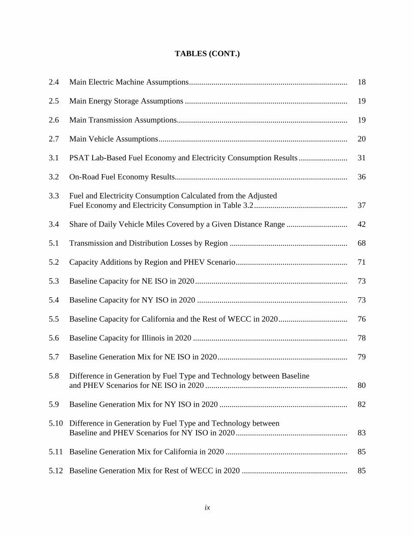
ix

TABLES (CONT.)

2.4 Main Electric Machine Assumptions .............................................................................. 18

2.5 Main Energy Storage Assumptions ................................................................................ 19

2.6 Main Transmission Assumptions .................................................................................... 19

2.7 Main Vehicle Assumptions ............................................................................................. 20

3.1 PSAT Lab-Based Fuel Economy and Electricity Consumption Results ........................ 31

3.2 On-Road Fuel Economy Results..................................................................................... 36

3.3 Fuel and Electricity Consumption Calculated from the Adjusted

Fuel Economy and Electricity Consumption in Table 3.2 .............................................. 37

3.4 Share of Daily Vehicle Miles Covered by a Given Distance Range .............................. 42

5.1 Transmission and Distribution Losses by Region .......................................................... 68

5.2 Capacity Additions by Region and PHEV Scenario ....................................................... 71

5.3 Baseline Capacity for NE ISO in 2020 ........................................................................... 73

5.4 Baseline Capacity for NY ISO in 2020 .......................................................................... 73

5.5 Baseline Capacity for California and the Rest of WECC in 2020 .................................. 76

5.6 Baseline Capacity for Illinois in 2020 ............................................................................ 78

5.7 Baseline Generation Mix for NE ISO in 2020 ................................................................ 79

5.8 Difference in Generation by Fuel Type and Technology between Baseline

and PHEV Scenarios for NE ISO in 2020 ...................................................................... 80

5.9 Baseline Generation Mix for NY ISO in 2020 ............................................................... 82

5.10 Difference in Generation by Fuel Type and Technology between

Baseline and PHEV Scenarios for NY ISO in 2020 ....................................................... 83

5.11 Baseline Generation Mix for California in 2020 ............................................................ 85

5.12 Baseline Generation Mix for Rest of WECC in 2020 .................................................... 85

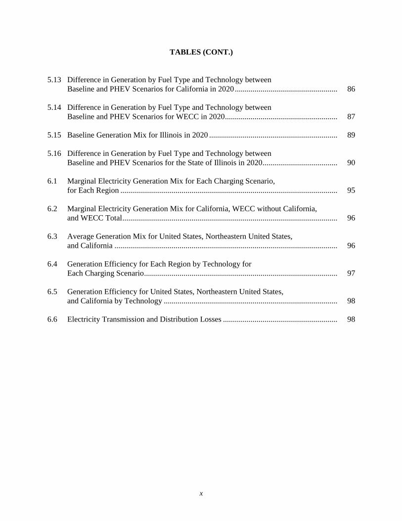
x

TABLES (CONT.)


Baseline and PHEV Scenarios for California in 2020 .................................................... 86


Baseline and PHEV Scenarios for WECC in 2020 ......................................................... 87

5.15 Baseline Generation Mix for Illinois in 2020 ................................................................. 89


Baseline and PHEV Scenarios for the State of Illinois in 2020 ...................................... 90

6.1 Marginal Electricity Generation Mix for Each Charging Scenario,

for Each Region .............................................................................................................. 95

6.2 Marginal Electricity Generation Mix for California, WECC without California,

and WECC Total ............................................................................................................. 96

6.3 Average Generation Mix for United States, Northeastern United States,

and California ................................................................................................................. 96

6.4 Generation Efficiency for Each Region by Technology for

Each Charging Scenario .................................................................................................. 97

6.5 Generation Efficiency for United States, Northeastern United States,

and California by Technology ........................................................................................ 98

6.6 Electricity Transmission and Distribution Losses .......................................................... 98

xi

ACKNOWLEDGMENTS

This study was supported by the Fuel Cell Technologies Program (U.S. Department of Energy,

Assistant Secretary for Energy Efficiency and Renewable Energy) under Contract Number DE-

AC02-06CH11357. We would like to thank Fred Joseck of the Fuel Cell Technologies Program

for his support of this study. We are also grateful to Audun Botterud, Jianhui Wang, Tom

Veselka, Guenter Conzelmann, Vladimir Koritarov, Jason Wang, Dan Santini, Mike Duoba,

Andrew Burnham, Neeraj Shidore, Theodore Bohn, Aurelien Sergent, and Phil Sharer of

Argonne National Laboratory for contributing their knowledge and experience in electricity

dispatch modeling, battery performance, and plug-in electric vehicles.

xii


xiii

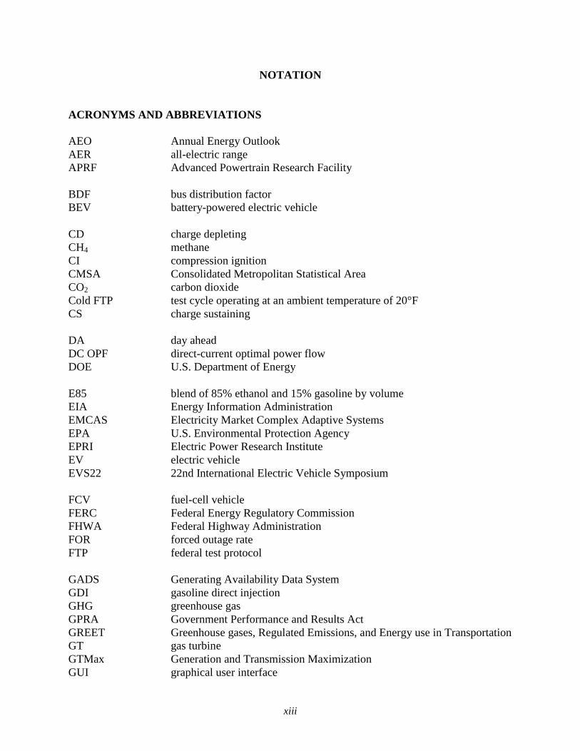
NOTATION

ACRONYMS AND ABBREVIATIONS

AEO Annual Energy Outlook

AER all-electric range

APRF Advanced Powertrain Research Facility

BDF bus distribution factor

BEV battery-powered electric vehicle

CD charge depleting

CH4 methane

CI compression ignition

CMSA Consolidated Metropolitan Statistical Area

CO2 carbon dioxide

Cold FTP test cycle operating at an ambient temperature of 20°F

CS charge sustaining

DA day ahead

DC OPF direct-current optimal power flow

DOE U.S. Department of Energy

E85 blend of 85% ethanol and 15% gasoline by volume

EIA Energy Information Administration

EMCAS Electricity Market Complex Adaptive Systems

EPA U.S. Environmental Protection Agency

EPRI Electric Power Research Institute

EV electric vehicle

EVS22 22nd International Electric Vehicle Symposium

FCV fuel-cell vehicle

FERC Federal Energy Regulatory Commission

FHWA Federal Highway Administration

FOR forced outage rate

FTP federal test protocol

GADS Generating Availability Data System

GDI gasoline direct injection

GHG greenhouse gas

GPRA Government Performance and Results Act

GREET Greenhouse gases, Regulated Emissions, and Energy use in Transportation

GT gas turbine

GTMax Generation and Transmission Maximization

GUI graphical user interface

xiv

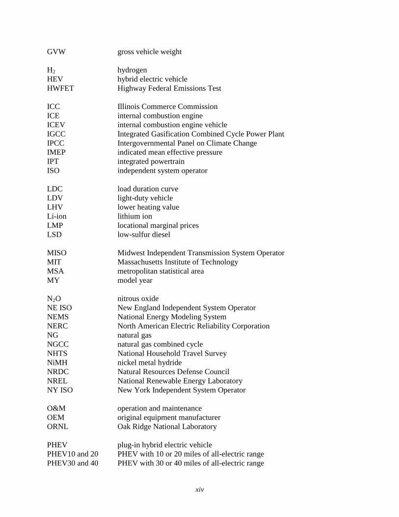
GVW gross vehicle weight

H2 hydrogen

HEV hybrid electric vehicle

HWFET Highway Federal Emissions Test

ICC Illinois Commerce Commission

ICE internal combustion engine

ICEV internal combustion engine vehicle

IGCC Integrated Gasification Combined Cycle Power Plant

IPCC Intergovernmental Panel on Climate Change

IMEP indicated mean effective pressure

IPT integrated powertrain

ISO independent system operator

LDC load duration curve

LDV light-duty vehicle

LHV lower heating value

Li-ion lithium ion

LMP locational marginal prices

LSD low-sulfur diesel

MISO Midwest Independent Transmission System Operator

MIT Massachusetts Institute of Technology

MSA metropolitan statistical area

MY model year

N2O nitrous oxide

NE ISO New England Independent System Operator

NEMS National Energy Modeling System

NERC North American Electric Reliability Corporation

NG natural gas

NGCC natural gas combined cycle

NHTS National Household Travel Survey

NiMH nickel metal hydride

NRDC Natural Resources Defense Council

NREL National Renewable Energy Laboratory

NY ISO New York Independent System Operator

O&M operation and maintenance

OEM original equipment manufacturer

ORNL Oak Ridge National Laboratory

PHEV plug-in hybrid electric vehicle

PHEV10 and 20 PHEV with 10 or 20 miles of all-electric range

PHEV30 and 40 PHEV with 30 or 40 miles of all-electric range

xv

PSAT Powertrain System Analysis Toolkit

PTW pump to wheels

PV photovoltaic

RPS Renewable Portfolio Standard

RT real time

RTO regional transmission organization

SAE Society of Automotive Engineers

SC03 test cycle operating at an ambient temperature of 95°F

SI spark ignition

SMR steam methane reformation

SOC state of charge

SUV sport utility vehicle

TEPPC Transmission Expansion Planning and Policy Committee

UDDS Urban Dynamometer Driving Schedule

UF utility factor

US06 duty cycle with aggressive highway driving

VMT vehicle miles traveled

WECC Western Electric Coordinating Council

WTP well to pump

WTW well-to-wheels

UNITS OF MEASURE

A ampere(s)

gal gallon(s)

h hour(s)

mi mile(s)

mpg mile(s) per gallon

mpgeg mile(s) per gasoline-equivalent gallon

MW megawatt(s)

V volt

Wh/mi Watt hour(s) per mile

xvi


1

WELL-TO-WHEELS ANALYSIS OF ENERGY USE AND GREENHOUSE GAS

EMISSIONS OF PLUG-IN HYBRID ELECTRIC VEHICLES

by

Amgad Elgowainy, Jeongwoo Han, Leslie Poch, Michael Wang, Anant Vyas, Matthew Mahalik,

and Aymeric Rousseau

EXECUTIVE SUMMARY

Plug-in hybrid electric vehicles (PHEVs) are being developed for mass production by

the automotive industry. PHEVs have been touted for their potential to reduce the

U.S. transportation sector’s dependence on petroleum and cut greenhouse gas (GHG) emissions

by (1) using off-peak excess electric generation capacity and (2) increasing vehicles’ energy

efficiency. A well-to-wheels (WTW) analysis — which examines energy use and emissions from

primary energy source through vehicle operation — can help researchers better understand the

impact of the upstream mix of electricity generation technologies for PHEV recharging, as well

as the powertrain technology and fuel sources for PHEVs. For the WTW analysis, Argonne

National Laboratory researchers used the Greenhouse gases, Regulated Emissions, and Energy

use in Transportation (GREET) model developed by Argonne to compare the WTW energy use

and GHG emissions associated with various transportation technologies to those associated with

PHEVs.

Argonne researchers estimated the fuel economy and electricity use of PHEVs and

alternative fuel/vehicle systems by using Argonne’s Powertrain System Analysis Toolkit (PSAT)

model. They examined two PHEV designs: the power-split configuration and the series

configuration. The first is a parallel hybrid configuration in which the engine and the electric

motor are connected to a single mechanical transmission that incorporates a power-split device,

which allows for parallel power paths — mechanical and electrical — from the engine to the

wheels, allowing the engine and the electric motor to share the power during acceleration. In the

second configuration, the engine powers a generator, which charges a battery that is used by the

electric motor to propel the vehicle; thus, the engine never directly powers the vehicle’s

transmission. The power-split configuration was adopted for PHEVs with a 10- and 20-mile

electric range because they require frequent use of the engine for acceleration, while the series

configuration was adopted for PHEVs with a 30- and 40-mile electric range because they rely

mostly on electrical power for propulsion over a longer electric range.

Argonne researchers calculated the equivalent ―on-road‖ (real-world) fuel economy on

the basis of U.S. Environmental Protection Agency miles per gallon (mpg)-based formulas. The

reduction in fuel economy attributable to the ―on-road‖ adjustment formula was capped at 30%

for advanced vehicle systems (e.g., PHEVs, fuel cell vehicles [FCVs], hybrid electric vehicles

[HEVs], and battery-powered electric vehicles [BEVs]). Simulations for calendar year 2020 with

model year 2015 mid-size vehicles were chosen for this analysis to address the implications of

PHEVs within a reasonable timeframe after their likely introduction over the next few years. For

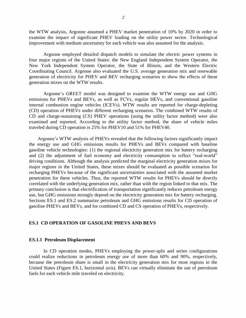
2

the WTW analysis, Argonne assumed a PHEV market penetration of 10% by 2020 in order to

examine the impact of significant PHEV loading on the utility power sector. Technological

improvement with medium uncertainty for each vehicle was also assumed for the analysis.

Argonne employed detailed dispatch models to simulate the electric power systems in

four major regions of the United States: the New England Independent System Operator, the

New York Independent System Operator, the State of Illinois, and the Western Electric

Coordinating Council. Argonne also evaluated the U.S. average generation mix and renewable

generation of electricity for PHEV and BEV recharging scenarios to show the effects of these

generation mixes on the WTW results.

Argonne’s GREET model was designed to examine the WTW energy use and GHG

emissions for PHEVs and BEVs, as well as FCVs, regular HEVs, and conventional gasoline

internal combustion engine vehicles (ICEVs). WTW results are reported for charge-depleting

(CD) operation of PHEVs under different recharging scenarios. The combined WTW results of

CD and charge-sustaining (CS) PHEV operations (using the utility factor method) were also

examined and reported. According to the utility factor method, the share of vehicle miles

traveled during CD operation is 25% for PHEV10 and 51% for PHEV40.

Argonne’s WTW analysis of PHEVs revealed that the following factors significantly impact

the energy use and GHG emissions results for PHEVs and BEVs compared with baseline

gasoline vehicle technologies: (1) the regional electricity generation mix for battery recharging

and (2) the adjustment of fuel economy and electricity consumption to reflect ―real-world‖

driving conditions. Although the analysis predicted the marginal electricity generation mixes for

major regions in the United States, these mixes should be evaluated as possible scenarios for

recharging PHEVs because of the significant uncertainties associated with the assumed market

penetration for these vehicles. Thus, the reported WTW results for PHEVs should be directly

correlated with the underlying generation mix, rather than with the region linked to that mix. The

primary conclusion is that electrification of transportation significantly reduces petroleum energy

use, but GHG emissions strongly depend on the electricity generation mix for battery recharging.

Sections ES.1 and ES.2 summarize petroleum and GHG emissions results for CD operation of

gasoline PHEVs and BEVs, and for combined CD and CS operation of PHEVs, respectively.

ES.1 CD OPERATION OF GASOLINE PHEVS AND BEVS

ES.1.1 Petroleum Displacement

In CD operation modes, PHEVs employing the power-split and series configurations

could realize reductions in petroleum energy use of more than 60% and 90%, respectively,

because the petroleum share is small in the electricity generation mix for most regions in the

United States (Figure ES.1, horizontal axis). BEVs can virtually eliminate the use of petroleum

fuels for each vehicle mile traveled on electricity.

3

0

0.2

0.4

0.6

0.8

1

1.2

0 0.2 0.4 0.6 0.8 1 1.2

GH

G E

mis

sio

ns (

rela

tive to

GV

)

Petroleum Use (relative to GV)

Regular HEV

Baseline Gasoline ICE Vehicle (GV)

Smart (least cost) ChargingUnconstrained Charging

PHEV10

BEV

PHEV30

PHEV40 PHEV20

Power-Split

Design

Series

Design

IL (coal intensive mix)

U.S. (average mix)

Renewable

WECC (dominated by NGCC)

Regular

Gasoline HEV

Source of Electricity

for Battery Recharging

FIGURE ES.1 WTW Petroleum Use and GHG Emissions for CD Operation of Gasoline PHEVs

and BEVs Compared with Baseline Gasoline ICEVs and Regular Gasoline HEVs

ES.1.2 GHG Emissions

Unconstrained charging (with investments in new generation capacity) reduces

GHG emissions (Figure ES.1, vertical axis) compared with smart charging (no

needed investment in new capacity) because of the high efficiency and low carbon

intensity associated with the added capacity in the unconstrained charging

scenario.

PHEVs recharging from a mix with a large share of coal generation (e.g., Illinois

marginal mix) produce GHG emissions comparable to those of baseline gasoline

ICEVs (with a range from -15% to +10%) but significantly higher than those of

gasoline HEVs (with a range from +20% to +60%). The range of the results is

primarily attributable to the different generation mix for the charging scenarios

considered and the different PHEV types (power-split versus series designs).

4

PHEVs recharging from a mix with a large share of efficient electricity generation

from natural gas (e.g., natural gas combined-cycle [NGCC] generation in the

Western Electric Coordinating Council region) produce GHG emissions

comparable to those of gasoline HEVs (with a range from -15% to +10%) but

significantly lower than those of baseline gasoline ICEVs (with a range from

-25% to -40%). The range of results is primarily attributable to the different

generation mix for the charging scenarios considered and the different PHEV

types (power-split versus series designs).

PHEVs recharging from a generation mix comparable to the U.S. average mix

produce lower GHG emissions than baseline gasoline ICEVs (with a range from

-20% to -25%) but higher than gasoline HEVs (with a range from +10% to

+20%).

To achieve significant reductions in GHG emissions, PHEVs and BEVs must

recharge from a generation mix with a large share of nonfossil sources (e.g.,

renewable or nuclear power generation). PHEVs recharging from a potential

renewable or nonfossil generation mix reduce GHG emissions by more than 60%

for the power-split PHEV configuration and by more than 90% for the series

configuration compared with baseline gasoline ICEVs. BEVs can virtually

eliminate GHG emissions (per mile traveled) if recharged from nonfossil

electricity generation.

ES.1.3 Electric Range of PHEVs and BEVs in Real-World Driving

The actual CD range of PHEVs could be lower or higher than the rated electric

range on the standard driving cycles, depending on the powertrain type and the

vehicle’s control strategy. Power-split PHEVs may extend the electric range if the

battery receives significant help from the engine, resulting in blended (i.e.,

blended use of battery and engine) operation in CD mode. However, the electric

range of BEVs and series PHEVs drops below the rated electric range because of

the higher battery discharge rate required to meet real-world driving conditions.

ES.2 COMBINED CD AND CS OPERATION OF PHEVS

ES.2.1 Petroleum Displacement

PHEVs powered by petroleum fuels (i.e., gasoline and diesel) reduce petroleum

energy use by 40–60% compared with conventional gasoline ICEVs, while

PHEVs powered by E85 (blend of 85% ethanol and 15% gasoline by volume)

reduce petroleum energy use by 80–90%, and PHEVs powered by hydrogen

reduce petroleum energy use by greater than 90% (Figure ES.2, horizontal axis).

5

0.0

0.1

0.2

0.3

0.4

0.5

0.6

0.7

0.8

0.9

1.0

0.0 0.1 0.2 0.3 0.4 0.5 0.6 0.7 0.8 0.9 1.0

GH

G E

mis

sio

ns (

rela

tive t

o G

V)


Small Marker for PHEV10Large Marker for PHEV40

Baseline (GV)

Regular HEV (AER 0)

US Ave. Mix

WECC Mix

NY Mix

IL Mix

Renewable

EV

PHEV SI Gasoline

PHEV CI DieselPHEV SI Corn-E85

PHEV SI H. Biomass-E85

PHEV FC Distributed SMR-H2

PHEV FC Central H. Biomass-H2

Petroleum

Fuels

E85H2

[VMTCD/VMTtotal]PHEV10 = 25%


FIGURE ES.2 WTW Petroleum Use and GHG Emissions for Combined CD and CS Operation

of PHEVs (unconstrained charging) Compared with Baseline Gasoline ICEVs

ES.2.2 GHG Emissions

Compared with conventional gasoline ICEVs, PHEVs powered by petroleum

fuels (i.e., gasoline and diesel) reduce GHG emissions by 10–60%, PHEVs

powered by E85 (blend of 85% ethanol and 15% gasoline by volume) reduce

GHG emissions by 20–80%, and PHEVs powered by hydrogen reduce these

emissions by 25–90%. The large range of GHG emissions reductions is

attributable to the variety of feedstock sources considered for producing the fuel

and electricity for each vehicle.

PHEVs achieve greater petroleum energy savings with increased electric range.

Conversely, more GHG emissions are produced with increased electric range

unless renewable or nonfossil electricity generation is used for recharging.

6

PHEVs employing biomass-based fuels (e.g., E85 or hydrogen from biomass

sources) may not achieve GHG emissions benefits compared with conventional

HEVs (employing the same fuel) if the electricity generation mix for PHEV

recharging is dominated by fossil fuel sources.

7

1 INTRODUCTION

1.1 PREVIOUS STUDIES

Because of increasing concerns about climate change, the growing demand for and

declining production of oil, and the associated increase in oil prices, many researchers have

investigated the cost and the potential reductions in petroleum use and greenhouse gas (GHG)

emissions associated with plug-in hybrid electric vehicles (PHEVs). Kromer and Heywood

(2007) evaluated the potential of electric and hybrid electric powertrains — such as PHEVs,

gasoline hybrid electric vehicles (HEVs), fuel-cell vehicles (FCVs), and battery-powered electric

vehicles (BEVs) — to reduce petroleum use and GHG emissions. Their study showed that a

PHEV30 uses only one-third the petroleum of a gasoline-fueled spark-ignition baseline vehicle

and one-half that of an HEV, while a PHEV recharging from the average Energy Information

Administration (EIA) projection of the electric grid in 2020 offers nearly the same GHG-

reduction benefits as an HEV. They concluded that the potential of PHEVs, BEVs, and FCVs to

offer the sought-after reduction in GHG emissions is constrained by continued reliance on fossil

fuels to produce the electricity and hydrogen needed to fuel these vehicles.

An International Energy Agency report examining hybrid and electric vehicle

technologies concluded that PHEVs operating in charge-depleting (CD) mode can outperform

HEVs in terms of GHG emission reductions if 75% or more of the required electricity is

generated from combined-cycle natural gas (Passier et al. 2007). The Electric Power Research

Institute (EPRI) and Natural Resources Defense Council (NRDC) (2007) examined the GHG

emissions of potentially large numbers of PHEVs over a time period from 2010 to 2050. Their

results revealed that in 2010, even with current coal technologies, a PHEV20 would produce 28–

34% lower GHG emissions compared with a conventional gasoline vehicle and 1–11% higher

GHG emissions compared with an HEV. In 2050, a PHEV20 would generate approximately the

same GHG emissions as an HEV powered by electricity from coal-fired power plants that do not

capture carbon dioxide (CO2) emissions and 37% lower GHG emissions than an HEV powered

by coal-fired power plants equipped with CO2 capture and storage technologies. EPRI and

NRDC examined several PHEV and electricity generation technology scenarios for 2050 and

concluded that PHEVs would generate lower GHG emissions than either conventional or hybrid

vehicles — improvements would range from 40–65% compared with a conventional vehicle and

from 7–46% compared with an HEV.

Gaines et al. (2008) examined WTW energy use and GHG emissions for several

fuel/vehicle systems that used different feedstock sources. They found that, regardless of

pathway, when switching to a feedstock other than conventional oil, the best option is a PHEV

operating in CD, rather than CS, mode. Morrow et al. (2008) evaluated the charging

infrastructure requirements for PHEVs and found that 40 miles of charge-depleting range is

necessary for an average PHEV if no infrastructure is available outside of the owner’s primary

residence; the charge-depleting range can be lowered to 13 miles if public charging infrastructure

is available. Morrow and his colleagues highlighted the fact that the availability of a robust

charging infrastructure can reduce onboard energy storage requirement (i.e., battery size), as well

as the charging time for PHEVs. They concluded that the overall transportation system cost can

8

be reduced by providing a robust charging infrastructure, rather than compensating for lean

infrastructure with additional battery size and range.

Thomas (2009) examined the cost and benefits of BEVs in comparison to FCVs. He

concluded that hydrogen-powered FCVs would use 33–55% less energy than BEVs in

converting natural gas to vehicle fuel with today’s electrical power plants. He calculated the ratio

of GHG emissions from BEVs (recharging from the U.S. average mix) to those from FCVs

(powered by hydrogen from natural gas sources). His results indicated ratios of 1.58 and 1.86 for

200- and 300-mile vehicle range, respectively. Thomas also showed that BEVs with a 300-mile

range would have higher GHG emissions compared with conventional gasoline ICEVs.

Recently, the National Research Council (2009) released a report assessing the cost and

environmental impact of PHEVs. The report concluded that a PHEV10 or a PHEV40 reduce oil

consumption by 20% and 55%, respectively, compared with a gasoline HEV. The report also

concluded that a PHEV10 generates fewer GHG emissions compared with conventional

(nonhybrid) vehicles, but more than HEVs after accounting for emissions at the generating

stations that supply electric power.

1.2 ANALYSIS OVERVIEW

This study is an extension of Argonne’s earlier analysis of the well-to-wheels (WTW)

energy use and GHG emissions associated with the possible introduction of plug-in hybrid

electric vehicles (PHEVs) and other alternative vehicle technologies into the marketplace

(Elgowainy et al. 2009). At the conclusion of phase I of our previous analysis, we identified two

main issues that required further investigation: the per-mile electricity use and fuel consumption

of alternative vehicle technologies and the marginal electricity generation mix for PHEVs

charging in different U.S. regions. The analysis described in this report addresses these two

issues in detail and evaluates their impact on the WTW energy use and GHG emissions in

different regions of the United States.

With funding from the U.S. Department of Energy (DOE), researchers in Argonne’s

Center for Transportation Research use Argonne’s Greenhouse gases, Regulated Emissions, and

Energy use in Transportation (GREET) model to estimate the full fuel-cycle energy use and

emissions for alternative transportation fuels and advanced vehicle systems (Wang 1999).

GREET estimates fuel-cycle energy use in British thermal units per mile (Btu/mi) and GHG

emissions in grams per mile (g/mi) for advanced vehicle technologies, including PHEVs.

GREET tracks fuel use and emissions from the primary energy source to vehicle operation; such

a study is known as a ―well-to-wheels‖ analysis. A WTW analysis is often divided into well-to-

pump (WTP) and pump-to-wheels (PTW) stages. The WTP stage starts with the fuel feedstock

recovery, followed by fuel production, and ends with the fuel available at the pump, while the

PTW stage represents the vehicle’s operation.

The engine/fuel combinations examined in this analysis are a spark ignition (SI) engine

fueled by gasoline, an SI engine fueled by a blend of 85% ethanol and 15% gasoline (E85), a

compression-ignition (CI) engine fueled by low-sulfur diesel (LSD), a fuel cell power system

fueled by gaseous hydrogen (H2), and a BEV fueled by electricity. The feedstock sources

9

considered are corn and switchgrass for E85 and distributed natural gas (NG) steam methane

reformation (SMR) and switchgrass (gasification) for H2. Table 1.1 summarizes the vehicle

technologies and fuels considered in this analysis, as well as the feedstock sources for these

fuels.

A conventional gasoline ICEV and a regular HEV employing an internal combustion

engine (ICE) and a fuel cell are compared with a PHEV using the same fuels to examine their

relative benefits with respect to energy use and GHG emissions. Simulations for calendar year

2020 with model year (MY) 2015 vehicles are chosen for this analysis to address the

implications of PHEVs within a reasonable timeframe after their likely introduction over the next

few years.

The fuel economy values for ICEVs and FCVs and the electricity consumption values for

CD modes of PHEVs and BEVs were obtained from Argonne’s Powertrain System Analysis

Toolkit (PSAT) simulations. PSAT is a forward-looking modeling package that can simulate any

standard or custom driving cycle for different vehicle configurations in the model’s database.

PSAT then estimates the fuel consumption by these vehicle technologies on selected driving

cycles. Two PHEV design configurations were considered for this analysis: a power-split design

for PHEV10 and 20 (i.e., with 10 and 20 miles of all-electric range [AER]) and a series design

for PHEV30 and 40 (i.e., with 30 and 40 miles of AER). The power-split design is a parallel

hybrid configuration in which the ICE and the electric motor are connected to a single

mechanical transmission. The design incorporates a power-split device that allows for power

paths from the engine to the wheels that can be either mechanical or electrical, thus decoupling

the power supplied by the ICE from the power demanded by the driver. The series design is

based on an ICE that powers a generator, which conveys the energy from the engine to power the

electric motor that drives the transmission or to charge the battery; the gasoline engine never

directly powers the vehicle in this configuration. For the power-split PHEV, the engine is sized

to meet the gradeability requirement. The size of the engine in the series PHEV is similar to the

one in the power-split PHEV, but with a higher power because of the added inefficiencies of the

TABLE 1.1 Vehicle Technologies, Fuels, and Feedstock Sources

Technology Fuel Feedstock

SI vehicles

Gasoline Conventional crude (82%) and

oil sand (18%)

Ethanol Corn

Herbaceous biomass (switchgrass)

CI vehicles Low-sulfur diesel Conventional crude (82%) and

oil sand (18%)

BEVs Electricity Mix of fuels for electricity generation

technologies

FCVs Hydrogen

Natural gas (SMR)

Electricity (electrolysis)

Herbaceous biomass (switchgrass)

10

driveline in the series configuration. The battery power for all PHEVs is sized to meet the Urban

Dynamometer Driving Schedule (UDDS) in all-electric mode, although the control strategy may

limit the use of battery power to maximize fuel efficiency during the blended-mode operation of

the power-split PHEVs. The electric machine is sized to meet the UDDS load for the power-split

PHEVs and to meet the US06 (cycle with aggressive highway driving) for the series PHEVs.

PSAT was employed to estimate the fuel and/or electricity consumption of the selected vehicle

technologies on the UDDS and the Highway Federal Emissions Test (HWFET) driving cycles.

One major improvement of this analysis compared with our previous study is the more

rigorous examination of the fuel economy adjustment factor for different vehicle technologies

(i.e., adjusting the fuel economy and electricity consumption from the UDDS and HWFET

values to the actual on-road estimates). In our previous analysis, we adjusted the cycles’ fuel

economy for all ICEVs, HEVs and FCVs according to the U.S. Environmental Protection

Agency (EPA) five-cycle, miles per gallon (mpg)-based formulas, but we did not adjust the

cycles’ electricity consumption for PHEVs because of a lack of guidance regarding the

appropriate adjustment factor. In this analysis, we adjust the electricity consumption of BEVs

and series PHEVs in CD operation based on a 0.7 degradation factor, as suggested by EPA and

other experts in this area. However, we did not adjust the electricity consumption of the power-

split PHEV design because the additional on-road load (above the cycle load) is assumed to be

handled by the engine (in the blended CD mode of operation). In such a case, we assume that the

additional load (over the test cycle load) would result in a fuel consumption increase similar to

one recorded during CS operation of the same vehicle for the same additional load. As discussed

in Section 6 of the report, these adjustment factors for fuel economy and electricity consumption

significantly impact the WTW energy use and GHG emissions of PHEVs and BEVs.

The PHEVs will draw electric energy from the national grid. The extent of this electricity

demand was estimated by examining patterns of vehicle usage and estimating the potential

number of PHEVs that will be plugged in. To conduct utility demand simulations, we estimated

daily electricity demands for various PHEVs by analyzing the following four factors: (1) daily

vehicle usage; (2) pattern of vehicle arrival at home at the end of the last trip; (3) number of

PHEVs of different AERs that will be plugged in each day; and (4) amount of electric power and

energy that will be drawn by each PHEV (of different AER), together with time required for

charging. For estimating electricity demand by PHEVs, we projected the number of PHEVs that

will be on road in 2020. We assumed a high–market-penetration scenario, in which 10% of all

registered light-duty vehicles (LDVs) in 2020 are PHEVs, classifying these vehicles as PHEVs

with 10-, 20-, 30-, and 40-mile AERs. Travel data from the 2001 National Household Travel

Survey (NHTS) were analyzed to develop distributions of vehicles by the hour of day when the

last vehicle trip ended. The time of the last trip ending is potentially the time when the

recharging of PHEVs would begin. We estimated the power demand and time required to charge

PHEVs of different AERs. Three different charging scenarios were assumed for use in evaluating

the impacts of PHEVs on electric utilities.

Another major improvement in this analysis over our previous study is the prediction of

the marginal electricity generation mix for PHEVs charging in different U.S. regions. Our

previous study relied on an Oak Ridge National Laboratory (ORNL) report by Hadley and

Tsvetkova (2008) as source for providing region-specific default marginal generation mixes for

11

PHEVs. In this analysis, Argonne employed sophisticated dispatch models to simulate the

electric power systems in four regions of the United States: the New England Independent

System Operator (NE ISO), the New York Independent System Operator (NY ISO), the State of

Illinois, and the Western Electric Coordinating Council (WECC). The NE ISO is a regional

electric balancing authority serving all states within the New England region, including Maine,

Vermont, New Hampshire, Connecticut, Massachusetts, and Rhode Island. The NY ISO is a

regional balancing authority serving all of the loads within the entire State of New York. WECC

is a reliability council responsible for coordinating and promoting the bulk power system in all or

portions of 14 western states. The State of Illinois is modeled as a single state, but consists of

five balancing authorities and two regional reliability councils. These regions were selected

because of their large population density, distinct mix of electricity generation technologies, and

different climatic conditions.

1.3 REPORT ORGANIZATION

The following sections provide an overview of the methodology used by Argonne to obtain

the key parameters included in the WTW analysis using GREET. Section 2 provides an

explanation of the methodology and assumptions used to obtain the fuel economy values for

ICEVs and FCVs and the electricity consumption values for PHEVs and BEVs. Section 3

describes the methodology employed to adjust fuel economy and electricity consumption for on-

road performance of the different vehicle technologies considered in this analysis. In section 4,

we introduce the PHEV market penetration scenario and explain the methodology behind the

PHEV technology mix used in the analysis, as well as the electric load associated with different

recharging scenarios. Section 5 describes the electric dispatch modeling technique for the

different regions considered in this analysis, the sources for the model’s input data, the marginal

electricity generation mix obtained for each region and scenario, and key issues and major

findings for each region/scenario. In Section 6, we present and discuss the WTW results for the

different vehicle technologies. Section 7 provides our conclusion, and Section 8 addresses the

remaining issues that need to be addressed in the next phase of WTW analysis.

12


13

2 FUEL AND ELECTRICITY CONSUMPTION BY PHEVS

2.1 PSAT OVERVIEW

2.1.1 Objectives

Because of the time and cost constraints involved in manually building and testing the

large number of possible advanced vehicle architectures, Argonne developed PSAT, a state-of-

the-art flexible and reusable simulation package that can be used to meet the requirements of

automotive engineers throughout the development process — from modeling to control.

After a thorough assessment, DOE selected PSAT as its primary vehicle simulation tool

to support its FreedomCAR and Vehicle Technologies Program. PSAT has been used in

numerous studies to guide the U.S. government’s advanced vehicle research efforts. Major

automotive companies and suppliers are also using PSAT to support their advanced vehicle

development programs.

2.1.2 Principles

PSAT is a forward-looking (also called ―driver-driven‖) simulation package. A driver

model follows any standard or custom driving cycle, sending a power demand to the vehicle

controller, which, in turn, sends a demand to the propulsion components. Component models

react to the demand and feed back their status to the vehicle controller, and the process iterates to

achieve the desired result. Each component model is a Simulink/Stateflow box, which uses the

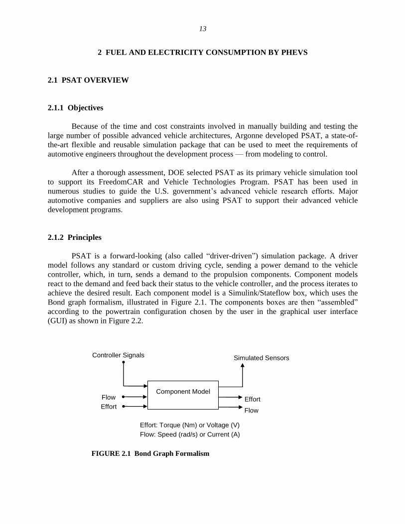
Bond graph formalism, illustrated in Figure 2.1. The components boxes are then ―assembled‖

according to the powertrain configuration chosen by the user in the graphical user interface

(GUI) as shown in Figure 2.2.

FIGURE 2.1 Bond Graph Formalism

Component Model

Effort Effort Flow

Flow

Controller Signals Simulated Sensors

Effort: Torque (Nm) or Voltage (V)

Flow: Speed (rad/s) or Current (A)

14

FIGURE 2.2 Simulink Vehicle Model Example

2.2 PROCESS DESCRIPTION

To evaluate the fuel efficiency benefits of advanced vehicles, model users design the

vehicles on the basis of component assumptions. The fuel efficiency is then simulated on the

UDDS and HWFET. The assumptions and results described in this report were generated to

support the 2009 Government Performance and Results Act (GPRA) analysis for the light-duty

vehicle research conducted at the U.S. DOE from fuel efficiency and cost perspectives.

Established in 1993, GPRA holds federal agencies accountable for using resources wisely and

achieving program results. A subset of the GPRA study was selected with a midsize car

representative of 2015 technologies. To properly assess the benefits of future technologies, the

following vehicle configurations and fuels were considered:

• Five powertrain configurations: conventional, HEV, PHEV, fuel cell HEV, and

battery electric vehicle (BEV)

• Four fuels: gasoline, diesel, ethanol, and hydrogen

Clutch

command

Motor

command

Shift

command

Brake

command

Engine Command

Accelerator/Brake Pedal

Controller Commands

15

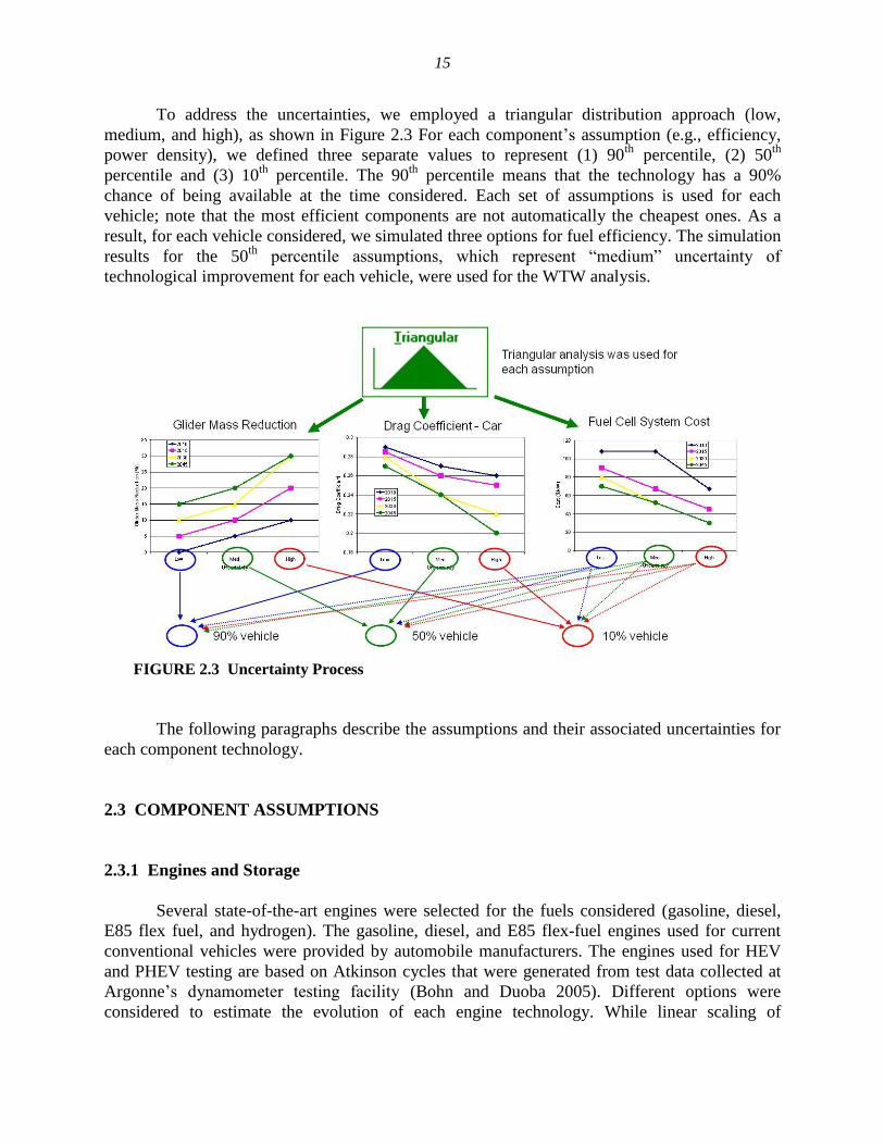
To address the uncertainties, we employed a triangular distribution approach (low,

medium, and high), as shown in Figure 2.3 For each component’s assumption (e.g., efficiency,

power density), we defined three separate values to represent (1) 90th

percentile, (2) 50th

percentile and (3) 10th

percentile. The 90th

percentile means that the technology has a 90%

chance of being available at the time considered. Each set of assumptions is used for each

vehicle; note that the most efficient components are not automatically the cheapest ones. As a

result, for each vehicle considered, we simulated three options for fuel efficiency. The simulation

results for the 50th

percentile assumptions, which represent ―medium‖ uncertainty of

technological improvement for each vehicle, were used for the WTW analysis.

FIGURE 2.3 Uncertainty Process

The following paragraphs describe the assumptions and their associated uncertainties for

each component technology.

2.3 COMPONENT ASSUMPTIONS

2.3.1 Engines and Storage

Several state-of-the-art engines were selected for the fuels considered (gasoline, diesel,

E85 flex fuel, and hydrogen). The gasoline, diesel, and E85 flex-fuel engines used for current

conventional vehicles were provided by automobile manufacturers. The engines used for HEV

and PHEV testing are based on Atkinson cycles that were generated from test data collected at

Argonne’s dynamometer testing facility (Bohn and Duoba 2005). Different options were

considered to estimate the evolution of each engine technology. While linear scaling of

16

performance was used for gasoline and E85 HEVs, as well as diesel engines, nonlinear scaling

based on AVL’s work (Bandel 2006) was used for gasoline and E85 conventional vehicles. For

the nonlinear scaling, different operating areas were improved by different amounts, resulting in

changes in the constant efficiency contours. Table 2.1 lists the peak efficiencies of the different

fuels and technologies.

TABLE 2.1 Main Engine Assumptions

2015 Low 2015 Medium 2015 High

Gasoline/Flex-fuel ICE for

conventional vehicle

Technology Spark

Homogeneous

Spark

Homogeneous

+5% IMEPa

Spray GDIa

Diesel ICE Peak efficiency 41% 42% 43%

Gasoline ICE for HEVs Peak efficiency 38% 38.5% 39.5%

Flex Fuel ICE for HEVs Peak efficiency 36% 36.5% 37.5% a IMEP = indicated mean effective pressure; GDI = gasoline direct injection.

2.3.1.1 Fuel Cell Systems

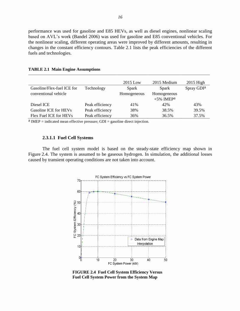
The fuel cell system model is based on the steady-state efficiency map shown in

Figure 2.4. The system is assumed to be gaseous hydrogen. In simulation, the additional losses

caused by transient operating conditions are not taken into account.

FIGURE 2.4 Fuel Cell System Efficiency Versus

Fuel Cell System Power from the System Map

17

Table 2.2 shows the peak efficiencies of the fuel cell system, as well as its associated

specific power and power density. The peak fuel cell efficiency is assumed to be constant at 60%

because most of the research is expected to focus on reducing cost. The 60% efficiency has

already been demonstrated in laboratories and, consequently, is expected to be implemented soon

in vehicles.

TABLE 2.2 Main Fuel Cell Assumptions


Specific power (W/kg) 428 519 617

Power density (W/L) 454 590 818

Peak efficiency (%) 60 60 60

2.3.1.2 Hydrogen Storage Systems

The evolution of hydrogen storage systems is vital to the introduction of hydrogen-

powered vehicles. Table 2.3 shows the evolution of the hydrogen storage capacity.

TABLE 2.3 Main Hydrogen Storage Assumptions


System gravimetric capacity (kWh/kg) 1.1 1.8 2.4

System volumetric capacity (kWh/L) 0.91 1.2 1.7

One of the requirements for vehicles in the study is that they be able to travel 320 miles

on the UDDS Driving Cycle on a full tank of fuel. However, to simulate 2015 vehicles with a

hydrogen storage system allowing a range of 320 miles, the amount of hydrogen needed, and

thus the corresponding fuel tank mass, would be excessive. As a result, a range of 250 miles was

selected.

2.3.1.3 Electric Machines

Table 2.4 lists the main electric machine characteristics. The values for the current

technologies are based on state-of-the-art electric machines currently used in vehicles (Olszewski

2008). The electric machine data from the Toyota Prius and Toyota Camry were used for the

power-split HEV applications, while the Ballard integrated powertrain (IPT) was selected for

series fuel cell HEVs.

18

TABLE 2.4 Main Electric Machine Assumptions


System peak efficiency (%) 95 96 97

Motor specific power (W/kg) 1,200 1,250 1,600

Power electronics specific power (W/kg) 10,000 11,000 13,000

2.3.1.4 Energy Storage System for Electric Vehicles

Energy storage systems are key components in advanced vehicles. While numerous

studies are currently being undertaken with ultracapacitors, only batteries were taken into

account in our study. While the current technologies are almost all based on nickel metal hydride

(NiMH), the lithium ion (Li-ion) technology is introduced for the medium and high cases in

2015. For HEV applications, the NiMH is based on the Toyota Prius battery pack and the Li-ion

battery pack is based on the 6Ah from Saft. For PHEV applications, we characterized the

VL41M battery pack from Saft. Because each vehicle is sized to maximize both power and

energy, in the case of a PHEV, a sizing algorithm was developed to design the batteries

specifically for each application (Sharer et al. 2006).

To ensure that the battery has similar performance at the beginning and end of life, the

packs were oversized in terms of both power and energy. However, it should be noted that the

additional battery capacity is initially clamped down and is only gradually released by the

vehicle’s controls as the battery performance degrades with usage and time. In addition, for

PHEV applications, the SOC window (difference between maximum and minimum allowable

SOC) increases over time, allowing a reduction in the size of the battery pack. Table 2.5 lists the

main characteristics of the energy storage systems. The high power applications are used for

HEVs while the high energy batteries are dedicated to PHEVs and BEVs. The SOC minimum

and maximum in Table 2.5 only apply to the high-energy batteries of PHEVs and BEVs.

2.3.2 Transmission

Table 2.6 lists the main assumptions about the transmissions used in the midsize vehicle

platform for the conventional powertrains. While most transmissions currently contain four or

five gears, it is expected that the number will increase to between five and eight in the near

future. The transmissions selected (gearbox and final drive ratios) are based on existing vehicles.

The power-split configurations are based on a single planetary gearset with ratios similar

to those of the Toyota Prius. The series configurations are based on a two-speed automated

manual transmission (ratios 1.8/1) in order to allow the vehicle to reach the maximum speed

(100 mph) without oversizing the components.

19

TABLE 2.5 Main Energy Storage Assumptions


High-Power Applications for HEVs

Technology NiMH Li-ion Li-ion

Energy oversize (%) 20 18 16

Power oversize (%) 20 18 16

High-Energy Applications for PHEVs and BEVs

Technology Li-ion Li-ion Li-ion

Energy oversize (%) 30 28 26

Power oversize (%) 20 18 16

SOC max (%) 90 90 95

SOC min (%) 30 30 25

TABLE 2.6 Main Transmission Assumptions (midsize conventional vehicle)


Technology Automatic 5-Speed Dual-Clutch 6-Speed Automatic 8-Speed

Gearbox ratio 4.15 / 2.37 / 1.56 / 1.16 /

0.86 / 0.69

3.45 / 2.045 / 1.452 /

1.114 / 1.078 / 0.921

4.6 / 2.72 / 1.86 / 1.46 /

1.23 / 1 / 0.824 / 0.685

Final drive 2.74 3.29 2.47

2.4 VEHICLE

As previously discussed, a midsize car with the following characteristics was selected for

the 2009 reference:

• Glider mass = 990 kg

• Frontal Area = 2.2 m2

• Tire = P195/65/R15

Because of improvements in materials, the glider mass is expected to significantly

decrease over time. The maximum value of 31% was defined on the basis of previous studies

(Stodolsky et al. 1995) that calculated the weight reduction achieved by replacing the entire

chassis frame with aluminum. Although frontal area is expected to differ from one vehicle

configuration to another (i.e., the electrical components will require more cooling capabilities),

the values were considered constant across the technologies. Table 2.7 lists the reductions in both

glider mass and frontal area.

20

TABLE 2.7 Main Vehicle Assumptions (midsize)


Glider mass (kg) 800 740 700

Frontal area (m2) 2.21 2.18 2.15

Drag coefficient 0.295 0.28 0.265

Rolling resistance 0.008 0.0075 0.007

Electrical load for conventional (W) 260 240 220

Electrical load for other configurations (W) 240 230 220

2.4.1 Vehicle Powertrain Assumptions

All the vehicles have been sized to meet the same requirements:

• 0–100 km/h in 9 sec +/-0.1

• Maximum grade of 6% at 105 km/h at gross vehicle weight (GVW)

• Maximum vehicle speed >160 km/h

For all cases, the engine or fuel cell is sized to reach the top of the grade without any

assistance from the battery. For HEVs, the battery was sized to recuperate the entire braking

energy during the UDDS drive cycle. For the PHEV case, the battery power is assumed to be

able to follow the UDDS in electric mode, while its energy is calculated to follow the trace for a

specific distance. For BEV, the battery was sized to provide a 150-mile range on the UDDS drive

cycle. Because of the multitude of vehicles considered, an automated sizing algorithm was

defined (Freyermuth et al. 2008).

2.4.2 Vehicle Architecture Selection

An HEV — by definition — combines at least two sources of energy. The main types of

HEVs are described below, along with their advantages and disadvantages.

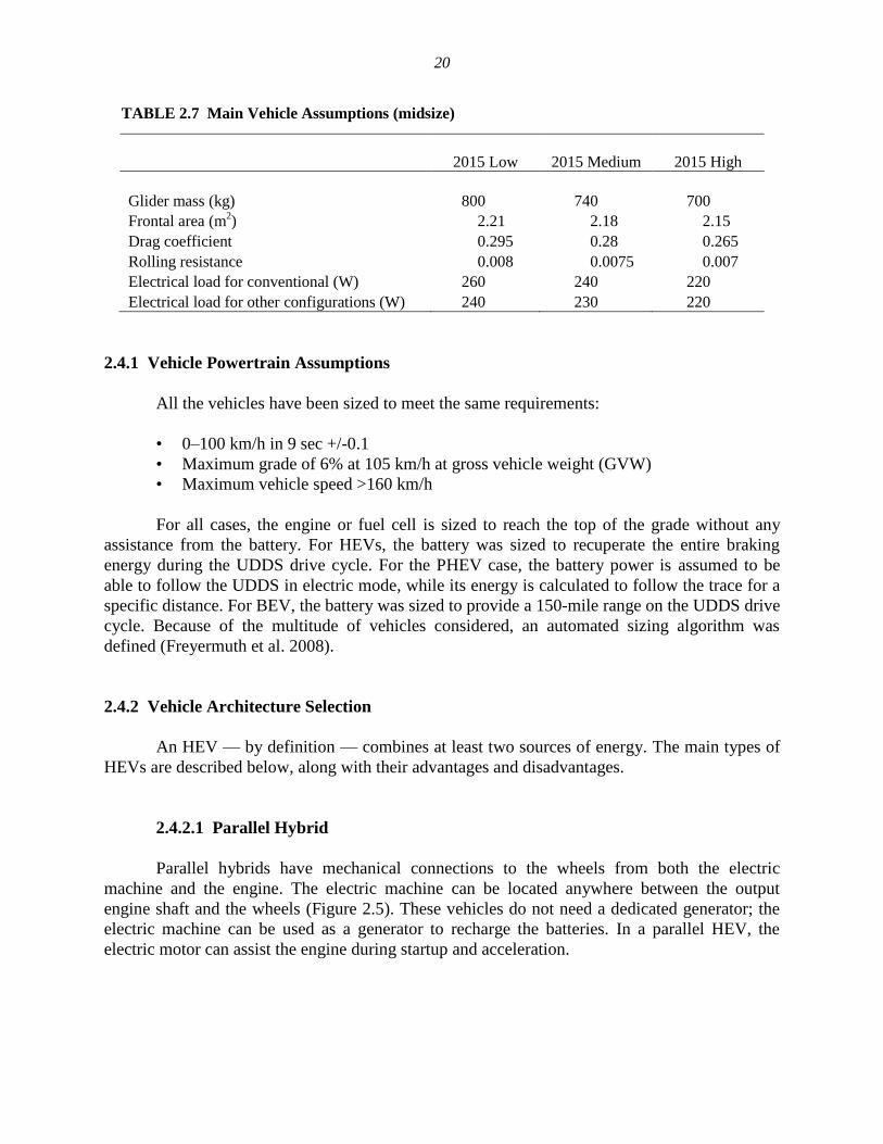
2.4.2.1 Parallel Hybrid

Parallel hybrids have mechanical connections to the wheels from both the electric

machine and the engine. The electric machine can be located anywhere between the output

engine shaft and the wheels (Figure 2.5). These vehicles do not need a dedicated generator; the

electric machine can be used as a generator to recharge the batteries. In a parallel HEV, the

electric motor can assist the engine during startup and acceleration.

21

Electric motor and engine both coupled

directly to wheels

Can operate with smaller batteries

Requires off-board charging

Accelerates faster due to dual power sources

Engine idles

Packaging of components less flexible

May not require a transmission

Requires medium-duty motor

P

A

R

A

L

L

E

L

FIGURE 2.5 Parallel HEV

Because the electric machine and the engine are both coupled directly to the wheels, they

can share the power during accelerations. Therefore, it is possible to downsize both the engine

and the electric machine compared to series hybrids (thus decreasing the vehicle mass). It is also

possible to increase the degree of hybridization by decreasing the size of the engine and

increasing the size of the electric machine. For some configurations, the engine can operate close

to its best efficiency curve (annex), the electric machine assisting it or recharging the battery.

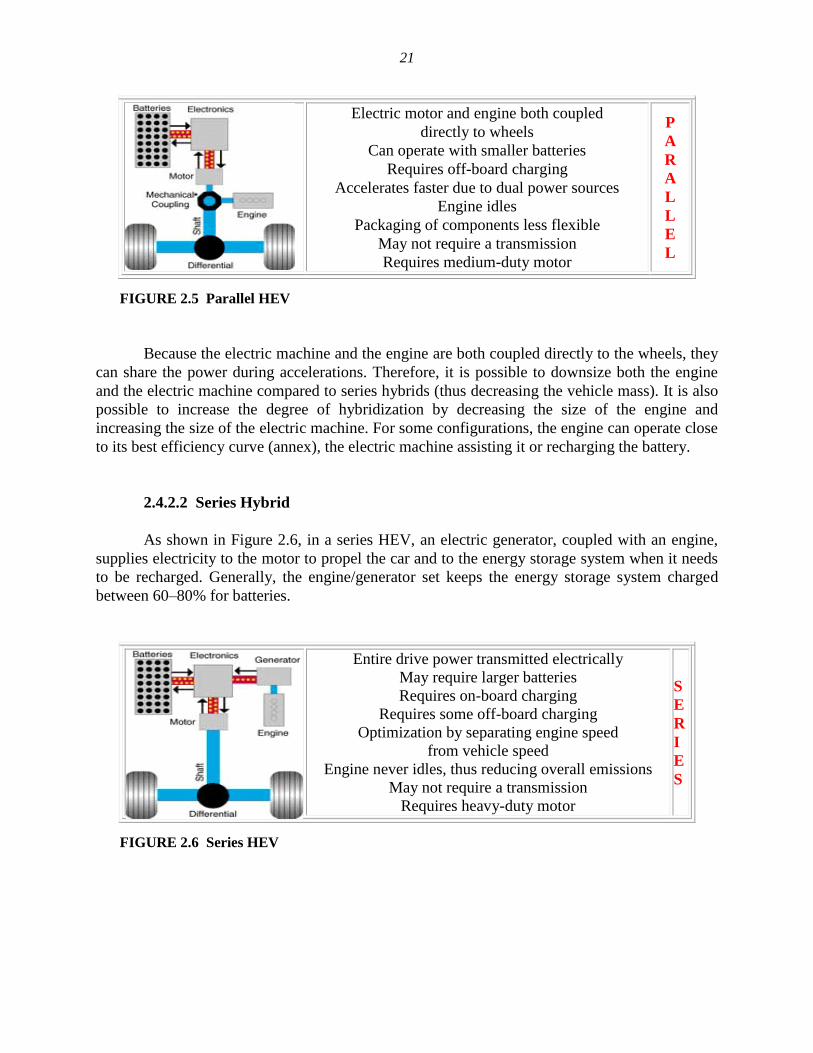
2.4.2.2 Series Hybrid

As shown in Figure 2.6, in a series HEV, an electric generator, coupled with an engine,

supplies electricity to the motor to propel the car and to the energy storage system when it needs

to be recharged. Generally, the engine/generator set keeps the energy storage system charged

between 60–80% for batteries.

Entire drive power transmitted electrically

May require larger batteries

Requires on-board charging

Requires some off-board charging

Optimization by separating engine speed

from vehicle speed

Engine never idles, thus reducing overall emissions


Requires heavy-duty motor

S

E

R

I

E

S

FIGURE 2.6 Series HEV

22

The main advantage of this configuration is that engine and vehicle speeds are decoupled,

and only the electric motor is connected to the wheels. The engine does not need to speed up or

slow down as the load varies. As a consequence, the engine can run at optimum performance

(best engine efficiency area), greatly improving the fuel economy. Moreover, the engine never

idles, thus reducing overall emissions. However, because the electric machine is the only one

connected directly to the wheels and the engine/generator set is sized for sustained gradeability,

this configuration requires large batteries, motor, and engine. For this system to be viable, it must

be highly efficient in terms of total power processing.

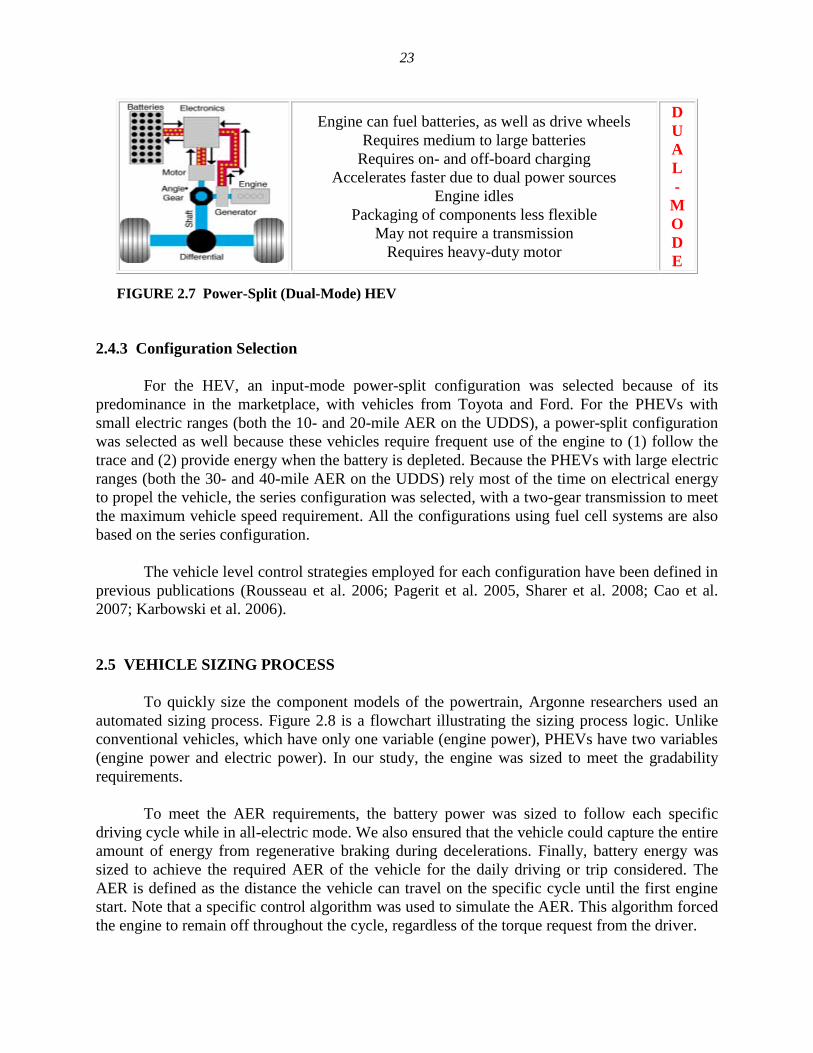
2.4.2.3 Power-Split Hybrid

Power split hybrids combine the best features of both series and parallel hybrids to create

an extremely efficient system.

As shown in Figure 2.7, this system divides the engine power along two paths: one goes

to the generator to produce electricity and one goes through a mechanical gear system to drive

the wheels. In addition, a regenerative system uses the kinetic energy of deceleration and braking

to produce electricity, which is stored in the battery.

The main components of this configuration are a power-split device (transmission), an

electric motor, a generator, and an engine. Depending on the situation, all these elements operate

differently. Indeed, the engine is not always ―on,‖ and the electricity from the generator may go

directly to the wheels to help propel the car or may go through an inverter to be stored in the

battery. The different possibilities are as follows:

• When starting out, moving slowly, or when the battery SOC is high enough, the

engine is not efficient, so it is turned off, and the motor alone propels the car.

• During normal operation, the engine power is split, with part going to drive the

vehicle and part being used to generate electricity. The electricity goes to the

motor, which assists in propelling the car.

• During full-throttle acceleration, the battery provides extra power.

• During deceleration or braking, the motor acts as a generator, transforming the

kinetic energy of the wheels into electricity.

23

Engine can fuel batteries, as well as drive wheels

Requires medium to large batteries

Requires on- and off-board charging

Accelerates faster due to dual power sources

Engine idles

Packaging of components less flexible


Requires heavy-duty motor

D

U

A

L

-

M

O

D

E

FIGURE 2.7 Power-Split (Dual-Mode) HEV

2.4.3 Configuration Selection

For the HEV, an input-mode power-split configuration was selected because of its

predominance in the marketplace, with vehicles from Toyota and Ford. For the PHEVs with

small electric ranges (both the 10- and 20-mile AER on the UDDS), a power-split configuration

was selected as well because these vehicles require frequent use of the engine to (1) follow the

trace and (2) provide energy when the battery is depleted. Because the PHEVs with large electric

ranges (both the 30- and 40-mile AER on the UDDS) rely most of the time on electrical energy

to propel the vehicle, the series configuration was selected, with a two-gear transmission to meet

the maximum vehicle speed requirement. All the configurations using fuel cell systems are also

based on the series configuration.

The vehicle level control strategies employed for each configuration have been defined in

previous publications (Rousseau et al. 2006; Pagerit et al. 2005, Sharer et al. 2008; Cao et al.

2007; Karbowski et al. 2006).

2.5 VEHICLE SIZING PROCESS

To quickly size the component models of the powertrain, Argonne researchers used an

automated sizing process. Figure 2.8 is a flowchart illustrating the sizing process logic. Unlike

conventional vehicles, which have only one variable (engine power), PHEVs have two variables

(engine power and electric power). In our study, the engine was sized to meet the gradability

requirements.

To meet the AER requirements, the battery power was sized to follow each specific

driving cycle while in all-electric mode. We also ensured that the vehicle could capture the entire

amount of energy from regenerative braking during decelerations. Finally, battery energy was

sized to achieve the required AER of the vehicle for the daily driving or trip considered. The

AER is defined as the distance the vehicle can travel on the specific cycle until the first engine

start. Note that a specific control algorithm was used to simulate the AER. This algorithm forced

the engine to remain off throughout the cycle, regardless of the torque request from the driver.

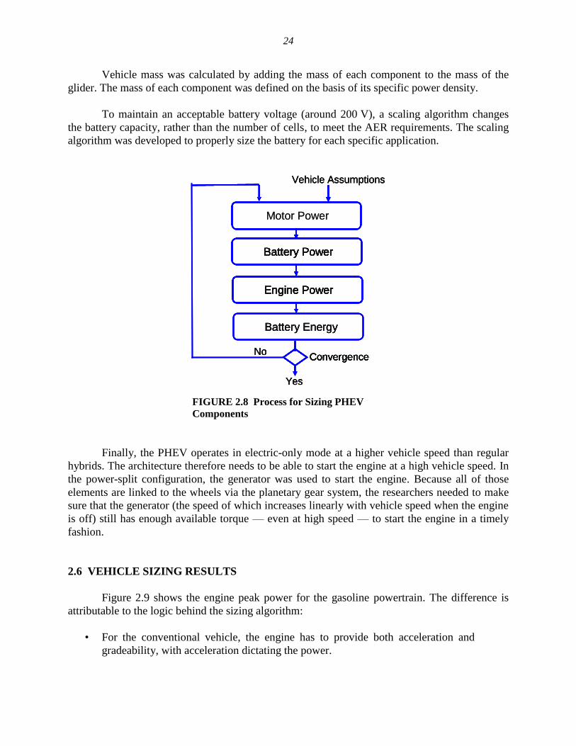
24

Vehicle mass was calculated by adding the mass of each component to the mass of the

glider. The mass of each component was defined on the basis of its specific power density.

To maintain an acceptable battery voltage (around 200 V), a scaling algorithm changes

the battery capacity, rather than the number of cells, to meet the AER requirements. The scaling

algorithm was developed to properly size the battery for each specific application.

Battery Power

Engine Power

Battery Energy

Convergence

Yes

Motor Power

Vehicle Assumptions

Battery PowerBattery Power

Engine PowerEngine Power

Battery Energy

ConvergenceConvergence

Yes

NoNo

Vehicle Assumptions



Battery Energy


Yes

Motor Power

Vehicle Assumptions



Battery Energy


Yes

NoNo

Vehicle Assumptions

FIGURE 2.8 Process for Sizing PHEV

Components

Finally, the PHEV operates in electric-only mode at a higher vehicle speed than regular

hybrids. The architecture therefore needs to be able to start the engine at a high vehicle speed. In

the power-split configuration, the generator was used to start the engine. Because all of those

elements are linked to the wheels via the planetary gear system, the researchers needed to make

sure that the generator (the speed of which increases linearly with vehicle speed when the engine

is off) still has enough available torque — even at high speed — to start the engine in a timely

fashion.

2.6 VEHICLE SIZING RESULTS

Figure 2.9 shows the engine peak power for the gasoline powertrain. The difference is

attributable to the logic behind the sizing algorithm:

• For the conventional vehicle, the engine has to provide both acceleration and

gradeability, with acceleration dictating the power.

25

• For HEVs, the engine is also sized to provide both acceleration and gradeability,

but the presence of the electric machine allows downsizing.

• For the power-split PHEVs (10-and 20-mile AER), the engine is sized for

gradeability because the electric machine power is sized for the UDDS.

• The engine of a series PHEV is sized similar to the engine of a power-split PHEV,

but with a higher power only because of the added inefficiencies of the driveline.

20150

20

40

60

80

100

120

IC

E P

ow

er

(kW

)

ICE Power for Midsize

SI Conv

SI Split HEV

SI Split HEV PHEV10

SI Split HEV PHEV20

SI Series HEV PHEV30


FIGURE 2.9 Engine Power for Gasoline Powertrains

Figure 2.10 shows the electric machine power for the gasoline HEVs and PHEVs. As the

figures shows, power-split PHEVs require higher power because one of their requirements is the

ability to follow the UDDS in electric mode. It is important to note that, although the vehicles

have the ability to drive the UDDS in electric mode, the control strategy employed during fuel

efficiency simulation is based on blended operation. The electric machine for the series

configuration is sized to follow the US06 in EV mode, thus requiring the highest power.

Figure 2.11 shows the fuel cell system peak power for the different configurations

considered. Figure 2.12 shows the battery power requirements for HEV and PHEV applications

for the gasoline vehicle. The sensitivity of battery power to vehicle mass increases with the

degree of electrification (i.e., higher for PHEV and lower for HEVs).

26

20150

20

40

60

80

100

120

140

Ele

ctr

ic M

achin

e (

kW

)

Electric Machine for Midsize

SI Split HEV

SI Split HEV PHEV10

SI Split HEV PHEV20



FIGURE 2.10 Electric Machine Power for Gasoline HEVs and PHEVs

20150

10

20

30

40

50

60

70

80

90

100

FC

Pow

er (

kW)

FC Power for Midsize

FC HEV

FC HEV PHEV10

FC HEV PHEV20

FC HEV PHEV30

FC HEV PHEV40

FIGURE 2.11 Fuel Cell Power for Hydrogen Vehicles

27

20150

20

40

60

80

100

120

140

160

Battery

(kW

)

Battery for Midsize

SI Split HEV

SI Split HEV PHEV10

SI Split HEV PHEV20



FIGURE 2.12 Battery Power for Gasoline HEVs and PHEVs

The usable battery energy is proportional to the AER of the different PHEVs. If the AER

is multiplied by two, the usable battery energy will also be multiplied by two. Figures 2.13 and

2.14 show the usable battery energy for PHEVs with gasoline engines and fuel cell systems.

20150

2000

4000

6000

8000

10000

12000

Ene

rgy

(Wh)

Energy for Midsize

SI Split HEV PHEV10

SI Split HEV PHEV20



FIGURE 2.13 Usable Battery Energy for PHEV Midsize Vehicle with

Gasoline Engine

28

20150

2000

4000

6000

8000

10000

12000

Energ

y (

Wh)

Usable Energy for FC PHEV for Midsize

FC HEV PHEV10

FC HEV PHEV20

FC HEV PHEV30

FC HEV PHEV40

FIGURE 2.14 Usable Battery Energy for PHEV Midsize Vehicle with Fuel Cell

Figure 2.15 shows the vehicle mass for the different configurations. As expected, an

increase in electrification leads to higher vehicle weight.

FIGURE 2.15 Vehicle Mass

29

Appendix 1 provides the main characteristics (e.g., power, energy, weight) for all of the

vehicles. The fuel and electricity consumption results from the PSAT model are provided in

Section 3.

30


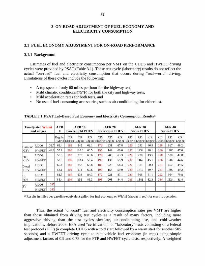
31

3 ON-ROAD ADJUSTMENT OF FUEL ECONOMY AND

ELECTRICITY CONSUMPTION

3.1 FUEL ECONOMY ADJUSTMENT FOR ON-ROAD PERFORMANCE

3.1.1 Background

Estimates of fuel and electricity consumption per VMT on the UDDS and HWFET driving

cycles were provided by PSAT (Table 3.1). These test cycle (laboratory) results do not reflect the

actual ―on-road‖ fuel and electricity consumption that occurs during ―real-world‖ driving.

Limitations of these cycles include the following:

• A top speed of only 60 miles per hour for the highway test,

• Mild climatic conditions (75°F) for both the city and highway tests,

• Mild acceleration rates for both tests, and

• No use of fuel-consuming accessories, such as air conditioning, for either test.

TABLE 3.1 PSAT Lab-Based Fuel Economy and Electricity Consumption Resultsa

Unadjusted Wh/mi

and mpgeg

AER

0

AER 10

Power-Split PHEV

AER 20

Power-Split PHEV

AER 30

Series PHEV

AER 40

Series PHEV

Regular

Hybrid

CD

Electric

CD

Engine

CS

Engine

CD

Electric

CD

Engine

CS

Engine

CD

Electric

CD

Engine

CS

Engine

CD

Electric

CD

Engine

CS

Engine

Gasoline

ICEV

UDDS 32.7 62.4 182 245 68.1 179 231 67.8 220 291 46.9 228 617 46.2

HWFET 44.1 55.9 200 110.8 60.5 195 149 60.0 237 1234 48.1 236 1280 47.6

E85

ICEV

UDDS 58.0 182 229 63.6 178 209 63.3 220 270 43.5 228 570 42.8

HWFET 52.0 198 103.4 56.4 193 136 55.9 237 1162 45.1 236 1202 44.6

Diesel

ICEV

UDDS 65.4 182 253 68.8 183 229 68.4 222 311 50.3 231 667 49.5

HWFET 58.1 201 114 60.6 199 154 59.9 239 1417 49.7 241 1509 49.2

H2

FCV

UDDS 81.5 166 233 84.3 172 221 83.1 221 508 81.1 222 964 79.8

HWFET 85.4 204 156 85.3 198 208 84.4 233 1881 82.3 234 1524 81.4

EV UDDS 237

HWFET 243

a Results in miles per gasoline-equivalent gallon for fuel economy or Wh/mi (shown in red) for electric operation.

Thus, the actual ―on-road‖ fuel and electricity consumption rates per VMT are higher

than those obtained from driving test cycles as a result of many factors, including more

aggressive driving than the test cycles simulate, air-conditioning use, and cold-weather

implications. Before 2008, EPA used ―certification‖ or ―laboratory‖ tests consisting of a federal

test protocol (FTP) (a complete UDDS with a cold start followed by a warm start for another 505

seconds) and a HWFET driving cycle to rate vehicle fuel economy (in mpg) using simple

adjustment factors of 0.9 and 0.78 for the FTP and HWFET cycle tests, respectively. A weighted

32

average of city (55%) and highway (45%) fuel economies was used to calculate a combined

(composite) ―label‖ fuel economy. However, several independent studies that compared EPA’s

fuel economy estimates to the real-world experience of consumers concluded that there was

considerable variation in real-world fuel economy and that EPA’s mileage ratings often

overestimated real-world fuel economy.

In the Energy Policy Act of 2005, the U.S. Congress required EPA to revise the fuel

economy labeling methods to better reflect a variety of real-world factors that affect fuel

economy. Consequently, EPA developed a new approach to estimate the on-road fuel economy

based on a five-cycle testing method (EPA 2006). Starting with 2008 MY vehicles, a new EPA

method required that vehicles be tested on three additional driving cycles: a high-speed,

aggressive driving cycle (US06), a cycle operating at an ambient temperature of 95°F (SC03),

and a cycle operating at an ambient temperature of 20°F (cold FTP). These five cycles are now

used to construct a weighted average fuel economy for city and highway driving. Alternatively,

manufacturers may calculate equivalent five-cycle fuel economy through MY 2010 using

regression lines, known as mpg-based formulas, from the city and highway fuel economy values.

Equations 1 and 2 represent the EPA’s mpg-based formulas for the city and highway cycles,

respectively.

Five-cycle city fuel economy = 1/(0.003259 + 1.1805/FTP fuel economy) [1]

Five-cycle highway fuel economy = 1/(0.001376 + 1.3466/HWFET fuel economy) [2]

For MY 2011 and beyond, if the five-cycle city and highway fuel economy values for an

emissions data vehicle group are not more than 4% and 5% below the mpg-based regression line,

respectively, all the vehicle configurations represented by the emissions data vehicle (e.g., all

vehicles within the vehicle test group) could continue to use the mpg-based

approach. Vehicles within a test group falling more than 5% below the tolerance band for

highway fuel economy values would be required to conduct US06 tests, while those falling more

than 4% below the city fuel economy tolerance band would be required to conduct US06, SC03,

and cold FTP tests (EPA 2006). Furthermore, EPA proposed a new harmonic weighting (43/57)

of the five-cycle city and highway fuel economies to calculate a combined fuel economy

consistent with the recent shift in consumer’s driving toward the highway driving style. Finally,

it should be noted that, because fuel economy depends on a wide variety of factors, individual

consumers will experience higher or lower fuel economy than a given estimate, depending on

their real-world driving conditions for any vehicle technology.

While PSAT is capable of simulating the US06 cycle, it cannot accurately simulate

vehicle operation with air-conditioning on or in cold weather. So Argonne sought an alternative

to the five-cycle testing methodology to adjust the PSAT fuel economy results for engine

operation (ICE or fuel cell) and electricity consumption (by the battery in PHEVs and BEVs) on

the test driving cycles (UDDS and HWFET) to account for the additional on-road driving load.

Figure 3.1 shows the ―on-road‖ adjustment factors, which are based on the mpg-based formulas

(equations 1 and 2). The adjustment factor is simply the ratio of the ―on-road‖ fuel economy to

the test cycle (laboratory) fuel economy.

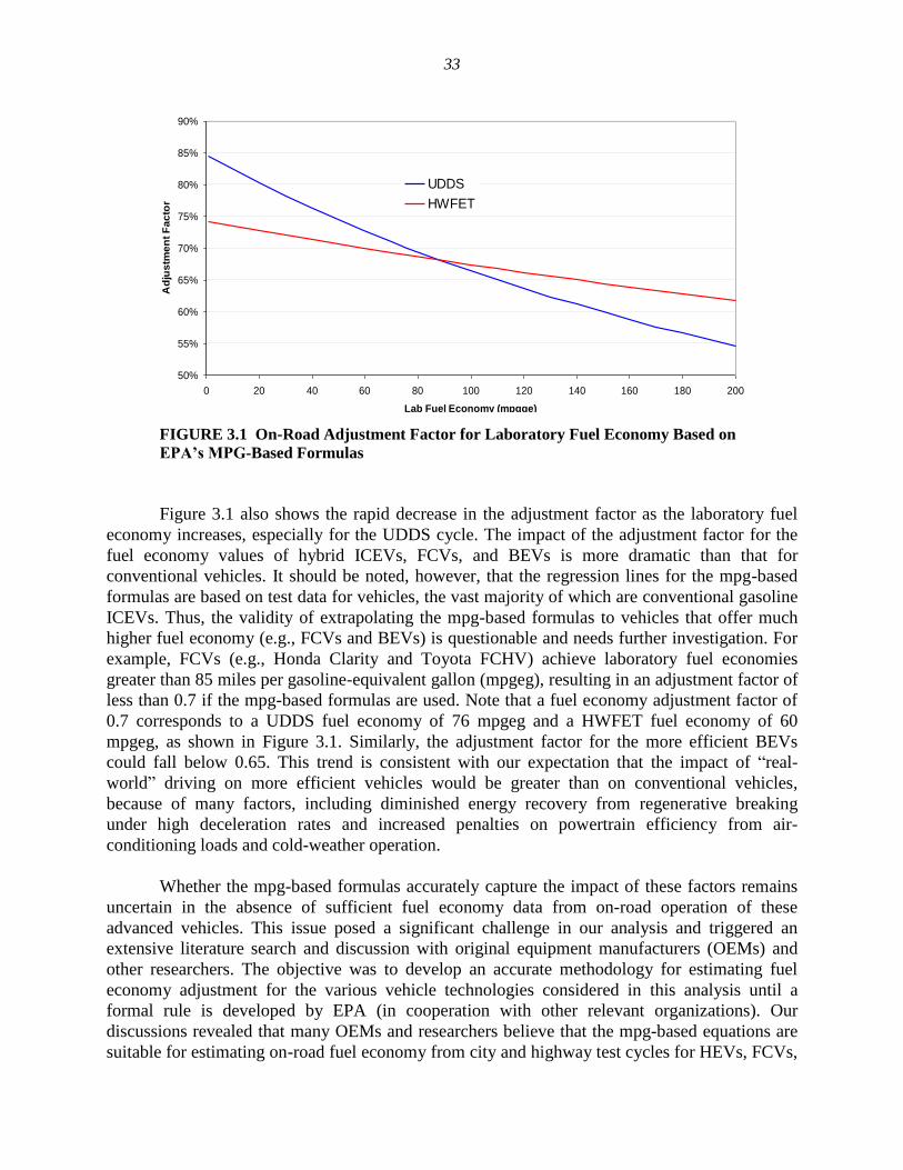
33

On-road Adjustment Factor as a Function of Fuel Economy

50%

55%

60%

65%

70%

75%

80%

85%

90%

0 20 40 60 80 100 120 140 160 180 200

Lab Fuel Economy (mpgge)

Ad

jus

tme

nt

Fa

cto

r

UDDS

HWFET

FIGURE 3.1 On-Road Adjustment Factor for Laboratory Fuel Economy Based on

EPA’s MPG-Based Formulas

Figure 3.1 also shows the rapid decrease in the adjustment factor as the laboratory fuel

economy increases, especially for the UDDS cycle. The impact of the adjustment factor for the

fuel economy values of hybrid ICEVs, FCVs, and BEVs is more dramatic than that for

conventional vehicles. It should be noted, however, that the regression lines for the mpg-based

formulas are based on test data for vehicles, the vast majority of which are conventional gasoline

ICEVs. Thus, the validity of extrapolating the mpg-based formulas to vehicles that offer much

higher fuel economy (e.g., FCVs and BEVs) is questionable and needs further investigation. For

example, FCVs (e.g., Honda Clarity and Toyota FCHV) achieve laboratory fuel economies

greater than 85 miles per gasoline-equivalent gallon (mpgeg), resulting in an adjustment factor of

less than 0.7 if the mpg-based formulas are used. Note that a fuel economy adjustment factor of

0.7 corresponds to a UDDS fuel economy of 76 mpgeg and a HWFET fuel economy of 60

mpgeg, as shown in Figure 3.1. Similarly, the adjustment factor for the more efficient BEVs

could fall below 0.65. This trend is consistent with our expectation that the impact of ―real-

world‖ driving on more efficient vehicles would be greater than on conventional vehicles,

because of many factors, including diminished energy recovery from regenerative breaking

under high deceleration rates and increased penalties on powertrain efficiency from air-

conditioning loads and cold-weather operation.

Whether the mpg-based formulas accurately capture the impact of these factors remains

uncertain in the absence of sufficient fuel economy data from on-road operation of these

advanced vehicles. This issue posed a significant challenge in our analysis and triggered an

extensive literature search and discussion with original equipment manufacturers (OEMs) and

other researchers. The objective was to develop an accurate methodology for estimating fuel

economy adjustment for the various vehicle technologies considered in this analysis until a

formal rule is developed by EPA (in cooperation with other relevant organizations). Our

discussions revealed that many OEMs and researchers believe that the mpg-based equations are

suitable for estimating on-road fuel economy from city and highway test cycles for HEVs, FCVs,

34

and BEVs. Other experts proposed a lower limit of 0.7 on the adjustment factor produced by the

mpg-based formulas (i.e., capping the reduction of fuel economy at 30%), which is consistent

with the suggested windows sticker calculation for the Mini-e EV (Weissler 2009). The

following sections describe the methodology we adopted for adjusting the laboratory fuel

economy and electricity consumption to on-road (―real-world‖) fuel economy and electricity

consumption for conventional ICEVs and HEVs (Section 3.1.2), FCVs (Section 3.1.3), Series

PHEV30 and 40 and BEVs (Section 3.1.4), and power-split PHEV10 and 20 (Section 3.1.5).

3.1.2 Conventional ICEVs and HEVs

In accordance with EPA’s final rule on fuel economy labeling for motor vehicles, we

used the mpg-based formulas (equations 1 and 2) to calculate the ―on-road‖ city and highway

fuel economies for conventional gasoline ICEVs, as well as all hybrid ICEVs (HEVs) from their

laboratory fuel economies (see adjustment arrow a-A in Figure 3.2). The composite city/highway

fuel economy was calculated on the basis of new proposed weighting factors of 43% for city

driving and 57% for highway driving. Table 3.1 shows the adjusted fuel economies for

conventional ICEVs and HEVs.

3.1.3 Hydrogen FCVs

The on-road fuel economy data for the second-generation hydrogen FCVs (collected as

part of DOE hydrogen fleet and infrastructure demonstration and validation projects) indicate an

adjustment factor range between 0.66 and 0.70, which is consistent with the mpg-based

equations (Wipke et al., 2009). The label fuel economy for the Honda Clarity also reflects an

adjustment factor of 0.7. For this analysis we used the mpg-based formulas (see adjustment

arrow a-A in Figure 3.2) to calculate the on-road fuel economy for all FCVs, but we capped the

adjustment factor at 0.7, which corresponds to a 30% reduction compared with the fuel

economies obtained from city and highway test cycles.

3.1.4 Series PHEV30 and 40 and BEVs

For the series-configuration PHEVs, the fuel economy in the CS operational mode was

adjusted according to the mpg-based formulas because that mode of operation is similar to the

operation of a regular HEV; the engine is the source of all the power needed to satisfy the

vehicle’s various loads. As we did for regular HEVs, we capped the adjustment factor at 0.7 to

correspond to a 30% reduction compared with the fuel economies from city and highway test

cycles. The electricity consumption in the CD operational mode for series PHEVs is assumed to

be similar to that of BEVs because the control strategy for series PHEVs maximizes the use of

battery power, and the electric machine is sized to meet the US06 cycle (which is more

aggressive than typical real-world driving); the on-road load is mostly met by the battery power,

with minor assistance from the engine (see Table 3.1). Consequently, we adjusted electricity

consumption for series PHEVs using the same adjustment suggested by EPA for the Mini-e EV:

a 0.7 adjustment factor (see adjustment arrow b-B in Figure 3.2). We also adjusted the relatively

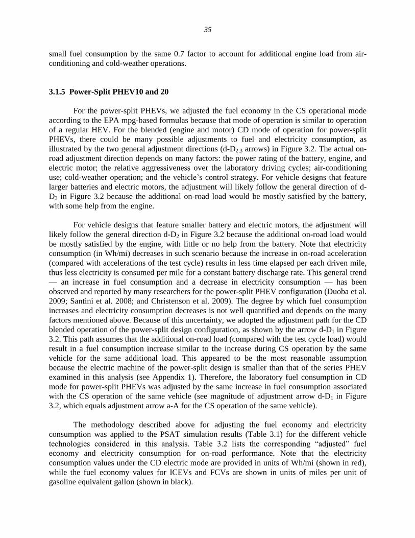
35

small fuel consumption by the same 0.7 factor to account for additional engine load from air-

conditioning and cold-weather operations.

3.1.5 Power-Split PHEV10 and 20

For the power-split PHEVs, we adjusted the fuel economy in the CS operational mode

according to the EPA mpg-based formulas because that mode of operation is similar to operation

of a regular HEV. For the blended (engine and motor) CD mode of operation for power-split

PHEVs, there could be many possible adjustments to fuel and electricity consumption, as

illustrated by the two general adjustment directions (d-D2,3 arrows) in Figure 3.2. The actual on-

road adjustment direction depends on many factors: the power rating of the battery, engine, and

electric motor; the relative aggressiveness over the laboratory driving cycles; air-conditioning

use; cold-weather operation; and the vehicle’s control strategy. For vehicle designs that feature

larger batteries and electric motors, the adjustment will likely follow the general direction of d-

D3 in Figure 3.2 because the additional on-road load would be mostly satisfied by the battery,

with some help from the engine.

For vehicle designs that feature smaller battery and electric motors, the adjustment will

likely follow the general direction d-D2 in Figure 3.2 because the additional on-road load would

be mostly satisfied by the engine, with little or no help from the battery. Note that electricity

consumption (in Wh/mi) decreases in such scenario because the increase in on-road acceleration

(compared with accelerations of the test cycle) results in less time elapsed per each driven mile,

thus less electricity is consumed per mile for a constant battery discharge rate. This general trend

— an increase in fuel consumption and a decrease in electricity consumption — has been

observed and reported by many researchers for the power-split PHEV configuration (Duoba et al.

2009; Santini et al. 2008; and Christenson et al. 2009). The degree by which fuel consumption

increases and electricity consumption decreases is not well quantified and depends on the many

factors mentioned above. Because of this uncertainty, we adopted the adjustment path for the CD

blended operation of the power-split design configuration, as shown by the arrow d-D1 in Figure

3.2. This path assumes that the additional on-road load (compared with the test cycle load) would

result in a fuel consumption increase similar to the increase during CS operation by the same

vehicle for the same additional load. This appeared to be the most reasonable assumption

because the electric machine of the power-split design is smaller than that of the series PHEV

examined in this analysis (see Appendix 1). Therefore, the laboratory fuel consumption in CD

mode for power-split PHEVs was adjusted by the same increase in fuel consumption associated

with the CS operation of the same vehicle (see magnitude of adjustment arrow d-D1 in Figure

3.2, which equals adjustment arrow a-A for the CS operation of the same vehicle).

The methodology described above for adjusting the fuel economy and electricity

consumption was applied to the PSAT simulation results (Table 3.1) for the different vehicle

technologies considered in this analysis. Table 3.2 lists the corresponding ―adjusted‖ fuel

economy and electricity consumption for on-road performance. Note that the electricity

consumption values under the CD electric mode are provided in units of Wh/mi (shown in red),

while the fuel economy values for ICEVs and FCVs are shown in units of miles per unit of

gasoline equivalent gallon (shown in black).

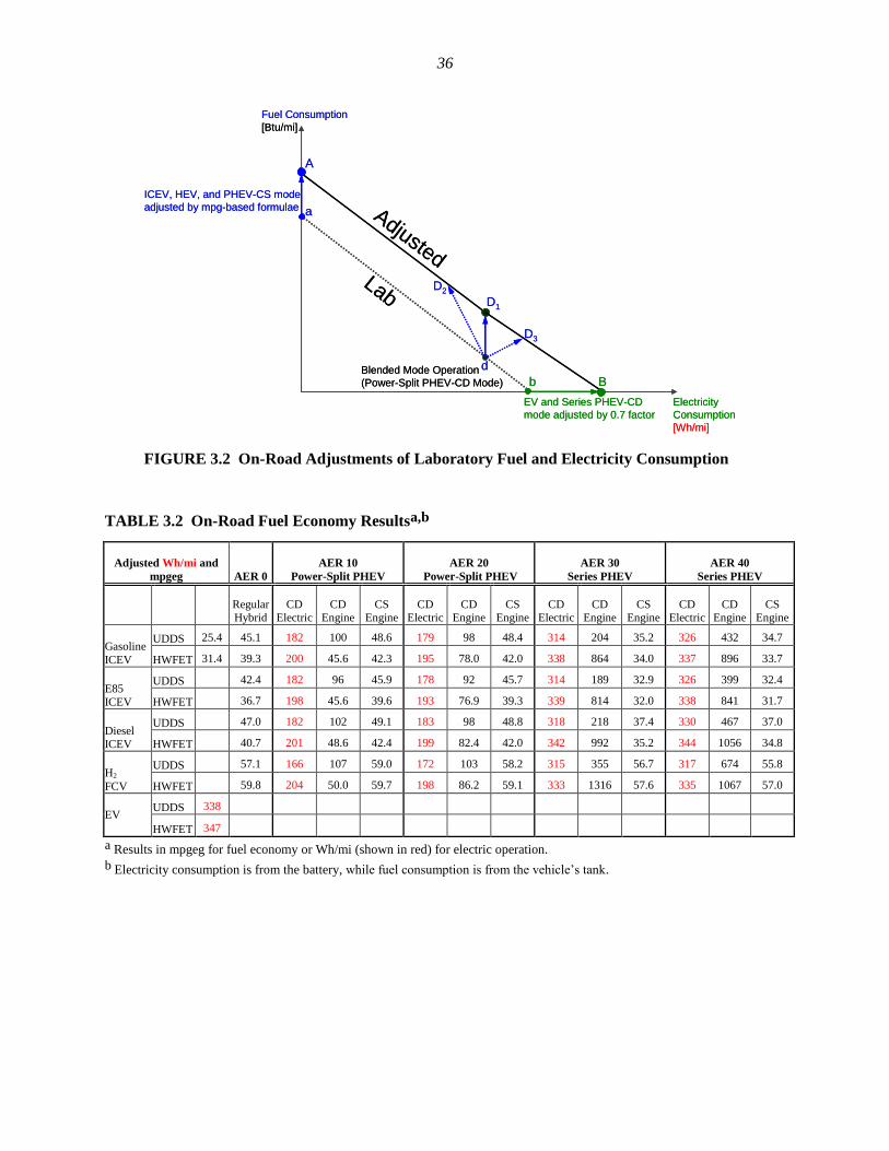
36

Electricity

Consumption

[Wh/mi]

Fuel Consumption

[Btu/mi]

ICEV, HEV, and PHEV-CS mode

adjusted by mpg-based formulae

EV and Series PHEV-CD

mode adjusted by 0.7 factor

Blended Mode Operation

(Power-Split PHEV-CD Mode)

Lab

Adjusted

D1

A

a

Bb

d

D3

D2

Electricity

Consumption

[Wh/mi]

Fuel Consumption

[Btu/mi]

ICEV, HEV, and PHEV-CS mode

adjusted by mpg-based formulae

EV and Series PHEV-CD

mode adjusted by 0.7 factor

Blended Mode Operation

(Power-Split PHEV-CD Mode)

Lab

Adjusted

D1

A

a

Bb

d

D3

D2

FIGURE 3.2 On-Road Adjustments of Laboratory Fuel and Electricity Consumption

TABLE 3.2 On-Road Fuel Economy Resultsa,b

Adjusted Wh/mi and

mpgeg AER 0

AER 10

Power-Split PHEV

AER 20

Power-Split PHEV

AER 30

Series PHEV

AER 40

Series PHEV

Regular Hybrid

CD Electric

CD Engine

CS Engine

CD Electric

CD Engine

CS Engine

CD Electric

CD Engine

CS Engine

CD Electric

CD Engine

CS Engine

Gasoline

ICEV

UDDS 25.4 45.1 182 100 48.6 179 98 48.4 314 204 35.2 326 432 34.7

HWFET 31.4 39.3 200 45.6 42.3 195 78.0 42.0 338 864 34.0 337 896 33.7

E85

ICEV

UDDS 42.4 182 96 45.9 178 92 45.7 314 189 32.9 326 399 32.4

HWFET 36.7 198 45.6 39.6 193 76.9 39.3 339 814 32.0 338 841 31.7

Diesel ICEV

UDDS 47.0 182 102 49.1 183 98 48.8 318 218 37.4 330 467 37.0

HWFET 40.7 201 48.6 42.4 199 82.4 42.0 342 992 35.2 344 1056 34.8

H2

FCV

UDDS 57.1 166 107 59.0 172 103 58.2 315 355 56.7 317 674 55.8

HWFET 59.8 204 50.0 59.7 198 86.2 59.1 333 1316 57.6 335 1067 57.0

EV UDDS 338

HWFET 347

a Results in mpgeg for fuel economy or Wh/mi (shown in red) for electric operation.

b Electricity consumption is from the battery, while fuel consumption is from the vehicle’s tank.

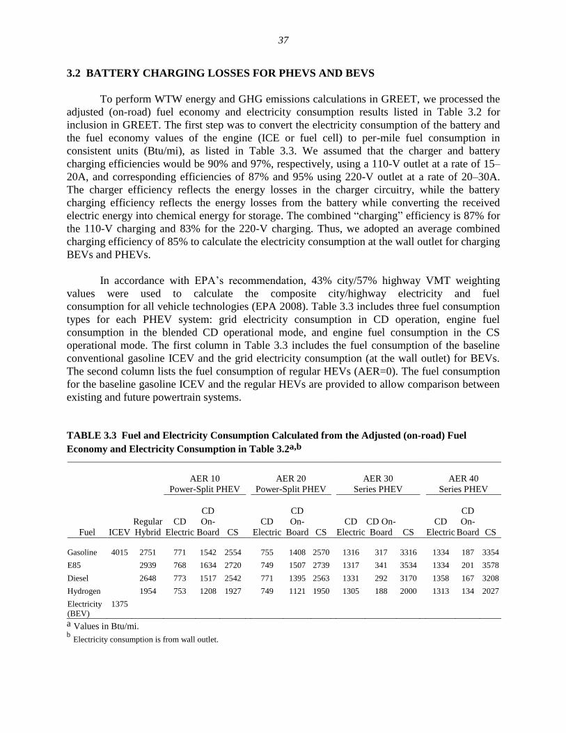
37

3.2 BATTERY CHARGING LOSSES FOR PHEVS AND BEVS

To perform WTW energy and GHG emissions calculations in GREET, we processed the

adjusted (on-road) fuel economy and electricity consumption results listed in Table 3.2 for

inclusion in GREET. The first step was to convert the electricity consumption of the battery and

the fuel economy values of the engine (ICE or fuel cell) to per-mile fuel consumption in

consistent units (Btu/mi), as listed in Table 3.3. We assumed that the charger and battery

charging efficiencies would be 90% and 97%, respectively, using a 110-V outlet at a rate of 15–

20A, and corresponding efficiencies of 87% and 95% using 220-V outlet at a rate of 20–30A.

The charger efficiency reflects the energy losses in the charger circuitry, while the battery

charging efficiency reflects the energy losses from the battery while converting the received

electric energy into chemical energy for storage. The combined ―charging‖ efficiency is 87% for

the 110-V charging and 83% for the 220-V charging. Thus, we adopted an average combined

charging efficiency of 85% to calculate the electricity consumption at the wall outlet for charging

BEVs and PHEVs.

In accordance with EPA’s recommendation, 43% city/57% highway VMT weighting

values were used to calculate the composite city/highway electricity and fuel

consumption for all vehicle technologies (EPA 2008). Table 3.3 includes three fuel consumption

types for each PHEV system: grid electricity consumption in CD operation, engine fuel

consumption in the blended CD operational mode, and engine fuel consumption in the CS

operational mode. The first column in Table 3.3 includes the fuel consumption of the baseline

conventional gasoline ICEV and the grid electricity consumption (at the wall outlet) for BEVs.

The second column lists the fuel consumption of regular HEVs (AER=0). The fuel consumption

for the baseline gasoline ICEV and the regular HEVs are provided to allow comparison between

existing and future powertrain systems.

TABLE 3.3 Fuel and Electricity Consumption Calculated from the Adjusted (on-road) Fuel

Economy and Electricity Consumption in Table 3.2a,b

AER 10

Power-Split PHEV

AER 20

Power-Split PHEV

AER 30

Series PHEV

AER 40

Series PHEV

Fuel ICEV

Regular

Hybrid

CD

Electric

CD

On-

Board CS

CD

Electric

CD

On-

Board CS

CD

Electric

CD On-

Board CS

CD

Electric

CD

On-

Board CS

Gasoline 4015 2751 771 1542 2554 755 1408 2570 1316 317 3316 1334 187 3354

E85 2939 768 1634 2720 749 1507 2739 1317 341 3534 1334 201 3578

Diesel 2648 773 1517 2542 771 1395 2563 1331 292 3170 1358 167 3208

Hydrogen 1954 753 1208 1927 749 1121 1950 1305 188 2000 1313 134 2027

Electricity

(BEV)

1375

a Values in Btu/mi. b Electricity consumption is from wall outlet.

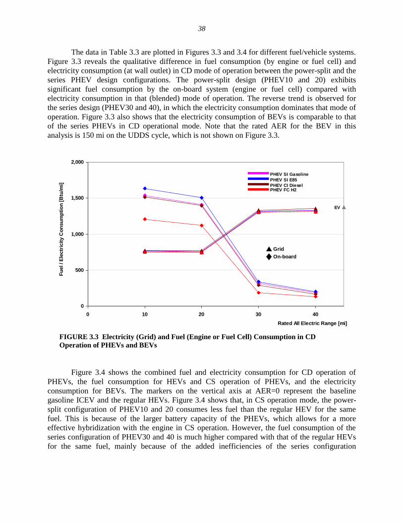
38

The data in Table 3.3 are plotted in Figures 3.3 and 3.4 for different fuel/vehicle systems.

Figure 3.3 reveals the qualitative difference in fuel consumption (by engine or fuel cell) and

electricity consumption (at wall outlet) in CD mode of operation between the power-split and the

series PHEV design configurations. The power-split design (PHEV10 and 20) exhibits

significant fuel consumption by the on-board system (engine or fuel cell) compared with

electricity consumption in that (blended) mode of operation. The reverse trend is observed for

the series design (PHEV30 and 40), in which the electricity consumption dominates that mode of

operation. Figure 3.3 also shows that the electricity consumption of BEVs is comparable to that

of the series PHEVs in CD operational mode. Note that the rated AER for the BEV in this

analysis is 150 mi on the UDDS cycle, which is not shown on Figure 3.3.

0

500

1,000

1,500

2,000

0 10 20 30 40

Rated All Electric Range [mi]

Fu

el / E

lectr

icit

y C

on

su

mp

tio

n [

Btu

/mi]

EV

PHEV SI Gasoline

PHEV SI E85

PHEV CI DieselPHEV FC H2

Grid

On-board

FIGURE 3.3 Electricity (Grid) and Fuel (Engine or Fuel Cell) Consumption in CD

Operation of PHEVs and BEVs

Figure 3.4 shows the combined fuel and electricity consumption for CD operation of

PHEVs, the fuel consumption for HEVs and CS operation of PHEVs, and the electricity

consumption for BEVs. The markers on the vertical axis at AER=0 represent the baseline

gasoline ICEV and the regular HEVs. Figure 3.4 shows that, in CS operation mode, the power-

split configuration of PHEV10 and 20 consumes less fuel than the regular HEV for the same

fuel. This is because of the larger battery capacity of the PHEVs, which allows for a more

effective hybridization with the engine in CS operation. However, the fuel consumption of the

series configuration of PHEV30 and 40 is much higher compared with that of the regular HEVs

for the same fuel, mainly because of the added inefficiencies of the series configuration

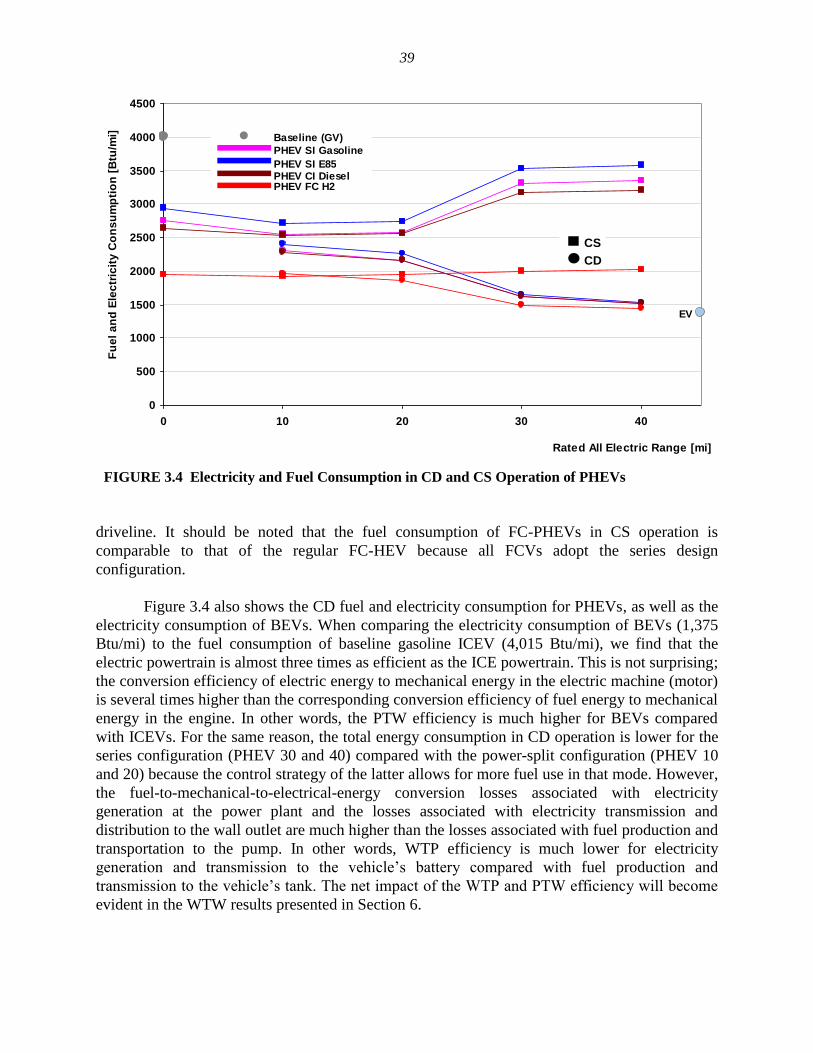
39

0

500

1000

1500

2000

2500

3000

3500

4000

4500

0 10 20 30 40

Rated All Electric Range [mi]

Fu

el

an

d E

lec

tric

ity

Co

ns

um

pti

on

[B

tu/m

i]

PHEV SI Gasoline

PHEV SI E85PHEV CI DieselPHEV FC H2

CS

CD

Baseline (GV)

EV

FIGURE 3.4 Electricity and Fuel Consumption in CD and CS Operation of PHEVs

driveline. It should be noted that the fuel consumption of FC-PHEVs in CS operation is

comparable to that of the regular FC-HEV because all FCVs adopt the series design

configuration.

Figure 3.4 also shows the CD fuel and electricity consumption for PHEVs, as well as the

electricity consumption of BEVs. When comparing the electricity consumption of BEVs (1,375

Btu/mi) to the fuel consumption of baseline gasoline ICEV (4,015 Btu/mi), we find that the

electric powertrain is almost three times as efficient as the ICE powertrain. This is not surprising;

the conversion efficiency of electric energy to mechanical energy in the electric machine (motor)

is several times higher than the corresponding conversion efficiency of fuel energy to mechanical

energy in the engine. In other words, the PTW efficiency is much higher for BEVs compared

with ICEVs. For the same reason, the total energy consumption in CD operation is lower for the

series configuration (PHEV 30 and 40) compared with the power-split configuration (PHEV 10

and 20) because the control strategy of the latter allows for more fuel use in that mode. However,

the fuel-to-mechanical-to-electrical-energy conversion losses associated with electricity

generation at the power plant and the losses associated with electricity transmission and

distribution to the wall outlet are much higher than the losses associated with fuel production and

transportation to the pump. In other words, WTP efficiency is much lower for electricity

generation and transmission to the vehicle’s battery compared with fuel production and

transmission to the vehicle’s tank. The net impact of the WTP and PTW efficiency will become

evident in the WTW results presented in Section 6.

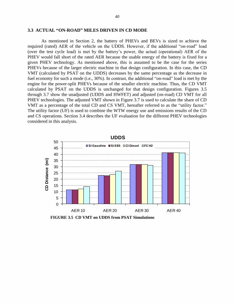
40

3.3 ACTUAL “ON-ROAD” MILES DRIVEN IN CD MODE

As mentioned in Section 2, the battery of PHEVs and BEVs is sized to achieve the

required (rated) AER of the vehicle on the UDDS. However, if the additional ―on-road‖ load

(over the test cycle load) is met by the battery’s power, the actual (operational) AER of the

PHEV would fall short of the rated AER because the usable energy of the battery is fixed for a

given PHEV technology. As mentioned above, this is assumed to be the case for the series

PHEVs because of the larger electric machine in that design configuration. In this case, the CD

VMT (calculated by PSAT on the UDDS) decreases by the same percentage as the decrease in

fuel economy for such a mode (i.e., 30%). In contrast, the additional ―on-road‖ load is met by the

engine for the power-split PHEVs because of the smaller electric machine. Thus, the CD VMT

calculated by PSAT on the UDDS is unchanged for that design configuration. Figures 3.5

through 3.7 show the unadjusted (UDDS and HWFET) and adjusted (on-road) CD VMT for all

PHEV technologies. The adjusted VMT shown in Figure 3.7 is used to calculate the share of CD

VMT as a percentage of the total CD and CS VMT, hereafter referred to as the ―utility factor.‖

The utility factor (UF) is used to combine the WTW energy use and emissions results of the CD

and CS operations. Section 3.4 describes the UF evaluation for the different PHEV technologies

considered in this analysis.

0

5

10

15

20

25

30

35

40

45

50

AER 10 AER 20 AER 30 AER 40

CD

Dis

tan

ce (

mi)

UDDS

SI Gasoline SI E85 CI Diesel FC H2

FIGURE 3.5 CD VMT on UDDS from PSAT Simulations

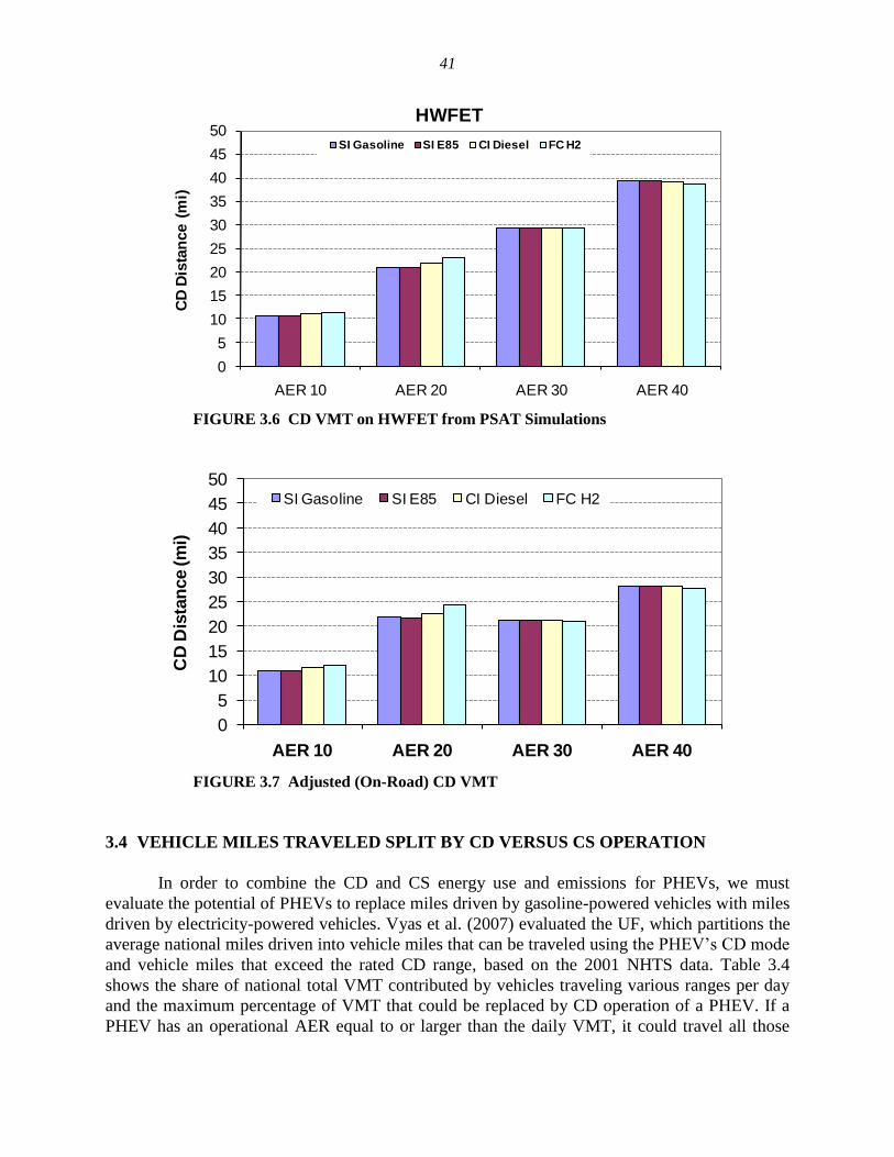
41

0

5

10

15

20

25

30

35

40

45

50


CD

Dis

tan

ce (

mi)

HWFET


FIGURE 3.6 CD VMT on HWFET from PSAT Simulations

0

5

10

15

20

25

30

35

40

45

50


CD

Dis

tan

ce (m

i)


FIGURE 3.7 Adjusted (On-Road) CD VMT

3.4 VEHICLE MILES TRAVELED SPLIT BY CD VERSUS CS OPERATION

In order to combine the CD and CS energy use and emissions for PHEVs, we must

evaluate the potential of PHEVs to replace miles driven by gasoline-powered vehicles with miles

driven by electricity-powered vehicles. Vyas et al. (2007) evaluated the UF, which partitions the

average national miles driven into vehicle miles that can be traveled using the PHEV’s CD mode

and vehicle miles that exceed the rated CD range, based on the 2001 NHTS data. Table 3.4

shows the share of national total VMT contributed by vehicles traveling various ranges per day

and the maximum percentage of VMT that could be replaced by CD operation of a PHEV. If a

PHEV has an operational AER equal to or larger than the daily VMT, it could travel all those

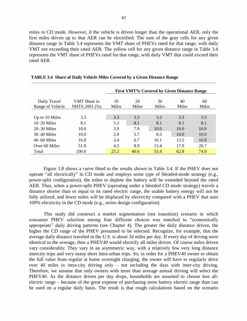
42

miles in CD mode. However, if the vehicle is driven longer than the operational AER, only the

first miles driven up to that AER can be electrified. The sum of the gray cells for any given

distance range in Table 3.4 represents the VMT share of PHEVs rated for that range, with daily

VMT not exceeding their rated AER. The yellow cell for any given distance range in Table 3.4

represents the VMT share of PHEVs rated for that range, with daily VMT that could exceed their

rated AER.

TABLE 3.4 Share of Daily Vehicle Miles Covered by a Given Distance Range

First VMT% Covered by Given Distance Range

Daily Travel

Range of Vehicle

VMT Share in

NHTS 2001 (%)

10

Miles

20

Miles

30

Miles

40

Miles

60

Miles

Up to 10 Miles 3.3 3.3 3.3 3.3 3.3 3.3

10–20 Miles 8.1 5.3 8.1 8.1 8.1 8.1

20–30 Miles 10.0 3.9 7.9 10.0 10.0 10.0

30–40 Miles 10.0 2.8 5.7 8.5 10.0 10.0

40–60 Miles 16.8 3.4 6.7 10.1 13.5 16.8

Over 60 Miles 51.8 4.5 8.9 13.4 17.9 26.7

Total 100.0 23.2 40.6 53.4 62.8 74.9

Figure 3.8 shows a curve fitted to the results shown in Table 3.4. If the PHEV does not

operate ―all electrically‖ in CD mode and employs some type of blended-mode strategy (e.g.,

power-split configuration), the miles to deplete the battery will be extended beyond the rated

AER. Thus, when a power-split PHEV (operating under a blended CD mode strategy) travels a

distance shorter than or equal to its rated electric range, the usable battery energy will not be

fully utilized, and fewer miles will be displaced by electricity compared with a PHEV that uses

100% electricity in the CD mode (e.g., series design configuration).

This study did construct a market segmentation (not transition) scenario in which

consumer PHEV selection among four different choices was matched to ―economically

appropriate‖ daily driving patterns (see Chapter 4). The greater the daily distance driven, the

higher the CD range of the PHEV presumed to be selected. Recognize, for example, that the

average daily distance traveled in the U.S. is about 34 miles per day. If every day of driving were

identical to the average, then a PHEV40 would electrify all miles driven. Of course miles driven

vary considerably. They vary in an asymmetric way, with a relatively few very long distance

intercity trips and very many short intra-urban trips. So, in order for a PHEV40 owner to obtain

the full value from regular at home overnight charging, the owner will have to regularly drive

over 40 miles in intra-city driving only – not including the days with inter-city driving.

Therefore, we assume that only owners with more than average annual driving will select the

PHEV40. As the distance driven per day drops, households are assumed to choose less all-

electric range – because of the great expense of purchasing more battery electric range than can

be used on a regular daily basis. The result is that rough calculations based on the scenario

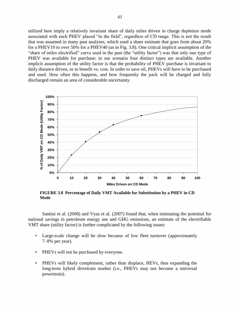
43

utilized here imply a relatively invariant share of daily miles driven in charge depletion mode

associated with each PHEV placed ―in the field‖, regardless of CD range. This is not the result

that was assumed in many past analyses, which used a share estimate that goes from about 20%

for a PHEV10 to over 50% for a PHEV40 (as in Fig. 3.8). One critical implicit assumption of the

―share of miles electrified‖ curve used in the past (the ―utility factor‖) was that only one type of

PHEV was available for purchase: in our scenario four distinct types are available. Another

implicit assumption of the utility factor is that the probability of PHEV purchase is invariant to

daily distance driven, or to benefit vs. cost. In order to save oil, PHEVs will have to be purchased

and used. How often this happens, and how frequently the pack will be charged and fully

discharged remain an area of considerable uncertainty.

0%

10%

20%

30%

40%

50%

60%

70%

80%

90%

100%

0 10 20 30 40 50 60 70 80 90 100

Miles Driven on CD Mode

% o

f D

aily

VM

T o

n C

D M

od

e (

Uti

lity

Fa

cto

r)

FIGURE 3.8 Percentage of Daily VMT Available for Substitution by a PHEV in CD

Mode

Santini et al. (2008) and Vyas et al. (2007) found that, when estimating the potential for

national savings in petroleum energy use and GHG emissions, an estimate of the electrifiable

VMT share (utility factor) is further complicated by the following issues:

• Large-scale change will be slow because of low fleet turnover (approximately

7–8% per year).

• PHEVs will not be purchased by everyone.

• PHEVs will likely complement, rather than displace, HEVs, thus expanding the

long-term hybrid drivetrain market (i.e., PHEVs may not become a universal

powertrain).

44

• Various control strategies for utilizing the engine and the electric machine could

result in a myriad of VMT shares in CD mode.

• PHEVs will vary in terms of their AER capability and will have different

configurations of the electric machine, battery, and engine.

• PHEVs purchased with a nominal range capability (AER rating) will not realize

that exact rated value in practice because of variations in driving conditions,

driver characteristics, accessory use, etc.

• Batteries for PHEVs may be charged more than once every day.

Because of these issues, we report the WTW energy use and emissions results for the CD

mode in addition to the WTW results for the combined CD and CS operations. The utility factor

was calculated from Figure 3.8 on the basis of the adjusted CD VMT in Figure 3.7. Then the

WTW results for the combined CD and CS operations were calculated on the basis of the utility

factor using the following equation:

Ecombined = (EGrid + EEngine)CD*UF + ECS*(1-UF)

where E refers to the energy consumption or emissions associated with the fuel and electricity

use by PHEVs, as well as those associated with the upstream processes of electricity generation,

fuel production, and their transmission and distribution to the vehicles.

45

4 PHEV POPULATION AND ELECTRIC LOAD PROFILE

PHEVs will draw electric energy from the electric grid. The extent of this electricity

demand was estimated by examining patterns of vehicle usage and calculating the potential

number of PHEVs that will be plugged in.

4.1 DATA SOURCES

To conduct utility demand simulations, we estimated daily electricity demand for various

PHEVs, specifically the following characteristics: (1) daily vehicle usage, (2) pattern of vehicle

arrival at home at the end of the last trip, (3) number of PHEVs of different AERs that will be

plugged in each day, and (4) amount of electric power and energy that will be drawn by each

PHEV (with different AERs), and (5) time required for charging.

Travel data from the 2001 NHTS were analyzed to determine the pattern of daily vehicle

usage and how much of that travel can potentially rely on electricity. In other words, we

examined, under different assumptions, the ending time of the last vehicle trip and the share of

VMT that can be electrified. The NHTS was conducted under the sponsorship of the Federal

Highway Administration (FHWA), Bureau of Transportation Statistics, and National Highway

Traffic Safety Administration (FHWA 2004). The NHTS files contain data on household

characteristics, household member characteristics, household vehicle characteristics, and

household travel characteristics. For travel data, the survey includes a one-day travel component

and a long-distance travel component. Data from the one-day travel component were used for the

PHEV analysis presented here. The 2001 NHTS was conducted from March 2001 through May

2002. Each sampled household was assigned a travel day to report all trips made on that day.

Travel days covering all seven days of the week (including holidays) were assigned. The travel

day began at 4:00 a.m. and ended at 3:59 a.m. of the following day. On a typical day, 4:00 a.m.

represents the time when the fewest number of people are in the middle of a trip. Care was taken

to have each month of the year and each day represented properly in the survey.

The NHTS covered 69,817 households, 160,758 persons, 139,382 vehicles, and 642,292

person trips on the assigned travel day. Of these 642,292 trips, 387,431 were made by personal

vehicles driven by one of the responding drivers and 172,879 were made by passengers in private

vehicles. When trips with unreported travel times and travel distances are dropped, 366,084 trips

made by 84,916 vehicles are available for further analysis. These trips and vehicles include

samples from areas that requested additional sampling. When these add-on samples are removed,

142,111 trips made by 32,022 vehicles remain. The sample without the add-ons is called the

―national sample‖ by the Federal Highway Administration; the national sample is used here

because it provides a random representation of national household travel.

Light-duty vehicle projections from EIA’s 2009 Annual Energy Outlook (AEO) (EIA

2009a) were used to estimate the number of PHEVs on the road in 2020. EIA is a part of DOE

and uses its National Energy Modeling System (NEMS) to project vehicle sales, vehicle stock

46

(number of vehicles on the road), and energy demand (EIA 2009b). The AEO provides national

projections of cars and light trucks on the road.

Argonne used population data from the U.S. Census Bureau to allocate national vehicle

projection to individual states. The Census Bureau projections provide population — by age

group — for each state (U.S. Census Bureau 2005). The 2007 state-level vehicle registration data

from Highway Statistics published by the FHWA (FHWA 2008) were used, together with the

population projections, to allocate EIA’s projected national vehicle population to each state. The

vehicle registration data were also used to determine the likelihood of each state to have more or

fewer vehicles per driving-age person.

4.2 PHEV POPULATION

For estimating electricity demand by PHEVs, Argonne estimated the number of PHEVs

that will be on road in 2020. Two alternatives were considered: (1) estimate new PHEV market

penetration profile for vehicles having 10-, 20-, 30-, and 40-mile AER or (2) assume that a

certain percent of registered vehicles in 2020 will be PHEVs and then allocate the resulting

vehicles as PHEVs with 10-, 20-, 30-, and 40-mile AERs.

The first approach would require development of detailed vehicle characteristics of

PHEVs and competing-technology vehicles to allow us to estimate PHEV market shares through

a vehicle choice model. These market shares then can be applied to new vehicle sales, and the

resulting new vehicles can be simulated by using a vehicle survival model. Because such a

detailed approach would take considerable time and effort, we decided to employ the second

approach and assume that 10% of all vehicles in 2020 will be PHEVs. The assumed 10% share

may appear high, compared with the historical shares by such technologies as diesel vehicles and

CS HEVs. However, because the intent of this analysis is to analyze the impact of a high level of

market penetration by PHEVs, the assumption of a 10% market share is justified.

Next, we estimated the 10% share of 2020 vehicle population as projected in AEO 2009.

AEO projections provide separate estimates for car and light truck stock, but not by vehicle type

within the light truck category. We assumed that PHEVs will not be offered in all light trucks;

only the sport utility vehicle (SUV) segment will offer PHEVs. FHWA’s 2007 Highway

Statistics provide registrations of light trucks by state and by category (i.e., pickups, vans, SUVs,

other light trucks, and farm trucks). The 2007 light truck shares by these vehicle types were

computed and were assumed to remain unchanged through 2020 for each state.

We estimated the 2007 light vehicle registration shares per driving-age population for

each state and each state’s share of the total driving-age population. (Note: for this purpose, the

16- to 84-year-old age group was considered as the driving-age population.) An analysis of the

2007 driving-age population share and vehicle registration share provided each state’s propensity

to own more or fewer light-duty vehicles per driving-age person. These propensity values were

assumed to remain unchanged through 2020 for each state.

47

The use of these estimates (2020 driving-age population share by state and each state’s

propensity to have more or fewer light-duty vehicles per driving-age person) allowed us to

allocate national light vehicle estimates from AEO 2009 to each state. We used the SUV share of

light truck registrations for each state to arrive at 2020 state-level SUV registrations. These

estimates were used the project the 2020 PHEV population in each state.

To analyze the impacts of such PHEV penetration on electric utilities, we selected four

study areas: (1) the area within the United States that is served by the WECC, (2) Illinois State,

(3) New York State, and (4) states within the U.S. Census Bureau’s New England division. To

develop detailed characteristics, we further subdivided the first three areas into eight subareas.

The state-level PHEV estimates described above were used to estimate PHEV population for the

following geographical areas:

1. Metropolitan Statistical Areas (MSAs) within WECC service area (excluding

California),

2. Non-MSA areas WECC service area (excluding California),

3. California’s large MSAs,

4. Rest of California,

5. Chicago MSA within Illinois,

6. Rest of Illinois,

7. New York City Consolidated Metropolitan Statistical Area (CMSA) within New

York State

8. Rest of New York State, and

9. New England states.

The WECC service area (excluding California) in our analysis encompassed Arizona,

Colorado, Idaho, Montana, New Mexico, Nevada, Oregon, Utah, Washington, and Wyoming.

We used the travel day data in the 2001 NHTS to allocate total PHEVs in each of these

geographical areas by 10-, 20-, 30-, and 40-mile AERs. Vehicles traveling 12–24 miles were

used to compute vehicle share by PHEVs with a 10-mile AER; those traveling 24–36 miles were

used for PHEVs with a 20-mile AER; those traveling 36–48 miles for were used for PHEVs with

a 30-mile AER; and those traveling 48–60 miles were used for PHEVs with a 40-mile AER. The

share of vehicles in each AER was determined and applied to PHEV estimates in each of the

analysis areas. Figure 4.1 shows 2020 PHEV population by various AER in each of the analysis

areas.

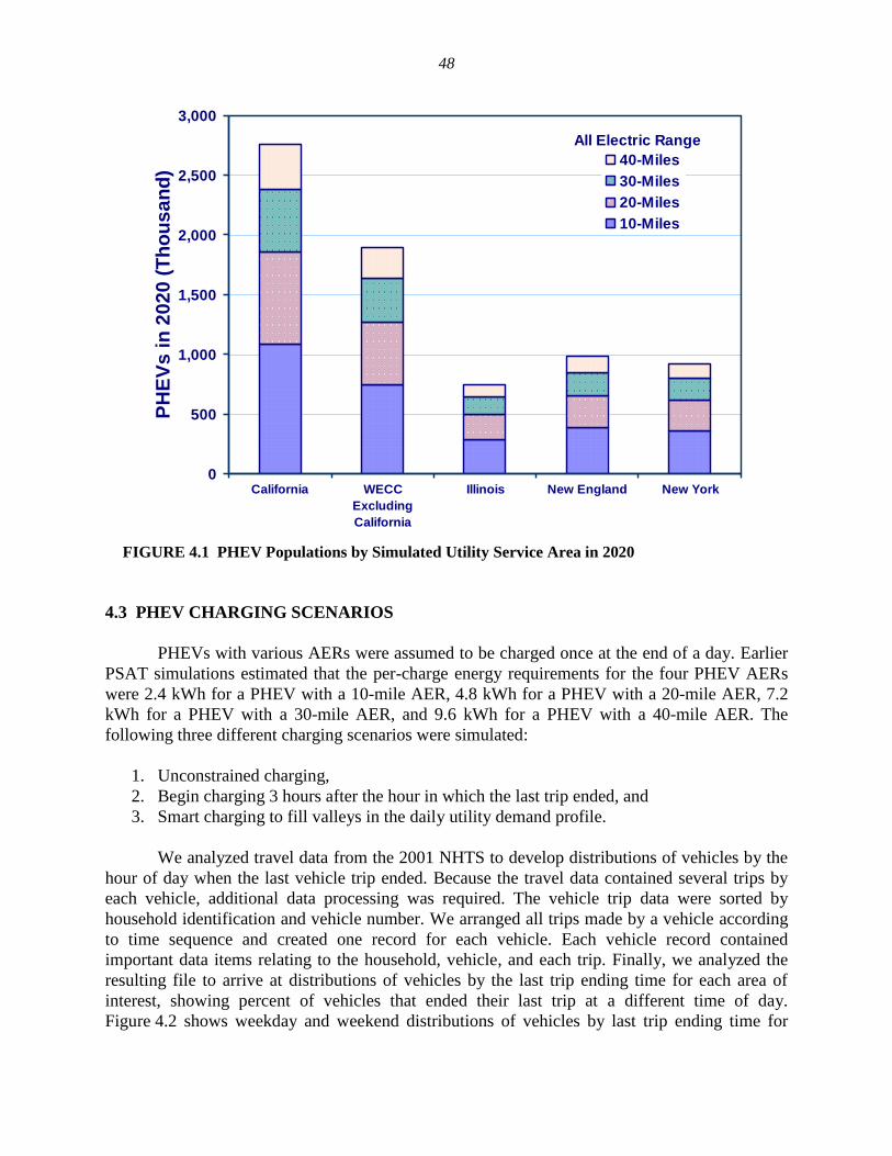
48

0

500

1,000

1,500

2,000

2,500

3,000

California WECC

Excluding

California

Illinois New England New York

PH

EV

s i

n 2

02

0 (

Th

ou

sa

nd

)40-Miles

30-Miles

20-Miles

10-Miles

All Electric Range

FIGURE 4.1 PHEV Populations by Simulated Utility Service Area in 2020

4.3 PHEV CHARGING SCENARIOS

PHEVs with various AERs were assumed to be charged once at the end of a day. Earlier

PSAT simulations estimated that the per-charge energy requirements for the four PHEV AERs

were 2.4 kWh for a PHEV with a 10-mile AER, 4.8 kWh for a PHEV with a 20-mile AER, 7.2

kWh for a PHEV with a 30-mile AER, and 9.6 kWh for a PHEV with a 40-mile AER. The

following three different charging scenarios were simulated:

1. Unconstrained charging,

2. Begin charging 3 hours after the hour in which the last trip ended, and

3. Smart charging to fill valleys in the daily utility demand profile.

We analyzed travel data from the 2001 NHTS to develop distributions of vehicles by the

hour of day when the last vehicle trip ended. Because the travel data contained several trips by

each vehicle, additional data processing was required. The vehicle trip data were sorted by

household identification and vehicle number. We arranged all trips made by a vehicle according

to time sequence and created one record for each vehicle. Each vehicle record contained

important data items relating to the household, vehicle, and each trip. Finally, we analyzed the

resulting file to arrive at distributions of vehicles by the last trip ending time for each area of

interest, showing percent of vehicles that ended their last trip at a different time of day.

Figure 4.2 shows weekday and weekend distributions of vehicles by last trip ending time for

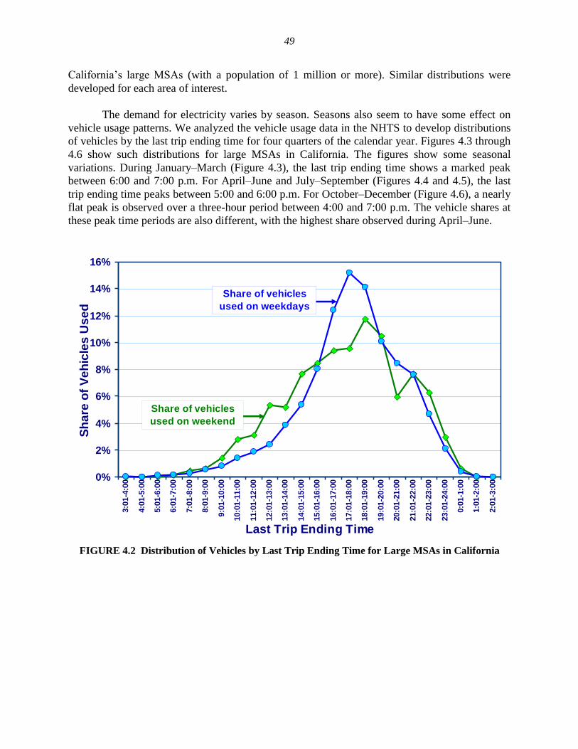
49

California’s large MSAs (with a population of 1 million or more). Similar distributions were

developed for each area of interest.

The demand for electricity varies by season. Seasons also seem to have some effect on

vehicle usage patterns. We analyzed the vehicle usage data in the NHTS to develop distributions

of vehicles by the last trip ending time for four quarters of the calendar year. Figures 4.3 through

4.6 show such distributions for large MSAs in California. The figures show some seasonal

variations. During January–March (Figure 4.3), the last trip ending time shows a marked peak

between 6:00 and 7:00 p.m. For April–June and July–September (Figures 4.4 and 4.5), the last

trip ending time peaks between 5:00 and 6:00 p.m. For October–December (Figure 4.6), a nearly

flat peak is observed over a three-hour period between 4:00 and 7:00 p.m. The vehicle shares at

these peak time periods are also different, with the highest share observed during April–June.

0%

2%

4%

6%

8%

10%

12%

14%

16%

3:0

1-4

:00

4:0

1-5

:00

5:0

1-6

:00

6:0

1-7

:00

7:0

1-8

:00

8:0

1-9

:00

9:0

1-1

0:0

0

10:0

1-1

1:0

0

11:0

1-1

2:0

0

12:0

1-1

3:0

0

13:0

1-1

4:0

0

14:0

1-1

5:0

0

15:0

1-1

6:0

0

16:0

1-1

7:0

0

17:0

1-1

8:0

0

18:0

1-1

9:0

0

19:0

1-2

0:0

0

20:0

1-2

1:0

0

21:0

1-2

2:0

0

22:0

1-2

3:0

0

23:0

1-2

4:0

0

0:0

1-1

:00

1:0

1-2

:00

2:0

1-3

:00

Last Trip Ending Time

Sh

are

of

Ve

hic

les

Us

ed

Share of vehicles

used on weekdays

Share of vehicles

used on weekend

FIGURE 4.2 Distribution of Vehicles by Last Trip Ending Time for Large MSAs in California

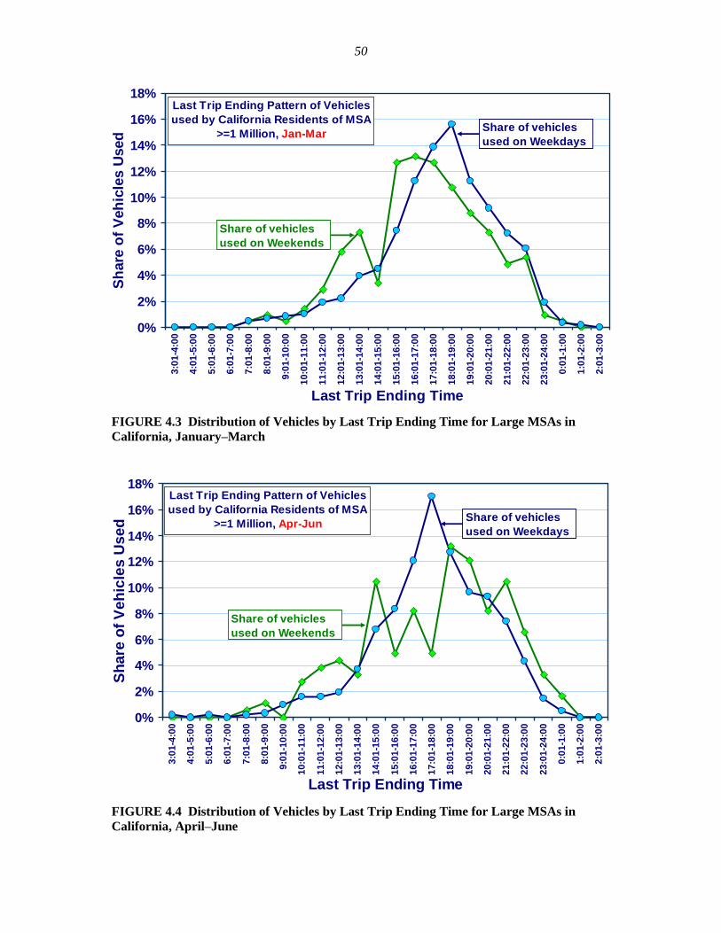
50

0%

2%

4%

6%

8%

10%

12%

14%

16%

18%

3:0

1-4

:00

4:0

1-5

:00

5:0

1-6

:00

6:0

1-7

:00

7:0

1-8

:00

8:0

1-9

:00

9:0

1-1

0:0

0

10

:01

-11

:00

11

:01

-12

:00

12

:01

-13

:00

13

:01

-14

:00

14

:01

-15

:00

15

:01

-16

:00

16

:01

-17

:00

17

:01

-18

:00

18

:01

-19

:00

19

:01

-20

:00

20

:01

-21

:00

21

:01

-22

:00

22

:01

-23

:00

23

:01

-24

:00

0:0

1-1

:00

1:0

1-2

:00

2:0

1-3

:00


Sh

are

of

Veh

icle

s U

sed

Last Trip Ending Pattern of Vehicles

used by California Residents of MSA

>=1 Million, Jan-MarShare of vehicles

used on Weekdays

Share of vehicles

used on Weekends

FIGURE 4.3 Distribution of Vehicles by Last Trip Ending Time for Large MSAs in

California, January–March

0%

2%

4%

6%

8%

10%

12%

14%

16%

18%

3:0

1-4

:00

4:0

1-5

:00

5:0

1-6

:00

6:0

1-7

:00

7:0

1-8

:00

8:0

1-9

:00

9:0

1-1

0:0

0

10

:01

-11

:00

11

:01

-12

:00

12

:01

-13

:00

13

:01

-14

:00

14

:01

-15

:00

15

:01

-16

:00

16

:01

-17

:00

17

:01

-18

:00

18

:01

-19

:00

19

:01

-20

:00

20

:01

-21

:00

21

:01

-22

:00

22

:01

-23

:00

23

:01

-24

:00

0:0

1-1

:00

1:0

1-2

:00

2:0

1-3

:00


Sh

are

of

Ve

hic

les

Us

ed



>=1 Million, Apr-JunShare of vehicles

used on Weekdays

Share of vehicles

used on Weekends


California, April–June

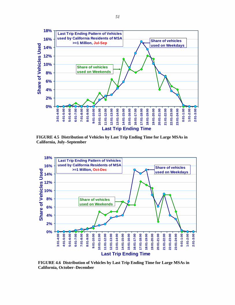
51

0%

2%

4%

6%

8%

10%

12%

14%

16%

18%

3:0

1-4

:00

4:0

1-5

:00

5:0

1-6

:00

6:0

1-7

:00

7:0

1-8

:00

8:0

1-9

:00

9:0

1-1

0:0

0

10

:01

-11

:00

11

:01

-12

:00

12

:01

-13

:00

13

:01

-14

:00

14

:01

-15

:00

15

:01

-16

:00

16

:01

-17

:00

17

:01

-18

:00

18

:01

-19

:00

19

:01

-20

:00

20

:01

-21

:00

21

:01

-22

:00

22

:01

-23

:00

23

:01

-24

:00

0:0

1-1

:00

1:0

1-2

:00

2:0

1-3

:00


Sh

are

of

Veh

icle

s U

sed



>=1 Million, Jul-SepShare of vehicles

used on Weekdays

Share of vehicles

used on Weekends


California, July–September

0%

2%

4%

6%

8%

10%

12%

14%

16%

18%

3:0

1-4

:00

4:0

1-5

:00

5:0

1-6

:00

6:0

1-7

:00

7:0

1-8

:00

8:0

1-9

:00

9:0

1-1

0:0

0

10

:01

-11

:00

11

:01

-12

:00

12

:01

-13

:00

13

:01

-14

:00

14

:01

-15

:00

15

:01

-16

:00

16

:01

-17

:00

17

:01

-18

:00

18

:01

-19

:00

19

:01

-20

:00

20

:01

-21

:00

21

:01

-22

:00

22

:01

-23

:00

23

:01

-24

:00

0:0

1-1

:00

1:0

1-2

:00

2:0

1-3

:00


Sh

are

of

Ve

hic

les

Us

ed



>=1 Million, Oct-DecShare of vehicles

used on Weekdays

Share of vehicles

used on Weekends


California, October–December

52

The next step was to determine the probable charging characteristics for PHEVs of each

AER. The NHTS analysis showed that more than 60% of vehicles end their last trip after 5:00

p.m. and 70% after 4:00 p.m. Also, 54% of vehicles begin their first trip between 6:00 and 9:00

a.m. on weekdays. We employed these vehicle-use characteristics to estimate PHEV charging

times for the four AERs.

As mentioned earlier, a PHEV with a 10-mile AER would need 2.4 kWh to be fully

charged after having depleted its battery pack to the lowest allowable SOC. This demand can be

met easily by a 110- to 120-V and 15-A (12-A average output) circuit drawing 1.3 kW on

average. A full charge would take nearly 2.1 hours. This estimate assumes a charger efficiency of

90% and a battery intake efficiency of 97%. Modern chargers are designed to have a near-unity

power factor.

The estimated electricity requirements were 4.8 kWh for a PHEV with a 20-mile AER,

7.2 kWh for a PHEV with a 30-mile AER, and 9.6 kWh for a PHEV with a 40-mile AER. A

PHEV with a 20-mile AER can be charged through a 110- to 120-V and 15-A (12-A average

output) circuit drawing 1.3 kW on average. A full charge would take 4.2 hours with a charger

efficiency of 90% and a battery intake efficiency of 97%.

A PHEV with a 30-mile AER can be charged through a 110- to 120-V and 20-A circuit in

4.8 hours drawing 1.75 kW, and a PHEV with a 40-mile AER can be charged through a 220- to

240-V and 20-A circuit in 3.3 hours drawing 3.5 kW. The charger and battery efficiencies for the

220- to 240-V circuit were assumed to be slightly lower, at 87% and 95%, respectively.

4.4 SUMMARY OF PHEV POPULATION AND ELECTRIC LOAD ANALYSIS

Argonne employed data from various sources in developing the vehicle-related

quantitative inputs necessary for this study. Our analytical work can be summarized as follows:

• We estimated populations of PHEVs with 10-, 20-, 30-, and 40-mile AERs in

each analysis region and used the U.S. Department of Transportation’s NHTS and

Highway Statistics publication, DOE’s vehicle stock projection, and U.S. Census

Bureau population projections.

• We developed distributions of vehicles by ending time of the last trip for each

analysis region by using the U.S. Department of Transportation’s NHTS.

• We analyzed seasonal variations in the distributions of vehicles by ending time of

the last trip by using the U.S. Department of Transportation’s NHTS.

• We estimated power demand and time required to charge PHEVs of different

AERs and developed three different charging scenarios to evaluate the impacts of

PHEVs on electric utilities.

53

5 ELECTRIC POWER SYSTEM DISPATCH

Argonne’s analysis included modeling of electric power systems in four regions of the

United States: the New England Independent System Operator (NE ISO), the New York

Independent System Operator (NY ISO), the state of Illinois, and the Western Electric

Coordinating Council (WECC). The NE ISO is a regional electric balancing authority serving all

of the states within the New England region, including Maine, Vermont, New Hampshire,

Connecticut, Massachusetts, and Rhode Island. The NY ISO is a regional balancing authority

serving all of the loads within the entire state of New York. WECC is a reliability council

responsible for coordinating and promoting the bulk power system in all or portions of

14 western states. The State of Illinois is modeled as a single state.

Different modeling techniques and methodologies were used to simulate the electric

power system dispatch in these regions on the basis of data that had been collected already on

each region and of data that was readily available from public sources. This section will describe

the modeling technique and methodology used in each region, the sources of the model’s input

data, the simulation results for each region and scenario, and key issues and major findings for

each region/scenario.

5.1 MODELING TECHNIQUE AND METHODOLOGY

5.1.1 NE and NY ISOs

Only the generators and loads were modeled for both of these systems. Treating the

model components this way assumes that the transmission system has no limitations; that is, it is

capable of transmitting any amount of electricity from generators at point A to loads at point B.

Therefore, the amount of electricity that a plant could generate at any time was not constrained

by the capacity of the transmission lines to which it was connected.

The future generation mix was estimated by simulating the operations of thermal and

renewable power plants in each region. Because hydropower provides a small but not

insignificant portion of the electric generation in both regions, special attention was paid to

interdependencies among hydropower and thermal power plant operations. Hydropower plants

currently provide almost 20% of the generation in New York and about 5% in New England.

Generation from wind power plants was also estimated for both regions. However, wind power

currently provides less than 1% in New York and about 0.2% in New England.

Thermal power plants were simulated at the unit level. A probabilistic dispatch model

was used to simulate thermal power plant production to meet load that is not served by

hydropower plants and other renewable resources, such as wind power. The thermal dispatch

model was run in the monthly load duration curves (LDCs) mode. In this mode, monthly average

capacity factors and generation levels were obtained for each unit in the inventory. Maintenance

54

and random forced outages were accounted for at the unit level. Data for unit characteristics

came from both ISO and EIA sources.

Hydropower plant generation is determined on an hourly time-step basis. Hydropower is

simulated as an aggregate generation resource that serves both base load and peaking duties.

Information is compiled for the aggregation from individual plant-level data. The hourly dispatch

of the aggregate power plant is based on (1) monthly generation control totals, (2) the amount of

water used for base load duties, (3) estimated monthly hydropower capability, and (4) an hourly

load profile for each ISO service territory. Section 5.3.1 describes the methodology used to

calculate base and peak generation from hydropower in greater detail.

Wind turbines are a nondispatchable resource, meaning that the operator has no control

over when the wind turbine generates electricity; turbines generate when the wind is blowing and

feed electricity into the grid. Data from the National Renewable Energy Laboratory (NREL)

Web site were used to estimate electricity generated from wind turbines. Section 5.3.1 describes

the methodology used to calculate electricity generated from wind turbines in greater detail.

Solar power is miniscule in both the NE ISO and NY ISO, and so it was ignored in the

study. Other plants using renewable fuel sources (such as geothermal, municipal solid waste,

wood, and biomass) were included in the thermal dispatch model because operators can control

when these plants produce power. These plants can be dispatched as necessary as opposed to

wind or non-storage hydroelectric sources.

An hourly electricity demand profile was constructed from historical hourly demand

profiles available on each ISO’s Web site (New England, www.iso-ne.com; New York,

www.nyiso.com). Forecasts of monthly peak loads and energy use for 2020 were also obtained

from forecasting documents available on the two ISOs’ Web sites.

The modeling methodology for both regions used several modeling tools. The sequence

of operations in the methodology is as follows:

1. Collect and process data and information;

2. Determine hourly generation from renewable resources, including dispatchable

and nondispatchable aggregate hydropower and other nondispatchable plants,

such as wind;

3. Determine current hourly electricity loads and forecast future load levels;

4. Adjust loads for nondispatchable renewable generation and hydropower plant

generation by subtracting nondispatchable renewable generation and peak shaving

dispatchable hydropower (such as plants with storage reservoirs or pumped

storage plants);

5. Develop a baseline plant inventory for 2020;

55

6. Run a probabilistic thermal dispatch model to estimate electricity generation by

thermal generation units for 2020;

7. Obtain monthly unit-level generation values and compute capacity factors;

8. Develop alternative PHEV scenarios;

9. Develop a capacity expansion plan for 2020 to meet additional loads from

PHEVs, starting with baseline expansion plan from step 5;

10. Run probabilistic dispatch model for the different scenarios to obtain unit-level

generation and compute capacity factors for 2020; and

11. Compare and summarize results.

The source of data for the steps in the above process is described in Section 5.3.

5.1.2 WECC

The WECC system encompasses a large geographic area in the western United States; it

covers all of the states west of the Rocky Mountains. Because the WECC system’s area extends

so widely and is known to have transmission congestion issues, its system topology was

simulated in finer detail for this study. The transmission system was modeled as a system of

nodes, with both loads and resources aggregated at each node. The nodes had links to

approximate the flow of power over transmission lines in WECC. Limits were placed on the

amount of energy that could be transferred over those links to approximate actual transmission

line constraints. For this study, the U.S. portion of WECC consisted of 23 nodes; there were also

links to nodes in Canada and Mexico and to other reliability councils in the United States.

Figure 5.1 shows the WECC system topology.

The Generation and Transmission Maximization (GTMax) model, developed by

Argonne, simulated the operation of both dispatchable and nondispatchable resources and power

transfer limitations of the transmission system. Additional details about this model are provided

in Section 5.6.2.

Thermal power plants and dispatchable renewable generators, such as geothermal,

municipal solid waste, wood, and biomass, were simulated at the unit level. Data for unit

characteristics were obtained from both EIA and WECC sources.

Hydroelectric power plays a key role in the WECC system; it can provide as much as

40% of the WECC load during wet hydrological conditions. Hydroelectric plants were modeled

on a plant-level basis. They were assigned to specific nodes within the network, and generation

was derived from historical data available in Form EIA-906. Section 5.3.2 describes the

methodology used to calculate generation from hydropower in greater detail.

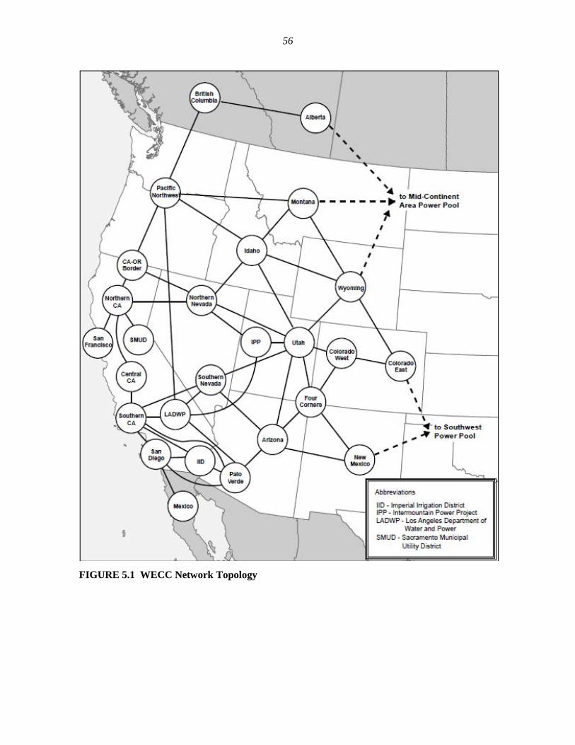
56

FIGURE 5.1 WECC Network Topology

57

Generation from wind and solar plants, both of which are nondispatchable sources, also

plays a role in the WECC system. Data from the NREL Web site was used to estimate electricity

generated from both wind turbines and solar generators. Section 5.3.2 describes the methodology

used to calculate electricity generated from wind and solar in greater detail.

An hourly electricity demand profile was constructed from hourly demand data available

from WECC. Forecasts of monthly peak loads and energy use for 2020 were also obtained from

forecasting documents available from WECC and supplemented by data from EIA Form-411.

5.1.3 State of Illinois

To explore the effect(s) on the transmission system more fully when serving increased

loads from PHEVs, the State of Illinois was modeled in the greatest level of detail (i.e., at the bus

level). A bus is defined as a nodal point in a transmission system — typically a point at which

major loads and generating resources connect. Buses are connected to each other via

transmission lines. The Illinois system consisted of more than 1,900 buses and more than

2,500 transmission lines. Figure 5.2 shows the topology of the Illinois electric power system.

In addition to the in-state transmission configuration, the power transfers into and out of

Illinois were accounted for in order to obtain an accurate picture of how its electric system would

perform. All of the tie lines between Illinois and surrounding states were identified and

aggregated into a small set of interconnection points. Eleven interconnection points covered an

area including Indiana, Michigan, and parts of Ohio in the east, Tennessee in the south, parts of

Missouri served by the Ameren and AECI utilities in the southwest, Iowa and parts of Minnesota

in the west, and Wisconsin in the north. These out-of-state connections are also shown in

Figure 5.2.

The Electricity Market Complex Adaptive Systems (EMCAS) model, developed by

Argonne, was used to simulate operation of the Illinois electric system, including all generating

resources and transmission line constraints. EMCAS uses an agent-based modeling structure to

simulate the operation of the different entities participating in the electricity market. Additional

detail on this model is provided in Section 5.6.3.

Hydroelectric power plays a miniscule role in Illinois’s power system, where only one

small plant feeds electricity into the Illinois grid. Section 5.3.3 describes in greater detail the

methodology used to calculate electricity generated from this unit.

Wind power is likely to play a large role in Illinois by 2020. Data from the NREL Web

site were used to estimate electricity generated from wind. Section 5.3.3 describes the

methodology used to calculate electricity generated from wind in greater detail.

An hourly electricity demand profile was constructed from hourly demand data available

from the Federal Energy Regulatory Commission (FERC) Form 714. Forecasts of monthly peak

loads and energy use for 2020 were extrapolated from data available on the PJM Interconnection

and Midwest Independent Transmission System Operator (MISO) Web sites.

58

FIGURE 5.2 State of Illinois Network Topology

59

Thermal power plants were simulated at the unit level. Data for unit characteristics were

obtained from EIA and utility sources.

5.2 DATA COLLECTION AND PREPARATION

The baseline analysis makes use of information from an extensive set of sources.

Underlying data were compiled from various sources; a considerable data validation effort helps

to ensure data consistency. The following is a list of the information sources used to compile the

inventory of existing and proposed power plants, hourly load profiles, load projections, fuel price

projections, and technology data.

5.2.1 Inventory of Existing and Proposed Power Plants

• Form EIA-860 (Annual Electric Generator Report 2007) (EIA 2007)

2008–2017 Capacity, Energy, Loads, and Transmission Report (NE ISO 2008a)

— for NE ISO data

2008 Load and Capacity Data ―Gold Book‖ (NY ISO 2008b) — for NY ISO data

– Identifies the generator location

– Identifies the generator owner(s)

– Provides information on summer and winter generating capability

– Identifies the type of primary mover

– Identifies the fuel type(s) used by the generator

• Form EIA-423 (Monthly Cost and Quality of Fuels Report 2007) (EIA 2007)

– Provides information on the price of the fuel(s) used by generator

– Provides information on the sources of the fuel(s) used by the generator

– Provides information on the quality of the fuel(s) used by the generator (e.g., sulfur

content, ash content, and higher heating value)

• Form EIA-906 (Power Plant Report 2007) (EIA 2007)

– Provides information on monthly fuel consumption levels by generator

– Provides information on monthly generation levels by generator

– Used to compute generator heat rates

• North American Electric Reliability Corporation (NERC), Generating Availability

Data System (GADS) (NERC 2008)

– Provides scheduled maintenance outage rates by type of technology

– Provides random outages by type of technology

• Power plant expansion plans from regional transmission organizations (RTOs)

– MISO Web site (www.midwestiso.com)

– PJM Interconnection Web site (www.pjm.com)

60

5.2.2 Historical Load Data

• NE ISO Web site (www.iso-ne.com)

NY ISO Web site (www.nyiso.com)

MISO Web site (www.midwestiso.com)

PJM Interconnection Web site (www.pjm.com)

Data used to prepare the WECC 2007 Transmission Expansion Planning and

Policy Committee (TEPPC) Annual Report (TEPPC 2008)

FERC Form 714 (Annual Electricity Balancing Authority Area and Planning Area

Report) (FERC 2009)

– Provides information on hourly load data for the entire region and various subregions

5.2.3 Load Projections

• NE ISO Web site (www.iso-ne.com)

NY ISO Web site (www.nyiso.com)

Data used to prepare the WECC 2007 TEPPC Annual Report (TEPPC 2008) — received

from WECC in April 2009

Form EIA-411 (Coordinated Bulk Power Supply Program Report) — WECC load

forecasts

FERC Form 714 (Annual Electricity Balancing Authority Area and Planning Area

Report) (FERC 2009)

– Provides data used to make annual load projections for 2020

5.2.4 Fuel Price Projections

• Annual Energy Outlook 2009 (EIA 2009a) projections

– Provides annual fuel price escalation rates by fuel type until 2030

5.2.5 Expansion Candidate Technology Data

• Assumptions to the Annual Energy Outlook 2008 (EIA 2008)

– Provides information on technical and economic performance parameters of

representative power-generation technologies

5.2.6 Wind and Solar Data

• NREL/3TIER Western Wind Resources Dataset (NREL 2009a)

NREL Eastern Wind Dataset (NREL 2009b)

– Has locations of wind power monitoring sites and historical time series of observed

wind power

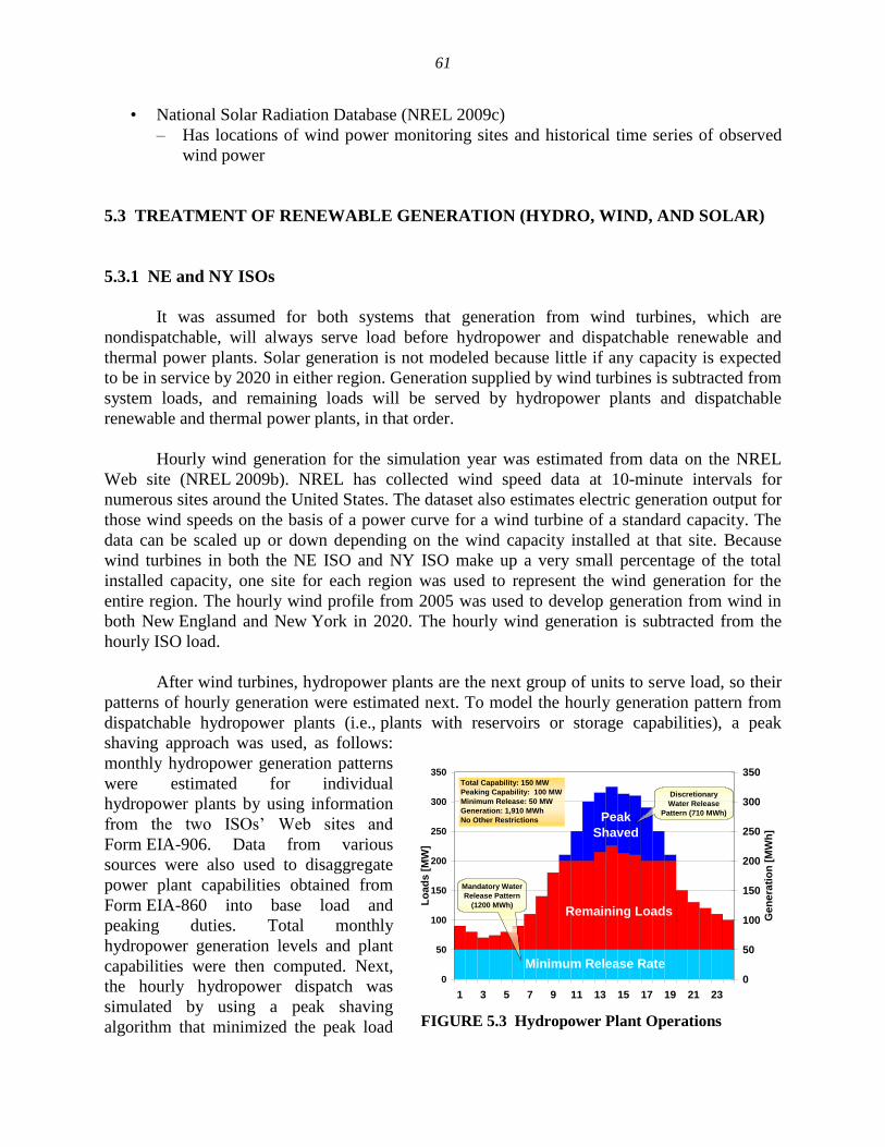
61

• National Solar Radiation Database (NREL 2009c)

– Has locations of wind power monitoring sites and historical time series of observed

wind power

5.3 TREATMENT OF RENEWABLE GENERATION (HYDRO, WIND, AND SOLAR)


It was assumed for both systems that generation from wind turbines, which are

nondispatchable, will always serve load before hydropower and dispatchable renewable and

thermal power plants. Solar generation is not modeled because little if any capacity is expected

to be in service by 2020 in either region. Generation supplied by wind turbines is subtracted from

system loads, and remaining loads will be served by hydropower plants and dispatchable

renewable and thermal power plants, in that order.

Hourly wind generation for the simulation year was estimated from data on the NREL

Web site (NREL 2009b). NREL has collected wind speed data at 10-minute intervals for

numerous sites around the United States. The dataset also estimates electric generation output for

those wind speeds on the basis of a power curve for a wind turbine of a standard capacity. The

data can be scaled up or down depending on the wind capacity installed at that site. Because

wind turbines in both the NE ISO and NY ISO make up a very small percentage of the total

installed capacity, one site for each region was used to represent the wind generation for the

entire region. The hourly wind profile from 2005 was used to develop generation from wind in

both New England and New York in 2020. The hourly wind generation is subtracted from the

hourly ISO load.

After wind turbines, hydropower plants are the next group of units to serve load, so their

patterns of hourly generation were estimated next. To model the hourly generation pattern from

dispatchable hydropower plants (i.e., plants with reservoirs or storage capabilities), a peak

shaving approach was used, as follows:

monthly hydropower generation patterns

were estimated for individual

hydropower plants by using information

from the two ISOs’ Web sites and

Form EIA-906. Data from various

sources were also used to disaggregate

power plant capabilities obtained from

Form EIA-860 into base load and

peaking duties. Total monthly

hydropower generation levels and plant

capabilities were then computed. Next,

the hourly hydropower dispatch was

simulated by using a peak shaving

algorithm that minimized the peak load

0

50

100

150

200

250

300

350

1 3 5 7 9 11 13 15 17 19 21 23

Lo

ad

s [

MW

]

0

50

100

150

200

250

300

350G

en

era

tio

n [

MW

h]

Minimum Release Rate

Remaining Loads

Peak

Shaved

Discretionary

Water Release

Pattern (710 MWh)

Mandatory Water

Release Pattern

(1200 MWh)

Total Capability: 150 MW

Peaking Capability: 100 MW

Minimum Release: 50 MW

Generation: 1,910 MWh

No Other Restrictions

FIGURE 5.3 Hydropower Plant Operations

62

that the thermal system must serve, subject to monthly hydropower capacity and energy

constraints, spinning reserve duties, hourly ramping constraints, and daily change limitations (see

Figure 5.3). The loads remaining after peak shaving were input to the thermal dispatch model.

5.3.2 WECC

Because hydropower provides a significant portion of electric generation in WECC, this

resource was modeled carefully in GTMax. Hydroelectric power was modeled on a plant-level

basis; each plant was assigned to a specific node in the network on the basis of WECC data.

Historical data from 1985 to 2005 in Form EIA-906 were used to develop an average monthly

capacity and energy value for each plant. Plants were categorized as providing baseload

generation (run-of-river plants), intermediate generation, or peaking generation. This information

was used to determine the amounts of both capacity and energy that would be available at

different times during the day. The data were summed for each node and input to the GTMax

model.

Wind and solar supply a smaller — but still significant — amount of electricity in

WECC. An inventory of wind and solar power plants was developed from EIA and WECC data.

This data identified capacity additions up to 2011. Projections of wind and solar capacity

additions from 2011 to 2020 were obtained from data in AEO 2009 (EIA 2009a). Capacity

projections were specified in each of four WECC subregions. Capacity was then assigned to

specific nodes on the basis of the node’s proportion of new capacity within the subregion.

Hourly wind and solar power profiles were developed from data available on the NREL

Web site. The NREL/3TIER Western Wind Resources Dataset was used for wind

(NREL 2009a), and the National Solar Radiation Database (NREL 2009c) was used for solar.

Data are available for numerous sites throughout the United States. Each dataset estimated

electric generation output for a wind or solar generating unit of a specific size based upon its

performance curve. The data were then scaled to the amount of wind and solar capacity assigned

to each node. Because nodes covered a wide geographic area, the generation at each node was

represented by the average of two sites that were highly rated for their wind potential and located

in different areas within the node. Wind and solar profiles from 2005 were used to develop

generation from both resources for WECC in 2020.


The Illinois electric system has only a single hydroelectric power plant, which is located

near Keokuk, Iowa, on the Mississippi River. It has no reservoir storage and is considered a run-

of-river plant. It has an installed capacity of about 112 MW. Because this plant contributes only a

small amount to the total Illinois generation, the plant was modeled as a thermal plant with fuel

costs equal to zero. Its capacity was set to 36 MW, which approximated the average capacity

factor of the plant.

63

The State of Illinois has enacted a Renewable Portfolio Standard (RPS), which specifies

through 2025 that an annually increasing amount of electric generation must be obtained from

renewable resources. In 2020, the RPS calls for 17.5% of Illinois’s energy to be supplied by

renewable resources, with a minimum of 75% coming from wind and 1% coming from solar

photovoltaic (PV). Because only a negligible amount of solar will be required by then, solar

energy was not modeled in this study. Although hydropower counts toward satisfying the RPS

requirement, the amount of hydropower in Illinois is miniscule. Therefore, it was decided that

wind alone would be used to comply with the RPS.

Using the NREL wind dataset, a site with strong wind potential was chosen from each of

four general geographic regions in Illinois (north, central, east, and west) to represent output

from wind turbines located in that region. NREL data showed hourly generation output at each

site for a wind turbine of a specific size. The hourly wind profile from 2005 was used to develop

generation from wind for 2020. Knowing the load profile for 2020, the hourly wind energy in

each region, and the RPS goal, an iterative technique was used to ―build‖ new wind capacity to

meet the RPS goal. An initial determination of the wind turbine capacity installed in each

geographic region was made such that the annual generation summed from all regions and all

hours met the annual RPS goal. This regional wind capacity was then placed geographically at

existing wind project sites and at proposed sites that have been publicly announced

(IWEA 2009). Wind turbines were connected to the grid at the nearest bus in the EMCAS

topology. If several buses were in close proximity to the wind site, the total wind turbine

capacity was divided equally among all nearby buses.

After placing the total installed wind turbine capacity, EMCAS was run to investigate the

amount of wind output that would be curtailed because of transmission congestion issues. Where

moderate congestion was observed, transmission line capability was increased by an amount

equal to the line’s capacity or 1,000 MW, whichever was smaller. Where excessive curtailment

was observed, wind capacity allocations were revised, moved to a different location, and/or

connected to a different bus. Several wind turbine capacity allocations and transmission line

capacity adjustments were made so that there was only a minor amount of wind curtailment in

the final configuration chosen for use in EMCAS.

5.4 DEVELOPING LOAD PROFILES


Figure 5.4 shows the process used to develop hourly load data for 2020 for both ISOs.

Historical hourly load data and future load forecasts were available on each ISO’s Web site.

Historical loads from 2000 to 2008 were used for the New England ISO and from 2001 to

2008 for the New York ISO. A model was used to determine which of those historical years was

most representative; that year was then used as the load shape for 2020.

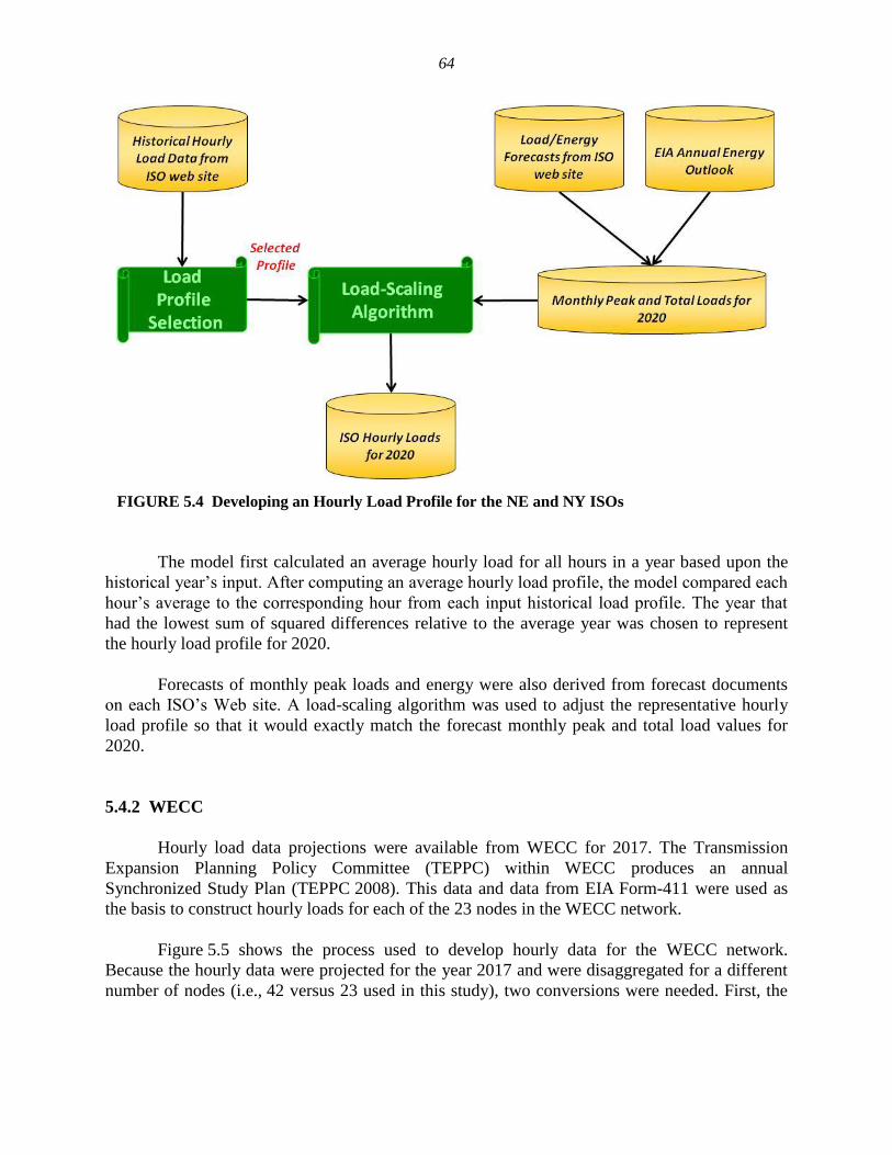
64

FIGURE 5.4 Developing an Hourly Load Profile for the NE and NY ISOs

The model first calculated an average hourly load for all hours in a year based upon the

historical year’s input. After computing an average hourly load profile, the model compared each

hour’s average to the corresponding hour from each input historical load profile. The year that

had the lowest sum of squared differences relative to the average year was chosen to represent

the hourly load profile for 2020.

Forecasts of monthly peak loads and energy were also derived from forecast documents

on each ISO’s Web site. A load-scaling algorithm was used to adjust the representative hourly

load profile so that it would exactly match the forecast monthly peak and total load values for

2020.

5.4.2 WECC

Hourly load data projections were available from WECC for 2017. The Transmission

Expansion Planning Policy Committee (TEPPC) within WECC produces an annual

Synchronized Study Plan (TEPPC 2008). This data and data from EIA Form-411 were used as

the basis to construct hourly loads for each of the 23 nodes in the WECC network.

Figure 5.5 shows the process used to develop hourly data for the WECC network.

Because the hourly data were projected for the year 2017 and were disaggregated for a different

number of nodes (i.e., 42 versus 23 used in this study), two conversions were needed. First, the

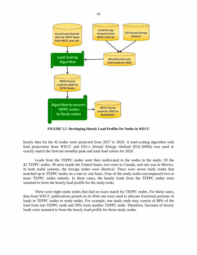
65

FIGURE 5.5 Developing Hourly Load Profiles for Nodes in WECC

hourly data for the 42 nodes were projected from 2017 to 2020. A load-scaling algorithm with

load projections from WECC and EIA’s Annual Energy Outlook (EIA 2009a) was used to

exactly match the forecast monthly peak and total load values for 2020.

Loads from the TEPPC nodes were then reallocated to the nodes in the study. Of the

42 TEPPC nodes, 39 were inside the United States, two were in Canada, and one was in Mexico.

In both nodal systems, the foreign nodes were identical. There were seven study nodes that

matched up to TEPPC nodes on a one-to–one basis. Four of the study nodes encompassed two or

more TEPPC nodes entirely. In these cases, the hourly loads from the TEPPC nodes were

summed to form the hourly load profile for the study node.

There were eight study nodes that had no exact match for TEPPC nodes. For these cases,

data from WECC publications posted on its Web site were used to allocate fractional portions of

loads in TEPPC nodes to study nodes. For example, one study node may consist of 88% of the

load from one TEPPC node and 50% from another TEPPC node. Therefore, fractions of hourly

loads were summed to form the hourly load profile for those study nodes.

66


Hourly load data for each bus was developed by first generating an hourly load profile

based upon historical data and then scaling that to match 2020 load and energy use projections.

As part of the original study for the Illinois Commerce Commission (ICC) (Cirillo et al. 2006),

hourly data were obtained from FERC Form 714, which contains total control area loads for all

hours of an historical year. This form also contains 10-year forecasts of seasonal peak loads and

total annual loads. To project hourly loads for a control area for the year 2007, historic hourly

loads were scaled such that the total annual load and both summer and winter peaks match the

Form 714 projection. This method produces results that exactly match the annual load factor

predicted by the reporting control areas.

Hourly loads at a bus are based on a bus distribution factor (BDF) that indicates the

portion of the total control area load assigned to that specific bus. The BDFs remain constant

throughout the simulation year and are based on input data for a peak load day using the

PowerWorld Simulator. PowerWorld Simulator is an interactive power system package designed

to simulate high-voltage power system operation. A BDF is multiplied by the hourly control area

load to obtain the hourly bus load; that is, the FERC Form 714 data that were scaled to the

projection year. This methodology assumed that the relative load contribution that a bus makes

to the control area total is constant throughout the year and will not change in the future. (Those

assumptions are reasonable for this type of study.) The procedure is described in greater detail in

Cirillo et al. (2006).

In order to extrapolate the load data for 2007 to year 2020, we first adjusted the 2007 load

data based on historical electricity sales from Illinois for that year. We then used peak load

forecasts from ComEd and the central region of the MISO to extrapolate the loads to 2020 by

multiplying the original hourly loads with a constant growth rate. In total, the hourly loads for

the ComEd region and the rest of Illinois were assumed to increase by 31% and 19%,

respectively, compared to the original study of Illinois. The growth rate for loads outside of the

state was assumed to be the same as for the rest of Illinois (i.e., 19%).

5.4.4 Forecasting PHEV Loads

For each study region, a set of three PHEV charging load profiles was developed; an

―unconstrained‖ scenario, a ―constrained‖ scenario, and a ―smart charge‖ scenario. Each profile

specifies the hourly amount of energy needed to charge PHEVs. This section describes how

these PHEV charging load profiles were developed. Load profiles for PHEV charging were

developed for a typical week in each of four seasons. PHEV charging loads were added to the

baseline scenario loads to determine the final load profiles for each scenario. It should be noted

that while each of the three scenarios use different amounts for PHEV hourly loads, the total

weekly PHEV load is the same.

Data used to calculate the PHEV charging profiles were presented in Chapter 3 and

include: (1) projections of the number of cars and SUVs on the road in each region; (2) the

hourly distribution of household vehicles arriving home after their last trips of the day; and

67

(3) the time required to charge PHEVs depending upon battery size. PHEVs were assumed to

comprise 10% of the vehicle fleet in 2020.

The number of vehicles on the road in each region was disaggregated by subregion based

upon U.S. Census data. In New England, data were aggregated for the whole region. In

New York, vehicle data were divided into the number of vehicles in the New York City

metropolitan statistical area (MSA) and the number of vehicles outside of New York City. In

WECC, vehicle data were divided into four WECC subregions: (1) California MSAs having a

population greater than 1 million; (2) vehicles in California MSAs having a population less than

1 million, including rural areas; (3) vehicles in MSAs within WECC but outside of California;

and (4) vehicles in non-MSAs within WECC but outside of California. In Illinois, vehicle data

were divided into the number of vehicles in the Chicago MSA and the number of vehicles in the

rest of Illinois.

PHEV charging loads were generated for a typical week in each of four seasons. To

generate hourly load profiles for the scenarios with PHEVs, seasonal PHEV hourly loads were

added to the baseline loads for that season.

5.4.4.1 Unconstrained Scenario

This scenario assumes that charging begins as soon as PHEVs arrive home after the final

trip of the day. The number of PHEVs by battery size was determined from the number of

conventional vehicles in a region and the distribution of PHEVs by battery size.

The hourly PHEV charging load is the sum of the load from PHEVs that arrived home in

that hour plus the load from PHEVs that arrived home in previous hours. Depending upon the

PHEV range (or battery type), a PHEV arriving home 1 to 4 hours earlier would still be

charging. Another consideration is that in the final hour of charge, the amount of energy needed

is less than that required in earlier hours. Therefore, a multiplier is used to modify the energy

needed in the final charging hour compared to earlier hours.

To determine PHEV charging load from vehicles that have arrived home, the total

number of PHEVs on the road by battery type is multiplied by the charge fraction. The charge

fraction is the distribution of vehicles arriving home after the last trip of the day for an entire

day. The charge fraction varies by season and type of day; namely, by weekday and weekend

day. Then, the number of vehicles arriving home in that hour is multiplied by the energy needed

to charge those vehicles. This multiplier varies by the type of electric service used at a

household; namely, voltage (V) and amperage (A). It was assumed that PHEV10 and PHEV20

owners have 110-V, 15-A service; PHEV30 owners have 110-V, 20-A service; and PHEV40

owners have 220-V, 20-A service.

To account for transmission losses and determine the load that the electric system must

serve, the PHEV hourly charging sum is divided by the transmission and distribution loss factor.

That factor varies by region, and the values used in this study are shown in Table 5.1.

68

TABLE 5.1 Transmission and Distribution Losses by

Region

Region

Transmission &

Distribution Loss

(%)

New England ISO 6.55

New York ISO 6.55

Illinois 5.54

California 7.96

WECC, excluding California 7.57

Source: EIA (2009b).

For the NE ISO case, the hourly PHEV charging profile was added to the baseline load

profile to determine the hourly load profile for this scenario. For the NY ISO case, hourly

profiles were developed for vehicles in the New York City MSA and for vehicles in the rest of

New York state. Both profiles were added to the baseline load profile to determine the hourly

load profile for this scenario.

In the WECC case, load profiles were developed for vehicles in each of the four

subregions. A methodology was developed to assign PHEV loads to appropriate nodes in the

network. The 23 nodes were grouped into three categories: namely, California urban, California

rural, and rest of WECC (i.e., no distinction between urban and rural). In California, it was clear

which nodes were urban and which rural; in the rest of WECC, however, some nodes had

characteristics of both profiles because of the fact that those nodes represented a wider

geographic area than those in California.

The PHEV charging load profiles developed for California urban MSAs (i.e., those with a

population greater than 1 million) were assigned to California urban nodes, and load profiles for

California suburban MSAs (i.e., those with a population of less than 1 million, including rural)

were assigned to California rural nodes. The PHEV load fraction assigned to each node equaled

its fraction of total California urban or rural baseline load.

The PHEV charging load profiles developed for the rest of the WECC MSAs and the rest

of the WECC non-MSAs were combined into one load profile. The PHEV load fraction assigned

to each rest-of-WECC node equaled its fraction of the total rest-of-WECC baseline load .

In the Illinois case, load profiles were developed for vehicles in each of 2 subregions.

Buses were categorized as either within the Chicago MSA or outside of Chicago (i.e., the rest of

Illinois). PHEV load profiles were assigned to the appropriate bus in the same proportion as the

bus’s contribution to the total baseline load for either the Chicago MSA or the rest of Illinois.

Loads in the nodes outside of Illinois were increased in the same proportions as the PHEV load

growth in the rest of Illinois.

69

5.4.4.2 Constrained Scenario

This scenario assumes charging begins 3 hours after the PHEV arrives home after the

final trip of the day. Determining the PHEV charging load in each hour of a typical seasonal

week is performed in the same way as in the unconstrained scenario; the hours to which the load

is assigned occur 3 hours later.

5.4.4.3 Smart Charge Scenario

This scenario assumes that smart meters are located in every home with a PHEV, and

PHEV charging is only performed during the hours with the lowest system loads. A load-shaping

algorithm was used on the baseline load profile for each region studied to determine when the

low load hours occurred and how much of the total load should be assigned to that hour to charge

PHEVs. This process is also known as ―valley filling.‖

Figure 5.6 compares the load profiles from all three scenarios in a typical week. It should

be noted that the area under the curves (i.e., the energy required to charge PHEVs in that week)

is the same for all scenarios.

5.5 CAPACITY EXPANSION MODELING

Both the unconstrained and constrained PHEV scenarios in each region had peak loads

that exceeded the peak loads in the base case. Because the Smart Charge scenario restricted

PHEV charging to only the lowest load hours of the day, it is the only scenario where the peak

load was the same as in the base case. Since peak loads increased in two scenarios, the impact on

system reliability was examined to determine whether additional capacity was needed to serve

this new load.

When deciding on new capacity additions, electric system operators are guided by the

reserve margin needed to maintain system reliability and the amount of new energy needed

within the time period. Operators add enough capacity to maintain a 15% reserve margin, that is,

an amount of installed capacity that is greater than the anticipated system peak load by 15%. The

overall capacity factor of the new additions is used to guide the selection of the type(s) of units

needed. Capacity factor is a measure of the plant’s actual output over a period of time compared

to the output it could generate if it operated at its maximum capacity over that same time period.

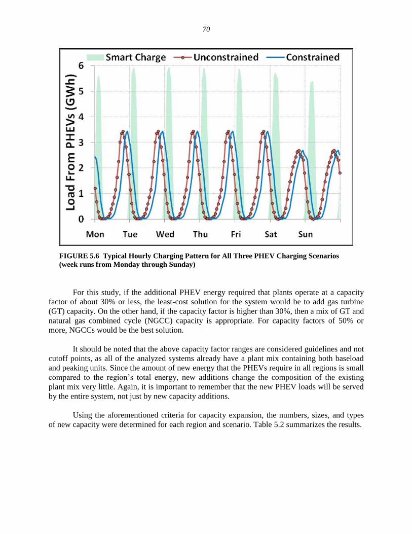
70

FIGURE 5.6 Typical Hourly Charging Pattern for All Three PHEV Charging Scenarios

(week runs from Monday through Sunday)

For this study, if the additional PHEV energy required that plants operate at a capacity

factor of about 30% or less, the least-cost solution for the system would be to add gas turbine

(GT) capacity. On the other hand, if the capacity factor is higher than 30%, then a mix of GT and

natural gas combined cycle (NGCC) capacity is appropriate. For capacity factors of 50% or

more, NGCCs would be the best solution.

It should be noted that the above capacity factor ranges are considered guidelines and not

cutoff points, as all of the analyzed systems already have a plant mix containing both baseload

and peaking units. Since the amount of new energy that the PHEVs require in all regions is small

compared to the region’s total energy, new additions change the composition of the existing

plant mix very little. Again, it is important to remember that the new PHEV loads will be served

by the entire system, not just by new capacity additions.

Using the aforementioned criteria for capacity expansion, the numbers, sizes, and types

of new capacity were determined for each region and scenario. Table 5.2 summarizes the results.

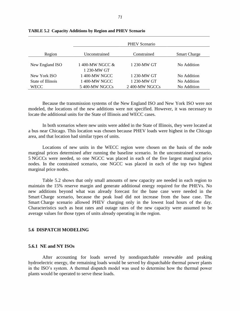
71

TABLE 5.2 Capacity Additions by Region and PHEV Scenario

Region

PHEV Scenario

Unconstrained Constrained Smart Charge

New England ISO 1 400-MW NGCC &

1 230-MW GT

1 230-MW GT No Addition

New York ISO 1 400-MW NGCC 1 230-MW GT No Addition

State of Illinois 1 400-MW NGCC 1 230-MW GT No Addition

WECC 5 400-MW NGCCs 2 400-MW NGCCs No Addition

Because the transmission systems of the New England ISO and New York ISO were not

modeled, the locations of the new additions were not specified. However, it was necessary to

locate the additional units for the State of Illinois and WECC cases.

In both scenarios where new units were added in the State of Illinois, they were located at

a bus near Chicago. This location was chosen because PHEV loads were highest in the Chicago

area, and that location had similar types of units.

Locations of new units in the WECC region were chosen on the basis of the node

marginal prices determined after running the baseline scenario. In the unconstrained scenario,

5 NGCCs were needed, so one NGCC was placed in each of the five largest marginal price

nodes. In the constrained scenario, one NGCC was placed in each of the top two highest

marginal price nodes.

Table 5.2 shows that only small amounts of new capacity are needed in each region to

maintain the 15% reserve margin and generate additional energy required for the PHEVs. No

new additions beyond what was already forecast for the base case were needed in the

Smart Charge scenario, because the peak load did not increase from the base case. The

Smart Charge scenario allowed PHEV charging only in the lowest load hours of the day.

Characteristics such as heat rates and outage rates of the new capacity were assumed to be

average values for those types of units already operating in the region.

5.6 DISPATCH MODELING


After accounting for loads served by nondispatchable renewable and peaking

hydroelectric energy, the remaining loads would be served by dispatchable thermal power plants

in the ISO’s system. A thermal dispatch model was used to determine how the thermal power

plants would be operated to serve these loads.

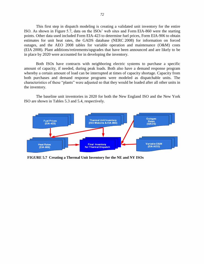
72

This first step in dispatch modeling is creating a validated unit inventory for the entire

ISO. As shown in Figure 5.7, data on the ISOs’ web sites and Form EIA-860 were the starting

points. Other data used included Form EIA-423 to determine fuel prices, Form EIA-906 to obtain

estimates for unit heat rates, the GADS database (NERC 2008) for information on forced

outages, and the AEO 2008 tables for variable operation and maintenance (O&M) costs

(EIA 2008). Plant additions/retirements/upgrades that have been announced and are likely to be

in place by 2020 were accounted for in developing the inventory.

Both ISOs have contracts with neighboring electric systems to purchase a specific

amount of capacity, if needed, during peak loads. Both also have a demand response program

whereby a certain amount of load can be interrupted at times of capacity shortage. Capacity from

both purchases and demand response programs were modeled as dispatchable units. The

characteristics of these ―plants‖ were adjusted so that they would be loaded after all other units in

the inventory.

The baseline unit inventories in 2020 for both the New England ISO and the New York

ISO are shown in Tables 5.3 and 5.4, respectively.

FIGURE 5.7 Creating a Thermal Unit Inventory for the NE and NY ISOs

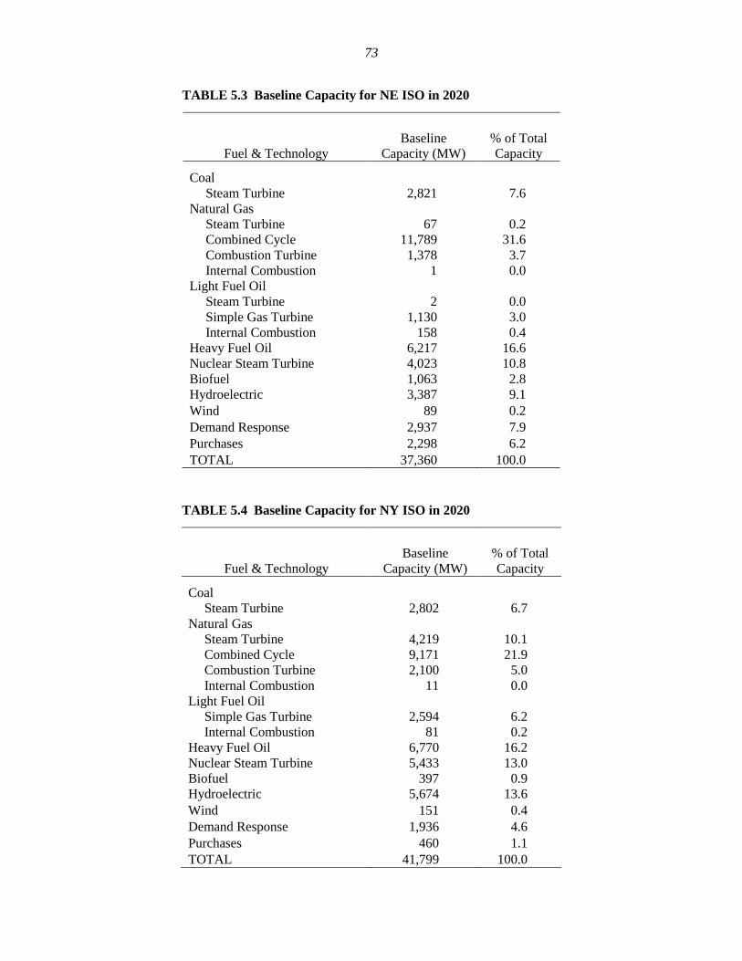
73

TABLE 5.3 Baseline Capacity for NE ISO in 2020

Fuel & Technology

Baseline

Capacity (MW)

% of Total

Capacity

Coal

Steam Turbine 2,821 7.6

Natural Gas

Steam Turbine 67 0.2

Combined Cycle 11,789 31.6

Combustion Turbine 1,378 3.7

Internal Combustion 1 0.0

Light Fuel Oil

Steam Turbine 2 0.0

Simple Gas Turbine 1,130 3.0


Heavy Fuel Oil 6,217 16.6

Nuclear Steam Turbine 4,023 10.8

Biofuel 1,063 2.8

Hydroelectric 3,387 9.1

Wind 89 0.2

Demand Response 2,937 7.9

Purchases 2,298 6.2

TOTAL 37,360 100.0

TABLE 5.4 Baseline Capacity for NY ISO in 2020

Fuel & Technology

Baseline

Capacity (MW)

% of Total

Capacity

Coal


Natural Gas





Light Fuel Oil

Simple Gas Turbine 2,594 6.2




Biofuel 397 0.9

Hydroelectric 5,674 13.6

Wind 151 0.4

Demand Response 1,936 4.6

Purchases 460 1.1

TOTAL 41,799 100.0

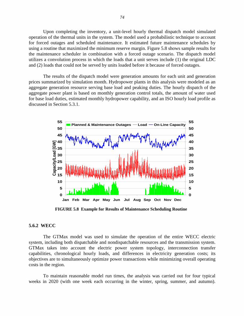
74

Upon completing the inventory, a unit-level hourly thermal dispatch model simulated

operation of the thermal units in the system. The model used a probabilistic technique to account

for forced outages and scheduled maintenance. It estimated future maintenance schedules by

using a routine that maximized the minimum reserve margin. Figure 5.8 shows sample results for

the maintenance scheduler in combination with a forced outage scenario. The dispatch model

utilizes a convolution process in which the loads that a unit serves include (1) the original LDC

and (2) loads that could not be served by units loaded before it because of forced outages.

The results of the dispatch model were generation amounts for each unit and generation

prices summarized by simulation month. Hydropower plants in this analysis were modeled as an

aggregate generation resource serving base load and peaking duties. The hourly dispatch of the

aggregate power plant is based on monthly generation control totals, the amount of water used

for base load duties, estimated monthly hydropower capability, and an ISO hourly load profile as

discussed in Section 5.3.1.

0

5

10

15

20

25

30

35

40

45

50

55

Jan Feb Mar Apr May Jun Jul Aug Sep Oct Nov Dec

Cap

ac

ity

/Lo

ad

[G

W]

0

5

10

15

20

25

30

35

40

45

50

55Planned & Maintenance Outages Load On-Line Capacity

FIGURE 5.8 Example for Results of Maintenance Scheduling Routine

5.6.2 WECC

The GTMax model was used to simulate the operation of the entire WECC electric

system, including both dispatchable and nondispatchable resources and the transmission system.

GTMax takes into account the electric power system topology, interconnection transfer

capabilities, chronological hourly loads, and differences in electricity generation costs; its

objectives are to simultaneously optimize power transactions while minimizing overall operating

costs in the region.

To maintain reasonable model run times, the analysis was carried out for four typical

weeks in 2020 (with one week each occurring in the winter, spring, summer, and autumn).

75

GTMax simulated hourly system operations during the second week of the months of January,

April, July, and October of 2020.

Simulating operation of WECC’s electric system on an hour-by-hour basis for an entire

week (168 consecutive hours) was considered very important in order to capture the operational

behavior of hydropower and pumped-storage power plants. Most hydropower plants in the

region have at least daily regulation capabilities and operate differently during the peak and off-

peak hours (e.g., during the day and during the night). Also, in the case of hydro plants with

greater storage capabilities, there are significant differences between their operation during the

weekdays and during the weekends.

To develop a validated unit inventory of thermal and dispatchable renewable power

plants to input to GTMax, a strategy similar to the New England and New York ISO cases was

used. Data from the WECC Web site and Form EIA-860 were the starting points. Fuel price data

were obtained from Form EIA-423, heat rates were estimated from Form EIA-906, forced outage

data from the GADS database, and O&M costs from AEO 2008 tables. Plant

additions/retirements/upgrades that have been announced and are likely to be in place by 2020

were accounted for in developing the inventory. The baseline unit inventories in 2020 that are

disaggregated by generators located in California and those located in the rest of WECC are

shown in Table 5.5.

Because of the large number of generating units in the WECC inventory, the dataset was

input to GTMax as a supply curve rather than as individual units. The generating units were

aggregated at the node to which they were assigned and represented as a curve of cost as a

function of capacity.

Data were input to GTMax for renewable generators such as hydroelectric, wind, and

solar by using the methodology described in Section 5.3.2.

Because the GTMax model does not automatically plan a maintenance schedule for

thermal units, a schedule was determined exogenously using a maintenance scheduler routine,

which was the same routine from the dispatch model used for the New England and New York

ISO cases (see Section 5.6.1). The thermal generating unit inventory was input, along with

annual hourly load data for 2020. The maintenance schedule was determined such that the

minimum reserve margin was maximized. After the maintenance schedule was determined, the

unit inventory input to GTMax was adjusted such that units were not allowed to operate in time

periods simulated by GTMax when the maintenance scheduler had determined that they would

be on maintenance.

Another point to consider is that the GTMax model does not automatically account for

forced outages at thermal plants. To adjust for this condition, the unit size was derated in

proportion to its forced outage rate (FOR); for example, if a plant’s FOR was 5%, its capacity

was reduced by 5%.

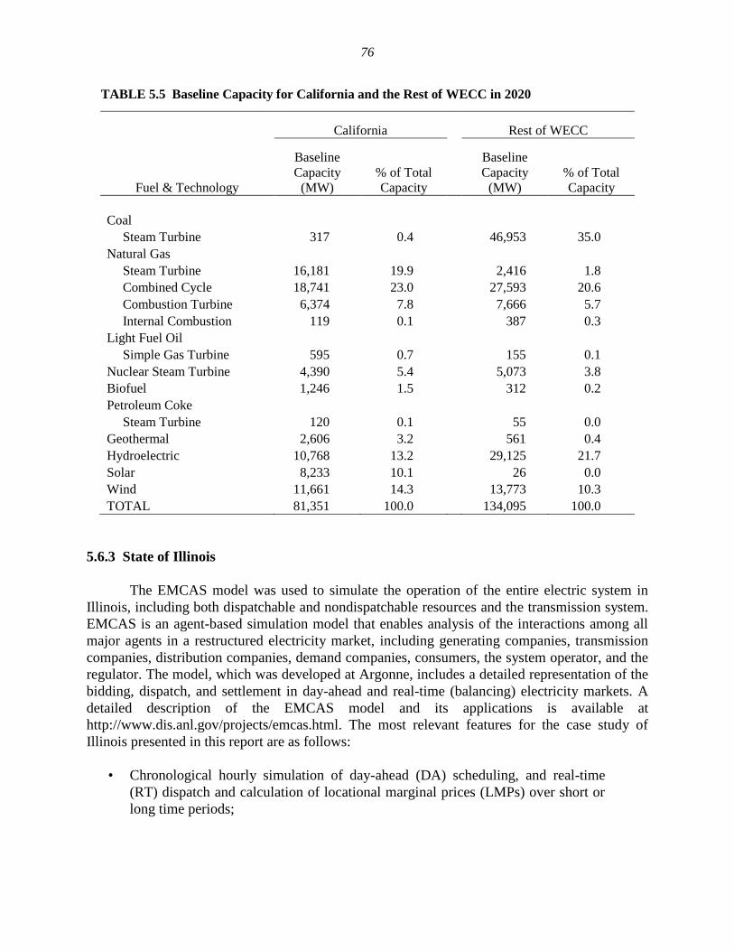
76

TABLE 5.5 Baseline Capacity for California and the Rest of WECC in 2020

California

Rest of WECC

Fuel & Technology

Baseline

Capacity

(MW)

% of Total

Capacity

Baseline

Capacity

(MW)

% of Total

Capacity

Coal

Steam Turbine 317 0.4 46,953 35.0

Natural Gas

Steam Turbine 16,181 19.9 2,416 1.8

Combined Cycle 18,741 23.0 27,593 20.6

Combustion Turbine 6,374 7.8 7,666 5.7

Internal Combustion 119 0.1 387 0.3

Light Fuel Oil

Simple Gas Turbine 595 0.7 155 0.1

Nuclear Steam Turbine 4,390 5.4 5,073 3.8

Biofuel 1,246 1.5 312 0.2

Petroleum Coke

Steam Turbine 120 0.1 55 0.0

Geothermal 2,606 3.2 561 0.4

Hydroelectric 10,768 13.2 29,125 21.7

Solar 8,233 10.1 26 0.0

Wind 11,661 14.3 13,773 10.3

TOTAL 81,351 100.0 134,095 100.0


The EMCAS model was used to simulate the operation of the entire electric system in

Illinois, including both dispatchable and nondispatchable resources and the transmission system.

EMCAS is an agent-based simulation model that enables analysis of the interactions among all

major agents in a restructured electricity market, including generating companies, transmission

companies, distribution companies, demand companies, consumers, the system operator, and the

regulator. The model, which was developed at Argonne, includes a detailed representation of the

bidding, dispatch, and settlement in day-ahead and real-time (balancing) electricity markets. A

detailed description of the EMCAS model and its applications is available at

http://www.dis.anl.gov/projects/emcas.html. The most relevant features for the case study of

Illinois presented in this report are as follows:

• Chronological hourly simulation of day-ahead (DA) scheduling, and real-time

(RT) dispatch and calculation of locational marginal prices (LMPs) over short or

long time periods;

77

• Hourly transmission-constrained market clearing by using a Direct-Current

Optimal Power Flow (DC OPF) algorithm in day-ahead and real-time markets;

• Inclusion of planned outages and random forced outages in market simulations;

• Possibility of specifying different market rules (e.g., regarding congestion

management, price caps and bid caps in the energy market);

• Calculation of prices and profits based on the ―two-settlement system‖ (i.e., DA

price for DA schedule, and RT price for deviations between RT dispatch and DA

schedule);

• Calculation of generation and emissions by generation unit, generating company,

and fuel type; and

• Calculation of cost, revenues, and profits for all market participants (agents).

The Illinois power system was simulated assuming a competitive electricity market into

which all generation is bid into the market based on its marginal production cost. Hence, the

simulated power system is dispatched according to a least-cost objective. The focus is placed on

how an increase in electric loads that results from charging PHEVs changes the dispatch and

operation of the system.

Similar to the WECC case, the analysis was carried out for four typical weeks in 2020

(one week each during the seasons of winter, spring, summer, and autumn) to maintain

reasonable model run times. EMCAS simulated hourly system operations during the second

week of the months of January, April, July, and October of 2020.

The same unit inventory of thermal power plants as in the original ICC study

(Cirillo et. al. 2006) was used as a starting point for this analysis. Fuel prices were updated based

on EIA projections for 2020. Plant additions/retirements/upgrades that have been announced and

are likely to be in place by 2020 were accounted for in developing the inventory. Furthermore,

because buses and transmission lines were explicitly modeled, new transmission lines and

upgrades to existing lines that are likely to be in place by 2020 were estimated. The baseline unit

inventory in 2020 for Illinois is shown in Table 5.6.

Data were input to EMCAS for renewable generators, such as hydroelectric and wind,

using the methodology described in Section 5.3.3. Generating capacity outside of Illinois was

represented in a simplified manner, similar to the representation in the original Illinois study

(Cirillo et al. 2006). Hence, all the generation capacity in each out-of-state node was represented

as an aggregate supply curve with multiple cost steps. The total capacity of each curve was

increased according to the assumed growth for out-of-state load (i.e., by 19%) to a total out-of-

state capacity of 201,600 MW. The costs of each supply step on the aggregated curves were also

adjusted according to the assumed fuel prices for 2020. The aggregate out-of-state supply curves

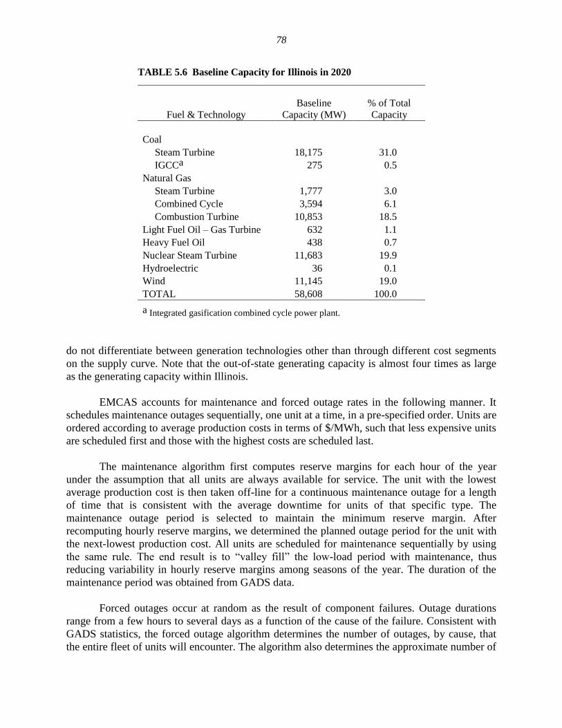
78

TABLE 5.6 Baseline Capacity for Illinois in 2020

Fuel & Technology

Baseline

Capacity (MW)

% of Total

Capacity

Coal


IGCCa 275 0.5

Natural Gas




Light Fuel Oil – Gas Turbine 632 1.1

Heavy Fuel Oil 438 0.7


Hydroelectric 36 0.1

Wind 11,145 19.0

TOTAL 58,608 100.0

a Integrated gasification combined cycle power plant.

do not differentiate between generation technologies other than through different cost segments

on the supply curve. Note that the out-of-state generating capacity is almost four times as large

as the generating capacity within Illinois.

EMCAS accounts for maintenance and forced outage rates in the following manner. It

schedules maintenance outages sequentially, one unit at a time, in a pre-specified order. Units are

ordered according to average production costs in terms of $/MWh, such that less expensive units

are scheduled first and those with the highest costs are scheduled last.

The maintenance algorithm first computes reserve margins for each hour of the year

under the assumption that all units are always available for service. The unit with the lowest

average production cost is then taken off-line for a continuous maintenance outage for a length

of time that is consistent with the average downtime for units of that specific type. The

maintenance outage period is selected to maintain the minimum reserve margin. After

recomputing hourly reserve margins, we determined the planned outage period for the unit with

the next-lowest production cost. All units are scheduled for maintenance sequentially by using

the same rule. The end result is to ―valley fill‖ the low-load period with maintenance, thus

reducing variability in hourly reserve margins among seasons of the year. The duration of the

maintenance period was obtained from GADS data.

Forced outages occur at random as the result of component failures. Outage durations

range from a few hours to several days as a function of the cause of the failure. Consistent with

GADS statistics, the forced outage algorithm determines the number of outages, by cause, that

the entire fleet of units will encounter. The algorithm also determines the approximate number of

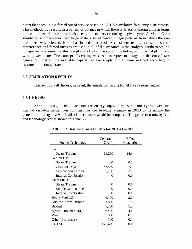
79

hours that each unit is forced out of service based on GADS cumulative frequency distributions.

This methodology results in a pattern of outages in which there is diversity among units in terms

of the number of hours that each one is out of service during a given year. A Monte Carlo

simulation approach was used to generate a set of forced outage patterns from which the one

used here was selected. Note that in order to produce consistent results, the same set of

maintenance and forced outages are used in all of the scenarios in the analysis. Furthermore, no

outages were assumed for the new plants added to the system, including both thermal plants and

wind power plants. The concept of derating was used to represent outages in the out-of-state

generation; that is, the available capacity of the supply curves were reduced according to

assumed total outage rates.

5.7 SIMULATION RESULTS

This section will discuss, in detail, the simulation results for all four regions studied.

5.7.1 NE ISO

After adjusting loads to account for energy supplied by wind and hydropower, the

thermal dispatch model was run first for the baseline scenario in 2020 to determine the

generation mix against which all other scenarios would be compared. The generation mix by fuel

and technology type is shown in Table 5.7.

TABLE 5.7 Baseline Generation Mix for NE ISO in 2020

Fuel & Technology

Generation

(GWh)

% Total

Generation

Coal


Natural Gas





Light Fuel Oil

Steam Turbine 0 0.0

Simple Gas Turbine 100 0.1




Biofuel 7,700 5.3

Hydro/pumped Storage 6,400 4.4

Wind 300 0.2

Other (Purchases) 100 0.1

TOTAL 145,400 100.0

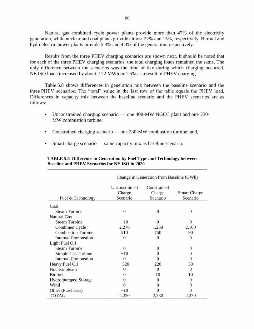
80

Natural gas combined cycle power plants provide more than 47% of the electricity

generation, while nuclear and coal plants provide almost 22% and 15%, respectively. Biofuel and

hydroelectric power plants provide 5.3% and 4.4% of the generation, respectively.

Results from the three PHEV charging scenarios are shown next. It should be noted that

for each of the three PHEV charging scenarios, the total charging loads remained the same. The

only difference between the scenarios was the time of day during which charging occurred.

NE ISO loads increased by about 2.22 MWh or 1.5% as a result of PHEV charging.

Table 5.8 shows differences in generation mix between the baseline scenario and the

three PHEV scenarios. The ―total‖ value in the last row of the table equals the PHEV load.

Differences in capacity mix between the baseline scenario and the PHEV scenarios are as

follows:

• Unconstrained charging scenario — one 400-MW NGCC plant and one 230-

MW combustion turbine;

• Constrained charging scenario — one 230-MW combustion turbine; and,

• Smart charge scenario — same capacity mix as baseline scenario.

TABLE 5.8 Difference in Generation by Fuel Type and Technology between

Baseline and PHEV Scenarios for NE ISO in 2020

Change in Generation from Baseline (GWh)

Fuel & Technology

Unconstrained

Charge

Scenario

Constrained

Charge

Scenario

Smart Charge

Scenario

Coal

Steam Turbine 0 0 0

Natural Gas

Steam Turbine −10 0 0

Combined Cycle 2,270 1,250 2,100

Combustion Turbine 510 750 90

Internal Combustion 0 0 0

Light Fuel Oil

Steam Turbine 0 0 0

Simple Gas Turbine −10 0 0


Heavy Fuel Oil −520 220 30

Nuclear Steam 0 0 0

Biofuel 0 10 10

Hydro/pumped Storage 0 0 0

Wind 0 0 0

Other (Purchases) −10 0 0

TOTAL 2,230 2,230 2,230

81

The following observations were made after comparing differences in the generation mix

between the baseline scenario and the PHEV charging scenarios. In the unconstrained scenario,

generation from natural gas–fired plants, particularly NGCCs, increased significantly; slightly

more than the load increased from PHEV charging. Baseloaded plants, such as coal and nuclear,

did not increase generation relative to the baseline. Generation from non-baseload plants, such as

those fueled by heavy fuel oil, decreased.

The reason that coal and nuclear plants were unable to increase generation in this

scenario can be seen by examining their capacity factors in the baseline scenario. Their capacity

factors were between 86% and 90%, which meant they were already fully loaded. Therefore,

they could not generate additional energy to serve new PHEV loads. Generation from

hydropower and wind turbines did not increase because those resources are limited.

NGCC plants were able to increase generation significantly because these plants operated

at less-than-full capacity in the baseline scenario; their average capacity factor was about 65%.

Operation of NGCC plants is generally the most economical after nuclear and coal plants. This

scenario also had one additional NGCC plant compared to the baseline scenario.

Generation from combustion turbines also increased partially due to operating at a

capacity factor of about 30%. Gas turbines typically generate during peak loads, and since some

PHEV loads occurred during peak afternoon hours, these plants were able to pick up the slack.

This scenario also had one additional combustion turbine compared to the baseline scenario.

In the constrained scenario, only a single 230-MW combustion turbine was added to the

inventory. As in the unconstrained scenario, natural gas–fired plants significantly increased their

generation. Plants using heavy fuel oil and biofuel increased generation only slightly. Generation

from baseload plants and plants using resource-constrained renewable fuels did not increase

similar to the unconstrained scenario. The reasons these generation patterns occurred were the

same as in the unconstrained scenario.

In the smart charge scenario, no new capacity was added. Natural gas–fired plants

generated 98% of the increase resulting from PHEV charging, with NGCC plants alone

generating almost 95%. As in the unconstrained and constrained scenarios, increased generation

from NGCCs was expected because they are efficient, have moderate production costs, and are

not fully loaded, especially at night when the PHEV charging occurs in this scenario. Therefore,

they are available to generate the electricity needed at a reasonable cost.

5.7.2 NY ISO

After adjusting loads to account for energy supplied by wind and hydropower, the

thermal dispatch model was run first for the baseline scenario in 2020 to determine the

generation mix against which all other scenarios would be compared. The generation mix by fuel

and technology type is shown in Table 5.9.

82

TABLE 5.9 Baseline Generation Mix for NY ISO in 2020

Fuel & Technology

Generation

(GWh)

% Total

Generation

Coal


Natural Gas





Light Fuel Oil

Simple Gas Turbine 90 0.1




Biofuel 30 0.0


Wind 450 0.3

Other (Purchases) 10 0.0

TOTAL 176,050 100.0

Natural gas–fired power plants provide 45% of the total electric generation; combined

cycle plants alone provide more than 33% of that total. Nuclear and coal plants provide about

24% and 12%, respectively, while hydroelectric power plants provide almost 15% of the system

generation.


for each of the three PHEV charging scenarios, the total charging loads remained the same. The

only difference between the scenarios was the time of day during which charging occurred.

NY ISO loads increased by about 2.09 MWh or 1.2% as a result of PHEV charging.


three PHEV scenarios. The ―total‖ value in the last row of the table equals the PHEV load.

Differences in capacity mix between the baseline scenario and the PHEV scenarios are as

follows:

• Unconstrained charging scenario — one 400-MW NGCC plant;

• Constrained charging scenario — one 230-MW combustion turbine; and,


83


Baseline and PHEV Scenarios for NY ISO in 2020


Fuel & Technology

Unconstrained

Charge

Scenario

Constrained

Charge

Scenario

Smart Charge

Scenario

Coal

Steam Turbine 0 0 0

Natural Gas

Steam Turbine −270 220 610

Combined Cycle 2,400 190 1,180

Combustion Turbine −70 1,620 280


Light Fuel Oil

Simple Gas Turbine 0 0 0


Heavy Fuel Oil 20 50 10

Nuclear Steam 0 0 0

Biofuel 0 0 0


Wind 0 0 0

Other (Purchases) 0 0 0

TOTAL 2,080 2,080 2,080

The following observations were made after comparing differences in the generation mix

between the baseline scenario and the PHEV charging scenarios. In the unconstrained scenario,

generation by NGCC plants increased more than the load increased as a result of PHEV

charging. Generation from baseloaded plants, such as coal and nuclear, did not increase relative

to the baseline. Generation by non-baseloaded plants decreased, except for plants fueled by

heavy fuel oil, which had only a marginal increase in generation.

The reason that coal and nuclear plants were unable to increase generation in this

scenario can be seen by examining their capacity factors in the baseline scenario. Their capacity

factors were between 85% and 90%, which meant they were already fully loaded. Therefore,

they could not generate additional energy to serve new PHEV loads. Generation from

hydropower and wind turbines did not increase because those resources are limited.

NGCC plants were able to increase generation significantly because these plants operated

at less-than-full capacity in the baseline scenario; their average capacity factor was about 70%.

Operation of NGCC plants is generally the most economical after nuclear and coal plants. This

scenario also had added one NGCC plant compared to the baseline scenario. Generation from

84

NGCCs also displaced generation from other natural gas–fired plants, whose generation

decreased in this scenario, because operation of NGCCs is more economical.


inventory. In this scenario, natural gas–fired plants significantly increased their generation, but

most of that increase came from combustion turbines. This result was expected because a

combustion turbine was added to the unit inventory. Generation from NGCC plants increased

because their operation is economical and their capacity was not fully utilized, as seen from the

capacity factors in the baseline scenario.

In the smart charge scenario, no new capacity was added. Natural gas–fired plants again

generated more than 99% of the increase resulting from PHEV charging, with NGCC plants

alone generating almost 57%. As in the unconstrained and constrained scenarios, generation

increase from NGCCs was expected because they are efficient, have moderate production costs,

and are not fully loaded, especially at night when the PHEV charging occurs in this scenario.

Other natural gas–fired plants increased generation because they also had excess capacity and a

moderate production cost.

5.7.3 WECC

The GTMax model was run first for the baseline scenario in 2020 to determine the

generation mix against which all other scenarios would be compared. Because California imports

a significant quantity of electricity from other areas of the WECC, the generation mix is

disaggregated into two subareas: (1) California including imports; and (2) the rest of WECC,

excluding California exports. The generation mixes by fuel and technology type for these two

areas are shown in Table 5.11 and Table 5.12, respectively. Because the model calculated results

for a typical week in each of four seasons, results for each season were estimated by multiplying

weekly results by approximately 13.0357. This factor was used to scale the results from a week,

which consists of 168 hours, to a season, which consists of 2,190 hours, assuming seasons are of

equal length. Values for all four seasons were then summed to obtain annual generation

estimates.

More than half of California’s electric generation is supplied by natural gas plants,

including more than 38% from NGCCs, 12% from steam turbines, and about 2% from

combustion turbines. Nuclear power plants supply more than 11% of the generation, while wind

turbines and hydropower supply about 10% each. Coal-fired power plants supply about 6% and

geothermal about 5%.

In the rest of WECC, more than 53% of the load is served by coal-fired power plants and

almost 25% by hydropower. Nuclear plants serve about 7%, and natural gas–fired plants serve

only 3%. The remaining generating sources serve less than 1% of the load.

85

TABLE 5.11 Baseline Generation Mix for California in 2020

(including imports)

Fuel & Technology

Generation

(MWh)

% Total

Generation

Coal


Natural Gas





Light Fuel Oil

Gas Turbine 0 0.0


Biofuel 3,600 1.1

Petroleum Coke 900 0.3

Geothermal 17,200 5.0


Solar 14,500 4.2

Wind 35,400 10.4

TOTAL 341,200 100.0

TABLE 5.12 Baseline Generation Mix for Rest of WECC

(excluding California exports) in 2020

Fuel & Technology

Generation

(GWh)

% Total

Generation

Coal


Natural Gas






Biofuel 200 0.04

Petroleum Coke 200 0.03

Geothermal 3,900 0.7


Solar 100 0.0

Wind 63,200 11.1

TOTAL 567,800 100.0

86

The model was run next with data for each of the three PHEV charging scenarios. It

should be noted that the total weekly charging load for all three PHEV scenarios was the same.

The only difference between the scenarios was the time of day during which charging occurred.

WECC loads in California increased by about 6.34 MWh or 1.9% as a result of PHEV charging;

the rest of the WECC loads increased by about 4.34 MWh or almost 0.8% as a result of PHEV

charging.

Tables 5.13 and 5.14 show differences in generation mix between the baseline scenario

and the three PHEV scenarios for California loads and the rest of the WECC loads, respectively.

The ―total‖ value in the last row of the table is the PHEV load. Differences in the capacity mix

between the baseline scenario and the PHEV scenarios are as follows:

• Unconstrained charging scenario — five 400-MW NGCC plants: four assigned to

California nodes and one to a node outside of California;

• Constrained charging scenario — two 400-MW NGCC plants: one assigned to a

California node and one to a node outside of California; and,


TABLE 5.13 Difference in Generation by Fuel Type and Technology between Baseline and

PHEV Scenarios for California in 2020


Fuel & Technology

Unconstrained

Charge Scenario

Constrained Charge

Scenario

Smart Charge

Scenario

Coal

Steam Turbine −1,750 −2,030 −2,550

Natural Gas

Steam Turbine 760 800 640

Combined Cycle 6,830 6,940 7,690



Light Fuel Oil


Nuclear Steam −20 −40 60

Biofuel −20 −50 10

Petroleum Coke 0 0 10

Geothermal 0 0 0


Solar 0 0 0

Wind 0 0 0

TOTAL 6,340 6,340 6,340

87

TABLE 5.14 Difference in Generation by Fuel Type and Technology between Baseline and

PHEV Scenarios for WECC (excluding California) in 2020


Fuel & Technology

Unconstrained

Charge Scenario

Constrained Charge

Scenario

Smart Charge

Scenario

Coal

Steam Turbine 1,830 2,460 4,010

Natural Gas

Steam Turbine 0 0 0

Combined Cycle 2,490 1,910 380

Combustion Turbine 20 −20 −40


Light Fuel Oil


Nuclear Steam 0 0 0

Biofuel 0 0 0

Petroleum Coke 0 0 0

Geothermal 0 0 0


Solar 0 0 0

Wind 0 0 0

TOTAL 4,340 4,340 4,340

The following observations can be made after comparing differences in the generation

mix between the baseline scenario and the PHEV charging scenarios. In the unconstrained

scenario for California, natural gas–fired power plants are virtually the only plants that increased

generation compared to the baseline scenario; there was either no change in generation from

other plants or there were only marginal changes. Generation from natural gas–fired plants

increased more than the load increase as a result of PHEV charging in California.

Examining details at the node level revealed that the reduction in coal generation serving

California loads was attributable to a combination of higher loads in the rest of WECC and

transmission congestion. Coal makes up less than 0.5% of the generation capacity located in

California, although more than 6% of the generation in the baseline scenario is from coal; the

majority is imported. However, in the unconstrained PHEV scenario, all of the WECC had

higher loads as a result of PHEV charging: that source of low-cost generation served nearby

loads and therefore was not available for export to California. Transmission congestion also

played a role; transmission lines reached their capacity limits, and therefore cheaper coal plants

could not export power to California. In one instance, an excess of wind turbine capacity caused

an ―over supply‖ pocket, which did not allow generation from low-cost coal plants to be

exported to California. Therefore, natural gas plants increased generation to serve the increased

loads. Furthermore, four of the five NGCCs that were added in this scenario were assigned to

nodes in California.

88

In the unconstrained scenario for the rest of WECC, coal and natural gas plants were the

only two fuel types that increased generation to serve the additional load. Natural gas plants

served about 58% of the load increase while coal plants served the remaining 42%. The increase

in NGCC generation was partially attributable to the addition of an NGCC unit at a node outside

of California.

In both California and the rest of the WECC cases, the amount of load served by nuclear

power plants did not increase; there was only a marginal decrease in California. Examination of

nuclear plant capacity factors in the baseline scenario showed that they were operating at a

maximum capacity factor and could not generate any additional energy to serve the new PHEV

charging load. The slight decrease in nuclear power plant generation in the California case may

be attributable to modeling ―noise‖ and transmission congestion.

Similar results were found in the constrained and smart charge scenarios. In the

California case, coal generation decreased sharply while natural gas generation, particularly from

NGCC plants, increased sharply. Generation from natural gas plants increased by more than the

increase from PHEV charging to compensate for coal imports lost because of transmission

congestion and for higher loads served in the locations outside of California. California had one

additional NGCC plant in the constrained scenario than it had in the baseline scenario, although

no capacity was added in the smart charge scenario.

In the rest of WECC, coal generation increased sharply in the constrained and smart

charge scenarios, providing 57% and 92%, respectively, of the increased generation. The

remainder was provided by increased generation from NGCC plants. The rest of WECC had one

additional NGCC plant in the constrained scenario compared to the baseline scenario, although

no capacity was added in the smart charge scenario.

Finally, nuclear power plants could not increase generation in either the constrained or

smart charge scenarios. As in the unconstrained case, these plants had no excess capacity with

which to serve the additional load.


The model was run first for the baseline scenario in 2020 to determine the generation mix

against which all other scenarios would be compared. The generation mix by fuel and technology

type is shown in Table 5.15. Because the model calculated results for a typical week in each of

four seasons, results for each season was estimated by multiplying weekly results by 13.0357.

This factor was used to scale the results from a week, which consists of 168 hours, to a season,

which consists of 2,190 hours (assuming seasons are of equal length). Values for all four seasons

were then summed to obtain annual generation estimates.

Coal-fired and nuclear power plants are the two largest types of electricity generators in

Illinois in 2020, providing more than 44% and nearly 35% of the electric power generation,

respectively. Wind turbines provide another 17% of the electric generation.

89

TABLE 5.15 Baseline Generation Mix for Illinois in 2020

Fuel & Technology

Generation

(GWh)

% Total

Generation

Coal


IGCC 640 0.3

Natural Gas




Light Fuel Oil

Combustion Turbine 70 0.0

Heavy Fuel Oil 130 0.1


Hydro/pumped Storage 240 0.1

Wind 36,850 17.2

Total IL Generation 214,660 100.0

IL Load 202,220

Net IL Export 12,440


for each of the three PHEV charging scenarios, the total weekly charging loads remained the

same. The only difference between the scenarios was the time of day during which PHEV

charging occurred. Loads in Illinois increased by about 1,660 GWh or 0.8% as a result of PHEV

charging.


three PHEV scenarios. The ―IL Load‖ value at the bottom of the table equals the PHEV load.

Differences in the capacity mix between the baseline scenario and the PHEV scenarios are as

follows:

• Unconstrained charging scenario: one 400-MW NGCC plant: assigned to a bus in

metropolitan Chicago;

• Constrained charging scenario: one 230-MW combustion turbine: assigned to a

bus in metropolitan Chicago; and,

• Smart charge scenario: same capacity mix as baseline scenario.

90


Baseline and PHEV Scenarios for the State of Illinois in 2020

Change in Energy from Baseline (GWh)

Fuel & Technology

Unconstrained

Charge

Scenario

Constrained

Charge

Scenario

Smart Charge

Scenario

Coal

Steam Turbine 1,950 1,730 1,110

IGCC 80 70 0

Natural Gas

Steam Turbine 20 20 0

Combined Cycle 690 280 0


Light Fuel Oil


Heavy Fuel Oil 20 20 0

Nuclear Steam 10 10 0


Wind −30 −20 10

Total IL Generation 3,020 2,320 1,120

IL PHEV Load 1,660 1,660 1,660

Net IL Export a 1,360 660 −540

a Amount of export increase or decrease relative to baseline export of 12,440 GWh.

The following observations were made after comparing the differences in the generation

mix between the baseline scenario and the PHEV charging scenarios. In the unconstrained

scenario, virtually all plants, except for wind turbines, increased their generation, with coal

plants accounting for more than 67% of the increase. The increase in NGCC generation

accounted for more than 23% of the increase. Coal plants, which account for 31% of the installed

capacity in 2020, increased their generation because they have a very low operating cost and

were not fully loaded, so they were able to produce additional electricity economically. In the

baseline scenario, coal plants have an average capacity factor of about 60%. The generation

increase from NGCC plants was attributable to their excess capacity; in the baseline scenario,

their capacity factor is less than 40%. Also, the unit inventory in this scenario had one additional

400-MW NGCC plant compared to the baseline scenario.

As in the WECC case, nuclear power plants did not increase their generation significantly

to serve the PHEV load. Results from the baseline scenario showed that nuclear power plants

were already fully loaded, with a capacity factor of almost 90%, and could not generate more

power. There was a very slight increase, which could be attributed to modeling noise and

transmission congestion.

91

Generation in Illinois increased by more than was necessary to serve the increase in

Illinois loads arising from PHEV charging, partially because of the way the Illinois system was

modeled and the underlying assumptions. As described earlier, nodes outside of Illinois were

modeled, and, in general, Illinois is a net exporter of electricity. The loads at the out-of-state

nodes were increased to account for increased loads because of PHEV charging, but no new

plants were added to the inventory of out-of-state generators. Therefore, generators in Illinois

stepped in to fill the generation gap. In fact, almost 46% of the generation increase in this

scenario was exported.


inventory. In this scenario, all plants, except for wind turbines, increased generation. Again,

while coal and natural gas–fired plants significantly increased their generation, it was to a lesser

extent than the increases in the constrained scenario. Coal generated slightly less in this scenario

than in the unconstrained scenario but accounted for 75% of the increase, while NGCC plants

accounted for 12% of the increase. Almost 29% of the generation increase in this scenario was

exported.

In the smart charge scenario, no new capacity was added. Energy to serve additional

PHEV load comes from plants increasing their generation in Illinois and decreasing their exports

outside Illinois. New generation serves about 67% of the additional system load; 99% of the

increased generation comes from coal plants. Wind turbines provided about 1% of the increased

generation. Although the same wind output profile is used for all scenarios, generation from

wind was higher in this scenario because there was less transmission congestion compared with

the other two scenarios. The remaining 33% (or 540 GWh) of the additional system load is

served by plants whose energy was exported under the baseline scenario. Illinois exports slightly

less energy under the smart charge scenario compared with the baseline scenario, but is — in all

cases — a net exporter.

5.8 CONCLUSIONS

A number of important conclusions can be drawn from this study concerning how PHEV

charging affects an electric power system, such as effects on the mix of generators serving the

load and on the transmission network. The results from simulations of electric power system

operations showed that plants supplying base load generation will often be unable to increase

generation if they are already operating at high capacity factors before loads increase from

PHEV charging. The plants that are able to serve the additional PHEV load are normally

operated at less than their maximum capacity factor and have the lowest operating costs after the

baseload plants. In many parts of the United States, this role is served by natural gas plants,

particularly NGCC plants.

An example of this conclusion can be seen by comparing results in Illinois to those in the

New England and New York ISOs. Coal plants in the New England and New York ISOs were

unable to generate more electricity to serve the new PHEV load because their capacity factors

exceeded 80% in the baseline scenario. However, in Illinois, coal plants had a capacity factor of

less than 70% in the baseline scenario and therefore were able to generate more electricity.

92

Limitations on transmission line transfer capabilities can have a major impact on the

operation of power plants within the system. In this analysis, it was observed that transmission

congestion can constrain generation from plants that are connected to those transmission lines;

that is, the plants can generate the needed electricity, but limitations on the power transfer

capacity of the transmission lines prevent the plant from doing so. Therefore, plants whose

operations may be less economical than those of the constrained plants — but whose generation

is not limited by congestion in the transmission network — increase their generation to serve the

new load.

In electric systems that extend over a wide geographic area, individual regions that

import large amounts of energy can also be adversely affected by system-wide load increases. In

this analysis, it was observed that imports from coal-fired power plants into California were

greatly reduced in the PHEV scenarios as compared to the baseline scenario. This reduction

resulted in a significant increase in natural gas generation, particularly by NGCC plants, to serve

California’s loads. This phenomenon was partially the result of loads increasing in regions closer

to where the coal plants were located and also because of transmission congestion. Therefore,

regions relying heavily on imports to serve their load may see a significant shift in their

generation mix under higher load scenarios.

93

6 GREET WTW ENERGY USE AND GHG EMISSIONS

6.1 INTRODUCTION

Table 1.1 (in Section 1) lists the vehicle technologies and the feedstock sources for the

fuels considered in this analysis. The selected vehicle platform for the WTW analysis is a MY

2015 mid-size vehicle. Although the PHEV penetration scenario considered a mix of PHEV

classes and technologies, we examined the impact of the combined PHEV load on the WTW

energy use and GHG emissions for each PHEV technology (e.g., 10-, 20-, 30-, and 40-mile

AERs). The fuel economy for each vehicle technology was based on components’ efficiencies

with a 50% chance of being available at the time of vehicle production (2015). This approach

represents a ―medium‖ uncertainty of technological improvement for each of the vehicles

analyzed.

The marginal electricity generation mixes considered for this WTW analysis include

those in WECC, Illinois, New York, and New England. For each of these regions, we examined

three scenarios for PHEV recharging: smart charging (i.e., charging at lowest cost, which occurs

during the lowest electricity demand period at night), unconstrained charging (i.e., PHEVs start

recharging as soon as the last daily trip is completed), and unconstrained charging delayed by

3 hours (i.e., recharging starts 3 hours after the last daily trip is completed). We also studied the

impact of average electricity generation mixes in California, the Northeastern United States, and

the entire United States on WTW energy use and GHG emissions and the impact of charging

PHEVs with electricity from potential renewable or nonfossil sources ( e.g., wind and nuclear).

Year 2020 was chosen for the simulations in order to address the implications of PHEVs

within a reasonable timeframe after their likely introduction in the next few years. This analysis

assumed a 10% PHEV market penetration for the on-road fleet by 2020. Because, on average,

the midpoint for U.S. light-duty vehicles is about five years, we adopted the fuel economy values

for vehicles’ MY 2015 (i.e., five years ahead of the calendar year targeted for simulation [2020]).

Table 6.1 lists the marginal generation mix for the unconstrained charging scenario, the

unconstrained 3-hour delay charging scenario, and the smart charging scenario. The table shows

that the dispatch model predicts a marginal mix with significant coal share for Illinois, while

predicting that NG technologies will dominate the marginal mix for all other regions (WECC,

NY ISO, and NE ISO). A negative share for a generation technology represents a displacement

of that share in the marginal mix by newly added generation capacity to satisfy PHEV load.

Table 6.2 lists the marginal mix in California and the rest of WECC (excluding California).

Table 6.3 lists the average generation mix for California, the Northeast United States, and the

entire United States. The efficiency for each generation technology in each region is shown in

Table 6.4 for each of the three charging scenarios. The source for the generation efficiency is

EIA form 906 (2007). The generation efficiencies are converted to a lower heating value (LHV)

basis for use in this analysis. Table 6.4 reveals wide variation in the generation efficiency

between regions for biomass-based power generation. Depending on the biomass feedstock type,

the generation efficiency could range from below 10% to over 30%. The low generation

efficiency for biomass power generation in NE and NY is attributed to the larger share of

94

municipal solid waste and wood waste in these regions. Table 6.5 lists the generation efficiencies

for the technologies associated with the average generation scenarios. The losses associated with

the average and marginal electricity transmission and distribution in each region, based on EIA’s

Annual Energy Outlook 2009 projections, are shown in Table 6.6.

Although the marginal generation mixes were produced by means of detailed and careful

dispatch modeling for selected regions, the actual mix for PHEV recharging could be

significantly different depending on many factors, including the following:

The actual penetration of PHEVs over time;

The impact of policy development at the state and federal levels (e.g., renewable

energy standards, energy efficiency and emissions standards, carbon tax or cap

and trade) on technology adopted for generation capacity expansion and actual

electricity pricing;

The impact of future fuel prices (e.g., natural gas) on generation technology

selection for capacity expansion; and

The impact of number of charges per day, as well as the time of recharging for the

actual technology being dispatched for the PHEV load.

Because significant uncertainties are associated with the predicted marginal mix for the

regions considered in this analysis, the predicted marginal mixes should be evaluated as possible

scenarios for recharging PHEVs. Thus, the objectives of this analysis are to evaluate (1) the

impact of key factors on the marginal electricity generation mix and (2) the impact of a variety of

possible generation mixes on the relative WTW performance of PHEVs compared with other

vehicle technologies. The WTW results for PHEVs in this analysis should be directly correlated

with the underlying generation mix rather than the region or state associated with that mix.

95

TABLE 6.1 Marginal Electricity Generation Mix for Each Charging Scenario, for Each Region

Charging Scenario

Unconstrained Charging (%)

Unconstrained (3h-delay)

Charging (%) Smart Charging (%)

Fuel Technology

WECC IL NY-ISO NE-ISO WECC IL NY-ISO NE-ISO WECC IL NY-ISO NE-ISO

Coal Utility Boiler / IGCC 0.7 67.2 0.0 0.0 4.1 77.8 0.0 0.0 13.7 99.5 0.0 0.0

Natural Gas Utility Boiler 7.1 0.7 -12.8 -0.5 7.5 0.7 10.8 0.2 5.9 0.0 29.5 0.1

Combined Cycle 87.2 22.6 115.2 102.0 82.8 11.9 9.2 56.3 75.6 0.0 56.8 94.7

Combustion Turbine 5.3 8.8 -3.5 23.1 6.5 8.7 77.7 33.6 4.2 0.0 13.3 3.7

Residual Oil Utility Boiler 0.0 1.2 1.1 -23.9 0.0 1.2 2.3 9.8 0.0 0.0 0.4 1.3

Nuclear -0.2 0.4 0.0 0.0 -0.4 0.4 0.0 0.0 0.5 0.0 0.0 0.0

Biomass Utility Boiler / IGCC -0.2 0.0 0.0 -0.1 -0.5 0.0 0.0 0.2 0.1 0.0 0.0 0.2

Other Renewable 0.0 -0.9 0.0 -0.6 0.0 -0.7 -0.1 -0.1 0.0 0.5 0.0 0.0

Total 100 100 100 100 100 100 100 100 100 100 100 100

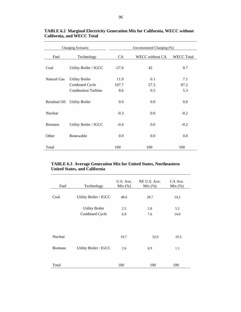
96

TABLE 6.2 Marginal Electricity Generation Mix for California, WECC without

California, and WECC Total

Charging Scenario Unconstrained Charging (%)

Fuel Technology CA WECC without CA WECC Total

Coal Utility Boiler / IGCC -27.6 42 0.7

Natural Gas Utility Boiler 11.9 0.1 7.1

Combined Cycle 107.7 57.3 87.2

Combustion Turbine 8.6 0.5 5.3

Residual Oil Utility Boiler 0.0 0.0 0.0

Nuclear -0.3 0.0 -0.2

Biomass Utility Boiler / IGCC -0.4 0.0 -0.2

Other Renewable 0.0 0.0 0.0

Total 100 100 100

TABLE 6.3 Average Generation Mix for United States, Northeastern

United States, and California

Fuel Technology

U.S. Ave.

Mix (%)

NE U.S. Ave.

Mix (%)

CA Ave.

Mix (%)

Coal Utility Boiler / IGCC 48.6 28.7 14.2

Utility Boiler 2.5 2.8 5.2

Combined Cycle 6.9 7.6 14.0

Nuclear 19.7 32.0 19.3

Biomass Utility Boiler / IGCC 2.6 6.9 1.1

Total 100 100 100

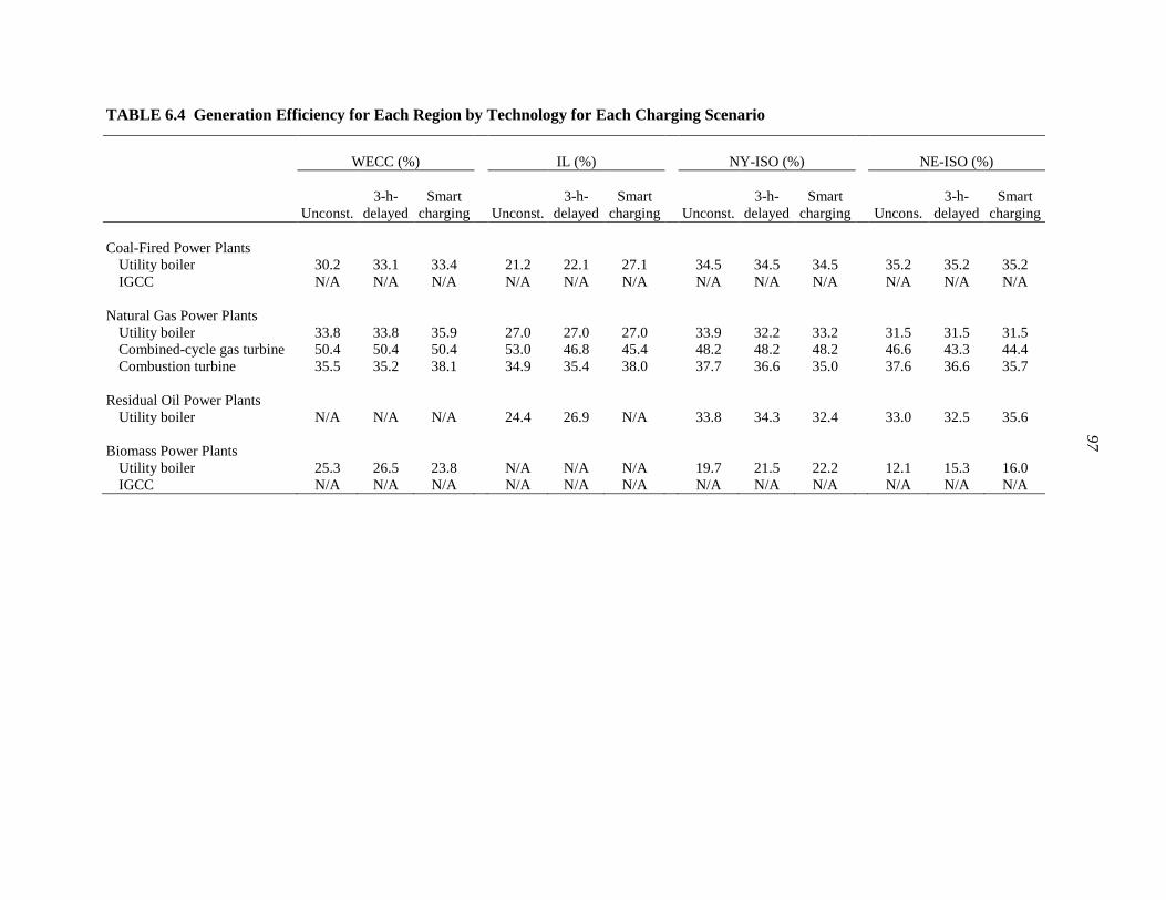
97

TABLE 6.4 Generation Efficiency for Each Region by Technology for Each Charging Scenario

WECC (%)

IL (%)

NY-ISO (%)

NE-ISO (%)

Unconst.

3-h-

delayed

Smart

charging

Unconst.

3-h-

delayed

Smart

charging

Unconst.

3-h-

delayed

Smart

charging

Uncons.

3-h-

delayed

Smart

charging

Coal-Fired Power Plants

Utility boiler 30.2 33.1 33.4 21.2 22.1 27.1 34.5 34.5 34.5 35.2 35.2 35.2

IGCC N/A N/A N/A N/A N/A N/A N/A N/A N/A N/A N/A N/A

Natural Gas Power Plants

Utility boiler 33.8 33.8 35.9 27.0 27.0 27.0 33.9 32.2 33.2 31.5 31.5 31.5

Combined-cycle gas turbine 50.4 50.4 50.4 53.0 46.8 45.4 48.2 48.2 48.2 46.6 43.3 44.4

Combustion turbine 35.5 35.2 38.1 34.9 35.4 38.0 37.7 36.6 35.0 37.6 36.6 35.7

Residual Oil Power Plants

Utility boiler N/A N/A N/A 24.4 26.9 N/A 33.8 34.3 32.4 33.0 32.5 35.6

Biomass Power Plants

Utility boiler 25.3 26.5 23.8 N/A N/A N/A 19.7 21.5 22.2 12.1 15.3 16.0

IGCC N/A N/A N/A N/A N/A N/A N/A N/A N/A N/A N/A N/A

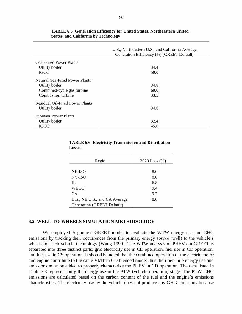
98

TABLE 6.5 Generation Efficiency for United States, Northeastern United

States, and California by Technology

U.S., Northeastern U.S., and California Average

Generation Efficiency (%) (GREET Default)

Coal-Fired Power Plants

Utility boiler 34.4

IGCC 50.0

Natural Gas-Fired Power Plants

Utility boiler 34.8

Combined-cycle gas turbine 60.0

Combustion turbine 33.5

Residual Oil-Fired Power Plants

Utility boiler 34.8

Biomass Power Plants

Utility boiler 32.4

IGCC 45.0

TABLE 6.6 Electricity Transmission and Distribution

Losses

Region 2020 Loss (%)

NE-ISO 8.0

NY-ISO 8.0

IL 6.8

WECC 9.4

CA 9.7

U.S., NE U.S., and CA Average

Generation (GREET Default)

8.0

6.2 WELL-TO-WHEELS SIMULATION METHODOLOGY

We employed Argonne’s GREET model to evaluate the WTW energy use and GHG

emissions by tracking their occurrences from the primary energy source (well) to the vehicle’s

wheels for each vehicle technology (Wang 1999). The WTW analysis of PHEVs in GREET is

separated into three distinct parts: grid electricity use in CD operation, fuel use in CD operation,

and fuel use in CS operation. It should be noted that the combined operation of the electric motor

and engine contribute to the same VMT in CD blended mode; thus their per-mile energy use and

emissions must be added to properly characterize the PHEV in CD operation. The data listed in

Table 3.3 represent only the energy use in the PTW (vehicle operation) stage. The PTW GHG

emissions are calculated based on the carbon content of the fuel and the engine’s emissions

characteristics. The electricity use by the vehicle does not produce any GHG emissions because

99

all emissions have already occurred upstream of the vehicle, during the electric power generation

and transmission stage (WTP). Thus, the WTP energy use and emissions must be calculated to

account for their occurrences during electricity generation, as well as during fuel production and

transportation to the refueling (or recharging) location. For each of the WTP and PTW stages,

GREET calculates total energy use, fossil energy use (combining petroleum, natural gas, and

coal), petroleum energy use, and carbon dioxide (CO2)-equivalent GHG emissions. The GHG

emissions calculation combines CO2, methane (CH4), and nitrous oxide (N2O) with their global

warming potentials of 1, 25, and 298, respectively, as recommended by the latest

Intergovernmental Panel on Climate Change for a 100-year time horizon (IPCC 2008).

We examined the CS operational mode separately from the CD mode for all PHEVs. For

the CS mode, we calculated and combined the energy use and emissions associated with the fuel

production and transportation to the pump (WTP) with the energy use and emissions by the

vehicle (PTW) in the form of a stacked bar that represents the WTW result for that mode of

operation. The PTW results are arbitrarily stacked on top of the WTP results in all graphical

representations in Section 6.3. The CD mode involves both fuel and electricity use that together

contribute to the same VMT in that mode. For the CD mode of operation, we calculated the WTP

energy use and emissions for fuel use and for electricity use and combined them with the PTW

energy use and emissions in the form of a stacked bar. Note that there is only energy use — but

no emissions — associated with the electricity use by PHEVs. Thus, the WTW energy use bar

for CD mode comprises four components, while the WTW emissions bar comprises only three

components. Finally, we combined the WTW results of the CD and CS modes by employing the

utility factor method, as explained in Section 3.4.

6.3 WTW SIMULATION RESULTS

Figures 6.1 show the WTW total energy use for PHEV10 (power-split configuration) and

PHEV40 (series configuration) side-by-side for different fuel/vehicle systems. The WECC

marginal mix for the unconstrained charging scenario was assumed for PHEV recharging in

Figure 6.1. As shown in Table 6.1, the marginal generation mix for the WECC region is

dominated by a low-carbon fuel (> 99% natural gas) — the majority of which (88%) is provided

by the efficient NGCC technology. Two stacked bars for CD and CS operations are shown in

Figure 6.1 for each vehicle technology. The stacked bar for the CD operation consists of four

components representing the vehicle’s (PTW) electricity and fuel use, followed by the upstream

(WTP) stages of electricity generation and fuel production, from top to bottom, respectively. The

stacked bar for the CS operation consists of the engine’s fuel consumption, followed by the

upstream stage of the fuel production. Note that the total energy includes fossil energy (e.g.,

petroleum, natural gas, and coal) as well as nonfossil energy (e.g., nuclear and renewables). For

example, the WTW total energy for E85 includes the renewable energy of the corn kernels that is

embedded in the ethanol fuel.

In Figure 6.1, the top component of the CD bar represents the amount of electricity

acquired from the grid to recharge the batteries of PHEVs. It is interesting to note that the series

design (PHEV40) allows for more electricity use per VMT in CD mode compared with the

power-split design (PHEV10) because of better utilization of the battery’s energy by the

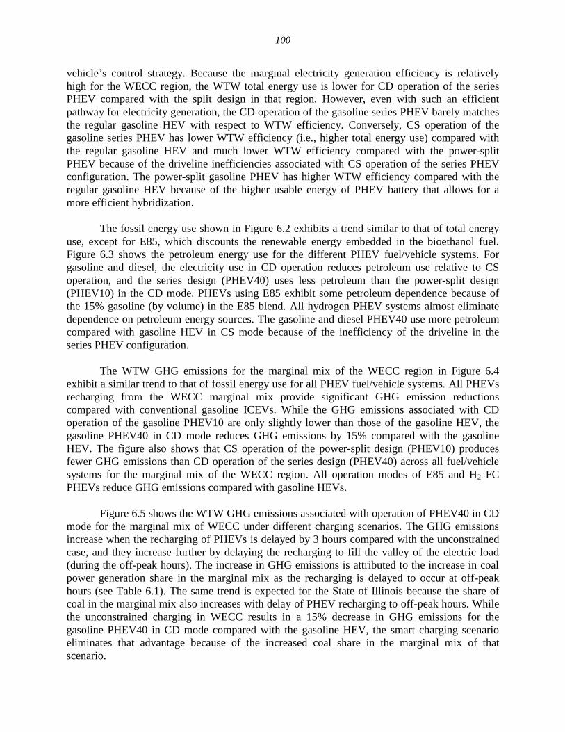
100

vehicle’s control strategy. Because the marginal electricity generation efficiency is relatively

high for the WECC region, the WTW total energy use is lower for CD operation of the series

PHEV compared with the split design in that region. However, even with such an efficient

pathway for electricity generation, the CD operation of the gasoline series PHEV barely matches

the regular gasoline HEV with respect to WTW efficiency. Conversely, CS operation of the

gasoline series PHEV has lower WTW efficiency (i.e., higher total energy use) compared with

the regular gasoline HEV and much lower WTW efficiency compared with the power-split

PHEV because of the driveline inefficiencies associated with CS operation of the series PHEV

configuration. The power-split gasoline PHEV has higher WTW efficiency compared with the

regular gasoline HEV because of the higher usable energy of PHEV battery that allows for a

more efficient hybridization.

The fossil energy use shown in Figure 6.2 exhibits a trend similar to that of total energy

use, except for E85, which discounts the renewable energy embedded in the bioethanol fuel.

Figure 6.3 shows the petroleum energy use for the different PHEV fuel/vehicle systems. For

gasoline and diesel, the electricity use in CD operation reduces petroleum use relative to CS

operation, and the series design (PHEV40) uses less petroleum than the power-split design

(PHEV10) in the CD mode. PHEVs using E85 exhibit some petroleum dependence because of

the 15% gasoline (by volume) in the E85 blend. All hydrogen PHEV systems almost eliminate

dependence on petroleum energy sources. The gasoline and diesel PHEV40 use more petroleum

compared with gasoline HEV in CS mode because of the inefficiency of the driveline in the

series PHEV configuration.

The WTW GHG emissions for the marginal mix of the WECC region in Figure 6.4

exhibit a similar trend to that of fossil energy use for all PHEV fuel/vehicle systems. All PHEVs

recharging from the WECC marginal mix provide significant GHG emission reductions

compared with conventional gasoline ICEVs. While the GHG emissions associated with CD

operation of the gasoline PHEV10 are only slightly lower than those of the gasoline HEV, the

gasoline PHEV40 in CD mode reduces GHG emissions by 15% compared with the gasoline

HEV. The figure also shows that CS operation of the power-split design (PHEV10) produces

fewer GHG emissions than CD operation of the series design (PHEV40) across all fuel/vehicle

systems for the marginal mix of the WECC region. All operation modes of E85 and H2 FC

PHEVs reduce GHG emissions compared with gasoline HEVs.

Figure 6.5 shows the WTW GHG emissions associated with operation of PHEV40 in CD

mode for the marginal mix of WECC under different charging scenarios. The GHG emissions

increase when the recharging of PHEVs is delayed by 3 hours compared with the unconstrained

case, and they increase further by delaying the recharging to fill the valley of the electric load

(during the off-peak hours). The increase in GHG emissions is attributed to the increase in coal

power generation share in the marginal mix as the recharging is delayed to occur at off-peak

hours (see Table 6.1). The same trend is expected for the State of Illinois because the share of

coal in the marginal mix also increases with delay of PHEV recharging to off-peak hours. While

the unconstrained charging in WECC results in a 15% decrease in GHG emissions for the

gasoline PHEV40 in CD mode compared with the gasoline HEV, the smart charging scenario

eliminates that advantage because of the increased coal share in the marginal mix of that

scenario.

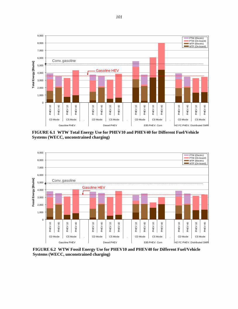
101

0

1,000

2,000

3,000

4,000

5,000

6,000

7,000

8,000

9,000

PH

EV

10

PH

EV

40

PH

EV

10

PH

EV

40

PH

EV

10

PH

EV

40

PH

EV

10

PH

EV

40

PH

EV

10

PH

EV

40

PH

EV

10

PH

EV

40

PH

EV

10

PH

EV

40

PH

EV

10

PH

EV

40

CD Mode CS Mode . CD Mode CS Mode . CD Mode CS Mode . CD Mode CS Mode

Gasoline PHEV Diesel PHEV E85 PHEV: Corn H2 FC PHEV: Distributed SMR

To

tal E

nerg

y [B

tu/m

i]

PTW (Electric)

PTW (On-board)

WTP (Electric)

WTP (On-board)

Gasoline HEV

Conv. gasoline

FIGURE 6.1 WTW Total Energy Use for PHEV10 and PHEV40 for Different Fuel/Vehicle

Systems (WECC, unconstrained charging)

0

1,000

2,000

3,000

4,000

5,000

6,000

7,000

8,000

9,000

PH

EV

10

PH

EV

40

PH

EV

10

PH

EV

40

PH

EV

10

PH

EV

40

PH

EV

10

PH

EV

40

PH

EV

10

PH

EV

40

PH

EV

10

PH

EV

40

PH

EV

10

PH

EV

40

PH

EV

10

PH

EV

40



Fo

ssil E

nerg

y [

Btu

/mi]

PTW (Electric)

PTW (On-board)

WTP (Electric)

WTP (On-board)

Gasoline HEV

Conv. gasoline

FIGURE 6.2 WTW Fossil Energy Use for PHEV10 and PHEV40 for Different Fuel/Vehicle


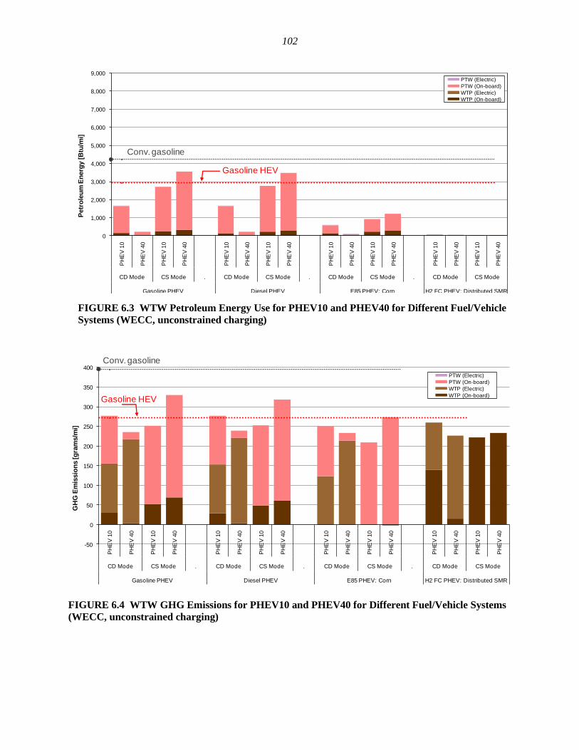
102

0

1,000

2,000

3,000

4,000

5,000

6,000

7,000

8,000

9,000

PH

EV

10

PH

EV

40

PH

EV

10

PH

EV

40

PH

EV

10

PH

EV

40

PH

EV

10

PH

EV

40

PH

EV

10

PH

EV

40

PH

EV

10

PH

EV

40

PH

EV

10

PH

EV

40

PH

EV

10

PH

EV

40



Petr

ole

um

En

erg

y [

Btu

/mi]

PTW (Electric)

PTW (On-board)

WTP (Electric)

WTP (On-board)

Gasoline HEV

Conv. gasoline

FIGURE 6.3 WTW Petroleum Energy Use for PHEV10 and PHEV40 for Different Fuel/Vehicle


-50

0

50

100

150

200

250

300

350

400

PH

EV

10

PH

EV

40

PH

EV

10

PH

EV

40

PH

EV

10

PH

EV

40

PH

EV

10

PH

EV

40

PH

EV

10

PH

EV

40

PH

EV

10

PH

EV

40

PH

EV

10

PH

EV

40

PH

EV

10

PH

EV

40



GH

G E

mis

sio

ns [g

ram

s/m

i]

PTW (Electric)

PTW (On-board)

WTP (Electric)

WTP (On-board)Gasoline HEV

Conv. gasoline

FIGURE 6.4 WTW GHG Emissions for PHEV10 and PHEV40 for Different Fuel/Vehicle Systems

(WECC, unconstrained charging)

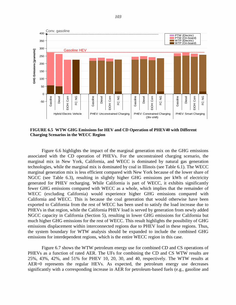
103

-50

0

50

100

150

200

250

300

350

400

Gasolin

e

Die

sel

EtO

H: C

orn

FC

: N

G

Gasolin

e

Die

sel

EtO

H: C

orn

FC

: N

G

Gasolin

e

Die

sel

EtO

H: C

orn

FC

: N

G

Gasolin

e

Die

sel

EtO

H: C

orn

FC

: N

G

Hybrid Electric Vehicle PHEV: Unconstrained Charging PHEV: Constrained Charging

(3hr-shift)

PHEV: Smart Charging

GH

G E

mis

sio

ns [

gra

ms/m

i]PTW (Electric)PTW (On-board)WTP (Electric)WTP (On-board)

Gasoline HEV

Conv. gasoline

-50

0

50

100

150

200

250

300

350

400

Gasolin

e

Die

sel

EtO

H: C

orn

FC

: N

G

Gasolin

e

Die

sel

EtO

H: C

orn

FC

: N

G

Gasolin

e

Die

sel

EtO

H: C

orn

FC

: N

G

Gasolin

e

Die

sel

EtO

H: C

orn

FC

: N

G

Hybrid Electric Vehicle PHEV: Unconstrained Charging PHEV: Constrained Charging

(3hr-shift)

PHEV: Smart Charging

GH

G E

mis

sio

ns [

gra

ms/m

i]PTW (Electric)PTW (On-board)WTP (Electric)WTP (On-board)

Gasoline HEV

Conv. gasoline

FIGURE 6.5 WTW GHG Emissions for HEV and CD Operation of PHEV40 with Different

Charging Scenarios in the WECC Region

Figure 6.6 highlights the impact of the marginal generation mix on the GHG emissions

associated with the CD operation of PHEVs. For the unconstrained charging scenario, the

marginal mix in New York, California, and WECC is dominated by natural gas generation

technologies, while the marginal mix is dominated by coal in Illinois (see Table 6.1). The WECC

marginal generation mix is less efficient compared with New York because of the lower share of

NGCC (see Table 6.3), resulting in slightly higher GHG emissions per kWh of electricity

generated for PHEV recharging. While California is part of WECC, it exhibits significantly

fewer GHG emissions compared with WECC as a whole, which implies that the remainder of

WECC (excluding California) would experience higher GHG emissions compared with

California and WECC. This is because the coal generation that would otherwise have been

exported to California from the rest of WECC has been used to satisfy the load increase due to

PHEVs in that region, while the California PHEV load is served by generation from newly added

NGCC capacity in California (Section 5), resulting in lower GHG emissions for California but

much higher GHG emissions for the rest of WECC. This result highlights the possibility of GHG

emissions displacement within interconnected regions due to PHEV load in these regions. Thus,

the system boundary for WTW analysis should be expanded to include the combined GHG

emissions for interdependent regions, which is the entire WECC region in this case.

Figure 6.7 shows the WTW petroleum energy use for combined CD and CS operations of

PHEVs as a function of rated AER. The UFs for combining the CD and CS WTW results are

25%, 43%, 42%, and 51% for PHEV 10, 20, 30, and 40, respectively. The WTW results at

AER=0 represents the regular HEVs. As expected, the petroleum energy use decreases

significantly with a corresponding increase in AER for petroleum-based fuels (e.g., gasoline and

104

-50

0

50

100

150

200

250

300

350

400

NY

-IS

O IL

WE

CC

Tota

l

CA

NY

-IS

O IL

WE

CC

Tota

l

CA

NY

-IS

O IL

WE

CC

Tota

l

CA

NY

-IS

O IL

WE

CC

Tota

l

CA


GH

G E

mis

sio

ns [g

ram

s/m

i]PTW (Electric)

PTW (On-board)

WTP (Electric)

WTP (On-board)

Gasoline HEV

Conv. gasoline

FIGURE 6.6 WTW GHG Emissions for CD Operation of PHEV40 with Unconstrained Charging

in Different Regions

diesel), mainly because of the displacement of petroleum fuels with electricity generated from

non-petroleum sources. A gasoline or diesel PHEV 40 provides an approximately 60% reduction

in petroleum energy use compared with a conventional gasoline ICEV. It should be noted that

the trend shown in Figure 6.7 is insensitive to the generation mix as long as the mix of fuels for

electricity generation is mainly from non-petroleum sources, which is the case for the WECC,

Illinois, New York, and U.S. mixes. The reduction in petroleum energy use with the increase in

AER is less significant for the E85 PHEVs because of the 15% share of gasoline in the E85

blend. All hydrogen fuel cell PHEVs are nearly free of petroleum energy use because the

feedstock sources of the hydrogen fuel are non-petroleum-based. For all AER ratings, including

AER=0 (regular HEV), the petroleum use is significantly reduced relative to the conventional

(baseline) gasoline ICEV.

Figures 6.8 and 6.9 show GHG emissions associated with PHEV operation for the best case

(WECC, unconstrained charging) and worst case (Illinois, smart charging) recharging scenarios,

as predicted by the dispatch modeling simulations, respectively. Figure 6.8 shows a slight

decrease in the WTW GHG emissions for the power-split PHEV design (AER10 and 20)

compared with the regular HEV (shown as AER0) using petroleum and corn-E85 fuels and

recharging from the WECC marginal generation mix (unconstrained scenario). An opposite trend

is observed for the series PHEV design (AER30 and 40) because of the driveline inefficiencies in

CS operation (as explained earlier). All PHEVs employing fuels produced from biomass sources

(e.g., E85 and hydrogen produced from switchgrass) exhibit a significant increase in GHG

emissions as AER increases, regardless of the PHEV design configuration. This trend is

attributed to much lower carbon emissions associated with these bio-based fuel options, which

favors the use of the biofuel rather than the electricity generated from fossil fuels, even if the

fossil fuel for electricity generation is a low carbon fuel (i.e., natural gas) and the generation

105

0

500

1,000

1,500

2,000

2,500

3,000

3,500

4,000

4,500

0 10 20 30 40

Pert

ole

um

[B

TU

/mi]

All Electric Range

WECC, Unconstrained Charging

Gasoline Baseline Gasoline HEV/PHEV

Diesel HEV/PHEV E85 HEV/PHEV: Corn

E85 HEV/PHEV: H. Biomass H2 FC HEV/PHEV: SMR

H2 FC HEV/PHEV: Biomass

Figure 6.7 WTW Petroleum Energy Use for Combined CD and CS Operations of PHEVs as a

Function of Rated AER (Note: Regular HEV and conventional gasoline ICEV are represented at

AER=0)

0

50

100

150

200

250

300

350

400

450

0 10 20 30 40

GH

G E

mis

sio

n [g

ram

s/m

i]

All Electric Range

WECC, Unconstrained Charging


Diesel HEV/PHEV EtOH HEV/PHEV: Corn

EtOH HEV/PHEV: H. Biomass FC HEV/PHEV: NG

FC HEV/PHEV: Biomass

FIGURE 6.8 WTW GHG Emissions for Combined CD and CS Operations of PHEVs in WECC

(unconstrained charging scenario) as a Function of Rated AER (Note: Regular HEV and

conventional gasoline ICEV are represented at AER=0)

106

0

50

100

150

200

250

300

350

400

450

0 10 20 30 40

GH

G E

mis

sio

n [g

ram

s/m

i]

All Electric Range

IL, Smart Charging


Diesel HEV/PHEV EtOH HEV/PHEV: Corn

EtOH HEV/PHEV: H. Biomass FC HEV/PHEV: NG

FC HEV/PHEV: Biomass

FIGURE 6.9 WTW GHG Emissions for Combined CD and CS Operations of PHEVs in IL

(smart charging scenario) as a Function of Rated AER (Note: Regular HEV and conventional

gasoline ICEV are represented at AER=0)

efficiency is high (~50%) — the case in the WECC region. Thus, PHEVs that employ biomass-

based fuels (e.g., biomass-E85 and biomass-hydrogen) may not realize GHG emissions benefits

compared with regular HEVs if the marginal generation mix is dominated by fossil sources.

Figure 6.9 shows that all PHEVs recharging from the Illinois marginal generation mix

(smart charging scenario) exhibit significant increases in GHG emissions compared with the

regular HEVs because coal dominates that generation mix (99.5% coal). The GHG emissions of

PHEVs increase proportionally with AER with a jump in emissions observed for the series

configuration (PHEV30 and 40). The GHG emissions of the gasoline PHEV40 are shown to

approach those of conventional gasoline ICEV for that generation mix.

Figures 6.10 through 6.12 show the GHG emissions associated with the combined CD and CS

operation of PHEVs, as well as the CD operation of BEVs for the U.S. average mix, the

Northeastern U.S. average mix, and the California average mix, respectively. Please note that we

could only examine BEVs with these average generation mixes since we did not consider any

BEV market penetration in our utility dispatch simulations. Figure 6.10 for the U.S. average mix

shows that GHG emissions from the power-split design of gasoline, diesel, and corn-E85 PHEVs

are only slightly lower than those of the regular HEVs, while the corresponding series designs

exhibit significantly more WTW GHG emissions compared with the regular HEVs. This is

attributed to the high share of coal in the U.S. generation mix (see Table 6.3). All PHEVs

powered by biomass-based fuels (e.g., E85 and H2 from switchgrass) show significant increases

107

U.S. Average Mix

0

50

100

150

200

250

300

350

400

450

0 10 20 30 40All Electric Range

GH

G E

mis

sio

n [

gra

ms/m

i]




H2 FC HEV/PHEV: Biomass EV

Regular Hybrid

U.S. Average Mix

0

50

100

150

200

250

300

350

400

450


GH

G E

mis

sio

n [

gra

ms/m

i]





Regular Hybrid

U.S. Average Mix

0

50

100

150

200

250

300

350

400

450


GH

G E

mis

sio

n [

gra

ms/m

i]





Regular Hybrid

FIGURE 6.10 WTW GHG Emissions for Combined CD and CS Operations

of PHEVs as a Function of Rated AER Using the U.S. Average Generation

Mix

Northeastern U.S. Average Mix

0

50

100

150

200

250

300

350

400

450

0 10 20 30 40

All Electric Range

GH

G E

mis

sio

n [

gra

ms/m

i]





Regular Hybrid

Northeastern U.S. Average Mix

0

50

100

150

200

250

300

350

400

450

0 10 20 30 40

All Electric Range

GH

G E

mis

sio

n [

gra

ms/m

i]





Regular Hybrid

Figure 6.11 WTW GHG Emissions for Combined CD and CS Operations of

PHEVs as a Function of Rated AER Using the Northeastern U.S. Average

Generation Mix

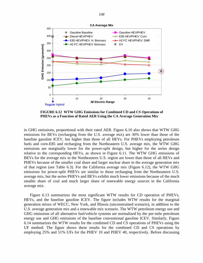
108

CA Average Mix

0

50

100

150

200

250

300

350

400

450

0 10 20 30 40

All Electric Range

GH

G E

mis

sio

n [

gra

ms/m

i]





Regular Hybrid

CA Average Mix

0

50

100

150

200

250

300

350

400

450

0 10 20 30 40

All Electric Range

GH

G E

mis

sio

n [

gra

ms/m

i]





Regular Hybrid

FIGURE 6.12 WTW GHG Emissions for Combined CD and CS Operations of

PHEVs as a Function of Rated AER Using the CA Average Generation Mix

in GHG emissions, proportional with their rated AER. Figure 6.10 also shows that WTW GHG

emissions for BEVs (recharging from the U.S. average mix) are 30% lower than those of the

baseline gasoline ICEV, but higher than those of all HEVs. For PHEVs employing petroleum

fuels and corn-E85 and recharging from the Northeastern U.S. average mix, the WTW GHG

emissions are marginally lower for the power-split design, but higher for the series design

relative to the corresponding HEVs, as shown in Figure 6.11. The WTW GHG emissions of

BEVs for the average mix in the Northeastern U.S. region are lower than those of all HEVs and

PHEVs because of the smaller coal share and larger nuclear share in the average generation mix

of that region (see Table 6.3). For the California average mix (Figure 6.12), the WTW GHG

emissions for power-split PHEVs are similar to those recharging from the Northeastern U.S.

average mix, but the series PHEVs and BEVs exhibit much lower emissions because of the much

smaller share of coal and much larger share of renewable energy sources in the California

average mix.

Figure 6.13 summarizes the most significant WTW results for CD operation of PHEVs,

HEVs, and the baseline gasoline ICEV. The figure includes WTW results for the marginal

generation mixes of WECC, New York, and Illinois (unconstrained scenario), in addition to the

U.S. average generation mix and a renewable mix scenario. The WTW petroleum energy use and

GHG emissions of all alternative fuel/vehicle systems are normalized by the per-mile petroleum

energy use and GHG emissions of the baseline conventional gasoline ICEV. Similarly, Figure

6.14 summarizes the WTW results for the combined CD and CS operations of PHEVs using the

UF method. The figure shows these results for the combined CD and CS operations by

employing 25% and 51% UFs for the PHEV 10 and PHEV 40, respectively. Before discussing

109

the WTW results in Figures 6.13 and 6.14, we provide the following guidelines to facilitate

easier interpretation of these two figures.

• The reference point for comparison with all PHEVs is (1,1), which represents the

baseline conventional gasoline ICEV’s petroleum energy use and GHG emissions as the

comparison basis.

• The color of the marker represents a particular PHEV fuel/vehicle technology.

The shape of the marker represents the marginal generation mix used for recharging the

PHEV batteries.

0.0

0.1

0.2

0.3

0.4

0.5

0.6

0.7

0.8

0.9

1.0

0.0 0.1 0.2 0.3 0.4 0.5 0.6 0.7 0.8 0.9 1.0


GH

G E

mis

sio

ns

(re

lati

ve

to

GV

)

EV (U.S. Average Mix)

PHEV SI Gasoline

PHEV CI Diesel

PHEV SI Corn-E85

PHEV SI H. Biomass-E85

PHEV FC Distributed SMR-H2

PHEV FC Central H. Biomass-H2

Small marker for PHEV10

Large marker for PHEV40

Baseline (GV)

Regular HEV (AER 0)

US Ave. Mix

WECC Mix

NY Mix

IL Mix

Renewable

IL (67% coal)

Renewable

WECC and NY

(NGCC)

US Ave. (49% coal)

FIGURE 6.13 WTW Petroleum Use and GHG Emissions for CD Operation of PHEVs

(unconstrained charging)

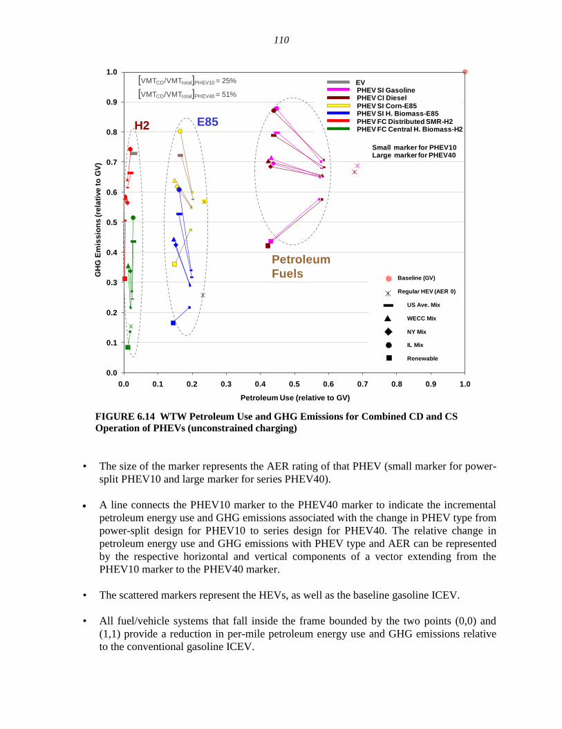
110

0.0

0.1

0.2

0.3

0.4

0.5

0.6

0.7

0.8

0.9

1.0

0.0 0.1 0.2 0.3 0.4 0.5 0.6 0.7 0.8 0.9 1.0

GH

G E

mis

sio

ns

(re

lati

ve

to

GV

)


Small marker for PHEV10Large marker for PHEV40

Baseline (GV)

Regular HEV (AER 0)

US Ave. Mix

WECC Mix

NY Mix

IL Mix

Renewable

EVPHEV SI GasolinePHEV CI DieselPHEV SI Corn-E85PHEV SI H. Biomass-E85PHEV FC Distributed SMR-H2PHEV FC Central H. Biomass-H2

Petroleum

Fuels

E85H2



FIGURE 6.14 WTW Petroleum Use and GHG Emissions for Combined CD and CS

Operation of PHEVs (unconstrained charging)

• The size of the marker represents the AER rating of that PHEV (small marker for power-

split PHEV10 and large marker for series PHEV40).

A line connects the PHEV10 marker to the PHEV40 marker to indicate the incremental

petroleum energy use and GHG emissions associated with the change in PHEV type from

power-split design for PHEV10 to series design for PHEV40. The relative change in

petroleum energy use and GHG emissions with PHEV type and AER can be represented

by the respective horizontal and vertical components of a vector extending from the

PHEV10 marker to the PHEV40 marker.

• The scattered markers represent the HEVs, as well as the baseline gasoline ICEV.

• All fuel/vehicle systems that fall inside the frame bounded by the two points (0,0) and

(1,1) provide a reduction in per-mile petroleum energy use and GHG emissions relative

to the conventional gasoline ICEV.

111

• All fuel/vehicle systems that fall inside the frame bounded by the two points (0,0) and

(0.69,0.69) provide a reduction in per-mile petroleum energy use and GHG emissions

relative to the gasoline HEV.

• The vehicle technology is less dependent on petroleum energy if its marker is closer to

the vertical coordinate. Similarly, the vehicle technology produces less GHG emissions

as its marker gets closer to the horizontal coordinate.

The implication of the electricity generation mix resides in the electricity generation stage

(WTP). In general, the electricity WTP energy use and GHG emissions increase progressively as

the marginal mix becomes less efficient and dominated by a larger share of oil or coal. It should

be noted that the petroleum share is insignificant in all considered generation mixes; thus, any

contribution of grid-electricity to PHEV’s VMT would result in a proportional reduction in

petroleum energy use.

Figure 6.13 shows the WTW results of PHEVs only for the CD mode of operation

(unconstrained charging scenario). The WTW results for CD operation of PHEVs (relative to the

gasoline baseline ICEV and HEV) can be grouped by the type of generation mix used for PHEV

recharging. Recharging from a mix with a large share of coal generation (e.g., 67% share in

Illinois and 49% share in the U.S. average mix) results in WTW GHG emissions higher than

those of the gasoline HEV but lower than those of the gasoline ICEV. For example, a PHEV40

recharging from the Illinois marginal mix (unconstrained charging) produces WTW GHG

emissions that are approximately 10% lower than those of the gasoline ICEV but 30% higher

than those of the gasoline HEV. Recharging from a mix with a large share of natural gas

generation (e.g., WECC and New York marginal generation mix) results in WTW GHG

emissions comparable to or less than those of gasoline HEV, but much lower compared with the

gasoline ICEV. For example, a PHEV40 recharging from NGCC produces WTW GHG

emissions that are 15–20% lower compared with the gasoline HEV and 40–45% lower than those

of the gasoline ICEV. However, the power-split gasoline PHEV10 produces WTW GHG

emissions similar to those of the gasoline HEV. Figure 6.13 shows that the power-split design

(AER10) for all PHEVs reduces petroleum use by more than 60%, while the series design

(AER40) reduces it by more than 90%. If a renewable or nonfossil generation mix is employed

to recharge PHEVs, the power-split configuration could realize reductions in WTW petroleum

use and GHG emissions of more than 60%, while the series configuration could realize

reductions of more than 90% in both. The impact of grid decarbonization on the per-mile GHG

emissions is demonstrated by the slope of the lines connecting PHEV10 markers to PHEV40

markers.

The WTW results shown in Figure 6.14 for the combined CD and CS operations of

PHEVs (relative to the gasoline baseline ICEV and HEV) can be grouped by the type of fuel.

Figure 6.14 shows three fuel groups (petroleum, E85, and hydrogen) with distinct petroleum

energy use and GHG emissions. The PHEVs that employ petroleum fuels, E85, and hydrogen

offer40–60%, 80–90%, and more-than-90% reductions in petroleum energy use, respectively,

compared with the conventional gasoline ICEV. The corresponding reductions in GHG

emissions for PHEVs that employ petroleum fuels, E85, and hydrogen are 10–60%, 20–80%,

and 25–90%, respectively. The spread of the WTW GHG emissions among the different fuel

112

groups is much higher compared with the spread of petroleum energy use, mainly because of the

wide variation in the electricity generation mix considered for PHEVs in this analysis. This

spread of GHG emissions is more apparent for E85 and hydrogen because of the diverse

production technologies and feedstock sources considered in this analysis for these fuels.

Overall, more petroleum energy savings are realized as the AER of the PHEVs increases.

Conversely, more WTW GHG emissions are produced with increased AER, except when a

renewable or nonfossil generation mix is used for PHEV recharging. The increase in GHG

emissions with AER for the combined CD and CS operations is opposite to the trend observed in

Figure 6.13 for CD operation, where GHG emissions are reduced with AER in WECC, New

York, and the U.S. average mix. The opposite trend for these generation mixes highlights the

impact of the much lower fuel economy in CS mode for the series design (PHEV40) compared

with the power-split design (PHEV10), as explained in Section 3.

Figure 6.15 shows the WTW results for CD operation of gasoline power-split and series

PHEVs (for both the unconstrained and smart charging scenarios), in addition to the baseline

conventional and regular hybrid gasoline vehicles. For the same PHEV powertrain (i.e., power-

split or series design), more petroleum savings and GHG emission reduction are realized with an

increase in AER. Furthermore, when the charging of PHEV occurs from a low-carbon generation

mix (e.g., NGCC in WECC and NY) or from a renewable source, the series design of PHEV

provides significantly more petroleum savings and GHG emissions reduction compared to the

power-split design. Figure 6.15 also shows that the unconstrained charging scenario (with

investment in new generation capacity) provide less GHG emissions compared to the smart

charging scenario (which requires no investment in new capacity) mainly due to the high

efficiency and low carbon intensity of the added capacity in the unconstrained charging scenario.

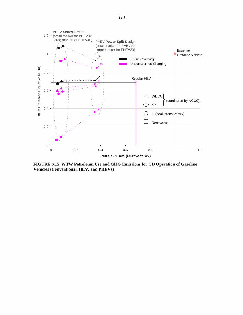
113

0

0.2

0.4

0.6

0.8

1

1.2

0 0.2 0.4 0.6 0.8 1 1.2


GH

G E

mis

sio

ns (

rela

tive t

o G

V)

Smart Charging

Unconstrained Charging

Regular HEV

WECC

(dominated by NGCC)

NY


Renewable

Baseline

Gasoline Vehicle

PHEV Series Design

(small marker for PHEV30

large marker for PHEV40)PHEV Power-Split Design


large marker for PHEV20)

0

0.2

0.4

0.6

0.8

1

1.2

0 0.2 0.4 0.6 0.8 1 1.2


GH

G E

mis

sio

ns (

rela

tive t

o G

V)

Smart Charging

Unconstrained Charging

Regular HEV

WECC

(dominated by NGCC)

NY


Renewable

Baseline

Gasoline Vehicle

PHEV Series Design


large marker for PHEV40)PHEV Power-Split Design


large marker for PHEV20)

FIGURE 6.15 WTW Petroleum Use and GHG Emissions for CD Operation of Gasoline

Vehicles (Conventional, HEV, and PHEVs)

114


115

7 CONCLUSIONS

Argonne’s WTW analysis of PHEVs revealed that the following factors significantly impact

the energy use and GHG emissions results for PHEVs and BEVs compared with baseline

gasoline vehicle technologies: (1) the regional electricity generation mix for battery recharging

and (2) the adjustment of fuel economy and electricity consumption to reflect ―real-world‖

driving conditions. Although the analysis predicted the marginal electricity generation mixes for

major regions in the United States, these mixes should be evaluated as possible scenarios for

recharging PHEVs because of the significant uncertainties associated with the assumed market

penetration for these vehicles. Thus, the reported WTW results for PHEVs should be directly

correlated with the underlying generation mix, rather than with the region linked to that mix. The

primary conclusion is that electrification of transportation significantly reduces petroleum energy

use, but GHG emissions strongly depend on the electricity generation mix for battery recharging.

Sections 7.1 and 7.2 summarize petroleum and GHG emissions results for CD operation of

gasoline PHEVs and BEVs, and for combined CD and CS operation of PHEVs, respectively.

7.1 CD OPERATION OF GASOLINE PHEVS AND BEVS

7.1.1 Petroleum Displacement

In CD operation modes, PHEVs employing the power-split and series configurations

could realize reductions in petroleum energy use of more than 60% and 90%, respectively,

because the petroleum share is small in the electricity generation mix for most regions in the

United States. BEVs can virtually eliminate the use of petroleum fuels for each vehicle mile

traveled on electricity.

7.1.2 GHG Emissions

Unconstrained charging (with investments in new generation capacity) reduces

GHG emissions (Figure ES.1, vertical axis) compared with smart charging (no

needed investment in new capacity) because of the high efficiency and low carbon

intensity associated with the added capacity in the unconstrained charging

scenario.

PHEVs recharging from a mix with a large share of coal generation (e.g., Illinois

marginal mix) produce GHG emissions comparable to those of baseline gasoline

ICEVs (with a range from -15% to +10%) but significantly higher than those of

gasoline HEVs (with a range from +20% to +60%). The range of the results is

primarily attributable to the different generation mix for the charging scenarios

considered and the different PHEV types (power-split versus series designs).

116

PHEVs recharging from a mix with a large share of efficient electricity generation

from natural gas (e.g., natural gas combined-cycle [NGCC] generation in the

Western Electric Coordinating Council region) produce GHG emissions

comparable to those of gasoline HEVs (with a range from -15% to +10%) but

significantly lower than those of baseline gasoline ICEVs (with a range from -

25% to -40%). The range of results is primarily attributable to the different

generation mix for the charging scenarios considered and the different PHEV

types (power-split versus series designs).

PHEVs recharging from a generation mix comparable to the U.S. average mix

produce lower GHG emissions than baseline gasoline ICEVs (with a range from

-20% to -25%) but higher than gasoline HEVs (with a range from +10% to

+20%).

To achieve significant reductions in GHG emissions, PHEVs and BEVs must

recharge from a generation mix with a large share of nonfossil sources (e.g.,

renewable or nuclear power generation). PHEVs recharging from a potential

renewable or nonfossil generation mix reduce GHG emissions by more than 60%

for the power-split PHEV configuration and by more than 90% for the series

configuration compared with baseline gasoline ICEVs. BEVs can virtually

eliminate GHG emissions (per mile traveled) if recharged from nonfossil

electricity generation.

7.1.3 Electric Range of PHEVs and BEVs in Real-World Driving

The actual CD range of PHEVs could be lower or higher than the rated electric

range on the standard driving cycles, depending on the powertrain type and the

vehicle’s control strategy. Power-split PHEVs may extend the electric range if the

battery receives significant help from the engine, resulting in blended (i.e.,

blended use of battery and engine) operation in CD mode. However, the electric

range of BEVs and series PHEVs drops below the rated electric range because of

the higher battery discharge rate required to meet real-world driving conditions.

7.2 COMBINED CD AND CS OPERATION OF PHEVS

7.2.1 Petroleum Displacement

PHEVs powered by petroleum fuels (i.e., gasoline and diesel) reduce petroleum

energy use by 40–60% compared with conventional gasoline ICEVs, while

PHEVs powered by E85 (blend of 85% ethanol and 15% gasoline by volume)

reduce petroleum energy use by 80–90%, and PHEVs powered by hydrogen

reduce petroleum energy use by greater than 90%.

117

7.2.2 GHG Emissions

Compared with conventional gasoline ICEVs, PHEVs powered by petroleum

fuels (i.e., gasoline and diesel) reduce GHG emissions by 10–60%, PHEVs

powered by E85 (blend of 85% ethanol and 15% gasoline by volume) reduce

GHG emissions by 20–80%, and PHEVs powered by hydrogen reduce these

emissions by 25–90%. The large range of GHG emissions reductions is

attributable to the variety of feedstock sources considered for producing the fuel

and electricity for each vehicle.

PHEVs achieve greater petroleum energy savings with increased electric range.

Conversely, more GHG emissions are produced with increased electric range

unless renewable or nonfossil electricity generation is used for recharging.

PHEVs employing biomass-based fuels (e.g., E85 or hydrogen from biomass

sources) may not achieve GHG emissions benefits compared with conventional

HEVs (employing the same fuel) if the electricity generation mix for PHEV

recharging is dominated by fossil fuel sources.

118


119

8 IMPLICATIONS FOR FUTURE ANALYSIS

Although the WTW results for PHEVs in this report addressed many of the outstanding

issues in our earlier report (Elgowainy at al. 2009), there are remaining issues that require further

analysis. The following paragraphs address these remaining issues and their implications for

future WTW analyses of PHEVs.

It is not clear what PHEV technology, i.e., power-split or series configuration or both,

and what electric range will gain consumer acceptance and attain significant market penetration.

Also, it is not clear whether the EPA mpg-based formulas for ―on-road‖ adjustment of fuel

economy accurately capture the impact of ―real-world‖ driving for advanced vehicle

technologies such as FCVs, PHEVs, and BEVs. Until a solid empirical basis is established to

capture the real-world driving fuel and electricity consumption for these vehicle technologies,

uncertainty in the on-road adjustment estimates will persist.

Other subtle, but important, complications include the rate of technological advancement

that will be made in the critical components of each vehicle technology, e.g., batteries and fuel

cells, and the specific control strategy adopted by each OEM for the combined operation of the

electric motor and engine of PHEVs. Such uncertainties associated with vehicle technologies and

operation impact the projection of fuel and electricity demand for vehicle operation which, in

turn, impacts the WTW results for each fuel/vehicle pathway.

In addition to the direct impact of PHEV’s electricity use, the impact of the generation

mix of technologies and their ―operating‖ (rather than nameplate) efficiencies on the WTW

results is crucial. Although many researchers argue that cross-sectional marginal analysis applied

to limited time intervals — such as that described here — is the appropriate methodology to

capture the impact of PHEV recharging from the grid, such analysis poses many challenges.

Also, by its nature, this method cannot account for changes in the generation mix induced by an

expanding PHEV fleet over time. Some of the challenges associated with the marginal analysis

method were overcome in our analysis, while others require further study. One of the biggest

challenges to marginal analysis is the market penetration of the mix of different PHEV and BEV

technologies in a given region and a given year. This is a complex subject that could be further

examined by using a market transition analysis.

One critical implicit assumption of the ―share of miles electrified‖ (the ―utility factor‖) is

that the probability of PHEV purchase is invariant to daily distance driven or to benefit vs. cost.

In order to save oil, PHEVs will have to be purchased and used. How often this will happen, and

how frequently the pack will be charged and fully discharged, remain topics of considerable

uncertainty.

Other uncertainties that impact the electricity dispatch modeling (which calculates the

share of electricity generation technologies dispatched to satisfy the vehicles’ electric load, i.e.,

the marginal generation mix) include the rate at which charging occurs, the number of charges

per day, and the time of day for each charge. All of these significantly impact the vehicles’

charging profiles which, in turn, impact the generation technology dispatched to satisfy the

120

additional load and the determination of whether generation capacity expansion is needed to

satisfy a specific reserve margin.

Adoption of a specific generation technology for capacity expansion is another

complication that depends, not only on the economics of each technology, but also on the

evolving regulations and standards — both at the local and national levels. Existing and evolving

policies aimed at reducing electricity demand, GHG emissions, and other criteria pollutants (e.g.,

Energy Efficiency Resource Standard [EERS] and Renewable Energy or Portfolio Standard

[RES or RPS], mercury regulations, and Clean Air Interstate Rule [CAIR], carbon tax) impact

the economics and — ultimately — the retirement of existing generation technologies, as well as

the selection of future generation technologies. While wind is a likely overnight renewable

source for battery recharging, its generation is intermittent (varies by time and region) and it

must be backed up by another generation source with a high ramping rate. Thus, the attainable

share of wind-electricity in the marginal mix and its complementary generation technology

require further analysis. While some of these issues could be addressed in further electric utility

dispatch simulations, others that are related to future electric utility operations are subject to

policy and behavior uncertainties. The latter may have to be addressed by using scenario

analysis.

121

9 REFERENCES

Bandel, W., 2006, ―The Turbocharged GDI Engine: Boosted Synergies for High Fuel Economy

plus Ultra-Low Emissions,‖ SAE paper 2006-01-1266, SAE World Congress, Detroit, MI, April.

Bohn, T., and M. Duoba, 2005, ―Implementation of a Non-Intrusive In-Vehicle Engine Torque

Sensor for Benchmarking the Toyota Prius HEV,‖ SAE paper 2005-01-1046, SAE World

Congress, Detroit, MI, April.

Cao, Q., S. Pagerit, R. Carlson, and A. Rousseau, 2007, ―PHEV Hymotion Prius Model

Validation and Control Improvements,‖ 23rd International Electric Vehicle Symposium (EVS23),

Anaheim, CA, Dec.

Christenson, M., R. Shinomiya, and D. Karman, 2009, ―PHEV Laboratory Test Results: Energy

Consumption and Emissions in Cold Climate,‖ PHEV’09 Conference, Sept. 28–30, Montreal,

Canada.

Cirillo, R.R., P. Thimmapuram, T. Veselka, V. Koritarov, G. Conzelmann, C. Macal, G. Boyd,

M. North, T. Overbye, and X. Cheng, 2006, ―Evaluating the Potential Impact of Transmission

Constraints on the Operation of a Competitive Electricity Market in Illinois,‖ Report ANL 16/06,

Argonne National Laboratory, April.

Duoba, M., R. Carlson, F. Jehlik, J. Smart, and S. White, 2009, ―Correlating Dynamometer

Testing to In-Use Fleet Results of Plug-In Hybrid Electric Vehicles,‖ EVS24 International

Battery, Hybrid and Fuel Cell Electric Vehicle Symposium, Stavanger, Norway, May 13–16.

EIA: See Energy Information Administration.

Electric Power Research Institute and Natural Resources Defense Council, 2007, Environmental

Assessment of Plug-In Hybrid Electric Vehicles, Volume 1: Nationwide Greenhouse Gas

Emissions, EPRI Report# 1015325, July.

Elgowainy, A., A. Burnham, M. Wang, J. Molburg, and A. Rousseau, 2009, Well-to-Wheels

Energy Use and Greenhouse Gas Emissions Analysis of Plug-In Hybrid Electric Vehicles,

ANL_ESD_09-2, Center for Transportation Research, Argonne National Laboratory, Argonne,

IL, Feb.

Energy Information Administration, 2007, EIA-411 — Coordinated Bulk Power Supply Program

Report, Form EIA-423 — Monthly Cost and Quality of Fuels for Electric Plants Report; Form

EIA-767 — Steam-Electric Plant Operation and Design Report; Form EIA-860 — Annual

Electric Generator Report; and Form EIA-906 — Power Plant Report available at

http://www.eia.doe.gov/oss/forms.html, accessed Feb. 2009.

122

Energy Information Administration, 2008, Assumptions to the Annual Energy Outlook 2008:

Electricity Market Module, Report Number DOE/EIA-0554(2008), U.S. Department of Energy,

June, available at [http://www.eia.doe.gov/oiaf/aeo/assumption/pdf/electricity.pdf], accessed

Feb. 2009.

Energy Information Administration, 2009a, Annual Energy Outlook 2009: Updated Reference

Case, April 2009, DOE/EIA-0383(2009), U.S. Department of Energy, Washington, D.C.

(Detailed tables were obtained from EIA.)

Energy Information Administration, 2009b, The National Energy Modeling System: An

Overview, DOE/EIA-0581(2009), U.S. Department of Energy, Washington, D.C.

EPA: see U.S. Environmental Protection Agency.

EPRI and NRDC: see Electric Power Research Institute and Natural Resources Defense Council.

Federal Energy Regulatory Commission, 2009, FERC Form 714 — Annual Electric Balancing

Authority Area and Planning Area Report, updated Jan. 8, available at [http://www.ferc.gov/

docs-filing/eforms/form-714/overview.asp], accessed Feb. 2009.

Federal Highway Administration, 2008, Highway Statistics 2007, U.S. Department of

Transportation, Washington, D.C., available at [http://www.fhwa.dot.gov/policyinformation/

statistics/2007//], accessed (Tables MV-1 and MV-9) March 2010.

Federal Highway Administration, 2004, The 2001 National Household Travel Survey: Compact

Disk and User’s Guide, U.S. Department of Transportation, Washington, D.C.

FERC: see Federal Energy Regulatory Commission.

Freyermuth, V., E. Fallas, and A. Rousseau, 2008, Comparison of Powertrain Configuration for

Plug-In HEVs from a Fuel Economy Perspective, SAE paper 2008-01-0461, SAE World

Congress, Detroit, MI, April.

FHWA: see Federal Highway Administration.

Gaines, L., A. Burnham, A. Rousseau, and D. Santini, 2008, ―Sorting through the Many Total-

Energy-Cycle Pathways Possible with Early Plug-in Hybrids,‖ The World Electric Vehicle

Journal, Volume 2, Sept.

Hadley, S., and A. Tsvetkova, 2008, Potential Impacts of Plug-in Hybrid Electric Vehicles on

Regional Power Generation, ORNL/TM-2007/150, Oak Ridge National Laboratory, Oak Ridge,

TN, Jan.

Intergovernmental Panel on Climate Change, 2008, 2008, Climate Change 2007: Technical

Summary, Cambridge University Press, Cambridge, UK.

123

IPCC: see Intergovernmental Panel on Climate Change.

IWEA: see Illinois Wind Energy Association.

Karbowski, J.D., A. Rousseau, S. Pagerit, and P. Sharer, 2006, ―Plug-In Vehicle Control

Strategy: From Global Optimization to Real-Time Application,‖ EVS22, Yokohama, Japan, Oct.,

available at [http://windforillinois.com/maps.php], accessed March 2010.

Kromer, M.A., and J.B. Heywood, 2007, Electric Powertrains: Opportunities and Challenges in

the U.S. Light-Duty Vehicle Fleet, Massachusetts Institute of Technology (MIT), Publication No.

LFEE 2007-03 RP, May.

Morrow, K., D. Karner, and J. Francfort, 2008, Plug-in Hybrid Electric Vehicle Charging

Infrastructure Review, INL/EXT-08-15058, Idaho National Laboratory, Nov.

National Renewable Energy Laboratory, 2009a, Western Wind Resources Dataset, available at

http://wind.nrel.gov/Web_nrel/, accessed in March 2010.

National Renewable Energy Laboratory, 2009b, NREL Western Wind and Solar Integration

Project, available at [http://mercator.nrel.gov/wwsi/], accessed in June 2009.

National Renewable Energy Laboratory, 2009c, National Solar Radiation Data Base 1991–2005

Update, available at [http://rredc.nrel.gov/solar/old_data/nsrdb/1991-2005/hourly/list_by_

USAFN.html], accessed in June 2009.

National Research Council, 2009, Transitions to Alternative Transportation Technologies —

Plug-in Hybrid Electric Vehicles, The National Academies Press, Washington D.C., ISBN: 0-

309-14851-0.

NE ISO: see New England Independent System Operator.

NERC: see North American Electric Reliability Corporation.

New England Independent System Operator, 2008a, 2008–2017 Forecast Report of Capacity,

Energy, Loads, and Transmission, April, available at [http://www.iso-ne.com/trans/celt/

report/2008/index.html], accessed March 2009.

New York Independent System Operator, 2008b, 2008 Load and Capacity Data (Gold Book),

April, available at http://www.nyiso.com/public/markets_operations/services/planning/document

ments/index.jsp, accessed in March 2009.

North American Electric Reliability Corporation, 2008, Generating Availability Data System

(GADS), [http://www.nerc.com/page.php?cid=4%7C43], accessed April 2009.

NRC: see National Research Council.

124

NREL: see National Renewable Energy Laboratory.

NY ISO: see New York Independent System Operator.

Olszewski, M., 2008, Evaluation of the 2007 Toyota Camry Hybrid Synergy Drive System, DOE

report, Jan.

Pagerit, S., A. Rousseau, and P. Sharer, 2005, ―Global Optimization to Real-Time Control of

HEV Power Flow: Example of a Fuel Cell Hybrid Vehicle,‖ 20th International Electric Vehicle

Symposium (EVS20), Monaco, April.

Passier, G., F.V. Conte, S. Smets, F. Badin, A. Brouwer, M. Alaküla, D. Santini, and M.

Alexander, 2007, Status Overview of Hybrid and Electric Vehicle Technology, MON-RPT-033-

DTS-2007-02955, International Energy Agency, Dec.6.

Rousseau, A., P. Sharer, S. Pagerit, and M. Duoba, 2006, ―Integrating Data, Performing Quality

Assurance, and Validating the Vehicle Model for the 2004 Prius Using PSAT,‖ SAE paper 2006-

01-0667, SAE World Congress, Detroit, MI, April.

Santini, D., and A. Vyas, 2008, ―More Complications in Estimation of Oil Savings via

Electrification of Light Duty Vehicles,‖ Plug-In 2008 Conference, San Jose, CA, July 21–24.

Sharer, P., A. Rousseau, D. Karbowski, and S. Pagerit, 2008, ―Plug-in Hybrid Electric Vehicle

Control Strategy: Comparison between EV and Charge-Depleting Options,‖ SAE paper 2008-01-

0460, SAE World Congress, Detroit, MI, April.

Sharer, P., A. Rousseau, P. Nelson, and S. Pagerit, 2006, ―Vehicle Simulation Results for PHEV

Battery Requirements,‖ 22nd International Electric Vehicle Symposium (EVS22), Yokohama,

Japan, Oct.

Stodolsky, F., A. Vyas, R. Cuenca, and L. Gaines, 1995, ―Life-Cycle Energy Savings Potential

from Aluminum- Intensive Vehicles,‖ 1995 Total Life Cycle Conference & Exposition, Oct.,

Vienna, Austria.

TEPPC: see Transmission Expansion Planning and Policy Committee.

Thomas, C.E., 2009, ―Cost-Benefit Analyses of Alternative Light-Duty Transportation Options

for the 21st Century,‖ National Hydrogen Association Conference, Columbia, SC, March 31.

Transmission Expansion Planning and Policy Committee, 2008, 2008 Annual Report of the

Transmission Expansion Planning Policy Subcommittee, WECC, March.

U.S. Census Bureau, 2005, State Interim Population Projections by Age and Sex: 2004–2030,

Detailed Data File 2, U.S. Department of Commerce, Washington, D.C., available at

[http://www.census.gov/population/www/projections/projectionsagesex.html], accessed March

2010.

125

U.S. Environmental Protection Agency, 2006, Fuel Economy Labeling of Motor Vehicle

Revisions to Improve Calculation of Fuel Economy Estimates, Final Technical Support

Document, EPA420-R-06-017, Dec., available at [http://www.epa.gov/fueleconomy/fe-labeling-

final-rule.pdf], accessed March 2010.

U.S. Environmental Protection Agency, 2008, Light-Duty Automotive Technology and Fuel

Economy Trends: 1975 through 2008, EPA420-R-08-015, Sept. available at

[http://www.epa.gov/oms/cert/mpg/fetrends/fetrends-archive.htm], accessed March 2010.

Vyas, A., D. Santini, M. Duoba, and M. Duvall, 2007, ―Plug-In Hybrid Electric Vehicles: How

Does One Determine Their Potential for Reducing U.S. Oil Dependence?‖ Proceedings of the

Electric Vehicle Symposium 23, Anaheim, CA, Dec. 2–5.

Wang, M., 1999, GREET 1.5 – Transportation Fuel-Cycle Model, ANL/ESD-39, Center for

Transportation Research, Argonne National Laboratory, Argonne, IL, Aug.

Weissler, P., 2009, ―Many Factors Figure in EV Fuel-Economy Calculation,‖

CURRENTEVENTS, Vol. 41, No. 8, Aug., available at [http://www.eaaev.org/CurrentEvents/

pdf/2009/CurrentEvents200908.pdf], accessed March 2010.

Wipke, K., S. Sprik, J. Kurtz, and T. Ramsden, 2009, Controlled Hydrogen Fleet Infrastructure

Demonstration and Validation Project, NREL/TP-560-45451, March 13, National Renewable

Energy Laboratory, Golden, CO.

126


127

APPENDIX 1: VEHICLE DESCRIPTIONS

1. Component Power

Component Power (W)

2008 2015

Reference Low Average High

Gasoline SI Conv ICE Power 120472 116993 109611 102785

Electric Machine

MC2/GC

Battery

Specific Power 76.25 74.14 73.07 71.13

Diesel CI Conv ICE Power 112837 110000 103673 98747

Electric Machine

MC2/GC

Battery

Specific Power 68.59 66.91 66.16 65.22

E85 Conv ICE Power 121988 120359 114374 106250

Electric Machine

MC2/GC

Battery

Specific Power 77.16 76.18 76.10 73.43

Gasoline SI Split HEV ICE Power 88869 88132 81212 74211

Electric Machine 63506 62801 59368 55932

MC2/GC 51429 51002 46998 42946

Battery 28733 28334 26738 25341

Specific Power 69.71 70.20 68.89 67.04

Gasoline SI Split HEV

PHEV10

ICE Power 63723 63096 58990 55290


MC2/GC 36877 36514 34138 31997

Battery 56979 56355 52082 48062

Specific Power 71.51 71.92 70.84 69.64

Gasoline SI Split HEV

PHEV20

ICE Power 64607 63952 59783 55822


MC2/GC 37388 37009 34597 32304

Battery 57790 57473 52986 48743

Specific Power 71.20 71.81 70.66 69.57

128

Component Power (W)

2008 2015


Gasoline SI Series HEV

PHEV30

ICE Power 77511 76037 69137 62271


MC2/GC 75186 73756 67063 60403

Battery 156120 153121 142017 130834

Specific Power 65.74 66.42 66.37 66.64

Gasoline SI Series HEV

PHEV40

ICE Power 79497 77901 70682 63701


MC2/GC 77112 75564 68562 61790

Battery 159736 156706 144871 133437

Specific Power 65.86 66.51 66.44 66.92

Diesel CI Split HEV ICE Power 78299 76983 71722 65009


MC2/GC 65528 64426 60024 54406

Battery 30330 29731 28334 26738

Specific Power 60.89 61.05 60.38 58.36

Diesel CI Split HEV

PHEV10

ICE Power 67488 66747 62474 58508


MC2/GC 56480 55860 52284 48965

Battery 53221 52432 48948 45544

Specific Power 67.47 67.75 66.88 65.94

Diesel CI Split HEV

PHEV20

ICE Power 67574 66776 63975 59627


MC2/GC 56552 55884 53540 49901

Battery 54016 53321 49648 46100

Specific Power 66.81 67.13 67.11 66.08

Diesel CI Series HEV

PHEV30

ICE Power 78703 77106 70177 63272


MC2/GC 76342 74793 68072 61374

Battery 158378 155206 144013 132818

Specific Power 65.43 66.06 66.02 66.31

Diesel CI Series HEV

PHEV40

ICE Power 80628 79001 71812 64731


MC2/GC 78209 76631 69658 62789

Battery 161992 158834 147039 135466

Specific Power 65.52 66.14 66.12 66.58

E85 Split HEV ICE Power 87862 86031 80131 73438


MC2/GC 50846 49786 46372 42499

Battery 28733 28135 26538 25341

Specific Power 69.03 68.90 68.12 66.52

129

Component Power (W)

2008 2015


E85 Split HEV PHEV10 ICE Power 63723 63096 58990 55290


MC2/GC 36877 36514 34138 31997

Battery 57315 56678 52388 48490

Specific Power 71.70 72.11 71.03 69.93

E85 Split HEV PHEV20 ICE Power 64636 63952 59754 55878


MC2/GC 37405 37009 34580 32337

Battery 58874 57805 53063 49137

Specific Power 71.81 72.00 70.73 69.78

E85 Series HEV

PHEV30

ICE Power 77511 76037 69137 62271


MC2/GC 75186 73756 67063 60403

Battery 156120 153121 142017 130834

Specific Power 65.74 66.42 66.37 66.64

E85 Series HEV

PHEV40

ICE Power 79497 77901 70682 63701


MC2/GC 77112 75564 68562 61790

Battery 159736 156706 144871 133437

Specific Power 65.86 66.51 66.44 66.92

FC HEV FC Power 91596 93081 78904 68251


MC2/GC

Battery 29531 29531 26938 25341

Specific Power 59.51 58.98 59.63 58.20

FC HEV PHEV10 FC Power 68104 68236 56932 51933


MC2/GC

Battery 57045 57280 49584 44610

Specific Power 59.14 59.22 59.74 59.22



MC2/GC

Battery 58044 58523 50625 45273

Specific Power 59.58 59.26 59.28 59.45



MC2/GC

Battery 152359 152513 137085 124858

Specific Power 65.23 65.25 67.07 67.98

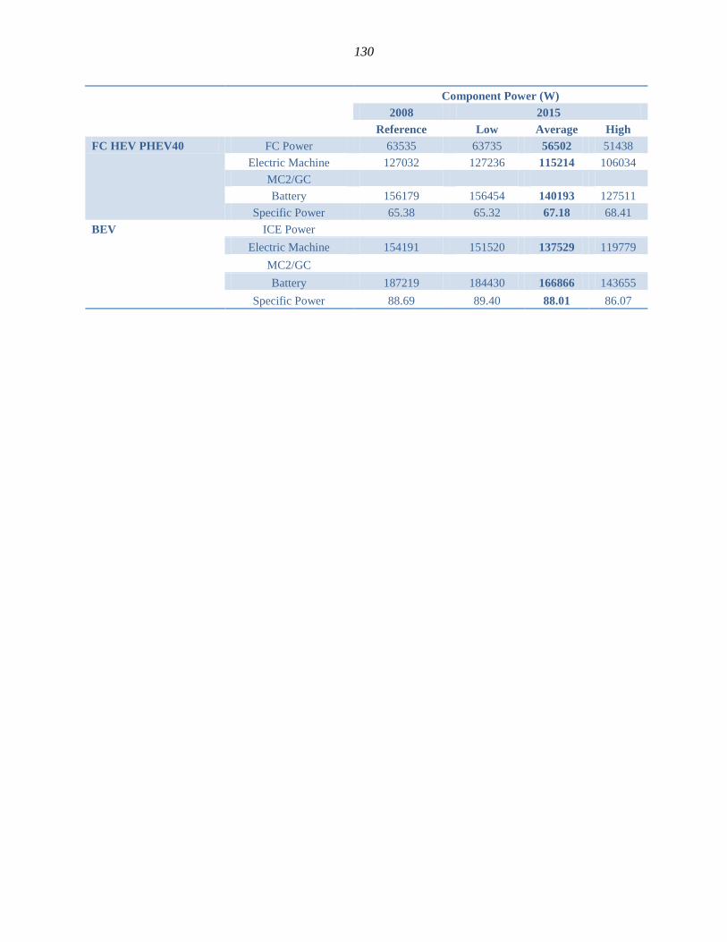
130

Component Power (W)

2008 2015




MC2/GC

Battery 156179 156454 140193 127511

Specific Power 65.38 65.32 67.18 68.41

BEV ICE Power


MC2/GC

Battery 187219 184430 166866 143655

Specific Power 88.69 89.40 88.01 86.07

131

2. Battery Energy

Battery Energy (Wh)

2008 2015


SI Split HEV Total Energy 1123.2 1107.6 1045.2 990.6

Usable Energy

SI Split HEV PHEV10 Total Energy 3866.7 3863.0 3474.6 2715.2

Usable Energy 2320.0 2317.8 2084.8 1900.6

SI Split HEV PHEV20 Total Energy 7534.6 7595.7 6829.6 5344.9

Usable Energy 4520.8 4557.4 4097.8 3741.4

SI Series HEV PHEV30 Total Energy 13066.1 12810.6 11593.9 8855.2

Usable Energy 7839.6 7686.4 6956.4 6198.6

SI Series HEV PHEV40 Total Energy 17627.2 17393.3 15593.6 11840.2

Usable Energy 10576.3 10436.0 9356.2 8288.2

CI Split HEV Total Energy 1185.6 1162.2 1107.6 1045.2

Usable Energy

CI Split HEV PHEV10 Total Energy 4199.0 4184.4 3698.2 2928.4

Usable Energy 2519.4 2510.7 2218.9 2049.9

CI Split HEV PHEV20 Total Energy 8041.7 7992.8 7201.0 5702.0

Usable Energy 4825.0 4795.7 4320.6 3991.4

CI Series HEV PHEV30 Total Energy 13206.7 13045.0 11739.5 8983.8

Usable Energy 7924.0 7827.0 7043.7 6288.6

CI Series HEV PHEV40 Total Energy 17848.6 17584.1 15812.2 12020.6

Usable Energy 10709.2 10550.4 9487.3 8414.4

E85 Split HEV Total Energy 1123.2 1099.8 1037.4 990.6

Usable Energy

E85 Split HEV PHEV10 Total Energy 3867.4 3864.0 3475.4 2714.5

Usable Energy 2320.5 2318.4 2085.2 1900.2

E85 Split HEV PHEV20 Total Energy 7627.3 7589.2 6734.9 5344.8

Usable Energy 4576.4 4553.5 4040.9 3741.4

E85 Series HEV PHEV30 Total Energy 13074.7 12816.2 11597.0 8857.3

Usable Energy 7844.8 7689.7 6958.2 6200.1

E85 Series HEV PHEV40 Total Energy 17639.8 17403.7 15598.1 11842.1

Usable Energy 10583.9 10442.2 9358.9 8289.5

H2 Split HEV Total Energy 1099.8 1076.4 1014.0 959.4

Usable Energy

H2 Split HEV PHEV10 Total Energy 3912.0 3895.8 3496.1 2727.9

Usable Energy 2347.2 2337.5 2097.6 1909.6

H2 Split HEV PHEV20 Total Energy 7467.7 7435.0 6751.3 5267.1

Usable Energy 4480.6 4461.0 4050.8 3687.0

H2 Series HEV PHEV30 Total Energy 12906.0 12623.6 11320.7 8703.0

Usable Energy 7743.6 7574.1 6792.4 6092.1

H2 Series HEV PHEV40 Total Energy 17389.4 17121.2 15358.0 11630.5

Usable Energy 10433.6 10272.7 9214.8 8141.4

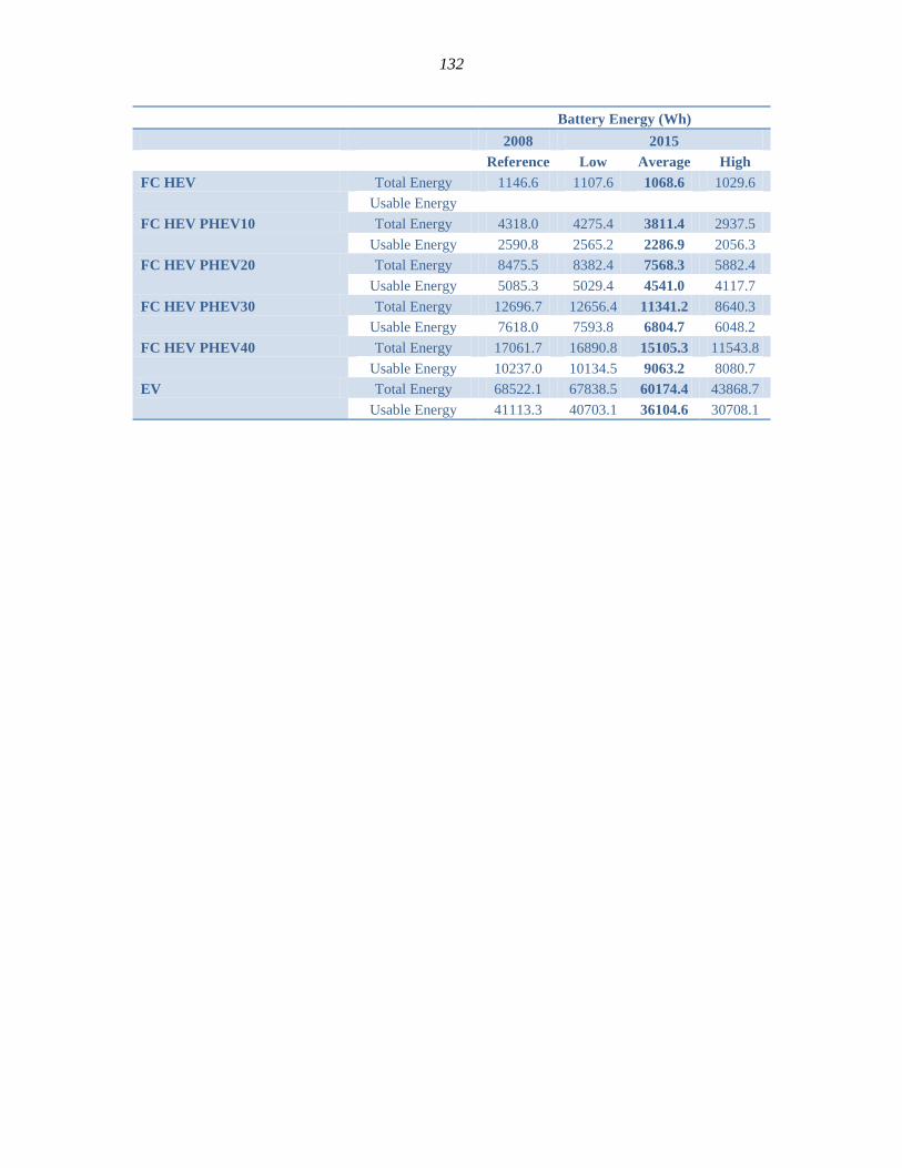
132

Battery Energy (Wh)

2008 2015


FC HEV Total Energy 1146.6 1107.6 1068.6 1029.6

Usable Energy

FC HEV PHEV10 Total Energy 4318.0 4275.4 3811.4 2937.5

Usable Energy 2590.8 2565.2 2286.9 2056.3


Usable Energy 5085.3 5029.4 4541.0 4117.7


Usable Energy 7618.0 7593.8 6804.7 6048.2


Usable Energy 10237.0 10134.5 9063.2 8080.7

EV Total Energy 68522.1 67838.5 60174.4 43868.7

Usable Energy 41113.3 40703.1 36104.6 30708.1

133

3. Vehicle Weight

Vehicle Test Weight (kg)

2008 2015


SI Conv Vehicle Mass 1580 1578 1500 1445

% of glider mass 62.7 62.7 61.1 59.9

CI Conv Vehicle Mass 1645 1644 1567 1514

% of glider mass 60.2 60.2 58.4 57.2

H2 Conv Vehicle Mass 1720 1771 1563 1470

% of glider mass 57.6 55.9 58.6 58.9

E85 Conv Vehicle Mass 1581 1580 1503 1447

% of glider mass 62.6 62.7 60.9 59.9

SI Split HEV Vehicle Mass 1687 1659 1567 1485

% of glider mass 58.7 59.7 58.4 58.3

SI Split HEV PHEV10 Vehicle Mass 1688 1661 1568 1484

% of glider mass 58.6 59.6 58.4 58.4

SI Split HEV PHEV20 Vehicle Mass 1719 1691 1596 1503

% of glider mass 57.6 58.5 57.4 57.6

SI Series HEV PHEV30 Vehicle Mass 1931 1874 1758 1631

% of glider mass 51.3 52.8 52.1 53.1

SI Series HEV PHEV40 Vehicle Mass 1973 1916 1792 1658

% of glider mass 50.2 51.7 51.1 52.2

CI Split HEV Vehicle Mass 1784 1748 1657 1572

% of glider mass 55.5 56.6 55.3 55.1

CI Split HEV PHEV10 Vehicle Mass 1789 1759 1666 1578

% of glider mass 55.3 56.3 55.0 54.9

CI Split HEV PHEV20 Vehicle Mass 1820 1789 1693 1600

% of glider mass 54.4 55.3 54.1 54.1

CI Series HEV PHEV30 Vehicle Mass 1968 1910 1792 1664

% of glider mass 50.3 51.8 51.1 52.1

CI Series HEV PHEV40 Vehicle Mass 2011 1953 1828 1692

% of glider mass 49.2 50.7 50.1 51.2

H2 Split HEV Vehicle Mass 1667 1652 1516 1421

% of glider mass 59.4 59.9 60.4 61.0

H2 Split HEV PHEV10 Vehicle Mass 1677 1663 1525 1424

% of glider mass 59.0 59.5 60.0 60.8

H2 Split HEV PHEV20 Vehicle Mass 1707 1692 1551 1447

% of glider mass 58.0 58.5 59.0 59.9

H2 Series HEV PHEV30 Vehicle Mass 1912 1873 1705 1566

% of glider mass 51.8 52.9 53.7 55.3

H2 Series HEV PHEV40 Vehicle Mass 1954 1915 1741 1590

% of glider mass 50.7 51.7 52.6 54.5

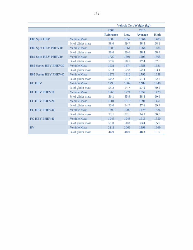
134

Vehicle Test Weight (kg)

2008 2015


E85 Split HEV Vehicle Mass 1689 1657 1566 1485

% of glider mass 58.6 59.7 58.5 58.3

E85 Split HEV PHEV10 Vehicle Mass 1688 1661 1568 1484

% of glider mass 58.6 59.6 58.4 58.4

E85 Split HEV PHEV20 Vehicle Mass 1720 1691 1595 1505

% of glider mass 57.6 58.5 57.4 57.6

E85 Series HEV PHEV30 Vehicle Mass 1931 1874 1758 1631

% of glider mass 51.3 52.8 52.1 53.1

E85 Series HEV PHEV40 Vehicle Mass 1973 1916 1792 1658

% of glider mass 50.2 51.7 51.1 52.2

FC HEV Vehicle Mass 1793 1809 1582 1440

% of glider mass 55.2 54.7 57.9 60.2

FC HEV PHEV10 Vehicle Mass 1765 1771 1557 1429

% of glider mass 56.1 55.9 58.8 60.6


% of glider mass 55.0 54.7 57.6 59.7


% of glider mass 52.1 52.1 54.5 56.8


% of glider mass 51.0 50.8 53.4 55.9

EV Vehicle Mass 2111 2063 1896 1669

% of glider mass 46.9 48.0 48.3 51.9

Documents

Well-To-Wheels Energy and Greenhouse Gas Analysis of … · 2.13 Usable Battery Energy for PHEV Midsize Vehicle with Gasoline Engine ..... 27 2.14 Usable Battery Energy for PHEV Midsize