Western Washington NPDES Phase I Stormwater … Washington . NPDES Phase I Stormwater Permit . ... 2010-2011 ... These monitoring requirements enabled uniform data collection and similar

Western Washington

NPDES Phase I Stormwater Permit

Final S8.D Data Characterization

2009-2013

February 2015

Publication No. 15-03-001

Publication information This report is available on the Department of Ecology’s website at https://fortress.wa.gov/ecy/publications/SummaryPages/1503001.html Suggested Citation: Hobbs, W., B. Lubliner, N. Kale, and E. Newell. 2015. Western Washington NPDES Phase 1 Stormwater Permit: Final Data Characterization 2009-2013. Washington State Department of Ecology, Olympia, WA. Publication No. 15-03-001. https://fortress.wa.gov/ecy/publications/SummaryPages/1503001.html Data for this project are available at Ecology’s Environmental Information Management (EIM) website www.ecy.wa.gov/eim/index.htm. Search Study IDs:

WAR044002_S8D WAR044003_S8D

WAR044200_S8D WAR044501_S8D

WAR044502_S8D WAR044503_S8D WAR044701_S8D WAR044001_S8D

The Activity Tracker Code for this study is 13-002. Contact information For more information contact: Publications Coordinator Environmental Assessment Program P.O. Box 47600, Olympia, WA 98504-7600 Phone: (360) 407-6764 Washington State Department of Ecology - www.ecy.wa.gov o Headquarters, Olympia (360) 407-6000 o Northwest Regional Office, Bellevue (425) 649-7000 o Southwest Regional Office, Olympia (360) 407-6300 o Central Regional Office, Yakima (509) 575-2490 o Eastern Regional Office, Spokane (509) 329-3400

Any use of product or firm names in this publication is for descriptive purposes only and

does not imply endorsement by the author or the Department of Ecology.

Accommodation Requests: To request ADA accommodation including materials in a format

for the visually impaired, call Ecology at 360-407-6764. Persons with impaired hearing may call

Washington Relay Service at 711. Persons with speech disability may call TTY at 877-833-6341.

https://fortress.wa.gov/ecy/publications/SummaryPages/1503001.html


http://www.ecy.wa.gov/eim/index.htm

http://www.ecy.wa.gov/

Page 1

Western Washington

NPDES Phase I Stormwater Permit

Final S8.D Data Characterization 2009-2013

by

William Hobbsa, Brandi Lublinerb*, Nathaniel Kaleb*, and Evan Newella

a Environmental Assessment Program Washington State Department of Ecology

Olympia, Washington 98504-7710

b Water Quality Program Washington State Department of Ecology

Olympia, Washington 98504-7600

*Corresponding author

Water Resource Inventory Area (WRIA) and 8-digit Hydrologic Unit Code (HUC) numbers for the study area: WRIAs 5, 7, 8, 9, 10, 12, and 28

HUC numbers 17080003, 17110010, 17110011, 17110012, 17110013, 17110014, 17110019

Page 2

This page is purposely left blank

Page 3

Table of Contents

Page

List of Figures and Tables....................................................................................................5

Abstract ................................................................................................................................7

Acknowledgements ..............................................................................................................8

Executive Summary .............................................................................................................9 Introduction ....................................................................................................................9 Purpose ...........................................................................................................................9 Methods........................................................................................................................11 Results ..........................................................................................................................11

Discussion ....................................................................................................................14 Recommendations ........................................................................................................16 Data Access ..................................................................................................................17

Introduction ........................................................................................................................18 Purpose .........................................................................................................................18 Permit-Defined Stormwater Monitoring ......................................................................19

Stormwater Monitoring Design .............................................................................19 Stormwater Sediment Monitoring Design .............................................................23 Laboratory Analytical Methods .............................................................................25 Laboratory Quality Assurance ...............................................................................25

Methods..............................................................................................................................26 Data Qualification ........................................................................................................26

Quantitation and Reporting Limits ........................................................................26 Qualified Data ........................................................................................................26

Data Compilation and Management ............................................................................29 Data Collection and Accessibility ..........................................................................29 Data Compilation ...................................................................................................29

Numerical Analysis ......................................................................................................32 Non-Detect Data ....................................................................................................32 Data Distributions ..................................................................................................32 Descriptive Statistics ..............................................................................................33

Multivariate Statistics ............................................................................................34 Comparison to Stormwater Studies and Water Quality Criteria ..................................35

Relevant Stormwater Studies Explored .................................................................35

Water Quality Criteria............................................................................................37

Approaches to Non-Detected Data in the Stormwater Literature ................................38

Results and Discussion ......................................................................................................39 Database Description ...................................................................................................39

Data Quality ...........................................................................................................40 Data Distribution and Case Summary....................................................................40 High Frequency Non-Detected Parameters ...........................................................41

Page 4

Hydrology ....................................................................................................................42

Storm Events ..........................................................................................................42 Sample Representativeness ....................................................................................44 Runoff Coefficients ................................................................................................45

Contaminant Concentrations ........................................................................................46 Conventional Parameters .......................................................................................47 Nutrients .................................................................................................................51 Metals .....................................................................................................................53 Hydrocarbons .........................................................................................................59 Phthalates ...............................................................................................................64 Pesticides................................................................................................................66 PCBs ......................................................................................................................68 Contaminant Concentrations - Summary of Findings ...........................................68

Land Use Significance .................................................................................................70

Peto-Prentice Test ..................................................................................................70 Principal Components Analysis .............................................................................72

Parameter Similarities ..................................................................................................75 Seasonality ...................................................................................................................75 Contaminant Loads ......................................................................................................78

Summary of Loads per Unit Area ..........................................................................78 Contaminant Load Summary .................................................................................82

Summary ............................................................................................................................83

Key Findings ......................................................................................................................84 Stormwater Monitoring Program .................................................................................84 Stormwater Discharge Quality .....................................................................................84

Stormwater Sediment Quality ......................................................................................85 Comparisons with Relevant National and Local Stormwater Studies .........................85

Recommendations ..............................................................................................................87

References ..........................................................................................................................89

Appendices .........................................................................................................................93 Appendix A. Municipal Stormwater Trout Embryo Toxicity Testing: Results from First Flush, 2010-2011 .................................................................................................94

Appendix B. Permittees’ Quality Assurance Project Plans ........................................99 Appendix C. Description of the Statistical Plots ......................................................100 Appendix D. Tables for Database Description .........................................................112 Appendix E. Hydrology ............................................................................................136 Appendix F. Data Plots for Contaminant Concentrations ........................................141

Appendix G. Contaminant Concentrations ...............................................................142 Appendix H. Data Plots for Contaminant Loads ......................................................148

Appendix I. Contaminant Loads ...............................................................................149 Appendix J. Glossary, Acronyms, and Abbreviations ..............................................150

Page 5

List of Figures and Tables

Page

Figures

Figure 1. Site location map. ..............................................................................................21

Figure 2. Simplified diagram of laboratory thresholds and data results. ..........................26

Figure 3. Non-detect reporting limits for dichlobenil by laboratory. ...............................28

Figure 4. Median measured event precipitation totals for sample locations in the Puget Sound region and Clark County, combined with daily precipitation totals from SeaTac International Airport and Vancouver, Washington. ...........43

Figure 5. Percent of each storm captured by sampling for each sample site. ...................45

Figure 6. Runoff coefficient for each catchment basin, categorized by land use, relative to the percent impervious surface within each catchment. ...................46

Figure 7. Summary of conventional parameters in water. ................................................47

Figure 8. Summary of nutrient concentrations in water. ..................................................51

Figure 9. Summary of metals concentrations in water. ....................................................53

Figure 10. Summary of metals concentrations in stormwater sediment. ..........................57

Figure 11. Summary of total PAH concentration sums in water. .....................................62

Figure 12. Summary of total PAH concentration sums in stormwater sediment. .............64

Figure 13. Summary of pesticide concentrations in stormwater. ......................................67

Figure 14. Principal components analysis of stormwater samples. ..................................73

Figure 15. Principal components analysis of stormwater sediment samples ....................74

Figure 16. Box plot of measured storm volume during the wet and dry season...............76

Tables Table 1. Phase I S8.D sites and land-use summary. .........................................................20

Table 2. Permittee-monitored parameters. ........................................................................24

Table 3. Summary of permittee data compiled for this report. .........................................29

Table 4. Summary of organizational considerations for stormwater data submitted to the EIM database. ...............................................................................................30

Table 5. Methods for estimating summary statistics. .......................................................33

Table 6. Number of records by permittee, land use, and year. .........................................39

Table 7. Stormwater and stormwater sediment parameters with >90% non-detect data. .42

Table 8. Number of unique sampling dates for each permittee and land use. ..................44

Table 9. Summary of fecal coliform bacteria data ............................................................48

Table 10. Summary of conductivity, hardness, pH, and chloride concentrations. ...........48

Table 11. Summary surfactants and biochemical oxygen demand concentrations. .........49

Page 6

Table 12. Summary of turbidity and total suspended solid concentrations. .....................50

Table 13. Summary of total organic carbon concentration in sediments. .........................50

Table 14. Summary of phosphorus concentrations. ..........................................................51

Table 15. Summary of nitrogen concentrations. ...............................................................52

Table 16. Summary of dissolved arsenic concentrations. .................................................54

Table 17. Summary of cadmium concentrations. .............................................................54

Table 18. Summary of copper concentrations. .................................................................55

Table 19. Summary of lead concentrations.......................................................................56

Table 20. Summary of mercury concentrations. ...............................................................57

Table 21. Summary of zinc concentrations.......................................................................58

Table 22. Summary of total petroleum hydrocarbon concentrations. ...............................59

Table 23. Summary of BTEX concentrations. ..................................................................60

Table 24. Summary of individual PAHs in stormwater. ...................................................61

Table 25. Summary of individual PAHs in stormwater sediments ...................................63

Table 26. Summary of phthalates in stormwater ..............................................................65

Table 27. Summary of individual phthalates in stormwater sediments ............................65

Table 28. Summary of pesticides in stormwater. ..............................................................66

Table 29. Summary of pesticides concentrations in stormwater sediments. ....................67

Table 30. Summary of total PCB concentrations in stormwater and stormwater sediments. ..........................................................................................................68

Table 31. Case A parameters with evidence of differences in water contaminant concentrations by land use. ...............................................................................70

Table 32. Seasonality of stormwater concentrations. .......................................................77

Page 7

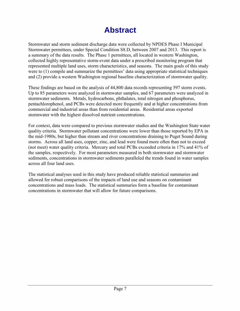
Abstract

Stormwater and storm sediment discharge data were collected by NPDES Phase I Municipal Stormwater permittees, under Special Condition S8.D, between 2007 and 2013. This report is a summary of the data results. The Phase 1 permittees, all located in western Washington, collected highly representative storm-event data under a prescribed monitoring program that represented multiple land uses, storm characteristics, and seasons. The main goals of this study were to (1) compile and summarize the permittees’ data using appropriate statistical techniques and (2) provide a western Washington regional baseline characterization of stormwater quality. These findings are based on the analysis of 44,800 data records representing 597 storm events. Up to 85 parameters were analyzed in stormwater samples, and 67 parameters were analyzed in stormwater sediments. Metals, hydrocarbons, phthalates, total nitrogen and phosphorus, pentachlorophenol, and PCBs were detected more frequently and at higher concentrations from commercial and industrial areas than from residential areas. Residential areas exported stormwater with the highest dissolved nutrient concentrations. For context, data were compared to previous stormwater studies and the Washington State water quality criteria. Stormwater pollutant concentrations were lower than those reported by EPA in the mid-1980s, but higher than stream and river concentrations draining to Puget Sound during storms. Across all land uses, copper, zinc, and lead were found more often than not to exceed (not meet) water quality criteria. Mercury and total PCBs exceeded criteria in 17% and 41% of the samples, respectively. For most parameters measured in both stormwater and stormwater sediments, concentrations in stormwater sediments paralleled the trends found in water samples across all four land uses. The statistical analyses used in this study have produced reliable statistical summaries and allowed for robust comparisons of the impacts of land use and seasons on contaminant concentrations and mass loads. The statistical summaries form a baseline for contaminant concentrations in stormwater that will allow for future comparisons.

Page 8

Acknowledgements

The authors thank the following for their contributions to this report. Permittees who contributed data for analysis:

Clark County

King County

Pierce County

Snohomish County

City of Seattle

City of Tacoma

Port of Seattle

Port of Tacoma

Washington State Department of Ecology staff:

Rachel McCrea, Ed O’Brien, Vince McGowan, Nancy Winters, Randall Marshall, Abbey Stockwell, and James Maroncelli for reviewing the draft report.

Adam Oestreich for data quality control and EIM support.

Dale Norton for project guidance.

Jean Maust, Joan LeTourneau, and Cindy Cook for formatting and proofing the final report.

Dennis Helsel, Practical Stats, Inc., for statistical assistance.

Page 9

Executive Summary

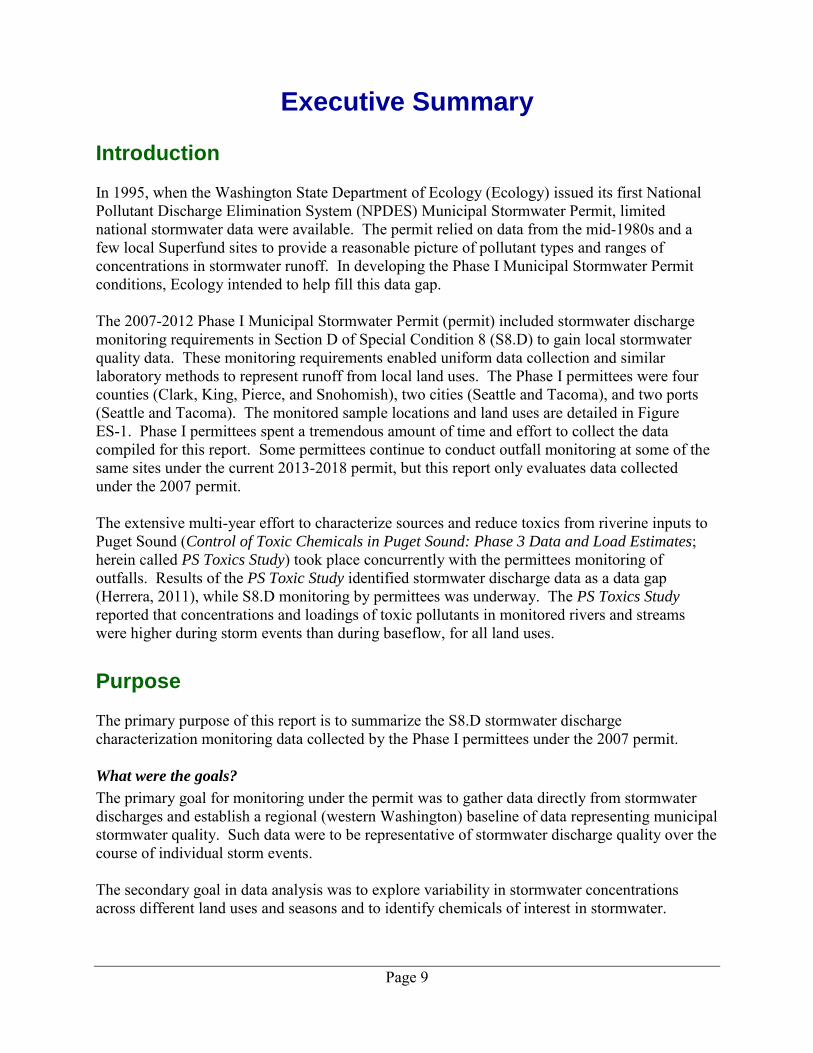
Introduction In 1995, when the Washington State Department of Ecology (Ecology) issued its first National Pollutant Discharge Elimination System (NPDES) Municipal Stormwater Permit, limited national stormwater data were available. The permit relied on data from the mid-1980s and a few local Superfund sites to provide a reasonable picture of pollutant types and ranges of concentrations in stormwater runoff. In developing the Phase I Municipal Stormwater Permit conditions, Ecology intended to help fill this data gap. The 2007-2012 Phase I Municipal Stormwater Permit (permit) included stormwater discharge monitoring requirements in Section D of Special Condition 8 (S8.D) to gain local stormwater quality data. These monitoring requirements enabled uniform data collection and similar laboratory methods to represent runoff from local land uses. The Phase I permittees were four counties (Clark, King, Pierce, and Snohomish), two cities (Seattle and Tacoma), and two ports (Seattle and Tacoma). The monitored sample locations and land uses are detailed in Figure ES-1. Phase I permittees spent a tremendous amount of time and effort to collect the data compiled for this report. Some permittees continue to conduct outfall monitoring at some of the same sites under the current 2013-2018 permit, but this report only evaluates data collected under the 2007 permit. The extensive multi-year effort to characterize sources and reduce toxics from riverine inputs to Puget Sound (Control of Toxic Chemicals in Puget Sound: Phase 3 Data and Load Estimates; herein called PS Toxics Study) took place concurrently with the permittees monitoring of outfalls. Results of the PS Toxic Study identified stormwater discharge data as a data gap (Herrera, 2011), while S8.D monitoring by permittees was underway. The PS Toxics Study reported that concentrations and loadings of toxic pollutants in monitored rivers and streams were higher during storm events than during baseflow, for all land uses.

Purpose The primary purpose of this report is to summarize the S8.D stormwater discharge characterization monitoring data collected by the Phase I permittees under the 2007 permit.

What were the goals?

The primary goal for monitoring under the permit was to gather data directly from stormwater discharges and establish a regional (western Washington) baseline of data representing municipal stormwater quality. Such data were to be representative of stormwater discharge quality over the course of individual storm events. The secondary goal in data analysis was to explore variability in stormwater concentrations across different land uses and seasons and to identify chemicals of interest in stormwater.

Page 10

Figure ES-1. Site locations of monitored stormwater catchments and corresponding land

use.

Land use types: LDR = low-density residential; HDR = high-density residential;

COM = commercial; IND = industrial

")

"/

#*

Clark

County

Cowlitz

County

COM

LDR

HDR

Vancouver

#*")#*#*

#*

")

"/

#*

Pierce

County

King

County

COM

LDR

HDR

COM

INDCOM

HDR

Tacoma

Federal Way

Kent

#*#*

"/

#*

#*#*

")

"/

#*

#*#*#*#*

")

")

#*

#*

#*

King

County

Snohomish

County

Island

County

KitsapCounty

IND

COM

COM

HDR

HDR

COM

COM

LDR

HDR

COM

LDR

PRECIP

Seattle

Everett

Bellevue

Kent

Renton

Shoreline

King

Lewis

Clallam

Pierce

Skagit

Jefferson

Whatcom

Snohomish

Yakima

Pacific

Skamania

Grays Harbor

Cowlitz

Mason

Clark

Kitsap

Thurston

Klickitat

Island

Kittitas

San Juan

Wahkiakum

Phase I Permittee S8.D

Monitoring Locations

Land Use

") High Density Residential

"/ Low Density Residential

#* Commercial

#* Industrial

Counties

saltwater

rivers

City (incorp)

¯

Created February 2014, BLEdited August 2014, WH

0 31.5

Miles

0 4 82

Miles

0 2 41

Miles

A

B

C

A

B C

Page 11

What was achieved?

This report provides statistical summaries for municipal storm-event concentrations for 172 parameters across four land uses and wet and dry seasons in western Washington. Ecology recognizes the substantial contribution made by the permittees to our collective understanding of stormwater chemistry in western Washington.

Methods For this final report, Ecology downloaded, compiled, and analyzed the complete permit monitoring data from Ecology’s Environmental Information Management (EIM) database. Stormwater was monitored from 2009 through 2013, and samples were collected using flow-weighted automatic composite samplers for most parameters. Each location has at least three years of data. Composite sample volumes were in compliance with the required collection approach of a storm’s hydrograph under the permit. Samples generally spanned 75% or more of the first 24 hours of each storm. Permittees submitted rainfall amount, runoff volume, and concentration data for stormwater samples to Ecology’s EIM database. Concentration data for stormwater-related sediments are also available in EIM; however, these data were collected less uniformly, using either grab samples or traps in the storm pipe system.

Results The final data set encompassed 44,800 records submitted to Ecology by Phase 1 permittees, representing an estimated 597 storm events. Up to 85 chemicals were analyzed for any given stormwater sample, and 67 chemicals were analyzed in stormwater sediment samples. The composite stormwater samples were found to be representative of storm length, storm volumes, and frequency of storm events in western Washington. The database is suitable for characterizing stormwater quality in western Washington. Detection Frequency

The rate of detection varied across land use and by parameter. Overall, metals, nutrients, and conventional parameters were detected in nearly all stormwater and stormwater sediment samples. The following parameters were frequently detected in stormwater: Conventional parameters (biochemical oxygen demand, pH, conductivity, chloride, turbidity,

total suspended solids) had a 98% detection rate. Surfactants were detected in 60% of the samples.

Metals except mercury were commonly detected; arsenic, copper, lead, magnesium, and zinc were found in 90% of the samples. Cadmium was detected in just over 60% of the samples.

Nutrients (nitrogen and phosphorus) were detected in 90% of the samples. Polycyclic aromatic hydrocarbon (PAHs) were detected in 73% of the samples. Total petroleum hydrocarbons (diesel range fractions) were detected in 73% of the samples. bis(2-ethylhexyl)phthalate was found in 62% of the samples.

Page 12

The detection rate of organic compounds (such as total petroleum hydrocarbons – diesel fractions, PAHs, and phthalates) and certain metals (copper, lead, and zinc) in stormwater sediments was more than 90%. Diesel, motor oil, copper, and zinc were found in all stormwater sediment samples collected. Chemicals are considered non-detect if the concentration was not measured above the method detection limit. The following parameters were either infrequently detected or not detected at all: Benzene, toluene, ethylbenzene, and xylenes (BTEX) in stormwater were found in less than

3% of the samples. Malathion, prometon, chlorpyrifos, and diazinon in stormwater and stormwater sediments

were found in less than 4% of the samples. Triclopyr and mecoprop was detected at a rate of 8% in stormwater sediments and

approximately 11% in stormwater samples. Most phenolics in stormwater sediments were not detected at all, except for

pentachlorophenol, o-cresol, and p-cresol (detection rates of 25, 19, and 77% respectively). Land Use

Metals, hydrocarbons, phthalates, total nitrogen and phosphorus, pentachlorophenol, and PCBs were detected more frequently and at higher concentrations from commercial and industrial lands than from residential lands. Residential lands exported stormwater with the highest dissolved nutrient concentrations. All parameters with high rates of detection exhibited statistically different concentrations across land uses. Individual parameters showed strong differences among land uses. However, when parameters were grouped or summed (e.g., sum of PAHs), greater overlap in stormwater chemistry among land uses was found. Chemicals of Interest and Importance

To put the results of this compilation effort into context, Ecology compared these results using two primary sources of information. The first source was a suite of literature including the Nationwide Urban Runoff Program (NURP; EPA, 1983) and analysis of the National Stormwater Quality Database (Maestre et al., 2005). These are discussed in the next section. The second primary source was the Washington State Water Quality Criteria. The national studies and Washington’s water quality criteria form the “bookends” for comparing the stormwater discharge results of this compilation. The intent of this report is to characterize data, not to evaluate compliance. The comparison to criteria presents an understanding of parameters and land uses where stormwater improvements and resources can be focused to improve water and sediment quality. Across all four land uses, copper, zinc, and lead were−more often than not−found to exceed (not meet) water quality criteria (Table ES-1). Dissolved zinc and copper in stormwater samples exceeded acute aquatic life criteria in 36% and 50% of the samples, respectively, over the three years of data. Mercury and total PCBs exceeded chronic aquatic life criteria in 17% and 41% of

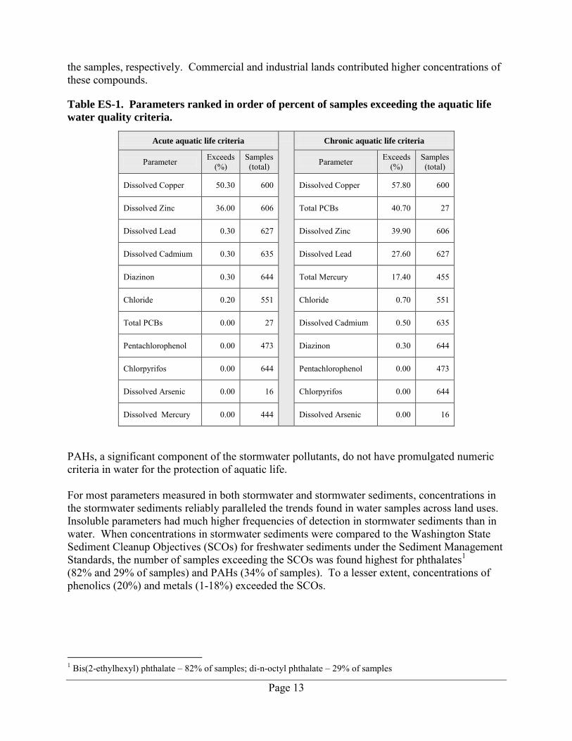
Page 13

the samples, respectively. Commercial and industrial lands contributed higher concentrations of these compounds.

Table ES-1. Parameters ranked in order of percent of samples exceeding the aquatic life

water quality criteria.

Acute aquatic life criteria

Chronic aquatic life criteria

Parameter Exceeds (%)

Samples (total) Parameter Exceeds

(%) Samples (total)

Dissolved Copper 50.30 600 Dissolved Copper 57.80 600

Dissolved Zinc 36.00 606 Total PCBs 40.70 27

Dissolved Lead 0.30 627 Dissolved Zinc 39.90 606

Dissolved Cadmium 0.30 635 Dissolved Lead 27.60 627

Diazinon 0.30 644 Total Mercury 17.40 455

Chloride 0.20 551 Chloride 0.70 551

Total PCBs 0.00 27 Dissolved Cadmium 0.50 635

Pentachlorophenol 0.00 473 Diazinon 0.30 644

Chlorpyrifos 0.00 644 Pentachlorophenol 0.00 473

Dissolved Arsenic 0.00 16 Chlorpyrifos 0.00 644

Dissolved Mercury 0.00 444 Dissolved Arsenic 0.00 16

PAHs, a significant component of the stormwater pollutants, do not have promulgated numeric criteria in water for the protection of aquatic life. For most parameters measured in both stormwater and stormwater sediments, concentrations in the stormwater sediments reliably paralleled the trends found in water samples across land uses. Insoluble parameters had much higher frequencies of detection in stormwater sediments than in water. When concentrations in stormwater sediments were compared to the Washington State Sediment Cleanup Objectives (SCOs) for freshwater sediments under the Sediment Management Standards, the number of samples exceeding the SCOs was found highest for phthalates1 (82% and 29% of samples) and PAHs (34% of samples). To a lesser extent, concentrations of phenolics (20%) and metals (1-18%) exceeded the SCOs.

1 Bis(2-ethylhexyl) phthalate – 82% of samples; di-n-octyl phthalate – 29% of samples

Page 14

Seasonality and Loads

Higher contaminant concentrations and mass loads were measured for nutrients and metals during the dry season (May through September). This provides strong evidence for an influence of seasonality (or antecedent dry periods) on stormwater concentrations, particularly in late summer through early fall; it also supports the idea that there is a degree of “buildup” in the dry periods between storms. Metals, diesel hydrocarbons, and total nutrient loads were higher in the dry season and highest from commercial and industrial areas. PAHs, phthalates, and detected pesticides (dichlobenil and pentachlorophenol) did not exhibit this significant seasonal difference, suggesting a consistent source throughout the year and no buildup in the dry months.

Discussion This study improves Ecology’s understanding of the quality of stormwater discharges to receiving waters. The study provides:

Local and land use-based stormwater quality data. Flow-weighted composite sample data which are superior in quality to grab samples and best

represent storm-event concentrations. Direct baseline to measure the performance of stormwater management actions at a regional

scale. Summary statistics from a very large data set that are not biased by substituting for non-

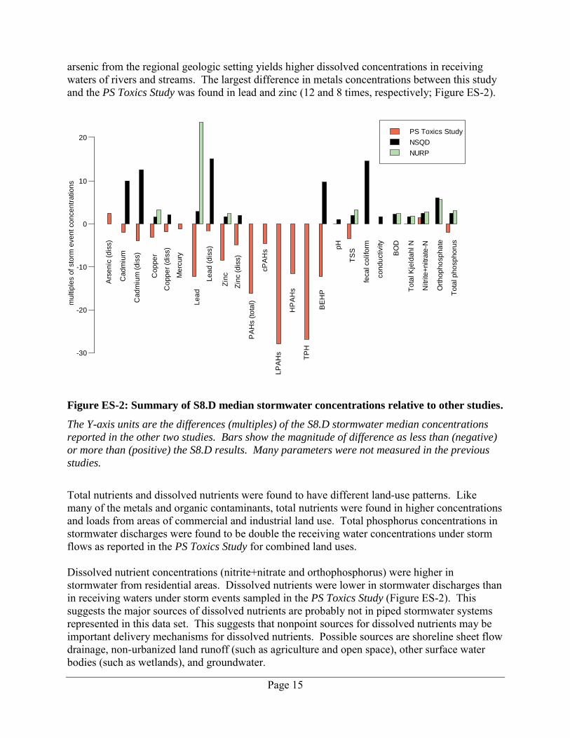
detect results. Generally in this stormwater discharge data set, individual storm-event concentrations were within the ranges reported in the National Stormwater Quality Database (NSQD) (Maestre et al., 2004 and 2005), but median values were consistently lower (Figure ES-2). These concentrations are also much lower in some cases (e.g., lead is 23 times lower) than those from the earliest national study on stormwater, NURP (EPA, 1983). This may be due to the age of the early studies, subsequent improvements in stormwater quality and management since the NURP sampling, or possibly our wetter climate that allows for more wash off between monitored storms. Nevertheless, the current study offers many of the same conclusions about land-use patterns as the PS Toxics Study (Herrera, 2011) and NURP/NSQD studies of the 1980s and 1990s. For example, concentrations of metals from commercial and industrial land uses have remained high. For many of the parameters, concentrations were higher in stormwater discharges in the current study than levels found in the recent PS Toxics Study (Figure ES-2). This finding is not surprising given the PS Toxics Study sampled ambient receiving waters, while these current stormwater data are representative of discharges to receiving waters. In the current study, metals (total and dissolved) were much lower (2 to 15 times) than in the NURP and NSQD data sets (Figure ES-2). Compared with the PS Toxics Study, metals were generally higher in stormwater, with the exception of dissolved arsenic. High background

Page 15

arsenic from the regional geologic setting yields higher dissolved concentrations in receiving waters of rivers and streams. The largest difference in metals concentrations between this study and the PS Toxics Study was found in lead and zinc (12 and 8 times, respectively; Figure ES-2).

Figure ES-2: Summary of S8.D median stormwater concentrations relative to other studies.

The Y-axis units are the differences (multiples) of the S8.D stormwater median concentrations

reported in the other two studies. Bars show the magnitude of difference as less than (negative)

or more than (positive) the S8.D results. Many parameters were not measured in the previous

studies. Total nutrients and dissolved nutrients were found to have different land-use patterns. Like many of the metals and organic contaminants, total nutrients were found in higher concentrations and loads from areas of commercial and industrial land use. Total phosphorus concentrations in stormwater discharges were found to be double the receiving water concentrations under storm flows as reported in the PS Toxics Study for combined land uses. Dissolved nutrient concentrations (nitrite+nitrate and orthophosphorus) were higher in stormwater from residential areas. Dissolved nutrients were lower in stormwater discharges than in receiving waters under storm events sampled in the PS Toxics Study (Figure ES-2). This suggests the major sources of dissolved nutrients are probably not in piped stormwater systems represented in this data set. This suggests that nonpoint sources for dissolved nutrients may be important delivery mechanisms for dissolved nutrients. Possible sources are shoreline sheet flow drainage, non-urbanized land runoff (such as agriculture and open space), other surface water bodies (such as wetlands), and groundwater.

Ars

en

ic(d

iss)

Ca

dm

ium

Cad

miu

m(d

iss)

Coppe

r

Co

pp

er

(dis

s)

Me

rcu

ry

Lea

d

Lead

(dis

s)

Zin

c

Zin

c(d

iss)

PA

Hs

(to

tal)

cP

AH

s

LP

AH

s

HP

AH

s

TP

H

BE

HP

pH

TS

S

feca

lco

lifo

rm

condu

ctivity

BO

D

To

talK

jeld

ah

lN

Nitri

te+

nitra

te-N

Ort

hopho

spha

te

To

talp

ho

spho

rus

PS Toxics Study

NSQD

NURP

-30

-20

-10

0

10

20

multip

les o

f sto

rm e

vent concentr

ations

Page 16

The permittees analyzed far more parameters than the two older national studies did, particularly organic parameters such as PAHs that were frequently detected in western Washington stormwater. Hydrocarbon median concentrations (PAHs and TPH) were measured at 5 to 26 times higher in this study than those in the PS Toxics Study (Figure ES-2). This compilation of stormwater discharge data corroborates the PS Toxics Study findings about the dominant source of PAHs. High concentrations of PAHs are observed during storm events, with the greatest contribution of PAHs from areas with commercial and industrial land uses. No seasonal differences in PAH concentrations were found in this study. Overall, the highest concentrations and the most frequent exceedances of water quality criteria for toxic compounds were found in stormwater and stormwater sediments discharged from basins with a higher percentage of commercial and industrial land uses. Residential lands contributed the highest concentrations of dissolved nutrients and the pesticides dichlobenil and triclopyr. Triclopyr, which had a high frequency of detection in the PS Toxics Study, was found in only 10% of the 575 stormwater samples analyzed under the permit in this current study.

Recommendations Future Monitoring and Stormwater Management

Continue collecting high quality data representing storm-event concentrations. This is realistic, since all eight permittees met sample frequency and representativeness of the qualifying storm event described in the permit.

Reduce or eliminate from future stormwater monitoring those parameters which were rarely detected:

Benzene, toluene, ethylbenzene, and xylenes (BTEX) in water. Malathion, prometon, chlorpyrifos, and diazinon in water and sediments. Triclopyr and mecoprop in sediments.

Limit testing of phenolics in sediments to pentachlorophenol, o- cresol, and p-cresol.

Expand the spatial scale and number of sites for collection of annual stormwater sediment samples to enhance the survey of possible contaminant sources. Stormwater sediment samples effectively reflect the relative contaminant concentrations by land use.

Apply the findings of this analysis to future stormwater management activities. Stormwater management programs can sweep and conduct other housekeeping best

management practices (BMPs) in industrial and commercial areas during the dry season to reduce high stormwater loads of metals, diesel hydrocarbons, and total nutrients during the first-season storms.

Page 17

Future Puget Sound Monitoring and Modeling

Use this study’s measurements of storm-event concentrations to fill data gaps in Puget Sound models (identified by the PS Toxics Study) for areas draining directly to marine or fresh receiving waters. These areas were missed when monitoring the larger drainages in that study (Herrera, 2011).

Use this stormwater data set in modeling studies for more accurate estimates of toxics loading from stormwater in the Puget Sound basin.

Conduct future studies of BMP effectiveness in the sampled basins, using a similar suite of stormwater chemistry for comparison to these baseline data. For example, evaluate the best timing for sweeping high traffic areas, ports, and parking lots.

Further Study

Consider providing the data online in a simple, user-friendly interface that stormwater managers could use to directly compare to future stormwater chemistry results.

Link this data set with the NSQD to increase the temporal range of the data set.

Further investigate statistical approaches to define "typical" stormwater chemistry for each land use or other basin characteristics (e.g., total impervious area, effective impervious area, vehicular uses, pollution-generating activities).

Continue analysis of unusually high runoff coefficients (percent of a storm’s rainfall that is directed through the stormwater system) that were calculated for some high-density residential sites. This could show whether the runoff coefficient influences the contaminant contributions from these sites.

Explicitly test the influence of antecedent dry periods and seasonal first-flush events in stormwater discharges.

Evaluate the data set for patterns that could help identify and reduce sources of pollution to stormwater. For example, analyze the relationship between the timing of the highest metals concentrations from commercial and industrial areas and whether BMPs can reduce the discharge of copper, zinc, and lead.

Further investigate the data set for relationships between seasonality and land use (or other basin characteristics) for each parameter (e.g., total phosphorus exhibits strong statistical differences among land uses during the wet season, but no significant differences during the dry season).

Evaluate more descriptive landscape variables (e.g., vehicle traffic or road density) with the concentration data.

Data Access This data set is available from Ecology’s Environmental Information Management (EIM) database. Inquiries can be made by contacting report authors B. Lubliner or N. Kale.

Page 18

Introduction

Stormwater transport of pollutants to receiving waters is a local and national concern. The U.S. Environmental Protection Agency (EPA) states, “Polluted stormwater is the leading cause

of impairment to the nearly 40% of surveyed U.S. waterbodies which do not meet water quality

standards.” (EPA Stormwater website). The Washington State Department of Ecology (Ecology) is authorized to administer the Clean Water Act’s National Pollutant Discharge Elimination System (NPDES) permits to implement controls designed to prevent stormwater pollutants from impairing local water bodies. To understand the extent of pollutant loading by stormwater to streams, lakes, rivers, and Puget Sound, Ecology included monitoring requirements in the 2007-2012 Phase I Municipal Stormwater permit (permit)2 (Ecology, 2006 and 2007). Ecology issued the permit to four counties, two cities, and two ports3. Special Condition 8 (S8) of the permit consisted of three main monitoring elements:

Stormwater discharge characterization monitoring and assessment of seasonal first flush toxicity (S8.D).

Stormwater treatment and hydrologic best management practices (BMP) evaluation monitoring (S8.E).

Targeted stormwater management program effectiveness monitoring (S8.F). This report summarizes the results of stormwater discharge characterization monitoring (S8.D) only. Appendix A provides a summary of the screening level toxicity of the first storms in the dry season. This report of the Phase I Permit’s S8.D stormwater monitoring data represents the largest local data set characterizing municipal stormwater discharge quality. Compilation and analysis of stormwater discharges helps fill a data gap identified by a receiving water study: Control of Toxic Chemicals in Puget Sound: Phase 3 Data and Load Estimates by Herrera Environmental Consultants, Inc. (Herrera, 2011), herein called the PS Toxics Study. The PS Toxics Study stated the major data gap was in regional stormwater quality information from conveyance systems, and that discharge data were needed to improve loading estimates to Puget Sound.

Purpose Characterization of stormwater pollutant discharges by land use on a regional scale is an Ecology priority. Stormwater management solutions and decisions are based on knowledge gathered from monitoring the types of pollutants in populated industrial, residential, and commercial land-use areas. The National Estuary Program (NEP) also identified stormwater discharge characterization as a priority. In 2012, NEP provided grant funding to Ecology to compile and

2 The 2012-2013 Phase I Municipal Stormwater Permit continued the 2007 permit’s monitoring requirements,

clarifying endpoints for these monitoring programs and requirements for data submission. 3 The Phase I Municipal Stormwater Permit also covers Secondary Permittees which were not required to conduct

the monitoring discussed in this report.

http://cfpub.epa.gov/npdes/faqs.cfm?program_id=6#1

Page 19

review the S8.D monitoring data collected from 2007 through 2012. An interim report was published based on results available at the time (Lubliner and Newell, 2013). After the interim report was published, the remaining stormwater monitoring data were submitted to Ecology. This final compilation builds on the interim report and establishes a regional baseline of stormwater discharge quality based on monitoring results from the Phase I Permit. The information presented herein provides natural resource managers and stormwater managers with actual stormwater discharge data in western Washington, which can decrease reliance on national studies that may not represent western Washington’s climate or land uses. Improved confidence in local stormwater event concentrations is useful for stormwater managers, regulators, treatment technology development, and future contaminant studies (e.g., source identification and loading studies). This report provides recommendations for future analysis of this data set and recommendations for separate studies. This report also identifies parameters that provide little information about stormwater quality.

Permit-Defined Stormwater Monitoring Stormwater Monitoring Design

Monitoring Permittees

The 2007 monitoring requirements applied to eight Phase I permittees: Cities of Tacoma and Seattle King, Snohomish, Pierce and Clark counties Ports of Tacoma and Seattle To ensure consistency across jurisdictions, monitoring was conducted under Quality Assurance (QA) Project Plans written by the permittees and approved by Ecology. The monitoring program for each permittee is described in detail in each permittees’ QA Project Plan (referenced in Appendix B and available from the permittees). A few aspects of the monitoring programs are important for understanding the monitoring results presented here. Site Selection for Stormwater Characterization

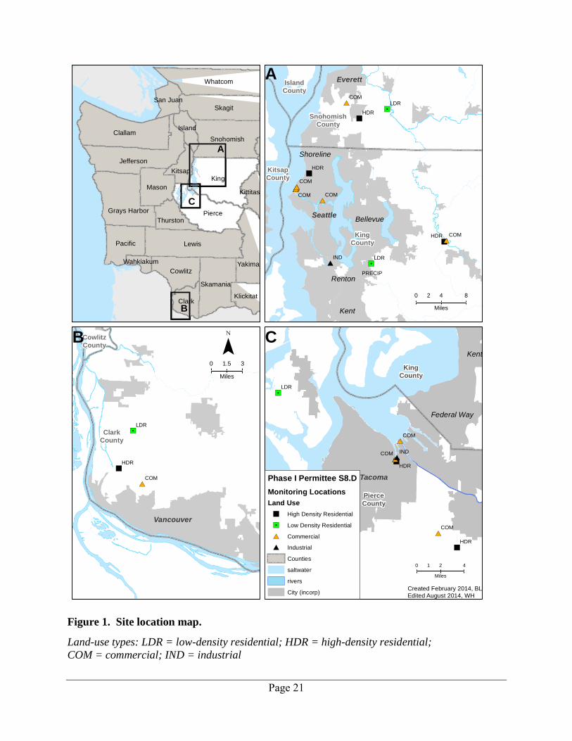
The permit instructed permittees to monitor land uses where, ideally, the drainage area would constitute ≥80% of a particular land use. However, Ecology and the permittees found that stormwater sub-basins tended to contain more variety of land uses and meeting this 80% goal was not possible in all circumstances (Table 1). Permittees monitored one location for each different land-use type. The land-use types monitored by permittees were:

Counties: commercial, high-density residential, and low-density residential. Cities: commercial, high-density residential, and industrial. Ports: commercial. The permit required stormwater monitoring for a total of three years of data collection for each site and each permittee. Table 1 shows the land-use characterization of the drainage areas monitored by each permittee and lists the total impervious area (TIA) estimated in each of the stormwater subbasins monitored. Because estimates of effective impervious area

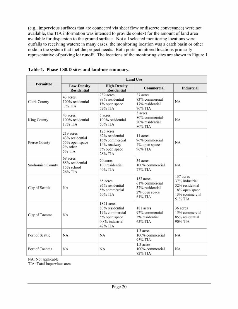
Page 20

(e.g., impervious surfaces that are connected via sheet flow or discrete conveyance) were not available, the TIA information was intended to provide context for the amount of land area available for dispersion to the ground surface. Not all selected monitoring locations were outfalls to receiving waters; in many cases, the monitoring location was a catch basin or other node in the system that met the project needs. Both ports monitored locations primarily representative of parking lot runoff. The locations of the monitoring sites are shown in Figure 1.

Table 1. Phase I S8.D sites and land-use summary.

Permittee

Land Use

Low-Density

Residential

High-Density

Residential Commercial Industrial

Clark County 43 acres 100% residential 7% TIA

239 acres 99% residential 1% open space 52% TIA

27 acres 83% commercial 17% residential 76% TIA

NA

King County 43 acres 100% residential 17% TIA

5 acres 100% residential 50% TIA


NA

Pierce County

219 acres 43% residential 55% open space 2% other 5% TIA

125 acres 62% residential 16% commercial 14% roadway 8% open space 28% TIA

11 acres 96% commercial 4% open space 96% TIA

NA

Snohomish County

68 acres 85% residential 15% school 26% TIA

20 acres 100 residential 40% TIA

34 acres 100% commercial 77% TIA

NA

City of Seattle NA

85 acres 95% residential 5% commercial 50% TIA

152 acres 61% commercial 37% residential 2% open space 61% TIA

137 acres 37% industrial 32% residential 18% open space 13% commercial 51% TIA

City of Tacoma NA

1821 acres 80% residential 19% commercial 5% open space 0.8% industrial 42% TIA



Port of Seattle NA NA 1.3 acres 100% commercial 95% TIA

NA

Port of Tacoma NA NA 1.3 acres 100% commercial 82% TIA

NA

NA: Not applicable TIA: Total impervious area

Page 21

Figure 1. Site location map.

Land-use types: LDR = low-density residential; HDR = high-density residential;


")

"/

#*

Clark

County

Cowlitz

County

COM

LDR

HDR

Vancouver

#*")#*#*

#*

")

"/

#*

Pierce

County

King

County

COM

LDR

HDR

COM

INDCOM

HDR

Tacoma

Federal Way

Kent

#*#*

"/

#*

#*#*

")

"/

#*

#*#*#*#*

")

")

#*

#*

#*

King

County

Snohomish

County

Island

County

KitsapCounty

IND

COM

COM

HDR

HDR

COM

COM

LDR

HDR

COM

LDR

PRECIP

Seattle

Everett

Bellevue

Kent

Renton

Shoreline

King

Lewis

Clallam

Pierce

Skagit

Jefferson

Whatcom

Snohomish

Yakima

Pacific

Skamania

Grays Harbor

Cowlitz

Mason

Clark

Kitsap

Thurston

Klickitat

Island

Kittitas

San Juan

Wahkiakum

Phase I Permittee S8.D

Monitoring Locations

Land Use

") High Density Residential

"/ Low Density Residential

#* Commercial

#* Industrial

Counties

saltwater

rivers

City (incorp)

¯

Created February 2014, BLEdited August 2014, WH

0 31.5

Miles

0 4 82

Miles

0 2 41

Miles

A

B

C

A

B C

Page 22

Storm-Event Criteria and Frequency

The permit specified the qualifying rainfall, antecedent dry period, and inter-event dry periods to define a storm event. The permit’s criteria were highly specific and necessary to ensure consistent sampling for a regional program, particularly when considering the Pacific Northwest’s winter climate with constant and sometimes overlapping wet weather patterns. Qualifying storm events were defined for the wet and dry season as follows: All Storms

Rainfall depth: 0.2 inch minimum, no maximum Rainfall duration: no fixed minimum or maximum Inter-event dry period: 6 hours

Wet Season (October 1 through April 30)

Antecedent dry period: ≤ 0.02 inch rain in the previous 24 hours

Dry Season (May 1 through September 30) Antecedent dry period: ≤0.02 inch rain in the previous 72 hours

Permittees were required to monitor 67% of the forecasted qualifying storm events, up to a maximum of 11 storms per water year. The goal was to distribute sampling across the year with 60-80% of the storms representative of the wet season and 20-40% representative of the dry season. If, for a variety of reasons and despite good faith efforts, 11 “qualifying” storms were not sampled in a given year, a permittee could submit data from three storms that were “non-qualifying” for the 0.2 inch rainfall depth criterion. Permittee information on timing of sampling or logistics in relation to storms is not evaluated in this report. Non-qualifying storm-event data were included in this project summary and were not differentially treated. Parameters

Parameters were specified in both S8.D and Appendix 9 of the permit and were prioritized for each land use when the sample volume was limited. Table 2 lists the water quality parameters monitored in stormwater. Stormwater Sample Collection

Stormwater samples were required to be collected using flow-weighted composite sampling techniques for all but two parameters. Flow-weighted composite samples best represent storm-event concentration. Flow-weighted stormwater samples were collected by automatic samplers (such as ISCO samplers), which were triggered to begin sampling once either the rainfall criteria of 0.02” of rainfall or a presence of flow in the conduit was detected. Permittees used telecommunications and automated equipment to ensure proper sample collection. A qualifying flow-weighted composite sample was required to be collected over 75% of the storm-event hydrograph. The permit defined a composite sample as at least ten aliquots, but as few as seven aliquots were accepted if all other criteria were met. Analytical results from this monitoring program are thus representative of storm-event concentrations, which provide the best indicator of the quality of the discharge over the length of a storm.

Page 23

Two parameters, fecal coliform bacteria and total petroleum hydrocarbons, were required to be collected as grab samples. Precipitation and flow volume data for each storm event were also monitored in real-time via electronic sensors. Stormwater Sediment Monitoring Design

Entrained stormwater solids and sediments (stormwater sediments) were collected once annually. The list of parameters monitored in the stormwater sediment matrix included conventional parameters, PCBs (Aroclors), and phenols (Table 2). The permit recommended that the sampling protocol use inline traps or other similar collection system, although a single specific sampling technique was not required. As a result, permittees used a variety of stormwater sediment sampling approaches from in-line traps to grab samples. Monitoring in-line stormwater solids using traps can be unpredictable and requires long periods of submersion and/or deployment to adequately trap sediments sufficient for analysis. Other permittees collected grab samples of stormwater sediments that had settled in catch basins. Permittees may also have treated samples differently following collection. Some may have decanted overlying water prior to laboratory analysis, whereas others may not have. Uncertainty is higher for this stormwater sediment data in general due to the lack of defined protocols for collection and post-collection processing. This variety in collection and processing methods has an unknown impact on the variability of the stormwater sediment concentrations in the data set. For simplicity, Ecology overlooked the method of collection and combined all the stormwater sediment data for analysis, because there are far fewer numbers of samples in the data set due to the monitoring design. For the purposes of this data summary, the annual stormwater sediment samples were presumed to be comparable, and all results were compiled and evaluated. All stormwater sediment results are reported on the basis of dry weight.

Page 24

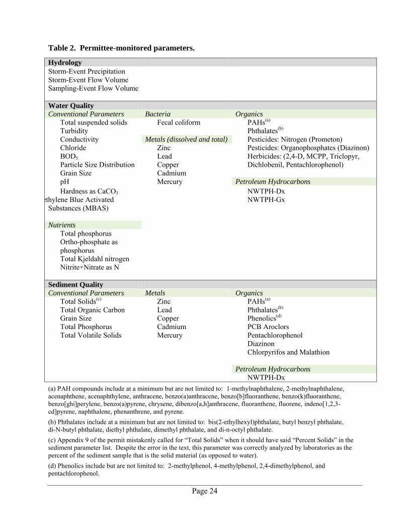
Table 2. Permittee-monitored parameters.

Hydrology

Storm-Event Precipitation Storm-Event Flow Volume Sampling-Event Flow Volume Water Quality

Conventional Parameters Bacteria Organics

Total suspended solids Fecal coliform PAHs(a) Turbidity Phthalates(b) Conductivity Metals (dissolved and total) Pesticides: Nitrogen (Prometon) Chloride Zinc Pesticides: Organophosphates (Diazinon) BOD5 Lead Herbicides: (2,4-D, MCPP, Triclopyr, Particle Size Distribution Copper Dichlobenil, Pentachlorophenol) Grain Size Cadmium

pH Mercury Petroleum Hydrocarbons

Hardness as CaCO3 NWTPH-Dx Methylene Blue Activated

Substances (MBAS) NWTPH-Gx

Nutrients

Total phosphorus Ortho-phosphate as phosphorus Total Kjeldahl nitrogen Nitrite+Nitrate as N

Sediment Quality

Conventional Parameters Metals Organics

Total Solids(c) Zinc PAHs(a) Total Organic Carbon Lead Phthalates(b) Grain Size Copper Phenolics(d) Total Phosphorus Cadmium PCB Aroclors Total Volatile Solids Mercury Pentachlorophenol Diazinon Chlorpyrifos and Malathion

Petroleum Hydrocarbons

NWTPH-Dx (a) PAH compounds include at a minimum but are not limited to: 1-methylnaphthalene, 2-methylnaphthalene, acenaphthene, acenaphthylene, anthracene, benzo(a)anthracene, benzo[b]fluoranthene, benzo(k)fluoranthene, benzo[ghi]perylene, benzo(a)pyrene, chrysene, dibenzo[a,h]anthracene, fluoranthene, fluorene, indeno[1,2,3-cd]pyrene, naphthalene, phenanthrene, and pyrene. (b) Phthalates include at a minimum but are not limited to: bis(2-ethylhexyl)phthalate, butyl benzyl phthalate, di-N-butyl phthalate, diethyl phthalate, dimethyl phthalate, and di-n-octyl phthalate. (c) Appendix 9 of the permit mistakenly called for “Total Solids” when it should have said “Percent Solids” in the sediment parameter list. Despite the error in the text, this parameter was correctly analyzed by laboratories as the percent of the sediment sample that is the solid material (as opposed to water). (d) Phenolics include but are not limited to: 2-methylphenol, 4-methylphenol, 2,4-dimethylphenol, and pentachlorophenol.

Page 25

Laboratory Analytical Methods

The permit specified analytical methods and reporting limit targets for each parameter to ensure the stormwater data under this monitoring program were analyzed consistently and with comparable rigor among the various laboratories. In some cases, it allowed multiple methods (thought to be comparable) to be used for analysis of a parameter, provided the reporting limit target could be met. For example, conductivity could be analyzed using SM 2510 or EPA Method 120.1. Permittees used 15 laboratories for analysis; no permittee used only a single laboratory for all parameters. All data for a given parameter were pooled for analysis regardless of laboratory and regardless of analytical method. Laboratory Quality Assurance

Each permittee’s QA Project Plan was approved by Ecology and contains sections outlining the QA process and quality control (QC) procedures for its stormwater monitoring program. QA is a decision-making process, based on all available information that determines whether the data are usable for all intended purposes (Lombard and Kirchmer, 2004). QC refers to a set of standard operating procedures for the field and laboratory that are used to evaluate and control the accuracy of measurement data. Determination of laboratory QC and the overall stormwater monitoring program QA was performed by each permittee, per their QA Project Plans. For this data analysis project, data entered into the EIM database are believed to be usable for the purpose of creating a baseline summary report as stated in the permittees’ QA Project Plans.

Page 26

Methods

Data Qualification Quantitation and Reporting Limits

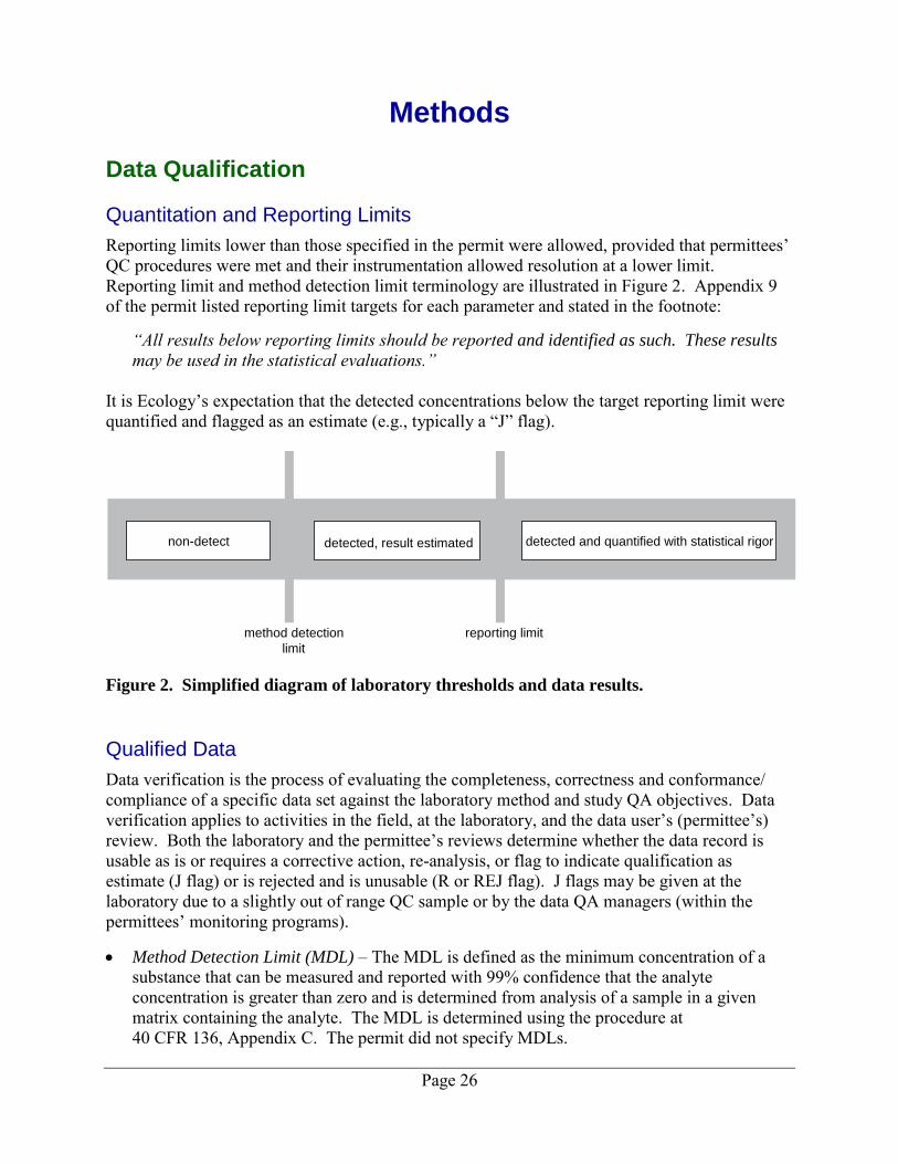
Reporting limits lower than those specified in the permit were allowed, provided that permittees’ QC procedures were met and their instrumentation allowed resolution at a lower limit. Reporting limit and method detection limit terminology are illustrated in Figure 2. Appendix 9 of the permit listed reporting limit targets for each parameter and stated in the footnote:

“All results below reporting limits should be reported and identified as such. These results

may be used in the statistical evaluations.”

It is Ecology’s expectation that the detected concentrations below the target reporting limit were quantified and flagged as an estimate (e.g., typically a “J” flag).

Figure 2. Simplified diagram of laboratory thresholds and data results.

Qualified Data

Data verification is the process of evaluating the completeness, correctness and conformance/ compliance of a specific data set against the laboratory method and study QA objectives. Data verification applies to activities in the field, at the laboratory, and the data user’s (permittee’s) review. Both the laboratory and the permittee’s reviews determine whether the data record is usable as is or requires a corrective action, re-analysis, or flag to indicate qualification as estimate (J flag) or is rejected and is unusable (R or REJ flag). J flags may be given at the laboratory due to a slightly out of range QC sample or by the data QA managers (within the permittees’ monitoring programs).

Method Detection Limit (MDL) – The MDL is defined as the minimum concentration of a substance that can be measured and reported with 99% confidence that the analyte concentration is greater than zero and is determined from analysis of a sample in a given matrix containing the analyte. The MDL is determined using the procedure at 40 CFR 136, Appendix C. The permit did not specify MDLs.

non-detect detected, result estimated detected and quantified with statistical rigor

method detection

limit

reporting limit

Page 27

Reporting Limit (RL) – The reporting limit has multiple definitions and values, because it is a user-defined value imposed upon the reporting laboratory. RL is the lowest concentration at which an analyte can be detected in a sample and its concentration can be reported with a reasonable degree of accuracy and precision. The reporting limit may vary based on the purpose and use of the data. Reporting limits should always be based on statistical rigor at each laboratory. Analyte detections between the MDL and the reporting limit are reported as having estimated concentrations. Reporting limits are typically three to five times the MDL.

Ultimately, a lack of a signal below the MDL or RL was flagged as “U” meaning the parameter was not detected. In this report Ecology refers to the non-detected data as “non-detect”. Variation in Reporting Limits

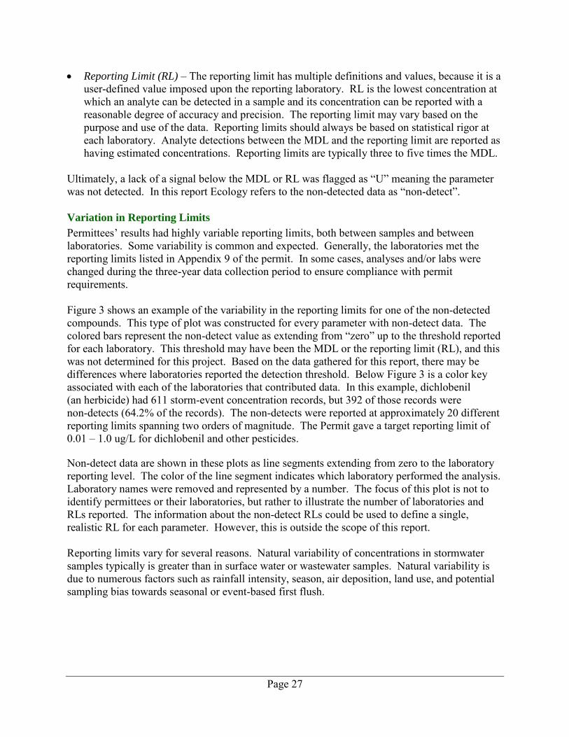
Permittees’ results had highly variable reporting limits, both between samples and between laboratories. Some variability is common and expected. Generally, the laboratories met the reporting limits listed in Appendix 9 of the permit. In some cases, analyses and/or labs were changed during the three-year data collection period to ensure compliance with permit requirements. Figure 3 shows an example of the variability in the reporting limits for one of the non-detected compounds. This type of plot was constructed for every parameter with non-detect data. The colored bars represent the non-detect value as extending from “zero” up to the threshold reported for each laboratory. This threshold may have been the MDL or the reporting limit (RL), and this was not determined for this project. Based on the data gathered for this report, there may be differences where laboratories reported the detection threshold. Below Figure 3 is a color key associated with each of the laboratories that contributed data. In this example, dichlobenil (an herbicide) had 611 storm-event concentration records, but 392 of those records were non-detects (64.2% of the records). The non-detects were reported at approximately 20 different reporting limits spanning two orders of magnitude. The Permit gave a target reporting limit of 0.01 – 1.0 ug/L for dichlobenil and other pesticides. Non-detect data are shown in these plots as line segments extending from zero to the laboratory reporting level. The color of the line segment indicates which laboratory performed the analysis. Laboratory names were removed and represented by a number. The focus of this plot is not to identify permittees or their laboratories, but rather to illustrate the number of laboratories and RLs reported. The information about the non-detect RLs could be used to define a single, realistic RL for each parameter. However, this is outside the scope of this report. Reporting limits vary for several reasons. Natural variability of concentrations in stormwater samples typically is greater than in surface water or wastewater samples. Natural variability is due to numerous factors such as rainfall intensity, season, air deposition, land use, and potential sampling bias towards seasonal or event-based first flush.

Page 28

Figure 3. Non-detect reporting limits for dichlobenil by laboratory.

Other reasons for variability come from sampling design or sampling bias (e.g., sample volume collected). The sample volume typically required for an analysis has a predictable error rate associated with the analysis. When a smaller than normal volume is analyzed, the standard error increases, which increases the reporting limit. The anticipated stormwater volume was difficult to predict; it depended on the climatic event and was constrained by the capacity of the compositors. As a result, some samples were likely sent to the laboratory with less than ideal volumes. Another major stormwater sampling source for variability is interference by compounds present in the stormwater sample (called interfering matrix). Stormwater samples can contain debris, sediment, oil, and other compounds that can interfere with sensitive analytical equipment. Laboratories must clean up dirty samples prior to analyzing for the contaminant of interest. This often results in loss of resolution at low levels and, in turn, elevates the reporting limit. Permittees were required to conduct QC and QA reviews on reported data. Because data verification was performed by the permittees, the data received by Ecology were thought to be usable. For this report, Ecology used the data as reported with few exceptions. Several obvious outliers were verified with permittees and errors resolved. Rejected records were not requested and, if supplied, were not used for summary statistics.

Page 29

Data Compilation and Management Data Collection and Accessibility

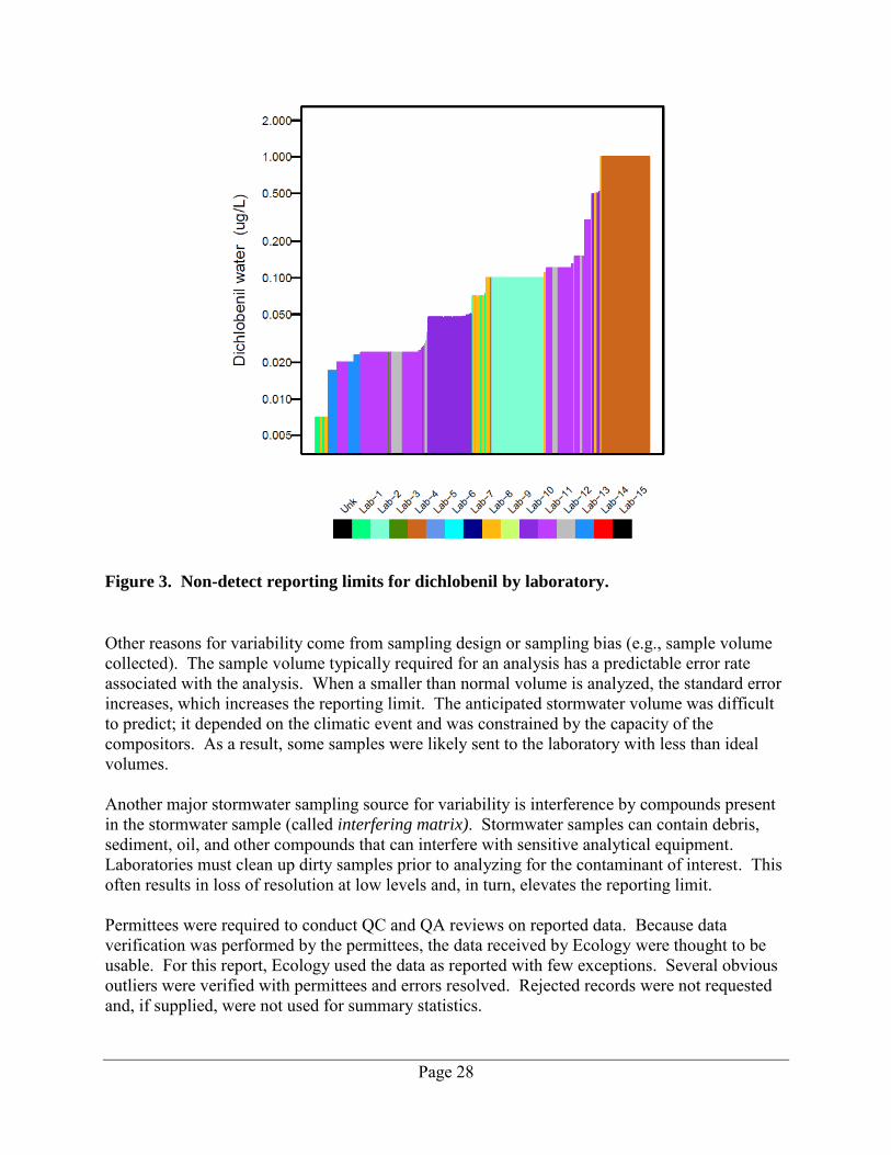
Permittees were responsible for submitting data collected under the S8.D stormwater monitoring permits, with the exception of the toxicity results, to Ecology for entry into the agency’s Environmental Information Management (EIM) system (http://www.ecy.wa.gov/eim/). Toxicity results were submitted to Ecology for review. Ecology prepared a summary of stormwater seasonal first-flush toxicity on trout embryos. This summary is presented in Appendix A. The S8.D data summarized and presented here are available in EIM. Data may be searched by various characteristics (e.g., parameter, study, geographic area). The study identification codes (IDs) for the S8.D data are detailed in Table 3.

Table 3. Summary of permittee data compiled for this report.

Permittee EIM Study ID Period

of Record

Clark County WAR044001_S8D 2009-2012 King County WAR044501_S8D 2009-2013 Pierce County WAR044002_S8D 2010-2013 Snohomish County WAR044502_S8.D 2009-2012 City of Seattle WAR044503_S8.D 2009-2012 City of Tacoma WAR044003_S8D 2009-2012 Port of Seattle WAR044701_S8.D 2009-2012 Port of Tacoma WAR044200_S8.D 2009-2012

Data Compilation

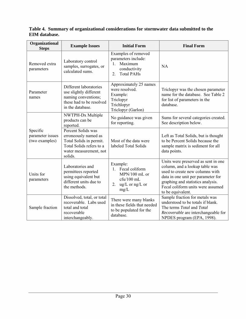
Ecology downloaded all data associated with the project into a Microsoft Access Database File (.accdb) to query, reorganize, and manage the data into a uniform output file for analysis (Table 4). Reorganization of the data set included such items as renaming a parameter due to variability in nomenclature among the 15 labs. In addition, a number of macros for Microsoft Excel were written in Visual Basic to sum selected parameters. Once the data set was in the final form, it was exported into a comma-separated value (.csv) format, where it could be easily used in a variety of statistical packages.

http://www.ecy.wa.gov/eim/

Page 30

Table 4. Summary of organizational considerations for stormwater data submitted to the

EIM database.

Organizational

Steps Example Issues Initial Form Final Form

Removed extra parameters

Laboratory control samples, surrogates, or calculated sums.

Examples of removed parameters include: 1. Maximum

conductivity 2. Total PAHs

NA

Parameter names

Different laboratories use slightly different naming conventions; these had to be resolved in the database.

Approximately 25 names were resolved. Example: Triclopyr Trichlopyr Triclopyr (Garlon)

Triclopyr was the chosen parameter name for the database. See Table 2 for list of parameters in the database.

Specific parameter issues (two examples)

NWTPH-Dx Multiple products can be reported.

No guidance was given for reporting.

Sums for several categories created. See description below.

Percent Solids was erroneously named as Total Solids in permit. Total Solids refers to a water measurement, not solids.

Most of the data were labeled Total Solids

Left as Total Solids, but is thought to be Percent Solids because the sample matrix is sediment for all data points.

Units for parameters

Laboratories and permittees reported using equivalent but different units due to the methods.

Example: 1. Fecal coliform

MPN/100 mL or cfu/100 mL

2. ug/L or ng/L or mg/L

Units were preserved as sent in one column, and a lookup table was used to create new columns with data in one unit per parameter for graphing and statistics analysis. Fecal coliform units were assumed to be equivalent.

Sample fraction

Dissolved, total, or total recoverable. Labs used total and total recoverable interchangeably.

There were many blanks in these fields that needed to be populated for the database.

Sample fraction for metals was understood to be totals if blank. The terms Total and Total

Recoverable are interchangeable for NPDES program (EPA, 1998).

Page 31

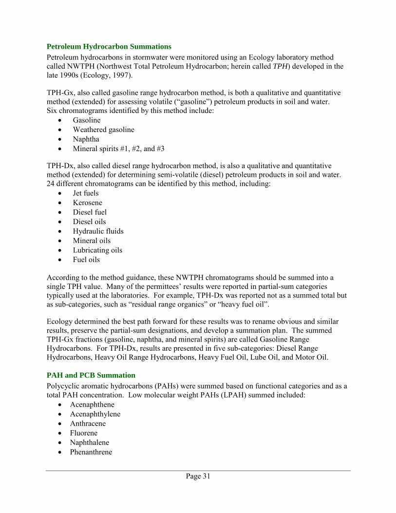
Petroleum Hydrocarbon Summations

Petroleum hydrocarbons in stormwater were monitored using an Ecology laboratory method called NWTPH (Northwest Total Petroleum Hydrocarbon; herein called TPH) developed in the late 1990s (Ecology, 1997).

TPH-Gx, also called gasoline range hydrocarbon method, is both a qualitative and quantitative method (extended) for assessing volatile (“gasoline”) petroleum products in soil and water. Six chromatograms identified by this method include:

Gasoline Weathered gasoline Naphtha Mineral spirits #1, #2, and #3

TPH-Dx, also called diesel range hydrocarbon method, is also a qualitative and quantitative method (extended) for determining semi-volatile (diesel) petroleum products in soil and water. 24 different chromatograms can be identified by this method, including:

Jet fuels Kerosene Diesel fuel Diesel oils Hydraulic fluids Mineral oils Lubricating oils Fuel oils

According to the method guidance, these NWTPH chromatograms should be summed into a single TPH value. Many of the permittees’ results were reported in partial-sum categories typically used at the laboratories. For example, TPH-Dx was reported not as a summed total but as sub-categories, such as “residual range organics” or “heavy fuel oil”. Ecology determined the best path forward for these results was to rename obvious and similar results, preserve the partial-sum designations, and develop a summation plan. The summed TPH-Gx fractions (gasoline, naphtha, and mineral spirits) are called Gasoline Range Hydrocarbons. For TPH-Dx, results are presented in five sub-categories: Diesel Range Hydrocarbons, Heavy Oil Range Hydrocarbons, Heavy Fuel Oil, Lube Oil, and Motor Oil. PAH and PCB Summation

Polycyclic aromatic hydrocarbons (PAHs) were summed based on functional categories and as a total PAH concentration. Low molecular weight PAHs (LPAH) summed included:

Acenaphthene Acenaphthylene Anthracene Fluorene Naphthalene Phenanthrene

Page 32

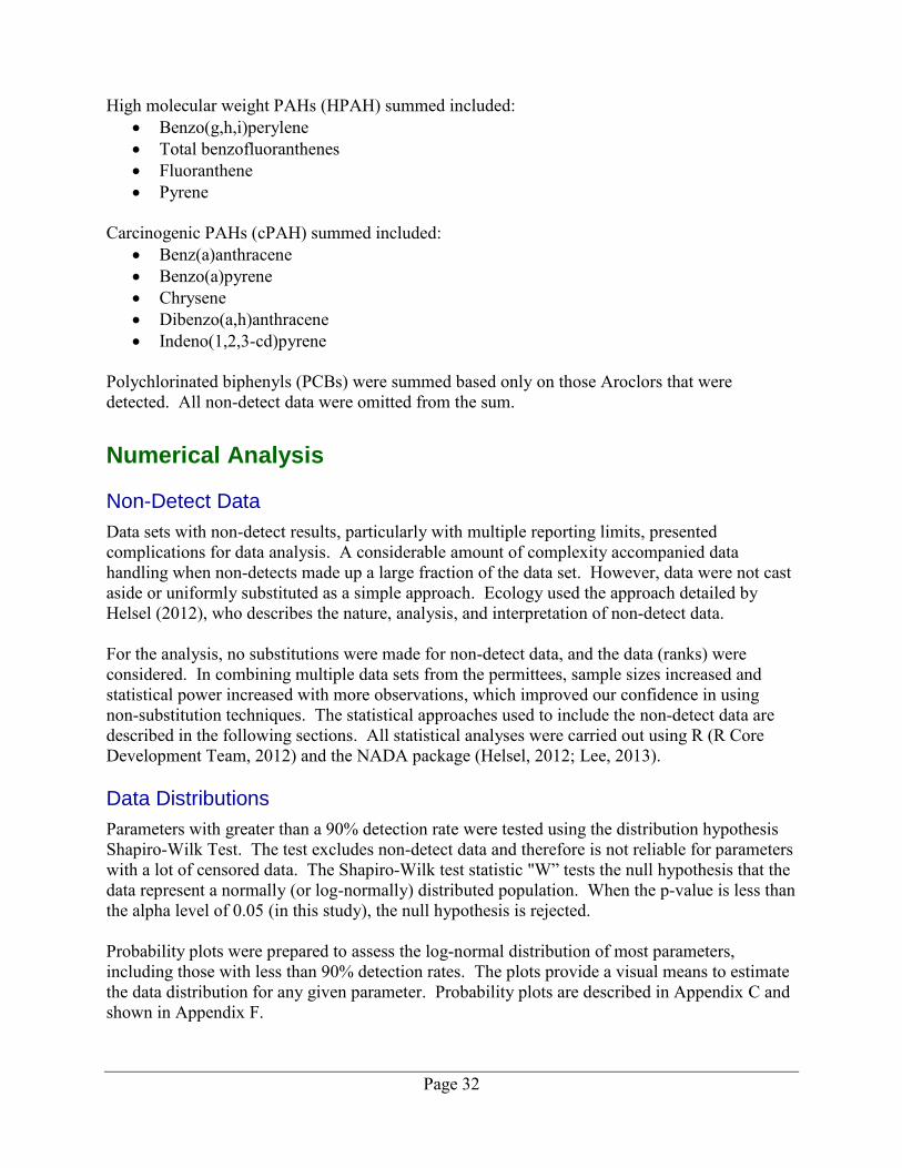
High molecular weight PAHs (HPAH) summed included: Benzo(g,h,i)perylene Total benzofluoranthenes Fluoranthene Pyrene

Carcinogenic PAHs (cPAH) summed included:

Benz(a)anthracene Benzo(a)pyrene Chrysene Dibenzo(a,h)anthracene Indeno(1,2,3-cd)pyrene

Polychlorinated biphenyls (PCBs) were summed based only on those Aroclors that were detected. All non-detect data were omitted from the sum.

Numerical Analysis Non-Detect Data

Data sets with non-detect results, particularly with multiple reporting limits, presented complications for data analysis. A considerable amount of complexity accompanied data handling when non-detects made up a large fraction of the data set. However, data were not cast aside or uniformly substituted as a simple approach. Ecology used the approach detailed by Helsel (2012), who describes the nature, analysis, and interpretation of non-detect data. For the analysis, no substitutions were made for non-detect data, and the data (ranks) were considered. In combining multiple data sets from the permittees, sample sizes increased and statistical power increased with more observations, which improved our confidence in using non-substitution techniques. The statistical approaches used to include the non-detect data are described in the following sections. All statistical analyses were carried out using R (R Core Development Team, 2012) and the NADA package (Helsel, 2012; Lee, 2013). Data Distributions

Parameters with greater than a 90% detection rate were tested using the distribution hypothesis Shapiro-Wilk Test. The test excludes non-detect data and therefore is not reliable for parameters with a lot of censored data. The Shapiro-Wilk test statistic "W” tests the null hypothesis that the data represent a normally (or log-normally) distributed population. When the p-value is less than the alpha level of 0.05 (in this study), the null hypothesis is rejected. Probability plots were prepared to assess the log-normal distribution of most parameters, including those with less than 90% detection rates. The plots provide a visual means to estimate the data distribution for any given parameter. Probability plots are described in Appendix C and shown in Appendix F.

Page 33

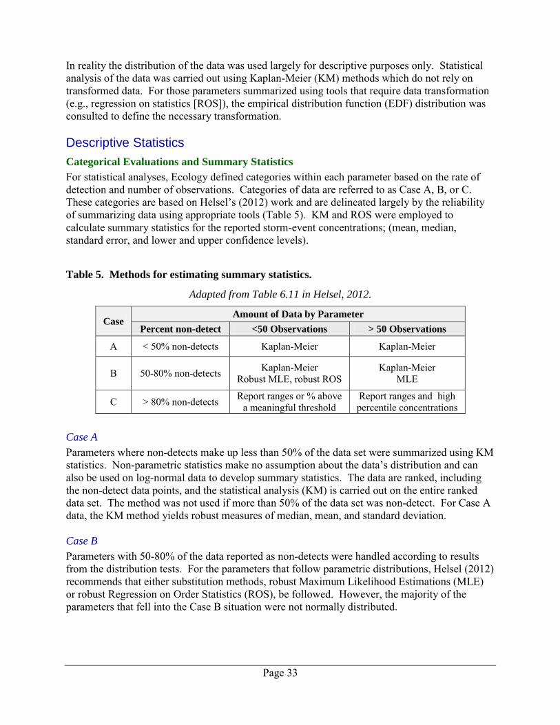
In reality the distribution of the data was used largely for descriptive purposes only. Statistical analysis of the data was carried out using Kaplan-Meier (KM) methods which do not rely on transformed data. For those parameters summarized using tools that require data transformation (e.g., regression on statistics [ROS]), the empirical distribution function (EDF) distribution was consulted to define the necessary transformation. Descriptive Statistics

Categorical Evaluations and Summary Statistics

For statistical analyses, Ecology defined categories within each parameter based on the rate of detection and number of observations. Categories of data are referred to as Case A, B, or C. These categories are based on Helsel’s (2012) work and are delineated largely by the reliability of summarizing data using appropriate tools (Table 5). KM and ROS were employed to calculate summary statistics for the reported storm-event concentrations; (mean, median, standard error, and lower and upper confidence levels).

Table 5. Methods for estimating summary statistics.

Adapted from Table 6.11 in Helsel, 2012.

Case Amount of Data by Parameter

Percent non-detect <50 Observations > 50 Observations

A < 50% non-detects Kaplan-Meier Kaplan-Meier

B 50-80% non-detects Kaplan-Meier Robust MLE, robust ROS

Kaplan-Meier MLE

C > 80% non-detects Report ranges or % above a meaningful threshold

Report ranges and high percentile concentrations

Case A

Parameters where non-detects make up less than 50% of the data set were summarized using KM statistics. Non-parametric statistics make no assumption about the data’s distribution and can also be used on log-normal data to develop summary statistics. The data are ranked, including the non-detect data points, and the statistical analysis (KM) is carried out on the entire ranked data set. The method was not used if more than 50% of the data set was non-detect. For Case A data, the KM method yields robust measures of median, mean, and standard deviation. Case B

Parameters with 50-80% of the data reported as non-detects were handled according to results from the distribution tests. For the parameters that follow parametric distributions, Helsel (2012) recommends that either substitution methods, robust Maximum Likelihood Estimations (MLE) or robust Regression on Order Statistics (ROS), be followed. However, the majority of the parameters that fell into the Case B situation were not normally distributed.

Page 34

For these, Ecology calculated summary statistics on the portion of Case B parameters that had more than 50 observations. ROS was used to estimate the summary statistics for this portion of the Case B data. However, for data sets with fewer than 50 observations, both ROS and MLE provide poor estimates of summary statistics. Thus these data were summarized as a Case C category because Ecology determined that the statistics would be unreliable. Case C

Case C data were simply summarized as ranges. Calculating other summary statistics would have been unreliable (Helsel, 2012). Land-Use Significance

To determine if there were significant differences between land uses for a given parameter, Ecology relied on the Peto-Prentice test. The Peto-Prentice score test has been shown to perform well with data sets that have unequal sample sizes and unequal censoring (i.e., detection limits) (Helsel, 2012). The Peto-Prentice is a modified generalized Wilcoxon test, where scores are weighted by the EDF. The Peto-Prentice test identifies when at least one land use among the four has significantly different concentrations. To visualize any significant differences among land uses for each parameter, a plot of the EDF can be produced. Summary Plots

Ecology relied on six types of plots as visual tools to describe the concentration data (Appendix C). Each set of plots for each parameter consists of:

Jitter Plot Probability Plot Non-Detects Empirical Distribution Function (EDF) Box Plot by Land Use Box Plot by Season Appendix C contains a description of how to read each of these six plots (reproduced from Lubliner and Newell, 2013). Appendix F contains a page for each parameter with all six plots and matrix combination. Ecology also used box plots, cumulative density functions, and jitter plots to describe the contaminant loads (Appendix H). Multivariate Statistics

In order to summarize multiple parameters for each stormwater catchment together with land use and observe any relevant similarities or associations among them, Ecology relied on principal components analysis (PCA). PCA is a statistical tool that describes the relative similarities among environmental variables (stormwater parameters) and study sites. Multiple axes or components are computed in decreasing order of strength or importance. Each axis represents a synthetic gradient across the sample sites, some more important than others. Visually, a plot of the two most dominant axes (an ordination diagram) can provide an effective means to describe large complex data sets. Points or sites on the plot that cluster together are more similar than

Page 35

those that are more distant. Ecology selected those variables that appeared to be statistically relevant from the prior Peto-Prentice test. The PCA was run on the median concentration values as described above using the statistical techniques for non-detect data. Only parameters which were complete across all study sites were included in the analysis. Data were log transformed, centered, and standardized prior to the analysis. PCAs were run using the R framework and the Vegan package (Oksanen et al., 2013). Additional tools used to detect similarities among the parameters across the land uses included a hierarchical cluster analysis and an analysis of similarities. The same data set used for the PCA analysis was used for the cluster analysis. Ecology calculated the Euclidean distance (measure of dissimilarity) between sample sites and computed the cluster analysis using Ward’s minimum variance method (Hartigan, 1975). This technique is a way of identifying groups of data (sites) that are similar. Visually, a cluster diagram or dendrogram shows the groups of sites starting with the most dissimilar and then continues to separate the sites into groups until each site is on its own branch of the tree (dendrogram). We used the first two major separations of sites in the cluster dendrogram to describe similar ‘groups’ of sites based on their stormwater chemistry. Analysis of similarities is a tool to statistically test whether there are significant differences between two or more groups of sampling units based on a dissimilarity matrix. We used the same dissimilarity matrix as the cluster analysis. Ecology employed this test to help determine whether there is a significant difference among land uses based on all sites and all relevant parameters. This differs from the previously described Peto-Prentice test for land-use significance, which tests a single parameter for significant differences.

Comparison to Stormwater Studies and Water Quality Criteria To put the results of this compilation effort into context, Ecology used three primary sources of information for comparison of these results:

A suite of literature including the Nationwide Urban Runoff Program (NURP) (EPA, 1983) and analysis of the National Stormwater Quality Database (Maestre et al., 2005).

Washington State Water Quality Criteria. The national studies and the WA state water quality criteria form the “bookends” for comparison of the stormwater discharge results of this compilation effort.

A local study to characterize stormwater concentrations and load to Puget Sound from the receiving water during storm events, Control of Toxic Chemicals in Puget Sound: Phase 3

Data and Load Estimates (Herrera, 2011) (called PS Toxics Study in this document). Relevant Stormwater Studies Explored

The median concentrations from this study are compared to the median concentrations of a few other stormwater studies where data exist. Comparisons made to these other studies are informative for this database and are included to give context to the results of this study.

The Nationwide Urban Runoff Program (NURP) (EPA, 1983).

Page 36

Nonparametric Statistical Tests Comparing First Flush and Composite Samples from the National Stormwater Quality Database (NSQD) (Maestre et al., 2004).

The National Stormwater Quality Database, Version 1.1; A Compilation and Analysis of NPDES Stormwater Monitoring Information (Maestre et al., 2005) http://rpitt.eng.ua.edu/Publications/Stormwater%20Characteristics/NSQD%20EPA.pdf

Control of Toxic Chemicals in Puget Sound: Phase 3 Data and Load Estimates (Herrera, 2011) (called PS Toxics Study in this document).

NURP and NSQD

The NURP study was a research project conducted by the U.S. Environmental Protection Agency (EPA) between 1979 and 1983. NURP was the first comprehensive study of urban stormwater pollution across the United States and established the national stormwater quality benchmark. NURP samples were also collected to represent the storm-event concentration, which allows us to compare results from the permittees directly. The study evaluated the stormwater data distributions and concluded that 90% of their study parameters followed a log-normal distribution. The NSQD was created in the mid-1980s to store stormwater data collected by the NURP study and other Phase I MS4 data. Over time, the database gained some specialized U.S. Geological Survey stormwater studies and more recently selected outfall data from the International BMP Database. Several reports have been published by Alex Maestre and Robert Pitt, summarizing the stormwater monitoring data contained in versions of the database over the last 20 years (Version 1.0, 1.1 and 2). Version 3 of the NSQD is available online at: http://unix.eng.ua.edu/~rpitt/Research/ms4/mainms4.shtml. PS Toxics Study

The PS Toxics Study, the largest local study of receiving waters to date, was initiated to assess the relative loading and identify sources of toxic contaminants to Puget Sound. River and streams were sampled in 2009-2010 in multiple watersheds during baseflow and storm-event flows. Stormwater discharges were not directly sampled. Contaminant concentrations were measured and annual mass loads and annual loading rates were calculated. In this report Ecology compares the stormwater discharge concentrations to the PS Toxics Study ambient data, and acknowledges this as an "apples to oranges" comparison. The permittees collected flow-weighted composites from stormwater discharges across 75% of the storm event’s hydrograph. The PS Toxics Study samples were collected as grab samples from the receiving waters during storm events. The instream concentrations as captured by the PS Toxics Study were anticipated to be lower than stormwater discharge concentrations, particularly in urban areas. Nevertheless, it does give us a sense of the scale of differences and an understanding of where patterns in the results are similar. Loads calculated for this stormwater discharge data compilation are event loads and not annual loads like those calculated in the PS Toxics Study. Thus, loading results are too dissimilar and are not comparable. Ecology can compare the trends across land uses for both concentrations and loads.

http://rpitt.eng.ua.edu/Publications/Stormwater%20Characteristics/NSQD%20EPA.pdf

http://unix.eng.ua.edu/~rpitt/Research/ms4/mainms4.shtml

Page 37

Water Quality Criteria

Promulgated water quality standards as well as non-promulgated criteria exist for a number of parameters measured in these stormwater discharges. The authors of this report used the Washington State acute and chronic freshwater standards (WAC4 173-201A), for comparison to provide context for the stormwater discharge results. For stormwater sediments, the authors made a comparison to freshwater sediment chemical criteria (Chapter 173-204 WAC). The comparisons do not include any consideration of the receiving water. These comparisons are not intended to, and are not appropriate for, determining compliance with regulatory requirements, such as water quality standards and permit conditions. Water

The criteria for the protection of aquatic life in surface waters of the State of Washington are promulgated under Chapter 173-201A WAC. As defined by EPA (1994), the exposure periods assigned to the acute criteria are expressed as: (1) an instantaneous concentration not to be exceeded at any time or (2) a 1-hour average concentration not to be exceeded more than once every three years on the average. The exposure periods for the chronic criteria are either: (1) a 24-hour average not to be exceeded at any time or (2) a 4-day average concentration not to be exceeded more than once every three years on the average. Each individual stormwater sample (recall that each sample is a composite across a storm event) was compared to the criteria value. For pH and hardness dependent criteria, Ecology wrote scripts in R to use each stormwater sample’s pH and hardness result. If the concentration for a sample was non-detect, then it was excluded from the comparison. See Table ES-1 for results of the criteria comparisons. Sediment

Sediment criteria are found in Washington State’s Sediment Management Standards (SMS) (Chapter 173-204 WAC). The marine Sediment Quality Standards (SQS) found in Part III of the SMS are approved by EPA as water quality standards for the protection of the benthic community. Because these promulgated water quality standards values are for marine sediments only, the authors compared the stormwater sediment data to the freshwater sediment chemical criteria established as Sediment Cleanup Objectives (SCOs) in WAC 173-204-563. These SCO criteria are based on a “no adverse effects level” to the freshwater benthic community. At the time of this publication, EPA has neither approved nor disapproved the numeric freshwater sediment criteria as water quality standards. Stormwater sediment concentrations are expressed as dry weight and not normalized to organic carbon content, which is suitable for the purposes of this contextual comparison (Michelson, 1992).

4 Washington Administrative Code

Page 38

Approaches to Non-Detected Data in the Stormwater Literature In the NSQD Version 1.1 review, Maestre et al. (2005; Chapter 3) provide a review of how non-detects have been handled in stormwater studies. More recent environmental, and particularly stormwater, studies have used substitution techniques to substitute either one-half or full value of the method detection limit (MDL) for the value of the non-detect. This has been a common practice for data sets with relatively few non-detect data points. Antweiler and Taylor (2008) indicate that using substitutions for non-detects produces comparable summary statistics. In the NURP study, non-detected data were summarized using substitution of the value of the reported detection limit. In the NSQD version 1.1 data summary, non-detected values were estimated using the Cohen’s maximum likelihood method. This is a method that randomly generates the missing data based on the known probability distributions of the data (Maestre et al., 2005). The PS Toxics Study estimated the non-detect values by substituting one-half the value of the detection limit (Herrera, 2011). Comparisons of the permittee’s data results to NURP, NSQD, and the PS Toxics Study are considered approximate because the methods for sample collection and data analysis differed among the studies. Despite different methods for handling non-detects, comparisons of median values were retained in this report because the NURP and NSQD represent the earliest and largest national stormwater quality characterization efforts in the United States. Most of the parameters monitored in the NURP and NSQD were limited to the conventional parameters, nutrients, and metals where non-detections are infrequent and typically have less influence on summary statistics. The PS Toxics Study is the most recent regional publication with wet weather surface water concentrations for toxic pollutants.

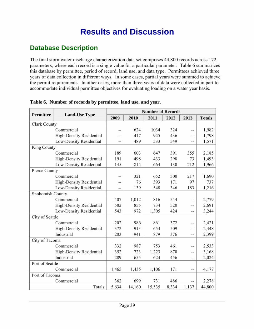
Page 39

Results and Discussion

Database Description The final stormwater discharge characterization data set comprises 44,800 records across 172 parameters, where each record is a single value for a particular parameter. Table 6 summarizes this database by permittee, period of record, land use, and data type. Permittees achieved three years of data collection in different ways. In some cases, partial years were summed to achieve the permit requirements. In other cases, more than three years of data were collected in part to accommodate individual permittee objectives for evaluating loading on a water year basis.

Table 6. Number of records by permittee, land use, and year.

Permittee Land-Use Type Number of Records

2009 2010 2011 2012 2013 Totals

Clark County Commercial -- 624 1034 324 -- 1,982

High-Density Residential -- 417 945 436 -- 1,798

Low-Density Residential -- 489 533 549 -- 1,571 King County Commercial 189 603 647 391 355 2,185

High-Density Residential 191 498 433 298 73 1,493

Low-Density Residential 145 815 664 130 212 1,966 Pierce County Commercial -- 321 652 500 217 1,690

High-Density Residential -- 76 393 171 97 737

Low-Density Residential -- 139 548 346 183 1,216 Snohomish County Commercial 407 1,012 816 544 -- 2,779

High-Density Residential 582 855 734 520 -- 2,691

Low-Density Residential 543 972 1,305 424 -- 3,244 City of Seattle Commercial 202 986 861 372 -- 2,421

High-Density Residential 372 913 654 509 -- 2,448

Industrial 203 941 879 376 -- 2,399 City of Tacoma Commercial 332 987 753 461 -- 2,533

High-Density Residential 352 723 1,223 870 -- 3,168

Industrial 289 655 624 456 -- 2,024 Port of Seattle Commercial 1,465 1,435 1,106 171 -- 4,177 Port of Tacoma Commercial 362 699 731 486 -- 2,278

Totals 5,634 14,160 15,535 8,334 1,137 44,800

Page 40

Data Quality

Suitability for All of Western Washington

Concentrations monitored under the Permit reflect a range of results by land uses that can be applied to urban and suburban stormwater discharges in western Washington. The permittees monitored both large and small drainages. Ecology determined that both the range of concentrations and median values were useable and represented stormwater quality in western Washington. By summarizing multiple years of data, Ecology also accounted for inter-annual variability. Pollutant concentrations overlapped between the land uses, and this variability increased confidence in the representativeness of the monitored basins. Table 1 illustrates the mix of land uses for each monitored basin. Laboratory and Field Quality Control

The data entered into EIM has already undergone external quality control methods (e.g., field replicates, laboratory and field blanks) as defined by the permit. Laboratory assigned data qualifiers were relied upon to define detection rates and the degree to which a parameter is censored. No further quality assessment of the data quality was carried out during this analysis. The number of samples with data qualifiers (flags) for each parameter is presented by matrix in Appendix D, Table D-2, and by land use in Table D-3. Data Distribution and Case Summary

The distribution defined by the Shapiro-Wilk test for each parameter is described in Table D-1. Parameters are divided into three categories: normal, log-normal, and distribution-free. Water samples were found to have the following distributions: log-normal (18 parameters) distribution-free (59 parameters) Sediment samples were distributed as follows: normally (3 parameters) log-normally (15 parameters) distribution-free (32 parameters). Ecology restricted distribution testing to the parameters with the highest rates of detection and found that many of the parameter’s probability plots (Appendix F) appeared nearly linear, indicating log-normal distribution. Data Case Summary

The reliability of the data summaries depends on the level of detection for each parameter and is defined by the "case" category for each parameter as indicated in Table 5. Table D-4 describes, by land use, the case category for each parameter. Overall, 88 parameters were classified as Case A, 31 parameters as Case B and 53 parameters as Case C.

Page 41

These results largely agree with the National Urban Runoff Program (NURP) results. NURP, a large national stormwater study, found that stormwater event mean concentrations (EMCs) for most parameters followed either log-normal distributions or were distribution-free (non-parametric) (EPA, 1983). High Frequency Non-Detected Parameters

This monitoring program provided a suitable sample number and range of conditions to determine whether certain parameters could be reduced in sampling frequency or excluded from future stormwater monitoring studies. Note however that site-specific or study-specific circumstances may still necessitate the collection of these parameters. With the exception of dissolved mercury (91.2% non-detect), the inorganic parameters were largely detected. Mercury was analyzed using a different method from other metals (SW7470). Reduction in frequency of dissolved mercury analysis using this method is justified; another method with a lower reporting limit may be more suitable in future studies. The parameters detailed in Table 7 for stormwater and stormwater sediments were almost completely (>90%) undetected. Insoluble Organics

The parameters in Table 7 were largely insoluble organic pollutants such as volatile and semi-volatiles; PCBs, phthalates, pesticides, or PAHs. Many organic compounds tend to adsorb to solids, making them easier to detect in the sediments. More volatile or more easily degraded (low molecular weight) chemicals may not have been found in stormwater samples, because they may have been older and weathered. However, monitoring costs would not likely be reduced by removing a limited number of organics from the monitoring list, since the non-detected parameters from the EPA Method 8270D analytical list are often measured at no additional fee. However, for parameters that require a separate sample or a different extraction method, elimination of those parameters would reduce costs. For example, several pesticides were not found in stormwater or stormwater sediments. In particular, malathion, diazinon, prometon and chlorpyrifos were infrequently detected in both water and sediment. Furthermore, many of the phenols analyzed in sediment samples were detected in only 1 or 2 samples, although the sediment data set has fewer sample number. Pentachlorophenol and phenol degradation products (e.g., p-cresol) may be the most worthwhile parameters to monitor on a consistent basis. Soluble Organics

The BTEX compounds were all listed in Table 7. This indicates that these four parameters are not found in stormwater, either because they are infrequent contaminants or because they volatilize prior to sampling.

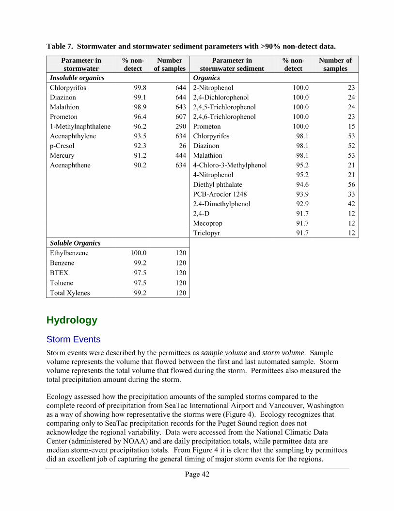
Page 42

Table 7. Stormwater and stormwater sediment parameters with >90% non-detect data.

Parameter in

stormwater

% non-

detect

Number

of samples

Parameter in

stormwater sediment % non-

detect

Number of

samples

Insoluble organics Organics Chlorpyrifos 99.8 644 2-Nitrophenol 100.0 23 Diazinon 99.1 644 2,4-Dichlorophenol 100.0 24 Malathion 98.9 643 2,4,5-Trichlorophenol 100.0 24 Prometon 96.4 607 2,4,6-Trichlorophenol 100.0 23 1-Methylnaphthalene 96.2 290 Prometon 100.0 15 Acenaphthylene 93.5 634 Chlorpyrifos 98.1 53 p-Cresol 92.3 26 Diazinon 98.1 52 Mercury 91.2 444 Malathion 98.1 53 Acenaphthene 90.2 634 4-Chloro-3-Methylphenol 95.2 21

4-Nitrophenol 95.2 21

Diethyl phthalate 94.6 56

PCB-Aroclor 1248 93.9 33

2,4-Dimethylphenol 92.9 42

2,4-D 91.7 12

Mecoprop 91.7 12

Triclopyr 91.7 12 Soluble Organics

Ethylbenzene 100.0 120 Benzene 99.2 120 BTEX 97.5 120 Toluene 97.5 120 Total Xylenes 99.2 120

Hydrology Storm Events

Storm events were described by the permittees as sample volume and storm volume. Sample volume represents the volume that flowed between the first and last automated sample. Storm volume represents the total volume that flowed during the storm. Permittees also measured the total precipitation amount during the storm. Ecology assessed how the precipitation amounts of the sampled storms compared to the complete record of precipitation from SeaTac International Airport and Vancouver, Washington as a way of showing how representative the storms were (Figure 4). Ecology recognizes that comparing only to SeaTac precipitation records for the Puget Sound region does not acknowledge the regional variability. Data were accessed from the National Climatic Data Center (administered by NOAA) and are daily precipitation totals, while permittee data are median storm-event precipitation totals. From Figure 4 it is clear that the sampling by permittees did an excellent job of capturing the general timing of major storm events for the regions.

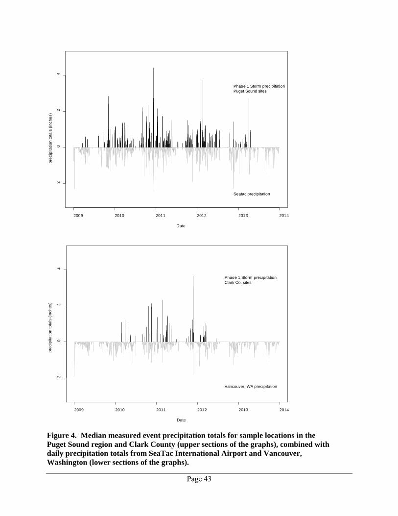
Page 43

Figure 4. Median measured event precipitation totals for sample locations in the

Puget Sound region and Clark County (upper sections of the graphs), combined with

daily precipitation totals from SeaTac International Airport and Vancouver,

Washington (lower sections of the graphs).

2009 2010 2011 2012 2013 2014

20

24

Date

pre

cip

ita

tio

n to

tals

(in

ch

es)

Seatac precipitation

Phase 1 Storm precipitation

Puget Sound sites

2009 2010 2011 2012 2013 2014

20

24

Date

pre

cip

ita

tio

n to

tals

(in

ch

es)

Vancouver, WA precipitation

Phase 1 Storm precipitation

Clark Co. sites

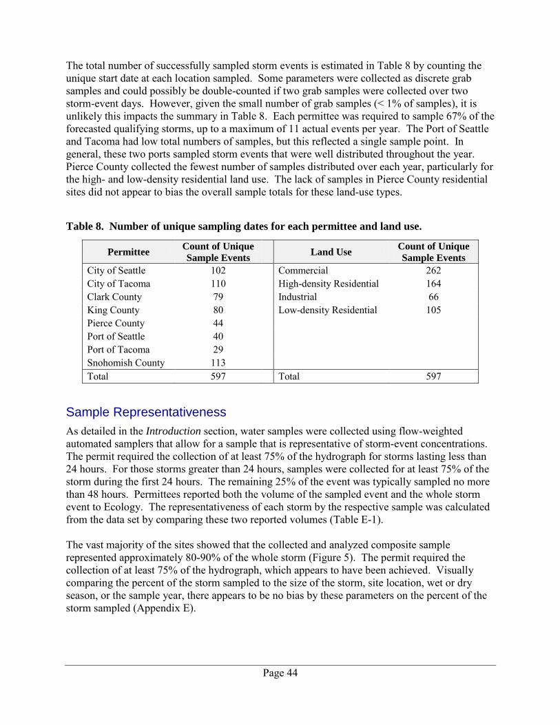
Page 44

The total number of successfully sampled storm events is estimated in Table 8 by counting the unique start date at each location sampled. Some parameters were collected as discrete grab samples and could possibly be double-counted if two grab samples were collected over two storm-event days. However, given the small number of grab samples (< 1% of samples), it is unlikely this impacts the summary in Table 8. Each permittee was required to sample 67% of the forecasted qualifying storms, up to a maximum of 11 actual events per year. The Port of Seattle and Tacoma had low total numbers of samples, but this reflected a single sample point. In general, these two ports sampled storm events that were well distributed throughout the year. Pierce County collected the fewest number of samples distributed over each year, particularly for the high- and low-density residential land use. The lack of samples in Pierce County residential sites did not appear to bias the overall sample totals for these land-use types.

Table 8. Number of unique sampling dates for each permittee and land use.

Permittee Count of Unique

Sample Events Land Use

Count of Unique

Sample Events

City of Seattle 102 Commercial 262 City of Tacoma 110 High-density Residential 164 Clark County 79 Industrial 66 King County 80 Low-density Residential 105 Pierce County 44 Port of Seattle 40 Port of Tacoma 29 Snohomish County 113 Total 597 Total 597

Sample Representativeness

As detailed in the Introduction section, water samples were collected using flow-weighted automated samplers that allow for a sample that is representative of storm-event concentrations. The permit required the collection of at least 75% of the hydrograph for storms lasting less than 24 hours. For those storms greater than 24 hours, samples were collected for at least 75% of the storm during the first 24 hours. The remaining 25% of the event was typically sampled no more than 48 hours. Permittees reported both the volume of the sampled event and the whole storm event to Ecology. The representativeness of each storm by the respective sample was calculated from the data set by comparing these two reported volumes (Table E-1). The vast majority of the sites showed that the collected and analyzed composite sample represented approximately 80-90% of the whole storm (Figure 5). The permit required the collection of at least 75% of the hydrograph, which appears to have been achieved. Visually comparing the percent of the storm sampled to the size of the storm, site location, wet or dry season, or the sample year, there appears to be no bias by these parameters on the percent of the storm sampled (Appendix E).

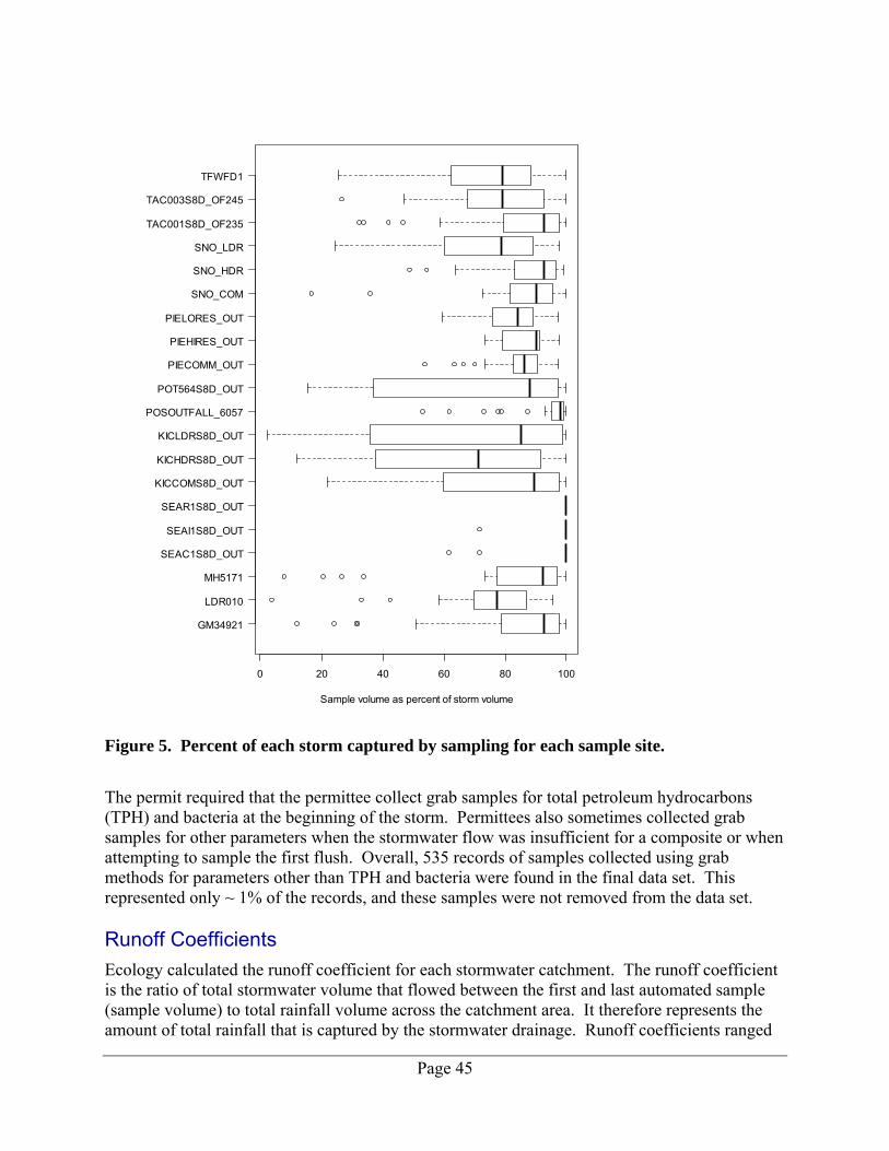
Page 45

Figure 5. Percent of each storm captured by sampling for each sample site.

The permit required that the permittee collect grab samples for total petroleum hydrocarbons (TPH) and bacteria at the beginning of the storm. Permittees also sometimes collected grab samples for other parameters when the stormwater flow was insufficient for a composite or when attempting to sample the first flush. Overall, 535 records of samples collected using grab methods for parameters other than TPH and bacteria were found in the final data set. This represented only ~ 1% of the records, and these samples were not removed from the data set. Runoff Coefficients

Ecology calculated the runoff coefficient for each stormwater catchment. The runoff coefficient is the ratio of total stormwater volume that flowed between the first and last automated sample (sample volume) to total rainfall volume across the catchment area. It therefore represents the amount of total rainfall that is captured by the stormwater drainage. Runoff coefficients ranged

GM34921

LDR010

MH5171

SEAC1S8D_OUT

SEAI1S8D_OUT

SEAR1S8D_OUT

KICCOMS8D_OUT

KICHDRS8D_OUT

KICLDRS8D_OUT

POSOUTFALL_6057

POT564S8D_OUT

PIECOMM_OUT

PIEHIRES_OUT

PIELORES_OUT

SNO_COM

SNO_HDR

SNO_LDR

TAC001S8D_OF235

TAC003S8D_OF245

TFWFD1

0 20 40 60 80 100

Sample volume as percent of storm volume

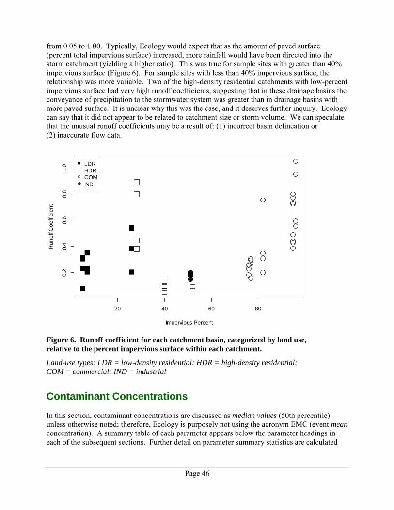
Page 46

from 0.05 to 1.00. Typically, Ecology would expect that as the amount of paved surface (percent total impervious surface) increased, more rainfall would have been directed into the storm catchment (yielding a higher ratio). This was true for sample sites with greater than 40% impervious surface (Figure 6). For sample sites with less than 40% impervious surface, the relationship was more variable. Two of the high-density residential catchments with low-percent impervious surface had very high runoff coefficients, suggesting that in these drainage basins the conveyance of precipitation to the stormwater system was greater than in drainage basins with more paved surface. It is unclear why this was the case, and it deserves further inquiry. Ecology can say that it did not appear to be related to catchment size or storm volume. We can speculate that the unusual runoff coefficients may be a result of: (1) incorrect basin delineation or (2) inaccurate flow data.

Figure 6. Runoff coefficient for each catchment basin, categorized by land use,

relative to the percent impervious surface within each catchment.

Land-use types: LDR = low-density residential; HDR = high-density residential;


Contaminant Concentrations In this section, contaminant concentrations are discussed as median values (50th percentile) unless otherwise noted; therefore, Ecology is purposely not using the acronym EMC (event mean concentration). A summary table of each parameter appears below the parameter headings in each of the subsequent sections. Further detail on parameter summary statistics are calculated

20 40 60 80

0.2

0.4

0.6

0.8

1.0

Impervious Percent

Ru

no

ff C

oe

ffic

ien

t

LDR

HDR

COM

IND

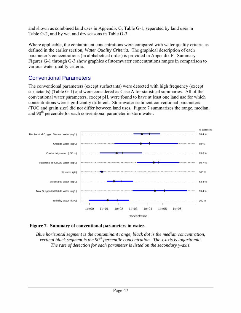
Page 47

and shown as combined land uses in Appendix G, Table G-1, separated by land uses in Table G-2, and by wet and dry seasons in Table G-3. Where applicable, the contaminant concentrations were compared with water quality criteria as defined in the earlier section, Water Quality Criteria. The graphical description of each parameter’s concentrations (in alphabetical order) is provided in Appendix F. Summary Figures G-1 through G-3 show graphics of stormwater concentrations ranges in comparison to various water quality criteria. Conventional Parameters

The conventional parameters (except surfactants) were detected with high frequency (except surfactants) (Table G-1) and were considered as Case A for statistical summaries. All of the conventional water parameters, except pH, were found to have at least one land use for which concentrations were significantly different. Stormwater sediment conventional parameters (TOC and grain size) did not differ between land uses. Figure 7 summarizes the range, median, and 90th percentile for each conventional parameter in stormwater.

Figure 7. Summary of conventional parameters in water.

Blue horizontal segment is the contaminant range, black dot is the median concentration,

vertical black segment is the 90th

percentile concentration. The x-axis is logarithmic.

The rate of detection for each parameter is listed on the secondary y-axis.

Concentration

1e+00 1e+01 1e+02 1e+03 1e+04 1e+05 1e+06

Biochemical Oxygen Demand water (ug/L)

Chloride water (ug/L)

Conductivity water (uS/cm)

Hardness as CaCO3 water (ug/L)

pH water (pH)

Surfactants water (ug/L)

Total Suspended Solids water (ug/L)

Turbidity water (NTU)

% Detected

78.4 %

98 %

99.8 %

99.7 %

100 %

63.4 %

99.4 %

100 %

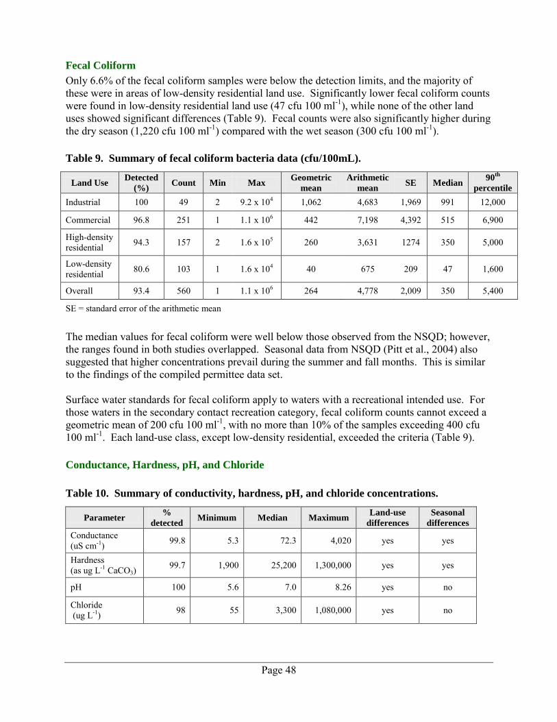
Page 48

Fecal Coliform

Only 6.6% of the fecal coliform samples were below the detection limits, and the majority of these were in areas of low-density residential land use. Significantly lower fecal coliform counts were found in low-density residential land use (47 cfu 100 ml-1), while none of the other land uses showed significant differences (Table 9). Fecal counts were also significantly higher during the dry season (1,220 cfu 100 ml-1) compared with the wet season (300 cfu 100 ml-1).

Table 9. Summary of fecal coliform bacteria data (cfu/100mL).

Land Use Detected

(%) Count Min Max

Geometric

mean

Arithmetic

mean SE Median

90th

percentile

Industrial 100 49 2 9.2 x 104 1,062 4,683 1,969 991 12,000

Commercial 96.8 251 1 1.1 x 106 442 7,198 4,392 515 6,900

High-density residential 94.3 157 2 1.6 x 105 260 3,631 1274 350 5,000

Low-density residential 80.6 103 1 1.6 x 104 40 675 209 47 1,600

Overall 93.4 560 1 1.1 x 106 264 4,778 2,009 350 5,400

SE = standard error of the arithmetic mean

The median values for fecal coliform were well below those observed from the NSQD; however, the ranges found in both studies overlapped. Seasonal data from NSQD (Pitt et al., 2004) also suggested that higher concentrations prevail during the summer and fall months. This is similar to the findings of the compiled permittee data set. Surface water standards for fecal coliform apply to waters with a recreational intended use. For those waters in the secondary contact recreation category, fecal coliform counts cannot exceed a geometric mean of 200 cfu 100 ml-1, with no more than 10% of the samples exceeding 400 cfu 100 ml-1. Each land-use class, except low-density residential, exceeded the criteria (Table 9). Conductance, Hardness, pH, and Chloride

Table 10. Summary of conductivity, hardness, pH, and chloride concentrations.

Parameter %

detected Minimum Median Maximum

Land-use

differences

Seasonal

differences

Conductance (uS cm-1) 99.8 5.3 72.3 4,020 yes yes

Hardness (as ug L-1 CaCO3)

99.7 1,900 25,200 1,300,000 yes yes

pH 100 5.6 7.0 8.26 yes no

Chloride (ug L-1) 98 55 3,300 1,080,000 yes no

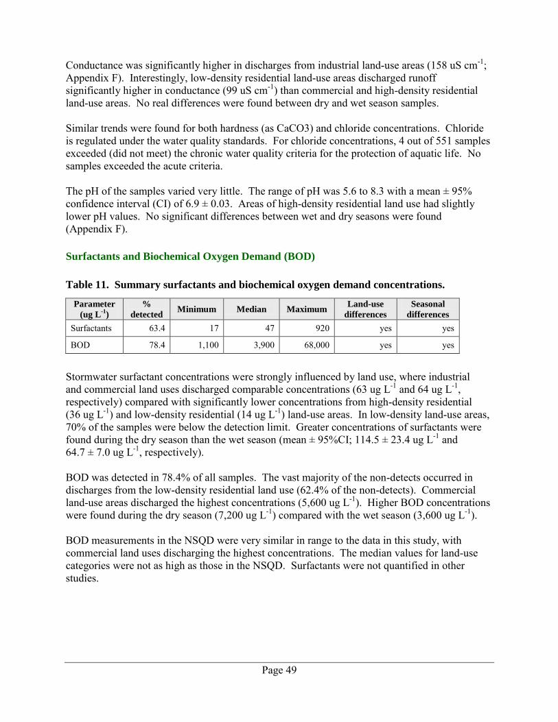
Page 49

Conductance was significantly higher in discharges from industrial land-use areas (158 uS cm-1; Appendix F). Interestingly, low-density residential land-use areas discharged runoff significantly higher in conductance (99 uS cm-1) than commercial and high-density residential land-use areas. No real differences were found between dry and wet season samples. Similar trends were found for both hardness (as CaCO3) and chloride concentrations. Chloride is regulated under the water quality standards. For chloride concentrations, 4 out of 551 samples exceeded (did not meet) the chronic water quality criteria for the protection of aquatic life. No samples exceeded the acute criteria. The pH of the samples varied very little. The range of pH was 5.6 to 8.3 with a mean ± 95% confidence interval (CI) of 6.9 ± 0.03. Areas of high-density residential land use had slightly lower pH values. No significant differences between wet and dry seasons were found (Appendix F). Surfactants and Biochemical Oxygen Demand (BOD)

Table 11. Summary surfactants and biochemical oxygen demand concentrations.

Parameter

(ug L-1

)

%


Land-use

differences

Seasonal

differences

Surfactants 63.4 17 47 920 yes yes

BOD 78.4 1,100 3,900 68,000 yes yes

Stormwater surfactant concentrations were strongly influenced by land use, where industrial and commercial land uses discharged comparable concentrations (63 ug L-1 and 64 ug L-1, respectively) compared with significantly lower concentrations from high-density residential (36 ug L-1) and low-density residential (14 ug L-1) land-use areas. In low-density land-use areas, 70% of the samples were below the detection limit. Greater concentrations of surfactants were found during the dry season than the wet season (mean ± 95%CI; 114.5 ± 23.4 ug L-1 and 64.7 ± 7.0 ug L-1, respectively). BOD was detected in 78.4% of all samples. The vast majority of the non-detects occurred in discharges from the low-density residential land use (62.4% of the non-detects). Commercial land-use areas discharged the highest concentrations (5,600 ug L-1). Higher BOD concentrations were found during the dry season (7,200 ug L-1) compared with the wet season (3,600 ug L-1). BOD measurements in the NSQD were very similar in range to the data in this study, with commercial land uses discharging the highest concentrations. The median values for land-use categories were not as high as those in the NSQD. Surfactants were not quantified in other studies.

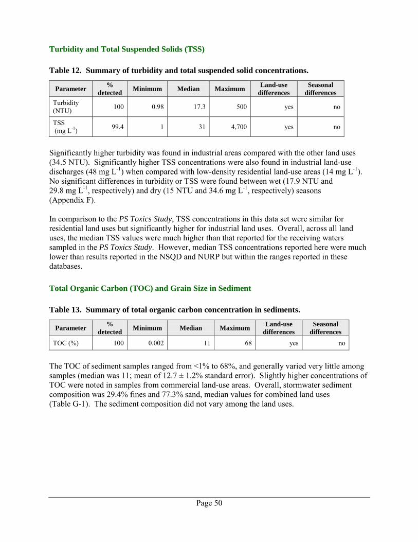
Page 50

Turbidity and Total Suspended Solids (TSS)

Table 12. Summary of turbidity and total suspended solid concentrations.

Parameter %


Land-use

differences

Seasonal

differences

Turbidity (NTU) 100 0.98 17.3 500 yes no

TSS (mg L-1) 99.4 1 31 4,700 yes no

Significantly higher turbidity was found in industrial areas compared with the other land uses (34.5 NTU). Significantly higher TSS concentrations were also found in industrial land-use discharges (48 mg L-1) when compared with low-density residential land-use areas (14 mg L-1). No significant differences in turbidity or TSS were found between wet (17.9 NTU and 29.8 mg L-1, respectively) and dry (15 NTU and 34.6 mg L-1, respectively) seasons (Appendix F). In comparison to the PS Toxics Study, TSS concentrations in this data set were similar for residential land uses but significantly higher for industrial land uses. Overall, across all land uses, the median TSS values were much higher than that reported for the receiving waters sampled in the PS Toxics Study. However, median TSS concentrations reported here were much lower than results reported in the NSQD and NURP but within the ranges reported in these databases. Total Organic Carbon (TOC) and Grain Size in Sediment

Table 13. Summary of total organic carbon concentration in sediments.

Parameter %


Land-use

differences

Seasonal

differences

TOC (%) 100 0.002 11 68 yes no

The TOC of sediment samples ranged from <1% to 68%, and generally varied very little among samples (median was 11; mean of 12.7 ± 1.2% standard error). Slightly higher concentrations of TOC were noted in samples from commercial land-use areas. Overall, stormwater sediment composition was 29.4% fines and 77.3% sand, median values for combined land uses (Table G-1). The sediment composition did not vary among the land uses.

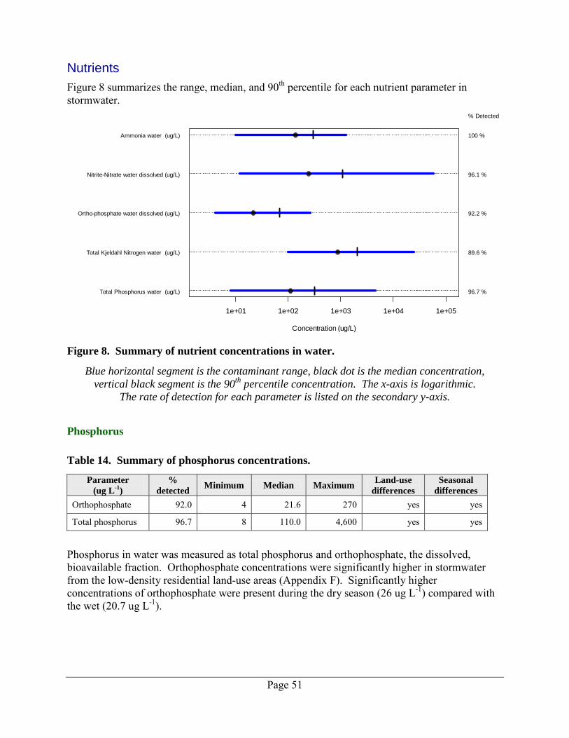
Page 51

Nutrients

Figure 8 summarizes the range, median, and 90th percentile for each nutrient parameter in stormwater.

Figure 8. Summary of nutrient concentrations in water.





Phosphorus

Table 14. Summary of phosphorus concentrations.

Parameter

(ug L-1

)

%


Land-use

differences

Seasonal

differences

Orthophosphate 92.0 4 21.6 270 yes yes

Total phosphorus 96.7 8 110.0 4,600 yes yes

Phosphorus in water was measured as total phosphorus and orthophosphate, the dissolved, bioavailable fraction. Orthophosphate concentrations were significantly higher in stormwater from the low-density residential land-use areas (Appendix F). Significantly higher concentrations of orthophosphate were present during the dry season (26 ug L-1) compared with the wet (20.7 ug L-1).

Concentration (ug/L)

1e+01 1e+02 1e+03 1e+04 1e+05

Ammonia water (ug/L)

Nitrite-Nitrate water dissolved (ug/L)

Ortho-phosphate water dissolved (ug/L)

Total Kjeldahl Nitrogen water (ug/L)

Total Phosphorus water (ug/L)

% Detected

100 %

96.1 %

92.2 %

89.6 %

96.7 %

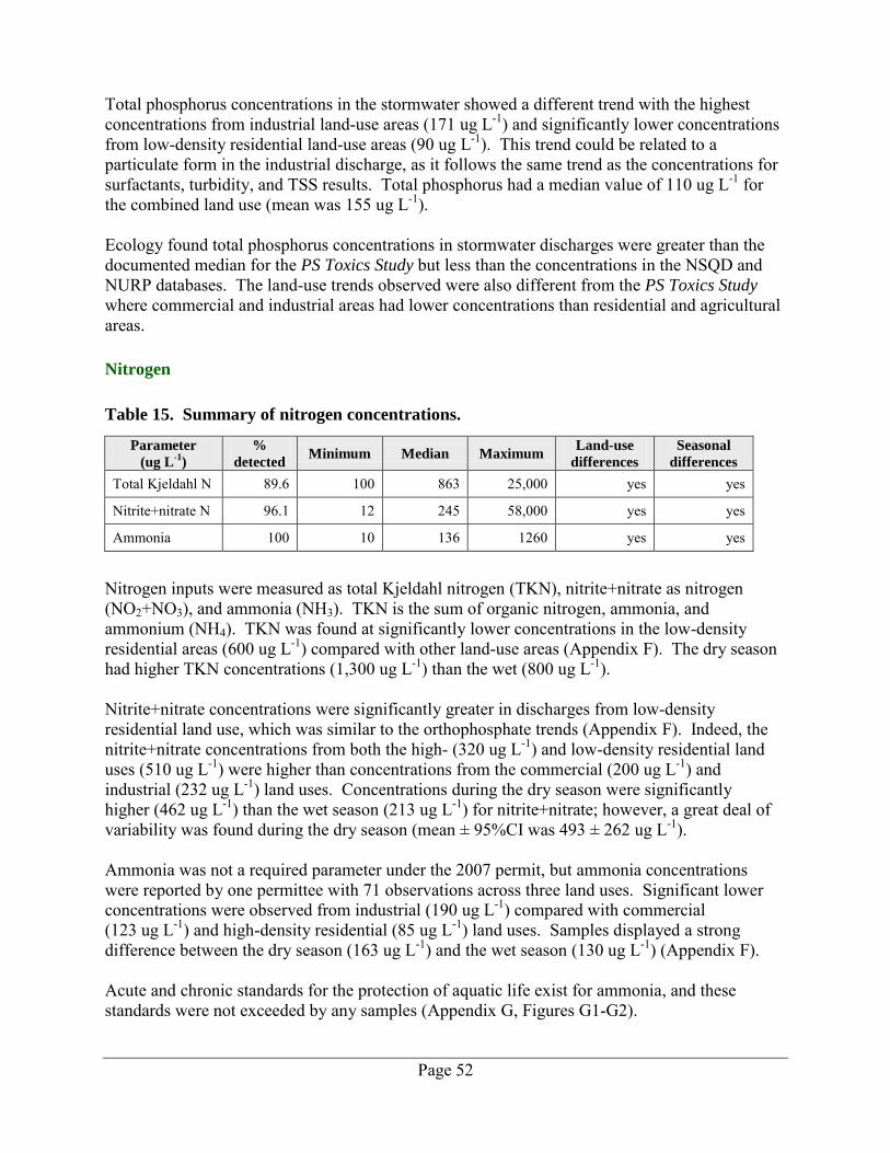
Page 52

Total phosphorus concentrations in the stormwater showed a different trend with the highest concentrations from industrial land-use areas (171 ug L-1) and significantly lower concentrations from low-density residential land-use areas (90 ug L-1). This trend could be related to a particulate form in the industrial discharge, as it follows the same trend as the concentrations for surfactants, turbidity, and TSS results. Total phosphorus had a median value of 110 ug L-1 for the combined land use (mean was 155 ug L-1). Ecology found total phosphorus concentrations in stormwater discharges were greater than the documented median for the PS Toxics Study but less than the concentrations in the NSQD and NURP databases. The land-use trends observed were also different from the PS Toxics Study where commercial and industrial areas had lower concentrations than residential and agricultural areas. Nitrogen

Table 15. Summary of nitrogen concentrations.

Parameter

(ug L-1

)

%


Land-use

differences

Seasonal

differences

Total Kjeldahl N 89.6 100 863 25,000 yes yes

Nitrite+nitrate N 96.1 12 245 58,000 yes yes

Ammonia 100 10 136 1260 yes yes

Nitrogen inputs were measured as total Kjeldahl nitrogen (TKN), nitrite+nitrate as nitrogen (NO2+NO3), and ammonia (NH3). TKN is the sum of organic nitrogen, ammonia, and ammonium (NH4). TKN was found at significantly lower concentrations in the low-density residential areas (600 ug L-1) compared with other land-use areas (Appendix F). The dry season had higher TKN concentrations (1,300 ug L-1) than the wet (800 ug L-1). Nitrite+nitrate concentrations were significantly greater in discharges from low-density residential land use, which was similar to the orthophosphate trends (Appendix F). Indeed, the nitrite+nitrate concentrations from both the high- (320 ug L-1) and low-density residential land uses (510 ug L-1) were higher than concentrations from the commercial (200 ug L-1) and industrial (232 ug L-1) land uses. Concentrations during the dry season were significantly higher (462 ug L-1) than the wet season (213 ug L-1) for nitrite+nitrate; however, a great deal of variability was found during the dry season (mean ± 95%CI was 493 ± 262 ug L-1). Ammonia was not a required parameter under the 2007 permit, but ammonia concentrations were reported by one permittee with 71 observations across three land uses. Significant lower concentrations were observed from industrial (190 ug L-1) compared with commercial (123 ug L-1) and high-density residential (85 ug L-1) land uses. Samples displayed a strong difference between the dry season (163 ug L-1) and the wet season (130 ug L-1) (Appendix F). Acute and chronic standards for the protection of aquatic life exist for ammonia, and these standards were not exceeded by any samples (Appendix G, Figures G1-G2).

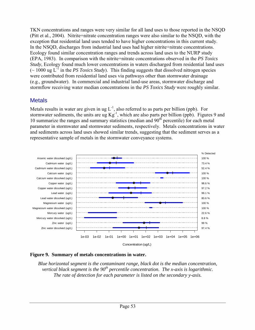
Page 53

TKN concentrations and ranges were very similar for all land uses to those reported in the NSQD (Pitt et al., 2004). Nitrite+nitrate concentration ranges were also similar to the NSQD, with the exception that residential land uses tended to have higher concentrations in this current study. In the NSQD, discharges from industrial land uses had higher nitrite+nitrate concentrations. Ecology found similar concentration ranges and trends across land uses to the NURP study (EPA, 1983). In comparison with the nitrite+nitrate concentrations observed in the PS Toxics

Study, Ecology found much lower concentrations in waters discharged from residential land uses (~ 1000 ug L-1 in the PS Toxics Study). This finding suggests that dissolved nitrogen species were contributed from residential land uses via pathways other than stormwater drainage (e.g., groundwater). In commercial and industrial land-use areas, stormwater discharge and stormflow receiving water median concentrations in the PS Toxics Study were roughly similar. Metals

Metals results in water are given in ug L-1, also referred to as parts per billion (ppb). For stormwater sediments, the units are ug Kg-1, which are also parts per billion (ppb). Figures 9 and 10 summarize the ranges and summary statistics (median and 90th percentile) for each metal parameter in stormwater and stormwater sediments, respectively. Metals concentrations in water and sediments across land uses showed similar trends, suggesting that the sediment serves as a representative sample of metals in the stormwater conveyance systems.

Figure 9. Summary of metals concentrations in water.






1e-03 1e-02 1e-01 1e+00 1e+01 1e+02 1e+03 1e+04 1e+05 1e+06

Arsenic water dissolved (ug/L)

Cadmium water (ug/L)

Cadmium water dissolved (ug/L)

Calcium water (ug/L)

Calcium water dissolved (ug/L)

Copper water (ug/L)

Copper water dissolved (ug/L)

Lead water (ug/L)

Lead water dissolved (ug/L)

Magnesium water (ug/L)

Magnesium water dissolved (ug/L)

Mercury water (ug/L)

Mercury water dissolved (ug/L)

Zinc water (ug/L)

Zinc water dissolved (ug/L)

% Detected

100 %

73.4 %

52.4 %

100 %

100 %

98.6 %

97.2 %

99.1 %

80.6 %

100 %

100 %

22.6 %

8.8 %

99 %

97.4 %

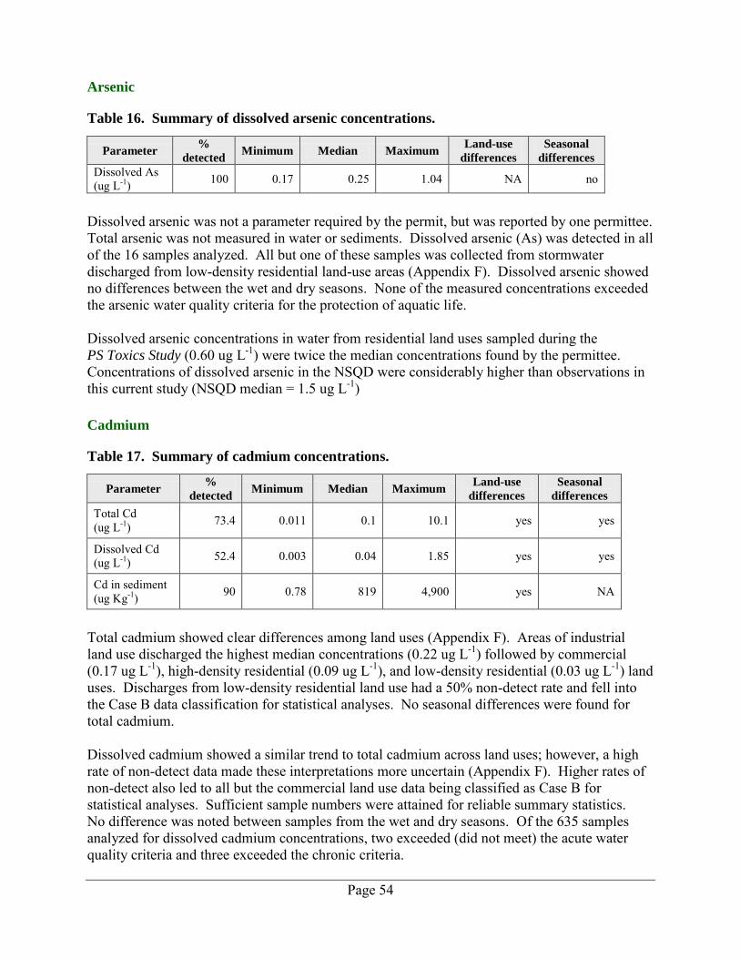
Page 54

Arsenic

Table 16. Summary of dissolved arsenic concentrations.

Parameter %


Land-use

differences

Seasonal

differences

Dissolved As (ug L-1) 100 0.17 0.25 1.04 NA no

Dissolved arsenic was not a parameter required by the permit, but was reported by one permittee. Total arsenic was not measured in water or sediments. Dissolved arsenic (As) was detected in all of the 16 samples analyzed. All but one of these samples was collected from stormwater discharged from low-density residential land-use areas (Appendix F). Dissolved arsenic showed no differences between the wet and dry seasons. None of the measured concentrations exceeded the arsenic water quality criteria for the protection of aquatic life. Dissolved arsenic concentrations in water from residential land uses sampled during the PS Toxics Study (0.60 ug L-1) were twice the median concentrations found by the permittee. Concentrations of dissolved arsenic in the NSQD were considerably higher than observations in this current study (NSQD median = 1.5 ug L-1) Cadmium

Table 17. Summary of cadmium concentrations.

Parameter %


Land-use

differences

Seasonal

differences

Total Cd (ug L-1) 73.4 0.011 0.1 10.1 yes yes

Dissolved Cd (ug L-1) 52.4 0.003 0.04 1.85 yes yes

Cd in sediment (ug Kg-1) 90 0.78 819 4,900 yes NA

Total cadmium showed clear differences among land uses (Appendix F). Areas of industrial land use discharged the highest median concentrations (0.22 ug L-1) followed by commercial (0.17 ug L-1), high-density residential (0.09 ug L-1), and low-density residential (0.03 ug L-1) land uses. Discharges from low-density residential land use had a 50% non-detect rate and fell into the Case B data classification for statistical analyses. No seasonal differences were found for total cadmium. Dissolved cadmium showed a similar trend to total cadmium across land uses; however, a high rate of non-detect data made these interpretations more uncertain (Appendix F). Higher rates of non-detect also led to all but the commercial land use data being classified as Case B for statistical analyses. Sufficient sample numbers were attained for reliable summary statistics. No difference was noted between samples from the wet and dry seasons. Of the 635 samples analyzed for dissolved cadmium concentrations, two exceeded (did not meet) the acute water quality criteria and three exceeded the chronic criteria.

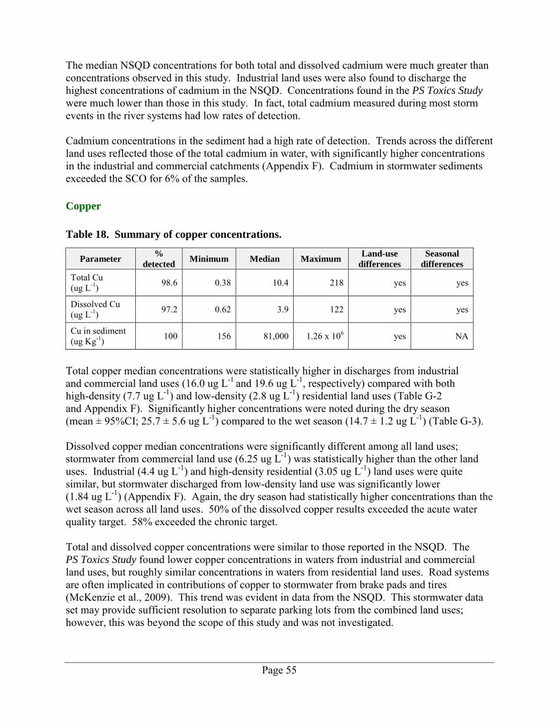
Page 55

The median NSQD concentrations for both total and dissolved cadmium were much greater than concentrations observed in this study. Industrial land uses were also found to discharge the highest concentrations of cadmium in the NSQD. Concentrations found in the PS Toxics Study were much lower than those in this study. In fact, total cadmium measured during most storm events in the river systems had low rates of detection. Cadmium concentrations in the sediment had a high rate of detection. Trends across the different land uses reflected those of the total cadmium in water, with significantly higher concentrations in the industrial and commercial catchments (Appendix F). Cadmium in stormwater sediments exceeded the SCO for 6% of the samples. Copper

Table 18. Summary of copper concentrations.

Parameter %


Land-use

differences

Seasonal

differences

Total Cu (ug L-1) 98.6 0.38 10.4 218 yes yes

Dissolved Cu (ug L-1) 97.2 0.62 3.9 122 yes yes

Cu in sediment (ug Kg-1) 100 156 81,000 1.26 x 106 yes NA

Total copper median concentrations were statistically higher in discharges from industrial and commercial land uses (16.0 ug L-1 and 19.6 ug L-1, respectively) compared with both high-density (7.7 ug L-1) and low-density (2.8 ug L-1) residential land uses (Table G-2 and Appendix F). Significantly higher concentrations were noted during the dry season (mean ± 95%CI; 25.7 ± 5.6 ug L-1) compared to the wet season (14.7 ± 1.2 ug L-1) (Table G-3). Dissolved copper median concentrations were significantly different among all land uses; stormwater from commercial land use (6.25 ug L-1) was statistically higher than the other land uses. Industrial (4.4 ug L-1) and high-density residential (3.05 ug L-1) land uses were quite similar, but stormwater discharged from low-density land use was significantly lower (1.84 ug L-1) (Appendix F). Again, the dry season had statistically higher concentrations than the wet season across all land uses. 50% of the dissolved copper results exceeded the acute water quality target. 58% exceeded the chronic target. Total and dissolved copper concentrations were similar to those reported in the NSQD. The PS Toxics Study found lower copper concentrations in waters from industrial and commercial land uses, but roughly similar concentrations in waters from residential land uses. Road systems are often implicated in contributions of copper to stormwater from brake pads and tires (McKenzie et al., 2009). This trend was evident in data from the NSQD. This stormwater data set may provide sufficient resolution to separate parking lots from the combined land uses; however, this was beyond the scope of this study and was not investigated.

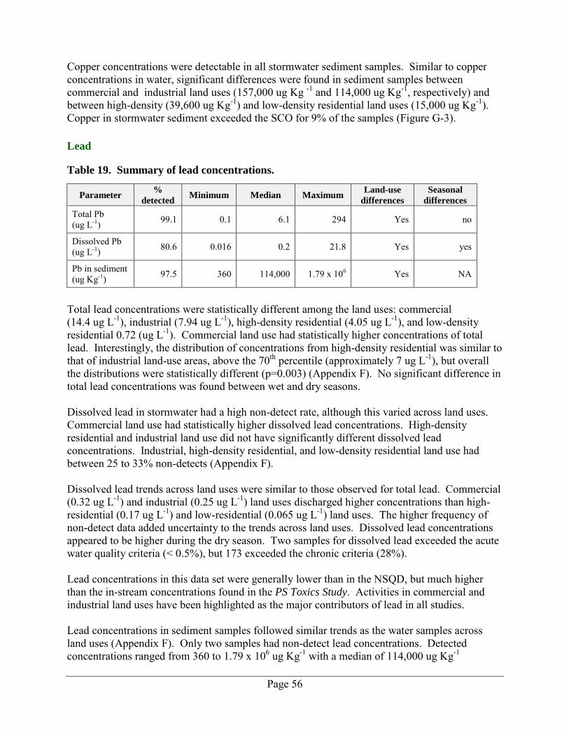
Page 56

Copper concentrations were detectable in all stormwater sediment samples. Similar to copper concentrations in water, significant differences were found in sediment samples between commercial and industrial land uses (157,000 ug Kg -1 and 114,000 ug Kg-1, respectively) and between high-density (39,600 ug Kg-1) and low-density residential land uses (15,000 ug Kg-1). Copper in stormwater sediment exceeded the SCO for 9% of the samples (Figure G-3). Lead

Table 19. Summary of lead concentrations.

Parameter %


Land-use

differences

Seasonal

differences

Total Pb (ug L-1) 99.1 0.1 6.1 294 Yes no

Dissolved Pb (ug L-1) 80.6 0.016 0.2 21.8 Yes yes

Pb in sediment (ug Kg-1) 97.5 360 114,000 1.79 x 106 Yes NA

Total lead concentrations were statistically different among the land uses: commercial (14.4 ug L-1), industrial (7.94 ug L-1), high-density residential (4.05 ug L-1), and low-density residential 0.72 (ug L-1). Commercial land use had statistically higher concentrations of total lead. Interestingly, the distribution of concentrations from high-density residential was similar to that of industrial land-use areas, above the 70th percentile (approximately 7 ug L-1), but overall the distributions were statistically different (p=0.003) (Appendix F). No significant difference in total lead concentrations was found between wet and dry seasons. Dissolved lead in stormwater had a high non-detect rate, although this varied across land uses. Commercial land use had statistically higher dissolved lead concentrations. High-density residential and industrial land use did not have significantly different dissolved lead concentrations. Industrial, high-density residential, and low-density residential land use had between 25 to 33% non-detects (Appendix F). Dissolved lead trends across land uses were similar to those observed for total lead. Commercial (0.32 ug L-1) and industrial (0.25 ug L-1) land uses discharged higher concentrations than high-residential (0.17 ug L-1) and low-residential (0.065 ug L-1) land uses. The higher frequency of non-detect data added uncertainty to the trends across land uses. Dissolved lead concentrations appeared to be higher during the dry season. Two samples for dissolved lead exceeded the acute water quality criteria (< 0.5%), but 173 exceeded the chronic criteria (28%). Lead concentrations in this data set were generally lower than in the NSQD, but much higher than the in-stream concentrations found in the PS Toxics Study. Activities in commercial and industrial land uses have been highlighted as the major contributors of lead in all studies. Lead concentrations in sediment samples followed similar trends as the water samples across land uses (Appendix F). Only two samples had non-detect lead concentrations. Detected concentrations ranged from 360 to 1.79 x 106 ug Kg-1 with a median of 114,000 ug Kg-1

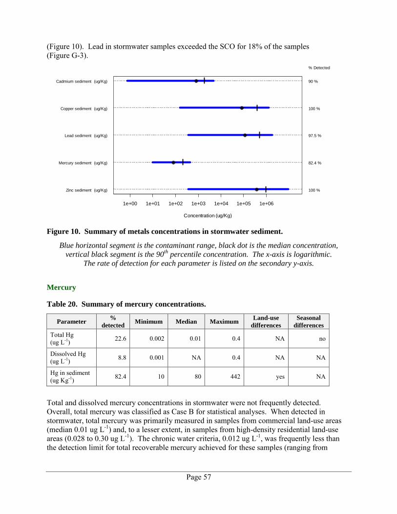
Page 57

(Figure 10). Lead in stormwater samples exceeded the SCO for 18% of the samples (Figure G-3).

Figure 10. Summary of metals concentrations in stormwater sediment.





Mercury

Table 20. Summary of mercury concentrations.

Parameter %


Land-use

differences

Seasonal

differences

Total Hg (ug L-1) 22.6 0.002 0.01 0.4 NA no

Dissolved Hg (ug L-1) 8.8 0.001 NA 0.4 NA NA

Hg in sediment (ug Kg-1) 82.4 10 80 442 yes NA

Total and dissolved mercury concentrations in stormwater were not frequently detected. Overall, total mercury was classified as Case B for statistical analyses. When detected in stormwater, total mercury was primarily measured in samples from commercial land-use areas (median 0.01 ug L-1) and, to a lesser extent, in samples from high-density residential land-use areas (0.028 to 0.30 ug L-1). The chronic water criteria, 0.012 ug L-1, was frequently less than the detection limit for total recoverable mercury achieved for these samples (ranging from

Concentration (ug/Kg)

1e+00 1e+01 1e+02 1e+03 1e+04 1e+05 1e+06

Cadmium sediment (ug/Kg)

Copper sediment (ug/Kg)

Lead sediment (ug/Kg)

Mercury sediment (ug/Kg)

Zinc sediment (ug/Kg)

% Detected

90 %

100 %

97.5 %

82.4 %

100 %

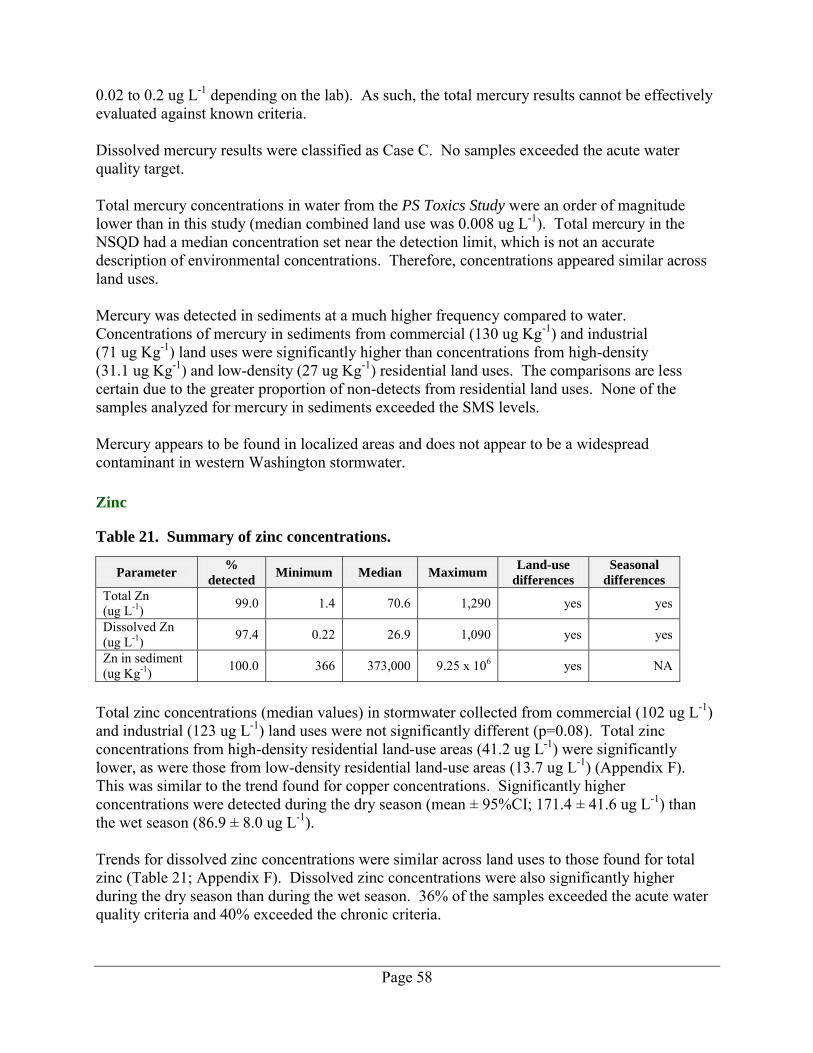
Page 58

0.02 to 0.2 ug L-1 depending on the lab). As such, the total mercury results cannot be effectively evaluated against known criteria. Dissolved mercury results were classified as Case C. No samples exceeded the acute water quality target. Total mercury concentrations in water from the PS Toxics Study were an order of magnitude lower than in this study (median combined land use was 0.008 ug L-1). Total mercury in the NSQD had a median concentration set near the detection limit, which is not an accurate description of environmental concentrations. Therefore, concentrations appeared similar across land uses. Mercury was detected in sediments at a much higher frequency compared to water. Concentrations of mercury in sediments from commercial (130 ug Kg-1) and industrial (71 ug Kg-1) land uses were significantly higher than concentrations from high-density (31.1 ug Kg-1) and low-density (27 ug Kg-1) residential land uses. The comparisons are less certain due to the greater proportion of non-detects from residential land uses. None of the samples analyzed for mercury in sediments exceeded the SMS levels. Mercury appears to be found in localized areas and does not appear to be a widespread contaminant in western Washington stormwater. Zinc

Table 21. Summary of zinc concentrations.

Parameter %


Land-use

differences

Seasonal

differences

Total Zn (ug L-1) 99.0 1.4 70.6 1,290 yes yes

Dissolved Zn (ug L-1) 97.4 0.22 26.9 1,090 yes yes

Zn in sediment (ug Kg-1) 100.0 366 373,000 9.25 x 106 yes NA

Total zinc concentrations (median values) in stormwater collected from commercial (102 ug L-1) and industrial (123 ug L-1) land uses were not significantly different (p=0.08). Total zinc concentrations from high-density residential land-use areas (41.2 ug L-1) were significantly lower, as were those from low-density residential land-use areas (13.7 ug L-1) (Appendix F). This was similar to the trend found for copper concentrations. Significantly higher concentrations were detected during the dry season (mean ± 95%CI; 171.4 ± 41.6 ug L-1) than the wet season (86.9 ± 8.0 ug L-1). Trends for dissolved zinc concentrations were similar across land uses to those found for total zinc (Table 21; Appendix F). Dissolved zinc concentrations were also significantly higher during the dry season than during the wet season. 36% of the samples exceeded the acute water quality criteria and 40% exceeded the chronic criteria.

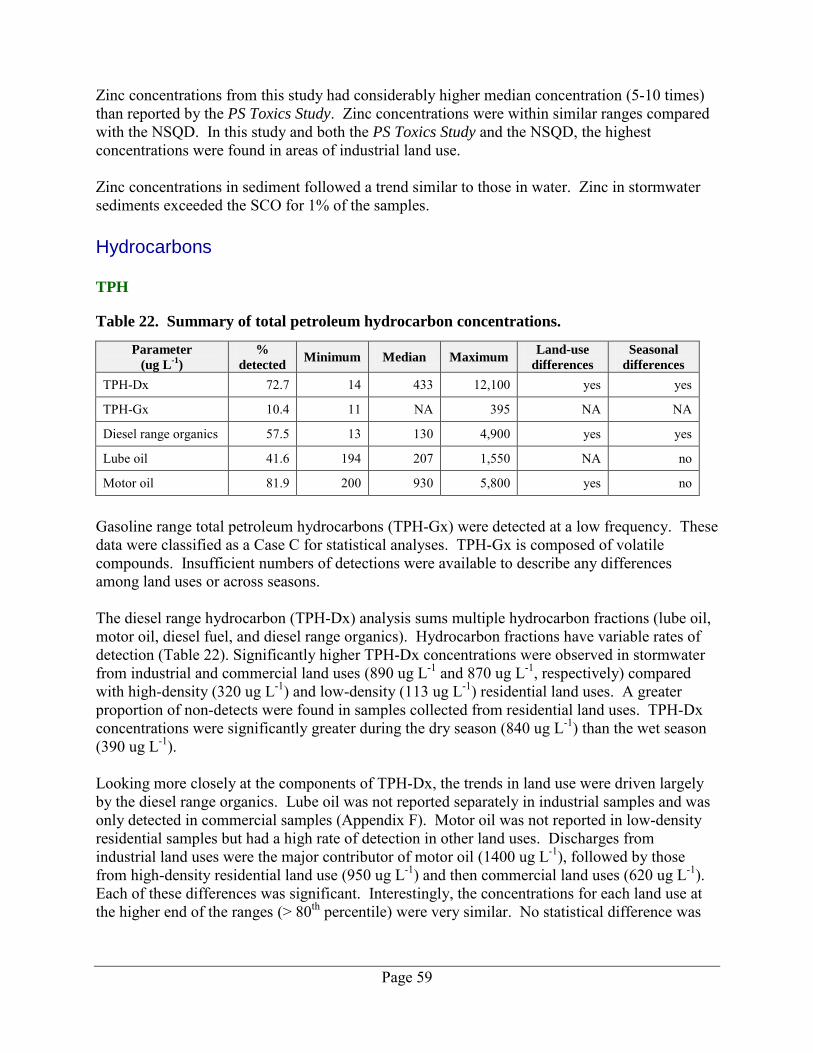
Page 59

Zinc concentrations from this study had considerably higher median concentration (5-10 times) than reported by the PS Toxics Study. Zinc concentrations were within similar ranges compared with the NSQD. In this study and both the PS Toxics Study and the NSQD, the highest concentrations were found in areas of industrial land use. Zinc concentrations in sediment followed a trend similar to those in water. Zinc in stormwater sediments exceeded the SCO for 1% of the samples. Hydrocarbons TPH

Table 22. Summary of total petroleum hydrocarbon concentrations.

Parameter

(ug L-1

)

%


Land-use

differences

Seasonal

differences

TPH-Dx 72.7 14 433 12,100 yes yes

TPH-Gx 10.4 11 NA 395 NA NA

Diesel range organics 57.5 13 130 4,900 yes yes

Lube oil 41.6 194 207 1,550 NA no

Motor oil 81.9 200 930 5,800 yes no

Gasoline range total petroleum hydrocarbons (TPH-Gx) were detected at a low frequency. These data were classified as a Case C for statistical analyses. TPH-Gx is composed of volatile compounds. Insufficient numbers of detections were available to describe any differences among land uses or across seasons. The diesel range hydrocarbon (TPH-Dx) analysis sums multiple hydrocarbon fractions (lube oil, motor oil, diesel fuel, and diesel range organics). Hydrocarbon fractions have variable rates of detection (Table 22). Significantly higher TPH-Dx concentrations were observed in stormwater from industrial and commercial land uses (890 ug L-1 and 870 ug L-1, respectively) compared with high-density (320 ug L-1) and low-density (113 ug L-1) residential land uses. A greater proportion of non-detects were found in samples collected from residential land uses. TPH-Dx concentrations were significantly greater during the dry season (840 ug L-1) than the wet season (390 ug L-1). Looking more closely at the components of TPH-Dx, the trends in land use were driven largely by the diesel range organics. Lube oil was not reported separately in industrial samples and was only detected in commercial samples (Appendix F). Motor oil was not reported in low-density residential samples but had a high rate of detection in other land uses. Discharges from industrial land uses were the major contributor of motor oil (1400 ug L-1), followed by those from high-density residential land use (950 ug L-1) and then commercial land uses (620 ug L-1). Each of these differences was significant. Interestingly, the concentrations for each land use at the higher end of the ranges (> 80th percentile) were very similar. No statistical difference was

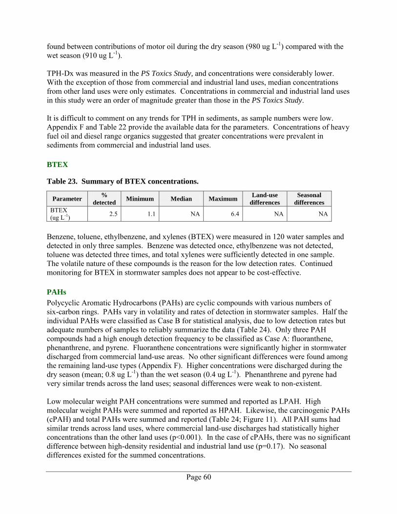
Page 60

found between contributions of motor oil during the dry season (980 ug L-1) compared with the wet season (910 ug L-1). TPH-Dx was measured in the PS Toxics Study, and concentrations were considerably lower. With the exception of those from commercial and industrial land uses, median concentrations from other land uses were only estimates. Concentrations in commercial and industrial land uses in this study were an order of magnitude greater than those in the PS Toxics Study. It is difficult to comment on any trends for TPH in sediments, as sample numbers were low. Appendix F and Table 22 provide the available data for the parameters. Concentrations of heavy fuel oil and diesel range organics suggested that greater concentrations were prevalent in sediments from commercial and industrial land uses. BTEX

Table 23. Summary of BTEX concentrations.

Parameter %


Land-use

differences

Seasonal

differences

BTEX (ug L-1) 2.5 1.1 NA 6.4 NA NA

Benzene, toluene, ethylbenzene, and xylenes (BTEX) were measured in 120 water samples and detected in only three samples. Benzene was detected once, ethylbenzene was not detected, toluene was detected three times, and total xylenes were sufficiently detected in one sample. The volatile nature of these compounds is the reason for the low detection rates. Continued monitoring for BTEX in stormwater samples does not appear to be cost-effective. PAHs

Polycyclic Aromatic Hydrocarbons (PAHs) are cyclic compounds with various numbers of six-carbon rings. PAHs vary in volatility and rates of detection in stormwater samples. Half the individual PAHs were classified as Case B for statistical analysis, due to low detection rates but adequate numbers of samples to reliably summarize the data (Table 24). Only three PAH compounds had a high enough detection frequency to be classified as Case A: fluoranthene, phenanthrene, and pyrene. Fluoranthene concentrations were significantly higher in stormwater discharged from commercial land-use areas. No other significant differences were found among the remaining land-use types (Appendix F). Higher concentrations were discharged during the dry season (mean; 0.8 ug L-1) than the wet season (0.4 ug L-1). Phenanthrene and pyrene had very similar trends across the land uses; seasonal differences were weak to non-existent. Low molecular weight PAH concentrations were summed and reported as LPAH. High molecular weight PAHs were summed and reported as HPAH. Likewise, the carcinogenic PAHs (cPAH) and total PAHs were summed and reported (Table 24; Figure 11). All PAH sums had similar trends across land uses, where commercial land-use discharges had statistically higher concentrations than the other land uses (p<0.001). In the case of cPAHs, there was no significant difference between high-density residential and industrial land use (p=0.17). No seasonal differences existed for the summed concentrations.

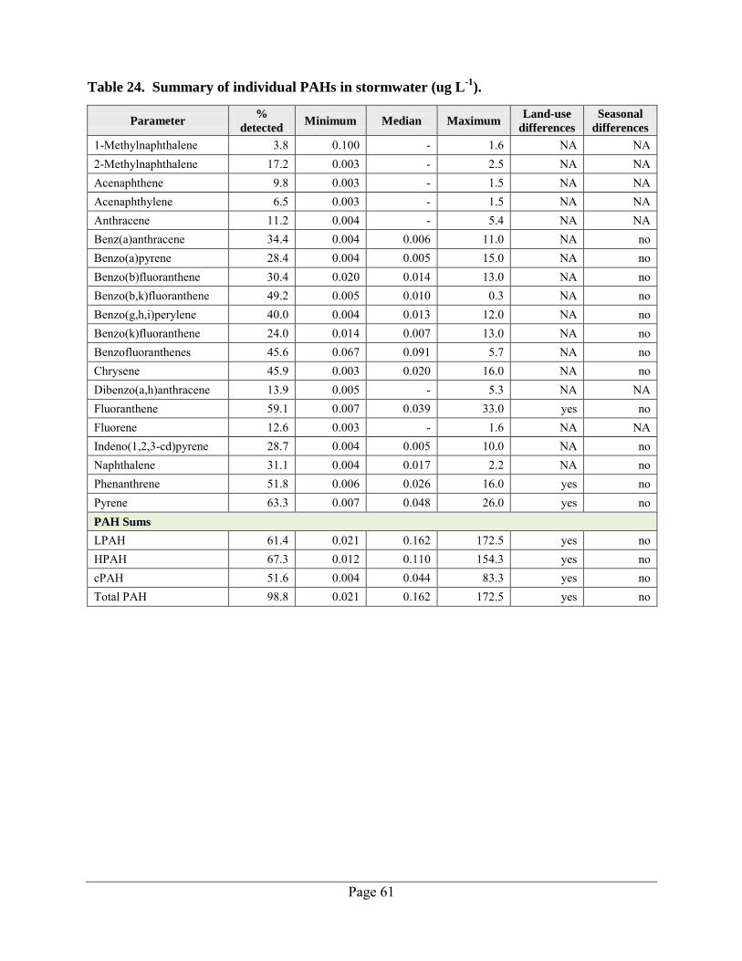
Page 61

Table 24. Summary of individual PAHs in stormwater (ug L-1

).

Parameter %


Land-use

differences

Seasonal

differences

1-Methylnaphthalene 3.8 0.100 - 1.6 NA NA 2-Methylnaphthalene 17.2 0.003 - 2.5 NA NA Acenaphthene 9.8 0.003 - 1.5 NA NA Acenaphthylene 6.5 0.003 - 1.5 NA NA Anthracene 11.2 0.004 - 5.4 NA NA Benz(a)anthracene 34.4 0.004 0.006 11.0 NA no Benzo(a)pyrene 28.4 0.004 0.005 15.0 NA no Benzo(b)fluoranthene 30.4 0.020 0.014 13.0 NA no Benzo(b,k)fluoranthene 49.2 0.005 0.010 0.3 NA no Benzo(g,h,i)perylene 40.0 0.004 0.013 12.0 NA no Benzo(k)fluoranthene 24.0 0.014 0.007 13.0 NA no Benzofluoranthenes 45.6 0.067 0.091 5.7 NA no Chrysene 45.9 0.003 0.020 16.0 NA no Dibenzo(a,h)anthracene 13.9 0.005 - 5.3 NA NA Fluoranthene 59.1 0.007 0.039 33.0 yes no Fluorene 12.6 0.003 - 1.6 NA NA Indeno(1,2,3-cd)pyrene 28.7 0.004 0.005 10.0 NA no Naphthalene 31.1 0.004 0.017 2.2 NA no Phenanthrene 51.8 0.006 0.026 16.0 yes no Pyrene 63.3 0.007 0.048 26.0 yes no PAH Sums

LPAH 61.4 0.021 0.162 172.5 yes no HPAH 67.3 0.012 0.110 154.3 yes no cPAH 51.6 0.004 0.044 83.3 yes no Total PAH 98.8 0.021 0.162 172.5 yes no

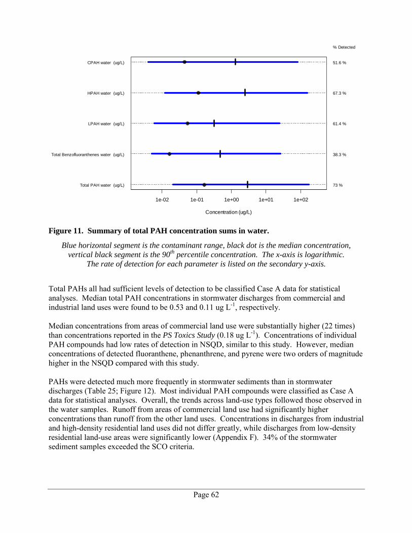
Page 62

Figure 11. Summary of total PAH concentration sums in water.





Total PAHs all had sufficient levels of detection to be classified Case A data for statistical analyses. Median total PAH concentrations in stormwater discharges from commercial and industrial land uses were found to be 0.53 and 0.11 ug L-1, respectively. Median concentrations from areas of commercial land use were substantially higher (22 times) than concentrations reported in the PS Toxics Study (0.18 ug L-1). Concentrations of individual PAH compounds had low rates of detection in NSQD, similar to this study. However, median concentrations of detected fluoranthene, phenanthrene, and pyrene were two orders of magnitude higher in the NSQD compared with this study. PAHs were detected much more frequently in stormwater sediments than in stormwater discharges (Table 25; Figure 12). Most individual PAH compounds were classified as Case A data for statistical analyses. Overall, the trends across land-use types followed those observed in the water samples. Runoff from areas of commercial land use had significantly higher concentrations than runoff from the other land uses. Concentrations in discharges from industrial and high-density residential land uses did not differ greatly, while discharges from low-density residential land-use areas were significantly lower (Appendix F). 34% of the stormwater sediment samples exceeded the SCO criteria.


1e-02 1e-01 1e+00 1e+01 1e+02

CPAH water (ug/L)

HPAH water (ug/L)

LPAH water (ug/L)

Total Benzofluoranthenes water (ug/L)

Total PAH water (ug/L)

% Detected

51.6 %

67.3 %

61.4 %

38.3 %

73 %

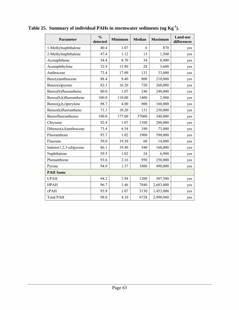
Page 63

Table 25. Summary of individual PAHs in stormwater sediments (ug Kg-1

).

Parameter %


Land-use

differences

1-Methylnaphthalene 40.4 1.07 6 870 yes 2-Methylnaphthalene 47.4 1.12 13 1,500 yes Acenaphthene 54.4 8.70 34 8,900 yes Acenaphthylene 32.9 15.80 28 3,600 yes Anthracene 73.4 17.00 131 33,000 yes Benz(a)anthracene 88.4 9.40 800 210,000 yes Benzo(a)pyrene 82.3 16.20 720 260,000 yes Benzo(b)fluoranthene 80.0 1.07 240 240,000 yes Benzo(b,k)fluoranthene 100.0 110.00 1400 2,900 yes Benzo(g,h,i)perylene 88.7 4.00 800 160,000 yes Benzo(k)fluoranthene 71.1 10.20 131 230,000 yes Benzofluoranthenes 100.0 177.00 57000 340,000 yes Chrysene 92.4 1.07 1100 280,000 yes Dibenzo(a,h)anthracene 73.4 6.54 190 73,000 yes Fluoranthene 93.7 1.02 1900 590,000 yes Fluorene 59.0 19.30 60 14,000 yes Indeno(1,2,3-cd)pyrene 86.1 19.40 540 160,000 yes Naphthalene 59.5 1.02 24 6,900 yes Phenanthrene 93.6 2.16 950 250,000 yes Pyrene 94.9 1.37 1800 490,000 yes PAH Sums

LPAH 94.2 1.94 1200 307,500 yes HPAH 96.7 3.46 7840 2,683,000 yes cPAH 93.9 1.07 3130 1,453,000 yes Total PAH 98.8 4.10 6728 2,990,960 yes

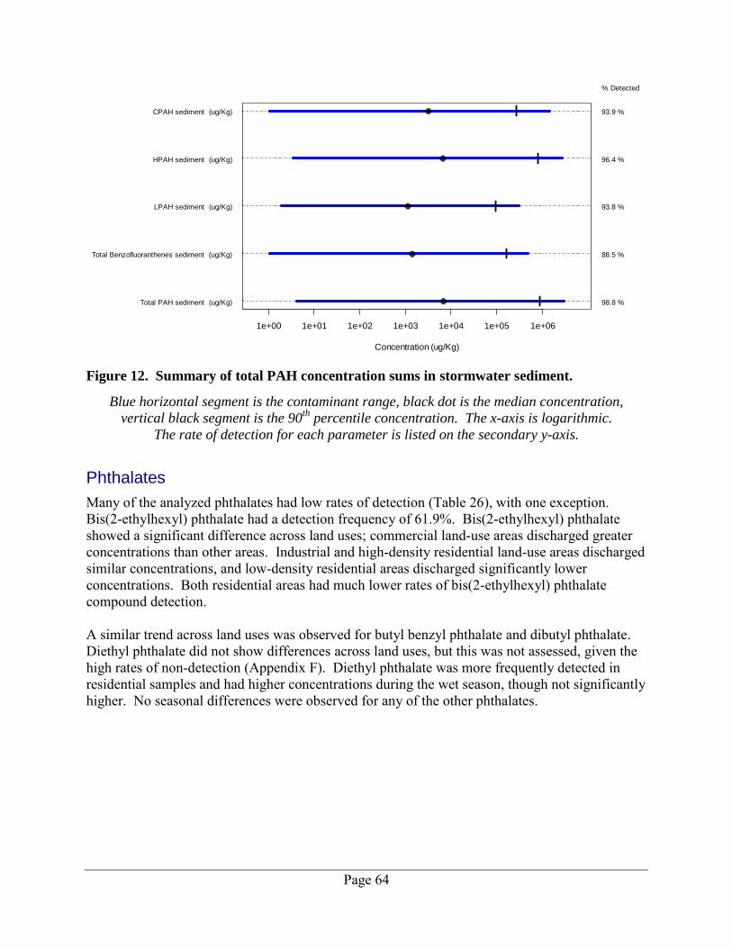
Page 64

Figure 12. Summary of total PAH concentration sums in stormwater sediment.





Phthalates

Many of the analyzed phthalates had low rates of detection (Table 26), with one exception. Bis(2-ethylhexyl) phthalate had a detection frequency of 61.9%. Bis(2-ethylhexyl) phthalate showed a significant difference across land uses; commercial land-use areas discharged greater concentrations than other areas. Industrial and high-density residential land-use areas discharged similar concentrations, and low-density residential areas discharged significantly lower concentrations. Both residential areas had much lower rates of bis(2-ethylhexyl) phthalate compound detection. A similar trend across land uses was observed for butyl benzyl phthalate and dibutyl phthalate. Diethyl phthalate did not show differences across land uses, but this was not assessed, given the high rates of non-detection (Appendix F). Diethyl phthalate was more frequently detected in residential samples and had higher concentrations during the wet season, though not significantly higher. No seasonal differences were observed for any of the other phthalates.

Concentration (ug/Kg)

1e+00 1e+01 1e+02 1e+03 1e+04 1e+05 1e+06

CPAH sediment (ug/Kg)

HPAH sediment (ug/Kg)

LPAH sediment (ug/Kg)

Total Benzofluoranthenes sediment (ug/Kg)

Total PAH sediment (ug/Kg)

% Detected

93.9 %

96.4 %

93.8 %

88.5 %

98.8 %

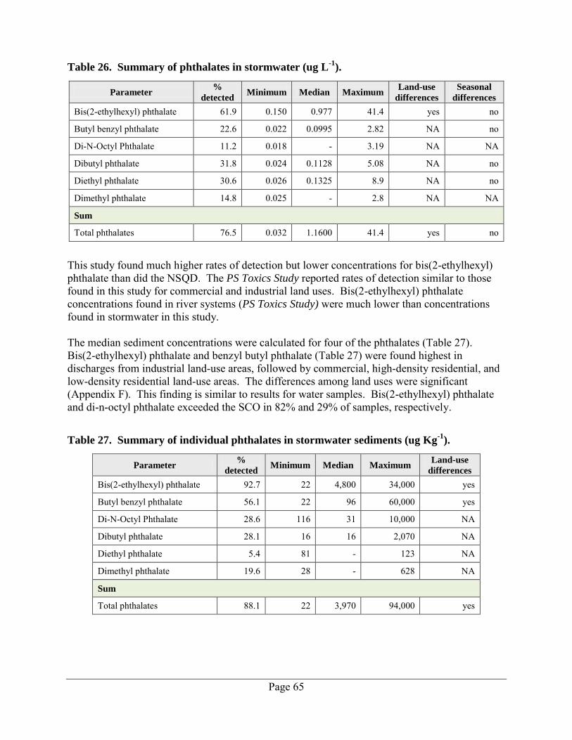
Page 65

Table 26. Summary of phthalates in stormwater (ug L-1

).

Parameter %


Land-use

differences

Seasonal

differences

Bis(2-ethylhexyl) phthalate 61.9 0.150 0.977 41.4 yes no

Butyl benzyl phthalate 22.6 0.022 0.0995 2.82 NA no

Di-N-Octyl Phthalate 11.2 0.018 - 3.19 NA NA

Dibutyl phthalate 31.8 0.024 0.1128 5.08 NA no

Diethyl phthalate 30.6 0.026 0.1325 8.9 NA no

Dimethyl phthalate 14.8 0.025 - 2.8 NA NA

Sum

Total phthalates 76.5 0.032 1.1600 41.4 yes no

This study found much higher rates of detection but lower concentrations for bis(2-ethylhexyl) phthalate than did the NSQD. The PS Toxics Study reported rates of detection similar to those found in this study for commercial and industrial land uses. Bis(2-ethylhexyl) phthalate concentrations found in river systems (PS Toxics Study) were much lower than concentrations found in stormwater in this study. The median sediment concentrations were calculated for four of the phthalates (Table 27). Bis(2-ethylhexyl) phthalate and benzyl butyl phthalate (Table 27) were found highest in discharges from industrial land-use areas, followed by commercial, high-density residential, and low-density residential land-use areas. The differences among land uses were significant (Appendix F). This finding is similar to results for water samples. Bis(2-ethylhexyl) phthalate and di-n-octyl phthalate exceeded the SCO in 82% and 29% of samples, respectively.

Table 27. Summary of individual phthalates in stormwater sediments (ug Kg-1

).

Parameter %


Land-use

differences

Bis(2-ethylhexyl) phthalate 92.7 22 4,800 34,000 yes

Butyl benzyl phthalate 56.1 22 96 60,000 yes

Di-N-Octyl Phthalate 28.6 116 31 10,000 NA

Dibutyl phthalate 28.1 16 16 2,070 NA

Diethyl phthalate 5.4 81 - 123 NA

Dimethyl phthalate 19.6 28 - 628 NA

Sum

Total phthalates 88.1 22 3,970 94,000 yes

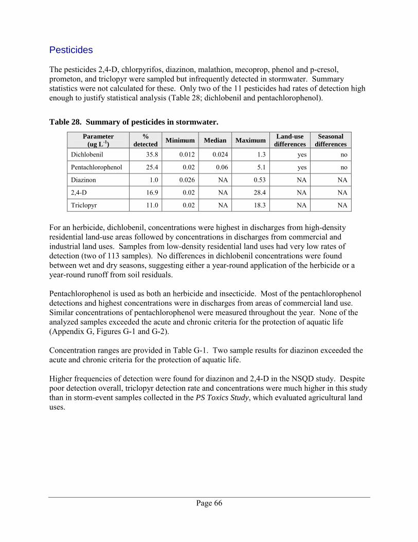
Page 66

Pesticides The pesticides 2,4-D, chlorpyrifos, diazinon, malathion, mecoprop, phenol and p-cresol, prometon, and triclopyr were sampled but infrequently detected in stormwater. Summary statistics were not calculated for these. Only two of the 11 pesticides had rates of detection high enough to justify statistical analysis (Table 28; dichlobenil and pentachlorophenol).

Table 28. Summary of pesticides in stormwater.

Parameter

(ug L-1

)

%


Land-use

differences

Seasonal

differences

Dichlobenil 35.8 0.012 0.024 1.3 yes no

Pentachlorophenol 25.4 0.02 0.06 5.1 yes no

Diazinon 1.0 0.026 NA 0.53 NA NA

2,4-D 16.9 0.02 NA 28.4 NA NA

Triclopyr 11.0 0.02 NA 18.3 NA NA

For an herbicide, dichlobenil, concentrations were highest in discharges from high-density residential land-use areas followed by concentrations in discharges from commercial and industrial land uses. Samples from low-density residential land uses had very low rates of detection (two of 113 samples). No differences in dichlobenil concentrations were found between wet and dry seasons, suggesting either a year-round application of the herbicide or a year-round runoff from soil residuals. Pentachlorophenol is used as both an herbicide and insecticide. Most of the pentachlorophenol detections and highest concentrations were in discharges from areas of commercial land use. Similar concentrations of pentachlorophenol were measured throughout the year. None of the analyzed samples exceeded the acute and chronic criteria for the protection of aquatic life (Appendix G, Figures G-1 and G-2). Concentration ranges are provided in Table G-1. Two sample results for diazinon exceeded the acute and chronic criteria for the protection of aquatic life. Higher frequencies of detection were found for diazinon and 2,4-D in the NSQD study. Despite poor detection overall, triclopyr detection rate and concentrations were much higher in this study than in storm-event samples collected in the PS Toxics Study, which evaluated agricultural land uses.

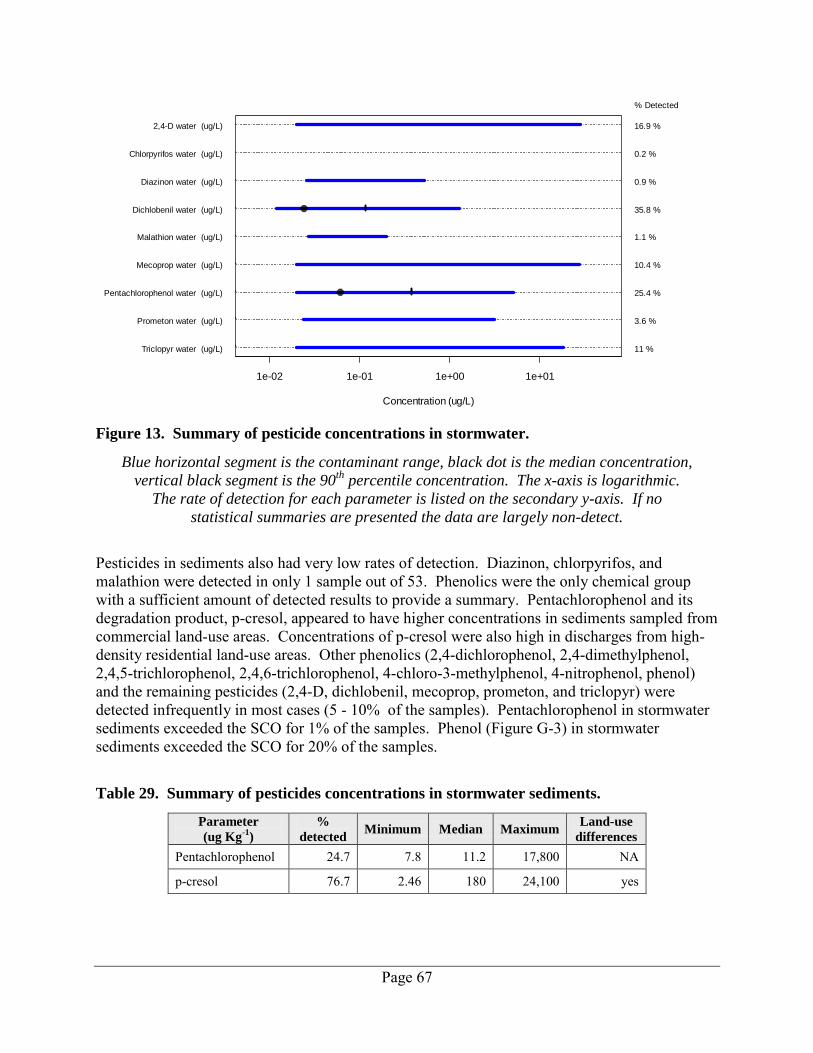
Page 67

Figure 13. Summary of pesticide concentrations in stormwater.




The rate of detection for each parameter is listed on the secondary y-axis. If no

statistical summaries are presented the data are largely non-detect.

Pesticides in sediments also had very low rates of detection. Diazinon, chlorpyrifos, and malathion were detected in only 1 sample out of 53. Phenolics were the only chemical group with a sufficient amount of detected results to provide a summary. Pentachlorophenol and its degradation product, p-cresol, appeared to have higher concentrations in sediments sampled from commercial land-use areas. Concentrations of p-cresol were also high in discharges from high-density residential land-use areas. Other phenolics (2,4-dichlorophenol, 2,4-dimethylphenol, 2,4,5-trichlorophenol, 2,4,6-trichlorophenol, 4-chloro-3-methylphenol, 4-nitrophenol, phenol) and the remaining pesticides (2,4-D, dichlobenil, mecoprop, prometon, and triclopyr) were detected infrequently in most cases (5 - 10% of the samples). Pentachlorophenol in stormwater sediments exceeded the SCO for 1% of the samples. Phenol (Figure G-3) in stormwater sediments exceeded the SCO for 20% of the samples.

Table 29. Summary of pesticides concentrations in stormwater sediments.

Parameter

(ug Kg-1

)

%


Land-use

differences

Pentachlorophenol 24.7 7.8 11.2 17,800 NA

p-cresol 76.7 2.46 180 24,100 yes


1e-02 1e-01 1e+00 1e+01

2,4-D water (ug/L)

Chlorpyrifos water (ug/L)

Diazinon water (ug/L)

Dichlobenil water (ug/L)

Malathion water (ug/L)

Mecoprop water (ug/L)

Pentachlorophenol water (ug/L)

Prometon water (ug/L)

Triclopyr water (ug/L)

% Detected

16.9 %

0.2 %

0.9 %

35.8 %

1.1 %

10.4 %

25.4 %

3.6 %

11 %

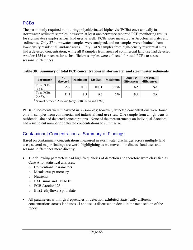
Page 68

PCBs

The permit only required monitoring polychlorinated biphenyls (PCBs) once annually in stormwater sediment samples; however, at least one permittee reported PCB monitoring results for stormwater samples across land uses as well. PCBs were measured as Aroclors in water and sediments. Only 27 stormwater samples were analyzed, and no samples were obtained from low-density residential land-use areas. Only 1 of 9 samples from high-density residential sites had a detected concentration, while all 8 samples from areas of commercial land use had detected Aroclor 1254 concentrations. Insufficient samples were collected for total PCBs to assess seasonal differences.

Table 30. Summary of total PCB concentrations in stormwater and stormwater sediments.

Parameter %


Land-use

differences

Seasonal

differences

Total PCBs1 (ug L-1) 55.6 0.01 0.011 0.096 NA NA

Total PCBs1 (ug Kg-1) 51.5 8.5 9.6 770 NA NA

1 Sum of detected Aroclors (only 1248, 1254 and 1260) PCBs in sediments were measured in 33 samples; however, detected concentrations were found only in samples from commercial and industrial land-use sites. One sample from a high-density residential site had detected concentrations. None of the measurements on individual Aroclors had a sufficient number of detected concentrations to summarize. Contaminant Concentrations - Summary of Findings

Based on contaminant concentrations measured in stormwater discharges across multiple land uses, several major findings are worth highlighting as we move on to discuss land uses and seasonal differences more directly. The following parameters had high frequencies of detection and therefore were classified as

Case A for statistical analyses: o Conventional parameters o Metals except mercury o Nutrients o PAH sums and TPH-Dx o PCB Aroclor 1254 o Bis(2-ethylhexyl) phthalate

All parameters with high frequencies of detection exhibited statistically different

concentrations across land uses. Land use is discussed in detail in the next section of the report.

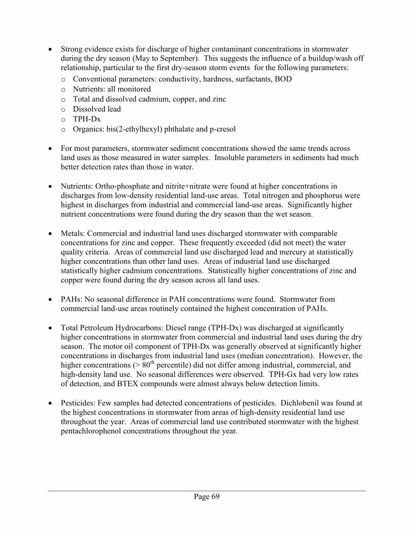
Page 69

Strong evidence exists for discharge of higher contaminant concentrations in stormwater during the dry season (May to September). This suggests the influence of a buildup/wash off relationship, particular to the first dry-season storm events for the following parameters: o Conventional parameters: conductivity, hardness, surfactants, BOD o Nutrients: all monitored o Total and dissolved cadmium, copper, and zinc o Dissolved lead o TPH-Dx o Organics: bis(2-ethylhexyl) phthalate and p-cresol

For most parameters, stormwater sediment concentrations showed the same trends across

land uses as those measured in water samples. Insoluble parameters in sediments had much better detection rates than those in water.

Nutrients: Ortho-phosphate and nitrite+nitrate were found at higher concentrations in

discharges from low-density residential land-use areas. Total nitrogen and phosphorus were highest in discharges from industrial and commercial land-use areas. Significantly higher nutrient concentrations were found during the dry season than the wet season.

Metals: Commercial and industrial land uses discharged stormwater with comparable

concentrations for zinc and copper. These frequently exceeded (did not meet) the water quality criteria. Areas of commercial land use discharged lead and mercury at statistically higher concentrations than other land uses. Areas of industrial land use discharged statistically higher cadmium concentrations. Statistically higher concentrations of zinc and copper were found during the dry season across all land uses.

PAHs: No seasonal difference in PAH concentrations were found. Stormwater from

commercial land-use areas routinely contained the highest concentration of PAHs. Total Petroleum Hydrocarbons: Diesel range (TPH-Dx) was discharged at significantly

higher concentrations in stormwater from commercial and industrial land uses during the dry season. The motor oil component of TPH-Dx was generally observed at significantly higher concentrations in discharges from industrial land uses (median concentration). However, the higher concentrations (> 80th percentile) did not differ among industrial, commercial, and high-density land use. No seasonal differences were observed. TPH-Gx had very low rates of detection, and BTEX compounds were almost always below detection limits.

Pesticides: Few samples had detected concentrations of pesticides. Dichlobenil was found at

the highest concentrations in stormwater from areas of high-density residential land use throughout the year. Areas of commercial land use contributed stormwater with the highest pentachlorophenol concentrations throughout the year.

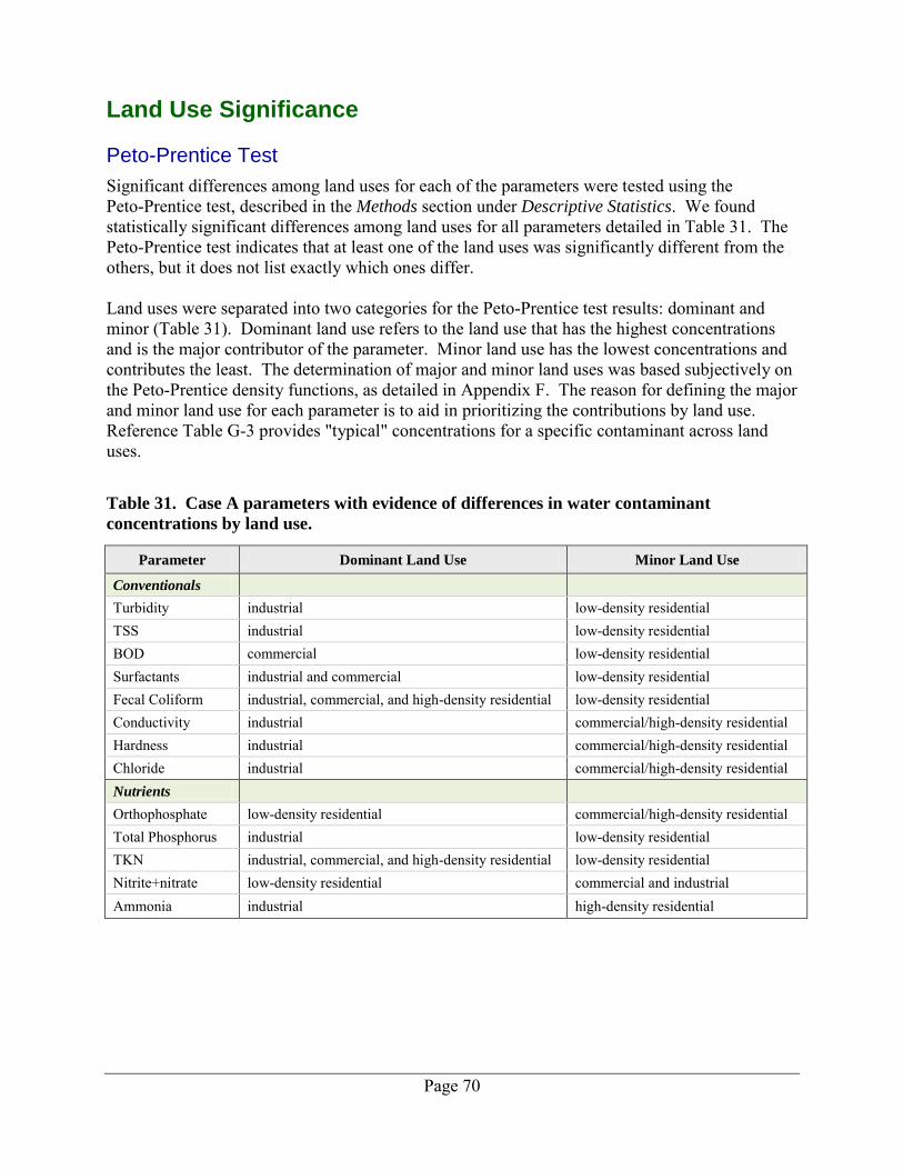
Page 70

Land Use Significance Peto-Prentice Test

Significant differences among land uses for each of the parameters were tested using the Peto-Prentice test, described in the Methods section under Descriptive Statistics. We found statistically significant differences among land uses for all parameters detailed in Table 31. The Peto-Prentice test indicates that at least one of the land uses was significantly different from the others, but it does not list exactly which ones differ. Land uses were separated into two categories for the Peto-Prentice test results: dominant and minor (Table 31). Dominant land use refers to the land use that has the highest concentrations and is the major contributor of the parameter. Minor land use has the lowest concentrations and contributes the least. The determination of major and minor land uses was based subjectively on the Peto-Prentice density functions, as detailed in Appendix F. The reason for defining the major and minor land use for each parameter is to aid in prioritizing the contributions by land use. Reference Table G-3 provides "typical" concentrations for a specific contaminant across land uses.

Table 31. Case A parameters with evidence of differences in water contaminant

concentrations by land use.

Parameter Dominant Land Use Minor Land Use

Conventionals

Turbidity industrial low-density residential TSS industrial low-density residential BOD commercial low-density residential Surfactants industrial and commercial low-density residential Fecal Coliform industrial, commercial, and high-density residential low-density residential Conductivity industrial commercial/high-density residential Hardness industrial commercial/high-density residential Chloride industrial commercial/high-density residential Nutrients Orthophosphate low-density residential commercial/high-density residential Total Phosphorus industrial low-density residential TKN industrial, commercial, and high-density residential low-density residential Nitrite+nitrate low-density residential commercial and industrial Ammonia industrial high-density residential

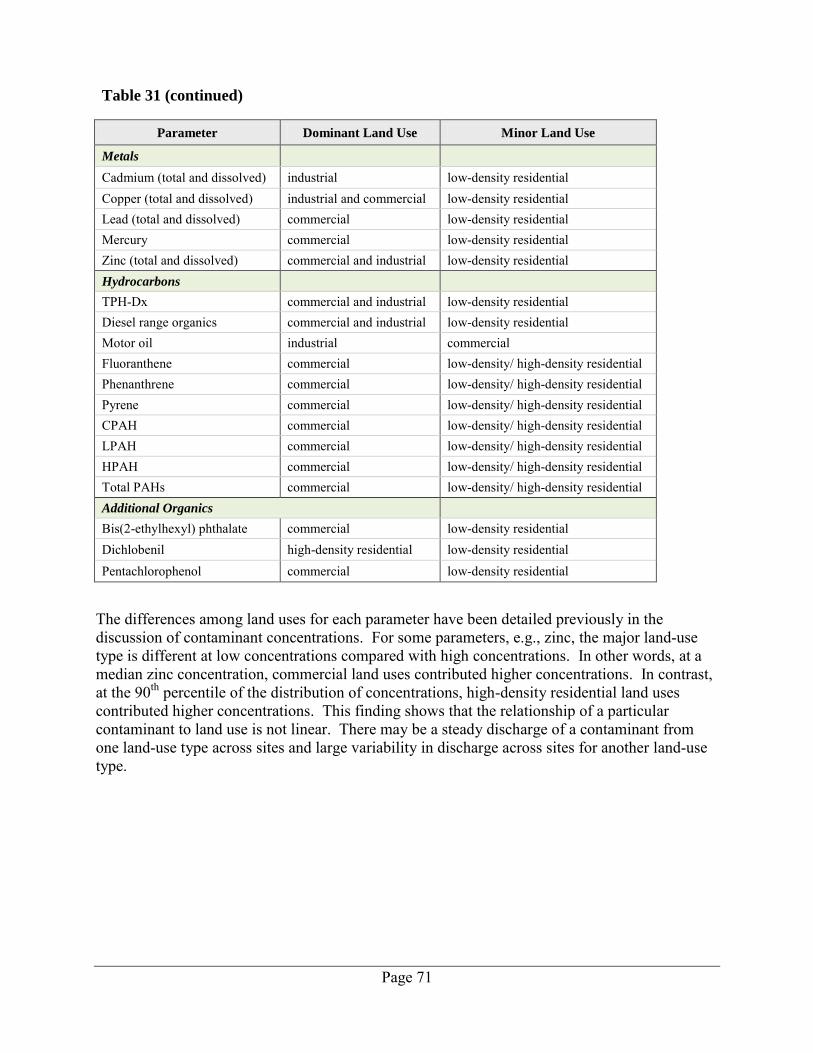
Page 71

Table 31 (continued)

Parameter Dominant Land Use Minor Land Use

Metals Cadmium (total and dissolved) industrial low-density residential Copper (total and dissolved) industrial and commercial low-density residential Lead (total and dissolved) commercial low-density residential Mercury commercial low-density residential Zinc (total and dissolved) commercial and industrial low-density residential Hydrocarbons TPH-Dx commercial and industrial low-density residential Diesel range organics commercial and industrial low-density residential Motor oil industrial commercial Fluoranthene commercial low-density/ high-density residential Phenanthrene commercial low-density/ high-density residential Pyrene commercial low-density/ high-density residential CPAH commercial low-density/ high-density residential LPAH commercial low-density/ high-density residential HPAH commercial low-density/ high-density residential Total PAHs commercial low-density/ high-density residential Additional Organics Bis(2-ethylhexyl) phthalate commercial low-density residential Dichlobenil high-density residential low-density residential Pentachlorophenol commercial low-density residential

The differences among land uses for each parameter have been detailed previously in the discussion of contaminant concentrations. For some parameters, e.g., zinc, the major land-use type is different at low concentrations compared with high concentrations. In other words, at a median zinc concentration, commercial land uses contributed higher concentrations. In contrast, at the 90th percentile of the distribution of concentrations, high-density residential land uses contributed higher concentrations. This finding shows that the relationship of a particular contaminant to land use is not linear. There may be a steady discharge of a contaminant from one land-use type across sites and large variability in discharge across sites for another land-use type.

Page 72

Principal Components Analysis

The Peto-Prentice test showed significant differences among land uses for individual parameters. We used multivariate statistics to decipher trends among the sample sites and parameters, combined. Using the variables from Table 31 in a principal components analysis (PCA), the distribution of sample sites relative to contaminant parameters can be plotted (Figure 14). In Figure 14, the arrows represent concentration gradients of the parameters, and the points (circles and squares) represent sample sites. The arrow points to increasing concentration of that parameter, and parameters that had similar concentration trends across the sample sites are close together. Sample sites (points on Figure 14) that had similar stormwater chemistry are grouped together. Sample sites the arrows point to are sites that have high concentrations of these parameters. The key observation from the PCA (Figure 14) is the general grouping of the sites (points) by land use, suggesting similar stormwater quality. For instance, all the low-density residential sites are grouped in the lower right quadrant of Figure 14. There is also considerable overlap for some sites. In particular, there is overlap between many commercial and high-density residential sites. This observation implies that stormwater chemistry from these land uses can be very similar. In addition, industrial sites do not group together and show more similarities to commercial and high-density residential sites. The overlap of land uses is likely due to characteristics of the drainage area as described by the permittees (Table 1). For example, Pierce County high-residential site (PIEHIRES_OUT) appeared more similar to a low-density residential site (Figure 14). As shown in Table 1, PIEHIRES_OUT had a very low total impervious surface area, which could explain why the stormwater chemistry resembled the low-density residential sites. By using multivariate statistics, we gained a greater understanding of how stormwater chemistry can be defined by land use; however, significant overlap or variability exists from site to site within the same land-use category.

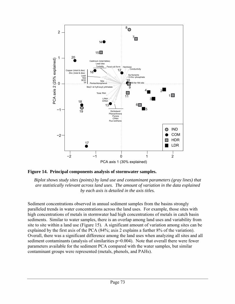
Page 73

Figure 14. Principal components analysis of stormwater samples.

Biplot shows study sites (points) by land use and contaminant parameters (gray lines) that are statistically relevant across land uses. The amount of variation in the data explained

by each axis is detailed in the axis titles.

Sediment concentrations observed in annual sediment samples from the basins strongly paralleled trends in water concentrations across the land uses. For example, those sites with high concentrations of metals in stormwater had high concentrations of metals in catch basin sediments. Similar to water samples, there is an overlap among land uses and variability from site to site within a land use (Figure 15). A significant amount of variation among sites can be explained by the first axis of the PCA (84%; axis 2 explains a further 8% of the variation). Overall, there was a significant difference among the land uses when analyzing all sites and all sediment contaminants (analysis of similarities p=0.004). Note that overall there were fewer parameters available for the sediment PCA compared with the water samples, but similar contaminant groups were represented (metals, phenols, and PAHs).

−2 −1 0 1 2

−2

−1

0

1

2

PCA axis 1 (30% explained)

PC

A a

xis

2 (2

5% e

xpla

ined

)

Turbidity

TSSBOD

ConductivityFecal coli form Hardness

Ortho−phosphate

TPTKN

Nit rite−Nit rate

Cadmium (total &diss)

Copper (total & diss)

Lead

Lead diss

Zinc (total & diss)

Fluo ranthene

PhenanthrenePyreneCPAH

LPAHHPAH

Total PAH

Bis(2−et hylhexyl) phthalate

Dichlobenil

Pentachlorophenol

Sur factants

18

16

11

5

3

9

12

1

2

17

10

20

15

19

13 6

4

14

8

7

IND

COM

HDR

LDR

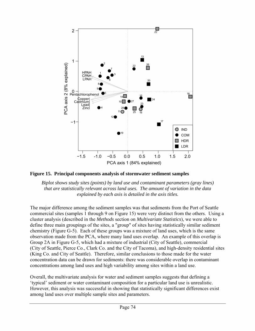
Page 74

Figure 15. Principal components analysis of stormwater sediment samples

Biplot shows study sites (points) by land use and contaminant parameters (gray lines) that are statistically relevant across land uses. The amount of variation in the data

explained by each axis is detailed in the axis titles.

The major difference among the sediment samples was that sediments from the Port of Seattle commercial sites (samples 1 through 9 on Figure 15) were very distinct from the others. Using a cluster analysis (described in the Methods section on Multivariate Statistics), we were able to define three main groupings of the sites, a "group" of sites having statistically similar sediment chemistry (Figure G-5). Each of these groups was a mixture of land uses, which is the same observation made from the PCA, where many land uses overlap. An example of this overlap is Group 2A in Figure G-5, which had a mixture of industrial (City of Seattle), commercial (City of Seattle, Pierce Co., Clark Co. and the City of Tacoma), and high-density residential sites (King Co. and City of Seattle). Therefore, similar conclusions to those made for the water concentration data can be drawn for sediments: there was considerable overlap in contaminant concentrations among land uses and high variability among sites within a land use. Overall, the multivariate analysis for water and sediment samples suggests that defining a ‘typical’ sediment or water contaminant composition for a particular land use is unrealistic. However, this analysis was successful in showing that statistically significant differences exist among land uses over multiple sample sites and parameters.

−1.5 −0.5 0.0 0.5 1.0 1.5 2.0

−1

0

1

2

PCA axis 1 (84% explained)

PC

A a

xis

2 (8

% e

xpla

ined

)

CadmiumCopper

CPAHHPAH

Lead

LPAH

Pentachlorophenol

Zinc 28

27

26

25

24

23

22

22

20

19

18

17

16

1514

13

12

11

10

9

8

7

6

5

4

3

2

1

IND

COM

HDR

LDR

-1.0

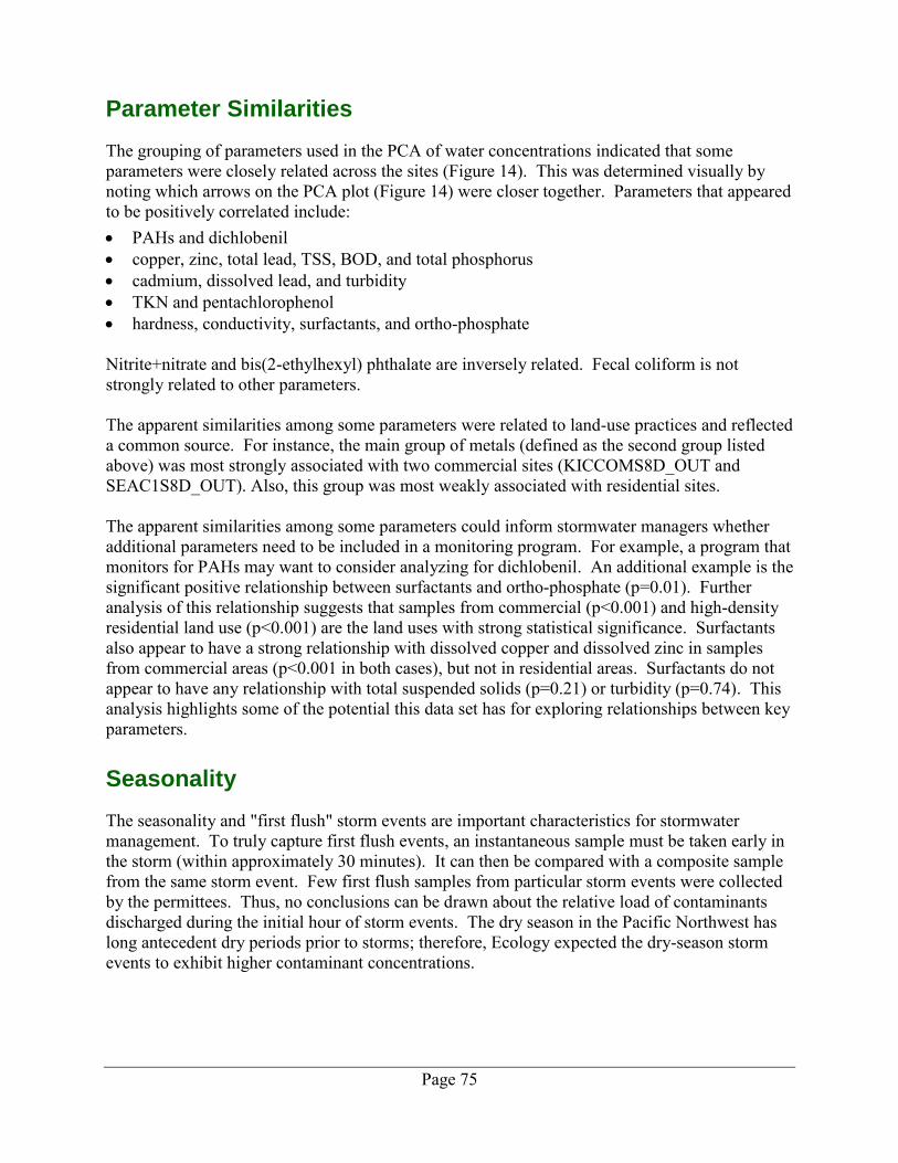
Page 75

Parameter Similarities The grouping of parameters used in the PCA of water concentrations indicated that some parameters were closely related across the sites (Figure 14). This was determined visually by noting which arrows on the PCA plot (Figure 14) were closer together. Parameters that appeared to be positively correlated include: PAHs and dichlobenil copper, zinc, total lead, TSS, BOD, and total phosphorus cadmium, dissolved lead, and turbidity TKN and pentachlorophenol hardness, conductivity, surfactants, and ortho-phosphate Nitrite+nitrate and bis(2-ethylhexyl) phthalate are inversely related. Fecal coliform is not strongly related to other parameters. The apparent similarities among some parameters were related to land-use practices and reflected a common source. For instance, the main group of metals (defined as the second group listed above) was most strongly associated with two commercial sites (KICCOMS8D_OUT and SEAC1S8D_OUT). Also, this group was most weakly associated with residential sites. The apparent similarities among some parameters could inform stormwater managers whether additional parameters need to be included in a monitoring program. For example, a program that monitors for PAHs may want to consider analyzing for dichlobenil. An additional example is the significant positive relationship between surfactants and ortho-phosphate (p=0.01). Further analysis of this relationship suggests that samples from commercial (p<0.001) and high-density residential land use (p<0.001) are the land uses with strong statistical significance. Surfactants also appear to have a strong relationship with dissolved copper and dissolved zinc in samples from commercial areas (p<0.001 in both cases), but not in residential areas. Surfactants do not appear to have any relationship with total suspended solids (p=0.21) or turbidity (p=0.74). This analysis highlights some of the potential this data set has for exploring relationships between key parameters.

Seasonality The seasonality and "first flush" storm events are important characteristics for stormwater management. To truly capture first flush events, an instantaneous sample must be taken early in the storm (within approximately 30 minutes). It can then be compared with a composite sample from the same storm event. Few first flush samples from particular storm events were collected by the permittees. Thus, no conclusions can be drawn about the relative load of contaminants discharged during the initial hour of storm events. The dry season in the Pacific Northwest has long antecedent dry periods prior to storms; therefore, Ecology expected the dry-season storm events to exhibit higher contaminant concentrations.

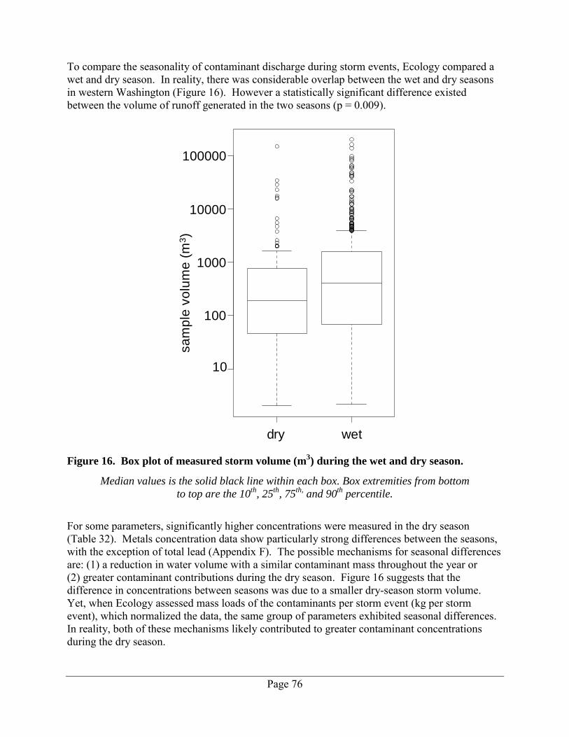
Page 76

To compare the seasonality of contaminant discharge during storm events, Ecology compared a wet and dry season. In reality, there was considerable overlap between the wet and dry seasons in western Washington (Figure 16). However a statistically significant difference existed between the volume of runoff generated in the two seasons (p = 0.009).

Figure 16. Box plot of measured storm volume (m3) during the wet and dry season.

Median values is the solid black line within each box. Box extremities from bottom

to top are the 10th

, 25th

, 75th,

and 90th

percentile.

For some parameters, significantly higher concentrations were measured in the dry season (Table 32). Metals concentration data show particularly strong differences between the seasons, with the exception of total lead (Appendix F). The possible mechanisms for seasonal differences are: (1) a reduction in water volume with a similar contaminant mass throughout the year or (2) greater contaminant contributions during the dry season. Figure 16 suggests that the difference in concentrations between seasons was due to a smaller dry-season storm volume. Yet, when Ecology assessed mass loads of the contaminants per storm event (kg per storm event), which normalized the data, the same group of parameters exhibited seasonal differences. In reality, both of these mechanisms likely contributed to greater contaminant concentrations during the dry season.

dry wet

10

sa

mp

levo

lum

e(m

3)

100

1000

10000

100000

Page 77

A further analysis of concentrations and loads compared to the antecedent dry-period length is a natural next step. Unfortunately, Ecology did not require antecedent dry period data to be submitted to EIM; therefore, the analysis could not be conducted.

Table 32. Seasonality of stormwater concentrations.

Conventional

Parameters Nutrients Metals Hydrocarbons Pesticides Phthalates PCBs

Significant seasonal difference

BOD Surfactants Fecal coliform Conductivity Hardness as CaCO3 Turbidity

Total phosphorus Ortho-phosphate TKN Nitrite+nitrate Ammonia

Cadmium (total and dissolved) Copper (total and dissolved) Lead (dissolved) Zinc (total and dissolved) Mercury

TPH-Dx Diesel Range Organics Fluoranthene Heavy Fuel Oil Pyrene

none none none

No seasonal difference

pH Total suspended solids

none Lead (total)

Benz(a)anthracene Benzo(a)pyrene Benzo(b)fluoranthene Benzo(k)fluoranthene Benzo(b,k)fluoranthene Benzo(g,h,i)perylene Indeno(1,2,3-cd)pyrene CPAH HPAH LPAH Lube Oil Motor Oil Phenanthrene Total PAH Total TPH-Dx

Dichlobenil Pentachlorophenol Phenol

Bis(2-ethylhexyl) phthalate Dibutyl phthalate Diethyl phthalate Total Phthalate

PCB-Aroclor 1254 PCB-Aroclor 1260 Total PCB

Findings in this study that the dry-season contaminant concentrations were significantly higher for some of the parameters was consistent with findings from the NSQD which show that first flush events were detectable for some parameters predominantly in areas of commercial and residential land uses (Maestre et al., 2004). The PS Toxics Study also observed greater concentrations during fall storm events when longer antecedent dry periods prevailed.

Page 78

Contaminant Loads Data summaries for storm-event contaminant loads were calculated for the Case A parameters. For those contaminants that were classified as Case B and had more than 50 observations (summarized used Robust ROS techniques), contaminant loads should be considered estimates. For all other parameters, a range of contaminant loads was given. Often the ranges were limited by the analytical detection limit, thus ranges were not an accurate assessment of environmental contaminant loads. Event loads were summarized using the same statistical approach as used for the concentration data (i.e., data qualifiers associated with the each concentration were used for the corresponding load). Loads were not calculated for parameters collected by grab samples, as these do not represent the load throughout a storm event. Ecology calculated both weight-based (mass) loads (kg per storm event) and loads per unit area (kg ha-1) based on the catchment area given in Table 1 for each stormwater basin. Loads calculated here are reliable, as no bias towards large volume storms was evident across the sample sites, and sample representation of the storms was excellent. Loads are summarized by land use in Table I-2 (mass) and I-5 (per unit area). All data summaries are detailed in Table I-1 through I-6. Graphical summaries for each parameter load are detailed in Appendix H. Peto-Prentice and Kaplan-Meier cumulative density functions were also run on the load by area to describe any significant differences among land uses. Unfortunately, Ecology could not directly compare to load estimates presented in the PS Toxics

Study, which were true annual loads; those presented in this study were event loads. However, trends across land uses were compared. In general, mass loads exhibited the same seasonal trends as contaminant concentrations. Contaminant loads per unit area in general followed seasonal trends, but with more exceptions. Contaminant loads per unit area for each parameter are discussed in greater detail below. Summary of Loads per Unit Area

In this section, contaminant loads (kg per hectare) are discussed as median values (50th percentile) unless otherwise noted. Tables I-3 through I-6 detail the data summaries for contaminant loads per unit area (hectares). Conventional Parameters

Surfactants

Contributions of surfactants were 0.0002 kg per hectare per storm event. Significant differences existed among land uses, but not between wet and dry seasons. Loading data followed trends similar to concentration data across land uses. Commercial and industrial land uses contributed greater loads. Total Suspended Solids (TSS)

TSS load varied significantly across land uses and showed a significant difference between wet and dry seasons (Table I-3). Loads from industrial and commercial land uses were significantly greater (0.71 kg ha-1 and 0.28 kg ha-1, respectively) than loads from high-density residential land

Page 79

use (0.06 kg ha-1) and low-density residential land use (0.04 kg ha-1). TSS load exhibited a clearer difference among land uses than concentration, consistent with findings from the PS Toxics Study. Nutrients

Phosphorus

Total phosphorus loads per unit area had a median value of 0.00045 kg ha-1 with 8.46 x 10-5 kg ha-1 contributed as ortho-phosphate. Land uses contributed significantly different loads on a per unit area basis. Seasonal loads were not different, in contrast to concentration data where concentrations were significantly higher during the dry season. As with concentration, total phosphorus loads were significantly greater in stormwater from the commercial and industrial land uses. The residential land uses were significantly lower and quite similar to each other (in kg ha-1; Table I-5). Dissolved phosphorus load (as ortho-phosphate) from low-density residential land use (1.1 x 10-4 kg ha-1) was similar to the load from industrial (1.5 x 10-4 kg ha-1) and commercial (1.1 x 10-4 kg ha-1) land use. These results are an order magnitude higher than high-density residential land use (3.5 x10-5 kg ha-1). Findings from this study agreed with the PS Toxics Study which found that commercial and industrial land uses contributed a higher load of total phosphorus than residential land uses. Dissolved phosphorus was not measured in the PS Toxics Study. Nitrogen

The observed nitrogen loads suggested that 0.0043 kg ha-1 of nitrogen was discharged per storm event (sum of total Kjeldahl N and nitrite+nitrate, as nitrogen), with a 90th percentile of 0.026 kg ha-1 N. The TKN loads (as kg ha-1) across land uses differed from that observed for concentrations. TKN loads were dominated by contributions from commercial and industrial land-use areas, with residential land-use contributions significantly lower. Nitrite+nitrate loads were also highest in discharges from commercial and industrial land uses. Above the 75th percentile of the distribution, the highest loads observed in the data set were discharged from residential land-use areas. This finding highlights the complexity and variability among land uses and among sites. There was no difference in nitrogen loads between wet and dry seasons. The PS Toxics Study found that residential land uses contributed the majority of nitrite+nitrate, which was similar to observations of this study. Commercial and industrial land uses were found to contribute the lowest nitrite+nitrate load in the PS Toxics Study, which was contrary to the findings of this study in which commercial and industrial land uses contributed the greatest median loads.

Page 80

Metals

Metals loading (as kg ha-1) generally followed trends similar to concentration data. Commercial and industrial land-use areas discharged the greatest load, followed by discharges from residential land uses. Some deviations from this trend were noted for lead. Similar loading trends during storm events among land uses were noted in the PS Toxics Study. All metals showed greater loading during the dry season. Cadmium

The 90th percentile of the total cadmium load from all land uses was 3.37 x 10-6 kg ha-1 per storm event with a median of 4.83 x 10-7 kg ha-1. Approximately 20% of the total cadmium was in dissolved form. The differences among land uses were similar to the cadmium concentration data, where commercial and industrial land uses discharged significantly higher loads than residential land uses. No significant differences were found between the wet and dry seasons for loads per unit area. Copper

The 90th percentile of copper load discharged during each storm was 3.6 x 10-4 kg ha-1 and the median was 5.1 x 10-5 kg ha-1. Approximately 25% of the copper was in dissolved form. Trends across land uses and between seasons were similar to those found for cadmium. Lead

The 90th percentile of the distribution of total lead load was 3.0 x 10-4 kg ha-1 per storm event, and the median was 2.7 x 10-5 kg ha-1 per storm event. Land-use trends for loads were similar to those found for concentrations. Commercial land-use areas discharged significantly higher loads; industrial and high-density residential land uses discharged roughly similar loads. Low-density residential land-use areas discharged significantly lower lead loads. No significant differences were found between the wet and dry seasons for loads per unit area. Mercury

Mercury loads were heavily influenced by the number of non-detect concentrations. Only for areas of commercial land use could the loads be quantified (Appendix I). No seasonal differences were apparent in the loads of mercury from commercial land-use areas. Zinc

The median zinc load was 3.1 x 10-4 kg ha-1 per storm event, while the 90th percentile of the load distribution was 1.5 x 10-3 kg ha-1 of zinc per storm event. Land-use trends for loads were very similar to those measured for concentrations, where commercial and industrial land uses showed nearly identical loads. Commercial and industrial lands had significantly higher loads of zinc, than did residential lands. No significant differences were found between the wet and dry seasons for loads per unit area.

Page 81

Hydrocarbons

TPH

TPH-Dx had significantly higher loads in stormwater (as kg ha-1) from commercial and industrial land uses compared with residential land uses, similar to the concentration trends. The 90th percentile of the distribution of TPH-Dx load was 0.02 kg ha-1 per storm event, and the median across all land uses was 2.0 x 10-3 kg ha-1. The motor oil component of TPH-Dx was discharged at a load of 0.02 kg ha-1(90th percentile), with a median of 3.0 x 10-3 kg ha-1 per storm event. The TPH-Dx load from high-density residential land use was significantly lower than the load from commercial and industrial land use. No significant differences were found between the wet and dry seasons for loads per unit area. Polycyclic Aromatic Hydrocarbons (PAHs)

Individual PAH compound concentrations were well-quantified for fluoranthene, phenanthrene, and pyrene. These three compounds displayed trends similar to concentration trends for land uses, where significant differences were present between loads from commercial, industrial, high-density residential, and low-density residential. The 90th percentile of the total PAH mass loads was 2.0 x 10-5 kg ha-1, and the median was 6.7 x 10-7 kg ha-1 contributed per storm event. Trends across land uses for loading of total PAHs, CPAHs, LPAHs, and HPAHs were the same as described for the individual PAH compounds. Significant differences in PAH loads were found between wet and dry seasons, contrary to concentration data. Greater PAH loads were found during the wet season. Phthalates

Bis(2-ethylhexyl)phthalate was the only well-quantified phthalate in stormwater from all land uses. Ecology estimated the 90th percentile of the load was 3.5 x 10 -5 kg ha-1, and the median was 3.9 x 10-6 kg ha-1 discharged per storm. Significant differences in load trended downward from commercial to industrial to high-density residential to low-density residential land uses. A similar pattern was observed for total phthalates across land uses. A significant difference was found between wet and dry seasons. Pesticides

The load of dichlobenil did not vary across the three land uses (commercial, industrial, and high-density residential) where concentrations were detected. The estimated load per unit area was a median of 4.82 x 10-8 kg ha-1 of dichlobenil per storm event. No difference in dichlobenil load was found between wet and dry seasons. Pentachlorophenol load in stormwater was calculated only for commercial land-use areas, where the estimated median was 6.31 x 10-8 kg ha-1 per storm event. No difference in pentachlorophenol load was found between wet and dry seasons.

Page 82

Contaminant Load Summary

Storm-event mass (kg) and load per unit area (kg ha-1) were calculated for contaminants that were quantified above detection limits in stormwater. Contaminant loads showed trends similar to the contaminant concentrations, with the exception of nutrients. While contaminant mass loads (kg) were not discussed in detail in this report, we observed similar seasonal trends to the contaminant concentration data. On the other hand, loads per unit area were generally constant throughout the year. Contaminant loads per unit area are summarized below: Nutrients: Total nitrogen and phosphorus loads were highest from commercial and industrial

land uses. Low-density residential land uses contributed as much ortho-phosphate load as the commercial and industrial land uses, while ortho-phosphate load from high-density residential land use was significantly lower. Dissolved nitrogen (as nitrite+nitrate) load from high-density residential land use was greater than the 75th percentile of the load from commercial and industrial land uses. Nutrient loads calculated per area were constant throughout the year, although nutrient concentrations were higher in the dry season.

Metals: Commercial and industrial land uses discharged the greatest metal loads, and lower loads were discharged from residential land uses. All metals showed no significant difference in loading between the wet and dry season, contrary to the concentration data and mass loads (kg). A high mass loading observed during the dry season seemed more highly influenced by elevated concentrations rather than by volume.

Hydrocarbons: Commercial and industrial land uses contributed the greatest loads of diesel

range total petroleum hydrocarbons (TPH-Dx) and PAHs. Overall, loads per unit area (kg ha-1) showed significant differences between seasons, with greater loads during the wet season.

Pesticides: Commercial, industrial, and high-density residential land uses had comparable dichlobenil loads. No seasonal differences in contaminant loads were noted.

Page 83

Summary

Stormwater and storm sediment discharge data were collected by NPDES Phase I Municipal Stormwater permittees, under Special Condition S8.D, between 2007 and 2012. This report is a summary of data results contained in Ecology’s Environmental Information Management (EIM) System. The eight Phase 1 permittees, all located in western Washington, collected highly representative storm-event data under a prescribed monitoring program that represented multiple land uses, storm characteristics, and seasons. The main goals of this study were to (1) compile and summarize the permittees’ data using appropriate statistical techniques and (2) provide a western Washington regional baseline characterization of stormwater quality. Ecology’s analysis provides a comprehensive review of the pollutants in western Washington stormwater from 2007 - 2012. These findings are based on the analysis of 44,800 data records representing 597 different storm events. Up to 85 chemicals were analyzed in stormwater samples, and 67 chemicals were analyzed in stormwater sediment samples. Compiling data from multiple sources was challenging due to differences in parameter names, sample fractions, units, reporting limits, and basin characteristics. The representativeness of the collected samples across storm events appeared to be of high quality, generally representing above 90% of storm hydrographs. Samples showed no bias of storm volume. The distribution of sampling events over the year was also of high quality with few exceptions. The statistical analyses used in this study have produced reliable statistical summaries and allowed for robust comparisons of the impacts of land use and seasons on contaminant concentrations and mass loads. The statistical summaries form a baseline for contaminant concentrations in stormwater that will allow for future comparisons. Results can be used to track improvement in stormwater quality as local programs continue to be implemented.

Page 84

Key Findings

The following key findings are highlighted from this report.

Stormwater Monitoring Program

Ecology finds the permittees’ stormwater monitoring data to be representative of storm events in western Washington. The stormwater discharge data set is large, captured a wide variety of storm events, and does not appear to have biases toward storm size, limb of hydrograph, land use, or season. Results are suitable for creating a baseline understanding of stormwater discharges in western Washington.

Stormwater monitoring as required in the 2007 permit was met (qualifying storm, sample frequency, and representativeness). The continued collection of high quality data representing storm-event pollutant concentrations seems realistic.

"Typical" stormwater chemistry for a particular land use was difficult to define.

This database is a suitable baseline to compare stormwater contaminant concentrations against management actions in future studies.

Permittees’ initial efforts to assess toxicity of stormwater on trout embryos per permit requirements in S8.F were met with considerable logistical and bioassay complexity. Twelve of the 17 samples analyzed using bioassays had no adverse effects. Only samples from larger commercial areas showed toxicity to trout embryos, with the likely toxicants being zinc and copper. Appendix A provides a summary of the bioassay effort and lessons learned.

Stormwater Discharge Quality

Commercial and industrial areas discharged stormwater with the highest concentrations of metals, hydrocarbons, phthalates, total nutrients, and a few pesticides.

Residential areas discharged stormwater with the highest dissolved nutrient concentrations.

Copper, zinc, and lead most frequently exceeded (did not meet) the water quality criteria for protection of aquatic life. Cadmium and mercury also exceeded criteria for protection of aquatic life. Mercury was not a widespread contaminant in western Washington stormwater, although localized areas of concern existed. Comparisons to water quality criteria were made for context in this report.

Metals concentrations monitored during the dry season (May through September) were statistically higher than concentrations monitored during the wet season. Dissolved zinc, copper, and lead exceeded acute and chronic water quality criteria regularly. Comparisons to water quality criteria were made for context in this report.

Higher contaminant concentrations and mass loads (kg per storm event) were measured for nutrients and metals during the dry season. This supports the idea that there is a "buildup" during the dry season, when the antecedent dry periods are longer.

Page 85

PAHs, phthalates, PCBs, and the few detected pesticides did not exhibit a significant seasonal difference, suggesting these parameters were being discharged from a consistent source throughout the year.

Bis(2-ethylhexyl) phthalate was frequently found in stormwater and stormwater sediment.

NWTPH-Dx compounds were persistent stormwater contaminants. Commercial and industrial areas discharged much higher concentrations and loads than did residential areas. When the motor oil fraction was considered separately, the highest load was from residential areas.

NWTPH-Gx was poorly detected and, if present, was likely volatized before monitoring.

Individual parameter concentrations showed strong differences between land uses.

The most volatile organics (some pesticides, lighter weight PCBs, and PAHs) were poorly detected (less than 10% of the samples).

The most volatile parameters (BTEX) provided less useful information when gathered from composite samples.

Stormwater Sediment Quality

While the data set for stormwater sediment samples is smaller the data set for stormwater samples, contaminants in stormwater sediments showed trends similar to contaminants in stormwater across land uses.

The stormwater sediment monitoring design precluded an understanding of sediment pollutants across seasons. A more refined sediment design for both spatial and temporal monitoring would improve our understanding of stormwater sediments.

Bis(2-ethylhexyl) phthalates in stormwater sediments exceeded the freshwater aquatic life criteria (Sediment Cleanup Objectives) 82% of the time. Di-n-octyl phthalate exceeded the criteria 29% of the time.

Total PAHs in stormwater sediments exceeded the freshwater aquatic life criteria (SCO) 34% of the time.

Copper (9%) and lead (18%) were the main metals in stormwater sediments exceeding the SCO. Zinc and mercury were not of concern in stormwater sediments.

Phenol in stormwater sediment exceeded the SCO 20% of the time.

Comparisons with Relevant National and Local Stormwater Studies

Generally, contaminant concentrations reported in this study were within the ranges reported in the National Stormwater Quality Database (NSQD), but median values were often lower. This is primarily due to the age of the NSQD (early 1980s) and improvements in stormwater quality and management since the National Urban Runoff Program (NURP) sampling. Many of the contaminant concentrations in this study were higher than those found in the PS Toxics Study.

Page 86

This finding is not surprising given that the PS Toxics Study sampled receiving waters, not stormwater discharges, during storm events.

The PS Toxics Study found high concentrations of PAHs in receiving waters during storm events. The majority of PAHs were contributed from commercial and industrial areas, which was corroborated by this current study. PAHs in stormwater discharges showed no seasonal differences in concentrations.

The pesticides, dichlobenil and pentachlorophenol, were reliably detected in this study. Triclopyr, which was detected in the PS Toxics Study, was found in only 10% of the 575 samples analyzed in this study.

The few samples with detected concentrations of PCBs in water showed much lower concentrations in this study than in the PS Toxics Study.

Dissolved nutrients (orthophosphate and nitrite+nitrate-nitrogen) were much lower in stormwater discharges as compared to receiving waters sampled in the PS Toxic Study. This suggests that dissolved nutrient contributions are larger to receiving waters from pathways other than stormwater drainages (e.g., tributary streams and groundwater).

Higher concentrations and storm-event loads of metals were contributed to receiving waters from commercial and industrial areas than from other land-use areas. The PS Toxics Study also found the highest metals concentrations in waters from commercial and industrial areas.

Page 87

Recommendations

Based on the findings of this study, further actions and data analysis are recommended.

Implement best management practices (BMPs) and adjust stormwater management programs based on these findings. Use findings to help prioritize activities within stormwater programs.

Present the data online in a simple, user-friendly interface that stormwater managers could use to directly compare with future stormwater chemistry results.

Link this database with the National Stormwater Quality Database (NSQD) to increase the temporal range of the data set.

Further investigate the relationships between seasonality and land use for each parameter. For example, total phosphorus exhibits strong statistical differences between land uses during the wet season but no significant differences during the dry season.

Conduct further analysis to identify the land use associated with each sample that exceeded (did not meet) water quality criteria.

Expand the number of sites for annual sediment sample collection to enhance the spatial survey of possible contaminant sources.

Use results from this study to fill gaps found in the Control of Toxic Chemicals in Puget

Sound: Phase 3 Data and Load Estimates (Herrera, 2011; PS Toxics study): for example, areas draining directly to marine waters or fresh receiving waters that were missed when monitoring the larger drainages in that study.

Reduce the sampling frequency of, or eliminate, the following parameters from further stormwater discharge sampling: BTEX in water and sediments. Malathion, prometon, chlorpyrifos, and diazinon in water and sediments. Triclopyr and mecoprop in sediments. Limit phenolics in sediments to pentachlorophenol, o- cresol, and p-cresol.

Evaluate the data set for patterns among parameters that could help identify sources of pollution to stormwater. Explicitly test the influence of seasonal first flush, or antecedent dry period lengths, on

stormwater discharge concentrations. Explore whether the correlations between some parameters and land uses are causative or

coincident. For example, surfactants and copper; does the application of surfactants increase the mobilization of copper from the catchment?

Investigate dissolved nutrient concentrations in stormwater from low-density residential areas and investigate pollution reduction approaches.

Page 88

Track and evaluate any BMPs within each basin using a similar suite of stormwater chemistry (e.g., timing of sweeping or cleaning of Ports or parking lots).

Explore the high-runoff coefficient calculated for specific high-density residential sites to determine whether the high-runoff coefficients influence the contaminant contributions from these sites.

Page 89

References

Websites Agency for Toxic Substances and Disease Registry (ATSDR) www.atsdr.cdc.gov/

Comprehensive R Archive Network (CRAN) http://cran.r-project.org/

Ecology’s Sediment Phthalate Work Group www.ecy.wa.gov/programs/tcp/smu/phthalates/phthalates_hp.htm

Ecology’s Control of Toxics Chemicals in Puget Sound www.ecy.wa.gov/programs/wq/pstoxics/index.html

EPA’s NPDES Stormwater “Frequently Asked Questions” http://cfpub.epa.gov/npdes/faqs.cfm?program_id=6

EPA’s Priority Persistent Bioaccumulative and Toxic Profiles www.epa.gov/pbt/pubs/cheminfo.htm

EPA’s Priority Pollutants http://water.epa.gov/scitech/methods/cwa/pollutants.cfm

NOAA’s National Atmospheric Deposition Program NTN Maps by Analyte http://nadp.sws.uiuc.edu/ntn/annualmapsbyanalyte.aspx References Cited in Text Antweiler, R.C. and Taylor, H.E., 2008. Evaluation of Statistical Treatments of Left-Censored Environmental Data using Coincident Uncensored Data Sets: I. Summary Statistics. Environmental Science and Technology, v. 42, p. 3732-3738. Burton, G.A. Jr. and R. Pitt, 2002. Stormwater Effects Handbook: A Tool Box for Watershed Managers, Scientists, and Engineers. CRC Press, Inc., Boca Raton, FL. 911 pgs. Ecology, 1997. Analytical Methods for Petroleum Hydrocarbons. Washington State Department of Ecology, Olympia, WA. June 1997. Publication No. 97-602. https://fortress.wa.gov/ecy/publications/SummaryPages/97602.html Ecology, 2006. Fact Sheet for National Pollutant Discharge Elimination System (NPDES) and State Waste Discharge General Permit for Discharges from Large and Medium Municipal Separate Storm Sewers. Washington State Department of Ecology, Olympia, WA. March 22, 2006. www.ecy.wa.gov/programs/wq/stormwater/municipal/phaseIpermit/phifinalfs.pdf

http://www.atsdr.cdc.gov/

http://cran.r-project.org/

http://www.ecy.wa.gov/programs/tcp/smu/phthalates/phthalates_hp.htm

http://www.ecy.wa.gov/programs/wq/pstoxics/index.html

http://cfpub.epa.gov/npdes/faqs.cfm?program_id=6

http://www.epa.gov/pbt/pubs/cheminfo.htm

http://water.epa.gov/scitech/methods/cwa/pollutants.cfm

http://nadp.sws.uiuc.edu/ntn/annualmapsbyanalyte.aspx


http://www.ecy.wa.gov/programs/wq/stormwater/municipal/phaseIpermit/phifinalfs.pdf

Page 90

Ecology, 2007. Phase I Municipal Stormwater Permit: National Pollutant Discharge Elimination System and State Waste Discharge General Permit for Discharges from Large and Medium Municipal Separate Storm Systems. Issued January 17, 2007. Last Modification September 1, 2010. Washington State Department of Ecology, Olympia, WA. www.ecy.wa.gov/programs/wq/stormwater/municipal/phaseIpermit/MODIFIEDpermitDOCS/PhaseIStormwaterGeneralPermit.pdf EPA, 1983. Results of the Nationwide Urban Runoff Program. Volume I – Final Report. U.S. Environmental Protection Agency, Water Planning Division, PB 84-185552, Washington, D.C. 20460. December 1983. EPA, 1994. Water Quality Standards Handbook, second edition. Updated in 2012. EPA-823-B-12-002. Office of Water, U.S. Environmental Protection Agency, Washington, D.C. http://water.epa.gov/scitech/swguidance/standards/handbook/index.cfm EPA, 1998. Total vs. Total Recoverable Metals. Memorandum from William A. Telliard, Director of Analytical Methods Staff for the Engineering and Analysis Division. U.S. Environmental Protection Agency. Dated August 19, 1998. Hartigan, J.A., 1975. Clustering Algorithms. New York: Wiley. Helsel, D.R., 2012. Statistics for Censored Environmental Data Using Minitab® and R. Second Edition. John Wiley & Sons, Inc., NJ, 342 p. Helsel, D.R. and R. M. Hirsch. 2002. Statistical Methods in Water Resources Techniques of Water Resources Investigations, Book 4, chapter A3. U.S. Geological Survey. 522 p. Herrera Environmental Consultants, Inc., 2011. Control of Toxic Chemicals in Puget Sound: Phase 3 Data and Load Estimates. Washington State Department of Ecology, Olympia, WA. Publication No. 11-03-010. https://fortress.wa.gov/ecy/publications/publications/1103010.pdf Lee, L., 2013. NADA: Non-detects And Data Analysis for environmental data. R package version 1.5-6. http://CRAN.R-project.org/package=NADA Lombard, S. and C. Kirchmer, 2004. Guidelines for Preparing Quality Assurance Project Plans for Environmental Studies. Washington State Department of Ecology, Olympia, WA. Publication No. 04-03-030. https://fortress.wa.gov/ecy/publications/SummaryPages/0403030.html Lubliner, B and E. Newell. 2013. Western Washington NPDES Phase 1 Stormwater Data Characterization: Interim Findings from 2007-2012. Washington State Department of Ecology, Olympia, WA. Publication No. 13-03-043. https://fortress.wa.gov/ecy/publications/publications/1303043.pdf McKenzie, E. R., Money, J. E., Green, P. G., & Young, T. M., 2009. Metals associated with stormwater-relevant brake and tire samples. Science of the Total Environment, 407: 5855-5860.

http://www.ecy.wa.gov/programs/wq/stormwater/municipal/phaseIpermit/MODIFIEDpermitDOCS/PhaseIStormwaterGeneralPermit.pdf

http://www.ecy.wa.gov/programs/wq/stormwater/municipal/phaseIpermit/MODIFIEDpermitDOCS/PhaseIStormwaterGeneralPermit.pdf

http://water.epa.gov/scitech/swguidance/standards/handbook/index.cfm

https://fortress.wa.gov/ecy/publications/publications/1103010.pdf

http://cran.r-project.org/package=NADA


https://fortress.wa.gov/ecy/publications/publications/1303043.pdf

Page 91

Maestre, A., Pitt, R.E., and Derek Williamson, 2004. Nonparametric statistical tests comparing first flush with composite samples from the NPDES Phase 1 municipal stormwater monitoring data. Stormwater and Urban Water Systems Modeling. Pp. 317–338 In: Models and Applications to Urban Water Systems, Vol. 12. W. James (ed.). Guelph, Ontario: CHI www.unix.eng.ua.edu/~rpitt/Publications/Stormwater%20Characteristics/first%20flush%20Maestre%20and%20Pitt%20James%202003.pdf Maestre, A. and R. Pitt, 2005. The National Stormwater Quality Database, Version 1.1, A Compilation and Analysis of NPDES Stormwater Monitoring Information. U.S. Environmental Protection Agency, Office of Water, Washington, D.C. Maestre, A., R. Pitt, S. R. Durrans and S. Chakraborti, 2005. Stormwater Quality Descriptions using the Three Parameter Lognormal Distribution. 2004 Stormwater and Urban Water Systems Modeling Conference pp. 247-274, Toronto, Ontario, Canada. Effective Modeling of Urban Water Systems, Monograph 13 Michelson, T., 1992. Organic Carbon Normalization of Sediment Data. Washington State Department of Ecology, Olympia, WA. Publication No. 05-09-050. https://fortress.wa.gov/ecy/publications/summarypages/0509050.html Microsoft, 2007. Microsoft Office XP Professional, Version 10.0. Microsoft Corporation. Oksanen, J., Blanchet, F.G., Kindt, R., Legendre, P., Minchin, P.R., O’Hara, R.B., Simpson, G.L., Solymos, P., Stevens, M.H.H., and Wagner, H., 2013. Vegan: Community Ecology Package. R package version 2.0-9. http://CRAN.R-project.org/package=vegan. Pitt, R, A. Maestre, R. Morquencho, T. Brown, T. Schueler, K. Cappiella, P. Sturm, and C. Swann. 2004. Findings from the National Stormwater Quality Database (NSQD). Research Progress Report. Center for Watershed Protection. 10 p. Pitt, R., 2011. The National Stormwater Quality Database, Version 3.1. Summary for EPA. http://rpitt.eng.ua.edu/Publications/4_Stormwater_Characteristics_Pollutant_Sources_and_Land_Development_Characteristics/Stormwater_characteristics_and_the_NSQD/NSQD%203.1%20summary%20for%20EPA%20Cadmus.pdf R Core Development Team, 2012. R: A language and environment for statistical computing. R Foundation for Statistical Computing, Vienna, Austria. ISBN 3-900051-07-0. www.R-project.org/. WAC 173-201A. Water Quality Standards for Surface Waters in the State of Washington. Washington State Department of Ecology, Olympia, WA. www.ecy.wa.gov/laws-rules/ecywac.html

WAC 173-204. Sediment Management Standards in the State of Washington. Washington State Department of Ecology, Olympia, WA. www.ecy.wa.gov/laws-rules/ecywac.html

http://www.unix.eng.ua.edu/~rpitt/Publications/Stormwater%20Characteristics/first%20flush%20Maestre%20and%20Pitt%20James%202003.pdf

http://www.unix.eng.ua.edu/~rpitt/Publications/Stormwater%20Characteristics/first%20flush%20Maestre%20and%20Pitt%20James%202003.pdf

http://www.chiwater.com/Publications/Papers/bookinfo.asp?bookid=R223

https://fortress.wa.gov/ecy/publications/summarypages/0509050.html

http://cran.r-project.org/package=vegan

http://rpitt.eng.ua.edu/Publications/4_Stormwater_Characteristics_Pollutant_Sources_and_Land_Development_Characteristics/Stormwater_characteristics_and_the_NSQD/NSQD%203.1%20summary%20for%20EPA%20Cadmus.pdf



http://www.r-project.org/

http://www.ecy.wa.gov/laws-rules/ecywac.html

http://www.ecy.wa.gov/laws-rules/ecywac.html

Page 92

This page is purposely left blank

Page 93

Appendices

Page 94

Appendix A. Municipal Stormwater Trout Embryo Toxicity Testing: Results from First Flush, 2010-2011

By

Randall Marshall

Water Quality Program, Washington State Department of Ecology

Monitoring Strategy The permittees under the Phase I Municipal Stormwater Permit made attempts to sample seasonal first flush stormwater for toxicity testing in August through October of 2010 and 2011. Each permittee sampled only in one of those years but targeted three of the following four landuse types:

Commercial. Industrial. Low density residential. High density residential. Half of the permittees could only sample the discharge from two landuse types because of inadequate discharge volumes during the seasonal first flush timeframe defined in the permit. This monitoring did not provide for results from multiple years or multiple seasons and must be considered no more than a snapshot of any of the discharge locations. In addition, only nine of the seventeen samples were collected in August and represented well a seasonal first flush. Five of the seventeen samples were collected in October. Metals in water with higher hardness are less toxic and water quality criteria for metals are calculated based upon hardness. The hardness of receiving water is often significantly higher than stormwater. The permit allowed the hardness of stormwater samples to be adjusted to match receiving water hardness to provide some environmental realism. However, other relevant features of the receiving water environment were not incorporated into test conditions. Features left out include:

Upstream sources of metals and other pollutants. Pulsed pollutant exposures. Dilution Dissolved organic carbon. Suspended solids. Variability of stream chemistry during storms.

The monitoring results have limited environmental relevance.

Page 95

The trout embryo viability test is good for assessing conditions for the first 7 days of a trout or salmon’s life. The test measures survival and development during this time. It misses other sensitive lifestage transitions such as hatch or swim-up. Since the toxicity testing did not include other organisms, lifestages, and biological endpoints, the results need to be considered solely within the context of the 7-day trout embryo test. Test Method and Results Labs conducted the Environment Canada 7-day trout embryo viability test5 on the stormwater samples. Tests began with freshly fertilized rainbow trout eggs and continued for a week. At the end of 7 days the labs counted the number of live embryos and the number of normally developed embryos. All tests provided valid results based upon control response. Twelve of the seventeen tests showed no adverse effects to either survival or development. Only the Port of Tacoma and Port of Seattle samples had EC50s equal to or less than 100% sample6 and triggered the follow-up actions in the permit. Follow-up actions compare chemical analysis results on split samples to published toxic thresholds. The comparison revealed zinc to be the likely toxicant for the Port of Tacoma sample and copper to be the likely toxicant for the Port of Seattle sample. Ports are especially large and intensive commercial operations. The dissolved copper and zinc concentrations in the samples from the commercial landuse types were 2 to 10 times higher than the concentrations of the same metals in samples from residential landuse. The Pierce County and Snohomish County commercial samples had higher concentrations of zinc than the one industrial landuse area sampled. The Snohomish County commercial sample also had higher copper than the industrial sample. Parking lots are significant sources of copper and zinc. Galvanized metal roofs can produce runoff with toxic concentrations of zinc. Commercial areas have abundant parking lots and galvanized steel. Table A-1 shows the average concentration of copper and zinc in the same samples from the various landuse types that were tested for toxicity.

Table A-1 – Average Copper and Zinc Concentrations

in Samples from Different Land Uses. Copper Zinc Commercial (n = 6) 17.9 100.8 Residential (n = 8) 5.4 18.4 Industrial (n = 1) 19.2 125.0 Port of Seattle 101.0 171.0 Port of Tacoma 13.7 767.0

Copper and zinc concentrations along with toxicity test results for all samples are listed in Table A-2. The samples from the commercial landuse types for the City of Seattle, Pierce County, and Snohomish County were moderately toxic. The toxicity test result for the Snohomish County 5 EPS 1/RM/28 6 This toxicity test used a series of dilutions of the sample (starting at 100% concentration). Therefore if the half maximal effective concentration (EC50) was equivalent to or less than the raw sample, the sample had regulatory significant toxicity.

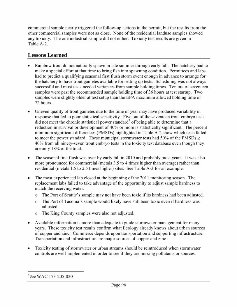
Page 96

commercial sample nearly triggered the follow-up actions in the permit, but the results from the other commercial samples were not as close. None of the residential landuse samples showed any toxicity. The one industrial sample did not either. Toxicity test results are given in Table A-2. Lessons Learned

Rainbow trout do not naturally spawn in late summer through early fall. The hatchery had to make a special effort at that time to bring fish into spawning condition. Permittees and labs had to predict a qualifying seasonal first flush storm event enough in advance to arrange for the hatchery to have trout gametes available for setting up tests. Scheduling was not always successful and most tests needed variances from sample holding times. Ten out of seventeen samples were past the recommended sample holding time of 36 hours at test startup. Two samples were slightly older at test setup than the EPA maximum allowed holding time of 72 hours.

Uneven quality of trout gametes due to the time of year may have produced variability in response that led to poor statistical sensitivity. Five out of the seventeen trout embryo tests did not meet the chronic statistical power standard7 of being able to determine that a reduction in survival or development of 40% or more is statistically significant. The percent minimum significant differences (PMSDs) highlighted in Table A-2 show which tests failed to meet the power standard. These municipal stormwater tests had 50% of the PMSDs ≥ 40% from all ninety-seven trout embryo tests in the toxicity test database even though they are only 18% of the total.

The seasonal first flush was over by early fall in 2010 and probably most years. It was also more pronounced for commercial (metals 3.5 to 4 times higher than average) rather than residential (metals 1.5 to 2.5 times higher) sites. See Table A-3 for an example.

The most experienced lab closed at the beginning of the 2011 monitoring season. The replacement labs failed to take advantage of the opportunity to adjust sample hardness to match the receiving water. o The Port of Seattle’s sample may not have been toxic if its hardness had been adjusted. o The Port of Tacoma’s sample would likely have still been toxic even if hardness was

adjusted. o The King County samples were also not adjusted.

Available information is more than adequate to guide stormwater management for many years. These toxicity test results confirm what Ecology already knows about urban sources of copper and zinc. Commerce depends upon transportation and supporting infrastructure. Transportation and infrastructure are major sources of copper and zinc.

Toxicity testing of stormwater or urban streams should be reintroduced when stormwater controls are well-implemented in order to see if they are missing pollutants or sources.

7 See WAC 173-205-020

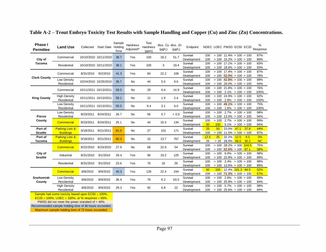
Page 97

Table A-2 – Trout Embryo Toxicity Test Results with Sample Handling and Copper (Cu) and Zinc (Zn) Concentrations.

Phase I

PermitteeLand Use Collected Start Date

Sample

Holding

Time

Hardness

Adjusted?

Test

Hardness

(ppm)

diss. Cu

(µg/L)

diss. Zn

(µg/L)Endpoint NOEC LOEC PMSD EC50 EC25

%

Response

Survival 100 > 100 11.4% > 100 > 100 87%

Development 100 > 100 15.2% > 100 > 100 89%

Survival 100 > 100 17.1% > 100 > 100 83%

Development 100 > 100 18.6% > 100 > 100 93%

Survival 100 > 100 17.4% > 100 > 100 87%

Development 100 > 100 52.0% > 100 > 100 78%

Survival 100 > 100 42.8% > 100 > 100 89%

Development 100 > 100 29.0% > 100 > 100 94%

Survival 100 > 100 21.8% > 100 > 100 76%

Development 100 > 100 2.1% > 100 > 100 100%

Survival 100 > 100 24.9% > 100 > 100 92%

Development 100 > 100 2.8% > 100 > 100 100%

Survival 100 > 100 49.1% > 100 > 100 75%

Development 100 > 100 1.8% > 100 > 100 100%

Survival 100 > 100 2.7% > 100 > 100 98%

Development 100 > 100 13.0% > 100 > 100 94%

Survival 100 > 100 2.7% > 100 > 100 99%

Development 50 100 9.1% > 100 > 100 84%

Survival 25 50 23.0% 47.1 37.8 44%

Development 100 > 100 11.5% > 100 > 100 87%

Survival 12.5 25 32.2% 12.5 9.5 0%

Development 25 > 25 28.0% 58.0 30.2 NC

Survival 100 > 100 28.2% > 100 104.5 75%

Development 100 > 100 62.6% > 100 87.1 58%

Survival 100 > 100 6.0% > 100 > 100 98%

Development 100 > 100 23.9% > 100 > 100 89%

Survival 100 > 100 2.4% > 100 > 100 98%

Development 100 > 100 13.6% > 100 > 100 89%

Survival 50 100 12.4% 101.3 84.5 52%

Development 100 > 100 71.3% > 100 > 100 57%

Survival 100 > 100 2.6% > 100 > 100 99%

Development 100 > 100 25.8% > 100 > 100 84%

Survival 100 > 100 5.7% > 100 > 100 98%

Development 100 > 100 25.6% > 100 > 100 84%

Maximum sample holding time of 72 hours exceeded.

City of

Tacoma

Clark County

King County

Pierce

County

City of

Seattle

Snohomish

County

PMSD did not meet the power standard of < 40%.

Recommended sample holding time of 36 hours exceeded.

Sample had some toxicity based upon EC50 ≤ 100%,

EC25 ≤ 100%, LOEC ≤ 100%, or % response ≤ 65%.

Commercial

Low Density

Residential

High Density

Residential

Low Density

Residential

Low Density

Residential

Commercial

Port of

Seattle

Parking Lots &

Buildings

Port of

Tacoma

Parking Lots &

Buildings

10/10/2010

10/10/2010

8/31/2010

10/24/2010

10/11/2011

10/11/2011

Commercial

Industrial

Residential

Commercial

Residential

Commercial

Low Density

Residential

Commercial

High Density

Residential

8/8/2010

8/8/2010 8/9/2010

8/9/2010

8/9/2010

9/1/2010

9/1/2010

10/11/2011

8/23/2011

8/23/2011

9/18/2011

9/18/2011

8/22/2010 8/23/2010

9/21/2011

9/21/2011

8/24/2011

8/24/2011

10/13/2011

8/31/2010

8/31/2010

8/8/2010

38.7

38.1

41.3

36.7

59.5

59.110/13/2011

10/13/2011

10/25/2010

9/2/2010

10/11/2010

10/11/2010

36.4

29.3 Yes

Yes

Yes

Yes

Yes

55.5

26.7

25.1

81.0

80.3

27.9 No

No

No

No

No

No

29.4

23.6

40.3

100

100

84

44

29

12No

No

No

Yes

Yes

Yes

76

92 6.8

6.2

22.4

16

19.2

9.4

56

44

27

15

68 22.6

13.7

101

15.4

0.7

3.1

96

76

128

51.7

19.4

106

9.6

14.9

2.41.9

6.6

5.5

22.2

3

18.2

125

26

244

63.5

22

4.0

< 0.5

134

171

767

54

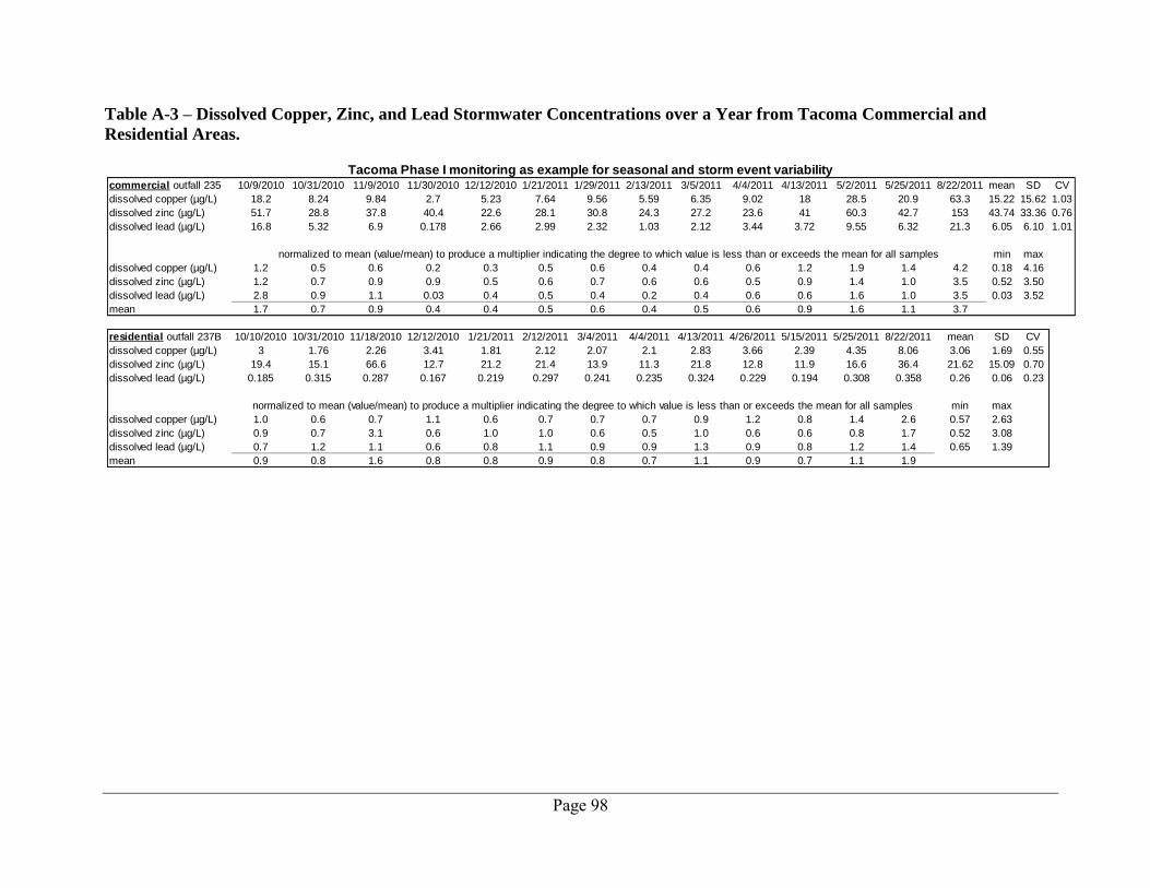
Page 98

Table A-3 – Dissolved Copper, Zinc, and Lead Stormwater Concentrations over a Year from Tacoma Commercial and

Residential Areas.

commercial outfall 235 10/9/2010 10/31/2010 11/9/2010 11/30/2010 12/12/2010 1/21/2011 1/29/2011 2/13/2011 3/5/2011 4/4/2011 4/13/2011 5/2/2011 5/25/2011 8/22/2011 mean SD CV

dissolved copper (µg/L) 18.2 8.24 9.84 2.7 5.23 7.64 9.56 5.59 6.35 9.02 18 28.5 20.9 63.3 15.22 15.62 1.03

dissolved zinc (µg/L) 51.7 28.8 37.8 40.4 22.6 28.1 30.8 24.3 27.2 23.6 41 60.3 42.7 153 43.74 33.36 0.76

dissolved lead (µg/L) 16.8 5.32 6.9 0.178 2.66 2.99 2.32 1.03 2.12 3.44 3.72 9.55 6.32 21.3 6.05 6.10 1.01

min max

dissolved copper (µg/L) 1.2 0.5 0.6 0.2 0.3 0.5 0.6 0.4 0.4 0.6 1.2 1.9 1.4 4.2 0.18 4.16

dissolved zinc (µg/L) 1.2 0.7 0.9 0.9 0.5 0.6 0.7 0.6 0.6 0.5 0.9 1.4 1.0 3.5 0.52 3.50

dissolved lead (µg/L) 2.8 0.9 1.1 0.03 0.4 0.5 0.4 0.2 0.4 0.6 0.6 1.6 1.0 3.5 0.03 3.52

mean 1.7 0.7 0.9 0.4 0.4 0.5 0.6 0.4 0.5 0.6 0.9 1.6 1.1 3.7

residential outfall 237B 10/10/2010 10/31/2010 11/18/2010 12/12/2010 1/21/2011 2/12/2011 3/4/2011 4/4/2011 4/13/2011 4/26/2011 5/15/2011 5/25/2011 8/22/2011 mean SD CV

dissolved copper (µg/L) 3 1.76 2.26 3.41 1.81 2.12 2.07 2.1 2.83 3.66 2.39 4.35 8.06 3.06 1.69 0.55

dissolved zinc (µg/L) 19.4 15.1 66.6 12.7 21.2 21.4 13.9 11.3 21.8 12.8 11.9 16.6 36.4 21.62 15.09 0.70

dissolved lead (µg/L) 0.185 0.315 0.287 0.167 0.219 0.297 0.241 0.235 0.324 0.229 0.194 0.308 0.358 0.26 0.06 0.23

min max

dissolved copper (µg/L) 1.0 0.6 0.7 1.1 0.6 0.7 0.7 0.7 0.9 1.2 0.8 1.4 2.6 0.57 2.63

dissolved zinc (µg/L) 0.9 0.7 3.1 0.6 1.0 1.0 0.6 0.5 1.0 0.6 0.6 0.8 1.7 0.52 3.08

dissolved lead (µg/L) 0.7 1.2 1.1 0.6 0.8 1.1 0.9 0.9 1.3 0.9 0.8 1.2 1.4 0.65 1.39

mean 0.9 0.8 1.6 0.8 0.8 0.9 0.8 0.7 1.1 0.9 0.7 1.1 1.9

Tacoma Phase I monitoring as example for seasonal and storm event variability

normalized to mean (value/mean) to produce a multiplier indicating the degree to which value is less than or exceeds the mean for all samples

normalized to mean (value/mean) to produce a multiplier indicating the degree to which value is less than or exceeds the mean for all samples

Page 99

Appendix B. Permittees’ Quality Assurance Project Plans Website link to QA Project Plans on file with Ecology www.ecy.wa.gov/programs/wq/stormwater/municipal/s8dswmonitoring.html

Clark County Quality Assurance Project Plan for Stormwater Characterization Monitoring. Conducted Under Section S8.D of the Phase I Municipal Stormwater Permit by Clark County. Prepared by U.S. Geological Survey, Oregon Water Science Center. Revised March 2011 by Clark County Department of Environmental Services, Clean Water Program, Vancouver, WA.

King County Quality Assurance Project Plan for King County Stormwater Monitoring Under the NPDES Phase 1 Municipal Permit WAR04-4501 (Issued February 2007). Updated November 2010. King County Department of Natural Resources and Parks, Water and Land Resources Division, Science Section. King Street Center, KSC-NR-0600, 201 South Jackson Street, Suite 600, Seattle, WA 98104.

Pierce County Quality Assurance Project Plan for Pierce County Phase I Municipal Stormwater NPDES Permit Section S8.D – Stormwater Characterization. November 5, 2009. Prepared for Pierce County Surface Water Management, 2702 South 42nd Street, Suite 201, Tacoma, WA 98409-7322. Prepared by Herrera Environmental Consultants.

Snohomish County Quality Assurance Project Plan (QAPP) Stormwater Characterization Monitoring S8.D Final. December 2008. Prepared by Snohomish County Public Works, Surface Water Management Division, 3000 Rockefeller Ave, Everett, WA 98201.

City of Seattle Section S8.D - Stormwater Characterization Quality Management System Planning Document, Quality Assurance Project Plan. NPDES Phase I Municipal Stormwater Permit, Permit No.: WAR04-4503. Revision: R2D0 (Final). Draft revised: 03/31/2011.

City of Tacoma Section S8.D - Stormwater Characterization Quality Assurance Project Plan, Phase I Municipal Stormwater NPDES Permit, Permit No.: WAR04-4003. Revision: S8.D-003 (Final). Revision Date: 08/16/2009. City of Tacoma, Tacoma, WA.

Port of Seattle Quality Assurance Project Plan for Stormwater Monitoring Conducted Under Section S8.D of the Phase I Municipal Stormwater Permit. Addendum #1. November 2011. Port of Seattle Marine Division. Prepared by TEC Inc. and Otak, Inc. for Port of Seattle.

Quality Assurance Project Plan for Stormwater Monitoring Conducted Under Section S8.D of the Phase I Municipal Stormwater Permit. February 20, 2009. Port of Seattle Marine Division. Prepared by TEC Inc. and Otak, Inc. for Port of Seattle.

Port of Tacoma Quality Assurance Project Plan for Stormwater Monitoring Conducted Under the Phase I Municipal Stormwater Permit by Port of Tacoma. Final August 2009.

http://www.ecy.wa.gov/programs/wq/stormwater/municipal/s8dswmonitoring.html

Page 100

Appendix C. Description of the Statistical Plots

This appendix describes each of the six plots created for data analysis. Four parameters are displayed and described for each of the six plot types. The four parameters are fecal coliform bacteria, total phosphorus, total copper, and Dichlobenil (an herbicide). These parameters were selected because they display a variety of discussion elements, considerations for data summaries, and peculiarities encountered in this report. For both the jitter and box plots, the x-axis is categorical and uses the abbreviations defined below: Land Uses

Ind = Industrial Com = Commercial HRes = High-Density Residential LRes = Low-Density Residential

Sample Result Det = Count of detected records ND = Count of non-detected records and the percent non-detected records of the total

Season Type Winter = Winter Quarter (January, February, March) Spring = Spring Quarter (April, May, June) Summer = Summer Quarter (July, August, September) Fall = Fall Quarter (October, November, December) DrySeas = Dry Season (May 1 through September 30) WetSeas = Wet Season (October 1 through April 30)

1. Jitter Plot

Jitter plots offer an excellent visual of the data. The jitter plot (Figure C-1) shows both the detected data as points and the non-detected data as bars extending from zero to provided reporting limit. The bar is useful in conveying the idea that the true value of the non-detect is unknown; only the range for which its true value may occur. The two-toned purple dots are the detected data points, divided into dry and wet seasons. The jitter plots are divided into four vertical panels. Each panel represents a different land-use type. Within each panel, the x-values are randomized (jittered) to spread the data out and make them easier to view. Land-use types are indicated by abbreviations below the x-axis, along with the number of detects, the number of non-detects, and the percentage of non-detect data. As seen in the jitter plots, most of the data for fecal coliform, total phosphorus, and dissolved copper were detected values, whereas the majority of the data for Dichlobenil were non-detects as indicated by the gray lines. The fecal coliform jitter plot shows that the data spans 5 orders of magnitude and includes non-detects.

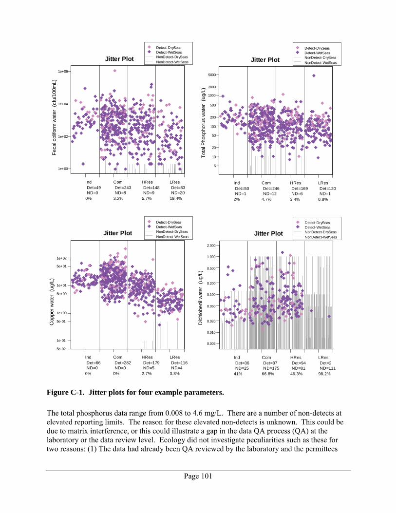
Page 101

Figure C-1. Jitter plots for four example parameters.

The total phosphorus data range from 0.008 to 4.6 mg/L. There are a number of non-detects at elevated reporting limits. The reason for these elevated non-detects is unknown. This could be due to matrix interference, or this could illustrate a gap in the data QA process (QA) at the laboratory or the data review level. Ecology did not investigate peculiarities such as these for two reasons: (1) The data had already been QA reviewed by the laboratory and the permittees

1e+00

1e+02

1e+04

1e+06

Jitter PlotF

ecalc

olif

orm

wate

r(c

fu/1

00m

L)

Ind

Det=49

ND=0

0%

Com

Det=243

ND=8

3.2%

HRes

Det=148

ND=9

5.7%

LRes

Det=83

ND=20

19.4%

Detect-DrySeas

Detect-WetSeas

NonDetect-DrySeas

NonDetect-WetSeas

5e-02

1e-01

5e-01

1e+00

5e+00

1e+01

5e+01

1e+02

Jitter Plot

Copper

wate

r(u

g/L

)

Ind

Det=66

ND=0

0%

Com

Det=282

ND=0

0%

HRes

Det=179

ND=5

2.7%

LRes

Det=116

ND=4

3.3%

Detect-DrySeas

Detect-WetSeas

NonDetect-DrySeas

NonDetect-WetSeas

5

10

20

50

100

200

500

1000

2000

5000

Jitter Plot

Tota

lPhosphoru

sw

ate

r(u

g/L

)

Ind

Det=50

ND=1

2%

Com

Det=246

ND=12

4.7%

HRes

Det=169

ND=6

3.4%

LRes

Det=120

ND=1

0.8%

Detect-DrySeas

Detect-WetSeas

NonDetect-DrySeas

NonDetect-WetSeas

0.005

0.010

0.020

0.050

0.100

0.200

0.500

1.000

2.000

Jitter Plot

Dic

hlo

benil

wate

r(u

g/L

)

Ind

Det=36

ND=25

41%

Com

Det=87

ND=175

66.8%

HRes

Det=94

ND=81

46.3%

LRes

Det=2

ND=111

98.2%

Detect-DrySeas

Detect-WetSeas

NonDetect-DrySeas

NonDetect-WetSeas

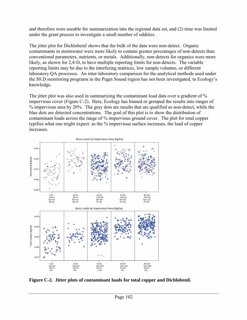
Page 102

and therefore were useable for summarization into the regional data set, and (2) time was limited under the grant process to investigate a small number of oddities. The jitter plot for Dichlobenil shows that the bulk of the data were non-detect. Organic contaminants in stormwater were more likely to contain greater percentages of non-detects than conventional parameters, nutrients, or metals. Additionally, non-detects for organics were more likely, as shown for 2,4-D, to have multiple reporting limits for non-detects. The variable reporting limits may be due to the interfering matrices, low sample volumes, or different laboratory QA processes. An inter-laboratory comparison for the analytical methods used under the S8.D monitoring programs in the Puget Sound region has not been investigated, to Ecology’s knowledge. The jitter plot was also used in summarizing the contaminant load data over a gradient of % impervious cover (Figure C-2). Here, Ecology has binned or grouped the results into ranges of % impervious area by 20%. The gray dots are results that are qualified as non-detect, while the blue dots are detected concentrations. The goal of this plot is to show the distribution of contaminant loads across the range of % impervious ground cover. The plot for total copper typifies what one might expect: as the % impervious surface increases, the load of copper increases.

Figure C-2. Jitter plots of contaminant loads for total copper and Dichlobenil.

1e-09

1e-08

1e-07

1e-06

1e-05

Area Loads by Impervious Area (kg/ha)

Dic

hlo

be

nil

(Kg/H

a)

0-20 Det=2

ND=5596.5%

20-40 Det=7

ND=4185.4%

40-60 Det=99

ND=8947.3%

60-80 Det=51

ND=5652.3%

80-100 Det=51

ND=12170.3%

1e-07

1e-06

1e-05

1e-04

1e-03

To

tal C

op

pe

r (K

g/H

a)

0-20 Det=67 ND=0

0%

20-40 Det=45 ND=0

0%

40-60 Det=197 ND=3

1.5%

60-80 Det=105 ND=0

0%

80-100 Det=196 ND=0

0%

Area Loads by Impervious Area (kg/ha)

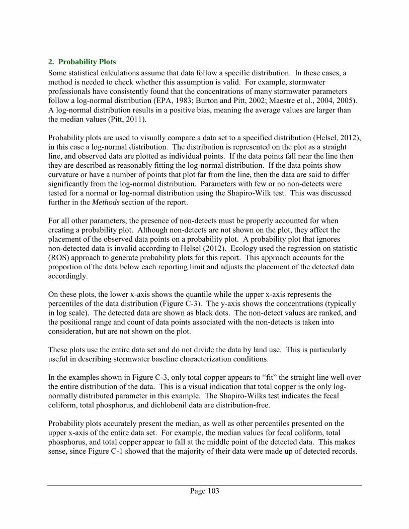
Page 103

2. Probability Plots

Some statistical calculations assume that data follow a specific distribution. In these cases, a method is needed to check whether this assumption is valid. For example, stormwater professionals have consistently found that the concentrations of many stormwater parameters follow a log-normal distribution (EPA, 1983; Burton and Pitt, 2002; Maestre et al., 2004, 2005). A log‐normal distribution results in a positive bias, meaning the average values are larger than the median values (Pitt, 2011). Probability plots are used to visually compare a data set to a specified distribution (Helsel, 2012), in this case a log-normal distribution. The distribution is represented on the plot as a straight line, and observed data are plotted as individual points. If the data points fall near the line then they are described as reasonably fitting the log-normal distribution. If the data points show curvature or have a number of points that plot far from the line, then the data are said to differ significantly from the log-normal distribution. Parameters with few or no non-detects were tested for a normal or log-normal distribution using the Shapiro-Wilk test. This was discussed further in the Methods section of the report. For all other parameters, the presence of non-detects must be properly accounted for when creating a probability plot. Although non-detects are not shown on the plot, they affect the placement of the observed data points on a probability plot. A probability plot that ignores non-detected data is invalid according to Helsel (2012). Ecology used the regression on statistic (ROS) approach to generate probability plots for this report. This approach accounts for the proportion of the data below each reporting limit and adjusts the placement of the detected data accordingly. On these plots, the lower x-axis shows the quantile while the upper x-axis represents the percentiles of the data distribution (Figure C-3). The y-axis shows the concentrations (typically in log scale). The detected data are shown as black dots. The non-detect values are ranked, and the positional range and count of data points associated with the non-detects is taken into consideration, but are not shown on the plot. These plots use the entire data set and do not divide the data by land use. This is particularly useful in describing stormwater baseline characterization conditions. In the examples shown in Figure C-3, only total copper appears to “fit” the straight line well over the entire distribution of the data. This is a visual indication that total copper is the only log-normally distributed parameter in this example. The Shapiro-Wilks test indicates the fecal coliform, total phosphorus, and dichlobenil data are distribution-free. Probability plots accurately present the median, as well as other percentiles presented on the upper x-axis of the entire data set. For example, the median values for fecal coliform, total phosphorus, and total copper appear to fall at the middle point of the detected data. This makes sense, since Figure C-1 showed that the majority of their data were made up of detected records.

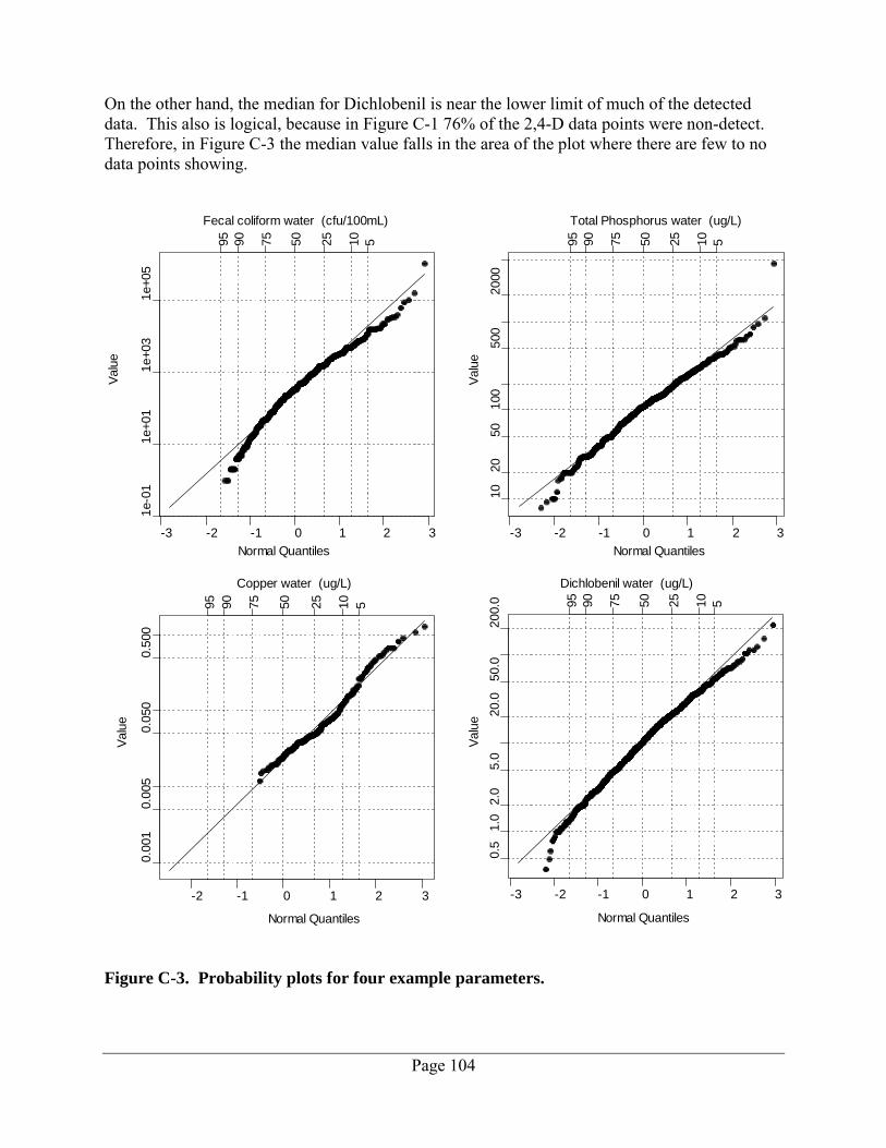
Page 104

On the other hand, the median for Dichlobenil is near the lower limit of much of the detected data. This also is logical, because in Figure C-1 76% of the 2,4-D data points were non-detect. Therefore, in Figure C-3 the median value falls in the area of the plot where there are few to no data points showing.

Figure C-3. Probability plots for four example parameters.

-3 -2 -1 0 1 2 3

Normal Quantiles

Valu

e

1e-0

11e+01

1e+03

1e+05

95

90

75

50

25

10

5

Fecal coliform water (cfu/100mL)

-3 -2 -1 0 1 2 3

Normal Quantiles

Valu

e

0.5

1.0

2.0

5.0

20.0

50.0

200.0 95

90

75

50

25

10

5

Copper water (ug/L)

-3 -2 -1 0 1 2 3

Normal Quantiles

Valu

e

10

20

50

100

500

2000

95

90

75

50

25

10

5

Total Phosphorus water (ug/L)

-2 -1 0 1 2 3

Normal Quantiles

Valu

e

0.0

01

0.0

05

0.0

50

0.5

00

95

90

75

50

25

10

5

Dichlobenil water (ug/L)

Page 105

3. Plots of Non-Detects

To understand differences in laboratory reporting levels, Ecology plotted non-detect thresholds reported by the permittees. Non-detect data are shown in these plots as line segments extending from zero to the laboratory reporting level. The color of the line segment indicates which laboratory performed the analysis. Laboratory names were removed and represented by a number. The focus of this plot is not to identify permittees or their laboratories, but rather to illustrate the number of laboratories and the numerous reporting limits reported. Within each plot, the non-detect data are spaced evenly and sorted from lowest to highest reporting level. Plots with few points show the lines distinctly, whereas plots with a large number of data points show no spaces between the lines. Examples are shown in Figure C-4.

Figure C-4. Non-detect plots for four example parameters.

1e+00

1e+02

1e+04

1e+06

Non-Detect Levels

Fe

ca

lc

olif

orm

wa

ter

(cfu

/100

mL

)

Unk

Lab-

1

Lab-

2

Lab-

3

Lab-

4

Lab-

5

Lab-

6

Lab-

7

Lab-

8

Lab-

9

Lab-

10

Lab-

11

Lab-

12

Lab-

13

Lab-

14

Lab-

15

5e-02

1e-01

5e-01

1e+00

5e+00

1e+01

5e+01

1e+02

Non-Detect Levels

Co

pp

er

wa

ter

(ug

/L)

Unk

Lab-

1

Lab-

2

Lab-

3

Lab-

4

Lab-

5

Lab-

6

Lab-

7

Lab-

8

Lab-

9

Lab-

10

Lab-

11

Lab-

12

Lab-

13

Lab-

14

Lab-

15

5

10

20

50

100

200

500

1000

2000

5000

Non-Detect Levels

To

talP

ho

spho

rus

wa

ter

(ug

/L)

Unk

Lab-

1

Lab-

2

Lab-

3

Lab-

4

Lab-

5

Lab-

6

Lab-

7

Lab-

8

Lab-

9

Lab-

10

Lab-

11

Lab-

12

Lab-

13

Lab-

14

Lab-

15

0.005

0.010

0.020

0.050

0.100

0.200

0.500

1.000

2.000

Non-Detect Levels

Dic

hlo

be

nil

wa

ter

(ug

/L)

Unk

Lab-

1

Lab-

2

Lab-

3

Lab-

4

Lab-

5

Lab-

6

Lab-

7

Lab-

8

Lab-

9

Lab-

10

Lab-

11

Lab-

12

Lab-

13

Lab-

14

Lab-

15

Page 106

These examples illustrate both the frequency a parameter was not detected and the variability in the reporting limit threshold for the non-detect data. Recall that variability comes from different samples’ matrices, sampling dates, handling techniques, and laboratories. The parameter data in Appendix F did not contain this plot if there were no non-detect data. 4. Empirical Distribution Function (EDF)

These plots (Figure C-5) help identify differences in concentrations among the four land-use types. EDF plots of the observed data are constructed by ranking the data from smallest to largest (Helsel, 2012). EDF plots are also known as the Kaplan-Meier (KM) Curves. The graph shows the likelihood of any given sample concentration to occur in the population of the data set by percentiles. Line type and color indicates land use, as shown in the plot legend. On these plots, Ecology swapped axes from the usual convention in order to allow comparison with the jitter plots and box plots. Only the detect values are actually plotted, but their positions are influenced by both detections and non-detections. This is a preferred method to display data sets that contain non-detects, as opposed to the traditional box and whisker plots that use only detected values. EDF plots were not shown if there were less than five detected values for any given parameter, and in this case, the data plots (Appendix F) will show the message: “Not Plotted

(Less than 5 detections)”. These four example parameters begin to illustrate the impact of the surrounding land use on the water quality of stormwater. In the case of fecal coliform, the EDF curve for industrial is similar to commercial but quite different from low-density residential. A vertical dashed line was placed on the fecal coliform plot to illustrate where the median value (50%) occurs by land use. A horizontal dashed line was placed to show that fecal concentrations of 100 cfu/100 mL or higher occur approximately >95% of the time for the industrial land use, > 75% for commercial, > 65% for high-density residential, and > 40% of the time for low-density land use. For total phosphorus, there is less difference observed among the four land-use types. For Dichlobenil, the EDF for high-density residential shows both a higher proportion of detections and consistently higher concentrations. The data for low-density residential land use reflects the large number of non-detects (98%) and low concentrations in the detected samples. When many non-detects occur at the same reporting level, this shows up in the EDF plot as a long horizontal line segment. EDF plots were also created for each parameter load as kg ha-1. These are part of the plot summaries for the loading per unit area in Appendix H. Data qualifiers associated with the parameter concentrations were incorporated into the Kaplan-Meier analysis with the load value.

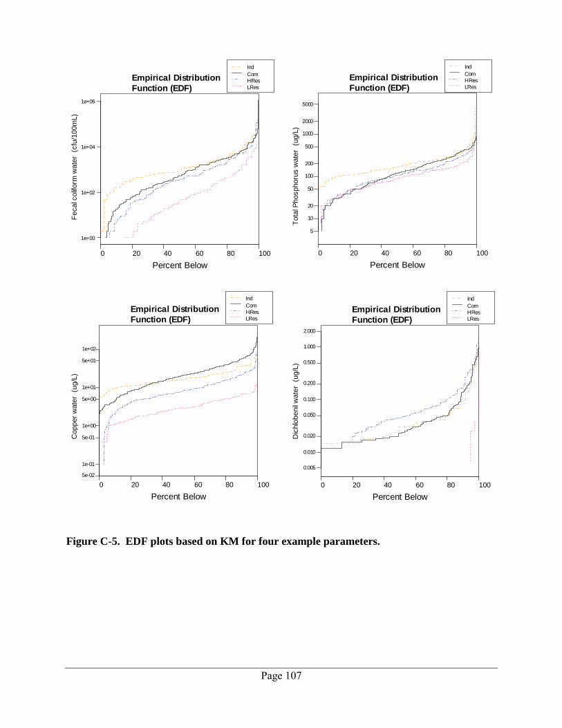
Page 107

Figure C-5. EDF plots based on KM for four example parameters.

1e+00

1e+02

1e+04

1e+06

Empirical Distribution

Function (EDF)

Fecalc

olif

orm

wate

r(c

fu/1

00m

L)

0 20 40 60 80 100

Percent Below

Ind

Com

HRes

LRes

5e-02

1e-01

5e-01

1e+00

5e+00

1e+01

5e+01

1e+02


Function (EDF)

Co

pp

er

wate

r(u

g/L

)

0 20 40 60 80 100

Percent Below

Ind

Com

HRes

LRes

5

10

20

50

100

200

500

1000

2000

5000


Function (EDF)

Tota

lPhosphoru

sw

ate

r(u

g/L

)

0 20 40 60 80 100

Percent Below

Ind

Com

HRes

LRes

0.005

0.010

0.020

0.050

0.100

0.200

0.500

1.000

2.000


Function (EDF)

Dic

hlo

be

nil

wate

r(u

g/L

)

0 20 40 60 80 100

Percent Below

Ind

Com

HRes

LRes

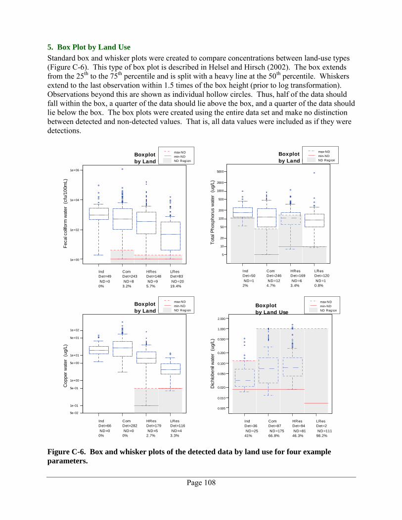
Page 108

5. Box Plot by Land Use

Standard box and whisker plots were created to compare concentrations between land-use types (Figure C-6). This type of box plot is described in Helsel and Hirsch (2002). The box extends from the 25th to the 75th percentile and is split with a heavy line at the 50th percentile. Whiskers extend to the last observation within 1.5 times of the box height (prior to log transformation). Observations beyond this are shown as individual hollow circles. Thus, half of the data should fall within the box, a quarter of the data should lie above the box, and a quarter of the data should lie below the box. The box plots were created using the entire data set and make no distinction between detected and non-detected values. That is, all data values were included as if they were detections.

Figure C-6. Box and whisker plots of the detected data by land use for four example

parameters.

1e+00

1e+02

1e+04

1e+06

Boxplot

by Land Use

Fecalc

olif

orm

wate

r(c

fu/1

00m

L)

Ind

Det=49

ND=0

0%

Com

Det=243

ND=8

3.2%

HRes

Det=148

ND=9

5.7%

LRes

Det=83

ND=20

19.4%

max-ND

min-ND

ND Region

5e-02

1e-01

5e-01

1e+00

5e+00

1e+01

5e+01

1e+02

Boxplot

by Land Use

Co

pp

er

wate

r(u

g/L

)

Ind

Det=66

ND=0

0%

Com

Det=282

ND=0

0%

HRes

Det=179

ND=5

2.7%

LRes

Det=116

ND=4

3.3%

max-ND

min-ND

ND Region

5

10

20

50

100

200

500

1000

2000

5000

Boxplot

by Land Use

Tota

lPhosphoru

sw

ate

r(u

g/L

)

Ind

Det=50

ND=1

2%

Com

Det=246

ND=12

4.7%

HRes

Det=169

ND=6

3.4%

LRes

Det=120

ND=1

0.8%

max-ND

min-ND

ND Region

0.005

0.010

0.020

0.050

0.100

0.200

0.500

1.000

2.000

Ind

Det=36

ND=25

41%

Com

Det=87

ND=175

66.8%

HRes

Det=94

ND=81

46.3%

LRes

Det=2

ND=111

98.2%

max-ND

min-ND

ND Region

Dic

hlo

benil

wate

r(u

g/L

)

Boxplot

by Land Use

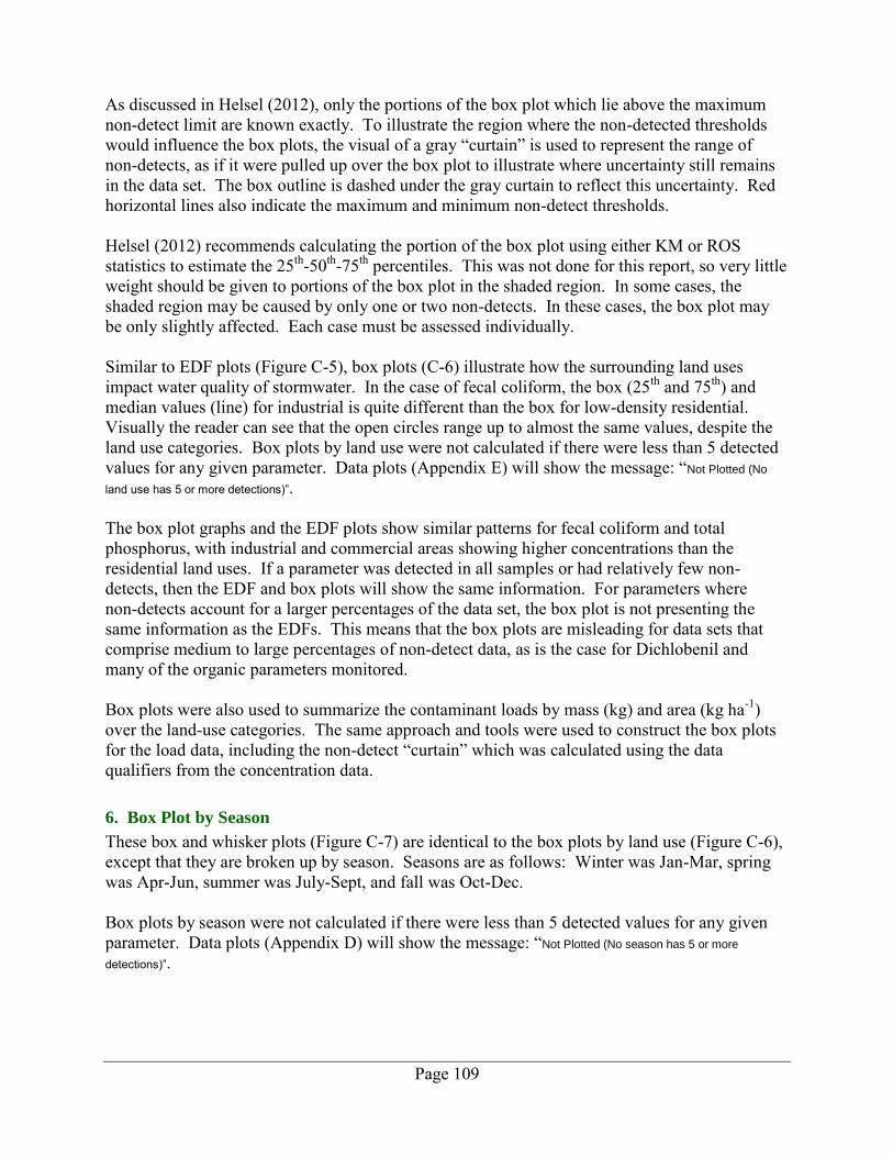
Page 109

As discussed in Helsel (2012), only the portions of the box plot which lie above the maximum non-detect limit are known exactly. To illustrate the region where the non-detected thresholds would influence the box plots, the visual of a gray “curtain” is used to represent the range of non-detects, as if it were pulled up over the box plot to illustrate where uncertainty still remains in the data set. The box outline is dashed under the gray curtain to reflect this uncertainty. Red horizontal lines also indicate the maximum and minimum non-detect thresholds. Helsel (2012) recommends calculating the portion of the box plot using either KM or ROS statistics to estimate the 25th-50th-75th percentiles. This was not done for this report, so very little weight should be given to portions of the box plot in the shaded region. In some cases, the shaded region may be caused by only one or two non-detects. In these cases, the box plot may be only slightly affected. Each case must be assessed individually. Similar to EDF plots (Figure C-5), box plots (C-6) illustrate how the surrounding land uses impact water quality of stormwater. In the case of fecal coliform, the box (25th and 75th) and median values (line) for industrial is quite different than the box for low-density residential. Visually the reader can see that the open circles range up to almost the same values, despite the land use categories. Box plots by land use were not calculated if there were less than 5 detected values for any given parameter. Data plots (Appendix E) will show the message: “Not Plotted (No

land use has 5 or more detections)”. The box plot graphs and the EDF plots show similar patterns for fecal coliform and total phosphorus, with industrial and commercial areas showing higher concentrations than the residential land uses. If a parameter was detected in all samples or had relatively few non-detects, then the EDF and box plots will show the same information. For parameters where non-detects account for a larger percentages of the data set, the box plot is not presenting the same information as the EDFs. This means that the box plots are misleading for data sets that comprise medium to large percentages of non-detect data, as is the case for Dichlobenil and many of the organic parameters monitored. Box plots were also used to summarize the contaminant loads by mass (kg) and area (kg ha-1) over the land-use categories. The same approach and tools were used to construct the box plots for the load data, including the non-detect “curtain” which was calculated using the data qualifiers from the concentration data. 6. Box Plot by Season

These box and whisker plots (Figure C-7) are identical to the box plots by land use (Figure C-6), except that they are broken up by season. Seasons are as follows: Winter was Jan-Mar, spring was Apr-Jun, summer was July-Sept, and fall was Oct-Dec. Box plots by season were not calculated if there were less than 5 detected values for any given parameter. Data plots (Appendix D) will show the message: “Not Plotted (No season has 5 or more

detections)”.

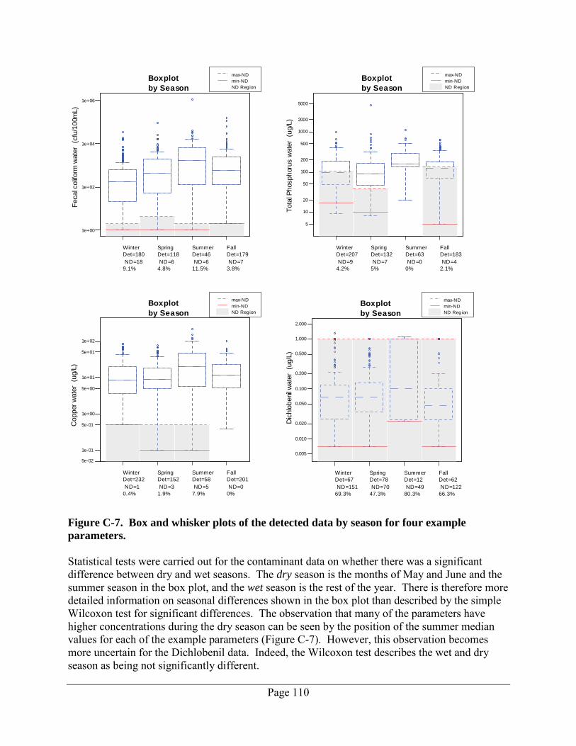
Page 110

Figure C-7. Box and whisker plots of the detected data by season for four example

parameters.

Statistical tests were carried out for the contaminant data on whether there was a significant difference between dry and wet seasons. The dry season is the months of May and June and the summer season in the box plot, and the wet season is the rest of the year. There is therefore more detailed information on seasonal differences shown in the box plot than described by the simple Wilcoxon test for significant differences. The observation that many of the parameters have higher concentrations during the dry season can be seen by the position of the summer median values for each of the example parameters (Figure C-7). However, this observation becomes more uncertain for the Dichlobenil data. Indeed, the Wilcoxon test describes the wet and dry season as being not significantly different.

1e+00

1e+02

1e+04

1e+06

Boxplot

by Season

Fecalc

olif

orm

wate

r(c

fu/1

00m

L)

Winter

Det=180

ND=18

9.1%

Spring

Det=118

ND=6

4.8%

Summer

Det=46

ND=6

11.5%

Fall

Det=179

ND=7

3.8%

max-ND

min-ND

ND Region

5e-02

1e-01

5e-01

1e+00

5e+00

1e+01

5e+01

1e+02

Boxplot

by Season

Co

pp

erw

ate

r(u

g/L

)

Winter

Det=232

ND=1

0.4%

Spring

Det=152

ND=3

1.9%

Summer

Det=58

ND=5

7.9%

Fall

Det=201

ND=0

0%

max-ND

min-ND

ND Region

5

10

20

50

100

200

500

1000

2000

5000

Boxplot

by Season

Tota

lPh

osp

horu

sw

ate

r(u

g/L

)

Winter

Det=207

ND=9

4.2%

Spring

Det=132

ND=7

5%

Summer

Det=63

ND=0

0%

Fall

Det=183

ND=4

2.1%

max-ND

min-ND

ND Region

0.005

0.010

0.020

0.050

0.100

0.200

0.500

1.000

2.000

Boxplot

by Season

Dic

hlo

beni

lwate

r(u

g/L

)

Winter

Det=67

ND=151

69.3%

Spring

Det=78

ND=70

47.3%

Summer

Det=12

ND=49

80.3%

Fall

Det=62

ND=122

66.3%

max-ND

min-ND

ND Region

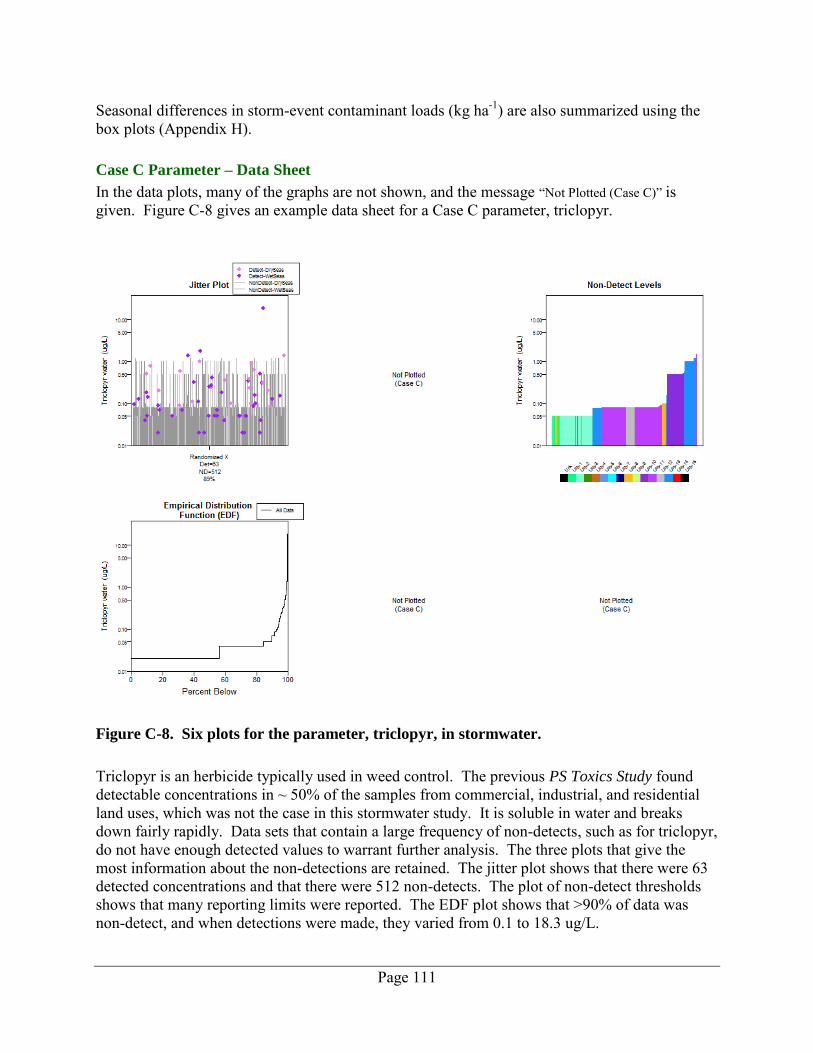
Page 111

Seasonal differences in storm-event contaminant loads (kg ha-1) are also summarized using the box plots (Appendix H).

Case C Parameter – Data Sheet

In the data plots, many of the graphs are not shown, and the message “Not Plotted (Case C)” is given. Figure C-8 gives an example data sheet for a Case C parameter, triclopyr.

Figure C-8. Six plots for the parameter, triclopyr, in stormwater.

Triclopyr is an herbicide typically used in weed control. The previous PS Toxics Study found detectable concentrations in ~ 50% of the samples from commercial, industrial, and residential land uses, which was not the case in this stormwater study. It is soluble in water and breaks down fairly rapidly. Data sets that contain a large frequency of non-detects, such as for triclopyr, do not have enough detected values to warrant further analysis. The three plots that give the most information about the non-detections are retained. The jitter plot shows that there were 63 detected concentrations and that there were 512 non-detects. The plot of non-detect thresholds shows that many reporting limits were reported. The EDF plot shows that >90% of data was non-detect, and when detections were made, they varied from 0.1 to 18.3 ug/L.

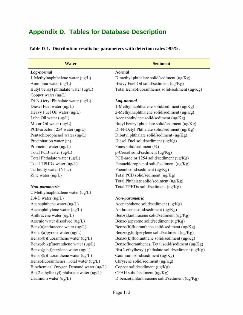
Page 112

Appendix D. Tables for Database Description

Table D-1. Distribution results for parameters with detection rates >95%.

Water Sediment

Log-normal Normal

1-Methylnaphthalene water (ug/L) Dimethyl phthalate solid/sediment (ug/Kg) Ammonia water (ug/L) Heavy Fuel Oil solid/sediment (ug/Kg) Butyl benzyl phthalate water (ug/L) Total Benzofluoranthenes solid/sediment (ug/Kg) Copper water (ug/L)

Di-N-Octyl Phthalate water (ug/L) Log-normal

Diesel Fuel water (ug/L) 1-Methylnaphthalene solid/sediment (ug/Kg) Heavy Fuel Oil water (ug/L) 2-Methylnaphthalene solid/sediment (ug/Kg) Lube Oil water (ug/L) Acenaphthylene solid/sediment (ug/Kg) Motor Oil water (ug/L) Butyl benzyl phthalate solid/sediment (ug/Kg) PCB-aroclor 1254 water (ug/L) Di-N-Octyl Phthalate solid/sediment (ug/Kg) Pentachlorophenol water (ug/L) Dibutyl phthalate solid/sediment (ug/Kg) Precipitation water (in) Diesel Fuel solid/sediment (ug/Kg) Prometon water (ug/L) Fines solid/sediment (%) Total PCB water (ug/L) p-Cresol solid/sediment (ug/Kg) Total Phthalate water (ug/L) PCB-aroclor 1254 solid/sediment (ug/Kg) Total TPHDx water (ug/L) Pentachlorophenol solid/sediment (ug/Kg) Turbidity water (NTU) Phenol solid/sediment (ug/Kg) Zinc water (ug/L) Total PCB solid/sediment (ug/Kg)

Total Phthalate solid/sediment (ug/Kg)

Non-parametric Total TPHDx solid/sediment (ug/Kg) 2-Methylnaphthalene water (ug/L)

2,4-D water (ug/L) Non-parametric

Acenaphthene water (ug/L) Acenaphthene solid/sediment (ug/Kg) Acenaphthylene water (ug/L) Anthracene solid/sediment (ug/Kg) Anthracene water (ug/L) Benz(a)anthracene solid/sediment (ug/Kg) Arsenic water dissolved (ug/L) Benzo(a)pyrene solid/sediment (ug/Kg) Benz(a)anthracene water (ug/L) Benzo(b)fluoranthene solid/sediment (ug/Kg) Benzo(a)pyrene water (ug/L) Benzo(g,h,i)perylene solid/sediment (ug/Kg) Benzo(b)fluoranthene water (ug/L) Benzo(k)fluoranthene solid/sediment (ug/Kg) Benzo(b,k)fluoranthene water (ug/L) Benzofluoranthenes, Total solid/sediment (ug/Kg) Benzo(g,h,i)perylene water (ug/L) Bis(2-ethylhexyl) phthalate solid/sediment (ug/Kg) Benzo(k)fluoranthene water (ug/L) Cadmium solid/sediment (ug/Kg) Benzofluoranthenes, Total water (ug/L) Chrysene solid/sediment (ug/Kg) Biochemical Oxygen Demand water (ug/L) Copper solid/sediment (ug/Kg) Bis(2-ethylhexyl) phthalate water (ug/L) CPAH solid/sediment (ug/Kg) Cadmium water (ug/L) Dibenzo(a,h)anthracene solid/sediment (ug/Kg)

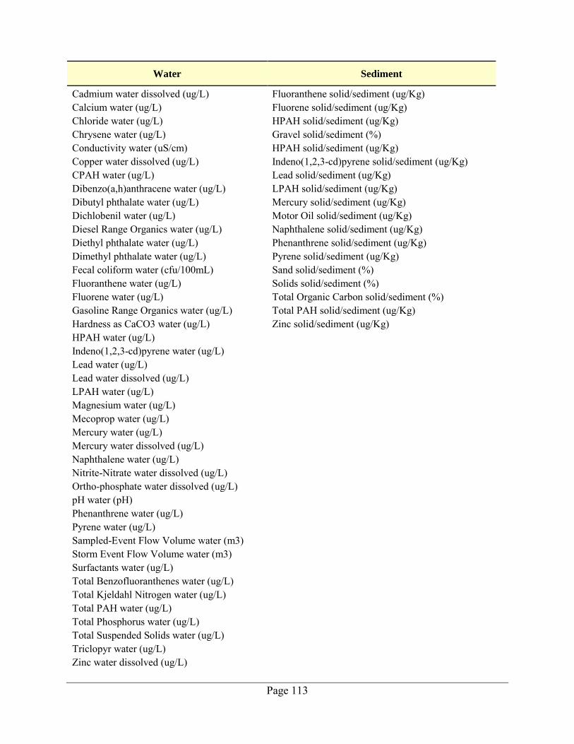
Page 113

Water Sediment

Cadmium water dissolved (ug/L) Fluoranthene solid/sediment (ug/Kg) Calcium water (ug/L) Fluorene solid/sediment (ug/Kg) Chloride water (ug/L) HPAH solid/sediment (ug/Kg) Chrysene water (ug/L) Gravel solid/sediment (%) Conductivity water (uS/cm) HPAH solid/sediment (ug/Kg) Copper water dissolved (ug/L) Indeno(1,2,3-cd)pyrene solid/sediment (ug/Kg) CPAH water (ug/L) Lead solid/sediment (ug/Kg) Dibenzo(a,h)anthracene water (ug/L) LPAH solid/sediment (ug/Kg) Dibutyl phthalate water (ug/L) Mercury solid/sediment (ug/Kg) Dichlobenil water (ug/L) Motor Oil solid/sediment (ug/Kg) Diesel Range Organics water (ug/L) Naphthalene solid/sediment (ug/Kg) Diethyl phthalate water (ug/L) Phenanthrene solid/sediment (ug/Kg) Dimethyl phthalate water (ug/L) Pyrene solid/sediment (ug/Kg) Fecal coliform water (cfu/100mL) Sand solid/sediment (%) Fluoranthene water (ug/L) Solids solid/sediment (%) Fluorene water (ug/L) Total Organic Carbon solid/sediment (%) Gasoline Range Organics water (ug/L) Total PAH solid/sediment (ug/Kg) Hardness as CaCO3 water (ug/L) Zinc solid/sediment (ug/Kg) HPAH water (ug/L)

Indeno(1,2,3-cd)pyrene water (ug/L) Lead water (ug/L) Lead water dissolved (ug/L) LPAH water (ug/L) Magnesium water (ug/L) Mecoprop water (ug/L) Mercury water (ug/L) Mercury water dissolved (ug/L) Naphthalene water (ug/L) Nitrite-Nitrate water dissolved (ug/L) Ortho-phosphate water dissolved (ug/L) pH water (pH) Phenanthrene water (ug/L) Pyrene water (ug/L) Sampled-Event Flow Volume water (m3) Storm Event Flow Volume water (m3) Surfactants water (ug/L) Total Benzofluoranthenes water (ug/L) Total Kjeldahl Nitrogen water (ug/L) Total PAH water (ug/L) Total Phosphorus water (ug/L) Total Suspended Solids water (ug/L) Triclopyr water (ug/L) Zinc water dissolved (ug/L)

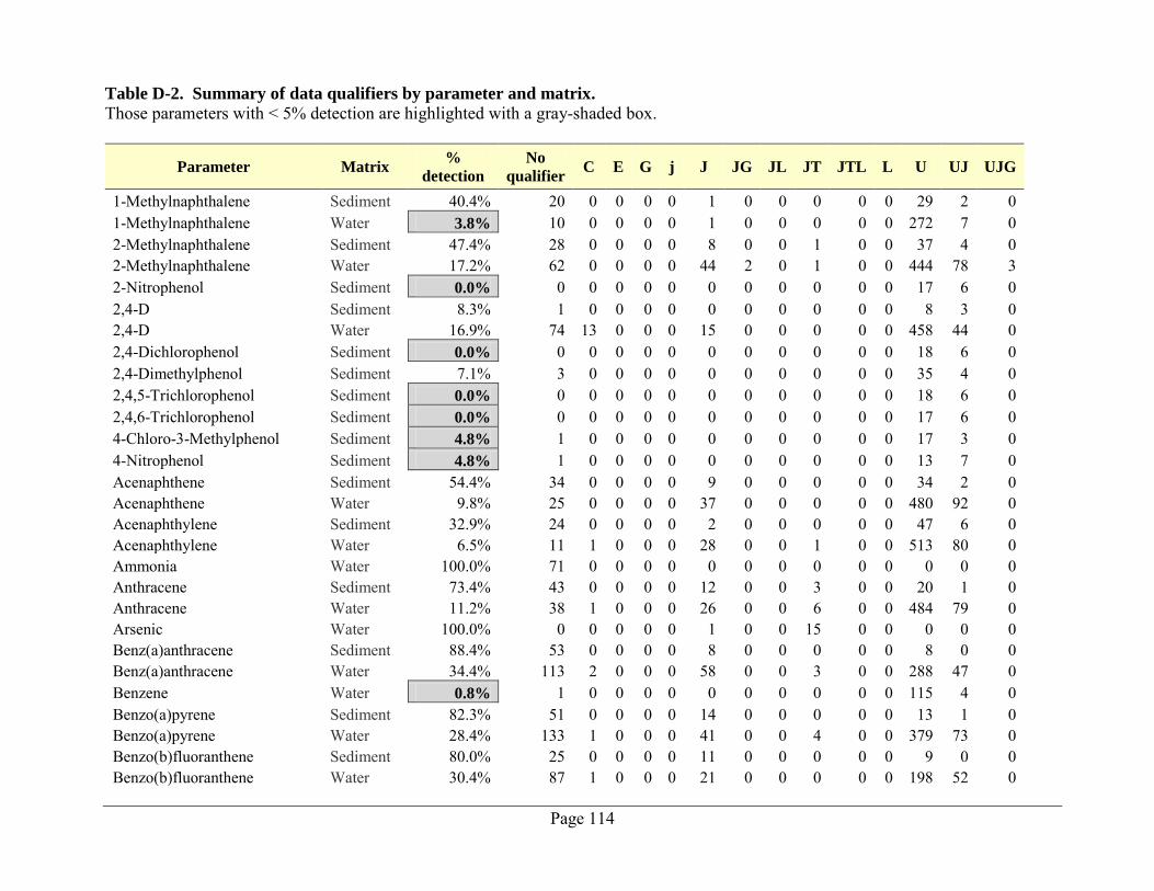
Page 114

Table D-2. Summary of data qualifiers by parameter and matrix.

Those parameters with < 5% detection are highlighted with a gray-shaded box.

Parameter Matrix %

detection

No

qualifier C E G j J JG JL JT JTL L U UJ UJG

1-Methylnaphthalene Sediment 40.4% 20 0 0 0 0 1 0 0 0 0 0 29 2 0 1-Methylnaphthalene Water 3.8% 10 0 0 0 0 1 0 0 0 0 0 272 7 0 2-Methylnaphthalene Sediment 47.4% 28 0 0 0 0 8 0 0 1 0 0 37 4 0 2-Methylnaphthalene Water 17.2% 62 0 0 0 0 44 2 0 1 0 0 444 78 3 2-Nitrophenol Sediment 0.0% 0 0 0 0 0 0 0 0 0 0 0 17 6 0 2,4-D Sediment 8.3% 1 0 0 0 0 0 0 0 0 0 0 8 3 0 2,4-D Water 16.9% 74 13 0 0 0 15 0 0 0 0 0 458 44 0 2,4-Dichlorophenol Sediment 0.0% 0 0 0 0 0 0 0 0 0 0 0 18 6 0 2,4-Dimethylphenol Sediment 7.1% 3 0 0 0 0 0 0 0 0 0 0 35 4 0 2,4,5-Trichlorophenol Sediment 0.0% 0 0 0 0 0 0 0 0 0 0 0 18 6 0 2,4,6-Trichlorophenol Sediment 0.0% 0 0 0 0 0 0 0 0 0 0 0 17 6 0 4-Chloro-3-Methylphenol Sediment 4.8% 1 0 0 0 0 0 0 0 0 0 0 17 3 0 4-Nitrophenol Sediment 4.8% 1 0 0 0 0 0 0 0 0 0 0 13 7 0 Acenaphthene Sediment 54.4% 34 0 0 0 0 9 0 0 0 0 0 34 2 0 Acenaphthene Water 9.8% 25 0 0 0 0 37 0 0 0 0 0 480 92 0 Acenaphthylene Sediment 32.9% 24 0 0 0 0 2 0 0 0 0 0 47 6 0 Acenaphthylene Water 6.5% 11 1 0 0 0 28 0 0 1 0 0 513 80 0 Ammonia Water 100.0% 71 0 0 0 0 0 0 0 0 0 0 0 0 0 Anthracene Sediment 73.4% 43 0 0 0 0 12 0 0 3 0 0 20 1 0 Anthracene Water 11.2% 38 1 0 0 0 26 0 0 6 0 0 484 79 0 Arsenic Water 100.0% 0 0 0 0 0 1 0 0 15 0 0 0 0 0 Benz(a)anthracene Sediment 88.4% 53 0 0 0 0 8 0 0 0 0 0 8 0 0 Benz(a)anthracene Water 34.4% 113 2 0 0 0 58 0 0 3 0 0 288 47 0 Benzene Water 0.8% 1 0 0 0 0 0 0 0 0 0 0 115 4 0 Benzo(a)pyrene Sediment 82.3% 51 0 0 0 0 14 0 0 0 0 0 13 1 0 Benzo(a)pyrene Water 28.4% 133 1 0 0 0 41 0 0 4 0 0 379 73 0 Benzo(b)fluoranthene Sediment 80.0% 25 0 0 0 0 11 0 0 0 0 0 9 0 0 Benzo(b)fluoranthene Water 30.4% 87 1 0 0 0 21 0 0 0 0 0 198 52 0

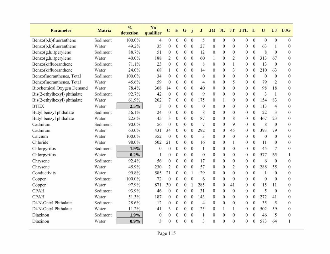
Page 115

Parameter Matrix %

detection

No


Benzo(b,k)fluoranthene Sediment 100.0% 4 0 0 0 0 5 0 0 0 0 0 0 0 0 Benzo(b,k)fluoranthene Water 49.2% 35 0 0 0 0 27 0 0 0 0 0 63 1 0 Benzo(g,h,i)perylene Sediment 88.7% 51 0 0 0 0 12 0 0 0 0 0 8 0 0 Benzo(g,h,i)perylene Water 40.0% 188 2 0 0 0 60 1 0 2 0 0 313 67 0 Benzo(k)fluoranthene Sediment 71.1% 23 0 0 0 0 8 0 0 1 0 0 13 0 0 Benzo(k)fluoranthene Water 24.0% 68 1 0 0 0 14 0 0 3 0 0 210 63 0 Benzofluoranthenes, Total Sediment 100.0% 34 0 0 0 0 0 0 0 0 0 0 0 0 0 Benzofluoranthenes, Total Water 45.6% 59 0 0 0 0 4 0 0 5 0 0 79 2 0 Biochemical Oxygen Demand Water 78.4% 368 14 0 0 0 40 0 0 0 0 0 98 18 0 Bis(2-ethylhexyl) phthalate Sediment 92.7% 42 0 0 0 0 9 0 0 0 0 0 3 1 0 Bis(2-ethylhexyl) phthalate Water 61.9% 202 7 0 0 0 175 0 1 0 0 0 154 83 0 BTEX Water 2.5% 3 0 0 0 0 0 0 0 0 0 0 113 4 0 Butyl benzyl phthalate Sediment 56.1% 24 0 0 0 0 8 0 0 0 0 0 22 3 0 Butyl benzyl phthalate Water 22.6% 45 3 0 0 0 87 0 0 8 0 0 467 23 0 Cadmium Sediment 90.0% 56 0 0 0 0 7 0 0 9 0 0 8 0 0 Cadmium Water 63.0% 431 34 0 0 0 292 0 0 45 0 0 393 79 0 Calcium Water 100.0% 352 0 0 0 0 3 0 0 0 0 0 0 0 0 Chloride Water 98.0% 502 21 0 0 0 16 0 0 1 0 0 11 0 0 Chlorpyrifos Sediment 1.9% 0 0 0 0 0 1 0 0 0 0 0 45 7 0 Chlorpyrifos Water 0.2% 1 0 0 0 0 0 0 0 0 0 0 577 65 1 Chrysene Sediment 92.4% 56 0 0 0 0 17 0 0 0 0 0 6 0 0 Chrysene Water 45.9% 230 2 0 0 0 57 0 0 2 0 0 288 55 0 Conductivity Water 99.8% 585 21 0 0 1 29 0 0 0 0 0 1 0 0 Copper Sediment 100.0% 72 0 0 0 0 6 0 0 0 0 0 0 0 0 Copper Water 97.9% 871 30 0 0 1 285 0 0 41 0 0 15 11 0 CPAH Sediment 93.9% 46 0 0 0 0 31 0 0 0 0 0 5 0 0 CPAH Water 51.3% 187 0 0 0 0 143 0 0 0 0 0 272 41 0 Di-N-Octyl Phthalate Sediment 28.6% 12 0 0 0 0 4 0 0 0 0 0 35 5 0 Di-N-Octyl Phthalate Water 11.2% 41 3 0 0 0 25 0 1 1 0 0 502 59 0 Diazinon Sediment 1.9% 0 0 0 0 0 1 0 0 0 0 0 46 5 0 Diazinon Water 0.9% 3 0 0 0 0 3 0 0 0 0 0 573 64 1

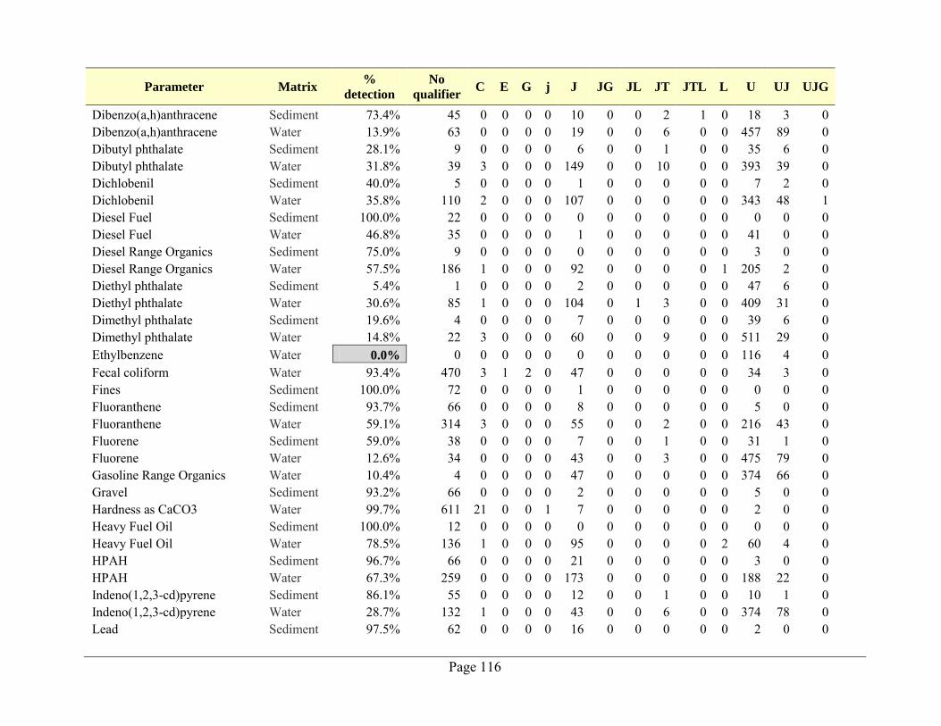
Page 116

Parameter Matrix %

detection

No


Dibenzo(a,h)anthracene Sediment 73.4% 45 0 0 0 0 10 0 0 2 1 0 18 3 0 Dibenzo(a,h)anthracene Water 13.9% 63 0 0 0 0 19 0 0 6 0 0 457 89 0 Dibutyl phthalate Sediment 28.1% 9 0 0 0 0 6 0 0 1 0 0 35 6 0 Dibutyl phthalate Water 31.8% 39 3 0 0 0 149 0 0 10 0 0 393 39 0 Dichlobenil Sediment 40.0% 5 0 0 0 0 1 0 0 0 0 0 7 2 0 Dichlobenil Water 35.8% 110 2 0 0 0 107 0 0 0 0 0 343 48 1 Diesel Fuel Sediment 100.0% 22 0 0 0 0 0 0 0 0 0 0 0 0 0 Diesel Fuel Water 46.8% 35 0 0 0 0 1 0 0 0 0 0 41 0 0 Diesel Range Organics Sediment 75.0% 9 0 0 0 0 0 0 0 0 0 0 3 0 0 Diesel Range Organics Water 57.5% 186 1 0 0 0 92 0 0 0 0 1 205 2 0 Diethyl phthalate Sediment 5.4% 1 0 0 0 0 2 0 0 0 0 0 47 6 0 Diethyl phthalate Water 30.6% 85 1 0 0 0 104 0 1 3 0 0 409 31 0 Dimethyl phthalate Sediment 19.6% 4 0 0 0 0 7 0 0 0 0 0 39 6 0 Dimethyl phthalate Water 14.8% 22 3 0 0 0 60 0 0 9 0 0 511 29 0 Ethylbenzene Water 0.0% 0 0 0 0 0 0 0 0 0 0 0 116 4 0 Fecal coliform Water 93.4% 470 3 1 2 0 47 0 0 0 0 0 34 3 0 Fines Sediment 100.0% 72 0 0 0 0 1 0 0 0 0 0 0 0 0 Fluoranthene Sediment 93.7% 66 0 0 0 0 8 0 0 0 0 0 5 0 0 Fluoranthene Water 59.1% 314 3 0 0 0 55 0 0 2 0 0 216 43 0 Fluorene Sediment 59.0% 38 0 0 0 0 7 0 0 1 0 0 31 1 0 Fluorene Water 12.6% 34 0 0 0 0 43 0 0 3 0 0 475 79 0 Gasoline Range Organics Water 10.4% 4 0 0 0 0 47 0 0 0 0 0 374 66 0 Gravel Sediment 93.2% 66 0 0 0 0 2 0 0 0 0 0 5 0 0 Hardness as CaCO3 Water 99.7% 611 21 0 0 1 7 0 0 0 0 0 2 0 0 Heavy Fuel Oil Sediment 100.0% 12 0 0 0 0 0 0 0 0 0 0 0 0 0 Heavy Fuel Oil Water 78.5% 136 1 0 0 0 95 0 0 0 0 2 60 4 0 HPAH Sediment 96.7% 66 0 0 0 0 21 0 0 0 0 0 3 0 0 HPAH Water 67.3% 259 0 0 0 0 173 0 0 0 0 0 188 22 0 Indeno(1,2,3-cd)pyrene Sediment 86.1% 55 0 0 0 0 12 0 0 1 0 0 10 1 0 Indeno(1,2,3-cd)pyrene Water 28.7% 132 1 0 0 0 43 0 0 6 0 0 374 78 0 Lead Sediment 97.5% 62 0 0 0 0 16 0 0 0 0 0 2 0 0

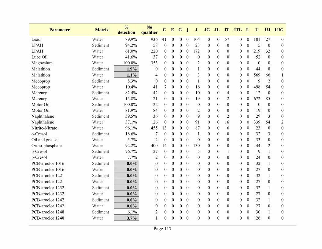
Page 117

Parameter Matrix %

detection

No


Lead Water 89.9% 936 41 0 0 0 104 0 0 57 0 0 101 27 0 LPAH Sediment 94.2% 58 0 0 0 0 23 0 0 0 0 0 5 0 0 LPAH Water 61.0% 220 0 0 0 0 172 0 0 0 0 0 219 32 0 Lube Oil Water 41.6% 37 0 0 0 0 0 0 0 0 0 0 52 0 0 Magnesium Water 100.0% 353 0 0 0 0 2 0 0 0 0 0 0 0 0 Malathion Sediment 1.9% 0 0 0 0 0 1 0 0 0 0 0 44 8 0 Malathion Water 1.1% 4 0 0 0 0 3 0 0 0 0 0 569 66 1 Mecoprop Sediment 8.3% 0 0 0 0 0 1 0 0 0 0 0 9 2 0 Mecoprop Water 10.4% 41 7 0 0 0 16 0 0 0 0 0 498 54 0 Mercury Sediment 82.4% 42 0 0 0 0 10 0 0 4 0 0 12 0 0 Mercury Water 15.8% 121 0 0 0 0 19 0 0 2 0 0 672 85 0 Motor Oil Sediment 100.0% 22 0 0 0 0 0 0 0 0 0 0 0 0 0 Motor Oil Water 81.9% 84 0 0 0 0 2 0 0 0 0 0 19 0 0 Naphthalene Sediment 59.5% 36 0 0 0 0 9 0 0 2 0 0 29 3 0 Naphthalene Water 37.1% 126 0 0 0 0 91 0 0 16 0 0 339 54 2 Nitrite-Nitrate Water 96.1% 455 13 0 0 0 87 0 0 6 0 0 23 0 0 o-Cresol Sediment 18.6% 7 0 0 0 0 1 0 0 0 0 0 32 3 0 Oil and grease Water 5.7% 2 0 0 0 0 0 0 0 0 0 0 33 0 0 Ortho-phosphate Water 92.2% 400 14 0 0 0 130 0 0 0 0 0 44 2 0 p-Cresol Sediment 76.7% 27 0 0 0 0 5 0 0 1 0 0 9 1 0 p-Cresol Water 7.7% 2 0 0 0 0 0 0 0 0 0 0 24 0 0 PCB-aroclor 1016 Sediment 0.0% 0 0 0 0 0 0 0 0 0 0 0 32 1 0 PCB-aroclor 1016 Water 0.0% 0 0 0 0 0 0 0 0 0 0 0 27 0 0 PCB-aroclor 1221 Sediment 0.0% 0 0 0 0 0 0 0 0 0 0 0 32 1 0 PCB-aroclor 1221 Water 0.0% 0 0 0 0 0 0 0 0 0 0 0 27 0 0 PCB-aroclor 1232 Sediment 0.0% 0 0 0 0 0 0 0 0 0 0 0 32 1 0 PCB-aroclor 1232 Water 0.0% 0 0 0 0 0 0 0 0 0 0 0 27 0 0 PCB-aroclor 1242 Sediment 0.0% 0 0 0 0 0 0 0 0 0 0 0 32 1 0 PCB-aroclor 1242 Water 0.0% 0 0 0 0 0 0 0 0 0 0 0 27 0 0 PCB-aroclor 1248 Sediment 6.1% 2 0 0 0 0 0 0 0 0 0 0 30 1 0 PCB-aroclor 1248 Water 3.7% 1 0 0 0 0 0 0 0 0 0 0 26 0 0

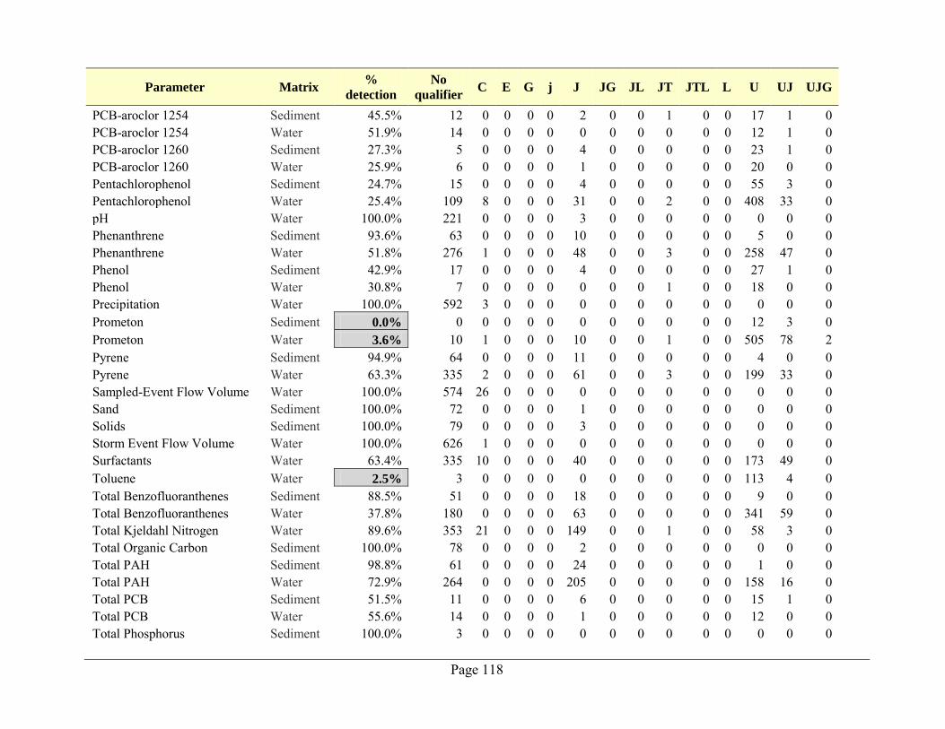
Page 118

Parameter Matrix %

detection

No


PCB-aroclor 1254 Sediment 45.5% 12 0 0 0 0 2 0 0 1 0 0 17 1 0 PCB-aroclor 1254 Water 51.9% 14 0 0 0 0 0 0 0 0 0 0 12 1 0 PCB-aroclor 1260 Sediment 27.3% 5 0 0 0 0 4 0 0 0 0 0 23 1 0 PCB-aroclor 1260 Water 25.9% 6 0 0 0 0 1 0 0 0 0 0 20 0 0 Pentachlorophenol Sediment 24.7% 15 0 0 0 0 4 0 0 0 0 0 55 3 0 Pentachlorophenol Water 25.4% 109 8 0 0 0 31 0 0 2 0 0 408 33 0 pH Water 100.0% 221 0 0 0 0 3 0 0 0 0 0 0 0 0 Phenanthrene Sediment 93.6% 63 0 0 0 0 10 0 0 0 0 0 5 0 0 Phenanthrene Water 51.8% 276 1 0 0 0 48 0 0 3 0 0 258 47 0 Phenol Sediment 42.9% 17 0 0 0 0 4 0 0 0 0 0 27 1 0 Phenol Water 30.8% 7 0 0 0 0 0 0 0 1 0 0 18 0 0 Precipitation Water 100.0% 592 3 0 0 0 0 0 0 0 0 0 0 0 0 Prometon Sediment 0.0% 0 0 0 0 0 0 0 0 0 0 0 12 3 0 Prometon Water 3.6% 10 1 0 0 0 10 0 0 1 0 0 505 78 2 Pyrene Sediment 94.9% 64 0 0 0 0 11 0 0 0 0 0 4 0 0 Pyrene Water 63.3% 335 2 0 0 0 61 0 0 3 0 0 199 33 0 Sampled-Event Flow Volume Water 100.0% 574 26 0 0 0 0 0 0 0 0 0 0 0 0 Sand Sediment 100.0% 72 0 0 0 0 1 0 0 0 0 0 0 0 0 Solids Sediment 100.0% 79 0 0 0 0 3 0 0 0 0 0 0 0 0 Storm Event Flow Volume Water 100.0% 626 1 0 0 0 0 0 0 0 0 0 0 0 0 Surfactants Water 63.4% 335 10 0 0 0 40 0 0 0 0 0 173 49 0 Toluene Water 2.5% 3 0 0 0 0 0 0 0 0 0 0 113 4 0 Total Benzofluoranthenes Sediment 88.5% 51 0 0 0 0 18 0 0 0 0 0 9 0 0 Total Benzofluoranthenes Water 37.8% 180 0 0 0 0 63 0 0 0 0 0 341 59 0 Total Kjeldahl Nitrogen Water 89.6% 353 21 0 0 0 149 0 0 1 0 0 58 3 0 Total Organic Carbon Sediment 100.0% 78 0 0 0 0 2 0 0 0 0 0 0 0 0 Total PAH Sediment 98.8% 61 0 0 0 0 24 0 0 0 0 0 1 0 0 Total PAH Water 72.9% 264 0 0 0 0 205 0 0 0 0 0 158 16 0 Total PCB Sediment 51.5% 11 0 0 0 0 6 0 0 0 0 0 15 1 0 Total PCB Water 55.6% 14 0 0 0 0 1 0 0 0 0 0 12 0 0 Total Phosphorus Sediment 100.0% 3 0 0 0 0 0 0 0 0 0 0 0 0 0

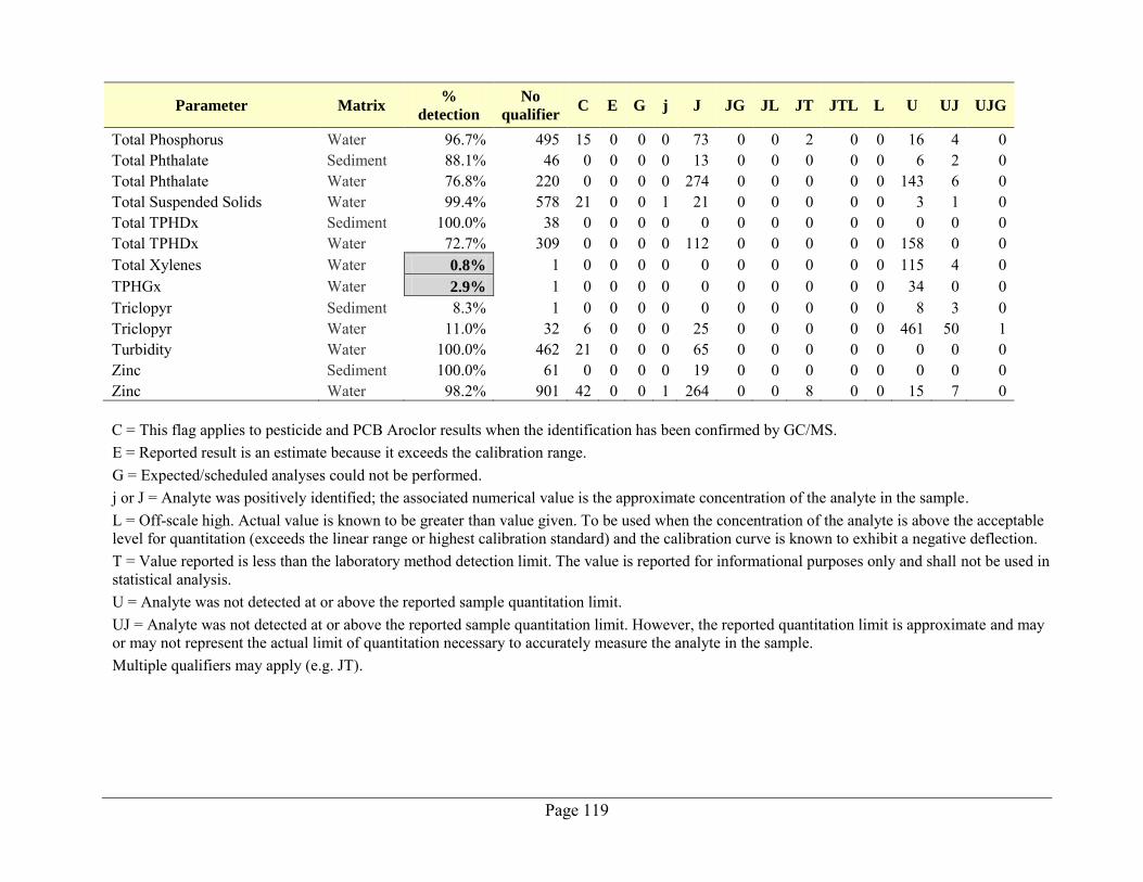
Page 119

Parameter Matrix %

detection

No


Total Phosphorus Water 96.7% 495 15 0 0 0 73 0 0 2 0 0 16 4 0 Total Phthalate Sediment 88.1% 46 0 0 0 0 13 0 0 0 0 0 6 2 0 Total Phthalate Water 76.8% 220 0 0 0 0 274 0 0 0 0 0 143 6 0 Total Suspended Solids Water 99.4% 578 21 0 0 1 21 0 0 0 0 0 3 1 0 Total TPHDx Sediment 100.0% 38 0 0 0 0 0 0 0 0 0 0 0 0 0 Total TPHDx Water 72.7% 309 0 0 0 0 112 0 0 0 0 0 158 0 0 Total Xylenes Water 0.8% 1 0 0 0 0 0 0 0 0 0 0 115 4 0 TPHGx Water 2.9% 1 0 0 0 0 0 0 0 0 0 0 34 0 0 Triclopyr Sediment 8.3% 1 0 0 0 0 0 0 0 0 0 0 8 3 0 Triclopyr Water 11.0% 32 6 0 0 0 25 0 0 0 0 0 461 50 1 Turbidity Water 100.0% 462 21 0 0 0 65 0 0 0 0 0 0 0 0 Zinc Sediment 100.0% 61 0 0 0 0 19 0 0 0 0 0 0 0 0 Zinc Water 98.2% 901 42 0 0 1 264 0 0 8 0 0 15 7 0

C = This flag applies to pesticide and PCB Aroclor results when the identification has been confirmed by GC/MS. E = Reported result is an estimate because it exceeds the calibration range. G = Expected/scheduled analyses could not be performed. j or J = Analyte was positively identified; the associated numerical value is the approximate concentration of the analyte in the sample. L = Off-scale high. Actual value is known to be greater than value given. To be used when the concentration of the analyte is above the acceptable level for quantitation (exceeds the linear range or highest calibration standard) and the calibration curve is known to exhibit a negative deflection. T = Value reported is less than the laboratory method detection limit. The value is reported for informational purposes only and shall not be used in statistical analysis. U = Analyte was not detected at or above the reported sample quantitation limit. UJ = Analyte was not detected at or above the reported sample quantitation limit. However, the reported quantitation limit is approximate and may or may not represent the actual limit of quantitation necessary to accurately measure the analyte in the sample. Multiple qualifiers may apply (e.g. JT).

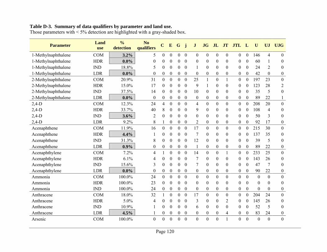
Page 120

Table D-3. Summary of data qualifiers by parameter and land use.

Those parameters with < 5% detection are highlighted with a gray-shaded box.

Parameter Land

use

%

detection

No

qualifiers C E G j J JG JL JT JTL L U UJ UJG

1-Methylnaphthalene COM 3.2% 5 0 0 0 0 0 0 0 0 0 0 146 4 0 1-Methylnaphthalene HDR 0.0% 0 0 0 0 0 0 0 0 0 0 0 60 1 0 1-Methylnaphthalene IND 18.8% 5 0 0 0 0 1 0 0 0 0 0 24 2 0 1-Methylnaphthalene LDR 0.0% 0 0 0 0 0 0 0 0 0 0 0 42 0 0 2-Methylnaphthalene COM 20.9% 31 0 0 0 0 25 1 0 1 0 0 197 23 0 2-Methylnaphthalene HDR 15.0% 17 0 0 0 0 9 1 0 0 0 0 123 28 2 2-Methylnaphthalene IND 37.5% 14 0 0 0 0 10 0 0 0 0 0 35 5 0 2-Methylnaphthalene LDR 0.0% 0 0 0 0 0 0 0 0 0 0 0 89 22 1 2,4-D COM 12.3% 24 4 0 0 0 4 0 0 0 0 0 208 20 0 2,4-D HDR 33.7% 40 8 0 0 0 9 0 0 0 0 0 108 4 0 2,4-D IND 3.6% 2 0 0 0 0 0 0 0 0 0 0 50 3 0 2,4-D LDR 9.2% 8 1 0 0 0 2 0 0 0 0 0 92 17 0 Acenaphthene COM 11.9% 16 0 0 0 0 17 0 0 0 0 0 215 30 0 Acenaphthene HDR 4.4% 1 0 0 0 0 7 0 0 0 0 0 137 35 0 Acenaphthene IND 31.3% 8 0 0 0 0 12 0 0 0 0 0 39 5 0 Acenaphthene LDR 0.9% 0 0 0 0 0 1 0 0 0 0 0 89 22 0 Acenaphthylene COM 7.2% 4 1 0 0 0 14 0 0 1 0 0 233 25 0 Acenaphthylene HDR 6.1% 4 0 0 0 0 7 0 0 0 0 0 143 26 0 Acenaphthylene IND 15.6% 3 0 0 0 0 7 0 0 0 0 0 47 7 0 Acenaphthylene LDR 0.0% 0 0 0 0 0 0 0 0 0 0 0 90 22 0 Ammonia COM 100.0% 24 0 0 0 0 0 0 0 0 0 0 0 0 0 Ammonia HDR 100.0% 23 0 0 0 0 0 0 0 0 0 0 0 0 0 Ammonia IND 100.0% 24 0 0 0 0 0 0 0 0 0 0 0 0 0 Anthracene COM 18.0% 32 1 0 0 0 17 0 0 0 0 0 204 24 0 Anthracene HDR 5.0% 4 0 0 0 0 3 0 0 2 0 0 145 26 0 Anthracene IND 10.9% 1 0 0 0 0 6 0 0 0 0 0 52 5 0 Anthracene LDR 4.5% 1 0 0 0 0 0 0 0 4 0 0 83 24 0 Arsenic COM 100.0% 0 0 0 0 0 0 0 0 1 0 0 0 0 0

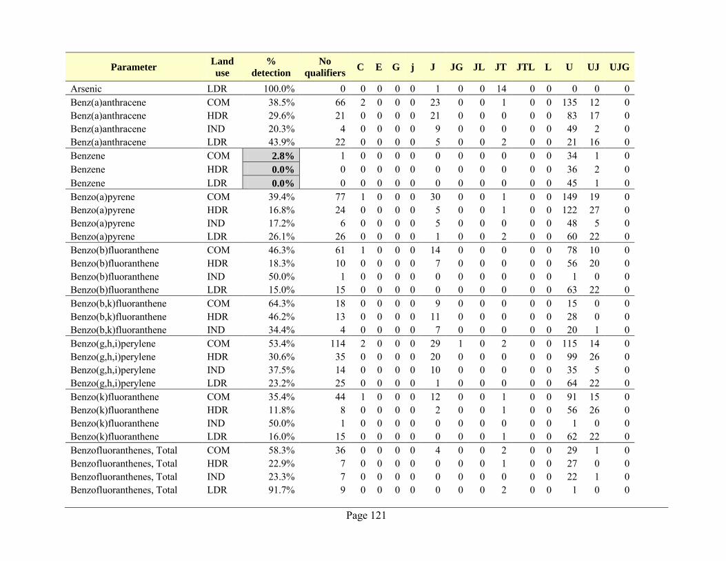
Page 121

Parameter Land

use

%

detection

No


Arsenic LDR 100.0% 0 0 0 0 0 1 0 0 14 0 0 0 0 0 Benz(a)anthracene COM 38.5% 66 2 0 0 0 23 0 0 1 0 0 135 12 0 Benz(a)anthracene HDR 29.6% 21 0 0 0 0 21 0 0 0 0 0 83 17 0 Benz(a)anthracene IND 20.3% 4 0 0 0 0 9 0 0 0 0 0 49 2 0 Benz(a)anthracene LDR 43.9% 22 0 0 0 0 5 0 0 2 0 0 21 16 0 Benzene COM 2.8% 1 0 0 0 0 0 0 0 0 0 0 34 1 0 Benzene HDR 0.0% 0 0 0 0 0 0 0 0 0 0 0 36 2 0 Benzene LDR 0.0% 0 0 0 0 0 0 0 0 0 0 0 45 1 0 Benzo(a)pyrene COM 39.4% 77 1 0 0 0 30 0 0 1 0 0 149 19 0 Benzo(a)pyrene HDR 16.8% 24 0 0 0 0 5 0 0 1 0 0 122 27 0 Benzo(a)pyrene IND 17.2% 6 0 0 0 0 5 0 0 0 0 0 48 5 0 Benzo(a)pyrene LDR 26.1% 26 0 0 0 0 1 0 0 2 0 0 60 22 0 Benzo(b)fluoranthene COM 46.3% 61 1 0 0 0 14 0 0 0 0 0 78 10 0 Benzo(b)fluoranthene HDR 18.3% 10 0 0 0 0 7 0 0 0 0 0 56 20 0 Benzo(b)fluoranthene IND 50.0% 1 0 0 0 0 0 0 0 0 0 0 1 0 0 Benzo(b)fluoranthene LDR 15.0% 15 0 0 0 0 0 0 0 0 0 0 63 22 0 Benzo(b,k)fluoranthene COM 64.3% 18 0 0 0 0 9 0 0 0 0 0 15 0 0 Benzo(b,k)fluoranthene HDR 46.2% 13 0 0 0 0 11 0 0 0 0 0 28 0 0 Benzo(b,k)fluoranthene IND 34.4% 4 0 0 0 0 7 0 0 0 0 0 20 1 0 Benzo(g,h,i)perylene COM 53.4% 114 2 0 0 0 29 1 0 2 0 0 115 14 0 Benzo(g,h,i)perylene HDR 30.6% 35 0 0 0 0 20 0 0 0 0 0 99 26 0 Benzo(g,h,i)perylene IND 37.5% 14 0 0 0 0 10 0 0 0 0 0 35 5 0 Benzo(g,h,i)perylene LDR 23.2% 25 0 0 0 0 1 0 0 0 0 0 64 22 0 Benzo(k)fluoranthene COM 35.4% 44 1 0 0 0 12 0 0 1 0 0 91 15 0 Benzo(k)fluoranthene HDR 11.8% 8 0 0 0 0 2 0 0 1 0 0 56 26 0 Benzo(k)fluoranthene IND 50.0% 1 0 0 0 0 0 0 0 0 0 0 1 0 0 Benzo(k)fluoranthene LDR 16.0% 15 0 0 0 0 0 0 0 1 0 0 62 22 0 Benzofluoranthenes, Total COM 58.3% 36 0 0 0 0 4 0 0 2 0 0 29 1 0 Benzofluoranthenes, Total HDR 22.9% 7 0 0 0 0 0 0 0 1 0 0 27 0 0 Benzofluoranthenes, Total IND 23.3% 7 0 0 0 0 0 0 0 0 0 0 22 1 0 Benzofluoranthenes, Total LDR 91.7% 9 0 0 0 0 0 0 0 2 0 0 1 0 0

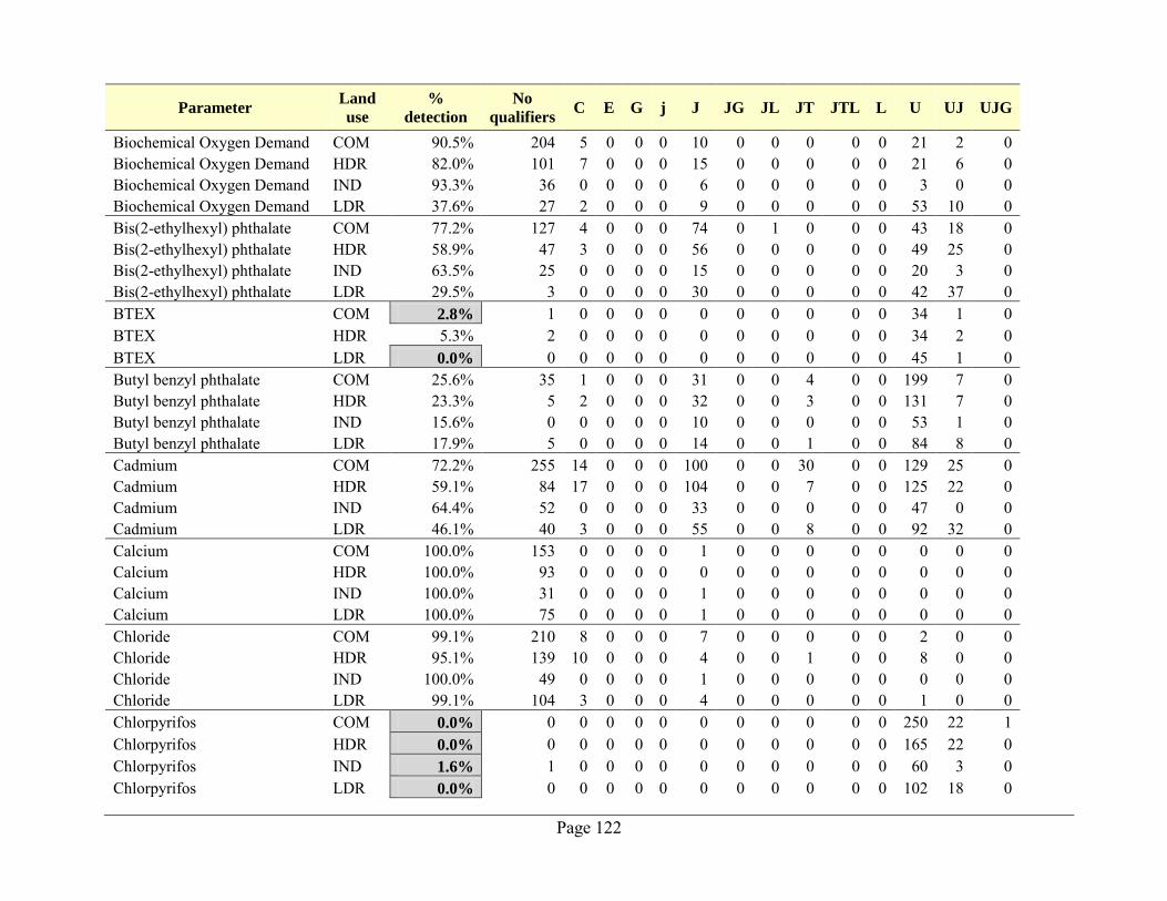
Page 122

Parameter Land

use

%

detection

No


Biochemical Oxygen Demand COM 90.5% 204 5 0 0 0 10 0 0 0 0 0 21 2 0 Biochemical Oxygen Demand HDR 82.0% 101 7 0 0 0 15 0 0 0 0 0 21 6 0 Biochemical Oxygen Demand IND 93.3% 36 0 0 0 0 6 0 0 0 0 0 3 0 0 Biochemical Oxygen Demand LDR 37.6% 27 2 0 0 0 9 0 0 0 0 0 53 10 0 Bis(2-ethylhexyl) phthalate COM 77.2% 127 4 0 0 0 74 0 1 0 0 0 43 18 0 Bis(2-ethylhexyl) phthalate HDR 58.9% 47 3 0 0 0 56 0 0 0 0 0 49 25 0 Bis(2-ethylhexyl) phthalate IND 63.5% 25 0 0 0 0 15 0 0 0 0 0 20 3 0 Bis(2-ethylhexyl) phthalate LDR 29.5% 3 0 0 0 0 30 0 0 0 0 0 42 37 0 BTEX COM 2.8% 1 0 0 0 0 0 0 0 0 0 0 34 1 0 BTEX HDR 5.3% 2 0 0 0 0 0 0 0 0 0 0 34 2 0 BTEX LDR 0.0% 0 0 0 0 0 0 0 0 0 0 0 45 1 0 Butyl benzyl phthalate COM 25.6% 35 1 0 0 0 31 0 0 4 0 0 199 7 0 Butyl benzyl phthalate HDR 23.3% 5 2 0 0 0 32 0 0 3 0 0 131 7 0 Butyl benzyl phthalate IND 15.6% 0 0 0 0 0 10 0 0 0 0 0 53 1 0 Butyl benzyl phthalate LDR 17.9% 5 0 0 0 0 14 0 0 1 0 0 84 8 0 Cadmium COM 72.2% 255 14 0 0 0 100 0 0 30 0 0 129 25 0 Cadmium HDR 59.1% 84 17 0 0 0 104 0 0 7 0 0 125 22 0 Cadmium IND 64.4% 52 0 0 0 0 33 0 0 0 0 0 47 0 0 Cadmium LDR 46.1% 40 3 0 0 0 55 0 0 8 0 0 92 32 0 Calcium COM 100.0% 153 0 0 0 0 1 0 0 0 0 0 0 0 0 Calcium HDR 100.0% 93 0 0 0 0 0 0 0 0 0 0 0 0 0 Calcium IND 100.0% 31 0 0 0 0 1 0 0 0 0 0 0 0 0 Calcium LDR 100.0% 75 0 0 0 0 1 0 0 0 0 0 0 0 0 Chloride COM 99.1% 210 8 0 0 0 7 0 0 0 0 0 2 0 0 Chloride HDR 95.1% 139 10 0 0 0 4 0 0 1 0 0 8 0 0 Chloride IND 100.0% 49 0 0 0 0 1 0 0 0 0 0 0 0 0 Chloride LDR 99.1% 104 3 0 0 0 4 0 0 0 0 0 1 0 0 Chlorpyrifos COM 0.0% 0 0 0 0 0 0 0 0 0 0 0 250 22 1 Chlorpyrifos HDR 0.0% 0 0 0 0 0 0 0 0 0 0 0 165 22 0 Chlorpyrifos IND 1.6% 1 0 0 0 0 0 0 0 0 0 0 60 3 0 Chlorpyrifos LDR 0.0% 0 0 0 0 0 0 0 0 0 0 0 102 18 0

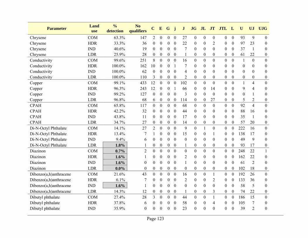
Page 123

Parameter Land

use

%

detection

No


Chrysene COM 63.3% 147 2 0 0 0 27 0 0 0 0 0 93 9 0 Chrysene HDR 33.3% 36 0 0 0 0 22 0 0 2 0 0 97 23 0 Chrysene IND 40.6% 19 0 0 0 0 7 0 0 0 0 0 37 1 0 Chrysene LDR 25.9% 28 0 0 0 0 1 0 0 0 0 0 61 22 0 Conductivity COM 99.6% 251 8 0 0 0 16 0 0 0 0 0 1 0 0 Conductivity HDR 100.0% 162 10 0 0 1 7 0 0 0 0 0 0 0 0 Conductivity IND 100.0% 62 0 0 0 0 4 0 0 0 0 0 0 0 0 Conductivity LDR 100.0% 110 3 0 0 0 2 0 0 0 0 0 0 0 0 Copper COM 99.1% 433 12 0 0 0 102 0 0 0 0 0 1 4 0 Copper HDR 96.3% 243 12 0 0 1 66 0 0 14 0 0 9 4 0 Copper IND 99.2% 127 0 0 0 0 3 0 0 0 0 0 0 1 0 Copper LDR 96.8% 68 6 0 0 0 114 0 0 27 0 0 5 2 0 CPAH COM 65.8% 117 0 0 0 0 68 0 0 0 0 0 92 4 0 CPAH HDR 42.2% 32 0 0 0 0 44 0 0 0 0 0 88 16 0 CPAH IND 43.8% 11 0 0 0 0 17 0 0 0 0 0 35 1 0 CPAH LDR 34.7% 27 0 0 0 0 14 0 0 0 0 0 57 20 0 Di-N-Octyl Phthalate COM 14.1% 27 2 0 0 0 9 0 1 0 0 0 222 16 0 Di-N-Octyl Phthalate HDR 13.4% 7 1 0 0 0 15 0 0 1 0 0 138 17 0 Di-N-Octyl Phthalate IND 9.4% 6 0 0 0 0 0 0 0 0 0 0 49 9 0 Di-N-Octyl Phthalate LDR 1.8% 1 0 0 0 0 1 0 0 0 0 0 93 17 0 Diazinon COM 0.7% 2 0 0 0 0 0 0 0 0 0 0 248 22 1 Diazinon HDR 1.6% 1 0 0 0 0 2 0 0 0 0 0 162 22 0 Diazinon IND 1.6% 0 0 0 0 0 1 0 0 0 0 0 61 2 0 Diazinon LDR 0.0% 0 0 0 0 0 0 0 0 0 0 0 102 18 0 Dibenzo(a,h)anthracene COM 21.6% 43 0 0 0 0 16 0 0 1 0 0 192 26 0 Dibenzo(a,h)anthracene HDR 6.1% 7 0 0 0 0 2 0 0 2 0 0 133 36 0 Dibenzo(a,h)anthracene IND 1.6% 1 0 0 0 0 0 0 0 0 0 0 58 5 0 Dibenzo(a,h)anthracene LDR 14.3% 12 0 0 0 0 1 0 0 3 0 0 74 22 0 Dibutyl phthalate COM 27.4% 28 3 0 0 0 44 0 0 1 0 0 186 15 0 Dibutyl phthalate HDR 37.8% 6 0 0 0 0 58 0 0 4 0 0 105 7 0 Dibutyl phthalate IND 35.9% 0 0 0 0 0 23 0 0 0 0 0 39 2 0

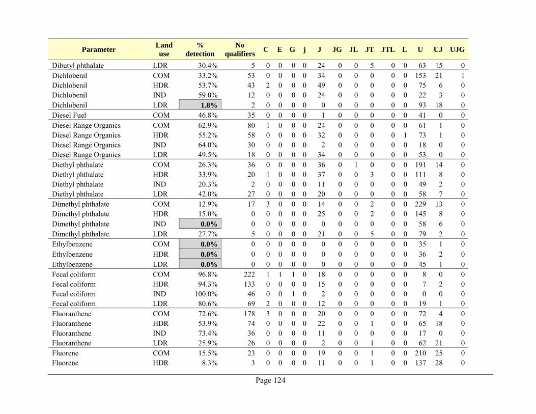
Page 124

Parameter Land

use

%

detection

No


Dibutyl phthalate LDR 30.4% 5 0 0 0 0 24 0 0 5 0 0 63 15 0 Dichlobenil COM 33.2% 53 0 0 0 0 34 0 0 0 0 0 153 21 1 Dichlobenil HDR 53.7% 43 2 0 0 0 49 0 0 0 0 0 75 6 0 Dichlobenil IND 59.0% 12 0 0 0 0 24 0 0 0 0 0 22 3 0 Dichlobenil LDR 1.8% 2 0 0 0 0 0 0 0 0 0 0 93 18 0 Diesel Fuel COM 46.8% 35 0 0 0 0 1 0 0 0 0 0 41 0 0 Diesel Range Organics COM 62.9% 80 1 0 0 0 24 0 0 0 0 0 61 1 0 Diesel Range Organics HDR 55.2% 58 0 0 0 0 32 0 0 0 0 1 73 1 0 Diesel Range Organics IND 64.0% 30 0 0 0 0 2 0 0 0 0 0 18 0 0 Diesel Range Organics LDR 49.5% 18 0 0 0 0 34 0 0 0 0 0 53 0 0 Diethyl phthalate COM 26.3% 36 0 0 0 0 36 0 1 0 0 0 191 14 0 Diethyl phthalate HDR 33.9% 20 1 0 0 0 37 0 0 3 0 0 111 8 0 Diethyl phthalate IND 20.3% 2 0 0 0 0 11 0 0 0 0 0 49 2 0 Diethyl phthalate LDR 42.0% 27 0 0 0 0 20 0 0 0 0 0 58 7 0 Dimethyl phthalate COM 12.9% 17 3 0 0 0 14 0 0 2 0 0 229 13 0 Dimethyl phthalate HDR 15.0% 0 0 0 0 0 25 0 0 2 0 0 145 8 0 Dimethyl phthalate IND 0.0% 0 0 0 0 0 0 0 0 0 0 0 58 6 0 Dimethyl phthalate LDR 27.7% 5 0 0 0 0 21 0 0 5 0 0 79 2 0 Ethylbenzene COM 0.0% 0 0 0 0 0 0 0 0 0 0 0 35 1 0 Ethylbenzene HDR 0.0% 0 0 0 0 0 0 0 0 0 0 0 36 2 0 Ethylbenzene LDR 0.0% 0 0 0 0 0 0 0 0 0 0 0 45 1 0 Fecal coliform COM 96.8% 222 1 1 1 0 18 0 0 0 0 0 8 0 0 Fecal coliform HDR 94.3% 133 0 0 0 0 15 0 0 0 0 0 7 2 0 Fecal coliform IND 100.0% 46 0 0 1 0 2 0 0 0 0 0 0 0 0 Fecal coliform LDR 80.6% 69 2 0 0 0 12 0 0 0 0 0 19 1 0 Fluoranthene COM 72.6% 178 3 0 0 0 20 0 0 0 0 0 72 4 0 Fluoranthene HDR 53.9% 74 0 0 0 0 22 0 0 1 0 0 65 18 0 Fluoranthene IND 73.4% 36 0 0 0 0 11 0 0 0 0 0 17 0 0 Fluoranthene LDR 25.9% 26 0 0 0 0 2 0 0 1 0 0 62 21 0 Fluorene COM 15.5% 23 0 0 0 0 19 0 0 1 0 0 210 25 0 Fluorene HDR 8.3% 3 0 0 0 0 11 0 0 1 0 0 137 28 0

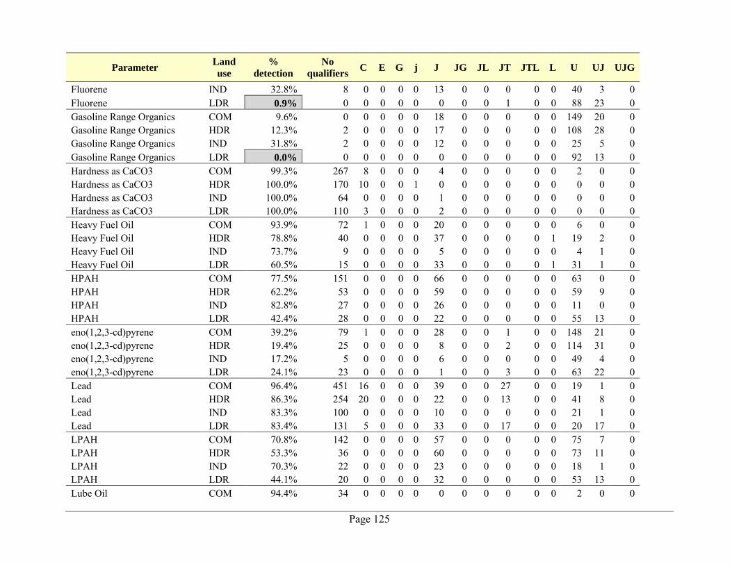
Page 125

Parameter Land

use

%

detection

No


Fluorene IND 32.8% 8 0 0 0 0 13 0 0 0 0 0 40 3 0 Fluorene LDR 0.9% 0 0 0 0 0 0 0 0 1 0 0 88 23 0 Gasoline Range Organics COM 9.6% 0 0 0 0 0 18 0 0 0 0 0 149 20 0 Gasoline Range Organics HDR 12.3% 2 0 0 0 0 17 0 0 0 0 0 108 28 0 Gasoline Range Organics IND 31.8% 2 0 0 0 0 12 0 0 0 0 0 25 5 0 Gasoline Range Organics LDR 0.0% 0 0 0 0 0 0 0 0 0 0 0 92 13 0 Hardness as CaCO3 COM 99.3% 267 8 0 0 0 4 0 0 0 0 0 2 0 0 Hardness as CaCO3 HDR 100.0% 170 10 0 0 1 0 0 0 0 0 0 0 0 0 Hardness as CaCO3 IND 100.0% 64 0 0 0 0 1 0 0 0 0 0 0 0 0 Hardness as CaCO3 LDR 100.0% 110 3 0 0 0 2 0 0 0 0 0 0 0 0 Heavy Fuel Oil COM 93.9% 72 1 0 0 0 20 0 0 0 0 0 6 0 0 Heavy Fuel Oil HDR 78.8% 40 0 0 0 0 37 0 0 0 0 1 19 2 0 Heavy Fuel Oil IND 73.7% 9 0 0 0 0 5 0 0 0 0 0 4 1 0 Heavy Fuel Oil LDR 60.5% 15 0 0 0 0 33 0 0 0 0 1 31 1 0 HPAH COM 77.5% 151 0 0 0 0 66 0 0 0 0 0 63 0 0 HPAH HDR 62.2% 53 0 0 0 0 59 0 0 0 0 0 59 9 0 HPAH IND 82.8% 27 0 0 0 0 26 0 0 0 0 0 11 0 0 HPAH LDR 42.4% 28 0 0 0 0 22 0 0 0 0 0 55 13 0 eno(1,2,3-cd)pyrene COM 39.2% 79 1 0 0 0 28 0 0 1 0 0 148 21 0 eno(1,2,3-cd)pyrene HDR 19.4% 25 0 0 0 0 8 0 0 2 0 0 114 31 0 eno(1,2,3-cd)pyrene IND 17.2% 5 0 0 0 0 6 0 0 0 0 0 49 4 0 eno(1,2,3-cd)pyrene LDR 24.1% 23 0 0 0 0 1 0 0 3 0 0 63 22 0 Lead COM 96.4% 451 16 0 0 0 39 0 0 27 0 0 19 1 0 Lead HDR 86.3% 254 20 0 0 0 22 0 0 13 0 0 41 8 0 Lead IND 83.3% 100 0 0 0 0 10 0 0 0 0 0 21 1 0 Lead LDR 83.4% 131 5 0 0 0 33 0 0 17 0 0 20 17 0 LPAH COM 70.8% 142 0 0 0 0 57 0 0 0 0 0 75 7 0 LPAH HDR 53.3% 36 0 0 0 0 60 0 0 0 0 0 73 11 0 LPAH IND 70.3% 22 0 0 0 0 23 0 0 0 0 0 18 1 0 LPAH LDR 44.1% 20 0 0 0 0 32 0 0 0 0 0 53 13 0 Lube Oil COM 94.4% 34 0 0 0 0 0 0 0 0 0 0 2 0 0

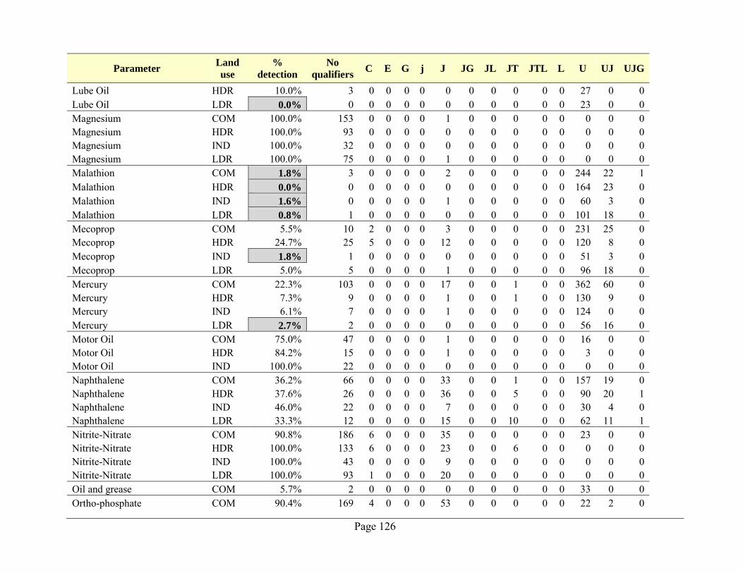
Page 126

Parameter Land

use

%

detection

No


Lube Oil HDR 10.0% 3 0 0 0 0 0 0 0 0 0 0 27 0 0 Lube Oil LDR 0.0% 0 0 0 0 0 0 0 0 0 0 0 23 0 0 Magnesium COM 100.0% 153 0 0 0 0 1 0 0 0 0 0 0 0 0 Magnesium HDR 100.0% 93 0 0 0 0 0 0 0 0 0 0 0 0 0 Magnesium IND 100.0% 32 0 0 0 0 0 0 0 0 0 0 0 0 0 Magnesium LDR 100.0% 75 0 0 0 0 1 0 0 0 0 0 0 0 0 Malathion COM 1.8% 3 0 0 0 0 2 0 0 0 0 0 244 22 1 Malathion HDR 0.0% 0 0 0 0 0 0 0 0 0 0 0 164 23 0 Malathion IND 1.6% 0 0 0 0 0 1 0 0 0 0 0 60 3 0 Malathion LDR 0.8% 1 0 0 0 0 0 0 0 0 0 0 101 18 0 Mecoprop COM 5.5% 10 2 0 0 0 3 0 0 0 0 0 231 25 0 Mecoprop HDR 24.7% 25 5 0 0 0 12 0 0 0 0 0 120 8 0 Mecoprop IND 1.8% 1 0 0 0 0 0 0 0 0 0 0 51 3 0 Mecoprop LDR 5.0% 5 0 0 0 0 1 0 0 0 0 0 96 18 0 Mercury COM 22.3% 103 0 0 0 0 17 0 0 1 0 0 362 60 0 Mercury HDR 7.3% 9 0 0 0 0 1 0 0 1 0 0 130 9 0 Mercury IND 6.1% 7 0 0 0 0 1 0 0 0 0 0 124 0 0 Mercury LDR 2.7% 2 0 0 0 0 0 0 0 0 0 0 56 16 0 Motor Oil COM 75.0% 47 0 0 0 0 1 0 0 0 0 0 16 0 0 Motor Oil HDR 84.2% 15 0 0 0 0 1 0 0 0 0 0 3 0 0 Motor Oil IND 100.0% 22 0 0 0 0 0 0 0 0 0 0 0 0 0 Naphthalene COM 36.2% 66 0 0 0 0 33 0 0 1 0 0 157 19 0 Naphthalene HDR 37.6% 26 0 0 0 0 36 0 0 5 0 0 90 20 1 Naphthalene IND 46.0% 22 0 0 0 0 7 0 0 0 0 0 30 4 0 Naphthalene LDR 33.3% 12 0 0 0 0 15 0 0 10 0 0 62 11 1 Nitrite-Nitrate COM 90.8% 186 6 0 0 0 35 0 0 0 0 0 23 0 0 Nitrite-Nitrate HDR 100.0% 133 6 0 0 0 23 0 0 6 0 0 0 0 0 Nitrite-Nitrate IND 100.0% 43 0 0 0 0 9 0 0 0 0 0 0 0 0 Nitrite-Nitrate LDR 100.0% 93 1 0 0 0 20 0 0 0 0 0 0 0 0 Oil and grease COM 5.7% 2 0 0 0 0 0 0 0 0 0 0 33 0 0 Ortho-phosphate COM 90.4% 169 4 0 0 0 53 0 0 0 0 0 22 2 0

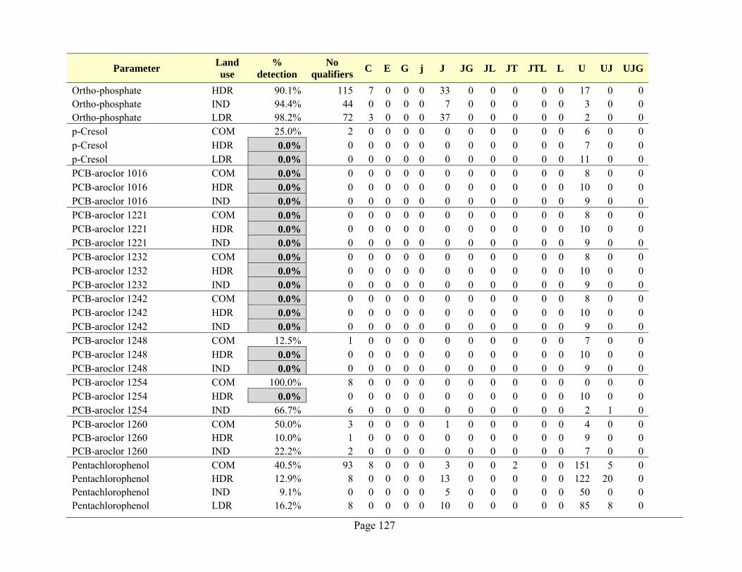
Page 127

Parameter Land

use

%

detection

No


Ortho-phosphate HDR 90.1% 115 7 0 0 0 33 0 0 0 0 0 17 0 0 Ortho-phosphate IND 94.4% 44 0 0 0 0 7 0 0 0 0 0 3 0 0 Ortho-phosphate LDR 98.2% 72 3 0 0 0 37 0 0 0 0 0 2 0 0 p-Cresol COM 25.0% 2 0 0 0 0 0 0 0 0 0 0 6 0 0 p-Cresol HDR 0.0% 0 0 0 0 0 0 0 0 0 0 0 7 0 0 p-Cresol LDR 0.0% 0 0 0 0 0 0 0 0 0 0 0 11 0 0 PCB-aroclor 1016 COM 0.0% 0 0 0 0 0 0 0 0 0 0 0 8 0 0 PCB-aroclor 1016 HDR 0.0% 0 0 0 0 0 0 0 0 0 0 0 10 0 0 PCB-aroclor 1016 IND 0.0% 0 0 0 0 0 0 0 0 0 0 0 9 0 0 PCB-aroclor 1221 COM 0.0% 0 0 0 0 0 0 0 0 0 0 0 8 0 0 PCB-aroclor 1221 HDR 0.0% 0 0 0 0 0 0 0 0 0 0 0 10 0 0 PCB-aroclor 1221 IND 0.0% 0 0 0 0 0 0 0 0 0 0 0 9 0 0 PCB-aroclor 1232 COM 0.0% 0 0 0 0 0 0 0 0 0 0 0 8 0 0 PCB-aroclor 1232 HDR 0.0% 0 0 0 0 0 0 0 0 0 0 0 10 0 0 PCB-aroclor 1232 IND 0.0% 0 0 0 0 0 0 0 0 0 0 0 9 0 0 PCB-aroclor 1242 COM 0.0% 0 0 0 0 0 0 0 0 0 0 0 8 0 0 PCB-aroclor 1242 HDR 0.0% 0 0 0 0 0 0 0 0 0 0 0 10 0 0 PCB-aroclor 1242 IND 0.0% 0 0 0 0 0 0 0 0 0 0 0 9 0 0 PCB-aroclor 1248 COM 12.5% 1 0 0 0 0 0 0 0 0 0 0 7 0 0 PCB-aroclor 1248 HDR 0.0% 0 0 0 0 0 0 0 0 0 0 0 10 0 0 PCB-aroclor 1248 IND 0.0% 0 0 0 0 0 0 0 0 0 0 0 9 0 0 PCB-aroclor 1254 COM 100.0% 8 0 0 0 0 0 0 0 0 0 0 0 0 0 PCB-aroclor 1254 HDR 0.0% 0 0 0 0 0 0 0 0 0 0 0 10 0 0 PCB-aroclor 1254 IND 66.7% 6 0 0 0 0 0 0 0 0 0 0 2 1 0 PCB-aroclor 1260 COM 50.0% 3 0 0 0 0 1 0 0 0 0 0 4 0 0 PCB-aroclor 1260 HDR 10.0% 1 0 0 0 0 0 0 0 0 0 0 9 0 0 PCB-aroclor 1260 IND 22.2% 2 0 0 0 0 0 0 0 0 0 0 7 0 0 Pentachlorophenol COM 40.5% 93 8 0 0 0 3 0 0 2 0 0 151 5 0 Pentachlorophenol HDR 12.9% 8 0 0 0 0 13 0 0 0 0 0 122 20 0 Pentachlorophenol IND 9.1% 0 0 0 0 0 5 0 0 0 0 0 50 0 0 Pentachlorophenol LDR 16.2% 8 0 0 0 0 10 0 0 0 0 0 85 8 0

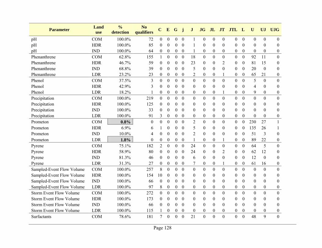
Page 128

Parameter Land

use

%

detection

No


pH COM 100.0% 72 0 0 0 0 1 0 0 0 0 0 0 0 0 pH HDR 100.0% 85 0 0 0 0 1 0 0 0 0 0 0 0 0 pH IND 100.0% 64 0 0 0 0 1 0 0 0 0 0 0 0 0 Phenanthrene COM 62.8% 155 1 0 0 0 18 0 0 0 0 0 92 11 0 Phenanthrene HDR 46.7% 59 0 0 0 0 23 0 0 2 0 0 81 15 0 Phenanthrene IND 68.8% 39 0 0 0 0 5 0 0 0 0 0 20 0 0 Phenanthrene LDR 23.2% 23 0 0 0 0 2 0 0 1 0 0 65 21 0 Phenol COM 37.5% 3 0 0 0 0 0 0 0 0 0 0 5 0 0 Phenol HDR 42.9% 3 0 0 0 0 0 0 0 0 0 0 4 0 0 Phenol LDR 18.2% 1 0 0 0 0 0 0 0 1 0 0 9 0 0 Precipitation COM 100.0% 219 0 0 0 0 0 0 0 0 0 0 0 0 0 Precipitation HDR 100.0% 125 0 0 0 0 0 0 0 0 0 0 0 0 0 Precipitation IND 100.0% 33 0 0 0 0 0 0 0 0 0 0 0 0 0 Precipitation LDR 100.0% 91 3 0 0 0 0 0 0 0 0 0 0 0 0 Prometon COM 0.8% 0 0 0 0 0 2 0 0 0 0 0 230 27 1 Prometon HDR 6.9% 6 1 0 0 0 5 0 0 0 0 0 135 26 1 Prometon IND 10.0% 4 0 0 0 0 2 0 0 0 0 0 51 3 0 Prometon LDR 1.8% 0 0 0 0 0 1 0 0 1 0 0 89 22 0 Pyrene COM 75.1% 182 2 0 0 0 24 0 0 0 0 0 64 5 0 Pyrene HDR 58.9% 80 0 0 0 0 24 0 0 2 0 0 62 12 0 Pyrene IND 81.3% 46 0 0 0 0 6 0 0 0 0 0 12 0 0 Pyrene LDR 31.3% 27 0 0 0 0 7 0 0 1 0 0 61 16 0 Sampled-Event Flow Volume COM 100.0% 257 8 0 0 0 0 0 0 0 0 0 0 0 0 Sampled-Event Flow Volume HDR 100.0% 154 10 0 0 0 0 0 0 0 0 0 0 0 0 Sampled-Event Flow Volume IND 100.0% 66 0 0 0 0 0 0 0 0 0 0 0 0 0 Sampled-Event Flow Volume LDR 100.0% 97 8 0 0 0 0 0 0 0 0 0 0 0 0 Storm Event Flow Volume COM 100.0% 272 0 0 0 0 0 0 0 0 0 0 0 0 0 Storm Event Flow Volume HDR 100.0% 173 0 0 0 0 0 0 0 0 0 0 0 0 0 Storm Event Flow Volume IND 100.0% 66 0 0 0 0 0 0 0 0 0 0 0 0 0 Storm Event Flow Volume LDR 100.0% 115 1 0 0 0 0 0 0 0 0 0 0 0 0 Surfactants COM 78.6% 181 7 0 0 0 21 0 0 0 0 0 48 9 0

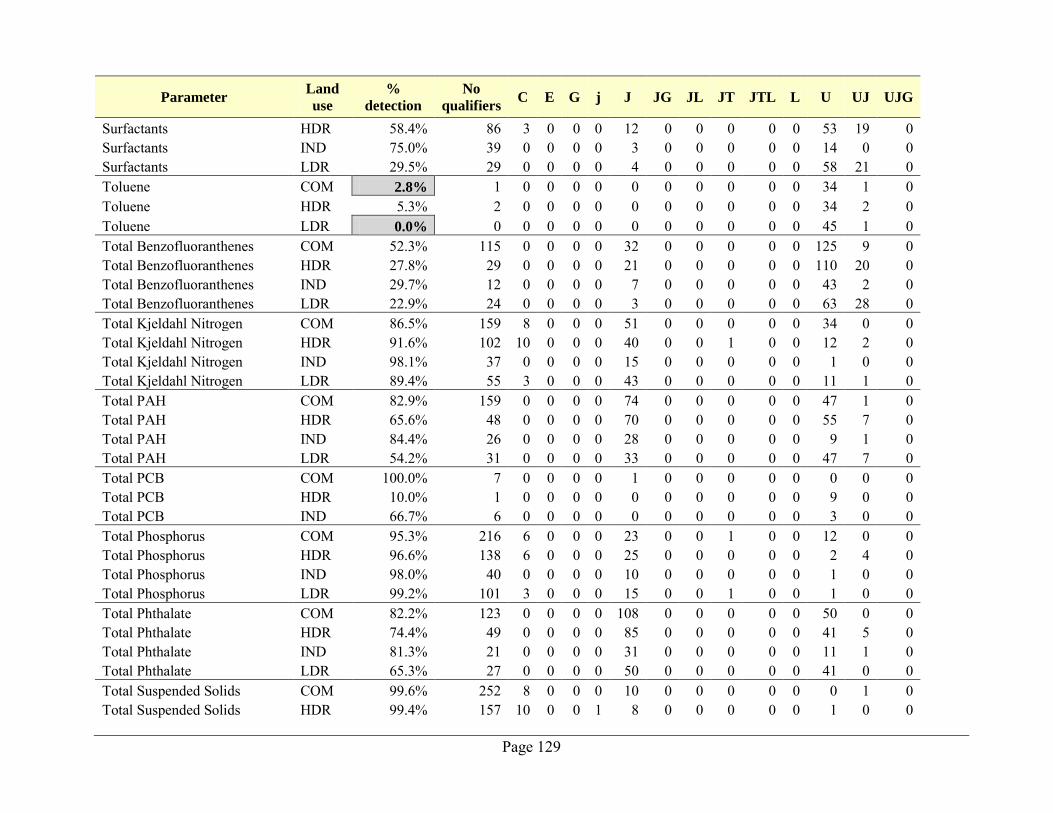
Page 129

Parameter Land

use

%

detection

No


Surfactants HDR 58.4% 86 3 0 0 0 12 0 0 0 0 0 53 19 0 Surfactants IND 75.0% 39 0 0 0 0 3 0 0 0 0 0 14 0 0 Surfactants LDR 29.5% 29 0 0 0 0 4 0 0 0 0 0 58 21 0 Toluene COM 2.8% 1 0 0 0 0 0 0 0 0 0 0 34 1 0 Toluene HDR 5.3% 2 0 0 0 0 0 0 0 0 0 0 34 2 0 Toluene LDR 0.0% 0 0 0 0 0 0 0 0 0 0 0 45 1 0 Total Benzofluoranthenes COM 52.3% 115 0 0 0 0 32 0 0 0 0 0 125 9 0 Total Benzofluoranthenes HDR 27.8% 29 0 0 0 0 21 0 0 0 0 0 110 20 0 Total Benzofluoranthenes IND 29.7% 12 0 0 0 0 7 0 0 0 0 0 43 2 0 Total Benzofluoranthenes LDR 22.9% 24 0 0 0 0 3 0 0 0 0 0 63 28 0 Total Kjeldahl Nitrogen COM 86.5% 159 8 0 0 0 51 0 0 0 0 0 34 0 0 Total Kjeldahl Nitrogen HDR 91.6% 102 10 0 0 0 40 0 0 1 0 0 12 2 0 Total Kjeldahl Nitrogen IND 98.1% 37 0 0 0 0 15 0 0 0 0 0 1 0 0 Total Kjeldahl Nitrogen LDR 89.4% 55 3 0 0 0 43 0 0 0 0 0 11 1 0 Total PAH COM 82.9% 159 0 0 0 0 74 0 0 0 0 0 47 1 0 Total PAH HDR 65.6% 48 0 0 0 0 70 0 0 0 0 0 55 7 0 Total PAH IND 84.4% 26 0 0 0 0 28 0 0 0 0 0 9 1 0 Total PAH LDR 54.2% 31 0 0 0 0 33 0 0 0 0 0 47 7 0 Total PCB COM 100.0% 7 0 0 0 0 1 0 0 0 0 0 0 0 0 Total PCB HDR 10.0% 1 0 0 0 0 0 0 0 0 0 0 9 0 0 Total PCB IND 66.7% 6 0 0 0 0 0 0 0 0 0 0 3 0 0 Total Phosphorus COM 95.3% 216 6 0 0 0 23 0 0 1 0 0 12 0 0 Total Phosphorus HDR 96.6% 138 6 0 0 0 25 0 0 0 0 0 2 4 0 Total Phosphorus IND 98.0% 40 0 0 0 0 10 0 0 0 0 0 1 0 0 Total Phosphorus LDR 99.2% 101 3 0 0 0 15 0 0 1 0 0 1 0 0 Total Phthalate COM 82.2% 123 0 0 0 0 108 0 0 0 0 0 50 0 0 Total Phthalate HDR 74.4% 49 0 0 0 0 85 0 0 0 0 0 41 5 0 Total Phthalate IND 81.3% 21 0 0 0 0 31 0 0 0 0 0 11 1 0 Total Phthalate LDR 65.3% 27 0 0 0 0 50 0 0 0 0 0 41 0 0 Total Suspended Solids COM 99.6% 252 8 0 0 0 10 0 0 0 0 0 0 1 0 Total Suspended Solids HDR 99.4% 157 10 0 0 1 8 0 0 0 0 0 1 0 0

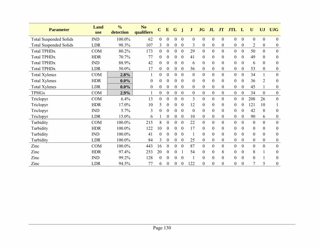
Page 130

Parameter Land

use

%

detection

No


Total Suspended Solids IND 100.0% 62 0 0 0 0 0 0 0 0 0 0 0 0 0 Total Suspended Solids LDR 98.3% 107 3 0 0 0 3 0 0 0 0 0 2 0 0 Total TPHDx COM 80.2% 173 0 0 0 0 29 0 0 0 0 0 50 0 0 Total TPHDx HDR 70.7% 77 0 0 0 0 41 0 0 0 0 0 49 0 0 Total TPHDx IND 88.9% 42 0 0 0 0 6 0 0 0 0 0 6 0 0 Total TPHDx LDR 50.0% 17 0 0 0 0 36 0 0 0 0 0 53 0 0 Total Xylenes COM 2.8% 1 0 0 0 0 0 0 0 0 0 0 34 1 0 Total Xylenes HDR 0.0% 0 0 0 0 0 0 0 0 0 0 0 36 2 0 Total Xylenes LDR 0.0% 0 0 0 0 0 0 0 0 0 0 0 45 1 0 TPHGx COM 2.9% 1 0 0 0 0 0 0 0 0 0 0 34 0 0 Triclopyr COM 6.4% 13 0 0 0 0 3 0 0 0 0 0 208 26 0 Triclopyr HDR 17.0% 10 5 0 0 0 12 0 0 0 0 0 121 10 1 Triclopyr IND 5.7% 3 0 0 0 0 0 0 0 0 0 0 42 8 0 Triclopyr LDR 15.0% 6 1 0 0 0 10 0 0 0 0 0 90 6 0 Turbidity COM 100.0% 215 8 0 0 0 22 0 0 0 0 0 0 0 0 Turbidity HDR 100.0% 122 10 0 0 0 17 0 0 0 0 0 0 0 0 Turbidity IND 100.0% 41 0 0 0 0 1 0 0 0 0 0 0 0 0 Turbidity LDR 100.0% 84 3 0 0 0 25 0 0 0 0 0 0 0 0 Zinc COM 100.0% 443 16 0 0 0 87 0 0 0 0 0 0 0 0 Zinc HDR 97.4% 253 20 0 0 1 54 0 0 8 0 0 8 1 0 Zinc IND 99.2% 128 0 0 0 0 1 0 0 0 0 0 0 1 0 Zinc LDR 94.5% 77 6 0 0 0 122 0 0 0 0 0 7 5 0

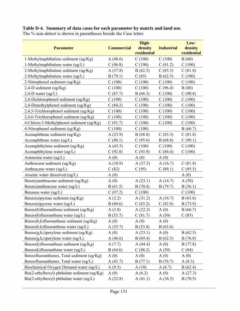
Page 131

Table D-4. Summary of data cases for each parameter by matrix and land use.

The % non-detect is shown in parentheses beside the Case letter.

Parameter Commercial

High-

density

residential

Industrial

Low-

density

residential

1-Methylnaphthalene sediment (ug/Kg) A (48.6) C (100) C (100) B (60) 1-Methylnaphthalene water (ug/L) C (96.8) C (100) C (81.2) C (100) 2-Methylnaphthalene sediment (ug/Kg) A (37.8) B (62.5) C (83.3) C (81.8) 2-Methylnaphthalene water (ug/L) B (79.1) C (85) B (62.5) C (100) 2-Nitrophenol sediment (ug/Kg) C (100) C (100) C (100) C (100) 2,4-D sediment (ug/Kg) C (100) C (100) C (96.4) B (80) 2,4-D water (ug/L) C (87.7) B (66.3) C (100) C (90.8) 2,4-Dichlorophenol sediment (ug/Kg) C (100) C (100) C (100) C (100) 2,4-Dimethylphenol sediment (ug/Kg) C (84.2) C (100) C (100) C (100) 2,4,5-Trichlorophenol sediment (ug/Kg) C (100) C (100) C (100) C (100) 2,4,6-Trichlorophenol sediment (ug/Kg) C (100) C (100) C (100) C (100) 4-Chloro-3-Methylphenol sediment (ug/Kg) C (91.7) C (100) C (100) C (100) 4-Nitrophenol sediment (ug/Kg) C (100) C (100)

B (66.7)

Acenaphthene sediment (ug/Kg) A (23.9) B (68.8) C (83.3) C (81.8) Acenaphthene water (ug/L) C (88.1) C (95.6) B (68.8) C (99.1) Acenaphthylene sediment (ug/Kg) A (43.5) C (100) C (100) C (100) Acenaphthylene water (ug/L) C (92.8) C (93.9) C (84.4) C (100) Ammonia water (ug/L) A (0) A (0) A (0)

Anthracene sediment (ug/Kg) A (10.9) A (37.5) A (16.7) C (81.8) Anthracene water (ug/L) C (82) C (95) C (89.1) C (95.5) Arsenic water dissolved (ug/L) A (0)

A (0)

Benz(a)anthracene sediment (ug/Kg) A (0) A (23.1) A (16.7) A (50) Benz(a)anthracene water (ug/L) B (61.5) B (70.4) B (79.7) B (56.1) Benzene water (ug/L) C (97.2) C (100)

C (100)

Benzo(a)pyrene sediment (ug/Kg) A (2.2) A (31.2) A (16.7) B (63.6) Benzo(a)pyrene water (ug/L) B (60.6) C (83.2) C (82.8) B (73.9) Benzo(b)fluoranthene sediment (ug/Kg) A (3.8) A (22.2) A (0) B (66.7) Benzo(b)fluoranthene water (ug/L) B (53.7) C (81.7) A (50) C (85) Benzo(b,k)fluoranthene sediment (ug/Kg) A (0) A (0) A (0)

Benzo(b,k)fluoranthene water (ug/L) A (35.7) B (53.8) B (65.6) Benzo(g,h,i)perylene sediment (ug/Kg) A (0) A (23.1) A (0) B (62.5)

Benzo(g,h,i)perylene water (ug/L) A (46.6) B (69.4) B (62.5) B (76.8) Benzo(k)fluoranthene sediment (ug/Kg) A (7.7) A (44.4) A (0) B (77.8) Benzo(k)fluoranthene water (ug/L) B (64.6) C (88.2) A (50) C (84) Benzofluoranthenes, Total sediment (ug/Kg) A (0) A (0) A (0) A (0) Benzofluoranthenes, Total water (ug/L) A (41.7) B (77.1) B (76.7) A (8.3) Biochemical Oxygen Demand water (ug/L) A (9.5) A (18) A (6.7) B (62.4) Bis(2-ethylhexyl) phthalate sediment (ug/Kg) A (0) A (6.2) A (0) A (27.3) Bis(2-ethylhexyl) phthalate water (ug/L) A (22.8) A (41.1) A (36.5) B (70.5)

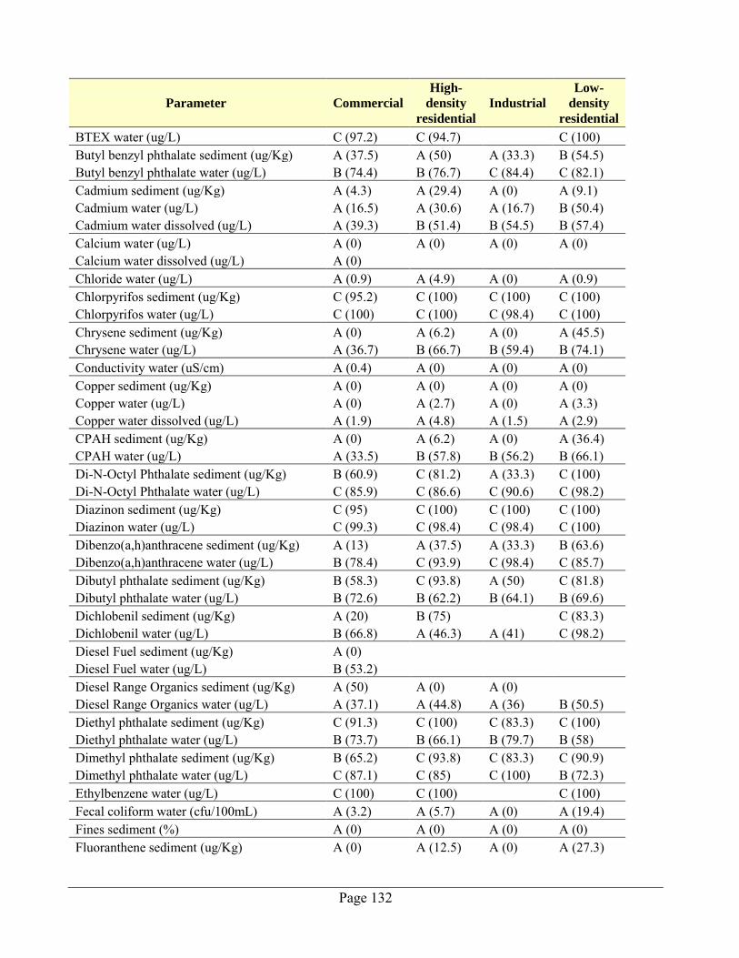
Page 132


High-

density

residential

Industrial

Low-

density

residential

BTEX water (ug/L) C (97.2) C (94.7)

C (100) Butyl benzyl phthalate sediment (ug/Kg) A (37.5) A (50) A (33.3) B (54.5) Butyl benzyl phthalate water (ug/L) B (74.4) B (76.7) C (84.4) C (82.1) Cadmium sediment (ug/Kg) A (4.3) A (29.4) A (0) A (9.1) Cadmium water (ug/L) A (16.5) A (30.6) A (16.7) B (50.4) Cadmium water dissolved (ug/L) A (39.3) B (51.4) B (54.5) B (57.4) Calcium water (ug/L) A (0) A (0) A (0) A (0) Calcium water dissolved (ug/L) A (0)

Chloride water (ug/L) A (0.9) A (4.9) A (0) A (0.9) Chlorpyrifos sediment (ug/Kg) C (95.2) C (100) C (100) C (100) Chlorpyrifos water (ug/L) C (100) C (100) C (98.4) C (100) Chrysene sediment (ug/Kg) A (0) A (6.2) A (0) A (45.5) Chrysene water (ug/L) A (36.7) B (66.7) B (59.4) B (74.1) Conductivity water (uS/cm) A (0.4) A (0) A (0) A (0) Copper sediment (ug/Kg) A (0) A (0) A (0) A (0) Copper water (ug/L) A (0) A (2.7) A (0) A (3.3) Copper water dissolved (ug/L) A (1.9) A (4.8) A (1.5) A (2.9) CPAH sediment (ug/Kg) A (0) A (6.2) A (0) A (36.4) CPAH water (ug/L) A (33.5) B (57.8) B (56.2) B (66.1) Di-N-Octyl Phthalate sediment (ug/Kg) B (60.9) C (81.2) A (33.3) C (100) Di-N-Octyl Phthalate water (ug/L) C (85.9) C (86.6) C (90.6) C (98.2) Diazinon sediment (ug/Kg) C (95) C (100) C (100) C (100) Diazinon water (ug/L) C (99.3) C (98.4) C (98.4) C (100) Dibenzo(a,h)anthracene sediment (ug/Kg) A (13) A (37.5) A (33.3) B (63.6) Dibenzo(a,h)anthracene water (ug/L) B (78.4) C (93.9) C (98.4) C (85.7) Dibutyl phthalate sediment (ug/Kg) B (58.3) C (93.8) A (50) C (81.8) Dibutyl phthalate water (ug/L) B (72.6) B (62.2) B (64.1) B (69.6) Dichlobenil sediment (ug/Kg) A (20) B (75)

C (83.3)

Dichlobenil water (ug/L) B (66.8) A (46.3) A (41) C (98.2) Diesel Fuel sediment (ug/Kg) A (0)

Diesel Fuel water (ug/L) B (53.2) Diesel Range Organics sediment (ug/Kg) A (50) A (0) A (0)

Diesel Range Organics water (ug/L) A (37.1) A (44.8) A (36) B (50.5) Diethyl phthalate sediment (ug/Kg) C (91.3) C (100) C (83.3) C (100) Diethyl phthalate water (ug/L) B (73.7) B (66.1) B (79.7) B (58) Dimethyl phthalate sediment (ug/Kg) B (65.2) C (93.8) C (83.3) C (90.9) Dimethyl phthalate water (ug/L) C (87.1) C (85) C (100) B (72.3) Ethylbenzene water (ug/L) C (100) C (100)

C (100)

Fecal coliform water (cfu/100mL) A (3.2) A (5.7) A (0) A (19.4) Fines sediment (%) A (0) A (0) A (0) A (0) Fluoranthene sediment (ug/Kg) A (0) A (12.5) A (0) A (27.3)

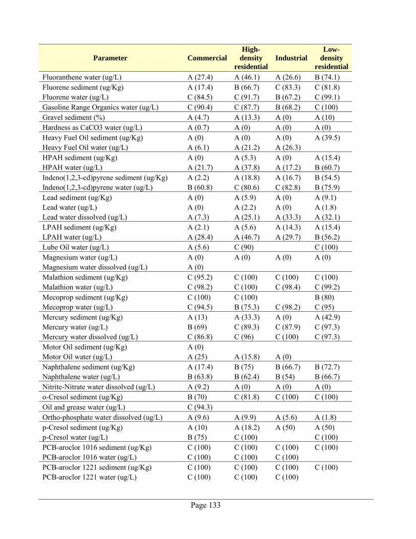
Page 133


High-

density

residential

Industrial

Low-

density

residential

Fluoranthene water (ug/L) A (27.4) A (46.1) A (26.6) B (74.1) Fluorene sediment (ug/Kg) A (17.4) B (66.7) C (83.3) C (81.8) Fluorene water (ug/L) C (84.5) C (91.7) B (67.2) C (99.1) Gasoline Range Organics water (ug/L) C (90.4) C (87.7) B (68.2) C (100) Gravel sediment (%) A (4.7) A (13.3) A (0) A (10) Hardness as CaCO3 water (ug/L) A (0.7) A (0) A (0) A (0) Heavy Fuel Oil sediment (ug/Kg) A (0) A (0) A (0) A (39.5) Heavy Fuel Oil water (ug/L) A (6.1) A (21.2) A (26.3)

HPAH sediment (ug/Kg) A (0) A (5.3) A (0) A (15.4) HPAH water (ug/L) A (21.7) A (37.8) A (17.2) B (60.7) Indeno(1,2,3-cd)pyrene sediment (ug/Kg) A (2.2) A (18.8) A (16.7) B (54.5) Indeno(1,2,3-cd)pyrene water (ug/L) B (60.8) C (80.6) C (82.8) B (75.9) Lead sediment (ug/Kg) A (0) A (5.9) A (0) A (9.1) Lead water (ug/L) A (0) A (2.2) A (0) A (1.8) Lead water dissolved (ug/L) A (7.3) A (25.1) A (33.3) A (32.1) LPAH sediment (ug/Kg) A (2.1) A (5.6) A (14.3) A (15.4) LPAH water (ug/L) A (28.4) A (46.7) A (29.7) B (56.2) Lube Oil water (ug/L) A (5.6) C (90)

C (100)

Magnesium water (ug/L) A (0) A (0) A (0) A (0) Magnesium water dissolved (ug/L) A (0)

Malathion sediment (ug/Kg) C (95.2) C (100) C (100) C (100) Malathion water (ug/L) C (98.2) C (100) C (98.4) C (99.2) Mecoprop sediment (ug/Kg) C (100) C (100)

B (80)

Mecoprop water (ug/L) C (94.5) B (75.3) C (98.2) C (95) Mercury sediment (ug/Kg) A (13) A (33.3) A (0) A (42.9) Mercury water (ug/L) B (69) C (89.3) C (87.9) C (97.3) Mercury water dissolved (ug/L) C (86.8) C (96) C (100) C (97.3) Motor Oil sediment (ug/Kg) A (0)

Motor Oil water (ug/L) A (25) A (15.8) A (0) Naphthalene sediment (ug/Kg) A (17.4) B (75) B (66.7) B (72.7)

Naphthalene water (ug/L) B (63.8) B (62.4) B (54) B (66.7) Nitrite-Nitrate water dissolved (ug/L) A (9.2) A (0) A (0) A (0) o-Cresol sediment (ug/Kg) B (70) C (81.8) C (100) C (100) Oil and grease water (ug/L) C (94.3)

Ortho-phosphate water dissolved (ug/L) A (9.6) A (9.9) A (5.6) A (1.8) p-Cresol sediment (ug/Kg) A (10) A (18.2) A (50) A (50) p-Cresol water (ug/L) B (75) C (100)

C (100)

PCB-aroclor 1016 sediment (ug/Kg) C (100) C (100) C (100) C (100) PCB-aroclor 1016 water (ug/L) C (100) C (100) C (100)


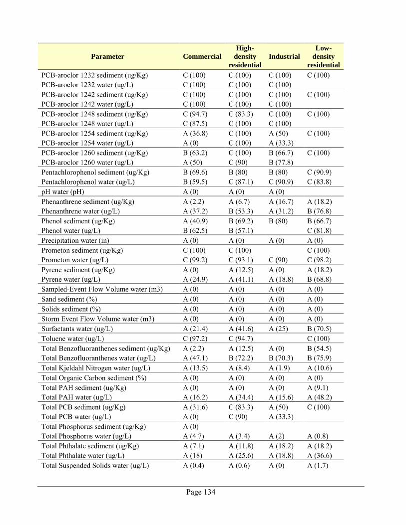
Page 134


High-

density

residential

Industrial

Low-

density

residential



PCB-aroclor 1248 sediment (ug/Kg) C (94.7) C (83.3) C (100) C (100) PCB-aroclor 1248 water (ug/L) C (87.5) C (100) C (100)

PCB-aroclor 1254 sediment (ug/Kg) A (36.8) C (100) A (50) C (100) PCB-aroclor 1254 water (ug/L) A (0) C (100) A (33.3)

PCB-aroclor 1260 sediment (ug/Kg) B (63.2) C (100) B (66.7) C (100) PCB-aroclor 1260 water (ug/L) A (50) C (90) B (77.8)

Pentachlorophenol sediment (ug/Kg) B (69.6) B (80) B (80) C (90.9) Pentachlorophenol water (ug/L) B (59.5) C (87.1) C (90.9) C (83.8) pH water (pH) A (0) A (0) A (0)

Phenanthrene sediment (ug/Kg) A (2.2) A (6.7) A (16.7) A (18.2) Phenanthrene water (ug/L) A (37.2) B (53.3) A (31.2) B (76.8) Phenol sediment (ug/Kg) A (40.9) B (69.2) B (80) B (66.7) Phenol water (ug/L) B (62.5) B (57.1)

C (81.8)

Precipitation water (in) A (0) A (0) A (0) A (0) Prometon sediment (ug/Kg) C (100) C (100)

C (100)

Prometon water (ug/L) C (99.2) C (93.1) C (90) C (98.2) Pyrene sediment (ug/Kg) A (0) A (12.5) A (0) A (18.2) Pyrene water (ug/L) A (24.9) A (41.1) A (18.8) B (68.8) Sampled-Event Flow Volume water (m3) A (0) A (0) A (0) A (0) Sand sediment (%) A (0) A (0) A (0) A (0) Solids sediment (%) A (0) A (0) A (0) A (0) Storm Event Flow Volume water (m3) A (0) A (0) A (0) A (0) Surfactants water (ug/L) A (21.4) A (41.6) A (25) B (70.5) Toluene water (ug/L) C (97.2) C (94.7)

C (100)

Total Benzofluoranthenes sediment (ug/Kg) A (2.2) A (12.5) A (0) B (54.5) Total Benzofluoranthenes water (ug/L) A (47.1) B (72.2) B (70.3) B (75.9) Total Kjeldahl Nitrogen water (ug/L) A (13.5) A (8.4) A (1.9) A (10.6) Total Organic Carbon sediment (%) A (0) A (0) A (0) A (0) Total PAH sediment (ug/Kg) A (0) A (0) A (0) A (9.1) Total PAH water (ug/L) A (16.2) A (34.4) A (15.6) A (48.2) Total PCB sediment (ug/Kg) A (31.6) C (83.3) A (50) C (100) Total PCB water (ug/L) A (0) C (90) A (33.3)

Total Phosphorus sediment (ug/Kg) A (0) Total Phosphorus water (ug/L) A (4.7) A (3.4) A (2) A (0.8)

Total Phthalate sediment (ug/Kg) A (7.1) A (11.8) A (18.2) A (18.2) Total Phthalate water (ug/L) A (18) A (25.6) A (18.8) A (36.6) Total Suspended Solids water (ug/L) A (0.4) A (0.6) A (0) A (1.7)

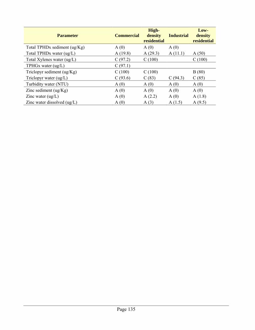
Page 135


High-

density

residential

Industrial

Low-

density

residential

Total TPHDx sediment (ug/Kg) A (0) A (0) A (0) Total TPHDx water (ug/L) A (19.8) A (29.3) A (11.1) A (50)

Total Xylenes water (ug/L) C (97.2) C (100)

C (100) TPHGx water (ug/L) C (97.1)

Triclopyr sediment (ug/Kg) C (100) C (100)

B (80) Triclopyr water (ug/L) C (93.6) C (83) C (94.3) C (85) Turbidity water (NTU) A (0) A (0) A (0) A (0) Zinc sediment (ug/Kg) A (0) A (0) A (0) A (0) Zinc water (ug/L) A (0) A (2.2) A (0) A (1.8) Zinc water dissolved (ug/L) A (0) A (3) A (1.5) A (9.5)

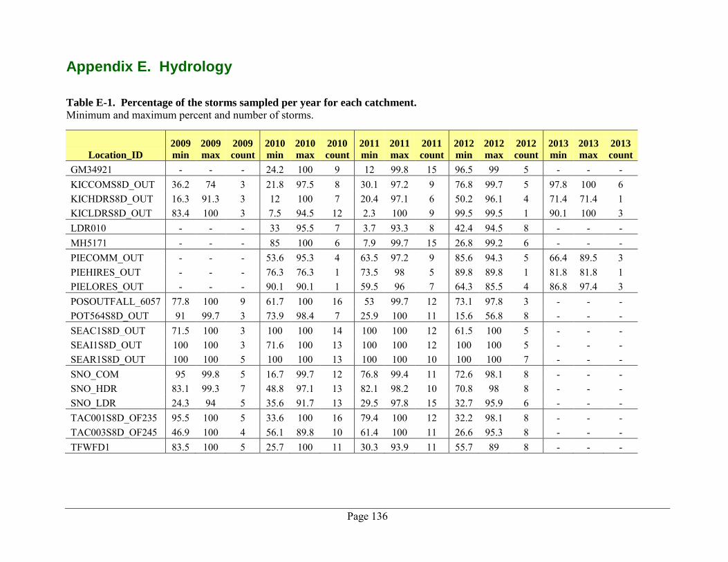
Page 136

Appendix E. Hydrology

Table E-1. Percentage of the storms sampled per year for each catchment.

Minimum and maximum percent and number of storms.

Location_ID

2009

min

2009

max

2009

count

2010

min

2010

max

2010

count

2011

min

2011

max

2011

count

2012

min

2012

max

2012

count

2013

min

2013

max

2013

count

GM34921 - - - 24.2 100 9 12 99.8 15 96.5 99 5 - - - KICCOMS8D_OUT 36.2 74 3 21.8 97.5 8 30.1 97.2 9 76.8 99.7 5 97.8 100 6 KICHDRS8D_OUT 16.3 91.3 3 12 100 7 20.4 97.1 6 50.2 96.1 4 71.4 71.4 1 KICLDRS8D_OUT 83.4 100 3 7.5 94.5 12 2.3 100 9 99.5 99.5 1 90.1 100 3 LDR010 - - - 33 95.5 7 3.7 93.3 8 42.4 94.5 8 - - - MH5171 - - - 85 100 6 7.9 99.7 15 26.8 99.2 6 - - - PIECOMM_OUT - - - 53.6 95.3 4 63.5 97.2 9 85.6 94.3 5 66.4 89.5 3 PIEHIRES_OUT - - - 76.3 76.3 1 73.5 98 5 89.8 89.8 1 81.8 81.8 1 PIELORES_OUT - - - 90.1 90.1 1 59.5 96 7 64.3 85.5 4 86.8 97.4 3 POSOUTFALL_6057 77.8 100 9 61.7 100 16 53 99.7 12 73.1 97.8 3 - - - POT564S8D_OUT 91 99.7 3 73.9 98.4 7 25.9 100 11 15.6 56.8 8 - - - SEAC1S8D_OUT 71.5 100 3 100 100 14 100 100 12 61.5 100 5 - - - SEAI1S8D_OUT 100 100 3 71.6 100 13 100 100 12 100 100 5 - - - SEAR1S8D_OUT 100 100 5 100 100 13 100 100 10 100 100 7 - - - SNO_COM 95 99.8 5 16.7 99.7 12 76.8 99.4 11 72.6 98.1 8 - - - SNO_HDR 83.1 99.3 7 48.8 97.1 13 82.1 98.2 10 70.8 98 8 - - - SNO_LDR 24.3 94 5 35.6 91.7 13 29.5 97.8 15 32.7 95.9 6 - - - TAC001S8D_OF235 95.5 100 5 33.6 100 16 79.4 100 12 32.2 98.1 8 - - - TAC003S8D_OF245 46.9 100 4 56.1 89.8 10 61.4 100 11 26.6 95.3 8 - - - TFWFD1 83.5 100 5 25.7 100 11 30.3 93.9 11 55.7 89 8 - - -

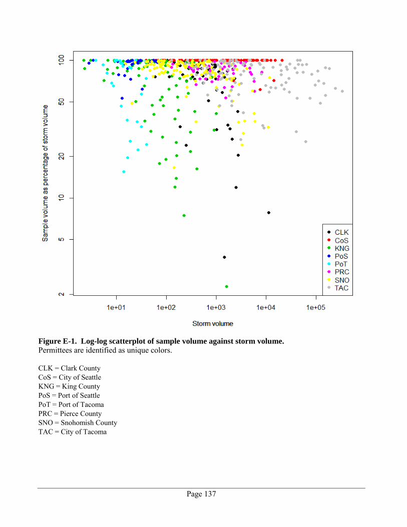
Page 137

Figure E-1. Log-log scatterplot of sample volume against storm volume.

Permittees are identified as unique colors. CLK = Clark County CoS = City of Seattle KNG = King County PoS = Port of Seattle PoT = Port of Tacoma PRC = Pierce County SNO = Snohomish County TAC = City of Tacoma

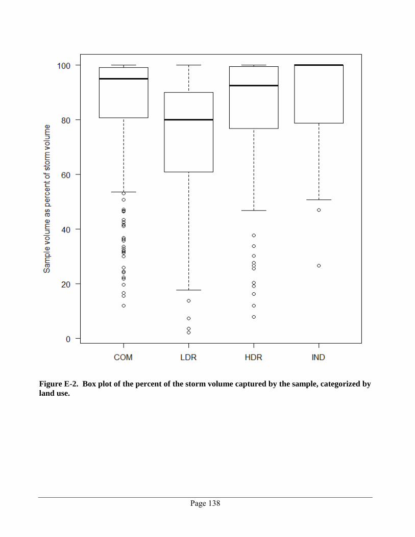
Page 138

Figure E-2. Box plot of the percent of the storm volume captured by the sample, categorized by

land use.

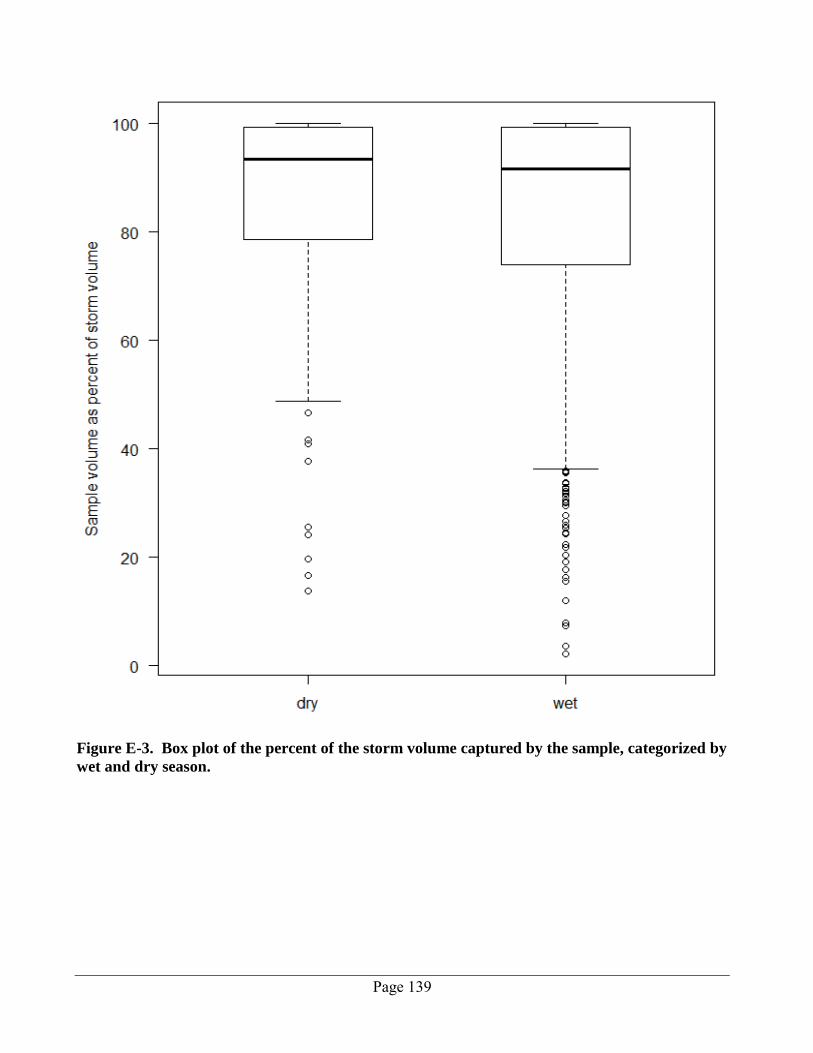
Page 139


wet and dry season.

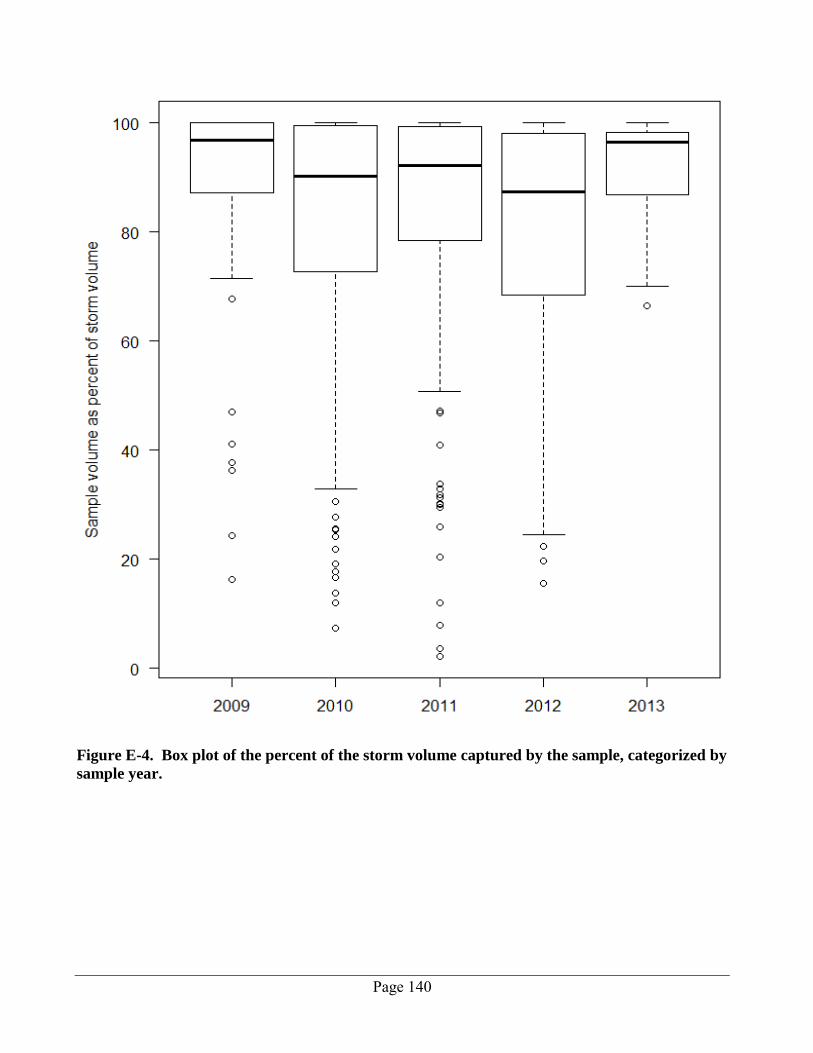
Page 140


sample year.

Page 141

Appendix F. Data Plots for Contaminant Concentrations Appendix F (172 pages) is available only online. It is linked to this report at https://fortress.wa.gov/ecy/publications/SummaryPages/1503001.html


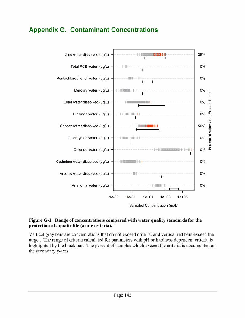
Page 142

Appendix G. Contaminant Concentrations

Figure G-1. Range of concentrations compared with water quality standards for the

protection of aquatic life (acute criteria).

Vertical gray bars are concentrations that do not exceed criteria, and vertical red bars exceed the target. The range of criteria calculated for parameters with pH or hardness dependent criteria is highlighted by the black bar. The percent of samples which exceed the criteria is documented on the secondary y-axis.

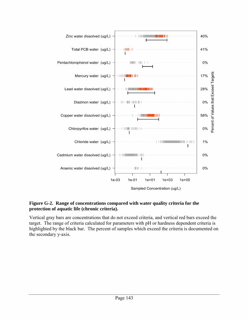
Page 143

Figure G-2. Range of concentrations compared with water quality criteria for the

protection of aquatic life (chronic criteria).

Vertical gray bars are concentrations that do not exceed criteria, and vertical red bars exceed the target. The range of criteria calculated for parameters with pH or hardness dependent criteria is highlighted by the black bar. The percent of samples which exceed the criteria is documented on the secondary y-axis.

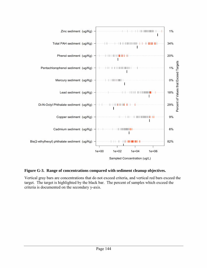
Page 144

Figure G-3. Range of concentrations compared with sediment cleanup objectives.

Vertical gray bars are concentrations that do not exceed criteria, and vertical red bars exceed the target. The target is highlighted by the black bar. The percent of samples which exceed the criteria is documented on the secondary y-axis.

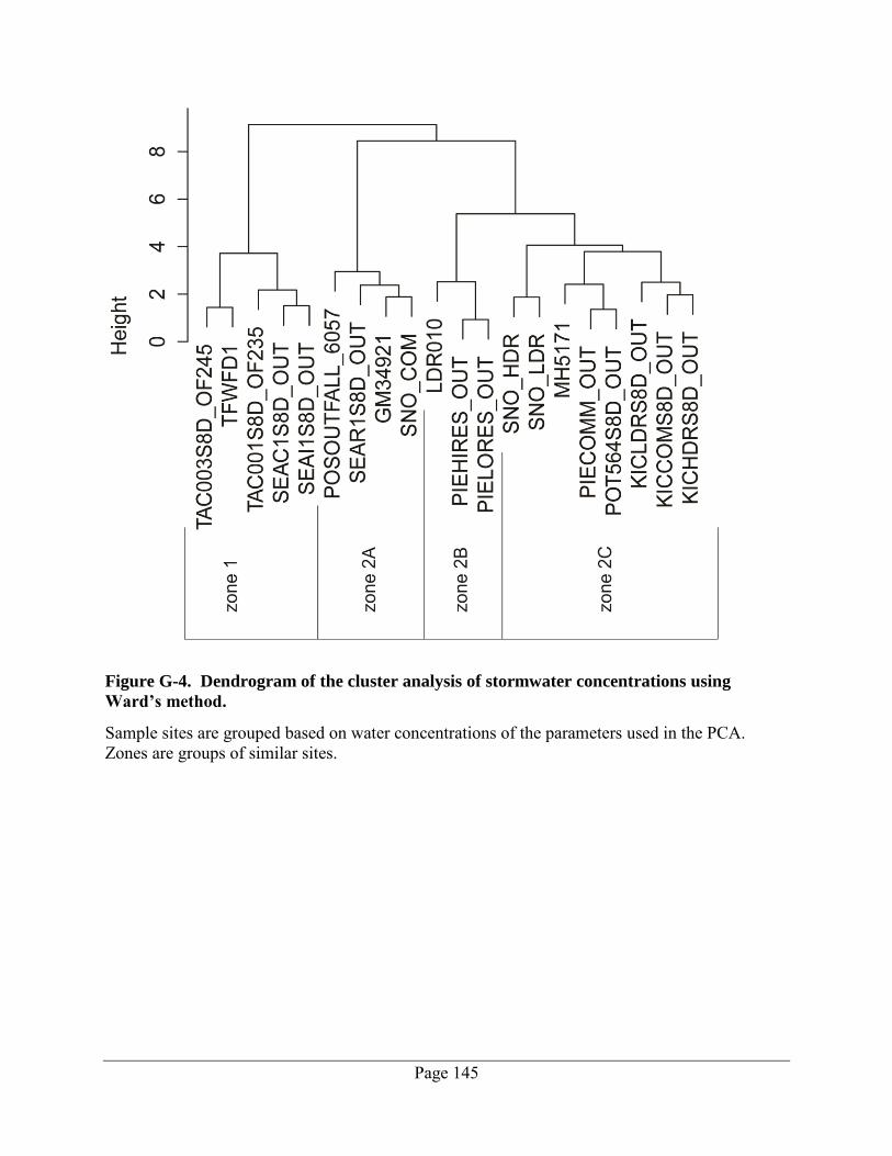
Page 145

Figure G-4. Dendrogram of the cluster analysis of stormwater concentrations using

Ward’s method.

Sample sites are grouped based on water concentrations of the parameters used in the PCA. Zones are groups of similar sites.

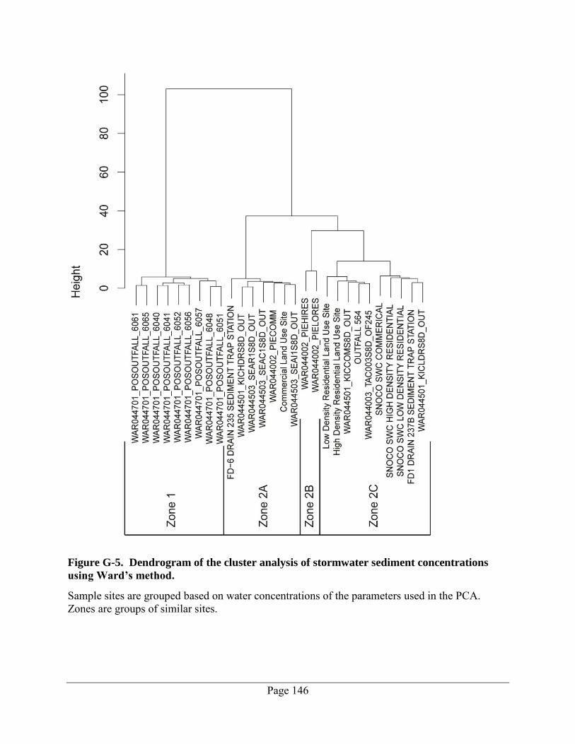
Page 146

Figure G-5. Dendrogram of the cluster analysis of stormwater sediment concentrations

using Ward’s method.

Sample sites are grouped based on water concentrations of the parameters used in the PCA. Zones are groups of similar sites.

Page 147

The following Appendix G tables are available only online as zip files. They are linked to this report at https://fortress.wa.gov/ecy/publications/SummaryPages/1503001.html

Table G-1. Statistical summary of contaminant concentrations by parameter and media.

Table G-2. Statistical summary of contaminant concentrations by parameter, media, and

land use.

Table G-3. Statistical summary of contaminant concentrations by parameter, media, and

season.


Page 148

Appendix H. Data Plots for Contaminant Loads Appendix H (89 pages) is available only online. It is linked to this report at https://fortress.wa.gov/ecy/publications/SummaryPages/1503001.html


Page 149

Appendix I. Contaminant Loads The following Appendix I tables are available only online as zip files. They are linked to this report at https://fortress.wa.gov/ecy/publications/SummaryPages/1503001.html Table I-1. Statistical summary of contaminant mass loads (kg) by parameter.

Table I-2. Statistical summary of contaminant mass loads (kg) by parameter and land use.

Table I-3. Statistical summary of contaminant mass loads (kg) by parameter and season.

Table I-4. Statistical summary of contaminant load per area (kg ha

-1).


-1) by parameter and

land use.


-1) by parameter and

season.


Page 150

Appendix J. Glossary, Acronyms, and Abbreviations Glossary

Clean Water Act: A federal act passed in 1972 that contains provisions to restore and maintain the quality of the nation’s waters. Section 303(d) of the Clean Water Act establishes the total maximum daily load (TMDL) program.

Conductivity: A measure of water’s ability to conduct an electrical current. Conductivity is related to the concentration and charge of dissolved ions in water.

Exceed criterion or standard: Did not meet (or violated) the criterion or standard.

Fecal coliform: That portion of the coliform group of bacteria which is present in intestinal tracts and feces of warm-blooded animals as detected by the product of acid or gas from lactose in a suitable culture medium within 24 hours at 44.5 plus or minus 0.2 degrees Celsius. Fecal coliform are “indicator” organisms that suggest the possible presence of disease-causing organisms. Concentrations are measured in colony forming units per 100 milliliters of water (cfu/100 mL).

National Pollutant Discharge Elimination System (NPDES): National program for issuing, modifying, revoking and reissuing, terminating, monitoring, and enforcing permits, and imposing and enforcing pretreatment requirements under the Clean Water Act. The NPDES program regulates discharges from wastewater treatment plants, large factories, and other facilities that use, process, and discharge water back into lakes, streams, rivers, bays, and oceans.

Nutrient: Substance such as carbon, nitrogen, and phosphorus used by organisms to live and grow. Too many nutrients in the water can promote algal blooms and rob the water of oxygen vital to aquatic organisms.

Parameter: A physical, chemical, or biological property whose values determine environmental characteristics or behavior.

Percentile: A statistical number obtained from a distribution of a data set.

pH: A measure of the acidity or alkalinity of water. A low pH value (0 to 7) indicates that an acidic condition is present, while a high pH (7 to 14) indicates a basic or alkaline condition. A pH of 7 is considered to be neutral. Since the pH scale is logarithmic, a water sample with a pH of 8 is ten times more basic than one with a pH of 7.

Pollution: Contamination or other alteration of the physical, chemical, or biological properties of any waters of the state. This includes change in temperature, taste, color, turbidity, or odor of the waters. It also includes discharge of any liquid, gaseous, solid, radioactive, or other substance into any waters of the state. This definition assumes that these changes will, or are likely to, create a nuisance or render such waters harmful, detrimental, or injurious to (1) public health, safety, or welfare, or (2) domestic, commercial, industrial, agricultural,

Page 151

recreational, or other legitimate beneficial uses, or (3) livestock, wild animals, birds, fish, or other aquatic life.

PS Toxics Study: Control of Toxic Chemicals in Puget Sound: Phase 3 Data and Load Estimates (Herrera, 2011).

Stormwater: The portion of precipitation that does not naturally percolate into the ground or evaporate but instead runs off roads, pavement, and roofs during rainfall or snow melt. Stormwater can also come from hard or saturated grass surfaces such as lawns, pastures, playfields, and from gravel roads and parking lots.

Total suspended solids (TSS): Portion of solids retained by a filter.

Turbidity: A measure of water clarity. High levels of turbidity can have a negative impact on aquatic life.

Acronyms and Abbreviations BEHP bis(2-Ethylhexyl) phthalate BMP Best management practice BOD Biological oxygen demand BTEX Benzene, toluene, ethylbenzene, and xylene Ecology Washington State Department of Ecology EDF Empirical Distribution Function EIM Environmental Information Management database EPA U.S. Environmental Protection Agency GIS Geographic Information System HPAH High molecular weight PAH KM Kaplan-Meier LPAH Low molecular weight PAH MDL Method detection limit MLE Maximum Likelihood Estimation MQO Measurement quality objective NOAA National Oceanic and Atmospheric Administration NPDES (See Glossary above) NSQD National Stormwater Quality Database NURP National Urban Runoff Program NWTPH Northwest Total Petroleum Hydrocarbon PAH Polycyclic aromatic hydrocarbon PCA Principal components analysis PCB Polychlorinated biphenyl QA Quality assurance QC Quality control RL Reporting limit ROS Regression on Order Statistics

Page 152

SCO Sediment Cleanup Objective SMS Sediment Management Standard SVOC Semi-volatile organic compound TIA Total impervious area TKN Total Kjeldahl nitrogen TOC Total organic carbon TPH Total petroleum hydrocarbon TSS (See Glossary above) WAC Washington Administrative Code WQP Water Quality Program Units of Measurement

°C degrees centigrade cfu colony forming units dw dry weight ha hectare kg kilograms, a unit of mass equal to 1,000 grams mg milligram mg/Kg milligrams per kilogram (parts per million)

mg/L milligrams per liter (parts per million) ng/L nanograms per liter (parts per trillion) NTU nephelometric turbidity units s.u. standard units ug/Kg micrograms per kilogram (parts per billion) ug/L micrograms per liter (parts per billion) umhos/cm micromhos per centimeter uS/cm microsiemens per centimeter, a unit of conductivity

Documents

Western Washington NPDES Phase I Stormwater … Washington . NPDES Phase I Stormwater Permit . ... 2010-2011 ... These monitoring requirements enabled uniform data collection and similar