Wettability Characterization by NMR T2 Measurements in Edwards Limestone

Master Thesis in Reservoir Physics

By

Lejla Tipura

Department of Physics and Technology

University of Bergen Norway

2008

I

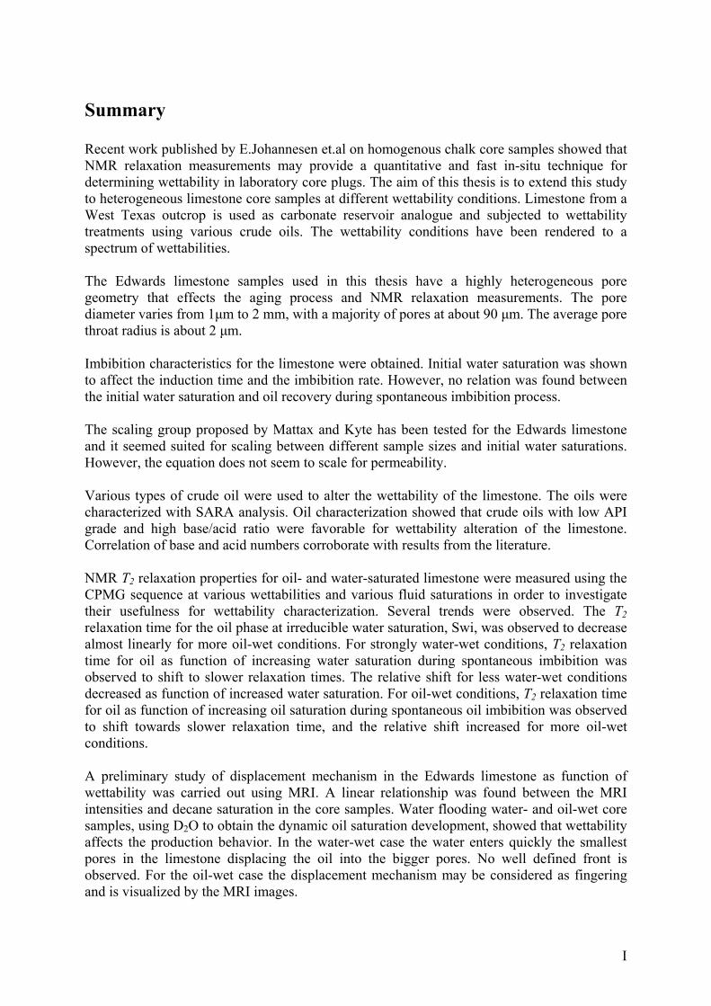
Summary Recent work published by E.Johannesen et.al on homogenous chalk core samples showed that NMR relaxation measurements may provide a quantitative and fast in-situ technique for determining wettability in laboratory core plugs. The aim of this thesis is to extend this study to heterogeneous limestone core samples at different wettability conditions. Limestone from a West Texas outcrop is used as carbonate reservoir analogue and subjected to wettability treatments using various crude oils. The wettability conditions have been rendered to a spectrum of wettabilities. The Edwards limestone samples used in this thesis have a highly heterogeneous pore geometry that effects the aging process and NMR relaxation measurements. The pore diameter varies from 1µm to 2 mm, with a majority of pores at about 90 µm. The average pore throat radius is about 2 µm. Imbibition characteristics for the limestone were obtained. Initial water saturation was shown to affect the induction time and the imbibition rate. However, no relation was found between the initial water saturation and oil recovery during spontaneous imbibition process. The scaling group proposed by Mattax and Kyte has been tested for the Edwards limestone and it seemed suited for scaling between different sample sizes and initial water saturations. However, the equation does not seem to scale for permeability. Various types of crude oil were used to alter the wettability of the limestone. The oils were characterized with SARA analysis. Oil characterization showed that crude oils with low API grade and high base/acid ratio were favorable for wettability alteration of the limestone. Correlation of base and acid numbers corroborate with results from the literature. NMR T2 relaxation properties for oil- and water-saturated limestone were measured using the CPMG sequence at various wettabilities and various fluid saturations in order to investigate their usefulness for wettability characterization. Several trends were observed. The T2 relaxation time for the oil phase at irreducible water saturation, Swi, was observed to decrease almost linearly for more oil-wet conditions. For strongly water-wet conditions, T2 relaxation time for oil as function of increasing water saturation during spontaneous imbibition was observed to shift to slower relaxation times. The relative shift for less water-wet conditions decreased as function of increased water saturation. For oil-wet conditions, T2 relaxation time for oil as function of increasing oil saturation during spontaneous oil imbibition was observed to shift towards slower relaxation time, and the relative shift increased for more oil-wet conditions. A preliminary study of displacement mechanism in the Edwards limestone as function of wettability was carried out using MRI. A linear relationship was found between the MRI intensities and decane saturation in the core samples. Water flooding water- and oil-wet core samples, using D2O to obtain the dynamic oil saturation development, showed that wettability affects the production behavior. In the water-wet case the water enters quickly the smallest pores in the limestone displacing the oil into the bigger pores. No well defined front is observed. For the oil-wet case the displacement mechanism may be considered as fingering and is visualized by the MRI images.

II

Acknowledgements I would like to thank everyone that has helped me through my Master project, especially my supervisor Professor Arne Graue, for guidance and opportunity to go aboard with this project. Thanks to James J. Howard, Jim Stevens and David R. Zorens at ConocoPhillips in Bartlesville, OK, for sharing their expertise and laboratory assistance. Thanks to Jill Buckley for her guidance and hospitality at New Mexico Tech., New Mexico. Thanks to Michael R. Talbot at University of Bergen for his geology expertise. Thanks to my fellow students, especially Else B. Johannesen, Haldis Riskedal, Are Severin Martinsen, Jarle Husebø, Martin Fernø. Thanks to my husband, Svein Arild Pedersen, for his patience and understanding. Thanks to my parents and my sister for their support. Bergen, 7 mars 2008 Lejla Tipura

III

Introduction Wettability is defined as “the tendency of one fluid to spread on or adhere to a solid surface in the presence of other immiscible fluids” (Craig 1971). Salathiel (1973) introduced mixed wettability in which the oil-wet surface from continuous paths for oil through the large pores and small pores remain water-wet. Wettability affects capillary pressure, relative permeability and residual oil saturation (Anderson, 1986, 1987a, 1987b, 1987c, 1987d, 1987e). Different methods for wettability measurements are reviewed in the literature [Anderson 1986b]. Two commonly used methods to measure quantitatively the wettability conditions in the laboratory are the Amott [Amott 1959] and the USBM method [Anderson 1987a]. However, both methods are time consuming and if applied on native state cores require that core wettability is undisturbed during the plug extraction from the rock formation, which is expensive and difficult due to operational handling. Due to these challenges it would be advantageous to develop a fast and less expensive in-situ wettability-predicting tool. One promising technique may be utilizing NMR-technology. The earliest attempt of using NMR relaxation methods to characterize wettability of porous media was published in 1956 by Brown and Fatt. They based their theory on the hypothesis that, at solid-liquid interface, molecular motion is slower than in the bulk liquid. In this solid-liquid interface the diffusion coefficient is reduced, which in turn is equivalent to a zone of higher viscosity. In the zone of higher viscosity the magnetically aligned protons can more easily transfer their energy to their surroundings. The magnitude of this effect depends on the wettability characteristics of the solid with respect to the liquid in contact with the surface. Brown and Fatt stated their work by measuring proton spin-lattice relaxation time (T1) of water in uncoated sand packs as water-wet media, and Dri-film treated sand packs as oil-wet porous media. Their experiments resulted in linear relation between relaxation rate and fractional oil wetted surface area. Because of advancements in low-field NMR technology and the interest in porous media in the 1990’s, the amount of experimental data related to wettability and NMR research increased significantly. Howard and Spinler (1995) reported how multi-component fitting of the relaxation data reveals more information than the single- and stretched-exponential fitting used in earlier studies. They compared NMR relaxation data measured on a large number of similar samples and demonstrated how multi-component fits made it possible to interpret the abundance of water and oil phases with proton measurement made in low field-strength spectrometers comparable to the fields used in this new generation of NMR logging tools. A model based on relative shift of T1 relaxation for water component as function saturation was proposed for quantifying the wettability changes in porous media [Howard et.al 1995]. Recent work published by E.Johannesen et.al. (2006) on homogenous chalk core samples showed that NMR relaxation measurements may provide a quantitative and fast technique for determining mixed wettability in laboratory core plugs. The aim of this thesis is to extend this study to heterogeneous limestone core samples at different wettability conditions. Limestone from a West Texas outcrop is used as carbonate reservoir analogue and subjected to wettability treatments using various crude oils. The wettability conditions have been rendered to a spectrum of wettability conditions. NMR T2 relaxation properties for oil- and water-saturated outcrop limestone were measured using CPMG sequence at various wettabilities and at various fluid saturations during imbibition to find trends for wettability characterization.

IV

Contents Summary ....................................................................................................................................I Acknowledgements.................................................................................................................. II Introduction ........................................................................................................................... III Contents...................................................................................................................................IV PART 1 Basic Concepts and Definitions in Reservoir Engineering ............................... - 1 -

1.1 Porosity........................................................................................................................ - 1 - 1.2 Saturation .................................................................................................................... - 2 - 1.3 Absolute Permeability ................................................................................................. - 2 - 1.4 Effective and Relative Permeability............................................................................ - 3 - 1.5 Rock Wettability ......................................................................................................... - 4 -

1.5.1 Types of Wettability............................................................................................. - 4 - 1.5.2 Factors Affecting Reservoir Wettability .............................................................. - 5 - 1.5.3 Wettability Measures............................................................................................ - 5 - 1.5.4 Wettability Effects on Relative Permeability and Capillary Pressure.................. - 9 -

1.6 Capillary Pressure ..................................................................................................... - 10 - 1.6.1 Capillary Pressure Curves .................................................................................. - 11 -

1.7 Oil Characterization .................................................................................................. - 13 - 1.7.1 SARA components ............................................................................................. - 13 - 1.7.2 Density and API ................................................................................................. - 13 - 1.7.3 Refractive Index (RI) ......................................................................................... - 14 - 1.7.4 Acid and Base Number ...................................................................................... - 14 - 1.7.5 Viscosity............................................................................................................. - 15 -

1.8 The Scaling Equation ................................................................................................ - 16 - 1.9 Nuclear Magnetic Resonance.................................................................................... - 18 -

1.9.1 The Spinning Proton........................................................................................... - 18 - 1.9.2 T2 Relaxation ...................................................................................................... - 21 - 1.9.3 Measuring Petrophysical Parameters by NMR .................................................. - 23 -

1.10 Principles of Magnetic Resonance Imaging............................................................ - 25 - 1.10.1 MRI Sequences ................................................................................................ - 25 -

PART 2 Experimental....................................................................................................... - 26 - 2.1 Core Material............................................................................................................. - 26 - 2.2 Fluids......................................................................................................................... - 26 - 2.3 Porosity Measurements ............................................................................................. - 27 - 2.4 Permeability Measurements ...................................................................................... - 28 - 2.5 Wettability Alteration – Aging.................................................................................. - 28 -

2.5.1 Aging Experimental Procedure .......................................................................... - 29 - 2.6 Wettability Measurements......................................................................................... - 30 - 2.7 Scaling – Size and Initial Water Saturation .............................................................. - 31 - 2.8 Oil Characterization .................................................................................................. - 31 -

2.8.1 SARA components ............................................................................................. - 31 - 2.8.2 Oil Density and Viscosity .................................................................................. - 32 - 2.8.3 Refractive Index (RI) ......................................................................................... - 32 - 2.8.4 Acid and Base Number ...................................................................................... - 32 -

2.9 NMR T2 Measurements............................................................................................. - 33 - 2.9.1. NMR Instrument ............................................................................................... - 33 - 2.9.2 NMR Instrument Parameters Setting ................................................................. - 34 - 2.9.3 NMR Measurements .......................................................................................... - 34 -

2.10 MRI Measurements ................................................................................................. - 35 -

V

PART 3 Results.................................................................................................................. - 36 - 3.1 Core Material............................................................................................................. - 36 -

3.1.1 Thin section ........................................................................................................ - 36 - 3.1.2 Mercury Injection- Pore Throat Distribution ..................................................... - 37 - 3.1.3 Porosity and Permeability .................................................................................. - 38 -

3.2 Scaling....................................................................................................................... - 39 - 3.2.1 Sample Dimensions............................................................................................ - 39 - 3.2.2 Scaling for Different Swi..................................................................................... - 42 - 3.2.3 Summary of Results from Scaling Tests ............................................................ - 44 -

3.3 Oil Characterization .................................................................................................. - 45 - 3.3.1 SARA Components ............................................................................................ - 46 - 3.3.2 Acid and Base Number ...................................................................................... - 47 - 3.3.3 Oil Density/API and Viscosity........................................................................... - 49 - 3.3.4 RI – Refractive Index ......................................................................................... - 51 - 3.3.5 API and Base/Acid Ratio ................................................................................... - 53 - 3.3.6 Summary of Chemical Analysis......................................................................... - 53 -

3.4 Wettability Characterization by NMR T2.................................................................. - 54 - 3.4.1 Effect of Wettability on Ultimate Oil Recovery ................................................ - 56 - 3.4.2 Bulk Measurements............................................................................................ - 57 - 3.4.3 Pore Size Distribution in Edwards Limestone ................................................... - 58 - 3.4.4 Saturation Calculation by NMR and Mass Balance........................................... - 60 - 3.4.5 Moderate to Strongly Water-Wet Conditions (Group 1) ................................... - 62 - 3.4.6 Weakly Water- Wet Conditions (Group 2) ........................................................ - 64 - 3.4.7 Neutral-Wet Conditions – Decane Flood (Group 3) .......................................... - 65 - 3.4.8 Weakly Oil-Wet Conditions (Group 4).............................................................. - 66 - 3.4.9 Moderate to Strongly Oil-Wet Conditions (Group 5) ........................................ - 68 - 3.4.10 Approximate Wettability Determination in Edwards Limestone Using NMR T2 Measurements.............................................................................................................. - 69 -

3.5 MRI Experiments ...................................................................................................... - 72 - 3.5.1 D2O flood of Water-Wet Edwards Limestone (HR27) ...................................... - 72 - 3.5.1 D2O flood of Oil-Wet Edwards Limestone (9) .................................................. - 74 -

PART 4 Conclusions and Future Work .......................................................................... - 82 - Refrences ............................................................................................................................ - 83 -

- 1 -

PART 1 Basic Concepts and Definitions in Reservoir Engineering

1.1 Porosity A rock must contain pores to act as a reservoir. The pore space, or voids, within reservoir rock contain water and hydrocarbons. Porosity is expressed as ratio of pore volume to total rock volume:

b

p

VV

=φ 1.1

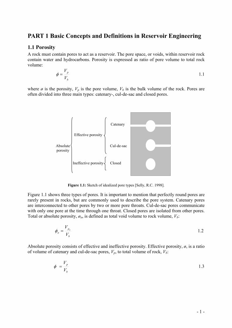
where ø is the porosity, Vp is the pore volume, Vb is the bulk volume of the rock. Pores are often divided into three main types: catenary-, cul-de-sac and closed pores.

Figure 1.1: Sketch of idealized pore types [Selly, R.C. 1998].

Figure 1.1 shows three types of pores. It is important to mention that perfectly round pores are rarely present in rocks, but are commonly used to describe the pore system. Catenary pores are interconnected to other pores by two or more pore throats. Cul-de-sac pores communicate with only one pore at the time through one throat. Closed pores are isolated from other pores. Total or absolute porosity, øa, is defined as total void volume to rock volume, Vb:

b

pa V

Va=φ 1.2

Absolute porosity consists of effective and ineffective porosity. Effective porosity, ø, is a ratio of volume of catenary and cul-de-sac pores, Vp, to total volume of rock, Vb:

b

p

VV

=φ 1.3

Cul-de-sac

Closed

Ineffective porosity

Absolute porosity

Catenary

Effective porosity

- 2 -

1.2 Saturation Void pore volumes are generally filled with water, oil and gas. This relationship may be expressed as: gwop VVVV ++= 1.4 where Vp is the total pore volume, Vo is the oil volume, Vg is the gas volume and Vw is the water volume occupying the pores. Saturation (S) is defined as the fraction of pore volume occupied by certain fluid:

niVV

Sp

ii ,....,1, == 1.5

where n is the total number of fluid phases present in the porous medium, leading to:

11

=∑=

n

iiS 1.6

Based on the definition above, the saturation may range from zero to one. Endpoint saturation values are important at experimental and reservoir scale providing information of rock performance. When oil migrated from the source rock it entered the reservoir rock that was occupied by water. Water saturation after oil displacement in a reservoir rock is called connate water saturation, Swc. Minimum water saturation obtained in laboratory experiments by oil flooding or centrifuge displacement is called irreducible water saturation, Swi. At this saturation water is no longer mobile in the pore system. After water flooding oil reservoir some oil will be trapped. This saturation is called residual oil saturation (Sorw).

1.3 Absolute Permeability The second essential parameter for a reservoir rock is permeability. The property of permeability is related to porosity. In qualitative terms, permeability is expressed as the capacity of a porous rock or soil to transmit a fluid. Large interconnected pore openings are associated with high permeability, while very small, unconnected pore openings are associated with low permeability. Permeability is a tensor, a directional property, varying through reservoir rock. Depending on depositional environment the permeability may be good vertically if it consists of vertically stacked channels but low horizontal permeability involving more complicated well placement. Darcy law is the youngest of several conduction laws; Ohm’s law, Fourier’s law and Fick’s law. Darcy Law for the linear, horizontal flow of incompressible fluid can be written as follows:

LPAKQ

µ∆

= 1.7

where Q is rate of flow [cm3/s], K is permeability [D], ∆P is absolute pressure drop across the sample [atm], A is the cross-sectional area of the sample [cm2], L is the length of the sample [cm], µ is the fluid viscosity [cP].

- 3 -

Dimensional analysis of Darcy Law shows that permeability has the dimension of surface area. By convention, the unit of permeability is called Darcy (D). One Darcy is the permeability of a porous media that allows fluid with viscosity of 1 cP and pressure difference of 1 atm/cm to flow through medium’s cross section of 1 cm2 at a rate of 1 cm3/s.

1.4 Effective and Relative Permeability If there are several mobile immiscible fluids present in a reservoir and a modification of Darcy Law is needed. Effective permeability (ki) for a given reservoir fluid is a function of fluid saturation, wettability, pore size distribution and saturation history. The effective permeability is defined as follows:

1.8

where i donate certain phase (e.g. oil, water or gas). The ratio of effective permeability, kei, for a phase i to absolute permeability, K, of the porous media is the relative permeability (kri):

Kk

k eiri = 1.9

Relative permeability is less than one for every phase present in a pore system but the sum of these is never unity. In order to visualize the fluid movement the relative permeability of each phase is plotted as a function of wetting phase saturation. Two processes are commonly described through the relative permeability curves: imbibition and drainage. Imbibition is a type of process where the wetting phase saturation increases while the drainage process describes a decrease in wetting phase saturation.

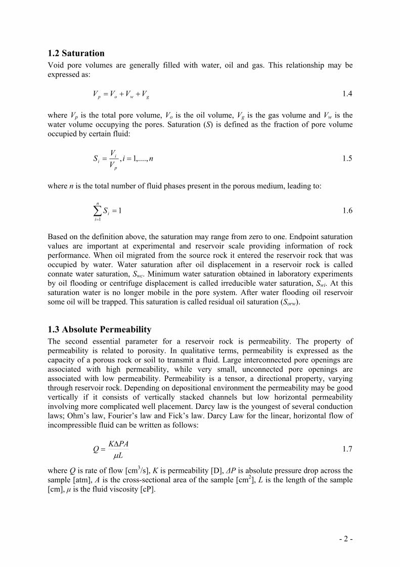
Figure 1.2: Relative permeability curves in a water-oil system. Swi and Sw=1-Sor are critical saturations where water and oil becomes immobile, respectively. At these endpoints the relative permeability becomes zero.

Figure 1.2 shows that both phases are mobile between Swi and Sor (Sw=1-Sor). At these saturations water and oil will lose their continuity, respectively. At the endpoints relative permeability values are called endpoint relative permeabilities; krw,or is the relative permeability to water at Sor and kro,iw is the relative permeability to water at Swi.

pL

Aqk ii

ei ∆=

µ

Sw 1.0

1.0

kro

Sw = 1-Sor Swi

kro,iw

0.0

kw krw,ro

- 4 -

1.5 Rock Wettability Wettability is defined as “the tendency for one fluid to spread or adhere to a solid surface in the presence of the immiscible phase”. It is a very important characteristic of a rock/fluid system as it affects many of the special core analysis properties, which are critical in reservoir engineering [Anderson 1987a-d]. These properties include: capillary pressure, relative permeability, water flood behavior, irreducible water saturation, residual oil saturation and electrical properties. In early days of Petroleum Engineering it was assumed that all or almost all reservoirs were what is called strongly water-wet reservoirs. This rational assumption was attributed to saturation history; i.e. the reservoir rock was completely saturated with water prior oil migration and there was no reason why this would be altered. In fact it now appears that strongly water-wet reservoirs are not very numerous, neither oil-wet. An intermediate wettability is now recognized as a dominating wettability by many researches.

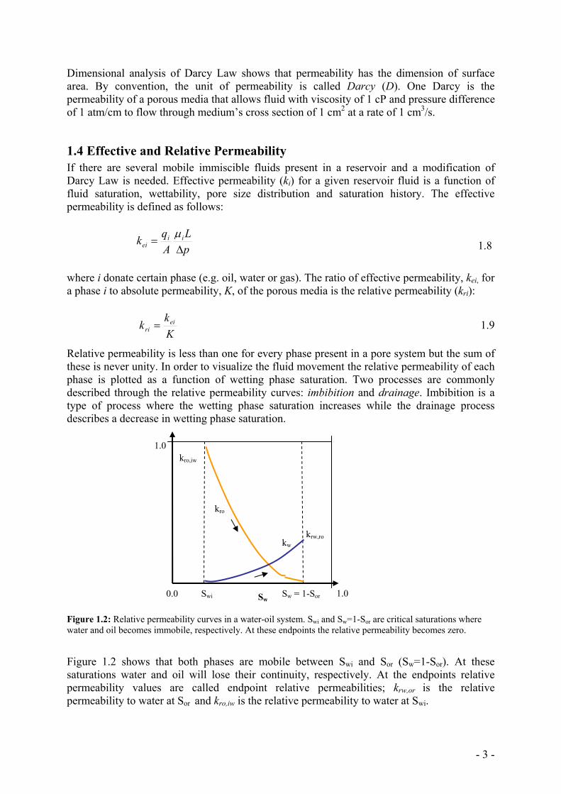
1.5.1 Types of Wettability Through the literature a variety of wettability states are defined: Water-Wet state: Before oil enters the reservoir it is most likely in water –wet state. When the rock is water-wet, there is a tendency for water to occupy small pores and to contact the majority of pore walls. If an oil phase is present in the rock it will occupy the bulk volume f the large pores being absent in the smallest pores. Intermediate state: Rock with intermediate wettability has slight but equal preference to both water and oil. Intermediate wettability includes both fractional and mixed wettability, which will be discussed below. An intermediate rock will imbibe both water and oil spontaneously. Neutral wettability is a special category of intermediate wettability. Natural-wet reservoirs will have an equal tendency for oil and water to wet rock surface. Oil-Wet state: In this wettability state, the oil phase and water phase locations in the pore system are reversed. Oil will contact most of the pore surfaces with water residing the pore centers.

Figure 1.3: Wetting in pores. In water-wet system water covers most of the mineral surface while oil remains in the centre of the pores. In mixed-wet system some parts of pore walls are rendered oil-wet, however, the oil is still in the centre of the pores. In oil-wet system oil covers most of the pore wall surfaces while water is observed in the centre of the pores [Abdallah et. al 2007].

- 5 -

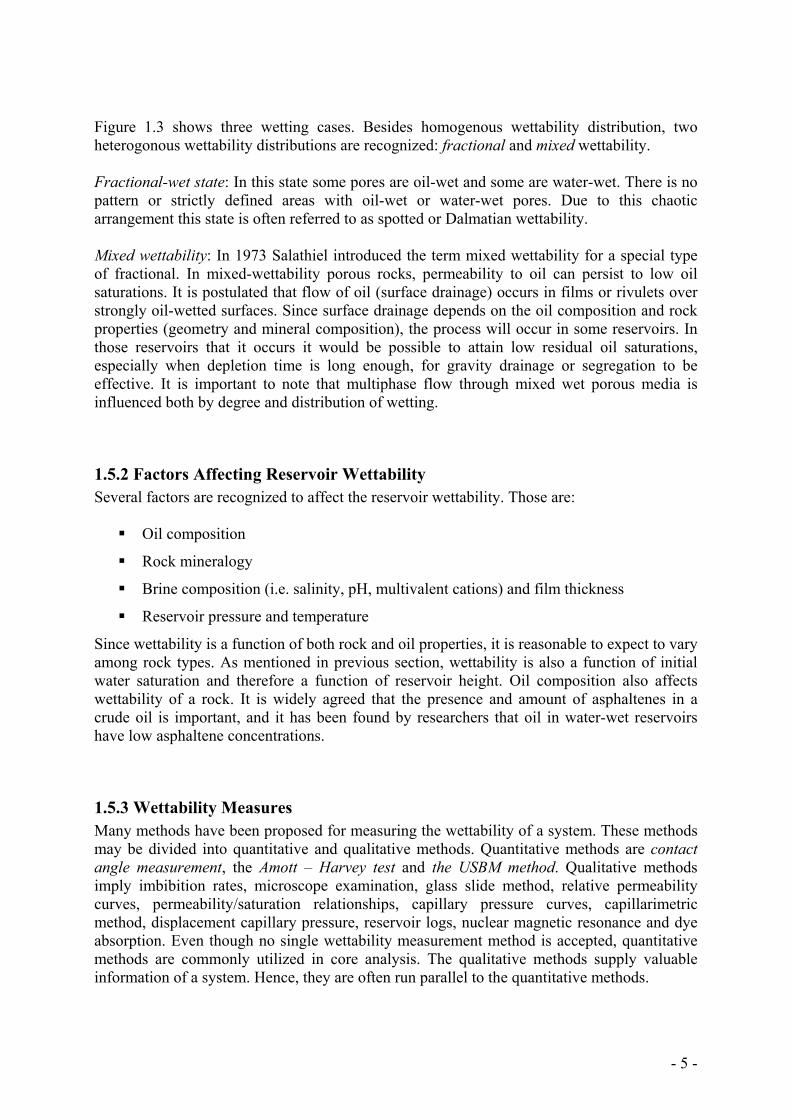
Figure 1.3 shows three wetting cases. Besides homogenous wettability distribution, two heterogonous wettability distributions are recognized: fractional and mixed wettability. Fractional-wet state: In this state some pores are oil-wet and some are water-wet. There is no pattern or strictly defined areas with oil-wet or water-wet pores. Due to this chaotic arrangement this state is often referred to as spotted or Dalmatian wettability. Mixed wettability: In 1973 Salathiel introduced the term mixed wettability for a special type of fractional. In mixed-wettability porous rocks, permeability to oil can persist to low oil saturations. It is postulated that flow of oil (surface drainage) occurs in films or rivulets over strongly oil-wetted surfaces. Since surface drainage depends on the oil composition and rock properties (geometry and mineral composition), the process will occur in some reservoirs. In those reservoirs that it occurs it would be possible to attain low residual oil saturations, especially when depletion time is long enough, for gravity drainage or segregation to be effective. It is important to note that multiphase flow through mixed wet porous media is influenced both by degree and distribution of wetting.

1.5.2 Factors Affecting Reservoir Wettability Several factors are recognized to affect the reservoir wettability. Those are:

Oil composition

Rock mineralogy

Brine composition (i.e. salinity, pH, multivalent cations) and film thickness

Reservoir pressure and temperature

Since wettability is a function of both rock and oil properties, it is reasonable to expect to vary among rock types. As mentioned in previous section, wettability is also a function of initial water saturation and therefore a function of reservoir height. Oil composition also affects wettability of a rock. It is widely agreed that the presence and amount of asphaltenes in a crude oil is important, and it has been found by researchers that oil in water-wet reservoirs have low asphaltene concentrations.

1.5.3 Wettability Measures Many methods have been proposed for measuring the wettability of a system. These methods may be divided into quantitative and qualitative methods. Quantitative methods are contact angle measurement, the Amott – Harvey test and the USBM method. Qualitative methods imply imbibition rates, microscope examination, glass slide method, relative permeability curves, permeability/saturation relationships, capillary pressure curves, capillarimetric method, displacement capillary pressure, reservoir logs, nuclear magnetic resonance and dye absorption. Even though no single wettability measurement method is accepted, quantitative methods are commonly utilized in core analysis. The qualitative methods supply valuable information of a system. Hence, they are often run parallel to the quantitative methods.

- 6 -

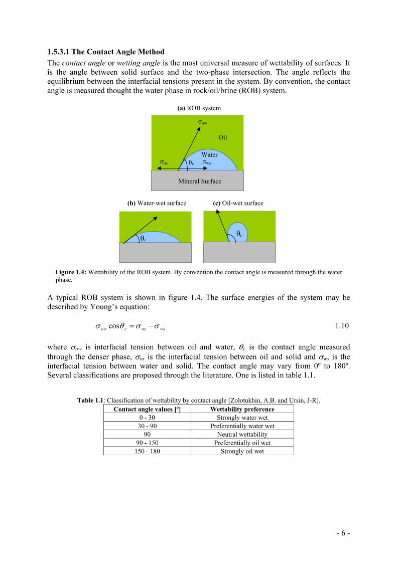
1.5.3.1 The Contact Angle Method The contact angle or wetting angle is the most universal measure of wettability of surfaces. It is the angle between solid surface and the two-phase intersection. The angle reflects the equilibrium between the interfacial tensions present in the system. By convention, the contact angle is measured thought the water phase in rock/oil/brine (ROB) system. (a) ROB system (b) Water-wet surface (c) Oil-wet surface

Figure 1.4: Wettability of the ROB system. By convention the contact angle is measured through the water phase. A typical ROB system is shown in figure 1.4. The surface energies of the system may be described by Young’s equation: wsoscow σσθσ −=cos 1.10 where σow is interfacial tension between oil and water, θc is the contact angle measured through the denser phase, σos is the interfacial tension between oil and solid and σws is the interfacial tension between water and solid. The contact angle may vary from 0º to 180º. Several classifications are proposed through the literature. One is listed in table 1.1.

Table 1.1: Classification of wettability by contact angle [Zolotukhin, A.B. and Ursin, J-R]. Contact angle values [º] Wettability preference

0 - 30 Strongly water wet 30 - 90 Preferentially water wet

90 Neutral wettability 90 - 150 Preferentially oil wet

150 - 180 Strongly oil wet

σow

Oil

Water σws σos θc

θc θc

Mineral Surface

- 7 -

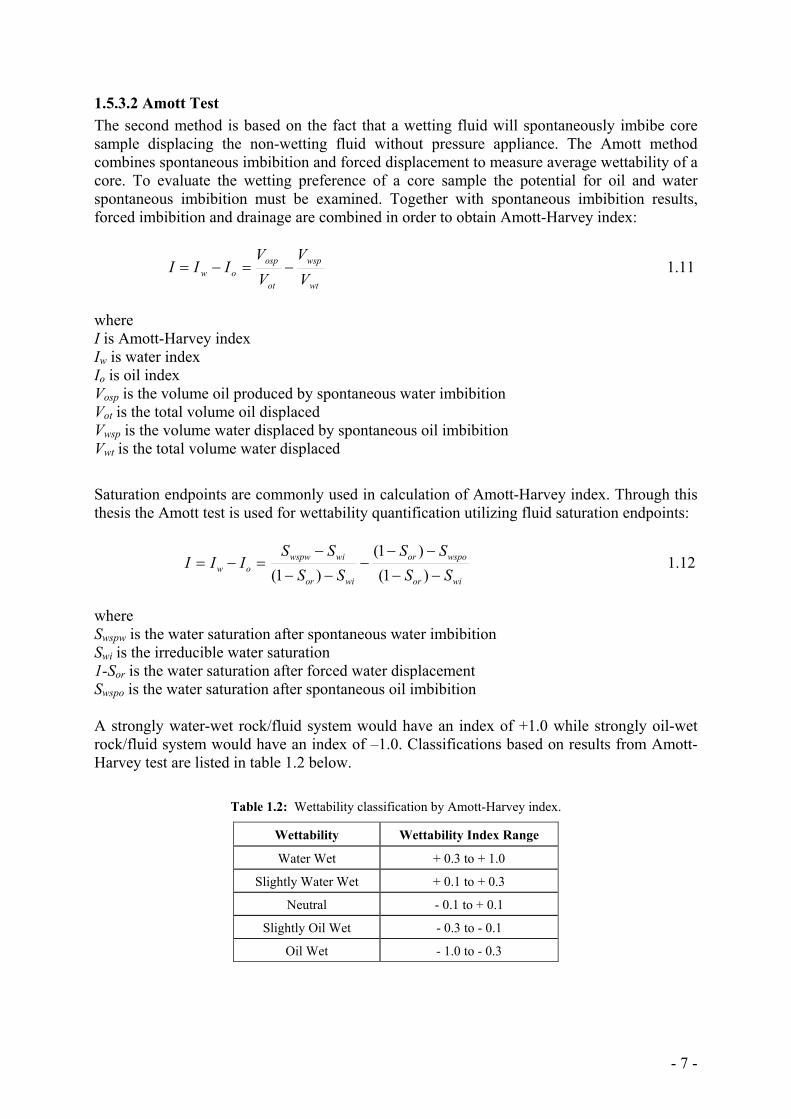
1.5.3.2 Amott Test The second method is based on the fact that a wetting fluid will spontaneously imbibe core sample displacing the non-wetting fluid without pressure appliance. The Amott method combines spontaneous imbibition and forced displacement to measure average wettability of a core. To evaluate the wetting preference of a core sample the potential for oil and water spontaneous imbibition must be examined. Together with spontaneous imbibition results, forced imbibition and drainage are combined in order to obtain Amott-Harvey index:

wt

wsp

ot

ospow V

VVV

III −=−= 1.11

where I is Amott-Harvey index Iw is water index Io is oil index Vosp is the volume oil produced by spontaneous water imbibition Vot is the total volume oil displaced Vwsp is the volume water displaced by spontaneous oil imbibition Vwt is the total volume water displaced

Saturation endpoints are commonly used in calculation of Amott-Harvey index. Through this thesis the Amott test is used for wettability quantification utilizing fluid saturation endpoints:

wior

wspoor

wior

wiwspwow SS

SSSS

SSIII

−−

−−−

−−

−=−=

)1()1(

)1( 1.12

where Swspw is the water saturation after spontaneous water imbibition Swi is the irreducible water saturation 1-Sor is the water saturation after forced water displacement Swspo is the water saturation after spontaneous oil imbibition A strongly water-wet rock/fluid system would have an index of +1.0 while strongly oil-wet rock/fluid system would have an index of –1.0. Classifications based on results from Amott-Harvey test are listed in table 1.2 below.

Table 1.2: Wettability classification by Amott-Harvey index.

Wettability Wettability Index Range

Water Wet + 0.3 to + 1.0

Slightly Water Wet + 0.1 to + 0.3

Neutral - 0.1 to + 0.1

Slightly Oil Wet - 0.3 to - 0.1

Oil Wet - 1.0 to - 0.3

- 8 -

The main problem with Amott wettability test is that it insensitive near neutral wettability. The test measures the ease with which the wetting fluid displaces the non-wetting fluid. However, neither fluid will spontaneously imbibe and displace the other fluid when contact angle varies roughly between 60 and 120°.

1.5.3.3 USBM Test A method also well utilized, USBM method, is sensitive near neutral wettability. USBM method compares the work needed for one fluid to displace another in the pore system. Due to favorable surface energy, less work is needed to displace a non-wetting fluid by wetting fluid than vice versa. All cores are driven to Swi, than placed in centrifuge and curve I is obtained by plotting the capillary pressure vs. the average water saturation for the brine drive. In the next step, the core is placed in oil and centrifuged. The results of oil drive are plotted as curve II. The work needed for displacement is found to be proportional with the area under the capillary pressure curves, leading to:

⎟⎟⎠

⎞⎜⎜⎝

⎛=

2

1logAA

W 1.13

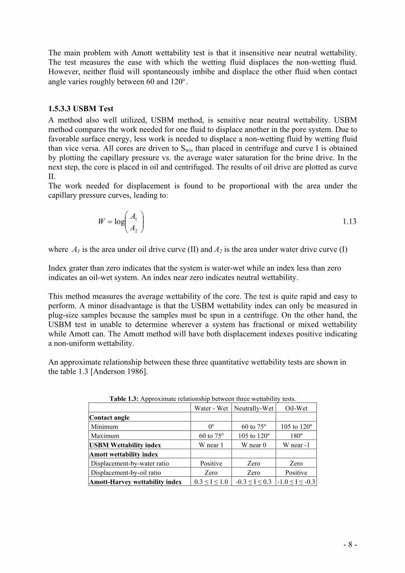
where A1 is the area under oil drive curve (II) and A2 is the area under water drive curve (I) Index grater than zero indicates that the system is water-wet while an index less than zero indicates an oil-wet system. An index near zero indicates neutral wettability. This method measures the average wettability of the core. The test is quite rapid and easy to perform. A minor disadvantage is that the USBM wettability index can only be measured in plug-size samples because the samples must be spun in a centrifuge. On the other hand, the USBM test in unable to determine wherever a system has fractional or mixed wettability while Amott can. The Amott method will have both displacement indexes positive indicating a non-uniform wettability. An approximate relationship between these three quantitative wettability tests are shown in the table 1.3 [Anderson 1986].

Table 1.3: Approximate relationship between three wettability tests. Water - Wet Neutrally-Wet Oil-Wet Contact angle Minimum 0º 60 to 75º 105 to 120º Maximum 60 to 75º 105 to 120º 180º USBM Wettability index W near 1 W near 0 W near -1 Amott wettability index Displacement-by-water ratio Positive Zero Zero Displacement-by-oil ratio Zero Zero Positive Amott-Harvey wettability index 0.3 ≤ I ≤ 1.0 -0.3 ≤ I ≤ 0.3 -1.0 ≤ I ≤ -0.3

- 9 -

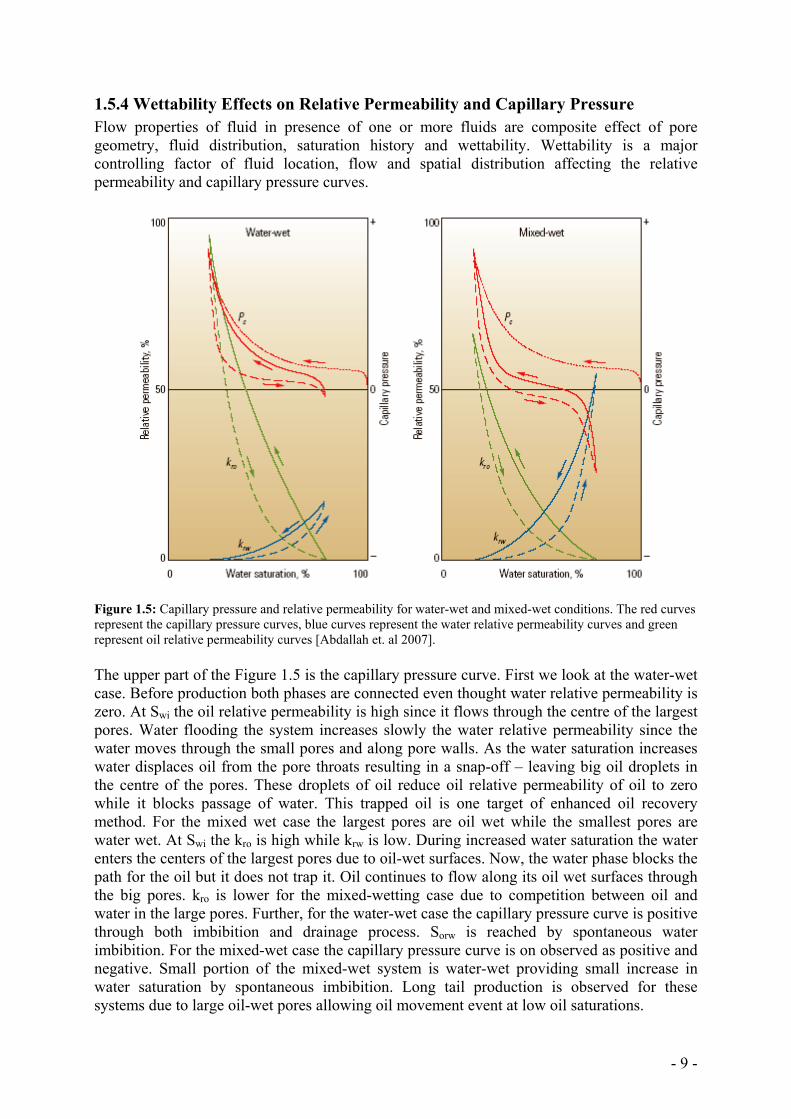
1.5.4 Wettability Effects on Relative Permeability and Capillary Pressure Flow properties of fluid in presence of one or more fluids are composite effect of pore geometry, fluid distribution, saturation history and wettability. Wettability is a major controlling factor of fluid location, flow and spatial distribution affecting the relative permeability and capillary pressure curves.

Figure 1.5: Capillary pressure and relative permeability for water-wet and mixed-wet conditions. The red curves represent the capillary pressure curves, blue curves represent the water relative permeability curves and green represent oil relative permeability curves [Abdallah et. al 2007]. The upper part of the Figure 1.5 is the capillary pressure curve. First we look at the water-wet case. Before production both phases are connected even thought water relative permeability is zero. At Swi the oil relative permeability is high since it flows through the centre of the largest pores. Water flooding the system increases slowly the water relative permeability since the water moves through the small pores and along pore walls. As the water saturation increases water displaces oil from the pore throats resulting in a snap-off – leaving big oil droplets in the centre of the pores. These droplets of oil reduce oil relative permeability of oil to zero while it blocks passage of water. This trapped oil is one target of enhanced oil recovery method. For the mixed wet case the largest pores are oil wet while the smallest pores are water wet. At Swi the kro is high while krw is low. During increased water saturation the water enters the centers of the largest pores due to oil-wet surfaces. Now, the water phase blocks the path for the oil but it does not trap it. Oil continues to flow along its oil wet surfaces through the big pores. kro is lower for the mixed-wetting case due to competition between oil and water in the large pores. Further, for the water-wet case the capillary pressure curve is positive through both imbibition and drainage process. Sorw is reached by spontaneous water imbibition. For the mixed-wet case the capillary pressure curve is on observed as positive and negative. Small portion of the mixed-wet system is water-wet providing small increase in water saturation by spontaneous imbibition. Long tail production is observed for these systems due to large oil-wet pores allowing oil movement event at low oil saturations.

- 10 -

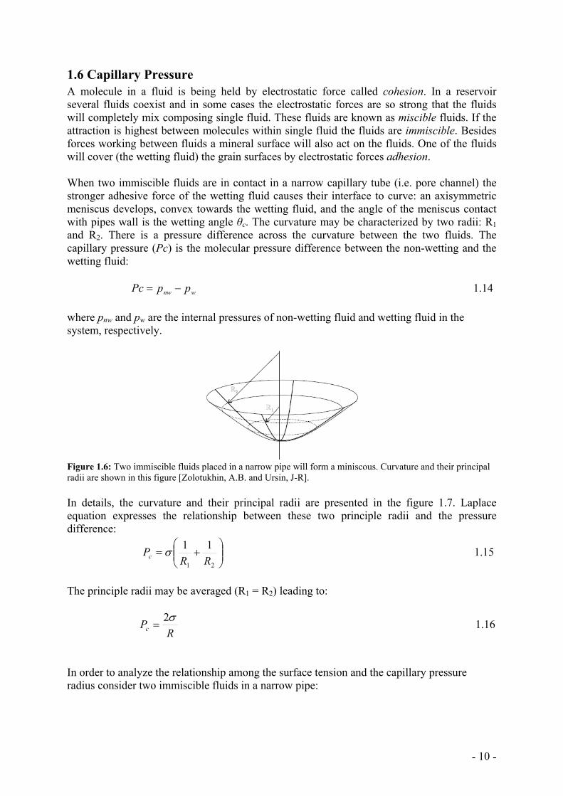
1.6 Capillary Pressure A molecule in a fluid is being held by electrostatic force called cohesion. In a reservoir several fluids coexist and in some cases the electrostatic forces are so strong that the fluids will completely mix composing single fluid. These fluids are known as miscible fluids. If the attraction is highest between molecules within single fluid the fluids are immiscible. Besides forces working between fluids a mineral surface will also act on the fluids. One of the fluids will cover (the wetting fluid) the grain surfaces by electrostatic forces adhesion. When two immiscible fluids are in contact in a narrow capillary tube (i.e. pore channel) the stronger adhesive force of the wetting fluid causes their interface to curve: an axisymmetric meniscus develops, convex towards the wetting fluid, and the angle of the meniscus contact with pipes wall is the wetting angle θc. The curvature may be characterized by two radii: R1 and R2. There is a pressure difference across the curvature between the two fluids. The capillary pressure (Pc) is the molecular pressure difference between the non-wetting and the wetting fluid: wnw ppPc −= 1.14 where pnw and pw are the internal pressures of non-wetting fluid and wetting fluid in the system, respectively.

Figure 1.6: Two immiscible fluids placed in a narrow pipe will form a miniscous. Curvature and their principal radii are shown in this figure [Zolotukhin, A.B. and Ursin, J-R]. In details, the curvature and their principal radii are presented in the figure 1.7. Laplace equation expresses the relationship between these two principle radii and the pressure difference:

⎟⎟⎠

⎞⎜⎜⎝

⎛+=

21

11RR

Pc σ 1.15

The principle radii may be averaged (R1 = R2) leading to:

R

Pcσ2

= 1.16

In order to analyze the relationship among the surface tension and the capillary pressure radius consider two immiscible fluids in a narrow pipe:

- 11 -

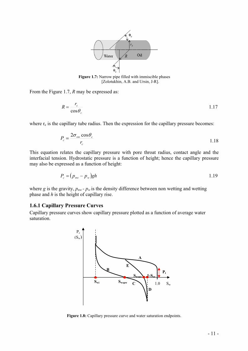
Figure 1.7: Narrow pipe filled with immiscible phases [Zolotukhin, A.B. and Ursin, J-R]. From the Figure 1.7, R may be expressed as:

c

crRθcos

= 1.17

where rc is the capillary tube radius. Then the expression for the capillary pressure becomes:

1.18

This equation relates the capillary pressure with pore throat radius, contact angle and the interfacial tension. Hydrostatic pressure is a function of height; hence the capillary pressure may also be expressed as a function of height: ( )ghppP wnwc −= 1.19 where g is the gravity, pnw - pw is the density difference between non wetting and wetting phase and h is the height of capillary rise.

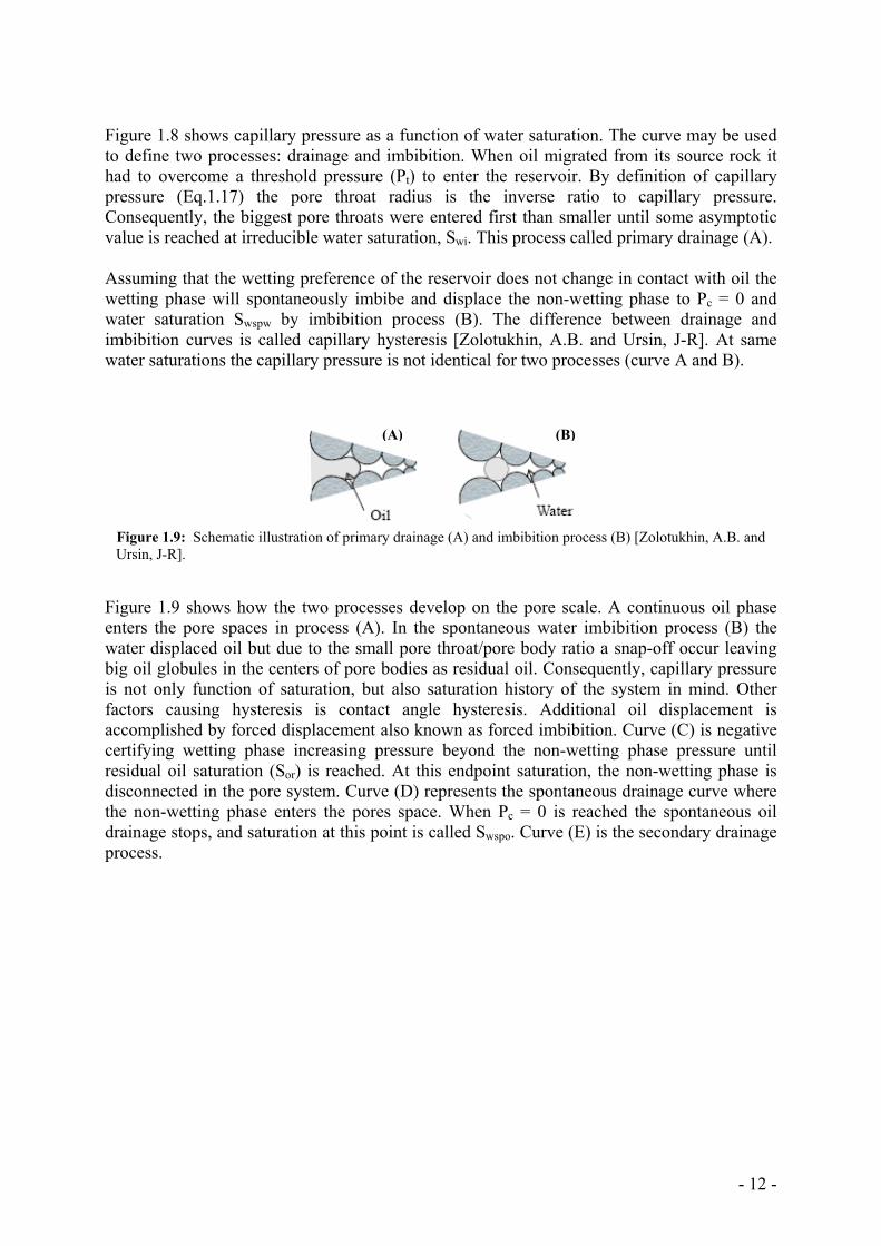
1.6.1 Capillary Pressure Curves Capillary pressure curves show capillary pressure plotted as a function of average water saturation.

Figure 1.8: Capillary pressure curve and water saturation endpoints.

c

cowc r

P θσ cos2=

1.0 Sw Swi

A

B

C D

E

Swspw

Swspo 1-Sor

Pc (Sw)

Pt

- 12 -

Figure 1.8 shows capillary pressure as a function of water saturation. The curve may be used to define two processes: drainage and imbibition. When oil migrated from its source rock it had to overcome a threshold pressure (Pt) to enter the reservoir. By definition of capillary pressure (Eq.1.17) the pore throat radius is the inverse ratio to capillary pressure. Consequently, the biggest pore throats were entered first than smaller until some asymptotic value is reached at irreducible water saturation, Swi. This process called primary drainage (A). Assuming that the wetting preference of the reservoir does not change in contact with oil the wetting phase will spontaneously imbibe and displace the non-wetting phase to Pc = 0 and water saturation Swspw by imbibition process (B). The difference between drainage and imbibition curves is called capillary hysteresis [Zolotukhin, A.B. and Ursin, J-R]. At same water saturations the capillary pressure is not identical for two processes (curve A and B).

Figure 1.9: Schematic illustration of primary drainage (A) and imbibition process (B) [Zolotukhin, A.B. and

Ursin, J-R].

Figure 1.9 shows how the two processes develop on the pore scale. A continuous oil phase enters the pore spaces in process (A). In the spontaneous water imbibition process (B) the water displaced oil but due to the small pore throat/pore body ratio a snap-off occur leaving big oil globules in the centers of pore bodies as residual oil. Consequently, capillary pressure is not only function of saturation, but also saturation history of the system in mind. Other factors causing hysteresis is contact angle hysteresis. Additional oil displacement is accomplished by forced displacement also known as forced imbibition. Curve (C) is negative certifying wetting phase increasing pressure beyond the non-wetting phase pressure until residual oil saturation (Sor) is reached. At this endpoint saturation, the non-wetting phase is disconnected in the pore system. Curve (D) represents the spontaneous drainage curve where the non-wetting phase enters the pores space. When Pc = 0 is reached the spontaneous oil drainage stops, and saturation at this point is called Swspo. Curve (E) is the secondary drainage process.

(A) (B)

- 13 -

1.7 Oil Characterization Adsorption of polar components from crude oil is one of the mechanisms that can alter wettability of a reservoir rock [Morrow et. al 1986]. Crude oils are complex mixtures of hydrocarbons, polar organic compounds containing oxygen, sulphur and nitrogen, and metalliferous components as vanadium, nickel, iron and copper [Skauge et.al 1999]. To understand the effect of interfacially active components in crude oil during interaction between crude oil, water and rock, the crude oil can be divided into different fractions. In order to explain and predict the ability of different oils to change wetting in a Edwards limestone, the following characteristics have been investigated: density/API grade, viscosity, refractive index (RI), acid and base number, SARA components; saturated hydrocarbons (saturates), asphaltenes and oils: NSO- compounds (resins) and aromatic (aromatic hydrocarbons).

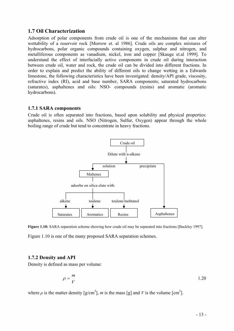
1.7.1 SARA components Crude oil is often separated into fractions, based upon solubility and physical properties: asphaltenes, resins and oils. NSO (Nitrogen, Sulfur, Oxygen) appear through the whole boiling range of crude but tend to concentrate in heavy fractions.

Figure 1.10: SARA separation scheme showing how crude oil may be separated into fractions [Buckley 1997].

Figure 1.10 is one of the many proposed SARA separation schemes.

1.7.2 Density and API Density is defined as mass per volume:

Vm

=ρ 1.20

where ρ is the matter density [g/cm3], m is the mass [g] and V is the volume [cm3].

Crude oil

Dilute with n-alkene

Maltenes

adsorbe on silica elute with:

solution

Saturates Aromatics Resins

alkene toulene toulene/mehtanol

Asphaltenes

precipitate

- 14 -

Another commonly applied measure of the density is API. Even though it has no units it is graduated in degrees. API is a measure of how light or heavy petroleum liquid is compared to water. If API is grater than 10, it is lighter than water and it floats on it. However, if it is lower than 10 it is heavier than water, hence it sinks. API is defined as:

5.1315.141−=

ρAPI 1.21

where ρ is density of an oil. It is also possible to calculate API from SARA test based on established relationship [Fan and Buckley 2002]: AsRASAPIcalculated *763.0*08.1*385.0*306.05.740 −−−−= 1.22 where S is the wt % of saturates, A is the wt % of aromatics, R is the wt % of resins and As is the wt % of asphaltenes.

1.7.3 Refractive Index (RI) Refractive index is a measure of how much the speed of light is reduced inside a medium. RI is defined as:

2

1

vvRI = 1.23

where v1 is the speed of light in vacuum or air and v2 is the speed of light for given material. The number is typically greater than one. RI is a function of density, hence a function of temperature. By SARA test it is possible to calculate RI:

100

6624.1*)(4982.1*4452.1* AsRASRI +++= 1.24

where S is the wt % of saturates, A is the wt % of aromatics, R is the wt % of resins and As is the wt % of asphaltenes.

1.7.4 Acid and Base Number Acid and base numbers are used to characterize the polar components of crude oils. Acid number is a measure of acid components in the oil while base number represents the basic compounds. Acid number is calculated from titration endpoints:

( )W

MWNVVAN bbi **−= 1.25

where AN is acid number (mg KOH/g oil) Vi is the volume of titrant at the sample inflection point (ml) Vb is the volume of titrant at the blank inflection point (ml) Nb is molar concentration of KOH titrant (mol/L) MW is the molar weight of KOH (56.1 g/mol) W is the amount of the oil sample (g)

- 15 -

Base number is calculated from titration endpoints:

( )W

MWNVVBN abi **−= 1.26

where BN is base number (mg KOH/g oil) Vi is the volume of titrant at the sample inflection point (ml) Vb is the volume of titrant at the blank inflection point (ml)

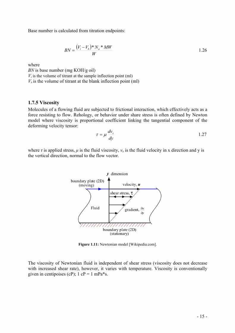
1.7.5 Viscosity Molecules of a flowing fluid are subjected to frictional interaction, which effectively acts as a force resisting to flow. Rehology, or behavior under share stress is often defined by Newton model where viscosity is proportional coefficient linking the tangential component of the deforming velocity tensor:

dydvxµτ = 1.27

where τ is applied stress, µ is the fluid viscosity, vx is the fluid velocity in x direction and y is the vertical direction, normal to the flow vector.

Figure 1.11: Newtonian model [Wikipedia.com].

The viscosity of Newtonian fluid is independent of shear stress (viscosity does not decrease with increased shear rate), however, it varies with temperature. Viscosity is conventionally given in centipoises (cP); 1 cP = 1 mPa*s.

- 16 -

1.8 The Scaling Equation Spontaneous imbibition has long been recognized as important phenomenon in oil recovery from water wet, fractured reservoirs subjected to water flood or water drive. Laboratory results of oil recovery through spontaneous imbibition are commonly scaled-up to forecast oil recovery from fractured reservoirs. Rate of mass transfer between the matrix and the fractures determines the oil production. The rate of imbibition is mainly dependent on porous media, fluids and their interaction. Underlying parameters are: matrix permeability and relative permeability, matrix shape and boundary conditions, fluid viscosity, IFT and wettability [Zhang et.al 1995]. Mattax and Kyte (1962) introduced a scaling group based on the theoretical analysis of Rapport and Leas:

2,1

)( Lorøktt

owMKD µµ

σ= 1.28

where tD,MK is the dimensionless time, t is time, k is absolute permeability, σ is the interfacial tension, µw is the water viscosity and L is the characteristic length. Several assumptions are made for equation 1.28: same wettability, similar pore structure, sample shape (and boundary conditions) must be identical; oil/water viscosity ratio must be duplicated. First equation for characteristic length proposed was a function of distance from the open surface to the center of the matrix. Since the distance of no-flow boundary varied (especially for one-face open imbibition), a modified characteristic length, LC , was proposed [Ma et.al 1995] :

∑=

= n

i Ai

i

bC

lA

VL

1

1.29

where Lc is the characteristic length, Vb is the bulk volume of the core, Ai is the area open to the imbibition in the ith direction and lAi is the distance traveled by the imbibition front from the open surface to the no-flow boundary. To account for the effect of viscosity ratio, sample shape and boundary conditions, the following modified scaling group was proposed:

2

1

CgD Lø

kttµσ

= 1.30

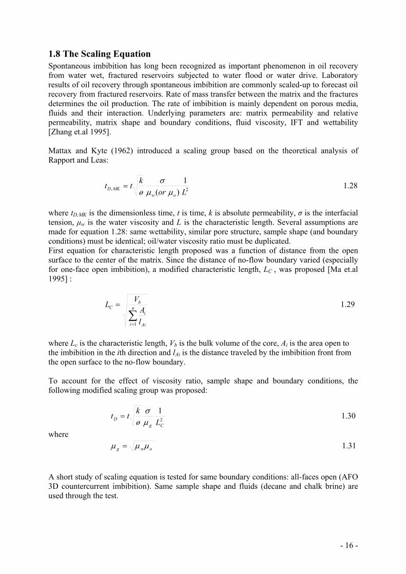
where owg µµµ = 1.31 A short study of scaling equation is tested for same boundary conditions: all-faces open (AFO 3D countercurrent imbibition). Same sample shape and fluids (decane and chalk brine) are used through the test.

- 17 -

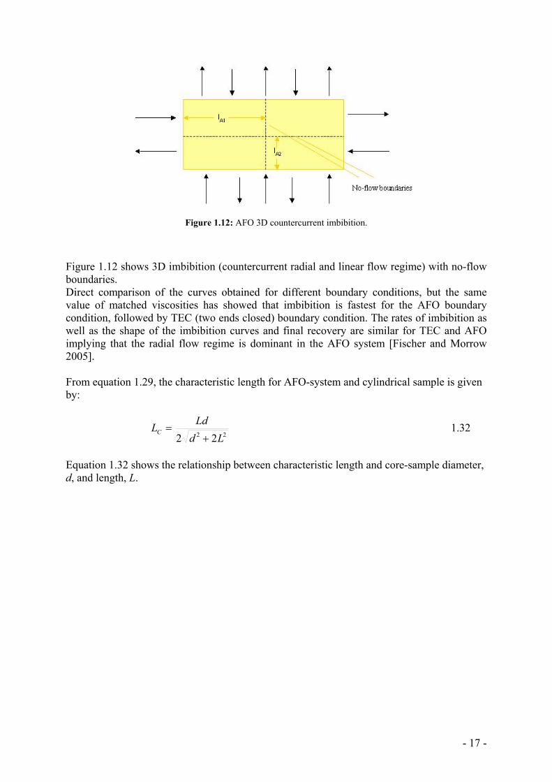
Figure 1.12: AFO 3D countercurrent imbibition.

Figure 1.12 shows 3D imbibition (countercurrent radial and linear flow regime) with no-flow boundaries. Direct comparison of the curves obtained for different boundary conditions, but the same value of matched viscosities has showed that imbibition is fastest for the AFO boundary condition, followed by TEC (two ends closed) boundary condition. The rates of imbibition as well as the shape of the imbibition curves and final recovery are similar for TEC and AFO implying that the radial flow regime is dominant in the AFO system [Fischer and Morrow 2005]. From equation 1.29, the characteristic length for AFO-system and cylindrical sample is given by:

22 22 Ld

LdLC+

= 1.32

Equation 1.32 shows the relationship between characteristic length and core-sample diameter, d, and length, L.

- 18 -

1.9 Nuclear Magnetic Resonance Bloch and Purcell independently discovered NMR in 1946. Six years later they were awarded the Nobel Prize for their achievements. Since then, the development of NMR spectrometers and NMR scanners has led to the opening up of whole new branches of physics, chemistry, biology and medicine. The application of NMR for petroleum exploration started as early as in 1950’s. Many of early applications of NMR spectra were investigations of the composition of petroleum. In NMR we stimulate the magnetic nuclei which absorb and re-emit energy through interactions with other nuclei undergoing terminal motions. The magnetic signals associated with re-emission of this energy tend to decay exponentially with time constants, T1 and T2.

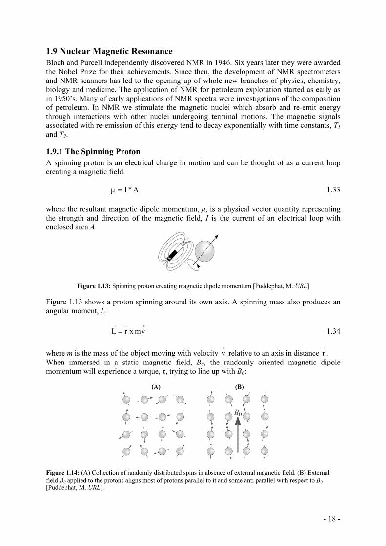
1.9.1 The Spinning Proton A spinning proton is an electrical charge in motion and can be thought of as a current loop creating a magnetic field. A*I=µ 1.33 where the resultant magnetic dipole momentum, µ, is a physical vector quantity representing the strength and direction of the magnetic field, I is the current of an electrical loop with enclosed area A.

Figure 1.13: Spinning proton creating magnetic dipole momentum [Puddephat, M.:URL]

Figure 1.13 shows a proton spinning around its own axis. A spinning mass also produces an angular moment, L: vmxrL = 1.34 where m is the mass of the object moving with velocity v relative to an axis in distance r . When immersed in a static magnetic field, B0, the randomly oriented magnetic dipole momentum will experience a torque, τ, trying to line up with B0: (A) (B)

Figure 1.14: (A) Collection of randomly distributed spins in absence of external magnetic field. (B) External field B0 applied to the protons aligns most of protons parallel to it and some anti parallel with respect to B0 [Puddephat, M.:URL].

- 19 -

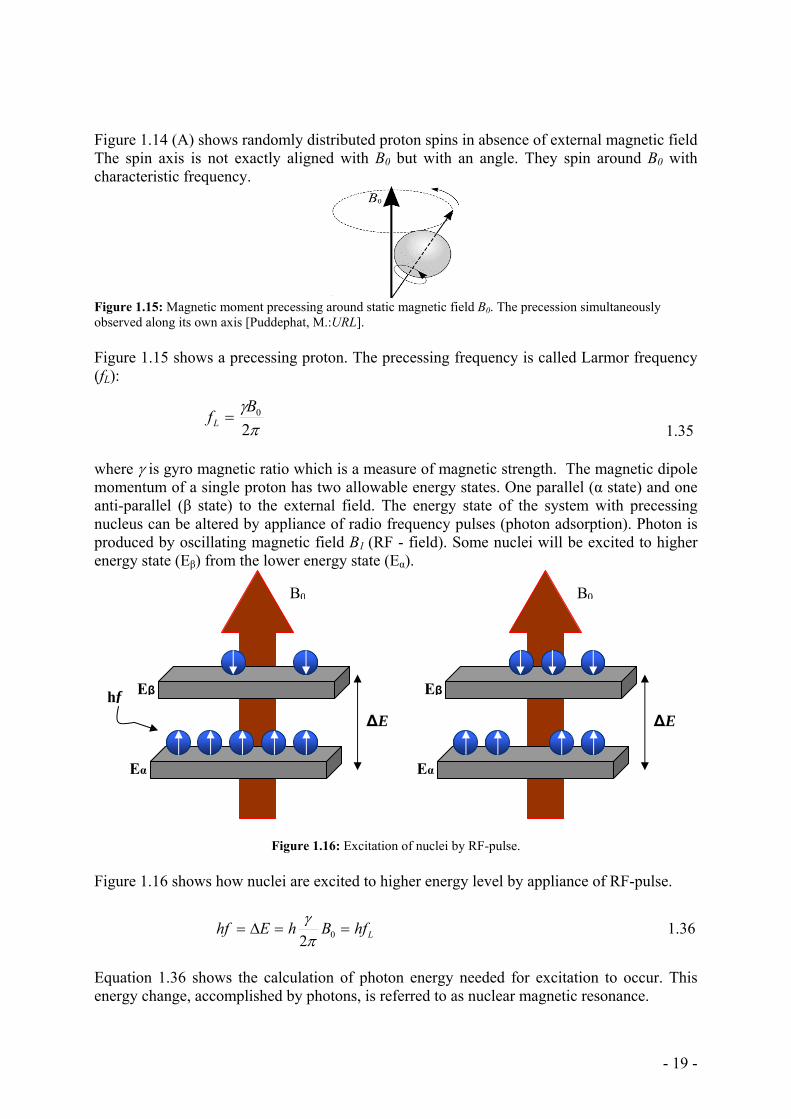
Figure 1.14 (A) shows randomly distributed proton spins in absence of external magnetic field The spin axis is not exactly aligned with B0 but with an angle. They spin around B0 with characteristic frequency.

Figure 1.15: Magnetic moment precessing around static magnetic field B0. The precession simultaneously observed along its own axis [Puddephat, M.:URL]. Figure 1.15 shows a precessing proton. The precessing frequency is called Larmor frequency (fL):

1.35

where γ is gyro magnetic ratio which is a measure of magnetic strength. The magnetic dipole momentum of a single proton has two allowable energy states. One parallel (α state) and one anti-parallel (β state) to the external field. The energy state of the system with precessing nucleus can be altered by appliance of radio frequency pulses (photon adsorption). Photon is produced by oscillating magnetic field B1 (RF - field). Some nuclei will be excited to higher energy state (Eβ) from the lower energy state (Eα).

Figure 1.16: Excitation of nuclei by RF-pulse. Figure 1.16 shows how nuclei are excited to higher energy level by appliance of RF-pulse.

LhfBhEhf ==∆= 02πγ 1.36

Equation 1.36 shows the calculation of photon energy needed for excitation to occur. This energy change, accomplished by photons, is referred to as nuclear magnetic resonance.

hf ∆E

Eβ

Eα

B0

∆E

Eβ

Eα

B0

πγ2

0BfL =

- 20 -

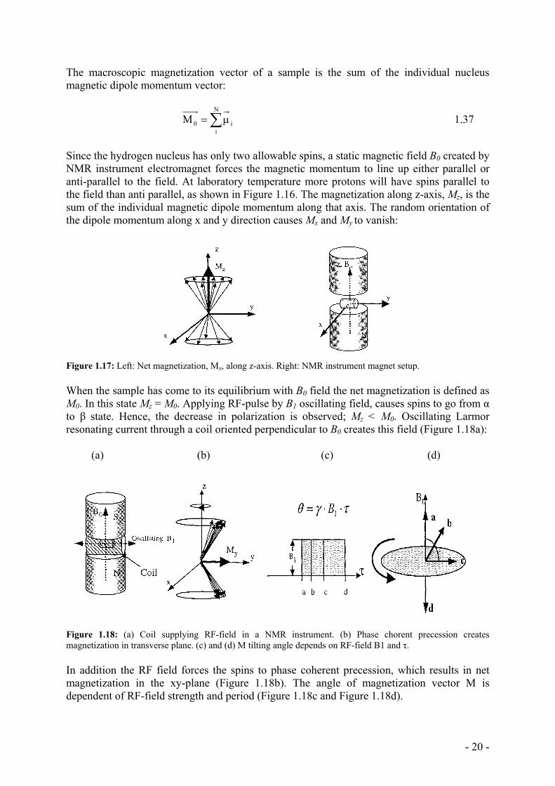
The macroscopic magnetization vector of a sample is the sum of the individual nucleus magnetic dipole momentum vector:

∑µ=N

ii0M 1.37

Since the hydrogen nucleus has only two allowable spins, a static magnetic field B0 created by NMR instrument electromagnet forces the magnetic momentum to line up either parallel or anti-parallel to the field. At laboratory temperature more protons will have spins parallel to the field than anti parallel, as shown in Figure 1.16. The magnetization along z-axis, Mz, is the sum of the individual magnetic dipole momentum along that axis. The random orientation of the dipole momentum along x and y direction causes Mx and My to vanish:

Figure 1.17: Left: Net magnetization, Mz, along z-axis. Right: NMR instrument magnet setup. When the sample has come to its equilibrium with B0 field the net magnetization is defined as M0. In this state Mz = M0. Applying RF-pulse by B1 oscillating field, causes spins to go from α to β state. Hence, the decrease in polarization is observed; Mz < M0. Oscillating Larmor resonating current through a coil oriented perpendicular to B0 creates this field (Figure 1.18a): (a) (b) (c) (d)

Figure 1.18: (a) Coil supplying RF-field in a NMR instrument. (b) Phase chorent precession creates magnetization in transverse plane. (c) and (d) M tilting angle depends on RF-field B1 and τ. In addition the RF field forces the spins to phase coherent precession, which results in net magnetization in the xy-plane (Figure 1.18b). The angle of magnetization vector M is dependent of RF-field strength and period (Figure 1.18c and Figure 1.18d).

- 21 -

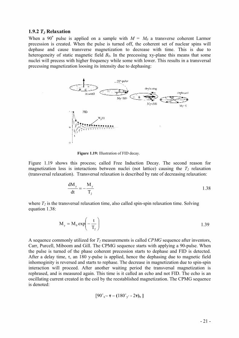
1.9.2 T2 Relaxation When a 90˚ pulse is applied on a sample with M = M0 a transverse coherent Larmor precession is created. When the pulse is turned off, the coherent set of nuclear spins will dephase and cause transverse magnetization to decrease with time. This is due to heterogeneity of static magnetic field B0. In the precessing xy-plane this means that some nuclei will precess with higher frequency while some with lower. This results in a transversal precessing magnetization loosing its intensity due to dephasing:

Figure 1.19: Illustration of FID decay. Figure 1.19 shows this process; called Free Induction Decay. The second reason for magnetization loss is interactions between nuclei (not lattice) causing the T2 relaxation (transversal relaxation). Transversal relaxation is described by rate of decreasing relaxation:

2

yy

TM

dtdM

−= 1.38

where T2 is the transversal relaxation time, also called spin-spin relaxation time. Solving equation 1.38:

1.39

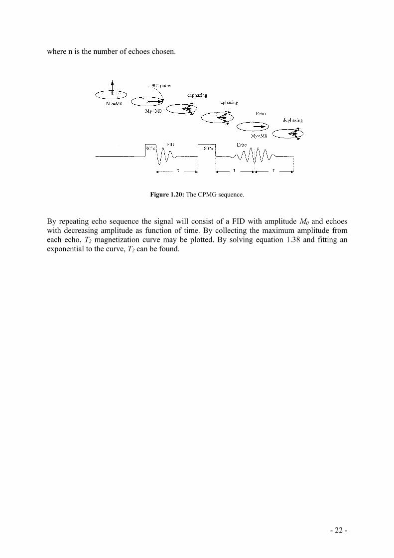
A sequence commonly utilized for T2 measurements is called CPMG sequence after inventors, Carr, Purcell, Miboom and Gill. The CPMG sequence starts with applying a 90-pulse. When the pulse is turned of the phase coherent precession starts to dephase and FID is detected. After a delay time, τ, an 180 y-pulse is applied, hence the dephasing due to magnetic field inhomoginity is reversed and starts to rephase. The decrease in magnetization due to spin-spin interaction will proceed. After another waiting period the transversal magnetization is rephrased, and is measured again. This time is it called an echo and not FID. The echo is an oscillating current created in the coil by the reestablished magnetization. The CPMG sequence is denoted:

[90˚x’- τ – (180˚y’ - 2τ)n ]

⎟⎟⎠

⎞⎜⎜⎝

⎛−=

20y T

texpMM

- 22 -

where n is the number of echoes chosen.

Figure 1.20: The CPMG sequence. By repeating echo sequence the signal will consist of a FID with amplitude M0 and echoes with decreasing amplitude as function of time. By collecting the maximum amplitude from each echo, T2 magnetization curve may be plotted. By solving equation 1.38 and fitting an exponential to the curve, T2 can be found.

- 23 -

1.9.3 Measuring Petrophysical Parameters by NMR By measuring T1 and T2 in porous rock saturated by fluids, petrophysical properties like pore size distributions, saturation and porosity may be defined. For fluids in porous rocks three independent relaxation processes are recognized:

bulk relaxation (affects T1 and T2) surface relaxation (affects T1 and T2) diffusion due to magnetic field gradients (affects T2)

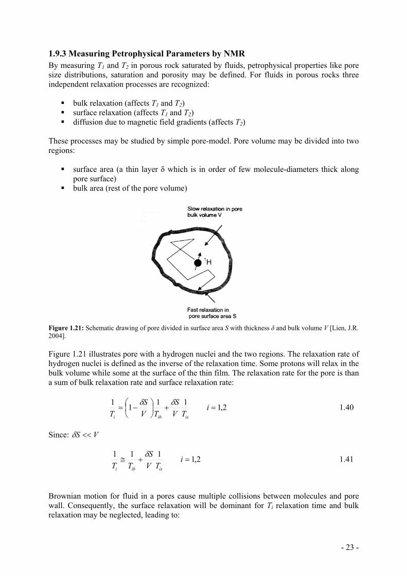
These processes may be studied by simple pore-model. Pore volume may be divided into two regions:

surface area (a thin layer δ which is in order of few molecule-diameters thick along pore surface)

bulk area (rest of the pore volume)

Figure 1.21: Schematic drawing of pore divided in surface area S with thickness δ and bulk volume V [Lien, J.R. 2004]. Figure 1.21 illustrates pore with a hydrogen nuclei and the two regions. The relaxation rate of hydrogen nuclei is defined as the inverse of the relaxation time. Some protons will relax in the bulk volume while some at the surface of the thin film. The relaxation rate for the pore is than a sum of bulk relaxation rate and surface relaxation rate:

2,11111=+⎟

⎠⎞

⎜⎝⎛ −= i

TVS

TVS

T isibi

δδ 1.40

Since: VS <<δ

2,1111=+≅ i

TVS

TT isibi

δ 1.41

Brownian motion for fluid in a pores cause multiple collisions between molecules and pore wall. Consequently, the surface relaxation will be dominant for Ti relaxation time and bulk relaxation may be neglected, leading to:

- 24 -

2,111=≅ i

TVS

T isi

δ 1.42

and

isTδρ = 1.43

Factor ρ is called surface relaxitivity and is a measure of relaxitivity process strength being in force at the pore surface. This factor is independent of the pore size. Acknowledging this, one may conclude:

dSVTi =∝ 1.44

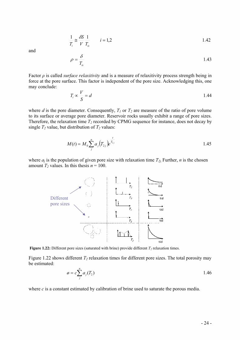
where d is the pore diameter. Consequently, T1 or T2 are measure of the ratio of pore volume to its surface or average pore diameter. Reservoir rocks usually exhibit a range of pore sizes. Therefore, the relaxation time T2 recorded by CPMG sequence for instance, does not decay by single T2 value, but distribution of T2 values:

( ) jTt

n

jjj eTaMtM 2

20)( ∑= 1.45

where aj is the population of given pore size with relaxation time T2j. Further, n is the chosen amount T2 values. In this thesis n = 100.

Figure 1.22: Different pore sizes (saturated with brine) provide different T2 relaxation times. Figure 1.22 shows different T2 relaxation times for different pore sizes. The total porosity may be estimated:

)( 2Tacøn

jj∑= 1.46

where c is a constant estimated by calibration of brine used to saturate the porous media.

Different pore sizes

- 25 -

B > B0

B0

B < B0

f > f0

fL

f < f0

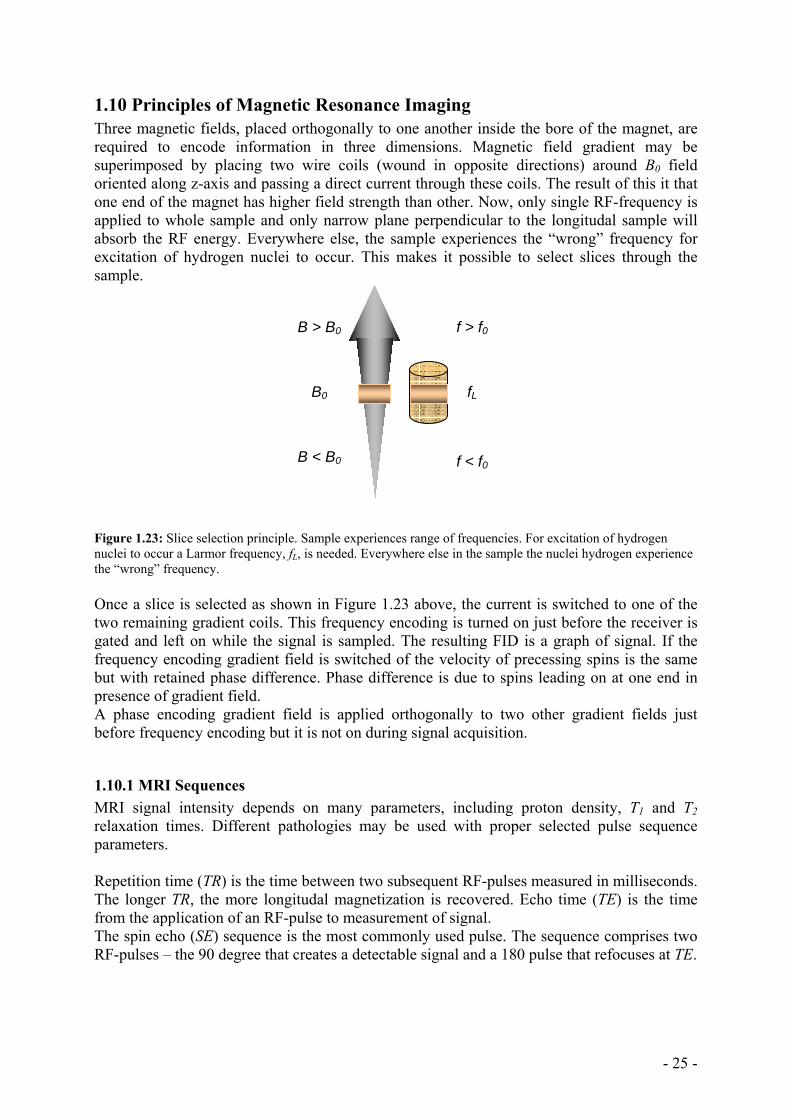
1.10 Principles of Magnetic Resonance Imaging Three magnetic fields, placed orthogonally to one another inside the bore of the magnet, are required to encode information in three dimensions. Magnetic field gradient may be superimposed by placing two wire coils (wound in opposite directions) around B0 field oriented along z-axis and passing a direct current through these coils. The result of this it that one end of the magnet has higher field strength than other. Now, only single RF-frequency is applied to whole sample and only narrow plane perpendicular to the longitudal sample will absorb the RF energy. Everywhere else, the sample experiences the “wrong” frequency for excitation of hydrogen nuclei to occur. This makes it possible to select slices through the sample.

Figure 1.23: Slice selection principle. Sample experiences range of frequencies. For excitation of hydrogen nuclei to occur a Larmor frequency, fL, is needed. Everywhere else in the sample the nuclei hydrogen experience the “wrong” frequency. Once a slice is selected as shown in Figure 1.23 above, the current is switched to one of the two remaining gradient coils. This frequency encoding is turned on just before the receiver is gated and left on while the signal is sampled. The resulting FID is a graph of signal. If the frequency encoding gradient field is switched of the velocity of precessing spins is the same but with retained phase difference. Phase difference is due to spins leading on at one end in presence of gradient field. A phase encoding gradient field is applied orthogonally to two other gradient fields just before frequency encoding but it is not on during signal acquisition.

1.10.1 MRI Sequences MRI signal intensity depends on many parameters, including proton density, T1 and T2 relaxation times. Different pathologies may be used with proper selected pulse sequence parameters. Repetition time (TR) is the time between two subsequent RF-pulses measured in milliseconds. The longer TR, the more longitudal magnetization is recovered. Echo time (TE) is the time from the application of an RF-pulse to measurement of signal. The spin echo (SE) sequence is the most commonly used pulse. The sequence comprises two RF-pulses – the 90 degree that creates a detectable signal and a 180 pulse that refocuses at TE.

- 26 -

PART 2 Experimental

2.1 Core Material In this thesis Edwards limestone from a quarry in West Texas is the porous material used in all tests. It is common to use outcrop core samples as analogues to reservoir rocks. Outcrop rocks are more accessible and less expensive than reservoir rocks. However, they are not always as representative as one should expect. The porosity, permeability, pore size distribution and mineralogy may vary. Before any testing is started it is desirable to get familiar with the core material. One common starting point is to create the thin sections of the sample. These thin sections are saturated with a low-viscosity epoxy. The epoxy is dyed blue for contrast with the mineral grains. Saturation is done with both vacuum and pressure. Most, if not all, connected pores are filled with epoxy. The impregnated core is then cut, ground and polished so that the rock section is approximately 30 microns thick. The pore throat distribution of a given rock type is usually determined by mercury injection test. Although this test is destructive, in the since that the sample cannot be used again, it has advantage that high pressures may be attained, where mercury, the non-wetting phase with the respect to air, can be forced into very small pores. Three samples from same block were prepared at University of Bergen and shipped to ConocoPhillips research center for mercury injection test. Applying equation 1.18 a relationship between pore throat radius and injection pressure is found.

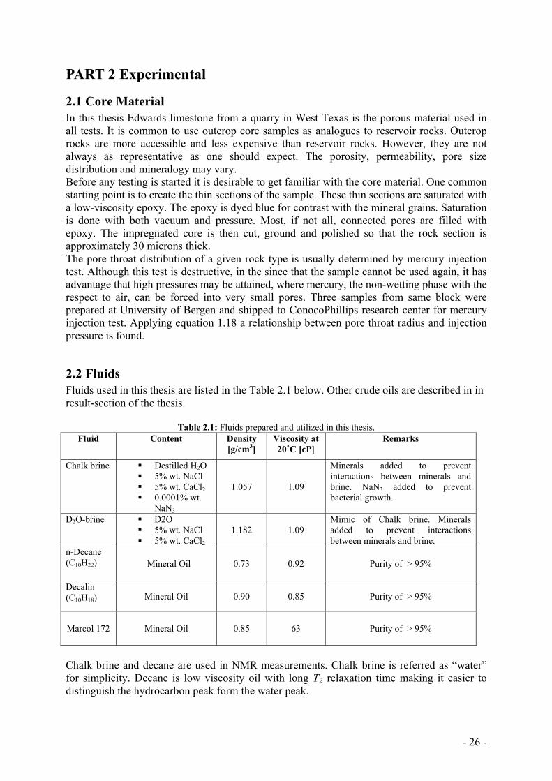
2.2 Fluids Fluids used in this thesis are listed in the Table 2.1 below. Other crude oils are described in in result-section of the thesis.

Table 2.1: Fluids prepared and utilized in this thesis. Fluid Content Density

[g/cm3] Viscosity at 20˚C [cP]

Remarks

Chalk brine Destilled H2O 5% wt. NaCl 5% wt. CaCl2 0.0001% wt.

NaN3

1.057

1.09

Minerals added to prevent interactions between minerals and brine. NaN3 added to prevent bacterial growth.

D2O-brine D2O 5% wt. NaCl 5% wt. CaCl2

1.182 1.09 Mimic of Chalk brine. Minerals added to prevent interactions between minerals and brine.

n-Decane (C10H22) Mineral Oil 0.73 0.92 Purity of > 95%

Decalin (C10H18) Mineral Oil 0.90 0.85 Purity of > 95%

Marcol 172 Mineral Oil 0.85 63 Purity of > 95%

Chalk brine and decane are used in NMR measurements. Chalk brine is referred as “water” for simplicity. Decane is low viscosity oil with long T2 relaxation time making it easier to distinguish the hydrocarbon peak form the water peak.

- 27 -

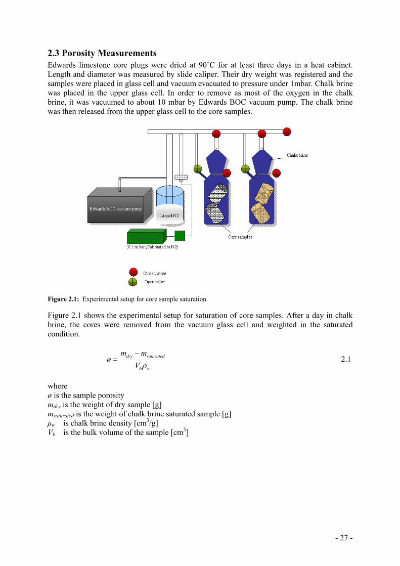
2.3 Porosity Measurements Edwards limestone core plugs were dried at 90˚C for at least three days in a heat cabinet. Length and diameter was measured by slide caliper. Their dry weight was registered and the samples were placed in glass cell and vacuum evacuated to pressure under 1mbar. Chalk brine was placed in the upper glass cell. In order to remove as most of the oxygen in the chalk brine, it was vacuumed to about 10 mbar by Edwards BOC vacuum pump. The chalk brine was then released from the upper glass cell to the core samples.

Figure 2.1: Experimental setup for core sample saturation. Figure 2.1 shows the experimental setup for saturation of core samples. After a day in chalk brine, the cores were removed from the vacuum glass cell and weighted in the saturated condition.

wb

saturateddry

Vmm

øρ

−= 2.1

where ø is the sample porosity mdry is the weight of dry sample [g] msaturated is the weight of chalk brine saturated sample [g] ρw is chalk brine density [cm3/g] Vb is the bulk volume of the sample [cm3]

- 28 -

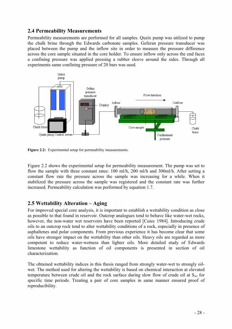
2.4 Permeability Measurements Permeability measurements are performed for all samples. Quzix pump was utilized to pump the chalk brine through the Edwards carbonate samples. Geferan pressure transducer was placed between the pump and the inflow site in order to measure the pressure difference across the core sample situated in the core holder. To ensure inflow only across the end faces a confining pressure was applied pressing a rubber sleeve around the sides. Through all experiments same confining pressure of 20 bars was used.

Figure 2.2: Experimental setup for permeability measurements. Figure 2.2 shows the experimental setup for permeability measurement. The pump was set to flow the sample with three constant rates: 100 ml/h, 200 ml/h and 300ml/h. After setting a constant flow rate the pressure across the sample was increasing for a while. When it stabilized the pressure across the sample was registered and the constant rate was further increased. Permeability calculation was performed by equation 1.7.

2.5 Wettability Alteration – Aging For improved special core analysis, it is important to establish a wettability condition as close as possible to that found in reservoir. Outcrop analogues tend to behave like water-wet rocks, however, the non-water wet reservoirs have been reported [Cuiec 1984]. Introducing crude oils to an outcrop rock tend to alter wettability conditions of a rock, especially in presence of asphaltenes and polar components. From previous experience it has become clear that some oils have stronger impact on the wettability than other oils. Heavy oils are regarded as more competent to reduce water-wetness than lighter oils. More detailed study of Edwards limestone wettability as function of oil components is presented in section of oil characterization. The obtained wettability indices in this thesis ranged from strongly water-wet to strongly oil-wet. The method used for altering the wettability is based on chemical interaction at elevated temperature between crude oil and the rock surface during slow flow of crude oil at Swi for specific time periods. Treating a pair of core samples in same manner ensured proof of reproducibility.

- 29 -

2.5.1 Aging Experimental Procedure A reproducible method for altering the wettability of an outcrop rock has earlier been reported [Graue et. al 1999, 2002]. Through this work several important aspects have been recognized when creating stable and homogenous wettability distribution:

Oil composition: Polar components such as resins and asphaltenes may alter wettability of porous rock. Different crude oil alter wetting to different extents [Jia et. al 1991].

Swi: Initial water saturation has been proven to impact the alteration process. Wettability alteration is more efficient at lower initial water saturation [Graue et.al 1999a]. Swi was established by injecting 2 PV crude oil in each direction [Zhang and Austad 2005].

Aging temperature: Most reactions speed up with increasing temperature. The diffusion of oil components increases and probability for collisions between components and pore wall increases. Increasing collision results in higher adsorption. [Jia et. al 1991].

Aging method: Submerging the core plug into the crude oil and aging for long times may cause heterogeneous wettability conditions. Wettability alteration is more efficient if crude oil is flushed at low rates through the core material during the aging process; however, by unidirectional oil flood non-uniform wettability conditions are created. The most uniform wettability condition is obtained by multidirectional oil flood [Graue et.al 2002]. Flooding the core sample adds new components continuously to the pore system.

Oil flood rate: Low oil flood rate is preferred because it gives components opportunity to adhere to the surface before they end up in the outflow end.

Aging time and pore volumes injected: A consistent decrease in Amott index is observed with increase in aging time [Graue et. al 1998, Jia et. al 1991].

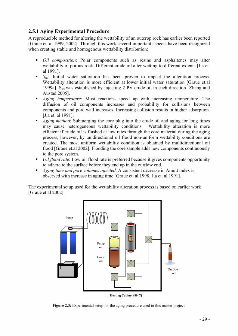
The experimental setup used for the wettability alteration process is based on earlier work [Graue et.al 2002].

Figure 2.3: Experimental setup for the aging procedure used in this master project.

Pump

Crude oil

Outflow end

Pump oil

Heating Cabinet (80˚C)

- 30 -

Figure 2.3 shows the experimental setup for the aging procedure used in this thesis. Following procedure steps are utilized for all cores:

1. The barrel containing oil was shaken and the crude oil was tapped form the centre of the barrel and stored in sealed glass containers at 20˚C.

2. The oil is filtered in the heating cabinet (at 80 ± 0.5˚C) through a 1-2 cm thick Edwards limestone plug in order to remove particles that could reduce samples permeability during the aging procedure. The core-filtered crude oil was stored at this temperature until used.

3. The cores were placed in a core holder. A confinement pressure of 20 bar was utilized. 4. All samples are drained (multidirectional) by constant pressure (1.5 bar/cm) with

crude oil to Swi. Two pore volumes with crude oil was flooded in each direction. 5. Produced water volume was recorded at the outflow end. 6. The pump was set to constant rate delivery option. A rate of 1.5 ml/h was chosen for

all cores (multidirectional). 7. After desired time span the crude oil was exchanged by decalin. Constant pressure was

utilized (1.5 bar/cm). Approximately 2.5 pore volumes of decalin were flooded in each direction.

8. Decalin was exchanged by decane – 2.5 pore volumes in each direction. 9. Cores were cooled off in decane filled containers before Amott test was initiated.

After aging, the crude oil was exchanged by decaline, which subsequently was exchanged by decane. Decane has been shown not to alter wettability in chalk [Graue et. al 2002]. Bottle tests have shown precipitation of asphaltenes (the aging is continued) when crude oil was contacted by decane. Decalin is for this reason used as a buffer between crude oil and decane.

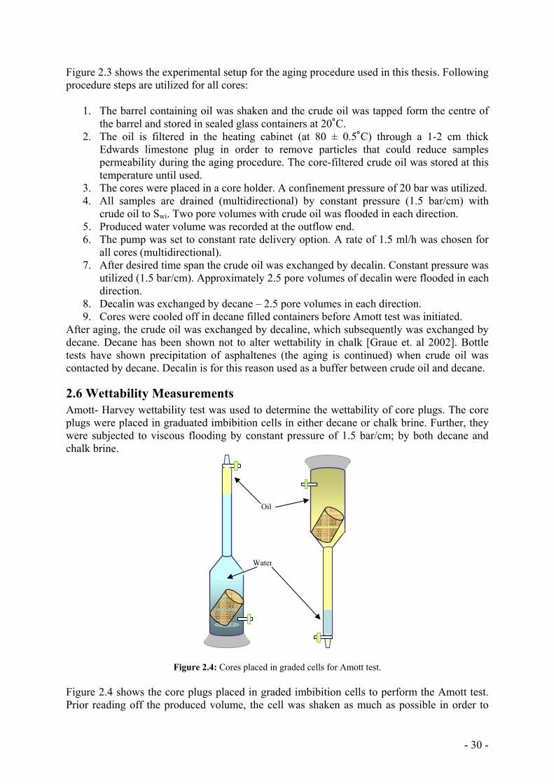
2.6 Wettability Measurements Amott- Harvey wettability test was used to determine the wettability of core plugs. The core plugs were placed in graduated imbibition cells in either decane or chalk brine. Further, they were subjected to viscous flooding by constant pressure of 1.5 bar/cm; by both decane and chalk brine.

Figure 2.4: Cores placed in graded cells for Amott test. Figure 2.4 shows the core plugs placed in graded imbibition cells to perform the Amott test. Prior reading off the produced volume, the cell was shaken as much as possible in order to

Water

Oil

- 31 -

register most precise volume values of spontaneously displaced fluid. Of course, in most cases there were always some drops of fluid attached at the plug surface that adhered so well to the surface that it was impossible to shake them of. For every reading the date and time was registered. Strongly wetted (water or oil) plugs initiated the imbibition quickly and reached their endpoint saturations after spontaneous imbibition fast while weakly wetted plugs had longer induction time (time before imbibition initiated). If there was no change in the saturation in the last month, the imbibition of the given phase was terminated. The Amott- Harvey index was calculated by equation 1.12.

2.7 Scaling – Size and Initial Water Saturation All samples had same shape (cylindrical) and all tests performed were three-dimensional imbibition tests. Desired irreducible water saturations were obtained by decane or marcol-172 flood (marcol-172 is carefully exchanged with decane prior imbibition test). Oil displaced as a function of time was measured as a function of time. The first scaling test was initiated to test the validation of scaling for different dimensions. Two 1.5 inch and two 2.0 inch samples were drained by decane to same initial water saturation. Besides different diameter the cores had a slightly different lengths, porosities and permabilities. The second test was about different Swi. Chalk brine and decane from Table 2.1 were used in these tests.

2.8 Oil Characterization In order to explain and predict the ability of different oils to change wetting in a Edwards limestone, the following characteristics have been investigated: density/API grade, viscosity, refractive index (RI), acid and base number, SARA components; saturated hydrocarbons (saturates), asphaltenes and oils: NSO- compounds (resins) and aromatic (aromatic hydrocarbons).

2.8.1 SARA components Preparation 1 g of crude was placed in small glass bottles (preparation bottles) and marked by crude ID number. 36 ml hexane was added to the bottles in order to force asphaltene precipitation. The oils SARA components were measured using standard HPLC methods [Fan and Buckley 2002]. Saturates and Aromatics 3 ml of maltenes were removed from each bottle placing the syringe on top of the interface. The precipitated asphaltenes were on the bottom of the bottle and are not disturbed in this procedure. The removed oil is placed in new bottles. 25 µml of oil was removed from the new bottles and injected to LC-20AT prominence liquid chromatograph (Shimazu). Two to three tops are observable in the chromotogram displayed on a PC screen. The first top represents saturates while the other represents aromatic with single ring and two rings, respectively. Resins Clean bottles were weight for the resin test. Two additional bottles were weight that would not be used in the test. About 2.5 ml of oil and hexane mixture is introduced to LC-20AT prominence liquid chromatograph. The column (µBondpak NH2) mounted in the system separates the components from the crude oil. The resins are absorbed in the cell due to its polarity. Saturates and aromatics leave the system first. Dichloromethane (DCM) is then

- 32 -

flushed through the cell and the system. DCM and resins are collected in the clean bottles that are weighted. Lids are removed allowing free evaporation of DCM. After 24 h the bottles with resin are placed in a heat cabinet for additional evaporation. Bottles were than weighted with their lids on to determine the amount of resin by weight measurements. The two bottles were also weighted so that the weight measurements of resins could be corrected (the bottles weighted 0.004 g less). Asphaltenes Nine paper filters were weight and placed in marked plastic cups by oil ID. Filter was placed on the beaker. The rest of the oil from the preparation bottles was poured onto the filter. A vacuum pump was started to increase flow rate through the filter. Further, the filters were removed from the beaker and placed on the plastic cups to dry over night. Next day, filters were weighted and amount of asphaltenes was obtained.

2.8.2 Oil Density and Viscosity The oil’s viscosity and density were measured as function of temperature (20, 25 and 30˚C) using Anton Paar SVM 3000 Stabinger Viscometer. 5 ml crude oil was injected into the instrument. For each temperature three measurements were made by the instrument giving an average value of viscosity and density.

2.8.3 Refractive Index (RI) Small amount of oil is introduced to the INDEX Automatic Refractometer GPR11-37 ‘X’ model. RI and temperature was ready immediately.

2.8.4 Acid and Base Number Acid Number (AN) Titration fluids were prepared following an established method for acid number measurements ATSM-D664-89 [Fan and Buckley 2006]. ASTM-D664-89 involves a potentiometric titration of a sample of crude oil (about 2 g) dissolved in 60 ml solvent. The method does not always give a clear inflection point. Spiking the crude oil with a 1 ml stearic acid forces a good inflection. Sampling rate was set to every 12th sec on the computer. Rate of the titration fluid was added from the Brinkmann dispenser of about 0.02 ml/min. Data acquisition was initiated at the same time as the Brinkmann dispenser was started. Blank measurements (spiked solvent) were made after crude oil titrations to compensate for the changes in electrode properties that occur when electrodes comes in contact with crude oil. Most inflection points were observed between -250mV and 400mV. Two tests were done for each crude oil. Base Number (BN) Method ASTM-D2896-88 [Fan and Buckley 2006] was adapted for determination of base number. The method involves potentiometric titration of crude oil in 50 ml solvent fluid. 1 ml base spike was added to the mixture of crude and solvent. Delivery rate from the Brinkmann dispenser was set to 0.1 ml/min. The end point was always observed between 400 and 500 mV. Two tests were done for each crude oil.

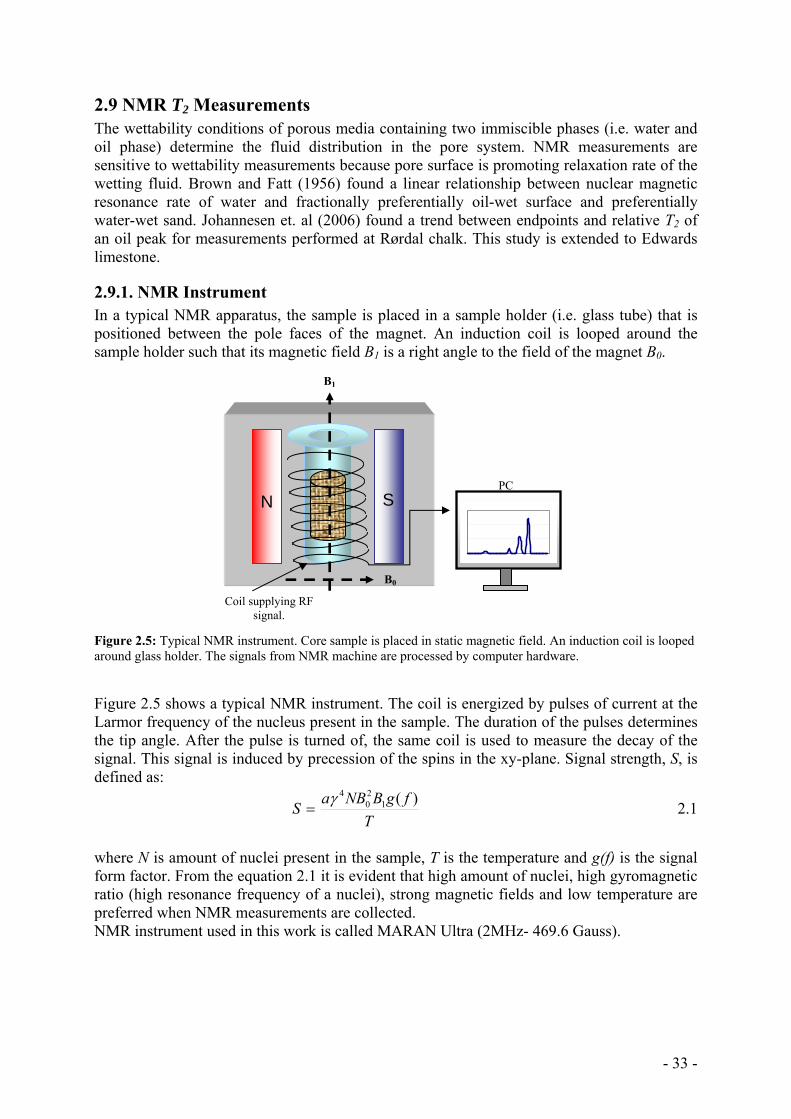
- 33 -

N S

Coil supplying RF signal.

PC

B1

B0

2.9 NMR T2 Measurements The wettability conditions of porous media containing two immiscible phases (i.e. water and oil phase) determine the fluid distribution in the pore system. NMR measurements are sensitive to wettability measurements because pore surface is promoting relaxation rate of the wetting fluid. Brown and Fatt (1956) found a linear relationship between nuclear magnetic resonance rate of water and fractionally preferentially oil-wet surface and preferentially water-wet sand. Johannesen et. al (2006) found a trend between endpoints and relative T2 of an oil peak for measurements performed at Rørdal chalk. This study is extended to Edwards limestone.

2.9.1. NMR Instrument In a typical NMR apparatus, the sample is placed in a sample holder (i.e. glass tube) that is positioned between the pole faces of the magnet. An induction coil is looped around the sample holder such that its magnetic field B1 is a right angle to the field of the magnet B0.

Figure 2.5: Typical NMR instrument. Core sample is placed in static magnetic field. An induction coil is looped around glass holder. The signals from NMR machine are processed by computer hardware.

Figure 2.5 shows a typical NMR instrument. The coil is energized by pulses of current at the Larmor frequency of the nucleus present in the sample. The duration of the pulses determines the tip angle. After the pulse is turned of, the same coil is used to measure the decay of the signal. This signal is induced by precession of the spins in the xy-plane. Signal strength, S, is defined as:

T

fgBNBaS )(120

4γ= 2.1

where N is amount of nuclei present in the sample, T is the temperature and g(f) is the signal form factor. From the equation 2.1 it is evident that high amount of nuclei, high gyromagnetic ratio (high resonance frequency of a nuclei), strong magnetic fields and low temperature are preferred when NMR measurements are collected. NMR instrument used in this work is called MARAN Ultra (2MHz- 469.6 Gauss).

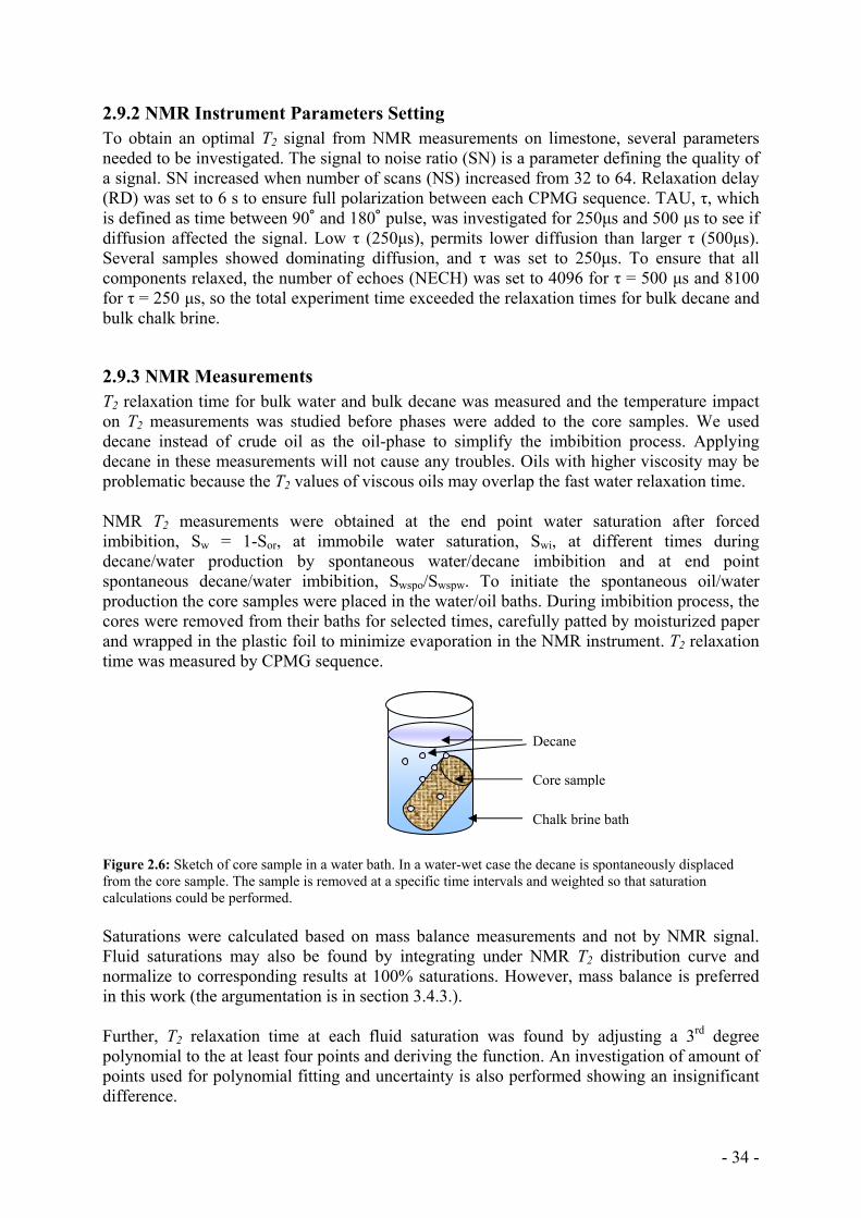
- 34 -

2.9.2 NMR Instrument Parameters Setting To obtain an optimal T2 signal from NMR measurements on limestone, several parameters needed to be investigated. The signal to noise ratio (SN) is a parameter defining the quality of a signal. SN increased when number of scans (NS) increased from 32 to 64. Relaxation delay (RD) was set to 6 s to ensure full polarization between each CPMG sequence. TAU, τ, which is defined as time between 90˚ and 180˚ pulse, was investigated for 250µs and 500 µs to see if diffusion affected the signal. Low τ (250µs), permits lower diffusion than larger τ (500µs). Several samples showed dominating diffusion, and τ was set to 250µs. To ensure that all components relaxed, the number of echoes (NECH) was set to 4096 for τ = 500 µs and 8100 for τ = 250 µs, so the total experiment time exceeded the relaxation times for bulk decane and bulk chalk brine.

2.9.3 NMR Measurements T2 relaxation time for bulk water and bulk decane was measured and the temperature impact on T2 measurements was studied before phases were added to the core samples. We used decane instead of crude oil as the oil-phase to simplify the imbibition process. Applying decane in these measurements will not cause any troubles. Oils with higher viscosity may be problematic because the T2 values of viscous oils may overlap the fast water relaxation time. NMR T2 measurements were obtained at the end point water saturation after forced imbibition, Sw = 1-Sor, at immobile water saturation, Swi, at different times during decane/water production by spontaneous water/decane imbibition and at end point spontaneous decane/water imbibition, Swspo/Swspw. To initiate the spontaneous oil/water production the core samples were placed in the water/oil baths. During imbibition process, the cores were removed from their baths for selected times, carefully patted by moisturized paper and wrapped in the plastic foil to minimize evaporation in the NMR instrument. T2 relaxation time was measured by CPMG sequence.

Figure 2.6: Sketch of core sample in a water bath. In a water-wet case the decane is spontaneously displaced from the core sample. The sample is removed at a specific time intervals and weighted so that saturation calculations could be performed.

Saturations were calculated based on mass balance measurements and not by NMR signal. Fluid saturations may also be found by integrating under NMR T2 distribution curve and normalize to corresponding results at 100% saturations. However, mass balance is preferred in this work (the argumentation is in section 3.4.3.). Further, T2 relaxation time at each fluid saturation was found by adjusting a 3rd degree polynomial to the at least four points and deriving the function. An investigation of amount of points used for polynomial fitting and uncertainty is also performed showing an insignificant difference.

Chalk brine bath

Core sample

Decane

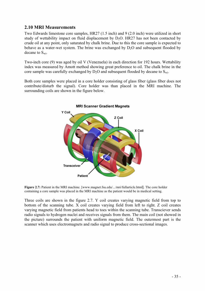
- 35 -

2.10 MRI Measurements Two Edwards limestone core samples, HR27 (1.5 inch) and 9 (2.0 inch) were utilized in short study of wettability impact on fluid displacement by D2O. HR27 has not been contacted by crude oil at any point, only saturated by chalk brine. Due to this the core sample is expected to behave as a water-wet system. The brine was exchanged by D2O and subsequent flooded by decane to Swi. Two-inch core (9) was aged by oil V (Venezuela) in each direction for 192 hours. Wettability index was measured by Amott method showing great preference to oil. The chalk brine in the core sample was carefully exchanged by D2O and subsequent flooded by decane to Swi. Both core samples were placed in a core holder consisting of glass fiber (glass fiber does not contribute/disturb the signal). Core holder was than placed in the MRI machine. The surrounding coils are shown in the figure below.

Figure 2.7: Patient in the MRI machine. [www.magnet.fsu.edu/.../mri/fullarticle.html]. The core holder containing a core sample was placed in the MRI machine as the patient would be in medical setting. Three coils are shown in the figure 2.7. Y coil creates varying magnetic field from top to bottom of the scanning tube. X coil creates varying field from left to right. Z coil creates varying magnetic field from patients head to toes within the scanning tube. Transciever sends radio signals to hydrogen nuclei and receives signals from them. The main coil (not showed in the picture) surrounds the patient with uniform magnetic field. The outermost part is the scanner which uses electromagnets and radio signal to produce cross-sectional images.

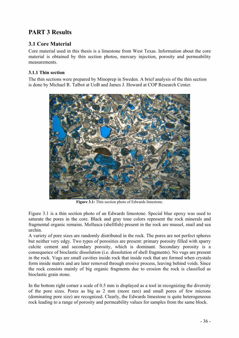
- 36 -

PART 3 Results

3.1 Core Material Core material used in this thesis is a limestone from West Texas. Information about the core material is obtained by thin section photos, mercury injection, porosity and permeability measurements.

3.1.1 Thin section The thin sections were prepared by Minoprep in Sweden. A brief analysis of the thin section is done by Michael R. Talbot at UoB and James J. Howard at COP Research Center.

Figure 3.1: Thin section photo of Edwards limestone.

Figure 3.1 is a thin section photo of an Edwards limestone. Special blue epoxy was used to saturate the pores in the core. Black and gray tone colors represent the rock minerals and fragmental organic remains. Mollusca (shellfish) present in the rock are mussel, snail and sea urchin. A variety of pore sizes are randomly distributed in the rock. The pores are not perfect spheres but neither very edgy. Two types of porosities are present: primary porosity filled with sparry calcite cement and secondary porosity, which is dominant. Secondary porosity is a consequence of bioclastic dissolution (i.e. dissolution of shell fragments). No vugs are present in the rock. Vugs are small cavities inside rock that inside rock that are formed when crystals form inside matrix and are later removed through erosive process, leaving behind voids. Since the rock consists mainly of big organic fragments due to erosion the rock is classified as bioclastic grain stone. In the bottom right corner a scale of 0.5 mm is displayed as a tool in recognizing the diversity of the pore sizes. Pores as big as 2 mm (more rare) and small pores of few microns (dominating pore size) are recognized. Clearly, the Edwards limestone is quite heterogeneous rock leading to a range of porosity and permeability values for samples from the same block.

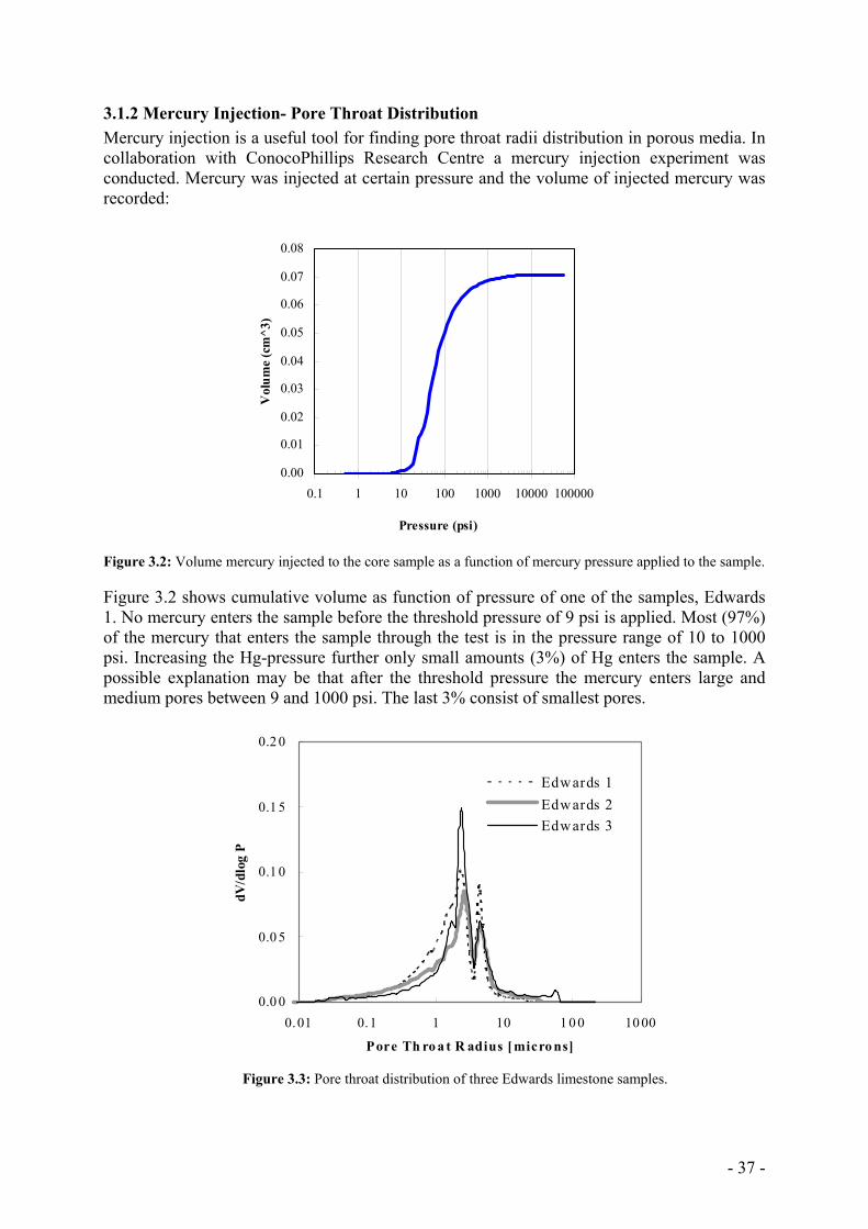
- 37 -

3.1.2 Mercury Injection- Pore Throat Distribution Mercury injection is a useful tool for finding pore throat radii distribution in porous media. In collaboration with ConocoPhillips Research Centre a mercury injection experiment was conducted. Mercury was injected at certain pressure and the volume of injected mercury was recorded:

0.00

0.01

0.02

0.03

0.04

0.05

0.06

0.07

0.08

0.1 1 10 100 1000 10000 100000

Pressure (psi)

Vol

ume

(cm

^3)

Figure 3.2: Volume mercury injected to the core sample as a function of mercury pressure applied to the sample. Figure 3.2 shows cumulative volume as function of pressure of one of the samples, Edwards 1. No mercury enters the sample before the threshold pressure of 9 psi is applied. Most (97%) of the mercury that enters the sample through the test is in the pressure range of 10 to 1000 psi. Increasing the Hg-pressure further only small amounts (3%) of Hg enters the sample. A possible explanation may be that after the threshold pressure the mercury enters large and medium pores between 9 and 1000 psi. The last 3% consist of smallest pores.

0.0 0

0.0 5

0.1 0

0.1 5

0.2 0

0.01 0.1 1 10 1 0 0 10 00

Pore Th ro a t R adius [ micro ns]

dV/d

log

P

Edwards 1Edwards 2Edwards 3

Figure 3.3: Pore throat distribution of three Edwards limestone samples.

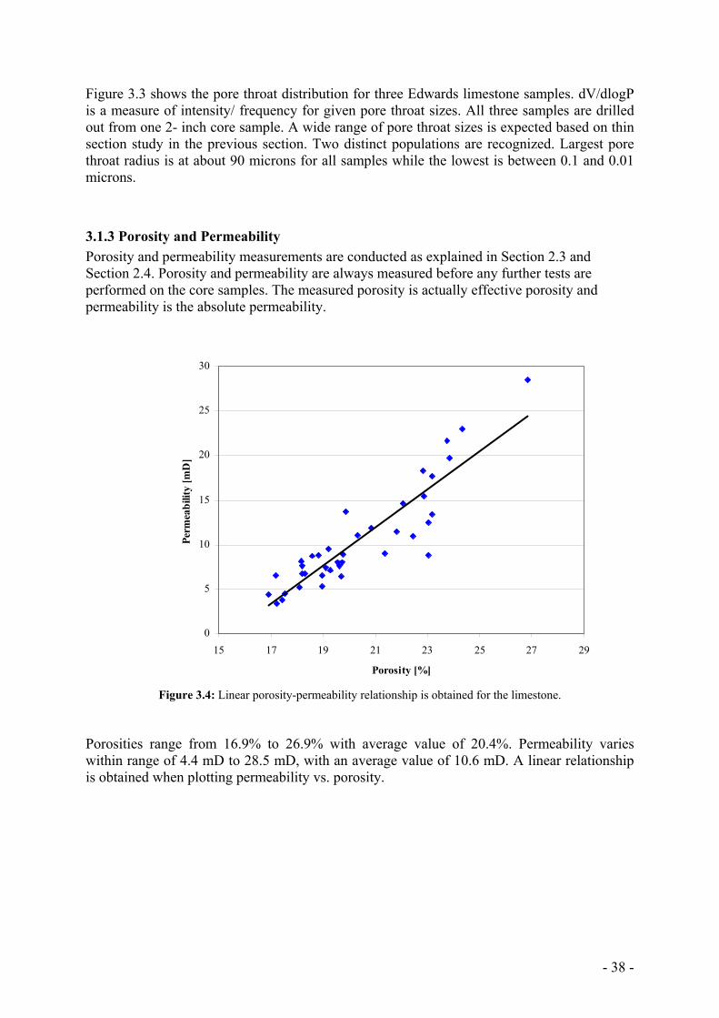
- 38 -

Figure 3.3 shows the pore throat distribution for three Edwards limestone samples. dV/dlogP is a measure of intensity/ frequency for given pore throat sizes. All three samples are drilled out from one 2- inch core sample. A wide range of pore throat sizes is expected based on thin section study in the previous section. Two distinct populations are recognized. Largest pore throat radius is at about 90 microns for all samples while the lowest is between 0.1 and 0.01 microns.

3.1.3 Porosity and Permeability Porosity and permeability measurements are conducted as explained in Section 2.3 and Section 2.4. Porosity and permeability are always measured before any further tests are performed on the core samples. The measured porosity is actually effective porosity and permeability is the absolute permeability.

0

5

10

15

20

25

30

15 17 19 21 23 25 27 29

Porosity [%]

Perm

eabi

lity

[mD

]

Figure 3.4: Linear porosity-permeability relationship is obtained for the limestone.

Porosities range from 16.9% to 26.9% with average value of 20.4%. Permeability varies within range of 4.4 mD to 28.5 mD, with an average value of 10.6 mD. A linear relationship is obtained when plotting permeability vs. porosity.

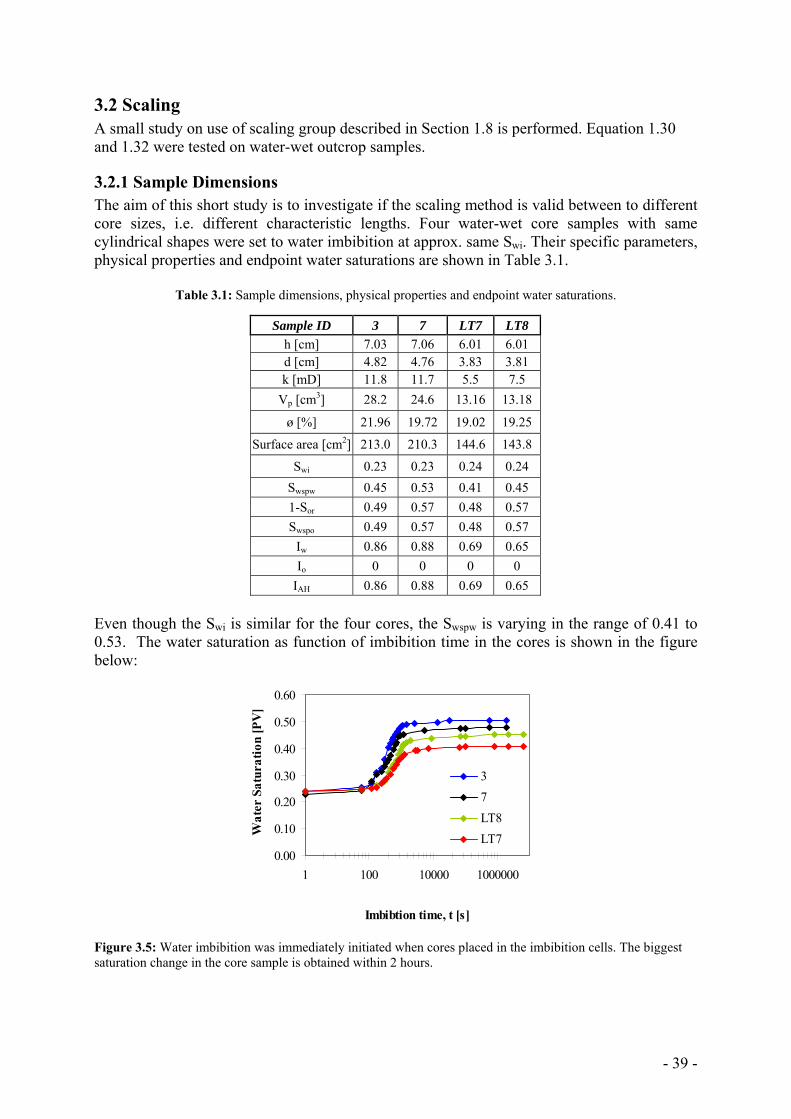
- 39 -

3.2 Scaling A small study on use of scaling group described in Section 1.8 is performed. Equation 1.30 and 1.32 were tested on water-wet outcrop samples.

3.2.1 Sample Dimensions The aim of this short study is to investigate if the scaling method is valid between to different core sizes, i.e. different characteristic lengths. Four water-wet core samples with same cylindrical shapes were set to water imbibition at approx. same Swi. Their specific parameters, physical properties and endpoint water saturations are shown in Table 3.1.

Table 3.1: Sample dimensions, physical properties and endpoint water saturations.

Even though the Swi is similar for the four cores, the Swspw is varying in the range of 0.41 to 0.53. The water saturation as function of imbibition time in the cores is shown in the figure below:

0.00

0.10

0.20

0.30

0.40

0.50

0.60

1 100 10000 1000000

Imbibtion time, t [s]

Wat

er S

atur

atio

n [P

V]

37LT8LT7

Figure 3.5: Water imbibition was immediately initiated when cores placed in the imbibition cells. The biggest saturation change in the core sample is obtained within 2 hours.

Sample ID 3 7 LT7 LT8 h [cm] 7.03 7.06 6.01 6.01 d [cm] 4.82 4.76 3.83 3.81 k [mD] 11.8 11.7 5.5 7.5

Vp [cm3] 28.2 24.6 13.16 13.18

ø [%] 21.96 19.72 19.02 19.25

Surface area [cm2] 213.0 210.3 144.6 143.8

Swi 0.23 0.23 0.24 0.24 Swspw 0.45 0.53 0.41 0.45 1-Sor 0.49 0.57 0.48 0.57 Swspo 0.49 0.57 0.48 0.57

Iw 0.86 0.88 0.69 0.65 Io 0 0 0 0

IAH 0.86 0.88 0.69 0.65

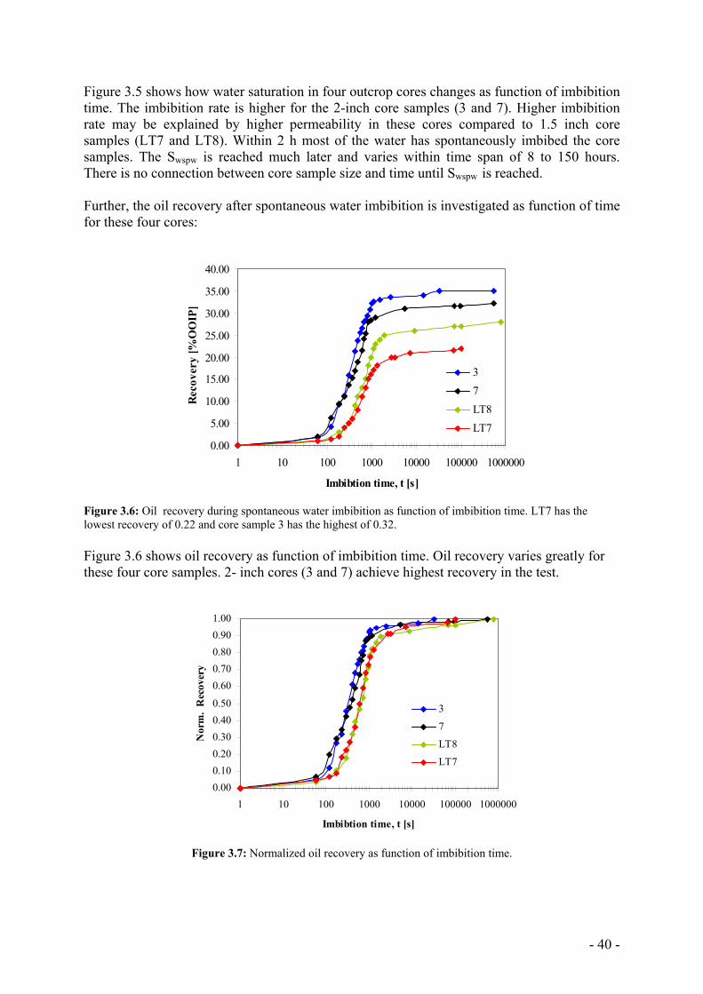
- 40 -

Figure 3.5 shows how water saturation in four outcrop cores changes as function of imbibition time. The imbibition rate is higher for the 2-inch core samples (3 and 7). Higher imbibition rate may be explained by higher permeability in these cores compared to 1.5 inch core samples (LT7 and LT8). Within 2 h most of the water has spontaneously imbibed the core samples. The Swspw is reached much later and varies within time span of 8 to 150 hours. There is no connection between core sample size and time until Swspw is reached. Further, the oil recovery after spontaneous water imbibition is investigated as function of time for these four cores:

0.00

5.00

10.00

15.00

20.00

25.00

30.00

35.00

40.00

1 10 100 1000 10000 100000 1000000

Imbibtion time, t [s]

Rec

over

y [%

OO

IP]

37LT8LT7

Figure 3.6: Oil recovery during spontaneous water imbibition as function of imbibition time. LT7 has the lowest recovery of 0.22 and core sample 3 has the highest of 0.32. Figure 3.6 shows oil recovery as function of imbibition time. Oil recovery varies greatly for these four core samples. 2- inch cores (3 and 7) achieve highest recovery in the test.

0.000.100.200.300.400.50

0.600.700.800.901.00

1 10 100 1000 10000 100000 1000000

Imbibtion time, t [s]

Nor

m.

Rec

over

y

3

7

LT8

LT7

Figure 3.7: Normalized oil recovery as function of imbibition time.

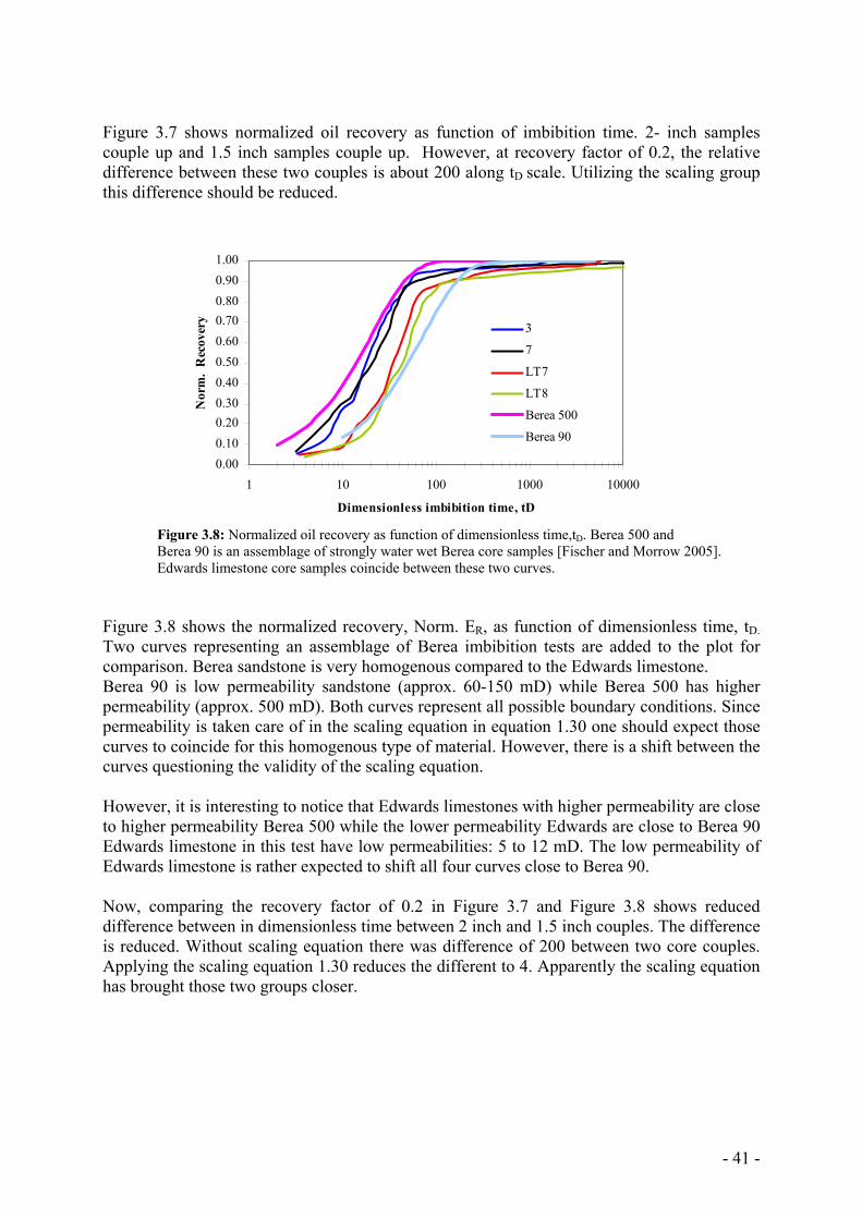
- 41 -

Figure 3.7 shows normalized oil recovery as function of imbibition time. 2- inch samples couple up and 1.5 inch samples couple up. However, at recovery factor of 0.2, the relative difference between these two couples is about 200 along tD scale. Utilizing the scaling group this difference should be reduced.

0.000.100.200.300.400.500.600.700.800.901.00

1 10 100 1000 10000

Dimensionless imbibition time, tD

Nor

m.

Rec

over

y

3

7

LT7

LT8

Berea 500

Berea 90

Figure 3.8: Normalized oil recovery as function of dimensionless time,tD. Berea 500 and Berea 90 is an assemblage of strongly water wet Berea core samples [Fischer and Morrow 2005]. Edwards limestone core samples coincide between these two curves. Figure 3.8 shows the normalized recovery, Norm. ER, as function of dimensionless time, tD. Two curves representing an assemblage of Berea imbibition tests are added to the plot for comparison. Berea sandstone is very homogenous compared to the Edwards limestone. Berea 90 is low permeability sandstone (approx. 60-150 mD) while Berea 500 has higher permeability (approx. 500 mD). Both curves represent all possible boundary conditions. Since permeability is taken care of in the scaling equation in equation 1.30 one should expect those curves to coincide for this homogenous type of material. However, there is a shift between the curves questioning the validity of the scaling equation. However, it is interesting to notice that Edwards limestones with higher permeability are close to higher permeability Berea 500 while the lower permeability Edwards are close to Berea 90 Edwards limestone in this test have low permeabilities: 5 to 12 mD. The low permeability of Edwards limestone is rather expected to shift all four curves close to Berea 90. Now, comparing the recovery factor of 0.2 in Figure 3.7 and Figure 3.8 shows reduced difference between in dimensionless time between 2 inch and 1.5 inch couples. The difference is reduced. Without scaling equation there was difference of 200 between two core couples. Applying the scaling equation 1.30 reduces the different to 4. Apparently the scaling equation has brought those two groups closer.

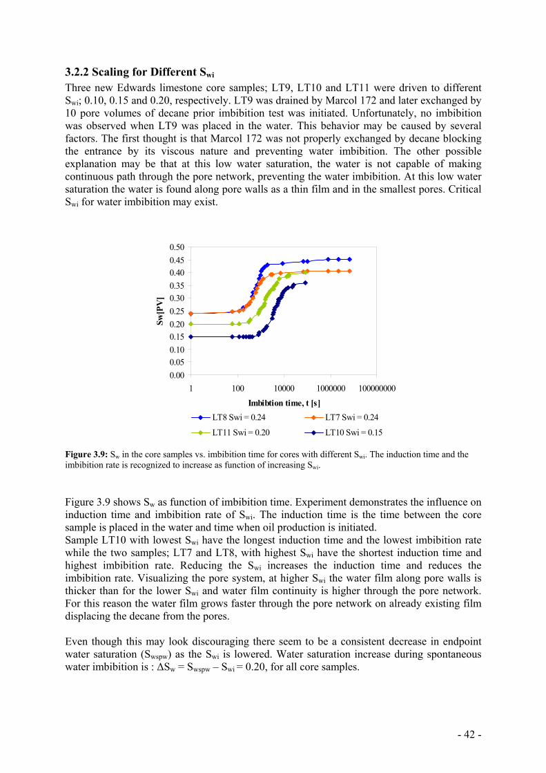
- 42 -

3.2.2 Scaling for Different Swi Three new Edwards limestone core samples; LT9, LT10 and LT11 were driven to different Swi; 0.10, 0.15 and 0.20, respectively. LT9 was drained by Marcol 172 and later exchanged by 10 pore volumes of decane prior imbibition test was initiated. Unfortunately, no imbibition was observed when LT9 was placed in the water. This behavior may be caused by several factors. The first thought is that Marcol 172 was not properly exchanged by decane blocking the entrance by its viscous nature and preventing water imbibition. The other possible explanation may be that at this low water saturation, the water is not capable of making continuous path through the pore network, preventing the water imbibition. At this low water saturation the water is found along pore walls as a thin film and in the smallest pores. Critical Swi for water imbibition may exist.

0.000.050.100.150.200.250.300.350.400.450.50

1 100 10000 1000000 100000000Imbibtion time, t [s]

Sw[P

V]

LT8 Swi = 0.24 LT7 Swi = 0.24

LT11 Swi = 0.20 LT10 Swi = 0.15

Figure 3.9: Sw in the core samples vs. imbibition time for cores with different Swi. The induction time and the imbibition rate is recognized to increase as function of increasing Swi. Figure 3.9 shows Sw as function of imbibition time. Experiment demonstrates the influence on induction time and imbibition rate of Swi. The induction time is the time between the core sample is placed in the water and time when oil production is initiated. Sample LT10 with lowest Swi have the longest induction time and the lowest imbibition rate while the two samples; LT7 and LT8, with highest Swi have the shortest induction time and highest imbibition rate. Reducing the Swi increases the induction time and reduces the imbibition rate. Visualizing the pore system, at higher Swi the water film along pore walls is thicker than for the lower Swi and water film continuity is higher through the pore network. For this reason the water film grows faster through the pore network on already existing film displacing the decane from the pores. Even though this may look discouraging there seem to be a consistent decrease in endpoint water saturation (Swspw) as the Swi is lowered. Water saturation increase during spontaneous water imbibition is : ∆Sw = Swspw – Swi = 0.20, for all core samples.

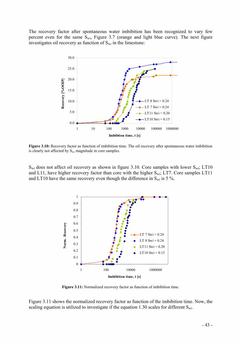
- 43 -

The recovery factor after spontaneous water imbibition has been recognized to vary few percent even for the same Swi, Figure 3.7 (orange and light blue curve). The next figure investigates oil recovery as function of Swi in the limestone:

0.0

5.0

10.0

15.0

20.0

25.0

30.0

1 10 100 1000 10000 100000 1000000

Imbibtion time, t [s]

LT 8 Swi = 0.24

LT 7 Swi = 0.24

LT11 Swi = 0.20

LT10 Swi = 0.15

Rec

over

y [%

OO

IP]

Figure 3.10: Recovery factor as function of imbibition time. The oil recovery after spontaneous water imbibition is clearly not affected by Swi magnitude in core samples. Swi does not affect oil recovery as shown in figure 3.10. Core samples with lower Swi; LT10 and L11, have higher recovery factor than core with the higher Swi; LT7. Core samples LT11 and LT10 have the same recovery even though the difference in Swi is 5 %.

0

0.1

0.2

0.3

0.4

0.5

0.6

0.7

0.8

0.9

1

1 100 10000 1000000

Imbibition time, t [s]

LT 7 Swi = 0.24

LT 8 Swi = 0.24

LT11 Swi = 0.20

LT10 Swi = 0.15

Nor

m.

Rec

over

y

Figure 3.11: Normalized recovery factor as function of imbibition time.

Figure 3.11 shows the normalized recovery factor as function of the imbibition time. Now, the scaling equation is utilized to investigate if the equation 1.30 scales for different Swi.

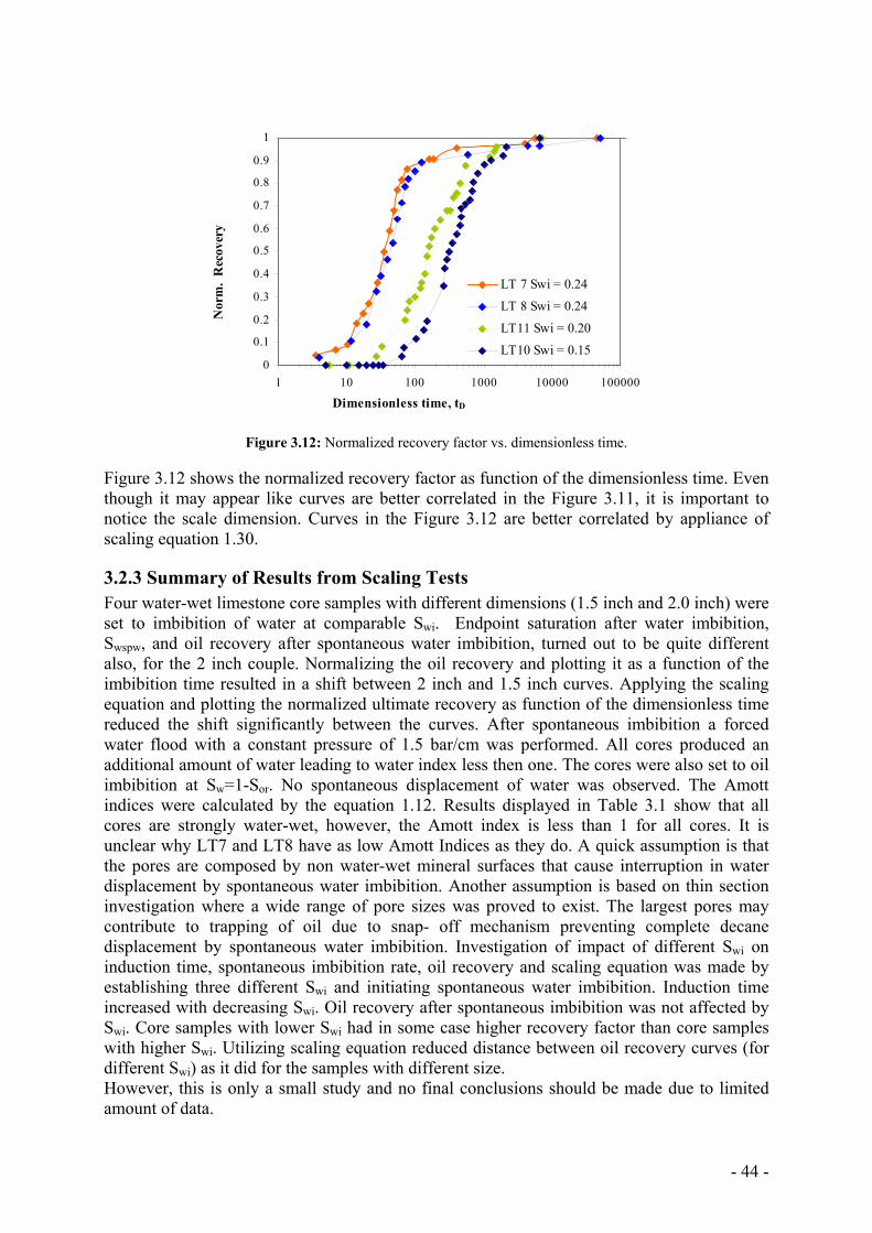
- 44 -

0

0.1

0.2

0.3

0.4

0.5

0.6

0.7

0.8

0.9

1

1 10 100 1000 10000 100000

LT 7 Swi = 0.24

LT 8 Swi = 0.24

LT11 Swi = 0.20

LT10 Swi = 0.15

Dimensionless time, tD

Nor

m.

Rec

over

y

Figure 3.12: Normalized recovery factor vs. dimensionless time.

Figure 3.12 shows the normalized recovery factor as function of the dimensionless time. Even though it may appear like curves are better correlated in the Figure 3.11, it is important to notice the scale dimension. Curves in the Figure 3.12 are better correlated by appliance of scaling equation 1.30.

3.2.3 Summary of Results from Scaling Tests Four water-wet limestone core samples with different dimensions (1.5 inch and 2.0 inch) were set to imbibition of water at comparable Swi. Endpoint saturation after water imbibition, Swspw, and oil recovery after spontaneous water imbibition, turned out to be quite different also, for the 2 inch couple. Normalizing the oil recovery and plotting it as a function of the imbibition time resulted in a shift between 2 inch and 1.5 inch curves. Applying the scaling equation and plotting the normalized ultimate recovery as function of the dimensionless time reduced the shift significantly between the curves. After spontaneous imbibition a forced water flood with a constant pressure of 1.5 bar/cm was performed. All cores produced an additional amount of water leading to water index less then one. The cores were also set to oil imbibition at Sw=1-Sor. No spontaneous displacement of water was observed. The Amott indices were calculated by the equation 1.12. Results displayed in Table 3.1 show that all cores are strongly water-wet, however, the Amott index is less than 1 for all cores. It is unclear why LT7 and LT8 have as low Amott Indices as they do. A quick assumption is that the pores are composed by non water-wet mineral surfaces that cause interruption in water displacement by spontaneous water imbibition. Another assumption is based on thin section investigation where a wide range of pore sizes was proved to exist. The largest pores may contribute to trapping of oil due to snap- off mechanism preventing complete decane displacement by spontaneous water imbibition. Investigation of impact of different Swi on induction time, spontaneous imbibition rate, oil recovery and scaling equation was made by establishing three different Swi and initiating spontaneous water imbibition. Induction time increased with decreasing Swi. Oil recovery after spontaneous imbibition was not affected by Swi. Core samples with lower Swi had in some case higher recovery factor than core samples with higher Swi. Utilizing scaling equation reduced distance between oil recovery curves (for different Swi) as it did for the samples with different size. However, this is only a small study and no final conclusions should be made due to limited amount of data.

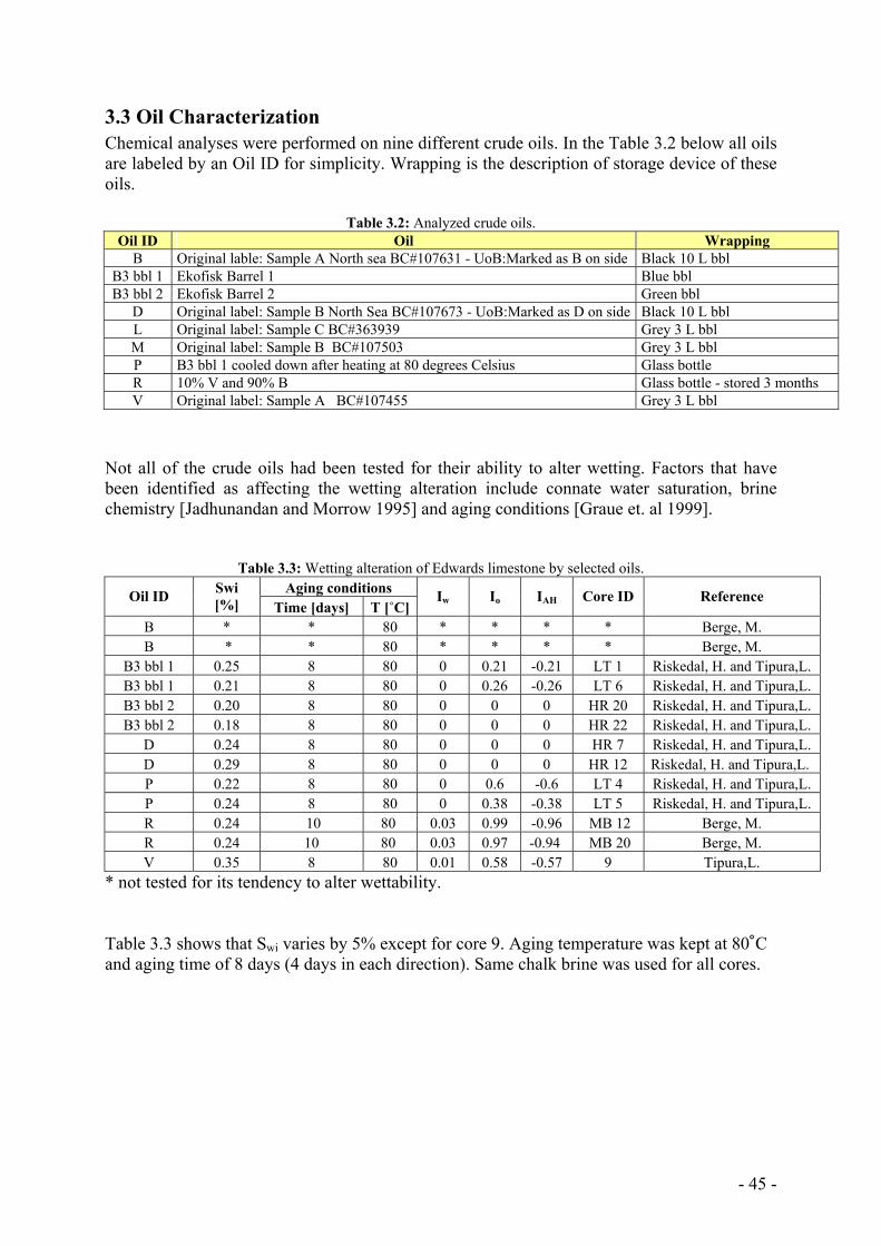
- 45 -

3.3 Oil Characterization Chemical analyses were performed on nine different crude oils. In the Table 3.2 below all oils are labeled by an Oil ID for simplicity. Wrapping is the description of storage device of these oils.

Table 3.2: Analyzed crude oils. Oil ID Oil Wrapping

B Original lable: Sample A North sea BC#107631 - UoB:Marked as B on side Black 10 L bbl B3 bbl 1 Ekofisk Barrel 1 Blue bbl B3 bbl 2 Ekofisk Barrel 2 Green bbl

D Original label: Sample B North Sea BC#107673 - UoB:Marked as D on side Black 10 L bbl L Original label: Sample C BC#363939 Grey 3 L bbl M Original label: Sample B BC#107503 Grey 3 L bbl P B3 bbl 1 cooled down after heating at 80 degrees Celsius Glass bottle R 10% V and 90% B Glass bottle - stored 3 months V Original label: Sample A BC#107455 Grey 3 L bbl

Not all of the crude oils had been tested for their ability to alter wetting. Factors that have been identified as affecting the wetting alteration include connate water saturation, brine chemistry [Jadhunandan and Morrow 1995] and aging conditions [Graue et. al 1999].

Table 3.3: Wetting alteration of Edwards limestone by selected oils.

Aging conditions Oil ID Swi [%] Time [days] T [˚C]

Iw Io IAH Core ID Reference

B * * 80 * * * * Berge, M. B * * 80 * * * * Berge, M.

B3 bbl 1 0.25 8 80 0 0.21 -0.21 LT 1 Riskedal, H. and Tipura,L. B3 bbl 1 0.21 8 80 0 0.26 -0.26 LT 6 Riskedal, H. and Tipura,L. B3 bbl 2 0.20 8 80 0 0 0 HR 20 Riskedal, H. and Tipura,L. B3 bbl 2 0.18 8 80 0 0 0 HR 22 Riskedal, H. and Tipura,L.

D 0.24 8 80 0 0 0 HR 7 Riskedal, H. and Tipura,L. D 0.29 8 80 0 0 0 HR 12 Riskedal, H. and Tipura,L. P 0.22 8 80 0 0.6 -0.6 LT 4 Riskedal, H. and Tipura,L. P 0.24 8 80 0 0.38 -0.38 LT 5 Riskedal, H. and Tipura,L. R 0.24 10 80 0.03 0.99 -0.96 MB 12 Berge, M. R 0.24 10 80 0.03 0.97 -0.94 MB 20 Berge, M. V 0.35 8 80 0.01 0.58 -0.57 9 Tipura,L.

* not tested for its tendency to alter wettability. Table 3.3 shows that Swi varies by 5% except for core 9. Aging temperature was kept at 80˚C and aging time of 8 days (4 days in each direction). Same chalk brine was used for all cores.

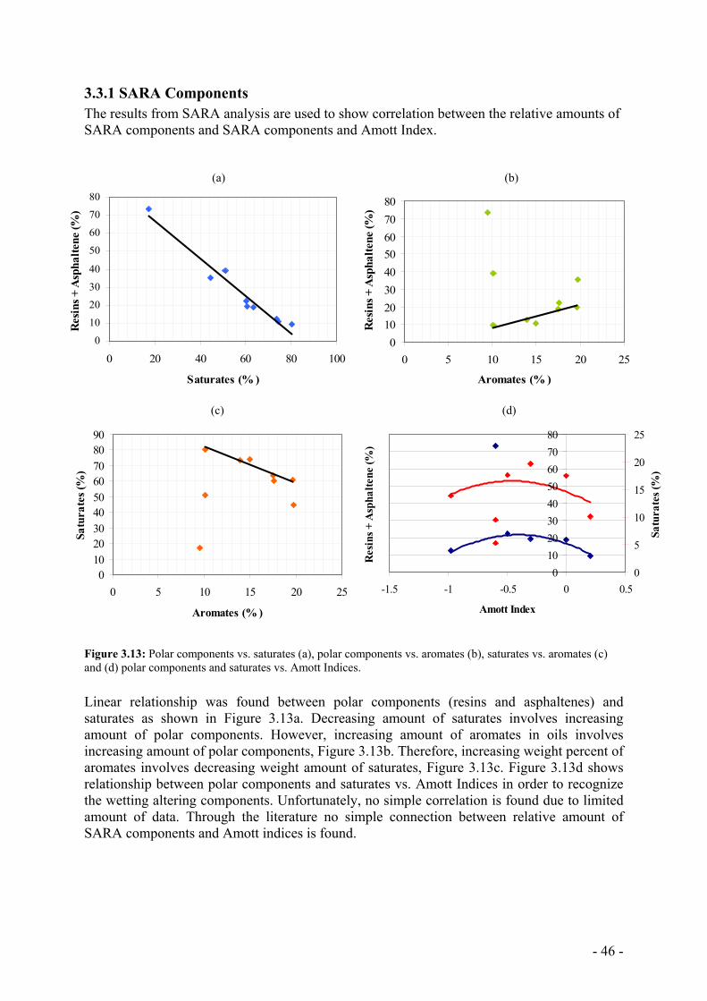
- 46 -

0

10

20

30

40

50

60

70

80

0 20 40 60 80 100

Saturates (% )

Res

ins +

Asp

halte

ne (%

)

01020304050607080

0 5 10 15 20 25

Aromates (% )R

esin

s + A

spha

ltene

(%)

0102030405060708090

0 5 10 15 20 25

Aromates (% )

Satu

rate

s (%

)

01020304050607080

-1.5 -1 -0.5 0 0.5

Amott Index

Res

ins +

Asp

halte

ne (%

)

0

5

10

15

20

25

Satu

rate

s (%

)

3.3.1 SARA Components The results from SARA analysis are used to show correlation between the relative amounts of SARA components and SARA components and Amott Index. (a) (b)

(c) (d)

Figure 3.13: Polar components vs. saturates (a), polar components vs. aromates (b), saturates vs. aromates (c) and (d) polar components and saturates vs. Amott Indices. Linear relationship was found between polar components (resins and asphaltenes) and saturates as shown in Figure 3.13a. Decreasing amount of saturates involves increasing amount of polar components. However, increasing amount of aromates in oils involves increasing amount of polar components, Figure 3.13b. Therefore, increasing weight percent of aromates involves decreasing weight amount of saturates, Figure 3.13c. Figure 3.13d shows relationship between polar components and saturates vs. Amott Indices in order to recognize the wetting altering components. Unfortunately, no simple correlation is found due to limited amount of data. Through the literature no simple connection between relative amount of SARA components and Amott indices is found.

- 47 -

0 1 2 3 4 5 6

D

B

R

P

B3 bbl 2

B3 bbl 1

L

M

Oil

ID

Base Number

3.3.2 Acid and Base Number Earlier wettability studies have shown that wetting depends on acid (AN) and base number (BN) [Wang and Buckley 2002]. Therefore, acid and base numbers were measured for all oils (except oil V which was to viscous for existing experimental procedure). (a) (b)

Figure 3.14. Acid (a) and base (b) numbers of selected crude oil samples.

Figure 3.14 summarizes acid and base number data for selected crude oils included in Table 3.2 and Table 3.2. Figure 3.14 proposes a trend in amount of acid and base number. Oils with high acid numbers tend to have high base numbers. Same trend is recognized in earlier work [Skauge et.al 1999]. Further, acid and base numbers were plotted as function of Amott Indices.

Figure 3.15: No simple correlation between acid and base number and Amott index is found. Figure 3.15 shows relationship between acid and base numbers and the Amott index for Edwards limestone. However, no obvious correlation between AN and BN and extent of wetting is immediately apparent.

0 1 2 3 4 5 6

B

D

R

P

B3 bbl 1

B3 bbl 2

L

M

Oil

ID

Acid Number

0.00

0.50

1.00

1.50

2.00

2.50

3.00

-1 -0.8 -0.6 -0.4 -0.2 0 0.2 0.4

Amott Index

Aci

d or

Bas

e N

umbe

r

Base #

Acid #PB3 bbl 1

B3 bbl 2

D

R

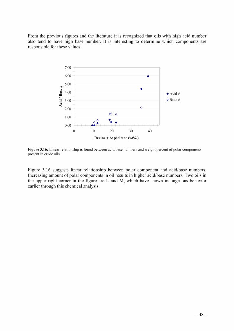
- 48 -

From the previous figures and the literature it is recognized that oils with high acid number also tend to have high base number. It is interesting to determine which components are responsible for these values. Figure 3.16: Linear relationship is found between acid/base numbers and weight percent of polar components present in crude oils. Figure 3.16 suggests linear relationship between polar component and acid/base numbers. Increasing amount of polar components in oil results in higher acid/base numbers. Two oils in the upper right corner in the figure are L and M, which have shown incongruous behavior earlier through this chemical analysis.

0.00

1.00

2.00

3.00

4.00

5.00

6.00

7.00

0 10 20 30 40

Resins + Asphaltene (wt% )

Aci

d / B

ase

#

Acid #Base #

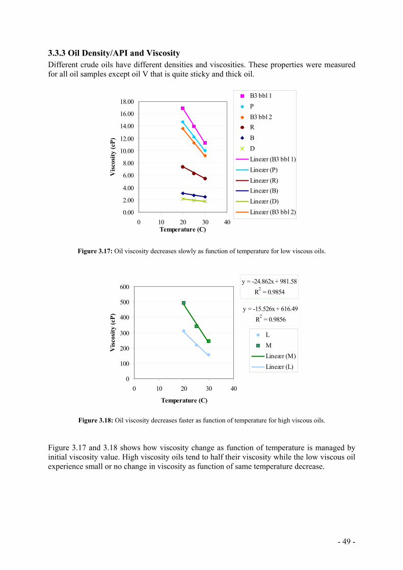
- 49 -

3.3.3 Oil Density/API and Viscosity Different crude oils have different densities and viscosities. These properties were measured for all oil samples except oil V that is quite sticky and thick oil.

0.00

2.00

4.00

6.00

8.00

10.00

12.00

14.00

16.00

18.00

0 10 20 30 40Temperature (C)

Vis

cosi

ty (c

P)

B3 bbl 1PB3 bbl 2RBDLineær (B3 bbl 1)Lineær (P)Lineær (R)Lineær (B)Lineær (D)Lineær (B3 bbl 2)

Figure 3.17: Oil viscosity decreases slowly as function of temperature for low viscous oils.

y = -24.862x + 981.58R2 = 0.9854

y = -15.526x + 616.49R2 = 0.9856

0

100

200

300

400

500

600

0 10 20 30 40

Temperature (C)

Vis

cosi

ty (c

P)

LMLineær (M)Lineær (L)

Figure 3.18: Oil viscosity decreases faster as function of temperature for high viscous oils.

Figure 3.17 and 3.18 shows how viscosity change as function of temperature is managed by initial viscosity value. High viscosity oils tend to half their viscosity while the low viscous oil experience small or no change in viscosity as function of same temperature decrease.

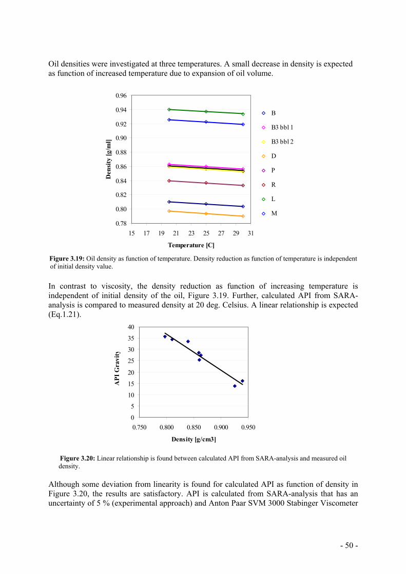
- 50 -

Oil densities were investigated at three temperatures. A small decrease in density is expected as function of increased temperature due to expansion of oil volume.

0.78

0.80

0.82

0.84

0.86

0.88

0.90

0.92

0.94

0.96

15 17 19 21 23 25 27 29 31

Temperature [C]

Den

sity

[g/m

l]B

B3 bbl 1

B3 bbl 2

D

P

R

L

M

Figure 3.19: Oil density as function of temperature. Density reduction as function of temperature is independent of initial density value. In contrast to viscosity, the density reduction as function of increasing temperature is independent of initial density of the oil, Figure 3.19. Further, calculated API from SARA-analysis is compared to measured density at 20 deg. Celsius. A linear relationship is expected (Eq.1.21).

Figure 3.20: Linear relationship is found between calculated API from SARA-analysis and measured oil density. Although some deviation from linearity is found for calculated API as function of density in Figure 3.20, the results are satisfactory. API is calculated from SARA-analysis that has an uncertainty of 5 % (experimental approach) and Anton Paar SVM 3000 Stabinger Viscometer

0

5

10

15

20

25

30

35

40

0.750 0.800 0.850 0.900 0.950

Density [g/cm3]

API

Gra

vity

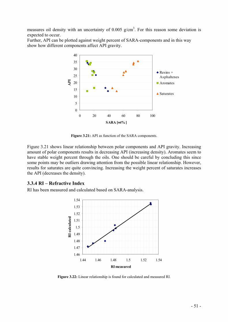
- 51 -

measures oil density with an uncertainty of 0.005 g/cm3. For this reason some deviation is expected to occur. Further, API can be plotted against weight percent of SARA-components and in this way show how different components affect API gravity.

Figure 3.21: API as function of the SARA components. Figure 3.21 shows linear relationship between polar components and API gravity. Increasing amount of polar components results in decreasing API (increasing density). Aromates seem to have stable weight percent through the oils. One should be careful by concluding this since some points may be outliers drawing attention from the possible linear relationship. However, results for saturates are quite convincing. Increasing the weight percent of saturates increases the API (decreases the density).

3.3.4 RI – Refractive Index RI has been measured and calculated based on SARA-analysis.

1.46

1.47

1.48

1.49

1.5

1.51

1.52

1.53

1.54

1.44 1.46 1.48 1.5 1.52 1.54

RI measured

RI c

alcu

late

d

Figure 3.22: Linear relationship is found for calculated and measured RI.

0

5

10

15

20

25

30

35

40

0 20 40 60 80 100

SARA [wt% ]

API

Resins +AsphaltenesAromates

Saturates

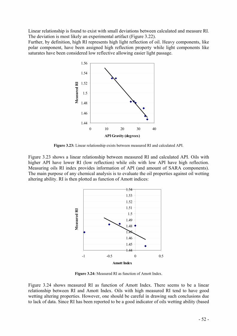
- 52 -

Linear relationship is found to exist with small deviations between calculated and measure RI. The deviation is most likely an experimental artifact (Figure 3.22). Further, by definition, high RI represents high light reflection of oil. Heavy components, like polar component, have been assigned high reflection property while light components like saturates have been considered low reflective allowing easier light passage.

1.44

1.46

1.48

1.5

1.52

1.54

1.56

0 10 20 30 40

API Gravity (degrees)

Mea

sure

d R

I

Figure 3.23: Linear relationship exists between measured RI and calculated API.

Figure 3.23 shows a linear relationship between measured RI and calculated API. Oils with higher API have lower RI (low reflection) while oils with low API have high reflection. Measuring oils RI index provides information of API (and amount of SARA components). The main purpose of any chemical analysis is to evaluate the oil properties against oil wetting altering ability. RI is then plotted as function of Amott indices:

1.441.451.461.471.481.491.5

1.511.521.531.54

-1 -0.5 0 0.5

Amott Index

Mea

sure

d R

I

Figure 3.24: Measured RI as function of Amott Index.

Figure 3.24 shows measured RI as function of Amott Index. There seems to be a linear relationship between RI and Amott Index. Oils with high measured RI tend to have good wetting altering properties. However, one should be careful in drawing such conclusions due to lack of data. Since RI has been reported to be a good indicator of oils wetting ability (based

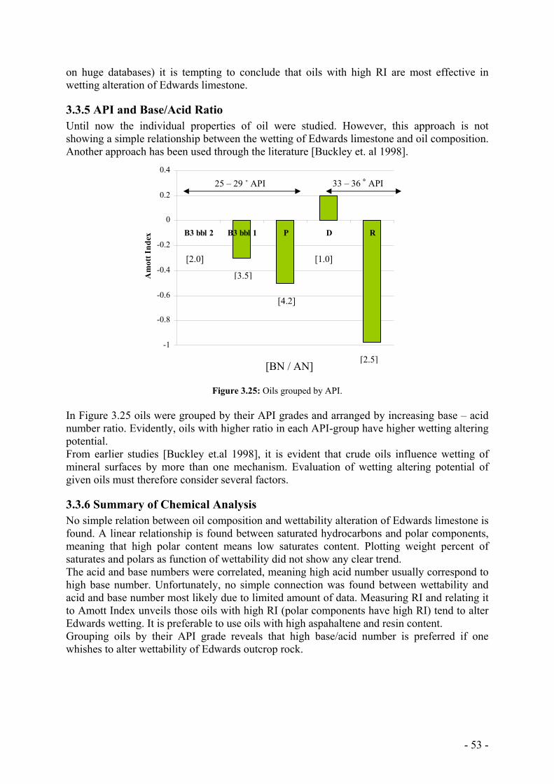
- 53 -

on huge databases) it is tempting to conclude that oils with high RI are most effective in wetting alteration of Edwards limestone.

3.3.5 API and Base/Acid Ratio Until now the individual properties of oil were studied. However, this approach is not showing a simple relationship between the wetting of Edwards limestone and oil composition. Another approach has been used through the literature [Buckley et. al 1998].

-1

-0.8

-0.6

-0.4

-0.2

0

0.2

0.4

B3 bbl 2 B3 bbl 1 P D R

Am

ott I

ndex

Figure 3.25: Oils grouped by API. In Figure 3.25 oils were grouped by their API grades and arranged by increasing base – acid number ratio. Evidently, oils with higher ratio in each API-group have higher wetting altering potential. From earlier studies [Buckley et.al 1998], it is evident that crude oils influence wetting of mineral surfaces by more than one mechanism. Evaluation of wetting altering potential of given oils must therefore consider several factors.

3.3.6 Summary of Chemical Analysis No simple relation between oil composition and wettability alteration of Edwards limestone is found. A linear relationship is found between saturated hydrocarbons and polar components, meaning that high polar content means low saturates content. Plotting weight percent of saturates and polars as function of wettability did not show any clear trend. The acid and base numbers were correlated, meaning high acid number usually correspond to high base number. Unfortunately, no simple connection was found between wettability and acid and base number most likely due to limited amount of data. Measuring RI and relating it to Amott Index unveils those oils with high RI (polar components have high RI) tend to alter Edwards wetting. It is preferable to use oils with high aspahaltene and resin content. Grouping oils by their API grade reveals that high base/acid number is preferred if one whishes to alter wettability of Edwards outcrop rock.

25 – 29 ˚ API 33 – 36 ˚ API

[2.0]

[3.5]

[4.2]

[1.0]

[2.5][BN / AN]

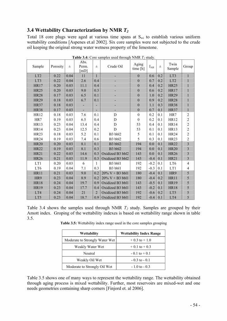
- 54 -

3.4 Wettability Characterization by NMR T2 Total 18 core plugs were aged at various time spans at Swi to establish various uniform wettability conditions [Aspenes et.al 2002]. Six core samples were not subjected to the crude oil keeping the original strong water wetness property of the limestone.

Table 3.4: Core samples used through NMR T2 study.

Sample Porosity ± Abs. Perm. [mD]

± Crude Oil Aging time [h] IAH ± Twin

Sample Group

LT2 0.22 0.04 11 1 - 0 0.6 0.2 LT3 1 LT3 0.22 0.04 2.6 0.4 - 0 0.7 0.2 LT2 1

HR17 0.20 0.03 11.1 0.4 - 0 0.4 0.2 HR25 1 HR25 0.20 0.03 9.0 0.3 - 0 0.6 0.2 HR17 1 HR28 0.17 0.03 6.5 0.1 - 0 1.0 0.2 HR29 1 HR29 0.18 0.03 6.7 0.1 - 0 0.9 0.2 HR28 1 HR37 0.18 0.03 - - - 0 1.1 0.3 HR38 1 HR38 0.17 0.03 - - - 0 0.7 0.1 HR37 1 HR12 0.18 0.03 7.6 0.1 D 0 0.2 0.1 HR7 2 HR7 0.19 0.03 6.5 0.4 D 0 0.2 0.1 HR12 2 HR13 0.23 0.04 13.4 0.4 D 53 0.4 0.1 HR14 2 HR14 0.23 0.04 12.5 0.2 D 53 0.1 0.1 HR13 2 HR23 0.18 0.03 5.2 0.1 B3 bbl2 5 0.1 0.1 HR24 2 HR24 0.19 0.03 7.4 0.6 B3 bbl2 5 0.3 0.1 HR23 2 HR20 0.20 0.03 8.1 0.1 B3 bbl2 194 0.0 0.1 HR22 3 HR22 0.19 0.03 8.1 0.3 B3 bbl2 194 0.0 0.1 HR20 3 HR21 0.22 0.03 14.6 0.3 Oxidized B3 bbl2 143 0.0 0.1 HR26 3 HR26 0.21 0.03 11.9 0.3 Oxidized B3 bbl2 143 -0.4 0.1 HR21 3 LT1 0.20 0.03 6 1 B3 bbl1 192 -0.2 0.1 LT6 4 LT6 0.19 0.04 7.1 0.3 B3 bbl1 192 -0.3 0.1 LT1 4

HR11 0.21 0.03 9.0 0.2 20% V + B3 bbl1 180 -0.4 0.1 HR9 5 HR9 0.23 0.04 8.9 0.2 20% V + B3 bbl1 180 -0.4 0.2 HR11 5 HR18 0.24 0.04 19.7 0.9 Oxidized B3 bbl1 143 -0.5 0.1 HR19 5 HR19 0.23 0.04 17.7 0.4 Oxidized B3 bbl1 143 -0.2 0.1 HR18 5 LT4 0.24 0.04 21 2 Oxidized B3 bbl1 192 -0.6 0.2 LT5 5 LT5 0.23 0.04 18.7 0.9 Oxidized B3 bbl1 192 -0.4 0.1 LT4 5

Table 3.4 shows the samples used through NMR T2 study. Samples are grouped by their Amott index. Groping of the wettability indexes is based on wettability range shown in table 3.5.

Table 3.5: Wettability index range used in the core samples grouping

Wettability Wettability Index Range

Moderate to Strongly Water Wet + 0.3 to + 1.0

Weakly Water Wet + 0.1 to + 0.3

Neutral - 0.1 to + 0.1

Weakly Oil Wet - 0.3 to - 0.1

Moderate to Strongly Oil Wet - 1.0 to - 0.3 Table 3.5 shows one of many ways to represent the wettability range. The wettability obtained through aging process is mixed wettability. Further, most reservoirs are mixed-wet and one needs geometries containing sharp corners [Finjord et. al 2006].

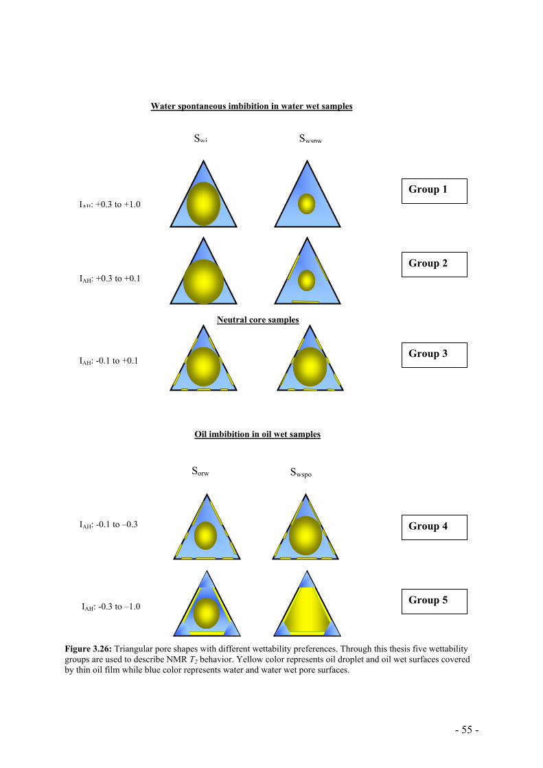
- 55 -

Sorw Swspo

Oil imbibition in oil wet samples

Figure 3.26: Triangular pore shapes with different wettability preferences. Through this thesis five wettability groups are used to describe NMR T2 behavior. Yellow color represents oil droplet and oil wet surfaces covered by thin oil film while blue color represents water and water wet pore surfaces.

IAH: +0.3 to +1.0

Swi Swspw

IAH: +0.3 to +0.1

IAH: -0.1 to +0.1

Water spontaneous imbibition in water wet samples

Neutral core samples

Group 1

Group 2

Group 3

IAH: -0.1 to –0.3

IAH: -0.3 to –1.0

Group 4

Group 5

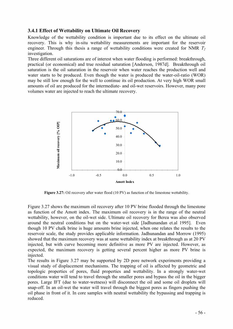
- 56 -

3.4.1 Effect of Wettability on Ultimate Oil Recovery Knowledge of the wettability condition is important due to its effect on the ultimate oil recovery. This is why in-situ wettability measurements are important for the reservoir engineer. Through this thesis a range of wettability conditions were created for NMR T2 investigation. Three different oil saturations are of interest when water flooding is performed: breakthrough, practical (or economical) and true residual saturation [Anderson, 1987d]. Breakthrough oil saturation is the oil saturation in the reservoir when water reaches the production well and water starts to be produced. Even though the water is produced the water-oil-ratio (WOR) may be still low enough for the well to continue its oil production. At very high WOR small amounts of oil are produced for the intermediate- and oil-wet reservoirs. However, many pore volumes water are injected to reach the ultimate recovery.

0.0

10.0

20.0

30.0

40.0

50.0

60.0

70.0

-1.0 -0.5 0.0 0.5 1.0

Amott Index

Max

imum

oil

reco

very

[% O

IP]

Figure 3.27: Oil recovery after water flood (10 PV) as function of the limestone wettability.

Figure 3.27 shows the maximum oil recovery after 10 PV brine flooded through the limestone as function of the Amott index. The maximum oil recovery is in the range of the neutral wettability, however, on the oil-wet side. Ultimate oil recovery for Berea was also observed around the neutral conditions but on the water-wet side [Jadhunandan et.al 1995]. Even though 10 PV chalk brine is huge amounts brine injected, when one relates the results to the reservoir scale, the study provides applicable information. Jadhunandan and Morrow (1995) showed that the maximum recovery was at same wettability index at breakthrough as at 20 PV injected, but with curve becoming more definitive as more PV are injected. However, as expected, the maximum recovery is getting several percent higher as more PV brine is injected. The results in Figure 3.27 may be supported by 2D pore network experiments providing a visual study of displacement mechanisms. The trapping of oil is affected by geometric and topologic properties of pores, fluid properties and wettability. In a strongly water-wet conditions water will tend to travel through the smaller pores and bypass the oil in the bigger pores. Large IFT (due to water-wetness) will disconnect the oil and some oil droplets will snap-off. In an oil-wet the water will travel through the biggest pores as fingers pushing the oil phase in front of it. In core samples with neutral wettability the bypassing and trapping is reduced.

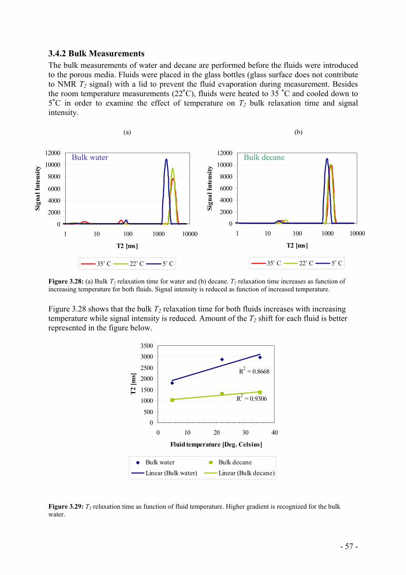
- 57 -

0

2000

4000

6000

8000

10000

12000

1 10 100 1000 10000

T2 [ms]

Sign

al In

tens

ity

35˚ C 22˚ C 5˚ C

0

2000

4000

6000

8000

10000

12000

1 10 100 1000 10000

T2 [ms]

Sign

al In

tens

ity

35˚ C 22˚ C 5˚ C

3.4.2 Bulk Measurements The bulk measurements of water and decane are performed before the fluids were introduced to the porous media. Fluids were placed in the glass bottles (glass surface does not contribute to NMR T2 signal) with a lid to prevent the fluid evaporation during measurement. Besides the room temperature measurements (22˚C), fluids were heated to 35 ˚C and cooled down to 5˚C in order to examine the effect of temperature on T2 bulk relaxation time and signal intensity. (a) (b)

Figure 3.28: (a) Bulk T2 relaxation time for water and (b) decane. T2 relaxation time increases as function of increasing temperature for both fluids. Signal intensity is reduced as function of increased temperature. Figure 3.28 shows that the bulk T2 relaxation time for both fluids increases with increasing temperature while signal intensity is reduced. Amount of the T2 shift for each fluid is better represented in the figure below.

Figure 3.29: T2 relaxation time as function of fluid temperature. Higher gradient is recognized for the bulk water.

Bulk water Bulk decane

R2 = 0.8668

R2 = 0.9306

0500

10001500

20002500

30003500

0 10 20 30 40

Fluid temperature [Deg. Celsius]

T2

[ms]

Bulk water Bulk decaneLinear (Bulk water) Linear (Bulk decane)

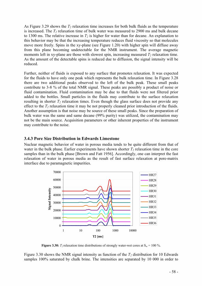
- 58 -

As Figure 3.29 shows the T2 relaxation time increases for both bulk fluids as the temperature is increased. The T2 relaxation time of bulk water was measured to 2900 ms and bulk decane to 1300 ms. The relative increase in T2 is higher for water than for decane. An explanation to this behavior may be that the increasing temperature reduces fluid viscosity so that molecules move more freely. Spins in the xy-plane (see Figure 1.20) with higher spin will diffuse away from this plane becoming undetectable for the NMR instrument. The average magnetic moments left in xy-plane are those with slowest spin, increasing measured T2 relaxation time. As the amount of the detectable spins is reduced due to diffusion, the signal intensity will be reduced. Further, neither of fluids is exposed to any surface that promotes relaxation. It was expected for the fluids to have only one peak which represents the bulk relaxation time. In Figure 3.28 there are two additional peaks observed to the left of the bulk peak. These small peaks contribute to 3-8 % of the total NMR signal. These peaks are possibly a product of noise or fluid contamination. Fluid contamination may be due to that fluids were not filtered prior added to the bottles. Small particles in the fluids may contribute to the surface relaxation resulting in shorter T2 relaxation times. Even though the glass surface does not provide any effect to the T2 relaxation time it may be not properly cleaned prior introduction of the fluids. Another assumption is that noise may be source of these small peaks. Since the preparation of bulk water was the same and same decane (99% purity) was utilized, the contamination may not be the main source. Acquisition parameters or other inherent properties of the instrument may contribute to the noise.

3.4.3 Pore Size Distribution in Edwards Limestone Nuclear magnetic behavior of water in porous media tends to be quite different from that of water in the bulk phase. Earlier experiments have shown shorter T2 relaxation time in the core samples than in the bulk phase [Brown and Fatt 1956]. Accordingly, one can interpret the fast relaxation of water in porous media as the result of fast surface relaxation at pore-matrix interface due to paramagnetic impurities.

0

10000

20000

30000

40000

50000

60000

70000

1 10 100 1000 10000

T2 [ms]

Sign

al In

tens

ity

HR27HR28HR29HR30HR31HR32HR33HR34HR35HR36

Figure 3.30: T2 relaxation time distributions of strongly water-wet cores at Sw = 100 %.

Figure 3.30 shows the NMR signal intensity as function of the T2 distribution for 10 Edwards samples 100% saturated by chalk brine. The intensities are separated by 10 000 in order to

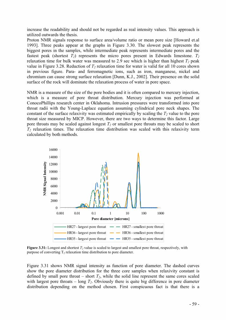
- 59 -

increase the readability and should not be regarded as real intensity values. This approach is utilized outwards the thesis. Proton NMR signals response to surface area/volume ratio or mean pore size [Howard et.al 1993]. Three peaks appear at the graphs in Figure 3.30. The slowest peak represents the biggest pores in the samples, while intermediate peak represents intermediate pores and the fastest peak (shortest T2) represents the micro pores present in Edwards limestone. T2 relaxation time for bulk water was measured to 2.9 sec which is higher than highest T2 peak value in Figure 3.28. Reduction of T2 relaxation time for water is valid for all 10 cores shown in previous figure. Para- and ferromagnetic ions, such as iron, manganese, nickel and chromium can cause strong surface relaxation [Dunn, K.J., 2002]. Their presence on the solid surface of the rock will dominate the relaxation process of water in pore space. NMR is a measure of the size of the pore bodies and it is often compared to mercury injection, which is a measure of pore throat distribution. Mercury injection was performed at ConocoPhillips research center in Oklahoma. Intrusion pressures were transformed into pore throat radii with the Young-Laplace equation assuming cylindrical pore neck shapes. The constant of the surface relaxivity was estimated empirically by scaling the T2 value to the pore throat size measured by MICP. However, there are two ways to determine this factor. Large pore throats may be scaled against longest T2 or smallest pore throats may be scaled to short T2 relaxation times. The relaxation time distribution was scaled with this relaxivity term calculated by both methods.

0

2000

4000

6000

8000

10000

12000

14000

16000

0.001 0.01 0.1 1 10 100 1000Pore diameter [microns]

NM

R S

igna

l Int

ensi

ty

HR27 - largest pore throat HR27 - smallest pore throatHR36 - largest pore throat HR36 - smallest pore throatHR35 - largest pore throat HR35 - smallest pore throat

Figure 3.31: Longest and shortest T2 value is scaled to largest and smallest pore throat, respectively, with purpose of converting T2 relaxation time distribution to pore diameter.

Figure 3.31 shows NMR signal intensity as function of pore diameter. The dashed curves show the pore diameter distribution for the three core samples when relaxivity constant is defined by small pore throat – short T2, while the solid line represent the same cores scaled with largest pore throats – long T2. Obviously there is quite big difference in pore diameter distribution depending on the method chosen. First conspicuous fact is that there is a

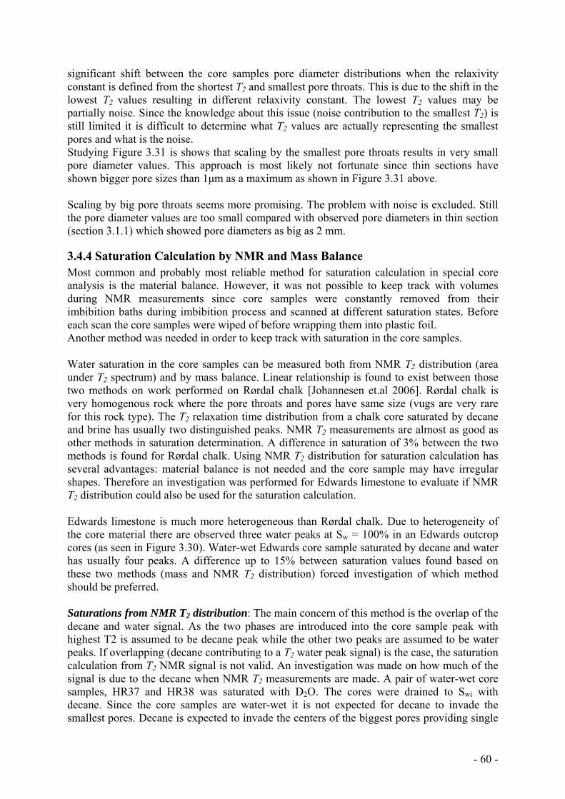
- 60 -

significant shift between the core samples pore diameter distributions when the relaxivity constant is defined from the shortest T2 and smallest pore throats. This is due to the shift in the lowest T2 values resulting in different relaxivity constant. The lowest T2 values may be partially noise. Since the knowledge about this issue (noise contribution to the smallest T2) is still limited it is difficult to determine what T2 values are actually representing the smallest pores and what is the noise. Studying Figure 3.31 is shows that scaling by the smallest pore throats results in very small pore diameter values. This approach is most likely not fortunate since thin sections have shown bigger pore sizes than 1µm as a maximum as shown in Figure 3.31 above. Scaling by big pore throats seems more promising. The problem with noise is excluded. Still the pore diameter values are too small compared with observed pore diameters in thin section (section 3.1.1) which showed pore diameters as big as 2 mm.

3.4.4 Saturation Calculation by NMR and Mass Balance Most common and probably most reliable method for saturation calculation in special core analysis is the material balance. However, it was not possible to keep track with volumes during NMR measurements since core samples were constantly removed from their imbibition baths during imbibition process and scanned at different saturation states. Before each scan the core samples were wiped of before wrapping them into plastic foil. Another method was needed in order to keep track with saturation in the core samples. Water saturation in the core samples can be measured both from NMR T2 distribution (area under T2 spectrum) and by mass balance. Linear relationship is found to exist between those two methods on work performed on Rørdal chalk [Johannesen et.al 2006]. Rørdal chalk is very homogenous rock where the pore throats and pores have same size (vugs are very rare for this rock type). The T2 relaxation time distribution from a chalk core saturated by decane and brine has usually two distinguished peaks. NMR T2 measurements are almost as good as other methods in saturation determination. A difference in saturation of 3% between the two methods is found for Rørdal chalk. Using NMR T2 distribution for saturation calculation has several advantages: material balance is not needed and the core sample may have irregular shapes. Therefore an investigation was performed for Edwards limestone to evaluate if NMR T2 distribution could also be used for the saturation calculation. Edwards limestone is much more heterogeneous than Rørdal chalk. Due to heterogeneity of the core material there are observed three water peaks at Sw = 100% in an Edwards outcrop cores (as seen in Figure 3.30). Water-wet Edwards core sample saturated by decane and water has usually four peaks. A difference up to 15% between saturation values found based on these two methods (mass and NMR T2 distribution) forced investigation of which method should be preferred. Saturations from NMR T2 distribution: The main concern of this method is the overlap of the decane and water signal. As the two phases are introduced into the core sample peak with highest T2 is assumed to be decane peak while the other two peaks are assumed to be water peaks. If overlapping (decane contributing to a T2 water peak signal) is the case, the saturation calculation from T2 NMR signal is not valid. An investigation was made on how much of the signal is due to the decane when NMR T2 measurements are made. A pair of water-wet core samples, HR37 and HR38 was saturated with D2O. The cores were drained to Swi with decane. Since the core samples are water-wet it is not expected for decane to invade the smallest pores. Decane is expected to invade the centers of the biggest pores providing single

- 61 -

T2 peak. The cores were placed in the D2O bath for imbibition. The baker had been equipped with the lid so no H2O adsorption from the humid air during D2O imbibition is expected. Utilizing NMR T2 relaxation distribution showed that 3-15 % of total NMR signal comes from the fast relaxation peaks/ water peaks.

0

10000

20000

30000

40000

50000

60000

70000

1.00 10.00 100.00 1000.00 10000.00

T2 [ms]

Sign

al In

tens

ity

Swi=0.23

Sw=0.29

Sw=0.34

Sw=0.39

1-Sor =0.40

Figure 3.32: Strongly water-wet core sample HR37. The sample was saturated by D2O, drained to Swi with decane and placed in D2O for imbibition. Decane is the only phase contributing to NMR signal. The small peaks to the left of the decane peak represent 3-15 % of the total NMR signal. Now, the question is why these peaks are present and what they are product of since there should be no water or other material contributing to the signal. Based on discussion with James J. Howard at ConocoPhillips, OK, several explanations were considered:

“D2O had adsorbed the H2O from the air during imbibition process”. This part of the signal has to be from water since water has faster relaxation time than decane. However, this is most likely not the case since the imbibition was performed within three hours using lid (avoiding H2O adsorption).

“Decane is in contact with pore walls in the small pores”. This is highly unlikely since capillary forces prevent decane to enter the smallest pores. If those peaks were due to the decane, the D2O would quickly displace it form the pores and the signal intensity would be reduced as D2O saturation continues. The signal intensity does not decrease excluding the possibility of decane being present in the smallest pores.

“Noise – this may not be signal at all”? It is possible that noise may be the source of this part of the NMR signal.

Contribution of small peaks was also discussed for bulk fluid T2 measurements (Section 3.4.1). Since only one phase was present and measurements were made in a sealed glass bottle noise was assumed to contribute to a signal with a magnitude of 3-8%. Overlapping fluids are most likely not a problem in NMR T2 measurements. Wettability is obtained by the Amott test. Oil wet cores placed at Sw = 1-Sor into decane was observed to produce water. From NMR T2 distribution signal the Swspo (endpoint water saturation after decane imbibition) is registered to be higher in some cases, which is clearly incorrect. These endpoints are employed to equation 1.12 for wettability calculation. Due to erroneous endpoint values some of the values exceeded positive and negative unity values. No

Decane peak

Fast peaks – noise?

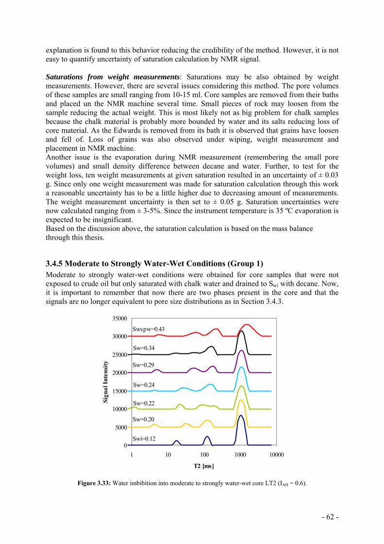
- 62 -

explanation is found to this behavior reducing the credibility of the method. However, it is not easy to quantify uncertainty of saturation calculation by NMR signal. Saturations from weight measurements: Saturations may be also obtained by weight measurements. However, there are several issues considering this method. The pore volumes of these samples are small ranging from 10-15 ml. Core samples are removed from their baths and placed un the NMR machine several time. Small pieces of rock may loosen from the sample reducing the actual weight. This is most likely not as big problem for chalk samples because the chalk material is probably more bounded by water and its salts reducing loss of core material. As the Edwards is removed from its bath it is observed that grains have loosen and fell of. Loss of grains was also observed under wiping, weight measurement and placement in NMR machine. Another issue is the evaporation during NMR measurement (remembering the small pore volumes) and small density difference between decane and water. Further, to test for the weight loss, ten weight measurements at given saturation resulted in an uncertainty of ± 0.03 g. Since only one weight measurement was made for saturation calculation through this work a reasonable uncertainty has to be a little higher due to decreasing amount of measurements. The weight measurement uncertainty is then set to ± 0.05 g. Saturation uncertainties were now calculated ranging from ± 3-5%. Since the instrument temperature is 35 ºC evaporation is expected to be insignificant. Based on the discussion above, the saturation calculation is based on the mass balance through this thesis.

3.4.5 Moderate to Strongly Water-Wet Conditions (Group 1) Moderate to strongly water-wet conditions were obtained for core samples that were not exposed to crude oil but only saturated with chalk water and drained to Swi with decane. Now, it is important to remember that now there are two phases present in the core and that the signals are no longer equivalent to pore size distributions as in Section 3.4.3.

0

5000

10000

15000

20000

25000

30000

35000

1 10 100 1000 10000

T2 [ms]

Sign

al In

tens

ity

Swi=0.12

Sw=0.20

Sw=0.22

Sw=0.24

Sw=0.29

Swspw=0.43

Sw=0.34

Figure 3.33: Water imbibition into moderate to strongly water-wet core LT2 (IAH = 0.6).

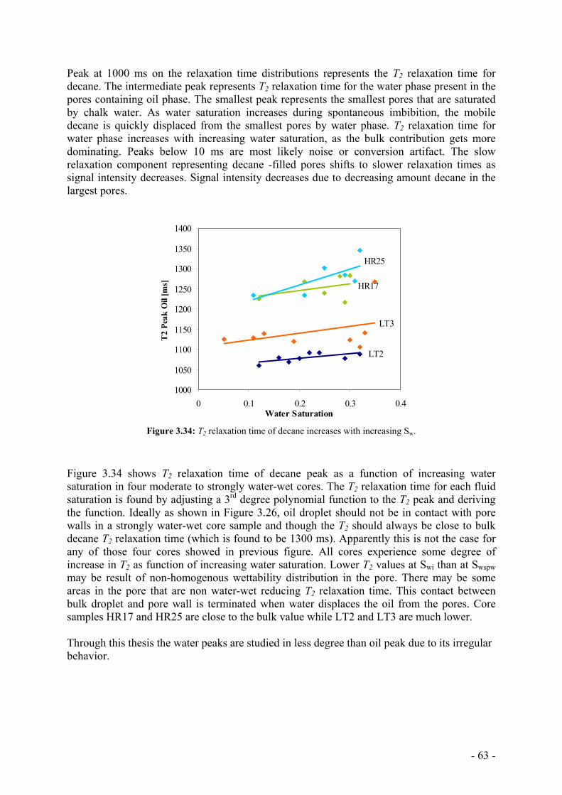
- 63 -

Peak at 1000 ms on the relaxation time distributions represents the T2 relaxation time for decane. The intermediate peak represents T2 relaxation time for the water phase present in the pores containing oil phase. The smallest peak represents the smallest pores that are saturated by chalk water. As water saturation increases during spontaneous imbibition, the mobile decane is quickly displaced from the smallest pores by water phase. T2 relaxation time for water phase increases with increasing water saturation, as the bulk contribution gets more dominating. Peaks below 10 ms are most likely noise or conversion artifact. The slow relaxation component representing decane -filled pores shifts to slower relaxation times as signal intensity decreases. Signal intensity decreases due to decreasing amount decane in the largest pores.

1000

1050

1100

1150

1200

1250

1300

1350

1400

0 0.1 0.2 0.3 0.4Water Saturation

T2

Peak

Oil

[ms]

HR25

HR17

LT3

LT2

Figure 3.34: T2 relaxation time of decane increases with increasing Sw.

Figure 3.34 shows T2 relaxation time of decane peak as a function of increasing water saturation in four moderate to strongly water-wet cores. The T2 relaxation time for each fluid saturation is found by adjusting a 3rd degree polynomial function to the T2 peak and deriving the function. Ideally as shown in Figure 3.26, oil droplet should not be in contact with pore walls in a strongly water-wet core sample and though the T2 should always be close to bulk decane T2 relaxation time (which is found to be 1300 ms). Apparently this is not the case for any of those four cores showed in previous figure. All cores experience some degree of increase in T2 as function of increasing water saturation. Lower T2 values at Swi than at Swspw may be result of non-homogenous wettability distribution in the pore. There may be some areas in the pore that are non water-wet reducing T2 relaxation time. This contact between bulk droplet and pore wall is terminated when water displaces the oil from the pores. Core samples HR17 and HR25 are close to the bulk value while LT2 and LT3 are much lower. Through this thesis the water peaks are studied in less degree than oil peak due to its irregular behavior.

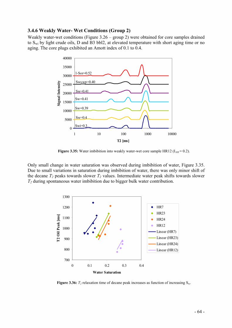
- 64 -

3.4.6 Weakly Water- Wet Conditions (Group 2) Weakly water-wet conditions (Figure 3.26 – group 2) were obtained for core samples drained to Swi by light crude oils, D and B3 bbl2, at elevated temperature with short aging time or no aging. The core plugs exhibited an Amott index of 0.1 to 0.4.

0

5000

10000

15000

20000

25000

30000

35000

40000

1 10 100 1000 10000

T2 [ms]

Sign

al In

tens

ity

Swi=0.3

Sw=0.4

Sw=0.39

Sw=0.41

Sw=0.41

Swswp=0.40

1-Sor=0.52

Figure 3.35: Water imbibition into weakly water-wet core sample HR12 (IAH = 0.2).

Only small change in water saturation was observed during imbibition of water, Figure 3.35. Due to small variations in saturation during imbibition of water, there was only minor shift of the decane T2 peaks towards slower T2 values. Intermediate water peak shifts towards slower T2 during spontaneous water imbibition due to bigger bulk water contribution.

700

800

900

1000

1100

1200

1300

0 0.1 0.2 0.3 0.4

Water Saturation

T2

Oil

Peak

[ms]

HR7HR23HR24HR12Linear (HR7)Linear (HR23)Linear (HR24)Linear (HR12)

Figure 3.36: T2 relaxation time of decane peak increases as function of increasing Sw.

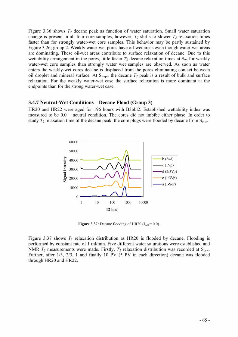
- 65 -

Figure 3.36 shows T2 decane peak as function of water saturation. Small water saturation change is present in all four core samples, however, T2 shifts to slower T2 relaxation times faster than for strongly water-wet core samples. This behavior may be partly sustained by Figure 3.26; group 2. Weakly water-wet pores have oil-wet areas even though water-wet areas are dominating. These oil-wet areas contribute to surface relaxation of decane. Due to this wettability arrangement in the pores, little faster T2 decane relaxation times at Swi for weakly water-wet core samples than strongly water wet samples are observed. As soon as water enters the weakly-wet cores decane is displaced from the pores eliminating contact between oil droplet and mineral surface. At Swspw the decane T2 peak is a result of bulk and surface relaxation. For the weakly water-wet case the surface relaxation is more dominant at the endpoints than for the strong water-wet case.

3.4.7 Neutral-Wet Conditions – Decane Flood (Group 3) HR20 and HR22 were aged for 196 hours with B3bbl2. Established wettability index was measured to be 0.0 – neutral condition. The cores did not imbibe either phase. In order to study T2 relaxation time of the decane peak, the core plugs were flooded by decane from Sorw.

0

10000

20000

30000

40000

50000

60000

1 10 100 1000 10000

T2 [ms]

Sign

al In

tens

ity b (Swi)e (1Vp)d (2/3Vp)c (1/3Vp)a (1-Sor)

Figure 3.37: Decane flooding of HR20 (IAH = 0.0).

Figure 3.37 shows T2 relaxation distribution as HR20 is flooded by decane. Flooding is performed by constant rate of 1 ml/min. Five different water saturations were established and NMR T2 measurements were made. Firstly, T2 relaxation distribution was recorded at Sorw. Further, after 1/3, 2/3, 1 and finally 10 PV (5 PV in each direction) decane was flooded through HR20 and HR22.

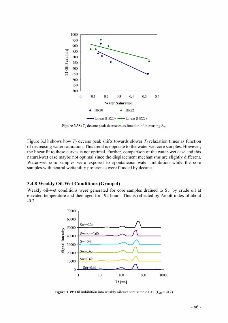
- 66 -

500550600650700750800850900950

1000

0 0.1 0.2 0.3 0.4 0.5 0.6

Water Saturation

T2

Oil

Peak

[ms]

HR20 HR22

Linear (HR20) Linear (HR22)

Figure 3.38: T2 decane peak decreases as function of increasing Sw. Figure 3.38 shows how T2 decane peak shifts towards slower T2 relaxation times as function of decreasing water saturation. This trend is opposite to the water wet core samples. However, the linear fit to these curves is not optimal. Further, comparison of the water-wet case and this natural-wet case maybe not optimal since the displacement mechanisms are slightly different. Water-wet core samples were exposed to spontaneous water imbibition while the core samples with neutral wettability preference were flooded by decane.

3.4.8 Weakly Oil-Wet Conditions (Group 4) Weakly oil-wet conditions were generated for core samples drained to Swi by crude oil at elevated temperature and then aged for 192 hours. This is reflected by Amott index of about -0.2.

0

10000

20000

30000

40000

50000

60000

70000

1 10 100 1000 10000

T2 [ms]

Sign

al In

tens

ity

1-Sor=0.69

Sw=0.62

Sw=0.63

Sw=0.61

Swspo=0.60

Swi=0.24

Figure 3.39: Oil imbibition into weakly oil-wet core sample LT1 (IAH = -0.2).

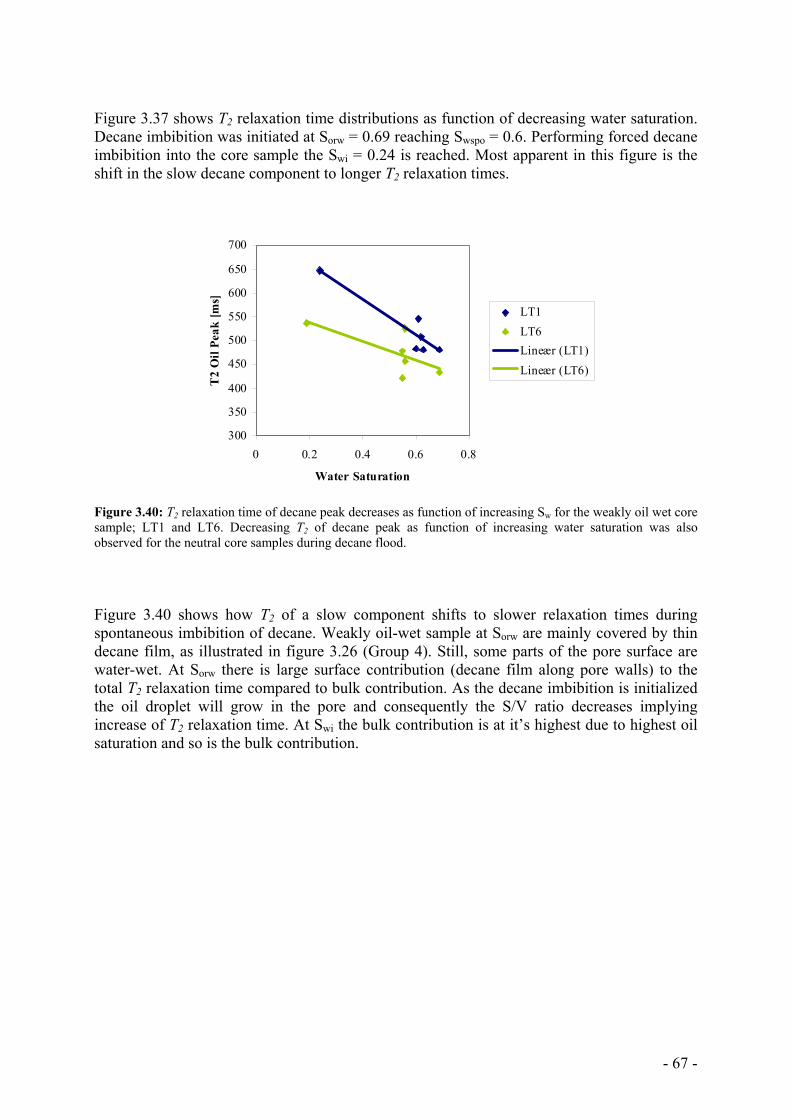
- 67 -

Figure 3.37 shows T2 relaxation time distributions as function of decreasing water saturation. Decane imbibition was initiated at Sorw = 0.69 reaching Swspo = 0.6. Performing forced decane imbibition into the core sample the Swi = 0.24 is reached. Most apparent in this figure is the shift in the slow decane component to longer T2 relaxation times.

300

350

400

450

500

550

600

650

700

0 0.2 0.4 0.6 0.8

Water Saturation

T2

Oil

Peak

[ms]

LT1LT6Lineær (LT1)Lineær (LT6)

Figure 3.40: T2 relaxation time of decane peak decreases as function of increasing Sw for the weakly oil wet core sample; LT1 and LT6. Decreasing T2 of decane peak as function of increasing water saturation was also observed for the neutral core samples during decane flood. Figure 3.40 shows how T2 of a slow component shifts to slower relaxation times during spontaneous imbibition of decane. Weakly oil-wet sample at Sorw are mainly covered by thin decane film, as illustrated in figure 3.26 (Group 4). Still, some parts of the pore surface are water-wet. At Sorw there is large surface contribution (decane film along pore walls) to the total T2 relaxation time compared to bulk contribution. As the decane imbibition is initialized the oil droplet will grow in the pore and consequently the S/V ratio decreases implying increase of T2 relaxation time. At Swi the bulk contribution is at it’s highest due to highest oil saturation and so is the bulk contribution.

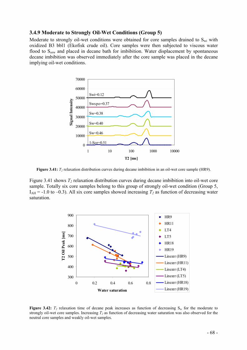
- 68 -

3.4.9 Moderate to Strongly Oil-Wet Conditions (Group 5) Moderate to strongly oil-wet conditions were obtained for core samples drained to Swi with oxidized B3 bbl1 (Ekofisk crude oil). Core samples were then subjected to viscous water flood to Sorw and placed in decane bath for imbibition. Water displacement by spontaneous decane imbibition was observed immediately after the core sample was placed in the decane implying oil-wet conditions.

0

10000

20000

30000

40000

50000

60000

70000

1 10 100 1000 10000

T2 [ms]

Sign

al In

tens

ity

1-Sor=0.51

Sw=0.46

Sw=0.40

Sw=0.38

Swspo=0.37

Swi=0.12

Figure 3.41: T2 relaxation distribution curves during decane imbibition in an oil-wet core sample (HR9).

Figure 3.41 shows T2 relaxation distribution curves during decane imbibition into oil-wet core sample. Totally six core samples belong to this group of strongly oil-wet condition (Group 5, IAH = -1.0 to –0.3). All six core samples showed increasing T2 as function of decreasing water saturation.

300

400

500

600

700

800

900

0 0.2 0.4 0.6 0.8

Water saturation

T2

Oil

Peak

[ms]

HR9HR11LT4LT5HR18HR19Lineær (HR9)Lineær (HR11)Lineær (LT4)Lineær (LT5)Lineær (HR18)Lineær (HR19)

Figure 3.42: T2 relaxation time of decane peak increases as function of decreasing Sw for the moderate to strongly oil-wet core samples. Increasing T2 as function of decreasing water saturation was also observed for the neutral core samples and weakly oil-wet samples.

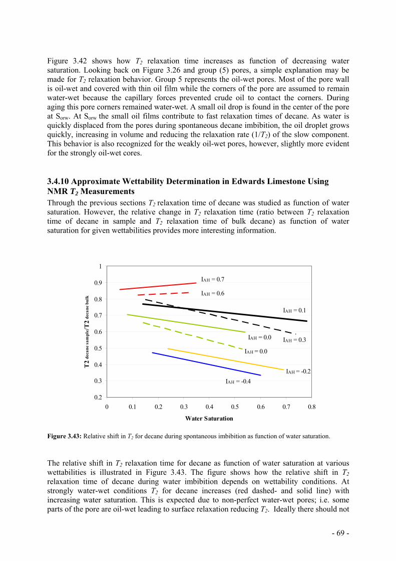
- 69 -

Figure 3.42 shows how T2 relaxation time increases as function of decreasing water saturation. Looking back on Figure 3.26 and group (5) pores, a simple explanation may be made for T2 relaxation behavior. Group 5 represents the oil-wet pores. Most of the pore wall is oil-wet and covered with thin oil film while the corners of the pore are assumed to remain water-wet because the capillary forces prevented crude oil to contact the corners. During aging this pore corners remained water-wet. A small oil drop is found in the center of the pore at Sorw. At Sorw the small oil films contribute to fast relaxation times of decane. As water is quickly displaced from the pores during spontaneous decane imbibition, the oil droplet grows quickly, increasing in volume and reducing the relaxation rate (1/T2) of the slow component. This behavior is also recognized for the weakly oil-wet pores, however, slightly more evident for the strongly oil-wet cores.

3.4.10 Approximate Wettability Determination in Edwards Limestone Using NMR T2 Measurements Through the previous sections T2 relaxation time of decane was studied as function of water saturation. However, the relative change in T2 relaxation time (ratio between T2 relaxation time of decane in sample and T2 relaxation time of bulk decane) as function of water saturation for given wettabilities provides more interesting information.

0.2

0.3

0.4

0.5

0.6

0.7

0.8

0.9

1

0 0.1 0.2 0.3 0.4 0.5 0.6 0.7 0.8

Water Saturation

T2

deca

ne s

ampl

e /T2

deca

ne b

ulk

IAH = 0.7

IAH = 0.6

IAH = 0.1

IAH = 0.3IAH = 0.0

IAH = 0.0

IAH = -0.2 IAH = -0.4

Figure 3.43: Relative shift in T2 for decane during spontaneous imbibition as function of water saturation. The relative shift in T2 relaxation time for decane as function of water saturation at various wettabilities is illustrated in Figure 3.43. The figure shows how the relative shift in T2 relaxation time of decane during water imbibition depends on wettability conditions. At strongly water-wet conditions T2 for decane increases (red dashed- and solid line) with increasing water saturation. This is expected due to non-perfect water-wet pores; i.e. some parts of the pore are oil-wet leading to surface relaxation reducing T2. Ideally there should not

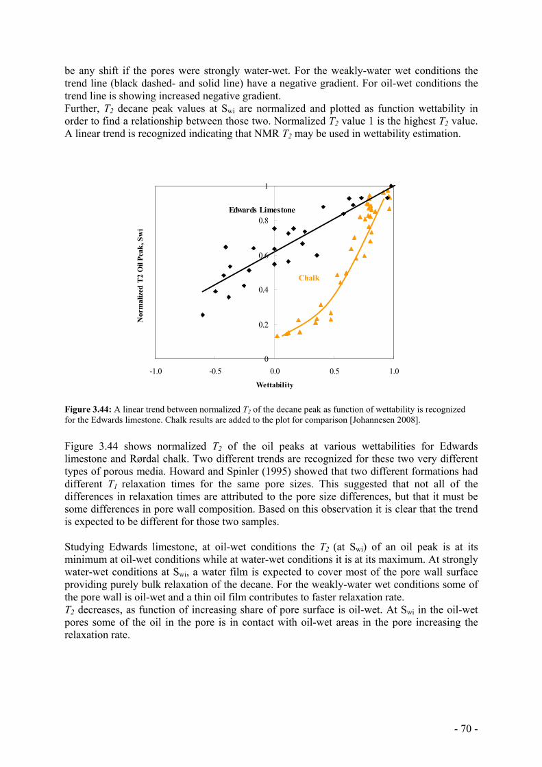
- 70 -

be any shift if the pores were strongly water-wet. For the weakly-water wet conditions the trend line (black dashed- and solid line) have a negative gradient. For oil-wet conditions the trend line is showing increased negative gradient. Further, T2 decane peak values at Swi are normalized and plotted as function wettability in order to find a relationship between those two. Normalized T2 value 1 is the highest T2 value. A linear trend is recognized indicating that NMR T2 may be used in wettability estimation.

0

0.2

0.4

0.6

0.8

1

-1.0 -0.5 0.0 0.5 1.0Wettability

Nor

mal

ized

T2

Oil

Peak

, Sw

i

Edwards Limestone

Chalk

Figure 3.44: A linear trend between normalized T2 of the decane peak as function of wettability is recognized for the Edwards limestone. Chalk results are added to the plot for comparison [Johannesen 2008]. Figure 3.44 shows normalized T2 of the oil peaks at various wettabilities for Edwards limestone and Rørdal chalk. Two different trends are recognized for these two very different types of porous media. Howard and Spinler (1995) showed that two different formations had different T1 relaxation times for the same pore sizes. This suggested that not all of the differences in relaxation times are attributed to the pore size differences, but that it must be some differences in pore wall composition. Based on this observation it is clear that the trend is expected to be different for those two samples. Studying Edwards limestone, at oil-wet conditions the T2 (at Swi) of an oil peak is at its minimum at oil-wet conditions while at water-wet conditions it is at its maximum. At strongly water-wet conditions at Swi, a water film is expected to cover most of the pore wall surface providing purely bulk relaxation of the decane. For the weakly-water wet conditions some of the pore wall is oil-wet and a thin oil film contributes to faster relaxation rate. T2 decreases, as function of increasing share of pore surface is oil-wet. At Swi in the oil-wet pores some of the oil in the pore is in contact with oil-wet areas in the pore increasing the relaxation rate.

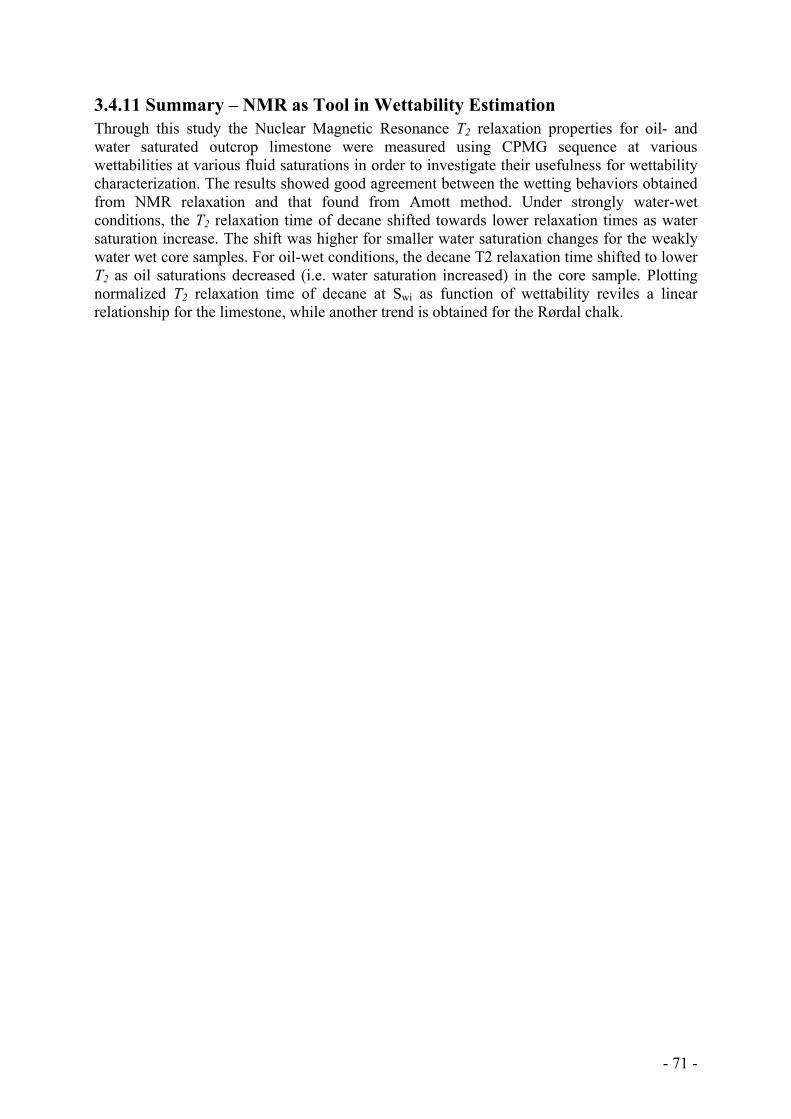
- 71 -

3.4.11 Summary – NMR as Tool in Wettability Estimation Through this study the Nuclear Magnetic Resonance T2 relaxation properties for oil- and water saturated outcrop limestone were measured using CPMG sequence at various wettabilities at various fluid saturations in order to investigate their usefulness for wettability characterization. The results showed good agreement between the wetting behaviors obtained from NMR relaxation and that found from Amott method. Under strongly water-wet conditions, the T2 relaxation time of decane shifted towards lower relaxation times as water saturation increase. The shift was higher for smaller water saturation changes for the weakly water wet core samples. For oil-wet conditions, the decane T2 relaxation time shifted to lower T2 as oil saturations decreased (i.e. water saturation increased) in the core sample. Plotting normalized T2 relaxation time of decane at Swi as function of wettability reviles a linear relationship for the limestone, while another trend is obtained for the Rørdal chalk.

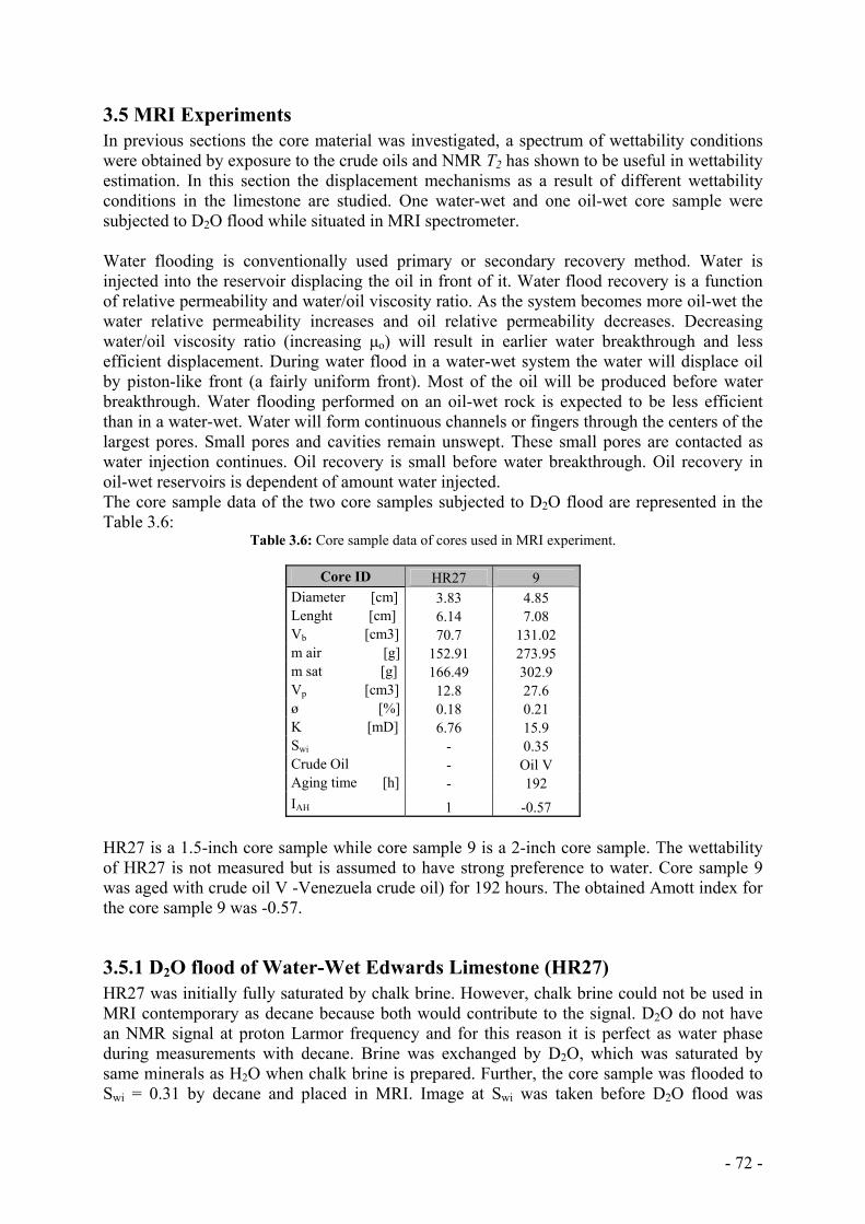
- 72 -

3.5 MRI Experiments In previous sections the core material was investigated, a spectrum of wettability conditions were obtained by exposure to the crude oils and NMR T2 has shown to be useful in wettability estimation. In this section the displacement mechanisms as a result of different wettability conditions in the limestone are studied. One water-wet and one oil-wet core sample were subjected to D2O flood while situated in MRI spectrometer. Water flooding is conventionally used primary or secondary recovery method. Water is injected into the reservoir displacing the oil in front of it. Water flood recovery is a function of relative permeability and water/oil viscosity ratio. As the system becomes more oil-wet the water relative permeability increases and oil relative permeability decreases. Decreasing water/oil viscosity ratio (increasing µo) will result in earlier water breakthrough and less efficient displacement. During water flood in a water-wet system the water will displace oil by piston-like front (a fairly uniform front). Most of the oil will be produced before water breakthrough. Water flooding performed on an oil-wet rock is expected to be less efficient than in a water-wet. Water will form continuous channels or fingers through the centers of the largest pores. Small pores and cavities remain unswept. These small pores are contacted as water injection continues. Oil recovery is small before water breakthrough. Oil recovery in oil-wet reservoirs is dependent of amount water injected. The core sample data of the two core samples subjected to D2O flood are represented in the Table 3.6:

Table 3.6: Core sample data of cores used in MRI experiment.

Core ID HR27 9 Diameter [cm] 3.83 4.85 Lenght [cm] 6.14 7.08 Vb [cm3] 70.7 131.02 m air [g] 152.91 273.95 m sat [g] 166.49 302.9 Vp [cm3] 12.8 27.6 ø [%] 0.18 0.21 K [mD] 6.76 15.9 Swi - 0.35 Crude Oil - Oil V Aging time [h] - 192 IAH 1 -0.57

HR27 is a 1.5-inch core sample while core sample 9 is a 2-inch core sample. The wettability of HR27 is not measured but is assumed to have strong preference to water. Core sample 9 was aged with crude oil V -Venezuela crude oil) for 192 hours. The obtained Amott index for the core sample 9 was -0.57.

3.5.1 D2O flood of Water-Wet Edwards Limestone (HR27) HR27 was initially fully saturated by chalk brine. However, chalk brine could not be used in MRI contemporary as decane because both would contribute to the signal. D2O do not have an NMR signal at proton Larmor frequency and for this reason it is perfect as water phase during measurements with decane. Brine was exchanged by D2O, which was saturated by same minerals as H2O when chalk brine is prepared. Further, the core sample was flooded to Swi = 0.31 by decane and placed in MRI. Image at Swi was taken before D2O flood was

- 73 -

initiated. The signal intensities from the MRI are now surly a product of decane – the machine “sees” only decane in the core sample. The signal intensity is related to given oil saturation known from the mass balance. As the flooding was initiated and D2O enters the core the signal intensity is reduced across the sample. The reduction of signal is expected since the fluid providing the signal (decane) is being displaced by D2O.

0.000

0.002

0.004

0.006

0.008

0.010

0.012

0.014

0.0 1.0 2.0 3.0 4.0 5.0 6.0

Sample lenght [cm]

MR

I Sig

nal I

nten

sity

00.050.080.130.160.220.240.30

PV D2O injected:

Figure 3.45: Flooding a water-wet Edwards limestone in MRI from Swi by D2O shows how decane is displaced across the sample length by decreasing signal intensity. Figure 3.45 shows how MRI signal intensity is reduced as D2O is injected to the core sample. The upper dark blue line represents signal intensity at Swi. The signal is quite irregular across the sample length. The author assumes that these irregularities are due to core sample heterogeneities or to saturation in homogeneities since they are repeatable as D2O is injected to the core sample. Normalizing intensities across the sample to the signal intensity at Soi may provide more clear description of the displacement front:

0

0.2

0.4

0.6

0.8

1

1.2

0.0 1.0 2.0 3.0 4.0 5.0 6.0

Sample lenght [cm]

Nor

m. M

RI

Sign

al I

nten

sity

00.050.080.130.160.220.240.30

PV D2O injected:

Figure 3.46: Normalizing the signal intensities to initial signal intensity at Soi for each slice shows a possible front which disperses through the sample.

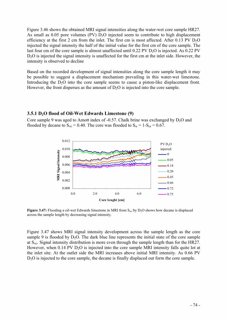
- 74 -

Figure 3.46 shows the obtained MRI signal intensities along the water-wet core sample HR27. As small as 0.05 pore volumes (PV) D2O injected seem to contribute to high displacement efficiency at the first 2 cm from the inlet. The first cm is most affected. After 0.13 PV D2O injected the signal intensity the half of the initial value for the first cm of the core sample. The last four cm of the core sample is almost unaffected until 0.22 PV D2O is injected. As 0.22 PV D2O is injected the signal intensity is unaffected for the first cm at the inlet side. However, the intensity is observed to decline Based on the recorded development of signal intensities along the core sample length it may be possible to suggest a displacement mechanism prevailing in this water-wet limestone. Introducing the D2O into the core sample seems to cause a piston-like displacement front. However, the front disperses as the amount of D2O is injected into the core sample.

3.5.1 D2O flood of Oil-Wet Edwards Limestone (9) Core sample 9 was aged to Amott index of -0.57. Chalk brine was exchanged by D2O and flooded by decane to Swi = 0.40. The core was flooded to Sw = 1-Sor = 0.67.

0.000

0.002

0.004

0.006

0.008

0.010

0.012

0.0 2.0 4.0 6.0

Core lenght [cm]

MR

I Si

gnal

Int

ensi

ty

0

0.05

0.14

0.20

0.45

0.66

0.72

0.75

PV D2O injected:

Figure 3.47: Flooding a oil-wet Edwards limestone in MRI from Swi by D2O shows how decane is displaced across the sample length by decreasing signal intensity. Figure 3.47 shows MRI signal intensity development across the sample length as the core sample 9 is flooded by D2O. The dark blue line represents the initial state of the core sample at Swi. Signal intensity distribution is more even through the sample length than for the HR27. However, when 0.14 PV D2O is injected into the core sample MRI intensity falls quite lot at the inlet site. At the outlet side the MRI increases above initial MRI intensity. As 0.66 PV D2O is injected to the core sample, the decane is finally displaced out form the core sample.

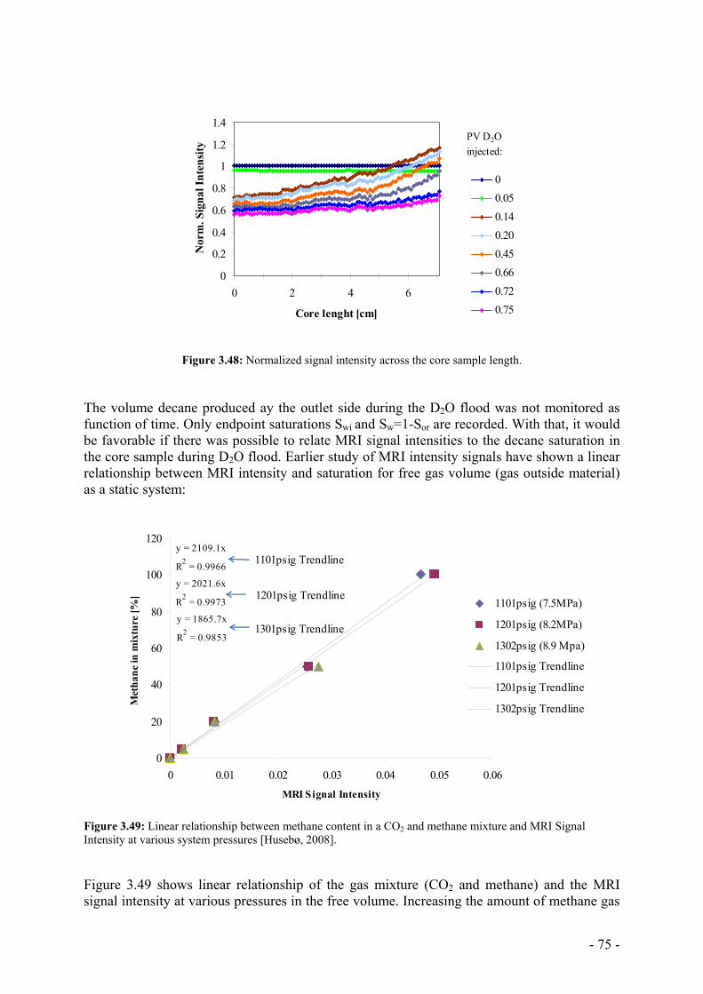
- 75 -

0

0.2

0.4

0.6

0.8

1

1.2

1.4

0 2 4 6

Core lenght [cm]

Nor

m. S

igna

l Int

ensi

ty

00.050.140.200.450.660.720.75

PV D2O injected:

Figure 3.48: Normalized signal intensity across the core sample length. The volume decane produced ay the outlet side during the D2O flood was not monitored as function of time. Only endpoint saturations Swi and Sw=1-Sor are recorded. With that, it would be favorable if there was possible to relate MRI signal intensities to the decane saturation in the core sample during D2O flood. Earlier study of MRI intensity signals have shown a linear relationship between MRI intensity and saturation for free gas volume (gas outside material) as a static system:

y = 2109.1x

R2 = 0.9966

y = 2021.6x

R2 = 0.9973

y = 1865.7x

R2 = 0.9853

0

20

40

60

80

100

120

0 0.01 0.02 0.03 0.04 0.05 0.06

MRI Signal Intensity

Met

hane

in m

ixtu

re [%

]

1101psig (7.5MPa)

1201psig (8.2MPa)

1302psig (8.9 Mpa)

1101psig Trendline

1201psig Trendline

1302psig Trendline

1101psig Trendline

1201psig Trendline

1301psig Trendline

Figure 3.49: Linear relationship between methane content in a CO2 and methane mixture and MRI Signal Intensity at various system pressures [Husebø, 2008]. Figure 3.49 shows linear relationship of the gas mixture (CO2 and methane) and the MRI signal intensity at various pressures in the free volume. Increasing the amount of methane gas

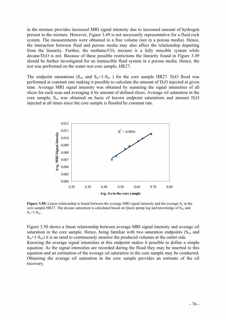
- 76 -

in the mixture provides increased MRI signal intensity due to increased amount of hydrogen present in the mixture. However, Figure 3.49 is not necessarily representative for a fluid-rock system. The measurements were obtained in a free volume (not in a porous media). Hence, the interaction between fluid and porous media may also affect the relationship departing from the linearity. Further, the methane/CO2 mixture is a fully miscible system while decane/D2O is not. Because of these possible restrictions the linearity found in Figure 3.49 should be further investigated for an immiscible fluid system in a porous media. Hence, the test was performed on the water-wet core sample, HR27. The endpoint saturations (Swi and Sw=1-Sor ) for the core sample HR27. D2O flood was performed at constant rate making it possible to calculate the amount of D2O injected at given time. Average MRI signal intensity was obtained by summing the signal intensities of all slices for each scan and averaging it by amount of defined slices. Average oil saturation in the core sample, So, was obtained on basis of known endpoint saturations and amount D2O injected at all times since the core sample is flooded by constant rate.

R2 = 0.9856

0.004

0.005

0.006

0.007

0.008

0.009

0.010

0.011

0.012

0.20 0.30 0.40 0.50 0.60 0.70 0.80

Avg. So in the core sample

Avg

. MR

I Sig

nal I

ntes

ity

Figure 3.50: Linear relationship is found between the average MRI signal intensity and the average So in the core sample HR27. The decane saturation is calculated based on Quzix pump log and knowledge of Swi and Sw=1-Sor. Figure 3.50 shows a linear relationship between average MRI signal intensity and average oil saturation in the core sample. Hence, being familiar with two saturation endpoints (Swi and Sw=1-Sor) it is no need to continuously monitor the produced volumes at the outlet side. Knowing the average signal intensities at this endpoint makes it possible to define a simple equation. As the signal intensities are recorded during the flood they may be inserted to this equation and an estimation of the average oil saturation in the core sample may be conducted. Obtaining the average oil saturation in the core sample provides an estimate of the oil recovery.

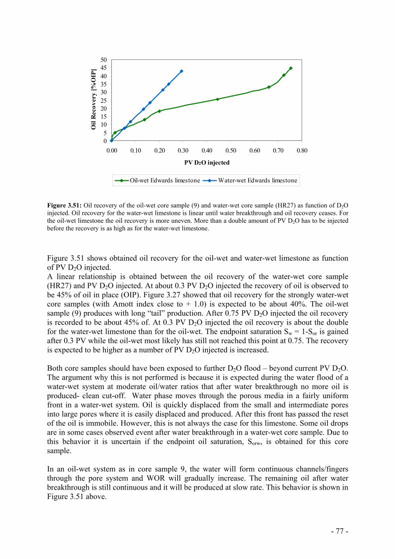
- 77 -

05

101520253035404550

0.00 0.10 0.20 0.30 0.40 0.50 0.60 0.70 0.80

PV D2O injected

Oil

Rec

over

y [%

OIP

]

Oil-wet Edwards limestone Water-wet Edwards limestone

Figure 3.51: Oil recovery of the oil-wet core sample (9) and water-wet core sample (HR27) as function of D2O injected. Oil recovery for the water-wet limestone is linear until water breakthrough and oil recovery ceases. For the oil-wet limestone the oil recovery is more uneven. More than a double amount of PV D2O has to be injected before the recovery is as high as for the water-wet limestone. Figure 3.51 shows obtained oil recovery for the oil-wet and water-wet limestone as function of PV D2O injected. A linear relationship is obtained between the oil recovery of the water-wet core sample (HR27) and PV D2O injected. At about 0.3 PV D2O injected the recovery of oil is observed to be 45% of oil in place (OIP). Figure 3.27 showed that oil recovery for the strongly water-wet core samples (with Amott index close to + 1.0) is expected to be about 40%. The oil-wet sample (9) produces with long “tail” production. After 0.75 PV D2O injected the oil recovery is recorded to be about 45% of. At 0.3 PV D2O injected the oil recovery is about the double for the water-wet limestone than for the oil-wet. The endpoint saturation Sw = 1-Sor is gained after 0.3 PV while the oil-wet most likely has still not reached this point at 0.75. The recovery is expected to be higher as a number of PV D2O injected is increased. Both core samples should have been exposed to further D2O flood – beyond current PV D2O. The argument why this is not performed is because it is expected during the water flood of a water-wet system at moderate oil/water ratios that after water breakthrough no more oil is produced- clean cut-off. Water phase moves through the porous media in a fairly uniform front in a water-wet system. Oil is quickly displaced from the small and intermediate pores into large pores where it is easily displaced and produced. After this front has passed the reset of the oil is immobile. However, this is not always the case for this limestone. Some oil drops are in some cases observed event after water breakthrough in a water-wet core sample. Due to this behavior it is uncertain if the endpoint oil saturation, Sorw, is obtained for this core sample. In an oil-wet system as in core sample 9, the water will form continuous channels/fingers through the pore system and WOR will gradually increase. The remaining oil after water breakthrough is still continuous and it will be produced at slow rate. This behavior is shown in Figure 3.51 above.

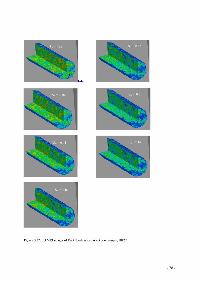
- 78 -

Figure 3.52: 3D MRI images of D2O flood on water-wet core sample, HR27.

Sw = 0.36

Sw = 0.38

Sw = 0.44

Sw = 0.48

Sw = 0.57

Sw = 0.61

Sw = 0.64

Inlet

- 79 -

Figure 3.52 shows images of water-wet core sample, HR27, subjected to D2O flood. The first image shows where the inlet side is. The decane provides a signal in these images. Signal intensities are here visualized by color scale. Red and yellow areas represent high intensity areas, i.e. high hydrogen density. Blue and dark blue areas represent the low intensity areas. The inlet side is in the left corner of the image. Studying the first image (Sw = 0.36) it is clear that there are certain areas in the core sample consisting of much higher hydrogen densities than other areas. Areas within the core sample with highest intensity seem to be drained most efficiently while remaining area show a minor change in signal intensity. The decane in a water-wet core sample is quickly displaced from the smallest pores and moved into the largest pores where the water displaces the oil with fairly uniform front. It is not easy observe this front in the Figure 3.52.

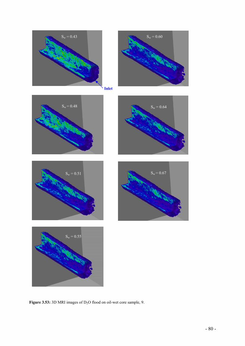
- 80 -

Figure 3.53: 3D MRI images of D2O flood on oil-wet core sample, 9.

Sw = 0.43

Sw = 0.48

Sw = 0.51

Sw = 0.55

Sw = 0.60

Sw = 0.64

Sw = 0.67

Inlet

- 81 -

Figure 3.55 shows 3D MRI images of an oil-wet core sample 9. The inlet side is in the left corner. Comparing these images with water-wet case flooding it is clear that two different displacement processes are different. As the D2O flood is initiated in the oil-wet sample 9 the development of the water-fingers is recognized. Large areas are swept by D2O. As D2O enters the core sample it will move through the biggest pores displacing the oil phase in front of it. At the breakthrough there is still producible oil in the pores. Due to this displacement mechanism much oil is produced after water breakthrough - long production tail is produced compared to water-wet case (see Figure 3.51).

- 82 -

PART 4 Conclusions and Future Work

o Based on the thin sections, mercury injection, porosity and permeability measurements for the Edwards limestone may be characterized as highly heterogeneous bioclastic grain stone.

o The scaling equation for spontaneous imbibition is shown to be valid for the Edwards

limestone; similar to the homogenous Berea sandstone.

o Swi affects the induction time and the imbibition rate during spontaneous brine imbibition. Oil recovery by spontaneous water imbibition does not seem to be affected by the Swi.

o The wettability index obtained for unaged Edwards limestone using the Amott method

was less than 1. This demonstrates the impact of high pore/throat aspect ratio in this limestone. During the decane production by spontaneous brine imbibition the main trapping mechanism for residual oil is believed to be snap-off mechanism leaving behind globules of decane in the largest pores. Thus additional decane production is obtained by viscous displacement, causing Amott index to be lower than 1.

o Oil characterization showed that oils with low API and high base/acid ratio are

favorable for wettability alteration in this limestone. Compared to some chalks the wettability of this limestone is easily altered from water- to oil-wet.

o The maximum oil recovery is obtained at neutral wettability conditions – on the

slightly oil-wet side.

o NMR T2 has shown to be useful in wettability estimation. A linear relationship is found between T2 for oil at Swi versus wettability. T2 for oil at Swi is increasing as wettability of Edwards limestone shifts towards more water-wet conditions. This method may have potential as wettability interpretation tool in the laboratory and maybe as in-situ logging tool in the future.

o Using low viscosity oil like decane makes it easier to distinguish T2 relaxation times

for the brine and the oil phase.

o A linear relationship between average MRI intensity and oil saturation has been confirmed. MRI intensities may be used for saturation calculation.

o The MRI intensities show a water front development as the water-wet core sample was

water flooded. This front disperses as the flooding is maintained.

o MRI images demonstrate fingering in the oil displacement process during the water flood of the oil-wet core sample.

o Applying MRI when water flooding water- and oil-wet cores demonstrates how

wettability affects in-situ oil production from the core sample. Local oil saturation development was different and the oil recovery was significantly impacted by the different wettability conditions.

- 83 -

Refrences Abdallah, W., Buckley,J.S., Carnegie,A., Herold, J.E.B., Fordham, E., Graue,A., Signer, T.H., Hussain,H., Montaron,B., Ziauddin,M.: “ Fundamentals of Wettability”, Oilfield Review (2007), 44-60. Amott, E.: “Observations Relating to the Wettability of Porous Rock”, (1959) Trans. AIME, 216, 156-162. Anderson, W.G.: “Wettability Literature Survey – Part 1: Rock/Oil/Brine Interactions and the Effects of Core Handling on Wettability”, JPT (1986) 1125-1149. Anderson, W.G.: “Wettability Literature Survey – Part 2: Wettability Measurement”, JPT (1987a) 1146-1262. Anderson, W.G.: “Wettability Literature Survey – Part 3: “The Effects of Wettability on the Electrical Properties of Porous Media”, JPT (1987b) 1283-1300. Anderson, W.G.: “Wettability Literature Survey – Part 4: “Effects of Wettability on Capillary pressure”, JPT (1987c) 1453-1468. Anderson, W.G.: “Wettability Literature Survey – Part 5: “Effects of Wettability on Relative Permeability”, JPT (1987d) 1605-1622. Anderson, W.G.: “Wettability Literature Survey – Part 6: “Effects of Wettability on Waterflooding”, JPT (1987e) 1605-1622. Aspenes,E., Graue, A. and Ramsdal, J.: “In situ wettability distribution and wettability stability in outcrop chalk aged in crude oil”, (2002) J. Petr. Sci. & Eng., 39, 337-350. Brown, R.J.S., Fatt, I.: “Measurements of Fractional Wettability of Oilfield Rocks by the Nuclear Magnetic Relaxation Method”, (1956) Trans. AIME, 207, 262-264. Buckley, J.S.: “Evaluation of Reservoir wettability and its Effect on Oil Recovery”, First Annual Report prepared by PRRC, New Mexico Institute of Mining and Technology (1997). Buckley, J.S., Liu,Y., Monsterleet, S.: “Mechanisms of Wetting Alteration by Crude Oils”, SPE/New Mexico Tech. (1998). Buckley, J.S.: Private communication (2007). Buckley, J.S., Jianxin, W.: “Crude Oil and Asphaltene Characterization for Prediction of Wetting Alteration”, JPT (2002). Craig, F.F.: “The Reservoir Engineering Aspects of Water flooding”, Monograph Volume 3 of the Henry L. Doherty Series, Society of Petroleum Engineers (1971). Cuiec, L.: “Rock/Crude-Oil Interactions and Wettability: An Attempt To Understand Their Interrelation”, SPE 12311 (1984).

- 84 -

Dunn, K.J, Bergman, D.J, LaTorraca, G.A.: Nuclear Magnetic Resonance Petrophysical and Logging Applications, Pergamon, (2002). Fan, T.: Private communication (2007). Fan,T. , Buckley, J.S.: “Evaluating Crude Oils by SARA Analysis”, SPE/New Mexico Tech. (2002). Fan,T. , Buckley, J.S.: “Acid Number Measurements Revisited”, SPE 99884 (2006). Fischer,H., Morrow,N.R.: “Spontaneous Imbibition with Matched Liquid Viscosities”, SPE 96812 (2005) Finjord, J., Hiorth,A., a Lad, U.H., Skjæveland, S.M.: “NMR for Equilateral Triangular Geometry Under Conditions of Surface Relaxivity- Analytical and Random Walk Solution,” Transport in Porous Media, Online First, 3 November, 21 pp. Graue, A., Viksund, B.G., Baldwin, B.A.: “Reproducible Wettability Alteration of Low Permeable-Permeable Outcrop Chalk”, SPE Res. Eval. & Eng., Vol.2, No.2, (1998). Graue,A.,Viksund,B.G.,Eilertsen,T., Moe,R.:” Systematic Wettability Alteration by Aging Sandstone and Carbonate Rock in Crude Oil”, 24 JPT, 85-97 (1999a). Graue,A., Aspenes,E., Bognø,T., Moe,R.W., Ramsdal,J.: “ Alteration of Wettability and Wettability Heterogeneity”, 33 JPT , 3-17 (2002). Husebø, J.: Private communication (2008). Howard, J.J., Spilner, E.A.:” Nuclear Magnetic Resonance Measurements of Wettability and Fluid Saturations in Chalk”, SPE 26471 (1995). Jadhunandan, P.P., Morrow, N.R. . “ Effect of Wettability on Water flood Recovery for COBR Systems”, SPE/ New Mexico PPRC (1995). Jia, D., Buckley, J.S., Morrow, N.R.,: “Control of Core Wettability With Crude Oil”, SPE 21041 (1991). Johannesen, E.B., Steinsbø, M., Howard, J.J., Graue,A.: “ Wettability Characterization by NMR T2 Measurements In Chalk”, Society of Core Ananlysists, (2006) Trondheim, September 12-16. Johannesen, E.B.: Private communication (2008). Mattax, C.C., Kyte, J.R.: “Imbibition Oil Recovery From Fractured Water drive Reservoirs”, SPEJ (June 1962) 177. Morrow, N.R., Lim, T.H., Ward, J.S.: “Effect of Crude Oil Induced Wettability Changes on Oil Recovery”, SPE 13215 (1986).

- 85 -

Morrow, N.R.: “ Wettability and Its Effect on Oil Recovery” NM PRRC, New Mexico Institute of Mining and Technology /SPE (1990) Puddephat, M.: “Principles of Magnetic Resonance Imagining” (19.10.2007). URL: http://www.easymeasure.co.uk/principlesmri.aspx Selly, R.C.: “Elements of Petroleum Geology”, Second Edition, Academic Press (1998). Skauge, A., Standal, S., Boe, S.O., Skauge, T., Blokhus, A.M.:” Effects of Organic Acids and Bases, and Oil Composition on Wettability”, SPE 56673 (1999). Wang, J.X., Buckley, J.S.: “An Experimental Approach to Predication of Asphaltene Flocculation”, NM PRRC, New Mexico Institute of Mining and Technology /SPE (2001) Zhang, P., Austad, T.: “The Relative Effects of Acid Number and Temperature on Chalk Wettability”, SPE 92999 (2005) Zhang, X., Morrow, N.R., Ma, S.: “Experimental Verification of a Modified Scaling Group for Spontaneous Imbibition”, SPE 30762 (1995)