What Caused the 1991 Currency Crisis in India? September 2002 · Valerie Cerra and Sweta Chaman Saxena 396. continues to monetize high deficits, this model illustrates an ongoing

What Caused the 1991 Currency Crisis in India?

VALERIE CERRA and SWETA CHAMAN SAXENA*

Which model best explains the 1991 currency crisis in India? Did real overvalua-tion contribute to the crisis? This paper seeks the answers through error correc-tion models and by constructing the equilibrium real exchange rate using atechnique developed by Gonzalo and Granger (1995). The evidence indicates thatovervaluation as well as current account deficits and investor confidence playedsignificant roles in the sharp exchange rate depreciation. The ECM model issupported by superior out-of-sample forecast performance versus a random walkmodel. [JEL F31, F32, F47]

In mid-1991, India’s exchange rate was subjected to a severe adjustment. Thisevent began with a slide in the value of the rupee leading up to mid-1991. The

authorities at the Reserve Bank of India slowed the decline in value by expendinginternational reserves. With reserves nearly depleted, however, the exchange ratewas devalued sharply on July 1 and July 3 against major foreign currencies.

India’s 1991 crisis provides an interesting case study with certain features thatare distinct from popular theoretical models. Although some elements werepresent, the crisis cannot adequately be described as a first generation currencycrisis model. It also didn’t follow the second generation models, nor the morerecent literature that emphasizes financial sector weakness, overlending cycles,and contagion. In addition, despite progress in liberalizing trade and capital flows,India is still relatively closed and capital inflows have been well below those in

395

IMF Staff PapersVol. 49, No. 3

© 2002 International Monetary Fund

*Valerie Cerra is an Economist in the European I Department of the IMF. Sweta Chaman Saxena isan Assistant Professor at the University of Pittsburgh. We would like to thank Timothy Callen, CharlesEngel, Robert Flood, David Goldsbrough, and Christopher Towe for helpful comments on this and earlierversions of this paper, and Janet Bungay for editorial suggestions.

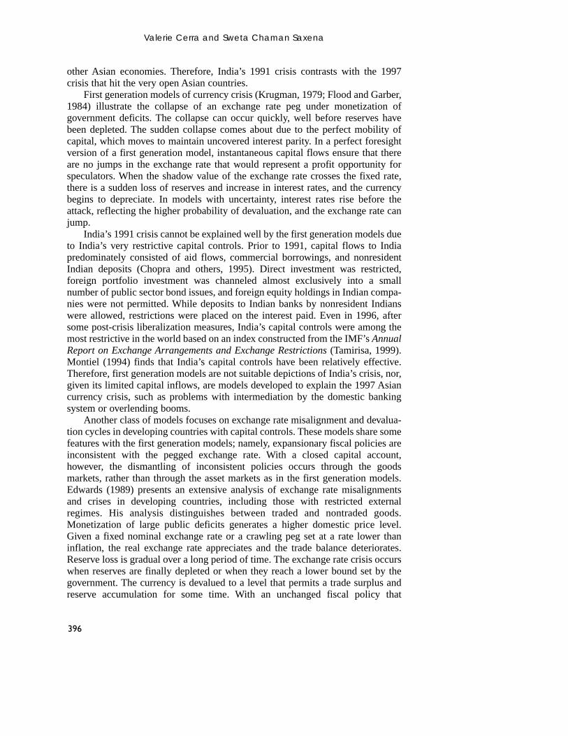
other Asian economies. Therefore, India’s 1991 crisis contrasts with the 1997crisis that hit the very open Asian countries.

First generation models of currency crisis (Krugman, 1979; Flood and Garber,1984) illustrate the collapse of an exchange rate peg under monetization ofgovernment deficits. The collapse can occur quickly, well before reserves havebeen depleted. The sudden collapse comes about due to the perfect mobility ofcapital, which moves to maintain uncovered interest parity. In a perfect foresightversion of a first generation model, instantaneous capital flows ensure that thereare no jumps in the exchange rate that would represent a profit opportunity forspeculators. When the shadow value of the exchange rate crosses the fixed rate,there is a sudden loss of reserves and increase in interest rates, and the currencybegins to depreciate. In models with uncertainty, interest rates rise before theattack, reflecting the higher probability of devaluation, and the exchange rate canjump.

India’s 1991 crisis cannot be explained well by the first generation models dueto India’s very restrictive capital controls. Prior to 1991, capital flows to Indiapredominately consisted of aid flows, commercial borrowings, and nonresidentIndian deposits (Chopra and others, 1995). Direct investment was restricted,foreign portfolio investment was channeled almost exclusively into a smallnumber of public sector bond issues, and foreign equity holdings in Indian compa-nies were not permitted. While deposits to Indian banks by nonresident Indianswere allowed, restrictions were placed on the interest paid. Even in 1996, aftersome post-crisis liberalization measures, India’s capital controls were among themost restrictive in the world based on an index constructed from the IMF’s AnnualReport on Exchange Arrangements and Exchange Restrictions (Tamirisa, 1999).Montiel (1994) finds that India’s capital controls have been relatively effective.Therefore, first generation models are not suitable depictions of India’s crisis, nor,given its limited capital inflows, are models developed to explain the 1997 Asiancurrency crisis, such as problems with intermediation by the domestic bankingsystem or overlending booms.

Another class of models focuses on exchange rate misalignment and devalua-tion cycles in developing countries with capital controls. These models share somefeatures with the first generation models; namely, expansionary fiscal policies areinconsistent with the pegged exchange rate. With a closed capital account,however, the dismantling of inconsistent policies occurs through the goodsmarkets, rather than through the asset markets as in the first generation models.Edwards (1989) presents an extensive analysis of exchange rate misalignmentsand crises in developing countries, including those with restricted externalregimes. His analysis distinguishes between traded and nontraded goods.Monetization of large public deficits generates a higher domestic price level.Given a fixed nominal exchange rate or a crawling peg set at a rate lower thaninflation, the real exchange rate appreciates and the trade balance deteriorates.Reserve loss is gradual over a long period of time. The exchange rate crisis occurswhen reserves are finally depleted or when they reach a lower bound set by thegovernment. The currency is devalued to a level that permits a trade surplus andreserve accumulation for some time. With an unchanged fiscal policy that

Valerie Cerra and Sweta Chaman Saxena

396

continues to monetize high deficits, this model illustrates an ongoing cycle ofreserve loss and exchange rate misalignment, followed by devaluation and reservegain.

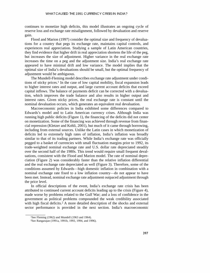
Flood and Marion (1997) consider the optimal size and frequency of devalua-tions for a country that pegs its exchange rate, maintains capital controls, andexperiences real appreciation. Studying a sample of Latin American countries,they find evidence that higher drift in real appreciation shortens the life of the peg,but increases the size of adjustment. Higher variance in the real exchange rateincreases the time on a peg and the adjustment size. India’s real exchange rateappeared to have minimal drift and low variance. The model implies that theoptimal size of India’s devaluations should be small, but the optimal frequency ofadjustment would be ambiguous.

The Mundell-Fleming model describes exchange rate adjustment under condi-tions of sticky prices.1 In the case of low capital mobility, fiscal expansion leadsto higher interest rates and output, and large current account deficits that exceedcapital inflows. The balance of payments deficit can be corrected with a devalua-tion, which improves the trade balance and also results in higher output andinterest rates. Given sticky prices, the real exchange rate is constant until thenominal devaluation occurs, which generates an equivalent real devaluation.

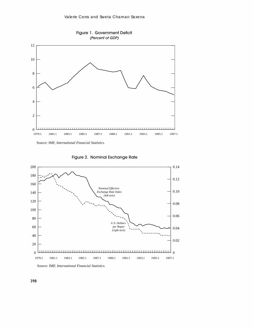
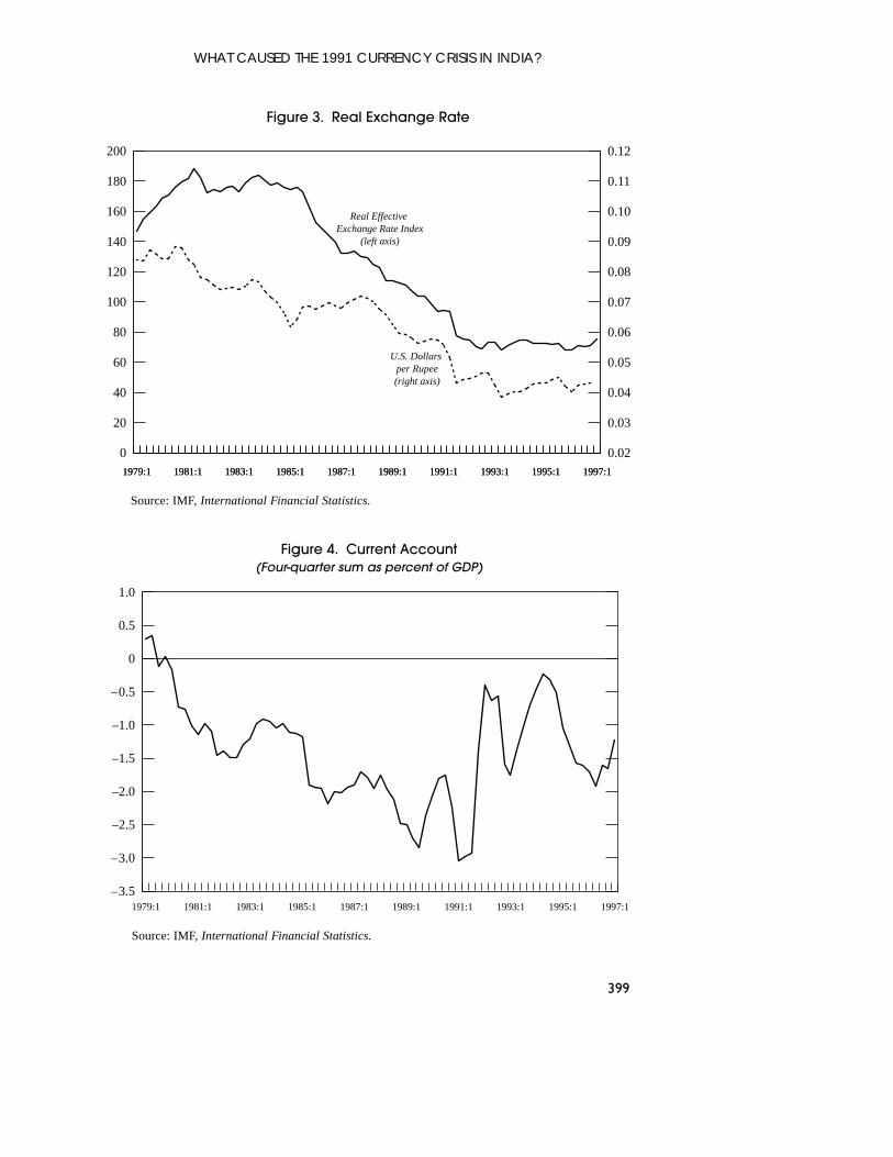
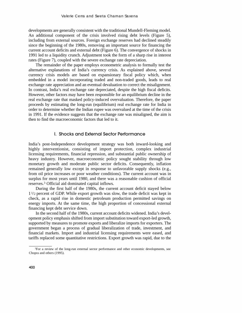
Macroeconomic policies in India exhibited some differences compared toEdwards’s model and to Latin American currency crises. Although India wasrunning high public deficits (Figure 1), the financing of the deficits did not centeron monetization. Some of the financing was achieved through revenue from finan-cial repression (Kletzer and Kohli, 2001), but much of it came through borrowing,including from external sources. Unlike the Latin cases in which monetization ofdeficits led to extremely high rates of inflation, India’s inflation was broadlysimilar to that of its trading partners. While India’s exchange rate was officiallypegged to a basket of currencies with small fluctuation margins prior to 1992, itstrade-weighted nominal exchange rate and U.S. dollar rate depreciated steadilyover the second half of the 1980s. This trend would require small frequent deval-uations, consistent with the Flood and Marion model. The rate of nominal depre-ciation (Figure 2) was considerably faster than the relative inflation differentialand the real exchange rate depreciated as well (Figure 3). Therefore, some of theconditions assumed by Edwards—high domestic inflation in combination with anominal exchange rate fixed to a low inflation country—do not appear to havebeen met. Instead, nominal exchange rate adjustment outpaced adjustment throughthe price level.

In official descriptions of the event, India’s exchange rate crisis has beenattributed to continued current account deficits leading up to the crisis (Figure 4),made worse by problems related to the Gulf War; and a loss of confidence in thegovernment as political problems compounded the weak credibility associatedwith high fiscal deficits.2 A more detailed description of the shocks and externalsector performance is provided in the next section. India’s macroeconomic

WHAT CAUSED THE 1991 CURRENCY CRISIS IN INDIA?

397

1See Fleming (1962) and Mundell (1963 and 1964).2See Rangarajan (1991a, 1991b, 1993, 1994, and 1996).


398

0

2

4

6

8

10

12

1997:11995:11993:11991:11989:11987:11985:11983:11981:11979:1

Figure 1. Government Deficit(Percent of GDP)

Source: IMF, International Financial Statistics.

0

20

40

60

80

100

120

140

160

180

200

1997:11995:11993:11991:11989:11987:11985:11983:11981:11979:1

0

0.02

0.04

0.06

0.08

0.10

0.12

0.14

U.S. Dollars per Rupee(right axis)

Nominal Effective Exchange Rate Index

(left axis)

Figure 2. Nominal Exchange Rate



399

0

20

40

60

80

100

120

140

160

180

200

1997:11995:11993:11991:11989:11987:11985:11983:11981:11979:1

0.02

0.03

0.04

0.05

0.06

0.07

0.08

0.09

0.10

0.11

0.12

1997:11995:11993:11991:11989:11987:11985:11983:11981:11979:1

U.S. Dollars per Rupee(right axis)

Real Effective Exchange Rate Index

(left axis)

Figure 3. Real Exchange Rate


–3.5

–3.0

–2.5

–2.0

–1.5

–1.0

–0.5

0

0.5

1.0

1997:11995:11993:11991:11989:11987:11985:11983:11981:11979:1

Figure 4. Current Account(Four-quarter sum as percent of GDP)


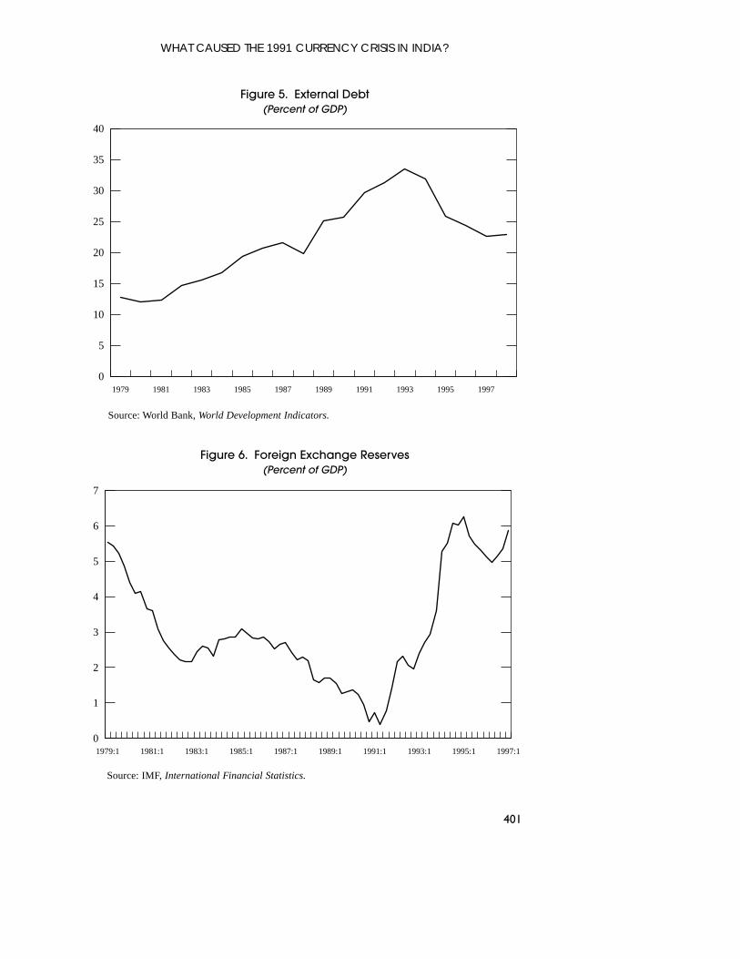
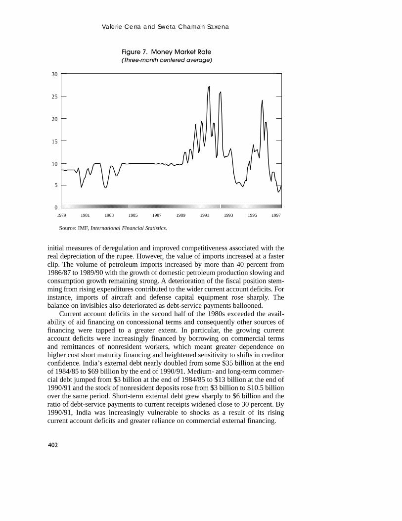
developments are generally consistent with the traditional Mundell-Fleming model.An additional component of the crisis involved rising debt levels (Figure 5),including from external sources. Foreign exchange reserves had declined steadilysince the beginning of the 1980s, removing an important source for financing thecurrent account deficits and external debt (Figure 6). The convergence of shocks in1991 led to a liquidity crunch. Adjustment took the form of a sharp rise in interestrates (Figure 7), coupled with the severe exchange rate depreciation.

The remainder of the paper employs econometric analysis to formally test thealternative explanations of India’s currency crisis. As explained above, severalcurrency crisis models are based on expansionary fiscal policy which, whenembedded in a model incorporating traded and non-traded goods, leads to realexchange rate appreciation and an eventual devaluation to correct the misalignment.In contrast, India’s real exchange rate depreciated, despite the high fiscal deficits.However, other factors may have been responsible for an equilibrium decline in thereal exchange rate that masked policy-induced overvaluation. Therefore, the paperproceeds by estimating the long-run (equilibrium) real exchange rate for India inorder to determine whether the Indian rupee was overvalued at the time of the crisisin 1991. If the evidence suggests that the exchange rate was misaligned, the aim isthen to find the macroeconomic factors that led to it.

I. Shocks and External Sector Performance

India’s post-Independence development strategy was both inward-looking andhighly interventionist, consisting of import protection, complex industriallicensing requirements, financial repression, and substantial public ownership ofheavy industry. However, macroeconomic policy sought stability through lowmonetary growth and moderate public sector deficits. Consequently, inflationremained generally low except in response to unfavorable supply shocks (e.g.,from oil price increases or poor weather conditions). The current account was insurplus for most years until 1980, and there was a reasonable cushion of officialreserves.3 Official aid dominated capital inflows.

During the first half of the 1980s, the current account deficit stayed below11/2 percent of GDP. While export growth was slow, the trade deficit was kept incheck, as a rapid rise in domestic petroleum production permitted savings onenergy imports. At the same time, the high proportion of concessional externalfinancing kept debt service down.

In the second half of the 1980s, current account deficits widened. India’s devel-opment policy emphasis shifted from import substitution toward export-led growth,supported by measures to promote exports and liberalize imports for exporters. Thegovernment began a process of gradual liberalization of trade, investment, andfinancial markets. Import and industrial licensing requirements were eased, andtariffs replaced some quantitative restrictions. Export growth was rapid, due to the


400

3For a review of the long-run external sector performance and other economic developments, seeChopra and others (1995).


401

0

5

10

15

20

25

30

35

40

1997199519931991198919871985198319811979

Figure 5. External Debt(Percent of GDP)

Source: World Bank, World Development Indicators.

0

1

2

3

4

5

6

7

1997:11995:11993:11991:11989:11987:11985:11983:11981:11979:1

Figure 6. Foreign Exchange Reserves(Percent of GDP)



402

initial measures of deregulation and improved competitiveness associated with thereal depreciation of the rupee. However, the value of imports increased at a fasterclip. The volume of petroleum imports increased by more than 40 percent from1986/87 to 1989/90 with the growth of domestic petroleum production slowing andconsumption growth remaining strong. A deterioration of the fiscal position stem-ming from rising expenditures contributed to the wider current account deficits. Forinstance, imports of aircraft and defense capital equipment rose sharply. Thebalance on invisibles also deteriorated as debt-service payments ballooned.

Current account deficits in the second half of the 1980s exceeded the avail-ability of aid financing on concessional terms and consequently other sources offinancing were tapped to a greater extent. In particular, the growing currentaccount deficits were increasingly financed by borrowing on commercial termsand remittances of nonresident workers, which meant greater dependence onhigher cost short maturity financing and heightened sensitivity to shifts in creditorconfidence. India’s external debt nearly doubled from some $35 billion at the endof 1984/85 to $69 billion by the end of 1990/91. Medium- and long-term commer-cial debt jumped from $3 billion at the end of 1984/85 to $13 billion at the end of1990/91 and the stock of nonresident deposits rose from $3 billion to $10.5 billionover the same period. Short-term external debt grew sharply to $6 billion and theratio of debt-service payments to current receipts widened close to 30 percent. By1990/91, India was increasingly vulnerable to shocks as a result of its risingcurrent account deficits and greater reliance on commercial external financing.

0

5

10

15

20

25

30

1997199519931991198919871985198319811979

Figure 7. Money Market Rate(Three-month centered average)



403

Two sources of external shocks contributed the most to India’s large currentaccount deficit in 1990/91. The first shock came from events in the Middle East in1990 and the consequent run-up in world oil prices, which helped precipitate thecrisis in India. In 1990/91, the value of petroleum imports increased by $2 billionto $5.7 billion as a result of both the spike in world prices associated with theMiddle East crisis and a surge in oil import volume, as domestic crude oil produc-tion was impaired by supply difficulties. In comparison, non-oil imports rose byonly 5 percent in value (1 percent in volume terms). The rise in oil imports led toa sharp deterioration in the trade account, worsened further by a partial loss ofexport markets (as the Middle East crisis disturbed conditions in the Soviet Union,one of India’s key trading partners). The Gulf crisis also resulted in a decline inworkers’ remittances, as well as an additional burden on repatriating and rehabil-itating nonresident Indians from the affected zones.

Second, the deterioration of the current account was also induced by slowgrowth in important trading partners. Export markets were weak in the periodleading up to India’s crisis, as world growth declined steadily from 41/2 percent in1988 to 21/4 percent in 1991. The decline was even greater for U.S. growth, India’ssingle largest export destination. U.S. growth fell from 3.9 percent in 1988 to 0.8percent in 1990 and to –1 percent in 1991. Consequently, India’s export volumegrowth slowed to 4 percent in 1990/91.

In addition to adverse shocks from external factors, there had been risingpolitical uncertainty, which peaked in 1990 and 1991. After a poor performancein the 1989 elections, the previous ruling party (Congress), chaired by RajivGandhi (the son of former Prime Minister Indira Gandhi), refused to form acoalition government. Instead, the next largest party, Janata Dal, formed a coali-tion government, headed by V.P. Singh. However, the coalition becameembroiled in caste and religious disputes and riots spread throughout thecountry. Singh’s government fell immediately after his forced resignation inDecember 1990. A caretaker government was set up until the new elections thatwere scheduled for May 1991. These events heightened political uncertainty,which came to a head when Rajiv Gandhi was assassinated on May 21, 1991,while campaigning for the elections.

India’s balance of payments in 1990/91 also suffered from capital accountproblems due to a loss of investor confidence. The widening current accountimbalances and reserve losses contributed to low investor confidence, which wasfurther weakened by political uncertainties and finally by a downgrade of India’scredit rating by the credit rating agencies. Commercial bank financing becamehard to obtain, and outflows began to take place on short-term external debt, ascreditors became reluctant to roll over maturing loans. Moreover, the previouslystrong inflows on nonresident Indian deposits shifted to net outflows.

The post-crisis adjustment program featured macroeconomic stabilizationand structural reforms. In response to the crisis, the government initiallyimposed administrative controls and obtained assistance from the IMF.Structural measures emphasized accelerating the process of industrial andimport delicensing and then shifted to further trade liberalization, financialsector reform, and tax reform.

II. Theoretical Explanations of Equilibrium Real Exchange Rates

This section discusses real fundamental determinants of the long-run real exchangerate based on the theoretical models of Montiel (1997) and Edwards (1989). Bothworks use intertemporal optimization techniques to determine how the equilibriumreal exchange rate is affected by real variables. While Montiel’s model is an infinitehorizon one, Edwards uses a two-period optimization model. Intuitively, the equi-librium real exchange rate—associated with the steady state in Montiel and thesecond period in Edwards—is consistent with simultaneous internal and externalbalance. The predictions from the two models can be summarized as follows:4

• Changes in the composition of government spending affect the long-run equilib-rium real effective exchange rate (REER) in different ways, depending onwhether the spending is directed toward traded or non-traded goods. If govern-ment spending is directed mainly toward traded goods and services, the tradebalance deteriorates. To bring the external balance in equilibrium, the REERmust depreciate. The expected sign on the coefficient is negative. Conversely,spending directed mainly toward non-traded goods and services generates excessdemand in the non-traded sector. To restore the sectoral balance, there must be anappreciation of the REER, which can be defined in terms of the relative price ofnontradables to tradables (an increase in the ratio is defined as an appreciation).The expected sign on the coefficient is positive.

• As the terms of trade improve, real wages in the export sector rise, drawing inlabor and leading to a trade surplus. To restore external balance, the REER mustappreciate. Hence, a positive coefficient is expected.

• As exchange and trade controls in the economy decrease, the demand forimports leads to external and internal imbalances, which require real deprecia-tion to correct them. The expected sign depends on the proxy used for exchangecontrols. Montiel uses the proxy openness (exports+imports/gdp) for a reductionin exchange controls, arguing that as trade barriers are reduced (including priceand quantity controls), the total amount of trade will increase. Accordingly, anincrease in openness should be associated with real depreciation, and theexpected sign is negative. However, Edwards uses other proxies for exchangecontrols—the ratio of import tariff revenue to imports and the spread betweenthe parallel and official rates in the foreign exchange market. If these proxies areused, then the expected sign is positive, since a reduction in the values of eachof these proxies implies a reduction in controls.5 Edwards stresses the limita-tions of his two proxies. While import tariffs ignore the role of non-tariffbarriers, the spread between the parallel and official rates depends on somefactors in addition to trade controls.


404

4Following the convention used by the IMF, an increase in the real effective exchange rate is anappreciation.

5In this case, the parallel and official rates are in rupees per dollar and the spread is the difference betweenthem. Therefore, a positive spread reflects a more depreciated parallel rate compared with the official rate.

• As capital controls decrease, private capital flows in and both the intertemporalsubstitution effect and the income effect operate to increase present consumption.6 There is pressure on the real exchange rate to appreciate in theshort run in order to induce greater production in the non-traded sector and toshift some of the increased consumption toward imports. However, the long-runeffect of a reduction in capital controls is ambiguous. The reduction in capitalcontrols is equivalent to a decrease in the tax on foreign borrowing that generatesa positive wealth effect, which increases consumption in all periods. Hence, anappreciation is required (positive sign) for equilibrium to hold. On the other hand,by the intertemporal substitution effect, future consumption is lower than presentconsumption, which exerts a downward pressure on the future (long-run) price ofnontradables, and hence a depreciation of the REER is required (negative sign).The overall sign of the equilibrium depends on which effect dominates.

• Balassa-Samuelson effect—technological progress: Higher differential productivity growth in the traded goods sector leads to increased demand andhigher real wages for labor in that sector. The traded goods sector expands,causing an incipient trade surplus. To restore both internal and external balance,the relative price of non-traded goods must rise (REER appreciation).

• Investment in the economy: According to Edwards, when investment is includedin the theoretical model, the intertemporal analysis includes supply-side effectsthat depend on the relative ordering of factor intensities across sectors. Therefore,the sign on the exchange rate in response to increased investment is ambiguous.

Permanent changes in the fundamentals above bring about changes in thelong-run equilibrium real exchange rate. In other words, strict purchasing powerparity does not hold, as the equilibrium real exchange rate is time varying. The realexchange rate therefore fluctuates around a time-varying equilibrium defined byits relationship with the long-run fundamental determinants.

In addition to the long-run relationship, Edwards considers macroeconomicpolicies that result in overvaluation of the domestic currency, that is, short-runmisalignments. He uses excess supply of domestic credit and a measure of fiscalpolicy (ratio of fiscal deficit to lagged high-powered money) as proxies of “incon-sistent” macroeconomic policies. As macroeconomic policies become highlyexpansive, the real exchange rate appreciates—reflecting a mounting disequilib-rium or real exchange rate overvaluation. Hence, in connection with Edwards’stheory of misalignment, variables for inconsistent macroeconomic policies areincluded in the short-run part of the specification. In addition, the 1991 crisis inIndia is believed to have been caused mainly by high fiscal deficits, the loss ofconfidence in the government, and mounting current account deficits. The nextsection attempts to verify these assertions through econometric investigation.


405

6The lifting of capital controls is typically associated with inflows of capital in developing countries, asforeign investors seek new investment opportunities and as domestic industries resort to borrowing abroad.The reduction of capital controls could also conceivably lead to an outflow of capital, although this wouldmost likely occur in response to a temporary loss of confidence in domestic policies or economic prospects.

III. Model Selection

This section estimates the intertemporal model discussed above, using an errorcorrection model (ECM).7 Before the cointegration technique was developed,researchers used partial adjustment or autoregressive models. These modelsassume that the variables are stationary and try to capture the serial correlation inthe endogenous variable by including lags of it or by including ARMA terms.These techniques do not account for the tendency of many economic variables tobe integrated and therefore also do not account for the possibility that theeconomic variables share a common stochastic trend. Any equilibrium relationshipamong a set of nonstationary variables implies that their stochastic trends must belinked. Then, since these variables are linked in the long run, their dynamic pathsshould also depend on their current deviations from their equilibrium paths. TheECM has the advantage of capturing the common stochastic trend among thenonstationary series and the deviations of each variable from its equilibrium.

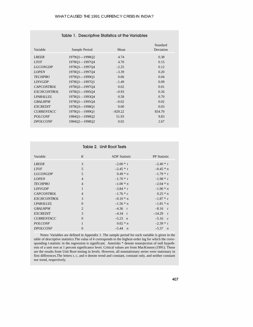
The variables used in the analysis are described in the data appendix and asummary of their descriptive statistics is presented in Table 1. The dependent vari-able for the models investigated below is the log of the real effective exchangerate, calculated by the IMF. The REER is a trade-weighted index using nationalconsumer prices to measure inflation. The weights take into account trade inmanufactured goods, primary commodities, and, where significant, touristservices. The trade weights also reflect both direct and third-market competition.8The other variables are selected to represent the set of fundamental determinantsof the real effective exchange rate and a set of exogenous variables that are thoughtto contribute to the short-run misalignment. The models described below, withquarterly frequency, are estimated over the longest sample for which all includedvariables are available in the period 1979 to 1997.

All of the variables are examined for unit roots to suggest their stochasticbehavior. The lag length is determined in a backward selection process that startswith a maximum lag length of eight quarters. Insignificant lags are sequentiallydropped until the highest order lag becomes significant. The deterministic compo-nents are included in the test only if significant. Unit test results are reported inTable 2. Standard unit root tests reveal that the null hypothesis of a unit root cannotbe rejected for the real exchange rate nor for any of its long-run fundamentals, butthat it can be rejected for the current account, excess credit, and the fiscal balanceto high-powered money.9 The inability to reject the unit root for the real exchangerate could be interpreted as evidence against purchasing power parity. The unitroot test cannot be rejected for the index of political confidence, but it can berejected for its first difference.


406

7For testable implications of the intertemporal model, refer to Saxena (1999).8See Zanello and Desruelle (1997) for a complete explanation of the methodology.9Of course, much research has shown that unit root tests of economic variables suffer from lack of

power. That is, when a series is stationary, but highly autocorrelated, rejection of the unit root hypothesisrequires a considerably longer sample period than the sample typically available. Nonetheless, the conse-quences of assuming that variables are stationary when they are not include finding spurious relationships.Hence, it is more conservative to assume that the variables are nonstationary even if they are not.


407

Table 1. Descriptive Statistics of the Variables

StandardVariable Sample Period Mean Deviation

LREER 1979Q1—1998Q2 4.74 0.38

LTOT 1978Q1—1997Q4 4.70 0.15

LGCONGDP 1978Q1—1997Q4 –2.25 0.12

LOPEN 1978Q1—1997Q4 –3.39 0.20

TECHPRO 1979Q1—1999Q1 0.06 0.04

LINVGDP 1978Q1—1997Q1 –1.49 0.09

CAPCONTROL 1978Q2—1997Q4 0.02 0.01

EXCHCONTROL 1978Q1—1995Q4 –0.93 0.26

LPARALLEL 1978Q1—1993Q4 0.58 0.70

GBALHPM 1978Q1—1995Q4 –0.02 0.02

EXCREDIT 1978Q3—1998Q1 0.00 0.03

CURRENTACC 1978Q1—1999Q1 –929.22 834.70

POLCONF 1984Q1—1998Q2 51.93 9.83

DPOLCONF 1984Q2—1998Q2 0.02 2.67

Table 2. Unit Root Tests

Variable K ADF Statistic PP Statistic

LREER 3 –2.00 * t –2.40 * t

LTOT 5 –2.45 * t –0.45 * n

LGCONGDP 5 0.49 * n –1.79 * t

LOPEN 4 –1.70 * t –1.98 * t

TECHPRO 4 –1.00 * n –2.04 * n

LINVGDP 1 –3.84 * t –1.90 * n

CAPCONTROL 4 –1.76 * c 0.25 * n

EXCHCONTROL 3 –0.10 * n –1.87 * c

LPARALLEL 0 –1.56 * n –1.81 * n

GBALHPM 2 –4.36 t –8.16 t

EXCREDIT 3 –4.34 t –14.29 t

CURRENTACC 0 –5.23 n –5.16 c

POLCONF 1 0.02 * n –2.39 * t

DPOLCONF 0 –5.44 n –5.37 n

Notes: Variables are defined in Appendix 1. The sample period for each variable is given in thetable of descriptive statistics.The value of k corresponds to the highest-order lag for which the corre-sponding t-statistic in the regression is significant. Asterisks * denote nonrejection of null hypoth-esis of a unit root at 1 percent significance level. Critical values are from MacKinnon (1991). Theseare the results from Unit Root testing in levels. However, all nonstationary series were stationary infirst differences.The letters t, c, and n denote trend and constant, constant only, and neither constantnor trend, respectively.

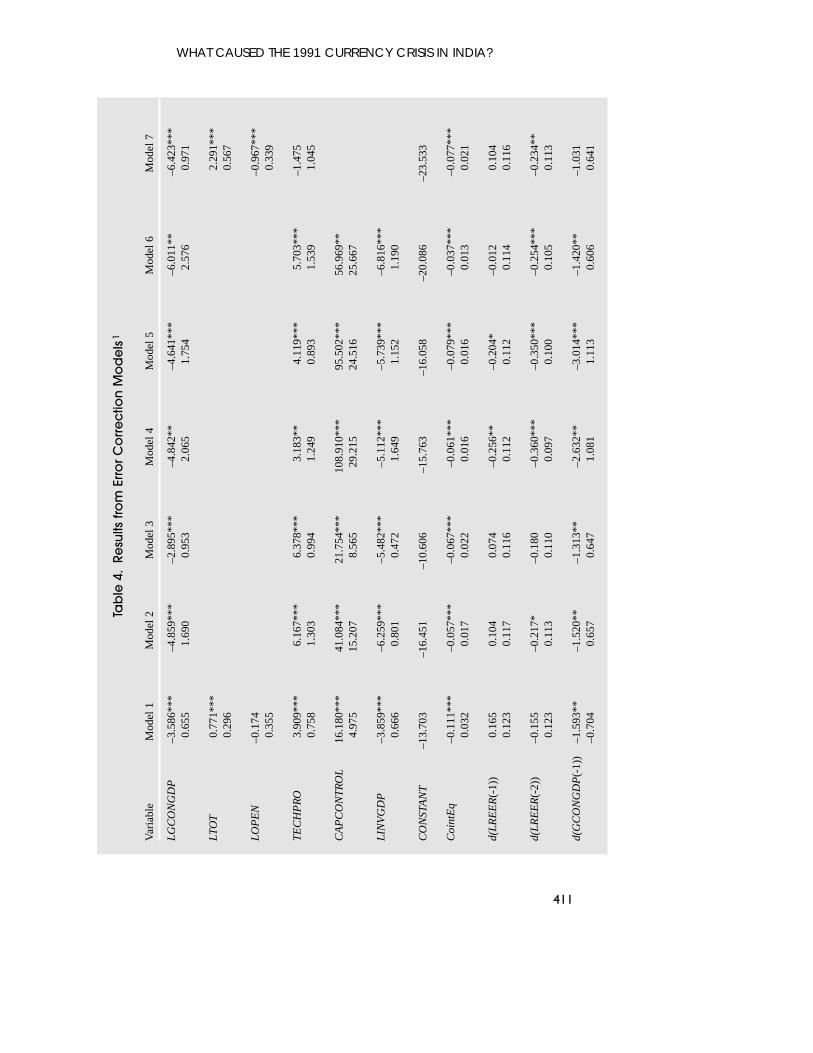
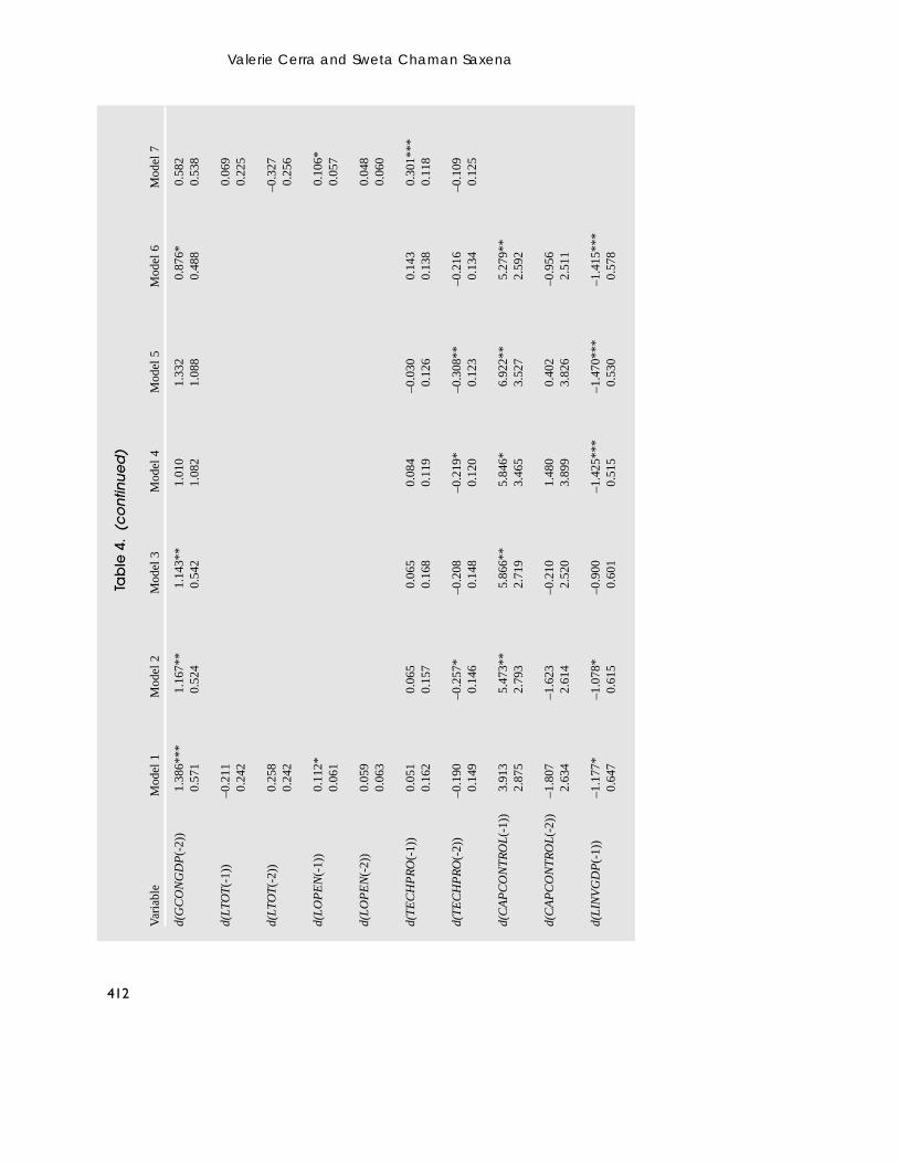
The empirical strategy is to find a set of significant long-run fundamentals andshort-run explanatory variables and use the analysis to distinguish between alter-native theoretical explanations for the behavior of India’s real exchange rate. Theseven models are described sequentially below. In summary, the first two modelsinvestigate the long-run determinants of the REER; Models 3–6 explore alterna-tive specifications of the short-term factors; and Model 7 is a sensitivity test of thelong-run fundamental factors.

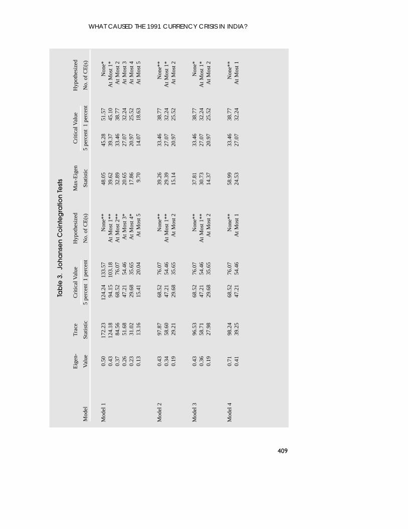
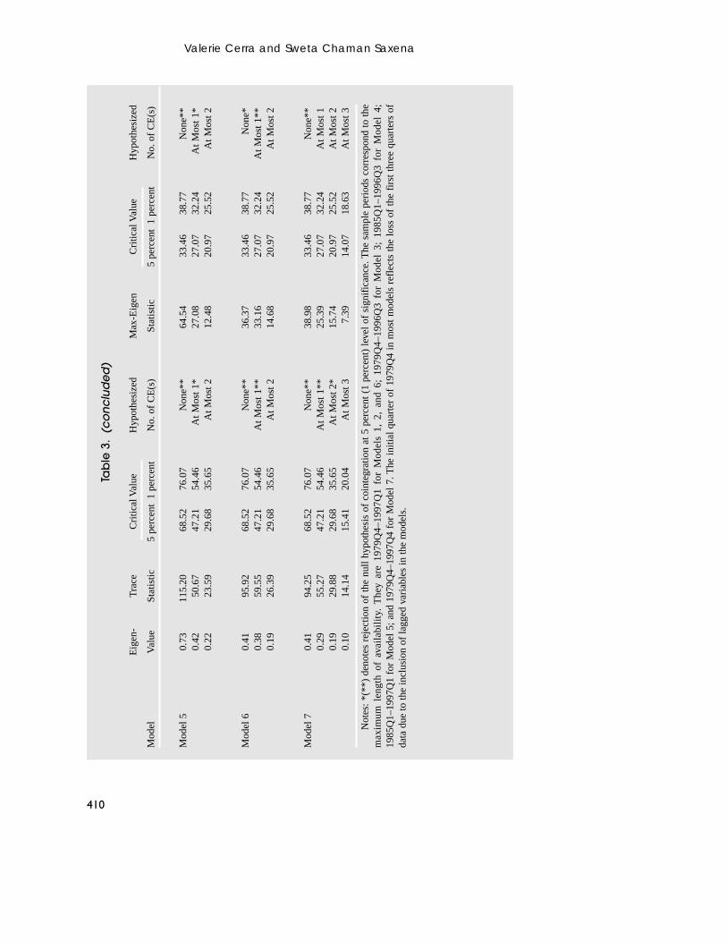
In accordance with the theory of error correction models, the series are firsttested for cointegration. The results from cointegration tests using Johansen’s(1991) method are reported in Table 3, including the number of cointegratingvectors. The lag length for the error correction model is determined by backwardselection, beginning at a lag length of four to economize on degrees of freedom.The likelihood ratio test indicates that an error correction model with two lags isthe most appropriate specification. The results reported in Table 4 are obtained byestimating the ECM by imposing one cointegrating vector for ease of interpreta-tion.10 However, the equilibrium real exchange rate and forecasting analysisdiscussed below are estimated with the number of cointegrating vectors stipulatedfrom the cointegration test.

We first estimate the ECM with all of the potential fundamental long-run vari-ables suggested from the theory (Model 1). The results indicate that all the funda-mentals are significant, except openness. The same model was estimated withEdwards’s proxies for openness, namely parallel market spread and exchangecontrols. However, they were insignificant as well. Government consumptionleads to a real depreciation, consistent with a higher proportion of governmentconsumption directed toward traded goods relative to private consumption. Animprovement in the terms of trade leads to an appreciation of the real exchangerate, while increases in openness and increases in investment lead to real depreci-ation. A decrease in capital controls leads to higher capital inflows, which appre-ciates the real exchange rate in the long run—indicating that the income effectdominates over the intertemporal substitution effect. Technological progress leadsto an appreciated real exchange rate—a result consistent with the Balassa-Samuelson effect.

Next, a general-to-specific modeling procedure is employed. The insignificantvariables from Model 1 are eliminated sequentially to arrive at the parsimoniousspecification, Model 2. The results remain the same as Model 1 in terms of signs,although the magnitudes change slightly.

Having arrived at a parsimonious specification involving significant fundamen-tals that affect the equilibrium exchange rate, we now examine the impact of short-run factors that can cause the exchange rate to deviate temporarily fromequilibrium.11 Model 3 is estimated with the same long-run fundamentals as in


408

10Note that this one cointegrating vector can also be obtained as a linear combination of the estimatedmultiple cointegrating vectors.

11Sensitivity tests indicated that there was no advantage in using the full specification of Model 1when analyzing the effects of the exogenous variables since the results were not significantly differentfrom those reported from the parsimonious specification, while several degrees of freedom were lost inthe process of carrying around the insignificant variables and their lags.


409

Tab

le 3

.Jo

ha

nse

n C

oin

teg

ratio

n T

est

s

Eig

en-

Tra

ceC

ritic

al V

alue

Hyp

othe

size

dM

ax-E

igen

Cri

tical

Val

ueH

ypot

hesi

zed

Mod

el

Val

ueSt

atis

tic5

perc

ent

1 pe

rcen

tN

o. o

f C

E(s

)St

atis

tic5

perc

ent

1 pe

rcen

tN

o. o

f C

E(s

)

Mod

el 1

0.50

172.

2312

4.24

133.

57N

one*

*48

.05

45.2

851

.57

Non

e*0.

4312

4.18

94.1

510

3.18

At M

ost 1

**39

.62

39.3

745

.10

At M

ost 1

*0.

3784

.56

68.5

276

.07

At M

ost 2

**32

.89

33.4

638

.77

At M

ost 2

0.26

51.6

847

.21

54.4

6A

t Mos

t 3*

20.6

527

.07

32.2

4A

t Mos

t 30.

2331

.02

29.6

835

.65

At M

ost 4

*17

.86

20.9

725

.52

At M

ost 4

0.13

13.1

615

.41

20.0

4A

t Mos

t 59.

7014

.07

18.6

3A

t Mos

t 5

Mod

el 2

0.43

97.8

768

.52

76.0

7N

one*

*39

.26

33.4

638

.77

Non

e**

0.34

58.6

047

.21

54.4

6A

t Mos

t 1**

29.3

927

.07

32.2

4A

t Mos

t 1*

0.19

29.2

129

.68

35.6

5A

t Mos

t 215

.14

20.9

725

.52

At M

ost 2

Mod

el 3

0.43

96.5

368

.52

76.0

7N

one*

*37

.81

33.4

638

.77

Non

e*0.

3658

.71

47.2

154

.46

At M

ost 1

**30

.73

27.0

732

.24

At M

ost 1

*0.

1927

.98

29.6

835

.65

At M

ost 2

14.3

720

.97

25.5

2A

t Mos

t 2

Mod

el 4

0.71

98.2

468

.52

76.0

7N

one*

*58

.99

33.4

638

.77

Non

e**

0.41

39.2

547

.21

54.4

6A

t Mos

t 124

.53

27.0

732

.24

At M

ost 1


410

Tab

le 3

.(c

on

clu

de

d)

Eig

en-

Tra

ceC

ritic

al V

alue

Hyp

othe

size

dM

ax-E

igen

Cri

tical

Val

ueH

ypot

hesi

zed

Mod

el

Val

ueSt

atis

tic5

perc

ent

1 pe

rcen

tN

o. o

f C

E(s

)St

atis

tic5

perc

ent

1 pe

rcen

tN

o. o

f C

E(s

)

Mod

el 5

0.73

115.

2068

.52

76.0

7N

one*

*64

.54

33.4

638

.77

Non

e**

0.42

50.6

747

.21

54.4

6A

t Mos

t 1*

27.0

827

.07

32.2

4A

t Mos

t 1*

0.22

23.5

929

.68

35.6

5A

t Mos

t 212

.48

20.9

725

.52

At M

ost 2

Mod

el 6

0.41

95.9

268

.52

76.0

7N

one*

*36

.37

33.4

638

.77

Non

e*0.

3859

.55

47.2

154

.46

At M

ost 1

**33

.16

27.0

732

.24

At M

ost 1

**0.

1926

.39

29.6

835

.65

At M

ost 2

14.6

820

.97

25.5

2A

t Mos

t 2

Mod

el 7

0.41

94.2

568

.52

76.0

7N

one*

*38

.98

33.4

638

.77

Non

e**

0.29

55.2

747

.21

54.4

6A

t Mos

t 1**

25.3

927

.07

32.2

4A

t Mos

t 10.

1929

.88

29.6

835

.65

At M

ost 2

*15

.74

20.9

725

.52

At M

ost 2

0.10

14.1

415

.41

20.0

4A

t Mos

t 37.

3914

.07

18.6

3A

t Mos

t 3

Not

es:

*(**

) de

note

s re

ject

ion

of t

he n

ull

hypo

thes

is o

f co

inte

grat

ion

at 5

per

cent

(1

perc

ent)

lev

el o

f si

gnif

ican

ce. T

he s

ampl

e pe

riod

s co

rres

pond

to

the

max

imum

len

gth

of a

vail

abil

ity.

The

y ar

e 19

79Q

4–19

97Q

1 fo

r M

odel

s 1,

2,an

d 6;

197

9Q4–

1996

Q3

for

Mod

el 3

; 19

85Q

1–19

96Q

3 fo

r M

odel

4;

1985

Q1–

1997

Q1

for

Mod

el 5

; an

d 19

79Q

4–19

97Q

4 fo

r M

odel

7. T

he i

nitia

l qu

arte

r of

197

9Q4

in m

ost

mod

els

refl

ects

the

los

s of

the

fir

st t

hree

qua

rter

s of

data

due

to th

e in

clus

ion

of la

gged

var

iabl

es in

the

mod

els.


411

Tab

le 4

.Re

sults

fro

m E

rro

r C

orr

ec

tion

Mo

de

ls1

Var

iabl

eM

odel

1M

odel

2M

odel

3M

odel

4M

odel

5M

odel

6M

odel

7

LG

CO

NG

DP

–3.5

86**

*–4

.859

***

–2.8

95**

*–4

.842

**–4

.641

***

–6.0

11**

–6.4

23**

*0.

655

1.69

00.

953

2.06

51.

754

2.57

60.

971

LTO

T0.

771*

**2.

291*

**0.

296

0.56

7

LO

PE

N–0

.174

–0.9

67**

*0.

355

0.33

9

TE

CH

PR

O3.

909*

**6.

167*

**6.

378*

**3.

183*

*4.

119*

**5.

703*

**–1

.475

0.75

81.

303

0.99

41.

249

0.89

31.

539

1.04

5

CA

PC

ON

TR

OL

16.1

80**

*41

.084

***

21.7

54**

*10

8.91

0***

95.5

02**

*56

.969

**4.

975

15.2

078.

565

29.2

1524

.516

25.6

67

LIN

VG

DP

–3.8

59**

*–6

.259

***

–5.4

82**

*–5

.112

***

–5.7

39**

*–6

.816

***

0.66

60.

801

0.47

21.

649

1.15

21.

190

CO

NST

AN

T–1

3.70

3–1

6.45

1–1

0.60

6–1

5.76

3–1

6.05

8–2

0.08

6–2

3.53

3

Coi

ntE

q–0

.111

***

–0.0

57**

*–0

.067

***

–0.0

61**

*–0

.079

***

–0.0

37**

*–0

.077

***

0.03

20.

017

0.02

20.

016

0.01

60.

013

0.02

1

d(L

RE

ER

(-1)

)0.

165

0.10

40.

074

–0.2

56**

–0.2

04*

–0.0

120.

104

0.12

30.

117

0.11

60.

112

0.11

20.

114

0.11

6

d(L

RE

ER

(-2)

)–0

.155

–0.2

17*

–0.1

80–0

.360

***

–0.3

50**

*–0

.254

***

–0.2

34**

0.12

30.

113

0.11

00.

097

0.10

00.

105

0.11

3

d(G

CO

NG

DP

(-1)

)–1

.593

**–1

.520

**–1

.313

**–2

.632

**–3

.014

***

–1.4

20**

–1.0

31–0

.704

0.65

70.

647

1.08

11.

113

0.60

60.

641


412

Tab

le 4

.(c

on

tinu

ed

)

Var

iabl

eM

odel

1M

odel

2M

odel

3M

odel

4M

odel

5M

odel

6M

odel

7

d(G

CO

NG

DP

(-2)

)1.

386*

**1.

167*

*1.

143*

*1.

010

1.33

20.

876*

0.58

20.

571

0.52

40.

542

1.08

21.

088

0.48

80.

538

d(LT

OT

(-1)

)–0

.211

0.06

90.

242

0.22

5

d(LT

OT

(-2)

)0.

258

–0.3

270.

242

0.25

6

d(L

OP

EN

(-1)

)0.

112*

0.10

6*0.

061

0.05

7

d(L

OP

EN

(-2)

)0.

059

0.04

80.

063

0.06

0

d(T

EC

HP

RO

(-1)

)0.

051

0.06

50.

065

0.08

4–0

.030

0.14

30.

301*

**0.

162

0.15

70.

168

0.11

90.

126

0.13

80.

118

d(T

EC

HP

RO

(-2)

)–0

.190

–0.2

57*

–0.2

08–0

.219

*–0

.308

**–0

.216

–0.1

090.

149

0.14

60.

148

0.12

00.

123

0.13

40.

125

d(C

AP

CO

NT

RO

L(-

1))

3.91

35.

473*

*5.

866*

*5.

846*

6.92

2**

5.27

9**

2.87

52.

793

2.71

93.

465

3.52

72.

592

d(C

AP

CO

NT

RO

L(-

2))

–1.8

07–1

.623

–0.2

101.

480

0.40

2–0

.956

2.63

42.

614

2.52

03.

899

3.82

62.

511

d(L

INV

GD

P(-

1))

–1.1

77*

–1.0

78*

–0.9

00–1

.425

***

–1.4

70**

*–1

.415

***

0.64

70.

615

0.60

10.

515

0.53

00.

578


413

Tab

le 4

.(c

on

clu

de

d)

Var

iabl

eM

odel

1M

odel

2M

odel

3M

odel

4M

odel

5M

odel

6M

odel

7

d(L

INV

GD

P(-

2))

1.39

9**

1.67

0**

1.83

8***

2.34

2***

2.40

5***

1.56

4**

0.70

90.

703

0.68

60.

586

0.61

10.

657

EX

CR

ED

IT(-

3)–0

.193

0.16

2G

BA

LH

PM

(-3)

0.29

70.

187

0.20

80.

191

DP

OL

CO

NF

(-3)

0.00

3*0.

003*

*0.

001

0.00

1C

UR

RE

NTA

CC

(-4)

0.00

002*

**0.

0000

2***

0.00

002*

**0.

0000

2***

0.00

00.

000

0.00

00.

000

CO

NST

AN

T–0

.014

***

–0.0

16**

*–0

.012

–0.0

09–0

.014

*0.

002

0.00

50.

005

0.00

50.

007

0.01

00.

008

0.00

70.

007

Adj

uste

d R

20.

343

0.32

60.

354

0.68

70.

675

0.42

00.

346

Sam

ple

Peri

od19

79Q

4–1

997Q

119

79Q

4–1

997Q

119

79Q

4–1

996Q

319

85Q

1–19

96Q

319

85Q

1–19

97Q

119

79Q

4–1

997Q

119

79Q

4–1

997Q

4

Not

es:A

ster

isks

***

,**,

and

* de

note

the

sign

ific

ance

of

the

vari

able

s at

1,5

,and

10

perc

ent l

evel

of

sign

ific

ance

,res

pect

ivel

y.1 T

he d

epen

dent

var

iabl

e is

d(L

RE

ER

).

Model 2, with proxies for inconsistent macroeconomic policies as used by Edwards(1989). The results indicate that the signs on the long-run fundamentals remain thesame as before and are significant. The coefficients on the policy variables areinsignificant—indicating that the empirical evidence does not provide support forEdwards’s description of misalignment in the case of India.12 Moreover, the signs ofour results are inconsistent with Edwards’s explanation of real exchange ratemisalignment in response to lax macroeconomic policy. Our (insignificant) resultsindicate that an improvement in the government fiscal balance leads to an apprecia-tion in the real exchange rate and conversely, that fiscal deficits correspond to adepreciation of the real exchange rate. Excessive domestic credit creation results ina depreciation of the real exchange rate. In Edwards’s model, the nominal exchangerate is fixed and higher government deficits that are monetized give rise to a higherdomestic price level and a corresponding appreciation of the real exchange rate.Given these assumptions, the lack of support for Edwards’s model for India is notsurprising: nominal depreciation of the rupee appears to have offset any domesticprice pressures arising from monetary expansion. In addition, the data do not indi-cate that India monetized its deficits to any significant extent. The increasing fiscaldeficits in the years leading up to the crisis were financed by borrowing, includingfrom foreign sources. The effect of this was a misalignment in the external sector asa result of fiscal deficits, which, at the prevailing levels, were inconsistent with anintertemporal budget constraint. Instead of Edwards’s framework, the exchange ratedepreciation resulting from fiscal deficits or high domestic credit creation is consis-tent with the classical Mundell-Fleming framework. Expansive fiscal or monetarypolicy—in the case of a country such as India with limited capital mobility—causesa balance of payments deficit and nominal exchange rate depreciation. With sluggishprices, the real exchange rate also depreciates.

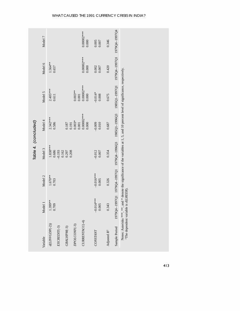
Having found that the Edwards model does not fit well for India, we nowinvestigate whether the evidence supports the descriptions of the causes of India’sbalance of payments crisis; namely, large current account deficits, fiscal deficits,and loss of confidence in the government. Hence, to Model 2, we add the short-run factors: the current account balance, the government fiscal balance to high-powered money (as above), and changes in political confidence.13 The results areshown in column 4 of Table 4. The long-run results do not change much as thefundamentals have the usual (significant) signs. Regarding the exogenous vari-ables, both the current account and the change in political confidence are signifi-cant, with positive signs.14 This indicates that as the current account balanceimproves and confidence in the government increases, the real exchange rateappreciates. The sign and significance of the political confidence indicator can beexpected since this variable proxies for the confidence of India’s creditors andtheir willingness to roll over debt or maintain deposits. Similar to the result


414

12The table shows the results for the most significant lag. The coefficients on other lags have the samesign as the third lag with one negligible exception.

13Since we could not reject the hypothesis of a unit root for the level of political confidence, its firstdifference was taken in the specification.

14The insignificant lags were eliminated.

reported in Model 3, the government balance is positive but insignificant. Theinsignificance of the fiscal variable here may be due to collinearity. Confidence inthe government is likely to decline as fiscal deficits grow and appear unsustain-able. Moreover, the inclusion of the current account deficit in the equation,according to the Mundell-Fleming model described above, captures the externaleffects of the expansionary fiscal policy.

Through elimination of the insignificant fiscal variable, we arrive at the parsi-monious Model 5. However, one difficulty with using this model for the analysisin the next sections is that data are available for political confidence only from1985. The loss of several years of data in the early 1980s causes the problem thatthere are not enough degrees of freedom to estimate a restricted sample for the out-of-sample forecasting exercise discussed below. Therefore, for purposes of theremaining analysis, the political confidence variable is dropped and the baselinespecification is shown as Model 6—which consists of the long-run variables fromthe parsimonious specification (Model 2) and the current account balance as theexogenous short-run variable.

As a sensitivity analysis, we estimate Model 7, where Edwards’s variables forcapital control and investment are ignored but openness and terms of trade arerestored, consistent with Montiel’s specification. The findings from Model 1 stillhold—increases in government consumption and openness lead to a depreciationof the real exchange rate, while an improvement in the terms of trade results in anappreciation of the real exchange rate. An improvement in the current accountbalance brings about real exchange rate appreciation. The coefficient on techno-logical progress, however, becomes insignificant.

One finding that emerges very clearly from the econometric investigation isthat the current account plays a very significant role in explaining short-run move-ments in the real exchange rate for India during the period of analysis. This vari-able is robust to all specifications (a significant positive sign). This result iscorroborated by Callen and Cashin (1999), who examine the sustainability ofIndia’s current account during the period 1952/53–1998/99 using three methods.They find that in the period prior to 1990/91, India’s intertemporal budgetconstraint was not satisfied and that the return to smaller current account deficitsfollowing the crisis was needed to reestablish solvency.

In this section, the current account has been discussed as an exogenous short-run explanatory variable. In general, however, the real effective exchange ratecould be expected to influence the current account. Indeed, the decline in the realexchange rate in the latter half of the 1980s was likely a contributing factor torapid export growth in particular, although the initial liberalization measuresimplemented to spur export-led growth are also thought to have been important.However, since the key feature of the current account from the mid-1980s throughthe crisis in mid-1991 was its sharp deterioration, it seems that the simultaneousrapid decline in the real exchange rate over this same period had at most a miti-gating influence. There were many other factors that jointly overwhelmed anybeneficial influence of the real exchange rate and produced the substantial deteri-oration in the current account. As mentioned in the introductory section, some ofthese factors included the increasing dependence on foreign oil imports and


415

consequently the greater vulnerability to oil price shocks; strong domestic demandas a result of both the initial liberalization efforts and deteriorating fiscal balances,but weak foreign demand in the years leading up to and including 1991; shocks toworkers’ remittances; and higher interest payments on external debt due to itshigher cost structure and growing size.

Moreover, these observations on the relationship between the real exchangerate and the current account in this period are borne out by evidence from Grangercausation tests (Table 5). The results of Granger causation tests lend support to theidea that movements in the current account had a strong impact on the realexchange rate, but that the opposite did not hold.

The null hypothesis that the current account does not Granger cause changesin the real effective exchange rate can be rejected at the 10 percent confidencelevel for 4 and 8 quarter lags and (marginally) at the 5 percent confidence level for12 quarter lags. In the other direction of causality, the hypothesis that changes inthe real effective exchange rate do not Granger cause the current account cannotbe rejected for 8 and 12 lags. This hypothesis can be (marginally) rejected at the10 percent confidence level for 4 lags. In the latter case, however, the sum of thelagged exchange rate coefficients in the current account equation is positive,counter to theoretical predictions that decreases in the real exchange rate shouldlead to improved current account balances. This evidence is in line with the discus-sion above that the current account balances were deteriorating at the same timethat the real exchange rate was declining substantially.

IV. Estimating the Equilibrium Real Exchange Rate

In order to determine whether the Indian rupee was overvalued prior to the crisisin 1991, we estimate the equilibrium real exchange rate, using the error correctionmodel estimated in Section III.15 Frequently, researchers construct the equilibriumreal exchange rate by multiplying the cointegrating vector with the actual valuesof the fundamentals. However, the fundamentals may have their own temporarycomponents, and by using the actual values of the fundamentals, the constructionof the equilibrium real exchange rate depends on these temporary components,when it should not. Edwards (1989) recognizes the problem with using actualvalues of the fundamentals to construct the equilibrium exchange rate. He tries tosolve this by means of two methods. He does a Beveridge-Nelson decompositionof each fundamental series or, alternatively, he uses moving averages of eachfundamental series. He then uses the constructed permanent component of eachvariable in his equilibrium equation. These are potential suggestions for findingthe equilibrium fundamentals, as would be other methods of univariate decompo-sition into permanent and temporary components.

This section estimates the equilibrium real effective exchange rate, usingthree different methods. First, the permanent components of the fundamentals


416

15We report only the equilibrium exchange rate estimated from the baseline ECM (Model 6), usingtwo cointegrating vectors as found in the cointegration test.

are constructed, using a Hodrick-Prescott filter and a 13-quarter (centered)moving average process as representative smoothing methods.16 These methodsare used for illustrative purposes only. While these methods produce smoothfundamental series that are appealing to the eye, there is no sound theoreticalbasis for these procedures. If simple smoothing processes were enough to arriveat the equilibrium values for the fundamental series, then the same smoothingprocesses could be employed on the real exchange rate series to estimate theequilibrium real exchange rate. But doing so would be devoid of economictheory such as that which describes a relationship between the exchange rate andother economic variables, a relationship that is estimated through an errorcorrection model in this paper. In addition, independently smoothing the funda-mentals does not take advantage of information arising from the interaction ofthe variables.

Gonzalo and Granger (1995) propose a more appealing way of solving thiseconometric problem so that the permanent (equilibrium) component of theendogenous variable of interest—in our case, the exchange rate—could beconstructed by means of the permanent components rather than the actual valuesof the fundamental determinants. It is done using the joint information in theerror correction system rather than preconstructing the equilibrium fundamentalvariables.17 Other procedures advanced in the literature to address this issueinclude those of Quah (1992) and Kasa (1992). However, these latter twodecomposition methods present the undesirable property that the transitorycomponent Granger causes the permanent component, leading a temporaryshock to have permanent effects on the actual aggregated series. Gonzalo andGranger derive a P-T decomposition such that the transitory component does notGranger cause the permanent component in the long run (i.e., the effects of


417

Table 5. Pairwise Granger Causality TestsPeriod: 1979:1 to 1997:1

Null Hypothesis Lags F-Statistic Probability

CA does not Granger cause d (LREER) 4 2.43485 0.05713d (LREER) does not Granger cause CA 4 2.07426 0.09561



16Previous work with the Beveridge-Nelson decomposition has shown that since the method assumesthat the permanent component is a random walk, the filtered series tends to closely replicate the actualdata; very little smoothing tends to occur.

17The procedure was also used by Alberola, and others (1999) in their study of euro-area exchange rates.

transitory shocks die out over time). They define the permanent and temporarycomponents so that only the innovations from the permanent component canaffect the long-run forecast. Innovations to the temporary components of all ofthe endogenous variables, including the fundamental determinants, do not affectthe long-run “equilibrium” forecast. So, for our purposes, cyclical deviations ofthe fundamentals will be removed in the construction of the equilibriumexchange rate. In addition, all of the information required to extract the perma-nent component is contained in the contemporaneous observations.

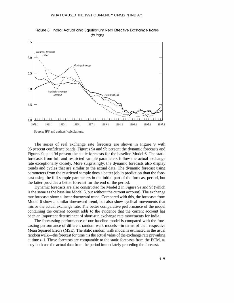
The equilibrium exchange rate is estimated for the baseline model (Model 6),using the three methods—the Hodrick-Prescott filter and a moving averageprocess for illustrative purposes, and the theoretically attractive Gonzalo-Grangermethod (Figure 8). The equilibrium exchange rate constructed by means of theHodrick-Prescott filtered series shows an overvalued exchange rate from 1985:2through 1995:5, while the one estimated by smoothing the series using the movingaverage shows an overvaluation of the exchange rate from 1986:3 through 1994:4.As mentioned above, these findings carry no theoretical value. In order to estimatethe exchange rate consistent with the fundamentals, we construct the equilibriumusing the Gonzalo and Granger method. Figure 8 shows the result—the real effec-tive exchange rate was overvalued for several years prior to and through the crisis(from 1985:3 through 1993:1). Indeed, the equilibrium path was below the actualpath of the exchange rate for several years of a downward trend, suggesting thatthe actual depreciation was moving in the direction of restoring equilibrium,although the equilibrium itself continued to move to lower levels. In 1993, theequilibrium comes into line with the actual data for the first time since the mid-1980s. Thereafter, the equilibrium is periodically above or below the actual, butthere is no clear trend. In summary, a strong result that emerges from all of theseestimations is that the real exchange rate for India was overvalued at the time ofcrisis in 1991.

V. Forecasting the Real Exchange Rate

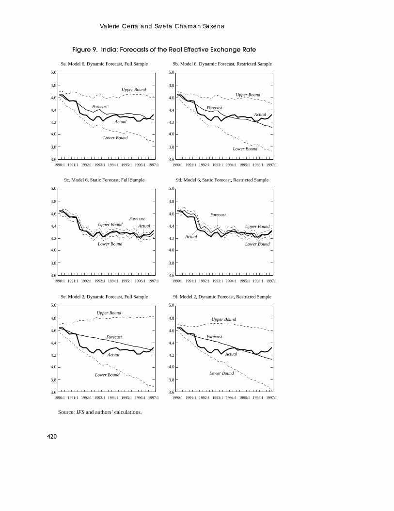
In order to test the forecasting performance of the baseline model (Model 6), wemake dynamic as well as static forecasts of the real exchange rate. For both typesof forecasts, the model is estimated for the full sample period (through 1997:1)and for a restricted sample period that ends at a point sufficiently earlier than thecrisis such that there would be time for adjustment (1989:4 is chosen as the endpoint).18 The parameters from the error correction model estimated over each ofthese two sample periods are used to form forecasts for the period 1990:1 through1997:1. While the static forecasts for the exchange rate are formed using actualdata for the lagged endogenous variables on the right-hand side of the ECM,dynamic forecasts use actual data for the endogenous variables only up to 1989:4and thereafter use forecasted data for all of the right-hand side endogenousvariables.


418

18The models are estimated using two cointegrating vectors, as found in the Johansen tests.

The series of real exchange rate forecasts are shown in Figure 9 with95 percent confidence bands. Figures 9a and 9b present the dynamic forecasts andFigures 9c and 9d present the static forecasts for the baseline Model 6. The staticforecasts from full and restricted sample parameters follow the actual exchangerate exceptionally closely. More surprisingly, the dynamic forecasts also displaytrends and cycles that are similar to the actual data. The dynamic forecast usingparameters from the restricted sample does a better job in prediction than the fore-cast using the full sample parameters in the initial part of the forecast period, butthe latter provides a better forecast for the end of the period.

Dynamic forecasts are also constructed for Model 2 in Figure 9e and 9f (whichis the same as the baseline Model 6, but without the current account). The exchangerate forecasts show a linear downward trend. Compared with this, the forecasts fromModel 6 show a similar downward trend, but also show cyclical movements thatmirror the actual exchange rate. The better comparative performance of the modelcontaining the current account adds to the evidence that the current account hasbeen an important determinant of short-run exchange rate movements for India.

The forecasting performance of our baseline model is compared with the fore-casting performance of different random walk models—in terms of their respectiveMean Squared Errors (MSE). The static random walk model is estimated as the usualrandom walk—the forecast for time t is the actual value of the exchange rate prevailingat time t–1. These forecasts are comparable to the static forecasts from the ECM, asthey both use the actual data from the period immediately preceding the forecast.


419

4.0

4.5

5.0

5.5

6.0

6.5

1997:11995:11993:11991:11989:11987:11985:11983:11981:11979:1

Actual REER

Moving Average

Hodrick-PrescottFilter

Gonzalo-GrangerMethod

Figure 8. India: Actual and Equilibrium Real Effective Exchange Rates(In logs)

Source: IFS and authors’ calculations.


420

3.6

3.8

4.0

4.2

4.4

4.6

4.8

5.0

1997:11996:11995:11994:11993:11992:11991:11990:1

9a. Model 6, Dynamic Forecast, Full Sample

3.6

3.8

4.0

4.2

4.4

4.6

4.8

5.0

1997:11996:11995:11994:11993:11992:11991:11990:1

9b. Model 6, Dynamic Forecast, Restricted Sample

Actual

Forecast

Upper Bound

Lower Bound

Actual

Forecast

Upper Bound

Lower Bound

3.6

3.8

4.0

4.2

4.4

4.6

4.8

5.0

1997:11996:11995:11994:11993:11992:11991:11990:1

9c. Model 6, Static Forecast, Full Sample

3.6

3.8

4.0

4.2

4.4

4.6

4.8

5.0

1997:11996:11995:11994:11993:11992:11991:11990:1

9d. Model 6, Static Forecast, Restricted Sample

Actual

Forecast

Upper Bound

Lower Bound

Actual

ForecastUpper Bound

Lower Bound

3.6

3.8

4.0

4.2

4.4

4.6

4.8

5.0

1997:11996:11995:11994:11993:11992:11991:11990:1

9e. Model 2, Dynamic Forecast, Full Sample

3.6

3.8

4.0

4.2

4.4

4.6

4.8

5.0

1997:11996:11995:11994:11993:11992:11991:11990:1

9f. Model 2, Dynamic Forecast, Restricted Sample

Actual

Forecast

Upper Bound

Lower Bound

Actual

Forecast

Upper Bound

Lower Bound

Figure 9. India: Forecasts of the Real Effective Exchange Rate

Source: IFS and authors’ calculations.

Some “dynamic” random walk models are also estimated so that they can becompared with our dynamic forecasts—which do not use any new informationafter the period of estimation.19 A simple dynamic random walk model forms aforecast for all future exchange rates based on the value of the exchange rate at theend of the estimation period (1989:4). The two dynamic random walk with trendmodels are comparable to our dynamic forecasts, where the trend is estimated overthe full and the restricted sample periods. These trends are combined with thevalue of the exchange rate prevailing in 1989:4 to construct the dynamic randomwalk forecasts.

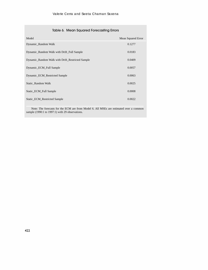
The MSE results from forecasting are reported in Table 6. The results providestriking evidence that the forecasts from the ECM perform better than the randomwalk models. The static forecasts from the ECM models outperform the staticrandom walk while the dynamic forecasts from the ECM models, including thoseusing parameters from the restricted sample, outperform all of the dynamicrandom walk models.

VI. Conclusions

This paper is concerned with explaining the 1991 crisis in India and contains threerelated points of interest. First, the paper uses error correction models to distin-guish between alternative theoretical explanations for the crisis. The error correc-tion models are estimated based on fundamentals that affect the long-run exchangerate and short-term variables. In terms of fundamentals, the Indian rupee appreci-ates in the long run in response to an improvement in terms of trade, technologicalprogress, and a relaxation of capital controls. The real exchange rate depreciateswhen government spending (on tradable goods) increases, the economy opens upand investment increases. The short-run variable, the current account, is found tobe significantly positive and robust to all specifications. The error correctionresults suggest that the Mundell-Fleming model provides a better explanation forexchange rate developments in India in this episode than do first generationmodels or the Edwards (1989) explanation of exchange rate misalignments indeveloping countries. The econometric evidence supports the position that thecurrent account deficits played a significant role in the crisis. It appears that aconfluence of exogenous shocks led to a loss in investor confidence and to esca-lating debt-service burdens that erupted in a currency crisis.

Second, the theoretically attractive method of Granger and Gonzalo (1995),which employs joint information from the error correction model, is used toconstruct the equilibrium real exchange rate and determine if overvaluationcontributed to the crisis. The estimates do show that the Indian rupee was over-valued at the time of crisis in 1991.

Finally, the forecasts from our ECM model outperform random walk modelsin out-of-sample exercises.


421

19Except for the exogenous variable, for which there is no forecast model in the ECM method, andthe parameters of the full sample model, which rely on the complete data set.


422

Table 6. Mean Squared Forecasting Errors

Model Mean Squared Error

Dynamic_Random Walk 0.1277

Dynamic_Random Walk with Drift_Full Sample 0.0183

Dynamic_Random Walk with Drift_Restricted Sample 0.0409

Dynamic_ECM_Full Sample 0.0057

Dynamic_ECM_Restricted Sample 0.0063

Static_Random Walk 0.0025

Static_ECM_Full Sample 0.0008

Static_ECM_Restricted Sample 0.0022

Note: The forecasts for the ECM are from Model 6. All MSEs are estimated over a commonsample (1990:1 to 1997:1) with 29 observations.

APPENDIX

Data Sources and Construction


423

Data Sources

Variable Description of the Variable Source

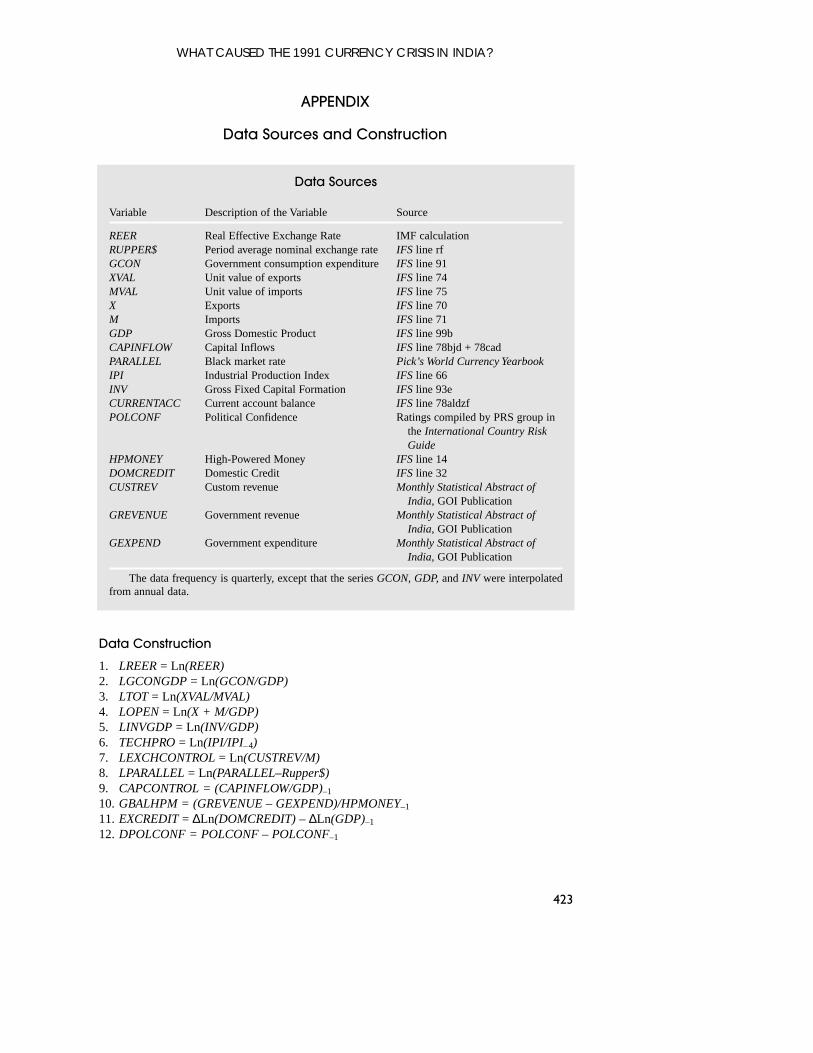
REER Real Effective Exchange Rate IMF calculationRUPPER$ Period average nominal exchange rate IFS line rfGCON Government consumption expenditure IFS line 91XVAL Unit value of exports IFS line 74MVAL Unit value of imports IFS line 75X Exports IFS line 70M Imports IFS line 71GDP Gross Domestic Product IFS line 99bCAPINFLOW Capital Inflows IFS line 78bjd + 78cadPARALLEL Black market rate Pick’s World Currency YearbookIPI Industrial Production Index IFS line 66INV Gross Fixed Capital Formation IFS line 93eCURRENTACC Current account balance IFS line 78aldzfPOLCONF Political Confidence Ratings compiled by PRS group in

the International Country Risk Guide

HPMONEY High-Powered Money IFS line 14DOMCREDIT Domestic Credit IFS line 32CUSTREV Custom revenue Monthly Statistical Abstract of

India, GOI PublicationGREVENUE Government revenue Monthly Statistical Abstract of

India, GOI PublicationGEXPEND Government expenditure Monthly Statistical Abstract of

India, GOI Publication

The data frequency is quarterly, except that the series GCON, GDP, and INV were interpolatedfrom annual data.

Data Construction

1. LREER = Ln(REER)2. LGCONGDP = Ln(GCON/GDP)3. LTOT = Ln(XVAL/MVAL)4. LOPEN = Ln(X + M/GDP)5. LINVGDP = Ln(INV/GDP)6. TECHPRO = Ln(IPI/IPI–4)7. LEXCHCONTROL = Ln(CUSTREV/M)8. LPARALLEL = Ln(PARALLEL–Rupper$)9. CAPCONTROL = (CAPINFLOW/GDP)–1

10. GBALHPM = (GREVENUE – GEXPEND)/HPMONEY–1

11. EXCREDIT = ∆Ln(DOMCREDIT) – ∆Ln(GDP)–1

12. DPOLCONF = POLCONF – POLCONF–1

REFERENCES

Alberola, Enrique, Susana Cervero, J. Humberto Lopez, and Angel Ubide, 1999, “GlobalEquilibrium Exchange Rates: Euro, Dollar, ‘Ins,’ ‘Outs,’ and Other Major Currencies in aPanel Cointegration Framework,” IMF Working Paper 99/175 (Washington: InternationalMonetary Fund).

Callen, Tim, and Paul Cashin, 1999, “Assessing External Sustainability in India,” IMF WorkingPaper 99/181 (Washington: International Monetary Fund).

Chopra, Ajai, Charles Collyns, Richard Hemming, Karen Parker, Woosik Chu, and OliverFratzscher, 1995, India: Economic Reforms and Growth, IMF Occasional Paper 134,(Washington: International Monetary Fund).

Edwards, Sebastian, 1989, Real Exchange Rates, Devaluations, and Adjustments, (Cambridge,Massachusetts: MIT Press).

Fleming, J. Marcus, 1962, “Domestic Financial Policies Under Fixed and Under FloatingExchange Rates,” IMF Staff Papers, Vol. 9 (November), pp. 369–79.

Flood, Robert, and Peter Garber, 1984, “Collapsing Exchange-Rate Regimes: Some LinearExamples,” Journal of International Economics, Vol. 17, pp. 1–13.

Flood, Robert, and Nancy Marion, 1997, “The Size and Timing of Devaluations in Capital-Controlled Economies,” Journal of Development Economics, Vol. 54, pp. 123–47.

Gonzalo, Jesus, and Clive Granger, 1995, “Estimation of Common Long Memory Componentsin Cointegrated Systems,” Journal of Business and Economic Statistics, Vol. 13, No. 1,pp. 27–35.

Johansen, Søren, 1991, “Estimation and Hypothesis Testing of Cointegration Vectors inGaussian Vector Autoregressive Models,” Econometrica, Vol. 59, pp. 1551–80.

Kasa, Kenneth, 1992, “Common Stochastic Trends in International Stock Market,” Journal ofMonetary Economics, Vol. 29, pp. 95–124.

Kletzer, Kenneth, and Renu Kohli, 2001, “Financial Repression and Exchange RateManagement in Developing Countries: Theory and Empirical Evidence for India,” IMFWorking Paper 01/103 (Washington: International Monetary Fund).

Krugman, Paul, 1979, “A Model of Balance-of-Payments Crises,” Journal of Money, Credit,and Banking, Vol. 11, pp. 311–25.

MacKinnon, James G., 1991. “Critical Values for Cointegration Tests,” in Long-Run EconomicRelationships: Readings in Cointegration, ed. by R.F. Engle and C.W.J. Granger (Oxford:Oxford University Press).

Montiel, Peter, 1994, “Capital Mobility in Developing Countries: Some Measurement Issuesand Empirical Estimates,” The World Bank Economic Review, Vol. 8, No. 3, pp. 311–50.

———, 1997, “The Theory of the Long-Run Equilibrium Real Exchange Rate,” Working Paper(Williamstown, Massachusetts: Department of Economics, Williams College).

Mundell, Robert, 1963, “Capital Mobility and Stabilization Policy under Fixed and FlexibleExchange Rates,” Canadian Journal of Economics and Political Science, Vol. 29(November), pp. 475–85.

———, 1964, “A Reply: Capital Mobility and Size,” Canadian Journal of Economics andPolitical Science, Vol. 30 (August), pp. 475–85.

Quah, Danny, 1992, “The Relative Importance of Permanent and Transitory Components:Identification and Some Theoretical Bounds,” Econometrica, Vol. 60, pp. 107–18.

Rangarajan, Chakravarti, 1991a, “Recent Monetary Policy Measures and the Balance ofPayments,” Reserve Bank of India Bulletin, New Delhi, July.


424

———, 1991b, “Exchange Rate Adjustments: Causes and Consequences” Reserve Bank of IndiaBulletin, New Delhi, September.

———, 1993, “India's Balance of Payments Problems,” in Indian Economy Since Independence,Fourth Edition, edited by Uma Kapila (New Delhi: Academic Foundation).

———, 1994, “India’s Balance of Payments: The Emerging Dimensions,” Shri Govind BallabhMemorial Lecture, Reserve Bank of India Bulletin, New Delhi, January.

———, 1996, “Impact of Liberalization on Foreign Direct Investment,” in UnderstandingIndia’s Economic Reforms, Vol. 5, ed. by Raj Kapila and Uma Kapila (New Delhi:Academic Foundation).

Saxena, Sweta C., 1999, “Exchange Rate Dynamics in Indonesia: 1980–98” (unpublished;Seattle: University of Washington).

Tamirisa, Natalia, 1999, “Exchange and Capital Controls as Barriers to Trade,” IMF StaffPapers, Vol. 46, No. 1, pp. 69–88.

Zanello, Alessandro, and Dominique Desruelle, 1997, “A Primer on the IMF's InformationNotice System,” IMF Working Paper 97/71 (Washington: International Monetary Fund).


425

Documents

What Caused the 1991 Currency Crisis in India? September 2002 · Valerie Cerra and Sweta Chaman Saxena 396. continues to monetize high deficits, this model illustrates an ongoing