Embed Size (px)
Citation preview
What Do University Endowment Managers Worry About?
An Analysis of Alternative Asset Investments and Background Income
by
Harvey S. Rosen, Princeton University Alexander J.W. Sappington, Sappington & Associates
Griswold Center for Economic Policy Studies
Working Paper No. 244, June 2015
Acknowledgements: We are grateful to Ken Redd of the National Association of College and University Business Officers for providing us with university endowment data, to Nemanja Antic, Will Dobbie, Stephen Dimmock, Henry Farber, Andrew Golden, Peter Perdue, Ulrich Mueller, and two referees for many helpful suggestions, and to Oscar Torres-Reyna for his generous assistance with coding issues. Financial support from Princeton’s Griswold Center for Economic Policy Studies is gratefully acknowledged.
Abstract
This paper examines whether university endowment managers think only in terms of the assets
they manage, or also take into account background income, the other flows of income to the
university. Specifically, we test whether the level and variability of a university’s background
income (e.g., from tuition and government grants) affect its endowment’s allocations to so-called
alternative assets such as hedge funds, private equity, and venture capital. We find that both the
probability of investing in alternative assets and the proportion of the portfolio invested in such
assets increase with expected background income and decrease with its variability.
1. Introduction
The management of university endowments has been the focus of increased attention in
recent years. As high-profile endowment portfolios outperformed the market year after year
during the 1990s and much of the 2000s, private investors and academics alike sought to
understand the reasons behind their success. One of the primary causes, it appears, was
increased investment in risky and illiquid assets, including so-called alternative assets such as
hedge funds, private equity, and venture capital. However, the Great Recession of 2008 changed
public perceptions of this approach. Endowments across the country suffered heavy losses. In
one particularly dramatic case, Antioch College nearly had to shut down in 2008 due to financial
distress (Lerner, 2008). Newspaper reports berated endowment managers who “took the plunge”
into alternative investments (Stewart, 2013), arguing that their reckless decisions had caused
universities to raise tuition, freeze campus construction projects, and lay off staff. Many
commentators concluded that endowment managers had gone the way of Wall Street by taking
on excessive risk and failing to provide adequate financial support to their universities against
negative revenue shocks. At the same time, universities that limited their investment in
alternative assets were praised for their prudence.1
This brief history raises at least two important questions. First, there has been substantial
heterogeneity both across universities and over time in the share of endowments invested in
alternative assets. What factors underlie universities’ asset allocation decisions? Second, are
endowments supporting their universities in times of financial distress, or are they serving some
1 For example, Humphreys et al. (2010) note approvingly that Boston College invested only a small portion of its
endowment in alternative assets, unlike other northeastern schools such as Harvard University.
2
other purpose such as stockpiling funds to enhance university prestige? We find that by
addressing the first question, we are able to shed some light on the second.
An issue of particular importance in this context is the extent to which the flows of
university income from non-endowment sources such as tuition, private donations, and public
funding affect portfolio decisions. Such nonfinancial flows are referred to as “background
income.” A substantial theoretical literature on household portfolio decision-making has shown
that uncertainty with respect to background income such as wages should affect asset allocation
decisions (See, for example, Merton (1971).) In the same way, Merton (1992) and others have
demonstrated that, under reasonable conditions, endowment managers’ optimal portfolio
decisions will depend upon both the expected value and standard deviation of background
income, inter alia. Specifically, Merton’s (1992) model predicts that, like households,
institutions that face substantial risk in their flows of background income will choose to reduce
their exposure to financial risk, other things being the same.2
A model of household portfolio behavior might not be entirely relevant to universities for
many reasons, but one deserving special attention is that the individuals who make endowment
decisions do not necessarily take into account the overall economic environment of the
university. While the assumption that a single individual considers her complete financial
situation when making personal portfolio decisions seems plausible, it is not as clear that
endowment managers are fully informed about the university’s background income, despite the
fact that university executives and trustees ultimately have legal control over portfolio decisions.
Even if endowment managers have the requisite information, there is a potential agency
2 An intriguing implication of Merton’s model is that universities whose donations are disproportionately from one
sector of the economy might hedge against variability in these donations by reducing the exposure of their endowment portfolios to that sector. Thus, for example, a university like Stanford that receives substantial contributions from Silicon Valley might hold very few technology stocks (or perhaps even short them).
3
problem—it might not be in their self-interest to use the information to advance the interests of
the institution as a whole (Gilbert and Hrdlicka (2013)).
In this paper we investigate whether universities’ asset allocations do in fact incorporate
information about fluctuations in background income. We examine both the decision whether or
not to hold alternative assets (the extensive margin) and the proportion of the portfolio held in
such assets (the intensive margin). Our results contribute to the growing empirical literature on
universities’ portfolio decisions, and also shed light on one of the major issues in the economics
of higher education, the role played by university endowments. Our main finding is that
expectations regarding background income play an important role in endowment managers’
decisions. Although we cannot exclude other possible objectives that endowment managers
might have, managers do appear to incorporate forecasts of the expected level of background
income and its variability into their portfolio allocation decisions. More precisely, universities
that expect higher levels of background income: (i) are more likely to invest in alternative assets;
and (ii) allocate a larger percentage of their endowments to alternative assets. According to our
estimates, the likelihood that a university decides to include alternative assets in its portfolio in a
given year increases by 11.3 percentage points with a one standard deviation increase in
expected background income, and decreases by 8.2 percentage points with a one standard
deviation increase in the variability of background income (“background risk”). In addition, the
share of a university’s portfolio held in alternative assets increases by 7.5 percentage points and
decreases by 1.1 percentage points with a one standard deviation increase in expected
background income and background risk, respectively. We also document considerable
heterogeneity across types of universities in the response of asset allocation decisions to the
expected value and variability of background income. Specifically, the asset allocation decisions
4
of public universities, universities not primarily focused on research, and universities with large
endowments are all particularly responsive to changes in the mean and variability of background
income.
Section 2 reviews the pertinent literature, with an emphasis on the predictions of
economic theory about how endowment decisions depend on background income. In Section 3
we describe the data and present some summary statistics. Section 4 details the empirical
methodology, including how the moments of background income are calculated. Section 5
presents the findings and assesses their robustness. We conclude in Section 6 with a summary
and suggestions for future research.
2. Literature Review
The purpose of endowments. Many universities maintain large endowments, but the reason for
their existence is not obvious. Companies that accumulate large amounts of cash are sometimes
viewed as weak because such behavior might suggest an absence of profitable investment
opportunities. Why, then, is a large endowment viewed as a sign of a university’s strength and
prestige? Hansmann (1990) argues that universities create endowment funds to preserve
reputational capital, to ensure intellectual freedom, and to protect against financial shocks.3 He
notes, however, that there is not strong support for any of these explanations, and indeed, a
leitmotif in the recent literature is that this rather benign view of the role of endowments is at
variance with reality. Goetzmann and Oster (2012) posit that, whatever the original reason for
creating endowments, the size and performance of a university’s endowment has now become so
3 He further observes that universities can be more affected by financial downturns than corporations because: (i)
universities cannot issue equity; (ii) it is relatively difficult for universities to take on debt (since their assets are organization-specific and serve as poor collateral); and (iii) costs for universities are largely fixed in the short-run due to the tenure system for faculty and the fact that the number of students cannot be immediately reduced.
5
associated with its prestige that universities pursue strategies that are designed solely to
maximize the endowment’s return.4 This notion is supported by Brown et al. (2014), whose
econometric analysis of payouts from endowments indicates that universities reduce spending
more in response to negative shocks than they increase spending in response to positive shocks.
They call such behavior “endowment hoarding,” because it is consistent with the notion that
university leaders and endowment managers seek to amass wealth for purposes beyond support
of university operations, perhaps because they believe their future employment opportunities or
compensation are functions of endowment size. The idea that endowments might be larger than
optimal is buttressed by the theoretical work of Gilbert and Hrdlicka (2013), who model the size
and composition of a university’s endowment as the outcome of a decision making process that
balances the objectives of self-interested stakeholders (say, those faculty members who are
interested only in their own salaries) and altruistic stakeholders, who want the university to use
its resources to undertake productive external projects. They show that the equilibrium outcome
in such a situation is for a university to have a risky and large endowment. In a sense, this
formalizes Hannsman’s (1990) observation that agency issues may lead universities to select
financial policies, including asset allocations, that “serve the personal interests of a university’s
faculty and administrators.”
The “endowment model” of investing. One reason for the relatively limited literature on
endowments is that, prior to the mid-1980s, they were of little interest to financial experts and
researchers. Historically, endowments had adopted conservative investment strategies, largely
investing in bonds and high-dividend stocks. The late 1960s saw endowment funds begin to shift
to riskier stocks and fewer bonds, but the stock market downturn of the 1970s abruptly ended 4 Although the U.S. News and World Report ranking formula does not include endowment size per se, financial
resources per student is an important factor, meaning that schools with large endowments tend to receive higher ranks, ceteris paribus (Morse, 2012).
6
that trend. In 1985, David Swensen and Dean Takahashi of Yale University developed the
“endowment model,” which dictates investing only a small amount in traditional choices like
U.S. equities and bonds, and devoting a more significant portion of the portfolio to a class of
non-traditional assets known as alternative assets (Swensen, 2009). These include hedge funds,
private equity funds, venture capital funds, oil and gas, and commodities. As shown by Kaplan
and Schoar (2005) and others, such assets are considerably more risky than traditional U.S.
equity investments.
Importantly, as well as being risky, alternative assets are relatively illiquid. Hedge funds,
private equity, and venture capital all tend to have long lock-up periods (Lerner, Schoar and
Wang 2008; Brown et al., 2008). The central idea behind the endowment model is that liquidity
should not be a primary concern for endowments. Unlike individuals, institutional investors like
universities have very long time horizons, and so liquidity, which comes at a high price in the
form of lower returns, is not essential.5 Despite the risks associated with alternative assets, their
upside potential has made them very popular among many universities. As noted below, in our
sample, about 90 percent of university endowments held alternative assets in 2009, and
conditional on holding alternative assets, the mean proportion in the portfolio was 30 percent.
Portfolio allocation. A substantial theoretical literature examines how household
investment decisions deviate from the predictions of classical portfolio theory in the presence of
background income. In settings where all income is derived from invested wealth, standard
portfolio theory characterizes optimal investment strategies as a balance between the risk and
return of the various asset classes. In practice, though, a household’s total income typically
consists of both financial portfolio returns and background income such as wages. Like financial
income, background income has a return (the expected value of the per-period income flow) and 5 Pension funds presumably face a similar situation.
7
a risk (the variability in the income flow). It is thus reasonable to think of background income as
another investment class in a more comprehensive portfolio. Because background income entails
a non-tradable risk and return, optimal investment policy typically would dictate changes in other
portfolio investments when background income is added to the portfolio. Merton (1971) shows
that under certain reasonable conditions, there is a positive “mean effect” of background income
– optimal portfolio riskiness increases with expected background income. Kimball (1993) and
Gollier and Pratt (1996) demonstrate a negative “variability effect” under similar assumptions,
showing that increased background risk leads to reduced portfolio risk.
The empirical literature on household portfolio choice, including Guiso et al. (1996) and
Vissing-Jorgensen (2002), suggests that observed behavior is consistent with Merton’s (1971)
basic model. In particular, when expected background income declines or background risk
increases, households reduce their holdings of relatively risky assets, holding other factors
constant.
Because of the long-standing debate over the purpose of endowments noted above, the
likely impact of background risk on university endowment decisions is not clear. Endowment
managers will consider background risk only to the extent that the endowment’s role is to hedge
against revenue shocks (Merton 1992)). If, alternatively, as Tobin (1974) suggests, the
endowment’s purpose is to generate a stable yearly payout in order to ensure intergenerational
fairness, then the university’s background income will have little effect on endowment portfolio
decisions. Similarly, if endowment managers simply try to maximize portfolio returns,
background income will not come into play when determining how to invest endowment assets.
In addition, regardless of the intended purposes of endowments, agency issues may be a factor.
As Dimmock (2012) notes, if managers tend to be rewarded for generating high returns rather

8
than for properly hedging risks, they may choose portfolio allocations that are unresponsive to
background income flows.
In addition to risk, the illiquidity of alternative assets may play a role in the determination
of asset selection and allocation.6 If endowments are used to smooth income during times of
financial stress, universities that are more likely to experience severe financial conditions – those
whose expected background income is relatively low and at the same time relatively highly
variable– will be more adversely affected by illiquidity and tend to shift away from alternative
assets. Thus, the illiquidity of alternative assets reinforces the positive mean effect and negative
variability effect of background income.
To our knowledge, Dimmock (2012) has provided the only econometric investigation of
the relationship between background income and university endowment decisions.7 This
important paper examines the impact that the variability of background income had on
endowment asset allocation in the 2002-2003 academic year.8 One key finding is that, indeed,
higher background risk reduces the fraction of the portfolio allocated to alternative assets, other
things being the same.
Our work has the same general goal as Dimmock’s (2012) analysis, but complements it
in at least three important respects. First, we estimate our model of the share of the portfolio
invested in alternative assets with panel data, which allows us to include time and entity fixed
effects. The inclusion of time effects reduces the likelihood that the results are idiosyncratic to 6 Arrondel et al. (2010) demonstrate that household portfolio investments are affected by the expected probability
that the household will become liquidity constrained. 7 Several other studies, including Brown et al. (2010) and Goetzmann and Oster (2012), examine a variety of
determinants of endowment investment behavior, but do not consider the role of background income. 8 Like Dimmock (2012), our data on portfolio allocations are provided by the National Association of College and
University Business Officers (NACUBO). His version of the NACUBO data did not allow one to link the investment allocations of individual endowments to specific universities prior to 1995. The more recent NACUBO data set that we employ allows us to draw these links. Consequently, we have access to both earlier and more recent data than Dimmock.
9
some particular year. The entity effects control for all time-invariant differences across
universities, including those associated with unobservable variables. In the context of Gilbert
and Hrdlicka’s (2013) model of endowment portfolio allocation, one important example of such
a fixed effect is the intensity of the non-altruistic stakeholders’ preferences for benefits that do
not promote the interests of the institution as a whole. Second, the only attribute of background
income included in Dimmock’s model is its riskiness. Following the theoretical models
discussed above as well as Vissing-Jorgensen’s (2002) empirical analysis of household
portfolios, we take into account the expected value of background income as well. Third, while
Dimmock (2012) focuses on how background risk affects the proportion of the endowment
allocated to each asset class, we extend his analysis to include the decision of whether to
participate in alternative assets at all.
3. Data
Our data come from two sources, the Integrated Postsecondary Education Data System
(IPEDS) and the National Association of College and University Business Officers (NACUBO).
IPEDS provides data on university finances, such as flows of tuition, government grants, and
alumni gifts, as well as fixed university characteristics like university type (for example, public
or private) and geographic location. The National Center for Education Statistics asks schools to
submit this information on an annual basis. For most variables, the dataset extends from 1983 to
2009. The information from IPEDS is publicly available.9
The NACUBO dataset supplements the IPEDS data with yearly information on the value
of each university’s endowment, the allocation of the endowment among the primary asset
classes, and the endowment’s annual return (net of fees). When NACUBO began the survey in 9 Our IPEDS analysis sample is available upon request.
10
1987, 275 schools accepted its invitation to participate. By 2009, the dataset included 729
schools. Universities that submit their data receive privileged access to the results of the survey.
One reason to participate is to learn about endowment practices at other institutions. While the
data are not publicly available, NACUBO grants access to researchers with bona fide proposals.
The NACUBO data have been used in several other studies, including Brown et al. (2014) and
Dimmock (2012).
Combining the two datasets gives us annual observations for 729 four-year institutions
between 1987 and 2009. Of these, 213 are public universities and 516 are private. These schools
comprise approximately one-third of all four-year institutions. Given that the NACUBO survey
is voluntary, these schools are not perfectly representative of all four-year institutions.10 Still,
the NACUBO dataset is an invaluable source of information on the investment behavior of an
important segment of US higher education.
The data do not provide complete information for every university for every year
between 1987 and 2009. On average, data are reported for a university in only 13 of the 23 years.
This is due primarily to the fact that the number of schools responding to the NACUBO survey
has been growing over time. Once a university reports its endowment data to NACUBO, it
typically does so consistently in all subsequent years. In contrast, the number of institutions in
the IPEDS dataset barely varies from year to year.
In order to avoid undue influence by outliers, we dropped observations with a mean or
standard deviation of background income in the top or bottom one percent. 11 This left us with an
10 Schools in the NACUBO sample are more likely to be private and have larger student populations than those in
the IPEDS data. See Lau and Rosen (2014). 11 In some cases, background income for an institution increased or decreased by extraordinary amounts in a short
period of time. The Chronicle of Higher Education (2013) reports large private gifts that, in some cases, induced increases in background income of more than 1000 percent in a single year. Also, in a few cases, the proportions
11
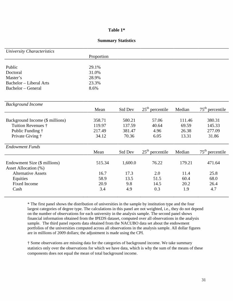
analysis sample consisting of 10,049 observations on 709 universities. Summary statistics are
provided in Table 1.12 The first bank of figures shows the proportion of the universities that are
private and the kinds of degrees they offer. Previous work indicates that such variables are
generally significant correlates of various kinds of financial behavior.13 Next are background
income and its primary components: tuition, public funding, and private giving. (All dollar
figures are converted to 2009 dollars using the consumer price index.) The large difference
between the mean ($358 million) and median ($111 million) reflects the well-known fact that
resources across universities are highly unequal (Desrochers and Wellman, 2011).
The last set of statistics shows total endowments and their allocation across asset classes.
The average endowment size, $515 million, masks considerable heterogeneity across institutions:
it is almost three times the median of $179 million. The value of endowments has varied across
time as well. During the economic boom of the 1990s, endowments increased in value rapidly –
the average value in the NACUBO data increased by $202 million dollars (in 2009 dollars)
between 1993 and 2000. That decade of growth ended abruptly with the collapse of the dot-com
bubble in 2001. Endowments subsequently increased as the economy improved until the onset of
the Great Recession of 2008, after which time endowment values fell by about 30 percent. Note,
however, that these trends must be interpreted cautiously because, as noted above, the
composition of the NACUBO sample has been changing over time.
of the various assets reported by NACUBO summed to less than 95 percent or more than 105 percent. To mitigate reporting error, we dropped these observations as well.
12 As noted above, the number of years that universities appear in the analysis sample varies across universities. The figures in the first panel of Table 1 do not weight by the number of observations; the rest of the figures do.
13 See, for example, Lerner et al. (2008).
12
The table indicates that alternative assets comprise about 17 percent of university
endowments in our analysis sample.14 This figure is the mean over all institutions; if we take the
mean conditional on having a positive amount invested in alternative assets, the share is 20
percent. In 1987, the beginning of our sample period, the unconditional mean share of
alternative assets was 5 percent, and only 62 percent of the endowments held any alternative
assets. By the end of our sample period, the unconditional proportion was 30 percent, and 90
percent of the institutions held alternative assets. In our data, a university makes a transition from
holding alternative assets to not holding them in only 2.5 percent of our observations (university-
pair years). That is, once an endowment includes alternative assets in its portfolio it hardly ever
reverses that decision, an observation that has important implications for our econometric
strategy.
4. Empirical Methodology
In this section we develop a framework for testing whether a university endowment
manager’s demand for alternative assets increases with expected background income and
decreases with its variability, other things being the same. Of course, endowment managers’
expectations of future background income and their beliefs about its variability are not
observable to the econometrician; they need to be constructed. In her analysis of household
portfolio decisions, Vissing-Jorgensen (2002) suggests a two-step procedure to deal with this
issue: First, construct for each agent in each year the expected value of background income and
14 Some alternative assets are illiquid, an observation that leads to the question of how they are valued. NACUBO
provides no guidelines to institutions with respect to valuation procedures, and receives no information about the procedures employed. According to our conversations with one endowment specialist, the manager of each alternative investment is generally asked by the head of the overall endowment to provide assessments of the value of the assets under his or her management. There are common industry practices for how the valuation is done. For example, venture capital is typically valued at the price paid in the last financing round or some lower value reflecting deteriorating business conditions. For real assets, standard appraisal techniques are used.
13
its variability; and second, use these as regressors in an equation explaining decisions about
investing in risky assets. We adopt this general strategy, and now discuss each step in turn.
Expected background income and its variability. Vissing-Jorgensen’s approach assumes
that the log of background income follows a simple autoregressive process. If the only relevant
information available to portfolio decision makers in a given year is past values of background
income, then estimates of the parameters of this process allow one to estimate expected
background income and its variability. Formally, assuming that the observational units are
universities, the forecasting equation is:
ln𝑌𝑌𝑖𝑖𝑖𝑖 = 𝛼𝛼 + 𝛽𝛽 ln𝑌𝑌𝑖𝑖,𝑖𝑖−1 + 𝜀𝜀𝑖𝑖𝑖𝑖 (1)
where 𝑌𝑌𝑖𝑖𝑖𝑖 is real background income for university 𝑖𝑖 in year t, 𝛼𝛼 and 𝛽𝛽 are parameters, and 𝜀𝜀𝑖𝑖𝑖𝑖 is
a normally distributed and uncorrelated error term. If we let Μ𝑖𝑖𝑖𝑖 denote the expected value of the
log of university 𝑖𝑖’s background income in period 𝑡𝑡, it follows that Μ𝑖𝑖𝑖𝑖 = 𝛼𝛼 + 𝛽𝛽 ln𝑌𝑌𝑖𝑖,𝑖𝑖−1. The
conditional second moment of the log of background income, denoted 𝜐𝜐𝑖𝑖𝑖𝑖, is
𝑉𝑉𝑉𝑉𝑉𝑉(ln𝑌𝑌𝑖𝑖𝑖𝑖 | ln𝑌𝑌𝑖𝑖,𝑖𝑖−1), which is the square of the standard deviation of the residuals over the time
period used to estimate the model. With Μ𝑖𝑖𝑖𝑖 and 𝜐𝜐𝑖𝑖𝑖𝑖 in hand, one can compute the expected
value (𝜇𝜇𝑖𝑖𝑖𝑖) and standard deviation (𝜎𝜎𝑖𝑖𝑖𝑖) of the level of background income as
𝜇𝜇𝑖𝑖𝑖𝑖 = 𝐸𝐸(𝑌𝑌𝑖𝑖𝑖𝑖|𝑌𝑌𝑖𝑖,𝑖𝑖−1) = 𝑒𝑒Μ𝑖𝑖𝑖𝑖+𝜐𝜐𝑖𝑖𝑖𝑖2 (2)
𝜎𝜎𝑖𝑖𝑖𝑖 = �𝑉𝑉𝑉𝑉𝑉𝑉�𝑌𝑌𝑖𝑖𝑖𝑖�𝑌𝑌𝑖𝑖,𝑖𝑖−1� = �𝑒𝑒(2Μ𝑖𝑖𝑖𝑖+𝜐𝜐𝑖𝑖𝑖𝑖)(𝑒𝑒𝜐𝜐𝑖𝑖𝑖𝑖 − 1) (3)
The variables 𝜇𝜇𝑖𝑖𝑖𝑖and 𝜎𝜎𝑖𝑖𝑖𝑖 are then the empirical counterparts of the expected value of background
income and its variability, respectively.15
15 The estimated values of 𝜇𝜇𝑖𝑖𝑖𝑖 and 𝜎𝜎𝑖𝑖𝑖𝑖 do not exhibit any discernible patterns over time.
14
Note that the parameters of the forecasting equation (1) do not vary by institution. That
is, the model constrains every school to have the same process for generating background
income. This formulation has the virtue of simplicity, but it is not hard to imagine that the
processes generating background income vary across institutions. A different tactic would be to
estimate the equation separately for each institution. However, we do not have enough
observations for each school to obtain meaningful estimates. As a compromise, we also
estimated equation (1) separately for various subsamples of our data. With this setup, the
background income generating process is the same for all institutions of a given type (say, public
or private), but can differ across types. As reported below, while our results are qualitatively
similar across different types of institutions, both statistical significance and point estimates do
differ.
A related question is how many years of data should be used to estimate equation (1). In
this context, we assume that the only data available to the endowment managers are the total
inflation-adjusted dollar amounts of background income for all years up to but not including the
year portfolio decisions are made.16 We also assume that endowment managers give primary
consideration to background income in relatively recent years when making their decisions.
Specifically, we assume that endowment managers only consider background income data from
a specified window of years prior to the year in which they make their portfolio decision. The
selection of a window length involves a tradeoff: a window that is too short will not provide
sufficient observations to generate meaningful parameter estimates; a window that is too long
will result in estimates based on information that endowment managers probably do not consider
very relevant to their current decision making problem. Theory provides no guidance here. We 16 Conceivably, universities could provide their endowment managers with some contemporaneous information to
help inform their investment decisions. However, without information on the precise timing of the portfolio decisions, we cannot know whether this is a realistic possibility.
15
experimented with various window lengths, and found that the best fit to the first stage equation
was obtained when we used data from six years prior to the year in question for estimation.
Therefore, we estimate equation (1) with data from years 𝑡𝑡 − 7 to 𝑡𝑡 − 1, and calculate the
standard deviation of the residuals from the estimated model over the same period.17 As noted
below, we also experimented with windows of 5 and 7 years and found quite similar results.
The portfolio share of alternative assets. Standard theoretical considerations suggest that
in addition to the first two moments of the background income generating process, a model of
portfolio selection needs to take into account other variables that might affect the decision-
maker’s utility function. Thus, for example, in her analysis of household demand for risky
assets, Vissing-Jorgensen (2002) includes variables such as education and race. In the same
spirit, Dimmock’s (2012) model of university portfolio allocation includes an indicator for
whether the school is public or private and measures of its selectivity, among other variables.
The panel nature of our data allows us to estimate a fixed effects model, and hence take into
account all university characteristics that do not change over time. We also include time effects
to control for factors that likely affect all institutions’ decisions in a given year, such as the
macroeconomic environment, the performance of the stock market, and so on. Thus, the
estimating equation for the proportion of the endowment held in alternative assets is
𝑆𝑆𝑆𝑆𝑆𝑆𝑆𝑆𝐸𝐸𝑖𝑖𝑖𝑖 = 𝛽𝛽0 + 𝛽𝛽1𝜇𝜇𝑖𝑖𝑖𝑖 + 𝛽𝛽2𝜎𝜎𝑖𝑖𝑖𝑖 + 𝛾𝛾𝑖𝑖 + 𝛿𝛿𝑖𝑖 + 𝜔𝜔𝑖𝑖𝑖𝑖 (4)
where 𝑆𝑆𝑆𝑆𝑆𝑆𝑆𝑆𝐸𝐸𝑖𝑖𝑖𝑖 is the proportion of the endowment that university 𝑖𝑖 invests in alternative assets
in year 𝑡𝑡, 𝛾𝛾𝑖𝑖 and 𝛿𝛿𝑖𝑖 represent the time and fixed effects, respectively, and 𝜔𝜔𝑖𝑖𝑖𝑖 is a random error.
17 Some schools in our sample reported data for fewer than 7 years, so they had no observations with the requisite 6
lagged values and therefore are not included in the regressions. This accounts for the fact that the number of schools used to estimate the models is less than the number of schools in the analysis sample.
16
By controlling for time and entity fixed effects, this model renders unnecessary most of the
independent variables included in previous models that rely on cross sectional data.18
As it stands, equation (4) does not include variables that vary over time and across
universities. In the literature on household investments, the most commonly included such
variable is the size of the portfolio (and often its square). However, the inclusion of portfolio size
in an equation estimating portfolio composition is problematic because these variables could be
jointly determined. Lerner et al. (2008) document a strong relationship between university
endowment size and portfolio performance, and note that the causality could run in either
direction. 19 Therefore, our preferred specification leaves out the size of the endowment.
Nevertheless, for the sake of comparison with previous studies we estimate a variation of the
model that includes a quadratic in endowment size. As shown below, this turns out not to affect
our substantive results.
The decision to own alternative assets. It is also of some interest to investigate whether a
university holds any alternative assets at all. In the literature on household portfolio allocation,
researchers typically address this issue by estimating a model in which the probability that a
household owns the risky asset in any given year depends on some set of variables such as
education, age and race. (See, for example, Bertaut and Starr-McCluer (2002).) Such a setup
implicitly allows the household to switch back and forth between holding and not holding the 18 Note that the inclusion of fixed effects takes into account any unchanging preferences for various perquisites
that are not associated with augmenting the general quality of the university, a factor that is central to Gilbert and Hrdlicka’s (2013) model of university endowment decisions. To allow for the possibility that such preferences might be changing over time, we estimated a variant of the basic model with interactions between the time and university effects. The results were essentially unchanged – the coefficients on 𝜇𝜇𝑖𝑖𝑖𝑖 and 𝜎𝜎𝑖𝑖𝑖𝑖 are the same up to the third significant digit.
19 The same concerns about the direction of causality apply to many other time-varying characteristics of institutions that might be candidates for right-hand-side variables, like number of students, faculty-student ratios, number of support staff, payout-to-income ratios, and so on. It is equally possible that the size of the endowment “determines” such variables as such variables “determine” the size of the endowment. Indeed, Michael (2005) posits just such a model, estimating regressions with variables such as faculty-student ratios and research expenditures on the left-hand side, and with the size of the endowment as an exploratory variable.
17
risky asset. This makes perfect sense in the household context because, as Chapman et al.
(2004) show, many households do such switching in response to changes in, for example, stock
prices. However, this model may not be well suited for examining the behavior of university
endowment managers. As noted earlier, once a university invests in alternative assets, it
virtually always does so continually thereafter. Hence, the appropriate question is not how
background income affects the probability of investing in alternative assets in a given year, but
rather how it affects the probability of making a permanent switch to including alternative assets
in its portfolio.
Formally, let the indicator variable 𝑆𝑆𝑖𝑖𝑖𝑖 equal one if university i owns alternative assets in
period t, and zero otherwise. Once a university achieves a value of 𝑆𝑆𝑖𝑖𝑖𝑖 = 1, it has reached an
absorbing state, and 𝑆𝑆𝑖𝑖𝑖𝑖 will be 1 in all subsequent periods. A suitable statistical framework is a
discrete-time hazard model in which the first period of positive investment in alternative assets
for a university represents the end of a duration period. In the jargon of statistics, this transition
into the absorbing state is called a “failure.” Every period of “survival” – in our context, each
year in which a university’s endowment portfolio includes no alternative assets – is included in
the sample as a university that did not fail. Every university that begins to invest in alternative
assets contributes only one failure observation to the sample. Using only observations for which
𝑆𝑆𝑖𝑖,𝑖𝑖−1 = 0, the probability that a university 𝑖𝑖 transitions to holding alternative assets in year 𝑡𝑡 is
estimated with a logit model.20 The right hand side variables include 𝜇𝜇𝑖𝑖𝑖𝑖, 𝜎𝜎𝑖𝑖𝑖𝑖, and time effects.
Because fixed effects cannot be incorporated into a discrete time hazard model, we also include a
vector of university characteristics on the right hand side.
20 For an example of the use of logit to estimate a discrete time hazard model, see Shumway’s (2001) study of the
determinants of bankruptcy.
18
A final econometric issue relates to the computation of standard errors for the estimated
coefficients of the share and participation equations. The standard errors should be clustered at
the university level to allow for correlation of errors within institutions. However, because 𝜇𝜇𝑖𝑖𝑖𝑖
and 𝜎𝜎𝑖𝑖𝑖𝑖 are generated by our estimates of the forecasting process of endowment managers, they
are estimated with error, so that conventional robust standard errors are not appropriate. We
therefore use the method of clustered bootstrapping to generate the standard errors throughout
the analysis (Efron and Tibshirani, 1986).
5. Findings
5.1 Basic results.
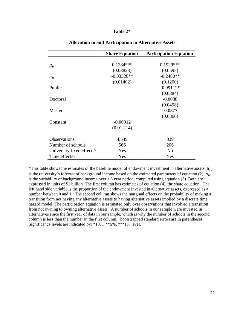
Portfolio share of alternative assets. We begin by estimating equation (4), which models
the share of the endowment held in alternative assets. The results are shown in the first column
of Table 2.21 The positive coefficient on 𝜇𝜇𝑖𝑖𝑖𝑖 implies that a higher level of expected background
income is associated with a larger proportion of alternative assets in the university endowment,
and the negative coefficient on 𝜎𝜎𝑖𝑖𝑖𝑖indicates that higher variability in background income is
associated with a smaller proportion. The positive mean-effect and the negative risk-effect are
both statistically significant at conventional levels.22 To assess the quantitative implications of
the results, we follow Dimmock (2012) and use the coefficients on 𝜇𝜇𝑖𝑖𝑖𝑖 and 𝜎𝜎𝑖𝑖𝑖𝑖 to simulate the
effects of one standard deviation increases in expected background income and background risk, 21 For brevity, the estimated time effects are not reported in Table 2. However, as would be expected from the
trends discussed above, the time effects indicate a gradual shift away from relatively safe, low-return investments to alternative assets after the widely observed success of the endowment model. The same result is present in all subsequent regressions as well.
22 Recall that the results are based on the use of a 6-year window to estimate equation (1). We also experimented with 5 and 7 year windows. For the 5-year window, the estimated coefficients on 𝜇𝜇𝑖𝑖𝑖𝑖 and 𝜎𝜎𝑖𝑖𝑖𝑖 were 0.1282 (s.e. = 0.0527) and -0.0324 (s.e. = 0.0592), respectively. For the 7-year window, the corresponding coefficients were 0.1198 (s.e. = 0.0293) and -0.0291 (s.e. = 0.0096), respectively. The point estimates are quite similar to the results in Table 2, although the coefficient on 𝜎𝜎𝑖𝑖𝑖𝑖 using the 5-year window is imprecisely estimated.
19
respectively. We find that a one standard deviation increase in expected background income
generates a 7.5 percentage point increase in the proportion of the endowment portfolio invested
in alternative assets. A one standard deviation increase in background risk decreases the
proportion of the endowment invested in alternative assets by 1.1 percentage points. Are changes
of this magnitude important? While importance is in the eye of the beholder, it seems to us that
7.5 and 1.1 percentage point increases from an average of 16.7 percentage points, representing
increases of 45 percent and 7 percent, respectively, are big enough to matter.
This approach to assessing the quantitative implications of our results is similar to that
used in previous papers (see Dimmock (2012)), and hence is useful for facilitating comparisons.
However, a possible drawback is that, given the skewness of the variables, looking at the effects
of one standard deviation increases might not be meaningful. As an alternative, we follow
Vissing-Jorgensen (2002) and also use our regression coefficients to estimate how the share of
the portfolio in alternative assets changes when we move from the 25th to 75th percentiles of the
distributions of 𝜇𝜇𝑖𝑖𝑖𝑖 and 𝜎𝜎𝑖𝑖𝑖𝑖, respectively. We find that the share of a university’s portfolio held in
alternative assets increases by 4.1 percentage points and decreases by 0.3 percentage points with
such increases in expected background income and background risk, respectively. These figures
tell essentially the same story as the computations based on one-standard deviation increases in
𝜇𝜇𝑖𝑖𝑖𝑖 and 𝜎𝜎𝑖𝑖𝑖𝑖.
Participation in alternative assets. We next turn to the decision of whether to invest in
alternative assets at all. As indicated above, we estimate a discrete-time hazard model to examine
how changes in expected background income and background risk affect the probability that a
university invests in alternative assets. The marginal effects implied by the logit coefficients are
presented in the second column of Table 2. The results are again consistent with the notion that
20
increases in expected background income increase the demand for alternative assets and
increases in background risk decrease it. The coefficients imply that a one standard deviation
increase in expected background income increases the probability of transitioning to alternative
assets by 11.3 percentage points, and a one standard deviation increase in background risk
decreases the likelihood of making an initial investment in alternative assets by 8.2 percentage
points. As above, we also examined the implications of our results for changes in the values of
𝜇𝜇𝑖𝑖𝑖𝑖 and 𝜎𝜎𝑖𝑖𝑖𝑖 from the 25th to 75th percentile. We find that the likelihood that a university decides to
include alternative assets in its portfolio in a given year increases by 6.2 percentage points with
such an increase in expected background income, and decreases by 2.4 percentage points with a
similar increase in background risk.
In the hazard model, there is effectively only one observation for each university, which
rules out the inclusion of fixed effects to take into account characteristics of universities that
might affect their portfolio decisions. We therefore augment the model with a set of indicator
variables for whether the school is public or private, and for the most advanced degree the school
offers. These variables, which are plausibly exogenous, have been shown to affect university
economic decisions in other contexts (Brown et al., 2010). An interesting result in this regard is
that the indicator for public universities is negative and statistically significant; that is, other
things being the same, public universities are less likely than private universities to start
investing in alternative assets in any given year.
In summary, whether we look at the portfolio share of alternative assets or at the decision
whether or not to invest in alternative assets, the results with respect to the role of background
income are the same. Both sets of estimates support the conclusion of a positive mean effect and
a negative variability effect on endowment managers’ demand for alternative assets. These
21
results are consistent with the models of Merton (1992) and others who argue that when flows of
income into a university become riskier, endowment managers take steps to reduce the riskiness
of their portfolio. Conversely, while these findings do not directly contradict other models that
posit goals such as endowment hoarding or return maximization, they do not offer any support
for such models either.
5.2 Alternative specifications
Including endowment size. Studies of household portfolio behavior typically include
financial wealth and perhaps its square as explanatory variables.23 The analog for a university,
the size of the endowment, varies both across universities and over time, and hence is not taken
into account by the inclusion of fixed effects. We did not include endowment size in our basic
model because of concerns that it might be jointly determined with portfolio composition. Still,
given that it is commonplace to include the size of portfolio, it seems worthwhile to see whether
doing so has any effect on our substantive findings.
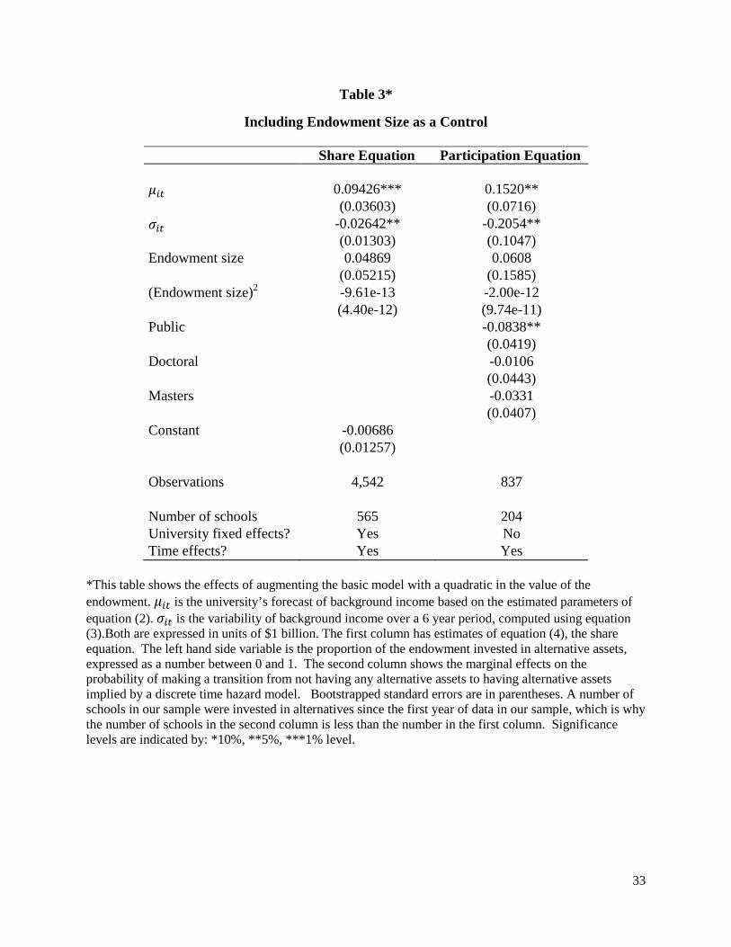
Table 3 presents the results when our basic models are augmented with a quadratic in the
size of the endowment. Neither endowment size nor its square has a significant impact on the
proportion of wealth invested in alternative assets or the decision to undertake investments in
them.24 Furthermore, the coefficients of primary interest, which measure the effects of 𝜇𝜇𝑖𝑖𝑖𝑖 and
𝜎𝜎𝑖𝑖𝑖𝑖 on share and participation decisions, retain the same signs and are still significant in the
augmented models, although in absolute value they are somewhat smaller. Hence, although our
preference is to exclude endowment size to avoid potential endogeneity bias, even if we follow
the conventional approach of including it, our substantive results do not change.
23 See, for example, the papers in the volume by Guiso et al. (2002). 24 Further, a test of the joint hypothesis that the coefficients on endowment size and its square are zero yields a p-
value of 0.375 for the share equation and 0.694 for the participation equation, indicating that they are not jointly significant.
22
Allowing behavior to vary by type of institution. It has been documented that different
types of universities vary in their financial behavior (Lowry, 2004). The distinction between
public and private institutions is salient in this respect (Carnesale, 2006). Endowment activities
are generally more transparent at public universities, since taxpayer dollars are at stake (Gordon
et al., 2002). This substantial risk of public embarrassment may make endowment managers at
public schools more averse to portfolio risk. Also, Dimmock (2012) notes that endowment
boards at private universities average twice as many members as their public counterparts. A
greater chance of agency problems arises from a larger and more complex governance structure,
as any given endowment manager may be less concerned with hedging background risk. Finally,
Martin (2002) reports that public institutions have historically been more dependent on external
support than private institutions. With less control over their own finances, public universities
may be particularly sensitive to fluctuations in background income.
It therefore is of some interest to explore the possibility that the impact of background
income on portfolio allocation decisions varies between public and private universities. We also
examine whether there are differences in this respect between research and non-research
institutions,25 and between universities that have relatively large endowments (above the median)
and relatively small ones (below the median). Our focus is solely on the share of the endowment
devoted to alternative assets (equation (4)). We are not able to estimate discrete-time hazard
models for making transitions to holding alternative assets because the various subsamples do
not have enough observations to obtain reliable estimates.
Table 4 shows the results when we estimate the share equation (4) for the various
subgroups. In order to facilitate comparisons across different types of institutions, we divide the 25 We define research universities as those that spend more than one percent of their background incomes on
research funding. This figure was chosen to yield roughly the same number of research and non-research universities.
23
regression coefficients on 𝜇𝜇𝑖𝑖𝑖𝑖 by the standard deviations of 𝜇𝜇𝑖𝑖𝑖𝑖 in the respective subgroups, and
report these normalized values. We normalize the regression coefficients on 𝜎𝜎𝑖𝑖𝑖𝑖 in the same way.
Thus, the figures in the table represent the change in the proportion of the endowment allocated
to alternative assets that results from a one standard deviation increase in either expected
background income or background risk.
Consider first the left panel of Table 4, which displays the results when we estimate the
share equation separately for public and private institutions. Higher expected background
income leads to a larger share of alternative assets for both types of institution. The magnitude
of the effect is larger for public universities. A one standard deviation increase in expected
background income raises the share in alternative assets by over 13 percentage points for public
universities but only 4 percentage points for private universities.26 The point estimates on 𝜎𝜎𝑖𝑖𝑖𝑖 are
negative for both public and private universities, although statistically significant only for public
universities. The point estimate for public universities implies that a one standard deviation
increase in 𝜎𝜎𝑖𝑖𝑖𝑖 decreases investment in alternative assets by 2 percentage points; for a private
university, the decrease is only about a third of that amount.27 The fact that public university
endowment managers are more sensitive to uncertainty in background income is consistent with
the notion discussed above, that differences in endowment governance structure tend to make
public sector endowment managers more conservative than their private sector counterparts. In
any case, it appears that our results with respect to the impact of background risk for the overall
sample are driven primarily by public institutions.
26 The differences between the coefficients on 𝜇𝜇𝑖𝑖𝑖𝑖 are statistically significant at conventional levels, as are the
differences between the coefficients on 𝜎𝜎𝑖𝑖𝑖𝑖. The same holds true for the differences we find below in the comparisons between research and non-research institutions, and between large-endowment and small-endowment institutions.
27 To help put these figures in perspective, note that in our analysis sample, conditional on having alternative assets, the portfolio share for private universities is 20 percent; for public universities, it is 17.5 percent.
24
Previous research has indicated that an institution’s research orientation affects the
riskiness of its endowment,28 so we next examine whether institutions that grant PhDs and those
that do not differ in how they respond to changes in 𝜇𝜇𝑖𝑖𝑖𝑖 and 𝜎𝜎𝑖𝑖𝑖𝑖.29 The results when we estimate
our basic share equation for the two groups are presented in the middle panel of Table 4. For
both types of schools, the signs on 𝜇𝜇𝑖𝑖𝑖𝑖 and 𝜎𝜎𝑖𝑖𝑖𝑖 are the same as in the basic model. The
coefficients for institutions that do not grant PhDs are statistically significant, and suggest that a
one standard deviation increase in expected background income increases the share of alternative
assets by about 4.4 percentage points, and an analogous increase in background risk decreases
the share by 1.2 percentage points. The coefficients for doctoral institutions are very close in
signs and magnitudes to those of non-doctoral institutions, but they are imprecisely estimated,
perhaps due to the smaller number of available observations.
Finally, we divide the sample based on the size of the endowment, estimating the baseline
equation separately for schools whose endowments are above and below the median value
(approximately $90 million in 2009 dollars).30 In doing so we recognize that, as mentioned
earlier, the magnitude of the endowment could very well be endogenous and stratifying on an
endogenous variable can lead to inconsistent parameter estimates. The results, presented in the
right panel of Table 4, indicate that endowment managers’ alternative asset allocations are more
sensitive to background risk for large than for small endowments. While the coefficients on 28 Dimmock (2012) includes research-to-income ratio as an independent variable in his analysis of endowment
responses to background risk, arguing that research spending serves as a proxy for university cost structure and for university type, both of which may have an impact on portfolio choice. He finds research spending to be a statistically significant determinant of overall portfolio risk.
29 As an alternative, we classified an institution as being a research university if it spent more than one percent of its background income on research funding. The results are similar to those presented below.
30 The number of observations for each subpopulation is not the same, as schools with larger endowments tend to have submitted more years of data to NACUBO. The correlation between the number of years of NACUBO data available for a university and the size of its endowment is +0.25. This correlation could reflect a variety of considerations, including the fact that universities with relatively small endowments might not care enough about endowment policies at other institutions to submit their information to NACUBO.
25
𝜇𝜇𝑖𝑖𝑖𝑖 and 𝜎𝜎𝑖𝑖𝑖𝑖 for both groups have the expected signs, only the coefficients for large-endowment
schools are significant, and the magnitudes of the effects of a one-standard deviation increase in
either variable are two to three times greater for large than for small endowments. A large-
endowment school would show a 5.8 percentage point increase and a 2.0 percentage point
decrease in the share of alternative assets in response to one standard deviation increases in
expected background income and background risk, respectively.
These findings are consistent with the fact that large endowments are more likely than
small endowments to have active, professional management. This is because, as Brown et al.
(2011) observe, the development of financial expertise is a fixed cost that “can be justified only
if it can be spread across a sufficiently large asset base.” We conjecture that such sophisticated
managers are more likely to update their decisions each year based on new data regarding
background income streams than the managers of endowments that follow more passive, or even
mechanical strategies.31
Volatility of the endowment. We have focused on endowment managers’ choices
regarding alternative assets, both because this has been the topic in much of the literature and it
is a prominent issue in popular discussions about university finances. One could argue, though,
that at least during certain time periods, some alternative assets might be less volatile than
“conventional” investments like publicly traded stocks, and therefore concentrating on
alternative assets could be inappropriate. To deal with this issue, we examine the impact of
background risk on the overall volatility of the endowment. To begin, we estimate an
autoregression of the logarithm of the real value of the endowment on its lagged value, and use
31 The fact that the size of the endowment is not statistically significant in Table 3 while our estimates of the
coefficients on 𝜇𝜇𝑖𝑖𝑖𝑖 and 𝜎𝜎𝑖𝑖𝑖𝑖 differ between high-endowment and low-endowment institutions suggests that the size of the endowment has no effect on the level of the proportion of the portfolio allocated to alternative assets, ceteris paribus. Rather, the effect operates through interactions with 𝜇𝜇𝑖𝑖𝑖𝑖 and 𝜎𝜎𝑖𝑖𝑖𝑖.
26
the estimated parameters to compute the expected value of the endowment (conditional on the
lagged value) and its volatility. In the second stage, we estimate a regression of the portfolio’s
volatility on the expected value of background income and its standard deviation (our 𝜇𝜇𝑖𝑖𝑖𝑖 and 𝜎𝜎𝑖𝑖𝑖𝑖
variables as above), as well as university and year effects. The key result is that the
endowment’s volatility increases with the expected value of background income and decreases
with the uncertainty of background income, ceteris paribus, and both coefficients are statistically
significant.32 In short, like our findings relating to portfolio allocations for alternative assets, the
evidence is consistent with the notion that endowment managers take both the level and riskiness
of background income into account when making their decisions.
6. Conclusions
What functions do university endowments serve? This question has been controversial
for a long time, and interest in it has intensified in recent years as more and more endowments
have invested in the relatively risky and illiquid assets collectively known as alternative assets.
In this context, two related questions are salient. First, when endowment managers make their
portfolio allocation decisions, do they think only in terms of the assets that they manage, or do
they also take into account background income, the other flows of income into the university?
Second, if they do take background income into account, do endowment managers hedge against
its risks? That is, if they perceive that background income is becoming more risky, do they
reduce the exposure of the endowment to risky assets? Although some theoretical models
suggest that endowment managers behave in this fashion, others indicate that, depending on the
form of their objective function, this need not be the case.
32 Specifically, the coefficient on 𝜇𝜇𝑖𝑖𝑖𝑖 is 0.0505 (s.e. = 0.0195) and the coefficient on 𝜎𝜎𝑖𝑖𝑖𝑖 is -0.0150 (s.e. = 0.00705).
27
To investigate these issues, we have analyzed panel data on 729 universities’ portfolio
decisions over the period 1987-2009. Our findings support the prediction that university
endowment managers are more likely to invest in alternative assets, and invest in them more
heavily, when expected university background income increases and when its variability
declines.
While we cannot rule out other views of the goals of university endowment managers,
our results suggest that one important function of university endowments is to hedge against
revenue shocks. Thus, universities with low expected levels of background income or more
variable streams of such income seek less risk in their financial investments. At the same time,
such institutions are also more likely to confront circumstances that require them to use some of
the endowment principal to maintain daily operations, increasing the importance of liquidity in
their portfolios. For both reasons, then, their endowment managers will tend to shy away from
alternative assets, which are the riskiest and the most illiquid of all the asset classes.
A number of issues remain to be explored. First, the role of higher-order moments of
background income merits consideration. Portfolio decisions might depend not only on the mean
and standard deviation of background income, but also on the probability of an extreme event,
such as a devastating shock to (say) state government grants income during a recession. Another
possible topic is suggested by the fact that while the investments that comprise the alternative
asset category can generally be characterized as illiquid and risky, in some respects they are
fairly heterogeneous. An investment in a hedge fund is different from an investment in a stand
of timber. It would be useful to examine in more detail the interactions among the demands for
the various categories within alternative assets, and in particular, if they respond differently to
changes in background income.
28
References
Agarwal, V. and Naik, N. (2004). Risk and Portfolio Decisions Involving Hedge Funds. Review of Financial Studies, 17(1), 63-98. Arrondel, L., Pardo H.C., and Oliver X. (2010). Temperance in Stock Market Participation: Evidence from France. Economica, 77(306), 314-333. Bertaut, C. C. and Starr-McCluer, M. (2002). Household Portfolios in the United States. In Guiso, Luigi, Michael Haliassos and Tullio Jappelli (eds.), Household Portfolios. Cambridge, MA: MIT Press. Black, F. (1976). The Investment Policy Spectrum: Individuals, Endowment Funds and Pension Funds. Financial Analysts Journal, 32(1), 23-31. Brown, J., Dimmock, S., Kang, J., and Weisbenner, S. (2014). How University Endowments Respond to Financial Market Shocks: Evidence and Implications. American Economic Review, 104(3), 931-962. Brown, J., Dimmock, S., Kang, J., Richardson, D., and Weisbenner, S. (2011). The Governance of University Endowments: Insights from a TIAA-CREF Institute Survey. TIAA-CREF Institute Research Dialogue, 102. Brown, K.C., Garlappi, L., and Tiu, C. (2010). Asset Allocation and Portfolio Performance: Evidence from University Endowment Funds. Journal of Financial Markets, 13(2), 268-294. Brown, S., Goetzmann, W., Liang, B., and Schwarz, C. (2008). Mandatory Disclosure and Operational Risk: Evidence from Hedge Fund Registration. Journal of Finance, 63(6), 2785-2815. Carnesale, A. (2006). The Private-Public Gap in Higher Education. The Chronicle of Higher Education, 15(18), B20. Cejneck, G., Franz, R., Randl, O., and Stoughton, N. (2013). A Survey of University Endowment Management Research. Available at SSRN 2205207. Chapman, K., Dow, J. P. Jr., and Hariharan, G. (2004). Changes in Stockholding Behavior: Evidence from Household Survey Data. Finance Research Letters, 2(2): 89-96. Desrochers, D.M. and Wellman, J.V. (2011) Trends in College Spending, 1999-2009, Delta Cost Project, Washington, DC. Dimmock, S.G. (2012). Background Risk and University Endowment Funds. The Review of Economics and Statistics, 94(3), 789-799.
29
Efron, B. and Tibshirani, R. (1986). Bootstrap methods for standard errors, confidence intervals, and other measures of statistical accuracy. Statistical science, 54-75. Gilbert, Thomas and Hrdlicka, Christopher, “Why Do University Endowments Invest So Much in Risky Assets?” Working Paper, University of Washington, March 2015. Goetzmann, W. N., and Oster, S. (2012). Competition among university endowments (No. w18173). National Bureau of Economic Research. Gollier, C. and Pratt, J.W. (1996). Risk Vulnerability and the Tempering Effect of Background Risk. Econometrica, 64(5), 1109-1123. Gordon, T., Fischer, M., Malone, D., and Tower, G. (2002). A Comparative Empirical Examination of Extent of Disclosure by Private and Public Colleges and Universities in the United States. Journal of Accounting and Public Policy, 21(3), 235-275. Guiso, L., Haliassos, M., and Jappelli, T. (2002). Household Portfolios. Cambridge, MA: MIT Press. Guiso, L., Jappelli, T., and Terlizzese, D. (1996). Income Risk, Borrowing Constraints, and Portfolio Choice. The American Economic Review, 86(1), 158-172. Hansmann, H. (1990). Why Do Universities Have Endowments? Journal of Legal Studies, 19, 3. Heaton, J. and Lucas, D. (2000). Portfolio Choice in the Presence of Background Risk. Economic Journal, 110(460), 1-26. Humphreys, J., Electris, C., Fapohunda, Y., Filosa, J., Goldstein, J., Grace, K. (2010). Educational Endowments and the Financial Crisis: Social Costs and Systemic Risks in the Shadow Banking System. Center for Social Philanthropy, Tellus Institute. Kaplan, S.N. and Schoar, A. (2005). Private Equity Performance: Returns, Persistence, and Capital Flows. Journal of Finance, 60(4), 1791-823. Kimball, M.S. (1993). Standard Risk Aversion. Econometrica, 61(3), 589-611. Lau, Y. and Rosen, H.S. (2014). Are Universities Becoming More Unequal? Working Paper, Princeton University. Lerner, J., Schoar, A., and Wang, J. (2008). Secrets of the Academy: The Drivers of University Endowment Success. Journal of Economic Perspectives 22(3): 207-22. Lowry, R.C. (2004). Markets, Governance, and University Priorities: Evidence on Undergraduate Education and Research. Economics of Governance, 5, 29-51.
30
Major Private Gifts to Higher Education. Chronicle.com. The Chronicle of Higher Education, 20 October 2013. Martin, Robert E. (2002). Why Tuition Costs Are Rising So Quickly. Challenge, 45(4), 88-108. Merton, Robert (1971). Optimum Consumption and Portfolio Rules in a Continuous-time Model. Journal of Economic Theory, 3(4), 373-413. Merton, Robert (1992). Optimal Investment Strategies for University Endowment Funds. In Studies of Supply and Demand in Higher Education, edited by C. Clotfelter and M. Rothschild. Chicago: University of Chicago Press. Michael, Steve O. (2005). The Cost of Excellence: The Financial Implications of Institutional Rankings. International Journal of Educational Management, 19(5), 365-382. Morse, Robert. Rise in Endowments May Impact Best Colleges’ Rankings. USNews.com. US News & World Report, 9 February 2012. Shumway, Tyler (2001). Forecasting Bankruptcy More Accurately: A Simple Hazard Model. The Journal of Business, 74(1), 101-124. Stewart, James (2013). How Cooper Union’s Endowment Failed in Its Mission. The New York Times 10 May 2013, Business sec. Web. Swensen, David F. (2009). Pioneering Portfolio Management: An Unconventional Approach to Institutional Investment. New York, NY. Print. Tobin, James (1974). What is Permanent Endowment Income? American Economic Review, 64(2), 427-432. Vissing-Jorgensen, A. (2002). Towards an Explanation of Household Portfolio Choice Heterogeneity: Nonfinancial Income and Participation Cost Structures. National Bureau of Economic Research, Working Paper No. 8884.
31
Table 1*
Summary Statistics
University Characteristics Proportion Public
29.1%
Doctoral 31.0% Master’s 28.9% Bachelor – Liberal Arts 23.3% Bachelor – General 8.6%
Background Income Mean Std Dev 25th percentile Median 75th percentile Background Income ($ millions) 358.71 580.21 57.06 111.46 380.31 Tuition Revenues † 119.97 137.59 40.64 69.59 145.33 Public Funding † 217.49 381.47 4.96 26.38 277.09 Private Giving † 34.12 70.36 6.05 13.31 31.86 Endowment Funds Mean Std Dev 25th percentile Median 75th percentile Endowment Size ($ millions) 515.34 1,600.0 76.22 179.21 471.64 Asset Allocation (%) Alternative Assets 16.7 17.3 2.0 11.4 25.8 Equities 58.9 13.5 51.5 60.4 68.0 Fixed Income 20.9 9.8 14.5 20.2 26.4 Cash 3.4 4.9 0.3 1.9 4.7
* The first panel shows the distribution of universities in the sample by institution type and the four largest categories of degree type. The calculations in this panel are not weighted, i.e., they do not depend on the number of observations for each university in the analysis sample. The second panel shows financial information obtained from the IPEDS dataset, computed over all observations in the analysis sample. The third panel reports data obtained from the NACUBO data set about the endowment portfolios of the universities computed across all observations in the analysis sample. All dollar figures are in millions of 2009 dollars; the adjustment is made using the CPI. † Some observations are missing data for the categories of background income. We take summary statistics only over the observations for which we have data, which is why the sum of the means of these components does not equal the mean of total background income.
32
Table 2*
Allocation to and Participation in Alternative Assets
Share Equation Participation Equation 𝜇𝜇𝑖𝑖𝑖𝑖 0.1284*** 0.1929*** (0.03823) (0.0595) 𝜎𝜎𝑖𝑖𝑖𝑖 -0.03328** -0.2480** (0.01402) (0.1200) Public -0.0911** (0.0384) Doctoral -0.0088 (0.0498) Masters -0.0377 (0.0360) Constant -0.00912 (0.01.214) Observations 4,549 839 Number of schools 566 206 University fixed effects? Yes No Time effects? Yes Yes
*This table shows the estimates of the baseline model of endowment investment in alternative assets. 𝜇𝜇𝑖𝑖𝑖𝑖 is the university’s forecast of background income based on the estimated parameters of equation (2). 𝜎𝜎𝑖𝑖𝑖𝑖 is the variability of background income over a 6 year period, computed using equation (3). Both are expressed in units of $1 billion. The first column has estimates of equation (4), the share equation. The left hand side variable is the proportion of the endowment invested in alternative assets, expressed as a number between 0 and 1. The second column shows the marginal effects on the probability of making a transition from not having any alternative assets to having alternative assets implied by a discrete time hazard model. The participation equation is estimated only over observations that involved a transition from not owning to owning alternative assets. A number of schools in our sample were invested in alternatives since the first year of data in our sample, which is why the number of schools in the second column is less than the number in the first column. Bootstrapped standard errors are in parentheses. Significance levels are indicated by: *10%, **5%, ***1% level.
33
Table 3*
Including Endowment Size as a Control
Share Equation Participation Equation 𝜇𝜇𝑖𝑖𝑖𝑖 0.09426*** 0.1520** (0.03603) (0.0716) 𝜎𝜎𝑖𝑖𝑖𝑖 -0.02642** -0.2054** (0.01303) (0.1047) Endowment size 0.04869 0.0608 (0.05215) (0.1585) (Endowment size)2 -9.61e-13 -2.00e-12 (4.40e-12) (9.74e-11) Public -0.0838** (0.0419) Doctoral -0.0106 (0.0443) Masters -0.0331 (0.0407) Constant -0.00686 (0.01257) Observations 4,542 837 Number of schools 565 204 University fixed effects? Yes No Time effects? Yes Yes
*This table shows the effects of augmenting the basic model with a quadratic in the value of the endowment. 𝜇𝜇𝑖𝑖𝑖𝑖 is the university’s forecast of background income based on the estimated parameters of equation (2). 𝜎𝜎𝑖𝑖𝑖𝑖 is the variability of background income over a 6 year period, computed using equation (3).Both are expressed in units of $1 billion. The first column has estimates of equation (4), the share equation. The left hand side variable is the proportion of the endowment invested in alternative assets, expressed as a number between 0 and 1. The second column shows the marginal effects on the probability of making a transition from not having any alternative assets to having alternative assets implied by a discrete time hazard model. Bootstrapped standard errors are in parentheses. A number of schools in our sample were invested in alternatives since the first year of data in our sample, which is why the number of schools in the second column is less than the number in the first column. Significance levels are indicated by: *10%, **5%, ***1% level.
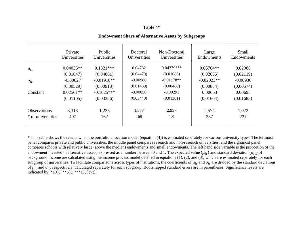
Table 4*
Endowment Share of Alternative Assets by Subgroups Private
Universities Public
Universities Doctoral
Universities Non-Doctoral Universities
Large Endowments
Small Endowments
𝜇𝜇𝑖𝑖𝑖𝑖 0.04036** 0.1321*** 0.04782 0.04379*** 0.05764** 0.02088 (0.01847) (0.04861) (0.04479) (0.01686) (0.02655) (0.02119) 𝜎𝜎𝑖𝑖𝑖𝑖 -0.00627 -0.01910** -0.00986 -0.01178** -0.02023** -0.00936 (0.00529) (0.00913) (0.01439) (0.00488) (0.00884) (0.00574) Constant 0.02561** -0.1025*** -0.00050 -0.00291 0.00663 0.00698 (0.01105) (0.03356) (0.03440) (0.01301) (0.01604) (0.01685) Observations 3,313 1,235 1,583 2,957 2,574 1,072 # of universities 407 162 169 401 287 237
* This table shows the results when the portfolio allocation model (equation (4)) is estimated separately for various university types. The leftmost panel compares private and public universities, the middle panel compares research and non-research universities, and the rightmost panel compares schools with relatively large (above the median) endowments and small endowments. The left hand side variable is the proportion of the endowment invested in alternative assets, expressed as a number between 0 and 1. The expected value (𝜇𝜇𝑖𝑖𝑖𝑖) and standard deviation (𝜎𝜎𝑖𝑖𝑖𝑖) of background income are calculated using the income process model detailed in equations (1), (2), and (3), which are estimated separately for each subgroup of universities. To facilitate comparisons across types of institutions, the coefficients of 𝜇𝜇𝑖𝑖𝑖𝑖 and 𝜎𝜎𝑖𝑖𝑖𝑖 are divided by the standard deviations of 𝜇𝜇𝑖𝑖𝑖𝑖 and 𝜎𝜎𝑖𝑖𝑖𝑖, respectively, calculated separately for each subgroup. Bootstrapped standard errors are in parentheses. Significance levels are indicated by: *10%, **5%, ***1% level.