Embed Size (px)
Citation preview

1
Who benefits from universal child care Estimating marginalreturns to early child care attendance
Thomas CornelissenChristian Dustmann
Anna RauteUta Schoumlnberg
This version September 2015
Abstract
In this paper we examine the heterogeneous treatment effects of a universalchild care (preschool) program in Germany by exploiting the exogenousvariation in attendance caused by a reform that led to a large staggeredexpansion across municipalities Drawing on unique administrative datafrom the full population of compulsory school entry examinations we findthat children with lower (observed and unobserved) gains are more likely toselect into child care than children with higher gains This pattern of reverseselection on gains is driven by unobserved family backgroundcharacteristics children from disadvantaged backgrounds are less likely toattend child care than children from advantaged backgrounds but have largertreatment effects because of their worse outcome when not enrolled in childcare
JEL J13 J15 I28Keywords Universal child care child development marginal treatment effects
Correspondence Thomas Cornelissen Department of Economics University College Londonand Centre for Research and Analysis of Migration (CReAM) 30 Gordon Street London WC1H 0AXUnited Kingdom (email tcornelissenuclacuk) Christian Dustmann Department of EconomicsUniversity College London and CReAM 30 Gordon Street London WC1H 0AX United Kingdom(email cdustmannuclacuk) Anna Raute Department of Economics University of Mannheim L73-5 68161 Mannheim Germany (email arauteuni-mannheimde) Uta Schoumlnberg Department ofEconomics University College London CReAM and IAB 30 Gordon Street London WC1H 0AXUnited Kingdom (email uschoenberguclacuk)
We are indebted to the Health Ministry of Lower Saxony (NLGA) for providing the data andparticularly grateful to Dr Johannes Dreesman for his advice and invaluable support with datamanagement Christian Dustmann acknowledges funding from the European Research Council (ERC)under Advanced Grant No 323992
2
1 Introduction
Preschool and early childhood programs are generally considered effective means of
influencing child development (see eg Currie and Almond 2011 Ruhm and Waldfogel
2012) both because many skills are best learnt when young (eg Shonkoff and Phillips 2000)
and because the longer pay-off period makes such learning more productive (Becker 1964)
There may also be important ldquodynamic complementaritiesrdquo of early learning with acquisition
of human capital at later stages (Cunha and Heckman 2007 Heckman 2007 Aizer and
Cunha 2012) In recognition of these benefits most European countries including the UK
France Germany and all Nordic nations offer publicly provided universal child care (or
preschool) programs aimed at promoting childrenrsquos social and cognitive development In the
US which offers no nationwide universal preschool program1 an important goal of the
Obama administrationrsquos Zero to Five Plan is to create similar initiatives represented in the
2016 presidential budget request by a 10-year $75 billion Preschool for All program and $750
million in grant funding to states for program development and expansion
Yet despite enormous policy interest evidence of the effectiveness of child care (or
preschool) programs is scarce and far from unified For example proponents of child care
programs often cite targeted programs like Head Start or the Perry Preschool Project which
have generated large long-term gains for participants2 Evidence on the effectiveness of
universal child care programs targeted at all children on the other hand is mixed with effects
ranging from negative to positive3 One important reason that targeted child care programs
1 State-level programs (often referred to as pre-K) are currently in place in Georgia Florida New JerseyNew York and Oklahoma and have been enacted or expanded in recent years in Alabama Michigan Minnesotaand Montana A subsidized universal child care program also exists in the Province of Quebec Canada
2 See for instance the papers by Currie and Thomas (1995) Garces Currie and Thomas (2002) Carneiroand Ginja (2014) and Heckman Moon Pinto Savelyev and Yavitz (2010ab)
3 For example whereas Berlinski Galiani and Gertler (2009) Berlinski Galiani and Manacorda (2008)Havnes and Mogstad (2011) and Felfe Nollenberger and Rodriguez-Planas (2015) find positive mean effects ofan expansion in pre-elementary education in Argentina Urugay Norway and Spain respectively Baker Gruberand Milligan (2008) report negative mean impacts of highly subsidized universal child care in Quebec onbehavioral and health outcomes Datta Gupta and Simonsen (2010) also find no evidence that enrollment incenter-based care at age 3 in Denmark improves child outcomes and Magnuson Ruhm and Waldfogel (2007)find mixed effects of pre-K attendance in the US including positive short-lived effects on academic skills andnegative and more persistent effects on behavioral outcomes (see Baker 2011 for an extensive review of thisliterature)
3
yield larger returns than large scale universal programs may be treatment effect heterogeneity
that is the former target children from disadvantaged backgrounds whose treatment effect
(ie difference between treated and untreated outcomes) may be higher than for the average
child This discrepancy may occur for instance because disadvantaged children experience
lower quality care in the untreated state (ie a worse home environment) but a similar
environment in the treated state (because child care programs are of similar quality)
In this paper we assess treatment effect heterogeneity in a universal preschool or child care
program aimed at 3- to 6-year-olds in Germany Our goal is to better understand which
children benefit most from the program and whether treatment effect heterogeneity can help
reconcile the divergent evidence on targeted and universal child care programs Specifically
we apply the marginal treatment effects (MTE) framework introduced by Bjoumlrklund and
Moffitt (1987) and generalized by Heckman and Vytlacil (1999 2005 2007) which relates the
heterogeneity in the treatment effect to observed and unobserved heterogeneity in the
propensity for child care enrollment Such a framework produces a more complete picture of
effect heterogeneity than the conventional IV analysis typically adopted in the literature
The study context offers two key advantages First it allows us to exploit a reform during
the 1990s that entitled every child in Germany to a heavily subsidized half-day child care
placement from the third birthday to school entry thereby greatly increasing the share of
children attending child care for at least 3 years (from 41 to 67 on average over the
program rollout period) Since the reform mainly affected the share of children attending
childcare for 3 years we define our treatment as attending child care for (at least) 3 years
which we also referred to as ldquoearly attendancerdquo This expansion in publicly provided child care
was staggered across municipalities creating variation in the availability of child care slots
(our instrument) not only across space but also across cohorts It thus permits a tighter design
for handling nonrandom selection into child care than is typical in the related literature
Second it offers the unique feature that prior to school entry at age 6 all children must
undergo compulsory school entry exams administered by pediatricians We have obtained rare
4
administrative data from these school entry examinations for the entire population of children
in one large region providing us with a measure of overall school readiness (which determines
whether the child is held back from school entry for another year) as well as measures of
motor skills and health including information on overweight These indicators are important
predictors of academic success and health later in life (eg Grissmer et al 2010 Wang et al
2011)
Unlike many previous studies that use administrative data on child outcomes we also
observe individual child care attendance which is crucial to our implementation of the MTE
framework4 We match the examination data with survey data on the local child care supply in
each municipality and base our instrument on changes in the local availability of child care
capturing only arguably exogenous changes in supply (conditional on municipality and cohort
effects)
We find substantial heterogeneity in returns to early child care attendance with respect to
both observed and unobserved characteristics Children of immigrant ancestry (hereafter
referred to as ldquominority childrenrdquo) are less likely to attend child care early but experience
higher returns in terms of overall school readiness than native children which points to a
reverse selection on gains based on observed characteristics The selection on unobserved
characteristics reinforces this finding for our primary outcome of overall school readiness
children with unobserved characteristics that predispose them to early child care entry (ldquolow
resistance childrenrdquo) benefit the least from early child care attendance whereas those least
likely to enter (ldquohigh resistance childrenrdquo) benefit the most As a consequence the effect of
treatment on the untreated (TUT) exceeds the average treatment effect (ATE) which in turn
exceeds the effect of treatment on the treated (TT) with TUT being strongly positive and
statistically significant and TT being negative Because conventional IV methods typically
estimate one overall effect they do not detect such important treatment effect heterogeneity
4 Most papers exploiting child care reforms focus on intention-to-treat effects partly because information onindividual child care attendance is unavailable (see eg Baker Gruber and Milligan 2008 Havnes and Mogstad2011 2014 Felfe Nollenberger and Rodriguez-Planas 2015) Without information on individual treatmentstatus however it is impossible to determine whether heterogeneity in intention-to-treat effects is caused by thedifferential take-up of children or by heterogeneous responses to child care attendance
5
Moreover in a difference-in-difference setting such as ours as we discuss in section 54 IV
aggregates the heterogeneous effects in a non-meaningful way
By digging deeper into the reasons for these findings we show that the higher returns to
treatment for high versus low resistance children are driven by worse outcomes in the untreated
statemdashwhich in the German context is almost exclusively family care by either parents or
grandparentsmdashwhereas outcomes in the treated state are more homogeneous in line with the
relatively small quality differences between child care programs in our context Thus formal
child care acts as an equalizer Our results also suggest that high resistance children are more
likely to come from more disadvantaged backgrounds
What then explains the pattern of reverse selection on gains revealed in this paper One
important reason could be that parental decisions about child care arrangements are based not
only on the childrsquos welfare but also the parentsrsquo own objectives For instance although well-
educated parents could provide their children with a high quality home environment they may
opt for child care because of their own career concerns and labor market involvement On the
other hand mothers from disadvantaged or minority backgrounds not only face higher relative
child care costs but may also have lower incentives to participate in the labor market and a
more critical attitude toward publicly provided child care At the same time the home
environment may deprive the children of exposure to peers and the learning activities provided
in child care thereby delaying development5
Hence in addition to highlighting the importance of heterogeneity in both parental
resistance to child care enrollment and the childrenrsquos response to child care attendance in child
care program evaluation our findings also reconcile the seemingly contradictory results of
positive effects for programs targeted at disadvantaged children but mixed effects for universal
programs In terms of relevant policy implications they suggest that parental choices may
5 The positive correlation between parental inputs and parental socioeconomic background is welldocumented For example Guryan Hurst and Kearney (2008) provide evidence for a positive relation betweenmaternal education and time spent with children for both nonworking and working mothers Hart and Risley(1995) and Rowe (2008) also report that low SES mothers talk less and use less varied vocabulary duringinteraction with their children than high SES mothers with the latter hearing approximately 11000 utterances aday compared to 700 utterances for (Hart and Risley cited in Rowe 2008)
6
differ from those that the children themselves would make potentially supporting the claim
that state involvement in the early child care market may ldquo[hellip] mimic the agreements that
would occur if children were capable of arranging for their [own] carerdquo (Becker and Murphy
1988 p 1) Our results also imply that policies which successfully attract high resistance
children not currently enrolled in early child care may yield large returns Further programs
targeted at minority and disadvantaged children are likely to be more cost effective and
beneficial than universal child care programs
Our paper makes several important contributions to the literature Above all in contrast to
the sparse research on heterogeneity in returns to child care which typically focuses on
treatment heterogeneity in observed characteristics6 it identifies novel patterns of treatment
effect heterogeneity in early child care attendance based on both observed and unobserved
characteristics The only two recent studies we know of that use an MTE framework to
estimate heterogeneity in returns to early child care attendance with respect to unobserved
characteristics are Kline and Walters (2015) and Felfe and Lalive (2014) The former evaluates
a targeted child care program (Head Start) with an emphasis on multiple untreated states (ie
home care vs other subsidized public child care) whereas the latter examines a much younger
preschool population We in contrast study a universal child care program in which the
untreated state is almost exclusively home care and concentrate on older preschool children
who are not only at the heart of the current US policy debate but in our context also permit a
more robust identification strategy7
Our study also contributes to the growing literature that estimates marginal treatment
effects in different contexts most of which has focused on returns to schooling at the college
(see eg Carneiro Heckman and Vytlacil 2011 for the US Balfe 2015 for the UK
6 Consistent with our findings Havnes and Mogstad (2014) by estimating quantile treatment effects andlocal linear regressions by family income provide evidence that children of low income parents benefitsubstantially from the child care expansion studied whereas upper class children suffer earnings losses SimilarlyBitler Hoynes and Domina (2014) identify the strongest distributional effects for the Head Start program amongchildren in the lower part of the outcome distribution
7 Felfe and Lalive (2014) exploit the onset of an ongoing expansion in early child care in Germany aimed atyounger children (0ndash2 years old) Over their 3-year observation period child care attendance increased by only 7percentage points (compared to an increase in attendance by 26 percentage points in our case) limiting thevariation in child care availability within municipalities across cohorts
7
Nybom 2014 for Sweden) or secondary school level (eg Carneiro Lokshin Ridao-Cano
and Umapathi 2014)8 typically producing evidence for a strong self-selection into treatment
based on net gains Our findings in contrast show that when someone other than the treatment
subject (eg the parents) decides on enrollment (the intervention) the relation between
selection and gains may be reversed so that individuals with the highest enrollment resistance
benefit most from the treatment9
We deviate from the existing MTE literature in the area of education by adopting a tighter
identification strategy that exploits variation in the instrument not only across areas (the main
variation used in existing studies) but also across cohorts thus enabling us to control for time-
constant unobserved area characteristics An additional strength is that the exogenous variation
from a strong sustained expansion of child care slots creates common support in the estimated
propensity score over virtually the full unit interval While rare in MTE applications this is
crucial to compute the TT and the TUT which heavily weight individuals at the extremes of
the treatment propensity distribution without having to extrapolate out of the common
support10
The paper proceeds as follows Section 2 outlines the empirical framework and the method
for estimating the marginal returns to child care attendance Sections 3 and 4 describe the data
the main features of the German public child care system and the child care reform Section 5
reports our main findings on treatment effect heterogeneity and its relation to the pattern of
selection into treatment Section 6 then offers a possible explanation for the main pattern of
findings and discusses policy simulations Section 7 concludes the paper with a discussion of
policy implications
8 The MTE framework has also been applied to measure the marginal treatment effects of foster care onfuture outcomes (Doyle 2007) heterogeneity in the impacts of comprehensive schools on long-term healthbehavior (Basu Jones and Rosa Dias 2014) and heterogeneity in the effects of disability insurance receipt onlabor supply (Maestas Mullen and Strand 2013 French and Song 2014)
9 Kline and Walters (2015) uncover a similar pattern for Head Start attendance when the nontreated state ishome care and Aaakvik Heckman and Vytlacil (2005) find evidence in line with the reverse selection on gains inthe context of a vocational rehabilitation program in Norway
10 For instance the common support in French and Song (2014) ranges from 045 to 085 while that in Felfeand Lalive (2014) ranges only between 0 and 05 Carneiro Heckman and Vytlacil (2011) in contrast achievenearly full common support by combining four different instruments
8
2 Estimating marginal returns to child care attendance
21 Model set up
We assess the extent and pattern of treatment effect heterogeneity with respect to both
observed and unobserved characteristics using the MTE framework proposed by Bjoumlrklund and
Moffitt (1987) and subsequently developed in a series of papers by Heckman (1997) and
Heckman and Vytlacil (1999 2005 2007) We use and ଵto designate the potential
outcome for individual i in the nontreated versus the treated state respectively and ଵ
embody the child outcomes from the school entrance exams which are observed for each
individual depending on treatment state ܦ (with =ܦ 1 denoting treatment) We then model
the potential outcomes as a function of the observed control variables (eg child gender
age and minority status) and dummies for municipality () and examination cohort ( )
= ߚ+ ߙ+ + = 01 (1)
Unlike most of the existing MTE applications which assumes independence of () and
we follow Brinch Mogstad and Wiswall 2014 and interpret equation (1) as a linear
projection of on () which implies that by definition is normalized to ܧ | =
ݔ = ݎ = =൧ݐ 0 11
For selection into treatment ܦ (child care attendance for at least 3 years) we use the
following latent index model
ܦlowast = ߚௗ minus
=ܦ 1 if ܦlowast ge 0 =ܦ 0 otherwise (2)
where = ( ෨) implying that includes the same covariates () as the outcome
equation (1) and an instrument ෨excluded from the outcome equation In our application ෨is
local child care supply as measured by the child care coverage rate (ie number of available
child care slots divided by number of eligible children in a municipality) 3 years prior to the
school entry examination (ie when the child was approximately aged 3) Because the error
11 The coefficient vector defined as prime(ߙߚ) = [() ᇱ() ]ଵ() ᇱ should therefore be
interpreted in terms of partial correlations rather than causal impacts
9
term enters the selection equation (2) with a negative sign it embodies the unobserved
characteristics that make individuals less likely to receive treatment We thus label
ldquounobserved resistancerdquo or ldquodistasterdquo for treatment
Equation (1) implies that the individual treatment effect (the difference between the
potential outcomes in the treated and untreated states) is given by ଵminus = (ߚଵminus (ߚ +
ଵminus Treatment effect heterogeneity may thus result from both observed (differences
between ߚଵ and ߚ) and unobserved characteristics (differences between ଵand )12 A
key feature of the MTE approach is that it allows the unobserved gain from treatment (ଵminus
) to be correlated with unobserved characteristics that affect selection ( ) In the remainder
of the exposition we drop the i index to simplify notation
In the MTE literature it is customary to trace out the treatment effect against the quantiles
of the distribution of rather than against its absolute values in line with the following
transformation of the selection rule in equation (2) ௗߚ minus ge 0 hArr ௗߚ ge hArr Φ(ߚௗ) ge
Φ() with Φ denoting the cdf of (in our application a standard normal distribution) The
term Φ(ߚௗ) also denoted by Φ(ߚௗ) equiv () is the propensity score (the probability that an
individual with observed characteristics will receive treatment) and Φ() denoted
byΦ() equiv Uୈ represents the quantiles of the distribution of unobserved resistance to
treatment The marginal treatment effect as a function of these quantiles can then be
expressed as
MTE( = ݔ Uୈ = (ݑ = )ܧ ଵminus | = ݔ Uୈ = (ݑ
where MTE is the gain from treatment for an individual with observed characteristics = ݔ
who is in the ݑ -th quantile of the distribution implying the individual is indifferent to
receiving treatment when having a propensity score () equal to ݑ
The above approach rests on the following assumptions First there must be a first stage in
which the instrument ෨(the child care coverage rate in the municipality) causes variation in the
12 Because the municipality and year dummies are restricted to having the same effect in the treated anduntreated outcome equations they have no influence on the treatment effect We allow all other covariates in X tohave different effects in treated versus untreated cases except for a set of birth month dummies
10
probability of treatment after controlling for () This relation does indeed exist in our
application (see Section 51 and Table 4) Second ෨must be independent of the unobserved
component of the outcome and selection equation conditional on the observed characteristics
and the municipality and cohort dummies that is ෨perp (ଵ) | () This assumption
requires that the instrument be as good as randomly assigned conditional on () It also
embodies the exclusion restriction that the child care coverage rate in the municipality 3 years
prior to the school entry examination must not directly affect the examination outcome
conditional on andܦ () It further implies that the way in which ଵ and depend on
(ie the MTE curve) must not depend on ෨ see Section 43 for evidence supporting the
validity of our instrument Third following Brinch Mogstad and Wiswall (2014) our
specification assumes that ൫ܧ | = ݔ = ݎ = ݐ Uୈ = =൯ݑ +ߚ +ߙ +
൫ܧ |Uୈ൯ = 01 which implies that the marginal treatment effect is additively separable
into an observed and an unobserved component
MTE(ݑݔ) = )ܧ ଵminus | = ݔ Uୈ = (ݑ
= minusଵߚ)ݔ )ᇣᇧᇧᇤᇧᇧᇥߚ୭ୠୱ ୡ୭୫ ୮୭୬ ୬୲
+ minusଵ)ܧ |Uୈ = )ᇣᇧᇧᇧᇧᇧᇧᇤᇧᇧᇧᇧᇧᇧᇥݑ୳୬୭ୠୱ ୴ ୡ୭୫ ୮୭୬ ୬୲
(3)
Accordingly the treatment effect heterogeneity resulting from the observed characteristics
affects the intercept of the MTE curve as a function of ݑ but its slope in ݑ does not depend
on This separability is a common feature of empirical MTE applications because it
considerably eases the data requirements for estimating the MTE curve13
22 Estimation
We estimate the MTE using the local instrumental variable estimator exploiting the fact that
the model described in Section 21 produces the following outcome equation as a function of
the observed regressors X and the propensity score () = ܦ]ܧ = 1|] (cf Heckman Urzua
and Vytlacil 2006 Carneiro Heckman and Vytlacil 2011)
13 The existing literature typically invokes the stronger assumption of full independence between (X RT ෨)
and (U0 U1UD) which implies separability as in equation (3) (eg Aakvik Heckman and Vytlacil 2005Carneiro Heckman and Vytlacil 2011 Carneiro Lokshin Ridao-Cano and Umapathi 2014)
11
|]ܧ = ݔ = ݎ = ()ݐ = [ = ߚ + +ߙ + minusଵߚ) +(ߚ ()ܭ
where ()ܭ is a nonlinear function of the propensity score As shown by Heckman Urzua and
Vytlacil (2006) and Carneiro Heckman and Vytlacil (2011) the derivative of this outcome
equation with respect to delivers the MTE for = ݔ and = 14
|]ܧ = ()ݔ = [
= minusଵߚ) (ߚ +
()ܭ
= MTE( = ݔ = (
We implement this approach by first estimating the treatment selection equation in (2) as a
probit model to obtain estimates of the propensity score =Ƹ Φ൫ መௗ൯andߚ then modeling ()ܭ
as a polynomial in of degree k and estimating the outcome equation
= ߚ + +ߙ + minusଵߚ) +(ߚ ߙ
ୀଶ
+ ߝ (4)
The MTE curve is then the derivative of equation (4) with respect to Ƹ As our baseline
specification we run second order polynomials (K=2) a choice that robustness checks for
K=3 K=4 and a semiparametric specification of ()ܭ confirm to not drive our results To
assess whether treatment effects vary with the unobserved resistance to treatment we run tests
for the joint significance of the second and higher order terms of the polynomial (ie the ߙ in
equation (4))15
The MTE can be aggregated over Uୈ in different ways to generate several meaningful
mean treatment parameters such as the effect of treatment on the treated (see Heckman and
Vytlacil 2005 2007) In this paper we derive the weights to compute the unconditional
treatment effects by aggregating the MTE in equation (3) not only over Uୈ but also over the
14 The derivative of the outcome with respect to the observed inducement into treatment (the propensityscore) yields the treatment effect for individuals at a given point in the distribution of the unobserved resistance totreatment ( ) because of the following First given a propensity score with the specific value of = individuals with lt are treated while individuals with = are indifferent If is increased from by asmall amount previously indifferent individuals with = are shifted into treatment with a marginaltreatment effect of MTE( = ( Outcome Y then increases by the share of shifted individuals times theirtreatment effect dY=dp MTE( = ( and the derivative of Y with respect to dp normalizes dY by dp (thechange in the explanatory variable) dYdp= MTE( = ( The derivative of the outcome with respect to thepropensity score thus yields the MTE at =
15 We estimate the model using our own modified and extended version of the Stata margte command (seeBrave and Walstrum 2014)
12
appropriate distributions of the covariates (see Appendix A) We report bootstrapped standard
errors throughout with clustering at the municipality level
3 Data
Our main data source is a set of 1994ndash2006 administrative records for one large region in
West Germany the Weser-Ems region in Lower-Saxony16 These records which represent an
unusually wide array of results for the school readiness examination administered by licensed
pediatricians cover the full population of school entry aged children We combine these data
with data on the local supply of child care slots obtained from our own survey as well as with
data on sociodemographic municipality characteristics and local child care quality measures
both computed from social security records This combination of different data sources
produced an extremely rich high quality data set that is unavailable for other countries
31 School entrance examination
A unique feature of the German school system is that in the year before entering
elementary school all children undergo a compulsory school entry examination designed to
assess their school readiness and identify any developmental delays or health problems needing
preventive treatment in the future Typically administered in a nearby elementary school in the
childrsquos municipality between the February and June before August school entry the 45-minute
test conducted by government pediatricians includes an interview with the child as well as a
battery of tests of motor skills and physical development Hence a major important advantage
of our outcomes is that they represent standardized assessments by health professionals rather
than subjective assessments by parents which may be prone to a number of sources of bias17
Our main variable is an indicator variable equal to 1 if the pediatrician assesses the child as
ready for school entry in the fall Because the pediatricians base such recommendations on all
school entry tests and general observations of the child during the examination this outcome
serves as a summary measure of all readiness assessments According to official guidelines
16 The region is mostly rural and the two largest cities are home to 270000 and 160000 inhabitantsrespectively
17 Baker Gruber and Milligan (2008) provide a detailed discussion on this issue in their appendix
13
delayed school entry is recommended in the case of major physical cognitive or emotional
developmental delays and if any therapeutic or special needs measures will not generate school
readiness before the start of school Similar indicators used to assess school preparedness in the
US have proven to be important predictors for later academic success (eg Duncan et al
2007 Grissmer et al 2010 Pagani et al 2010) Since parents and schools almost always
comply with the pediatricianrsquos recommendation deferment from school entry also leads to
significant earnings losses later in life through delayed entry into the labor market18 For
example Dustmann Puhani and Schoumlnberg (2015) show that in Germany delayed school
entry leads to 23 lower earnings between 30 and 4519 Likewise our own calculations based
on the earnings profiles of all men born between 1961 and 1964 discounted to age 3 using a
discount factor of 097 suggest that delayed school entry lowers lifetime earnings by euro16878
($22397) in 2010 prices20
In addition to our central measure of school readiness we investigate further more specific
examination outcomes a diagnosis of motor skill problems (based on balancing jumping and
ball exercise tests for body coordination)21 the logarithm of the childrsquos body mass index (BMI)
and a binary indicator for overweight as two important predictors of adult health (Ebbeling
Pawlak and Ludwig 2002 Wang et al 2011) and a physician recommendation for
compensatory sport when the child shows any postural or coordination problems lack of
muscular tension or psychosomatic developmental problems For child overweight we follow
the official German pediatric guidelines of a BMI above the 90th percentile of the age- and
18 In 2005 the actual deferment rate in our region was nearly identical to the deferment rate recommended bythe pediatrician (author calculations based on data from the Lower Saxony State Office of Statistics 2005)
19 Dustmann Puhani and Schoumlnberg (2015) report that individuals born in June are 219 percentage pointsmore likely to start school at age 6 than those born in July (see Appendix A2) At the same time the wages of 30-to 45-year-old men born in July are 05 lower than men of the same age group born in July (compare column(1) panel A and row (i) of Table 3 in Dustmann Puhani and Schoumlnberg (2015)) suggesting that delaying schoolentry by one year reduces wages by 23
20 For men in this cohort born in June versus July the difference in discounted lifetime earnings based on ourdata is euro3696 Thus delaying school entry by one year lowers lifetime earnings by euro16878 (36960219)Lifetime earnings are approximated as earnings earned from labor market entry onward until age 42 after whichthey are no longer affected by delayed school entry (see also Figure 4 in Dustmann Puhani and Schoumlnberg2015)
21 In our data motor skill problems take four values depending on the severity of the abnormality As verysevere levels are a rare outcome and the multivalued outcome variable lacks a meaningful cardinal scale (seeCunha and Heckman 2008) we have transformed them into binary outcome variables
14
gender-specific BMI distribution (see Kromeyer-Hauschild et al 2001) Our data also include
the number of years a child has spent in public child care (information rarely available in
administrative data sources) but only contain parental background information (eg education)
from 2001 onward Therefore we only exploit the latter in an auxiliary analysis
From this data set we sample all children examined for the first time between 1994 and
2002 which are the school entry cohorts most affected by the child care program expansion
(see Section 42) We further restrict the sample to municipalities for which we have data on
available child care slots (see Section 32 below)22 which yields a baseline sample of 135906
children in 80 municipalities As Table 1 panel A shows 51 of the children in this final
sample attended child care for at least 3 years (our treatment variable)23 Children of immigrant
ancestry make up about 12 of our sample24 Although 91 of all the children examined were
assessed as ready for immediate school entry considerable individual heterogeneity is
observable in this measure based on a probit regression using the same covariates as in our
baseline specification predicted school readiness ranges from 031 to 1 and is less than 079 for
10 of children It should be noted that these numbers capture individual heterogeneity in
school readiness based on observed characteristics only individual heterogeneity based on
unobserved characteristics is likely to be even larger Regarding the other outcomes 85 of
the children showed no lack of motor skills 82 had no need for compensatory sport and only
8 of the children could be classified as overweight
32 Data on child care slots
We supplement the school entrance examination data with information on the number of
child care slots available in each year and municipality collected individually from regional
youth welfare offices for lack of a central source For the handful of municipalities that could
22 One additional municipality was dropped because of partial data (caused by IT problems)23 Only 56 of the children in our sample attended child care for longer than 3 years so the vast majority
(88) of treated children attended child care for 3 years24 Roughly 40 of these minority children are ethnic Germans from the former Soviet Union whose parents
arrived in Germany mostly in the early 1990s after the breakdown of the Eastern European communist regimesChildren of Turkish descent form the second largest immigrant group making up roughly one quarter ofimmigrant children in our sample Although the Turkish arrived in Germany predominantly in the 1960s and1970s many still do not use German at home (see Casey and Dustmann 2008 for evidence)
15
not provide us with such information we successfully contacted all child care centers in the
municipality via email and telephone interviews25 Overall we were able to gather detailed
information on child care provision during 1990ndash2003 for 81 of the 118 municipalities in our
data set encompassing around 77 of all the children examined26
33 Sociodemographic municipality characteristics and local child care quality
We also supplement the examination information with yearly data on local
sociodemographic and child care quality characteristics measured at the municipality level
Municipality characteristics include the number of inhabitants median wage and the share of
individuals with medium and tertiary education in the workforce as well as the share of
immigrants and women in the workforce obtained either from the statistical office of Lower
Saxony or computed from social security records on all men and women covered by the social
security system in the region Local child care quality indicators are derived from social
security records on all child care teachers employed in the region with a focus on two
characteristics identified as central to child care program success (cf Walters 2015) class size
and teacher education (see eg Chetty et al 2011) We also consider the presence of male
child care teachers which is allowed to affect outcomes differently by gender The summary
characteristics of the child care quality measures reported in Table 1 panel B reveal a median
child-to-staff ratio of 94 an average share of 9 of child care teachers with a university
degree and a male staff share of 227
4 Background
41 Child care provision in Germany
To facilitate interpretation of our findings we first briefly outline the main elements of
formal child care provision for 3- to 6-year-olds in Germany which is almost exclusively
25 To ensure coverage of the universe of child care centers we draw on detailed information provided bymunicipalities and a detailed directory of child care centers issued by the Lower Saxony State Office for Statistics
26 Nearly all the municipalities that were unable to provide child care slot data also provided only partialschool entry examination data meaning that they had to be dropped from the sample anyway
27 Child care teachers in Germany mostly have a vocational degree which is equivalent to a communitycollege degree in the US University degrees among child care workers are less common so the 9 of staff witha university degree are likely to be center managers
16
public As in other countries the German universal child care program is a half-day program
with strict nationwide quality standards the student-teacher ratio must not exceed 25 children
per 2 teachers and teachers must have completed at least a two-year state-certified vocational
program followed by a one-year internship as a child care teacher Other regulations govern the
space provided for each child and learning goals pursued by the centers Overall these
standards lead to a relatively homogenous child care environment compared to for example
the US
In terms of quality standards Germany occupies an intermediate position in the
international context the 1251 student-teacher ratio lies between the 81 ratio for 3- to 7-year-
olds in UK center-based programs the maximum ratio of 101 in the US Head Start
program and the 251 ratio in French programs (OECD 2006) As of 2002 the estimated
annual expenditure per child in Germany was $4998 comparable to that of other continental
European universal child care programs (eg $4512 in France $4923 in the Netherlands) but
well below high quality intensive programs like Head Start which invests about $7200 per
child (OECD 2005 2006)
As in most universal child care programs the majority of children in Germany (over
90)28 attend child care part time for 4 hours in the morning As is typical for the age group
considered learning is mostly informal and play oriented and carried out in the context of day-
to-day social interactions between children and teachers Like the US HighScope (Ypsilanti)
program or UK Early Years Foundation Stage29 the programs emphasize as their main
learning goals personal and emotional development social skills the development of cognitive
abilities and positive attitudes toward learning physical development creative development
and language and communication skills An important additional element of German formal
child care (and similar programs) is cooperation with parents to inform them about their
childrenrsquos developmental and learning progress and provide them with educational guidance
28 This calculation is based on data from the Statistical Report on Child Care Institutions from the LowerSaxony State Office for Statistics (Niedersaumlchsisches Landesamt fuumlr Statistik 2004 p 19)
29 See Samuelsson Sheridan and Williams (2006) and the Department for Education (2014) for a descriptionof the learning goals of the HighScope and Early Years Foundation Stage programs respectively
17
42 The child care expansion policy
In Germany child care for children aged 3 to 6 is heavily subsidized with parental fees
covering on average only about 10 of the overall child care costs and the remainder shared by
the municipality and state government Until the early 1990s however legal definitions of how
the state and local municipalities should share child care provision responsibilities were vague
and subsidies for the creation of formal child care slots were limited As a result such slots
were severely rationed and waiting lists were long At this time open slots were first allocated
according to age so 3-year-olds were the most affected by the rationing followed by time on
the waiting list Then in August 1992 after the burden imposed on families by low child care
availability had dominated the political discussion for well over a year the federal government
introduced a legal mandate that by January 1 1996 every child would be guaranteed a
subsidized 4-hour slot from the third birthday until school entry Although slot provision would
be the responsibility of the residential municipality the state would provide generous financial
aid for the construction and running of child care facilities Municipalities with relatively lower
child care coverage rates would be eligible for the highest subsidies30 Despite these subsidies
however creating child care slots imposed too many constraints on municipalities so the
introduction of the legal mandate by January 1 1996 was no longer considered feasible
Consequently the state government of Lower Saxony allowed exceptions until December 31
1998
Overall between 1992 and 2002 around 11000 new child care slots were created for
children aged 3 to 6 in the 80 municipalities in our sample (an increase of close to 40) Part A
of Figure 1 plots the evolution of the child care coverage rate computed as the number of
available child care slots in a municipality 3 years prior to the school entry examination (ie
when the child was approximately aged 3) divided by the number of 3- to 6-year-old children
30 Lower Saxony introduced subsidies in 1993 to cover about 25 of the construction costs for newlyestablished institutions and about 20 of center staff expenses The municipalities were even allowed to go intodebt to finance the creation of new child care slots with the debt partly leveled through equalization transfersfrom richer to poorer municipalities
18
living in that municipality at that time31 Coverage increases strongly from 059 slots per
eligible child in the 1994 examination cohort to just over 08 slots for those in the 2002
examination cohort Part B of Figure 1 plots the proportion of children who attended child care
by length of child care attendance for the 1994ndash2002 examination cohorts The evolution of the
share of children attending for at least 3 years closely mirrors the evolution of the child care
supply Among children in the 1994 examination cohort (who would have entered child care at
the earliest in 1991 before child care expansion) around 41 attended child care for the full 3
years For children examined in 2002 who benefited fully from the child care extension the 3-
year attendance rate rose to 67 an increase of nearly 63 compared to 1994 Part B also
reveals that attendance rates for children spending less than 3 years in child care (who enter
child care at age 4 or 5) did not rise over the expansion period implying that the main pre-
reform constraint was on early child care entry (ie at age 3) because prior to the expansion
preference was given to older children when demand was excessive This observation
motivates our decision to define treatment as attending child care for (at least) 3 years (or
ldquoattending child care earlyrdquo)
43 Exogeneity of the child care expansion
Because the child care expansion was staggered across time and municipalities in the
empirical analysis we are able to exploit sharp shifts in the supply within municipalities across
nearby cohorts Specifically we use the child care coverage rate in t-3 (3 years before the
school entry exam at approximately age 3) as an instrument for early child care attendance
conditional on municipality and cohort dummies thereby accounting for time-constant
differences across municipalities (such as residential sorting) This identification strategy is
tighter than typically adopted in the MTE literature on returns to schooling which mainly
employs spatial variation in instruments
31 We divide by the number of 3- to 6-year-olds because it is this age group that is eligible for child caremeaning that the coverage rate demonstrates the undersupply of child care Alternative normalizations such as thenumber of 3-year-olds or 3- to 5-year-olds do not greatly affect our estimates
19
For the instrument to be valid the timing and intensity of the child care expansion must be
as good as random (cf the second assumption discussed in Section 21) Hence in column (1)
Table 2 we obtain an initial picture of which municipalities in our sample experienced an
above-average 1994ndash2002 expansion in child care slots by regressing the change in child care
coverage between 1991 and 1999 (ie from our 1994 [oldest] cohortrsquos child care attendance in
t-3 to our 2002 [youngest] cohortrsquos attendance) on the initial coverage rate in 199132 As
expected the change in child care supply is strongly negatively related to its baseline
availability reflecting both the higher state subsidies received by municipalities with lower
initial coverage rates and the greater political pressure they felt to expand availability relative
to municipalities with higher initial coverage rates Then in column (2) we add a number of
baseline (1990) municipality characteristics including the median wage and the shares of
medium and highly skilled individuals in the workforce Reassuringly none but one of these
baseline characteristics helps to predict the size of the child care expansion in the municipality
(either individually or jointly) rather the initial coverage rate remains strongly correlated with
the expansion intensity However even if the municipality characteristics at baseline did
predict child care expansion in the municipality it would not generally invalidate our
identification strategy because these characteristics at baseline mostly reflect time-constant
differences which are accounted for by the inclusion of municipality dummies in our
estimation
In addition to exploiting across-municipality variation in expansion intensity we also
investigate whether the timing of the creation of child care slots is quasi-random To do so we
regress the child care coverage rates per 3- to 6-year-old in t-3 (3 years before the school entry
examination) our instrument on sociodemographic municipality characteristics measured in t-
4 (4 years before the examination and one year prior to the measurement of child care
availability) while conditioning on municipality and cohort dummies As Table 3 shows none
of the municipality characteristics is statistically significant and changes in the municipalityrsquos
32 If the initial or final cohort was not observed in a municipality we used the value from the adjacent cohort
20
socioeconomic characteristics appear to be uncorrelated with changes in the child care supply
Hence the results in both Table 2 and Table 3 support our identifying assumption that both the
intensity and timing of new child care slot creation are plausibly exogenous Nevertheless as a
robustness check we also report results from a specification that exploits solely variation
across municipalities in the intensity but not the timing of child care slot creation (see Section
55)
Another threat to identification is the possibility that child care expansion could crowd out
other public expenditure or reduce household income which might negatively affect child
outcomes Two factors limit this concern because income taxes are set on the federal level
municipalities could not increase them to finance the increased child care expenditure and
because social and unemployment benefits are regulated at the federal level they are
independent of local government finances An additional threat is that child care expansion
might negatively change child care quality affecting not only children pulled into child care by
the creation of new slots but also those whose child care attendance is unaffected To assess
this possibility in our baseline specification we condition on the child care quality measures
available in our data including child-teacher ratio teacher education and teacher gender We
find that excluding the child care quality measures has little effect on our results (see Section
55) The final threat is endogenous mobility families with strong preferences for early child
care attendance may move to municipalities with a larger supply of child care In our sample
however this bias is unlikely to be a concern not only because only 44 of the families
moved to a new municipality in the 2 years prior to the examination but also because the
mobility rate is uncorrelated with changes in municipal child care availability33
33 Regressing the share of families that moved to a new municipality during the previous 2 years on thenumber of available child care slots as measured by the coverage rate (our instrument) yields a small andstatistically insignificant coefficient Specifically the point estimate suggests that a 10 increase in the coveragerate decreases the mobility rate by 04 (standard error 029) providing no evidence of selective migrationbased on child care availability Results when using changes in the number of 0-3 year old children in t-3 as analternative dependent variable are very similar
21
5 Results
51 First-stage selection equation
The parameter estimates for the first-stage probit selection equation (2) are shown in the
first two columns of Table 4 which reports the average marginal effects of the main
explanatory variables (ie the instrument as well as binary indicators for female and minority
status)34 The first column shows the results when our instruments are the child care coverage
rate in the municipality 3 years prior to the examination (relative to its mean) and its square
Here the child care coverage rate is a strong predictor of early child care attendance and the
instruments both individually and jointly are highly significant The estimates also reveal a
concave relation between the child care supply at the time the child care decision was made
and the decision to enroll early This concavity suggests that a continuing expansion of child
care draws fewer and fewer children into early child care
To investigate which type of children the expansion draws in we interact the child care
coverage rate (whose coefficients now refer to a German boy of average age) and its square
with individual child characteristics (minority status gender and age) in the second column of
Table 4 Doing so has little impact on the main parameter estimates To ease the interpretation
of the interaction terms (which for brevity are not reported in the table) in Figure 2 we plot the
predicted probability of selection into early child care (ie the propensity score) as a function
of the child care coverage rate by minority status and gender The differences by gender are
comparatively small with girls having a slightly higher propensity to attend child care early
but few noticeable gender differences in the slope of the curve There are however strong
differences by minority status At all levels of the coverage rate minority children have a 20ndash
30 percentage points lower propensity for early child care attendance Moreover at lower
values of the coverage rate the curve for minority children has a steeper slope implying that
34 In addition to the coefficients shown specifications (1) and (2) in Table 4 also control for a quadratic inage at examination dummies for year municipality and birth month time-variant municipality characteristics(median wage educational shares number of inhabitants share of immigrants share of women in the workforce)in t-4 and child care quality indicators (above-median child to staff ratio share of university graduates amongchild care staff male staff share interacted with child gender) in t-3 Specification (2) in Table 4 further controlsfor interactions between the child care coverage rate and its square and individual child characteristics (age agesquared gender minority status)
22
the expansion of available child care initially shifted minority children into child care more
strongly than it did majority children In contrast at higher values of the coverage rate
additional increases in child care slots have no effect on minority children although they still
have a moderate effect on majority children
Compared to the existing MTE literature our instruments generate an unusually large
common support for the propensity score P(Z) which ranges from 001 to 096 in parts A and B
of Figure 3 regardless of whether the coverage rate is or is not interacted (Table 4 column (1)
and column (2) respectively) with the individual characteristics
52 Treatment effect heterogeneity in observed child characteristics
In the last two columns of Table 4 we report estimates based on equation (4) for the
effects of early child care attendance on our main outcome of school readiness These two
columns refer to the two specifications of the probit selection equation reported in the first two
columns of the table35 Regardless of the specification the results point to an equalizing effect
of early child care attendance on the outcomes of children with different observed
characteristics Most important in the untreated state minority children are about 12
percentage points less likely than majority children to be judged ready for immediate school
entry (see the coefficient on minority in columns (3) and (4) which refers to ߚ in equation
(4)) At the same time their treatment effect is about 12 percentage points higher than that of
majority students (see the minoritytimespropensity score coefficient which refers to minusଵߚ) (ߚ in
equation (4)) This latter observation implies that attending child care early helps minority
children to catch up fully with majority children in terms of school readiness A similar pattern
emerges with respect to gender When attending child care for fewer than 3 years boys are less
likely than girls to be assessed as ready for school This disadvantage disappears for those who
attend child care for at least 3 years
35 As before specifications (3) and (4) in Table 4 control for female and minority dummies (shown in Table4) as well as a quadratic in age dummies for year municipality and birth month time-variant municipalitycharacteristics and child care quality indicators The female and minority dummies as well as the age quadraticmunicipality characteristics and the child care quality indicators are also interacted with the propensity scoreSpecification (3) in Table 4 uses the propensity score predicted from the first stage regression in column (1) andspecification (4) uses the propensity score predicted from the first stage in column (2)
23
Interestingly based on the selection equation discussed above groups that show higher
treatment effectsmdashthat is boys and particularly minority childrenmdashhave a lower propensity to
attend treatment (see Table 4 columns (1) and (2)) This observation points to a pattern of
reverse selection on gains in terms of observed characteristics
53 Marginal treatment effects and summary treatment effect measures
Part A of Figure 4 provides evidence of a similar reverse selection on gains in terms of
unobserved characteristics The figure shows the MTE curve described by equation (2) for
mean values of X in our sample and relates the unobserved components of the treatment effect
on school readiness ଵminus and the unobserved component of treatment choice The
MTE curve refers to specifications (2) and (4) in Table 4 (in which we interact the instruments
with observed child characteristics) but the results are very similar when these interactions are
excluded (cf the estimates in columns (1) and (3)) Because higher values of imply lower
probabilities of treatment can be interpreted as resistance to enrolling early The MTE
curve increases with this resistance mimicking the pattern of reverse selection on gains found
for observed child characteristics Thus based on unobserved characteristics children who are
most likely to enroll in child care early appear to benefit the least from early child care
attendance a pattern of heterogeneity (slope of the MTE curve) that is statistically significant
at the 5 level (see the p-value for the test of heterogeneity at the bottom of column (3) Table
4)
Interestingly for the 40 of children who are most likely to attend child care for 3 years or
more ( lt 04) the returns to child care in terms of school readiness are negative albeit not
statistically significant (see Figure 4 part A) In contrast children with a higher resistance to
enrolling in child care early show returns that are not only positive but statistically significant
for the 30 of children with the highest resistance to treatment ( gt 07)
In column (1) of Table 5 based on the same specification as used in Figure 4 part A we
derive the standard treatment parameters ATE (average treatment effect) TT ( effect of
treatment on the treated) and TUT (effect of treatment on the untreated) by appropriately
24
aggregating over the MTE curve The ATE of 0059 computed as an equally weighted average
over the MTE curve in Figure 4 part A evaluated at mean values of X implies that for a child
picked at random from the population of children attending child care early lowers the
probability of being recommended for elementary school entrance without delay by 59
percentage points The estimated parameter is however not statistically significantly different
from zero
To compute the TT and TUT respectively we aggregate over the MTE curves evaluated at
the Xs of the treated and untreated (depicted in Figure 4 part B) The MTE curve at the Xs of
the untreated lies above the MTE curve at the s of the treated reflecting the reverse selection
on gains based on observed child characteristics documented in Table 4 Part B of Figure 4 also
displays the weights applied to these curves to compute the TT and TUT respectively (see
equations (A1) and (A2) in the appendix for the exact calculation) Whereas the TT gives
most weight to low values of (since individuals with low resistance to treatment are more
likely to be treated) the TUT gives most weight to high values of (because individuals with
high resistance to treatment are more likely to be untreated)
Our findings for the TT suggest that for the average treated child treatment results in a 5
percentage point lower probability of a recommendation to enter school without delay Like the
ATE however this effect is not statistically different from zero For the average untreated
child in contrast attending child care for 3 years or more increases the probability of
immediate school entry readiness by over 17 percentage points an effect that is statistically
significant at the 5 level This sizable effect is approximately equal to a move from the 5th to
the 50th percentile of the school readiness distribution predicted from the observed
characteristics (the percentiles reported in Table 1)
54 IV estimates
As Heckman and Vytlacil (1999 2005 2007) demonstrate IV estimates can like ATE
TT and TUT be represented as weighted averages over the MTE curve with the weights
dependent on the type of individuals who change treatment status in response to changes in the
25
instrument We plot these weights in Figure 4 part C which also displays the MTE curve
evaluated at the covariate values for children who changed treatment status in response to
changes in the instrument (see equation (A4) in the appendix for exact calculations) The IV
estimator gives the largest weight to children with intermediate resistance to early child care
attendance When applying these weights to the MTE curve we obtain a weighted effect of 06
(dotted horizontal line in part C) which is close to the linear IV effect of 07 (dashed horizontal
line) obtained from the 2SLS estimation This closeness of results is reassuring and can be
considered a specification check for the MTE curve
Nevertheless conventional IV estimates in addition to masking considerable heterogeneity
in the response to treatment are difficult to interpret especially in a difference-in-difference
setting like ours To illustrate this consider the case of two cohorts and two regions that
experienced child care expansion with Region 1 (higher expansion) as the treatment region
and Region 2 (less expansion) the control region In this case linear IV (which uses child care
availability for each region and cohort to instrument for individual child care attendance
conditional on region and cohort dummies) identifies a weighted average of two local average
treatment effects (LATE) that capture the effects of child care attendance on children shifted
into child care because of the expansion in each region36 However whereas the LATE in the
treatment region receives a positive weight the LATE in the control region is negatively
weighted precluding any meaningful and intuitive interpretation of the linear IV estimate37
This arises because after double differencing the transformed enrollment rate is not
monotonously related to the treatment probabilitymdashit rises in one region and falls in the other
36 It should be noted that LATE in itself may not necessarily identify an economically interesting and policy-relevant parameter even if the uniformity assumption holds within each region and therefore LATE is a well-defined weighted average of the treatment effects of individuals who change treatment status in response to achange of the instrument (Heckman 1997 Heckman and Vytlacil 2005)
37 The weight given to the LATE in the treatment region is equal to the increase in enrollment in thetreatment region divided by the difference in the increase in enrollment in both the treatment and control regions
ୈഥ౪౨౪
ୈഥ౪౨౪ ୈഥౙ౪౨ whereas the weight given to the LATE in the control region equals minus
ୈഥౙ౪౨
ୈഥ౪౨౪ ୈഥౙ౪౨ These
weightings follow from the definition of the IV difference-in-difference estimator as the ratio of the difference-in-difference of the outcome to the difference-in-difference of the treatment (de Chaisemartin and DHaultfoeuille2015)
26
(relative to the average) even though the treatment probability rises in both regions38 As de
Chaisemartin (2013) and de Chaisemartin and DrsquoHaultfoeuille (2015) show strong restrictions
on treatment effect heterogeneity are required for the difference-in-differences IV framework
to identify a well-defined average of the underlying heterogeneous treatment effects MTE
estimation in contrast does permit meaningful application of a difference-in-difference type
variation to multiple regions and cohorts when heterogeneous treatment effects are present
This is achieved by first estimating the full distribution of treatment effects (thereby avoiding
the arbitrary averaging of effects produced by 2SLS) and then aggregating the individual
treatment effects in a meaningful way such as aggregating them into policy-relevant treatment
effects which capture the net gains of different simulated policy changes (section 62)
55 Robustness checks
The basic pattern of reverse selection on gains documented above is robust to a number of
alternative specifications First we relax the assumption implied by a linear MTE curve that
returns to treatment either increase or decrease monotonically with resistance to enrollment in
treatment Accordingly in Figure 5 we depict MTE curves based on specifications that include
a cubic and quartic of the propensity score in equation (4) enabling richer patterns such as a U-
shaped MTE curve These curves also increase monotonically with resistance to early child
care enrollment with a shape that is generally similar to our baseline linear MTE curve A
monotonically rising MTE curve is also observable using a semiparametric approach39 Hence
the basic shape of the MTE curve is a robust phenomenon independent of the particular
functional form
In Table 5 we report additional robustness checks that assume a linear MTE curve like that
in our baseline specification In column (2) the instrument is the initial child care coverage rate
in 1991 (when the oldest cohort in our sample was 3 years old) interacted with cohort
38 Imbens and Angrist (1994 Condition 3) show that in the case without covariates linear IV provides apositive average of underlying LATEs only if the instrument is monotonously related to the treatment probabilityThe double-differenced transformation of the continuous instrument (which difference-in-differences IV implicitlyuses) clearly does not fulfil this condition
39 To estimate the semiparametric MTE curve we follow the procedure detailed in Heckman Urzua andVytlacil (2006 Appendix B2) using local quadratic regression to approximate K(p)
27
dummies40 This specification thus only uses the variation in child care supply across
municipalities which can be explained by the predetermined degree of rationing at baseline a
key predictor of municipal child care expansion (Table 2) In column (3) in contrast we
discard the intermediate examination years from 1996 to 2000 and employ only the variation
between the pooled examination years 199495 and 200102 thereby exploiting solely
variation across municipalities in the intensity but not the timing of child care slot creation In
both specifications the pattern of reverse selection on gains remains statistically significant at
the 10 level (see p-value in penultimate row of columns (2) and (3)) In column (4) we
restrict the sample to children born in the first half of the calendar year ensuring that all
children are examined in the year they turn 6 making the sample more homogeneous Again
the shape of the MTE curve is very similar to that in our baseline specification These findings
also remain largely unaffected when we eliminate the controls for child care quality (see
column (5)) implying overall that the pattern of reverse selection on gains for the unobserved
characteristics in the selection and outcome equations for school readiness is a robust
phenomenon
56 Other outcomes and child care quality characteristics
Having focused so far on school readiness as an index for the pediatricianrsquos overall
assessment of the childrsquos physical and behavioral development we now assess four additional
outcomes linked to the school readiness examination no motor skill problems no
compensatory sport required and two measures relating to BMI (for which smaller effects are
ldquobetterrdquo) The summary treatment effects are reported in Table 6 panel A which reveals the
same selection pattern for all outcomes with the most beneficial effects of child care being
found for untreated children As indicated by the reported p-values selection based on
unobserved gains is not statistically significant for motor skills and no compensatory sport (a
zero slope of the MTE curve cannot be rejected) For the overweight indicator (BMIgt90th
40 When the 1991 coverage rate missing we used the 1992 coverage rate instead
28
percentile) reverse selection on unobserved gains is significant at the 10 level while for log
BMI significance falls just short of the 15 level
Turning to the sign and magnitude of treatment effects the estimated ATE and TUT for no
compensatory sport are sizable and statistically significant implying that entering child care
early improves physical health for the average child and for the currently untreated child The
point estimates further suggest that child care attendance increases BMI and the risk of
overweight for the currently treated child however they are too imprecisely estimated to be
statistically significantly different from zero41
Panel B of Table 6 reports the results related to child care quality characteristics which in
line with recent findings (eg Walters 2015 for evidence on Head Start) generally show no
strong treatment effects on the different outcomes for either child-to-staff ratio or staff
education Interestingly however they do provide some evidence that having male staff
improves treatment effects across all outcomes for boys and also increases motor skills and
reduces the potentially harmful effects of early child care attendance on BMI and overweight
for girls This effect could result from male teachers serving as role models for boys involving
them in activities they like and being generally more likely than female staff to engage
children in activities conducive to physical exercise42
6 Interpretation and implications
61 The role of family background
Given our finding that in terms of both observed and unobserved characteristics children
with the lowest resistance to early child care enrollment benefit the least from early child care
attendance we now attempt to throw more light on the reverse selection on gains it implies To
this end we first investigate whether the increasing gains from treatment by resistance to
treatment (ie minusଵ)ܧ |Uୈ = (ݑ in equation (3)) are driven by differences in the outcome
41 In the US context Herbst and Tekin (2010 2012) report sizable increases in BMI and overweight becauseof subsidized child care
42 The evidence in the school literature on the effects of teacher gender is mixed For example whereas Dee(2006) finds that teacher gender has a notable effect on the test performance of a sample of 8th graders Bertrandand Pan (2013) identify no effect of teacher gender on the gap in behavioral problems between boys and girls Weare unaware of any evidence of teacher gender effects in the child care context
29
when untreated (ie |Uୈ)ܧ = ((ݑ or by the differences in outcome when treated (ie
ଵ|Uୈ)ܧ = ((ݑ Specifically adopting the procedure proposed by Brinch Mogstad and
Wiswall (2014) based on the control function estimator described in Heckman and Vytlacil
(2007) in Figure 6 part A we plot the separate curves for ଵ and for our main outcome
variable of school readiness The pattern is striking whereas the curve in the untreated state
is falling it is nearly flat in the treated state ଵ This pattern not only implies that the larger
treatment effect on school readiness among high versus low resistance children can be entirely
explained by the formerrsquos lower school readiness in the untreated state (falling ) but also that
early child care attendance serves as an equalizer that almost removes the intergroup difference
in school readiness (flat ଵ) The nearly flat curve in the treated state further implies that
quality differences between child care centers are small reflecting the relatively homogenous
quality of child care centers in Germany (see Section 41)
This latter observation makes us wonder what type of child care arrangements families in
Germany use when their children are not enrolled in early child care According to German
Family Survey data by the German institute for youth research (DJI) on child care attendance
alternative child care arrangements and maternal labor force participation for 3-year-olds
residing in West Germany 1994 and 2000 the alternative to formal child care is almost
exclusively family care either by parents or grandparents Care outside the family by a child
minder or nanny is extremely rare and used by fewer than 2 of families43 This finding stands
in contrast to the US where childhood interventions not only replace family care but also
partly crowd out other forms of center-based child care (Bitler Hoynes and Domina 2014
Kline and Walters 2015 Walters 2015) Another feature of our setting is that mothersrsquo labor
force participation ratesmdash31 in 1994 and 39 in 2000mdashare much lower than their
offspringrsquos child care attendance rates Thus even though early child care attendance is higher
for the children of working mothers it is also common for those whose mothers do not work
43 Even among highly educated mothers the share using other types of informal care was only 4 in 2000
30
We are also curious to know how families with low early enrollment resistance differ from
those with high resistance To this end in parts B to E of Figure 6 we again plot separate
curves for ଵ and (as in part A) but using family background characteristics as the
dependent variable Once we net out the effects of the observed characteristics included in the
prior analyses ଵ and must be interpreted as the unobserved components of family
background characteristics In parts B and C the dependent variables are equal to 1 if the
parents attended routine medical postnatal checkups when the child was under 3 (ie prior to
early child care attendance) and presented the checkup record at the school entry
examination44 Both variables are strongly positively associated with a more favorable family
background45 and represent the only family background-related data available over our entire
sample period According to the figure regardless of the childrsquos early care enrollment status
parents with low resistance to enrollment are more likely than those with high resistance to
have attended routine checkups and brought the checkup record to the examination
In parts D to F of the figure we confirm a similar pattern using more standard family
background characteristics such as parental education Because such variables are only
included in our data from 2001 onward however these illustrations refer to the 2001ndash2003
time period when the child care expansion was almost complete and the analysis is thus based
on a less stringent identification strategy than previously Nevertheless it still provides
interesting insights into the differences between low and high resistance children First
regardless of the childrsquos enrollment status the parents of low resistance (versus high resistance)
children are more likely to be college educated (parts C and D) and the mothers of low
resistance children are more likely to have only one child (part F) Overall therefore the
findings reported in Figure 6 parts B to F suggest that children with high resistance to early
child care enrollment come from a more disadvantaged family background than those with low
44 In Germany all vaccinations and medical checkups (9 in total) a child has are documented in this checkupbooklet
45 For instance for the examination cohorts 2001-2003 only 81 of mothers without any schooling degreepresented the checkup record vs around 93 of mothers with an apprenticeship qualification (or higher)
31
resistance which explains why the former face worse outcomes than the latter when not
enrolled (see part A)46
These observations give rise to two questions First given the potentially large benefits to
the children why do disadvantaged parents not enroll their offspring in early child care
Conversely why do advantaged parents enroll their children even when there are no apparent
benefits One important reason for these decisions may be that when choosing their childrenrsquos
care arrangements parents maximize a welfare function that includes a combination of their
own utility and the childrsquos utility (see also Havnes and Mogstad 2014) Thus although
advantaged parents could provide their children with a high quality home environment they
may nevertheless opt for child care because of their own labor market involvement or their
own preferences for leisure consumption which may induce them to enroll their child into
early care even when not working On the other hand disadvantaged mothers are not only less
likely to participate in the labor market than advantaged mothers they may also be more
critical of the benefits of public child care for cultural or religious reasons47 In addition
despite heavy subsidies disadvantaged families face higher child care costs (relative to
income) than advantaged families which may deter them from early child care enrollment
because they cannot borrow against their childrsquos future income Finally disadvantaged families
may not be as well informed as advantaged families about the local availability of child care
prices and the application process48
46 Similar to our findings for the school readiness indicator Philipps et al (1998) show that measures ofquality in the childrenrsquos home environment which are highest for middle class families are important predictorsof childrenrsquos cognitive test scores at ages 5 and 6
47 Schober and Stahl (2014) using data from the International Social Survey for West Germany show thatnegative attitudes toward child care (measured by agreement with such statements as ldquofamily members should bethe main care providers for children not attending school yetrdquo) are negatively correlated with individualsrsquoeducation and also more common for non-German respondents As regards the latter a recent study by the ExpertCouncil of German Foundations on Integration and Migration (2015) finds in addition to cultural factors likedifferent child-rearing beliefs (love and care by the mother instead of fostering early independence) a focus on theGerman language and absence of multilingualism in child care are important reasons that minority children areless likely than majority children to be enrolled in early child care
48 An additional aspect of the language barrier factor is that the parents often cannot communicate with childcare staff in German which also makes the enrollment process more difficult (Expert Council of GermanFoundations on Integration and Migration 2015)
32
62 Policy simulations
The higher returns to treatment for children with high versus low resistance to early child
care enrollment imply that policies which succeed in attracting high resistance children into
child care have large benefits We therefore quantify these benefits for four different policies
with a focus on our main outcome variable of school readiness To do so we compute policy-
relevant treatment effects (PRTE see Heckman and Vytlacil 2001 2005 Carneiro Heckman
and Vytlacil 2011) as a weighted average over the MTE curve with the weights reflecting the
population of individuals shifted by the policy (see equation A3 in the appendix for a formal
definition)
We first simulate a policy that brings the average early attendance rate (or equivalently the
propensity score) from its 2002 level of 67 to a level of 9 as advocated by the European
Union in its Barcelona targets (European Union 2002) Similar to Carneiro Heckman and
Vytlacil (2011) we model the increase in the propensity score in two different ways by adding
the same constant to each childrsquos 2002 propensity score to produce an average of 09 and by
multiplying each score by the same constant We set to 1 any resulting propensity scores that
would be greater than one Both procedures give very similar results (see Table 8 rows (1) and
(2)) and show large and statistically significant PRTEs implying an increase in school
readiness of 16-17 percentage points per child shifted
Modelling a policy by direct manipulation of the propensity score however says nothing
about how to actually draw more highly resistant children into early child care Because one
intuitive solution is to create more child care slots in rows (3) and (4) of Table 8 we simulate
two policies that directly manipulate the child care coverage rate (our instrument) and thus
affect the propensity score indirectly through the number of available child care places In the
first policy (row (3)) we simulate the effect of increasing the 2002 cohortrsquos coverage rate (ie
the coverage rate measured in 1999 when the 2002 cohort was 3 years old) to 1 for
municipalities in which it is below 1 In the second policy (row (4)) we simply add a constant
of 04 to the 2002 cohortrsquos coverage rate Both these policies shift children with high treatment
33
effects from unobserved characteristics into treatment thereby increasing the probability of
school readiness by 123 and 141 percentage points respectively per child shifted which in
the latter case is statistically significant at the 10 level Nevertheless despite the sizable
expansion in child care slots these policies only increase early child care attendance by 4ndash5
percentage points and induce no change in the early child care attendance rate of minority
children (who experience particularly large improvements in school readiness from early child
care) We attribute this minimal effect to the concavity of the relation between the child care
supply and the propensity to early child care attendance in both majority and (particularly)
minority children (see Table 4 and Figure 2) These findings emphasize that creating additional
child care slots alone is not enough to attract more children (and specifically minority children)
into child care Thus to achieve attendance rates of 90 as advocated by the European Union
the expansion in child care slots needs to be complemented by other policies such as
informational campaigns or free access to child care for disadvantaged and minority families
7 Conclusions
In this paper we assess the heterogeneity in the effects of universal child care on child
development at the age of school entry by estimating marginal returns to early child care
attendance Building on a tighter identification strategy than adopted in the related MTE
literature and using novel administrative data on child outcomes in a context in which all
children undergo standardized and mandatory school entry examinations we document
substantial heterogeneity in the returns to early child care attendance with respect to both
observed and unobserved child characteristics For our main outcome of school readiness we
find that when attending child care late minority children are 12 percentage points less likely
to be ready for school than majority children Attending child care early however nearly
eliminates the differences between minority and majority children Yet despite these larger
returns from treatment minority children are substantially less likely than majority children to
enter child care at age 3 pointing to a pattern of reverse selection on gains based on these
observed child characteristics We document a similar pattern for unobserved child
34
characteristics children with unobserved characteristics that make them least likely to enter
child care early benefit the most from early child care attendance We also provide evidence
that these children may be disproportionally drawn from disadvantaged family backgrounds
Overall our results show not only that heterogeneity in childrenrsquos responses to early child
care attendance and parental resistance to child enrollment are key when evaluating universal
child care programs but also that parentsrsquo choices on behalf of their children may differ from
those that the children themselves would make They further suggest that the universal child
care program which we study disproportionally subsidizes advantaged families whose children
have the least to gain from early child care attendance At the same time it does not
sufficiently reach minority and disadvantaged families whose children would benefit the most
from the program
These observations raise the question of what type of policies could be implemented to
draw these hard-to-reach children into early child care One important first step (recently
enacted by some German states) may be to make child care free for disadvantaged families
while eliminating or at least reducing subsidies to advantaged families thereby possibly
improving child outcomes without increasing public spending Such a policy however does
not address the cultural or religious concerns that may make disadvantaged and minority
families resistant to enrollment in public child care and prevent them from fully appreciating its
advantages Hence policies that inform disadvantaged families about the benefits of early child
care and actively support their childrenrsquos enrollment in such programs may increase the take-up
rate of hard-to-reach children
References
Aakvik Arild James J Heckman and Edward J Vytlacil 2005 ldquoEstimating Treatment
Effects for Discrete Outcomes when Responses to Treatment Vary An Application to
Norwegian Vocational Rehabilitation Programsrdquo Journal of Econometrics 125(1ndash2) 15ndash51
Aizer Anna and Flavio Cunha 2012 ldquoThe Production of Child Human Capital Endowments
Investments and Fertilityrdquo Unpublished Manuscript Brown University
35
Baker Michael 2011 ldquoInnis Lecture Universal Early Childhood Interventions What Is theEvidence Baserdquo Canadian Journal of EconomicsRevue canadienne drsquoeacuteconomique 44(4)1069ndash1105
Baker Michael Jonathan Gruber and Kevin Milligan 2008 ldquoUniversal Child Care Maternal
Labor Supply and Family Well‐Beingrdquo Journal of Political Economy 116(4) 709ndash745
Balfe Cathy 2015 ldquoHeterogeneity Selection and Advantage in the Graduate and Non-
Graduate Labour Marketrdquo Unpublished Manuscript University College London
Basu Anirban Andrew M Jones and Pedro Rosa Dias 2014 ldquoThe Roles of Cognitive and
Non-Cognitive Skills in Moderating the Effects of Mixed-Ability Schools on Long-Term
Healthrdquo NBER Working Paper 20811 National Bureau of Economic Research
Becker Gary S 1964 Human Capital A Theoretical and Empirical Analysis with Special
Reference to Education Chicago University of Chicago Press
Becker Gary S and Kevin M Murphy 1988 ldquoThe Family and the Staterdquo Journal of Law and
Economics 31 (1) 1ndash18
Berlinski Samuel Sebastian Galiani and Marco Manacorda 2008 ldquoGiving Children a Better
Start Preschool Attendance and School-Age Profilesrdquo Journal of Public Economics 92 (5ndash6)
1416ndash40
Berlinski Samuel Sebastian Galiani and Paul Gertler 2009 ldquoThe Effect of Pre-primary
Education on Primary School Performancerdquo Journal of Public Economics 93(1ndash2) 219ndash234
Bertrand Marianne and Jessica Pan 2013 ldquoThe Trouble with Boys Social Influences and the
Gender Gap in Disruptive Behaviorrdquo American Economic Journal Applied Economics 5(1)
32ndash64
Bitler Marianne P Hilary W Hoynes and Thurston Domina 2014 ldquoExperimental Evidence
on Distributional Effects of Head Startrdquo NBER Working Paper 20434 National Bureau of
Economic Research
Bjoumlrklund Anders and Robert Moffitt 1987 ldquoThe Estimation of Wage Gains and Welfare
Gains in Self-Selection Modelsrdquo Review of Economics and Statistics 69(1) 42ndash49
Brave Scott and T Walstrum 2014 ldquoEstimating Marginal Treatment Effects Using
Parametric and Semiparametric Methodsrdquo Stata Journal 14(1) 191ndash217
Brinch Christian N Magne Mogstad and Matthew Wiswall 2014 ldquoBeyond LATE with a
Discrete Instrumentrdquo Unpublished Manuscript University of Chicago
Carneiro Pedro and Rita Ginja 2014 ldquoLong-Term Impacts of Compensatory Preschool on
Health and Behavior Evidence from Head Startrdquo American Economic Journal Economic
Policy 6(4) 135ndash73
Carneiro Pedro James J Heckman and Edward J Vytlacil 2011 ldquoEstimating Marginal
Returns to Educationrdquo American Economic Review 101(6) 2754ndash2781
Carneiro Pedro Michael Lokshin Cristobal Ridao-Cano and Nithin Umapathi 2014
ldquoAverage and Marginal Returns to Upper Secondary Schooling in Indonesiardquo Unpublished
Manuscript University College London
36
Casey Teresa and Christian Dustmann 2008 ldquoIntergenerational Transmission of Language
Capital and Economic Outcomesrdquo Journal of Human Resources 43(3) 660ndash687
Chetty Raj John N Friedman Nathaniel Hilger Emmanuel Saez Diane Whitmore
Schanzenbach and Danny Yagan 2011 ldquoHow Does Your Kindergarten Classroom Affect
Your Earnings Evidence from Project Starrdquo Quarterly Journal of Economics 126(4) 1593ndash
1660
Cunha Flavio and James Heckman 2007 ldquoThe Technology of Skill Formationrdquo American
Economic Review 97 (2) 31ndash47
Cunha Flavio and James J Heckman 2008 ldquoFormulating Identifying and Estimating the
Technology of Cognitive and Noncognitive Skill Formationrdquo Journal of Human Resources
43(4)
Currie Janet and Douglas Almond 2011 ldquoHuman Capital Development Before Age Fiverdquo
Chap 15 in Handbook of Labor Economics Volume 4 Part B ed by David Card and Orley
Ashenfelter Amsterdam Elsevier
Currie Janet and Duncan Thomas 1995 ldquoDoes Head Start Make a Differencerdquo American
Economic Review 85(3) 341ndash364
Datta Gupta Nabanita and Marianne Simonsen 2010 ldquoNon-cognitive Child Outcomes and
Universal High Quality Child Carerdquo Journal of Public Economics 94(1ndash2) 30ndash43
De Chaisemartin Clement 2013 ldquoA Note on the Assumptions Underlying Instrumented
Difference in Differencesrdquo Unpublished Manuscript University of Warwick
De Chaisemartin Clement and Xavier DrsquoHaultfoeuille 2015 ldquoFuzzy Differences-in-
Differencesrdquo Unpublished Manuscript University of Warwick
Dee Thomas S 2006 ldquoThe Why Chromosome How a Teacherrsquos Gender Affects Boys and
Girlsrdquo Education Next 6(4) 68ndash75
Department for Education 2014 Early Years Foundation Stage Profile Handbook
available at httpswwwgovukgovernmentuploadssystemuploadsattachment_datafile301
2562014_EYFS_handbookpdf
Doyle Joseph J 2007 ldquoChild Protection and Child Outcomes Measuring the Effects of Foster
Carerdquo American Economic Review 97 (5) 1583ndash1610
Duncan Greg J Chantelle J Dowsett Amy Claessens Katherine Magnuson Aletha C
Huston Pamela Klebanov and Linda S Pagani 2007 ldquoSchool Readiness and Later
Achievementrdquo Developmental Psychology 43(6) 1428ndash1446
Dustmann Christian Patrick Puhani and Uta Schoumlnberg 2015 ldquoThe Long-Term Effects of
Early Track Choicerdquo Unpublished Manuscript University College London
European Union 2002 Presidency Conclusions Barcelona European Council 15 and 16
March available at httpwwwconsiliumeuropaeuuedocscms_datadocspressdataenec7
1025pdf
Ebbeling Cara B Dorota B Pawlak and David S Ludwig ldquoChildhood Obesity Public
Health Crisis Common Sense Curerdquo Lancet 360 (9331) 473ndash482
37
Expert Council of German Foundations on Integration and Migration 2015 Huumlrdenlauf zur
Kita Warum Eltern mit Migrationshintergrund ihr Kind seltener in die fruumlhkindliche
Tagesbetreuung schicken available at httpwwwsvr-migrationdewp-
contentuploads201411SVR_FB_Kita_Webpdf
Felfe Christina and Rafael Lalive 2014 ldquoDoes Early Child Care Help or Hurt Childrenrsquos
Developmentrdquo IZA Discussion Paper 8484 Institute for the Study of Labor Bonn Germany
Felfe Christina Natalia Nollenberger and Nuria Rodriguez-Planas 2015 ldquoCanrsquot Buy
Mommyrsquos Love Universal Childcare and Childrenrsquos Long-Term Cognitive Developmentrdquo
Journal of Population Economics 28(2) 393ndash422
French Eric and Jae Song 2014 ldquoThe Effect of Disability Insurance Receipt on Labor
Supplyrdquo American Economic Journal Economic Policy 6(2) 291ndash337
Garces Eliana Duncan Thomas and Janet Currie 2002 ldquoLonger Term Effects of Head Startrdquo
American Economic Review 92(4) 999ndash1012
Grissmer David Kevin J Grimm Sophie M Aiyer William M Murrah and Joel S Steele
2010 ldquoFine Motor Skills and Early Comprehension of the World Two New School Readiness
Indicatorsrdquo Developmental Psychology 46 (5) 1008ndash17
Guryan Jonathan Erik Hurst and Melissa Kearney 2008 ldquoParental Education and Parental
Time with Childrenrdquo Journal of Economic Perspectives 22 (3) 23ndash46
Hart Betty and Todd R Risley 1995 Meaningful Differences in the Everyday Experience of
Young American Children Baltimore MD Paul H Brookes Publishing Co
Havnes Tarjei and Magne Mogstad 2011 ldquoNo Child Left Behind Subsidized Child Care and
Childrenrsquos Long-Run Outcomesrdquo American Economic Journal Economic Policy 3(2) 97ndash
129
Havnes Tarjei and Magne Mogstad 2014 ldquoIs Universal Child Care Leveling the Playing
Fieldrdquo Journal of Public Economics forthcoming
Heckman James J 1997 ldquoInstrumental Variables A Study of Implicit Behavioral
Assumptions Used in Making Program Evaluationsrdquo Journal of Human Resources 32(3) 441ndash
462
Heckman James J 2007 ldquoThe Economics Technology and Neuroscience of Human
Capability Formationrdquo Proceedings of the National Academy of Sciences 104 (33) 13250ndash
13255
Heckman James J and Edward J Vytlacil 1999 ldquoLocal Instrumental Variables and Latent
Variable Models for Identifying and Bounding Treatment Effectsrdquo Proceedings of the
National Academy of Sciences 96(8) 4730ndash4734
Heckman James J and Edward Vytlacil 2001 ldquoPolicy-Relevant Treatment Effectsrdquo
American Economic Review 91(2) 107ndash111
Heckman James J and Edward Vytlacil 2005 ldquoStructural Equations Treatment Effects and
Econometric Policy Evaluationrdquo Econometrica 73(3) 669ndash738
38
Heckman James J and Edward J Vytlacil 2007 ldquoEconometric Evaluation of Social
Programs Part II Using the Marginal Treatment Effect to Organize Alternative Econometric
Estimators to Evaluate Social Programs and to Forecast their Effects in New Environmentsrdquo
Chap 71 in Handbook of Econometrics ed by James J Heckman and Edward E Leamer
Amsterdam Elsevier
Heckman James J Sergio Urzua and Edward Vytlacil 2006 ldquoUnderstanding Instrumental
Variables in Models with Essential Heterogeneityrdquo Review of Economics and Statistics 88(3)
389ndash432
Heckman James J Seong Hyeok Moon Rodrigo Pinto Peter A Savelyev and Adam Yavitz
2010a ldquoThe Rate of Return to the HighScope Perry Preschool Programrdquo Journal of Public
Economics 94(1-2) 114ndash128
Heckman James Seong Hyeok Moon Rodrigo Pinto Peter Savelyev and Adam Yavitz
2010b ldquoAnalyzing Social Experiments as Implemented A Reexamination of the Evidence
from the HighScope Perry Preschool Programrdquo Quantitative Economics 1(1) 1ndash46
Herbst Chris M and Erdal Tekin 2010 ldquoChild Care Subsidies and Childhood Obesityrdquo
Review of Economics of the Household 9 (3) 349ndash378
Herbst Chris M and Erdal Tekin 2012 ldquoThe Geographic Accessibility of Child Care
Subsidies and Evidence on the Impact of Subsidy Receipt on Childhood Obesityrdquo Journal of
Urban Economics 71 (1) 37ndash52
Imbens Guido W and Joshua D Angrist 1994 ldquoIdentification and Estimation of Local
Average Treatment Effectsrdquo Econometrica 62(2) 467ndash475
Kline Patrick and Christopher Walters 2015 ldquoEvaluating Public Programs with Close
Substitutes The Case of Head Startrdquo Unpublished Manuscript University of California
Berkeley
Kromeyer-Hauschild Katrin Martin Wabitsch Diana L Kunze Frank Gellert Hans ChristianGeiszlig V Hesse Albrecht von Hippel Uwe Jaeger David C Johnsen Wolfgang C Korte KMenner and Gerhard J Muumlller 2001 ldquoPerzentile fuumlr den Body-mass-Index fuumlr das Kindes-und Jugendalter unter Heranziehung verschiedener deutscher Stichprobenrdquo MonatsschriftKinderheilkunde 149(8) 807ndash818
Lower Saxony State Office for Statistics 2004 ldquoEinrichtungen und Personal der Jugendhilfe
2002rdquo Statistische Berichte Niedersachsen Niedersaumlchsisches Landesamt fuumlr Statistik
Hannover
Lower Saxony State Office for Statistics 2005 ldquoTabelle D111 Anteil der vorzeitig bzw
verspaumltet eingeschulten Kinderrdquo httpswwwbildungsmonitoringdebildungonline (accessed
May 13 2015)
Maestas Nicole Kathleen J Mullen and Alexander Strand 2013 ldquoDoes Disability Insurance
Receipt Discourage Work Using Examiner Assignment to Estimate Causal Effects of SSDI
Receiptrdquo American Economic Review 103 (5) 1797ndash1829
Magnuson K A C Ruhm and J Waldfogel 2007 ldquoDoes Prekindergarten Improve School
Preparation and Performancerdquo Economics of Education Review 26(1) 33ndash51
39
Nybom Martin 2014 ldquoThe Distribution of Lifetime Earnings Returns to Collegerdquo Working
Paper 22014 Swedish Institute for Social Research Stockholm University
OECD 2005 Education at a Glance 2005 Organisation for Economic Co-operation and
Development Paris
OECD 2006 Starting Strong II Organisation for Economic Co-operation and Development
Paris
Pagani Linda S Caroline Fitzpatrick Isabelle Archambault and Michel Janosz 2010
ldquoSchool Readiness and Later Achievement A French Canadian Replication and Extensionrdquo
Developmental Psychology 46(5) 984ndash994
Phillips Meredith Brooks-Gunn Jeanne Duncan Greg J Klebanov Pamela and Jonathan
Crane 1998 ldquoFamily Background Parenting Practices and the Black-White Test Score Gaprdquo
In The Black-White Test Score Gap ed by Christopher Jencks and Meredith Phillips
Brookings Institution Press Washington DC pp 102ndash145
Rowe Meredith L 2008 ldquoChild-Directed Speech Relation to Socioeconomic Status
Knowledge of Child Development and Child Vocabulary Skillrdquo Journal of Child Language
35 185ndash205
Ruhm Christopher J and Jane Waldfogel 2012 ldquoLong-Term Effects of Early Childhood Care
and Educationrdquo Nordic Economic Policy Review 2012 (1) 23_51
Samuelsson Ingrid Pramling Sonja Sheridan and Pia Williams 2006 ldquoFive Preschool
CurriculamdashComparative Perspectiverdquo International Journal of Early Childhood 38(1) 11ndash30
Schober Pia S and Juliane F Stahl 2014 Trends in Der Kinderbetreuung
Soziooumlkonomische Unterschiede Verstaumlrken Sich in Ost Und West DIW Wochenbericht No
40 available at httpwwwdiwdesixcmsdetailphpid=diw_01c483741de
Shonkoff Jack P and Deborah A Philipps 2000 From Neurons to Neighborhoods The
Science of Early Childhood Development National Academy Press Washington DC
Walters Christopher 2015 ldquoInputs in the Production of Early Childhood Human Capital
Evidence from Head Startrdquo American Economic Journal Applied Economics forthcoming
Wang Claire Y Klim McPherson Tim Marsh Steven L Gortmaker and Martin Brown 2011
ldquoHealth and Economic Burden of the Projected Obesity Trends in the USA and the UKrdquo
Lancet 378 815ndash25
40
APPENDIX A Weights and treatment effects
The MTE in equation (3) can be aggregated over Uୈ in several different ways to generate
meaningful mean treatment parameters (see Heckman and Vytlacil 2005 2007) We derive the
average treatment effect (ATE) the treatment effect on the treated (TT) the treatment effect on
the untreated (TUT) as well as policy-relevant treatment effects (PRTE) and IV effects We
aggregate the MTE not only over Uୈ but also over the appropriate distributions of the
covariates in order to compute unconditional treatment effects
ATE
An equally weighted average of the MTE over the full distribution of Uୈ and X yields the
average treatment effect (ATE) given by
ܧܣ = )ܧ ଵminus ) = ത(ߚଵminus (ߚ + minusଵ)ܧ )
which designates the expected treatment effect for an individual with average Xs picked at
random from the distribution of Uୈ
TT
The treatment effect on the treated (TT) on the other hand is an average of the MTE over
individuals whose Uୈ is such that at their given values of = ݔ and = ݖ (and thus a given
propensity score ( they choose to take the treatment In the following we assume N
individuals indexed i each with 100 realizations of Uୈ discretely distributed in the range 01
02 hellip 99 1 and we denote the propensity score by and the indicator function that takes
the value 1 if its argument is true and 0 otherwise by )ܫ ) The TT is thus
=1
sum sum lt൫ܫ ݑ100ൗ ൯ଵ
௨ୀଵேୀଵ
lt൫ܫ ݑ100ൗ ൯
ଵ
௨ವୀଵ
ே
ୀଵ
MTE(ݑݔ)
=1
ҧ100 lt൫ܫ ݑ
100ൗ ൯
ଵ
௨ୀଵ
ே
ୀଵ
(ߚଵminus (ߚ + ൫ܧ ଵminus |Uୈ = ݑ100ൗ ൯൧
=1
ҧ100 [(ߚଵminus )]ߚ lt൫ܫ ݑ
100ൗ ൯
ଵ
௨ୀଵ
ே
ୀଵ
+1
ҧ100 ൫ܧ ଵminus |Uୈ = ݑ
100ൗ ൯
ଵ
௨ୀଵ
lt൫ܫ ݑ100ൗ ൯
ே
ୀଵ
=1
[(ߚଵ minus [(ߚ
ே
ୀଵᇣᇧᇧᇧᇧᇧᇧᇤᇧᇧᇧᇧᇧᇧᇥMTE base at means of treated
+ ൫ܧ ଵminus |Uୈ = ݑ100ൗ ൯
ଵ
௨ୀଵ
൫gt ݑ100ൗ ൯
ᇣᇧᇧᇧᇧᇤᇧᇧᇧᇧᇥ100Weight TT (A1)
Here the first part evaluates the observed part of the MTE at the means of the treated
subpopulation (giving more weight to individuals with observed characteristics that lead to a
high propensity score) The second part weights the unobserved part of the MTE
41
proportionately to the share of individuals treated at each value of Uୈ (given the overall
propensity score distribution)
TUT
A similar reasoning applies to the TUT which is given by
=1
[(ߚଵminus [(ߚ
1 minus 1 minus
ே
ୀଵᇣᇧᇧᇧᇧᇧᇧᇧᇤᇧᇧᇧᇧᇧᇧᇧᇥMTE base at means of untreated
+ ൫ܧ ଵminus |Uୈ = ݑ100ൗ ൯
ଵ
௨ୀଵ
ge)ݑ
100ൗ )
100(1 minus ᇣᇧᇧᇧᇧᇤᇧᇧᇧᇧᇥ(Weight TUT
(A2)
The TUT weights the observed part of the treatment effect more strongly for individuals with a
low propensity score and the unobserved part more strongly for individuals at the higher end of
the Uୈ distribution who have a stronger unobserved resistance to treatment
PRTE
To evaluate alternative policies we compute policy-relevant treatment effects (PRTE)
defined by Heckman and Vytlacil (2005) as the mean effect of going from a baseline policy to
an alternative policy per net person shifted
ܧ =alternative|]ܧ policy] minus baseline|]ܧ policy]
alternative|ܦ]ܧ policy] minus baseline|ܦ]ܧ policy]
The PRTE can be expressed in terms of the treatment effect on the treated under the alternative
policy (TTrsquo) and the baseline policy (TT) and the average propensity score under both policies
(ҧ)
ܧ =alternative|]ܧ policy] minus baseline|]ܧ policy]
alternative|ܦ]ܧ policy] minus baseline|ܦ]ܧ policy]=ᇱҧprime minus ҧ
minusҧᇱ ҧ
Substituting the above for the TT as a function of the MTE gives
42
ܧ =1
minusᇱ
1
[(ߚଵminus )[(ߚ
ᇱminus (
ே
ୀଵ
+ ൫ܧ ଵminus |Uୈ
ଵ
௨ವୀଵ
= ݑ100ൗ ൯ቆ
൫prime gt ݑ100ൗ ൯minus lt) ݑ
100ൗ )
100ቇ
(A3)
which allows computation of the PRTE in terms of observed and unobserved characteristics for
any pair of baseline or alternative propensity score distributions If every individualrsquos
propensity score is shifted by the same amount )ᇱminus = minusҧᇱ (ҧ then the part of the PRTE
that results from observed characteristics is equal to the ATE
IV
Denoting the IV weights using J as an instrument conditional on X and Uୈ by IV (ௗݑݔ)
the IV effect using J as an instrument can be expressed as
ܫ = MTE൫ݔݑ
100ൗ ൯
ଵ
௨ୀଵ
ே
ୀଵ
IV ൫ݔ
ݑ100ൗ ൯
= (ߚଵminus (ߚ + ൫ܧ ଵminus |Uୈ = ݑ100ൗ ൯൧
ଵ
௨ୀଵ
ே
ୀଵ
IV ൫ݔ
ݑ100ൗ ൯
= (ߚଵminus )ߚ IV ൫ݔ
ݑ100ൗ ൯
ଵ
௨ୀଵ
൩
ே
ୀଵ
+ ܧ൫ ଵminus |Uୈ = ݑ100ൗ ൯ IV
൫ݔݑ
100ൗ ൯
ே
ୀଵ
൩
ଵ
௨ୀଵ
= (ߚଵminus )IVߚ ൧(ݔ)
ே
ୀଵᇣᇧᇧᇧᇧᇧᇧᇧᇤᇧᇧᇧᇧᇧᇧᇧᇥMTE base at means of individuals
shifted by the instrument
+ ൫ܧ ଵminus |Uୈ = ݑ100ൗ ൯ IV
൫ݑ 100ൗ ൯൧
ଵ
௨ୀଵ(A4)
Here IV൫ݑ 100ൗ ൯ represents the IV weights conditional on Uୈ after integrating out X which
give the weights on the unobserved part of the MTE along the Uୈdistribution We compute
these weights as follows
1 Running the 2SLS first stage regression of the treatment onܦ the covariates and
the vector of excluded instruments andܬ predicting ܦ from this regression
2 Regressing ܦ on the covariates and predicting the residual መߴ from this
regression መߴaggregates the excluded instruments into one scalar instrument that is
43
orthogonal to the covariates The bivariate IV estimator IV =Cov൫ణ൯
Cov൫ణ൯ using መߴ
as a single instrument reproduces the exact same IV estimate as a 2SLS second
stage regression of Y on andܦ
3 Computing IV (ݔ) =
భ
( ഥ)൫ణ ణഥ൯
Cov൫ ణ൯ the weight given by each individualrsquos
contribution to the first stage covariance Cov൫ܦ መߴ൯ divided by this covariance
[rationalized by assuming that = + ܦ and noting that in this case because
=መ൯ߴ൫ܧ 0 Cov൫ መߴ൯= Cov൫ ܦ መߴ൯= ൫ܧ ܦߴመ൯ so Cov ൫ መߴ൯=
ଵ
ேsum ܦߴመ Similarly Cov ൫ܦ መߴ൯=
ଵ
ேsum መߴܦ meaning that ොIV =
Cov ൫ణ൯
Cov ൫ణ൯=
ଵ
ேsum
ణభ
sum ణ
and is weighted by each individualrsquos contribution to the first stage
covariance]
4 Computing IV൫ݑ 100ൗ ൯as the sample analog of
ଵ
ଵ
ா൫ణหவ௨ଵൗ ൯ ா(ణ)൧൫வ
௨ଵൗ ൯
Cov൫ ణ൯
(see eg equation (19) and Appendix B3 in Heckman Urzua and Vytlacil 2006)
Figure 1 Evolution of Child Care Coverage and Child Care Attendance
A Child care coverage rate B Child care attendance rates by length of attendance
Notes Part A shows the evolution of the child care coverage rate (our instrument) which we compute as the number of available child care
places in a municipality three years prior to the school entry examination (at approximately age 3 of the child) divided by the number of 3- to
6-year-old children living in that municipality at that time Part B shows the accompanying changes in child care attendance by length of
attendance
Data Sources Child care coverage rates Own calculations based on a) data on child care slot availability by year and municipality obtained
from own data survey and b) number of 3- to 6-year-olds living in the municipality provided by Statistical Office of Lower Saxony Attendance
rates Main data source School Entry Examinations Weser Ems 1994-2002
66
57
75
8C
hild
care
cove
rage
rate
1994 1995 1996 1997 1998 1999 2000 2001 2002Examination cohort
02
46
8
1994 1995 1996 1997 1998 1999 2000 2001 2002Examination cohort
no attendance 1 year
2 years 3 or more years
Notes The graph displays based on the same specification as in Column (2) of Table 4 the propensity
score predicted from a probit regression as a function of the child care coverage rate (Z) by minority
status and gender holding all other control variables at mean values
Figure 2 The propensity score P(Z) as a function of the child care coverage rate (Z) by gender and
minority status
Main data source School Entry Examinations Weser Ems 1994-2002
02
46
P(Z
)
2 4 6 8 1Z
Majority male Majority female
Minority male Minority female
Main data source School Entry Examinations Weser Ems 1994-2002
A Propensity score from non-interacted first stage B Propensity score from interacted first stage
Notes The figures plot the frequency distribution of the propensity score by treatment status Part A uses the propensity score from the regression in Column
(1) of Table 4 in which the child care coverage rate and its square (our instruments) are not interacted with other covariates Part B uses the propensity score
from the regression in column (2) of Table 4 in which the instruments are interacted with individual child characteristics (gender minority status and age)
Figure 3 Common Support
A MTE curve at average values of the covariates
B MTE curves and weights for the treated and untreated
C MTE curve and weights for individuals shifted by the instrument
Notes Part A depicts the MTE curve for school readiness based on the specification in Columns (2) and (4) in Table 4 and
evaluated at mean values of the covariates The 90 confidence interval is based on bootstrapped standard errors clustered at
the municipality level Part B displays the MTE curves evaluated at covariate means for treated and untreated individuals and
the associated weights to compute the treatment effects on the treated and on the untreated (see equations (A2) and (A3) in
the appendix) Part C plots the MTE curve evaluated at covariate means of those children who are shifted into early child care
in response to changes in the instrument and the associated weights to compute the IV effect (see equation A4 in the
appendix) The two horizontal lines refer to the IV (2SLS) effect estimated from our data (dashed line) and aggregated over the
MTE curve (dotted line)
Figure 4 MTE curves for School Readiness
00
05
01
015
02
-2
-1
01
23
0 2 4 6 8 1U_D
MTE at X of treated MTE at X of untreated
TT weights TUT weights
-4
-2
02
4
0 2 4 6 8 1U_D
MTE 90 CI
Estimated Marginal Treatment Effects
00
05
01
015
02
IVw
eig
hts
-1
01
23
0 2 4 6 8 1U_D
MTE at X of compliers 2SLS estimate (07)
IV weights Weighted MTE (06)
Main data source School Entry Examinations Weser Ems 1994-2002
Notes The figure displays MTE curves for the outcome of school readiness evaluated at mean values of the
covariates The solid MTE curve refers to our baseline specification where the propensity score and its square is
included in equation (4) implying a linear MTE curve The figure also shows three additional MTE curves which
allow for richer patterns such as a U-shaped MTE curve one curve obtained from a semiparametric approach and
two curves based on specifications which include a cubic and quartic of the propensity score in equation (4)
Figure 5 MTE curves - functional form robustness checks-
4-
20
24
0 2 4 6 8 1U_D
Baseline Third order polynomial
Semiparametric Fourth order polynomial
Main data source School Entry Examinations Weser Ems 1994-2002
Notes Part A plots for our main outcome of school readiness the unobserved component of the outcome against
the unobserved resistance to treatment U_D separately for the treated (ie E(U_1 |U_D=u_D ) solid line) and
untreated (ie E(U_0 |U_D=u_D ) dashed line) state following Brinch Mogstad and Wiswall (2014) Panels B to F
repeat the exercise but use indicator variables for whether the child attended all routine postnatal medical
checkups (Part B) whether the postnatal checkup book is present at the examination (Part C) whether the mother
or father hold a college degree (Panels D and E) and whether the child is a single child (Part F) as dependent
variables to learn about how families with a low resistance to enroll their child in early child care differ from
families with a high resistance
Figure 6 Unobserved component of outcomes as a function of resistance
to treatment by treatment state
A School Readiness B Attendance at routine postnatal checkups
D College degree mother
E College degree father F Only child
C Postnatal checkup book present
-05
00
5
0 2 4 6 8 1U_D
Untreated Treated
-1
-05
00
51
0 2 4 6 8 1U_D
Untreated Treated
-4
-2
02
4
0 2 4 6 8 1U_D
Untreated Treated
-4
-2
02
4
0 2 4 6 8 1U_D
Untreated Treated
-4
-2
02
4
0 2 4 6 8 1U_D
Untreated Treated
-15
-1
-05
00
51
0 2 4 6 8 1U_D
Untreated Treated
Treatment variable
Child care attendance for at least 3 years 051
Selected Covariates
Minority 012
Female 049
Age at examination in months 7468
Outcomes
School Readiness 091
Predicted School Readiness
Minimum 031
5th percentile 074
10th percentile 079
25th percentile 087
50th percentile 093
75th percentile 097
90th percentile 098
Motor Skills 085
No Compensatory Sport Required 082
BMI 1561
Overweight (BMI gt 90th percentile) 008
Child to staff ratio (median) 944
Share of high educated among staff 009
Share of male staff 002
Data Sources Panel A School Entry Examinations Weser Ems 1994-2002
Panel B Social Security Records Weser-Ems 1990-1998 18-65 year olds
Panel A Individual characteristics
Panel B Child care quality indicators
Table 1 Descriptive statistics
Notes Panel A reports sample means of early child care attendance (our
treatment variable) of selected child characteristics and of child outcomes in
our sample Panel B displays sample means of child care quality indicators at
the municipality level referring to when the child was 3 years old
(1) (2)
Initial Coverage Rate -0437 -0478
(0175) (0190)
Median wage level 0000
(0002)
Share of high educated 0010
(0011)
Share of medium educated 0003
(0003)
Number of inhabitants in 1000 00001
(0000)
Share of immigrants in workforce 0014
(0007)
Share of women in workforce -00002
(0002)
Constant 0172 0202
(0016) (0026)
p-value for joint significance of other covariates
(excluding initial coverage rate)01855
Table 2 Determinants of the child care expansion
Notes The table investigates the determinants of the expansion in child care slots in
the municipality by regressing the change in the child care coverage rate in the
municipality between examination cohorts 1994 and 2001 on the initial coverage rate
for the 1994 cohort (Column (1)) and baseline municipality characteristics (Column (2))
The child care coverage rate is measured 3 years prior to the school entry examination
(ie when the cohort is approximately aged 3) In municipalities where information for
1994 or 2001 was missing we used the adjacent cohort The last row reports the p-
value for the hypothesis that municipality characteristics at baseline are jointly equal to
zero All coefficients on shares refer to one-percentage point changes in these shares
Bootstrapped standard errors clustered at the municipality level are reported in
parentheses Statistically significant at 010 level at 005 level at 001 level
Data Sources Child care coverage rates Own calculations based on a) data on child
care slot availability by year and municipality obtained from own data survey and b)
number of 3-6 year olds living in the municipality provided by Statistical Office of Lower
Saxony Median wage educational shares share of immigrants and women in
workforce Social Security Records Weser-Ems 1990-1998 18-65 year olds Number of
inhabitants Statistical Office of Lower Saxony
child care coverage rate
Age -000001
(00001)
Age Squared 00000
(00020)
Female -00003
(00002)
Minority child -000003
(00005)
Median wage level 0002
(0001)
Share of high educated 0009
(0011)
Share of medium educated -0002
(0002)
Number of inhabitants in 1000 0000
(0003)
Share of immigrants in workforce 0003
(0006)
Share of women working 0004
(0003)
Municipality dummies Yes
Cohort dummies Yes
p-value for joint significance of covariates 0254
Table 3 Balancing tests
Note The table reports coefficients from regressions of the instrument (the
child care coverage rate) on individual and municipality-level covariates
measured in the previous period conditional on municipality and cohort
dummies The child care coverage rate is measured 3 years prior to the school
entry examination (ie when the cohort is approximately aged 3) The last
row reports the p-value for the hypothesis that the covariates are jointly
equal to zero All coefficients on shares refer to one-percentage point changes
in these shares Bootstrapped standard errors clustered at the municipality
level are reported in parentheses Statistically significant at 010 level at
005 level at 001 level
Data sources Child care coverage rates Own calculations based on a) data on
child care slot availability by year and municipality obtained from own data
survey and b) number of 3-6 year olds living in the municipality provided by
Statistical Office of Lower Saxony Individual characteristics School Entry
Examinations Weser Ems 1994-2002 Median wage educational shares
share of immigrants and women in workforce Social Security Records Weser-
Ems 1990-1998 18-65 year olds Number of inhabitants Statistical Office of
Lower Saxony
noninteracted interacted noninteracted interacted
(1) (2) (3) (4)
Child care coverage rate 0324 0331
(0042) (0043)
Child care coverage rate squared -0243 -0220
(0086) (0108)
Female 0016 0014 0092 0092
(0002) (0003) (0009) (0009)
Minority -0211 -0198 -0123 -0120
(0010) (0011) (0021) (0020)
Propensity Score -0168 -0135
(0128) (0115)
Propensity Score squared 0239 0215
(0111) (0099)
Female Propensity Score -0087 -0086
(0014) (0014)
Minority Propensity Score 0120 0117
(0038) (0035)
Chi-squared for test of excluded instruments 3241 5683
p-value for test of excluded instruments 00000 00000
P-value for test of heterogeneity 0031 0029
N 135906 135906 135906 135906
Main data source School Entry Examinations Weser Ems 1994-2002
Table 4 Selection Equation and School Readiness Outcome Equation
Notes Columns (1) and (2) report average marginal effects from probit selection models where the
dependent variable is equal to 1 if the child attends public child care for at least three years (ldquofirst
stagerdquo) The child care coverage rate (our instrument) is measured relative to its overall mean In
Column (2) (ldquointeractedrdquo) the instrument in the probit selection equation is interacted with
individual characteristics (age gender ethnic minority status) interaction terms are not shown to
save space The coefficients on the child care coverage rate now refer to a German boy of average
age Columns (3) and (4) display estimates from the outcome equation (see equation (4) in the text)
where the dependent variable is an indicator variable for school readiness the two specifications
refer to the non-interacted and interacted probit selection models in Columns (1) and (2)
respectively Coefficients of regressors not interacted with the propensity score measure effects on
the outcome in the untreated state (ie β0 in equation (4)) whereas coefficients of regressors
interacted with the propensity score measure the difference of the effects between the treated and
the untreated state (β1-β0 in equation (4)) Further included controls not displayed in the table are
age and age squared and time-varying municipality sociodemographic characteristics in t-4 as well as
child care quality indicators in t-3 each interacted with the propensity score as well as cohort
dummies municipality dummies and birth month dummies (not interacted with the propensity
score) Bootstrapped standard errors clustered at the municipality level are reported in parentheses
Statistically significant at 010 level at 005 level at 001 level
Selection Equation Outcome equation
Child care gt=3 years School Readiness
(1) (2) (3) (4) (5)
BaselineInitial coverage
rate IV
Long
difference
Birth months Jan
- Jun
No quality
controls
ATE 0059 0130 -0005 0114 0073
(0072) (0105) (0084) (0092) (0072)
TT -0051 0008 -0152 -0020 -0072
(0080) (0109) (0118) (0128) (0082)
TUT 0173 0251 0160 0219 0223
(0085) (0120) (0113) (0106) (0082)
P-value for test of
heterogeneity0029 0028 0074 0119 0008
N 135906 146522 56942 66865 135906
Main data source School Entry Examinations Weser Ems 1994-2002
Table 5 Robustness checks
Notes The table reports for our main outcome variable of school readiness the average
treatment effect (ATE) the treatment effect on the treated (TT) treatment effect on the
untreated (TUT) and the p-value for a test of essential heterogeneity for various alternative
specifications Column (1) refers to the baseline regression from column (4) in Table 4 In Column
(2) the instrument is the initial child care coverage rate (for the oldest cohort in our data)
interacted with cohort dummies (and gender minority status and age as in column (4) in Table 4)
Column (3) only exploits variation across municipalities in the intensity of the child care expansion
and restricts the analysis to the (pooled) oldest and youngest examination cohorts 199495 vs
200102 In Column (4) the sample is restricted to children born in the first half of the calendar
year and in Column (5) child care quality controls are not included in the regressions The
reported P-value for a test of heterogeneity is a test for a non-zero slope of the MTE curve (see
also Section 22) Bootstrapped standard errors clustered at the municipality level are reported in
parentheses Statistically significant at 010 level at 005 level at 001 level
School
Readiness
Motor
Skills
No
Compensatory
Sport
Overweight Log BMI
Panel A Conventional Treatment Effects
ATE 0059 0018 0203 0017 0025
(0072) (0088) (0092) (0034) (0023)
TT -0051 0001 0099 0052 0045
(0080) (0118) (0119) (0045) (0028)
TUT 0173 0035 0308 -0019 0003
(0085) (0103) (0115) (0037) (0027)
P-value for test of heterogeneity 0029 0767 0214 0071 0152
Panel B Effects of child care quality characteristics
Above-median child to staff ratio 0005 0041 -0044 -0016 -0008
Propensity Score (0031) (0034) (0045) (0019) (0010)
Share of high educated among staff 0025 0465 -0229 -0003 0035
Propensity Score (0258) (0267) (0406) (0113) (0075)
Share of male staff Male child 0013 0028 0033 -0008 -0005
Propensity Score (0007) (0007) (0014) (0004) (0002)
Share of male staff Female child 0008 0015 0009 -0009 -0006
Propensity Score (0007) (0008) (0012) (0003) (0002)
Main data source School Entry Examinations Weser Ems 1994-2002
Table 6 Other Outcomes
Notes Panel A reports the average treatment effect (ATE) the treatment effect on the treated (TT)
treatment effect on the untreated (TUT) and the p-value for a test of essential heterogeneity for
five outcomes our main outcome of school readiness no motor skill problems no compensatory
sport required overweight measured as the BMI above the (age- and gender-specific) 90th
percentile and the log BMI Panel B displays coefficient estimates of the interaction terms between
child care quality indicators and the propensity score these terms measure how child care quality
influences the returns to early child care attendance Further included controls not displayed in the
table are age and age squared and time-varying municipality sociodemographic characteristics as
well as child care quality indicators (interacted with the propensity score) as well as cohort
dummies municipality dummies and birth month dummies (not interacted with the propensity
score) Coefficients on the interaction terms of share of male staff refer to a one-percentage point
change in this share Bootstrapped standard errors clustered at the municipality level are reported
in parentheses Statistically significant at 010 level at 005 level at 001 level
1994 2000
public child care 412 758
only family care (parents and other relatives) 583 227
exclusively maternal care 393 188
informal care (nanny other non-relatives) 12 15
Maternal labour force participation (3-year-olds) 312 387
public child care children of working mothers 429 815
public child care children of non-working mothers 405 722
Table 7 Child care arrangements for 3-year-olds 1994 and 2000
Notes The table provides for the years 1994 and 2000 information on child care
arrangements of 3-year-olds distinguishing between public child care only family care by
parents or grandparents only maternal care and care by a child-minder or nanny The table
also reports labor force participation rates of mothers of 3-year-olds as well as public child
care attendance rates of 3-year-olds separately by the motherrsquos labor force status
Data source Own calculation based on Family Survey from the German Youth Institute (DJI)
Munich 2nd and 3rd wave (1994 and 2000) The sample refers to 3-year-olds in West
Germany and consists of 262 children in 1994 and 354 children in 2000
(1) (2) (3)
PRTE Baseline Policy
(1) Bring 2002 P(Z) to 9 by adding 275 0160 067 090
(0085)
(2) Bring 2002 P(Z) to 9 by multiplying 15 0165 067 090
(0087)
(3) Lift 2002 cohorts coverage rate (Z) to 1 if lt1 0123 067 071
(0077)
(4) Add 04 to 2002 cohorts coverage rate (Z) 0141 067 072
(0086)
Main data source School Entry Examinations Weser Ems 1994-2002
Propensity score
Table 8 Policy-relevant treatment effects
Notes The table reports in Column (1) policy-relevant treatment effects (PRTE) per net child shifted for four
different policies In Rows (1) and (2) we simulate a policy which brings the average early attendance rate (or
equivalently the propensity score) from its 2002 level of 67 to a level of 9 by adding a constant of 0275 to
each childrsquos 2002 propensity score (Row (1)) or by multiplying each childrsquos 2002 propensity score by a
constant of 15 (Row (2)) In Rows (3) and (4) we instead directly manipulate the 2002 cohorts child care
coverage rate (ie the coverage rate measured in 1999 when the 2002 cohort was 3 years oldndashour
instrument) In Row (3) we set the coverage rate to 1 for municipalities in which it is below 1 in Row (4) we
instead add a constant of 04 to the coverage rate allowing for coverage rates greater than 1 in some
municipalities Columns (2) and (3) show the increase in the propensity score which each policy induces
Estimates refer to our baseline specification displayed in Columns (2) and (4) of Table 4 and Panel A of Figure
4 Bootstrapped standard errors clustered at the municipality level are reported in parentheses Statistically
significant at 010 level at 005 level at 001 level

4
administrative data from these school entry examinations for the entire population of children
in one large region providing us with a measure of overall school readiness (which determines
whether the child is held back from school entry for another year) as well as measures of
motor skills and health including information on overweight These indicators are important
predictors of academic success and health later in life (eg Grissmer et al 2010 Wang et al
2011)
Unlike many previous studies that use administrative data on child outcomes we also
observe individual child care attendance which is crucial to our implementation of the MTE
framework4 We match the examination data with survey data on the local child care supply in
each municipality and base our instrument on changes in the local availability of child care
capturing only arguably exogenous changes in supply (conditional on municipality and cohort
effects)
We find substantial heterogeneity in returns to early child care attendance with respect to
both observed and unobserved characteristics Children of immigrant ancestry (hereafter
referred to as ldquominority childrenrdquo) are less likely to attend child care early but experience
higher returns in terms of overall school readiness than native children which points to a
reverse selection on gains based on observed characteristics The selection on unobserved
characteristics reinforces this finding for our primary outcome of overall school readiness
children with unobserved characteristics that predispose them to early child care entry (ldquolow
resistance childrenrdquo) benefit the least from early child care attendance whereas those least
likely to enter (ldquohigh resistance childrenrdquo) benefit the most As a consequence the effect of
treatment on the untreated (TUT) exceeds the average treatment effect (ATE) which in turn
exceeds the effect of treatment on the treated (TT) with TUT being strongly positive and
statistically significant and TT being negative Because conventional IV methods typically
estimate one overall effect they do not detect such important treatment effect heterogeneity
4 Most papers exploiting child care reforms focus on intention-to-treat effects partly because information onindividual child care attendance is unavailable (see eg Baker Gruber and Milligan 2008 Havnes and Mogstad2011 2014 Felfe Nollenberger and Rodriguez-Planas 2015) Without information on individual treatmentstatus however it is impossible to determine whether heterogeneity in intention-to-treat effects is caused by thedifferential take-up of children or by heterogeneous responses to child care attendance
5
Moreover in a difference-in-difference setting such as ours as we discuss in section 54 IV
aggregates the heterogeneous effects in a non-meaningful way
By digging deeper into the reasons for these findings we show that the higher returns to
treatment for high versus low resistance children are driven by worse outcomes in the untreated
statemdashwhich in the German context is almost exclusively family care by either parents or
grandparentsmdashwhereas outcomes in the treated state are more homogeneous in line with the
relatively small quality differences between child care programs in our context Thus formal
child care acts as an equalizer Our results also suggest that high resistance children are more
likely to come from more disadvantaged backgrounds
What then explains the pattern of reverse selection on gains revealed in this paper One
important reason could be that parental decisions about child care arrangements are based not
only on the childrsquos welfare but also the parentsrsquo own objectives For instance although well-
educated parents could provide their children with a high quality home environment they may
opt for child care because of their own career concerns and labor market involvement On the
other hand mothers from disadvantaged or minority backgrounds not only face higher relative
child care costs but may also have lower incentives to participate in the labor market and a
more critical attitude toward publicly provided child care At the same time the home
environment may deprive the children of exposure to peers and the learning activities provided
in child care thereby delaying development5
Hence in addition to highlighting the importance of heterogeneity in both parental
resistance to child care enrollment and the childrenrsquos response to child care attendance in child
care program evaluation our findings also reconcile the seemingly contradictory results of
positive effects for programs targeted at disadvantaged children but mixed effects for universal
programs In terms of relevant policy implications they suggest that parental choices may
5 The positive correlation between parental inputs and parental socioeconomic background is welldocumented For example Guryan Hurst and Kearney (2008) provide evidence for a positive relation betweenmaternal education and time spent with children for both nonworking and working mothers Hart and Risley(1995) and Rowe (2008) also report that low SES mothers talk less and use less varied vocabulary duringinteraction with their children than high SES mothers with the latter hearing approximately 11000 utterances aday compared to 700 utterances for (Hart and Risley cited in Rowe 2008)
6
differ from those that the children themselves would make potentially supporting the claim
that state involvement in the early child care market may ldquo[hellip] mimic the agreements that
would occur if children were capable of arranging for their [own] carerdquo (Becker and Murphy
1988 p 1) Our results also imply that policies which successfully attract high resistance
children not currently enrolled in early child care may yield large returns Further programs
targeted at minority and disadvantaged children are likely to be more cost effective and
beneficial than universal child care programs
Our paper makes several important contributions to the literature Above all in contrast to
the sparse research on heterogeneity in returns to child care which typically focuses on
treatment heterogeneity in observed characteristics6 it identifies novel patterns of treatment
effect heterogeneity in early child care attendance based on both observed and unobserved
characteristics The only two recent studies we know of that use an MTE framework to
estimate heterogeneity in returns to early child care attendance with respect to unobserved
characteristics are Kline and Walters (2015) and Felfe and Lalive (2014) The former evaluates
a targeted child care program (Head Start) with an emphasis on multiple untreated states (ie
home care vs other subsidized public child care) whereas the latter examines a much younger
preschool population We in contrast study a universal child care program in which the
untreated state is almost exclusively home care and concentrate on older preschool children
who are not only at the heart of the current US policy debate but in our context also permit a
more robust identification strategy7
Our study also contributes to the growing literature that estimates marginal treatment
effects in different contexts most of which has focused on returns to schooling at the college
(see eg Carneiro Heckman and Vytlacil 2011 for the US Balfe 2015 for the UK
6 Consistent with our findings Havnes and Mogstad (2014) by estimating quantile treatment effects andlocal linear regressions by family income provide evidence that children of low income parents benefitsubstantially from the child care expansion studied whereas upper class children suffer earnings losses SimilarlyBitler Hoynes and Domina (2014) identify the strongest distributional effects for the Head Start program amongchildren in the lower part of the outcome distribution
7 Felfe and Lalive (2014) exploit the onset of an ongoing expansion in early child care in Germany aimed atyounger children (0ndash2 years old) Over their 3-year observation period child care attendance increased by only 7percentage points (compared to an increase in attendance by 26 percentage points in our case) limiting thevariation in child care availability within municipalities across cohorts
7
Nybom 2014 for Sweden) or secondary school level (eg Carneiro Lokshin Ridao-Cano
and Umapathi 2014)8 typically producing evidence for a strong self-selection into treatment
based on net gains Our findings in contrast show that when someone other than the treatment
subject (eg the parents) decides on enrollment (the intervention) the relation between
selection and gains may be reversed so that individuals with the highest enrollment resistance
benefit most from the treatment9
We deviate from the existing MTE literature in the area of education by adopting a tighter
identification strategy that exploits variation in the instrument not only across areas (the main
variation used in existing studies) but also across cohorts thus enabling us to control for time-
constant unobserved area characteristics An additional strength is that the exogenous variation
from a strong sustained expansion of child care slots creates common support in the estimated
propensity score over virtually the full unit interval While rare in MTE applications this is
crucial to compute the TT and the TUT which heavily weight individuals at the extremes of
the treatment propensity distribution without having to extrapolate out of the common
support10
The paper proceeds as follows Section 2 outlines the empirical framework and the method
for estimating the marginal returns to child care attendance Sections 3 and 4 describe the data
the main features of the German public child care system and the child care reform Section 5
reports our main findings on treatment effect heterogeneity and its relation to the pattern of
selection into treatment Section 6 then offers a possible explanation for the main pattern of
findings and discusses policy simulations Section 7 concludes the paper with a discussion of
policy implications
8 The MTE framework has also been applied to measure the marginal treatment effects of foster care onfuture outcomes (Doyle 2007) heterogeneity in the impacts of comprehensive schools on long-term healthbehavior (Basu Jones and Rosa Dias 2014) and heterogeneity in the effects of disability insurance receipt onlabor supply (Maestas Mullen and Strand 2013 French and Song 2014)
9 Kline and Walters (2015) uncover a similar pattern for Head Start attendance when the nontreated state ishome care and Aaakvik Heckman and Vytlacil (2005) find evidence in line with the reverse selection on gains inthe context of a vocational rehabilitation program in Norway
10 For instance the common support in French and Song (2014) ranges from 045 to 085 while that in Felfeand Lalive (2014) ranges only between 0 and 05 Carneiro Heckman and Vytlacil (2011) in contrast achievenearly full common support by combining four different instruments
8
2 Estimating marginal returns to child care attendance
21 Model set up
We assess the extent and pattern of treatment effect heterogeneity with respect to both
observed and unobserved characteristics using the MTE framework proposed by Bjoumlrklund and
Moffitt (1987) and subsequently developed in a series of papers by Heckman (1997) and
Heckman and Vytlacil (1999 2005 2007) We use and ଵto designate the potential
outcome for individual i in the nontreated versus the treated state respectively and ଵ
embody the child outcomes from the school entrance exams which are observed for each
individual depending on treatment state ܦ (with =ܦ 1 denoting treatment) We then model
the potential outcomes as a function of the observed control variables (eg child gender
age and minority status) and dummies for municipality () and examination cohort ( )
= ߚ+ ߙ+ + = 01 (1)
Unlike most of the existing MTE applications which assumes independence of () and
we follow Brinch Mogstad and Wiswall 2014 and interpret equation (1) as a linear
projection of on () which implies that by definition is normalized to ܧ | =
ݔ = ݎ = =൧ݐ 0 11
For selection into treatment ܦ (child care attendance for at least 3 years) we use the
following latent index model
ܦlowast = ߚௗ minus
=ܦ 1 if ܦlowast ge 0 =ܦ 0 otherwise (2)
where = ( ෨) implying that includes the same covariates () as the outcome
equation (1) and an instrument ෨excluded from the outcome equation In our application ෨is
local child care supply as measured by the child care coverage rate (ie number of available
child care slots divided by number of eligible children in a municipality) 3 years prior to the
school entry examination (ie when the child was approximately aged 3) Because the error
11 The coefficient vector defined as prime(ߙߚ) = [() ᇱ() ]ଵ() ᇱ should therefore be
interpreted in terms of partial correlations rather than causal impacts
9
term enters the selection equation (2) with a negative sign it embodies the unobserved
characteristics that make individuals less likely to receive treatment We thus label
ldquounobserved resistancerdquo or ldquodistasterdquo for treatment
Equation (1) implies that the individual treatment effect (the difference between the
potential outcomes in the treated and untreated states) is given by ଵminus = (ߚଵminus (ߚ +
ଵminus Treatment effect heterogeneity may thus result from both observed (differences
between ߚଵ and ߚ) and unobserved characteristics (differences between ଵand )12 A
key feature of the MTE approach is that it allows the unobserved gain from treatment (ଵminus
) to be correlated with unobserved characteristics that affect selection ( ) In the remainder
of the exposition we drop the i index to simplify notation
In the MTE literature it is customary to trace out the treatment effect against the quantiles
of the distribution of rather than against its absolute values in line with the following
transformation of the selection rule in equation (2) ௗߚ minus ge 0 hArr ௗߚ ge hArr Φ(ߚௗ) ge
Φ() with Φ denoting the cdf of (in our application a standard normal distribution) The
term Φ(ߚௗ) also denoted by Φ(ߚௗ) equiv () is the propensity score (the probability that an
individual with observed characteristics will receive treatment) and Φ() denoted
byΦ() equiv Uୈ represents the quantiles of the distribution of unobserved resistance to
treatment The marginal treatment effect as a function of these quantiles can then be
expressed as
MTE( = ݔ Uୈ = (ݑ = )ܧ ଵminus | = ݔ Uୈ = (ݑ
where MTE is the gain from treatment for an individual with observed characteristics = ݔ
who is in the ݑ -th quantile of the distribution implying the individual is indifferent to
receiving treatment when having a propensity score () equal to ݑ
The above approach rests on the following assumptions First there must be a first stage in
which the instrument ෨(the child care coverage rate in the municipality) causes variation in the
12 Because the municipality and year dummies are restricted to having the same effect in the treated anduntreated outcome equations they have no influence on the treatment effect We allow all other covariates in X tohave different effects in treated versus untreated cases except for a set of birth month dummies
10
probability of treatment after controlling for () This relation does indeed exist in our
application (see Section 51 and Table 4) Second ෨must be independent of the unobserved
component of the outcome and selection equation conditional on the observed characteristics
and the municipality and cohort dummies that is ෨perp (ଵ) | () This assumption
requires that the instrument be as good as randomly assigned conditional on () It also
embodies the exclusion restriction that the child care coverage rate in the municipality 3 years
prior to the school entry examination must not directly affect the examination outcome
conditional on andܦ () It further implies that the way in which ଵ and depend on
(ie the MTE curve) must not depend on ෨ see Section 43 for evidence supporting the
validity of our instrument Third following Brinch Mogstad and Wiswall (2014) our
specification assumes that ൫ܧ | = ݔ = ݎ = ݐ Uୈ = =൯ݑ +ߚ +ߙ +
൫ܧ |Uୈ൯ = 01 which implies that the marginal treatment effect is additively separable
into an observed and an unobserved component
MTE(ݑݔ) = )ܧ ଵminus | = ݔ Uୈ = (ݑ
= minusଵߚ)ݔ )ᇣᇧᇧᇤᇧᇧᇥߚ୭ୠୱ ୡ୭୫ ୮୭୬ ୬୲
+ minusଵ)ܧ |Uୈ = )ᇣᇧᇧᇧᇧᇧᇧᇤᇧᇧᇧᇧᇧᇧᇥݑ୳୬୭ୠୱ ୴ ୡ୭୫ ୮୭୬ ୬୲
(3)
Accordingly the treatment effect heterogeneity resulting from the observed characteristics
affects the intercept of the MTE curve as a function of ݑ but its slope in ݑ does not depend
on This separability is a common feature of empirical MTE applications because it
considerably eases the data requirements for estimating the MTE curve13
22 Estimation
We estimate the MTE using the local instrumental variable estimator exploiting the fact that
the model described in Section 21 produces the following outcome equation as a function of
the observed regressors X and the propensity score () = ܦ]ܧ = 1|] (cf Heckman Urzua
and Vytlacil 2006 Carneiro Heckman and Vytlacil 2011)
13 The existing literature typically invokes the stronger assumption of full independence between (X RT ෨)
and (U0 U1UD) which implies separability as in equation (3) (eg Aakvik Heckman and Vytlacil 2005Carneiro Heckman and Vytlacil 2011 Carneiro Lokshin Ridao-Cano and Umapathi 2014)
11
|]ܧ = ݔ = ݎ = ()ݐ = [ = ߚ + +ߙ + minusଵߚ) +(ߚ ()ܭ
where ()ܭ is a nonlinear function of the propensity score As shown by Heckman Urzua and
Vytlacil (2006) and Carneiro Heckman and Vytlacil (2011) the derivative of this outcome
equation with respect to delivers the MTE for = ݔ and = 14
|]ܧ = ()ݔ = [
= minusଵߚ) (ߚ +
()ܭ
= MTE( = ݔ = (
We implement this approach by first estimating the treatment selection equation in (2) as a
probit model to obtain estimates of the propensity score =Ƹ Φ൫ መௗ൯andߚ then modeling ()ܭ
as a polynomial in of degree k and estimating the outcome equation
= ߚ + +ߙ + minusଵߚ) +(ߚ ߙ
ୀଶ
+ ߝ (4)
The MTE curve is then the derivative of equation (4) with respect to Ƹ As our baseline
specification we run second order polynomials (K=2) a choice that robustness checks for
K=3 K=4 and a semiparametric specification of ()ܭ confirm to not drive our results To
assess whether treatment effects vary with the unobserved resistance to treatment we run tests
for the joint significance of the second and higher order terms of the polynomial (ie the ߙ in
equation (4))15
The MTE can be aggregated over Uୈ in different ways to generate several meaningful
mean treatment parameters such as the effect of treatment on the treated (see Heckman and
Vytlacil 2005 2007) In this paper we derive the weights to compute the unconditional
treatment effects by aggregating the MTE in equation (3) not only over Uୈ but also over the
14 The derivative of the outcome with respect to the observed inducement into treatment (the propensityscore) yields the treatment effect for individuals at a given point in the distribution of the unobserved resistance totreatment ( ) because of the following First given a propensity score with the specific value of = individuals with lt are treated while individuals with = are indifferent If is increased from by asmall amount previously indifferent individuals with = are shifted into treatment with a marginaltreatment effect of MTE( = ( Outcome Y then increases by the share of shifted individuals times theirtreatment effect dY=dp MTE( = ( and the derivative of Y with respect to dp normalizes dY by dp (thechange in the explanatory variable) dYdp= MTE( = ( The derivative of the outcome with respect to thepropensity score thus yields the MTE at =
15 We estimate the model using our own modified and extended version of the Stata margte command (seeBrave and Walstrum 2014)
12
appropriate distributions of the covariates (see Appendix A) We report bootstrapped standard
errors throughout with clustering at the municipality level
3 Data
Our main data source is a set of 1994ndash2006 administrative records for one large region in
West Germany the Weser-Ems region in Lower-Saxony16 These records which represent an
unusually wide array of results for the school readiness examination administered by licensed
pediatricians cover the full population of school entry aged children We combine these data
with data on the local supply of child care slots obtained from our own survey as well as with
data on sociodemographic municipality characteristics and local child care quality measures
both computed from social security records This combination of different data sources
produced an extremely rich high quality data set that is unavailable for other countries
31 School entrance examination
A unique feature of the German school system is that in the year before entering
elementary school all children undergo a compulsory school entry examination designed to
assess their school readiness and identify any developmental delays or health problems needing
preventive treatment in the future Typically administered in a nearby elementary school in the
childrsquos municipality between the February and June before August school entry the 45-minute
test conducted by government pediatricians includes an interview with the child as well as a
battery of tests of motor skills and physical development Hence a major important advantage
of our outcomes is that they represent standardized assessments by health professionals rather
than subjective assessments by parents which may be prone to a number of sources of bias17
Our main variable is an indicator variable equal to 1 if the pediatrician assesses the child as
ready for school entry in the fall Because the pediatricians base such recommendations on all
school entry tests and general observations of the child during the examination this outcome
serves as a summary measure of all readiness assessments According to official guidelines
16 The region is mostly rural and the two largest cities are home to 270000 and 160000 inhabitantsrespectively
17 Baker Gruber and Milligan (2008) provide a detailed discussion on this issue in their appendix
13
delayed school entry is recommended in the case of major physical cognitive or emotional
developmental delays and if any therapeutic or special needs measures will not generate school
readiness before the start of school Similar indicators used to assess school preparedness in the
US have proven to be important predictors for later academic success (eg Duncan et al
2007 Grissmer et al 2010 Pagani et al 2010) Since parents and schools almost always
comply with the pediatricianrsquos recommendation deferment from school entry also leads to
significant earnings losses later in life through delayed entry into the labor market18 For
example Dustmann Puhani and Schoumlnberg (2015) show that in Germany delayed school
entry leads to 23 lower earnings between 30 and 4519 Likewise our own calculations based
on the earnings profiles of all men born between 1961 and 1964 discounted to age 3 using a
discount factor of 097 suggest that delayed school entry lowers lifetime earnings by euro16878
($22397) in 2010 prices20
In addition to our central measure of school readiness we investigate further more specific
examination outcomes a diagnosis of motor skill problems (based on balancing jumping and
ball exercise tests for body coordination)21 the logarithm of the childrsquos body mass index (BMI)
and a binary indicator for overweight as two important predictors of adult health (Ebbeling
Pawlak and Ludwig 2002 Wang et al 2011) and a physician recommendation for
compensatory sport when the child shows any postural or coordination problems lack of
muscular tension or psychosomatic developmental problems For child overweight we follow
the official German pediatric guidelines of a BMI above the 90th percentile of the age- and
18 In 2005 the actual deferment rate in our region was nearly identical to the deferment rate recommended bythe pediatrician (author calculations based on data from the Lower Saxony State Office of Statistics 2005)
19 Dustmann Puhani and Schoumlnberg (2015) report that individuals born in June are 219 percentage pointsmore likely to start school at age 6 than those born in July (see Appendix A2) At the same time the wages of 30-to 45-year-old men born in July are 05 lower than men of the same age group born in July (compare column(1) panel A and row (i) of Table 3 in Dustmann Puhani and Schoumlnberg (2015)) suggesting that delaying schoolentry by one year reduces wages by 23
20 For men in this cohort born in June versus July the difference in discounted lifetime earnings based on ourdata is euro3696 Thus delaying school entry by one year lowers lifetime earnings by euro16878 (36960219)Lifetime earnings are approximated as earnings earned from labor market entry onward until age 42 after whichthey are no longer affected by delayed school entry (see also Figure 4 in Dustmann Puhani and Schoumlnberg2015)
21 In our data motor skill problems take four values depending on the severity of the abnormality As verysevere levels are a rare outcome and the multivalued outcome variable lacks a meaningful cardinal scale (seeCunha and Heckman 2008) we have transformed them into binary outcome variables
14
gender-specific BMI distribution (see Kromeyer-Hauschild et al 2001) Our data also include
the number of years a child has spent in public child care (information rarely available in
administrative data sources) but only contain parental background information (eg education)
from 2001 onward Therefore we only exploit the latter in an auxiliary analysis
From this data set we sample all children examined for the first time between 1994 and
2002 which are the school entry cohorts most affected by the child care program expansion
(see Section 42) We further restrict the sample to municipalities for which we have data on
available child care slots (see Section 32 below)22 which yields a baseline sample of 135906
children in 80 municipalities As Table 1 panel A shows 51 of the children in this final
sample attended child care for at least 3 years (our treatment variable)23 Children of immigrant
ancestry make up about 12 of our sample24 Although 91 of all the children examined were
assessed as ready for immediate school entry considerable individual heterogeneity is
observable in this measure based on a probit regression using the same covariates as in our
baseline specification predicted school readiness ranges from 031 to 1 and is less than 079 for
10 of children It should be noted that these numbers capture individual heterogeneity in
school readiness based on observed characteristics only individual heterogeneity based on
unobserved characteristics is likely to be even larger Regarding the other outcomes 85 of
the children showed no lack of motor skills 82 had no need for compensatory sport and only
8 of the children could be classified as overweight
32 Data on child care slots
We supplement the school entrance examination data with information on the number of
child care slots available in each year and municipality collected individually from regional
youth welfare offices for lack of a central source For the handful of municipalities that could
22 One additional municipality was dropped because of partial data (caused by IT problems)23 Only 56 of the children in our sample attended child care for longer than 3 years so the vast majority
(88) of treated children attended child care for 3 years24 Roughly 40 of these minority children are ethnic Germans from the former Soviet Union whose parents
arrived in Germany mostly in the early 1990s after the breakdown of the Eastern European communist regimesChildren of Turkish descent form the second largest immigrant group making up roughly one quarter ofimmigrant children in our sample Although the Turkish arrived in Germany predominantly in the 1960s and1970s many still do not use German at home (see Casey and Dustmann 2008 for evidence)
15
not provide us with such information we successfully contacted all child care centers in the
municipality via email and telephone interviews25 Overall we were able to gather detailed
information on child care provision during 1990ndash2003 for 81 of the 118 municipalities in our
data set encompassing around 77 of all the children examined26
33 Sociodemographic municipality characteristics and local child care quality
We also supplement the examination information with yearly data on local
sociodemographic and child care quality characteristics measured at the municipality level
Municipality characteristics include the number of inhabitants median wage and the share of
individuals with medium and tertiary education in the workforce as well as the share of
immigrants and women in the workforce obtained either from the statistical office of Lower
Saxony or computed from social security records on all men and women covered by the social
security system in the region Local child care quality indicators are derived from social
security records on all child care teachers employed in the region with a focus on two
characteristics identified as central to child care program success (cf Walters 2015) class size
and teacher education (see eg Chetty et al 2011) We also consider the presence of male
child care teachers which is allowed to affect outcomes differently by gender The summary
characteristics of the child care quality measures reported in Table 1 panel B reveal a median
child-to-staff ratio of 94 an average share of 9 of child care teachers with a university
degree and a male staff share of 227
4 Background
41 Child care provision in Germany
To facilitate interpretation of our findings we first briefly outline the main elements of
formal child care provision for 3- to 6-year-olds in Germany which is almost exclusively
25 To ensure coverage of the universe of child care centers we draw on detailed information provided bymunicipalities and a detailed directory of child care centers issued by the Lower Saxony State Office for Statistics
26 Nearly all the municipalities that were unable to provide child care slot data also provided only partialschool entry examination data meaning that they had to be dropped from the sample anyway
27 Child care teachers in Germany mostly have a vocational degree which is equivalent to a communitycollege degree in the US University degrees among child care workers are less common so the 9 of staff witha university degree are likely to be center managers
16
public As in other countries the German universal child care program is a half-day program
with strict nationwide quality standards the student-teacher ratio must not exceed 25 children
per 2 teachers and teachers must have completed at least a two-year state-certified vocational
program followed by a one-year internship as a child care teacher Other regulations govern the
space provided for each child and learning goals pursued by the centers Overall these
standards lead to a relatively homogenous child care environment compared to for example
the US
In terms of quality standards Germany occupies an intermediate position in the
international context the 1251 student-teacher ratio lies between the 81 ratio for 3- to 7-year-
olds in UK center-based programs the maximum ratio of 101 in the US Head Start
program and the 251 ratio in French programs (OECD 2006) As of 2002 the estimated
annual expenditure per child in Germany was $4998 comparable to that of other continental
European universal child care programs (eg $4512 in France $4923 in the Netherlands) but
well below high quality intensive programs like Head Start which invests about $7200 per
child (OECD 2005 2006)
As in most universal child care programs the majority of children in Germany (over
90)28 attend child care part time for 4 hours in the morning As is typical for the age group
considered learning is mostly informal and play oriented and carried out in the context of day-
to-day social interactions between children and teachers Like the US HighScope (Ypsilanti)
program or UK Early Years Foundation Stage29 the programs emphasize as their main
learning goals personal and emotional development social skills the development of cognitive
abilities and positive attitudes toward learning physical development creative development
and language and communication skills An important additional element of German formal
child care (and similar programs) is cooperation with parents to inform them about their
childrenrsquos developmental and learning progress and provide them with educational guidance
28 This calculation is based on data from the Statistical Report on Child Care Institutions from the LowerSaxony State Office for Statistics (Niedersaumlchsisches Landesamt fuumlr Statistik 2004 p 19)
29 See Samuelsson Sheridan and Williams (2006) and the Department for Education (2014) for a descriptionof the learning goals of the HighScope and Early Years Foundation Stage programs respectively
17
42 The child care expansion policy
In Germany child care for children aged 3 to 6 is heavily subsidized with parental fees
covering on average only about 10 of the overall child care costs and the remainder shared by
the municipality and state government Until the early 1990s however legal definitions of how
the state and local municipalities should share child care provision responsibilities were vague
and subsidies for the creation of formal child care slots were limited As a result such slots
were severely rationed and waiting lists were long At this time open slots were first allocated
according to age so 3-year-olds were the most affected by the rationing followed by time on
the waiting list Then in August 1992 after the burden imposed on families by low child care
availability had dominated the political discussion for well over a year the federal government
introduced a legal mandate that by January 1 1996 every child would be guaranteed a
subsidized 4-hour slot from the third birthday until school entry Although slot provision would
be the responsibility of the residential municipality the state would provide generous financial
aid for the construction and running of child care facilities Municipalities with relatively lower
child care coverage rates would be eligible for the highest subsidies30 Despite these subsidies
however creating child care slots imposed too many constraints on municipalities so the
introduction of the legal mandate by January 1 1996 was no longer considered feasible
Consequently the state government of Lower Saxony allowed exceptions until December 31
1998
Overall between 1992 and 2002 around 11000 new child care slots were created for
children aged 3 to 6 in the 80 municipalities in our sample (an increase of close to 40) Part A
of Figure 1 plots the evolution of the child care coverage rate computed as the number of
available child care slots in a municipality 3 years prior to the school entry examination (ie
when the child was approximately aged 3) divided by the number of 3- to 6-year-old children
30 Lower Saxony introduced subsidies in 1993 to cover about 25 of the construction costs for newlyestablished institutions and about 20 of center staff expenses The municipalities were even allowed to go intodebt to finance the creation of new child care slots with the debt partly leveled through equalization transfersfrom richer to poorer municipalities
18
living in that municipality at that time31 Coverage increases strongly from 059 slots per
eligible child in the 1994 examination cohort to just over 08 slots for those in the 2002
examination cohort Part B of Figure 1 plots the proportion of children who attended child care
by length of child care attendance for the 1994ndash2002 examination cohorts The evolution of the
share of children attending for at least 3 years closely mirrors the evolution of the child care
supply Among children in the 1994 examination cohort (who would have entered child care at
the earliest in 1991 before child care expansion) around 41 attended child care for the full 3
years For children examined in 2002 who benefited fully from the child care extension the 3-
year attendance rate rose to 67 an increase of nearly 63 compared to 1994 Part B also
reveals that attendance rates for children spending less than 3 years in child care (who enter
child care at age 4 or 5) did not rise over the expansion period implying that the main pre-
reform constraint was on early child care entry (ie at age 3) because prior to the expansion
preference was given to older children when demand was excessive This observation
motivates our decision to define treatment as attending child care for (at least) 3 years (or
ldquoattending child care earlyrdquo)
43 Exogeneity of the child care expansion
Because the child care expansion was staggered across time and municipalities in the
empirical analysis we are able to exploit sharp shifts in the supply within municipalities across
nearby cohorts Specifically we use the child care coverage rate in t-3 (3 years before the
school entry exam at approximately age 3) as an instrument for early child care attendance
conditional on municipality and cohort dummies thereby accounting for time-constant
differences across municipalities (such as residential sorting) This identification strategy is
tighter than typically adopted in the MTE literature on returns to schooling which mainly
employs spatial variation in instruments
31 We divide by the number of 3- to 6-year-olds because it is this age group that is eligible for child caremeaning that the coverage rate demonstrates the undersupply of child care Alternative normalizations such as thenumber of 3-year-olds or 3- to 5-year-olds do not greatly affect our estimates
19
For the instrument to be valid the timing and intensity of the child care expansion must be
as good as random (cf the second assumption discussed in Section 21) Hence in column (1)
Table 2 we obtain an initial picture of which municipalities in our sample experienced an
above-average 1994ndash2002 expansion in child care slots by regressing the change in child care
coverage between 1991 and 1999 (ie from our 1994 [oldest] cohortrsquos child care attendance in
t-3 to our 2002 [youngest] cohortrsquos attendance) on the initial coverage rate in 199132 As
expected the change in child care supply is strongly negatively related to its baseline
availability reflecting both the higher state subsidies received by municipalities with lower
initial coverage rates and the greater political pressure they felt to expand availability relative
to municipalities with higher initial coverage rates Then in column (2) we add a number of
baseline (1990) municipality characteristics including the median wage and the shares of
medium and highly skilled individuals in the workforce Reassuringly none but one of these
baseline characteristics helps to predict the size of the child care expansion in the municipality
(either individually or jointly) rather the initial coverage rate remains strongly correlated with
the expansion intensity However even if the municipality characteristics at baseline did
predict child care expansion in the municipality it would not generally invalidate our
identification strategy because these characteristics at baseline mostly reflect time-constant
differences which are accounted for by the inclusion of municipality dummies in our
estimation
In addition to exploiting across-municipality variation in expansion intensity we also
investigate whether the timing of the creation of child care slots is quasi-random To do so we
regress the child care coverage rates per 3- to 6-year-old in t-3 (3 years before the school entry
examination) our instrument on sociodemographic municipality characteristics measured in t-
4 (4 years before the examination and one year prior to the measurement of child care
availability) while conditioning on municipality and cohort dummies As Table 3 shows none
of the municipality characteristics is statistically significant and changes in the municipalityrsquos
32 If the initial or final cohort was not observed in a municipality we used the value from the adjacent cohort
20
socioeconomic characteristics appear to be uncorrelated with changes in the child care supply
Hence the results in both Table 2 and Table 3 support our identifying assumption that both the
intensity and timing of new child care slot creation are plausibly exogenous Nevertheless as a
robustness check we also report results from a specification that exploits solely variation
across municipalities in the intensity but not the timing of child care slot creation (see Section
55)
Another threat to identification is the possibility that child care expansion could crowd out
other public expenditure or reduce household income which might negatively affect child
outcomes Two factors limit this concern because income taxes are set on the federal level
municipalities could not increase them to finance the increased child care expenditure and
because social and unemployment benefits are regulated at the federal level they are
independent of local government finances An additional threat is that child care expansion
might negatively change child care quality affecting not only children pulled into child care by
the creation of new slots but also those whose child care attendance is unaffected To assess
this possibility in our baseline specification we condition on the child care quality measures
available in our data including child-teacher ratio teacher education and teacher gender We
find that excluding the child care quality measures has little effect on our results (see Section
55) The final threat is endogenous mobility families with strong preferences for early child
care attendance may move to municipalities with a larger supply of child care In our sample
however this bias is unlikely to be a concern not only because only 44 of the families
moved to a new municipality in the 2 years prior to the examination but also because the
mobility rate is uncorrelated with changes in municipal child care availability33
33 Regressing the share of families that moved to a new municipality during the previous 2 years on thenumber of available child care slots as measured by the coverage rate (our instrument) yields a small andstatistically insignificant coefficient Specifically the point estimate suggests that a 10 increase in the coveragerate decreases the mobility rate by 04 (standard error 029) providing no evidence of selective migrationbased on child care availability Results when using changes in the number of 0-3 year old children in t-3 as analternative dependent variable are very similar
21
5 Results
51 First-stage selection equation
The parameter estimates for the first-stage probit selection equation (2) are shown in the
first two columns of Table 4 which reports the average marginal effects of the main
explanatory variables (ie the instrument as well as binary indicators for female and minority
status)34 The first column shows the results when our instruments are the child care coverage
rate in the municipality 3 years prior to the examination (relative to its mean) and its square
Here the child care coverage rate is a strong predictor of early child care attendance and the
instruments both individually and jointly are highly significant The estimates also reveal a
concave relation between the child care supply at the time the child care decision was made
and the decision to enroll early This concavity suggests that a continuing expansion of child
care draws fewer and fewer children into early child care
To investigate which type of children the expansion draws in we interact the child care
coverage rate (whose coefficients now refer to a German boy of average age) and its square
with individual child characteristics (minority status gender and age) in the second column of
Table 4 Doing so has little impact on the main parameter estimates To ease the interpretation
of the interaction terms (which for brevity are not reported in the table) in Figure 2 we plot the
predicted probability of selection into early child care (ie the propensity score) as a function
of the child care coverage rate by minority status and gender The differences by gender are
comparatively small with girls having a slightly higher propensity to attend child care early
but few noticeable gender differences in the slope of the curve There are however strong
differences by minority status At all levels of the coverage rate minority children have a 20ndash
30 percentage points lower propensity for early child care attendance Moreover at lower
values of the coverage rate the curve for minority children has a steeper slope implying that
34 In addition to the coefficients shown specifications (1) and (2) in Table 4 also control for a quadratic inage at examination dummies for year municipality and birth month time-variant municipality characteristics(median wage educational shares number of inhabitants share of immigrants share of women in the workforce)in t-4 and child care quality indicators (above-median child to staff ratio share of university graduates amongchild care staff male staff share interacted with child gender) in t-3 Specification (2) in Table 4 further controlsfor interactions between the child care coverage rate and its square and individual child characteristics (age agesquared gender minority status)
22
the expansion of available child care initially shifted minority children into child care more
strongly than it did majority children In contrast at higher values of the coverage rate
additional increases in child care slots have no effect on minority children although they still
have a moderate effect on majority children
Compared to the existing MTE literature our instruments generate an unusually large
common support for the propensity score P(Z) which ranges from 001 to 096 in parts A and B
of Figure 3 regardless of whether the coverage rate is or is not interacted (Table 4 column (1)
and column (2) respectively) with the individual characteristics
52 Treatment effect heterogeneity in observed child characteristics
In the last two columns of Table 4 we report estimates based on equation (4) for the
effects of early child care attendance on our main outcome of school readiness These two
columns refer to the two specifications of the probit selection equation reported in the first two
columns of the table35 Regardless of the specification the results point to an equalizing effect
of early child care attendance on the outcomes of children with different observed
characteristics Most important in the untreated state minority children are about 12
percentage points less likely than majority children to be judged ready for immediate school
entry (see the coefficient on minority in columns (3) and (4) which refers to ߚ in equation
(4)) At the same time their treatment effect is about 12 percentage points higher than that of
majority students (see the minoritytimespropensity score coefficient which refers to minusଵߚ) (ߚ in
equation (4)) This latter observation implies that attending child care early helps minority
children to catch up fully with majority children in terms of school readiness A similar pattern
emerges with respect to gender When attending child care for fewer than 3 years boys are less
likely than girls to be assessed as ready for school This disadvantage disappears for those who
attend child care for at least 3 years
35 As before specifications (3) and (4) in Table 4 control for female and minority dummies (shown in Table4) as well as a quadratic in age dummies for year municipality and birth month time-variant municipalitycharacteristics and child care quality indicators The female and minority dummies as well as the age quadraticmunicipality characteristics and the child care quality indicators are also interacted with the propensity scoreSpecification (3) in Table 4 uses the propensity score predicted from the first stage regression in column (1) andspecification (4) uses the propensity score predicted from the first stage in column (2)
23
Interestingly based on the selection equation discussed above groups that show higher
treatment effectsmdashthat is boys and particularly minority childrenmdashhave a lower propensity to
attend treatment (see Table 4 columns (1) and (2)) This observation points to a pattern of
reverse selection on gains in terms of observed characteristics
53 Marginal treatment effects and summary treatment effect measures
Part A of Figure 4 provides evidence of a similar reverse selection on gains in terms of
unobserved characteristics The figure shows the MTE curve described by equation (2) for
mean values of X in our sample and relates the unobserved components of the treatment effect
on school readiness ଵminus and the unobserved component of treatment choice The
MTE curve refers to specifications (2) and (4) in Table 4 (in which we interact the instruments
with observed child characteristics) but the results are very similar when these interactions are
excluded (cf the estimates in columns (1) and (3)) Because higher values of imply lower
probabilities of treatment can be interpreted as resistance to enrolling early The MTE
curve increases with this resistance mimicking the pattern of reverse selection on gains found
for observed child characteristics Thus based on unobserved characteristics children who are
most likely to enroll in child care early appear to benefit the least from early child care
attendance a pattern of heterogeneity (slope of the MTE curve) that is statistically significant
at the 5 level (see the p-value for the test of heterogeneity at the bottom of column (3) Table
4)
Interestingly for the 40 of children who are most likely to attend child care for 3 years or
more ( lt 04) the returns to child care in terms of school readiness are negative albeit not
statistically significant (see Figure 4 part A) In contrast children with a higher resistance to
enrolling in child care early show returns that are not only positive but statistically significant
for the 30 of children with the highest resistance to treatment ( gt 07)
In column (1) of Table 5 based on the same specification as used in Figure 4 part A we
derive the standard treatment parameters ATE (average treatment effect) TT ( effect of
treatment on the treated) and TUT (effect of treatment on the untreated) by appropriately
24
aggregating over the MTE curve The ATE of 0059 computed as an equally weighted average
over the MTE curve in Figure 4 part A evaluated at mean values of X implies that for a child
picked at random from the population of children attending child care early lowers the
probability of being recommended for elementary school entrance without delay by 59
percentage points The estimated parameter is however not statistically significantly different
from zero
To compute the TT and TUT respectively we aggregate over the MTE curves evaluated at
the Xs of the treated and untreated (depicted in Figure 4 part B) The MTE curve at the Xs of
the untreated lies above the MTE curve at the s of the treated reflecting the reverse selection
on gains based on observed child characteristics documented in Table 4 Part B of Figure 4 also
displays the weights applied to these curves to compute the TT and TUT respectively (see
equations (A1) and (A2) in the appendix for the exact calculation) Whereas the TT gives
most weight to low values of (since individuals with low resistance to treatment are more
likely to be treated) the TUT gives most weight to high values of (because individuals with
high resistance to treatment are more likely to be untreated)
Our findings for the TT suggest that for the average treated child treatment results in a 5
percentage point lower probability of a recommendation to enter school without delay Like the
ATE however this effect is not statistically different from zero For the average untreated
child in contrast attending child care for 3 years or more increases the probability of
immediate school entry readiness by over 17 percentage points an effect that is statistically
significant at the 5 level This sizable effect is approximately equal to a move from the 5th to
the 50th percentile of the school readiness distribution predicted from the observed
characteristics (the percentiles reported in Table 1)
54 IV estimates
As Heckman and Vytlacil (1999 2005 2007) demonstrate IV estimates can like ATE
TT and TUT be represented as weighted averages over the MTE curve with the weights
dependent on the type of individuals who change treatment status in response to changes in the
25
instrument We plot these weights in Figure 4 part C which also displays the MTE curve
evaluated at the covariate values for children who changed treatment status in response to
changes in the instrument (see equation (A4) in the appendix for exact calculations) The IV
estimator gives the largest weight to children with intermediate resistance to early child care
attendance When applying these weights to the MTE curve we obtain a weighted effect of 06
(dotted horizontal line in part C) which is close to the linear IV effect of 07 (dashed horizontal
line) obtained from the 2SLS estimation This closeness of results is reassuring and can be
considered a specification check for the MTE curve
Nevertheless conventional IV estimates in addition to masking considerable heterogeneity
in the response to treatment are difficult to interpret especially in a difference-in-difference
setting like ours To illustrate this consider the case of two cohorts and two regions that
experienced child care expansion with Region 1 (higher expansion) as the treatment region
and Region 2 (less expansion) the control region In this case linear IV (which uses child care
availability for each region and cohort to instrument for individual child care attendance
conditional on region and cohort dummies) identifies a weighted average of two local average
treatment effects (LATE) that capture the effects of child care attendance on children shifted
into child care because of the expansion in each region36 However whereas the LATE in the
treatment region receives a positive weight the LATE in the control region is negatively
weighted precluding any meaningful and intuitive interpretation of the linear IV estimate37
This arises because after double differencing the transformed enrollment rate is not
monotonously related to the treatment probabilitymdashit rises in one region and falls in the other
36 It should be noted that LATE in itself may not necessarily identify an economically interesting and policy-relevant parameter even if the uniformity assumption holds within each region and therefore LATE is a well-defined weighted average of the treatment effects of individuals who change treatment status in response to achange of the instrument (Heckman 1997 Heckman and Vytlacil 2005)
37 The weight given to the LATE in the treatment region is equal to the increase in enrollment in thetreatment region divided by the difference in the increase in enrollment in both the treatment and control regions
ୈഥ౪౨౪
ୈഥ౪౨౪ ୈഥౙ౪౨ whereas the weight given to the LATE in the control region equals minus
ୈഥౙ౪౨
ୈഥ౪౨౪ ୈഥౙ౪౨ These
weightings follow from the definition of the IV difference-in-difference estimator as the ratio of the difference-in-difference of the outcome to the difference-in-difference of the treatment (de Chaisemartin and DHaultfoeuille2015)
26
(relative to the average) even though the treatment probability rises in both regions38 As de
Chaisemartin (2013) and de Chaisemartin and DrsquoHaultfoeuille (2015) show strong restrictions
on treatment effect heterogeneity are required for the difference-in-differences IV framework
to identify a well-defined average of the underlying heterogeneous treatment effects MTE
estimation in contrast does permit meaningful application of a difference-in-difference type
variation to multiple regions and cohorts when heterogeneous treatment effects are present
This is achieved by first estimating the full distribution of treatment effects (thereby avoiding
the arbitrary averaging of effects produced by 2SLS) and then aggregating the individual
treatment effects in a meaningful way such as aggregating them into policy-relevant treatment
effects which capture the net gains of different simulated policy changes (section 62)
55 Robustness checks
The basic pattern of reverse selection on gains documented above is robust to a number of
alternative specifications First we relax the assumption implied by a linear MTE curve that
returns to treatment either increase or decrease monotonically with resistance to enrollment in
treatment Accordingly in Figure 5 we depict MTE curves based on specifications that include
a cubic and quartic of the propensity score in equation (4) enabling richer patterns such as a U-
shaped MTE curve These curves also increase monotonically with resistance to early child
care enrollment with a shape that is generally similar to our baseline linear MTE curve A
monotonically rising MTE curve is also observable using a semiparametric approach39 Hence
the basic shape of the MTE curve is a robust phenomenon independent of the particular
functional form
In Table 5 we report additional robustness checks that assume a linear MTE curve like that
in our baseline specification In column (2) the instrument is the initial child care coverage rate
in 1991 (when the oldest cohort in our sample was 3 years old) interacted with cohort
38 Imbens and Angrist (1994 Condition 3) show that in the case without covariates linear IV provides apositive average of underlying LATEs only if the instrument is monotonously related to the treatment probabilityThe double-differenced transformation of the continuous instrument (which difference-in-differences IV implicitlyuses) clearly does not fulfil this condition
39 To estimate the semiparametric MTE curve we follow the procedure detailed in Heckman Urzua andVytlacil (2006 Appendix B2) using local quadratic regression to approximate K(p)
27
dummies40 This specification thus only uses the variation in child care supply across
municipalities which can be explained by the predetermined degree of rationing at baseline a
key predictor of municipal child care expansion (Table 2) In column (3) in contrast we
discard the intermediate examination years from 1996 to 2000 and employ only the variation
between the pooled examination years 199495 and 200102 thereby exploiting solely
variation across municipalities in the intensity but not the timing of child care slot creation In
both specifications the pattern of reverse selection on gains remains statistically significant at
the 10 level (see p-value in penultimate row of columns (2) and (3)) In column (4) we
restrict the sample to children born in the first half of the calendar year ensuring that all
children are examined in the year they turn 6 making the sample more homogeneous Again
the shape of the MTE curve is very similar to that in our baseline specification These findings
also remain largely unaffected when we eliminate the controls for child care quality (see
column (5)) implying overall that the pattern of reverse selection on gains for the unobserved
characteristics in the selection and outcome equations for school readiness is a robust
phenomenon
56 Other outcomes and child care quality characteristics
Having focused so far on school readiness as an index for the pediatricianrsquos overall
assessment of the childrsquos physical and behavioral development we now assess four additional
outcomes linked to the school readiness examination no motor skill problems no
compensatory sport required and two measures relating to BMI (for which smaller effects are
ldquobetterrdquo) The summary treatment effects are reported in Table 6 panel A which reveals the
same selection pattern for all outcomes with the most beneficial effects of child care being
found for untreated children As indicated by the reported p-values selection based on
unobserved gains is not statistically significant for motor skills and no compensatory sport (a
zero slope of the MTE curve cannot be rejected) For the overweight indicator (BMIgt90th
40 When the 1991 coverage rate missing we used the 1992 coverage rate instead
28
percentile) reverse selection on unobserved gains is significant at the 10 level while for log
BMI significance falls just short of the 15 level
Turning to the sign and magnitude of treatment effects the estimated ATE and TUT for no
compensatory sport are sizable and statistically significant implying that entering child care
early improves physical health for the average child and for the currently untreated child The
point estimates further suggest that child care attendance increases BMI and the risk of
overweight for the currently treated child however they are too imprecisely estimated to be
statistically significantly different from zero41
Panel B of Table 6 reports the results related to child care quality characteristics which in
line with recent findings (eg Walters 2015 for evidence on Head Start) generally show no
strong treatment effects on the different outcomes for either child-to-staff ratio or staff
education Interestingly however they do provide some evidence that having male staff
improves treatment effects across all outcomes for boys and also increases motor skills and
reduces the potentially harmful effects of early child care attendance on BMI and overweight
for girls This effect could result from male teachers serving as role models for boys involving
them in activities they like and being generally more likely than female staff to engage
children in activities conducive to physical exercise42
6 Interpretation and implications
61 The role of family background
Given our finding that in terms of both observed and unobserved characteristics children
with the lowest resistance to early child care enrollment benefit the least from early child care
attendance we now attempt to throw more light on the reverse selection on gains it implies To
this end we first investigate whether the increasing gains from treatment by resistance to
treatment (ie minusଵ)ܧ |Uୈ = (ݑ in equation (3)) are driven by differences in the outcome
41 In the US context Herbst and Tekin (2010 2012) report sizable increases in BMI and overweight becauseof subsidized child care
42 The evidence in the school literature on the effects of teacher gender is mixed For example whereas Dee(2006) finds that teacher gender has a notable effect on the test performance of a sample of 8th graders Bertrandand Pan (2013) identify no effect of teacher gender on the gap in behavioral problems between boys and girls Weare unaware of any evidence of teacher gender effects in the child care context
29
when untreated (ie |Uୈ)ܧ = ((ݑ or by the differences in outcome when treated (ie
ଵ|Uୈ)ܧ = ((ݑ Specifically adopting the procedure proposed by Brinch Mogstad and
Wiswall (2014) based on the control function estimator described in Heckman and Vytlacil
(2007) in Figure 6 part A we plot the separate curves for ଵ and for our main outcome
variable of school readiness The pattern is striking whereas the curve in the untreated state
is falling it is nearly flat in the treated state ଵ This pattern not only implies that the larger
treatment effect on school readiness among high versus low resistance children can be entirely
explained by the formerrsquos lower school readiness in the untreated state (falling ) but also that
early child care attendance serves as an equalizer that almost removes the intergroup difference
in school readiness (flat ଵ) The nearly flat curve in the treated state further implies that
quality differences between child care centers are small reflecting the relatively homogenous
quality of child care centers in Germany (see Section 41)
This latter observation makes us wonder what type of child care arrangements families in
Germany use when their children are not enrolled in early child care According to German
Family Survey data by the German institute for youth research (DJI) on child care attendance
alternative child care arrangements and maternal labor force participation for 3-year-olds
residing in West Germany 1994 and 2000 the alternative to formal child care is almost
exclusively family care either by parents or grandparents Care outside the family by a child
minder or nanny is extremely rare and used by fewer than 2 of families43 This finding stands
in contrast to the US where childhood interventions not only replace family care but also
partly crowd out other forms of center-based child care (Bitler Hoynes and Domina 2014
Kline and Walters 2015 Walters 2015) Another feature of our setting is that mothersrsquo labor
force participation ratesmdash31 in 1994 and 39 in 2000mdashare much lower than their
offspringrsquos child care attendance rates Thus even though early child care attendance is higher
for the children of working mothers it is also common for those whose mothers do not work
43 Even among highly educated mothers the share using other types of informal care was only 4 in 2000
30
We are also curious to know how families with low early enrollment resistance differ from
those with high resistance To this end in parts B to E of Figure 6 we again plot separate
curves for ଵ and (as in part A) but using family background characteristics as the
dependent variable Once we net out the effects of the observed characteristics included in the
prior analyses ଵ and must be interpreted as the unobserved components of family
background characteristics In parts B and C the dependent variables are equal to 1 if the
parents attended routine medical postnatal checkups when the child was under 3 (ie prior to
early child care attendance) and presented the checkup record at the school entry
examination44 Both variables are strongly positively associated with a more favorable family
background45 and represent the only family background-related data available over our entire
sample period According to the figure regardless of the childrsquos early care enrollment status
parents with low resistance to enrollment are more likely than those with high resistance to
have attended routine checkups and brought the checkup record to the examination
In parts D to F of the figure we confirm a similar pattern using more standard family
background characteristics such as parental education Because such variables are only
included in our data from 2001 onward however these illustrations refer to the 2001ndash2003
time period when the child care expansion was almost complete and the analysis is thus based
on a less stringent identification strategy than previously Nevertheless it still provides
interesting insights into the differences between low and high resistance children First
regardless of the childrsquos enrollment status the parents of low resistance (versus high resistance)
children are more likely to be college educated (parts C and D) and the mothers of low
resistance children are more likely to have only one child (part F) Overall therefore the
findings reported in Figure 6 parts B to F suggest that children with high resistance to early
child care enrollment come from a more disadvantaged family background than those with low
44 In Germany all vaccinations and medical checkups (9 in total) a child has are documented in this checkupbooklet
45 For instance for the examination cohorts 2001-2003 only 81 of mothers without any schooling degreepresented the checkup record vs around 93 of mothers with an apprenticeship qualification (or higher)
31
resistance which explains why the former face worse outcomes than the latter when not
enrolled (see part A)46
These observations give rise to two questions First given the potentially large benefits to
the children why do disadvantaged parents not enroll their offspring in early child care
Conversely why do advantaged parents enroll their children even when there are no apparent
benefits One important reason for these decisions may be that when choosing their childrenrsquos
care arrangements parents maximize a welfare function that includes a combination of their
own utility and the childrsquos utility (see also Havnes and Mogstad 2014) Thus although
advantaged parents could provide their children with a high quality home environment they
may nevertheless opt for child care because of their own labor market involvement or their
own preferences for leisure consumption which may induce them to enroll their child into
early care even when not working On the other hand disadvantaged mothers are not only less
likely to participate in the labor market than advantaged mothers they may also be more
critical of the benefits of public child care for cultural or religious reasons47 In addition
despite heavy subsidies disadvantaged families face higher child care costs (relative to
income) than advantaged families which may deter them from early child care enrollment
because they cannot borrow against their childrsquos future income Finally disadvantaged families
may not be as well informed as advantaged families about the local availability of child care
prices and the application process48
46 Similar to our findings for the school readiness indicator Philipps et al (1998) show that measures ofquality in the childrenrsquos home environment which are highest for middle class families are important predictorsof childrenrsquos cognitive test scores at ages 5 and 6
47 Schober and Stahl (2014) using data from the International Social Survey for West Germany show thatnegative attitudes toward child care (measured by agreement with such statements as ldquofamily members should bethe main care providers for children not attending school yetrdquo) are negatively correlated with individualsrsquoeducation and also more common for non-German respondents As regards the latter a recent study by the ExpertCouncil of German Foundations on Integration and Migration (2015) finds in addition to cultural factors likedifferent child-rearing beliefs (love and care by the mother instead of fostering early independence) a focus on theGerman language and absence of multilingualism in child care are important reasons that minority children areless likely than majority children to be enrolled in early child care
48 An additional aspect of the language barrier factor is that the parents often cannot communicate with childcare staff in German which also makes the enrollment process more difficult (Expert Council of GermanFoundations on Integration and Migration 2015)
32
62 Policy simulations
The higher returns to treatment for children with high versus low resistance to early child
care enrollment imply that policies which succeed in attracting high resistance children into
child care have large benefits We therefore quantify these benefits for four different policies
with a focus on our main outcome variable of school readiness To do so we compute policy-
relevant treatment effects (PRTE see Heckman and Vytlacil 2001 2005 Carneiro Heckman
and Vytlacil 2011) as a weighted average over the MTE curve with the weights reflecting the
population of individuals shifted by the policy (see equation A3 in the appendix for a formal
definition)
We first simulate a policy that brings the average early attendance rate (or equivalently the
propensity score) from its 2002 level of 67 to a level of 9 as advocated by the European
Union in its Barcelona targets (European Union 2002) Similar to Carneiro Heckman and
Vytlacil (2011) we model the increase in the propensity score in two different ways by adding
the same constant to each childrsquos 2002 propensity score to produce an average of 09 and by
multiplying each score by the same constant We set to 1 any resulting propensity scores that
would be greater than one Both procedures give very similar results (see Table 8 rows (1) and
(2)) and show large and statistically significant PRTEs implying an increase in school
readiness of 16-17 percentage points per child shifted
Modelling a policy by direct manipulation of the propensity score however says nothing
about how to actually draw more highly resistant children into early child care Because one
intuitive solution is to create more child care slots in rows (3) and (4) of Table 8 we simulate
two policies that directly manipulate the child care coverage rate (our instrument) and thus
affect the propensity score indirectly through the number of available child care places In the
first policy (row (3)) we simulate the effect of increasing the 2002 cohortrsquos coverage rate (ie
the coverage rate measured in 1999 when the 2002 cohort was 3 years old) to 1 for
municipalities in which it is below 1 In the second policy (row (4)) we simply add a constant
of 04 to the 2002 cohortrsquos coverage rate Both these policies shift children with high treatment
33
effects from unobserved characteristics into treatment thereby increasing the probability of
school readiness by 123 and 141 percentage points respectively per child shifted which in
the latter case is statistically significant at the 10 level Nevertheless despite the sizable
expansion in child care slots these policies only increase early child care attendance by 4ndash5
percentage points and induce no change in the early child care attendance rate of minority
children (who experience particularly large improvements in school readiness from early child
care) We attribute this minimal effect to the concavity of the relation between the child care
supply and the propensity to early child care attendance in both majority and (particularly)
minority children (see Table 4 and Figure 2) These findings emphasize that creating additional
child care slots alone is not enough to attract more children (and specifically minority children)
into child care Thus to achieve attendance rates of 90 as advocated by the European Union
the expansion in child care slots needs to be complemented by other policies such as
informational campaigns or free access to child care for disadvantaged and minority families
7 Conclusions
In this paper we assess the heterogeneity in the effects of universal child care on child
development at the age of school entry by estimating marginal returns to early child care
attendance Building on a tighter identification strategy than adopted in the related MTE
literature and using novel administrative data on child outcomes in a context in which all
children undergo standardized and mandatory school entry examinations we document
substantial heterogeneity in the returns to early child care attendance with respect to both
observed and unobserved child characteristics For our main outcome of school readiness we
find that when attending child care late minority children are 12 percentage points less likely
to be ready for school than majority children Attending child care early however nearly
eliminates the differences between minority and majority children Yet despite these larger
returns from treatment minority children are substantially less likely than majority children to
enter child care at age 3 pointing to a pattern of reverse selection on gains based on these
observed child characteristics We document a similar pattern for unobserved child
34
characteristics children with unobserved characteristics that make them least likely to enter
child care early benefit the most from early child care attendance We also provide evidence
that these children may be disproportionally drawn from disadvantaged family backgrounds
Overall our results show not only that heterogeneity in childrenrsquos responses to early child
care attendance and parental resistance to child enrollment are key when evaluating universal
child care programs but also that parentsrsquo choices on behalf of their children may differ from
those that the children themselves would make They further suggest that the universal child
care program which we study disproportionally subsidizes advantaged families whose children
have the least to gain from early child care attendance At the same time it does not
sufficiently reach minority and disadvantaged families whose children would benefit the most
from the program
These observations raise the question of what type of policies could be implemented to
draw these hard-to-reach children into early child care One important first step (recently
enacted by some German states) may be to make child care free for disadvantaged families
while eliminating or at least reducing subsidies to advantaged families thereby possibly
improving child outcomes without increasing public spending Such a policy however does
not address the cultural or religious concerns that may make disadvantaged and minority
families resistant to enrollment in public child care and prevent them from fully appreciating its
advantages Hence policies that inform disadvantaged families about the benefits of early child
care and actively support their childrenrsquos enrollment in such programs may increase the take-up
rate of hard-to-reach children
References
Aakvik Arild James J Heckman and Edward J Vytlacil 2005 ldquoEstimating Treatment
Effects for Discrete Outcomes when Responses to Treatment Vary An Application to
Norwegian Vocational Rehabilitation Programsrdquo Journal of Econometrics 125(1ndash2) 15ndash51
Aizer Anna and Flavio Cunha 2012 ldquoThe Production of Child Human Capital Endowments
Investments and Fertilityrdquo Unpublished Manuscript Brown University
35
Baker Michael 2011 ldquoInnis Lecture Universal Early Childhood Interventions What Is theEvidence Baserdquo Canadian Journal of EconomicsRevue canadienne drsquoeacuteconomique 44(4)1069ndash1105
Baker Michael Jonathan Gruber and Kevin Milligan 2008 ldquoUniversal Child Care Maternal
Labor Supply and Family Well‐Beingrdquo Journal of Political Economy 116(4) 709ndash745
Balfe Cathy 2015 ldquoHeterogeneity Selection and Advantage in the Graduate and Non-
Graduate Labour Marketrdquo Unpublished Manuscript University College London
Basu Anirban Andrew M Jones and Pedro Rosa Dias 2014 ldquoThe Roles of Cognitive and
Non-Cognitive Skills in Moderating the Effects of Mixed-Ability Schools on Long-Term
Healthrdquo NBER Working Paper 20811 National Bureau of Economic Research
Becker Gary S 1964 Human Capital A Theoretical and Empirical Analysis with Special
Reference to Education Chicago University of Chicago Press
Becker Gary S and Kevin M Murphy 1988 ldquoThe Family and the Staterdquo Journal of Law and
Economics 31 (1) 1ndash18
Berlinski Samuel Sebastian Galiani and Marco Manacorda 2008 ldquoGiving Children a Better
Start Preschool Attendance and School-Age Profilesrdquo Journal of Public Economics 92 (5ndash6)
1416ndash40
Berlinski Samuel Sebastian Galiani and Paul Gertler 2009 ldquoThe Effect of Pre-primary
Education on Primary School Performancerdquo Journal of Public Economics 93(1ndash2) 219ndash234
Bertrand Marianne and Jessica Pan 2013 ldquoThe Trouble with Boys Social Influences and the
Gender Gap in Disruptive Behaviorrdquo American Economic Journal Applied Economics 5(1)
32ndash64
Bitler Marianne P Hilary W Hoynes and Thurston Domina 2014 ldquoExperimental Evidence
on Distributional Effects of Head Startrdquo NBER Working Paper 20434 National Bureau of
Economic Research
Bjoumlrklund Anders and Robert Moffitt 1987 ldquoThe Estimation of Wage Gains and Welfare
Gains in Self-Selection Modelsrdquo Review of Economics and Statistics 69(1) 42ndash49
Brave Scott and T Walstrum 2014 ldquoEstimating Marginal Treatment Effects Using
Parametric and Semiparametric Methodsrdquo Stata Journal 14(1) 191ndash217
Brinch Christian N Magne Mogstad and Matthew Wiswall 2014 ldquoBeyond LATE with a
Discrete Instrumentrdquo Unpublished Manuscript University of Chicago
Carneiro Pedro and Rita Ginja 2014 ldquoLong-Term Impacts of Compensatory Preschool on
Health and Behavior Evidence from Head Startrdquo American Economic Journal Economic
Policy 6(4) 135ndash73
Carneiro Pedro James J Heckman and Edward J Vytlacil 2011 ldquoEstimating Marginal
Returns to Educationrdquo American Economic Review 101(6) 2754ndash2781
Carneiro Pedro Michael Lokshin Cristobal Ridao-Cano and Nithin Umapathi 2014
ldquoAverage and Marginal Returns to Upper Secondary Schooling in Indonesiardquo Unpublished
Manuscript University College London
36
Casey Teresa and Christian Dustmann 2008 ldquoIntergenerational Transmission of Language
Capital and Economic Outcomesrdquo Journal of Human Resources 43(3) 660ndash687
Chetty Raj John N Friedman Nathaniel Hilger Emmanuel Saez Diane Whitmore
Schanzenbach and Danny Yagan 2011 ldquoHow Does Your Kindergarten Classroom Affect
Your Earnings Evidence from Project Starrdquo Quarterly Journal of Economics 126(4) 1593ndash
1660
Cunha Flavio and James Heckman 2007 ldquoThe Technology of Skill Formationrdquo American
Economic Review 97 (2) 31ndash47
Cunha Flavio and James J Heckman 2008 ldquoFormulating Identifying and Estimating the
Technology of Cognitive and Noncognitive Skill Formationrdquo Journal of Human Resources
43(4)
Currie Janet and Douglas Almond 2011 ldquoHuman Capital Development Before Age Fiverdquo
Chap 15 in Handbook of Labor Economics Volume 4 Part B ed by David Card and Orley
Ashenfelter Amsterdam Elsevier
Currie Janet and Duncan Thomas 1995 ldquoDoes Head Start Make a Differencerdquo American
Economic Review 85(3) 341ndash364
Datta Gupta Nabanita and Marianne Simonsen 2010 ldquoNon-cognitive Child Outcomes and
Universal High Quality Child Carerdquo Journal of Public Economics 94(1ndash2) 30ndash43
De Chaisemartin Clement 2013 ldquoA Note on the Assumptions Underlying Instrumented
Difference in Differencesrdquo Unpublished Manuscript University of Warwick
De Chaisemartin Clement and Xavier DrsquoHaultfoeuille 2015 ldquoFuzzy Differences-in-
Differencesrdquo Unpublished Manuscript University of Warwick
Dee Thomas S 2006 ldquoThe Why Chromosome How a Teacherrsquos Gender Affects Boys and
Girlsrdquo Education Next 6(4) 68ndash75
Department for Education 2014 Early Years Foundation Stage Profile Handbook
available at httpswwwgovukgovernmentuploadssystemuploadsattachment_datafile301
2562014_EYFS_handbookpdf
Doyle Joseph J 2007 ldquoChild Protection and Child Outcomes Measuring the Effects of Foster
Carerdquo American Economic Review 97 (5) 1583ndash1610
Duncan Greg J Chantelle J Dowsett Amy Claessens Katherine Magnuson Aletha C
Huston Pamela Klebanov and Linda S Pagani 2007 ldquoSchool Readiness and Later
Achievementrdquo Developmental Psychology 43(6) 1428ndash1446
Dustmann Christian Patrick Puhani and Uta Schoumlnberg 2015 ldquoThe Long-Term Effects of
Early Track Choicerdquo Unpublished Manuscript University College London
European Union 2002 Presidency Conclusions Barcelona European Council 15 and 16
March available at httpwwwconsiliumeuropaeuuedocscms_datadocspressdataenec7
1025pdf
Ebbeling Cara B Dorota B Pawlak and David S Ludwig ldquoChildhood Obesity Public
Health Crisis Common Sense Curerdquo Lancet 360 (9331) 473ndash482
37
Expert Council of German Foundations on Integration and Migration 2015 Huumlrdenlauf zur
Kita Warum Eltern mit Migrationshintergrund ihr Kind seltener in die fruumlhkindliche
Tagesbetreuung schicken available at httpwwwsvr-migrationdewp-
contentuploads201411SVR_FB_Kita_Webpdf
Felfe Christina and Rafael Lalive 2014 ldquoDoes Early Child Care Help or Hurt Childrenrsquos
Developmentrdquo IZA Discussion Paper 8484 Institute for the Study of Labor Bonn Germany
Felfe Christina Natalia Nollenberger and Nuria Rodriguez-Planas 2015 ldquoCanrsquot Buy
Mommyrsquos Love Universal Childcare and Childrenrsquos Long-Term Cognitive Developmentrdquo
Journal of Population Economics 28(2) 393ndash422
French Eric and Jae Song 2014 ldquoThe Effect of Disability Insurance Receipt on Labor
Supplyrdquo American Economic Journal Economic Policy 6(2) 291ndash337
Garces Eliana Duncan Thomas and Janet Currie 2002 ldquoLonger Term Effects of Head Startrdquo
American Economic Review 92(4) 999ndash1012
Grissmer David Kevin J Grimm Sophie M Aiyer William M Murrah and Joel S Steele
2010 ldquoFine Motor Skills and Early Comprehension of the World Two New School Readiness
Indicatorsrdquo Developmental Psychology 46 (5) 1008ndash17
Guryan Jonathan Erik Hurst and Melissa Kearney 2008 ldquoParental Education and Parental
Time with Childrenrdquo Journal of Economic Perspectives 22 (3) 23ndash46
Hart Betty and Todd R Risley 1995 Meaningful Differences in the Everyday Experience of
Young American Children Baltimore MD Paul H Brookes Publishing Co
Havnes Tarjei and Magne Mogstad 2011 ldquoNo Child Left Behind Subsidized Child Care and
Childrenrsquos Long-Run Outcomesrdquo American Economic Journal Economic Policy 3(2) 97ndash
129
Havnes Tarjei and Magne Mogstad 2014 ldquoIs Universal Child Care Leveling the Playing
Fieldrdquo Journal of Public Economics forthcoming
Heckman James J 1997 ldquoInstrumental Variables A Study of Implicit Behavioral
Assumptions Used in Making Program Evaluationsrdquo Journal of Human Resources 32(3) 441ndash
462
Heckman James J 2007 ldquoThe Economics Technology and Neuroscience of Human
Capability Formationrdquo Proceedings of the National Academy of Sciences 104 (33) 13250ndash
13255
Heckman James J and Edward J Vytlacil 1999 ldquoLocal Instrumental Variables and Latent
Variable Models for Identifying and Bounding Treatment Effectsrdquo Proceedings of the
National Academy of Sciences 96(8) 4730ndash4734
Heckman James J and Edward Vytlacil 2001 ldquoPolicy-Relevant Treatment Effectsrdquo
American Economic Review 91(2) 107ndash111
Heckman James J and Edward Vytlacil 2005 ldquoStructural Equations Treatment Effects and
Econometric Policy Evaluationrdquo Econometrica 73(3) 669ndash738
38
Heckman James J and Edward J Vytlacil 2007 ldquoEconometric Evaluation of Social
Programs Part II Using the Marginal Treatment Effect to Organize Alternative Econometric
Estimators to Evaluate Social Programs and to Forecast their Effects in New Environmentsrdquo
Chap 71 in Handbook of Econometrics ed by James J Heckman and Edward E Leamer
Amsterdam Elsevier
Heckman James J Sergio Urzua and Edward Vytlacil 2006 ldquoUnderstanding Instrumental
Variables in Models with Essential Heterogeneityrdquo Review of Economics and Statistics 88(3)
389ndash432
Heckman James J Seong Hyeok Moon Rodrigo Pinto Peter A Savelyev and Adam Yavitz
2010a ldquoThe Rate of Return to the HighScope Perry Preschool Programrdquo Journal of Public
Economics 94(1-2) 114ndash128
Heckman James Seong Hyeok Moon Rodrigo Pinto Peter Savelyev and Adam Yavitz
2010b ldquoAnalyzing Social Experiments as Implemented A Reexamination of the Evidence
from the HighScope Perry Preschool Programrdquo Quantitative Economics 1(1) 1ndash46
Herbst Chris M and Erdal Tekin 2010 ldquoChild Care Subsidies and Childhood Obesityrdquo
Review of Economics of the Household 9 (3) 349ndash378
Herbst Chris M and Erdal Tekin 2012 ldquoThe Geographic Accessibility of Child Care
Subsidies and Evidence on the Impact of Subsidy Receipt on Childhood Obesityrdquo Journal of
Urban Economics 71 (1) 37ndash52
Imbens Guido W and Joshua D Angrist 1994 ldquoIdentification and Estimation of Local
Average Treatment Effectsrdquo Econometrica 62(2) 467ndash475
Kline Patrick and Christopher Walters 2015 ldquoEvaluating Public Programs with Close
Substitutes The Case of Head Startrdquo Unpublished Manuscript University of California
Berkeley
Kromeyer-Hauschild Katrin Martin Wabitsch Diana L Kunze Frank Gellert Hans ChristianGeiszlig V Hesse Albrecht von Hippel Uwe Jaeger David C Johnsen Wolfgang C Korte KMenner and Gerhard J Muumlller 2001 ldquoPerzentile fuumlr den Body-mass-Index fuumlr das Kindes-und Jugendalter unter Heranziehung verschiedener deutscher Stichprobenrdquo MonatsschriftKinderheilkunde 149(8) 807ndash818
Lower Saxony State Office for Statistics 2004 ldquoEinrichtungen und Personal der Jugendhilfe
2002rdquo Statistische Berichte Niedersachsen Niedersaumlchsisches Landesamt fuumlr Statistik
Hannover
Lower Saxony State Office for Statistics 2005 ldquoTabelle D111 Anteil der vorzeitig bzw
verspaumltet eingeschulten Kinderrdquo httpswwwbildungsmonitoringdebildungonline (accessed
May 13 2015)
Maestas Nicole Kathleen J Mullen and Alexander Strand 2013 ldquoDoes Disability Insurance
Receipt Discourage Work Using Examiner Assignment to Estimate Causal Effects of SSDI
Receiptrdquo American Economic Review 103 (5) 1797ndash1829
Magnuson K A C Ruhm and J Waldfogel 2007 ldquoDoes Prekindergarten Improve School
Preparation and Performancerdquo Economics of Education Review 26(1) 33ndash51
39
Nybom Martin 2014 ldquoThe Distribution of Lifetime Earnings Returns to Collegerdquo Working
Paper 22014 Swedish Institute for Social Research Stockholm University
OECD 2005 Education at a Glance 2005 Organisation for Economic Co-operation and
Development Paris
OECD 2006 Starting Strong II Organisation for Economic Co-operation and Development
Paris
Pagani Linda S Caroline Fitzpatrick Isabelle Archambault and Michel Janosz 2010
ldquoSchool Readiness and Later Achievement A French Canadian Replication and Extensionrdquo
Developmental Psychology 46(5) 984ndash994
Phillips Meredith Brooks-Gunn Jeanne Duncan Greg J Klebanov Pamela and Jonathan
Crane 1998 ldquoFamily Background Parenting Practices and the Black-White Test Score Gaprdquo
In The Black-White Test Score Gap ed by Christopher Jencks and Meredith Phillips
Brookings Institution Press Washington DC pp 102ndash145
Rowe Meredith L 2008 ldquoChild-Directed Speech Relation to Socioeconomic Status
Knowledge of Child Development and Child Vocabulary Skillrdquo Journal of Child Language
35 185ndash205
Ruhm Christopher J and Jane Waldfogel 2012 ldquoLong-Term Effects of Early Childhood Care
and Educationrdquo Nordic Economic Policy Review 2012 (1) 23_51
Samuelsson Ingrid Pramling Sonja Sheridan and Pia Williams 2006 ldquoFive Preschool
CurriculamdashComparative Perspectiverdquo International Journal of Early Childhood 38(1) 11ndash30
Schober Pia S and Juliane F Stahl 2014 Trends in Der Kinderbetreuung
Soziooumlkonomische Unterschiede Verstaumlrken Sich in Ost Und West DIW Wochenbericht No
40 available at httpwwwdiwdesixcmsdetailphpid=diw_01c483741de
Shonkoff Jack P and Deborah A Philipps 2000 From Neurons to Neighborhoods The
Science of Early Childhood Development National Academy Press Washington DC
Walters Christopher 2015 ldquoInputs in the Production of Early Childhood Human Capital
Evidence from Head Startrdquo American Economic Journal Applied Economics forthcoming
Wang Claire Y Klim McPherson Tim Marsh Steven L Gortmaker and Martin Brown 2011
ldquoHealth and Economic Burden of the Projected Obesity Trends in the USA and the UKrdquo
Lancet 378 815ndash25
40
APPENDIX A Weights and treatment effects
The MTE in equation (3) can be aggregated over Uୈ in several different ways to generate
meaningful mean treatment parameters (see Heckman and Vytlacil 2005 2007) We derive the
average treatment effect (ATE) the treatment effect on the treated (TT) the treatment effect on
the untreated (TUT) as well as policy-relevant treatment effects (PRTE) and IV effects We
aggregate the MTE not only over Uୈ but also over the appropriate distributions of the
covariates in order to compute unconditional treatment effects
ATE
An equally weighted average of the MTE over the full distribution of Uୈ and X yields the
average treatment effect (ATE) given by
ܧܣ = )ܧ ଵminus ) = ത(ߚଵminus (ߚ + minusଵ)ܧ )
which designates the expected treatment effect for an individual with average Xs picked at
random from the distribution of Uୈ
TT
The treatment effect on the treated (TT) on the other hand is an average of the MTE over
individuals whose Uୈ is such that at their given values of = ݔ and = ݖ (and thus a given
propensity score ( they choose to take the treatment In the following we assume N
individuals indexed i each with 100 realizations of Uୈ discretely distributed in the range 01
02 hellip 99 1 and we denote the propensity score by and the indicator function that takes
the value 1 if its argument is true and 0 otherwise by )ܫ ) The TT is thus
=1
sum sum lt൫ܫ ݑ100ൗ ൯ଵ
௨ୀଵேୀଵ
lt൫ܫ ݑ100ൗ ൯
ଵ
௨ವୀଵ
ே
ୀଵ
MTE(ݑݔ)
=1
ҧ100 lt൫ܫ ݑ
100ൗ ൯
ଵ
௨ୀଵ
ே
ୀଵ
(ߚଵminus (ߚ + ൫ܧ ଵminus |Uୈ = ݑ100ൗ ൯൧
=1
ҧ100 [(ߚଵminus )]ߚ lt൫ܫ ݑ
100ൗ ൯
ଵ
௨ୀଵ
ே
ୀଵ
+1
ҧ100 ൫ܧ ଵminus |Uୈ = ݑ
100ൗ ൯
ଵ
௨ୀଵ
lt൫ܫ ݑ100ൗ ൯
ே
ୀଵ
=1
[(ߚଵ minus [(ߚ
ே
ୀଵᇣᇧᇧᇧᇧᇧᇧᇤᇧᇧᇧᇧᇧᇧᇥMTE base at means of treated
+ ൫ܧ ଵminus |Uୈ = ݑ100ൗ ൯
ଵ
௨ୀଵ
൫gt ݑ100ൗ ൯
ᇣᇧᇧᇧᇧᇤᇧᇧᇧᇧᇥ100Weight TT (A1)
Here the first part evaluates the observed part of the MTE at the means of the treated
subpopulation (giving more weight to individuals with observed characteristics that lead to a
high propensity score) The second part weights the unobserved part of the MTE
41
proportionately to the share of individuals treated at each value of Uୈ (given the overall
propensity score distribution)
TUT
A similar reasoning applies to the TUT which is given by
=1
[(ߚଵminus [(ߚ
1 minus 1 minus
ே
ୀଵᇣᇧᇧᇧᇧᇧᇧᇧᇤᇧᇧᇧᇧᇧᇧᇧᇥMTE base at means of untreated
+ ൫ܧ ଵminus |Uୈ = ݑ100ൗ ൯
ଵ
௨ୀଵ
ge)ݑ
100ൗ )
100(1 minus ᇣᇧᇧᇧᇧᇤᇧᇧᇧᇧᇥ(Weight TUT
(A2)
The TUT weights the observed part of the treatment effect more strongly for individuals with a
low propensity score and the unobserved part more strongly for individuals at the higher end of
the Uୈ distribution who have a stronger unobserved resistance to treatment
PRTE
To evaluate alternative policies we compute policy-relevant treatment effects (PRTE)
defined by Heckman and Vytlacil (2005) as the mean effect of going from a baseline policy to
an alternative policy per net person shifted
ܧ =alternative|]ܧ policy] minus baseline|]ܧ policy]
alternative|ܦ]ܧ policy] minus baseline|ܦ]ܧ policy]
The PRTE can be expressed in terms of the treatment effect on the treated under the alternative
policy (TTrsquo) and the baseline policy (TT) and the average propensity score under both policies
(ҧ)
ܧ =alternative|]ܧ policy] minus baseline|]ܧ policy]
alternative|ܦ]ܧ policy] minus baseline|ܦ]ܧ policy]=ᇱҧprime minus ҧ
minusҧᇱ ҧ
Substituting the above for the TT as a function of the MTE gives
42
ܧ =1
minusᇱ
1
[(ߚଵminus )[(ߚ
ᇱminus (
ே
ୀଵ
+ ൫ܧ ଵminus |Uୈ
ଵ
௨ವୀଵ
= ݑ100ൗ ൯ቆ
൫prime gt ݑ100ൗ ൯minus lt) ݑ
100ൗ )
100ቇ
(A3)
which allows computation of the PRTE in terms of observed and unobserved characteristics for
any pair of baseline or alternative propensity score distributions If every individualrsquos
propensity score is shifted by the same amount )ᇱminus = minusҧᇱ (ҧ then the part of the PRTE
that results from observed characteristics is equal to the ATE
IV
Denoting the IV weights using J as an instrument conditional on X and Uୈ by IV (ௗݑݔ)
the IV effect using J as an instrument can be expressed as
ܫ = MTE൫ݔݑ
100ൗ ൯
ଵ
௨ୀଵ
ே
ୀଵ
IV ൫ݔ
ݑ100ൗ ൯
= (ߚଵminus (ߚ + ൫ܧ ଵminus |Uୈ = ݑ100ൗ ൯൧
ଵ
௨ୀଵ
ே
ୀଵ
IV ൫ݔ
ݑ100ൗ ൯
= (ߚଵminus )ߚ IV ൫ݔ
ݑ100ൗ ൯
ଵ
௨ୀଵ
൩
ே
ୀଵ
+ ܧ൫ ଵminus |Uୈ = ݑ100ൗ ൯ IV
൫ݔݑ
100ൗ ൯
ே
ୀଵ
൩
ଵ
௨ୀଵ
= (ߚଵminus )IVߚ ൧(ݔ)
ே
ୀଵᇣᇧᇧᇧᇧᇧᇧᇧᇤᇧᇧᇧᇧᇧᇧᇧᇥMTE base at means of individuals
shifted by the instrument
+ ൫ܧ ଵminus |Uୈ = ݑ100ൗ ൯ IV
൫ݑ 100ൗ ൯൧
ଵ
௨ୀଵ(A4)
Here IV൫ݑ 100ൗ ൯ represents the IV weights conditional on Uୈ after integrating out X which
give the weights on the unobserved part of the MTE along the Uୈdistribution We compute
these weights as follows
1 Running the 2SLS first stage regression of the treatment onܦ the covariates and
the vector of excluded instruments andܬ predicting ܦ from this regression
2 Regressing ܦ on the covariates and predicting the residual መߴ from this
regression መߴaggregates the excluded instruments into one scalar instrument that is
43
orthogonal to the covariates The bivariate IV estimator IV =Cov൫ణ൯
Cov൫ణ൯ using መߴ
as a single instrument reproduces the exact same IV estimate as a 2SLS second
stage regression of Y on andܦ
3 Computing IV (ݔ) =
భ
( ഥ)൫ణ ణഥ൯
Cov൫ ణ൯ the weight given by each individualrsquos
contribution to the first stage covariance Cov൫ܦ መߴ൯ divided by this covariance
[rationalized by assuming that = + ܦ and noting that in this case because
=መ൯ߴ൫ܧ 0 Cov൫ መߴ൯= Cov൫ ܦ መߴ൯= ൫ܧ ܦߴመ൯ so Cov ൫ መߴ൯=
ଵ
ேsum ܦߴመ Similarly Cov ൫ܦ መߴ൯=
ଵ
ேsum መߴܦ meaning that ොIV =
Cov ൫ణ൯
Cov ൫ణ൯=
ଵ
ேsum
ణభ
sum ణ
and is weighted by each individualrsquos contribution to the first stage
covariance]
4 Computing IV൫ݑ 100ൗ ൯as the sample analog of
ଵ
ଵ
ா൫ణหவ௨ଵൗ ൯ ா(ణ)൧൫வ
௨ଵൗ ൯
Cov൫ ణ൯
(see eg equation (19) and Appendix B3 in Heckman Urzua and Vytlacil 2006)
Figure 1 Evolution of Child Care Coverage and Child Care Attendance
A Child care coverage rate B Child care attendance rates by length of attendance
Notes Part A shows the evolution of the child care coverage rate (our instrument) which we compute as the number of available child care
places in a municipality three years prior to the school entry examination (at approximately age 3 of the child) divided by the number of 3- to
6-year-old children living in that municipality at that time Part B shows the accompanying changes in child care attendance by length of
attendance
Data Sources Child care coverage rates Own calculations based on a) data on child care slot availability by year and municipality obtained
from own data survey and b) number of 3- to 6-year-olds living in the municipality provided by Statistical Office of Lower Saxony Attendance
rates Main data source School Entry Examinations Weser Ems 1994-2002
66
57
75
8C
hild
care
cove
rage
rate
1994 1995 1996 1997 1998 1999 2000 2001 2002Examination cohort
02
46
8
1994 1995 1996 1997 1998 1999 2000 2001 2002Examination cohort
no attendance 1 year
2 years 3 or more years
Notes The graph displays based on the same specification as in Column (2) of Table 4 the propensity
score predicted from a probit regression as a function of the child care coverage rate (Z) by minority
status and gender holding all other control variables at mean values
Figure 2 The propensity score P(Z) as a function of the child care coverage rate (Z) by gender and
minority status
Main data source School Entry Examinations Weser Ems 1994-2002
02
46
P(Z
)
2 4 6 8 1Z
Majority male Majority female
Minority male Minority female
Main data source School Entry Examinations Weser Ems 1994-2002
A Propensity score from non-interacted first stage B Propensity score from interacted first stage
Notes The figures plot the frequency distribution of the propensity score by treatment status Part A uses the propensity score from the regression in Column
(1) of Table 4 in which the child care coverage rate and its square (our instruments) are not interacted with other covariates Part B uses the propensity score
from the regression in column (2) of Table 4 in which the instruments are interacted with individual child characteristics (gender minority status and age)
Figure 3 Common Support
A MTE curve at average values of the covariates
B MTE curves and weights for the treated and untreated
C MTE curve and weights for individuals shifted by the instrument
Notes Part A depicts the MTE curve for school readiness based on the specification in Columns (2) and (4) in Table 4 and
evaluated at mean values of the covariates The 90 confidence interval is based on bootstrapped standard errors clustered at
the municipality level Part B displays the MTE curves evaluated at covariate means for treated and untreated individuals and
the associated weights to compute the treatment effects on the treated and on the untreated (see equations (A2) and (A3) in
the appendix) Part C plots the MTE curve evaluated at covariate means of those children who are shifted into early child care
in response to changes in the instrument and the associated weights to compute the IV effect (see equation A4 in the
appendix) The two horizontal lines refer to the IV (2SLS) effect estimated from our data (dashed line) and aggregated over the
MTE curve (dotted line)
Figure 4 MTE curves for School Readiness
00
05
01
015
02
-2
-1
01
23
0 2 4 6 8 1U_D
MTE at X of treated MTE at X of untreated
TT weights TUT weights
-4
-2
02
4
0 2 4 6 8 1U_D
MTE 90 CI
Estimated Marginal Treatment Effects
00
05
01
015
02
IVw
eig
hts
-1
01
23
0 2 4 6 8 1U_D
MTE at X of compliers 2SLS estimate (07)
IV weights Weighted MTE (06)
Main data source School Entry Examinations Weser Ems 1994-2002
Notes The figure displays MTE curves for the outcome of school readiness evaluated at mean values of the
covariates The solid MTE curve refers to our baseline specification where the propensity score and its square is
included in equation (4) implying a linear MTE curve The figure also shows three additional MTE curves which
allow for richer patterns such as a U-shaped MTE curve one curve obtained from a semiparametric approach and
two curves based on specifications which include a cubic and quartic of the propensity score in equation (4)
Figure 5 MTE curves - functional form robustness checks-
4-
20
24
0 2 4 6 8 1U_D
Baseline Third order polynomial
Semiparametric Fourth order polynomial
Main data source School Entry Examinations Weser Ems 1994-2002
Notes Part A plots for our main outcome of school readiness the unobserved component of the outcome against
the unobserved resistance to treatment U_D separately for the treated (ie E(U_1 |U_D=u_D ) solid line) and
untreated (ie E(U_0 |U_D=u_D ) dashed line) state following Brinch Mogstad and Wiswall (2014) Panels B to F
repeat the exercise but use indicator variables for whether the child attended all routine postnatal medical
checkups (Part B) whether the postnatal checkup book is present at the examination (Part C) whether the mother
or father hold a college degree (Panels D and E) and whether the child is a single child (Part F) as dependent
variables to learn about how families with a low resistance to enroll their child in early child care differ from
families with a high resistance
Figure 6 Unobserved component of outcomes as a function of resistance
to treatment by treatment state
A School Readiness B Attendance at routine postnatal checkups
D College degree mother
E College degree father F Only child
C Postnatal checkup book present
-05
00
5
0 2 4 6 8 1U_D
Untreated Treated
-1
-05
00
51
0 2 4 6 8 1U_D
Untreated Treated
-4
-2
02
4
0 2 4 6 8 1U_D
Untreated Treated
-4
-2
02
4
0 2 4 6 8 1U_D
Untreated Treated
-4
-2
02
4
0 2 4 6 8 1U_D
Untreated Treated
-15
-1
-05
00
51
0 2 4 6 8 1U_D
Untreated Treated
Treatment variable
Child care attendance for at least 3 years 051
Selected Covariates
Minority 012
Female 049
Age at examination in months 7468
Outcomes
School Readiness 091
Predicted School Readiness
Minimum 031
5th percentile 074
10th percentile 079
25th percentile 087
50th percentile 093
75th percentile 097
90th percentile 098
Motor Skills 085
No Compensatory Sport Required 082
BMI 1561
Overweight (BMI gt 90th percentile) 008
Child to staff ratio (median) 944
Share of high educated among staff 009
Share of male staff 002
Data Sources Panel A School Entry Examinations Weser Ems 1994-2002
Panel B Social Security Records Weser-Ems 1990-1998 18-65 year olds
Panel A Individual characteristics
Panel B Child care quality indicators
Table 1 Descriptive statistics
Notes Panel A reports sample means of early child care attendance (our
treatment variable) of selected child characteristics and of child outcomes in
our sample Panel B displays sample means of child care quality indicators at
the municipality level referring to when the child was 3 years old
(1) (2)
Initial Coverage Rate -0437 -0478
(0175) (0190)
Median wage level 0000
(0002)
Share of high educated 0010
(0011)
Share of medium educated 0003
(0003)
Number of inhabitants in 1000 00001
(0000)
Share of immigrants in workforce 0014
(0007)
Share of women in workforce -00002
(0002)
Constant 0172 0202
(0016) (0026)
p-value for joint significance of other covariates
(excluding initial coverage rate)01855
Table 2 Determinants of the child care expansion
Notes The table investigates the determinants of the expansion in child care slots in
the municipality by regressing the change in the child care coverage rate in the
municipality between examination cohorts 1994 and 2001 on the initial coverage rate
for the 1994 cohort (Column (1)) and baseline municipality characteristics (Column (2))
The child care coverage rate is measured 3 years prior to the school entry examination
(ie when the cohort is approximately aged 3) In municipalities where information for
1994 or 2001 was missing we used the adjacent cohort The last row reports the p-
value for the hypothesis that municipality characteristics at baseline are jointly equal to
zero All coefficients on shares refer to one-percentage point changes in these shares
Bootstrapped standard errors clustered at the municipality level are reported in
parentheses Statistically significant at 010 level at 005 level at 001 level
Data Sources Child care coverage rates Own calculations based on a) data on child
care slot availability by year and municipality obtained from own data survey and b)
number of 3-6 year olds living in the municipality provided by Statistical Office of Lower
Saxony Median wage educational shares share of immigrants and women in
workforce Social Security Records Weser-Ems 1990-1998 18-65 year olds Number of
inhabitants Statistical Office of Lower Saxony
child care coverage rate
Age -000001
(00001)
Age Squared 00000
(00020)
Female -00003
(00002)
Minority child -000003
(00005)
Median wage level 0002
(0001)
Share of high educated 0009
(0011)
Share of medium educated -0002
(0002)
Number of inhabitants in 1000 0000
(0003)
Share of immigrants in workforce 0003
(0006)
Share of women working 0004
(0003)
Municipality dummies Yes
Cohort dummies Yes
p-value for joint significance of covariates 0254
Table 3 Balancing tests
Note The table reports coefficients from regressions of the instrument (the
child care coverage rate) on individual and municipality-level covariates
measured in the previous period conditional on municipality and cohort
dummies The child care coverage rate is measured 3 years prior to the school
entry examination (ie when the cohort is approximately aged 3) The last
row reports the p-value for the hypothesis that the covariates are jointly
equal to zero All coefficients on shares refer to one-percentage point changes
in these shares Bootstrapped standard errors clustered at the municipality
level are reported in parentheses Statistically significant at 010 level at
005 level at 001 level
Data sources Child care coverage rates Own calculations based on a) data on
child care slot availability by year and municipality obtained from own data
survey and b) number of 3-6 year olds living in the municipality provided by
Statistical Office of Lower Saxony Individual characteristics School Entry
Examinations Weser Ems 1994-2002 Median wage educational shares
share of immigrants and women in workforce Social Security Records Weser-
Ems 1990-1998 18-65 year olds Number of inhabitants Statistical Office of
Lower Saxony
noninteracted interacted noninteracted interacted
(1) (2) (3) (4)
Child care coverage rate 0324 0331
(0042) (0043)
Child care coverage rate squared -0243 -0220
(0086) (0108)
Female 0016 0014 0092 0092
(0002) (0003) (0009) (0009)
Minority -0211 -0198 -0123 -0120
(0010) (0011) (0021) (0020)
Propensity Score -0168 -0135
(0128) (0115)
Propensity Score squared 0239 0215
(0111) (0099)
Female Propensity Score -0087 -0086
(0014) (0014)
Minority Propensity Score 0120 0117
(0038) (0035)
Chi-squared for test of excluded instruments 3241 5683
p-value for test of excluded instruments 00000 00000
P-value for test of heterogeneity 0031 0029
N 135906 135906 135906 135906
Main data source School Entry Examinations Weser Ems 1994-2002
Table 4 Selection Equation and School Readiness Outcome Equation
Notes Columns (1) and (2) report average marginal effects from probit selection models where the
dependent variable is equal to 1 if the child attends public child care for at least three years (ldquofirst
stagerdquo) The child care coverage rate (our instrument) is measured relative to its overall mean In
Column (2) (ldquointeractedrdquo) the instrument in the probit selection equation is interacted with
individual characteristics (age gender ethnic minority status) interaction terms are not shown to
save space The coefficients on the child care coverage rate now refer to a German boy of average
age Columns (3) and (4) display estimates from the outcome equation (see equation (4) in the text)
where the dependent variable is an indicator variable for school readiness the two specifications
refer to the non-interacted and interacted probit selection models in Columns (1) and (2)
respectively Coefficients of regressors not interacted with the propensity score measure effects on
the outcome in the untreated state (ie β0 in equation (4)) whereas coefficients of regressors
interacted with the propensity score measure the difference of the effects between the treated and
the untreated state (β1-β0 in equation (4)) Further included controls not displayed in the table are
age and age squared and time-varying municipality sociodemographic characteristics in t-4 as well as
child care quality indicators in t-3 each interacted with the propensity score as well as cohort
dummies municipality dummies and birth month dummies (not interacted with the propensity
score) Bootstrapped standard errors clustered at the municipality level are reported in parentheses
Statistically significant at 010 level at 005 level at 001 level
Selection Equation Outcome equation
Child care gt=3 years School Readiness
(1) (2) (3) (4) (5)
BaselineInitial coverage
rate IV
Long
difference
Birth months Jan
- Jun
No quality
controls
ATE 0059 0130 -0005 0114 0073
(0072) (0105) (0084) (0092) (0072)
TT -0051 0008 -0152 -0020 -0072
(0080) (0109) (0118) (0128) (0082)
TUT 0173 0251 0160 0219 0223
(0085) (0120) (0113) (0106) (0082)
P-value for test of
heterogeneity0029 0028 0074 0119 0008
N 135906 146522 56942 66865 135906
Main data source School Entry Examinations Weser Ems 1994-2002
Table 5 Robustness checks
Notes The table reports for our main outcome variable of school readiness the average
treatment effect (ATE) the treatment effect on the treated (TT) treatment effect on the
untreated (TUT) and the p-value for a test of essential heterogeneity for various alternative
specifications Column (1) refers to the baseline regression from column (4) in Table 4 In Column
(2) the instrument is the initial child care coverage rate (for the oldest cohort in our data)
interacted with cohort dummies (and gender minority status and age as in column (4) in Table 4)
Column (3) only exploits variation across municipalities in the intensity of the child care expansion
and restricts the analysis to the (pooled) oldest and youngest examination cohorts 199495 vs
200102 In Column (4) the sample is restricted to children born in the first half of the calendar
year and in Column (5) child care quality controls are not included in the regressions The
reported P-value for a test of heterogeneity is a test for a non-zero slope of the MTE curve (see
also Section 22) Bootstrapped standard errors clustered at the municipality level are reported in
parentheses Statistically significant at 010 level at 005 level at 001 level
School
Readiness
Motor
Skills
No
Compensatory
Sport
Overweight Log BMI
Panel A Conventional Treatment Effects
ATE 0059 0018 0203 0017 0025
(0072) (0088) (0092) (0034) (0023)
TT -0051 0001 0099 0052 0045
(0080) (0118) (0119) (0045) (0028)
TUT 0173 0035 0308 -0019 0003
(0085) (0103) (0115) (0037) (0027)
P-value for test of heterogeneity 0029 0767 0214 0071 0152
Panel B Effects of child care quality characteristics
Above-median child to staff ratio 0005 0041 -0044 -0016 -0008
Propensity Score (0031) (0034) (0045) (0019) (0010)
Share of high educated among staff 0025 0465 -0229 -0003 0035
Propensity Score (0258) (0267) (0406) (0113) (0075)
Share of male staff Male child 0013 0028 0033 -0008 -0005
Propensity Score (0007) (0007) (0014) (0004) (0002)
Share of male staff Female child 0008 0015 0009 -0009 -0006
Propensity Score (0007) (0008) (0012) (0003) (0002)
Main data source School Entry Examinations Weser Ems 1994-2002
Table 6 Other Outcomes
Notes Panel A reports the average treatment effect (ATE) the treatment effect on the treated (TT)
treatment effect on the untreated (TUT) and the p-value for a test of essential heterogeneity for
five outcomes our main outcome of school readiness no motor skill problems no compensatory
sport required overweight measured as the BMI above the (age- and gender-specific) 90th
percentile and the log BMI Panel B displays coefficient estimates of the interaction terms between
child care quality indicators and the propensity score these terms measure how child care quality
influences the returns to early child care attendance Further included controls not displayed in the
table are age and age squared and time-varying municipality sociodemographic characteristics as
well as child care quality indicators (interacted with the propensity score) as well as cohort
dummies municipality dummies and birth month dummies (not interacted with the propensity
score) Coefficients on the interaction terms of share of male staff refer to a one-percentage point
change in this share Bootstrapped standard errors clustered at the municipality level are reported
in parentheses Statistically significant at 010 level at 005 level at 001 level
1994 2000
public child care 412 758
only family care (parents and other relatives) 583 227
exclusively maternal care 393 188
informal care (nanny other non-relatives) 12 15
Maternal labour force participation (3-year-olds) 312 387
public child care children of working mothers 429 815
public child care children of non-working mothers 405 722
Table 7 Child care arrangements for 3-year-olds 1994 and 2000
Notes The table provides for the years 1994 and 2000 information on child care
arrangements of 3-year-olds distinguishing between public child care only family care by
parents or grandparents only maternal care and care by a child-minder or nanny The table
also reports labor force participation rates of mothers of 3-year-olds as well as public child
care attendance rates of 3-year-olds separately by the motherrsquos labor force status
Data source Own calculation based on Family Survey from the German Youth Institute (DJI)
Munich 2nd and 3rd wave (1994 and 2000) The sample refers to 3-year-olds in West
Germany and consists of 262 children in 1994 and 354 children in 2000
(1) (2) (3)
PRTE Baseline Policy
(1) Bring 2002 P(Z) to 9 by adding 275 0160 067 090
(0085)
(2) Bring 2002 P(Z) to 9 by multiplying 15 0165 067 090
(0087)
(3) Lift 2002 cohorts coverage rate (Z) to 1 if lt1 0123 067 071
(0077)
(4) Add 04 to 2002 cohorts coverage rate (Z) 0141 067 072
(0086)
Main data source School Entry Examinations Weser Ems 1994-2002
Propensity score
Table 8 Policy-relevant treatment effects
Notes The table reports in Column (1) policy-relevant treatment effects (PRTE) per net child shifted for four
different policies In Rows (1) and (2) we simulate a policy which brings the average early attendance rate (or
equivalently the propensity score) from its 2002 level of 67 to a level of 9 by adding a constant of 0275 to
each childrsquos 2002 propensity score (Row (1)) or by multiplying each childrsquos 2002 propensity score by a
constant of 15 (Row (2)) In Rows (3) and (4) we instead directly manipulate the 2002 cohorts child care
coverage rate (ie the coverage rate measured in 1999 when the 2002 cohort was 3 years oldndashour
instrument) In Row (3) we set the coverage rate to 1 for municipalities in which it is below 1 in Row (4) we
instead add a constant of 04 to the coverage rate allowing for coverage rates greater than 1 in some
municipalities Columns (2) and (3) show the increase in the propensity score which each policy induces
Estimates refer to our baseline specification displayed in Columns (2) and (4) of Table 4 and Panel A of Figure
4 Bootstrapped standard errors clustered at the municipality level are reported in parentheses Statistically
significant at 010 level at 005 level at 001 level

5
Moreover in a difference-in-difference setting such as ours as we discuss in section 54 IV
aggregates the heterogeneous effects in a non-meaningful way
By digging deeper into the reasons for these findings we show that the higher returns to
treatment for high versus low resistance children are driven by worse outcomes in the untreated
statemdashwhich in the German context is almost exclusively family care by either parents or
grandparentsmdashwhereas outcomes in the treated state are more homogeneous in line with the
relatively small quality differences between child care programs in our context Thus formal
child care acts as an equalizer Our results also suggest that high resistance children are more
likely to come from more disadvantaged backgrounds
What then explains the pattern of reverse selection on gains revealed in this paper One
important reason could be that parental decisions about child care arrangements are based not
only on the childrsquos welfare but also the parentsrsquo own objectives For instance although well-
educated parents could provide their children with a high quality home environment they may
opt for child care because of their own career concerns and labor market involvement On the
other hand mothers from disadvantaged or minority backgrounds not only face higher relative
child care costs but may also have lower incentives to participate in the labor market and a
more critical attitude toward publicly provided child care At the same time the home
environment may deprive the children of exposure to peers and the learning activities provided
in child care thereby delaying development5
Hence in addition to highlighting the importance of heterogeneity in both parental
resistance to child care enrollment and the childrenrsquos response to child care attendance in child
care program evaluation our findings also reconcile the seemingly contradictory results of
positive effects for programs targeted at disadvantaged children but mixed effects for universal
programs In terms of relevant policy implications they suggest that parental choices may
5 The positive correlation between parental inputs and parental socioeconomic background is welldocumented For example Guryan Hurst and Kearney (2008) provide evidence for a positive relation betweenmaternal education and time spent with children for both nonworking and working mothers Hart and Risley(1995) and Rowe (2008) also report that low SES mothers talk less and use less varied vocabulary duringinteraction with their children than high SES mothers with the latter hearing approximately 11000 utterances aday compared to 700 utterances for (Hart and Risley cited in Rowe 2008)
6
differ from those that the children themselves would make potentially supporting the claim
that state involvement in the early child care market may ldquo[hellip] mimic the agreements that
would occur if children were capable of arranging for their [own] carerdquo (Becker and Murphy
1988 p 1) Our results also imply that policies which successfully attract high resistance
children not currently enrolled in early child care may yield large returns Further programs
targeted at minority and disadvantaged children are likely to be more cost effective and
beneficial than universal child care programs
Our paper makes several important contributions to the literature Above all in contrast to
the sparse research on heterogeneity in returns to child care which typically focuses on
treatment heterogeneity in observed characteristics6 it identifies novel patterns of treatment
effect heterogeneity in early child care attendance based on both observed and unobserved
characteristics The only two recent studies we know of that use an MTE framework to
estimate heterogeneity in returns to early child care attendance with respect to unobserved
characteristics are Kline and Walters (2015) and Felfe and Lalive (2014) The former evaluates
a targeted child care program (Head Start) with an emphasis on multiple untreated states (ie
home care vs other subsidized public child care) whereas the latter examines a much younger
preschool population We in contrast study a universal child care program in which the
untreated state is almost exclusively home care and concentrate on older preschool children
who are not only at the heart of the current US policy debate but in our context also permit a
more robust identification strategy7
Our study also contributes to the growing literature that estimates marginal treatment
effects in different contexts most of which has focused on returns to schooling at the college
(see eg Carneiro Heckman and Vytlacil 2011 for the US Balfe 2015 for the UK
6 Consistent with our findings Havnes and Mogstad (2014) by estimating quantile treatment effects andlocal linear regressions by family income provide evidence that children of low income parents benefitsubstantially from the child care expansion studied whereas upper class children suffer earnings losses SimilarlyBitler Hoynes and Domina (2014) identify the strongest distributional effects for the Head Start program amongchildren in the lower part of the outcome distribution
7 Felfe and Lalive (2014) exploit the onset of an ongoing expansion in early child care in Germany aimed atyounger children (0ndash2 years old) Over their 3-year observation period child care attendance increased by only 7percentage points (compared to an increase in attendance by 26 percentage points in our case) limiting thevariation in child care availability within municipalities across cohorts
7
Nybom 2014 for Sweden) or secondary school level (eg Carneiro Lokshin Ridao-Cano
and Umapathi 2014)8 typically producing evidence for a strong self-selection into treatment
based on net gains Our findings in contrast show that when someone other than the treatment
subject (eg the parents) decides on enrollment (the intervention) the relation between
selection and gains may be reversed so that individuals with the highest enrollment resistance
benefit most from the treatment9
We deviate from the existing MTE literature in the area of education by adopting a tighter
identification strategy that exploits variation in the instrument not only across areas (the main
variation used in existing studies) but also across cohorts thus enabling us to control for time-
constant unobserved area characteristics An additional strength is that the exogenous variation
from a strong sustained expansion of child care slots creates common support in the estimated
propensity score over virtually the full unit interval While rare in MTE applications this is
crucial to compute the TT and the TUT which heavily weight individuals at the extremes of
the treatment propensity distribution without having to extrapolate out of the common
support10
The paper proceeds as follows Section 2 outlines the empirical framework and the method
for estimating the marginal returns to child care attendance Sections 3 and 4 describe the data
the main features of the German public child care system and the child care reform Section 5
reports our main findings on treatment effect heterogeneity and its relation to the pattern of
selection into treatment Section 6 then offers a possible explanation for the main pattern of
findings and discusses policy simulations Section 7 concludes the paper with a discussion of
policy implications
8 The MTE framework has also been applied to measure the marginal treatment effects of foster care onfuture outcomes (Doyle 2007) heterogeneity in the impacts of comprehensive schools on long-term healthbehavior (Basu Jones and Rosa Dias 2014) and heterogeneity in the effects of disability insurance receipt onlabor supply (Maestas Mullen and Strand 2013 French and Song 2014)
9 Kline and Walters (2015) uncover a similar pattern for Head Start attendance when the nontreated state ishome care and Aaakvik Heckman and Vytlacil (2005) find evidence in line with the reverse selection on gains inthe context of a vocational rehabilitation program in Norway
10 For instance the common support in French and Song (2014) ranges from 045 to 085 while that in Felfeand Lalive (2014) ranges only between 0 and 05 Carneiro Heckman and Vytlacil (2011) in contrast achievenearly full common support by combining four different instruments
8
2 Estimating marginal returns to child care attendance
21 Model set up
We assess the extent and pattern of treatment effect heterogeneity with respect to both
observed and unobserved characteristics using the MTE framework proposed by Bjoumlrklund and
Moffitt (1987) and subsequently developed in a series of papers by Heckman (1997) and
Heckman and Vytlacil (1999 2005 2007) We use and ଵto designate the potential
outcome for individual i in the nontreated versus the treated state respectively and ଵ
embody the child outcomes from the school entrance exams which are observed for each
individual depending on treatment state ܦ (with =ܦ 1 denoting treatment) We then model
the potential outcomes as a function of the observed control variables (eg child gender
age and minority status) and dummies for municipality () and examination cohort ( )
= ߚ+ ߙ+ + = 01 (1)
Unlike most of the existing MTE applications which assumes independence of () and
we follow Brinch Mogstad and Wiswall 2014 and interpret equation (1) as a linear
projection of on () which implies that by definition is normalized to ܧ | =
ݔ = ݎ = =൧ݐ 0 11
For selection into treatment ܦ (child care attendance for at least 3 years) we use the
following latent index model
ܦlowast = ߚௗ minus
=ܦ 1 if ܦlowast ge 0 =ܦ 0 otherwise (2)
where = ( ෨) implying that includes the same covariates () as the outcome
equation (1) and an instrument ෨excluded from the outcome equation In our application ෨is
local child care supply as measured by the child care coverage rate (ie number of available
child care slots divided by number of eligible children in a municipality) 3 years prior to the
school entry examination (ie when the child was approximately aged 3) Because the error
11 The coefficient vector defined as prime(ߙߚ) = [() ᇱ() ]ଵ() ᇱ should therefore be
interpreted in terms of partial correlations rather than causal impacts
9
term enters the selection equation (2) with a negative sign it embodies the unobserved
characteristics that make individuals less likely to receive treatment We thus label
ldquounobserved resistancerdquo or ldquodistasterdquo for treatment
Equation (1) implies that the individual treatment effect (the difference between the
potential outcomes in the treated and untreated states) is given by ଵminus = (ߚଵminus (ߚ +
ଵminus Treatment effect heterogeneity may thus result from both observed (differences
between ߚଵ and ߚ) and unobserved characteristics (differences between ଵand )12 A
key feature of the MTE approach is that it allows the unobserved gain from treatment (ଵminus
) to be correlated with unobserved characteristics that affect selection ( ) In the remainder
of the exposition we drop the i index to simplify notation
In the MTE literature it is customary to trace out the treatment effect against the quantiles
of the distribution of rather than against its absolute values in line with the following
transformation of the selection rule in equation (2) ௗߚ minus ge 0 hArr ௗߚ ge hArr Φ(ߚௗ) ge
Φ() with Φ denoting the cdf of (in our application a standard normal distribution) The
term Φ(ߚௗ) also denoted by Φ(ߚௗ) equiv () is the propensity score (the probability that an
individual with observed characteristics will receive treatment) and Φ() denoted
byΦ() equiv Uୈ represents the quantiles of the distribution of unobserved resistance to
treatment The marginal treatment effect as a function of these quantiles can then be
expressed as
MTE( = ݔ Uୈ = (ݑ = )ܧ ଵminus | = ݔ Uୈ = (ݑ
where MTE is the gain from treatment for an individual with observed characteristics = ݔ
who is in the ݑ -th quantile of the distribution implying the individual is indifferent to
receiving treatment when having a propensity score () equal to ݑ
The above approach rests on the following assumptions First there must be a first stage in
which the instrument ෨(the child care coverage rate in the municipality) causes variation in the
12 Because the municipality and year dummies are restricted to having the same effect in the treated anduntreated outcome equations they have no influence on the treatment effect We allow all other covariates in X tohave different effects in treated versus untreated cases except for a set of birth month dummies
10
probability of treatment after controlling for () This relation does indeed exist in our
application (see Section 51 and Table 4) Second ෨must be independent of the unobserved
component of the outcome and selection equation conditional on the observed characteristics
and the municipality and cohort dummies that is ෨perp (ଵ) | () This assumption
requires that the instrument be as good as randomly assigned conditional on () It also
embodies the exclusion restriction that the child care coverage rate in the municipality 3 years
prior to the school entry examination must not directly affect the examination outcome
conditional on andܦ () It further implies that the way in which ଵ and depend on
(ie the MTE curve) must not depend on ෨ see Section 43 for evidence supporting the
validity of our instrument Third following Brinch Mogstad and Wiswall (2014) our
specification assumes that ൫ܧ | = ݔ = ݎ = ݐ Uୈ = =൯ݑ +ߚ +ߙ +
൫ܧ |Uୈ൯ = 01 which implies that the marginal treatment effect is additively separable
into an observed and an unobserved component
MTE(ݑݔ) = )ܧ ଵminus | = ݔ Uୈ = (ݑ
= minusଵߚ)ݔ )ᇣᇧᇧᇤᇧᇧᇥߚ୭ୠୱ ୡ୭୫ ୮୭୬ ୬୲
+ minusଵ)ܧ |Uୈ = )ᇣᇧᇧᇧᇧᇧᇧᇤᇧᇧᇧᇧᇧᇧᇥݑ୳୬୭ୠୱ ୴ ୡ୭୫ ୮୭୬ ୬୲
(3)
Accordingly the treatment effect heterogeneity resulting from the observed characteristics
affects the intercept of the MTE curve as a function of ݑ but its slope in ݑ does not depend
on This separability is a common feature of empirical MTE applications because it
considerably eases the data requirements for estimating the MTE curve13
22 Estimation
We estimate the MTE using the local instrumental variable estimator exploiting the fact that
the model described in Section 21 produces the following outcome equation as a function of
the observed regressors X and the propensity score () = ܦ]ܧ = 1|] (cf Heckman Urzua
and Vytlacil 2006 Carneiro Heckman and Vytlacil 2011)
13 The existing literature typically invokes the stronger assumption of full independence between (X RT ෨)
and (U0 U1UD) which implies separability as in equation (3) (eg Aakvik Heckman and Vytlacil 2005Carneiro Heckman and Vytlacil 2011 Carneiro Lokshin Ridao-Cano and Umapathi 2014)
11
|]ܧ = ݔ = ݎ = ()ݐ = [ = ߚ + +ߙ + minusଵߚ) +(ߚ ()ܭ
where ()ܭ is a nonlinear function of the propensity score As shown by Heckman Urzua and
Vytlacil (2006) and Carneiro Heckman and Vytlacil (2011) the derivative of this outcome
equation with respect to delivers the MTE for = ݔ and = 14
|]ܧ = ()ݔ = [
= minusଵߚ) (ߚ +
()ܭ
= MTE( = ݔ = (
We implement this approach by first estimating the treatment selection equation in (2) as a
probit model to obtain estimates of the propensity score =Ƹ Φ൫ መௗ൯andߚ then modeling ()ܭ
as a polynomial in of degree k and estimating the outcome equation
= ߚ + +ߙ + minusଵߚ) +(ߚ ߙ
ୀଶ
+ ߝ (4)
The MTE curve is then the derivative of equation (4) with respect to Ƹ As our baseline
specification we run second order polynomials (K=2) a choice that robustness checks for
K=3 K=4 and a semiparametric specification of ()ܭ confirm to not drive our results To
assess whether treatment effects vary with the unobserved resistance to treatment we run tests
for the joint significance of the second and higher order terms of the polynomial (ie the ߙ in
equation (4))15
The MTE can be aggregated over Uୈ in different ways to generate several meaningful
mean treatment parameters such as the effect of treatment on the treated (see Heckman and
Vytlacil 2005 2007) In this paper we derive the weights to compute the unconditional
treatment effects by aggregating the MTE in equation (3) not only over Uୈ but also over the
14 The derivative of the outcome with respect to the observed inducement into treatment (the propensityscore) yields the treatment effect for individuals at a given point in the distribution of the unobserved resistance totreatment ( ) because of the following First given a propensity score with the specific value of = individuals with lt are treated while individuals with = are indifferent If is increased from by asmall amount previously indifferent individuals with = are shifted into treatment with a marginaltreatment effect of MTE( = ( Outcome Y then increases by the share of shifted individuals times theirtreatment effect dY=dp MTE( = ( and the derivative of Y with respect to dp normalizes dY by dp (thechange in the explanatory variable) dYdp= MTE( = ( The derivative of the outcome with respect to thepropensity score thus yields the MTE at =
15 We estimate the model using our own modified and extended version of the Stata margte command (seeBrave and Walstrum 2014)
12
appropriate distributions of the covariates (see Appendix A) We report bootstrapped standard
errors throughout with clustering at the municipality level
3 Data
Our main data source is a set of 1994ndash2006 administrative records for one large region in
West Germany the Weser-Ems region in Lower-Saxony16 These records which represent an
unusually wide array of results for the school readiness examination administered by licensed
pediatricians cover the full population of school entry aged children We combine these data
with data on the local supply of child care slots obtained from our own survey as well as with
data on sociodemographic municipality characteristics and local child care quality measures
both computed from social security records This combination of different data sources
produced an extremely rich high quality data set that is unavailable for other countries
31 School entrance examination
A unique feature of the German school system is that in the year before entering
elementary school all children undergo a compulsory school entry examination designed to
assess their school readiness and identify any developmental delays or health problems needing
preventive treatment in the future Typically administered in a nearby elementary school in the
childrsquos municipality between the February and June before August school entry the 45-minute
test conducted by government pediatricians includes an interview with the child as well as a
battery of tests of motor skills and physical development Hence a major important advantage
of our outcomes is that they represent standardized assessments by health professionals rather
than subjective assessments by parents which may be prone to a number of sources of bias17
Our main variable is an indicator variable equal to 1 if the pediatrician assesses the child as
ready for school entry in the fall Because the pediatricians base such recommendations on all
school entry tests and general observations of the child during the examination this outcome
serves as a summary measure of all readiness assessments According to official guidelines
16 The region is mostly rural and the two largest cities are home to 270000 and 160000 inhabitantsrespectively
17 Baker Gruber and Milligan (2008) provide a detailed discussion on this issue in their appendix
13
delayed school entry is recommended in the case of major physical cognitive or emotional
developmental delays and if any therapeutic or special needs measures will not generate school
readiness before the start of school Similar indicators used to assess school preparedness in the
US have proven to be important predictors for later academic success (eg Duncan et al
2007 Grissmer et al 2010 Pagani et al 2010) Since parents and schools almost always
comply with the pediatricianrsquos recommendation deferment from school entry also leads to
significant earnings losses later in life through delayed entry into the labor market18 For
example Dustmann Puhani and Schoumlnberg (2015) show that in Germany delayed school
entry leads to 23 lower earnings between 30 and 4519 Likewise our own calculations based
on the earnings profiles of all men born between 1961 and 1964 discounted to age 3 using a
discount factor of 097 suggest that delayed school entry lowers lifetime earnings by euro16878
($22397) in 2010 prices20
In addition to our central measure of school readiness we investigate further more specific
examination outcomes a diagnosis of motor skill problems (based on balancing jumping and
ball exercise tests for body coordination)21 the logarithm of the childrsquos body mass index (BMI)
and a binary indicator for overweight as two important predictors of adult health (Ebbeling
Pawlak and Ludwig 2002 Wang et al 2011) and a physician recommendation for
compensatory sport when the child shows any postural or coordination problems lack of
muscular tension or psychosomatic developmental problems For child overweight we follow
the official German pediatric guidelines of a BMI above the 90th percentile of the age- and
18 In 2005 the actual deferment rate in our region was nearly identical to the deferment rate recommended bythe pediatrician (author calculations based on data from the Lower Saxony State Office of Statistics 2005)
19 Dustmann Puhani and Schoumlnberg (2015) report that individuals born in June are 219 percentage pointsmore likely to start school at age 6 than those born in July (see Appendix A2) At the same time the wages of 30-to 45-year-old men born in July are 05 lower than men of the same age group born in July (compare column(1) panel A and row (i) of Table 3 in Dustmann Puhani and Schoumlnberg (2015)) suggesting that delaying schoolentry by one year reduces wages by 23
20 For men in this cohort born in June versus July the difference in discounted lifetime earnings based on ourdata is euro3696 Thus delaying school entry by one year lowers lifetime earnings by euro16878 (36960219)Lifetime earnings are approximated as earnings earned from labor market entry onward until age 42 after whichthey are no longer affected by delayed school entry (see also Figure 4 in Dustmann Puhani and Schoumlnberg2015)
21 In our data motor skill problems take four values depending on the severity of the abnormality As verysevere levels are a rare outcome and the multivalued outcome variable lacks a meaningful cardinal scale (seeCunha and Heckman 2008) we have transformed them into binary outcome variables
14
gender-specific BMI distribution (see Kromeyer-Hauschild et al 2001) Our data also include
the number of years a child has spent in public child care (information rarely available in
administrative data sources) but only contain parental background information (eg education)
from 2001 onward Therefore we only exploit the latter in an auxiliary analysis
From this data set we sample all children examined for the first time between 1994 and
2002 which are the school entry cohorts most affected by the child care program expansion
(see Section 42) We further restrict the sample to municipalities for which we have data on
available child care slots (see Section 32 below)22 which yields a baseline sample of 135906
children in 80 municipalities As Table 1 panel A shows 51 of the children in this final
sample attended child care for at least 3 years (our treatment variable)23 Children of immigrant
ancestry make up about 12 of our sample24 Although 91 of all the children examined were
assessed as ready for immediate school entry considerable individual heterogeneity is
observable in this measure based on a probit regression using the same covariates as in our
baseline specification predicted school readiness ranges from 031 to 1 and is less than 079 for
10 of children It should be noted that these numbers capture individual heterogeneity in
school readiness based on observed characteristics only individual heterogeneity based on
unobserved characteristics is likely to be even larger Regarding the other outcomes 85 of
the children showed no lack of motor skills 82 had no need for compensatory sport and only
8 of the children could be classified as overweight
32 Data on child care slots
We supplement the school entrance examination data with information on the number of
child care slots available in each year and municipality collected individually from regional
youth welfare offices for lack of a central source For the handful of municipalities that could
22 One additional municipality was dropped because of partial data (caused by IT problems)23 Only 56 of the children in our sample attended child care for longer than 3 years so the vast majority
(88) of treated children attended child care for 3 years24 Roughly 40 of these minority children are ethnic Germans from the former Soviet Union whose parents
arrived in Germany mostly in the early 1990s after the breakdown of the Eastern European communist regimesChildren of Turkish descent form the second largest immigrant group making up roughly one quarter ofimmigrant children in our sample Although the Turkish arrived in Germany predominantly in the 1960s and1970s many still do not use German at home (see Casey and Dustmann 2008 for evidence)
15
not provide us with such information we successfully contacted all child care centers in the
municipality via email and telephone interviews25 Overall we were able to gather detailed
information on child care provision during 1990ndash2003 for 81 of the 118 municipalities in our
data set encompassing around 77 of all the children examined26
33 Sociodemographic municipality characteristics and local child care quality
We also supplement the examination information with yearly data on local
sociodemographic and child care quality characteristics measured at the municipality level
Municipality characteristics include the number of inhabitants median wage and the share of
individuals with medium and tertiary education in the workforce as well as the share of
immigrants and women in the workforce obtained either from the statistical office of Lower
Saxony or computed from social security records on all men and women covered by the social
security system in the region Local child care quality indicators are derived from social
security records on all child care teachers employed in the region with a focus on two
characteristics identified as central to child care program success (cf Walters 2015) class size
and teacher education (see eg Chetty et al 2011) We also consider the presence of male
child care teachers which is allowed to affect outcomes differently by gender The summary
characteristics of the child care quality measures reported in Table 1 panel B reveal a median
child-to-staff ratio of 94 an average share of 9 of child care teachers with a university
degree and a male staff share of 227
4 Background
41 Child care provision in Germany
To facilitate interpretation of our findings we first briefly outline the main elements of
formal child care provision for 3- to 6-year-olds in Germany which is almost exclusively
25 To ensure coverage of the universe of child care centers we draw on detailed information provided bymunicipalities and a detailed directory of child care centers issued by the Lower Saxony State Office for Statistics
26 Nearly all the municipalities that were unable to provide child care slot data also provided only partialschool entry examination data meaning that they had to be dropped from the sample anyway
27 Child care teachers in Germany mostly have a vocational degree which is equivalent to a communitycollege degree in the US University degrees among child care workers are less common so the 9 of staff witha university degree are likely to be center managers
16
public As in other countries the German universal child care program is a half-day program
with strict nationwide quality standards the student-teacher ratio must not exceed 25 children
per 2 teachers and teachers must have completed at least a two-year state-certified vocational
program followed by a one-year internship as a child care teacher Other regulations govern the
space provided for each child and learning goals pursued by the centers Overall these
standards lead to a relatively homogenous child care environment compared to for example
the US
In terms of quality standards Germany occupies an intermediate position in the
international context the 1251 student-teacher ratio lies between the 81 ratio for 3- to 7-year-
olds in UK center-based programs the maximum ratio of 101 in the US Head Start
program and the 251 ratio in French programs (OECD 2006) As of 2002 the estimated
annual expenditure per child in Germany was $4998 comparable to that of other continental
European universal child care programs (eg $4512 in France $4923 in the Netherlands) but
well below high quality intensive programs like Head Start which invests about $7200 per
child (OECD 2005 2006)
As in most universal child care programs the majority of children in Germany (over
90)28 attend child care part time for 4 hours in the morning As is typical for the age group
considered learning is mostly informal and play oriented and carried out in the context of day-
to-day social interactions between children and teachers Like the US HighScope (Ypsilanti)
program or UK Early Years Foundation Stage29 the programs emphasize as their main
learning goals personal and emotional development social skills the development of cognitive
abilities and positive attitudes toward learning physical development creative development
and language and communication skills An important additional element of German formal
child care (and similar programs) is cooperation with parents to inform them about their
childrenrsquos developmental and learning progress and provide them with educational guidance
28 This calculation is based on data from the Statistical Report on Child Care Institutions from the LowerSaxony State Office for Statistics (Niedersaumlchsisches Landesamt fuumlr Statistik 2004 p 19)
29 See Samuelsson Sheridan and Williams (2006) and the Department for Education (2014) for a descriptionof the learning goals of the HighScope and Early Years Foundation Stage programs respectively
17
42 The child care expansion policy
In Germany child care for children aged 3 to 6 is heavily subsidized with parental fees
covering on average only about 10 of the overall child care costs and the remainder shared by
the municipality and state government Until the early 1990s however legal definitions of how
the state and local municipalities should share child care provision responsibilities were vague
and subsidies for the creation of formal child care slots were limited As a result such slots
were severely rationed and waiting lists were long At this time open slots were first allocated
according to age so 3-year-olds were the most affected by the rationing followed by time on
the waiting list Then in August 1992 after the burden imposed on families by low child care
availability had dominated the political discussion for well over a year the federal government
introduced a legal mandate that by January 1 1996 every child would be guaranteed a
subsidized 4-hour slot from the third birthday until school entry Although slot provision would
be the responsibility of the residential municipality the state would provide generous financial
aid for the construction and running of child care facilities Municipalities with relatively lower
child care coverage rates would be eligible for the highest subsidies30 Despite these subsidies
however creating child care slots imposed too many constraints on municipalities so the
introduction of the legal mandate by January 1 1996 was no longer considered feasible
Consequently the state government of Lower Saxony allowed exceptions until December 31
1998
Overall between 1992 and 2002 around 11000 new child care slots were created for
children aged 3 to 6 in the 80 municipalities in our sample (an increase of close to 40) Part A
of Figure 1 plots the evolution of the child care coverage rate computed as the number of
available child care slots in a municipality 3 years prior to the school entry examination (ie
when the child was approximately aged 3) divided by the number of 3- to 6-year-old children
30 Lower Saxony introduced subsidies in 1993 to cover about 25 of the construction costs for newlyestablished institutions and about 20 of center staff expenses The municipalities were even allowed to go intodebt to finance the creation of new child care slots with the debt partly leveled through equalization transfersfrom richer to poorer municipalities
18
living in that municipality at that time31 Coverage increases strongly from 059 slots per
eligible child in the 1994 examination cohort to just over 08 slots for those in the 2002
examination cohort Part B of Figure 1 plots the proportion of children who attended child care
by length of child care attendance for the 1994ndash2002 examination cohorts The evolution of the
share of children attending for at least 3 years closely mirrors the evolution of the child care
supply Among children in the 1994 examination cohort (who would have entered child care at
the earliest in 1991 before child care expansion) around 41 attended child care for the full 3
years For children examined in 2002 who benefited fully from the child care extension the 3-
year attendance rate rose to 67 an increase of nearly 63 compared to 1994 Part B also
reveals that attendance rates for children spending less than 3 years in child care (who enter
child care at age 4 or 5) did not rise over the expansion period implying that the main pre-
reform constraint was on early child care entry (ie at age 3) because prior to the expansion
preference was given to older children when demand was excessive This observation
motivates our decision to define treatment as attending child care for (at least) 3 years (or
ldquoattending child care earlyrdquo)
43 Exogeneity of the child care expansion
Because the child care expansion was staggered across time and municipalities in the
empirical analysis we are able to exploit sharp shifts in the supply within municipalities across
nearby cohorts Specifically we use the child care coverage rate in t-3 (3 years before the
school entry exam at approximately age 3) as an instrument for early child care attendance
conditional on municipality and cohort dummies thereby accounting for time-constant
differences across municipalities (such as residential sorting) This identification strategy is
tighter than typically adopted in the MTE literature on returns to schooling which mainly
employs spatial variation in instruments
31 We divide by the number of 3- to 6-year-olds because it is this age group that is eligible for child caremeaning that the coverage rate demonstrates the undersupply of child care Alternative normalizations such as thenumber of 3-year-olds or 3- to 5-year-olds do not greatly affect our estimates
19
For the instrument to be valid the timing and intensity of the child care expansion must be
as good as random (cf the second assumption discussed in Section 21) Hence in column (1)
Table 2 we obtain an initial picture of which municipalities in our sample experienced an
above-average 1994ndash2002 expansion in child care slots by regressing the change in child care
coverage between 1991 and 1999 (ie from our 1994 [oldest] cohortrsquos child care attendance in
t-3 to our 2002 [youngest] cohortrsquos attendance) on the initial coverage rate in 199132 As
expected the change in child care supply is strongly negatively related to its baseline
availability reflecting both the higher state subsidies received by municipalities with lower
initial coverage rates and the greater political pressure they felt to expand availability relative
to municipalities with higher initial coverage rates Then in column (2) we add a number of
baseline (1990) municipality characteristics including the median wage and the shares of
medium and highly skilled individuals in the workforce Reassuringly none but one of these
baseline characteristics helps to predict the size of the child care expansion in the municipality
(either individually or jointly) rather the initial coverage rate remains strongly correlated with
the expansion intensity However even if the municipality characteristics at baseline did
predict child care expansion in the municipality it would not generally invalidate our
identification strategy because these characteristics at baseline mostly reflect time-constant
differences which are accounted for by the inclusion of municipality dummies in our
estimation
In addition to exploiting across-municipality variation in expansion intensity we also
investigate whether the timing of the creation of child care slots is quasi-random To do so we
regress the child care coverage rates per 3- to 6-year-old in t-3 (3 years before the school entry
examination) our instrument on sociodemographic municipality characteristics measured in t-
4 (4 years before the examination and one year prior to the measurement of child care
availability) while conditioning on municipality and cohort dummies As Table 3 shows none
of the municipality characteristics is statistically significant and changes in the municipalityrsquos
32 If the initial or final cohort was not observed in a municipality we used the value from the adjacent cohort
20
socioeconomic characteristics appear to be uncorrelated with changes in the child care supply
Hence the results in both Table 2 and Table 3 support our identifying assumption that both the
intensity and timing of new child care slot creation are plausibly exogenous Nevertheless as a
robustness check we also report results from a specification that exploits solely variation
across municipalities in the intensity but not the timing of child care slot creation (see Section
55)
Another threat to identification is the possibility that child care expansion could crowd out
other public expenditure or reduce household income which might negatively affect child
outcomes Two factors limit this concern because income taxes are set on the federal level
municipalities could not increase them to finance the increased child care expenditure and
because social and unemployment benefits are regulated at the federal level they are
independent of local government finances An additional threat is that child care expansion
might negatively change child care quality affecting not only children pulled into child care by
the creation of new slots but also those whose child care attendance is unaffected To assess
this possibility in our baseline specification we condition on the child care quality measures
available in our data including child-teacher ratio teacher education and teacher gender We
find that excluding the child care quality measures has little effect on our results (see Section
55) The final threat is endogenous mobility families with strong preferences for early child
care attendance may move to municipalities with a larger supply of child care In our sample
however this bias is unlikely to be a concern not only because only 44 of the families
moved to a new municipality in the 2 years prior to the examination but also because the
mobility rate is uncorrelated with changes in municipal child care availability33
33 Regressing the share of families that moved to a new municipality during the previous 2 years on thenumber of available child care slots as measured by the coverage rate (our instrument) yields a small andstatistically insignificant coefficient Specifically the point estimate suggests that a 10 increase in the coveragerate decreases the mobility rate by 04 (standard error 029) providing no evidence of selective migrationbased on child care availability Results when using changes in the number of 0-3 year old children in t-3 as analternative dependent variable are very similar
21
5 Results
51 First-stage selection equation
The parameter estimates for the first-stage probit selection equation (2) are shown in the
first two columns of Table 4 which reports the average marginal effects of the main
explanatory variables (ie the instrument as well as binary indicators for female and minority
status)34 The first column shows the results when our instruments are the child care coverage
rate in the municipality 3 years prior to the examination (relative to its mean) and its square
Here the child care coverage rate is a strong predictor of early child care attendance and the
instruments both individually and jointly are highly significant The estimates also reveal a
concave relation between the child care supply at the time the child care decision was made
and the decision to enroll early This concavity suggests that a continuing expansion of child
care draws fewer and fewer children into early child care
To investigate which type of children the expansion draws in we interact the child care
coverage rate (whose coefficients now refer to a German boy of average age) and its square
with individual child characteristics (minority status gender and age) in the second column of
Table 4 Doing so has little impact on the main parameter estimates To ease the interpretation
of the interaction terms (which for brevity are not reported in the table) in Figure 2 we plot the
predicted probability of selection into early child care (ie the propensity score) as a function
of the child care coverage rate by minority status and gender The differences by gender are
comparatively small with girls having a slightly higher propensity to attend child care early
but few noticeable gender differences in the slope of the curve There are however strong
differences by minority status At all levels of the coverage rate minority children have a 20ndash
30 percentage points lower propensity for early child care attendance Moreover at lower
values of the coverage rate the curve for minority children has a steeper slope implying that
34 In addition to the coefficients shown specifications (1) and (2) in Table 4 also control for a quadratic inage at examination dummies for year municipality and birth month time-variant municipality characteristics(median wage educational shares number of inhabitants share of immigrants share of women in the workforce)in t-4 and child care quality indicators (above-median child to staff ratio share of university graduates amongchild care staff male staff share interacted with child gender) in t-3 Specification (2) in Table 4 further controlsfor interactions between the child care coverage rate and its square and individual child characteristics (age agesquared gender minority status)
22
the expansion of available child care initially shifted minority children into child care more
strongly than it did majority children In contrast at higher values of the coverage rate
additional increases in child care slots have no effect on minority children although they still
have a moderate effect on majority children
Compared to the existing MTE literature our instruments generate an unusually large
common support for the propensity score P(Z) which ranges from 001 to 096 in parts A and B
of Figure 3 regardless of whether the coverage rate is or is not interacted (Table 4 column (1)
and column (2) respectively) with the individual characteristics
52 Treatment effect heterogeneity in observed child characteristics
In the last two columns of Table 4 we report estimates based on equation (4) for the
effects of early child care attendance on our main outcome of school readiness These two
columns refer to the two specifications of the probit selection equation reported in the first two
columns of the table35 Regardless of the specification the results point to an equalizing effect
of early child care attendance on the outcomes of children with different observed
characteristics Most important in the untreated state minority children are about 12
percentage points less likely than majority children to be judged ready for immediate school
entry (see the coefficient on minority in columns (3) and (4) which refers to ߚ in equation
(4)) At the same time their treatment effect is about 12 percentage points higher than that of
majority students (see the minoritytimespropensity score coefficient which refers to minusଵߚ) (ߚ in
equation (4)) This latter observation implies that attending child care early helps minority
children to catch up fully with majority children in terms of school readiness A similar pattern
emerges with respect to gender When attending child care for fewer than 3 years boys are less
likely than girls to be assessed as ready for school This disadvantage disappears for those who
attend child care for at least 3 years
35 As before specifications (3) and (4) in Table 4 control for female and minority dummies (shown in Table4) as well as a quadratic in age dummies for year municipality and birth month time-variant municipalitycharacteristics and child care quality indicators The female and minority dummies as well as the age quadraticmunicipality characteristics and the child care quality indicators are also interacted with the propensity scoreSpecification (3) in Table 4 uses the propensity score predicted from the first stage regression in column (1) andspecification (4) uses the propensity score predicted from the first stage in column (2)
23
Interestingly based on the selection equation discussed above groups that show higher
treatment effectsmdashthat is boys and particularly minority childrenmdashhave a lower propensity to
attend treatment (see Table 4 columns (1) and (2)) This observation points to a pattern of
reverse selection on gains in terms of observed characteristics
53 Marginal treatment effects and summary treatment effect measures
Part A of Figure 4 provides evidence of a similar reverse selection on gains in terms of
unobserved characteristics The figure shows the MTE curve described by equation (2) for
mean values of X in our sample and relates the unobserved components of the treatment effect
on school readiness ଵminus and the unobserved component of treatment choice The
MTE curve refers to specifications (2) and (4) in Table 4 (in which we interact the instruments
with observed child characteristics) but the results are very similar when these interactions are
excluded (cf the estimates in columns (1) and (3)) Because higher values of imply lower
probabilities of treatment can be interpreted as resistance to enrolling early The MTE
curve increases with this resistance mimicking the pattern of reverse selection on gains found
for observed child characteristics Thus based on unobserved characteristics children who are
most likely to enroll in child care early appear to benefit the least from early child care
attendance a pattern of heterogeneity (slope of the MTE curve) that is statistically significant
at the 5 level (see the p-value for the test of heterogeneity at the bottom of column (3) Table
4)
Interestingly for the 40 of children who are most likely to attend child care for 3 years or
more ( lt 04) the returns to child care in terms of school readiness are negative albeit not
statistically significant (see Figure 4 part A) In contrast children with a higher resistance to
enrolling in child care early show returns that are not only positive but statistically significant
for the 30 of children with the highest resistance to treatment ( gt 07)
In column (1) of Table 5 based on the same specification as used in Figure 4 part A we
derive the standard treatment parameters ATE (average treatment effect) TT ( effect of
treatment on the treated) and TUT (effect of treatment on the untreated) by appropriately
24
aggregating over the MTE curve The ATE of 0059 computed as an equally weighted average
over the MTE curve in Figure 4 part A evaluated at mean values of X implies that for a child
picked at random from the population of children attending child care early lowers the
probability of being recommended for elementary school entrance without delay by 59
percentage points The estimated parameter is however not statistically significantly different
from zero
To compute the TT and TUT respectively we aggregate over the MTE curves evaluated at
the Xs of the treated and untreated (depicted in Figure 4 part B) The MTE curve at the Xs of
the untreated lies above the MTE curve at the s of the treated reflecting the reverse selection
on gains based on observed child characteristics documented in Table 4 Part B of Figure 4 also
displays the weights applied to these curves to compute the TT and TUT respectively (see
equations (A1) and (A2) in the appendix for the exact calculation) Whereas the TT gives
most weight to low values of (since individuals with low resistance to treatment are more
likely to be treated) the TUT gives most weight to high values of (because individuals with
high resistance to treatment are more likely to be untreated)
Our findings for the TT suggest that for the average treated child treatment results in a 5
percentage point lower probability of a recommendation to enter school without delay Like the
ATE however this effect is not statistically different from zero For the average untreated
child in contrast attending child care for 3 years or more increases the probability of
immediate school entry readiness by over 17 percentage points an effect that is statistically
significant at the 5 level This sizable effect is approximately equal to a move from the 5th to
the 50th percentile of the school readiness distribution predicted from the observed
characteristics (the percentiles reported in Table 1)
54 IV estimates
As Heckman and Vytlacil (1999 2005 2007) demonstrate IV estimates can like ATE
TT and TUT be represented as weighted averages over the MTE curve with the weights
dependent on the type of individuals who change treatment status in response to changes in the
25
instrument We plot these weights in Figure 4 part C which also displays the MTE curve
evaluated at the covariate values for children who changed treatment status in response to
changes in the instrument (see equation (A4) in the appendix for exact calculations) The IV
estimator gives the largest weight to children with intermediate resistance to early child care
attendance When applying these weights to the MTE curve we obtain a weighted effect of 06
(dotted horizontal line in part C) which is close to the linear IV effect of 07 (dashed horizontal
line) obtained from the 2SLS estimation This closeness of results is reassuring and can be
considered a specification check for the MTE curve
Nevertheless conventional IV estimates in addition to masking considerable heterogeneity
in the response to treatment are difficult to interpret especially in a difference-in-difference
setting like ours To illustrate this consider the case of two cohorts and two regions that
experienced child care expansion with Region 1 (higher expansion) as the treatment region
and Region 2 (less expansion) the control region In this case linear IV (which uses child care
availability for each region and cohort to instrument for individual child care attendance
conditional on region and cohort dummies) identifies a weighted average of two local average
treatment effects (LATE) that capture the effects of child care attendance on children shifted
into child care because of the expansion in each region36 However whereas the LATE in the
treatment region receives a positive weight the LATE in the control region is negatively
weighted precluding any meaningful and intuitive interpretation of the linear IV estimate37
This arises because after double differencing the transformed enrollment rate is not
monotonously related to the treatment probabilitymdashit rises in one region and falls in the other
36 It should be noted that LATE in itself may not necessarily identify an economically interesting and policy-relevant parameter even if the uniformity assumption holds within each region and therefore LATE is a well-defined weighted average of the treatment effects of individuals who change treatment status in response to achange of the instrument (Heckman 1997 Heckman and Vytlacil 2005)
37 The weight given to the LATE in the treatment region is equal to the increase in enrollment in thetreatment region divided by the difference in the increase in enrollment in both the treatment and control regions
ୈഥ౪౨౪
ୈഥ౪౨౪ ୈഥౙ౪౨ whereas the weight given to the LATE in the control region equals minus
ୈഥౙ౪౨
ୈഥ౪౨౪ ୈഥౙ౪౨ These
weightings follow from the definition of the IV difference-in-difference estimator as the ratio of the difference-in-difference of the outcome to the difference-in-difference of the treatment (de Chaisemartin and DHaultfoeuille2015)
26
(relative to the average) even though the treatment probability rises in both regions38 As de
Chaisemartin (2013) and de Chaisemartin and DrsquoHaultfoeuille (2015) show strong restrictions
on treatment effect heterogeneity are required for the difference-in-differences IV framework
to identify a well-defined average of the underlying heterogeneous treatment effects MTE
estimation in contrast does permit meaningful application of a difference-in-difference type
variation to multiple regions and cohorts when heterogeneous treatment effects are present
This is achieved by first estimating the full distribution of treatment effects (thereby avoiding
the arbitrary averaging of effects produced by 2SLS) and then aggregating the individual
treatment effects in a meaningful way such as aggregating them into policy-relevant treatment
effects which capture the net gains of different simulated policy changes (section 62)
55 Robustness checks
The basic pattern of reverse selection on gains documented above is robust to a number of
alternative specifications First we relax the assumption implied by a linear MTE curve that
returns to treatment either increase or decrease monotonically with resistance to enrollment in
treatment Accordingly in Figure 5 we depict MTE curves based on specifications that include
a cubic and quartic of the propensity score in equation (4) enabling richer patterns such as a U-
shaped MTE curve These curves also increase monotonically with resistance to early child
care enrollment with a shape that is generally similar to our baseline linear MTE curve A
monotonically rising MTE curve is also observable using a semiparametric approach39 Hence
the basic shape of the MTE curve is a robust phenomenon independent of the particular
functional form
In Table 5 we report additional robustness checks that assume a linear MTE curve like that
in our baseline specification In column (2) the instrument is the initial child care coverage rate
in 1991 (when the oldest cohort in our sample was 3 years old) interacted with cohort
38 Imbens and Angrist (1994 Condition 3) show that in the case without covariates linear IV provides apositive average of underlying LATEs only if the instrument is monotonously related to the treatment probabilityThe double-differenced transformation of the continuous instrument (which difference-in-differences IV implicitlyuses) clearly does not fulfil this condition
39 To estimate the semiparametric MTE curve we follow the procedure detailed in Heckman Urzua andVytlacil (2006 Appendix B2) using local quadratic regression to approximate K(p)
27
dummies40 This specification thus only uses the variation in child care supply across
municipalities which can be explained by the predetermined degree of rationing at baseline a
key predictor of municipal child care expansion (Table 2) In column (3) in contrast we
discard the intermediate examination years from 1996 to 2000 and employ only the variation
between the pooled examination years 199495 and 200102 thereby exploiting solely
variation across municipalities in the intensity but not the timing of child care slot creation In
both specifications the pattern of reverse selection on gains remains statistically significant at
the 10 level (see p-value in penultimate row of columns (2) and (3)) In column (4) we
restrict the sample to children born in the first half of the calendar year ensuring that all
children are examined in the year they turn 6 making the sample more homogeneous Again
the shape of the MTE curve is very similar to that in our baseline specification These findings
also remain largely unaffected when we eliminate the controls for child care quality (see
column (5)) implying overall that the pattern of reverse selection on gains for the unobserved
characteristics in the selection and outcome equations for school readiness is a robust
phenomenon
56 Other outcomes and child care quality characteristics
Having focused so far on school readiness as an index for the pediatricianrsquos overall
assessment of the childrsquos physical and behavioral development we now assess four additional
outcomes linked to the school readiness examination no motor skill problems no
compensatory sport required and two measures relating to BMI (for which smaller effects are
ldquobetterrdquo) The summary treatment effects are reported in Table 6 panel A which reveals the
same selection pattern for all outcomes with the most beneficial effects of child care being
found for untreated children As indicated by the reported p-values selection based on
unobserved gains is not statistically significant for motor skills and no compensatory sport (a
zero slope of the MTE curve cannot be rejected) For the overweight indicator (BMIgt90th
40 When the 1991 coverage rate missing we used the 1992 coverage rate instead
28
percentile) reverse selection on unobserved gains is significant at the 10 level while for log
BMI significance falls just short of the 15 level
Turning to the sign and magnitude of treatment effects the estimated ATE and TUT for no
compensatory sport are sizable and statistically significant implying that entering child care
early improves physical health for the average child and for the currently untreated child The
point estimates further suggest that child care attendance increases BMI and the risk of
overweight for the currently treated child however they are too imprecisely estimated to be
statistically significantly different from zero41
Panel B of Table 6 reports the results related to child care quality characteristics which in
line with recent findings (eg Walters 2015 for evidence on Head Start) generally show no
strong treatment effects on the different outcomes for either child-to-staff ratio or staff
education Interestingly however they do provide some evidence that having male staff
improves treatment effects across all outcomes for boys and also increases motor skills and
reduces the potentially harmful effects of early child care attendance on BMI and overweight
for girls This effect could result from male teachers serving as role models for boys involving
them in activities they like and being generally more likely than female staff to engage
children in activities conducive to physical exercise42
6 Interpretation and implications
61 The role of family background
Given our finding that in terms of both observed and unobserved characteristics children
with the lowest resistance to early child care enrollment benefit the least from early child care
attendance we now attempt to throw more light on the reverse selection on gains it implies To
this end we first investigate whether the increasing gains from treatment by resistance to
treatment (ie minusଵ)ܧ |Uୈ = (ݑ in equation (3)) are driven by differences in the outcome
41 In the US context Herbst and Tekin (2010 2012) report sizable increases in BMI and overweight becauseof subsidized child care
42 The evidence in the school literature on the effects of teacher gender is mixed For example whereas Dee(2006) finds that teacher gender has a notable effect on the test performance of a sample of 8th graders Bertrandand Pan (2013) identify no effect of teacher gender on the gap in behavioral problems between boys and girls Weare unaware of any evidence of teacher gender effects in the child care context
29
when untreated (ie |Uୈ)ܧ = ((ݑ or by the differences in outcome when treated (ie
ଵ|Uୈ)ܧ = ((ݑ Specifically adopting the procedure proposed by Brinch Mogstad and
Wiswall (2014) based on the control function estimator described in Heckman and Vytlacil
(2007) in Figure 6 part A we plot the separate curves for ଵ and for our main outcome
variable of school readiness The pattern is striking whereas the curve in the untreated state
is falling it is nearly flat in the treated state ଵ This pattern not only implies that the larger
treatment effect on school readiness among high versus low resistance children can be entirely
explained by the formerrsquos lower school readiness in the untreated state (falling ) but also that
early child care attendance serves as an equalizer that almost removes the intergroup difference
in school readiness (flat ଵ) The nearly flat curve in the treated state further implies that
quality differences between child care centers are small reflecting the relatively homogenous
quality of child care centers in Germany (see Section 41)
This latter observation makes us wonder what type of child care arrangements families in
Germany use when their children are not enrolled in early child care According to German
Family Survey data by the German institute for youth research (DJI) on child care attendance
alternative child care arrangements and maternal labor force participation for 3-year-olds
residing in West Germany 1994 and 2000 the alternative to formal child care is almost
exclusively family care either by parents or grandparents Care outside the family by a child
minder or nanny is extremely rare and used by fewer than 2 of families43 This finding stands
in contrast to the US where childhood interventions not only replace family care but also
partly crowd out other forms of center-based child care (Bitler Hoynes and Domina 2014
Kline and Walters 2015 Walters 2015) Another feature of our setting is that mothersrsquo labor
force participation ratesmdash31 in 1994 and 39 in 2000mdashare much lower than their
offspringrsquos child care attendance rates Thus even though early child care attendance is higher
for the children of working mothers it is also common for those whose mothers do not work
43 Even among highly educated mothers the share using other types of informal care was only 4 in 2000
30
We are also curious to know how families with low early enrollment resistance differ from
those with high resistance To this end in parts B to E of Figure 6 we again plot separate
curves for ଵ and (as in part A) but using family background characteristics as the
dependent variable Once we net out the effects of the observed characteristics included in the
prior analyses ଵ and must be interpreted as the unobserved components of family
background characteristics In parts B and C the dependent variables are equal to 1 if the
parents attended routine medical postnatal checkups when the child was under 3 (ie prior to
early child care attendance) and presented the checkup record at the school entry
examination44 Both variables are strongly positively associated with a more favorable family
background45 and represent the only family background-related data available over our entire
sample period According to the figure regardless of the childrsquos early care enrollment status
parents with low resistance to enrollment are more likely than those with high resistance to
have attended routine checkups and brought the checkup record to the examination
In parts D to F of the figure we confirm a similar pattern using more standard family
background characteristics such as parental education Because such variables are only
included in our data from 2001 onward however these illustrations refer to the 2001ndash2003
time period when the child care expansion was almost complete and the analysis is thus based
on a less stringent identification strategy than previously Nevertheless it still provides
interesting insights into the differences between low and high resistance children First
regardless of the childrsquos enrollment status the parents of low resistance (versus high resistance)
children are more likely to be college educated (parts C and D) and the mothers of low
resistance children are more likely to have only one child (part F) Overall therefore the
findings reported in Figure 6 parts B to F suggest that children with high resistance to early
child care enrollment come from a more disadvantaged family background than those with low
44 In Germany all vaccinations and medical checkups (9 in total) a child has are documented in this checkupbooklet
45 For instance for the examination cohorts 2001-2003 only 81 of mothers without any schooling degreepresented the checkup record vs around 93 of mothers with an apprenticeship qualification (or higher)
31
resistance which explains why the former face worse outcomes than the latter when not
enrolled (see part A)46
These observations give rise to two questions First given the potentially large benefits to
the children why do disadvantaged parents not enroll their offspring in early child care
Conversely why do advantaged parents enroll their children even when there are no apparent
benefits One important reason for these decisions may be that when choosing their childrenrsquos
care arrangements parents maximize a welfare function that includes a combination of their
own utility and the childrsquos utility (see also Havnes and Mogstad 2014) Thus although
advantaged parents could provide their children with a high quality home environment they
may nevertheless opt for child care because of their own labor market involvement or their
own preferences for leisure consumption which may induce them to enroll their child into
early care even when not working On the other hand disadvantaged mothers are not only less
likely to participate in the labor market than advantaged mothers they may also be more
critical of the benefits of public child care for cultural or religious reasons47 In addition
despite heavy subsidies disadvantaged families face higher child care costs (relative to
income) than advantaged families which may deter them from early child care enrollment
because they cannot borrow against their childrsquos future income Finally disadvantaged families
may not be as well informed as advantaged families about the local availability of child care
prices and the application process48
46 Similar to our findings for the school readiness indicator Philipps et al (1998) show that measures ofquality in the childrenrsquos home environment which are highest for middle class families are important predictorsof childrenrsquos cognitive test scores at ages 5 and 6
47 Schober and Stahl (2014) using data from the International Social Survey for West Germany show thatnegative attitudes toward child care (measured by agreement with such statements as ldquofamily members should bethe main care providers for children not attending school yetrdquo) are negatively correlated with individualsrsquoeducation and also more common for non-German respondents As regards the latter a recent study by the ExpertCouncil of German Foundations on Integration and Migration (2015) finds in addition to cultural factors likedifferent child-rearing beliefs (love and care by the mother instead of fostering early independence) a focus on theGerman language and absence of multilingualism in child care are important reasons that minority children areless likely than majority children to be enrolled in early child care
48 An additional aspect of the language barrier factor is that the parents often cannot communicate with childcare staff in German which also makes the enrollment process more difficult (Expert Council of GermanFoundations on Integration and Migration 2015)
32
62 Policy simulations
The higher returns to treatment for children with high versus low resistance to early child
care enrollment imply that policies which succeed in attracting high resistance children into
child care have large benefits We therefore quantify these benefits for four different policies
with a focus on our main outcome variable of school readiness To do so we compute policy-
relevant treatment effects (PRTE see Heckman and Vytlacil 2001 2005 Carneiro Heckman
and Vytlacil 2011) as a weighted average over the MTE curve with the weights reflecting the
population of individuals shifted by the policy (see equation A3 in the appendix for a formal
definition)
We first simulate a policy that brings the average early attendance rate (or equivalently the
propensity score) from its 2002 level of 67 to a level of 9 as advocated by the European
Union in its Barcelona targets (European Union 2002) Similar to Carneiro Heckman and
Vytlacil (2011) we model the increase in the propensity score in two different ways by adding
the same constant to each childrsquos 2002 propensity score to produce an average of 09 and by
multiplying each score by the same constant We set to 1 any resulting propensity scores that
would be greater than one Both procedures give very similar results (see Table 8 rows (1) and
(2)) and show large and statistically significant PRTEs implying an increase in school
readiness of 16-17 percentage points per child shifted
Modelling a policy by direct manipulation of the propensity score however says nothing
about how to actually draw more highly resistant children into early child care Because one
intuitive solution is to create more child care slots in rows (3) and (4) of Table 8 we simulate
two policies that directly manipulate the child care coverage rate (our instrument) and thus
affect the propensity score indirectly through the number of available child care places In the
first policy (row (3)) we simulate the effect of increasing the 2002 cohortrsquos coverage rate (ie
the coverage rate measured in 1999 when the 2002 cohort was 3 years old) to 1 for
municipalities in which it is below 1 In the second policy (row (4)) we simply add a constant
of 04 to the 2002 cohortrsquos coverage rate Both these policies shift children with high treatment
33
effects from unobserved characteristics into treatment thereby increasing the probability of
school readiness by 123 and 141 percentage points respectively per child shifted which in
the latter case is statistically significant at the 10 level Nevertheless despite the sizable
expansion in child care slots these policies only increase early child care attendance by 4ndash5
percentage points and induce no change in the early child care attendance rate of minority
children (who experience particularly large improvements in school readiness from early child
care) We attribute this minimal effect to the concavity of the relation between the child care
supply and the propensity to early child care attendance in both majority and (particularly)
minority children (see Table 4 and Figure 2) These findings emphasize that creating additional
child care slots alone is not enough to attract more children (and specifically minority children)
into child care Thus to achieve attendance rates of 90 as advocated by the European Union
the expansion in child care slots needs to be complemented by other policies such as
informational campaigns or free access to child care for disadvantaged and minority families
7 Conclusions
In this paper we assess the heterogeneity in the effects of universal child care on child
development at the age of school entry by estimating marginal returns to early child care
attendance Building on a tighter identification strategy than adopted in the related MTE
literature and using novel administrative data on child outcomes in a context in which all
children undergo standardized and mandatory school entry examinations we document
substantial heterogeneity in the returns to early child care attendance with respect to both
observed and unobserved child characteristics For our main outcome of school readiness we
find that when attending child care late minority children are 12 percentage points less likely
to be ready for school than majority children Attending child care early however nearly
eliminates the differences between minority and majority children Yet despite these larger
returns from treatment minority children are substantially less likely than majority children to
enter child care at age 3 pointing to a pattern of reverse selection on gains based on these
observed child characteristics We document a similar pattern for unobserved child
34
characteristics children with unobserved characteristics that make them least likely to enter
child care early benefit the most from early child care attendance We also provide evidence
that these children may be disproportionally drawn from disadvantaged family backgrounds
Overall our results show not only that heterogeneity in childrenrsquos responses to early child
care attendance and parental resistance to child enrollment are key when evaluating universal
child care programs but also that parentsrsquo choices on behalf of their children may differ from
those that the children themselves would make They further suggest that the universal child
care program which we study disproportionally subsidizes advantaged families whose children
have the least to gain from early child care attendance At the same time it does not
sufficiently reach minority and disadvantaged families whose children would benefit the most
from the program
These observations raise the question of what type of policies could be implemented to
draw these hard-to-reach children into early child care One important first step (recently
enacted by some German states) may be to make child care free for disadvantaged families
while eliminating or at least reducing subsidies to advantaged families thereby possibly
improving child outcomes without increasing public spending Such a policy however does
not address the cultural or religious concerns that may make disadvantaged and minority
families resistant to enrollment in public child care and prevent them from fully appreciating its
advantages Hence policies that inform disadvantaged families about the benefits of early child
care and actively support their childrenrsquos enrollment in such programs may increase the take-up
rate of hard-to-reach children
References
Aakvik Arild James J Heckman and Edward J Vytlacil 2005 ldquoEstimating Treatment
Effects for Discrete Outcomes when Responses to Treatment Vary An Application to
Norwegian Vocational Rehabilitation Programsrdquo Journal of Econometrics 125(1ndash2) 15ndash51
Aizer Anna and Flavio Cunha 2012 ldquoThe Production of Child Human Capital Endowments
Investments and Fertilityrdquo Unpublished Manuscript Brown University
35
Baker Michael 2011 ldquoInnis Lecture Universal Early Childhood Interventions What Is theEvidence Baserdquo Canadian Journal of EconomicsRevue canadienne drsquoeacuteconomique 44(4)1069ndash1105
Baker Michael Jonathan Gruber and Kevin Milligan 2008 ldquoUniversal Child Care Maternal
Labor Supply and Family Well‐Beingrdquo Journal of Political Economy 116(4) 709ndash745
Balfe Cathy 2015 ldquoHeterogeneity Selection and Advantage in the Graduate and Non-
Graduate Labour Marketrdquo Unpublished Manuscript University College London
Basu Anirban Andrew M Jones and Pedro Rosa Dias 2014 ldquoThe Roles of Cognitive and
Non-Cognitive Skills in Moderating the Effects of Mixed-Ability Schools on Long-Term
Healthrdquo NBER Working Paper 20811 National Bureau of Economic Research
Becker Gary S 1964 Human Capital A Theoretical and Empirical Analysis with Special
Reference to Education Chicago University of Chicago Press
Becker Gary S and Kevin M Murphy 1988 ldquoThe Family and the Staterdquo Journal of Law and
Economics 31 (1) 1ndash18
Berlinski Samuel Sebastian Galiani and Marco Manacorda 2008 ldquoGiving Children a Better
Start Preschool Attendance and School-Age Profilesrdquo Journal of Public Economics 92 (5ndash6)
1416ndash40
Berlinski Samuel Sebastian Galiani and Paul Gertler 2009 ldquoThe Effect of Pre-primary
Education on Primary School Performancerdquo Journal of Public Economics 93(1ndash2) 219ndash234
Bertrand Marianne and Jessica Pan 2013 ldquoThe Trouble with Boys Social Influences and the
Gender Gap in Disruptive Behaviorrdquo American Economic Journal Applied Economics 5(1)
32ndash64
Bitler Marianne P Hilary W Hoynes and Thurston Domina 2014 ldquoExperimental Evidence
on Distributional Effects of Head Startrdquo NBER Working Paper 20434 National Bureau of
Economic Research
Bjoumlrklund Anders and Robert Moffitt 1987 ldquoThe Estimation of Wage Gains and Welfare
Gains in Self-Selection Modelsrdquo Review of Economics and Statistics 69(1) 42ndash49
Brave Scott and T Walstrum 2014 ldquoEstimating Marginal Treatment Effects Using
Parametric and Semiparametric Methodsrdquo Stata Journal 14(1) 191ndash217
Brinch Christian N Magne Mogstad and Matthew Wiswall 2014 ldquoBeyond LATE with a
Discrete Instrumentrdquo Unpublished Manuscript University of Chicago
Carneiro Pedro and Rita Ginja 2014 ldquoLong-Term Impacts of Compensatory Preschool on
Health and Behavior Evidence from Head Startrdquo American Economic Journal Economic
Policy 6(4) 135ndash73
Carneiro Pedro James J Heckman and Edward J Vytlacil 2011 ldquoEstimating Marginal
Returns to Educationrdquo American Economic Review 101(6) 2754ndash2781
Carneiro Pedro Michael Lokshin Cristobal Ridao-Cano and Nithin Umapathi 2014
ldquoAverage and Marginal Returns to Upper Secondary Schooling in Indonesiardquo Unpublished
Manuscript University College London
36
Casey Teresa and Christian Dustmann 2008 ldquoIntergenerational Transmission of Language
Capital and Economic Outcomesrdquo Journal of Human Resources 43(3) 660ndash687
Chetty Raj John N Friedman Nathaniel Hilger Emmanuel Saez Diane Whitmore
Schanzenbach and Danny Yagan 2011 ldquoHow Does Your Kindergarten Classroom Affect
Your Earnings Evidence from Project Starrdquo Quarterly Journal of Economics 126(4) 1593ndash
1660
Cunha Flavio and James Heckman 2007 ldquoThe Technology of Skill Formationrdquo American
Economic Review 97 (2) 31ndash47
Cunha Flavio and James J Heckman 2008 ldquoFormulating Identifying and Estimating the
Technology of Cognitive and Noncognitive Skill Formationrdquo Journal of Human Resources
43(4)
Currie Janet and Douglas Almond 2011 ldquoHuman Capital Development Before Age Fiverdquo
Chap 15 in Handbook of Labor Economics Volume 4 Part B ed by David Card and Orley
Ashenfelter Amsterdam Elsevier
Currie Janet and Duncan Thomas 1995 ldquoDoes Head Start Make a Differencerdquo American
Economic Review 85(3) 341ndash364
Datta Gupta Nabanita and Marianne Simonsen 2010 ldquoNon-cognitive Child Outcomes and
Universal High Quality Child Carerdquo Journal of Public Economics 94(1ndash2) 30ndash43
De Chaisemartin Clement 2013 ldquoA Note on the Assumptions Underlying Instrumented
Difference in Differencesrdquo Unpublished Manuscript University of Warwick
De Chaisemartin Clement and Xavier DrsquoHaultfoeuille 2015 ldquoFuzzy Differences-in-
Differencesrdquo Unpublished Manuscript University of Warwick
Dee Thomas S 2006 ldquoThe Why Chromosome How a Teacherrsquos Gender Affects Boys and
Girlsrdquo Education Next 6(4) 68ndash75
Department for Education 2014 Early Years Foundation Stage Profile Handbook
available at httpswwwgovukgovernmentuploadssystemuploadsattachment_datafile301
2562014_EYFS_handbookpdf
Doyle Joseph J 2007 ldquoChild Protection and Child Outcomes Measuring the Effects of Foster
Carerdquo American Economic Review 97 (5) 1583ndash1610
Duncan Greg J Chantelle J Dowsett Amy Claessens Katherine Magnuson Aletha C
Huston Pamela Klebanov and Linda S Pagani 2007 ldquoSchool Readiness and Later
Achievementrdquo Developmental Psychology 43(6) 1428ndash1446
Dustmann Christian Patrick Puhani and Uta Schoumlnberg 2015 ldquoThe Long-Term Effects of
Early Track Choicerdquo Unpublished Manuscript University College London
European Union 2002 Presidency Conclusions Barcelona European Council 15 and 16
March available at httpwwwconsiliumeuropaeuuedocscms_datadocspressdataenec7
1025pdf
Ebbeling Cara B Dorota B Pawlak and David S Ludwig ldquoChildhood Obesity Public
Health Crisis Common Sense Curerdquo Lancet 360 (9331) 473ndash482
37
Expert Council of German Foundations on Integration and Migration 2015 Huumlrdenlauf zur
Kita Warum Eltern mit Migrationshintergrund ihr Kind seltener in die fruumlhkindliche
Tagesbetreuung schicken available at httpwwwsvr-migrationdewp-
contentuploads201411SVR_FB_Kita_Webpdf
Felfe Christina and Rafael Lalive 2014 ldquoDoes Early Child Care Help or Hurt Childrenrsquos
Developmentrdquo IZA Discussion Paper 8484 Institute for the Study of Labor Bonn Germany
Felfe Christina Natalia Nollenberger and Nuria Rodriguez-Planas 2015 ldquoCanrsquot Buy
Mommyrsquos Love Universal Childcare and Childrenrsquos Long-Term Cognitive Developmentrdquo
Journal of Population Economics 28(2) 393ndash422
French Eric and Jae Song 2014 ldquoThe Effect of Disability Insurance Receipt on Labor
Supplyrdquo American Economic Journal Economic Policy 6(2) 291ndash337
Garces Eliana Duncan Thomas and Janet Currie 2002 ldquoLonger Term Effects of Head Startrdquo
American Economic Review 92(4) 999ndash1012
Grissmer David Kevin J Grimm Sophie M Aiyer William M Murrah and Joel S Steele
2010 ldquoFine Motor Skills and Early Comprehension of the World Two New School Readiness
Indicatorsrdquo Developmental Psychology 46 (5) 1008ndash17
Guryan Jonathan Erik Hurst and Melissa Kearney 2008 ldquoParental Education and Parental
Time with Childrenrdquo Journal of Economic Perspectives 22 (3) 23ndash46
Hart Betty and Todd R Risley 1995 Meaningful Differences in the Everyday Experience of
Young American Children Baltimore MD Paul H Brookes Publishing Co
Havnes Tarjei and Magne Mogstad 2011 ldquoNo Child Left Behind Subsidized Child Care and
Childrenrsquos Long-Run Outcomesrdquo American Economic Journal Economic Policy 3(2) 97ndash
129
Havnes Tarjei and Magne Mogstad 2014 ldquoIs Universal Child Care Leveling the Playing
Fieldrdquo Journal of Public Economics forthcoming
Heckman James J 1997 ldquoInstrumental Variables A Study of Implicit Behavioral
Assumptions Used in Making Program Evaluationsrdquo Journal of Human Resources 32(3) 441ndash
462
Heckman James J 2007 ldquoThe Economics Technology and Neuroscience of Human
Capability Formationrdquo Proceedings of the National Academy of Sciences 104 (33) 13250ndash
13255
Heckman James J and Edward J Vytlacil 1999 ldquoLocal Instrumental Variables and Latent
Variable Models for Identifying and Bounding Treatment Effectsrdquo Proceedings of the
National Academy of Sciences 96(8) 4730ndash4734
Heckman James J and Edward Vytlacil 2001 ldquoPolicy-Relevant Treatment Effectsrdquo
American Economic Review 91(2) 107ndash111
Heckman James J and Edward Vytlacil 2005 ldquoStructural Equations Treatment Effects and
Econometric Policy Evaluationrdquo Econometrica 73(3) 669ndash738
38
Heckman James J and Edward J Vytlacil 2007 ldquoEconometric Evaluation of Social
Programs Part II Using the Marginal Treatment Effect to Organize Alternative Econometric
Estimators to Evaluate Social Programs and to Forecast their Effects in New Environmentsrdquo
Chap 71 in Handbook of Econometrics ed by James J Heckman and Edward E Leamer
Amsterdam Elsevier
Heckman James J Sergio Urzua and Edward Vytlacil 2006 ldquoUnderstanding Instrumental
Variables in Models with Essential Heterogeneityrdquo Review of Economics and Statistics 88(3)
389ndash432
Heckman James J Seong Hyeok Moon Rodrigo Pinto Peter A Savelyev and Adam Yavitz
2010a ldquoThe Rate of Return to the HighScope Perry Preschool Programrdquo Journal of Public
Economics 94(1-2) 114ndash128
Heckman James Seong Hyeok Moon Rodrigo Pinto Peter Savelyev and Adam Yavitz
2010b ldquoAnalyzing Social Experiments as Implemented A Reexamination of the Evidence
from the HighScope Perry Preschool Programrdquo Quantitative Economics 1(1) 1ndash46
Herbst Chris M and Erdal Tekin 2010 ldquoChild Care Subsidies and Childhood Obesityrdquo
Review of Economics of the Household 9 (3) 349ndash378
Herbst Chris M and Erdal Tekin 2012 ldquoThe Geographic Accessibility of Child Care
Subsidies and Evidence on the Impact of Subsidy Receipt on Childhood Obesityrdquo Journal of
Urban Economics 71 (1) 37ndash52
Imbens Guido W and Joshua D Angrist 1994 ldquoIdentification and Estimation of Local
Average Treatment Effectsrdquo Econometrica 62(2) 467ndash475
Kline Patrick and Christopher Walters 2015 ldquoEvaluating Public Programs with Close
Substitutes The Case of Head Startrdquo Unpublished Manuscript University of California
Berkeley
Kromeyer-Hauschild Katrin Martin Wabitsch Diana L Kunze Frank Gellert Hans ChristianGeiszlig V Hesse Albrecht von Hippel Uwe Jaeger David C Johnsen Wolfgang C Korte KMenner and Gerhard J Muumlller 2001 ldquoPerzentile fuumlr den Body-mass-Index fuumlr das Kindes-und Jugendalter unter Heranziehung verschiedener deutscher Stichprobenrdquo MonatsschriftKinderheilkunde 149(8) 807ndash818
Lower Saxony State Office for Statistics 2004 ldquoEinrichtungen und Personal der Jugendhilfe
2002rdquo Statistische Berichte Niedersachsen Niedersaumlchsisches Landesamt fuumlr Statistik
Hannover
Lower Saxony State Office for Statistics 2005 ldquoTabelle D111 Anteil der vorzeitig bzw
verspaumltet eingeschulten Kinderrdquo httpswwwbildungsmonitoringdebildungonline (accessed
May 13 2015)
Maestas Nicole Kathleen J Mullen and Alexander Strand 2013 ldquoDoes Disability Insurance
Receipt Discourage Work Using Examiner Assignment to Estimate Causal Effects of SSDI
Receiptrdquo American Economic Review 103 (5) 1797ndash1829
Magnuson K A C Ruhm and J Waldfogel 2007 ldquoDoes Prekindergarten Improve School
Preparation and Performancerdquo Economics of Education Review 26(1) 33ndash51
39
Nybom Martin 2014 ldquoThe Distribution of Lifetime Earnings Returns to Collegerdquo Working
Paper 22014 Swedish Institute for Social Research Stockholm University
OECD 2005 Education at a Glance 2005 Organisation for Economic Co-operation and
Development Paris
OECD 2006 Starting Strong II Organisation for Economic Co-operation and Development
Paris
Pagani Linda S Caroline Fitzpatrick Isabelle Archambault and Michel Janosz 2010
ldquoSchool Readiness and Later Achievement A French Canadian Replication and Extensionrdquo
Developmental Psychology 46(5) 984ndash994
Phillips Meredith Brooks-Gunn Jeanne Duncan Greg J Klebanov Pamela and Jonathan
Crane 1998 ldquoFamily Background Parenting Practices and the Black-White Test Score Gaprdquo
In The Black-White Test Score Gap ed by Christopher Jencks and Meredith Phillips
Brookings Institution Press Washington DC pp 102ndash145
Rowe Meredith L 2008 ldquoChild-Directed Speech Relation to Socioeconomic Status
Knowledge of Child Development and Child Vocabulary Skillrdquo Journal of Child Language
35 185ndash205
Ruhm Christopher J and Jane Waldfogel 2012 ldquoLong-Term Effects of Early Childhood Care
and Educationrdquo Nordic Economic Policy Review 2012 (1) 23_51
Samuelsson Ingrid Pramling Sonja Sheridan and Pia Williams 2006 ldquoFive Preschool
CurriculamdashComparative Perspectiverdquo International Journal of Early Childhood 38(1) 11ndash30
Schober Pia S and Juliane F Stahl 2014 Trends in Der Kinderbetreuung
Soziooumlkonomische Unterschiede Verstaumlrken Sich in Ost Und West DIW Wochenbericht No
40 available at httpwwwdiwdesixcmsdetailphpid=diw_01c483741de
Shonkoff Jack P and Deborah A Philipps 2000 From Neurons to Neighborhoods The
Science of Early Childhood Development National Academy Press Washington DC
Walters Christopher 2015 ldquoInputs in the Production of Early Childhood Human Capital
Evidence from Head Startrdquo American Economic Journal Applied Economics forthcoming
Wang Claire Y Klim McPherson Tim Marsh Steven L Gortmaker and Martin Brown 2011
ldquoHealth and Economic Burden of the Projected Obesity Trends in the USA and the UKrdquo
Lancet 378 815ndash25
40
APPENDIX A Weights and treatment effects
The MTE in equation (3) can be aggregated over Uୈ in several different ways to generate
meaningful mean treatment parameters (see Heckman and Vytlacil 2005 2007) We derive the
average treatment effect (ATE) the treatment effect on the treated (TT) the treatment effect on
the untreated (TUT) as well as policy-relevant treatment effects (PRTE) and IV effects We
aggregate the MTE not only over Uୈ but also over the appropriate distributions of the
covariates in order to compute unconditional treatment effects
ATE
An equally weighted average of the MTE over the full distribution of Uୈ and X yields the
average treatment effect (ATE) given by
ܧܣ = )ܧ ଵminus ) = ത(ߚଵminus (ߚ + minusଵ)ܧ )
which designates the expected treatment effect for an individual with average Xs picked at
random from the distribution of Uୈ
TT
The treatment effect on the treated (TT) on the other hand is an average of the MTE over
individuals whose Uୈ is such that at their given values of = ݔ and = ݖ (and thus a given
propensity score ( they choose to take the treatment In the following we assume N
individuals indexed i each with 100 realizations of Uୈ discretely distributed in the range 01
02 hellip 99 1 and we denote the propensity score by and the indicator function that takes
the value 1 if its argument is true and 0 otherwise by )ܫ ) The TT is thus
=1
sum sum lt൫ܫ ݑ100ൗ ൯ଵ
௨ୀଵேୀଵ
lt൫ܫ ݑ100ൗ ൯
ଵ
௨ವୀଵ
ே
ୀଵ
MTE(ݑݔ)
=1
ҧ100 lt൫ܫ ݑ
100ൗ ൯
ଵ
௨ୀଵ
ே
ୀଵ
(ߚଵminus (ߚ + ൫ܧ ଵminus |Uୈ = ݑ100ൗ ൯൧
=1
ҧ100 [(ߚଵminus )]ߚ lt൫ܫ ݑ
100ൗ ൯
ଵ
௨ୀଵ
ே
ୀଵ
+1
ҧ100 ൫ܧ ଵminus |Uୈ = ݑ
100ൗ ൯
ଵ
௨ୀଵ
lt൫ܫ ݑ100ൗ ൯
ே
ୀଵ
=1
[(ߚଵ minus [(ߚ
ே
ୀଵᇣᇧᇧᇧᇧᇧᇧᇤᇧᇧᇧᇧᇧᇧᇥMTE base at means of treated
+ ൫ܧ ଵminus |Uୈ = ݑ100ൗ ൯
ଵ
௨ୀଵ
൫gt ݑ100ൗ ൯
ᇣᇧᇧᇧᇧᇤᇧᇧᇧᇧᇥ100Weight TT (A1)
Here the first part evaluates the observed part of the MTE at the means of the treated
subpopulation (giving more weight to individuals with observed characteristics that lead to a
high propensity score) The second part weights the unobserved part of the MTE
41
proportionately to the share of individuals treated at each value of Uୈ (given the overall
propensity score distribution)
TUT
A similar reasoning applies to the TUT which is given by
=1
[(ߚଵminus [(ߚ
1 minus 1 minus
ே
ୀଵᇣᇧᇧᇧᇧᇧᇧᇧᇤᇧᇧᇧᇧᇧᇧᇧᇥMTE base at means of untreated
+ ൫ܧ ଵminus |Uୈ = ݑ100ൗ ൯
ଵ
௨ୀଵ
ge)ݑ
100ൗ )
100(1 minus ᇣᇧᇧᇧᇧᇤᇧᇧᇧᇧᇥ(Weight TUT
(A2)
The TUT weights the observed part of the treatment effect more strongly for individuals with a
low propensity score and the unobserved part more strongly for individuals at the higher end of
the Uୈ distribution who have a stronger unobserved resistance to treatment
PRTE
To evaluate alternative policies we compute policy-relevant treatment effects (PRTE)
defined by Heckman and Vytlacil (2005) as the mean effect of going from a baseline policy to
an alternative policy per net person shifted
ܧ =alternative|]ܧ policy] minus baseline|]ܧ policy]
alternative|ܦ]ܧ policy] minus baseline|ܦ]ܧ policy]
The PRTE can be expressed in terms of the treatment effect on the treated under the alternative
policy (TTrsquo) and the baseline policy (TT) and the average propensity score under both policies
(ҧ)
ܧ =alternative|]ܧ policy] minus baseline|]ܧ policy]
alternative|ܦ]ܧ policy] minus baseline|ܦ]ܧ policy]=ᇱҧprime minus ҧ
minusҧᇱ ҧ
Substituting the above for the TT as a function of the MTE gives
42
ܧ =1
minusᇱ
1
[(ߚଵminus )[(ߚ
ᇱminus (
ே
ୀଵ
+ ൫ܧ ଵminus |Uୈ
ଵ
௨ವୀଵ
= ݑ100ൗ ൯ቆ
൫prime gt ݑ100ൗ ൯minus lt) ݑ
100ൗ )
100ቇ
(A3)
which allows computation of the PRTE in terms of observed and unobserved characteristics for
any pair of baseline or alternative propensity score distributions If every individualrsquos
propensity score is shifted by the same amount )ᇱminus = minusҧᇱ (ҧ then the part of the PRTE
that results from observed characteristics is equal to the ATE
IV
Denoting the IV weights using J as an instrument conditional on X and Uୈ by IV (ௗݑݔ)
the IV effect using J as an instrument can be expressed as
ܫ = MTE൫ݔݑ
100ൗ ൯
ଵ
௨ୀଵ
ே
ୀଵ
IV ൫ݔ
ݑ100ൗ ൯
= (ߚଵminus (ߚ + ൫ܧ ଵminus |Uୈ = ݑ100ൗ ൯൧
ଵ
௨ୀଵ
ே
ୀଵ
IV ൫ݔ
ݑ100ൗ ൯
= (ߚଵminus )ߚ IV ൫ݔ
ݑ100ൗ ൯
ଵ
௨ୀଵ
൩
ே
ୀଵ
+ ܧ൫ ଵminus |Uୈ = ݑ100ൗ ൯ IV
൫ݔݑ
100ൗ ൯
ே
ୀଵ
൩
ଵ
௨ୀଵ
= (ߚଵminus )IVߚ ൧(ݔ)
ே
ୀଵᇣᇧᇧᇧᇧᇧᇧᇧᇤᇧᇧᇧᇧᇧᇧᇧᇥMTE base at means of individuals
shifted by the instrument
+ ൫ܧ ଵminus |Uୈ = ݑ100ൗ ൯ IV
൫ݑ 100ൗ ൯൧
ଵ
௨ୀଵ(A4)
Here IV൫ݑ 100ൗ ൯ represents the IV weights conditional on Uୈ after integrating out X which
give the weights on the unobserved part of the MTE along the Uୈdistribution We compute
these weights as follows
1 Running the 2SLS first stage regression of the treatment onܦ the covariates and
the vector of excluded instruments andܬ predicting ܦ from this regression
2 Regressing ܦ on the covariates and predicting the residual መߴ from this
regression መߴaggregates the excluded instruments into one scalar instrument that is
43
orthogonal to the covariates The bivariate IV estimator IV =Cov൫ణ൯
Cov൫ణ൯ using መߴ
as a single instrument reproduces the exact same IV estimate as a 2SLS second
stage regression of Y on andܦ
3 Computing IV (ݔ) =
భ
( ഥ)൫ణ ణഥ൯
Cov൫ ణ൯ the weight given by each individualrsquos
contribution to the first stage covariance Cov൫ܦ መߴ൯ divided by this covariance
[rationalized by assuming that = + ܦ and noting that in this case because
=መ൯ߴ൫ܧ 0 Cov൫ መߴ൯= Cov൫ ܦ መߴ൯= ൫ܧ ܦߴመ൯ so Cov ൫ መߴ൯=
ଵ
ேsum ܦߴመ Similarly Cov ൫ܦ መߴ൯=
ଵ
ேsum መߴܦ meaning that ොIV =
Cov ൫ణ൯
Cov ൫ణ൯=
ଵ
ேsum
ణభ
sum ణ
and is weighted by each individualrsquos contribution to the first stage
covariance]
4 Computing IV൫ݑ 100ൗ ൯as the sample analog of
ଵ
ଵ
ா൫ణหவ௨ଵൗ ൯ ா(ణ)൧൫வ
௨ଵൗ ൯
Cov൫ ణ൯
(see eg equation (19) and Appendix B3 in Heckman Urzua and Vytlacil 2006)
Figure 1 Evolution of Child Care Coverage and Child Care Attendance
A Child care coverage rate B Child care attendance rates by length of attendance
Notes Part A shows the evolution of the child care coverage rate (our instrument) which we compute as the number of available child care
places in a municipality three years prior to the school entry examination (at approximately age 3 of the child) divided by the number of 3- to
6-year-old children living in that municipality at that time Part B shows the accompanying changes in child care attendance by length of
attendance
Data Sources Child care coverage rates Own calculations based on a) data on child care slot availability by year and municipality obtained
from own data survey and b) number of 3- to 6-year-olds living in the municipality provided by Statistical Office of Lower Saxony Attendance
rates Main data source School Entry Examinations Weser Ems 1994-2002
66
57
75
8C
hild
care
cove
rage
rate
1994 1995 1996 1997 1998 1999 2000 2001 2002Examination cohort
02
46
8
1994 1995 1996 1997 1998 1999 2000 2001 2002Examination cohort
no attendance 1 year
2 years 3 or more years
Notes The graph displays based on the same specification as in Column (2) of Table 4 the propensity
score predicted from a probit regression as a function of the child care coverage rate (Z) by minority
status and gender holding all other control variables at mean values
Figure 2 The propensity score P(Z) as a function of the child care coverage rate (Z) by gender and
minority status
Main data source School Entry Examinations Weser Ems 1994-2002
02
46
P(Z
)
2 4 6 8 1Z
Majority male Majority female
Minority male Minority female
Main data source School Entry Examinations Weser Ems 1994-2002
A Propensity score from non-interacted first stage B Propensity score from interacted first stage
Notes The figures plot the frequency distribution of the propensity score by treatment status Part A uses the propensity score from the regression in Column
(1) of Table 4 in which the child care coverage rate and its square (our instruments) are not interacted with other covariates Part B uses the propensity score
from the regression in column (2) of Table 4 in which the instruments are interacted with individual child characteristics (gender minority status and age)
Figure 3 Common Support
A MTE curve at average values of the covariates
B MTE curves and weights for the treated and untreated
C MTE curve and weights for individuals shifted by the instrument
Notes Part A depicts the MTE curve for school readiness based on the specification in Columns (2) and (4) in Table 4 and
evaluated at mean values of the covariates The 90 confidence interval is based on bootstrapped standard errors clustered at
the municipality level Part B displays the MTE curves evaluated at covariate means for treated and untreated individuals and
the associated weights to compute the treatment effects on the treated and on the untreated (see equations (A2) and (A3) in
the appendix) Part C plots the MTE curve evaluated at covariate means of those children who are shifted into early child care
in response to changes in the instrument and the associated weights to compute the IV effect (see equation A4 in the
appendix) The two horizontal lines refer to the IV (2SLS) effect estimated from our data (dashed line) and aggregated over the
MTE curve (dotted line)
Figure 4 MTE curves for School Readiness
00
05
01
015
02
-2
-1
01
23
0 2 4 6 8 1U_D
MTE at X of treated MTE at X of untreated
TT weights TUT weights
-4
-2
02
4
0 2 4 6 8 1U_D
MTE 90 CI
Estimated Marginal Treatment Effects
00
05
01
015
02
IVw
eig
hts
-1
01
23
0 2 4 6 8 1U_D
MTE at X of compliers 2SLS estimate (07)
IV weights Weighted MTE (06)
Main data source School Entry Examinations Weser Ems 1994-2002
Notes The figure displays MTE curves for the outcome of school readiness evaluated at mean values of the
covariates The solid MTE curve refers to our baseline specification where the propensity score and its square is
included in equation (4) implying a linear MTE curve The figure also shows three additional MTE curves which
allow for richer patterns such as a U-shaped MTE curve one curve obtained from a semiparametric approach and
two curves based on specifications which include a cubic and quartic of the propensity score in equation (4)
Figure 5 MTE curves - functional form robustness checks-
4-
20
24
0 2 4 6 8 1U_D
Baseline Third order polynomial
Semiparametric Fourth order polynomial
Main data source School Entry Examinations Weser Ems 1994-2002
Notes Part A plots for our main outcome of school readiness the unobserved component of the outcome against
the unobserved resistance to treatment U_D separately for the treated (ie E(U_1 |U_D=u_D ) solid line) and
untreated (ie E(U_0 |U_D=u_D ) dashed line) state following Brinch Mogstad and Wiswall (2014) Panels B to F
repeat the exercise but use indicator variables for whether the child attended all routine postnatal medical
checkups (Part B) whether the postnatal checkup book is present at the examination (Part C) whether the mother
or father hold a college degree (Panels D and E) and whether the child is a single child (Part F) as dependent
variables to learn about how families with a low resistance to enroll their child in early child care differ from
families with a high resistance
Figure 6 Unobserved component of outcomes as a function of resistance
to treatment by treatment state
A School Readiness B Attendance at routine postnatal checkups
D College degree mother
E College degree father F Only child
C Postnatal checkup book present
-05
00
5
0 2 4 6 8 1U_D
Untreated Treated
-1
-05
00
51
0 2 4 6 8 1U_D
Untreated Treated
-4
-2
02
4
0 2 4 6 8 1U_D
Untreated Treated
-4
-2
02
4
0 2 4 6 8 1U_D
Untreated Treated
-4
-2
02
4
0 2 4 6 8 1U_D
Untreated Treated
-15
-1
-05
00
51
0 2 4 6 8 1U_D
Untreated Treated
Treatment variable
Child care attendance for at least 3 years 051
Selected Covariates
Minority 012
Female 049
Age at examination in months 7468
Outcomes
School Readiness 091
Predicted School Readiness
Minimum 031
5th percentile 074
10th percentile 079
25th percentile 087
50th percentile 093
75th percentile 097
90th percentile 098
Motor Skills 085
No Compensatory Sport Required 082
BMI 1561
Overweight (BMI gt 90th percentile) 008
Child to staff ratio (median) 944
Share of high educated among staff 009
Share of male staff 002
Data Sources Panel A School Entry Examinations Weser Ems 1994-2002
Panel B Social Security Records Weser-Ems 1990-1998 18-65 year olds
Panel A Individual characteristics
Panel B Child care quality indicators
Table 1 Descriptive statistics
Notes Panel A reports sample means of early child care attendance (our
treatment variable) of selected child characteristics and of child outcomes in
our sample Panel B displays sample means of child care quality indicators at
the municipality level referring to when the child was 3 years old
(1) (2)
Initial Coverage Rate -0437 -0478
(0175) (0190)
Median wage level 0000
(0002)
Share of high educated 0010
(0011)
Share of medium educated 0003
(0003)
Number of inhabitants in 1000 00001
(0000)
Share of immigrants in workforce 0014
(0007)
Share of women in workforce -00002
(0002)
Constant 0172 0202
(0016) (0026)
p-value for joint significance of other covariates
(excluding initial coverage rate)01855
Table 2 Determinants of the child care expansion
Notes The table investigates the determinants of the expansion in child care slots in
the municipality by regressing the change in the child care coverage rate in the
municipality between examination cohorts 1994 and 2001 on the initial coverage rate
for the 1994 cohort (Column (1)) and baseline municipality characteristics (Column (2))
The child care coverage rate is measured 3 years prior to the school entry examination
(ie when the cohort is approximately aged 3) In municipalities where information for
1994 or 2001 was missing we used the adjacent cohort The last row reports the p-
value for the hypothesis that municipality characteristics at baseline are jointly equal to
zero All coefficients on shares refer to one-percentage point changes in these shares
Bootstrapped standard errors clustered at the municipality level are reported in
parentheses Statistically significant at 010 level at 005 level at 001 level
Data Sources Child care coverage rates Own calculations based on a) data on child
care slot availability by year and municipality obtained from own data survey and b)
number of 3-6 year olds living in the municipality provided by Statistical Office of Lower
Saxony Median wage educational shares share of immigrants and women in
workforce Social Security Records Weser-Ems 1990-1998 18-65 year olds Number of
inhabitants Statistical Office of Lower Saxony
child care coverage rate
Age -000001
(00001)
Age Squared 00000
(00020)
Female -00003
(00002)
Minority child -000003
(00005)
Median wage level 0002
(0001)
Share of high educated 0009
(0011)
Share of medium educated -0002
(0002)
Number of inhabitants in 1000 0000
(0003)
Share of immigrants in workforce 0003
(0006)
Share of women working 0004
(0003)
Municipality dummies Yes
Cohort dummies Yes
p-value for joint significance of covariates 0254
Table 3 Balancing tests
Note The table reports coefficients from regressions of the instrument (the
child care coverage rate) on individual and municipality-level covariates
measured in the previous period conditional on municipality and cohort
dummies The child care coverage rate is measured 3 years prior to the school
entry examination (ie when the cohort is approximately aged 3) The last
row reports the p-value for the hypothesis that the covariates are jointly
equal to zero All coefficients on shares refer to one-percentage point changes
in these shares Bootstrapped standard errors clustered at the municipality
level are reported in parentheses Statistically significant at 010 level at
005 level at 001 level
Data sources Child care coverage rates Own calculations based on a) data on
child care slot availability by year and municipality obtained from own data
survey and b) number of 3-6 year olds living in the municipality provided by
Statistical Office of Lower Saxony Individual characteristics School Entry
Examinations Weser Ems 1994-2002 Median wage educational shares
share of immigrants and women in workforce Social Security Records Weser-
Ems 1990-1998 18-65 year olds Number of inhabitants Statistical Office of
Lower Saxony
noninteracted interacted noninteracted interacted
(1) (2) (3) (4)
Child care coverage rate 0324 0331
(0042) (0043)
Child care coverage rate squared -0243 -0220
(0086) (0108)
Female 0016 0014 0092 0092
(0002) (0003) (0009) (0009)
Minority -0211 -0198 -0123 -0120
(0010) (0011) (0021) (0020)
Propensity Score -0168 -0135
(0128) (0115)
Propensity Score squared 0239 0215
(0111) (0099)
Female Propensity Score -0087 -0086
(0014) (0014)
Minority Propensity Score 0120 0117
(0038) (0035)
Chi-squared for test of excluded instruments 3241 5683
p-value for test of excluded instruments 00000 00000
P-value for test of heterogeneity 0031 0029
N 135906 135906 135906 135906
Main data source School Entry Examinations Weser Ems 1994-2002
Table 4 Selection Equation and School Readiness Outcome Equation
Notes Columns (1) and (2) report average marginal effects from probit selection models where the
dependent variable is equal to 1 if the child attends public child care for at least three years (ldquofirst
stagerdquo) The child care coverage rate (our instrument) is measured relative to its overall mean In
Column (2) (ldquointeractedrdquo) the instrument in the probit selection equation is interacted with
individual characteristics (age gender ethnic minority status) interaction terms are not shown to
save space The coefficients on the child care coverage rate now refer to a German boy of average
age Columns (3) and (4) display estimates from the outcome equation (see equation (4) in the text)
where the dependent variable is an indicator variable for school readiness the two specifications
refer to the non-interacted and interacted probit selection models in Columns (1) and (2)
respectively Coefficients of regressors not interacted with the propensity score measure effects on
the outcome in the untreated state (ie β0 in equation (4)) whereas coefficients of regressors
interacted with the propensity score measure the difference of the effects between the treated and
the untreated state (β1-β0 in equation (4)) Further included controls not displayed in the table are
age and age squared and time-varying municipality sociodemographic characteristics in t-4 as well as
child care quality indicators in t-3 each interacted with the propensity score as well as cohort
dummies municipality dummies and birth month dummies (not interacted with the propensity
score) Bootstrapped standard errors clustered at the municipality level are reported in parentheses
Statistically significant at 010 level at 005 level at 001 level
Selection Equation Outcome equation
Child care gt=3 years School Readiness
(1) (2) (3) (4) (5)
BaselineInitial coverage
rate IV
Long
difference
Birth months Jan
- Jun
No quality
controls
ATE 0059 0130 -0005 0114 0073
(0072) (0105) (0084) (0092) (0072)
TT -0051 0008 -0152 -0020 -0072
(0080) (0109) (0118) (0128) (0082)
TUT 0173 0251 0160 0219 0223
(0085) (0120) (0113) (0106) (0082)
P-value for test of
heterogeneity0029 0028 0074 0119 0008
N 135906 146522 56942 66865 135906
Main data source School Entry Examinations Weser Ems 1994-2002
Table 5 Robustness checks
Notes The table reports for our main outcome variable of school readiness the average
treatment effect (ATE) the treatment effect on the treated (TT) treatment effect on the
untreated (TUT) and the p-value for a test of essential heterogeneity for various alternative
specifications Column (1) refers to the baseline regression from column (4) in Table 4 In Column
(2) the instrument is the initial child care coverage rate (for the oldest cohort in our data)
interacted with cohort dummies (and gender minority status and age as in column (4) in Table 4)
Column (3) only exploits variation across municipalities in the intensity of the child care expansion
and restricts the analysis to the (pooled) oldest and youngest examination cohorts 199495 vs
200102 In Column (4) the sample is restricted to children born in the first half of the calendar
year and in Column (5) child care quality controls are not included in the regressions The
reported P-value for a test of heterogeneity is a test for a non-zero slope of the MTE curve (see
also Section 22) Bootstrapped standard errors clustered at the municipality level are reported in
parentheses Statistically significant at 010 level at 005 level at 001 level
School
Readiness
Motor
Skills
No
Compensatory
Sport
Overweight Log BMI
Panel A Conventional Treatment Effects
ATE 0059 0018 0203 0017 0025
(0072) (0088) (0092) (0034) (0023)
TT -0051 0001 0099 0052 0045
(0080) (0118) (0119) (0045) (0028)
TUT 0173 0035 0308 -0019 0003
(0085) (0103) (0115) (0037) (0027)
P-value for test of heterogeneity 0029 0767 0214 0071 0152
Panel B Effects of child care quality characteristics
Above-median child to staff ratio 0005 0041 -0044 -0016 -0008
Propensity Score (0031) (0034) (0045) (0019) (0010)
Share of high educated among staff 0025 0465 -0229 -0003 0035
Propensity Score (0258) (0267) (0406) (0113) (0075)
Share of male staff Male child 0013 0028 0033 -0008 -0005
Propensity Score (0007) (0007) (0014) (0004) (0002)
Share of male staff Female child 0008 0015 0009 -0009 -0006
Propensity Score (0007) (0008) (0012) (0003) (0002)
Main data source School Entry Examinations Weser Ems 1994-2002
Table 6 Other Outcomes
Notes Panel A reports the average treatment effect (ATE) the treatment effect on the treated (TT)
treatment effect on the untreated (TUT) and the p-value for a test of essential heterogeneity for
five outcomes our main outcome of school readiness no motor skill problems no compensatory
sport required overweight measured as the BMI above the (age- and gender-specific) 90th
percentile and the log BMI Panel B displays coefficient estimates of the interaction terms between
child care quality indicators and the propensity score these terms measure how child care quality
influences the returns to early child care attendance Further included controls not displayed in the
table are age and age squared and time-varying municipality sociodemographic characteristics as
well as child care quality indicators (interacted with the propensity score) as well as cohort
dummies municipality dummies and birth month dummies (not interacted with the propensity
score) Coefficients on the interaction terms of share of male staff refer to a one-percentage point
change in this share Bootstrapped standard errors clustered at the municipality level are reported
in parentheses Statistically significant at 010 level at 005 level at 001 level
1994 2000
public child care 412 758
only family care (parents and other relatives) 583 227
exclusively maternal care 393 188
informal care (nanny other non-relatives) 12 15
Maternal labour force participation (3-year-olds) 312 387
public child care children of working mothers 429 815
public child care children of non-working mothers 405 722
Table 7 Child care arrangements for 3-year-olds 1994 and 2000
Notes The table provides for the years 1994 and 2000 information on child care
arrangements of 3-year-olds distinguishing between public child care only family care by
parents or grandparents only maternal care and care by a child-minder or nanny The table
also reports labor force participation rates of mothers of 3-year-olds as well as public child
care attendance rates of 3-year-olds separately by the motherrsquos labor force status
Data source Own calculation based on Family Survey from the German Youth Institute (DJI)
Munich 2nd and 3rd wave (1994 and 2000) The sample refers to 3-year-olds in West
Germany and consists of 262 children in 1994 and 354 children in 2000
(1) (2) (3)
PRTE Baseline Policy
(1) Bring 2002 P(Z) to 9 by adding 275 0160 067 090
(0085)
(2) Bring 2002 P(Z) to 9 by multiplying 15 0165 067 090
(0087)
(3) Lift 2002 cohorts coverage rate (Z) to 1 if lt1 0123 067 071
(0077)
(4) Add 04 to 2002 cohorts coverage rate (Z) 0141 067 072
(0086)
Main data source School Entry Examinations Weser Ems 1994-2002
Propensity score
Table 8 Policy-relevant treatment effects
Notes The table reports in Column (1) policy-relevant treatment effects (PRTE) per net child shifted for four
different policies In Rows (1) and (2) we simulate a policy which brings the average early attendance rate (or
equivalently the propensity score) from its 2002 level of 67 to a level of 9 by adding a constant of 0275 to
each childrsquos 2002 propensity score (Row (1)) or by multiplying each childrsquos 2002 propensity score by a
constant of 15 (Row (2)) In Rows (3) and (4) we instead directly manipulate the 2002 cohorts child care
coverage rate (ie the coverage rate measured in 1999 when the 2002 cohort was 3 years oldndashour
instrument) In Row (3) we set the coverage rate to 1 for municipalities in which it is below 1 in Row (4) we
instead add a constant of 04 to the coverage rate allowing for coverage rates greater than 1 in some
municipalities Columns (2) and (3) show the increase in the propensity score which each policy induces
Estimates refer to our baseline specification displayed in Columns (2) and (4) of Table 4 and Panel A of Figure
4 Bootstrapped standard errors clustered at the municipality level are reported in parentheses Statistically
significant at 010 level at 005 level at 001 level

8
2 Estimating marginal returns to child care attendance
21 Model set up
We assess the extent and pattern of treatment effect heterogeneity with respect to both
observed and unobserved characteristics using the MTE framework proposed by Bjoumlrklund and
Moffitt (1987) and subsequently developed in a series of papers by Heckman (1997) and
Heckman and Vytlacil (1999 2005 2007) We use and ଵto designate the potential
outcome for individual i in the nontreated versus the treated state respectively and ଵ
embody the child outcomes from the school entrance exams which are observed for each
individual depending on treatment state ܦ (with =ܦ 1 denoting treatment) We then model
the potential outcomes as a function of the observed control variables (eg child gender
age and minority status) and dummies for municipality () and examination cohort ( )
= ߚ+ ߙ+ + = 01 (1)
Unlike most of the existing MTE applications which assumes independence of () and
we follow Brinch Mogstad and Wiswall 2014 and interpret equation (1) as a linear
projection of on () which implies that by definition is normalized to ܧ | =
ݔ = ݎ = =൧ݐ 0 11
For selection into treatment ܦ (child care attendance for at least 3 years) we use the
following latent index model
ܦlowast = ߚௗ minus
=ܦ 1 if ܦlowast ge 0 =ܦ 0 otherwise (2)
where = ( ෨) implying that includes the same covariates () as the outcome
equation (1) and an instrument ෨excluded from the outcome equation In our application ෨is
local child care supply as measured by the child care coverage rate (ie number of available
child care slots divided by number of eligible children in a municipality) 3 years prior to the
school entry examination (ie when the child was approximately aged 3) Because the error
11 The coefficient vector defined as prime(ߙߚ) = [() ᇱ() ]ଵ() ᇱ should therefore be
interpreted in terms of partial correlations rather than causal impacts
9
term enters the selection equation (2) with a negative sign it embodies the unobserved
characteristics that make individuals less likely to receive treatment We thus label
ldquounobserved resistancerdquo or ldquodistasterdquo for treatment
Equation (1) implies that the individual treatment effect (the difference between the
potential outcomes in the treated and untreated states) is given by ଵminus = (ߚଵminus (ߚ +
ଵminus Treatment effect heterogeneity may thus result from both observed (differences
between ߚଵ and ߚ) and unobserved characteristics (differences between ଵand )12 A
key feature of the MTE approach is that it allows the unobserved gain from treatment (ଵminus
) to be correlated with unobserved characteristics that affect selection ( ) In the remainder
of the exposition we drop the i index to simplify notation
In the MTE literature it is customary to trace out the treatment effect against the quantiles
of the distribution of rather than against its absolute values in line with the following
transformation of the selection rule in equation (2) ௗߚ minus ge 0 hArr ௗߚ ge hArr Φ(ߚௗ) ge
Φ() with Φ denoting the cdf of (in our application a standard normal distribution) The
term Φ(ߚௗ) also denoted by Φ(ߚௗ) equiv () is the propensity score (the probability that an
individual with observed characteristics will receive treatment) and Φ() denoted
byΦ() equiv Uୈ represents the quantiles of the distribution of unobserved resistance to
treatment The marginal treatment effect as a function of these quantiles can then be
expressed as
MTE( = ݔ Uୈ = (ݑ = )ܧ ଵminus | = ݔ Uୈ = (ݑ
where MTE is the gain from treatment for an individual with observed characteristics = ݔ
who is in the ݑ -th quantile of the distribution implying the individual is indifferent to
receiving treatment when having a propensity score () equal to ݑ
The above approach rests on the following assumptions First there must be a first stage in
which the instrument ෨(the child care coverage rate in the municipality) causes variation in the
12 Because the municipality and year dummies are restricted to having the same effect in the treated anduntreated outcome equations they have no influence on the treatment effect We allow all other covariates in X tohave different effects in treated versus untreated cases except for a set of birth month dummies
10
probability of treatment after controlling for () This relation does indeed exist in our
application (see Section 51 and Table 4) Second ෨must be independent of the unobserved
component of the outcome and selection equation conditional on the observed characteristics
and the municipality and cohort dummies that is ෨perp (ଵ) | () This assumption
requires that the instrument be as good as randomly assigned conditional on () It also
embodies the exclusion restriction that the child care coverage rate in the municipality 3 years
prior to the school entry examination must not directly affect the examination outcome
conditional on andܦ () It further implies that the way in which ଵ and depend on
(ie the MTE curve) must not depend on ෨ see Section 43 for evidence supporting the
validity of our instrument Third following Brinch Mogstad and Wiswall (2014) our
specification assumes that ൫ܧ | = ݔ = ݎ = ݐ Uୈ = =൯ݑ +ߚ +ߙ +
൫ܧ |Uୈ൯ = 01 which implies that the marginal treatment effect is additively separable
into an observed and an unobserved component
MTE(ݑݔ) = )ܧ ଵminus | = ݔ Uୈ = (ݑ
= minusଵߚ)ݔ )ᇣᇧᇧᇤᇧᇧᇥߚ୭ୠୱ ୡ୭୫ ୮୭୬ ୬୲
+ minusଵ)ܧ |Uୈ = )ᇣᇧᇧᇧᇧᇧᇧᇤᇧᇧᇧᇧᇧᇧᇥݑ୳୬୭ୠୱ ୴ ୡ୭୫ ୮୭୬ ୬୲
(3)
Accordingly the treatment effect heterogeneity resulting from the observed characteristics
affects the intercept of the MTE curve as a function of ݑ but its slope in ݑ does not depend
on This separability is a common feature of empirical MTE applications because it
considerably eases the data requirements for estimating the MTE curve13
22 Estimation
We estimate the MTE using the local instrumental variable estimator exploiting the fact that
the model described in Section 21 produces the following outcome equation as a function of
the observed regressors X and the propensity score () = ܦ]ܧ = 1|] (cf Heckman Urzua
and Vytlacil 2006 Carneiro Heckman and Vytlacil 2011)
13 The existing literature typically invokes the stronger assumption of full independence between (X RT ෨)
and (U0 U1UD) which implies separability as in equation (3) (eg Aakvik Heckman and Vytlacil 2005Carneiro Heckman and Vytlacil 2011 Carneiro Lokshin Ridao-Cano and Umapathi 2014)
11
|]ܧ = ݔ = ݎ = ()ݐ = [ = ߚ + +ߙ + minusଵߚ) +(ߚ ()ܭ
where ()ܭ is a nonlinear function of the propensity score As shown by Heckman Urzua and
Vytlacil (2006) and Carneiro Heckman and Vytlacil (2011) the derivative of this outcome
equation with respect to delivers the MTE for = ݔ and = 14
|]ܧ = ()ݔ = [
= minusଵߚ) (ߚ +
()ܭ
= MTE( = ݔ = (
We implement this approach by first estimating the treatment selection equation in (2) as a
probit model to obtain estimates of the propensity score =Ƹ Φ൫ መௗ൯andߚ then modeling ()ܭ
as a polynomial in of degree k and estimating the outcome equation
= ߚ + +ߙ + minusଵߚ) +(ߚ ߙ
ୀଶ
+ ߝ (4)
The MTE curve is then the derivative of equation (4) with respect to Ƹ As our baseline
specification we run second order polynomials (K=2) a choice that robustness checks for
K=3 K=4 and a semiparametric specification of ()ܭ confirm to not drive our results To
assess whether treatment effects vary with the unobserved resistance to treatment we run tests
for the joint significance of the second and higher order terms of the polynomial (ie the ߙ in
equation (4))15
The MTE can be aggregated over Uୈ in different ways to generate several meaningful
mean treatment parameters such as the effect of treatment on the treated (see Heckman and
Vytlacil 2005 2007) In this paper we derive the weights to compute the unconditional
treatment effects by aggregating the MTE in equation (3) not only over Uୈ but also over the
14 The derivative of the outcome with respect to the observed inducement into treatment (the propensityscore) yields the treatment effect for individuals at a given point in the distribution of the unobserved resistance totreatment ( ) because of the following First given a propensity score with the specific value of = individuals with lt are treated while individuals with = are indifferent If is increased from by asmall amount previously indifferent individuals with = are shifted into treatment with a marginaltreatment effect of MTE( = ( Outcome Y then increases by the share of shifted individuals times theirtreatment effect dY=dp MTE( = ( and the derivative of Y with respect to dp normalizes dY by dp (thechange in the explanatory variable) dYdp= MTE( = ( The derivative of the outcome with respect to thepropensity score thus yields the MTE at =
15 We estimate the model using our own modified and extended version of the Stata margte command (seeBrave and Walstrum 2014)
12
appropriate distributions of the covariates (see Appendix A) We report bootstrapped standard
errors throughout with clustering at the municipality level
3 Data
Our main data source is a set of 1994ndash2006 administrative records for one large region in
West Germany the Weser-Ems region in Lower-Saxony16 These records which represent an
unusually wide array of results for the school readiness examination administered by licensed
pediatricians cover the full population of school entry aged children We combine these data
with data on the local supply of child care slots obtained from our own survey as well as with
data on sociodemographic municipality characteristics and local child care quality measures
both computed from social security records This combination of different data sources
produced an extremely rich high quality data set that is unavailable for other countries
31 School entrance examination
A unique feature of the German school system is that in the year before entering
elementary school all children undergo a compulsory school entry examination designed to
assess their school readiness and identify any developmental delays or health problems needing
preventive treatment in the future Typically administered in a nearby elementary school in the
childrsquos municipality between the February and June before August school entry the 45-minute
test conducted by government pediatricians includes an interview with the child as well as a
battery of tests of motor skills and physical development Hence a major important advantage
of our outcomes is that they represent standardized assessments by health professionals rather
than subjective assessments by parents which may be prone to a number of sources of bias17
Our main variable is an indicator variable equal to 1 if the pediatrician assesses the child as
ready for school entry in the fall Because the pediatricians base such recommendations on all
school entry tests and general observations of the child during the examination this outcome
serves as a summary measure of all readiness assessments According to official guidelines
16 The region is mostly rural and the two largest cities are home to 270000 and 160000 inhabitantsrespectively
17 Baker Gruber and Milligan (2008) provide a detailed discussion on this issue in their appendix
13
delayed school entry is recommended in the case of major physical cognitive or emotional
developmental delays and if any therapeutic or special needs measures will not generate school
readiness before the start of school Similar indicators used to assess school preparedness in the
US have proven to be important predictors for later academic success (eg Duncan et al
2007 Grissmer et al 2010 Pagani et al 2010) Since parents and schools almost always
comply with the pediatricianrsquos recommendation deferment from school entry also leads to
significant earnings losses later in life through delayed entry into the labor market18 For
example Dustmann Puhani and Schoumlnberg (2015) show that in Germany delayed school
entry leads to 23 lower earnings between 30 and 4519 Likewise our own calculations based
on the earnings profiles of all men born between 1961 and 1964 discounted to age 3 using a
discount factor of 097 suggest that delayed school entry lowers lifetime earnings by euro16878
($22397) in 2010 prices20
In addition to our central measure of school readiness we investigate further more specific
examination outcomes a diagnosis of motor skill problems (based on balancing jumping and
ball exercise tests for body coordination)21 the logarithm of the childrsquos body mass index (BMI)
and a binary indicator for overweight as two important predictors of adult health (Ebbeling
Pawlak and Ludwig 2002 Wang et al 2011) and a physician recommendation for
compensatory sport when the child shows any postural or coordination problems lack of
muscular tension or psychosomatic developmental problems For child overweight we follow
the official German pediatric guidelines of a BMI above the 90th percentile of the age- and
18 In 2005 the actual deferment rate in our region was nearly identical to the deferment rate recommended bythe pediatrician (author calculations based on data from the Lower Saxony State Office of Statistics 2005)
19 Dustmann Puhani and Schoumlnberg (2015) report that individuals born in June are 219 percentage pointsmore likely to start school at age 6 than those born in July (see Appendix A2) At the same time the wages of 30-to 45-year-old men born in July are 05 lower than men of the same age group born in July (compare column(1) panel A and row (i) of Table 3 in Dustmann Puhani and Schoumlnberg (2015)) suggesting that delaying schoolentry by one year reduces wages by 23
20 For men in this cohort born in June versus July the difference in discounted lifetime earnings based on ourdata is euro3696 Thus delaying school entry by one year lowers lifetime earnings by euro16878 (36960219)Lifetime earnings are approximated as earnings earned from labor market entry onward until age 42 after whichthey are no longer affected by delayed school entry (see also Figure 4 in Dustmann Puhani and Schoumlnberg2015)
21 In our data motor skill problems take four values depending on the severity of the abnormality As verysevere levels are a rare outcome and the multivalued outcome variable lacks a meaningful cardinal scale (seeCunha and Heckman 2008) we have transformed them into binary outcome variables
14
gender-specific BMI distribution (see Kromeyer-Hauschild et al 2001) Our data also include
the number of years a child has spent in public child care (information rarely available in
administrative data sources) but only contain parental background information (eg education)
from 2001 onward Therefore we only exploit the latter in an auxiliary analysis
From this data set we sample all children examined for the first time between 1994 and
2002 which are the school entry cohorts most affected by the child care program expansion
(see Section 42) We further restrict the sample to municipalities for which we have data on
available child care slots (see Section 32 below)22 which yields a baseline sample of 135906
children in 80 municipalities As Table 1 panel A shows 51 of the children in this final
sample attended child care for at least 3 years (our treatment variable)23 Children of immigrant
ancestry make up about 12 of our sample24 Although 91 of all the children examined were
assessed as ready for immediate school entry considerable individual heterogeneity is
observable in this measure based on a probit regression using the same covariates as in our
baseline specification predicted school readiness ranges from 031 to 1 and is less than 079 for
10 of children It should be noted that these numbers capture individual heterogeneity in
school readiness based on observed characteristics only individual heterogeneity based on
unobserved characteristics is likely to be even larger Regarding the other outcomes 85 of
the children showed no lack of motor skills 82 had no need for compensatory sport and only
8 of the children could be classified as overweight
32 Data on child care slots
We supplement the school entrance examination data with information on the number of
child care slots available in each year and municipality collected individually from regional
youth welfare offices for lack of a central source For the handful of municipalities that could
22 One additional municipality was dropped because of partial data (caused by IT problems)23 Only 56 of the children in our sample attended child care for longer than 3 years so the vast majority
(88) of treated children attended child care for 3 years24 Roughly 40 of these minority children are ethnic Germans from the former Soviet Union whose parents
arrived in Germany mostly in the early 1990s after the breakdown of the Eastern European communist regimesChildren of Turkish descent form the second largest immigrant group making up roughly one quarter ofimmigrant children in our sample Although the Turkish arrived in Germany predominantly in the 1960s and1970s many still do not use German at home (see Casey and Dustmann 2008 for evidence)
15
not provide us with such information we successfully contacted all child care centers in the
municipality via email and telephone interviews25 Overall we were able to gather detailed
information on child care provision during 1990ndash2003 for 81 of the 118 municipalities in our
data set encompassing around 77 of all the children examined26
33 Sociodemographic municipality characteristics and local child care quality
We also supplement the examination information with yearly data on local
sociodemographic and child care quality characteristics measured at the municipality level
Municipality characteristics include the number of inhabitants median wage and the share of
individuals with medium and tertiary education in the workforce as well as the share of
immigrants and women in the workforce obtained either from the statistical office of Lower
Saxony or computed from social security records on all men and women covered by the social
security system in the region Local child care quality indicators are derived from social
security records on all child care teachers employed in the region with a focus on two
characteristics identified as central to child care program success (cf Walters 2015) class size
and teacher education (see eg Chetty et al 2011) We also consider the presence of male
child care teachers which is allowed to affect outcomes differently by gender The summary
characteristics of the child care quality measures reported in Table 1 panel B reveal a median
child-to-staff ratio of 94 an average share of 9 of child care teachers with a university
degree and a male staff share of 227
4 Background
41 Child care provision in Germany
To facilitate interpretation of our findings we first briefly outline the main elements of
formal child care provision for 3- to 6-year-olds in Germany which is almost exclusively
25 To ensure coverage of the universe of child care centers we draw on detailed information provided bymunicipalities and a detailed directory of child care centers issued by the Lower Saxony State Office for Statistics
26 Nearly all the municipalities that were unable to provide child care slot data also provided only partialschool entry examination data meaning that they had to be dropped from the sample anyway
27 Child care teachers in Germany mostly have a vocational degree which is equivalent to a communitycollege degree in the US University degrees among child care workers are less common so the 9 of staff witha university degree are likely to be center managers
16
public As in other countries the German universal child care program is a half-day program
with strict nationwide quality standards the student-teacher ratio must not exceed 25 children
per 2 teachers and teachers must have completed at least a two-year state-certified vocational
program followed by a one-year internship as a child care teacher Other regulations govern the
space provided for each child and learning goals pursued by the centers Overall these
standards lead to a relatively homogenous child care environment compared to for example
the US
In terms of quality standards Germany occupies an intermediate position in the
international context the 1251 student-teacher ratio lies between the 81 ratio for 3- to 7-year-
olds in UK center-based programs the maximum ratio of 101 in the US Head Start
program and the 251 ratio in French programs (OECD 2006) As of 2002 the estimated
annual expenditure per child in Germany was $4998 comparable to that of other continental
European universal child care programs (eg $4512 in France $4923 in the Netherlands) but
well below high quality intensive programs like Head Start which invests about $7200 per
child (OECD 2005 2006)
As in most universal child care programs the majority of children in Germany (over
90)28 attend child care part time for 4 hours in the morning As is typical for the age group
considered learning is mostly informal and play oriented and carried out in the context of day-
to-day social interactions between children and teachers Like the US HighScope (Ypsilanti)
program or UK Early Years Foundation Stage29 the programs emphasize as their main
learning goals personal and emotional development social skills the development of cognitive
abilities and positive attitudes toward learning physical development creative development
and language and communication skills An important additional element of German formal
child care (and similar programs) is cooperation with parents to inform them about their
childrenrsquos developmental and learning progress and provide them with educational guidance
28 This calculation is based on data from the Statistical Report on Child Care Institutions from the LowerSaxony State Office for Statistics (Niedersaumlchsisches Landesamt fuumlr Statistik 2004 p 19)
29 See Samuelsson Sheridan and Williams (2006) and the Department for Education (2014) for a descriptionof the learning goals of the HighScope and Early Years Foundation Stage programs respectively
17
42 The child care expansion policy
In Germany child care for children aged 3 to 6 is heavily subsidized with parental fees
covering on average only about 10 of the overall child care costs and the remainder shared by
the municipality and state government Until the early 1990s however legal definitions of how
the state and local municipalities should share child care provision responsibilities were vague
and subsidies for the creation of formal child care slots were limited As a result such slots
were severely rationed and waiting lists were long At this time open slots were first allocated
according to age so 3-year-olds were the most affected by the rationing followed by time on
the waiting list Then in August 1992 after the burden imposed on families by low child care
availability had dominated the political discussion for well over a year the federal government
introduced a legal mandate that by January 1 1996 every child would be guaranteed a
subsidized 4-hour slot from the third birthday until school entry Although slot provision would
be the responsibility of the residential municipality the state would provide generous financial
aid for the construction and running of child care facilities Municipalities with relatively lower
child care coverage rates would be eligible for the highest subsidies30 Despite these subsidies
however creating child care slots imposed too many constraints on municipalities so the
introduction of the legal mandate by January 1 1996 was no longer considered feasible
Consequently the state government of Lower Saxony allowed exceptions until December 31
1998
Overall between 1992 and 2002 around 11000 new child care slots were created for
children aged 3 to 6 in the 80 municipalities in our sample (an increase of close to 40) Part A
of Figure 1 plots the evolution of the child care coverage rate computed as the number of
available child care slots in a municipality 3 years prior to the school entry examination (ie
when the child was approximately aged 3) divided by the number of 3- to 6-year-old children
30 Lower Saxony introduced subsidies in 1993 to cover about 25 of the construction costs for newlyestablished institutions and about 20 of center staff expenses The municipalities were even allowed to go intodebt to finance the creation of new child care slots with the debt partly leveled through equalization transfersfrom richer to poorer municipalities
18
living in that municipality at that time31 Coverage increases strongly from 059 slots per
eligible child in the 1994 examination cohort to just over 08 slots for those in the 2002
examination cohort Part B of Figure 1 plots the proportion of children who attended child care
by length of child care attendance for the 1994ndash2002 examination cohorts The evolution of the
share of children attending for at least 3 years closely mirrors the evolution of the child care
supply Among children in the 1994 examination cohort (who would have entered child care at
the earliest in 1991 before child care expansion) around 41 attended child care for the full 3
years For children examined in 2002 who benefited fully from the child care extension the 3-
year attendance rate rose to 67 an increase of nearly 63 compared to 1994 Part B also
reveals that attendance rates for children spending less than 3 years in child care (who enter
child care at age 4 or 5) did not rise over the expansion period implying that the main pre-
reform constraint was on early child care entry (ie at age 3) because prior to the expansion
preference was given to older children when demand was excessive This observation
motivates our decision to define treatment as attending child care for (at least) 3 years (or
ldquoattending child care earlyrdquo)
43 Exogeneity of the child care expansion
Because the child care expansion was staggered across time and municipalities in the
empirical analysis we are able to exploit sharp shifts in the supply within municipalities across
nearby cohorts Specifically we use the child care coverage rate in t-3 (3 years before the
school entry exam at approximately age 3) as an instrument for early child care attendance
conditional on municipality and cohort dummies thereby accounting for time-constant
differences across municipalities (such as residential sorting) This identification strategy is
tighter than typically adopted in the MTE literature on returns to schooling which mainly
employs spatial variation in instruments
31 We divide by the number of 3- to 6-year-olds because it is this age group that is eligible for child caremeaning that the coverage rate demonstrates the undersupply of child care Alternative normalizations such as thenumber of 3-year-olds or 3- to 5-year-olds do not greatly affect our estimates
19
For the instrument to be valid the timing and intensity of the child care expansion must be
as good as random (cf the second assumption discussed in Section 21) Hence in column (1)
Table 2 we obtain an initial picture of which municipalities in our sample experienced an
above-average 1994ndash2002 expansion in child care slots by regressing the change in child care
coverage between 1991 and 1999 (ie from our 1994 [oldest] cohortrsquos child care attendance in
t-3 to our 2002 [youngest] cohortrsquos attendance) on the initial coverage rate in 199132 As
expected the change in child care supply is strongly negatively related to its baseline
availability reflecting both the higher state subsidies received by municipalities with lower
initial coverage rates and the greater political pressure they felt to expand availability relative
to municipalities with higher initial coverage rates Then in column (2) we add a number of
baseline (1990) municipality characteristics including the median wage and the shares of
medium and highly skilled individuals in the workforce Reassuringly none but one of these
baseline characteristics helps to predict the size of the child care expansion in the municipality
(either individually or jointly) rather the initial coverage rate remains strongly correlated with
the expansion intensity However even if the municipality characteristics at baseline did
predict child care expansion in the municipality it would not generally invalidate our
identification strategy because these characteristics at baseline mostly reflect time-constant
differences which are accounted for by the inclusion of municipality dummies in our
estimation
In addition to exploiting across-municipality variation in expansion intensity we also
investigate whether the timing of the creation of child care slots is quasi-random To do so we
regress the child care coverage rates per 3- to 6-year-old in t-3 (3 years before the school entry
examination) our instrument on sociodemographic municipality characteristics measured in t-
4 (4 years before the examination and one year prior to the measurement of child care
availability) while conditioning on municipality and cohort dummies As Table 3 shows none
of the municipality characteristics is statistically significant and changes in the municipalityrsquos
32 If the initial or final cohort was not observed in a municipality we used the value from the adjacent cohort
20
socioeconomic characteristics appear to be uncorrelated with changes in the child care supply
Hence the results in both Table 2 and Table 3 support our identifying assumption that both the
intensity and timing of new child care slot creation are plausibly exogenous Nevertheless as a
robustness check we also report results from a specification that exploits solely variation
across municipalities in the intensity but not the timing of child care slot creation (see Section
55)
Another threat to identification is the possibility that child care expansion could crowd out
other public expenditure or reduce household income which might negatively affect child
outcomes Two factors limit this concern because income taxes are set on the federal level
municipalities could not increase them to finance the increased child care expenditure and
because social and unemployment benefits are regulated at the federal level they are
independent of local government finances An additional threat is that child care expansion
might negatively change child care quality affecting not only children pulled into child care by
the creation of new slots but also those whose child care attendance is unaffected To assess
this possibility in our baseline specification we condition on the child care quality measures
available in our data including child-teacher ratio teacher education and teacher gender We
find that excluding the child care quality measures has little effect on our results (see Section
55) The final threat is endogenous mobility families with strong preferences for early child
care attendance may move to municipalities with a larger supply of child care In our sample
however this bias is unlikely to be a concern not only because only 44 of the families
moved to a new municipality in the 2 years prior to the examination but also because the
mobility rate is uncorrelated with changes in municipal child care availability33
33 Regressing the share of families that moved to a new municipality during the previous 2 years on thenumber of available child care slots as measured by the coverage rate (our instrument) yields a small andstatistically insignificant coefficient Specifically the point estimate suggests that a 10 increase in the coveragerate decreases the mobility rate by 04 (standard error 029) providing no evidence of selective migrationbased on child care availability Results when using changes in the number of 0-3 year old children in t-3 as analternative dependent variable are very similar
21
5 Results
51 First-stage selection equation
The parameter estimates for the first-stage probit selection equation (2) are shown in the
first two columns of Table 4 which reports the average marginal effects of the main
explanatory variables (ie the instrument as well as binary indicators for female and minority
status)34 The first column shows the results when our instruments are the child care coverage
rate in the municipality 3 years prior to the examination (relative to its mean) and its square
Here the child care coverage rate is a strong predictor of early child care attendance and the
instruments both individually and jointly are highly significant The estimates also reveal a
concave relation between the child care supply at the time the child care decision was made
and the decision to enroll early This concavity suggests that a continuing expansion of child
care draws fewer and fewer children into early child care
To investigate which type of children the expansion draws in we interact the child care
coverage rate (whose coefficients now refer to a German boy of average age) and its square
with individual child characteristics (minority status gender and age) in the second column of
Table 4 Doing so has little impact on the main parameter estimates To ease the interpretation
of the interaction terms (which for brevity are not reported in the table) in Figure 2 we plot the
predicted probability of selection into early child care (ie the propensity score) as a function
of the child care coverage rate by minority status and gender The differences by gender are
comparatively small with girls having a slightly higher propensity to attend child care early
but few noticeable gender differences in the slope of the curve There are however strong
differences by minority status At all levels of the coverage rate minority children have a 20ndash
30 percentage points lower propensity for early child care attendance Moreover at lower
values of the coverage rate the curve for minority children has a steeper slope implying that
34 In addition to the coefficients shown specifications (1) and (2) in Table 4 also control for a quadratic inage at examination dummies for year municipality and birth month time-variant municipality characteristics(median wage educational shares number of inhabitants share of immigrants share of women in the workforce)in t-4 and child care quality indicators (above-median child to staff ratio share of university graduates amongchild care staff male staff share interacted with child gender) in t-3 Specification (2) in Table 4 further controlsfor interactions between the child care coverage rate and its square and individual child characteristics (age agesquared gender minority status)
22
the expansion of available child care initially shifted minority children into child care more
strongly than it did majority children In contrast at higher values of the coverage rate
additional increases in child care slots have no effect on minority children although they still
have a moderate effect on majority children
Compared to the existing MTE literature our instruments generate an unusually large
common support for the propensity score P(Z) which ranges from 001 to 096 in parts A and B
of Figure 3 regardless of whether the coverage rate is or is not interacted (Table 4 column (1)
and column (2) respectively) with the individual characteristics
52 Treatment effect heterogeneity in observed child characteristics
In the last two columns of Table 4 we report estimates based on equation (4) for the
effects of early child care attendance on our main outcome of school readiness These two
columns refer to the two specifications of the probit selection equation reported in the first two
columns of the table35 Regardless of the specification the results point to an equalizing effect
of early child care attendance on the outcomes of children with different observed
characteristics Most important in the untreated state minority children are about 12
percentage points less likely than majority children to be judged ready for immediate school
entry (see the coefficient on minority in columns (3) and (4) which refers to ߚ in equation
(4)) At the same time their treatment effect is about 12 percentage points higher than that of
majority students (see the minoritytimespropensity score coefficient which refers to minusଵߚ) (ߚ in
equation (4)) This latter observation implies that attending child care early helps minority
children to catch up fully with majority children in terms of school readiness A similar pattern
emerges with respect to gender When attending child care for fewer than 3 years boys are less
likely than girls to be assessed as ready for school This disadvantage disappears for those who
attend child care for at least 3 years
35 As before specifications (3) and (4) in Table 4 control for female and minority dummies (shown in Table4) as well as a quadratic in age dummies for year municipality and birth month time-variant municipalitycharacteristics and child care quality indicators The female and minority dummies as well as the age quadraticmunicipality characteristics and the child care quality indicators are also interacted with the propensity scoreSpecification (3) in Table 4 uses the propensity score predicted from the first stage regression in column (1) andspecification (4) uses the propensity score predicted from the first stage in column (2)
23
Interestingly based on the selection equation discussed above groups that show higher
treatment effectsmdashthat is boys and particularly minority childrenmdashhave a lower propensity to
attend treatment (see Table 4 columns (1) and (2)) This observation points to a pattern of
reverse selection on gains in terms of observed characteristics
53 Marginal treatment effects and summary treatment effect measures
Part A of Figure 4 provides evidence of a similar reverse selection on gains in terms of
unobserved characteristics The figure shows the MTE curve described by equation (2) for
mean values of X in our sample and relates the unobserved components of the treatment effect
on school readiness ଵminus and the unobserved component of treatment choice The
MTE curve refers to specifications (2) and (4) in Table 4 (in which we interact the instruments
with observed child characteristics) but the results are very similar when these interactions are
excluded (cf the estimates in columns (1) and (3)) Because higher values of imply lower
probabilities of treatment can be interpreted as resistance to enrolling early The MTE
curve increases with this resistance mimicking the pattern of reverse selection on gains found
for observed child characteristics Thus based on unobserved characteristics children who are
most likely to enroll in child care early appear to benefit the least from early child care
attendance a pattern of heterogeneity (slope of the MTE curve) that is statistically significant
at the 5 level (see the p-value for the test of heterogeneity at the bottom of column (3) Table
4)
Interestingly for the 40 of children who are most likely to attend child care for 3 years or
more ( lt 04) the returns to child care in terms of school readiness are negative albeit not
statistically significant (see Figure 4 part A) In contrast children with a higher resistance to
enrolling in child care early show returns that are not only positive but statistically significant
for the 30 of children with the highest resistance to treatment ( gt 07)
In column (1) of Table 5 based on the same specification as used in Figure 4 part A we
derive the standard treatment parameters ATE (average treatment effect) TT ( effect of
treatment on the treated) and TUT (effect of treatment on the untreated) by appropriately
24
aggregating over the MTE curve The ATE of 0059 computed as an equally weighted average
over the MTE curve in Figure 4 part A evaluated at mean values of X implies that for a child
picked at random from the population of children attending child care early lowers the
probability of being recommended for elementary school entrance without delay by 59
percentage points The estimated parameter is however not statistically significantly different
from zero
To compute the TT and TUT respectively we aggregate over the MTE curves evaluated at
the Xs of the treated and untreated (depicted in Figure 4 part B) The MTE curve at the Xs of
the untreated lies above the MTE curve at the s of the treated reflecting the reverse selection
on gains based on observed child characteristics documented in Table 4 Part B of Figure 4 also
displays the weights applied to these curves to compute the TT and TUT respectively (see
equations (A1) and (A2) in the appendix for the exact calculation) Whereas the TT gives
most weight to low values of (since individuals with low resistance to treatment are more
likely to be treated) the TUT gives most weight to high values of (because individuals with
high resistance to treatment are more likely to be untreated)
Our findings for the TT suggest that for the average treated child treatment results in a 5
percentage point lower probability of a recommendation to enter school without delay Like the
ATE however this effect is not statistically different from zero For the average untreated
child in contrast attending child care for 3 years or more increases the probability of
immediate school entry readiness by over 17 percentage points an effect that is statistically
significant at the 5 level This sizable effect is approximately equal to a move from the 5th to
the 50th percentile of the school readiness distribution predicted from the observed
characteristics (the percentiles reported in Table 1)
54 IV estimates
As Heckman and Vytlacil (1999 2005 2007) demonstrate IV estimates can like ATE
TT and TUT be represented as weighted averages over the MTE curve with the weights
dependent on the type of individuals who change treatment status in response to changes in the
25
instrument We plot these weights in Figure 4 part C which also displays the MTE curve
evaluated at the covariate values for children who changed treatment status in response to
changes in the instrument (see equation (A4) in the appendix for exact calculations) The IV
estimator gives the largest weight to children with intermediate resistance to early child care
attendance When applying these weights to the MTE curve we obtain a weighted effect of 06
(dotted horizontal line in part C) which is close to the linear IV effect of 07 (dashed horizontal
line) obtained from the 2SLS estimation This closeness of results is reassuring and can be
considered a specification check for the MTE curve
Nevertheless conventional IV estimates in addition to masking considerable heterogeneity
in the response to treatment are difficult to interpret especially in a difference-in-difference
setting like ours To illustrate this consider the case of two cohorts and two regions that
experienced child care expansion with Region 1 (higher expansion) as the treatment region
and Region 2 (less expansion) the control region In this case linear IV (which uses child care
availability for each region and cohort to instrument for individual child care attendance
conditional on region and cohort dummies) identifies a weighted average of two local average
treatment effects (LATE) that capture the effects of child care attendance on children shifted
into child care because of the expansion in each region36 However whereas the LATE in the
treatment region receives a positive weight the LATE in the control region is negatively
weighted precluding any meaningful and intuitive interpretation of the linear IV estimate37
This arises because after double differencing the transformed enrollment rate is not
monotonously related to the treatment probabilitymdashit rises in one region and falls in the other
36 It should be noted that LATE in itself may not necessarily identify an economically interesting and policy-relevant parameter even if the uniformity assumption holds within each region and therefore LATE is a well-defined weighted average of the treatment effects of individuals who change treatment status in response to achange of the instrument (Heckman 1997 Heckman and Vytlacil 2005)
37 The weight given to the LATE in the treatment region is equal to the increase in enrollment in thetreatment region divided by the difference in the increase in enrollment in both the treatment and control regions
ୈഥ౪౨౪
ୈഥ౪౨౪ ୈഥౙ౪౨ whereas the weight given to the LATE in the control region equals minus
ୈഥౙ౪౨
ୈഥ౪౨౪ ୈഥౙ౪౨ These
weightings follow from the definition of the IV difference-in-difference estimator as the ratio of the difference-in-difference of the outcome to the difference-in-difference of the treatment (de Chaisemartin and DHaultfoeuille2015)
26
(relative to the average) even though the treatment probability rises in both regions38 As de
Chaisemartin (2013) and de Chaisemartin and DrsquoHaultfoeuille (2015) show strong restrictions
on treatment effect heterogeneity are required for the difference-in-differences IV framework
to identify a well-defined average of the underlying heterogeneous treatment effects MTE
estimation in contrast does permit meaningful application of a difference-in-difference type
variation to multiple regions and cohorts when heterogeneous treatment effects are present
This is achieved by first estimating the full distribution of treatment effects (thereby avoiding
the arbitrary averaging of effects produced by 2SLS) and then aggregating the individual
treatment effects in a meaningful way such as aggregating them into policy-relevant treatment
effects which capture the net gains of different simulated policy changes (section 62)
55 Robustness checks
The basic pattern of reverse selection on gains documented above is robust to a number of
alternative specifications First we relax the assumption implied by a linear MTE curve that
returns to treatment either increase or decrease monotonically with resistance to enrollment in
treatment Accordingly in Figure 5 we depict MTE curves based on specifications that include
a cubic and quartic of the propensity score in equation (4) enabling richer patterns such as a U-
shaped MTE curve These curves also increase monotonically with resistance to early child
care enrollment with a shape that is generally similar to our baseline linear MTE curve A
monotonically rising MTE curve is also observable using a semiparametric approach39 Hence
the basic shape of the MTE curve is a robust phenomenon independent of the particular
functional form
In Table 5 we report additional robustness checks that assume a linear MTE curve like that
in our baseline specification In column (2) the instrument is the initial child care coverage rate
in 1991 (when the oldest cohort in our sample was 3 years old) interacted with cohort
38 Imbens and Angrist (1994 Condition 3) show that in the case without covariates linear IV provides apositive average of underlying LATEs only if the instrument is monotonously related to the treatment probabilityThe double-differenced transformation of the continuous instrument (which difference-in-differences IV implicitlyuses) clearly does not fulfil this condition
39 To estimate the semiparametric MTE curve we follow the procedure detailed in Heckman Urzua andVytlacil (2006 Appendix B2) using local quadratic regression to approximate K(p)
27
dummies40 This specification thus only uses the variation in child care supply across
municipalities which can be explained by the predetermined degree of rationing at baseline a
key predictor of municipal child care expansion (Table 2) In column (3) in contrast we
discard the intermediate examination years from 1996 to 2000 and employ only the variation
between the pooled examination years 199495 and 200102 thereby exploiting solely
variation across municipalities in the intensity but not the timing of child care slot creation In
both specifications the pattern of reverse selection on gains remains statistically significant at
the 10 level (see p-value in penultimate row of columns (2) and (3)) In column (4) we
restrict the sample to children born in the first half of the calendar year ensuring that all
children are examined in the year they turn 6 making the sample more homogeneous Again
the shape of the MTE curve is very similar to that in our baseline specification These findings
also remain largely unaffected when we eliminate the controls for child care quality (see
column (5)) implying overall that the pattern of reverse selection on gains for the unobserved
characteristics in the selection and outcome equations for school readiness is a robust
phenomenon
56 Other outcomes and child care quality characteristics
Having focused so far on school readiness as an index for the pediatricianrsquos overall
assessment of the childrsquos physical and behavioral development we now assess four additional
outcomes linked to the school readiness examination no motor skill problems no
compensatory sport required and two measures relating to BMI (for which smaller effects are
ldquobetterrdquo) The summary treatment effects are reported in Table 6 panel A which reveals the
same selection pattern for all outcomes with the most beneficial effects of child care being
found for untreated children As indicated by the reported p-values selection based on
unobserved gains is not statistically significant for motor skills and no compensatory sport (a
zero slope of the MTE curve cannot be rejected) For the overweight indicator (BMIgt90th
40 When the 1991 coverage rate missing we used the 1992 coverage rate instead
28
percentile) reverse selection on unobserved gains is significant at the 10 level while for log
BMI significance falls just short of the 15 level
Turning to the sign and magnitude of treatment effects the estimated ATE and TUT for no
compensatory sport are sizable and statistically significant implying that entering child care
early improves physical health for the average child and for the currently untreated child The
point estimates further suggest that child care attendance increases BMI and the risk of
overweight for the currently treated child however they are too imprecisely estimated to be
statistically significantly different from zero41
Panel B of Table 6 reports the results related to child care quality characteristics which in
line with recent findings (eg Walters 2015 for evidence on Head Start) generally show no
strong treatment effects on the different outcomes for either child-to-staff ratio or staff
education Interestingly however they do provide some evidence that having male staff
improves treatment effects across all outcomes for boys and also increases motor skills and
reduces the potentially harmful effects of early child care attendance on BMI and overweight
for girls This effect could result from male teachers serving as role models for boys involving
them in activities they like and being generally more likely than female staff to engage
children in activities conducive to physical exercise42
6 Interpretation and implications
61 The role of family background
Given our finding that in terms of both observed and unobserved characteristics children
with the lowest resistance to early child care enrollment benefit the least from early child care
attendance we now attempt to throw more light on the reverse selection on gains it implies To
this end we first investigate whether the increasing gains from treatment by resistance to
treatment (ie minusଵ)ܧ |Uୈ = (ݑ in equation (3)) are driven by differences in the outcome
41 In the US context Herbst and Tekin (2010 2012) report sizable increases in BMI and overweight becauseof subsidized child care
42 The evidence in the school literature on the effects of teacher gender is mixed For example whereas Dee(2006) finds that teacher gender has a notable effect on the test performance of a sample of 8th graders Bertrandand Pan (2013) identify no effect of teacher gender on the gap in behavioral problems between boys and girls Weare unaware of any evidence of teacher gender effects in the child care context
29
when untreated (ie |Uୈ)ܧ = ((ݑ or by the differences in outcome when treated (ie
ଵ|Uୈ)ܧ = ((ݑ Specifically adopting the procedure proposed by Brinch Mogstad and
Wiswall (2014) based on the control function estimator described in Heckman and Vytlacil
(2007) in Figure 6 part A we plot the separate curves for ଵ and for our main outcome
variable of school readiness The pattern is striking whereas the curve in the untreated state
is falling it is nearly flat in the treated state ଵ This pattern not only implies that the larger
treatment effect on school readiness among high versus low resistance children can be entirely
explained by the formerrsquos lower school readiness in the untreated state (falling ) but also that
early child care attendance serves as an equalizer that almost removes the intergroup difference
in school readiness (flat ଵ) The nearly flat curve in the treated state further implies that
quality differences between child care centers are small reflecting the relatively homogenous
quality of child care centers in Germany (see Section 41)
This latter observation makes us wonder what type of child care arrangements families in
Germany use when their children are not enrolled in early child care According to German
Family Survey data by the German institute for youth research (DJI) on child care attendance
alternative child care arrangements and maternal labor force participation for 3-year-olds
residing in West Germany 1994 and 2000 the alternative to formal child care is almost
exclusively family care either by parents or grandparents Care outside the family by a child
minder or nanny is extremely rare and used by fewer than 2 of families43 This finding stands
in contrast to the US where childhood interventions not only replace family care but also
partly crowd out other forms of center-based child care (Bitler Hoynes and Domina 2014
Kline and Walters 2015 Walters 2015) Another feature of our setting is that mothersrsquo labor
force participation ratesmdash31 in 1994 and 39 in 2000mdashare much lower than their
offspringrsquos child care attendance rates Thus even though early child care attendance is higher
for the children of working mothers it is also common for those whose mothers do not work
43 Even among highly educated mothers the share using other types of informal care was only 4 in 2000
30
We are also curious to know how families with low early enrollment resistance differ from
those with high resistance To this end in parts B to E of Figure 6 we again plot separate
curves for ଵ and (as in part A) but using family background characteristics as the
dependent variable Once we net out the effects of the observed characteristics included in the
prior analyses ଵ and must be interpreted as the unobserved components of family
background characteristics In parts B and C the dependent variables are equal to 1 if the
parents attended routine medical postnatal checkups when the child was under 3 (ie prior to
early child care attendance) and presented the checkup record at the school entry
examination44 Both variables are strongly positively associated with a more favorable family
background45 and represent the only family background-related data available over our entire
sample period According to the figure regardless of the childrsquos early care enrollment status
parents with low resistance to enrollment are more likely than those with high resistance to
have attended routine checkups and brought the checkup record to the examination
In parts D to F of the figure we confirm a similar pattern using more standard family
background characteristics such as parental education Because such variables are only
included in our data from 2001 onward however these illustrations refer to the 2001ndash2003
time period when the child care expansion was almost complete and the analysis is thus based
on a less stringent identification strategy than previously Nevertheless it still provides
interesting insights into the differences between low and high resistance children First
regardless of the childrsquos enrollment status the parents of low resistance (versus high resistance)
children are more likely to be college educated (parts C and D) and the mothers of low
resistance children are more likely to have only one child (part F) Overall therefore the
findings reported in Figure 6 parts B to F suggest that children with high resistance to early
child care enrollment come from a more disadvantaged family background than those with low
44 In Germany all vaccinations and medical checkups (9 in total) a child has are documented in this checkupbooklet
45 For instance for the examination cohorts 2001-2003 only 81 of mothers without any schooling degreepresented the checkup record vs around 93 of mothers with an apprenticeship qualification (or higher)
31
resistance which explains why the former face worse outcomes than the latter when not
enrolled (see part A)46
These observations give rise to two questions First given the potentially large benefits to
the children why do disadvantaged parents not enroll their offspring in early child care
Conversely why do advantaged parents enroll their children even when there are no apparent
benefits One important reason for these decisions may be that when choosing their childrenrsquos
care arrangements parents maximize a welfare function that includes a combination of their
own utility and the childrsquos utility (see also Havnes and Mogstad 2014) Thus although
advantaged parents could provide their children with a high quality home environment they
may nevertheless opt for child care because of their own labor market involvement or their
own preferences for leisure consumption which may induce them to enroll their child into
early care even when not working On the other hand disadvantaged mothers are not only less
likely to participate in the labor market than advantaged mothers they may also be more
critical of the benefits of public child care for cultural or religious reasons47 In addition
despite heavy subsidies disadvantaged families face higher child care costs (relative to
income) than advantaged families which may deter them from early child care enrollment
because they cannot borrow against their childrsquos future income Finally disadvantaged families
may not be as well informed as advantaged families about the local availability of child care
prices and the application process48
46 Similar to our findings for the school readiness indicator Philipps et al (1998) show that measures ofquality in the childrenrsquos home environment which are highest for middle class families are important predictorsof childrenrsquos cognitive test scores at ages 5 and 6
47 Schober and Stahl (2014) using data from the International Social Survey for West Germany show thatnegative attitudes toward child care (measured by agreement with such statements as ldquofamily members should bethe main care providers for children not attending school yetrdquo) are negatively correlated with individualsrsquoeducation and also more common for non-German respondents As regards the latter a recent study by the ExpertCouncil of German Foundations on Integration and Migration (2015) finds in addition to cultural factors likedifferent child-rearing beliefs (love and care by the mother instead of fostering early independence) a focus on theGerman language and absence of multilingualism in child care are important reasons that minority children areless likely than majority children to be enrolled in early child care
48 An additional aspect of the language barrier factor is that the parents often cannot communicate with childcare staff in German which also makes the enrollment process more difficult (Expert Council of GermanFoundations on Integration and Migration 2015)
32
62 Policy simulations
The higher returns to treatment for children with high versus low resistance to early child
care enrollment imply that policies which succeed in attracting high resistance children into
child care have large benefits We therefore quantify these benefits for four different policies
with a focus on our main outcome variable of school readiness To do so we compute policy-
relevant treatment effects (PRTE see Heckman and Vytlacil 2001 2005 Carneiro Heckman
and Vytlacil 2011) as a weighted average over the MTE curve with the weights reflecting the
population of individuals shifted by the policy (see equation A3 in the appendix for a formal
definition)
We first simulate a policy that brings the average early attendance rate (or equivalently the
propensity score) from its 2002 level of 67 to a level of 9 as advocated by the European
Union in its Barcelona targets (European Union 2002) Similar to Carneiro Heckman and
Vytlacil (2011) we model the increase in the propensity score in two different ways by adding
the same constant to each childrsquos 2002 propensity score to produce an average of 09 and by
multiplying each score by the same constant We set to 1 any resulting propensity scores that
would be greater than one Both procedures give very similar results (see Table 8 rows (1) and
(2)) and show large and statistically significant PRTEs implying an increase in school
readiness of 16-17 percentage points per child shifted
Modelling a policy by direct manipulation of the propensity score however says nothing
about how to actually draw more highly resistant children into early child care Because one
intuitive solution is to create more child care slots in rows (3) and (4) of Table 8 we simulate
two policies that directly manipulate the child care coverage rate (our instrument) and thus
affect the propensity score indirectly through the number of available child care places In the
first policy (row (3)) we simulate the effect of increasing the 2002 cohortrsquos coverage rate (ie
the coverage rate measured in 1999 when the 2002 cohort was 3 years old) to 1 for
municipalities in which it is below 1 In the second policy (row (4)) we simply add a constant
of 04 to the 2002 cohortrsquos coverage rate Both these policies shift children with high treatment
33
effects from unobserved characteristics into treatment thereby increasing the probability of
school readiness by 123 and 141 percentage points respectively per child shifted which in
the latter case is statistically significant at the 10 level Nevertheless despite the sizable
expansion in child care slots these policies only increase early child care attendance by 4ndash5
percentage points and induce no change in the early child care attendance rate of minority
children (who experience particularly large improvements in school readiness from early child
care) We attribute this minimal effect to the concavity of the relation between the child care
supply and the propensity to early child care attendance in both majority and (particularly)
minority children (see Table 4 and Figure 2) These findings emphasize that creating additional
child care slots alone is not enough to attract more children (and specifically minority children)
into child care Thus to achieve attendance rates of 90 as advocated by the European Union
the expansion in child care slots needs to be complemented by other policies such as
informational campaigns or free access to child care for disadvantaged and minority families
7 Conclusions
In this paper we assess the heterogeneity in the effects of universal child care on child
development at the age of school entry by estimating marginal returns to early child care
attendance Building on a tighter identification strategy than adopted in the related MTE
literature and using novel administrative data on child outcomes in a context in which all
children undergo standardized and mandatory school entry examinations we document
substantial heterogeneity in the returns to early child care attendance with respect to both
observed and unobserved child characteristics For our main outcome of school readiness we
find that when attending child care late minority children are 12 percentage points less likely
to be ready for school than majority children Attending child care early however nearly
eliminates the differences between minority and majority children Yet despite these larger
returns from treatment minority children are substantially less likely than majority children to
enter child care at age 3 pointing to a pattern of reverse selection on gains based on these
observed child characteristics We document a similar pattern for unobserved child
34
characteristics children with unobserved characteristics that make them least likely to enter
child care early benefit the most from early child care attendance We also provide evidence
that these children may be disproportionally drawn from disadvantaged family backgrounds
Overall our results show not only that heterogeneity in childrenrsquos responses to early child
care attendance and parental resistance to child enrollment are key when evaluating universal
child care programs but also that parentsrsquo choices on behalf of their children may differ from
those that the children themselves would make They further suggest that the universal child
care program which we study disproportionally subsidizes advantaged families whose children
have the least to gain from early child care attendance At the same time it does not
sufficiently reach minority and disadvantaged families whose children would benefit the most
from the program
These observations raise the question of what type of policies could be implemented to
draw these hard-to-reach children into early child care One important first step (recently
enacted by some German states) may be to make child care free for disadvantaged families
while eliminating or at least reducing subsidies to advantaged families thereby possibly
improving child outcomes without increasing public spending Such a policy however does
not address the cultural or religious concerns that may make disadvantaged and minority
families resistant to enrollment in public child care and prevent them from fully appreciating its
advantages Hence policies that inform disadvantaged families about the benefits of early child
care and actively support their childrenrsquos enrollment in such programs may increase the take-up
rate of hard-to-reach children
References
Aakvik Arild James J Heckman and Edward J Vytlacil 2005 ldquoEstimating Treatment
Effects for Discrete Outcomes when Responses to Treatment Vary An Application to
Norwegian Vocational Rehabilitation Programsrdquo Journal of Econometrics 125(1ndash2) 15ndash51
Aizer Anna and Flavio Cunha 2012 ldquoThe Production of Child Human Capital Endowments
Investments and Fertilityrdquo Unpublished Manuscript Brown University
35
Baker Michael 2011 ldquoInnis Lecture Universal Early Childhood Interventions What Is theEvidence Baserdquo Canadian Journal of EconomicsRevue canadienne drsquoeacuteconomique 44(4)1069ndash1105
Baker Michael Jonathan Gruber and Kevin Milligan 2008 ldquoUniversal Child Care Maternal
Labor Supply and Family Well‐Beingrdquo Journal of Political Economy 116(4) 709ndash745
Balfe Cathy 2015 ldquoHeterogeneity Selection and Advantage in the Graduate and Non-
Graduate Labour Marketrdquo Unpublished Manuscript University College London
Basu Anirban Andrew M Jones and Pedro Rosa Dias 2014 ldquoThe Roles of Cognitive and
Non-Cognitive Skills in Moderating the Effects of Mixed-Ability Schools on Long-Term
Healthrdquo NBER Working Paper 20811 National Bureau of Economic Research
Becker Gary S 1964 Human Capital A Theoretical and Empirical Analysis with Special
Reference to Education Chicago University of Chicago Press
Becker Gary S and Kevin M Murphy 1988 ldquoThe Family and the Staterdquo Journal of Law and
Economics 31 (1) 1ndash18
Berlinski Samuel Sebastian Galiani and Marco Manacorda 2008 ldquoGiving Children a Better
Start Preschool Attendance and School-Age Profilesrdquo Journal of Public Economics 92 (5ndash6)
1416ndash40
Berlinski Samuel Sebastian Galiani and Paul Gertler 2009 ldquoThe Effect of Pre-primary
Education on Primary School Performancerdquo Journal of Public Economics 93(1ndash2) 219ndash234
Bertrand Marianne and Jessica Pan 2013 ldquoThe Trouble with Boys Social Influences and the
Gender Gap in Disruptive Behaviorrdquo American Economic Journal Applied Economics 5(1)
32ndash64
Bitler Marianne P Hilary W Hoynes and Thurston Domina 2014 ldquoExperimental Evidence
on Distributional Effects of Head Startrdquo NBER Working Paper 20434 National Bureau of
Economic Research
Bjoumlrklund Anders and Robert Moffitt 1987 ldquoThe Estimation of Wage Gains and Welfare
Gains in Self-Selection Modelsrdquo Review of Economics and Statistics 69(1) 42ndash49
Brave Scott and T Walstrum 2014 ldquoEstimating Marginal Treatment Effects Using
Parametric and Semiparametric Methodsrdquo Stata Journal 14(1) 191ndash217
Brinch Christian N Magne Mogstad and Matthew Wiswall 2014 ldquoBeyond LATE with a
Discrete Instrumentrdquo Unpublished Manuscript University of Chicago
Carneiro Pedro and Rita Ginja 2014 ldquoLong-Term Impacts of Compensatory Preschool on
Health and Behavior Evidence from Head Startrdquo American Economic Journal Economic
Policy 6(4) 135ndash73
Carneiro Pedro James J Heckman and Edward J Vytlacil 2011 ldquoEstimating Marginal
Returns to Educationrdquo American Economic Review 101(6) 2754ndash2781
Carneiro Pedro Michael Lokshin Cristobal Ridao-Cano and Nithin Umapathi 2014
ldquoAverage and Marginal Returns to Upper Secondary Schooling in Indonesiardquo Unpublished
Manuscript University College London
36
Casey Teresa and Christian Dustmann 2008 ldquoIntergenerational Transmission of Language
Capital and Economic Outcomesrdquo Journal of Human Resources 43(3) 660ndash687
Chetty Raj John N Friedman Nathaniel Hilger Emmanuel Saez Diane Whitmore
Schanzenbach and Danny Yagan 2011 ldquoHow Does Your Kindergarten Classroom Affect
Your Earnings Evidence from Project Starrdquo Quarterly Journal of Economics 126(4) 1593ndash
1660
Cunha Flavio and James Heckman 2007 ldquoThe Technology of Skill Formationrdquo American
Economic Review 97 (2) 31ndash47
Cunha Flavio and James J Heckman 2008 ldquoFormulating Identifying and Estimating the
Technology of Cognitive and Noncognitive Skill Formationrdquo Journal of Human Resources
43(4)
Currie Janet and Douglas Almond 2011 ldquoHuman Capital Development Before Age Fiverdquo
Chap 15 in Handbook of Labor Economics Volume 4 Part B ed by David Card and Orley
Ashenfelter Amsterdam Elsevier
Currie Janet and Duncan Thomas 1995 ldquoDoes Head Start Make a Differencerdquo American
Economic Review 85(3) 341ndash364
Datta Gupta Nabanita and Marianne Simonsen 2010 ldquoNon-cognitive Child Outcomes and
Universal High Quality Child Carerdquo Journal of Public Economics 94(1ndash2) 30ndash43
De Chaisemartin Clement 2013 ldquoA Note on the Assumptions Underlying Instrumented
Difference in Differencesrdquo Unpublished Manuscript University of Warwick
De Chaisemartin Clement and Xavier DrsquoHaultfoeuille 2015 ldquoFuzzy Differences-in-
Differencesrdquo Unpublished Manuscript University of Warwick
Dee Thomas S 2006 ldquoThe Why Chromosome How a Teacherrsquos Gender Affects Boys and
Girlsrdquo Education Next 6(4) 68ndash75
Department for Education 2014 Early Years Foundation Stage Profile Handbook
available at httpswwwgovukgovernmentuploadssystemuploadsattachment_datafile301
2562014_EYFS_handbookpdf
Doyle Joseph J 2007 ldquoChild Protection and Child Outcomes Measuring the Effects of Foster
Carerdquo American Economic Review 97 (5) 1583ndash1610
Duncan Greg J Chantelle J Dowsett Amy Claessens Katherine Magnuson Aletha C
Huston Pamela Klebanov and Linda S Pagani 2007 ldquoSchool Readiness and Later
Achievementrdquo Developmental Psychology 43(6) 1428ndash1446
Dustmann Christian Patrick Puhani and Uta Schoumlnberg 2015 ldquoThe Long-Term Effects of
Early Track Choicerdquo Unpublished Manuscript University College London
European Union 2002 Presidency Conclusions Barcelona European Council 15 and 16
March available at httpwwwconsiliumeuropaeuuedocscms_datadocspressdataenec7
1025pdf
Ebbeling Cara B Dorota B Pawlak and David S Ludwig ldquoChildhood Obesity Public
Health Crisis Common Sense Curerdquo Lancet 360 (9331) 473ndash482
37
Expert Council of German Foundations on Integration and Migration 2015 Huumlrdenlauf zur
Kita Warum Eltern mit Migrationshintergrund ihr Kind seltener in die fruumlhkindliche
Tagesbetreuung schicken available at httpwwwsvr-migrationdewp-
contentuploads201411SVR_FB_Kita_Webpdf
Felfe Christina and Rafael Lalive 2014 ldquoDoes Early Child Care Help or Hurt Childrenrsquos
Developmentrdquo IZA Discussion Paper 8484 Institute for the Study of Labor Bonn Germany
Felfe Christina Natalia Nollenberger and Nuria Rodriguez-Planas 2015 ldquoCanrsquot Buy
Mommyrsquos Love Universal Childcare and Childrenrsquos Long-Term Cognitive Developmentrdquo
Journal of Population Economics 28(2) 393ndash422
French Eric and Jae Song 2014 ldquoThe Effect of Disability Insurance Receipt on Labor
Supplyrdquo American Economic Journal Economic Policy 6(2) 291ndash337
Garces Eliana Duncan Thomas and Janet Currie 2002 ldquoLonger Term Effects of Head Startrdquo
American Economic Review 92(4) 999ndash1012
Grissmer David Kevin J Grimm Sophie M Aiyer William M Murrah and Joel S Steele
2010 ldquoFine Motor Skills and Early Comprehension of the World Two New School Readiness
Indicatorsrdquo Developmental Psychology 46 (5) 1008ndash17
Guryan Jonathan Erik Hurst and Melissa Kearney 2008 ldquoParental Education and Parental
Time with Childrenrdquo Journal of Economic Perspectives 22 (3) 23ndash46
Hart Betty and Todd R Risley 1995 Meaningful Differences in the Everyday Experience of
Young American Children Baltimore MD Paul H Brookes Publishing Co
Havnes Tarjei and Magne Mogstad 2011 ldquoNo Child Left Behind Subsidized Child Care and
Childrenrsquos Long-Run Outcomesrdquo American Economic Journal Economic Policy 3(2) 97ndash
129
Havnes Tarjei and Magne Mogstad 2014 ldquoIs Universal Child Care Leveling the Playing
Fieldrdquo Journal of Public Economics forthcoming
Heckman James J 1997 ldquoInstrumental Variables A Study of Implicit Behavioral
Assumptions Used in Making Program Evaluationsrdquo Journal of Human Resources 32(3) 441ndash
462
Heckman James J 2007 ldquoThe Economics Technology and Neuroscience of Human
Capability Formationrdquo Proceedings of the National Academy of Sciences 104 (33) 13250ndash
13255
Heckman James J and Edward J Vytlacil 1999 ldquoLocal Instrumental Variables and Latent
Variable Models for Identifying and Bounding Treatment Effectsrdquo Proceedings of the
National Academy of Sciences 96(8) 4730ndash4734
Heckman James J and Edward Vytlacil 2001 ldquoPolicy-Relevant Treatment Effectsrdquo
American Economic Review 91(2) 107ndash111
Heckman James J and Edward Vytlacil 2005 ldquoStructural Equations Treatment Effects and
Econometric Policy Evaluationrdquo Econometrica 73(3) 669ndash738
38
Heckman James J and Edward J Vytlacil 2007 ldquoEconometric Evaluation of Social
Programs Part II Using the Marginal Treatment Effect to Organize Alternative Econometric
Estimators to Evaluate Social Programs and to Forecast their Effects in New Environmentsrdquo
Chap 71 in Handbook of Econometrics ed by James J Heckman and Edward E Leamer
Amsterdam Elsevier
Heckman James J Sergio Urzua and Edward Vytlacil 2006 ldquoUnderstanding Instrumental
Variables in Models with Essential Heterogeneityrdquo Review of Economics and Statistics 88(3)
389ndash432
Heckman James J Seong Hyeok Moon Rodrigo Pinto Peter A Savelyev and Adam Yavitz
2010a ldquoThe Rate of Return to the HighScope Perry Preschool Programrdquo Journal of Public
Economics 94(1-2) 114ndash128
Heckman James Seong Hyeok Moon Rodrigo Pinto Peter Savelyev and Adam Yavitz
2010b ldquoAnalyzing Social Experiments as Implemented A Reexamination of the Evidence
from the HighScope Perry Preschool Programrdquo Quantitative Economics 1(1) 1ndash46
Herbst Chris M and Erdal Tekin 2010 ldquoChild Care Subsidies and Childhood Obesityrdquo
Review of Economics of the Household 9 (3) 349ndash378
Herbst Chris M and Erdal Tekin 2012 ldquoThe Geographic Accessibility of Child Care
Subsidies and Evidence on the Impact of Subsidy Receipt on Childhood Obesityrdquo Journal of
Urban Economics 71 (1) 37ndash52
Imbens Guido W and Joshua D Angrist 1994 ldquoIdentification and Estimation of Local
Average Treatment Effectsrdquo Econometrica 62(2) 467ndash475
Kline Patrick and Christopher Walters 2015 ldquoEvaluating Public Programs with Close
Substitutes The Case of Head Startrdquo Unpublished Manuscript University of California
Berkeley
Kromeyer-Hauschild Katrin Martin Wabitsch Diana L Kunze Frank Gellert Hans ChristianGeiszlig V Hesse Albrecht von Hippel Uwe Jaeger David C Johnsen Wolfgang C Korte KMenner and Gerhard J Muumlller 2001 ldquoPerzentile fuumlr den Body-mass-Index fuumlr das Kindes-und Jugendalter unter Heranziehung verschiedener deutscher Stichprobenrdquo MonatsschriftKinderheilkunde 149(8) 807ndash818
Lower Saxony State Office for Statistics 2004 ldquoEinrichtungen und Personal der Jugendhilfe
2002rdquo Statistische Berichte Niedersachsen Niedersaumlchsisches Landesamt fuumlr Statistik
Hannover
Lower Saxony State Office for Statistics 2005 ldquoTabelle D111 Anteil der vorzeitig bzw
verspaumltet eingeschulten Kinderrdquo httpswwwbildungsmonitoringdebildungonline (accessed
May 13 2015)
Maestas Nicole Kathleen J Mullen and Alexander Strand 2013 ldquoDoes Disability Insurance
Receipt Discourage Work Using Examiner Assignment to Estimate Causal Effects of SSDI
Receiptrdquo American Economic Review 103 (5) 1797ndash1829
Magnuson K A C Ruhm and J Waldfogel 2007 ldquoDoes Prekindergarten Improve School
Preparation and Performancerdquo Economics of Education Review 26(1) 33ndash51
39
Nybom Martin 2014 ldquoThe Distribution of Lifetime Earnings Returns to Collegerdquo Working
Paper 22014 Swedish Institute for Social Research Stockholm University
OECD 2005 Education at a Glance 2005 Organisation for Economic Co-operation and
Development Paris
OECD 2006 Starting Strong II Organisation for Economic Co-operation and Development
Paris
Pagani Linda S Caroline Fitzpatrick Isabelle Archambault and Michel Janosz 2010
ldquoSchool Readiness and Later Achievement A French Canadian Replication and Extensionrdquo
Developmental Psychology 46(5) 984ndash994
Phillips Meredith Brooks-Gunn Jeanne Duncan Greg J Klebanov Pamela and Jonathan
Crane 1998 ldquoFamily Background Parenting Practices and the Black-White Test Score Gaprdquo
In The Black-White Test Score Gap ed by Christopher Jencks and Meredith Phillips
Brookings Institution Press Washington DC pp 102ndash145
Rowe Meredith L 2008 ldquoChild-Directed Speech Relation to Socioeconomic Status
Knowledge of Child Development and Child Vocabulary Skillrdquo Journal of Child Language
35 185ndash205
Ruhm Christopher J and Jane Waldfogel 2012 ldquoLong-Term Effects of Early Childhood Care
and Educationrdquo Nordic Economic Policy Review 2012 (1) 23_51
Samuelsson Ingrid Pramling Sonja Sheridan and Pia Williams 2006 ldquoFive Preschool
CurriculamdashComparative Perspectiverdquo International Journal of Early Childhood 38(1) 11ndash30
Schober Pia S and Juliane F Stahl 2014 Trends in Der Kinderbetreuung
Soziooumlkonomische Unterschiede Verstaumlrken Sich in Ost Und West DIW Wochenbericht No
40 available at httpwwwdiwdesixcmsdetailphpid=diw_01c483741de
Shonkoff Jack P and Deborah A Philipps 2000 From Neurons to Neighborhoods The
Science of Early Childhood Development National Academy Press Washington DC
Walters Christopher 2015 ldquoInputs in the Production of Early Childhood Human Capital
Evidence from Head Startrdquo American Economic Journal Applied Economics forthcoming
Wang Claire Y Klim McPherson Tim Marsh Steven L Gortmaker and Martin Brown 2011
ldquoHealth and Economic Burden of the Projected Obesity Trends in the USA and the UKrdquo
Lancet 378 815ndash25
40
APPENDIX A Weights and treatment effects
The MTE in equation (3) can be aggregated over Uୈ in several different ways to generate
meaningful mean treatment parameters (see Heckman and Vytlacil 2005 2007) We derive the
average treatment effect (ATE) the treatment effect on the treated (TT) the treatment effect on
the untreated (TUT) as well as policy-relevant treatment effects (PRTE) and IV effects We
aggregate the MTE not only over Uୈ but also over the appropriate distributions of the
covariates in order to compute unconditional treatment effects
ATE
An equally weighted average of the MTE over the full distribution of Uୈ and X yields the
average treatment effect (ATE) given by
ܧܣ = )ܧ ଵminus ) = ത(ߚଵminus (ߚ + minusଵ)ܧ )
which designates the expected treatment effect for an individual with average Xs picked at
random from the distribution of Uୈ
TT
The treatment effect on the treated (TT) on the other hand is an average of the MTE over
individuals whose Uୈ is such that at their given values of = ݔ and = ݖ (and thus a given
propensity score ( they choose to take the treatment In the following we assume N
individuals indexed i each with 100 realizations of Uୈ discretely distributed in the range 01
02 hellip 99 1 and we denote the propensity score by and the indicator function that takes
the value 1 if its argument is true and 0 otherwise by )ܫ ) The TT is thus
=1
sum sum lt൫ܫ ݑ100ൗ ൯ଵ
௨ୀଵேୀଵ
lt൫ܫ ݑ100ൗ ൯
ଵ
௨ವୀଵ
ே
ୀଵ
MTE(ݑݔ)
=1
ҧ100 lt൫ܫ ݑ
100ൗ ൯
ଵ
௨ୀଵ
ே
ୀଵ
(ߚଵminus (ߚ + ൫ܧ ଵminus |Uୈ = ݑ100ൗ ൯൧
=1
ҧ100 [(ߚଵminus )]ߚ lt൫ܫ ݑ
100ൗ ൯
ଵ
௨ୀଵ
ே
ୀଵ
+1
ҧ100 ൫ܧ ଵminus |Uୈ = ݑ
100ൗ ൯
ଵ
௨ୀଵ
lt൫ܫ ݑ100ൗ ൯
ே
ୀଵ
=1
[(ߚଵ minus [(ߚ
ே
ୀଵᇣᇧᇧᇧᇧᇧᇧᇤᇧᇧᇧᇧᇧᇧᇥMTE base at means of treated
+ ൫ܧ ଵminus |Uୈ = ݑ100ൗ ൯
ଵ
௨ୀଵ
൫gt ݑ100ൗ ൯
ᇣᇧᇧᇧᇧᇤᇧᇧᇧᇧᇥ100Weight TT (A1)
Here the first part evaluates the observed part of the MTE at the means of the treated
subpopulation (giving more weight to individuals with observed characteristics that lead to a
high propensity score) The second part weights the unobserved part of the MTE
41
proportionately to the share of individuals treated at each value of Uୈ (given the overall
propensity score distribution)
TUT
A similar reasoning applies to the TUT which is given by
=1
[(ߚଵminus [(ߚ
1 minus 1 minus
ே
ୀଵᇣᇧᇧᇧᇧᇧᇧᇧᇤᇧᇧᇧᇧᇧᇧᇧᇥMTE base at means of untreated
+ ൫ܧ ଵminus |Uୈ = ݑ100ൗ ൯
ଵ
௨ୀଵ
ge)ݑ
100ൗ )
100(1 minus ᇣᇧᇧᇧᇧᇤᇧᇧᇧᇧᇥ(Weight TUT
(A2)
The TUT weights the observed part of the treatment effect more strongly for individuals with a
low propensity score and the unobserved part more strongly for individuals at the higher end of
the Uୈ distribution who have a stronger unobserved resistance to treatment
PRTE
To evaluate alternative policies we compute policy-relevant treatment effects (PRTE)
defined by Heckman and Vytlacil (2005) as the mean effect of going from a baseline policy to
an alternative policy per net person shifted
ܧ =alternative|]ܧ policy] minus baseline|]ܧ policy]
alternative|ܦ]ܧ policy] minus baseline|ܦ]ܧ policy]
The PRTE can be expressed in terms of the treatment effect on the treated under the alternative
policy (TTrsquo) and the baseline policy (TT) and the average propensity score under both policies
(ҧ)
ܧ =alternative|]ܧ policy] minus baseline|]ܧ policy]
alternative|ܦ]ܧ policy] minus baseline|ܦ]ܧ policy]=ᇱҧprime minus ҧ
minusҧᇱ ҧ
Substituting the above for the TT as a function of the MTE gives
42
ܧ =1
minusᇱ
1
[(ߚଵminus )[(ߚ
ᇱminus (
ே
ୀଵ
+ ൫ܧ ଵminus |Uୈ
ଵ
௨ವୀଵ
= ݑ100ൗ ൯ቆ
൫prime gt ݑ100ൗ ൯minus lt) ݑ
100ൗ )
100ቇ
(A3)
which allows computation of the PRTE in terms of observed and unobserved characteristics for
any pair of baseline or alternative propensity score distributions If every individualrsquos
propensity score is shifted by the same amount )ᇱminus = minusҧᇱ (ҧ then the part of the PRTE
that results from observed characteristics is equal to the ATE
IV
Denoting the IV weights using J as an instrument conditional on X and Uୈ by IV (ௗݑݔ)
the IV effect using J as an instrument can be expressed as
ܫ = MTE൫ݔݑ
100ൗ ൯
ଵ
௨ୀଵ
ே
ୀଵ
IV ൫ݔ
ݑ100ൗ ൯
= (ߚଵminus (ߚ + ൫ܧ ଵminus |Uୈ = ݑ100ൗ ൯൧
ଵ
௨ୀଵ
ே
ୀଵ
IV ൫ݔ
ݑ100ൗ ൯
= (ߚଵminus )ߚ IV ൫ݔ
ݑ100ൗ ൯
ଵ
௨ୀଵ
൩
ே
ୀଵ
+ ܧ൫ ଵminus |Uୈ = ݑ100ൗ ൯ IV
൫ݔݑ
100ൗ ൯
ே
ୀଵ
൩
ଵ
௨ୀଵ
= (ߚଵminus )IVߚ ൧(ݔ)
ே
ୀଵᇣᇧᇧᇧᇧᇧᇧᇧᇤᇧᇧᇧᇧᇧᇧᇧᇥMTE base at means of individuals
shifted by the instrument
+ ൫ܧ ଵminus |Uୈ = ݑ100ൗ ൯ IV
൫ݑ 100ൗ ൯൧
ଵ
௨ୀଵ(A4)
Here IV൫ݑ 100ൗ ൯ represents the IV weights conditional on Uୈ after integrating out X which
give the weights on the unobserved part of the MTE along the Uୈdistribution We compute
these weights as follows
1 Running the 2SLS first stage regression of the treatment onܦ the covariates and
the vector of excluded instruments andܬ predicting ܦ from this regression
2 Regressing ܦ on the covariates and predicting the residual መߴ from this
regression መߴaggregates the excluded instruments into one scalar instrument that is
43
orthogonal to the covariates The bivariate IV estimator IV =Cov൫ణ൯
Cov൫ణ൯ using መߴ
as a single instrument reproduces the exact same IV estimate as a 2SLS second
stage regression of Y on andܦ
3 Computing IV (ݔ) =
భ
( ഥ)൫ణ ణഥ൯
Cov൫ ణ൯ the weight given by each individualrsquos
contribution to the first stage covariance Cov൫ܦ መߴ൯ divided by this covariance
[rationalized by assuming that = + ܦ and noting that in this case because
=መ൯ߴ൫ܧ 0 Cov൫ መߴ൯= Cov൫ ܦ መߴ൯= ൫ܧ ܦߴመ൯ so Cov ൫ መߴ൯=
ଵ
ேsum ܦߴመ Similarly Cov ൫ܦ መߴ൯=
ଵ
ேsum መߴܦ meaning that ොIV =
Cov ൫ణ൯
Cov ൫ణ൯=
ଵ
ேsum
ణభ
sum ణ
and is weighted by each individualrsquos contribution to the first stage
covariance]
4 Computing IV൫ݑ 100ൗ ൯as the sample analog of
ଵ
ଵ
ா൫ణหவ௨ଵൗ ൯ ா(ణ)൧൫வ
௨ଵൗ ൯
Cov൫ ణ൯
(see eg equation (19) and Appendix B3 in Heckman Urzua and Vytlacil 2006)
Figure 1 Evolution of Child Care Coverage and Child Care Attendance
A Child care coverage rate B Child care attendance rates by length of attendance
Notes Part A shows the evolution of the child care coverage rate (our instrument) which we compute as the number of available child care
places in a municipality three years prior to the school entry examination (at approximately age 3 of the child) divided by the number of 3- to
6-year-old children living in that municipality at that time Part B shows the accompanying changes in child care attendance by length of
attendance
Data Sources Child care coverage rates Own calculations based on a) data on child care slot availability by year and municipality obtained
from own data survey and b) number of 3- to 6-year-olds living in the municipality provided by Statistical Office of Lower Saxony Attendance
rates Main data source School Entry Examinations Weser Ems 1994-2002
66
57
75
8C
hild
care
cove
rage
rate
1994 1995 1996 1997 1998 1999 2000 2001 2002Examination cohort
02
46
8
1994 1995 1996 1997 1998 1999 2000 2001 2002Examination cohort
no attendance 1 year
2 years 3 or more years
Notes The graph displays based on the same specification as in Column (2) of Table 4 the propensity
score predicted from a probit regression as a function of the child care coverage rate (Z) by minority
status and gender holding all other control variables at mean values
Figure 2 The propensity score P(Z) as a function of the child care coverage rate (Z) by gender and
minority status
Main data source School Entry Examinations Weser Ems 1994-2002
02
46
P(Z
)
2 4 6 8 1Z
Majority male Majority female
Minority male Minority female
Main data source School Entry Examinations Weser Ems 1994-2002
A Propensity score from non-interacted first stage B Propensity score from interacted first stage
Notes The figures plot the frequency distribution of the propensity score by treatment status Part A uses the propensity score from the regression in Column
(1) of Table 4 in which the child care coverage rate and its square (our instruments) are not interacted with other covariates Part B uses the propensity score
from the regression in column (2) of Table 4 in which the instruments are interacted with individual child characteristics (gender minority status and age)
Figure 3 Common Support
A MTE curve at average values of the covariates
B MTE curves and weights for the treated and untreated
C MTE curve and weights for individuals shifted by the instrument
Notes Part A depicts the MTE curve for school readiness based on the specification in Columns (2) and (4) in Table 4 and
evaluated at mean values of the covariates The 90 confidence interval is based on bootstrapped standard errors clustered at
the municipality level Part B displays the MTE curves evaluated at covariate means for treated and untreated individuals and
the associated weights to compute the treatment effects on the treated and on the untreated (see equations (A2) and (A3) in
the appendix) Part C plots the MTE curve evaluated at covariate means of those children who are shifted into early child care
in response to changes in the instrument and the associated weights to compute the IV effect (see equation A4 in the
appendix) The two horizontal lines refer to the IV (2SLS) effect estimated from our data (dashed line) and aggregated over the
MTE curve (dotted line)
Figure 4 MTE curves for School Readiness
00
05
01
015
02
-2
-1
01
23
0 2 4 6 8 1U_D
MTE at X of treated MTE at X of untreated
TT weights TUT weights
-4
-2
02
4
0 2 4 6 8 1U_D
MTE 90 CI
Estimated Marginal Treatment Effects
00
05
01
015
02
IVw
eig
hts
-1
01
23
0 2 4 6 8 1U_D
MTE at X of compliers 2SLS estimate (07)
IV weights Weighted MTE (06)
Main data source School Entry Examinations Weser Ems 1994-2002
Notes The figure displays MTE curves for the outcome of school readiness evaluated at mean values of the
covariates The solid MTE curve refers to our baseline specification where the propensity score and its square is
included in equation (4) implying a linear MTE curve The figure also shows three additional MTE curves which
allow for richer patterns such as a U-shaped MTE curve one curve obtained from a semiparametric approach and
two curves based on specifications which include a cubic and quartic of the propensity score in equation (4)
Figure 5 MTE curves - functional form robustness checks-
4-
20
24
0 2 4 6 8 1U_D
Baseline Third order polynomial
Semiparametric Fourth order polynomial
Main data source School Entry Examinations Weser Ems 1994-2002
Notes Part A plots for our main outcome of school readiness the unobserved component of the outcome against
the unobserved resistance to treatment U_D separately for the treated (ie E(U_1 |U_D=u_D ) solid line) and
untreated (ie E(U_0 |U_D=u_D ) dashed line) state following Brinch Mogstad and Wiswall (2014) Panels B to F
repeat the exercise but use indicator variables for whether the child attended all routine postnatal medical
checkups (Part B) whether the postnatal checkup book is present at the examination (Part C) whether the mother
or father hold a college degree (Panels D and E) and whether the child is a single child (Part F) as dependent
variables to learn about how families with a low resistance to enroll their child in early child care differ from
families with a high resistance
Figure 6 Unobserved component of outcomes as a function of resistance
to treatment by treatment state
A School Readiness B Attendance at routine postnatal checkups
D College degree mother
E College degree father F Only child
C Postnatal checkup book present
-05
00
5
0 2 4 6 8 1U_D
Untreated Treated
-1
-05
00
51
0 2 4 6 8 1U_D
Untreated Treated
-4
-2
02
4
0 2 4 6 8 1U_D
Untreated Treated
-4
-2
02
4
0 2 4 6 8 1U_D
Untreated Treated
-4
-2
02
4
0 2 4 6 8 1U_D
Untreated Treated
-15
-1
-05
00
51
0 2 4 6 8 1U_D
Untreated Treated
Treatment variable
Child care attendance for at least 3 years 051
Selected Covariates
Minority 012
Female 049
Age at examination in months 7468
Outcomes
School Readiness 091
Predicted School Readiness
Minimum 031
5th percentile 074
10th percentile 079
25th percentile 087
50th percentile 093
75th percentile 097
90th percentile 098
Motor Skills 085
No Compensatory Sport Required 082
BMI 1561
Overweight (BMI gt 90th percentile) 008
Child to staff ratio (median) 944
Share of high educated among staff 009
Share of male staff 002
Data Sources Panel A School Entry Examinations Weser Ems 1994-2002
Panel B Social Security Records Weser-Ems 1990-1998 18-65 year olds
Panel A Individual characteristics
Panel B Child care quality indicators
Table 1 Descriptive statistics
Notes Panel A reports sample means of early child care attendance (our
treatment variable) of selected child characteristics and of child outcomes in
our sample Panel B displays sample means of child care quality indicators at
the municipality level referring to when the child was 3 years old
(1) (2)
Initial Coverage Rate -0437 -0478
(0175) (0190)
Median wage level 0000
(0002)
Share of high educated 0010
(0011)
Share of medium educated 0003
(0003)
Number of inhabitants in 1000 00001
(0000)
Share of immigrants in workforce 0014
(0007)
Share of women in workforce -00002
(0002)
Constant 0172 0202
(0016) (0026)
p-value for joint significance of other covariates
(excluding initial coverage rate)01855
Table 2 Determinants of the child care expansion
Notes The table investigates the determinants of the expansion in child care slots in
the municipality by regressing the change in the child care coverage rate in the
municipality between examination cohorts 1994 and 2001 on the initial coverage rate
for the 1994 cohort (Column (1)) and baseline municipality characteristics (Column (2))
The child care coverage rate is measured 3 years prior to the school entry examination
(ie when the cohort is approximately aged 3) In municipalities where information for
1994 or 2001 was missing we used the adjacent cohort The last row reports the p-
value for the hypothesis that municipality characteristics at baseline are jointly equal to
zero All coefficients on shares refer to one-percentage point changes in these shares
Bootstrapped standard errors clustered at the municipality level are reported in
parentheses Statistically significant at 010 level at 005 level at 001 level
Data Sources Child care coverage rates Own calculations based on a) data on child
care slot availability by year and municipality obtained from own data survey and b)
number of 3-6 year olds living in the municipality provided by Statistical Office of Lower
Saxony Median wage educational shares share of immigrants and women in
workforce Social Security Records Weser-Ems 1990-1998 18-65 year olds Number of
inhabitants Statistical Office of Lower Saxony
child care coverage rate
Age -000001
(00001)
Age Squared 00000
(00020)
Female -00003
(00002)
Minority child -000003
(00005)
Median wage level 0002
(0001)
Share of high educated 0009
(0011)
Share of medium educated -0002
(0002)
Number of inhabitants in 1000 0000
(0003)
Share of immigrants in workforce 0003
(0006)
Share of women working 0004
(0003)
Municipality dummies Yes
Cohort dummies Yes
p-value for joint significance of covariates 0254
Table 3 Balancing tests
Note The table reports coefficients from regressions of the instrument (the
child care coverage rate) on individual and municipality-level covariates
measured in the previous period conditional on municipality and cohort
dummies The child care coverage rate is measured 3 years prior to the school
entry examination (ie when the cohort is approximately aged 3) The last
row reports the p-value for the hypothesis that the covariates are jointly
equal to zero All coefficients on shares refer to one-percentage point changes
in these shares Bootstrapped standard errors clustered at the municipality
level are reported in parentheses Statistically significant at 010 level at
005 level at 001 level
Data sources Child care coverage rates Own calculations based on a) data on
child care slot availability by year and municipality obtained from own data
survey and b) number of 3-6 year olds living in the municipality provided by
Statistical Office of Lower Saxony Individual characteristics School Entry
Examinations Weser Ems 1994-2002 Median wage educational shares
share of immigrants and women in workforce Social Security Records Weser-
Ems 1990-1998 18-65 year olds Number of inhabitants Statistical Office of
Lower Saxony
noninteracted interacted noninteracted interacted
(1) (2) (3) (4)
Child care coverage rate 0324 0331
(0042) (0043)
Child care coverage rate squared -0243 -0220
(0086) (0108)
Female 0016 0014 0092 0092
(0002) (0003) (0009) (0009)
Minority -0211 -0198 -0123 -0120
(0010) (0011) (0021) (0020)
Propensity Score -0168 -0135
(0128) (0115)
Propensity Score squared 0239 0215
(0111) (0099)
Female Propensity Score -0087 -0086
(0014) (0014)
Minority Propensity Score 0120 0117
(0038) (0035)
Chi-squared for test of excluded instruments 3241 5683
p-value for test of excluded instruments 00000 00000
P-value for test of heterogeneity 0031 0029
N 135906 135906 135906 135906
Main data source School Entry Examinations Weser Ems 1994-2002
Table 4 Selection Equation and School Readiness Outcome Equation
Notes Columns (1) and (2) report average marginal effects from probit selection models where the
dependent variable is equal to 1 if the child attends public child care for at least three years (ldquofirst
stagerdquo) The child care coverage rate (our instrument) is measured relative to its overall mean In
Column (2) (ldquointeractedrdquo) the instrument in the probit selection equation is interacted with
individual characteristics (age gender ethnic minority status) interaction terms are not shown to
save space The coefficients on the child care coverage rate now refer to a German boy of average
age Columns (3) and (4) display estimates from the outcome equation (see equation (4) in the text)
where the dependent variable is an indicator variable for school readiness the two specifications
refer to the non-interacted and interacted probit selection models in Columns (1) and (2)
respectively Coefficients of regressors not interacted with the propensity score measure effects on
the outcome in the untreated state (ie β0 in equation (4)) whereas coefficients of regressors
interacted with the propensity score measure the difference of the effects between the treated and
the untreated state (β1-β0 in equation (4)) Further included controls not displayed in the table are
age and age squared and time-varying municipality sociodemographic characteristics in t-4 as well as
child care quality indicators in t-3 each interacted with the propensity score as well as cohort
dummies municipality dummies and birth month dummies (not interacted with the propensity
score) Bootstrapped standard errors clustered at the municipality level are reported in parentheses
Statistically significant at 010 level at 005 level at 001 level
Selection Equation Outcome equation
Child care gt=3 years School Readiness
(1) (2) (3) (4) (5)
BaselineInitial coverage
rate IV
Long
difference
Birth months Jan
- Jun
No quality
controls
ATE 0059 0130 -0005 0114 0073
(0072) (0105) (0084) (0092) (0072)
TT -0051 0008 -0152 -0020 -0072
(0080) (0109) (0118) (0128) (0082)
TUT 0173 0251 0160 0219 0223
(0085) (0120) (0113) (0106) (0082)
P-value for test of
heterogeneity0029 0028 0074 0119 0008
N 135906 146522 56942 66865 135906
Main data source School Entry Examinations Weser Ems 1994-2002
Table 5 Robustness checks
Notes The table reports for our main outcome variable of school readiness the average
treatment effect (ATE) the treatment effect on the treated (TT) treatment effect on the
untreated (TUT) and the p-value for a test of essential heterogeneity for various alternative
specifications Column (1) refers to the baseline regression from column (4) in Table 4 In Column
(2) the instrument is the initial child care coverage rate (for the oldest cohort in our data)
interacted with cohort dummies (and gender minority status and age as in column (4) in Table 4)
Column (3) only exploits variation across municipalities in the intensity of the child care expansion
and restricts the analysis to the (pooled) oldest and youngest examination cohorts 199495 vs
200102 In Column (4) the sample is restricted to children born in the first half of the calendar
year and in Column (5) child care quality controls are not included in the regressions The
reported P-value for a test of heterogeneity is a test for a non-zero slope of the MTE curve (see
also Section 22) Bootstrapped standard errors clustered at the municipality level are reported in
parentheses Statistically significant at 010 level at 005 level at 001 level
School
Readiness
Motor
Skills
No
Compensatory
Sport
Overweight Log BMI
Panel A Conventional Treatment Effects
ATE 0059 0018 0203 0017 0025
(0072) (0088) (0092) (0034) (0023)
TT -0051 0001 0099 0052 0045
(0080) (0118) (0119) (0045) (0028)
TUT 0173 0035 0308 -0019 0003
(0085) (0103) (0115) (0037) (0027)
P-value for test of heterogeneity 0029 0767 0214 0071 0152
Panel B Effects of child care quality characteristics
Above-median child to staff ratio 0005 0041 -0044 -0016 -0008
Propensity Score (0031) (0034) (0045) (0019) (0010)
Share of high educated among staff 0025 0465 -0229 -0003 0035
Propensity Score (0258) (0267) (0406) (0113) (0075)
Share of male staff Male child 0013 0028 0033 -0008 -0005
Propensity Score (0007) (0007) (0014) (0004) (0002)
Share of male staff Female child 0008 0015 0009 -0009 -0006
Propensity Score (0007) (0008) (0012) (0003) (0002)
Main data source School Entry Examinations Weser Ems 1994-2002
Table 6 Other Outcomes
Notes Panel A reports the average treatment effect (ATE) the treatment effect on the treated (TT)
treatment effect on the untreated (TUT) and the p-value for a test of essential heterogeneity for
five outcomes our main outcome of school readiness no motor skill problems no compensatory
sport required overweight measured as the BMI above the (age- and gender-specific) 90th
percentile and the log BMI Panel B displays coefficient estimates of the interaction terms between
child care quality indicators and the propensity score these terms measure how child care quality
influences the returns to early child care attendance Further included controls not displayed in the
table are age and age squared and time-varying municipality sociodemographic characteristics as
well as child care quality indicators (interacted with the propensity score) as well as cohort
dummies municipality dummies and birth month dummies (not interacted with the propensity
score) Coefficients on the interaction terms of share of male staff refer to a one-percentage point
change in this share Bootstrapped standard errors clustered at the municipality level are reported
in parentheses Statistically significant at 010 level at 005 level at 001 level
1994 2000
public child care 412 758
only family care (parents and other relatives) 583 227
exclusively maternal care 393 188
informal care (nanny other non-relatives) 12 15
Maternal labour force participation (3-year-olds) 312 387
public child care children of working mothers 429 815
public child care children of non-working mothers 405 722
Table 7 Child care arrangements for 3-year-olds 1994 and 2000
Notes The table provides for the years 1994 and 2000 information on child care
arrangements of 3-year-olds distinguishing between public child care only family care by
parents or grandparents only maternal care and care by a child-minder or nanny The table
also reports labor force participation rates of mothers of 3-year-olds as well as public child
care attendance rates of 3-year-olds separately by the motherrsquos labor force status
Data source Own calculation based on Family Survey from the German Youth Institute (DJI)
Munich 2nd and 3rd wave (1994 and 2000) The sample refers to 3-year-olds in West
Germany and consists of 262 children in 1994 and 354 children in 2000
(1) (2) (3)
PRTE Baseline Policy
(1) Bring 2002 P(Z) to 9 by adding 275 0160 067 090
(0085)
(2) Bring 2002 P(Z) to 9 by multiplying 15 0165 067 090
(0087)
(3) Lift 2002 cohorts coverage rate (Z) to 1 if lt1 0123 067 071
(0077)
(4) Add 04 to 2002 cohorts coverage rate (Z) 0141 067 072
(0086)
Main data source School Entry Examinations Weser Ems 1994-2002
Propensity score
Table 8 Policy-relevant treatment effects
Notes The table reports in Column (1) policy-relevant treatment effects (PRTE) per net child shifted for four
different policies In Rows (1) and (2) we simulate a policy which brings the average early attendance rate (or
equivalently the propensity score) from its 2002 level of 67 to a level of 9 by adding a constant of 0275 to
each childrsquos 2002 propensity score (Row (1)) or by multiplying each childrsquos 2002 propensity score by a
constant of 15 (Row (2)) In Rows (3) and (4) we instead directly manipulate the 2002 cohorts child care
coverage rate (ie the coverage rate measured in 1999 when the 2002 cohort was 3 years oldndashour
instrument) In Row (3) we set the coverage rate to 1 for municipalities in which it is below 1 in Row (4) we
instead add a constant of 04 to the coverage rate allowing for coverage rates greater than 1 in some
municipalities Columns (2) and (3) show the increase in the propensity score which each policy induces
Estimates refer to our baseline specification displayed in Columns (2) and (4) of Table 4 and Panel A of Figure
4 Bootstrapped standard errors clustered at the municipality level are reported in parentheses Statistically
significant at 010 level at 005 level at 001 level

20
socioeconomic characteristics appear to be uncorrelated with changes in the child care supply
Hence the results in both Table 2 and Table 3 support our identifying assumption that both the
intensity and timing of new child care slot creation are plausibly exogenous Nevertheless as a
robustness check we also report results from a specification that exploits solely variation
across municipalities in the intensity but not the timing of child care slot creation (see Section
55)
Another threat to identification is the possibility that child care expansion could crowd out
other public expenditure or reduce household income which might negatively affect child
outcomes Two factors limit this concern because income taxes are set on the federal level
municipalities could not increase them to finance the increased child care expenditure and
because social and unemployment benefits are regulated at the federal level they are
independent of local government finances An additional threat is that child care expansion
might negatively change child care quality affecting not only children pulled into child care by
the creation of new slots but also those whose child care attendance is unaffected To assess
this possibility in our baseline specification we condition on the child care quality measures
available in our data including child-teacher ratio teacher education and teacher gender We
find that excluding the child care quality measures has little effect on our results (see Section
55) The final threat is endogenous mobility families with strong preferences for early child
care attendance may move to municipalities with a larger supply of child care In our sample
however this bias is unlikely to be a concern not only because only 44 of the families
moved to a new municipality in the 2 years prior to the examination but also because the
mobility rate is uncorrelated with changes in municipal child care availability33
33 Regressing the share of families that moved to a new municipality during the previous 2 years on thenumber of available child care slots as measured by the coverage rate (our instrument) yields a small andstatistically insignificant coefficient Specifically the point estimate suggests that a 10 increase in the coveragerate decreases the mobility rate by 04 (standard error 029) providing no evidence of selective migrationbased on child care availability Results when using changes in the number of 0-3 year old children in t-3 as analternative dependent variable are very similar
21
5 Results
51 First-stage selection equation
The parameter estimates for the first-stage probit selection equation (2) are shown in the
first two columns of Table 4 which reports the average marginal effects of the main
explanatory variables (ie the instrument as well as binary indicators for female and minority
status)34 The first column shows the results when our instruments are the child care coverage
rate in the municipality 3 years prior to the examination (relative to its mean) and its square
Here the child care coverage rate is a strong predictor of early child care attendance and the
instruments both individually and jointly are highly significant The estimates also reveal a
concave relation between the child care supply at the time the child care decision was made
and the decision to enroll early This concavity suggests that a continuing expansion of child
care draws fewer and fewer children into early child care
To investigate which type of children the expansion draws in we interact the child care
coverage rate (whose coefficients now refer to a German boy of average age) and its square
with individual child characteristics (minority status gender and age) in the second column of
Table 4 Doing so has little impact on the main parameter estimates To ease the interpretation
of the interaction terms (which for brevity are not reported in the table) in Figure 2 we plot the
predicted probability of selection into early child care (ie the propensity score) as a function
of the child care coverage rate by minority status and gender The differences by gender are
comparatively small with girls having a slightly higher propensity to attend child care early
but few noticeable gender differences in the slope of the curve There are however strong
differences by minority status At all levels of the coverage rate minority children have a 20ndash
30 percentage points lower propensity for early child care attendance Moreover at lower
values of the coverage rate the curve for minority children has a steeper slope implying that
34 In addition to the coefficients shown specifications (1) and (2) in Table 4 also control for a quadratic inage at examination dummies for year municipality and birth month time-variant municipality characteristics(median wage educational shares number of inhabitants share of immigrants share of women in the workforce)in t-4 and child care quality indicators (above-median child to staff ratio share of university graduates amongchild care staff male staff share interacted with child gender) in t-3 Specification (2) in Table 4 further controlsfor interactions between the child care coverage rate and its square and individual child characteristics (age agesquared gender minority status)
22
the expansion of available child care initially shifted minority children into child care more
strongly than it did majority children In contrast at higher values of the coverage rate
additional increases in child care slots have no effect on minority children although they still
have a moderate effect on majority children
Compared to the existing MTE literature our instruments generate an unusually large
common support for the propensity score P(Z) which ranges from 001 to 096 in parts A and B
of Figure 3 regardless of whether the coverage rate is or is not interacted (Table 4 column (1)
and column (2) respectively) with the individual characteristics
52 Treatment effect heterogeneity in observed child characteristics
In the last two columns of Table 4 we report estimates based on equation (4) for the
effects of early child care attendance on our main outcome of school readiness These two
columns refer to the two specifications of the probit selection equation reported in the first two
columns of the table35 Regardless of the specification the results point to an equalizing effect
of early child care attendance on the outcomes of children with different observed
characteristics Most important in the untreated state minority children are about 12
percentage points less likely than majority children to be judged ready for immediate school
entry (see the coefficient on minority in columns (3) and (4) which refers to ߚ in equation
(4)) At the same time their treatment effect is about 12 percentage points higher than that of
majority students (see the minoritytimespropensity score coefficient which refers to minusଵߚ) (ߚ in
equation (4)) This latter observation implies that attending child care early helps minority
children to catch up fully with majority children in terms of school readiness A similar pattern
emerges with respect to gender When attending child care for fewer than 3 years boys are less
likely than girls to be assessed as ready for school This disadvantage disappears for those who
attend child care for at least 3 years
35 As before specifications (3) and (4) in Table 4 control for female and minority dummies (shown in Table4) as well as a quadratic in age dummies for year municipality and birth month time-variant municipalitycharacteristics and child care quality indicators The female and minority dummies as well as the age quadraticmunicipality characteristics and the child care quality indicators are also interacted with the propensity scoreSpecification (3) in Table 4 uses the propensity score predicted from the first stage regression in column (1) andspecification (4) uses the propensity score predicted from the first stage in column (2)
23
Interestingly based on the selection equation discussed above groups that show higher
treatment effectsmdashthat is boys and particularly minority childrenmdashhave a lower propensity to
attend treatment (see Table 4 columns (1) and (2)) This observation points to a pattern of
reverse selection on gains in terms of observed characteristics
53 Marginal treatment effects and summary treatment effect measures
Part A of Figure 4 provides evidence of a similar reverse selection on gains in terms of
unobserved characteristics The figure shows the MTE curve described by equation (2) for
mean values of X in our sample and relates the unobserved components of the treatment effect
on school readiness ଵminus and the unobserved component of treatment choice The
MTE curve refers to specifications (2) and (4) in Table 4 (in which we interact the instruments
with observed child characteristics) but the results are very similar when these interactions are
excluded (cf the estimates in columns (1) and (3)) Because higher values of imply lower
probabilities of treatment can be interpreted as resistance to enrolling early The MTE
curve increases with this resistance mimicking the pattern of reverse selection on gains found
for observed child characteristics Thus based on unobserved characteristics children who are
most likely to enroll in child care early appear to benefit the least from early child care
attendance a pattern of heterogeneity (slope of the MTE curve) that is statistically significant
at the 5 level (see the p-value for the test of heterogeneity at the bottom of column (3) Table
4)
Interestingly for the 40 of children who are most likely to attend child care for 3 years or
more ( lt 04) the returns to child care in terms of school readiness are negative albeit not
statistically significant (see Figure 4 part A) In contrast children with a higher resistance to
enrolling in child care early show returns that are not only positive but statistically significant
for the 30 of children with the highest resistance to treatment ( gt 07)
In column (1) of Table 5 based on the same specification as used in Figure 4 part A we
derive the standard treatment parameters ATE (average treatment effect) TT ( effect of
treatment on the treated) and TUT (effect of treatment on the untreated) by appropriately
24
aggregating over the MTE curve The ATE of 0059 computed as an equally weighted average
over the MTE curve in Figure 4 part A evaluated at mean values of X implies that for a child
picked at random from the population of children attending child care early lowers the
probability of being recommended for elementary school entrance without delay by 59
percentage points The estimated parameter is however not statistically significantly different
from zero
To compute the TT and TUT respectively we aggregate over the MTE curves evaluated at
the Xs of the treated and untreated (depicted in Figure 4 part B) The MTE curve at the Xs of
the untreated lies above the MTE curve at the s of the treated reflecting the reverse selection
on gains based on observed child characteristics documented in Table 4 Part B of Figure 4 also
displays the weights applied to these curves to compute the TT and TUT respectively (see
equations (A1) and (A2) in the appendix for the exact calculation) Whereas the TT gives
most weight to low values of (since individuals with low resistance to treatment are more
likely to be treated) the TUT gives most weight to high values of (because individuals with
high resistance to treatment are more likely to be untreated)
Our findings for the TT suggest that for the average treated child treatment results in a 5
percentage point lower probability of a recommendation to enter school without delay Like the
ATE however this effect is not statistically different from zero For the average untreated
child in contrast attending child care for 3 years or more increases the probability of
immediate school entry readiness by over 17 percentage points an effect that is statistically
significant at the 5 level This sizable effect is approximately equal to a move from the 5th to
the 50th percentile of the school readiness distribution predicted from the observed
characteristics (the percentiles reported in Table 1)
54 IV estimates
As Heckman and Vytlacil (1999 2005 2007) demonstrate IV estimates can like ATE
TT and TUT be represented as weighted averages over the MTE curve with the weights
dependent on the type of individuals who change treatment status in response to changes in the
25
instrument We plot these weights in Figure 4 part C which also displays the MTE curve
evaluated at the covariate values for children who changed treatment status in response to
changes in the instrument (see equation (A4) in the appendix for exact calculations) The IV
estimator gives the largest weight to children with intermediate resistance to early child care
attendance When applying these weights to the MTE curve we obtain a weighted effect of 06
(dotted horizontal line in part C) which is close to the linear IV effect of 07 (dashed horizontal
line) obtained from the 2SLS estimation This closeness of results is reassuring and can be
considered a specification check for the MTE curve
Nevertheless conventional IV estimates in addition to masking considerable heterogeneity
in the response to treatment are difficult to interpret especially in a difference-in-difference
setting like ours To illustrate this consider the case of two cohorts and two regions that
experienced child care expansion with Region 1 (higher expansion) as the treatment region
and Region 2 (less expansion) the control region In this case linear IV (which uses child care
availability for each region and cohort to instrument for individual child care attendance
conditional on region and cohort dummies) identifies a weighted average of two local average
treatment effects (LATE) that capture the effects of child care attendance on children shifted
into child care because of the expansion in each region36 However whereas the LATE in the
treatment region receives a positive weight the LATE in the control region is negatively
weighted precluding any meaningful and intuitive interpretation of the linear IV estimate37
This arises because after double differencing the transformed enrollment rate is not
monotonously related to the treatment probabilitymdashit rises in one region and falls in the other
36 It should be noted that LATE in itself may not necessarily identify an economically interesting and policy-relevant parameter even if the uniformity assumption holds within each region and therefore LATE is a well-defined weighted average of the treatment effects of individuals who change treatment status in response to achange of the instrument (Heckman 1997 Heckman and Vytlacil 2005)
37 The weight given to the LATE in the treatment region is equal to the increase in enrollment in thetreatment region divided by the difference in the increase in enrollment in both the treatment and control regions
ୈഥ౪౨౪
ୈഥ౪౨౪ ୈഥౙ౪౨ whereas the weight given to the LATE in the control region equals minus
ୈഥౙ౪౨
ୈഥ౪౨౪ ୈഥౙ౪౨ These
weightings follow from the definition of the IV difference-in-difference estimator as the ratio of the difference-in-difference of the outcome to the difference-in-difference of the treatment (de Chaisemartin and DHaultfoeuille2015)
26
(relative to the average) even though the treatment probability rises in both regions38 As de
Chaisemartin (2013) and de Chaisemartin and DrsquoHaultfoeuille (2015) show strong restrictions
on treatment effect heterogeneity are required for the difference-in-differences IV framework
to identify a well-defined average of the underlying heterogeneous treatment effects MTE
estimation in contrast does permit meaningful application of a difference-in-difference type
variation to multiple regions and cohorts when heterogeneous treatment effects are present
This is achieved by first estimating the full distribution of treatment effects (thereby avoiding
the arbitrary averaging of effects produced by 2SLS) and then aggregating the individual
treatment effects in a meaningful way such as aggregating them into policy-relevant treatment
effects which capture the net gains of different simulated policy changes (section 62)
55 Robustness checks
The basic pattern of reverse selection on gains documented above is robust to a number of
alternative specifications First we relax the assumption implied by a linear MTE curve that
returns to treatment either increase or decrease monotonically with resistance to enrollment in
treatment Accordingly in Figure 5 we depict MTE curves based on specifications that include
a cubic and quartic of the propensity score in equation (4) enabling richer patterns such as a U-
shaped MTE curve These curves also increase monotonically with resistance to early child
care enrollment with a shape that is generally similar to our baseline linear MTE curve A
monotonically rising MTE curve is also observable using a semiparametric approach39 Hence
the basic shape of the MTE curve is a robust phenomenon independent of the particular
functional form
In Table 5 we report additional robustness checks that assume a linear MTE curve like that
in our baseline specification In column (2) the instrument is the initial child care coverage rate
in 1991 (when the oldest cohort in our sample was 3 years old) interacted with cohort
38 Imbens and Angrist (1994 Condition 3) show that in the case without covariates linear IV provides apositive average of underlying LATEs only if the instrument is monotonously related to the treatment probabilityThe double-differenced transformation of the continuous instrument (which difference-in-differences IV implicitlyuses) clearly does not fulfil this condition
39 To estimate the semiparametric MTE curve we follow the procedure detailed in Heckman Urzua andVytlacil (2006 Appendix B2) using local quadratic regression to approximate K(p)
27
dummies40 This specification thus only uses the variation in child care supply across
municipalities which can be explained by the predetermined degree of rationing at baseline a
key predictor of municipal child care expansion (Table 2) In column (3) in contrast we
discard the intermediate examination years from 1996 to 2000 and employ only the variation
between the pooled examination years 199495 and 200102 thereby exploiting solely
variation across municipalities in the intensity but not the timing of child care slot creation In
both specifications the pattern of reverse selection on gains remains statistically significant at
the 10 level (see p-value in penultimate row of columns (2) and (3)) In column (4) we
restrict the sample to children born in the first half of the calendar year ensuring that all
children are examined in the year they turn 6 making the sample more homogeneous Again
the shape of the MTE curve is very similar to that in our baseline specification These findings
also remain largely unaffected when we eliminate the controls for child care quality (see
column (5)) implying overall that the pattern of reverse selection on gains for the unobserved
characteristics in the selection and outcome equations for school readiness is a robust
phenomenon
56 Other outcomes and child care quality characteristics
Having focused so far on school readiness as an index for the pediatricianrsquos overall
assessment of the childrsquos physical and behavioral development we now assess four additional
outcomes linked to the school readiness examination no motor skill problems no
compensatory sport required and two measures relating to BMI (for which smaller effects are
ldquobetterrdquo) The summary treatment effects are reported in Table 6 panel A which reveals the
same selection pattern for all outcomes with the most beneficial effects of child care being
found for untreated children As indicated by the reported p-values selection based on
unobserved gains is not statistically significant for motor skills and no compensatory sport (a
zero slope of the MTE curve cannot be rejected) For the overweight indicator (BMIgt90th
40 When the 1991 coverage rate missing we used the 1992 coverage rate instead
28
percentile) reverse selection on unobserved gains is significant at the 10 level while for log
BMI significance falls just short of the 15 level
Turning to the sign and magnitude of treatment effects the estimated ATE and TUT for no
compensatory sport are sizable and statistically significant implying that entering child care
early improves physical health for the average child and for the currently untreated child The
point estimates further suggest that child care attendance increases BMI and the risk of
overweight for the currently treated child however they are too imprecisely estimated to be
statistically significantly different from zero41
Panel B of Table 6 reports the results related to child care quality characteristics which in
line with recent findings (eg Walters 2015 for evidence on Head Start) generally show no
strong treatment effects on the different outcomes for either child-to-staff ratio or staff
education Interestingly however they do provide some evidence that having male staff
improves treatment effects across all outcomes for boys and also increases motor skills and
reduces the potentially harmful effects of early child care attendance on BMI and overweight
for girls This effect could result from male teachers serving as role models for boys involving
them in activities they like and being generally more likely than female staff to engage
children in activities conducive to physical exercise42
6 Interpretation and implications
61 The role of family background
Given our finding that in terms of both observed and unobserved characteristics children
with the lowest resistance to early child care enrollment benefit the least from early child care
attendance we now attempt to throw more light on the reverse selection on gains it implies To
this end we first investigate whether the increasing gains from treatment by resistance to
treatment (ie minusଵ)ܧ |Uୈ = (ݑ in equation (3)) are driven by differences in the outcome
41 In the US context Herbst and Tekin (2010 2012) report sizable increases in BMI and overweight becauseof subsidized child care
42 The evidence in the school literature on the effects of teacher gender is mixed For example whereas Dee(2006) finds that teacher gender has a notable effect on the test performance of a sample of 8th graders Bertrandand Pan (2013) identify no effect of teacher gender on the gap in behavioral problems between boys and girls Weare unaware of any evidence of teacher gender effects in the child care context
29
when untreated (ie |Uୈ)ܧ = ((ݑ or by the differences in outcome when treated (ie
ଵ|Uୈ)ܧ = ((ݑ Specifically adopting the procedure proposed by Brinch Mogstad and
Wiswall (2014) based on the control function estimator described in Heckman and Vytlacil
(2007) in Figure 6 part A we plot the separate curves for ଵ and for our main outcome
variable of school readiness The pattern is striking whereas the curve in the untreated state
is falling it is nearly flat in the treated state ଵ This pattern not only implies that the larger
treatment effect on school readiness among high versus low resistance children can be entirely
explained by the formerrsquos lower school readiness in the untreated state (falling ) but also that
early child care attendance serves as an equalizer that almost removes the intergroup difference
in school readiness (flat ଵ) The nearly flat curve in the treated state further implies that
quality differences between child care centers are small reflecting the relatively homogenous
quality of child care centers in Germany (see Section 41)
This latter observation makes us wonder what type of child care arrangements families in
Germany use when their children are not enrolled in early child care According to German
Family Survey data by the German institute for youth research (DJI) on child care attendance
alternative child care arrangements and maternal labor force participation for 3-year-olds
residing in West Germany 1994 and 2000 the alternative to formal child care is almost
exclusively family care either by parents or grandparents Care outside the family by a child
minder or nanny is extremely rare and used by fewer than 2 of families43 This finding stands
in contrast to the US where childhood interventions not only replace family care but also
partly crowd out other forms of center-based child care (Bitler Hoynes and Domina 2014
Kline and Walters 2015 Walters 2015) Another feature of our setting is that mothersrsquo labor
force participation ratesmdash31 in 1994 and 39 in 2000mdashare much lower than their
offspringrsquos child care attendance rates Thus even though early child care attendance is higher
for the children of working mothers it is also common for those whose mothers do not work
43 Even among highly educated mothers the share using other types of informal care was only 4 in 2000
30
We are also curious to know how families with low early enrollment resistance differ from
those with high resistance To this end in parts B to E of Figure 6 we again plot separate
curves for ଵ and (as in part A) but using family background characteristics as the
dependent variable Once we net out the effects of the observed characteristics included in the
prior analyses ଵ and must be interpreted as the unobserved components of family
background characteristics In parts B and C the dependent variables are equal to 1 if the
parents attended routine medical postnatal checkups when the child was under 3 (ie prior to
early child care attendance) and presented the checkup record at the school entry
examination44 Both variables are strongly positively associated with a more favorable family
background45 and represent the only family background-related data available over our entire
sample period According to the figure regardless of the childrsquos early care enrollment status
parents with low resistance to enrollment are more likely than those with high resistance to
have attended routine checkups and brought the checkup record to the examination
In parts D to F of the figure we confirm a similar pattern using more standard family
background characteristics such as parental education Because such variables are only
included in our data from 2001 onward however these illustrations refer to the 2001ndash2003
time period when the child care expansion was almost complete and the analysis is thus based
on a less stringent identification strategy than previously Nevertheless it still provides
interesting insights into the differences between low and high resistance children First
regardless of the childrsquos enrollment status the parents of low resistance (versus high resistance)
children are more likely to be college educated (parts C and D) and the mothers of low
resistance children are more likely to have only one child (part F) Overall therefore the
findings reported in Figure 6 parts B to F suggest that children with high resistance to early
child care enrollment come from a more disadvantaged family background than those with low
44 In Germany all vaccinations and medical checkups (9 in total) a child has are documented in this checkupbooklet
45 For instance for the examination cohorts 2001-2003 only 81 of mothers without any schooling degreepresented the checkup record vs around 93 of mothers with an apprenticeship qualification (or higher)
31
resistance which explains why the former face worse outcomes than the latter when not
enrolled (see part A)46
These observations give rise to two questions First given the potentially large benefits to
the children why do disadvantaged parents not enroll their offspring in early child care
Conversely why do advantaged parents enroll their children even when there are no apparent
benefits One important reason for these decisions may be that when choosing their childrenrsquos
care arrangements parents maximize a welfare function that includes a combination of their
own utility and the childrsquos utility (see also Havnes and Mogstad 2014) Thus although
advantaged parents could provide their children with a high quality home environment they
may nevertheless opt for child care because of their own labor market involvement or their
own preferences for leisure consumption which may induce them to enroll their child into
early care even when not working On the other hand disadvantaged mothers are not only less
likely to participate in the labor market than advantaged mothers they may also be more
critical of the benefits of public child care for cultural or religious reasons47 In addition
despite heavy subsidies disadvantaged families face higher child care costs (relative to
income) than advantaged families which may deter them from early child care enrollment
because they cannot borrow against their childrsquos future income Finally disadvantaged families
may not be as well informed as advantaged families about the local availability of child care
prices and the application process48
46 Similar to our findings for the school readiness indicator Philipps et al (1998) show that measures ofquality in the childrenrsquos home environment which are highest for middle class families are important predictorsof childrenrsquos cognitive test scores at ages 5 and 6
47 Schober and Stahl (2014) using data from the International Social Survey for West Germany show thatnegative attitudes toward child care (measured by agreement with such statements as ldquofamily members should bethe main care providers for children not attending school yetrdquo) are negatively correlated with individualsrsquoeducation and also more common for non-German respondents As regards the latter a recent study by the ExpertCouncil of German Foundations on Integration and Migration (2015) finds in addition to cultural factors likedifferent child-rearing beliefs (love and care by the mother instead of fostering early independence) a focus on theGerman language and absence of multilingualism in child care are important reasons that minority children areless likely than majority children to be enrolled in early child care
48 An additional aspect of the language barrier factor is that the parents often cannot communicate with childcare staff in German which also makes the enrollment process more difficult (Expert Council of GermanFoundations on Integration and Migration 2015)
32
62 Policy simulations
The higher returns to treatment for children with high versus low resistance to early child
care enrollment imply that policies which succeed in attracting high resistance children into
child care have large benefits We therefore quantify these benefits for four different policies
with a focus on our main outcome variable of school readiness To do so we compute policy-
relevant treatment effects (PRTE see Heckman and Vytlacil 2001 2005 Carneiro Heckman
and Vytlacil 2011) as a weighted average over the MTE curve with the weights reflecting the
population of individuals shifted by the policy (see equation A3 in the appendix for a formal
definition)
We first simulate a policy that brings the average early attendance rate (or equivalently the
propensity score) from its 2002 level of 67 to a level of 9 as advocated by the European
Union in its Barcelona targets (European Union 2002) Similar to Carneiro Heckman and
Vytlacil (2011) we model the increase in the propensity score in two different ways by adding
the same constant to each childrsquos 2002 propensity score to produce an average of 09 and by
multiplying each score by the same constant We set to 1 any resulting propensity scores that
would be greater than one Both procedures give very similar results (see Table 8 rows (1) and
(2)) and show large and statistically significant PRTEs implying an increase in school
readiness of 16-17 percentage points per child shifted
Modelling a policy by direct manipulation of the propensity score however says nothing
about how to actually draw more highly resistant children into early child care Because one
intuitive solution is to create more child care slots in rows (3) and (4) of Table 8 we simulate
two policies that directly manipulate the child care coverage rate (our instrument) and thus
affect the propensity score indirectly through the number of available child care places In the
first policy (row (3)) we simulate the effect of increasing the 2002 cohortrsquos coverage rate (ie
the coverage rate measured in 1999 when the 2002 cohort was 3 years old) to 1 for
municipalities in which it is below 1 In the second policy (row (4)) we simply add a constant
of 04 to the 2002 cohortrsquos coverage rate Both these policies shift children with high treatment
33
effects from unobserved characteristics into treatment thereby increasing the probability of
school readiness by 123 and 141 percentage points respectively per child shifted which in
the latter case is statistically significant at the 10 level Nevertheless despite the sizable
expansion in child care slots these policies only increase early child care attendance by 4ndash5
percentage points and induce no change in the early child care attendance rate of minority
children (who experience particularly large improvements in school readiness from early child
care) We attribute this minimal effect to the concavity of the relation between the child care
supply and the propensity to early child care attendance in both majority and (particularly)
minority children (see Table 4 and Figure 2) These findings emphasize that creating additional
child care slots alone is not enough to attract more children (and specifically minority children)
into child care Thus to achieve attendance rates of 90 as advocated by the European Union
the expansion in child care slots needs to be complemented by other policies such as
informational campaigns or free access to child care for disadvantaged and minority families
7 Conclusions
In this paper we assess the heterogeneity in the effects of universal child care on child
development at the age of school entry by estimating marginal returns to early child care
attendance Building on a tighter identification strategy than adopted in the related MTE
literature and using novel administrative data on child outcomes in a context in which all
children undergo standardized and mandatory school entry examinations we document
substantial heterogeneity in the returns to early child care attendance with respect to both
observed and unobserved child characteristics For our main outcome of school readiness we
find that when attending child care late minority children are 12 percentage points less likely
to be ready for school than majority children Attending child care early however nearly
eliminates the differences between minority and majority children Yet despite these larger
returns from treatment minority children are substantially less likely than majority children to
enter child care at age 3 pointing to a pattern of reverse selection on gains based on these
observed child characteristics We document a similar pattern for unobserved child
34
characteristics children with unobserved characteristics that make them least likely to enter
child care early benefit the most from early child care attendance We also provide evidence
that these children may be disproportionally drawn from disadvantaged family backgrounds
Overall our results show not only that heterogeneity in childrenrsquos responses to early child
care attendance and parental resistance to child enrollment are key when evaluating universal
child care programs but also that parentsrsquo choices on behalf of their children may differ from
those that the children themselves would make They further suggest that the universal child
care program which we study disproportionally subsidizes advantaged families whose children
have the least to gain from early child care attendance At the same time it does not
sufficiently reach minority and disadvantaged families whose children would benefit the most
from the program
These observations raise the question of what type of policies could be implemented to
draw these hard-to-reach children into early child care One important first step (recently
enacted by some German states) may be to make child care free for disadvantaged families
while eliminating or at least reducing subsidies to advantaged families thereby possibly
improving child outcomes without increasing public spending Such a policy however does
not address the cultural or religious concerns that may make disadvantaged and minority
families resistant to enrollment in public child care and prevent them from fully appreciating its
advantages Hence policies that inform disadvantaged families about the benefits of early child
care and actively support their childrenrsquos enrollment in such programs may increase the take-up
rate of hard-to-reach children
References
Aakvik Arild James J Heckman and Edward J Vytlacil 2005 ldquoEstimating Treatment
Effects for Discrete Outcomes when Responses to Treatment Vary An Application to
Norwegian Vocational Rehabilitation Programsrdquo Journal of Econometrics 125(1ndash2) 15ndash51
Aizer Anna and Flavio Cunha 2012 ldquoThe Production of Child Human Capital Endowments
Investments and Fertilityrdquo Unpublished Manuscript Brown University
35
Baker Michael 2011 ldquoInnis Lecture Universal Early Childhood Interventions What Is theEvidence Baserdquo Canadian Journal of EconomicsRevue canadienne drsquoeacuteconomique 44(4)1069ndash1105
Baker Michael Jonathan Gruber and Kevin Milligan 2008 ldquoUniversal Child Care Maternal
Labor Supply and Family Well‐Beingrdquo Journal of Political Economy 116(4) 709ndash745
Balfe Cathy 2015 ldquoHeterogeneity Selection and Advantage in the Graduate and Non-
Graduate Labour Marketrdquo Unpublished Manuscript University College London
Basu Anirban Andrew M Jones and Pedro Rosa Dias 2014 ldquoThe Roles of Cognitive and
Non-Cognitive Skills in Moderating the Effects of Mixed-Ability Schools on Long-Term
Healthrdquo NBER Working Paper 20811 National Bureau of Economic Research
Becker Gary S 1964 Human Capital A Theoretical and Empirical Analysis with Special
Reference to Education Chicago University of Chicago Press
Becker Gary S and Kevin M Murphy 1988 ldquoThe Family and the Staterdquo Journal of Law and
Economics 31 (1) 1ndash18
Berlinski Samuel Sebastian Galiani and Marco Manacorda 2008 ldquoGiving Children a Better
Start Preschool Attendance and School-Age Profilesrdquo Journal of Public Economics 92 (5ndash6)
1416ndash40
Berlinski Samuel Sebastian Galiani and Paul Gertler 2009 ldquoThe Effect of Pre-primary
Education on Primary School Performancerdquo Journal of Public Economics 93(1ndash2) 219ndash234
Bertrand Marianne and Jessica Pan 2013 ldquoThe Trouble with Boys Social Influences and the
Gender Gap in Disruptive Behaviorrdquo American Economic Journal Applied Economics 5(1)
32ndash64
Bitler Marianne P Hilary W Hoynes and Thurston Domina 2014 ldquoExperimental Evidence
on Distributional Effects of Head Startrdquo NBER Working Paper 20434 National Bureau of
Economic Research
Bjoumlrklund Anders and Robert Moffitt 1987 ldquoThe Estimation of Wage Gains and Welfare
Gains in Self-Selection Modelsrdquo Review of Economics and Statistics 69(1) 42ndash49
Brave Scott and T Walstrum 2014 ldquoEstimating Marginal Treatment Effects Using
Parametric and Semiparametric Methodsrdquo Stata Journal 14(1) 191ndash217
Brinch Christian N Magne Mogstad and Matthew Wiswall 2014 ldquoBeyond LATE with a
Discrete Instrumentrdquo Unpublished Manuscript University of Chicago
Carneiro Pedro and Rita Ginja 2014 ldquoLong-Term Impacts of Compensatory Preschool on
Health and Behavior Evidence from Head Startrdquo American Economic Journal Economic
Policy 6(4) 135ndash73
Carneiro Pedro James J Heckman and Edward J Vytlacil 2011 ldquoEstimating Marginal
Returns to Educationrdquo American Economic Review 101(6) 2754ndash2781
Carneiro Pedro Michael Lokshin Cristobal Ridao-Cano and Nithin Umapathi 2014
ldquoAverage and Marginal Returns to Upper Secondary Schooling in Indonesiardquo Unpublished
Manuscript University College London
36
Casey Teresa and Christian Dustmann 2008 ldquoIntergenerational Transmission of Language
Capital and Economic Outcomesrdquo Journal of Human Resources 43(3) 660ndash687
Chetty Raj John N Friedman Nathaniel Hilger Emmanuel Saez Diane Whitmore
Schanzenbach and Danny Yagan 2011 ldquoHow Does Your Kindergarten Classroom Affect
Your Earnings Evidence from Project Starrdquo Quarterly Journal of Economics 126(4) 1593ndash
1660
Cunha Flavio and James Heckman 2007 ldquoThe Technology of Skill Formationrdquo American
Economic Review 97 (2) 31ndash47
Cunha Flavio and James J Heckman 2008 ldquoFormulating Identifying and Estimating the
Technology of Cognitive and Noncognitive Skill Formationrdquo Journal of Human Resources
43(4)
Currie Janet and Douglas Almond 2011 ldquoHuman Capital Development Before Age Fiverdquo
Chap 15 in Handbook of Labor Economics Volume 4 Part B ed by David Card and Orley
Ashenfelter Amsterdam Elsevier
Currie Janet and Duncan Thomas 1995 ldquoDoes Head Start Make a Differencerdquo American
Economic Review 85(3) 341ndash364
Datta Gupta Nabanita and Marianne Simonsen 2010 ldquoNon-cognitive Child Outcomes and
Universal High Quality Child Carerdquo Journal of Public Economics 94(1ndash2) 30ndash43
De Chaisemartin Clement 2013 ldquoA Note on the Assumptions Underlying Instrumented
Difference in Differencesrdquo Unpublished Manuscript University of Warwick
De Chaisemartin Clement and Xavier DrsquoHaultfoeuille 2015 ldquoFuzzy Differences-in-
Differencesrdquo Unpublished Manuscript University of Warwick
Dee Thomas S 2006 ldquoThe Why Chromosome How a Teacherrsquos Gender Affects Boys and
Girlsrdquo Education Next 6(4) 68ndash75
Department for Education 2014 Early Years Foundation Stage Profile Handbook
available at httpswwwgovukgovernmentuploadssystemuploadsattachment_datafile301
2562014_EYFS_handbookpdf
Doyle Joseph J 2007 ldquoChild Protection and Child Outcomes Measuring the Effects of Foster
Carerdquo American Economic Review 97 (5) 1583ndash1610
Duncan Greg J Chantelle J Dowsett Amy Claessens Katherine Magnuson Aletha C
Huston Pamela Klebanov and Linda S Pagani 2007 ldquoSchool Readiness and Later
Achievementrdquo Developmental Psychology 43(6) 1428ndash1446
Dustmann Christian Patrick Puhani and Uta Schoumlnberg 2015 ldquoThe Long-Term Effects of
Early Track Choicerdquo Unpublished Manuscript University College London
European Union 2002 Presidency Conclusions Barcelona European Council 15 and 16
March available at httpwwwconsiliumeuropaeuuedocscms_datadocspressdataenec7
1025pdf
Ebbeling Cara B Dorota B Pawlak and David S Ludwig ldquoChildhood Obesity Public
Health Crisis Common Sense Curerdquo Lancet 360 (9331) 473ndash482
37
Expert Council of German Foundations on Integration and Migration 2015 Huumlrdenlauf zur
Kita Warum Eltern mit Migrationshintergrund ihr Kind seltener in die fruumlhkindliche
Tagesbetreuung schicken available at httpwwwsvr-migrationdewp-
contentuploads201411SVR_FB_Kita_Webpdf
Felfe Christina and Rafael Lalive 2014 ldquoDoes Early Child Care Help or Hurt Childrenrsquos
Developmentrdquo IZA Discussion Paper 8484 Institute for the Study of Labor Bonn Germany
Felfe Christina Natalia Nollenberger and Nuria Rodriguez-Planas 2015 ldquoCanrsquot Buy
Mommyrsquos Love Universal Childcare and Childrenrsquos Long-Term Cognitive Developmentrdquo
Journal of Population Economics 28(2) 393ndash422
French Eric and Jae Song 2014 ldquoThe Effect of Disability Insurance Receipt on Labor
Supplyrdquo American Economic Journal Economic Policy 6(2) 291ndash337
Garces Eliana Duncan Thomas and Janet Currie 2002 ldquoLonger Term Effects of Head Startrdquo
American Economic Review 92(4) 999ndash1012
Grissmer David Kevin J Grimm Sophie M Aiyer William M Murrah and Joel S Steele
2010 ldquoFine Motor Skills and Early Comprehension of the World Two New School Readiness
Indicatorsrdquo Developmental Psychology 46 (5) 1008ndash17
Guryan Jonathan Erik Hurst and Melissa Kearney 2008 ldquoParental Education and Parental
Time with Childrenrdquo Journal of Economic Perspectives 22 (3) 23ndash46
Hart Betty and Todd R Risley 1995 Meaningful Differences in the Everyday Experience of
Young American Children Baltimore MD Paul H Brookes Publishing Co
Havnes Tarjei and Magne Mogstad 2011 ldquoNo Child Left Behind Subsidized Child Care and
Childrenrsquos Long-Run Outcomesrdquo American Economic Journal Economic Policy 3(2) 97ndash
129
Havnes Tarjei and Magne Mogstad 2014 ldquoIs Universal Child Care Leveling the Playing
Fieldrdquo Journal of Public Economics forthcoming
Heckman James J 1997 ldquoInstrumental Variables A Study of Implicit Behavioral
Assumptions Used in Making Program Evaluationsrdquo Journal of Human Resources 32(3) 441ndash
462
Heckman James J 2007 ldquoThe Economics Technology and Neuroscience of Human
Capability Formationrdquo Proceedings of the National Academy of Sciences 104 (33) 13250ndash
13255
Heckman James J and Edward J Vytlacil 1999 ldquoLocal Instrumental Variables and Latent
Variable Models for Identifying and Bounding Treatment Effectsrdquo Proceedings of the
National Academy of Sciences 96(8) 4730ndash4734
Heckman James J and Edward Vytlacil 2001 ldquoPolicy-Relevant Treatment Effectsrdquo
American Economic Review 91(2) 107ndash111
Heckman James J and Edward Vytlacil 2005 ldquoStructural Equations Treatment Effects and
Econometric Policy Evaluationrdquo Econometrica 73(3) 669ndash738
38
Heckman James J and Edward J Vytlacil 2007 ldquoEconometric Evaluation of Social
Programs Part II Using the Marginal Treatment Effect to Organize Alternative Econometric
Estimators to Evaluate Social Programs and to Forecast their Effects in New Environmentsrdquo
Chap 71 in Handbook of Econometrics ed by James J Heckman and Edward E Leamer
Amsterdam Elsevier
Heckman James J Sergio Urzua and Edward Vytlacil 2006 ldquoUnderstanding Instrumental
Variables in Models with Essential Heterogeneityrdquo Review of Economics and Statistics 88(3)
389ndash432
Heckman James J Seong Hyeok Moon Rodrigo Pinto Peter A Savelyev and Adam Yavitz
2010a ldquoThe Rate of Return to the HighScope Perry Preschool Programrdquo Journal of Public
Economics 94(1-2) 114ndash128
Heckman James Seong Hyeok Moon Rodrigo Pinto Peter Savelyev and Adam Yavitz
2010b ldquoAnalyzing Social Experiments as Implemented A Reexamination of the Evidence
from the HighScope Perry Preschool Programrdquo Quantitative Economics 1(1) 1ndash46
Herbst Chris M and Erdal Tekin 2010 ldquoChild Care Subsidies and Childhood Obesityrdquo
Review of Economics of the Household 9 (3) 349ndash378
Herbst Chris M and Erdal Tekin 2012 ldquoThe Geographic Accessibility of Child Care
Subsidies and Evidence on the Impact of Subsidy Receipt on Childhood Obesityrdquo Journal of
Urban Economics 71 (1) 37ndash52
Imbens Guido W and Joshua D Angrist 1994 ldquoIdentification and Estimation of Local
Average Treatment Effectsrdquo Econometrica 62(2) 467ndash475
Kline Patrick and Christopher Walters 2015 ldquoEvaluating Public Programs with Close
Substitutes The Case of Head Startrdquo Unpublished Manuscript University of California
Berkeley
Kromeyer-Hauschild Katrin Martin Wabitsch Diana L Kunze Frank Gellert Hans ChristianGeiszlig V Hesse Albrecht von Hippel Uwe Jaeger David C Johnsen Wolfgang C Korte KMenner and Gerhard J Muumlller 2001 ldquoPerzentile fuumlr den Body-mass-Index fuumlr das Kindes-und Jugendalter unter Heranziehung verschiedener deutscher Stichprobenrdquo MonatsschriftKinderheilkunde 149(8) 807ndash818
Lower Saxony State Office for Statistics 2004 ldquoEinrichtungen und Personal der Jugendhilfe
2002rdquo Statistische Berichte Niedersachsen Niedersaumlchsisches Landesamt fuumlr Statistik
Hannover
Lower Saxony State Office for Statistics 2005 ldquoTabelle D111 Anteil der vorzeitig bzw
verspaumltet eingeschulten Kinderrdquo httpswwwbildungsmonitoringdebildungonline (accessed
May 13 2015)
Maestas Nicole Kathleen J Mullen and Alexander Strand 2013 ldquoDoes Disability Insurance
Receipt Discourage Work Using Examiner Assignment to Estimate Causal Effects of SSDI
Receiptrdquo American Economic Review 103 (5) 1797ndash1829
Magnuson K A C Ruhm and J Waldfogel 2007 ldquoDoes Prekindergarten Improve School
Preparation and Performancerdquo Economics of Education Review 26(1) 33ndash51
39
Nybom Martin 2014 ldquoThe Distribution of Lifetime Earnings Returns to Collegerdquo Working
Paper 22014 Swedish Institute for Social Research Stockholm University
OECD 2005 Education at a Glance 2005 Organisation for Economic Co-operation and
Development Paris
OECD 2006 Starting Strong II Organisation for Economic Co-operation and Development
Paris
Pagani Linda S Caroline Fitzpatrick Isabelle Archambault and Michel Janosz 2010
ldquoSchool Readiness and Later Achievement A French Canadian Replication and Extensionrdquo
Developmental Psychology 46(5) 984ndash994
Phillips Meredith Brooks-Gunn Jeanne Duncan Greg J Klebanov Pamela and Jonathan
Crane 1998 ldquoFamily Background Parenting Practices and the Black-White Test Score Gaprdquo
In The Black-White Test Score Gap ed by Christopher Jencks and Meredith Phillips
Brookings Institution Press Washington DC pp 102ndash145
Rowe Meredith L 2008 ldquoChild-Directed Speech Relation to Socioeconomic Status
Knowledge of Child Development and Child Vocabulary Skillrdquo Journal of Child Language
35 185ndash205
Ruhm Christopher J and Jane Waldfogel 2012 ldquoLong-Term Effects of Early Childhood Care
and Educationrdquo Nordic Economic Policy Review 2012 (1) 23_51
Samuelsson Ingrid Pramling Sonja Sheridan and Pia Williams 2006 ldquoFive Preschool
CurriculamdashComparative Perspectiverdquo International Journal of Early Childhood 38(1) 11ndash30
Schober Pia S and Juliane F Stahl 2014 Trends in Der Kinderbetreuung
Soziooumlkonomische Unterschiede Verstaumlrken Sich in Ost Und West DIW Wochenbericht No
40 available at httpwwwdiwdesixcmsdetailphpid=diw_01c483741de
Shonkoff Jack P and Deborah A Philipps 2000 From Neurons to Neighborhoods The
Science of Early Childhood Development National Academy Press Washington DC
Walters Christopher 2015 ldquoInputs in the Production of Early Childhood Human Capital
Evidence from Head Startrdquo American Economic Journal Applied Economics forthcoming
Wang Claire Y Klim McPherson Tim Marsh Steven L Gortmaker and Martin Brown 2011
ldquoHealth and Economic Burden of the Projected Obesity Trends in the USA and the UKrdquo
Lancet 378 815ndash25
40
APPENDIX A Weights and treatment effects
The MTE in equation (3) can be aggregated over Uୈ in several different ways to generate
meaningful mean treatment parameters (see Heckman and Vytlacil 2005 2007) We derive the
average treatment effect (ATE) the treatment effect on the treated (TT) the treatment effect on
the untreated (TUT) as well as policy-relevant treatment effects (PRTE) and IV effects We
aggregate the MTE not only over Uୈ but also over the appropriate distributions of the
covariates in order to compute unconditional treatment effects
ATE
An equally weighted average of the MTE over the full distribution of Uୈ and X yields the
average treatment effect (ATE) given by
ܧܣ = )ܧ ଵminus ) = ത(ߚଵminus (ߚ + minusଵ)ܧ )
which designates the expected treatment effect for an individual with average Xs picked at
random from the distribution of Uୈ
TT
The treatment effect on the treated (TT) on the other hand is an average of the MTE over
individuals whose Uୈ is such that at their given values of = ݔ and = ݖ (and thus a given
propensity score ( they choose to take the treatment In the following we assume N
individuals indexed i each with 100 realizations of Uୈ discretely distributed in the range 01
02 hellip 99 1 and we denote the propensity score by and the indicator function that takes
the value 1 if its argument is true and 0 otherwise by )ܫ ) The TT is thus
=1
sum sum lt൫ܫ ݑ100ൗ ൯ଵ
௨ୀଵேୀଵ
lt൫ܫ ݑ100ൗ ൯
ଵ
௨ವୀଵ
ே
ୀଵ
MTE(ݑݔ)
=1
ҧ100 lt൫ܫ ݑ
100ൗ ൯
ଵ
௨ୀଵ
ே
ୀଵ
(ߚଵminus (ߚ + ൫ܧ ଵminus |Uୈ = ݑ100ൗ ൯൧
=1
ҧ100 [(ߚଵminus )]ߚ lt൫ܫ ݑ
100ൗ ൯
ଵ
௨ୀଵ
ே
ୀଵ
+1
ҧ100 ൫ܧ ଵminus |Uୈ = ݑ
100ൗ ൯
ଵ
௨ୀଵ
lt൫ܫ ݑ100ൗ ൯
ே
ୀଵ
=1
[(ߚଵ minus [(ߚ
ே
ୀଵᇣᇧᇧᇧᇧᇧᇧᇤᇧᇧᇧᇧᇧᇧᇥMTE base at means of treated
+ ൫ܧ ଵminus |Uୈ = ݑ100ൗ ൯
ଵ
௨ୀଵ
൫gt ݑ100ൗ ൯
ᇣᇧᇧᇧᇧᇤᇧᇧᇧᇧᇥ100Weight TT (A1)
Here the first part evaluates the observed part of the MTE at the means of the treated
subpopulation (giving more weight to individuals with observed characteristics that lead to a
high propensity score) The second part weights the unobserved part of the MTE
41
proportionately to the share of individuals treated at each value of Uୈ (given the overall
propensity score distribution)
TUT
A similar reasoning applies to the TUT which is given by
=1
[(ߚଵminus [(ߚ
1 minus 1 minus
ே
ୀଵᇣᇧᇧᇧᇧᇧᇧᇧᇤᇧᇧᇧᇧᇧᇧᇧᇥMTE base at means of untreated
+ ൫ܧ ଵminus |Uୈ = ݑ100ൗ ൯
ଵ
௨ୀଵ
ge)ݑ
100ൗ )
100(1 minus ᇣᇧᇧᇧᇧᇤᇧᇧᇧᇧᇥ(Weight TUT
(A2)
The TUT weights the observed part of the treatment effect more strongly for individuals with a
low propensity score and the unobserved part more strongly for individuals at the higher end of
the Uୈ distribution who have a stronger unobserved resistance to treatment
PRTE
To evaluate alternative policies we compute policy-relevant treatment effects (PRTE)
defined by Heckman and Vytlacil (2005) as the mean effect of going from a baseline policy to
an alternative policy per net person shifted
ܧ =alternative|]ܧ policy] minus baseline|]ܧ policy]
alternative|ܦ]ܧ policy] minus baseline|ܦ]ܧ policy]
The PRTE can be expressed in terms of the treatment effect on the treated under the alternative
policy (TTrsquo) and the baseline policy (TT) and the average propensity score under both policies
(ҧ)
ܧ =alternative|]ܧ policy] minus baseline|]ܧ policy]
alternative|ܦ]ܧ policy] minus baseline|ܦ]ܧ policy]=ᇱҧprime minus ҧ
minusҧᇱ ҧ
Substituting the above for the TT as a function of the MTE gives
42
ܧ =1
minusᇱ
1
[(ߚଵminus )[(ߚ
ᇱminus (
ே
ୀଵ
+ ൫ܧ ଵminus |Uୈ
ଵ
௨ವୀଵ
= ݑ100ൗ ൯ቆ
൫prime gt ݑ100ൗ ൯minus lt) ݑ
100ൗ )
100ቇ
(A3)
which allows computation of the PRTE in terms of observed and unobserved characteristics for
any pair of baseline or alternative propensity score distributions If every individualrsquos
propensity score is shifted by the same amount )ᇱminus = minusҧᇱ (ҧ then the part of the PRTE
that results from observed characteristics is equal to the ATE
IV
Denoting the IV weights using J as an instrument conditional on X and Uୈ by IV (ௗݑݔ)
the IV effect using J as an instrument can be expressed as
ܫ = MTE൫ݔݑ
100ൗ ൯
ଵ
௨ୀଵ
ே
ୀଵ
IV ൫ݔ
ݑ100ൗ ൯
= (ߚଵminus (ߚ + ൫ܧ ଵminus |Uୈ = ݑ100ൗ ൯൧
ଵ
௨ୀଵ
ே
ୀଵ
IV ൫ݔ
ݑ100ൗ ൯
= (ߚଵminus )ߚ IV ൫ݔ
ݑ100ൗ ൯
ଵ
௨ୀଵ
൩
ே
ୀଵ
+ ܧ൫ ଵminus |Uୈ = ݑ100ൗ ൯ IV
൫ݔݑ
100ൗ ൯
ே
ୀଵ
൩
ଵ
௨ୀଵ
= (ߚଵminus )IVߚ ൧(ݔ)
ே
ୀଵᇣᇧᇧᇧᇧᇧᇧᇧᇤᇧᇧᇧᇧᇧᇧᇧᇥMTE base at means of individuals
shifted by the instrument
+ ൫ܧ ଵminus |Uୈ = ݑ100ൗ ൯ IV
൫ݑ 100ൗ ൯൧
ଵ
௨ୀଵ(A4)
Here IV൫ݑ 100ൗ ൯ represents the IV weights conditional on Uୈ after integrating out X which
give the weights on the unobserved part of the MTE along the Uୈdistribution We compute
these weights as follows
1 Running the 2SLS first stage regression of the treatment onܦ the covariates and
the vector of excluded instruments andܬ predicting ܦ from this regression
2 Regressing ܦ on the covariates and predicting the residual መߴ from this
regression መߴaggregates the excluded instruments into one scalar instrument that is
43
orthogonal to the covariates The bivariate IV estimator IV =Cov൫ణ൯
Cov൫ణ൯ using መߴ
as a single instrument reproduces the exact same IV estimate as a 2SLS second
stage regression of Y on andܦ
3 Computing IV (ݔ) =
భ
( ഥ)൫ణ ణഥ൯
Cov൫ ణ൯ the weight given by each individualrsquos
contribution to the first stage covariance Cov൫ܦ መߴ൯ divided by this covariance
[rationalized by assuming that = + ܦ and noting that in this case because
=መ൯ߴ൫ܧ 0 Cov൫ መߴ൯= Cov൫ ܦ መߴ൯= ൫ܧ ܦߴመ൯ so Cov ൫ መߴ൯=
ଵ
ேsum ܦߴመ Similarly Cov ൫ܦ መߴ൯=
ଵ
ேsum መߴܦ meaning that ොIV =
Cov ൫ణ൯
Cov ൫ణ൯=
ଵ
ேsum
ణభ
sum ణ
and is weighted by each individualrsquos contribution to the first stage
covariance]
4 Computing IV൫ݑ 100ൗ ൯as the sample analog of
ଵ
ଵ
ா൫ణหவ௨ଵൗ ൯ ா(ణ)൧൫வ
௨ଵൗ ൯
Cov൫ ణ൯
(see eg equation (19) and Appendix B3 in Heckman Urzua and Vytlacil 2006)
Figure 1 Evolution of Child Care Coverage and Child Care Attendance
A Child care coverage rate B Child care attendance rates by length of attendance
Notes Part A shows the evolution of the child care coverage rate (our instrument) which we compute as the number of available child care
places in a municipality three years prior to the school entry examination (at approximately age 3 of the child) divided by the number of 3- to
6-year-old children living in that municipality at that time Part B shows the accompanying changes in child care attendance by length of
attendance
Data Sources Child care coverage rates Own calculations based on a) data on child care slot availability by year and municipality obtained
from own data survey and b) number of 3- to 6-year-olds living in the municipality provided by Statistical Office of Lower Saxony Attendance
rates Main data source School Entry Examinations Weser Ems 1994-2002
66
57
75
8C
hild
care
cove
rage
rate
1994 1995 1996 1997 1998 1999 2000 2001 2002Examination cohort
02
46
8
1994 1995 1996 1997 1998 1999 2000 2001 2002Examination cohort
no attendance 1 year
2 years 3 or more years
Notes The graph displays based on the same specification as in Column (2) of Table 4 the propensity
score predicted from a probit regression as a function of the child care coverage rate (Z) by minority
status and gender holding all other control variables at mean values
Figure 2 The propensity score P(Z) as a function of the child care coverage rate (Z) by gender and
minority status
Main data source School Entry Examinations Weser Ems 1994-2002
02
46
P(Z
)
2 4 6 8 1Z
Majority male Majority female
Minority male Minority female
Main data source School Entry Examinations Weser Ems 1994-2002
A Propensity score from non-interacted first stage B Propensity score from interacted first stage
Notes The figures plot the frequency distribution of the propensity score by treatment status Part A uses the propensity score from the regression in Column
(1) of Table 4 in which the child care coverage rate and its square (our instruments) are not interacted with other covariates Part B uses the propensity score
from the regression in column (2) of Table 4 in which the instruments are interacted with individual child characteristics (gender minority status and age)
Figure 3 Common Support
A MTE curve at average values of the covariates
B MTE curves and weights for the treated and untreated
C MTE curve and weights for individuals shifted by the instrument
Notes Part A depicts the MTE curve for school readiness based on the specification in Columns (2) and (4) in Table 4 and
evaluated at mean values of the covariates The 90 confidence interval is based on bootstrapped standard errors clustered at
the municipality level Part B displays the MTE curves evaluated at covariate means for treated and untreated individuals and
the associated weights to compute the treatment effects on the treated and on the untreated (see equations (A2) and (A3) in
the appendix) Part C plots the MTE curve evaluated at covariate means of those children who are shifted into early child care
in response to changes in the instrument and the associated weights to compute the IV effect (see equation A4 in the
appendix) The two horizontal lines refer to the IV (2SLS) effect estimated from our data (dashed line) and aggregated over the
MTE curve (dotted line)
Figure 4 MTE curves for School Readiness
00
05
01
015
02
-2
-1
01
23
0 2 4 6 8 1U_D
MTE at X of treated MTE at X of untreated
TT weights TUT weights
-4
-2
02
4
0 2 4 6 8 1U_D
MTE 90 CI
Estimated Marginal Treatment Effects
00
05
01
015
02
IVw
eig
hts
-1
01
23
0 2 4 6 8 1U_D
MTE at X of compliers 2SLS estimate (07)
IV weights Weighted MTE (06)
Main data source School Entry Examinations Weser Ems 1994-2002
Notes The figure displays MTE curves for the outcome of school readiness evaluated at mean values of the
covariates The solid MTE curve refers to our baseline specification where the propensity score and its square is
included in equation (4) implying a linear MTE curve The figure also shows three additional MTE curves which
allow for richer patterns such as a U-shaped MTE curve one curve obtained from a semiparametric approach and
two curves based on specifications which include a cubic and quartic of the propensity score in equation (4)
Figure 5 MTE curves - functional form robustness checks-
4-
20
24
0 2 4 6 8 1U_D
Baseline Third order polynomial
Semiparametric Fourth order polynomial
Main data source School Entry Examinations Weser Ems 1994-2002
Notes Part A plots for our main outcome of school readiness the unobserved component of the outcome against
the unobserved resistance to treatment U_D separately for the treated (ie E(U_1 |U_D=u_D ) solid line) and
untreated (ie E(U_0 |U_D=u_D ) dashed line) state following Brinch Mogstad and Wiswall (2014) Panels B to F
repeat the exercise but use indicator variables for whether the child attended all routine postnatal medical
checkups (Part B) whether the postnatal checkup book is present at the examination (Part C) whether the mother
or father hold a college degree (Panels D and E) and whether the child is a single child (Part F) as dependent
variables to learn about how families with a low resistance to enroll their child in early child care differ from
families with a high resistance
Figure 6 Unobserved component of outcomes as a function of resistance
to treatment by treatment state
A School Readiness B Attendance at routine postnatal checkups
D College degree mother
E College degree father F Only child
C Postnatal checkup book present
-05
00
5
0 2 4 6 8 1U_D
Untreated Treated
-1
-05
00
51
0 2 4 6 8 1U_D
Untreated Treated
-4
-2
02
4
0 2 4 6 8 1U_D
Untreated Treated
-4
-2
02
4
0 2 4 6 8 1U_D
Untreated Treated
-4
-2
02
4
0 2 4 6 8 1U_D
Untreated Treated
-15
-1
-05
00
51
0 2 4 6 8 1U_D
Untreated Treated
Treatment variable
Child care attendance for at least 3 years 051
Selected Covariates
Minority 012
Female 049
Age at examination in months 7468
Outcomes
School Readiness 091
Predicted School Readiness
Minimum 031
5th percentile 074
10th percentile 079
25th percentile 087
50th percentile 093
75th percentile 097
90th percentile 098
Motor Skills 085
No Compensatory Sport Required 082
BMI 1561
Overweight (BMI gt 90th percentile) 008
Child to staff ratio (median) 944
Share of high educated among staff 009
Share of male staff 002
Data Sources Panel A School Entry Examinations Weser Ems 1994-2002
Panel B Social Security Records Weser-Ems 1990-1998 18-65 year olds
Panel A Individual characteristics
Panel B Child care quality indicators
Table 1 Descriptive statistics
Notes Panel A reports sample means of early child care attendance (our
treatment variable) of selected child characteristics and of child outcomes in
our sample Panel B displays sample means of child care quality indicators at
the municipality level referring to when the child was 3 years old
(1) (2)
Initial Coverage Rate -0437 -0478
(0175) (0190)
Median wage level 0000
(0002)
Share of high educated 0010
(0011)
Share of medium educated 0003
(0003)
Number of inhabitants in 1000 00001
(0000)
Share of immigrants in workforce 0014
(0007)
Share of women in workforce -00002
(0002)
Constant 0172 0202
(0016) (0026)
p-value for joint significance of other covariates
(excluding initial coverage rate)01855
Table 2 Determinants of the child care expansion
Notes The table investigates the determinants of the expansion in child care slots in
the municipality by regressing the change in the child care coverage rate in the
municipality between examination cohorts 1994 and 2001 on the initial coverage rate
for the 1994 cohort (Column (1)) and baseline municipality characteristics (Column (2))
The child care coverage rate is measured 3 years prior to the school entry examination
(ie when the cohort is approximately aged 3) In municipalities where information for
1994 or 2001 was missing we used the adjacent cohort The last row reports the p-
value for the hypothesis that municipality characteristics at baseline are jointly equal to
zero All coefficients on shares refer to one-percentage point changes in these shares
Bootstrapped standard errors clustered at the municipality level are reported in
parentheses Statistically significant at 010 level at 005 level at 001 level
Data Sources Child care coverage rates Own calculations based on a) data on child
care slot availability by year and municipality obtained from own data survey and b)
number of 3-6 year olds living in the municipality provided by Statistical Office of Lower
Saxony Median wage educational shares share of immigrants and women in
workforce Social Security Records Weser-Ems 1990-1998 18-65 year olds Number of
inhabitants Statistical Office of Lower Saxony
child care coverage rate
Age -000001
(00001)
Age Squared 00000
(00020)
Female -00003
(00002)
Minority child -000003
(00005)
Median wage level 0002
(0001)
Share of high educated 0009
(0011)
Share of medium educated -0002
(0002)
Number of inhabitants in 1000 0000
(0003)
Share of immigrants in workforce 0003
(0006)
Share of women working 0004
(0003)
Municipality dummies Yes
Cohort dummies Yes
p-value for joint significance of covariates 0254
Table 3 Balancing tests
Note The table reports coefficients from regressions of the instrument (the
child care coverage rate) on individual and municipality-level covariates
measured in the previous period conditional on municipality and cohort
dummies The child care coverage rate is measured 3 years prior to the school
entry examination (ie when the cohort is approximately aged 3) The last
row reports the p-value for the hypothesis that the covariates are jointly
equal to zero All coefficients on shares refer to one-percentage point changes
in these shares Bootstrapped standard errors clustered at the municipality
level are reported in parentheses Statistically significant at 010 level at
005 level at 001 level
Data sources Child care coverage rates Own calculations based on a) data on
child care slot availability by year and municipality obtained from own data
survey and b) number of 3-6 year olds living in the municipality provided by
Statistical Office of Lower Saxony Individual characteristics School Entry
Examinations Weser Ems 1994-2002 Median wage educational shares
share of immigrants and women in workforce Social Security Records Weser-
Ems 1990-1998 18-65 year olds Number of inhabitants Statistical Office of
Lower Saxony
noninteracted interacted noninteracted interacted
(1) (2) (3) (4)
Child care coverage rate 0324 0331
(0042) (0043)
Child care coverage rate squared -0243 -0220
(0086) (0108)
Female 0016 0014 0092 0092
(0002) (0003) (0009) (0009)
Minority -0211 -0198 -0123 -0120
(0010) (0011) (0021) (0020)
Propensity Score -0168 -0135
(0128) (0115)
Propensity Score squared 0239 0215
(0111) (0099)
Female Propensity Score -0087 -0086
(0014) (0014)
Minority Propensity Score 0120 0117
(0038) (0035)
Chi-squared for test of excluded instruments 3241 5683
p-value for test of excluded instruments 00000 00000
P-value for test of heterogeneity 0031 0029
N 135906 135906 135906 135906
Main data source School Entry Examinations Weser Ems 1994-2002
Table 4 Selection Equation and School Readiness Outcome Equation
Notes Columns (1) and (2) report average marginal effects from probit selection models where the
dependent variable is equal to 1 if the child attends public child care for at least three years (ldquofirst
stagerdquo) The child care coverage rate (our instrument) is measured relative to its overall mean In
Column (2) (ldquointeractedrdquo) the instrument in the probit selection equation is interacted with
individual characteristics (age gender ethnic minority status) interaction terms are not shown to
save space The coefficients on the child care coverage rate now refer to a German boy of average
age Columns (3) and (4) display estimates from the outcome equation (see equation (4) in the text)
where the dependent variable is an indicator variable for school readiness the two specifications
refer to the non-interacted and interacted probit selection models in Columns (1) and (2)
respectively Coefficients of regressors not interacted with the propensity score measure effects on
the outcome in the untreated state (ie β0 in equation (4)) whereas coefficients of regressors
interacted with the propensity score measure the difference of the effects between the treated and
the untreated state (β1-β0 in equation (4)) Further included controls not displayed in the table are
age and age squared and time-varying municipality sociodemographic characteristics in t-4 as well as
child care quality indicators in t-3 each interacted with the propensity score as well as cohort
dummies municipality dummies and birth month dummies (not interacted with the propensity
score) Bootstrapped standard errors clustered at the municipality level are reported in parentheses
Statistically significant at 010 level at 005 level at 001 level
Selection Equation Outcome equation
Child care gt=3 years School Readiness
(1) (2) (3) (4) (5)
BaselineInitial coverage
rate IV
Long
difference
Birth months Jan
- Jun
No quality
controls
ATE 0059 0130 -0005 0114 0073
(0072) (0105) (0084) (0092) (0072)
TT -0051 0008 -0152 -0020 -0072
(0080) (0109) (0118) (0128) (0082)
TUT 0173 0251 0160 0219 0223
(0085) (0120) (0113) (0106) (0082)
P-value for test of
heterogeneity0029 0028 0074 0119 0008
N 135906 146522 56942 66865 135906
Main data source School Entry Examinations Weser Ems 1994-2002
Table 5 Robustness checks
Notes The table reports for our main outcome variable of school readiness the average
treatment effect (ATE) the treatment effect on the treated (TT) treatment effect on the
untreated (TUT) and the p-value for a test of essential heterogeneity for various alternative
specifications Column (1) refers to the baseline regression from column (4) in Table 4 In Column
(2) the instrument is the initial child care coverage rate (for the oldest cohort in our data)
interacted with cohort dummies (and gender minority status and age as in column (4) in Table 4)
Column (3) only exploits variation across municipalities in the intensity of the child care expansion
and restricts the analysis to the (pooled) oldest and youngest examination cohorts 199495 vs
200102 In Column (4) the sample is restricted to children born in the first half of the calendar
year and in Column (5) child care quality controls are not included in the regressions The
reported P-value for a test of heterogeneity is a test for a non-zero slope of the MTE curve (see
also Section 22) Bootstrapped standard errors clustered at the municipality level are reported in
parentheses Statistically significant at 010 level at 005 level at 001 level
School
Readiness
Motor
Skills
No
Compensatory
Sport
Overweight Log BMI
Panel A Conventional Treatment Effects
ATE 0059 0018 0203 0017 0025
(0072) (0088) (0092) (0034) (0023)
TT -0051 0001 0099 0052 0045
(0080) (0118) (0119) (0045) (0028)
TUT 0173 0035 0308 -0019 0003
(0085) (0103) (0115) (0037) (0027)
P-value for test of heterogeneity 0029 0767 0214 0071 0152
Panel B Effects of child care quality characteristics
Above-median child to staff ratio 0005 0041 -0044 -0016 -0008
Propensity Score (0031) (0034) (0045) (0019) (0010)
Share of high educated among staff 0025 0465 -0229 -0003 0035
Propensity Score (0258) (0267) (0406) (0113) (0075)
Share of male staff Male child 0013 0028 0033 -0008 -0005
Propensity Score (0007) (0007) (0014) (0004) (0002)
Share of male staff Female child 0008 0015 0009 -0009 -0006
Propensity Score (0007) (0008) (0012) (0003) (0002)
Main data source School Entry Examinations Weser Ems 1994-2002
Table 6 Other Outcomes
Notes Panel A reports the average treatment effect (ATE) the treatment effect on the treated (TT)
treatment effect on the untreated (TUT) and the p-value for a test of essential heterogeneity for
five outcomes our main outcome of school readiness no motor skill problems no compensatory
sport required overweight measured as the BMI above the (age- and gender-specific) 90th
percentile and the log BMI Panel B displays coefficient estimates of the interaction terms between
child care quality indicators and the propensity score these terms measure how child care quality
influences the returns to early child care attendance Further included controls not displayed in the
table are age and age squared and time-varying municipality sociodemographic characteristics as
well as child care quality indicators (interacted with the propensity score) as well as cohort
dummies municipality dummies and birth month dummies (not interacted with the propensity
score) Coefficients on the interaction terms of share of male staff refer to a one-percentage point
change in this share Bootstrapped standard errors clustered at the municipality level are reported
in parentheses Statistically significant at 010 level at 005 level at 001 level
1994 2000
public child care 412 758
only family care (parents and other relatives) 583 227
exclusively maternal care 393 188
informal care (nanny other non-relatives) 12 15
Maternal labour force participation (3-year-olds) 312 387
public child care children of working mothers 429 815
public child care children of non-working mothers 405 722
Table 7 Child care arrangements for 3-year-olds 1994 and 2000
Notes The table provides for the years 1994 and 2000 information on child care
arrangements of 3-year-olds distinguishing between public child care only family care by
parents or grandparents only maternal care and care by a child-minder or nanny The table
also reports labor force participation rates of mothers of 3-year-olds as well as public child
care attendance rates of 3-year-olds separately by the motherrsquos labor force status
Data source Own calculation based on Family Survey from the German Youth Institute (DJI)
Munich 2nd and 3rd wave (1994 and 2000) The sample refers to 3-year-olds in West
Germany and consists of 262 children in 1994 and 354 children in 2000
(1) (2) (3)
PRTE Baseline Policy
(1) Bring 2002 P(Z) to 9 by adding 275 0160 067 090
(0085)
(2) Bring 2002 P(Z) to 9 by multiplying 15 0165 067 090
(0087)
(3) Lift 2002 cohorts coverage rate (Z) to 1 if lt1 0123 067 071
(0077)
(4) Add 04 to 2002 cohorts coverage rate (Z) 0141 067 072
(0086)
Main data source School Entry Examinations Weser Ems 1994-2002
Propensity score
Table 8 Policy-relevant treatment effects
Notes The table reports in Column (1) policy-relevant treatment effects (PRTE) per net child shifted for four
different policies In Rows (1) and (2) we simulate a policy which brings the average early attendance rate (or
equivalently the propensity score) from its 2002 level of 67 to a level of 9 by adding a constant of 0275 to
each childrsquos 2002 propensity score (Row (1)) or by multiplying each childrsquos 2002 propensity score by a
constant of 15 (Row (2)) In Rows (3) and (4) we instead directly manipulate the 2002 cohorts child care
coverage rate (ie the coverage rate measured in 1999 when the 2002 cohort was 3 years oldndashour
instrument) In Row (3) we set the coverage rate to 1 for municipalities in which it is below 1 in Row (4) we
instead add a constant of 04 to the coverage rate allowing for coverage rates greater than 1 in some
municipalities Columns (2) and (3) show the increase in the propensity score which each policy induces
Estimates refer to our baseline specification displayed in Columns (2) and (4) of Table 4 and Panel A of Figure
4 Bootstrapped standard errors clustered at the municipality level are reported in parentheses Statistically
significant at 010 level at 005 level at 001 level

23
Interestingly based on the selection equation discussed above groups that show higher
treatment effectsmdashthat is boys and particularly minority childrenmdashhave a lower propensity to
attend treatment (see Table 4 columns (1) and (2)) This observation points to a pattern of
reverse selection on gains in terms of observed characteristics
53 Marginal treatment effects and summary treatment effect measures
Part A of Figure 4 provides evidence of a similar reverse selection on gains in terms of
unobserved characteristics The figure shows the MTE curve described by equation (2) for
mean values of X in our sample and relates the unobserved components of the treatment effect
on school readiness ଵminus and the unobserved component of treatment choice The
MTE curve refers to specifications (2) and (4) in Table 4 (in which we interact the instruments
with observed child characteristics) but the results are very similar when these interactions are
excluded (cf the estimates in columns (1) and (3)) Because higher values of imply lower
probabilities of treatment can be interpreted as resistance to enrolling early The MTE
curve increases with this resistance mimicking the pattern of reverse selection on gains found
for observed child characteristics Thus based on unobserved characteristics children who are
most likely to enroll in child care early appear to benefit the least from early child care
attendance a pattern of heterogeneity (slope of the MTE curve) that is statistically significant
at the 5 level (see the p-value for the test of heterogeneity at the bottom of column (3) Table
4)
Interestingly for the 40 of children who are most likely to attend child care for 3 years or
more ( lt 04) the returns to child care in terms of school readiness are negative albeit not
statistically significant (see Figure 4 part A) In contrast children with a higher resistance to
enrolling in child care early show returns that are not only positive but statistically significant
for the 30 of children with the highest resistance to treatment ( gt 07)
In column (1) of Table 5 based on the same specification as used in Figure 4 part A we
derive the standard treatment parameters ATE (average treatment effect) TT ( effect of
treatment on the treated) and TUT (effect of treatment on the untreated) by appropriately
24
aggregating over the MTE curve The ATE of 0059 computed as an equally weighted average
over the MTE curve in Figure 4 part A evaluated at mean values of X implies that for a child
picked at random from the population of children attending child care early lowers the
probability of being recommended for elementary school entrance without delay by 59
percentage points The estimated parameter is however not statistically significantly different
from zero
To compute the TT and TUT respectively we aggregate over the MTE curves evaluated at
the Xs of the treated and untreated (depicted in Figure 4 part B) The MTE curve at the Xs of
the untreated lies above the MTE curve at the s of the treated reflecting the reverse selection
on gains based on observed child characteristics documented in Table 4 Part B of Figure 4 also
displays the weights applied to these curves to compute the TT and TUT respectively (see
equations (A1) and (A2) in the appendix for the exact calculation) Whereas the TT gives
most weight to low values of (since individuals with low resistance to treatment are more
likely to be treated) the TUT gives most weight to high values of (because individuals with
high resistance to treatment are more likely to be untreated)
Our findings for the TT suggest that for the average treated child treatment results in a 5
percentage point lower probability of a recommendation to enter school without delay Like the
ATE however this effect is not statistically different from zero For the average untreated
child in contrast attending child care for 3 years or more increases the probability of
immediate school entry readiness by over 17 percentage points an effect that is statistically
significant at the 5 level This sizable effect is approximately equal to a move from the 5th to
the 50th percentile of the school readiness distribution predicted from the observed
characteristics (the percentiles reported in Table 1)
54 IV estimates
As Heckman and Vytlacil (1999 2005 2007) demonstrate IV estimates can like ATE
TT and TUT be represented as weighted averages over the MTE curve with the weights
dependent on the type of individuals who change treatment status in response to changes in the
25
instrument We plot these weights in Figure 4 part C which also displays the MTE curve
evaluated at the covariate values for children who changed treatment status in response to
changes in the instrument (see equation (A4) in the appendix for exact calculations) The IV
estimator gives the largest weight to children with intermediate resistance to early child care
attendance When applying these weights to the MTE curve we obtain a weighted effect of 06
(dotted horizontal line in part C) which is close to the linear IV effect of 07 (dashed horizontal
line) obtained from the 2SLS estimation This closeness of results is reassuring and can be
considered a specification check for the MTE curve
Nevertheless conventional IV estimates in addition to masking considerable heterogeneity
in the response to treatment are difficult to interpret especially in a difference-in-difference
setting like ours To illustrate this consider the case of two cohorts and two regions that
experienced child care expansion with Region 1 (higher expansion) as the treatment region
and Region 2 (less expansion) the control region In this case linear IV (which uses child care
availability for each region and cohort to instrument for individual child care attendance
conditional on region and cohort dummies) identifies a weighted average of two local average
treatment effects (LATE) that capture the effects of child care attendance on children shifted
into child care because of the expansion in each region36 However whereas the LATE in the
treatment region receives a positive weight the LATE in the control region is negatively
weighted precluding any meaningful and intuitive interpretation of the linear IV estimate37
This arises because after double differencing the transformed enrollment rate is not
monotonously related to the treatment probabilitymdashit rises in one region and falls in the other
36 It should be noted that LATE in itself may not necessarily identify an economically interesting and policy-relevant parameter even if the uniformity assumption holds within each region and therefore LATE is a well-defined weighted average of the treatment effects of individuals who change treatment status in response to achange of the instrument (Heckman 1997 Heckman and Vytlacil 2005)
37 The weight given to the LATE in the treatment region is equal to the increase in enrollment in thetreatment region divided by the difference in the increase in enrollment in both the treatment and control regions
ୈഥ౪౨౪
ୈഥ౪౨౪ ୈഥౙ౪౨ whereas the weight given to the LATE in the control region equals minus
ୈഥౙ౪౨
ୈഥ౪౨౪ ୈഥౙ౪౨ These
weightings follow from the definition of the IV difference-in-difference estimator as the ratio of the difference-in-difference of the outcome to the difference-in-difference of the treatment (de Chaisemartin and DHaultfoeuille2015)
26
(relative to the average) even though the treatment probability rises in both regions38 As de
Chaisemartin (2013) and de Chaisemartin and DrsquoHaultfoeuille (2015) show strong restrictions
on treatment effect heterogeneity are required for the difference-in-differences IV framework
to identify a well-defined average of the underlying heterogeneous treatment effects MTE
estimation in contrast does permit meaningful application of a difference-in-difference type
variation to multiple regions and cohorts when heterogeneous treatment effects are present
This is achieved by first estimating the full distribution of treatment effects (thereby avoiding
the arbitrary averaging of effects produced by 2SLS) and then aggregating the individual
treatment effects in a meaningful way such as aggregating them into policy-relevant treatment
effects which capture the net gains of different simulated policy changes (section 62)
55 Robustness checks
The basic pattern of reverse selection on gains documented above is robust to a number of
alternative specifications First we relax the assumption implied by a linear MTE curve that
returns to treatment either increase or decrease monotonically with resistance to enrollment in
treatment Accordingly in Figure 5 we depict MTE curves based on specifications that include
a cubic and quartic of the propensity score in equation (4) enabling richer patterns such as a U-
shaped MTE curve These curves also increase monotonically with resistance to early child
care enrollment with a shape that is generally similar to our baseline linear MTE curve A
monotonically rising MTE curve is also observable using a semiparametric approach39 Hence
the basic shape of the MTE curve is a robust phenomenon independent of the particular
functional form
In Table 5 we report additional robustness checks that assume a linear MTE curve like that
in our baseline specification In column (2) the instrument is the initial child care coverage rate
in 1991 (when the oldest cohort in our sample was 3 years old) interacted with cohort
38 Imbens and Angrist (1994 Condition 3) show that in the case without covariates linear IV provides apositive average of underlying LATEs only if the instrument is monotonously related to the treatment probabilityThe double-differenced transformation of the continuous instrument (which difference-in-differences IV implicitlyuses) clearly does not fulfil this condition
39 To estimate the semiparametric MTE curve we follow the procedure detailed in Heckman Urzua andVytlacil (2006 Appendix B2) using local quadratic regression to approximate K(p)
27
dummies40 This specification thus only uses the variation in child care supply across
municipalities which can be explained by the predetermined degree of rationing at baseline a
key predictor of municipal child care expansion (Table 2) In column (3) in contrast we
discard the intermediate examination years from 1996 to 2000 and employ only the variation
between the pooled examination years 199495 and 200102 thereby exploiting solely
variation across municipalities in the intensity but not the timing of child care slot creation In
both specifications the pattern of reverse selection on gains remains statistically significant at
the 10 level (see p-value in penultimate row of columns (2) and (3)) In column (4) we
restrict the sample to children born in the first half of the calendar year ensuring that all
children are examined in the year they turn 6 making the sample more homogeneous Again
the shape of the MTE curve is very similar to that in our baseline specification These findings
also remain largely unaffected when we eliminate the controls for child care quality (see
column (5)) implying overall that the pattern of reverse selection on gains for the unobserved
characteristics in the selection and outcome equations for school readiness is a robust
phenomenon
56 Other outcomes and child care quality characteristics
Having focused so far on school readiness as an index for the pediatricianrsquos overall
assessment of the childrsquos physical and behavioral development we now assess four additional
outcomes linked to the school readiness examination no motor skill problems no
compensatory sport required and two measures relating to BMI (for which smaller effects are
ldquobetterrdquo) The summary treatment effects are reported in Table 6 panel A which reveals the
same selection pattern for all outcomes with the most beneficial effects of child care being
found for untreated children As indicated by the reported p-values selection based on
unobserved gains is not statistically significant for motor skills and no compensatory sport (a
zero slope of the MTE curve cannot be rejected) For the overweight indicator (BMIgt90th
40 When the 1991 coverage rate missing we used the 1992 coverage rate instead
28
percentile) reverse selection on unobserved gains is significant at the 10 level while for log
BMI significance falls just short of the 15 level
Turning to the sign and magnitude of treatment effects the estimated ATE and TUT for no
compensatory sport are sizable and statistically significant implying that entering child care
early improves physical health for the average child and for the currently untreated child The
point estimates further suggest that child care attendance increases BMI and the risk of
overweight for the currently treated child however they are too imprecisely estimated to be
statistically significantly different from zero41
Panel B of Table 6 reports the results related to child care quality characteristics which in
line with recent findings (eg Walters 2015 for evidence on Head Start) generally show no
strong treatment effects on the different outcomes for either child-to-staff ratio or staff
education Interestingly however they do provide some evidence that having male staff
improves treatment effects across all outcomes for boys and also increases motor skills and
reduces the potentially harmful effects of early child care attendance on BMI and overweight
for girls This effect could result from male teachers serving as role models for boys involving
them in activities they like and being generally more likely than female staff to engage
children in activities conducive to physical exercise42
6 Interpretation and implications
61 The role of family background
Given our finding that in terms of both observed and unobserved characteristics children
with the lowest resistance to early child care enrollment benefit the least from early child care
attendance we now attempt to throw more light on the reverse selection on gains it implies To
this end we first investigate whether the increasing gains from treatment by resistance to
treatment (ie minusଵ)ܧ |Uୈ = (ݑ in equation (3)) are driven by differences in the outcome
41 In the US context Herbst and Tekin (2010 2012) report sizable increases in BMI and overweight becauseof subsidized child care
42 The evidence in the school literature on the effects of teacher gender is mixed For example whereas Dee(2006) finds that teacher gender has a notable effect on the test performance of a sample of 8th graders Bertrandand Pan (2013) identify no effect of teacher gender on the gap in behavioral problems between boys and girls Weare unaware of any evidence of teacher gender effects in the child care context
29
when untreated (ie |Uୈ)ܧ = ((ݑ or by the differences in outcome when treated (ie
ଵ|Uୈ)ܧ = ((ݑ Specifically adopting the procedure proposed by Brinch Mogstad and
Wiswall (2014) based on the control function estimator described in Heckman and Vytlacil
(2007) in Figure 6 part A we plot the separate curves for ଵ and for our main outcome
variable of school readiness The pattern is striking whereas the curve in the untreated state
is falling it is nearly flat in the treated state ଵ This pattern not only implies that the larger
treatment effect on school readiness among high versus low resistance children can be entirely
explained by the formerrsquos lower school readiness in the untreated state (falling ) but also that
early child care attendance serves as an equalizer that almost removes the intergroup difference
in school readiness (flat ଵ) The nearly flat curve in the treated state further implies that
quality differences between child care centers are small reflecting the relatively homogenous
quality of child care centers in Germany (see Section 41)
This latter observation makes us wonder what type of child care arrangements families in
Germany use when their children are not enrolled in early child care According to German
Family Survey data by the German institute for youth research (DJI) on child care attendance
alternative child care arrangements and maternal labor force participation for 3-year-olds
residing in West Germany 1994 and 2000 the alternative to formal child care is almost
exclusively family care either by parents or grandparents Care outside the family by a child
minder or nanny is extremely rare and used by fewer than 2 of families43 This finding stands
in contrast to the US where childhood interventions not only replace family care but also
partly crowd out other forms of center-based child care (Bitler Hoynes and Domina 2014
Kline and Walters 2015 Walters 2015) Another feature of our setting is that mothersrsquo labor
force participation ratesmdash31 in 1994 and 39 in 2000mdashare much lower than their
offspringrsquos child care attendance rates Thus even though early child care attendance is higher
for the children of working mothers it is also common for those whose mothers do not work
43 Even among highly educated mothers the share using other types of informal care was only 4 in 2000
30
We are also curious to know how families with low early enrollment resistance differ from
those with high resistance To this end in parts B to E of Figure 6 we again plot separate
curves for ଵ and (as in part A) but using family background characteristics as the
dependent variable Once we net out the effects of the observed characteristics included in the
prior analyses ଵ and must be interpreted as the unobserved components of family
background characteristics In parts B and C the dependent variables are equal to 1 if the
parents attended routine medical postnatal checkups when the child was under 3 (ie prior to
early child care attendance) and presented the checkup record at the school entry
examination44 Both variables are strongly positively associated with a more favorable family
background45 and represent the only family background-related data available over our entire
sample period According to the figure regardless of the childrsquos early care enrollment status
parents with low resistance to enrollment are more likely than those with high resistance to
have attended routine checkups and brought the checkup record to the examination
In parts D to F of the figure we confirm a similar pattern using more standard family
background characteristics such as parental education Because such variables are only
included in our data from 2001 onward however these illustrations refer to the 2001ndash2003
time period when the child care expansion was almost complete and the analysis is thus based
on a less stringent identification strategy than previously Nevertheless it still provides
interesting insights into the differences between low and high resistance children First
regardless of the childrsquos enrollment status the parents of low resistance (versus high resistance)
children are more likely to be college educated (parts C and D) and the mothers of low
resistance children are more likely to have only one child (part F) Overall therefore the
findings reported in Figure 6 parts B to F suggest that children with high resistance to early
child care enrollment come from a more disadvantaged family background than those with low
44 In Germany all vaccinations and medical checkups (9 in total) a child has are documented in this checkupbooklet
45 For instance for the examination cohorts 2001-2003 only 81 of mothers without any schooling degreepresented the checkup record vs around 93 of mothers with an apprenticeship qualification (or higher)
31
resistance which explains why the former face worse outcomes than the latter when not
enrolled (see part A)46
These observations give rise to two questions First given the potentially large benefits to
the children why do disadvantaged parents not enroll their offspring in early child care
Conversely why do advantaged parents enroll their children even when there are no apparent
benefits One important reason for these decisions may be that when choosing their childrenrsquos
care arrangements parents maximize a welfare function that includes a combination of their
own utility and the childrsquos utility (see also Havnes and Mogstad 2014) Thus although
advantaged parents could provide their children with a high quality home environment they
may nevertheless opt for child care because of their own labor market involvement or their
own preferences for leisure consumption which may induce them to enroll their child into
early care even when not working On the other hand disadvantaged mothers are not only less
likely to participate in the labor market than advantaged mothers they may also be more
critical of the benefits of public child care for cultural or religious reasons47 In addition
despite heavy subsidies disadvantaged families face higher child care costs (relative to
income) than advantaged families which may deter them from early child care enrollment
because they cannot borrow against their childrsquos future income Finally disadvantaged families
may not be as well informed as advantaged families about the local availability of child care
prices and the application process48
46 Similar to our findings for the school readiness indicator Philipps et al (1998) show that measures ofquality in the childrenrsquos home environment which are highest for middle class families are important predictorsof childrenrsquos cognitive test scores at ages 5 and 6
47 Schober and Stahl (2014) using data from the International Social Survey for West Germany show thatnegative attitudes toward child care (measured by agreement with such statements as ldquofamily members should bethe main care providers for children not attending school yetrdquo) are negatively correlated with individualsrsquoeducation and also more common for non-German respondents As regards the latter a recent study by the ExpertCouncil of German Foundations on Integration and Migration (2015) finds in addition to cultural factors likedifferent child-rearing beliefs (love and care by the mother instead of fostering early independence) a focus on theGerman language and absence of multilingualism in child care are important reasons that minority children areless likely than majority children to be enrolled in early child care
48 An additional aspect of the language barrier factor is that the parents often cannot communicate with childcare staff in German which also makes the enrollment process more difficult (Expert Council of GermanFoundations on Integration and Migration 2015)
32
62 Policy simulations
The higher returns to treatment for children with high versus low resistance to early child
care enrollment imply that policies which succeed in attracting high resistance children into
child care have large benefits We therefore quantify these benefits for four different policies
with a focus on our main outcome variable of school readiness To do so we compute policy-
relevant treatment effects (PRTE see Heckman and Vytlacil 2001 2005 Carneiro Heckman
and Vytlacil 2011) as a weighted average over the MTE curve with the weights reflecting the
population of individuals shifted by the policy (see equation A3 in the appendix for a formal
definition)
We first simulate a policy that brings the average early attendance rate (or equivalently the
propensity score) from its 2002 level of 67 to a level of 9 as advocated by the European
Union in its Barcelona targets (European Union 2002) Similar to Carneiro Heckman and
Vytlacil (2011) we model the increase in the propensity score in two different ways by adding
the same constant to each childrsquos 2002 propensity score to produce an average of 09 and by
multiplying each score by the same constant We set to 1 any resulting propensity scores that
would be greater than one Both procedures give very similar results (see Table 8 rows (1) and
(2)) and show large and statistically significant PRTEs implying an increase in school
readiness of 16-17 percentage points per child shifted
Modelling a policy by direct manipulation of the propensity score however says nothing
about how to actually draw more highly resistant children into early child care Because one
intuitive solution is to create more child care slots in rows (3) and (4) of Table 8 we simulate
two policies that directly manipulate the child care coverage rate (our instrument) and thus
affect the propensity score indirectly through the number of available child care places In the
first policy (row (3)) we simulate the effect of increasing the 2002 cohortrsquos coverage rate (ie
the coverage rate measured in 1999 when the 2002 cohort was 3 years old) to 1 for
municipalities in which it is below 1 In the second policy (row (4)) we simply add a constant
of 04 to the 2002 cohortrsquos coverage rate Both these policies shift children with high treatment
33
effects from unobserved characteristics into treatment thereby increasing the probability of
school readiness by 123 and 141 percentage points respectively per child shifted which in
the latter case is statistically significant at the 10 level Nevertheless despite the sizable
expansion in child care slots these policies only increase early child care attendance by 4ndash5
percentage points and induce no change in the early child care attendance rate of minority
children (who experience particularly large improvements in school readiness from early child
care) We attribute this minimal effect to the concavity of the relation between the child care
supply and the propensity to early child care attendance in both majority and (particularly)
minority children (see Table 4 and Figure 2) These findings emphasize that creating additional
child care slots alone is not enough to attract more children (and specifically minority children)
into child care Thus to achieve attendance rates of 90 as advocated by the European Union
the expansion in child care slots needs to be complemented by other policies such as
informational campaigns or free access to child care for disadvantaged and minority families
7 Conclusions
In this paper we assess the heterogeneity in the effects of universal child care on child
development at the age of school entry by estimating marginal returns to early child care
attendance Building on a tighter identification strategy than adopted in the related MTE
literature and using novel administrative data on child outcomes in a context in which all
children undergo standardized and mandatory school entry examinations we document
substantial heterogeneity in the returns to early child care attendance with respect to both
observed and unobserved child characteristics For our main outcome of school readiness we
find that when attending child care late minority children are 12 percentage points less likely
to be ready for school than majority children Attending child care early however nearly
eliminates the differences between minority and majority children Yet despite these larger
returns from treatment minority children are substantially less likely than majority children to
enter child care at age 3 pointing to a pattern of reverse selection on gains based on these
observed child characteristics We document a similar pattern for unobserved child
34
characteristics children with unobserved characteristics that make them least likely to enter
child care early benefit the most from early child care attendance We also provide evidence
that these children may be disproportionally drawn from disadvantaged family backgrounds
Overall our results show not only that heterogeneity in childrenrsquos responses to early child
care attendance and parental resistance to child enrollment are key when evaluating universal
child care programs but also that parentsrsquo choices on behalf of their children may differ from
those that the children themselves would make They further suggest that the universal child
care program which we study disproportionally subsidizes advantaged families whose children
have the least to gain from early child care attendance At the same time it does not
sufficiently reach minority and disadvantaged families whose children would benefit the most
from the program
These observations raise the question of what type of policies could be implemented to
draw these hard-to-reach children into early child care One important first step (recently
enacted by some German states) may be to make child care free for disadvantaged families
while eliminating or at least reducing subsidies to advantaged families thereby possibly
improving child outcomes without increasing public spending Such a policy however does
not address the cultural or religious concerns that may make disadvantaged and minority
families resistant to enrollment in public child care and prevent them from fully appreciating its
advantages Hence policies that inform disadvantaged families about the benefits of early child
care and actively support their childrenrsquos enrollment in such programs may increase the take-up
rate of hard-to-reach children
References
Aakvik Arild James J Heckman and Edward J Vytlacil 2005 ldquoEstimating Treatment
Effects for Discrete Outcomes when Responses to Treatment Vary An Application to
Norwegian Vocational Rehabilitation Programsrdquo Journal of Econometrics 125(1ndash2) 15ndash51
Aizer Anna and Flavio Cunha 2012 ldquoThe Production of Child Human Capital Endowments
Investments and Fertilityrdquo Unpublished Manuscript Brown University
35
Baker Michael 2011 ldquoInnis Lecture Universal Early Childhood Interventions What Is theEvidence Baserdquo Canadian Journal of EconomicsRevue canadienne drsquoeacuteconomique 44(4)1069ndash1105
Baker Michael Jonathan Gruber and Kevin Milligan 2008 ldquoUniversal Child Care Maternal
Labor Supply and Family Well‐Beingrdquo Journal of Political Economy 116(4) 709ndash745
Balfe Cathy 2015 ldquoHeterogeneity Selection and Advantage in the Graduate and Non-
Graduate Labour Marketrdquo Unpublished Manuscript University College London
Basu Anirban Andrew M Jones and Pedro Rosa Dias 2014 ldquoThe Roles of Cognitive and
Non-Cognitive Skills in Moderating the Effects of Mixed-Ability Schools on Long-Term
Healthrdquo NBER Working Paper 20811 National Bureau of Economic Research
Becker Gary S 1964 Human Capital A Theoretical and Empirical Analysis with Special
Reference to Education Chicago University of Chicago Press
Becker Gary S and Kevin M Murphy 1988 ldquoThe Family and the Staterdquo Journal of Law and
Economics 31 (1) 1ndash18
Berlinski Samuel Sebastian Galiani and Marco Manacorda 2008 ldquoGiving Children a Better
Start Preschool Attendance and School-Age Profilesrdquo Journal of Public Economics 92 (5ndash6)
1416ndash40
Berlinski Samuel Sebastian Galiani and Paul Gertler 2009 ldquoThe Effect of Pre-primary
Education on Primary School Performancerdquo Journal of Public Economics 93(1ndash2) 219ndash234
Bertrand Marianne and Jessica Pan 2013 ldquoThe Trouble with Boys Social Influences and the
Gender Gap in Disruptive Behaviorrdquo American Economic Journal Applied Economics 5(1)
32ndash64
Bitler Marianne P Hilary W Hoynes and Thurston Domina 2014 ldquoExperimental Evidence
on Distributional Effects of Head Startrdquo NBER Working Paper 20434 National Bureau of
Economic Research
Bjoumlrklund Anders and Robert Moffitt 1987 ldquoThe Estimation of Wage Gains and Welfare
Gains in Self-Selection Modelsrdquo Review of Economics and Statistics 69(1) 42ndash49
Brave Scott and T Walstrum 2014 ldquoEstimating Marginal Treatment Effects Using
Parametric and Semiparametric Methodsrdquo Stata Journal 14(1) 191ndash217
Brinch Christian N Magne Mogstad and Matthew Wiswall 2014 ldquoBeyond LATE with a
Discrete Instrumentrdquo Unpublished Manuscript University of Chicago
Carneiro Pedro and Rita Ginja 2014 ldquoLong-Term Impacts of Compensatory Preschool on
Health and Behavior Evidence from Head Startrdquo American Economic Journal Economic
Policy 6(4) 135ndash73
Carneiro Pedro James J Heckman and Edward J Vytlacil 2011 ldquoEstimating Marginal
Returns to Educationrdquo American Economic Review 101(6) 2754ndash2781
Carneiro Pedro Michael Lokshin Cristobal Ridao-Cano and Nithin Umapathi 2014
ldquoAverage and Marginal Returns to Upper Secondary Schooling in Indonesiardquo Unpublished
Manuscript University College London
36
Casey Teresa and Christian Dustmann 2008 ldquoIntergenerational Transmission of Language
Capital and Economic Outcomesrdquo Journal of Human Resources 43(3) 660ndash687
Chetty Raj John N Friedman Nathaniel Hilger Emmanuel Saez Diane Whitmore
Schanzenbach and Danny Yagan 2011 ldquoHow Does Your Kindergarten Classroom Affect
Your Earnings Evidence from Project Starrdquo Quarterly Journal of Economics 126(4) 1593ndash
1660
Cunha Flavio and James Heckman 2007 ldquoThe Technology of Skill Formationrdquo American
Economic Review 97 (2) 31ndash47
Cunha Flavio and James J Heckman 2008 ldquoFormulating Identifying and Estimating the
Technology of Cognitive and Noncognitive Skill Formationrdquo Journal of Human Resources
43(4)
Currie Janet and Douglas Almond 2011 ldquoHuman Capital Development Before Age Fiverdquo
Chap 15 in Handbook of Labor Economics Volume 4 Part B ed by David Card and Orley
Ashenfelter Amsterdam Elsevier
Currie Janet and Duncan Thomas 1995 ldquoDoes Head Start Make a Differencerdquo American
Economic Review 85(3) 341ndash364
Datta Gupta Nabanita and Marianne Simonsen 2010 ldquoNon-cognitive Child Outcomes and
Universal High Quality Child Carerdquo Journal of Public Economics 94(1ndash2) 30ndash43
De Chaisemartin Clement 2013 ldquoA Note on the Assumptions Underlying Instrumented
Difference in Differencesrdquo Unpublished Manuscript University of Warwick
De Chaisemartin Clement and Xavier DrsquoHaultfoeuille 2015 ldquoFuzzy Differences-in-
Differencesrdquo Unpublished Manuscript University of Warwick
Dee Thomas S 2006 ldquoThe Why Chromosome How a Teacherrsquos Gender Affects Boys and
Girlsrdquo Education Next 6(4) 68ndash75
Department for Education 2014 Early Years Foundation Stage Profile Handbook
available at httpswwwgovukgovernmentuploadssystemuploadsattachment_datafile301
2562014_EYFS_handbookpdf
Doyle Joseph J 2007 ldquoChild Protection and Child Outcomes Measuring the Effects of Foster
Carerdquo American Economic Review 97 (5) 1583ndash1610
Duncan Greg J Chantelle J Dowsett Amy Claessens Katherine Magnuson Aletha C
Huston Pamela Klebanov and Linda S Pagani 2007 ldquoSchool Readiness and Later
Achievementrdquo Developmental Psychology 43(6) 1428ndash1446
Dustmann Christian Patrick Puhani and Uta Schoumlnberg 2015 ldquoThe Long-Term Effects of
Early Track Choicerdquo Unpublished Manuscript University College London
European Union 2002 Presidency Conclusions Barcelona European Council 15 and 16
March available at httpwwwconsiliumeuropaeuuedocscms_datadocspressdataenec7
1025pdf
Ebbeling Cara B Dorota B Pawlak and David S Ludwig ldquoChildhood Obesity Public
Health Crisis Common Sense Curerdquo Lancet 360 (9331) 473ndash482
37
Expert Council of German Foundations on Integration and Migration 2015 Huumlrdenlauf zur
Kita Warum Eltern mit Migrationshintergrund ihr Kind seltener in die fruumlhkindliche
Tagesbetreuung schicken available at httpwwwsvr-migrationdewp-
contentuploads201411SVR_FB_Kita_Webpdf
Felfe Christina and Rafael Lalive 2014 ldquoDoes Early Child Care Help or Hurt Childrenrsquos
Developmentrdquo IZA Discussion Paper 8484 Institute for the Study of Labor Bonn Germany
Felfe Christina Natalia Nollenberger and Nuria Rodriguez-Planas 2015 ldquoCanrsquot Buy
Mommyrsquos Love Universal Childcare and Childrenrsquos Long-Term Cognitive Developmentrdquo
Journal of Population Economics 28(2) 393ndash422
French Eric and Jae Song 2014 ldquoThe Effect of Disability Insurance Receipt on Labor
Supplyrdquo American Economic Journal Economic Policy 6(2) 291ndash337
Garces Eliana Duncan Thomas and Janet Currie 2002 ldquoLonger Term Effects of Head Startrdquo
American Economic Review 92(4) 999ndash1012
Grissmer David Kevin J Grimm Sophie M Aiyer William M Murrah and Joel S Steele
2010 ldquoFine Motor Skills and Early Comprehension of the World Two New School Readiness
Indicatorsrdquo Developmental Psychology 46 (5) 1008ndash17
Guryan Jonathan Erik Hurst and Melissa Kearney 2008 ldquoParental Education and Parental
Time with Childrenrdquo Journal of Economic Perspectives 22 (3) 23ndash46
Hart Betty and Todd R Risley 1995 Meaningful Differences in the Everyday Experience of
Young American Children Baltimore MD Paul H Brookes Publishing Co
Havnes Tarjei and Magne Mogstad 2011 ldquoNo Child Left Behind Subsidized Child Care and
Childrenrsquos Long-Run Outcomesrdquo American Economic Journal Economic Policy 3(2) 97ndash
129
Havnes Tarjei and Magne Mogstad 2014 ldquoIs Universal Child Care Leveling the Playing
Fieldrdquo Journal of Public Economics forthcoming
Heckman James J 1997 ldquoInstrumental Variables A Study of Implicit Behavioral
Assumptions Used in Making Program Evaluationsrdquo Journal of Human Resources 32(3) 441ndash
462
Heckman James J 2007 ldquoThe Economics Technology and Neuroscience of Human
Capability Formationrdquo Proceedings of the National Academy of Sciences 104 (33) 13250ndash
13255
Heckman James J and Edward J Vytlacil 1999 ldquoLocal Instrumental Variables and Latent
Variable Models for Identifying and Bounding Treatment Effectsrdquo Proceedings of the
National Academy of Sciences 96(8) 4730ndash4734
Heckman James J and Edward Vytlacil 2001 ldquoPolicy-Relevant Treatment Effectsrdquo
American Economic Review 91(2) 107ndash111
Heckman James J and Edward Vytlacil 2005 ldquoStructural Equations Treatment Effects and
Econometric Policy Evaluationrdquo Econometrica 73(3) 669ndash738
38
Heckman James J and Edward J Vytlacil 2007 ldquoEconometric Evaluation of Social
Programs Part II Using the Marginal Treatment Effect to Organize Alternative Econometric
Estimators to Evaluate Social Programs and to Forecast their Effects in New Environmentsrdquo
Chap 71 in Handbook of Econometrics ed by James J Heckman and Edward E Leamer
Amsterdam Elsevier
Heckman James J Sergio Urzua and Edward Vytlacil 2006 ldquoUnderstanding Instrumental
Variables in Models with Essential Heterogeneityrdquo Review of Economics and Statistics 88(3)
389ndash432
Heckman James J Seong Hyeok Moon Rodrigo Pinto Peter A Savelyev and Adam Yavitz
2010a ldquoThe Rate of Return to the HighScope Perry Preschool Programrdquo Journal of Public
Economics 94(1-2) 114ndash128
Heckman James Seong Hyeok Moon Rodrigo Pinto Peter Savelyev and Adam Yavitz
2010b ldquoAnalyzing Social Experiments as Implemented A Reexamination of the Evidence
from the HighScope Perry Preschool Programrdquo Quantitative Economics 1(1) 1ndash46
Herbst Chris M and Erdal Tekin 2010 ldquoChild Care Subsidies and Childhood Obesityrdquo
Review of Economics of the Household 9 (3) 349ndash378
Herbst Chris M and Erdal Tekin 2012 ldquoThe Geographic Accessibility of Child Care
Subsidies and Evidence on the Impact of Subsidy Receipt on Childhood Obesityrdquo Journal of
Urban Economics 71 (1) 37ndash52
Imbens Guido W and Joshua D Angrist 1994 ldquoIdentification and Estimation of Local
Average Treatment Effectsrdquo Econometrica 62(2) 467ndash475
Kline Patrick and Christopher Walters 2015 ldquoEvaluating Public Programs with Close
Substitutes The Case of Head Startrdquo Unpublished Manuscript University of California
Berkeley
Kromeyer-Hauschild Katrin Martin Wabitsch Diana L Kunze Frank Gellert Hans ChristianGeiszlig V Hesse Albrecht von Hippel Uwe Jaeger David C Johnsen Wolfgang C Korte KMenner and Gerhard J Muumlller 2001 ldquoPerzentile fuumlr den Body-mass-Index fuumlr das Kindes-und Jugendalter unter Heranziehung verschiedener deutscher Stichprobenrdquo MonatsschriftKinderheilkunde 149(8) 807ndash818
Lower Saxony State Office for Statistics 2004 ldquoEinrichtungen und Personal der Jugendhilfe
2002rdquo Statistische Berichte Niedersachsen Niedersaumlchsisches Landesamt fuumlr Statistik
Hannover
Lower Saxony State Office for Statistics 2005 ldquoTabelle D111 Anteil der vorzeitig bzw
verspaumltet eingeschulten Kinderrdquo httpswwwbildungsmonitoringdebildungonline (accessed
May 13 2015)
Maestas Nicole Kathleen J Mullen and Alexander Strand 2013 ldquoDoes Disability Insurance
Receipt Discourage Work Using Examiner Assignment to Estimate Causal Effects of SSDI
Receiptrdquo American Economic Review 103 (5) 1797ndash1829
Magnuson K A C Ruhm and J Waldfogel 2007 ldquoDoes Prekindergarten Improve School
Preparation and Performancerdquo Economics of Education Review 26(1) 33ndash51
39
Nybom Martin 2014 ldquoThe Distribution of Lifetime Earnings Returns to Collegerdquo Working
Paper 22014 Swedish Institute for Social Research Stockholm University
OECD 2005 Education at a Glance 2005 Organisation for Economic Co-operation and
Development Paris
OECD 2006 Starting Strong II Organisation for Economic Co-operation and Development
Paris
Pagani Linda S Caroline Fitzpatrick Isabelle Archambault and Michel Janosz 2010
ldquoSchool Readiness and Later Achievement A French Canadian Replication and Extensionrdquo
Developmental Psychology 46(5) 984ndash994
Phillips Meredith Brooks-Gunn Jeanne Duncan Greg J Klebanov Pamela and Jonathan
Crane 1998 ldquoFamily Background Parenting Practices and the Black-White Test Score Gaprdquo
In The Black-White Test Score Gap ed by Christopher Jencks and Meredith Phillips
Brookings Institution Press Washington DC pp 102ndash145
Rowe Meredith L 2008 ldquoChild-Directed Speech Relation to Socioeconomic Status
Knowledge of Child Development and Child Vocabulary Skillrdquo Journal of Child Language
35 185ndash205
Ruhm Christopher J and Jane Waldfogel 2012 ldquoLong-Term Effects of Early Childhood Care
and Educationrdquo Nordic Economic Policy Review 2012 (1) 23_51
Samuelsson Ingrid Pramling Sonja Sheridan and Pia Williams 2006 ldquoFive Preschool
CurriculamdashComparative Perspectiverdquo International Journal of Early Childhood 38(1) 11ndash30
Schober Pia S and Juliane F Stahl 2014 Trends in Der Kinderbetreuung
Soziooumlkonomische Unterschiede Verstaumlrken Sich in Ost Und West DIW Wochenbericht No
40 available at httpwwwdiwdesixcmsdetailphpid=diw_01c483741de
Shonkoff Jack P and Deborah A Philipps 2000 From Neurons to Neighborhoods The
Science of Early Childhood Development National Academy Press Washington DC
Walters Christopher 2015 ldquoInputs in the Production of Early Childhood Human Capital
Evidence from Head Startrdquo American Economic Journal Applied Economics forthcoming
Wang Claire Y Klim McPherson Tim Marsh Steven L Gortmaker and Martin Brown 2011
ldquoHealth and Economic Burden of the Projected Obesity Trends in the USA and the UKrdquo
Lancet 378 815ndash25
40
APPENDIX A Weights and treatment effects
The MTE in equation (3) can be aggregated over Uୈ in several different ways to generate
meaningful mean treatment parameters (see Heckman and Vytlacil 2005 2007) We derive the
average treatment effect (ATE) the treatment effect on the treated (TT) the treatment effect on
the untreated (TUT) as well as policy-relevant treatment effects (PRTE) and IV effects We
aggregate the MTE not only over Uୈ but also over the appropriate distributions of the
covariates in order to compute unconditional treatment effects
ATE
An equally weighted average of the MTE over the full distribution of Uୈ and X yields the
average treatment effect (ATE) given by
ܧܣ = )ܧ ଵminus ) = ത(ߚଵminus (ߚ + minusଵ)ܧ )
which designates the expected treatment effect for an individual with average Xs picked at
random from the distribution of Uୈ
TT
The treatment effect on the treated (TT) on the other hand is an average of the MTE over
individuals whose Uୈ is such that at their given values of = ݔ and = ݖ (and thus a given
propensity score ( they choose to take the treatment In the following we assume N
individuals indexed i each with 100 realizations of Uୈ discretely distributed in the range 01
02 hellip 99 1 and we denote the propensity score by and the indicator function that takes
the value 1 if its argument is true and 0 otherwise by )ܫ ) The TT is thus
=1
sum sum lt൫ܫ ݑ100ൗ ൯ଵ
௨ୀଵேୀଵ
lt൫ܫ ݑ100ൗ ൯
ଵ
௨ವୀଵ
ே
ୀଵ
MTE(ݑݔ)
=1
ҧ100 lt൫ܫ ݑ
100ൗ ൯
ଵ
௨ୀଵ
ே
ୀଵ
(ߚଵminus (ߚ + ൫ܧ ଵminus |Uୈ = ݑ100ൗ ൯൧
=1
ҧ100 [(ߚଵminus )]ߚ lt൫ܫ ݑ
100ൗ ൯
ଵ
௨ୀଵ
ே
ୀଵ
+1
ҧ100 ൫ܧ ଵminus |Uୈ = ݑ
100ൗ ൯
ଵ
௨ୀଵ
lt൫ܫ ݑ100ൗ ൯
ே
ୀଵ
=1
[(ߚଵ minus [(ߚ
ே
ୀଵᇣᇧᇧᇧᇧᇧᇧᇤᇧᇧᇧᇧᇧᇧᇥMTE base at means of treated
+ ൫ܧ ଵminus |Uୈ = ݑ100ൗ ൯
ଵ
௨ୀଵ
൫gt ݑ100ൗ ൯
ᇣᇧᇧᇧᇧᇤᇧᇧᇧᇧᇥ100Weight TT (A1)
Here the first part evaluates the observed part of the MTE at the means of the treated
subpopulation (giving more weight to individuals with observed characteristics that lead to a
high propensity score) The second part weights the unobserved part of the MTE
41
proportionately to the share of individuals treated at each value of Uୈ (given the overall
propensity score distribution)
TUT
A similar reasoning applies to the TUT which is given by
=1
[(ߚଵminus [(ߚ
1 minus 1 minus
ே
ୀଵᇣᇧᇧᇧᇧᇧᇧᇧᇤᇧᇧᇧᇧᇧᇧᇧᇥMTE base at means of untreated
+ ൫ܧ ଵminus |Uୈ = ݑ100ൗ ൯
ଵ
௨ୀଵ
ge)ݑ
100ൗ )
100(1 minus ᇣᇧᇧᇧᇧᇤᇧᇧᇧᇧᇥ(Weight TUT
(A2)
The TUT weights the observed part of the treatment effect more strongly for individuals with a
low propensity score and the unobserved part more strongly for individuals at the higher end of
the Uୈ distribution who have a stronger unobserved resistance to treatment
PRTE
To evaluate alternative policies we compute policy-relevant treatment effects (PRTE)
defined by Heckman and Vytlacil (2005) as the mean effect of going from a baseline policy to
an alternative policy per net person shifted
ܧ =alternative|]ܧ policy] minus baseline|]ܧ policy]
alternative|ܦ]ܧ policy] minus baseline|ܦ]ܧ policy]
The PRTE can be expressed in terms of the treatment effect on the treated under the alternative
policy (TTrsquo) and the baseline policy (TT) and the average propensity score under both policies
(ҧ)
ܧ =alternative|]ܧ policy] minus baseline|]ܧ policy]
alternative|ܦ]ܧ policy] minus baseline|ܦ]ܧ policy]=ᇱҧprime minus ҧ
minusҧᇱ ҧ
Substituting the above for the TT as a function of the MTE gives
42
ܧ =1
minusᇱ
1
[(ߚଵminus )[(ߚ
ᇱminus (
ே
ୀଵ
+ ൫ܧ ଵminus |Uୈ
ଵ
௨ವୀଵ
= ݑ100ൗ ൯ቆ
൫prime gt ݑ100ൗ ൯minus lt) ݑ
100ൗ )
100ቇ
(A3)
which allows computation of the PRTE in terms of observed and unobserved characteristics for
any pair of baseline or alternative propensity score distributions If every individualrsquos
propensity score is shifted by the same amount )ᇱminus = minusҧᇱ (ҧ then the part of the PRTE
that results from observed characteristics is equal to the ATE
IV
Denoting the IV weights using J as an instrument conditional on X and Uୈ by IV (ௗݑݔ)
the IV effect using J as an instrument can be expressed as
ܫ = MTE൫ݔݑ
100ൗ ൯
ଵ
௨ୀଵ
ே
ୀଵ
IV ൫ݔ
ݑ100ൗ ൯
= (ߚଵminus (ߚ + ൫ܧ ଵminus |Uୈ = ݑ100ൗ ൯൧
ଵ
௨ୀଵ
ே
ୀଵ
IV ൫ݔ
ݑ100ൗ ൯
= (ߚଵminus )ߚ IV ൫ݔ
ݑ100ൗ ൯
ଵ
௨ୀଵ
൩
ே
ୀଵ
+ ܧ൫ ଵminus |Uୈ = ݑ100ൗ ൯ IV
൫ݔݑ
100ൗ ൯
ே
ୀଵ
൩
ଵ
௨ୀଵ
= (ߚଵminus )IVߚ ൧(ݔ)
ே
ୀଵᇣᇧᇧᇧᇧᇧᇧᇧᇤᇧᇧᇧᇧᇧᇧᇧᇥMTE base at means of individuals
shifted by the instrument
+ ൫ܧ ଵminus |Uୈ = ݑ100ൗ ൯ IV
൫ݑ 100ൗ ൯൧
ଵ
௨ୀଵ(A4)
Here IV൫ݑ 100ൗ ൯ represents the IV weights conditional on Uୈ after integrating out X which
give the weights on the unobserved part of the MTE along the Uୈdistribution We compute
these weights as follows
1 Running the 2SLS first stage regression of the treatment onܦ the covariates and
the vector of excluded instruments andܬ predicting ܦ from this regression
2 Regressing ܦ on the covariates and predicting the residual መߴ from this
regression መߴaggregates the excluded instruments into one scalar instrument that is
43
orthogonal to the covariates The bivariate IV estimator IV =Cov൫ణ൯
Cov൫ణ൯ using መߴ
as a single instrument reproduces the exact same IV estimate as a 2SLS second
stage regression of Y on andܦ
3 Computing IV (ݔ) =
భ
( ഥ)൫ణ ణഥ൯
Cov൫ ణ൯ the weight given by each individualrsquos
contribution to the first stage covariance Cov൫ܦ መߴ൯ divided by this covariance
[rationalized by assuming that = + ܦ and noting that in this case because
=መ൯ߴ൫ܧ 0 Cov൫ መߴ൯= Cov൫ ܦ መߴ൯= ൫ܧ ܦߴመ൯ so Cov ൫ መߴ൯=
ଵ
ேsum ܦߴመ Similarly Cov ൫ܦ መߴ൯=
ଵ
ேsum መߴܦ meaning that ොIV =
Cov ൫ణ൯
Cov ൫ణ൯=
ଵ
ேsum
ణభ
sum ణ
and is weighted by each individualrsquos contribution to the first stage
covariance]
4 Computing IV൫ݑ 100ൗ ൯as the sample analog of
ଵ
ଵ
ா൫ణหவ௨ଵൗ ൯ ா(ణ)൧൫வ
௨ଵൗ ൯
Cov൫ ణ൯
(see eg equation (19) and Appendix B3 in Heckman Urzua and Vytlacil 2006)
Figure 1 Evolution of Child Care Coverage and Child Care Attendance
A Child care coverage rate B Child care attendance rates by length of attendance
Notes Part A shows the evolution of the child care coverage rate (our instrument) which we compute as the number of available child care
places in a municipality three years prior to the school entry examination (at approximately age 3 of the child) divided by the number of 3- to
6-year-old children living in that municipality at that time Part B shows the accompanying changes in child care attendance by length of
attendance
Data Sources Child care coverage rates Own calculations based on a) data on child care slot availability by year and municipality obtained
from own data survey and b) number of 3- to 6-year-olds living in the municipality provided by Statistical Office of Lower Saxony Attendance
rates Main data source School Entry Examinations Weser Ems 1994-2002
66
57
75
8C
hild
care
cove
rage
rate
1994 1995 1996 1997 1998 1999 2000 2001 2002Examination cohort
02
46
8
1994 1995 1996 1997 1998 1999 2000 2001 2002Examination cohort
no attendance 1 year
2 years 3 or more years
Notes The graph displays based on the same specification as in Column (2) of Table 4 the propensity
score predicted from a probit regression as a function of the child care coverage rate (Z) by minority
status and gender holding all other control variables at mean values
Figure 2 The propensity score P(Z) as a function of the child care coverage rate (Z) by gender and
minority status
Main data source School Entry Examinations Weser Ems 1994-2002
02
46
P(Z
)
2 4 6 8 1Z
Majority male Majority female
Minority male Minority female
Main data source School Entry Examinations Weser Ems 1994-2002
A Propensity score from non-interacted first stage B Propensity score from interacted first stage
Notes The figures plot the frequency distribution of the propensity score by treatment status Part A uses the propensity score from the regression in Column
(1) of Table 4 in which the child care coverage rate and its square (our instruments) are not interacted with other covariates Part B uses the propensity score
from the regression in column (2) of Table 4 in which the instruments are interacted with individual child characteristics (gender minority status and age)
Figure 3 Common Support
A MTE curve at average values of the covariates
B MTE curves and weights for the treated and untreated
C MTE curve and weights for individuals shifted by the instrument
Notes Part A depicts the MTE curve for school readiness based on the specification in Columns (2) and (4) in Table 4 and
evaluated at mean values of the covariates The 90 confidence interval is based on bootstrapped standard errors clustered at
the municipality level Part B displays the MTE curves evaluated at covariate means for treated and untreated individuals and
the associated weights to compute the treatment effects on the treated and on the untreated (see equations (A2) and (A3) in
the appendix) Part C plots the MTE curve evaluated at covariate means of those children who are shifted into early child care
in response to changes in the instrument and the associated weights to compute the IV effect (see equation A4 in the
appendix) The two horizontal lines refer to the IV (2SLS) effect estimated from our data (dashed line) and aggregated over the
MTE curve (dotted line)
Figure 4 MTE curves for School Readiness
00
05
01
015
02
-2
-1
01
23
0 2 4 6 8 1U_D
MTE at X of treated MTE at X of untreated
TT weights TUT weights
-4
-2
02
4
0 2 4 6 8 1U_D
MTE 90 CI
Estimated Marginal Treatment Effects
00
05
01
015
02
IVw
eig
hts
-1
01
23
0 2 4 6 8 1U_D
MTE at X of compliers 2SLS estimate (07)
IV weights Weighted MTE (06)
Main data source School Entry Examinations Weser Ems 1994-2002
Notes The figure displays MTE curves for the outcome of school readiness evaluated at mean values of the
covariates The solid MTE curve refers to our baseline specification where the propensity score and its square is
included in equation (4) implying a linear MTE curve The figure also shows three additional MTE curves which
allow for richer patterns such as a U-shaped MTE curve one curve obtained from a semiparametric approach and
two curves based on specifications which include a cubic and quartic of the propensity score in equation (4)
Figure 5 MTE curves - functional form robustness checks-
4-
20
24
0 2 4 6 8 1U_D
Baseline Third order polynomial
Semiparametric Fourth order polynomial
Main data source School Entry Examinations Weser Ems 1994-2002
Notes Part A plots for our main outcome of school readiness the unobserved component of the outcome against
the unobserved resistance to treatment U_D separately for the treated (ie E(U_1 |U_D=u_D ) solid line) and
untreated (ie E(U_0 |U_D=u_D ) dashed line) state following Brinch Mogstad and Wiswall (2014) Panels B to F
repeat the exercise but use indicator variables for whether the child attended all routine postnatal medical
checkups (Part B) whether the postnatal checkup book is present at the examination (Part C) whether the mother
or father hold a college degree (Panels D and E) and whether the child is a single child (Part F) as dependent
variables to learn about how families with a low resistance to enroll their child in early child care differ from
families with a high resistance
Figure 6 Unobserved component of outcomes as a function of resistance
to treatment by treatment state
A School Readiness B Attendance at routine postnatal checkups
D College degree mother
E College degree father F Only child
C Postnatal checkup book present
-05
00
5
0 2 4 6 8 1U_D
Untreated Treated
-1
-05
00
51
0 2 4 6 8 1U_D
Untreated Treated
-4
-2
02
4
0 2 4 6 8 1U_D
Untreated Treated
-4
-2
02
4
0 2 4 6 8 1U_D
Untreated Treated
-4
-2
02
4
0 2 4 6 8 1U_D
Untreated Treated
-15
-1
-05
00
51
0 2 4 6 8 1U_D
Untreated Treated
Treatment variable
Child care attendance for at least 3 years 051
Selected Covariates
Minority 012
Female 049
Age at examination in months 7468
Outcomes
School Readiness 091
Predicted School Readiness
Minimum 031
5th percentile 074
10th percentile 079
25th percentile 087
50th percentile 093
75th percentile 097
90th percentile 098
Motor Skills 085
No Compensatory Sport Required 082
BMI 1561
Overweight (BMI gt 90th percentile) 008
Child to staff ratio (median) 944
Share of high educated among staff 009
Share of male staff 002
Data Sources Panel A School Entry Examinations Weser Ems 1994-2002
Panel B Social Security Records Weser-Ems 1990-1998 18-65 year olds
Panel A Individual characteristics
Panel B Child care quality indicators
Table 1 Descriptive statistics
Notes Panel A reports sample means of early child care attendance (our
treatment variable) of selected child characteristics and of child outcomes in
our sample Panel B displays sample means of child care quality indicators at
the municipality level referring to when the child was 3 years old
(1) (2)
Initial Coverage Rate -0437 -0478
(0175) (0190)
Median wage level 0000
(0002)
Share of high educated 0010
(0011)
Share of medium educated 0003
(0003)
Number of inhabitants in 1000 00001
(0000)
Share of immigrants in workforce 0014
(0007)
Share of women in workforce -00002
(0002)
Constant 0172 0202
(0016) (0026)
p-value for joint significance of other covariates
(excluding initial coverage rate)01855
Table 2 Determinants of the child care expansion
Notes The table investigates the determinants of the expansion in child care slots in
the municipality by regressing the change in the child care coverage rate in the
municipality between examination cohorts 1994 and 2001 on the initial coverage rate
for the 1994 cohort (Column (1)) and baseline municipality characteristics (Column (2))
The child care coverage rate is measured 3 years prior to the school entry examination
(ie when the cohort is approximately aged 3) In municipalities where information for
1994 or 2001 was missing we used the adjacent cohort The last row reports the p-
value for the hypothesis that municipality characteristics at baseline are jointly equal to
zero All coefficients on shares refer to one-percentage point changes in these shares
Bootstrapped standard errors clustered at the municipality level are reported in
parentheses Statistically significant at 010 level at 005 level at 001 level
Data Sources Child care coverage rates Own calculations based on a) data on child
care slot availability by year and municipality obtained from own data survey and b)
number of 3-6 year olds living in the municipality provided by Statistical Office of Lower
Saxony Median wage educational shares share of immigrants and women in
workforce Social Security Records Weser-Ems 1990-1998 18-65 year olds Number of
inhabitants Statistical Office of Lower Saxony
child care coverage rate
Age -000001
(00001)
Age Squared 00000
(00020)
Female -00003
(00002)
Minority child -000003
(00005)
Median wage level 0002
(0001)
Share of high educated 0009
(0011)
Share of medium educated -0002
(0002)
Number of inhabitants in 1000 0000
(0003)
Share of immigrants in workforce 0003
(0006)
Share of women working 0004
(0003)
Municipality dummies Yes
Cohort dummies Yes
p-value for joint significance of covariates 0254
Table 3 Balancing tests
Note The table reports coefficients from regressions of the instrument (the
child care coverage rate) on individual and municipality-level covariates
measured in the previous period conditional on municipality and cohort
dummies The child care coverage rate is measured 3 years prior to the school
entry examination (ie when the cohort is approximately aged 3) The last
row reports the p-value for the hypothesis that the covariates are jointly
equal to zero All coefficients on shares refer to one-percentage point changes
in these shares Bootstrapped standard errors clustered at the municipality
level are reported in parentheses Statistically significant at 010 level at
005 level at 001 level
Data sources Child care coverage rates Own calculations based on a) data on
child care slot availability by year and municipality obtained from own data
survey and b) number of 3-6 year olds living in the municipality provided by
Statistical Office of Lower Saxony Individual characteristics School Entry
Examinations Weser Ems 1994-2002 Median wage educational shares
share of immigrants and women in workforce Social Security Records Weser-
Ems 1990-1998 18-65 year olds Number of inhabitants Statistical Office of
Lower Saxony
noninteracted interacted noninteracted interacted
(1) (2) (3) (4)
Child care coverage rate 0324 0331
(0042) (0043)
Child care coverage rate squared -0243 -0220
(0086) (0108)
Female 0016 0014 0092 0092
(0002) (0003) (0009) (0009)
Minority -0211 -0198 -0123 -0120
(0010) (0011) (0021) (0020)
Propensity Score -0168 -0135
(0128) (0115)
Propensity Score squared 0239 0215
(0111) (0099)
Female Propensity Score -0087 -0086
(0014) (0014)
Minority Propensity Score 0120 0117
(0038) (0035)
Chi-squared for test of excluded instruments 3241 5683
p-value for test of excluded instruments 00000 00000
P-value for test of heterogeneity 0031 0029
N 135906 135906 135906 135906
Main data source School Entry Examinations Weser Ems 1994-2002
Table 4 Selection Equation and School Readiness Outcome Equation
Notes Columns (1) and (2) report average marginal effects from probit selection models where the
dependent variable is equal to 1 if the child attends public child care for at least three years (ldquofirst
stagerdquo) The child care coverage rate (our instrument) is measured relative to its overall mean In
Column (2) (ldquointeractedrdquo) the instrument in the probit selection equation is interacted with
individual characteristics (age gender ethnic minority status) interaction terms are not shown to
save space The coefficients on the child care coverage rate now refer to a German boy of average
age Columns (3) and (4) display estimates from the outcome equation (see equation (4) in the text)
where the dependent variable is an indicator variable for school readiness the two specifications
refer to the non-interacted and interacted probit selection models in Columns (1) and (2)
respectively Coefficients of regressors not interacted with the propensity score measure effects on
the outcome in the untreated state (ie β0 in equation (4)) whereas coefficients of regressors
interacted with the propensity score measure the difference of the effects between the treated and
the untreated state (β1-β0 in equation (4)) Further included controls not displayed in the table are
age and age squared and time-varying municipality sociodemographic characteristics in t-4 as well as
child care quality indicators in t-3 each interacted with the propensity score as well as cohort
dummies municipality dummies and birth month dummies (not interacted with the propensity
score) Bootstrapped standard errors clustered at the municipality level are reported in parentheses
Statistically significant at 010 level at 005 level at 001 level
Selection Equation Outcome equation
Child care gt=3 years School Readiness
(1) (2) (3) (4) (5)
BaselineInitial coverage
rate IV
Long
difference
Birth months Jan
- Jun
No quality
controls
ATE 0059 0130 -0005 0114 0073
(0072) (0105) (0084) (0092) (0072)
TT -0051 0008 -0152 -0020 -0072
(0080) (0109) (0118) (0128) (0082)
TUT 0173 0251 0160 0219 0223
(0085) (0120) (0113) (0106) (0082)
P-value for test of
heterogeneity0029 0028 0074 0119 0008
N 135906 146522 56942 66865 135906
Main data source School Entry Examinations Weser Ems 1994-2002
Table 5 Robustness checks
Notes The table reports for our main outcome variable of school readiness the average
treatment effect (ATE) the treatment effect on the treated (TT) treatment effect on the
untreated (TUT) and the p-value for a test of essential heterogeneity for various alternative
specifications Column (1) refers to the baseline regression from column (4) in Table 4 In Column
(2) the instrument is the initial child care coverage rate (for the oldest cohort in our data)
interacted with cohort dummies (and gender minority status and age as in column (4) in Table 4)
Column (3) only exploits variation across municipalities in the intensity of the child care expansion
and restricts the analysis to the (pooled) oldest and youngest examination cohorts 199495 vs
200102 In Column (4) the sample is restricted to children born in the first half of the calendar
year and in Column (5) child care quality controls are not included in the regressions The
reported P-value for a test of heterogeneity is a test for a non-zero slope of the MTE curve (see
also Section 22) Bootstrapped standard errors clustered at the municipality level are reported in
parentheses Statistically significant at 010 level at 005 level at 001 level
School
Readiness
Motor
Skills
No
Compensatory
Sport
Overweight Log BMI
Panel A Conventional Treatment Effects
ATE 0059 0018 0203 0017 0025
(0072) (0088) (0092) (0034) (0023)
TT -0051 0001 0099 0052 0045
(0080) (0118) (0119) (0045) (0028)
TUT 0173 0035 0308 -0019 0003
(0085) (0103) (0115) (0037) (0027)
P-value for test of heterogeneity 0029 0767 0214 0071 0152
Panel B Effects of child care quality characteristics
Above-median child to staff ratio 0005 0041 -0044 -0016 -0008
Propensity Score (0031) (0034) (0045) (0019) (0010)
Share of high educated among staff 0025 0465 -0229 -0003 0035
Propensity Score (0258) (0267) (0406) (0113) (0075)
Share of male staff Male child 0013 0028 0033 -0008 -0005
Propensity Score (0007) (0007) (0014) (0004) (0002)
Share of male staff Female child 0008 0015 0009 -0009 -0006
Propensity Score (0007) (0008) (0012) (0003) (0002)
Main data source School Entry Examinations Weser Ems 1994-2002
Table 6 Other Outcomes
Notes Panel A reports the average treatment effect (ATE) the treatment effect on the treated (TT)
treatment effect on the untreated (TUT) and the p-value for a test of essential heterogeneity for
five outcomes our main outcome of school readiness no motor skill problems no compensatory
sport required overweight measured as the BMI above the (age- and gender-specific) 90th
percentile and the log BMI Panel B displays coefficient estimates of the interaction terms between
child care quality indicators and the propensity score these terms measure how child care quality
influences the returns to early child care attendance Further included controls not displayed in the
table are age and age squared and time-varying municipality sociodemographic characteristics as
well as child care quality indicators (interacted with the propensity score) as well as cohort
dummies municipality dummies and birth month dummies (not interacted with the propensity
score) Coefficients on the interaction terms of share of male staff refer to a one-percentage point
change in this share Bootstrapped standard errors clustered at the municipality level are reported
in parentheses Statistically significant at 010 level at 005 level at 001 level
1994 2000
public child care 412 758
only family care (parents and other relatives) 583 227
exclusively maternal care 393 188
informal care (nanny other non-relatives) 12 15
Maternal labour force participation (3-year-olds) 312 387
public child care children of working mothers 429 815
public child care children of non-working mothers 405 722
Table 7 Child care arrangements for 3-year-olds 1994 and 2000
Notes The table provides for the years 1994 and 2000 information on child care
arrangements of 3-year-olds distinguishing between public child care only family care by
parents or grandparents only maternal care and care by a child-minder or nanny The table
also reports labor force participation rates of mothers of 3-year-olds as well as public child
care attendance rates of 3-year-olds separately by the motherrsquos labor force status
Data source Own calculation based on Family Survey from the German Youth Institute (DJI)
Munich 2nd and 3rd wave (1994 and 2000) The sample refers to 3-year-olds in West
Germany and consists of 262 children in 1994 and 354 children in 2000
(1) (2) (3)
PRTE Baseline Policy
(1) Bring 2002 P(Z) to 9 by adding 275 0160 067 090
(0085)
(2) Bring 2002 P(Z) to 9 by multiplying 15 0165 067 090
(0087)
(3) Lift 2002 cohorts coverage rate (Z) to 1 if lt1 0123 067 071
(0077)
(4) Add 04 to 2002 cohorts coverage rate (Z) 0141 067 072
(0086)
Main data source School Entry Examinations Weser Ems 1994-2002
Propensity score
Table 8 Policy-relevant treatment effects
Notes The table reports in Column (1) policy-relevant treatment effects (PRTE) per net child shifted for four
different policies In Rows (1) and (2) we simulate a policy which brings the average early attendance rate (or
equivalently the propensity score) from its 2002 level of 67 to a level of 9 by adding a constant of 0275 to
each childrsquos 2002 propensity score (Row (1)) or by multiplying each childrsquos 2002 propensity score by a
constant of 15 (Row (2)) In Rows (3) and (4) we instead directly manipulate the 2002 cohorts child care
coverage rate (ie the coverage rate measured in 1999 when the 2002 cohort was 3 years oldndashour
instrument) In Row (3) we set the coverage rate to 1 for municipalities in which it is below 1 in Row (4) we
instead add a constant of 04 to the coverage rate allowing for coverage rates greater than 1 in some
municipalities Columns (2) and (3) show the increase in the propensity score which each policy induces
Estimates refer to our baseline specification displayed in Columns (2) and (4) of Table 4 and Panel A of Figure
4 Bootstrapped standard errors clustered at the municipality level are reported in parentheses Statistically
significant at 010 level at 005 level at 001 level

24
aggregating over the MTE curve The ATE of 0059 computed as an equally weighted average
over the MTE curve in Figure 4 part A evaluated at mean values of X implies that for a child
picked at random from the population of children attending child care early lowers the
probability of being recommended for elementary school entrance without delay by 59
percentage points The estimated parameter is however not statistically significantly different
from zero
To compute the TT and TUT respectively we aggregate over the MTE curves evaluated at
the Xs of the treated and untreated (depicted in Figure 4 part B) The MTE curve at the Xs of
the untreated lies above the MTE curve at the s of the treated reflecting the reverse selection
on gains based on observed child characteristics documented in Table 4 Part B of Figure 4 also
displays the weights applied to these curves to compute the TT and TUT respectively (see
equations (A1) and (A2) in the appendix for the exact calculation) Whereas the TT gives
most weight to low values of (since individuals with low resistance to treatment are more
likely to be treated) the TUT gives most weight to high values of (because individuals with
high resistance to treatment are more likely to be untreated)
Our findings for the TT suggest that for the average treated child treatment results in a 5
percentage point lower probability of a recommendation to enter school without delay Like the
ATE however this effect is not statistically different from zero For the average untreated
child in contrast attending child care for 3 years or more increases the probability of
immediate school entry readiness by over 17 percentage points an effect that is statistically
significant at the 5 level This sizable effect is approximately equal to a move from the 5th to
the 50th percentile of the school readiness distribution predicted from the observed
characteristics (the percentiles reported in Table 1)
54 IV estimates
As Heckman and Vytlacil (1999 2005 2007) demonstrate IV estimates can like ATE
TT and TUT be represented as weighted averages over the MTE curve with the weights
dependent on the type of individuals who change treatment status in response to changes in the
25
instrument We plot these weights in Figure 4 part C which also displays the MTE curve
evaluated at the covariate values for children who changed treatment status in response to
changes in the instrument (see equation (A4) in the appendix for exact calculations) The IV
estimator gives the largest weight to children with intermediate resistance to early child care
attendance When applying these weights to the MTE curve we obtain a weighted effect of 06
(dotted horizontal line in part C) which is close to the linear IV effect of 07 (dashed horizontal
line) obtained from the 2SLS estimation This closeness of results is reassuring and can be
considered a specification check for the MTE curve
Nevertheless conventional IV estimates in addition to masking considerable heterogeneity
in the response to treatment are difficult to interpret especially in a difference-in-difference
setting like ours To illustrate this consider the case of two cohorts and two regions that
experienced child care expansion with Region 1 (higher expansion) as the treatment region
and Region 2 (less expansion) the control region In this case linear IV (which uses child care
availability for each region and cohort to instrument for individual child care attendance
conditional on region and cohort dummies) identifies a weighted average of two local average
treatment effects (LATE) that capture the effects of child care attendance on children shifted
into child care because of the expansion in each region36 However whereas the LATE in the
treatment region receives a positive weight the LATE in the control region is negatively
weighted precluding any meaningful and intuitive interpretation of the linear IV estimate37
This arises because after double differencing the transformed enrollment rate is not
monotonously related to the treatment probabilitymdashit rises in one region and falls in the other
36 It should be noted that LATE in itself may not necessarily identify an economically interesting and policy-relevant parameter even if the uniformity assumption holds within each region and therefore LATE is a well-defined weighted average of the treatment effects of individuals who change treatment status in response to achange of the instrument (Heckman 1997 Heckman and Vytlacil 2005)
37 The weight given to the LATE in the treatment region is equal to the increase in enrollment in thetreatment region divided by the difference in the increase in enrollment in both the treatment and control regions
ୈഥ౪౨౪
ୈഥ౪౨౪ ୈഥౙ౪౨ whereas the weight given to the LATE in the control region equals minus
ୈഥౙ౪౨
ୈഥ౪౨౪ ୈഥౙ౪౨ These
weightings follow from the definition of the IV difference-in-difference estimator as the ratio of the difference-in-difference of the outcome to the difference-in-difference of the treatment (de Chaisemartin and DHaultfoeuille2015)
26
(relative to the average) even though the treatment probability rises in both regions38 As de
Chaisemartin (2013) and de Chaisemartin and DrsquoHaultfoeuille (2015) show strong restrictions
on treatment effect heterogeneity are required for the difference-in-differences IV framework
to identify a well-defined average of the underlying heterogeneous treatment effects MTE
estimation in contrast does permit meaningful application of a difference-in-difference type
variation to multiple regions and cohorts when heterogeneous treatment effects are present
This is achieved by first estimating the full distribution of treatment effects (thereby avoiding
the arbitrary averaging of effects produced by 2SLS) and then aggregating the individual
treatment effects in a meaningful way such as aggregating them into policy-relevant treatment
effects which capture the net gains of different simulated policy changes (section 62)
55 Robustness checks
The basic pattern of reverse selection on gains documented above is robust to a number of
alternative specifications First we relax the assumption implied by a linear MTE curve that
returns to treatment either increase or decrease monotonically with resistance to enrollment in
treatment Accordingly in Figure 5 we depict MTE curves based on specifications that include
a cubic and quartic of the propensity score in equation (4) enabling richer patterns such as a U-
shaped MTE curve These curves also increase monotonically with resistance to early child
care enrollment with a shape that is generally similar to our baseline linear MTE curve A
monotonically rising MTE curve is also observable using a semiparametric approach39 Hence
the basic shape of the MTE curve is a robust phenomenon independent of the particular
functional form
In Table 5 we report additional robustness checks that assume a linear MTE curve like that
in our baseline specification In column (2) the instrument is the initial child care coverage rate
in 1991 (when the oldest cohort in our sample was 3 years old) interacted with cohort
38 Imbens and Angrist (1994 Condition 3) show that in the case without covariates linear IV provides apositive average of underlying LATEs only if the instrument is monotonously related to the treatment probabilityThe double-differenced transformation of the continuous instrument (which difference-in-differences IV implicitlyuses) clearly does not fulfil this condition
39 To estimate the semiparametric MTE curve we follow the procedure detailed in Heckman Urzua andVytlacil (2006 Appendix B2) using local quadratic regression to approximate K(p)
27
dummies40 This specification thus only uses the variation in child care supply across
municipalities which can be explained by the predetermined degree of rationing at baseline a
key predictor of municipal child care expansion (Table 2) In column (3) in contrast we
discard the intermediate examination years from 1996 to 2000 and employ only the variation
between the pooled examination years 199495 and 200102 thereby exploiting solely
variation across municipalities in the intensity but not the timing of child care slot creation In
both specifications the pattern of reverse selection on gains remains statistically significant at
the 10 level (see p-value in penultimate row of columns (2) and (3)) In column (4) we
restrict the sample to children born in the first half of the calendar year ensuring that all
children are examined in the year they turn 6 making the sample more homogeneous Again
the shape of the MTE curve is very similar to that in our baseline specification These findings
also remain largely unaffected when we eliminate the controls for child care quality (see
column (5)) implying overall that the pattern of reverse selection on gains for the unobserved
characteristics in the selection and outcome equations for school readiness is a robust
phenomenon
56 Other outcomes and child care quality characteristics
Having focused so far on school readiness as an index for the pediatricianrsquos overall
assessment of the childrsquos physical and behavioral development we now assess four additional
outcomes linked to the school readiness examination no motor skill problems no
compensatory sport required and two measures relating to BMI (for which smaller effects are
ldquobetterrdquo) The summary treatment effects are reported in Table 6 panel A which reveals the
same selection pattern for all outcomes with the most beneficial effects of child care being
found for untreated children As indicated by the reported p-values selection based on
unobserved gains is not statistically significant for motor skills and no compensatory sport (a
zero slope of the MTE curve cannot be rejected) For the overweight indicator (BMIgt90th
40 When the 1991 coverage rate missing we used the 1992 coverage rate instead
28
percentile) reverse selection on unobserved gains is significant at the 10 level while for log
BMI significance falls just short of the 15 level
Turning to the sign and magnitude of treatment effects the estimated ATE and TUT for no
compensatory sport are sizable and statistically significant implying that entering child care
early improves physical health for the average child and for the currently untreated child The
point estimates further suggest that child care attendance increases BMI and the risk of
overweight for the currently treated child however they are too imprecisely estimated to be
statistically significantly different from zero41
Panel B of Table 6 reports the results related to child care quality characteristics which in
line with recent findings (eg Walters 2015 for evidence on Head Start) generally show no
strong treatment effects on the different outcomes for either child-to-staff ratio or staff
education Interestingly however they do provide some evidence that having male staff
improves treatment effects across all outcomes for boys and also increases motor skills and
reduces the potentially harmful effects of early child care attendance on BMI and overweight
for girls This effect could result from male teachers serving as role models for boys involving
them in activities they like and being generally more likely than female staff to engage
children in activities conducive to physical exercise42
6 Interpretation and implications
61 The role of family background
Given our finding that in terms of both observed and unobserved characteristics children
with the lowest resistance to early child care enrollment benefit the least from early child care
attendance we now attempt to throw more light on the reverse selection on gains it implies To
this end we first investigate whether the increasing gains from treatment by resistance to
treatment (ie minusଵ)ܧ |Uୈ = (ݑ in equation (3)) are driven by differences in the outcome
41 In the US context Herbst and Tekin (2010 2012) report sizable increases in BMI and overweight becauseof subsidized child care
42 The evidence in the school literature on the effects of teacher gender is mixed For example whereas Dee(2006) finds that teacher gender has a notable effect on the test performance of a sample of 8th graders Bertrandand Pan (2013) identify no effect of teacher gender on the gap in behavioral problems between boys and girls Weare unaware of any evidence of teacher gender effects in the child care context
29
when untreated (ie |Uୈ)ܧ = ((ݑ or by the differences in outcome when treated (ie
ଵ|Uୈ)ܧ = ((ݑ Specifically adopting the procedure proposed by Brinch Mogstad and
Wiswall (2014) based on the control function estimator described in Heckman and Vytlacil
(2007) in Figure 6 part A we plot the separate curves for ଵ and for our main outcome
variable of school readiness The pattern is striking whereas the curve in the untreated state
is falling it is nearly flat in the treated state ଵ This pattern not only implies that the larger
treatment effect on school readiness among high versus low resistance children can be entirely
explained by the formerrsquos lower school readiness in the untreated state (falling ) but also that
early child care attendance serves as an equalizer that almost removes the intergroup difference
in school readiness (flat ଵ) The nearly flat curve in the treated state further implies that
quality differences between child care centers are small reflecting the relatively homogenous
quality of child care centers in Germany (see Section 41)
This latter observation makes us wonder what type of child care arrangements families in
Germany use when their children are not enrolled in early child care According to German
Family Survey data by the German institute for youth research (DJI) on child care attendance
alternative child care arrangements and maternal labor force participation for 3-year-olds
residing in West Germany 1994 and 2000 the alternative to formal child care is almost
exclusively family care either by parents or grandparents Care outside the family by a child
minder or nanny is extremely rare and used by fewer than 2 of families43 This finding stands
in contrast to the US where childhood interventions not only replace family care but also
partly crowd out other forms of center-based child care (Bitler Hoynes and Domina 2014
Kline and Walters 2015 Walters 2015) Another feature of our setting is that mothersrsquo labor
force participation ratesmdash31 in 1994 and 39 in 2000mdashare much lower than their
offspringrsquos child care attendance rates Thus even though early child care attendance is higher
for the children of working mothers it is also common for those whose mothers do not work
43 Even among highly educated mothers the share using other types of informal care was only 4 in 2000
30
We are also curious to know how families with low early enrollment resistance differ from
those with high resistance To this end in parts B to E of Figure 6 we again plot separate
curves for ଵ and (as in part A) but using family background characteristics as the
dependent variable Once we net out the effects of the observed characteristics included in the
prior analyses ଵ and must be interpreted as the unobserved components of family
background characteristics In parts B and C the dependent variables are equal to 1 if the
parents attended routine medical postnatal checkups when the child was under 3 (ie prior to
early child care attendance) and presented the checkup record at the school entry
examination44 Both variables are strongly positively associated with a more favorable family
background45 and represent the only family background-related data available over our entire
sample period According to the figure regardless of the childrsquos early care enrollment status
parents with low resistance to enrollment are more likely than those with high resistance to
have attended routine checkups and brought the checkup record to the examination
In parts D to F of the figure we confirm a similar pattern using more standard family
background characteristics such as parental education Because such variables are only
included in our data from 2001 onward however these illustrations refer to the 2001ndash2003
time period when the child care expansion was almost complete and the analysis is thus based
on a less stringent identification strategy than previously Nevertheless it still provides
interesting insights into the differences between low and high resistance children First
regardless of the childrsquos enrollment status the parents of low resistance (versus high resistance)
children are more likely to be college educated (parts C and D) and the mothers of low
resistance children are more likely to have only one child (part F) Overall therefore the
findings reported in Figure 6 parts B to F suggest that children with high resistance to early
child care enrollment come from a more disadvantaged family background than those with low
44 In Germany all vaccinations and medical checkups (9 in total) a child has are documented in this checkupbooklet
45 For instance for the examination cohorts 2001-2003 only 81 of mothers without any schooling degreepresented the checkup record vs around 93 of mothers with an apprenticeship qualification (or higher)
31
resistance which explains why the former face worse outcomes than the latter when not
enrolled (see part A)46
These observations give rise to two questions First given the potentially large benefits to
the children why do disadvantaged parents not enroll their offspring in early child care
Conversely why do advantaged parents enroll their children even when there are no apparent
benefits One important reason for these decisions may be that when choosing their childrenrsquos
care arrangements parents maximize a welfare function that includes a combination of their
own utility and the childrsquos utility (see also Havnes and Mogstad 2014) Thus although
advantaged parents could provide their children with a high quality home environment they
may nevertheless opt for child care because of their own labor market involvement or their
own preferences for leisure consumption which may induce them to enroll their child into
early care even when not working On the other hand disadvantaged mothers are not only less
likely to participate in the labor market than advantaged mothers they may also be more
critical of the benefits of public child care for cultural or religious reasons47 In addition
despite heavy subsidies disadvantaged families face higher child care costs (relative to
income) than advantaged families which may deter them from early child care enrollment
because they cannot borrow against their childrsquos future income Finally disadvantaged families
may not be as well informed as advantaged families about the local availability of child care
prices and the application process48
46 Similar to our findings for the school readiness indicator Philipps et al (1998) show that measures ofquality in the childrenrsquos home environment which are highest for middle class families are important predictorsof childrenrsquos cognitive test scores at ages 5 and 6
47 Schober and Stahl (2014) using data from the International Social Survey for West Germany show thatnegative attitudes toward child care (measured by agreement with such statements as ldquofamily members should bethe main care providers for children not attending school yetrdquo) are negatively correlated with individualsrsquoeducation and also more common for non-German respondents As regards the latter a recent study by the ExpertCouncil of German Foundations on Integration and Migration (2015) finds in addition to cultural factors likedifferent child-rearing beliefs (love and care by the mother instead of fostering early independence) a focus on theGerman language and absence of multilingualism in child care are important reasons that minority children areless likely than majority children to be enrolled in early child care
48 An additional aspect of the language barrier factor is that the parents often cannot communicate with childcare staff in German which also makes the enrollment process more difficult (Expert Council of GermanFoundations on Integration and Migration 2015)
32
62 Policy simulations
The higher returns to treatment for children with high versus low resistance to early child
care enrollment imply that policies which succeed in attracting high resistance children into
child care have large benefits We therefore quantify these benefits for four different policies
with a focus on our main outcome variable of school readiness To do so we compute policy-
relevant treatment effects (PRTE see Heckman and Vytlacil 2001 2005 Carneiro Heckman
and Vytlacil 2011) as a weighted average over the MTE curve with the weights reflecting the
population of individuals shifted by the policy (see equation A3 in the appendix for a formal
definition)
We first simulate a policy that brings the average early attendance rate (or equivalently the
propensity score) from its 2002 level of 67 to a level of 9 as advocated by the European
Union in its Barcelona targets (European Union 2002) Similar to Carneiro Heckman and
Vytlacil (2011) we model the increase in the propensity score in two different ways by adding
the same constant to each childrsquos 2002 propensity score to produce an average of 09 and by
multiplying each score by the same constant We set to 1 any resulting propensity scores that
would be greater than one Both procedures give very similar results (see Table 8 rows (1) and
(2)) and show large and statistically significant PRTEs implying an increase in school
readiness of 16-17 percentage points per child shifted
Modelling a policy by direct manipulation of the propensity score however says nothing
about how to actually draw more highly resistant children into early child care Because one
intuitive solution is to create more child care slots in rows (3) and (4) of Table 8 we simulate
two policies that directly manipulate the child care coverage rate (our instrument) and thus
affect the propensity score indirectly through the number of available child care places In the
first policy (row (3)) we simulate the effect of increasing the 2002 cohortrsquos coverage rate (ie
the coverage rate measured in 1999 when the 2002 cohort was 3 years old) to 1 for
municipalities in which it is below 1 In the second policy (row (4)) we simply add a constant
of 04 to the 2002 cohortrsquos coverage rate Both these policies shift children with high treatment
33
effects from unobserved characteristics into treatment thereby increasing the probability of
school readiness by 123 and 141 percentage points respectively per child shifted which in
the latter case is statistically significant at the 10 level Nevertheless despite the sizable
expansion in child care slots these policies only increase early child care attendance by 4ndash5
percentage points and induce no change in the early child care attendance rate of minority
children (who experience particularly large improvements in school readiness from early child
care) We attribute this minimal effect to the concavity of the relation between the child care
supply and the propensity to early child care attendance in both majority and (particularly)
minority children (see Table 4 and Figure 2) These findings emphasize that creating additional
child care slots alone is not enough to attract more children (and specifically minority children)
into child care Thus to achieve attendance rates of 90 as advocated by the European Union
the expansion in child care slots needs to be complemented by other policies such as
informational campaigns or free access to child care for disadvantaged and minority families
7 Conclusions
In this paper we assess the heterogeneity in the effects of universal child care on child
development at the age of school entry by estimating marginal returns to early child care
attendance Building on a tighter identification strategy than adopted in the related MTE
literature and using novel administrative data on child outcomes in a context in which all
children undergo standardized and mandatory school entry examinations we document
substantial heterogeneity in the returns to early child care attendance with respect to both
observed and unobserved child characteristics For our main outcome of school readiness we
find that when attending child care late minority children are 12 percentage points less likely
to be ready for school than majority children Attending child care early however nearly
eliminates the differences between minority and majority children Yet despite these larger
returns from treatment minority children are substantially less likely than majority children to
enter child care at age 3 pointing to a pattern of reverse selection on gains based on these
observed child characteristics We document a similar pattern for unobserved child
34
characteristics children with unobserved characteristics that make them least likely to enter
child care early benefit the most from early child care attendance We also provide evidence
that these children may be disproportionally drawn from disadvantaged family backgrounds
Overall our results show not only that heterogeneity in childrenrsquos responses to early child
care attendance and parental resistance to child enrollment are key when evaluating universal
child care programs but also that parentsrsquo choices on behalf of their children may differ from
those that the children themselves would make They further suggest that the universal child
care program which we study disproportionally subsidizes advantaged families whose children
have the least to gain from early child care attendance At the same time it does not
sufficiently reach minority and disadvantaged families whose children would benefit the most
from the program
These observations raise the question of what type of policies could be implemented to
draw these hard-to-reach children into early child care One important first step (recently
enacted by some German states) may be to make child care free for disadvantaged families
while eliminating or at least reducing subsidies to advantaged families thereby possibly
improving child outcomes without increasing public spending Such a policy however does
not address the cultural or religious concerns that may make disadvantaged and minority
families resistant to enrollment in public child care and prevent them from fully appreciating its
advantages Hence policies that inform disadvantaged families about the benefits of early child
care and actively support their childrenrsquos enrollment in such programs may increase the take-up
rate of hard-to-reach children
References
Aakvik Arild James J Heckman and Edward J Vytlacil 2005 ldquoEstimating Treatment
Effects for Discrete Outcomes when Responses to Treatment Vary An Application to
Norwegian Vocational Rehabilitation Programsrdquo Journal of Econometrics 125(1ndash2) 15ndash51
Aizer Anna and Flavio Cunha 2012 ldquoThe Production of Child Human Capital Endowments
Investments and Fertilityrdquo Unpublished Manuscript Brown University
35
Baker Michael 2011 ldquoInnis Lecture Universal Early Childhood Interventions What Is theEvidence Baserdquo Canadian Journal of EconomicsRevue canadienne drsquoeacuteconomique 44(4)1069ndash1105
Baker Michael Jonathan Gruber and Kevin Milligan 2008 ldquoUniversal Child Care Maternal
Labor Supply and Family Well‐Beingrdquo Journal of Political Economy 116(4) 709ndash745
Balfe Cathy 2015 ldquoHeterogeneity Selection and Advantage in the Graduate and Non-
Graduate Labour Marketrdquo Unpublished Manuscript University College London
Basu Anirban Andrew M Jones and Pedro Rosa Dias 2014 ldquoThe Roles of Cognitive and
Non-Cognitive Skills in Moderating the Effects of Mixed-Ability Schools on Long-Term
Healthrdquo NBER Working Paper 20811 National Bureau of Economic Research
Becker Gary S 1964 Human Capital A Theoretical and Empirical Analysis with Special
Reference to Education Chicago University of Chicago Press
Becker Gary S and Kevin M Murphy 1988 ldquoThe Family and the Staterdquo Journal of Law and
Economics 31 (1) 1ndash18
Berlinski Samuel Sebastian Galiani and Marco Manacorda 2008 ldquoGiving Children a Better
Start Preschool Attendance and School-Age Profilesrdquo Journal of Public Economics 92 (5ndash6)
1416ndash40
Berlinski Samuel Sebastian Galiani and Paul Gertler 2009 ldquoThe Effect of Pre-primary
Education on Primary School Performancerdquo Journal of Public Economics 93(1ndash2) 219ndash234
Bertrand Marianne and Jessica Pan 2013 ldquoThe Trouble with Boys Social Influences and the
Gender Gap in Disruptive Behaviorrdquo American Economic Journal Applied Economics 5(1)
32ndash64
Bitler Marianne P Hilary W Hoynes and Thurston Domina 2014 ldquoExperimental Evidence
on Distributional Effects of Head Startrdquo NBER Working Paper 20434 National Bureau of
Economic Research
Bjoumlrklund Anders and Robert Moffitt 1987 ldquoThe Estimation of Wage Gains and Welfare
Gains in Self-Selection Modelsrdquo Review of Economics and Statistics 69(1) 42ndash49
Brave Scott and T Walstrum 2014 ldquoEstimating Marginal Treatment Effects Using
Parametric and Semiparametric Methodsrdquo Stata Journal 14(1) 191ndash217
Brinch Christian N Magne Mogstad and Matthew Wiswall 2014 ldquoBeyond LATE with a
Discrete Instrumentrdquo Unpublished Manuscript University of Chicago
Carneiro Pedro and Rita Ginja 2014 ldquoLong-Term Impacts of Compensatory Preschool on
Health and Behavior Evidence from Head Startrdquo American Economic Journal Economic
Policy 6(4) 135ndash73
Carneiro Pedro James J Heckman and Edward J Vytlacil 2011 ldquoEstimating Marginal
Returns to Educationrdquo American Economic Review 101(6) 2754ndash2781
Carneiro Pedro Michael Lokshin Cristobal Ridao-Cano and Nithin Umapathi 2014
ldquoAverage and Marginal Returns to Upper Secondary Schooling in Indonesiardquo Unpublished
Manuscript University College London
36
Casey Teresa and Christian Dustmann 2008 ldquoIntergenerational Transmission of Language
Capital and Economic Outcomesrdquo Journal of Human Resources 43(3) 660ndash687
Chetty Raj John N Friedman Nathaniel Hilger Emmanuel Saez Diane Whitmore
Schanzenbach and Danny Yagan 2011 ldquoHow Does Your Kindergarten Classroom Affect
Your Earnings Evidence from Project Starrdquo Quarterly Journal of Economics 126(4) 1593ndash
1660
Cunha Flavio and James Heckman 2007 ldquoThe Technology of Skill Formationrdquo American
Economic Review 97 (2) 31ndash47
Cunha Flavio and James J Heckman 2008 ldquoFormulating Identifying and Estimating the
Technology of Cognitive and Noncognitive Skill Formationrdquo Journal of Human Resources
43(4)
Currie Janet and Douglas Almond 2011 ldquoHuman Capital Development Before Age Fiverdquo
Chap 15 in Handbook of Labor Economics Volume 4 Part B ed by David Card and Orley
Ashenfelter Amsterdam Elsevier
Currie Janet and Duncan Thomas 1995 ldquoDoes Head Start Make a Differencerdquo American
Economic Review 85(3) 341ndash364
Datta Gupta Nabanita and Marianne Simonsen 2010 ldquoNon-cognitive Child Outcomes and
Universal High Quality Child Carerdquo Journal of Public Economics 94(1ndash2) 30ndash43
De Chaisemartin Clement 2013 ldquoA Note on the Assumptions Underlying Instrumented
Difference in Differencesrdquo Unpublished Manuscript University of Warwick
De Chaisemartin Clement and Xavier DrsquoHaultfoeuille 2015 ldquoFuzzy Differences-in-
Differencesrdquo Unpublished Manuscript University of Warwick
Dee Thomas S 2006 ldquoThe Why Chromosome How a Teacherrsquos Gender Affects Boys and
Girlsrdquo Education Next 6(4) 68ndash75
Department for Education 2014 Early Years Foundation Stage Profile Handbook
available at httpswwwgovukgovernmentuploadssystemuploadsattachment_datafile301
2562014_EYFS_handbookpdf
Doyle Joseph J 2007 ldquoChild Protection and Child Outcomes Measuring the Effects of Foster
Carerdquo American Economic Review 97 (5) 1583ndash1610
Duncan Greg J Chantelle J Dowsett Amy Claessens Katherine Magnuson Aletha C
Huston Pamela Klebanov and Linda S Pagani 2007 ldquoSchool Readiness and Later
Achievementrdquo Developmental Psychology 43(6) 1428ndash1446
Dustmann Christian Patrick Puhani and Uta Schoumlnberg 2015 ldquoThe Long-Term Effects of
Early Track Choicerdquo Unpublished Manuscript University College London
European Union 2002 Presidency Conclusions Barcelona European Council 15 and 16
March available at httpwwwconsiliumeuropaeuuedocscms_datadocspressdataenec7
1025pdf
Ebbeling Cara B Dorota B Pawlak and David S Ludwig ldquoChildhood Obesity Public
Health Crisis Common Sense Curerdquo Lancet 360 (9331) 473ndash482
37
Expert Council of German Foundations on Integration and Migration 2015 Huumlrdenlauf zur
Kita Warum Eltern mit Migrationshintergrund ihr Kind seltener in die fruumlhkindliche
Tagesbetreuung schicken available at httpwwwsvr-migrationdewp-
contentuploads201411SVR_FB_Kita_Webpdf
Felfe Christina and Rafael Lalive 2014 ldquoDoes Early Child Care Help or Hurt Childrenrsquos
Developmentrdquo IZA Discussion Paper 8484 Institute for the Study of Labor Bonn Germany
Felfe Christina Natalia Nollenberger and Nuria Rodriguez-Planas 2015 ldquoCanrsquot Buy
Mommyrsquos Love Universal Childcare and Childrenrsquos Long-Term Cognitive Developmentrdquo
Journal of Population Economics 28(2) 393ndash422
French Eric and Jae Song 2014 ldquoThe Effect of Disability Insurance Receipt on Labor
Supplyrdquo American Economic Journal Economic Policy 6(2) 291ndash337
Garces Eliana Duncan Thomas and Janet Currie 2002 ldquoLonger Term Effects of Head Startrdquo
American Economic Review 92(4) 999ndash1012
Grissmer David Kevin J Grimm Sophie M Aiyer William M Murrah and Joel S Steele
2010 ldquoFine Motor Skills and Early Comprehension of the World Two New School Readiness
Indicatorsrdquo Developmental Psychology 46 (5) 1008ndash17
Guryan Jonathan Erik Hurst and Melissa Kearney 2008 ldquoParental Education and Parental
Time with Childrenrdquo Journal of Economic Perspectives 22 (3) 23ndash46
Hart Betty and Todd R Risley 1995 Meaningful Differences in the Everyday Experience of
Young American Children Baltimore MD Paul H Brookes Publishing Co
Havnes Tarjei and Magne Mogstad 2011 ldquoNo Child Left Behind Subsidized Child Care and
Childrenrsquos Long-Run Outcomesrdquo American Economic Journal Economic Policy 3(2) 97ndash
129
Havnes Tarjei and Magne Mogstad 2014 ldquoIs Universal Child Care Leveling the Playing
Fieldrdquo Journal of Public Economics forthcoming
Heckman James J 1997 ldquoInstrumental Variables A Study of Implicit Behavioral
Assumptions Used in Making Program Evaluationsrdquo Journal of Human Resources 32(3) 441ndash
462
Heckman James J 2007 ldquoThe Economics Technology and Neuroscience of Human
Capability Formationrdquo Proceedings of the National Academy of Sciences 104 (33) 13250ndash
13255
Heckman James J and Edward J Vytlacil 1999 ldquoLocal Instrumental Variables and Latent
Variable Models for Identifying and Bounding Treatment Effectsrdquo Proceedings of the
National Academy of Sciences 96(8) 4730ndash4734
Heckman James J and Edward Vytlacil 2001 ldquoPolicy-Relevant Treatment Effectsrdquo
American Economic Review 91(2) 107ndash111
Heckman James J and Edward Vytlacil 2005 ldquoStructural Equations Treatment Effects and
Econometric Policy Evaluationrdquo Econometrica 73(3) 669ndash738
38
Heckman James J and Edward J Vytlacil 2007 ldquoEconometric Evaluation of Social
Programs Part II Using the Marginal Treatment Effect to Organize Alternative Econometric
Estimators to Evaluate Social Programs and to Forecast their Effects in New Environmentsrdquo
Chap 71 in Handbook of Econometrics ed by James J Heckman and Edward E Leamer
Amsterdam Elsevier
Heckman James J Sergio Urzua and Edward Vytlacil 2006 ldquoUnderstanding Instrumental
Variables in Models with Essential Heterogeneityrdquo Review of Economics and Statistics 88(3)
389ndash432
Heckman James J Seong Hyeok Moon Rodrigo Pinto Peter A Savelyev and Adam Yavitz
2010a ldquoThe Rate of Return to the HighScope Perry Preschool Programrdquo Journal of Public
Economics 94(1-2) 114ndash128
Heckman James Seong Hyeok Moon Rodrigo Pinto Peter Savelyev and Adam Yavitz
2010b ldquoAnalyzing Social Experiments as Implemented A Reexamination of the Evidence
from the HighScope Perry Preschool Programrdquo Quantitative Economics 1(1) 1ndash46
Herbst Chris M and Erdal Tekin 2010 ldquoChild Care Subsidies and Childhood Obesityrdquo
Review of Economics of the Household 9 (3) 349ndash378
Herbst Chris M and Erdal Tekin 2012 ldquoThe Geographic Accessibility of Child Care
Subsidies and Evidence on the Impact of Subsidy Receipt on Childhood Obesityrdquo Journal of
Urban Economics 71 (1) 37ndash52
Imbens Guido W and Joshua D Angrist 1994 ldquoIdentification and Estimation of Local
Average Treatment Effectsrdquo Econometrica 62(2) 467ndash475
Kline Patrick and Christopher Walters 2015 ldquoEvaluating Public Programs with Close
Substitutes The Case of Head Startrdquo Unpublished Manuscript University of California
Berkeley
Kromeyer-Hauschild Katrin Martin Wabitsch Diana L Kunze Frank Gellert Hans ChristianGeiszlig V Hesse Albrecht von Hippel Uwe Jaeger David C Johnsen Wolfgang C Korte KMenner and Gerhard J Muumlller 2001 ldquoPerzentile fuumlr den Body-mass-Index fuumlr das Kindes-und Jugendalter unter Heranziehung verschiedener deutscher Stichprobenrdquo MonatsschriftKinderheilkunde 149(8) 807ndash818
Lower Saxony State Office for Statistics 2004 ldquoEinrichtungen und Personal der Jugendhilfe
2002rdquo Statistische Berichte Niedersachsen Niedersaumlchsisches Landesamt fuumlr Statistik
Hannover
Lower Saxony State Office for Statistics 2005 ldquoTabelle D111 Anteil der vorzeitig bzw
verspaumltet eingeschulten Kinderrdquo httpswwwbildungsmonitoringdebildungonline (accessed
May 13 2015)
Maestas Nicole Kathleen J Mullen and Alexander Strand 2013 ldquoDoes Disability Insurance
Receipt Discourage Work Using Examiner Assignment to Estimate Causal Effects of SSDI
Receiptrdquo American Economic Review 103 (5) 1797ndash1829
Magnuson K A C Ruhm and J Waldfogel 2007 ldquoDoes Prekindergarten Improve School
Preparation and Performancerdquo Economics of Education Review 26(1) 33ndash51
39
Nybom Martin 2014 ldquoThe Distribution of Lifetime Earnings Returns to Collegerdquo Working
Paper 22014 Swedish Institute for Social Research Stockholm University
OECD 2005 Education at a Glance 2005 Organisation for Economic Co-operation and
Development Paris
OECD 2006 Starting Strong II Organisation for Economic Co-operation and Development
Paris
Pagani Linda S Caroline Fitzpatrick Isabelle Archambault and Michel Janosz 2010
ldquoSchool Readiness and Later Achievement A French Canadian Replication and Extensionrdquo
Developmental Psychology 46(5) 984ndash994
Phillips Meredith Brooks-Gunn Jeanne Duncan Greg J Klebanov Pamela and Jonathan
Crane 1998 ldquoFamily Background Parenting Practices and the Black-White Test Score Gaprdquo
In The Black-White Test Score Gap ed by Christopher Jencks and Meredith Phillips
Brookings Institution Press Washington DC pp 102ndash145
Rowe Meredith L 2008 ldquoChild-Directed Speech Relation to Socioeconomic Status
Knowledge of Child Development and Child Vocabulary Skillrdquo Journal of Child Language
35 185ndash205
Ruhm Christopher J and Jane Waldfogel 2012 ldquoLong-Term Effects of Early Childhood Care
and Educationrdquo Nordic Economic Policy Review 2012 (1) 23_51
Samuelsson Ingrid Pramling Sonja Sheridan and Pia Williams 2006 ldquoFive Preschool
CurriculamdashComparative Perspectiverdquo International Journal of Early Childhood 38(1) 11ndash30
Schober Pia S and Juliane F Stahl 2014 Trends in Der Kinderbetreuung
Soziooumlkonomische Unterschiede Verstaumlrken Sich in Ost Und West DIW Wochenbericht No
40 available at httpwwwdiwdesixcmsdetailphpid=diw_01c483741de
Shonkoff Jack P and Deborah A Philipps 2000 From Neurons to Neighborhoods The
Science of Early Childhood Development National Academy Press Washington DC
Walters Christopher 2015 ldquoInputs in the Production of Early Childhood Human Capital
Evidence from Head Startrdquo American Economic Journal Applied Economics forthcoming
Wang Claire Y Klim McPherson Tim Marsh Steven L Gortmaker and Martin Brown 2011
ldquoHealth and Economic Burden of the Projected Obesity Trends in the USA and the UKrdquo
Lancet 378 815ndash25
40
APPENDIX A Weights and treatment effects
The MTE in equation (3) can be aggregated over Uୈ in several different ways to generate
meaningful mean treatment parameters (see Heckman and Vytlacil 2005 2007) We derive the
average treatment effect (ATE) the treatment effect on the treated (TT) the treatment effect on
the untreated (TUT) as well as policy-relevant treatment effects (PRTE) and IV effects We
aggregate the MTE not only over Uୈ but also over the appropriate distributions of the
covariates in order to compute unconditional treatment effects
ATE
An equally weighted average of the MTE over the full distribution of Uୈ and X yields the
average treatment effect (ATE) given by
ܧܣ = )ܧ ଵminus ) = ത(ߚଵminus (ߚ + minusଵ)ܧ )
which designates the expected treatment effect for an individual with average Xs picked at
random from the distribution of Uୈ
TT
The treatment effect on the treated (TT) on the other hand is an average of the MTE over
individuals whose Uୈ is such that at their given values of = ݔ and = ݖ (and thus a given
propensity score ( they choose to take the treatment In the following we assume N
individuals indexed i each with 100 realizations of Uୈ discretely distributed in the range 01
02 hellip 99 1 and we denote the propensity score by and the indicator function that takes
the value 1 if its argument is true and 0 otherwise by )ܫ ) The TT is thus
=1
sum sum lt൫ܫ ݑ100ൗ ൯ଵ
௨ୀଵேୀଵ
lt൫ܫ ݑ100ൗ ൯
ଵ
௨ವୀଵ
ே
ୀଵ
MTE(ݑݔ)
=1
ҧ100 lt൫ܫ ݑ
100ൗ ൯
ଵ
௨ୀଵ
ே
ୀଵ
(ߚଵminus (ߚ + ൫ܧ ଵminus |Uୈ = ݑ100ൗ ൯൧
=1
ҧ100 [(ߚଵminus )]ߚ lt൫ܫ ݑ
100ൗ ൯
ଵ
௨ୀଵ
ே
ୀଵ
+1
ҧ100 ൫ܧ ଵminus |Uୈ = ݑ
100ൗ ൯
ଵ
௨ୀଵ
lt൫ܫ ݑ100ൗ ൯
ே
ୀଵ
=1
[(ߚଵ minus [(ߚ
ே
ୀଵᇣᇧᇧᇧᇧᇧᇧᇤᇧᇧᇧᇧᇧᇧᇥMTE base at means of treated
+ ൫ܧ ଵminus |Uୈ = ݑ100ൗ ൯
ଵ
௨ୀଵ
൫gt ݑ100ൗ ൯
ᇣᇧᇧᇧᇧᇤᇧᇧᇧᇧᇥ100Weight TT (A1)
Here the first part evaluates the observed part of the MTE at the means of the treated
subpopulation (giving more weight to individuals with observed characteristics that lead to a
high propensity score) The second part weights the unobserved part of the MTE
41
proportionately to the share of individuals treated at each value of Uୈ (given the overall
propensity score distribution)
TUT
A similar reasoning applies to the TUT which is given by
=1
[(ߚଵminus [(ߚ
1 minus 1 minus
ே
ୀଵᇣᇧᇧᇧᇧᇧᇧᇧᇤᇧᇧᇧᇧᇧᇧᇧᇥMTE base at means of untreated
+ ൫ܧ ଵminus |Uୈ = ݑ100ൗ ൯
ଵ
௨ୀଵ
ge)ݑ
100ൗ )
100(1 minus ᇣᇧᇧᇧᇧᇤᇧᇧᇧᇧᇥ(Weight TUT
(A2)
The TUT weights the observed part of the treatment effect more strongly for individuals with a
low propensity score and the unobserved part more strongly for individuals at the higher end of
the Uୈ distribution who have a stronger unobserved resistance to treatment
PRTE
To evaluate alternative policies we compute policy-relevant treatment effects (PRTE)
defined by Heckman and Vytlacil (2005) as the mean effect of going from a baseline policy to
an alternative policy per net person shifted
ܧ =alternative|]ܧ policy] minus baseline|]ܧ policy]
alternative|ܦ]ܧ policy] minus baseline|ܦ]ܧ policy]
The PRTE can be expressed in terms of the treatment effect on the treated under the alternative
policy (TTrsquo) and the baseline policy (TT) and the average propensity score under both policies
(ҧ)
ܧ =alternative|]ܧ policy] minus baseline|]ܧ policy]
alternative|ܦ]ܧ policy] minus baseline|ܦ]ܧ policy]=ᇱҧprime minus ҧ
minusҧᇱ ҧ
Substituting the above for the TT as a function of the MTE gives
42
ܧ =1
minusᇱ
1
[(ߚଵminus )[(ߚ
ᇱminus (
ே
ୀଵ
+ ൫ܧ ଵminus |Uୈ
ଵ
௨ವୀଵ
= ݑ100ൗ ൯ቆ
൫prime gt ݑ100ൗ ൯minus lt) ݑ
100ൗ )
100ቇ
(A3)
which allows computation of the PRTE in terms of observed and unobserved characteristics for
any pair of baseline or alternative propensity score distributions If every individualrsquos
propensity score is shifted by the same amount )ᇱminus = minusҧᇱ (ҧ then the part of the PRTE
that results from observed characteristics is equal to the ATE
IV
Denoting the IV weights using J as an instrument conditional on X and Uୈ by IV (ௗݑݔ)
the IV effect using J as an instrument can be expressed as
ܫ = MTE൫ݔݑ
100ൗ ൯
ଵ
௨ୀଵ
ே
ୀଵ
IV ൫ݔ
ݑ100ൗ ൯
= (ߚଵminus (ߚ + ൫ܧ ଵminus |Uୈ = ݑ100ൗ ൯൧
ଵ
௨ୀଵ
ே
ୀଵ
IV ൫ݔ
ݑ100ൗ ൯
= (ߚଵminus )ߚ IV ൫ݔ
ݑ100ൗ ൯
ଵ
௨ୀଵ
൩
ே
ୀଵ
+ ܧ൫ ଵminus |Uୈ = ݑ100ൗ ൯ IV
൫ݔݑ
100ൗ ൯
ே
ୀଵ
൩
ଵ
௨ୀଵ
= (ߚଵminus )IVߚ ൧(ݔ)
ே
ୀଵᇣᇧᇧᇧᇧᇧᇧᇧᇤᇧᇧᇧᇧᇧᇧᇧᇥMTE base at means of individuals
shifted by the instrument
+ ൫ܧ ଵminus |Uୈ = ݑ100ൗ ൯ IV
൫ݑ 100ൗ ൯൧
ଵ
௨ୀଵ(A4)
Here IV൫ݑ 100ൗ ൯ represents the IV weights conditional on Uୈ after integrating out X which
give the weights on the unobserved part of the MTE along the Uୈdistribution We compute
these weights as follows
1 Running the 2SLS first stage regression of the treatment onܦ the covariates and
the vector of excluded instruments andܬ predicting ܦ from this regression
2 Regressing ܦ on the covariates and predicting the residual መߴ from this
regression መߴaggregates the excluded instruments into one scalar instrument that is
43
orthogonal to the covariates The bivariate IV estimator IV =Cov൫ణ൯
Cov൫ణ൯ using መߴ
as a single instrument reproduces the exact same IV estimate as a 2SLS second
stage regression of Y on andܦ
3 Computing IV (ݔ) =
భ
( ഥ)൫ణ ణഥ൯
Cov൫ ణ൯ the weight given by each individualrsquos
contribution to the first stage covariance Cov൫ܦ መߴ൯ divided by this covariance
[rationalized by assuming that = + ܦ and noting that in this case because
=መ൯ߴ൫ܧ 0 Cov൫ መߴ൯= Cov൫ ܦ መߴ൯= ൫ܧ ܦߴመ൯ so Cov ൫ መߴ൯=
ଵ
ேsum ܦߴመ Similarly Cov ൫ܦ መߴ൯=
ଵ
ேsum መߴܦ meaning that ොIV =
Cov ൫ణ൯
Cov ൫ణ൯=
ଵ
ேsum
ణభ
sum ణ
and is weighted by each individualrsquos contribution to the first stage
covariance]
4 Computing IV൫ݑ 100ൗ ൯as the sample analog of
ଵ
ଵ
ா൫ణหவ௨ଵൗ ൯ ா(ణ)൧൫வ
௨ଵൗ ൯
Cov൫ ణ൯
(see eg equation (19) and Appendix B3 in Heckman Urzua and Vytlacil 2006)
Figure 1 Evolution of Child Care Coverage and Child Care Attendance
A Child care coverage rate B Child care attendance rates by length of attendance
Notes Part A shows the evolution of the child care coverage rate (our instrument) which we compute as the number of available child care
places in a municipality three years prior to the school entry examination (at approximately age 3 of the child) divided by the number of 3- to
6-year-old children living in that municipality at that time Part B shows the accompanying changes in child care attendance by length of
attendance
Data Sources Child care coverage rates Own calculations based on a) data on child care slot availability by year and municipality obtained
from own data survey and b) number of 3- to 6-year-olds living in the municipality provided by Statistical Office of Lower Saxony Attendance
rates Main data source School Entry Examinations Weser Ems 1994-2002
66
57
75
8C
hild
care
cove
rage
rate
1994 1995 1996 1997 1998 1999 2000 2001 2002Examination cohort
02
46
8
1994 1995 1996 1997 1998 1999 2000 2001 2002Examination cohort
no attendance 1 year
2 years 3 or more years
Notes The graph displays based on the same specification as in Column (2) of Table 4 the propensity
score predicted from a probit regression as a function of the child care coverage rate (Z) by minority
status and gender holding all other control variables at mean values
Figure 2 The propensity score P(Z) as a function of the child care coverage rate (Z) by gender and
minority status
Main data source School Entry Examinations Weser Ems 1994-2002
02
46
P(Z
)
2 4 6 8 1Z
Majority male Majority female
Minority male Minority female
Main data source School Entry Examinations Weser Ems 1994-2002
A Propensity score from non-interacted first stage B Propensity score from interacted first stage
Notes The figures plot the frequency distribution of the propensity score by treatment status Part A uses the propensity score from the regression in Column
(1) of Table 4 in which the child care coverage rate and its square (our instruments) are not interacted with other covariates Part B uses the propensity score
from the regression in column (2) of Table 4 in which the instruments are interacted with individual child characteristics (gender minority status and age)
Figure 3 Common Support
A MTE curve at average values of the covariates
B MTE curves and weights for the treated and untreated
C MTE curve and weights for individuals shifted by the instrument
Notes Part A depicts the MTE curve for school readiness based on the specification in Columns (2) and (4) in Table 4 and
evaluated at mean values of the covariates The 90 confidence interval is based on bootstrapped standard errors clustered at
the municipality level Part B displays the MTE curves evaluated at covariate means for treated and untreated individuals and
the associated weights to compute the treatment effects on the treated and on the untreated (see equations (A2) and (A3) in
the appendix) Part C plots the MTE curve evaluated at covariate means of those children who are shifted into early child care
in response to changes in the instrument and the associated weights to compute the IV effect (see equation A4 in the
appendix) The two horizontal lines refer to the IV (2SLS) effect estimated from our data (dashed line) and aggregated over the
MTE curve (dotted line)
Figure 4 MTE curves for School Readiness
00
05
01
015
02
-2
-1
01
23
0 2 4 6 8 1U_D
MTE at X of treated MTE at X of untreated
TT weights TUT weights
-4
-2
02
4
0 2 4 6 8 1U_D
MTE 90 CI
Estimated Marginal Treatment Effects
00
05
01
015
02
IVw
eig
hts
-1
01
23
0 2 4 6 8 1U_D
MTE at X of compliers 2SLS estimate (07)
IV weights Weighted MTE (06)
Main data source School Entry Examinations Weser Ems 1994-2002
Notes The figure displays MTE curves for the outcome of school readiness evaluated at mean values of the
covariates The solid MTE curve refers to our baseline specification where the propensity score and its square is
included in equation (4) implying a linear MTE curve The figure also shows three additional MTE curves which
allow for richer patterns such as a U-shaped MTE curve one curve obtained from a semiparametric approach and
two curves based on specifications which include a cubic and quartic of the propensity score in equation (4)
Figure 5 MTE curves - functional form robustness checks-
4-
20
24
0 2 4 6 8 1U_D
Baseline Third order polynomial
Semiparametric Fourth order polynomial
Main data source School Entry Examinations Weser Ems 1994-2002
Notes Part A plots for our main outcome of school readiness the unobserved component of the outcome against
the unobserved resistance to treatment U_D separately for the treated (ie E(U_1 |U_D=u_D ) solid line) and
untreated (ie E(U_0 |U_D=u_D ) dashed line) state following Brinch Mogstad and Wiswall (2014) Panels B to F
repeat the exercise but use indicator variables for whether the child attended all routine postnatal medical
checkups (Part B) whether the postnatal checkup book is present at the examination (Part C) whether the mother
or father hold a college degree (Panels D and E) and whether the child is a single child (Part F) as dependent
variables to learn about how families with a low resistance to enroll their child in early child care differ from
families with a high resistance
Figure 6 Unobserved component of outcomes as a function of resistance
to treatment by treatment state
A School Readiness B Attendance at routine postnatal checkups
D College degree mother
E College degree father F Only child
C Postnatal checkup book present
-05
00
5
0 2 4 6 8 1U_D
Untreated Treated
-1
-05
00
51
0 2 4 6 8 1U_D
Untreated Treated
-4
-2
02
4
0 2 4 6 8 1U_D
Untreated Treated
-4
-2
02
4
0 2 4 6 8 1U_D
Untreated Treated
-4
-2
02
4
0 2 4 6 8 1U_D
Untreated Treated
-15
-1
-05
00
51
0 2 4 6 8 1U_D
Untreated Treated
Treatment variable
Child care attendance for at least 3 years 051
Selected Covariates
Minority 012
Female 049
Age at examination in months 7468
Outcomes
School Readiness 091
Predicted School Readiness
Minimum 031
5th percentile 074
10th percentile 079
25th percentile 087
50th percentile 093
75th percentile 097
90th percentile 098
Motor Skills 085
No Compensatory Sport Required 082
BMI 1561
Overweight (BMI gt 90th percentile) 008
Child to staff ratio (median) 944
Share of high educated among staff 009
Share of male staff 002
Data Sources Panel A School Entry Examinations Weser Ems 1994-2002
Panel B Social Security Records Weser-Ems 1990-1998 18-65 year olds
Panel A Individual characteristics
Panel B Child care quality indicators
Table 1 Descriptive statistics
Notes Panel A reports sample means of early child care attendance (our
treatment variable) of selected child characteristics and of child outcomes in
our sample Panel B displays sample means of child care quality indicators at
the municipality level referring to when the child was 3 years old
(1) (2)
Initial Coverage Rate -0437 -0478
(0175) (0190)
Median wage level 0000
(0002)
Share of high educated 0010
(0011)
Share of medium educated 0003
(0003)
Number of inhabitants in 1000 00001
(0000)
Share of immigrants in workforce 0014
(0007)
Share of women in workforce -00002
(0002)
Constant 0172 0202
(0016) (0026)
p-value for joint significance of other covariates
(excluding initial coverage rate)01855
Table 2 Determinants of the child care expansion
Notes The table investigates the determinants of the expansion in child care slots in
the municipality by regressing the change in the child care coverage rate in the
municipality between examination cohorts 1994 and 2001 on the initial coverage rate
for the 1994 cohort (Column (1)) and baseline municipality characteristics (Column (2))
The child care coverage rate is measured 3 years prior to the school entry examination
(ie when the cohort is approximately aged 3) In municipalities where information for
1994 or 2001 was missing we used the adjacent cohort The last row reports the p-
value for the hypothesis that municipality characteristics at baseline are jointly equal to
zero All coefficients on shares refer to one-percentage point changes in these shares
Bootstrapped standard errors clustered at the municipality level are reported in
parentheses Statistically significant at 010 level at 005 level at 001 level
Data Sources Child care coverage rates Own calculations based on a) data on child
care slot availability by year and municipality obtained from own data survey and b)
number of 3-6 year olds living in the municipality provided by Statistical Office of Lower
Saxony Median wage educational shares share of immigrants and women in
workforce Social Security Records Weser-Ems 1990-1998 18-65 year olds Number of
inhabitants Statistical Office of Lower Saxony
child care coverage rate
Age -000001
(00001)
Age Squared 00000
(00020)
Female -00003
(00002)
Minority child -000003
(00005)
Median wage level 0002
(0001)
Share of high educated 0009
(0011)
Share of medium educated -0002
(0002)
Number of inhabitants in 1000 0000
(0003)
Share of immigrants in workforce 0003
(0006)
Share of women working 0004
(0003)
Municipality dummies Yes
Cohort dummies Yes
p-value for joint significance of covariates 0254
Table 3 Balancing tests
Note The table reports coefficients from regressions of the instrument (the
child care coverage rate) on individual and municipality-level covariates
measured in the previous period conditional on municipality and cohort
dummies The child care coverage rate is measured 3 years prior to the school
entry examination (ie when the cohort is approximately aged 3) The last
row reports the p-value for the hypothesis that the covariates are jointly
equal to zero All coefficients on shares refer to one-percentage point changes
in these shares Bootstrapped standard errors clustered at the municipality
level are reported in parentheses Statistically significant at 010 level at
005 level at 001 level
Data sources Child care coverage rates Own calculations based on a) data on
child care slot availability by year and municipality obtained from own data
survey and b) number of 3-6 year olds living in the municipality provided by
Statistical Office of Lower Saxony Individual characteristics School Entry
Examinations Weser Ems 1994-2002 Median wage educational shares
share of immigrants and women in workforce Social Security Records Weser-
Ems 1990-1998 18-65 year olds Number of inhabitants Statistical Office of
Lower Saxony
noninteracted interacted noninteracted interacted
(1) (2) (3) (4)
Child care coverage rate 0324 0331
(0042) (0043)
Child care coverage rate squared -0243 -0220
(0086) (0108)
Female 0016 0014 0092 0092
(0002) (0003) (0009) (0009)
Minority -0211 -0198 -0123 -0120
(0010) (0011) (0021) (0020)
Propensity Score -0168 -0135
(0128) (0115)
Propensity Score squared 0239 0215
(0111) (0099)
Female Propensity Score -0087 -0086
(0014) (0014)
Minority Propensity Score 0120 0117
(0038) (0035)
Chi-squared for test of excluded instruments 3241 5683
p-value for test of excluded instruments 00000 00000
P-value for test of heterogeneity 0031 0029
N 135906 135906 135906 135906
Main data source School Entry Examinations Weser Ems 1994-2002
Table 4 Selection Equation and School Readiness Outcome Equation
Notes Columns (1) and (2) report average marginal effects from probit selection models where the
dependent variable is equal to 1 if the child attends public child care for at least three years (ldquofirst
stagerdquo) The child care coverage rate (our instrument) is measured relative to its overall mean In
Column (2) (ldquointeractedrdquo) the instrument in the probit selection equation is interacted with
individual characteristics (age gender ethnic minority status) interaction terms are not shown to
save space The coefficients on the child care coverage rate now refer to a German boy of average
age Columns (3) and (4) display estimates from the outcome equation (see equation (4) in the text)
where the dependent variable is an indicator variable for school readiness the two specifications
refer to the non-interacted and interacted probit selection models in Columns (1) and (2)
respectively Coefficients of regressors not interacted with the propensity score measure effects on
the outcome in the untreated state (ie β0 in equation (4)) whereas coefficients of regressors
interacted with the propensity score measure the difference of the effects between the treated and
the untreated state (β1-β0 in equation (4)) Further included controls not displayed in the table are
age and age squared and time-varying municipality sociodemographic characteristics in t-4 as well as
child care quality indicators in t-3 each interacted with the propensity score as well as cohort
dummies municipality dummies and birth month dummies (not interacted with the propensity
score) Bootstrapped standard errors clustered at the municipality level are reported in parentheses
Statistically significant at 010 level at 005 level at 001 level
Selection Equation Outcome equation
Child care gt=3 years School Readiness
(1) (2) (3) (4) (5)
BaselineInitial coverage
rate IV
Long
difference
Birth months Jan
- Jun
No quality
controls
ATE 0059 0130 -0005 0114 0073
(0072) (0105) (0084) (0092) (0072)
TT -0051 0008 -0152 -0020 -0072
(0080) (0109) (0118) (0128) (0082)
TUT 0173 0251 0160 0219 0223
(0085) (0120) (0113) (0106) (0082)
P-value for test of
heterogeneity0029 0028 0074 0119 0008
N 135906 146522 56942 66865 135906
Main data source School Entry Examinations Weser Ems 1994-2002
Table 5 Robustness checks
Notes The table reports for our main outcome variable of school readiness the average
treatment effect (ATE) the treatment effect on the treated (TT) treatment effect on the
untreated (TUT) and the p-value for a test of essential heterogeneity for various alternative
specifications Column (1) refers to the baseline regression from column (4) in Table 4 In Column
(2) the instrument is the initial child care coverage rate (for the oldest cohort in our data)
interacted with cohort dummies (and gender minority status and age as in column (4) in Table 4)
Column (3) only exploits variation across municipalities in the intensity of the child care expansion
and restricts the analysis to the (pooled) oldest and youngest examination cohorts 199495 vs
200102 In Column (4) the sample is restricted to children born in the first half of the calendar
year and in Column (5) child care quality controls are not included in the regressions The
reported P-value for a test of heterogeneity is a test for a non-zero slope of the MTE curve (see
also Section 22) Bootstrapped standard errors clustered at the municipality level are reported in
parentheses Statistically significant at 010 level at 005 level at 001 level
School
Readiness
Motor
Skills
No
Compensatory
Sport
Overweight Log BMI
Panel A Conventional Treatment Effects
ATE 0059 0018 0203 0017 0025
(0072) (0088) (0092) (0034) (0023)
TT -0051 0001 0099 0052 0045
(0080) (0118) (0119) (0045) (0028)
TUT 0173 0035 0308 -0019 0003
(0085) (0103) (0115) (0037) (0027)
P-value for test of heterogeneity 0029 0767 0214 0071 0152
Panel B Effects of child care quality characteristics
Above-median child to staff ratio 0005 0041 -0044 -0016 -0008
Propensity Score (0031) (0034) (0045) (0019) (0010)
Share of high educated among staff 0025 0465 -0229 -0003 0035
Propensity Score (0258) (0267) (0406) (0113) (0075)
Share of male staff Male child 0013 0028 0033 -0008 -0005
Propensity Score (0007) (0007) (0014) (0004) (0002)
Share of male staff Female child 0008 0015 0009 -0009 -0006
Propensity Score (0007) (0008) (0012) (0003) (0002)
Main data source School Entry Examinations Weser Ems 1994-2002
Table 6 Other Outcomes
Notes Panel A reports the average treatment effect (ATE) the treatment effect on the treated (TT)
treatment effect on the untreated (TUT) and the p-value for a test of essential heterogeneity for
five outcomes our main outcome of school readiness no motor skill problems no compensatory
sport required overweight measured as the BMI above the (age- and gender-specific) 90th
percentile and the log BMI Panel B displays coefficient estimates of the interaction terms between
child care quality indicators and the propensity score these terms measure how child care quality
influences the returns to early child care attendance Further included controls not displayed in the
table are age and age squared and time-varying municipality sociodemographic characteristics as
well as child care quality indicators (interacted with the propensity score) as well as cohort
dummies municipality dummies and birth month dummies (not interacted with the propensity
score) Coefficients on the interaction terms of share of male staff refer to a one-percentage point
change in this share Bootstrapped standard errors clustered at the municipality level are reported
in parentheses Statistically significant at 010 level at 005 level at 001 level
1994 2000
public child care 412 758
only family care (parents and other relatives) 583 227
exclusively maternal care 393 188
informal care (nanny other non-relatives) 12 15
Maternal labour force participation (3-year-olds) 312 387
public child care children of working mothers 429 815
public child care children of non-working mothers 405 722
Table 7 Child care arrangements for 3-year-olds 1994 and 2000
Notes The table provides for the years 1994 and 2000 information on child care
arrangements of 3-year-olds distinguishing between public child care only family care by
parents or grandparents only maternal care and care by a child-minder or nanny The table
also reports labor force participation rates of mothers of 3-year-olds as well as public child
care attendance rates of 3-year-olds separately by the motherrsquos labor force status
Data source Own calculation based on Family Survey from the German Youth Institute (DJI)
Munich 2nd and 3rd wave (1994 and 2000) The sample refers to 3-year-olds in West
Germany and consists of 262 children in 1994 and 354 children in 2000
(1) (2) (3)
PRTE Baseline Policy
(1) Bring 2002 P(Z) to 9 by adding 275 0160 067 090
(0085)
(2) Bring 2002 P(Z) to 9 by multiplying 15 0165 067 090
(0087)
(3) Lift 2002 cohorts coverage rate (Z) to 1 if lt1 0123 067 071
(0077)
(4) Add 04 to 2002 cohorts coverage rate (Z) 0141 067 072
(0086)
Main data source School Entry Examinations Weser Ems 1994-2002
Propensity score
Table 8 Policy-relevant treatment effects
Notes The table reports in Column (1) policy-relevant treatment effects (PRTE) per net child shifted for four
different policies In Rows (1) and (2) we simulate a policy which brings the average early attendance rate (or
equivalently the propensity score) from its 2002 level of 67 to a level of 9 by adding a constant of 0275 to
each childrsquos 2002 propensity score (Row (1)) or by multiplying each childrsquos 2002 propensity score by a
constant of 15 (Row (2)) In Rows (3) and (4) we instead directly manipulate the 2002 cohorts child care
coverage rate (ie the coverage rate measured in 1999 when the 2002 cohort was 3 years oldndashour
instrument) In Row (3) we set the coverage rate to 1 for municipalities in which it is below 1 in Row (4) we
instead add a constant of 04 to the coverage rate allowing for coverage rates greater than 1 in some
municipalities Columns (2) and (3) show the increase in the propensity score which each policy induces
Estimates refer to our baseline specification displayed in Columns (2) and (4) of Table 4 and Panel A of Figure
4 Bootstrapped standard errors clustered at the municipality level are reported in parentheses Statistically
significant at 010 level at 005 level at 001 level
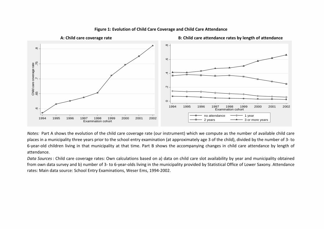
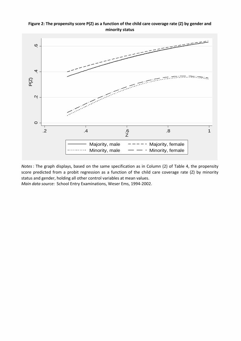
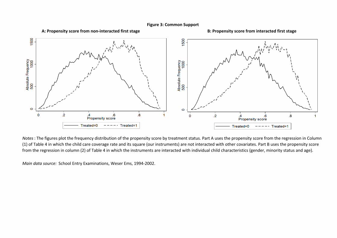
Main data source School Entry Examinations Weser Ems 1994-2002
A Propensity score from non-interacted first stage B Propensity score from interacted first stage
Notes The figures plot the frequency distribution of the propensity score by treatment status Part A uses the propensity score from the regression in Column
(1) of Table 4 in which the child care coverage rate and its square (our instruments) are not interacted with other covariates Part B uses the propensity score
from the regression in column (2) of Table 4 in which the instruments are interacted with individual child characteristics (gender minority status and age)
Figure 3 Common Support
A MTE curve at average values of the covariates
B MTE curves and weights for the treated and untreated
C MTE curve and weights for individuals shifted by the instrument
Notes Part A depicts the MTE curve for school readiness based on the specification in Columns (2) and (4) in Table 4 and
evaluated at mean values of the covariates The 90 confidence interval is based on bootstrapped standard errors clustered at
the municipality level Part B displays the MTE curves evaluated at covariate means for treated and untreated individuals and
the associated weights to compute the treatment effects on the treated and on the untreated (see equations (A2) and (A3) in
the appendix) Part C plots the MTE curve evaluated at covariate means of those children who are shifted into early child care
in response to changes in the instrument and the associated weights to compute the IV effect (see equation A4 in the
appendix) The two horizontal lines refer to the IV (2SLS) effect estimated from our data (dashed line) and aggregated over the
MTE curve (dotted line)
Figure 4 MTE curves for School Readiness
00
05
01
015
02
-2
-1
01
23
0 2 4 6 8 1U_D
MTE at X of treated MTE at X of untreated
TT weights TUT weights
-4
-2
02
4
0 2 4 6 8 1U_D
MTE 90 CI
Estimated Marginal Treatment Effects
00
05
01
015
02
IVw
eig
hts
-1
01
23
0 2 4 6 8 1U_D
MTE at X of compliers 2SLS estimate (07)
IV weights Weighted MTE (06)
Main data source School Entry Examinations Weser Ems 1994-2002
Notes The figure displays MTE curves for the outcome of school readiness evaluated at mean values of the
covariates The solid MTE curve refers to our baseline specification where the propensity score and its square is
included in equation (4) implying a linear MTE curve The figure also shows three additional MTE curves which
allow for richer patterns such as a U-shaped MTE curve one curve obtained from a semiparametric approach and
two curves based on specifications which include a cubic and quartic of the propensity score in equation (4)
Figure 5 MTE curves - functional form robustness checks-
4-
20
24
0 2 4 6 8 1U_D
Baseline Third order polynomial
Semiparametric Fourth order polynomial
Main data source School Entry Examinations Weser Ems 1994-2002
Notes Part A plots for our main outcome of school readiness the unobserved component of the outcome against
the unobserved resistance to treatment U_D separately for the treated (ie E(U_1 |U_D=u_D ) solid line) and
untreated (ie E(U_0 |U_D=u_D ) dashed line) state following Brinch Mogstad and Wiswall (2014) Panels B to F
repeat the exercise but use indicator variables for whether the child attended all routine postnatal medical
checkups (Part B) whether the postnatal checkup book is present at the examination (Part C) whether the mother
or father hold a college degree (Panels D and E) and whether the child is a single child (Part F) as dependent
variables to learn about how families with a low resistance to enroll their child in early child care differ from
families with a high resistance
Figure 6 Unobserved component of outcomes as a function of resistance
to treatment by treatment state
A School Readiness B Attendance at routine postnatal checkups
D College degree mother
E College degree father F Only child
C Postnatal checkup book present
-05
00
5
0 2 4 6 8 1U_D
Untreated Treated
-1
-05
00
51
0 2 4 6 8 1U_D
Untreated Treated
-4
-2
02
4
0 2 4 6 8 1U_D
Untreated Treated
-4
-2
02
4
0 2 4 6 8 1U_D
Untreated Treated
-4
-2
02
4
0 2 4 6 8 1U_D
Untreated Treated
-15
-1
-05
00
51
0 2 4 6 8 1U_D
Untreated Treated
Treatment variable
Child care attendance for at least 3 years 051
Selected Covariates
Minority 012
Female 049
Age at examination in months 7468
Outcomes
School Readiness 091
Predicted School Readiness
Minimum 031
5th percentile 074
10th percentile 079
25th percentile 087
50th percentile 093
75th percentile 097
90th percentile 098
Motor Skills 085
No Compensatory Sport Required 082
BMI 1561
Overweight (BMI gt 90th percentile) 008
Child to staff ratio (median) 944
Share of high educated among staff 009
Share of male staff 002
Data Sources Panel A School Entry Examinations Weser Ems 1994-2002
Panel B Social Security Records Weser-Ems 1990-1998 18-65 year olds
Panel A Individual characteristics
Panel B Child care quality indicators
Table 1 Descriptive statistics
Notes Panel A reports sample means of early child care attendance (our
treatment variable) of selected child characteristics and of child outcomes in
our sample Panel B displays sample means of child care quality indicators at
the municipality level referring to when the child was 3 years old
(1) (2)
Initial Coverage Rate -0437 -0478
(0175) (0190)
Median wage level 0000
(0002)
Share of high educated 0010
(0011)
Share of medium educated 0003
(0003)
Number of inhabitants in 1000 00001
(0000)
Share of immigrants in workforce 0014
(0007)
Share of women in workforce -00002
(0002)
Constant 0172 0202
(0016) (0026)
p-value for joint significance of other covariates
(excluding initial coverage rate)01855
Table 2 Determinants of the child care expansion
Notes The table investigates the determinants of the expansion in child care slots in
the municipality by regressing the change in the child care coverage rate in the
municipality between examination cohorts 1994 and 2001 on the initial coverage rate
for the 1994 cohort (Column (1)) and baseline municipality characteristics (Column (2))
The child care coverage rate is measured 3 years prior to the school entry examination
(ie when the cohort is approximately aged 3) In municipalities where information for
1994 or 2001 was missing we used the adjacent cohort The last row reports the p-
value for the hypothesis that municipality characteristics at baseline are jointly equal to
zero All coefficients on shares refer to one-percentage point changes in these shares
Bootstrapped standard errors clustered at the municipality level are reported in
parentheses Statistically significant at 010 level at 005 level at 001 level
Data Sources Child care coverage rates Own calculations based on a) data on child
care slot availability by year and municipality obtained from own data survey and b)
number of 3-6 year olds living in the municipality provided by Statistical Office of Lower
Saxony Median wage educational shares share of immigrants and women in
workforce Social Security Records Weser-Ems 1990-1998 18-65 year olds Number of
inhabitants Statistical Office of Lower Saxony
child care coverage rate
Age -000001
(00001)
Age Squared 00000
(00020)
Female -00003
(00002)
Minority child -000003
(00005)
Median wage level 0002
(0001)
Share of high educated 0009
(0011)
Share of medium educated -0002
(0002)
Number of inhabitants in 1000 0000
(0003)
Share of immigrants in workforce 0003
(0006)
Share of women working 0004
(0003)
Municipality dummies Yes
Cohort dummies Yes
p-value for joint significance of covariates 0254
Table 3 Balancing tests
Note The table reports coefficients from regressions of the instrument (the
child care coverage rate) on individual and municipality-level covariates
measured in the previous period conditional on municipality and cohort
dummies The child care coverage rate is measured 3 years prior to the school
entry examination (ie when the cohort is approximately aged 3) The last
row reports the p-value for the hypothesis that the covariates are jointly
equal to zero All coefficients on shares refer to one-percentage point changes
in these shares Bootstrapped standard errors clustered at the municipality
level are reported in parentheses Statistically significant at 010 level at
005 level at 001 level
Data sources Child care coverage rates Own calculations based on a) data on
child care slot availability by year and municipality obtained from own data
survey and b) number of 3-6 year olds living in the municipality provided by
Statistical Office of Lower Saxony Individual characteristics School Entry
Examinations Weser Ems 1994-2002 Median wage educational shares
share of immigrants and women in workforce Social Security Records Weser-
Ems 1990-1998 18-65 year olds Number of inhabitants Statistical Office of
Lower Saxony
noninteracted interacted noninteracted interacted
(1) (2) (3) (4)
Child care coverage rate 0324 0331
(0042) (0043)
Child care coverage rate squared -0243 -0220
(0086) (0108)
Female 0016 0014 0092 0092
(0002) (0003) (0009) (0009)
Minority -0211 -0198 -0123 -0120
(0010) (0011) (0021) (0020)
Propensity Score -0168 -0135
(0128) (0115)
Propensity Score squared 0239 0215
(0111) (0099)
Female Propensity Score -0087 -0086
(0014) (0014)
Minority Propensity Score 0120 0117
(0038) (0035)
Chi-squared for test of excluded instruments 3241 5683
p-value for test of excluded instruments 00000 00000
P-value for test of heterogeneity 0031 0029
N 135906 135906 135906 135906
Main data source School Entry Examinations Weser Ems 1994-2002
Table 4 Selection Equation and School Readiness Outcome Equation
Notes Columns (1) and (2) report average marginal effects from probit selection models where the
dependent variable is equal to 1 if the child attends public child care for at least three years (ldquofirst
stagerdquo) The child care coverage rate (our instrument) is measured relative to its overall mean In
Column (2) (ldquointeractedrdquo) the instrument in the probit selection equation is interacted with
individual characteristics (age gender ethnic minority status) interaction terms are not shown to
save space The coefficients on the child care coverage rate now refer to a German boy of average
age Columns (3) and (4) display estimates from the outcome equation (see equation (4) in the text)
where the dependent variable is an indicator variable for school readiness the two specifications
refer to the non-interacted and interacted probit selection models in Columns (1) and (2)
respectively Coefficients of regressors not interacted with the propensity score measure effects on
the outcome in the untreated state (ie β0 in equation (4)) whereas coefficients of regressors
interacted with the propensity score measure the difference of the effects between the treated and
the untreated state (β1-β0 in equation (4)) Further included controls not displayed in the table are
age and age squared and time-varying municipality sociodemographic characteristics in t-4 as well as
child care quality indicators in t-3 each interacted with the propensity score as well as cohort
dummies municipality dummies and birth month dummies (not interacted with the propensity
score) Bootstrapped standard errors clustered at the municipality level are reported in parentheses
Statistically significant at 010 level at 005 level at 001 level
Selection Equation Outcome equation
Child care gt=3 years School Readiness
(1) (2) (3) (4) (5)
BaselineInitial coverage
rate IV
Long
difference
Birth months Jan
- Jun
No quality
controls
ATE 0059 0130 -0005 0114 0073
(0072) (0105) (0084) (0092) (0072)
TT -0051 0008 -0152 -0020 -0072
(0080) (0109) (0118) (0128) (0082)
TUT 0173 0251 0160 0219 0223
(0085) (0120) (0113) (0106) (0082)
P-value for test of
heterogeneity0029 0028 0074 0119 0008
N 135906 146522 56942 66865 135906
Main data source School Entry Examinations Weser Ems 1994-2002
Table 5 Robustness checks
Notes The table reports for our main outcome variable of school readiness the average
treatment effect (ATE) the treatment effect on the treated (TT) treatment effect on the
untreated (TUT) and the p-value for a test of essential heterogeneity for various alternative
specifications Column (1) refers to the baseline regression from column (4) in Table 4 In Column
(2) the instrument is the initial child care coverage rate (for the oldest cohort in our data)
interacted with cohort dummies (and gender minority status and age as in column (4) in Table 4)
Column (3) only exploits variation across municipalities in the intensity of the child care expansion
and restricts the analysis to the (pooled) oldest and youngest examination cohorts 199495 vs
200102 In Column (4) the sample is restricted to children born in the first half of the calendar
year and in Column (5) child care quality controls are not included in the regressions The
reported P-value for a test of heterogeneity is a test for a non-zero slope of the MTE curve (see
also Section 22) Bootstrapped standard errors clustered at the municipality level are reported in
parentheses Statistically significant at 010 level at 005 level at 001 level
School
Readiness
Motor
Skills
No
Compensatory
Sport
Overweight Log BMI
Panel A Conventional Treatment Effects
ATE 0059 0018 0203 0017 0025
(0072) (0088) (0092) (0034) (0023)
TT -0051 0001 0099 0052 0045
(0080) (0118) (0119) (0045) (0028)
TUT 0173 0035 0308 -0019 0003
(0085) (0103) (0115) (0037) (0027)
P-value for test of heterogeneity 0029 0767 0214 0071 0152
Panel B Effects of child care quality characteristics
Above-median child to staff ratio 0005 0041 -0044 -0016 -0008
Propensity Score (0031) (0034) (0045) (0019) (0010)
Share of high educated among staff 0025 0465 -0229 -0003 0035
Propensity Score (0258) (0267) (0406) (0113) (0075)
Share of male staff Male child 0013 0028 0033 -0008 -0005
Propensity Score (0007) (0007) (0014) (0004) (0002)
Share of male staff Female child 0008 0015 0009 -0009 -0006
Propensity Score (0007) (0008) (0012) (0003) (0002)
Main data source School Entry Examinations Weser Ems 1994-2002
Table 6 Other Outcomes
Notes Panel A reports the average treatment effect (ATE) the treatment effect on the treated (TT)
treatment effect on the untreated (TUT) and the p-value for a test of essential heterogeneity for
five outcomes our main outcome of school readiness no motor skill problems no compensatory
sport required overweight measured as the BMI above the (age- and gender-specific) 90th
percentile and the log BMI Panel B displays coefficient estimates of the interaction terms between
child care quality indicators and the propensity score these terms measure how child care quality
influences the returns to early child care attendance Further included controls not displayed in the
table are age and age squared and time-varying municipality sociodemographic characteristics as
well as child care quality indicators (interacted with the propensity score) as well as cohort
dummies municipality dummies and birth month dummies (not interacted with the propensity
score) Coefficients on the interaction terms of share of male staff refer to a one-percentage point
change in this share Bootstrapped standard errors clustered at the municipality level are reported
in parentheses Statistically significant at 010 level at 005 level at 001 level
1994 2000
public child care 412 758
only family care (parents and other relatives) 583 227
exclusively maternal care 393 188
informal care (nanny other non-relatives) 12 15
Maternal labour force participation (3-year-olds) 312 387
public child care children of working mothers 429 815
public child care children of non-working mothers 405 722
Table 7 Child care arrangements for 3-year-olds 1994 and 2000
Notes The table provides for the years 1994 and 2000 information on child care
arrangements of 3-year-olds distinguishing between public child care only family care by
parents or grandparents only maternal care and care by a child-minder or nanny The table
also reports labor force participation rates of mothers of 3-year-olds as well as public child
care attendance rates of 3-year-olds separately by the motherrsquos labor force status
Data source Own calculation based on Family Survey from the German Youth Institute (DJI)
Munich 2nd and 3rd wave (1994 and 2000) The sample refers to 3-year-olds in West
Germany and consists of 262 children in 1994 and 354 children in 2000
(1) (2) (3)
PRTE Baseline Policy
(1) Bring 2002 P(Z) to 9 by adding 275 0160 067 090
(0085)
(2) Bring 2002 P(Z) to 9 by multiplying 15 0165 067 090
(0087)
(3) Lift 2002 cohorts coverage rate (Z) to 1 if lt1 0123 067 071
(0077)
(4) Add 04 to 2002 cohorts coverage rate (Z) 0141 067 072
(0086)
Main data source School Entry Examinations Weser Ems 1994-2002
Propensity score
Table 8 Policy-relevant treatment effects
Notes The table reports in Column (1) policy-relevant treatment effects (PRTE) per net child shifted for four
different policies In Rows (1) and (2) we simulate a policy which brings the average early attendance rate (or
equivalently the propensity score) from its 2002 level of 67 to a level of 9 by adding a constant of 0275 to
each childrsquos 2002 propensity score (Row (1)) or by multiplying each childrsquos 2002 propensity score by a
constant of 15 (Row (2)) In Rows (3) and (4) we instead directly manipulate the 2002 cohorts child care
coverage rate (ie the coverage rate measured in 1999 when the 2002 cohort was 3 years oldndashour
instrument) In Row (3) we set the coverage rate to 1 for municipalities in which it is below 1 in Row (4) we
instead add a constant of 04 to the coverage rate allowing for coverage rates greater than 1 in some
municipalities Columns (2) and (3) show the increase in the propensity score which each policy induces
Estimates refer to our baseline specification displayed in Columns (2) and (4) of Table 4 and Panel A of Figure
4 Bootstrapped standard errors clustered at the municipality level are reported in parentheses Statistically
significant at 010 level at 005 level at 001 level
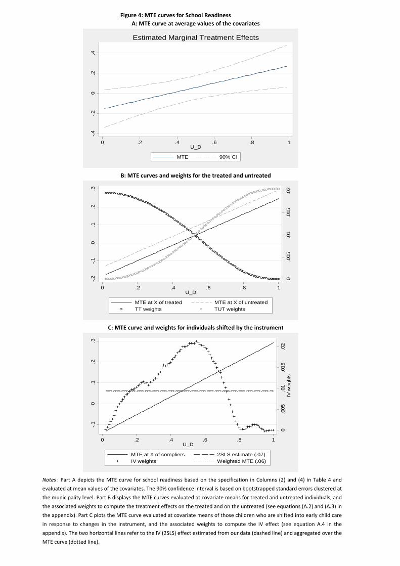

Main data source School Entry Examinations Weser Ems 1994-2002
Notes The figure displays MTE curves for the outcome of school readiness evaluated at mean values of the
covariates The solid MTE curve refers to our baseline specification where the propensity score and its square is
included in equation (4) implying a linear MTE curve The figure also shows three additional MTE curves which
allow for richer patterns such as a U-shaped MTE curve one curve obtained from a semiparametric approach and
two curves based on specifications which include a cubic and quartic of the propensity score in equation (4)
Figure 5 MTE curves - functional form robustness checks-
4-
20
24
0 2 4 6 8 1U_D
Baseline Third order polynomial
Semiparametric Fourth order polynomial
Main data source School Entry Examinations Weser Ems 1994-2002
Notes Part A plots for our main outcome of school readiness the unobserved component of the outcome against
the unobserved resistance to treatment U_D separately for the treated (ie E(U_1 |U_D=u_D ) solid line) and
untreated (ie E(U_0 |U_D=u_D ) dashed line) state following Brinch Mogstad and Wiswall (2014) Panels B to F
repeat the exercise but use indicator variables for whether the child attended all routine postnatal medical
checkups (Part B) whether the postnatal checkup book is present at the examination (Part C) whether the mother
or father hold a college degree (Panels D and E) and whether the child is a single child (Part F) as dependent
variables to learn about how families with a low resistance to enroll their child in early child care differ from
families with a high resistance
Figure 6 Unobserved component of outcomes as a function of resistance
to treatment by treatment state
A School Readiness B Attendance at routine postnatal checkups
D College degree mother
E College degree father F Only child
C Postnatal checkup book present
-05
00
5
0 2 4 6 8 1U_D
Untreated Treated
-1
-05
00
51
0 2 4 6 8 1U_D
Untreated Treated
-4
-2
02
4
0 2 4 6 8 1U_D
Untreated Treated
-4
-2
02
4
0 2 4 6 8 1U_D
Untreated Treated
-4
-2
02
4
0 2 4 6 8 1U_D
Untreated Treated
-15
-1
-05
00
51
0 2 4 6 8 1U_D
Untreated Treated
Treatment variable
Child care attendance for at least 3 years 051
Selected Covariates
Minority 012
Female 049
Age at examination in months 7468
Outcomes
School Readiness 091
Predicted School Readiness
Minimum 031
5th percentile 074
10th percentile 079
25th percentile 087
50th percentile 093
75th percentile 097
90th percentile 098
Motor Skills 085
No Compensatory Sport Required 082
BMI 1561
Overweight (BMI gt 90th percentile) 008
Child to staff ratio (median) 944
Share of high educated among staff 009
Share of male staff 002
Data Sources Panel A School Entry Examinations Weser Ems 1994-2002
Panel B Social Security Records Weser-Ems 1990-1998 18-65 year olds
Panel A Individual characteristics
Panel B Child care quality indicators
Table 1 Descriptive statistics
Notes Panel A reports sample means of early child care attendance (our
treatment variable) of selected child characteristics and of child outcomes in
our sample Panel B displays sample means of child care quality indicators at
the municipality level referring to when the child was 3 years old
(1) (2)
Initial Coverage Rate -0437 -0478
(0175) (0190)
Median wage level 0000
(0002)
Share of high educated 0010
(0011)
Share of medium educated 0003
(0003)
Number of inhabitants in 1000 00001
(0000)
Share of immigrants in workforce 0014
(0007)
Share of women in workforce -00002
(0002)
Constant 0172 0202
(0016) (0026)
p-value for joint significance of other covariates
(excluding initial coverage rate)01855
Table 2 Determinants of the child care expansion
Notes The table investigates the determinants of the expansion in child care slots in
the municipality by regressing the change in the child care coverage rate in the
municipality between examination cohorts 1994 and 2001 on the initial coverage rate
for the 1994 cohort (Column (1)) and baseline municipality characteristics (Column (2))
The child care coverage rate is measured 3 years prior to the school entry examination
(ie when the cohort is approximately aged 3) In municipalities where information for
1994 or 2001 was missing we used the adjacent cohort The last row reports the p-
value for the hypothesis that municipality characteristics at baseline are jointly equal to
zero All coefficients on shares refer to one-percentage point changes in these shares
Bootstrapped standard errors clustered at the municipality level are reported in
parentheses Statistically significant at 010 level at 005 level at 001 level
Data Sources Child care coverage rates Own calculations based on a) data on child
care slot availability by year and municipality obtained from own data survey and b)
number of 3-6 year olds living in the municipality provided by Statistical Office of Lower
Saxony Median wage educational shares share of immigrants and women in
workforce Social Security Records Weser-Ems 1990-1998 18-65 year olds Number of
inhabitants Statistical Office of Lower Saxony
child care coverage rate
Age -000001
(00001)
Age Squared 00000
(00020)
Female -00003
(00002)
Minority child -000003
(00005)
Median wage level 0002
(0001)
Share of high educated 0009
(0011)
Share of medium educated -0002
(0002)
Number of inhabitants in 1000 0000
(0003)
Share of immigrants in workforce 0003
(0006)
Share of women working 0004
(0003)
Municipality dummies Yes
Cohort dummies Yes
p-value for joint significance of covariates 0254
Table 3 Balancing tests
Note The table reports coefficients from regressions of the instrument (the
child care coverage rate) on individual and municipality-level covariates
measured in the previous period conditional on municipality and cohort
dummies The child care coverage rate is measured 3 years prior to the school
entry examination (ie when the cohort is approximately aged 3) The last
row reports the p-value for the hypothesis that the covariates are jointly
equal to zero All coefficients on shares refer to one-percentage point changes
in these shares Bootstrapped standard errors clustered at the municipality
level are reported in parentheses Statistically significant at 010 level at
005 level at 001 level
Data sources Child care coverage rates Own calculations based on a) data on
child care slot availability by year and municipality obtained from own data
survey and b) number of 3-6 year olds living in the municipality provided by
Statistical Office of Lower Saxony Individual characteristics School Entry
Examinations Weser Ems 1994-2002 Median wage educational shares
share of immigrants and women in workforce Social Security Records Weser-
Ems 1990-1998 18-65 year olds Number of inhabitants Statistical Office of
Lower Saxony
noninteracted interacted noninteracted interacted
(1) (2) (3) (4)
Child care coverage rate 0324 0331
(0042) (0043)
Child care coverage rate squared -0243 -0220
(0086) (0108)
Female 0016 0014 0092 0092
(0002) (0003) (0009) (0009)
Minority -0211 -0198 -0123 -0120
(0010) (0011) (0021) (0020)
Propensity Score -0168 -0135
(0128) (0115)
Propensity Score squared 0239 0215
(0111) (0099)
Female Propensity Score -0087 -0086
(0014) (0014)
Minority Propensity Score 0120 0117
(0038) (0035)
Chi-squared for test of excluded instruments 3241 5683
p-value for test of excluded instruments 00000 00000
P-value for test of heterogeneity 0031 0029
N 135906 135906 135906 135906
Main data source School Entry Examinations Weser Ems 1994-2002
Table 4 Selection Equation and School Readiness Outcome Equation
Notes Columns (1) and (2) report average marginal effects from probit selection models where the
dependent variable is equal to 1 if the child attends public child care for at least three years (ldquofirst
stagerdquo) The child care coverage rate (our instrument) is measured relative to its overall mean In
Column (2) (ldquointeractedrdquo) the instrument in the probit selection equation is interacted with
individual characteristics (age gender ethnic minority status) interaction terms are not shown to
save space The coefficients on the child care coverage rate now refer to a German boy of average
age Columns (3) and (4) display estimates from the outcome equation (see equation (4) in the text)
where the dependent variable is an indicator variable for school readiness the two specifications
refer to the non-interacted and interacted probit selection models in Columns (1) and (2)
respectively Coefficients of regressors not interacted with the propensity score measure effects on
the outcome in the untreated state (ie β0 in equation (4)) whereas coefficients of regressors
interacted with the propensity score measure the difference of the effects between the treated and
the untreated state (β1-β0 in equation (4)) Further included controls not displayed in the table are
age and age squared and time-varying municipality sociodemographic characteristics in t-4 as well as
child care quality indicators in t-3 each interacted with the propensity score as well as cohort
dummies municipality dummies and birth month dummies (not interacted with the propensity
score) Bootstrapped standard errors clustered at the municipality level are reported in parentheses
Statistically significant at 010 level at 005 level at 001 level
Selection Equation Outcome equation
Child care gt=3 years School Readiness
(1) (2) (3) (4) (5)
BaselineInitial coverage
rate IV
Long
difference
Birth months Jan
- Jun
No quality
controls
ATE 0059 0130 -0005 0114 0073
(0072) (0105) (0084) (0092) (0072)
TT -0051 0008 -0152 -0020 -0072
(0080) (0109) (0118) (0128) (0082)
TUT 0173 0251 0160 0219 0223
(0085) (0120) (0113) (0106) (0082)
P-value for test of
heterogeneity0029 0028 0074 0119 0008
N 135906 146522 56942 66865 135906
Main data source School Entry Examinations Weser Ems 1994-2002
Table 5 Robustness checks
Notes The table reports for our main outcome variable of school readiness the average
treatment effect (ATE) the treatment effect on the treated (TT) treatment effect on the
untreated (TUT) and the p-value for a test of essential heterogeneity for various alternative
specifications Column (1) refers to the baseline regression from column (4) in Table 4 In Column
(2) the instrument is the initial child care coverage rate (for the oldest cohort in our data)
interacted with cohort dummies (and gender minority status and age as in column (4) in Table 4)
Column (3) only exploits variation across municipalities in the intensity of the child care expansion
and restricts the analysis to the (pooled) oldest and youngest examination cohorts 199495 vs
200102 In Column (4) the sample is restricted to children born in the first half of the calendar
year and in Column (5) child care quality controls are not included in the regressions The
reported P-value for a test of heterogeneity is a test for a non-zero slope of the MTE curve (see
also Section 22) Bootstrapped standard errors clustered at the municipality level are reported in
parentheses Statistically significant at 010 level at 005 level at 001 level
School
Readiness
Motor
Skills
No
Compensatory
Sport
Overweight Log BMI
Panel A Conventional Treatment Effects
ATE 0059 0018 0203 0017 0025
(0072) (0088) (0092) (0034) (0023)
TT -0051 0001 0099 0052 0045
(0080) (0118) (0119) (0045) (0028)
TUT 0173 0035 0308 -0019 0003
(0085) (0103) (0115) (0037) (0027)
P-value for test of heterogeneity 0029 0767 0214 0071 0152
Panel B Effects of child care quality characteristics
Above-median child to staff ratio 0005 0041 -0044 -0016 -0008
Propensity Score (0031) (0034) (0045) (0019) (0010)
Share of high educated among staff 0025 0465 -0229 -0003 0035
Propensity Score (0258) (0267) (0406) (0113) (0075)
Share of male staff Male child 0013 0028 0033 -0008 -0005
Propensity Score (0007) (0007) (0014) (0004) (0002)
Share of male staff Female child 0008 0015 0009 -0009 -0006
Propensity Score (0007) (0008) (0012) (0003) (0002)
Main data source School Entry Examinations Weser Ems 1994-2002
Table 6 Other Outcomes
Notes Panel A reports the average treatment effect (ATE) the treatment effect on the treated (TT)
treatment effect on the untreated (TUT) and the p-value for a test of essential heterogeneity for
five outcomes our main outcome of school readiness no motor skill problems no compensatory
sport required overweight measured as the BMI above the (age- and gender-specific) 90th
percentile and the log BMI Panel B displays coefficient estimates of the interaction terms between
child care quality indicators and the propensity score these terms measure how child care quality
influences the returns to early child care attendance Further included controls not displayed in the
table are age and age squared and time-varying municipality sociodemographic characteristics as
well as child care quality indicators (interacted with the propensity score) as well as cohort
dummies municipality dummies and birth month dummies (not interacted with the propensity
score) Coefficients on the interaction terms of share of male staff refer to a one-percentage point
change in this share Bootstrapped standard errors clustered at the municipality level are reported
in parentheses Statistically significant at 010 level at 005 level at 001 level
1994 2000
public child care 412 758
only family care (parents and other relatives) 583 227
exclusively maternal care 393 188
informal care (nanny other non-relatives) 12 15
Maternal labour force participation (3-year-olds) 312 387
public child care children of working mothers 429 815
public child care children of non-working mothers 405 722
Table 7 Child care arrangements for 3-year-olds 1994 and 2000
Notes The table provides for the years 1994 and 2000 information on child care
arrangements of 3-year-olds distinguishing between public child care only family care by
parents or grandparents only maternal care and care by a child-minder or nanny The table
also reports labor force participation rates of mothers of 3-year-olds as well as public child
care attendance rates of 3-year-olds separately by the motherrsquos labor force status
Data source Own calculation based on Family Survey from the German Youth Institute (DJI)
Munich 2nd and 3rd wave (1994 and 2000) The sample refers to 3-year-olds in West
Germany and consists of 262 children in 1994 and 354 children in 2000
(1) (2) (3)
PRTE Baseline Policy
(1) Bring 2002 P(Z) to 9 by adding 275 0160 067 090
(0085)
(2) Bring 2002 P(Z) to 9 by multiplying 15 0165 067 090
(0087)
(3) Lift 2002 cohorts coverage rate (Z) to 1 if lt1 0123 067 071
(0077)
(4) Add 04 to 2002 cohorts coverage rate (Z) 0141 067 072
(0086)
Main data source School Entry Examinations Weser Ems 1994-2002
Propensity score
Table 8 Policy-relevant treatment effects
Notes The table reports in Column (1) policy-relevant treatment effects (PRTE) per net child shifted for four
different policies In Rows (1) and (2) we simulate a policy which brings the average early attendance rate (or
equivalently the propensity score) from its 2002 level of 67 to a level of 9 by adding a constant of 0275 to
each childrsquos 2002 propensity score (Row (1)) or by multiplying each childrsquos 2002 propensity score by a
constant of 15 (Row (2)) In Rows (3) and (4) we instead directly manipulate the 2002 cohorts child care
coverage rate (ie the coverage rate measured in 1999 when the 2002 cohort was 3 years oldndashour
instrument) In Row (3) we set the coverage rate to 1 for municipalities in which it is below 1 in Row (4) we
instead add a constant of 04 to the coverage rate allowing for coverage rates greater than 1 in some
municipalities Columns (2) and (3) show the increase in the propensity score which each policy induces
Estimates refer to our baseline specification displayed in Columns (2) and (4) of Table 4 and Panel A of Figure
4 Bootstrapped standard errors clustered at the municipality level are reported in parentheses Statistically
significant at 010 level at 005 level at 001 level
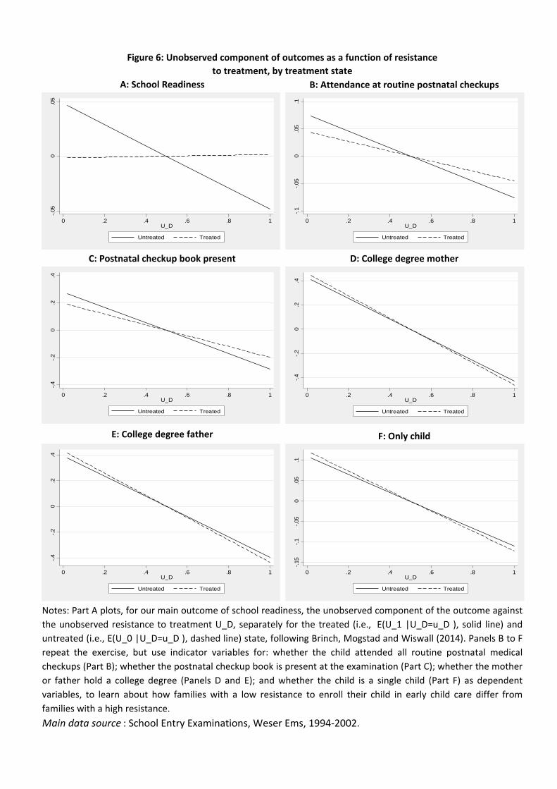
Main data source School Entry Examinations Weser Ems 1994-2002
Notes Part A plots for our main outcome of school readiness the unobserved component of the outcome against
the unobserved resistance to treatment U_D separately for the treated (ie E(U_1 |U_D=u_D ) solid line) and
untreated (ie E(U_0 |U_D=u_D ) dashed line) state following Brinch Mogstad and Wiswall (2014) Panels B to F
repeat the exercise but use indicator variables for whether the child attended all routine postnatal medical
checkups (Part B) whether the postnatal checkup book is present at the examination (Part C) whether the mother
or father hold a college degree (Panels D and E) and whether the child is a single child (Part F) as dependent
variables to learn about how families with a low resistance to enroll their child in early child care differ from
families with a high resistance
Figure 6 Unobserved component of outcomes as a function of resistance
to treatment by treatment state
A School Readiness B Attendance at routine postnatal checkups
D College degree mother
E College degree father F Only child
C Postnatal checkup book present
-05
00
5
0 2 4 6 8 1U_D
Untreated Treated
-1
-05
00
51
0 2 4 6 8 1U_D
Untreated Treated
-4
-2
02
4
0 2 4 6 8 1U_D
Untreated Treated
-4
-2
02
4
0 2 4 6 8 1U_D
Untreated Treated
-4
-2
02
4
0 2 4 6 8 1U_D
Untreated Treated
-15
-1
-05
00
51
0 2 4 6 8 1U_D
Untreated Treated
Treatment variable
Child care attendance for at least 3 years 051
Selected Covariates
Minority 012
Female 049
Age at examination in months 7468
Outcomes
School Readiness 091
Predicted School Readiness
Minimum 031
5th percentile 074
10th percentile 079
25th percentile 087
50th percentile 093
75th percentile 097
90th percentile 098
Motor Skills 085
No Compensatory Sport Required 082
BMI 1561
Overweight (BMI gt 90th percentile) 008
Child to staff ratio (median) 944
Share of high educated among staff 009
Share of male staff 002
Data Sources Panel A School Entry Examinations Weser Ems 1994-2002
Panel B Social Security Records Weser-Ems 1990-1998 18-65 year olds
Panel A Individual characteristics
Panel B Child care quality indicators
Table 1 Descriptive statistics
Notes Panel A reports sample means of early child care attendance (our
treatment variable) of selected child characteristics and of child outcomes in
our sample Panel B displays sample means of child care quality indicators at
the municipality level referring to when the child was 3 years old
(1) (2)
Initial Coverage Rate -0437 -0478
(0175) (0190)
Median wage level 0000
(0002)
Share of high educated 0010
(0011)
Share of medium educated 0003
(0003)
Number of inhabitants in 1000 00001
(0000)
Share of immigrants in workforce 0014
(0007)
Share of women in workforce -00002
(0002)
Constant 0172 0202
(0016) (0026)
p-value for joint significance of other covariates
(excluding initial coverage rate)01855
Table 2 Determinants of the child care expansion
Notes The table investigates the determinants of the expansion in child care slots in
the municipality by regressing the change in the child care coverage rate in the
municipality between examination cohorts 1994 and 2001 on the initial coverage rate
for the 1994 cohort (Column (1)) and baseline municipality characteristics (Column (2))
The child care coverage rate is measured 3 years prior to the school entry examination
(ie when the cohort is approximately aged 3) In municipalities where information for
1994 or 2001 was missing we used the adjacent cohort The last row reports the p-
value for the hypothesis that municipality characteristics at baseline are jointly equal to
zero All coefficients on shares refer to one-percentage point changes in these shares
Bootstrapped standard errors clustered at the municipality level are reported in
parentheses Statistically significant at 010 level at 005 level at 001 level
Data Sources Child care coverage rates Own calculations based on a) data on child
care slot availability by year and municipality obtained from own data survey and b)
number of 3-6 year olds living in the municipality provided by Statistical Office of Lower
Saxony Median wage educational shares share of immigrants and women in
workforce Social Security Records Weser-Ems 1990-1998 18-65 year olds Number of
inhabitants Statistical Office of Lower Saxony
child care coverage rate
Age -000001
(00001)
Age Squared 00000
(00020)
Female -00003
(00002)
Minority child -000003
(00005)
Median wage level 0002
(0001)
Share of high educated 0009
(0011)
Share of medium educated -0002
(0002)
Number of inhabitants in 1000 0000
(0003)
Share of immigrants in workforce 0003
(0006)
Share of women working 0004
(0003)
Municipality dummies Yes
Cohort dummies Yes
p-value for joint significance of covariates 0254
Table 3 Balancing tests
Note The table reports coefficients from regressions of the instrument (the
child care coverage rate) on individual and municipality-level covariates
measured in the previous period conditional on municipality and cohort
dummies The child care coverage rate is measured 3 years prior to the school
entry examination (ie when the cohort is approximately aged 3) The last
row reports the p-value for the hypothesis that the covariates are jointly
equal to zero All coefficients on shares refer to one-percentage point changes
in these shares Bootstrapped standard errors clustered at the municipality
level are reported in parentheses Statistically significant at 010 level at
005 level at 001 level
Data sources Child care coverage rates Own calculations based on a) data on
child care slot availability by year and municipality obtained from own data
survey and b) number of 3-6 year olds living in the municipality provided by
Statistical Office of Lower Saxony Individual characteristics School Entry
Examinations Weser Ems 1994-2002 Median wage educational shares
share of immigrants and women in workforce Social Security Records Weser-
Ems 1990-1998 18-65 year olds Number of inhabitants Statistical Office of
Lower Saxony
noninteracted interacted noninteracted interacted
(1) (2) (3) (4)
Child care coverage rate 0324 0331
(0042) (0043)
Child care coverage rate squared -0243 -0220
(0086) (0108)
Female 0016 0014 0092 0092
(0002) (0003) (0009) (0009)
Minority -0211 -0198 -0123 -0120
(0010) (0011) (0021) (0020)
Propensity Score -0168 -0135
(0128) (0115)
Propensity Score squared 0239 0215
(0111) (0099)
Female Propensity Score -0087 -0086
(0014) (0014)
Minority Propensity Score 0120 0117
(0038) (0035)
Chi-squared for test of excluded instruments 3241 5683
p-value for test of excluded instruments 00000 00000
P-value for test of heterogeneity 0031 0029
N 135906 135906 135906 135906
Main data source School Entry Examinations Weser Ems 1994-2002
Table 4 Selection Equation and School Readiness Outcome Equation
Notes Columns (1) and (2) report average marginal effects from probit selection models where the
dependent variable is equal to 1 if the child attends public child care for at least three years (ldquofirst
stagerdquo) The child care coverage rate (our instrument) is measured relative to its overall mean In
Column (2) (ldquointeractedrdquo) the instrument in the probit selection equation is interacted with
individual characteristics (age gender ethnic minority status) interaction terms are not shown to
save space The coefficients on the child care coverage rate now refer to a German boy of average
age Columns (3) and (4) display estimates from the outcome equation (see equation (4) in the text)
where the dependent variable is an indicator variable for school readiness the two specifications
refer to the non-interacted and interacted probit selection models in Columns (1) and (2)
respectively Coefficients of regressors not interacted with the propensity score measure effects on
the outcome in the untreated state (ie β0 in equation (4)) whereas coefficients of regressors
interacted with the propensity score measure the difference of the effects between the treated and
the untreated state (β1-β0 in equation (4)) Further included controls not displayed in the table are
age and age squared and time-varying municipality sociodemographic characteristics in t-4 as well as
child care quality indicators in t-3 each interacted with the propensity score as well as cohort
dummies municipality dummies and birth month dummies (not interacted with the propensity
score) Bootstrapped standard errors clustered at the municipality level are reported in parentheses
Statistically significant at 010 level at 005 level at 001 level
Selection Equation Outcome equation
Child care gt=3 years School Readiness
(1) (2) (3) (4) (5)
BaselineInitial coverage
rate IV
Long
difference
Birth months Jan
- Jun
No quality
controls
ATE 0059 0130 -0005 0114 0073
(0072) (0105) (0084) (0092) (0072)
TT -0051 0008 -0152 -0020 -0072
(0080) (0109) (0118) (0128) (0082)
TUT 0173 0251 0160 0219 0223
(0085) (0120) (0113) (0106) (0082)
P-value for test of
heterogeneity0029 0028 0074 0119 0008
N 135906 146522 56942 66865 135906
Main data source School Entry Examinations Weser Ems 1994-2002
Table 5 Robustness checks
Notes The table reports for our main outcome variable of school readiness the average
treatment effect (ATE) the treatment effect on the treated (TT) treatment effect on the
untreated (TUT) and the p-value for a test of essential heterogeneity for various alternative
specifications Column (1) refers to the baseline regression from column (4) in Table 4 In Column
(2) the instrument is the initial child care coverage rate (for the oldest cohort in our data)
interacted with cohort dummies (and gender minority status and age as in column (4) in Table 4)
Column (3) only exploits variation across municipalities in the intensity of the child care expansion
and restricts the analysis to the (pooled) oldest and youngest examination cohorts 199495 vs
200102 In Column (4) the sample is restricted to children born in the first half of the calendar
year and in Column (5) child care quality controls are not included in the regressions The
reported P-value for a test of heterogeneity is a test for a non-zero slope of the MTE curve (see
also Section 22) Bootstrapped standard errors clustered at the municipality level are reported in
parentheses Statistically significant at 010 level at 005 level at 001 level
School
Readiness
Motor
Skills
No
Compensatory
Sport
Overweight Log BMI
Panel A Conventional Treatment Effects
ATE 0059 0018 0203 0017 0025
(0072) (0088) (0092) (0034) (0023)
TT -0051 0001 0099 0052 0045
(0080) (0118) (0119) (0045) (0028)
TUT 0173 0035 0308 -0019 0003
(0085) (0103) (0115) (0037) (0027)
P-value for test of heterogeneity 0029 0767 0214 0071 0152
Panel B Effects of child care quality characteristics
Above-median child to staff ratio 0005 0041 -0044 -0016 -0008
Propensity Score (0031) (0034) (0045) (0019) (0010)
Share of high educated among staff 0025 0465 -0229 -0003 0035
Propensity Score (0258) (0267) (0406) (0113) (0075)
Share of male staff Male child 0013 0028 0033 -0008 -0005
Propensity Score (0007) (0007) (0014) (0004) (0002)
Share of male staff Female child 0008 0015 0009 -0009 -0006
Propensity Score (0007) (0008) (0012) (0003) (0002)
Main data source School Entry Examinations Weser Ems 1994-2002
Table 6 Other Outcomes
Notes Panel A reports the average treatment effect (ATE) the treatment effect on the treated (TT)
treatment effect on the untreated (TUT) and the p-value for a test of essential heterogeneity for
five outcomes our main outcome of school readiness no motor skill problems no compensatory
sport required overweight measured as the BMI above the (age- and gender-specific) 90th
percentile and the log BMI Panel B displays coefficient estimates of the interaction terms between
child care quality indicators and the propensity score these terms measure how child care quality
influences the returns to early child care attendance Further included controls not displayed in the
table are age and age squared and time-varying municipality sociodemographic characteristics as
well as child care quality indicators (interacted with the propensity score) as well as cohort
dummies municipality dummies and birth month dummies (not interacted with the propensity
score) Coefficients on the interaction terms of share of male staff refer to a one-percentage point
change in this share Bootstrapped standard errors clustered at the municipality level are reported
in parentheses Statistically significant at 010 level at 005 level at 001 level
1994 2000
public child care 412 758
only family care (parents and other relatives) 583 227
exclusively maternal care 393 188
informal care (nanny other non-relatives) 12 15
Maternal labour force participation (3-year-olds) 312 387
public child care children of working mothers 429 815
public child care children of non-working mothers 405 722
Table 7 Child care arrangements for 3-year-olds 1994 and 2000
Notes The table provides for the years 1994 and 2000 information on child care
arrangements of 3-year-olds distinguishing between public child care only family care by
parents or grandparents only maternal care and care by a child-minder or nanny The table
also reports labor force participation rates of mothers of 3-year-olds as well as public child
care attendance rates of 3-year-olds separately by the motherrsquos labor force status
Data source Own calculation based on Family Survey from the German Youth Institute (DJI)
Munich 2nd and 3rd wave (1994 and 2000) The sample refers to 3-year-olds in West
Germany and consists of 262 children in 1994 and 354 children in 2000
(1) (2) (3)
PRTE Baseline Policy
(1) Bring 2002 P(Z) to 9 by adding 275 0160 067 090
(0085)
(2) Bring 2002 P(Z) to 9 by multiplying 15 0165 067 090
(0087)
(3) Lift 2002 cohorts coverage rate (Z) to 1 if lt1 0123 067 071
(0077)
(4) Add 04 to 2002 cohorts coverage rate (Z) 0141 067 072
(0086)
Main data source School Entry Examinations Weser Ems 1994-2002
Propensity score
Table 8 Policy-relevant treatment effects
Notes The table reports in Column (1) policy-relevant treatment effects (PRTE) per net child shifted for four
different policies In Rows (1) and (2) we simulate a policy which brings the average early attendance rate (or
equivalently the propensity score) from its 2002 level of 67 to a level of 9 by adding a constant of 0275 to
each childrsquos 2002 propensity score (Row (1)) or by multiplying each childrsquos 2002 propensity score by a
constant of 15 (Row (2)) In Rows (3) and (4) we instead directly manipulate the 2002 cohorts child care
coverage rate (ie the coverage rate measured in 1999 when the 2002 cohort was 3 years oldndashour
instrument) In Row (3) we set the coverage rate to 1 for municipalities in which it is below 1 in Row (4) we
instead add a constant of 04 to the coverage rate allowing for coverage rates greater than 1 in some
municipalities Columns (2) and (3) show the increase in the propensity score which each policy induces
Estimates refer to our baseline specification displayed in Columns (2) and (4) of Table 4 and Panel A of Figure
4 Bootstrapped standard errors clustered at the municipality level are reported in parentheses Statistically
significant at 010 level at 005 level at 001 level


![arXiv:2006.03023v2 [cs.CY] 5 Jun 2020g.goodell@ucl.ac.uk Hazem Danny Al-Nakib hnakib@cs.ucl.ac.uk Paolo Tasca p.tasca@ucl.ac.uk University College London Centre for Blockchain Technologies](https://img.pdfslide.net/doc/110x75/5f739644a35b916dfb64802d/arxiv200603023v2-cscy-5-jun-2020-ggoodelluclacuk-hazem-danny-al-nakib-hnakibcsuclacuk.jpg)


![k.friston@ucl.ac.uk arXiv:1705.08265v1 [q-bio.NC] 18 May 2017Karl Friston Wellcome Trust Centre for Neuroimaging University College London k.friston@ucl.ac.uk Abstract Theoretical](https://img.pdfslide.net/doc/110x75/5ea37e64bca8250b21594868/kfristonuclacuk-arxiv170508265v1-q-bionc-18-may-2017-karl-friston-wellcome.jpg)


![b.roads,b.love @ucl.ac.uk arXiv:2011.11015v1 [cs.CV] 22](https://img.pdfslide.net/doc/110x75/61b26b1a8031d6711d14734d/broadsblove-uclacuk-arxiv201111015v1-cscv-22-.jpg)