Why are ethnically divided countries poor?

Available online at www.sciencedirect.com

Journal of Macroeconomics 30 (2008) 1–18

www.elsevier.com/locate/jmacro

Why are ethnically divided countries poor?

Benjamin Bridgman *

Bureau of Economic Analysis, Department of Commerce, Washington, DC 20230, United States

Received 27 July 2005; accepted 14 August 2006Available online 19 April 2007

Abstract

Ethnic divisions are associated with poor economic performance. This paper develops a model ofethnic conflict and finds that it is a significant source of poverty. Ethnic divisions lead the govern-ment to make ethnic transfers, which distort investment decisions, and lead to civil war becausegroups fight for control of the government. The simulated model generates the income gap betweencountries with and without ethnic divisions. Redistribution is the most important source of poverty.War costs cause less than a quarter of the reduction in income and divided countries are poorer evenif they do not fight a war.Published by Elsevier Inc.

JEL classification: O11

Keywords: Ethnic divisions; Economic growth; Civil war

1. Introduction

Ethnically divided countries tend to be poorer than homogeneous countries. Beginningwith Easterly and Levine (1997), an empirical literature finds that countries with ethnicdivisions tend to have lower levels of income and slower economic growth. As a result,measures of ethnic divisions are often included in cross-country studies of economicdevelopment.

0164-0704/$ - see front matter Published by Elsevier Inc.

doi:10.1016/j.jmacro.2006.08.007

* Tel.: +1 202 606 9991; fax: +1 202 606 5366.E-mail address: [email protected]

mailto:[email protected]

2 B. Bridgman / Journal of Macroeconomics 30 (2008) 1–18

Why ethnic divisions lead to lower income remains an open issue. Many researchershave focussed on conflict between ethnic groups. Ethnic groups do not agree on policies,leading to lower public goods provision (Alesina et al., 1999). They do not trust each otherenough to extend credit to outsiders (Fafchamps, 2000). The conflict is often so bitter thatthey fight civil wars (Elbawadi and Sambanis, 2002).

While there is strong evidence that such conflicts occur, they have not yet been shown tobe a quantitatively important source of international income differences. This paper devel-ops and parameterizes a model of ethnic conflict and finds that this conflict is a significantsource of poverty in countries with ethnic divisions.

The model incorporates ethnic divisions into a dynamic growth model. As in standardgrowth models, households invest to accumulate capital. They are divided into ethnicgroups and the government is controlled by one of these groups. The government cantax output and make transfers to members of the ruling group. Other groups can resistthis expropriation by raising armies to fight for control of the government. Followingthe theoretical literature analyzing conflict, such as Hirshleifer (1991) and Grossman(1991), military success is influenced by the relative sizes of group’s armies. The group withthe largest army has the best chance of winning.

The simulated model generates the empirical income gap between countries with andwithout ethnic divisions. Ethnic redistribution directly lowers income by reducing capitalaccumulation. Capital owned by members of the non-ruling groups is taxed to pay fortransfers to the ruling group, which distorts investment decisions. These distortions arestronger in divided countries since the ruling ethnic group is smaller and a larger portionof the population is expropriated.

Redistribution also indirectly reduces income by causing civil war. It is easier for largegroups to raise an army since the cost is spread over more households. In divided countriesthe ruling group is smaller, reducing its military advantage over rivals. Therefore, non-rul-ing groups are more difficult to deter from fighting for control of the government. Dividedcountries suffer more war damage and divert more resources to the military.

While ethnically divided countries are more prone to war, war damage and militaryspending represent less than a quarter of the reduction in income caused by ethnic conflict.In fact, divided countries are poorer even if they do not fight a war. Peaceful ethnicallydivided countries have incomes more than a third lower than homogeneous ones. Theyare subject to many of the same forces that affect those that do fight. Ethnic redistributionstill distorts the investment decisions of the members of non-ruling groups. And whilethere is no war damage since no wars are fought, the threat of an uprising forces the rulinggroup to raise an army to deter other groups from attempting to take power.

This paper is related to a growing literature studying the theory of ethnic conflict. Anumber of papers have linked ethnic divisions with conflict, including Caselli and Coleman(2002); Azam (2001) and Tangeras and Lagerlof (2002). The only theoretical paper that Iam aware of that links ethnic divisions with economic development is Benhabib and Rust-ichini (1996). They present a growth model with two groups where the government mayfavor one group over the other and show that growth is slower when groups are treatedunequally. This paper differs in that it focusses on the quantitative impact of ethnic divi-sions on development.

The organization of the rest of the paper is as follows: Section 2 discusses the empiricalevidence regarding ethnic divisions. Section 3 presents the model. Section 4 discusses theequilibrium. Section 5 presents the results of numerical simulations. Section 6 concludes.

B. Bridgman / Journal of Macroeconomics 30 (2008) 1–18 3

2. Evidence

This section examines the relationship of ethnic divisions with redistribution, civil war,and output.

2.1. Ethnic divisions and redistribution

Ethnic divisions lead to redistribution. One method of redistribution is direct transfers.Barkan and Chege (1989) find that a change in the ethnicity of the President of Kenya ledto a shift in public spending to the new President’s ethnic base. Redistribution also takesthe form of patronage. For example, Alesina et al. (2000) find that racially heterogeneouslocalities in the United States have larger public employment than homogenous ones.They suggest that this is a transfer to ethnically defined interest groups. (Bridgman(2004) provides a more detailed survey of relationship between redistribution and ethnicdivisions.)

2.2. Ethnic divisions and civil war

Going back to at least Collier and Hoeffler (1998), a large literature has linked civil warto ethnic divisions. (See Sandler (2000) for an introduction.) Collier et al. (2004) andElbawadi and Sambanis (2002) find ethnically divided countries have a higher incidencecivil war compared to homogenous ones. The effect is strongest for polarized countries(those divided into two groups of similar size). Ethnically divided countries are more likelyto be fighting a civil war at a given time since wars in such countries tend to be longer thanthose in more homogenous countries.

2.3. Ethnic divisions and output

Easterly and Levine (1997) find that ethnic divisions are associated with lower growthrates and levels of output. They attribute much of Africa’s poor economic performance tothese divisions. Their work has inspired a large literature. While their findings are notwithout critics,1 they have found support in subsequent work (see Alesina and La Ferrara(2005) for a survey) and led to the inclusion of ethnic measures in many empirical growthpapers.

Ethnic divisions are associated with poverty beyond the damage caused by war. Giventhat ethnic divisions lead to war and war leads to poverty, some of the poverty experiencedby divided nations is due to war. However, accounting for the direct effects of conflict doesnot account for much of the effect of ethnic divisions on development. Easterly and Levine(1997) add a dummy to account for military conflict and find that ethnic divisions continueto have a negative effect on economic performance.

1 For example, Arcand et al. (2000) argue their results suffer from selection bias.


3. Model

3.1. Households

There is a measure one of infinitely lived households divided into two groups. The mea-sure of each group is given by ki. The households in each group are altruistic toward eachother and are not altruistic to households outside the group. Groups can perfectly andcostlessly coordinate their actions in each period. Each group maximizes the average util-ity of households in the group. The preferences of group i are given by

X1t¼0

Etbt CiðtÞ

ki; ð1Þ

where Ci(t) is group i’s consumption of the consumption good in period t. Households areendowed with one unit of labor in each period and have an initial endowment of capitalK(0). Throughout the paper, upper case variables indicate aggregate quantities and lowercase variables indicate per capita quantities. (For example, ciðtÞ ¼ CiðtÞ

ki.)

3.2. Government

The government taxes proportion s of output in each period and gives the revenueT = s(Y1 + Y2) to the ruling group. The government is initially controlled by one of thegroups, denoted by i*. The government coordinates its policy with the ruling group andacts in its interests.

3.3. Production

Output Yi is produced by a technology that uses capital Ki and labor devoted to pro-duction Li,P as inputs. Production is given by the Cobb–Douglas functionY i ¼ AKa

i L1�ai;P . Output can be converted into the consumption good and an investment

good Xi. Each group faces the resource constraint: Ci + Xi 6 (1 � s)Y(Ki,Li,P) + Ti.I restrict the support of capital stocks to two points, kH and kL where kH > kL. Invest-

ment increases the probability that k 0 = kH. Next period’s capital stock is a probabilisticfunction of the current period’s investment and capital stock:

k0i ¼ kH w:p: pKðxi; kiÞ¼ kL w:p: 1� pKðxi; kiÞ: ð2Þ

Define yPi ¼ Aka

i , the output of a group without war damage or military spending. The

probability of having the high value of capital stock is given by pk xiyP

i

� �¼ 1� exp �m xi

yPi

� �.

There is another technology that produces military arms. It converts labor devoted tothe military Li,M into military arms Mi: Mi = Li,M. Feasible military spending and laborused in production cannot be larger than the labor endowment: Li,P + Li,M 6 ki.

3.4. War

Groups can attempt to seize control of the government using military arms. Theychoose whether to fight or concede. The strategy for fighting is given by /i, the probability


that group i fights. The set of groups that are fighting is given by U. If the groups fight, theprobability that group one wins is given by the function p (M1,M2):

pðM1;M2Þ ¼1

2þ j

2ðM1 �M2Þ

¼ 0 if M2 P1

jþM1

¼ 1 if M1 P1

jþM2:

ð3Þ

The winning probability p is a linear function with boundary conditions to assure that p isa probability.2 If a group fights, it loses a portion h 2 [0,1] of its output to war damage. If agroup wins, it receives the government’s revenue for that period. If no group fights the rul-ing group, the incumbent group receives the revenue.

The winning group chooses the incumbent in the next period i*0. (The group may select

itself). Let the strategy ii denote the probability group i chooses itself to be the incumbent.Finally, there is a probability 1 � w the group selected will lose power before the next per-iod begins. This shock is denoted by n. If n = 1, then the selected group retains power. Ifn = 0, then the other group is selected. This shock corresponds to coups and assassina-tions, which are revolutions won off of the battlefield and do not have a strong link tothe relative sizes of armies. The law of motion on next period’s incumbent given ii, is givenby:

i�0 ¼ i w:p: wii þ ð1� wÞð1� iiÞ¼ �i w:p: ð1� wÞii þ ð1� iiÞw:

ð4Þ

3.5. Timing

The timing in each period is as follows:

1. The ruling group chooses army size Mi� .2. The other group chooses army size M�i� .3. The ruling group chooses fighting probability /i� .4. Other group chooses fighting probability /�i� .5. Based on the vector /, the set of fighting groups U is realized. Based on the vector M,

control of the government i** is realized. Tax revenue is collected and transferred to thewinning group.

6. The new ruling group chooses X i�� .7. The other group chooses X�i�� : Next period’s capital stock fk01; k02g is realized.8. The winning group chooses next period’s ruling group ii�0 .9. The shock n is realized.

2 The winning probability function (called a Contest Success Function or CSF in the literature) is similar to thelogistic form discussed in Hirshleifer (1991), without the convexity of the logistic CSF. Quantitatively, it is verysimilar to a logistic with a smaller ‘‘mass effect parameter.’’ The CSF satisfies most of the axioms proposed bySkaperdas (1996). The only violation is the possibility of a zero probability of winning with positive militaryspending when border conditions operate. In what follows, the border condition never operates.


There is no private information in the model. Therefore, actions and outcomes of the pre-vious stages of the game are common knowledge.

4. Equilibrium

The interaction of the groups is a dynamic stochastic game. This section describes strat-egies and payoffs and defines equilibrium.

4.1. Definition

Actions are sequential and observable. In each period, strategies at each node are func-tions of the actions and realizations at the previous nodes and the history ht prior to theperiod. (Appendix A develops the notation for strategies and payoffs in detail.) The strat-egies of group i at t are summarized by rt

i and the strategies of all groups at t by rt. Theexpected payoff to a group for a strategy profile ri, given the initial state and strategies forother groups, is given by Ui(ri,r�i).

The equilibrium concept used is Markov Perfect Equilibrium. In Markov Equilibria,strategies depend only on the state and are independent of time. The state variables arethe distribution of capital stocks K and the ruling group at the beginning of each periodi*. Let the state variables be summarized as s = (k1,k2,i*). Let S be the set of states. Markov

strategies are strategies that map from S instead of set of histories Ht. (Strategies are nottime dependent.)

Definition 4.1. A Markov Perfect Equilibrium (MPE) is feasible Markov strategyfunctions for each group r�i such that:

1. For all i, given r��i, Uiðr�i ; r��iÞP U iðaiðhtÞ; r��iÞ for all feasible strategies ai(ht).

2. At each node of the stage game, the strategy function maximizes payoff subject to fea-sibility for all feasible prior actions.

3. Laws of motion for the state variables are consistent.

The first and third parts of the definition are standard. The second part imposes perfec-tion. Strategy functions must maximize payoffs for all possible previous actions, not justthose played in equilibrium.

4.2. Existence

This section establishes the existence of equilibria. The model satisfies the assumptions,aside from some minor differences, of the existence proof in Chakrabarti (1999).

Proposition 4.2. A Markov Perfect Equilibrium exists.

Proof. The model satisfies the assumptions of Theorem 1 in Chakrabarti (1999), asidefrom boundedness of the period utility function and state invariant action spaces. Wecan modify the game slightly so that these assumptions are satisfied and the set of equilib-ria is the same for the game using the modified utility function as for the original game.


Since the state and action spaces are bounded, we can use a modified period utilityfunction u such that for u < B, u = u and for u P B, ~u ¼ B for some sufficiently large B.

We can further modify the game to make the action sets state invariant. Investment isthe only state dependant action. Define a modified set of investment actions~Cið�Þ ¼

Ss2SCið�; sÞ. Modify the utility function so that ~ui ¼ B if xi is infeasible in state

s, where B is a sufficiently negative number. (Otherwise, ~ui ¼ ui.) By construction, noinfeasible action is a best response in any state and the set of Nash equilibria is unchanged.This change introduces a discontinuity in the utility function, but does not affect existence.The correspondence of equilibrium payoffs is measurable and upper semi-continuous inthe original game since ui is continuous. Equilibria are unchanged in the modified game, sothe properties of the correspondence are also unchanged. h

4.3. Invariant distributions

The fighting and investment probabilities in the MPE define a Markov transitionmatrix. Later, it will be convenient to use the invariant distribution generated by the tran-sition matrix. The following lemma establishes the uniqueness of this distribution.

Lemma 4.3. If 0 < w < 1, then there exists a unique invariant distribution.

Proof. Given the investment technology, there is always positive probability of entering astate where (k1,k2) = (kL,kL). Since 0 < w < 1, there is a positive probability entering astate where i* = i for i = 1,2. Therefore, Theorem 11.4 of Stokey et al. (1989) applies. h

5. Numerical simulations

5.1. Algorithm

Since equilibrium cannot be fully characterized analytically, I compute the solutionnumerically. The method I use is value function iteration. The algorithm is:

1. Guess an initial V 0i ðsÞ for each i.

2. V Tþ1i ðsÞ is given by solving the static maximization problem for each state, given VT(s).

3. Iteration ends when V Tþ1i ðsÞ � V T

i ðsÞ < e, for all s and i.

5.2. Functional forms

Given that it is not standard, I will discuss the choice of functional form for the law ofmotion for capital.

The law of motion was selected to reduce the state space and make the numericalapproximation simpler. Two capital stocks is the smallest support where investment isnot trivial. Given the complexity of the game, using the standard law of motion for capitalwould have been computationally intensive.

To assure the existence of equilibria, a probabilistic rather than deterministic transitionfunction is required. A deterministic transition function with discrete capital stocks wouldnot be continuous in the actions of the groups, so the existence proof would fail.


Due to the linear preferences, a linear probability function cannot be used. Linear prob-ability function generates the unattractive result that groups are usually in a corner. Theyeither invest or consume all output. For a group to both consume and invest in the sameperiod would require razor’s edge indifference between the two activities.

The investment is divided by a measure of output to capture two features of the neo-classical growth model with the standard law of motion for capital. First, the growth rateof capital in the neoclassical model is an increasing function of the investment–capitalratio. Second, in the one sector growth model, optimal consumption- and investment-out-put ratios are unaffected by the level of the capital stock. The law of motion captures thesefeatures.3

The measure of output used is not actual output, but potential output: the output whenthere is no war or military spending. If actual output were used, then there would be anadvantage to military spending for investment. Raising a large army would increase theprobability of getting a high level of capital.

5.3. Parameters

I now turn to the selection of parameters for the numerical simulations of the model.The investment and production technology parameters are selected to approximate thestandard one sector neoclassical growth model. I chose parameters such that the modelmatches some facts when k1 = 1. I selected Japan as a baseline because it is an ethnicallyhomogenous country. Japan also has a special institutional arrangement where nationaldefense is largely ceded to the United States. Therefore, distortions from military spendingto defend against external threats are likely to be small. (Japan spends about 1% of GDPon the military.) Following Hayashi and Prescott (2002), I chose parameters to match datafrom Japan in the 1980s.

The capital share in goods production a and discount factor b are taken from Hayashiand Prescott (2002). The capital stocks kL and kH, investment probability parameter m, andproductivity A were selected to minimize the sum of errors (in percentage terms) for threeconditions4: First, I restrict the parameters such that investing one unit gives an expectedmarginal increase in capital stock of one unit. This restriction is:

Xs2S

PðsÞ opK

oxðsÞ ðkH � kLÞ ¼ 1; ð5Þ

where P(s) is the probability of being in the state s given by the invariant distribution. Sec-ond, the expected capital-output ratio K

Y is 1.8, and third, the expected investment-outputratio is 0.28. The latter conditions are the period average for Japan from 1984 to 1990.

The probability of holding power w is 0.95. This represents a 5% annual probability oflosing power, the probability of a coup in Africa in the period 1960–1982 (Johnson et al.,1984).

The war damage parameter h equal is 0.04, a 4% drop per year of war. This number wasselected on the basis of average annual deviation from trend in countries that have fought

3 The first feature is captured imperfectly. While capital growth is increasing in the investment–capital ratio, therelationship is not linear as it is in the standard case.

4 Specifically, I set kL = 1 and did a grid search over the remaining parameters.


civil wars. (The results are given in Appendix B.) Deviations of minus one to 6% areobserved. A negative deviation indicates a country grew above trend during war. Basedon the data, a three to 5% annual decline from the onset of war is reasonable.

The parameter s represents the government’s ability to expropriate. It reflects morethan just explicit tax rates. Governments in many countries have had institutions and pol-icies that transfer wealth to itself or its clients aside from taxation. These include state-owned enterprises, export licensing, and capital controls.

To select a value of s, I consider the case of Algeria. Using common measures used inthe literature, Algeria has level of ethnic divisions similar to the maximum amount admit-ted by the model. Using the indicator in Easterly and Levine (1997), Ethnolinguistic Frac-tionalization (ELF), Algeria has a value of 0.43 while the most divided example in themodel has a value of 0.5. Algeria also fought a civil war. During the 1970s and 1980s,the World Bank (1995) reports that state-owned enterprises accounted for about 70% ofGDP. Government consumption accounts for another 15% of GDP. I set s equal to 0.85.

Algeria was not unique in having having high levels of state intervention. In Sub-Sah-aran Africa in the period 1966–1986, the government employment (government and state-owned enterprises) averaged half of formal sector employment. Widespread corruptionmade control of the government worth more than what is reflected in the official budget.Exportable commodities were often sold through monopsony marketing boards. Theboards set purchase prices well below international prices, imposing high implicit taxeson tradable commodities. For a sub-sample of highly interventionist countries, the govern-ment employed 71% of formal sector labor and agricultural taxation averaged 75.6%(Quinn, 2002).

I set the parameter in the winning probability j equal to 2.5. The literature provideslittle guidance as to the proper value for this parameter. I know of no specific proposedvalues based on data. Hirshleifer (1991) suggests that having a small advantage in thearmy size is associated with winning a battle, suggesting that j should be ‘‘large.’’ I discussthe effects of alternative values for j below.

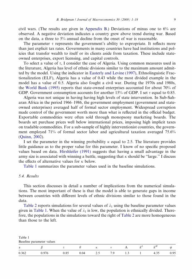
Table 1 summarizes the parameter values used in the baseline simulations.

5.4. Results

This section discusses in detail a number of implications from the numerical simula-tions. The most important of these is that the model is able to generate gaps in incomebetween countries with different levels of ethnic divisions similar to those found in thedata.

Table 2 reports simulations for several values of k1 using the baseline parameter valuesgiven in Table 1. When the value of k1 is low, the population is ethnically divided. There-fore, the populations in the simulations toward the right of Table 2 are more homogeneousthan those to the left.

Table 1Baseline parameter values

a b s h j m A kL kH w

0.362 0.976 0.85 0.04 2.5 7.9 1.3 1 4.35 0.95

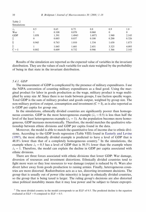
Table 2Simulations

k1 0.5 0.65 0.75 0.8 0.9 1.0War 1 0.108 0.070 0.060 0 0GDP 1.058 1.391 1.4943 1.6971 1.940 2.143XY 0 0.003 0.037 0.100 0.200 0.326KY 0.945 0.763 1.010 1.334 1.630 1.873KL 1 1.045 1.601 2.451 3.325 4.093C + I 0.802 0.609 0.732 0.946 1.366 2.143


Results of the simulation are reported as the expected value of variables in the invariantdistribution. They are the values of each variable for each state weighted by the probabilityof being in that state in the invariant distribution.

5.4.1. GDP

The measurement of GDP is complicated by the presence of military expenditures. I usethe NIPA convention of counting military expenditures as a final good. Using the mar-ginal product for labor in goods production as the wage, military product is wage multi-plied by army size M. Since there is no trade between groups, I use faction specific wages.Total GDP is the sum of military product and goods output, weighted by group size. Thenon-military portion of output, consumption and investment (C + I), as is also reported asis GDP per capita for group one.

In the simulations, ethnically divided countries are significantly poorer than homoge-neous countries. GDP in the most heterogeneous example (k1 = 0.5) is less than half thelevel of the least heterogeneous example (k1 = 1). As the population becomes more homo-geneous, GDP increases monotonically. Therefore, the model matches the qualitative rela-tionship between ethnic divisions and GDP per capita found in the data.

Moreover, the model is able to match the quantitative loss of income due to ethnic divi-sions. According to the GDP levels regression (Table VIII) found in Easterly and Levine(1997), the most ethnically divided example is predicted to have a level of GDP that is48.8% lower than that of a completely homogeneous country.5 In the simulations, theexample where k1 = 0.5 has a level of GDP that is 50.3% lower than the example wherek1 = 1. Therefore, the model can explain the decline in GDP per capita associated withethnic divisions.

There are three forces associated with ethnic divisions that lower GDP: War damage,diversion of resources and investment distortions. Ethnically divided countries tend tofight more wars so they lose resources to war damage (output is reduced by h). Wars alsodivert labor away from goods production to raising armies. Finally, heterogeneous coun-tries are more distorted. Redistribution acts as a tax, distorting investment decisions. Thegroup that is usually out of power (the minority) is larger in ethnically divided countries,so the group that is being taxed is larger. The ruling group’s decisions are also distortedsince political instability means that it may lose power and be subject to future expropri-

5 The most divided country in the model corresponds to an ELF of 0.5. The predicted decline is the equationevaluated at ELF = 0 compared to ELF = 0.5.

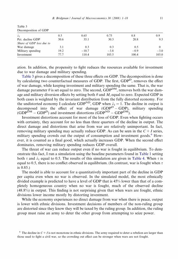
Table 3Decomposition of GDP

k1 0.5 0.65 0.75 0.8 0.9Pct. decline GDP 50.6 35.1 30.3 20.8 9.5Share of GDP loss due to

War damage 3.1 0.3 0.3 0.5 0Military spending 19.2 �10.7 �3.8 �0.9 �3.0Investment 77.7 110.4 103.5 100.4 103.0


ation. In addition, the propensity to fight reduces the resources available for investmentdue to war damage and military spending.

Table 3 gives a decomposition of these three effects on GDP. The decomposition is doneby calculating two counterfactual measures of GDP. The first, GDPD, removes the effectof war damage, while keeping investment and military spending the same. That is, the wardamage parameter h is set equal to zero. The second, GDPDM, removes both the war dam-age and military diversion effects by setting both h and Mi equal to zero. Expected GDP inboth cases is weighted by the invariant distribution from the fully distorted economy. Forthe undistorted economy I calculate GDPND, GDP when k1 = 1. The decline in output isdecomposed into the effect of war damage (GDPD � GDP), military spending(GDPDM � GDPD) and investment distortions (GDPND � GDPDM).

Investment distortions account for most of the loss of GDP. Even when fighting occurswith certainty, they account for no less than three quarters of the decline in output. Thedirect damage and distortions that arise from war are relatively unimportant. In fact,removing military spending may actually reduce GDP. As can be seen in the C + I series,military spending crowds out the output of consumption and investment goods.6 How-ever, it is counted as a final good, which actually increases GDP. When the second effectdominates, removing military spending reduces GDP overall.

The threat of war can reduce output even if no war is fought in equilibrium. To dem-onstrate this fact, I run a simulation using the baseline parameters found in Table 1 settingboth s and k1 equal to 0.5. The results of this simulation are given in Table 4. When s isequal to 0.5, there is no conflict observed in equilibrium. (In contrast, war is fought when sis 0.85.)

The model is able to account for a quantitatively important part of the decline in GDPper capita even when no war is observed. In the simulated model, the most ethnicallydivided example is predicted to have a level of GDP that is 45% lower than that of a com-pletely homogeneous country when no war is fought, much of the observed decline(48.8%) in output. This finding is not surprising given that when wars are fought, ethnicdivisions lower income mostly by distorting investment.

While the economy experiences no direct damage from war when there is peace, outputis lower with ethnic divisions. Investment decisions of members of the non-ruling groupare distorted since they know they will be taxed by the ruling group. In addition, the rulinggroup must raise an army to deter the other group from attempting to seize power.

6 The decline in C + I is not monotone in ethnic divisions. The army required to deter a rebelion are larger thanthose used to fight a civil war, so the crowding out effect can be stronger when wars are not fought.

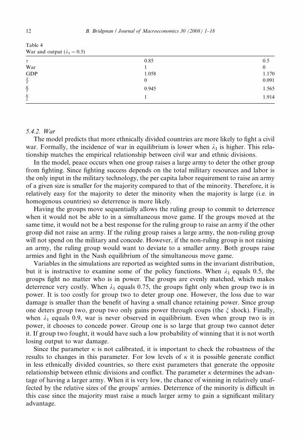
Table 4War and output (k1 = 0.5)

s 0.85 0.5War 1 0GDP 1.058 1.170XY 0 0.091KY 0.945 1.565KL 1 1.914


5.4.2. War

The model predicts that more ethnically divided countries are more likely to fight a civilwar. Formally, the incidence of war in equilibrium is lower when k1 is higher. This rela-tionship matches the empirical relationship between civil war and ethnic divisions.

In the model, peace occurs when one group raises a large army to deter the other groupfrom fighting. Since fighting success depends on the total military resources and labor isthe only input in the military technology, the per capita labor requirement to raise an armyof a given size is smaller for the majority compared to that of the minority. Therefore, it isrelatively easy for the majority to deter the minority when the majority is large (i.e. inhomogenous countries) so deterrence is more likely.

Having the groups move sequentially allows the ruling group to commit to deterrencewhen it would not be able to in a simultaneous move game. If the groups moved at thesame time, it would not be a best response for the ruling group to raise an army if the othergroup did not raise an army. If the ruling group raises a large army, the non-ruling groupwill not spend on the military and concede. However, if the non-ruling group is not raisingan army, the ruling group would want to deviate to a smaller army. Both groups raisearmies and fight in the Nash equilibrium of the simultaneous move game.

Variables in the simulations are reported as weighted sums in the invariant distribution,but it is instructive to examine some of the policy functions. When k1 equals 0.5, thegroups fight no matter who is in power. The groups are evenly matched, which makesdeterrence very costly. When k1 equals 0.75, the groups fight only when group two is inpower. It is too costly for group two to deter group one. However, the loss due to wardamage is smaller than the benefit of having a small chance retaining power. Since groupone deters group two, group two only gains power through coups (the n shock). Finally,when k1 equals 0.9, war is never observed in equilibrium. Even when group two is inpower, it chooses to concede power. Group one is so large that group two cannot deterit. If group two fought, it would have such a low probability of winning that it is not worthlosing output to war damage.

Since the parameter j is not calibrated, it is important to check the robustness of theresults to changes in this parameter. For low levels of j it is possible generate conflictin less ethnically divided countries, so there exist parameters that generate the oppositerelationship between ethnic divisions and conflict. The parameter j determines the advan-tage of having a larger army. When it is very low, the chance of winning in relatively unaf-fected by the relative sizes of the groups’ armies. Deterrence of the minority is difficult inthis case since the majority must raise a much larger army to gain a significant militaryadvantage.


5.5. Discussion

This section discusses the model’s policy implications and how sensitive the results areto the assumptions on government policy.

5.5.1. Reducing the impact of ethnic divisions

The model generates low incomes and conflict when both ethnic divisions and the abil-ity of the government to redistribute (s) are high. Policies that reduce divisions and redis-tribution would raise incomes.

Reducing ethnic divisions increases income but doing so directly is often difficult. Eth-nically divided countries could separate into two or more homogenous countries. Whilehas been done successfully in some cases (e.g. Czechoslovakia), different groups are oftengeographically interspersed. Sambanis (2000) finds that ethnic partition is generally a poormethod of reducing violence.

For a given level of ethnic divisions, reducing s also raises income. (See Table 4.) Infact, income in divided countries is the same as in the homogenous case (k1 = 1) whenthere is no redistribution (s = 0). Therefore, divided countries are not inherently confinedto poverty. This observation is supported by work that finds that the relationship betweenethnic divisions and poverty (and war) is weaker once measures of institutional quality,which include constraints on the government, are included (Easterly, 2001).

However, more divided countries require stronger constraints to achieve the sameincome level. These constraints may need to be very strong for the most divided countries,which is illustrated by comparing the results in Tables 2 and 4. Starting from the casewhere k1 = 0.5 and s = 0.85, reducing expropriation 35% points has less effect on incomethan reallocating a 15% share of the population to the majority. (Expected GDP is 1.170when k1 = 0.5 and s = 0.5 while it is 1.391 when k1 = 0.65 and s = 0.85.) Strong limits aredifficult to implement and may interfere with the government’s legitimate functions. Forexample, a ceiling on government spending would reduce redistribution but also limit pro-vision of public goods. (The conflict between redistribution and public goods is discussedin Bridgman (2004).)

5.5.2. Government policyGovernment policy in the model is quite stark. The tax rate is exogenous and ruling

group must accept all transfers. Because the incumbent cannot commit to future redistri-bution policy, there is little incentive for the ruling group to change its policy from thatwhich is assumed. The policy assumptions would be more restrictive if the incumbentcould commit.

Since the policy is set after control of the government is resolved, the group winningpower has little incentive to redistribute less to prevent fighting. Strategies only dependon the state of the economy, so reducing the net tax burden of the non-ruling group inthe current period will not directly affect its actions in the next period.7 In fact, the ruling

7 They may affect actions indirectly. Positive transfers could increase the non-ruling groups’ capital stock whichcould change its strategies next period or increase future revenues for transfers. An early version of the modelallowed the new ruling group i** to make group specific transfers after taking power (stage 5 in the timing). Innumerous simulations, such transfers were never made so transfers were made exogenous to reduce computationtime.


group would like to raise taxes on other group if it could. (The exogenous tax rate s can bethought of as the maximum share that can be expropriated.)

If the incumbent group could commit to a tax and transfer policy before decisionsabout military spending were made, it might choose low net taxes on the other groupto remove that group’s incentive to rebel. Adding commitment would decrease the nega-tive impact of ethnic divisions by reducing the likelihood of fighting and tax distortionsrelative to what the model predicts. (If there are many groups, the ruling group still hasan incentive to impose high tax rates to increase its ability to manipulate other groups withtransfers. See Acemoglu et al. (2004).)

The model without commitment is probably to be more empirically relevant for manycountries with weak institutions and frequent civil wars. However, the main finding (ethnicredistribution is a quantitatively important source of poverty) is unlikely to be overturnedeven if commitment were relevant. If the incumbent group chooses a policy that will resultin a civil war, it does not have much incentive to choose a low tax rate for the other group.Therefore, equilibria with fighting should feature high degrees of redistribution regardlessof whether there was commitment or not. As documented above, such fighting equilibriaare empirically relevant.

In fact, the model may underestimate the importance of distortions from redistributionsince it abstracts from the internal structure of ethnic groups. In the model, transfers areefficiently shared equally among ruling group members. In reality, ethnic groups requiremobilization, often by elites who benefit much more than rank and file members.8 Elitestypically use inefficient redistribution within the group to maintain their status (Padro iMiquel, 2004). Inefficient transfers within a group introduce additional distortions andmay dissipate some of the value of ruling, reducing military distortions.

6. Conclusion

The tendency for ethnically divided countries to be poorer than homogeneous countrieshas been widely documented. However, the reason ethnic divisions lower incomes is muchless clear. The main contribution of this paper is to model a mechanism, conflict overredistribution, by which ethnic divisions can lower income and show that it can generatequantitatively important income gaps. The most important source of poverty is the distor-tions from redistribution, not conflict.

An interesting extension of the model would add additional groups. The model onlydivides the population into two groups. Therefore, it is silent about countries with threeor more groups. Doing so could help shed light on the proper measure of ethnic divisionsin the empirical growth literature. Despite (or perhaps because of) wide use of measures ofethnic divisions, there has been controversy about the measurement of ethnicity. The mea-sure used in Easterly and Levine (1997) (ELF) has been criticized.9 A competing polariza-tion indicator has been proposed the proper measure, both in a general theory of conflict(Esteban and Ray, 1999) and specifically for ethnic conflict (Montalvo and Reynal-Querol,2005). An augmented model with multiple groups could provide guidance on this issue.

8 See Fearon (2006) for a survey of the literature on ethnic mobilization.9 The underlying data has also been criticized. See Posner (2004); Reilly (2000) and Alesina et al. (2003).


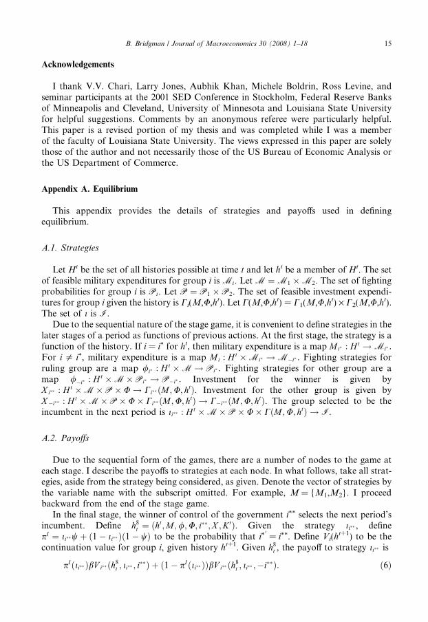
Acknowledgements

I thank V.V. Chari, Larry Jones, Aubhik Khan, Michele Boldrin, Ross Levine, andseminar participants at the 2001 SED Conference in Stockholm, Federal Reserve Banksof Minneapolis and Cleveland, University of Minnesota and Louisiana State Universityfor helpful suggestions. Comments by an anonymous referee were particularly helpful.This paper is a revised portion of my thesis and was completed while I was a memberof the faculty of Louisiana State University. The views expressed in this paper are solelythose of the author and not necessarily those of the US Bureau of Economic Analysis orthe US Department of Commerce.

Appendix A. Equilibrium

This appendix provides the details of strategies and payoffs used in definingequilibrium.

A.1. Strategies

Let Ht be the set of all histories possible at time t and let ht be a member of Ht. The setof feasible military expenditures for group i is Mi. Let M ¼M1 �M2. The set of fightingprobabilities for group i is Pi. Let P ¼ P1 �P2. The set of feasible investment expendi-tures for group i given the history is Ci(M,U,ht). Let C(M,U,ht) = C1(M,U,ht) · C2(M,U,ht).The set of i is I.

Due to the sequential nature of the stage game, it is convenient to define strategies in thelater stages of a period as functions of previous actions. At the first stage, the strategy is afunction of the history. If i = i* for ht, then military expenditure is a map Mi� : H t !Mi� .For i 5 i*, military expenditure is a map Mi : Ht �Mi� !M�i� . Fighting strategies forruling group are a map /i� : H t �M! Pi� . Fighting strategies for other group are amap /�i� : H t �M�Pi� ! P�i� . Investment for the winner is given byX i�� : Ht �M�P� U! Ci�� ðM ;U; htÞ. Investment for the other group is given byX�i�� : H t �M�P� U� Ci�� ðM ;U; htÞ ! C�i�� ðM ;U; htÞ. The group selected to be theincumbent in the next period is ii�� : Ht �M�P� U� CðM ;U; htÞ ! I.

A.2. Payoffs

Due to the sequential form of the games, there are a number of nodes to the game ateach stage. I describe the payoffs to strategies at each node. In what follows, take all strat-egies, aside from the strategy being considered, as given. Denote the vector of strategies bythe variable name with the subscript omitted. For example, M = {M1,M2}. I proceedbackward from the end of the stage game.

In the final stage, the winner of control of the government i** selects the next period’sincumbent. Define h8

t ¼ ðht;M ;/;U; i��;X ;K 0Þ. Given the strategy ii�� , definepI ¼ ii��wþ ð1� ii�� Þð1� wÞ to be the probability that i*

0= i**. Define Vi(h

t+1) to be thecontinuation value for group i, given history ht+1. Given h8

t , the payoff to strategy ii�� is

pIðii�� ÞbV i�� ðh8t ; ii�� ; i��Þ þ ð1� pIðii�� ÞÞbV i�� ðh8

t ; ii�� ;�i��Þ: ð6Þ


In the previous stage, the group that did not win power (�i**) chooses its investment. De-fine h7

t ¼ ðht;M ;/;U; i��;X i�� Þ. Define yFi ðK;MÞ ¼

ð1�hÞY ðK;ki�MÞki

and yPi ðK;MÞ ¼

Y ðK;ki�MÞki

:Let f 2 {F,P} indicate whether a group fought or not respectively. These expressions arethe per capita output given a group fighting and not fighting respectively. Let ti be the

per capita transfers group i receives, where ti�� ¼sP

ikiy

fið Þ

kiand t�i�� ¼ 0. Given h7

t , the pay-off to strategy X�i�� is

ð1� sÞyf�i�� x�i�� þ

Z ZpIðh7

t ;X�i�� ;K 0ÞbV �i�� ðh7t ;X�i�� ;K 0; i��Þ

þ ð1� pIðh7t ;X�i�� ;K 0ÞÞbV �i�� ðh7

t ;X�i�� ;K 0;�i��ÞdF ðX�i�� ;K�i�� ÞdF ðX i�� ;Ki�� Þ;ð7Þ

where F(Xi,Ki) is the distribution function for K 0i.In the previous stage, the group that won power (i**) chooses its investment. Define

h6t ¼ ðht;M ;/;U; i��Þ. Given h6

t , the payoff to strategy X i�� is

ð1� sÞyfi�� xi�� þ ti�� þ

Z ZpIðh6

t ;X i�� ;X�i�� ðX i�� Þ;K 0ÞbV i�� ðh6t ;X i�� ;X�i�� ðX i�� Þ;K 0; i��Þ

þ ð1� pIðh6t ;X i�� ;X�i�� ðX i�� Þ;K 0ÞÞ

� bV i�� ðh6t ;X i�� ;X�i�� ðX i�� Þ;K 0;�i��ÞdF ðX i�� ;Ki�� ÞdF ðX�i�� ðX i�� Þ;K�i�� Þ ð8Þ

In stage four, the non-ruling group �i* chooses its fighting strategy. Defineh4

t ¼ ðht;M ;/i� Þ. Define

W fi ði��Þ ¼ ð1� sÞyf

i � xi þ ti þZ Z

pIð�ÞbV ið�; i��Þ

þ ð1� pIð�ÞÞbV ið�;�i��ÞdF ðX i;KiÞdF ðX�i;K�iÞ; ð9Þ

the expected payoff for the rest of the game given group i** wins control of the govern-ment. The payoff to strategy /�i� given h4

t is

/�i� /i� pðMÞW F�i� ð1Þ þ ð1� pðMÞÞW F

�i� ð2Þ� �

þ ð1� /i� ÞW P�i� ð�i�Þ

� �þ ð1� /�i� ÞW P

�i� ði�Þ ð10Þ

In stage three, the ruling group i* chooses its fighting strategy. Define h3t ¼ ðht;MÞ: Given

the strategies at future stages of the game, the strategy induces future actions. The payoffto strategy /i� given h3

t is Eq. (10) where /�i� ¼ /�i� ðh3t ;/i� Þ.

In stage two, the non-ruling group �i* chooses its military spending strategy. Defineh2

t ¼ ðht;Mi� Þ. The payoff to strategy M�i� given h2t is Eq. (10) where /i� ¼ /i� ðh2

t ;Mi� Þand /�i� ¼ /�i� ðh2

t ;Mi� ;/iðh2t ;Mi� ÞÞ.

In the first stage, the ruling group i* chooses its military spending strategy. The payoffto strategy Mi� given ht is Eq. (10) where M�i� ¼ M�i� ðht;Mi� Þ, /i� ¼/i� ðht;Mi� ;M�i� ðht;Mi� ÞÞ and /�i� ¼ /�i� ðht;Mi� ;M�i� ðht;Mi� Þ;/i� ðht;Mi� ;M�i� ðht;Mi� ÞÞ.

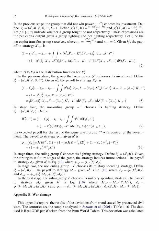
Appendix B. War damage

This appendix reports the results of the deviations from trend caused by protracted civilwars. The countries are the sample analyzed in Stewart et al. (2001), Table 4.16. The dataused is Real GDP per Worker, from the Penn World Tables. This deviation was calculated

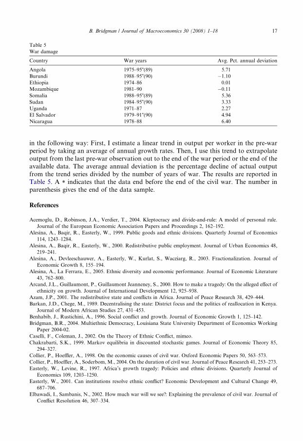
Table 5War damage

Country War years Avg. Pct. annual deviation

Angola 1975–95*(89) 5.71Burundi 1988–95*(90) �1.10Ethiopia 1974–86 0.01Mozambique 1981–90 �0.11Somalia 1988–95*(89) 5.36Sudan 1984–95*(90) 3.33Uganda 1971–87 2.27El Salvador 1979–91*(90) 4.94Nicaragua 1978–88 6.40


in the following way: First, I estimate a linear trend in output per worker in the pre-warperiod by taking an average of annual growth rates. Then, I use this trend to extrapolateoutput from the last pre-war observation out to the end of the war period or the end of theavailable data. The average annual deviation is the percentage decline of actual outputfrom the trend series divided by the number of years of war. The results are reported inTable 5. A * indicates that the data end before the end of the civil war. The number inparenthesis gives the end of the data sample.

References

Acemoglu, D., Robinson, J.A., Verdier, T., 2004. Kleptocracy and divide-and-rule: A model of personal rule.Journal of the European Economic Association Papers and Proceedings 2, 162–192.

Alesina, A., Baqir, R., Easterly, W., 1999. Public goods and ethnic divisions. Quarterly Journal of Economics114, 1243–1284.

Alesina, A., Baqir, R., Easterly, W., 2000. Redistributive public employment. Journal of Urban Economics 48,219–241.

Alesina, A., Devleeschauwer, A., Easterly, W., Kurlat, S., Wacziarg, R., 2003. Fractionalization. Journal ofEconomic Growth 8, 155–194.

Alesina, A., La Ferrara, E., 2005. Ethnic diversity and economic performance. Journal of Economic Literature43, 762–800.

Arcand, J.L., Guillaumont, P., Guillaumont Jeanneney, S., 2000. How to make a tragedy: On the alleged effect ofethnicity on growth. Journal of International Development 12, 925–938.

Azam, J.P., 2001. The redistributive state and conflicts in Africa. Journal of Peace Research 38, 429–444.Barkan, J.D., Chege, M., 1989. Decentralising the state: District focus and the politics of reallocation in Kenya.

Journal of Modern African Studies 27, 431–453.Benhabib, J., Rustichini, A., 1996. Social conflict and growth. Journal of Economic Growth 1, 125–142.Bridgman, B.R., 2004. Multiethnic Democracy, Louisiana State University Department of Economics Working

Paper 2004-02.Caselli, F., Coleman, J., 2002. On the Theory of Ethnic Conflict, mimeo.Chakrabarti, S.K., 1999. Markov equilibria in discounted stochastic games. Journal of Economic Theory 85,

294–327.Collier, P., Hoeffler, A., 1998. On the economic causes of civil war. Oxford Economic Papers 50, 563–573.Collier, P., Hoeffler, A., Soderbom, M., 2004. On the duration of civil war. Journal of Peace Research 41, 253–273.Easterly, W., Levine, R., 1997. Africa’s growth tragedy: Policies and ethnic divisions. Quarterly Journal of

Economics 109, 1203–1250.Easterly, W., 2001. Can institutions resolve ethnic conflict? Economic Development and Cultural Change 49,

687–706.Elbawadi, I., Sambanis, N., 2002. How much war will we see?: Explaining the prevalence of civil war. Journal of

Conflict Resolution 46, 307–334.


Esteban, J., Ray, D., 1999. Conflict and distribution. Journal of Economic Theory 87, 379–415.Fearon, J., 2006. Ethnic mobilization and ethnic violence. In: Weingast, B.R., Wittman, D. (Eds.), Oxford

Handbook of Political Economy. Oxford University Press, Oxford.Fafchamps, M., 2000. Ethnicity and credit in African manufacturing. Journal of Development Economics 61,

205–235.Grossman, H.I., 1991. A general equilibrium model of insurrections. American Economic Review 81, 912–921.Hayashi, F., Prescott, E.C., 2002. The 1990s in Japan: A lost decade. Review of Economic Dynamics 5, 206–235.Hirshleifer, J., 1991. The technology of conflict as an economic activity. American Economic Review Papers and

Proceedings 81, 130–134.Johnson, T.H., Slater, R.O., McGowan, P., 1984. Explaining African military coups d’etat 1960–1982. American

Political Science Review 78, 622–640.Montalvo, J.G., Reynal-Querol, M., 2005. Ethnic diversity and economic development. Journal of Economic

Development 76, 293–323.Padro i Miquel, G., 2004. The Control of Politicians in Divided Societies: The Politics of Fear, mimeo.Posner, D.N., 2004. Measuring ethnic fractionalization in Africa. American Journal of Political Science 48, 849–

863.Quinn, J.J., 2002. The Road Oft Traveled: Development Policies and Majority State Ownership of Industry in

Africa. Praeger, Westport.Reilly, B., 2000. Democracy, ethnic fragmentation, and internal conflict: Confused theories, faulty data, and the

’crucial case’ of Papua New Guinea. International Security 25, 162–185.Sambanis, N., 2000. Ethnic partition as a solution to ethnic war: An empirical critique of the theoretical

literature. World Politics 52, 437–483.Sandler, T., 2000. Economic analysis of conflict. Journal of Conflict Resolution 44, 723–729.Skaperdas, S., 1996. Contest success functions. Economic Theory 7, 283–290.Stewart, F., Huang, C., Wang, M., 2001. Internal wars in developing countries: An empirical overview of

economic and social consequences. In: Stewart, F., FitzGerald, V. (Eds.), War and UnderdevelopmentVolume One: The Economic and Social Consequences of Conflict. Oxford University Press, Oxford.

Stokey, N.L., Lucas, R.E., Prescott, E.C., 1989. Recursive Methods in Economic Dynamics. Harvard UniversityPress, Cambridge.

Tangeras, T.P., Lagerlof, N.P., 2002. Ethnic Diversity and Civil War, mimeo.World Bank, 1995. Bureaucrats in Business: The Economics and Politics of Government Ownership. Oxford

University Press, Oxford.

Documents

Why are ethnically divided countries poor?