Why do stocks and consumption imply such different gains from international risk sharing?

Journal of International Economics 52 (2000) 1–35www.elsevier.nl / locate /econbase

Why do stocks and consumption imply such differentqgains from international risk sharing?

a,b ,*Karen K. Lewisa2300 SH-DH, Wharton School, University of Pennsylvania, Philadelphia, PA 19104-6367, USA

bNational Bureau of Economic Research, Cambridge, MA 02138, USA

Received 15 April 1997; received in revised form 17 September 1998; accepted 18 May 1999

Abstract

Estimates of the gains to international risk-sharing based upon stock returns tend to finddramatically higher gains than do estimates from consumption-based models. In this paper,I examine the reasons for these differences. Using a common theoretical framework for bothapproaches, I find that the differences are largely due to the much higher variability of stockreturns and its implied intertemporal substitution in marginal utility. Also, contrary toconventional wisdom, the differences in gains from the two approaches do not arise fromtreating stock returns as exogenous rather than endogenous. 2000 Elsevier Science B.V.All rights reserved.

Keywords: International risk sharing; Stock returns; Consumption

JEL classification: F4; F36

1. Introduction

Domestic investors do not appear to hold a sufficient proportion of their wealthin foreign assets to diversify away domestic idiosyncratic risk. This is the

qEarlier versions of this paper were circulated under the titles, ‘Consumption, stock returns, and thegains from international risk-sharing’ (NBER Working Paper No. 5410) and ‘Why do stocks andconsumption imply such different costs of imperfect international risk-sharing?’

*Tel.: 11-215-898-7637; fax: 11-215-898-6200.E-mail address: [email protected] (K.K. Lewis).

0022-1996/00/$ – see front matter 2000 Elsevier Science B.V. All rights reserved.PI I : S0022-1996( 99 )00027-6

2 K.K. Lewis / Journal of International Economics 52 (2000) 1 –35

1conclusion of research using both consumption data and stock return data. Sinceimperfect risk-sharing means that potential welfare gains are being foregone, theobservation leads directly to the question: how large are these gains?

On this issue, the literature has been quite divided. Some calculations of risksharing gains based upon international consumption data suggest that these gainsare quite small. For example, Cole and Obstfeld (1991) find that for representativeconsumers calibrated to US data, the gains are less than 0.5% of permanentconsumption for plausible parameter values. Tesar (1995) and van Wincoop(1994) report similarly small gains from international risk sharing.

On the other hand, calculations of the gains from risk-sharing based upon stockreturns give much larger estimates. The approach typically constructs combina-tions of domestic and foreign portfolios that minimize variance and maximizereturns and asks whether domestic portfolios are dominated by these portfolios. Inpapers at least as early as Levy and Sarnat (1970), portfolios with foreign stockswere shown to strictly dominate domestic US portfolios. Using utility functionssimilar to those used in the general equilibrium literature, I show below that thissimple partial equilibrium framework implies welfare gains of at least 20% ofpermanent consumption and often-times near 100%.

In this paper, I address the question: why are the magnitudes of the gains based2upon these two approaches so different? I develop a common unifying framework

and then show that the differences can come from three potential avenues: (1) thetreatment of stock returns as exogenous or endogenous; (2) the statisticalproperties of stock returns relative to consumption growth; and (3) the set of

3preference parameters. Since these three factors are at the core of this in-vestigation, I next discuss the significance of each in turn.

(1) The equity-based approach takes the stock price as exogenous and asks howan investor would choose an optimal portfolio given the mean and variance of thisprocess. Thus, an investor does not take into account the effect that his decisionmay have on the stock price. On the other hand, the consumption-based approachtakes a production process as exogenous and asks how optimal risk-sharing wouldaffect the investor’s consumption path. This approach implies that stock prices willchange as a result of risk-sharing. This distinction suggests an intuitive reason whythe equity-based approach leads to significantly higher gains than the consum-ption-based approach: the equity-based approach does not incorporate the effect ofrisk-sharing on the stock price.

1For a recent discussion of these two literatures and their relationship, see Lewis (1999).2A related question is: what is the ‘true’ risk-sharing gain? In this paper, I examine only the narrower

question articulated in the title.3Note that these avenues need not be independent. For example, it is well known that by treating

stock returns as endogenous [avenue (1)] with a set of plausible preference parameters [avenue (3)]implies that the statistical properties of stock returns are difficult to reconcile with consumption growth[avenue (2)]. Below, I discuss and focus upon this interdependence.

K.K. Lewis / Journal of International Economics 52 (2000) 1 –35 3

In this paper, I show that this intuition is not true in general. The reason issimple. When stock prices are endogenous, these prices must adjust to makeinternational investors willing to buy the country’s equity. This adjustment inprices leads to a one-time intertemporal substitution of consumption from lowgrowth economies to high growth economies that leaves all countries better off. Asa result, the endogenous stock price reaction allows for an extra avenue of welfaregains that are not present when stock prices are treated as exogenous. Therefore,the partial equilibrium nature of the equity approach does not independentlyexplain the difference in welfare gains.

(2) The gains from risk-sharing depend crucially upon the benefits of reducingthe variability of the marginal utility over time. In the equity-based approach, thismarginal utility depends upon stock returns, while in the consumption-basedapproach this marginal utility depends upon consumption. Thus, an obvious reasonfor the difference in measuring gains in the two approaches arises from the greatervariability in stock returns relative to consumption.

In an international growing economy, the potential gains from moving to an4integrated world capital market depends upon the means as well as the variances.

To see why, consider the common consumption approach of assuming that meanconsumption growth across countries is equal. This assumption has the effect ofmaking the deterministic growth rate the same so that international capital marketintegration only reduces the variability of consumption around this common worldgrowth rate. On the other hand, the equity approach focuses upon increasing meanreturns while minimizing variance. When the mean stock price returns differ acrosscountries, then the differences between growth rates imply that internationalcapital markets allow domestic investors to move to a different deterministicgrowth rate in consumption and thereby intertemporally smooth.

Therefore, the difference between the risk-sharing gains may appear to arisefrom the combination of assumed: (a) common consumption growth acrosscountries; and (b) higher variability of stock returns compared to consumptiongrowth. In this paper, I show that the difference in consumption growth hassurprisingly little effect upon risk-sharing gains, while the higher variability ofequity returns does.

(3) Both consumption-based and equity-based approaches must specify prefer-ence parameters that govern risk-aversion and intertemporal substitution. However,the low variability of consumption growth relative to equity returns has an

4Whether the underlying process has permanent or transitory disturbances is another important effect.As Obstfeld (1994a) shows, permanent disturbances to idiosyncratic consumption imply that risk-sharing gains are higher. In this paper, I assume that the disturbances to idiosyncratic consumption arepermanent (i.e. shocks are permanent and not cointegrated across countries.) Therefore, if thedisturbances are not permanent, I am biasing upward my gains from the consumption approach. Since Ifind that even the estimates based upon permanent shocks to consumption are dramatically smaller thanthe equity approach gains, transitory shocks to consumption will only deepen the gap between gainsfrom the two approaches.


important effect upon the measured gains from risk-sharing. This observationcoupled with plausible preference parameters leads to well-known inconsistenciesbetween consumption-based models and observed financial market data.

To investigate the importance of reconciling preference parameters in theconsumption based approach with the observed behavior of stock prices, I conducttwo sets of experiments to solve for risk aversion and intertemporal substitutabilityendogenously. First, I set the means of stock returns and the risk-free rate to equaltheir values implied by the consumption model. In this case, risk aversion andintertemporal substitution are high. Since higher risk aversion and intertemporalsubstitutability both increases the value of reducing variability in the future, therisk-sharing gains are quite high, consistent with the equity approach gains.Second, I set the variances of stock returns equal to their values implied by theconsumption model. To explain the high variance, risk aversion and intertemporalsubstitutability must be low. In this case, risk-sharing gains are quite low, evenlower than those implied by the standard consumption approach.

The structure of the paper is as follows. In Section 1, I describe the welfare gainfunction. In Section 2, I use stock returns to provide measures of risk-sharing gainsusing the equity-based approach. In Section 3, I use consumption data to calculaterisk-sharing gains using a standard consumption-based approach. In Section 4, Iuse stock return data to calculate gains using the consumption-based approach. InSection 5, I use moments of stock return data to back out implied preferenceparameters and re-examine the consumption-based gains. Concluding remarksfollow.

2. The gain function

2.1. The basic framework

To calculate welfare gains, I follow standard practice and calculate theequivalent variation of current utility that brings the investor /consumer up to the

5same utility level as he would enjoy under optimal risk-sharing. In the consum-ption-based literature this utility depends upon the consumption level. In theequity-based literature, utility depends upon wealth directly. For now, I simplydenote the argument in utility at time t as X for generality.t

6Below, I assume that X is log-normally distributed:t

1 2 2]x 5 x 1 m 2 s 1 ´ where ´ | N(0, s ) (1)t11 t t t2

5For example, see Lucas (1987) and Obstfeld (1994a,b).6In simulation experiments, serially correlated consumption and equity returns gave similar results to

those found below. I focus upon the analytical solutions in the text, however.


and where both here and below the lower-case letters refer to the natural logarithmof the variable [i.e. x 5 ln(X)], unless noted otherwise. Furthermore, the optimalpath for X is denoted as X while its counterparts to m and s are defined as m andt t] ]s, respectively.]

Thus, the welfare gain d is defined by the equation:

U(X (1 1 d ), m, s) 5 U(X , m, s) (2)t t] ]]

where U is the utility function. Where possible below, I denote the utilityconditioned on the time t variable as simply U .t

Calculating the gains requires specifying a utility function. Constant-relativerisk aversion (CRRA) is a standard utility function used in asset pricing as well ascalculating welfare gains. However, this utility function assumes that the coeffi-cient of relative risk aversion is the same as the inverse of the intertemporalelasticity of substitution. As shown in Obstfeld (1994a), risk aversion and theinverse of intertemporal substitutability have opposite effects upon welfare gains.Therefore, it is important to use a utility function that does not impose thisconstraint upon preferences.

7For this reason, I use the Epstein and Zin (1989) utility function:

12u 12g (12u ) / (12g ) 1 / (12u )U 5 hX 1 b[E (U )] j for g, u . 0, ± 1 (3)t t t t11

The parameter u can be interpreted as the inverse of the intertemporal elasticity ofsubstitution in consumption. On the other hand, g is the parameter of relative riskaversion. The standard time-additive utility function results when g 5u.

When X is log-normally distributed, Appendix B shows that time t utility is:

2(1 / (12u ))1 2]S F S DGDU 5 U(X , m, s) 5 X 1 2 b exp (1 2u ) m 2 gs (4)t t t 2

Similarly, utility under optimal risk-sharing is given by:

2(1 / (12u ))1 2]S F S DGDU 5 U(X , m, s) 5X 1 2 b exp (1 2u ) m 2 gs (49)t t t] ] ] ]2] ]

where risk-sharing suggests that s , s. This relationship will be determined]

endogenously below.The two parameters, g and u, are important in the welfare gain analysis. The

role of these two key parameters therefore warrants inspection.First, note that utility is increasing in the certainty equivalent log consumption

21]growth path, m 2 gs . Therefore, reductions in the variance of this path will2

7While I use the Epstein-Zin function because it provides a more parsimonious representation ofreduced-form utility, Obstfeld (1994a,b) uses the Weil (1990) utility function. However, the Weilfunction is a monotonic transformation of the Epstein-Zin function so that the gain function and allasset pricing relationships are identical using the two utilities.


increase this certainty equivalent according to the parameter of risk aversion, g.Clearly, then, higher risk aversion g will lead to greater welfare gains.

Second, note that intertemporal elasticity declines as u increases. Therefore, theutility value of gains along the CE path in the future declines. For this reason,higher values of u will lead to lower welfare gains from a reduction in variance.

To solve explicitly for the gain function, substitute Eq. (4) and Eq. (49) into the8gain definition Eq. (2) and solve for d at an initial time period 0. This implies:

1 / (12u )1 2]S F S DGDX 1 2 b exp (1 2u ) m 2 gs0 2]]]]]]]]]]]]]d 5 2 1 (5)1 / (12u )1 2]S F S DGDX 1 2 b exp (1 2u ) m 2 gs0] ]2]

Thus, the welfare gains depend upon, first, the current level of the utilitydeterminant relative to the optimal X /X , and, second, the relationship between0 0] 2 21 1

] ]the two certainty equivalent growth paths, m 2 gs and m 2 gs evaluated2 2 ]]with the intertemporal elasticity of substitution parameter, u.

2.2. Components of the gain function

Below, I examine the equity-based and consumption-based literature on risk-sharing gains using the gain function Eq. (5). To describe the experiments below, Iwrite this function generally as:

d 5 d(m, m, s, s ; g, u, b ; X /X ) 5 d(M; V ; I) (59)0 0] ]]

where M is a moment matrix of means and variances of disturbances along theautarky and optimal growth path; V is the set of preference parameters; andI ; X /X .0 0]

I consider two sets of values for the moment matrix M. For the equity-basedapproach, M corresponds to the moments of stock-returns defined as M . On thes

other hand, for consumption-based calculations, M is comprised of moments ofconsumption growth rates, defined as M .c

I evaluate the welfare gains over two ranges of the parameter vector V : a set ofplausplausible parameters, denoted V , and a set of parameters that match certain

matchmoments of asset prices, denoted V .plausTo determine values for V , I consult the literature. Plausible values for risk

9aversion are considered to be between 1 and 10. On the other hand, u is typically

8This is the same gain function as used in Obstfeld (1994a) for the case where X 5X .t t]9Risk aversion coefficients within this range are examined in studies for the welfare gains ofinternational risk-sharing, such as Obstfeld (1994a), Cole and Obstfeld (1991), and Tesar (1995).Mehra and Prescott (1985) consider risk aversion of 10 to be too high.


10 11assumed to be rather high. Finally, b is usually assumed to be less than 1. Forplaus

V , I assume b equals 0.98, following Obstfeld (1994a), and allow u and g tovary between 2 and 5.

Since these values for parameters cannot explain asset pricing relationships, Imatchalso investigate the set of parameters V which includes values that do match

certain relationships. To determine these values, I choose the parameters to equatethe means and variances of stock returns and the risk-free rate in the data to theirtheoretically predicted values.

Finally, the gain function depends upon the variable I which depends upon theratio of the determinant of utility in autarky to its counterpart under risk-sharing.

2.3. Outline of the remaining analysis

Below, I begin by calculating the gain function for two benchmark casesassuming plausible preference parameters.

In Section 2, I examine the first benchmark case. I show that the equity-basedmodel implies the gain value:

plausd 5 d(M ; V ; 1) (6)s

plausThat is, for plausible parameters, V , the gains depend upon the means andvariances of stock returns, M . Also, since initial wealth, W , is unaffected bys 0

risk-sharing, I 5 W /W 5 X /X 5 1.0 0 0 0] ]]In Section 3, I study the second benchmark case. I show that the consumption-

based approach implies the gain value:

plausd 5 d(M ; V ; C /C ) (7)c 0 0]

where the endogenous determination of stock prices implies that initial autarkyconsumption does not equal initial consumption under risk-sharing. As describedin the introduction, the gains in Eq. (6) are much larger than the gains obtainedfrom Eq. (7).

I then investigate the reasons for these differences. In Section 4, I focus uponthe endogenous equity gain function Eq. (7) and ask what assumption can makethe gains match those of the exogenous equity gain function Eq. (6). I first relaxthe common assumption that mean consumption growth rates are common acrosscountries. I next use exogenous equity return moments to counterfactuallycalculate the endogenous equity welfare gains. Thus, the gain is:

plausd 5 d(M ; V ; W /W ) (8)s 0 0]

10For example, Hall (1988) argues that u is probably not less than 10.11See Kocherlakota (1990), however, for an argument that b can exceed 1.


Finally, in Section 5, I study the effects of preference parameters using theconsumption moments. In this case, the gains are the same as in Eq. (7) but withdifferent preference parameters:

matchd 5 d(M ; V ; C /C ) (9)c 0 0]

These experiments in Eqs. (8) and (9) demonstrate the important role played byhigh variability in marginal utility of consumption, whether in the form of actualequity returns as in Eq. (8) or in risk aversion as in Eq. (9).

3. Equity-based gains using equity returns

3.1. The basic framework

The gains from international diversification in stocks have been noted since atleast the 1970s. A standard approach for examining these gains is to calculate thehistorical means and variances of portfolios that include foreign stocks anddetermine whether they dominate portfolios of domestic stocks alone. I follow thisapproach below although clearly this approach ignores the potential for estimation

12risk to affect portfolio decisions. These more diversified portfolios generatelower variance and/or higher means than do domestic equities alone.

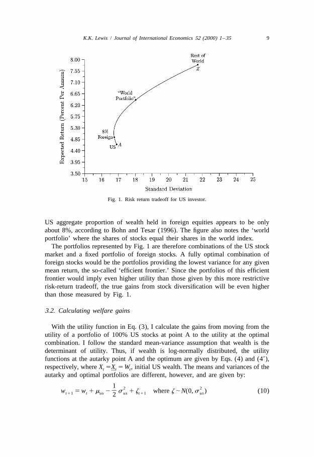
To illustrate, Fig. 1 depicts a combination of mean returns and standarddeviations of portfolio combinations that allow for different weights on foreignstocks in the portfolio of a domestic US investor. In particular, I take the returnson the stock market indices from Morgan Stanley International Capital MarketPerspectives for the G-7 from 1969 to 1993. I then construct a mutual fund bytaking a population-weighted average of the non-US country equities, converting

13the foreign returns into dollars and then deflating by the US price level. Detailsare provided in Appendix A.

In Fig. 1, Point A represents the mean and standard deviation (S.D.) of the USstock market over the period, corresponding to a zero weight on foreign stocks.Moving along the curve represents higher weights to the foreign stock. Clearly, theUS stock market is dominated by portfolios include foreign stocks. However, the

12Lewis (1999) discusses a recent empirical literature that considers estimation risk in internationalportfolio allocation and has even questioned the presence of equity home bias. For different evidenceon this issue, see Gorman and Jorgensen (1996), Bekaert and Urias (1996), Stambaugh (1997), andPastor (1999). The question addressed in this paper pertains only to the conventional analysis ofwelfare gains based upon historical means and variances.

13I choose a population-weighted average in order to make the analysis consistent with theconsumption-based representative agent framework of the next section and thereby to facilitate theexperiments using moments of stock returns below. However, similar results were obtained using,alternatively, a capitalization-weighted average and a simple average of equities.


Fig. 1. Risk return tradeoff for US investor.

US aggregate proportion of wealth held in foreign equities appears to be onlyabout 8%, according to Bohn and Tesar (1996). The figure also notes the ‘worldportfolio’ where the shares of stocks equal their shares in the world index.

The portfolios represented by Fig. 1 are therefore combinations of the US stockmarket and a fixed portfolio of foreign stocks. A fully optimal combination offoreign stocks would be the portfolios providing the lowest variance for any givenmean return, the so-called ‘efficient frontier.’ Since the portfolios of this efficientfrontier would imply even higher utility than those given by this more restrictiverisk-return tradeoff, the true gains from stock diversification will be even higherthan those measured by Fig. 1.

3.2. Calculating welfare gains

With the utility function in Eq. (3), I calculate the gains from moving from theutility of a portfolio of 100% US stocks at point A to the utility at the optimalcombination. I follow the standard mean-variance assumption that wealth is thedeterminant of utility. Thus, if wealth is log-normally distributed, the utilityfunctions at the autarky point A and the optimum are given by Eqs. (4) and (49),respectively, where X 5X 5 W , initial US wealth. The means and variances of thet t t]autarky and optimal portfolios are different, however, and are given by:

1 2 2]w 5 w 1 m 2 s 1 z where z | N(0, s ) (10)t11 t us us t11 us2


1 2 2]w 5w 1m 2 s 1z where z | N(0, s ) (109)t11 t t11] ] ] ]2] ] ]

The mean and return of the foreign-allocated wealth portfolio depends upon themean and variance of the overall portfolio. The evolution of this portfolio can beapproximated as:

us *w 5w 1 (1 2 f)R 1 fR (11)t11 t t11 t11] ]

us *where R and R are the returns in the US and foreign equity markets,t t

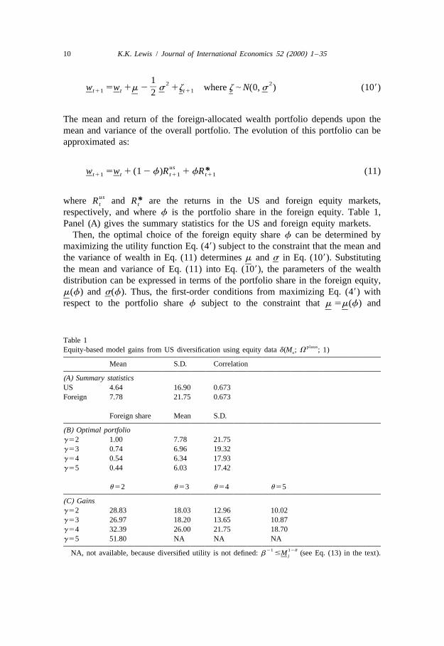
respectively, and where f is the portfolio share in the foreign equity. Table 1,Panel (A) gives the summary statistics for the US and foreign equity markets.

Then, the optimal choice of the foreign equity share f can be determined bymaximizing the utility function Eq. (49) subject to the constraint that the mean andthe variance of wealth in Eq. (11) determines m and s in Eq. (109). Substituting

]]the mean and variance of Eq. (11) into Eq. (109), the parameters of the wealthdistribution can be expressed in terms of the portfolio share in the foreign equity,m(f) and s(f). Thus, the first-order conditions from maximizing Eq. (49) with

]]respect to the portfolio share f subject to the constraint that m 5m(f) and] ]

Table 1plausEquity-based model gains from US diversification using equity data d(M ; V ; 1)s

Mean S.D. Correlation

(A) Summary statisticsUS 4.64 16.90 0.673Foreign 7.78 21.75 0.673

Foreign share Mean S.D.

(B) Optimal portfoliog 52 1.00 7.78 21.75g 53 0.74 6.96 19.32g 54 0.54 6.34 17.93g 55 0.44 6.03 17.42

u 52 u 53 u 54 u 55

(C) Gainsg 52 28.83 18.03 12.96 10.02g 53 26.97 18.20 13.65 10.87g 54 32.39 26.00 21.75 18.70g 55 51.80 NA NA NA

21 12uNA, not available, because diversified utility is not defined: b #M (see Eq. (13) in the text).j]


s 5s(f) is:] ]

1](≠m /≠f) 5 g(≠s /≠f) (12)

]2]

Solving Eq. (12) for f determines the optimal portfolio. Note that the portfolioallocation decision depends only upon the degree of risk aversion and no otherpreference parameters. Details are given in Appendix C.

Panel (B) reports the optimal allocation into the foreign equity as the riskaversion parameter varies from 2 to 5. For g equal to 2, the investor allocates hisportfolio 100% in foreign stocks. However, as risk aversion rises up to g equal to5, the investor reduces the variability of his portfolio by moving his foreignallocation share down to 44%. Correspondingly, the mean of his portfolio alsodeclines.

Given these optimal portfolios based upon g, the gain function can be calculatedas in Eq. (5) where X 5X and m and s, and m and s are determined by the US0 0] ]]stock market and the optimal portfolio of US and foreign stock markets,respectively. Table 1 reports the welfare gains in Panel (C). As noted above, thesemeasures represent the lower bounds for the true gains since the feasible set ofportfolios is restricted to linear combinations of the US stock market and a fixedmutual fund of foreign stocks.

Each row of Panel (C) reports the gains for a given level of g, and therefore agiven portfolio allocation. From left to right, as u increases the welfare gainsdecrease since the elasticity of substitution decreases and the investor places lessutility on future gains in certainty equivalent consumption. For example, for g 5 2,the gains are 28.8% of current wealth when u 52, but only 10% of wealth when

14u 55. For higher risk aversion, the gains generally increase. For example, wheng 55 and u 52, the gains are about 52% of wealth. For high levels of g and u,expected utility is not defined.

2To see why utility is not defined as u and/or g times the variance s increases,note that utility in Eq. (4) depends upon the condition that:

121 2]F S DGb . exp (1 2u ) m 2 gs (13)2

21]This is because the inverse of b exp[(1 2u )(m 2 gs )] acts as an overall2

15discount rate for future returns. When Eq. (13) does not hold, as can happen21

]when the certainty equivalent growth rate (m 2 gs ) is negative, utility does not2

converge as t goes to infinity and this discount rate exceeds unity. This possibility2is more likely as g or s increase. In the present case, the condition is violated

14Note that welfare gains are strictly increasing in g for given distribution parameters: m, s, m and]]

s. However, the distribution parameters for the optimal portfolio vary with g as noted above.15See the discussion in Obstfeld (1994a).


Fig. 2. Log consumption profile for US investor facing exogenous stock returns.

because the variability of stock returns is high. In Section 5 below, the conditionwill be violated in some circumstances because risk aversion is too high.

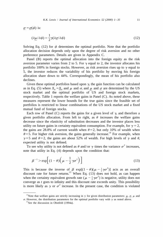
3.3. Graphical description of the gains from diversification

Fig. 2 illustrates the gains to an individual US investor to moving from thegrowth path associated with domestic returns alone to the path associated with theoptimal portfolio. The top two lines show the difference in growth paths associatedwith holding the foreign relative to the domestic portfolio in the case where thereis no uncertainty. Clearly, the higher returns, labeled m , correspond to the investors]with the optimal portfolio having a much higher consumption profile than thelower mean US returns, labeled m .s

The lower two lines show the certainty equivalent paths in the presence ofuncertainty. Both paths are lower than their counterparts in the absence ofuncertainty. However, the portfolio with foreign returns also has lower variancethan the domestic portfolio.

4. Consumption-based gains using consumption growth

I now provide a simple framework for assessing gains from risk-sharing usingthe consumption-based approach. Following the literature, I assume that identicalrepresentative agents in country j for each of N countries receive their own

jcountry’s per capita output stream, Y . For simplicity, I assume that the productiont


of this output is given as an exogenous endowment process. As before, I calculatewelfare gains by solving for and comparing the certainty equivalent consumptionpaths in the absence of risk-sharing and under perfect risk-sharing. To do so, I firstbriefly review the closed economy case in the absence of international risk sharingbefore constructing the diversified equilibrium.

4.1. Autarky

The equilibrium consumption process without access to international markets istrivially given by the endowment process. For countries with identical preferences,the pricing of risk will differ in the N closed economies if the output processesdiffer across countries. This closed economy equilibrium is well-known and

16therefore is only briefly summarized here.Defining s as the state of the economy at time t, including realizations of thet

endowment, the representative agent will maximize utility in Eq. (3) such that hisbudget constraint holds. Specifically, he will consume each period and buy sharesin the domestic equity. This optimization is given by the Bellman equation:

j j 12u j 12g (12u ) / (12g ) (1 / (12u ))V(W , s ) 5Max[(C ) 1 bE (V(W , s ) ) ] (14)t t t t t11 t11j jC ,kt t

s.t.j j j j j jC 1 k Q 5 (Q 1 Y )k (15)t11 t11 t11 t11 t11 t

where V is the value function based upon utility Eq. (3) which is in turn a functionjof the wealth of a country j investor at time t, W , and the state vector at time t, s .t t

j j j jIn particular, W ; k Q where k are the shares held of stocks paying out the pert t t tjcapita endowment of country j and Q is the stock price. This maximizationt

implies the first-order condition:

(g 21) / (u 21) j j 2u (g 21) / (u 21) j (g 21) / (u 21)b E h(C /C ) (1 1 R ) j 5 1 (16)t t11 t t11

jwhere R is the return on the domestic stock paying domestic per capitatjendowments, Y . I assume that the endowment process is log-normally distributedt

j jas above. Defining y ; ln(Y ),t t

1j j 2 2]y 5 y 1 m 2 s 1 z where z | N(0, s ) (17)t11 t j j t11 j2

In this case, Appendix B shows that the stock price has an analytical solution thatdepends upon the current level of output as well as the distribution and preference

j j j 2 jparameters: Q 5 Q (Y ; m , s ; g, u, b ). In equilibrium, k 5 1 so that eacht t j j t

investor holds one share of per capita output.

16See Epstein (1988) and, for the time additive case, Lucas (1982).


4.2. Risk-sharing with open financial markets

Suppose now that international capital markets are opened so that each countrycan trade in the equities of all other countries. In the new equilibrium, investors in

ijcountry j hold k shares in stocks of country i output. Instead of Eq. (15), thebudget constraint becomes:

N Nj ij i ij i iC 1O k Q #O k (Y 1 Q ) (18)t t t t21 t t

i51 i51

j ijwhere the maximization in Eq. (14) is now over C and k , ;i 5 1, . . . , N.t

Since all countries have the same homothetic utility function, then each country17holds the same portfolio allocation in equilibrium. Therefore, the problem can be

rewritten in terms of a world mutual fund paying out the world per capitaendowment, defined as Y. At time t, shares of the mutual fund held by country j

] jand its price are defined as k and Q , respectively. Rewriting the budgett t] ]constraint Eq. (18) with these definitions implies:

j j jC 1k #k (Y 1Q ) (19)t t t21 t t] ] ] ]

This maximization implies the first-order condition,

(g 21) / (u 21) j j 2u (g 21) / (u 21) (g 2u ) / (u 21) jb E h(C /C ) (1 1R ) (1 1R )j 5 1t t11 t t11 t11] ]

(20)

jwhere R and R are, respectively, the returns on the world mutual fund and thet t] ]domestic equity at world market prices. The world endowment process is log-

18normally distributed as above,

1 2 2]y 5y 1m 2 s 1 z where z | N(0, s ) (21)t11 t t11] ]2] ] ]

Appendix B shows that the world mutual fund price, Q, and the domestic stockj ] j j jprice in world markets, Q , have analytical solutions of the form: Q 5Q (Y ; m ,t t j] j ] ]

s , m, s ; g, u, b ) and Q 5Q (Y ; m, s ; g, u, b ) where s is the covariance of thej t t j] ] ] ] ]] ] ] ]world production process and the domestic production process.The equilibrium allocation of shares of the world mutual fund depends upon

these stock prices. Investors in each country sell off claims to current and futureoutput from their own country in exchange for claims to current and future world

joutput. Residents in country j sell their equity at price Q and for each unit oft]

17See, for example, Ingersoll (1987).18Note that, as with equity, this specification implies an approximation that both the sum of the

output processes and the output processes themselves are log-normally distributed. See Lewis (1996)for Monte Carlo simulations that suggest this approximation is relatively innocuous.


good, they will purchase the quantity 1 /Q of shares in the mutual fund. Therefore,tj j ]in equilibrium, k 5Q /Q .t t t] ] ]

4.3. Calculating welfare gains

Using the autarky equilibrium in Section (3.1) and the open economy equilib-rium in Section (3.2), welfare gains can be calculated using Eq. (5). Note that,

junder autarky, the initial level of consumption, C 5 Y , while the optimal initial0 0

level of consumption depends upon the value of the economy’s share in worldj joutput, C 5k Y 5 (Q /Q )Y . Therefore, the gain function can be rewritten as in0 0 0 0 0 0] ] ] ]] ]j jEq. (5) where X /X 5 (Y Q ) /(Y Q ). Since these prices depend only upon the0 0 0 0 0 0] ]] ]parameters of the distribution and the utility function, the gains can be calculated

for each country given the consumption means and variances as detailed in Eq. (7)plaus

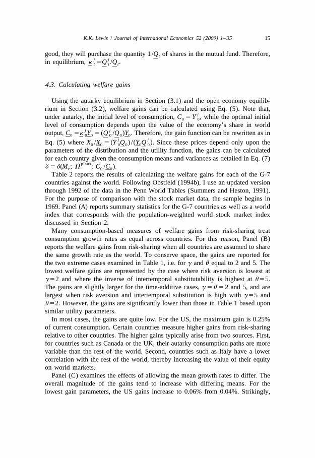
d 5 d(M ; V ; C /C ).c 0 0]Table 2 reports the results of calculating the welfare gains for each of the G-7

countries against the world. Following Obstfeld (1994b), I use an updated versionthrough 1992 of the data in the Penn World Tables (Summers and Heston, 1991).For the purpose of comparison with the stock market data, the sample begins in1969. Panel (A) reports summary statistics for the G-7 countries as well as a worldindex that corresponds with the population-weighted world stock market indexdiscussed in Section 2.

Many consumption-based measures of welfare gains from risk-sharing treatconsumption growth rates as equal across countries. For this reason, Panel (B)reports the welfare gains from risk-sharing when all countries are assumed to sharethe same growth rate as the world. To conserve space, the gains are reported forthe two extreme cases examined in Table 1, i.e. for g and u equal to 2 and 5. Thelowest welfare gains are represented by the case where risk aversion is lowest atg 52 and where the inverse of intertemporal substitutability is highest at u 55.The gains are slightly larger for the time-additive cases, g 5u 5 2 and 5, and arelargest when risk aversion and intertemporal substitution is high with g 55 andu 52. However, the gains are significantly lower than those in Table 1 based uponsimilar utility parameters.

In most cases, the gains are quite low. For the US, the maximum gain is 0.25%of current consumption. Certain countries measure higher gains from risk-sharingrelative to other countries. The higher gains typically arise from two sources. First,for countries such as Canada or the UK, their autarky consumption paths are morevariable than the rest of the world. Second, countries such as Italy have a lowercorrelation with the rest of the world, thereby increasing the value of their equityon world markets.

Panel (C) examines the effects of allowing the mean growth rates to differ. Theoverall magnitude of the gains tend to increase with differing means. For thelowest gain parameters, the US gains increase to 0.06% from 0.04%. Strikingly,


Table 2plausConsumption-based model gains from diversification using consumption data d(M ; V ; C /C )c 0 0]

Mean S.D. Correlation matrix

Canada US Japan France Germany Italy UK World

(A) Summary statisticsCanada 2.61 2.70 1.00 0.62 0.20 0.24 0.42 0.32 0.34 0.62US 1.86 1.91 – 1.00 0.57 0.50 0.54 0.02 0.63 0.95Japan 3.18 1.91 – – 1.00 0.73 0.45 0.11 0.68 0.74France 2.07 1.06 – – – 1.00 0.58 0.17 0.46 0.65Germany 2.26 1.67 – – – – 1.00 0.26 0.39 0.65Italy 2.98 1.76 – – – – – 1.00 0.18 0.21UK 2.58 2.93 – – – – – – 1.00 0.77World 2.34 1.53 – – – – – – – 1.00

u 55 u 55 u 52 u 52g 52 g 55 g 52 g 55

(B) Same meansUS 0.04 0.08 0.10 0.25Canada 0.39 0.97 1.01 2.47Japan 0.15 0.36 0.38 0.95France 0.13 0.34 0.32 0.83Germany 0.17 0.42 0.42 1.05Italy 0.40 1.00 1.01 2.53UK 0.35 0.86 0.92 2.30

(C) Differing meansUS 0.06 0.16 0.85 1.11Canada 0.79 1.30 1.68 3.09Japan 2.16 2.36 4.91 5.47France 0.00 0.19 0.40 0.83Germany 0.10 0.35 0.37 1.00Italy 1.76 2.38 3.91 5.60UK 0.68 1.11 1.44 2.66

the maximum welfare gains for Japan increase to 5.5% relative to only 0.95% inPanel (B). Thus, much of the gains to Japan derive from the strong equity value ofits high growth rate. I illustrate this effect graphically below.

Although these values are larger than when the means are assumed to be thesame, they remain significantly smaller than the stock return gains in Table 1.

4.4. Graphical representation of the gains

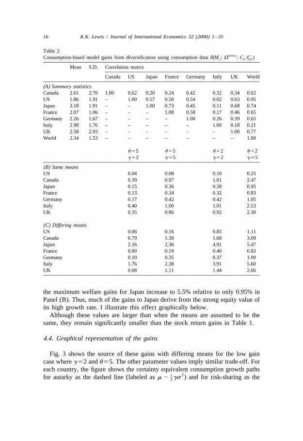
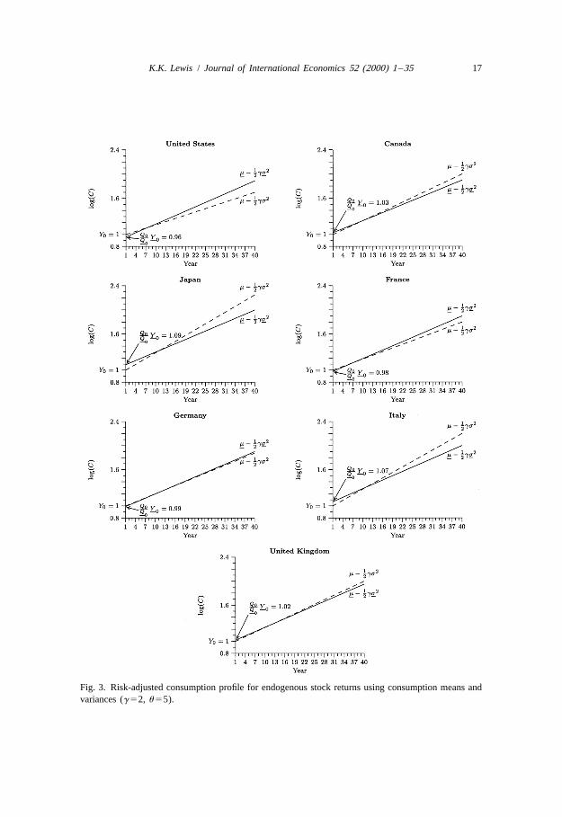
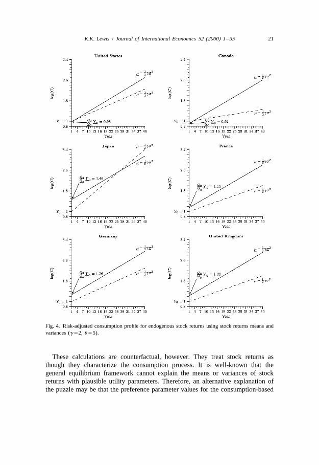
Fig. 3 shows the source of these gains with differing means for the low gaincase where g 52 and u 55. The other parameter values imply similar trade-off. Foreach country, the figure shows the certainty equivalent consumption growth paths

21]for autarky as the dashed line (labeled as m 2 gs ) and for risk-sharing as the2


Fig. 3. Risk-adjusted consumption profile for endogenous stock returns using consumption means andvariances (g 52, u 55).


21]solid line (labeled as m 2 gs ). The intercepts show the level of consumption2 ]]associated with the path at time 0.

This figure makes clear why Japan has relatively large gains while the US haslow gains. The Japanese sell off their claims to their high growth economy byreceiving a relatively high price in the beginning of time. The Japanese participatebecause they substitute current consumption for future consumption. The rest ofthe world wants the higher growth and provides this intertemporal substitution.Therefore, Japan enjoys large gains.

On the other hand, the US has low gains because Americans trade off currentconsumption for future consumption. Furthermore, since the US output stream ishighly correlated with the world output stream, the price of US equity is relativelylow. Similar trade-offs are shown for the other countries as well.

4.5. Conclusions from consumption gains

Overall, the evidence in Tables 1 and 2 shows that the equity-based approachgenerates significantly higher gains than the consumption-based approach. Whileboth measures are based upon a similar gain function, the analysis so far points totwo main potential reasons.

First, the consumption approach treats stock prices as endogenous and therebyallows for an intertemporal substitution across countries as well as the opportunityto reduce risk. This intertemporal substitution is missing in the exogenousstock-based approach. Clearly, this intertemporal substitution can potentiallyexacerbate the gains for some countries such as Japan with high growth rates.Therefore, this explanation alone does not appear to explain the puzzle.

Second, the measures of risk-adjusted growth paths are different. The consump-tion approach calculates this path from the means and variances of consumptiongrowth. The equity approach generates this path using the means and variances ofequity returns. This approach treats the underlying utility as generated from thestock return process. This distinction suggests a simple, counterfactual experimentfor studying the implications of this assumption, as I describe next.

5. Consumption-based gains using equity returns

To investigate the importance of treating the underlying determinant as utility ofstock returns as opposed to consumption, I recalculate the consumption approachgains using stock return data instead of consumption data. Although calculatingthe gains in this way is clearly counterfactual, it addresses the question: are thehigher gains measured by equity generated by the higher variability and/ordifferences in mean returns in stocks as opposed to consumption growth?


5.1. Measuring the gains

I calculate the general equilibrium gain using Eq. (5) where as for the generalj jequilibrium results in Table 2, X /X 5 (Y Q ) /(Y Q ) ± 1. In this case, however,0 0 0 0 0 0] ]] ]the stock prices depend upon the means and variances of stock returns as opposed

to consumption and the initial consumption level is treated as the wealth level,j jX /X 5 (Y Q ) /(Y Q ) 5 W /W . Furthermore, the utility level itself depends0 0 0 0 0 0 0 0] ] ]] ]upon the means and variances, so that the gain function can be written in the

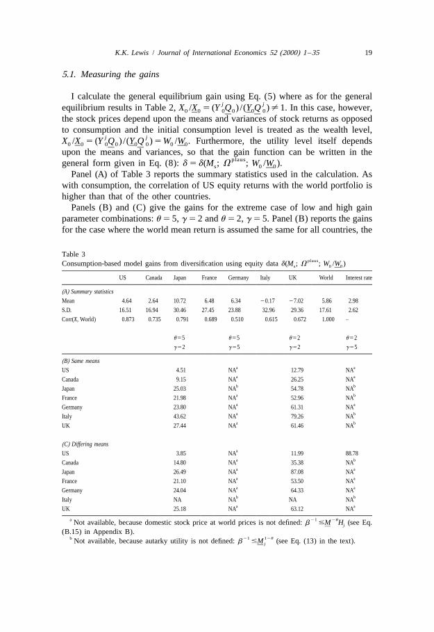
plausgeneral form given in Eq. (8): d 5 d(M ; V ; W /W ).s 0 0]Panel (A) of Table 3 reports the summary statistics used in the calculation. As

with consumption, the correlation of US equity returns with the world portfolio ishigher than that of the other countries.

Panels (B) and (C) give the gains for the extreme case of low and high gainparameter combinations: u 5 5, g 5 2 and u 5 2, g 5 5. Panel (B) reports the gainsfor the case where the world mean return is assumed the same for all countries, the

Table 3plausConsumption-based model gains from diversification using equity data d(M ; V ; W /W )s 0 0]

US Canada Japan France Germany Italy UK World Interest rate

(A) Summary statistics

Mean 4.64 2.64 10.72 6.48 6.34 20.17 27.02 5.86 2.98

S.D. 16.51 16.94 30.46 27.45 23.88 32.96 29.36 17.61 2.62

Corr(X, World) 0.873 0.735 0.791 0.689 0.510 0.615 0.672 1.000 –

u 55 u 55 u 52 u 52

g 52 g 55 g 52 g 55

(B) Same meansa aUS 4.51 NA 12.79 NAa aCanada 9.15 NA 26.25 NAb bJapan 25.03 NA 54.78 NAa bFrance 21.98 NA 52.96 NAa aGermany 23.80 NA 61.31 NAa bItaly 43.62 NA 79.26 NAa bUK 27.44 NA 61.46 NA

(C) Differing meansaUS 3.85 NA 11.99 88.78a bCanada 14.80 NA 35.38 NAa aJapan 26.49 NA 87.08 NAa aFrance 21.10 NA 53.50 NAa aGermany 24.04 NA 64.33 NAb bItaly NA NA NA NAa aUK 25.18 NA 63.12 NA

a 21 2uNot available, because domestic stock price at world prices is not defined: b #M H (see Eq.j](B.15) in Appendix B).

b 21 12uNot available, because autarky utility is not defined: b #M (see Eq. (13) in the text).j]


counterpart of Panel (B) in Table 2. Panel (C) reports the gains when the meansare allowed to differ by country, the standard assumption in the equity approachliterature.

Clearly these gains are substantially larger than those in Table 2. As with theconsumption-based gains, the gains are lower for the US than the other countriessince its correlation with the world is higher. For the other countries, the gains arequite large. Even for the low gain parameter case, the benefits to these countriesfrom risk-sharing range from about 15% to 26% of permanent consumption.


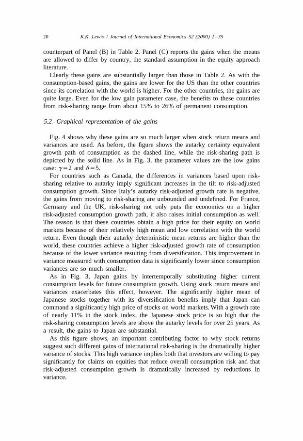
Fig. 4 shows why these gains are so much larger when stock return means andvariances are used. As before, the figure shows the autarky certainty equivalentgrowth path of consumption as the dashed line, while the risk-sharing path isdepicted by the solid line. As in Fig. 3, the parameter values are the low gainscase: g 52 and u 55.

For countries such as Canada, the differences in variances based upon risk-sharing relative to autarky imply significant increases in the tilt to risk-adjustedconsumption growth. Since Italy’s autarky risk-adjusted growth rate is negative,the gains from moving to risk-sharing are unbounded and undefined. For France,Germany and the UK, risk-sharing not only puts the economies on a higherrisk-adjusted consumption growth path, it also raises initial consumption as well.The reason is that these countries obtain a high price for their equity on worldmarkets because of their relatively high mean and low correlation with the worldreturn. Even though their autarky deterministic mean returns are higher than theworld, these countries achieve a higher risk-adjusted growth rate of consumptionbecause of the lower variance resulting from diversification. This improvement invariance measured with consumption data is significantly lower since consumptionvariances are so much smaller.

As in Fig. 3, Japan gains by intertemporally substituting higher currentconsumption levels for future consumption growth. Using stock return means andvariances exacerbates this effect, however. The significantly higher mean ofJapanese stocks together with its diversification benefits imply that Japan cancommand a significantly high price of stocks on world markets. With a growth rateof nearly 11% in the stock index, the Japanese stock price is so high that therisk-sharing consumption levels are above the autarky levels for over 25 years. Asa result, the gains to Japan are substantial.

As this figure shows, an important contributing factor to why stock returnssuggest such different gains of international risk-sharing is the dramatically highervariance of stocks. This high variance implies both that investors are willing to paysignificantly for claims on equities that reduce overall consumption risk and thatrisk-adjusted consumption growth is dramatically increased by reductions invariance.


Fig. 4. Risk-adjusted consumption profile for endogenous stock returns using stock returns means andvariances (g 52, u 55).

These calculations are counterfactual, however. They treat stock returns asthough they characterize the consumption process. It is well-known that thegeneral equilibrium framework cannot explain the means or variances of stockreturns with plausible utility parameters. Therefore, an alternative explanation ofthe puzzle may be that the preference parameter values for the consumption-based


model are inconsistent with the behavior of stock returns. I consider thispossibility next.

6. Consumption-based gains using preference parameters that match equityreturns

The inconsistency between stock return behavior and its predictions fromconsumption-based models using conventional utility parameter values has beenestablished repeatedly in the literature. For example, Mehra and Prescott (1985)show that, with time-additive utility, the mean excess return on equity over therisk-free rate in the US requires very high levels of risk-aversion. This relationshipis verified in Weil (1989) who shows that high levels of risk-aversion also generateimplausibly high levels of the risk-free rate. Kandel and Stambaugh (1991) arguethat, while the equity premium and the risk-free rate can be explained by highlevels of risk-aversion, other features of stock returns cannot.

In this section, I ask whether parameter values that match features of returnbehavior can help reconcile the difference in implied gains between equity andconsumption risk-sharing.

6.1. Matching the mean equity returns and risk-free rate

I begin by solving for the risk-aversion parameter g and the intertemporalelasticity parameter u that match the mean of the equity returns and the risk-free

19rate implied by the model to their counterparts in the data. That is, theconsumption-based model in Section 3 implies stock returns given the moments ofconsumption, M , and parameters, V. The form of these returns is derived inc

Appendix D. Table 2, Panel (A) reports the means and variances of these returns.Therefore, solving the two equations for the mean of equity and the mean of therisk-free rate for the two unknown parameters, g and u, provides the values for the

matchmatching parameters, V .Table 4 reports these combinations of g and u matching three different equity

returns: the autarky US stock price in Panel (A), the US stock price in integratedworld markets in Panel (B), and the world mutual fund price in Panel (C). Foreach combination of preference parameters, the table provides summary statisticsfor each country’s implied returns from the model.

In all three panels of Table 4, u is quite low while g is quite high. In fact, toexplain both the high world mutual fund price of 5.86% and the 3% risk-free rate

19For the purposes of calculating the risk-free rate, I use the dollar London-Interbank Offer Rate(LIBOR) deflated by US inflation. See Appendix A.


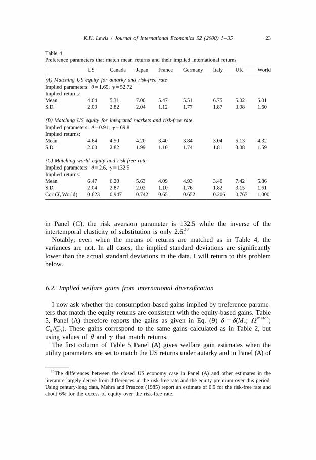
Table 4Preference parameters that match mean returns and their implied international returns

US Canada Japan France Germany Italy UK World

(A) Matching US equity for autarky and risk-free rateImplied parameters: u 51.69, g 552.72Implied returns:Mean 4.64 5.31 7.00 5.47 5.51 6.75 5.02 5.01S.D. 2.00 2.82 2.04 1.12 1.77 1.87 3.08 1.60

(B) Matching US equity for integrated markets and risk-free rateImplied parameters: u 50.91, g 569.8Implied returns:Mean 4.64 4.50 4.20 3.40 3.84 3.04 5.13 4.32S.D. 2.00 2.82 1.99 1.10 1.74 1.81 3.08 1.59

(C) Matching world equity and risk-free rateImplied parameters: u 52.6, g 5132.5Implied returns:Mean 6.47 6.20 5.63 4.09 4.93 3.40 7.42 5.86S.D. 2.04 2.87 2.02 1.10 1.76 1.82 3.15 1.61Corr(X, World) 0.623 0.947 0.742 0.651 0.652 0.206 0.767 1.000

in Panel (C), the risk aversion parameter is 132.5 while the inverse of the20intertemporal elasticity of substitution is only 2.6.

Notably, even when the means of returns are matched as in Table 4, thevariances are not. In all cases, the implied standard deviations are significantlylower than the actual standard deviations in the data. I will return to this problembelow.

6.2. Implied welfare gains from international diversification

I now ask whether the consumption-based gains implied by preference parame-ters that match the equity returns are consistent with the equity-based gains. Table

match5, Panel (A) therefore reports the gains as given in Eq. (9) d 5 d(M ; V ;c

C /C ). These gains correspond to the same gains calculated as in Table 2, but0 0]using values of u and g that match returns.

The first column of Table 5 Panel (A) gives welfare gain estimates when theutility parameters are set to match the US returns under autarky and in Panel (A) of

20The differences between the closed US economy case in Panel (A) and other estimates in theliterature largely derive from differences in the risk-free rate and the equity premium over this period.Using century-long data, Mehra and Prescott (1985) report an estimate of 0.9 for the risk-free rate andabout 6% for the excess of equity over the risk-free rate.


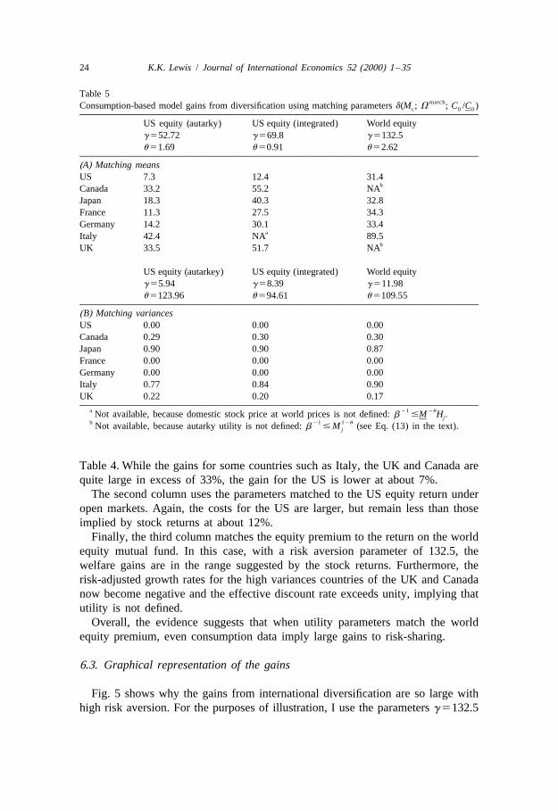
Table 5matchConsumption-based model gains from diversification using matching parameters d(M ; V ; C /C )c 0 0]

US equity (autarky) US equity (integrated) World equityg 552.72 g 569.8 g 5132.5u 51.69 u 50.91 u 52.62

(A) Matching meansUS 7.3 12.4 31.4

bCanada 33.2 55.2 NAJapan 18.3 40.3 32.8France 11.3 27.5 34.3Germany 14.2 30.1 33.4

aItaly 42.4 NA 89.5bUK 33.5 51.7 NA

US equity (autarkey) US equity (integrated) World equityg 55.94 g 58.39 g 511.98u 5123.96 u 594.61 u 5109.55

(B) Matching variancesUS 0.00 0.00 0.00Canada 0.29 0.30 0.30Japan 0.90 0.90 0.87France 0.00 0.00 0.00Germany 0.00 0.00 0.00Italy 0.77 0.84 0.90UK 0.22 0.20 0.17

a 21 2uNot available, because domestic stock price at world prices is not defined: b #M H .j]b 21 12uNot available, because autarky utility is not defined: b # M (see Eq. (13) in the text).j

Table 4. While the gains for some countries such as Italy, the UK and Canada arequite large in excess of 33%, the gain for the US is lower at about 7%.

The second column uses the parameters matched to the US equity return underopen markets. Again, the costs for the US are larger, but remain less than thoseimplied by stock returns at about 12%.

Finally, the third column matches the equity premium to the return on the worldequity mutual fund. In this case, with a risk aversion parameter of 132.5, thewelfare gains are in the range suggested by the stock returns. Furthermore, therisk-adjusted growth rates for the high variances countries of the UK and Canadanow become negative and the effective discount rate exceeds unity, implying thatutility is not defined.

Overall, the evidence suggests that when utility parameters match the worldequity premium, even consumption data imply large gains to risk-sharing.


Fig. 5 shows why the gains from international diversification are so large withhigh risk aversion. For the purposes of illustration, I use the parameters g 5132.5


Fig. 5. Risk-adjusted consumption profile for endogenous stock returns using consumption means andvariances (g 5132.5, u 52.6).


and u 52.6 which match the world equity premium and the risk-free rate [Table 4,Panel (C)]. With high risk aversion, the autarky consumption profiles aresignificantly flatter than their low risk aversion counterparts depicted in Fig. 3. Forthe US, in fact, the high risk aversion implies that the autarky risk-adjustedconsumption profile is negative. Furthermore, the risk-adjusted consumption pathsfor the UK and Canada are sufficiently negative to violate the condition in Eq.(13) that the discount rate is less than 1. As a result, utility is undefined for thesetwo countries at these parameter values.

The risk-sharing equilibrium leads to significant welfare gains. With highrisk-aversion, investors in each country value greatly even small reductions inconsumption variances. As a result, the stocks from countries such as Italy havinglow covariances with the rest of the world become much more valuable. Thisphenomenon also shows why the US has lower gains than the other countries.Since the US has the highest covariances with the rest of the world, its stock is lessvaluable on the world market. This is depicted in Fig. 5 by a drop in the intercept,representing a decline in initial consumption. However, the gains from buying anincreasing risk-adjusted consumption path significantly outweigh the losses fromthe low equity value.

Comparing Figs. 4 and 5 shows that the profiles measured using stock returndata and plausible preference parameters are quite different from those measuredusing consumption data and preference parameters that make consumption datamatch stock returns in the model. The stock return calculations in Fig. 4 using lowrisk aversion imply steeply rising consumption paths. The gains derive from ahigher growth rate, an intertemporal substitution toward higher current consump-tion, or both. On the other hand, Fig. 5 show that high risk aversion coupled withconsumption data lower the risk-adjusted consumption growth rate both in autarkyand under risk-sharing. Thus, for countries other than the US, the gains derivelargely from a higher value of domestic equity on world markets, depicted by theshift in intercept.

6.4. Matching variances

Above, I described the gains from diversification using preference parametersthat match the means of stock returns. However, Table 4 demonstrates that themodels imply variances that are too low to be consistent with actual stock returnvariances. I therefore consider a different set of parameters that match thevariance, instead of the mean, of stock returns. These calculations are detailed inAppendix D.

Panel (B) of Table 5 reports the results for the three stock returns describedpreviously: the autarky domestic stock return, the domestic stock return at worldprices, and the world equity return. As the table shows, the intertemporalsubstitutability must be very low to match the stock return variances. u, the inverseof this substitution parameter, ranges from 94.61 in the case of domestic equity at


world prices to 123.96 for domestic equity at autarky. Intuitively, for investors tobe willing to accept such high variability, they must be relatively indifferent tochanges in marginal utility over time. For this indifference to be true, the elasticityof substitution must be extremely low (u high). At the same time, risk aversion ismoderate with g ranging from about 6 to 12.

As described above, low intertemporal substitution mitigates the gains fromrisk-sharing. In this case, investors do not value strongly the future gains of lowervariability in the consumption profile. Thus, some countries such as the US thatmust substitute current for future consumption in the risk-sharing equilibrium gainless than 0.01% of permanent consumption. These gains are clearly lower than themore standard consumption-based gains measured in Table 2.

7. Conclusion

In this paper, I have examined the sources of differences between equity-basedand consumption-based calculations of the welfare gains from international risk-sharing. The differences largely come from differences in the utility gain ofrealized variability. This utility gain can arise in two ways. First, the variability ofthe determinant of utility can itself be high. Thus, when the determinant of utilityis assumed to be equity, the high return variance implies significantly highervariability of utility over time compared to the case when this determinant isassumed to be consumption. Second, the value of reducing the variability may behigh. For example, when risk aversion is sufficiently high to explain the equitypremium on an international diversified world mutual fund, the implied gains fromrisk-sharing measured from consumption is comparable to the gains based uponequity directly.

The paper shows that either of these factors can explain the differences betweenthe high gains from equity-based risk-sharing compared to consumption-basedrisk-sharing. However, the analysis also demonstrates that these two effectsoperate through somewhat different channels. Using stock return data in aconsumption-based model, the gains largely arise from increases in the growth rateof the certainty equivalent path of consumption. However, using high risk aversionimplies flatter certainty equivalent consumption paths but greater gains fromintertemporal substitution.

The paper also rules out the importance of some other plausible explanations fordifferences in measured gains. Conventional wisdom suggests that calculationsbased upon exogenous stock returns do not allow the investor to internalize theeffects of his actions on the stock return and thereby exacerbate the gains frominternational diversification. However, I show that internalizing these effects canactually increase the gains from diversification for high growth countries.

This paper pinpoints the reasons for significant differences in apparent gains torisk sharing between equity-based and consumption-based measures. Therefore,


these results should be useful for future research on measuring internationalrisk-sharing gains.

Acknowledgements

I am grateful for support by the National Science Foundation and for commentsby seminar participants at the National Bureau of Economic Research, theUniversity of Michigan, Princeton University, the Board of Governors of theFederal Reserve System, the Federal Reserve Bank of St. Louis, the InternationalMonetary Fund, Uppsala University, Stockholm University, the Stockholm Schoolof Economics, the University of Virginia, and the Wharton Macro Lunch group. Inparticular, I thank Andy Atkeson, Dave Backus, Bob Hodrick, and threeanonymous referees for useful comments. Any errors and omissions are minealone.

Appendix A. Data sources and construction

The data for the stock market series are the country stock market indexes fromMorgan Stanley (MSCI) with gross dividends reinvested. The series are measuredin dollars and converted into December year-over-year growth rates in real USterms by deflating the index using the ‘consumer price index for all goods’reported in the Economic Report of the President. The foreign mutual fund used inFig. 1 and Table 1 is a 1969 population-weighted average of the non-US G-7countries excluding Italy. The stock on Italy was excluded since its negativeaverage return and higher variance made it clearly dominated by the other stocks.The risk-free rate is the six month London Interbank Offer Rate (LIBOR) from theLondon Financial Times. Following standard practice in the literature, theconsumption data were taken from an updated version of the Penn World Tablesdescribed in Summers and Heston (1991).

Appendix B. Deriving the theoretical welfare gains

B.1. Deriving expected utility under the assumption of log-normality

Assume that the distributions for, alternatively, wealth in the equity case andconsumption in the consumption case are log-normally distributed:

1 2 2]x 5 x 1 m 2 s 1 ´ where j | N(0, s ) (B.1)t t21 t t2

Solving for the utility at time t requires forming a guess about the solution and


verifying. By straightforward iteration of Eq. (1) in the text and using properties ofthe log-normal distribution, the guess for the case when u ± 1 is taken to be:

2(1 / (12u ))1]H F S DGJU 5 X 1 2 b exp (1 2u ) m 2 gs (B.2)t t 2

Leading Eq. (B.2) one period and substituting the result into (1) implies:

1(12u ) ]H F S DGJU 5 X 1 bY 1 2 b exp (1 2u ) m 2 gsF F Gt t 2(1 / 12u )

(12g ) (12u ) / (12g )G3(E [X ])t t11

1]F F H F S DGJG5 X 1 1 b / 1 2 b exp (1 2u ) m 2 gst 2

(1 / 12u )(12g ) (12u ) / (12g )G3(E [(X /X ) ]) (B.3)t t11 t

But by the property of log-normal distributions:

1 1(12g ) 2 2 2] ]F S D GE((X /X ) ) 5 exp (1 2 g ) m 2 s 1 (1 2 g ) st11 t 2 2(12g )1 2]F G5 exp m 2 gs (B.4)2

Substituting Eq. (B.4) into Eq. (B.3) and rearranging yields Eq. (B.2) so that theguess is verified.

B.2. Deriving the welfare gains

The gain function d is defined by Eq. (2) in the text: U [(1 1 d )X , m,t2 2

s ] 5 U [X , m, s ] where X (X ) is the initial autarky (optimal) time t wealth int t t] ] ]]the stock case and consumption in the consumption case. Also, m and s are themeans and variances along the autarky path and m and s are the means and

]]variances along the optimal path. Substituting the utility function in Eq. (B.2) intoEq. (2) implies:

2(1 / (12u ))1 2]H F S DGJ(1 1 d )X 1 2 b exp (1 2u ) m 2 gst 22(1 / (12u ))1 2]H F S DGJ5X 1 2 b exp (1 2u ) m 2 gs (B.5)t] ]2]

Solving for d for t 5 0 implies Eq. (5) in the text.

B.2.1. Welfare gains for the equity based approach (Table 1)In this case, initial wealth is unaffected by risk-sharing. Therefore, W 5 X 5X0 0 0]

so that the gain function Eq. (5) becomes:


1 2]HS F S DGDd 5 1 2 b exp (1 2u ) m 2 gs2(1 / (12u ))1 2]S F S DGDJ4 1 2 b exp (1 2u ) m 2 gs 2 1 (B.6)

]2]

Note that this gain function is identical to the gain function obtained by Obstfeld(1994a) [p. 1478, Eq. (11)] since Obstfeld considers a representative agent in aclosed economy who cannot change his initial endowment level by risk-sharing.

B.2.2. Welfare gains for the general equilibrium case (Tables 2, 3 and 5)In this case, initial wealth is affected by risk-sharing since high growth countries

can intertemporally substitute future consumption into present consumption andvice versa. In this case, the initial autarky endowment level for country j is:

j j jX 5 Y . The initial risk-sharing endowment level is: X 5 (Q /Q )Y where Q is0 0 0 0 0 0 t] ]] ] ]the world price of equity which pays out country j’s endowment every period, Qt]is the price of a world mutual fund which pays out the world endowment everyperiod, and Y is the world endowment at time t. In this case, introducing thet]subscript j to indicate the country, the gain function becomes:

1j j 2]HS F S DGDd 5 (Y Q ) /(Y Q ) 1 2 b exp (1 2u ) m 2 gs0 0 0 0 j j] 2] ](1 / (12u ))1 2]S F S DGDJ4 1 2 b exp (1 2u ) m 2 gs 2 1 (B.7)

]2]

This gain function differs from that in Obstfeld (1994a) according to thej jmultiplying term, (Y Q ) /(Y Q ), which reflects the initial substitution of country0 0 0 0]] ]j’s autarky endowment for country j’s share of the world endowment.

B.3. Deriving the general equilibrium stock prices

The following describes the derivation of three prices: (a) the autarky price ofjdomestic equity, Q ; (b) the world mutual fund, Q; and (c) the world price ofj ]domestic equity, Q .

]

B.3.1. Autarky price of domestic equityEq. (16) in the text gives the first-order condition as:

j j j j1 1 R 5 (Y 1 Q ) /Q (B.8)t11 t11 t11 t

The stock price can be solved by guessing and verifying the solution. In this case,the guess is:


1j j 2]F S DGQ 5 Y b exp (1 2u ) m 2 gst t j j21 2]S F S DGD4 1 2 b exp (1 2u ) m 2 gs (B.9)j j2

21]Defining the certainty-equivalent consumption path as: M ; exp(m 2 gs ), thej j j2

stock price guess in Eq. (B.9) can be rewritten as:

j j (12u ) (12u )Q 5 Y b M /(1 2 b M ) (B.99)t t j j

Substituting Eq. (B.99) into Eq. (B.8) and the result into Eq. (16) in the textverifies the conjecture.

B.3.2. Price of the world mutual fundDeriving the price of the world mutual fund follows exactly the same steps as

the domestic price in autarky. The first-order condition becomes:

(g 21) / (u 21) j j 2u (g 21) / (u 21) (g 21) / (u 21)b E h(c /c ) (1 1R ) j 5 1 (B.10)t t11 t t11]

where

1 1R 5 (Y 1Q ) /Q (B.11)t11 t11 t11 t] ] ] ]

The stock price guess now becomes:

(12u ) (12u )Q 5Y bM /(1 2 bM ) (B.12)t t] ] ]]

where the certainty-equivalent mutual fund consumption path is: M ; exp(m 2]2 ]1

]gs ). Following the same steps as above verifies the guess.2 ]

B.3.3. World price of domestic equityEq. (20) in the text gives the first-order condition where:

j j j j1 1R 5 (Y 1Q ) /Q (B.13)t11 t11 t11 t] ] ]

The stock price guess is:

1j j 2]F GQ 5 Y b exp 2um 1 m 1 gs (1 1u ) 2 gst t j j] ]2] ]

1 2]S F GD4 1 2 b exp 2um 1 m 1 gs (1 1u ) 2 gs (B.14)j j] ]2]jwhere s is Cov(R, R ), the covariance between the return on the world mutualj] ] ]

fund and the return on the domestic equity in world markets. Using the definition21

]for M along with the definition, H ; exp[m 1 gs 2 gs ], the stock price can bej j j2] ] ]rewritten as,

j j 2u 2uQ 5 Y bM H /(1 2 bM H ) (B.15)t t j j] ]]


jSubstituting Eq. (B.15) into Eq. (B.13) and using this solution for R (along with]

the solution for R) in the first-order condition Eq. (20) in the text verifies the]

conjecture.

Appendix C. Calculating the welfare gain estimates

C.1. Equity-based model results in Table 1

As derived in Appendix B, Eq. (B.6) gives the equity-based gain function where2

m and s are, respectively, the mean and variance for the return on the domestic2country stock return, while m and s are the mean and variance for the return on

]]the optimal portfolio given the utility parameters.

C.1.1. Calculating the optimal portfolioTo obtain closed form solutions, I have assumed that the individual country

returns are log-normally distributed. As an approximation, I have also assumedthat the optimal portfolio returns are log-normally distributed, although this isstrictly incorrect. Lewis (1996) reports Monte Carlo experiments that suggest thisapproximation is innocuous.

To obtain the optimal portfolio, I take the risk-return trade-off between the USmarket and the foreign mutual fund as given. This trade-off is depicted in Fig. 1determined by the means and variances of the portfolio process (Eq. (11) in thetext.) For each set of parameter values, I then conduct a grid search overincrements of 1 /1000 of a portfolio share in the foreign stock, derive m and s, anduse these estimates to calculate the utility using Eq. (B.2). The share thatmaximizes the utility for these parameters is chosen as the optimal portfolio with

2corresponding mean m and variance s . This is equivalent to maximizing Eq. (49)]]subject to Eq. (109) and Eq. (11) in the text.

C.1.2. Calculating the welfare gainsUsing the optimal m and s determined by g and the US stock return means and

]]standard deviations m and s , the next step is to calculate the welfare gains.us us

Plugging these means and variances into Eq. (B.6) above gives the welfare gainsin Table 1.

C.2. Consumption-based model results in Tables 2, 3 and 5

Substituting into Eq. (B.7) the solutions for the stock prices Q [Eq. (B.99)] andtj ]Q [Eq. (B.15)] and using the definitions of M , M and H , the gain function can bet j j]]rewritten:

2u 2u (12u ) (12u ) (12u )d 5 [h[M H /(1 2 bM H )] 4 [M /(1 2 bM )]jh[1 2 bM ]j j j] ] ] ]

(12u )4 [1 2 bM ]j] 2 1 (C.1)

]


C.2.1. Table 2, Panel (C) gainsFor each country, I take the consumption means, variances and covariances with

2the world given in Table 2, Panel (A) and use these estimates as m , s and s ,j j j]respectively. I also take the means and variances of the world to be estimates of m

2 ]and s . Plugging these moments into Eq. (C.1), I vary u and g. For each pair of u]

and g, I report the gains.

C.2.2. Table 2, Panel (B) gainsThese gains are calculated the same as Table 2, Panel (C) gains except that the

assumption is imposed that the individual country means are equal to the worldmean; i.e. m 5m ; j.j ]

C.2.3. Table 3, Panel (B) gainsThese gains are calculated the same as Table 2, Panel (C) gains except that for

each country’s equity, I take the means, variances and covariances with the world2equity fund given in Table 3, Panel (A) and use these estimates as m , s and s ,j j j]

respectively. I also take the means and variances of the world equity fund to be2estimates of m and s .

]]

C.2.4. Table 3, Panel (B) gainsThese gains are calculated the same as Table 3, Panel (C) gains except that the

assumption is imposed that the individual country means are equal to the worldmean; i.e. m 5m ; j.j ]

C.2.5. Table 5 gainsThese gains are calculated as for the Table 2, Panel (C) gains described in

Section C.2.1. However, instead of varying the pair of parameters g and u

exogenously, these parameters are determined by matching moments of therisk-free rate and a particular stock price. For example, Panel (A) reports the gainswhen matching the means of the risk-free rate and, alternatively, the US stockreturn under autarky (Column 1), the US stock return under world prices (Column2), and the world stock return (Column 3). (The implied returns for these cases arereported in Table 4.) Table 5, Panel (B) reports the gains when g and s are chosento match the variances of these same pairs of returns.

Appendix D. Calculation of the return series

D.1. Deriving means and variances of equity returns

The equity returns all have the general form: (1 1 R ) 5 ( y /y )(1 /A) wheret t t21(12u ) j (12u )A 5 bM when R 5 R , the autarky domestic return; A 5 bM when R 5R,j ] ]2u jthe world mutual fund return; and A 5 bM H when R 5R , the domestic equityj] ]

at world prices. Therefore, the mean returns have the form: E(1 1 R) 5


21exp(m)A . Similarly, the variances of the returns have the form: Var(1 1 R) 52 22exp(2m)(exp(s ) 2 1)A .

D.2. Deriving the risk-free rates

rfSetting R in the Euler equation Eq. (20) equal to the risk-free rate, R , implies:t t

1rf 21 2]S D1 1R 5 b exp um 2 gs (1 1u ) Risk-free rate at world pricest] ]2]

(D.1)

The counterpart for the autarky domestic economy is:

1rf 21 2]S D1 1 R 5 b exp um 2 gs (1 1u ) Risk-free rate at autarky pricest j j2(D.2)

D.3. Matching parameters

The parameters in Table 4 are determined through the following steps. First, theconsumption means and variances from Table 2, Panel (A) are used to obtainvalues for m , s , m, s and s . Second, the means of stock returns and the risk-freej j j] ]]rates given in Table 3, Panel (A) are used to obtain estimates for the risk-free rateand the means of US and world stock returns. Third, the means of stock returns areset equal to its theoretical value and the mean of the risk-free rate is set equal to itstheoretical value implying two equations in the two unknown parameters, u and g.The solution implies parameter pairs which match the mean returns. Thus, Table 4Panel (A) is determined by setting the theoretical autarky equity return equal to themean of US stock returns and the theoretical risk-free rate equal to the mean of therisk-free rate implying u 51.69 and g 552.72. In addition to this restriction fromthe risk-free rate, Panel (B) is derived by setting the theoretical domestic equityreturn on world markets equal to the mean of US returns. Finally, Panel (C) setsthe theoretical world equity return equal to the mean of the world stock return andtreats the risk-free rate as in Panels (A) and (B).

References

Bekaert, G., Urias, M.S., 1996. Diversification, integration, and emerging market closed-end funds.Journal of Finance 51, 835–869.

Bohn, H., Tesar, L.L., 1996. US equity investment in foreign markets: Portfolio rebalancing or returnchasing? American Economic Review 86, 77–81.

Cole, H., Obstfeld, M., 1991. Commodity trade and international risk sharing: How much do financialmarkets matter? Journal of Monetary Economics 28, 3–24.

Epstein, L.G., 1988. Risk aversion and asset prices. Journal of Monetary Economics 22, 179–192.


Epstein, L.G., Zin, S.E., 1989. Substitution, risk-aversion, and the temporal behavior of consumptionand asset returns: A theoretical framework. Econometrica 57, 937–969.

Gorman, L.R., Jorgensen, B.N., 1996. Domestic versus international portfolio selections: A statisticalexamination of the home bias, Working Paper, Kellogg Graduate School of Management,Northwestern University, Evanston, IL.

Hall, R.E., 1988. Intertemporal substitution in consumption. Journal of Political Economy 96, 339–357.Ingersoll, Jr. J.E., 1987. Portfolio separation theorems. Theory of financial decision making. Rowman

& Littlefield, Savage, MD.Kandel, S., Stambaugh, R., 1991. Asset returns and intertemporal preferences. Journal of Monetary

Economics 27, 39–71.Kocherlakota, N., 1990. On the ‘discount’ factor in growth economies. Journal of Monetary Economics

25, 43–47.Levy, H., Sarnat, M., 1970. International diversification of investment portfolios. American Economic

Review 60, 668–675.Lewis, K.K., 1996. Consumption, stock returns, and the gains from international risk-sharing, Working

Paper No. 5410, National Bureau of Economic Research, Cambridge, MA.Lewis, K.K., 1999. Trying to explain home bias in equities and consumption. Journal of Economic

Literature 37, 571–608.Lucas, Jr. R.E., 1982. Interest rates and currency prices in a two-country world. Journal of Monetary

Economics 10, 335–359.Lucas, Jr. R.E., 1987. Models of business cycles. Basil Blackwell, Oxford, New York.Mehra, R., Prescott, E.C., 1985. The equity premium: A puzzle. Journal of Monetary Economics 15,

145–162.Obstfeld, M., 1994a. Evaluating risky consumption paths: The role of intertemporal substitutability.

European Economic Review 38, 1471–1486.Obstfeld, M., 1994b. Risk-taking, global diversification, and growth. American Economic Review 84,

1310–1329.Pastor, L., 1999. Portfolio selection and asset pricing models, Journal of Finance 54, in press.Stambaugh, R.F., 1997. Analyzing investments whose histories differ in length. Journal of Financial

Economics 45, 285–331.Summers, R., Heston, A., 1991. The Penn World Table (Mark 5): An expanded set of international

comparisons, 1950–1988. Quarterly Journal of Economics 106, 327–368.Tesar, L., 1995. Evaluating the gains from international risk-sharing. Carnegie Rochester Conferences

on Public Policy 42, 95–143.van Wincoop, E., 1994. Welfare gains from international risk-sharing. Journal of Monetary Economics

34, 175–200.Weil, P., 1989. The equity premium puzzle and the risk-free rate puzzle. Journal of Monetary

Economics 24, 401–421.Weil, P., 1990. Nonexpected utility in macroeconomics. Quarterly Journal of Economics 105, 29–42.

Documents

Why do stocks and consumption imply such different gains from international risk sharing?